Generating Function Analysis of Wireless Networks and ARQ Systems by Shihyu Chang A dissertation submitted in partial fulfillment of the requirements for the degree of Doctor of Philosophy (Electrical Engineering: Systems) in The University of Michigan 2006 Doctoral Committee: Professor Wayne E. Stark, Co-Chair Associate Professor Achilleas Anastasopoulos, Co-Chair Professor Arthur G. Wasserman Assistant Professor Mingyan Liu

Welcome message from author
This document is posted to help you gain knowledge. Please leave a comment to let me know what you think about it! Share it to your friends and learn new things together.
Transcript

Generating Function Analysis of Wireless
Networks and ARQ Systems
by
Shihyu Chang
A dissertation submitted in partial fulfillmentof the requirements for the degree of
Doctor of Philosophy(Electrical Engineering: Systems)
in The University of Michigan2006
Doctoral Committee:
Professor Wayne E. Stark, Co-ChairAssociate Professor Achilleas Anastasopoulos, Co-ChairProfessor Arthur G. WassermanAssistant Professor Mingyan Liu

c© Shihyu Chang 2006All Rights Reserved

ACKNOWLEDGEMENTS
I am most grateful to my Ph.D. advisors Professor Wayne E. Stark and Professor
Achilleas Anastasopoulos, for their invaluable guidance and continued support during
the course of this research work at the University of Michigan. I am also extremely
grateful to Professor Stark for his patient rectification of my English pronunciation
and academic writing skills.
I would like to thank the other members of my committee, Professor Mingyan Liu
and Professor Arthur G. Wasserman, for their time and effort in reading this work
and providing worthwhile comments and suggestions.
I would also like to present my gratitude to my colleagues, Kar-Peo Yar, Chih-
Wei Wang, Jinho Kim and Changhun Bae, at the Wireless Communication Lab at
the University of Michigan. I have enjoyed supportive and resourceful discussion
with them during our group meetings. In addition, I would like to acknowledge my
financial support from the Office of Naval Research under Grant N00014-03-1-0232.
Finally, my sincere thanks goes to my parents and siblings. Without their sup-
port and love, it is impossible for me to finish my Ph.D study at the University of
Michigan. They have always been there to encourage me when I needed them.
ii

TABLE OF CONTENTS
ACKNOWLEDGEMENTS . . . . . . . . . . . . . . . . . . . . . . . . . . . . . . . . . . ii
LIST OF FIGURES . . . . . . . . . . . . . . . . . . . . . . . . . . . . . . . . . . . . . . v
LIST OF TABLES . . . . . . . . . . . . . . . . . . . . . . . . . . . . . . . . . . . . . . . viii
LIST OF APPENDICES . . . . . . . . . . . . . . . . . . . . . . . . . . . . . . . . . . . ix
CHAPTER
I. Introduction . . . . . . . . . . . . . . . . . . . . . . . . . . . . . . . . . . . . . . . 1
1.1 Wireless Network Architectures and Protocol Layers . . . . . . . . . . . . . . 21.1.1 Wireless Network Architectures . . . . . . . . . . . . . . . . . . . . 21.1.2 Protocol Layers . . . . . . . . . . . . . . . . . . . . . . . . . . . . . 3
1.2 Motivation . . . . . . . . . . . . . . . . . . . . . . . . . . . . . . . . . . . . . 61.3 Literature Review for IEEE 802.11 DCF Analysis . . . . . . . . . . . . . . . 9
1.3.1 PHY and MAC Cross-layer Analysis . . . . . . . . . . . . . . . . . 101.3.2 Priority and Scheduling Analysis . . . . . . . . . . . . . . . . . . . 121.3.3 Other Research . . . . . . . . . . . . . . . . . . . . . . . . . . . . . 14
1.4 Thesis Contributions and Outline . . . . . . . . . . . . . . . . . . . . . . . . 15
II. Energy-Delay Analysis of MAC Protocols in Wireless Networks . . . . . . 19
2.1 Introduction . . . . . . . . . . . . . . . . . . . . . . . . . . . . . . . . . . . . 192.2 System Description . . . . . . . . . . . . . . . . . . . . . . . . . . . . . . . . 222.3 Energy-Delay Analysis . . . . . . . . . . . . . . . . . . . . . . . . . . . . . . 24
2.3.1 Three Nonlinear System Equations . . . . . . . . . . . . . . . . . . 252.3.2 Joint Generating Function of Energy and Delay . . . . . . . . . . . 292.3.3 Mean System Energy Consumption and Delay . . . . . . . . . . . . 342.3.4 Average Energy with Delay Constraint . . . . . . . . . . . . . . . . 37
2.4 Energy-Delay Optimization . . . . . . . . . . . . . . . . . . . . . . . . . . . . 392.5 Numerical Results . . . . . . . . . . . . . . . . . . . . . . . . . . . . . . . . . 462.6 Conclusion . . . . . . . . . . . . . . . . . . . . . . . . . . . . . . . . . . . . . 51
III. Variations of 802.11 MAC Protocol . . . . . . . . . . . . . . . . . . . . . . . . 53
3.1 Adaptive Energy Scheme for Wireless Network Systems . . . . . . . . . . . . 533.1.1 System Description . . . . . . . . . . . . . . . . . . . . . . . . . . . 563.1.2 System Delay and Energy Analysis . . . . . . . . . . . . . . . . . . 583.1.3 Numerical Results . . . . . . . . . . . . . . . . . . . . . . . . . . . 65
3.2 802.11 Protocol with ARQ . . . . . . . . . . . . . . . . . . . . . . . . . . . . 713.2.1 System Description . . . . . . . . . . . . . . . . . . . . . . . . . . . 743.2.2 Analysis . . . . . . . . . . . . . . . . . . . . . . . . . . . . . . . . . 75
iii

3.2.3 Numerical Results . . . . . . . . . . . . . . . . . . . . . . . . . . . 803.3 Conclusion . . . . . . . . . . . . . . . . . . . . . . . . . . . . . . . . . . . . . 82
IV. Analysis of Energy and Delay for ARQ Systems over Time Varying Chan-nels . . . . . . . . . . . . . . . . . . . . . . . . . . . . . . . . . . . . . . . . . . . . . 85
4.1 Introduction . . . . . . . . . . . . . . . . . . . . . . . . . . . . . . . . . . . . 854.2 FSM Model, Channel Model and Assumptions for ARQ Systems . . . . . . . 884.3 Generating Function Analysis for General ARQ Systems . . . . . . . . . . . 934.4 Some Practical ARQ Systems . . . . . . . . . . . . . . . . . . . . . . . . . . 106
4.4.1 SW-ARQ over Time-Varying Channels: No Repetition . . . . . . . 1064.4.2 SW-ARQ over Time-Varying Channels: Repetition . . . . . . . . . 112
4.5 Go-Back-N ARQ . . . . . . . . . . . . . . . . . . . . . . . . . . . . . . . . . . 1174.6 Cutoff Rate for Memory Receiver over Memoryless Channels . . . . . . . . . 121
4.6.1 Random Coding Bound for Memory Receiver in AWGN channel-Part I: Perfect Channel Knowledge . . . . . . . . . . . . . . . . . . 122
4.6.2 Random Coding Bound for Memory Receiver - Part II : ImperfectChannel Knowledge . . . . . . . . . . . . . . . . . . . . . . . . . . . 124
4.6.3 Existence of Codes for Memory Receiver . . . . . . . . . . . . . . . 1284.6.4 Cutoff Rate Optimization . . . . . . . . . . . . . . . . . . . . . . . 130
4.7 Numerical Results . . . . . . . . . . . . . . . . . . . . . . . . . . . . . . . . . 1344.8 Conclusion . . . . . . . . . . . . . . . . . . . . . . . . . . . . . . . . . . . . . 141
V. Conclusion and Future Research . . . . . . . . . . . . . . . . . . . . . . . . . . 142
5.1 Contributions . . . . . . . . . . . . . . . . . . . . . . . . . . . . . . . . . . . 1425.2 Future Research . . . . . . . . . . . . . . . . . . . . . . . . . . . . . . . . . . 144
APPENDICES . . . . . . . . . . . . . . . . . . . . . . . . . . . . . . . . . . . . . . . . . . 147
BIBLIOGRAPHY . . . . . . . . . . . . . . . . . . . . . . . . . . . . . . . . . . . . . . . . 163
iv

LIST OF FIGURES
Figure
1.1 An infrastructure network. . . . . . . . . . . . . . . . . . . . . . . . . . . . . . . . 3
1.2 An ad hoc network. Each station communicates mutually without the help of AP. 4
1.3 The illustration of fundamental tradeoff between energy and delay. . . . . . . . . . 7
1.4 The hidden stations problem. Station A and B are hidden station of each other. . 8
2.1 Timing diagram for the protocol under investigation. The numbers j0 and j1 rep-resent random numbers at stage i = 0, and i = 1, respectively. . . . . . . . . . . . . 25
2.2 Illustration of the random processes, b(τ), s(τ) and their discrete-time counterpartsbt, st. . . . . . . . . . . . . . . . . . . . . . . . . . . . . . . . . . . . . . . . . . . . . 26
2.3 Markov chain for backoff counter and contention window stage. . . . . . . . . . . . 28
2.4 State diagram representation of the 802.11 MAC protocol. Transform variables Xand Y are omitted for simplicity. . . . . . . . . . . . . . . . . . . . . . . . . . . . . 30
2.5 Energy-delay curves for different KDT with n = 10. . . . . . . . . . . . . . . . . . . 47
2.6 Energy-delay curves for different number of users n with KDT = 6400. . . . . . . . 48
2.7 Energy delay curves for different number of users and packet sizes. The lines withsquares represent numerical results and the lines with circles represent simulationresults. . . . . . . . . . . . . . . . . . . . . . . . . . . . . . . . . . . . . . . . . . . 49
2.8 Normalized standard deviation of delay vs. average delay curves for different n andKDT . Lines with a square symbol represent the case of KDT = 4400 and lines witha star symbol represent the case of KDT = 2400. . . . . . . . . . . . . . . . . . . . 49
2.9 Energy-delay curves for various outage delay probabilities and different values forthe outage probability Pr(Td > γd) (m = 1, n = 10,W = 8, KDT = 640). Theaverage energy and delay curve (circle symbol) is also shown for comparison. . . . 50
2.10 Energy-delay curves for various outage energy probabilities and different values forthe outage probability Pr(Et > γe) (m = 1, n = 10,W = 8,KDT = 640). Theaverage energy and delay curve (circle symbol) is also shown for comparison. . . . 51
2.11 Energy-delay tradeoff curves evaluated from the approximation method (star sym-bol) and the exact energy-delay tradeoff curves (square symbol) with n = 10 . . . . 52
v

3.1 Timing diagram for protocol. The j0 and j1 are backoff random numbers at CWstage i = 0, and i = 1, respectively. . . . . . . . . . . . . . . . . . . . . . . . . . . . 57
3.2 State diagram for the protocol. . . . . . . . . . . . . . . . . . . . . . . . . . . . . . 62
3.3 The STd comparison of convolutional codes for different KDT with code rate 12 and
n = 10. . . . . . . . . . . . . . . . . . . . . . . . . . . . . . . . . . . . . . . . . . . 67
3.4 The STd comparison of Reed-Solomn codes for different KDT with code rate 12 and
n = 10. . . . . . . . . . . . . . . . . . . . . . . . . . . . . . . . . . . . . . . . . . . 68
3.5 The STd comparison of convolutional and Reed-Solomn codes for different coderate with KDT = 128 and n = 10. . . . . . . . . . . . . . . . . . . . . . . . . . . . 69
3.6 The STd comparison of Reed-Solomn codes for different code rate with KDT = 128and n = 10. . . . . . . . . . . . . . . . . . . . . . . . . . . . . . . . . . . . . . . . . 70
3.7 Comparison of energy and delay curves for different ∆ with n = 10 and KDT = 64. 71
3.8 Comparison of energy and delay curves for different n and KDT with ∆ = 0.3(dB). 72
3.9 State diagram for the protocol. Solid lines represent successful reservation or trans-mission, while dotted lines represent unsuccessful reservation or transmission. . . . 77
3.10 Energy-delay curves for n = 10 and KDT = 1400. Solid lines represent the curves af-ter packets optimization. Dashed lines represent the energy-delay curves for Ec/N0
of 0 and 3 dB using the optimal packet lengths. . . . . . . . . . . . . . . . . . . . . 83
3.11 The dashed lines represent SWARQ after optimization. The number beside thecurve is the redundant bits. . . . . . . . . . . . . . . . . . . . . . . . . . . . . . . . 84
4.1 Gilbert-Elliott channel model for time varying channel. . . . . . . . . . . . . . . . 91
4.2 An example for a general ARQ system with mR = 2. The first slot representsthe state of the channel and transmitter. The second and third slots represent thestate of the receiver memory. The second (third) slot is used to represent the first(second) position of the the receiver memory. . . . . . . . . . . . . . . . . . . . . . 95
4.3 Stop-and-Wait ARQ protocol with increment redundancy. . . . . . . . . . . . . . 107
4.4 FSM representation for SW-ARQ protocol with increment redundancy. . . . . . . . 108
4.5 Operation of sliding window. . . . . . . . . . . . . . . . . . . . . . . . . . . . . . . 109
4.6 FSM representation for Stop-and-Wait ARQ protocol with m = 2 and mR = 1. . . 110
4.7 Three different repetition ARQ protocols with m = 2 considered in this section. . 113
4.8 State diagram for R-SW-ARQ-ML. . . . . . . . . . . . . . . . . . . . . . . . . . . . 114
4.9 FSM representation for repetition SW-ARQ systems with sliding window memorywith m = 2 and mR = 1. . . . . . . . . . . . . . . . . . . . . . . . . . . . . . . . . . 117
vi

4.10 FSM representation for repetition SW-ARQ systems with non-overlapping windowmemory with m = 2 and mR = 1. . . . . . . . . . . . . . . . . . . . . . . . . . . . . 118
4.11 Cutoff rate comparison for two different receiver structures. . . . . . . . . . . . . . 129
4.12 The comparison of cutoff rate for uniform and optimal priori probability for inputsignals. . . . . . . . . . . . . . . . . . . . . . . . . . . . . . . . . . . . . . . . . . . 132
4.13 The comparison of cutoff rate for different average energy constraints for 8 QAM . 135
4.14 Energy-Delay curves for different KDT . . . . . . . . . . . . . . . . . . . . . . . . . . 137
4.15 Energy-Delay curves for different λ with fixed average SNR. . . . . . . . . . . . . . 138
4.16 Normalized average delay relations with λ. . . . . . . . . . . . . . . . . . . . . . . 139
4.17 Energy-Delay curves for different average channel SNRs. . . . . . . . . . . . . . . . 140
4.18 Energy-Delay curves for repetition ARQ. . . . . . . . . . . . . . . . . . . . . . . . 140
4.19 Energy-Delay curves for GBNARQ with different Nrt. . . . . . . . . . . . . . . . . 141
vii

LIST OF TABLES
Table
1.1 The OSI network’s seven-layer model. . . . . . . . . . . . . . . . . . . . . . . . . . 4
2.1 System Parameters for Numerical Results . . . . . . . . . . . . . . . . . . . . . . . 47
3.1 System Parameters for Numerical Results . . . . . . . . . . . . . . . . . . . . . . . 66
3.2 System Parameters for Numerical Results . . . . . . . . . . . . . . . . . . . . . . . 81
4.1 Output functions and state transition probabilities for SWARQ . . . . . . . . . . . 108
4.2 Output functions and state transition probabilities for SWMARQ . . . . . . . . . . 111
4.3 Table for transition probabilities and output functions of R-SW-ARQ-ML . . . . . 115
4.4 Table for transition probabilities and output functions of R-SW-ARQ-SWM . . . . 116
4.5 Table for transition probabilities and output functions of R-SW-ARQ-NOM . . . . 119
viii
LIST OF APPENDICES
Appendix
A. Generating Function Analysis for NR-ARQ Systems . . . . . . . . . . . . . . . . . . . 148
A.1 Memoryless Receiver . . . . . . . . . . . . . . . . . . . . . . . . . . . . . . . 148A.2 Memory Receiver . . . . . . . . . . . . . . . . . . . . . . . . . . . . . . . . . 150
B. Generating Function Analysis for R-ARQ Systems . . . . . . . . . . . . . . . . . . . . 153
B.1 Memoryless Receiver . . . . . . . . . . . . . . . . . . . . . . . . . . . . . . . 153B.2 Memory Receiver : Sliding Window . . . . . . . . . . . . . . . . . . . . . . . 155B.3 Memory Receiver : Non Overlap . . . . . . . . . . . . . . . . . . . . . . . . . 159
ix

CHAPTER I
Introduction
Future wireless systems may change the way people communicate, shop and work
significantly by establishing ubiquitous communication among people and devices.
For example, globalization of business will be realized by trading among companies
located at different countries via internet; distance eduction enables students and
teachers to communicate through information technology without the necessity for
the students and teachers to be physically in same location and time; mobile access
to work environment will allow people to work anywhere in the world. These goals
will be fulfilled by interconnecting any devices at anywhere and anytime through
wired and wireless communication.
A lot of challenges have not been solved in implementing the future wireless
systems. Some of them are:
• Channel and network characteristics are random and time varying.
• Because most devices are battery powered and the energy of a battery is a
limiting resource, energy efficient network techniques are crucial to design of a
network system to meet some performance criteria.
• In order to have seamless communication between all existing different wired
and wireless communication protocols, vertical handoff algorithms need to be
1

2
developed.
• Advanced coding schemes and multiple antenna systems are indispensable and
an intelligent controller for radio resources is still missing.
In this thesis, we will concentrate on discussing the issue of energy efficiency. To
combat severe channel conditions of wireless networks compared to wired networks,
we need more energy in packet transmission to decrease packet error probability. On
the other hand, if less energy is used, the loss of data packets could increase the delay
to transmit a packet successfully. For instance, decreasing the transmission delay by
increasing the transmission rate often results in less energy efficiency. Therefore,
the requirements for optimizing performance are often contradictory and there is a
fundamental tradeoff between energy and delay. These two factors are crucial in
designing an energy efficient wireless network. In the rest of this thesis, we will
determine the tradeoff between energy and delay analytically.
1.1 Wireless Network Architectures and Protocol Layers
We will describe briefly network architectures and the wireless protocol stack.
1.1.1 Wireless Network Architectures
There are two different network architectures: infrastructure and ad hoc networks.
A wireless network in which stations communicate with each other by first going
through an access point (AP) is called an infrastructure network. In an infrastructure
network, wireless stations can communicate with each other or can communicate
through a wired network with other stations not in radio range. A set of wireless
stations which are connected to an AP is referred to as a basic service set (BSS).
Most corporate wireless local area networks (LANs) operate in infrastructure mode

3
because they require access to the wired LAN in order to use services such as file
servers or printers. Fig. 1.1 shows an infrastructure network. The big circle around
each AP represents the communication range of each AP.
AP
: station
AP
Wired Backbone
Figure 1.1: An infrastructure network.
A wireless network in which stations communicate directly with each other, with-
out the use of an AP is called a network with ad hoc mode. An ad hoc network
architecture is also referred to as peer-to-peer architecture or an independent basic
service set (IBSS). Ad hoc networks are useful in cases that temporary network con-
nectivity is required, and are often used for battlefields or disaster scenes. Fig. 1.2
shows an ad hoc network.
1.1.2 Protocol Layers
The concepts of protocol layering provides a basis for knowing how a complicated
set of protocols cooperate together with the hardware to provide a complete wireless
network system. Although new protocol stacks such as the infrared data associa-
tion (IRDa) protocol stack for point-to-point wireless infrared communication and

4
: station
Figure 1.2: An ad hoc network. Each station communicates mutually without the help of AP.
Table 1.1: The OSI network’s seven-layer model.Application and Services layer
Presentation layerSession layer
Transport layerNetwork layerDate link layer
A. Logical control sublayerB. Media access control sublayer
Physical layer
the wireless application protocol (WAP) Forum protocol stack for building more ad-
vanced services have been proposed for wireless networks [2, 1], we will concentrate
our discuss on the traditional OSI protocol stack. There are seven layers regulated
by OSI, shown in Table 1.1.
Physical Layer:
The physical layer (PHY) is made up by radio frequency (RF) circuits, modula-
tion, and channel coding systems. The major functions and services performed by
the physical layer are :
• establishment and termination of a connection to a communications medium;

5
• conversion between the representation of digital data in user equipment and the
corresponding signals transmitted over a communications channel.
Data Link Layer:
The function of data link layer is to establish a reliable logical link over the
unreliable wireless channel. The data link layer is responsible for security, link error
control, transferring network layer packets into frames and packet retransmission.
The media access control (MAC), a sublayer of data link layer is responsible for the
task of sharing the wireless channel used by stations in the network.
Network Layer:
The task of network layer is to rout packets, establish the network service type
(connectionless vs. connection-oriented), and transfer packets between the transport
and link layers. In the scenario of mobility of stations, this layer is also responsible
for mobility management.
Transport Layer:
The transport layer provides transparent transfer of data between hosts. It is usu-
ally responsible for end-to-end error recovery and flow control, and ensuring complete
data transfer. In the Internet protocol suite this function is achieved by the connec-
tion oriented transmission control protocol (TCP). The purpose of the transport layer
is to provide transparent transfer of data between end users, thus relieving the upper
layers from any concern with providing reliable and cost-effective data transfer.
Session Layer:
The session layer sets up, coordinates, and terminates conversations, exchanges,
and dialogs between the applications at each end. It deals with session and connection
coordination.
Presentation Layer:

6
The presentation layer converts incoming and outgoing data from one presentation
format to another.
Application and Services Layer:
Source coding, digital signal processing (DSP), and context adaption are imple-
mented in this layer. Services provided at this layer depend on the various users
requirements.
Layered architectures have been used in most data networks such as Internet.
Since all layers of the protocol stack affect the energy consumption and delay for the
end-to-end transmission of each bit, an efficient system requires a joint design across
all these layers. In this thesis, we focus on the lowest two layers of OSI seven layer
architecture mentioned in Sec. 1.1.2. In the rest of section, we are going to determine
the tradeoff between energy and delay in wireless networks taking into account the
data link and physical layers.
1.2 Motivation
Time varying channels (e.g., multipath fading, shadowing) are often encountered
in wireless and mobile systems. Given the energy used per information bit, a wireless
communication system adopting forward-error-correction (FEC) can provide higher
protection with lower code rate. However, a system with lower code rate needs longer
delay to transmit the same information packet due to the fixed bandwidth. If we
want to decrease the delay to transmit the same information packet, the system re-
quires higher energy per information bit to achieve the same reliability as a system
with lower code rate. Another example is shown in Fig. 1.3. The horizontal axis
represents the system time and the vertical axis indicates the signal-to-noise ratio
(SNR) of the channel. We plot a channel SNR realization with respect to the system

7
time in Fig 1.3. In Fig. 1.3(a), the transmitter waits until the channel SNR becomes
high before transmissions. In this case, the system will spend large delay to finish
transmission. In Fig. 1.3(b), the transmitter transmits immediately even when the
channel SNR is low. However, the transmitter needs to spend more energy in trans-
mission in order to keep the same reliability as in the previous case. Therefore, there
is a fundamental tradeoff between energy and delay of a wireless communication
system.
CH. SNR
Time
TX waits TX transmits
Large delay
Time
Large energy
TX transmits
CH. SNR
(a)
(b)
Figure 1.3: The illustration of fundamental tradeoff between energy and delay.
Hidden stations in a wireless network refer to stations which are out of the com-
munication range of other stations. Take a physical star topology with an AP with
many stations surrounding it in a circular fashion; each station is within communi-
cation range of the AP, however, not each station can communicate with each other.
For example, it is likely that the station at the far edge of the circle can access the
AP since the distance between the station and AP is less than the communication

8
range, say r, but it is unlikely that the same station can detect a station on the
opposite end of the circle because the distance between these two stations exceeds
the communication range r. These two stations are known as hidden stations with
respect to each other. Fig. 1.4 illustrates the hidden stations problem of a wireless
network. Hidden stations problem leads to difficulties in media access control.
A BAP
Figure 1.4: The hidden stations problem. Station A and B are hidden station of each other.
In order to solve the problem of hidden stations [33], which occurs when some
stations in the network are unable to detect each other, the 802.11 protocol uses
a mechanism known as request-to-send/clear-to-send (RTS/CTS). Before transmit-
ting the data packet, the source station sends a request-to-send (RTS) packet. If
the RTS packet is received correctly at the destination station (there is no collision
with other RTS packets sent by other competing stations and the receiver correctly
decodes the packet) the destination station broadcasts a clear-to-send (CTS) packet.
If the CTS packet is successfully received by the source station, the channel reser-
vation is successful and the source station will begin to send data and wait for the
acknowledgement (ACK) packet. The source station detects an unsuccessful channel
reservation by the lack of a correct CTS packet. The MAC protocol investigated in

9
this thesis is RTS/CTS protocol adopted in IEEE 802.11 standard.
It is a well known fact that a packet with more redundant bits have smaller error
probability. This means that longer packets can be transmitted successfully with
lower energy demand. However, longer packets require larger delay to transmit. In
order to determine the tradeoff between energy and delay of a wireless system, we
need to have a relation between error probability, energy and delay for each type
of packet in the system. In this thesis, we will use the reliability function bounds
for a channel to determine the packet error probability. Let K be the number of
information bits in a packet and N be the number of coded symbols for this packet.
Then there exists an encoder and decoder for which the packet error probability
Pe,K,N is bounded by
Pe,K,N ≤ 2K−NR0 , (1.1)
where R0 is the cutoff rate determined by channel characteristics. For an additive
white Gaussian noise (AWGN) channel using binary input the cutoff rate is R0 =
1 − log2(1 + e−Ec/N0), where Ec/N0 is the received signal-to-noise ratio per coded
symbol.
1.3 Literature Review for IEEE 802.11 DCF Analysis
We will begin with a brief introduction of IEEE 802.11 protocol followed by re-
viewing literatures about its analysis. The IEEE 802.11 protocol for wireless LANs is
a multiple access technique based on carrier sense multiple access/collision avoidance
(CSMA/CA). The basic operation of this protocol is described as follows. A station
with a packet ready to transmit listens the activity of transmission channel. If the
channel is sensed idle, the station captures the channel and transmits data packets.
Otherwise, the station defers transmission and keeps in the backoff state. There are

10
two basic techniques to access the medium. The first one is called distributed coor-
dination function (DCF). There is no centralized coordinator in the system to assign
the medium to the users in the network. This is a random access scheme, based on
the CSMA/CA protocol. Whenever the packets collide or have errors, the protocol
adopts a random exponential backoff scheme before retransmitting the packets. Our
work is based on using DCF to access the medium. Another medium access method is
called point coordinator function (PCF) to implement medium access control. There
is a centralized coordinator to provide collision free and time bounded services.
Because the analysis of network performance in this thesis is based on Bianchi’s
distributed coordination function (DCF) analysis, we will give a literature review of
papers which use Bianchi’s DCF analysis in this section for comparison. From these
papers, we classify them into three categories. The first category is to use Bianchi’s
model to perform the cross-layer analysis (PHY and MAC). The second category
is to use Bianchi’s model to perform the priority and scheduling analysis. We put
other applications in the third category due to their variety. Some use Bianchi’s
model to improve channel utilization and some modifies Bianchi’s model to consider
non-saturation traffic scenario. We will begin with the first category.
1.3.1 PHY and MAC Cross-layer Analysis
In [24], a theoretical cross-layer saturation goodput model for the IEEE 802.11a
PHY layer and DCF basic access scheme MAC protocol is developed. The proposed
analytical approach relates the system performance to channel load, contention win-
dow (CW) resolution algorithms, distinct modulation schemes (BPSK and QPSK),
FEC schemes (convolutional code), receiver structures (maximum ratio combining)
and channel models (uncorrelated Nakagami-m fading channel). In [32], the authors
study the impact of frequency-nonselective slowly time-variant Rician fading chan-

11
nels on the performance of single-hop ad hoc networks using the IEEE 802.11 DCF
in saturation. They study the throughput performance of the four-way handshake
mechanism under direct sequence spread spectrum (DSSS) with differential binary
phase shift keying (DBPSK) modulation.
In an ad hoc network, it is important that all stations are synchronized to a
common clock. Synchronization is necessary for frequency hopping spread spectrum
(FHSS) to ensure that all stations hop at the same time; it is also necessary for both
FHSS and direct sequence spread spectrum (DSSS) to perform power management.
In [25],the authors evaluates the synchronization mechanism, which is a distributed
algorithm, specified in the IEEE 802.11 standards. By both analysis and simulation,
it is shown that when the number of stations in an IBSS is not very small, there is
a non-negligible probability that stations may get out of synchronization. The more
stations, the higher probability of asynchronism. Thus, the current IEEE 802.11s
synchronization mechanism does not scale; it cannot support a large-scale ad hoc
network. To alleviate the asynchronism problem, this paper also proposes a simple
modification to the current synchronization algorithm. The modified algorithm is
shown to work well for large ad hoc networks.
In [46], a cross-layer analytical approach from both the PHY layer and the MAC
layer to evaluate the performance of the IEEE 802.11 is developed. From the PHY
layer, this analytical approach incorporates the effects of both capture and directional
antenna, while from the MAC layer, the model takes account of the CSMA/CA
protocol. Through a cross-layer modelling technique, this analytical framework can
provide valuable insights of the PHY layer impact on the throughput performance
of the CSMA/CA MAC protocol. These insights can be helpful in developing a
MAC protocol to fully take advantage of directional antennas for enhancing the

12
performance of the WLAN. In [36], the proposed model computes its saturation
throughput by relating to the positions of the other concurrent stations. Further,
this model provides the total saturation throughput of the medium. They solve the
model numerically and show that the saturation throughput per station is strongly
dependent not only on the stations position but also on the positions of the other
stations.
1.3.2 Priority and Scheduling Analysis
In [28, 29], the authors develop two mechanisms for QoS communication in multi-
hop wireless networks. First, they propose distributed priority scheduling, a tech-
nique that piggybacks the priority tag of a stations head-of-line packet onto hand-
shake and data packets; e.g., RTS/DATA packets in IEEE 802.11. By monitoring
transmitted packets, each station maintains a scheduling table which is used to as-
sess the station’s priority level relative to other stations. They then incorporate this
scheduling table into existing IEEE 802.11 priority back-off schemes to approximate
the idealized schedule. Second, they observe that congestion, link errors, and the
random nature of medium access prohibit an exact realization of the ideal schedule.
Consequently, they provide a scheduling scheme named multi-hop coordination so
that downstream stations can increase a packets relative priority to compensate for
excessive delays incurred upstream. From these aspects, the authors develop an ana-
lytical model to quantitatively explore these two mechanisms according to the model
of Bianchi. In the former mechanism, they study the impact of the probability of
overhearing another packets priority index. In the latter mechanism, the proposed
analytical model is provided for multi-hop coordination and it is used to compare
the probability of meeting an end-to-end delay bound over a multi-hop path with
and without coordination.

13
In [31], the authors develop a model-based frame scheduling scheme, called MFS,
to enhance the capacity of IEEE 802.11-operated wireless LANs. In MFS each station
estimates the current network status by keeping track of the number of collisions it
encounters between its two consecutive successful frame transmissions, and, based on
the the estimated information, computes the current network utilization. The result
is then used to determine a scheduling delay that is introduced (with the objective
of avoiding collision) before a station attempts for transmission of its pending frame.
In order to accurately calculate the current utilization in WLANs, they develop
an analytical model that characterizes data transmission activities in IEEE 802.11-
operated WLANs with/without the RTS/CTS mechanism, and validate the model
with ns-2 simulation.
In [7], a number of service differentiation mechanisms have been proposed for,
in general, CSMA/CA systems, and, in particular, the 802.11 enhanced DCF. An
effective way to provide prioritized service support is to use different inter frame
spaces (IFS) for stations belonging to different priority classes. This paper proposes
an analytical approach to evaluate throughput and delay performance of IFS based
priority mechanisms for different priority classes. This work extends previous work of
Bianchi by adding a further state to model different IFS for different priority classes.
However, the model does not rely on traditional multi-dimensional Markov chains
because the crucial assumption of a constant probability to access the channel in
a given time slot is not always correct. For an example, the model fails when the
difference between the IFS of two classes is greater than the minimum contention
window.

14
1.3.3 Other Research
In [43], the authors analyze the performance of channel utilization, based on data
burst transmissions, supported by the emerging IEEE 802.11e. They develop an
analytical framework to evaluate the impact of different access modes (i.e., 2-way/4-
way handshaking) and acknowledgment policies (i.e., immediate/block ACK) on the
overall system performance. Through the analytical modelling, they show that, given
a data packet size and a retransmission limit, the access mode and the ACK policy
have a great impact on the overall system throughput, and some optimizations are
possible. For example, they show that the block ACK is generally not useful for low
data rates and low value for retransmission limit, while it is very attractive for high
data rate transmissions. Another interesting conclusion is that the optimal selection
between immediate and block ACK does not depend on the number of contending
stations. They quantify these comparisons by providing the efficiency thresholds
needed to select the best possible mechanism. Finally, they discuss the role of the
block ACK protection mechanisms, i.e., of the HOB (head of burst) immediate ACK.
Most of analytical models proposed so far for EEE 802.11 DCF focus on satura-
tion performance. In [41, 30], the authors develop an analytic model for unsatura-
tion throughput evaluation of 802.11 DCF, based on Bianchi’s model. The model
explicitly takes into account both the carrier sensing mechanism and an additional
backoff interval after successful frame transmission, which can be ignored under sat-
uration conditions. Expressions are also derived by means of the equilibrium point
analysis in [41]. In [19], a model is proposed to predict the throughput, delay and
frame dropping probabilities of the different traffic classes in the range from a lightly
loaded, non-saturated channel to a heavily congested, saturated medium. Further-
more, the model describes differentiation based on different AIFS-values (Arbitration

15
Inter Frame Space), in addition to the other adjustable parameters (i.e. window-
sizes, retransmission limits etc.) also encompassed by previous non-saturated mod-
els. AIFS differentiation is described by a simple equation that enables access points
to determine at which traffic loads starvation of a traffic class will occur.
In [52], the authors propose a new contention algorithm called parallel contention
algorithm that divides the subcarriers into multiple groups to reduce the contention
time. They analyze the proposed scheme by extending the Markov chain model and
verify the accuracy of the analysis through the simulations. The protocol performs
well especially when the transmission speed and the number of users are getting
higher, thereby achieving a better performance improvement ratio than the original
IEEE 802.11a standard.
1.4 Thesis Contributions and Outline
The most important contribution of this thesis is to represent the operation of a
system by a state diagram and use the generating function approach to derive its
energy and delay consumption. The goal of this thesis is to investigate the energy
and delay tradeoff of a wireless communication system. In the first part of this thesis,
we will concentrate on communication networks, and in the second part of this thesis,
we will study a single link wireless ARQ communication system.
Previous research on performance evaluation of 802.11 has been carried out by
two methods. Crow [18], [6] and Weinmiller et al. [48] used computer simulations
to evaluate the network throughput. In [23, 17, 11], the system performance was
evaluated by an analytical model. Bianchi [5] used a simple but accurate model that
characterizes the random exponential backoff protocol. These papers did not incor-
porate channel noise in the analysis, which is an important factor in wireless network.

16
Although Hadzi-Velkov and Spasenovski [22] considered the effects of packet errors in
the analysis, they did not relate the packet error probability to the energy used and
the number of redundant bits used for error control coding. We extend the results
from Bianchi [5] and Hadzi-Velkov [22] by considering the effects packet errors in
the analysis. In their original work, they did not relate the packet error probability
to the energy used and the number of redundant bits used for error control coding.
The motivation for this thesis is to understand the role energy and codeword length
(number of redundant bits) at the PHY layer have on the total energy and delay of
the network. We propose a state diagram representation the operation of the MAC
layer and obtain the joint generating function of the energy and delay by incorporat-
ing the effects of the PHY layer. Next, we optimize numerically over the code rate for
each type of packet to minimize the average transmission delay. We use the random
coding bound to represent the packet error probability as a function of the delay
and energy. By changing the signal-to-noise ratio, the energy-delay tradeoff curves
for minimum delay are obtained. Finally, we propose an approximation method to
express the energy-delay tradeoff curves analytically and show the proposed approx-
imation is extremely accurate especially when the number of information bits per
packet is large.
Another contribution of this thesis is to apply our proposed generating function
method to the analysis and design of other wireless network protocols. The first pro-
posed protocol is an energy adaptation scheme with original IEEE 802.11 protocol
in which the transmitter will increase the energy level per coded symbol whenever it
suffers an unsuccessful transmission. The numerical results show that the proposed
protocol can improve system performance significantly when the channel condition
is bad. By using Reed-Solomon codes we can optimize the system performance over

17
the code rate and energy per coded bit. Although the packet error probabilities are
evaluated with Reed-Solomon codes over an additive white Gaussian noise (AWGN)
channel, the framework of our analysis can be used for other coding and modulation
schemes over various wireless channels. Finally, we also compare the system perfor-
mance between Reed-Solomon codes and convolutional codes. The second proposed
protocol is an ARQ mechanism for data packets transmission with 802.11 proto-
col. The motivation of this analysis is to demonstrate that the generating function
approach can be applied to analyze more function layers jointly by including the
analysis of logical link control (LLC) sublayer into the original protocol (MAC and
PHY layers only). The numerical results show that the IEEE 802.11 original protocol
and the proposed one have almost identical performances and are equally sensitive
to the knowledge of the channel quality at the transmitter.
For wireless ARQ systems, we extend the traditional Markov chain model for the
channel state as well as the transmitter state [13] by using a state diagram that
takes into account the states of transmitter, receiver and channel jointly. The states
of the transmitter can be used to model the different packet lengths adopted by
the transmitter and the states of the receiver can be utilized to model the receiver
memory content [27]. From the system state diagram, we are able to characterize
the joint energy and delay distribution of the system incorporating physical layer
characteristics (packet error probability as a function of energy and delay) through
generating function approach. The effect of transition probability which depends on
the packet length is also investigated. As the numerical results demonstrate, the time-
varying characteristics of the channel have a great influence on system performance
especially at low channel SNR.
The outline of the rest of the thesis is as follows. In Chapter 2, we will use the

18
proposed generating function method to analyze the energy and delay consumption of
wireless networks and discuss the tradeoff between energy and delay. The application
of generating function method in designing and analyzing other wireless network
protocols are presented in Chapter 3. In Chapter 4, we give the analysis of energy and
delay expense for ARQ systems over time varying channels and derive the cutoff rate
for different memory receiver structure. Finally in Chapter 5, we briefly summarize
the conclusions from the thesis and suggest possible future research directions.

CHAPTER II
Energy-Delay Analysis of MAC Protocols in WirelessNetworks
2.1 Introduction
Recently there has been considerable interest in the design and performance eval-
uation of wireless local area networks (WLANs). Some WLANs must operate solely
on battery power. In such cases it is important to consider energy consumption
in the system design and analysis. It is possible to reduce energy consumption by
increasing delay incurred. Two critical components of a wireless network are the
medium access control (MAC) protocol and the physical layer (PHY). The MAC
protocol resolves conflicts between users attempting to access the channel. Gener-
ally users make reservations for transmissions in a decentralized way. Thus there is
some amount of delay in accessing the channel and there is energy used in reserving
the channel. An important component of the PHY layer is forward error control
coding, which mitigates the effect of channel noise at the receiver. By transmit-
ting redundant bits in addition to information bits, error control coding reduces the
energy needed for transmission at the expense of increased delay.
There are many MAC protocols that have been developed for wireless voice and
data communication networks. Typical examples include the time-division multi-
ple access (TDMA), code-division multiple access (CDMA), and contention-based
19

20
protocols such as IEEE 802.11 [3], [4]. In this paper, we adopt the MAC protocol
used in the 802.11 standard. There are two basic techniques to access the medium
in the 802.11 standard. The first one called the distributed coordination function
(DCF), is employed when there is no centralized coordinator in the system to as-
sign the medium to users in the network. The DCF is a random access scheme,
based on carrier sense multiple access with collision avoidance (CSMA/CA). When
packets collide or have errors, the transmitter performs a random backoff before re-
transmitting the packets. Another MAC method in the 802.11 standard called point
coordinator function (PCF), is used when there is a centralized coordinator to co-
ordinate the access of the medium. In this paper we focus on the DCF protocol for
accessing the medium.
In order to combat the problem of hidden terminals [33], which occurs when some
stations in the network are unable to detect each other, the 802.11 protocol uses
a mechanism known as request-to-send/clear-to-send (RTS/CTS). Before transmit-
ting the data packet, the source station sends a request-to-send (RTS) packet. If
the RTS packet is received correctly at the destination station (there is no collision
with other RTS packets sent by other competing stations and the receiver correctly
decodes the packet) the destination station broadcasts a clear-to-send (CTS) packet.
If the CTS packet is successfully received by the source station, the channel reser-
vation is successful and the source station will begin to send data and wait for the
acknowledgement (ACK) packet. The source station detects an unsuccessful channel
reservation by the lack of a correct CTS packet.
Many previous research on performance evaluation of 802.11 has been based on an
analytical model proposed by Bianchi [5]. Bianchi used a simple but accurate model
that characterizes the random exponential backoff protocol. In [22, 46, 32, 24], the

21
authors used Bianchi’s model to perform the cross-layer analysis (PHY and MAC).
For example, a theoretical cross-layer saturation goodput model for the IEEE 802.11a
PHY and MAC layers was developed in [24]. The proposed analytical approach re-
lates the system performance to channel load, contention window (CW) resolution
algorithms, distinct modulation schemes (BPSK and QPSK), FEC schemes (convo-
lutional code), receiver structures (maximum ratio combining) and channel models
(uncorrelated Nakagami-m fading channel). In [28, 29, 7, 31], the authors adopted
Bianchi’s model to perform the priority and scheduling analysis. For example, in [7],
a number of service differentiation mechanisms have been designed for CSMA/CA
systems, and, in particular, the 802.11 enhanced DCF. The authors proposed an
effective way to provide prioritized service support by using different inter frame
spaces (IFS) for stations belonging to different priority classes. Although some of
the above papers considered the effects of packet errors in the analysis, they did not
relate the packet error probability to the energy used and the number of redundant
bits used for error control coding. The motivation for this paper is to understand
the role of energy and codeword length (number of redundant bits) at the PHY layer
have on the total energy and delay of the network. The contributions in this chapter
are as follows:
1. We propose a state diagram representing the operation of the MAC layer and
obtain the joint generating function of the energy and delay by incorporating
the effects of the PHY layer. This is a universal approach and could be applied
to other MAC protocols.
2. By taking the partial derivative for the joint generating of the energy and delay,
we determine the average energy and delay of a successful packet transmission
by taking the packet error probability into consideration. The results obtained

22
from the generating function approach will be agree with the results derived
from the renewal cycle method proposed in [22].
3. We optimize numerically over code rate to have minimum average transmission
delay over different packet by introducing the random coding bound to represent
the packet error probability. By changing the signal-to-noise ratio, the energy-
delay tradeoff curves for minimum delay are obtained.
4. We propose an approximation method to express the energy-delay tradeoff
curves analytically. The comparison of the energy-delay tradeoff curves eval-
uated from this approximation method with the exact energy-delay tradeoff
curves (from numerical optimization) indicates that this approximation method
is extremely accurate especially when the number of information bits per packet
is large.
The remainder of this chapter is organized as follows. In Section 2.2, we give
a brief description for the protocol used in our analysis and introduce the system
assumptions. In Section 2.3, we discuss our system state diagram and utilize it to
derive the joint generating function of energy and delay. Then the average energy
with outage delay constraint and average delay with outage energy constraint are
analyzed with generating function. The proposed approximation method for energy-
delay tradeoff curves is given in Section 2.4. We demonstrate that the energy and
delay relationship with random coding under AWGN channel through numerical
method in Section 2.5. Finally, Section 2.6 gives the conclusion and future research.
2.2 System Description
The wireless networks that we analyze here have the following network layer spec-
ifications. First, each station with a fixed position can hear (detect and decode) the

23
transmission of n − 11 other stations in the network. Second, stations always have
a packet ready to transmit. Third, each station uses the 802.11 MAC protocol. At
the PHY layer, a packet of K information bits is encoded into a packet of N coded
symbols. It is assumed that the receivers have no multiple-access capability (i.e.,
they can only receive one packet at a time) and they cannot transmit and receive
simultaneously. The packet error probability depends on the parameters K, N , and
Ec/N0, where Ec is the received coded symbol energy and N0 is the one-sided power
spectral density level of the thermal noise at the receiver.
In the following we give a brief description of the most salient features of the
IEEE 802.11 MAC protocol (more details can be found in [3] and [4]). When a
station is ready to transmit a packet, it senses the channel for DIFS seconds. If the
channel is sensed idle, the transmission station picks a random number j, uniformly
distributed in {0, 1, . . . , Wi − 1}, where Wi = 2iW is the contention window (CW)
size, i is the contention stage (initially i = 0), and W is the minimum CW size. A
backoff time counter begins to count down with an initial value j: it decreases by
one for every idle slot of duration σ seconds (also referred to as the standard slot) as
long as the channel is sensed idle, stops the count down when the channel is sensed
busy, and reactivates when the channel is sensed idle again. The station transmits
an RTS packet when the counter counts down to zero. After transmitting the RTS
packet, the station will wait for a CTS packet from the receiving station. If there
is a collision of the RTS packet with other competing stations or a transmission
error occurs in the RTS or CTS packet, the transmitting station doubles the CW
size (increases the contention stage i by one) and picks another random number j as
before. If there are no collisions or errors in the RTS and CTS packets, the station
1n− 1 is the number of stations in the communication range of the reference station.

24
begins to transmit the data packet and waits for an acknowledgment (ACK) packet.
However, if the data or the ACK packet is not successfully received, the CW size will
also be doubled (the contention stage i will increase by one) and the transmitting
station will join the contention period again. The contention stage is reset (i is set
to zero) when the transmitting station receives an ACK correctly. A time diagram
indicating the sequence of these events is depicted in Fig. 2.1. It is also noted that
there is a maximum CW size (or equivalently, a maximum contention stage, m);
when the transmitter is in this maximum stage and needs to join the contention
period again, it does not increase further the CW, but picks a random number in
{0, 1, . . . , Wm − 1}.
2.3 Energy-Delay Analysis
In this section, we analyze the energy and delay characteristics of the wireless
networks described above. The delay Td of each data packet is defined as the time
duration from the moment the backoff procedure is initiated until DIFS seconds after
the ACK packet is received correctly by the transmitting station, as shown in Fig. 2.1.
Similarly, the energy Et is defined as the energy consumed by both transmitting and
receiving stations in the duration of Td. Without loss of the generality, for notational
simplicity we assume that the propagation loss between transmitter and receiver is
one (0 dB). We also assume that the propagation time is negligible. In this chapter,
we only consider the energy consumption for packet transmission and omit the energy
required for signal processing and channel sensing. The system parameter SIFS is
defined as the time between the end of a packet reception, say RTS and the beginning
of a packet transmission, say CTS. This time includes the time required for decoding
a packet and other processing functions at the receiver.

25
frozen slot counter frozen slot counter
reference station unsuccessful transmission
frozen slot counter reference station
successful transmission
T d begin
DIFS
j 0 ~ U(0, W 0 -1)
Trc
0
DIFS
frozen slot counter
j 1 ~ U(0, W 1 -1)
stage number is increased by 1
0
T coe
stage number is set back to 0
T d end
DIFS
Figure 2.1: Timing diagram for the protocol under investigation. The numbers j0 and j1 representrandom numbers at stage i = 0, and i = 1, respectively.
2.3.1 Three Nonlinear System Equations
In order to analyze energy and delay relationships, we need to define two random
processes to characterize the backoff counter state and the CW size. The first process
b(τ) represents the backoff time counter for the reference station (this is the station
for which we evaluate energy and delay). The second random process s(τ) is used
to represent the CW stage i ∈ {0, 1, . . . , m} of the station at time τ . In order to
analyze the energy and delay characteristics it is sufficient to only consider the time
instances the backoff counter (and CW stage) changes value. To this end we further
define the discrete-time random processes bt = b(τt) and st = s(τt), where τt is the
time instance of the t-th change in value of b(τ). A realization of these random
processes is shown in Fig. 2.2. In this realization, b3 = 4 is the value of the counter
just before being frozen and b4 = 3 is the value of the counter after the channel has
been sensed idle for DIFS seconds, and the counter becomes active again.

26
frozen slot counter
DIFS
7 6 5 4
reference station
unsuccessful transmission
3 2 19 8
)(τb
)(τs
1)( =τs
τ
0)( =τs
0τ 1τ 2τ 3τ 4τ 6τ5τ 7τ 8τ 9τ τ
τ
Figure 2.2: Illustration of the random processes, b(τ), s(τ) and their discrete-time counterparts bt,st.
The first assumption made in this analysis is that the event of packet collision
is independent of past collisions and thus independent of the contention stage. The
second assumption is that the packet collision is identical for all states (values of bt
and st) of a user. As verified in [5], these two assumptions are extremely accurate
when the number of stations in the network is large (say greater then 10). As a
result of the above assumptions, the two dimensional process (st, bt) is a discrete-
time Markov chain. With the assumption that errors in transmission can occur only
due to collisions, the one-step transition probabilities developed in [5] are given by
P{i, k | j, l} = P{st+1 = i, bt+1 = k | st = j, bt = l} with
P{i, k | i, k + 1} = 1, 0 ≤ k ≤ Wi − 2, 0 ≤ i ≤ m (2.1a)
P{0, k | i, 0} = 1−pc
W0, 0 ≤ k ≤ W0 − 1, 0 ≤ i ≤ m (2.1b)
P{i, k | i− 1, 0} = pc
Wi, 0 ≤ k ≤ Wi − 1, 1 ≤ i ≤ m (2.1c)
P{m, k | m, 0} = pc
Wm, 0 ≤ k ≤ Wm − 1, (2.1d)

27
where pc is the conditional collision probability, i.e., the probability of a collision
given a packet transmitted on the channel. The first equation in (3.1) corresponds
to the decrement of the backoff counter at the beginning of each time slot. The
second equation accounts for the fact that a new packet following a successful packet
transmission starts at contention stage i = 0, and thus the backoff counter is initially
uniformly chosen in the range of {0, 1, . . . , W0 − 1}. The other two cases describe
the system evolution after an unsuccessful transmission. As described in the third
equation, when an unsuccessful transmission occurs at contention stage i − 1, the
contention stage increases and the backoff counter is initialized with a uniformly
chosen value in the range {0, 1, . . . , Wi}. Finally, the last case models the fact that
the contention stage is not increased in subsequent packet transmissions when the
contention window size reaches the maximum.
By modifying the Markov chain model described above, we can take into account
packet errors as shown in Fig. 2.3. We denote the error probability of the four kinds
of packets in the system as Pe,RTS, Pe,CTS, Pe,DT and Pe,ACK . We assume that the
channel is memoryless between packets. These probabilities depend on the particular
channel, coding, modulation etc (a specific example will be given in Section 2.5). A
successful packet transmission requires that the RTS, CTS, DT, and ACK packets
are received correctly. Let pce denote the probability of the complement of this
event, i.e., collision in the RTS packet or error in any of the packets. This is also the
transition probability from one contention stage to the next in the two-dimensional
Markov chain, as shown in Fig. 2.3. Using similar assumptions as in [5] for the packet
collision probability pc, and since the events of packet collision and packet error are

28
0,0 0,1 0, W 0 - 2 0, W 0 - 1
1,0 1,1 1, W 1 - 2 - 1
m, 0 m, 1 m,W m - 2 m,W m -1
1 1 1 1
1 1 1 1
1 1 1 1
p ce /W m
p ce /W m
1, W 1
p ce /W 1
(1 -p ce ) /W 0
Figure 2.3: Markov chain for backoff counter and contention window stage.

29
independent, the probability of pce can be expressed as
pce = pc + (1− pc)[Pe,RTS + (1− Pe,RTS)Pe,CTS + (1− Pe,RTS)(1− Pe,CTS)Pe,DT
+(1− Pe,RTS)(1− Pe,CTS)(1− Pe,DT )Pe,ACK ]. (2.2)
Following the derivation in [5], we can evaluate the stationary probability P (i, j) of
each state (i, j) of the Markov chain. Let ptx be the probability of a transmitting sta-
tion sending an RTS packet during each backoff slots. The transmission probability
ptx and the collision probability pc can be related as in [5]
ptx ,m∑
i=0
P (i, 0) =2(1− 2pce)
(1− 2pce)(W + 1) + pceW (1− (2pce)m)(2.3)
pc = 1− (1− ptx)n−1. (2.4)
From the above three nonlinear equations, (2.2)–(2.4), the probabilities pce, ptx and
pc can be evaluated numerically. Another important probability that will be used in
our analysis later is the probability of a transmission of an RTS packet from exactly
one of the remaining n− 1 stations given that at least one of the remaining stations
is transmitting. It is denoted by ptx1 and can be expressed as
ptx1 =(n− 1)ptx(1− ptx)
n−2
pc
. (2.5)
2.3.2 Joint Generating Function of Energy and Delay
Our goal in this section is to obtain the joint generating function of energy and
delay for a successful data packet transmission, which can be expressed as
Gs(X,Y ) =∞∑i=0
∞∑j=0
Pr(Td = i∆t, Et = j∆e)XiY j, (2.6)
where ∆t, ∆e are parameters that determine the resolution of our analysis (we choose
∆t = Tb and ∆e = Ec in the remaining part of our analysis). We further define the

30
quantities NSIFS = TSIFS/∆t, NDIFS = TDIFS/∆t, and Nσ = σ/∆t, and make the
additional assumption that NSIFS, NDIFS and Nσ are integers.
Wait DIFS
successful. channel
reservation ?
successful DT
transmission ?
Wait DIFS
G bs,0
G r s
G t s G t s G t s
G r s G r s
G rf G bs,1
G tf G bs,1 G tf G bs,2
G rf G bs,2
G tf G bs,m
G rf G bs,m
G rf G bs,m
G tf G bs,m
successful. channel
reservation ?
successful. channel
reservation ?
successful DT
transmission ?
successful DT
transmission ?
Figure 2.4: State diagram representation of the 802.11 MAC protocol. Transform variables X andY are omitted for simplicity.
Based on the protocol description in Section 2.2, the state flow diagram shown in
Fig. 2.4 can be obtained. Each transition from state A to state B in this diagram is
labelled with the conditional joint generating function of the additional energy and
delay incurred when the protocol makes a transition from state A to state B. For

31
instance, the generating function Grs corresponding to a channel reservation success
is
Grs(X, Y ) = (1− pc)(1− Pe,RTS)(1− Pe,CTS)XNRTS+NCTS+2NSIFSY NRTS+NCTS ,
(2.7)
where (1−pc)(1−Pe,RTS)(1−Pe,CTS) is the probability of not having a collision and
having a correct reception of the RTS and CTS packets, [NRTS + NCTS + NSIFS +
TDIFS] × Tb is the delay incurred during this transition, and [NRTS + NCTS] × Ec
is the corresponding energy consumed. Similarly, the generating function Gts corre-
sponding to a data packet transmission success once the channel is reserved can be
expressed as
Gts(X,Y ) = (1− Pe,DT )(1− Pe,ACK)XNDT +NACK+NSIFS+NDIFSY NDT +NACK .
(2.8)
The generating functions associated with failure to either reserve a channel or
to transmit a data packet are products of two generating functions. Each product
contains a factor that is independent of the particular CW stage, and a factor that
depends on the contention stage i. We first describe the factors that are indepen-
dent of the CW stage. The generating function Grf , corresponding to a channel
reservation failure is given by
Grf (X,Y ) = [pc + (1− pc)Pe,RTS]XNRTS+NDIFSY NRTS + (1− pc)(1− Pe,RTS)Pe,CTS ·
XNRTS+NCTS+NSIFS+NDIFSY NRTS+NCTS , (2.9)
the meaning of which is that a failure can be due to either a collision/RTS trans-
mission error, or a CTS transmission error. Similarly, after reserving the channel, a
data packet transmission failure is either due to a data packet transmission error, or

32
an acknowledgement packet transmission error, which is captured by the generating
function Gtf as follows
Gtf (X, Y ) = Pe,DT XNDT +NDIFSY NDT + (1− Pe,DT )Pe,ACK ·
XNDT +NACK+NSIFS+NDIFSY NDT +NACK . (2.10)
We now evaluate the generating functions denoted by Gbs,i of the state diagram.
This generating function characterizes the delay for the transmitting station from
the instant of starting the backoff procedure to the instant that the backoff counter
reaches to zero at stage i. We do not need to consider energy consumption here
since the reference station is not transmitting during this period. Thus, Gbs,i is not a
function of the variable Y . The probability of a busy slot due to the transmission of
other stations is pc and this event is independent and identical for each slot from our
previous assumptions. At contention stage i, the range of possible backoff slots is
from 1 to 2iW . Let j be the backoff slot chosen uniformly from the above range. The
number of the occupied slots in these j slots is binomialy distributed with parameters
(j, pc). Hence, the generating function, Gbs,i, is
Gbs,i(X) =2iW∑j=1
1
2iW
j∑
k=0
(j
k
)[(1− pc)X
Nσ ]j−k(pcGoc(X))k. (2.11)
where Goc(X) is the generating function of the delay due to an occupied slot. We
define an occupied slot as a slot when the transmitting station senses the channel is
busy due to the transmission of one of the n− 1 remaining stations. In an occupied
slot, there are four possible cases. The first case is when two or more RTS packets
from the remaining n − 1 stations collide or have a packet error. The second case
is when the RTS packet is correctly received without collision but there is an error
in the CTS packet transmission. The third case is when the RTS packet is correctly
received without collision and there is no error in the CTS packet but there is an error

33
in the DT packet transmission. The last case is when there is a correct reception
of RTS, CTS, and DT and either correct or erroneous reception of the ACK packet.
Note that the time duration of successful or unsuccessful ACK transmission are the
same. Therefore, the corresponding generating function is
Goc(X) = [(1− ptx1) + ptx1Pe,RTS]XNRTS+NDIFS
+ptx1(1− Pe,RTS)Pe,CTSXNRTS+NCTS+NSIFS+NDIFS
+ptx1(1− Pe,RTS)(1− Pe,CTS)Pe,DT XNRTS+NCTS+NDT +NSIFS+NDIFS
+ptx1(1− Pe,RTS)(1− Pe,CTS)(1− Pe,DT ) ·
XNRTS+NCTS+NDT +NACK+NSIFS+NDIFS . (2.12)
From the state diagram and Mason’s gain formula [20], we obtain the following
backward recursive equations for the generating function Gs.
Gs(X,Y ) = Gbs,0
{1 +
m−1∑j=1
[Grf + GrsGtf ]j
(j∏
i=1
Gbs,i
)+
[Grf + GrsGtf ]m
1− [Grf + GrsGtf ]Gbs,m
(m∏
i=1
Gbs,i
)}GrsGts. (2.13)
where i (1 ≤ i ≤ m) is the index of the CW stage.
From the joint generating function, the average energy and delay can be easily
evaluated as
T d = ∆t∂Gs
∂X|X=Y =1, (2.14a)
Et = ∆e∂Gs
∂Y|X=Y =1 . (2.14b)
Below, we will utilize the generating function to derive the average energy with an
outage delay constraint.

34
2.3.3 Mean System Energy Consumption and Delay
In this section, we analyze average energy and delay of our system. The average
delay analysis is presented first. In each CW stage i ∈ {0, 1, 2, . . . , m}, the initial
value of the backoff counter has mean of (Wi + 1)/2, so that the average number of
deferred slots (include standard slots and interrupted slots) before a retransmission
attempt is (Wi +1)/2. The average number of consecutive standard slots ns between
two consecutive interrupted slots due to the transmission of the remaining n − 1
stations can be evaluated as
ns =∞∑i=0
i(1− pc)ipc =
1
pc
− 1. (2.15)
We define a renewal cycle as the period between two consecutive transmission of
the n − 1 remaining stations including multiple consecutive standard slots and an
interrupted slot as shown in Fig. 2.1. There are four possible cases in an interrupted
slot. The first case is that the RTS packet from the remaining n− 1 stations suffers
collision or packet error. The second case is that the RTS packet from the remaining
n− 1 stations is correctly received and collision free but there is an error in the CTS
packet transmission. The third case is that the RTS packet from the remaining n−1
stations is correctly received and no collision occurs, moreover there is no error in
the CTS packet. However, there is an error happened in the DT packet transmission.
The last case is to extend case three with a correct DT packet transmission so there
is an ACK packet transmission. The average duration of a renewal cycle can be
expressed as
Trc = nsσ + [(1− ptx1) + ptx1Pe,RTS)]Ts,RTS
+[ptx1(1− Pe,RTS)Pe,CTS]Ts,CTS
+[ptx1(1− Pe,RTS)(1− Pe,CTS)Pe,DT ]Ts,DT
+[ptx1(1− Pe,RTS)(1− Pe,CTS)(1− Pe,DT )]Ts,ACK , (2.16)

35
and
Ts,RTS = NRTSTb + TDIFS (2.17a)
Ts,CTS = (NRTS + NCTS)Tb + TSIFS + TDIFS (2.17b)
Ts,DT = (NRTS + NCTS + NDT )Tb + 2TSIFS + TDIFS (2.17c)
Ts,ACK = (NRTS + NCTS + NDT + NACK)Tb + 3TSIFS + TDIFS, (2.17d)
where Tb is the time duration to transmit each coded bit, and TDIFS, TSIFS are
system delay parameters defined by the standard.
Since the retransmission attempt of a reference station in contention stage i is
on the average preceded by (Wi + 1)/[2(ns + 1)] = (Wi + 1)pc/2 renewal cycles
of n − 1 remaining stations, the average time duration between two consecutive
retransmissions of the reference station is (Wi + 1)pcTrc/2. If the reference station
fails to receive the ACK packet correctly, i.e., it is not a successful transmission,
there are four possible cases of unsuccessful transmission. The previous three cases
are the same as the first three cases of the above interrupted slot. But the last case
will be modified as that the reference station receives ACK packet incorrectly. The
average duration while the reference station itself occupies the channel during each
unsuccessful retransmission attempt, denoted as Tcoe, is
Tcoe =1
pce
[(pc + (1− pc)Pe,RTS)Ts,RTS
+(1− pc)(1− Pe,RTS)Pe,CTSTs,CTS
+(1− pc)(1− Pe,RTS)(1− Pe,CTS)Pe,DT Ts,DT
+(1− pc)(1− Pe,RTS)(1− Pe,CTS)(1− Pe,DT )Pe,ACKTs,ACK ]. (2.18)
The average time before the reference station makes its (i + 1)-th retransmission

36
attempt, denoted as Tr,i, is
Tr,i =i∑
k=0
[(Wk + 1)
2pcTrc
]+ iTcoe (2.19a)
=
iTcoe + (i + 1)pcTrc
2+ W (2i+1 − 1)pcTrc
2for 0 ≤ i ≤ m− 1
iTcoe + (i + 1)pcTrc
2+ W (2m+1 − 1 + 2m(i−m))pcTrc
2for m ≤ i.
(2.19b)
Finally, the average delay of a successful data packet transmission can be obtained
from (2.14) by taking the partial derivative of Gs(X, Y ) with respect to X. It is
expressed with Ts,ACK , Tcoe and Trc as
T d = Ts,ACK +∞∑i=0
(1− pce)piceTr,i (2.20a)
= Ts,ACK + Tcoepce
1− pce
+Trc
[pcW
2
1− 2(2pce)m(1− pce) + pm
ce(1− 2pce)
1− 2pce
+
pcW
2(2m+1 − 1 +
2mpce
1− pce
)pmce +
pc
2(1− pce)
]. (2.20b)
The average transmission energy Et of each data packet is the total energy con-
sumed in the transmitting and receiving stations from the moment the backoff pro-
cedure is initiated until the moment the ACK packet is received by the transmitting
station correctly. We will consider only the energy spent in packet transmission and
assume that the energy consumption for each packet transmission is NEc for a packet
of length N . The four possibilities of consuming energy when the reference station
fails to receive the ACK packet correctly are the same in the previous delay analysis.
The average energy consumption can be expressed as
Ecoe =1
pce
[(pc + (1− pc)Pe,RTS)Es,RTS
+(1− pc)(1− Pe,RTS)Pe,CTSEs,CTS
+(1− pc)(1− Pe,RTS)(1− Pe,CTS)Pe,DT Es,DT
+(1− pc)(1− Pe,RTS)(1− Pe,CTS)(1− Pe,DT )Pe,ACKEs,ACK ], (2.21)
37
where
Es,RTS = NRTSEc (2.22a)
Es,CTS = (NRTS + NCTS)Ec (2.22b)
Es,DT = (NRTS + NCTS + NDT )Ec (2.22c)
Es,ACK = (NRTS + NCTS + NDT + NACK)Ec. (2.22d)
In the above equations, Es,RTS, Es,CTS, Es,DT , and Es,ACK denote the energy con-
sumed for the four above mentioned cases. Hence, the average transmitting energy
for a successful data packet transmission can also be derived from (2.14) by taking
the partial derivative of Gs(X, Y ) with respect to Y . It can be written with Es,ACK
and Ecoe as
Et = Es,ACK +∞∑i=0
i(1− pce)piceEcoe (2.23a)
= Es,ACK + Ecoepce
1− pce
. (2.23b)
2.3.4 Average Energy with Delay Constraint
We define the transform, denoted X+, for a sequence of numbers (n0, n1, n2, · · · )
by
X+(x) ,∞∑
k=1
nkxk. (2.24)
The average energy with delay constraint γd is calculated as follows. Let nd =
γd/∆t be the normalized delay constraint (which we assume is an integer). Then

38
E[Et | Td ≤ γd] =∞∑
j=0
j∆ePr(Et = j∆e | Td ≤ γd) (2.25a)
= ∆e
∑∞j=0 j
∑nd
i=0 Pr(Td = i∆t, Et = j∆e)
Pr(Td ≤ γd)(2.25b)
= ∆e
∑nd
i=0
∑∞j=0 jPr(Td = i∆t, Et = j∆e)
Pr(Td ≤ γd)(2.25c)
= ∆e
∑nd
i=0
∑∞j=0 jPr(Td = i∆t, Et = j∆e)∑nd
i=0 Pr(Td = i∆t)(2.25d)
In order to evaluate the denominator of (2.25) we proceed as follows. We let
sl =∑l
i=0 Pr(Td = i∆t) and S(X) =∑∞
l=0 slXl. Then we have
sl − sl−1 =∞∑
j=0
Pr(Td = l∆t, Et = j∆e), l = 1, 2, . . . . (2.26)
Multiplying both sides by X l, summing over l, and taking into account that s0 =
∑∞j=0 Pr(Td = 0∆t, Et = j∆e), we have
S(X)(1−X) =∞∑
l=0
∞∑j=0
Pr(Td = l∆t, Et = j∆e)Xl
= Gs(X, Y ) |Y =1 . (2.27)
Thus,
S(X) =Gs(X,Y ) |Y =1
1−X. (2.28)
Therefore, the denominator of (2.25) is the coefficient of term in S(X) that has
degree equal to nd and can be found by inverse transforming X+.
The numerator of (2.25) can also be expressed with system generating function
Gs. By setting ul =∑∞
j=0 jPr(Td = l∆t, Et = j∆e) and taking the transform of {ul}
with dummy variable X, we get
U(X) =∂Gs(X, Y )
∂Y|Y =1 . (2.29)

39
Following a similar procedure as in (2.26) and (2.27), the numerator becomes
nd∑i=0
ui = ∆e
∂Gs(X,Y )∂Y
|Y =1
1−X. (2.30)
Finally, E[Et | Td ≤ γd] can be written as
E[Et | Td ≤ γd] = ∆e
coef(∂Gs(X,Y )
∂Y|Y =1
1−X, Xnd)
coef(Gs(X,Y )|Y =1
1−X, Xnd)
, (2.31)
where coef(f(X), X i) is the coefficient of the term X i in the polynomial expansion
of f(X). By a similar approach as above, we can also determine the average delay
with an energy constraint. The quantity E[Td | Et ≤ ne∆e] can be written as
E[Td | Et < ne∆e] = ∆t
coef(∂Gs(X,Y )
∂X|X=1
1−Y, Y ne)
coef(Gs(X,Y )|X=1
1−Y, Y ne)
. (2.32)
2.4 Energy-Delay Optimization
In order to evaluate the energy and delay characteristics, we need to have a
relation between error probability, energy and delay for each type of packet in the
system. We will use the reliability function bounds for a memoryless channel to
determine the packet error probability. Let K be the number of information bits in
a packet (specified by the 802.11 standard) and N be the number of coded symbols
for this packet. Then there exist an encoder and decoder for which the packet error
probability Pe,K,N is bounded by
Pe,K,N ≤ 2K−NR0 , (2.33)
where R0 is the cutoff rate. For an additive white Gaussian noise (AWGN) channel
using binary input the cutoff rate is R0 = 1− log2(1 + e−Ec/N0), where Ec/N0 is the
received signal-to-noise ratio per coded symbol. An interesting observation is that
there is an optimal N for minimum delay. For small N the packet error probability of

40
a random code will be large. Large packet error probability will increase the system
delay and energy due to the high chance of packet retransmission. On the other
hand, if N is large, the packet error probability for a random code will be small but
the transmission time will be large. Our goal is to find the best N for each kind of
packet to minimize system delay. To achieve this, we fix Ec/N0, and optimize delay
(average or energy constrained) over the corresponding packet lengths NRTS, NCTS,
NDT and NACK . Based on these optimal values, we evaluate the energy consumption
(average or delay constrained). Repeating the above procedure for different Ec/N0,
we get a curve quantifying the tradeoff between energy and delay. For the case
when the number of information bits is large, we propose an approximate method
to determine the energy and delay tradeoff curves mentioned above. The purpose to
provide the approximation method to determine the energy and delay curve is that
it can reduce the time dramatically in evaluating the energy and delay curve. The
numerical results of energy and delay curves will be given in Section 2.5. In this
section, we will concentrate on deriving the approximate equations for energy and
delay tradeoff curves.
The first step of this approximation is to derive the average delay T d when there
is only one transmitting station in the network. Some approximations are made to
obtain the estimates of the packet error probabilities that achieve minimum average
delay, T d. We then evaluate the corresponding packet lengths by solving (2.33) for
N (used as an equality) with the optimal packet error probabilities. After getting
the optimal packet error probabilities and lengths, the average energy Et and delay
T d are evaluated according to Section 2.3.1 and 2.3.3.
We begin by considering the average delay with only one transmitting station
that uses the same protocol as described in Section 2.2. This means that there are

41
no RTS packet collisions in the medium. We need to modify the analysis for the
single station case by excluding the effects of packet collision. Therefore, the packet
collision probability pc becomes zero. We still use pce to represent the probability
from one stage to next. An unsuccessful transmission can happen only due to packet
errors. Now the probability pce can be rewritten as
pce = Pe,RTS + (1− Pe,RTS)Pe,CTS + (1− Pe,RTS)(1− Pe,CTS)Pe,DT
+(1− Pe,RTS)(1− Pe,CTS)(1− Pe,DT )Pe,ACK . (2.34)
There are four possible cases of an unsuccessful transmission. The first case is
packet error of the RTS packet. The second case is that the RTS packet is correctly
received but there is an error in the CTS packet transmission. The third case is
that the RTS packet is correctly received, there is no error in the CTS packet, but,
there is an error happened in the DT packet transmission. The last case is that
the RTS, CTS and DT packets are successful but there is an error at the ACK
packet. The time duration of each above cases is Ts,RTS, Ts,CTS, Ts,DT and Ts,ACK .
The average duration while the reference station itself occupies the channel during
each unsuccessful retransmission attempt, denoted as Tcoe, is
Tcoe =1
pce
[Pe,RTSTs,RTS + (1− Pe,RTS)Pe,CTSTs,CTS
+(1− Pe,RTS)(1− Pe,CTS)Pe,DT Ts,DT
+(1− Pe,RTS)(1− Pe,CTS)(1− Pe,DT )Pe,ACKTs,ACK ]. (2.35)
The average elapsed time Tr,i before the reference station makes its (i+1)th retrans-

42
mission attempt is
Tr,i = (i∑
k=0
Wkσ
2) + iTcoe
=
iTcoe + Wσ(2i+1−1)2
for 0 ≤ i ≤ m− 1
iTcoe + Wσ(2m+1−1+2m(i−m))2
for m ≤ i.
(2.36)
Observed that (2.36) is not derived from (2.19) by substituting pc = 0. The reason
is that (2.19) is derived under the assumption of large n while (2.36) is derived
separately for n = 1 since the large n approximation does not hold. Finally, the
average system delay for successful transmission is
T d = Ts,ACK +∞∑i=0
(1− pce)piceTr,i
= Ts,ACK + Tcoepce
1− pce
+Wσ
2
[1− 2(2pce)m(1− pce) + pm
ce(1− 2pce)
1− 2pce
+
(2m+1 − 1 +2mpce
1− pce
)pmce
]. (2.37)
If we assume that the optimal error probability of each packet is quite small (i.e.,
Pe,RTS ¿ 1, Pe,CTS ¿ 1, Pe,DT ¿ 1 and Pe,ACK ¿ 1), then pce will also be very
small compared to 1, as can be seen from the (2.34). The validity of this assumption
will be verified later. The average system delay in (2.37) can be approximated by
keeping the first order terms in Pce as
T d ≈ Td = Ts,ACK + Tcoepce
1− pce
+Wσ
2(1 + 2pce). (2.38)
Using the assumption that the number of information bits K is large for each kind
of packet, TSIFS and TDIFS can be ignored in the evaluation of Ts,ACK and Tcoe,
resulting in
Ts,ACK = (NRTS + NCTS + NDT + NACK)Tb + 3TSIFS + TDIFS
≈ (NRTS + NCTS + NDT + NACK)Tb, (2.39)

43
and
Tcoe =1
pce
[Pe,RTSTs,RTS + (1− Pe,RTS)Pe,CTSTs,CTS
+(1− Pe,RTS)(1− Pe,CTS)Pe,DT Ts,DT
+(1− Pe,RTS)(1− Pe,CTS)(1− Pe,DT )Pe,ACKTs,ACK ]
=1
pce
[Pe,RTS(NRTSTb + TDIFS) + (1− Pe,RTS)Pe,CTS((NRTS + NCTS)Tb +
TSIFS + TDIFS) + (1− Pe,RTS)(1− Pe,CTS)Pe,DT ((NRTS + NCTS + NDT )Tb +
2TSIFS + TDIFS) + (1− Pe,RTS)(1− Pe,CTS)(1− Pe,DT )Pe,ACK ·
((NRTS + NCTS + NDT + NACK)Tb + 3TSIFS + TDIFS)]
≈ 1
pce
[Pe,RTSNRTSTb + (1− Pe,RTS)Pe,CTS(NRTS + NCTS)Tb
+(1− Pe,RTS)(1− Pe,CTS)Pe,DT (NRTS + NCTS + NDT )Tb
+(1− Pe,RTS)(1− Pe,CTS)(1− Pe,DT )Pe,ACK ·
(NRTS + NCTS + NDT + NACK)Tb]. (2.40)
By using (2.39) and (2.38), the approximate average delay of the system becomes
Td = (NRTS + NCTS + NDT + NACK)Tb +1
1− pce
[Pe,RTSNRTSTb
+(1− Pe,RTS)Pe,CTS(NRTS + NCTS)Tb
+(1− Pe,RTS)(1− Pe,CTS)Pe,DT (NRTS + NCTS + NDT )Tb
+(1− Pe,RTS)(1− Pe,CTS)(1− Pe,DT )Pe,ACK ·
(NRTS + NCTS + NDT + NACK)Tb
]+
Wσ
2(1 + 2pce) (2.41a)
≈ (NRTS + NCTS + NDT + NACK)Tb +[Pe,RTSNRTSTb
+Pe,CTS(NRTS + NCTS)Tb + Pe,DT (NRTS + NCTS + NDT )Tb
+Pe,ACK(NRTS + NCTS + NDT + NACK)Tb
]
+Wσ
2(1 + 2(Pe,RTS + Pe,CTS + Pe,DT + Pe,ACK)), (2.41b)

44
where we have used the assumption that the optimal packet error probabilities are
small.
Our goal is to find the packet lengths N∗RTS, N∗
CTS, N∗DT and N∗
ACK that minimize
the average system delay Td. After taking the partial derivative with respect to
the four packet lengths and setting them equal to zero, we get four packet error
probabilities that achieve minimum average delay. We will derive the optimal packet
probability of ACK as an example. The other three optimal packet error probabilities
can be obtained in a similar way. We have
∂Td
∂NACK
= Tb(1 + Pe,ACK)−WσPe,ACKR0 ln(2)
−Pe,ACKR0 ln(2)(NRTS + NCTS + NDT + NACK)
= Tb(1 + Pe,ACK)−WσPe,ACKR0 ln(2)
+Pe,ACK [ln(2−NRTSR0) + ln(2−NCTSR0) + ln(2−NDT R0) + ln(2−NACKR0)]
= Tb(1 + Pe,ACK)−WσPe,ACKR0 ln(2)
+Pe,ACK [ln(2−NRTSR02KRTS2−KRTS) + ln(2−NCTSR02KCTS2−KCTS)
+ ln(2−NDT R02KDT 2−KDT ) + ln(2−NACKR02KACK2−KACK )]
= Tb(1 + Pe,ACK)−WσPe,ACKR0 ln(2) + Pe,ACK(ln(Pe,RTS2−KRTS)
+ ln(Pe,CTS2−KRTS) + ln(Pe,DT 2−KDT ) + ln(Pe,ACK2−KACK ))
= Tb(1 + Pe,ACK)−WσPe,ACKR0 ln(2)
+Pe,ACK [ln Pe,RTS −KRTS ln(2) + ln Pe,CTS −KCTS ln(2)
+ ln Pe,DT −KDT ln(2) + ln Pe,ACK −KACK ln(2)]
≈ Tb −WσPe,ACKR0 ln(2)− Pe,ACK ln(2)(KRTS + KCTS + KDT + KACK).
(2.42)
By setting (2.42) equal to zero, we obtain the optimal probability for the ACK packet

45
as
P ∗e,ACK ≈ 1
ln(2)(KRTS + KCTS + KDT + KACK + WσR0/Tb). (2.43a)
Using a similar derivation as above, the other optimal packet error probabilities are
given as
P ∗e,RTS ≈ Tb
Tb + ln(2)(TbKRTS + WR0)(2.43b)
P ∗e,CTS ≈ Tb
Tb + ln(2)(Tb(KRTS + KCTS) + WR0)(2.43c)
P ∗e,DT ≈ Tb
Tb + ln(2)(Tb(KRTS + KCTS + KDT ) + WR0). (2.43d)
Note that the optimal packet error probabilities in (2.43) are consistent with the
assumption that they are small compared to 1 when KRTS, KCTS, KDT and KACK
are large. Furthermore, we can also solve for the optimal packet lengths by using
(2.33) as an equality, thus obtaining
N∗RTS ≈ KRTS + log2(ln(2)(KRTS + WσR0/Tb))
R0
(2.44a)
N∗CTS ≈ KCTS + log2(ln(2)((KRTS + KCTS) + WσR0/Tb))
R0
(2.44b)
N∗DT ≈ KDT + log2(ln(2)((KRTS + KCTS + KDT ) + WσR0/Tb))
R0
(2.44c)
N∗ACK ≈ KACK + log2(ln(2)(KRTS + KCTS + KDT + KACK) + WσR0/Tb))
R0
.
(2.44d)
For the single user case, we can derive the approximate energy-delay values ana-
lytically from (2.43) and (2.44). Since p∗ce is evaluated from (2.34) with (2.43) and
T ∗s,ACK , T ∗
coe, E∗s,ACK and E∗
coe can be determined from (2.17), (2.21), (2.22), and
(2.35) with (2.44), the energy-delay values can be analytically obtained as:
(T ∗d , E∗
t ) = (T ∗s,ACK +
p∗ce1− p∗ce
T ∗coe + B∗
single, E∗s,ACK +
p∗ce1− p∗ce
E∗coe), (2.45)

46
where B∗single is
B∗single =
Wσ
2[1− 2(2p∗ce)
m(1− p∗ce) + p∗mce (1− 2p∗ce)1− 2p∗ce
+ (2m+1 − 1 +2mp∗ce1− p∗ce
)p∗mce ].
(2.46)
For the multiuser case, the probabilities of p∗ce, p∗c , p∗tx and p∗tx1will be evaluated
according to (2.2), (2.3), (2.4) and (2.5) with (2.43). By using the optimal probabil-
ities of p∗ce, p∗c , p∗tx and p∗tx1and the optimal packet lengths obtained from (2.44), the
approximate energy-delay values for the multiuser case can be obtained in a similar
manner to the single user case as
(T ∗d , E∗
t ) = (T ∗s,ACK +
p∗ce1− p∗ce
T ∗coe + B∗
multiT∗rc, E
∗s,ACK +
p∗ce1− p∗ce
E∗coe), (2.47)
where B∗multi is
B∗multi =
p∗cWσ
2[1− 2(2p∗ce)
m(1− p∗ce) + p∗mce (1− 2p∗ce)1− 2p∗ce
+ (2m+1 − 1 +2mp∗ce1− p∗ce
)p∗mce ].
(2.48)
2.5 Numerical Results
In this section we present and discuss our numerical results for various scenarios
and system parameters. Table 3.1 summarizes the system parameters used to obtain
the numerical results. In all plots, both energy and delay are normalized with respect
to KDT to allow for a fair comparison. In addition, we normalize the energy by N0
since all results depend on the ratio of energy to noise power spectral density.
In Fig. 2.5, we plot the average energy and delay tradeoff curves for different KDT .
The interesting observation in Fig. 2.5 is that while both energy and delay increase
with KDT , the normalized energy and delay decrease. The explanation is that the
delay or energy consumption of the overhead transmissions, such as RTS, CTS and

47
Table 2.1: System Parameters for Numerical ResultsKRTS 128 bitsKCTS 128 bitsKACK 128 bits
Channel Bit Rate, 1/Tb 1 Mbit/sSlot Duration, σ 50µs
Maximum Contention Stage, m 5Minimum Contention Window Size, W 8 slots
TSIFS 28µsTDIFS 128µs
10 15 20 25 30 35 40 452
2.5
3
3.5
4
4.5
5
5.5
Td/K
DT (µ sec)
Et/(
KD
TN
0) (d
B)
KDT
=6400K
DT=5400
KDT
=4400K
DT=3400
KDT
=2400
Figure 2.5: Energy-delay curves for different KDT with n = 10.
ACK, become less significant for larger data packet lengths. To study the effect of
different users, we fix the data packet length as KDT = 6400 and plot the average
energy-delay curves for different n. We can see from Fig. 2.6 that both energy and
delay increase with the number of users. We also plot the single user case for the
same protocol (802.11) and the simple ARQ. These two curves are lower bounds to
the multiuser curves.
To verify the energy and delay tradeoff curves, we used C++ programming lan-
guage to write an event-driven custom simulation program for 802.11 MAC protocol.
In Fig. 2.7, we plot the average energy and delay tradeoff curves evaluated via our

48
0 10 20 30 40 50 60 701.5
2
2.5
3
3.5
4
4.5
5
Td/K
DT (µ sec)
Et/(
KD
TN
0) (d
B)
n=10n=12n=14n=16n=18n=1, ARQn=1,802.11
Figure 2.6: Energy-delay curves for different number of users n with KDT = 6400.
numerical analysis and via simulation for different KDT and n with parameters de-
scribed in Table 3.1. We observe that the average energy and delay tradeoff curves
obtained from analytical model is very accurate.
The delay variance can be calculated from the generating function as σ2d =
∆2t
∂2Gs
∂X2 |X=Y =1 +∆tT d − T2
d. In Fig. 2.8, we plot the normalized standard devia-
tion of the delay vs. the normalized average delay for different n and KDT . We
observe that the normalized standard deviation of the delay decreases as KDT in-
creases. It is also clear from the figure that the normalized standard deviation is
grown in proportion to the normalized average delay with a factor of 1.5.
The average energy-delay tradeoff curves with different delay constraints are
shown in Fig. 2.9. We fix Ec/N0 and optimize T d over NRTS, NCTS, NDT , NACK .
Let N∗RTS, N∗
CTS, N∗DT , N∗
ACK be the packet lengths that minimize T d. The system
generating function with these packet lengths and Ec/N0 is denoted as G∗s. If outage
delay probability is given, we can evaluate both outage delay γd and E[Et | Td < γd]

49
0 10 20 30 40 50 602
2.5
3
3.5
4
4.5
5
5.5
Td/K
DT (µ sec)
Et/(
KD
TN
0) (d
B)
n=10, KDT
=6400
n=15, KDT
=6400
n=10, KDT
=3200
n=15, KDT
=3200
Figure 2.7: Energy delay curves for different number of users and packet sizes. The lines withsquares represent numerical results and the lines with circles represent simulation re-sults.
10 20 30 40 50 60 70 80 90 10020
40
60
80
100
120
140
160
Td/K
DT
stan
dard
dev
iatio
n of
del
ay/K
DT
n=20 n=10
Figure 2.8: Normalized standard deviation of delay vs. average delay curves for different n andKDT . Lines with a square symbol represent the case of KDT = 4400 and lines with astar symbol represent the case of KDT = 2400.

50
from G∗s. Repeating the above procedure for different Ec/N0, we obtain the average
energy-delay tradeoff curve with a delay constraint. Fig. 2.9 shows that when the
outage delay probability increases, the range of outage delay decreases and condi-
tional average energy also decreases. For comparison, we also plot the average energy
vs. average delay curve. We see that the average energy used can be quite different
depending on whether an average delay or a strict delay requirement is imposed.
0 50 100 150 200 250 300 3500
5
10
15
20
25
30
γd/K
DT (µ sec)
E[E
t|Td<
γ d]/KD
T (
dB)
0.5
0.1
0.01
Figure 2.9: Energy-delay curves for various outage delay probabilities and different values for theoutage probability Pr(Td > γd) (m = 1, n = 10,W = 8,KDT = 640). The averageenergy and delay curve (circle symbol) is also shown for comparison.
The average energy-delay tradeoff curves with different energy constraints is given
in Fig. 2.10. Given an outage energy probability constraint, we can evaluate both
the outage energy γe and E[Td | Et < γe]. Then using the same procedure as above
we obtain the average energy-delay tradeoff curve with an energy constraint. The
observations made for Fig. 2.9 apply to Fig. 2.10 as well.
In Fig. 2.11, we plot energy-delay curves of under different KDT with n = 10 users
in the network. It is observed that the approximate method is very accurate over a

51
10 20 30 40 50 60 70 80 905
6
7
8
9
10
11
12
13
E[Td|E
t<γ
e ]/K
DT (µ sec)
γ e/(K
DTN
0) (d
B)
0.5
0.1
0.01
Figure 2.10: Energy-delay curves for various outage energy probabilities and different values for theoutage probability Pr(Et > γe) (m = 1, n = 10, W = 8,KDT = 640). The averageenergy and delay curve (circle symbol) is also shown for comparison.
wide range of KDT .
2.6 Conclusion
In this chapter we obtained the joint distribution of energy and delay for packet
transmission using RTS/CTS-type MAC protocols taking into account the PHY
layer. By representing the protocol using a state diagram we derived the joint gen-
erating function of energy and delay. The generating function was used to obtain
various statistics such as the average energy and delay, the average energy with a
delay constraint, etc. This approach allows us to optimize the performance over
the block lengths used for different packets. Finally, a very accurate analytical ap-
proximation for the minimum average delay and corresponding delay was derived
that enabled us to get the optimal energy-delay tradeoff curves analytically. We be-
lieve that our methods can be extended to the analysis of other protocols, including
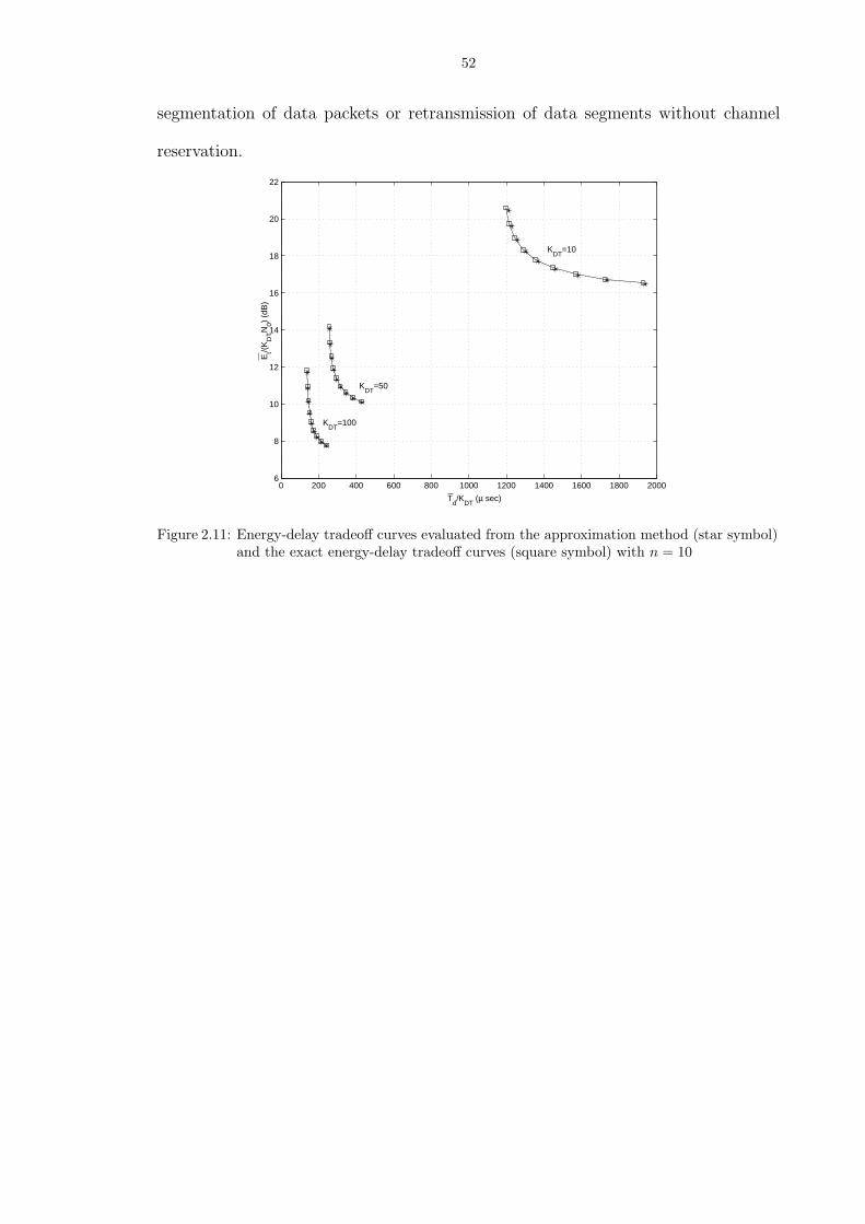
52
segmentation of data packets or retransmission of data segments without channel
reservation.
0 200 400 600 800 1000 1200 1400 1600 1800 20006
8
10
12
14
16
18
20
22
Td/K
DT (µ sec)
Et/(
KD
TN
0) (d
B)
KDT
=10
KDT
=50
KDT
=100
Figure 2.11: Energy-delay tradeoff curves evaluated from the approximation method (star symbol)and the exact energy-delay tradeoff curves (square symbol) with n = 10

CHAPTER III
Variations of 802.11 MAC Protocol
In this chapter, we apply our proposed generating function method to the analysis
and design of two different wireless network protocols modified from the original
IEEE 802.11 protocol. The first wireless network protocol, discussed in Section 3.1,
adapts the energy per coded symbol whenever it suffers a failed transmission. The
second wireless network protocol related to the application of ARQ to IEEE 802.11
is investigated in Section 3.2. The tradeoff between energy and delay is studied for
both proposed protocols. The conclusion of this chapter is stated in Section 3.3.
3.1 Adaptive Energy Scheme for Wireless Network Systems
Wireless networks consists of mobile and sensors devices. Most such devices are
battery powered. Since the energy of a battery is a limiting resource it is important
to have an energy efficient network design. Higher energy efficiency protocols and
signal design may extend the battery lifetime or result in using batteries with smaller
required energy capacity. However, wireless channels have fading that typically re-
quires more energy for transmission than an unfaded channel for the same packet
error probability. Decreasing the amount of energy used in transmission increases
the packet error probability and can increase the delay for a successfully received
packet. Decreasing the transmission delay by increasing the transmission rate gen-
53

54
erally requires more energy. Hence, there is a fundamental tradeoff between energy
and delay in designing a wireless network.
The energy efficiency of wireless networks has been a subject of current research.
In order to synchronize different stations in a wireless network, the beacon needs to be
sent out repeatedly for some time interval. The duration of this time interval is called
beacon interval. In [16], the authors presented a new MAC protocol for energy saving
mode in IEEE 802.11 by proposing a quorum-based sleep/wake-up mechanism, which
conserves energy by allowing the host to sleep for more than one beacon interval if
few transmissions are involved. This new scheme is more energy efficiency compared
to the original IEEE 802.11 energy saving mode since the original scheme fails to
adjust a station’s sleep duration according to its traffic and nearby network topology.
In [8], the authors proposed a new scheduling scheme called adaptive Weighted Round
Robin (WRR) scheme that provides service differentiation in multiple data class
queuing system by considering battery life and load of traffic. As actual energy of
the battery becomes low, the proposed scheme gives more weight to high priority
queue. So high priority data flows would get more chance to be served when energy
in the battery becomes lower. They studied and analyzed the performance of this
scheme and compare its performance with the original IEEE 802.11 standard. Their
results showed that the proposed scheme improves overall end-to-end throughput
as well as support service differentiation over multi-hop wireless networks. The
authors in [51, 42] proposed a novel MAC scheme that changes the duration of
listen/sleep modes adaptively according to the information about the network, e.g.,
network topology and network traffic flows. Their analytical and simulation results
demonstrated a significant decrease in energy consumption.
In a wireless environment, the packet error probability is an important parame-

55
ter in overall system performance. However, in all the above mentioned papers, the
effects of energy consumption for each kind of packet error probability used in IEEE
802.11 (RTS, CTS, DATA and ACK packets) was not considered. Moreover, none of
the above papers consider the energy and delay consumption jointly of transmitting
a data packet in the system. The motivation of this section is to understand the
energy and delay relation of networks by simultaneously incorporating the packet
error probabilities (physical layer) and basic access method (MAC layer) in the per-
formance analysis.
In this section, we propose and analyze an adaptive protocol in which the trans-
mitter will increase the energy level per coded symbol whenever it suffers a failure
transmission. The numerical results show that the proposed scheme can improve sys-
tem performance significantly compared to the original IEEE 802.11 protocol when
the channel condition is bad. By using Reed-Solomon codes we can optimize the
system performance over the code rate and energy per coded bit. Although we use
Reed-Solomon codes over an additive white Gaussian noise (AWGN) channel to rep-
resent packet error probabilities, the framework of our analysis can be used for other
coding and modulation schemes over various wireless channels. Finally, we also com-
pare the system performance between Reed-Solomon codes and convolutional codes.
The rest of this section is organized as follows. In Subsection 3.1.1, we introduce
the system assumptions and give a brief description for the protocol used in our anal-
ysis. In Subsection 3.1.2, we introduce the generating function and determine the
joint generating function for energy and delay. In Subsection 3.1.3, we present nu-
merical results regarding the throughput, energy efficiency and energy/delay tradeoff
with Reed-Solomon codes over an AWGN channel.

56
3.1.1 System Description
The wireless networks that we analyze here have the following specifications. First,
each station with a fixed position can hear (detect and synchronize) the transmission
of n−11 other stations in the network. Second, stations always have a packet ready to
transmit. Third, the receivers have no multiple-access capability (i.e., they can only
receive one packet at a time). Fourth, all stations have fixed position (no mobility).
Fifth, we assume that the propagation loss between transmitter and receiver is one
(0 dB) and also assume that the propagation time is negligible. These assumptions
are valid for local area networks. Finally, each station uses 802.11 protocol for
medium access control (MAC).
In the following we give a brief description of the most salient features of the
IEEE 802.11 MAC protocol (more details can be found in [3] and [4]). When a
station is ready to transmit a packet, it picks randomly a number j, uniformly
distributed in {0, 1, . . . , Wi − 1}, where Wi = 2iW is the contention window (CW)
size, i is the contention stage (initially i = 0), and W is the minimum CW size. A
backoff time counter begins to count down with an initial value j: it decreases by one
for every idle slot of duration σ seconds as long as the channel is sensed idle, stops
the count down when the channel is sensed busy, and reactivates when the channel
is sensed idle again. The station transmits a request-to-send (RTS) packet when
the counter counts down to zero. After transmitting the RTS packet, the station
will wait for a clear-to-send (CTS) packet from the receiving station. If there is a
collision of the RTS packet with other competing stations or a transmission error
occurs in the RTS or CTS packet, the transmitting station doubles the CW size
(increases the contention stage i by one) and picks a random number j as before. If
1n is the density of stations.

57
there are no collisions or errors in the RTS and CTS packets, the station begins to
transmit the data packet and waits for an acknowledgment (ACK) packet. However,
if the data or the ACK packet is not successfully received, the CW size will also be
doubled (the contention stage i will increase by one) and the transmitting station
will join the contention period again. The contention stage is reset (i is set to zero)
when the transmitting station receives an ACK correctly. A time diagram indicating
the sequence of these events is depicted in Fig. 3.1. It is also noted that there is
a maximum CW size (or equivalently, a maximum contention stage, m); when the
transmitter is in this maximum stage and needs to join the contention period again,
it does not increase further the contention window, but picks a random number in
{0, 1, . . . , 2mW − 1}.
The proposed adaptive scheme uses the same MAC protocol as above, however,
the transmitter increases the energy level per coded symbol whenever the CW stage
increases and let Ec,i represent the energy level per coded symbol at transmission
with CW stage i− 1.
frozen slot counter frozen slot counter
reference station unsuccessful transmission
frozen slot counter reference station
successful transmission
T d begin
DIFS
j 0 ~ U(0,W 0 -1)
DIFS
0
DIFS
frozen slot counter
j 1 ~ U(0,W 1 -1)
stage number is increased by 1
DIFS
0
stage number is set back to 0
T d end
DIFS
energy level is E c,1
energy level is E c,0
energy level is E c,0
Figure 3.1: Timing diagram for protocol. The j0 and j1 are backoff random numbers at CW stagei = 0, and i = 1, respectively.

58
3.1.2 System Delay and Energy Analysis
In this section, we analyze the energy and delay characteristics of the wireless
networks described above. The delay Td of each data packet is defined as the time
duration from the moment the backoff procedure is initiated until DIFS seconds after
the ACK packet is received correctly by the transmitting station, as shown in Fig. 3.1.
Similarly, the energy Et is defined as the energy consumed by both transmitting
and receiving stations in the duration of Td. In this paper, we only consider the
energy consumption for packet transmission and omit the energy required for signal
processing and channel sensing since the energy consumption for packets transmission
requires most energy compared to other energy consumption aspects.
Nonlinear System Equations
As in [5], we define two random processes to characterize the random backoff
scheme. The first process bt represents the value of the backoff counter while it
is active. The second random process st is used to represent the contention stage
i ∈ {0, 1, . . . , m} of the station. It uses the same time scale as the backoff counter
process. The first assumption made in this analysis is that the event of packet
collision is independent of past collisions and thus independent of the contention
stage. The second assumption is that the packet collision is identical for all states
(values of bt and st) of a user. As verified in [5], these two assumptions are extremely
accurate when the number of stations in the network is large (say greater then 10).
Let pcc be the conditional collision probability, i.e., the probability of a collision given
a packet transmitted on the channel. As a result of the above assumptions, we will
model the two dimensional process (st, bt) by a discrete-time Markov chain. With
the assumption that errors in transmission can occur only due to collision, the one-

59
step transition probabilities developed in [5] are given by P{i, k | j, l} = P{st+1 =
i, bt+1 = k | st = j, bt = l} with
P{i, k | i, k + 1} = 1, 0 ≤ k ≤ Wi − 2, 0 ≤ i ≤ m
P{0, k | i, 0} = 1−pc
W0, 0 ≤ k ≤ W0 − 1, 0 ≤ i ≤ m
P{i, k | i− 1, 0} = pc
Wi, 0 ≤ k ≤ Wi − 1, 1 ≤ i ≤ m
P{m, k | m, 0} = pc
Wm, 0 ≤ k ≤ Wm − 1.
(3.1)
The first equation in (3.1) corresponds to the decrement of the backoff counter at the
beginning of each time slot. The second equation accounts for the fact that a new
packet following a successful packet transmission starts at contention stage i = 0, and
thus the backoff counter is initially uniformly chosen in the range of {0, 1, . . . ,W0−1}.
The other two cases describe the system evolution after an unsuccessful transmission.
As described in the third equation, when an unsuccessful transmission occurs at
contention stage i − 1, the contention stage increases and the backoff counter is
initialized with a uniformly chosen value in the range {0, 1, . . . ,Wi}. Finally, the
last case models the fact that the contention stage is not increased in subsequent
packet transmissions when the contention window size reaches the maximum. Fig.
4 in [5] depicts the aforementioned two-dimensional Markov chain.
By modifying the Markov chain model described above, we can take into account
packets errors with different energy level per coded symbols. We denote the error
probability of the four kinds of packets at CW stage i in the system as Pe,RTS,i,
Pe,CTS,i, Pe,DT,i and Pe,ACK,i, where i in {0, 1, . . . , m}. Packets which are transmitted
at stage i will be transmitted with energy level Ec,i per coded symbol. We assume
that the channel is memoryless between packets. These probabilities depend on
the particular channel, coding, modulation etc (a specific example will be given in
Section 3.1.3). Let pce,i represent the transition probability from CW stage i to

60
the next. This is also the probability of an unsuccessful transmission attempt seen
by the transmitting station when its packet is being transmitted on the channel.
However, in this paper, an unsuccessful transmission can happen not only due to
packet collision, but also due to packet errors. Using similar assumptions as in [5]
for the packet collision probability pc, and since the events of packet collision and
the event of packet error are independent, pce,i can be expressed as
pce,i = pc + (1− pc)[Pe,RTS,i + (1− Pe,RTS,i)Pe,CTS,i
+ (1− Pe,RTS,i)(1− Pe,CTS,i)Pe,DT,i
+ (1− Pe,RTS,i)(1− Pe,CTS,i)(1− Pe,DT,i)Pe,ACK,i]. (3.2)
The one-step transition probabilities are modified as
P{i, k | i, k + 1} = 1, 0 ≤ k ≤ Wi − 2, 0 ≤ i ≤ m
P{0, k | i, 0} =1−pce,i
W0, 0 ≤ k ≤ W0 − 1, 0 ≤ i ≤ m
P{i, k | i− 1, 0} =pce,(i−1)
Wi, 0 ≤ k ≤ Wi − 1, 1 ≤ i ≤ m
P{m, k | m, 0} = pce,m
Wm, 0 ≤ k ≤ Wm − 1
(3.3)
The packet transmission probability ptx which is the probability of a transmitting
station sending an RTS packet during each backoff slot is obtained by summing over
the stationary probability of all the states at first column of the two-dimensional
Markov diagram as shown in Fig. 4 at [5]. It can be shown as
ptx =2(1 +
∑m−1j=1 (
∏j−1i=0 pce,i) +
∏m−1i=0 pce,i/(1− pce,m))
D, (3.4)
where D is expressed as
D = 1 +m−1∑j=1
(
j−1∏i=0
pce,i) +
∏m−1i=0 pce,i
1− pce,m
+
W (1 +m−1∑j=1
(
j−1∏i=0
2i+1pce,i) +2m
∏m−1i=0 pce,i
1− pce,m
). (3.5)

61
The collision probability pc can be expressed as
pc = 1− (1− ptx)n−1, (3.6)
since the collision will happen if there are at least one remaining n − 1 stations
transmitting packets.
From the above nonlinear equations, (3.2), (3.4) and (3.6), one can evaluate the
probabilities pce,i, ptx and pc. Another important probability that will be used in our
analysis later is the probability of exactly one transmission of an RTS packet from
one of the remaining n− 1 stations given that at least one of the remaining stations
is transmitting. It is denoted by ptx1 and can be expressed as
ptx1 =(n− 1)ptx(1− ptx)
n−2
pc
. (3.7)
Delay/Energy Joint Generating Function
We assume that stations spend energy only in packet transmission and that the
energy consumption for each packet transmission is proportional to the packet length.
Then the energy transmission for a packet of length N (normalized to the thermal
noise energy level, N0) is NEc,i/N0, where i is the stage of CW. Similarly, the trans-
mission delay of each packet is also proportional to the packet length. Let Rt be the
transmitting rate in bits per second. The delay, in seconds, for a packet transmission
with packet length N is N/Rt.
Based on the protocol description in Section 3.1.1, the state flow diagram shown
in Fig. 3.2 can be built. Solid lines represent successful reservation or transmission,
while dotted lines represent unsuccessful reservation or transmission.
Let TRTS, TCTS, TDT and TACK denote the time duration for the transmission
of RTS, CTS, DT and ACK packets, respectively. Similarly, let ERTS,i, ECTS,i,

62
Wait DIFS
successful. channel
reservation ?
successful DT
transmission ?
Wait DIFS
G r s,0
G t s,0 G t s,1 G t s,m
G r s,1 G r s,m
G fr,0 G bs,1
G tf,0 G bs,1 G tf,1 G bs,2
G fr,1 G bs,2
G tf,m-1 G bs,m-1
G fr,m-1 G bs,m-1 G fr,m G bs,m
G tf,m G bs,m
successful. channel
reservation ?
successful. channel
reservation ?
successful DT
transmission ?
successful DT
transmission ?
G bs,0
Figure 3.2: State diagram for the protocol.
EDT,i and EACK,i denote the energy for the transmission of RTS, CTS, DT and
ACK packets at CW stage i, respectively. Finally, let TDIFS and TSIFS be system
delay parameters defined by the standard. We will now derive the conditional joint
generating function of the delay and energy random variables, associated with the
transitions in the state diagram in Fig. 3.2. In all the derivations below, functions
are of the form G(X, Y ), where the variables X, Y are the transform variables of the
delay and energy, respectively.
The generating function Grs,i corresponding to successful channel reservation at
CW stage i is
Grs,i(X,Y ) = (1− pc)(1− Pe,RTS,i)(1− Pe,CTS,i)
XTRTS+TCTS+2TSIFSY ERTS,i+ECTS,i . (3.8)
Similarly, the generating function Gts corresponding to successful transmission of a

63
data packet at CW stage i can be expressed as
Gts,i(X, Y ) = (1− Pe,DT,i)(1− Pe,ACK,i)
XTDT +TACK+TSIFS+TDIFSY EDT,i+EACK,i . (3.9)
We now develop expressions for the generating functions associated with failure to
either reserve a channel or to transmit data. We first derive the generating function
Gfr,i, corresponding to failure to reserve the channel at stage i is given by
Gfr,i(X,Y ) = [pc + (1− pc)Pe,RTS,i]XTRTS+TDIFSY ERTS,i
+ (1− pc)(1− Pe,RTS,i)Pe,CTS,i
XTRTS+TCTS+TSIFS+TDIFSY ERTS,i+ECTS,i , (3.10)
the meaning of which is that a failure can be due to either a collision or RTS trans-
mission error, or a CTS transmission error. Similarly, after reserving the channel, a
failure to transmit a data packet at CW stage i is either due to the data packet trans-
mission error, or the acknowledgement packet transmission error, which is captured
by the generating function Gtf,i as follows
Gtf,i(X, Y ) = Pe,DT,iXTDT +TDIFSY EDT,i + (1− Pe,DT )
· Pe,ACKXTDT +TACK+TSIFS+TDIFS
· Y EDT,i+EACK,i . (3.11)
We now evaluate the generating functions denoted by Gbs,i of the state diagram. This
generating function will characterize the delay for the transmitting station from the
instant of starting the backoff procedure to the instant that the backoff counter
reaches to zero at stage i. We do not need to consider energy consumption here since
the transmitting station stops any transmission at this period. The probability of

64
each slot being sensed busy due to the transmission of other stations is pc and this
event is independent and identical to each slot from our previous assumptions. At
backoff stage i, the range of possible backoff slots is from 1 to 2iW . Let j be the
backoff slots randomly chosen uniformly from the above range, then the number of
the occupied slots in these j slots is binomialy distributed with parameters (j, pc).
Hence, the generating function, Gbs,i, of backoff procedure at stage i is
Gbs,i(X) =2iW∑j=1
1
2iW
j∑
k=0
(j
k
)[(1− pcc)X
σ]j−k
(pcGoc(X))k. (3.12)
where Goc(X) is the generating function for an slot sensed busy by a station. We
define an occupied slot as a slot when the transmitting station senses the channel is
busy due to the transmission of one of the n− 1 remaining stations. There are four
possible cases of an occupied slot. The first case is when two or more RTS packets
from the remaining n − 1 stations collide or have a packet error. The second case
is when the RTS packet is correctly received without collision but there is an error
in the CTS packet transmission. The third case is when the RTS packet is correctly
received without collision and there is no error in the CTS packet but there is an
error in the DT packet transmission. The last case is correct reception of RTS, CTS,
and DT and either correct or erroneous reception of the ACK packet. Since there
are m possible CW stages of packets transmission from the other n − 1 stations,
the probability of the transmission come from CW stage i given only one remaining
n− 1 station transmission is bi,0/ptx, where bi,0 is the stationary probability of state
that CW stage is i and the counter reaches to zero. Note that the time duration
of successful or unsuccessful ACK transmission are same. Therefore, the correspond

65
generating function for this occupied slot is
Goc(X) = (1− ptx1)XTRTS+TDIFS
+ptx1
ptx
l=m∑
l=0
bl,0[Pe,RTS,lXTRTS+TDIFS
+ (1− Pe,RTS,l)Pe,CTS,lXTRTS+TCTS+TSIFS+TDIFS
+ (1− Pe,RTS,l)(1− Pe,CTS,l)Pe,DT,l
XTRTS+TCTS+TDT +2TSIFS+TDIFS
+ (1− Pe,RTS,l)(1− Pe,CTS,l)(1− Pe,DT,l)
XTRTS+TCTS+TDT +TACK+3TSIFS+TDIFS ]. (3.13)
From the state diagram and Mason’s gain formula, we obtain the following back-
ward recursive generating function to characterize the energy and delay of the system.
Let Gs be the system generating function. Then the recursion is
fm(X, Y ) =Grs,mGts,m
1−Gfr,mGbs,m −Grs,mGtf,mGbs,m
fi−1(X, Y ) = Grs,i−1Gts,i−1 + (Gfr,i−1 + Grs,i−1Gtf,i−1)Gbs,ifi
Gs(X, Y ) = Gbs,0f0, (3.14)
where i is the index of the CW stage from 1 to m. Hence, we can evaluate any joint
statistics of the energy and delay of a successful packet transmission. In particular,
the mean values are given by
Td,avg =∂Gs
∂X|X=Y =1, Et,avg =
∂Gs
∂Y|X=Y =1 . (3.15)
3.1.3 Numerical Results
In this section we present and discuss our numerical results for various scenarios
and system parameters. Table 3.1 summarizes the system parameters used to obtain

66
Table 3.1: System Parameters for Numerical ResultsKRTS 128 bitsKCTS 128 bitsKACK 128 bits
Channel Bit Rate, 1/Tb 1 Mbit/sSlot Duration, σ 50µs
Maximum Contention Stage, m 3Minimum Contention Window Size, W 8 slots
TSIFS 28µsTDIFS 128µs
the numerical results. We will use Reed-Solomon codes and convolutional codes to
represent packet error probabilities. Let K be the number of information symbols
(1 symbol = 8 bits) in a packet (specified by the 802.11 standard) and N be the
number of coded symbols for this packet, then the packet error probability PRSe,K,N
over an AWGN channel with BPSK modulation can be expressed as
PRSe,K,N =
N∑
l=t+1
(N
l
)P l
s(1− Ps)N−l, (3.16)
where t = bN−K2c and Ps = 1 − (1 − Q(
√2EbKNN0
))8 is the symbol error probability.
Note that Eb is the energy used per information bit.
In Fig. 3.3, the relation between the average delay throughput STd and the channel
SNR with code rate 12
for different KDT of convolutional codes is shown. For high
SNR, we can find that the throughput increases with longer information packets
because the system with longer information packets has smaller overhead redundant
in RTS/CTS MAC protocol. For low SNR, we observe that the throughput decreases
with longer information packets since the packet error probability for convolutional
codes increases when the length of information packets becomes larger. Moreover,
if longer information packets are used, the effect of packet error probability to the
STd will be more significant compared to the effect of less overhead redundant for
low channel SNR condition. We expect that there is an optimal value of KDT which
achieves the largest throughput for each given channel SNR.
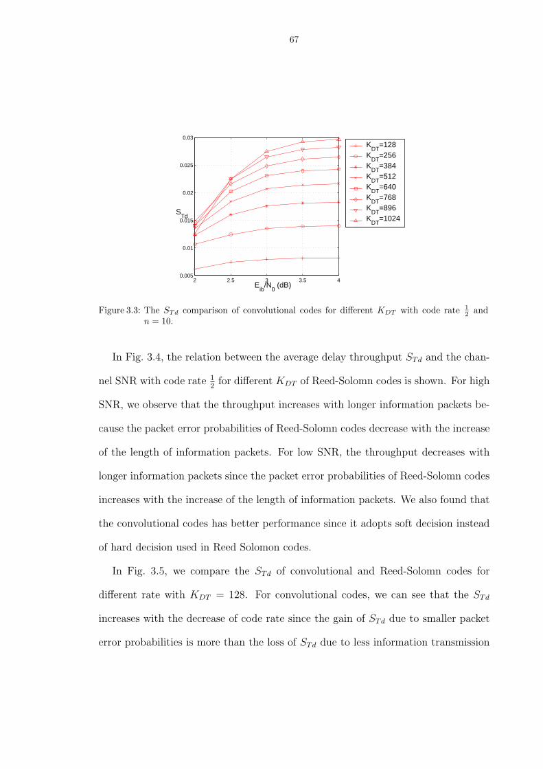
67
2 2.5 3 3.5 40.005
0.01
0.015
0.02
0.025
0.03
Eib
/N0 (dB)
KDT
=128K
DT=256
KDT
=384K
DT=512
KDT
=640K
DT=768
KDT
=896K
DT=1024
STd
Figure 3.3: The STd comparison of convolutional codes for different KDT with code rate 12 and
n = 10.
In Fig. 3.4, the relation between the average delay throughput STd and the chan-
nel SNR with code rate 12
for different KDT of Reed-Solomn codes is shown. For high
SNR, we observe that the throughput increases with longer information packets be-
cause the packet error probabilities of Reed-Solomn codes decrease with the increase
of the length of information packets. For low SNR, the throughput decreases with
longer information packets since the packet error probabilities of Reed-Solomn codes
increases with the increase of the length of information packets. We also found that
the convolutional codes has better performance since it adopts soft decision instead
of hard decision used in Reed Solomon codes.
In Fig. 3.5, we compare the STd of convolutional and Reed-Solomn codes for
different rate with KDT = 128. For convolutional codes, we can see that the STd
increases with the decrease of code rate since the gain of STd due to smaller packet
error probabilities is more than the loss of STd due to less information transmission

68
4.5 5 5.5 6 6.5 7 7.5 8 8.5 9
10−7
10−6
10−5
10−4
10−3
10−2
10−1
KDT
=128K
DT=256
KDT
=384K
DT=512
KDT
=640K
DT=768
KDT
=896K
DT=1024
Eib
/N0 (dB)
STd
Figure 3.4: The STd comparison of Reed-Solomn codes for different KDT with code rate 12 and
n = 10.
efficiency per coded packet when the code rate becomes smaller. For Reed-Solomn
codes, we observe that the STd increases with the increase of code rate since the
loss of STd due to larger packet error probabilities is less than the gain of STd due
to higher information transmission efficiency per coded packet when the code rate
becomes larger.
In Fig. 3.6, we plot the STd of Reed-Solomn codes with the channel SNR for
different code rate as KDT = 128. The STd is affected by two factors, packet er-
ror probabilities and the information transmission efficiency per coded packet (code
rate). For lower code rate, we will have lower information transmission efficiency per
coded packet, however, packet error probabilities may not decrease since the energy
used per coded bit also decreases with the lower code rate from (3.16). Therefore,
the total system throughput STd is the tradeoff result of these two factors. For higher
SNR, since the packet error probabilities are almost zero, the value of STd is dom-
inated directly by the information transmission efficiency per coded packet (code

69
−2 −1.5 −1 −0.5 0 0.5 1 1.5 2 2.510
−18
10−16
10−14
10−12
10−10
10−8
10−6
10−4
10−2
Eib
/N0 (dB)
ST
d
CV, r=1/2RS, r=1/2CV, r=1/3RS, r=1/3CV, r=1/4RS, r=1/4CV, r=2/3RS, r=2/3CV, r=3/4RS, r=3/4CV, r=7/8RS, r=7/8CV, r=15/16RS, r=16/16
Figure 3.5: The STd comparison of convolutional and Reed-Solomn codes for different code ratewith KDT = 128 and n = 10.
rate). For lower SNR, since the gain of STd due to smaller packet error probabilities
is more than the loss of STd due to less information transmission efficiency when the
code rate becomes smaller. Therefore, we can find that there is a cross of STd values
for curve with code rate 78
and curve with code rate 14
at 5.6 dB.
An interesting observation is that there is an optimal N . For small N the packet
error probability of a random code will be large. Large packet error probability will
increase the system delay and energy due to the high chance of packet retransmission.
On the other hand, if N is large, the packet error probability for a random code will
be small but the transmission time will be large. Our goal is to find the best N
for each kind of packet to minimize system delay. We first fix Ec,1/N0 and optimize
the Td,avg to get the corresponding packet lengths for NRTS, NCTS, NDT and NACK .
From this, we can evaluate both average delay and average energy consumption.
Repeating the above argument for different Ec,1/N0, we get the energy-delay curve.
In Fig. 3.7, we compare energy and delay tradeoff curves for different values of

70
2 3 4 5 6 7 810
−8
10−7
10−6
10−5
10−4
10−3
Eib
/N0 (dB)
ST
d
rate :1/2rate :1/3rate :1/4rate :2/3rate :3/4rate :7/8rate :15/16
Figure 3.6: The STd comparison of Reed-Solomn codes for different code rate with KDT = 128 andn = 10.
∆. We observe that the adaptation scheme can improve the system performance
by reducing both average energy and delay as the channel SNR is small. At good
channel condition, although higher value of ∆ can reduce the average delay, the
system incurs higher energy consumption (compared to the system with smaller
value of ∆) to transmit a data packet successfully. This demonstrates that that the
system performance was improved significantly when the channel SNR is low and the
average delay is reduced insignificantly even consuming more energy at high channel
SNR case.
For the effect of different users, we fix the data packet length as KDT = 64
symbols and plot energy-delay curve for different n. We can see from Fig. 3.8 that
both energy and delay increase with the number of users. The other fact shown in
this figure is that both energy and delay increase with the increment of KDT but
the normalized (with respect to KDT ) energy and delay decrease with increasing of
KDT . The explanation of this is that the delay or energy consumption of overhead

71
30 40 50 60 70 80 90 100 1109.6
9.8
10
10.2
10.4
10.6
10.8
11
11.2
11.4
11.6
Td/(8*K
DT) (µ sec)
Et/(
N08*
KD
T)
(dB
)
∆=0 dB
∆=0.6 dB
∆=0.3 dB
Figure 3.7: Comparison of energy and delay curves for different ∆ with n = 10 and KDT = 64.
transmissions such as RTS, CTS and ACK will become less significant for larger data
packet lengths. Hence, when the data packet length is large, we can almost assume
that delay or energy consumption comes solely from KDT .
3.2 802.11 Protocol with ARQ
Recently there has been considerable interest in the design and performance eval-
uation of wireless local area networks (WLANs). According to the OSI protocol
layers specification, the physical layer (lowest layer) handles the transmission of bits
through a communication link and includes the forward error control (FEC) and
modulator/demodulator. The forward error control (FEC) coding technique is used
to mitigate the effect of channel noise at the receiver. The error control coding tech-
nique reduces the required energy needed for transmission at the expense of increased
delay and reduced data rate. The second layer is the data link layer which is respon-
sible for establishing a reliable and secure logical link over the unreliable wireless link.

72
0 50 100 150 200 2509
10
11
12
13
14
15
16
Td/(8*K
DT) (µ sec)
Et/(
N08*
KD
T)
(dB
)
n=10, KDT
=16
n=10, KDT
=32
n=10, KDT
=64
n=30, KDT
=64
n=20, KDT
=64
Figure 3.8: Comparison of energy and delay curves for different n and KDT with ∆ = 0.3(dB).
The lower sublayer of data link layer is the medium access control (MAC) protocol
layer which resolves conflicts between two users attempting to access the channel.
Thus there is some amount of energy and delay spent in reserving the channel. The
upper sublayer of the data link layer (DDL) is logical link control (LLC) sublayer
that implements error control involving feedback from the receiver. The most com-
mon technique to combat errors used in this sublayer is automatic repeat request
(ARQ). Given the energy used per data packet, a wireless communication system
adopting ARQ scheme can provide higher protection by allowing larger retransmis-
sion attempts. However, a system with larger retransmission attempts needs longer
delay to transmit the same data packet. If we want to decrease the delay to transmit
the same data packet, the system requires higher energy per data packet to achieve
the same reliability as a system with lower retransmission attempts. Therefore, there
is an energy and delay tradeoff problem happened in both layers (PHY and DLL).
Several papers have investigated the effects of using ARQ techniques in cross-layer

73
design2 of wireless networks. In [21], the authors explored the possibilities of cross-
layer design as a candidate tool for performance optimization, focusing on problems
deriving from the usage of ARQ schemes in today’s wireless networks and proposed a
novel and general cross-layer interaction scheme between the transport and the link
layers. The proposed design achieves the performance in the framework of a IEEE
802.11-based multi-hop wireless network which demonstrates the value of the pro-
posed framework. In [10], a new cross-layer ARQ algorithm for video streaming over
802.11 wireless networks was presented. The algorithm combines application-level
information about the perceptual and temporal importance of each packet into a sin-
gle priority value, which drives packet selection at each retransmission opportunity.
Hence, only the most most perceptually important packets are retransmitted, deliv-
ering higher perceptual quality and less bandwidth usage compared to the standard
802.11 MAC-layer ARQ scheme. Their results showed that the proposed method
consistently outperforms the standard MAC-layer 802.11 retransmission scheme, de-
livering more than 1.5 dB PSNR gains using approximately half of the retransmission
bandwidth. In [45], the authors proposed a class-based adaptive ARQ scheme with
QoS support for multimedia traffic to increase the throughput through the reduction
of MAC overhead. Different QoS support in the MAC layer is implemented by using
service differentiation and traffic class prioritization. An OPNET simulation model
is used to show that the proposed ARQ enhancement increases system performance.
In a wireless environment, the value of packet error probability can affect the
overall system performance significantly. However, in all above described papers, the
issue of energy consumption for each kind of packet error probability used in IEEE
802.11 (RTS, CTS, DATA and ACK packets) is not discussed. Moreover, none of
2A network system design methodology which considers at least two different function layers jointly during thedesign task.

74
the above papers consider the energy and delay consumption jointly of transmitting
a data packet by considering the effects of physical layer and data link layer char-
acteristics. The contribution of this section is that we propose a state diagram to
represent the operation of the system that allows us to analyze the energy and delay
consumption of the system. We determine the generating function of the state dia-
gram and use it to characterize the joint energy and delay distribution of the system
incorporating physical layer and data link layer characteristics. By using a random
coding bound we can optimize the system performance over the code rate and energy
per coded bit. Although we use random coding for an AWGN channel to represent
packet error probabilities, the framework of our analysis can be used for other coding
and modulation schemes and various wireless channel.
The rest of this section is organized as follows. In Subsection 3.2.1, we introduce
the system assumptions and give a brief description for the protocol used in our
analysis. In Subsection 3.2.2, we introduce the generating function and determine
the joint generating function for energy and delay. In Subsection 3.2.3, we present
numerical results to demonstrate the energy-delay tradeoff with random coding.
3.2.1 System Description
The operation of MAC protocol will be the same as 802.11 standard except the
transmission of data packets. Suppose each transmitter has K (fixed) information
bits to be transmitted. These K bits will be encoded to form a packet with length N1
and transmit. If the receiver decodes this packet correctly, it sends an ACK to the
transmitter. Otherwise, if decoding is not correct, after the expiration of a timeout
the transmitter encodes the same number of information bits K to a packet of length
N2 and transmits it again. This procedure will continue (using length Nl packets for
the l-th transmission) until either the transmitter receives the ACK correctly or the

75
total number of attempts achieves a maximum allowed number, d.
3.2.2 Analysis
In this section, we analyze the energy and delay characteristics of the wireless
networks operated according to previous subsection. The delay Td and Et of each
data packet is defined as before.
We begin by calculating some important event probabilities that are crucial in
later analysis. The performance evaluation is based on the Markov chain model
described in [5] and [22]. The state of the Markov chain represents the value of the
backoff counter and the contention window stage. Our model differs from the model
proposed in [5, 22] in that packet error probabilities are included in the CW stage
transition probability. By modifying the Markov chain model described in [5, 22],
we can incorporate the packet error probabilities into the analysis. We denote the
error probability of an RTS packet as Pe,RTS, a CTS packet as Pe,CTS and an ACK
packet as Pe,ACK . The probability Pe,DTirepresents the error probability of ith
transmission of a data packet, where 1 ≤ i ≤ d. We assume that the channel is
memoryless between packets. These probabilities depend on the particular channel,
channel coding, modulation etc. (a specific example will be given in Section 3.2.3).
Let pce represent the transition probability (as defined in [5]) from one CW stage to
the next. This is also the probability of an unsuccessful transmission attempt seen
by the transmitting station when its packet is being transmitted on the channel.
However, in this work, an unsuccessful transmission can happen not only due to
packet collision, but also due to packet errors. There are four possible cases when
the channel is sensed busy. The first case is that the RTS packet suffers a collision
or packet error. The second case is that the RTS packet is correctly received and
collision free but there is an error in the CTS packet transmission. The third case is
76
that the RTS packet is correctly received and collision free, there is no error in CTS
packet, but there is an error in all d transmissions of the DT packet. The last case
is that the data packet is correctly received in one of these d transmissions but there
is an error in the corresponding ACK packet. Because the event of packet collision
and the event of packet error are independent, pce can be expressed as
pce = pc + (1− pc)[Pe,RTS + (1− Pe,RTS)Pe,CTS+
(1− Pe,RTS)(1− Pe,CTS)d∏
i=1
Pe,DTi+ (1− Pe,RTS)·
(1− Pe,CTS)(d∑
i=1
i−1∏j=0
Pe,DTj(1− Pe,DTi
))Pe,ACK ]. (3.17)
where pc is the packet collision probability and we set Pe,DT0 = 1. The packet
transmission probability ptx which is the probability of a transmitting station sending
an RTS packet during each backoff slot, and the collision probability pc can be
expressed as (see [5])
ptx =2(1− 2pce)
(1− 2pce)(W + 1) + pceW (1− (2pce)m)(3.18)
and
pc = 1− (1− ptx)n−1. (3.19)
From the above three nonlinear equations, (3.17)–(3.19), one can evaluate the
probabilities pce, ptx and pc. Another important probability that will be used in our
analysis later is the probability of a transmission of an RTS packet from exactly one
of the remaining n − 1 stations given that at least one of the remaining stations is
transmitting. It is denoted by ptx1 and can be expressed as
ptx1 =(n− 1)ptx(1− ptx)
n−2
pc
. (3.20)
We assume that stations spend energy only in packets transmission and that the
energy consumption for each packet transmission is proportional to the packet length.

77
In particular, let αEc be the energy required to transmit one coded bit, where α > 1
is the inverse of the path loss between transmitter and receiver. Then the energy
received for a packet of length N (normalized to the thermal noise energy level, N0)
is NEc/N0. Similarly, the transmission delay of each packet is also proportional to
the packet length. Let Rt be the transmitting rate in bits per second. The delay,
in seconds, for a packet transmission with packet length N is N/Rt. Based on the
protocol description in Section 3.2.1, the state flow diagram shown in Fig. 3.9 can
be built.
Wait DIFS
successful. channel
reservation ?
successful DT
transmission ?
Wait DIFS
G bs,0
G r s
G t s G t s G t s
G r s G r s
G rf G bs,1
G tf G bs,1 G tf G bs,2
G rf G bs,2
G tf G bs,m
G rf G bs,m
G rf G bs,m
G tf G bs,m
successful. channel
reservation ?
successful. channel
reservation ?
successful DT
transmission ?
successful DT
transmission ?
Figure 3.9: State diagram for the protocol. Solid lines represent successful reservation or transmis-sion, while dotted lines represent unsuccessful reservation or transmission.
Let TRTS, TCTS, TDTkand TACK denote the time duration for the transmission
of RTS, CTS, k-th DT and ACK packets, respectively. Similarly, let ERTS, ECTS,
EDTkand EACK denote the (received) energy for the transmission of RTS, CTS,
k-th DT and ACK packets, respectively. Finally, let TDIFS and TSIFS be system
delay parameters defined by the standard. We will now derive the joint generating

78
function of the delay and energy random variables associated with the transitions
in the state diagram in Fig. 3.9. In all the derivations below, functions are of the
form G(X,Y ), where the variables X, Y are the transform variables of the delay and
energy, respectively.
The generating function Grs corresponding to successful channel reservation is
Grs(X, Y ) = (1− pc)(1− Pe,RTS)(1− Pe,CTS)
XTRTS+TCTS+2TSIFSY ERTS+ECTS . (3.21)
Similarly, the generating function Gts corresponding to successful transmission of a
data packet can be expressed as
Gts(X, Y ) =d∑
i=1
(i−1∏j=0
Pe,DTj)(1− Pe,DTi
)(1− Pe,ACK)
XPi
k=1 TDTk+TACK+iTSIFS+TDIFSY
Pik=1 EDTk
+EACK . (3.22)
We now develop expressions for the generating functions associated with failure
to either reserve a channel or to transmit data. As can be seen from the state
diagram, these functions are products of two generating functions. Each product
contains a factor that is independent of the particular contention stage, and a factor
that depends on the contention stage i. We first describe the constant factors. The
generating function Gfr, corresponding to failure to reserve the channel is given by
Gfr(X,Y ) = [pc + (1− pc)Pe,RTS]XTRTS+TDIFSY ERTS
+ (1− pc)(1− Pe,RTS)Pe,CTS
XTRTS+TCTS+TSIFS+TDIFSY ERTS+ECTS , (3.23)
the meaning of which is that a failure can be due to either a collision/RTS trans-
mission error, or a CTS transmission error. Similarly, after reserving the channel,

79
a failure to transmit a data packet is either due to the data packets transmission
error, or the acknowledgement packet transmission error, which is captured by the
generating function Gtf as follows
Gtf (X, Y ) = (d∏
i=1
Pe,DTi)X
Pdk=1 TDTk
+(d−1)TSIFS+TDIFS ·
YPd
k=1 EDTk +d∑
i=1
(i−1∏j=0
Pe,DTj(1− Pe,DTi
)Pe,ACK ·
XPi
k=1 TDTk+TACK+iTSIFS+TDIFSY
Pik=1 EDTk
+EACK ). (3.24)
We now evaluate the generating functions denoted by Gbs,i of the state diagram.
This generating function characterizes the delay for the transmitting station from
the instant of starting the backoff procedure to the instant that the backoff counter
reaches to zero at stage i. We do not need to consider energy consumption here since
the transmitting station stops any transmission during this period. The event of
each slot being sensed busy due to the transmission of other stations is independent
for each slot and has the same probability, pc, for each slot (from our previous
assumptions). At backoff stage i, the range of possible backoff slots is from 1 to
2iW . Let j be the backoff slots randomly chosen uniformly from the above range,
then the number of the occupied slots in these j slots is binomially distributed with
parameters (j, pc). Hence, the generating function, Gbs,i, of backoff procedure at
stage i is
Gbs,i(X) =2iW∑j=1
1
2iW
j∑
k=0
(j
k
)[(1− pc)X
σ]j−k(pcGoc(X))k, (3.25)
where Goc(X) is the generating function for an occupied slot. We define an occupied
slot as a slot when the transmitting station senses the channel is busy due to the
transmission of one of the remaining n− 1 stations. Using arguments similar to the

80
ones used in the derivation of (3.17), we can express Goc(X) as follows
Goc(X) = [(1− ptx1) + ptx1Pe,RTS]XTRTS+TDIFS+
ptx1(1− Pe,RTS)Pe,CTSXTRTS+TCTS+TSIFS+TDIFS+
ptx1(1− Pe,RTS)(1− Pe,CTS)(d∏
i=1
Pe,DTi)·
XTRTS+TCTS+Pd
k=1 TDTk+(d+1)TSIFS+TDIFS+
ptx1(1− Pe,RTS)(1− Pe,CTS)d∑
i=1
i−1∏j=0
Pe,DTj·
(1− Pe,DTi)X
Pik=1 TDTk
+TACK+(i+2)TSIFS+TDIFS . (3.26)
From the state diagram and Mason’s gain formula, we obtain the following backward
recursive generating function to characterize the energy and delay of the system. Let
Gs be the system generating function. Then the recursion is
fm(X, Y ) =GrsGts
1−GfrGbs,m −GrsGtfGbs,m
fi−1(X, Y ) = GrsGts + (Gfr + GrsGtf )Gbs,ifi
Gs(X, Y ) = Gbs,0f0, (3.27)
where i is the index of the CW stage from 1 to m. Hence, we can evaluate any joint
statistics of the energy and delay of a successful packet transmission. In particular,
the mean values are given by
T d =∂Gs
∂X|X=Y =1, Et =
∂Gs
∂Y|X=Y =1 . (3.28)
3.2.3 Numerical Results
We will use channel reliability based bounds for an AWGN channel to estimate the
packet error probability. Let K be the number of information bits in a packet (spec-
ified by the 802.11 standard) and N be the number of coded bits in a packet. Then
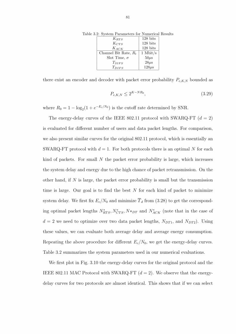
81
Table 3.2: System Parameters for Numerical ResultsKRTS 128 bitsKCTS 128 bitsKACK 128 bits
Channel Bit Rate, Rt 1 Mbit/sSlot Time, σ 50µs
TSIFS 28µsTDIFS 128µs
there exist an encoder and decoder with packet error probability Pe,K,N bounded as
Pe,K,N ≤ 2K−NR0 , (3.29)
where R0 = 1− log2(1 + e−Ec/N0) is the cutoff rate determined by SNR.
The energy-delay curves of the IEEE 802.11 protocol with SWARQ-FT (d = 2)
is evaluated for different number of users and data packet lengths. For comparison,
we also present similar curves for the original 802.11 protocol, which is essentially an
SWARQ-FT protocol with d = 1. For both protocols there is an optimal N for each
kind of packets. For small N the packet error probability is large, which increases
the system delay and energy due to the high chance of packet retransmission. On the
other hand, if N is large, the packet error probability is small but the transmission
time is large. Our goal is to find the best N for each kind of packet to minimize
system delay. We first fix Ec/N0 and minimize T d from (3.28) to get the correspond-
ing optimal packet lengths N∗RTS, N∗
CTS, N∗DT and N∗ACK (note that in the case of
d = 2 we need to optimize over two data packet lengths, NDT1, and NDT2). Using
these values, we can evaluate both average delay and average energy consumption.
Repeating the above procedure for different Ec/N0, we get the energy-delay curves.
Table 3.2 summarizes the system parameters used in our numerical evaluations.
We first plot in Fig. 3.10 the energy-delay curves for the original protocol and the
IEEE 802.11 MAC Protocol with SWARQ-FT (d = 2). We observe that the energy-
delay curves for two protocols are almost identical. This shows that if we can select

82
packet lengths properly, the SWARQ-FT does not give significant improvement. To
compare these two protocols with respect to their robustness to SNR, we fix the
packet lengths, vary Ec/N0 and plot energy and delay for both protocols. We observe
that both systems are equally and very sensitive to SNR. Essentially, the reduction
in delay the SWARQ achieves by immediately retransmitting an erroneously received
packet, is compensated by the increased delay needed to access the channel, since
other users use the same protocol. While ARQ provides some robustness to SNR
uncertainty in conventional single user system, this is not the case in this multiuser
scenario.
In Fig. 3.11, the energy-delay tradeoff is plotted for the SWARQ protocol for dif-
ferent values of quantity NDT −KDT /R0(Ec/N0). This figure shows that the optimal
packet lengths are on the order of 60 bits larger than the minimum length implied
by the cutoff rate. For high SNR values as small as 10 will provide almost optimal
performance, while for low SNR, the number of redundant bits has to increase.
3.3 Conclusion
In this chapter, we applied our generating function method to characterize the
energy and delay of a wireless network for two proposed protocols modified from
802.11 standard. The first proposed protocol is related to the adaptive energy scheme
which is implemented by increasing the energy level per coded bit due to previous
failure transmission attempts. The numerical results indicated that both throughput
and energy efficiency are improved significantly when the channel SNR is low. The
second proposed protocol is to incorporate the IEEE 802.11 protocol with SWARQ-
FT. Our results demonstrated that both protocols (original IEEE 802.11 and IEEE
802.11 with SWARQ-FT) are sensitive to the knowledge at the transmitter of the

83
received SNR. This is a consequence of the steep falloff of packet error probability
with respect to SNR for random coding. We expect similar results when LDPC or
turbo codes are used. Our methods can be extended to the analysis of other protocols
or to consider a wireless network system where more function layers are involved by
representing the operation of a protocol with a system state diagram. Once the
system state diagram is obtained, we shall be able to derive the joint generating
function of interesting random variables for the state diagram. In this thesis, we
select energy and delay consumption as our interesting variables since we want to
determine the energy and delay tradeoff. However, one may select other variables
in the generating function for their analysis purpose, such as event’s cost, event’s
reliability, etc. Therefore, the generating function approach allows one to find the
entire system performance distribution based on the performance distribution of its
elements by using algebraic procedures in a systematic way.
15 20 25 30 35 40 45 503
3.5
4
4.5
5
5.5
6
6.5
7
Td/(K
DTN
0) (µsec)
Et/K
DT (
dB)
10
Figure 3.10: Energy-delay curves for n = 10 and KDT = 1400. Solid lines represent the curvesafter packets optimization. Dashed lines represent the energy-delay curves for Ec/N0
of 0 and 3 dB using the optimal packet lengths.

84
15 20 25 30 35 40 45 50 55 603
4
5
6
7
8
9
Td/K
DT (µ sec)
Et/(
KD
TN
0) (d
B)
210
110
60
10
Optimal SWARQ
Figure 3.11: The dashed lines represent SWARQ after optimization. The number beside the curveis the redundant bits.

CHAPTER IV
Analysis of Energy and Delay for ARQ Systems over TimeVarying Channels
4.1 Introduction
Error control techniques can generally be classified either as forward-error-correction
(FEC) or as automatic-repeat-request (ARQ). Although FEC can provide a commu-
nication system with a fixed throughput which is equal to the code rate, the dis-
advantage of a conventional FEC system without feedback is that the transmitter
does not adjust the error correction capability according to the channel variations.
Thus the code rate must be low enough for the worst-case channel. An ARQ system
changes the error correction capability to adapt to the channel variation by using
a feedback channel. Therefore, ARQ error control systems are more suitable than
FEC systems for error control in data communication systems having time varying
channels where a feedback channel is available [35, 47]. The advantages of both FEC
and ARQ techniques can be obtained by combining the techniques within a single
hybrid-ARQ protocol [34].
In general, ARQ protocols are classified into three basic schemes: stop-and-wait
(SW), go-back-N (GBN), and selective-repeat (SR). In SW-ARQ, the transmitter
must receive the ACK of a packet before transmitting the next packet. This scheme
preserves the order of packets but results in low channel utilization if the round-
85

86
trip delay is large. In GBN-ARQ, packets are transmitted continuously without
waiting for ACKs/NACKs. Upto to N subsequent packets can be transmitted before
receiving an ACK/NACK for a given packet. If a NACK is received, the transmitter
retransmits the negatively acknowledged packet and all subsequent packets regardless
of their acknowledgments. The round trip delay is assumed to be smaller than
N times the packet duration and the transmitter is capable of storing N packets.
In SR-ARQ, packets are transmitted continuously as in GBN, but only negatively
acknowledged packets are retransmitted. Of the three schemes, SR-ARQ achieves
the highest throughput but requires the most feedback.
For a fixed amount of energy used per information bit, a wireless communication
system adopting FEC can provide higher protection by using a lower code rate.
However, a system with lower code rate needs longer delay to transmit the same
information packet due to the fixed bandwidth. If we want to decrease the delay
required to transmit the same information packet, a system with high code rate
requires higher energy per information bit to achieve the same reliability as a system
with lower code rate. Similarly, an ARQ system requires higher energy to transmit
an information packet successfully with fewer trials (shorter delay to transmit a
packet). On the other hand, we may use more attempts (longer delay) to transmit
the same information packet successfully and use smaller energy. Therefore, there
is a fundamental tradeoff between energy and delay in a wireless communication
system.
Many adaptive ARQ protocols have been suggested in the literature to improve
the system delay (or equivalently throughput). In [9, 37, 50], different block (packet)
sizes and multicopy transmission schemes were used as adaptation mechanisms, re-
spectively. On the other hand, in [44, 26, 40], the authors suggested to vary the

87
FEC code rate to compensate for the variations in the channel conditions. Although
the above papers consider the analysis based on time varying channels, they do not
consider the energy consumption as part of the system performance. In [38], the au-
thors investigated the energy savings of an ARQ strategy within two different time
varying channels; fast Rayleigh fading and log-normally shadowed Rayleigh fading.
However, their work does not provide the exact method to evaluate the system delay.
Another important issue that previous research has not addressed is the relation of
the channel transition probability with the transmission delay of a packet. Most
previous papers just assume that the channel transition probability is the same for
different packet lengths. However, this assumption is not reasonable if the variation
of packet lengths is large.
In this chapter, we propose an analytical method to determine the joint distribu-
tion of the energy and delay of automatic repeat request (ARQ) schemes over time
varying channels. By extending the traditional Markov chain [13] that models the
channel as well as the transmitter, the overall system operation can be represented
by a state diagram that takes into account the joint operation of the transmitter, re-
ceiver and channel. The model of the transmitter accounts for different packet lengths
used by the transmitter and the model of the receiver accounts for the receiver mem-
ory [27]. We determine the joint generating function of the energy consumed and
delay incurred of an ARQ system from its state diagram. The joint generating func-
tion enables us to characterize the joint energy and delay distribution of the system
incorporating physical layer characteristics (packet error probability as a function of
energy and delay). The effect of packet length on the channel transition probability
is also investigated. As the numerical results demonstrate, the time-varying charac-
teristics of the channel have a great influence on system performance especially at

88
low channel SNR.
The rest of the chapter is organized as follows. In Section 4.2, we model an ARQ
system with a finite state machine (FSM) by considering the transmitter, receiver
and channel states jointly. A general ARQ system which allows different packet
lengths in each retransmission is discussed and analyzed in Section 4.3. Several
practical ARQ systems with specific packet lengths are considered in Section 4.4.
The detailed derivation of the generating functions for systems discussed in Sub-
section 4.4.1 and 4.4.2 will be presented in the appendices. Another kind of ARQ
system, go-back-N ARQ (GBN-ARQ), will be investigated in Section 4.5 and its joint
generating function for energy and delay over time varying channels will be derived.
In Section 4.6, the cutoff rate for two kinds of receiver structures that contain mem-
ory is derived. In Section 4.7, we present numerical results for the performance by
considering the energy and delay relationship with random coding for Gilbert-Elliott
channels. The conclusions are given in Section 4.8.
4.2 FSM Model, Channel Model and Assumptions for ARQ Systems
A finite state machine (FSM) or finite automaton is a model of a system which
is composed of states, transitions and actions. Originally defined in the automata
theory, FSM’s are used in the theory of computation [12]. Finite state machines
are very widely used in modeling of application behavior, design of hardware digital
systems, software engineering, study of computation and languages. A state stores
a cumulative information about the past, i.e. it reflects the input changes from
the system start to the present moment. The content of a state depends on the
characteristics and behaviors of the system that we are interested in. A transition
indicates a state change and is described by a condition that would need to be fulfilled
89
to enable the transition. An action is a description of an activity that is to be
performed at a given state. A finite state machine is a sextuple < Σ, Γ, S, s0, δ, ω >,
where:
• Σ is the alphabet of the input variables.
• Γ is the alphabet of the output variables.
• S is a finite non empty set of states.
• s0 is an initial state.
• δ is the state transition function: δ : S × Σ → S.
• ω is the output function ω : S × Σ → Γ.
By extending the traditional Markov chain that models the channel state, the
overall ARQ system operation is represented by a modified FSM that also takes into
account the states of the transmitter and the receiver. The states of the transmitter
can be used to model the different coding or modulation schemes and the states of
the receiver can be utilized to model the receiver memory content or different decod-
ing schemes. For our communication system model, the state for the transmitter,
channel and receiver we be consider jointly in the system state space S. Also for our
purpose the output of modified transition functions δ, i.e., the next state, is a ran-
dom state with some probability distribution due to the uncertainty of the channel
characteristic. To determine the energy and delay generating function of the system,
the output at each state is used to characterize the energy and delay consumed at
the state. By using the concept of signal flow proposed by Mason [20], the total
energy and delay generating function from the initial state to the final state can be
obtained from Mason’s gain formula.

90
Gilbert-Elliott Channel Model
To model time-varying channels, the Gilbert-Elliott channel model is widely used [26].
It uses two states to characterize the channel condition, the state for good channel
condition is designated by G and the state for bad channel condition is designated by
B. In each channel state, we model the channel as AWGN channel and assume that
the channel signal-to-noise ratio (SNR)1 of good state is SNRG and the channel SNR
of bad state is SNRB. We define r as the ratio of the channel SNR between good
and bad states, i.e., r = SNRG
SNRB. We assume that the duration of the good and bad
states are exponentially distributed with mean 1/λ and 1/µ, respectively. The value
λ is the transition rate from good to bad channel condition and µ is the transition
rate from bad to good channel condition. From the above system parameters, we
can determine the average channel SNR (SNRavg), i.e., SNRavg = µSNRG+λSNRB
λ+µ.
The Gilbert-Elliott channel model can be specified completely if the following four
parameters are given : (r, SNRavg, λ, µ). The crossover probabilities between chan-
nel states are determined by the time duration of occupying the current state before
the event of next channel transition and the channel transition rates. If the time
duration for a packet transmission is T∗ where the subscript is used to distinguish
different packet types, then the channel transition probability from good state to
good (bad) state is e−λT∗ (1 − e−λT∗). Similarly, the channel transition probability
from bad state to bad (good) state is e−µT∗ (1−e−µT∗). The channel model is shown
in the Fig. 4.1
General ARQ Systems
A general stop and wait (SW) ARQ protocol is described as follows. Whenever
there is an information packet with length K generated, it will be encoded to a
1The SNR is the power ratio between a signal (meaningful information) and the background noise.

91
Good state(High SNR)
Bad state(Low SNR)
Figure 4.1: Gilbert-Elliott channel model for time varying channel.
data packet with length N1. The coded bits are passed to the modulator. The
modulator maps the input sequence of bits to a signal waveform. We will assume
binary phase-shift keying (BPSK) modulation scheme is used by the transmitter.
After the modulated waveform is generated, it is propagated through the channel.
We use the symbol Tb to represent the time duration needed to transmit a coded bit
and the symbol Ec to indicate the energy consumption required to transmit a coded
bit.
The demodulator of the receiver is implemented by a maximum a posterior prob-
ability (MAP) criterion in determining the transmitted signal. After demodulation,
the data packet will be decoded. If the data packet is decoded correctly at the re-
ceiver, the receiver will send an ACK packet back to the transmitter. If it is decoded
incorrectly at the receiver, a NACK packet will be sent back to the transmitter and
the received signal samples corresponding to the erroneously decoded packet will be
stored in the receiver memory. Then the transmitter will encode the same informa-
tion packet again to a data packet with length N2 and transmit it. After receiving
this packet with length N2, the receiver will decode this new packet jointly with those
packets stored in the receiver memory. If the data packet is decoded correctly at the
receiver, the receiver will send an ACK packet back to the transmitter. If it is de-

92
coded incorrectly at the receiver, a NACK packet will be sent back to the transmitter
and the new erroneously decoded packet (N2) will be stored in the receiver memory.
After receiving the NACK packet, the transmitter will encode the same information
packet with length N3 and retransmit. The above procedure will be repeated until
an ACK is received by the transmitter. Because we allow different packet lengths
used in each retransmission, therefore, the sequence of packet lengths in transmission
given an information packet has the following form: {N1, N2, N3, · · · }. If we use no-
tation N to represent a set of natural numbers, then the set of {N1, N2, N3, · · · } can
be written as {Ni|i ∈ N}. When an ACK is received by the transmitter, a new coded
packet is transmitted with length N1. Let mR be the maximum number of packets
that the receiver can store in its memory. If the number of consecutive packet errors
is greater then mR, the receiver memory will take some action to keep the number
of stored packets smaller or equal than mR. For example, the receiver may update
the receiver memory content by storing the newest erroneous packet and discarding
the oldest erroneous packet.
We make following assumptions about our system: (1) The ACK and NACK pack-
ets are error free, (2) the round-trip delay and the transmission time of the ACK and
NACK packets are negligible, (3) delay is incurred only during data packet trans-
mission, (4) energy is consumed only during data packet transmission, the trans-
mission energy of ACK and NACK packets are negligible, (5) the Gilbert-Elliott
channel model will be adopted. (6) the event of packet errors is independent of the
event of channel transition. However, it is straightforward to consider the cases with
ACK/NACK packet error and the round-trip delay under our analytical framework.

93
4.3 Generating Function Analysis for General ARQ Systems
We will derive the generating function of energy and delay consumption for a
general ARQ system in this section. For the notational clarity, the corresponding
elements of the FSM for a generalized ARQ system are listed as follows :
• (Input variables) Since the system will change its state when an ACK or NACK
packet is received by the transmitter, we use Σ to represent the input space,
i.e., Σ = {ACK, NACK}.
• (Output variables) For the requirements of the generating function approach
for the energy and delay consumption between each state transition (as shown
in Chapter 2), the symbol Γ is used to represent the output space, i.e., Γ =
{XNiTbY NiEc |i ∈ N}.
• (State space) Because the transmitter can use different packet lengths for each
retransmission, we use ST to represent the state space for the transmitter, i.e.,
ST = {Ni|i ∈ N}. The channel state space for one packet transmission is de-
noted as SC and SC = {G, B} since the Gilbert-Elliott model is adopted.
The state space for the receiver represents the lengths of the packets stored
in the memory and the corresponding channel condition. If a memory loca-
tion does not contain a packet, e.g., at startup, then we represent that by a
packet length N0. The state space for the receiver is denoted by SR which is
a collection of vectors of length 2mR. The first pair contains the channel state
and packet length of the most recently received erroneous packet. The next
pair contains the channel state and packet length of the previous erroneously
received packet. For example, the state of the receiver for memory with mR = 3
might be [G,N3, B,N2, G, N1]. After receiving a packet with length N4 trans-

94
mitted in the bad channel condition, the next state of the receiver memory will
be [B, N4, G, N3, B, N2]. We will use use a shorthand notation for the state of
the receiver memory by representing Gi as a packet of length Ni received when
this packet is transmitted in the good channel condition. So the receiver state
[G,N3, B, N2, G, N1] can be written compactly as [G3, B2, G1]. Therefore, the
total state space of the system which contains the information about the chan-
nel, the transmitter, and the receiver is denoted as vectors of length 2(mR + 1).
The first component of this vector represents the channel state and the second
component of this vector represents the transmitter state. The remaining 2mR
components represent the receiver memory state. A state of the system, de-
noted as s, can be written as s = [sC , sT , sR]. For notational simplicity, the
total system state can also be expressed as [Gi, sR] ([Bi, sR]) for the case that
the transmitter sends a packet with length Ni in good (bad) channel condition
given that the receiver state is sR. In Fig. 4.2, we show an example about the
transition of states for a system with mR = 2 with the sliding window operation
in the receiver memory. The detail about the sliding window operation in the
receiver memory will be presented in subsection 4.4.1.
For later derivation convenience, the state space of packet lengths for the re-
ceiver is denoted by SR which is a collection of vectors of length mR. The first
component of SR contains the packet length of the most recently received er-
roneous packet. The next component of SR contains the packet lengths of the
previous erroneously received packets. For example, if the state space for the
receiver is [G,N3, B, N2, G, N1], then the the corresponding state space for the
packet lengths is [N3, N2, N1]. Given an element from SR, say sR, and we assume
that there are a packet lengths in the vector sR. In order to consider all possibil-

95
GN1 Φ ΦGN2 ΦGN1
GN3 GN2 GN1
BN4 GN3 GN2
BN5 BN4
1-st TX, with N1 in G channel
2-nd TX, with N2 in G channel
3-rd TX, with N3 in G channel
4-th TX, with N4 in B channel
5-th TX, with N5 in B channel
NACK
NACK
NACK
NACK
After receiving ACK, the 1-st TX begin with N1
GN3
Figure 4.2: An example for a general ARQ system with mR = 2. The first slot represents the stateof the channel and transmitter. The second and third slots represent the state of thereceiver memory. The second (third) slot is used to represent the first (second) positionof the the receiver memory.
ities for the receiver memory states that have these a packet lengths, the index
l for 1 ≤ l ≤ 2a, called channel realization index, is used to distinguish different
memory states introduced by the randomness of the channel. The channel real-
ization index l is assigned to the set of all channel realizations of these a packets
according to the lexicographically order by assuming G > B and the position
order of the receiver memory. The symbol sR(l) represents a state of the re-
ceiver memory that the state of packet lengths for the receiver is sR and the
channel realization index is l. For example, if mR = a = 2 and sR = [N3, N3],
then all possible states of the memory are {[G3, G3], [G3, B3], [B3, G3], [B3, B3]}.
By the above ordering regulation, we have sR(1) = [G3, G3], sR(2) = [G3, B3],
sR(3) = [B3, G3] and sR(4) = [B3, B3]. We have two ways to represent the mem-
ory content; one is sR and the other is sR(l). Each element of SR may differ
in the number of packets stored in the receiver memory. However, all memory
states associated with sR(l) have the same number of packets and packet length
indices stored in the receiver memory for each channel realization index l.

96
• (Initial state) The initial state is represented by the symbol sini. This is a state
used at the first time transmission of an information packet. If the memory
content is empty at the first transmission, then sini = G1 if the initial channel
condition is good and sini = B1 if the initial channel condition is bad.
• (State transition function) The state transition function, δ, will define the tran-
sition between states for different input. It will map an element of space S ×Σ
to an element of space S. If the input is a NACK after the k-th transmis-
sion, then the state of the system sk will be mapped into the state sk+1 by
the transition function δ as δ(sk, NACK) → sk+1. The k-th transmission is
counted from the transmission of the original K information bits with packet
length N1 (1-st transmission). If the input is an ACK, then the state of sk will
be mapped into the state of sini by function δ as δ(sk, ACK) → sini. Since
s = [sC , sT , sR], we also have δ([skC , sk
T , skR], NACK) → [sk+1
C , sk+1T , sk+1
R ] and
δ([skC , sk
T , skR], ACK) → [sini
C , siniT , sini
R ]. The state transition function δ will be
determined by specified protocol and this is often represented by a state dia-
gram.
• (Output functions) The output function will map a system with state sk to
XNkTbY NkTc since the packet length used in the k-th transmission is Nk.
Recall that an event is a set of random outcomes to which a probability is assigned.
For the energy and delay analysis of ARQ systems, we then define the joint generating
function of an event as:
Gevent(X,Y ) = Pr(event)XTeventY Eevent , (4.1)
where Tevent(Eevent) is the required delay (energy) for this event. If we are interested
in evaluating the generating function for a set of disjoint events, then the generating

97
function for all events in this group has the following form
Ggroup(X,Y ) =∑
i∈group
Pr(eventi)XTeventi Y Eeventi , (4.2)
where i is the index for events in this group and Teventi(Eeventi) is the required delay
(energy) for this i-th event.
We use symbol Ef,Gi|siR
to represent the event that the transmitter receives a
NACK (failure) after the i-th transmission of a given packet in the good channel
condition given that the receiver memory state is siR. Note that the state space of
the system can be expressed as [Gi, siR] when this event happens because the packet
length used in the i-th transmission is Ni. The generating function of this event is
represented by Gf,Gi|siR
according to (4.1). Similarly, Gf,Bi|siR
is used to represent the
generating function for the event that the transmitter receives a NACK after the i-th
transmission in bad channel condition given that the receiver memory state is siR.
The probability Pe,Gi|siR
(Pe,Bi|siR) is used to represent the packet error probability
for the i-th transmission in the good (bad) channel condition given that the memory
state is siR. If the memory content is empty at i-th transmission, the probability Pe,Gi
(Pe,Bi) is used to represent the packet error probability for the i-th transmission in
the good (bad) channel condition. We will use the shorthand notation, α = 1 − α,
for the following derivation.
Because the i-th (for i ≥ 2) unsuccessful transmission is preceded by (i − 1)
unsuccessful transmissions, the recursive formulas for Gf,Gi|siR
and Gf,Bi|siR
for ARQ
systems can be expressed as
Gf,Gi|siR(X, Y ) =
∑
si−1R ∈SR
[Gf,Gi−1|si−1
R(X, Y )e−λNi−1TbI(δ([Gi−1, s
i−1R ], NACK) = [Gi, s
iR]) +
Gf,Bi−1|si−1R
(X, Y )e−µNi−1TbI(δ([Bi−1, si−1R ], NACK) = [Gi, s
iR])
]·
Pe,Gi|siRXNiTbY NiEc

98
Gf,Bi|siR(X,Y ) =
∑
si−1R ∈SR
[Gf,Gi−1|si−1
R(X, Y )e−λNi−1TbI(δ([Gi−1, s
i−1R ], NACK) = [Bi, s
iR]) +
Gf,Bi−1|si−1R
(X, Y )e−µNi−1TbI(δ([Bi−1, si−1R ], NACK) = [Bi, s
iR])
]·
Pe,Bi|siRXNiTbY NiEc (4.3)
where I(δ(si−1, NACK) = si) is an indicator function. The function I(δ(si−1, NACK) =
si) is 1 if the inside condition is true and I(δ(si−1, NACK) = si) = 0 if the inside
condition is false.
By assuming that the system begins with the state space [G1] or [B1] (the receiver
memory content is empty) and the channel has reached a stationary condition, we
set Gf,G1|s1R
= µλ+µ
Pe,G1XN1TbY N1Ec and Gf,B1|s1
R= λ
λ+µPe,B1X
N1TbY N1Ec . Since the
(i + 1)-th successful transmission is preceded by i unsuccessful transmissions and
a successful transmission at the (i + 1)-th trial, the total generating function for a
successful transmission can be written as
Gs(X, Y ) =µ
λ + µPe,G1X
N1TbY N1Ec +λ
λ + µPe,B1X
N1TbY N1Ec +∞∑i=1
{ ∑
siR∈SR
∑
si+1R ∈SR[
Gf,Gi|siRe−λNiTbPe,Gi+1|si+1
RI(δ([Gi, s
iR], NACK) = [Gi+1, s
i+1R ]) +
Gf,Bi|siRe−µNiTbPe,Gi+1|si+1
RI(δ([Bi, s
iR], NACK) = [Gi+1, s
i+1R ]) +
Gf,Gi|siRe−λNiTbPe,Bi+1|si+1
RI(δ([Gi, s
iR], NACK) = [Bi+1, s
i+1R ]) +
Gf,Bi|siRe−µNiTbPe,Bi+1|si+1
RI(δ([Bi, s
iR], NACK) = [Bi+1, s
i+1R ])
]·
XNi+1TbY Ni+1Ec
}, (4.4)
where the index i represents the event that the system fails at the i-th transmission
but succeeds in the (i + 1)-th transmission.
The symbol s is used to the set of packet lengths transmitted and stored in
the receiver, i.e., s = [sT , sR]. For the ij-th transmission, the packet lengths used

99
for the transmitter state is sijT and the receiver state is s
ijR. Let mj be the mini-
mum number (if it exists) such that sij+mj
T = sijT and s
ij+mj
R = sijR. We will group
all transmission with transmission indices with form as (ij + kmj) for k ∈ Z =
{· · · ,−2,−1, 0, 1, 2, · · · } into a group and denote this group as gj. The number mj
is called the transmission period of this group. The set H contains those indices
which are not belonged to any group gj. If a set C is the union of two sets A and B
and A⋂
B = φ, we then write C = A⊕
B. We have the following theorem about
our general ARQ systems for the set of all transmission indices N, denoted as TI.
Theorem: If the number of different packet lengths used in the trans-
mitter and the receiver memory size are finite, then the set of TI, can
be classified as TI = H⊕ m⊕
j=1
gj according to the state of packet lengths,
sT and sR. The transmission indices in the same group have same packet
length indices set s and each group has same period m.
Proof :
Let d be the number of different packet lengths used in the system, then the total
possible system states for the system is less then (2(d + 1))mR+1, which is a finite
integer. Suppose the system begins with the initial state sini ≡ s0, then sk =
δk(s0, NACK) represents the system state after k failures for k ∈ N. We cannot
require that the system states are always different after (2(d + 1))mR+1 failures by
the Pigeonhole Principle. Therefore, the number of mj must be finite.
By examining the states of packet lengths for all transmission indices from sini =
s1, if the state si1+m1 is the first repeating state of any one state for packet lengths
state in previous (i1 + m1 − 1) transmissions, say si1 . We claim that the state for
packet lengths s is the same for those indices (i1 + km1) for k ∈ {0}⋃N. Because
the state si1+1+m1 will be equal to the state si1+1 since they are the outputs of the

100
same inputs (si1+m1 = si1). From the mathematical induction, the state si1+n will be
equal to the state si1+m1+n for any positive integer n. Therefore, if we set n = k′m1
(k′ ∈ N), then si1+k′m1 = si1+m1+k′m1 . Therefore, the state for packet lengths s is the
same for those indices (i1 + km1) for k ∈ {0}⋃N.
If m1 6= 1, the state s(i1+1) is different from si1 since there are no repeating states
in
{s(i1+1), si1+2, · · · , si1+m1−1} for si1 . Then the system state s(i1+1)+m1 will be equal to
the system state s(i1+1) since they are the outputs of the same inputs (si1+m1 = si1)
by state transition function δ. Again, by mathematical induction, the state s(i1+1)+n
will be equal to the state s(i1+1)+m1+n for any positive integer n. Therefore, the state
for packet lengths s is the same for those indices ((i1 + 1) + km1) for k ∈ {0}⋃N.
The states for s(i1+j−1) are different from each other for 1 ≤ j ≤ m1 since m1
is the period of the group g1 and, for each j, we know that the states for indices
((i1 +j−1)+km1) for k ∈ {0}⋃N are same from mathematical induction argument
shown in the previous paragraph. Therefore, for each j ∈ {1, 2, · · · ,m1}, we group
the transmission indices ((i1 + j − 1) + km1) as group gj. It is easy to see that
gk1
⋂gk2 = {((i1 + k1 − 1) + km1)}
⋂{((i1 + k2 − 1) + km1)} = φ if k1 6= k1, hence,
there are m1 groups since k1 ∈ {1, 2, · · · ,m1}. And we set m1 = m.
The elements in group H will be {1, 2, · · · , (i1−1)} from above construction since
the indices {1, 2, · · · , (i1− 1)} do not belong to any groups in gk for 1 ≤ k ≤ m. We
can find that the set of TI = {1, 2, 3, · · · } = H⊕ m⊕
j=1
gj.
If m1 = 1, the state with transmission indices i1 + km1 = i1 + k will be same.
In this case, the set of TI will become H⊕
g1 and g1 = {i1, i1 + 1, i1 + 2, · · · }since
there is only one group.
¤

101
If we consider a general ARQ system with finite number of different packet lengths,
then the general formula of total generating function shown in (4.4) can be expressed
in a more structured way due to the previous theorem. Because the generating
function for those unsuccessful transmissions with transmission indices in group gj
can be evaluated systematically with closed form. We define a packet length index
assignment function, T , which assigns the p-th transmission to q = T (p) where q
is the index for packet length used in the p-th transmission. The function T is
determined by the state transition function δ. Then T (ij) will indicate the packet
length used for transmissions in group gj. The symbol sR,gj(lj) (lj is the channel
realization index) is used to represent a state of the receiver memory in group gj.
We use symbol Ef,GT (ij)|esR,gj(lj) to represent the group of events that the transmit-
ter receives a NACK after the (ij + km)-th transmission in the good channel state
given that the receiver memory state is sR,gj(lj). The generating function of this
group is denoted as Gf,GT (ij)|esR,gj(lj), Similarly, Ef,BT (ij)|esR,gj
(lj) is used to represent
the group of the events that the transmitter receives a NACK after the (ij + km)-
th transmission in the bad channel state given that the receiver memory state is
sR,gj(lj). Let P
ij+qm
f,GT (ij)|esR,gj(lj)
(Pij+qm
f,BT (ij)|esR,gj(lj)
) be the probability of the event that
the transmitter can not receive an ACK packet after the (ij + qm)-th transmission
with good (bad) channel condition given that the receiver memory state is sR,gj(lj).
Then, we have
Gf,GT (ij)|esR,gj(lj) =
∞∑q=0
Pij+qm
f,GT (ij)|esR,gj(lj)
X[(Pij
k=1 NT (k))+q(ij+mP
p=ij+1NT (p))]Tb
×
Y[(Pij
k=1 NT (k))+q(ij+mP
p=ij+1NT (p))]Ec

102
Gf,BT (ij)|esR,gj(lj) =
∞∑q=0
Pij+qm
f,BT (ij)|esR,gj(lj)
X[(Pij
k=1 NT (k))+q(ij+mP
p=ij+1NT (p))]Tb
×
Y[(Pij
k=1 NT (k))+q(ij+mP
p=ij+1NT (p))]Ec
. (4.5)
We should note that it is possible that the packet length used in the k1-th transmis-
sion may equal to the packet used in the k2-th transmission for k1 6= k2.
We have the following recursion formulas for probabilities Pij+qm
f,GT (ij)|esR,gj(lj)
and
Pij+qm
f,BT (ij)|esR,gj(lj)
from the state transition diagram specified by any protocol,
Pij+(q+1)m
f,GT (ij)|esR,gj(1)
Pij+(q+1)m
f,GT (ij)|esR,gj(2)
...
Pij+(q+1)m
f,GT (ij)|esR,gj(2
mR,gj )
Pij+(q+1)m
f,BT (ij)|esR,gj(1)
Pij+(q+1)m
f,BT (ij)|esR,gj(2)
...
Pij+(q+1)m
f,BT (ij)|esR,gj(2
mR,gj )
=
[cgj
G(k)G(l)
] [cgj
B(k)G(l)
]
[cgj
G(k)B(l)
] [cgj
B(k)B(l)
]
Pij+qm
f,GT (ij)|esR,gj(1)
Pij+qm
f,GT (ij)|esR,gj(2)
...
Pij+qm
f,GT (ij)|esR,gj(2
mR,gj )
Pij+qm
f,BT (ij)|esR,gj(1)
Pij+qm
f,BT (ij)|esR,gj(2)
...
Pij+qm
f,BT (ij)|esR,gj(2
mR,gj )
,
(4.6)
where the symbol mR,gjrepresents the number of packets stored in the receiver
memory for transmissions in group gj. The components of matrix[cgj
G(k)G(l)
]are the
transition probabilities for the system which suffers an unsuccessful transmission at
the (ij + qm)-th transmission with good channel condition to the system which has
an unsuccessful transmission at the (ij +(q+1)m)-th transmission with good channel
condition. The component for the position (k, l) of matrix[cgj
G(k)G(l)
]is obtained by
considering the m consecutive packet errors and channel transitions from the system

103
state [GT (ij), sR,gj(k)] to [GT (ij), sR,gj
(l)]. Similar explanations could be applied for
components in matrices[cgj
G(k)B(l)
],[cgj
B(k)G(l)
]and
[cgj
B(k)B(l)
].
The value of[cgj
G(k)G(l)
]is derived as follows
cgj
G(k)G(l) =
(m−1) fold︷ ︸︸ ︷∑
s(ij+m−1)∈S
∑
s(ij+m−2)∈S
· · ·∑
s(ij+1)∈S
[(m−2∏
k=1
tsij+k+1
sij+k )tsij+1
[GT (ij),esR,gj(k)]t
[GT (ij),esR,gj(l)]
sij+m−1
],
(4.7)
where the summation symbol∑
sp∈S
for p ∈ N denotes the sum over all possible sys-
tem states at the p-th transmission. The symbol tsp+1
sp for p ∈ N denotes the state
transition probability from a state, sp = [spC , sp
T , spR], at the p-th transmission to a
state, sp+1 = [sp+1C , sp+1
T , sp+1R ], at the (p + 1)-th transmission. It is given by
ts(p+1)
sp =
e−λNT (p)TbPe,GT (p)|spR, if sp
C = G, s(p+1)C = G, δ(sp, NACK) = s(p+1)
e−λNT (p)TbPe,BT (p)|spR, if sp
C = G, s(p+1)C = B, δ(sp, NACK) = s(p+1)
e−µNT (p)TbPe,GT (p)|spR, if sp
C = B, s(p+1)C = G, δ(sp, NACK) = s(p+1)
e−µNT (p)TbPe,BT (p)|spR, if sp
C = B, s(p+1)C = B, δ(sp, NACK) = s(p+1)
0, otherwise
,
(4.8)
where spC and s
(p+1)C are the channel condtions for the p and (p+1)-th transmissions.
The components in matrix[cgj
G(k)B(l)
],[cgj
B(k)G(l)
]and
[cgj
B(k)B(l)
]can be derived simi-
larly as shown in (4.7) by just changing the channel condtions at the ij-th and (ij+m)-
th transmissions. If we multiply both sides of (4.6) by X[(Pij
k=1 NT (k))+q(ij+mP
p=ij+1NT (p))]Tb

104
and Y[(Pij
k=1 NT (k))+q(ij+mP
p=ij+1NT (p))]Ec
and sum over q, we obtain
Gf,GT (ij)|esR,gj(1)
Gf,GT (ij)|esR,gj(2)
...
Gf,GT (ij)|esR,gj
(2mR,gj )
Gf,BT (ij)|esR,gj(1)
Gf,BT (ij)|esR,gj(2)
...
Gf,BT (ij)|esR,gj
(2mR,gj )
−
Af,GT (ij)|esR,gj(1)
Af,GT (ij)|esR,gj(2)
...
Af,GT (ij)|esR,gj
(2mR,gj )
Af,BT (ij)|esR,gj(1)
Af,BT (ij)|esR,gj(2)
...
Af,BT (ij)|esR,gj
(2mR,gj )
=
[cgj
G(k)G(l)
] [cgj
B(k)G(l)
]
[cgj
G(k)B(l)
] [cgj
B(k)B(l)
]
·
Gf,GT (ij)|esR,gj(1)
Gf,GT (ij)|esR,gj(2)
...
Gf,GT (ij)|esR,gj
(2mR,gj )
Gf,BT (ij)|esR,gj(1)
Gf,BT (ij)|esR,gj(2)
...
Gf,BT (ij)|esR,gj
(2mR,gj )
, (4.9)
where
Af,GT (ij)|esR,gj(lj) = G
f,GT (ij)|sT (ij)
R
,
Af,BT (ij)|esR,gj(lj) = G
f,BT (ij)|sT (ij)
R
. (4.10)
The quanity in (4.10) can be evaluted from (4.3) by setting i in (4.3) as T (ij) and
siR in (4.3) as sR,gj
(lj).
From (4.9), we can solve the generating functions of Gf,GT (ij)|esR,gj(lj) and Gf,BT (ij)|esR,gj
(lj)
for 1 ≤ lj ≤ 2mR,gj in closed form. The symbol sR,gj ,G represents the state of the

105
memory for the system state generated by δ([GT (ij), sR,gj(lj)], NACK). Similarly, the
symbol sR,gj ,B represents the state of the memory for the system state generated
by δ([BT (ij), sR,gj(lj)], NACK). Therefore, the total generating function is composed
of two parts. The first part is the generating function for those successful trans-
missions which do not belong to any indices of the form (ij + km + 1). We use
Gi(X, Y ) to represent the generating function for the i-th successful transmission.
This part of the generating function can be evaluated from (4.3). The second part is
the generating function for those successful transmissions with transmission indices
form (ij + km + 1). Hence, we can express the total generating function, Gs, for the
system as
Gs(X, Y ) =
i1∑i=1
Gi(X, Y ) +m∑
j=1
{ 2mR,gj∑
lj=1
[Gf,GT (ij)|esR,gj
(lj)e−λNT (ij)TbPe,GT (ij+1)|sR,gj,G
+
Gf,BT (ij)|esR,gj(lj)e
−µNT (ij)TbPe,GT (ij+1)|sR,gj,B+
Gf,GT (ij)|esR,gj(lj)e
−λNT (ij)TbPe,BT (ij+1)|sR,gj,G+
Gf,BT (ij)|esR,gj(lj)e
−µNT (ij)TbPe,BT (ij+1)|sR,gj,B
]X
NT (ij+1)TbYNT (ij+1)Ec
}(4.11)
where
Gi(X, Y ) =∑
si−1R ∈SR
∑
siR∈SR
[
Gf,GT (i−1)|si−1R
e−λNT (i−1)TbPe,GT (i)|siRI(δ([GT (i−1), s
i−1R ], NACK) = [GT (i), s
iR]) +
Gf,BT (i−1)|si−1R
e−µNT (i−1)TbPe,GT (i)|siRI(δ([BT (i−1), s
i−1R ], NACK) = [GT (i), s
iR]) +
Gf,GT (i−1)|si−1R
e−λNT (i−1)TbPe,BT (i)|siRI(δ([GT (i−1), s
i−1R ], NACK) = [BT (i), s
iR]) +
Gf,BT (i−1)|si−1R
e−µNT (i−1)TbPe,BT (i)|siRI(δ([BT (i−1), s
i−1R ], NACK) = [BT (i), s
iR])
]·
XNT (i)TbY NT (i)Ec . (4.12)

106
4.4 Some Practical ARQ Systems
In this section, we will specialize the general ARQ systems to two special cate-
gories. In the first category, we will consider ARQ systems which have the sequence
of packets with the following form : {N1, N2, · · · , Nm, Nm, · · · }. We call this version
of ARQ as nonrepeating ARQ (NR-ARQ). This category will be discussed in Sub-
section 4.4.1. In the second category, we will consider ARQ systems which have the
sequence of packets with the following form :
{N1, N2, · · · , Nm, N1, N2, · · · , Nm, N1, N2, · · · , Nm, · · · }. We call this repeating ARQ
(R-ARQ). This category will be discussed in Subsection 4.4.2.
4.4.1 SW-ARQ over Time-Varying Channels: No Repetition
In this section, we will first consider a NR-ARQ system which the receiver does
not contain any memory. Then, we will discuss a NR-ARQ system with memory in
the receiver.
Memoryless Receiver
The protocol of SW-ARQ with incremental redundancy is described as follows.
Whenever there is an information packet with length K generated, it will be encoded
to a data packet with length N1. If the data packet is decoded correctly at the
receiver, the receiver will send an ACK packet back to the transmitter. If it is decoded
incorrectly at the receiver, a NACK packet will be sent back to the transmitter. Then
the transmitter will encode the same information packet again to a data packet with
length N2 and retransmit it. If the data packet is decoded correctly at the receiver,
the receiver will send an ACK packet back to the transmitter. If it is decoded
incorrectly at the receiver, a NACK packet will be sent back to the transmitter. Let
m be the number of different packet lengths adopted by the transmitter. The coded

107
packet lengths have the following relation : N1 < N2 < · · · < Nm.
Start TX N i Suc .? End
i=i+1
i=m
i<m ?
YES
NO
YES NO
i=1
Figure 4.3: Stop-and-Wait ARQ protocol with increment redundancy.
We can use a FSM to model this system. The set of Σ is composed of {ACK, NACK}.
The set Γ, which indicates the output functions of energy and delay for pack-
ets transmission, is composed of Γ = {XN1TbY N1Ec , XN2TbY N2Ec , · · · , XNmTbY NmTb}
where Tb is the transmission time of a coded bit and the Ec is the transmission
energy of a coded bit. The transmitter/channel state space, [SC , ST ], consists of
{G1, B1, G2, B2, · · · , Gm, Bm}. The symbol Gi(Bi) for (1 ≤ i ≤ m) represents a
packet of packet length index i ready to be transmitted and the channel condition
is good (bad) in transmitting this packet. We do not assign states to the receiver
because a receiver without memory only decodes the latest packet sent from the
transmitter for the whole ARQ procedure. The initial state is G1 or B1 depend-
ing on whether the channel condition is in a good or bad state. The channel state
transition probability from a good state to a bad state after transmitting a packet
with length Ni is 1− e−λNiTb due to the exponential distribution of the channel state
duration. Similarly, e−λNiTb , e−µNiTb and 1−e−µNiTb are state transition probabilities
from G-G, B-B, and B-G, respectively. According to our protocol shown in Fig. 4.3,
we can summarize the FSM states in Fig. 4.4. The state transition probabilities and
output functions are given in Table 4.1. Note that P = 1 − P for a probability

108
Table 4.1: Output functions and state transition probabilities for SWARQprevious state next state transition prob. output function
Gi+1 e−λNiTbPe,GiXNiTbY NiEc
Gi Bi+1 e−λNiTbPe,GiXNiTbY NiEc
1 ≤ i ≤ m− 1 G1 e−λNiTbPe,GiXNiTbY NiEc
B1 e−λNiTbPe,GiXNiTbY NiEc
Gm e−λNmTbPe,GmXNmTbY NmEc
Bm e−λNmTbPe,GmXNmTbY NmEc
Gm G1 e−λNmTbPe,Gm XNmTbY NmEc
B1 e−λNmTbPe,Gm XNmTbY NmEc
Gi+1 e−µNiTbPe,BiXNiTbY NiEc
Bi Bi+1 e−µNiTbPe,BiXNiTbY NiEc
1 ≤ i ≤ m− 1 G1 e−µNiTbPe,BiXNiTbY NiEc
B1 e−µNiTbPe,BiXNiTbY NiEc
Gm e−µNmTbPe,BmXNmTbY NmEc
Bm e−µNmTbPe,BmXNmTbY NmEc
Bm G1 e−µNmTbPe,BmXNmTbY NmEc
B1 e−µNmTbPe,Bm XNmTbY NmEc
quantity P.
GN1
BN1
GN2
BN2
GN3
BN3
GNm
BNm
GN1 BN1
GN1 BN1
GN1 BN1
GN1 BN1
GN1 BN1 GN1 BN1
GN1 BN1 GN1 BN1
Figure 4.4: FSM representation for SW-ARQ protocol with increment redundancy.
Memory Receiver
Memory ARQ (MARQ) is a method of improving the performance of ARQ over
a non-stationary channel by storing and using received erroneous packets to aid
decoding which are discarded by a memoryless ARQ protocol. We begin with the
description of our SW-MARQ protocol.
The MARQ protocol is the same as the SW-ARQ protocol described in subsec-
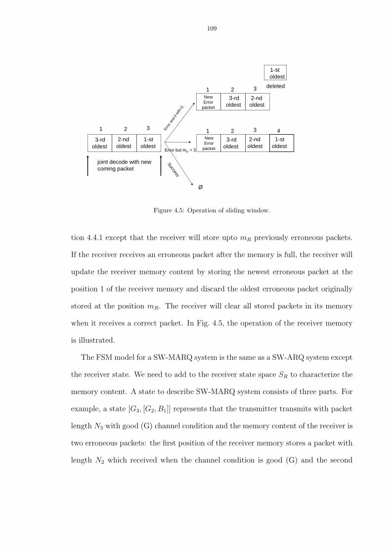
109
3-rdoldest
2-nd oldest
Erro
r and
if m
R=3
,
New Error
packet
1-st oldest
Error but mR > 3
Ø
Success
joint decode with new coming packet
1 2 3
1 2 3
1 2 3 4New Error
packet
3-rdoldest
2-nd oldest
1-st oldest
2-nd oldest
3-rdoldest
deleted
1-st oldest
Figure 4.5: Operation of sliding window.
tion 4.4.1 except that the receiver will store upto mR previously erroneous packets.
If the receiver receives an erroneous packet after the memory is full, the receiver will
update the receiver memory content by storing the newest erroneous packet at the
position 1 of the receiver memory and discard the oldest erroneous packet originally
stored at the position mR. The receiver will clear all stored packets in its memory
when it receives a correct packet. In Fig. 4.5, the operation of the receiver memory
is illustrated.
The FSM model for a SW-MARQ system is the same as a SW-ARQ system except
the receiver state. We need to add to the receiver state space SR to characterize the
memory content. A state to describe SW-MARQ system consists of three parts. For
example, a state [G3, [G2, B1]] represents that the transmitter transmits with packet
length N3 with good (G) channel condition and the memory content of the receiver is
two erroneous packets: the first position of the receiver memory stores a packet with
length N2 which received when the channel condition is good (G) and the second

110
GN1
BN1
GN1 BN1
GN1 BN1
GN1 BN1
GN1 BN1
GN1 BN1
GN1 BN1
GN1 BN1
GN1 BN1
GN1 BN1
GN1 BN1
GN2|GN1
BN2|GN1
GN2|BN1
BN2|BN1
GN2|GN2
BN2|GN2
GN2|BN2
BN2|BN2
Figure 4.6: FSM representation for Stop-and-Wait ARQ protocol with m = 2 and mR = 1.
position of the receiver memory stores a packet with length N1 which is received
when the channel condition is bad (B). The packet error probability corresponding
to this state is Pe,G3|G2B1 . In Fig. 4.6, the FSM diagram for SW-MARQ with m = 2
and mR = 1 is shown.
For general values of m and mR, we can summarize the FSM states, state tran-
sition probabilities, and output functions (denoted by energy and delay generating
function) in table 4.2. In the following tables of this section, we only write those
components of the system state vector, e.g., G1 will be equal to a system state
[G1,
mRterms︷ ︸︸ ︷φ, · · · , φ]. The symbol Ri represents the memory content of some position in
the receiver memory, the subscript i is used to distinguish the different position of
the receiver memory. In the columns of the ”previous state” and ”probability”, Ri
represents the memory content of the i-th position in the receiver memory. However,
in the column of the ”next state”, Ri represents the memory content of the (i+1)-th
position in the receiver memory. The symbol Ri could be Gj or Bj where j is the
index of the packet length.

111
Table 4.2: Output functions and state transition probabilities for SWMARQprevious state; next state probabilityoutput
G1 e−λN1TbPe,G1
G1 B1 e−λN1TbPe,G1
XN1TbY N1Ec [G2, G1] e−λN1TbPe,G1
[B2, G1] e−λN1TbPe,G1
G1 e−µN1TbPe,B1B1 B1 e−µN1TbPe,B1
XN1TbY N1Ec [G2, B1] e−µN1TbPe,B1
[B2, B1] e−µN1TbPe,B1
G1 e−λNiTbPe,Gi|R1R2···Rk
[Gi, R1, R2, · · · , Rk] B1 e−λNiTbPe,Gi|R1R2···Rk
i < m, k < mR; [Gi+1, Gi, R1, · · · , Rk] e−λNiTbPe,Gi|R1R2···Rk
XNiTbY NiEc [Bi+1, Gi, R1, · · · , Rk] e−λNiTbPe,Gi|R1R2···Rk
G1 e−µNiTbPe,Bi|R1R2···Rk
[Bi, R1, R2, · · · , Rk] B1 e−µNiTbPe,Bi|R1R2···Rk
i < m, k < mR; [Gi+1, Bi, R1, · · · , Rk] e−µNiTbPe,Bi|R1R2···Rk
XNiTbY NiEc [Bi+1, Bi, R1, · · · , Rk] e−µNiTbPe,Bi|R1R2···Rk
G1 e−λNmTbPe,Gm|R1R2···Rk
[Gm, R1, R2, · · · , Rk] B1 e−λNmTbPe,Gm|R1R2···Rk
k < mR; [Gm, Gm, R1, · · · , Rk] e−λNmTbPe,Gmi|R1R2···Rk
XNmTbY NmEc [Bm, Gm, R1, · · · , Rk] e−λNmTbPe,Gm|R1R2···Rk
G1 e−µNmTbPe,Bm|R1R2···Rk
[Bm, R1, R2, · · · , Rk] B1 e−µNmTbPe,Bm|R1R2···Rk
k < mR; [Gm, Bm, R1, · · · , Rk] e−µNmTbPe,Bm|R1R2···Rk
XNmTbY NmEc [Bm, Bm, R1, · · · , Rk] e−µNmTbPe,Bm|R1R2···Rk
G1 e−λNiTbPe,Gi|R1R2···RmR
[Gi, R1, R2, · · · , RmR ] B1 e−λNiTbPe,Gi|R1R2···RmR
i < m; [Gi+1, Gi, R1, · · · , RmR−1] e−λNiTbPe,Gi|R1R2···RmR
XNiTbY NiEc [Bi+1, Gi, R1, · · · , RmR−1] e−λNiTbPe,Gi|R1R2···RmR
G1 e−µNiTbPe,Bi|R1R2···RmR
[Bi, R1, R2, · · · , RmR ] B1 e−µNiTbPe,Bi|R1R2···RmR
i < m; [Gi+1, Bi, R1, · · · , RmR−1] e−µNiTbPe,Bi|R1R2···RmR
XNiTbY NiEc [Bi+1, Bi, R1, · · · , RmR−1] e−µNiTbPe,Bi|R1R2···RmR
G1 e−λNmTbPe,Gm|R1R2···RmR[Gm, R1, R2, · · · , RmR ] B1 e−λNmTbPe,Gm|R1R2···RmR
XNmTbY NmEc [Gm, Gm, R1, · · · , RmR−1] e−λNmTbPe,Gm|R1R2···RmR
[Bm, Gm, R1, · · · , RmR−1] e−λNmTbPe,Gm|R1R2···RmR
G1 e−µNmTbPe,Bm|R1R2···RmR[Bm, R1, R2, · · · , RmR] B1 e−µNmTbPe,Bm|R1R2···RmR
XNmTbY NmEc [Gm, Bm, R1, · · · , RmR−1] e−µNmTbPe,Bm|R1R2···RmR
[Bm, Bm, R1, · · · , RmR−1] e−µNmTbPe,Bm|R1R2···RmR

112
4.4.2 SW-ARQ over Time-Varying Channels: Repetition
In this section, we will consider an ARQ systems with repetition packet length.
There are three kinds of repetition ARQ systems analyzed in this section; the first
ARQ system does not contain any memory in the receiver, the second ARQ system
equips the receiver with memory and uses a sliding window scheme as mentioned
in Section 4.4.1, the third ARQ system also equips the receiver with memory but
the receiver memory contents will be updated to be empty after the receiver cannot
decode correctly when the memory buffer is full.
Memoryless Receiver
In this subsection, we will consider ARQ systems with a memoryless receiver.
The protocol, named repetition SW-ARQ with memoryless receiver (R-SW-ARQ-
ML), operates as follows. At the transmitter, whenever there is an information
packet with length K generated, it will be encoded to a data packet with length
N1. If the data packet is decoded correctly at the receiver, the receiver will send an
ACK packet back to the transmitter. If a detectable but uncorrectable error occurs
at the receiver, a NACK packet will be sent back to the transmitter. Then the
transmitter will encode the same information packet to a data packet with length
N2 and transmit the packet. If the data packet is decoded correctly at the receiver,
the receiver will send an ACK packet back to the transmitter. If a detectable but
uncorrectable error occurs at the receiver, a NACK packet will be sent back to the
transmitter. Let m be the number of different packet lengths used by the transmitter.
Therefore, if the transmitter can not receive an ACK by sending a data packet with
length Nm at m-th transmission, the transmitter will encode the information packet
to a data packet with length N1 again. If it is decoded in error at the receiver, the

113
N 1 N 2 N 1 N 2
N 1 N 2 N 1 N 2
N 1 N 2 N 1 N 2
(b) Memory : Sliding Window
(a) No memory
(c) Memory : Renew Window
Figure 4.7: Three different repetition ARQ protocols with m = 2 considered in this section.
transmitter will encode the same information packet to a data packet with length
N2 again. If the transmitter can not receive an ACK by sending a data packet with
length Nm at 2m-th transmission, it will encode the information packet to a data
packet with length N1 at 2m + 1-th transmission. The repetition procedure of these
m different packet lengths will be terminated if an ACK packet is received. The
operation of this protocol is shown in part (a) of Fig. 4.7. Each piece of the bold
line in Fig. 4.7 indicates the packets in the receiver memory used to decode jointly
when the transmitter has transmitted the last packet underscored by each piece of
the bold line.
By using the FSM model described in Section 4.2, we can summarize the state

114
GN1 BN1 GN1 BN1 GN1 BN1GN1 BN1
GN1 BN1 GN1 BN1 GN1 BN1GN1 BN1
GN1 GN2 GN3 GNm
BN1 BN2 BN3 BNm
Figure 4.8: State diagram for R-SW-ARQ-ML.
transition probabilities and output functions (denoted by energy and delay generating
function) in Table 4.3.
Memory Receiver: Sliding Window
The protocol discussed in this subsection is the same as the repetition SW-ARQ
protocol described in 4.4.2 except that the receiver will store up to mR previously
erroneous packets. We set mR = m− 1 be the maximum number of packets that the
receiver can store in its memory. If the receiver receives an erroneous packet after
the memory is full, the receiver will update its memory content by storing the newest
erroneous packet and discarding the oldest erroneous packet. The receiver will clear
all stored packets in its memory when it receives a correct packet.
The FSM model for repetition SW-ARQ systems with sliding window memory
(R-SW-ARQ-SWM) is extended to a repetition SW-ARQ system by including the
receiver state. We need to add the receiver state SR to characterize the memory
content. A state space to describe R-SW-ARQ-SWM system consists of three parts.
The first part of the state represents the channel condition. The second part is
used to represent the packet lengths for transmission. The third part denotes the

115
Table 4.3: Table for transition probabilities and output functions of R-SW-ARQ-MLprevious state next state transition prob. output function
Gi+1 e−λNiTbPe,GiXNiTbY NiEc
Gi Bi+1 e−λNiTbPe,GiXNiTbY NiEc
1 ≤ i ≤ m− 1 G1 e−λNiTbPe,GiXNiTbY NiEc
B1 e−λNiTbPe,GiXNiTbY NiEc
G1 e−λNmTbPe,GmXNmTbY NmEc
B1 e−λNmTbPe,GmXNmTbY NmEc
Gm G1 e−λNmTbPe,Gm XNmTbY NmEc
B1 e−λNmTbPe,Gm XNmTbY NmEc
Gi+1 e−µNiTbPe,BiXNiTbY NiEc
Bi Bi+1 e−µNiTbPe,BiXNiTbY NiEc
1 ≤ i ≤ m− 1 G1 e−µNiTbPe,BiXNiTbY NiEc
B1 e−µNiTbPe,BiXNiTbY NiEc
G1 e−µNmTbPe,BmXNmTbY NmEc
B1 e−µNmTbPe,BmXNmTbY NmEc
Bm G1 e−µNmTbPe,BmXNmTbY NmEc
B1 e−µNmTbPe,Bm XNmTbY NmEc
contents of the receiver memory. For example, state [G3, G2, B1] represents that the
transmitter transmits with packet length N3 with good (G) channel condition and
the memory contents of the receiver is two erroneous packets: the first packet with
length N1 is received when the channel condition is bad (B) and the second packet
with length N2 is received when the channel condition is good (G). The packet error
probability corresponding to this state is Pe,G3|G2B1 . In Fig. 4.9, the FSM diagram
for SW-MARQ with m = 2 and mR = 1 is shown.
For general values of m and mR, we summarize the FSM states, state transi-
tion probabilities, and output functions (denoted by energy and delay generating
function) in Table 4.4.
Memory Receiver: Non Overlap
In this section, we consider the case that mR = m − 1 is the maximum number
of packets that the receiver can store in its memory. The protocol is the same as
the repetition SW-ARQ protocol with the receiver memory described in 4.4.2 except

116
Table 4.4: Table for transition probabilities and output functions of R-SW-ARQ-SWMprevious state; next state probabilityoutput
G1 e−λN1TbPe,G1G1 B1 e−λN1TbPe,G1
XN1TbY N1Ec [G2, G1] e−λN1TbPe,G1
[B2, G1] e−λN1TbPe,G1
G1 e−µN1TbPe,B1B1 B1 e−µN1TbPe,B1
XN1TbY N1Ec [G2, B1] e−µN1TbPe,B1
[B2, B1] e−µN1TbPe,B1
G1 e−λNiTbPe,Gi|R1R2···Ri−1
[Gi, R1, R2, · · · , Ri−1] B1 e−λNiTbPe,Gi|R1R2···Ri−1
i < m [Gi+1, Gi, R1, · · · , Ri−1] e−λNiTbPe,Gi|R1R2···Ri−1
XNiTbY NiEc [Bi+1, Gi, R1, · · · , Ri−1] e−λNiTbPe,Gi|R1R2···Ri−1
G1 e−µNiTbPe,Bi|R1R2···Ri−1
[Bi, R1, R2, · · · , Ri−1] B1 e−µNiTbPe,Bi|R1R2···Ri−1
i < m [Gi+1, Bi, R1, · · · , Ri−1] e−µNiTbPe,Bi|R1R2···Ri−1
XNiTbY NiEc [Bi+1, Bi, R1, · · · , Ri−1] e−µNiTbPe,Bi|R1R2···Ri−1
G1 e−λNiTbPe,Gi|R1R2···RmR
[Gi, R1, R2, · · · , RmR ] B1 e−λNiTbPe,Gi|R1R2···RmR
1 ≤ i ≤ m; [Gi+1, Gi, R1, · · · , RmR−1] e−λNiTbPe,Gi|R1R2···RmR
XNiTbY NiEc [Bi+1, Gi, R1, · · · , RmR−1] e−λNiTbPe,Gi|R1R2···RmR
G1 e−µNiTbPe,Bi|R1R2···RmR
[Bi, R1, R2 · · ·RmR] B1 e−µNiTbPe,Bi|R1R2···RmR
1 ≤ i ≤ m; [Gi+1, Bi, R1, · · ·RmR−1] e−µNiTbPe,Bi|R1R2···RmR
XNiTbY NiEc [Bi+1, Bi, R1, · · ·RmR−1] e−µNiTbPe,Bi|R1R2···RmR

117
GN1
BN1
GN1 BN1
GN1 BN1
GN1 BN1
GN1 BN1
GN1 BN1
GN1 BN1 GN1 BN1
GN1 BN1
GN1 BN1
GN1 BN1
GN2|GN1
BN2|GN1
GN2|BN1
BN2|BN1
GN2|GN2
BN2|GN2
GN2|BN2
BN2|BN2
Figure 4.9: FSM representation for repetition SW-ARQ systems with sliding window memory withm = 2 and mR = 1.
that the receiver will also refresh its memory contents to be empty after the capacity
of the receiver memory reaches mR as shown in part (c) of Fig. 4.7. In Fig. 4.10, the
FSM diagram for SW-ARQ systems with non-overlapping window memory (R-SW-
ARQ-NOM) with m = 2 and mR = 1 is shown. For general values of m and mR, we
can summarize the FSM states, state transition probabilities, and output functions
in Table 4.5.
4.5 Go-Back-N ARQ
We begin this section by describing the operation of Go-Back-N ARQ (GBN-ARQ)
protocol. The transmitter sends packets with a sequence number contiguously. Once
the transmitter receives a negative acknowledge (NACK) packet after one round-
trip propagation time, the transmitter retransmits the received erroneously decoded
packet and succeeding packets. If the receiver decodes a packet correctly, it will send

118
GN1
BN1
GN2|GN1
GN1 BN1
GN1 BN1
GN1 BN1
GN1 BN1
GN1 BN1
GN1 BN1
BN2|GN1
GN2|BN1
BN2|BN1
Figure 4.10: FSM representation for repetition SW-ARQ systems with non-overlapping windowmemory with m = 2 and mR = 1.

119
Table 4.5: Table for transition probabilities and output functions of R-SW-ARQ-NOMprevious state; next state probabilityoutput
G1 e−λN1TbPe,G1G1; B1 e−λN1TbPe,G1
XN1TbY N1Ec [G2, G1] e−λN1TbPe,G1
[B2, G1] e−λN1TbPe,G1
G1 e−µN1TbPe,B1B1; B1 e−µN1TbPe,B1
XN1TbY N1Ec [G2, B1] e−µN1TbPe,B1
[B2, B1] e−µN1TbPe,B1
G1 e−λNiTbPe,Gi|R1R2···Ri−1
[Gi, R1, R2, · · · , Ri−1] B1 e−λNiTbPe,Gi|R1R2···Ri−1
i < m [Gi+1, Gi, R1, · · · , Ri−1] e−λNiTbPe,Gi|R1R2···Ri−1
XNiTbY NiEc [Bi+1, Gi, R1, · · · , Ri−1] e−λNiTbPe,Gi|R1R2···Ri−1
G1 e−µNiTbPe,Bi|R1R2···Ri−1
[Bi, R1, R2, · · · , Ri−1] B1 e−µNiTbPe,Bi|R1R2···Ri−1
i < m [Gi+1, Bi, R1, · · · , Ri−1] e−µNiTbPe,Bi|R1R2···Ri−1
XNiTbY NiEc [Bi+1, Bi, R1, · · · , Ri−1] e−µNiTbPe,Bi|R1R2···Ri−1
G1 e−λNmTbPe,Gm|R1R2···RmR
[Gm, R1, R2, · · · , RmR ] B1 e−λNmTbPe,Gm|R1R2···RmR
XNmTbY NmEc G1 e−λNmTbPe,Gm|R1R2···RmR
B1 e−λNmTbPe,Gm|R1R2···RmR
G1 e−µNmTbPe,Bm|R1R2···RmR
[Bm, R1, R2, · · · , RmR] B1 e−µNmTbPe,Bm|R1R2···RmR
XNmTbY NmEc G1 e−µNmTbPe,Bm|R1R2···RmR
B1 e−µNmTbPe,Bm|R1R2···RmR

120
an acknowledge (ACK) back to the transmitter. The receiver will send a NACK
packet back to the transmitter if a packet can not be decoded correctly. From the
described protocol of GBN-ARQ, we can incorporate the previous SW-ARQ with
incremental redundancy and the receiver memory scheme into GBN-ARQ protocol
by using different packet lengths and modifying the decoding structure (from a non-
memory receiver to a memory receiver).
Let T(Ni) be the channel transition probability matrix after transmitting a packet
with length Ni. It can be written as:
T(Ni) =
∣∣∣∣∣∣∣
e−λNiTb (1− e−λNiTb)
(1− e−µNiTb) e−µNiTb
∣∣∣∣∣∣∣. (4.13)
Then the transition probability matrix after Nrt transmissions of a packet with length
Ni is
T(NrtNi) = [T(Ni)]Nrt
=1
2− e−λNiTb − e−µNiTb(
∣∣∣∣∣∣∣
(1− e−µNiTb) (1− e−λNiTb)
(1− e−µNiTb) (1− e−λNiTb)
∣∣∣∣∣∣∣+
(e−λNiTb + e−µNiTb − 1)Nrt
∣∣∣∣∣∣∣
(1− e−λNiTb) −(1− e−λNiTb)
−(1− e−µNiTb) (1− e−µNiTb)
∣∣∣∣∣∣∣),(4.14)
where the Nrt is the number of packets in a round trip delay. From this transition
probability matrix, the transition probability from G to G after one round trip time
of transmitting packets with length Ni, denoted as TGiGirt , is
TGiGirt = 1− (1− e−µNiTb)
1− (e−λNiTb + e−µNiTb − 1)Nrt
2− e−λNiTb − e−µNiTb
Similarly, we can obtain the transition probability from G to B, B to G and B to B.
121
They are
TGiBirt = (1− e−µNiTb)
1− (e−λNiTb + e−µNiTb − 1)Nrt
2− e−λNiTb − e−µNiTb
TBiGirt = (1− e−λNiTb)
1− (e−λNiTb + e−µNiTb − 1)Nrt
2− e−λNiTb − e−µNiTb
TBiBirt = 1− (1− e−λNiTb)
1− (e−λNiTb + e−µNiTb − 1)Nrt
2− e−λNiTb − e−µNiTb(4.15)
We will give an example about calculating the generating function for a GBNARQ
system with m = 2 and mR = 0 by using the approach presented in subSection 4.4.1
and the channel transition probabilities (4.15). The generating function is
Gs = PG(1− Pe,G1)XNrtN1TbY NrtN1Ec + PB ∗ (1− Pe,B1)X
NrtN1TbY NrtN1Ec +
(PGPe,G1TGiGirt + PBPe,B1T
B1G1rt )XNrtN1TbY NrtN1EcGG +
(PGPe,G1TGiBirt + PBPe,B1T
B1B1rt )XNrtN1TbY NrtN1EcGB, (4.16)
where
GG =(XN2TbY N2Ec(1− Pe,B2 − [(1− Pe,B2)Pe,G2T
B2B2rt − Pe,B2(1− Pe,G2)T
G2B2rt ]Z))
1− [Pe,B2TG2G2rt + Pe,G2T
B2B2rt ]Z + Pe,B2Pe,G2(T
G2G2rt + TB2B2
rt − 1)Z2
GB =(XN2TbY N2Ec(1− Pe,G2 − [(1− Pe,G2)Pe,B2T
G2G2rt − Pe,G2(1− Pe,B2)T
B2G2rt ]Z))
1− [Pe,G2TB2B2rt + Pe,B2T
G2G2rt ]Z + Pe,G2Pe,B2(T
B2B2rt + TG2G2
rt − 1)Z2
(4.17)
and Z = XNrtN2TbY NrtN2Ec . We also can obtain the generating function of GBN-ARQ
with the receiver memory scheme by using the same method as we derived before.
The only change is to modify the channel transition probabilities and multiply the
round trip factor Nrt in energy and delay components at each transmission.
4.6 Cutoff Rate for Memory Receiver over Memoryless Channels
Let K be the number of information bits in a packet and N be the number of
coded bits for this packet. From the random coding argument, it is well known that

122
there exist an encoder and decoder that has packet error probability Pe,K,N bounded
as
Pe,K,N ≤ 2K−NR0 , (4.18)
where R0 is the cutoff rate determined by the channel SNR and other channel charac-
teristics. Because the channel SNR and packet length used for packets transmission
are two crucial components in determining the energy and delay tradeoff of an ARQ
system. By using the cutoff rate to represent the packet error probability, we can
relate the channel SNR and packet length N with system performance.
The cutoff rate of two different kinds of receiver structure will be derived in this
section. The first cutoff rate is evaluated by assuming that the receiver has all
the channel state information. The second cutoff rate is calculated according to the
imperfect channel state information by using estimated channel transition probability
of each signal. The third cutoff rate is derived by the same assumption as second
cutoff rate, however, the receiver with memory will utilize more information (the
failure information) to decode.
4.6.1 Random Coding Bound for Memory Receiver in AWGN channel- Part I: PerfectChannel Knowledge
Let m be the total number of packets combined at the receiver which are used to
decode jointly. Let Nj be the number of coded symbols used at j-th packet at the
receiver memory, where j ∈ {1, 2, · · · ,m}. Here we consider a set of M -ary coded
signals constructed from∑m
j=1 Nj-dimensional q symbols. Let si be the signal vector
received at the receiver end. It is
si = [
packet 1︷ ︸︸ ︷si11si12 · · · si1N1
packet 2︷ ︸︸ ︷si21si22 · · · si2Nm
· · ·packet m︷ ︸︸ ︷
sim1sim2 · · · simNm], (4.19)
where sij,kare selected from the signal set {a1, a2, · · · aq} of q elements.

123
According to the random coding argument, there are B = qMPm
j=1 Nj possible sets
of M signals since there are∑m
j=1 Nj positions can be chosen from q symbols. Let
Pe,i(k) be the error probability of signal set k given the i-th message was transmitted.
The average error probability given the transmission of the i-th message is P e,i =B∑
k=1
Pe,i(k). By the union-Bhattacharyya bound for an AWGN channel, the average
error probability of transmitting i-th message over the ensemble of codewords sets is
P e,i ≤∑
i6=j
E[e− ‖si−sj‖2
4N0 ]. (4.20)
If we can show that P e,i ≤ α, then there exists a signal set with Pe,i ≤ α. Let
dl,m = Ek ‖ al − am ‖2, where Ek is the received energy level of packet k and
‖ al− am ‖ is the distance between signal al and am. If we assume that the selection
of symbols {a1, a2, · · · aq} is according to probabilities {p1, p2, · · · pq}. Then we have
P e,i ≤∑
i6=j
m∏
k=1
(
q∑
lk=1
q∑mk=1
plkpmke−
d2lkmk4N0 )Nk (4.21)
Therefore, if we set R0,k = − log2(∑q
lk=1
∑qmk=1 plkpmk
e−
d2lkmk4N0 ) we can further express
the right hand side of (4.21) as
P e,i ≤ (M − 1)m∏
k=1
(
q∑
lk=1
q∑mk=1
plkpmke−
d2lkmk4N0 )Nk
< M
m∏
k=1
2−NkR0,k
= 2−(Pm
k=1 Nk)(R0,MRX−R), (4.22)
where R = log2 MPmk=1 Nk
is the code rate after packets combination and R0,MRX is
R0,MRX =N1∑m
k=1 Nk
R0,1 +N2∑m
k=1 Nk
R0,2 + · · ·+ Nm∑mk=1 Nk
R0,m. (4.23)
We can interpret R0,MRX as the cutoff rate by combining m packets according to
their packet length ratio to the total length of m packets at the receiver. We only

124
show that there exist a signal, say i-th signal, for which the average error probability
can be made arbitrary small as packets length becomes large. We will show that we
can find a single codeword set such that the error probability of each signal of this
codeword set approaches to zero as packets length approaches to infinity.
Choosing a code with M = 2 · 2R0,MRX(Pm
k=1 Nk) codewords that the average error
probability of this code is less then ε/2 for large∑m
k=1 Nk. There are at least M/2
of the codewords with error probability less then ε (otherwise the average error
probability of this code will greater then ε/2). By deleting those bad codewords (their
error probability is greater then ε), we obtain a code with (at least) 2R0,MRX(Pm
k=1 Nk)
codewords with error probability small as∑m
k=1 Nk −→∞.
4.6.2 Random Coding Bound for Memory Receiver - Part II : Imperfect ChannelKnowledge
In this section, we consider that the receiver uses the channel transition probabil-
ities p∗(y|x) as if they were the true transition probabilities. We will derive random
coding bound of the receiver with memory with m packets. When the channel con-
dition is good, the receiver end has signal-to-noise ratio EG/N0 but the receiver uses
the incorrect signal-to-noise ratio E∗G/N0 to decode. Similarly, the receiver end has
signal-to-noise ratio EB/N0 when the channel condition is bad but the receiver uses
the incorrect signal-to-noise ratio E∗B/N0 to decode.
Let si be the signal vector received at the receiver end. It is
si = [
packet 1︷ ︸︸ ︷si11si12 · · · si1N1
packet 2︷ ︸︸ ︷si21si22 · · · si2Nm
· · ·packet m︷ ︸︸ ︷
sim1sim2 · · · simNm], (4.24)
where sij,k∈ {a1, a2, · · · , aq}.
The decision region are
R∗i = {y : p∗(y|si, sR) > p∗(y|sj, sR)for all j 6= i}, (4.25)

125
where sR is the receiver memory state. Let R∗i be the region where signal i is not
decided. Then
R∗i =
⋃
j 6=i
R∗i,j, (4.26)
where R∗i,j = {y : p∗(y|si) < p∗(y|sj)}. Then we have
Pe,i = P (R∗i |Hi)
≤∑
j 6=i
P (R∗i,j). (4.27)
For each term of above summand, we have
P (R∗i,j) =
∫
y∈R∗i,j
p(y|si, sR). (4.28)
Since
p∗(y|sj, sR)
p∗(y|si, sR)> 1, y ∈ R∗
i,j, (4.29)
we can further bound (4.28) as follows
P (R∗i,j) <
∫
y∈R∗i,j
p(y|si, sR)[p∗(y|sj, sR)
p∗(y|si, sR)
]λ
, (4.30)
where λ > 0. By relaxing the integral domain, we can upper bound (4.30) as
P (R∗i,j) <
∫
y∈RPm
k=1Nk
p(y|si, sR)[p∗(y|sj, sR)
p∗(y|si, sR)
]λ
. (4.31)

126
Thus, the error probability Pe,i is upper bounded by
Pe,i <∑
j 6=i
∫
y∈RPm
k=1Nk
p(y|si, sR)[p∗(y|sj, sR)
p∗(y|si, sR)
]λ
=∑
j 6=i
∫
y∈RPm
k=1Nk
( N1∏
l1=1
p(yl1|si1l1, R1)
[p∗(yl1|sj1l1, R1)
p∗(yl1|si1l1, R1)
]λ)×
( N2∏
l2=1
p(yl2|si2l2, R2)
[p∗(yl2|sj2l2, R2)
p∗(yl2|si2l2, R2)
]λ)· · ·
( Nm∏
lm=1
p(ylm |simlm, Rm)
[p∗(ylm|sjmlm, Rm)
p∗(ylm |simlm, Rm)
]λ)
=∑
j 6=i
( N1∏
l1=1
∫
yl1∈R
p(yl1|si1l1, R1)
[p∗(yl1|sj1l1, R1)
p∗(yl1|si1l1, R1)
]λ)×
( N2∏
l2=1
∫
yl2∈R
p(yl2|si2l2, R2)
[p∗(yl2|sj2l2, R2)
p∗(yl2|si2l2, R2)
]λ)· · ·
( Nm∏
lm=1
∫
ylm∈R
p(ylm|simlm, Rm)
[p∗(ylm|sjmlm, Rm)
p∗(ylm|simlm, Rm)
]λ). (4.32)
By taking the error probability over all possible codes and let p(si) =∏m
k=1(∏Nk
lk=1 p(siklk)).

127
Then
P e,i <∑
j 6=i
∑si
∑sj
( N1∏
l1=1
p(si1l1)p(sj1l1
)
∫
yl1∈R
p(yl1|si1l1, R1)
[p∗(yl1|sj1l1, R1)
p∗(yl1|si1l1, R1)
]λ)×
( N2∏
l2=1
p(si2l2)p(sj2l2
)
∫
yl2∈R
p(yl2|si2l2, R2)
[p∗(yl2|sj2l2, R2)
p∗(yl2|si2l2, R2)
]λ)· · ·
( Nm∏
lm=1
p(simlm)p(sjmlm
)
∫
ylm∈R
p(ylm|simlm, Rm)
[p∗(ylm|sjmlm, Rm)
p∗(ylm|simlm, Rm)
]λ)
=∑
j 6=i
( N1∏
l1=1
∑si1l1
∑sj1l1
p(si1l1)p(sj1l1
)
∫
yl1∈R
p(yl1|si1l1, R1)
[p∗(yl1|sj1l1, R1)
p∗(yl1|si1l1, R1)
]λ)×
( N2∏
l2=1
∑si2l2
∑sj2l2
p(si2l2)p(sj2l2
)
∫
yl2∈R
p(yl2|si2l2, R2)
[p∗(yl2|sj2l2, R2)
p∗(yl2|si2l2, R2)
]λ)· · ·
( Nm∏
lm=1
∑simlm
∑sjmlm
p(simlm)p(sjmlm
)
∫
ylm∈R
p(ylm |simlm, Rm)
[p∗(ylm |sjmlm, Rm)
p∗(ylm |simlm, Rm)
]λ)
=∑
j 6=i
[E[J∗λ,1(X1, X2)]]N1 [E[J∗λ,2(X1, X2)]]
N2 · · · [E[J∗λ,m(X1, X2)]]Nm
= (M − 1)[E[J∗λ,1(X1, X2)]]N1 [E[J∗λ,2(X1, X2)]]
N2 · · · [E[J∗λ,m(X1, X2)]]Nm (4.33)
where E[J∗λ,n(X1, X2)] is∑
sinln
∑sjnln
p(sinln)p(sjnln
)∫
ynln∈Rp(ynln|sinln
, Rn)[
p∗(ynln |sjnln,Rn)
p∗(ynln |sinln,Rn)
]λ
for the n-th packets in the receiver memory. The random variable X1 represents
source signals silk and X2 represents source signals sjlk. If let R∗
0,k(λ) as
R∗0,k(λ) = max
p(siklk)− log2
{ ∑siklk
∑sjklk
p(siklk)p(sjklk
)
∫
kylk∈R
p(yklk |siklk, Rk)
[p∗(yklk |sjklk, Rk)
p∗(yklk |siklk, Rk)
]λ},
and siklk∈ {a1, a2, · · · aq}. (4.34)
Then we can further upper bound of (4.33) as
P e,i < 2−(Pm
k=1 Nk)(R∗0,MRX−R), (4.35)
where R = log2 MPmk=1 Nk
is the code rate after packets combination. R∗0,MRX is
R∗0,MRX = max
λ
[ N1∑mk=1 Nk
R∗0,1(λ) +
N2∑mk=1 Nk
R∗0,2(λ) + · · ·+ Nm∑m
k=1 Nk
R∗0,m(λ)
].
(4.36)
128
The channel model used in the following cutoff rate evaluation is Gilbert-Elliott
channel model described at the beginning of subsection 4.4.1. We assume that the
first packet with length N1 is decoded erroneously after receiving over the good
channel condition. Therefore, it is stored in the receiver memory. The cutoff rate is
evaluated by considering the first erroneous packet stored in the receiver memory and
the second incoming packet with length N2 from bad channel condition jointly. The
cutoff rate is plotted with respect to good channel SNR for the memory receiver with
perfect channel knowledge described in Subsection 4.6.1 (indicated by symbol I) and
the memory receiver with imperfect channel knowledge described in Subsection 4.6.2
(represented by symbol II) in Fig.4.11. We observe that the cutoff rate of the memory
receiver structure I is higher than the cutoff rate of the memory receiver structure
II because the receiver of structure I has much more information about the channel
condition. Since the cutoff rate with parameters N1 = 2N2 has higher chance for the
joint packet (the packet combining the first erroneous one and the second incoming
one) to stay at good channel condition compared to the cutoff rate with parameters
N2 = 2N1, the cutoff rate represented by the solid lines is lower then the cutoff rate
represented by the dashed lines. The cutoff rate with symbol + is higher then the
cutoff rate with symbol o because the lines with symbol + have higher bad channel
SNR compared to the lines with symbol o.
4.6.3 Existence of Codes for Memory Receiver
In the previous derivation of cutoff rate for the receiver with memory, we know
that there is an ensemble random codes of m blocks, (C1, C2, · · · , Cm) satisfying the
random coding bound if there m−1 packets stored in the receiver memory. However,
it does not guarantee that the same code ensemble can satisfy the random coding
bound for any usage of previous k codes for k < m, i.e., there are only k− 1 packets

129
−3 −2 −1 0 1 2 3 4 50
0.1
0.2
0.3
0.4
0.5
0.6
0.7
0.8
0.9
EG
/N0 (dB)
R0
r=2, I, N2=2N
1r=2, II, N
2=2N
1r=8, I, N
2=2N
1r=8, II, N
2=2N
1r=2, I, N
1=2N
2r=2, II, N
1=2N
2r=8, I, N
1=2N
2r=8, II, N
1=2N
2
Figure 4.11: Cutoff rate comparison for two different receiver structures.
stored in the receiver memory. The following theorem indicates such ensemble codes
exist [49].
Theorem : There exists an ensemble of codes (C1, C2, · · · , Cm) satisfying
Pe(C1, C2, · · · , Ck) ≤ 2−(Pk
l=1)(Rk0,MRX−R) for 1 ≤ k ≤ m.
Proof : By applying Markov inequality, we have
Pr(Pe,k > β2−(Pk
l=1)(Rk0,MRX−R)) ≤ 1
β, for 1 ≤ k ≤ m. (4.37)
where Pe,k is the probability of error for previous k codes. Note that Pe,k is a random
number since we use random coding selection for codes construction. Hence,
Pr(m⋂
k=1
{Pe,k > β2−(Pk
l=1)(Rk0,MRX−R)}) = 1− Pr(
m⋃
k=1
{Pe,k > β2−(Pk
l=1)(Rk0,MRX−R)})
≥ 1−m∑
k=1
Pr(Pe,k > β2−(Pk
l=1)(Rk0,MRX−R))
≥ 1− m
β> 0 (4.38)
by choosing a suitable β, say β = 2m. This implies that there exist at least an

130
ensemble of m blocks, (C∗1 , C∗2 , · · · , C∗m) with
P ∗e,k ≤ β2−(
Pkl=1)(R
k0,MRX−R)), for 1 ≤ k ≤ m. (4.39)
Here we can see that the factor β has no effect on the cutoff rate. ¤
4.6.4 Cutoff Rate Optimization
In the previous derivation of cutoff rate, we need to optimize the following cutoff
rate per waveform given λ
R0(λ) , maxPj
{− log
[∑j
∑
k
PjPk
∫
z
f(z|k)[f ∗(z|j)f ∗(z|k)]λdz
]}, (4.40)
where
1. Pj is the a priori probability of the j-th symbol selected by the transmitter.
2. z denotes a received signal.
3. j, k are the index for symbols.
4. f(z|j) is the true channel transition probability, i.e., the probability density
function of the receiver output, assuming the j-th symbol was transmitted.
The superscript symbol ∗ indicates the incorrect channel transition probability
used by the receiver to decode.
Denote Dj,k by the quantity∫
zf(z|k)[f ∗(z|j)f ∗(z|k)]λdz. If λ = 1/2, f(z|k) =
f ∗(z|k) and the system is operated in an AWGN channel, the value∫
zf(z|k)[f ∗(z|j)f ∗(z|k)]λdz
is equal to e−dB(j,k) where dB(j, k) is Bhattachryya distance. We want to find the
priori probability of the input symbol Pj in two cases; (1) there is no constraint of Pj
except that its components are sum up to one and (2) there is an energy constraint
of input symbols.

131
We will consider the case (1) first. The optimization problem of this case can be
formulated as follows:
R0 = maxPj
{− log[∑
j
∑
k
PjPkDj,k]}
= maxPj
{− log[PTDP]}, (4.41)
under constraint
∑j
Pj = 1. (4.42)
From the signal constellation, the matrix D has the following form
1 D1,2 · · · D1,M
D2,1 1 · · · D2,M
...... · · · ...
DM,1 DM,2 · · · 1
, (4.43)
and Di,j = Dj,i due to the symmetry of the Bhattachryya distance function. From
this, we can write the term PTDP as
PTDP =M∑i=1
P 2i + 2
∑1≤i<j≤M
Di,jPiPj. (4.44)
The quantity PTDP is a quadratic function of P, therefore, it is a convex⋃
func-
tion. From Kuhn-Tucker theorem, the necessary and sufficient conditions on the
probability vector P that minimizes PTDP are
Pi +M∑
s=1, 6=i
Ds,iPs ≥ −2detD∑Ms=1 det[D,1s]
; for all i (4.45)
where [D,1s] is matrix obtained by replacing the s-th column of matrix D by one
vector. The equality will hold for all i such that Pi > 0. Because the probability
vector obtained in (4.45) minimizes PTDP, it will also maximize the cutoff rate R0.

132
According to the previous derivation, we can calculate the cutoff rate for optimal a
priori probability input signals. In Fig.4.12, we plot the cutoff rates for uniform and
optimal priori probability input signals for PAM modulation scheme with M = 3
and M = 4. The amplitude levels are assigned equally spaced over the interval
[−√Ec, +√
Ec]. We observe that there is about 40% increase of cutoff rate at -10
dB for M = 3 and about 60% increase of cutoff rate at -10 dB for M = 4. This
indicates that the suitable selection of a priori probability for the input signals is
crucial especially for the bad channel condition. We also note that when the channel
SNR is low, the cutoff rate of smaller input signals is higher then the larger input
signals due to larger distance between signals. However, when the channel SNR is
high, the cutoff rate of smaller input signals is lower then the larger input signals
due to high bandwidth efficiency.
−10 −5 0 5 10 15 20 25 3010
−2
10−1
100
101
R0
Ec/N
0 (dB)
Unif. M=3Opt.M=3Unif. M=4Opt.M=4
Figure 4.12: The comparison of cutoff rate for uniform and optimal priori probability for inputsignals.

133
Now, we will consider the case (2). The optimization problem of this case can be
formulated as follows:
R0 = maxPj
{− log[∑
j
∑
k
PjPkDj,k]}
= maxPj
{− log[PTDP]}, (4.46)
under constraint
∑j
Pj = 1, and∑
j
PjEj = PTE = Eav, (4.47)
where Ej is the energy used in j-th signal and Eav is the average energy constraint.
In order to minimize PTDP with these two constraints, we write the constrained
minimization using Lagrange multipliers as the minimization of
J(p) =M∑i=1
P 2i + 2
∑1≤i<j≤M
Di,jPiPj + λ1(M∑i=1
Pi − 1) + λ2(M∑i=1
PiEi − Eav).(4.48)
Differentiating with respect to Pi, we get
∂J
∂Pi
= 2Pi +M∑
s=1,6=i
Ds,iPs + λ1 + λ2Ei. (4.49)
Setting the derivative to 0, we obtain a system of linear equations of Pi
2Pi +M∑
s=1,6=i
Ds,iPs = −λ1 − λ2Ei, for 1 ≤ i ≤ M . (4.50)
Solving this, the Pi can be expressed as
Pi =
det[D;
−λ1 − λ2E1
−λ1 − λ2E2
...
−λ1 − λ2EM
i
]
detD
=−λ1det[D;1i]− λ2det[D;Ei]
detD, (4.51)

134
where Di,j = Di,j for i 6= j and Di,i = 2 for 1 ≤ i ≤ M . The matrix [D;Ei] is
obtained by replacing its i-th column by the energy vector E = [E1, E2, · · · , EM ]T .
Substituting (4.51) into the two constraints, we can solve for λ1 and λ2. The solutions
are
λ1 =
det
1 bT1
Eav bTE
det
aT1 bT1
aTE bTE
, λ2 =
det
aT1 1
aTE Eav
det
aT1 bT1
aTE bTE
(4.52)
where
a =
−det[eD;11]
deteD−det[eD;12]
deteD...
−det[eD;1M ]
deteD
, b =
−det[eD;E1]
deteD−det[eD;E2]
deteD...
−det[eD;EM ]
deteD
(4.53)
From the Kuhn-Tucker theorem, the necessary and sufficient conditions on the
probability vector P that minimizes PTDP are
Pi +M∑
s=1,6=i
Ds,iPs ≥ −λ1 − λ2Ei
2; for all i (4.54)
According to the previous derivation, we can calculate the cutoff rate for a optimal
priori probability with average energy constraints. In Fig.4.13, we plot the cutoff rate
for different average energy constraints for 8 QAM.
4.7 Numerical Results
In this section, we will compare the system performance of SW-ARQ ,SW-MARQ
and repetition ARQ over time varying channels. The modulation adopted in the
transmitter is BPSK. The channel model used for the numerical evaluation is the

135
−10 −5 0 5 10 15 20 25 3010
−2
10−1
100
101
Ec/N
0
R0
0.3 Ec/N
00.4 E
c/N
00.5 E
c/N
00.6 E
c/N
00.7 E
c/N
0
Figure 4.13: The comparison of cutoff rate for different average energy constraints for 8 QAM
two state Gilbert-Elliott model. All packet error probabilities are evaluated with the
random coding bound derived in Section 4.6 by assuming that the receiver has perfect
knowledge of the channel state information. Let K be the number of information
bits in a packet and N be the number of coded bits for this packet, then there exist
an encoder and decoder that has packet error probability Pe,K,N bounded by
Pe,K,N,{G,B} ≤ 2K−NR0,{G,B} , (4.55)
where R0,{G,B} = 1 − log2(1 + e−Ec,{G,B}/N0) is the cutoff rate determined by the
channel SNR which will depend on the packet is transmitted in the good or bad
channel state. For the receiver with memory, the packet error probability can be
written as:
Pe,K,N,{G,B};SR≤ 2K−NR0,{GN,BN};SR , (4.56)
where R0,N,{GN,BN};SRis the cutoff rate determined by the channel SNR of trans-
mitting the describe packet with packet length N and the receiver memory state

136
SR as derived in Section 4.6. For example, the packet error probability of transmit-
ting a packet with length N2 through the good channel when the memory content
is BN1 (the first packet with length N1 is transmitted through the bad channel
and decoded incorrectly), is Pe,K,GN2;BN1 = 2K−(N1+N2)R0,GN2;BN1 where R0,GN2;BN1 =
N1R0,B+N2R0,G
N1+N2.
From the packet error probability formulas (4.55) and (4.56), we observe that
there is an optimal N for each information packet that minimizes the average system
delay. The reason is that if N is small, then the packet error probability becomes
large. This increases the system delay and energy due to the high possibility of
packet retransmission. On the other hand, if N is large, although the packet error
probability is small, the transmission time per packet is large. Our goal is to find the
best Ni to minimize the average delay. We first fix Ec/N0 and optimize the average
delay to get the corresponding packet lengths for Ni. From this, we can evaluate
both average delay and average energy consumption. Repeating the above argument
for different Ec/N0, we get the energy-delay curve. All the following figures show the
energy-delay curves when the bad channel SNR varies from −3 to 3 dB.
We plot SW-ARQ and SW-MARQ for different K in Fig.4.14. The system uses
the following parameters, m = 2, mR = 1, λ = µ = 0.0001 and r = 2. We observe
that the average delay of MARQ at low channel SNR is smaller by 20% compared
to ARQ. At high channel SNR, the two systems have almost the same performance
because the transmitter has a higher chance to get an ACK on the first transmission
with higher channel SNR. The effect of the receiver memory improvement to the
system performance goes away due to the lack of the receiver memory. Therefore,
MARQ outperforms ARQ since MARQ can decode more efficiently by utilizing the
previous erroneous packets. We also note that the normalized average delay and

137
energy of systems decreases as K increases. In [15], we showed the optimal error
probability that achieves the minimum average delay is approximated as 11+K ln 2
when the packet error probability represented by (4.55). From this, we can express
the normalized average delay with respect to the number of information bits K as
Td,avg/K =1 + log2(ln K)
K
R0
, (4.57)
for a fixed channel condition with cutoff rate R0. From (4.57), we know that the
normalized delay decreases as K increases for any channel condition (cutoff rate).
Because the average performance (delay or energy) of ARQ systems over time varying
channels could be treated as a mix of performance of ARQ systems over a good
channel and a bad channel with some proportion to each, hence, this explains why
the normalized average values decrease as K increases as indicated in the figure.
1 1.5 2 2.5 3 3.5 44
4.5
5
5.5
6
6.5
7
7.5
Td,avg
/KDT
(µ secs)
Et,a
vg/K
DT (
dB)
MARQ,K=50ARQ,K=50MARQ,K=75ARQ,K=75MARQ,K=100ARQ,K=100
λ=µ=0.001, r=2
Figure 4.14: Energy-Delay curves for different KDT .
We plot energy-delay curves of SW-ARQ and SW-MARQ for different λ in Fig.4.15
with a fixed average channel SNR. The systems use following parameters, m = 2,
mR = 1, K = 100 and r = 2(3dB). We observe that the average delay and energy
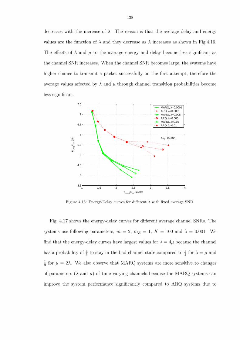
138
decreases with the increase of λ. The reason is that the average delay and energy
values are the function of λ and they decrease as λ increases as shown in Fig.4.16.
The effects of λ and µ to the average energy and delay become less significant as
the channel SNR increases. When the channel SNR becomes large, the systems have
higher chance to transmit a packet successfully on the first attempt, therefore the
average values affected by λ and µ through channel transition probabilities become
less significant.
1 1.5 2 2.5 3 3.5 43.5
4
4.5
5
5.5
6
6.5
7
7.5
Td,avg
/KDT
(µ secs)
Et,a
vg/K
DT (
dB)
MARQ, λ=0.0001ARQ, λ=0.0001MARQ, λ=0.005ARQ, λ=0.005MARQ, λ=0.01ARQ, λ=0.01
λ=µ, K=100
Figure 4.15: Energy-Delay curves for different λ with fixed average SNR.
Fig. 4.17 shows the energy-delay curves for different average channel SNRs. The
systems use following parameters, m = 2, mR = 1, K = 100 and λ = 0.001. We
find that the energy-delay curves have largest values for λ = 4µ because the channel
has a probability of 45
to stay in the bad channel state compared to 12
for λ = µ and
13
for µ = 2λ. We also observe that MARQ systems are more sensitive to changes
of parameters (λ and µ) of time varying channels because the MARQ systems can
improve the system performance significantly compared to ARQ systems due to

139
10−7
10−6
10−5
10−4
10−3
10−2
10−1
100
100
101
102
103
104
105
λ
Td,
avg/K
DT
µ=4λµ=λµ=1/4λ
Figure 4.16: Normalized average delay relations with λ.
better error correction capability. Therefore, MARQ has better performance but is
more sensitive than ARQ.
The comparison of three different repetition ARQ schemes is given in Fig. 4.18.
The systems uses the following parameters, m = 2, mR = 1, K = 100 and λ = 0.0001.
From Fig. 4.18, we see that the system has worst performance when it does not utilize
the previous error packet information (memoryless at the receiver). For the receiver
with memory, the R-ARQ-SWM has better performance compared to R-ARQ-NOW
because R-ARQ-NOW refreshes the memory buffer with the repetition period of
packet lengths even the previous packet is erroneous received. Accordingly, it cannot
utilize all the information of previous erroneous packets.
The effect of different Nrt for GBN-ARQ is shown in Fig. 4.18. The systems use
following parameters, m = 2, mR = 1, K = 100 and λ = 0.001. It shows that the
average delay and energy consumed by the systems are proportional to the quantity
Nrt since this is a go-back-Nrt protocol. Therefore, we need to retransmit all the

140
1 1.5 2 2.5 3 3.53.5
4
4.5
5
5.5
6
6.5
7
7.5
Td,avg
/KDT
(µ secs)
Et,a
vg/K
DT (
dB)
MARQ, λ=4µARQ, λ=4µMARQ, λ=µARQ, λ=µMARQ, µ=2λARQ, µ=2λ
Figure 4.17: Energy-Delay curves for different average channel SNRs.
1 1.5 2 2.5 3 3.55
6
7
8
9
10
11
Td,avg
/KDT
(µ secs)
Et,a
vg/K
DT (
dB)
RARQRARQSWMRARQNOM
K=100,λ=0.0001
Figure 4.18: Energy-Delay curves for repetition ARQ.

141
following Nrt packets when the transmitter receives a NACK packet. In other words,
the system needs to spend Nrt times in delay and energy for each packet transmission.
2 4 6 8 10 12 147
8
9
10
11
12
13
14
Td,avg
/KDT
(µ secs)
Et,a
vg/K
DT (
dB)
MARQ,Nrt=2
ARQ,Nrt=2
MARQ,Nrt=3
ARQ,Nrt=3
MARQ,Nrt=4
ARQ,Nrt=4
Figure 4.19: Energy-Delay curves for GBNARQ with different Nrt.
4.8 Conclusion
In this chapter we modeled an ARQ system with a FSM to obtain the joint dis-
tribution of energy and delay for packet transmission over time varying channels.
According to the state diagram constructed from the FSM, we derived the joint gen-
erating function of energy and delay. The generating function was used to obtain
the energy and delay tradeoff curves of an ARQ system. This comprehensive ap-
proach allows us to analyze the overall system by taking into account the states of
the transmitter, receiver and channel. Finally, the numerical results demonstrated
the time-varying characteristics of the channel have a great influence on the system
performance.

CHAPTER V
Conclusion and Future Research
In this chapter, we conclude this dissertation by summarizing the content of the
thesis and proposing possible future research directions.
5.1 Contributions
The most important contribution of this thesis is to represent the operation of a
system by a state diagram and use the generating function approach to derive the
statistics of the energy and delay consumption. We investigated the energy and delay
tradeoff of a wireless communication system. In the first part (Chapter 2 and 3) of
this thesis, we analyzed the energy and delay for a communication network. In the
second part (Chapter 4) of this thesis, we studied an ARQ communication system.
In Chapter 2, we began by extending the approach proposed in [22] to determine
average energy and delay of a successful packet transmission by taking into consider-
ation the dependence of packet error probability on energy and delay. Thereupon, we
proposed a state diagram representation of the operation of the MAC layer to obtain
the joint generating function of the energy and delay by considering the effects of
the PHY and MAC layer jointly. Furthermore, channel coding was incorporated in
the analysis by estimating the packet error probability using error-exponent-based
bounds under an AWGN channel. Using these analysis tools, the code rate and the
142

143
signal-to-noise ratio per dimension were optimized to achieve minimum average delay
per information bit. By changing the signal-to-noise ratio, the energy-delay trade-
off curves for minimum delay were obtained. Finally, an approximation method to
express the energy-delay tradeoff curves analytically was provided. The comparison
of the energy-delay tradeoff curves evaluated from this approximation method with
the exact energy-delay tradeoff curves (from numerical optimization) demonstrated
that this approximation method is extremely accurate especially when the number
of information bits per packet is large.
In Chapter 3, we applied our proposed generating analysis method to analyze
and design other wireless network protocols. We first designed an energy adaptation
scheme with original IEEE 802.11 protocol in which the transmitter increases the
energy level per coded symbol whenever it suffers an unsuccessful transmission. The
numerical results showed that the proposed protocol can improve the energy and
delay throughput of the system significantly when the channel condition is bad. By
using Reed-Solomon codes we optimized the system performance over the code rate
and energy per coded bit. Although we used Reed-Solomon codes over AWGN chan-
nel to represent packet error probabilities, the framework of our analysis can be used
for other coding and modulation schemes over various wireless channels. The second
proposed protocol is an ARQ scheme for data packets transmission with 802.11 pro-
tocol. The purpose of this analysis is to demonstrate that the generating function
approach can be applied to analyze more protocol layers jointly by including the
analysis of the logical link control (LLC) sublayer into the original protocol (MAC
and PHY layers only). The numerical results showed that the IEEE 802.11 original
protocol and the proposed one have almost identical performances and are equally
sensitive to the knowledge of the channel quality, say channel SNR, at the transmit-

144
ter. We also observed that the reduction in delay of a SWARQ-FT system achieved
by immediately retransmitting an erroneously received packet, is compensated by
the increased delay needed to access the channel, since other users use the same pro-
tocol. While ARQ provides some robustness to SNR uncertainty in a conventional
single user system, this is not the case in this multiuser scenario.
In Chapter 4, we modeled an ARQ system with a FSM to obtain the joint dis-
tribution of energy and delay for successful packet transmission over a time varying
channels. According to the state diagram constructed from FSM, we derived the
joint generating function of energy and delay. The generating function was used to
obtain the energy and delay tradeoff curves of an ARQ system. This comprehen-
sive approach allows us to analyze the overall system taking into account the states
of transmitter, receiver and channel. Finally, the numerical results demonstrated
the time-varying characteristics of the channel have a great influence on the system
performance. The cutoff rate for two different memory receiver structures was de-
rived and the optimization of the cutoff rate under average energy constraint was
discussed.
5.2 Future Research
In this thesis, packet error probabilities are represented by random coding bounds.
One extension is to consider the packet error probability for specific coding schemes,
such as LDPC or turbo codes. The other research direction that can be explored
is to relax the assumption of the saturation traffic by analyzing the non-saturation
traffic. For a different traffic model, we can further consider the delay spent in a
buffer. By regulating the desired quality of services (QoS), we also can investigate
the best energy allocation strategy for transmitting stations.

145
Although some research in [22, 39, 14, 15] considered the effects of packet errors
in their analysis, they all assumed that all stations in a wireless network share an
identical channel condition. However, this assumption is not realistic in practice, the
wireless communication-links between any pair of source and destination stations may
differ from each other due to the different physical objects in between. Therefore,
one possible future research is to relax the restriction of the homogeneous channel
condition for all the contending stations by considering the channel inhomogeneity
incurred among different users. We believe that the proposed generating function
method described in this thesis could be applied to other MAC protocols with more
complicated channel conditions.
The energy considered in the thesis is just transmission energy. We also can
consider other energy consumption, such as hardware processing energy, antenna
switching energy between transmitting and receiving modes. In commercial wireless
networks, mobility is an important issue, however, we do not consider mobility issue
in this thesis. Future research is needed to quantify how the energy and delay
consumption changes when stations are mobile.
For ARQ systems, we only considered error free case for the ACK and NACK
packets in this thesis. One future research direction is to analyze an ARQ system
by taking into consideration the nonzero ACK and NACK packet error probabilities
and the energy and delay consumption for ACK and NACK packets. The spatial
dimension provided by multiple antennas is known to dramatically increase system
capacity. As a result, combining multiple-input multiple-out (MIMO) with ARQ
systems has become an important and popular research subject. In particular, the
combination of MIMO spatial diversity with temporal diversity has led to widespread
development of space−time coding (STC) schemes. Many approaches have been

146
proposed for STC, for example, space−time trellis coding, space−time bit-interleaved
coded modulation (BICM), and space−time block coding. Another future research
direction is to develop some new ARQ protocols for MIMO systems which adapt the
signal constellation of each ARQ retransmission.

APPENDICES
147

148
APPENDIX A
Generating Function Analysis for NR-ARQ Systems
A.1 Memoryless Receiver
In this section, we will determine the joint generating function of the energy
consumed and delay incurred for a NR-ARQ system without the receiver memory
according to the general formulas provided in Chapter 4.3. In order to illustrate
the meaning for those formulas, we consider a system with some specific parame-
ters. We assume that the sequence of packet lengths used for each transmission is
{N1, N2, N2, · · · }. For all appendices, we use P = 1−P for an event with probability
value P .
From the state transition diagram shown in Fig. 4.3, we can group all transmis-
sions with transmission indices from as (2 + k · 1) for k ∈ {0, 1, 2, · · · } into a group
since these transmissions use same packet length N2 to transmission. We can see
that there is only one group, g1, in this system and T (i1) = T (2) = 2.
We first derive the first part of the generating function for those successful trans-
missions which are not belonged to (2 + k · 1 + 1). Therefore, we need to evaluate
the generating functions for G1(X, Y ) and G2(X,Y ). The generating function for
the event that the packet is transmitted successfully in the first transmission is
G1(X, Y ) = (PG(1− Pe,G1) + PB(1− Pe,B1))XN1TbY N1Ec , (A.1)

149
where PG and PB are the probabilities that the initial transmission was in good and
bad states, respectively. We assume that PG is equal to stationary probability of
good channel ( µλ+µ
) and PB is equal to stationary probability of bad channel ( λλ+µ
)
if the system has operated for a long time period already. Because min i1 = 2, we
need to evaluate the generating function of G2 by using the recursion formula shown
in (4.12) and obtain
G2(X, Y ) = [PGPe,G1e−λN1Tb + PBPe,B1e
−µN1Tb)]Pe,G2X(N1+N2)TbY (N1+N2)Ec +
[PGPe,G1e−λN1Tb + PBPe,B1e
−µN1Tb ]Pe,B2X(N1+N2)TbY (N1+N2)Ec .(A.2)
For the second part of the generating function for those successful transmissions
with transmission indices form as (2+k ·1+1) for k ∈ {0, 1, 2, · · · }, we need to obtain
the generating functions of Gf,G2 and Gf,B2 by solving a set of linear equations. We
omit the memory content parts in Gf,G2 and Gf,B2 for further notational simplicity
since this is a memoryless system. From the systems of equations shown in (4.9),
the generating functions of Gf,G2 and Gf,B2 will be determined if the transition
probability matrix for the system states and the initial conditions are given. For
transition matrix, it is
Pe,G2eλN2Tb Pe,G2(1− eλN2Tb)
Pe,B2(1− eµN2Tb) Pe,B2eµN2Tb)
, (A.3)
and the initial conditions are
Af,G2 = [PGPe,G1e−λN1Tb + PBPe,B1(1− e−µN1Tb)]Pe,G2X
(N1+N2)TbY (N1+N2)Ec
Af,B2 = [PGPe,G1(1− e−λN1Tb) + PBPe,B1e−µN1Tb ]Pe,B2X
(N1+N2)TbY (N1+N2)Ec .
(A.4)

150
Therefore, the total generating function for this system is
Gs = G1 + G2 + [Gf,G2e−λN2Tb(1− Pe,G2) + Gf,B2(1− e−µN2Tb)(1− Pe,G2) +
Gf,G2(1− e−λN2Tb)(1− Pe,B2) + Gf,B2e−µN2Tb (1− Pe,B2)]X
N2TbY N2Ec .(A.5)
A.2 Memory Receiver
In this section, we will determine the joint generating function of the energy and
delay required for a NR-ARQ system with the receiver memory. We assume that the
sequence of packet lengths used for each transmission is {N1, N2, N2, · · · }.
From the state transition diagram shown in Fig. 4.6, we can group all transmis-
sions with transmission indices from as (3 + k · 1) for k ∈ {0, 1, 2, · · · } into a group
since these transmissions use same packet length N2 to transmission. We can see
that there is only one group, g1, in this system and T (i1) = T (3) = 2.
We first derive the first part of the generating functions for those successful trans-
missions which are not belonged to indices (3 + k · 1). Since i1 = 3, we need to
evaluate G1, G2, and G3 recursively from (4.12). They are
G1(X, Y ) = (PG(1− Pe,G1) + PB(1− Pe,B1))XN1TbY N1Ec
G2(X, Y ) = [PGPe,G1(e−λN1Tb(1− Pe,G2|G1) + (1− e−λN1Tb)(1− Pe,B2|G1)) +
PBPe,B1((1− e−µN1Tb)(1− Pe,G2|B1) + e−µN1Tb(1− Pe,B2|B1))] ·
X(N1+N2)TbY (N1+N2)Ec
G3(X, Y ) = [PGPe,G1(e−λN1TbPe,G2|G1e
−λN2TbPe,G2|G2 + e−λN1TbPe,G2|G1e−λN2TbPe,B2|G2 +
e−λN1TbPe,B2|G1e−µN2TbPe,G2|B2 + e−λN1TbPe,B2|G1e
−µN2TbPe,B2|B2) +
PBPe,B1(e−µN1TbPe,G2|B1e
−λN2TbPe,G2|G2 + e−µN1TbPe,G2|B1e−λN2TbPe,B2|G2 +
e−µN1TbPe,B2|B1e−λN2TbPe,G2|B2 + e−µN1TbPe,B2|B1e
−µN2TbPe,B2|B2)] ·
X(N1+N2+N3)TbY (N1+N2+N3)Ec , (A.6)

151
For the second part of the generating function for those successful transmissions
with transmission indices form as (3 + k · 1 + 1) for k ∈ {0, 1, 2, · · · }, we need
to obtain the generating functions of Gf,G2|G2, Gf,B2|G2, Gf,G2|B2 and Gf,B2|B2 by
solving a set of linear equations. From the systems of equations shown in (4.9), the
generating functions of Gf,G2|G2, Gf,B2|G2, Gf,G2|B2 and Gf,B2|B2 will be determined
if the transition probability matrix for the system states and the initial conditions
are given. For transition matrix, it is
Pe,G2|G2eλN2Tb 0 Pe,G2|G2e
λN2Tb 0
Pe,G2|B2eλN2Tb 0 Pe,G2|B2e
λN2Tb 0
0 Pe,B2|G2eµN2Tb 0 Pe,B2|G2e
µN2Tb
0 Pe,B2|B2eλN2Tb 0 Pe,B2|B2e
λN2Tb
, (A.7)
and the initial conditions are
Af,G2|G2 = (PGPe,G1e−λN1TbPe,G2|G1 + PBPe,B1e
−µN1TbPe,G2|B1)e−λN2TbPe,G2|G2 ·
X(N1+2N2)TbY (N1+2N2)Ec
Af,G2|B2 = (PGPe,G1e−λN1TbPe,B2|G1 + PBPe,B1e
−µN1TbPe,B2|B1)e−µN2TbPe,G2|B2 ·
X(N1+2N2)TbY (N1+2N2)Ec
Af,B2|G2 = (PGPe,G1e−λN1TbPe,G2|G1 + PBPe,B1e
−µN1TbPe,G2|B1)e−λN2TbPe,B2|G2 ·
X(N1+2N2)TbY (N1+2N2)Ec
Af,B2|B2 = (PGPe,G1e−λN1TbPe,B2|G1 + PBPe,B1e
−µN1TbPe,B2|B1)e−µN2TbPe,B2|B2 ·
X(N1+2N2)TbY (N1+2N2)Ec (A.8)

152
Therefore, the total generating function for this system is
Gs = G1 + G2 + G3 + [Gf,G2|G2e−λN2Tb(1− Pe,G2|G2) + Gf,G2|G2e
−λN2Tb(1− Pe,B2|G2) +
Gf,G2|B2e−λN2Tb(1− Pe,G2|G2) + Gf,G2|B2e
−λN2Tb(1− Pe,B2|G2) +
Gf,B2|G2e−µN2Tb(1− Pe,B2|B2) + Gf,B2|B2e
−µN2Tb(1− Pe,G2|B2) +
Gf,B2|B2e−µN2Tb(1− Pe,B2|B2) + Gf,B2|B2e
−µN2Tb(1− Pe,G2|B2)]XN2TbY N2Ec . (A.9)

153
APPENDIX B
Generating Function Analysis for R-ARQ Systems
B.1 Memoryless Receiver
In this section, we will determine the joint generating function of the energy
consumed and delay incurred for a R-ARQ system without the receiver memory
according to the general formulas provided in Chapter 4.3. We consider a system
with some specific parameters by assuming that the sequence of packet lengths used
for each transmission is {N1, N2, N1, N2, N1, N2, · · · }.
From the state transition diagram shown in Fig. 4.8, we can group all transmis-
sions with transmission indices from as (1 + k · 2) for k ∈ {0, 1, 2, · · · } into a group
g1 and (2 + k · 1) for k ∈ {0, 1, 2, · · · } into another group g2. There are two groups,
g1, g2, in this system and T (i1) = T (1) = 1, T (i2) = T (2) = 2.
We first derive the first part of the generating function. Since i1 = 1, i2 = 2,
the only term in the first part of the generating function is G1(X, Y ). The gener-
ating function for the event that the packet is transmitted successfully in the first
transmission is
G1(X, Y ) = (PG(1− Pe,G1) + PB(1− Pe,B1))XN1TbY N1Ec , (B.1)
where PG and PB are the probabilities that the initial transmission was in good and
bad states, respectively. We assume that PG is equal to stationary probability of

154
good channel ( µλ+µ
) and PB is equal to stationary probability of bad channel ( λλ+µ
)
if the system has operated for a long time period already.
For the second part of the generating function for those successful transmissions
with transmission indices form as (1 + k · 2 + 1) for k ∈ {0, 1, 2, · · · }, we need
to obtain the generating functions of Gf,G1 and Gf,B1 by solving a set of linear
equations. Similarly, for those successful transmissions with transmission indices
form as (2+k ·2+1) for k ∈ {0, 1, 2, · · · }, we need to obtain the generating functions
of Gf,G2 and Gf,B2 by solving a set of linear equations.
From the systems of equations shown in (4.9), the generating functions of Gf,G1
and Gf,B1 will be determined if the transition probability matrix, Mg1 , for the system
states and the initial conditions are given. For transition matrix, it is
Mg1 =
cg1
11 cg1
12
cg1
21 cg1
22
, (B.2)
where
cg1
11 = Pe,G1Pe,G2e−λN1Tbe−λN2Tb + Pe,G1Pe,B2e
−λN1Tbe−µN2Tb
cg1
12 = Pe,G1Pe,G2e−λN1Tbe−λN2Tb + Pe,G1Pe,B2e
−λN1Tbe−µN2Tb
cg1
21 = Pe,B1Pe,G2e−µN1Tbe−λN2Tb + Pe,B1Pe,B2e
−µN1Tbe−µN2Tb
cg1
22 = Pe,B1Pe,G2e−µN1Tbe−λN2Tb + Pe,B1Pe,B2e
−µN1Tbe−µN2Tb . (B.3)
And the initial conditions are
Af,G1 = PGPe,G1XN1TbY N1Ec
Af,B1 = PBPe,B1XN1TbY N1Ec . (B.4)
Similarly, the generating functions of Gf,G2 and Gf,B2 will be determined if the
transition probability matrix, Mg2 , for the system states and the initial conditions

155
are given. For transition matrix, it is
Mg2 =
cg2
11 cg2
12
cg2
21 cg2
22
, (B.5)
where
cg2
11 = Pe,G2Pe,G1e−λN2Tbe−λN1Tb + Pe,G2Pe,B1e
−λN2Tbe−µN1Tb
cg2
12 = Pe,G2Pe,G1e−λN2Tbe−λN1Tb + Pe,G2Pe,B1e
−λN2Tbe−µN1Tb
cg2
21 = Pe,B2Pe,G1e−µN2Tbe−λN1Tb + Pe,B2Pe,B1e
−µN2Tbe−µN1Tb
cg2
22 = Pe,B2Pe,G1e−µN2Tbe−λN1Tb + Pe,B2Pe,B1e
−µN2Tbe−µN1Tb . (B.6)
And the initial conditions are
Af,G2 = [PGPe,G1e−λN1Tb + PBPe,B1(1− e−µN1Tb)]Pe,G2X
(N1+N2)TbY (N1+N2)Ec
Af,B2 = [PGPe,G1(1− e−λN1Tb) + PBPe,B1e−µN1Tb ]Pe,B2X
(N1+N2)TbY (N1+N2)Ec .
(B.7)
Therefore, the total generating function for this system is
Gs = G1 + [Gf,G1(e−λN1TbPe,G2 + e−λN1TbPe,B2)
Gf,B1(e−µN1TbPe,G2 + e−µN1TbPe,B2)]X
N2TbY N2Ec +
[Gf,G2(e−λN2TbPe,G1 + e−λN2TbPe,B1)
Gf,B2(e−µN2TbPe,G1 + e−µN2TbPe,B1)]X
N1TbY N1Ec (B.8)
B.2 Memory Receiver : Sliding Window
In this section, we will determine the generating function for a R-ARQ system
with the receiver memory which updates its memory contents by the sliding window
operation. We assume that the sequence of packet lengths used for each transmission
is {N1, N2, N1, N2, N1, N2, · · · }.

156
From the state transition diagram shown in Fig. 4.9, we can group all transmis-
sions with transmission indices from as (2 + k · 2) for k ∈ {0, 1, 2, · · · } into a group
g1 and (3 + k · 2) for k ∈ {0, 1, 2, · · · } into another group g2. There are two groups,
g1, g2, in this system and T (i1) = T (2) = 2, T (i2) = T (3) = 1.
We first derive the first part of the generating function. Since i1 = 2, i2 = 3, the
terms in the first part of the generating function are G1, G2. They are
G1(X,Y ) = (PG(1− Pe,G1) + PB(1− Pe,B1))XN1TbY N1Ec
G2(X,Y ) = [PGPe,G1(e−λN1TbPe,G2|G1 + e−λN1TbPe,B2|G1) +
PBPe,B1(e−µN1TbPe,B2|B1 + e−µN1TbPe,G2|B1)]X
(N1+N2)TbY (N1+N2)Ec ,
(B.9)
where PG and PB are the probabilities that the initial transmission was in good and
bad states, respectively. We assume that PG is equal to stationary probability of
good channel ( µλ+µ
) and PB is equal to stationary probability of bad channel ( λλ+µ
)
if the system has operated for a long time period already.
For the second part of the generating function for those successful transmissions
with transmission indices form as (2 + k · 2 + 1) for k ∈ {0, 1, 2, · · · }, we need
to obtain the generating functions of Gf,G2|G1 , Gf,G2|B1 , Gf,B2|G1 , and Gf,B2|B1 by
solving a set of linear equations. Similarly, for those successful transmissions with
transmission indices form as (3 + k · 2 + 1) for k ∈ {0, 1, 2, · · · }, we need to obtain
the generating functions of Gf,G1|G2 , Gf,G1|B2 , Gf,B1|G2 , and Gf,B1|B2 by solving a set
of linear equations.
From the systems of equations shown in (4.9), the generating functions of Gf,G2|G1 ,
Gf,G2|B1 , Gf,B2|G1 , and Gf,B2|B1 will be determined if the transition probability matrix,
Mg1 , for the system states and the initial conditions are given. For transition matrix,

157
it is
Mg1 =
cg1
11 cg1
12 cg1
13 cg1
14
cg1
21 cg1
22 cg1
23 cg1
24
cg1
31 cg1
32 cg1
33 cg1
34
cg1
41 cg1
42 cg1
43 cg1
44
, (B.10)
where
cg1
11 = Pe,G2|G1Pe,G1|G2e−λN2Tbe−λN1Tb , cg1
12 = Pe,G2|G1Pe,B1|G2e−λN2Tbe−µN1Tb
cg1
13 = Pe,G2|G1Pe,G1|G2e−λN2Tbe−λN1Tb , cg1
14 = Pe,G2|G1Pe,B1|G2e−λN2Tbe−µN1Tb
cg1
21 = Pe,G2|B1Pe,G1|G2e−λN2Tbe−λN1Tb , cg1
22 = Pe,G2|B1Pe,B1|G2e−λN2Tbe−µN1Tb
cg1
23 = Pe,G2|B1Pe,G1|G2e−λN2Tbe−λN1Tb , cg1
24 = Pe,G2|B1Pe,B1|G2e−λN2Tbe−µN1Tb
cg1
31 = Pe,B2|G1Pe,G1|B2e−µN2Tbe−λN1Tb , cg1
32 = Pe,B2|G1Pe,B1|B2e−µN2Tbe−µN1Tb
cg1
33 = Pe,B2|G1Pe,G1|B2e−µN2Tbe−λN1Tb , cg1
34 = Pe,B2|G1Pe,B1|B2e−µN2Tbe−µN1Tb
cg1
41 = Pe,B2|B1Pe,G1|B2e−µN2Tbe−λN1Tb , cg1
42 = Pe,B2|B1Pe,B1|B2e−µN2Tbe−µN1Tb
cg1
43 = Pe,B2|B1Pe,G1|B2e−µN2Tbe−λN1Tb , cg1
44 = Pe,B2|B1Pe,B1|B2e−µN2Tbe−µN1Tb
. (B.11)
And the initial conditions are
Af,G2|G1 = PGPe,G1Pe,G2|G1e−λN1TbX(N1+N2)TbY (N1+N2)Ec
Af,G2|B1 = PBPe,B1Pe,G2|B1e−µN1TbX(N1+N2)TbY (N1+N2)Ec
Af,B2|G1 = PGPe,G1Pe,B2|G1e−λN1TbX(N1+N2)TbY (N1+N2)Ec
Af,B2|B1 = PBPe,B1Pe,B2|B1e−µN1TbX(N1+N2)TbY (N1+N2)Ec . (B.12)
Similarly, for those successful transmissions with transmission indices form as
(3 + k · 2 + 1) for k ∈ {0, 1, 2, · · · }, we need to obtain the generating functions of
Gf,G1|G2 , Gf,G1|B2 , Gf,B1|G2 , and Gf,B1|B2 by solving a set of linear equations.

158
From the systems of equations shown in (4.9), the generating functions of Gf,G1|G2 ,
Gf,G1|B2 , Gf,B1|G2 , and Gf,B1|B2 will be determined if the transition probability matrix,
Mg2 , for the system states and the initial conditions are given. For transition matrix,
it is
Mg2 =
cg2
11 cg2
12 cg2
13 cg2
14
cg2
21 cg2
22 cg2
23 cg2
24
cg2
31 cg2
32 cg2
33 cg2
34
cg2
41 cg2
42 cg2
43 cg2
44
, (B.13)
where
cg2
11 = Pe,G1|G2Pe,G2|G1e−λN1Tbe−λN2Tb , cg2
12 = Pe,G1|G2Pe,B2|G1e−λN1Tbe−µN2Tb
cg2
13 = Pe,G1|G2Pe,G2|G1e−λN1Tbe−λN2Tb , cg2
14 = Pe,G1|G2Pe,B2|G1e−λN1Tbe−µN2Tb
cg2
21 = Pe,G1|B2Pe,G2|G1e−λN1Tbe−λN2Tb , cg2
22 = Pe,G1|B2Pe,B2|G1e−λN1Tbe−µN2Tb
cg2
23 = Pe,G1|B2Pe,G2|G1e−λN1Tbe−λN2Tb , cg2
24 = Pe,G1|B2Pe,B2|G1e−λN1Tbe−µN2Tb
cg2
31 = Pe,B1|G2Pe,G2|B1e−µN1Tbe−λN2Tb , cg2
32 = Pe,B1|G2Pe,B2|B1e−µN1Tbe−µN2Tb
cg2
33 = Pe,B1|G2Pe,G2|B1e−µN1Tbe−λN2Tb , cg2
34 = Pe,B1|G2Pe,B2|B1e−µN1Tbe−µN2Tb
cg2
41 = Pe,B1|B2Pe,G2|B1e−µN1Tbe−λN2Tb , cg2
42 = Pe,B1|B2Pe,B2|B1e−µN1Tbe−µN2Tb
cg2
43 = Pe,B1|B2Pe,G2|B1e−µN1Tbe−λN2Tb , cg2
44 = Pe,B1|B2Pe,B2|B1e−µN1Tbe−µN2Tb .
(B.14)
159
And the initial conditions are
Af,G1|G2 = (PGPe,G1Pe,G2|G1e−λN1Tbe−λN2Tb + PBPe,B1Pe,G2|B1e
−µN1Tbe−λN2Tb)Pe,G1|G2 ·
X(2N1+N2)TbY (2N1+N2)Ec
Af,G1|B2 = (PGPe,G1Pe,B2|G1e−λN1Tbe−µN2Tb + PBPe,B1Pe,B2|B1e
−µN1Tbe−µN2Tb)Pe,G1|B2 ·
X(2N1+N2)TbY (2N1+N2)Ec
Af,B1|G2 = (PGPe,G1Pe,G2|G1e−λN1Tbe−µN2Tb + PBPe,B1Pe,G2|B1e
−µN1Tbe−λN2Tb)Pe,B1|G2 ·
X(2N1+N2)TbY (2N1+N2)Ec
Af,B1|B2 = (PGPe,G1Pe,B2|G1e−λN1Tbe−µN2Tb + PBPe,B1Pe,B2|B1e
−µN1Tbe−µN2Tb)Pe,B1|B2 ·
X(2N1+N2)TbY (2N1+N2)Ec . (B.15)
Therefore, the total generating function for this system is
Gs = G1(X,Y ) + G2(X, Y ) + [(Gf,G2|G1 + Gf,G2|B1)(e−λN2TbPe,G1|G2 + e−λN2TbPe,B1|G2) +
(Gf,B2|G1 + Gf,B2|B1)(e−µN2TbPe,G1|B2 + e−µN2TbPe,B1|B2)]X
N1TbY N1Ec +
[(Gf,G1|G2 + Gf,G1|B2)(e−λN1TbPe,G2|G1 + e−λN1TbPe,B2|G1) +
(Gf,B1|G2 + Gf,B1|B2)(e−µN1TbPe,G2|B1 + e−µN1TbPe,B2|B1)]X
N2TbY N2Ec . (B.16)
B.3 Memory Receiver : Non Overlap
In this section, we will determine the generating function of energy and delay
to transmit a data packet successfully for a R-ARQ system with the receiver mem-
ory. We assume that the sequence of packet lengths used for each transmission is
{N1, N2, N1, N2, N1, N2, · · · }.
From the state transition diagram shown in Fig. 4.10, we can group all transmis-
sions with transmission indices from as (1 + k · 2) for k ∈ {0, 1, 2, · · · } into a group
g1 and (2 + k · 2) for k ∈ {0, 1, 2, · · · } into another group g2. There are two groups,
g1, g2, in this system and T (i1) = T (1) = 1, T (i2) = T (2) = 2.
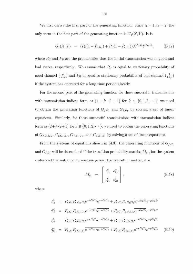
160
We first derive the first part of the generating function. Since i1 = 1, i2 = 2, the
only term in the first part of the generating function is G1(X, Y ). It is
G1(X, Y ) = (PG(1− Pe,G1) + PB(1− Pe,B1))XN1TbY N1Ec . (B.17)
where PG and PB are the probabilities that the initial transmission was in good and
bad states, respectively. We assume that PG is equal to stationary probability of
good channel ( µλ+µ
) and PB is equal to stationary probability of bad channel ( λλ+µ
)
if the system has operated for a long time period already.
For the second part of the generating function for those successful transmissions
with transmission indices form as (1 + k · 2 + 1) for k ∈ {0, 1, 2, · · · }, we need
to obtain the generating functions of Gf,G1 and Gf,B1 by solving a set of linear
equations. Similarly, for those successful transmissions with transmission indices
form as (2+k ·2+1) for k ∈ {0, 1, 2, · · · }, we need to obtain the generating functions
of Gf,G2|G1 , Gf,G2|B1 , Gf,B2|G1 , and Gf,B2|B1 by solving a set of linear equations.
From the systems of equations shown in (4.9), the generating functions of Gf,G1
and Gf,B1 will be determined if the transition probability matrix, Mg1 , for the system
states and the initial conditions are given. For transition matrix, it is
Mg1 =
cg1
11 cg1
12
cg1
21 cg1
22
, (B.18)
where
cg1
11 = Pe,G1Pe,G2|G1e−λN1Tbe−λN2Tb + Pe,G1Pe,B2|G1e
−λN1Tbe−µN2Tb
cg1
12 = Pe,G1Pe,G2|G1e−λN1Tbe−λN2Tb + Pe,G1Pe,B2|G1e
−λN1Tbe−µN2Tb
cg1
21 = Pe,B1Pe,G2|B1e−µN1Tbe−λN2Tb + Pe,B1Pe,B2|B1e
−µN1Tbe−µN2Tb
cg1
22 = Pe,B1Pe,G2|B1e−λN1Tbe−λN2Tb + Pe,B1Pe,B2|B1e
−µN1Tbe−µN2Tb (B.19)

161
And the initial conditions are
Af,G1 = PGPe,G1XN1TbY N1Ec
Af,B1 = PBPe,B1XN1TbY N1Ec . (B.20)
Similarly, for those successful transmissions with transmission indices form as
(2 + k · 2 + 1) for k ∈ {0, 1, 2, · · · }, we need to obtain the generating functions of
Gf,G2|G1 , Gf,G2|B1 , Gf,B2|G1 , and Gf,B2|B1 by solving a set of linear equations.
From the systems of equations shown in (4.9), the generating functions of Gf,G2|G1 ,
Gf,G2|B1 , Gf,B2|G1 , and Gf,B2|B1 will be determined if the transition probability matrix,
Mg2 , for the system states and the initial conditions are given. For transition matrix,
it is
Mg2 =
cg2
11 cg2
12 cg2
13 cg2
14
cg2
21 cg2
22 cg2
23 cg2
24
cg2
31 cg2
32 cg2
33 cg2
34
cg2
41 cg2
42 cg2
43 cg2
44
, (B.21)
where
cg2
11 = Pe,G2|G1Pe,G1e−λN2Tbe−λN1Tb , cg2
12 = Pe,G2|G1Pe,B1e−λN2Tbe−µN2Tb
cg2
13 = Pe,G2|G1Pe,G1e−λN2Tbe−λN1Tb , cg2
14 = Pe,G2|G1Pe,B1e−λN2Tbe−µN1Tb
cg2
21 = Pe,G2|B1Pe,G1e−λN2Tbe−λN1Tb , cg2
22 = Pe,G2|B1Pe,B1e−λN2Tbe−µN1Tb
cg2
23 = Pe,G2|B1Pe,G1e−λN2Tbe−λN1Tb , cg2
24 = Pe,G2|B1Pe,B1e−λN2Tbe−µN1Tb
cg2
31 = Pe,B2|G1Pe,G1e−λN2Tbe−λN1Tb , cg2
32 = Pe,B2|G1Pe,B1e−µN2Tbe−µN2Tb
cg2
33 = Pe,B2|G1Pe,G1e−µN2Tbe−λN1Tb , cg2
34 = Pe,B2|G1Pe,B1e−µN2Tbe−µN1Tb
cg2
41 = Pe,B2|B1Pe,G1e−µN2Tbe−λN1Tb , cg2
42 = Pe,B2|B1Pe,B1e−µN2Tbe−µN2Tb
cg2
43 = Pe,B2|B1Pe,G1e−µN2Tbe−λN1Tb , cg2
44 = Pe,B2|G1Pe,B1e−µN2Tbe−µN1Tb .(B.22)

162
And the initial conditions are
Af,G2|G1 = PGPe,G1Pe,G2|G1e−λN1TbX(N1+N2)TbY (N1+N2)Ec
Af,G2|B1 = PBPe,B1Pe,G2|B1e−µN1TbX(N1+N2)TbY (N1+N2)Ec
Af,B2|G1 = PGPe,G1Pe,B2|G1e−λN1TbX(N1+N2)TbY (N1+N2)Ec
Af,B2|B1 = PBPe,B1Pe,B2|B1e−µN1TbX(N1+N2)TbY (N1+N2)Ec . (B.23)
Therefore, the total generating function for this system is
Gs = G1 + [Gf,G1(e−λN1TbPe,G2|G1 + e−λN1TbPe,B2|G1) +
Gf,B1(e−µN1TbPe,G2|B1 + e−µN1TbPe,B2|B1)]X
N2TbY N2Ec +
[(Gf,G2|G1 + Gf,G2|B1)(e−λN2TbPe,G1 + e−λN2TbPe,B1) +
(Gf,B2|G1 + Gf,B2|B1)(e−µN2TbPe,G1 + e−µN2TbPe,B1)]X
N1TbY N1Ec .(B.24)

BIBLIOGRAPHY
163

164
BIBLIOGRAPHY
[1] Forum, wireless applicaion protocol architecture specification (2000),http://www.wapforum.org/what/technical.html.
[2] Irda sir data specification (2000), http://www.irda.org/standards/specifications.asp.
[3] IEEE standard for 802.11 wireless lan medium access control (MAC) and physical layer (phy)specifications, Nov. 1997.
[4] IEEE standard for 802.11 wireless lan medium access control (MAC) and physical layer (phy)specifications, Nov. 1999.
[5] G. Bianchi, Performance analysis of the IEEE 802.11 distributed coordination function, IEEEJ. Select. Areas Commun. 18 (2000), no. 3, 535–547.
[6] G. Bianchi, L. Fratta, and M. Oliveri, Performance analysis of IEEE 802.11 CSMA/CAmedium access control protocol, Proc. IEEE Intn’l Symposium on Personal, Indoor, and MobileRadio Communications (Taipei, Taiwan), Oct. 1996, pp. 407–411.
[7] G. Bianchi and I. Tinnirello, Analysis of priority mechanisms based on differentiated interframe spacing in csma-ca, Proc. Vehicular Tech. Conf., Oct. 2003, pp. 1401–1405.
[8] M. Brahma, K. W. Kim, M. E. Hachimi, A. Abouaissa, and P. Lorenz, A buffer and energybased scheduling in mobile ad hoc networks over link layer, Proc. Advanced Intn’l. Conf. onTelecom. and Web Applications and Services, Mar. 2006, pp. 19–25.
[9] H. Bruneel and M. Moeneclaey, On throughput performance of some continuous ARQ strategieswith repeated transmissions, IEEE Trans. Communications 34 (1986), 244–249.
[10] P. Bucciol, G. Davini, E. Masala, E. Filippi, and J. C. De Martin, Cross-layer perceptual ARQfor h.264 video streaming over 802.11 wireless networks, Proc. Globecom Conf., Dec. 2004,pp. 3027–3031.
[11] F. Cali, M. Conti, and E. Gregori, IEEE 802.11 wireless LAN: capacity analysis and protocolenhancement, Proc. INFOCOM. (San Francisco, CA), Mar. 1998, pp. 142–149.
[12] X. R. Cao and Y. C. Ho, Models of discrete event dynamic systems, IEEE Control Sys-tems. Mag. 10 (1990), 69–76.
[13] S. S. Chakraborty and M. Liinaharja, Performance analysis of an adaptive SR ARQ scheme fortime-varying rayleigh fading channels, Proc. Intn’l Communications Conf. (Helsinki, Finland),June 2001, pp. 2478–2482.
[14] S. Y. Chang, A. Anastaspoulos, and W. E. Stark, Energy-delay analysis of wireless systemswith random coding, Proc. Globecom Conf. (Dallas, USA), Dec. 2004, pp. 3270 – 3274.
[15] S. Y. Chang, W. E. Stark, and A. Anastasopolous, Energy-delay analysis of MAC protocols inwireless networks, IEEE Trans. Communications (2005), (Submitted).

165
[16] C. M Chao, J. P. Sheu, and I. C. Chou, An adaptive quorum-based energy conserving protocolfor IEEE 802.11 ad hoc networks, IEEE Trans. Mobile Computing 5 (2006), 560–570.
[17] H. S. Chhaya and S. Gupta, Performance modeling of asynchronous data transfer methods ofIEEE 802.11 MAC protocol, Wireless Networks 3 (1997), no. 3, 217–234.
[18] B. P. Crow, Performance evaluaion of the IEEE 802.11 wireless local area network protocol,Master’s thesis, University of Arizona, Tucson, AZ, 1996.
[19] P. E. Engelstad and O. N. Osterbo, Non-saturation and saturation analysis of IEEE 802.11eedca with starvation prediction, Proc. MSWiM (Montreal, Quebec, Canada), Oct. 2005,pp. 224–233.
[20] G. F. Franklin, J. D. Powell, and A. Emami-Naeini (eds.), Feedback control of dynamic systems,Addision Wesely, 1994.
[21] F. Granelli and D. Kliazovich, Cross-layering for performance improvement in multi-hop wire-less networks, Proc. Intn’l Symposium on Parallel Architectures, Algorithms and Networks,Dec. 2005, pp. 1–6.
[22] Z. Hadzi-Velkov and B. Spasenovski, Saturation throughput-delay analysis of IEEE 802.11 DCFin fading channel, Proc. Intn’l Communications Conf., vol. 1, Sept. 2004, pp. 121–126.
[23] T. S. Ho and K. C. Chen, Performance evaluation and enhancement of the CAMA/CA MACprotocol for 802.11 wireless LANs, Proc. IEEE Intn’l Symposium on Personal, Indoor, andMobile Radio Communications (Taipei, Taiwan), Oct. 1996, pp. 392–396.
[24] R. P. F. Hoefel, A cross-layer saturation goodput analysis for IEEE 802.11a networks, Proc. Ve-hicular Tech. Conf. (Stockholm, Sweden), May 2005, pp. 2051–2055.
[25] L. Huang and T. H. Lai, On the scalability of IEEE 802.11 ad hoc networks, Proc. MOBIHOC(Lausanne, Switzerland), June 2002, pp. 173–182.
[26] S. Kallel, Analysis of memory and incremental redundancy ARQ schemes over a nonstationarychannel, IEEE Trans. Communications 40 (1992), 1474–1480.
[27] S. Kallel, R. Link, and S. Bakhtiyari, Throughput performance of memory ARQ schemes,Proc. Vehicular Tech. Conf. 48 (1999), 891–899.
[28] V. Kanodia, C. Li, A. Sabharwal, B. Sadeghi, and E. Knightly, Distributed multi-hop schedulingand medium access with delay and throughput constraints, Proc. SIGMOBILE (Rome, Italy),July 2001, pp. 200–209.
[29] , Distributed priority scheduling and medium access in ad hoc networks, Wireless Net-works 8 (2002), 455–466.
[30] , Modeling the 802.11 distributed coordination function in non-saturated conditions,Communications Lett. 9 (2005), 715–717.
[31] H. Kim and J. C. Hou, Improving protocol capacity with model-based frame scheduling in IEEE802.11-operated wlans, Proc. MobiCom (San Diego, California, USA), Sept. 2003, pp. 14–19.
[32] , Modeling single-hop wireless networks under rician fading channels, Mar. 2004,pp. 219–224.
[33] L. Kleinrock and F. Tobagi, Packet switching in radio channels, part II-the hidden terminalproblem in carrier sense multiple access and the busy tone solution, IEEE Trans. Communica-tions 33 (1975), no. 12, 1417–1433.
[34] S. Lin and D. J. Costello (eds.), Error control coding: Fundamentals and applications, 1983.

166
[35] S. Lin, D. J. Costello, and M. J. Miller, Automatic-repeat-request rrror control scheme, IEEECommun. Mag. 22 (1984), no. 12, 5–17.
[36] M. H. Manshaei, G. R. Cantieni, C. Barakat, and T. Turletti, Performance analysis of theIEEE 802.11 MAC and physical layer protocol, Proc. Intn’l Symposium on World of WirelessMobile and Multimedia Networks, June 2005, pp. 88–97.
[37] A. C. Martins and J. C. Alves, ARQ protocols with adaptive block size perform better over awide range of bit error rates, IEEE Trans. Communications 38 (1990), 737–739.
[38] J. J. Metzner and J. M. Chung, Efficient energy utilization with time constraints in mobiletime varying channels, IEEE Trans. Veh. Tech. 49 (2000), 1169–1177.
[39] Qiang Ni, Performance analysis and enhancements for IEEE 802.11e wireless networks, IEEENetwork 19 (2005), 21–27.
[40] M. Rice and S. B. Wicker, A sequential scheme for adaptive error control over slowly varyingchannels, IEEE Trans. Communications 42 (1994), 1533–1543.
[41] K. Sakakibara, S. Chikada, and J. Yamakita, Analysis of unsaturation throughput of IEEE802.11 dcf, Proc. Intn’l Conf. on Personal Wireless Communications, Jan. 2005, pp. 134–138.
[42] C. Suh and Y. B. Ko, A traffic aware, energy efficient MAC protocol for wireless sensornetworks, Proc. Intn’l Symposium on Circuits and Systems, May 2005, pp. 2975–2978.
[43] I. Tinnirello and S. Choi, Efficiency analysis of burst transmissions with block ack in contention-based 802.11e wlans, Proc. Intn’l Communications Conf. (Seoul, Korea), May 2005, pp. 3455–3460.
[44] B. Vucetic, An adaptive coding scheme for time-varying channels, IEEE Trans. Communica-tions 39 (1991), 653–663.
[45] J. Wall and J. Y. Khan, An adaptive ARQ enhancement to support multimedia traffic using802.11 wireless lans, Proc. Globecom Conf., Dec. 2004, pp. 3037–3041.
[46] L. C. Wang, S. Y. Huang, and A. Chen, On the throughput performance of csma-based wire-less local area network with directional antennas and capture effect: A cross-layer analyticalapproach, Mar. 2004, pp. 1879–1884.
[47] Y. M. Wang and S. Lin, A modified selective-repeat type-II hybrid ARQ system and its perofr-mance analysis, IEEE Trans. Communications 31 (1988), 593–608.
[48] J. Weinmiller, M. Schlager, A. Festag, and A. Wolisz, Performance study of access control inwireless LANs IEEE 802.11 DFWMAC and ETSI RES 10 HIPERLAN, Mobile Networks andApplications 2 (1997), no. 1, 55–67.
[49] Lie Hua Wong, Error exponent regions for multi-user channels, Ph.D. thesis, Department ofElec. and Comp. Engin., University of Michigan, Ann Arbor, 2005.
[50] Y. D. Yao, An effective go-back-N ARQ scheme for variable-errorrate channels, IEEETrans. Communications 43 (1995), 20–23.
[51] W. Ye, J. Heidemann, and D. Estrin, Medium access control with coordinated adaptive sleepingfor wireless sensor networks, IEEE/ACM Trans. Networking 12 (2004), 493–506.
[52] J. Yun and S. Bahk, Parallel contention algorithm with csmaka for ofdm based high speedwireless lans, Proc. IEEE Intn’l Symposium on Personal, Indoor, and Mobile Radio Commu-nications, Sept. 2003, pp. 2581–2585.

ABSTRACT
Generating Function Analysis of Wireless Networks and ARQ Systems
by
Shihyu Chang
Co-Chair: Professor Wayne E. Stark
Co-Chair: Associate Professor Achilleas Anastasopoulos
In this thesis, there are two main themes. The first part of the thesis is to study
the tradeoff between energy and delay for wireless networks. A network using a
request-to-send (RTS) and clear-to-send (CTS) type medium access control (MAC)
protocol is considered. We first determine the average delay incurred and the average
energy consumed when the effects of an imperfect channel are incorporated in the
model. In order to incorporate the relation between packet error probability, energy,
and delay, we use the reliability function bounds for different channel models on
the error probability of a coded system. Further, we present a generic framework
that allows us to obtain the joint statistics of energy and delay through their joint
generating function. Several important design tradeoffs are studied from the joint
generating function, such as the average energy with an outage delay constraint. This
framework allows us to optimize over the system parameters for various objective

functions, such as average delay. An approximation method is also proposed to
calculate the average energy and average delay analytically. This approximation is
found to be quite accurate for a wide range of lengths. The inhomogeneous and
time-varying effects for the tradeoff between energy and delay are also studied.
The second part of the thesis is to propose an analytical method to determine the
joint distribution of the energy and delay of automatic repeat request (ARQ) proto-
cols over time varying channels. A finite state machine (FSM) is used to model the
transmitter, receiver and channel. From the state transition diagram of the FSM, the
generating function of energy and delay consumption can be evaluated according to
the Manson’s gain formula while incorporating physical layer characteristics (packet
error probability as a function of energy and delay). We also consider a receiver con-
taining memory of previously received samples and derive the cutoff rate for three
different receiver structures. As the numerical results demonstrate, the time-varying
characteristic of the channel have a great influence on the system performance.
Related Documents