Generalized Supersymmetric Quantum Mechanics and Reflectionless Fermion Bags in 1+1 Dimensions

arX

iv:h

ep-t

h/01

0904

5v1

6 S

ep 2

001

Generalized Supersymmetric Quantum

Mechanics and Reflectionless Fermion Bags in

1 + 1 Dimensions

Joshua Feinberga ∗ & A. Zeeb ∗

a)Physics Department,University of Haifa at Oranim, Tivon 36006, Israel∗∗

andPhysics Department,

Technion, Israel Institute of Technology, Haifa 32000, Israel

b)Institute for Theoretical PhysicsUniversity of California

Santa Barbara, CA 93106, USA

Abstract

We study static fermion bags in the 1 + 1 dimensional Gross-Neveu and Nambu-

Jona-Lasinio models. It has been known, from the work of Dashen, Hasslacher and Neveu

(DHN), followed by Shei’s work, in the 1970’s, that the self-consistent static fermion bags in

these models are reflectionless. The works of DHN and of Shei were based on inverse scattering

theory. Several years ago, we offered an alternative argument to establish the reflectionless

nature of these fermion bags, which was based on analysis of the spatial asymptotic behavior

of the resolvent of the Dirac operator in the background of a static bag, subjected to the

appropriate boundary conditions. We also calculated the masses of fermion bags based on the

resolvent and the Gelfand-Dikii identity. Based on arguments taken from a certain generalized

one dimensional supersymmetric quantum mechanics, which underlies the spectral theory of

these Dirac operators, we now realize that our analysis of the asymptotic behavior of the resolvent

was incomplete. We offer here a critique of our asymptotic argument.

PACS numbers: 11.10.Lm, 11.15.Pg, 11.10.Kk, 71.27.+a

∗e-mail addresses: [email protected], [email protected]∗∗permanent address

1 Introduction

Many years ago, Dashen, Hasslacher and Neveu (DHN) [1], and following them Shei

[2], used inverse scattering analysis [3] to find static fermion-bag [5, 6] soliton solutions

to the large-N saddle point equations of the Gross-Neveu (GN) [7] and of the 1 + 1

dimensional, multi-flavor Nambu-Jona-Lasinio (NJL) [8] models. In the GN model,

with its discrete chiral symmetry, a topological soliton, the so called Callan-Coleman-

Gross-Zee (CCGZ) kink [9], was discovered prior to the work of DHN.

One version of writing the action of the 1 + 1 dimensional NJL model is

S =∫

d2x

{

N∑

a=1

ψa

[

i∂/ − (σ + iπγ5)]

ψa −1

2g2(σ2 + π2)

}

, (1.1)

where the ψa (a = 1, . . . , N) are N flavors of massless Dirac fermions, with Yukawa

couplings to the scalar and pseudoscalar auxiliary fields σ(x), π(x)1.

The remarkable discovery DHN made was that all these static bag configurations

were reflectionless. More precisely, the static σ(x) and π(x) configurations, that solve

the saddle point equations of the NJL model, are such that the the Dirac equation

[

i∂/ − σ(x) − iπ(x)γ5

]

ψ(x) = 0 (1.2)

in these backgrounds has scattering solutions, whose reflection amplitudes at momen-

tum k vanish identically for all values of k. In other words, a fermion wave packet

impinging on one side of the potential well σ(x)+ iπ(x)γ5, will be totally transmitted

through the well (up to phase shifts, of course).

We note in passing that besides their role in soliton theory [3, 4], reflectionless

potentials appear in other diverse areas of theoretical physics [10, 11, 12]. For a

review, which discusses reflectionless potentials (among other things) in the context

of supersymmetric quantum mechanics, see [13].

Since the works of DHN and of Shei, these fermion bags were discussed in the

literature several other times, using alternative methods [14]. For a recent review on

1The fermion bag solitons in these models arise, as is well known, at the level of the effectiveaction, after integrating the fermions out, and not at the level of the action (1.1).

1

these and related matters, see [15]. Very recently, static chiral fermion bag solitons

[16] in a 1 + 1 dimensional model, as well as non-chiral (real scalar) fermion bag

solitons [17], were discussed, in which the scalar field that couples to the fermions

was dynamical already at the classical level (unlike the auxiliary fields σ and π in

(1.1)).

In many of these treatments, one solves the variational, saddle point equations

by performing mode summations over energies and phase shifts. An alternative to

such summations is to solve the saddle point equations by manipulating the resolvent

of the Dirac operator as a whole, with the help of simple tools from Sturm-Liouville

operator theory. The resolvent of the Dirac operator takes care of mode summation

automatically.

Some time ago, one of us had developed such an alternative to the inverse scat-

tering method, which was based on the Gel’fand-Dikii (GD) identity [18] (an identity

obeyed by the diagonal resolvent of one-dimensional Schrodinger operators)2, to study

fermion bags in the GN model[19] as well as other problems [20]. That method was

later applied by us to study fermion bags in the NJL model [21] and in the massive

GN model [22]. Similar ideas were later used in [23] to calculate the free energy of

inhomogeneous superconductors.

Application of this method in [19] and in [21] reproduced the static bag results of

DHN and of Shei in what seems to be a simpler manner than in the inverse scattering

formalism. In [21], we followed the method introduced in [19, 20], and simply wrote

down an efficient, parameter dependent, ansatz for the diagonal resolvent of the Dirac

operator in a static σ(x), π(x) background. Construction of that ansatz was based

on simple dimensional analysis, and on the Gelfand-Dikii identity. Nowhere in the

construction, did we use the theory of reflectionless potentials. With the help of that

ansatz, we were able to reproduce in [21] Shei’s inverse scattering results, in a similar

manner to the reproduction of DHN’s results in [19].

In addition to rederivation of bag profiles, masses and quantum numbers found

2For a simple derivation of the GD identity, see [20, 21].

2

by DHN and Shei, we tried in [21] to explain the reflectionless property of the static

background in simple terms, by studying the expectation value of the fermion current

〈j1(x)〉 = 〈ψ(x)γ1ψ(x)〉 in a given background σ(x)+ iγ5π(x), at spatial asymptotics.

However, after careful reexamination, we now realize that the part of the analysis

in [21] on the reflectionless nature of the background was incomplete.3 We realized

this with the help of a certain version of generalized one dimensional supersymmetric

(SUSY) quantum mechanics [24], that underlies the spectral theory of the Dirac

operator in (1.2).

This paper offers critique of our asymptotic argument from [21]. The rest of the

results in [21], namely, bag profiles etc., remain intact, and will not be discussed here.

Before discussing this issue in detail, and in order to set our notations, let us recall

some basic facts about dynamics of the NJL model:

The partition function associated with (1.1) is4

Z =∫

DσDπDψDψ exp i∫

d2x

{

ψ[

i∂/ − (σ + iπγ5)]

ψ − 1

2g2

(

σ2 + π2)

}

(1.3)

Integrating over the grassmannian variables leads to Z =∫ DσDπ exp{iSeff [σ, π]}

where the bare effective action is

Seff [σ, π] = − 1

2g2

∫

d2x(

σ2 + π2)

− iN Tr log[

i∂/ − (σ + iπγ5)]

(1.4)

and the trace is taken over both functional and Dirac indices.

This theory has been studied in the limit N → ∞ with Ng2 held fixed[7]. In this

limit (1.3) is governed by saddle points of (1.4) and the small fluctuations around

them. The most general saddle point condition reads

δSeff

δσ (x, t)= −σ (x, t)

g2+ iN tr

[

〈x, t| 1

i∂/ − (σ + iπγ5)|x, t〉

]

= 0

3We thank R. Jaffe and N. Graham for useful correspondence on this point.4From this point to the end of this paper flavor indices are usually suppressed. Thus iψ∂/ψ should

be understood as i

N∑

a=1

ψa∂/ψa. Similarly ψΓψ stands for

N∑

a=1

ψaΓψa, where Γ = 1, γ5.

3

δSeff

δπ (x, t)= −π (x, t)

g2− N tr

[

γ5 〈x, t| 1

i∂/ − (σ + iπγ5)|x, t〉

]

= 0 . (1.5)

In particular, the non-perturbative vacuum of (1.1) is governed by the simplest

large N saddle points of the path integral associated with it, where the composite

scalar operator ψψ and the pseudoscalar operator iψγ5ψ develop space-time indepen-

dent expectation values.

These saddle points are extrema of the effective potential Veff associated with

(1.1), namely, the value of −Seff for space-time independent σ, π configurations per

unit time per unit length. The effective potential Veff depends only on the combina-

tion ρ2 = σ2 + π2 as a result of chiral symmetry. Veff has a minimum as a function

of ρ at ρ = m 6= 0 that is fixed by the (bare) gap equation[7]

−m+ iNg2 tr∫

d2k

(2π)21

k/ −m= 0 (1.6)

which yields the dynamical mass

m = Λ e− π

Ng2(Λ) . (1.7)

Here Λ is an ultraviolet cutoff. The massmmust be a renormalization group invariant.

Thus, the model is asymptotically free. We can get rid of the cutoff at the price of in-

troducing an arbitrary renormalization scale µ. The renormalized coupling gR (µ) and

the cut-off dependent bare coupling are then related through Λ e− π

Ng2(Λ) = µ e1− π

Ng2R

(µ)

in a convention where Ng2R (m) = 1

π. Trading the dimensionless coupling g2

R for

the dynamical mass scale m represents the well known phenomenon of dimensional

transmutation.

The vacuum manifold of (1.1) is therefore a circle ρ = m in the σ, π plane, and

the equivalent vacua are parametrized by the chiral angle θ = arctanπσ. Therefore,

small fluctuations of the Dirac fields around the vacuum manifold develop dynamical

chiral mass m exp(iθγ5).

Note in passing that the massless fluctuations of θ along the vacuum manifold

decouple from the spectrum [25] so that the axial U(1) symmetry does not break

4

dynamically in this two dimensional model [26], in accordance with the Coleman-

Mermin-Wagner theorem.

Non-trivial excitations of the vacuum, on the other hand, are described semi-

classically by large N saddle points of the path integral over (1.1) at which σ and π

develop space-time dependent expectation values[27, 4]. These expectation values are

the space-time dependent solution of (1.5). Saddle points of this type are important

also in discussing the large order behavior[28, 29] of the 1N

expansion of the path

integral over (1.1).

These saddle points describe sectors of (1.1) that include scattering states of the

(dynamically massive) fermions in (1.1), as well as a rich collection of bound states

thereof.

These bound states result from the strong infrared interactions, which polarize the

vacuum inhomogeneously, causing the composite scalar ψψ and pseudoscalar iψγ5ψ

fileds to form finite action space-time dependent condensates. These condensates are

stable because of the binding energy released by the trapped fermions and therefore

cannot form without such binding. This description agrees with the general physical

picture drawn in [30]. We may regard these condensates as one dimensional chiral

bags [5, 6] that trap the original fermions (“quarks”) into stable finite action extended

entities (“hadrons”).

If we set π(x) in (1.1) to be identically zero, we recover the Gross-Neveu model,

defined by

SGN =∫

d2x

{

ψ[

i∂/ − σ]

ψ − σ2

2g2

}

. (1.8)

In spite of their similarities, these two field theories are quite different, as is well-

known from the field theoretic literature of the seventies. The crucial difference is

that the Gross-Neveu model possesses a discrete symmetry, σ → −σ, rather than

the continuous axial U(1) symmetry σ + iγ5π → e−iγ5α(σ + iγ5π) in the NJL model

(1.1). This discrete symmetry is dynamically broken by the non-perturbative vacuum,

and thus there is a kink solution [9, 1, 19], the CCGZ kink mentioned above, σ(x) =

m tanh(mx), interpolating between ±m at x = ±∞ respectively. Therefore, topology

5

insures the stability of these kinks.

In contrast, the NJL model, with its continuous symmetry, does not have a topo-

logically stable soliton solution. The solitons arising in the NJL model can only be

stabilized by binding fermions, namely, stability of fermion bags in the NJL model is

not due to topology, but to dynamics.

The rest of the paper is organized as follows: In Section 2 we review the results

of [24]. We study the resolvent of the Dirac operator in a given static σ(x) + iγ5π(x)

background. The Dirac equation in any such background has special properties.

In fact, we show that it is equivalent to a pair of two isospectral Sturm-Liouville

equations in one dimension, which generalize the well known one-dimensional super-

symmetric quantum mechanics. We use this generalized supersymmetry to express all

four entries of the space-diagonal Dirac resolvent (i.e., the resolvent evaluated at co-

incident spatial coordinates) in terms of a single function. As a result, we can prove

that each frequency mode of the spatial current 〈ψ(x)γ1ψ(x)〉 vanishes identically,

contrary to the argument we made in [21]. The findings of Section 2 are then used

in Section 3 to simplify the saddle point equations (1.5). We then study the spa-

tial asymptotic behavior of the simplified equations. We use the spatial asymptotic

expression of the resolvent of the Dirac operator (summarized in the Appendinx) to

generate an asymptotic expansion of the quantitiesδSeff

δσ(x,t)and

δSeff

δπ(x,t), evaluated on a

static background (σ(x), π(x)) (consistent with the physical boundary conditions at

spatial infinity). We prove that these asymptotic expansions vanish term by term to

any power in 1/x, for any static σ(x) and π(x) that are consistent with the physical

boundary conditions, and not just for reflectionless backgrounds, as we have claimed

in [21]. In the Appendix we recall the asymptotic behavior of resolvents of Sturm-

Liouville operators and use them to derive the asymptotic behavior of the resolvent

of the Dirac operator in a static bag background.

6

2 Resolvent of the Dirac Operator With Static

Background Fields

As was explained in the introduction, we are interested in static space dependent

solutions of the extremum condition on Seff . To this end we need to invert the Dirac

operator

D ≡ i∂/ − (σ(x) + iπ(x)γ5) (2.1)

in a given background of static field configurations σ(x) and π(x). In particular,

we have to find the diagonal resolvent of (2.1) in that background. We stress that

inverting (2.1) has nothing to do with the large N approximation, and consequently

our results in this section are valid for any value of N . For example, our results may

be of use in generalizations of supersymmetric quantum mechanics.

For the usual physical reasons, we set boundary conditions on our static back-

ground fields such that σ(x) and π(x) start from a point on the vacuum manifold

σ2 + π2 = m2 at x = −∞, wander around in the σ − π plane, and then relax back

to another point on the vacuum manifold at x = +∞. Thus, we must have the

asymptotic behavior

σ −→x→±∞

mcosθ± , σ′ −→x→±∞

0

π −→x→±∞

msinθ± , π′ −→x→±∞

0 (2.2)

where θ± are the asymptotic chiral alignment angles. Only the difference θ+ − θ− is

meaningful, of course, and henceforth we use the axial U(1) symmetry to set θ− = 0,

such that σ(−∞) = m and π(−∞) = 0. We also omit the subscript from θ+ and

denote it simply by θ from now on. As typical of solitonic configurations, we expect,

that σ(x) and π(x) tend to their asymptotic boundary values (2.2) on the vacuum

manifold at an exponential rate which is determined, essentially, by the mass gap m

of the model. It is in the background of such fields that we wish to invert (2.1).

7

In this paper we use the Majorana representation

γ0 = σ2 , γ1 = iσ3 and γ5 = −γ0γ1 = σ1 (2.3)

for γ matrices. In this representation (2.1) becomes

D =

−∂x − σ −iω − iπ

iω − iπ ∂x − σ

=

−Q −iω − iπ

iω − iπ −Q†

, (2.4)

where we introduced the pair of adjoint operators

Q = σ(x) + ∂x , Q† = σ(x) − ∂x . (2.5)

(To obtain (2.4), we have naturally transformed i∂/− (σ(x)+ iπ(x)γ5) to the ω plane,

since the background fields σ(x), π(x) are static.)

Inverting (2.4) is achieved by solving

−Q −iω − iπ(x)

iω − iπ(x) −Q†

·

a(x, y) b(x, y)

c(x, y) d(x, y)

= −i1δ(x − y) (2.6)

for the Green’s function of (2.4) in a given background σ(x), π(x). By dimensional

analysis, we see that the quantities a, b, c and d are dimensionless.

2.1 Generalized “Supersymmetry” in a Chiral Bag Back-

ground

Interestingly, the spectral theory of the Dirac operator (2.4) is underlined by a certain

generalized one dimensional supersymmetric quantum mechanics [24]. This general-

ized supersymmetry is very helpful in simplifying various calculations involving the

Dirac operator and its resolvent. In the remaining part of this section, we review the

discussion in [24].

The diagonal elements a(x, y), d(x, y) in (2.6) may be expressed in term of the

off-diagonal elements as

a(x, y) =−i

ω − π(x)Q†c(x, y) , d(x, y) =

i

ω + π(x)Qb(x, y) (2.7)

8

which in turn satisfy the second order partial differential equations[

Q† 1

ω + π(x)Q− (ω − π(x))

]

b(x, y) =

−∂x

[

∂xb(x, y)

ω + π(x)

]

+

[

σ(x)2 + π(x)2 − σ′(x) − ω2 +σ(x)π′(x)

ω + π(x)

]

b(x, y)

ω + π(x)= δ(x− y)

[

Q1

ω − π(x)Q† − (ω + π(x))

]

c(x, y) =

−∂x

[

∂xc(x, y)

ω − π(x)

]

+

[

σ(x)2 + π(x)2 + σ′(x) − ω2 +σ(x)π′(x)

ω − π(x)

]

c(x, y)

ω − π(x)= −δ(x− y) .

(2.8)

Thus, b(x, y) and −c(x, y) are simply the Green’s functions of the corresponding

second order Sturm-Liouville operators5

Lb(ω)b(x) = −∂x

[

∂xb(x)

ω + π(x)

]

+

[

σ(x)2 + π(x)2 − σ′(x) − ω2 +σ(x)π′(x)

ω + π(x)

]

b(x)

ω + π(x)

Lc(ω)c(x) = −∂x

[

∂xc(x)

ω − π(x)

]

+

[

σ(x)2 + π(x)2 + σ′(x) − ω2 +σ(x)π′(x)

ω − π(x)

]

c(x)

ω − π(x)

(2.9)

in (2.8), namely,

b(x, y) =θ (x− y) b2(x)b1(y) + θ (y − x) b2(y)b1(x)

Wb

c(x, y) = −θ (x− y) c2(x)c1(y) + θ (y − x) c2(y)c1(x)

Wc

. (2.10)

Here {b1(x), b2(x)} and {c1(x), c2(x)} are pairs of independent fundamental solutions

of the two equations Lbb(x) = 0 and Lcc(x) = 0, subjected to the boundary conditions

b1(x) , c1(x) −→x→−∞

A(1)b,c (k)e

−ikx , b2(x) , c2(x) −→x→+∞

Ab,c(k)(2)eikx (2.11)

5Note that ω plays here a dual role: in addition to its role as the spectral parameter (the ω2

terms in (2.9)), it also appears as a parameter in the definition of these operators-hence the explicitω dependence in our notations for these operators in (2.9). However, in order to avoid notationalcluttering, from now on we will denote these operators simply as Lb and Lc.

9

with some possibly k dependent coefficients A(1)b,c (k), A

(2)b,c (k) and with6

k =√ω2 −m2 , Imk ≥ 0 . (2.12)

The purpose of introducing the (yet unspecified) coefficients A(1)b,c (k), A

(2)b,c (k) will be-

come clear following Eqs. (2.15) and (2.16). The boundary conditions (2.11) are

consistent, of course, with the asymptotic behavior (2.2) of σ and π due to which

both Lb and Lc tend to a free particle hamiltonian [−∂2x +m2 − ω2] as x → ±∞.

The wronskians of these pairs of solutions are

Wb(k) =b2(x)b

′

1(x) − b1(x)b′

2(x)

ω + π(x)

Wc(k) =c2(x)c

′

1(x) − c1(x)c′

2(x)

ω − π(x)

(2.13)

As is well known, Wb(k) and Wc(k) are independent of x.

Note in passing that the canonical asymptotic behavior assumed in the scattering

theory of the operators Lb and Lc corresponds to setting A(1)b,c = A

(2)b,c = 1 in (2.11).

Thus, the wronskians in (2.13) are not the canonical wronskians used in scattering

theory. As is well known in the literature[3], the canonical wronskians are proportional

(with a k independent coefficient) to k/t(k), where t(k) is the transmission amplitude

of the corresponding operator Lb or Lc. Thus, on top of the well-known features

of t(k), the wronskians in (2.13) will have additional spurious k-dependence coming

from the amplitudes A(1)b,c (k), A

(2)b,c (k) in (2.11).

Substituting the expressions (2.10) for the off-diagonal entries b(x, y) and c(x, y)

into (2.7), we obtain the appropriate expressions for the diagonal entries a(x, y) and

d(x, y). We do not bother to write these expressions here. It is useful however to

note, that despite the ∂x’s in the Q operators in (2.7), that act on the step functions

in (2.10), neither a(x, y) nor d(x, y) contain pieces proportional to δ(x − y) . Such

pieces cancel one another due to the symmetry of (2.10) under x↔ y.6We see that if Imk > 0, b1 and c1 decay exponentially to the left, and b2 and c2 decay to the

right. Thus, if Imk > 0, both b(x, y) and c(x, y) decay as |x− y| tends to infinity.

10

We will now prove that the spectra of the operators Lb and Lc are essentially the

same. Our proof is based on the fact that we can factorize the eigenvalue equations

Lbb(x) = 0 and Lcc(x) = 0 as

1

ω − π(x)Q† 1

ω + π(x)Qb = b

1

ω + π(x)Q

1

ω − π(x)Q† c = c ,

(2.14)

as should be clear from (2.8) and (2.9).

The factorized equations (2.14) suggest the following map between their solutions.

Indeed, given that Lbb(x) = 0, then clearly

c(x) =1

ω + π(x)Qb(x) (2.15)

is a solution of Lcc(x) = 0. Similarly, if Lcc(x) = 0, then

b(x) =1

ω − π(x)Q† c(x) (2.16)

solves Lbb(x) = 0.

Thus, in particular, given a pair {b1(x), b2(x)} of independent fundamental so-

lutions of Lbb(x) = 0, we can obtain from it a pair {c1(x), c2(x)} of independent

fundamental solutions of Lcc(x) = 0 by using (2.15), and vice versa. Therefore, with

no loss of generality, we henceforth assume, that the two pairs of independent funda-

mental solutions {b1(x), b2(x)} and {c1(x), c2(x)}, are related by (2.15) and (2.16).

The coefficients A(1)b,c (k), A

(2)b,c (k) in (2.11) are to be adjusted according to (2.15)

and (2.16), and this was the purpose of introducing them in the first place.

Thus, with no loss of generality, we may make the standard choice

A(1)b = A

(2)b = 1 (2.17)

in (2.11). The coefficients A(1)c , A(2)

c are then determined by (2.15):

A(1)c =

σ(−∞) − ik

π(−∞) + ω

11

A(2)c =

σ(∞) + ik

π(∞) + ω. (2.18)

We note that these b(x) ↔ c(x) mappings can break only if

Qb = 0 or Q† c = 0 , (2.19)

for b(x) or c(x) that solve (2.14). Do such solutions exist? Let us assume, for example,

that Qb = 0 and that Lbb = 0. From the first equation in (2.14) (or in (2.8)), we

see that this is possible if and only if ω ± π(x) ≡ 0, which clearly cannot hold if

∂xπ(x) 6= 0. A similar argument holds for Q† c = 0. Thus, if ∂xπ(x) 6= 0, the

mappings (2.15) and (2.16) are one-to-one. In particular, a bound state in Lb implies

a bound state in Lc (at the same energy) and vice-versa.

An interesting related result concerns the wronskians Wb and Wc. From (2.13),

and from (2.15) and (2.16) it follows immediately that for pairs of independent fun-

damental solutions {b1(x), b2(x)} and {c1(x), c2(x)} we have

Wc =c2∂xc1 − c1∂xc2

ω − π(x)= c1b2 − c2b1 =

b2∂xb1 − b1∂xb2ω + π(x)

= Wb . (2.20)

The wronskians of pairs of independent fundamental solutions of Lb and Lc, which

are related via (2.15) and (2.16) are equal!

To summarize, if ∂xπ(x) 6= 0, Lb and Lc have the same set of energy eigenvalues

and their eigenfunctions are in one-to-one correspondence.

If, however, π =const., then we are back to the familiar “supersymmetric” factor-

ization

Q†Qb = (ω2 − π2) b , QQ† c = (ω2 − π2) c , (2.21)

and mappings

c(x) =1

ω + πQ b(x) , b(x) =

1

ω − πQ† c(x) . (2.22)

As is well known from the literature on supersymmetric quantum mechanics, the

mappings (2.22) break down if either Qb = 0 or Q†c = 0, in which case the two

operators Q†Q and QQ† are isospectral, but only up to a “zero-mode” (or rather, an

12

ω2 = π2 mode), which belongs to the spectrum of only one of the operators7. The

case π(x) ≡ 0 brings us back to the GN model. Supersymmetric quantum mechanical

considerations were quite useful in the study of fermion bags in [19].

The “Witten index” associated with the pair of isospectral operators Lb and Lc,

is always null for backgrounds in which ∂xπ(x) 6= 0, since they are absolutely isospec-

tral, and not only up to zero modes. There is no interesting topology associated with

spectral mismatches of Lb and Lc. This is not surprising at all, since, as we have

already stressed in the introduction, the NJL model, with its continuous axial sym-

metry, does not support topological solitons. This is in contrast to the GN model, for

which π ≡ 0, which contains topological kinks, whose topological charge is essentially

the Witten index of the pair of operators (2.21).

We note in passing that isospectrality of Lb and Lc which we have just proved,

is consistent with the γ5 symmetry of the system of equations in (2.6), which relates

the resolvent of D with that of D = −γ5Dγ5. Due to this symmetry, we can map the

pair of equations Lbb(x, y) = δ(x− y) and Lcc(x, y) = −δ(x− y) (Eqs. (2.8)) on each

other by

b(x, y) ↔ −c(x, y) together with (σ, π) → (−σ,−π) . (2.23)

(Note that under these reflections we also have a(x, y) ↔ −d(x, y), as we can see from

(2.7).) The reflection (σ, π) → (−σ,−π) just shifts both asymptotic chiral angles θ±

by the same amount π, and clearly does not change the physics. Since this reflection

interchanges b(x, y) and c(x, y) without affecting the physics, these two objects must

have the same singularities as functions of ω, consistent with isospectrality of Lb and

Lc.

7This is true for short range decaying potentials on the whole real line. For periodic potentialsboth operators may have that ω2 = π2 mode in their spectrum [31]. Strictly speaking, (to thebest of our knowledge) only the case π = 0 appears in the literature on supersymmetric quantummechanics.

13

2.2 The Diagonal Resolvent

Following [20, 21] we define the diagonal resolvent 〈x |iD−1|x 〉 symmetrically as

〈x | − iD−1|x 〉 ≡

A(x) B(x)

C(x) D(x)

=1

2lim

ǫ→0+

a(x, y) + a(y, x) b(x, y) + b(y, x)

c(x, y) + c(y, x) d(x, y) + d(y, x)

y=x+ǫ

(2.24)

Here A(x) through D(x) stand for the entries of the diagonal resolvent, which follow-

ing (2.7) and (2.10) have the compact representation8

B(x) =b1(x)b2(x)

Wb

, D(x) =i

2

[∂x + 2σ(x)]B (x)

ω + π(x),

C(x) = −c1(x)c2(x)Wc

, A(x) =i

2

[∂x − 2σ(x)]C (x)

ω − π(x). (2.25)

We now use the generalized “supersymmetry” of the Dirac operator, which we

discussed in the previous subsection, to deduce some important properties of the

functions A(x) through D(x).

From (2.25) and from (2.5) we we have

A(x) =i

2

∂x − 2σ(x)

ω − π(x)

(

−c1c2Wc

)

=i

2Wc

c2Q†c1 + c1Q

†c2ω − π(x)

.

Using (2.16) first, and then (2.15), we rewrite this expression as

A(x) =i

2Wc

(c2b1 + c1b2) =i

2Wc

b1Qb2 + b2Qb1ω + π(x)

.

Then, using the fact that Wc = Wb (Eq. (2.20)) and (2.25), we rewrite the last

expression as

A(x) =i

2

∂x + 2σ

ω + π(x)

(

b1b2Wb

)

=i

2

(∂x + 2σ)B(x)

ω + π(x).

8A,B,C and D are obviously functions of ω as well. For notational simplicity we suppress theirexplicit ω dependence.

14

Thus, finally,

A(x) = D(x) . (2.26)

Supersymmetry renders the diagonal elements A and D equal.

Due to (2.25), A = D is also a first order differential equation relating B and C.

We can also relate the off diagonal elements B and C to each other more directly.

From (2.25) and from (2.15) we find

C(x) = −c1c2Wc

= − (Qb1)(Qb2)

(ω + π)2Wc

. (2.27)

After some algebra, and using (2.20), we can rewrite this as

−(ω + π)2C = σ2B + σB′ +b′1b

′2

Wb

The combination b′1b′2/Wb appears in B′′ = (b1b2/Wb)

′′. After using Lbb1,2 = 0 to

eliminate b′′1 and b′′2 from B′′, we find

b′1b′2

Wb

=1

2B′′ − π′B′

2(ω + π)−(

σ2 + π2 − σ′ − ω2 +σπ′

ω + π

)

B

Thus, finally, we have

− (ω + π)2C =1

2B′′ +

(

σ − π′

2(ω + π)

)

B′ −(

π2 − σ′ − ω2 +σπ′

ω + π

)

B . (2.28)

In a similar manner we can prove that

(ω − π)2B = −1

2C ′′ +

(

σ − π′

2(ω − π)

)

C ′ +

(

π2 + σ′ − ω2 +σπ′

ω − π

)

C . (2.29)

We can simplify (2.28) and (2.29) further. After some algebra, and using (2.25) we

arrive at

C(x) =i

ω + π(x)∂xD(x) − ω − π(x)

ω + π(x)B(x)

B(x) =i

ω − π(x)∂xA(x) − ω + π(x)

ω − π(x)C(x) . (2.30)

Supersymmetry, namely, isospectrality of Lb and Lc, enables us to relate the diagonal

resolvents of these operators, B and C, to each other.

15

Thus, we can use (2.25), (2.26) and (2.30) to eliminate three of the entries of the

diagonal resolvent in (2.25), in terms of the fourth.

Note that the two relations in (2.30) transform into each other under

B ↔ −C simultaneously with (σ, π) → (−σ,−π) , (2.31)

in consistency with (2.23). The relations in (2.30) are linear and homogeneous, with

coefficients that for ∂xπ(x) 6= 0 do not introduce additional singularities in the ω

plane. Thus, we see, once more, that B and C have the same singularities in the ω

plane. We refer the reader to Section 4 in [21] for concrete examples of such resolvents.

The case π(x) ≡ 0 brings us back to the GN model. In the GN model, our B

and C, coincide, respectively, with ωR− and −ωR+, defined in Eqs. (9) and (10) in

[19]. With these identifications, the relation A = D (Eq. (2.26)) coincides essentially

with Eq. (18) of [19]. The relations (2.28) and (2.29) were not discussed in [19], but

one can verify them, for example, for the resolvents corresponding to the kink case

σ(x) = m tanhmx (Eq. (29) in [19]), for which

C = − ω

2√m2 − ω2

, B =

(

m sechmx

ω

)2

− 1

C .

16

2.3 Bilinear Fermion Condensates and Vanishing of the Spa-

tial Fermion Current

Following basic principles of quantum field theory, we may write the most generic

flavor-singlet bilinear fermion condensate in our static background as

〈ψaα(t, x) Γαβ ψaβ(t, x)〉reg = N∫ dω

2πtr

[

Γ〈x| −iωγ0 + iγ1∂x − (σ + iπγ5)

|x〉reg]

= N∫

dω

2πtr

Γ

A(x) B(x)

C(x) D(x)

−

A B

C D

V AC

, (2.32)

where we have used (2.24). Here a = 1, · · · , N is a flavor index, and the trace is taken

over Dirac indices α, β. As usual, we regularized this condensate by subtracting from

it a short distance divergent piece embodied here by the diagonal resolvent

〈x | − iD−1|x 〉V AC

=

A B

C D

V AC

=1

2√m2 − ω2

imcosθ ω +msinθ

−ω +msinθ imcosθ

(2.33)

of the Dirac operator in a vacuum configuration σV AC

= mcosθ and πV AC

= msinθ.

In our convention for γ matrices (2.3) we have

A(x) B(x)

C(x) D(x)

=A(x) +D(x)

21+

A(x) −D(x)

2iγ1+i

B(x) − C(x)

2γ0+

B(x) + C(x)

2γ5 .

(2.34)

An important condensate is the expectation value of the fermion current 〈jµ(x)〉.In particular, consider its spatial component. In our static background (σ(x), π(x)),

it must, of course, vanish identically

〈j1(x)〉 = 0 . (2.35)

Thus, substituting Γ = γ1 in (2.32) and using (2.34) we find

〈j1(x)〉 = iN∫ dω

2π[A(x) −D(x)] . (2.36)

17

But we have already proved that A(x) = D(x) in any static background (σ(x), π(x))

(Eq.(2.26)). Thus, each frequency component of 〈j1〉 vanishes separately, and (2.35)

holds identically. It is remarkable that the generalized supersymmetry of the Dirac

operator guarantees the consistency of any static (σ(x), π(x)) background.

We discussed < j1(x) >= 0 in [21]. However, that analysis was incomplete as it

considered only the asymptotic behavior of < j1(x) >, which misled us to draw an

overrestrictive necessary consistency condition on the background.

Expressions for other bilinear condensates may be derived in a similar manner

to the derivation of < j1(x) > (here we write the unsubtracted quantities). Thus,

substituting Γ = γ0 in (2.32) and using (2.34), (2.26) and (2.30), we find that the

fermion density is

〈j0(x)〉 = iN∫

dω

2π[B(x) − C(x)] = iN

∫

dω

2π

2ωB(x) − i∂xD(x)

ω + π(x). (2.37)

Similarly, the scalar and pseudoscalar condensates are

〈ψ(x)ψ(x)〉 = N∫

dω

2π[A(x) +D(x)] = 2N

∫

dω

2πD(x) , (2.38)

and

〈ψ(x)γ5ψ(x)〉 = N∫ dω

2π[B(x) + C(x)] = N

∫ dω

2π

2π(x)B(x) + i∂xD(x)

ω + π(x). (2.39)

18

3 The Saddle point Equations and Reflectionless

Backgrounds

For static backgrounds (σ(x), π(x)) we have the (divergent) formal relation

〈x, t| 1

i∂/ − (σ + iπγ5)|x, t〉 =

∫ dω

2π〈x| 1

ωγ0 + iγ1∂x − (σ + iπγ5)|x〉

= i∫

dω

2π

A(x) B(x)

C(x) D(x)

(see Eq. (2.32)). Therefore, using (2.3) and (2.26), the bare saddle point equations

(1.5) for static bags are

δSeff

δσ (x, t) |static= −σ (x)

g2− 2N

∫

dω

2πA(x) = 0

δSeff

δπ (x, t) |static= −π (x)

g2− iN

∫

dω

2π[B(x) + C(x)] = 0 , (3.1)

where (σ(x), π(x)) are subjected to the asymptotic boundary conditions (2.2). As was

already mentioned following (2.2), we further assume that σ(x) and π(x) tend to their

asymptotic boundary values on the vacuum manifold at an exponential rate which

is determined, essentially, by the mass gap m of the model, as typical of solitonic

configurations.

The ω-integrals in (3.1) are divergent. For bounded bag profiles which satisfy the

boundary conditions (2.2), the diagonal resolvent (2.24) tends, for large ω, to that

of the vacuum background (2.33). Thus, we note from (2.33), that while each of the

integrals∫

dω B(x) and∫

dω C(x) diverges linearly with the ultraviolet cutoff, their

sum diverges only logarithmically, as does∫

dω A(x). The saddle point equations for

vacuum condensates, i.e., the gap equations

−σV AC

g2− 2N

∫

dω

2πA

V AC= 0

−πV AC

g2− iN

∫ dω

2π[B

V AC+ C

V AC] = 0 , (3.2)

19

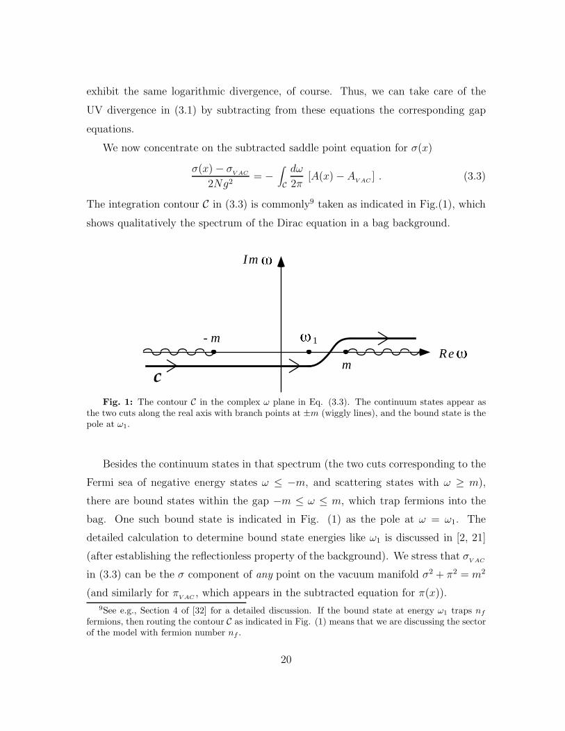
exhibit the same logarithmic divergence, of course. Thus, we can take care of the

UV divergence in (3.1) by subtracting from these equations the corresponding gap

equations.

We now concentrate on the subtracted saddle point equation for σ(x)

σ(x) − σV AC

2Ng2= −

∫

C

dω

2π[A(x) − A

V AC] . (3.3)

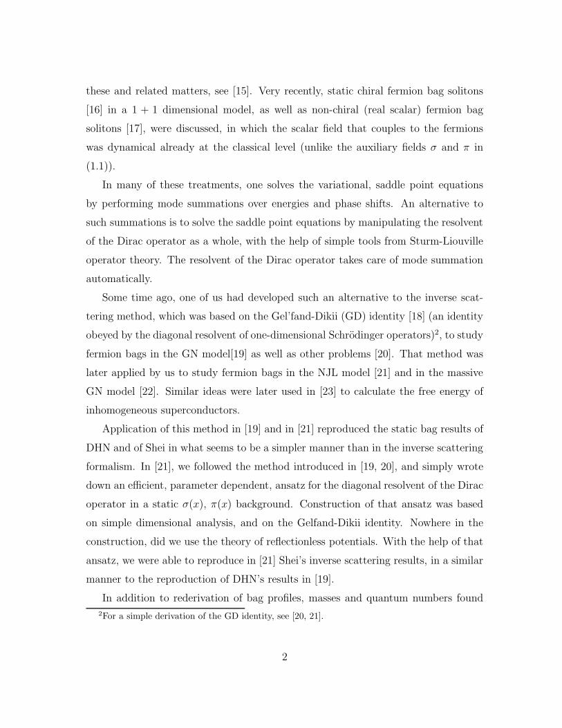
The integration contour C in (3.3) is commonly9 taken as indicated in Fig.(1), which

shows qualitatively the spectrum of the Dirac equation in a bag background.

- m

m

1

Re

Im

c

Fig. 1: The contour C in the complex ω plane in Eq. (3.3). The continuum states appear asthe two cuts along the real axis with branch points at ±m (wiggly lines), and the bound state is thepole at ω1.

Besides the continuum states in that spectrum (the two cuts corresponding to the

Fermi sea of negative energy states ω ≤ −m, and scattering states with ω ≥ m),

there are bound states within the gap −m ≤ ω ≤ m, which trap fermions into the

bag. One such bound state is indicated in Fig. (1) as the pole at ω = ω1. The

detailed calculation to determine bound state energies like ω1 is discussed in [2, 21]

(after establishing the reflectionless property of the background). We stress that σV AC

in (3.3) can be the σ component of any point on the vacuum manifold σ2 + π2 = m2

(and similarly for πV AC

, which appears in the subtracted equation for π(x)).

9See e.g., Section 4 of [32] for a detailed discussion. If the bound state at energy ω1 traps nf

fermions, then routing the contour C as indicated in Fig. (1) means that we are discussing the sectorof the model with fermion number nf .

20

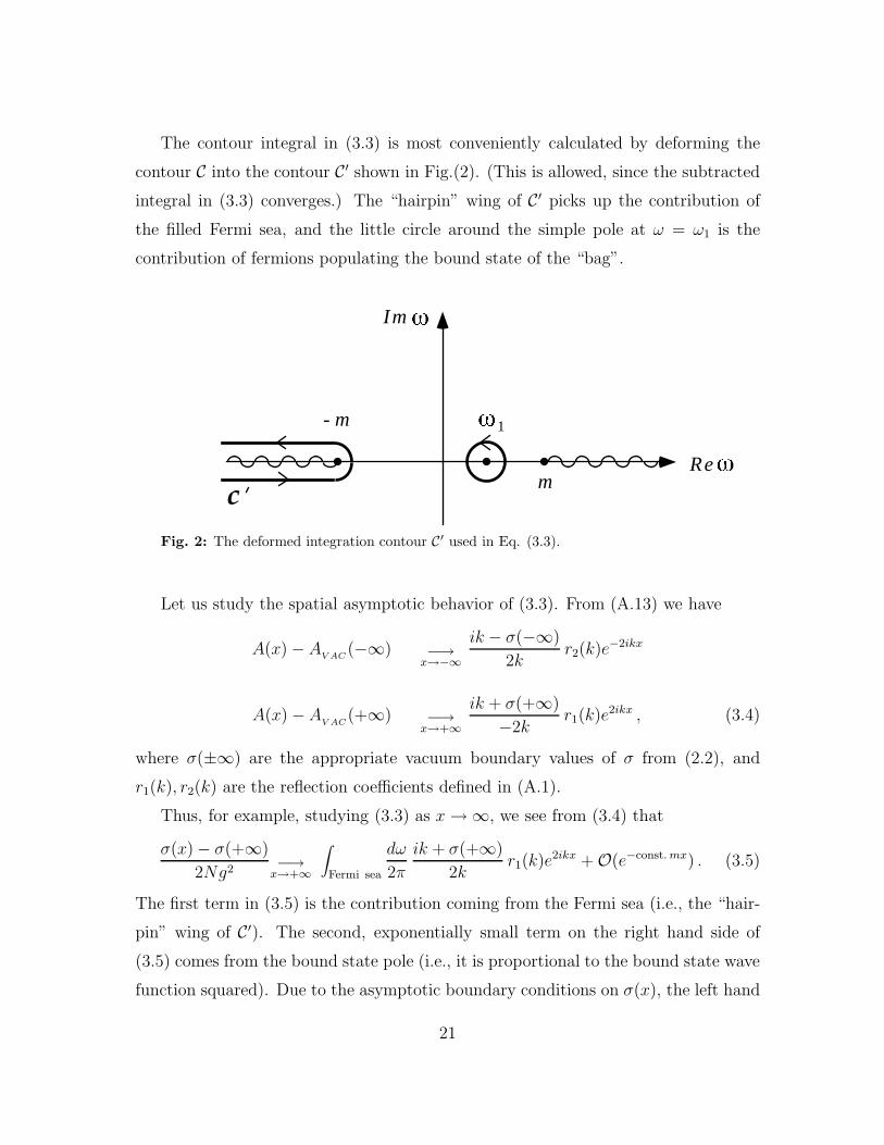
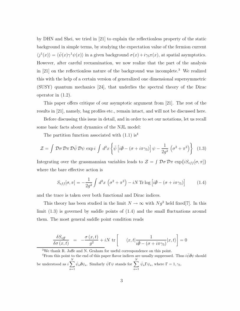
The contour integral in (3.3) is most conveniently calculated by deforming the

contour C into the contour C′ shown in Fig.(2). (This is allowed, since the subtracted

integral in (3.3) converges.) The “hairpin” wing of C′ picks up the contribution of

the filled Fermi sea, and the little circle around the simple pole at ω = ω1 is the

contribution of fermions populating the bound state of the “bag”.

- m

m

1

Re

Im

c

Fig. 2: The deformed integration contour C′ used in Eq. (3.3).

Let us study the spatial asymptotic behavior of (3.3). From (A.13) we have

A(x) − AV AC

(−∞) −→x→−∞

ik − σ(−∞)

2kr2(k)e

−2ikx

A(x) −AV AC

(+∞) −→x→+∞

ik + σ(+∞)

−2kr1(k)e

2ikx , (3.4)

where σ(±∞) are the appropriate vacuum boundary values of σ from (2.2), and

r1(k), r2(k) are the reflection coefficients defined in (A.1).

Thus, for example, studying (3.3) as x → ∞, we see from (3.4) that

σ(x) − σ(+∞)

2Ng2 −→x→+∞

∫

Fermi sea

dω

2π

ik + σ(+∞)

2kr1(k)e

2ikx + O(e−const. mx) . (3.5)

The first term in (3.5) is the contribution coming from the Fermi sea (i.e., the “hair-

pin” wing of C′). The second, exponentially small term on the right hand side of

(3.5) comes from the bound state pole (i.e., it is proportional to the bound state wave

function squared). Due to the asymptotic boundary conditions on σ(x), the left hand

21

side of (3.5) is also exponentially small as x → ∞. Thus, the first term on the right

hand side of (3.5) must have an exponentially small bound as x→ ∞.

We now change the variable to k =√ω2 −m2. When mapping into the k-plane,

the lower wing of the cut in Fig.(2) is transformed into k = |k|eiδ, and the upper

wing is transformed into −|k|e−iδ, with δ → 0+10. Thus, we may write the dispersion

integral on the right hand side of (3.5) coming from states in the Fermi sea as −∆(x),

where

∆(x) =

∞∫

0

dk

4π

(ik + σ(∞)) r1(k)e2ikx + (k → −k)√

k2 +m2

= Re

∞∫

0

dk

2π

(ik + σ(∞)) r1(k)e2ikx

√k2 +m2

, (3.6)

where in the last equality we used the reflection property r1(−k) = r∗1(k) (A.2) of

r1(k).

The function ∆(x) has to die off at least at an exponential rate as x→ ∞. Thus,

we are to study the asymptotic behavior of

G(x) =

∞∫

0

dk

2π

(ik + σ(∞)) r1(k)e2ikx

√k2 +m2

(3.7)

at large x. To this end we have to invoke some of the general properties of the

reflection coefficient r1(k) of the operator Lb in (2.9).

Due to the boundary conditions (2.2) on the background fields σ(x) and π(x), the

operator Lb tends exponentially fast (in x) to its asymptotic free particle form. Thus,

its “scattering potential” is localized in a finite region in space.

From the literature on scattering theory (in one space dimension) [3] we know

that the reflection coefficient r(k) of Schrodinger operators with short range potential

wells11 is analytic on the real k axis (and generally follows the threshold behavior

10For example, just above the cut ω − m = |ω − m|ei(π−δ) and ω + m = |ω + m|ei(π−δ), withδ → 0+. Thus, just above the cut, k =

√ω2 −m2 =

√

|ω2 −m2|ei(π−δ) = −|k|e−iδ.11We tacitly assume that the potential wells in question tend to the same asymptotic value at

x = ±∞ (as Lb does with σ(x), π(x) satisfying (2.2)), and that they do not have any barriers abovethese asymptotic values.

22

r(k) = −1 + ak + · · ·) and dies off like 1/k as k → ∞, i.e., at large kinetic energy.

Strictly speaking, the discussion of these issues in the various references in [3] con-

centrates mostly on Schrodinger operators of the standard form −∂2x + V (x), but the

arguments leading to the conclusions about the behavior of r(k) may be easily gen-

eralized to the scattering theory of the Sturm-Liouville operators Lb and Lc in (2.9)

(with σ(x) and π(x) relaxing fast to (2.2)).

Therefore, in deriving the asymptotic behavior of G(x) and ∆(x) we may use as

an input that r1(k) is analytic on the real k axis and that it decays at least as fast

as 1/k as k → ∞. Given these properties of r1(k), we are allowed to expand G(x)

in powers of 1/x in the most natural way, namely, by repeatedly integrating by parts

over k in (3.7).

Thus, for example, after three integrations we find

2πG(x) = −σ(∞)r1(0)

2imx+imr1(0) +mσ(∞)r′1(0)

(2imx)2

− −σ(∞)r1(0) + 2im2r′1(0) +m2σ(∞)r′′1(0)

(2imx)3

−∞∫

0

dke2ikx

(2ix)3

∂3

∂k3

(

ik + σ(∞)√k2 +m2

r1(k)

)

, (3.8)

and so on and so forth. Clearly, the remaining integral in each step is subdominant by

a power of 1/x relative to its predecessor, and thus, the expansion of G(x) generated

in this way is an asymptotic expansion.

From (3.8) (or by working out a few more terms in the asymptotic expansion if

necessary) the following pattern emerges: the coefficient of (1/2ix)2n+1 is a linear

combination of the form2n∑

j=0

cjijr

(j)1 (0)

with real coefficients cj, and the coefficient of (1/2ix)2n is a linear combination of the

form

i2n−1∑

j=0

cjijr

(j)1 (0)

23

with some other real coefficients cj.

From the reflection property (A.2) r1(−k) = r∗1(k) we immediately conclude that

r(n)1 (0) = (−1)nr

(n)1 (0)∗: the even derivatives r

(2j)1 (0) are real, and the odd derivatives

r(2j+1)1 (0) are imaginary. Thus, the linear combinations

∑

cjijr

(j)1 (0) are real, which

makes each term on the right hand side of the asymptotic expansion (3.8) of G(x)

pure imaginary.

Using this result in (3.6) we conclude that all terms in the asymptotic expansion

of ∆(x) in powers of 1/x vanish. Thus, ∆(x) vanishes faster than any power of 1/x

as x→ ∞. This is consistent with our expectation that ∆(x) vanishes at least at an

exponential rate when x→ ∞.

This concludes our discussion of the subtracted saddle point equation (3.3) for

σ(x) and its asymptotic behavior.

We can repeat the same story for the subtracted saddle point equation for π(x)

π (x) − πV AC

iNg2= −

∫

dω

2π[(B(x) − B

V AC) + (C(x) − C

V AC)] . (3.9)

In a similar manner to our derivation of (3.5) and (3.6), we can show that

π(x) − π(∞)

Ng2 −→x→+∞

exponentially small contribution of bound states

−Re

∞∫

0

dk

2π

(√k2 +m2 − π(∞)) − (

√k2 +m2 + π(∞))σ(∞)+ik

σ(∞)−ik√k2 +m2

r1(k)e2ikx

. (3.10)

Due to the asymptotic boundary conditions on π(x), the left hand side of (3.10) is

exponentially small as x → ∞, which bounds the dispersion integral on the right

hand side of (3.10). As in our analysis of (3.7), we expand the integral in the square

brackets in (3.10) in powers of 1/x, and similarly to (3.8), we can show that all terms

in that asymptotic series are pure imaginary. Thus, the right hand side of (3.10)

vanishes faster than any power of 1/x, consistent with the boundary conditions on

π(x).

We conclude that the asymptotic behavior of the static saddle point equations

(3.3) and (3.9) is consistent with the asymptotic boundary conditions (2.2) on σ(x)

24

and π(x) for any reflection amplitude r1(k): all terms in the asymptotic expansions

of the dispersion integral in the square brackets in (3.10) and also of G(x) in (3.7) in

powers of 1/x are imaginary.

Contrary to the argument we made in [21], the reflectionless property of the solu-

tions σ(x) and π(x) of (3.1) does not emerge as a necessary condition from consistency

of the asymptotic behavior of (3.5) and (3.10) and the boundary conditions on the

background fileds.

25

Appendix: Asymptotics of the Dirac Resolvent

In this Appendix we discuss the spatial asymptotic behavior of the diagonal resolvent

of the Dirac operator (2.24).

According to our discussion in Section 2.2, given, for example, B(x), we may

determine D(x), A(x) and C(x) using (2.25) first, then (2.26) and finally, (2.28).

Thus, it is enough to determine the asymptotic behavior of B(x). According to

(2.25), B(x) = b1(x)b2(x)/Wb, so we need to determine the asymptotic behavior of

b1(x), b2(x), the fundamental solutions of Lbb(x) = 0.

By definition, according to (2.11), and with the standard choice (2.17) of the

coefficients A(1)b = A

(2)b = 1, these functions satisfy

b1(x) −→x→−∞

e−ikx , b2(x) −→x→+∞

eikx

at the two opposite sides of the one dimensional world. Thus, what remains is to

determine the asymptotic behavior of each of these functions on the other side of the

world. Since σ and π relax to the vacuum manifold as x → ±∞ (Eq. (2.2)), the

operators Lb and Lc in (2.9) degenerate into free particle operators, and thus we must

have

b1(x) −→x→+∞

1

t1(k)e−ikx +

r1(k)

t1(k)eikx

b2(x) −→x→−∞

1

t2(k)eikx +

r2(k)

t2(k)e−ikx , (A.1)

where t1,2(k), r1,2(k) are the appropriate transmission and reflection amplitudes, re-

spectively.

It is enough to consider k ≥ 0, since the operators Lb and Lc in (2.9) are real and

thus b1,2(x,−k) = b∗1,2(x, k), leading to

t1,2(−k) = t∗1,2(k) and r1,2(−k) = r∗1,2(k) . (A.2)

Thus, b1(x) corresponds to a setting with a source at x = +∞ which emits to the

left, and b2(x) describes a source at x = −∞ which emits to the right.

26

The wronskian of b1(x) and b2(x) (Eq. (2.13))

Wb(ω) =b2(x)b

′

1(x) − b1(x)b′

2(x)

ω + π(x)

is independent of x. Thus, evaluating it at x→ ±∞ we find

Wb(ω) =−2ik

t2(k)(ω + π(−∞))=

−2ik

t1(k)(ω + π(+∞)), (A.3)

and thus,

t1(k)(ω + π(+∞)) = t2(k)(ω + π(−∞)) . (A.4)

Like the wronskian of {b1(x), b2(x)}, the wronkians of the pairs of independent

solutions {b1(x), b∗1(x)} and {b2(x), b∗2(x)} (here we assume that k is real) are also

independent of x. In fact, these wronskians are proportional to the Schrodinger

probability currents carried by b1(x) and b2(x), respectively. Thus, using (2.11) and

(A.1) to evaluate each of these wronskians at x = ±∞ and then equating the results,

we obtain

Wb[b1, b∗1] =

b∗1(x)b′

1(x) − b1(x)b∗′

1 (x)

ω + π(x)

=−2ik

ω + π(−∞)=

−2ik

ω + π(+∞)

1 − |r1|2|t1|2

;

Wb[b2, b∗2] =

b∗2(x)b′

2(x) − b2(x)b∗′

2 (x)

ω + π(x)

=2ik

ω + π(+∞)=

2ik

ω + π(−∞)

1 − |r2|2|t2|2

. (A.5)

Thus, we deduce the generalized unitarity conditions

1 − |r1|2|t1|2

=|t2|2

1 − |r2|2=ω + π(+∞)

ω + π(−∞). (A.6)

The usual unitarity condition |t|2 + |r|2 = 1 holds for backgrounds in which π(+∞) =

π(−∞).

27

Putting every thing together, we finally learn that

B(x) −→x→−∞

1 + r2(k)e−2ikx

−2ik(ω + π(−∞))

B(x) −→x→+∞

1 + r1(k)e2ikx

−2ik(ω + π(+∞)) . (A.7)

Recall from (2.33) that

BV AC

(±∞) =ω + π(±∞)

2√m2 − ω2

=ω + π(±∞)

−2ik(A.8)

corresponds to the appropriate vacuum configurations (σ(±∞), π(±∞)). Thus, we

can rewrite (A.7) as

B(x) −→x→−∞

BV AC

(−∞)(

1 + r2(k)e−2ikx

)

B(x) −→x→+∞

BV AC

(+∞)(

1 + r1(k)e2ikx

)

. (A.9)

Using (2.26), (2.27) and (2.28) we then find the asymptotic behaviors of the re-

maining entries of the diagonal resolvent (2.24):

A(x) = D(x) −→x→−∞

DV AC

(−∞) +ik − σ(−∞)

2kr2(k)e

−2ikx

A(x) = D(x) −→x→+∞

DV AC

(+∞) − ik + σ(+∞)

2kr1(k)e

2ikx , (A.10)

and

C(x) −→x→−∞

CV AC

(−∞)

[

1 +σ(−∞) − ik

σ(−∞) + ikr2(k)e

−2ikx

]

C(x) −→x→+∞

CV AC

(+∞)

[

1 +σ(+∞) + ik

σ(+∞) − ikr1(k)e

2ikx

]

, (A.11)

with

CV AC

(±∞) =−ω + π(±∞)

2√m2 − ω2

=ω − π(±∞)

2ik(A.12)

from (2.33).

28

Finally, we can write these results more compactly as

A(x) B(x)

C(x) D(x)

−→x→+∞

A(+∞) B(+∞)

C(+∞) D(+∞)

V AC

+

ik+σ(+∞)−2k

BV AC

(+∞)

CV AC

(+∞)σ(+∞)+ik

σ(+∞)−ik

ik+σ(+∞)−2k

r1(k)e2ikx ,

A(x) B(x)

C(x) D(x)

−→x→−∞

A(−∞) B(−∞)

C(−∞) D(−∞)

V AC

+

ik−σ(−∞)2k

BV AC

(−∞)

CV AC

(−∞)σ(−∞)+ik

σ(−∞)−ik

ik−σ(−∞)2k

r2(k)e−2ikx . (A.13)

Acknowledgements We would like to thank R. Jaffe and N. Graham for useful

correspondence and for pointing out a problem in the “proof” of reflectionless in [21].

J.F. thanks M. Moshe and J. Avron for useful discussions. The work of A.Z. was

supported in part by the National Science Foundation under Grant No. PHY 94-

07194. J.F.’s research has been supported in part by the Israeli Science Foundation

grant number 307/98 (090-903).

29

References

[1] R.F. Dashen, B. Hasslacher and A. Neveu, Phys. Rev. D 12, 2443 (1975).

[2] S. Shei, Phys. Rev. D 14, 535 (1976).

[3] L.D. Faddeev and L.A. Takhtajan, Hamiltonian Methods in the Theory of Soli-

tons (Springer Verlag, Berlin, 1987).

L.D. Faddeev, J. Sov. Math. 5 (1976) 334. This paper is reprinted in

L.D. Faddeev, 40 Years in Mathematical Physics (World Scientific, Singapore,

1995). In section 2.2 of that paper there is a brief discussion of some aspects of

the inverse scattering problem for the Dirac equation (1.2).

S. Novikov, S.V. Manakov, L.P. Pitaevsky and V.E. Zakharov, Theory of Soli-

tons - The Inverse Scattering Method (Consultants Bureau, New York, 1984)

( Contemporary Soviet Mathematics).

[4] J. Goldstone and R. Jackiw, Phys. Rev. D 11, 1486 (1975).

[5] T. D. Lee and G. Wick, Phys. Rev. D 9, 2291 (1974);

R. Friedberg, T.D. Lee and R. Sirlin, Phys. Rev. D 13, 2739 (1976);

R. Friedberg and T.D. Lee, Phys. Rev. D 15, 1694 (1976), ibid. 16, 1096 (1977);

A. Chodos, R. Jaffe, K. Johnson, C. Thorn, and V. Weisskopf, Phys. Rev. D 9,

3471 (1974).

[6] W. A. Bardeen, M. S. Chanowitz, S. D. Drell, M. Weinstein and T. M. Yan,

Phys. Rev. D 11, 1094 (1974);

M. Creutz, Phys. Rev. D 10, 1749 (1974).

[7] D.J. Gross and A. Neveu, Phys. Rev. D 10, 3235 (1974).

[8] Y. Nambu and G. Jona-Lasinio, Phys. Rev. 122, 345 (1961), ibid 124, 246 (1961).

[9] C.G. Callan, S. Coleman, D.J. Gross and A. Zee, unpublished; This work is

described by D.J. Gross in Methods in Field Theory , R. Balian and J. Zinn-

30

Justin (Eds.), Les-Houches session XXVIII 1975 (North Holland, Amsterdam,

1976).

[10] H. B. Thacker, C. Quigg and J. L. Rosner, Phys. Rev. D 18, 274 (1978);

J. F. Schonfeld, W. Kwong, J. L. Rosner, C. Quigg and H. B. Thacker, Ann.

Phys. 128, 1 (1980);

W. Kwong and J. L. Rosner, Prog. Theor. Phys. (Suppl.) 86, 366 (1986);

J. L. Rosner, Ann. Phys. 200, 101 (1990);

A. K. Grant and J. L. Rosner, Jour. Math. Phys. 35, 2142 (1994), and references

therein.

[11] S. Chandrasekhar, The Mathematical Theory of Black Holes, chapter 4 (Oxford

University Press, New York, 1992).

[12] B. Zwiebach, JHEP 0009:028,2000 (hep-th/0008227); J. A. Minahan and B.

Zwiebach, JHEP 0009:029,2000 (hep-th/0008231), JHEP 0103:038,2001 (hep-

th/0009246), JHEP 0102:034,2001 (hep-th/0011226).

[13] F. Cooper, A. Khare and U. Sukhatme, Phys. Rep. 251, 267 (1995).

[14] See e.g., A. Klein, Phys. Rev. D 14, 558 (1976);

R. Pausch, M. Thies and V. L. Dolman, Z. Phys. A 338, 441 (1991).

[15] V. Schoen and M. Thies, 2d Model Field Theories at Finite Temperature and

Density, Contribution to the Festschrift in honor of Boris Ioffe, (M. Shifman

Ed.), hep-th/0008175.

[16] E. Farhi, N. Graham, R.L. Jaffe and H. Weigel, Nucl. Phys. B585, 443 (2000);

Phys. Lett. B475, 335 (2000).

[17] S. V. Bashinsky, Phys. Rev. D 61, 105003 (2000).

[18] I.M. Gel’fand and L.A. Dikii, Russian Math. Surveys 30, 77 (1975).

[19] J. Feinberg, Phys. Rev. D 51, 4503 (1995).

31

[20] J. Feinberg, Nucl. Phys. B433, 625 (1995).

[21] J. Feinberg and A. Zee, Phys. Rev. D 56,5050 (1997); Int. J. Mod. Phys. A12,

1133 (1997).

[22] J. Feinberg and A. Zee, Phys. Lett. B411, 134 (1997)

[23] I. Kosztin, S. Kos, M. Stone and A. J. Leggett, Phys. Rev. B 58, 9365 (1998);

S. Kos and M. Stone, Phys. Rev. B 59, 9545 (1999).

[24] J. Feinberg “The Dirac Operator in a Fermion Bag Background in 1+1 Dimen-

sions and Generalized Supersymmetric Quantum Mechanics”, hep-th/0109043.

[25] See the concluding remarks in [2] who brings an unpublished argument for de-

coupling of θ due to R. Dashen, along the lines of

M.B. Halpern, Phys. Rev. D 12 1684 (1975).

See also E. Witten, Nucl. Phys. B145, 110 (1978).

[26] N. D. Mermin and H. Wagner, Phys. Rev. Lett. 17, 1133 (1966);

S. Coleman, Commun. Math. Phys. 31, 259 (1973).

[27] J.M. Cornwal, R. Jackiw, and E. Tomboulis, Phys. Rev. D 10, 2428 (1974).

[28] S. Hikami and E. Brezin, J. Phys. A (Math. Gen.) 12, 759 (1979).

[29] H.J. de Vega, Commun. Math. Phys. 70, 29 (1979);

J. Avan and H.J. de Vega, Phys. Rev. D 29, 2891 and 1904 (1984)

[30] R. MacKenzie, F. Wilczek and A.Zee, Phys. Rev. Lett 53, 2203 (1984).

[31] G. Dunne and J. Feinberg, Phys. Rev. D 57, 1271 (1998).

[32] R.F. Dashen, B. Hasslacher and A. Neveu, Phys. Rev. D 10, 4130 (1974).

32