GENERALIZED RICCI CURVATURE BOUNDS FOR THREE DIMENSIONAL CONTACT SUBRIEMANNIAN MANIFOLDS ANDREI AGRACHEV AND PAUL W.Y. LEE Abstract. Measure contraction property is one of the possible generalizations of Ricci curvature bound to more general metric measure spaces. In this paper, we discover sucient conditions for a three dimensional contact subriemannian manifold to satisfy this property. 1. Introduction In the past few years, several connections between the optimal trans- portation problems and curvature of Riemannian manifolds were found. One of them is the use of optimal transportation for an alternative def- inition of Ricci curvature lower bound developed in a series of papers [38, 18, 41]. Based on the ideas in these papers, a generalization of Ricci curvature lower bound for general metric measure spaces, called curvature-dimension condition, is introduced in [30, 31, 39, 40] (see section 5 for a quick overview of these results). Recently the case of a Finsler manifold was studied in [36] and the results are very similar to that of the Riemannian case due to strict convexity of the correspond- ing Hamiltonian. The situation changes dramatically in the case of subriemannian manifolds. The reason is that the class of metric spaces we are dealing with have Hausdor dimensions strictly greater than their topologi- cal dimensions. Therefore, the interplay between the metrics and the measures of these spaces should be signicantly dierent from that of the Riemannian or Finsler case. One particular case of subriemannian manifolds, the Heisenberg group, is studied in [24]. In this case the space does not satisfy any curvature-dimension condition mentioned above (however, see [9, 11, 10] for a dierent denition of curvature- dimension condition in the subriemannian setting). Instead it satises a weaker condition, called measure contraction property, introduced in Date : June 5, 2011. The rst author was partially supported by PRIN and the second author was supported by NSERC postgraduate scholarship and postdoctoral fellowship. 1

Welcome message from author
This document is posted to help you gain knowledge. Please leave a comment to let me know what you think about it! Share it to your friends and learn new things together.
Transcript

GENERALIZED RICCI CURVATURE BOUNDS FORTHREE DIMENSIONAL CONTACT SUBRIEMANNIAN
MANIFOLDS
ANDREI AGRACHEV AND PAUL W.Y. LEE
Abstract. Measure contraction property is one of the possiblegeneralizations of Ricci curvature bound to more general metricmeasure spaces. In this paper, we discover sufficient conditions fora three dimensional contact subriemannian manifold to satisfy thisproperty.
1. Introduction
In the past few years, several connections between the optimal trans-portation problems and curvature of Riemannian manifolds were found.One of them is the use of optimal transportation for an alternative def-inition of Ricci curvature lower bound developed in a series of papers[38, 18, 41]. Based on the ideas in these papers, a generalization ofRicci curvature lower bound for general metric measure spaces, calledcurvature-dimension condition, is introduced in [30, 31, 39, 40] (seesection 5 for a quick overview of these results). Recently the case of aFinsler manifold was studied in [36] and the results are very similar tothat of the Riemannian case due to strict convexity of the correspond-ing Hamiltonian.
The situation changes dramatically in the case of subriemannianmanifolds. The reason is that the class of metric spaces we are dealingwith have Hausdorff dimensions strictly greater than their topologi-cal dimensions. Therefore, the interplay between the metrics and themeasures of these spaces should be significantly different from that ofthe Riemannian or Finsler case. One particular case of subriemannianmanifolds, the Heisenberg group, is studied in [24]. In this case thespace does not satisfy any curvature-dimension condition mentionedabove (however, see [9, 11, 10] for a different definition of curvature-dimension condition in the subriemannian setting). Instead it satisfiesa weaker condition, called measure contraction property, introduced in
Date: June 5, 2011.The first author was partially supported by PRIN and the second author was
supported by NSERC postgraduate scholarship and postdoctoral fellowship.1

2 ANDREI AGRACHEV AND PAUL W.Y. LEE
[40, 35] (see Section 5 for the definition). Like the curvature-dimensioncondition, measure contraction property is a generalization of Ricci cur-vature lower bound on Riemannian manifolds. However, it is a weakercondition for general metric measure spaces.
The approach used by [24] relies on the complete integrability ofthe subriemannian geodesic flow on the Heisenberg group. Because ofthis, the changes in the measure along the geodesic flow can be writtendown explicitly in this case, which is not possible for subriemannianmanifolds in general.
The goal of this paper is to study a subriemannian version of the mea-sure contraction property for three dimensional contact subriemannianmanifolds under certain curvature conditions. This study uses a sub-riemannian generalization of the classical Riemannian curvature. Thegeneralized Ricci curvature was introduced by the first author in the90s for some special cases (including the three dimensional contact sub-riemannian structures), and in full generality by the first author andI. Zelenko (see [7]). Later C.-B. Li and I. Zelenko found a completesystem of curvature invariants (see [27, 28]). To state some interestingconsequences of the main result in this paper, let us first give a briefintroduction to the curvature invariants (see Section 6 for a more detaildiscussion of these invariants).
Let etH be the subriemannian geodesic flow defined on the cotangentbundle T ∗M and let � be in T ∗M . In a similar spirit of the Frenet-Serret frame, one can find a special moving frame along the trajectory
t 7→ etH(�). The main property of this frame is that it satisfies certainfirst order equations when pulled back to the tangent space T�T
∗M at
the point � by the geodesic flow etH . The pulled back frame is calledthe canonical Darboux frame.
In the Riemannian case, the canonical Darboux frame
{e1(t), ..., en(t), f1(t), ..., fn(t)}
satisfies the following equations which is the Jacobi field equation (upto certain identifications of tangent and cotangent spaces)
ei(t) = fi(t), fi(t) = −Rij� (t)ej(t).
The matrix R� := R�(0) with ij-th entries given by Rij� (0) above is the
Riemannian curvature operator (again up to certain identifications).In the three dimensional contact subriemannian case, the canonical
Darboux frame
{e1(t), e2(t), e3(t), f1(t), f2(t), f3(t)}
RICCI CURVATURE FOR CONTACT 3-MANIFOLDS 3
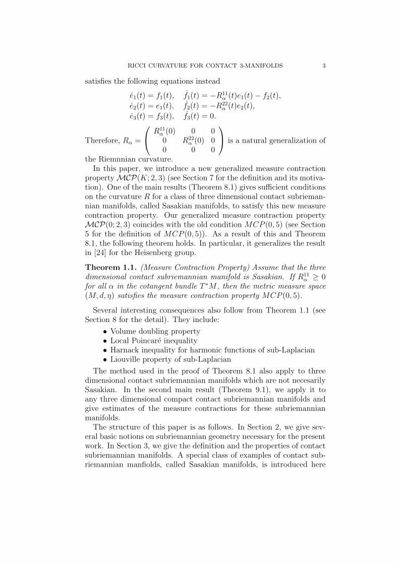
satisfies the following equations instead
e1(t) = f1(t), f1(t) = −R11� (t)e1(t)− f2(t),
e2(t) = e1(t), f2(t) = −R22� (t)e2(t),
e3(t) = f3(t), f3(t) = 0.
Therefore, R� =
⎛⎝ R11� (0) 0 00 R22
� (0) 00 0 0
⎞⎠ is a natural generalization of
the Riemnnian curvature.In this paper, we introduce a new generalized measure contraction
propertyℳCP(K; 2, 3) (see Section 7 for the definition and its motiva-tion). One of the main results (Theorem 8.1) gives sufficient conditionson the curvature R for a class of three dimensional contact subrieman-nian manifolds, called Sasakian manifolds, to satisfy this new measurecontraction property. Our generalized measure contraction propertyℳCP(0; 2, 3) coincides with the old condition MCP (0, 5) (see Section5 for the definition of MCP (0, 5)). As a result of this and Theorem8.1, the following theorem holds. In particular, it generalizes the resultin [24] for the Heisenberg group.
Theorem 1.1. (Measure Contraction Property) Assume that the threedimensional contact subriemannian manifold is Sasakian. If R11
� ≥ 0for all � in the cotangent bundle T ∗M , then the metric measure space(M,d, �) satisfies the measure contraction property MCP (0, 5).
Several interesting consequences also follow from Theorem 1.1 (seeSection 8 for the detail). They include:
∙ Volume doubling property∙ Local Poincare inequality∙ Harnack inequality for harmonic functions of sub-Laplacian∙ Liouville property of sub-Laplacian
The method used in the proof of Theorem 8.1 also apply to threedimensional contact subriemannian manifolds which are not necesarilySasakian. In the second main result (Theorem 9.1), we apply it toany three dimensional compact contact subriemannian manifolds andgive estimates of the measure contractions for these subriemannianmanifolds.
The structure of this paper is as follows. In Section 2, we give sev-eral basic notions on subriemannian geometry necessary for the presentwork. In Section 3, we give the definition and the properties of contactsubriemannian manifolds. A special class of examples of contact sub-riemannian manfiolds, called Sasakian manifolds, is introduced here

4 ANDREI AGRACHEV AND PAUL W.Y. LEE
as well. Sasakian manifolds serve as examples to the main result ofthis paper. In Section 4, we recall the definition and some basic re-sults on the optimal transportatin problem. In Section 5, we give abrief overview on how the optimal transportation problem gives rise tothe curvature-dimension condition and the measure contraction prop-erty. We also give the motivation of the present work in this section.In Section 6, we recall and specialize the recent result of [27, 28] onthe curvature type invariants of subriemannian manifolds to the threedimensional contact case. We also give explicit formulas for these in-variants. In section 7, we give the definition of the new generalizedmeasure contraction property. We will also motivate its definition byconsidering how measures contract in the Sasakian version of spaceform. In Section 8, we state the main theorem (Theorem 8.1) and itsconsqeuences. The main theorem gives sufficient conditions on when athree dimensional contact subriemannian satisfies the generalized gen-eralized measure contraction property ℳCP(K; 2, 3). (see Definition7.3 below). In particular, ℳCP(K; 2, 3) coincides with the old mea-sure contraction property MCP (0, 5). As a consequence, these spacessatisfy the volume doubling property, the local Poincare inequality, theHarnack inequality and the Liouville property for harmonic functionsof the sub-Laplacian. In Section 9, we give the measure contractionestimates for three dimensional compact contact subriemannian man-ifolds. The proofs of all the results of this paper are given in the restof the sections.
Acknowledgment
We thank Igor Zelenko and Cheng-Bo Li for very interesting andstimulating discussions. We would also like to thank the referees fortheir useful comments on improving the paper. This work is part ofthe PhD thesis of the second author. He would like to express deepgratitude to his supervisor, Boris Khesin, for his continuous support.He would like to thank Professor Karl-Theodor Sturm for the fruitfuldiscussions. He is also grateful to SISSA for their kind hospitalitywhere part of this work is done.

RICCI CURVATURE FOR CONTACT 3-MANIFOLDS 5
A table of notationsM a metric space or a manifold⟨⋅, ⋅⟩, ∣⋅∣ a subriemannian metric and its normΔ a distribution on M� the Popp’s measure�, �0, �1, �t measures on MΠ a measure on M ×Md a distance function on MU a Borel set in MH subriemannian Hamiltonian
etH subriemannian geodesic flowei(t), fi(t) canonical Darboux frameRij� (t) curvature invariants
v tangent vectors� covectors�0 contact formv0 the Reeb fieldv1, v2 subriemannian orthonormal basis�0, �1, �2 dual basis of v0, v1, v2
� tautological 1-form on T ∗M! standard symplectic 2-form on T ∗MX a tangent vector in TT ∗Mℒ Lie derivative∇H horizontal gradientΔH sub-Laplacian
2. Subriemannian Manifolds and Their Geodesics
In this section, we recall several basic notions in subriemannian ge-ometry. For a detail discussion of various topics, see [34].
Recall that a Riemannian manifold is a manifold M together with afibrewise inner product defined on the tangent bundle TM . The lengthof a curve is defined by this inner product and the Riemannian distancebetween two points is the length of the shortest curve connecting them.For a subriemannian manifold the fibrewise inner product is defined ona family of subspaces Δ inside the tangent bundle TM . Therefore,the notion of length can only be defined for curves which are tangentto this family Δ. These curves are called horizontal curves and thesubriemannian distance between two points is the length of the shortesthorizontal curve connecting them.

6 ANDREI AGRACHEV AND PAUL W.Y. LEE
More precisely, a subriemannian manifold is a triple (M,Δ, ⟨⋅, ⋅⟩),where M is a smooth manifold, Δ is a distribution (a vector subbundleΔ of the tangent bundle TM of the manifold M), and ⟨⋅, ⋅⟩ is a fibrewiseinner product defined on the distribution Δ. The inner product ⟨⋅, ⋅⟩is also called a subriemannian metric. An absolutely continuous curve : [0, 1] → M on the manifold M is called horizontal if it is almosteverywhere tangent to the distribution Δ. Using the inner product⟨⋅, ⋅⟩, we can define the length l( ) of a horizontal curve by
l( ) =
∫ 1
0
∣ (t)∣dt,
where ∣ ⋅ ∣ denotes the norm of the subriemannian metric ⟨⋅, ⋅⟩.The subriemannian or Carnot-Caratheodory distance d between two
points x and y on the manifold M is defined by
(2.1) d(x, y) = inf l( ),
where the infimum is taken over all horizontal curves which start fromx and end at y.
The above distance function may not be well-defined since there mayexist two points which are not connected by any horizontal curve. Forthis we assume that the distribution Δ is bracket-generating. Beforedefining what a bracket-generating distribution is, let us introduce sev-eral notions. Let Δ1 and Δ2 be two distributions on a manifold M , andlet X(Δi) be the space of all vector fields contained in the distributionΔi. The distribution formed by the Lie brackets of the elements inX(Δ1) with those in X(Δ2) is denoted by [Δ1,Δ2]. More precisely,
[Δ1,Δ2]x = span{w1(x), [w2, w3](x)∣wi ∈ X(Δj), i = 1, 2, 3, j = 1, 2}.
We define inductively the following distributions: [Δ,Δ] = Δ2 andΔk = [Δ,Δk−1]. A distribution Δ is called k-generating if Δk = TMand the smallest such k is called the degree of nonholonomy. Finally thedistribution is called bracket-generating if it is k-generating for some k.
Under the bracket-generating assumption, the subriemannian dis-tance is well-defined thanks to the following famous Chow-RashevskiiTheorem (see [34, Chapter 2] for a proof):
Theorem 2.1. (Chow-Rashevskii) Assume that the manifold M is con-nected and the distribution Δ is bracket-generating. Then there is ahorizontal curve joining any two given points.
Finally, let us discuss the subriemannian geodesics and the corre-sponding geodesic flow. As in Riemannian geometry, horizontal curveswhich realize the infimum in (2.1) are called length minimizing geodesics

RICCI CURVATURE FOR CONTACT 3-MANIFOLDS 7
(or simply geodesics). From now on, all subriemannian manifolds areassumed to be complete as a metric space. It follows that given anytwo points on the manifold, there is at least one constant speed geo-desic joining them. Next we will discuss one type of geodesics callednormal geodesics. For this let us recall several notions in the symplec-tic geometry of the cotangent bundle T ∗M . Let � : T ∗M →M be theprojection map, the tautological one-form � on T ∗M is defined by
��(X) = �(d�(X)),
where � is in the cotangent bundle T ∗M and X is a tangent vector onthe manifold T ∗M at �.
The symplectic two-form ! on T ∗M is defined as the exterior de-rivative of the tautological one-form: ! = d�. It is nondegenerate inthe sense that !(X, ⋅) = 0 if and only if X = 0. Given a functionH : T ∗M → ℝ on the cotangent bundle, the Hamiltonian vector fieldH is defined by iH! = −dH. By the nondegeneracy of the symplectic
form !, the Hamiltonian vector field H is uniquely defined.Given a distribution Δ and a subriemannian metric ⟨⋅, ⋅⟩ on it, we can
associate with it a Hamiltonian H, called subriemannian Hamiltonian,on the cotangent bundle T ∗M . To do this, let � be in the cotangentspace T ∗xM at the point x. The subriemannian metric ⟨⋅, ⋅⟩ defines abundle isomorphism I : Δ∗ → Δ between the distribution Δ and itsdual Δ∗. It is defined by
⟨I(�), ⋅⟩ = �(⋅),
where � is an element in the dual bundle Δ∗ of the distribution Δ.By restricting the domain of the covector � to the subspace Δx of
the tangent space TxM , it defines an element, still called �, in thedual space Δ∗. Therefore, I(�) is a tangent vector contained in thespace Δx and the subriemannian Hamiltonian H corresponding to thesubriemannian metric ⟨⋅, ⋅⟩ is defined by
H(�) :=1
2�(I(�)) =
1
2⟨I(�), I(�)⟩ .
Note that this construction defines the usual kinetic energy Hamilton-ian in the Riemannian case.
Let H be the Hamiltonian vector field corresponding to the sub-riemannian Hamiltonian H and we denote the corresponding flow, the
subriemannian geodesic flow, by etH . If t 7→ etH(�) is a trajectory of the
subriemannian geodesic flow, then its projection t 7→ (t) = �(etH(�))is a locally minimizing geodesic. That means sufficiently short segmentof the curve is a minimizing geodesic between its endpoints. The

8 ANDREI AGRACHEV AND PAUL W.Y. LEE
minimizing geodesics obtained this way are called normal geodesics. Inthe special case where the distribution Δ is the whole tangent bun-dle TM , the distance function (2.1) is the usual Riemannian distanceand all geodesics are normal. The same is true for subriemannianmanifolds, called contact subriemannian manifolds (see Section 3 forthe definition), studied in this paper. However, this is not the casefor general subriemannian manifolds. To introduce another class ofgeodesics, consider the space Ω of horizontal curves with square in-tegrable derivatives. The endpoint map end : Ω → M is defined bytaking an element in space of curves Ω and giving the endpoint (1)of the curve: end( ) = (1). Geodesics which are regular points of theendpoint map are automatically normal and those which are criticalpoints are called abnormal. However, there are geodesics which areboth normal and abnormal (see [34, Chapter 3] and reference thereinfor more detail about abnormal geodesics).
3. Contact Subriemannian and Sasakian Manifolds
In this section, we recall the definition of contact subriemannianmanifolds which is the main object of study for this paper. We will alsorecall the definition of Sasakian manifolds which served as key examplesof various results. Finally we will mention some explicit examples inthe three dimensional case.
A distribution Δ on a manifold M is contact if there exists a 1-form�0, called contact form, for which the kernel of �0 is Δ and the dif-ferential d�0 is nondegenerate on Δ. In other words, a tangent vectorv is contained in Δ if and only if �0(v) = 0 and d�0(v, ⋅) ≡ 0 if andonly if v = 0. Note that the second condition implies the manifoldM is odd dimensional. Once a contact distribution is fixed, there arelots of contact form associated with it. However, if a subriemannianmetric ⟨⋅, ⋅⟩ is also fixed on the distribution, then there is a uniquecontact form �0 such that the restriction of the 2n-form d�0 ∧ ...∧ d�0
to the distribution Δ coincides with the volume form induced by thesubriemannian metric ⟨⋅, ⋅⟩ on Δ. Therefore, we say that the subrie-mannian manifold (M,Δ, ⟨⋅, ⋅⟩) is a contact subriemannian manifold ifΔ is a contact distribution and we call the 1-form �0 defined above theinduced contact form of (M,Δ, ⟨⋅, ⋅⟩).
For each contact subriemannian manifold (M,Δ, ⟨⋅, ⋅⟩), we can asso-ciate with it a unique vector field v0, called the Reeb field. If �0 is theinduced contact form, then v0 is defined by conditions �0(v0) = 1 andd�0(v0, ⋅) = 0. Note that the second condition implies the Reeb fieldv0 is transversal to the distribution Δ.

RICCI CURVATURE FOR CONTACT 3-MANIFOLDS 9
Using the Reeb field v0, we can define a natural measure on thesubriemannian manifold. Let v1, ..., v2n be a basis in the contact dis-tribution Δ which is orthonormal with respect to the given subrie-mannian metric. Let � be the (2n + 1)-form defined by the condition�(v0, ..., v2n) = 1. The measure induced by this volume form �, whichwill be denoted by the same symbol throughout this paper, is an ex-ample of a Popp’s measure. Popp’s measures can be defined for anysubriemannian manifold. For the detail definition of this measure ingeneral, see [34, Chapter 10]. From now on, when we consider a contactsubriemannian manifold as a metric measure space, it always refers tothe triple (M,d, �) where d is the subriemannian distance and � is thePopp’s measure.
Before giving examples of contact subriemannian manifolds, let usrecall the definition of an important class of manifolds, called Sasakianmanifolds. They are contact subriemannian manifolds for which theReeb field v0 is a subriemannian isometry. Note that by the definitionof the Reeb field v0, the flow of v0 preserves the induced contact formand hence the distribution Δ. Therefore, subriemannian isometry heremeans the flow of the Reeb field v0 preserves the subriemannian lengthof tangent vectors in Δ.
If we assume further that the Reeb field v0 of the Sasakian manifoldgenerates a free and proper group action (i.e. the flow of v0 is a free andproper group action), then the quotient N := M/G of the manifold Mby this G-action (G = S1 or ℝ) is again a manifold. Let �M : M →N be the quotient map. Then there is a Riemannian metric on Nsuch that the restriction of d� to the distribution Δ is an isometry.Many of the interesting examples of subriemannian manifolds have thisstructure. The Heisenberg group ℍn is one of them.
The standard subriemannian structure of the Heisenberg group ℍn
can be defined as follows. The underlying manifold of ℍn is the 2n+1-dimensional Euclidean space M = ℝ2n+1. If we denote the coordinatesof this Euclidean space by {x0, x1, ..., x2n}, then the distribution Δ isdefined by
Δ = span {Xi, Yi∣i = 1, ..., n} ,
where Xi = ∂xi − 12xn+i∂x0 and Yi = ∂xn+i + 1
2xi∂x0 .
The standard subriemannian metric ⟨⋅, ⋅⟩ is the one for which thevector fields {Xi, Yi∣i = 1, ..., n} are orthonormal. The induced contactform �0 is given by
�0 = −dx0 +1
2
n∑i=1
(xidxn+i − xn+idxi).

10 ANDREI AGRACHEV AND PAUL W.Y. LEE
The Reeb field v0 in this case is −∂x0 and the Popp’s measure � is the2n+ 1-dimensional Lebesgue measure. The Reeb field v0, in this case,is a subriemannian isometry. It also defines a proper ℝ-action and thequotient manifold N is the 2n-dimensional Euclidean space ℝ2n. Thestandard subriemannian structure ⟨⋅, ⋅⟩ on ℍn descends to the standardEuclidean structure on ℝ2n.
We end this section with two more examples of contact subrieman-nian manifolds with the above symmetry structure. For more examplesof subriemannian manifolds with symmetry, see [34, Chapter 11]. Forother examples of contact manifolds, see [14].
Recall that SU(2), the special unitary group, consists of 2×2 matri-ces with complex coefficients and determinant 1. The Lie algebra su(2)consists of skew Hermitian matrices with trace zero. The left invariantvector fields of the following two elements in su(2)
v1 =
(0 1/2−1/2 0
), v2 =
(0 i/2i/2 0
)span the standard distribution Δ on SU(2). The standard subrieman-nian metric is given by the condition ⟨vi, vj⟩ = �ij, i = 1, 2. The Reebfield v0 is given by
v0 =
(0 −1/2
1/2 0
).
The flow of the Reeb field defines a S1-action on SU(2) called theHopf fibration. The quotient N of SU(2) by this action is the standard2-sphere S2. The standard subriemannian metric on SU(2) descendsto the Riemannian metric on S2 of contant curvature 1.
The special linear group SL(2) is the set of all 2 × 2 matrices withreal coefficients and determinant 1. The Lie algebra sl(2) is the set ofall 2× 2 real matrices with trace zero. The left invariant vector fieldsof the following two elements in sl(2)
v1 =
(1/2 00 −1/2
), v2 =
(0 1/2
1/2 0
)span the standard distribution Δ on SL(2). The standard subrieman-nian metric on SL(2) is defined by ⟨vi, vj⟩ = �ij, i = 1, 2. The Reebfield in this case is v0, where
v0 =
(0 −1/2
1/2 0
).
The flow of the Reeb field also defines a S1-action on SU(2). Thequotient N of SL(2) by this action is the upper half-space with thestandard non-Euclidean structure.

RICCI CURVATURE FOR CONTACT 3-MANIFOLDS 11
4. Introduction to Optimal Transportation
In this section, we give a quick introduction to the optimal trans-portation problem. A standard reference on this is the book [42].
Let M be a metric space with distance function d. Let �0 and �1
be two Borel probability measures on M . The theory of optimal trans-portation starts with the following minimization problem
(4.1) inf'∗�0=�1
∫M
d2(x, '(x)) d�0(x)
where the infimum is taken over all Borel maps ' : M → M whichpushes �0 forward to �1 (i.e. �0('−1(U)) = �1(U) for all Borel sets Uin M).
By the famous work of [25], the relaxed version of the above problemgiven below in (4.2) always has a solution (i.e. existence of minimizer).
(4.2) inf(�1)∗Π=�0,(�2)∗Π=�1
∫M×M
d2(x, y) dΠ(x, y)
where �1, �2 : M × M → M are projections onto the first and sec-ond component, respectively, and the infimum is taken over all Borelmeasures Π on M ×M satisfying (�1)∗Π = �0 and (�2)∗Π = �1 (i.e.Π(U ×M) = �0(U) and Π(M ×U) = �1(U) for all Borel sets U in M).
The existence and uniqueness of solution to the origin problem (4.1)were proved much later in ([15]) in the Euclidean setting under certainassumptions on the measures �0 and �1. It was later extended tothe compact Riemannian setting by [33]. The following is a summaryof their results (see also the result in [19] where all the compactnessassumptions are removed).
Theorem 4.1. [15, 33] Let M be a Riemannian manifold with Rie-mannian distance d. Assume that the measures �0 and �1 have com-pact supports and the measure �0 is absolutely continuous with respectto the Riemannian volume. Then the optimal transportation problem(4.1) has a solution ' which is unique up to a set of �-measure zero.Moreover, there exists a Lipschitz function f : M → ℝ such that themap ' is given by
'(x) = exp(∇f(x)).
The problem (4.1) in the subriemannian setting was first consideredin [8]. Under the same assumptions as in Theorem 4.1 on the mea-sures, the existence and uniqueness of the solution was shown whenthe space is the Heisenberg group equipped with the standard subrie-mannian metric (see Section 2 for the defintion). The generalization

12 ANDREI AGRACHEV AND PAUL W.Y. LEE
to more general subriemannian manifolds is later done in [4]. In [4],the authors proved that the existence and uniqueness theorem holdswhen the subriemannian manifold is 2-generating (see Section 2 for thedefinition of k-generating distribution). In particular, it is applicableto the contact subriemannian case considered in the present work.
Theorem 4.2. [4] Let M is a subriemannian manifold with subrieman-nian distance d and a 2-generating distribution Δ. Assume that themeasures �0 and �1 have compact supports and the measure �0 is abso-lutely continuous with respect to a Riemannian volume. Then the opti-mal transportation problem (4.1) has a solution ' which is unique up toa set of �0-measure zero. Moreover, there exists a function f : M → ℝwhich is Lipschitz with respect to a Riemannian metric such that themap ' is given by
'(x) = �(e1⋅H(dfx)).
where etH denotes the subriemannian geodesic flow and � : T ∗M →Mis the natural projection.
The difficulty in extending the above theorem to all subriemannianmanifolds lies in the presence of abnormal minimizers. Using geometricmeasure theory, [20] is able to extend Theorem 4.2 to more general sub-riemannian manifolds. However, the problem of showing uniqueness ornon-uniqueness of solutions to (4.1) in the subriemannian case remainsunsolved in general.
5. Optimal Transportation and Ricci Curvature
In this section, we give a very brief overview of results concerning theconnection of optimal transportation with generalized Ricci curvaturelower bound (see [30, 31, 39, 40] for a detail discussion).
The optimal transportation problem in (4.2) defines a distance func-tion on the space of all Borel probability measures of a given metricspace. More precisely, let P , called the Wasserstein space, be the spaceof all Borel probability measures � such that the following integral isfinite for some point x0 in M∫
M
d2(x, x0)d�(x).
The Wasserstein distance functionW on P is defined by the optimaltransportation problem as follows.
(5.1) W(�0, �1) =
(inf
(�1)∗Π=�0,(�2)∗Π=�1
∫M×M
d2(x, y) dΠ(x, y)
)1/2
.

RICCI CURVATURE FOR CONTACT 3-MANIFOLDS 13
Assume that the space M is locally compact complete separable met-ric space. Then the Wasserstein space P equipped with the WassersteindistanceW is a geodesic space (i.e. distance between two points is givenby the length of the shortest curve, called geodesic, connecting them,see [40] for the precise definition of geodesic space and the proof of thisfact).
Remark 5.1. Assume that the metric space (M,d) is a contact sub-riemannian manifold and the measure �0 is absolutely continuous withrespect to a Riemannian volume. Then the geodesics of the correspond-ing Wasserstein distance are given by
t 7→ ('t)∗�0
where 't = �(etH(df)) and f is defined as in Theorem 4.2. These pathsof measures, called displacement interpolations, were first introducedin [32].
Finally let us fix a locally finite measure � and introduce the relativeentropy functional Ent(�∣�) on P by
Ent(�∣�) =
{∫Mg log g d� if � = g�
+∞ otherwise.
Formally, a metric measure space (M,d, �) satisfies the curvature-dimension condition CD(K,∞) if the above relative entropy functionalhas second derivative bounded below by K along any geodesic in theWasserstein space P of M equipped with the Wasserstein distance W .More precisely, the second derivative is replaced by the following dif-ference quotient.
Definition 5.2. The metric measure space (M,d, �) satisfies the con-dition CD(K,∞), called curvature-dimension condition, if for any ge-odesic �t in P the following holds
K
2t(1− t)W2(�0, �1) ≤ (1− t)Ent(�0∣�) + tEnt(�1∣�)− Ent(�t∣�).
There are also other curvature-dimension conditions CD(K,N) forN > 0 finite. The definitions of these conditions are similar to that ofCD(K,∞) but are more involved. Their detail definitions as well asrelated results can found in [40].
In the Riemannian case, the condition CD(K,∞) is the same asRicci curvature bounded below by K. More precisely, the followingholds.

14 ANDREI AGRACHEV AND PAUL W.Y. LEE
Theorem 5.3. [38, 18, 41] Assume that M is a complete Riemannianmanifold with Riemannian distance d and a measure � induced by theRiemannian volume form. If we denote the Ricci curvature by Ricand the Riemannian metric by ⟨⋅, ⋅⟩, then the the metric measure space(M,d, �) satisfies curvature-dimension condition CD(K,∞) if and onlyif
Ric(v, v) ≥ K∣v∣2
for all tangent vector v in the tangent bundle TM .
Besides Riemannian manifolds, it was shown in [36] that CD(K,∞)is equivalent to the flag Ricci tensor bounded below by K in the Finslercase. The situation in the subriemannian case is completely different.In [24], it was shown that the most basic subriemannian example, theHeisenberg group (see Section 3 for the precise definition of the Heisen-berg group and the standard subriemannian structure on it), does notsatisfy any curvature-dimension condition mentioned above (howeversee [9, 11, 10] for a different curvature-dimension condition in the sub-riemannian setting which is satisfied by the Heisenberg group in par-ticular). On the other hand, it was shown in [24] that the Heisenberggroup satisfies the measure contraction property MCP (K,N) definedbelow.
Definition 5.4. The metric measure space (M,d, �) satisfies the mea-sure contraction property MCP (K,N) if for any point x0 in the spaceM , for any geodesic �t in P satisfying �1 = �x0 (the delta mass at x0)and �0 = �, the following holds
�0('t(U)) ≥∫U
(1− t)(sK((1− t)D(x))
sK(D(x))
)N−1
d�t(x)
for any Borel set U , where
sK(r) =
⎧⎨⎩1√K
sin(√K r) if K > 0
r if K = 01√−K sinh(
√−K r) if K < 0
and D(x) = d(x0,x)√N−1
.
As mentioned in the introduction, MCP (K,N) is another character-ization of Ricci curvature lower bound for N -dimensional Riemannianmanifolds.
Theorem 5.5. [40, 35] Assume that M is a N-dimensional completeRiemannian manifold with Riemannian distance d and a measure �

RICCI CURVATURE FOR CONTACT 3-MANIFOLDS 15
induced by the Riemannian volume form. If we denote the Ricci cur-vature by Ric and the Riemannian metric by ⟨⋅, ⋅⟩, then the the met-ric measure space (M,d, �) satisfies the measure contraction propertyMCP (K,N) if and only if
Ric(v, v) ≥ K∣v∣2
for all tangent vector v in the tangent bundle TM .
Finally we end this section with the following theorem, proved in[24], which motivates the present work.
Theorem 5.6. [24] Let ℍn be the 2n+1 dimensional Heisenberg group.Let d be the standard subriemannian distance and � be the (2n + 1)-dimensional Lebesgue measure dx2n+1. Then the metric measure space(ℍn, d, dx2n+1) satisfies the measure contraction property MCP (0, 2n+3).
6. Generalized Curvatures on Subriemannian Manifolds
In this section, we recall the definition of the curvature type invari-ants studied in [3, 7, 27, 28] and specialize it to the case of a threedimensional contact subriemannian manifold.
Let etH be the subriemannian geodesic flow defined in Section 2 andlet � be a point in the manifold T ∗M . As mentioned in the introduc-tion, the idea is to construct a Frenet-Serret type frame along the curve
t 7→ etH(�) so that the pulled back frame, called canonical Darbouxframe, satisfies certain differential equations, called structural equa-tions. The coefficients of these equations, in turn, defines the curvatureoperator that we need.
The vertical space V� at � of the bundle � : T ∗M →M is defined asthe kernel of the map d�� : T�T
∗M → T�(�)M . Recall that a subspaceV of a symplectic vector space of dimension 2m is Lagrangian if thesymmplectic form restricted to V vanishes and the dimension of Vis m. Each of these vertical spaces V� is a Lagrangian subspace withrespect to the canonical symplectic form ! defined in Section 2. On the
other hand, the differential de−tH : TetH(�)T∗M → T�T
∗M of the map
e−tH is a symplectic transformation (i.e. it preserves the symplecticform) between the symplectic vector spaces TetH(�)T
∗M and T�T∗M .
Therefore, the one parameter family of subspaces
t 7→ J�(t) := de−tH(VetH(�))
defines a curve of Lagrangian subspaces contained in a single symplecticvector space T�T
∗M . This curve is called the Jacobi curve at �.

16 ANDREI AGRACHEV AND PAUL W.Y. LEE
Recall that the space of all Lagrangian subspaces in a symplecticvector space Σ is a finite dimensional manifold (in fact a homogeneousspace of the symplectic group), called the Lagrangian GrassmannianLG(Σ) of Σ. The Jacobi curve defined above is a smooth curve in theLagrangian Grassmannian LG(T�T
∗M). The curvature type invariants
of the geodesic flow etH are simply differential invariants of the Jacobicurve under the action of the symplectic group (see [27, 28] for furtherdetail). The construction of differential invariants for a general curvet 7→ J(t) in the Lagrangian Grassmannian LG(Σ) of a symplectic vectorspace Σ was done in the recent papers [27, 28], though partial resultswere obtained earlier (see [3, 7]).
Recall that a basis {e1, ..., en, f1, ..., fn} in a symplectic vector spacewith a symplectic form ! is a Darboux basis if it satisfies !(ei, ej) =!(fi, fj) = 0, and !(fi, ej) = �ij. Given a subriemannian Hamilton-ian, there is a moving Darboux basis {e1(t), ..., en(t), f1(t), ..., fn(t)},called canonical Darboux frame, of the symplectic vector space T�T
∗Msuch that J�(t) = span{e1(t), ..., en(t)} and, more importantly, thecanonical Darboux frame satisfies a system of first order ODEs ofspecific form, called structural equations. This defines a splitting ofthe symplectic vector space T�T
∗M = J�(t) ⊕ J�(t), where J�(t) =span{f1(t), ..., fn(t)}. In particular, the subspace J�(0) is the vertical
space V� of the bundle � : T ∗M →M and the subspace J�(0) is a com-
plimentary subspace to J�(0) = V� at time t = 0. Hence,∪�∈T ∗M J�(0)
defines an Ehresmann connection on the bundle � : T ∗M →M .In the Riemannian case, this is, under the identification of the tan-
gent and cotangent spaces by the Riemannian metric, simply the Levi-Civita connection (see [3, Proposition 5.2]). The canonical Darbouxframe, in this case, satisfies the following equations which is the Jacobifield equation (up to certain identifications of tangent and cotangentspaces)
ei(t) = fi(t), fi(t) = −Rij� (t)ej(t).
The matrix R� := R�(0) with ij-th entries given by Rij� (0) above is the
Riemannian curvature operator (again up to certain identifications).Using the above splitting we can also define a generalization of the
Ricci curvature in the Riemannian geometry. Indeed let �J�(t) and�J�(t) be the projections, corresponding to the splitting T�T
∗M =
J�(t) ⊕ J�(t), onto the subspaces J�(t) and J�(t), respectively. Letw(⋅) be a path contained in the Jacobi curve J�(⋅) (i.e. w(t) ∈ J�(t)for all t). Then the projection �J�(t)w(t) of its derivative w(t) onto the
subspace J�(t) depends only on the vector w(t) but not on the curve

RICCI CURVATURE FOR CONTACT 3-MANIFOLDS 17
w(⋅). Therefore, it defines a linear operator ΦtJ�J�
: J�(t)→ J�(t)
ΦtJ�J�
(v) = �J�(t) (w(t)) .
Similarly we can also define another operator ΦtJ�J�
: J�(t)→ J�(t) by
switching the role of J and J above. The composition of Φ0J�J�
and
Φ0J�J�
defines a linear operator Φ0J�J�∘ Φ0
J�J�: J�(0) = V� → V� of
the vertical space V�. Finally the generalized Ricci curvature ℜic(�)at � is defined by the negative of the trace of Φ0
J�J�∘Φ0
J�J�. When the
geodesic flow etH is Riemannian, the generalized Ricci curvature ℜicreduces to the usual Ricci curvature (under certain identifications oftangent and cotangent spaces).
Now let us consider the three dimensional contact subriemanniancase. The structural equations, in this case, have the following form(see Section 10 for the proof):
Theorem 6.1. Let (M,Δ, ⟨⋅, ⋅⟩) be a three dimensional contact sub-riemannian manifold. For each fixed � in T ∗M , there is a movingDarboux frame
e1(t), e2(t), e3(t), f1(t), f2(t), f3(t)
of the symplectic vector space T�T∗M and functions R11
� (t), R22� (t) of
time t such that {e1(t), e2(t), e3(t)} form a basis for the Jacobi curveJ�(t) and it satisfies the following structural equations⎧⎨⎩
e1(t) = f1(t),e2(t) = e1(t),e3(t) = f3(t),
f1(t) = −R11� (t)e1(t)− f2(t),
f2(t) = −R22� (t)e2(t),
f3(t) = 0.
Moreover, the generalized Ricci curvature ℜic(�) at � is given byℜic(�) = R11
� (0).
Next we will write down explicit formulas (Theorem 6.2) for thecanonical Darboux frame and the differential invariants R11(t) andR22(t) in Theorem 6.1. Let {v1, v2} be a local orthonormal frame in thecontact distribution Δ with respect to the subriemannian metric ⟨⋅, ⋅⟩and let v0 be the Reeb field. This defines a convenient frame {v0, v1, v2}in (a neighborhood of) the tangent bundle TM and we let {�0, �1, �2}be the corresponding dual co-frame in the cotangent bundle T ∗M (i.e.�i(vj) = �ij).

18 ANDREI AGRACHEV AND PAUL W.Y. LEE
The frame {v0, v1, v2} and the co-frame {�0, �1, �2} defined aboveinduces a frame in the tangent bundle TT ∗M of the cotangent bundleT ∗M . Indeed, let �i be the vector fields on the cotangent bundle T ∗Mdefined by i�i! = −�i. Note that the symbol �i in the definitionof �i represents the pull back �∗�i of the 1-form � on the manifoldM by the projection � : T ∗M → M . This convention of identifyingforms in the manifold M and its pull back on the cotangent bundleT ∗M will be used for the rest of this paper without mentioning. Let
�1 and �2 be the vector fields defined by �1 = ℎ1�2 − ℎ2�1 and �2 =ℎ1�1 + ℎ2�2. Finally if we let ℎi : T ∗M → ℝ be the Hamiltonianlift of the vector fields vi, defined by ℎi(�) = �(vi), then the vector
fields ℎ0, ℎ1, ℎ2, �0, �1, �2 define a local frame for the tangent bundleTT ∗M of the cotangent bundle T ∗M . Under the above notation thesubriemannian Hamiltonian is given by H = 1
2((ℎ1)2 + (ℎ2)2) and the
Hamiltonian vector field is H = ℎ1ℎ1 + ℎ2ℎ2. Let ds : T ∗M → T ∗Mbe the dilation in the fibre direction defined by ds(�) = s� and let E
be the Euler field defined by E(�) = ddsds(�)
∣∣∣s=1
. It is also given by
E = −ℎ0�0 − �2.We also need the bracket relations of the vector fields v0, v1, v2. Let
ckij be the functions on the manifold M defined by
(6.1) [vi, vj] = c0ijv0 + c1
ijv1 + c2ijv2.
Note that ckij = −ckji. The dual version of the above relation is
(6.2) d�k = −∑
0≤i<j≤2
ckij�i ∧ �j.
By (6.2) and the definition of the Reeb field v0, it follows that d� =d�0 = �1 ∧ �2. Therefore, c0
01 = c002 = 0 and c0
12 = −1. If we also takethe exterior derivative of the equation in (6.2), we get c1
01 + c202 = 0.
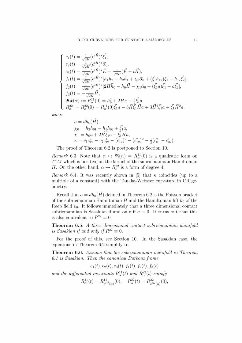
Finally we come to the main theorem of this section. Note that allvector fields in Theorem 6.2, Theorem 6.6, and their proofs should beevaluated at �. They are omitted to avoid heavy notations.
Theorem 6.2. The canonical Darboux frame
e1(t), e2(t), e3(t), f1(t), f2(t), f3(t)
and the differential invariants R11� (t) and R22
� (t) in Theorem 6.1 satisfyR11� (t) = R11
etH(�)(0), R22
� (t) = R22
etH(�)(0), and
RICCI CURVATURE FOR CONTACT 3-MANIFOLDS 19
⎧⎨⎩
e1(t) = 1√2H
(etH)∗�1,
e2(t) = 1√2H
(etH)∗�0,
e3(t) = 1√2H
(etH)∗E = 1√2H
(E − tH),
f1(t) = 1√2H
(etH)∗[ℎ1ℎ2 − ℎ2ℎ1 + �0�0 + (�1ℎ12)�1 − ℎ12�2],
f2(t) = 1√2H
(etH)∗[2Hℎ0 − ℎ0H − �1�0 + (�1a)�1 − a�2],
f3(t) = − 1√2HH,
ℜic(�) := R11� (0) = ℎ2
0 + 2H�− 32�1a,
R22� := R22
� (0) = R11� (0)�1a− 3H�1Ha+ 3H2�1a+ �1H
2a.
where
a = dℎ0(H),
�0 = ℎ2ℎ01 − ℎ1ℎ02 + �1a,
�1 = ℎ0a+ 2H�1a− �1Ha,� = v1c
212 − v2c
112 − (c1
12)2 − (c212)2 − 1
2(c2
01 − c102).
The proof of Theorem 6.2 is postponed to Section 10.
Remark 6.3. Note that � 7→ ℜ(�) = R11� (0) is a quadratic form on
T ∗M which is positive on the kernel of the subriemannian HamiltonianH. On the other hand, � 7→ R22
� is a form of degree 4.
Remark 6.4. It was recently shown in [5] that � coincides (up to amultiple of a constant) with the Tanaka-Webster curvature in CR ge-ometry.
Recall that a = dℎ0(H) defined in Theorem 6.2 is the Poisson bracketof the subriemannian Hamiltonian H and the Hamiltonian lift ℎ0 of theReeb field v0. It follows immediately that a three dimensional contactsubriemannian is Sasakian if and only if a ≡ 0. It turns out that thisis also equivalent to R22 ≡ 0.
Theorem 6.5. A three dimensional contact subriemannian manifoldis Sasakian if and only if R22 ≡ 0.
For the proof of this, see Section 10. In the Sasakian case, theequations in Theorem 6.2 simplify to
Theorem 6.6. Assume that the subriemannian manifold in Theorem6.1 is Sasakian. Then the canonical Darboux frame
e1(t), e2(t), e3(t), f1(t), f2(t), f3(t)
and the differential invariants R11� (t) and R22
� (t) satisfy
R11� (t) = R11
etH(�)(0), R22
� (t) = R22
etH(�)(0),

20 ANDREI AGRACHEV AND PAUL W.Y. LEE
and⎧⎨⎩
e1(t) = 1√2H
(etH)∗�1,
e2(t) = 1√2H
(etH)∗�0,
e3(t) = 1√2H
(etH)∗E = 1√2H
(E − tH),
f1(t) = 1√2H
(etH)∗[ℎ1ℎ2 − ℎ2ℎ1 + 2Hc201�0 + (�1ℎ12)�1 − ℎ12�2],
f2(t) = 1√2H
(etH)∗[2Hℎ0 − ℎ0H],
f3(t) = − 1√2HH,
ℜic(�) := R11� (0) = ℎ2
0 + 2H�,R22� := R22
� (0) = 0.
where � = v1c212 − v2c
112 − (c1
12)2 − (c212)2 − c2
01.
If we assume that the flow of the Reeb field v0 defines a free andproper group action, then the quotient N of the manifold M by thisgroup action is a manifold and the subriemannian metric on M inducesa Riemannian metric on N . In this case, � is simply the Gauss curva-ture of N (see Section 11 for the proof of the following proposition).
Proposition 6.7. Assume that the Reeb field v0 defines a proper G-action (G = S1 or ℝ) on the subriemannian manifold M . If the quo-tient manifold N = M/G is equipped with the Riemannian metric in-duced by the subriemannian in M . Then the Gauss curvature of Ncoincides with � defined in Theorem 6.6.
In particular, Proposition 6.7 shows that ℍ3, SU(2), and SL(2) withstandard subriemannian structures defined in Section 3 satisfies � = 0,� = 1, and � = −1, respectively.
7. Sasakian Space Forms and Generalized MeasureContraction Property
In this section, we specialize the definition of measure contractionproperty to the contact subriemannian case and rewrite it as a condi-tion on the volume growth of the Popp’s measure along subriemanniangeodesics. Then we go on and compute explicitly this volume growthfor the Sasakian manifolds with � defined in Theorem equal to a con-stant. We will refer to these Sasakian manifolds as Sasakian spaceforms. With this as a motivation, we will introduce the generalizedmeasure contraction property ℳCP(K; 2, 3) at the end.
Let (M,Δ, ⟨⋅, ⋅⟩) be a contact subriemannian manifold with subrie-mannian distance function d and let x0 be a point in M . Let f be thefunction defined by f(x) = −1
2d2(x0, x). According to the result in [4],
the function f is Lipshitz with respect to a Riemannian distance. In

RICCI CURVATURE FOR CONTACT 3-MANIFOLDS 21
particular, it is differentiable almost everywhere. Therefore, we candefine the map 't by
(7.1) 't(x) = �(etH(dfx)),
where etH is the subriemannian geodesic flow and � : T ∗M →M is thenatural projection.
For each fixed x in the manifold M , the curve t 7→ 't(x) is a mini-mizing geodesic starting from x and ending at x0. In particular, '1 isthe constant map '1(x) = x0. It follows that '1 is the unique solutionto the optimal transportation problem (4.1) when the final measure �1
is a delta mass �x0 at the point x0. It also follows that the path of mea-sures 't∗� defines a Wasserstein geodesic and all Wasserstein geodesics�t with �1 = �x0 is of this form. If we substitute the map 't into thedefinition of measure contraction property, we have the following.
Proposition 7.1. Let (M,Δ, ⟨⋅, ⋅⟩) be a contact subriemannian man-ifold with subriemannian distance d and Popp’s measure �. Then themetric measure space (M,d, �) satisfies the measure contraction prop-erty MCP (K,N) if and only if for any point x0 in the space M thefollowing holds
�('t(U)) ≥∫U
(1− t)(sK((1− t)D(x))
sK(D(x))
)N−1
d�(x)
for any Borel set U , where
sK(r) =
⎧⎨⎩1√K
sin(√K r) if K > 0
r if K = 01√−K sinh(
√−K r) if K < 0,
D(x) = d(x0,x)√N−1
, and the map 't is defined in (7.1).
It follows from Proposition 7.1 that the measure contraction propertyis a control on the volume growth �('t(U)) of the set U along geodesicst 7→ 't(x) which end at x0. In the case of Sasakian space form, thevolume growth �('t(U)) is given by the following equality (see Section12 for the proof).
Theorem 7.2. Let (M,Δ, ⟨⋅, ⋅⟩) be a Sasakian manifold with � = Ka constant. Let d be the subriemannian distance and � be the Popp’smeasure. Let x0 be a point on the manifold M and let 't be defined asin (7.1). Then the following holds
�('t(U)) =
∫U
(1− t)(s(k(x), (1− t)D(x))
s(k(x), D(x))
)d�(x)

22 ANDREI AGRACHEV AND PAUL W.Y. LEE
for any Borel set U , where
s(k, r) =
⎧⎨⎩12(2−2 cos(
√kr)−
√k r sin(
√k r)
k2if k > 0
r4 if k = 012(2−2 cosh(
√−k r)+(
√−k r) sinh(
√−k r))
k2if k < 0
k(x) = (v0D)2(x) +K, and D(x) = d(x0, x).
Note that
s(k(x), (1− t)D(x))
s(k(x), D(x))≥ s(K, (1− t)D(x))
s(K,D(x)).
In view of this and Theorem 7.2, we define the generalized measurecontraction property as follows.
Definition 7.3. The metric measure space (M,d, �) satisfies the gen-eralized measure contraction property ℳCP(K; 2, 3) if for any point x0
in the space M , for any geodesic �t in P satisfying �1 = �x0 (the deltamass at x0) and �0 = �, the following holds
�0('t(U)) ≥∫U
(1− t)(sK((1− t)D(x))
sK(D(x))
)d�t(x)
for any Borel set U , where
sK(r) =
⎧⎨⎩12(2−2 cos(
√Kr)−
√K r sin(
√K r)
K2 if K > 0
r4 if K = 012(2−2 cosh(
√−K r)+(
√−K r) sinh(
√−K r))
K2 if K < 0
and D(x) = d(x0, x).
Remark 7.4. Note that the condition ℳCP(0; 2, 3) coincides with thecondition MCP (0, 5).
Remark 7.5. sK in the Definition 7.3 satisfies
sK(r) = r4 + o(r4) as r → 0.
Therefore, ℳCP(K; 2, 3) does not imply MCP (0, N) for any N > 5.
8. The Main Result and its Consequences
In this section, we state our main result and its consequences. Fortheir proofs, see Section 13.

RICCI CURVATURE FOR CONTACT 3-MANIFOLDS 23
Theorem 8.1. (Generalized Measure Contraction Property) Assumethat the three dimensional contact subriemannian manifold is Sasakian(i.e. R22 ≡ 0) and there is a constant K such that R11
� ≥ 2KH(�)for all � in the cotangent bundle T ∗M . Then the metric measurespace (M,d, �) satisfies the generalized measure contraction propertyℳCP(K; 2, 3), where d is the subriemannian distance and � is thePopp’s measure (see Section 2 for the defintions).
Recall thatℳCP(0; 2, 3) is the same as MCP (0, 5). Therefore, The-orem 1.1 follows from Theorem 8.1.
Remark 8.2. The proof of Theorem 6.2 also works when we assume thatR22� ≥ 0 for all � in the cotangent bundle. However, it is I. Zelenkos
observation (private communications) that R22� ≥ 0 for all � implies
R22 ≡ 0. On the other hand, see Section 9 for result with relaxedassumption on R22.
Remark 8.3. If Δ is a bracket-generating distribution, then it definesa flag of distribution by
Δ1 := Δ ⊂ Δ2 ⊂ ... ⊂ TM.
If we denote the dimension of the vector space Δix by nix, then the
growth vector of the distribution Δ at the point x is defined by
(n1x, n
2x, ..., n
kx).
The pair (2, 3) in the generalized measure contraction property is thegrowth vector of the three dimensional contact subriemannian mani-fold. In this paper, we add ℳCP(K; 2, 3) to the measure contractionproperty MCP (K,N) introduced earlier by Sturm. It would be veryinteresting to find appropriate measure contraction properties for othersubriemannian manifolds with different growth vectors.
Remark 8.4. Many ingredients used in the proof of Theorem 8.1 alsopresent in the higher dimensional contact subriemannian case. Thisincludes the recent result in [27, 28], a comparison principle of matrixRiccati equations, and the solvability of matrix Riccati equations withconstant coefficients. Therefore, results similar to Theorem 8.1 canbe proved in a similar way in the higher dimensional case where thecanonical Darboux frames and curvature invariants are well understood(i.e. an analog of Theorem 6.2). For instance, the result in [24] for thehigher dimensional Heisenberg group can be proved in the same wayas in Theorem 8.1.
Let Bx(R) be the subriemannian ball of radius R centered at a pointx in the manifold M and let � : T ∗M →M be the natural projection.

24 ANDREI AGRACHEV AND PAUL W.Y. LEE
The proof of Theorem 8.1 is still valid if the curvature assumptionsonly holds on a ball Bx(R) and the measure is contracted towards theceneter of the ball x. Therefore, the following volume doubling propertyholds.
Corollary 8.5. (Volume Doubling Property) Assume that there is apoint x0 in the three dimensional contact subriemannian manifold anda constant R > 0 such that R11
� ≥ 2KH(�) and R22� = 0 for all � in
�−1(Bx0(2R)) and for some constant K > 0. Then
�(Bx0(2kR)) ≤ 25�(Bx0(kR))
for all 0 < k < 1.
Remark 8.6. Note that although the generalized measure contractionproperty is sharp (see Section 7), the constant 25 in Corollary 8.5 is not.This is because the generalized measure contraction property, which isa condition on general sets, does not take into account the symmetryof the subriemannian balls.
The local Poincare inequality also holds under the assumptions inCorollary 8.5. For this, let ∇Hf be the horizontal gradient of thefunction f defined by the condition df(v) = ⟨∇f, v⟩ for all v in thedistribution Δ. For the proof of the following Corollary, see Section13.
Corollary 8.7. (Local Poincare Inequality) Under the assumptionsin Corollary 8.5, the following local Poincare inequality holds for allsmooth functions f and all 0 < k < 1
1
�(Bx0(kR))
∫Bx0 (kR)
∣f(x)− ⟨f⟩Bx0 (kR) ∣d�(x)
≤ CR
�(Bx0(2kR))
∫Bx0 (2kR)
∣∇Hf ∣d�(x),
for some constant C and where
⟨f⟩Bx0 (kR) =1
�(Bx0(kR))
∫Bx0 (kR)
f(x)d�(x).
Let ΔH be the sub-Laplacian defined by ΔH = div�∇H , where div�denotes the divergence with respect to �. Under the assumptions inTheorem 1.1, the results in [17] together with Corollary 8.5 and 8.7show that any positive harmonic function of the sub-Laplacian ΔH
satisfies the Harnack inequality. More precisely,

RICCI CURVATURE FOR CONTACT 3-MANIFOLDS 25
Theorem 8.8. (Harnack inequality for sub-Laplacian) Under the as-sumptions in Corollary 8.5, any positive solution to the equation ΔHf =0 satisfies
supBx0 (kR)
f ≤ C infBx0 (kR)
f
for all 0 < k < 1.
For the proof of Theorem 8.8, see [17]. Finally, by letting R goes to+∞ in Theorem 8.8, the following Liouville theorem holds.
Corollary 8.9. (Liouville Theorem for sub-Laplacian) Under the as-sumptions in Theorem 1.1, any non-negative solution to the equationΔHf = 0 is a constant.
9. More General Situations and Final Remark
In this section, we show that the assumption on R22 in Theorem 8.1can be relaxed. To do this, let Ωx be the injectivity domain at a pointx in M defined as the set of all covectors � in T ∗xM such that
t 7→ �(etH(�)), 0 ≤ t ≤ 1
is length minimizing between its end points. Finally, let Ω =∪x Ωx be
the injectivity domain.One can apply similar arguments as in the proof of Theorem 8.1
under the assmption that R22 is bounded below by a constant on Ωinstead of bounded by zero. This will give certain measure contractionproperty.
Theorem 9.1. Assume that M is a three dimensional contact sub-riemannian manifold with subriemannian distance d and Popp’s mea-sure �. Assume further that there are constants C1 and C2 such thatR11� ≥ 2C1H(�) and R22
� ≥ −C22 for all � in Ω. Let 't be as in (7.1).
Then the metric measure space (M,d, �) satisfies
�('t(U)) ≥∫U
(1− t)
(sC1,C2(
√2(1− t))
sC1,C2(√
2)
)d�(x)

26 ANDREI AGRACHEV AND PAUL W.Y. LEE
for any Borel set U , where
sC1,C2(r) =
⎧⎨⎩
24(
cosh(a2r)−1a4
+ cos(b2r)−1b4
)if a > 0 and b > 0,
24(r2
2+ cos(b2r)−1
b4
)if a = 0 and b > 0,
24(
cosh(a2r)−1a4
− r2
2
)if a > 0 and b = 0,
24(− cosh(a2r)−1
a4+ cosh(b2r)−1
b4
)if a > 0 and b < 0,
24(− r2
2+ cosh(b2r)−1
b4
)if a = 0 and b < 0,
24(
cosh(a2r)−1a4
+ r2
2
)if a > 0 and b = 0,
24(− cos(a2r)−1
a4+ cos(b2r)−1
b2
)if a < 0 and b < 0,
24(r2
2+ cos(b2r)−1
b4
)if a = 0 and b < 0,
24(
cos(a2r)−1a4
− r2
2
)if a < 0 and b = 0,
r4 if a = b = 0,
a(x) = C2 − 12C1d
2(x0, x), and b(x) = C2 + 12C1d
2(x0, x).
The proof of Theorem 9.1 is very similar to that of Theorem 8.1and will be omitted. Finally, we show that the any compact threedimensional contact subriemannian manifold satisifies the assumptionsin Theorem 9.1.
Theorem 9.2. Assume that the three dimensional contact subrieman-nian manifold is compact. Then R22
�
∣∣∣�∈Ω
is bounded.
For the proof of Theorem 9.2, see Section 14.
After the submission of this paper, there are some very interestingworks which are also on Ricci curvature type condition and its con-sequences to subriemannian geometry and PDE ([9, 29, 11, 10, 5]).Among them, [9, 11, 10] uses an apporach very different from ours.It would be very interesting to establish connections between the twoapproaches. Finally, we would like to point out that curvature typeinvariants on three-dimensional contact subriemannian manifolds wereconsidered in [22] and a Bonnet-Myer theorem is proved there. Wewould like to thank one of the referees who pointed this out.
10. Proof of Theorem 6.1, 6.2, and 6.5
In this section, we give the proof of Theorem 6.1, 6.2, and 6.5. Letus start with a lemma on Euler field. Recall that E denotes the Eulerfield and H denotes the subriemannian Hamiltonian.

RICCI CURVATURE FOR CONTACT 3-MANIFOLDS 27
Lemma 10.1. (etH)∗E = E − tH
Proof. Recall ds : T ∗M → T ∗M is the dilation map ds(�) = s�. Bythe definition of the symplectic form,
d∗s! = s!.
It follows that
!(dds(H(�)), X(s�))
= s!(H(�), dd−1s (X(s�)))
= −sdH(dd1/s(X(s�))),
where X is any tangent vector in the tangent bundle TT ∗M .The subriemannian Hamiltonian H is homogeneous of degree two in
the fibre direction. In other words,
H(ds(�)) = s2H(�).
Therefore,
!(d�s(H(�)), X(s�)) = −1
sdH(X(s�)) =
1
s!(H(s�), X(s�)).
It follows that d∗sH = sH, where d∗sH is the pullback of the vector
field H by the map �s. By comparing the flow of the above vectorfields, we have
etH ∘ �s = �s ∘ etsH .By differentiating the above equation with respect to s and set s to 1,
it follows that (etH)∗E = E − tH as claimed. □
Proof of Theorem 6.1. According to the main result in [27, 28], thereexists a family of Darboux frames
{e1(t), e2(t), e3(t), f1(t), f2(t), f3(t)}and functions Rij
� (t) which satisfy⎧⎨⎩
e1(t) = f1(t),e2(t) = e1(t),e3(t) = f3(t),
f1(t) = −R11� (t)e1(t)−R31
� (t)e3(t)− f2(t),
f2(t) = −R22� (t)e2(t)−R32
� (t)e3(t),
f3(t) = −R31� (t)e1(t)−R32
� (t)e2(t)−R33� (t)e3(t).
Remark 10.2. In the language of [27, 28], the Young diagram associatedwith the above structural equations consists of two columns with twoboxes in the first column and one box in the second column.

28 ANDREI AGRACHEV AND PAUL W.Y. LEE
Note that d�(E) = 0. Therefore, E(etH(�)) is contained in the
vertical space at etH(�) for each time t. Hence, by the definition of the
Jacobi curve J�(t), the vector (etH)∗E(�) is contained in J�(t) for eacht. It follows from Lemma 10.1 that
E(�)− tH(�) =3∑i=1
ai(t)ei(t)
for some functions ai of time t. If we differentiate with respect to timet twice, we get
2a1(t)f1(t) + 2a2(t)e1(t) + 2a3(t)f3(t)− a1(t)(R11� (t)e1(t)+
+R31� (t)e3(t) + f2(t)) + a2(t)f1(t)− a3(t)(R31
� (t)e1(t) +R32� (t)e2(t)+
+R33� (t)e3(t)) + a1(t)e1(t) + a2(t)e2(t) + a3(t)e3(t) = 0.
If we equate the coefficients of the fi(t)’s, we get a1 ≡ a2 ≡ a3 ≡ 0.
Therefore, E(�)− tH(�) = a3e3(t) and −H(�) = a3f3(t) for some con-
stant a3 satisfying (a3)2 = !(a3f3(t), a3e3(t)) = dH(E(�)) = 2H(�).It follows that R31
� (t) = R32� (t) = R33
� (t) = 0. Moreover, we also have(10.1)
e3(t) =1
(2H(�))1/2(E(�)− tH(�)), f3(t) = − 1
(2H(�))1/2H(�).
□
For the proof of Theorem 6.2, we need a few more lemmas. Letℎij : T ∗M → ℝ be the Hamiltonian lift of the vector field [vi, vj] definedby
ℎij(�) = �([vi, vj]).
The commutator relations of the frame {ℎi, �i∣i = 1, 2, 3} are given bythe following:
Lemma 10.3.
[ℎi, ℎj] = ℎij, [ℎi, �j] = −∑k
cjik�k, [�i, �j] = 0.
Proof. Since the Lie derivative ℒ of the symplectic form ! along the
Hamiltonian vector field ℎi vanishes,
(10.2) i[ℎi ,ℎj ]! = ℒℎiiℎj! − iℎjℒℎi! = ℒℎiiℎj! = −d(!(ℎi, ℎj)).
The function !(ℎi, ℎj) is equal to ℎij. Indeed, since d�(ℎi) = vi, wehave
��(ℎi) = �(d�(ℎi)) = �(vi) = ℎi(�).
It follows from this and the Cartan’s formula that
dℎj (ℎi) = !(ℎi, ℎj) = d�(ℎi, ℎj) = dℎj (ℎi)− dℎi(ℎj)− �([ℎi, ℎj]).

RICCI CURVATURE FOR CONTACT 3-MANIFOLDS 29
If we apply again d�(ℎi) = vi, then we have
��([ℎi, ℎj]) = �(d�([ℎi, ℎj])) = �([vi, vj]) = ℎij(�).
Therefore, we have
(10.3) !(ℎi, ℎj) = −dℎi(ℎj) = ℎij.
If we combine this with (10.2), the first assertion of the lemma follows.A calculation similar to the above one shows that
i[ℎi,�j ]! = ℒℎii�j!.
By Cartan’s formula, the above equation becomes
i[ℎi,�j ]! = −iℎi�∗d�j = −�∗(ivid�j).
The second assertion follows from this and (6.2).If we apply Cartan’s formula again,
i[�i,�j ]! = ℒ�ii�j! − i�jℒ�i! = −i�id(�∗�j) + i�jd(�∗�i)
Since d�(�i) = 0, it follows that i[�i,�j ]! = 0. Therefore, the thirdassertion holds by the nondegeneracy of !. □
Let � = ℎ1dℎ2 − ℎ2dℎ1, then we also have the following relations:
Lemma 10.4.
dℎi(ℎj) = −ℎij, �i(ℎj) = −dℎi(�j) = �ij, �i(�j) = 0,
�(�2) = dH(�1) = 0, �(�1) = dH(�2) = −2H.
Proof. The first assertion follows from (10.3) and the next two asser-
tions follow from d�(ℎi) = vi and d�(�i) = 0. A computation using
�i(ℎj) = �ij proves the rest of the assertions. □
Proof of Theorem 6.2. Recall J�(⋅) denotes the Jacobi curve at thepoint � in the cotangent bundle T ∗M . By Theorem 6.1, there exists afamily of Darboux frame
{e1(t), e2(t), e3(t), f1(t), f2(t), f3(t)}
and functions Rij� (t) such that
J�(t) = span{e1(t), e2(t), e3(t)}

30 ANDREI AGRACHEV AND PAUL W.Y. LEE
and ⎧⎨⎩
e1(t) = f1(t),e2(t) = e1(t),e3(t) = f3(t),
f1(t) = −R11� (t)e1(t)− f2(t),
f2(t) = −R22� (t)e2(t),
f3(t) = 0.
Let ℰ(t) be defined by
ℰ(t) = (etH)∗�0(�) = de−tH(�0(etH(�))).
By the definition of the Jacobi curve J�(⋅), we known that ℰ(t) iscontained in J�(t) for each t. Since e1(t), e2(t), e3(t) span J�(t), wemust have
ℰ(t) = c1(t)e1(t) + c2(t)e2(t) + c3(t)e3(t)
for some functions ci of time t, i = 1, 2, 3.Let � : T ∗M → M be the natural projection. The Hamiltonian
vector field H of the subriemannian Hamiltonian H satisfies
d�(H(�)) = d�(ℎ1(�)v1 + ℎ2(�)v2) = 0.
It follows that
!(�0, H) = −�∗�0(H) = 0.
Since the flow etH preserves the symplectic form !, it follow fromthe definition of ℰ(t) that
!(ℰ , H) = 0.
By (10.1), we know that f3(t) = − 1(2H)1/2
H. Since {ei(t), fi(t)∣i =
1, 2, 3} is a Darboux basis, we have
0 = !(ℰ , H) = (2H)1/2c3(t).
This shows that c3 ≡ 0 and so
ℰ(t) = c1(t)e1(t) + c2(t)e2(t).
By the definition of ℰ(t), if we differentiate this with respect to time t,then we have
(etH)∗[H, �0] = ℰ(t) = c1(t)e1(t) + c1(t)f1(t) + c2(t)e2(t) + c2(t)e1(t).
By the Cartan’s formula and �0(H) = 0, it follows that
!(ℰ(t), ℰ(t)) = !([H, �0], �0) = �∗�0([H, �0]) = −�∗d�0(H, �0) = 0.

RICCI CURVATURE FOR CONTACT 3-MANIFOLDS 31
By combining this with the above equation for ℰ and ℰ , we havec1 ≡ 0. If we differentiate the equation
ℰ(t) = c2(t)e2(t)
with respect to time t again, we get
(etH)∗(adH(�0)) = c2(t)e2(t) + c2(t)e1(t)
(etH)∗(ad2H
(�0)) = c2(t)e2(t) + 2c2(t)e1(t) + c2(t)f1(t).
Here adH denotes adH(⋅) = [H, ⋅].Since {ei(t), fi(t)∣i = 1, 2, 3} is a Darboux basis and the flow etH
preserves the symplectic form !,
(c2(t))2 = !�((etH)∗ad2H
(�0), (etH)∗adH(�0)))
= (etH∗ !)etH(�)(ad2H
(�0), adH(�0)))
= !etH(�)(ad2H
(�0), adH(�0)))
Therefore, c2(t) = (etH)∗(
1c
), where c(�) := 1
(!�(ad2H
(�0),adH
(�0)))1/2.
It follows from the definition of ℰ that
e2(t) =1
c2(t)ℰ(t) = (etH)∗(c�0).
To find out what c is more explicitly, we first compute [H, �0]. TheLie bracket is a derivation in each of its entries, so
[H, �0] = [ℎ1ℎ1 + ℎ2ℎ2, �0]
= −dℎ1(�0)ℎ1 − dℎ2(�0)ℎ2 + ℎ1 [ℎ1, �0] + ℎ2 [ℎ2, �0].
It follows from this, Lemma 10.3, and Lemma 10.4 that
[H, �0] = ℎ1�2 − ℎ2�1 = �1.
Next, we want to compute [H, �1]. For this, let
(10.4) [H, �1] = k0�0 + k1�1 + k2�2 +2∑i=0
ciℎi
for some functions ci and ki.To compute c0 for instance, we apply �0 on both sides of (10.4).
Using Lemma 10.4 and Cartan’s formula, we have c0 = 0. Similarcomputation gives c1 = −ℎ2 and c2 = ℎ1. This shows that
(10.5) [H, �1] = k0�0 + k1�1 + k2�2 + ℎ1ℎ2 − ℎ2ℎ1.

32 ANDREI AGRACHEV AND PAUL W.Y. LEE
By applying dℎ0 on both sides of (10.5) and using Lemma 10.4 again,
we have k0 = ℎ2ℎ01−ℎ1ℎ02 + �1a. Similar calculations using � and dHgive
(10.6) [H, �1] = ℎ1ℎ2 − ℎ2ℎ1 + �0�0 + (�1ℎ12)�1 − ℎ12�2.
where �0 = ℎ2ℎ01 − ℎ1ℎ02 + �1a and a = dℎ0(H).It follows that
c−2 = !(ad2H
(�), adH(�)) = 2H
and e2(0) = 1√2H�0. It also follows from Theorem 6.1 that
(10.7)
e1(0) = 1√2H�1,
f1(0) = 1√2H
[H, �1],
f1(0) = 1√2H
[H, [H, �1]],
f1(0) = 1√2H
[H, [H, [H, �1]]].
A computation similar to that of (10.6) gives
(10.8) [H, [H, �1]] = −2Hℎ0 + ℎ0H + �1�0 + (�2 + �0 − �1a)�1 + a�2
where �1 = ℎ0a+ 2H�1a− �1Ha and �2 = ℎ0ℎ12 + 2H�1ℎ12 − �1Hℎ12.It follows from Theorem 6.1, (10.6), (10.7) and (10.8) that
R11� (0) = !(f1(0), f1(0))
= −�0 − �2.(10.9)
Note that, in (10.9), �1a does not appear. This is because
!(−2Hℎ0, ℎ1ℎ2 − ℎ2ℎ1 + �0�0) = −2H�1a
and!(−(�1a)�1, ℎ1ℎ2 − ℎ2ℎ1) = 2H�1a.
Since f1(0) = −R11� (0)e1(0) − f2(0), it follows from (10.7), (10.8),
and (10.9) that
f2(0) =1√2H
[2Hℎ0 − ℎ0H − �1�0 + (�1a)�1 − a�2].
A long computation using the bracket relations (6.1) gives
�2 = −(ℎ0)2 + 2H[(c112)2 + (c2
12)2 − v1c212 + v2c
112] + �1a.
and
�0 −1
2�1a = ℎ2ℎ01 − ℎ1ℎ02 +
1
2�1a = H(c2
01 − c102).

RICCI CURVATURE FOR CONTACT 3-MANIFOLDS 33
It follows as claimed that
R11� (0) = ℎ2
0 + 2H�− 3
2�1a.
To prove the formula for R22, we differentiate the equation
f1(t) = −R11� (t)e1(t)− f2(t)
and combine it with the equation
f2(t) = −R22� (t)e2(t).
We have
R22� (0)e2(0) = f1(0) + HR11
� (0)e1(0) +R11� (0)f1(0).
Therefore, by applying dℎ0 on both sides and using dℎ0(e1(0)) = 0,we get
R22� (0) = −
√2H[dℎ0(f1(0)) +R11
� (0)dℎ0(f1(0))].
By using Cartan’s formula and (10.7), it follows that√
2Hdℎ0(f1(0)) = dℎ0([H, �1]) = −�1a,√
2Hdℎ0(f1(0)) = dℎ0([H, [H, �1]]) = �1Ha− 2H�1a,√
2Hdℎ0(f1(0)) = 3H�1Ha− 3H2�1a− �1H2a.
The formula for R22� (0) follows from this.
□
Finally, we come to the proof of Theorem 6.5. The proof involveslengthy computations of R22. Therefore, only a sketch is given below.
Proof of Theorem 6.5. Clearly, if a ≡ 0, then R22 ≡ 0 by Theorem 6.2.Conversely, assume that R22 ≡ 0. By using the expression of R22 inTheorem 6.2 and Lemma 10.4, we can rewrite R22 as a homogeneouspolynomial of degree 4 with three variables ℎ0, ℎ1, and ℎ2. A longcomputation shows that the coefficients of ℎ2
0ℎ21 and ℎ2
0ℎ1ℎ2 are−3(c201+
c102) and 12c1
01, respectively. Therefore, if R22 ≡ 0, then c201 + c1
02 = 0and c1
01 = −c202 = 0. It follows that
a = dℎ0(H)
= ℎ1dℎ0(ℎ1) + ℎ2dℎ0(ℎ2)
= −c101ℎ
21 − (c2
01 + c102)ℎ1ℎ2 + c1
01ℎ22
= 0.
□

34 ANDREI AGRACHEV AND PAUL W.Y. LEE
11. Proof of Theorem 6.6 and Proposition 6.7
In this section, we will give the proof of Theorem 6.6 and Proposition6.7. The result of Theorem 6.6 follows from the following two lemmas.
Lemma 11.1. Under the above assumptions, the functions ckij in thebracket relation (6.1) satisfies
c001 = c0
02 = c101 = c2
02 = 0 and c201 = −c1
02.
Proof of Lemma 11.1. If the flow of the vector field e = v0 is denotedby etv0 , then the invariance of the subriemannian metric under thegroup action implies that⟨
(etv0)∗vi, (etv0)∗vj
⟩= �ij, �((etv0)∗vj) = 0, i, j = 1, 2.
By differentiating the above equations with respect to time t, it followsthat
�j([e, vi]) + �i([e, vj]) = 0, �([e, vj]) = 0, i, j = 1, 2.
If we apply the bracket relations (6.1) of the frame v1, v2, v3, we have
cj0i+ci0j = �j([e, vi])+�i([e, vj]) = 0, c0
0j = �([e, vj]) = 0, i, j = 1, 2.
□
It follows that
Lemma 11.2. The function ℎ0 is a constant of motion of the flow etH .i.e. a = dℎ0(H) = 0.
Proof of Lemma 11.2. This follows from general result in Hamiltonianreduction. In this special case this can also be seen as follow. ByLemma 10.4
(11.1) dℎ0(H) = dℎ0(ℎ1ℎ1 + ℎ2ℎ2) = ℎ1ℎ10 + ℎ2ℎ20.
By Lemma 11.1 we also have
ℎ10 = −c001ℎ0 − c1
01ℎ1 − c201ℎ2 = −c2
01ℎ2.
Similarly ℎ20 = −c102ℎ1. The result follows from this, (11.1), and
Lemma 11.1. □
Proof of Proposition 6.7. Let �M : M → N be the quotient map. Letw1 and w2 be a local orthonormal frame on the surface N . Since � is asubmersion, there are unique vector fields w1 and w2 in the distributionΔ such that d�(wi) = wi. If Φt is the flow of the Reeb field v0, then�(Φt(x)) = �(x) by the definition of the quotient map. Therefore,

RICCI CURVATURE FOR CONTACT 3-MANIFOLDS 35
d�(dΦt(wi)) = d�(wi). Since dΦt(wi) is in Δ, we have (Φt)∗wi = wi. Ifwe differentiate this equation and set t to zero, then we have [v0, wi] = 0.
Since w1 and w2 are orthonormal with respect to the subriemannianmetric, we can set vi = wi. It follows that c2
01 = 0 and � is simplifiedto
(11.2) � = v1c212 − v2c
112 − (c1
12)2 − (c212)2.
From (6.1), we also have [v1, v2] = c012v0 + c1
12v1 + c212v2. If we apply
d�M to the equation, then we get [w1, w2] = c112w1 + c2
12w2.Let us denote the covariant derivative on the Riemannian manifold
N by ∇. It follows from Koszul formula ([37, Theorem 3.11]) that
(11.3)∇w1w1 = −c1
12w2, ∇w2w2 = −c212w1,
∇w1w2 = c112w1, ∇w2w1 = −c2
12w2.
Since the covariant derivative ∇ is tensorial in the bottom slot andis a derivation in the other slot, it follows from (11.3) that
∇[w1,w2]w1 = ∇c112w1+c212w2w1
= c112∇w1w1 + c2
12∇w2w1
= −[(c112)2 + (c2
12)2]w2
and
[∇w1 ,∇w2 ]w1 = ∇w1∇w2w1 −∇w2∇w1w1
= −∇w1(c212w2) +∇w2(c
112w2)
= −(w1c212)w2 + (w2c
112)w2 − 2c1
12c212w1.
Therefore, it follows from the above calculation that the Gauss cur-vature is given by
< ∇[w1,w2]w1 − [∇w1 ,∇w2 ]w1, w2 >= w1c212 − w2c
112 − (c1
12)2 − (c212)2.
By (11.2), this agrees with �. □
12. Proof of Theorem 7.2
Proof of Theorem 7.2. From the main result in [16], the function f =−1
2d2(x, x0) is locally semiconcave on M − {x0}, so it is differentiable
almost everywhere. Assume that x′ is a point where f is differentiable.
It follows that the map t 7→ 't(x′) := �(etH(dfx′)) is the unique mini-
mizing geodesic connecting x′ and x0. An argument similar to the Rie-mannian case using inverse function theorem shows that the functionf is C∞ in a neighborhood of the curve t 7→ 't(x
′) (see, for instance,[23]). Moreover, it follows from [1, Theorem 1.2] that there is no con-jugate point along the curve t 7→ 't(x
′). Therefore, the map (d't)x′ isnonsingular for each t < 1.

36 ANDREI AGRACHEV AND PAUL W.Y. LEE
If we denote the differential of the map x 7→ dfx by ddf, then
d't = d�(detH(ddf)). Let ei(t) and fi(t) be the Darboux frame atdfx′ defined as in Theorem 6.1 and let &i = d�(fi(0)). Then the vec-tors {ddf(&1), ddf(&2), ddf(&3)} span a linear subspace W of Tdfx′T
∗M .Therefore ddf(&i) can be written as
(12.1) ddf(&i) =3∑
k=1
(aij(t)ej(t) + bij(t)fj(t)) or Ψ = AtEt +BtFt,
where At is the matrix with entries aij(t), Bt is the matrix with entriesbij(t), and Ψ, Et, and Ft are matrices with rows ddf(&i), ei(t), and fi(t),respectively.
By a result in [20], the measure 't∗� is absolutely continuous withrespect to �. Let gt be the density of 't∗� (i.e. 't∗� = gt�). Since 'tis smooth in a neigborhood of x′, we can consider � as a volume form.It follows from 't∗� = gt� that
gt('t(x′)) ∣�(d'(&1), d'(&2), d'(&3))∣ = ∣�(&1, &2, &3)∣.
By Theorem 6.2,
∣�(d'(&1), d'(&2), d'(&3))∣ = ∣�(&1, &2, &3) detBt∣.Note also that since (d't)x′ is nonsingular, Bt is invertible for all
t < 1. Since B0 is the identity matrix, detBt > 0 for all t < 1.Therefore, we have proved the following lemma.
Lemma 12.1.
gt('t(x′)) =
1
detBt
.
If we differentiate (12.1) with respect to time t and apply Theorem6.1, then we have
0 = AtEt + AtEt + BtFt +BtFt
= AtEt + At(C1Et + C2Ft) + BtFt −Bt(R + CT1 Ft),
where
C1 =
⎛⎝ 0 0 01 0 00 0 0
⎞⎠ , C2 =
⎛⎝ 1 0 00 0 00 0 1
⎞⎠ ,
R =
⎛⎝ r 0 00 0 00 0 0
⎞⎠ ,
r(x′) = ℎ20(dfx′) + 2KH(dfx′) = (v0f(x
′))2 −Kf(x′),
and CT1 denotes the transpose of C1.

RICCI CURVATURE FOR CONTACT 3-MANIFOLDS 37
Therefore, we have the following equations for the matrices At andBt.
(12.2) At + AtC1 −BtR = 0, Bt + AtC2 −BtCT1 = 0.
If st = gt('t(x)), then we have, by (12.1) and (12.2), the following:
detBtd
dtdet(B−1
t ) = −tr(B−1t Bt) = tr(B−1
t AtC2).
Therefore, if we let St = B−1t At, then we have the following lemma.
Lemma 12.2.
detBt = e−∫ t0 tr(SsC2)ds.
By (12.2), the matrix St defined by St = B−1t At satisfies the following
matrix Ricatti equation
St −R + StC1 + CT1 St − StC2St = 0.
Since '1(x) = x0 for all x, we have d'1(&i) = 0. Therefore, byTheorem 6.2 and (12.1), B1 = 0. Therefore, S−1
t satisfies the followingmatrix Ricatti equation
d
dt(S−1
t ) + S−1t RS−1
t − C1S−1t − S−1
t CT1 + C2 = 0 and S−1
1 = 0.
Since the coefficient of the above equation does not depend on timet, the solution to this equation can be found explicitly by the result in[26] as follows.
Let us consider the matrix
Q =
(C1 −C2
R −CT1
)and the corresponding matrix differential equation d
dtq = Qq together
with the condition q(1) = I.The fundamental solution is given by
q(t) = e(t−1)Q =
⎛⎜⎜⎜⎜⎜⎜⎝
cos �t 0 0 sin �t�0
1−cos �t�20
0
− sin �t�0
1 0 cos �t−1�20
sin �t−�t�30
0
0 0 1 0 0 1− t−�0 sin �t 0 0 cos �t
sin �t�0
0
0 0 0 0 1 00 0 0 0 0 1
⎞⎟⎟⎟⎟⎟⎟⎠ .
if r > 0,
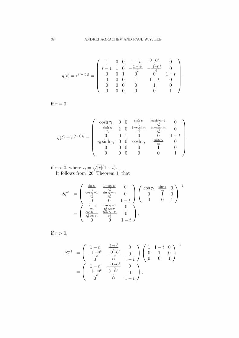
38 ANDREI AGRACHEV AND PAUL W.Y. LEE
q(t) = e(t−1)Q =
⎛⎜⎜⎜⎜⎜⎜⎝1 0 0 1− t (1−t)2
20
t− 1 1 0 − (1−t)22
− (1−t)36
00 0 1 0 0 1− t0 0 0 1 1− t 00 0 0 0 1 00 0 0 0 0 1
⎞⎟⎟⎟⎟⎟⎟⎠ .
if r = 0,
q(t) = e(t−1)Q =
⎛⎜⎜⎜⎜⎜⎜⎜⎝
cosh �t 0 0 sinh �t�0
cosh �t−1�20
0
− sinh �t�0
1 0 1−cosh �t�20
�t−sinh �t�30
0
0 0 1 0 0 1− t�0 sinh �t 0 0 cosh �t
sinh �t�0
0
0 0 0 0 1 00 0 0 0 0 1
⎞⎟⎟⎟⎟⎟⎟⎟⎠.
if r < 0, where �t =√∣r∣(1− t).
It follows from [26, Theorem 1] that
S−1t =
⎛⎜⎝sin �t�0
1−cos �t�20
0cos �t−1�20
sin �t−�t�30
0
0 0 1− t
⎞⎟⎠⎛⎝ cos �t
sin �t�0
0
0 1 00 0 1
⎞⎠−1
=
⎛⎝ tan �t�0
cos �t−1�20 cos �t
0cos �t−1�20 cos �t
tan �t−�t�30
0
0 0 1− t
⎞⎠ ,
if r > 0,
S−1t =
⎛⎝ 1− t (1−t)22
0
− (1−t)22
− (1−t)36
00 0 1− t
⎞⎠⎛⎝ 1 1− t 00 1 00 0 1
⎞⎠−1
=
⎛⎝ 1− t − (1−t)22
0
− (1−t)22
(1−t)33
00 0 1− t
⎞⎠ ,

RICCI CURVATURE FOR CONTACT 3-MANIFOLDS 39
if r = 0, and
S−1t =
⎛⎜⎝sinh �t�0
cosh �t−1�20
01−cosh �t
�20
�t−sinh �t�30
0
0 0 1− t
⎞⎟⎠⎛⎝ cosh �t
sinh �t�0
0
0 1 00 0 1
⎞⎠−1
=
⎛⎜⎝tanh �t�0
1−cosh �t�20 cosh �t
01−cosh �t�20 cosh �t
�t−tanh �t�30
0
0 0 1− t
⎞⎟⎠ .
if r < 0.Therefore, inverting the above matrix gives the following. If r > 0,
then
St =
⎛⎜⎝ �0(sin �t−�t cos �t)D
�20 (1−cos �t)
D 0�20 (1−cos �t)
D�30 sin �tD 0
0 0 11−t
⎞⎟⎠where D = 2− 2 cos �t − �t sin �t.
If r = 0, then
St =1
(1− t)3
⎛⎝ 4(1− t)2 6(1− t) 06(1− t) 12 0
0 0 (1− t)2
⎞⎠ .
If r < 0, then
St =
⎛⎜⎝ �0(�t cosh �t−sinh �t)Dℎ
�20 (cosh �t−1)
Dℎ 0�20 (cosh �t−1)
Dℎ�30 sinh �tDℎ 0
0 0 11−t
⎞⎟⎠where Dℎ = 2− 2 cosh �t + �t sinh �t.
If r > 0, then
tr(C2St) =�0(sin �t − �t cos �t)
2− 2 cos �t − �t sin �t+
1
1− t.
If r = 0, then
tr(C2St) =5
1− t.
If r < 0, then
tr(C2St) =�0(�t cosh �t − sinh �t)
2− 2 cosh �t + �t sinh �t+
1
1− t.
If we integrate the above equations, we get
(12.3)
∫ t
0
tr(C2Ss)ds = − log
[(1− t)(2− 2 cos �t − �t sin �t)
(2− 2 cos �0 − �0 sin �0)
].

40 ANDREI AGRACHEV AND PAUL W.Y. LEE
if r > 0,
(12.4)
∫ t
0
tr(C2Ss)ds = − log(1− t)5.
if r = 0, and
(12.5)
∫ t
0
tr(C2Ss)ds = − log
[(1− t)(2− 2 cosh �t + �t sinh �t)
(2− 2 cosh �0 + �0 sinh �0)
].
if r < 0.Since all the above computations hold for �-almost all x′, we can
combine them with Lemma 12.1 and 12.2 and obtain
�('t(U)) =
∫U
1
gt('t(x))d�(x)
=
∫U
detBt d�(x)
=
∫U
e−∫ t0 tr(SsC2)dsd�(x)
=
⎧⎨⎩∫U
(1−t)(2−2 cos �t−�t sin �t)(2−2 cos �0−�0 sin �0)
d� if r > 0,
(1− t)5 �(U) if r = 0,∫U
(1−t)(2−2 cosh �t+�t sinh �t)(2−2 cosh �0+�0 sinh �0)
d� if r < 0.
Here we recall that �t = (1− t)√∣(v0f)2(x)−Kf(x)∣. □
13. Proof of Theorem 8.1 and its Consequences
Proof of Theorem 8.1. We use the setup and notations as in the proofof Theorem 7.2. Both Lemma 12.1 and 12.2 still hold in this case. Theonly difference is that the curvature R�(t) now is not given explicitlyand, more importantly, it depends on time t.
Let us consider the following matrix Riccati equation with constantcoefficients:
(13.1)d
dt(S−1
t ) + S−1t RtS
−1t − C1S
−1t − S−1
t CT1 + C2 = 0
together with the condition S−11 = 0, where R =
⎛⎝ 2KH 0 00 0 00 0 0
⎞⎠.
It follows from the assumption of the theorem that
R11dfx′
(t) ≥ 2KH(dfx′)

RICCI CURVATURE FOR CONTACT 3-MANIFOLDS 41
and
R22dfx′
(t) = 0.
Therefore, by comparison theorem of the matrix Riccati equation (see[21, Theorem 2.1]), we have S−1
t ≥ S−1t ≥ 0 for t close enough to 1.
Here A ≥ B means that A−B is nonnegative definite. By monotonicity(see [13, Proposition V.1.6]), 0 ≤ St ≤ St for t close enough to 1. If weapply the same comparison principle to St and St, then 0 ≤ St ≤ Stfor all t in [0, 1]. Therefore,
tr(StC2) ≥ tr(StC2).
It follows from Lemma 12.1 and 12.2 that
gt('t(z)) = e∫ t0 tr(SsC2)ds ≤ e
∫ t0 tr(SsC2)ds.
The last term of the above inequality can be computed as in theproof of Theorem 7.2 and this finishes the proof. □
Proof of Corollary 8.5. From the proof of Theorem 8.1, we have
�('1/2(Bx0(2kR))) ≥ 1
25�(Bx0(2kR)).
Since '1/2(Bx0(2kR)) is contained in Bx0(kR), the result follows. □
The proof of Corollary 8.7 can be found, for instance, in [31, 43], formetric spaces satisfying condition MCP (0, 5). We give the proof herein the subriemannian case for completeness.
Proof of Corollary 8.7. Let x′ and x be two points on the manifold M .Let f(x) = −1
2d2(x, x′) and let f(x) = −1
2d2(x, x). Let
't(x) := �(etH(dfx)), 't(x) := �(etH(dfx)).
Recall that t 7→ 't(x) is a minimizing geodesic connecting x and x′
for �-almost all x. Assume that both x′ and x are contained in the ballBx0(kR). Then
∣f(x)− f(x′)∣ ≤ 2R
(∫ 1/2
0
∣∇Hf('t(x))∣dt+
∫ 1/2
0
∣∇Hf('t(x′))∣dt
).
By the proof of Theorem 8.1, we have∫Bx0 (kR)
∫ 1/2
0
∣∇Hf('t(x))∣dtd�(x)
≤∫ 1/2
0
∫'t(Bx0 (kR))
∣∇Hf(x)∣(1− t)5
d�(x)dt.

42 ANDREI AGRACHEV AND PAUL W.Y. LEE
Since 't(Bx0(kR)) is contained in Bx0(2kR), it follows that∫Bx0 (kR)
∫ 1
0
∣∇Hf('t(x))∣dtd�(x) ≤ 15
4
∫Bx0 (2kR)
∣∇Hf(x)∣d�(x).
Therefore,∫Bx0 (kR)
∣f(x′)− ⟨f⟩Bx0 (kR) ∣d�(x′)
≤ 1
�(Bx0(kR))
∫Bx0 (kR)
∫Bx0 (kR)
∣f(x)− f(x′)∣d�(x)d�(x′)
≤ 15R
2
∫Bx0 (2kR)
∣∇Hf(x)∣d�(x)
Finally, if we apply Corollary 8.5, then we get
1
�(Bx0(kR))
∫Bx0 (kR)
∣f(x′)− ⟨f⟩Bx0 (kR) ∣d�(x′)
≤ 15R
2�(Bx0(kR))
∫Bx0 (2kR)
∣∇Hf(x)∣d�(x)
≤ 240R
�(Bx0(2kR))
∫Bx0 (2kR)
∣∇Hf(x)∣d�(x).
□
14. Proof of Theorem 9.2
In this section, we give the proof of Theorem 9.2. Like the proofof Theorem 6.5, it involves the expansion of R22 found after a lengthycalculations. So only a sketch of the proof will be given.
Proof of Theorem 9.2. Let �i be an unbounded sequence in Ω. It fol-lows that ℎ2
0(�i)+H(�i)→∞ as i→∞. By [2, Theorem 3], it followsthat H(�i) → 0 and so ℎ2
0(�i) → ∞ as i → ∞. On the other hand,recall that R22 is a degree 4 polynomial of ℎ0, ℎ1, and ℎ2. But R22 isalso quadratic in ℎ0 and the coefficient of R22
�iin ℎ2
0 is given by
3(c201 + c1
02)ℎ22 + 12c1
01ℎ1ℎ2 − 3(c201 + c1
02)ℎ21.
Moreover, by [1, Theorem 3.1],√ℎ2
1(�i) + ℎ22(�i) =
√2H(�i) =
2�
ℎ0(�i)+O
(1
ℎ20(�i)
)as i→∞.
It follows that R22�i
stays bounded as i→∞ and the bound is inde-pendent of the sequence by compactness of the manifold. □

RICCI CURVATURE FOR CONTACT 3-MANIFOLDS 43
References
[1] A. Agrachev: Exponential mappings for contact sub-Riemannian structures.J. Dynamical and Control Systems, 2 (1996), 321–358
[2] A. Agrachev: Compactness for sub-Riemannian length-minimizers and sub-analyticity. Rend. Semin. Mat. Torino, 1998, v.56, 1–12
[3] A. Agrachev, R. Gamkrelidze: Feedback–invariant optimal control theoryand differential geometry, I. Regular extremals. J. Dynamical and ControlSystems, 3 (1997), 343–389
[4] A. Agrachev, P.W.Y. Lee: Optimal transport under nonholonomic con-straints. Trans. Amer. Math. Soc. 361 (2009), 6019-6047.
[5] A. Agrachev, P.W.Y. Lee: Bishop and Laplacian comparison theorems onthree dimensional contact subriemannian manifolds with symmetry, preprint,arXiv:1105.2206.
[6] A. Agrachev, Y. Sachkov: Control theory from the geometric viewpoint. En-cyclopaedia of Mathematical Sciences, 87. Control Theory and Optimization,II. Springer-Verlag, Berlin, 2004.
[7] A. Agrachev, I. Zelenko: Geometry of Jacobi curves, I, II. J. Dynamical andControl Systems, 8 (2002), 93–140, 167–215
[8] L. Ambrosio, S. Rigot: Optimal mass transportation in the Heisenberg group,J. Func. Anal. 208(2004), 261-301
[9] F. Baudoin, N. Garofalo: Generalized Bochner formulas and Ricci lowerbounds for sub-Riemannian manifolds of rank two, preprint, arXiv:0904.1623.
[10] F. Baudoin, N. Garofalo: Curvature-dimension inequalities and Ricci lowerbounds for sub-Riemannian manifolds with transverse symmetries, preprint,arXiv:1101.3590.
[11] F. Baudoin, M. Bonnefont, N. Garofalo: A sub-riemannian curvature-dimension inequality, voluem doubling property and the Poincare inequality,preprint, arxiv: 1007.1600.
[12] P. Bernard, B. Buffoni: Optimal mass transportation and Mather theory. J.Eur. Math. Soc. (JEMS) 9 (2007), no. 1, 85–121
[13] R. Bhatia: Matrix analysis. Graduate Texts in Mathematics, 169. Springer-Verlag, New York, 1997
[14] D.E. Blair: Riemannian geometry of contact and symplectic manifolds. Sec-ond edition. Progress in Mathematics, 203. Birkhuser Boston, Inc., Boston,MA, 2010.
[15] Y. Brenier: Polar factorization and monotome rearrangement of vector-valuedfunctions, Comm. Pure Appl. Math. 44, 4(1991), 323-351
[16] Cannarsa, L. Rifford: Semiconcavity results for optimal control problemsadmitting no singular minimizing controls. Ann. Inst. H. Poincare Anal. NonLineaire 25 (2008), no. 4, 773–802
[17] T. Coulhon, I. Holopainen, L. Saloff-Coste: Harnack inequality and hyperbol-icity for subelliptic p-Laplacians with applications to Picard type theorems.Geom. Funct. Anal. 11 (2001), no. 6, 1139-1191.
[18] D. Cordero-Erausquin, R. McCann, M. Schmuckenschlager: A Riemannianinterpolation inequality a la Borell, Brascamb and Lieb. Invent. Math., 146:219-257, 2001.
[19] A. Figalli: Existence, uniqueness and regularity of optimal transport maps,SIAM J. Math. Anal., 39 (2007), no. 1, 126-137.
44 ANDREI AGRACHEV AND PAUL W.Y. LEE
[20] A. Figalli, L. Rifford: Mass Transportation on Sub-Riemannian Manifolds,Geom. Funct. Anal., 20 (2010), no. 1, 124-159.
[21] G. Freiling, G. Jank, H. Abou-Kandil: Generalized Riccati difference anddifferential equations. Linear Algebra Appl., 241/242, 291-303 (1996)
[22] K. Hughen: The geometry of sub-riemannian three-manifolds, Ph.D. Disser-tation 1995.
[23] S. Jacquet, Regularity of the sub-Riemannian distance and cut locus. In:Nonlinear control in the year 2000, Springer Verlag, 2001, 521533.
[24] N. Juillet: Geometric inequalities and generalized Ricci bounds in the Heisen-berg group. Int. Math. Res. Not. IMRN 2009, no. 13, 23472373.
[25] L. Kantorovich: On the translocation of masses, C.R. (Doklady) Acad. Sci.URSS(N.S.), 37, 1942, 199-201
[26] J.J. Levin: On the matrix Riccati equation. Proc. Amer. Math. Soc. 10 1959519–524.
[27] C.B. Li, I. Zelenko: Differential geometry of curves in Lagrange Grassman-nians with given Young diagram. Differential Geom. Appl. 27 (2009), no. 6,723742.
[28] C.B. Li, I. Zelenko: Parametrized curves in Lagrange Grassmannians, C.R.Acad. Sci. Paris, Ser. I, Vol. 345, Issue 11, 647-652
[29] C.B. Li, I. Zelenko: Jacobi Equations and Comparison Theorems for Corank1 sub-Riemannian Structures with Symmetries, Journal of Geometry andPhysics 61 (2011) 781-807
[30] J. Lott, C. Villani: Ricci curvature for metric-measure spaces via optimaltransport, Ann. of Math. (2) 169 (2009), no. 3, 903991
[31] J. Lott, c. Villani: Weak curvature conditions and functional inequalities. J.Funct. Anal. 245 (2007), no. 1, 311–333
[32] R.J. McCann: A convexity principle for interacting gases. Adv. Math. 128, 1(1997), 153179.
[33] R.J. McCann: Polar factorization of maps on Riemannian manifolds. Geom.Funct. Anal. 11 (2001) 589-608.
[34] R. Montgomery: A tour of subriemannian geometries, their geodesics andapplications. Mathematical Surveys and Monographs, 91. American Mathe-matical Society, Providence, RI, 2002
[35] S. Ohta: On the measure contraction property of metric measure spaces.Comment. Math. Helv. 82 (2007), no. 4, 805–828
[36] S. Ohta: Finsler interpolation inequalities, Calc. Var. Partial DifferentialEquations 36 (2009), no. 2, 211249.
[37] B. O’neill: Semi-Riemannian geometry. With applications to relativity. Pureand Applied Mathematics, 103. Academic Press, Inc., New York, 1983.
[38] F. Otto, C. Villani: Generalization of an inequality by Talagrand and linkswith the logarithmic Sobolev inequality. J. Funct. Anal., 173(2):361-400, 200
[39] K.T. Sturm: On the geometry of metric measure spaces. Acta Math. 196,no.1, 65-131 (2006)
[40] K.T. Sturm: On the geometry of metric measure spaces II. Acta Math. 196,no. 1, 133-177 (2006)
[41] K.T. Sturm and M.K. von Renesse: Transport inequalities, gradient esti-mates, entropy and Ricci curvature, Comm. Pure Appl. Math. 58 (2005),923-940

RICCI CURVATURE FOR CONTACT 3-MANIFOLDS 45
[42] C. Villani: Optimal Transport: old and new, Grundlehren der mathematis-chen Wissenschaften, 338. Springer-Verlag, Berlin, 2009.
[43] M.-K. von Renesse: On local Poincar via transportation, Math. Z. 259 (2008),no. 1, 2131
E-mail address: [email protected]
International School for Advanced Studies via Beirut 4 - 34014,Trieste, Italy and Steklov Mathematical Institute, ul. Gubkina 8,Moscow, 119991 Russia
E-mail address: [email protected]
Department of Mathematics, University of California at Berkeley,970 Evans Hall #3840 Berkeley, CA 94720-3840 USA
Related Documents


![Prashanth Swaminathanbyteofprash.com/CV/Prashanth_Swaminathan_CV.pdf[1] S. Prashanth Ga Shanmugha Sundaram, Sp Geetha. Demand responsive public trans-portation using wireless technologies.](https://static.cupdf.com/doc/110x72/5ed39f2218dc2351871e3ec4/prashanth-s-1-s-prashanth-ga-shanmugha-sundaram-sp-geetha-demand-responsive.jpg)
![Locally convex topologies and control theoryandrew/papers/pdf/2014b.pdf · 1978]; see also [Agrachev and Sachkov 2004].) In the \bundle" view of control systems, rst espoused byBrockett](https://static.cupdf.com/doc/110x72/5f93be239922c50bc94b6a41/locally-convex-topologies-and-control-theory-andrewpaperspdf2014bpdf-1978.jpg)

![Performance Characterization of Multi-threaded Graph ...dsc.soic.indiana.edu/publications/ispass2018... · large-scale graphs [26], [35] include social networks, trans-portation networks,](https://static.cupdf.com/doc/110x72/5f1831a84ef85424ef1fc78f/performance-characterization-of-multi-threaded-graph-dscsoic-large-scale-graphs.jpg)