Generalized Regression Model Based on Greene’s Note 15 (Chapter 8)

Generalized Regression Model

Based on Greene’s Note 15 (Chapter 8)

Generalized Regression Model

Setting: The classical linear model assumes that E[] = Var[] = 2I. That is, observations are uncorrelated and all are drawn from a distribution with the same variance. The generalized regression (GR) model allows the variances to differ across observations and allows correlation across observations.

Implications• The assumption that Var[] = 2I is used to derive the

result Var[b] = 2(XX)-1. If it is not true, then the use of s2(XX)-1 to estimate Var[b] is inappropriate.

• The assumption was used to derive most of our test statistics, so they must be revised as well.

• Least squares gives each observation a weight of 1/n. But, if the variances are not equal, then some observations are more informative than others.

• Least squares is based on simple sums, so the information that one observation might provide about another is never used.

GR Model• The generalized regression model:

y = X + , E[|X] = 0, Var[|X] = 2.

Regressors are well behaved. We consider some examples with Trace = n. (This is a normalization with no content.)

• Leading Cases– Simple heteroscedasticity– Autocorrelation– Panel data and heterogeneity more generally.

Least Squares• Still unbiased. (Proof did not rely on )• For consistency, we need the true variance of b,

Var[b|X] = E[(b-β)(b-β)’|X] = (X’X)-1 E[X’εε’X] (X’X)-1 = 2 (X’X)-1 XX (X’X)-1 .

Divide all 4 terms by n. If the middle one converges to a finite matrix of constants, we have the result, so we need to examine

(1/n)XX = (1/n)ij ij xi xj.

This will be another assumption of the model.• Asymptotic normality? Easy for heteroscedasticity case, very

difficult for autocorrelation case.

Robust Covariance Matrix• Robust estimation:• How to estimate Var[b|X] = 2 (X’X)-1 XX (X’X)-1

for the LS b? • The distinction between estimating

2 an n by n matrix

and estimating

2 XX = 2 ijij xi xj

• For modern applied econometrics, – The White estimator– Newey-West.

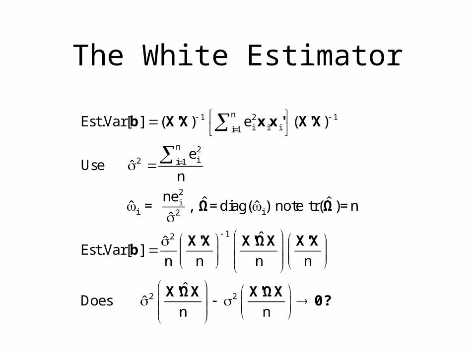
The White Estimator

n1 2 1i i ii 1

n 2i2 i 1

2i

i i2

12

2 2

Est.Var[ ] ( ) e ( )

eUse ˆ

nne ˆ ˆ = , =diag( ) note tr( )=nˆ ˆˆ

ˆˆEst.Var[ ]n n n n

ˆDoes ˆ

n n

b X'X x x' X'X

Ω Ω

X'X X'ΩX X'Xb

X'ΩX X'ΩX

0?

Newey-West Estimator

n 20 i i ii 1

L n

1 l t t l t t l t l tl 1 t l 1

l

Heteroscedasticity Component - Diagonal Elements

1e

nAutocorrelation Component - Off Diagonal Elements

1we e ( )

nl

w 1 = "Bartlett weight"L 1

1Est.Var[ ]=

n

S x x'

S x x x x

Xb

1 1

0 1[ ]n n

'X X'XS S

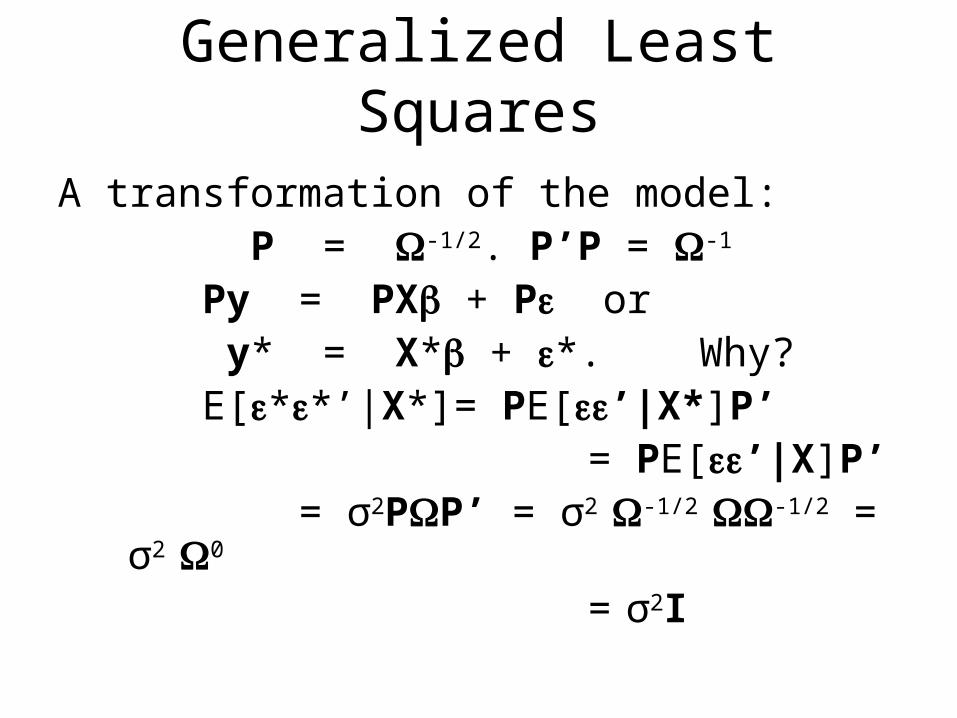
Generalized Least SquaresA transformation of the model: P = -1/2. P’P = -1

Py = PX + P or y* = X* + *. Why? E[**’|X*]= PE[’|X*]P’ = PE[’|X]P’ = σ2PP’ = σ2 -1/2 -1/2 = σ2 0

= σ2I

Generalized Least Squares

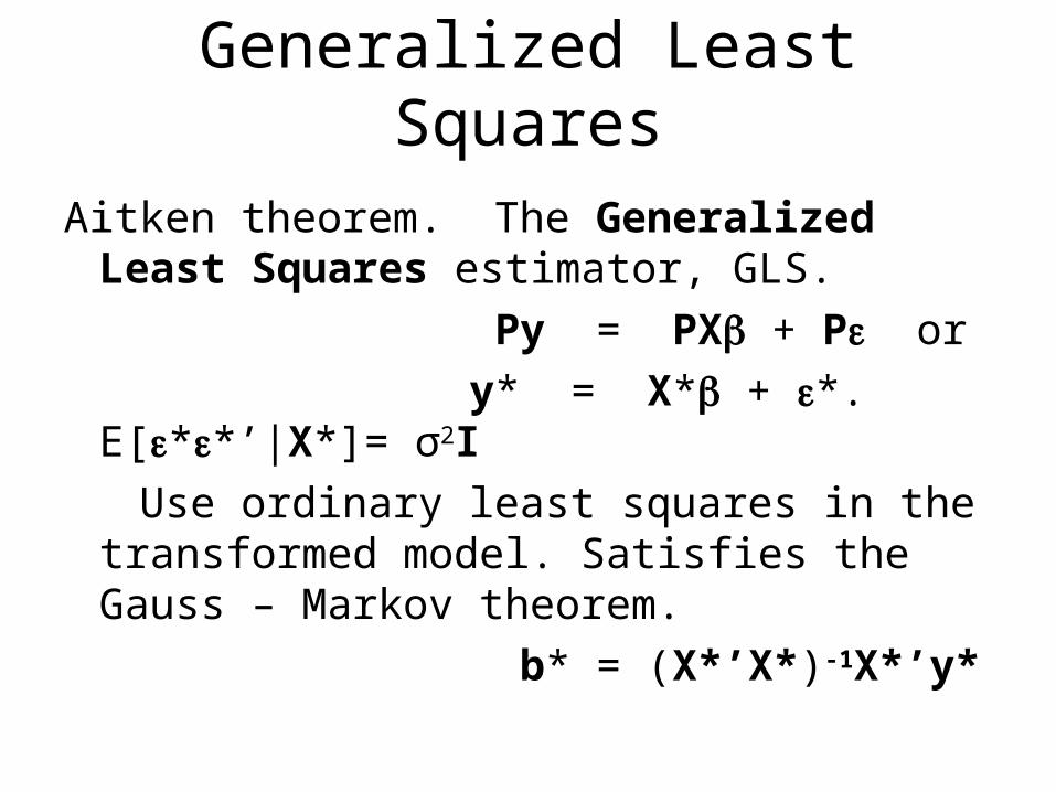
Aitken theorem. The Generalized Least Squares estimator, GLS.

Py = PX + P or

y* = X* + *. E[**’|X*]= σ2I

Use ordinary least squares in the transformed model. Satisfies the Gauss – Markov theorem.

b* = (X*’X*)-1X*’y*

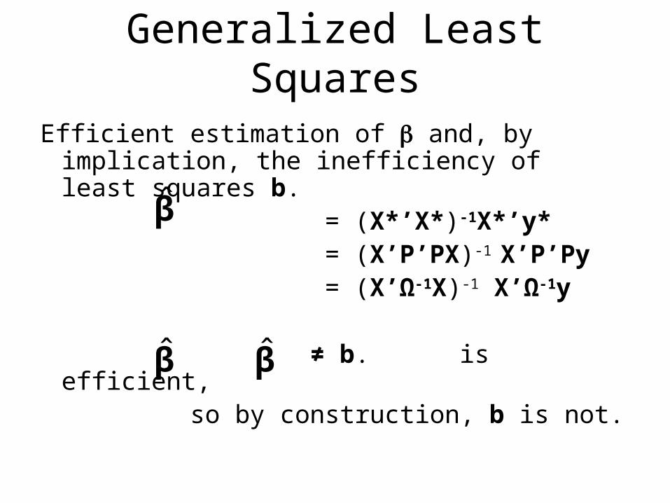
Generalized Least SquaresEfficient estimation of and, by implication,

the inefficiency of least squares b. = (X*’X*)-1X*’y* = (X’P’PX)-1 X’P’Py = (X’Ω-1X)-1 X’Ω-1y

≠ b. is efficient, so by construction, b is not.

β̂

β̂β̂

Asymptotics for GLS

Asymptotic distribution of GLS. (NOTE: We apply the full set of results of the classical model to the transformed model).

Unbiasedness

Consistency - “well behaved data”

Asymptotic distribution

Test statistics

Unbiasedness

1

1

1

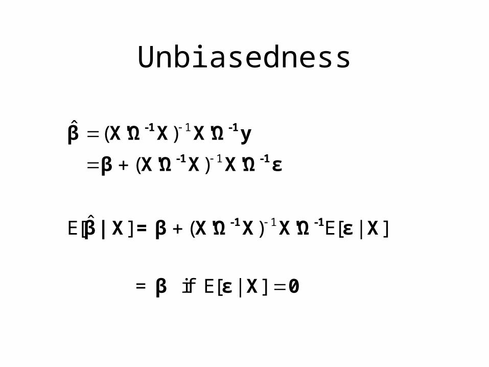
ˆ ( )

( )

ˆE[ ] ( ) E[ | ]

= if E[ | ]

-1 -1

-1 -1

-1 -1

β X'Ω X X'Ω y

β X'Ω X X'Ω ε

β| X =β X'Ω X X'Ω ε X

β ε X 0

Consistency

12

n

i ii 1ii

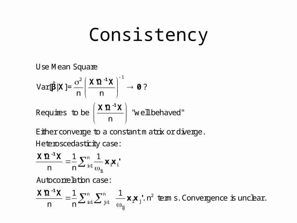
Use Mean Square

ˆVar[ | ]= ?n n

Requires to be "well behaved"n

Either converge to a constant matrix or diverge.

Heteroscedasticity case:

1 1n n

Autocorrelatio

-1

-1

-1

X'Ω Xβ X 0

X'Ω X

X'Ω Xx x'

n n 2i ji 1 j 1

ij

n case:

1 1. n terms. Convergence is unclear.

n n

-1X'Ω X

x x '

Asymptotic Normality

111

11

1

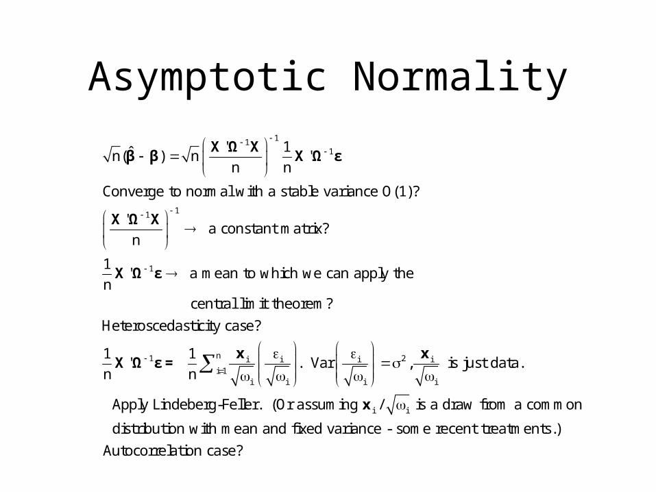
' 1ˆn( ) n 'n n

Converge to normal with a stable variance O(1)?

' a constant matrix?

n

1' a mean to which we can apply the

n central limit theorem?

Het

X Ω Xβ β X Ω ε

X Ω X

X Ω ε

n1 2i i i ii 1

i i i i

i i

eroscedasticity case?

1 1' . Var , is just data.

n n

Apply Lindeberg-Feller. (Or assuming / is a draw from a common

distribution with mean and fixed va

x xX Ω ε =

x

riance - some recent treatments.)

Autocorrelation case?

Asymptotic Normality (Cont.)

n n1i j i ii 1 j 1

1

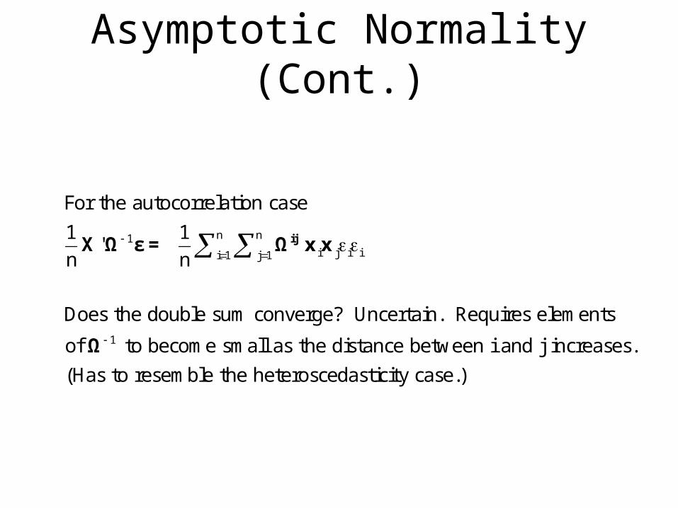
For the autocorrelation case

1 1'

n n

Does the double sum converge? Uncertain. Requires elements

of to become small as the distance between i and j increases.

(Has to resem

ijX Ω ε = Ω x x

Ω

ble the heteroscedasticity case.)

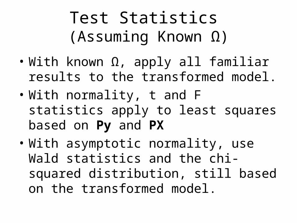
Test Statistics (Assuming Known Ω)

• With known Ω, apply all familiar results to the transformed model.

• With normality, t and F statistics apply to least squares based on Py and PX

• With asymptotic normality, use Wald statistics and the chi-squared distribution, still based on the transformed model.

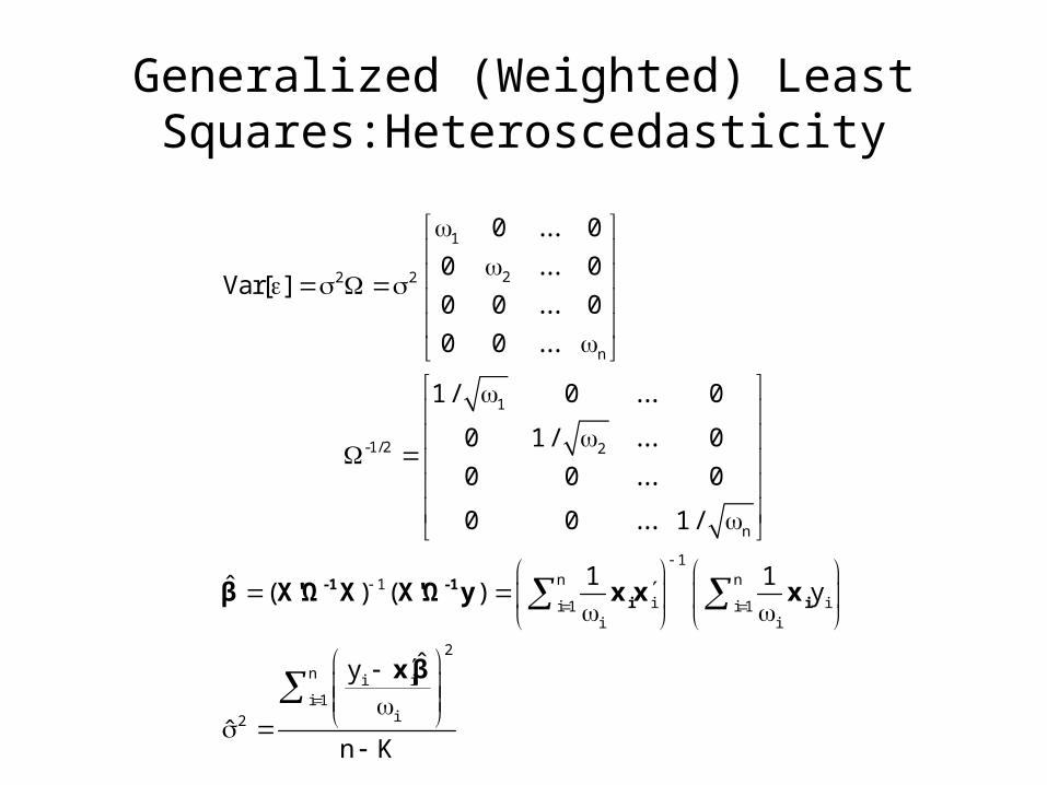
Generalized (Weighted) Least Squares:Heteroscedasticity

1

22 2

n

1

-1/2 2

n

1n n1

i ii 1 i 1i i

i i

i2

0 ... 0

0 ... 0Var[ ]

0 0 ... 0

0 0 ...

1/ 0 ... 0

0 1/ ... 0

0 0 ... 0

0 0 ... 1/

1 1ˆ ( ) ( ) y

ˆy

ˆ

-1 -1i iβ X'Ω X X'Ω y x x x

xβ2

n

i 1

n K

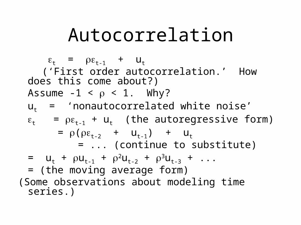
Autocorrelation t = t-1 + ut (‘First order autocorrelation.’ How does this come

about?) Assume -1 < < 1. Why?ut = ‘nonautocorrelated white noise’t = t-1 + ut (the autoregressive form) = (t-2 + ut-1) + ut

= ... (continue to substitute)= ut + ut-1 + 2ut-2 + 3ut-3 + ...= (the moving average form)

(Some observations about modeling time series.)

Autocorrelation

2t t t 1 t 1

it ii=0

22i 2 u

u 2i=0

t t 1 t t 1 t

2t t 1 t t 1 t

Var[ ] Var[u u u ...]

= Var u

=1

An easier way: Since Var[ ] Var[ ] and u

Var[ ] Var[ ] Var[u ] 2 Cov[ ,u ]

=

2 2t u

2u

2

Var[ ]

1

Autocovariances

t t 1 t 1 t t 1

t 1 t 1 t t 1

t-1 t

2u

2

t t 2 t 1 t t 2

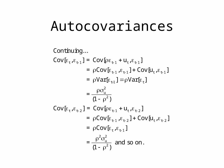
Continuing...

Cov[ , ] = Cov[ u , ]

= Cov[ , ] Cov[u , ]

= Var[ ] Var[ ]

=(1 )

Cov[ , ] = Cov[ u , ]

t 1 t 2 t t 2

t t 1

2 2u2

= Cov[ , ] Cov[u , ]

= Cov[ , ]

= and so on.(1 )

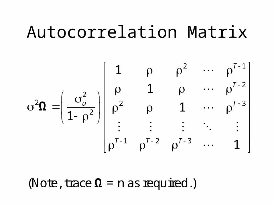
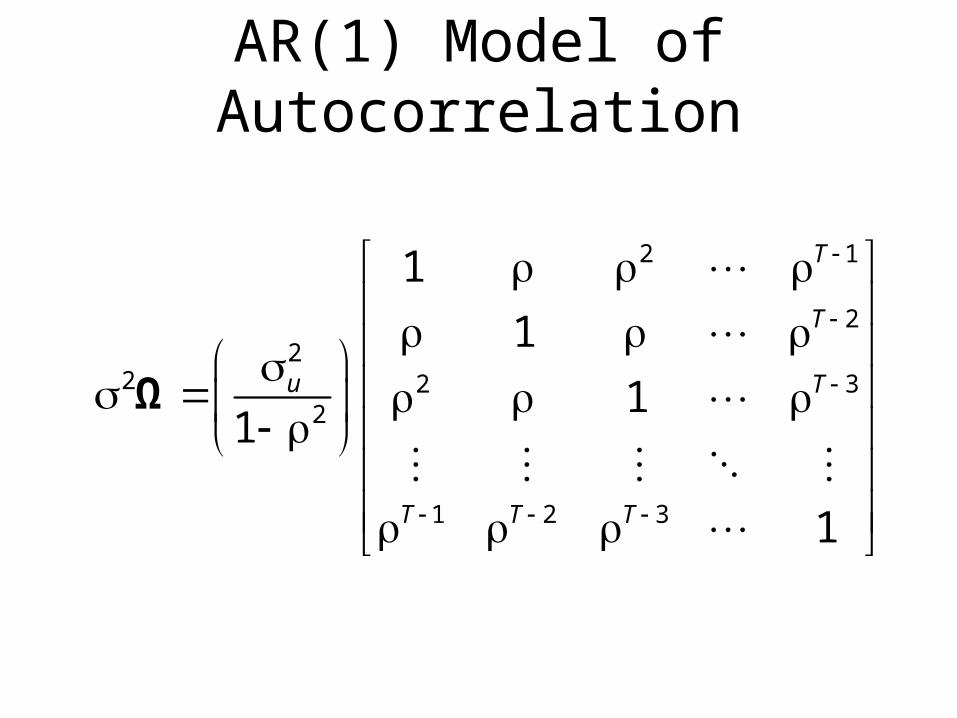
Autocorrelation Matrix

2 1

22

2 2 32

1 2 3

1

1

11

1

(Note, trace = n as required.)

Ω

Ω

T

T

u T

T T T

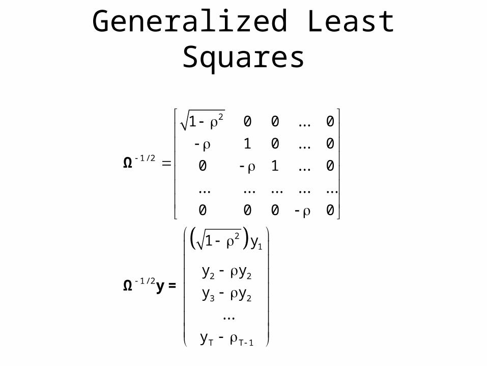
Generalized Least Squares

2

1/ 2

21

2 21/ 2

3 2

T T 1

1 0 0 ... 0

1 0 ... 0

0 1 ... 0

... ... ... ... ...

0 0 0 0

1 y

y y

y y

...

y

Ω

Ω y=

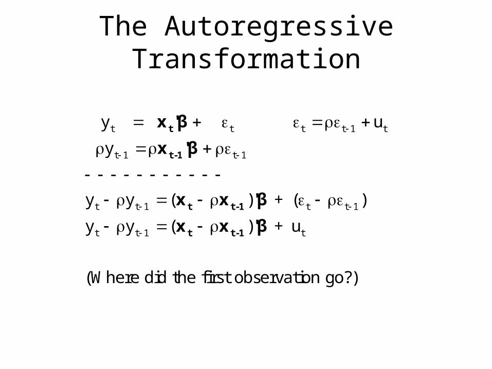
The Autoregressive Transformation

t t t t 1 t

t 1 t 1

t t 1 t t 1

t t 1 t

y u

y

y y ( ) + ( )

y y ( ) + u

(Where did the first observation go?)

t

t-1

t t-1

t t-1

x 'β

x 'β

x x 'β

x x 'β

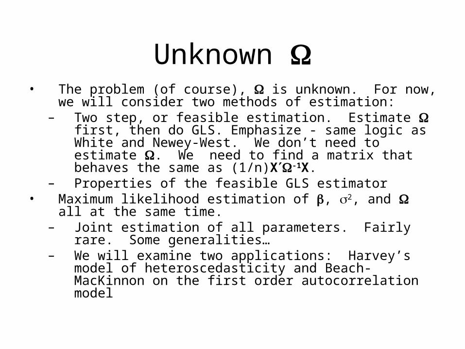
Unknown • The problem (of course), is unknown. For now, we

will consider two methods of estimation:– Two step, or feasible estimation. Estimate first,

then do GLS. Emphasize - same logic as White and Newey-West. We don’t need to estimate . We need to find a matrix that behaves the same as (1/n)X-1X.

– Properties of the feasible GLS estimator• Maximum likelihood estimation of , 2, and all at the

same time.– Joint estimation of all parameters. Fairly rare. Some

generalities…– We will examine two applications: Harvey’s model of

heteroscedasticity and Beach-MacKinnon on the first order autocorrelation model

Specification must be specified first.• A full unrestricted contains n(n+1)/2 - 1

parameters. (Why minus 1? Remember, tr() = n, so one element is determined.)

is generally specified in terms of a few parameters. Thus, = () for some small parameter vector . It becomes a question of estimating .

• Examples:

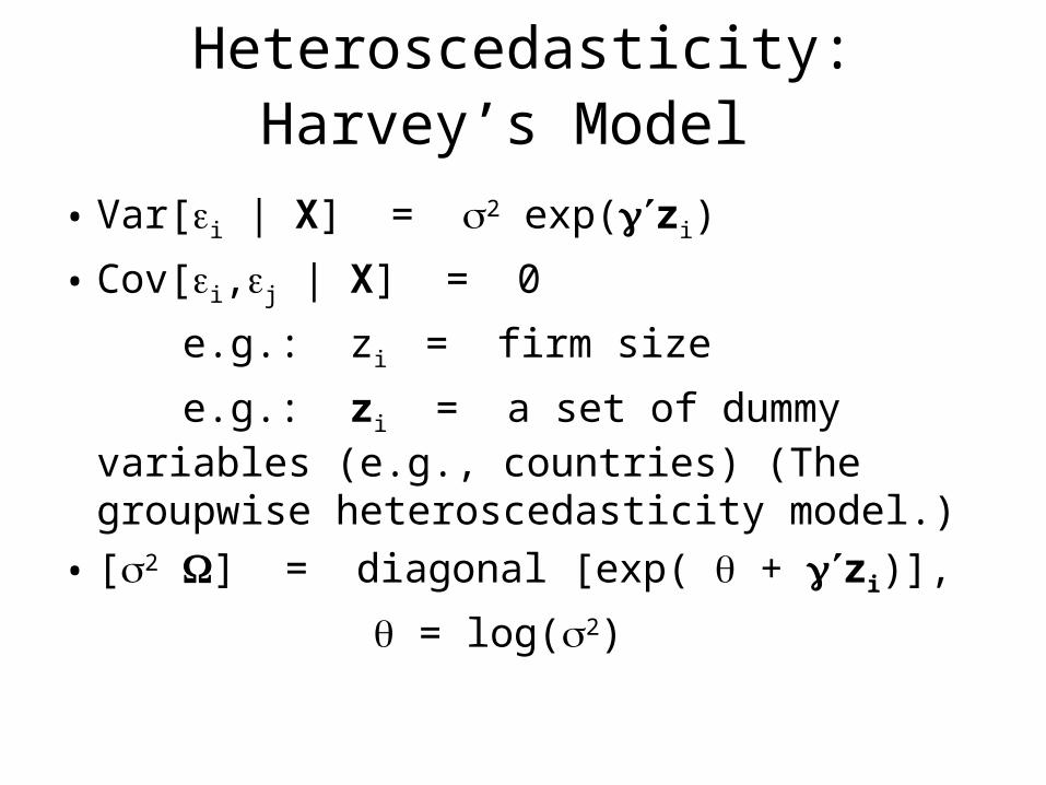
Heteroscedasticity: Harvey’s Model

• Var[i | X] = 2 exp(zi)

• Cov[i,j | X] = 0

e.g.: zi = firm size

e.g.: zi = a set of dummy variables (e.g., countries) (The groupwise heteroscedasticity model.)

• [2 ] = diagonal [exp( + zi)],

= log(2)

AR(1) Model of Autocorrelation

2 1

22

2 2 32

1 2 3

1

1

11

1

Ω

T

T

u T

T T T

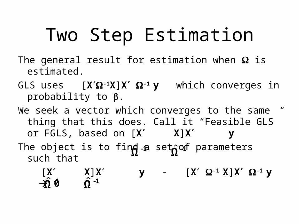
Two Step EstimationThe general result for estimation when is

estimated.

GLS uses [X-1X]X -1 y which converges in probability to .

We seek a vector which converges to the same thing that this does. Call it “Feasible GLS” or FGLS, based on [X X]X y

The object is to find a set of parameters such that

[X X]X y - [X -1 X]X -1 y 0

ˆ -1Ω ˆ -1Ω

ˆ -1Ω ˆ -1Ω

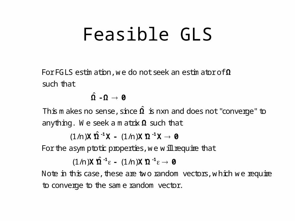
Feasible GLS

For FGLS estimation, we do not seek an estimator of

such that

ˆ

ˆThis makes no sense, since is nxn and does not "converge" to

anything. We seek a matrix such that

Ω

Ω- Ω 0

Ω

Ω

ˆ (1/n) (1/n)

For the asymptotic properties, we will require that

ˆ (1/n) (1/n)

Note in this case, these are two random vectors, which we require

to converge

-1 -1

-1 -1

X'Ω X - X'Ω X 0

X'Ω - X'Ω 0

to the same random vector.

Two Step FGLS

(Theorem 8.5) To achieve full efficiency, we do not need an efficient estimate of the parameters in , only a consistent one. Why?

Harvey’s ModelExamine Harvey’s model once again.

Methods of estimation:

Two step FGLS: Use the least squares residuals to estimate , then use

{X[Ω()]-1 X}-1X’[Ω()]-1y to estimate .

Full maximum likelihood estimation. Estimate all parameters simultaneously.

A handy result due to Oberhofer and Kmenta - the “zig-zag” approach.

Examine a model of groupwise heteroscedasticity.

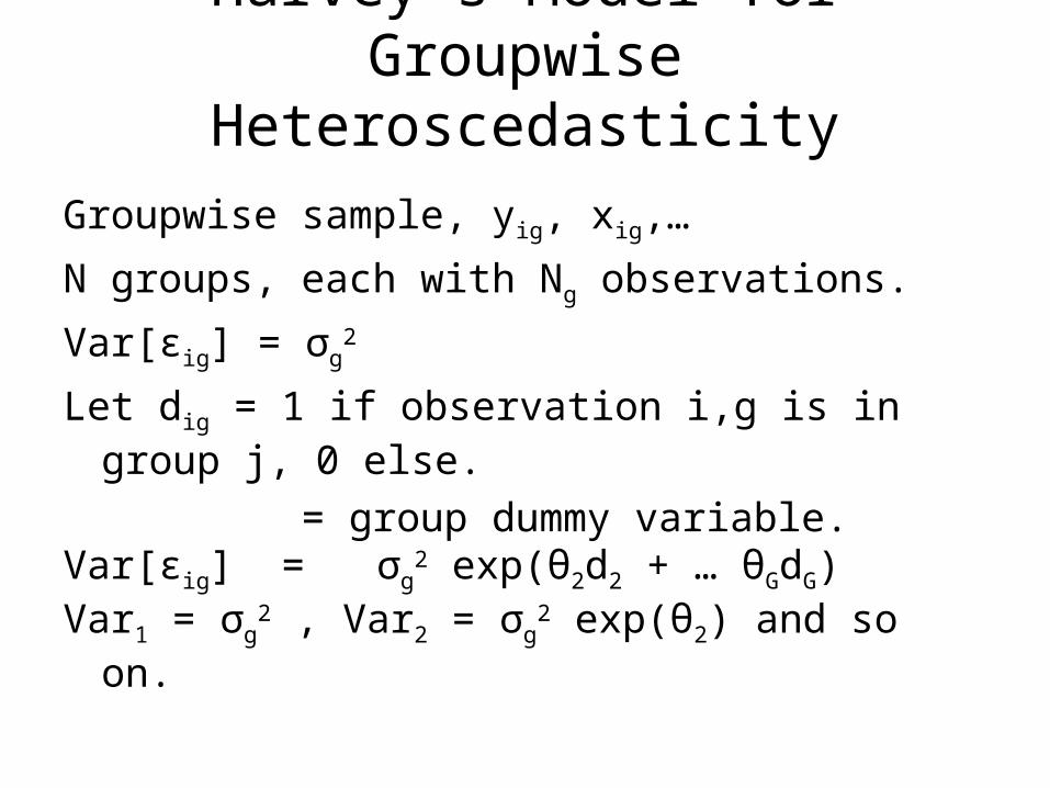
Harvey’s Model for Groupwise Heteroscedasticity

Groupwise sample, yig, xig,…

N groups, each with Ng observations.

Var[εig] = σg2

Let dig = 1 if observation i,g is in group j, 0 else.

= group dummy variable.Var[εig] = σg

2 exp(θ2d2 + … θGdG)Var1 = σg

2 , Var2 = σg2 exp(θ2) and so on.

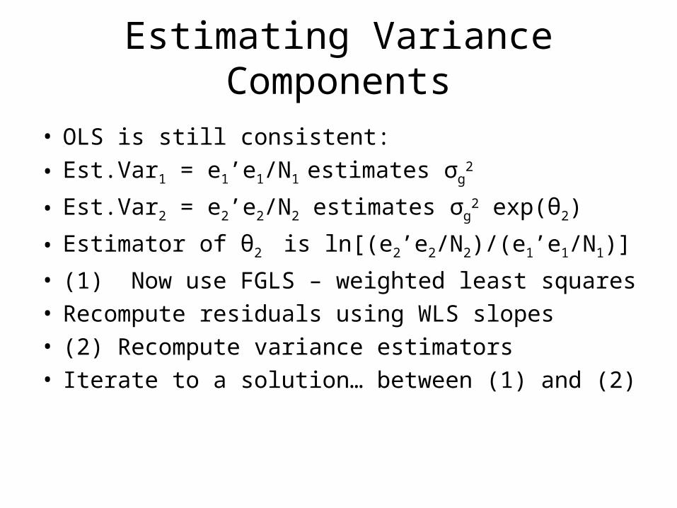
Estimating Variance Components

• OLS is still consistent:

• Est.Var1 = e1’e1/N1 estimates σg2

• Est.Var2 = e2’e2/N2 estimates σg2 exp(θ2)

• Estimator of θ2 is ln[(e2’e2/N2)/(e1’e1/N1)]

• (1) Now use FGLS – weighted least squares• Recompute residuals using WLS slopes• (2) Recompute variance estimators• Iterate to a solution… between (1) and (2)