GENERALIZED RECONFIGURABLE 6 - JOINT ROBOT MODELING A. M. Djuric aud W. H. ElMaraghy* Intelligent Manufacturing Systems (lMS) Centre, University of Windsor 401 Sunset Ave., Windsor, ON N9B 3P4, CANADA E-Mails:[email protected]@uwindsor.ca Received May 2006, Accepted December 2006 No. 06-CSME-22, E.I.C. Accession 2941 ABSTRACT Automated model generation and solution for motion planning and re-planning of robotic systems will play an important role in the future reconfigurable manufacturing systems. Solving the inverse kinematic problem has always been the key issue for computer-controlled robots. Considering the large amount of similarities that exist among the industrial 6R robotic systems, this work classifies them into two main types (puma-type and Fanuc-type) and then provides a unified geometric solution based on a unified kinematic structure called Generic Puma-Fanuc (GPF) model. A widespread study of different kinematic groups originating from eleven robot manufacturers made it possible to develop the GPF model that can be reconfigured according to the D-H rules (Denavit, and Hartenberg 1 ). A graphical interface by which the robot kinematic model is represented and the D-H parameters are auto-generated for use in solving the inverse kinematic problem. A generic solution module called Unified Kinematic Modeler and Solver (UKMS) implements the geometric approach for solving the inverse kinematic problem. The outcomes are then employed for robot control. Numerical examples are presented for exploring the solution capabilities of our unified approach. . Key words: Industrial 6R robots, Inverse kinematics, Reconfigurable model, Generic solution. MODELISATION RECONFIGURABLE ET GENERALISEE POUR LES SYSTEMES 6-R ROBOTISES RESUME La generation et la solution modeles automatise pour la planification de mouvement et re-planifiant de systemes robotises joueront un role important dans Ie reconfigurable futur les systemes industriels. Resoudre Ie probleme de cinematique inverse toujours a ete Ie probleme cle pour les robots commandes par ordinateur. Considerer la grande quantite de similarites qui existent parmi l'industriel 6R systemes robotises, ce travailles c1assifie dans deux types principaux (Ie Puma-Type et Ie Fanuc-Type) et fournit alors une solution geometrique unifiee a base une structure de cinematique unifiee Puma-Fanuc Generique appelee (GPF) Ie modele. Une etude repandue de structures de cinematique differentes provenant d'onze fabricants de robot l'a fait possible de developper Ie modele de GPF qui peut etre modifie la composition d'un ordinateur selon les regles de D-H (Denavit, et Hartenberg1). Une interface graphiquepar laquelle Ie modele de cinematique de robot est represente et les parametres de D-H sont auto-prodUits pour l'usage dans resoudre Ie probleme de cinematique inverse. Un module generique de solution a appele A Unifie Ie Modeliste de Cin6matiqueet Solver (UKMS) applique l'approche geometrique pour resoudre Ie probleme de cinematique inverse. Les issues sont alors employees pour Ie controle de robot. Les exemples numeriques sont· presentes pour explorer les capacites· de solution de notre approche unifiee. Mots cles: systemes 6-R robotises, cinematique inverse, modelisation reconfigurable, solution generique Transactions ofthe CSMElde la SCGM Vol. 30, No.4, 2006 533

Welcome message from author
This document is posted to help you gain knowledge. Please leave a comment to let me know what you think about it! Share it to your friends and learn new things together.
Transcript
GENERALIZED RECONFIGURABLE 6 - JOINT ROBOT MODELING
A. M. Djuric aud W. H. ElMaraghy*Intelligent Manufacturing Systems (lMS) Centre, University ofWindsor
401 Sunset Ave., Windsor, ON N9B 3P4, CANADAE-Mails:[email protected]@uwindsor.ca
Received May 2006, Accepted December 2006No. 06-CSME-22, E.I.C. Accession 2941
ABSTRACTAutomated model generation and solution for motion planning and re-planning of robotic systems willplay an important role in the future reconfigurable manufacturing systems. Solving the inverse kinematicproblem has always been the key issue for computer-controlled robots. Considering the large amount ofsimilarities that exist among the industrial 6R robotic systems, this work classifies them into two maintypes (puma-type and Fanuc-type) and then provides a unified geometric solution based on a unifiedkinematic structure called Generic Puma-Fanuc (GPF) model. A widespread study of different kinematicgroups originating from eleven robot manufacturers made it possible to develop the GPF model that canbe reconfigured according to the D-H rules (Denavit, and Hartenberg1
). A graphical interface by whichthe robot kinematic model is represented and the D-H parameters are auto-generated for use in solvingthe inverse kinematic problem. A generic solution module called Unified Kinematic Modeler and Solver(UKMS) implements the geometric approach for solving the inverse kinematic problem. The outcomesare then employed for robot control. Numerical examples are presented for exploring the solutioncapabilities of our unified approach. .Key words: Industrial 6R robots, Inverse kinematics, Reconfigurable model, Generic solution.
MODELISATION RECONFIGURABLE ET GENERALISEE POURLES SYSTEMES 6-R ROBOTISES
RESUMELa generation et la solution modeles automatise pour la planification de mouvement et re-planifiant desystemes robotises joueront un role important dans Ie reconfigurable futur les systemes industriels.Resoudre Ie probleme de cinematique inverse toujours a ete Ie probleme cle pour les robots commandespar ordinateur. Considerer la grande quantite de similarites qui existent parmi l'industriel 6R systemesrobotises, ce travailles c1assifie dans deux types principaux (Ie Puma-Type et Ie Fanuc-Type) et fournitalors une solution geometrique unifiee a base une structure de cinematique unifiee Puma-FanucGenerique appelee (GPF) Ie modele. Une etude repandue de structures de cinematique differentesprovenant d'onze fabricants de robot l'a fait possible de developper Ie modele de GPF qui peut etremodifie la composition d'un ordinateur selon les regles de D-H (Denavit, et Hartenberg1). Une interfacegraphiquepar laquelle Ie modele de cinematique de robot est represente et les parametres de D-H sontauto-prodUits pour l'usage dans resoudre Ie probleme de cinematique inverse. Un module generique desolution a appele A Unifie Ie Modeliste de Cin6matiqueet Solver (UKMS) applique l'approchegeometrique pour resoudre Ie probleme de cinematique inverse. Les issues sont alors employees pour Iecontrole de robot. Les exemples numeriques sont· presentes pour explorer les capacites· de solution denotre approche unifiee.Mots cles: systemes 6-R robotises, cinematique inverse, modelisation reconfigurable, solutiongenerique
Transactions ofthe CSMElde la SCGM Vol. 30, No.4, 2006 533
1. INTRODUCTION
Unified reconfigurable open control architecture, UROCA, is under development by ourresearch team for application to industrial robotic and CNC systems [2]. As UROCA isintended for controlling a wide variety of industrial machines, it has the feature of easyreconfiguration from one machine to another as well as from one application to another with thelowest amount of change. The UKMS represents one of the most· important modules thatUROCA counts on. This UKMS represents a forward step towards having a mobilereconfigurable architecture that accepts either new models or new applications without restoringourselves to rebuilding from scratch whenever software-, hardware-, control-, and physical-levelreconfigurations are needed. This UROCA architecture meets the requirements of portability,scalability, changeability and responsiveness of future reconfigurable manufacturing systems.
A generic, reconfigurable kinematic module was an important need for UROCA. Previousresearch investigations, for the sake of having several generic solutions, classified robotkinematic groups into groups according to their twist angles, which are fixed for each group [3].Accordingly, a different solution was provided for each group. This approach is truly away ofwhat we do in this work. The UKMS, unlike the others, accepts all the possible orientations foreach joint within the GPF model, and therefore, it discards any classification that is based onhaving fixed twist angles. Instead,the UKMS unifies the model and generalizes the solution forrobots of different twist angles rather than having different solutions for small groups of 6Rrobots with fixed twist angles.
There are different approaches for solving the inverse kinematic problem: algebraic, iterativeand geometric. Different investigators used the following methods: the screw algebra [6], theinverse transform [7], the dual matrices [8], the dual quaterian [9], the iterative method [10], andthe homogeneo.us matrix approach [11, 12]. [13] presented an analytical approach for the inversekinematic problem that requires solving a system of eight second-order equations in eightunknowns. A semi-analytical method for solving the inverse kinematics for Fanuc Arc MateSeries was presented by [14]. It is based on parameterised joint variables and analytical inversekinematic solutions, which were proposed for some classes of robots according to aclassification made by the authors. [15] have implemented the artificial neural-networkapproach for solving the inverse kinematics of one type of six-joints robots. The well-knownfixed-point iteration algorithm for solving a non-linear system of equations was applied by [16]for solving the inverse kinematic problem of 6R robots. [17-20] made a series of publicationsfor solving the inverse kinematics of 6R manipulators by applying iterative and one-dimensionalnumerical approaches.
The geometric approach for solving the inverse kinematic problem was applied for threejoint place-able robots with either rotational or translational joints by [21]. [22] extended thegeometric method for application to the seven-joints Space Station Remote Manipulator System(SSRMS). [23] have presented new four geometric invariants for the 6R manipulators in order toeliminate the joint variables in closure equations developed for solving this type of manipulator.These four invariants replace the Gaussian elimination process that was frequently used by otherresearchers. [24] implemented an evolutionary symbolic regression algorithm for approximatingthe inverse kinematic model of any generic 6R manipulators. [25] presented another paper thatconcerned the inverse kinematic approximation by using a fuzzy logic method tuned by a
Transactions o/the CSME/de la SCGM Vol. 30, No.4, 2006 534
genetic algorithm. A common deficiency in the above-mentioned methods occurs when oneattempts to select the most appropriate solution among all the possible ones. [27] used thegeometric approach for solving the inverse kinematics for robots with offset wrist. His workconcerned a group of robots, which does not belong to our GPF model for the moment. But theGPF model will be extended in future to include this type ofrobot.
In this paper, solving the inverse kinematic problem by using the GPF model, which has thefirst three joints rotating and the last three joints axes intersecting at a point, is performed by thegeometric approach [28]. This approach, as was more elaborated by [4] and [5], is generalizedfor application-to a wide class-of 6R industrial robots that faUs within the scope of ourOPFmodel. Some modifications and adjustments made to the geometric approach were necessary inorder to generalize it for application to the GPF model. In the first place, we have chosen toimplement this approach because it is much simpler than the other methods for application todifferent robotic systems having rotational joints. The resulting unified geometric-based solutioncan be used for any robotic manipulator that has a kinematic structure falling within the scope ofthe GPF structure. The main feature of this solution is that one can use the same equations,which include newly introduced configuration parameters, for solving a wide variety of 6Rkinematic groups in the GPF model.
Currently there is interest in research on the modeling and creation of reconfigurablesystems, modular robots and machines [29], [30], [31], [32], [33], [34]. This work is based onthe power of comparison between different robotic systems and the result of it is thedevelopment of reconfigurable parameters for solving their inverse kinematics. Future researchwill extend the unified approach to reconfigurable robots.
2. DEVELOPMENT OF THE GPF MODEL
As a preliminary step towards having theGPF model, we analyzed the kinematic structuresof 197 different industrial robots from 11 different manufacturers: ABB, Adept, Coinau, Fanuc,Kawasaki, Kuka, Motoman, Nachi, Panasonic, Staubli, and Daihen. The goal of this analysiswas to classify these robots into a Puma-like group, a Fanuc-like group, and a group of otherkinematic structures. The results are reported in Table 1. From this table, the most recognizable(in-common) feature is that 174 robots are of6-rotational joints with either Puma or Fanucgroups as depicted in Figures 1 and 2, respectively. While the most noticeable differencebetween the two groups of robots is in the direction ofjoint 3, which is reflected by having two
different values for the twist angleaz. This twist angle is a2 =00 for Puma group and
a2 =1800 for Fanuc group as indicated in Tables 2 and 3.The result that we obtained above is of great importance since the major part ·of the daily
used industrial robot has either six or five rotational joints with either Puma or Fanuc group.Among those robots there are too many communalities and one major difference (in thedirection of joint3) that would inhabit the generalization of any solution for these robots. Itfurther complicates the automation of any procedural inverse kinematic computations. In fact,this is the main issue in our work where the UKMS module merges the two kinematic groupsinto one GPF structure by using graphical and concurrent computational means. The GPF(Figure 3) contains all the possible link lengths and offsets that are different from zero except
Transactions ofthe CSMElde la SCGM Vol. 30, No.4, 2006 535
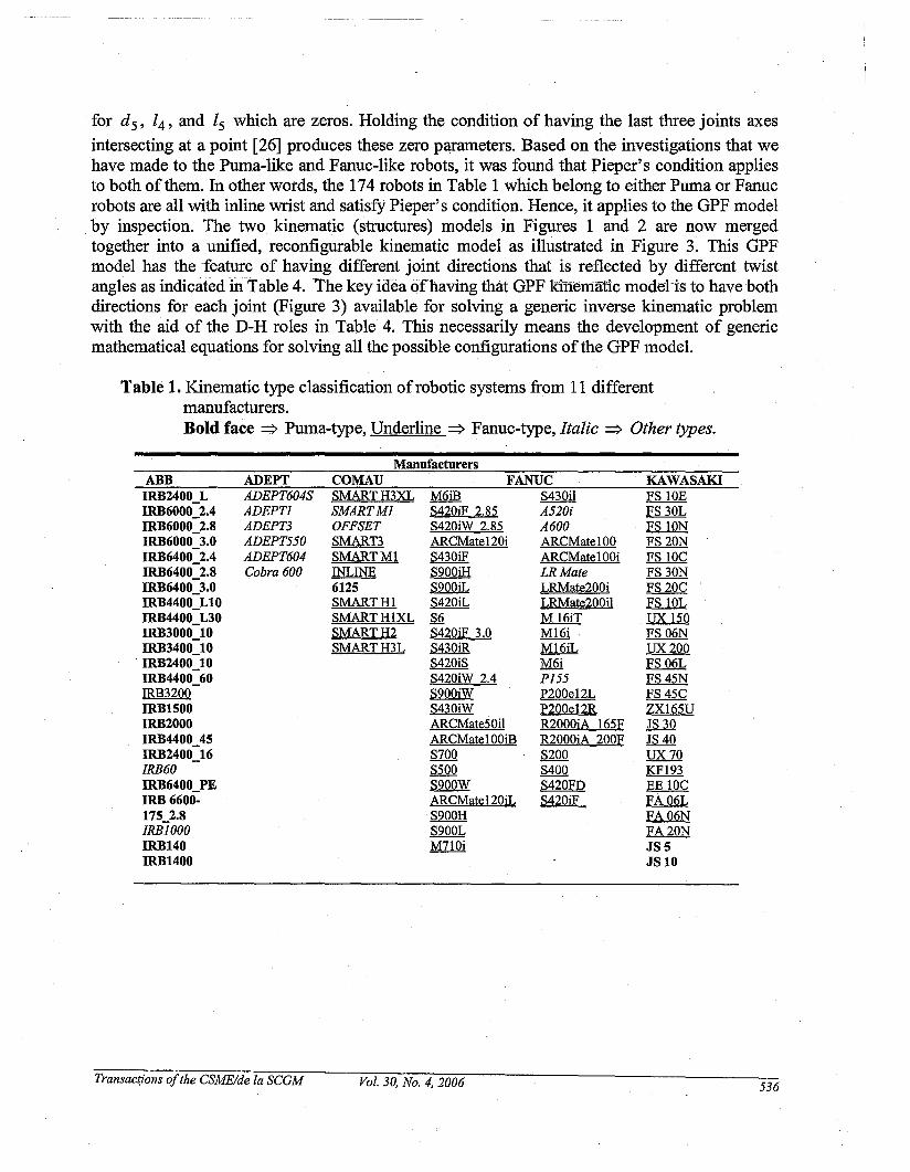
for dS' 14 , and Is which are zeros. Holding the condition of having the last three joints axesintersecting at a point [26] produces these zero parameters. Based on the investigations that wehave made to the Puma-like and Fanuc-like robots, it was found that Pieper's condition appliesto both of them. In other words, the 174 robots in Table 1 which belong to either Puma or Fanucrobots are all with inline wrist and satisfy Pieper's condition. Hence, it applies to the GPF modelby inspection. The two kinematic (structures) models in Figures 1 and 2 are now mergedtogether into a unified, reconfigurable kinematic model as illustrated in Figure 3. This GPFmodel has the feature of having different joint directions that is reflected by different twistangles as indicated iiltable 4. The key idea ()fhaving that GPF kinematic modelis to have-bothdirections for each joint (Figure 3) available for solving a generic inverse kinematic problemwith the aid of the D-H roles in Table 4. This necessarily means the development of genericmathematical equations for solving all the possible configurations of the GPF model.
Table 1. Kinematic type classification ofrobotic systems from 11 differentmanufacturers.Bold face => Puma-type, Underline => Fanuc-type, Italic => Other types.
ABB ADEPT COMAUManufacturers
FANUC KAWASAKIIRB2400_LIRB6000_2.4IRB6000_2.8IRB6000_3.0IRB6400-.!.4IRB6400_2.8IRB6400_3.0IRB4400_L10IRB4400_L30IRB3000_10IRB3400_10
. IRB2400_10IRB4400_60IRB3200IRB1500IRB2000IRB4400_45IRB2400 16IRB60 -IRB6400]EIRB 6600175_2.8IRBIOOOIRB140IRB1400
ADEPT604SADEPTIADEPT3ADEPT550ADEPT604Cobra 600
SMARTH3XLSMARTMIOFFSETSMART3SMARTMIINLINE6125SMART HISMART HIXLSMARTH2SMARTH3L
M6iBS420iF 2.8SS420iW 2.8SARCMate120iS430iFS900iHS900iLS420iLS6S420iF 3.0S430iRS420iSS420iW 2.4S900iWS430iWARCMateSOilARCMatelOOiBS700SSOOS900WARCMate120iLS900HS900LM710i
S430ilA520iA600ARCMatelOOARCMatelOOiLRMateLRMate200iLRMate200ilM 16iTM16iM16iLM6iPI55P200e12LP200e12RR2000iA 16SFR2000iA 200FS200S400S420FDS420iF
FS lOEFS30LFS IONFS20NFS lOCFS30NFS20CFS 10LUX ISOFS06NUX200FS06LFS4SNFS4SCZX16SUJS 30JS40UX70~EE lOCFA06LFA06NFA20NJS5JS 10
Transac(ions ofthe CSME/de la SCGM Vol. 30, No.4, 2006 536

Table 1. (Continued).
ManufacturersKUKA MOTOMAN NACHI PANASONIC STAUBLIKR 150-2KR200-2KR l50L120-2KR30L15-2KR l50L150-2KR6-2KR2_00L120-2KR15-2KR30-2KR45-2KR 200L150-2KR125L90-3KR15L6-2KR125_2KR 350L280-2KR150KKR150LllOKKR150L130KKR125-2KR125-3KR l25LlOO-2KR125L90-2
III
dl II.. ;F;
K30SSK16-6SV3XLUP165-100UP6RK3SSV3XK60CSHSK45-30SK6UP6SK120-80SV3SV16-640K120SSK120-75SV16-650UP50UP20SK45SK120-150SK16
SK120UP200UP6-CUP20MSK150UP130SK16MuP165SV3CRK30SH.KlOORSHKlOOSKlOMKlOS
d
SF200SF133SC35FSC80LFSC300FSC06FSC120FSC120LFSC15FSF133TSF200T
VR120VR032VR016VR008LVR004VR006VR006LVR008
zs•••·l1s~......··· aTn
Y2
RX90LRX90RX130LRX60RX60LPuma560Puma76l
an
Figure 1. Generic Puma kinematic model. Figure 2. Generic Fanuc kinematic model.
Transactions ofthe CSME/de la SCGM Vol. 30, No.4, 2006 537

Table 2. D-H parameters for Puma-like Table 3. D-H parameters for Fanuc-likekinematic model. kinematic model.
Joint (Ji d i Ii ai Joint ()i di Ii ai
1 ()1 d1 II -90 1 ()1 d1 II -902 ()2 d2 12 0 2 ()2 d2 12 1803 ()3 d3 13 90 3 ()3 d3 13 904 ()4 d4 0 -90 4 ()4 d4 0 -905 ()s 0 0 90 5 ()s 0 0 906 ()6 d6 16 ± 180; 0 6 ()6 d6 16 ± 180; 0
Zs a n
r5t s
..........~:~ a
n
Figure 3. GPF kinematic model.
Table 4. D-H parameters for the GPF model.
Joint12
3456
±90± 180; 0
±90±90±90
± 180; 0
Transactions ofthe CSME/de la SCGM Vol. 30, No.4, 2006 538

The GPF model can be reconfigured from one kinematic group to another or from oneapplication to another by using configuration parameters K 1 ,K2 ,K3 , K 4 , K s, and K 6 as ..defined in equation (1):
K l =sinab K 2 =cosa2' K3 = sina3,
. K4 = sina4' K s =sinas, K6 =cos a 6' (1)
These -parameters·· are used todetennine the signs in the. joints equations, of the differentrobot configurations by calculating sine and cosine of the twist angles which are different for allthe robots that belong to the two main kinematic groups (puma and Fanuc) in the GPF model asshown in Table 4. Except for K 2, all the other parameters (K1 ,K3 ,K4 ,Ks , K 6) are used for
configuring all the Puma and Fanuc groups in the GPF model. K 2 totally switches the modeling
process from Puma type to Fanuc type and vice versa within the GPF model. K l controls the
direction ofjoint 1 relative to joint 2 by controlling the sign of their twist angle al as shown in
Figure 4. Thus, one can say that K 1 provides eight different combinations ofjoints 1 and 2
orientations by having two different values for their embraced twist angle. Note here that al is
one of the important D-H parameters. Similarly, the other configuration parametersK3 ,K4 ,Ks,and K6 controls the relative directions between the joints (3,4), (4,5), (5,6), and (6, flange),
respectively. This is possible by lettingK3 ,K4 ,Ks, and K 6 control the signs of the twist
angles a3' a4' as, and a6' respectively.
. zl Xl
x~~~& ~tXlXo 0 YI XO Yo Zl Xl
lal =-90°F+!K1 =-11 lat=+90o~Kl =+11Zl
~~B T~ oJ)()1 .:2 ...B2
Zo YI I . zl Y zO· B2~~zl Xl
lat =+90oJ.e+IKl =+11 lal =-90°r+tKl =-11
Figure 4. Eight combinations for joints 1 and 2 controlled by the configuration parameter K l .
Transactions ofthe CSME/de la SCGM Vol. 30, No.4, 2006 539
Once the GPF kinematic model is established as in Figure 3, we need to solve the kinematicsproblem which consists of two subproblems: (i) the direct kinematic problem and (ii) the inversekinematic problem. The direct kinematics problem is to find the position and orientation of therobot's end effector relative to the base coordinate frame for a given set of joint angles. Theinverse kinematic problem is to calculate the robot's joint angles for a given position andorientation of the robot's end effector. We will devote the rest of this work for a geometricbased generic inverse kinematic solution for all the possible configurations of the GPF model.
3. A UNIFIED GEOMETRIC-BASED SOLUTION
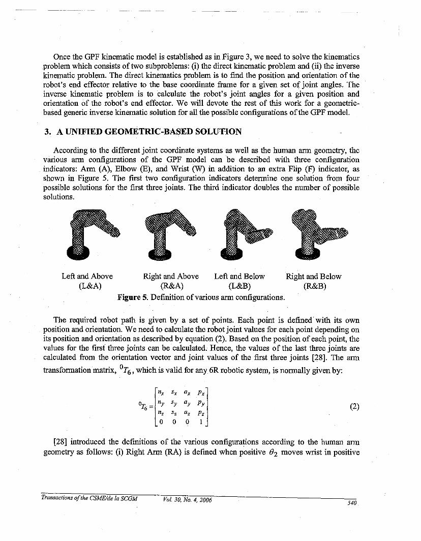
According to the different joint coordinate systems as well as the human arm geometry, thevarious arm configurations of the GPF model can be described with three configurationindicators: Arm (A), Elbow (E), and Wrist (W) in addition to an extra Flip (F) indicator, asshown in Figure 5. The first two configuration indicators determine one solution from fourpossible solutions for the first three joints. The third indicator doubles the number of possiblesolutions.
Left and Above(L&A)
Right and Above Left and Below(R&A) (L&B)
Figure 5. Definition ofvarious arm configurations.
Right and Below(R&B)
The required robot path is given by a set of points. Each point is defined' with its ownposition and orientation. We need to calculate the robot joint values for each point depending onits position and orientation as described by equation (2). Based on the position of each point, thevalues for the first three joints can be calculated. Hence, the values of the last three joints arecalculated from the orientation vector and joint values of the first three joints [28]. The arm
transformation matrix, °T6 , which is valid for any 6R robotic system, is normally given by:
(2)
[28] introduced the definitions of the various configura~ons according to the human armgeometry as follows: (i) Right Arm (RA) is defined when positive fh moves wrist in positive
Transactions ofthe CSME/de la SCGM Vol. 30, No.4, 2006540
zo direction, while 83 is not active, (ii) Left Ann (LA) is defined when positive 82 moves
wrist in negative zo direction while 83 is not active, (iii) Above Ann (AA) (elbow above wrist)
is defmed when the position of the wrist of th~ Right/Left Arm with respect to the shouldercoordinate system has negative/positive coordinate value along the Y2 axis, (iv) Below Ann(BA) (elbow below wrist) is defined when the position of the wrist.ofthe Right/Left Arm withrespect to the shoulder coordinate system has positive/negative coordinate value along the Y2
axis, (v) Wrist Down (WD) is defined when the s unit vector ofthe hand coordinate system andthe Ys unitvector of the (xs, Ys, zs)coordinate system have a positive dot product, s· Ys > 0,
and (vi) Wrist Up (WU) is defined when the $ unit vector of the hand coordinate system and theYs unit vector of the (xs, Ys, zs) coordinate system have a negative dot product, s· Ys < O.
The forth indicator is introduced as a Flip (F) indicator or Do not Flip (DF) indicator.According to the previous definitions of the robot configurations we have the following basic
definitions:
A={+1, RA}, E={+1, AA}-1, LA -1, BA
W={+ 1, D}, F={+ 1, F}.-1, U -1, DF
(3,4)
(5,6)
The user must specify the signed values of the indicators in equations (3)-(5) to be able tofmd the inverse kinematics solution. These indicators can be calculated from the values of thejoint angles of the robot. The equations for calculating these indicators are:
(8)
(9)
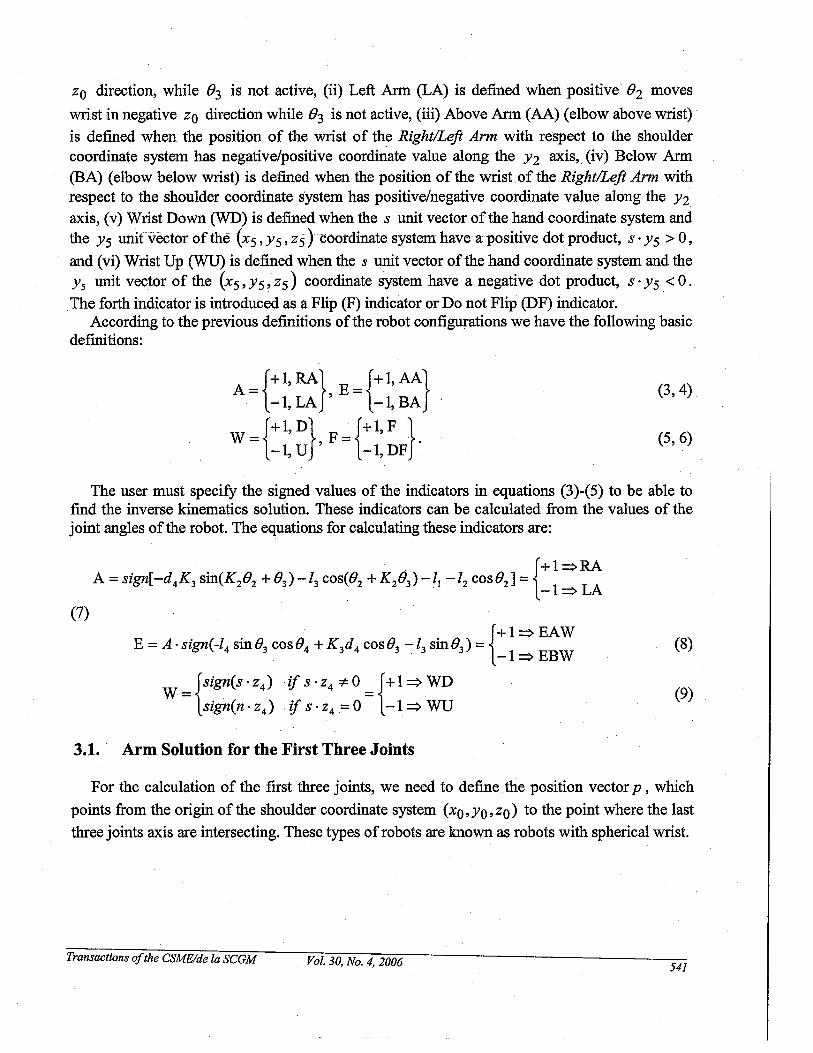
3.1. Arm Solution for the First Three Joints
For the calculation of the first three joints, we need to define the position vector p, which
points from the origin of the shoulder coordinate system (xo,Yo,zo) to the point where the last
three joints axis are intersecting. These types of robots are known as robots with spherical wrist.
Transactions ofthe CSME/de la SCGM Vol. 30, No.4, 2006 541

...............-.--.. ..... ~ ...p ..+ ~.... ... ...-' ...
• + --".... ..--.+ .", """
••+ .", P6.+ ,.".. ..... ...••..:- fill'
Figure 6, Position vectorp for spherical wrist robots.
From Figure 6, we calculate the position vector p = P6 - (d6a +16n) = (Px' Py, pz)T, which
corresponds to the position vectoroT4. It can be calculated from the right hand side of equation(10):
[
Px] [COS III [d4K, sin(K,II, + 11,).+ 13cos(B2 + K,II,) + II + I, co,II,] +.K1(d2 + K2d3)SinB1]Py = smB1[d4K3 sm(K2B2 +B3)+13cos(B2 +K2B3)+11 +12 cosB2]-K1(d2 +K2d3)cosBlpz -d4KIK3cos(K2B2 +B3)+13K1sin(B2 +K2B3)+12KlsinB2 +d1
3.1.1. Solution for Joint 1
(10)
To calculate the angle B1 ofjoint 1, we need to have the projections of the position vector P
onto the xoYo plane as depicted in Figures 7 and 8. For the two values of the A configurations
we have two different solutions forB1: el as shown in Figure 7 and B1R as shown in Figure 8.
According to the similarities and differences that exist between the Puma and Fanuc kinematicgroups within the GPF modyl, we developed the equations for calculating B1. Strictly speaking,the main difference between Puma-like and Fanuc-like kinematic groups is that directions ofJoints 2 and 3 are the same for Puma type and opposite to each other for Fanuc type. When thejoints are in the same directions it means that their rotational vectors are equal, zl = Z2' and for
the opposite direction they have opposite sign, zl = -z2.
Transactions ofthe CSMElde la SCGM Vol. 30, No.4, 2006 542

Yo
.j"~
"
Figure 7. LA projections of the positionvector p onto the XoYo plane.
Figure 8. RA projections of the position vectorp onto the xoYo plane.
From Figure 7, equations for calculating the angle OIL can be derived. To calculate the
distance OA in Figure 7 as in equation (13), we use the configuration parameter K 2 (which
controls the sign of d3 ) as previously introduced in equation (1):
, BtL = ¢ - qJ
. OA AB. '" Py Pxsmcp=-, coscp=-, smlf' =-, COSrjJ =-.R R R R
OA=d2 +K2d3, OB=R=~P;+p;,----'-----.,.----
AB=r=~R2-0A2=~p;+p;-(d2+K2d3)2
. eL '. ('" ) pyr-px(d2 +K2d3)sm 1 =sm If'-rp = R2
L Pxr +p y(d2 +K2d3 )COS 01 =COS(rjJ - rp) = 2
R
(11)
(12)
(13)
(14)
(15)
(16)
Now we solve for Of. From Figure 8, we obtained the following equations for the angle
ot·
Combining equations (11) - (17), we obtain the sine and cosine functions of Of :
(17)
Transactions ofthe CSMElde la SCGM Vol. 30, No.4, 2006 ·543

(18)
(19)
Combining the solutions for the LA, O{, and the RA, of, we obtain solution for 01 as
expressed below:
(20)
3.1.2. Solution for Joint 2
To calculate the angle O2 of joint 2, the projections of the position vector p onto the x1Y1
plane should be defined as shown in Figures 9 and 10. From Figure 9, the equations forcalculating the joint angle O2 can be easily deduced as follows:
r=AE=~BEZ _ABz =~(px -11 cosBI)Z +(py -11 sinBI)Z -(dz + K zd3 )Z
R=AD=~rZ +DEZ =~(px -11 cosBI)Z +(py -11 sinBI)Z -(dz + Kzd3 )Z +(Pz -ldII)Z
AF=lzFe=13
(21)
(22)
(23)
(24)
XoFigure 9. Projections of the position vector
p onto the XtYt plane.
E
D
IUft & Above Irp-fJ
Figure 10. Four combinations ofA and E
configurations for joint 2 solution.
Transactions ofthe CSME/de la SCGM Vol. 30, No.4, 2006 544
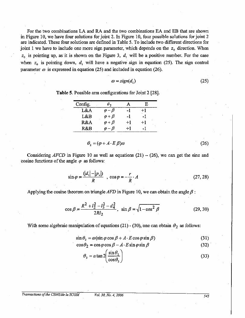
For the two combinations LA and RA and the two combinations EA and EE that are shownin Figure 10, we have four solutions for joint 2. In Figure 10, four possible solutions for joint 2are indicated. These four solutions are defined in Table 5. To include two different directions forjoint 1 we have to include one more sign parameter, 'which depends on the Zo direction. When
Zo is pointing up, as it is shown on the Figure 3, d1 will be a positive number. For the case
when Zo is pointing down, d1 will have a negative sign in equation (25). The sign control
parameter 01 is expressed in equation (25) and included in equation (26).
(25)
Table 5. Possible arm configurations for Joint 2 [28].
Config.L&AL&BR&AR&B
rp-fJrp+/3rp+ /3rp-/3
A-1-1+1+1
E+1-1
+1-1
B2 =(rp + A .E {3)01 (26)
Considering AFCD in Figure 10 as well as equations (21) - (26), we can get the sine andcosine functions of the angle rp as follows:
. (ldll-IPzl) rSln m = cos m = --·A
r R ' r R (27,28)
Applying the cosine theorem on triangle AFD in Figure 10, we can obtain the angle fJ :
R2 +z2 _Z2 _d2 ,,----cos fJ ;:::: 2 3. 4, sin {3 = 'V1-cos2 fJ
2RZ2(29,30)
With some algebraic manipulation ofequations (21) - (30), one can obtain B2 as follows:
sin B2 =01(sin rp cos fJ + A .E cos rp sin fJ)
cosB2 = cosrpcos fJ - A· EsinrpsinfJ
(sinB )B2 = atan2--2cosB2
(31)
(32)
(33)
Transactions ofthe CSME/de la SCGM Vol. 30, No.4, 2006 545

3.1.3. Solution for Joint 3
The calculation of the angle 83 (between the axes x2 andx3) for joint 3 requires projecting
the position vector p onto the x2Y2 plane as shown in Figures 11 and 12.
C D
D
A
••••• X2- .... .- _....... .t.- - - '*. x2D
X3Y2
Figure 11. Joint 3 angle for Puma group.group.
Figure 12. Joint 3 angle for Fanuc
For Puma and Fanuc kinematic groups the angle 83 is, respectively, given by:
83 =¢ - fJ
83 = 3600 -(¢ - fJ)
(34)
(35)
From Figures 11 and 12 we can see that the x2Y2 coordinate system for the Puma group isdifferent from the Fanuc one. The difference between the two groups is imparted by thedifference in the directions of joint 2 and joint 3 with respect to each other. The directions ofthese two joints are the same for the Puma type and they oppose each other for the Fanuc type.This fact is clearly described in Tables 6 and 7. As we discussed above, this difference can behandled with the control parameter K 2 . Considering AFCD in Figures 11 and 12, we can
calculate the angle f3 as follows:
(36)
(37)
Applying the cosine theorem to the triangle AFD in Figure 10 or Figure 11, we can calculatethe angle ¢ as follows:
Transactions ofthe CSME/de la SCGM Vol. 30, No.4, 2006 546
< •
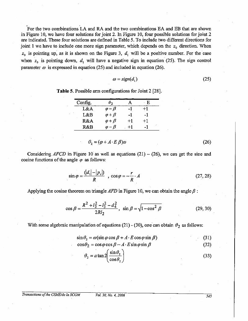
For the two combinations LA and RA and the two combinations EA and EB that are shownin Figure 10, we have four solutions for joint 2. In Figure 10, four possible solutions for joint 2are indicated. These four solutions are defmed in Table 5. To include two different directions forjoint 1 we have to include one more sign parameter, which depends on the Zo direction. When
Zo is pointing up, as it is shown on the Figure 3, d1 will be a positive number. For the case
when Zo is pointing down, d1 will have a negative sign in equation (25). The sign control
parameter OJ is expressed in equation (25) and included in equation (26).
(25)
Table 5. Possible arm configurations for Joint 2 [28].
Config. ()2 A EL&A rp-fJ -1 +1L&B rp+fJ -1 -1R&A rp+/3 +1 +1R&B rp-fJ +1 -1
82 =(rp+A·E I3)OJ (26)
Considering APeD in Figure 10· as well as equations (21) - (26), we can get the sine andcosine functions of the angle rp as follows:
. (ldll-IPzl) rSln m = cos m = --·A
't' R ' 't' R (27,28)
Applying the cosine theorem on triangle AFD in Figure 10, we can obtain the angle 13 :
(29,30)
With some algebraic manipulation of equations (21) - (30), one can obtain 82 as follows:
sin 82 = m(sin rp cos f3 + A .E cos rp sin 13)cos82 = cos rp cos 13 - A· E sin rp sin 13
8 (Sin82 J2 = a tan 2 _-=:...cos82
(31)
(32)
(33)
Transactions ofthe CSME/de la SCGM Vol. 30, No.4, 2006 545

3.1.3. Solution for Joint 3
The calculation of the angle 83 (between the axes x2 andx3) for joint 3 requires projecting
the position vector p onto the x2Y2 plane as shown in Figures 11 and 12.
A
c
Y2
D
•••• x••• •• 2-- ... ~.- - -~'*'D
Y2
D
Figure 11. Joint 3 angle for Puma group.group.
Figure 12. Joint 3 angle for Fanuc
For Puma and Fanuc kinematic groups the angle 83 is, respectively, given by:
83 =¢ - f3
83 =360° -(¢-fJ)
(34)
(35)
From Figures 11 and 12 we can see that the x2Y2 coordinate system for the Puma group isdifferent from the Fanuc one. The difference between the two groups is imparted by thedifference in the directions of joint 2 and joint 3 with respect to each other. The directions ofthese two joints are the same for the Puma type and they oppose each other for the Fanuc type.This fact is clearly described in Tables 6 and 7. As we discussed above, this difference can behandled with the control parameter K2' Considering AFCD in Figures 11 and 12, we can
calculate the angle fJ as follows:
(36)
(37)
Applying the cosine theorem to the triangle AFD in Figure 10 or Figure 11, we can calculate
the angle ¢ as follows:
Transactions ofthe CSME/de la SCGM Vol. 30, No. 4,2006 546
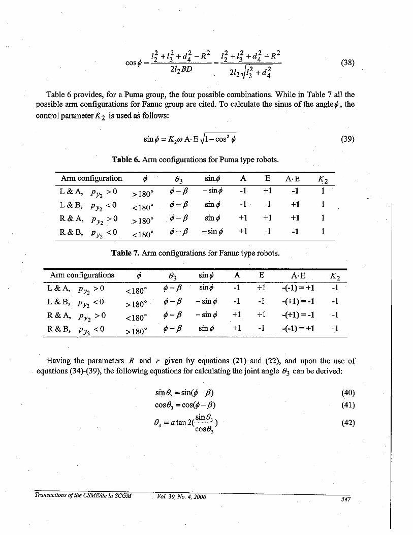
(38)
Table 6 provides, for a Puma group, the four possible combinations. While in Table 7 all thepossible arm configurations for Fanuc group are cited. To calculate the sinus of the angle ¢ , the
control parameter K 2 is used as follows:
sin¢ = K2aJA.E~I-cos2 ¢ (39)
Table 6. Arm configurations for Puma type robots.
Arm configuration ¢ 03 sin¢ A E A·E ~2
L&A, PY2 >0 >1800 ¢-p -sin¢ -1 +1 -1 1
L&B, PY2 <0 <1800 ¢-p sin¢ -1 . -1 +1 1
R&A, PY2 >0 >1800 ¢-p sin¢ +1 +1 +1 1
R&B, PY2 <0 <1800 ¢-p -sin¢ +1 -1 -1 1
Table 7. Arm configurations for Fanuc type robots.
Arm configurations ¢ 03 sin¢ A E A·E K 2
L&A, PY2 >0 <1800 ¢-p sin¢ -1 +1 -(-1) = +1 -1
L&B, PY2 <0 >1800 ¢-p -sin¢ -1 -1 -(+1) =-1 -1
R&A, Pyz >0 <1800 ¢-p -sin¢ +1 +1 -(+1) =-1 -1
R&B, FY2 <0 >1800 ¢-p sin¢ +1 -1 -(-1) = +1 -,1
Having the parameters R and r given by equations (21) and (22), and upon the use of, equations (34)-(39), the following equations for calculating the joint angle 03 can be derived:
Transactions ofthe CSME/de la SCGM
sin03 = sin(¢- P)cosB3 =cos(¢- P)
sinO03
= a tan 2(__3 )
cos03
Vol. 30, No.4, 2006
(40)
(41)
(42)
547

3.2. Arm Solution for the Last Three Joints
The solution ofthe last three joints for the GPF model can be acquired from the joint values
of the first three joints (i.e., calculation of matrix °T3) and by setting these joints to meet the
following criterion [28].
(43)
a=±zs, a=(ax,ay,az)T
s=Y6, s=(sx,Sy,sz)T, where n=(nx,ny,nz)T
(44)
(45)
The condition in equation (43) is used to set joint 4 such that a rotation about joint 5 will alignthe coordinate system ofjoint 6 with approach vector a. If the vector cross product from equation(43) is zero, it will create the degenerate case. This problem appears when joint 4 and joint 6 areparallel. Second condition in equation (44) set joint 5 to align the coordinate system of joint 6with approach vector. Equation (45) is used to align the axis of joint 6 with the sliding andnormal vectors.
3.2.1. Solution for Joint 4
The orientations for the wrist are given in equation (9) and shown in Table 8. The sign of thevector Z4 is defined with Q that is described by the orientation of either n or s unit vector with
respect to Ys unit vector. More details are given by [28].
Table 8. Various orientations for the wrist.
Wrist orientation Q= s· Ys or n· Ys W
D ~O +1D <0 +1U ~O -1U <0 -1
M = W· sign(Q)
+1-1-1+1
Projections of the (x4,Y4,z4) coordinate frame on the (x3,Y3) plane, for two different
directions of e4, are shown in Figure 13.
Transactions oftheCSUE/de la SCGU Vol. 30, No.4, 2006 548

Z4 z4..., ~ .•••• •• Fanucp ....... (J4 {)4···••Y3 Y3 •• •• •• •• •();.. •
x /()4• 4.x3 ~X4 ~
x3
Figure13. Joint 4 angle for Puma and Fanuc groups.
Considering the wrist orientations as given in Table 8, we can obtain the following equationsfor calculating the joint angle B4:
Z4' Y3 =cosB4
z4 ,x3 =cos(B4 +90°) =-sinB4sinB4 = -M(z4 ,x3)
cosB4 = K 2M(z4 .Y3)
(46)
(47)
(48)
(49)
The vectors x3· and Y3 are the x- and Y -column vectors of the matrix °T3 which is obtained
by plugging the D-H parameters (Table 3) into the homogeneous transformation matrices as inequations (50) and (51):
cosBi
sinBr
oo
-cosa· sinB·l l
cosai cosBisinai
sinai sinBi-sinai cosBi
cosa i
/. cosB·l l
/i sinBid·!1
(50)
(51)
(52)
Combining equations (46) - (52), one can obtainB4 :
(53)
where the configurations parameters K 1, K 2, K 3 areas defined in equation (1). The resulting
equation (53) is used to solve for both directions of B4 . For the degenerate case we can set any ,
Transactions ofthe CSME/de la SCGM Vol. 30, No.4, 2006 549
value for B4 with the proper wrist orientation (U/D). We can start by setting B4 equal to its
current value. Using the F indicator in equation (6), we can obtain the other solutions for B4
including B4 =B4 +1800
[28].
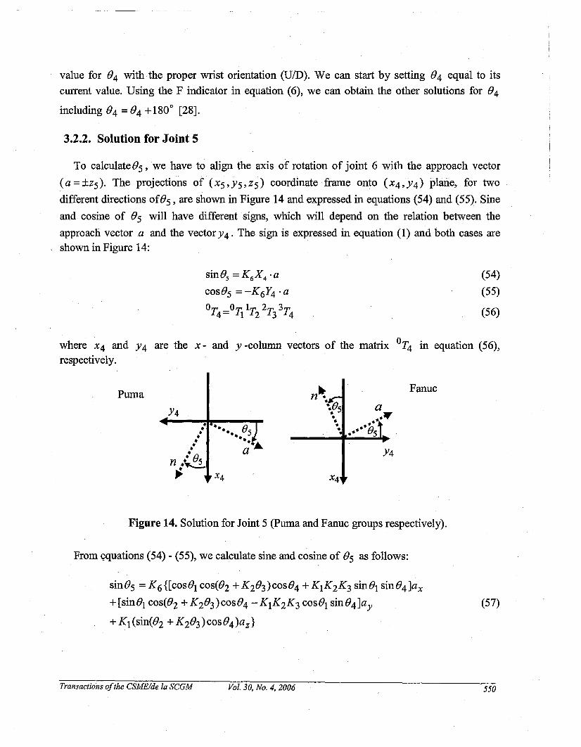
3.2.2. Solution for Joint 5
To calculateBs, we have to align the axis of rotation of joint 6 with the approach vector
(a =±z5). The projections of (xS,Y5,z5) coordinate frame onto (x4,Y4) plane, for two
different directions ofB5 , are shown in Figure 14 and expressed in equations (54) and (55). Sine
and cosine of Bs will have different signs, which will depend on the relation between the
approach vector a and the vectorY4. The sign is expressed in equation (1) and both cases areshown in Figure 14:
sinBs = K 6X 4 ·acosB5 = -K6Y4 . a
00123T4= Ii T2 T3 T4
(54)
(55)
(56)
where X4 and Y4 are the x- and Y -column vectors of the matrix °T4 in equation (56),respectively.
Puma
••• B: ....... 5. .. .... .. ..... a:&.
n ..~~
Y4
Fanuc
Figure 14. Solution for Joint 5 (Puma and Fanuc groups respectively).
From <:;:quations (54) - (55), we calculate sine and cosine of B5 as follows:
sinB5 =K6{[cosBI cos(B2 + K2B3)cos B4 + KIK2K3 sinBI sinB4]ax
+ [sinBI cos(B2 + K2B3)cosB4 - KIK2K3 cosBI sinB4]ay
+ KI(sin(B2 + K2B3)cosB4)az }
(57)
Transactions ofthe CSMElde la SCGM Vol. 30, No.4, 2006 550

cosOs =-K6 {[K3K 4 COSOl sin(K202 +(3)]ax + K 3K 4 [sin 0l sin(K202 +(3)]ay
-[KlK 2K 3K 4 cosK202 +(3)]az }(58)
The parameter K4 is defmed as in equation (1). Combining equations (54) to (58), we obtain
the 8s :
(Sin8 )8
5= atan2 .__5.
cos 85
(59)
The resulting solution (59) is used to solve for both directions of 8s . Note here that if 8s ~ 0the degenerate case occurs.
3.2.3. Solution for Joint 6
The rotation axis ofjoint 6 is aligned with the approach vector a. Also, we need to align theorientation of the end effector in order to facilitate applications like picking up an object bysetting s =Y6' The projections of the flange (n,s,a) coordinate frame onto the (xs,Ys) plane,
for two different directions of 86 , are shown in Figure 15 and expressed in equations (60) and
(61). When a =-Zs, the twist angle a6 is equal to zero and that will make 86 of negative
cosine. In the cases when a =zs, the angle 86 will be of positive cosine. The parameter K 6 inequation (1) controls such a difference.
Puma.~."
~n Fanucs
(}6/•• ....••••• (}6 ••• •(}6· ..•••
•Ys •
•••• Y5•(}6\ n
•Xs ~ x5
Figure 15. Solution for Joint 6.
sin86 = n· Ys
cosB6 =K6s .Ys
(60)
(61)
The parameter K 6 is defined as in equation (1). The vector Ys is the Y -column vectorof the
°Ts matrix, while n and s are the normal and sliding vectors of the °T6 matrix, respectively:
Transactions ofthe CSME/de fa SCGM Vol. 30, No.4, 2006
(62)
551

sin86 =[K4K S (cos81 cos(8Z + Kz83)sin 84 - KIKzK3K4Ks sin 81 cos84)]nx
+ [K4Ks(sin81 cos(8z + K z83)sin 84 + KIKzK3K4Ks cos81 cos84)]ny
+ [KIK4K s sin(8z + K z83)sin 84]nz
cos86 =K6 {[K4Ks(cos81 cos(8z + K z83)sin 84 -KIKzK3K4Ks sin 81 cos84 )]sx
+ [K4Ks (sin81 cos(8z + K z83)sin 84 +KIKzK3K4Ks cos 81 cos 84)]sy
+ [KIK4K s sin(8z + K z83)sin 84]sz}
Combining equations (60) to (64), we can obtain the angle 06 :
(SinO)06 =atan2 .__6
cos06
(63)
(64)
(65)
The solution procedure outlined above provides eight solutions for the inverse kinematicsproblem of the six-joints GPF robots. The first (three-joints) solutions (ObB2,03) represent the
position of the end-effector, whereas the last three-joints solutions (04,05,06) represent theorientation of the end-effector. Our results are applicable for all types of robots that can beincluded within the GPF model. Note here that all the six angles are in the range of ( -1r,+1r ).
4. SIMULATION RESULTS AND DISCUSSIONS
A generic geometric-based solution for solving the inverse kinematic problem of the GPFmodel has been presented in the preceding section.
The solutions for the joint angles contain proposed configurationparametersKl ,K2 ,K3 ,K4, K5,K6 and all the non-zero D-H parameters. This provided us witha systematic approach for cop.structing the GPF model and enabled the development of theUKMS by using a hybrid graphical and computational means. With the UKMS that is based onthe GPF model in our software, We are able to represent most of the 6R industrial robots and tosolve their inverse kinematic problem. A simple graphical user interface will be used for fastrobot modeling and simulation of different industrial applications. To represent a robot inUROCA software, one needs to define all the joints coordinate systems with their orientationsand positions relative to the base frame. This is accomplished by using simple drag-and-dropfeature that is available via the graphical interface. Arm lengths and offsets are systematicallygenerated according the chosen positions of the axis systems. Figures 16 schematically explainthis procedure, in three major steps with an application to the ABB IRB1400 robot arm whichrepresents a Puma-type robot. The solution module was written as an OOP in Visual C++ code.Each robot path as shown in Figure 17 and 18 consists of five points and a home position. In thesimulation we obtained the inverse kinematic for all the· designated path points as well as therobot's home position. Two examplesfrom each kinematic group where presented.
Transactions ofthe CSME/de la SCGM Vol. 30, No.4, 2006 552
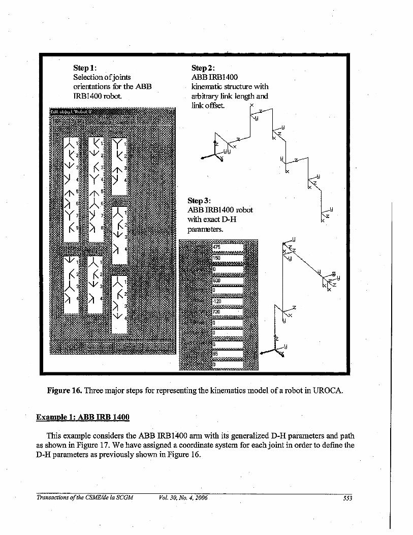
Step 1:Selectionofjointsorientations fur the ABBIRB1400 robot.
Step 2:ABBIRB1400kinematic structure witharbitrary link length andlink offset.
Step 3:ABBIRB1400 robotwith exact D-Hpara:n::eters.
y
yz
Figure 16. Three major steps for representing the kinematics model of a robot in UROCA.
Example 1: ABB IRB 1400
This example considers the ABB IRB1400 arm with its generalized D-H parameters and pathas shown in Figure 17. We have assigned a coordinate system for each joint in order to define theD-H parameters as previously shown in Figure 16.
Transactions ofthe CSME/de la SCGM Vol. 30, No.4, 2006 553
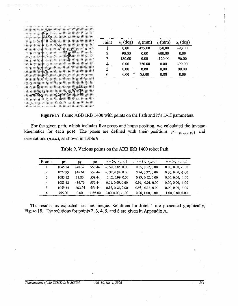
Joint Bi (deg) di(mm) li(mm) ai (deg)1 0.00 475.00 150.00 -90.00
2 -90.00 0.00 600.00 0.00
3 180.00 0.00 -120.00 90.00
4 0.00 720.00 0.00 -90.00
5 0.00 0.00 0.00 90.00
6 0.00 85.00 0.00 0.00
Figurel7. Fanuc ABB IRB 1400 with points on the Path and it's D-H parameters.
For the given path, which includes five poses and home position, we calculated the inversekinematics for each pose. The poses are defined with their positions p =(Px' PY' pz) and
orientations (n,s,a), as shown in Table 9.
Table 9. Various points on the ABB IRB 1400 robot Path
Points px py pz n =(nx,hy,n.) s =(sx,Sy,sz) a = (ax,ay,az)
1 1045.54 240.32 559.44 -0.52,0.85,0.00 0.85,0.52,0.00 0.00,0.00, -1.00
2 1072.93 146.64 559.44 -0.32, 0.94, 0.00 0.94, 0.32, 0.00 0.00,0.00, -1.00
3 1085.12 31.86 559.44 -0.12,0.99,0.00 0.99,0.12,0.00 0.00,0.00, -1.00
4 1081.42 - 86.70 559.44 0.01,0.99,0.00 0.99, -0.01, 0.00 0.00,0.00, -1.00
5 1059.54 -202.24 559.44 0.16,0.98,0.00 0.98, -0.16, 0.00 0.00,0.00, -1.00
6 955.00 0.00 1195.00 0.00, 0.00, -1.00 0.00, 1.00, 0.00 1.00, 0.00, 0.00
The results, as expected, are not unique. Solutions for Joint 1 are presented graphically,Figure 18. The solutions for points 2,3,4,5, and 6 are given in Appendix A.
Transactions ofthe CSME/de la SCGM Vol. 30, No.4, 2006 554

8
17.3777
j-----.1 Config. I
1: -1,-1,-1 I
1 14.2372 :
7
14.2372
Config,-1,+1,-1
17.3777
3.6027
165.856
Solutions for Joint 31
111
•111I1
o 1 0
Solutions for Joint 11III111 119.944711
7 8
Solutions for Joint 4
Solutions for Joint 61-----
Solutions for Joint 5
6
6
-165.7628
6
180
1III
•11 11- I
I1-103.6635I II I1 1, 11 1
I 17.3777 1I 1
-----,1, Config.I +1,-1,-11,
, I1 ,, -81.6072 II ,1 ,I I, ,I II II 1I 1
5
5
5
180
14.2372
165.856
Config.+1,+1,-1
135.9113
119.9447
-162.6223
4
165.856
119:9447
180
4
4
1I1111I 135.911311
------,: Config,1 -1,-1,+1I1 14.2372
3
3
180
3.6027
3
14.2372
Config.-1,+1,+1
-162.6223
2
o
,1-81.6072 1I1II111,
1111I1
103.66351
Config, 1. 1
+1,-1,+1 111
-165.7628
-----..,
,11I I'-162.6223 I
" 1, 1' 1
o
-81.6072
103.6635
Config.+1,+1,+1
-165.7628
-162.6223
200100
O++--"'''''''''''''''---+-,--I--'''''''''''''---j-,-1-----I-r-+_
2
200
100o
-100-200
200
100
o-100
50o
-50-100-150-200
JOINT 6
JOINT 3
JOINT 4200
150
100
500-H1----J-,-1----t-r-+_
JOINT 5
JOINTl
JOINT 2
~on,-... 100= lZl< ~ 0.... ... -100.S ~.Q ~ -200
Figure 18. Joint solutions for point 1.
Transactions ofthe CSME/de la SCGM Vol. 30, No.4, 2006 555
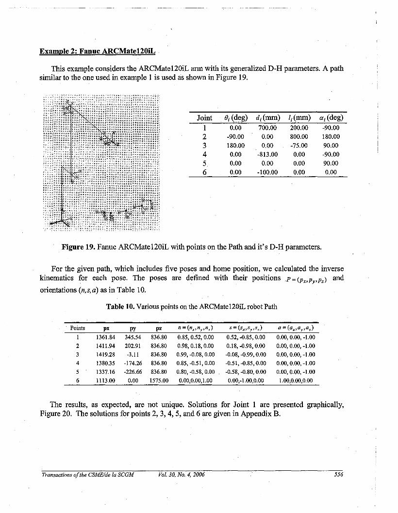
Example 2: Fanuc ARCMate120iL .
This example considers the ARCMate120iL ann with its generalized D-H parameters. A pathsimilar to the one used in example 1 is used as shown in Figure 19.
Joint ()i (4~g) di(mm) li(mm) ai(deg)1 0.00 700.00 200.00 -90.00
2 -90.00 0.00 800.00 180.00
3 180.00 0.00 -75.00 90.00
4 0.00 -813.00 0.00 -90.00
5 0.00 0.00 0.00 90.00
6 0.00 -100.00 0.00 0.00
Figure 19. Fanuc ARCMate120iL with points on the Path and it's D-H parameters.
For the given path, which includes five poses and home position, we calculated the inversekinematics for each pose. The poses are defined with their positions ,P = (Px, Py, pz) and
orientations (n,s,a) as in Table 10.
Table 10. Various pointson the ARCMate120iL robot Path
Points px py pz n =(nx,ny,nz) s = (sx,Sy,sz) a =(ax,ay,a z)
1 1361.84 345.54 836.80 0.85, 0.52, 0.00 0.52, -0.85, 0.00 0.00,0.00, -1.00
2 1411.94 202.91 836.80 0.98,0.18,0.00 0.18, -0.98, 0.00 0.00,0.00, -1.00
3 1419.28 -3.11 836.80 0.99, -0.08, 0.00 -0.08, -0.99, 0.00 0.00,0.00, -1.00
4 1380.35 -174.26 836.80 0.85, -0.51, 0.00 -0.51, -0.85, 0.00 0.00,0.00, -1.00
5 1337.16 -226.66 836.80 0.80, -0.58, 0.00 -0.58, -0.80, 0.00 0.00,0.00, -1.00
6 1113.00 0.00 1575.00 0.00,0.00,1.00 0.00,-1.00,0.00 1.00,0.00,0.00
The results, as expected, are not unique. Solutions for Joint 1 are presented graphically,Figure 20. The solutions for points 2,3,4,5, and 6 are given in Appendix B.
Transactions ofthe CSME/de la SCGM Vol. 30, No.4, 2006 556

876
~'----1 ~-----
I Config. I Config. I Config.I +1,-1,-1 I -1,+1,-1 I -1 -1 -1I I I "I I 1I I 12.9452 I 12.9452
-57.0074
Config.+1,+1,-1
-167.0548
4
4
-----I
Config. I
-1,-1,+1 :I
12.9452 I
130.6644
3
3
12.9452
28.5263
Cotrlig.-1,+1,+1
I 1I I 7 I 8 II -167.0548 I I I
: : Solutions for Joint 1 :I I II I 1I I 1I I 1 II 253.6859II ... ... 11 I 1 130.6644 II I 28.5263 I 1
'-I---rl--"'=---h--r----!l-Jr-rI--._.---1-n-- 4--r1----"=---h.;----1l-,-,2
253.6859
-167.0548
.. ----,Config.+1,-1,+1
-57.9074
Config.+1,+1,+1
200
o-200
JOINT 2
JOINT 1
~ 4000.0 """'~ 3 200........ 0 +-1---"""",......-+,;--.S ~.Q S -200
Solutions for Joint 2JOINT 3
~00 .,.....,c:: <Il 200-< ~.5 ~ 0.Q S -200 -36?6403
10.2809
3
10.2809
7-171.3563
JOINT 4Solutions for Joint 3
20015010050o
180 180
o o o o
180 180
87
II
1 I-108.517 1 -108.51791
Solutions for Joint 6 :1 1
III1-130.6919I
Solutions for Joint 5
. Solutions for Joint 4
6
II
1-127.0456 II 1I 1I II II II II I
5
71.4821
4 I11I1I
130.6919 rII
I1III
I I1- I
3
71.4821
2
71.4821
IIIIII
127.0456 III
I1IIII IL _
71.4821
JOINT 6
JOINT 5
~ 2000.0 """'c:: <Il 100-< (I)
~ 0.5 ~.Q S -100
-200
.£00 """' 100~ ~ 50........ 0.S ~ -50,Q S -100
-150
Figure 20. Joint solutions for point 1.
Transactions ofthe CSME/de la SCGM Vol. 30, No.4, 2006 557
5. CONCLUSION
Based on the urgent need for a generic robotic model that can be easily reconfigured toidentify a specific kinematic model for a specific robot, we developed a generalized approachfor systematic modeling and solving the inverse kinematic problem of 6R industrial robots. Aunified kinematic modeler and solver called UKMS employs a generic Puma-Fanuc (GPF)model for solving the inverse kinematic problem using a geometric approach. It is worth notingthat solutions for different robotic systems having different twist angles are produced using thesame mathematIcal equations. This fact holds true .for any 6R· robot of kinematic structurefalling within the scope of our GPF model. Numerical examples are presented for exploring thepotentials of our unified approach. The results that UKMS model can provide will be used fordeveloping Generic, Puma-Fanuc Dynamic Model (GPFDM) for the same group of robots. Theextension of the dynamic model will be Generic, Puma-Fanuc Controller (GPFC) which is thefinal goal of our research project. All three models are based on the same configurationparametersK1, K 2 , K 3 , K 4 , Ks, and K6'
ACKNOWLEDGMENT
The Natural Science and Engineering Council of Canada (NSERC) under a Strategic ProjectGrant in "Reconfigurable Control Process for Manufacturing" supported the work reported inthis paper.
REFERENCES
[1] J. Denavit, and R S Hartenberg, A kinematic notation for lower-pair mechanisms based onmatrices, Journal ofApplied Mechanics Vol. 77, 1955,pp.215-221.
[2] E.M. ElBeheiry, W. ELMaraghy, and H. ELMaraghy, The structured design of areconfigurable control process, Proc. CIRP Design Seminar, Cairo, Egypt, 2004.
[3] M. T. Balkan, M.A. K. Ozgoren, S. Arikan, and H. M. Baykurt, A kinematic structurebased classification and compact equations for six-dof industrial robotic manipulators,Mechanism and Machine Theory Vol. 36,2001, pp. 817-832.
[4] K.S. Fu, RC. Gonzalez, and C.S.G. Lee, Robotics: control, sensing, vision, andintelligence, McGraw-Hill Inc., 1987, pp.12-82
[5] J. P. Owens, Industrial Robot Simulation, Ph. D. Thesis, Department of Electrical andElectronic Engineering, University ofNewcastle Upon Tyne, UK, 1990.
[6] D. Kohil, and A. H. Soni, Kinematic analysis of spatial mechanisms via successive screwdisplacements, ASME Journal ofEngineering for Industry 2(B) 1975, pp.739-747.
[7] P.R Paul, Robot manipulator: mathematics, programming and control, MIT Press,Cambridge, MA, 1981.
[8] G. R Pennock and A. T. Yang, Application of dual:·number matrices to the inversekinematics problem of robot manipulators, ASME Journal of Mechanisms, Transmissionsand Automation in Design VoLl07, 1985, pp.201-208.
Transactions ofthe CSME/de la SCGM Vol. 30, No.4, 2006 558

[9] A. T. Yang, and R. Freudenstein, Application of dual number quaternian algebra to theanalysis of spatial mechanisms, ASME, Journal of Applied Mechanics 31(E), 1964,pp152-157.
[10] J. J. Jr. Dicker, J. Denavit, and R. S. Hartenberg, An iterative method for the displacementanalysis of spatial mechanisms, ASME, Journal of Applied Mechanics 31(E), 1964,pp.309-'314.
[11] G. Legnani, F. Casolo, P. Righettini and B. Zappa, A homogeneous matrix approach to 3Dkinematics and dynamics -1 theory, Mechanism and Machine Theory Vo1.31, No.5, 1996,pp.573-'587. ,
[12] G. Legnani, F. Casolo, P. Righettini and B. Zappa, A homogeneous matrix approach to 3Dkinematics and dynamics -II. Theory, Applications to chains of rigid bodies and serialmanipulators, Mechanism and Machine Theory, Elsevier Science Ltd., Great· Britain,Vo1.31 , No.5, 1996, pp.589-605. .
[13] L.W. Tsai, Solving the kinematics of the most general six-and five-degree-of freedommanipulators by continuation methods, ASME Journal of Mechanisms, Transmissions andAutomation in Design, Vo1.107, No.2, 1985, pp.189-200.
[14] M. T. Balkan, M.A. K. Ozgoren, S. Arikan, and H. M. Baykurt, A method of inversekinematics solution including singular and multiple configurations for a class of roboticmanipulators, Mechanism and Machine Theory Vo1.35, 2000, pp.1221-1237.
[15] K. Bekir and A. Serkan, An improved approach to the solution of inverse kinematicsproblems for robot manipulators, Engineering Application of Artificial IntelligenceVoU3, 2000, pp.159-164.
[16] V. D. Tourassis, M. H.Ang, Jr, A modular architecture for inverse robot kinematics, IEEETransaction ofRobotics and Automation Vo1.5, No.5, 1989, pp.555-568.
[17] R. Manseur and K. L. Doty, Structural kinematics of 6-revolute-axis robot manipulators,Mechanism and Machine Theory Vo1.31, No.5, 1996, pp.647-657.
[18] R. Manseur and K. L. Doty, Fast inverse kinematics of five-revolute-axis robotmanipulators, Mechanism and Machine Theory Vo1.27, No.5, 1992, pp.587-5977.
[19] R. Manseur and K. L. Doty, A robot manipulator with 16 real inverse kinematics solutionssets, The International Journal ofRobotics Research Vo1.8, No.5, 1989, pp.75-79.
[20] R. Manseur and K. L. Doty, A fast algorithm for inverse kinematic analysis of robotmanipulators, The International Journal ofRobotics Research Vo1.7, No.3, 1988, pp.52-63.
[21] H. Fu, L. Yang, and C. Zhou, A computer-aided geometric approach to inverse kinematics,Journal ofRobotic Systems VoU5, No.3, 1998, pp.131-143.
[22] I.S. Fischer, A geometric method for determining joint rotations in the inverse kinematicsofrobotic manipulators, Journal ofRobotic Systems VoU7, No.2, 2000, pp.l07-117.
[23] H. Fu, L. Yang, J. Zhang, A set of geometric invariants for kinematic analysis of 6Rmanipulators, The International Journal ofRobotics Research Vo1.19, No.8, 2000, pp.784792.
[24] F. Chapelle, P. Bidaud, A Closed Form for Inverse Kinematics Approximation of General6R Manipulators using Genetic Programming, Proceedings of the 2001 IEEE InternationalConference on Robotics and Automation, Seoul, Korea, 2001, pp.3364-3369.
Transactions ofthe CSMElde la SCGM Vol. 30, No.4, 2006 559

[25] M. G. Her, C. Y. Chen, Y. C. Hung, M. Karkoub, Approximating a Robot InverseKinematics Solution Using Fazzy Logic Tuned by Genetic Algorithms, InternationalJournal ofAdvanced Manufacturing TechnologyVol.20, No.5, 2002, pp.375-380.
[26] D. L Pieper, The kinematics of manipulators under computer control, Computer ScienceDepartment, Stanford University, Artificial Intelligence Project Memo 72, 1968.
[27] A. Pashkevich, Real-time inverse kinematics for robots with offset and reduced wrist,Control Engineering Practice Vol.5, No. 10, 1997, pp.1443-1450.
[28] C. S. G. Lee, and M. Ziegler, A geometric approach in solving the inverse kinematics ofPUMArebots, IEEE Transactions on Aerospace and Electronic Systems- Vol.20, No.6,1984, pp.695-706.
[29] Takafumi Matsumaru, Design and Control of the Modular Robot System: TOMMS, IEEEInternational Conference on Robotics and Automation, Nagoya, Japan, 1995, pp.21252131.
[30] L. Kelmar and P. Khosla, "Automatic generation of kinematics for a reconfigurablemodular manipulator system, Proceedings of IEEE Conference on Robotics andAutomation, Philadelphia, PA, 1988, pp.663-668.
[31] B. Benhabib, G. Zak, and M.G. Lipton, "A generalized kinematic modeling method formodular robots," Journal ofRobotic Systems Vol.6, No.5, 1989, pp.545-571.
[32] T. Matsumaru, "Design and control of the modular robot system: TOMMS," Proceedingsof IEEE Conference on Robotics and Automation, Nagoya, Japan, 1995, pp.2125-2131.
[33] 1. M. Chen, G. Yang, "Configuration Independent Kinematics for Modular Robots," Proc.IEEE Int'l Conf. Robotics and Automation, Minneapolis, MN, 1996, pp.1440-1445,
[34] Podhorodeski, RP., and S.B. Nokleby, "Reconfigurable Main-Arm for Assembly of allRevolute-onlyKS Branches," J. ofRobotic Systems, Vol. 17, No.7, 2000, pp. 365-373.
AppendixA.
Table 11. Joint solutions for point 2.
Point #2Solutions 2 3 4 5 6 7 8
A,E, W +1,+1,+1 +1, -1, +1 -1, +1, +1 -1,-1,+1 +1,+1,-1 +1, -1,-1 -1, +1,-1 -1, -1,-1
JOINT! -172.2175 -172.2175 7.7825 7.7825 -172.2175 -172.2175 7.7825 7.7825
JOINT2 -59.3014 254.9523 29.3682 130.0427 -59.3014 254.9523 29.3682 130.0427
JOINT3 -122.0437 -39.0317 9.0554 -170.1308 -122.0437 -39.0317 9.0554 -170.1308
JOINT4 180.0000 180.0000 0 0 0 0 180.0000 180.0000
JOINT5 88.6549 125.9207 51.5764 130.0880 -88.6549 -125.9207 -51.5764 -130.0880
JOINT6 78.9125 78.9125 78.9125 78.9125 -101.0875 -101.0875 -101.0875 -101.0875
Transactions ofthe CSME/de la SCGM Vol. 30, No.4, 2006 560

Table 12. Joint solutions for point 3.
Point #3Solutions 2 3 4 5 6 7 8
A,E, W +1,+1,+1 +1,-1,+1 -1,+1,+1 -1, -1, +1 +1, +1,-1 +1, -1,-1 -1, +1,-1 -1, -1,-1
JOINTl -178.3182 -178.3182 1.6818 1.6818 -178.3182 -178.3182 1.6818 1.6818
JOINT2 -59.6845 255.3018 29.5929 129.8760 -59.6845 255.3018 29.5929 129.8760
JOINT3 -121.3845 -39.6908 8.7269 -169.8023 -121.3845 -39.6908 8.7269 -169.8023
JOINT4 180.0000 180.000 0 0 0 0 180.000 180.000
JOINT5 88.9310 125.6109 51.6802 129.9263 -88.9310 -125.6109 -51.6802 -129.9263
JOINT6 84.4949 84.4949 84.4949 84.4949 -95.5051 -95.5051 -95.5051 -95.5051
Table 13. Joint solutions for point 4..
Point #4Solutions 2 3 4 5 6 7 8
A,E, W +1,+1,+1 +1, -1,+1 -1, +1, +1 -1, -1,+1 +1,+1,-1 +1, -1,-1 -1, +1,-1 -1, -1,-1
JOINTI 175.4159 175.4159 -4.5841 -4.5841 175.4159 175.4159 -4.5841 -4.5841
JOINT2 -59.5843 255.2103 29.5344 129.9194 -59.5843 255.2103 29.5344 129.9194
JOINTI -121.5571 -39.5183 8.8125 -1 (j9.8879 -121.5571 -39.5183 8.8125 -169.8879
JOINT4 180.0000 180.0000 0 0 0 0 180.0000 180.0000
JOINT5 88.8587 125.6920 51.6531 129.9684 -88.8587 -125.6920 -51.6531 -129.9684
JOINT6 85.9264 85.9264 85.9264 85.9264 -94.0736 -94.0736 -94.0736 -94.0736
Table 14. Joint solutions for point 5.
Point #5Solutions 2 3 4 5 6 7 8
A,E,W +1,+1,+1 +1, -1, +1 -1, +1, +1 -1, -1,+1 +1,+1,-1 +1, -1,-1 -1,+1,-1 -1,-1,-1
JOINTl 169.1933 169.1933 -10.8067 -10.8067 169.1933 169.1933 -10.8067 -10.8067
JOINT2 -58.7096 254.4137 29.0154 130.3039 -58.7096 254.4137 29.0154 130.3039
JOINT3 -123.0603 -38.0150 9.5700 -170.6454 -123.0603 -38.0150 9.5700 -170.6454
JOINT4 180.0000 180.0000 0 0 0 0 180.0000 180.0000
JOINT5 88.2301 126.3987 51.4146 130.3415 -88.2301 -126.3987 -51.4146 -130.3415
JOINT6 88.4083 88.4083 88.4083 88.4083 -91.5917 -91.5917 -91.5917 -91.5917
Transactions ofthe CSME/de fa SCGM Vol. 30, No.4, 2006 561

Table 15. Joint solutions for Point 6.
Point #6(Home position)Solutions 2 3 4 5 6 7 8
A,E, W +1,+1,+1 +1, -1, +1 -1, +1, +1 -1, -I, +1 +1, +1,-1 +1, -1,-1 -I, +1,-1 -I, -1,-1
JOINTl -180.0000 -180.0000 0 0 -180.0000 -180.0000 0 0
JOINT2 -32.4652 -77.0996 0 90.0000 -32.4652 -77.0996 0 90.0000
JOINT3 -121.0430 -40.0323 0 -161.0754 -121.0430 -40.0323 0 -161.0754
JOINT4 180.0000 180.0000 0 0 0 0 0 180.0000
JOINT5 26.4917 62.8681 0 71.0754 -26.4917 -62.8681 0 -71.0754
JOINT6 0.0000 0.0000 0 0 180.0000 180.0000 0 -180.0000
Appendix B.
Table 16. Joint solutions for point 2.
Point #2Solutions 2 3 4 5 6 7 8
A,E, W +1, +1, +1 +1, -I, +1 -I, +1, +1 -1, -1, +1 +1, +1,-1 +1, -1,-1 -I, +1, - -I, -1,-11
JOINTl -171.8218 -171.8218 8.1782 8.1782 -171.8218 -171.8218 8.1782 8.1782
JOINT2 -81.7163 -81.7163 39.1914 118.9525 -81.7163 -81.7163 39.1914 118.9525
JOINT3 84.7293 ·84.7293 5.9263 163.5324 84.7293 84.7293 5.9263 163.5324
JOINT4 0 0 180.0000 180.0000 180.0000 180.0000 0 0
JOINT5 103.5543 103.5543 56.7349 134.5799 -103.5543 -103.5543 -;;6.7349 -134.5799
JOINT6 -177.2633 -177.2633 -177.2633 -177.2633 2.7367 2.7367 2.7367 2.7367
Table 17. Joint solutions for point 3.
Point #3Solutions 2 3 4 5 6 7 8
A,E, W +1,+1,+1 +1,-1,+1 -1, +1, +1 -1,-1,+1 +1, +1,-1 +1, -1,-1 -1, +1, -1 . -1, -1,-1
JOINTI 179.8743 179.8743 -0.1257 -0.1257 179.8743 179.8743 -0.1257 -0.1257
JOINT2 -81.6802 -81.6802 38.7306 119.2879 -81.6802 -81.6802 38.7306 119.2879
JOINT3 84.7293 84.7293 5.1435 164.3152 84.7293 84.7293 5.1435 164.3152
JOINT4 0 0 180.0000 180.0000 180.0000 180.0000 0 0
JOINT5 103.5905 103.5905 56.4129 135.0273 -103.5905 -103.5905 -56.4129 -135.0273
JOINT6 175.1117 175.1117 175.1117 175.1117 -4.8883 -4.8883 -4.8883 -4.8883
Transactions ofthe CSME/de la SCGM Vol. 30, No.4, 2006 562
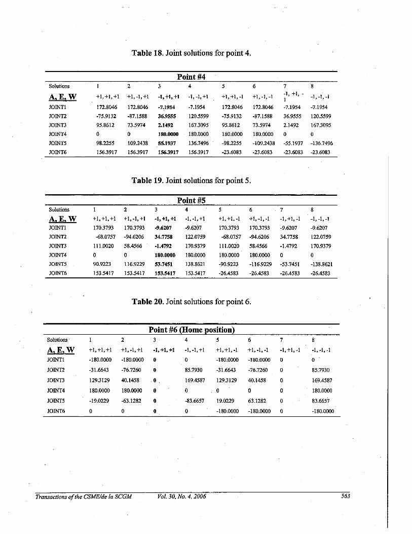
Table 18. Joint solutions for point 4.
Point #4Solutions 2 3 4 5 6 7 8
A,E, W +1,+1,+1 +1, -1, +1 -1, +1, +1 -1, -1, +1 +1, +1,-1 +1,-1,-1 -1, +1, - -1,-1,-11
JOINT! 172.8046 172.8046 -7.1954 -7.1954 172.8046 172.8046 -7.1954 -7.1954
JOINT2 -75.9132 -87.1588 36.9555 120.5599 -75.9132 -87.1588 36.9555 120.5599
JOINT3 95.8612 73.5974 2.1492 167.3095 95.8612 73.5974 2.1492 167.3095
JOINT4 0 0 180.0000 180.0000 180.0000 180.0000 0 0
JOINT5 98.2255 109.2438 55.1937 136.7496 -98.2255 -109.2438 -55.1937 -136.7496
JOINT6 156.3917 156.3917 156.3917 156.3917 -23.6083 -23.6083 -23.6083 -23.6083
Table 19. Joint solutions for point 5.
Point #5Solutions 2 3 4 5 6 7 8
A,E, W +1,+1,+1 +1, -1, +1 -1, +1, +1 -1,-1,+1 +1,+1,-1 +1,-1,-1 -1, +1,-1 -1, -1, -1
JOINT! 170.3793 170.3793 -9.6207 -9.6207 170.3793 170.3793 -9.6207 -9.6207
JOINT2 -68.0757 -94.6206 34.7758 122.0759 -68.0757 -94.6206 34.7758 122.0759
JOINT3 111.0020 58.4566 -1.4792 170.9379 111.0020 58.4566 -1.4792 170.9379
JOINT4 0 0 180.0000 180.0000 180.0000 180.0000 0 0
JOINT5 90.9223 116.9229 53.7451 138.8621 -90.9223 -116.9229 -53.7451 -138.8621
JOINT6 153.5417 153.5417 153.5417 153.5417 -26.4583 -26.4583 -26.4583 -26.4583
Table 20. Joint solutions for point 6.
Point#6 (Home position)Solutions 2 3 4 5 6 7 8
A,E,W +1,+1,+1 +1, -1, +1 -1, +1, +1 -1,-1,+1 +1, +1,-1 +1, -1,-1 -1, +1,-1 -1, -1,-1
JOINT! -180.0000 -180.0000 0 0 -180.0000 -180.0000 0 0
JOINT2 -31.6643 -76.7260 0 85.7930 -31.6643 -76.7260 0 85.7930
JOINT3 129.3129 40.1458 0, 169.4587 129.3129 40.1458 0 169.4587
JOINT4 180.0000 180.0000 0 0 0 0 0 180.0000
JOINTS -19.0229 -63.1282 0 -83.6657 19.0229 63.1282 0 83.6657
JOINT6 0 0 0 0 -180.0000 -180.0000 0 -180.0000
Transactions ofthe CSME/de la SCGM Vol. 30, No.4, 2006 563
Nomenclature
AbbreviationsA: Arm.AA : Above ann.BA : Below ann.D : DownDF : Do not flip.D-H: Denavit - Hartenberg.E: Elbow.EA : Elbow above.EB : Elbow below.F: Flip.GPF : Generic Puma-Fanuc.LA : Left arm.L&A : Left and above.L&B : Left and belowRA : Right arm.R&A : Right and above.R&B : Right and below.U:UpUKMS : Unified Kinematic Modeler and SolverUROCA : Unified Reconfigurable Open Control Architecture.W: WristWD : Wrist down.WU : Wrist up.
Symbolsa : Approach vectorI : Link offset.d : Link length.n : Nonnal vector;s : Sliding vector.M : parameter.p : Position vector which points from the origin ofthe shoulder coordinate system
(xo, Yo, zo) to the point where the last three joints are intersecting.
P6 : Position vector which points from the origin of the shoulder coordinate system
(xo, Yo, zo) to the position of the end-effector.
Px' Py , pz : Coordinates of the position vector p with respect to the (xo,Yo,zo)'
K i : i th configuration parameter ofthe i th twist angel ai'
Transactionsofthe CSME/de la SCGM Vol. 30, No.4, 2006 564

°T6 : Homogeneous transformation matrix, which specifies the position and orientation oftheend point ofmanipulator with respect to the base coordinate system.
a : Twist anglef3: Angle.rp: Angle.B: Joint angle.n :Parameter.
Transactions ofthe CSME/de la SCGM Vol. 30, No.4, 2006 565
Related Documents