Generalized Pauli principle for Read- Rezayi non-Abelian ...ykis07.ws/presen_files/21/Haldane.pdf · Generalized Pauli principle for Read-Rezayi non ... A b e lia n c u rre n t o

Generalized Pauli principle for Read-Rezayi non-Abelian Quantum Hall States

F. D. M. Haldane, Princeton University

Supported in part by NSF MRSEC DMR-0213706 at Princeton Center for Complex Materials

A selection rule on “admissible configurations” in model FQHE wavefunctions

From polynomial wavefunctions to topological/conformal field theories

Numerical studies: effects on entanglement spectrum

Collaborations with Emil Prodan, Andrei Bernevig, and Hui Li

YKIS 2007 Workshop on Interaction and Nanostructural Effects in Low-Dimensional Systems, Yukawa Institute for Theoretical Physics, Kyoto University, Kyoto, Nov. 21-23, 2007

This Article

Full Text (PDF)

Alert me when this article is cited

Alert me if a correction is posted

Services

Email this article to a friend

Similar articles in this journal

Alert me to new issues of the journal

Add to My Personal Archive

Download to citation manager

Request Permissions

How to cite this article

Google Scholar

Articles by Feigin, B.

Articles by Mukhin, E.

Search for Related Content

International Mathematics Research Notices

Oxford JournalsMathematics & Physical SciencesInt Math Res NotVol. 2002Pp. 1223-1237

Perform your original search, Jimbo Jack Miwa, in Int Math Res Notices Search

International Mathematics Research Notices (2002) 2002:1223-1237 , doi:10.1155/S1073792802112050

Copyright © 2002 Hindawi Publishing Corporation. All rights reserved.

A differential ideal of symmetric polynomials spanned by Jack polynomials at rß = -(r=1)/(k+1)

B. Feigin, M. Jimbo, T. Miwa and E. Mukhin

For each pair of positive integers (k,r) such that k+1, r–1 are coprime, we introduce an ideal of

the ring of symmetric polynomials . The ideal has a basis consisting of Jack

polynomials with parameter rß=-(r–1)/(k+1), and admits an action of a family of differential

operators of Dunkl type including the positive half of the Virasoro algebra. The space

coincides with the space of all symmetric polynomials in n variables which vanish when k+1

variables are set equal. The space coincides with the space of correlation functions of an

Abelian current of a vertex operator algebra related to Virasoro minimal series (3,r+2).

Disclaimer:

This Article

Full Text (PDF)

Alert me when this article is cited

Alert me if a correction is posted

Services

Email this article to a friend

Similar articles in this journal

Alert me to new issues of the journal

Add to My Personal Archive

Download to citation manager

Request Permissions

How to cite this article

Google Scholar

Articles by Feigin, B.

Articles by Mukhin, E.

Search for Related Content

International Mathematics Research Notices

Oxford JournalsMathematics & Physical SciencesInt Math Res NotVol. 2002Pp. 1223-1237

Perform your original search, Jimbo Jack Miwa, in Int Math Res Notices Search

International Mathematics Research Notices (2002) 2002:1223-1237 , doi:10.1155/S1073792802112050

Copyright © 2002 Hindawi Publishing Corporation. All rights reserved.

A differential ideal of symmetric polynomials spanned by Jack polynomials at rß = -(r=1)/(k+1)

B. Feigin, M. Jimbo, T. Miwa and E. Mukhin

For each pair of positive integers (k,r) such that k+1, r–1 are coprime, we introduce an ideal of

the ring of symmetric polynomials . The ideal has a basis consisting of Jack

polynomials with parameter rß=-(r–1)/(k+1), and admits an action of a family of differential

operators of Dunkl type including the positive half of the Virasoro algebra. The space

coincides with the space of all symmetric polynomials in n variables which vanish when k+1

variables are set equal. The space coincides with the space of correlation functions of an

Abelian current of a vertex operator algebra related to Virasoro minimal series (3,r+2).

Disclaimer:

! = !(k + 1)/(r ! 1)

After I had empirically found much of what I will describe in numerical studies, A. Bernevig found (by Google!) a remarkable earlier 2002 Kyoto mathematical paper (RIMS) that related a Bosonic variant of my results to Jack Polynomials (known earlier from the 1D integrable Sutherland-Calogero model)

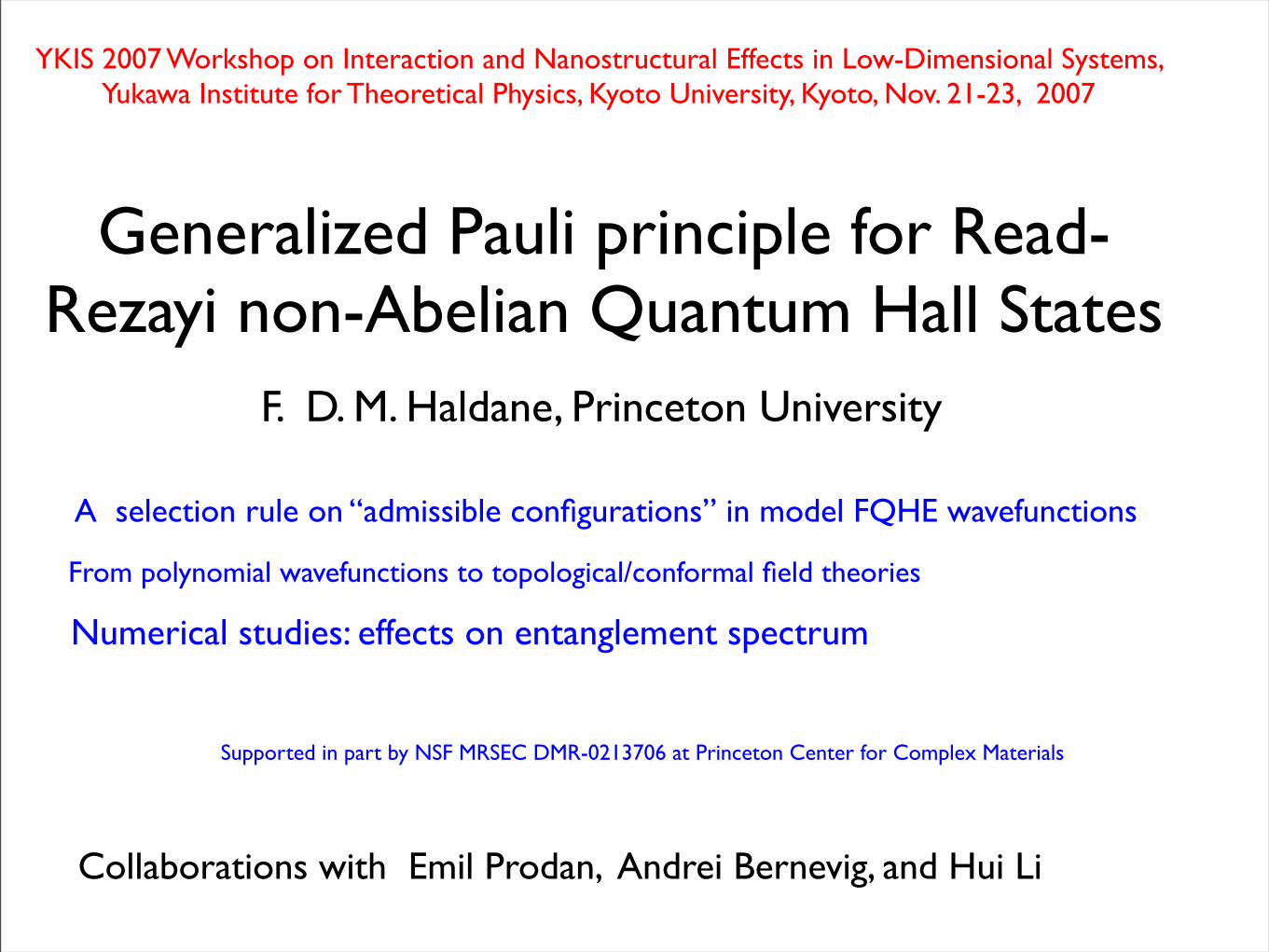
Laughlin FQHE state

• ν = 1/m Laughlin state

• “occupation number”-like representation in orbitals zm, m = 0,1,..., NΦ = m(N-1) orbitals

! = "(z1, z2, . . . , zN )N!

i=1

e!!(ri)

!2!(r) = 2"B(r)/!0N-variable (anti)symmetric polynomial

!(z1, z2, . . . , zN ) =!

i<j

(zi ! zj)m

1001001001001001001...1001 (m=3)

lowest Landau level

This is the “dominant” configuration of the Laughlin state

m=0 orbital

“Dominance”

• convert occupation pattern to a partition λ, “padded” with zeroes to length N:

• 1001001 → λ = {λ 1,λ2,λ3} = {6,3,0}

• λ dominates λ′ if

• |λ| ≡ (∑i λi )= |λ′| = M

• (∑j≤i λ′j )≤ ( ∑j≤i λj ) for all i = 1,2,..N-1

“Dominance” is a partial ordering relations between partitions of a (non-negative) integer intoN (non-negative) integer parts. (related to what was called “squeezing” in Sutherlands solution of the periodic Calogero model......)

“dominance” and “squeezing”

• (pairwise) squeezing: move a particle from orbital m1-1 to m1

and another from m2+1 to m2 where m1 ≤ m2.

• dominance is a partial ordering: if A > B and B > C, then A > C.

1001001001001001001...10011000101001001010001...1001

A dominates B ( A > B)

AB

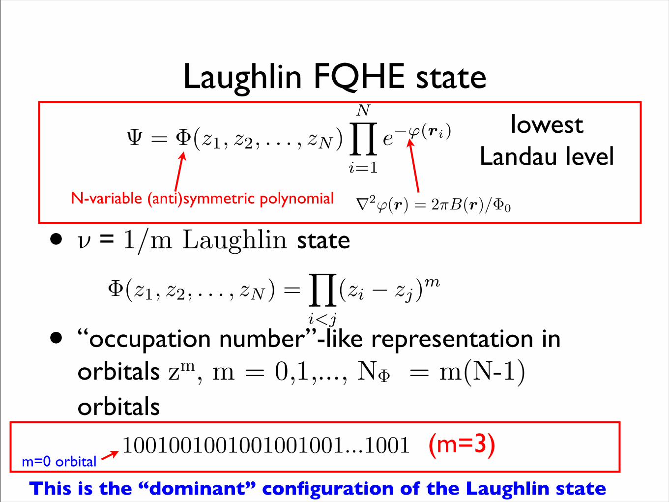
• When expanded in occupation number states, the (polynomial) 1/m Laughlin state only contains configurations dominated by the most compressed (minimum M) “(1,m)-admissible configuration” where no group of m consecutive orbitals contains more than 1 particle.

• “admissibility” can be thought of as a generalized Pauli principle.

• For symmetric (Boson)states the 1/2 (circular droplet) Laughlin state is “dominated” by the configuration 1010101010101...1010000000....

• polynomial part of 1/2 Laughlin wavefunction

centerof droplet

edgeof droplet

incompressible region empty region outside droplet

J!2!0

(z1, z2, . . . , zN )negative jack parameter

partition corresponding to 1010101..

Laughlin state is a Jack Polynomial!

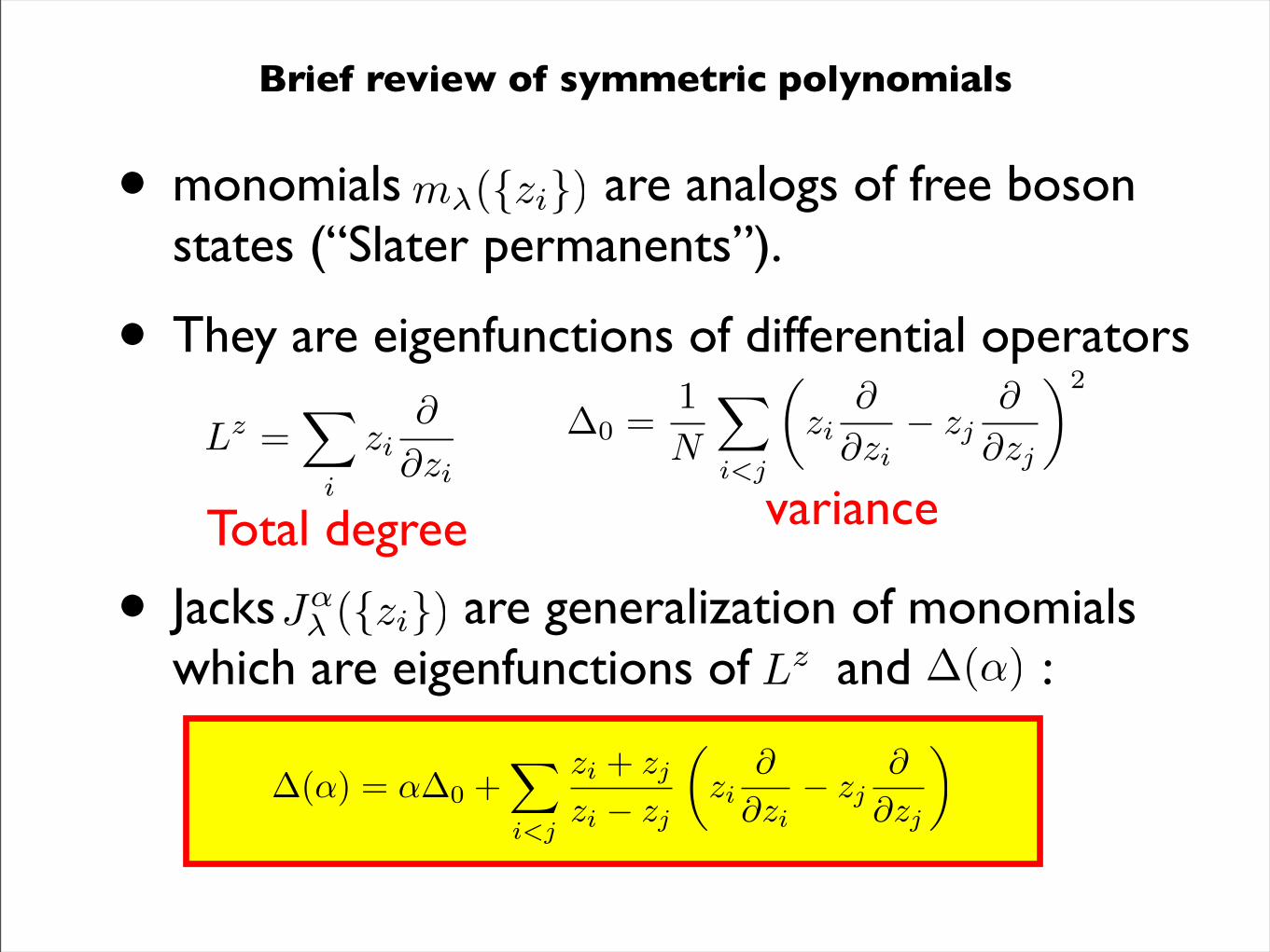
Brief review of symmetric polynomials

• monomials are analogs of free boson states (“Slater permanents”).

• They are eigenfunctions of differential operators

• Jacks are generalization of monomials which are eigenfunctions of and :

Lz =!

i

zi!

!zi

m!({zi})

!0 =1N

!

i<j

"zi

!

!zi! zj

!

!zj

#2

Total degree variance

J!" ({zi})

Lz !(!)

!(!) = !!0 +!

i<j

zi + zj

zi ! zj

"zi

"

"zi! zj

"

"zj

#

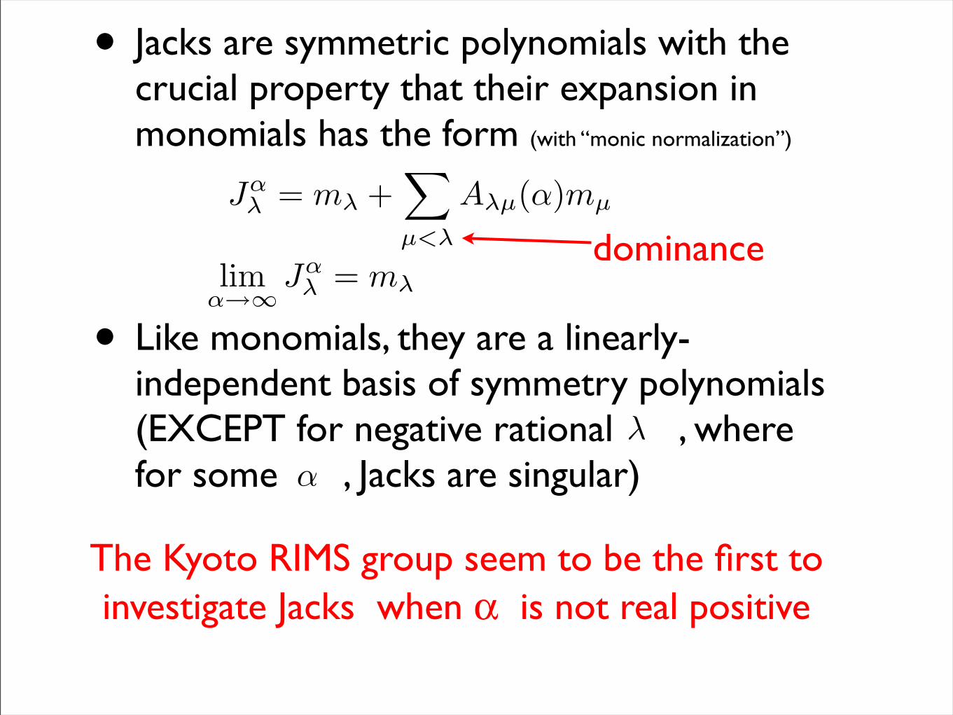
• Jacks are symmetric polynomials with the crucial property that their expansion in monomials has the form (with “monic normalization”)

• Like monomials, they are a linearly-independent basis of symmetry polynomials (EXCEPT for negative rational , where for some , Jacks are singular)

lim!!"

J!" = m"

!

!

The Kyoto RIMS group seem to be the first to investigate Jacks when α is not real positive

dominanceJ!

" = m" +!

µ<"

A"µ(!)mµ

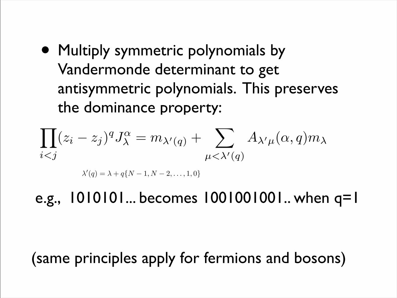
• Multiply symmetric polynomials by Vandermonde determinant to get antisymmetric polynomials. This preserves the dominance property:

!

i<j

(zi ! zj)qJ!" = m"!(q) +

"

µ<"!(q)

A"!µ(!, q)m"

!!(q) = ! + q{N ! 1, N ! 2, . . . , 1, 0}

e.g., 1010101... becomes 1001001001.. when q=1

(same principles apply for fermions and bosons)

• RIMS group looked at Jacks with α = -(k+1)/(r-1) (relatively prime, and k > 0, which is all negative rationals except -1/(r-1))

• For r=2, they found that a SUBSET of the non-singular Jacks are a basis of polynomials that vanish if more than k coordinates coincide....

• The SUBSET is the “(k,r,N) admissible” partitions. For general r, these span space of polynomials that vanish as

!(Z, . . . , Z, zk+1, . . . zN ) !!

j>k

(zj " Z)r

• More generally, multiply by q powers of the Vandermonde determinant to get “(k,q,r,N) admissible” polynomials.

• k=1 is the Laughlin states (can always choose r=2)

• r=2 is the Laughlin,Moore-Read,Read-Rezayi sequences. For k > 1, these are the non-Abelian FQHE states which are currently popular candidates for topological quantum computing!

• Polynomial equations can be solved using linear-independence, NOT orthogonality

• characterized by zeroes of polynomials:

• “quasihole” state defined by!W (Z, . . . , Z, zk . . . , zN ) ! (W " Z)

can’t bring k particles together at quasihole position W!

Can find the representation of this in terms of (admissible) Jacks purely with polynomial algebra! (no quantum mechanics needed!)

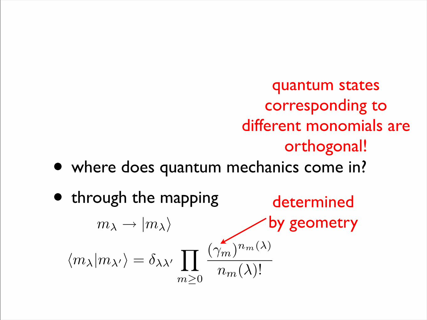
• where does quantum mechanics come in?

• through the mapping

m! ! |m!"

!m!|m!!" = !!!!

!

m!0

("m)nm(!)

nm(#)!

quantum states corresponding to

different monomials are orthogonal!

determinedby geometry

Compactification of the Lowest Landau level on the Riemann sphere.

Identify orbitals m = 0,1,...,NΦ

with orbitals Lz = S,S-1,...,-S on asphere enclosing magnetic monopole charge NΦ= 2S

Uniform QHE states are rotationally-invariant, Ltot = 0.

Beyond “standard” occupation number formalism

• k-particle 1/m Laughlin droplet creation operator (circular droplet centered at R):

!km(R)†|vac! "!

i>j

(zi # zj)mk!

i=1

"R(ri)

• For k = 1, (m has no meaning in this case), this is just the standard lowest Landau-level single-particle creation operator

c(R)†|vac! " !R(r1)

Gaussian centered

at R

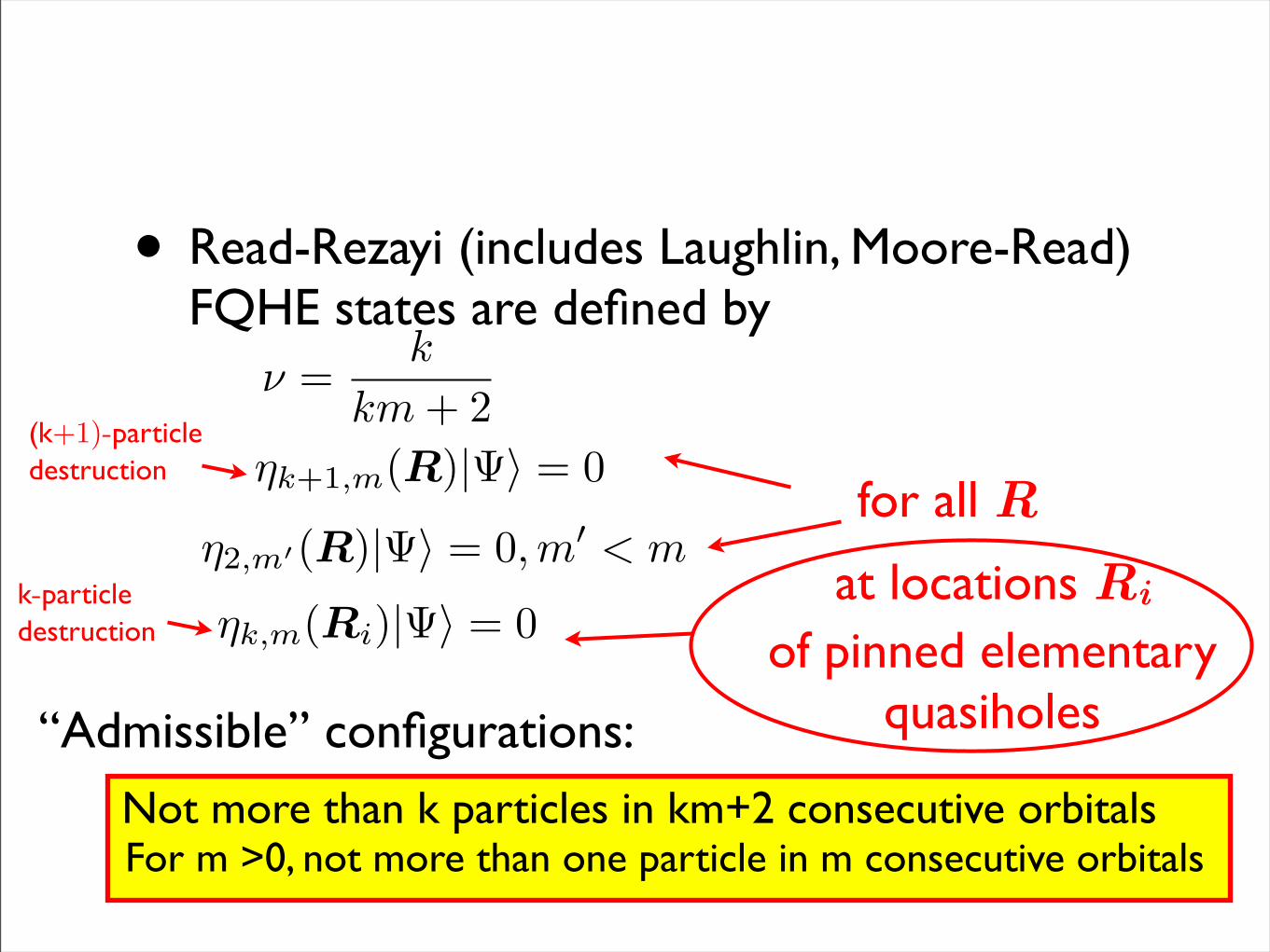
• Read-Rezayi (includes Laughlin, Moore-Read) FQHE states are defined by

! =k

km + 2!k+1,m(R)|!! = 0

!2,m!(R)|!! = 0,m! < mfor all R

!k,m(Ri)|!! = 0at locations Ri

of pinned elementaryquasiholes“Admissible” configurations:

Not more than k particles in km+2 consecutive orbitalsFor m >0, not more than one particle in m consecutive orbitals

(k+1)-particle destruction

k-particle destruction

• On the sphere, the number of charge -e/(km+2) elementary quasiholes for a given N, NΦ is

• The size of the basis set of quantum states (with unpinned quasi holes) is equal to the number of admissible configurations.

• The states can be completely constructed out of configurations dominated by the dominant admissible configuration (“top” configuration).

• These are a very small subset of lowest Landau level states!

Nqh = k(N! ! 12mk(k ! 1))! (km + 2)(N ! k)

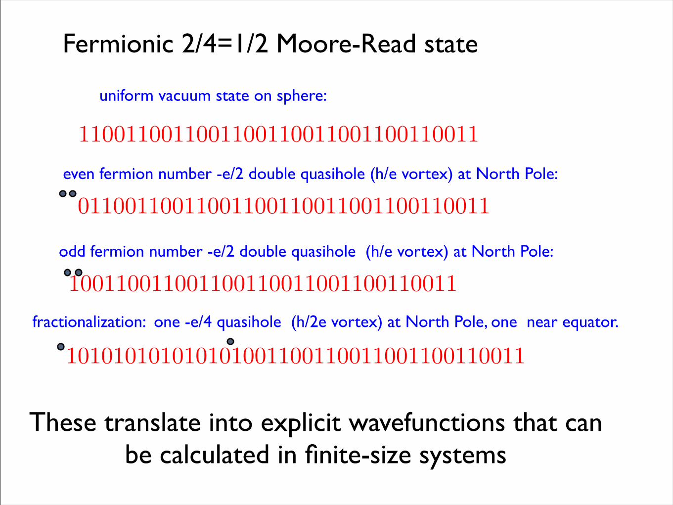
Fermionic 2/4=1/2 Moore-Read state

1100110011001100110011001100110011

uniform vacuum state on sphere:

even fermion number -e/2 double quasihole (h/e vortex) at North Pole:

odd fermion number -e/2 double quasihole (h/e vortex) at North Pole:

01100110011001100110011001100110011

100110011001100110011001100110011fractionalization: one -e/4 quasihole (h/2e vortex) at North Pole, one near equator.

101010101010101001100110011001100110011

These translate into explicit wavefunctions that can be calculated in finite-size systems

3/5 (fibonacci) Read-Rezayi state primary configurations

11010110101101011010110101101 . . .

1001110011100111001110011100111 . . .

01110011100111001110011100111 . . .

111001110011100111001110011100 . . .

110011100111001110011100111001 . . .10101101011010110101101011010 . . .

01101011010110101101011010110 . . .

0101101011010110101101011010 . . .

elementary -e/5 vortex at North polevortex movesby hopping5 orbitals at atime

For charge -ne/5, n > 1 there are always 2 orthogonal primary states.

• Counting of states determines all “trace formulas” of cft, fusion rules, etc.

• . . . 202020202020200000000000. . . 111111111110000000000. . . 111111111100000000000

. . . 02020202020202020000000000

. . . 02020202020202010000000000

. . . 02020202020202000000000000

S=0 primary

S=1/2 primary

S=1 primary

example: SU(2)k=2 (= Moore Read state)

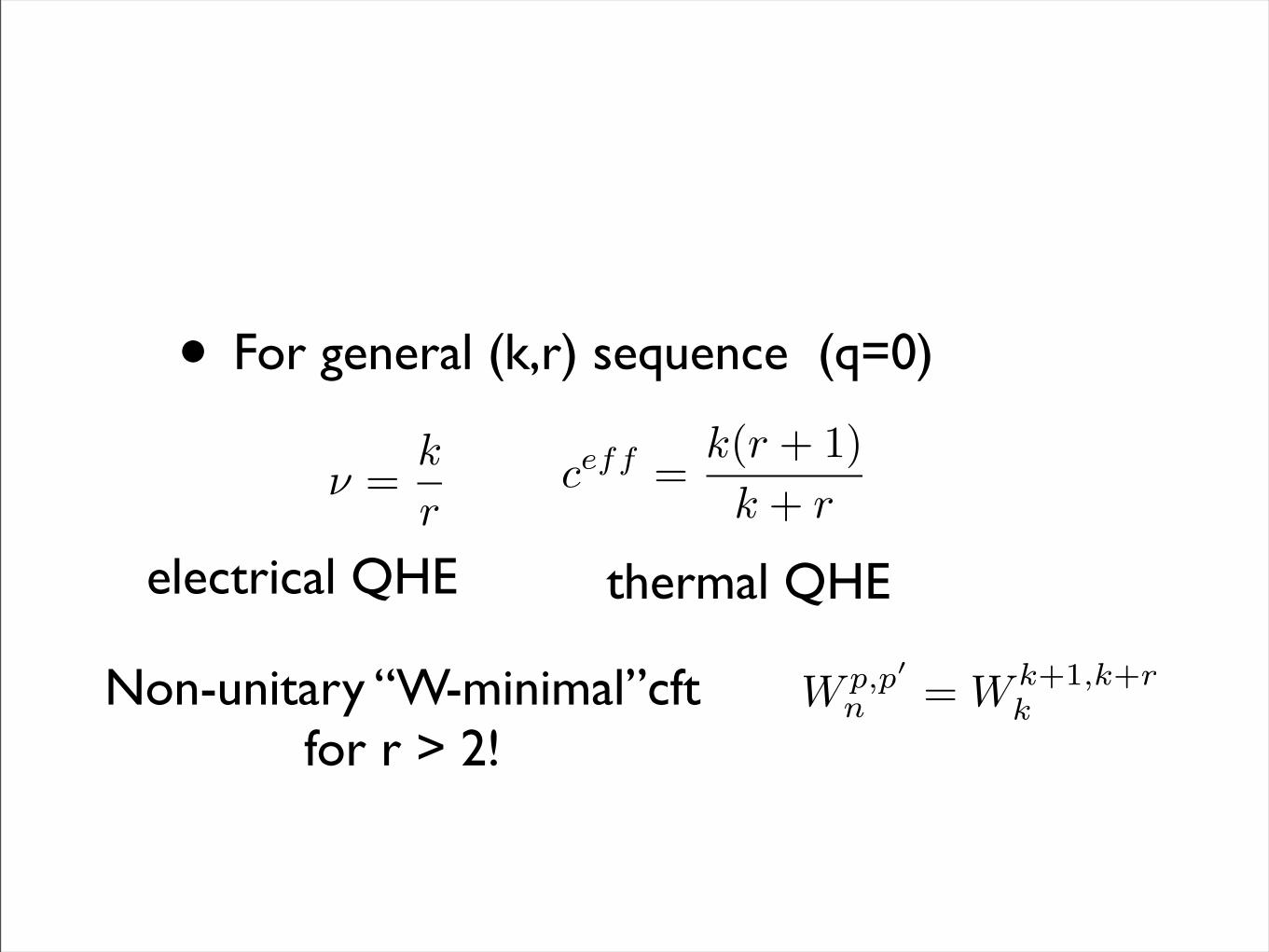
• For general (k,r) sequence (q=0)

! =k

r

electrical QHE thermal QHE

Non-unitary “W-minimal”cft for r > 2!

W p,p!

n = W k+1,k+rk

ceff =k(r + 1)k + r

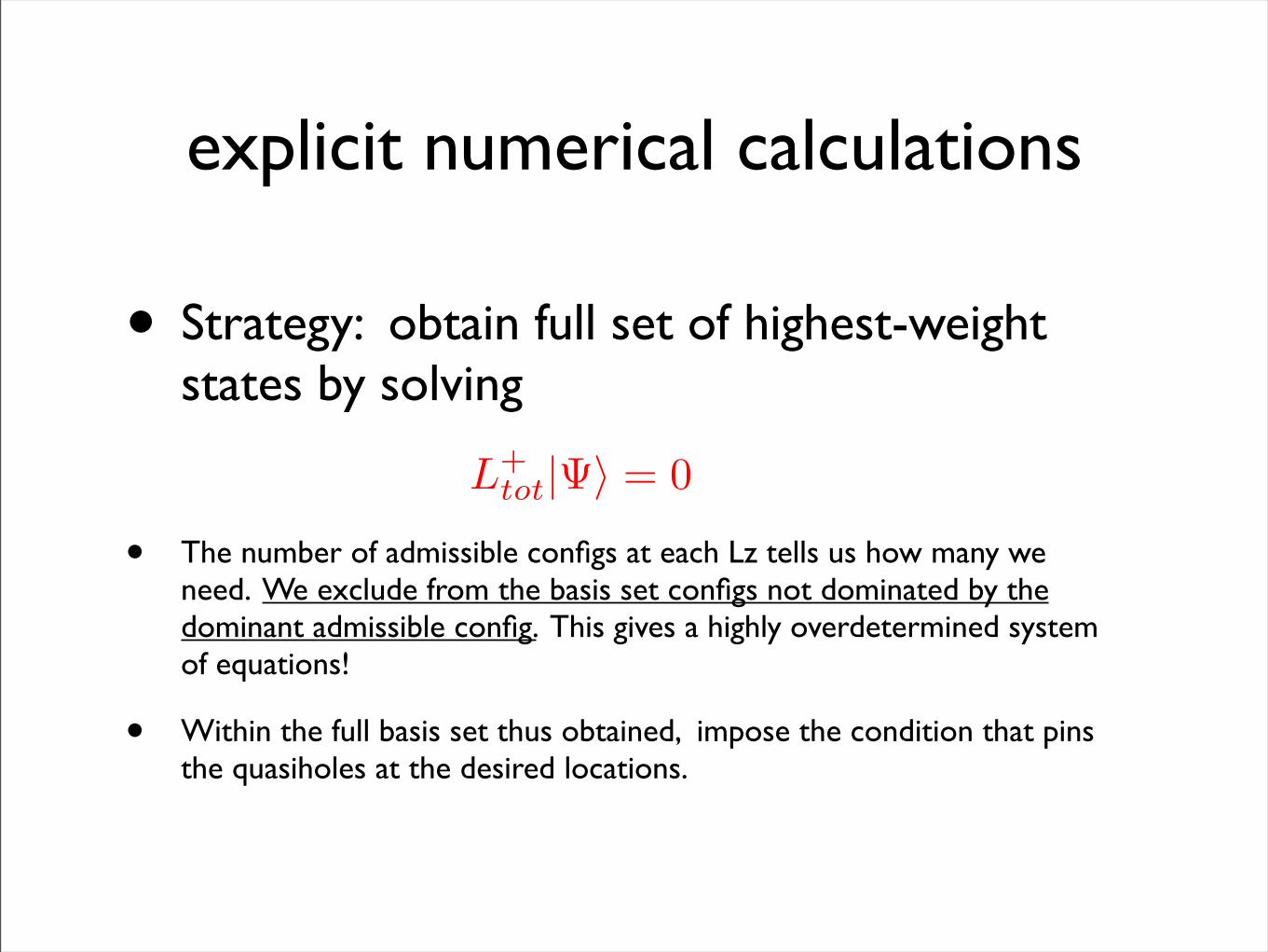
explicit numerical calculations

• Strategy: obtain full set of highest-weight states by solving

• The number of admissible configs at each Lz tells us how many we need. We exclude from the basis set configs not dominated by the dominant admissible config. This gives a highly overdetermined system of equations!

• Within the full basis set thus obtained, impose the condition that pins the quasiholes at the desired locations.

L+tot|!! = 0

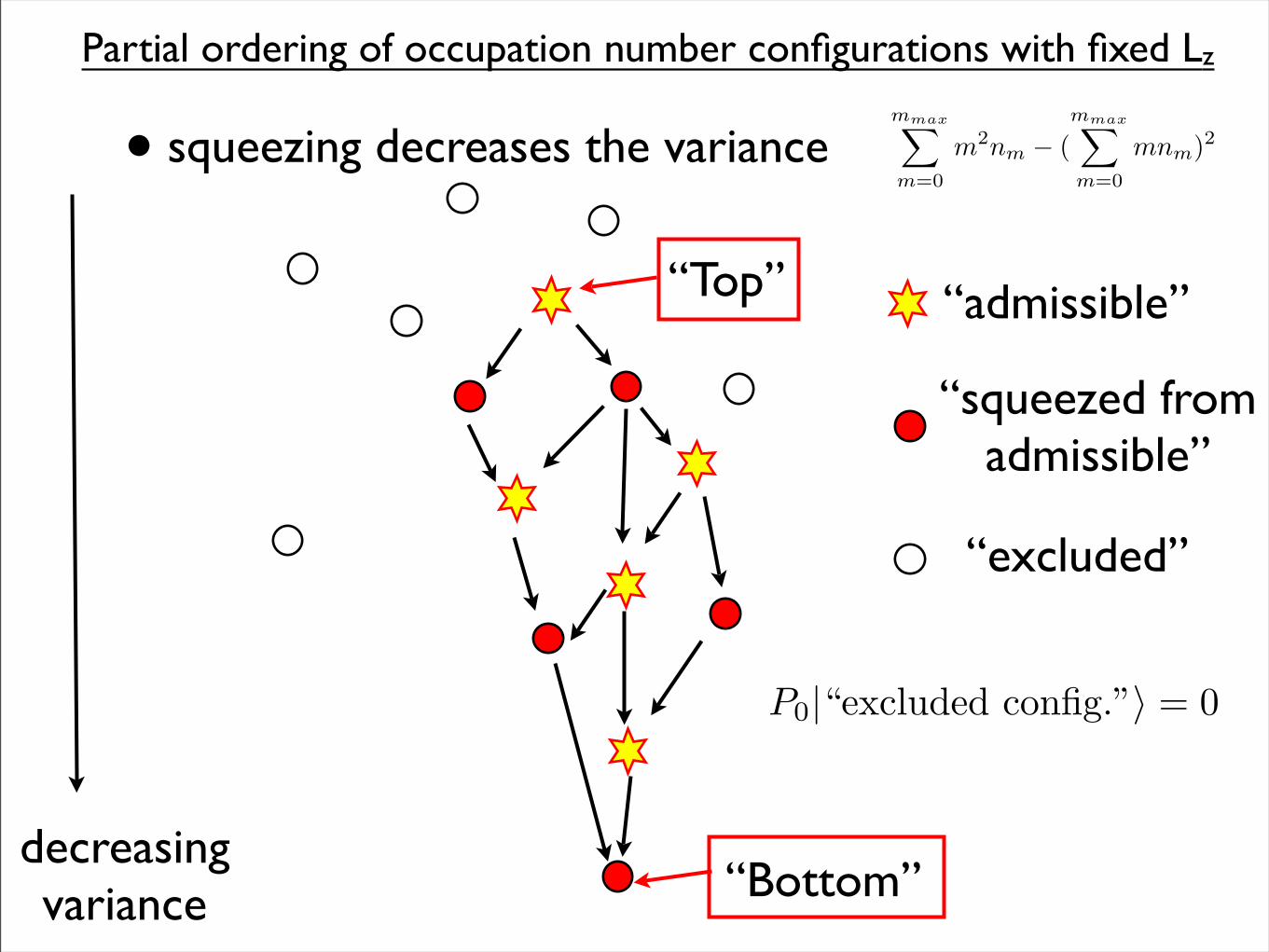
Partial ordering of occupation number configurations with fixed Lz

• squeezing decreases the variancemmax!

m=0

m2nm ! (mmax!

m=0

mnm)2

decreasing variance

“Top”

“Bottom”

“admissible”

“squeezed from admissible”

“excluded”

P0|“excluded config.”! = 0

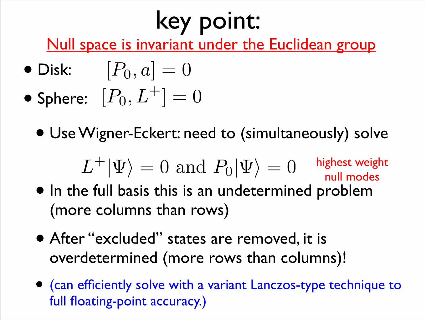
• Use Wigner-Eckert: need to (simultaneously) solve

• In the full basis this is an undetermined problem (more columns than rows)

• After “excluded” states are removed, it is overdetermined (more rows than columns)!

• (can efficiently solve with a variant Lanczos-type technique to full floating-point accuracy.)

• Disk:

• Sphere:

key point:

[P0, a] = 0[P0, L

+] = 0

Null space is invariant under the Euclidean group

highest weight null modes

L+|!! = 0 and P0|!! = 0

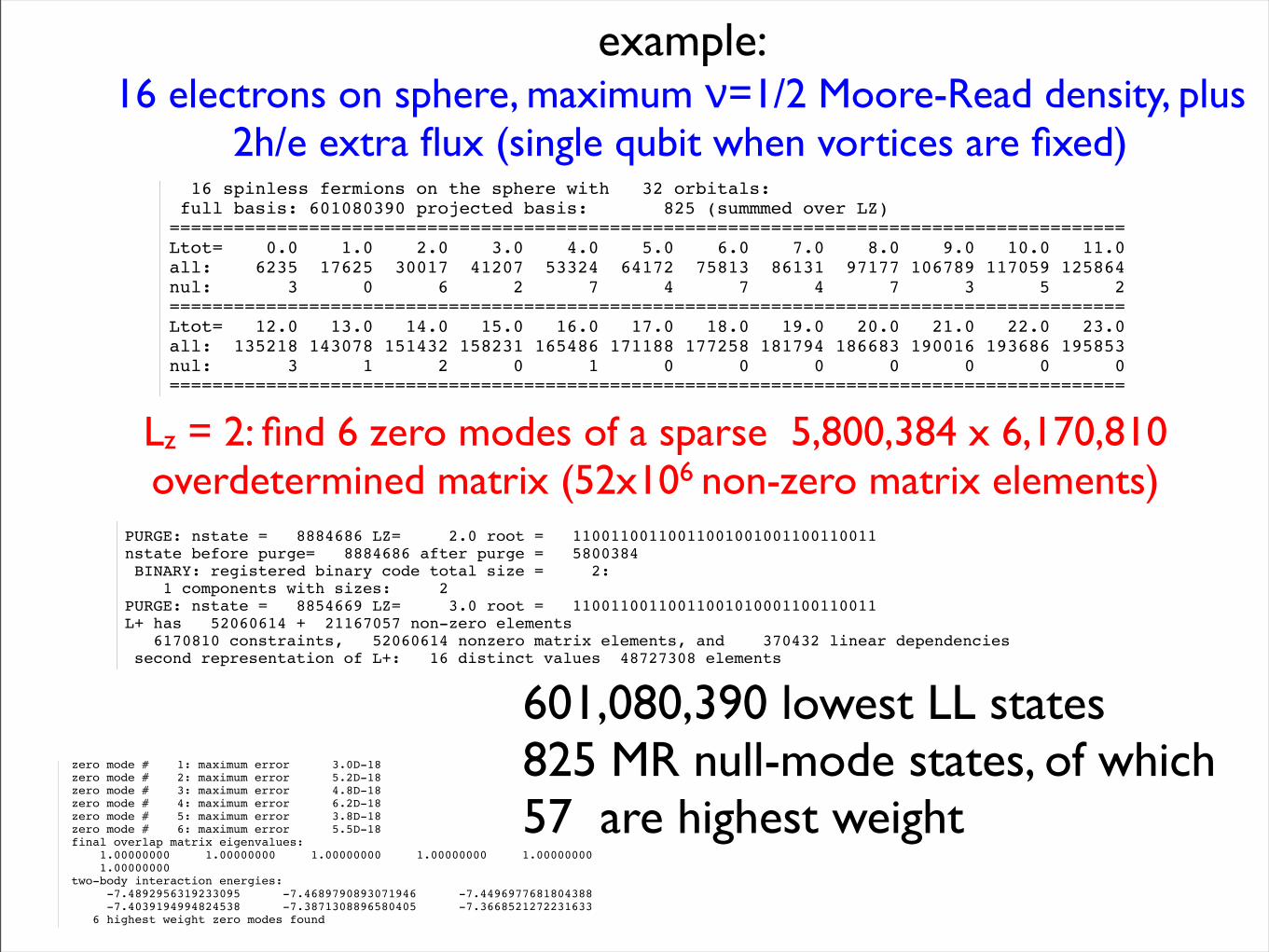
example: 16 electrons on sphere, maximum ν=1/2 Moore-Read density, plus

2h/e extra flux (single qubit when vortices are fixed)

output Wed Jun 21 19:14:22 2006 1

Program ZSPHERE: projection into FQHE zero-mode spaces

large arrays limits set by adjustable parameter variables:MXNSTATE= 10000000 (configurations with fixed Lz)STORAGE = 20000000 (MXNSTATE x SIZE of binary config code)STORELST= 40000000 (total STORAGE for all Lz sectors)MAXLLIST= 90000000 (number of non-zero elements of L+ )ZSTORE = 70000000 (space for stored zeromodes)

give datafile name (6 characters, in quotes) enter 0 to do full calculation enter n to do only subspace n enter -1 to do only Wigner Eckert with pair density enter -2 to do only Wigner Eckert without pair density enter 0 or 1 for " fast" or "debug" calculations;also give a seed integer for a random numbers (use different seeds when combining calculations)NEL = number of particles NORB = 2L+1 = Nflux +1 = number of orbitals give nel,norb for k > 0, nu_max = k0/(k0*m0+2) ; (k=0, m even/odd for free bosons/fermions) give projection type k0,m0: default interaction (n=0 landau level, Coulomb) BINARY: registered binary code total size = 2: 1 components with sizes: 2 16 spinless fermions on the sphere with 32 orbitals: full basis: 601080390 projected basis: 825 (summmed over LZ)=========================================================================================Ltot= 0.0 1.0 2.0 3.0 4.0 5.0 6.0 7.0 8.0 9.0 10.0 11.0all: 6235 17625 30017 41207 53324 64172 75813 86131 97177 106789 117059 125864nul: 3 0 6 2 7 4 7 4 7 3 5 2=========================================================================================Ltot= 12.0 13.0 14.0 15.0 16.0 17.0 18.0 19.0 20.0 21.0 22.0 23.0all: 135218 143078 151432 158231 165486 171188 177258 181794 186683 190016 193686 195853nul: 3 1 2 0 1 0 0 0 0 0 0 0=========================================================================================Ltot= 24.0 25.0 26.0 27.0 28.0 29.0 30.0 31.0 32.0 33.0 34.0 35.0all: 198308 199313 200616 200495 200691 199542 198684 196573 194791 191805 189174 185450nul: 0 0 0 0 0 0 0 0 0 0 0 0=========================================================================================Ltot= 36.0 37.0 38.0 39.0 40.0 41.0 42.0 43.0 44.0 45.0 46.0 47.0all: 182078 177713 173741 168841 164375 159089 154232 148660 143557 137800 132538 126726nul: 0 0 0 0 0 0 0 0 0 0 0 0=========================================================================================Ltot= 48.0 49.0 50.0 51.0 52.0 53.0 54.0 55.0 56.0 57.0 58.0 59.0all: 121404 115614 110338 104648 99488 93993 89004 83748 79012 74039 69580 64944nul: 0 0 0 0 0 0 0 0 0 0 0 0=========================================================================================Ltot= 60.0 61.0 62.0 63.0 64.0 65.0 66.0 67.0 68.0 69.0 70.0 71.0

output Wed Jun 21 19:14:22 2006 4

starting polishing phase 4 5 niter= 67 error in/out= 0.614D-15 0.475D-15 no more significant error improvement zeromode 5 is computed no useable data in "zeromode.006" using random data type 2 termination 1 6 niter= 4994 error in/out= 0.103D+01 0.268D-01 reached error limit of 0.600D-15 2 6 niter= 3136 error in/out= 0.268D-01 0.665D-05 reached error limit of 0.600D-15 3 6 niter= 2109 error in/out= 0.665D-05 0.116D-08 reached error limit of 0.600D-15 4 6 niter= 804 error in/out= 0.116D-08 0.607D-15 reached error limit of 0.600D-15 starting polishing phase 5 6 niter= 60 error in/out= 0.617D-15 0.496D-15 no more significant error improvement zeromode 6 is computed overlap matrix eigenvalues, trace = 6.00000000 1.00000000 1.00000000 1.00000000 1.00000000 1.00000000 1.00000000 quality control of 6 zero modes, basis size 5800384, satisfying 6170810 constraints zero mode # 1: maximum error 3.0D-18 zero mode # 2: maximum error 5.2D-18 zero mode # 3: maximum error 4.8D-18 zero mode # 4: maximum error 6.2D-18 zero mode # 5: maximum error 3.8D-18 zero mode # 6: maximum error 5.5D-18 final overlap matrix eigenvalues: 1.00000000 1.00000000 1.00000000 1.00000000 1.00000000 1.00000000 two-body interaction energies: -7.4892956319233095 -7.4689790893071946 -7.4496977681804388 -7.4039194994824538 -7.3871308896580405 -7.3668521272231633 6 highest weight zero modes foundstorage used: 34802304

output Wed Jun 21 19:14:22 2006 2

all: 60792 56506 52696 48770 45304 41758 38630 35450 32675 29846 27396 24917nul: 0 0 0 0 0 0 0 0 0 0 0 0=========================================================================================Ltot= 72.0 73.0 74.0 75.0 76.0 77.0 78.0 79.0 80.0 81.0 82.0 83.0all: 22776 20617 18772 16906 15329 13742 12403 11059 9945 8816 7891 6961nul: 0 0 0 0 0 0 0 0 0 0 0 0=========================================================================================Ltot= 84.0 85.0 86.0 87.0 88.0 89.0 90.0 91.0 92.0 93.0 94.0 95.0all: 6201 5436 4824 4200 3710 3212 2821 2424 2123 1809 1575 1333nul: 0 0 0 0 0 0 0 0 0 0 0 0=========================================================================================Ltot= 96.0 97.0 98.0 99.0 100.0 101.0 102.0 103.0 104.0 105.0 106.0 107.0all: 1155 968 837 693 596 490 418 339 290 231 196 155nul: 0 0 0 0 0 0 0 0 0 0 0 0=========================================================================================Ltot= 108.0 109.0 110.0 111.0 112.0 113.0 114.0 115.0 116.0 117.0 118.0 119.0all: 131 101 86 64 55 41 34 24 21 14 12 8nul: 0 0 0 0 0 0 0 0 0 0 0 0=========================================================================================Ltot= 120.0 121.0 122.0 123.0 124.0 125.0 126.0 127.0 128.0 129.0 130.0 131.0all: 7 4 4 2 2 1 1 0 1 0 0 0nul: 0 0 0 0 0 0 0 0 0 0 0 0=========================================================================================Ltot= 132.0 133.0 134.0 135.0 136.0all: 0 0 0 0 0nul: 0 0 0 0 0=========================================================================================PURGE: nstate = 8884686 LZ= 2.0 root = 11001100110011001001001100110011nstate before purge= 8884686 after purge = 5800384 BINARY: registered binary code total size = 2: 1 components with sizes: 2PURGE: nstate = 8854669 LZ= 3.0 root = 11001100110011001010001100110011L+ has 52060614 + 21167057 non-zero elements 6170810 constraints, 52060614 nonzero matrix elements, and 370432 linear dependencies second representation of L+: 16 distinct values 48727308 elements subspace 2 L = 2.0 zeromode problem has: nvec= 6170810 nbasis = 5800384 nzero= 6 ndefect = 370432 LZERO v0.1: workspace = 35000000 no useable data in "zeromode.001" using random data type 2 termination 1 1 niter= 4660 error in/out= 0.103D+01 0.180D-01 reached error limit of 0.600D-15 2 1 niter= 3187 error in/out= 0.180D-01 0.386D-05 reached error limit of 0.600D-15 3 1 niter= 2060 error in/out= 0.386D-05 0.610D-15 reached error limit of 0.600D-15 starting polishing phase 4 1 niter= 76 error in/out= 0.612D-15 0.477D-15 no more significant error improvement

Lz = 2: find 6 zero modes of a sparse 5,800,384 x 6,170,810 overdetermined matrix (52x106 non-zero matrix elements)

601,080,390 lowest LL states825 MR null-mode states, of which57 are highest weight

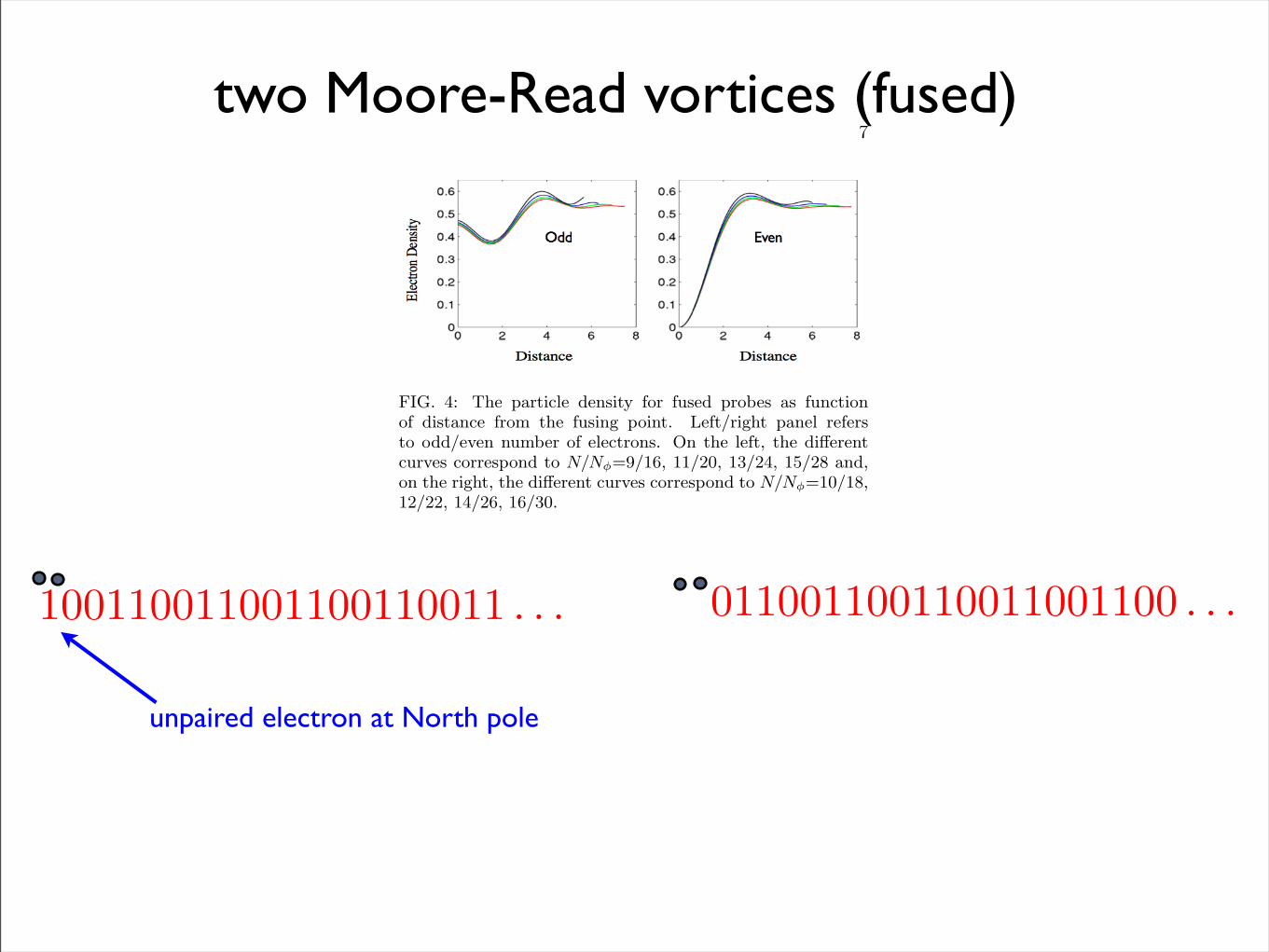
two Moore-Read vortices (fused)7

!"#$%&'( !"#$%&'(

FIG. 3: The spectrum of H(w1, w2)!H0 as function of distancebetween the probes, which are moved along the meridians(!, " = 0) and (!, " = #), with ! increasing from 0 to #/2.The left /right column corresponds to odd/even number ofelectrons. Starting from the top, the left panels correspondto N/N!=9/16, 11/20, 13/24, 15/28 and the right panels toN/N!=10/18, 12/22, 14/26, 16/30.

number of electrons). In this cases, the total many-bodyHilbert spaces have staggering dimensions of 77,558,760and 300,540,195, respectively. In this extremely largeHilbert spaces, we find a number of zero modes of H(2,2)

equal to 36 in the first case and 45 in the second case(in total agreement with Eq. (22)). If we fix w1 and w2

and diagonalize H(w1, w2)!H0 , we find one zero modefor both cases, with a precision better than 10!12. Of

FIG. 4: The particle density for fused probes as functionof distance from the fusing point. Left/right panel refersto odd/even number of electrons. On the left, the di!erentcurves correspond to N/N!=9/16, 11/20, 13/24, 15/28 and,on the right, the di!erent curves correspond to N/N!=10/18,12/22, 14/26, 16/30.

course, finding these zero modes would have been impos-sible without taking full advantage of the translationalsymmetry at the first step.

To visualize a state, we compute the correspondingparticle density and pair amplitude as functions of posi-tion on the sphere. The latest is given by the expectationvalue of !(2,2)(w)†!(2,2)(w). A plot of these quantitiesfor the zero modes discussed above, is shown in Fig. 2.The positions of the probes were chosen as ("=#/2,$=0)and ("=#/2,$ = #), so that we have maximum possi-ble separation between the trapped anyons. One can seethat, because the anyons are far apart, there is no visi-ble di!erence between even and odd cases (or S=0 andS=1). This is precisely what one should see in a topolog-ical degeneracy. As we shall see, things look completelydi!erent when we bring the anyons close to each other.Other things to remark about Fig. 2 are the fact that thedensity is finite while the pair amplitude is exactly zeroat the probe locations and the fact that the two anyonsappear to be totally separated.

Let us take a few lines here and explain our plots.Quantities that depend on the position on the sphere willbe shown as surface plots, with the quantity of intereston the z axis. The cartesian coordinates x and y describepoints of the sphere. If " and $ are the usual angles onthe sphere, then the relation between (",$) and (x, y) isgiven by "=

!x2 + y2 and $=arctan(y/x).

Next, we take a look at the spectrum of H(w1, w2)!H0

as function of probe separation, d(") =!

N! sin "2 , grad-

ually increasing the number of electrons from 9 to 16.For each size, the probes were moved along the merid-ians (",$=0) and (",$=#), with " increasing from 0 to#/2. The strength of the probe potential was fixed at%=1. The results are shown in Fig. 3, where each paneldisplays a number of bands (equal todimH0), each of them representing the flow of one eigen-value with the distance d. There is one and only oneeigenvalue that remains strictly zero (within a numericalerror that is less than 10!12!). The energy gap separat-ing the zero mode from the rest of the spectrum goes to

100110011001100110011 . . . 011001100110011001100 . . .

unpaired electron at North pole

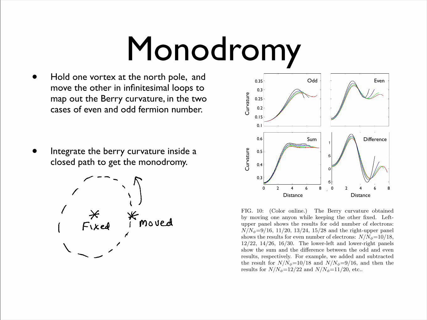
Monodromy• Hold one vortex at the north pole, and

move the other in infinitesimal loops to map out the Berry curvature, in the two cases of even and odd fermion number.

• Integrate the berry curvature inside a closed path to get the monodromy.

12

2n! 1 quasi-holes, the 2n!1 zero modes have the generalform:50

!i(w) = Ai(w)!̃i(w), (46)

where !̃i(w) is an analytic function of w and Ai(w) is anormalization factor that is not analytic of w. We have:

Tr{F̂ (w)} = 2Im!

i

"!1!i(w), [1! Pw]!2!i(w)#. (47)

Due to the presence of 1 ! Pw, the derivatives act onlyon the tilde part of the wave-functions and, consequently,we can pull out the normalization constants like below:

TrF̂ (w) = 2"i|Ai(w)|2

$Im"!1!̃i(w), [1! Pw]!2!̃i(w)#.(48)

Next we use the fact that !̃i are analytic functions:

TrF̂ (w) = 2"i|Ai(w)|2

$Im{"!w!̃i(w), [1! Pw]!w!̃i(w)#(!1w)"!2w}.(49)

The factor containing the expectation value is real, whichallows us to easily compute the imaginary part, resultingin:

TrF̂ (w) = 2"i|Ai(w)|2

$"!w!̃i(w), [1! Pw]!w!̃i(w)#.(50)

If one repeats exactly the same arguments for the quan-tum metric tensor given in Eq. 43, he will arrive to theconclusion:

gqµ!(w) = 2

"i|Ai(w)|2

$"!w!̃i(w), [1! Pw]!w!̃i(w)#"µ! .(51)

Since w1 and w2 coincide with the geodesic coordinates ofthe sphere at x (i.e. the coordinates in which the metrictensor is the identity matrix at x), the proof of Eq. 45is completed. The result, of course, extends also to theparafermion Hall sequences,34 and to geometries otherthan the sphere.

VII. ONE FLUX ADDED.

In this case we have 2 quasi-holes and the zero modesspace is 1-dimensional, which means we are in an Abeliansituation. We will keep one probe fixed and move theother along di"erent braiding paths. For the Abeliancase, the monodromy of any path # is determined bythe Berry phase #!, W!=ei"! . The Berry phase can becomputed from the curvature:

#! =#

S!

dF, (52)

Even Nel Odd Nel

Distance Distance

Curvature

Odd Even

Distance

Curv

atu

re D

iffe

renceSum Difference

0 2 4 6 8 0 2 4 6 8

0.3

0.4

0.5

0.6

0.1

0.15

0.2

0.25

0.3

0.35

Distance Distance

Curvatu

reC

urvatu

re

FIG. 10: (Color online.) The Berry curvature obtainedby moving one anyon while keeping the other fixed. Left-upper panel shows the results for odd number of electrons:N/N!=9/16, 11/20, 13/24, 15/28 and the right-upper panelshows the results for even number of electrons: N/N!=10/18,12/22, 14/26, 16/30. The lower-left and lower-right panelsshow the sum and the di!erence between the odd and evenresults, respectively. For example, we added and subtractedthe result for N/N!=10/18 and N/N!=9/16, and then theresults for N/N!=12/22 and N/N!=11/20, etc..

where S! is the surface enclosed by #. It is then veryuseful to map the curvature first.

We compute the coe$cient F of the curvature formfrom:

F (x) = limS!#0

W! ! 1iS!

, (53)

where # is a small path around x. We obtain the limitby considering paths of decreasing radiuses. The valueof F computed this way coincides with the coe$cient ofthe curvature corresponding to the coordinates (w1, w2)introduced at the beginning of the previous section.

The upper panels in Fig. 10 plot F (w) as a functionof the distance to the fixed probe for odd (left panel)and even (right panel) number of electrons. The curvesin Fig. 10 go asymptotically towards a constant value,which is precisely equal to the quasi-hole charge e"=e/4(when working on the sphere, there is a small correctionto this value, correction that goes to zero as the size isincreased). The most remarkable thing about these plotsis that the curvatures for odd/even number of electronshave di"erent thermodynamic limits, as one can clearlysee when looking at the di"erence, plotted in the lower-right panel of Fig. 10.

From the Berry curvature we compute the Berryphases accumulated as we move one probe along di"erentpaths of the form $=ct., while keeping the other probefixed at the North Pole. Fig. 11 shows the Berry phase

13

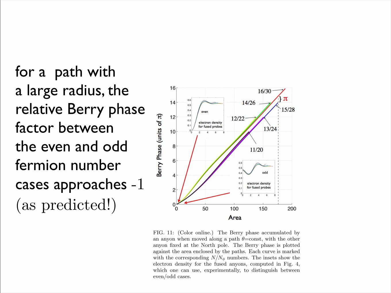
FIG. 11: (Color online.) The Berry phase accumulated byan anyon when moved along a path !=const, with the otheranyon fixed at the North pole. The Berry phase is plottedagainst the area enclosed by the paths. Each curve is markedwith the corresponding N/N! numbers. The insets show theelectron density for the fused anyons, computed in Fig. 4,which one can use, experimentally, to distinguish betweeneven/odd cases.

as function of the area enclosed by the path. We use thisfigure to draw several important conclusions. First, wepoint out that the Berry phase plotted in this figure in-cludes also the trivial Aharonov-Bohm phase due to themagnetic flux: !AB = e!!B . Thus it was expected thatthe total Berry phase, as a function of the enclosed area,to go asymptotically to a linear curve. The slope of thisasymptotic curve is equal to the charge of the quasi-holes.The second and most important fact is that the graphsfor even/odd number of electrons are shifted by ", as itwas previously predicted.46,48

We conclude this subsection with the observation thatthe coe!cient F depends on how we compute the areaenclosed by " in Eq. 53, more precisely on what metrictensor is used. The plots shown so far used the standardmetric of the sphere. We have repeated the calculationsusing the quantum metric tensor Eq. (43), in which casewe have to re-scale the coe!cient:

F q(w) = F (w)/!

det gqµ!(w). (54)

According to the our previous analytic prediction (seeEq. 45), F q(w) should be identically 1. We numericallychecked this prediction in the following way. The quan-tity that is readily available in the numerical calcualtionsis the quantum distance. We can compute the determi-nant of the quantum metric tensor by considering a circleof radius # (in the standard metric of the sphere) centered

12/23

14/27

10/19

15/29

13/25

11/21

FIG. 12: Plots of f0(x) for di!erent system sizes (each panelis marked with the corresponding N/N!). For each size, weshow f0(x) calculated with the standard metric tensor (left)and with the quantum metric tensor (right).

at w and calculate the quantum distance between w andthe points of this circle. If dq

M and dqm denote the max-

imum, respectively minimum quantum distance to thepoints of the circle, then

det gqµ!(w) = lim

""0

(dqmdq

M )2

#4. (55)

The computation of the determinant is done in the simul-taneously with the calculation of the curvature. The nu-merical calculation confirms that F q(w)=1 for all pointsof the sphere (excepting the North pole).

A. Two fluxes added.

In this case we have 4 quasi-holes and the zero modesspace is 2-dimensional. We will keep 3 quasi-holes fixedand move the forth one along di#erent braiding paths.

For the Non-Abelian case, there is no simple Stokestheorem,59,60 which means the monodromy can not besimply computed from the curvature. Even so, map-ping the curvature provides a clear picture of the non-comutative and topological properties of the states.

The parameter space remains 2-dimensional anddF=F̂ dw1!dw2, where F̂ is a 2"2 matrix now. Wecompute F̂ (x) using the algorithm presented above (seeEq. 53). Using the Pauli’s matrices, $i, i=1, 2, 3, F̂ (w)can be uniquely decomposed as:

F̂ (x) = f0(x) + f(x)!, (56)

where f0(w)= 12TrF̂ (w) and f is 3-component vector. We

will refer to f0 as the Abelian and to f! as the Non-Abelian part of the curvature.

for a path witha large radius, therelative Berry phase factor betweenthe even and odd fermion number cases approaches -1(as predicted!)

4 well-separated vortices (a qubit)

Note that the two state have slightly different“interference ripple” patterns in the electron density

that will be exponentially small as the distance betweenthe vortices increases, but which is a residual local physical

difference between the states.

single-particle density

m=1 two-particle density

Tetrahedral arrangement of 4 MR h/2e vortices, (14 electrons, 28 orbitals)

Sphere is mapped to unit disk.

the qubit doublet is split by the Coulomb interaction, both states are shown.THE SPLITTING AND LOCAL DIFFERENCE BETWEEN THE TWO STATES IS EXPECTED TO DISAPPEAR AS THE SYSTEM SIZE INCREASES.

One qubit is left after positions of vortices are fixed.

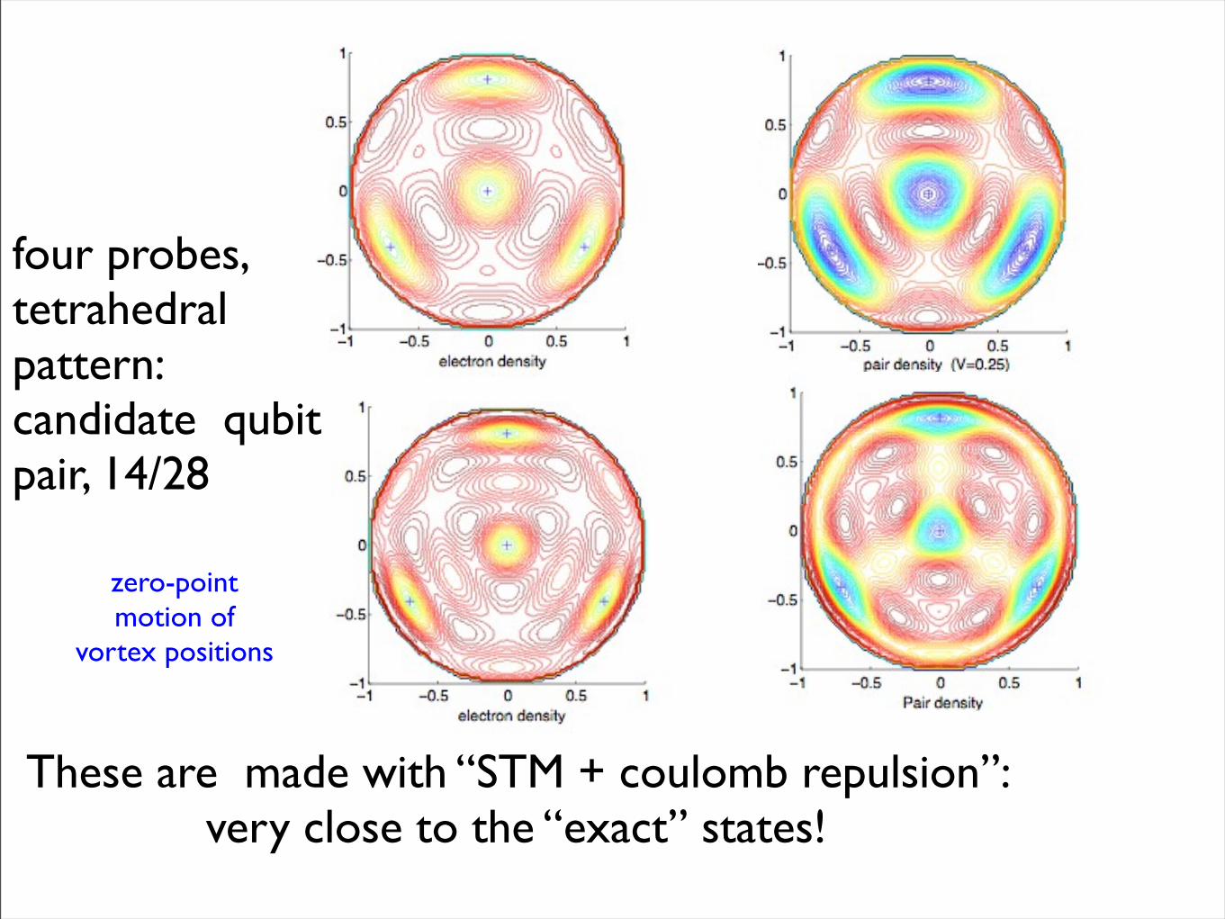
four probes, tetrahedral pattern: candidate qubit pair, 14/28

These are made with “STM + coulomb repulsion”: very close to the “exact” states!

zero-pointmotion of

vortex positions

non-Abelian Berry curvature , for increasing size (10-15 electrons)

10/2011/22

12/24 13/26

as size increases, the (magnititude) of the non-abelian curvature field is seen to be concentrated near the quasiparticle cores, consistent with braiding. (For widely separated vortices, there should be vanishing non-abelian curvature in the regions in between the vortices, so the monodromy becomes purely topological)

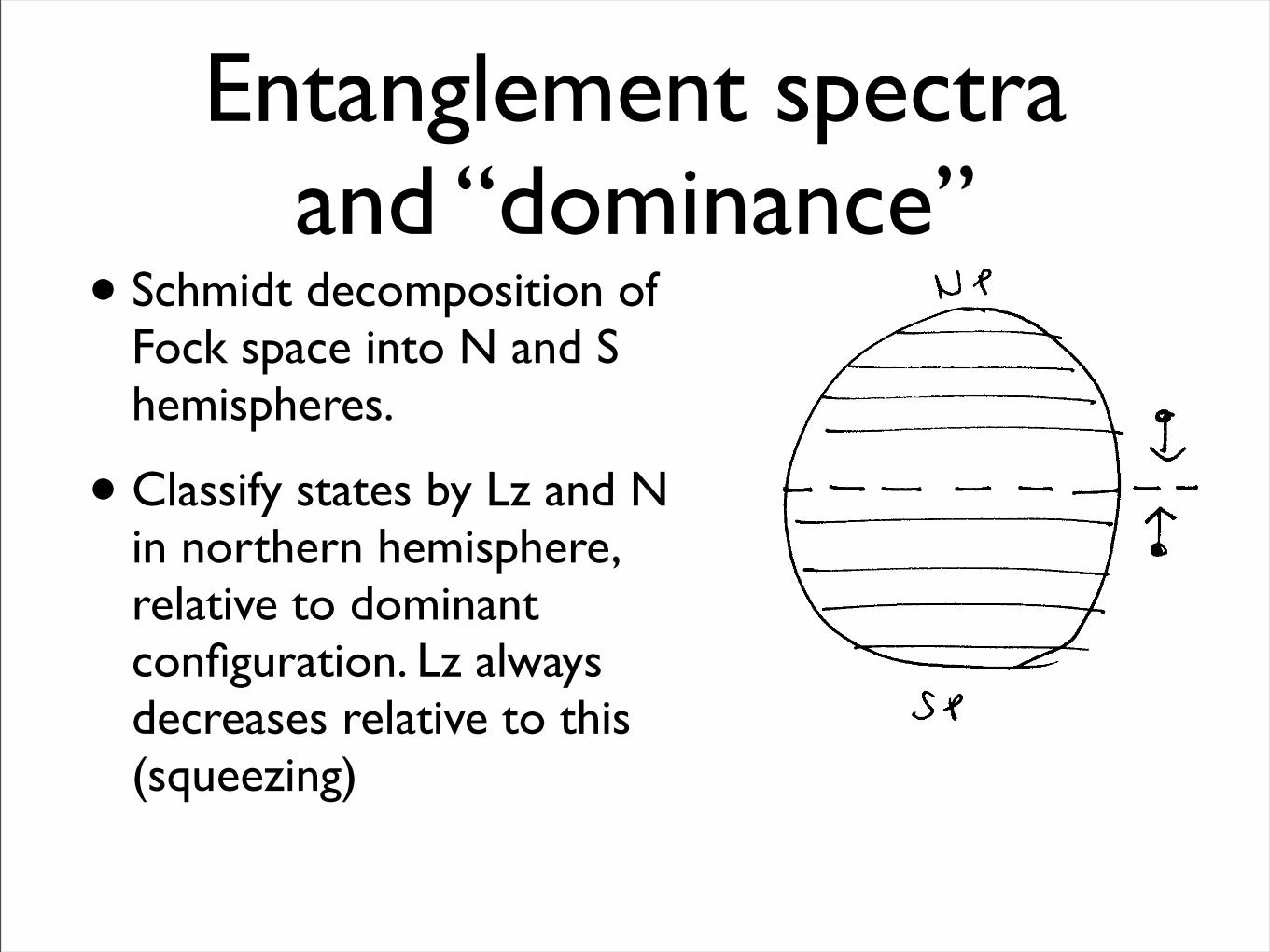
Entanglement spectra and “dominance”

• Schmidt decomposition of Fock space into N and S hemispheres.

• Classify states by Lz and N in northern hemisphere, relative to dominant configuration. Lz always decreases relative to this (squeezing)

Represent bipartite Schmidt decomposition like an excitation

spectrum (with Hui Li)

• like CFT of edge states.

• A lot more information than single number (entropy)

• many zero eigenvalues

|!! =!

!

e!"!/2|!N!! " |!S!!

2

(a) N = 10, N! = 27

(b) N = 12, N! = 33

FIG. 1: Entanglement spectrum for the 1/3-filling Laughlinstates, for N = 10, m = 3, N! = 27 and N = 12, m = 3, N! =33. Only sectors of NA = NB = N/2 are shown.

have a single element and their singular values are de-generate.

These features are indeed expected from the specialform of !N . Arbitrarily divide the subscripts in Eq. (2),i.e., l in ul and vl, into two subsets, say I and J . Let |I|be the number of elements in I and similarly |J |, notethat |I| + |J | = N . Re-write Eq. (2) as

!N = !I · !J ·!

i,j(uivj ! ujvi)

m (3)

where !I ="

i<i!(uivi! ! ui!vi)m, !J ="

j<j! (ujvj! !uj!vj)m, and i, i! " I, j, j! " J . The first two terms inthe product in Eq. (3), !I and !J , describe two Laugh-lin droplets that consist of particles in subsets I and J ,respectively. Expanding the third term, we get

!N = !(0)I !(0)

J + m · !(1)I !(1)

J + · · · (4)

where

!(0)I = !I ·

!

ium|J|

i (5)

!(0)J = !J ·

!

jvm|I|

j (6)

!(1)I = !I ·

!

ium|J|

i ·#

i

vi

ui(7)

!(1)J = !J ·

!

jvm|I|

j ·#

j

uj

vj(8)

and · · · represents other terms that are not of our con-cern here. Equation (4) indicates that the sectors at thegreatest two Lz

A’s each contains only one singular value.In order to explain the degeneracy of the two singularvalues, we need to show that the norms of the above fourstates are related by

#!(0)I ##!(0)

J # = m#!(1)I ##!(1)

J # (9)

Note that the total angular momentum operators of

subset I are LzI = 1

2

$

I"I

%

ui!

!ui! vi

!!vi

&

, L+I =

$

i"Iui!

!vi, L+

I =$

i"Ivi!

!ui. It is easy to show that

LzI!

(0)I = m

2 |I||J |!(0)I , L+

I !(0)I = 0, L#

I !(0)I = m|J |!(1)

I ,

which means that !(0)I and !(1)

I belong to the same ir-

reducible representation of which "L2I = S(S + 1) where

S = m2 |I||J |. Thus using L#

I |lz,S$ = [S(S + 1) ! lz(lz !

1)]1/2|lz ! 1,S$ and lz = S, we get

#!(1)I #2 =

1

m2|J |2#L#

I !(0)i #2 =

|I|

m|J |#!(0)

I #2 (10)

Similarly we have

#!(1)J #2 =

|J |

m|I|#!(0)

J #2 (11)

Therefore Eq. (9) is obtained.The alert readers may argue that partitioning sub-

scripts as done in Eq. (3) is not equivalent to partition-ing of Landau-level orbitals. However, the first two termsin Eq. (4) are in fact equivalent to what we would getfrom partitioning Landau-level orbitals, even though therest [those represented by · · · in Eq. (4)] are generally

TABLE I: The multiplicity M(!L) versus !L for electronicLaughlin states of di"erent sizes, for !L ! N/2. N is thenumbers of electrons, 1/m is the filling fraction.

!L 0 1 2 3 4 5 6

N = 6, m = 5 1 1 2 3

N = 8, m = 5 1 1 2 3 5

N = 8, m = 3 1 1 2 3 5

N = 10, m = 3 1 1 2 3 5 7

N = 12, m = 3 1 1 2 3 5 7 11

e!!! = 0

Look at difference between Laughlin state,entanglement spectrum and state that interpolates to Coulomb ground state.

3

(a) x = 1 (b) x = 1/3 (c) x = 1/10

FIG. 2: Entanglement spectrum for the ground state, for a system of N = 10 electrons in the lowest Landau level on a sphereenclosing N! = 27 flux quanta, of the Hamiltonian in Eq. (12) for various values of x.

not. By setting |I| = |J | = N/2, we see that the first twoterms in Eq. (4) indeed correspond to the Lz

A = max(LzA)

and LzA = max(Lz

A) ! 1 sectors in Fig. 1. This not onlyexplains why these two sectors each has only one singu-lar value and why the two singular values are degenerate,but also explicitly gives max(Lz

A) = mN2/8.

The most interesting feature of the spectra shown inFig. 1 may be the counting structure. We define a newsymbol !L := max(Lz

A) ! LzA to label the sectors, and

M(!L) be the multiplicity of the sector, i.e., the numberof singular values in the sector. In Table I we list a fewvalues of M(!L) for several small !L, for systems ofdi"erent sizes. Interestingly, M(!L) listed there seemsto be the number of integer partitions of !L. We spec-ulate that in the thermodynamic limit where N " #,M(!L)is exactly the number of integer partitions for any!L. Our numerical study also indicates that this is a

FIG. 3: The gap in various sectors of the entanglement spec-trum of the ground state of the Hamiltonian in Eq. (12) fora system of N = 10 electrons in the lowest Landau level ona sphere enclosing N! = 27 flux quanta. At x ! 1, the gapappears to be linear in " log x.

unique feature for all states in the Laughlin sequence,independent of filling fraction.

This can be understood when we further review theform of Laughlin wave-functions in Eq. (3). Eventhough it is not explicitly about partitioning Landau-level orbitals, it reveals the origin of the entanglement inLaughlin states, correlated quasi-hole excitations in thetwo blocks. Thus the multiplicity M(!L) is simply thenumber of linearly-independent quasi-hole excitations inblock A that have total Lz angular momentum equal to!L, which, in a su#ciently large system, is exactly thenumber of ways that the integer !L can be partitioned.For any finite system, as soon as !L > N/2, some ofthe partitions of !L may contain parts that are greaterthan N/2. Since no quasi-hole can carry angular momen-tum larger than N/2, multiplicity of such a !L will besmaller than the number of partitions. Indeed, this is infull consistency with our numerical analysis.

Now we turn to the entanglement spectrum of trueground states of Coulomb interaction. The system wewill be interested in has N = 10 electrons in the lowestLandau level on the sphere that contains N! = 28 fluxquanta. This system has the same size of one that sup-ports an N = 10, m = 3 Laughlin state. We will studythe numerically obtained ground state of the followingHamiltonian [9]

H = xHc + (1 ! x)V1 (12)

where x $ [0, 1] is the tuning parameter, Hc is the Hamil-tonian of Coulomb interaction in the lowest Landau level,while V1 is the pseudo-potential that gives unit energywhenever the relative angular momentum of a pair ofelectrons is 1. For a few typical values of x, the spectraare presented in Fig. 2.

For the ground state of the unmodified Coulomb inter-action in the lowest Landau level (x = 1), the spectrumshows a clear gap near max(Lz

A) which in our case here is752 , which gradually closes as Lz

A decreases to % 30. Thegap becomes clearer for all Lz

A ! max(LzA) at x = 1/3,

3

(a) x = 1 (b) x = 1/3 (c) x = 1/10

FIG. 2: Entanglement spectrum for the ground state, for a system of N = 10 electrons in the lowest Landau level on a sphereenclosing N! = 27 flux quanta, of the Hamiltonian in Eq. (12) for various values of x.

not. By setting |I| = |J | = N/2, we see that the first twoterms in Eq. (4) indeed correspond to the Lz

A = max(LzA)

and LzA = max(Lz

A) ! 1 sectors in Fig. 1. This not onlyexplains why these two sectors each has only one singu-lar value and why the two singular values are degenerate,but also explicitly gives max(Lz

A) = mN2/8.

The most interesting feature of the spectra shown inFig. 1 may be the counting structure. We define a newsymbol !L := max(Lz

A) ! LzA to label the sectors, and

M(!L) be the multiplicity of the sector, i.e., the numberof singular values in the sector. In Table I we list a fewvalues of M(!L) for several small !L, for systems ofdi"erent sizes. Interestingly, M(!L) listed there seemsto be the number of integer partitions of !L. We spec-ulate that in the thermodynamic limit where N " #,M(!L)is exactly the number of integer partitions for any!L. Our numerical study also indicates that this is a

FIG. 3: The gap in various sectors of the entanglement spec-trum of the ground state of the Hamiltonian in Eq. (12) fora system of N = 10 electrons in the lowest Landau level ona sphere enclosing N! = 27 flux quanta. At x ! 1, the gapappears to be linear in " log x.

unique feature for all states in the Laughlin sequence,independent of filling fraction.

This can be understood when we further review theform of Laughlin wave-functions in Eq. (3). Eventhough it is not explicitly about partitioning Landau-level orbitals, it reveals the origin of the entanglement inLaughlin states, correlated quasi-hole excitations in thetwo blocks. Thus the multiplicity M(!L) is simply thenumber of linearly-independent quasi-hole excitations inblock A that have total Lz angular momentum equal to!L, which, in a su#ciently large system, is exactly thenumber of ways that the integer !L can be partitioned.For any finite system, as soon as !L > N/2, some ofthe partitions of !L may contain parts that are greaterthan N/2. Since no quasi-hole can carry angular momen-tum larger than N/2, multiplicity of such a !L will besmaller than the number of partitions. Indeed, this is infull consistency with our numerical analysis.

Now we turn to the entanglement spectrum of trueground states of Coulomb interaction. The system wewill be interested in has N = 10 electrons in the lowestLandau level on the sphere that contains N! = 28 fluxquanta. This system has the same size of one that sup-ports an N = 10, m = 3 Laughlin state. We will studythe numerically obtained ground state of the followingHamiltonian [9]

H = xHc + (1 ! x)V1 (12)

where x $ [0, 1] is the tuning parameter, Hc is the Hamil-tonian of Coulomb interaction in the lowest Landau level,while V1 is the pseudo-potential that gives unit energywhenever the relative angular momentum of a pair ofelectrons is 1. For a few typical values of x, the spectraare presented in Fig. 2.

For the ground state of the unmodified Coulomb inter-action in the lowest Landau level (x = 1), the spectrumshows a clear gap near max(Lz

A) which in our case here is752 , which gradually closes as Lz

A decreases to % 30. Thegap becomes clearer for all Lz

A ! max(LzA) at x = 1/3,

x=0 is pureLaughlin

Can we identify topological order in “physical as opposed to model wavefunctions from low-energy entanglement spectra?

Summary

• Generalized Pauli-like “admissibility” criterion gives counting of Laughlin/Moore-Read/Read-Rezayi states with quasi-holes, and specifies “dominant” configurations.

• Gives a simplified basis for practical calculations (analog of projection into the lowest Landau level, now into Read-Rezayi zero mode space)

• (Generalizes to describe quasiPARTICLES too, - with A. Bernevig)

• Entanglement spectra.

• Finally, non-Unitary cft’s seem to be well-behaved and regularized when derived from polynomials: expect heff instead of h for primary field propagators!

• Idea runs counter to Read’s idea that non-Unitary means a gapless bulk theory inside the droplet,