Generalized nonlinear models in R: An overview of the gnm package Heather Turner and David Firth * University of Warwick, UK For gnm version 1.1-0 , 2018-06-20 Contents 1 Introduction 2 2 Generalized linear models 2 2.1 Preamble ..................................................... 2 2.2 Diag and Symm .................................................. 2 2.3 Topo ........................................................ 3 2.4 The wedderburn family ............................................. 5 2.5 termPredictors ................................................. 5 3 Nonlinear terms 6 3.1 Basic mathematical functions of predictors .................................... 6 3.2 MultHomog .................................................... 7 3.3 Dref ....................................................... 7 3.4 instances .................................................... 8 3.5 Custom nonlin functions ............................................. 8 3.5.1 General description ............................................ 8 3.5.2 Example: a logistic function ....................................... 9 3.5.3 Example: MultHomog .......................................... 9 4 Controlling the fitting procedure 10 4.1 Basic control parameters ............................................. 10 4.2 Specifying starting values ............................................. 10 4.2.1 Using start ............................................... 10 4.2.2 Using etastart or mustart ...................................... 11 4.3 Using constrain ................................................. 12 4.4 Using eliminate ................................................. 14 5 Methods and accessor functions 17 5.1 Methods ...................................................... 17 5.2 ofInterest and pickCoef ........................................... 19 5.3 checkEstimable ................................................. 19 5.4 getContrasts, se ................................................ 21 5.5 residSVD ..................................................... 23 6 gnm or (g)nls? 24 * This work was supported by the Economic and Social Research Council (UK) through Professorial Fellowship RES-051-27-0055. 1

Welcome message from author
This document is posted to help you gain knowledge. Please leave a comment to let me know what you think about it! Share it to your friends and learn new things together.
Transcript
Generalized nonlinear models in R: An overview of the gnm
package
Heather Turner and David Firth*
University of Warwick, UK
For gnm version 1.1-0 , 2018-06-20
Contents
1 Introduction 2
2 Generalized linear models 2
2.1 Preamble . . . . . . . . . . . . . . . . . . . . . . . . . . . . . . . . . . . . . . . . . . . . . . . . . . . . . 2
2.2 Diag and Symm . . . . . . . . . . . . . . . . . . . . . . . . . . . . . . . . . . . . . . . . . . . . . . . . . . 2
2.3 Topo . . . . . . . . . . . . . . . . . . . . . . . . . . . . . . . . . . . . . . . . . . . . . . . . . . . . . . . . 3
2.4 The wedderburn family . . . . . . . . . . . . . . . . . . . . . . . . . . . . . . . . . . . . . . . . . . . . . 5
2.5 termPredictors . . . . . . . . . . . . . . . . . . . . . . . . . . . . . . . . . . . . . . . . . . . . . . . . . 5
3 Nonlinear terms 6
3.1 Basic mathematical functions of predictors . . . . . . . . . . . . . . . . . . . . . . . . . . . . . . . . . . . . 6
3.2 MultHomog . . . . . . . . . . . . . . . . . . . . . . . . . . . . . . . . . . . . . . . . . . . . . . . . . . . . 7
3.3 Dref . . . . . . . . . . . . . . . . . . . . . . . . . . . . . . . . . . . . . . . . . . . . . . . . . . . . . . . 7
3.4 instances . . . . . . . . . . . . . . . . . . . . . . . . . . . . . . . . . . . . . . . . . . . . . . . . . . . . 8
3.5 Custom nonlin functions . . . . . . . . . . . . . . . . . . . . . . . . . . . . . . . . . . . . . . . . . . . . . 8
3.5.1 General description . . . . . . . . . . . . . . . . . . . . . . . . . . . . . . . . . . . . . . . . . . . . 8
3.5.2 Example: a logistic function . . . . . . . . . . . . . . . . . . . . . . . . . . . . . . . . . . . . . . . 9
3.5.3 Example: MultHomog . . . . . . . . . . . . . . . . . . . . . . . . . . . . . . . . . . . . . . . . . . 9
4 Controlling the fitting procedure 10
4.1 Basic control parameters . . . . . . . . . . . . . . . . . . . . . . . . . . . . . . . . . . . . . . . . . . . . . 10
4.2 Specifying starting values . . . . . . . . . . . . . . . . . . . . . . . . . . . . . . . . . . . . . . . . . . . . . 10
4.2.1 Using start . . . . . . . . . . . . . . . . . . . . . . . . . . . . . . . . . . . . . . . . . . . . . . . 10
4.2.2 Using etastart or mustart . . . . . . . . . . . . . . . . . . . . . . . . . . . . . . . . . . . . . . 11
4.3 Using constrain . . . . . . . . . . . . . . . . . . . . . . . . . . . . . . . . . . . . . . . . . . . . . . . . . 12
4.4 Using eliminate . . . . . . . . . . . . . . . . . . . . . . . . . . . . . . . . . . . . . . . . . . . . . . . . . 14
5 Methods and accessor functions 17
5.1 Methods . . . . . . . . . . . . . . . . . . . . . . . . . . . . . . . . . . . . . . . . . . . . . . . . . . . . . . 17
5.2 ofInterest and pickCoef . . . . . . . . . . . . . . . . . . . . . . . . . . . . . . . . . . . . . . . . . . . 19
5.3 checkEstimable . . . . . . . . . . . . . . . . . . . . . . . . . . . . . . . . . . . . . . . . . . . . . . . . . 19
5.4 getContrasts, se . . . . . . . . . . . . . . . . . . . . . . . . . . . . . . . . . . . . . . . . . . . . . . . . 21
5.5 residSVD . . . . . . . . . . . . . . . . . . . . . . . . . . . . . . . . . . . . . . . . . . . . . . . . . . . . . 23
6 gnm or (g)nls? 24
*This work was supported by the Economic and Social Research Council (UK) through Professorial Fellowship RES-051-27-0055.
1
7 Examples 25
7.1 Row-column association models . . . . . . . . . . . . . . . . . . . . . . . . . . . . . . . . . . . . . . . . . 25
7.1.1 RC(1) model . . . . . . . . . . . . . . . . . . . . . . . . . . . . . . . . . . . . . . . . . . . . . . . 25
7.1.2 RC(2) model . . . . . . . . . . . . . . . . . . . . . . . . . . . . . . . . . . . . . . . . . . . . . . . 27
7.1.3 Homogeneous effects . . . . . . . . . . . . . . . . . . . . . . . . . . . . . . . . . . . . . . . . . . . 28
7.2 Diagonal reference models . . . . . . . . . . . . . . . . . . . . . . . . . . . . . . . . . . . . . . . . . . . . 30
7.3 Uniform difference (UNIDIFF) models . . . . . . . . . . . . . . . . . . . . . . . . . . . . . . . . . . . . . . 37
7.4 Generalized additive main effects and multiplicative interaction (GAMMI) models . . . . . . . . . . . . . . 39
7.5 Biplot models . . . . . . . . . . . . . . . . . . . . . . . . . . . . . . . . . . . . . . . . . . . . . . . . . . . 41
7.6 Stereotype model for multinomial response . . . . . . . . . . . . . . . . . . . . . . . . . . . . . . . . . . . 46
7.7 Lee-Carter model for trends in age-specific mortality . . . . . . . . . . . . . . . . . . . . . . . . . . . . . . 51
7.8 Exponential and sum-of-exponentials models for decay curves . . . . . . . . . . . . . . . . . . . . . . . . . 56
7.8.1 Example: single exponential decay term . . . . . . . . . . . . . . . . . . . . . . . . . . . . . . . . . 56
7.8.2 Example: sum of two exponentials . . . . . . . . . . . . . . . . . . . . . . . . . . . . . . . . . . . . 56
A User-level functions 59
1 Introduction
The gnm package provides facilities for fitting generalized nonlinear models, i.e., regression models in which the
link-transformed mean is described as a sum of predictor terms, some of which may be non-linear in the unknown
parameters. Linear and generalized linear models, as handled by the lm and glm functions in R, are included in
the class of generalized nonlinear models, as the special case in which there is no nonlinear term.
This document gives an extended overview of the gnm package, with some examples of applications. The
primary package documentation in the form of standard help pages, as viewed in R by, for example, ?gnm or
help(gnm), is supplemented rather than replaced by the present document.
We begin below with a preliminary note (Section 2) on some ways in which the gnm package extends R’s fa-
cilities for specifying, fitting and working with generalized linear models. Then (Section 3 onwards) the facilities
for nonlinear terms are introduced, explained and exemplified.
The gnm package is installed in the standard way for CRAN packages, for example by using install.packages.
Once installed, the package is loaded into an R session by
> library(gnm)
2 Generalized linear models
2.1 Preamble
Central to the facilities provided by the gnm package is the model-fitting function gnm , which interprets a model
formula and returns a model object. The user interface of gnm is patterned after glm (which is included in
R’s standard stats package), and indeed gnm can be viewed as a replacement for glm for specifying and fitting
generalized linear models. In general there is no reason to prefer gnm to glm for fitting generalized linear models,
except perhaps when the model involves a large number of incidental parameters which are treatable by gnm’s
eliminate mechanism (see Section 4.4).
While the main purpose of the gnm package is to extend the class of models to include nonlinear terms,
some of the new functions and methods can be used also with the familiar lm and glm model-fitting functions.
These are: three new data-manipulation functions Diag, Symm and Topo, for setting up structured interactions
between factors; a new family function, wedderburn, for modelling a continuous response variable in [0, 1] with
the variance function V(µ) = µ2(1 − µ)2 as in Wedderburn (1974); and a new generic function termPredictors
which extracts the contribution of each term to the predictor from a fitted model object. These functions are
briefly introduced here, before we move on to the main purpose of the package, nonlinear models, in Section 3.
2.2 Diag and Symm
When dealing with homologous factors, that is, categorical variables whose levels are the same, statistical models
often involve structured interaction terms which exploit the inherent symmetry. The functions Diag and Symm
facilitate the specification of such structured interactions.
2
As a simple example of their use, consider the log-linear models of quasi-independence, quasi-symmetry and
symmetry for a square contingency table. Agresti (2002), Section 10.4, gives data on migration between regions
of the USA between 1980 and 1985:
> count <- c(11607, 100, 366, 124,
+ 87, 13677, 515, 302,
+ 172, 225, 17819, 270,
+ 63, 176, 286, 10192 )
> region <- c("NE", "MW", "S", "W")
> row <- gl(4, 4, labels = region)
> col <- gl(4, 1, length = 16, labels = region)
The comparison of models reported by Agresti can be achieved as follows:
> independence <- glm(count ~ row + col, family = poisson)
> quasi.indep <- glm(count ~ row + col + Diag(row, col), family = poisson)
> symmetry <- glm(count ~ Symm(row, col), family = poisson)
> quasi.symm <- glm(count ~ row + col + Symm(row, col), family = poisson)
> comparison1 <- anova(independence, quasi.indep, quasi.symm)
> print(comparison1, digits = 7)
Analysis of Deviance Table
Model 1: count ~ row + col
Model 2: count ~ row + col + Diag(row, col)
Model 3: count ~ row + col + Symm(row, col)
Resid. Df Resid. Dev Df Deviance
1 9 125923.29
2 5 69.51 4 125853.78
3 3 2.99 2 66.52
> comparison2 <- anova(symmetry, quasi.symm)
> print(comparison2)
Analysis of Deviance Table
Model 1: count ~ Symm(row, col)
Model 2: count ~ row + col + Symm(row, col)
Resid. Df Resid. Dev Df Deviance
1 6 243.550
2 3 2.986 3 240.56
The Diag and Symm functions also generalize the notions of diagonal and symmetric interaction to cover
situations involving more than two homologous factors.
2.3 Topo
More general structured interactions than those provided by Diag and Symm can be specified using the function
Topo. (The name of this function is short for ‘topological interaction’, which is the nomenclature often used in
sociology for factor interactions with structure derived from subject-matter theory.)
The Topo function operates on any number (k, say) of input factors, and requires an argument named spec
which must be an array of dimension L1 × . . . × Lk, where Li is the number of levels for the ith factor. The spec
argument specifies the interaction level corresponding to every possible combination of the input factors, and the
result is a new factor representing the specified interaction.
As an example, consider fitting the ‘log-multiplicative layer effects’ models described in Xie (1992). The data
are 7 by 7 versions of social mobility tables from Erikson et al. (1982):
3
> ### Collapse to 7 by 7 table as in Erikson et al. (1982)
> erikson <- as.data.frame(erikson)
> lvl <- levels(erikson$origin)
> levels(erikson$origin) <- levels(erikson$destination) <-
+ c(rep(paste(lvl[1:2], collapse = " + "), 2), lvl[3],
+ rep(paste(lvl[4:5], collapse = " + "), 2), lvl[6:9])
> erikson <- xtabs(Freq ~ origin + destination + country, data = erikson)
From sociological theory — for which see Erikson et al. (1982) or Xie (1992) — the log-linear interaction between
origin and destination is assumed to have a particular structure:
> levelMatrix <- matrix(c(2, 3, 4, 6, 5, 6, 6,
+ 3, 3, 4, 6, 4, 5, 6,
+ 4, 4, 2, 5, 5, 5, 5,
+ 6, 6, 5, 1, 6, 5, 2,
+ 4, 4, 5, 6, 3, 4, 5,
+ 5, 4, 5, 5, 3, 3, 5,
+ 6, 6, 5, 3, 5, 4, 1), 7, 7, byrow = TRUE)
The models of table 3 of Xie (1992) can now be fitted as follows:
> ## Null association between origin and destination
> nullModel <- gnm(Freq ~ country:origin + country:destination,
+ family = poisson, data = erikson, verbose = FALSE)
>
> ## Interaction specified by levelMatrix, common to all countries
> commonTopo <- update(nullModel, ~ . +
+ Topo(origin, destination, spec = levelMatrix),
+ verbose = FALSE)
>
> ## Interaction specified by levelMatrix, different multiplier for each country
> multTopo <- update(nullModel, ~ . +
+ Mult(Exp(country), Topo(origin, destination, spec = levelMatrix)),
+ verbose = FALSE)
>
> ## Interaction specified by levelMatrix, different effects for each country
> separateTopo <- update(nullModel, ~ . +
+ country:Topo(origin, destination, spec = levelMatrix),
+ verbose = FALSE)
>
> anova(nullModel, commonTopo, multTopo, separateTopo)
Analysis of Deviance Table
Model 1: Freq ~ country:origin + country:destination
Model 2: Freq ~ Topo(origin, destination, spec = levelMatrix) + country:origin +
country:destination
Model 3: Freq ~ Mult(country, Topo(origin, destination, spec = levelMatrix)) +
country:origin + country:destination
Model 4: Freq ~ country:origin + country:destination + country:Topo(origin,
destination, spec = levelMatrix)
Resid. Df Resid. Dev Df Deviance
1 108 4860.0
2 103 244.3 5 4615.7
3 101 216.4 2 28.0
4 93 208.5 8 7.9
Here we have used gnm to fit all of these log-link models; the first, second and fourth are log-linear and could
equally well have been fitted using glm .
4

2.4 The wedderburn family
In Wedderburn (1974) it was suggested to represent the mean of a continuous response variable in [0, 1] using
a quasi-likelihood model with logit link and the variance function µ2(1 − µ)2. This is not one of the variance
functions made available as standard in R’s quasi family. The wedderburn family provides it. As an example,
Wedderburn’s analysis of data on leaf blotch on barley can be reproduced as follows:
> ## data from Wedderburn (1974), see ?barley
> logitModel <- glm(y ~ site + variety, family = wedderburn, data = barley)
> fit <- fitted(logitModel)
> print(sum((barley$y - fit)^2 / (fit * (1-fit))^2))
[1] 71.17401
This agrees with the chi-squared value reported on page 331 of McCullagh and Nelder (1989), which differs
slightly from Wedderburn’s own reported value.
2.5 termPredictors
The generic function termPredictors extracts a term-by-term decomposition of the predictor function in a
linear, generalized linear or generalized nonlinear model.
As an illustrative example, we can decompose the linear predictor in the above quasi-symmetry model as
follows:
> print(temp <- termPredictors(quasi.symm))
(Intercept) row col Symm(row, col)
1 9.359364 0.0000000 0.0000000 0.0000000
2 9.359364 0.0000000 -3.8411328 -0.9560870
3 9.359364 0.0000000 -3.2719227 -0.1727563
4 9.359364 0.0000000 0.2708672 -4.8117742
5 9.359364 -3.8900969 0.0000000 -0.9560870
6 9.359364 -3.8900969 -3.8411328 7.8953369
7 9.359364 -3.8900969 -3.2719227 4.0206235
8 9.359364 -3.8900969 0.2708672 0.0000000
9 9.359364 -4.0652507 0.0000000 -0.1727563
10 9.359364 -4.0652507 -3.8411328 4.0206235
11 9.359364 -4.0652507 -3.2719227 7.7658304
12 9.359364 -4.0652507 0.2708672 0.0000000
13 9.359364 -0.4008725 0.0000000 -4.8117742
14 9.359364 -0.4008725 -3.8411328 0.0000000
15 9.359364 -0.4008725 -3.2719227 0.0000000
16 9.359364 -0.4008725 0.2708672 0.0000000
> rowSums(temp) - quasi.symm$linear.predictors
1 2 3 4 5
0.000000e+00 0.000000e+00 0.000000e+00 8.881784e-16 -8.881784e-16
6 7 8 9 10
0.000000e+00 0.000000e+00 -8.881784e-16 0.000000e+00 0.000000e+00
11 12 13 14 15
0.000000e+00 0.000000e+00 0.000000e+00 0.000000e+00 8.881784e-16
16
0.000000e+00
Such a decomposition might be useful, for example, in assessing the relative contributions of different terms
or groups of terms.
5

3 Nonlinear terms
The main purpose of the gnm package is to provide a flexible framework for the specification and estimation
of generalized models with nonlinear terms. The facility provided with gnm for the specification of nonlinear
terms is designed to be compatible with the symbolic language used in formula objects. Primarily, nonlinear
terms are specified in the model formula as calls to functions of the class nonlin. There are a number of nonlin
functions included in the gnm package. Some of these specify simple mathematical functions of predictors: Exp,
Mult, and Inv. Others specify more specialized nonlinear terms, in particular MultHomog specifies homogeneous
multiplicative interactions and Dref specifies diagonal reference terms. Users may also define their own nonlin
functions.
3.1 Basic mathematical functions of predictors
Most of the nonlin functions included in gnm are basic mathematical functions of predictors:
Exp: the exponential of a predictor
Inv: the reciprocal of a predictor
Mult: the product of predictors
Predictors are specified by symbolic expressions that are interpreted as the right-hand side of a formula object,
except that an intercept is not added by default.
The predictors may contain nonlinear terms, allowing more complex functions to be built up. For example,
suppose we wanted to specify a logistic predictor with the same form as that used by SSlogis (a selfStart model
for use with nls— see section 6 for more on gnm vs. nls):
Asym
1 + exp((xmid − x)/scal).
This expression could be simplified by re-parameterizing in terms of xmid/scal and 1/scal, however we shall
continue with this form for illustration. We could express this predictor symbolically as follows
~ -1 + Mult(1, Inv(Const(1) + Exp(Mult(1 + offset(-x), Inv(1)))))
where Const is a convenience function to specify a constant in a nonlin term, equivalent to offset(rep(1,
nObs)) where nObs is the number of observations. However, this is rather convoluted and it may be preferable
to define a specialized nonlin function in such a case. Section 3.5 explains how users can define custom nonlin
functions, with a function to specify logistic terms as an example.
One family of models usefully specified with the basic functions is the family of models with multiplicative
interactions. For example, the row-column association model
log µrc = αr + βc + γrδc,
also known as the Goodman RC model (Goodman, 1979), would be specified as a log-link model (for response
variable resp, say), with formula
resp ~ R + C + Mult(R, C)
where R and C are row and column factors respectively. In some contexts, it may be desirable to constrain one or
more of the constituent multipliers1 in a multiplicative interaction to be nonnegative . This may be achieved by
specifying the multiplier as an exponential, as in the following ‘uniform difference’ model (Xie, 1992; Erikson
and Goldthorpe, 1992)
log µrct = αrt + βct + eγtδrc,
which would be represented by a formula of the form
resp ~ R:T + C:T + Mult(Exp(T), R:C)
1 A note on terminology: the rather cumbersome phrase ‘constituent multiplier’, or sometimes the abbreviation ‘multiplier’, will be used
throughout this document in preference to the more elegant and standard mathematical term ‘factor’. This will avoid possible confusion with
the completely different meaning of the word ‘factor’ — that is, a categorical variable — in R.
6

3.2 MultHomog
MultHomog is a nonlin function to specify multiplicative interaction terms in which the constituent multipliers
are the effects of two or more factors and the effects of these factors are constrained to be equal when the factor
levels are equal. The arguments of MultHomog are the factors in the interaction, which are assumed to be objects
of class factor.
As an example, consider the following association model with homogeneous row-column effects:
log µrc = αr + βc + θrI(r = c) + γrγc.
To fit this model, with response variable named resp, say, the formula argument to gnm would be
resp ~ R + C + Diag(R, C) + MultHomog(R, C)
If the factors passed to MultHomog do not have exactly the same levels, a common set of levels is obtained by
taking the union of the levels of each factor, sorted into increasing order.
3.3 Dref
Dref is a nonlin function to fit diagonal reference terms (Sobel, 1981, 1985) involving two or more factors
with a common set of levels. A diagonal reference term comprises an additive component for each factor. The
component for factor f is given by
w fγl
for an observation with level l of factor f , where w f is the weight for factor f and γl is the “diagonal effect” for
level l.
The weights are constrained to be nonnegative and to sum to one so that a “diagonal effect”, say γl, is the
value of the diagonal reference term for data points with level l across the factors. Dref specifies the constraints
on the weights by defining them as
w f =eδ f
∑
i eδi
where the δ f are the parameters to be estimated.
Factors defining the diagonal reference term are passed as unspecified arguments to Dref . For example, the
following diagonal reference model for a contingency table classified by the row factor R and the column factor
C,
µrc =eδ1
eδ1 + eδ2γr +
eδ2
eδ1 + eδ2γc,
would be specified by a formula of the form
resp ~ -1 + Dref(R, C)
The Dref function has one specified argument, delta, which is a formula with no left-hand side, specifying
the dependence (if any) of δ f on covariates. For example, the formula
resp ~ -1 + x + Dref(R, C, delta = ~ 1 + x)
specifies the generalized diagonal reference model
µrci = βxi +eξ01+ξ11 xi
eξ01+ξ11 xi + eξ02+ξ12 xiγr +
eξ02+ξ12 xi
eξ01+ξ11 xi + eξ02+ξ12 xiγc.
The default value of delta is ~1, so that constant weights are estimated. The coefficients returned by gnm
are those that are directly estimated, i.e. the δ f or the ξ. f , rather than the implied weights w f . However, these
weights may be obtained from a fitted model using the DrefWeights function, which computes the corresponding
standard errors using the delta method.
7

3.4 instances
Multiple instances of a linear term will be aliased with each other, but this is not necessarily the case for nonlinear
terms. Indeed, there are certain types of model where adding further instances of a nonlinear term is a natural
way to extend the model. For example, Goodman’s RC model, introduced in section 3.1
log µrc = αr + βc + γrδc,
is naturally extended to the RC(2) model, with a two-component interaction
log µrc = αr + βc + γrδc + θrφc.
Currently all of the nonlin functions in gnm except Dref have an inst argument to allow the specification of
multiple instances. So the RC(2) model could be specified as follows
resp ~ R + C + Mult(R, C, inst = 1) + Mult(R, C, inst = 2)
The convenience function instances allows multiple instances of a term to be specified at once
resp ~ R + C + instances(Mult(R, C), 2)
The formula is expanded by gnm , so that the instances are treated as separate terms. The instances function
may be used with any function with an inst argument.
3.5 Custom nonlin functions
3.5.1 General description
Users may write their own nonlin functions to specify nonlinear terms which can not (easily) be specified using
the nonlin functions in the gnm package. A function of class nonlin should return a list of arguments for the
internal function nonlinTerms. The following arguments must be specified in all cases:
predictors: a list of symbolic expressions or formulae with no left hand side which represent (possibly
nonlinear) predictors that form part of the term.
term : a function that takes the arguments predLabels and varLabels, which are labels generated by gnm
for the specified predictors and variables (see below), and returns a deparsed mathematical expression of
the nonlinear term. Only functions recognised by deriv should be used in the expression, e.g. + rather
than sum .
If predictors are named, these names are used as a prefix for parameter labels or as the parameter label itself in
the single-parameter case.
The following arguments of nonlinTerms must be specified whenever applicable to the nonlinear term:
variables: a list of expressions representing variables in the term (variables with a coefficient of 1).
common: a numeric index of predictors with duplicated indices identifying single factor predictors for
which homologous effects are to be estimated.
The arguments below are optional:
call: a call to be used as a prefix for parameter labels.
match : (if call is non-NULL) a numeric index of predictors specifying which arguments of call the
predictors match to — zero indicating no match. If NULL, predictors will not be matched to the arguments
of call.
start: a function which takes a named vector of parameters corresponding to the predictors and returns a
vector of starting values for those parameters. This function is ignored if the term is nested within another
nonlinear term.
Predictors which are matched to a specified argument of call should be given the same name as the argument.
Matched predictors are labelled using “dot-style” labelling, e.g. the label for the intercept in the first constituent
multiplier of the term Mult(A, B) would be "Mult(. + A, 1 + B).(Intercept)". It is recommended that
matches are specified wherever possible, to ensure parameter labels are well-defined.
The arguments of nonlin functions are as suited to the particular term, but will usually include symbolic
representations of predictors in the term and/or the names of variables in the term. The function may also have an
inst argument to allow specification of multiple instances (see 3.4).
8

3.5.2 Example: a logistic function
As an example, consider writing a nonlin function for the logistic term discussed in 3.1:
Asym
1 + exp((xmid − x)/scal).
We can consider Asym, xmid and scal as the parameters of three separate predictors, each with a single intercept
term. Thus we specify the predictors argument to nonlinTerms as
predictors = list(Asym = 1, xmid = 1, scal = 1)
The term also depends on the variable x, which would need to be specified by the user. Suppose this is specified
to our nonlin function through an argument named x. Then our nonlin function would specify the following
variables argument
variables = list(substitute(x))
We need to use substitute here to list the variable specified by the user rather than the variable named “x” (if
it exists).
Our nonlin function must also specify the term argument to nonlinTerms. This is a function that will paste
together an expression for the term, given labels for the predictors and the variables:
term = function(predLabels, varLabels) {
paste(predLabels[1], "/(1 + exp((", predLabels[2], "-",
varLabels[1], ")/", predLabels[3], "))")
}
We now have all the necessary ingredients of a nonlin function to specify the logistic term. Since the param-
eterization does not depend on user-specified values, it does not make sense to use call-matched labelling in this
case. The labels for our parameters will be taken from the labels of the predictors argument. Since we do not
anticipate fitting models with multiple logistic terms, our nonlin function will not specify a call argument with
which to prefix the parameter labels. We do however, have some idea of useful starting values, so we will specify
the start argument as
start = function(theta){
theta[3] <- 1
theta
}
which sets the initial scale parameter to one.
Putting all these ingredients together we have
Logistic <- function(x){
list(predictors = list(Asym = 1, xmid = 1, scal = 1),
variables = list(substitute(x)),
term = function(predLabels, varLabels) {
paste(predLabels[1], "/(1 + exp((", predLabels[2], "-",
varLabels[1], ")/", predLabels[3], "))")
},
start = function(theta){
theta[3] <- 1
theta
})
}
class(Logistic) <- "nonlin"
3.5.3 Example: MultHomog
The MultHomog function included in the gnm package provides a further example of a nonlin function, showing
how to specify a term with quite different features from the preceding example. The definition is
9
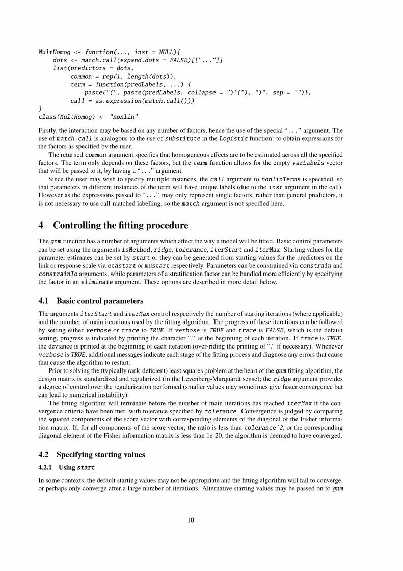
MultHomog <- function(..., inst = NULL){
dots <- match.call(expand.dots = FALSE)[["..."]]
list(predictors = dots,
common = rep(1, length(dots)),
term = function(predLabels, ...) {
paste("(", paste(predLabels, collapse = ")*("), ")", sep = "")},
call = as.expression(match.call()))
}
class(MultHomog) <- "nonlin"
Firstly, the interaction may be based on any number of factors, hence the use of the special “...” argument. The
use of match.call is analogous to the use of substitute in the Logistic function: to obtain expressions for
the factors as specified by the user.
The returned common argument specifies that homogeneous effects are to be estimated across all the specified
factors. The term only depends on these factors, but the term function allows for the empty varLabels vector
that will be passed to it, by having a “...” argument.
Since the user may wish to specify multiple instances, the call argument to nonlinTerms is specified, so
that parameters in different instances of the term will have unique labels (due to the inst argument in the call).
However as the expressions passed to “...” may only represent single factors, rather than general predictors, it
is not necessary to use call-matched labelling, so the match argument is not specified here.
4 Controlling the fitting procedure
The gnm function has a number of arguments which affect the way a model will be fitted. Basic control parameters
can be set using the arguments lsMethod , ridge, tolerance, iterStart and iterMax. Starting values for the
parameter estimates can be set by start or they can be generated from starting values for the predictors on the
link or response scale via etastart or mustart respectively. Parameters can be constrained via constrain and
constrainTo arguments, while parameters of a stratification factor can be handled more efficiently by specifying
the factor in an eliminate argument. These options are described in more detail below.
4.1 Basic control parameters
The arguments iterStart and iterMax control respectively the number of starting iterations (where applicable)
and the number of main iterations used by the fitting algorithm. The progress of these iterations can be followed
by setting either verbose or trace to TRUE. If verbose is TRUE and trace is FALSE, which is the default
setting, progress is indicated by printing the character “.” at the beginning of each iteration. If trace is TRUE,
the deviance is printed at the beginning of each iteration (over-riding the printing of “.” if necessary). Whenever
verbose is TRUE, additional messages indicate each stage of the fitting process and diagnose any errors that cause
that cause the algorithm to restart.
Prior to solving the (typically rank-deficient) least squares problem at the heart of the gnm fitting algorithm, the
design matrix is standardized and regularized (in the Levenberg-Marquardt sense); the ridge argument provides
a degree of control over the regularization performed (smaller values may sometimes give faster convergence but
can lead to numerical instability).
The fitting algorithm will terminate before the number of main iterations has reached iterMax if the con-
vergence criteria have been met, with tolerance specified by tolerance. Convergence is judged by comparing
the squared components of the score vector with corresponding elements of the diagonal of the Fisher informa-
tion matrix. If, for all components of the score vector, the ratio is less than toleranceˆ2, or the corresponding
diagonal element of the Fisher information matrix is less than 1e-20, the algorithm is deemed to have converged.
4.2 Specifying starting values
4.2.1 Using start
In some contexts, the default starting values may not be appropriate and the fitting algorithm will fail to converge,
or perhaps only converge after a large number of iterations. Alternative starting values may be passed on to gnm
10

by specifying a start argument. This should be a numeric vector of length equal to the number of parameters
(or possibly the non-eliminated parameters, see Section 4.4), however missing starting values (NAs) are allowed.
If there is no user-specified starting value for a parameter, the default value is used. This feature is particularly
useful when adding terms to a model, since the estimates from the original model can be used as starting values,
as in this example:
model1 <- gnm(mu ~ R + C + Mult(R, C))
model2 <- gnm(mu ~ R + C + instances(Mult(R, C), 2),
start = c(coef(model1), rep(NA, 10)))
The gnm call can be made with method = "coefNames" to identify the parameters of a model prior to estimation,
to assist with the specification of arguments such as start. For example, to get the number 10 for the value of
start above, we could have done
gnm(mu ~ R + C + instances(Mult(R, C), 2), method = "coefNames")
from whose output it would be seen that there are 10 new coefficients in model2. When called with method
= "coefNames", gnm makes no attempt to fit the specified model; instead it returns just the names that the
coefficients in the fitted model object would have.
The starting procedure used by gnm is as follows:
1. Begin with all parameters set to NA .
2. Replace NA values with any starting values set by nonlin functions.
3. Replace current values with any (non-NA) starting values specified by the start argument of gnm .
4. Set any values specified by the constrain argument to the values specified by the constrainTo argument
(see Section 4.3).
5. Categorise remaining NA parameters as linear or nonlinear, treating non-NA parameters as fixed. Initialise
the nonlinear parameters by generating values θi from the Uniform(−0.1, 0.1) distribution and shifting these
values away from zero as follows
θi =
θi − 0.1 if θi < 1
θi + 0.1 otherwise
6. Compute the glm estimate of the linear parameters, offsetting the contribution to the predictor of any terms
fully determined by steps 2 to 5.
7. Run starting iterations: update nonlinear parameters one at a time, jointly re-estimating linear parameters
after each round of updates.
Note that no starting iterations (step 7) will be run if all parameters are linear, or if all nonlinear parameters are
specified by start, constrain or a nonlin function.
4.2.2 Using etastart or mustart
An alternative way to set starting values for the parameters is to specify starting values for the predictors.
If there are linear parameters in the model, the predictor starting values are first used to fit a model with only
the linear terms (offsetting any terms fully specified by starting values given by start, constrain or a nonlin
function). In this case the parameters corresponding to the predictor starting values can be computed analytically.
If the fitted model reproduces the predictor starting values, then these values contain no further information and
they are replaced using the initialize function of the specified family.
The predictor starting values or their replacement are then used as the response variable in a nonlinear least
squares model with only the unspecified nonlinear terms, offsetting the contribution of any other terms. Since
the model is over-parameterized, the model is approximated using iterStart iterations of the “L-BFGS-B”
algorithm of optim , assuming parameters lie in the range (-10, 10).
Starting values for the predictors can be specified explicitly via etastart or implicitly by passing starting
values for the fitted means to mustart. For example, when extending a model, the fitted predictors from the first
model can be used to find starting values for the parameters of the second model:
11

model1 <- gnm(mu ~ R + C + Mult(R, C))
model2 <- gnm(mu ~ R + C + instances(Mult(R, C), 2), etastart = model1$predictors)
Using etastart avoids the one-parameter-at-a-time starting iterations, so is quicker than using start to pass
on information from a nested model. However start will generally produce better starting values so should be
used when feasible. For multiplicative terms, the residSVD functions provides a better way to avoid starting
iterations.
4.3 Using constrain
By default, gnm only imposes identifiability constraints according to the general conventions used by R to handle
linear aliasing. Therefore models that have any nonlinear terms will be typically be over-parameterized, and gnm
will return a random parameterization for unidentified coefficients (determined by the randomly chosen starting
values for the iterative algorithm, step 5 above).
To illustrate this point, consider the following application of gnm , discussed later in Section 7.1:
> set.seed(1)
> RChomog1 <- gnm(Freq ~ origin + destination + Diag(origin, destination) +
+ MultHomog(origin, destination), family = poisson,
+ data = occupationalStatus, verbose = FALSE)
Running the analysis again from a different seed
> set.seed(2)
> RChomog2 <- update(RChomog1)
gives a different representation of the same model:
> compareCoef <- cbind(coef(RChomog1), coef(RChomog2))
> colnames(compareCoef) <- c("RChomog1", "RChomog2")
> round(compareCoef, 4)
RChomog1 RChomog2
(Intercept) 0.2404 0.3058
origin2 0.5101 0.5052
origin3 1.5928 1.5744
origin4 1.8892 1.8577
origin5 0.6692 0.6373
origin6 2.7113 2.6679
origin7 1.3687 1.3159
origin8 1.0974 1.0392
destination2 0.9291 0.9242
destination3 1.9372 1.9188
destination4 2.1776 2.1461
destination5 1.5686 1.5367
destination6 3.0148 2.9714
destination7 2.1203 2.0675
destination8 1.6728 1.6146
Diag(origin, destination)1 1.5267 1.5267
Diag(origin, destination)2 0.4560 0.4560
Diag(origin, destination)3 -0.0160 -0.0160
Diag(origin, destination)4 0.3892 0.3892
Diag(origin, destination)5 0.7385 0.7385
Diag(origin, destination)6 0.1347 0.1347
Diag(origin, destination)7 0.4576 0.4576
Diag(origin, destination)8 0.3885 0.3885
MultHomog(origin, destination)1 -1.4646 1.4421
MultHomog(origin, destination)2 -1.2463 1.2238
12
MultHomog(origin, destination)3 -0.6481 0.6256
MultHomog(origin, destination)4 -0.0642 0.0417
MultHomog(origin, destination)5 -0.0471 0.0246
MultHomog(origin, destination)6 0.4647 -0.4872
MultHomog(origin, destination)7 0.8808 -0.9033
MultHomog(origin, destination)8 1.1244 -1.1469
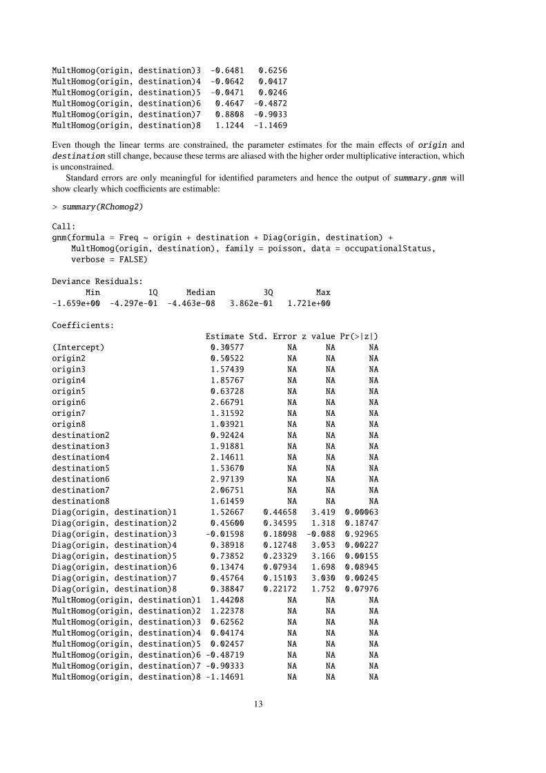
Even though the linear terms are constrained, the parameter estimates for the main effects of origin and
destination still change, because these terms are aliased with the higher order multiplicative interaction, which
is unconstrained.
Standard errors are only meaningful for identified parameters and hence the output of summary.gnm will
show clearly which coefficients are estimable:
> summary(RChomog2)
Call:
gnm(formula = Freq ~ origin + destination + Diag(origin, destination) +
MultHomog(origin, destination), family = poisson, data = occupationalStatus,
verbose = FALSE)
Deviance Residuals:
Min 1Q Median 3Q Max
-1.659e+00 -4.297e-01 -4.463e-08 3.862e-01 1.721e+00
Coefficients:
Estimate Std. Error z value Pr(>|z|)
(Intercept) 0.30577 NA NA NA
origin2 0.50522 NA NA NA
origin3 1.57439 NA NA NA
origin4 1.85767 NA NA NA
origin5 0.63728 NA NA NA
origin6 2.66791 NA NA NA
origin7 1.31592 NA NA NA
origin8 1.03921 NA NA NA
destination2 0.92424 NA NA NA
destination3 1.91881 NA NA NA
destination4 2.14611 NA NA NA
destination5 1.53670 NA NA NA
destination6 2.97139 NA NA NA
destination7 2.06751 NA NA NA
destination8 1.61459 NA NA NA
Diag(origin, destination)1 1.52667 0.44658 3.419 0.00063
Diag(origin, destination)2 0.45600 0.34595 1.318 0.18747
Diag(origin, destination)3 -0.01598 0.18098 -0.088 0.92965
Diag(origin, destination)4 0.38918 0.12748 3.053 0.00227
Diag(origin, destination)5 0.73852 0.23329 3.166 0.00155
Diag(origin, destination)6 0.13474 0.07934 1.698 0.08945
Diag(origin, destination)7 0.45764 0.15103 3.030 0.00245
Diag(origin, destination)8 0.38847 0.22172 1.752 0.07976
MultHomog(origin, destination)1 1.44208 NA NA NA
MultHomog(origin, destination)2 1.22378 NA NA NA
MultHomog(origin, destination)3 0.62562 NA NA NA
MultHomog(origin, destination)4 0.04174 NA NA NA
MultHomog(origin, destination)5 0.02457 NA NA NA
MultHomog(origin, destination)6 -0.48719 NA NA NA
MultHomog(origin, destination)7 -0.90333 NA NA NA
MultHomog(origin, destination)8 -1.14691 NA NA NA
13

(Dispersion parameter for poisson family taken to be 1)
Std. Error is NA where coefficient has been constrained or is unidentified
Residual deviance: 32.561 on 34 degrees of freedom
AIC: 414.9
Number of iterations: 7
Additional constraints may be specified through the constrain and constrainTo arguments of gnm . These
arguments specify respectively parameters that are to be constrained in the fitting process and the values to which
they should be constrained. Parameters may be specified by a regular expression to match against the parameter
names, a numeric vector of indices, a character vector of names, or, if constrain = "[?]" they can be selected
through a Tk dialog. The values to constrain to should be specified by a numeric vector; if constrainTo is
missing, constrained parameters will be set to zero.
In the case above, constraining one level of the homogeneous multiplicative factor is sufficient to make the
parameters of the nonlinear term identifiable, and hence all parameters in the model identifiable. Figure 1 illus-
trates how the coefficient to be constrained may be specified via a Tk dialog, an approach which can be helpful in
interactive R sessions.
However for reproducible code, it is best to specify the constrained coefficients directly. For example, the
following code specifies that the last level of the homogeneous multiplicative factor should be constrained to
zero,
> set.seed(1)
> RChomogConstrained1 <- update(RChomog1, constrain = length(coef(RChomog1)))
Since all the parameters are now constrained, re-fitting the model will give the same results, regardless of the
random seed set beforehand:
> set.seed(2)
> RChomogConstrained2 <- update(RChomogConstrained1)
> identical(coef(RChomogConstrained1), coef(RChomogConstrained2))
[1] FALSE
It is not usually so straightforward to constrain all the parameters in a generalized nonlinear model. However
use of constrain in conjunction with constrainTo is usually sufficient to make coefficients of interest identifi-
able . The functions checkEstimable or getContrasts, described in Section 5, may be used to check whether
particular combinations of parameters are estimable.
4.4 Using eliminate
When a model contains the additive effect of a factor which has a large number of levels, the iterative algorithm by
which maximum likelihood estimates are computed can usually be accelerated by use of the eliminate argument
to gnm . A factor passed to eliminate specifies the first term in the model, replacing any intercept term. So, for
example
gnm(mu ~ A + B + Mult(A, B), eliminate = strata1:strata2)
is equivalent, in terms of the structure of the model, to
gnm(mu ~ -1 + strata1:strata2 + A + B + Mult(A, B))
However, specifying a factor through eliminate has two advantages over the standard specification. First, the
structure of the eliminated factor is exploited so that computational speed is improved — substantially so if
the number of eliminated parameters is large. Second, eliminated parameters are returned separately from non-
eliminated parameters (as an attribute of the coefficients component of the returned object). Thus eliminated
parameters are excluded from printed model summaries by default and disregarded by gnm methods that would
not be relevant to such parameters (see Section 5).
14
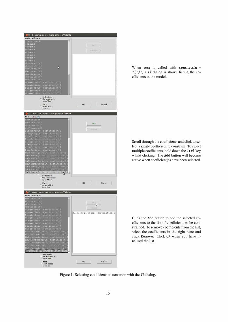
When gnm is called with constrain =
"[?]", a Tk dialog is shown listing the co-
efficients in the model.
Scroll through the coefficients and click to se-
lect a single coefficient to constrain. To select
multiple coefficients, hold down the Ctrl key
whilst clicking. The Add button will become
active when coefficient(s) have been selected.
Click the Add button to add the selected co-
efficients to the list of coefficients to be con-
strained. To remove coefficients from the list,
select the coefficients in the right pane and
click Remove. Click OK when you have fi-
nalised the list.
Figure 1: Selecting coefficients to constrain with the Tk dialog.
15

The eliminate feature is useful, for example, when multinomial-response models are fitted by using the well
known equivalence between multinomial and (conditional) Poisson likelihoods. In such situations the sufficient
statistic involves a potentially large number of fixed multinomial row totals, and the corresponding parameters are
of no substantive interest. For an application see Section 7.6 below. Here we give an artificial illustration: 1000
randomly-generated trinomial responses, and a single predictor variable (whose effect on the data generation is
null):
> set.seed(1)
> n <- 1000
> x <- rep(rnorm(n), rep(3, n))
> counts <- as.vector(rmultinom(n, 10, c(0.7, 0.1, 0.2)))
> rowID <- gl(n, 3, 3 * n)
> resp <- gl(3, 1, 3 * n)
The logistic model for dependence on x can be fitted as a Poisson log-linear model2, using either glm or gnm :
> ## Timings on a Xeon 2.33GHz, under Linux
> system.time(temp.glm <- glm(counts ~ rowID + resp + resp:x,
family = poisson))[1]
user.self
37.126
> system.time(temp.gnm <- gnm(counts ~ resp + resp:x, eliminate = rowID,
family = poisson, verbose = FALSE))[1]
user.self
0.04
> c(deviance(temp.glm), deviance(temp.gnm))
[1] 2462.556 2462.556
Here the use of eliminate causes the gnm calculations to run much more quickly than glm . The speed advantage
increases with the number of eliminated parameters (here 1000). By default,the eliminated parameters do not
appear in printed model summaries as here:
> summary(temp.gnm)
Call:
gnm(formula = counts ~ resp + resp:x, eliminate = rowID, family = poisson,
verbose = FALSE)
Deviance Residuals:
Min 1Q Median 3Q Max
-2.852038 -0.786172 -0.004534 0.645278 2.755013
Coefficients of interest:
Estimate Std. Error z value Pr(>|z|)
resp2 -1.961448 0.034007 -57.678 <2e-16
resp3 -1.255846 0.025359 -49.523 <2e-16
resp1:x -0.007726 0.024517 -0.315 0.753
resp2:x -0.023340 0.037611 -0.621 0.535
resp3:x 0.000000 NA NA NA
2For this particular example, of course, it would be more economical to fit the model directly using multinom (from the recommended
package nnet). But fitting as here via the ‘Poisson trick’ allows the model to be elaborated within the gnm framework using Mult or other
nonlin terms.
16

(Dispersion parameter for poisson family taken to be 1)
Std. Error is NA where coefficient has been constrained or is unidentified
Residual deviance: 2462.6 on 1996 degrees of freedom
AIC: 12028
Number of iterations: 4
although the summary method has a logical with.eliminate that can toggled so that the eliminated parameters
are included if desired.
The eliminate feature as implemented in gnm extends the earlier work of Hatzinger and Francis (2004) to
a broader class of models and to over-parameterized model representations.
5 Methods and accessor functions
5.1 Methods
The gnm function returns an object of class c("gnm", "glm", "lm"). There are several methods that have been
written for objects of class glm or lm to facilitate inspection of fitted models. Out of the generic functions in the
base, stats and graphics packages for which methods have been written for glm or lm objects, Figure 2 shows
those that can be used to analyse gnm objects, whilst Figure 3 shows those that are not implemented for gnm
objects.
add1∗ family print
anova formula profile
case.names hatvalues residuals
coef labels rstandard
cooks.distance logLik summary
confint model.frame variable.names
deviance model.matrix vcov
drop1∗ plot weights
extractAIC predict
Figure 2: Generic functions in the base, stats and graphics packages that can be used to analyse gnm objects.
Starred functions are implemented for models with linear terms only.
alias effects
dfbeta influence
dfbetas kappa
dummy.coef proj
Figure 3: Generic functions in the base, stats and graphics packages for which methods have been written for
glm or lm objects, but which are not implemented for gnm objects.
In addition to the accessor functions shown in Figure 2, the gnm package provides a new generic function
called termPredictors that has methods for objects of class gnm, glm and lm. This function returns the additive
contribution of each term to the predictor. See Section 2.5 for an example of its use.
Most of the functions listed in Figure 2 can be used as they would be for glm or lm objects, however care must
be taken with vcov.gnm , as the variance-covariance matrix will depend on the parameterization of the model.
In particular, standard errors calculated using the variance-covariance matrix will only be valid for parameters or
contrasts that are estimable!
Similarly, profile.gnm and confint.gnm are only applicable to estimable parameters. The deviance func-
tion of a generalized nonlinear model can sometimes be far from quadratic and profile.gnm attempts to detect
17
asymmetry or asymptotic behaviour in order to return a sufficient profile for a given parameter. As an example,
consider the following model, described later in Section 7.3:
unidiff <- gnm(Freq ~ educ*orig + educ*dest + Mult(Exp(educ), orig:dest),
constrain = "[.]educ1", family = poisson, data = yaish,
subset = (dest != 7))
prof <- profile(unidiff, which = 61:65, trace = TRUE)
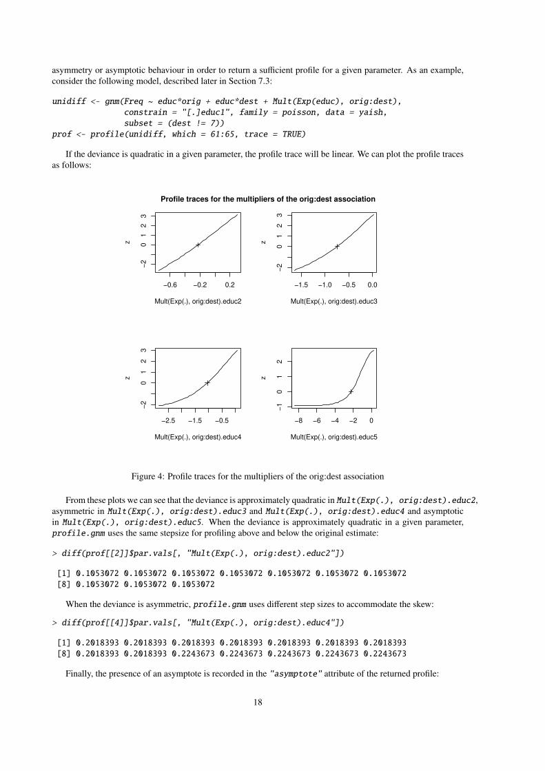
If the deviance is quadratic in a given parameter, the profile trace will be linear. We can plot the profile traces
as follows:
−0.6 −0.2 0.2
−2
01
23
Mult(Exp(.), orig:dest).educ2
z
−1.5 −1.0 −0.5 0.0−
20
12
3
Mult(Exp(.), orig:dest).educ3
z
−2.5 −1.5 −0.5
−2
01
23
Mult(Exp(.), orig:dest).educ4
z
−8 −6 −4 −2 0
−1
01
2
Mult(Exp(.), orig:dest).educ5
z
Profile traces for the multipliers of the orig:dest association
Figure 4: Profile traces for the multipliers of the orig:dest association
From these plots we can see that the deviance is approximately quadratic in Mult(Exp(.), orig:dest).educ2,
asymmetric in Mult(Exp(.), orig:dest).educ3 and Mult(Exp(.), orig:dest).educ4 and asymptotic
in Mult(Exp(.), orig:dest).educ5. When the deviance is approximately quadratic in a given parameter,
profile.gnm uses the same stepsize for profiling above and below the original estimate:
> diff(prof[[2]]$par.vals[, "Mult(Exp(.), orig:dest).educ2"])
[1] 0.1053072 0.1053072 0.1053072 0.1053072 0.1053072 0.1053072 0.1053072
[8] 0.1053072 0.1053072 0.1053072
When the deviance is asymmetric, profile.gnm uses different step sizes to accommodate the skew:
> diff(prof[[4]]$par.vals[, "Mult(Exp(.), orig:dest).educ4"])
[1] 0.2018393 0.2018393 0.2018393 0.2018393 0.2018393 0.2018393 0.2018393
[8] 0.2018393 0.2018393 0.2243673 0.2243673 0.2243673 0.2243673 0.2243673
Finally, the presence of an asymptote is recorded in the "asymptote" attribute of the returned profile:
18
> attr(prof[[5]], "asymptote")
[1] TRUE FALSE
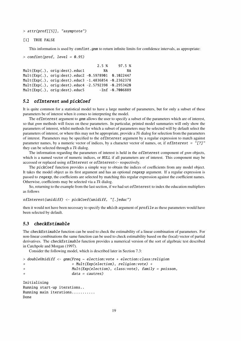
This information is used by confint.gnm to return infinite limits for confidence intervals, as appropriate:
> confint(prof, level = 0.95)
2.5 % 97.5 %
Mult(Exp(.), orig:dest).educ1 NA NA
Mult(Exp(.), orig:dest).educ2 -0.5978901 0.1022447
Mult(Exp(.), orig:dest).educ3 -1.4836854 -0.2362378
Mult(Exp(.), orig:dest).educ4 -2.5792398 -0.2953420
Mult(Exp(.), orig:dest).educ5 -Inf -0.7006889
5.2 ofInterest and pickCoef
It is quite common for a statistical model to have a large number of parameters, but for only a subset of these
parameters be of interest when it comes to interpreting the model.
The ofInterest argument to gnm allows the user to specify a subset of the parameters which are of interest,
so that gnm methods will focus on these parameters. In particular, printed model summaries will only show the
parameters of interest, whilst methods for which a subset of parameters may be selected will by default select the
parameters of interest, or where this may not be appropriate, provide a Tk dialog for selection from the parameters
of interest. Parameters may be specified to the ofInterest argument by a regular expression to match against
parameter names, by a numeric vector of indices, by a character vector of names, or, if ofInterest = "[?]"
they can be selected through a Tk dialog.
The information regarding the parameters of interest is held in the ofInterest component of gnm objects,
which is a named vector of numeric indices, or NULL if all parameters are of interest. This component may be
accessed or replaced using ofInterest or ofInterest<- respectively.
The pickCoef function provides a simple way to obtain the indices of coefficients from any model object.
It takes the model object as its first argument and has an optional regexp argument. If a regular expression is
passed to regexp, the coefficients are selected by matching this regular expression against the coefficient names.
Otherwise, coefficients may be selected via a Tk dialog.
So, returning to the example from the last section, if we had set ofInterest to index the education multipliers
as follows
ofInterest(unidiff) <- pickCoef(unidiff, "[.]educ")
then it would not have been necessary to specify the which argument of profile as these parameters would have
been selected by default.
5.3 checkEstimable
The checkEstimable function can be used to check the estimability of a linear combination of parameters. For
non-linear combinations the same function can be used to check estimability based on the (local) vector of partial
derivatives. The checkEstimable function provides a numerical version of the sort of algebraic test described
in Catchpole and Morgan (1997).
Consider the following model, which is described later in Section 7.3:
> doubleUnidiff <- gnm(Freq ~ election:vote + election:class:religion
+ + Mult(Exp(election), religion:vote) +
+ Mult(Exp(election), class:vote), family = poisson,
+ data = cautres)
Initialising
Running start-up iterations..
Running main iterations...........
Done
19

The effects of the first constituent multiplier in the first multiplicative interaction are identified when the parameter
for one of the levels — say for the first level — is constrained to zero. The parameters to be estimated are then
the differences between each other level and the first. These differences can be represented by a contrast matrix
as follows:
> coefs <- names(coef(doubleUnidiff))
> contrCoefs <- coefs[grep(", religion:vote", coefs)]
> nContr <- length(contrCoefs)
> contrMatrix <- matrix(0, length(coefs), nContr,
+ dimnames = list(coefs, contrCoefs))
> contr <- contr.sum(contrCoefs)
> # switch round to contrast with first level
> contr <- rbind(contr[nContr, ], contr[-nContr, ])
> contrMatrix[contrCoefs, 2:nContr] <- contr
> contrMatrix[contrCoefs, 2:nContr]
Mult(Exp(.), religion:vote).election2
Mult(Exp(.), religion:vote).election1 -1
Mult(Exp(.), religion:vote).election2 1
Mult(Exp(.), religion:vote).election3 0
Mult(Exp(.), religion:vote).election4 0
Mult(Exp(.), religion:vote).election3
Mult(Exp(.), religion:vote).election1 -1
Mult(Exp(.), religion:vote).election2 0
Mult(Exp(.), religion:vote).election3 1
Mult(Exp(.), religion:vote).election4 0
Mult(Exp(.), religion:vote).election4
Mult(Exp(.), religion:vote).election1 -1
Mult(Exp(.), religion:vote).election2 0
Mult(Exp(.), religion:vote).election3 0
Mult(Exp(.), religion:vote).election4 1
Then their estimability can be checked using checkEstimable
> checkEstimable(doubleUnidiff, contrMatrix)
Mult(Exp(.), religion:vote).election1 Mult(Exp(.), religion:vote).election2
NA TRUE
Mult(Exp(.), religion:vote).election3 Mult(Exp(.), religion:vote).election4
TRUE TRUE
which confirms that the effects for the other three levels are estimable when the parameter for the first level is set
to zero.
However, applying the equivalent constraint to the second constituent multiplier in the interaction is not suffi-
cient to make the parameters in that multiplier estimable:
> coefs <- names(coef(doubleUnidiff))
> contrCoefs <- coefs[grep("[.]religion", coefs)]
> nContr <- length(contrCoefs)
> contrMatrix <- matrix(0, length(coefs), length(contrCoefs),
+ dimnames = list(coefs, contrCoefs))
> contr <- contr.sum(contrCoefs)
> contrMatrix[contrCoefs, 2:nContr] <- rbind(contr[nContr, ], contr[-nContr, ])
> checkEstimable(doubleUnidiff, contrMatrix)
Mult(Exp(election), .).religion1:vote1 Mult(Exp(election), .).religion2:vote1
NA FALSE
Mult(Exp(election), .).religion3:vote1 Mult(Exp(election), .).religion4:vote1
20
FALSE FALSE
Mult(Exp(election), .).religion1:vote2 Mult(Exp(election), .).religion2:vote2
FALSE FALSE
Mult(Exp(election), .).religion3:vote2 Mult(Exp(election), .).religion4:vote2
FALSE FALSE
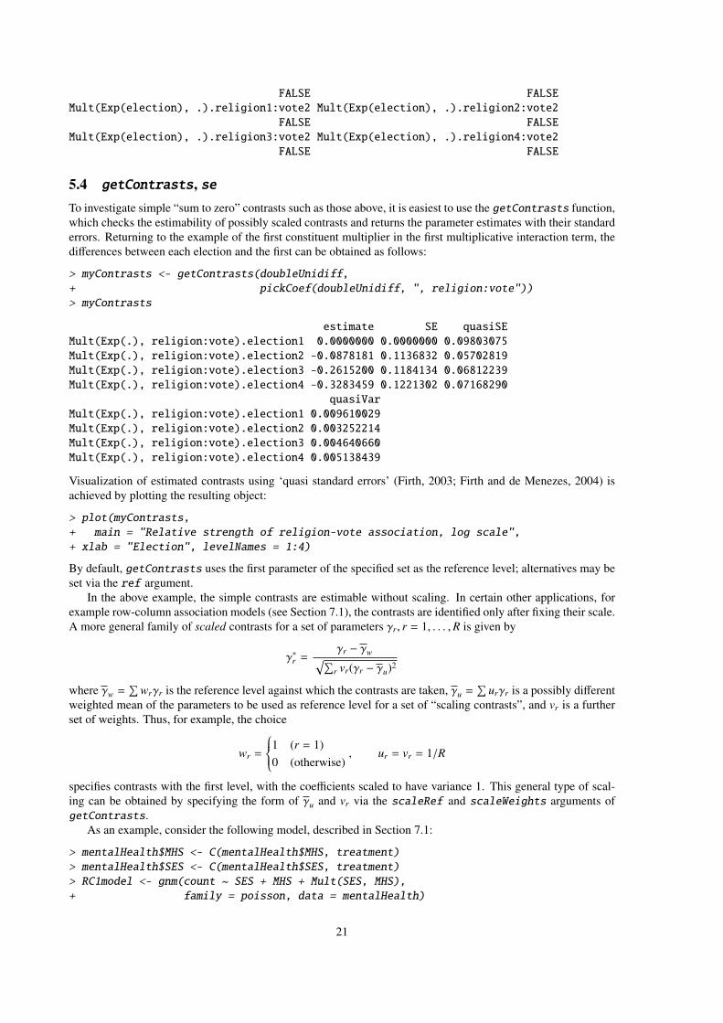
5.4 getContrasts, se
To investigate simple “sum to zero” contrasts such as those above, it is easiest to use the getContrasts function,
which checks the estimability of possibly scaled contrasts and returns the parameter estimates with their standard
errors. Returning to the example of the first constituent multiplier in the first multiplicative interaction term, the
differences between each election and the first can be obtained as follows:
> myContrasts <- getContrasts(doubleUnidiff,
+ pickCoef(doubleUnidiff, ", religion:vote"))
> myContrasts
estimate SE quasiSE
Mult(Exp(.), religion:vote).election1 0.0000000 0.0000000 0.09803075
Mult(Exp(.), religion:vote).election2 -0.0878181 0.1136832 0.05702819
Mult(Exp(.), religion:vote).election3 -0.2615200 0.1184134 0.06812239
Mult(Exp(.), religion:vote).election4 -0.3283459 0.1221302 0.07168290
quasiVar
Mult(Exp(.), religion:vote).election1 0.009610029
Mult(Exp(.), religion:vote).election2 0.003252214
Mult(Exp(.), religion:vote).election3 0.004640660
Mult(Exp(.), religion:vote).election4 0.005138439
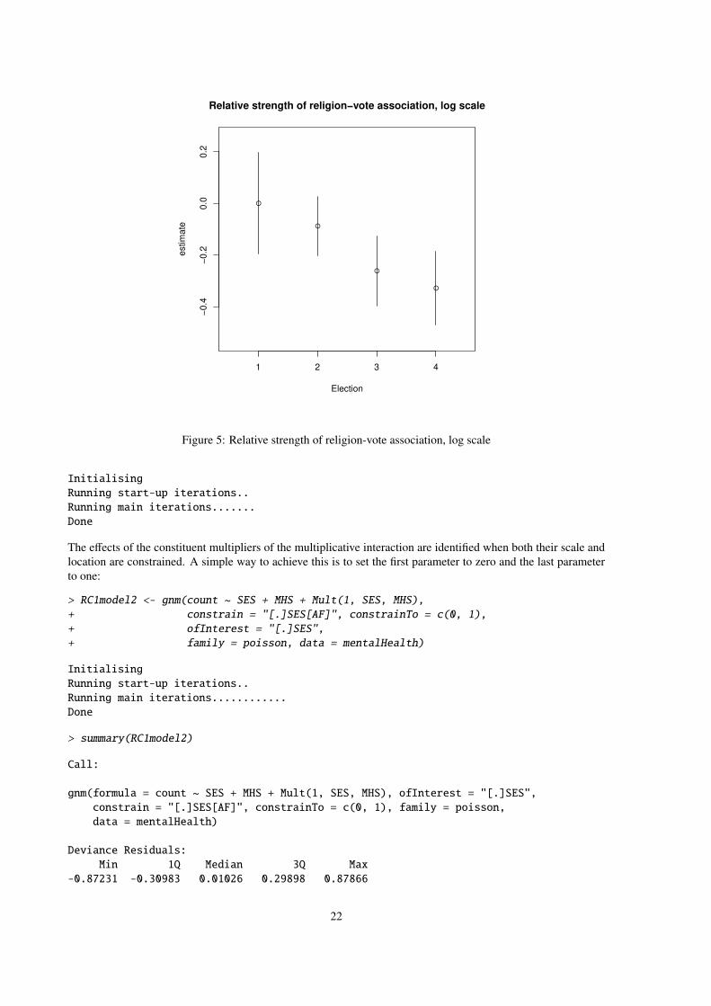
Visualization of estimated contrasts using ‘quasi standard errors’ (Firth, 2003; Firth and de Menezes, 2004) is
achieved by plotting the resulting object:
> plot(myContrasts,
+ main = "Relative strength of religion-vote association, log scale",
+ xlab = "Election", levelNames = 1:4)
By default, getContrasts uses the first parameter of the specified set as the reference level; alternatives may be
set via the ref argument.
In the above example, the simple contrasts are estimable without scaling. In certain other applications, for
example row-column association models (see Section 7.1), the contrasts are identified only after fixing their scale.
A more general family of scaled contrasts for a set of parameters γr, r = 1, . . . ,R is given by
γ∗r =γr − γw
√
∑
r vr(γr − γu)2
where γw =∑
wrγr is the reference level against which the contrasts are taken, γu =∑
urγr is a possibly different
weighted mean of the parameters to be used as reference level for a set of “scaling contrasts”, and vr is a further
set of weights. Thus, for example, the choice
wr =
1 (r = 1)
0 (otherwise), ur = vr = 1/R
specifies contrasts with the first level, with the coefficients scaled to have variance 1. This general type of scal-
ing can be obtained by specifying the form of γu and vr via the scaleRef and scaleWeights arguments of
getContrasts.
As an example, consider the following model, described in Section 7.1:
> mentalHealth$MHS <- C(mentalHealth$MHS, treatment)
> mentalHealth$SES <- C(mentalHealth$SES, treatment)
> RC1model <- gnm(count ~ SES + MHS + Mult(SES, MHS),
+ family = poisson, data = mentalHealth)
21
1 2 3 4
−0.4
−0.2
0.0
0.2
Relative strength of religion−vote association, log scale
Election
estim
ate
●
●
●
●
Figure 5: Relative strength of religion-vote association, log scale
Initialising
Running start-up iterations..
Running main iterations.......
Done
The effects of the constituent multipliers of the multiplicative interaction are identified when both their scale and
location are constrained. A simple way to achieve this is to set the first parameter to zero and the last parameter
to one:
> RC1model2 <- gnm(count ~ SES + MHS + Mult(1, SES, MHS),
+ constrain = "[.]SES[AF]", constrainTo = c(0, 1),
+ ofInterest = "[.]SES",
+ family = poisson, data = mentalHealth)
Initialising
Running start-up iterations..
Running main iterations............
Done
> summary(RC1model2)
Call:
gnm(formula = count ~ SES + MHS + Mult(1, SES, MHS), ofInterest = "[.]SES",
constrain = "[.]SES[AF]", constrainTo = c(0, 1), family = poisson,
data = mentalHealth)
Deviance Residuals:
Min 1Q Median 3Q Max
-0.87231 -0.30983 0.01026 0.29898 0.87866
22

Coefficients of interest:
Estimate Std. Error z value Pr(>|z|)
Mult(1, ., MHS).SESA 0.000000 NA NA NA
Mult(1, ., MHS).SESB -0.003107 0.181567 -0.017 0.986
Mult(1, ., MHS).SESC 0.252939 0.158922 1.592 0.111
Mult(1, ., MHS).SESD 0.388785 0.144164 2.697 0.007
Mult(1, ., MHS).SESE 0.724329 0.172325 4.203 2.63e-05
Mult(1, ., MHS).SESF 1.000000 NA NA NA
(Dispersion parameter for poisson family taken to be 1)
Std. Error is NA where coefficient has been constrained or is unidentified
Residual deviance: 3.5706 on 8 degrees of freedom
AIC: 179.74
Number of iterations: 12
Note that a constant multiplier must be incorporated into the interaction term, i.e., the multiplicative term Mult(SES,
MHS) becomes Mult(1, SES, MHS), in order to maintain equivalence with the original model specification. The
constraints specified for RC1model2 result in the estimation of scaled contrasts with level A of SES, in which the
scaling fixes the magnitude of the contrast between level F and level A to be equal to 1. The equivalent use of
getContrasts, together with the unconstrained fit (RC1model), in this case is as follows:
> getContrasts(RC1model, pickCoef(RC1model, "[.]SES"), ref = "first",
+ scaleRef = "first", scaleWeights = c(rep(0, 5), 1))
Estimate Std. Error
Mult(., MHS).SESA 0.000000000 0.0000000
Mult(., MHS).SESB -0.003107289 0.1815672
Mult(., MHS).SESC 0.252939253 0.1589218
Mult(., MHS).SESD 0.388785114 0.1441637
Mult(., MHS).SESE 0.724328752 0.1723247
Mult(., MHS).SESF 1.000000000 0.0000000
Quasi-variances and standard errors are not returned here as they can not (currently) be computed for scaled
contrasts. When the scaling uses the same reference level as the contrasts, equal scale weights produce “spherical”
contrasts, whilst unequal weights produce “elliptical” contrasts. Further examples are given in Sections 7.1 and
7.4.
For more general linear combinations of parameters than contrasts, the lower-level se function (which is
called internally by getContrasts and by the summary method) can be used directly. See help(se) for details.
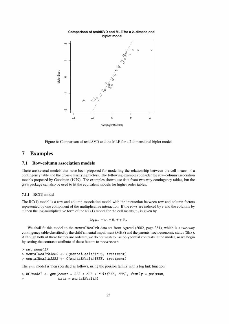
5.5 residSVD
Sometimes it is useful to operate on the residuals of a model in order to create informative summaries of residual
variation, or to obtain good starting values for additional parameters in a more elaborate model. The relevant
arithmetical operations are weighted means of the so-called working residuals.
The residSVD function facilitates one particular residual analysis that is often useful when considering mul-
tiplicative interaction between factors as a model elaboration: in effect, residSVD provides a direct estimate of
the parameters of such an interaction, by performing an appropriately weighted singular value decomposition on
the working residuals.
As an illustration, consider the barley data from Wedderburn (1974). These data have the following two-way
structure:
> xtabs(y ~ site + variety, barley)
23
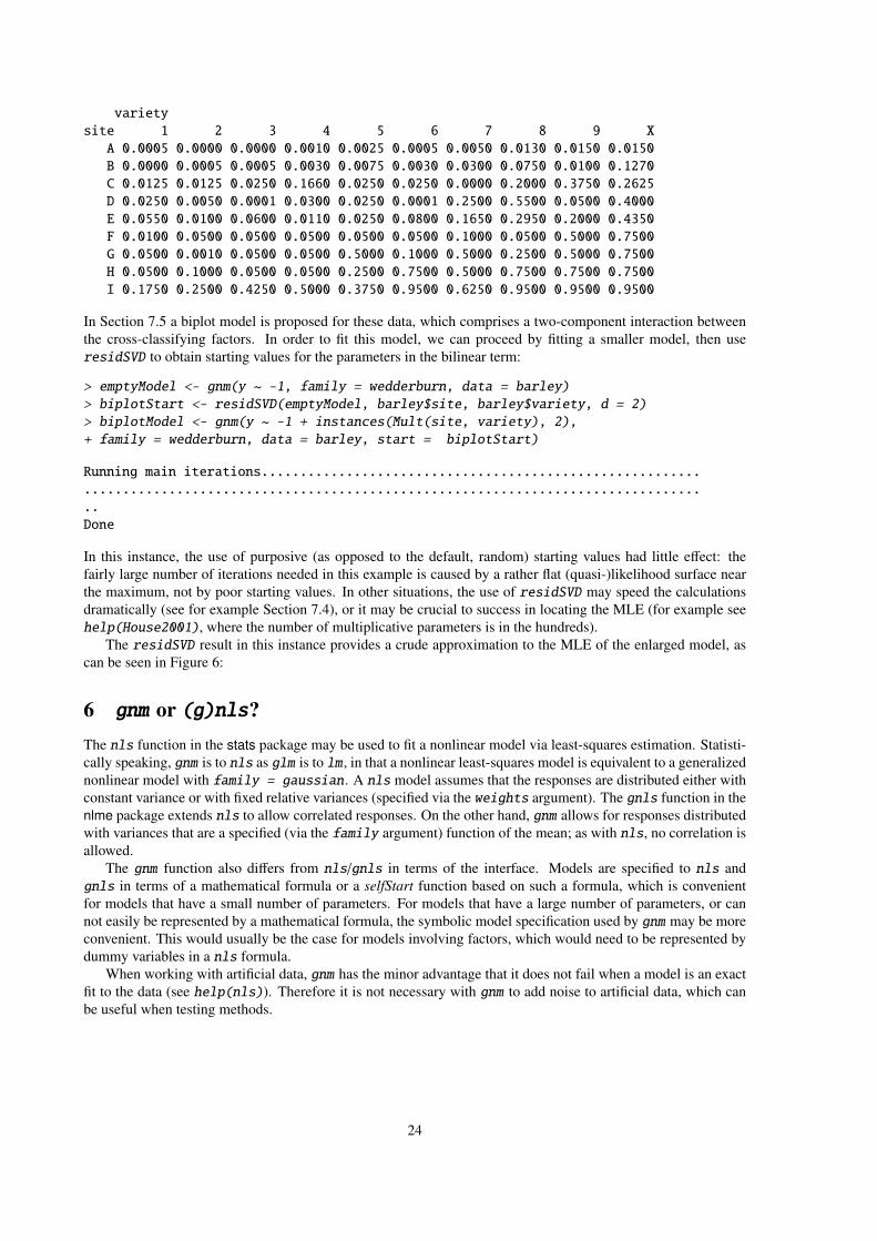
variety
site 1 2 3 4 5 6 7 8 9 X
A 0.0005 0.0000 0.0000 0.0010 0.0025 0.0005 0.0050 0.0130 0.0150 0.0150
B 0.0000 0.0005 0.0005 0.0030 0.0075 0.0030 0.0300 0.0750 0.0100 0.1270
C 0.0125 0.0125 0.0250 0.1660 0.0250 0.0250 0.0000 0.2000 0.3750 0.2625
D 0.0250 0.0050 0.0001 0.0300 0.0250 0.0001 0.2500 0.5500 0.0500 0.4000
E 0.0550 0.0100 0.0600 0.0110 0.0250 0.0800 0.1650 0.2950 0.2000 0.4350
F 0.0100 0.0500 0.0500 0.0500 0.0500 0.0500 0.1000 0.0500 0.5000 0.7500
G 0.0500 0.0010 0.0500 0.0500 0.5000 0.1000 0.5000 0.2500 0.5000 0.7500
H 0.0500 0.1000 0.0500 0.0500 0.2500 0.7500 0.5000 0.7500 0.7500 0.7500
I 0.1750 0.2500 0.4250 0.5000 0.3750 0.9500 0.6250 0.9500 0.9500 0.9500
In Section 7.5 a biplot model is proposed for these data, which comprises a two-component interaction between
the cross-classifying factors. In order to fit this model, we can proceed by fitting a smaller model, then use
residSVD to obtain starting values for the parameters in the bilinear term:
> emptyModel <- gnm(y ~ -1, family = wedderburn, data = barley)
> biplotStart <- residSVD(emptyModel, barley$site, barley$variety, d = 2)
> biplotModel <- gnm(y ~ -1 + instances(Mult(site, variety), 2),
+ family = wedderburn, data = barley, start = biplotStart)
Running main iterations.........................................................
................................................................................
..
Done
In this instance, the use of purposive (as opposed to the default, random) starting values had little effect: the
fairly large number of iterations needed in this example is caused by a rather flat (quasi-)likelihood surface near
the maximum, not by poor starting values. In other situations, the use of residSVD may speed the calculations
dramatically (see for example Section 7.4), or it may be crucial to success in locating the MLE (for example see
help(House2001), where the number of multiplicative parameters is in the hundreds).
The residSVD result in this instance provides a crude approximation to the MLE of the enlarged model, as
can be seen in Figure 6:
6 gnm or (g)nls?
The nls function in the stats package may be used to fit a nonlinear model via least-squares estimation. Statisti-
cally speaking, gnm is to nls as glm is to lm , in that a nonlinear least-squares model is equivalent to a generalized
nonlinear model with family = gaussian. A nls model assumes that the responses are distributed either with
constant variance or with fixed relative variances (specified via the weights argument). The gnls function in the
nlme package extends nls to allow correlated responses. On the other hand, gnm allows for responses distributed
with variances that are a specified (via the family argument) function of the mean; as with nls, no correlation is
allowed.
The gnm function also differs from nls/gnls in terms of the interface. Models are specified to nls and
gnls in terms of a mathematical formula or a selfStart function based on such a formula, which is convenient
for models that have a small number of parameters. For models that have a large number of parameters, or can
not easily be represented by a mathematical formula, the symbolic model specification used by gnm may be more
convenient. This would usually be the case for models involving factors, which would need to be represented by
dummy variables in a nls formula.
When working with artificial data, gnm has the minor advantage that it does not fail when a model is an exact
fit to the data (see help(nls)). Therefore it is not necessary with gnm to add noise to artificial data, which can
be useful when testing methods.
24
●●
● ●●●
●
●
●
●●● ●●●
●
●●
●
●
●
●
●●
●
●
●
●
●●
●●
●
●
●
●
●
●
−4 −2 0 2 4
−2
−1
01
2
Comparison of residSVD and MLE for a 2−dimensional
biplot model
coef(biplotModel)
bip
lotS
tart
Figure 6: Comparison of residSVD and the MLE for a 2-dimensional biplot model
7 Examples
7.1 Row-column association models
There are several models that have been proposed for modelling the relationship between the cell means of a
contingency table and the cross-classifying factors. The following examples consider the row-column association
models proposed by Goodman (1979). The examples shown use data from two-way contingency tables, but the
gnm package can also be used to fit the equivalent models for higher order tables.
7.1.1 RC(1) model
The RC(1) model is a row and column association model with the interaction between row and column factors
represented by one component of the multiplicative interaction. If the rows are indexed by r and the columns by
c, then the log-multiplicative form of the RC(1) model for the cell means µrc is given by
log µrc = αr + βc + γrδc.
We shall fit this model to the mentalHealth data set from Agresti (2002, page 381), which is a two-way
contingency table classified by the child’s mental impairment (MHS) and the parents’ socioeconomic status (SES).
Although both of these factors are ordered, we do not wish to use polynomial contrasts in the model, so we begin
by setting the contrasts attribute of these factors to treatment:
> set.seed(1)
> mentalHealth$MHS <- C(mentalHealth$MHS, treatment)
> mentalHealth$SES <- C(mentalHealth$SES, treatment)
The gnm model is then specified as follows, using the poisson family with a log link function:
> RC1model <- gnm(count ~ SES + MHS + Mult(SES, MHS), family = poisson,
+ data = mentalHealth)
25

Initialising
Running start-up iterations..
Running main iterations........
Done
> RC1model
Call:
gnm(formula = count ~ SES + MHS + Mult(SES, MHS), family = poisson,
data = mentalHealth)
Coefficients:
(Intercept) SESB SESC
3.83543 -0.06739 0.10800
SESD SESE SESF
0.40196 0.01966 -0.20842
MHSmild MHSmoderate MHSimpaired
0.71188 0.20370 0.24956
Mult(., MHS).SESA Mult(., MHS).SESB Mult(., MHS).SESC
0.95853 0.96636 0.32099
Mult(., MHS).SESD Mult(., MHS).SESE Mult(., MHS).SESF
-0.02141 -0.86716 -1.56200
Mult(SES, .).MHSwell Mult(SES, .).MHSmild Mult(SES, .).MHSmoderate
0.32802 0.03048 -0.02322
Mult(SES, .).MHSimpaired
-0.27035
Deviance: 3.570562
Pearson chi-squared: 3.568088
Residual df: 8
The row scores (parameters 10 to 15) and the column scores (parameters 16 to 19) of the multiplicative interaction
can be normalized as in Agresti’s eqn (9.15):
> rowProbs <- with(mentalHealth, tapply(count, SES, sum) / sum(count))
> colProbs <- with(mentalHealth, tapply(count, MHS, sum) / sum(count))
> rowScores <- coef(RC1model)[10:15]
> colScores <- coef(RC1model)[16:19]
> rowScores <- rowScores - sum(rowScores * rowProbs)
> colScores <- colScores - sum(colScores * colProbs)
> beta1 <- sqrt(sum(rowScores^2 * rowProbs))
> beta2 <- sqrt(sum(colScores^2 * colProbs))
> assoc <- list(beta = beta1 * beta2,
+ mu = rowScores / beta1,
+ nu = colScores / beta2)
> assoc
$beta
[1] 0.1664874
$mu
Mult(., MHS).SESA Mult(., MHS).SESB Mult(., MHS).SESC Mult(., MHS).SESD
1.11233085 1.12143706 0.37107608 -0.02702931
Mult(., MHS).SESE Mult(., MHS).SESF
-1.01036141 -1.81823304
$nu
26

Mult(SES, .).MHSwell Mult(SES, .).MHSmild Mult(SES, .).MHSmoderate
1.6775144 0.1403989 -0.1369926
Mult(SES, .).MHSimpaired
-1.4136909
Alternatively, the elliptical contrasts mu and nu can be obtained using getContrasts, with the advantage that
the standard errors for the contrasts will also be computed:
> mu <- getContrasts(RC1model, pickCoef(RC1model, "[.]SES"),
+ ref = rowProbs, scaleWeights = rowProbs)
> nu <- getContrasts(RC1model, pickCoef(RC1model, "[.]MHS"),
+ ref = colProbs, scaleWeights = colProbs)
> mu
Estimate Std. Error
Mult(., MHS).SESA 1.11136052 0.2992108
Mult(., MHS).SESB 1.12045878 0.3142156
Mult(., MHS).SESC 0.37075238 0.3191514
Mult(., MHS).SESD -0.02700573 0.2732755
Mult(., MHS).SESE -1.00948003 0.3146991
Mult(., MHS).SESF -1.81664693 0.2809530
> nu
Estimate Std. Error
Mult(SES, .).MHSwell 1.6737834 0.1904282
Mult(SES, .).MHSmild 0.1400866 0.2001792
Mult(SES, .).MHSmoderate -0.1366879 0.2794787
Mult(SES, .).MHSimpaired -1.4105466 0.1741818
Since the value of beta is dependent upon the particular scaling used for the contrasts, it is typically not of
interest to conduct inference on this parameter directly. The standard error for beta could be obtained, if desired,
via the delta method.
7.1.2 RC(2) model
The RC(1) model can be extended to an RC(m) model with m components of the multiplicative interaction. For
example, the RC(2) model is given by
log µrc = αr + βc + γrδc + θrφc.
Extra instances of the multiplicative interaction can be specified by the multiplicity argument of Mult, so the
RC(2) model can be fitted to the mentalHealth data as follows
> RC2model <- gnm(count ~ SES + MHS + instances(Mult(SES, MHS), 2),
+ family = poisson, data = mentalHealth)
Initialising
Running start-up iterations..
Running main iterations................
Done
> RC2model
Call:
gnm(formula = count ~ SES + MHS + instances(Mult(SES, MHS), 2),
family = poisson, data = mentalHealth)
Coefficients:
27
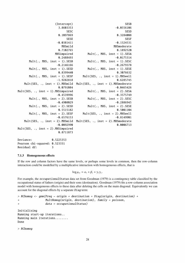
(Intercept) SESB
3.8603353 -0.0556106
SESC SESD
0.1097869 0.3284008
SESE SESF
-0.0381411 -0.1524531
MHSmild MHSmoderate
0.7102765 0.1892520
MHSimpaired Mult(., MHS, inst = 1).SESA
0.2488493 -0.0175314
Mult(., MHS, inst = 1).SESB Mult(., MHS, inst = 1).SESC
-0.2146166 -0.2679378
Mult(., MHS, inst = 1).SESD Mult(., MHS, inst = 1).SESE
0.8399440 0.3076632
Mult(., MHS, inst = 1).SESF Mult(SES, ., inst = 1).MHSwell
-1.9282818 0.6285745
Mult(SES, ., inst = 1).MHSmild Mult(SES, ., inst = 1).MHSmoderate
0.0791084 -0.0465426
Mult(SES, ., inst = 1).MHSimpaired Mult(., MHS, inst = 2).SESA
-0.4539996 -0.3575749
Mult(., MHS, inst = 2).SESB Mult(., MHS, inst = 2).SESC
-0.4908029 -0.2886945
Mult(., MHS, inst = 2).SESD Mult(., MHS, inst = 2).SESE
0.5515182 0.5001104
Mult(., MHS, inst = 2).SESF Mult(SES, ., inst = 2).MHSwell
-0.6576153 -0.8149901
Mult(SES, ., inst = 2).MHSmild Mult(SES, ., inst = 2).MHSmoderate
-0.0092990 0.0006713
Mult(SES, ., inst = 2).MHSimpaired
0.8711873
Deviance: 0.5225353
Pearson chi-squared: 0.523331
Residual df: 3
7.1.3 Homogeneous effects
If the row and column factors have the same levels, or perhaps some levels in common, then the row-column
interaction could be modelled by a multiplicative interaction with homogeneous effects, that is
log µrc = αr + βc + γrγc.
For example, the occupationalStatus data set from Goodman (1979) is a contingency table classified by the
occupational status of fathers (origin) and their sons (destination). Goodman (1979) fits a row-column association
model with homogeneous effects to these data after deleting the cells on the main diagonal. Equivalently we can
account for the diagonal effects by a separate Diag term:
> RChomog <- gnm(Freq ~ origin + destination + Diag(origin, destination) +
+ MultHomog(origin, destination), family = poisson,
+ data = occupationalStatus)
Initialising
Running start-up iterations..
Running main iterations........
Done
> RChomog
28
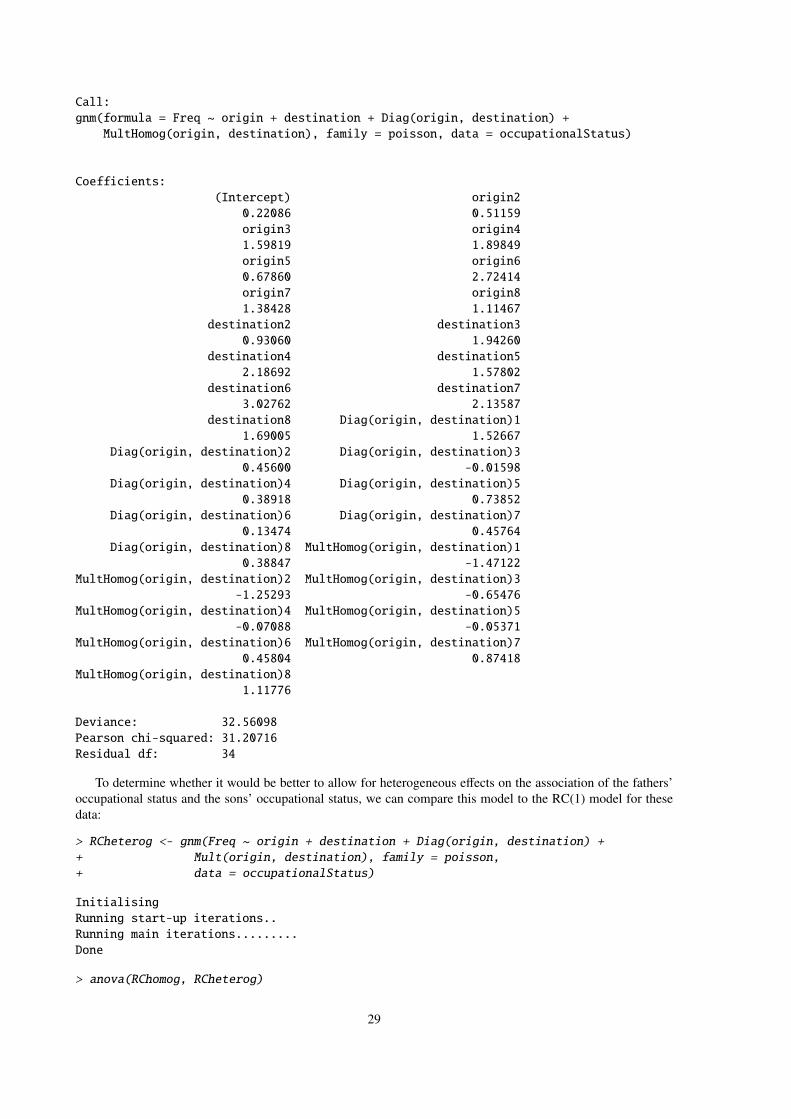
Call:
gnm(formula = Freq ~ origin + destination + Diag(origin, destination) +
MultHomog(origin, destination), family = poisson, data = occupationalStatus)
Coefficients:
(Intercept) origin2
0.22086 0.51159
origin3 origin4
1.59819 1.89849
origin5 origin6
0.67860 2.72414
origin7 origin8
1.38428 1.11467
destination2 destination3
0.93060 1.94260
destination4 destination5
2.18692 1.57802
destination6 destination7
3.02762 2.13587
destination8 Diag(origin, destination)1
1.69005 1.52667
Diag(origin, destination)2 Diag(origin, destination)3
0.45600 -0.01598
Diag(origin, destination)4 Diag(origin, destination)5
0.38918 0.73852
Diag(origin, destination)6 Diag(origin, destination)7
0.13474 0.45764
Diag(origin, destination)8 MultHomog(origin, destination)1
0.38847 -1.47122
MultHomog(origin, destination)2 MultHomog(origin, destination)3
-1.25293 -0.65476
MultHomog(origin, destination)4 MultHomog(origin, destination)5
-0.07088 -0.05371
MultHomog(origin, destination)6 MultHomog(origin, destination)7
0.45804 0.87418
MultHomog(origin, destination)8
1.11776
Deviance: 32.56098
Pearson chi-squared: 31.20716
Residual df: 34
To determine whether it would be better to allow for heterogeneous effects on the association of the fathers’
occupational status and the sons’ occupational status, we can compare this model to the RC(1) model for these
data:
> RCheterog <- gnm(Freq ~ origin + destination + Diag(origin, destination) +
+ Mult(origin, destination), family = poisson,
+ data = occupationalStatus)
Initialising
Running start-up iterations..
Running main iterations.........
Done
> anova(RChomog, RCheterog)
29

Analysis of Deviance Table
Model 1: Freq ~ origin + destination + Diag(origin, destination) + MultHomog(origin,
destination)
Model 2: Freq ~ origin + destination + Diag(origin, destination) + Mult(origin,
destination)
Resid. Df Resid. Dev Df Deviance
1 34 32.561
2 28 29.149 6 3.4118
In this case there is little gain in allowing heterogeneous effects.
7.2 Diagonal reference models
Diagonal reference models, proposed by Sobel (1981, 1985), are designed for contingency tables classified by
factors with the same levels. The cell means are modelled as a function of the diagonal effects, i.e., the mean
responses of the ‘diagonal’ cells in which the levels of the row and column factors are the same.
Dref example 1: Political consequences of social mobility
To illustrate the use of diagonal reference models we shall use the voting data from Clifford and Heath (1993).
The data come from the 1987 British general election and are the percentage voting Labour in groups cross-
classified by the class of the head of household (destination) and the class of their father (origin). In order
to weight these percentages by the group size, we first back-transform them to the counts of those voting Labour
and those not voting Labour:
> set.seed(1)
> count <- with(voting, percentage/100 * total)
> yvar <- cbind(count, voting$total - count)
The grouped percentages may be modelled by a basic diagonal reference model, that is, a weighted sum of
the diagonal effects for the corresponding origin and destination classes. This model may be expressed as
µod =eδ1
eδ1 + eδ2γo +
eδ2
eδ1 + eδ2γd.
See Section 3.3 for more detail on the parameterization.
The basic diagonal reference model may be fitted using gnm as follows
> classMobility <- gnm(yvar ~ Dref(origin, destination),
+ family = binomial, data = voting)
Initialising
Running main iterations........
Done
> classMobility
Call:
gnm(formula = yvar ~ Dref(origin, destination), family = binomial,
data = voting)
Coefficients:
(Intercept) Dref(origin, destination)delta1
-1.34325 -0.30736
Dref(origin, destination)delta2 Dref(., .).origin|destination1
-0.05501 -0.83454
Dref(., .).origin|destination2 Dref(., .).origin|destination3
0.21066 -0.61159
30

Dref(., .).origin|destination4 Dref(., .).origin|destination5
0.76500 1.38370
Deviance: 21.22093
Pearson chi-squared: 18.95311
Residual df: 19
and the origin and destination weights can be evaluated as below
> DrefWeights(classMobility)
$origin
weight se
0.43724694 0.03996404
$destination
weight se
0.56275306 0.03996404
These results are slightly different from those reported by Clifford and Heath (1993). The reason for this is
unclear: we are confident that the above results are correct for the data as given in Clifford and Heath (1993), but
have not been able to confirm that the data as printed in the journal were exactly as used in Clifford and Heath’s
analysis.
Clifford and Heath (1993) suggest that movements in and out of the salariat (class 1) should be treated differ-
ently from movements between the lower classes (classes 2 - 5), since the former has a greater effect on social
status. Thus they propose the following model
µod =
eδ1
eδ1 + eδ2γo +
eδ2
eδ1 + eδ2γd if o = 1
eδ3
eδ3 + eδ4γo +
eδ4
eδ3 + eδ4γd if d = 1
eδ5
eδ5 + eδ6γo +
eδ6
eδ5 + eδ6γd if o , 1 and d , 1
To fit this model we define factors indicating movement in (upward) and out (downward) of the salariat
> upward <- with(voting, origin != 1 & destination == 1)
> downward <- with(voting, origin == 1 & destination != 1)
Then the diagonal reference model with separate weights for socially mobile groups can be estimated as follows
> socialMobility <- gnm(yvar ~ Dref(origin, destination,
+ delta = ~ 1 + downward + upward),
+ family = binomial, data = voting)
Initialising
Running main iterations.........
Done
> socialMobility
Call:
gnm(formula = yvar ~ Dref(origin, destination, delta = ~1 + downward +
upward), family = binomial, data = voting)
Coefficients:
(Intercept)
31
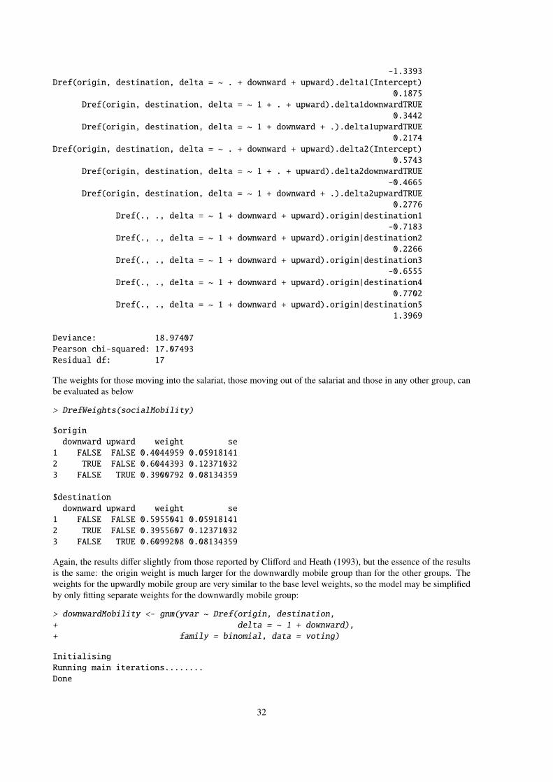
-1.3393
Dref(origin, destination, delta = ~ . + downward + upward).delta1(Intercept)
0.1875
Dref(origin, destination, delta = ~ 1 + . + upward).delta1downwardTRUE
0.3442
Dref(origin, destination, delta = ~ 1 + downward + .).delta1upwardTRUE
0.2174
Dref(origin, destination, delta = ~ . + downward + upward).delta2(Intercept)
0.5743
Dref(origin, destination, delta = ~ 1 + . + upward).delta2downwardTRUE
-0.4665
Dref(origin, destination, delta = ~ 1 + downward + .).delta2upwardTRUE
0.2776
Dref(., ., delta = ~ 1 + downward + upward).origin|destination1
-0.7183
Dref(., ., delta = ~ 1 + downward + upward).origin|destination2
0.2266
Dref(., ., delta = ~ 1 + downward + upward).origin|destination3
-0.6555
Dref(., ., delta = ~ 1 + downward + upward).origin|destination4
0.7702
Dref(., ., delta = ~ 1 + downward + upward).origin|destination5
1.3969
Deviance: 18.97407
Pearson chi-squared: 17.07493
Residual df: 17
The weights for those moving into the salariat, those moving out of the salariat and those in any other group, can
be evaluated as below
> DrefWeights(socialMobility)
$origin
downward upward weight se
1 FALSE FALSE 0.4044959 0.05918141
2 TRUE FALSE 0.6044393 0.12371032
3 FALSE TRUE 0.3900792 0.08134359
$destination
downward upward weight se
1 FALSE FALSE 0.5955041 0.05918141
2 TRUE FALSE 0.3955607 0.12371032
3 FALSE TRUE 0.6099208 0.08134359
Again, the results differ slightly from those reported by Clifford and Heath (1993), but the essence of the results
is the same: the origin weight is much larger for the downwardly mobile group than for the other groups. The
weights for the upwardly mobile group are very similar to the base level weights, so the model may be simplified
by only fitting separate weights for the downwardly mobile group:
> downwardMobility <- gnm(yvar ~ Dref(origin, destination,
+ delta = ~ 1 + downward),
+ family = binomial, data = voting)
Initialising
Running main iterations........
Done
32

> downwardMobility
Call:
gnm(formula = yvar ~ Dref(origin, destination, delta = ~1 + downward),
family = binomial, data = voting)
Coefficients:
(Intercept)
-1.32007
Dref(origin, destination, delta = ~ . + downward).delta1(Intercept)
0.05458
Dref(origin, destination, delta = ~ 1 + .).delta1downwardTRUE
0.16498
Dref(origin, destination, delta = ~ . + downward).delta2(Intercept)
0.46337
Dref(origin, destination, delta = ~ 1 + .).delta2downwardTRUE
-0.64576
Dref(., ., delta = ~ 1 + downward).origin|destination1
-0.74980
Dref(., ., delta = ~ 1 + downward).origin|destination2
0.21354
Dref(., ., delta = ~ 1 + downward).origin|destination3
-0.67158
Dref(., ., delta = ~ 1 + downward).origin|destination4
0.74699
Dref(., ., delta = ~ 1 + downward).origin|destination5
1.37637
Deviance: 18.99389
Pearson chi-squared: 17.09981
Residual df: 18
> DrefWeights(downwardMobility)
$origin
downward weight se
1 FALSE 0.3992031 0.04750643
2 TRUE 0.5991570 0.11951340
$destination
downward weight se
1 FALSE 0.6007969 0.04750643
2 TRUE 0.4008430 0.11951340
Dref example 2: conformity to parental rules
Another application of diagonal reference models is given by van der Slik et al. (2002). The data from this paper
are not publicly available3, but we shall show how the models presented in the paper may be estimated using gnm .
The data relate to the value parents place on their children conforming to their rules. There are two response
variables: the mother’s conformity score (MCFM) and the father’s conformity score (FCFF). The data are cross-
classified by two factors describing the education level of the mother (MOPLM) and the father (FOPLF), and
there are six further covariates (AGEM, MRMM, FRMF, MWORK, MFCM and FFCF).
In their baseline model for the mother’s conformity score, van der Slik et al. (2002) include five of the six
covariates (leaving out the father’s family conflict score, FCFF) and a diagonal reference term with constant
3 We thank Frans van der Slik for his kindness in sending us the data.
33

weights based on the two education factors. This model may be expressed as
µrci = β1x1i + β2x2i + β3x3i + β4x4i + β5x5i +eδ1
eδ1 + eδ2γr +
eδ2
eδ1 + eδ2γc.
The baseline model can be fitted as follows:
> set.seed(1)
> A <- gnm(MCFM ~ -1 + AGEM + MRMM + FRMF + MWORK + MFCM +
+ Dref(MOPLM, FOPLF), family = gaussian, data = conformity,
+ verbose = FALSE)
> A
Call:
gnm(formula = MCFM ~ -1 + AGEM + MRMM + FRMF + MWORK + MFCM +
Dref(MOPLM, FOPLF), family = gaussian, data = conformity,
verbose = FALSE)
Coefficients:
AGEM MRMM FRMF
0.06363 -0.32425 -0.25324
MWORK MFCM Dref(MOPLM, FOPLF)delta1
-0.06430 -0.06043 -0.33731
Dref(MOPLM, FOPLF)delta2 Dref(., .).MOPLM|FOPLF1 Dref(., .).MOPLM|FOPLF2
-0.02505 4.95121 4.86329
Dref(., .).MOPLM|FOPLF3 Dref(., .).MOPLM|FOPLF4 Dref(., .).MOPLM|FOPLF5
4.86458 4.72343 4.43516
Dref(., .).MOPLM|FOPLF6 Dref(., .).MOPLM|FOPLF7
4.18873 4.43378
Deviance: 425.3389
Pearson chi-squared: 425.3389
Residual df: 576
The coefficients of the covariates are not aliased with the parameters of the diagonal reference term and thus the
basic identifiability constraints that have been imposed are sufficient for these parameters to be identified. The
diagonal effects do not need to be constrained as they represent contrasts with the off-diagonal cells. Therefore
the only unidentified parameters in this model are the weight parameters. This is confirmed in the summary of
the model:
> summary(A)
Call:
gnm(formula = MCFM ~ -1 + AGEM + MRMM + FRMF + MWORK + MFCM +
Dref(MOPLM, FOPLF), family = gaussian, data = conformity,
verbose = FALSE)
Deviance Residuals:
Min 1Q Median 3Q Max
-3.63688 -0.50383 0.01714 0.56753 2.25139
Coefficients:
Estimate Std. Error t value Pr(>|t|)
AGEM 0.06363 0.07375 0.863 0.38859
MRMM -0.32425 0.07766 -4.175 3.44e-05
FRMF -0.25324 0.07681 -3.297 0.00104
MWORK -0.06430 0.07431 -0.865 0.38727
MFCM -0.06043 0.07123 -0.848 0.39663
34
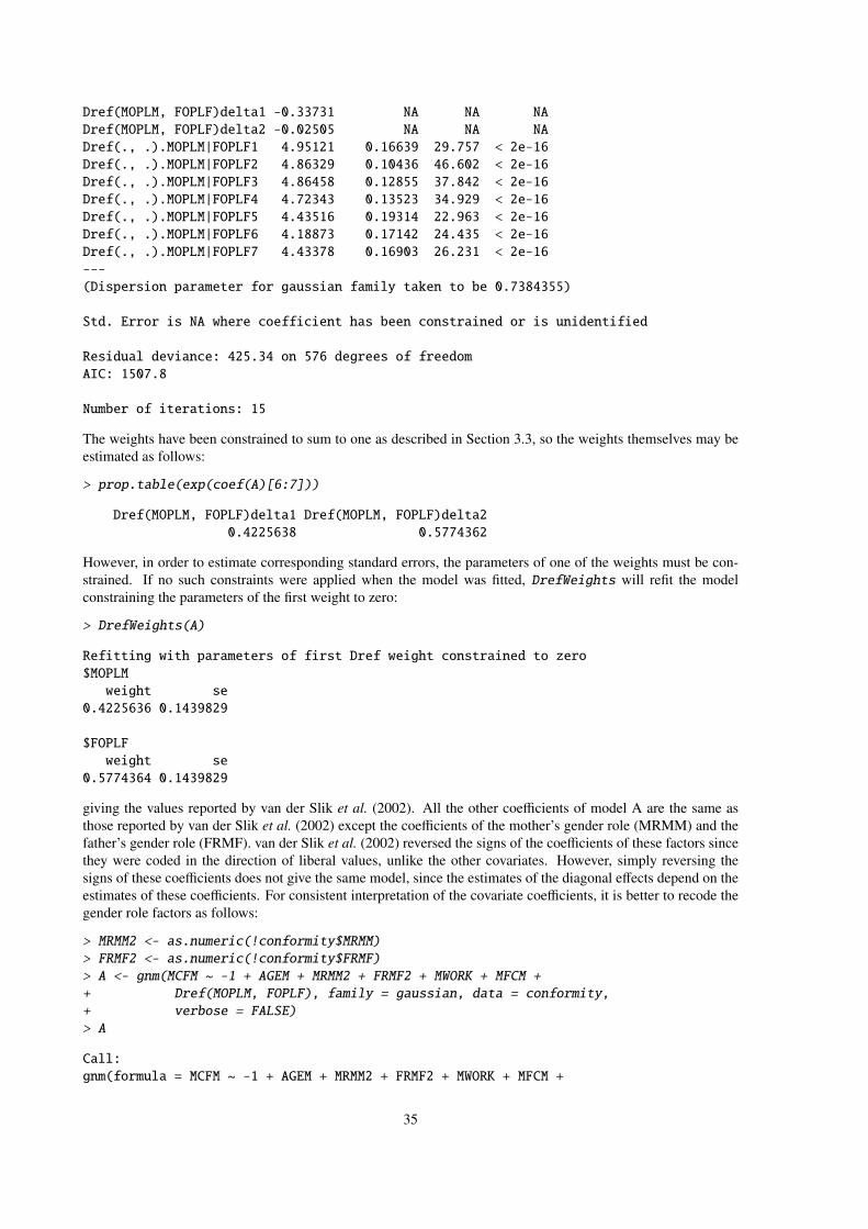
Dref(MOPLM, FOPLF)delta1 -0.33731 NA NA NA
Dref(MOPLM, FOPLF)delta2 -0.02505 NA NA NA
Dref(., .).MOPLM|FOPLF1 4.95121 0.16639 29.757 < 2e-16
Dref(., .).MOPLM|FOPLF2 4.86329 0.10436 46.602 < 2e-16
Dref(., .).MOPLM|FOPLF3 4.86458 0.12855 37.842 < 2e-16
Dref(., .).MOPLM|FOPLF4 4.72343 0.13523 34.929 < 2e-16
Dref(., .).MOPLM|FOPLF5 4.43516 0.19314 22.963 < 2e-16
Dref(., .).MOPLM|FOPLF6 4.18873 0.17142 24.435 < 2e-16
Dref(., .).MOPLM|FOPLF7 4.43378 0.16903 26.231 < 2e-16
---
(Dispersion parameter for gaussian family taken to be 0.7384355)
Std. Error is NA where coefficient has been constrained or is unidentified
Residual deviance: 425.34 on 576 degrees of freedom
AIC: 1507.8
Number of iterations: 15
The weights have been constrained to sum to one as described in Section 3.3, so the weights themselves may be
estimated as follows:
> prop.table(exp(coef(A)[6:7]))
Dref(MOPLM, FOPLF)delta1 Dref(MOPLM, FOPLF)delta2
0.4225638 0.5774362
However, in order to estimate corresponding standard errors, the parameters of one of the weights must be con-
strained. If no such constraints were applied when the model was fitted, DrefWeights will refit the model
constraining the parameters of the first weight to zero:
> DrefWeights(A)
Refitting with parameters of first Dref weight constrained to zero
$MOPLM
weight se
0.4225636 0.1439829
$FOPLF
weight se
0.5774364 0.1439829
giving the values reported by van der Slik et al. (2002). All the other coefficients of model A are the same as
those reported by van der Slik et al. (2002) except the coefficients of the mother’s gender role (MRMM) and the
father’s gender role (FRMF). van der Slik et al. (2002) reversed the signs of the coefficients of these factors since
they were coded in the direction of liberal values, unlike the other covariates. However, simply reversing the
signs of these coefficients does not give the same model, since the estimates of the diagonal effects depend on the
estimates of these coefficients. For consistent interpretation of the covariate coefficients, it is better to recode the
gender role factors as follows:
> MRMM2 <- as.numeric(!conformity$MRMM)
> FRMF2 <- as.numeric(!conformity$FRMF)
> A <- gnm(MCFM ~ -1 + AGEM + MRMM2 + FRMF2 + MWORK + MFCM +
+ Dref(MOPLM, FOPLF), family = gaussian, data = conformity,
+ verbose = FALSE)
> A
Call:
gnm(formula = MCFM ~ -1 + AGEM + MRMM2 + FRMF2 + MWORK + MFCM +
35
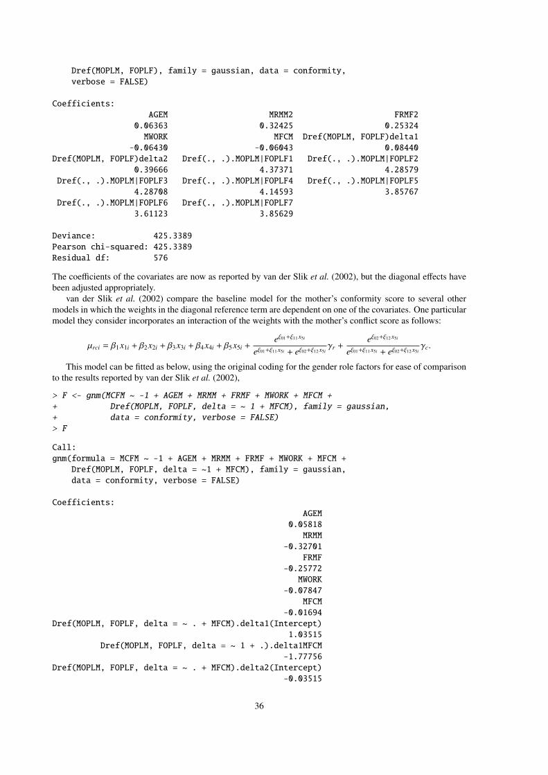
Dref(MOPLM, FOPLF), family = gaussian, data = conformity,
verbose = FALSE)
Coefficients:
AGEM MRMM2 FRMF2
0.06363 0.32425 0.25324
MWORK MFCM Dref(MOPLM, FOPLF)delta1
-0.06430 -0.06043 0.08440
Dref(MOPLM, FOPLF)delta2 Dref(., .).MOPLM|FOPLF1 Dref(., .).MOPLM|FOPLF2
0.39666 4.37371 4.28579
Dref(., .).MOPLM|FOPLF3 Dref(., .).MOPLM|FOPLF4 Dref(., .).MOPLM|FOPLF5
4.28708 4.14593 3.85767
Dref(., .).MOPLM|FOPLF6 Dref(., .).MOPLM|FOPLF7
3.61123 3.85629
Deviance: 425.3389
Pearson chi-squared: 425.3389
Residual df: 576
The coefficients of the covariates are now as reported by van der Slik et al. (2002), but the diagonal effects have
been adjusted appropriately.
van der Slik et al. (2002) compare the baseline model for the mother’s conformity score to several other
models in which the weights in the diagonal reference term are dependent on one of the covariates. One particular
model they consider incorporates an interaction of the weights with the mother’s conflict score as follows:
µrci = β1x1i + β2x2i + β3x3i + β4x4i + β5x5i +eξ01+ξ11 x5i
eξ01+ξ11 x5i + eξ02+ξ12 x5iγr +
eξ02+ξ12 x5i
eξ01+ξ11 x5i + eξ02+ξ12 x5iγc.
This model can be fitted as below, using the original coding for the gender role factors for ease of comparison
to the results reported by van der Slik et al. (2002),
> F <- gnm(MCFM ~ -1 + AGEM + MRMM + FRMF + MWORK + MFCM +
+ Dref(MOPLM, FOPLF, delta = ~ 1 + MFCM), family = gaussian,
+ data = conformity, verbose = FALSE)
> F
Call:
gnm(formula = MCFM ~ -1 + AGEM + MRMM + FRMF + MWORK + MFCM +
Dref(MOPLM, FOPLF, delta = ~1 + MFCM), family = gaussian,
data = conformity, verbose = FALSE)
Coefficients:
AGEM
0.05818
MRMM
-0.32701
FRMF
-0.25772
MWORK
-0.07847
MFCM
-0.01694
Dref(MOPLM, FOPLF, delta = ~ . + MFCM).delta1(Intercept)
1.03515
Dref(MOPLM, FOPLF, delta = ~ 1 + .).delta1MFCM
-1.77756
Dref(MOPLM, FOPLF, delta = ~ . + MFCM).delta2(Intercept)
-0.03515
36
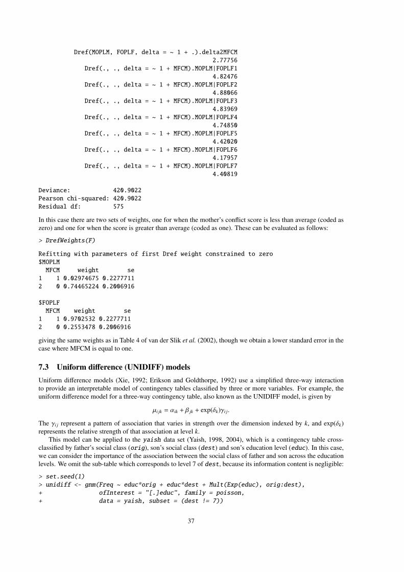
Dref(MOPLM, FOPLF, delta = ~ 1 + .).delta2MFCM
2.77756
Dref(., ., delta = ~ 1 + MFCM).MOPLM|FOPLF1
4.82476
Dref(., ., delta = ~ 1 + MFCM).MOPLM|FOPLF2
4.88066
Dref(., ., delta = ~ 1 + MFCM).MOPLM|FOPLF3
4.83969
Dref(., ., delta = ~ 1 + MFCM).MOPLM|FOPLF4
4.74850
Dref(., ., delta = ~ 1 + MFCM).MOPLM|FOPLF5
4.42020
Dref(., ., delta = ~ 1 + MFCM).MOPLM|FOPLF6
4.17957
Dref(., ., delta = ~ 1 + MFCM).MOPLM|FOPLF7
4.40819
Deviance: 420.9022
Pearson chi-squared: 420.9022
Residual df: 575
In this case there are two sets of weights, one for when the mother’s conflict score is less than average (coded as
zero) and one for when the score is greater than average (coded as one). These can be evaluated as follows:
> DrefWeights(F)
Refitting with parameters of first Dref weight constrained to zero
$MOPLM
MFCM weight se
1 1 0.02974675 0.2277711
2 0 0.74465224 0.2006916
$FOPLF
MFCM weight se
1 1 0.9702532 0.2277711
2 0 0.2553478 0.2006916
giving the same weights as in Table 4 of van der Slik et al. (2002), though we obtain a lower standard error in the
case where MFCM is equal to one.
7.3 Uniform difference (UNIDIFF) models
Uniform difference models (Xie, 1992; Erikson and Goldthorpe, 1992) use a simplified three-way interaction
to provide an interpretable model of contingency tables classified by three or more variables. For example, the
uniform difference model for a three-way contingency table, also known as the UNIDIFF model, is given by
µi jk = αik + β jk + exp(δk)γi j.
The γi j represent a pattern of association that varies in strength over the dimension indexed by k, and exp(δk)
represents the relative strength of that association at level k.
This model can be applied to the yaish data set (Yaish, 1998, 2004), which is a contingency table cross-
classified by father’s social class (orig), son’s social class (dest) and son’s education level (educ). In this case,
we can consider the importance of the association between the social class of father and son across the education
levels. We omit the sub-table which corresponds to level 7 of dest, because its information content is negligible:
> set.seed(1)
> unidiff <- gnm(Freq ~ educ*orig + educ*dest + Mult(Exp(educ), orig:dest),
+ ofInterest = "[.]educ", family = poisson,
+ data = yaish, subset = (dest != 7))
37
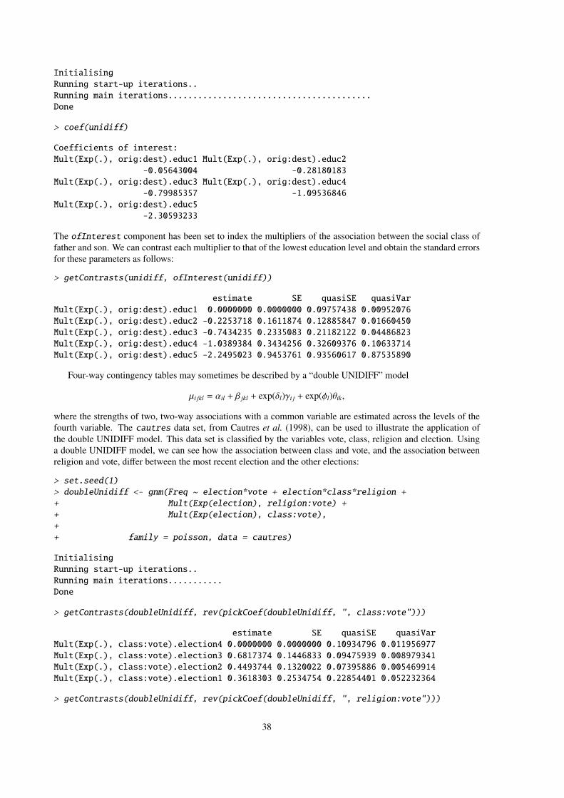
Initialising
Running start-up iterations..
Running main iterations.........................................
Done
> coef(unidiff)
Coefficients of interest:
Mult(Exp(.), orig:dest).educ1 Mult(Exp(.), orig:dest).educ2
-0.05643004 -0.28180183
Mult(Exp(.), orig:dest).educ3 Mult(Exp(.), orig:dest).educ4
-0.79985357 -1.09536846
Mult(Exp(.), orig:dest).educ5
-2.30593233
The ofInterest component has been set to index the multipliers of the association between the social class of
father and son. We can contrast each multiplier to that of the lowest education level and obtain the standard errors
for these parameters as follows:
> getContrasts(unidiff, ofInterest(unidiff))
estimate SE quasiSE quasiVar
Mult(Exp(.), orig:dest).educ1 0.0000000 0.0000000 0.09757438 0.00952076
Mult(Exp(.), orig:dest).educ2 -0.2253718 0.1611874 0.12885847 0.01660450
Mult(Exp(.), orig:dest).educ3 -0.7434235 0.2335083 0.21182122 0.04486823
Mult(Exp(.), orig:dest).educ4 -1.0389384 0.3434256 0.32609376 0.10633714
Mult(Exp(.), orig:dest).educ5 -2.2495023 0.9453761 0.93560617 0.87535890
Four-way contingency tables may sometimes be described by a “double UNIDIFF” model
µi jkl = αil + β jkl + exp(δl)γi j + exp(φl)θik,
where the strengths of two, two-way associations with a common variable are estimated across the levels of the
fourth variable. The cautres data set, from Cautres et al. (1998), can be used to illustrate the application of
the double UNIDIFF model. This data set is classified by the variables vote, class, religion and election. Using
a double UNIDIFF model, we can see how the association between class and vote, and the association between
religion and vote, differ between the most recent election and the other elections:
> set.seed(1)
> doubleUnidiff <- gnm(Freq ~ election*vote + election*class*religion +
+ Mult(Exp(election), religion:vote) +
+ Mult(Exp(election), class:vote),
+
+ family = poisson, data = cautres)
Initialising
Running start-up iterations..
Running main iterations...........
Done
> getContrasts(doubleUnidiff, rev(pickCoef(doubleUnidiff, ", class:vote")))
estimate SE quasiSE quasiVar
Mult(Exp(.), class:vote).election4 0.0000000 0.0000000 0.10934796 0.011956977
Mult(Exp(.), class:vote).election3 0.6817374 0.1446833 0.09475939 0.008979341
Mult(Exp(.), class:vote).election2 0.4493744 0.1320022 0.07395886 0.005469914
Mult(Exp(.), class:vote).election1 0.3618303 0.2534754 0.22854401 0.052232364
> getContrasts(doubleUnidiff, rev(pickCoef(doubleUnidiff, ", religion:vote")))
38

estimate SE quasiSE
Mult(Exp(.), religion:vote).election4 0.0000000 0.00000000 0.07168290
Mult(Exp(.), religion:vote).election3 -0.0878181 0.09906916 0.06812239
Mult(Exp(.), religion:vote).election2 -0.2615200 0.09116479 0.05702819
Mult(Exp(.), religion:vote).election1 -0.3283459 0.12213023 0.09803075
quasiVar
Mult(Exp(.), religion:vote).election4 0.005138439
Mult(Exp(.), religion:vote).election3 0.004640660
Mult(Exp(.), religion:vote).election2 0.003252214
Mult(Exp(.), religion:vote).election1 0.009610029
7.4 Generalized additive main effects and multiplicative interaction (GAMMI) models
Generalized additive main effects and multiplicative interaction models, or GAMMI models, were motivated by
two-way contingency tables and comprise the row and column main effects plus one or more components of the
multiplicative interaction. The singular value corresponding to each multiplicative component is often factored
out, as a measure of the strength of association between the row and column scores, indicating the importance of
the component, or axis.
For cell means µrc a GAMMI-K model has the form
g(µrc) = αr + βc +
K∑
k=1
σkγkrδkc, (1)
in which g is a link function, αr and βc are the row and column main effects, γkr and δkc are the row and column
scores for multiplicative component k and σk is the singular value for component k. The number of multiplicative
components, K, is less than or equal to the rank of the matrix of residuals from the main effects.
The row-column association models discussed in Section 7.1 are examples of GAMMI models, with a log link
and poisson variance. Here we illustrate the use of an AMMI model, which is a GAMMI model with an identity
link and a constant variance.
We shall use the wheat data set taken from Vargas et al. (2001), which gives wheat yields measured over
ten years. First we scale these yields and create a new treatment factor, so that we can reproduce the analysis of
Vargas et al. (2001):
> set.seed(1)
> yield.scaled <- wheat$yield * sqrt(3/1000)
> treatment <- interaction(wheat$tillage, wheat$summerCrop, wheat$manure,
+ wheat$N, sep = "")
Now we can fit the AMMI-1 model, to the scaled yields using the combined treatment factor and the year factor
from the wheat dataset. We will proceed by first fitting the main effects model, then using residSVD (see Section
5.5) for the parameters of the multiplicative term:
> mainEffects <- gnm(yield.scaled ~ year + treatment, family = gaussian,
+ data = wheat)
> svdStart <- residSVD(mainEffects, year, treatment, 3)
> bilinear1 <- update(mainEffects, . ~ . + Mult(year, treatment),
+ start = c(coef(mainEffects), svdStart[,1]))
Running main iterations
Done
We can compare the AMMI-1 model to the main effects model,
> anova(mainEffects, bilinear1, test = "F")
Analysis of Deviance Table
Model 1: yield.scaled ~ year + treatment
39
Model 2: yield.scaled ~ year + treatment + Mult(year, treatment)
Resid. Df Resid. Dev Df Deviance F Pr(>F)
1 207 279515
2 176 128383 31 151133 6.6835 < 2.2e-16
giving the same results as in Table 1 of Vargas et al. (2001) (up to error caused by rounding).
Thus the significance of the multiplicative interaction can be tested without applying constraints to this term.
If the multiplicative interaction is significant, we may wish to apply constraints to obtain estimates of the row
and column scores. We illustrate this using the barleyHeights data, which records the average height for 15
genotypes of barley over 9 years.
For this small dataset the AMMI-1 model is easily estimated with the default settings:
> set.seed(1)
> barleyModel <- gnm(height ~ year + genotype + Mult(year, genotype),
+ data = barleyHeights)
Initialising
Running start-up iterations..
Running main iterations.......
Done
To obtain the parameterization of Equation 1 in which σk is the singular value for component k, the row and
column scores must be constrained so that the scores sum to zero and the squared scores sum to one. These
contrasts can be obtained using getContrasts:
> gamma <- getContrasts(barleyModel, pickCoef(barleyModel, "[.]y"),
+ ref = "mean", scaleWeights = "unit")
> delta <- getContrasts(barleyModel, pickCoef(barleyModel, "[.]g"),
+ ref = "mean", scaleWeights = "unit")
> gamma
Estimate Std. Error
Mult(., genotype).year1974 0.22662083 0.05621029
Mult(., genotype).year1975 0.51350519 0.04856519
Mult(., genotype).year1976 0.43898738 0.05124785
Mult(., genotype).year1977 -0.20046457 0.05658391
Mult(., genotype).year1978 -0.53320298 0.04775769
Mult(., genotype).year1979 0.14181352 0.05724921
Mult(., genotype).year1980 -0.33249439 0.05418746
Mult(., genotype).year1981 -0.17553769 0.05689550
Mult(., genotype).year1982 -0.07922728 0.05770322
> delta
Estimate Std. Error
Mult(year, .).genotype1 0.079143300 0.05913864
Mult(year, .).genotype10 -0.335345232 0.05564859
Mult(year, .).genotype11 -0.375909514 0.05466190
Mult(year, .).genotype12 0.285239058 0.05669279
Mult(year, .).genotype13 -0.168316668 0.05843057
Mult(year, .).genotype14 0.293052673 0.05654225
Mult(year, .).genotype15 0.460366625 0.05216774
Mult(year, .).genotype2 0.007543294 0.05933628
Mult(year, .).genotype3 0.169718829 0.05841527
Mult(year, .).genotype4 -0.047168473 0.05926732
Mult(year, .).genotype5 0.181497848 0.05828153
Mult(year, .).genotype6 0.129417613 0.05880326
Mult(year, .).genotype7 0.013581894 0.05933222
Mult(year, .).genotype8 -0.422242966 0.05337051
Mult(year, .).genotype9 -0.270578282 0.05696326
40
Confidence intervals based on the assumption of asymptotic normality can be computed as follows:
> gamma[[2]][,1] + (gamma[[2]][,2]) %o% c(-1.96, 1.96)
[,1] [,2]
[1,] 0.11644866 0.33679300
[2,] 0.41831741 0.60869296
[3,] 0.33854160 0.53943316
[4,] -0.31136904 -0.08956010
[5,] -0.62680805 -0.43959792
[6,] 0.02960507 0.25402198
[7,] -0.43870182 -0.22628697
[8,] -0.28705286 -0.06402252
[9,] -0.19232559 0.03387103
> delta[[2]][,1] + (delta[[2]][,2]) %o% c(-1.96, 1.96)
[,1] [,2]
[1,] -0.03676844 0.19505504
[2,] -0.44441647 -0.22627399
[3,] -0.48304683 -0.26877219
[4,] 0.17412119 0.39635693
[5,] -0.28284059 -0.05379275
[6,] 0.18222986 0.40387548
[7,] 0.35811786 0.56261539
[8,] -0.10875581 0.12384240
[9,] 0.05522490 0.28421275
[10,] -0.16333242 0.06899548
[11,] 0.06726605 0.29572965
[12,] 0.01416323 0.24467200
[13,] -0.10270926 0.12987305
[14,] -0.52684917 -0.31763677
[15,] -0.38222628 -0.15893028
which broadly agree with Table 8 of Chadoeuf and Denis (1991), allowing for the change in sign.
On the basis of such confidence intervals we can investigate simplifications of the model such as combining
levels of the factors or fitting an additive model to a subset of the data.
The singular value σk may be obtained as follows
> svd(termPredictors(barleyModel)[, "Mult(year, genotype)"])$d
[1] 43.49601
This parameter is of little interest in itself, given that the significance of the term as a whole can be tested using
ANOVA.
The SVD representation can also be obtained quite easily for AMMI and GAMMI models with interaction
rank greater than 1. See example(wheat) for an example of this in an AMMI model with rank 2. (The calcu-
lation of standard errors and confidence regions for the SVD representation with rank greater than 1 is not yet
implemented, though.)
7.5 Biplot models
Biplots are graphical displays of two-dimensional arrays, which represent the objects that index both dimensions
of the array on the same plot. Here we consider the case of a two-way table, where a biplot may be used to
represent both the row and column categories simultaneously.
A two-dimensional biplot is constructed from a rank-2 representation of the data. For two-way tables, the
generalized bilinear model defines one such representation:
g(µi j) = ηi j = α1iβ1 j + α2iβ2 j
41
since we can alternatively write
η =
α11 α21
......
α1n α2n
(
β11 . . . β1p
β21 . . . β2p
)
= ABT
where the columns of A and B are linearly independent by definition.
To demonstrate how the biplot is obtained from this model, we shall use the barley data set which gives
the percentage of leaf area affected by leaf blotch for ten varieties of barley grown at nine sites (Wedderburn,
1974; Gabriel, 1998). As suggested by Wedderburn (1974) we model these data using a logit link and a variance
proportional to the square of that of the binomial, implemented as the wedderburn family in gnm (see also
Section 2):
> set.seed(83)
> biplotModel <- gnm(y ~ -1 + instances(Mult(site, variety), 2),
+ family = wedderburn, data = barley)
Initialising
Running start-up iterations..
Running main iterations.........................................................
............................................................................
Done
The effect of site i can be represented by the point
(α1i, α2i)
in the space spanned by the linearly independent basis vectors
a1 = (α11, α12, . . . α19)T
a2 = (α21, α22, . . . α29)T
and the variety effects can be similarly represented.
Thus we can represent the sites and varieties separately as follows
sites <- pickCoef(biplotModel, "[.]site")
coefs <- coef(biplotModel)
A <- matrix(coefs[sites], nc = 2)
B <- matrix(coefs[-sites], nc = 2)
par(mfrow = c(1, 2))
plot(A, pch = levels(barley$site), xlim = c(-5, 5), ylim = c(-5, 5),
main = "Site Effects", xlab = "Component 1", ylab = "Component 2")
plot(B, pch = levels(barley$variety), xlim = c(-5, 5), ylim = c(-5, 5),
main = "Variety Effects", xlab = "Component 1", ylab = "Component 2")
Of course the parameterization of the bilinear model is not unique and therefore the scale and rotation of the
points in these plots will depend on the random seed. By rotation and reciprocal scaling of the matrices A and B,
we can obtain basis vectors with desirable properties without changing the fitted model.
In particular, if we rotate the matrices A and B so that their columns are orthogonal, then the corresponding
plots will display the euclidean distances between sites and varieties respectively. If we also scale the matrices A
and B so that the corresponding plots have the same units, then we can combine the two plots to give a conventional
biplot display.
The required rotation and scaling can be performed via singular value decomposition of the fitted predictors:
42

A
B
C
D
EF
G
HI
−4 −2 0 2 4
−4
−2
02
4Site Effects
Component 1
Co
mp
on
en
t 2 1
2345
6789X
−4 −2 0 2 4
−4
−2
02
4
Variety Effects
Component 1C
om
po
ne
nt
2
Figure 7: Plots of site and variety effects from the generalized bilinear model of the barley data.
> barleyMatrix <- xtabs(biplotModel$predictors ~ site + variety,
+ data = barley)
> barleySVD <- svd(barleyMatrix)
> A <- sweep(barleySVD$u, 2, sqrt(barleySVD$d), "*")[, 1:2]
> B <- sweep(barleySVD$v, 2, sqrt(barleySVD$d), "*")[, 1:2]
> rownames(A) <- levels(barley$site)
> rownames(B) <- levels(barley$variety)
> colnames(A) <- colnames(B) <- paste("Component", 1:2)
> A
Component 1 Component 2
A 4.1948225 -0.39186724
B 2.7642412 -0.33951385
C 1.4250454 -0.04654266
D 1.8463067 0.33365989
E 1.2704088 0.15776723
F 1.1562913 0.40048199
G 1.0172048 0.72727987
H 0.6451366 1.46162701
I -0.1470898 2.13234201
> B
Component 1 Component 2
1 -2.0673648 -0.97420446
2 -3.0599797 -0.50683007
3 -2.9598031 -0.33190626
4 -1.8086247 -0.49758477
5 -1.5579477 -0.08444511
6 -1.8939995 1.08460553
7 -1.1790432 0.40687014
8 -0.8490092 1.14671349
9 -0.9704664 1.26558202
X -0.6036789 1.39655881
43
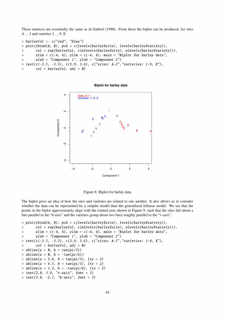
These matrices are essentially the same as in Gabriel (1998). From these the biplot can be produced, for sites
A . . . I and varieties 1 . . . 9, X:
> barleyCol <- c("red", "blue")
> plot(rbind(A, B), pch = c(levels(barley$site), levels(barley$variety)),
+ col = rep(barleyCol, c(nlevels(barley$site), nlevels(barley$variety))),
+ xlim = c(-4, 4), ylim = c(-4, 4), main = "Biplot for barley data",
+ xlab = "Component 1", ylab = "Component 2")
> text(c(-3.5, -3.5), c(3.9, 3.6), c("sites: A-I","varieties: 1-9, X"),
+ col = barleyCol, adj = 0)
ABC
DE
FG
H
I
1
23
4
5
6
7
89X
−4 −2 0 2 4
−4
−2
02
4
Biplot for barley data
Component 1
Com
ponent 2
sites: A−Ivarieties: 1−9, X
Figure 8: Biplot for barley data
The biplot gives an idea of how the sites and varieties are related to one another. It also allows us to consider
whether the data can be represented by a simpler model than the generalized bilinear model. We see that the
points in the biplot approximately align with the rotated axes shown in Figure 9, such that the sites fall about a
line parallel to the “h-axis” and the varieties group about two lines roughly parallel to the “v-axis”.
> plot(rbind(A, B), pch = c(levels(barley$site), levels(barley$variety)),
+ col = rep(barleyCol, c(nlevels(barley$site), nlevels(barley$variety))),
+ xlim = c(-4, 4), ylim = c(-4, 4), main = "Biplot for barley data",
+ xlab = "Component 1", ylab = "Component 2")
> text(c(-3.5, -3.5), c(3.9, 3.6), c("sites: A-I","varieties: 1-9, X"),
+ col = barleyCol, adj = 0)
> abline(a = 0, b = tan(pi/3))
> abline(a = 0, b = -tan(pi/6))
> abline(a = 2.6, b = tan(pi/3), lty = 2)
> abline(a = 4.5, b = tan(pi/3), lty = 2)
> abline(a = 1.3, b = -tan(pi/6), lty = 2)
> text(2.8, 3.9, "v-axis", font = 3)
> text(3.8, -2.7, "h-axis", font = 3)
44
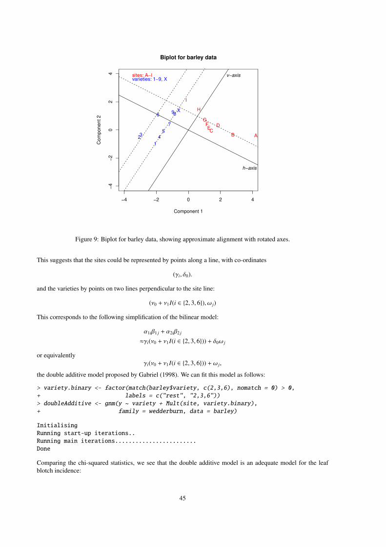
ABC
DE
FG
H
I
1
23
4
5
6
7
89X
−4 −2 0 2 4
−4
−2
02
4
Biplot for barley data
Component 1
Com
ponent 2
sites: A−Ivarieties: 1−9, X
v−axis
h−axis
Figure 9: Biplot for barley data, showing approximate alignment with rotated axes.
This suggests that the sites could be represented by points along a line, with co-ordinates
(γi, δ0).
and the varieties by points on two lines perpendicular to the site line:
(ν0 + ν1I(i ∈ {2, 3, 6}), ω j)
This corresponds to the following simplification of the bilinear model:
α1iβ1 j + α2iβ2 j
≈γi(ν0 + ν1I(i ∈ {2, 3, 6})) + δ0ω j
or equivalently
γi(ν0 + ν1I(i ∈ {2, 3, 6})) + ω j,
the double additive model proposed by Gabriel (1998). We can fit this model as follows:
> variety.binary <- factor(match(barley$variety, c(2,3,6), nomatch = 0) > 0,
+ labels = c("rest", "2,3,6"))
> doubleAdditive <- gnm(y ~ variety + Mult(site, variety.binary),
+ family = wedderburn, data = barley)
Initialising
Running start-up iterations..
Running main iterations........................
Done
Comparing the chi-squared statistics, we see that the double additive model is an adequate model for the leaf
blotch incidence:
45

> biplotModChiSq <- sum(residuals(biplotModel, type = "pearson")^2)
> doubleAddChiSq <- sum(residuals(doubleAdditive, type = "pearson")^2)
> c(doubleAddChiSq - biplotModChiSq,
+ doubleAdditive$df.residual - biplotModel$df.residual)
[1] 9.513773 15.000000
7.6 Stereotype model for multinomial response
The stereotype model was proposed by Anderson (1984) for ordered categorical data. It is a special case of
the multinomial logistic model, in which the covariate coefficients are common to all categories but the scale of
association is allowed to vary between categories such that
pic =exp(β0c + γcβ
Txi)
∑Kk=1 exp(β0k + γkβ
Txi)
where pic is the probability that the response for individual i is category c and K is the number of categories. Like
the multinomial logistic model, the stereotype model specifies a simple form for the log odds of one category
against another, e.g.
log
(
pic
pik
)
= (β0c − β0k) + (γc − γk)βTxi
In order to model a multinomial response in the generalized nonlinear model framework, we must re-express
the data as category counts Yi = (Yi1, . . . ,YiK) for each individual (or group). Then assuming a Poisson distribution
for the counts Yic, the joint distribution of Yi is Multinomial(Ni, pi1, . . . , piK) conditional on the total count for
each individual Ni. The expected counts are then µic = Ni pic and the parameters of the stereotype model can be
estimated through fitting the following model
log µic = log(Ni) + log(pic)
= αi + β0c + γc
∑
r
βr xir
where the “nuisance” parameters αi ensure that the multinomial denominators are reproduced exactly, as required.
The gnm package includes the utility function expandCategorical to re-express the categorical response as
category counts. By default, individuals with common values across all covariates are grouped together, to avoid
redundancy.
For example, the backPain data set from Anderson (1984) describes the progress of patients with back pain.
The data set consists of an ordered factor quantifying the progress of each patient, and three prognostic variables.
We re-express the data as follows:
> set.seed(1)
> subset(backPain, x1 == 1 & x2 == 1 & x3 == 1)
x1 x2 x3 pain
1 1 1 1 same
2 1 1 1 marked.improvement
3 1 1 1 complete.relief
41 1 1 1 marked.improvement
42 1 1 1 complete.relief
43 1 1 1 complete.relief
44 1 1 1 complete.relief
> backPainLong <- expandCategorical(backPain, "pain")
> head(backPainLong)
x1 x2 x3 pain id count
1 1 1 1 worse 1 0
46

2 1 1 1 same 1 1
3 1 1 1 slight.improvement 1 0
4 1 1 1 moderate.improvement 1 0
5 1 1 1 marked.improvement 1 2
6 1 1 1 complete.relief 1 4
We can now fit the stereotype model to these data:
> oneDimensional <- gnm(count ~ pain + Mult(pain, x1 + x2 + x3),
+ eliminate = id, family = "poisson", data = backPainLong)
Initialising
Running start-up iterations..
Running main iterations..............
Done
> oneDimensional
Call:
gnm(formula = count ~ pain + Mult(pain, x1 + x2 + x3), eliminate = id,
family = "poisson", data = backPainLong)
Coefficients of interest:
painsame
16.1578
painslight.improvement
15.6848
painmoderate.improvement
12.4556
painmarked.improvement
19.9140
paincomplete.relief
21.6653
Mult(., x1 + x2 + x3).painworse
0.3322
Mult(., x1 + x2 + x3).painsame
-1.9147
Mult(., x1 + x2 + x3).painslight.improvement
-1.7935
Mult(., x1 + x2 + x3).painmoderate.improvement
-1.2625
Mult(., x1 + x2 + x3).painmarked.improvement
-2.4609
Mult(., x1 + x2 + x3).paincomplete.relief
-2.9214
Mult(pain, . + x2 + x3).x1
1.6510
Mult(pain, x1 + . + x3).x2
0.9470
Mult(pain, x1 + x2 + .).x3
0.8338
Deviance: 55.90786
Pearson chi-squared: 49.61719
Residual df: 48
specifying the id factor through eliminate so that the 12 id effects are estimated more efficiently and are
excluded from printed model summaries by default. This model is one dimensional since it involves only one
47
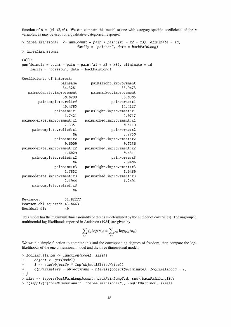
function of x = (x1, x2, x3). We can compare this model to one with category-specific coefficients of the x
variables, as may be used for a qualitative categorical response:
> threeDimensional <- gnm(count ~ pain + pain:(x1 + x2 + x3), eliminate = id,
+ family = "poisson", data = backPainLong)
> threeDimensional
Call:
gnm(formula = count ~ pain + pain:(x1 + x2 + x3), eliminate = id,
family = "poisson", data = backPainLong)
Coefficients of interest:
painsame painslight.improvement
34.3281 33.9473
painmoderate.improvement painmarked.improvement
30.8299 38.0305
paincomplete.relief painworse:x1
40.4785 14.4127
painsame:x1 painslight.improvement:x1
1.7421 2.0717
painmoderate.improvement:x1 painmarked.improvement:x1
2.3351 0.5119
paincomplete.relief:x1 painworse:x2
NA 3.2750
painsame:x2 painslight.improvement:x2
0.6009 0.7236
painmoderate.improvement:x2 painmarked.improvement:x2
1.6029 0.4311
paincomplete.relief:x2 painworse:x3
NA 2.9406
painsame:x3 painslight.improvement:x3
1.7852 1.6486
painmoderate.improvement:x3 painmarked.improvement:x3
2.1944 1.2491
paincomplete.relief:x3
NA
Deviance: 51.82277
Pearson chi-squared: 43.86631
Residual df: 40
This model has the maximum dimensionality of three (as determined by the number of covariates). The ungrouped
multinomial log-likelihoods reported in Anderson (1984) are given by
∑
i,c
yic log(pic) =∑
i,c
yic log(µic/nic)
We write a simple function to compute this and the corresponding degrees of freedom, then compare the log-
likelihoods of the one dimensional model and the three dimensional model:
> logLikMultinom <- function(model, size){
+ object <- get(model)
+ l <- sum(object$y * log(object$fitted/size))
+ c(nParameters = object$rank - nlevels(object$eliminate), logLikelihood = l)
+ }
> size <- tapply(backPainLong$count, backPainLong$id, sum)[backPainLong$id]
> t(sapply(c("oneDimensional", "threeDimensional"), logLikMultinom, size))
48
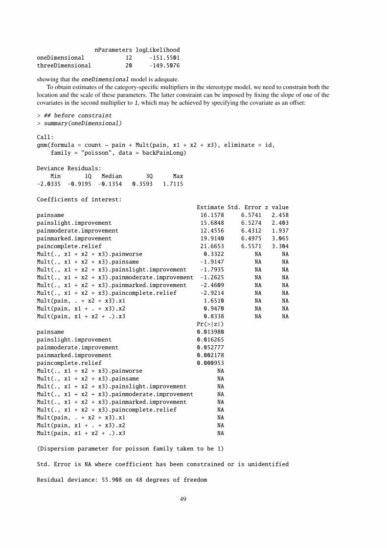
nParameters logLikelihood
oneDimensional 12 -151.5501
threeDimensional 20 -149.5076
showing that the oneDimensional model is adequate.
To obtain estimates of the category-specific multipliers in the stereotype model, we need to constrain both the
location and the scale of these parameters. The latter constraint can be imposed by fixing the slope of one of the
covariates in the second multiplier to 1, which may be achieved by specifying the covariate as an offset:
> ## before constraint
> summary(oneDimensional)
Call:
gnm(formula = count ~ pain + Mult(pain, x1 + x2 + x3), eliminate = id,
family = "poisson", data = backPainLong)
Deviance Residuals:
Min 1Q Median 3Q Max
-2.0335 -0.9195 -0.1354 0.3593 1.7115
Coefficients of interest:
Estimate Std. Error z value
painsame 16.1578 6.5741 2.458
painslight.improvement 15.6848 6.5274 2.403
painmoderate.improvement 12.4556 6.4312 1.937
painmarked.improvement 19.9140 6.4975 3.065
paincomplete.relief 21.6653 6.5571 3.304
Mult(., x1 + x2 + x3).painworse 0.3322 NA NA
Mult(., x1 + x2 + x3).painsame -1.9147 NA NA
Mult(., x1 + x2 + x3).painslight.improvement -1.7935 NA NA
Mult(., x1 + x2 + x3).painmoderate.improvement -1.2625 NA NA
Mult(., x1 + x2 + x3).painmarked.improvement -2.4609 NA NA
Mult(., x1 + x2 + x3).paincomplete.relief -2.9214 NA NA
Mult(pain, . + x2 + x3).x1 1.6510 NA NA
Mult(pain, x1 + . + x3).x2 0.9470 NA NA
Mult(pain, x1 + x2 + .).x3 0.8338 NA NA
Pr(>|z|)
painsame 0.013980
painslight.improvement 0.016265
painmoderate.improvement 0.052777
painmarked.improvement 0.002178
paincomplete.relief 0.000953
Mult(., x1 + x2 + x3).painworse NA
Mult(., x1 + x2 + x3).painsame NA
Mult(., x1 + x2 + x3).painslight.improvement NA
Mult(., x1 + x2 + x3).painmoderate.improvement NA
Mult(., x1 + x2 + x3).painmarked.improvement NA
Mult(., x1 + x2 + x3).paincomplete.relief NA
Mult(pain, . + x2 + x3).x1 NA
Mult(pain, x1 + . + x3).x2 NA
Mult(pain, x1 + x2 + .).x3 NA
(Dispersion parameter for poisson family taken to be 1)
Std. Error is NA where coefficient has been constrained or is unidentified
Residual deviance: 55.908 on 48 degrees of freedom
49

AIC: 211.81
Number of iterations: 14
> oneDimensional <- gnm(count ~ pain + Mult(pain, offset(x1) + x2 + x3),
+ eliminate = id, family = "poisson", data = backPainLong)
Initialising
Running start-up iterations..
Running main iterations..............
Done
> ## after constraint
> summary(oneDimensional)
Call:
gnm(formula = count ~ pain + Mult(pain, offset(x1) + x2 + x3),
eliminate = id, family = "poisson", data = backPainLong)
Deviance Residuals:
Min 1Q Median 3Q Max
-2.0335 -0.9195 -0.1354 0.3593 1.7115
Coefficients of interest:
Estimate Std. Error
painsame 16.1578 6.5742
painslight.improvement 15.6848 6.5274
painmoderate.improvement 12.4556 6.4312
painmarked.improvement 19.9140 6.4976
paincomplete.relief 21.6654 6.5571
Mult(., x2 + x3 + offset(x1)).painworse 1.4679 NA
Mult(., x2 + x3 + offset(x1)).painsame -2.2419 NA
Mult(., x2 + x3 + offset(x1)).painslight.improvement -2.0418 NA
Mult(., x2 + x3 + offset(x1)).painmoderate.improvement -1.1651 NA
Mult(., x2 + x3 + offset(x1)).painmarked.improvement -3.1437 NA
Mult(., x2 + x3 + offset(x1)).paincomplete.relief -3.9040 NA
Mult(pain, . + x3 + offset(x1)).x2 0.5736 0.2178
Mult(pain, x2 + . + offset(x1)).x3 0.5050 0.2431
z value Pr(>|z|)
painsame 2.458 0.013980
painslight.improvement 2.403 0.016265
painmoderate.improvement 1.937 0.052777
painmarked.improvement 3.065 0.002178
paincomplete.relief 3.304 0.000953
Mult(., x2 + x3 + offset(x1)).painworse NA NA
Mult(., x2 + x3 + offset(x1)).painsame NA NA
Mult(., x2 + x3 + offset(x1)).painslight.improvement NA NA
Mult(., x2 + x3 + offset(x1)).painmoderate.improvement NA NA
Mult(., x2 + x3 + offset(x1)).painmarked.improvement NA NA
Mult(., x2 + x3 + offset(x1)).paincomplete.relief NA NA
Mult(pain, . + x3 + offset(x1)).x2 2.633 0.008451
Mult(pain, x2 + . + offset(x1)).x3 2.077 0.037808
(Dispersion parameter for poisson family taken to be 1)
Std. Error is NA where coefficient has been constrained or is unidentified
50

Residual deviance: 55.908 on 48 degrees of freedom
AIC: 211.81
Number of iterations: 14
The location of the category-specific multipliers can constrained by setting one of the parameters to zero, either
through the constrain argument of gnm or with getContrasts:
> getContrasts(oneDimensional, pickCoef(oneDimensional, "[.]pain"))
estimate SE
Mult(., x2 + x3 + offset(x1)).painworse 0.000000 0.000000
Mult(., x2 + x3 + offset(x1)).painsame -3.709738 1.825568
Mult(., x2 + x3 + offset(x1)).painslight.improvement -3.509697 1.791732
Mult(., x2 + x3 + offset(x1)).painmoderate.improvement -2.632943 1.669256
Mult(., x2 + x3 + offset(x1)).painmarked.improvement -4.611597 1.895240
Mult(., x2 + x3 + offset(x1)).paincomplete.relief -5.371854 1.999657
quasiSE quasiVar
Mult(., x2 + x3 + offset(x1)).painworse 1.7797353 3.16745779
Mult(., x2 + x3 + offset(x1)).painsame 0.4281334 0.18329821
Mult(., x2 + x3 + offset(x1)).painslight.improvement 0.4024684 0.16198083
Mult(., x2 + x3 + offset(x1)).painmoderate.improvement 0.5518548 0.30454368
Mult(., x2 + x3 + offset(x1)).painmarked.improvement 0.3133220 0.09817066
Mult(., x2 + x3 + offset(x1)).paincomplete.relief 0.4919550 0.24201969
giving the required estimates.
7.7 Lee-Carter model for trends in age-specific mortality
In the study and projection of population mortality rates, the model proposed by Lee and Carter (1992) forms the
basis of many if not most current analyses. Here we consider the quasi-Poisson version of the model (Wilmoth,
1993; Alho, 2000; Brouhns et al., 2002; Renshaw and Haberman, 2003), in which the death count Day for indi-
viduals of age a in year y has mean µay and variance φµay (where φ is 1 for Poisson-distributed counts, and is
respectively greater than or less than 1 in cases of over-dispersion or under-dispersion). In the Lee-Carter model,
the expected counts follow the log-bilinear form
log(µay/eay) = αa + βaγy,
where eay is the ‘exposure’ (number of lives at risk). This is a generalized nonlinear model with a single multi-
plicative term.
The use of gnm to fit this model is straightforward. We will illustrate by using data downloaded on 2006-11-
14 from the Human Mortality Database4 (HMD, made available by the University of California, Berkeley, and
Max Planck Institute for Demographic Research, at http://www.mortality.org) on male deaths in Canada
between 1921 and 2003. The data are not made available as part of gnm because of license restrictions; but they
are readily available via the web simply by registering with the HMD. We assume that the data for Canadian
males (both deaths and exposure-to-risk) have been downloaded from the HMD and organised into a data frame
named Canada in R, with columns Year (a factor, with levels 1921 to 2003), Age (a factor, with levels 20 to
99), mDeaths and mExposure (both quantitative). The Lee-Carter model may then be specified as
LCmodel.male <- gnm(mDeaths ~ Age + Mult(Exp(Age), Year),
offset = log(mExposure), family = "quasipoisson",
data = Canada)
Here we have acknowledged the fact that the model only really makes sense if all of the βa parameters, which
represent the ‘sensitivity’ of age group a to a change in the level of general mortality (e.g., Brouhns et al., 2002),
have the same sign. Without loss of generality we assume βa > 0 for all a, and we impose this constraint by using
Exp(Age) instead of just Age in the multiplicative term. Convergence is to a fitted model with residual deviance
4Thanks to Iain Currie for helpful advice relating to this section
51
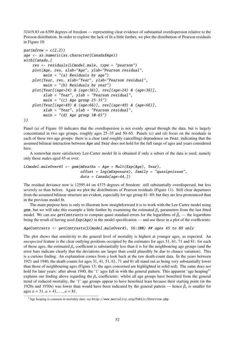
32419.83 on 6399 degrees of freedom — representing clear evidence of substantial overdispersion relative to the
Poisson distribution. In order to explore the lack of fit a little further, we plot the distribution of Pearson residuals
in Figure 10:
par(mfrow = c(2,2))
age <- as.numeric(as.character(Canada$Age))
with(Canada,{
res <- residuals(LCmodel.male, type = "pearson")
plot(Age, res, xlab="Age", ylab="Pearson residual",
main = "(a) Residuals by age")
plot(Year, res, xlab="Year", ylab="Pearson residual",
main = "(b) Residuals by year")
plot(Year[(age>24) & (age<36)], res[(age>24) & (age<36)],
xlab = "Year", ylab = "Pearson residual",
main = "(c) Age group 25-35")
plot(Year[(age>49) & (age<66)], res[(age>49) & (age<66)],
xlab = "Year", ylab = "Pearson residual",
main = "(d) Age group 50-65")
})
Panel (a) of Figure 10 indicates that the overdispersion is not evenly spread through the data, but is largely
concentrated in two age groups, roughly ages 25–35 and 50–65. Panels (c) and (d) focus on the residuals in
each of these two age groups: there is a clear (and roughly cancelling) dependence on Year, indicating that the
assumed bilinear interaction between Age and Year does not hold for the full range of ages and years considered
here.
A somewhat more satisfactory Lee-Carter model fit is obtained if only a subset of the data is used, namely
only those males aged 45 or over:
LCmodel.maleOver45 <- gnm(mDeaths ~ Age + Mult(Exp(Age), Year),
offset = log(mExposure), family = "quasipoisson",
data = Canada[age>44,])
The residual deviance now is 12595.44 on 4375 degrees of freedom: still substantially overdispersed, but less
severely so than before. Again we plot the distributions of Pearson residuals (Figure 11). Still clear departures
from the assumed bilinear structure are evident, especially for age group 81–89; but they are less pronounced than
in the previous model fit.
The main purpose here is only to illustrate how straightforward it is to work with the Lee-Carter model using
gnm , but we will take this example a little further by examining the estimated βa parameters from the last fitted
model. We can use getContrasts to compute quasi standard errors for the logarithms of βa — the logarithms
being the result of having used Exp(Age) in the model specification — and use these in a plot of the coefficients:
AgeContrasts <- getContrasts(LCmodel.maleOver45, 56:100) ## ages 45 to 89 only
The plot shows that sensitivity to the general level of mortality is highest at younger ages, as expected. An
unexpected feature is the clear outlying positions occupied by the estimates for ages 51, 61, 71 and 81: for each
of those ages, the estimated βa coefficient is substantially less than it is for the neighbouring age groups (and the
error bars indicate clearly that the deviations are larger than could plausibly be due to chance variation). This
is a curious finding. An explanation comes from a look back at the raw death-count data. In the years between
1921 and 1940, the death counts for ages 31, 41, 51, 61, 71 and 81 all stand out as being very substantially lower
than those of neighbouring ages (Figure 13: the ages concerned are highlighted in solid red). The same does not
hold for later years: after about 1940, the ‘1’ ages fall in with the general pattern. This apparent ‘age heaping5’
explains our finding above regarding the βa coefficients: whilst all age groups have benefited from the general
trend of reduced mortality, the ‘1’ age groups appear to have benefited least because their starting point (in the
1920s and 1930s) was lower than would have been indicated by the general pattern — hence βa is smaller for
ages a = 31, a = 41,. . . , a = 81.
5Age heaping is common in mortality data: see http://www.mortality.org/Public/Overview.php
52
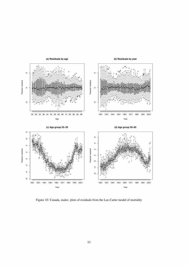
●●
● ●
●
●●
●
●
●
●●
●●
●
●
●
●
●
●●
●
●
●
●
●
●
●
●●
●●
●●
●
20 26 32 38 44 50 56 62 68 74 80 86 92 98
−5
05
(a) Residuals by age
Age
Pears
on r
esid
ual
●
●●
●
●
●
●
●
●
●
●
●●
●●●
●
●●
●
●●
●
●●
●
●
●●●
1921 1931 1941 1951 1961 1971 1981 1991 2001
−5
05
(b) Residuals by year
Year
Pears
on r
esid
ual
●●
●●
●
●
●
●
●
●
●
●
●●
●
●
●
●
●
●
●
●
●
●
1921 1931 1941 1951 1961 1971 1981 1991 2001
−6
−4
−2
02
46
8
(c) Age group 25−35
Year
Pears
on r
esid
ual
●
●
●
●
●
●
●
●
●
●●
●
●
●
● ●
●
●
●
●
●
●
●
●
●
●
●
1921 1931 1941 1951 1961 1971 1981 1991 2001
−6
−4
−2
02
46
(d) Age group 50−65
Year
Pears
on r
esid
ual
Figure 10: Canada, males: plots of residuals from the Lee-Carter model of mortality
53

●
●
●
●
●●
●●
●●●
●
●
●●
●
●
●
●
●●
●
●
●
●●
●
●
●
●
●
●
●●
●●●●
●
●●
●
●
20 26 32 38 44 50 56 62 68 74 80 86 92 98
−6
−4
−2
02
46
8
(a) Residuals by age
Age
Pears
on r
esid
ual
●●
●
●
●
●
●
●●
●
●
●
●
●
●
●
●
●
●
●
●●
●● ●●
●
●
●●●●
●
●
●
●
●
●●
●●
●
●
●
●
●
●
●
●●
●●●
●
●
●
●
●
●
●
●
●
●
●
●
●●
●
1921 1931 1941 1951 1961 1971 1981 1991 2001
−6
−4
−2
02
46
8
(b) Residuals by year
Year
Pears
on r
esid
ual
●●
●
●
●
●
●
●
●
●
●
●
●●
●
●
●
●
●
●
●
●
●
●
●
●
●
●
1921 1931 1941 1951 1961 1971 1981 1991 2001
−6
−4
−2
02
46
(c) Age group 50−65
Year
Pears
on r
esid
ual
●
●
●
●
●
●
●●
●
●
●
●
●
●
●
●
●
●
●
●
●
●
●
●
●
●
●
●
●
●●
●
●●
●
●
●
●
●●
●
●
●
●
●
1921 1931 1941 1951 1961 1971 1981 1991 2001
−4
−2
02
4
(d) Age group 81−89
Year
Pears
on r
esid
ual
Figure 11: Canada, males over 45: plots of residuals from the Lee-Carter model of mortality
54
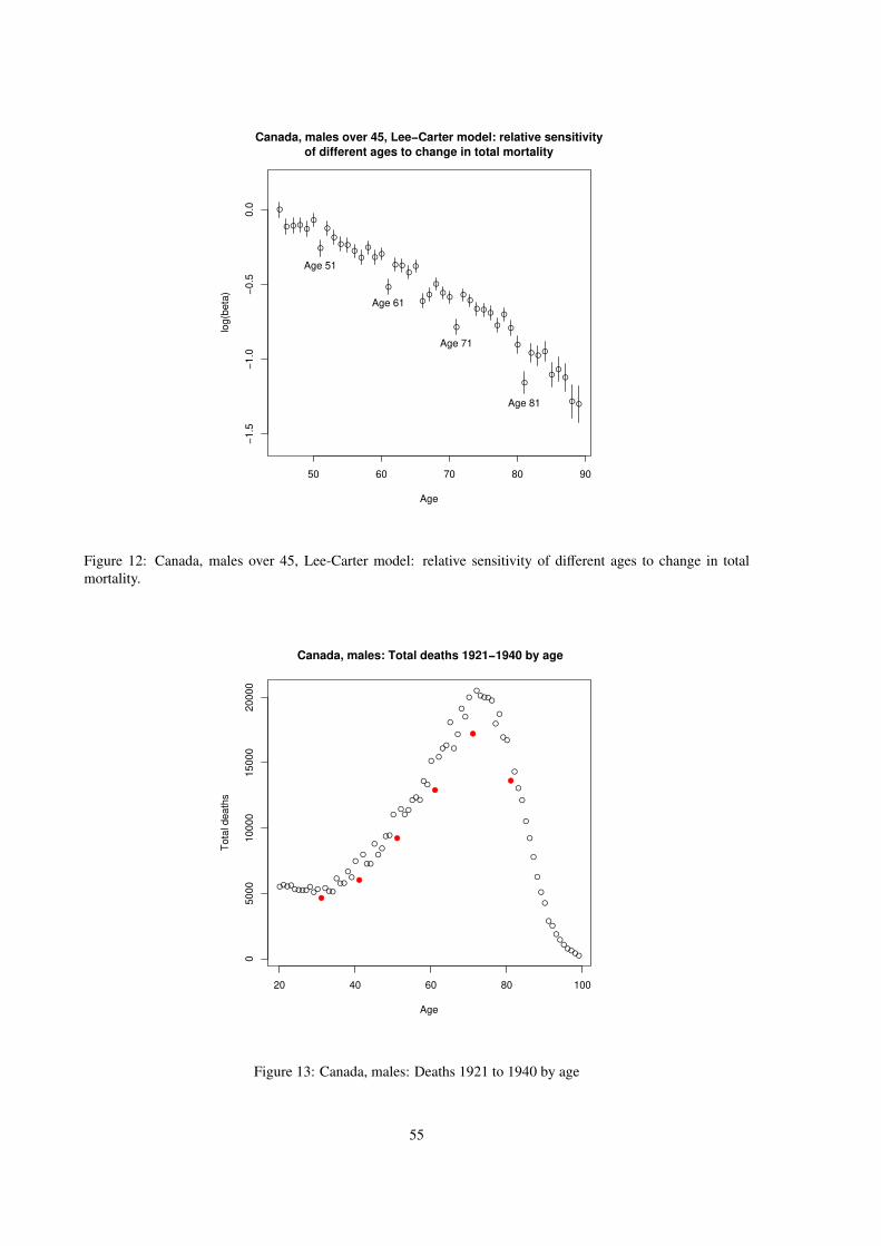
●
● ● ●●
●
●
●
●● ●
●●
●
●●
●
● ●●
●
●●
●
●●
●
●●
● ●●
●
●
●
●
●
● ●●
●●
●
● ●
50 60 70 80 90
−1
.5−
1.0
−0
.50
.0
Canada, males over 45, Lee−Carter model: relative sensitivity
of different ages to change in total mortality
Age
log
(be
ta)
Age 81
Age 71
Age 61
Age 51
Figure 12: Canada, males over 45, Lee-Carter model: relative sensitivity of different ages to change in total
mortality.
●●●●●●●●
●●●
●
●●●
●●●
●●
●
●
●
●●
●
●●
●●
●
●
●●
●
●●●
●●
●
●
●
●●
●
●
●
●
●
●
●
●●●●●
●
●
●●
●
●
●
●
●
●
●
●
●
●
●●
●●
●●●●●
20 40 60 80 100
05
00
01
00
00
15
00
02
00
00
Canada, males: Total deaths 1921−1940 by age
Age
To
tal d
ea
ths
Figure 13: Canada, males: Deaths 1921 to 1940 by age
55

7.8 Exponential and sum-of-exponentials models for decay curves
A class of nonlinear functions which arise in various application contexts — a notable one being pharmacokinetic
studies – involves one or more exponential decay terms. For example, a simple decay model with additive error is
y = α + exp(β + γx) + e (2)
(with γ < 0), while a more complex (‘sum of exponentials’) model might involve two decay terms:
y = α + exp(β1 + γ1x) + exp(β2 + γ2x) + e. (3)
Estimation and inference with such models are typically not straightforward, partly on account of multiple local
maxima in the likelihood (e.g., Seber and Wild, 1989, Ch.3). We illustrate the difficulties here, with a couple
of artificial examples. These examples will make clear the value of making repeated calls to gnm , in order to
use different, randomly-generated parameterizations and starting values and thus improve the chances of locating
both the global maximum and all local maxima of the likelihood.
7.8.1 Example: single exponential decay term
Let us first construct some data from model (2). For our illustrative purposes here, we will use noise-free data,
i.e., we fix the variance of e to be zero; for the other parameters we will use α = 0, β = 0, γ = −0.1.
> x <- 1:100
> y <- exp(- x / 10)
> set.seed(1)
> saved.fits <- list()
> for (i in 1:100) saved.fits[[i]] <- gnm(y ~ Exp(1 + x), verbose = FALSE)
> table(zapsmall(sapply(saved.fits, deviance)))
0 3.612654
52 48
The saved.fits object thus contains the results of 100 calls to gnm , each using a different, randomly-generated
starting value for the vector of parameters (α, β, γ). Out of 100 fits, 52 reproduce the data exactly, to machine
accuracy. The remaining 48 fits are all identical to one another, but they are far from globally optimal, with
residual sum of squares 3.61: they result from divergence of γ to +∞, and correspondingly of β to −∞, such that
the fitted ‘curve’ is in fact just a constant, with level equal to y = 0.09508. For example, the second of the 100 fits
is of this kind:
> saved.fits[[2]]
Call:
gnm(formula = y ~ Exp(1 + x), verbose = FALSE)
Coefficients:
(Intercept) Exp(. + x).(Intercept) Exp(1 + .).x
9.508e-02 -1.493e+04 5.463e+01
Deviance: 3.612654
Pearson chi-squared: 3.612654
Residual df: 99
The use of repeated calls to gnm , as here, allows the local and global maxima to be easily distinguished.
7.8.2 Example: sum of two exponentials
We can conduct a similar exercise based on the more complex model (3):
56
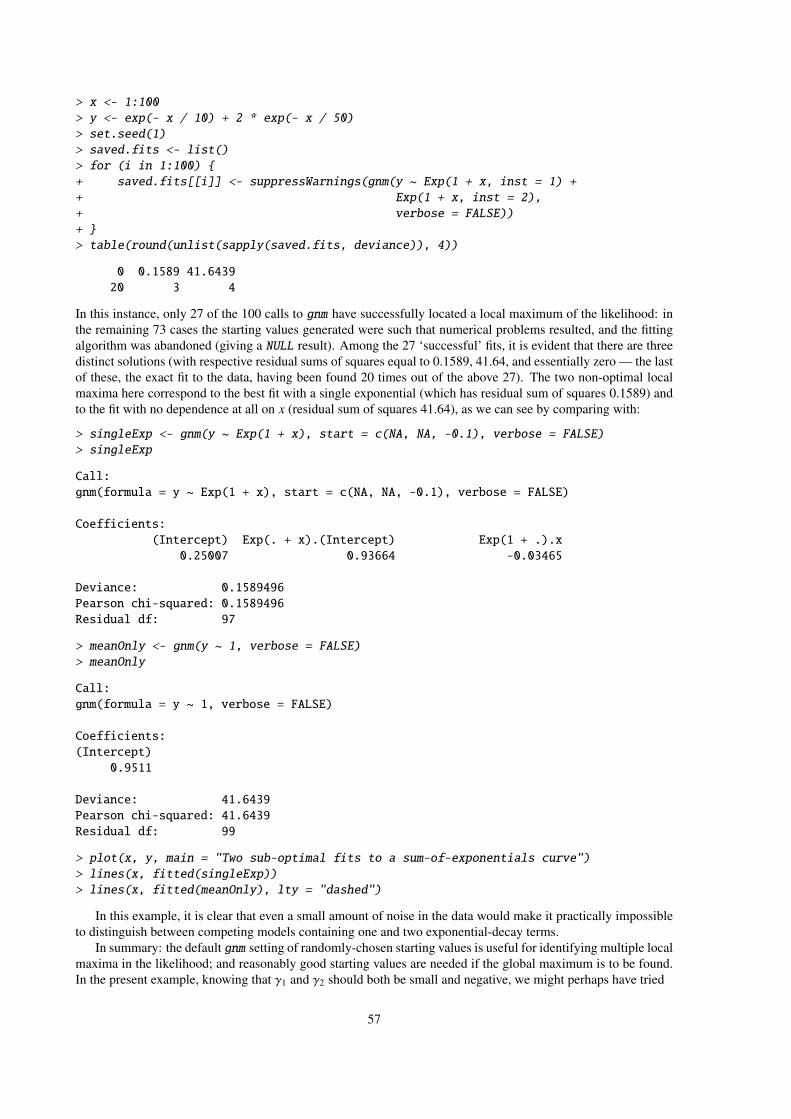
> x <- 1:100
> y <- exp(- x / 10) + 2 * exp(- x / 50)
> set.seed(1)
> saved.fits <- list()
> for (i in 1:100) {
+ saved.fits[[i]] <- suppressWarnings(gnm(y ~ Exp(1 + x, inst = 1) +
+ Exp(1 + x, inst = 2),
+ verbose = FALSE))
+ }
> table(round(unlist(sapply(saved.fits, deviance)), 4))
0 0.1589 41.6439
20 3 4
In this instance, only 27 of the 100 calls to gnm have successfully located a local maximum of the likelihood: in
the remaining 73 cases the starting values generated were such that numerical problems resulted, and the fitting
algorithm was abandoned (giving a NULL result). Among the 27 ‘successful’ fits, it is evident that there are three
distinct solutions (with respective residual sums of squares equal to 0.1589, 41.64, and essentially zero — the last
of these, the exact fit to the data, having been found 20 times out of the above 27). The two non-optimal local
maxima here correspond to the best fit with a single exponential (which has residual sum of squares 0.1589) and
to the fit with no dependence at all on x (residual sum of squares 41.64), as we can see by comparing with:
> singleExp <- gnm(y ~ Exp(1 + x), start = c(NA, NA, -0.1), verbose = FALSE)
> singleExp
Call:
gnm(formula = y ~ Exp(1 + x), start = c(NA, NA, -0.1), verbose = FALSE)
Coefficients:
(Intercept) Exp(. + x).(Intercept) Exp(1 + .).x
0.25007 0.93664 -0.03465
Deviance: 0.1589496
Pearson chi-squared: 0.1589496
Residual df: 97
> meanOnly <- gnm(y ~ 1, verbose = FALSE)
> meanOnly
Call:
gnm(formula = y ~ 1, verbose = FALSE)
Coefficients:
(Intercept)
0.9511
Deviance: 41.6439
Pearson chi-squared: 41.6439
Residual df: 99
> plot(x, y, main = "Two sub-optimal fits to a sum-of-exponentials curve")
> lines(x, fitted(singleExp))
> lines(x, fitted(meanOnly), lty = "dashed")
In this example, it is clear that even a small amount of noise in the data would make it practically impossible
to distinguish between competing models containing one and two exponential-decay terms.
In summary: the default gnm setting of randomly-chosen starting values is useful for identifying multiple local
maxima in the likelihood; and reasonably good starting values are needed if the global maximum is to be found.
In the present example, knowing that γ1 and γ2 should both be small and negative, we might perhaps have tried
57
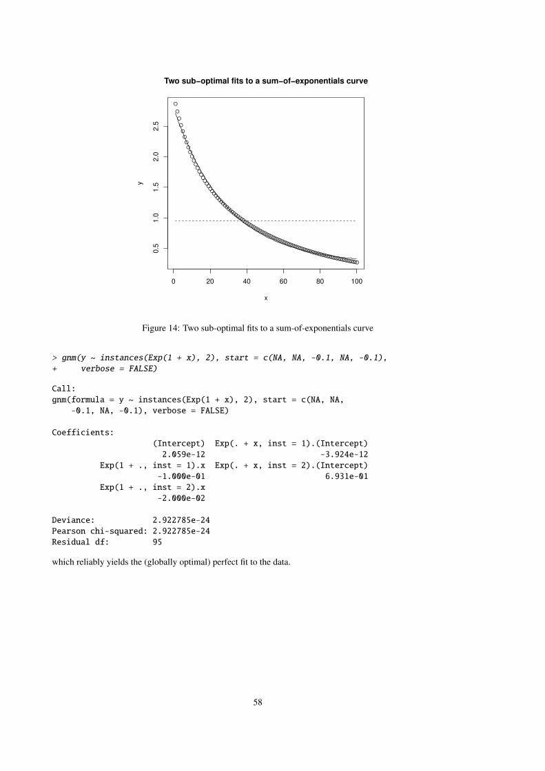
●
●
●
●
●
●
●●●●●●●●●●●●●●●●●●●●●●●●●●●●●●●●●●●●●●●●●●●●●●●●●●●●●●●●●●●●●●●●●●●●●●●●●●●●●●●●●●●●●●●●●●●●●●
0 20 40 60 80 100
0.5
1.0
1.5
2.0
2.5
Two sub−optimal fits to a sum−of−exponentials curve
x
y
Figure 14: Two sub-optimal fits to a sum-of-exponentials curve
> gnm(y ~ instances(Exp(1 + x), 2), start = c(NA, NA, -0.1, NA, -0.1),
+ verbose = FALSE)
Call:
gnm(formula = y ~ instances(Exp(1 + x), 2), start = c(NA, NA,
-0.1, NA, -0.1), verbose = FALSE)
Coefficients:
(Intercept) Exp(. + x, inst = 1).(Intercept)
2.059e-12 -3.924e-12
Exp(1 + ., inst = 1).x Exp(. + x, inst = 2).(Intercept)
-1.000e-01 6.931e-01
Exp(1 + ., inst = 2).x
-2.000e-02
Deviance: 2.922785e-24
Pearson chi-squared: 2.922785e-24
Residual df: 95
which reliably yields the (globally optimal) perfect fit to the data.
58

A User-level functions
We list here, for easy reference, all of the user-level functions in the gnm package. For full documentation see the
package help pages.
Model Fitting
gnm fit generalized nonlinear models
Model Specification
Diag create factor differentiating diagonal elements
Symm create symmetric interaction of factors
Topo create ‘topological’ interaction factors
Const specify a constant in a nonlin function predictor
Dref specify a diagonal reference term in a gnm model formula
Mult specify a product of predictors in a gnm formula
MultHomog specify a multiplicative interaction with homogeneous effects in a gnm formula
Exp specify the exponential of a predictor in a gnm formula
Inv specify the reciprocal of a predictor in a gnm formula
wedderburn specify the Wedderburn quasi-likelihood family
Methods and Accessor Functions
confint.gnm compute confidence intervals of gnm parameters based on the profiled deviance
confint.profile.gnm compute confidence intervals of parameters from a profile.gnm object
predict.gnm predict from a gnm model
profile.gnm profile deviance for parameters in a gnm model
plot.profile.gnm plot profile traces from a profile.gnm object
summary.gnm summarize gnm fits
residSVD multiplicative approximation of model residuals
exitInfo print numerical details of last iteration when gnm has not converged
ofInterest extract the ofInterest component of a gnm object
ofInterest<- replace the ofInterest component of a gnm object
parameters get model parameters from a gnm object, including parameters that were con-
strained
pickCoef get indices of model parameters
getContrasts estimate contrasts and their standard errors for parameters in a gnm model
checkEstimable check whether one or more parameter combinations in a gnm model is identified
se get standard errors of linear parameter combinations in gnm models
Dref estimate weights and corresponding standard errors for a diagonal reference term
in a gnm model
termPredictors (generic) extract term contributions to predictor
Auxiliary Functions
asGnm coerce an object of class lm or glm to class gnm
expandCategorical expand a data frame by re-expressing categorical data as counts
getModelFrame get the model frame in use by gnm
MPinv Moore-Penrose pseudoinverse of a real-valued matrix
qrSolve Minimum-length solution of a linear system
59
References
Agresti A (2002). Categorical Data Analysis. 2nd edition. New York: Wiley.
Alho JM (2000). “Discussion of Lee (2000).” North American Actuarial Journal, 4, 91–93.
Anderson JA (1984). “Regression and Ordered Categorical Variables.” J. R. Statist. Soc. B, 46(1), 1–30.
Brouhns N, Denuit M, Vermunt JK (2002). “A Poisson log-bilinear regression approach to the construction of
projected lifetables.” Insurance Mathematics and Economics, 31, 373–393.
Catchpole E, Morgan B (1997). “Detecting parameter redundancy.” Biometrika, 84, 187–196.
Cautres B, Heath AF, Firth D (1998). “Class, religion and vote in Britain and France.” La Lettre de la Maison
Française, 8.
Clifford P, Heath AF (1993). “The Political Consequences of Social Mobility.” J. Roy. Stat. Soc. A, 156(1), 51–61.
Erikson R, Goldthorpe JH (1992). The Constant Flux. Oxford: Clarendon Press.
Erikson R, Goldthorpe JH, Portocarero L (1982). “Social fluidity in Industrial nations: England, France and
Sweden.” British Journal of Sociology, 33, 1–34.
Firth D (2003). “Overcoming the reference category problem in the presentation of statistical models.” Sociolog-
ical Methodology, 33, 1–18.
Firth D, de Menezes RX (2004). “Quasi-variances.” Biometrika, 91, 65–80.
Gabriel KR (1998). “Generalised bilinear regression.” Biometrika, 85, 689–700.
Goodman LA (1979). “Simple models for the analysis of association in cross-classifications having ordered
categories.” J. Amer. Statist. Assoc., 74, 537–552.
Hatzinger R, Francis BJ (2004). “Fitting Paired Comparison Models in R.” Technical Report 3, Department of
Statistics and Mathematics, Wirtschaftsuniversität Wien.
Lee RD, Carter L (1992). “Modelling and forecasting the time series of US mortality.” Journal of the American
Statistical Association, 87, 659–671.
McCullagh P, Nelder JA (1989). Generalized Linear Models (Second Edition). Chapman & Hall Ltd.
Renshaw A, Haberman S (2003). “Lee-Carter mortality forecasting: a parallel generalized linear modelling
approach for England and Wales mortality projections.” Applied Statistics, 52, 119–137.
Seber GAF, Wild CJ (1989). Nonlinear Regression. Wiley.
Sobel ME (1981). “Diagonal mobility models: A substantively motivated class of designs for the analysis of
mobility effects.” Amer. Soc. Rev., 46, 893–906.
Sobel ME (1985). “Social mobility and fertility revisited: Some new models for the analysis of the mobility
effects hypothesis.” Amer. Soc. Rev., 50, 699–712.
van der Slik FWP, de Graaf ND, Gerris JRM (2002). “Conformity to Parental Rules: Asymmetric Influences of
Father’s and Mother’s Levels of Education.” Europ. Soc. Rev., 18, 489–502.
Vargas M, Crossa J, van Eeuwijk F, Sayre KD, Reynolds MP (2001). “Interpreting treatment by environment
interaction in agronomy trials.” Agronomy Journal, 93, 949–960.
Wedderburn RWM (1974). “Quasi-likelihood Functions, Generalized Linear Models, and the Gauss-Newton
Method.” Biometrika, 61, 439–447.
Wilmoth JR (1993). “Computational methods for fitting and extrapolating the Lee-Carter model of mortality
change.” Technical report, Department of Demography, University of California, Berkeley.
60

Xie Y (1992). “The log-multiplicative layer effect model for comparing mobility tables.” American Sociological
Review, 57, 380–395.
Yaish M (1998). Opportunities, Little Change. Class Mobility in Israeli Society, 1974–1991. Ph.D. thesis, Nuffield
College, University of Oxford.
Yaish M (2004). Class Mobility Trends in Israeli Society, 1974-1991. Edwin Mellen Press, Lewiston.
61
Related Documents