Generalized multiprobe decoherent transport: Recursive algorithms and applications

arX

iv:1

311.

2231

v1 [

cond

-mat

.mes

-hal

l] 9

Nov

201

3

Generalized multiprobe decoherent transport: Recursive algorithms and applications.

Carlos J. Cattena1, Raul A. Bustos-Marun1,2, Lucas J.

Fernandez-Alcazar1, Daijiro Nozaki3 and Horacio M. Pastawski11Instituto de Fısica Enrique Gaviola and Facultad de Matematica Astronomıa y Fısica,

Universidad Nacional de Cordoba, Ciudad Universitaria, Cordoba, 5000, Argentina,2Facultad de Ciencias Quımicas, Universidad Nacional de Cordoba,

Ciudad Universitaria, Cordoba, 5000, Argentina, and3Institute for Materials Science and Max Bergmann Center of Biomaterials,

Dresden University of Technology, D-01062 Dresden, Germany

Decoherent transport in mesoscopic and nanoscopic systems can be formulated in terms of theD’Amato-Pastawski (DP) model. This generalizes the Landauer-Buttiker picture by consideringa distribution of decoherent local scattering centers of decoherence. However, its generalizationfor multiterminal setups is lacking. We first review the original formulation of the DP modelfor decoherent transport. We then extend it to the multiprobe configuration and introduce anefficient recursive algorithm that yields the effective conductances and voltage profiles. We present adecimation procedure based on matrix continued fractions for the recursive evaluation of the Green’sfunctions of banded Hamiltonians. The decimation procedure may also provides the cornerstone ofefficient computational schemes for the calculation of multiterminal decoherent conductances. Weillustrate the method by analyzing the decoherent transport through a quantum dot where electronsare strongly coupled to optical phonons. Our approach allows us to consider the full electron-phononFock space and we show how typical interferences and antiresonances are smoothed by decoherence.The presented method should pave the way for computationally demanding calculations of transportthrough nanodevices, bridging the gap between fully-coherent and fully decoherent schemes.

PACS numbers: 71.15.Dx, 71.23.An, 72.10.-d, 73.20.Jc, 73.23.-b, 73.63.-b, 63.22.-m

I. INTRODUCTION

Quantum transport at the nanoscale1,2 is a bloomingfield where the properties of matter can be explored ina realm where quantum effects become crucial. In par-ticular, the control of quantum interference phenomenaand their interplay with the electronic structure offers afascinating opportunity to overcome some of the usualconstraints of our macroscopic classical world.3–7 How-ever, at the nanoscale both quantum and classical be-havior are usually expected. This last emerges from en-vironmental degrees of freedom whose description alsobecomes important.8 An exciting example of the compe-tition among those behaviors is electron-transfer in natu-ral and artificial photosynthesis. There the interplay be-tween interferences and decoherence induced by the envi-ronment seems to play a fundamental role in optimizingexcitonic transfer.9,10 This phenomenon falls in line withwhat is known in low dimensional conductors. Indeed, inhighly ordered 1-D systems the interferences would leadto a fast quantum diffusion of local excitations, whichbecomes weakened by decoherence. On the other hand,in disordered 1-D wires, quantum coherence allows thedestructive interferences that produce electronic local-ization. While these phenomena are already describedin terms of the variants of the Kubo formulation, thesefail to satisfy charge conservation.11

While many recent studies in the field of quantumpropagation of electronic excitations at the nanoscale relyon density matrix formulation, Landauer’s picture hasalmost no rival in what concerns to electronic coherent

transport.12 In its simplest form, conductance is deter-mined by the transmission probability (either quantumor classical) among electrodes. Paradoxically, quantumtransmittance is much simpler to evaluate than its clas-sical counterpart. Thus, the great majority of work fo-cus on the evaluation of the coherent transmittance set-ting aside incoherent propagations. An extension of thisapproach, developed by Markus Buttiker,13 applies theKirchhoff laws to a system connected to multiple ter-minals. Now, one may consider voltage probes besidesto the current sources and drains. Self-consistent non-equilibrium chemical potentials at the voltmeters mustensure current cancellation. Thus, the resulting trans-port coefficients fulfill the Onsager’s reciprocity relations.Additionally, Buttiker made the initial observation14 thata voltage probe implies a classical measurement and thusit acts as a decoherence source. This concept was fur-ther formulated by D’Amato and Pastawski in a Hamil-tonian description15, henceforth the DP model. Theyalso provided a compact solution for an arbitrary dis-tribution of incoherent local scattering processes. Thisdescription,16,17 is founded in the Keldysh, Kadanoffand Baym’s quantum fields formalism18 for the non-equilibrium Green’s functions.18–20 The resulting integro-differential equations are simplified by evaluating the cur-rents and chemical potentials in a linearized scheme thatinvolves a matrix containing only transmittances amongdifferent points in the sample. The final set of linearequations relate the local chemical potentials and thecurrents via the transmittances matrix. This results inthe “Generalized Landauer-Buttiker equations” (GLBE)

2

that solve the DP model. In spite of the GLBE simplic-ity, dealing with a great number of self-consistent localchemical potentials involves a cumbersome matrix inver-sion. Thus, the practical applications remained mostlyreduced to a few one-dimensional problems.21–27 Thus,in spite of the need to include the effects of decoher-ent processes,28,29 a practical implementation of the DPmodel for decoherent transport is still lacking. Thus, anefficient computational strategy would greatly improvethe prospects for better transport computation at thenanoscale.In this paper we generalize the D’Amato-Pastawski

(DP) scheme for multichannel problems, presenting adecimation-based method for the calculation of the de-coherent conductance. This should allow the solution ofa wide variety of problems beyond the typical 1-D twoterminal calculations where it has been applied so far. InSec. II we introduce the basic tools, based on a decima-tion procedure that yields the parameters of an effectiveHamiltonian. In Sec. III we overview the original DPmodel, which is also based on a decimation strategy toprovide an effective transmittance. In Sec. IV, we useboth ideas to build an efficient recursive algorithm forthe calculation of Green’s functions. Then, we obtainthe total decoherent transmission for a general multiter-minal setup. In Sec. V, we exemplify these proceduresby applying them to a system where a single vibrationaldegree of freedom is tightly coupled to a local electronicstate of a quantum dot. There, the effects of decoherenceon electronic transport are accounted by the multiprobeDP model. Final remarks are summarized in Sec. VI.

II. DECIMATION PROCEDURES AND

EFFECTIVE HAMILTONIANS

Complex systems involve a huge number of degreesof freedom and thus their study can not be carried outwithout proper simplifications. The decimation proce-dures, inspired in the renormalization group techniquesof statistical mechanics30,31, seek to recursively reducethe number of degrees of freedom of a general N × NHamiltonian into another of lower rank, without alter-ing the physical properties. For example, a tight-bindingHamiltonian describing a device or molecule with eigen-states filled up to the Fermi energy εF is,32

HS =

N∑

i=1

Eic

†i ci +

N∑

j=1(j 6=i)

[Vi,j c

†i cj + Vj,ic

†j ci

]

. (1)

The basic idea can be captured by considering a systemwith N = 3 states (or orbitals) whose secular equationis:ε− E1 −V12 −V13

−V21 ε− E2 −V23

−V31 −V32 ε− E3

u1

u2

u3

= [εI−HS ]

−→u ≡−→0 .

(2)

Assume that, for some reason, we are interested in thetransfer of an excitation from state 1 to 2. We couldisolate u3 from the third row and use it to eliminate u3

in the first and the second equations. In this way, weobtain a new set of equations where u3 is decimated :

[ε− E1 −V 12

−V 21 ε− E2

](u1

u2

)= [εI−Heff.]~u = 0. (3)

The renormalized coefficients hide their non-linear de-pendence on the energy variable ε :

E1 = E1 +Σ1(ε) = E1 + V131

ε− E3V31

E2 = E2 +Σ2(ε) = E2 + V231

ε− E3V32

V 12 = V12 + V131

ε− E3V32

(4)

In this case, the terms Σk(ε); k = 1, 2 are the real self-energies accounting for the energy shifts due to the cou-pling with the eliminated state. Notice that as long asone conserves the analytical dependence on ε of Σk, theactual secular equation is still cubic in ε and providesthe exact spectrum of the whole system. This proce-dure can be performed systematically in a Hamiltonianof any size N × N to end up in an effective Hamilto-nian with the size one desires, in particular a 2 × 2 one.The effective interaction parameter V 12, together withthe self-energies Σk, accounts for transport through thewhole sample. Their dependence on ε provides all theneeded information on the steady state transport as wellas on quantum dynamics.33 In practice, it is convenientto add an infinitesimal imaginary part, −iη, to each en-ergy Ek → Ek − iη. This ensures that one recovers theretarded time dependences of the observables through awell defined Fourier transform.The terminals connected to the system are described

as semi-infinite leads coupled to it. They are handled in asimilar way as the system itself. The idea is to eliminateall the internal degrees of freedom decimating them pro-gressively, renormalizing the states of the system whichare directly coupled to the external reservoirs. For fur-ther clarification we consider a one dimensional chain,

HL =

−∞∑

i=0

Eic

†i ci − V

[c†i ci−1 + c†i−1ci

], (5)

whose secular equation gives rise to a tridiagonal matrixof infinite dimension. The elements Ei’s and V ’s are nowthe diagonal and off-diagonal terms of a tridiagonal ma-trix HL. This lead is connected at the left of the system,say, with site 1:

VSL = VL

[c†1c0 + c†0c1

]. (6)

Instead of dealing with the whole Hamiltonian

H = HS + HL + VSL,

3

we perform the elimination procedure. It becomes partic-ularly simple because of the chain structure of the lead.The energy of the i-th site, is “shifted” by the elimina-tion of (i − 1)-th site, which itself is shifted by sites atits left32, with the self-energies resulting in a continued-fraction:

Σi = Vi,i−11

ε− Ei−1 − Σi−1Vi−1,i (7)

(i = 0,−1,−2, ...−∞)

In a perfect propagating channel: Vi,i−1 ≡ V and Ei =E0, and thus, Σi = Σi−1 ≡ Σ, we arrive to the self-consistent solution:

Σ(ε) =V 2

ε− E0 − Σ= ∆(ε)− iΓ(ε). (8)

=ε− E0 + iη

2− sgn(ε− E0)

√(ε− E0 + iη

2

)2

− V 2(9)

where the generalized square root34 in the limit η → 0+,yields the imaginary component of the self-energy withthe energy band and becomes real otherwise.Thus, once the states in the left lead are fully deci-

mated the energy of the first site becomes

E1(ε) = E1(ε) + ΣL1(ε) (10)

with ΣL1(ε) =

(VL

V

)2

Σ(ε) (11)

= ∆L1(ε)− iΓL1(ε) (12)

As before, the real part ∆L1(ε) indicates how the unper-turbed site energies are shifted by the leads. The im-portant difference with the simple decimation examplediscussed above is that, as a consequence of the infinitenature of the lead, the self-energies may acquire a finiteimaginary component, ΓL1(ε), even in the limit η → 0 .It describes the rate at which coherent density excitationin the system decays into the lead propagating states.Note that, the imaginary part is roughly consistent

with the exponential decays of the survival probabilitypredicted by the Fermi Golden Rule (FGR). For a “sys-tem” with a single state |1〉, as expressed by the Green’sfunction GR

ji(t), which gives [−i/~] times the probabilityamplitude to find a particle in state j at time t after ithas been placed in state i. Of particular interest is,

∣∣i~GR11(t)

∣∣2 ≡∣∣∣θ(t) 〈1| exp[−iH t/~] |1〉

∣∣∣2

(13)

≃ exp[−2ΓL1(E1)t/~]. (14)

However, we remember that the self-energies obtainedabove have an explicit functional dependence on ε. Inconsequence, the decay can depart from the naive expo-nential approximation. Indeed, a quantum decay shouldstart quadratically as 1 − (VLt/~)

2showing the non-

exponential for very short times. The exponential mayeven become a non-monotonous decay in the very longtime regime.35 In practice, we will neglect the dependenceon ε unless explicitly needed.

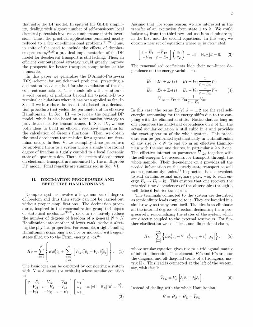
For the sake of simplicity, we may idealize the termi-nal leads as quasi 1-D wires. As waveguides, they can bedescribed in terms of open channels at the Fermi energyor propagating modes. Thus, we chose a basis for thesystem’s Hamiltonian in which each independent prop-agation mode l of a lead is connected to a single sys-tem’s state. This might require a unitary transformationto choose a system’s basis that matches the propagatingmodes of leads (see Fig. 1). There is no restriction tothe converse: i.e. each “site” can be coupled to differentquantum channels. Since in this case the leads can be rep-resented by homogeneous infinite tight-binding chains,their decimation is just the procedure implemented abovewith the V ’s and E’s appropriate to describe each mode l.The observation of DP was that any weak coupling of the“local” electronic states with the huge number of environ-mental degrees of freedom should produce a decay fromits initial decoupled state which can be described by theFGR. This would require a restitution or re-injection ofany escaping particle into the same quantum state. Thusthe DP model treats these decoherent scattering channelssources as on-site fictitious voltage probes. Much as it oc-curs with real voltmeters, local current conservation oneach scattering channels must be imposed. This ensuresthat each electron escaping from a state to the fictitiousprobe at a given energy is balanced with an electron with

the same energy re-injected into the same state. In theDP model, these channels are described by local correc-tions to site energies of the sample, on the same footingas the real channels:

Σφi = −iΓφic†i ci. (15)

Here Γφi represents an energy uncertainty associatedwith the interaction process φ that mixes the local elec-tron state i with environmental degrees of freedom. Thisintroduces a decay of the state i that can be describedby the FGR. Notice that the state i does not necessarilyrepresent a local basis, but it could be a channel modeor a momentum basis state as well. The energy uncer-tainties due to decoherent processes can be estimated foreach specific process,25 and may not necessarily be thesame for every state i.Accordingly, each “site” i may be subject to different

decay processes α: those associated with real leads, α =l, and those related to decoherent processes (or fictitiousprobes), α = φ. The resulting effective Hamiltonian,

Heff., that includes the real and fictitious probes, is non-Hermitian36:

Heff. = (HS − iηI) +∑

α

N∑

i=1

Σαi. (16)

Here, ImΣαi 6= 0 only for those sites i subject to deco-herent processes when α = φ, or escapes to the leadswhen α = l. Trivially, if the full imaginary part correc-tion were homogeneous (the same value for each statei) it would not produce a change in the spectral prop-

erties of HS , but just a shift of its eigenenergies into

4

FIG. 1. Diagrammatic representation of an unitary transformation of the system to a basis in which leads are independent.Here, dots represent diagonal elements of the Hamiltonian in a site basis and lines non-diagonal ones.

the complex plane. Inhomogeneous corrections, in con-trast, might produce quantum dynamical phase transi-tions when some values Γφi become comparable withother Hamiltonian parameters.37 We also note that, sincea finite η is equivalent to a decay process, it would affectthe chemical potentials as presented below. Therefore,one should be careful to evaluate all physical quantitiesin the limit η → 0+.In transport problems, most of the information on sys-

tem dynamics is distilled into the retarded and advancedGreen functions. More practical expressions are obtainedusing its Fourier transform into the energy variable ε,from the effective Hamiltonian given by Eq. 16. In ma-trix representation:

GR(ε) = [εI−Heff.]

−1 = GA†(ε) (17)

These Green’s functions contain all the information ofthe quantum system coupled to the leads and environ-ment and constitute the kernel to move into the non-equilibrium problem. Also, diagonal elements providethe “local” density of states

Ni(ε) = −1

πImGR

i,i(ε) = −1

2πi

[GR

i,i(ε)−GAi,i(ε)

](18)

In particular, the transmission amplitudes of electronicexcitations between the channels identified with processα at site i and process β at site j can be evaluated fromthe generalized form of Fisher-Lee formula32:

tαi,βj(ε) = i2√Γβj(ε)G

Rj,i(ε)

√Γαi(ε) (19)

and the transmission probabilities are given by:

Tαi,βj(ε) = |tαi,βj(ε)|2

(αi 6= βj)

= 4Γβj(ε)GRj,i(ε)Γαi(ε)G

Ai,j(ε) (20)

where Γαi = i(ΣRα,i − ΣA

α,i)/2 is proportional the escaperate at site i due to a process α.

III. D’AMATO-PASTAWSKI MODEL:

DECIMATION OF THE LANDAUER-BUTTIKER

EQUATIONS

Retarded and advanced Green’s functions and thetransmission probabilities associated with them containthe basic quantum dynamics in a Hartree-Fock approx-imation. In order to describe the non-equilibrium prop-erties of a system one has to evaluate the density matrixor simply the diagonal terms of non-equilibrium densityfunctions,

G<j,j(ε) = i2πNj(ε)fj(ε), (21)

which, in turn, are determined by the boundary con-ditions imposed by the external reservoirs βj that actas a source or drain of particles. Their occupationis described by a non-equilibrium distribution functionapproximated by a shifted Fermi distribution fβj(ε) =1/(exp[(ε− εF − δµβj) /kBT ]). In the Quantum Fieldsformalism, the G<

φj,φj(ε) Green’s functions result fromthe quantum evolution in presence of the boundary condi-tions. In the time independent case, energy is conserved,and the non-equilibrium density function takes the form,

G<j,k(ε) = 2i

∑

αi

GRj,i(ε)Γαi(ε)fαi(ε)G

Ai,k(ε), (22)

i.e. densities and correlations inside the system resultfrom the occupations fβi(ε) imposed by the experimen-talist at the current terminals and the environment atthe “fictitious” probes. Actual observables are evaluatedfrom this non-equilibrium density function. The changein local density can be expressed in terms of the aboveboundary conditions as17:

δρj = −i

2π

∫ [G<

j,j −G(0)<j,j

]dε (23)

≃ Nj(εF )δµj

while the currents between sites i and j are given by

Ii,j =

∫ [Vi,jG

<j,i − Vj,iG

<i,j

]dε (24)

5

These integral expressions of the observables, expressedin the linear response approximation of small biaseseVL = µLi−εF ≪ εF , become the Generalized Landauer-Buttiker equations that describe the balance of electriccurrent. These are no other than the Kirchhoff laws ex-pressed in terms of the generalized Landauer’s conduc-tances, which are given by the generalizes Fisher-Lee for-mulas of Eq. 20. Because of the linear approximationthese transmittances are evaluated at the Fermi energy,and now become:

Iαi =e

h

∑

β=L,φ

processes

N∑

j=1(αi6=βj)

sites

(Tαi,βjδµβj − Tβj,αiδµαi)

(25)where the quantities δµαi = µαi−εF , represent the chem-ical potentials of the electron reservoirs, at state i for aprocess α.The requirement in the DP model that no net current

flows through the decoherent channels imposes the con-strains

0 ≡ Iφi. (26)

These equations imply the self-consistent determinationof the internal non-equilibrium chemical potentials δµφi.Thus, we are faced to a linear problem. Once again, itssolution can be laid as a decimation procedure, as we didto obtain the effective Hamiltonian. Consider the casewhere two real leads are connected to the sites 1 and Nof the system (thus identified as channels ℓ1 and ℓN),and a single decoherent process φk is connected to thestate k. Thus, charge conservation implies:

0 = Tφk,ℓ1δµℓ1 + Tφk,ℓNδµℓN − (Tℓ1,φk + TℓN,φk)δµφk,(27)

which can be rewritten as:

δµφk =Tφk,ℓN

(Tℓ1,φk + TℓN,φk)δµLN +

Tφk,ℓ1

(Tℓ1,φk + TℓN,φk)δµℓ1

(28)Using this relation for the current on real channels weobtain:

IℓN = −Iℓ1 =e

hTℓN,ℓ1(δµℓN − δµℓ1), (29)

where TℓN,ℓ1 represent the “effective” transmission be-tween leads ℓ1 and ℓN after the decimation of the inco-herent channel associated with φk, given by:

TℓN,ℓ1 = TℓN,ℓ1 + TℓN,φk

1

(Tℓ1,φk + TℓN,φk)Tφk,ℓ1. (30)

Note that zero current constrain of decoherent probes al-

lows us to decimate the transmission coefficients that in-

volve decoherent processes. This is the reason why Eq. 26is the key factor in the computation of the total trans-mission. At this point one recognizes the analogy of thesecond term on the right-hand side of Eq. 30 with the

effective interaction shown in Eq. 4. This analogy isused in the following section to develop a simple matrixsolution for the total decoherent transmission in a multi-terminal setup. In the case of two current probes, iden-tifying the index label L = ℓ1 and R = ℓR for the leads,and φk = k for the decoherence probes, it was shown15

that the total transmission probability is given by:

TL,R = TL,R +∑

i,j

TR,i

[W

−1]i,j

Tj,L. (31)

Here, the elements of the matrix W are15:

Wij = −Tij +

∑

j=L,i,R

Tij

δij . (32)

Eq. 31 needs to be reformulated for the general multi-terminal case. This will be easier if we present a com-putational scheme to achieve a matrix inversion by deci-mating it block by block.

IV. DECIMATION PROCEDURE FOR THE

DECOHERENT MULTICHANNEL PROBLEM

The two-probe Landauer conductance requires thecomputation of only one element of the Green’s func-tion matrix: that connecting sites where the leads areattached. In a 1-D case, this is G1N (where N is the num-ber of sites of the system) and can be calculated througha decimation procedure.33 While this can be readily gen-eralized to deal with finite systems of any dimension,not all formulations results numerically stable in pres-ence of strong disorder or band gaps.38 We will presenta particular algorithm that is stable in such conditions.The method is applicable to block tridiagonal Hamiltoni-ans. These are very common in many physical examples,specifically when interactions are truncated, or when theHamiltonian matrix presents some form of banded struc-ture.The DP model requires the computation of the trans-

missions functions for all possible pairs of points wherefictitious probes are attached, roughly M(M − 1)/2,where M (≤ N) is the number of phase-breaking scat-tering channels. Also the computation of the effectivetransmission requires the inversion of W, a M ×M ma-trix, as expressed in Eq. 31. It is our purpose to extendthe scheme of the DP model to account for decoherencein quantum transport problems involving many termi-nals. We seek for a decoherent transmission analogousto Eq. 31 for each pair of physical leads. Thus, the com-putational approach to the DP model would require anefficient matrix inversion algorithm.In this section we present a computational procedure

that, being based on decimation schemes, preserves thephysical meaning of matrix inversions. This may allowone to take advantage of system’s symmetries as they canusually be expressed as relations between G’s elements.

6

A. Green’s Function

In order to obtain the Green’s functions matrix, matrixinversion of Eq. 17 is needed. The matrix continued frac-

tions39,40 scheme offers a decimative approach well suitedto perform this task. This procedure can be constructedrecalling the well known 2× 2 block matrix inversion,

[A B

C D

]−1

=

[(A− BD

−1C)−1 −A−1B(D− CA

−1B)−1

−D−1C(A− BD−1

C)−1 (D− CA−1

B)−1

], (33)

where A, B, C and D are arbitrary size subdivisions ofthe original matrix.Let’s assume that we have an effective Hamiltonian,

Heff. which has block tridiagonal structure. We start“partitioning” the basis states in two portions: a clusterlabeled as 1 that contains the first block, and the clusterof remaining states of the system which we label as B.Thus, the Green’s function matrix in Eq. 17 is subdividedinto four blocks, (εI−E1),(εI−EB),−V1B, and −VB1 ofdimensions N1 ×N1, NB ×NB, N1 ×NB and NB ×N1

respectively. Thus,

GR(ε) =

[G11 G1B

GB1 GBB

]=

[εI− E1 −V1B

−VB1 εI− EB

]−1

.

(34)Here, it is important to recall that the effective Hamil-tonian Heff. already includes all corrections due to ficti-tious and real probes, by virtue of Eq. 16. In this way,the block with energies and interactions, denoted here byEi, contain the self-energies that account for the opennessof the system, and may be complex numbers. CombiningEq. 33 and Eq. 34 is easy to show that,

G11 =(εI− E1 −Σ

(B)1

)−1

=(εI− E1

)−1

,

GBB =(εI− EB −Σ

(1)B

)−1

=(εI− EB

)−1

,

G1B = G11V1B(εI− EB)−1 = G11

[Σ

(B)1 V

−1B1

], and

GB1 = GBBVB1(εI− E1)−1 = GBB

[Σ

(1)B V

−11B

].

(35)Here, the similarity with Eq. 4 allows us to define theblock self energies, Σ’s, which in this simple 2 × 2 blockscheme, are given by:

[Σ

(B)1 V

−1B1

]=[V1B(εI− EB)

−1],[

Σ(1)B V

−11B

]=[VB1(εI− E1)

−1].

(36)

Notice, that in the expressions of Eqs. 35 and 36, theinverse of the hopping matrix must cancel with the hop-ping that enters in the self-energies definition. Since thehoppings may be non-square matrices, this definition iscrucial to avoid its inversion. Considering the bracket

factors[ΣV−1

]as a single object ensures stability of the

recurrence procedure. The decimation of the degrees offreedom associated with the portion B of the effectiveHamiltonian is implied in Eq. 35, where:

E1 = E1 +Σ(B)1 = E1 +

[V1B(εI− EB)

−1]VB1. (37)

Likewise, the decimation of block 1 into B gives the ef-fective block:

EB = EB +Σ(1)B = EB +

[VB1(εI− E1)

−1]V1B . (38)

Note that with the adopted notation for the self energies,

Σ(j)i is the correction to block site i when all block sites

between i and j (with j included) are decimated. There-fore the supra-index in parentheses indicate the subspacethat has been decimated.

Since we are dealing with tridiagonal block matrices,we may resort to a further partition for the matrix in-version involved in Eq. 37. i.e. the block B describesstates that can be subdivided into two clusters where thefirst one, labeled 2, corresponds to the first tridiagonalblock from (εI − EB). The other block B′ now satisfiesV1B′ ≡ O. Then, we have

G(ε) =

εI− E1 −V12 O

−V21 εI− E2 −V2B′

O −VB′2 εI− EB′

−1

. (39)

Again, we can also decimate the degrees of freedom as-sociated with block 2, taking

E1 = E1 +Σ(2)1 , EB′ = EB′ +Σ

(2)B′

V1B′ = V12(εI− E2)−1V2B′

which leads to an effective equation analogous to Eq. 34,in terms of the new effective block sites:

[G11 G1B′

GB′1 GB′B′

]=

[εI− E1 −V1B′

−VB′1 εI− EB′

]−1

(40)

7

Therefore, an expression analogous to Eq. 35 is obtained:

G11 =(εI− E1 −Σ

(B′)1

)−1

GB′B′ =(εI− EB′ −Σ

(1)B′

)−1

G1B′ = G11V1B′(εI− EB′)−1

GB′1 = GB′B′VB′1(εI− E1)−1

(41)

where the diagonal blocks of the Green’s function matrixinvolve

Σ(B′)1 =

[V12(εI− E2 −Σ

(B′)2 )−1

]V12

Σ(1)B′ =

[VB′2(εI− E2 −Σ

(1)2 )−1

]V2B′

(42)

Note that in the self-energies of Eq. 42, the decimatedspace (denoted by the supra-index) always includes oneof the border blocks (in this case, 1 or B). However, asshown hereafter, the non-diagonal terms can also be writ-ten in terms of the block self-energies Σ(1)’s and Σ

(B′)’s:

G1B′ = G11[Σ(B′)1 V

−112 ][Σ

(B′)2 V

−1B′2],

GB′1 = GB′B′ [Σ(1)B′ V

−11B′ ][Σ

(1)2 V

−112 ].

(43)

Eq. 43 is crucial to visualize the seed of our recursiveprocedure. The generalization by further partition intoan arbitrary number of clusters is straightforward. TheGreen’s functions are expressed as a product of non-singular self-energy blocks that are calculated recursively.Independently of how the effective Hamiltonian is subdi-vided, if there are N blocks of arbitrary size and theentire system is decimated into the i-th and j-th block,we have simply as matrix continued fraction:

Σ(j)i =

[Vi,i+1

(εI− Ei+1 −Σ

(j)i+1

)−1]Vi+1,i

Σ(i)j =

[Vj,j−1

(εI− Ej−1 −Σ

(i)j−1

)−1]Vj−1,j

for j > i,

(44)

provided that the final structure preserves a block three-diagonal. We recall that matrix inversions are furtherstabilized by the presence of the imaginary site energiesimposed by the real and fictitious probes (Eq. 16). Inthis way, the decimation of the entire system into the ar-bitrary “block” sites i and j, leads to the effective quan-tities

Ei = Ei +Σ(1)i +Σ

(j)i

Ej = Ej +Σ(i)j +Σ

(N)j

Vi,j = Vi,j−1(εI− Ej −Σ(1)j )−1Vj−1,j

(45)

which determine exactly each (i, j) element of the totalGreen’s function,

[Gii Gij

Gij Gjj

]=

[εI− Ei −Vij

−Vji εI− Ej

]−1

. (46)

The last expression is similar to Eq. 34, and therefore wehave,

Gii =[(εI− Ei)−Σ

(1)i −Σ

(N)i

]−1

,

Gjj =[(εI− Ej)−Σ

(1)j −Σ

(N)j

]−1

,

Gij = Gii

[Vij(εI− Ej)

−1],

Gji = Gjj

[Vji(εI− Ei)

−1].

(47)

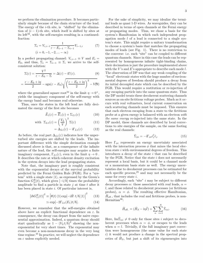
This procedure is shown diagrammatically on Fig. 2.Note that the diagonal elements are easily calculated

evaluating O(N) energy corrections of the form Σ(1)i and

Σ(N)i , where all the sites have been decimated into site i.

Also, in order to compute all the non diagonal elementsof the Green’s function matrix in Eq. 41 and 47 we would

need to evaluate ∼ N2 energy corrections Σ(j)i ’s. How-

ever, for tridiagonal block Hamiltonians, non-diagonalblock matrix elements of the Green function can be ob-tained in terms of the diagonal ones, avoiding the need

of the evaluation of ∼ N2 Σ(j)i ’s, following the insight

given in Eq. 43. In this case, if the Hamiltonian matrixis subdivided in N arbitrary blocks, we have

Gij = Gii

j−1∏

k=i

[Σ

(N)k V

−1k+1,k

]

where i<j

, (48)

Gji = Gjj

i+1∏

k=j

[Σ

(1)k V

−1k−1,k

]

where i<j

. (49)

Note that now it is not necessary to evaluate any extraΣ in order to calculate Gij for i 6= j, because those self-energies have been already calculated for the diagonalGreen’s Functions matrix blocks, Gii. This implies thatonly O (N) self-energies are required for the calculationof the whole Green’s function. These equations can helpto take advantage of possible symmetries of the V and Σ

matrices to speed up even more the calculation of Green’sFunctions.Although Eqs. 48-49 have been written in terms of

hopping matrix inverses, V−1, these expressions are ac-curate even when the hopping matrices are singular. Thisis because the hopping matrix inverse cancels out withthe hopping in the Σ definition, as it can be seen, for ex-ample, in Eq. 36. In most cases, GR

ij = GRji, and therefore

Eqs. 48 and 49 are equivalent. However, both equationsare needed in some cases of quantum pumping41 or in thepresence of magnetic fields. The origin of the extraordi-nary stability of Eqs. 48-49 can be easily grasped analyt-ically by considering a linear chain with three sites andexpressing the self-energies in terms of continued frac-tions before applying Eq. 43. Explicitly,

8

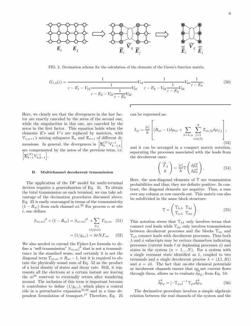
FIG. 2. Decimation scheme for the calculation of the elements of the Green’s function matrix.

G1,3(ε) =1

ε− E1 − V12

1

ε− E2 − V23

1

ε− E3V32

V21

V12

1

ε− E2 − V23

1

ε− E3V32

V23

1

ε− E3. (50)

Here, we clearly see that the divergences in the last fac-tor are exactly canceled by the zeros of the second one,while the singularities in this one, are canceled by thezeros in the first factor. This equation holds when theelements E’s and V ’s are replaced by matrices, withVn,n+1’s mixing subspaces En and En+1 of different di-

mensions. In general, the divergences in[Σ

(N)k V

−1k−1,k

]

are compensated by the zeros of the previous term, i.e.[Σ

(N)k−1V

−1k,k−1

].

B. Multichannel decoherent transmission

The application of the DP model for multi-terminaldevices requires a generalization of Eq. 31. To obtainthe total transmission on each terminal, we can take ad-vantage of the decimation procedures discussed above.Eq. 25 is easily rearranged in terms of the transmissivity(1 − Rαi) from each channel αi.32 For process α at sitei, one defines

|tαi,αi|2+ (1 −Rαi) = |tαi,αi|

2+∑

β,j

(βj 6=αi)

Tβj,αi (51)

= (1/gα,i) = 4πNiΓαi (52)

We also needed to extend the Fisher-Lee formula to de-fine a “self-transmission” |tαi,αi|

2 that is not a transmit-tance in the standard sense, and certainly it is not thediagonal term Tαi,αi ≡ Rαi − 1, but it is required to ob-tain the physically sound sum of Eq. 52 as the productof a local density of states and decay rate. Still, it rep-resents all the electrons at a certain instant are leavingthe αith reservoir to eventually return after wanderingaround. The inclusion of this term is important becauseit contributes to define (1/gα,i), which plays a centralrole in a perturbative expansion16,32 and in a time de-pendent formulation of transport.17 Therefore, Eq. 25

can be expressed as:

Iαi =|e|

h

(Rαi − 1)δµαi +

∑

β=L,φ

N∑

j=1

αi6=βj

Tαi,βjδµβ,j

,

(53)and it can be arranged in a compact matrix notation,separating the processes associated with the leads fromthe decoherent ones:

( −→I λ

0

)=

|e|

hT

(δ−→µλ

δ−→µφ

). (54)

Here, the non-diagonal elements of T are transmissionprobabilities and thus, they are definite positive. In con-trast, the diagonal elements are negative. Thus, a sumover any column or row cancels out. This matrix can alsobe subdivided in the same block structure:

T =

(Tλ,λ Tλφ

Tφ,λ Tφφ

). (55)

This notation stress that Tλλ only involves terms thatconnect real leads while Tφφ only involves transmissionsbetween decoherent processes and the blocks Tλφ andTφλ connect leads with decoherent processes. Thus bothλ and φ subscripts may be vectors themselves indicatingprocesses (current leads ℓ or dephasing processes φ) andstates in the system (n = 1, ...N). For a system witha single resonant state identified as 1, coupled to twoterminals and a single decoherent process λ = (L1, R1)and φ = φ1. The fact that on-site chemical potentialsat incoherent channels ensure that no net current flowsthrough them, allows us to evaluate

−→δµϕ, from Eq. 54:

−→δµϕ = [−Tϕϕ]

−1Tϕλ

−→δµλ. (56)

The decimative procedure involves a simple algebraicrelation between the real channels of the system and the

9

chemical potentials associated with currents drains orsources. From Eq. 54, it is straightforward to isolate−→I λ, arriving to the expression:

−→I λ =

|e|

h

(Tλλ + Tλϕ[−Tϕϕ]

−1Tϕλ

)−→δµλ (57)

=e

hTλλ

−→δµλ (58)

and therefore, the classical conductances are the non-diagonal elements of the matrix

Tλλ = Tλλ + Tλϕ[−Tϕϕ]−1

Tϕλ. (59)

This formula involves the inversion of a typically bigN × N matrix. Notice that the matrix in square brack-ets would correspond to W in the original D’Amato andPastawski’s paper , see Eq. 31.15 However, this task canbe performed resorting to a recursive decimation of the Ndephasing channels, taken one by one. Starting from thefirst one, at each stage of decimation, all the remainingprobes and dephasing channels become renormalized ac-cording to the following recursive scheme for the matrixelements of T:

T[0]ij = Tij (60)

T[k]ij = T

[k−1]ij + T

[k−1]i,k

−1

T[k−1]k,k

T[k−1]k,j . (61)

Here, k runs over the dephasing channel index φ1...φN

and T[k]ij stands for the matrix element i, j (each of them

take the values ℓ1...ℓM,φ1,..., φN) of matrix T, afterthe decimation of k incoherent channels. Once that all ofthem were decimated, we have an effective transmissionmatrix T ≡ T(N) given by:

T =

Rℓ1 − 1 Tℓ1,L2 · · · Tℓ1,ℓM

......

. . ....

TℓM,ℓ1 TℓM,ℓ2 · · · RℓM − 1

(62)

which accounts for the overall (coherent plus incoherent)transmission through the system between different cur-rent channels. This effective transmission matrix relatesreal currents on each site of the sample with the volt-ages associated with each electron reservoir. It shouldby noticed that sums over rows or columns, both on theoriginal T and on T, must be zero, in accordance to theKirchhoff law.Eq. 62 is the general solution to the multichannel DP

model. However, one frequently deals with situations inwhich there is a unique voltage difference between twochannel sets. In this case, the problem can be reducedto one with a single chemical potential difference. Forexample, assuming that all the channels associated with acurrent source in the “left” lead L have the same chemicalpotential, δµL. Similarly, all the channels constitutingthe current sink R, have δµR. We can rewrite the net

current as:

I =∑

i

Ii =e

h

MR∑

j

ML∑

i

TRj,Li(δµL − δµR) (63)

= Tr[4ΓRG

RN1ΓLG

A1N

](δµL − δµR) (64)

= GV (65)

where G is the effective conductance, V = (δµL − δµR)/eis the applied voltage, and the labels L and R standfor right and left leads respectively. Notice that ΓL andΓR are square matrices with dimensions ML × ML andMR ×MR associated with the M = ML +MR quantumchannels at the leads L and R. Since the final expressionis the trace of a matrix product, we see that its resultdoes not depend on the used basis.

V. APPLICATION EXAMPLE: MODEL FOR

SASER AND INELASTIC TUNNELING

Most electronic nanodevices are intrinsically multi-channel systems. Even two probe experiments may re-quire a multichannel description to incorporate vibra-tional degrees of freedom. Indeed, in these cases aFock-space representation of the Hamiltonian is needed.Other situations are vibrational spectroscopy in molec-ular electronics, polaronic models or Floquet represen-tations of time-dependent interactions. In order to il-lustrate the methodology presented in the previous sec-tions, we will analyze an example of this family of prob-lems: independent electrons tunneling into a resonancewhere they are strongly coupled to an optical vibrationalmode. Because of its importance for the phonon laser(SASER),42 its coherent treatment was developed ear-lier in some detail.43,44 Here, we are going to add deco-herent processes that we expect will affect the specificinterferences45 manifested in such case. Consider a “lo-

FIG. 3. Fock-space representation of states |j, n〉. The middlerow represents local electronic states j with n phonons. Lowerand upper rows describe the same electronic tight-bindingchain but with different numbers of phonons. Vertical linesrepresent local electron-phonon couplings.

cal” electronic state at a particular site or resonant state

10

labeled as 0. There, it is coupled to a single vibrationalmode ω0 with the associated bosonic number operator

b†b. This is represented by the isolated electron-phononHamiltonian,

HS = E0c+0 c0 +

(~ω0 +

12

)b+b + Vg(b

+ + b)c+0 c0. (66)

The eigenstates of this Hamiltonian are the polaronstates,46,47 whose eigenenergies are

E0,n = E0 + ~ω0

(n+

1

2

)−

|Vg |2

~ω0. (67)

Here, we are just interested to show how energy conserv-ing decoherence affects the conductance when emissionor absorption of phonons are known to produce interfer-ences. The electrons can jump in and out the resonantstate to the left and right leads. They can also sufferdecoherent processes due to interactions with acousticphonons. The effective Hamiltonian results:

Heff. = HS + ΣL + ΣR + Σφ, (68)

where ΣL and ΣR describe the escape to the current leadsand Σφ the escape associated with decoherence and theyare,

ΣL + ΣR + Σφ = [−iΣL(ε)− iΣR(ε)− iΓφ] c+0 c0. (69)

The third term is the coupling with the dephasing degreesof freedom in a FGR approximation. Notice that, theseself-energies may contain the high voltage difference re-quired by SASER operation as a difference in the bandcenters of the left and right leads EL − ER = eV. Wehave omitted a real part of the decoherent process whichis not relevant in the present case. As discussed before43,the optical phonon absorption and emission processes canbe viewed as a “vertical” processes in a two-dimensionalnetwork. Thus, transport in the Fock space is compu-tationally equivalent to a tight-binding model with anexpanded dimensionality shown in Fig. 3.43,46,48 Whenan electron comes from the left side, it arrives at the res-onant site where it couples to the n0 phonons present inthe well. It can either keep its original kinetic energyE orchange it by emitting or absorbing n phonons. Thus, thetransmission probabilities of each contribution are givenby:

TR(n0+n),Ln0= 2ΓR(n0+n)G

Rn0+n,n0

2ΓLn0GA

n0,n0+n.

(70)Notice that the subscripts represent channels in the Fockspace. As a consequence of the trivial energy shift, asso-ciated with the presence of phonons,

Γαn(ε) = Γ(ε− Eα −

(n+ 1

2

)~ω0

), (71)

for α = L,R. Voltages are accounted by Eα. Each of thisprocesses contributes to the total coherent transmissionwhich is given by,

TRL(ε) =

∞∑

n=−n0

Tn0+n,n0(ε). (72)

The device current would be obtained integrating ε withthe appropriate Fermi functions. Here, we might recallthat Ref.49 suggested that in the Fock space, “vertical”hoppings could be blocked by the presence of other elec-trons arriving with different initial energies. However, inthe situation we want to describe, the kinetic energy ofthe incoming electrons satisfies EF ≤ ~ω0 ≤ eV. i.e. theapplied voltage always enables phonon emission43,46,48

ruling out the eventual problem of overflow by propernormalization.50

In order to account for the effect of decoherence in thetransport properties, we introduce a finite lifetime for thepolaron states through an imaginary correction to theelectron’s resonant energies as in Eq. 15. Once that self-energies of the environment are included into the Green’sFunction of the system, the available “direct” channelsare associated with the transmission probabilities of Eq.70. Because of the wide band approximation implicit inthe FGR approach, in the dephasing channels, the energyshift is independent of ε:

Γφn(ε) ≡ Γφ. (73)

The available incoherent channels, are those related tofictitious probes and phonon emission or absorption,

Tβ(n0+n),αn0= 2Γβ(n0+n)(ε)|G

Rn0+n,n0

(ǫ)|22Γαn(ε) (74)

where α,β are either R,L or φ. From these transmis-sions, and using Eqs. 59 and 62, we obtain the effectivetransmissions through the available real channels. If weassume that injected electrons find n0 = 0 phonons inthe well, then the total transmission is simply,

TLR =

N∑

n=0

T(n)LR , (75)

where each T(n)LR includes the decimation of the incoherent

channels, just as in Eq. 30. In what follows we will ana-lyze TLR(ε) which is also the relevant quantity to studythe non-linear response (see Eq. 134 in Ref.32).The total transmission as function of energy is shown

in Fig. 4. The Hamiltonian parameters are roughly rep-resentative of a double-well resonant tunneling deviceswhere electron-phonon interactions manifest as a satel-lite peak in the conductance.45 There E0 = −1.5 eV,VR = VL = −0.1 eV, ~ω0 = 0.2 eV and Vg ≃ −0.1 eV.We discriminate among different vertical processes con-tributing to the total transmittance. When the couplingbetween the local electronic state and the phonon mode isneglected, Vg = 0, the problem becomes one dimensionalwith a unique resonance, as shown in Fig. 4-a. The ef-fect of the environment, accounted with the DP model,is a broadening of the original resonance. When the lo-cal electronic state is strongly coupled with the phononfield, |Vg| ≫ 0, there are extra available paths for theconduction electrons in the Fock space. Different pathsin the coherent picture can interfere destructively, giving

11

FIG. 4. Multichannel decoherent transmission for the polaron model, with ~ω0 = 0.2 eV, E0 = −1.5 eV. (a) Local electronicstate without coupling with the phonons (Vg = 0); (b) Transmission probability for an electron leaving the sample without achange in the phonon state (Vg = 0.1); (c) Transmission probability for an electron that leaves the sample emitting one phonon(Vg = 0.1); (d) Total decoherent transmission probability

rise to anti-resonances in Figs. 4-b and 4-c. Since an-tiresonances are coherent phenomena, they are destroyedwhen decoherent events are incorporated. Finally, in Fig.4-d the total electron transmission probability in a multi-phonon process is compared with the same configurationwith added decoherence, according to the multiterminalDP model.

The energy uncertainty used is Γφ = 0.026 eV ∼ kBTR,where kB is the Boltzmann constant and TR stands forroom temperature of 300K. Although one might evalu-ate Γφ from the electronic energy uncertainties obtainedwith the help of ab-initio computations, the behavior ofT as a function of Γφ is smooth, provided that these localuncertainties are small compared with typical tunnelingrates from the local resonances, ΓL(R) ≫ Γφ. Therefore,small variations of the precise value of Γφ do not change

the general behavior of T . This is illustrated in Fig. 5where a color map shows how Γφ affects the total trans-mission probability in the range [0 eV,0.025 eV]. As ageneral trend extracted from the figures, we may say thatthe effect of decoherence on transmission is: resonancesbroadening and lowering, and tails raising. Note also thatowing to the decoherent processes the anti-resonances,i.e. dips in the individual interchannel transmittances,

are destroyed.

VI. CONCLUSION

In this work, we presented a reviewed version of theoriginal DP model, which accounts for decoherent effectsin quantum transport. The incorporation of a unifiednotation, gives a better understanding for its potential-ities, and allowed us to solve generalized multichannelproblems.We made special emphasis on the role of decimation

procedures in the context of banded effective Hamilto-nians, since they can be used as the basis for efficientcomputational schemes. In particular, one of the keysfor this is given by Eqs. 48-49. Note that, in the mostcommon situation of block tridiagonal (i.e. banded) ma-trix Hamiltonians, they provide an efficient decimationprocedure that allows one to obtain all the N × (N − 1)non-diagonal blocks of the whole Green’s function matrixjust in terms of the N diagonal blocks.We also derived a compact matrix equation for the

quantum decoherent transmission coefficients in a gen-eralized multichannel scheme, highlighting a straightfor-

12

FIG. 5. Multichannel decoherent transmission for the polaronmodel in a color map. The transmission probability is shownin a color scale, as a function of the incident electron Fermienergy and the strength of the imaginary energy shift Γφ. The

behavior of T is shown to be a smooth function of Γφ.

ward parallelism with the original expressions of the DPmodel. Here, we present a recursive algorithm, that re-lies on decimation procedures, for the calculation of theeffective transmittance matrix.This, can result specially useful for the calculation of

quantum decoherent transport in real mesoscopic situa-tions, where there are more than two physical probes orwhere the system’s complexity precludes the direct use ofthe original DP model. Examples of this are many-bodyinteractions that yield extra degrees of freedom when rep-resented in the Fock space.

Even though, spin degeneracy was not discussed ex-plicitly, it can be easily included by considering each spinorientation as a different conduction channel. This strat-egy can be of great practical interest in spintronics wherenon-diagonal terms in the Hamiltonian connect differentspin-channels.51

As a pedagogical application, we solved a polaronicmodel that includes decoherent processes in addition tothe standard absorption and emission of phonons. Thissystem can be readily mapped to a multichannel trans-port problem, where the transmissions between each arbi-trary pair of electron-phonon channels can be evaluatedindependently, keeping track of the phononic processesinvolved. As expected, the effect of decoherence is givenmainly by the destruction of interferences in this space.This suppresses the anti-resonances in the transmissioncoefficients, which in our example result from the inter-ference between different paths in Fock’s space.43

With increasing system’s size, molecular electronicssuffers a paradigm shift on its dominant transport mech-anism, from “coherent tunneling” to “incoherent hop-ping”. Within this context, the present work should re-sult specially helpful in providing a computational bridgebetween these limiting situations, while maintaining ageneral, transparent, and efficient approach to quantumtransport.

VII. ACKNOWLEDGMENTS

We acknowledge the financial support of ANPCyT,CONICET, MiNCyT-Cor, and SeCyT-UNC, as well asL. E. F. Foa Torres for his comments and stimulatingdiscussions.

1 A. Pecchia and A. Di Carlo, Rep. Prog. Phys. 67, 1497(2004)

2 N. A. Zimbovskaya and M. R. Pedersonc, Phys. Rep. 509,1 (2011)

3 W. Liang, M. Bockrath, D. Bozovic, J. H. Hafner, M. Tin-kham, and H. Park, Nature 411, 665 (Jun. 2001)

4 S. P. Giblin, M. Kataoka, J. D. Fletcher, P. See, T. J. B. M.Janssen, J. P. Griffiths, G. A. C. Jones, I. Farrer, and D. A.Ritchie, Nature Communications 3, 930 (Jul. 2012), doi:“bibinfo doi 10.1038/ncomms1935

5 A. Nitzan and M. A. Ratner, Science 300, 1384 (2003)6 R. Bustos-Marun, G. Refael, and F. von Oppen,Phys. Rev. Lett. 111, 060802 (Aug 2013)

7 P. Rickhaus, R. Maurand, M.-H. Liu, M. Weiss, K. Richter,and C. Schnenberger, Nat Commun 4, 2342 (2013)

8 C. George, I. Szleifer, and M. Ratner, ACS Nano 7, 108(2013)

9 M. B. Plenio and S. F. Huelga, New J. Phys. 10, 113019(2008)

10 P. Rebentrost, M. Mohseni, I. Kassal, S. Lloyd, andA. Aspuru-Guzik, New J. Phys. 11, 033003 (2009)

11 D. J. Thouless and S. Kirkpatrick, J. Phys. C: Solid StatePhys. 14, 235 (1981)

12 Y. Imry and R. Landauer, Rev. Mod. Phys. 71, S306(1999)

13 M. Buttiker, Phys. Rev. Lett. 57, 1761 (1986)14 M. Buttiker, Phys. Rev. B 33, 3020 (Mar 1986)15 J. L. D’Amato and H. M. Pastawski, Phys. Rev. B 41,

7411 (1990)16 H. M. Pastawski, Phys. Rev. B 44, 6329 (1991)17 H. M. Pastawski, Phys. Rev. B 46, 4053 (1992)18 P. Danielewicz, Ann. Phys. 152, 239 (1984)19 L. Kadanoff and G. Baym, Quantum Statistical Mechan-

ics: Green’s Function Methods in Equilibrium and Non-

Equilibrium Problems, Advanced Book Classics (PerseusBooks, 1989) ISBN 9780201094220

20 J. Rammer and H. Smith, Rev. Mod. Phys 58, 323 (1986)21 N. Zimbovskaya and G. Gumbs, Appl. Phys. Lett. 81, 1518

(2002)22 M. Zwolak and M. Di Ventra, Appl. Phys. Lett. 81, 925

(2002)23 F. Gagel and K. Maschke, Phys. Rev. B 54, 13885 (1996)

13

24 D. Nozaki, Y. Girard, and K. Yoshizawa, J. Chem. Phys.C 112, 17408 (2008)

25 C. J. Cattena, R. Bustos-Marun, and H. M. Pastawski,Phys. Rev. B 82, 144201 (2010)

26 D. Nozaki, C. G. Rocha, H. M. Pastawski, and G. Cunib-erti, Phys. Rev. B 85, 155327 (2012)

27 J. Qi, N. Edirisinghe, M. G. Rabbani, and M. P. Anantram,Phys. Rev. B 87, 085404 (Feb 2013)

28 J. Maassen, F. Zahid, and H. Guo, Phys. Rev. B 80, 125423(2009)

29 M. Znidaric and M. Horvat, Eur. Phys. J. B 86, 1 (2013),ISSN 1434-6028

30 E. Domany, S. Alexander, D. Bensimon, and L. P.Kadanoff, Phys. Rev. B 28, 3110 (Sep 1983)

31 J. B. Sokoloff and J. V. Jose, Phys. Rev. Lett. 49, 700(Aug 1982)

32 H. M. Pastawski and E. Medina, Rev. Mex. Fis. 47, 1(2001)

33 P. R. Levstein, H. M. Pastawski, and J. L. D’Amato, J.Phys.: Condens. Matter 2, 1781 (1990)

34 The infinitesimal η with the chosen sign ensures the correctbranches of the solution. Note that this expression is easilyobtained from the definition of the square root of a complexnumber:√x+ iy =

√

r+x

2+ isgn(y)

√

r−x

2where r = |x+ iy|.

Also note that the sign of this infinitesimal is consistentwith its introduction in Eq. 13.

35 E. Rufeil Fiori and H. M. Pastawski, Chem. Phys. Lett.420, 35 (2006)

36 I. Rotter, J. Phys. A: Math. Theor. 42, 153001 (2009)37 A. D. Dente, R. A. Bustos-Marun, and H. M. Pastawski,

Phys. Rev. A 78, 062116 (2008)38 H. M. Pastawski, C. M. Slutzky, and J. F. Weisz,

Phys. Rev. B 32, 3642 (Sep 1985)39 W. H. Butler, Phys. Rev. B 8, 4499 (1973)40 H. M. Pastawski, J. F. Weisz, and S. Albornoz, Phys. Rev.

B 28, 6896 (1983)41 L. E. F. Foa Torres, Phys. Rev. B 72, 245339 (2005)42 R. P. Beardsley, A. V. Akimov, M. Henini, and A. J. Kent,

Phys. Rev. Lett. 104, 085501 (2010)43 H. M. Pastawski, L. E. F. Foa Torres, and E. Medina,

Chem. Phys. 281, 257 (2002)44 I. Camps, S. Makler, H. Pastawski, and L. E. F. Foa Torres,

Phys. Rev. B 64, 125311 (2001)45 L. E. F. Foa Torres, H. M. Pastawski, and S. S. Makler,

Phys. Rev. B 64, 193304 (Oct 2001)46 E. V. Anda, S. S. Makler, H. M. Pastawski, and R. G.

Barrera, Braz. J. Phys. 24, 330 (1994)47 N. S. Wingreen, K. W. Jacobsen, and J. W. Wilkins, Phys.

Rev. Lett. 61, 1396 (1988)48 Bonca and Trugman, Phys. Rev. Lett. 75, 2566 (1995)49 E. G. Emberly and G. Kirczenow, Phys. Rev. B 61, 5740

(2000)50 C. J. Cattena, Quantum decoherence effects on electronic

transport in molecular wires and nanodevices, Ph.D. thesis,Universidad Nacional de Cordoba (March 2012)

51 V. A. Gopar, D. Weinmann, R. A. Jalabert, and R. L.Stamps, Phys. Rev. B 69, 014426 (Jan 2004)