GENERALIZED AND RESTRICTED MULTIPLICATION TABLES OF INTEGERS BY DIMITRIOS KOUKOULOPOULOS DISSERTATION Submitted in partial fulfillment of the requirements for the degree of Doctor of Philosophy in Mathematics in the Graduate College of the University of Illinois at Urbana-Champaign, 2010 Urbana, Illinois Doctoral Committee: Professor Bruce C. Berndt, Chair Professor Kevin Ford, Director of Research Professor A.J. Hildebrand, Contingent Chair Associate Professor Scott Ahlgren

Welcome message from author
This document is posted to help you gain knowledge. Please leave a comment to let me know what you think about it! Share it to your friends and learn new things together.
Transcript
GENERALIZED AND RESTRICTED MULTIPLICATION TABLES OF INTEGERS
BY
DIMITRIOS KOUKOULOPOULOS
DISSERTATION
Submitted in partial fulfillment of the requirementsfor the degree of Doctor of Philosophy in Mathematics
in the Graduate College of theUniversity of Illinois at Urbana-Champaign, 2010
Urbana, Illinois
Doctoral Committee:
Professor Bruce C. Berndt, ChairProfessor Kevin Ford, Director of ResearchProfessor A.J. Hildebrand, Contingent ChairAssociate Professor Scott Ahlgren
Abstract
In 1955 Erdos posed the multiplication table problem: Given a large integer N , how many
distinct products of the form ab with a ≤ N and b ≤ N are there? The order of magnitude
of the above quantity was determined by Ford. The purpose of this thesis is to study
generalizations of Erdos’s question in two different directions. The first one concerns the
k-dimensional version of the multiplication table problem: for a fixed integer k ≥ 3 and a
large parameter N , we establish the order of magnitude of the number of distinct products
n1 · · ·nk with ni ≤ N for all i ∈ 1, . . . , k. The second question we shall discuss is the
restricted multiplication table problem. More precisely, for B ⊂ N we seek estimates on the
number of distinct products ab ∈ B with a ≤ N and b ≤ N . This problem is intimately
connected with the available information on the distribution of B in arithmetic progressions.
We focus on the special and important case when B = Ps = p + s : p prime for some
fixed s ∈ Z \ 0. Ford established upper bounds of the expected order of magnitude for
|ab ∈ Ps : a ≤ N, b ≤ N|. We prove the corresponding lower bounds thus determining the
size of the quantity in question up to multiplicative constants.
ii
To my parents, Dimitra and Paris
iii

Acknowledgements
I would like to express my warmest thanks to my advisor Professor Kevin Ford for his help
and encouragement over the years.
Part of the research that led to this dissertation was carried out with support from
National Science Foundation grants DMS 05-55367 and DMS 08-38434 “EMSW21-MCTP:
Research Experience for Graduate Students”. Also, the writing of this dissertation was
partially supported from National Science Foundation grant DMS 09-01339.
iv

Table of Contents
Chapter 1 Introduction . . . . . . . . . . . . . . . . . . . . . . . . . . . . . 11.1 The Erdos multiplication table problem . . . . . . . . . . . . . . . . . . . . . 11.2 The (k + 1)-dimensional multiplication table problem . . . . . . . . . . . . . 41.3 Shifted primes in the multiplication table . . . . . . . . . . . . . . . . . . . . 51.4 Outline of the dissertation . . . . . . . . . . . . . . . . . . . . . . . . . . . . 71.5 Notation . . . . . . . . . . . . . . . . . . . . . . . . . . . . . . . . . . . . . . 8
Chapter 2 Main results . . . . . . . . . . . . . . . . . . . . . . . . . . . . . 102.1 Local divisor functions . . . . . . . . . . . . . . . . . . . . . . . . . . . . . . 102.2 From local to global divisor functions . . . . . . . . . . . . . . . . . . . . . . 142.3 A heuristic argument for H(k+1)(x,y, 2y) . . . . . . . . . . . . . . . . . . . . 172.4 Some comments about the proof of Theorem 2.6 . . . . . . . . . . . . . . . . 20
Chapter 3 Auxiliary results . . . . . . . . . . . . . . . . . . . . . . . . . . . 233.1 Number theoretic results . . . . . . . . . . . . . . . . . . . . . . . . . . . . . 233.2 The Vitali covering lemma . . . . . . . . . . . . . . . . . . . . . . . . . . . . 333.3 Estimates from order statistics . . . . . . . . . . . . . . . . . . . . . . . . . . 33
Chapter 4 Local-to-global estimates . . . . . . . . . . . . . . . . . . . . . . 384.1 The lower bound in Theorem 2.8 . . . . . . . . . . . . . . . . . . . . . . . . 394.2 The upper bound in Theorem 2.8 . . . . . . . . . . . . . . . . . . . . . . . . 414.3 Proof of Theorem 2.5 . . . . . . . . . . . . . . . . . . . . . . . . . . . . . . . 514.4 Divisors of shifted primes . . . . . . . . . . . . . . . . . . . . . . . . . . . . . 53
Chapter 5 Localized factorizations of integers . . . . . . . . . . . . . . . . 625.1 The upper bound in Theorem 2.6 . . . . . . . . . . . . . . . . . . . . . . . . 625.2 The lower bound in Theorem 2.6: outline of the proof . . . . . . . . . . . . . 675.3 The method of low moments: interpolating between L1 and L2 estimates . . 715.4 The method of low moments: combinatorial arguments . . . . . . . . . . . . 775.5 The method of low moments: completion of the proof . . . . . . . . . . . . . 805.6 The lower bound in Theorem 2.6: completion of the proof . . . . . . . . . . 83
Chapter 6 Work in progress . . . . . . . . . . . . . . . . . . . . . . . . . . . 87
References . . . . . . . . . . . . . . . . . . . . . . . . . . . . . . . . . . . . . . 89
v

Chapter 1
Introduction
1.1 The Erdos multiplication table problem
When we learn to multiply in base 10 we memorize the following table.
Table 1.1: The 10× 10 multiplication table
1 2 3 4 5 6 7 8 9 101 1 2 3 4 5 6 7 8 9 102 2 4 6 8 10 12 14 16 18 203 3 6 9 12 15 18 21 24 27 304 4 8 12 16 20 24 28 32 36 405 5 10 15 20 25 30 35 40 45 506 6 12 18 24 30 36 42 48 54 607 7 14 21 28 35 42 49 56 63 708 8 16 24 32 40 48 56 64 72 809 9 18 27 36 45 54 63 72 81 9010 10 20 30 40 50 60 70 80 90 100
Even though this multiplication table has 100 entries, only 42 distinct numbers appear
in it. In 1955 Erdos [Erd55, Erd60] asked what happens if one considers larger tables, that
is for a large integer N what is the asymptotic behavior of
A(N) := |ab : a ≤ N, b ≤ N|?
An argument based on the number of prime factors of a ‘typical’ integer quickly reveals that
A(N) = o(N2) (N →∞).
1

Indeed, we have that
ω(n) := |p prime : p|n| ∼ log log n
on a sequence of integers n of density 1 (see Theorem 1.1 below). So for most pairs of
integers (a, b) with a ≤ N and b ≤ N the product ab has about 2 log logN prime factors
and hence the density of such products in [1, N2] tends to 0 as N → ∞. Even though this
argument may seem a bit naive, a simple generalization of it quickly leads to relatively sharp
upper bounds on A(N). Before we proceed we state a well-known result due to Hardy and
Ramanujan.
Theorem 1.1 (Hardy-Ramanujan [HarR]). There are absolute constants C1 and C2 such
that for all x ≥ 2 and all r ∈ N we have
πr(x) := |n ≤ x : ω(n) = r| ≤ C1x
log x
(log log x+ C2)r−1
(r − 1)!.
Fix now a parameter λ > 1 and set L = bλ log logNc and
Q(λ) = λ log λ− λ+ 1.
Then
A∗(N) := |ab : a ≤ N, b ≤ N, (a, b) = 1|
≤ |n ≤ N2 : ω(n) > L|+ |(a, b) : a ≤ N, b ≤ N,ω(a) + ω(b) ≤ L|
=∑r>L
πr(N2) +
∑r+s≤L
πr(N)πs(N)
λ
(1 + (logN)λ log 2−1
) N2
(logN)Q(λ)(log logN)1/2,
by Theorem 1.1 and Stirling’s formula. Choosing λ = 1/ log 2 in order to optimize the above
estimate yields
A∗(N) N2
(logN)Q(1/ log 2)(log logN)1/2.
2
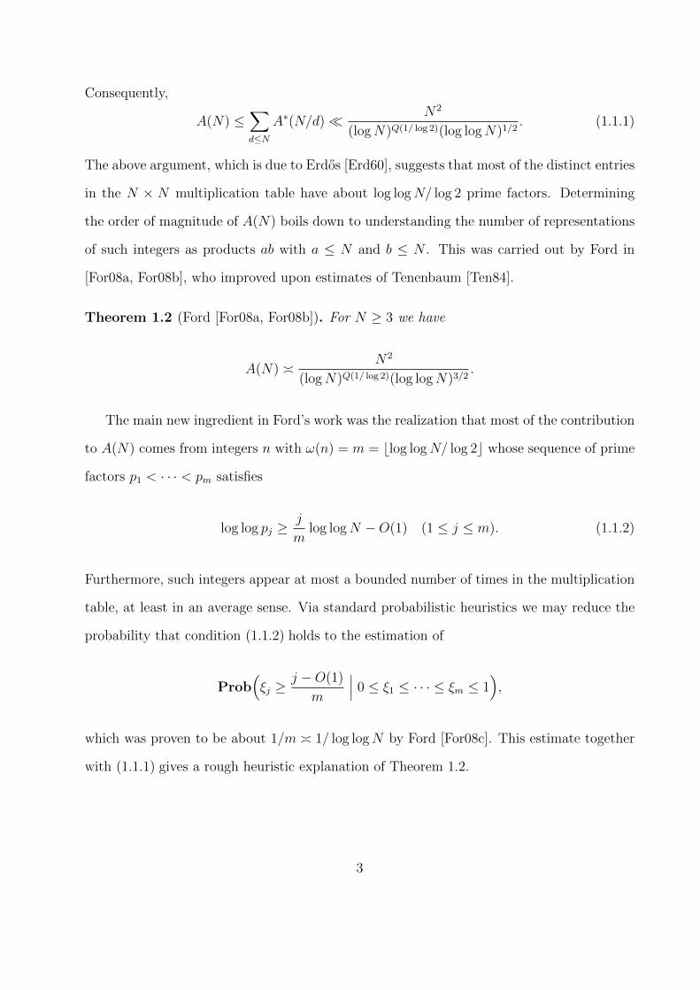
Consequently,
A(N) ≤∑d≤N
A∗(N/d) N2
(logN)Q(1/ log 2)(log logN)1/2. (1.1.1)
The above argument, which is due to Erdos [Erd60], suggests that most of the distinct entries
in the N × N multiplication table have about log logN/ log 2 prime factors. Determining
the order of magnitude of A(N) boils down to understanding the number of representations
of such integers as products ab with a ≤ N and b ≤ N . This was carried out by Ford in
[For08a, For08b], who improved upon estimates of Tenenbaum [Ten84].
Theorem 1.2 (Ford [For08a, For08b]). For N ≥ 3 we have
A(N) N2
(logN)Q(1/ log 2)(log logN)3/2.
The main new ingredient in Ford’s work was the realization that most of the contribution
to A(N) comes from integers n with ω(n) = m = blog logN/ log 2c whose sequence of prime
factors p1 < · · · < pm satisfies
log log pj ≥j
mlog logN −O(1) (1 ≤ j ≤ m). (1.1.2)
Furthermore, such integers appear at most a bounded number of times in the multiplication
table, at least in an average sense. Via standard probabilistic heuristics we may reduce the
probability that condition (1.1.2) holds to the estimation of
Prob(ξj ≥
j −O(1)
m
∣∣∣ 0 ≤ ξ1 ≤ · · · ≤ ξm ≤ 1),
which was proven to be about 1/m 1/ log logN by Ford [For08c]. This estimate together
with (1.1.1) gives a rough heuristic explanation of Theorem 1.2.
3

1.2 The (k + 1)-dimensional multiplication table
problem
A natural generalization of the Erdos multiplication table problem comes from looking at
products of more than two integers. More precisely, for a fixed integer k ≥ 2 and a large
integer N we seek estimates for
Ak+1(N) := |n1 · · ·nk+1 : ni ≤ N (1 ≤ i ≤ k + 1)|.
A similar argument with the one leading to (1.1.1) implies
Ak+1(N)kNk+1
(logN)Q(k/ log(k+1))(log logN)1/2. (1.2.1)
This estimate suggests that most of the distinct entries in the N × · · · ×N︸ ︷︷ ︸k+1 times
multiplication
table have about
m =
⌊k log logN
log(k + 1)
⌋prime factors. Further analysis of the multiplicative structure of such integers indicates that
most of the contribution to Ak+1(N) comes from integers n with ω(n) = m whose prime
factors p1 < · · · < pm satisfy
log log pj ≥j
mlog logN −O(1) (1 ≤ j ≤ m). (1.2.2)
As in Ford’s work when k = 1, this suggests that the order of magnitude of Ak+1(N) is the
right hand side of (1.2.1) multiplied by 1/ log logN . Indeed, we have the following theorem,
which was proven in [Kou10a].
4

Theorem 1.3. Fix k ≥ 2. For all N ≥ 3 we have
Ak+1(N) kNk+1
(logN)Q(k/ log(k+1))(log logN)3/2.
In Section 2.3 we shall give a more precise heuristic explanation of the above theorem.
The proof of Theorem 1.3 is based on the methods developed by Ford in [For08a, For08b] to
handle the case k = 1. The hardest part of the argument consists of showing that the average
number of representations in the (k + 1)-dimensional multiplication table of integers that
satisfy (1.2.2) is bounded. We shall elaborate further on this in Section 2.4.
1.3 Shifted primes in the multiplication table
In the previous section we discussed the analogue of the Erdos multiplication table for
products of three or more integers. However, even when we consider products of just two
integers there are still unresolved questions. For example, given an arithmetic sequence
B ⊂ N, how many elements of B appear in the N ×N multiplication table, that is what is
the size of
A(N ; B) := |ab ∈ B : a ≤ N, b ≤ N|
as N →∞? We call this the restricted multiplication table problem. If B is reasonably well-
distributed in arithmetic progressions 0 (mod d), then a relatively straightforward heuristic
argument shows that we should have
A(N ; B) ≈ |B ∩ [1, N2]|N2
A(N).
We focus on the special and important case when B = Ps := p + s : p prime for some
fixed s ∈ Z \ 0. In [For08b] Ford proved the expected upper bound on A(N ;Ps) using the
techniques he developed to handle A(N) together with upper sieve estimates.
5

Theorem 1.4 (Ford [For08b]). Fix s ∈ Z \ 0. For all N ≥ 3 we have
A(N ;Ps)sA(N)
logN.
Lower bounds on A(N ;Ps) are harder because they need as input more precise informa-
tion on primes in arithmetic progressions, a problem which is notoriously difficult. The most
straightforward way to bound A(N ;Ps) from below is to use a linear sieve, whose successful
application is vitally dependent on having good control of the counting function of primes
in arithmetic progressions on average. The standard way of obtaining such control is via
the Bombieri-Vinogradov theorem [Dav, p. 161]. However, in this setting this theorem is
inapplicable. Indeed, the function A(N ;Ps) counts shifted primes of the form p + s = ab
with a ≤ N and b ≤ N , which means that in order to bound A(N ;Ps) we need control
of the number of primes p ≤ N2 − s in arithmetic progressions −s (mod a) of modulus a
that can be as large as N ∼√N2 − s. The Bombieri-Vinogradov theorem can only handle
arithmetic progressions of modulus a ≤ N1−ε for an arbitrarily small, but nevertheless fixed,
positive ε. To overcome this problem we appeal to a result proven by Bombieri, Friedlander
and Iwaniec, which is Theorem 9 in [BFI].
Theorem 1.5 (Bombieri, Friedlander, Iwaniec [BFI]). Fix a ∈ Z \ 0, C > 0 and ε > 0.
There exists a constant C ′ depending at most on C such that
∑r≤R
∣∣∣∣∑q≤Q
(π(x; rq, a)− li(x)
φ(rq)
)∣∣∣∣a,C,εx
(log x)C
uniformly in R ≤ x1/10−ε and RQ ≤ x(log x)−C′.
Remark 1.3.1. In fact, Theorem 9 in [BFI] is stated in terms of
ψ(x; d, a) :=∑pm≤x
pm≡a (mod d)
log p,
6

but a standard partial summation argument can easily convert it to the above form.
Using Theorem 1.5 together with a preliminary sieve, via the fundamental lemma of sieve
methods (cf. Lemma 3.1.2) to smoothen certain summands 1, we establish the expected lower
bound for A(N ;Ps), a result which appeared in [Kou10b].
Theorem 1.6. Fix s ∈ Z \ 0. For all N ≥ 3 we have
A(N ;Ps)sA(N)
logN.
1.4 Outline of the dissertation
In Chapter 2 we introduce certain divisor functions, which are the main objects of investi-
gation of this work, and show how to pass from them to the results of Chapter 1. Also, we
state our main results about these divisor functions and comment on some of the methods
and ideas that are central in their study. In Chapter 3 we list several preliminary results
from number theory, analysis and statistics that will be used in subsequent chapters. The
first result of Chapter 4 is a reduction theorem that is the starting point towards the proof
of our main results. Also, we demonstrate how to reduce the problem of bounding A(N ;Ps)
to the problem of bounding A(N) and prove Theorem 1.6. Chapter 5 is dedicated to the
(k + 1)-dimensional problem, translated in the language of divisor functions. Finally, in
Chapter 6 we comment on some work still in progress and state some preliminary results
which generalize our estimates for Ak+1(N).
1A way to view the fundamental lemma, which lies at the heart of classical sieve methods, is as anattempt to approximate the characteristic function of integers n whose prime factors are greater than z witha ‘smooth’ function using combinatorial and other methods. Here the role of the smooth approximation isplayed by a convolution λ ∗ 1, where λ has small support. The adjective ‘smooth’ is justified because, byopening the summation in λ ∗ 1, a single sum weighted with λ ∗ 1 can be converted to a double sum whoseinner sum is weighted with the smooth function 1 and the outer sum has small support
7
1.5 Notation
We make use of some standard notation. The symbol Sk stands for the set of permutations of
1, . . . , k. If a(n), b(n) are two arithmetic functions, then we denote with a∗b their Dirichlet
convolution. For n ∈ N we use P+(n) and P−(n) to denote the largest and smallest prime
factor of n, respectively, with the notational conventions that P+(1) = 0 and P−(1) = +∞.
Furthermore, τ(n) stands for the number of divisors of n, ω(n) for the number of distinct
prime factors of n and Ω(n) for the total number of prime factors of n. Given 1 ≤ y < z,
P(y, z) denotes the set of all integers n such that P+(n) ≤ z and P−(n) > y. Finally,
π(x; q, a) stands for the number of primes up to x in the arithmetic progression a (mod q)
and li(x) for the logarithmic integral∫ x
2dt/ log t.
Constants implied by , and are absolute unless otherwise specified, e.g. by a
subscript. Also, we use the letters c and C to denote constants, not necessarily the same
ones in every place, possibly depending on certain parameters that will be specified by
subscripts and other means. Also, bold letters always denote vectors whose coordinates are
indexed by the same letter with subscripts, e.g. a = (a1, . . . , ak) and ξ = (ξ1, . . . , ξr). The
dimension of the vectors will not be explicitly specified if it is clear by the context.
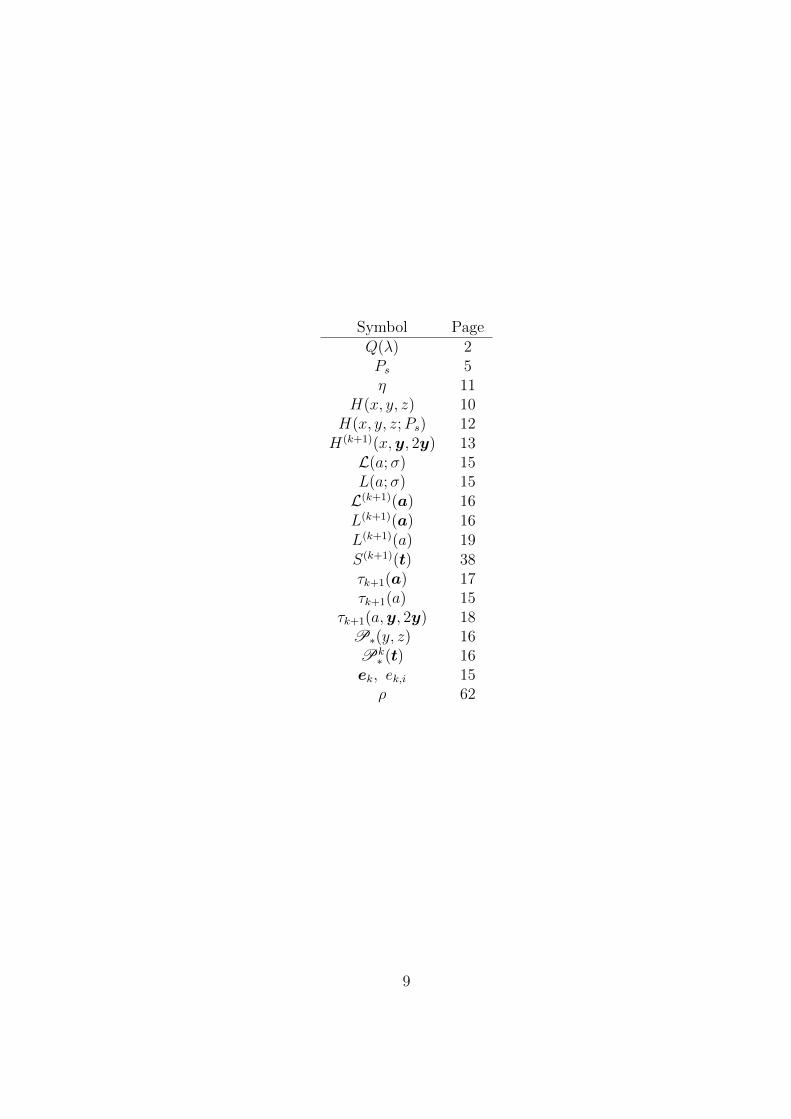
Finally, we give a table of some basic non-standard notation that we will be using with
references to page numbers for its definition.
8
Symbol PageQ(λ) 2Ps 5η 11
H(x, y, z) 10H(x, y, z;Ps) 12H(k+1)(x,y, 2y) 13L(a;σ) 15L(a;σ) 15L(k+1)(a) 16L(k+1)(a) 16L(k+1)(a) 19S(k+1)(t) 38τk+1(a) 17τk+1(a) 15
τk+1(a,y, 2y) 18P∗(y, z) 16Pk∗ (t) 16
ek, ek,i 15ρ 62
9
Chapter 2
Main results
In this chapter we shift our focus from the multiplication table to certain divisor functions
which will be the main technical objects of investigation.
2.1 Local divisor functions
In [For08b] Ford deduced Theorem 1.2 via his bounds on a closely related function: For
positive real numbers x, y and z define
H(x, y, z) = |n ≤ x : ∃ d|n with y < d ≤ z|.
Using dyadic decomposition we can relate A(N) to the size of H(x, y, 2y). Indeed, we have
that
H(N2
2,N
2, N)≤ A(N) ≤
∑m≥0
H(N2
2m,N
2m+1,N
2m
). (2.1.1)
There are two main advantages in working with H(x, y, 2y) - and, more generally, with
H(x, y, z) - instead of A(N). Firstly, bounds on H(x, y, 2y) are applicable to problems
beyond the N × N multiplication table; we refer the reader to [For08b] for several such
applications. Secondly, bounding H(x, y, 2y) is technically slightly easier than bounding
A(N).
In [For08b] Ford determined the order of magnitude of H(x, y, z) uniformly for all choices
of parameters x, y, z. In order to state his result we introduce some notation. For a given
10

pair (y, z) with 2 ≤ y < z define η, u, β and ξ by
z = eηy = y1+u, η = (log y)−β, β = log 4− 1 +ξ√
log log y.
Furthermore, set
z0(y) = y exp(log y)− log 4+1 ≈ y + y(log y)− log 4+1
and
G(β) =
Q(1 + β
log 2
), 0 ≤ β ≤ log 4− 1,
β, log 4− 1 ≤ β.
Theorem 2.1 (Ford [For08b]). Let 3 ≤ y + 1 ≤ z ≤ x.
(a) If y ≤√x, then
H(x, y, z)
x
log(z/y) = η, y + 1 ≤ z ≤ z0(y),
β
max1,−ξ(log y)G(β), z0(y) ≤ z ≤ 2y,
uQ(1/ log 2)(log 2u)−3/2, 2y ≤ z ≤ y2,
1, z ≥ y2.
(b) If y >√x, then
H(x, y, z)
H(x, x
z, xy), if x
y≥ x
z+ 1,
ηx, else.
Theorem 1.2 then follows as an immediate corollary of the above theorem and inequal-
ity (2.1.1).
11
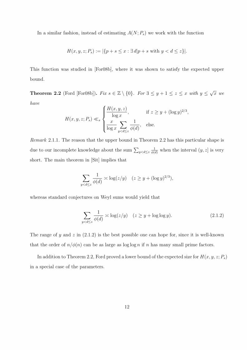
In a similar fashion, instead of estimating A(N ;Ps) we work with the function
H(x, y, z;Ps) := |p+ s ≤ x : ∃ d|p+ s with y < d ≤ z|.
This function was studied in [For08b], where it was shown to satisfy the expected upper
bound.
Theorem 2.2 (Ford [For08b]). Fix s ∈ Z \ 0. For 3 ≤ y + 1 ≤ z ≤ x with y ≤√x we
have
H(x, y, z;Ps)s
H(x, y, z)
log x, if z ≥ y + (log y)2/3,
x
log x
∑y<d≤z
1
φ(d), else.
Remark 2.1.1. The reason that the upper bound in Theorem 2.2 has this particular shape is
due to our incomplete knowledge about the sum∑
y<d≤z1
φ(d)when the interval (y, z] is very
short. The main theorem in [Sit] implies that
∑y<d≤z
1
φ(d) log(z/y) (z ≥ y + (log y)2/3),
whereas standard conjectures on Weyl sums would yield that
∑y<d≤z
1
φ(d) log(z/y) (z ≥ y + log log y). (2.1.2)
The range of y and z in (2.1.2) is the best possible one can hope for, since it is well-known
that the order of n/φ(n) can be as large as log log n if n has many small prime factors.
In addition to Theorem 2.2, Ford proved a lower bound of the expected size forH(x, y, z;Ps)
in a special case of the parameters.
12

Theorem 2.3 (Ford [For08b]). Fix s ∈ Z \ 0, 0 ≤ a < b ≤ 1. For x ≥ 2 we have
H(x, xa, xb;Ps)s,a,bx
log x.
In [Kou10b] we extended the range of validity of the above theorem significantly. We
state below a weak form of Theorem 6 in [Kou10b].
Theorem 2.4. Fix s ∈ Z \ 0 and C ≥ 2. For 3 ≤ y + 1 ≤ z ≤ x with y ≤√x and
z ≥ y + y(log y)−C we have
H(x, y, z;Ps)s,CH(x, y, z)
log x.
Remark 2.1.2. In [Kou10b] more general results were proven, which partially cover the range
z ≤ y + y(log y)−C as well. However, for the sake of the economy of the exposition we
shall not state or prove these results, since the main motivation of this dissertation is the
multiplication table and its generalizations for which Theorem 2.4 is sufficient.
Theorem 2.4 will be shown in Section 4.4. Combining Theorems 2.2 and 2.4 with an
inequality similar to (2.1.1) we immediately obtain Theorems 1.2 and 1.6.
Finally, continuing in the above spirit, instead of studying Ak+1(N) directly, we focus
on the counting function of localized factorizations of integers, which is defined for x ≥ 1,
y ∈ [0,+∞)k and z ∈ [0,+∞)k by
H(k+1)(x,y, 2y) = |n ≤ x : ∃ d1 · · · dk|n with yi < di ≤ zi (1 ≤ i ≤ k)|.
Theorem 2.5 establishes the expected quantitative relation between H(k+1)(x,y, 2y) and
Ak+1(N1, . . . , Nk+1) := |n1 · · ·nk+1 : ni ≤ Ni (1 ≤ i ≤ k + 1)|,
where N1, . . . , Nk+1 are large integers.
13

Theorem 2.5. Fix k ≥ 2. For 3 ≤ N1 ≤ N2 ≤ · · · ≤ Nk+1 we have
Ak+1(N1, . . . , Nk+1) k H(k+1)(N1 · · ·Nk+1,
(N1
2, . . . ,
Nk
2
), (N1, . . . , Nk)
).
Remark 2.1.3. We call the problem of estimating Ak+1(N1, . . . , Nk+1) for arbitrary choices
of N1, . . . , Nk+1 the generalized multiplication table problem.
The proof of Theorem 2.5 will be given in Section 4.3. It is worth noticing that its proof
does not depend on knowing the exact size of H(k+1)(x,y, 2y); rather, we deduce it from a
reduction result for H(k+1)(x,y, 2y) (cf. Theorem 2.8). In view of Theorem 2.5, in order
to bound Ak+1(N) it suffices to bound H(k+1)(x,y, 2y) when y1 = · · · = yk, uniformly in x
and y1. Thus the following estimate, which appeared in [Kou10a], completes the proof of
Theorem 1.3.
Theorem 2.6. Fix k ≥ 2 and c ≥ 1. Let x ≥ 1 and 3 ≤ y1 ≤ · · · ≤ yk ≤ yc1 with
2ky1 · · · yk ≤ x/yk. Then
H(k+1)(x,y, 2y) k,cx
(log y1)Q(k/ log(k+1))(log log y1)3/2.
Theorem 2.6 will be proven in Chapter 5.
Remark 2.1.4. The condition 2ky1 · · · yk ≤ x/yk causes essentially no harm to generality
because of the following elementary reason: if d1 · · · dk|n and we set dk+1 = n/(d1 · · · dk),
then d1 · · · dk−1dk+1|n.
2.2 From local to global divisor functions
In [For08b] the first important step in the study of H(x, y, z) is the reduction of the counting
in H(x, y, z), which contains information about the local distribution of the divisors of
an integer, to the estimation of certain quantities that carry information about the global
14

distribution of the divisors of integers. More precisely, for a ∈ N and σ > 0 define
L(a;σ) =⋃d|a
[log d− σ, log d)
and
L(a;σ) = Vol(L(a;σ)).
Then we have the following theorem.
Theorem 2.7 (Ford [For08b]). Fix ε > 0 and B > 0. For 3 ≤ y + 1 ≤ z ≤ x with y ≤√x
and
y +y
(log y)B≤ z ≤ y101/100
we have
H(x, y, z) ε,Bx
log2 y
∑a≤yε
µ2(a)=1
L(a; η)
a.
Remark 2.2.1. Even though the above theorem is not stated explicitly in [For08b], it is a
direct corollary of the methods there: see Theorem 1 and Lemmas 4.1, 4.2, 4.5, 4.8 and 4.9
in [For08b].
As we will demonstrate in Section 4.4, the proof of Theorem 2.4 passes through the proof
of a reduction result for H(x, y, z;Ps) analogous to Theorem 2.7 for H(x, y, z).
Similarly, the first step towards the proof of Theorem 2.5 consists of showing a general-
ization of Theorem 2.7. First, let
ek = (ek,1, . . . , ek,k) = (1, 1, . . . , 1, 2) ∈ Rk.
For a ∈ N and a ∈ Nk define
τk+1(a) = |(d1, . . . , dk) ∈ Nk : d1 · · · dk|a|,
15

L(k+1)(a) =⋃
d1···di|a1···ai1≤i≤k
[log(d1/2), log d1)× · · · × [log(dk/2), log dk)
and
L(k+1)(a) = Vol(L(k+1)(a)).
Also, for 1 ≤ y < z set
P∗(y, z) = n ∈P(y, z) : µ2(n) = 1
and for t = (t1, . . . , tk) with 1 = t0 ≤ t1 ≤ · · · ≤ tk set
Pk∗ (t) = a ∈ Nk : ai ∈P∗(ti−1, ti) (1 ≤ i ≤ k).
Theorem 2.8. Fix k ≥ 1. For x ≥ 1 and 3 ≤ y1 ≤ · · · ≤ yk with 2ky1 · · · yk ≤ x/yk we have
H(k+1)(x,y, 2y)
xk( k∏i=1
log−ek,i yi
) ∑a∈Pk
∗ (y)
L(k+1)(a)
a1 · · · ak.
Theorem 2.8 will be proven in Sections 4.1 and 4.2. As an immediate consequence of it,
we have the following result.
Corollary 2.1. Let k ≥ 2 and for i ∈ 1, 2 consider xi ≥ 1 and yi = (yi,1, . . . , yi,k) ∈
[1,+∞)k. Assume that 2kyi,1 · · · yi,k ≤ xi/yi,k for i ∈ 1, 2 and that there exist constants c
and C such that yc1,j ≤ y2,j ≤ yC1,j for all j ∈ 1, . . . , k. Then
H(k+1)(x1,y1, 2y1)
x1
k,c,CH(k+1)(x2,y2, 2y2)
x2
.
Proof. The result follows easily by Theorem 2.8, Lemma 2.3.1(b) below and the standard
estimate ∑a∈P∗(t,tB)
τm(a)
am,B 1 (t ≥ 1),
16

which holds for every fixed m ≥ 1 and B ≥ 1.
When k = 1, a stronger version of the above corollary is known to be true: see Corollary
1 in [For08b].
2.3 A heuristic argument for H(k+1)(x,y, 2y)
In this section we develop a heuristic argument which gives a rough explanation of Theo-
rem 2.6 as well as how condition (1.2.2) makes its appearance in the study of Ak+1(N). It is
a generalization of an argument given by Ford in [For08a] for the case k = 1. Before we delve
into the details of this argument, we state a simple but basic result we will be using exten-
sively throughout this dissertation. With a slight abuse of notation, for a = (a1, . . . , ak) ∈ Nk
set
τk+1(a) = |(d1, . . . , dk) ∈ Nk : d1 · · · di|a1 · · · ai (1 ≤ i ≤ k)|.
Then we have the following lemma.
Lemma 2.3.1. (a) For a ∈ Nk we have
L(k+1)(a) ≤ minτk+1(a)(log 2)k,
k∏i=1
(log a1 + · · ·+ log ai + log 2).
(b) If (a1 · · · ak, b1 · · · bk) = 1, then
L(k+1)(a1b1, . . . , akbk) ≤ τk+1(a)L(k+1)(b).
(c) For (a, b) = 1 and σ > 0 we have
L(ab;σ) ≤ τ(a)L(b;σ).
17

Proof. Parts (a) and (b) have very similar proofs with items (i) and (ii) of Lemma 3.1
in [For08b], respectively. Part (c) is item (ii) of Lemma 3.1 in [For08b].
Consider real numbers x ≥ 1 and 3 ≤ y1 ≤ · · · ≤ yk as in Theorem 2.6. Given n ∈
N ∩ [1, x] we decompose it as n = ab, where
a =∏
pl‖n,p≤2yk
pl.
For simplicity assume that a is square-free and that log a log y1. The integer n is counted
by H(k+1)(x,y, 2y) if, and only if,
τk+1(n,y, 2y) := |(d1, . . . , dk) ∈ Nk : d1 · · · dk|n, yi < di ≤ 2yi (1 ≤ i ≤ k)| ≥ 1.
Consider the set
Dk+1(a) = (log d1, . . . , log dk) : d1 · · · dk|a
and assume for the moment that Dk+1(a) is well-distributed in [0, log a]k. Then we would
expect that
τk+1(n,y, 2y) = τk+1(a,y, 2y) ≈ (log 2)k
(log a)kτk+1(a) ≈ (k + 1)ω(a)
(log y1)k.
Therefore we should have that τk+1(n,y, 2y) ≥ 1 precisely when
ω(a) ≥ m =
⌊k log log y1
log(k + 1)+O(1)
⌋.
Since
|n ≤ x : ω(a) = r| ≈ x
log y1
(log log y1)r−1
(r − 1)!
18

(see [Ten, Theorem 4, p. 205]), we arrive at the heuristic estimate
H(k+1)(x,y, 2y) ≈ x
log y1
∑r≥m
(log log y1)r−1
(r − 1)!
x
(log y1)Q(k/ log(k+1))(log log y1)1/2.
Comparing this estimate with Theorem 2.6 we see that we are off by a factor of log log y1. The
reason for this discrepancy lies in our assumption that Dk+1(a) is well-distributed. Actually,
most of the time the elements of Dk+1(a) form big clumps. A way to measure this clustering
is the quantity
L(k+1)(a) := L(k+1)(a, 1, 1, . . . , 1)
= Vol( ⋃d1···dk|a
[log(d1/2), log d1)× · · · × [log(dk/2), log dk)).
Consider n with ω(a) = m and let p1 < · · · < pm be the sequence of prime factors of a. We
expect that the numbers p1, . . . , pm are uniformly distributed on a log log scale, that is
log log pj ∼j
mlog log y1 (1 ≤ j ≤ m).
But we also expect that the quantities log log pj deviate from their mean value j log log y1/m.
In particular, the Law of the Iterated Logarithm [HT, Theorem 11] implies that if C =
O(√
log log y1), then with probability tending to 1 as y1 →∞ there is some j ∈ 1, . . . ,m
such that
log log pj ≤j
mlog log y1 − C.
19
Therefore Lemma 2.3.1 yields
L(k+1)(a) ≤ τk+1(pj+1 · · · pk)L(k+1)(p1 · · · pj) ≤ (k + 1)m−j logk(2p1 · · · pj)
/ (k + 1)m−j logk pj
≤ (k + 1)m−jekj log log y1/m−kC
(k + 1)me−kC ,
which is much less than τk+1(a) = (k + 1)m if C → ∞ as y1 → ∞. This suggests that we
should focus on integers n for which
log log pj ≥j
mlog log y1 −O(1) (1 ≤ j ≤ m). (2.3.1)
As we mentioned in Chapter 1, the probability that the above condition holds is about
1/m 1/ log log y1 [For07]. So we deduce the refined heuristic estimate
H(k+1)(x,y, 2y) ≈ x
(log y1)Q(k/ log(k+1))(log log y1)3/2,
which turns out to be the correct one.
2.4 Some comments about the proof of Theorem 2.6
The hardest part in the proof of Theorem 1.3 is showing that if n satisfies (2.3.1), then
Dk+1(a) is well-distributed in the sense that L(k+1)(a) (k + 1)m (log a)k on average.
One way to bound L(k+1)(a) from below is to use Holder’s inequality. In turn, this reduces
to estimating sums of the form ∑a
Mp(a)wa,
20
where wa are certain weights and
Mp(a) =
∫τk+1(a, eu, 2eu)pdu
with the notational convention that eu = (eu1 , . . . , euk) for u = (u1, . . . , uk). Indeed, this
approach with p = 2 is used in [For08a, For08b] in order to bound H(x, y, 2y) and can be
generalized to show Theorem 2.6 when k ≤ 3. However, when k > 3 this method breaks
down because the L2 norm under consideration is too big. To overcome this problem we are
forced to consider Lp norms for some fixed p ∈ (1, 2). The main difficulty in this modified
approach can be described as follows. A straightforward computation shows that
Mp(a) ≈∑
d1···dk|a
( ∑e1···ek|a
| log(ei/di)|<log 21≤i≤k
1
)p−1
. (2.4.1)
A key feature of the L2 norm, which is taken advantage of in [For08a, For08b], is its combina-
torial interpretation: as (2.4.1) indicates, it can be viewed as counting pairs of points under
certain constraints. However, when one considers Lp norms for p ∈ (1, 2), this combinatorial
interpretation is lost due to the fractional exponent p − 1 in the right hand side of (2.4.1).
In order to circumvent this problem we perform a special type of interpolation between L1
and L2 estimates. We have
∑a
Mp(a)wa ≈∑a
wa∑
d1···dk|a
( ∑e1···ek|a
| log(ei/di)|<log 21≤i≤k
1
)p−1
=∑
d1,...,dk
∑a≡0 (mod d1···dk)
wa
( ∑e1···ek|a
| log(ei/di)|<log 21≤i≤k
1
)p−1
.
21

Hence Holder’s inequality implies that
∑a
Mp(a)wa /∑
d1,...,dk
( ∑a≡0 (mod d1···dk)
wa
)2−p( ∑a≡0 (mod d1···dk)
wa∑
e1···ek|a| log(ei/di)|<log 2
1≤i≤k
1
)p−1
.
Note that the sums
∑a≡0 (mod d1···dk)
wa and∑
a≡0 (mod d1···dk)
wa∑
e1···ek|a| log(ei/di)|<log 2
1≤i≤k
1
can be viewed as incomplete first and second moments, respectively. The crucial feature of
the interpolation described above is that Holder’s inequality is applied at a point where it
is essentially sharp: the contribution from the incomplete second moment is tamed by the
small exponent p − 1. Lastly, the incomplete first and second moments are estimated via
combinatorial means. We shall describe this argument rigorously in Sections 5.3 and 5.4.
See also Remark 5.2.1.
22

Chapter 3
Auxiliary results
In this chapter we list various results from number theory, analysis and statistics we will be
using throughout the rest of this work.
3.1 Number theoretic results
We shall need various results from number theory, predominantly from sieve methods. We
start with the following standard estimate [HR, Theorem 8.4].
Lemma 3.1.1. Uniformly in 4 ≤ 2z ≤ x we have
|n ≤ x : P−(n) > z| x
log z.
Next, we state a result known as the ‘fundamental lemma’ of sieve methods. It has
appeared in the literature in several different forms (see for example [HR, Theorem 2.5, p.
82]). We need a version of it that can be found in [FI] and [Iwa80b].
Lemma 3.1.2. Let D ≥ 2, D = Zt with t ≥ 3.
(a) Fix κ > 0. There exist two sequences λ+(d)d≤D, and λ−(d)d≤D such that
|λ±(d)| ≤ 1,
(λ− ∗ 1)(n) = (λ+ ∗ 1)(n) = 1 if P−(n) > Z,
(λ− ∗ 1)(n) ≤ 0 ≤ (λ+ ∗ 1)(n) otherwise,
23
and, for any multiplicative function f(d) with 0 ≤ f(p) ≤ minκ, p− 1,
∑d≤D
λ±(d)f(d)
d=∏p≤Z
(1− f(p)
p
)(1 +Oκ(e
−t)).
(b) There exists a sequence λ0(d)d≤D such that
|λ0(d)| ≤ 1, (3.1.1)
(λ0 ∗ 1)(n) = 1 if P−(n) > Z,
(λ0 ∗ 1)(n) ≤ 0 otherwise,
(3.1.2)
and, for any multiplicative function f(d) satisfying 0 ≤ f(p) ≤ p− 1 and
∏y<p≤w
(1− f(p)
p
)−1
≤ logw
log y
(1 +
C
log y
)(3/2 ≤ y ≤ w), (3.1.3)
we have ∑d≤D
λ0(d)f(d)
d∏p≤Z
(1− f(p)
p
), (3.1.4)
provided that D ≥ D0(C), where D0(C) is a constant depending only on C.
Proof. (a) The result follows by [FI, Lemma 5, p. 732].
(b) The construction of the sequence λ0(d)d≤D and the proof that it satisfies the desired
properties is based on [FI, Lemma 5] and [Iwa80b, Lemma 3]. We sketch the proof below.
Without loss of generality we may assume that Z /∈ N. Set P (Z) =∏
p<Z p and λ0(d) =
µ(d)1A (d), where 1A is the characteristic function of the set
A = d|P (Z) : d = p1 · · · pr, pr < · · · < p1 < Z, p32lp2l−1 · · · p1 < D (1 ≤ l ≤ r/2).
By the proof of Lemma 5 in [FI], the sequence λ0(d)∞d=1 is supported in d ∈ N : d < D
24

and satisfies (3.1.1) and (3.1.2). Finally, by Lemma 3 in [Iwa80b], there exists a function h,
independent of the parameters D, Z and K, such that
∑d≤D
λ0(d)f(d)
d≥(h(t) +O(e
√C−t(logD)−1/3)
)∏p<Z
(1− f(p)
p
)
for all multiplicative functions f(d) that satisfy 0 ≤ f(p) ≤ p− 1 and (3.1.3). In addition, h
is increasing and h(3) > 0, by [Iwa80a, p. 172-173]. This proves that (3.1.4) holds too and
completes the proof of the lemma.
The next two lemmas are concerned with estimates of functions that satisfy certain
growth conditions of multiplicative nature.
Lemma 3.1.3. Let f : N→ [0,+∞) be an arithmetic function. Assume that there exists a
constant Cf depending only on f such that f(ap) ≤ Cff(a) for all a ∈ N and all primes p
with (a, p) = 1.
(a) For 3/2 ≤ y ≤ x and n ∈ N ∪ 0 we have
∑a∈P∗(y,x)
f(a)(log a)n
aCf
n!(n+ 1)cf
2n(log x+ 1)n
∑a∈P∗(y,x)
f(a)
a,
where cf is a constant depending only on Cf .
(b) Let A ∈ R and 3/2 ≤ y ≤ x ≤ zC for some C > 0. Then
∑a∈P∗(y,x)
a>z
f(a)
alogA(P+(a))Cf ,A,C exp
− log z
2 log x
(log x)A
∑a∈P∗(y,x)
f(a)
a.
Proof. (a) We claim that for all n ≥ 0 and every number x > 0,
n∑m=0
(n
m
)1
n−m+ 1
m−1∏i=0
(x+
i
2
)≤
n∏i=1
(x+
i
2
). (3.1.5)
25

Observe that each side of (3.1.5) is a polynomial of degree n in x. Therefore it suffices to
compare the coefficients of xr of the two sides. Note that the coefficient of xr of the right
hand side of (3.1.5) is equal to
1
2n−r
∑1≤i1<···<in−r≤n
i1 · · · in−r, (3.1.6)
where the sum is interpreted to be 1 if r = n. For each summand i1 · · · in−r in (3.1.6) there
is a unique j ∈ 0, 1, . . . , n− r such that in−r = n, in−r−1 = n− 1, . . . , in−r−j+1 = n− j+ 1
and in−r−j < n− j. So
∑1≤i1<···<in−r≤n
i1 · · · in−r =n−r∑j=0
n(n− 1) · · · (n− j + 1)∑
1≤i1<···<in−r−j<n−j
i1 · · · in−r−j. (3.1.7)
But the coefficient of xr of the left hand side of (3.1.5) is equal to
n∑m=r
(n
m
)1
n−m+ 1
1
2m−r
∑1≤i1<···<im−r≤m−1
i1 · · · im−r
=n−r∑j=0
(n
j
)1
j + 1
1
2n−r−j
∑1≤i1<···<in−r−j<n−j
i1 · · · in−r−j
=1
2n−r
n−r∑j=0
2j
(j + 1)!n(n− 1) · · · (n− j + 1)
∑1≤i1<···<in−r−j<n−j
i1 · · · in−r−j
≤ 1
2n−r
∑1≤i1<···<in−r≤n
i1 · · · in−r,
by (3.1.7) and the inequality 2j ≤ (j + 1)! for j ∈ N ∪ 0. This shows (3.1.5). Also, for
every r ≥ 0 Mertens’s estimate on the sum∑
p≤t log p/p and partial summation imply that
∑p≤x
(log p)r+1
p=
(log x)r+1
r + 1+O((log x)r) ≤M
(log x+ 1)r+1
r + 1 (3.1.8)
for some absolute constant M . Set c = CfM . We shall prove the lemma with cf = 2c − 1.
26
In fact, we are going to prove that
∑a∈P∗(y,x)
f(a)(log a)n
a≤ (log x+ 1)n
n−1∏i=0
(c+
i
2
) ∑a∈P∗(y,x)
f(a)
a(3.1.9)
for all n ≥ 0. We argue inductively. If n = 0, it is clear that (3.1.9) is true. Fix now n ≥ 0
and suppose that (3.1.9) holds for all m ≤ n. Then
∑a∈P∗(y,x)
f(a)(log a)n+1
a=
∑a∈P∗(y,x)
f(a)(log a)n
a
∑p|a
log p
=∑y<p≤x
log p
p
∑b∈P∗(y,x)
p-b
f(bp)
b(log b+ log p)n
≤ Cf∑p≤x
log p
p
∑b∈P∗(y,x)
f(b)
b
n∑m=0
(n
m
)(log b)m(log p)n−m
= Cf
n∑m=0
(n
m
)∑p≤x
(log p)1+n−m
p
∑b∈P∗(y,x)
f(b)(log b)m
b.
So, by the induction hypothesis, (3.1.5) and (3.1.8), we find that
∑a∈P∗(y,x)
f(a)(log a)n+1
a
≤ CfM(log x+ 1)n+1
n∑m=0
(n
m
)1
n−m+ 1
m−1∏i=0
(c+
i
2
) ∑a∈P∗(y,x)
f(a)
a
≤ c(log x+ 1)n+1
n∏i=1
(c+
i
2
) ∑a∈P∗(y,x)
f(a)
a.
This completes the inductive step and thus the proof of (3.1.9). Finally, observe that
n−1∏i=0
(c+
i
2
)=
1
2nΓ(2c+ n)
Γ(2c)c
(n+ 1)2c−1n!
2n,
by Stirling’s formula.
27

(b) By part (a) we have that
∑a∈P∗(y,x)
f(a)
a1−1/(2 log x)=
∑a∈P∗(y,x)
f(a)
a
∞∑n=0
1
n!
(log a)n
(2 log x)n
Cf
∞∑n=0
(n+ 1)cf
4n
(1 +
1
log x
)n ∑a∈P∗(y,x)
f(a)
a
Cf
∑a∈P∗(y,x)
f(a)
a
(3.1.10)
for all x ≥ 2, since 1 + 1/ log 2 < 3. Thus we have
∑a∈P∗(y,x)
a>z
f(a)
alogA(P+(a)) =
∑y<p≤x
(log p)A
p
∑b∈P∗(y,p)p-b,b>z/p
f(bp)
b
≤ Cf∑
p≤minx,z
(log p)A
pexp− log(z/p)
2 log p
∑b∈P∗(y,p)
f(b)
b1−1/(2 log p)
+ Cf∑
minx,z<p≤x
(log p)A
p
∑b∈P∗(y,x)
f(b)
b
Cf
∑a∈P∗(y,x)
f(a)
a
( ∑p≤minx,z
(log p)A
pexp− log z
2 log p
+
∑minx,z<p≤x
(log p)A
p
),
(3.1.11)
by (3.1.10). Moreover, if z < x, then
∑minx,z<p≤x
(log p)A
p≤ e1/2
∑minx,z<p≤x
(log p)A
pexp− log z
2 log p
. (3.1.12)
On the other hand, if z ≥ x, then both sides of (3.1.12) are equal to zero. In any case,
(3.1.12) holds. Combining this with (3.1.11) we find that
∑a∈P∗(y,x)
a>z
f(a)
alogA(P+(a))Cf
∑a∈P∗(y,x)
f(a)
a
∑p≤x
(log p)A
pexp− log z
2 log p
.
28
So it suffices to show that
T :=∑p≤x
(log p)A
pexp− log z
2 log p
A,C exp
− log z
2 log x
(log x)A.
Set µ = exp log z2 log x
. Note that µ ≥ e1/(2C) > 1. Thus for x ≥ 100 we have that
T ≤∑
1≤n≤√
log x
µ−n∑
x1/(n+1)<p≤x1/n
(log p)A
p+ exp
− log z
2√
log x
∑p≤e
√log x
(log p)A
p
A (log x)A∞∑n=1
1
µnnA+1+ exp
− log z
2√
log x
(log x)|A|/2 log log x
A,C (log x)A exp− log z
2 log x
,
which completes the proof of the lemma.
LetM denote the class of functions f : N→ [0,+∞) for which there exist constants Af
and Bf,ε, ε > 0, such that
f(nm) ≤ minAΩ(m)f , Bf,εm
εf(n)
for all (m,n) = 1 and all ε > 0. The following lemma is an easy application of the results
and methods in [NT].
Lemma 3.1.4. Let f ∈M, a ∈ Z\0 and 1 ≤ q ≤ h ≤ x such that (a, q) = 1 and x > |a|.
If q ≤ x1−ε and h/q ≥ ((x− a)/q)ε for some ε > 0, then
∑x−h<p≤xp≡ a(mod q)
f(p− a
q
)a,ε,f
h
φ(q)(log x)2
∑n≤x
f(n)
n;
the implied constant depends on f only via the constants Af and Bf,α, α > 0.
Proof. Observe that it suffices to show the lemma for the function f defined for n = 2rm
29
with (m, 2) = 1 by
f(n) = minArf ,minε>0
(Bf,ε2rε)f(m).
We have that f ∈ M with parameters Af and B2f,α, α > 0. Without loss of generality
we may assume that f(1) = 1. Also, suppose that x ≥ x0(ε, a, f), where x0(a, ε, f) is a
sufficiently large constant; otherwise, the result is trivial. Set
q1 =
q, if 2|aq
2q, if 2 - aq,
and note that if p ≡ a (mod q) and p > 2, then p ≡ a (mod q1). So if we set p = q1m + a
for p > 2, then
∑x−h<p≤xp≡ a(mod q)
f(p− a
q
)≤
∑X−H<m≤X
P−(q1m+a)>√X
f(q1
qm)
+∑
X−H<m≤X3≤q1m+a≤
√X
f(q1
qm)
+Oa,f (1)
a,f
∑X−H<m≤X
P−(q1m+a)>√X
f(m) +∑
X−H<m≤Xm≤√X−a
f(m) + 1,
since q1/q ∈ 1, 2 and f(2n) f f(n) for all n ∈ N. Let f1(n) = f(n) and f2(n) be the
characteristic function of integers n such that P−(n) >√X. Let Q1(x) = x, Q2(x) = q1x+a
and Q = Q1Q2. Also, if P (x) ∈ Z[x], then let ρP (m) be the number of solution of the
congruence P (x) ≡ 0 (mod m). By Corollary 3 in [NT], we have that
∑X−H<m≤X
P−(q1m+a)>√X
f(m) =∑
X−H<m≤X
f1(m)f2(q1m+ a)
a,ε,f H∏p≤X
(1− ρQ(p)
p
) 2∏j=1
∑n≤X
fj(n)ρQj(n)
n
a,εh
φ(q)
1
log2 x
∑n≤X
f(n)
n,
(3.1.13)
30
since 2|aq1, H ≥ Xε, q ≤ x1−ε and the discriminant of Q depends only on a. Also, if the
sum ∑X−H<m≤Xm≤√X−a
f(m)
is non-zero, then H ≥ X/2. In this case, Corollary 3 in [NT] implies that
∑X−H<m≤Xm≤√X−a
f(m)a,ε,F
√X
logX
∑n≤X
f(n)
na,ε
h
q log2 x
∑n≤X
f(n)
n,
which, combined with (3.1.13), completes the proof of the lemma.
Lastly, we state an estimate on the summatory function of the reciprocals of Euler’s φ
function and other closely related quantities. Such a result was proved by Sitaramachandra
Rao [Sit]. Using the methods of [Sit] we extend this result according to our needs.
Lemma 3.1.5. Let a ∈ N, s ∈ N and x ≥ 1 with s ≤ x. Then
∑n≤x
(n,s)=1
φ(a)
φ(an)=
315ζ(3)
2π4
φ(s)
sg(as)
(log x+ γ −
∑p-as
log p
p2 − p+ 1+∑p|s
log p
p− 1
)
+O(τ(s)
as
φ(as)
(log 2x)2/3
x
),
where g(as) =∏
p|asp(p−1)p2−p+1
.
Proof. Since the proof of this part is along the same lines with the proof of the main result
in [Sit], we simply sketch it. Let P (x) = x − 1/2, where x denotes the fractional part
of x. Then using the estimate
∑n≤x
P (x/n)
n (log 2x)2/3,
which was proved in [Wal, p. 98], along with a similar argument with the one leading to
31

Lemma 2.2 in [Sit], we find that
∑n≤x
(n,r)=1
µ2(n)
φ(n)P (x/n) r
φ(r)(log 2x)2/3 (3.1.14)
for every r ∈ N. Also, by the Euler-McLaurin summation formula we have
∑n≤x
1
n= log x+ γ − P (x)
x+O
( 1
x2
). (3.1.15)
Observe that the arithmetic function n → φ(a)/φ(an) is multiplicative. In particular, we
have
φ(a)
φ(an)=
∑ml=n
(m,a)=1
µ2(m)
mφ(m)l. (3.1.16)
Using relations (3.1.14), (3.1.15) and (3.1.16) and estimating the error terms as in [Sit] gives
us
∑n≤x
(n,s)=1
φ(a)
φ(an)=
∑m≤x
(m,as)=1
µ2(m)
mφ(m)
∑l≤x/m(l,s)=1
1
l=∑d|s
µ(d)
d
∑m≤x/d
(m,as)=1
µ2(m)
mφ(m)
∑b≤x/dm
1
b
=∑d|s
µ(d)
d
∑m≤x/d
(m,as)=1
µ2(m)
mφ(m)
(log
x/d
m+ γ − m
x/dP(x/dm
)+O
( m2
(x/d)2
))
=∑d|s
µ(d)
d
∞∑m=1
(m,as)=1
µ2(m)
mφ(m)
(log
x/d
m+ γ)
+O(τ(s)as
φ(as)
(log 2x)2/3
x
),
since s ≤ x. Finally, a simple calculation and the identity
∞∑m=1
µ2(m)
mφ(m)=
315ζ(3)
2π4
complete the proof.
32

3.2 The Vitali covering lemma
We state below a simple but very useful covering lemma, which is a variation of the Vitali
covering lemma [Fol, Lemma 3.15]. For a positive real number r and a k-dimensional rect-
angle I we denote with rI the rectangle which has the same center with I and r times its
diameter. More formally, if x0 is the center of I, then rI := r(x− x0) + x0 : x ∈ I.
Lemma 3.2.1. Let I1, ..., IN be k-dimensional cubes of the form [a1, b1) × · · · × [ak, bk)
(b1 − a1 = · · · = bk − ak > 0). Then there exists a sub-collection Ii1 , . . . , IiM of mutually
disjoint cubes such thatN⋃n=1
In ⊂M⋃m=1
3Iim .
3.3 Estimates from order statistics
In this section we extend some results about uniform order statistics proven in [For08b]. Set
Sr(u, v) =ξ ∈ Rr : 0 ≤ ξ1 ≤ · · · ≤ ξr ≤ 1, ξi ≥
i− uv
(1 ≤ i ≤ r)
and
Qr(u, v) = Prob(ξi ≥
i− uv
(1 ≤ i ≤ k)∣∣∣ 0 ≤ ξ1 ≤ · · · ≤ ξr ≤ 1
)= r! Vol(Sr(u, v)).
Combining Theorem 1 in [For08c] and Lemma 11.1 in [For08b] we have the following
result.
Lemma 3.3.1. Let w = u+ v − r. Uniformly in u > 0, w > 0 and r ∈ N, we have
Qr(u, v) (u+ 1)(w + 1)
r.
33

Furthermore, if 1 ≤ u ≤ r, then
Qr(u, r + 1− u) ≥ u− 1/2
r + 1/2.
Next, we state a slightly stronger version of Lemma 4.3 in [For08a]. The proof is very
similar; the only difference is that we use Lemma 3.3.1 in place of [For08a, Lemma 4.1].
Lemma 3.3.2. Suppose j, h, r, u, v ∈ N satisfy
2 ≤ j ≤ r/2, h ≥ 0, r ≤ 10v, u ≥ 0, w = u+ v − r ≥ 1.
Let R be the set of ξ ∈ Sr(u, v) such that for some l ≥ j + 1 we have
l − uv≤ ξl ≤
l − u+ 1
v, ξl−j ≥
l − u− hv
.
Then
Vol(R) (10(h+ 1))j
(j − 2)!
(u+ 1)w
(r + 1)!.
For µ > 1 define
Tµ(r, v, γ) = 0 ≤ ξ1 ≤ · · · ≤ ξr ≤ 1 : µvξ1 + · · ·+ µvξj ≥ µj−γ (1 ≤ j ≤ r). (3.3.1)
Using Lemmas 3.3.1 and 3.3.2 we estimate Vol(Tµ(r, v, γ) using a similar argument with the
one leading to Lemma 4.4 in [For08a].
Lemma 3.3.3. Let u ≥ 0, v ≥ 1 and r ∈ N such that w = u+ v − r ≥ −C, where C ≥ 0 is
a constant. Then
Vol(Tµ(r, v, u))C,µ(u+ 1)(w + C + 1)
(r + 1)!.
Proof. Note that if r ≥ 2v, then the result follows by the trivial bound Vol(Tµ(r, v, u)) ≤ 1/r!,
since in this case u ≥ r/2− C. So assume that 1 ≤ r ≤ 2v. Moreover, suppose that C ∈ N
34

and C ≥ 2 + log 32/ log µ. For every ξ ∈ Tµ(r, v, u) either
ξj >j − u− C
v(1 ≤ j ≤ r) (3.3.2)
or there are integers h ≥ C + 1 and 1 ≤ l ≤ r such that
min1≤j≤r
(ξj −
j − uv
)= ξl −
l − uv∈[−hv,−h+ 1
v
]. (3.3.3)
Let V1 be the volume of ξ ∈ Tµ(r, v, u) that satisfy (3.3.2) and let V2 be the volume of
ξ ∈ Tµ(r, v, u) that satisfy (3.3.3) for some integers h ≥ C + 1 and 1 ≤ l ≤ r. Then
Lemma 3.3.1 implies that
V1 ≤Qr(u+ C, v)
r!C
(u+ 1)(w + C + 1)
(r + 1)!,
which is admissible. To bound V2 fix h ≥ C + 1 and 1 ≤ l ≤ r and consider ξ ∈ Tµ(r, v, u)
that satisfies (3.3.3). Then
− l − uv≤ ξl −
l − uv≤ −h+ 1
v
and consequently
l ≥ u+ h− 1 ≥ u+ C > 2.
Set
h0 = h− 1−⌈ log 4
log µ
⌉≥ C −
( log 4
log µ+ 1)≥ 1 +
log 8
log µ. (3.3.4)
We claim that there exists some m ∈ N with m ≥ h0, bµmc < l/2 and
ξl−bµmc ≥l − u− 2m
v. (3.3.5)
35

Indeed, note that
µvξ1 + · · ·+ µvξl ≤ 2∑
l/2<j≤l
µvξj
≤ 2(µvξl +
∑m≥0
bµmc<l/2
∑bµmc≤j<bµm+1c
µvξl−j)
≤ 2(µh0µvξl +
∑m≥h0bµmc<l/2
(bµm+1c − bµmc)µvξl−bµmc).
(3.3.6)
So if (3.3.5) failed for all m ≥ h0 with bµmc < l/2, then (3.3.3) and (3.3.6) would imply that
µvξ1 + · · ·+ µvξl < 2(µh0µl−u−h+1 +
∑m≥h0
(bµm+1c − bµmc)µl−u−2m)
= 2µl−u(µ−d
log 4log µe + (µ2 − 1)
∑m≥h0+1
bµmcµ−2m − bµh0cµ−2h0)
≤ 2µl−u(1
4+µh0+1 + 1
µ2h0
)≤ 2µl−u
(1
4+
2
µh0−1
)≤ µl−u,
by (3.3.4), which is a contradiction. Hence (3.3.5) does hold and Lemma 3.3.2 applied with
u+ h, bµmc and 2m in place of u, j and h, respectively, implies that
V2 ∑
h≥C+1
∑m≥h0
(u+ h)(w + h)
(r + 1)!
(10(2m+ 1))bµmc
(bµmc − 1)!C,µ
(u+ 1)(w + C + 1)
(r + 1)!,
which completes the proof.
We conclude this section with the following lemma.
Lemma 3.3.4. Let µ > 1, r ∈ N, u and v with 1 ≤ v ≤ r ≤ 100(v − 1) and u+ v = r + 1.
If r is large enough, then ∫Sr(u,v)
r∑j=1
µj−vξjdξ µµuu
(r + 1)!.
36

Proof. In [For08b, Lemma 4.9, p. 423-424] it is shown that
∫Sr(u,v)
r∑j=1
2j−vξjdξ 2uu
(r + 1)!
under the same conditions for u, v, r. Following the same argument we deduce the desired
result; the only thing we need to check is that∫∞
0(y + 1)3µ−ydy < +∞.
37

Chapter 4
Local-to-global estimates
In the first two sections of this chapter we reduce the counting in H(k+1)(x,y, 2y) to the
estimation of
S(k+1)(a) :=∑
a∈Pk∗ (t)
L(k+1)(a)
a1 · · · ak
and prove Theorem 2.8. The basic ideas behind this reduction can be found in [For08a,
For08b, Kou10a]. However, the details are more complicated, especially in the proof of the
upper bound implicit in Theorem 2.4, because of the presence of more parameters. Finally,
in Sections 4.3 and 4.4 we show Theorems 2.5 and 2.4, respectively.
Remark 4.0.1. In order to show Theorem 2.8 we may assume without loss of generality that
y1 > Ck, where Ck is a sufficiently large constant. Indeed, suppose for the moment that
Theorem 2.8 holds for all k ≥ 1 if y1 > Ck and consider the case when y1 ≤ Ck. Then either
yk ≤ Ck, in which case Theorem 2.8 follows immediately, or there exists l ∈ 1, . . . , k − 1
such that yl ≤ Ck < yl+1. In the latter case let y′ = (yl+1, . . . , yk) and d = b2y1c · · · b2ylc ≤
2ly1 · · · yl ≤ (2Ck)k and note that
H(k−l+1)(xd,y′, 2y′
)≤ H(k+1)(x,y, 2y) ≤ H(k−l+1)(x,y′, 2y′),
Moreover,
x/d
yl+1 · · · yk≥ x
2ly1 · · · yk≥ 2k−lyk.
So the desired bound onH(k+1)(x,y, 2y) follows by Theorem 2.8 applied toH(k−l+1)(x,y′, 2y′)
and H(k−l+1)(x/d,y′, 2y′), which holds since yl+1 > Ck.
38

4.1 The lower bound in Theorem 2.8
We start with the proof of the lower bound implicit in Theorem 2.4, which is simpler. First,
we prove a weaker result; then we use Lemma 3.1.3 to complete the proof. Note that the
lemma below is similar to Lemma 2.1 in [For08a], Lemma 4.1 in [For08b] and Lemma 3.2 in
[Kou10a].
Lemma 4.1.1. Fix k ≥ 1. For x ≥ 1 and 3 ≤ y1 ≤ y2 ≤ · · · ≤ yk with 2ky1 · · · yk ≤ x/yk
and y1 > Ck, we have that
Hk+1(x,y, 2y)
xk
( k∏i=1
log−ek,i yi
) ∑a∈Pk
∗ (2y)
ai≤y1/8ki (1≤i≤k)
L(k+1)(a)
a1 · · · ak.
Proof. Consider integers n = a1 · · · akp1 · · · pkb ∈ (x/2, x] such that
(1) a ∈Pk∗ (2y) and ai ≤ y
1/8ki for i = 1, . . . , k;
(2) p1, . . . , pk are prime numbers with (log(y1/p1), . . . , log(yk/pk)) ∈ L(k+1)(a);
(3) P−(b) > y1/8k and b has at most one prime factor in (y
1/8k , 2yk].
Note that for every i ∈ 1, . . . , k all prime factors of ai lie in (yi−1, y1/8ki ]. Also, condition
(2) is equivalent to the existence of integers d1, . . . , dk such that d1 · · · di|a1 · · · ai and yi/pi <
di ≤ 2yi/pi, i = 1, . . . k. In particular, τk+1(n,y, 2y) ≥ 1. Furthermore,
y7/8i ≤ yi
a1 · · · ai≤ yidi< pi ≤ 2
yidi≤ 2yi.
So (a1 · · · ak, p1 · · · pkb) = 1 and hence this representation of n, if it exists, is unique up to
a possible permutation of p1, . . . , pk and the prime factors of b that lie in (y7/81 , 2yk]. Since
b has at most one such prime factor, n has a bounded number of such representations. Fix
39

a1, . . . , ak and p1, . . . , pk and note that
X :=x
a1 · · · akp1 · · · pk≥ x
2ky1 · · · yk1
y1/8k
≥ y7/8k .
So Lemma 3.1.1 and the Prime Number Theorem yield
∑b admissible
1 ≥ 1
2
( ∑X/2<p≤X
1 +∑m≤X
P−(m)>2yk
1
)k
X
log yk
and consequently
Hk+1(x,y, 2y)kx
log yk
∑a∈Pk
∗ (2y)
ai≤y1/8ki (1≤i≤k)
1
a1 · · · ak
∑(log
y1p1,...,log
ykpk
)∈L(k+1)(a)
1
p1 · · · pk. (4.1.1)
Fix a ∈ Pk∗ (2y) with ai ≤ y
1/8i for i = 1, . . . , k. Let IrRr=1 be the collection of cubes
[log(d1/2), log d1) × · · · × [log(dk/2), log dk) with d1 · · · di|a1 · · · ai, 1 ≤ i ≤ k. Then for
I = [log(d1/2), log d1)× · · · × [log(dk/2), log dk) in this collection we have
∑(log
y1p1,...,log
ykpk
)∈I
1
p1 · · · pk=
k∏i=1
∑yi/di<pi≤2yi/di
1
pik
1
log y1 · · · log yk
because di ≤ a1 · · · ai ≤ y1/8i for 1 ≤ i ≤ k. By Lemma 3.2.1, there exists a sub-collection
IrjJj=1 of mutually disjoint cubes such that
J(log 2)k = Vol( J⋃j=1
Irj
)≥ 1
3kVol( R⋃r=1
Ir
)=L(k+1)(a)
3k.
Hence
∑(log
y1p1,...,log
ykpk
)∈L(k+1)(a)
1
p1 · · · pk≥
J∑j=1
∑(log
y1p1,...,log
ykpk
)∈Irj
1
p1 · · · pkk
L(k+1)(a)
log y1 · · · log yk.
40

Combining the above estimate with (4.1.1) completes the proof of the lemma.
Proof of Theorem 2.8(lower bound). For fixed i ∈ 1, . . . , k as well as integers a1, . . . , ai−1
and ai+1, . . . , ak, the function ai → L(k+1)(a) satisfies the hypothesis of Lemma 3.1.3 with
Cf = k − i+ 2 ≤ k + 1, by Lemma 2.3.1(b). So if we set
P = a ∈ Nk : ai ∈P∗(2yi−1, y1/Ci ) (1 ≤ i ≤ k)
for some sufficiently large C = C(k), then
∑a∈Pk
∗ (2y)
ai≤y1/8ki
1≤i≤k
L(k+1)(a)
a1 · · · ak≥
∑a∈P
ai≤y1/8ki
1≤i≤k
L(k+1)(a)
a1 · · · ak=∑a∈P
L(k+1)(a)
a1 · · · ak(1 +Ok
(e−
C16k
))≥ 1
2
∑a∈P
L(k+1)(a)
a1 · · · ak.
By the above inequality and Lemma 2.3.1(b), we deduce that
S(k+1)(y) ≤∑a∈P
L(k+1)(a)
a1 · · · ak
k∏i=1
∑bi∈P∗(yi−1,2yi−1)
or bi∈P∗(y1/Ci ,yi)
τk−i+2(bi)
bik
∑a∈Pk
∗ (2y)
ai≤y1/8ki
1≤i≤k
L(k+1)(a)
a1 · · · ak.
Combining the above estimate with Lemma 4.1.1 completes the proof of the lower bound in
Theorem 2.8.
4.2 The upper bound in Theorem 2.8
In this section we complete the proof of Theorem 2.8. Before we proceed to the proof, we
need to define some auxiliary notation. For y, z ∈ Rk and x ≥ 1 set
H(k+1)∗ (x,y, z) = |n ≤ x : µ2(n) = 1, τk+1(n,y, z) ≥ 1|.
41

Also, for t ∈ [1,+∞)k, h ∈ [0,+∞)k and ε > 0 define
Pk∗ (t; ε) =
a ∈ Nk : P+(ai−1) < P−(ai) (2 ≤ i ≤ k), ai ∈P∗
( tεi−1
a1 . . . ai−1
, ti
)(1 ≤ i ≤ k)
,
where t0 = 1, and
S(k+1)(t;h, ε) =∑
a∈Pk∗ (t;ε)
L(k+1)(a)
a1 . . . ak
k∏i=1
log−hi(P+(a1 · · · ai) +
tεia1 · · · ai
).
Then we have the following estimate.
Lemma 4.2.1. Let 3 ≤ y1 ≤ · · · ≤ yk ≤ x with 2k+1y1 · · · yk ≤ x/(2yk)7/8. Then
H(k+1)∗ (x,y, 2y)−H(k+1)
∗ (x/2,y, 2y)k xS(k+1)(2y; ek, 7/8).
Proof. Let n ∈ (x/2, x] be a square-free integer such that τk+1(n,y, 2y) ≥ 1. Then we may
write n = d1 · · · dk+1 with yi < di ≤ 2yi for i = 1, . . . , k. So if we set yk+1 = x/(2k+1y1 · · · yk),
then yi < di ≤ 2k+1yi for 1 ≤ i ≤ k+1. Let z1, . . . , zk+1 be the sequence y1, . . . , yk+1 ordered
in increasing order. For a unique permutation σ ∈ Sk+1 we have that P+(dσ(1)) < · · · <
P+(dσ(k+1)). Set pj = P+(dσ(j)) for 1 ≤ j ≤ k+1 and p0 = 1 and write n = a1 · · · akp1 · · · pkb
with P−(b) > pk and ai ∈P∗(pi−1, pi) for all 1 ≤ i ≤ k. We claim that
pi > Qi := maxP+(a1 · · · ai),
(2yi)7/8
a1 . . . ai
(1 ≤ i ≤ k). (4.2.1)
Indeed, we have that yσ(i) < dσ(i) = pid for some d|a1 . . . ai. Hence yσ(i) < pia1 . . . ai for all
i ∈ 1, . . . , k and consequently
pi > max1≤j≤i
yσ(j)
a1 · · · aj≥
max1≤j≤i yσ(j)
a1 · · · ai≥ zia1 · · · ai
≥ (2yi)7/8
a1 · · · ai(1 ≤ i ≤ k),
by our assumption that y1 ≤ · · · ≤ yk ≤ 12y
8/7k+1 and the definition of z1, . . . , zk+1. Since we
42

also have that pi > max1≤j≤i P+(aj) = P+(a1 · · · ai) by definition, (4.2.1) follows. Moreover,
P+(ai) < pi = P+(dσ(i)) ≤ max1≤j≤i
P+(dj) ≤ 2yi (1 ≤ i ≤ k),
by the choice of σ, and
P−(ai) > pi−1 > Qi−1.
In particular, a = (a1, . . . , ak) ∈ P∗(2y; 7/8). Next, note that pk+1|b and consequently
b ≥ pk+1 > pk. So for fixed a1, . . . , ak and p1, . . . , pk the number of possibilities for b is at
most ∑pk<b≤x/(a1···akp1···pk)
P−(b)>pk
1 x
a1 · · · akp1 · · · pk log pk≤ x
a1 · · · akp1 · · · pk logQk
,
by Lemma 3.1.1 and relation (4.2.1). Therefore
H(k+1)∗ (x,y, 2y)−H(k+1)
∗ (x/2,y, 2y)k x∑
σ∈Sk+1
∑a1,...,akp1,...,pk
1
a1 · · · akp1 · · · pk logQk
. (4.2.2)
Fix a1, . . . , ak and σ ∈ Sk+1 as above and note that
(dσ(1)/p1) · · · (dσ(i)/pi)|a1 · · · ai andyσ(i)
pi<dσ(i)
pi≤
2k+1yσ(i)
pi(1 ≤ i ≤ k).
The above relation implies that for some l1, . . . , lk ∈ 1, 2, 22, . . . , 2k we have that
y′ :=
(log
l1yσ(1)
p1
, . . . , loglkyσ(k)
pk
)∈ L(k+1)(a).
Let m1, . . . ,mk be integers with m1 · · ·mi|a1 . . . ai for all i = 1, . . . , k. Set
I = [log(m1/2), logm1)× · · · × [log(mk/2), logmk)
43
and
Ui =liyσ(i)
2mi
(1 ≤ i ≤ k).
Then we find that y′ ∈ 3I = [log(m1/4), log(2m1))×· · ·× [log(mk/4), log(2mk)) if, and only
if, Ui < pi ≤ 8Ui for all i = 1, . . . , k. So
∑p1<···<pk
pi>Qi (1≤i≤k)y′∈3I
1
p1 · · · pk≤
k∏i=1
∑Ui<pi≤8Uipi>Qi
1
pik
k∏i=1
1
log(maxUi, Qi)≤
k∏i=1
1
logQi
.
Combine the above estimate with Lemma 3.2.1 to deduce that
∑p1<···<pk
pi>Qi (1≤i≤k)
y′∈L(k+1)(a1,...,ak)
1
p1 · · · pkk
L(k+1)(a)
logQ1 · · · logQk
.
Inserting the above estimate into (4.2.2) and summing over all permutations σ ∈ Sk+1 and
all l1, . . . , lk ∈ 1, 2, 22, . . . , 2k completes the proof of the lemma.
Next, we bound the sum S(k+1)(t;h, ε) from above in terms of S(k+1)(t), by establishing an
iterative inequality that simplifies the complicated range of summation Pk∗ (t; ε) by gradually
reducing it to the much simpler set Pk∗ (t) and, at the same time, eliminates the complicated
logarithms that appear in the summands of S(k+1)(t;h, ε). Lemma 3.1.3 plays a crucial role
in the proof of this inequality
Lemma 4.2.2. Fix k ≥ 1, ε > 0 and h = (h1, . . . , hk) ∈ [0,+∞)k. For t = (t1, . . . , tk) with
3 ≤ t1 ≤ · · · ≤ tk we have
S(k+1)(t;h, ε)k,h,ε
( k∏i=1
log−hi ti
)S(k+1)(t).
44

Proof. Set δ = ε/2k and t0 = 1. For l ∈ 1, . . . , k, define
hl,i =
hi if i ∈ 1, . . . , l − 1 ∪ k,
hi + k − i+ 1 if l ≤ i ≤ k − 1
and
Pl(t) =
a ∈ Nk :ai ∈P∗
(max
P+(a1 · · · ai−1),
tε/2+lδi−1
a1 · · · ai−1
, ti
)(1 ≤ i ≤ l),
ai ∈P∗(ti−1, ti) (l + 1 ≤ i ≤ k)
.
Also, let h0,i = h1,i for i ∈ 1, . . . , k and P0(t) = P1(t). Lastly, for l ∈ 0, . . . , k set
hl = (hl,1, . . . , hl,k) and
S(k+1)l (t;hl) =
∑a∈Pl(t)
L(k+1)(a)
a1 · · · ak
l∏i=1
log−hl,i(P+(a1 · · · ai) +
tε/2+lδi
a1 · · · ai
)
×k∏
i=l+1
log−hl,i(P+(a1 · · · al) +
tε/2+lδi
a1 · · · al
).
We shall prove that
S(k+1)l (t;hl)k,h,ε (log 2tl−1)k−l+2S
(k+1)l−1 (t;hl−1) (1 ≤ l ≤ k). (4.2.3)
Fix l ∈ 1, . . . , k. Consider integers a1, . . . , al−1 such that
ai ∈P∗
(max
P+(a1 · · · ai−1),
tε/2+lδi−1
a1 · · · ai−1
, ti
)(1 ≤ i ≤ l − 1)
and al+1, . . . , ak such that
ai ∈P∗(ti−1, ti) (l + 1 ≤ i ≤ k)
45

and set
t′l−1 = max
P+(a1 · · · al−1),
tε/2+lδl−1
a1 · · · al−1
.
Observe that in order to show (4.2.3) it suffices to prove that
T : =∑
al∈P∗(t′l−1,tl)
L(k+1)(a)
al
k∏i=l
log−hl,i(P+(a1 · · · al) +
tε/2+lδi
a1 · · · al
)
k,h,ε
∑al∈P∗(t′l−1,tl)
L(k+1)(a)
al
k∏i=l
log−hl,i(P+(a1 · · · al−1) +
tε/2+(l−1)δi
a1 · · · al−1
).
(4.2.4)
Indeed, if (4.2.4) holds, then Lemma 2.3.1(b) and the relation
∑a∈P∗(t′l−1,tl−1)
τk−l+2(a)
a=
∏t′l−1<p≤tl−1
(1 +
k − l + 2
p
)k
( log 2tl−1
log 2t′l−1
)k−l+2
complete the proof of (4.2.3). To prove (4.2.4) we decompose T into the sums
Tm =∑
al∈P∗(t′l−1,tl)
al∈Im
L(k+1)(a)
al
k∏i=l
log−hl,i(P+(a1 · · · al) +
tε/2+lδi
a1 · · · al
)(l ≤ m ≤ k + 1),
where Il = (0, tδl ], Im = (tδm−1, tδm] if m ∈ l + 1, . . . , k and Ik+1 = (tδk,+∞). First, we
estimate Tl. If al ∈ Il, then
P+(a1 · · · al) +tε/2+lδi
a1 · · · al≥ P+(a1 · · · al−1) +
tε/2+(l−1)δi
a1 · · · al−1
(l ≤ i ≤ k)
and thus we immediately deduce that
Tl ≤∑
al∈P∗(t′l−1,tl)
L(k+1)(a)
al
k∏i=l
log−hl,i(P+(a1 · · · al−1) +
tε/2+(l−1)δi
a1 · · · al−1
). (4.2.5)
46
Next, we fix m ∈ l + 1, . . . , k + 1 and bound Tm. For every al ∈ Im we have that
P+(a1 · · · al) +tε/2+lδi
a1 · · · al≥
P+(al) if l ≤ i < m,
P+(a1 · · · al−1) +tε/2+(l−1)δi
a1 · · · al−1
if m ≤ i ≤ k.
Moreover, the function al → L(k+1)(a) satisfies the hypothesis of Lemma 3.1.3 with Cf =
k − l + 2, by Lemma 2.3.1(b). Hence
Tm ≤( k∏i=m
log−hl,i(P+(a1 · · · al−1) +
tε/2+(l−1)δi
a1 · · · al−1
)) ∑al∈P∗(t′l−1,tl)
al>tδm−1
L(k+1)(a)
al(logP+(al))hl,l+···+hl,m−1
k,h,ε
( k∏i=l
log−hl,i(P+(a1 · · · al−1) +
tε/2+(l−2)δi
a1 · · · al−1
))(m−1∏i=l
loghl,i ti
)× exp
−δ log tm−1
2 log tl
(log tl)
−(hl,l+···+hl,m−1)∑
al∈P∗(t′l−1,tl)
L(k+1)(a)
al
k,h,ε
∑al∈P∗(t′l−1,tl)
L(k+1)(a)
al
k∏i=l
log−hl,i(P+(a1 · · · al−1) +
tε/2+(l−1)δi
a1 · · · al−1
).
Combining the above estimate with (4.2.5) shows (4.2.4) and hence (4.2.3). Finally, iterat-
ing (4.2.3) completes the proof of the lemma.
Before we prove the upper bound in Theorem 2.8, we need one last intermediate result.
Lemma 4.2.3. Let 1 ≤ l ≤ k − 1 and 3 ≤ t1 ≤ · · · ≤ tk. Then
S(k−l+1)(tl+1, . . . , tk) ≤ (log 2)−lS(k+1)(t1, . . . , tk).
47

Proof. Note that
L(k+1)(a) ⊃⋃
d1···di|a1···ai (1≤i≤k)di=1 (1≤i≤l)
[log(d1/2), log d1)× · · · × [log(dk/2), log dk)
= [− log 2, 0)l × L(k−l+1)(a1 · · · al+1, al+2, . . . , ak)
and consequently
L(k+1)(a) ≥ (log 2)lL(k−l+1)(a1 · · · al+1, al+2, . . . , ak).
The desired result then follows immediately.
We are now in position to show the upper bound in Theorem 2.8. In fact, we shall prove
a slightly stronger estimate, which will be useful in the proof of Theorem 2.6.
Theorem 4.1. Fix k ≥ 1. Let x ≥ 1 and 3 ≤ y1 ≤ · · · ≤ yk with 2ky1 · · · yk ≤ x/yk. There
exists a constant Ck such that
H(k+1)(x,y, 2y)
xk
( k∏i=1
log−ek,i yi
) ∑a∈Pk
∗ (y)
ai≤yCki (1≤i≤k)
L(k+1)(a)
a1 · · · ak.
Proof. Observe that it suffices to show that
H(k+1)(x,y, 2y)k x( k∏i=1
log−ek,i yi
)T, (4.2.6)
where
T := maxS(k+1)(t) : 1 ≤ t1 ≤ · · · ≤ tk,√yi ≤ ti ≤ 2yi (m ≤ i ≤ k).
Indeed, assume for the moment that (4.2.6) holds. Note that
T k S(k+1)(y),
48

by Lemma 2.3.1(b) and the inequality
∑a∈P∗(t,tc)
τl(a)
al,c 1.
Also, ∑a∈Pk
∗ (y)
ai>yCki
L(k+1)(a)
a1 · · · akk e
−1/(2Ck)S(k+1)(y) (1 ≤ i ≤ k),
by Lemma 3.1.3(b) applied to the arithmetic function ai → L(k+1)(a). Hence if Ck is large
enough, then we find that
T k S(k+1)(y) ≤ 2
∑a∈Pk
∗ (y)
ai≤yCki (1≤i≤k)
L(k+1)(a)
a1 · · · ak,
which together with (4.2.6) completes the proof of the theorem.
In order to prove (4.2.6) we first reduce the counting in H(k+1)(x,y, 2y) to square-free
integers. Let n ≤ x be such that τk+1(n,y, 2y) ≥ 1. Write n = ab with a being square-full,
b square-free and (a, b) = 1. The number of n ≤ x with a > (log yk)2k+2 is at most
x∑
a>(log yk)2k+2
a square−full
1
ak
x
(log yk)k+1.
Assume now that a ≤ (log yk)2k+2. Set y0 = 1 and
Ij = a ∈ N ∩ ((log yj−1)2k+2, (log yj)2k+2] : a square− full (1 ≤ j ≤ k).
Let d1 · · · dk|n with yi < di ≤ 2yi for 1 ≤ i ≤ k. Then we may uniquely write di = fiei with
49
f1 · · · fk|a and e1 · · · ek|b. Therefore
H(k+1)(x,y, 2y) ≤k∑
m=1
∑a∈Im
∑f1···fk|a
H(k+1)∗
(xa,
(y1
f1
, . . . ,ykfk
), 2(y1
f1
, . . . ,ykfk
))+O( x
(log yk)k+1
).
(4.2.7)
Fix m ∈ 1, . . . , k, a ∈ Im and positive integers f1, . . . , fk such that f1 · · · fk|a. Set x′ = x/a,
and y′i = yi/fi for 1 ≤ i ≤ k. Let z1, . . . , zk be the sequence y′1, . . . , y′k in increasing order.
Define a permutation σ ∈ Sk by zi = y′σ(i) for i = 1, . . . , k. Set z′ = (zm, . . . , zk) and note
that
H(k+1)∗ (x′,y′, 2y′) ≤ H(k−m+2)
∗ (x′, z′, 2z′). (4.2.8)
Also,
fi ≤ a ≤ (log ym)2k+2 ≤ √yi (m ≤ i ≤ k), (4.2.9)
provided that y1 is large enough. Let i ∈ m, . . . , k. By the pigeonhole principle, there
exists some j ∈ 1, . . . , i such that σ(j) ≥ i ≥ m. So
zi ≥ zj =yσ(j)
fσ(j)
≥ √yσ(j) ≥√yi, (4.2.10)
by (4.2.9). Similarly, there exists some j′ ∈ i, . . . , k such that σ(j′) ≤ i and consequently
zi ≤ zj′ =yσ(j′)
fσ(j′)≤ yσ(j′) ≤ yi. (4.2.11)
Each n ∈ (x′/(log yk)k+1, x′] lies in a interval (2−r−1x′, 2−rx′] for some integer 0 ≤ r ≤
(k + 1) log log yk/ log 2. Note that
x′2−r
2k−m+2zm · · · zk≥ x′2−r
2k+1z1 · · · zk=
x
2ky1 · · · ykf1 · · · fk2r+1a
≥ (2yk)7/8 ≥ (2zk)
7/8.
Thus Lemma 4.2.1 with k −m+ 1 in place of k, 2−rx′ in place of x and zm, . . . , zk in place
50
of y1, . . . , yk, combined with Lemmas 4.2.2 and 4.2.3, relations (4.2.8), (4.2.10) and (4.2.11)
and the observation that
T ≥ L(k+1)(1, . . . , 1) = (log 2)k, (4.2.12)
yields
H(k+1)∗ (x′,y′, 2y′)k
∑r≥0
x′
2r
( k∏i=m
(log yi)−ek,i
)S(k−m+2)(2z′) +
x′
(log yk)k+1
k x′( k∏i=m
log−ek,i yi
)T k x
′(log 2ym−1)m−1( k∏i=1
log−ek,i yi
)T.
(4.2.13)
Furthermore, ∑a>(log ym−1)2k+2
a square-full
τk+1(a)
ak
1
(log 2ym−1)k,
which together with (4.2.13) implies
∑a∈Im
∑f1···fk|a
H(k+1)∗
(xa,(y1
f1
, . . . ,ykfk
), 2(y1
f1
, . . . ,ykfk
))k
x(∏k
i=1 log−ek,i yi)T
(log 2ym−1)k−m+1.
Inserting the above estimate into (4.2.7) and combining the resulting inequality with (4.2.12)
shows (4.2.6) and therefore concludes the proof of the theorem.
4.3 Proof of Theorem 2.5
In this section we prove Theorem 2.5. Let 3 = N0 ≤ N1 ≤ · · · ≤ Nk+1. We have that
Ak+1(N1, . . . , Nk+1) ≥ H(k+1)(N1 · · ·Nk+1
2k2,(N1
2k, . . . ,
Nk
2k
),( N1
2k−1, . . . ,
Nk
2k−1
))k H(k+1)(N1 · · ·Nk+1,
(N1
2, . . . ,
Nk
2
), (N1, . . . , Nk+1)
),
(4.3.1)
51
by Corollary 2.1. Also,
Ak+1(N1, . . . , Nk+1) ≤∑
1≤2mi≤Ni1≤i≤k
H(k+1)(N1 · · ·Nk+1
2m1+···+mk,( N1
2m1+1, . . . ,
Nk
2mk
),( N1
2m1, . . . ,
Nk
2mk
)).
(4.3.2)
For fixed i ∈ 0, 1, . . . , k, letMi be the set of vectors m ∈ (N∪0)k such that 2mj ≤√Nj
for i < j ≤ k and√Ni < 2mi ≤ Ni and set
Ti =∑m∈Mi
H(k+1)(N1 · · ·Nk+1
2m1+···+mk,( N1
2m1+1, . . . ,
Nk
2mk+1
),( N1
2m1, . . . ,
Nk
2mk+1
)).
To bound Ti consider m ∈Mi and let N ′ = (N ′i+1, . . . , N′k) be the vector whose coordinates
are the sequence Nj/2mj+1kj=i+1 in increasing order. Then Corollary 2.1, Theorem 2.4,
Lemma 4.2.3 and the fact that√Nj ≤ N ′j ≤ Nj for j ∈ i+ 1, . . . , k imply that
H(k+1)(N1 · · ·Nk+1
2m1+···+mk,( N1
2m1+1, . . . ,
Nk
2mk+1
),( N1
2m1, . . . ,
Nk
2mk
))≤ H(k−i+1)
(N1 · · ·Nk+1
2m1+···+mk,N ′, 2N ′
)k
N1 · · ·Nk+1
2m1+···+mkS(k−i+1)(N ′)
k∏j=i+1
(logN ′j)−ek,j
kN1 · · ·Nk+1
2m1+···+mkS(k+1)(
√N1, . . . ,
√Ni,N
′)k∏
j=i+1
(logNj)−ek,j
kH(k+1)(N1 · · ·Nk+1, (N1, . . . , Nk)/2, (N1, . . . , Nk))
2m1+···+mk
i∏j=1
(logNj)ek,j .
Summing the above inequality over m ∈Mi gives us that
Ti k
H(k+1)(N1 · · ·Nk+1, (N1, . . . , Nk)/2, (N1, . . . , Nk))
√Ni
i∏j=1
(logNj)ek,j ,
which together with (4.3.1) and (4.3.2) completes the proof of Theorem 2.5.
52
4.4 Divisors of shifted primes
We conclude this chapter with the proof of Theorem 2.4. Fix C ≥ 2 and s ∈ Z \ 0 and
let x, y, z be as in the statement of Theorem 2.4. Without loss of generality, we may assume
that
z ≤ y101/100. (4.4.1)
Indeed, if Theorem 2.4 is true when (4.4.1) holds, then for z > y101/100 we have
H(x, y, z;Ps) ≥ H(x, y, y101/100;Ps)sH(x, y, y101/100)
log x H(x, y, z)
log x,
by Theorem 2.1, and consequently Theorem 2.4 is true for z > y101/100 as well. So assume
that (4.4.1) does hold. Let y0 = y0(s, C) be a large positive constant. If y ≤ y0, then
H(x, y, z;Ps) ≥ maxy<d≤z(d,s)=1
π(x− s; d,−s)y0
x
log xy0
H(x, y, z)
log x,
by the Prime Number Theorem for arithmetic progressions [Dav, p. 123] and our assumption
that y < d ≤ z : (d, s) = 1 6= ∅. Suppose now that y > y0. Fix an integer t = t(s) ≥ 3 and
set w = z1/20t. We will choose t later; till then, all implied constants will be independent of
t. Consider integers n = aqb1b2s1 ≤ x such that
(1) s1 = 2/(s, 2);
(2) a ≤ w, µ2(a) = 1 and (a, 2s) = 1;
(3) log(y/q) ∈ L(a; η), P−(q) > w and (q, 2s) = 1;
(4) b1 ∈P(w, z) and τ(b1) ≤ t2;
(5) P−(b2) > z;
(6) n ∈ Ps.
53
Condition (3) implies that there exists d|a such that y/d < q ≤ z/d; in particular, we have
that τ(n, y, z) ≥ 1 and thus n is counted by H(x, y, z;Ps). Also, Ω(q) ≤ log z/ logw = 20t
and therefore
τ(qb1) ≤ 2Ω(q)τ(b1) ≤ 220tt2.
Since each n has at most τ(qb1) ≤ 220tt2 representations of the above form, we find that
220tt2H(x, y, z;Ps) ≥∑a≤w
µ2(a)=1(a,2s)=1
∑log(y/q)∈L(a;η)
P−(q)>w(q,2s)=1
∑b1b2≤x/aqs1
b1∈P(w,z), P−(b2)>zτ(b1)≤t2
aqb1b2s1−s prime
1 =:∑a≤w
µ2(a)=1(a,2s)=1
∑log(y/q)∈L(a;η)
P−(q)>w(q,2s)=1
B0(a, q).
(4.4.2)
For a and q as above let
B(a, q) =∑
b≤x/aqs1P−(b)>w
aqbs1−s prime
1 and R(a, q) = B(a, q)−B0(a, q).
Given b with P−(b) > w, write b = b1b2 with b1 ∈ P(w, z) and P−(b2) > z and put
f(b) = τ(b1). Then, for fixed a and q with (aq, 2s) = 1, we have that
R(a, q) ≤ 1
t2
∑b≤x/aqs1P−(b)>w
aqbs1−s prime
f(b) =1
t2
∑p+s≤x
p≡−s (mod aqs1)
P−( p+saqs1
)>w
f(p+ s
aqs1
)s
1
t
x
φ(aq) log x logw,
by Lemma 3.1.4. Inserting the above estimate into (4.4.2) yields that
220tt2H(x, y, z;Ps) ≥∑a≤w
µ2(a)=1(a,2s)=1
∑log(y/q)∈L(a;η)
P−(q)>w(q,2s)=1
B(a, q)
−Os
(1
t
x
log x logw
∑a≤w
µ2(a)=1(a,2s)=1
∑log(y/q)∈L(a;η)
P−(q)>w(q,2s)=1
1
φ(aq)
).
(4.4.3)
54
Next, we need to approximate the characteristic function of integers n with P−(n) > w
with a ‘smoother’ function, the reason being that the error term π(x; rq, a)− li(x)/φ(rq) in
Theorem 1.5 is weighted with the smooth function 1 as q runs through [1, Q]∩N. To do this
we appeal to Lemma 3.1.2(a) with Z = w, D = z1/20 and κ = 2. Then
220tt2H(x, y, z;Ps) ≥∑a≤w
µ2(a)=1,(a,2s)=1
∑log(y/q)∈L(a;η)
(q,2s)=1
(λ− ∗ 1)(q)B(a, q)−Os(R1)
=∑a≤w
µ2(a)=1,(a,2s)=1
∑log(y/q)∈L(a;η)
(q,2s)=1
(λ+ ∗ 1)(q)B(a, q)−Os(R1 + R2),
(4.4.4)
where
R1 :=1
t
x
log x logw
∑a≤w
µ2(a)=1,(a,2s)=1
∑log(y/q)∈L(a;η)
(q,2s)=1
(λ+ ∗ 1)(q)
φ(aq)
and
R2 :=∑a≤w
µ2(a)=1,(a,2s)=1
∑log(y/q)∈L(a;η)
(q,2s)=1
((λ+ ∗ 1)(q)− (λ− ∗ 1)(q)
)B(a, q).
First, we bound R2 from above. For fixed a and q with (aq, 2s) = 1 we have
B(a, q)sx
φ(aq) log x logw,
by Lemma 3.1.4. Since λ+ ∗ 1− λ− ∗ 1 is always non-negative, we get that
R2 sx
log x logw
∑a≤w
µ2(a)=1,(a,2s)=1
∑log(y/q)∈L(a;η)
(q,2s)=1
(λ+ ∗ 1)(q)− (λ− ∗ 1)(q)
φ(aq). (4.4.5)
Fix a ≤ w with (a, 2s) = 1 and let IrRr=1 be the collection of the intervals [log d− η, log d)
with d|a. Then for I = [log d − η, log d) in this collection Lemmas 3.1.5 and 3.1.2(a) imply
55

that
∑log(y/q)∈3I
(q,2s)=1
(λ+ ∗ 1)(q)− (λ− ∗ 1)(q)
φ(aq)
=∑
h≤z1/20(h,2s)=1
(λ+(h)− λ−(h))∑
e−ηy/hd<m≤e2ηy/hd(m,2s)=1
1
φ(ahm)
=315ζ(3)
2π4
g(2as)φ(2s)
2|s|φ(a)
∑h≤z1/20(c,2s)=1
λ+(h)− λ−(h)
h
g(ah)
g(a)
hφ(a)
φ(ah)
(3η +Os(y
−2/3))
sη
etφ(a)
∏p≤wp-2s,p|a
(1− 1
p
) ∏p≤wp-2sa
(1− g(p)
p− 1
)+
1
φ(a)√ys
1
etη
φ(a) logw,
provided that y0 is large enough, since g(p)p/(p − 1) ≤ minp − 1, 2 for p ≥ 3, g(p) =
1 +O(p−2) and g(a) 1. Hence Lemma 3.2.1 implies that
∑log(y/q)∈L(a;η)
(q,2s)=1
(λ+ ∗ 1)(q)− (λ− ∗ 1)(q)
φ(aq)s
1
etL(a; η)
φ(a) logw, (4.4.6)
since λ+ ∗ 1− λ− ∗ 1 is always non-negative. By the above inequality and (4.4.5) we deduce
that
R2 s1
etx
log x log2w
∑a≤w
µ2(a)=1,(a,2s)=1
L(a; η)
φ(a).
(4.4.7)
Next, we bound from below the sum
S :=∑a≤w
µ2(a)=1,(a,2s)=1
∑log(y/q)∈L(a;η)
(q,2s)=1
(λ+ ∗ 1)(q)B(a, q).
We fix a and q with (aq, 2s) = 1 and seek a lower bound on B(a, q). By Lemma 3.1.2(b)
applied with Z = w and D = w3, there exists a sequence λ0(d)d≤w3 such that λ0 ∗ 1 is
56

bounded above by the characteristic function of integers b with P−(b) > w. Thus
B(a, q) =∑p≤x−x
p≡−s (mod aqs1)P−((p+s)/aqs1)>w
1 ≥∑p≤x−s
p≡−s (mod aqs1)p-s
(λ0 ∗ 1)(p+ s
aqs1
)
=∑m≤w3
(m,s)=1
λ0(m)π(x− s; aqs1m,−s) +Os(1).
So, if we set
E(x;m, a) = π(x− s;m, a)− li(x− s)φ(m)
,
then Lemma 3.1.2(b) and the fact that 2|s1s imply that
B(a, q) ≥ li(x− s)∑m≤w3
(m,s)=1
λ0(m)
φ(aqs1m)+Os(1) + R ′aqs1 ≥ C1(s)
x
φ(aq) log x logw+ R ′aqs1
for some positive constant C1(s), where
R ′aqs1 =∑m≤w3
(m,s)=1
λ0(m)E(x; aqs1m,−s).
Since λ+ ∗ 1 is always non-negative, we deduce that
S ≥ C1(s)x
log x logw
∑a≤w
µ2(a)=1,(a,2s)=1
∑log(y/q)∈L(a;η)
(q,2s)=1
(λ+ ∗ 1)(q)
φ(aq)+ R ′, (4.4.8)
where
R ′ =∑a≤w
µ2(a)=1,(a,2s)=1
∑log(y/q)∈L(a;η)
(q,2s)=1
(λ+ ∗ 1)(q)R ′aqs1 .
57
Combining (4.4.4), (4.4.7) and (4.4.8) we get that
220tt2H(x, y, z;Ps) ≥C1(s)
2
x
log x logw
∑a≤w
µ2(a)=1,(a,2s)=1
∑log(y/q)∈L(a;η)
(q,2s)=1
(λ+ ∗ 1)(q)
φ(aq)
−Os
(|R ′|+ 1
etx
log x log2w
∑a≤w
µ2(a)=1,(a,2s)=1
L(a; η)
φ(a)
),
(4.4.9)
provided that t is large enough. Following a similar argument with the one leading to (4.4.6)
and using the fact that λ+ ∗ 1 is non-negative, we find that for every a ≤ w with (a, 2s) = 1
we have ∑log(y/q)∈L(a;η)
(q,2s)=1
(λ+ ∗ 1)(q)
φ(aq)s
L(a; η)
φ(a) logw,
provided that y0 and t are large enough. Inserting this inequality into (4.4.9) and choosing
a large enough t we conclude that
H(x, y, z;Ps) ≥ C2(s)x
log x log2 y
∑a≤w
µ2(a)=1,(a,2s)=1
L(a; η)
φ(a)−Os(|R ′|) (4.4.10)
for some positive constant C2(s). Furthermore, note that if a is squarefree, we may uniquely
write a = db, where d|2s, µ2(d) = µ2(b) = 1 and (b, 2s) = 1, in which case L(a; η) ≤
τ(d)L(b; η), by Lemma 2.3.1(c). Thus
∑a≤w
µ2(a)=1
L(a; η)
φ(a)≤
∑d|2s,µ2(d)=1
τ(d)
φ(d)
∑b≤w/dµ2(b)=1(b,2s)=1
L(b; η)
φ(b)≤(∑d|2s
τ(d)
φ(d)
) ∑b≤w
µ2(b)=1(b,2s)=1
L(b; η)
φ(b),
which, combined with (4.4.10), Theorem 2.7 and the trivial inequality φ(a) ≤ a, implies that
H(x, y, z;Ps) ≥ C3(s)H(x, y, z)
log x−Os(|R ′|)
58
for some positive constant C3(s). In addition, observe that
H(x, y, z) x
(log y)C,
by Theorem 2.1 and our assumption that z − y ≥ y(log y)−C . Hence
H(x, y, z;Ps)sH(x, y, z)
log x
(1−Os
((log x)(log y)C |R ′|x
)).
So in order to prove Theorem 2.4 it suffices to show that
|R ′| s,Cx
(log x)(log y)C+1. (4.4.11)
For every a ∈ N there is a unique set Da of pairs (d, d′) with d ≤ d′, d|a and d′|a such that
L(a; η) =⋃
(d,d′)∈Da
[log d− η, log d′)
and the intervals [log d− η, log d′) for (d, d′) ∈ Da are mutually disjoint. With this notation
we have that
|R ′| =∣∣∣∑a
∑m
λ0(m)∑
(d,d′)∈Da
∑y/d′<q≤z/d
(q,2s)=1
(λ+ ∗ 1)(q)E(x; ams1q,−s)∣∣∣
=∣∣∣∑a
∑m
λ0(m)∑
(d,d′)∈Da
∑h
λ+(h)∑
y/hd′<l≤z/hd(l,2s)=1
E(x; ams1hl,−s)∣∣∣
≤∑a≤w
(a,2s)=1
∑m≤w3
(m,s)=1
∑h≤z1/20(h,2s)=1
∑(d,d′)∈Da
∣∣∣ ∑y/hd′<l≤z/hd
(l,2s)=1
E(x; ams1hl,−s)∣∣∣.
59

So writing the inner sum as a difference of two sums we obtain that
|R ′| ≤ 2 supy≤T≤z
∑a≤w
(a,2s)=1
∑m≤w3
(m,s)=1
∑h≤z1/20(h,2s)=1
∑b|ams1h
∣∣∣ ∑l≤T/b
(l,2s)=1
E(x; ams1hl,−s)∣∣∣
≤ 2 supy≤T≤z
∑r≤2z7/60
(r,s)=1
τ3(r)∑b|r
∣∣∣ ∑l≤T/b
(l,2s)=1
E(x; rl,−s)∣∣∣
≤ 4 supy≤T≤z
∑r≤z1/8(r,s)=1
τ3(r)∑b|r
∣∣∣ ∑l≤T/b(l,s)=1
E(x; rl,−s)∣∣∣,
(4.4.12)
since w4z1/20 ≤ z7/60 ≤ z1/8/4 for all t ≥ 3. Put µ = 1 + (log y)−C−7 and cover the interval
[1, z1/8] by intervals of the form [µn, µn+1) for n = 0, 1, . . . , N . We may take N (log y)C+8.
Since |E(x;m,−s)| s x/(φ(m) log x) for m ≤ z9/8 ≤ x3/4 with (m, s) = 1 by Lemma 3.1.4,
we have that
∑r≤z1/8(r,s)=1
τ3(r)N∑n=0
∑b|r
µn≤b<µn+1
∣∣∣ ∑l≤T/b(l,s)=1
E(x; rl,−s)−∑
l≤T/µn(l,s)=1
E(x; rl,−s)∣∣∣
s
∑r≤z1/8(r,s)=1
τ3(r)N∑n=0
∑b|r
µn≤b<µn+1
∑T/µn+1<l≤T/µn
x
φ(rl) log x
x log µ
log x
∑r≤z1/8
τ3(r)
φ(r)
∑b|r
1 x
(log x)(log y)C+1
for all T ∈ [y, z], by Lemma 3.1.5, which is admissible. Combining the above estimate
with (4.4.12) we find that
|R ′| s supy≤T≤z
N∑n=0
∑r≤z1/8(r,s)=1
τ3(r)τ(r)∣∣∣ ∑l≤T/µn(l,s)=1
E(x; rl,−s)∣∣∣+
x
(log x)(log y)C+1. (4.4.13)
60

Finally, Theorem 1.5 applied with 4C + 56 in place of C and the Cauchy-Schwarz inequality
yield
∑r≤z1/8(r,s)=1
τ3(r)τ(r)∣∣∣ ∑l≤T/µn(g,s)=1
E(x; rl,−s)∣∣∣
s
(x
log x
∑r≤z1/8
∑l≤T/µn
(τ3(r)τ(r))2
φ(rl)
)1/2( ∑r≤z1/8(r,s)=1
∣∣∣ ∑l≤T/µn(l,s)=1
E(x; rl,−s)∣∣∣)1/2
s,Cx
(log x)2C+10
for all T ∈ [y, z] and all n ∈ 0, 1, . . . , N, since z1/8 ≤ x1/12 and z9/8 ≤ x3/4. Plugging this
estimate into (4.4.13) gives us
|R ′| s,C Nx
(log x)2C+10+
x
(log x)(log y)C+1 x
(log x)(log y)C+1,
which shows (4.4.11) and thus completes the proof of Theorem 2.4.
61

Chapter 5
Localized factorizations of integers
In this chapter we prove Theorem 2.6.
5.1 The upper bound in Theorem 2.6
We start with the proof of the upper bound in Theorem 2.6, which is easier. In view of
Corollary 2.1 and Theorem 4.1, it suffices to show that
S(k+1)(y1) :=∑
P+(a)≤y1a≤yCk1 , µ2(a)=1
L(k+1)(a)
ak
(log y1)k+1−Q(k/ log(k+1))
(log log y1)3/2, (5.1.1)
where Ck is some sufficiently large constant. Before we proceed to the proof, we make some
definitions. Set
ρ = (k + 1)1/k.
We start with the construction of a sequence of primes `1, `2, ..., as in [For08a, For08b,
Kou10a]. Set `0 = minp prime : p ≥ k+ 1− 1 and then define inductively `j as the largest
prime such that ∑`j−1<p≤`j
1
p≤ log ρ. (5.1.2)
Note that 1/(`0 + 1) ≤ 1/(k + 1) < log ρ because (k + 1) log ρ = (k + 1) log(k + 1)/k is an
increasing function of k and log 4 > 1. Thus the sequence `j∞j=1 is well-defined. Set
Dj = p prime : `j−1 < p ≤ `j (j ∈ N).
62

We have the following lemma.
Lemma 5.1.1. There exists a positive integer Lk such that
ρj−Lk ≤ log `j ≤ ρj+Lk (j ∈ N).
Proof. By the Prime Number Theorem with de la Valee Poussin error term [Dav, p. 111],
there exists some positive constant c1 such that
log log `j − log log `j−1 = log ρ+O(e−c1√
log `j−1) (5.1.3)
for all j ∈ N. In addition, `j →∞ as j →∞, by construction. So if we fix ρ′ ∈ (1, ρ), then
(5.1.3) implies that
log `jlog `j−1
≥ ρ′
for sufficiently large j, which in turn implies that that the series∑
j e−c1√
log `j converges.
Hence telescoping the summation of (5.1.3) completes the proof of the lemma.
We are now ready to start our course towards the proof of (5.1.1). Set
ωk(a) = |p|a : p > k|
and
S(k+1)r (y1) =
∑P+(a)≤y1,a≤y
Ck1
ωk(a)=r,µ2(a)=1
L(k+1)(a)
a.
Lemma 5.1.2. Let y1 ≥ 3 and set v = blog log y1/ log ρc. For r ≥ 0 we have that
S(k+1)r (y1)k
(log log y1 +Ok(1))r(k + 1)minr,v(1 + |r − v|)(r + 1)!
.
63
Proof. First, note that
∑P+(n)≤kµ2(n)=1
L(k+1)(n)
n≤ (log 2)k
∑P+(n)≤kµ2(n)=1
τk+1(n)
nk 1, (5.1.4)
by Lemma 2.3.1(a). This completes the proof if r = 0. So from now on we assume that
r ≥ 1. For the sets Dj constructed above we have
p prime : k < p ≤ y1 ⊂v+Lk+1⋃j=1
Dj,
by Lemma 5.1.1. Consider a square-free integer a = bp1 · · · pr with a ≤ yCk1 and P+(b) ≤
k < p1 < · · · < pr and define ji by pi ∈ Dji , 1 ≤ i ≤ r. By Lemmas 2.3.1 and 5.1.1, we have
L(k+1)(a) ≤ τk+1(b)L(k+1)(p1 · · · pr)
≤ τk+1(b) min0≤i≤r
(k + 1)r−i(log p1 + · · ·+ log pi + log 2)k
k τk+1(b)(k + 1)r min1, F (j)k,
(5.1.5)
where
F (j) = min1≤i≤r
ρ−i(ρj1 + · · ·+ ρji).
Observe that
F (j) ≤ ρ−r(ρj1 + · · ·+ ρjr)k ρr log ak ρ
v−r, (5.1.6)
by Lemma 5.1.1. Let J denote the set of vectors j = (j1, . . . , jr) satisfying 1 ≤ j1 ≤ · · · ≤
jr ≤ v + Lk + 1 and (5.1.6). Then (5.1.4) and (5.1.5) imply that
S(k+1)r (y1)k (k + 1)r
∑j∈J
min1, F (j)k∑
p1<···<prpi∈Dji (1≤i≤r)
1
p1 · · · pr. (5.1.7)
Fix j = (j1, . . . , jr) ∈ J and let bm = |1 ≤ i ≤ r : ji = m| for 1 ≤ m ≤ v + Lk + 1. By
64
(5.1.2) , the sum over p1, . . . , pr in (5.1.7) is at most
v+Lk+1∏m=1
1
bm!
(∑p∈Dm
1
p
)bm≤ (log ρ)r
b1! · · · bv+Lk+1!= ((v + Lk + 1) log ρ)r Vol(I(j))
= (log log y1 +Ok(1))r Vol(I(j)),
(5.1.8)
where
I(j) := 0 ≤ ξ1 ≤ · · · ≤ ξr ≤ 1 : ji − 1 ≤ (v + Lk + 1)ξi < ji (1 ≤ i ≤ r).
Inserting (5.1.8) into (5.1.7) we deduce that
S(k+1)r (y1)k (log log y1 +Ok(1))r(k + 1)r
∑j∈J
min1, F (j)k Vol(I(j)). (5.1.9)
Note that for every ξ ∈ I(j) we have that
ρji ≤ ρ1+(v+Lk+1)ξi ≤ ρLk+2ρvξi ≤ ρLk+2ρji
and thus
F (j)k min1≤i≤r
ρr−i(ρvξ1 + · · ·+ ρvξi) =: F (ξ) ≤ F (j),
which in turn implies that
∑j∈J
min1, F (j)k Vol(I(j))k
∫· · ·∫
0≤ξ1≤···≤ξr≤1
F (ξ)≤ρv−r+ck
min1, F (ξ)kdξ (5.1.10)
65
for some sufficiently large constant ck. Finally, note that
∫· · ·∫
0≤ξ1≤···≤ξr≤1
F (ξ)≤ρv−r+ck
min1, F (ξ)kdξ
=
∫ min1,ρv−r+ck
0
kαk−1 Vol(0 ≤ ξ1 ≤ · · · ≤ ξr ≤ 1 : F (ξ) > α)dα
=
∫ min1,ρv−r+ck
0
kαk−1 Vol(Tρ(r, v,− logα
log ρ
))dα,
where Tρ(r, v,− logα/ log ρ) is defined by (3.3.1). Hence making the change of variable
α = ρ−u and applying Lemma 3.3.4 yields
∫· · ·∫
0≤ξ1≤···≤ξr≤1
F (ξ)≤ρv−r+ck
min1, F (ξ)kdξ = log(k + 1)
∫ ∞max0,r−v−ck
(k + 1)−u Vol(Tρ(r, v, u))du
k
∫ ∞max0,r−v−ck
(u+ 1)(u+ v − r + ck + 1)
(r + 1)!(k + 1)udu
k1 + |r − v|
(r + 1)!(1 + (k + 1)r−v).
Combining the above inequality with (5.1.9) and (5.1.10) completes the proof of the lemma.
Having proven the above result, it easy to bound S(k+1)(y1) from above. Indeed, if we
set v = blog log y1/ log ρc, then
S(k+1)(y1) =∞∑r=0
S(k+1)r (y1)k
∞∑r=0
(k + 1)minv,r(log log y1 +Ok(1))r(1 + |v − r|)(r + 1)!
k(k + 1)v(log log y1 +Ok(1))v
(v + 1)!
k(log y1)k+1−Q(1/ log ρ)
(log log y1)3/2,
66

by Lemma 5.1.2, Stirling’s formula and the inequalities
1
k + 1< log ρ < 1.
This establishes (5.1.1) and thus completes the proof of the upper bound in Theorem 2.6.
5.2 The lower bound in Theorem 2.6: outline of the
proof
In this section we give the main steps towards the proof of the lower bound in Theorem 2.6.
As in the previous section, observe that it is sufficient to show that
∑P+(a)≤y1µ2(a)=1
L(k+1)(a)
ak
(log y1)k+1−Q(k/ log(k+1))
(log log y1)3/2; (5.2.1)
then Corollary 2.1 and Theorem 2.8 yield the lower bound in Theorem 2.6 immediately.
As we mentioned in Section 2.4, the main tool we use in order to bound L(k+1)(a) from
below is Holder’s inequality. To this end, given P ∈ (1,+∞) and a ∈ N set
W Pk+1(a) =
∑d1···dk|a
∣∣∣∣(e1, . . . , ek) ∈ Nk : e1 · · · ek|a,∣∣∣log
eidi
∣∣∣ < log 2 (1 ≤ i ≤ k)
∣∣∣∣P−1
.
Lemma 5.2.1. Let A be a finite set of positive integers and P ∈ (1,+∞). Then
∑a∈A
τk+1(a)
a≤
(∑a∈A
W Pk+1(a)
a
)1/P(1
(log 2)k
∑a∈A
L(k+1)(a)
a
)1−1/P
.
Proof. For d = (d1, . . . , dk) ∈ Rk let χd be the characteristic function of the k-dimensional
67
cube [log(d1/2), log d1)× · · · × [log(dk/2), log dk). Then it is easy to see that
τk+1(a, eu, 2eu) =∑
d1···dk|a
χd(u)
for all a ∈ N, where eu = (eu1 , . . . , euk) for u = (u1, . . . , uk) ∈ Rk. Hence
∫Rkτk+1(a, eu, 2eu)du = τk+1(a)(log 2)k
and a double application of Holder’s inequality yields
(log 2)k∑a∈A
τk+1(a)
a≤(∑a∈A
1
a
∫Rkτk+1(a, eu, 2eu)Pdu
)1/P(∑a∈A
L(k+1)(a)
a
)1−1/P
. (5.2.2)
Finally, note that
τk+1(a, eu, 2eu)P =∑
d1···dk|aui<log di≤ui+log 2
1≤i≤k
( ∑e1···ek|a
ui<log ei≤ui+log 21≤i≤k
1
)P−1
≤∑
d1···dk|aui<log di≤ui+log 2
1≤i≤k
( ∑e1···ek|a
| log(ei/di)|<log 21≤i≤k
1
)P−1
.
So
∫Rkτ(a, eu, 2eu)Pdu ≤
∑d1···dk|a
( ∑e1···ek|a
| log(ei/di)|<log 21≤i≤k
1
)P−1 ∫Rkχd(u)du = (log 2)kW P
k+1(a),
which together with (5.2.2) completes the proof of the lemma.
Our next goal is to estimate ∑a∈A
W Pk+1(a)
a
68

for suitably chosen setsA. Recall the setsDj constructed in Section 5.1. For b = (b1, . . . , bH) ∈
(N ∪ 0)H let A(b) be the set of square-free integers composed of exactly bj prime factors
from Dj for each j. Set B = b1 + · · ·+ bH , B0 = 0 and Bi = b1 + · · ·+ bi for all i = 1, . . . , H.
Lemma 5.2.2. Let P ∈ (1, 2] and b = (b1, . . . , bH) ∈ (N ∪ 0)H . Then
∑a∈A(b)
W Pk+1(a)
ak
((k + 1) log ρ)B
b1! · · · bH !
∑0≤j1≤···≤jk≤H
(ρP−1)−(j1+···+jk)
×k∏i=1
(i− 1 + (k − i+ 2)P
i+ (k − i+ 1)P
)Bji.
The proof of Lemma 5.2.2 will be given in three steps: the first one is carried out in
Section 5.3, the second one in Section 5.4 and the last one in Section 5.5.
Remark 5.2.1. 1 Lemma 5.2.2 is essentially sharp. To see this H = blog log y1/ log ρc and
note that for every fixed l ∈ 0, 1, . . . , k we have
(k + 1)Bk∏i=1
(ρP−1)−ji(i− 1 + (k − i+ 2)P
i+ (k − i+ 1)P
)Bji (l + (k − l + 1)P )B
(log y1)(P−1)(k−l) , (5.2.3)
when ji = 0 for i ≤ l, and ji = H for i > l . Moreover, we claim that if a ∈ N is such that
µ2(a) = 1, ω(a) = B and log a log y1, then
W Pk+1(a) (l + (k − l + 1)P )B
(log y1)(P−1)(k−l) . (5.2.4)
Indeed, recall that
W Pk+1(a) =
∑d1···dk|a
( ∑e1···ek|a
| log(ei/di)|<log 21≤i≤k
)P−1
.
1The argument given here was discovered in conversations with Kevin Ford
69

So setting ei = di for 1 ≤ i ≤ l in the inner sum yields
W Pk+1(a) ≥
∑d|a
τl(d)W Pk−l+1(a/d)
for every a ∈ N. By Lemma 5.2.1, we get that
W Pk−l+1(b) ≥ (log 2)(k−l+1)(P−1)τk−l+1(b)P
L(k−l+1)(b)P−1 (k − l + 1)Pω(b)
(log y1)(P−1)(k−l)
for all b ∈ N. So
W Pk+1(a) (log y1)−(P−1)(k−l)
∑d|a
lω(d)(k − l + 1)Pω(a/d) =(l + (k − l + 1)P )ω(a)
(log y1)(P−1)(k−l) , (5.2.5)
which proves (5.2.4). In view of Lemma (5.2.2) and relations (5.2.3) and (5.2.4), it is rea-
sonable to assume that
W Pk+1(a) ≈
k∑l=0
(l + (k − l + 1)P )B
(log y1)(P−1)(k−l)
for a ∈ N with ω(a) = B and log a log y1. In order to make Holder’s inequality (cf.
Lemma 5.2.1) sharp, we would like to show that
W Pk+1(a) ≈ (k + 1)B, (5.2.6)
which essentially reduces to showing that
l + (k − l + 1)P
k + 1≤ (ρP−1)k−l (0 ≤ l < k).
This is accomplished by choosing P small enough (see Lemmas 5.2.3 and 5.5.1 below).
Next, we impose some conditions on b and P to simplify the upper bound in Lemma 5.2.2.
70

More precisely, set
P = min
2,(k + 1)2 log2 ρ
(k + 1)2 log2 ρ− 1
(5.2.7)
and let B be the set of vectors (b1, . . . , bH) such that Bi ≤ i for all i ∈ 1, . . . , H. Lastly,
set
ν =(k + 1)P
kP + 1> 1.
Lemma 5.2.3. Let k ≥ 2 and b = (b1, . . . , bH) ∈ B. If P is defined by (5.2.7), then
∑a∈A(b)
W Pk+1(a)
ak
((k + 1) log ρ)B
b1! · · · bH !
(1 +
H∑j=1
νBj−j).
The proof of Lemma 5.2.3 will be given in Section 5.5. Using this result, we complete
the proof of (5.2.1) - and consequently of the lower bound in Theorem 2.6 - in Section 5.6.
5.3 The method of low moments: interpolating
between L1 and L2 estimates
In this section we carry out the first step towards the proof of Lemma 5.2.2. Before we
proceed, we introduce some notation. Given b ∈ (N ∪ 0)H and I ∈ 0, 1, . . . , B, define
Eb(I) by BEb(I)−1 < I ≤ BEb(I) if I > 0 and set Eb(I) = 0 if I = 0. Also, for R ∈ N let
PkR = (Y1, . . . , Yk) : Yi ⊂ 1, . . . , R, Yi ∩ Yj = ∅ if i 6= j.
For Y ∈PkR and I ∈ 0, 1, . . . , Rk set
MkR(Y ; I) =
∣∣∣Z ∈PR :k⋃r=j
(Zr ∩ (Ij, R]
)=
k⋃r=j
(Yr ∩ (Ij, R]
)(1 ≤ j ≤ k)
∣∣∣.
71

Lastly, for a family of sets Xjj∈J define
U(Xj : j ∈ J) =x ∈
⋃j∈J
Xj : |i ∈ J : x ∈ Xi| = 1.
In particular,
U(X1, X2) = X14X2,
the symmetric difference of X1 and X2, and
U(∅) = ∅.
Remark 5.3.1. Assume that Y1, . . . , Yn and Z1, . . . , Zn satisfy Yi∩Yj = Zi∩Zj = ∅ for i 6= j.
Then the condition
U(Yj4Zj : 1 ≤ j ≤ n) = ∅
is equivalent ton⋃j=1
Yj =n⋃j=1
Zj.
Lemma 5.3.1. Let k ≥ 2, P ∈ (1, 2] and b = (b1, . . . , bH) ∈ (N ∪ 0)H . Then
∑a∈A(b)
W Pk+1(a)
ak
(log ρ)B
b1! · · · bH !
∑0≤I1,...,Ik≤B
k∏j=1
(ρP−1)−Eb(Ij)∑Y ∈Pk
B
(Mk
B(Y ; I))P−1
.
Proof. Let a = p1 · · · pB ∈ A(b), where
pBi−1+1, . . . , pBi ∈ Di (1 ≤ i ≤ H), (5.3.1)
and the primes in each interval Dj for j = 1, . . . , H are unordered. Observe that, since
a = p1 · · · pB is square-free and has precisely B prime factors, the k-tuples (d1, . . . , dk) ∈ Nk
with d1 · · · dk|a are in one to one correspondence with k-tuples (Y1, . . . , Yk) ∈ PkB; this
72
correspondence is given by
dj =∏i∈Yj
pi (1 ≤ j ≤ k).
Using this observation twice we find that
W Pk+1(a) =
∑(Y1,...,Yk)∈Pk
B
∣∣∣∣(e1, . . . , ek) ∈ Nk : e1 · · · ek|a,
∣∣∣log ej −∑i∈Yj
log pi
∣∣∣ < log 2 (1 ≤ j ≤ k)
∣∣∣∣P−1
=∑
(Y1,...,Yk)∈PkB
( ∑(Z1,...,Zk)∈Pk
B(5.3.2)
1
)P−1
,
where for two k-tuples (Y1, . . . , Yk) and (Z1, . . . , Zk) in PkB condition (5.3.2) is defined by
− log 2 <∑i∈Yj
log pi −∑i∈Zj
log pi < log 2 (1 ≤ j ≤ k). (5.3.2)
Moreover, every integer a ∈ A(b) has exactly b1! · · · bH ! representations of the form a =
p1 · · · pB, corresponding to the possible permutations of the primes p1, . . . , pB under condition
(5.3.1). Thus
∑a∈A(b)
W Pk+1(a)
a=
1
b1! · · · bH !
∑p1,...,pB(5.3.1)
1
p1 · · · pB
∑Y ∈Pk
B
( ∑Z∈Pk
B(5.3.2)
1
)P−1
=1
b1! · · · bH !
∑Y ∈Pk
B
∑p1,...,pB(5.3.1)
1
p1 · · · pB
( ∑Z∈Pk
B(5.3.2)
1
)P−1
≤ 1
b1! · · · bH !
∑Y ∈Pk
B
( ∑p1,...,pB(5.3.1)
1
p1 · · · pB
)2−P( ∑p1,...,pB(5.3.1)
1
p1 · · · pB
∑Z∈Pk
B(5.3.2)
1
)P−1
,
73
by Holder’s inequality if P < 2 and trivially if P = 2. Observe that
∑p1,...,pB(5.3.1)
1
p1 · · · pB≤
H∏j=1
(∑p∈Dj
1
p
)bj≤ (log ρ)B,
by (5.1.2). Consequently,
∑a∈A(b)
W Pk+1(a)
a≤ (log ρ)(2−P )B
b1! · · · bH !
∑Y ∈Pk
B
( ∑p1,...,pB(5.3.1)
1
p1 · · · pB
∑Z∈Pk
B(5.3.2)
1
)P−1
=(log ρ)(2−P )B
b1! · · · bH !
∑Y ∈Pk
B
( ∑Z∈Pk
B
∑p1,...,pB
(5.3.1),(5.3.2)
1
p1 · · · pB
)P−1
.
(5.3.3)
Next, we fix Y ∈PkB and Z ∈Pk
B and proceed to the estimation of the sum
∑p1,...,pB
(5.3.1),(5.3.2)
1
p1 · · · pB.
Note that (5.3.2) is equivalent to
− log 2 <∑
i∈Yj\Zj
log pi −∑
i∈Zj\Yj
log pi < log 2 (1 ≤ j ≤ k). (5.3.4)
Conditions (5.3.4), 1 ≤ j ≤ k, are a system of k inequalities. For every j ∈ 1, . . . , k and
every Ij ∈ Yj4Zj (5.3.4) implies that pIj ∈ [Xj, 4Xj], where Xj is a constant depending
only on the primes pi for i ∈ Yj4Zj \ Ij. In order to exploit this simple observation to its
full potential we need to choose I1, . . . , Ik as large as possible. After this is done, we fix the
primes pi for i ∈ 1, . . . , B\I1, . . . , Ik and estimate the sum over pI1 , . . . , pIk . The obvious
choice is to set Ij = maxYj4Zj, 1 ≤ j ≤ k. However, in this case the indices I1, . . . , Ik and
the numbers X1, . . . , Xk might be interdependent in a complicated way, which would make
the estimation of the sum over pI1 , . . . , pIk very hard. So it is important to choose large
I1, . . . , Ik for which at the same time the dependence of X1, . . . , Xk is simple enough to allow
74
the estimation of the sum over pI1 , . . . , pIk . What we will do is to construct large I1, . . . , Ik
such that if we fix the primes pi for i ∈ 1, . . . , B\I1, . . . , Ik, then (5.3.4) becomes a linear
system of inequalities with respect to log pI1 , . . . , log pIk that corresponds to a triangular
matrix and hence is easily solvable (actually, we have to be slightly more careful, but this is
the main idea).
Define I1, . . . , Ik and m1, . . . ,mk with Ii ∈ (Ymi4Zmi) ∪ 0 for all i ∈ 1, . . . , k induc-
tively, as follows. Let
I1 = maxU(Y14Z1, . . . , Yk4Zk) ∪ 0
.
If I1 = 0, set m1 = 1. Else, define m1 to be the unique element of 1, . . . , k such that
I1 ∈ Ym14Zm1 . Assume we have defined I1, . . . , Ii and m1, . . . ,mi for some i ∈ 1, . . . , k−1
with Ir ∈ (Ymr4Zmr) ∪ 0 for r = 1, . . . , i. Then set
Ii+1 = maxU(Yj4Zj : j ∈ 1, . . . , k \ m1, . . . ,mi
)∪ 0
.
If Ii+1 = 0, set mi+1 = min(1, . . . , k \ m1, . . . ,mi
). Otherwise, define mi+1 to be the
unique element of 1, . . . , k \ m1, . . . ,mi such that Ii+1 ∈ Ymi+14Zmi+1
. This completes
the inductive step. Let 1 ≤ j ≤ k : Ij > 0 = j1, . . . , jn, where j1 < · · · < jn, and
put J = mjr : 1 ≤ r ≤ n. Notice that, by construction, we have that m1, . . . ,mk =
1, . . . , k and Ijr 6= Ijs for 1 ≤ r < s ≤ n.
Fix the primes pi for i ∈ I = 1, . . . , B \ Ij1 , . . . , Ijn. By the definition of the
indices I1, . . . , Ik, for every r ∈ 1, . . . , n the prime number pIjr appears in (5.3.4) for
j = mjr , but does not appear in (5.3.4) for j ∈ mjr+1 , . . . ,mjn. So (5.3.4), j ∈ J , is a
linear system with respect to log pIj1 , . . . , log pIjn corresponding to a triangular matrix (up
to a permutation of its rows) and a straightforward manipulation of its rows implies that
pIjr ∈ [Vr, 4kVr], 1 ≤ r ≤ n, for some numbers Vr that depend only on the primes pi for i ∈ I
75

and the k-tuples Y and Z, which we have fixed. Therefore
∑pIj1
,...,pIjn(5.3.1),(5.3.2)
1
pIj1 · · · pIjn≤
n∏r=1
∑Vr≤pIjr≤4kVrpIjr∈DEb(Ijr )
1
pIjrk
n∏r=1
1
log(maxVr, `Eb(Ijr )−1)k
n∏r=1
ρ−Eb(Ijr ),
by Lemma 5.1.1, and consequently
∑p1,...,pB
(5.3.1),(5.3.2)
1
p1 · · · pBk
n∏r=1
ρ−Eb(Ijr )∑pi, i∈I(5.3.1)
∏i∈I
1
p i≤ (log ρ)B−n
k∏j=1
ρ−Eb(Ij),
by (5.1.2). Inserting the above estimate into (5.3.3) we deduce that
∑a∈A(b)
W Pk+1(a)
ak
(log ρ)B
b1! · · · bH !
∑Y ∈Pk
B
( ∑Z∈Pk
B
k∏j=1
ρ−Eb(Ij)
)P−1
. (5.3.5)
Next, observe that the definition of I1, . . . , Ik implies that
(Ij, B] ∩ U(Ymr4Zmr : j ≤ r ≤ k
)= ∅ (1 ≤ j ≤ k)
or, equivalently,
k⋃r=j
(Zmr ∩ (Ij, B]
)=
k⋃r=j
(Ymr ∩ (Ij, B]
)(1 ≤ j ≤ k),
by Remark 5.3.1. Hence for fixed Y ∈PkB, I1, . . . , Ik ∈ 0, 1, . . . , B and m = (m1, . . . ,mk)
with m1, . . . ,mk = 1, . . . , k, the number of admissible k-tuples Z ∈ PkB is at most
MkB(Y m; I), where Y m = (Ym1 , . . . , Ymk), which together with (5.3.5) yields that
∑a∈A(b)
W Pk+1(a)
ak
(log ρ)B
b1! · · · bH !
∑Y ∈Pk
B
( ∑0≤I1,...,Ik≤B
∑m
MkB(Y m; I)
k∏j=1
ρ−Eb(Ij))P−1
.
So, by the inequality inequality (a + b)P−1 ≤ aP−1 + bP−1 for a ≥ 0 and b ≥ 0, which holds
76
precisely when 1 < P ≤ 2, we find that
∑a∈A(b)
W Pk+1(a)
ak
(log ρ)B
b1! · · · bH !
∑m
∑0≤I1,...,Ik≤B
k∏j=1
(ρP−1)−Eb(Ij)∑Y ∈Pk
B
(Mk
B(Y m; I))P−1
.
Finally, note that ∑Y ∈Pk
B
(Mk
B(Y m; I))P−1
=∑Y ∈Pk
B
(Mk
B(Y ; I))P−1
for every m = (m1, . . . ,mk) with m1, . . . ,mk = 1, . . . , k, which completes the proof of
the lemma.
5.4 The method of low moments: combinatorial
arguments
In this section we show the second step towards the proof of Lemma 5.2.2.
Lemma 5.4.1. Let P ∈ (1,+∞) and 0 ≤ I1, . . . , Ik ≤ B so that Iσ(1) ≤ · · · ≤ Iσ(k) for some
permutation σ ∈ Sk. Then
∑Y ∈Pk
B
(Mk
B(Y ; I))P−1 ≤ (k + 1)B
k∏j=1
(j − 1 + (k − j + 2)P
j + (k − j + 1)P
)Iσ(j).
Proof. First, we calculate MkB(Y ; I) for fixed Y = (Y1, . . . , Yk) ∈Pk
B. Set I0 = 0, Ik+1 = B,
σ(0) = 0, σ(k + 1) = k + 1 and
Nj = (Iσ(j), Iσ(j+1)] ∩ 1, . . . , B (0 ≤ j ≤ k).
In addition, put
Y0 = 1, . . . , B \k⋃j=1
Yj
77

as well as
Yi,j = Ni ∩ Yj and yi,j = |Yi,j| (0 ≤ i ≤ k, 0 ≤ j ≤ k). (5.4.1)
A k-tuple (Z1, . . . , Zk) ∈PkB is counted by Mk
B(Y ; I) if, and only if,
k⋃r=j
(Zr ∩ (Ij, B]
)=
k⋃r=j
(Yr ∩ (Ij, B]
)(1 ≤ j ≤ k). (5.4.2)
If we set
Z0 = 1, . . . , B \k⋃j=1
Zj
and
Zi,j = Ni ∩ Zj (0 ≤ i ≤ k, 0 ≤ j ≤ k),
then (5.4.2) is equivalent to
k⋃r=σ(j)
Zi,r =k⋃
r=σ(j)
Yi,r (0 ≤ i ≤ k, 0 ≤ j ≤ i). (5.4.3)
For every i ∈ 0, 1, . . . , k let χi(0), . . . , χi(i+1) be the sequence σ(0), σ(1), . . . , σ(i), σ(k+1)
ordered increasingly. In particular, χi(0) = σ(0) = 0 and χi(i+ 1) = σ(k+ 1) = k+ 1. With
this notation (5.4.3) becomes
k⋃r=χi(j)
Zi,r =k⋃
r=χi(j)
Yi,r (0 ≤ i ≤ k, 0 ≤ j ≤ i),
which is equivalent to
χi(j+1)−1⋃r=χi(j)
Zi,r =
χi(j+1)−1⋃r=χi(j)
Yi,r (0 ≤ i ≤ k, 0 ≤ j ≤ i).
For each i ∈ 0, 1, . . . , k let Mi denote the total number of mutually disjoint (k+ 1)-tuples
78
(Zi,0, Zi,1, . . . , Zi,k) such that
χi(j+1)−1⋃r=χi(j)
Zi,r =
χi(j+1)−1⋃r=χi(j)
Yi,r (0 ≤ j ≤ i).
Then
MkB(Y ; I) =
k∏i=0
Mi. (5.4.4)
Moreover, it is immediate from the definition of Mi that
Mi =i∏
j=0
(χi(j + 1)− χi(j))yi,χi(j)+···+yi,χi(j+1)−1 .
Set vi,j+1 = χi(j + 1)−χi(j) for j ∈ 0, . . . , i. Note that vi,1 + · · ·+ vi,i+1 = k+ 1 and that
vi,j+1 ≥ 1 for all j ∈ 0, . . . , i. Let
Wi,j =
χi(j+1)−1⋃r=χi(j)
Yi,r, wi,j = |Wi,j| (0 ≤ j ≤ i). (5.4.5)
With this notation we have that
Mi =i∏
j=0
vwi,ji,j+1 (0 ≤ i ≤ k). (5.4.6)
Inserting (5.4.6) into (5.4.4) we deduce that
MkB(Y ; I) =
k∏i=0
i∏j=0
vwi,ji,j+1. (5.4.7)
Therefore
T :=∑Y ∈Pk
B
(Mk
B(Y ; I))P−1
=k∏i=0
∑Yi,0,...,Yi,k
i∏j=0
(vP−1i,j+1)wi,j ,
where the sets Yi,j are defined by (5.4.1). Fix i ∈ 0, 1, . . . , k. Given Wi,0, . . . ,Wi,i, a
79
partition of Ni, the number of Yi,0, . . . , Yi,k satisfying (5.4.5) is
i∏j=0
(χi(j + 1)− χi(j))|Wi,j | =i∏
j=0
vwi,ji,j+1.
Hence
∑Yi,0,...,Yi,k
i∏j=0
(vP−1i,j+1)wi,j =
∑Wi,0,...,Wi,i
i∏j=0
(vi,j+1)Pwi,j = (vPi,1 + · · ·+ vPi,i+1)|Ni|,
by the multinomial theorem. So
T =k∏i=0
(vPi,1 + · · ·+ vPi,i+1)|Ni| =k∏i=0
(vPi,1 + · · ·+ vPi,i+1)Iσ(i+1)−Iσ(i) .
Finally, recall that vi,1 + · · · + vi,i+1 = k + 1 as well as vi,j+1 ≥ 1 for all 0 ≤ j ≤ i ≤ k, and
note that
max
i+1∑j=1
xPj :i+1∑j=1
xj = k + 1, xj ≥ 1 (1 ≤ j ≤ i+ 1)
= i+ (k + 1− i)P (0 ≤ i ≤ k),
since the maximum of a convex function in a simplex occurs at its vertices. Hence we
conclude that
T ≤k∏i=0
(i+ (k + 1− i)P
)Iσ(i+1)−Iσ(i) = (k + 1)Bk∏i=1
(i− 1 + (k − i+ 2)P
i+ (k − i+ 1)P
)Iσ(i),
which completes the proof of the lemma.
5.5 The method of low moments: completion of the
proof
In this section we prove Lemmas 5.2.2 and 5.2.3.
80
Proof of Lemma 5.2.2. Lemmas 5.3.1 and 5.4.1 imply that
∑a∈A(b)
W Pk+1(a)
ak
((k + 1) log ρ)B
b1! · · · bH !
∑0≤I1≤···≤Ik≤B
k∏m=1
(ρP−1)−Eb(Im)(m− 1 + (k −m+ 2)P
m+ (k −m+ 1)P
)Imk
((k + 1) log ρ)B
b1! · · · bH !
∑0=j0≤j1≤···≤jk≤H
(ρP−1)−(j1+···+jk)
×k∏
m=1
∑Bjm−1
≤Im≤Bjm
(m− 1 + (k −m+ 2)P
m+ (k −m+ 1)P
)Imk
((k + 1) log ρ)B
b1! · · · bH !
∑0≤j1≤···≤jk≤H
k∏m=1
(ρP−1)−jm(m− 1 + (k −m+ 2)P
m+ (k −m+ 1)P
)Bjm,
since the sequence m− 1 + (k−m+ 2)Pk+1m=1 is strictly decreasing. This proves the desired
result.
Before we prove Lemma 5.2.3, we establish the following crucial inequality.
Lemma 5.5.1. Let k ≥ 2 and P defined by (5.2.7). Then
i− 1 + (k − i+ 2)P
k + 1< (ρP−1)k−i+1 (2 ≤ i ≤ k).
Proof. Set
f(x) = (k + 1)(ρP−1)x + x− (x+ 1)P − k, x ∈ [0, k].
It suffices to show that f(x) > 0 for 1 ≤ x ≤ k−1. Observe that f(0) = f(k) = 0. Moreover,
since 1 < P ≤ 2, f ′′′(x) > 0 for all x. Hence f ′′ is strictly increasing. Note that
f ′′(k) = (P − 1)2(log ρ)2(k + 1)P − P (P − 1)(k + 1)P−2 ≤ 0,
by our choice of P . Hence f ′′(x) < 0 for x ∈ (0, k), that is f is a concave function and thus
it is positive for x ∈ (0, k).
81

Proof of Lemma 5.2.3. Set
νi =i− 1 + (k − i+ 2)P
k + 1(1 ≤ i ≤ k + 1).
Then Lemma 5.2.2 implies that
∑a∈A(b)
W Pk+1(a)
ak
((k + 1) log ρ)B
b1! · · · bH !
∑0≤j1≤···≤jk≤H
k∏i=1
(ρP−1)−ji( νiνi+1
)Bji. (5.5.1)
Moreover,k∏i=1
( νiνi+1
)Bji ≤ (ν1
ν2
)Bj1 k∏i=2
( νiνi+1
)ji=(ν1
ν2
)Bj1νj12
k∏i=2
νji−ji−1
i ,
by our assumption that b ∈ B. Thus, setting r1 = j1 and ri = ji− ji−1 for i = 2, . . . , k yields
k∏i=1
(ρP−1)−ji( νiνi+1
)Bji ≤ (ρP−1)−(j1+···+jk)(ν1
ν2
)Bj1νj12
k∏i=2
νji−ji−1
i
=(ν1
ν2
)Br1( ν2
ρ(P−1)k
)r1 k∏i=2
( νi(ρP−1)k−i+1
)ri= νBr1−r1
k∏i=2
( νi(ρP−1)k−i+1
)ri,
since ρ(P−1)k = ν1 and ν1/ν2 = ν. Consequently,
∑0≤j1≤···≤jk≤H
k∏i=1
(ρP−1)−ji( νiνi+1
)Bji ≤ ∑0≤ri≤H1≤i≤k
νBr1−r1k∏i=2
( νi(ρP−1)k−i+1
)rik
H∑r1=0
νBr1−r1 ,
(5.5.2)
since νi < (ρP−1)k−i+1 for i = 2, . . . , k by Lemma 5.5.1. Inserting (5.5.2) into (5.5.1) completes
the proof of the lemma.
82

5.6 The lower bound in Theorem 2.6: completion of
the proof
In this section we complete the proof of the lower bound in Theorem 2.6, by showing
that (5.2.1) holds. We may assume that y1 is large enough. Let N = N(k) be a suffi-
ciently large integer to be chosen later and set
H =⌊ log log y1
log ρ− Lk
⌋and B = H −N + 1.
Consider the set B∗ of vectors (b1, . . . , bH) ∈ (N ∪ 0)H such that bi = 0 for i < N ,
Bi ≤ i−N + 1 (N ≤ i ≤ H) (5.6.1)
andH∑
m=N
νBm−m ≤ ν + ν−N
1− 1/ν. (5.6.2)
Lemma 5.1.1 and the definition of H imply that log `H ≤ ρH+Lk ≤ log y1. Hence
⋃b∈B∗A(b) ⊂ a ∈ N : P+(a) ≤ y1, µ
2(a) = 1. (5.6.3)
Fix for the moment b ∈ B∗ ⊂ B. By Lemma 5.2.3 and relation (5.6.2) we have that
∑a∈A(b)
W Pk+1(a)
ak
((k + 1) log ρ)B
bN ! · · · bH !
(1 +
H∑m=N
νBm−m)k
((k + 1) log ρ)B
bN ! · · · bH !. (5.6.4)
83
Also, if N is large enough, then Lemma 5.1.1 and relation (5.6.1) imply that
∑a∈A(b)
τk+1(a)
a= (k + 1)B
H∏j=N
1
bj!
(∑p1∈Dj
1
p1
∑p2∈Djp2 6=p1
1
p2
· · ·∑
pbj∈Djpbj /∈p1,...,pbj−1
1
pbj
)
≥ (k + 1)B
bN ! · · · bH !
H∏j=N
(log ρ− bj
`j−1
)bj≥ ((k + 1) log ρ)B
bN ! · · · bH !
H∏j=N
(1− j −N + 1
(log ρ) expρj−Lk−1
)j−N+1
≥ 1
2
((k + 1) log ρ)B
bN ! · · · bH !.
(5.6.5)
Combining Lemma 5.2.1 with relations (5.6.3), (5.6.4) and (5.6.5) we deduce that
∑P+(a)≤y1µ2(a)=1
L(k+1)(a)
a≥∑b∈B∗
∑a∈A(b)
L(k+1)(a)
ak ((k + 1) log ρ)B
∑b∈B∗
1
bN ! · · · bH !.
For i ∈ 1, . . . , B set gi = bN−1+i and let Gi = g1 + · · ·+ gi. Then
Gi = Bi+N−1 ≤ i (1 ≤ i ≤ B) (5.6.6)
andB∑i=1
νGi−i = νN−1
H∑m=N
νBm−m ≤ νN + 1/ν
1− 1/ν, (5.6.7)
by (5.6.1) and (5.6.2), respectively. With this notation we have that
∑P+(a)≤tµ2(a)=1
L(k+1)(a)
ak ((k + 1) log ρ)B
∑g∈G
1
g1! · · · gB!, (5.6.8)
where G is the set of vectors g ∈ (N ∪ 0)B with g1 + · · · + gB = B and such that (5.6.6)
and (5.6.7) hold. For g ∈ G let R(g) be the set of x ∈ RB such that 0 ≤ x1 ≤ · · · ≤ xB ≤ B
84

and exactly gi of the numbers xj lie in [i− 1, i) for each i. Then
∑g∈G
1
g1! · · · gB!=∑g∈G
Vol(R(g)) = Vol(∪g∈GR(g)). (5.6.9)
We claim that
Vol(∪g∈GR(g)) ≥ BB Vol(YB(N)), (5.6.10)
where YB(N) is the set of ξ = (ξ1, . . . , ξB) ∈ SB(1, B) that satisfy
B∑j=1
νj−Bξj ≤ νN (5.6.11)
(see Section 3.3 for the definition of SB(1, B)). Indeed, let ξ ∈ YB(N) with ξB < 1 and set
xj = Bξj. Let gi = |1 ≤ j ≤ B : i − 1 ≤ xj < i| for 1 ≤ i ≤ B. It suffices to show that
g = (g1, . . . , gB) ∈ G. First, we have that
xi+1 ≥ i (1 ≤ i ≤ B − 1),
which yields (5.6.6). Finally, inequality (5.6.11) implies
νN
1− 1/ν≥ 1
1− 1/ν
B∑j=1
νj−xj ≥ 1
1− 1/ν
B∑i=1
ν−i∑
j:xj∈[i−1,i)
νj ≥B∑i=1
B∑m=i
ν−m∑
j:xj∈[i−1,i)
νj
=B∑
m=1
ν−m∑
j:xj<m
νj ≥∑
1≤m≤BGm>0
ν−m+Gm ≥ − 1
ν − 1+
B∑m=1
ν−m+Gm ,
that is (5.6.7) holds. To conclude, we have showed that g ∈ G, which proves that inequality
(5.6.10) does hold. To bound Vol(YB(N)) from below set
f(ξ) =B∑j=1
νj−Bξj
85

and observe that
Vol(YB(N)) = Vol(SB(1, B))− Vol(ξ ∈ SB(1, B) : f(ξ) > νN)
≥ 1
(2B + 1)B!− 1
νN
∫SB(1,B)
f(ξ)dξ
=1
(2B + 1)B!−Ok
( ν−N
(B + 1)!
)≥ 1
4(B + 1)!,
(5.6.12)
by Lemmas 3.3.1 and 3.3.4, provided that N is large enough. The above inequality along
with relations (5.6.8), (5.6.9) and (5.6.10) yields that
∑P+(a)≤y1µ2(a)=1
L(k+1)(a)
ak
((k + 1)B log ρ)B
(B + 1)!.
Applying Stirling’s formula to the right hand side of the above inequality completes the
proof of (5.2.1) and thus of the lower bound in Theorem 2.6.
86

Chapter 6
Work in progress
In general, our knowledge on H(k+1)(x,y, 2y) is rather incomplete, especially when the sizes
of log y1, . . . , log yk are vastly different. We have made partial progress towards understand-
ing the behavior of H(k+1)(x,y, 2y) beyond the range of validity of Theorem 2.5: in [Kou] we
determine the order of magnitude of H(k+1)(x,y, 2y) uniformly for all choices of y1, . . . , yk
when k ≤ 5. In order to state our result we need to introduce some notation. Given numbers
3 = y0 ≤ y1 ≤ · · · ≤ yk, set
Li = log3 log yilog yi−1
(1 ≤ i ≤ k).
Also, let i1 be the smallest element of 1, . . . , k such that
Li1 = maxLi : 1 ≤ i ≤ k
and define Θ = Θ(k;y) by
Θ = min
1,(1 + L1 + · · ·+ Li1−1)(1 + Li1+1 + · · ·+ Lk)
Li1
.
Lastly, define ϑ = ϑ(k;y) implicitly, via the equation
k∑i=1
(k − i+ 2)ϑ log(k − i+ 2)Li =k∑i=1
(k − i+ 1)Li.
Theorem 6.1. Let k ∈ 2, 3, 4, 5, x ≥ 3 and 3 ≤ y1 ≤ · · · ≤ yk such that 2ky1 · · · yk ≤ x/yk.
87

Then
H(k+1)(x,y, 2y)
x Θ√
log log yk
k∏i=1
( log yilog yi−1
)−Q((k−i+2)ϑ)
.
Moreover, we show that if k ≥ 6, then Theorem 6.1 does not hold in general, namely
there are choices of y1, . . . , yk for which the size of H(k+1)(x,y, 2y) is smaller than the one
predicted by Theorem 6.1.
The ultimate goal of this project would be to determine the order of H(k+1)(x,y, 2y)
uniformly in x and y for all k ≥ 6, or at least understand the case k = 6.
88

References
[BFI] E. Bombieri, J. B. Friedlander and H. Iwaniec, Primes in arithmetic progressions tolarge moduli, Acta Math. 156 (1986), no. 3-4, 203–251.
[Dav] H. Davenport, Multiplicative Number Theory, third. ed., Graduate Texts in Mathe-matics, vol. 74, Springer-Verlag, New York, 2000, Revised and with a preface by HughL. Montgomery.
[Erd55] P. Erdos, Some remarks on number theory, Riveon Lematematika 9 (1955), 45–48,(Hebrew. English summary).
[Erd60] P. Erdos, An asymptotic inequality in the theory of numbers, Vestnik LeningradUniv. 15 (1960), 41–49 (Russian).
[Fol] G. B. Folland, Real Analysis. Modern Techniques and their Applications, second ed.,Pure and Applied Mathematics (New York), A Wiley-Interscience Publication, JohnWiley and Sons, Inc., New York, 1999.
[For07] K. Ford, Generalized Smirnov statistics and the distribution of prime factors, Funct.Approx. Comment. Math. 37 (2007), part 1, 119–129.
[For08a] K. Ford, Integers with a divisor in (y, 2y], Anatomy of integers (Jean-Marie Kon-inck, Andrew Granville, and Florian Luca, eds.) CRM Proc. and Lect. Notes 46, Amer.Math. Soc., Providence, RI, 2008, 65–81.
[For08b] K. Ford, The distribution of integers with a divisor in a given interval, Annals ofMath. (2) 168 (2008), 367–433.
[For08c] K. Ford, Sharp probability estimates for generalized Smirnov statistics, Monat-shefte Math. 153 (2008), 205–216.
[FI] J. Friedlander and H. Iwaniec, On Bombieri’s asymptotic sieve, Ann. Scuola Norm.Sup. Pisa Cl. Sci (4) 5 (1978), 719–756.
[HR] H. Halberstam and H. -E. Richert, Sieve Methods, Academic Press [A subsidiary ofHarcourt Brace Jovanovich, Publishers], London-New York, 1974, London Mathemati-cal Society Monographs, No. 4.
[HT] R. R. Hall and G. Tenenbaum, Divisors, Cambridge Tracts in Mathematics, vol. 90,Cambridge University Press, Cambridge, 2008.
89
[HarR] G. H. Hardy and S. Ramanujan, The normal number of prime factors of a numbern, Quart. J. Math. 48 (1917), 76–92.
[Iwa80a] H. Iwaniec, Rosser’s sieve, Acta Arith. 36 (1980), 171–202.
[Iwa80b] H. Iwaniec, A new form of the error term in the linear sieve, Acta Arith. 37 (1980),307–320.
[Kou10a] D. Koukoulopoulos, Localized factorizations of integers, Proc. London Math. Soc.(2010); doi: 10.1112/plms/pdp056.
[Kou10b] D. Koukoulopoulos, Divisors of shifted primes, Int. Math. Res. Not. (2010); doi:10.1093/imrn/rnq045.
[Kou] D. Koukoulopoulos, On the number of integers in a generalized multiplication table,in preparation.
[NT] M. Nair and G. Tenenbaum, Short sums of certain arithmetic functions, Acta Math.180 (1998), 119–144.
[Sit] R. Sitaramachandra Rao, On an error term of Landau, Indian J. Pure Appl. Math. 13(1982), no. 8, 882–885.
[Ten] G. Tenenbaum, Introduction to analytic and probabilistic number theory, Translatedfrom the second French edition (1995) by C. B. Thomas. Cambridge Studies in AdvancedMathematics, 46. Cambridge University Press, Cambridge, 1995.
[Ten84] G. Tenenbaum, Sur la probabilite qu ’un entier possede un diviseur dans un inter-valle donne, Compositio Math. 51 (1984), no. 2, 243–263.
[Wal] A. Walfisz, Weylsche Exponentialsummen in der Neuen Zahlentheorie, MathematischeForschungsberichte, XV. VEB Deutscher Verlag der Wissenschaften, Berlin 1963, 231pp.
90
Related Documents