Generalized Aliasing as a Basis for Program Analysis Tools

Generalized Aliasing as aBasis for Program Analysis Tools

Robert O’CallahanNovember 2000

CMU-CS-01-124

School of Computer ScienceCarnegie Mellon University

Pittsburgh, PA

Submitted in partial fulfillment of the requirementsfor the Degree of Doctor of Philosophy

Thesis Committee:Jeannette Wing (co-chair)Daniel Jackson (co-chair)

Frank PfenningCraig Chambers

Copyright 2001, Robert O’Callahan

This research was sponsored by the National Science Foundation (NSF) under grant no. CCR9523972, the Defense Advance Research Projects Agency (DARPA) and Air Force (USAF) agreement no. F33615-93-1-1330, the Air Force Research Laboratory (AFRL) under agreement no. F306029720031, and a Microsoft Fellowship.

The views and conclusions contained in this document are those of the author and should not be interpreted as representing the official policies, either expressed or implied, of the NSF, DARPA, USAF, AFRL, or the U.S. government.

Keywords: alias analysis, Java, program analysis, software engineering tools, program understanding, scalability, polymorphic type inference, polymorphic recursion, object models, object oriented program analysis, SEMI, VPR

3

Abstract

Tools for automatic program analysis promise to improve programmer productivity by searching and summarizing large bodies of code. However, the phenomenon of aliasing — different names being used to refer to the same data — reduces the effectiveness of simple textual analyses. This dissertation describes the design of a system, Ajax, that addresses this problem by using semantics-based program analysis as the basis for a number of different tools to aid Java programmers.

To enable the construction of many tools, Ajax imposes a clean separation between analysis engines that produce alias information and tools that consume it. Analyses are treated as “black boxes” satisfying a simple, formal specification given in terms of the semantics of Java bytecode. Knowing only this specification, one can build many different tools with only a small amount of code. The thesis explores the flexibility and efficiency of the design by describing the construction and evaluation of several different tools: tools to find dead code, resolve Java virtual method calls, statically check Java downcasts, search for accesses to objects, and build object models.

To support these tools, Ajax includes a novel static analysis engine for Java called SEMI, based on type inference with polymorphic recursion. SEMI provides fully context sensitive analysis of large programs. Using SEMI with the downcast checking tool, Ajax can prove the safety of more than 50% of the downcast instructions in some real-life Java programs, such as Sun’s bytecode disassembler and the JavaCC parser generator. Ajax is the first system to address this particular task.

One of the key goals of this thesis is to study issues bearing on the practical utility of static analysis tools for programmers. This document describes some of the challenges involved in building an analysis system for off-the-shelf Java applications, and suggests some possible avenues for future research.

4

5

Acknowledgements

It almost goes without saying that I could not have completed this thesis without the support and tireless efforts of my advisors, Daniel Jackson and Jeannette Wing. With their help, I have learned far more during my graduate studies than I ever expected. Not only are they excellent supervisors and colleagues, but they are also marvellous people with whom I am fortunate to be acquainted. Thank you!

I am extraordinarily grateful to all my friends and colleagues in the Carnegie Mellon School of Computer Science. They have created an environment that is friendly, well-organized, incredibly stimulating, and designed to allow students to focus on learning and getting their work done rather than dealing with secondary issues. I can honestly say I do not expect ever again to work in such a wonderful setting.

In the two and a half years since our marriage, my wife Janet has consistently supported me in my work and indulged me when it interfered with our lives together. Fortunately such interference was not too frequent, and her love and companionship have been truly delightful.

My parents tolerated my obsession with computers from a young age, and have also supported me wholeheartedly during my interminable studenthood. Thanks Mum and Dad!

Much of the joy and support in the lives of Janet and I has come from our walk with God in the fellowship of the Pittsburgh Chinese Church. I would like to especially thank Yuan Chou and the other brothers and sisters who provided us with a spiritual home and great examples of servanthood for Janet and I to follow.

6

7

Table of Contents

Abstract . . . . . . . . . . . . . . . . . . . . . . . . . . . . . . . . . . . . . . . . . . . . . . . . . . . . . . . . . . . . . .3

Acknowledgements . . . . . . . . . . . . . . . . . . . . . . . . . . . . . . . . . . . . . . . . . . . . . . . . . . . . .5

CHAPTER 1 Introduction . . . . . . . . . . . . . . . . . . . . . . . . . . . . . . . . . . . . . . . . . . . . .23

1.1 Setting . . . . . . . . . . . . . . . . . . . . . . . . . . . . . . . . . . . . . . . . . . . . . . . . . . . . . . . . . . . . . . . . . . . . . . 23

1.1.1 Software Engineering and Alias Analysis . . . . . . . . . . . . . . . . . . . . . . . . . . . . . . . . . . . . . . . . 23

1.1.2 The Need For Alias Information . . . . . . . . . . . . . . . . . . . . . . . . . . . . . . . . . . . . . . . . . . . . . . . 24

1.1.3 Shortcomings of Existing Tools. . . . . . . . . . . . . . . . . . . . . . . . . . . . . . . . . . . . . . . . . . . . . . . . 24

1.1.4 Assumptions. . . . . . . . . . . . . . . . . . . . . . . . . . . . . . . . . . . . . . . . . . . . . . . . . . . . . . . . . . . . . . . 25

1.1.5 Goal . . . . . . . . . . . . . . . . . . . . . . . . . . . . . . . . . . . . . . . . . . . . . . . . . . . . . . . . . . . . . . . . . . . . . 26

1.2 Approach . . . . . . . . . . . . . . . . . . . . . . . . . . . . . . . . . . . . . . . . . . . . . . . . . . . . . . . . . . . . . . . . . . . . 26

1.2.1 Support For Multiple Tools and Analyses . . . . . . . . . . . . . . . . . . . . . . . . . . . . . . . . . . . . . . . . 26

1.2.2 Support For Java Programs . . . . . . . . . . . . . . . . . . . . . . . . . . . . . . . . . . . . . . . . . . . . . . . . . . . 28

1.2.3 Simple Context Sensitive Analysis . . . . . . . . . . . . . . . . . . . . . . . . . . . . . . . . . . . . . . . . . . . . . 28

1.2.4 Distinguishing Features . . . . . . . . . . . . . . . . . . . . . . . . . . . . . . . . . . . . . . . . . . . . . . . . . . . . . . 29

1.3 Contributions . . . . . . . . . . . . . . . . . . . . . . . . . . . . . . . . . . . . . . . . . . . . . . . . . . . . . . . . . . . . . . . . . 30

1.4 Thesis Overview . . . . . . . . . . . . . . . . . . . . . . . . . . . . . . . . . . . . . . . . . . . . . . . . . . . . . . . . . . . . . . 30

CHAPTER 2 Related Work . . . . . . . . . . . . . . . . . . . . . . . . . . . . . . . . . . . . . . . . . . . .33

2.1 Introduction . . . . . . . . . . . . . . . . . . . . . . . . . . . . . . . . . . . . . . . . . . . . . . . . . . . . . . . . . . . . . . . . . . 33

2.2 Program Analyses . . . . . . . . . . . . . . . . . . . . . . . . . . . . . . . . . . . . . . . . . . . . . . . . . . . . . . . . . . . . . 33

2.2.1 Distinguishing Analysis Techniques from Analysis Problems . . . . . . . . . . . . . . . . . . . . . . . . 33

2.2.2 Classifying Analyses . . . . . . . . . . . . . . . . . . . . . . . . . . . . . . . . . . . . . . . . . . . . . . . . . . . . . . . . 34

2.2.3 Describing Results . . . . . . . . . . . . . . . . . . . . . . . . . . . . . . . . . . . . . . . . . . . . . . . . . . . . . . . . . . 35

2.2.4 Flow Sensitive, Context Insensitive Analyses . . . . . . . . . . . . . . . . . . . . . . . . . . . . . . . . . . . . . 35

2.2.5 Flow Sensitive, Context Sensitive Analyses . . . . . . . . . . . . . . . . . . . . . . . . . . . . . . . . . . . . . . 37

2.2.6 Simpler Analyses . . . . . . . . . . . . . . . . . . . . . . . . . . . . . . . . . . . . . . . . . . . . . . . . . . . . . . . . . . . 39

2.2.7 Flow Insensitive, Context Sensitive Analyses . . . . . . . . . . . . . . . . . . . . . . . . . . . . . . . . . . . . . 40

2.2.8 Type Inference for Object Oriented Languages. . . . . . . . . . . . . . . . . . . . . . . . . . . . . . . . . . . . 41

2.2.9 Composing Analyses . . . . . . . . . . . . . . . . . . . . . . . . . . . . . . . . . . . . . . . . . . . . . . . . . . . . . . . . 42

2.2.10 Analysis Toolkits . . . . . . . . . . . . . . . . . . . . . . . . . . . . . . . . . . . . . . . . . . . . . . . . . . . . . . . . . . 42

2.3 Software Engineering Tools . . . . . . . . . . . . . . . . . . . . . . . . . . . . . . . . . . . . . . . . . . . . . . . . . . . . . 43

2.3.1 Software Engineering Tools for Program Understanding . . . . . . . . . . . . . . . . . . . . . . . . . . . . 43

2.3.2 Semantics-based Tools For Program Understanding. . . . . . . . . . . . . . . . . . . . . . . . . . . . . . . . 44

2.4 Language Semantics . . . . . . . . . . . . . . . . . . . . . . . . . . . . . . . . . . . . . . . . . . . . . . . . . . . . . . . . . . . 44

CHAPTER 3 The Value-Point Relation: Separating Analyses from Tools . . . . . .45

3.1 Overview . . . . . . . . . . . . . . . . . . . . . . . . . . . . . . . . . . . . . . . . . . . . . . . . . . . . . . . . . . . . . . . . . . . . 45

3.1.1 Desirability of Simple Semantics. . . . . . . . . . . . . . . . . . . . . . . . . . . . . . . . . . . . . . . . . . . . . . . 45

3.1.2 The Value-Point Relation . . . . . . . . . . . . . . . . . . . . . . . . . . . . . . . . . . . . . . . . . . . . . . . . . . . . 45

3.2 Semantics of the Micro Java Bytecode Language. . . . . . . . . . . . . . . . . . . . . . . . . . . . . . . . . . . . . 46

8

3.2.1 Preamble. . . . . . . . . . . . . . . . . . . . . . . . . . . . . . . . . . . . . . . . . . . . . . . . . . . . . . . . . . . . . . . . . . 46

3.2.2 Programs. . . . . . . . . . . . . . . . . . . . . . . . . . . . . . . . . . . . . . . . . . . . . . . . . . . . . . . . . . . . . . . . . . 47

3.2.3 State . . . . . . . . . . . . . . . . . . . . . . . . . . . . . . . . . . . . . . . . . . . . . . . . . . . . . . . . . . . . . . . . . . . . . 49

3.2.4 Initial State . . . . . . . . . . . . . . . . . . . . . . . . . . . . . . . . . . . . . . . . . . . . . . . . . . . . . . . . . . . . . . . . 50

3.2.5 Transition Rules . . . . . . . . . . . . . . . . . . . . . . . . . . . . . . . . . . . . . . . . . . . . . . . . . . . . . . . . . . . . 50

3.2.6 Differences between JBC and MJBC. . . . . . . . . . . . . . . . . . . . . . . . . . . . . . . . . . . . . . . . . . . . 51

3.3 The Value-Point Relation. . . . . . . . . . . . . . . . . . . . . . . . . . . . . . . . . . . . . . . . . . . . . . . . . . . . . . . . 55

3.3.1 Bytecode Expressions . . . . . . . . . . . . . . . . . . . . . . . . . . . . . . . . . . . . . . . . . . . . . . . . . . . . . . . 55

3.3.2 The Value-Point Relation. . . . . . . . . . . . . . . . . . . . . . . . . . . . . . . . . . . . . . . . . . . . . . . . . . . . . 56

3.4 Generalizing Alias Analysis Using Tagging . . . . . . . . . . . . . . . . . . . . . . . . . . . . . . . . . . . . . . . . . 57

3.4.1 Overview . . . . . . . . . . . . . . . . . . . . . . . . . . . . . . . . . . . . . . . . . . . . . . . . . . . . . . . . . . . . . . . . . 57

3.4.2 Tagged State . . . . . . . . . . . . . . . . . . . . . . . . . . . . . . . . . . . . . . . . . . . . . . . . . . . . . . . . . . . . . . . 57

3.4.3 Tagged Transition Rules . . . . . . . . . . . . . . . . . . . . . . . . . . . . . . . . . . . . . . . . . . . . . . . . . . . . . 58

3.4.4 Correspondence Between Tagged Semantics and Untagged Semantics . . . . . . . . . . . . . . . . . 58

3.4.5 Correspondence of Traces . . . . . . . . . . . . . . . . . . . . . . . . . . . . . . . . . . . . . . . . . . . . . . . . . . . . 63

3.4.6 Defining the VPR Using Tags . . . . . . . . . . . . . . . . . . . . . . . . . . . . . . . . . . . . . . . . . . . . . . . . . 64

3.5 Examples of Using the Value-Point Relation . . . . . . . . . . . . . . . . . . . . . . . . . . . . . . . . . . . . . . . . 64

3.5.1 Finding Writers to a Field . . . . . . . . . . . . . . . . . . . . . . . . . . . . . . . . . . . . . . . . . . . . . . . . . . . . 64

3.5.2 Downcast Checking . . . . . . . . . . . . . . . . . . . . . . . . . . . . . . . . . . . . . . . . . . . . . . . . . . . . . . . . . 65

3.6 Properties of the Value-Point Relation . . . . . . . . . . . . . . . . . . . . . . . . . . . . . . . . . . . . . . . . . . . . . 65

3.7 Extensions . . . . . . . . . . . . . . . . . . . . . . . . . . . . . . . . . . . . . . . . . . . . . . . . . . . . . . . . . . . . . . . . . . . 66

CHAPTER 4 Efficient Queries over the Value-Point Relation . . . . . . . . . . . . . . . .69

4.1 Introduction . . . . . . . . . . . . . . . . . . . . . . . . . . . . . . . . . . . . . . . . . . . . . . . . . . . . . . . . . . . . . . . . . . 69

4.2 Analysis Parameters . . . . . . . . . . . . . . . . . . . . . . . . . . . . . . . . . . . . . . . . . . . . . . . . . . . . . . . . . . . . 69

4.2.1 Restricting the Domain of the Value-Point Relation . . . . . . . . . . . . . . . . . . . . . . . . . . . . . . . . 69

4.2.2 Avoiding Explicit Products . . . . . . . . . . . . . . . . . . . . . . . . . . . . . . . . . . . . . . . . . . . . . . . . . . . 70

4.2.3 General Framework . . . . . . . . . . . . . . . . . . . . . . . . . . . . . . . . . . . . . . . . . . . . . . . . . . . . . . . . . 72

4.2.4 Tool Target Data . . . . . . . . . . . . . . . . . . . . . . . . . . . . . . . . . . . . . . . . . . . . . . . . . . . . . . . . . . . 73

4.2.5 Summary of Analysis Parameters . . . . . . . . . . . . . . . . . . . . . . . . . . . . . . . . . . . . . . . . . . . . . . 73

4.3 Examples . . . . . . . . . . . . . . . . . . . . . . . . . . . . . . . . . . . . . . . . . . . . . . . . . . . . . . . . . . . . . . . . . . . . 74

4.3.1 Finding Writers to a Field . . . . . . . . . . . . . . . . . . . . . . . . . . . . . . . . . . . . . . . . . . . . . . . . . . . . 74

4.3.2 Finding Unused Fields . . . . . . . . . . . . . . . . . . . . . . . . . . . . . . . . . . . . . . . . . . . . . . . . . . . . . . . 74

4.3.3 Downcast Checking . . . . . . . . . . . . . . . . . . . . . . . . . . . . . . . . . . . . . . . . . . . . . . . . . . . . . . . . . 75

4.3.4 Method Call Resolution . . . . . . . . . . . . . . . . . . . . . . . . . . . . . . . . . . . . . . . . . . . . . . . . . . . . . . 76

4.3.5 Live Code Detection. . . . . . . . . . . . . . . . . . . . . . . . . . . . . . . . . . . . . . . . . . . . . . . . . . . . . . . . . 77

4.4 Additional Features of the Ajax Implementation. . . . . . . . . . . . . . . . . . . . . . . . . . . . . . . . . . . . . . 78

4.4.1 Query Families and Query Fields. . . . . . . . . . . . . . . . . . . . . . . . . . . . . . . . . . . . . . . . . . . . . . . 78

4.4.2 Incrementality. . . . . . . . . . . . . . . . . . . . . . . . . . . . . . . . . . . . . . . . . . . . . . . . . . . . . . . . . . . . . . 78

4.4.3 Code Mutation . . . . . . . . . . . . . . . . . . . . . . . . . . . . . . . . . . . . . . . . . . . . . . . . . . . . . . . . . . . . . 79

4.4.4 Analysis Scoping . . . . . . . . . . . . . . . . . . . . . . . . . . . . . . . . . . . . . . . . . . . . . . . . . . . . . . . . . . . 79

4.4.5 Intersection . . . . . . . . . . . . . . . . . . . . . . . . . . . . . . . . . . . . . . . . . . . . . . . . . . . . . . . . . . . . . . . . 79

CHAPTER 5 Implementing the Value-Point Relation With RTA . . . . . . . . . . . . .81

5.1 Introduction . . . . . . . . . . . . . . . . . . . . . . . . . . . . . . . . . . . . . . . . . . . . . . . . . . . . . . . . . . . . . . . . . . 81

5.1.1 Introduction to Rapid Type Analysis . . . . . . . . . . . . . . . . . . . . . . . . . . . . . . . . . . . . . . . . . . . . 81

9

5.1.2 Decomposing RTA in Ajax . . . . . . . . . . . . . . . . . . . . . . . . . . . . . . . . . . . . . . . . . . . . . . . . . . . 82

5.2 Approximating the Value-Point Relation . . . . . . . . . . . . . . . . . . . . . . . . . . . . . . . . . . . . . . . . . . . 83

5.2.1 Overview . . . . . . . . . . . . . . . . . . . . . . . . . . . . . . . . . . . . . . . . . . . . . . . . . . . . . . . . . . . . . . . . . 83

5.2.2 Types for Bytecode Expressions . . . . . . . . . . . . . . . . . . . . . . . . . . . . . . . . . . . . . . . . . . . . . . . 83

5.2.3 Computing the Relation . . . . . . . . . . . . . . . . . . . . . . . . . . . . . . . . . . . . . . . . . . . . . . . . . . . . . . 84

5.2.4 Exact Class Types . . . . . . . . . . . . . . . . . . . . . . . . . . . . . . . . . . . . . . . . . . . . . . . . . . . . . . . . . . 85

5.3 Implementing the Ajax Analysis Interface . . . . . . . . . . . . . . . . . . . . . . . . . . . . . . . . . . . . . . . . . . 86

5.3.1 The Data Propagation Graph . . . . . . . . . . . . . . . . . . . . . . . . . . . . . . . . . . . . . . . . . . . . . . . . . . 87

5.3.2 Computing Analysis Results . . . . . . . . . . . . . . . . . . . . . . . . . . . . . . . . . . . . . . . . . . . . . . . . . . 89

5.3.3 Example . . . . . . . . . . . . . . . . . . . . . . . . . . . . . . . . . . . . . . . . . . . . . . . . . . . . . . . . . . . . . . . . . . 90

5.3.4 Performance . . . . . . . . . . . . . . . . . . . . . . . . . . . . . . . . . . . . . . . . . . . . . . . . . . . . . . . . . . . . . . . 91

5.3.5 Incrementality . . . . . . . . . . . . . . . . . . . . . . . . . . . . . . . . . . . . . . . . . . . . . . . . . . . . . . . . . . . . . 91

5.4 RTA++: Tracking Typecases. . . . . . . . . . . . . . . . . . . . . . . . . . . . . . . . . . . . . . . . . . . . . . . . . . . . . 91

5.4.1 Motivation . . . . . . . . . . . . . . . . . . . . . . . . . . . . . . . . . . . . . . . . . . . . . . . . . . . . . . . . . . . . . . . . 91

5.4.2 Refining the Bytecode Type Assignment . . . . . . . . . . . . . . . . . . . . . . . . . . . . . . . . . . . . . . . . 92

CHAPTER 6 The SEMI Analysis. . . . . . . . . . . . . . . . . . . . . . . . . . . . . . . . . . . . . . . .93

6.1 Introduction . . . . . . . . . . . . . . . . . . . . . . . . . . . . . . . . . . . . . . . . . . . . . . . . . . . . . . . . . . . . . . . . . . 93

6.1.1 Chapter Overview . . . . . . . . . . . . . . . . . . . . . . . . . . . . . . . . . . . . . . . . . . . . . . . . . . . . . . . . . . 93

6.1.2 Approach . . . . . . . . . . . . . . . . . . . . . . . . . . . . . . . . . . . . . . . . . . . . . . . . . . . . . . . . . . . . . . . . . 94

6.1.3 Implications . . . . . . . . . . . . . . . . . . . . . . . . . . . . . . . . . . . . . . . . . . . . . . . . . . . . . . . . . . . . . . . 94

6.1.4 Relationship to the Implementation . . . . . . . . . . . . . . . . . . . . . . . . . . . . . . . . . . . . . . . . . . . . . 95

6.1.5 Chapter Organization . . . . . . . . . . . . . . . . . . . . . . . . . . . . . . . . . . . . . . . . . . . . . . . . . . . . . . . . 95

6.2 Constraint System . . . . . . . . . . . . . . . . . . . . . . . . . . . . . . . . . . . . . . . . . . . . . . . . . . . . . . . . . . . . . 96

6.2.1 Constraints . . . . . . . . . . . . . . . . . . . . . . . . . . . . . . . . . . . . . . . . . . . . . . . . . . . . . . . . . . . . . . . . 96

6.2.1.1 Constraint Structures . . . . . . . . . . . . . . . . . . . . . . . . . . . . . . . . . . . . . . . . . . . . . . . . . . . . . 96

6.2.1.2 Relationship to Terms . . . . . . . . . . . . . . . . . . . . . . . . . . . . . . . . . . . . . . . . . . . . . . . . . . . . 96

6.2.2 Solutions . . . . . . . . . . . . . . . . . . . . . . . . . . . . . . . . . . . . . . . . . . . . . . . . . . . . . . . . . . . . . . . . . 97

6.2.3 Remarks . . . . . . . . . . . . . . . . . . . . . . . . . . . . . . . . . . . . . . . . . . . . . . . . . . . . . . . . . . . . . . . . . . 98

6.3 The Encoding. . . . . . . . . . . . . . . . . . . . . . . . . . . . . . . . . . . . . . . . . . . . . . . . . . . . . . . . . . . . . . . . . 99

6.3.1 Introduction . . . . . . . . . . . . . . . . . . . . . . . . . . . . . . . . . . . . . . . . . . . . . . . . . . . . . . . . . . . . . . . 99

6.3.2 Methods . . . . . . . . . . . . . . . . . . . . . . . . . . . . . . . . . . . . . . . . . . . . . . . . . . . . . . . . . . . . . . . . . . 99

6.3.3 Global Variables . . . . . . . . . . . . . . . . . . . . . . . . . . . . . . . . . . . . . . . . . . . . . . . . . . . . . . . . . . 100

6.3.4 Object Encoding. . . . . . . . . . . . . . . . . . . . . . . . . . . . . . . . . . . . . . . . . . . . . . . . . . . . . . . . . . . 101

6.3.5 Method Encoding. . . . . . . . . . . . . . . . . . . . . . . . . . . . . . . . . . . . . . . . . . . . . . . . . . . . . . . . . . 102

6.3.5.1 Static Methods . . . . . . . . . . . . . . . . . . . . . . . . . . . . . . . . . . . . . . . . . . . . . . . . . . . . . . . . . 102

6.3.5.2 Nonstatic Methods . . . . . . . . . . . . . . . . . . . . . . . . . . . . . . . . . . . . . . . . . . . . . . . . . . . . . . 102

6.3.5.3 Type Checking/Inference For Nonstatic Methods . . . . . . . . . . . . . . . . . . . . . . . . . . . . . . 103

6.3.5.4 Treatment Of Polymorphism . . . . . . . . . . . . . . . . . . . . . . . . . . . . . . . . . . . . . . . . . . . . . . 104

6.3.5.5 Polymorphism In Object Creation . . . . . . . . . . . . . . . . . . . . . . . . . . . . . . . . . . . . . . . . . . 104

6.3.6 Extensible Records and Object Classes . . . . . . . . . . . . . . . . . . . . . . . . . . . . . . . . . . . . . . . . . 105

6.3.7 Mutability. . . . . . . . . . . . . . . . . . . . . . . . . . . . . . . . . . . . . . . . . . . . . . . . . . . . . . . . . . . . . . . . 106

6.3.8 Control Flow . . . . . . . . . . . . . . . . . . . . . . . . . . . . . . . . . . . . . . . . . . . . . . . . . . . . . . . . . . . . . 106

6.3.9 Exception Handling . . . . . . . . . . . . . . . . . . . . . . . . . . . . . . . . . . . . . . . . . . . . . . . . . . . . . . . . 107

6.4 Initial Constraint Set . . . . . . . . . . . . . . . . . . . . . . . . . . . . . . . . . . . . . . . . . . . . . . . . . . . . . . . . . . 108

6.4.1 Constraint Variables. . . . . . . . . . . . . . . . . . . . . . . . . . . . . . . . . . . . . . . . . . . . . . . . . . . . . . . . 108

10

6.4.2 Instance Labels . . . . . . . . . . . . . . . . . . . . . . . . . . . . . . . . . . . . . . . . . . . . . . . . . . . . . . . . . . . . 108

6.4.3 Component Labels . . . . . . . . . . . . . . . . . . . . . . . . . . . . . . . . . . . . . . . . . . . . . . . . . . . . . . . . . 109

6.4.4 Program Constraints . . . . . . . . . . . . . . . . . . . . . . . . . . . . . . . . . . . . . . . . . . . . . . . . . . . . . . . . 110

6.4.5 Query Constraints. . . . . . . . . . . . . . . . . . . . . . . . . . . . . . . . . . . . . . . . . . . . . . . . . . . . . . . . . . 113

6.4.6 Canonical Constraint Set . . . . . . . . . . . . . . . . . . . . . . . . . . . . . . . . . . . . . . . . . . . . . . . . . . . . 113

6.4.7 Example . . . . . . . . . . . . . . . . . . . . . . . . . . . . . . . . . . . . . . . . . . . . . . . . . . . . . . . . . . . . . . . . . 114

6.4.7.1 Initial Constraints . . . . . . . . . . . . . . . . . . . . . . . . . . . . . . . . . . . . . . . . . . . . . . . . . . . . . . . 114

6.4.7.2 Finding a Closed Form . . . . . . . . . . . . . . . . . . . . . . . . . . . . . . . . . . . . . . . . . . . . . . . . . . . 114

6.5 Extracting the VPR Approximation . . . . . . . . . . . . . . . . . . . . . . . . . . . . . . . . . . . . . . . . . . . . . . . 116

6.5.1 Overview . . . . . . . . . . . . . . . . . . . . . . . . . . . . . . . . . . . . . . . . . . . . . . . . . . . . . . . . . . . . . . . . 116

6.5.2 Relating Bytecode Expressions to Variables . . . . . . . . . . . . . . . . . . . . . . . . . . . . . . . . . . . . . 117

6.5.3 Constraints to Support Query Expressions. . . . . . . . . . . . . . . . . . . . . . . . . . . . . . . . . . . . . . . 122

6.5.3.1 Inadequacy of Program Constraints . . . . . . . . . . . . . . . . . . . . . . . . . . . . . . . . . . . . . . . . . 122

6.5.3.2 Query Constraints . . . . . . . . . . . . . . . . . . . . . . . . . . . . . . . . . . . . . . . . . . . . . . . . . . . . . . . 122

6.6 Implementing the Ajax Interface . . . . . . . . . . . . . . . . . . . . . . . . . . . . . . . . . . . . . . . . . . . . . . . . . 122

6.6.1 The Graph. . . . . . . . . . . . . . . . . . . . . . . . . . . . . . . . . . . . . . . . . . . . . . . . . . . . . . . . . . . . . . . . 123

6.6.2 Computing Analysis Results . . . . . . . . . . . . . . . . . . . . . . . . . . . . . . . . . . . . . . . . . . . . . . . . . 124

6.6.3 Incrementality. . . . . . . . . . . . . . . . . . . . . . . . . . . . . . . . . . . . . . . . . . . . . . . . . . . . . . . . . . . . . 124

6.7 Proving Soundness . . . . . . . . . . . . . . . . . . . . . . . . . . . . . . . . . . . . . . . . . . . . . . . . . . . . . . . . . . . . 124

6.7.1 Overview . . . . . . . . . . . . . . . . . . . . . . . . . . . . . . . . . . . . . . . . . . . . . . . . . . . . . . . . . . . . . . . . 124

6.7.1.1 Strategy. . . . . . . . . . . . . . . . . . . . . . . . . . . . . . . . . . . . . . . . . . . . . . . . . . . . . . . . . . . . . . . 124

6.7.1.2 Note: Unique Justification for Transitions . . . . . . . . . . . . . . . . . . . . . . . . . . . . . . . . . . . . 125

6.7.2 The Creation Function . . . . . . . . . . . . . . . . . . . . . . . . . . . . . . . . . . . . . . . . . . . . . . . . . . . . . . 126

6.7.2.1 “Creation” Is a Function . . . . . . . . . . . . . . . . . . . . . . . . . . . . . . . . . . . . . . . . . . . . . . . . . . 126

6.7.3 The CallerState Function . . . . . . . . . . . . . . . . . . . . . . . . . . . . . . . . . . . . . . . . . . . . . . . . . . . . 126

6.7.3.1 Definition . . . . . . . . . . . . . . . . . . . . . . . . . . . . . . . . . . . . . . . . . . . . . . . . . . . . . . . . . . . . . 126

6.7.3.2 Scope of Definition . . . . . . . . . . . . . . . . . . . . . . . . . . . . . . . . . . . . . . . . . . . . . . . . . . . . . 128

6.7.3.3 Nested Call Stack . . . . . . . . . . . . . . . . . . . . . . . . . . . . . . . . . . . . . . . . . . . . . . . . . . . . . . . 129

6.7.3.4 Preservation of Caller State . . . . . . . . . . . . . . . . . . . . . . . . . . . . . . . . . . . . . . . . . . . . . . . 129

6.7.3.5 Method Entry Correspondence. . . . . . . . . . . . . . . . . . . . . . . . . . . . . . . . . . . . . . . . . . . . . 130

6.7.4 The Context Function . . . . . . . . . . . . . . . . . . . . . . . . . . . . . . . . . . . . . . . . . . . . . . . . . . . . . . . 130

6.7.4.1 Definition of the Context Function . . . . . . . . . . . . . . . . . . . . . . . . . . . . . . . . . . . . . . . . . 131

6.7.4.2 Preservation of Return Types . . . . . . . . . . . . . . . . . . . . . . . . . . . . . . . . . . . . . . . . . . . . . . 132

6.7.5 Proving the Conformance Lemma . . . . . . . . . . . . . . . . . . . . . . . . . . . . . . . . . . . . . . . . . . . . . 133

6.7.5.1 Base Case . . . . . . . . . . . . . . . . . . . . . . . . . . . . . . . . . . . . . . . . . . . . . . . . . . . . . . . . . . . . . 135

6.7.5.2 Preservation of Virtual Call Types . . . . . . . . . . . . . . . . . . . . . . . . . . . . . . . . . . . . . . . . . . 135

6.7.5.3 Globals Hypothesis. . . . . . . . . . . . . . . . . . . . . . . . . . . . . . . . . . . . . . . . . . . . . . . . . . . . . . 137

6.7.5.4 Field Dereferences . . . . . . . . . . . . . . . . . . . . . . . . . . . . . . . . . . . . . . . . . . . . . . . . . . . . . . 139

6.7.5.5 Static Field Expressions . . . . . . . . . . . . . . . . . . . . . . . . . . . . . . . . . . . . . . . . . . . . . . . . . . 142

6.7.5.6 Cases For Simple Expressions . . . . . . . . . . . . . . . . . . . . . . . . . . . . . . . . . . . . . . . . . . . . . 143

6.7.5.7 Reduction Function . . . . . . . . . . . . . . . . . . . . . . . . . . . . . . . . . . . . . . . . . . . . . . . . . . . . . 143

6.7.5.8 Succession Lemma . . . . . . . . . . . . . . . . . . . . . . . . . . . . . . . . . . . . . . . . . . . . . . . . . . . . . . 143

6.7.5.9 Step: ORDG rule . . . . . . . . . . . . . . . . . . . . . . . . . . . . . . . . . . . . . . . . . . . . . . . . . . . . . . . . 144

6.7.5.10 Induction Step: VWRUH rule . . . . . . . . . . . . . . . . . . . . . . . . . . . . . . . . . . . . . . . . . . . . . 145

6.7.5.11 Induction Step: QHZ rule. . . . . . . . . . . . . . . . . . . . . . . . . . . . . . . . . . . . . . . . . . . . . . . . 146

6.7.5.12 Induction Step: DFRQVWBQXOO rule . . . . . . . . . . . . . . . . . . . . . . . . . . . . . . . . . . . . . . 147

11

6.7.5.13 Induction Step: ELSXVK rule. . . . . . . . . . . . . . . . . . . . . . . . . . . . . . . . . . . . . . . . . . . . 147

6.7.5.14 Induction Step: rule for spontaneous exception throw . . . . . . . . . . . . . . . . . . . . . . . . . 147

6.7.5.15 Induction Step: LQYRNHVWDWLF rule . . . . . . . . . . . . . . . . . . . . . . . . . . . . . . . . . . . . 147

6.7.5.16 Induction Step: LQYRNHYLUWXDO rule . . . . . . . . . . . . . . . . . . . . . . . . . . . . . . . . . . . 148

6.7.5.17 Induction Step: UHWXUQ rule. . . . . . . . . . . . . . . . . . . . . . . . . . . . . . . . . . . . . . . . . . . . 149

6.7.5.18 Induction Step: exceptional returns . . . . . . . . . . . . . . . . . . . . . . . . . . . . . . . . . . . . . . . 151

6.7.5.19 Induction Step: DWKURZ rule. . . . . . . . . . . . . . . . . . . . . . . . . . . . . . . . . . . . . . . . . . . . 152

6.7.5.20 Induction Step: rule for exception catching . . . . . . . . . . . . . . . . . . . . . . . . . . . . . . . . . 153

6.7.5.21 Induction Step: JHWILHOG rule . . . . . . . . . . . . . . . . . . . . . . . . . . . . . . . . . . . . . . . . . 154

6.7.5.22 Induction Step: SXWILHOG rule . . . . . . . . . . . . . . . . . . . . . . . . . . . . . . . . . . . . . . . . . 155

6.7.5.23 Induction Step: JHWVWDWLF rule . . . . . . . . . . . . . . . . . . . . . . . . . . . . . . . . . . . . . . . . 155

6.7.5.24 Induction Step: SXWVWDWLF rule . . . . . . . . . . . . . . . . . . . . . . . . . . . . . . . . . . . . . . . . 156

6.7.5.25 Induction Step: LDGG rule . . . . . . . . . . . . . . . . . . . . . . . . . . . . . . . . . . . . . . . . . . . . . . 157

6.7.5.26 Induction Step: LIFPSHT rules . . . . . . . . . . . . . . . . . . . . . . . . . . . . . . . . . . . . . . . . . . 157

6.7.5.27 Induction Step: JRWR rule . . . . . . . . . . . . . . . . . . . . . . . . . . . . . . . . . . . . . . . . . . . . . . 158

6.7.5.28 Induction Step: LQVWDQFHRI rules . . . . . . . . . . . . . . . . . . . . . . . . . . . . . . . . . . . . . . 159

6.7.5.29 Induction Step: FKHFNFDVW rule . . . . . . . . . . . . . . . . . . . . . . . . . . . . . . . . . . . . . . . . 159

CHAPTER 7 SEMI Implementation . . . . . . . . . . . . . . . . . . . . . . . . . . . . . . . . . . . .161

7.1 Introduction . . . . . . . . . . . . . . . . . . . . . . . . . . . . . . . . . . . . . . . . . . . . . . . . . . . . . . . . . . . . . . . . . 161

7.1.1 Solver Specification . . . . . . . . . . . . . . . . . . . . . . . . . . . . . . . . . . . . . . . . . . . . . . . . . . . . . . . . 161

7.1.2 Decidability and Performance . . . . . . . . . . . . . . . . . . . . . . . . . . . . . . . . . . . . . . . . . . . . . . . . 161

7.1.3 Refined Specification. . . . . . . . . . . . . . . . . . . . . . . . . . . . . . . . . . . . . . . . . . . . . . . . . . . . . . . 162

7.1.4 Basic Structure . . . . . . . . . . . . . . . . . . . . . . . . . . . . . . . . . . . . . . . . . . . . . . . . . . . . . . . . . . . . 163

7.2 Basic Algorithm. . . . . . . . . . . . . . . . . . . . . . . . . . . . . . . . . . . . . . . . . . . . . . . . . . . . . . . . . . . . . . 163

7.2.1 Representation of Equality. . . . . . . . . . . . . . . . . . . . . . . . . . . . . . . . . . . . . . . . . . . . . . . . . . . 163

7.2.2 Functional Representation of Components and Instances . . . . . . . . . . . . . . . . . . . . . . . . . . . 163

7.2.3 Component Propagation. . . . . . . . . . . . . . . . . . . . . . . . . . . . . . . . . . . . . . . . . . . . . . . . . . . . . 164

7.2.4 Saving Time By Recording Additional Dirtiness Information . . . . . . . . . . . . . . . . . . . . . . . 165

7.2.5 Overview of an Algorithm Step . . . . . . . . . . . . . . . . . . . . . . . . . . . . . . . . . . . . . . . . . . . . . . . 165

7.2.6 The Extended Occurs Check . . . . . . . . . . . . . . . . . . . . . . . . . . . . . . . . . . . . . . . . . . . . . . . . . 166

7.2.7 Nondeterminism. . . . . . . . . . . . . . . . . . . . . . . . . . . . . . . . . . . . . . . . . . . . . . . . . . . . . . . . . . . 167

7.3 Optimizing the Occurs Check: Clusters. . . . . . . . . . . . . . . . . . . . . . . . . . . . . . . . . . . . . . . . . . . . 168

7.3.1 Constraint Structure . . . . . . . . . . . . . . . . . . . . . . . . . . . . . . . . . . . . . . . . . . . . . . . . . . . . . . . . 168

7.3.2 Clusters . . . . . . . . . . . . . . . . . . . . . . . . . . . . . . . . . . . . . . . . . . . . . . . . . . . . . . . . . . . . . . . . . 168

7.3.3 Optimizing the Extended Occurs Check Using Clusters . . . . . . . . . . . . . . . . . . . . . . . . . . . . 168

7.3.4 Cluster Levels . . . . . . . . . . . . . . . . . . . . . . . . . . . . . . . . . . . . . . . . . . . . . . . . . . . . . . . . . . . . 169

7.3.5 Optimizing the Extended Occurs Check Using Cluster Levels . . . . . . . . . . . . . . . . . . . . . . . 169

7.3.6 Replacing the Extended Occurs Check with a Conservative Approximation . . . . . . . . . . . . 170

7.4 Scheduling the Worklist Using Cluster Levels . . . . . . . . . . . . . . . . . . . . . . . . . . . . . . . . . . . . . . 170

7.4.1 The Scheduling Problem . . . . . . . . . . . . . . . . . . . . . . . . . . . . . . . . . . . . . . . . . . . . . . . . . . . . 170

7.4.2 Using Cluster Levels . . . . . . . . . . . . . . . . . . . . . . . . . . . . . . . . . . . . . . . . . . . . . . . . . . . . . . . 170

7.5 Suppressing Components: Advertisements . . . . . . . . . . . . . . . . . . . . . . . . . . . . . . . . . . . . . . . . . 171

7.5.1 Useless Component Propagation . . . . . . . . . . . . . . . . . . . . . . . . . . . . . . . . . . . . . . . . . . . . . . 171

7.5.2 Illustration . . . . . . . . . . . . . . . . . . . . . . . . . . . . . . . . . . . . . . . . . . . . . . . . . . . . . . . . . . . . . . . 171

7.5.3 Quasi-closure Conditions. . . . . . . . . . . . . . . . . . . . . . . . . . . . . . . . . . . . . . . . . . . . . . . . . . . . 172

12

7.5.4 Advertisements . . . . . . . . . . . . . . . . . . . . . . . . . . . . . . . . . . . . . . . . . . . . . . . . . . . . . . . . . . . . 173

7.5.5 Example . . . . . . . . . . . . . . . . . . . . . . . . . . . . . . . . . . . . . . . . . . . . . . . . . . . . . . . . . . . . . . . . . 174

7.5.6 Ensuring Quasi-closure: Fill-in . . . . . . . . . . . . . . . . . . . . . . . . . . . . . . . . . . . . . . . . . . . . . . . 174

7.5.7 Ensuring Quasi-closure: Detecting Conflicting Sources . . . . . . . . . . . . . . . . . . . . . . . . . . . . 175

7.5.8 Simple Example . . . . . . . . . . . . . . . . . . . . . . . . . . . . . . . . . . . . . . . . . . . . . . . . . . . . . . . . . . . 176

7.5.9 Advertisement Source Updates . . . . . . . . . . . . . . . . . . . . . . . . . . . . . . . . . . . . . . . . . . . . . . . 176

7.5.10 Implementation. . . . . . . . . . . . . . . . . . . . . . . . . . . . . . . . . . . . . . . . . . . . . . . . . . . . . . . . . . . 177

7.6 Globals . . . . . . . . . . . . . . . . . . . . . . . . . . . . . . . . . . . . . . . . . . . . . . . . . . . . . . . . . . . . . . . . . . . . . 178

7.6.1 Handling Program Global Variables . . . . . . . . . . . . . . . . . . . . . . . . . . . . . . . . . . . . . . . . . . . 178

7.6.2 Characterization of Constraints for Globals . . . . . . . . . . . . . . . . . . . . . . . . . . . . . . . . . . . . . . 178

7.6.3 Implementation. . . . . . . . . . . . . . . . . . . . . . . . . . . . . . . . . . . . . . . . . . . . . . . . . . . . . . . . . . . . 179

7.6.4 Exceptions . . . . . . . . . . . . . . . . . . . . . . . . . . . . . . . . . . . . . . . . . . . . . . . . . . . . . . . . . . . . . . . 179

7.7 A Failed Optimization: Cut-throughs. . . . . . . . . . . . . . . . . . . . . . . . . . . . . . . . . . . . . . . . . . . . . . 179

7.7.1 Example . . . . . . . . . . . . . . . . . . . . . . . . . . . . . . . . . . . . . . . . . . . . . . . . . . . . . . . . . . . . . . . . . 179

7.7.2 Cut-throughs. . . . . . . . . . . . . . . . . . . . . . . . . . . . . . . . . . . . . . . . . . . . . . . . . . . . . . . . . . . . . . 180

7.8 Reducing the Number of Initial Constraints . . . . . . . . . . . . . . . . . . . . . . . . . . . . . . . . . . . . . . . . 180

7.8.1 Dynamic Method Call Resolution . . . . . . . . . . . . . . . . . . . . . . . . . . . . . . . . . . . . . . . . . . . . . 180

7.8.2 Lazy Method Slot Stuffing . . . . . . . . . . . . . . . . . . . . . . . . . . . . . . . . . . . . . . . . . . . . . . . . . . . 181

7.8.3 Instance Suppression . . . . . . . . . . . . . . . . . . . . . . . . . . . . . . . . . . . . . . . . . . . . . . . . . . . . . . . 181

7.8.4 Disabling Intra-method Polymorphism . . . . . . . . . . . . . . . . . . . . . . . . . . . . . . . . . . . . . . . . . 181

7.8.5 Structural Shortcuts . . . . . . . . . . . . . . . . . . . . . . . . . . . . . . . . . . . . . . . . . . . . . . . . . . . . . . . . 181

7.9 Reducing the Number of Inferred Constraints . . . . . . . . . . . . . . . . . . . . . . . . . . . . . . . . . . . . . . . 182

7.9.1 Component Partitioning . . . . . . . . . . . . . . . . . . . . . . . . . . . . . . . . . . . . . . . . . . . . . . . . . . . . . 182

7.10 Suppressing Components: Modality . . . . . . . . . . . . . . . . . . . . . . . . . . . . . . . . . . . . . . . . . . . . . 183

7.10.1 Example . . . . . . . . . . . . . . . . . . . . . . . . . . . . . . . . . . . . . . . . . . . . . . . . . . . . . . . . . . . . . . . . 183

7.10.2 Approach . . . . . . . . . . . . . . . . . . . . . . . . . . . . . . . . . . . . . . . . . . . . . . . . . . . . . . . . . . . . . . . 183

7.10.3 Solver Rules . . . . . . . . . . . . . . . . . . . . . . . . . . . . . . . . . . . . . . . . . . . . . . . . . . . . . . . . . . . . . 185

7.10.4 Example . . . . . . . . . . . . . . . . . . . . . . . . . . . . . . . . . . . . . . . . . . . . . . . . . . . . . . . . . . . . . . . . 185

7.10.5 Implementation. . . . . . . . . . . . . . . . . . . . . . . . . . . . . . . . . . . . . . . . . . . . . . . . . . . . . . . . . . . 185

7.10.6 Detecting Unused Fields . . . . . . . . . . . . . . . . . . . . . . . . . . . . . . . . . . . . . . . . . . . . . . . . . . . 186

7.11 Nondeterministic Virtual Method Calls . . . . . . . . . . . . . . . . . . . . . . . . . . . . . . . . . . . . . . . . . . . 187

7.12 Future Work and Related Work . . . . . . . . . . . . . . . . . . . . . . . . . . . . . . . . . . . . . . . . . . . . . . . . . 187

CHAPTER 8 Analyzing The Inscrutable . . . . . . . . . . . . . . . . . . . . . . . . . . . . . . . .189

8.1 Introduction . . . . . . . . . . . . . . . . . . . . . . . . . . . . . . . . . . . . . . . . . . . . . . . . . . . . . . . . . . . . . . . . . 189

8.2 Foreign and Unknown Code . . . . . . . . . . . . . . . . . . . . . . . . . . . . . . . . . . . . . . . . . . . . . . . . . . . . 189

8.2.1 Foreign Code . . . . . . . . . . . . . . . . . . . . . . . . . . . . . . . . . . . . . . . . . . . . . . . . . . . . . . . . . . . . . 189

8.2.2 Unknown Code. . . . . . . . . . . . . . . . . . . . . . . . . . . . . . . . . . . . . . . . . . . . . . . . . . . . . . . . . . . . 190

8.2.3 Possible Approaches . . . . . . . . . . . . . . . . . . . . . . . . . . . . . . . . . . . . . . . . . . . . . . . . . . . . . . . 190

8.3 Salamis: A Specification Language for Foreign Code. . . . . . . . . . . . . . . . . . . . . . . . . . . . . . . . . 190

8.3.1 The Need For A Separate Specification Language . . . . . . . . . . . . . . . . . . . . . . . . . . . . . . . . 190

8.3.2 Example and Overview . . . . . . . . . . . . . . . . . . . . . . . . . . . . . . . . . . . . . . . . . . . . . . . . . . . . . 191

8.3.3 Salamis Syntax . . . . . . . . . . . . . . . . . . . . . . . . . . . . . . . . . . . . . . . . . . . . . . . . . . . . . . . . . . . . 192

8.3.4 Other Salamis Features. . . . . . . . . . . . . . . . . . . . . . . . . . . . . . . . . . . . . . . . . . . . . . . . . . . . . . 194

8.3.5 Implementation. . . . . . . . . . . . . . . . . . . . . . . . . . . . . . . . . . . . . . . . . . . . . . . . . . . . . . . . . . . . 195

8.4 Salamis Specifications . . . . . . . . . . . . . . . . . . . . . . . . . . . . . . . . . . . . . . . . . . . . . . . . . . . . . . . . . 195

13

8.4.1 Omissions. . . . . . . . . . . . . . . . . . . . . . . . . . . . . . . . . . . . . . . . . . . . . . . . . . . . . . . . . . . . . . . . 195

8.4.2 Risks. . . . . . . . . . . . . . . . . . . . . . . . . . . . . . . . . . . . . . . . . . . . . . . . . . . . . . . . . . . . . . . . . . . . 195

8.4.3 Handling Strings . . . . . . . . . . . . . . . . . . . . . . . . . . . . . . . . . . . . . . . . . . . . . . . . . . . . . . . . . . 196

8.4.4 Other Areas Of Interest . . . . . . . . . . . . . . . . . . . . . . . . . . . . . . . . . . . . . . . . . . . . . . . . . . . . . 196

8.5 Reflection And Serialization . . . . . . . . . . . . . . . . . . . . . . . . . . . . . . . . . . . . . . . . . . . . . . . . . . . . 197

8.5.1 Introduction . . . . . . . . . . . . . . . . . . . . . . . . . . . . . . . . . . . . . . . . . . . . . . . . . . . . . . . . . . . . . . 197

8.5.2 The Reflection Services . . . . . . . . . . . . . . . . . . . . . . . . . . . . . . . . . . . . . . . . . . . . . . . . . . . . . 197

8.5.3 Reflection Specifications . . . . . . . . . . . . . . . . . . . . . . . . . . . . . . . . . . . . . . . . . . . . . . . . . . . . 198

8.5.4 Reflection Specification Syntax. . . . . . . . . . . . . . . . . . . . . . . . . . . . . . . . . . . . . . . . . . . . . . . 199

8.5.5 Creating The Specifications . . . . . . . . . . . . . . . . . . . . . . . . . . . . . . . . . . . . . . . . . . . . . . . . . . 200

8.5.6 Using Reflection Specifications. . . . . . . . . . . . . . . . . . . . . . . . . . . . . . . . . . . . . . . . . . . . . . . 201

8.6 Conclusions . . . . . . . . . . . . . . . . . . . . . . . . . . . . . . . . . . . . . . . . . . . . . . . . . . . . . . . . . . . . . . . . . 202

CHAPTER 9 Performance . . . . . . . . . . . . . . . . . . . . . . . . . . . . . . . . . . . . . . . . . . . .203

9.1 Introduction . . . . . . . . . . . . . . . . . . . . . . . . . . . . . . . . . . . . . . . . . . . . . . . . . . . . . . . . . . . . . . . . . 203

9.2 Benchmark Environment . . . . . . . . . . . . . . . . . . . . . . . . . . . . . . . . . . . . . . . . . . . . . . . . . . . . . . . 203

9.2.1 System . . . . . . . . . . . . . . . . . . . . . . . . . . . . . . . . . . . . . . . . . . . . . . . . . . . . . . . . . . . . . . . . . . 203

9.2.2 Benchmark Examples . . . . . . . . . . . . . . . . . . . . . . . . . . . . . . . . . . . . . . . . . . . . . . . . . . . . . . 203

9.3 Tools . . . . . . . . . . . . . . . . . . . . . . . . . . . . . . . . . . . . . . . . . . . . . . . . . . . . . . . . . . . . . . . . . . . . . . 206

9.3.1 Virtual Call Resolution . . . . . . . . . . . . . . . . . . . . . . . . . . . . . . . . . . . . . . . . . . . . . . . . . . . . . 206

9.3.2 Live Code Identification . . . . . . . . . . . . . . . . . . . . . . . . . . . . . . . . . . . . . . . . . . . . . . . . . . . . 209

9.4 Performance of RTA++ . . . . . . . . . . . . . . . . . . . . . . . . . . . . . . . . . . . . . . . . . . . . . . . . . . . . . . . . 210

9.5 Performance of SEMI . . . . . . . . . . . . . . . . . . . . . . . . . . . . . . . . . . . . . . . . . . . . . . . . . . . . . . . . . 210

9.5.1 Overview . . . . . . . . . . . . . . . . . . . . . . . . . . . . . . . . . . . . . . . . . . . . . . . . . . . . . . . . . . . . . . . . 210

9.5.2 Performance of SEMI in Different Configurations . . . . . . . . . . . . . . . . . . . . . . . . . . . . . . . . 212

9.5.3 Accuracy of SEMI in Different Configurations. . . . . . . . . . . . . . . . . . . . . . . . . . . . . . . . . . . 212

9.5.4 Component Partitioning in SEMI . . . . . . . . . . . . . . . . . . . . . . . . . . . . . . . . . . . . . . . . . . . . . 215

9.6 RTA++ and SEMI Intersection . . . . . . . . . . . . . . . . . . . . . . . . . . . . . . . . . . . . . . . . . . . . . . . . . . 215

9.6.1 Basic Results . . . . . . . . . . . . . . . . . . . . . . . . . . . . . . . . . . . . . . . . . . . . . . . . . . . . . . . . . . . . . 215

9.6.2 Set Sizes . . . . . . . . . . . . . . . . . . . . . . . . . . . . . . . . . . . . . . . . . . . . . . . . . . . . . . . . . . . . . . . . . 219

9.7 Summary of Ajax Performance . . . . . . . . . . . . . . . . . . . . . . . . . . . . . . . . . . . . . . . . . . . . . . . . . . 219

9.7.1 Algorithm Selection . . . . . . . . . . . . . . . . . . . . . . . . . . . . . . . . . . . . . . . . . . . . . . . . . . . . . . . . 219

9.7.2 Summary Results . . . . . . . . . . . . . . . . . . . . . . . . . . . . . . . . . . . . . . . . . . . . . . . . . . . . . . . . . . 219

9.7.3 Conclusions . . . . . . . . . . . . . . . . . . . . . . . . . . . . . . . . . . . . . . . . . . . . . . . . . . . . . . . . . . . . . . 220

CHAPTER 10 Proving Downcast Safety . . . . . . . . . . . . . . . . . . . . . . . . . . . . . . . . .223

10.1 Introduction . . . . . . . . . . . . . . . . . . . . . . . . . . . . . . . . . . . . . . . . . . . . . . . . . . . . . . . . . . . . . . . . 223

10.1.1 Parametric Polymorphism and Downcasts . . . . . . . . . . . . . . . . . . . . . . . . . . . . . . . . . . . . . 223

10.1.2 Using SEMI To Prove Downcasts Correct . . . . . . . . . . . . . . . . . . . . . . . . . . . . . . . . . . . . . 223

10.2 The Downcast Checking Tool . . . . . . . . . . . . . . . . . . . . . . . . . . . . . . . . . . . . . . . . . . . . . . . . . . 224

10.2.1 Interface to the VPR. . . . . . . . . . . . . . . . . . . . . . . . . . . . . . . . . . . . . . . . . . . . . . . . . . . . . . . 224

10.2.2 User Interface. . . . . . . . . . . . . . . . . . . . . . . . . . . . . . . . . . . . . . . . . . . . . . . . . . . . . . . . . . . . 224

10.3 Quantitative Results . . . . . . . . . . . . . . . . . . . . . . . . . . . . . . . . . . . . . . . . . . . . . . . . . . . . . . . . . . 224

10.3.1 Proving Downcasts Safe Using RTA++ . . . . . . . . . . . . . . . . . . . . . . . . . . . . . . . . . . . . . . . 224

10.3.2 Proving Downcasts Safe Using SEMI . . . . . . . . . . . . . . . . . . . . . . . . . . . . . . . . . . . . . . . . . 225

10.3.3 Proving Downcasts Safe Using SEMI with RTA++ . . . . . . . . . . . . . . . . . . . . . . . . . . . . . . 225

14

10.3.4 Summary . . . . . . . . . . . . . . . . . . . . . . . . . . . . . . . . . . . . . . . . . . . . . . . . . . . . . . . . . . . . . . . 227

10.4 Unresolvable Downcasts . . . . . . . . . . . . . . . . . . . . . . . . . . . . . . . . . . . . . . . . . . . . . . . . . . . . . . 228

10.4.1 Confusion Involving Sum Types . . . . . . . . . . . . . . . . . . . . . . . . . . . . . . . . . . . . . . . . . . . . . 228

10.4.2 “Out Of Band” Dynamic Type Knowledge . . . . . . . . . . . . . . . . . . . . . . . . . . . . . . . . . . . . . 228

10.5 Conclusions . . . . . . . . . . . . . . . . . . . . . . . . . . . . . . . . . . . . . . . . . . . . . . . . . . . . . . . . . . . . . . . . 229

10.5.1 Summary . . . . . . . . . . . . . . . . . . . . . . . . . . . . . . . . . . . . . . . . . . . . . . . . . . . . . . . . . . . . . . . 229

10.5.2 Other Applications . . . . . . . . . . . . . . . . . . . . . . . . . . . . . . . . . . . . . . . . . . . . . . . . . . . . . . . . 229

10.5.3 Limitations of Downcast Checking . . . . . . . . . . . . . . . . . . . . . . . . . . . . . . . . . . . . . . . . . . . 229

CHAPTER 11 Ajax Object Models . . . . . . . . . . . . . . . . . . . . . . . . . . . . . . . . . . . . .231

11.1 Introduction . . . . . . . . . . . . . . . . . . . . . . . . . . . . . . . . . . . . . . . . . . . . . . . . . . . . . . . . . . . . . . . . 231

11.1.1 Overview of Object Models . . . . . . . . . . . . . . . . . . . . . . . . . . . . . . . . . . . . . . . . . . . . . . . . . 231

11.1.2 A Definition of Object Models. . . . . . . . . . . . . . . . . . . . . . . . . . . . . . . . . . . . . . . . . . . . . . . 233

11.2 Computing Object Models with Ajax . . . . . . . . . . . . . . . . . . . . . . . . . . . . . . . . . . . . . . . . . . . . 234

11.2.1 Overview . . . . . . . . . . . . . . . . . . . . . . . . . . . . . . . . . . . . . . . . . . . . . . . . . . . . . . . . . . . . . . . 234

11.2.2 Computing Heap Graphs With The VPR . . . . . . . . . . . . . . . . . . . . . . . . . . . . . . . . . . . . . . . 237

11.2.2.1 Approach . . . . . . . . . . . . . . . . . . . . . . . . . . . . . . . . . . . . . . . . . . . . . . . . . . . . . . . . . . . . 237

11.2.2.2 Method . . . . . . . . . . . . . . . . . . . . . . . . . . . . . . . . . . . . . . . . . . . . . . . . . . . . . . . . . . . . . . 237

11.2.2.3 Correctness . . . . . . . . . . . . . . . . . . . . . . . . . . . . . . . . . . . . . . . . . . . . . . . . . . . . . . . . . . . 237

11.2.2.4 Solution . . . . . . . . . . . . . . . . . . . . . . . . . . . . . . . . . . . . . . . . . . . . . . . . . . . . . . . . . . . . . 238

11.2.2.5 Implementing Substitutability In RTA++ . . . . . . . . . . . . . . . . . . . . . . . . . . . . . . . . . . . 239

11.2.2.6 Implementing Substitutability In SEMI . . . . . . . . . . . . . . . . . . . . . . . . . . . . . . . . . . . . . 239

11.2.2.7 Improving The Heap Graph Algorithm . . . . . . . . . . . . . . . . . . . . . . . . . . . . . . . . . . . . . 239

11.2.2.8 Reducing Space Consumption . . . . . . . . . . . . . . . . . . . . . . . . . . . . . . . . . . . . . . . . . . . . 239

11.2.3 Lossless Improvement to the Model . . . . . . . . . . . . . . . . . . . . . . . . . . . . . . . . . . . . . . . . . . 243

11.2.3.1 Superflous Leaf Classes . . . . . . . . . . . . . . . . . . . . . . . . . . . . . . . . . . . . . . . . . . . . . . . . . 243

11.2.3.2 Merging Identical Subgraphs . . . . . . . . . . . . . . . . . . . . . . . . . . . . . . . . . . . . . . . . . . . . . 243

11.2.4 User Interface . . . . . . . . . . . . . . . . . . . . . . . . . . . . . . . . . . . . . . . . . . . . . . . . . . . . . . . . . . . . 244

11.3 Examples . . . . . . . . . . . . . . . . . . . . . . . . . . . . . . . . . . . . . . . . . . . . . . . . . . . . . . . . . . . . . . . . . . 244

11.3.1 JavaP Example . . . . . . . . . . . . . . . . . . . . . . . . . . . . . . . . . . . . . . . . . . . . . . . . . . . . . . . . . . . 244

11.3.2 CTAS Example . . . . . . . . . . . . . . . . . . . . . . . . . . . . . . . . . . . . . . . . . . . . . . . . . . . . . . . . . . 246

11.3.3 Improving The Model By Discarding Information . . . . . . . . . . . . . . . . . . . . . . . . . . . . . . . 248

11.3.3.1 Removing “Lumps” . . . . . . . . . . . . . . . . . . . . . . . . . . . . . . . . . . . . . . . . . . . . . . . . . . . . 248

11.3.3.2 Hiding Strings And Other Classes . . . . . . . . . . . . . . . . . . . . . . . . . . . . . . . . . . . . . . . . . 248

11.3.4 Jess Example . . . . . . . . . . . . . . . . . . . . . . . . . . . . . . . . . . . . . . . . . . . . . . . . . . . . . . . . . . . . 248

11.4 Conclusions . . . . . . . . . . . . . . . . . . . . . . . . . . . . . . . . . . . . . . . . . . . . . . . . . . . . . . . . . . . . . . . . 252

11.4.1 Contributions . . . . . . . . . . . . . . . . . . . . . . . . . . . . . . . . . . . . . . . . . . . . . . . . . . . . . . . . . . . . 252

11.4.2 Future Work . . . . . . . . . . . . . . . . . . . . . . . . . . . . . . . . . . . . . . . . . . . . . . . . . . . . . . . . . . . . . 252

CHAPTER 12 A Scanning Tool . . . . . . . . . . . . . . . . . . . . . . . . . . . . . . . . . . . . . . . .253

12.1 Introduction . . . . . . . . . . . . . . . . . . . . . . . . . . . . . . . . . . . . . . . . . . . . . . . . . . . . . . . . . . . . . . . . 253

12.2 The JGrep Tool . . . . . . . . . . . . . . . . . . . . . . . . . . . . . . . . . . . . . . . . . . . . . . . . . . . . . . . . . . . . . 253

12.2.1 User Interface . . . . . . . . . . . . . . . . . . . . . . . . . . . . . . . . . . . . . . . . . . . . . . . . . . . . . . . . . . . . 253

12.2.2 Implementation. . . . . . . . . . . . . . . . . . . . . . . . . . . . . . . . . . . . . . . . . . . . . . . . . . . . . . . . . . . 253

12.3 Examples . . . . . . . . . . . . . . . . . . . . . . . . . . . . . . . . . . . . . . . . . . . . . . . . . . . . . . . . . . . . . . . . . . 254

12.3.1 Checking an Anomaly . . . . . . . . . . . . . . . . . . . . . . . . . . . . . . . . . . . . . . . . . . . . . . . . . . . . . 254

15

12.3.2 Checking Field Accesses . . . . . . . . . . . . . . . . . . . . . . . . . . . . . . . . . . . . . . . . . . . . . . . . . . . 255

12.4 Conclusions . . . . . . . . . . . . . . . . . . . . . . . . . . . . . . . . . . . . . . . . . . . . . . . . . . . . . . . . . . . . . . . . 256

CHAPTER 13 Conclusions . . . . . . . . . . . . . . . . . . . . . . . . . . . . . . . . . . . . . . . . . . . .257

13.1 Summary . . . . . . . . . . . . . . . . . . . . . . . . . . . . . . . . . . . . . . . . . . . . . . . . . . . . . . . . . . . . . . . . . . 257

13.2 Outlook . . . . . . . . . . . . . . . . . . . . . . . . . . . . . . . . . . . . . . . . . . . . . . . . . . . . . . . . . . . . . . . . . . . 258

Bibliography . . . . . . . . . . . . . . . . . . . . . . . . . . . . . . . . . . . . . . . . . . . . . . . . . . . . . . . .261

APPENDIX A Polymorphic Recursion, Unrestricted Recursive Types and Principal Types . . . . . . . . . . . . . . . . . . . . . . . . . . . . . . . . . . . . . . . . . . . . . . . . . . . . . . . . . . . . . .271

APPENDIX B Ajax Foreign Code Specifications . . . . . . . . . . . . . . . . . . . . . . . . . .275

APPENDIX C Ajax Reflection Specifications . . . . . . . . . . . . . . . . . . . . . . . . . . . . .291

16

17

List of FiguresCHAPTER 1 Introduction ..........................................................................................23

Figure 1-1. Example of Java code exhibiting aliasing .................................................................... 23Figure 1-2. Example of an Ajax configuration ............................................................................... 27Figure 1-3. Example of an Ajax configuration with composition .................................................. 29

CHAPTER 2 Related Work ........................................................................................33

CHAPTER 3 The Value-Point Relation: Separating Analyses from Tools ...........45

Figure 3-1. The Micro Java Bytecode instruction set ..................................................................... 48Figure 3-2. Rules defining the transition relation ........................................................................... 52Figure 3-3. The language of bytecode expressions......................................................................... 55Figure 3-4. Rules defining the evaluation of bytecode expressions ............................................... 56Figure 3-5. Rules defining the tagged transition relation................................................................ 59Figure 3-6. Rules defining the evaluation of bytecode expressions in tagged states...................... 64

CHAPTER 4 Efficient Queries over the Value-Point Relation ...............................69

Figure 4-1. Example of Java code exhibiting aliasing .................................................................... 71Figure 4-2. Example of an analysis graph used by the downcast checking tool............................. 71Figure 4-3. Example of non-lattice behavior due to interfaces....................................................... 76

CHAPTER 5 Implementing the Value-Point Relation With RTA..........................81

Figure 5-1. A simple Java program................................................................................................. 81Figure 5-2. Example of a bytecode type graph ............................................................................... 85Figure 5-3. A fragment illustrating the need for exact class types ................................................. 86Figure 5-4. Example of a bytecode type graph ............................................................................... 87Figure 5-5. Example of a propagation graph .................................................................................. 88Figure 5-6. A Java program using LQVWDQFHRI and FKHFNFDVW ............................................ 92

CHAPTER 6 The SEMI Analysis...............................................................................93

Figure 6-1. Static Method Example .............................................................................................. 102Figure 6-2. Static Method Translation .......................................................................................... 102Figure 6-3. Nonstatic Method Example........................................................................................ 103Figure 6-4. Nonstatic Method Translation .................................................................................... 103Figure 6-5. Extensible Record Example ....................................................................................... 105Figure 6-6. A Simple Java Program.............................................................................................. 114Figure 6-7. Rules defining the mapping from bytecode expressions to constraint variables and

components ........................................................................................................... 117Figure 6-8. Rules defining evaluation through components ......................................................... 117Figure 6-9. Rules defining evaluation through instances.............................................................. 118Figure 6-10. Rule assigning a ground variable to an expression in a given context..................... 118Figure 6-11. Rules defining the Creation function........................................................................ 127

CHAPTER 7 SEMI Implementation .......................................................................161

Figure 7-2. Closed constraint set................................................................................................... 172

18

Figure 7-1. Initial constraint set ....................................................................................................172Figure 7-3. Use of advertisements.................................................................................................174Figure 7-4. Initial constraint set before fill-in ...............................................................................175Figure 7-5. Advertisement constructed before fill-in ....................................................................175Figure 7-6. Advertisement replaced with component ...................................................................175Figure 7-7. After fill-in..................................................................................................................175Figure 7-8. Initial constraints leading to advertisement source conflict .......................................177Figure 7-9. Initial constraints requiring advertisement source update ..........................................177Figure 7-10. Initial constraints requiring advertisement source update ........................................178Figure 7-11. Advertisement proliferation ......................................................................................182Figure 7-12. Advertisement proliferation averted .........................................................................183Figure 7-13. Constraint Structures Leading to Excessive Merging ..............................................184Figure 7-14. Modal Annotations ...................................................................................................185Figure 7-15. Query widget ............................................................................................................186

CHAPTER 8 Analyzing The Inscrutable ................................................................189

Figure 8-1. Application code using using native methods ............................................................191Figure 8-2. Specification for MDYD�LR�)LOH,QSXW6WUHDP�RSHQ .....................................191Figure 8-3. Salamis grammar ........................................................................................................193Figure 8-4. Sample reflection specification ..................................................................................198Figure 8-5. Reflection specification grammar...............................................................................199

CHAPTER 9 Performance........................................................................................203

Figure 9-1. Example program sizes...............................................................................................206Figure 9-2. Correlation between number of methods and number of classes ...............................207Figure 9-3. Correlation between bytecode bytes and number of methods....................................207Figure 9-4. Correlation between bytecode bytes and number of methods, for application code..208Figure 9-5. Correlation between number of methods and number of classes, for application code208Figure 9-6. Memory consumption of RTA++................................................................................210Figure 9-7. Time consumption of RTA++.....................................................................................211Figure 9-8. Space consumption of SEMI configured for high accuracy.......................................211Figure 9-9. Time consumption of SEMI configured for high accuracy ........................................212Figure 9-10. Space consumption of SEMI in four configurations, for live method detection......213Figure 9-11. Time consumption of different SEMI configurations, for live method detection ....213Figure 9-12. Accuracy of SEMI configurations for live method detection...................................214Figure 9-13. Accuracy of SEMI configurations for virtual method call resolution ......................214Figure 9-14. Memory consumption for different component partitioning schemes .....................216Figure 9-15. Time consumption for different component partitioning schemes...........................216Figure 9-16. Example Of RTA++ Improving SEMI .....................................................................217Figure 9-17. Accuracy of three different analyses for virtual call resolution ...............................217Figure 9-18. Accuracy of three different analyses for live method detection ...............................218Figure 9-19. Time required by three different analyses for virtual call resolution .......................218Figure 9-20. Space required by three different analyses for virtual call resolution ......................219Figure 9-21. Effect of different set sizes on virtual call resolution accuracy................................220Figure 9-22. Accuracy of the three contending algorithms...........................................................220Figure 9-23. Time consumption of the three contending algorithms ............................................221Figure 9-24. Space consumption of the three contending algorithms...........................................221

CHAPTER 10 Proving Downcast Safety .................................................................223

19

Figure 10-1. Example of a Java generic container requiring downcasts ...................................... 223Figure 10-2. Downcasts proven safe using RTA and RTA++....................................................... 225Figure 10-3. Downcasts proven safe using SEMI......................................................................... 226Figure 10-4. Downcasts proven safe using SEMI & RTA++ ....................................................... 226Figure 10-5. Overall results .......................................................................................................... 227

CHAPTER 11 Ajax Object Models..........................................................................231

Figure 11-1. A class hierarchy object model ................................................................................ 231Figure 11-2. An example Java program........................................................................................ 232Figure 11-3. A richer object model ............................................................................................... 232Figure 11-4. Ajax heap graph........................................................................................................ 235Figure 11-5. Ajax heap graph with unique field edges (simple object model) ............................. 235Figure 11-7. Ajax object model with superclass suppression ....................................................... 236Figure 11-6. Ajax object model with classes and inheritance....................................................... 236Figure 11-8. Basic heap graph construction algorithm ................................................................. 238Figure 11-9. Example of substitutability violation ....................................................................... 238Figure 11-10. More efficient heap graph construction algorithm ................................................. 240Figure 11-11. Heap graph construction algorithm with reduced peak space consumption .......... 242Figure 11-12. Example of field retargeting leaving unreachable nodes ....................................... 244Figure 11-13. Example of merging duplicate subgraphs .............................................................. 244Figure 11-14. JavaP object model ................................................................................................. 245Figure 11-15. CTAS object model ................................................................................................ 247Figure 11-16. Jess object model.................................................................................................... 250

CHAPTER 12 A Scanning Tool ...............................................................................253

Figure 12-1. Output of the creation sites and method calls on the PBFOHDUDEOHV object ....... 255Figure 12-2. Accesses to the IODJV field of %DWFK(QYLURQPHQW ........................................ 256

CHAPTER 13 Conclusions .......................................................................................257

20

21

List of TablesCHAPTER 1 Introduction ..........................................................................................23

CHAPTER 2 Related Work ........................................................................................33

CHAPTER 3 The Value-Point Relation: Separating Analyses from Tools ...........45

CHAPTER 4 Efficient Queries over the Value-Point Relation ...............................69

CHAPTER 5 Implementing the Value-Point Relation With RTA..........................81

CHAPTER 6 The SEMI Analysis...............................................................................93

Table 6-1. Instruction Constraints ................................................................................................. 111Table 6-2. A Simple Bytecode Program and its Constraints......................................................... 115

CHAPTER 7 SEMI Implementation .......................................................................161

CHAPTER 8 Analyzing The Inscrutable ................................................................189

CHAPTER 9 Performance........................................................................................203

Table 9-1. Environment specifications.......................................................................................... 204Table 9-2. The example programs................................................................................................. 204Table 9-3. Size statistics for the example programs...................................................................... 205

CHAPTER 10 Proving Downcast Safety .................................................................223

CHAPTER 11 Ajax Object Models..........................................................................231

CHAPTER 12 A Scanning Tool ...............................................................................253

CHAPTER 13 Conclusions .......................................................................................257

22

23

1 Introduction

1.1 Setting

1.1.1 Software Engineering and Alias AnalysisBuilding large, complex software systems is difficult. Human beings have limited capacity to understand and recall the details of such systems. Since computers are adept at handling large quantities of data, one would expect automatic tools to be useful for helping programmers to understand large programs.

Indeed, many such tools do exist. Program code is partitioned into files and organized using file systems. Data about programs are stored in bug databases [88] and design documents [70].

In my thesis, I focus on tools that work directly with program code. A key phenomenon that makes program code difficult to understand is aliasing: the use of multiple names to refer to the same entity. For example, consider the fragment of Java code shown in Figure 1-1. In this code, a reference to the string object “Hello” is stored in V� and inserted into the 9HFWRU, and then extracted into V. Therefore the variables V and V� are aliased. Likewise V and V� are aliased.

Suppose the programmer wants to find out information about the object referred to by V� — for example, what methods are called on it, and where in the program those calls occur. It is insufficient to search the text for the name “V�”. The programmer must also examine V�’s aliases — in this case, V. In general, whenever the programmer is interested in

VWDWLF�YRLG�PDLQ��^��6WULQJ�V�� ³+HOOR´��6WULQJ�V�� ³.LWW\´��9HFWRU�Y� �QHZ�9HFWRU��&UHDWH�D�QHZ�9HFWRU�FRQWDLQLQJ��Y�DGG(OHPHQW�V��V��DQG�V��DQG�SULQW�RXW�LWV��Y�DGG(OHPHQW�V��HOHPHQWV

��,QWHJHU�L�� QHZ�,QWHJHU��9HFWRU�Y�� QHZ�9HFWRU��Y��DGG(OHPHQW�L��

��IRU��(QXPHUDWLRQ�H� �Y�HOHPHQWV��H�KDV0RUH(OHPHQWV��^��6WULQJ�V� ��6WULQJ�H�QH[W(OHPHQW��6\VWHP�RXW�SULQWOQ�V�OHQJWK��``

Figure 1-1. Example of Java code exhibiting aliasing

24

properties of data which may be accessed through different names, alias information is required.

Most tools for understanding code make no attempt to handle aliasing. The programmer must manually peruse the source code to discover aliasing relationships and to gather infor-mation about the referenced data. This thesis describes the design of a practical alias analysis system for a modern programming language (Java), and code understanding tools based on it.

1.1.2 The Need For Alias InformationMany different questions which arise during programming involve alias information. Consider these questions that a programmer might ask:1

1. “What kind of objects can be in the container X?”

2. “What does the structure of object X and its contents look like?”

3. “Which methods of object X are invoked, and where are they called?”

4. “Is this line of code ever executed or not?”

The programmer might specify “object X” by giving, for example, a program location and the name of a variable in scope at that location.

All of these questions require alias information. Questions 1, 2 and 3 clearly require infor-mation about objects; collecting this information will require knowledge of which names refer to the objects of interest. In an object-oriented setting, question 4 also requires alias information because tracing the flow of control requires information about objects that are targets of method invocations.

This thesis demonstrates that not only do these questions require alias information, but once alias information is available in a convenient format, these questions are relatively easy to answer.

1.1.3 Shortcomings of Existing ToolsExisting practical tools use very simple approximations whenever they need alias infor-mation. A common and useful approximation is to compare the declared types of variables to see whether they may be aliases [23]. For example, in Figure 1-1, the 9HFWRU Y and the 6WULQJ V cannot be aliases because the Java class hierarchy does not permit any object to be simultaneously a 6WULQJ and a 9HFWRU.

However, code reuse frequently leads to different instances of the same type being used in different ways. For example, in Figure 1-1 Y and Y� are 9HFWRUV, a generic container type frequently used in Java. Suppose the programmer wishes to prove that the 9HFWRU in Figure 1-1 contains only 6WULQJV. She must find all aliases to Y and show that the objects inserted into those 9HFWRUV are 6WULQJV. An alias analysis based on declared types

1. These questions are all phrased in terms of object-oriented programs, but similar questions and observations apply to programs written in C, or any modern programming language.

25

alone will imply that Y and Y� are aliases, and therefore Y’s 9HFWRU might contain ,QWHJHUV as well as 6WULQJV. Such an analysis will inaccurately conclude that the downcast to 6WULQJ might fail.

Researchers have devised much more sophisticated alias analyses. However, the fruits of this research are not being used by production-line programmers. The motivation for this thesis is to attack this adoption barrier.

Therefore I have constructed a program analysis system called Ajax. The design goals of Ajax reflect perceived limitations of previous attempts at implementing analysis tools.

• ScalabilityAn analysis that produces wonderfully detailed information will be useless if it is unable to handle large programs. If a program is small enough to be easily understood by a programmer, then the programmer does not need an analysis tool.

• ApplicabilityMany analyses are not useful because they do not deal well with features of modern programming languages and modern programs, such as

• Higher order control flow and dynamic method dispatch;

• Ubiquitous dynamic memory allocation;

• Large, complex dynamic data structures;

• Multiple levels of data encapsulation;

• Class library code used in multiple contexts

Ajax is designed to handle programs written in a modern language with all these fea-tures — Java — and is specifically designed to handle these features well.

• UsabilityPrevious work such as Lackwit [54] erred by exposing the results of analysis very directly to the user, with little summarization or interpretation. It was often unclear to a normal programmer how the results should be interpreted. Therefore, instead of build-ing a single monolithic tool, Ajax is designed to be a platform upon which a variety of tools can be built, each addressing a particular kind of task or question that the pro-grammer may pose. The user interface to each tool is customized for its particular func-tion.

An additional implied design goal is that Ajax must be powerful enough to be worth using while meeting the above requirements. At the least, it must discover useful information that could not be obtained by simple methods based on local reasoning. This thesis shows how Ajax achieves all these goals simultaneously.

1.1.4 AssumptionsApart from the requirements above, the design of Ajax was constrained by assumptions about the nature of the solution. These assumptions stemmed from the background of this work, and have some independent justification, but are not fundamental.

26

• Sound Static AnalysisAjax is designed to produce static guarantees: results that are valid for all possible inputs and executions of the program. Therefore it must use conservative analysis. For example, when finding the sites of all method invocations on a particular object or set of objects, it only promises to return a superset of the true sites. One justification for using sound analysis is that the meaning of the results is easier to define; the results do not need to be qualified by the limits of a test suite or the nature of heuristics used by the system. Also, for some applications, such as compilation or automatic transforma-tion, it is intrinsically important that the results be sound. However, an analysis need not be sound to be useful, so the choice to explore this part of the design space was not a necessary decision.

• Global AnalysisAjax analyzes whole programs. The behavior of any unavailable parts must be repre-sented by specifications. This is desirable because behaviors due to component interac-tions are often the most difficult to understand, and therefore the most useful to be able to analyze automatically. Also, sound analysis of partial programs requires some sort of description of the missing parts, or else one must make “worst case” assumptions about those parts. The quality of the analysis results is likely to be severely degraded by such pessimistic assumptions.

1.1.5 GoalThe goal of this thesis is to demonstrate that sound, static, global alias analysis can be the basis for tools that accurately answer programmers’ questions about real, large object-oriented programs.

By “accurately”, I mean that the results are significantly more accurate than those provided by existing tools.

1.2 ApproachAjax incorporates several key features to achieve the above goal.

1.2.1 Support For Multiple Tools and AnalysesThe key to the design of Ajax is its division into tools and analyses. In Ajax, a tool is a component presenting a single interface to the user (typically, a programmer), designed to aid the user in a specific task by providing specific information in a specific way. An analysis is a component that produces alias information to be consumed by tools. Each analysis implements a simple, fixed, and rigorously defined interface, which presents aliasing information to tools in the form of an abstraction called the value-point relation (or VPR). This is illustrated in Figure 1-2.

This design has major benefits:

27

• One can use Ajax to construct one tool for each specific task that requires alias infor-mation. Ajax is carefully organised so that each tool requires little effort to implement. In particular, unlike some other analysis toolkits such as BANE [28], knowledge of the semantics of the target language is built into Ajax’s analyses and does not have to be provided by the tool.

• Ajax offers a suite of different analysis engines. One can select an engine for a given problem to achieve an appropriate tradeoff between accuracy and resource consump-tion. Results show that the appropriate analysis configuration varies significantly according to the task being addressed. Because the VPR interface is fixed and fully defined, there are no fundamental restrictions on combining analyses with tools; any tool will operate correctly with any analysis. A given combination may or may not give good quality results, but it will give correct results.

• Ajax allows composition of analyses. Two analyses can be “intersected” to combine the best results of both to solve a particular problem. Alternatively, one analysis can be used as a “preprocessing step” to provide information that will speed up or improve the accuracy of another analysis. These capabilities are both crucial to good performance and accuracy in Ajax. To implement composition, an analysis simply uses the VPR interface to consume alias information produced by one or more other analyses. One such configuration is illustrated in Figure 1-3 below.

Conceptually, the value-point relation is simply the aliasing relation between program variables (and expressions). The difficult part of the design is defining a concrete interface connecting tools to analyses that allows efficient, simple implementations of both. The VPR also generalizes alias analysis to provide information about values which are not object references — e.g., integers. The details are explained in Chapter 3 and Chapter 4.

The design is exercised by constructing multiple analysis engines (see Section 1.2.3 below), and tools for the following tasks:

• Proving the safety of Java downcasts

Figure 1-2. Example of an Ajax configuration

.classfiles

CodeResultsTool

Code

Analysis1

CodeAnalysis2

Code

VPR

Results

ToolVPR

Find DeadCode

ObjectModel

28

• Identifying dead code

• Resolving virtual method calls

• Computing object models

• Scanning the program for accesses to objects satisfying certain criteria

1.2.2 Support For Java ProgramsAs mentioned above, Ajax is designed to handle general Java programs. Java programs exhibit a variety of “modern” language features that are becoming common:

• Objects — that is, inheritance, dynamic method dispatch, and data abstraction

• Extensive use of class libraries, such as the Java standard library and the Abstract Win-dow Toolkit user-interface and graphics library

• Well-defined semantics; the language specification defines the behavior of all Java code

• Reflection and dynamic loading; Java programs can dynamically load new code at run-time, and metadata describing and providing access to loaded code and data is exported to the running program

• Exceptions

• Thread-based concurrency

To simplify the presentation and implementation, Ajax actually processes Java bytecode programs. This also makes it possible for Ajax to process programs whose source code is not available.

1.2.3 Simple Context Sensitive AnalysisTo give significantly more accurate results than local analyses such as those based on declared types, an alias analysis must be able to distinguish between different data accessed with the same variable/type names. In complex programs, the interesting data are often constructed and accessed through one or more levels of indirection. For example, in object oriented programs, patterns such as constructors, abstract factories, and field access methods are ubiquitous. For these programs, some context sensitive analysis is required.

The goal is not to have the most sophisticated analysis, but rather one that significantly improves on existing fast analyses by providing context sensitivity. Therefore I chose to base Ajax’s primary analysis on the simplest analysis with a high degree of context sensi-tivity: Hindley-Milner style polymorphic type inference [49].

Hindley-Milner type inference is the basis for type inference in Standard ML [50]. The basic idea of applying this procedure to analyze aliasing in Java programs is to erase the declared types of variables, and perform type inference based only on the type constraints induced by operators used in the program code. The inferred type information is used to resolve aliasing questions in a similar way to which declared type information is used. However, inferred types give more precise information than declared types, because the inferred types can be finer and their type system richer, by virtue of polymorphism. For

29

example, in Figure 1-1 Ajax can automatically prove that the 9HFWRU Y contains only 6WULQJV, and therefore the downcast cannot fail. This example requires context sensitive analysis (see Section 2.2.2); no other comparable system provides it.

Based on experiences with Lackwit [54], a similar system for analyzing C programs, I extended the analysis in several ways:

• The addition of polymorphic recursion [42] prevents loss of polymorphism in the pres-ence of mutually recursive declarations.

• To better handle Java objects, the analysis treats “extensible records” [65] in a clean way.

• I changed some details of the theory and implementation to improve performance and better fit Java programs.

These features are extensively discussed and evaluated in this thesis. The general problem of type inference with polymorphic recursion can be reduced to the formal problem of semiunification [42]; for this reason I call this alias analysis engine “SEMI”.

I also implemented a variant of Rapid Type Analysis [9], an analysis based on reasoning about the declared types of variables. Figure 1-3 shows an example Ajax configuration using one instance of SEMI and two instances of RTA. This configuration is explained further in Section 4.4.5 and Section 9.6.

1.2.4 Distinguishing FeaturesSome unique features distinguish Ajax from all prior work:

• The SEMI analysis engine is the only engine combining full support for the Java lan-guage, context sensitivity, and higher-order control flow analysis.

• SEMI is the only analysis engine for a real programming language that provides poly-morphic recursion and also distinguishes different fields of structures.

Figure 1-3. Example of an Ajax configuration with composition

.classfiles

AnalysisVPR

VPR

Analysis

AnalysisVPR Analysis

VPR

RTA

RTA

SEMI

Intersect

Code

Code

Results

ToolJGrep

Code

Code

30

• Ajax is the only analysis toolkit able to provide aliasing information directly to tools in a clean, efficient and analysis-independent way.

• Ajax is the only system able to prove the safety of Java downcasts related to generic data structures (effectively reverse engineering the type parametricity of those struc-tures).

• Ajax has the only object modelling tool able to automatically and soundly “split” classes in the model.

1.3 ContributionsThis thesis makes the following technical contributions:

• It introduces and evaluates new techniques for performing generalized context-sensi-tive alias analysis of Java code. These techniques extend previously published work in several directions.

• It defines the value-point relation, and uses it to describe a flexible and general inter-face for efficiently transmitting generalized alias information from analyses to tools and other analyses. The ideas behind the value-point relation are not new, but the rela-tion has not previously been formally specified and used as the basis for an implemen-tation. Similarly, the interface between tools and analyses formalizes and generalizes some existing ideas.

• It demonstrates a variety of tools that programmers can use to analyze Java programs, including a tool for building object models and a tool that proves the safety of down-casts associated with the use of Java generic containers.

• It shows how all the above contributions are achieved in the context of the full Java lan-guage and realistic Java programs. This context imposes some fundamental difficulties that must be faced by any system for global static analysis. The thesis explains the dif-ficulties and how they are addressed by Ajax.

1.4 Thesis OverviewThe thesis comprises five major sections.

The first section of the thesis introduces my work and places it in the context of other work on program analysis and software engineering. Chapter 2 surveys the related work and discusses its relationship to Ajax.

The second section of the thesis explains the architecture of Ajax, in particular the “value-point relation” interface that separates tools from analyses. In Chapter 3, I introduce the VPR abstraction and describe how it is used to communicate alias information. It takes some thought to actually realize this abstraction in a way that permits efficient implemen-tation; the resulting interface is described in Chapter 4. In Chapter 5, I present an extension of RTA as an example of how an analysis can implement the VPR interface.

The third section of the thesis describes Ajax’s SEMI analysis. Chapter 6 formally defines the analysis over a subset of the Java bytecode language, and proves that the analysis is sound. Perhaps surprisingly, the proof reveals that the soundness of SEMI does not depend

31

on any static type safety properties of the analyzed program; if the class file can be parsed, then the code can be correctly analyzed. Chapter 7 describes some of the actual implemen-tation details, in particular those that aim to improve performance. Unfortunately Java has some features that are hard to treat with global static analysis; these features are discussed in Chapter 8.

The fourth section of the thesis is a description of five tools built using Ajax, along with quantitative and qualitative evaluations of those tools using a suite of example programs. The example programs — which include “real-life” programs such as MDYDF and some large GUI applications, along with the standard Java library — are described in Chapter 9. Chapter 9 also presents quantitative results for two tools: one for resolving dynamic method invocations, and one for finding dead code. This chapter focuses on comparing the effectiveness of different analysis engines in different configurations. In Chapter 10 I present and evaluate a tool for checking the validity of downcasts. Chapter 11 describes the implementation and results of a tool for producing object models (similar to storage shape graphs), which requires the use of multiple VPR queries and some amount of post-processing. In Chapter 12, I present “JGrep,” a simple tool with a variety of uses, that simply scans for certain kinds of aliases to expressions specified by the user.

Chapter 13 contains the conclusions of the thesis. In brief, I have achieved the main goal of the thesis: Ajax performs sound, static, global alias analysis; provides tools to answer programmers’ questions using this information; gives results significantly more useful than those obtainable using previous systems; and is practically applicable to real programs and problems. However, I have identified some major barriers to adoption for general purpose, large scale programming. One problem is that the analysis is still not scalable enough; SEMI consumes too many resources and seems less accurate as programs get larger. More importantly, most real Java programs use language features — such as reflection and dynamic loading — that are inherently inimical to sound global static analysis.

32

33

2 Related Work

2.1 IntroductionMuch work has been done in areas related to this thesis. The Ajax analysis engines are related to work on global flow and closure analysis, alias analysis, and type inference systems. The Ajax tools are similar to previous systems for program understanding.

As discussed in Section 1.2.1, Ajax separates analyses from tools. Analyses compute generalized alias information about a program, and tools consume the information. Ajax is the only toolkit able to provide alias information directly to tools in a clean, efficient and analysis-independent way.

The SEMI analysis engine also has unique properties. It is designed to handle real programs using modern features such as objects and many levels of indirection. No other alias analysis engine combines context sensitivity and higher-order control flow analysis with full support for a modern programming language and the ability to handle realistically large programs. SEMI is also the only engine for any language which uses polymorphic recursion and also distinguishes different fields of structures.

Ajax provides some unique tools to demonstrate its power. Its downcast checking tool is the only system able to prove the safety of Java downcasts related to generic data structures (effectively reverse engineering the type parametricity of those structures). Ajax also provides the only object modelling tool able to “split” classes in the model both automati-cally and soundly; see Chapter 11 for details.

2.2 Program AnalysesThis section describes related work in program analysis. Section 2.2.1 explains why it is important to distinguish fundamental analysis techniques from the particular problems to which they are applied. Sections 2.2.2 and 2.2.3 define some terms useful for classifying analyses, and give some general comments about interpreting the results of work in this area. The following sections describe the actual related work, clustered according to the characteristics of each analysis technique.

The final sections deal with work that is not about specific program analysis techniques. Section 2.2.8 covers type inference for type checking in programming languages. Section 2.2.9 presents work on composing analyses, and Section 2.2.10 compares program analysis toolkits.

2.2.1 Distinguishing Analysis Techniques from Analysis ProblemsThe problems of “flow analysis,” “closure analysis,” “higher-order control-flow analysis,” “alias analysis,” and “concrete type inference” are all closely related, being attempts to

34

automatically and statically characterize the values of program variables. They differ only in the types of the values they characterize and in the kinds of characterizations they make.

The same basic analysis techniques are often applied to different problems to yield appar-ently different solutions. For example, a closure analysis is so called because it determines which function bodies may be evaluated to by an expression denoting a higher-order function. Alias analysis is so called because it determines which abstract memory locations may be evaluated to by an expression denoting a pointer value. However, despite the different contexts, and often radically different presentation styles, the same techniques can be used to solve both problems. (Some alias analysis techniques are applicable only to first-order code, limiting their utility for closure analysis.)

Prior to Ajax, applying an existing analysis technique to a new problem domain often required significant effort. For example, researchers first described how to use declared type information to resolve higher-order control flow [22] and then later showed how to use the same techniques to perform general alias analysis [23]. As discussed in Section 1.2.1, Ajax completely separates analyses from problem contexts. In Ajax, matching an analysis to a problem context is a simple runtime configuration decision. No prior work has this property.

As well as adding useful implementation flexibility, the decoupling of analysis techniques from problem contexts makes for easier comparison of the underlying techniques. For example, in Chapter 5 I show that the two analyses mentioned above, both based on declared types and superficially similar, are actually subtly different in precision.

In this discussion, I deemphasize the original context in which work was presented and focus on underlying techniques.

2.2.2 Classifying AnalysesIt is helpful to classify analyses according to whether they possess “flow sensitivity” and/or “context sensitivity”. These terms are used informally and inconsistently in the liter-ature. I adopt the following definitions:

• An analysis is flow sensitive if, when expressed in the form of constraints, it uses inclu-sion (subtype or subset) constraints.

The intuition behind flow sensitivity is that, considering the program fragment “if x then y else z”, a flow sensitive analysis can determine that the result is either y or z while still distinguishing y and z.

Many authors use “flow sensitive” to mean that the analysis may produce different results depending on the ordering of statements within a method or function. However, with this definition, any analysis can trivially be made flow-sensitive simply by converting the program to single static assignment form (for local variables) as the first phase of the analysis. Therefore, such a definition does not usefully characterize the analysis technique itself.

• An analysis is context sensitive if, when expressed in the form of constraints, it is possi-ble for two occurrences of the same program variable to induce equality or inclusion constraints whose sets of free variables are disjoint.

35

The intuition behind context sensitivity is that the information obtained by a context sensitive algorithm will not necessarily be improved by duplicating code that is used multiple times in the analyzed programs. This includes analyses described as “polyvariant” or “polymorphic,” and also some uses of intersection types [59].

Both of these definitions refer to data flow sensitivity, i.e., they describe the kinds of constraints used to approximate data flow in the program. I am not concerned with control flow sensitivity.

These crude definitions can be usefully applied to most of the related work. They are used inconsistently in the literature, and therefore other authors may apply them differently.

2.2.3 Describing ResultsI deliberately emphasize performance demonstrated in practice over asymptotic worst-case complexity. Complexity results can be very misleading because real programs almost always have characteristic properties that prevent them from triggering the worst-case behavior of many algorithms (ML type inference is the classic example). Unfortunately, published benchmark results can also be misleading, because real programs almost always have properties (such as internal code reuse) that are not exhibited by most small benchmark programs.

Many authors report results in terms of the number of abstract locations associated with load or store operations in the program (i.e., sizes of points-to sets). Unfortunately, this metric is not very useful, because the domain of abstract locations often varies from analysis to analysis. Indeed, type inference analyses do not directly define a domain of abstract locations. Furthermore, it is not clear how the sizes of the sets relate to the utility of the results. An analysis that maps the result of every C PDOORF operation to the same abstract location could easily produce very small points-to sets but be absolutely useless in practice. Measurements that relate the dynamic behavior of a program to its static approx-imation, such as the work of Grove et al. [37], are much more useful.

Many of the alias analyses presented below assume that pointed-to memory locations can have only one outgoing pointer, or in other words, every structure can have only one field. For structures with more than one field, the fields are treated as one and not distinguished. This can drastically change the performance characteristics of an analysis, because it effec-tively reduces program data structure shape graphs from branching trees to linear sequences, and ensures that all recursive structures become pure cycles. This approxi-mation is so common that it is not always clearly stated.

2.2.4 Flow Sensitive, Context Insensitive AnalysesOne area of analysis where scalability is often an explicit goal is alias analysis and related problems, such as side effect estimation.

Andersen [5] gives a simple flow-sensitive algorithm based on inclusion constraints for alias analysis of C programs. It is often thought of as context-sensitive, because passing a parameter to a called procedure is treated as assignment of the actual parameter to the formal parameter; flow sensitivity ensures that different actual parameters at different call sites can be distinguished even when they map onto the same formal parameter. Unfortu-nately the result of a called procedure is never handled context sensitively; a returned

36

pointer always maps to the same set of abstract locations regardless of the calling context. Thus, if access to object fields is consistently performed through accessor methods of the object (as is often the case in Java programs), Andersen’s algorithm is equivalent to requiring, for each declared field of a class, a single abstract storage location that summa-rizes the contents of every runtime instance of that field.

In a series of reports [30] [75], Aiken and his collaborators describe methods for improving the performance of inclusion-based analyses such as Andersen’s algorithm. This work is almost exclusively aimed at analyzing large C programs and does not consider context sensitivity. Their work makes Andersen’s algorithm practically applicable to large programs. Note however that even their most recent results make the “one field per structure” approximation; this is especially significant because their “projection merging” technique relies on type constructors having small arity.

Rountev, Milanova and Ryder [66] extend the improved algorithm to model multiple fields per object, and apply it to Java programs. Their method effectively transforms programs to first-order code before analysis, using declared type information and analysis of the class hierarchy to determine possible callees of indirect method calls. They do not attempt to handle reflection and completely ignore the effects of library code; therefore it is difficult to interpret their results. In particular, the numbers of methods they find to be dead in their test programs are suspiciously large.

A classic approach to “higher order control flow analysis” (“CFA”) was presented by Shivers [71]. Heintze [39] introduced set-based analysis. Both of these techniques can be thought of as methods for higher-order control flow analysis using inclusion constraints. Since then, much work has been done to decrease the time and space requirements of these techniques, especially when some kind of context sensitivity is required.

Heintze and McAllester [41] describe an implementation of CFA that answers certain questions in linear time for programs that have types that are bounded in size. Unfortu-nately this approach cannot be directly applied to C and Java programs because its treatment of recursive types is based on ML datatypes. If the entire Object type were treated as one datatype, there would be a great loss of accuracy: it would be impossible to distin-guish different fields of the same object (other than scalar fields). This is because an ML datatype has a fixed pattern of type recursion, so modelling Object with a datatype requires all fields holding object references to have the same type as the containing object. Heintze and McAllester's analysis uses type information to guide its approximations for dealing with recursive types, and in this case it will resort to the gross approximation mentioned above. Another problem with their method is that extending it with some kind of polyvariance or polymorphism could lead to serious performance problems.

Flanagan and Felleisen [33] describe an implementation of set-based analysis designed to handle large programs. It analyzes each component separately, generating a collection of set constraints that approximate the behavior of the component, then simplifying the constraints. Finally the sets of simplified constraints are combined and solved. This reduces the amount of space required to analyze an entire program. The improvement over the basic algorithm is very impressive, but the largest program analyzed is 18,000 lines of Scheme, so it is difficult to draw conclusions about scalability, or about its behavior on object oriented programs.

37

DeFouw, Grove and Chambers [21] consider a framework of “fast” algorithms posessing varying degrees of flow sensitivity and ranging from linear to cubic time complexity in the size of the program. Sudaresan et al. [76] present new algorithms in this class, as do Tip and Palsberg [80]. All these algorithms could easily and profitably be implemented to produce VPR approximations in Ajax.

2.2.5 Flow Sensitive, Context Sensitive AnalysesRuf [67] compares two flow-sensitive algorithms, one context-sensitive and the other context-insensitive. The sets of possible locations at each load or store were almost identical, leading him to conclude that for those benchmarks, context sensitivity was worthless. However, he suggests in the paper that those results may not generalize to larger programs. (The largest program considered was less than 7,000 lines of C.)

A similar study was done by Foster et al. [34]; they conclude that adding context sensitivity improves the accuracy of a flow insensitive analysis, but not a flow sensitive analysis (Andersen’s algorithm). Unfortunately their context-sensitive analyses do not distinguish memory objects created by the same textual occurrence of “malloc”, and therefore may be failing to exploit some of the power of context sensitivity (for example, by failing to distin-guish instances of heap-allocated abstract data types, which Lackwit and Ajax are able to do). They observe that the main advantage a true context-sensitive algorithm has over a flow-sensitive algorithm (such as Andersen’s algorithm) is that results or “out parameters” of function calls can be distinguished in different contexts, and that their C programs do not exhibit much of this kind of polymorphism, functions being mostly executed for their side effects. However, Java and C++ encourage reads of object state to be encapsulated in accessor methods, so “result polymorphism” is much more common in programs for these languages.

Ryder and her collaborators [74] [14] developed a series of algorithms for large-scale flow-sensitive alias analysis, and embodied them in a toolkit. Their approach is based on the propagation of “points-to sets” encoding the aliasing relationships that hold at each program point. Each points-to set is a set of abstract locations that a pointer may be referring to. This basic method is extended to handle higher-order code (by dynamically updating a call graph and incrementally propagating information between new callees and callers); other extensions are introduced to handle structures, exceptions and other modern language features. Their most sophisticated general-purpose algorithm which is also context-sensitive [14] is only demonstrated on programs with less than 7,000 lines of C++ code. (It does not explicitly handle higher-order code; the programs are first reduced to first-order by applying class hierarchy analysis.) Also, they have one abstract location for each occurrence of a call to “malloc” in the source code. Therefore this analysis can never treat memory allocation context-sensitively, and can never distinguish instances of abstract data types which are allocated by a common constructor function.

Wilson and Lam [84] give an algorithm for context-sensitive, flow-sensitive alias analysis for C programs that computes abstractions of procedures, called “partial transfer functions”, that depend on the calling context but can often be reused between calling contexts (often, only one PTF is ever computed for a procedure). Unfortunately, they only report results for small, mostly numeric applications (no larger than 5,000 lines), though their results are excellent. Because their PTFs depend on the alias patterns in the calling

38

context, and in particular depend on the actual values of function pointers passed in by the caller, it is not clear how much expensive reanalysis would be required for larger programs with complex data structures and/or use of function pointers (object oriented programs fall into this category). They give no measurements of the quality of the results of their algorithm. Also, they only analyzed C programs with mostly first-order code.

Cheng and Hwu [16] describe another PTF-based technique that trades off accuracy in exchange for better scalability. Their system has been successfully used as part of an optimizing compiler for the C SPEC benchmarks. According to my definitions, it is both flow sensitive and context sensitive, but it does make a number of approximations that make it hard to compare with other algorithms. It is unclear how it would fare on object-oriented programs.

Plevyak’s analysis [63] for object-oriented programs is based on “adaptive splitting,” which dynamically adds context and flow sensitivity when needed to improve the accuracy of the analysis on some particular task. The analysis is used as the basis for a number of optimizations in an optimizing compiler for a Java-like language, ICC++. The analysis looks promising but, as is often the case, only relative small programs are targeted (up to 25,000 lines in later work [24], which does not report absolute performance results) and direct comparisons with other systems are difficult.

Grove, Dean, DeFouw and Chambers [37] survey a number of algorithms for “call graph construction” for object oriented languages. The algorithms studied include those of Palsberg and Schwartzbach [60], Oxhøj, Palsberg and Schwartzbach [56], and Agesen [1]. The call graph construction problem is essentially the same as higher-order control flow analysis: identify the possible targets of an indirect function (or procedure, or method) invocation. They conclude “our experiments demonstrated that scalability problems prevent the flow-sensitive algorithms from being applied beyond the domain of small benchmark [Cecil] programs.” All of the context-sensitive algorithms they consider are also flow-sensitive. The algorithms performed much better on Java programs, presumably because Java is not as “pure” an object-oriented language as Cecil and therefore method dispatches are less ubiquitous.

Their results show that for resolving dispatches, adding flow sensitivity makes more difference than adding context-sensitivity, if the context-sensitive analysis is also flow sensitive. Unfortunately it is hard to compare their results to mine, because our systems make different assumptions. For example, we handle library code differently — see Chapter 8.

Fähndrich and Aiken [29] describe how to construct an interesting analysis framework that incorporates inclusion constraints and polymorphism, but uses equational (i.e., flow insen-sitive) constraints judiciously to improve the efficiency of the algorithm, where loss of information is not as important. They apply the framework to the problem of inferring uncaught exceptions in ML programs, but provide very little information on the actual performance of their algorithm.

39

2.2.6 Simpler AnalysesIn response to the expense of applying known flow-sensitive or context-sensitive analyses, researchers have developed fast, but somewhat crude algorithms for answering various program analysis questions, mostly in the context of compilation and optimization.

A classic algorithm for determining the possible targets of a method call is “class hierarchy analysis.” In a statically typed language, it examines the class that the source program declared for the object reference in a method call; the run-time class of the object must be a subclass of the declared class, and so the possible targets of the dispatch are the method in the declared class (if there is one), and any overriding method declarations in those subclasses [32, 20, both cited in 9]. Even languages such as Smalltalk that lack a static type discipline can use similar approaches, by computing the set of classes which declare or inherit a method implementation compatible with the call.

Diwan, Moss and McKinley [22] [23] extend this basic method with intraprocedural flow analysis and some very simple (context insensitive) interprocedural propagation and handling of data structures, resulting in an analysis that is still linear in practice. Their algorithms are quite effective for their benchmarks, but the benchmarks are mostly small. In their system for resolving dynamic method invocations [22], the only program (“Trestle”) that consists of more than 20,000 lines of code gives their second-poorest result, resolving almost none of the 20% or so dynamic method invocations that are invoked at monomorphic call sites (i.e., call sites observed always to call the same method implemen-tation at run-time). Interestingly, they comment that this program is the only one of their benchmarks that might benefit significantly from context sensitivity.

Bacon and Sweeney [9] extend class hierarchy analysis with “Rapid Type Analysis,” which essentially eliminates dead code and classes in C++ programs, by starting with the assumption that only “main” is called and adding in classes, procedures and methods as necessary until a safe approximation is reached. The analysis runs in linear time and gives good results for many programs, particularly because stripping out entire unused classes can often improve the results of class hierarchy analysis. However, most of their bench-marks do not exploit subclass polymorphism, and the benchmarks are mostly small (only one has more than 20,000 lines of code). An interesting lesson from their work is that it is highly desirable for an analysis to ignore code shown to be dead. RTA achieves this by approximating the set of live methods from below; Ajax generalizes this strategy and uses it for all its analyses. Also, because of RTA’s simplicity, efficiency and effectiveness, I have used it as the basis for one of the Ajax analysis engines.

Steensgaard [72] applied a very simple type inference scheme to analyze aliasing for C programs. In its original incarnation, it did not distinguish members of the same record, and it was context and flow insensitive. The ability to distinguish record members was added in later work [73]. In practice, these schemes scale to very large programs with millions of lines of code. Other variations have been created which introduce carefully limited flow sensitivity while retaining scalability [19].

Heintze [40] describes extensions of the equivalence results of Palsberg and O'Keefe [58] that, among other things, show the equivalence of unification-based type inference (i.e., without subtyping) to a simple closure analysis. There are no empirical results, and polymorphic type systems are not treated. The type system obtained is very similar to that

40

used for binding time analysis by Bondorf and Jørgensen [8]. The analysis is more powerful than Steensgaard's [72], but less powerful than Wright and Cartwright's [85] (see below).

2.2.7 Flow Insensitive, Context Sensitive AnalysesSeveral researchers have produced flow insensitive, context sensitive program analyses based on the Hindley-Milner algorithm for inferring polymorphic types in languages based on lambda calculi [49]. This algorithm is attractive because of its exceptional simplicity, its elegant handling of higher-order code and complex data structures, and its proven scalability in some contexts, such as type inference for ML [50].

Tofte and Talpin's region inference [81] is somewhat similar to the SEMI algorithm used in Ajax, partly because it uses polymorphic recursion [42]. There are significant differ-ences, however. Their system is unnecessarily complex (for my purposes) because it includes effect inference, which I do not need. On the other hand, their treatment of recursive types is insufficient for my needs because they analyze ML programs which have explicit datatype declarations describing the recursive types. Their use of polymorphic recursion is also limited to the region variables, but my usage is much more general. Also, my work is in totally different application domains from theirs, so the results are incompa-rable.

Wright and Cartwright's soft typing system for Scheme [85] handles recursive types, records, and polymorphism, but it does not distinguish different instances of the same basic type, which is a fundamental requirement for many of my applications. For example, if two variables both refer to lists of integers, Soft Scheme must assume that the references are aliased.

Lackwit [54] [55] is a system using polymorphic type inference to perform alias analyis of large C programs. It was the direct predecessor to Ajax. Lackwit’s analysis worked well — analyzing more than 100,000 lines of code in less than 64MB of RAM — and handled recursive types, structures, and some uses of type casting. However SEMI improves on it in several ways, as discussed in Section 1.2.3. Also, the design of Ajax as a “tool suite” stems directly from the shortcomings of Lackwit as an “all in one” tool.

Liang and Harrold [62] constructed a similar analysis for C programs by extending Steens-gaard’s algorithm. They do not distinguish structure fields or handle higher-order code. Their test programs have less than 25,000 lines of code.

Fähndrich et al. [31] built an analysis similar to Lackwit, adding polymorphic recursion and “polarity” information to instantiation constraints. The polarity information improves accuracy without much effect on performance. They achieve good scalability results on C programs, but their system is not discriminating between the fields of structures, which avoids some of the performance problems which I had to address in SEMI. My SEMI analysis could exploit polarity information in the same way to improve its accuracy.

Pessaux and Leroy [61] created an analysis for finding uncaught exceptions in O’Caml programs. Previous approaches had used inclusion constraints; they abandoned these in favor of unification-based type inference and polymorphic recursion. They have some interesting comments about the tradeoffs involved; they saw little degradation in accuracy, and were actually able to increase precision because the simpler technology allowed them to build a more complete analysis. Their analysis is impressive; they can analyze nearly

41

20,000 lines of (non-object-oriented) O’Caml code. Because they are interested in recov-ering only the concrete types of exceptions which can be thrown, their analysis and results are not directly comparable with systems such as Ajax.

There has been much recent work on specialised alias analyses for Java for tasks such as escape analysis and synchronization removal [17] [10] [11] [83] [4]. The analysis most similar to SEMI is Ruf’s [69]. It computes similar information to Ajax, partitioning object references into equivalence classes and propagating information from callees to callers in a context-sensitive manner. His analysis is much faster than SEMI. This is partly because it is applied to programs that have already been transformed to be first-order, and it does not support polymorphic recursion. He also uses several tricks to improve performance for his particular task. Even when SEMI is configured to reduce the program to first-order before analysis, and full polymorphic recursion is disabled, Ruf’s analysis is still much faster. This indicates that when polymorphic recursion or incremental analysis are not required, deterministic propagation of summaries along the call graph is much more efficient than using a general incremental constraint system like SEMI. Lackwit used a similar single-pass deterministic algorithm to propagate type information from the leaves of the graph of program declarations up to the root, and it also seems to be much faster than SEMI.

2.2.8 Type Inference for Object Oriented LanguagesMany researchers have developed sophisticated type inference systems, and there has been much recent work on integrating object-oriented features into languages with type inference. These systems mostly rely on introducing inclusion (subtyping) constraints, and their performance is usually not evaluated. Furthermore, as for the soft typing system discussed above, these inference systems are oriented towards finding type errors and do not attempt to distinguish values with the same concrete type (e.g., two integers, or two objects with identical structure).

Although not for object oriented programs, Henglein’s exposition of type inference for polymorphic recursion [42] was a major influence on my work and the work of others.

Eifrig, Smith and Trifonov [27] give a rich type inference system for languages with object oriented features (with support for state and records). There is no mention at all of any implementation or its performance.

Palsberg and O'Keefe [58] prove that a certain simple type inference system with recursive types and subtyping is equivalent to a standard closure analysis. Obviously performance problems exhibited by flow analyses will carry over to the equivalent type inference systems, unless we relinquish some expressive power. Context sensitive closure analyses or polymorphic type systems are not treated.

Palsberg [57] describes a type inference algorithm for Abadi and Cardelli's object calculus. The algorithm incorporates subtype constraints, and requires O(n3) time in the worst case because it computes a transitive closure; empirical results are not reported. It does not incorporate parametric polymorphism. Because the subtyping rule is based on record extension (requiring common fields to have the same type), parametric polymorphism would be required to ensure true context sensitivity.

42

Rémy and Vouillon [65] describe the type system of Objective Caml, which provides type inference for an object-oriented extension of ML, without the use of subtype constraints. They use polymorphic row variable types to write functions that are polymorphic over object types. (Row variables range over a set of unknown fields and their types.) They require explicit coercions in other situations (e.g., heterogeneous containers). They can infer recursive types in function and method signatures. This type system is very close to the type system used by SEMI, except that because their source programs have properly block-structured declarations, they have no need for polymorphic recursion. Furthermore, like Wright and Cartwright's Soft Scheme, the system is designed to prove type safety, and has none of the extensions required to collect other information. Also, the language is intended to be class-based, but class types are not suitable for my purposes. In my system, the type inferred for an object of class A may encode information about the subclasses of A as well, since the object could be one of those subclasses. This information is neither needed nor allowed in O'Caml, since it breaks modularity and is not useful for typechecking.

Duggan [25] proposes a type inference procedure for reverse engineering parameterized types from Java code. His system is significantly more complex than SEMI and Ajax’s downcast checker, because it is construed as a source-to-source translation from Java to “PolyJava”, an extension of Java with bounded parameteric polymorphism. Therefore he is concerned with ensuring that the translated code typechecks and has the same semantics as the original code. Most importantly, he has not implemented the analysis, so its behavior in practice is unknown.

2.2.9 Composing AnalysesHybrid approaches to closure analysis and alias analysis have been proposed, that combine traditional flow analysis of abstract values with type inference. Ruf [68] and Zhang, Ryder and Landi [86] [87] suggest similar schemes for alias analysis that first apply a fast type inference analysis, and then use the results to select a subset of the program to be analyzed with a more expensive flow analysis to obtain more precise information for a certain set of values. In fact, this approach can actually improve the accuracy of the results because analyses are often precise or imprecise in different ways, and taking the intersection of the results can be better than any single set of results. The Ajax framework explicitly supports this kind of composition; see Section 4.4.5.

2.2.10 Analysis ToolkitsOne of the strengths of Ajax is its modular design, enabling tools for different tasks to be quickly and easily built using a simple, powerful abstraction of alias information. Two “state of the art” toolkits for global static analysis are BANE [2] and PAF [74].

BANE [2] provides an engine for solving term equality and set inclusion constraints. It also supports Hindley-Milner style polymorphism (but not polymorphic recursion). To implement a task-specific tool using BANE, the implementor must create a front end to traverse program code and build a set of constraints to be solved. The implementor must also create a “back end” to interpret the solved constraints in order to solve the problem at hand. In particular, the implementor must determine how to express the problem in the form of constraints, and prove that the constraint problem corresponds to the real problem. In

43

contrast, an Ajax tool implementor is provided with the VPR abstraction of semantic infor-mation, without having to write any front end code, and without having to worry about how the information was produced. In most cases the implementor’s desired information can be extracted directly from the VPR. The price is that Ajax can only provide aliasing infor-mation; BANE could be reused in other contexts.

Like Ajax, PAF [74] computes alias analyses of programs. However, it does not provide an abstract interface comparable to the VPR. Instead, the analyses produce “points-to sets” listing, for each pointer dereference in the program, the abstract locations the pointer could be pointing to. For a tool to use this information, it must encode the meaning of the abstract locations; this is undesirable because the domain of abstract locations could change depending on the analysis method being used. It is also undesirable because it places an unnecessary burden of understanding on the tool implementor. Also, it is not always efficient to explicitly convert analysis results into points-to sets and then interpret those sets; the points-to sets can be very large. The VPR is designed to avoid this bottleneck.

2.3 Software Engineering Tools

2.3.1 Software Engineering Tools for Program UnderstandingThere are many tools that address aspects of the program understanding task, some built as research projects and some as commercial products. Almost exclusively, such tools that aim to be scalable do not rely on semantics-based analyses, but operate at the lexical or syntactic level. For example, the products of Imagix Corporation [90] provide a number of different views and summaries of program source code, all of which rely on lexical and syntactic information, or on profile information gathered by running the program. The C Information Abstraction system [15], and its successors and many other similar systems, essentially treat a program as an abstract syntax tree without assigning meaning to the syntax elements. In CIA, this information is imported into a database, and various relational queries can then be used to extract useful information. For example, the tool could rapidly locate all mentions of a particular field of a given structure type. My work extends these ideas by providing much richer information about the semantics of the program.

Murphy and Notkin developed some lexical analyses that are particularly efficient and easy to customize [51]. Due to its lexical nature, their tool can be more flexible (for example, it can analyze programs written in multiple languages), and will be more efficient in most cases. Its strength is also its weakness. By operating purely at the lexical level, it cannot address semantic queries with the precision or soundness of semantics-based analysis.

The same researchers' Reflection Model Tool (“RMT”) [52] allows the results of a static analysis to be presented at a more abstract level than the code, such as an architecture diagram, and to be compared to the expectations that the user has for that level. It assumes that the result of the source code analysis is a graph, and produces diagrams to show how the abstracted graph differs from that expected. RMT is independent of the tool used to analyze the source code, and my tools could be used in that role.

Bowdidge and Griswold's “Star Diagram” tool [7] and its successors aid in encapsulating abstract data types, by presenting a special view of the program that focuses on a particular variable. They assume that there is a single variable to be abstracted, but they discuss

44

extending their method to operate on data structures with multiple instances. They consider operating on all data structures of a certain type, but comment “The potential shortcoming of this approach is that two data structures of the same representation type, particularly two arrays, might be used for sufficiently different purposes that they are not really instances of the same type abstraction.” Ajax and SEMI solve this problem.

The Womble object modelling tool [46] uses syntactic analysis, intraprocedural analysis, heuristics and built-in knowledge of the Java class library to produce object models [70] of Java programs. It is not sound; its object models can fail to reveal class relationships that actually exist in the program. In contrast, the Ajax object modelling tool is sound, and can accurately “split” classes without being given any special information other than the code. See Chapter 11 for more details.

2.3.2 Semantics-based Tools For Program UnderstandingThe majority of work from the software engineering community that tries to capture truly semantic information is concerned with slicing [82] [78] — that is, the identification of a subset of a program that completely determines the value of a given variable at a given program point. This kind of information may be useful for testing, debugging and other applications. Unfortunately, most efforts to date have failed to achieve any kind of scalability or to operate on realistic languages and programs. The most realistic slicing tool available is Grammatech’s CodeSurfer product [89]. CodeSurfer analyzes C programs and relies on Andersen’s algorithm to resolve aliasing in order to compute more accurate dataflow graphs. My work shows that alias information itself can be used to solve several problems of interest to the software engineering community.

The Anno Domini tool [26] uses monomorphic, unification-based type inference to compute “Y2K” type information for data in COBOL programs. Anno Domini is a tool designed to support one task very well. Ajax is designed to enable cheap construction of many such “domain specific” tools.

2.4 Language SemanticsThis thesis presents a soundness proof for SEMI, which requires specification of the semantics of the source language — in this case, a large subset of Java bytecode. The semantics presented here are a correction and simplification of the work of Qian [64]. In contrast with other semantics for Java bytecode, my semantics are completely dynamic and rather “lax”. There are no static checks, and the only run-time checks are those necessary to ensure deterministic and sensible execution. This is because Ajax is not concerned with verifying the static safety of Java bytecode; in fact, the soundness proofs demonstrate that SEMI can soundly analyze bytecode which violates any and all static safety constraints.

However, it is also true that the techniques that underly Ajax, and SEMI in particular, can be useful in performing static typechecking of bytecode. I have done some work in this area [53], but it is beyond the scope of this thesis.

45

3 The Value-Point Relation: Separating Analyses from Tools

3.1 OverviewThe design of Ajax separates analyses, which produce alias information, from tools, which consume the information. This chapter presents a high level functional specification of the interface between tools and analyses. Chapter 4 describes details of the interface which allow analyses and tools to work together efficiently.

3.1.1 Desirability of Simple SemanticsIn previous systems, alias information is encoded in formats specific to the analysis used. For example, many analyses compute “points-to” sets. For a pointer variable or expression in a program, such an algorithm computes a static set of abstract locations; each abstract location represents one or more real memory locations that the variable may point to at run time. A tool that interprets points-to sets requires knowledge of the abstraction mapping, which varies from analysis to analysis. Furthermore, in practice, an analysis will compute points-to information for some subset of the pointer variables and expressions in the program; tools need to know exactly which subset, or be able to specify it in advance. If the analysis treats the program in some intermediate form, tools need to understand the same format.

This dependence on details of specific analyses prevents arbitrary combination of analyses with tools. More importantly, it also increases the cost of tool construction even if only one analysis is provided. Tool designers must understand details of the analysis, and this knowledge must be encoded in the tool code.

Therefore, I propose that an interface between tools and analyses should reveal as little as possible of the mechanism of the analysis. The specification of the interface presented to a tool, written out purely in terms of the semantics of the programming language, should be as simple as possible.

3.1.2 The Value-Point RelationThe value-point relation (VPR) is a well-defined abstract property of Java bytecode programs, encoding generalized alias information. The VPR for a given program is static; it summarizes all possible executions of the program. An analysis is required to compute a conservative approximation to the VPR, that is, any relation that includes the VPR.

46

The VPR is defined directly in terms of the Java bytecode language (“JBC”). A full formal definition would require complete semantics for JBC, the definition of which is beyond the scope of this thesis. Instead, the VPR is defined in terms of a subset language, “Micro” Java bytecode (“MJBC”), for which I provide complete semantics.

3.2 Semantics of the Micro Java Bytecode LanguageThis section formally defines the semantics of MJBC. Both natural (untagged) and tagged semantics are given. The style is small-step operational semantics.

3.2.1 PreambleThe MJBC language was originally based on Qian’s formalization of a JBC subset [64].

There is no single syntactic entity corresponding to a “JBC program”. At any given moment at run time, there is a set of class files that have been loaded into the virtual machine. New class files could be added at any time, for example, from a user-specified location in the Internet. To avoid issues of unknown code and dynamic loading, the MJBC semantics assume that the set of class files is fixed and that this set constitutes the entire program. I abstract away the class file format and the linkage process, and consider a program to be a tuple of sets and functions representing the information in the class files after parsing and linking.

These sets and functions are described in terms of some basic types:

• ClassIdentifier, the type of abstract names for classes.

• MethodIdentifier, the type of abstract names for methods.

• FieldIdentifier, the type of abstract names for fields.

In the Java Virtual Machine, a ClassIdentifier corresponds to a fully qualified class name paired with a reference to the class loader that loaded it. A MethodIdentifier corresponds to a method signature including a method name, a return type and a list of parameter types (because overloading is resolved at compile time). A FieldIdentifier corresponds to the name of a field paired with the class in which it was declared — an object can have multiple fields of the same name, inherited from different classes.

ClassIdentifier has a distinguished subset (UURU&ODVV,'V��UHSUHVHQWLQJ�WKH�FODVVHV�RI�H[FHS�WLRQV�WKURZQ�E\�WKH�UXQWLPH�V\VWHP��H�J��2XW2I0HPRU\(UURU�RU�1XOO3RLQWHU([FHSWLRQ��

There are also some frequently used compound types:

• MethodImpl� �ClassIdentifier��MethodIdentifierValues of this type identify method implementations. The ClassIdentifier is the class that implements the method, and the MethodIdentifier names the implemented method. The following projection functions are useful:

MethodImplClass(classID, methodID) = classIDMethodImplName(classID, methodID) = methodID

47

• CodeLoc� �MethodImpl��=7KLV�LV�WKH�W\SH�RI�FRGH�ORFDWLRQV��7KH�MethodImpl�LGHQWLILHV�WKH�PHWKRG�ERG\��DQG�WKH�LQWHJHU�LV�DQ�RIIVHW�ZLWKLQ�WKH�PHWKRG¶V�FRGH� Only non-negative offsets are actually used. The following projection functions are useful:

CodeLocMethod(method, offset) = methodCodeLocOffset(method, offset) = offset

7KH�DGGLWLRQ�RSHUDWRU�LV�RYHUORDGHG�DW��&RGH/RF��=��&RGH/RF�DV�IROORZV�

(method, offset) + disp = (method, offset + disp)

Some of the runtime structures use lists. The empty list is written as “e” and list consing is written as “::”. For example, 3::2::1::e denotes a list of the first three positive integers.

The empty finite map is written as “[]”. The extension of a finite map M with a mapping from k to v is written “M[k � v]”.

3.2.2 ProgramsA program is a tuple of several components:

� 0DLQ��MethodImpl7KLV�LV�WKH�LGHQWLILHU�RI�WKH�PHWKRG�WKDW�VWDUWV�WKH�SURJUDP��LW�LV�WKH�VWDWLF�PHWKRG�PDLQ�RI�VRPH�FODVV�

• ,QLW)LHOGV��ClassIdentifier�V��FieldIdentifier�V�InitValue)7KLV�PDSV�HDFK�FODVV�LQ�WKH�SURJUDP�WR�WKH�LQLWLDO�YDOXHV�RI�WKH�ILHOGV�ZKHQ�DQ�REMHFW�RI�WKDW�FODVV�LV�FUHDWHG��7KXV�LW�HQFRGHV�ZKLFK�ILHOGV�DUH�SUHVHQW�LQ�DQ\�JLYHQ�FODVV�DV�ZHOO�DV�WKHLU�GHIDXOW�YDOXHV��]HUR�IRU�VFDODUV��QXOO�IRU�REMHFW�UHIHUHQFHV��,QLW)LHOGV�LV�QRW�GHILQHG�IRU�FODVVHV�ZKLFK�FDQQRW�EH�LQVWDQWLDWHG��L�H��LQWHUIDFHV�RU�DEVWUDFW�FODVVHV��,QLW9DOXH�LV�VLPSO\�HLWKHU�³�´�RU�³QXOO´��FRPSOLFDWHG�LQLWLDOL]DWLRQ�H[SUHVVLRQV�DUH�DFWXDOO\�H[HFXWHG�LQ�HDFK�REMHFW¶V�FRQVWUXFWRU�

• InitStaticFields : FieldIdentifier�V�InitValueThis finite map assigns an initial value to each static field in the program.

• 6XEFODVVHV2I��ClassIdentifier�V 3�ClassIdentifier�7KLV�UHWXUQV�WKH�VHW�RI�VXEFODVVHV�RI�WKH�FODVV��,I�WKH�FODVV�LV�DFWXDOO\�DQ�LQWHUIDFH��LWV�VXELQWHUIDFHV�DQG�WKH�FODVVHV�LPSOHPHQWLQJ�LW�DUH�LQFOXGHG��7KH�VXEFODVV�UHODWLRQ�LV�UHIOH[LYHO\�DQG�WUDQVLWLYHO\�FORVHG�

• 'LVSDWFK��ClassIdentifier��MethodIdentifier�V�MethodImpl7KLV�SDUWLDO�IXQFWLRQ�PDSV�D�FODVV�DQG�D�PHWKRG�VLJQDWXUH�WR�WKH�LPSOHPHQWDWLRQ�FDOOHG�ZKHQ�WKH�PHWKRG�LV�LQYRNHG�RQ�DQ�REMHFW�RI�WKH�JLYHQ�FODVV�

• Instruction : CodeLoc V InstThis maps code locations to the instructions at those locations. The set of instructions Inst is described in Figure 3-1. Except as noted, the names of the instructions are the same as the names of their counterparts in the official Java Virtual Machine specifica-tion.

48

• &DWFK%ORFN2IIVHW��CodeLoc��ClassIdentifier�V�=7KLV�SDUWLDO�IXQFWLRQ�JLYHV�WKH�FRGH�RIIVHW�RI�WKH�KDQGOHU�LQYRNHG�ZKHQ�DQ�H[FHSWLRQ�RI�D�JLYHQ�FODVV�LV�WKURZQ�DW�D�VSHFLILHG�SURJUDP�SRLQW��,W�LV�XQGHILQHG�LI�WKH�H[FHSWLRQ�VKRXOG�EH�SURSDJDWHG�WR�WKH�FDOOLQJ�PHWKRG��7KLV�IXQFWLRQ�LV�FRPSXWHG�IURP�³FDWFK�UHJLRQ´�LQIRUPDWLRQ�VWRUHG�LQ�WKH�FODVV�ILOHV�

The instruction DFRQVWBQXOO pushes a null reference onto the working stack. The ELSXVK instruction pushes an integer constant onto the stack. The LDGG instruction pops to integers off the working stack, adds them, and pushes the result back onto the stack. The ORDG and VWRUH instructions are used to move values between the local variable file and the working stack. The instruction LIBFPSHT branches if the top of the stack is zero. The JRWR instruction transfers control to another instruction within a method. Programs use the UHWXUQ instruction to terminate the invocation of the current method and return a value to the caller. The QHZ instruction creates a new object instance of the given class. The JHWILHOG and SXWILHOG instructions read and write the given field of the object indicated by the reference on top of the working stack. Similar instructions JHWVWDWLF and SXWVWDWLF read and write static fields; no object reference is required. The LQYRNHYLUWXDO instruction performs a dynamic method call to the method with signature methodID as implemented by the object whose reference is the first method parameter. The LQYRNHVWDWLF instruction performs a static function call to the given method. Both of the method invocation instructions take the top two elements of the working stack as the parameters to the callee method. The FKHFNFDVW instruction tests whether the object referred to by the top of the working stack is a subclass of the class specified in the instruction (or null); if it is, then no action is taken and the object reference remains on the working stack, but if it is not a valid subclass, an exception is thrown. Alter-natively, LQVWDQFHRI performs a similar check and then stores the result in a boolean

Inst ::=DFRQVWBQXOO| ELSXVK byte| LDGG| ORDG index (stands for DORDG*, LORDG* forms)| VWRUH index (stands for DVWRUH*, LVWRUH* forms)| LIBFPSHT offset (stands for LIBLFPSHT, LIBDFPSHT)| JRWR offset| UHWXUQ (stands for LUHWXUQ, DUHWXUQ)| QHZ classID| JHWILHOG fieldID| SXWILHOG fieldID| JHWVWDWLF fieldID| SXWVWDWLF fieldID| LQYRNHYLUWXDO methodID| LQYRNHVWDWLF methodImpl| FKHFNFDVW classID| LQVWDQFHRI classID| DWKURZ

Figure 3-1. The Micro Java Bytecode instruction set

49

value on top of the stack. The check is different because LQVWDQFHRI returns false if the argument is null. The DWKURZ instruction raises an exception; on entry to the instruction, the top of stack holds a reference to the exception object to be raised.

The instruction set was designed to be an expressive subset of the JVM instructions, with some streamlining, e.g., there are no per-datatype variants of ORDG/VWRUH instructions, and all methods take exactly two parameters. (I chose two parameters because the first parameter is usually the WKLV parameter used for dispatch, and for completeness it seems helpful to have another parameter that is not used for dispatch.) Almost all the interesting behaviors of Java bytecode instructions are captured in this instruction set, with the notable omission of bytecode subroutines, which are of no importance in practice.

MJBC does not define any static constraints on the program beyond the syntactic constraints imposed by the above definitions. In this respect it is much more lenient than the JVM. This is useful because it shows that the definitions and proofs presented in this thesis are independent of any particular static type discipline for JVM bytecode.

3.2.3 StateThe description of state requires some additional basic types:

• ObjectReference, the type of heap locations.

• NullRef, the type of the null reference. There is just one value of this type, “null”.

7KH�W\SH�RI�YDOXHV�LV�GHILQHG�DV�

Value� �=��ObjectReference��NullRef

There is a natural embedding of InitValue into Value that maps 0 to the 0 in =, and maps null to the null in NullRef.

The semantic rules require some additional compound types:

• HeapObj� �ClassIdentifier��FieldIdentifier�V�Value�$�KHDS�PDSV�REMHFW�UHIHUHQFHV�WR�YDOXHV�RI�WKLV�W\SH��+HDS�REMHFWV�UHWDLQ�WKHLU�G\QDPLF�FODVV��XVHG�WR�GLVSDWFK�YLUWXDO�PHWKRGV��DQG�WKH�FXUUHQW�YDOXHV�RI�WKHLU�ILHOGV��7KH�IRO�ORZLQJ�SURMHFWLRQ�IXQFWLRQV�DUH�XVHIXO�

• HeapObjClass(classID, fields) = classID

• HeapObjFields(classID, fields) = fields

• StackFrame� �CodeLoc��9DOXH�OLVW��=�V�Value�$�WXSOH�RI�WKH�IRUP��SF, 6��/��UHSUHVHQWV�WKH�VDYHG�VWDWH�RI�D�FDOOLQJ�PHWKRG��

• pc is the location of the method call instruction that transferred control to the callee.

• / is the saved local variables of the calling method, defined below.

• 6 is the saved working stack of the calling method, defined below.

$�SURJUDP�VWDWH�X�LV�D�UHFRUG�RI�WKH�IRUP

where

mode: mode pc: pc wstack: 6 locals: / mstack: - heap: + globals: *, , , , , ,[ ]

50

• mode ³ { RUNNING, THROWING }THROWING indicates that the program is in the process of throwing an exception.

• pc : CodeLocThis is the location of the next instruction to be executed.

• 6��9DOXH�OLVWThe working stack is used to evaluate expressions, and is local to the currently execut-ing method. :KHQ�DQ�H[FHSWLRQ�LV�EHLQJ�WKURZQ��WKH�VWDFN�FRQWDLQV�D�VLQJOH�HOHPHQW�²�D�UHIHUHQFH�WR�WKH�H[FHSWLRQ�REMHFW�EHLQJ�WKURZQ�

• /��=�V�ValueThe local variable file is a finite map recording the state of the local variables. ,Q�-%&�DQG�0-%&��ORFDO�YDULDEOHV�DUH�QXPEHUHG��QRW�QDPHG��In MJBC all methods take two parameters, so on entry to a method, / has mappings for local variables 0 and 1, hold-ing the actual values of the parameters.

• - : StackFrame listThis is the method invocation stack, UHFRUGLQJ�WKH�VDYHG�VWDWH�RI�WKH�PHWKRGV�DERYH�WKH�FXUUHQWO\�H[HFXWLQJ�PHWKRG�LQ�WKH�FDOO�VWDFN�

• + : ObjectReference V HeapObjThe heap is a finite partial map from object references to the stored objects.

• * : FieldIdentifier V ValueThe globals are a finite map from each static field (i.e., global variable) to its value.

To make semantic rules shorter and more readable, state records are written in the form

[elem1 � value1, ..., elemn � valuen, r]

where r is a variable denoting arbitrary values for the additional elements. However, whenever the element mode is given a value by r, then the value is required to be RUNNING; this is convenient because most patterns matching a state record are only applicable when the machine is in the RUNNING state.

3.2.4 Initial StateThe initial state is

>mode��RUNNING��pc��(Main, 0)��wstack��e, locals: [], mstack: e, heap: [], globals: InitStaticFields]

MJBC does not define any notion of termination; it is not needed for the purposes of this thesis.

3.2.5 Transition Rules7KH�WUDQVLWLRQ�UHODWLRQ�LV�D�UHODWLRQ�RYHU�VWDWHV��,W�FRQWDLQV�DQ�HOHPHQW�X��ã�X��LI�DQG�RQO\�LI�LQ�RQH�VWHS��WKH�SURJUDP�LQ�VWDWH�X��FDQ�SURJUHVV�WR�VWDWH�X��

,Q�JHQHUDO�D�JLYHQ�VWDWH�X��FDQ�WUDQVLWLRQ�WR�PRUH�WKDQ�RQH�SRVVLEOH�X��EHFDXVH�FHUWDLQ�H[FHSWLRQV�FDQ�EH�³VSRQWDQHRXVO\´�UDLVHG�DW�DQ\�WLPH��E\�WUDQVLWLRQ�UXOH��,Q�WKH�-DYD�9LUWXDO�0DFKLQH��VXFK�H[FHSWLRQV�FDQ�RFFXU�ZKHQ�WKH�YLUWXDO�PDFKLQH�UXQV�RXW�RI�PHPRU\�

51

RU�HQFRXQWHUV�VRPH�RWKHU�NLQG�RI�FULWLFDO�HUURU��When a program encounters a runtime error (e.g., it tries to pop an empty stack), no normal transition is possible. However, the program is never “stuck” because it can always make a transition by raising a spontaneous exception. This models the raising of exceptions in response to runtime errors — both errors that would normally caught by static checks, and errors that cannot be caught stati-cally such as failed FKHFNFDVW instructions throwing a &ODVV&DVW([FHSWLRQ.

The transition rules are given in Figure 3-2.

The exception throwing and handling mechanism requires some explanation. When an exception is thrown (rules (20) and (21)), the current working stack is cleared and a reference to the exception object is pushed onto it. The state switches to THROWING mode. In THROWING mode, at each step, control either transfers to an exception handler within the current method (rule (22)), or leaves the current method to continue exception throwing at the caller (rule (23)). In the latter case, the new pc is the location of the method call instruction, rather than its successor as in the case of a normal return. This is necessary for a catch block enclosing the method call instruction to correctly catch the exception. The state switches back to RUNNING mode when the exception is caught by a handler.

3.2.6 Differences between JBC and MJBC7KH�IROORZLQJ�IHDWXUHV�RI�IXOO�-%&�KDYH�EHHQ�RPLWWHG�RU�DEVWUDFWHG�DZD\�LQ�0-%&��WKUHDGV�DQG�WKHLU�DVVRFLDWHG�V\QFKURQL]DWLRQ�RSHUDWLRQV��DUUD\V��VFDODU�W\SHV�RWKHU�WKDQ�LQW��ILQLWH�SUHFLVLRQ�ILQLWH�ELW�ZLGWK�DULWKPHWLF��DFFHVV�FRQWURO��YLD�SDFNDJHV��SXEOLF��SULYDWH�DQG�SURWHFWHG��QDWLYH�PHWKRGV��WKH�IDFW�WKDW�LQVWUXFWLRQV�KDYH�YDULDEOH�OHQJWKV��FRPSOH[�FRQWURO�LQVWUXFWLRQV�VXFK�DV�ORRNXSVZLWFK�DQG�WDEOHVZLWFK��YDULDWLRQV�RQ�VLPSOH�LQVWUXFWLRQV�VXFK�DV�ZLGH��LQVWUXFWLRQV�ZLWK�WKH�VDPH�VHPDQWLFV�WKDW�YDU\�RQO\�LQ�WKH�W\SHV�RI�WKHLU�DUJXPHQWV��ZKLFK�H[LVW�WR�DLG�WKH�-DYD�E\WHFRGH�YHULILHU��FRQYHQLHQFH�LQVWUXFWLRQV�IRU�PDQLSXODWLQJ�WKH�VWDFN�VXFK�DV�GXS��WKH�IXOO�VXLWH�RI�DULWKPHWLF�RSHUDWRUV��WKH�VSHFLDOL]HG�PHWKRG�LQYRFDWLRQ�LQVWUXFWLRQV�LQYRNHVSHFLDO�DQG�LQYRNHLQWHUIDFH��PHWKRGV�WKDW�UHWXUQ�YRLG��PHWKRGV�WKDW�WDNH�PRUH�RU�OHVV�WKDQ�WZR�SDUDPHWHUV��E\WHFRGH�VXEURXWLQHV��WKH�UXQWLPH�HUURU�H[FHSWLRQV�WKURZQ�E\�YDULRXV�LQVWUXF�WLRQV��H�J��1XOO3RLQWHU([FHSWLRQ��JDUEDJH�FROOHFWLRQ�DQG�ILQDOL]DWLRQ��PXOWLSOH�FODVVORDGHUV��GHWDLOV�RI�WKH�FODVV�ILOH�IRUPDW��DQG�G\QDPLF�ORDGLQJ�

However, it does have the stack-based instruction set, local variables, integer and object types (with classes and interfaces), exceptions (both explicitly and implicitly thrown) and exception handling, dynamic type checks, and virtual and static methods and fields. The JBC does not have constructors, since these are reduced to method calls at the bytecode level; therefore MJBC does not have constructors either.

The features abstracted away in MJBC to simplify the formal presentation are still handled by the Ajax implementation. Most of the features are straightforward. Chapter 8 discusses issues related to native code and dynamic loading.

The Java Virtual Machine calls the ILQDOL]H�� methods on objects as they are garbage collected. This can happen at any time after the object becomes garbage. Ajax models this as a call to ILQDOL]H�� on every object that can happen at any time. This is slightly more general than the actual behavior, but none of the implemented or contemplated analyses would be sensitive enough to detect the difference.

52

(1)

(2)

(3)

(4)

(5)

(6)

(7)

(8)

(9)

Figure 3-2. Rules defining the transition relation

Instruction pc( ) DFRQVWBQXOO=

pc: pc wstack: 6 r, ,[ ] pc: pc 1+ wstack: null 6:: r, ,[ ]ã---------------------------------------------------------------------------------------------------------------------------------------

Instruction pc( ) ELSXVK byte=

pc: pc wstack: 6 r, ,[ ] pc: pc 1+ wstack: byte 6:: r, ,[ ]ã---------------------------------------------------------------------------------------------------------------------------------------

Instruction pc( ) LDGG=

pc: pc wstack: v1 v2 6:: :: r, ,[ ] pc: pc 1+ wstack: v1 v2+( ) 6:: r, ,[ ]ã--------------------------------------------------------------------------------------------------------------------------------------------------------------------------

Instruction pc( ) ORDG index=

pc: pc wstack: 6 locals: / r, , ,[ ] pc: pc 1+ wstack: / index( ) 6:: locals: / r, , ,[ ]ã---------------------------------------------------------------------------------------------------------------------------------------------------------------------------------------------

Instruction pc( ) VWRUH index=

pc: pc wstack: Y 6:: locals: / r, , ,[ ] pc: pc 1+ wstack: 6 locals: / index v�[ ] r, , ,[ ]ã--------------------------------------------------------------------------------------------------------------------------------------------------------------------------------------------------------

Instruction pc( ) LIBFPSHT offset=

Y 0�

pc: pc wstack: v 6:: r, ,[ ] pc: pc 1+ wstack: 6 r, ,[ ]ã--------------------------------------------------------------------------------------------------------------------------------


Y 0=

pc: pc wstack: v 6:: r, ,[ ] pc: pc offset+ wstack: 6 r, ,[ ]ã------------------------------------------------------------------------------------------------------------------------------------------

Instruction pc( ) JRWR offset=

pc: pc r,[ ] pc: pc offset+ r,[ ]ã---------------------------------------------------------------------------------

Instruction pc( ) UHWXUQ=

pc: pc wstack: Y 6:: locals: / mstack: pc� 6� /�, ,( ) -:: r, , , ,[ ]

ã pc: pc� 1+ wstack: Y 6�:: locals: /� mstack: - r, , , ,[ ]

--------------------------------------------------------------------------------------------------------------------------------------------

53

(10)

(11)

(12)

(13)

(14)

(15)


Instruction pc( ) QHZ classID=

ref dom +´

pc: pc wstack: 6 heap: + r, , ,[ ]

ã pc: pc 1+ wstack: ref 6:: heap: + ref classID InitFields classID( ),( )�[ ] r, , ,[ ]

--------------------------------------------------------------------------------------------------------------------------------------------------------------------------------------------------

Instruction pc( ) JHWILHOG fieldID=

pc: pc wstack: ref 6:: heap: + r, , ,[ ]

ã pc: pc 1+ wstack: HeapObjFields + ref( )( ) fieldID( ) 6:: heap: + r, , ,[ ]

-----------------------------------------------------------------------------------------------------------------------------------------------------------------------------

Instruction pc( ) SXWILHOG fieldID=

classID HeapObjClass + ref( )( )=

fields HeapObjFields + ref( )( )=

ILHOG,' dom InitFields FODVV,'( )³

pc: pc wstack: Y ref 6:: :: heap: + r, , ,[ ]

ã pc: pc 1+ wstack: 6 heap: + ref classID fields fieldID Y�[ ],( )�[ ] r, , ,[ ]

---------------------------------------------------------------------------------------------------------------------------------------------------------------------------------------

Instruction pc( ) JHWVWDWLF fieldID=

pc: pc wstack: 6 globals: * r, , ,[ ] pc: pc 1+ wstack: * fieldID( ) 6:: globals: * r, , ,[ ]ã------------------------------------------------------------------------------------------------------------------------------------------------------------------------------------------------------

Instruction pc( ) SXWVWDWLF fieldID=

ILHOG,' dom *³

pc: pc wstack: Y 6:: globals: * r, , ,[ ]

ã pc: pc 1+ wstack: 6 globals: * fieldID Y�[ ] r, , ,[ ]

-------------------------------------------------------------------------------------------------------------------------------

Instruction pc( ) LQYRNHYLUWXDO methodID=

pc� Dispatch HeapObjClass + Y0( )( ) methodID,( ) 0,( )=

pc: pc wstack: Y1 Y0 6:: :: locals: / mstack: - heap: + r, , , , ,[ ]

ã pc: pc� wstack: e locals: [0 Y� 0, 1 Y� 1] mstack: pc 6 /, ,( ) -:: heap: + r, , , , ,[ ]

-------------------------------------------------------------------------------------------------------------------------------------------------------------------------------------------------

54

(16)

(17)

(18)

(19)

(20)

(21)

(22)


Instruction pc( ) LQYRNHVWDWLF methodImpl=

pc� methodImpl 0,( )=

pc: pc wstack: Y1 Y0 6:: :: locals: / mstack: - r, , , ,[ ]

ã pc: pc� wstack: e locals: [0 Y� 0, 1 Y� 1] mstack: pc 6 /, ,( ) -:: r, , , ,[ ]

----------------------------------------------------------------------------------------------------------------------------------------------------------------------------

Instruction pc( ) FKHFNFDVW classID=

ref null= HeapObjClass + ref( )( ) SubclassesOf classID( )³¿

pc: pc wstack: ref 6:: heap: + r, , ,[ ] pc: pc 1+ wstack: ref 6:: heap: + r, , ,[ ]ã----------------------------------------------------------------------------------------------------------------------------------------------------------------------------------------

Instruction pc( ) LQVWDQFHRI classID=

HeapObjClass + ref( )( ) SubclassesOf classID( )³

pc: pc wstack: ref 6:: heap: + r, , ,[ ] pc: pc 1+ wstack: 1 6:: heap: + r, , ,[ ]ã------------------------------------------------------------------------------------------------------------------------------------------------------------------------------------


ref null= HeapObjClass + ref( )( ) SubclassesOf classID( )´¿

pc: pc wstack: ref 6:: heap: + r, , ,[ ] pc: pc 1+ wstack: 0 6:: heap: + r, , ,[ ]ã------------------------------------------------------------------------------------------------------------------------------------------------------------------------------------

Instruction pc( ) DWKURZ=

UHI null�

mode: RUNNING pc: pc wstack: UHI 6:: r, , ,[ ]

ã mode: THROWING pc: pc wstack: UHI e:: r, , ,[ ]

------------------------------------------------------------------------------------------------------------------

classID ErrorClassIDs³

ref dom +´

obj classID InitFields classID( ),( )=

mode: RUNNING pc: pc wstack: 6 heap: + r, , , ,[ ]

ã mode: THROWING pc: pc wstack: ref e:: heap: + ref obj�[ ] r, , , ,[ ]

--------------------------------------------------------------------------------------------------------------------------------------------------------------------

handler CatchBlockOffset method offset,( ) HeapObjClass + ref( )( ),( )=

mode: THROWING pc: method offset,( ) wstack: ref e:: heap: + r, , , ,[ ]

ã mode: RUNNING pc: method handler,( ) wstack: ref e:: heap: + r, , , ,[ ]

-----------------------------------------------------------------------------------------------------------------------------------------------------------------------------

55

The most significant issue is threads. Ajax uses the definition of the VPR presented here, but assumes that a program state includes a list of thread stacks, and that the semantics of JBC include non-deterministic context switching transitions. Handling threads has no practical consequences for the implementation of Ajax, because the analyses implemented in Ajax to date are oblivious to the order in which statements are executed (as far as the heap is concerned, which is where all inter-thread interference occurs).

3.3 The Value-Point Relation

3.3.1 Bytecode ExpressionsTo describe the properties of a program, it is useful to be able to name values such as stack elements and local variables at particular program points. Thus I define a small language of “bytecode expressions”, shown in Figure 3-3.

$�E\WHFRGH�H[SUHVVLRQ�LQFOXGHV�D�FRGH�ORFDWLRQ�IRU�FRQWH[W��D�BExpRoot�GHVLJQDWLQJ�D�VWDFN�HOHPHQW��ORFDO�YDULDEOH��VWDWLF�ILHOG�RU�FXUUHQWO\�WKURZLQJ�H[FHSWLRQ��DQG�DQ�RSWLRQDO�OLVW�RI�ILHOGV�WR�EH�GHUHIHUHQFHG��(DFK�)LHOG,'�LV�IXOO\�TXDOLILHG�E\�WKH�QDPH�RI�WKH�FODVV�WKH�ILHOG�LV�GHFODUHG�LQ�

*LYHQ�D�SURJUDP�VWDWH��D�E\WHFRGH�H[SUHVVLRQ�FDQ�EH�HYDOXDWHG�WR�D�YDOXH��$Q�H[SUHVVLRQ�PD\�QRW�HYDOXDWH�WR�DQ\�YDOXH�LI�DQ�REMHFW�GRHV�QRW�KDYH�DQ�DSSURSULDWH�ILHOG��RU�D�VWDFN�RU�ORFDO�YDULDEOH�GRHV�QRW�H[LVW��RU�WKH�VWDWH¶V�SURJUDP�FRXQWHU�LV�QRW�DW�WKH�ORFDWLRQ�VSHFLILHG�LQ�WKH�H[SUHVVLRQ��7KH�UXOHV�IRU�HYDOXDWLQJ�DQ�H[SUHVVLRQ�%�LQ�VWDWH�X��JLYLQJ�D�SDUWLDO�MXGJHPHQW�RI�WKH�IRUP��X��%��Ä�Y��DUH�JLYHQ�LQ�)LJXUH ��

(23)

BExp ::= pc�BExpPath

BExpPath ::= BExpRoot BExpFields

BExpRoot ::= VWDFN�n| ORFDO�n| FieldID| H[Q

BExpFields ::= �FieldID BExpFields| e

Figure 3-3. The language of bytecode expressions


method offset,( ) HeapObjClass + ref( )( ),( ) dom CatchBlockOffset´

mode: THROWING pc: pc wstack: ref e:: locals: / mstack: pc� 6� /�, ,( ) -:: heap: + r, , , , , ,[ ]

ã mode: THROWING pc: pc� wstack: ref e:: locals: /� mstack: - heap: + r, , , , , ,[ ]

--------------------------------------------------------------------------------------------------------------------------------------------------------------------------------------------------------------

56

The rule for extracts the n-th element of the stack, if the program is not throwing an exception. The rule for extracts the n-th local variable; local variables are available whether or not the program is throwing an exception. The H[Q expression is available only when the program is throwing an exception; the currently throwing exception is stored on the top of the stack. The values of static fields are extracted from the static field map. Field dereference expressions first evaluate the dereferenced expression; if that returns a value, then it is looked up in the heap and the field of the resulting object is extracted.

3.3.2 The Value-Point Relation$�WUDFH�7�RI�D�SURJUDP�3�LV�D�VHTXHQFH�RI�VWDWHV��X0��«��XQ!�VXFK�WKDW�X0�LV�WKH�LQLWLDO�SURJUDP�VWDWH�IRU�SURJUDP�3��DQG� �

/HW�H��DQG�H��EH�E\WHFRGH�H[SUHVVLRQV��'HILQH�WKH�YDOXH�SRLQW�UHODWLRQ �3�of a program P as follows:

H��3�H��LII

$�D�WUDFH�7�RI�3�DQG�VWDWHV�XL�DQG�XM�LQ�7��VXFK�WKDW��XL� H�� Ä Y�DQG��XM��H��Ä�Y�IRU�

VRPH�YDOXH�Y��ZKHUH�Y�LV�QRW�HTXDO�WR�QXOO�

Informally, two bytecode expressions are related if there is a common value Y that both expressions evaluate to. If Y is an object reference, then the two expressions are aliased. Such a Y is called a witness value.

Null values are not permitted as witnesses because aliasing is only induced when the two expressions refer to actual objects.

(24)

(25)

(26)

(27)

(28)

Figure 3-4. Rules defining the evaluation of bytecode expressions

mode: RUNNING pc: pc wstack: Y0 ... Yn 6:: :: :: r, , ,[ ] SF�VWDFN�Q( , ) YnÄ

------------------------------------------------------------------------------------------------------------------------------------------------------------------------------

/ Q( ) Y=mode: PRGH pc: pc locals: / r, , ,[ ] SF�ORFDO�Q,( ) YÄ

-------------------------------------------------------------------------------------------------------------------------------

mode: THROWING pc: pc wstack: Y e:: r, , ,[ ] SF�H[Q( , ) YÄ

----------------------------------------------------------------------------------------------------------------------------------------

* staticField( ) Y= mode: PRGH pc: pc globals: * r, , ,[ ] SF�staticField,( ) YÄ

------------------------------------------------------------------------------------------------------------------------------------

mode: PRGH pc: pc heap: + r, , ,[ ] SF�exp,( ) XÄ

HeapObjFields + X( )( ) field( ) Y=

mode: PRGH pc: pc heap: + r, , ,[ ] SF�exp�field,( ) YÄ-----------------------------------------------------------------------------------------------------------------------------

VWDFN�QORFDO�Q

0 L Q�< . XL 1– XLã"

57

3.4 Generalizing Alias Analysis Using Tagging

3.4.1 OverviewThe VPR as defined above does not only relate expressions yielding object references. It can also relate expressions yielding scalar values (integers, in MJBC). However, computing a sound approximation to the definition above would require analysis of arith-metic, which is difficult to do efficiently. The definition would also not be very useful, because most pairs of expressions take on overlapping ranges of values (including, e.g., zero).

A more useful definition distinguishes expressions having the same value by an accident of arithmetic from expressions yielding values copied from some common source. Concep-tually, scalar values can be treated as “boxed” and alias analysis performed on the box objects. This enables tracking of the propagation and use of scalar values as well as objects.

Formally, we construct an “instrumented” semantics for MJBC associating labels with values. The labels, called tags, are similar to object references. When a scalar value is “created” by using a constant or performing arithmetic, a fresh tag is generated and associated with the value to form a tagged value. Two tagged values may have the same actual value but different tags. For example, two expressions may both evaluate to tagged values of zero, but with different tags, indicating that the values were not obtained from a common source.

Tags on non-null object references are superfluous, because two equal object references must have the same tag; the MJBC semantics never reuse a heap location once it has been allocated. However, all values are tagged for the sake of uniformity.

3.4.2 Tagged StateTags are drawn from an infinite uninterpreted set, Tag.

Tagged values are defined as

• Value = Value � Tag

The following projection function is useful:

• Val(value, tag) = value

The following derived types follow immediately:

• HeapObj = ClassIdentifier � �FieldIdentifier�V�Value�

• StackFrame� �CodeLoc��9DOXH�OLVW��=�V�Value�

A tagged program state is a record of the form

>mode��PRGH��pc��SF��wstack��6, locals: /, mstack: -, heap: +, globals: *, used: used]

where

• mode : { RUNNING, THROWING }

• pc : CodeLoc

58

• 6��9DOXH�OLVW

• /��=�V�Value

• - : StackFrame list

• + : ObjectReference V HeapObj

• * : FieldIdentifier V Value

• used : 3(Tag)This part of the state records all the tags that have been allocated so far in the execution. This is used to help generate unique fresh tags. This set is always finite.

I define the projection functions Mode, PC, WStack, Locals, Globals, MStack, Heap and Used to return the corresponding component of a tagged state.

The initial tagged state is

>mode��RUNNING��pc��(Main, 0)��wstack��e, locals: [], mstack: e, heap: [], globals: InitStaticFields, used: range InitialTags]

where InitialTags is any bijection from the domain of InitStaticFields (the static fields used by the program) to some subset of Tag. InitStaticFields is defined to have the same domain as InitStaticFields, and

InitStaticFields(f) = (InitStaticFields(f), InitialTag(f))

In other words, in the initial state, every global variable is initialized to zero or null, each with a unique tag.

3.4.3 Tagged Transition RulesThe inference rules defining the tagged transition relation are given in Figure 3-5.

These rules are almost identical to the untagged transition rules. There are two sets of differences. Whenever a new value is created (by DFRQVWBQXOO, ELSXVK, LDGG, QHZ, LQVWDQFHRI, or a runtime exception throw), a fresh tag t is chosen nondeterministically and associated with the new value. Also, whenever the actual value of a tagged value is required, a Val projection is inserted.

3.4.4 Correspondence Between Tagged Semantics and Untagged SemanticsDefine the function Untag from tagged states to untagged states as follows:

8QWDJ�>mode��PRGH��pc��SF��wstack��6, locals: /, mstack: -, heap: +, globals: *, used: used])= >mode��PRGH��pc��SF��wstack��8QWDJ6�6), locals: UntagL(/), mstack: UntagJ(-),

heap: UntagH(+), globals: UntagG(*)]

In other words, Untag just strips off all the tags from the state.

It is also useful to define Untagr(r) to untag partial records r.

59

(29)

(30)

(31)

(32)

(33)

(34)

(35)

(36)

Figure 3-5. Rules defining the tagged transition relation

Instruction pc( ) DFRQVWBQXOO=

W used´

pc: pc wstack: 6 used: used r, , ,[ ]

ã pc: pc 1+ wstack: null W,( ) 6 :: used: used W{ } r, , ,[ ]

-----------------------------------------------------------------------------------------------------------------------------------------

Instruction pc( ) ELSXVK byte=

W used´

pc: pc wstack: 6 used: used r, , ,[ ]

ã pc: pc 1+ wstack: byte W,( ) 6 :: used: used W{ } r, , ,[ ]

------------------------------------------------------------------------------------------------------------------------------------------

Instruction pc( ) LDGG=

W used´

pc: pc wstack: v1 v2 6 :: :: used: used r, , ,[ ]

ã pc: pc 1+ wstack: Val v1( ) Val v2( )+ W,( ) 6 :: used: used W{ } r, , ,[ ]

----------------------------------------------------------------------------------------------------------------------------------------------------------------------------

Instruction pc( ) ORDG index=

pc: pc wstack: 6 locals: / r, , ,[ ] pc: pc 1+ wstack: / index( ) 6 :: locals: / r, , ,[ ]ã ---------------------------------------------------------------------------------------------------------------------------------------------------------------------------------------------

Instruction pc( ) VWRUH index=

pc: pc wstack: Y 6 :: locals: / r, , ,[ ] pc: pc 1+ wstack: 6 locals: / index Y�[ ] r, , ,[ ]ã --------------------------------------------------------------------------------------------------------------------------------------------------------------------------------------------------------


Val Y( ) 0�

pc: pc wstack: v 6 :: r, ,[ ] pc: pc 1+ wstack: 6 r, ,[ ]ã --------------------------------------------------------------------------------------------------------------------------------


Val Y( ) 0=

pc: pc wstack: v 6 :: r, ,[ ] pc: pc offset+ wstack: 6 r, ,[ ]ã ------------------------------------------------------------------------------------------------------------------------------------------

Instruction pc( ) JRWR offset=

pc: pc r,[ ] pc: pc offset+ r,[ ]ã ---------------------------------------------------------------------------------

60

(37)

(38)

(39)

(40)

(41)

(42)


Instruction pc( ) UHWXUQ=

pc: pc wstack: Y 6 :: locals: / mstack: pc� 6 � / �, ,( ) - :: r, , , ,[ ]

ã pc: pc� 1+ wstack: Y 6 �:: locals: / � mstack: - r, , , ,[ ]

--------------------------------------------------------------------------------------------------------------------------------------------

Instruction pc( ) QHZ classID=

r dom + ´

dom ILHOGV dom WDJV dom InitFields classID( )= =I dom ILHOGV³ . " ILHOGV f( ) InitFields classID( ) I( ) WDJV I( ),( )=

+ � + r classID ILHOGV,( )�[ ]=

W{ } range WDJV( ) XVHG¬ «=

W range WDJV´

WDJV is a bijection

pc: pc wstack: 6 heap: + used: used r, , , ,[ ]

ã pc: pc 1+ wstack: r W,( ) 6 :: heap: + � used: used W{ } range WDJV r, , , ,[ ]

----------------------------------------------------------------------------------------------------------------------------------------------------------------------------------------

Instruction pc( ) JHWILHOG fieldID=

pc: pc wstack: UHI 6 :: heap: + r, , ,[ ]

ã pc: pc 1+ wstack: HeapObjFields + Val UHI( )( )( ) fieldID( ) 6 :: heap: + r, , ,[ ]

------------------------------------------------------------------------------------------------------------------------------------------------------------------------------------------

Instruction pc( ) SXWILHOG fieldID=

classID HeapObjClass + Val UHI( )( )( )=

fields HeapObjFields + Val UHI( )( )( )=

ILHOG,' dom InitFields classID( )³

pc: pc wstack: Y UHI 6 :: :: heap: + r, , ,[ ]

ã pc: pc 1+ wstack: 6 heap: + Val UHI( ) classID fields fieldID Y�[ ],( )�[ ] r, , ,[ ]

-----------------------------------------------------------------------------------------------------------------------------------------------------------------------------------------------------

Instruction pc( ) JHWVWDWLF fieldID=

pc: pc wstack: 6 globals: * r, , ,[ ] pc: pc 1+ wstack: * fieldID( ) 6 :: globals: * r, , ,[ ]ã ------------------------------------------------------------------------------------------------------------------------------------------------------------------------------------------------------

Instruction pc( ) SXWVWDWLF fieldID=

ILHOG,' dom * ³

pc: pc wstack: Y 6 :: globals: * r, , ,[ ]

ã pc: pc 1+ wstack: 6 globals: * fieldID Y�[ ] r, , ,[ ]

-------------------------------------------------------------------------------------------------------------------------------

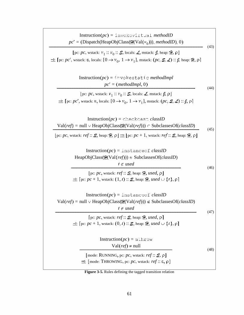
61

(43)

(44)

(45)

(46)

(47)

(48)


Instruction pc( ) LQYRNHYLUWXDO methodID=

pc� Dispatch HeapObjClass + Val Y0( )( )( ) methodID,( ) 0,( )=

pc: pc wstack: Y1 Y0 6 :: :: locals: / mstack: - heap: + r, , , , ,[ ]

ã pc: pc� wstack: e locals: [0 Y� 0, 1 Y� 1] mstack: pc 6 / , ,( ) - :: heap: + r, , , , ,[ ]

-------------------------------------------------------------------------------------------------------------------------------------------------------------------------------------------------

Instruction pc( ) LQYRNHVWDWLF methodImpl=


pc: pc wstack: Y1 Y0 6 :: :: locals: / mstack: - r, , , ,[ ]

ã pc: pc� wstack: e locals: [0 Y� 0, 1 Y� 1] mstack: pc 6 / , ,( ) - :: r, , , ,[ ]

------------------------------------------------------------------------------------------------------------------------------------------------------------------------------

Instruction pc( ) FKHFNFDVW classID=

Val ref( ) null= HeapObjClass + Val UHI( )( )( ) SubclassesOf classID( )³¿

pc: pc wstack: ref 6 :: heap: + r, , ,[ ] pc: pc 1+ wstack: UHI 6 :: heap: + r, , ,[ ]ã ----------------------------------------------------------------------------------------------------------------------------------------------------------------------------------------


HeapObjClass + Val ref( )( )( ) SubclassesOf classID( )³

W used´

pc: pc wstack: ref 6 :: heap: + used r, , , ,[ ]

ã pc: pc 1+ wstack: 1 W,( ) 6 :: heap: + used W{ } r, , , ,[ ]

------------------------------------------------------------------------------------------------------------------------------------------


Val ref( ) null= HeapObjClass + Val ref( )( )( ) SubclassesOf classID( )´¿

W used´

pc: pc wstack: ref 6 :: heap: + used r, , , ,[ ]

ã pc: pc 1+ wstack: 0 W,( ) 6 :: heap: + used W{ } r, , , ,[ ]

---------------------------------------------------------------------------------------------------------------------------------------------------------------------------------

Instruction pc( ) DWKURZ=

Val ref( ) null�

mode: RUNNING pc: pc wstack: ref 6 :: r, , ,[ ]

ã mode: THROWING pc: pc wstack: ref e:: r, , ,[ ]

--------------------------------------------------------------------------------------------------------------------

62

The following two lemmas express the fact that executions in the tagged semantics mirror executations in the untagged semantics.

Lemma 3-1.

Lemma 3-2.

The proofs are by case analysis of the hypothesized transition relation. I present one case for the proof of each lemma to illustrate the form of the proofs.

Proof of Lemma 3-1: Suppose and consider the case in which the transition is justified by the LDGG rule. From the LDGG tagged transition rule,

Then

(49)

(50)

(51)



r dom + ´

dom ILHOGV dom WDJV dom InitFields classID( )= =

I dom ILHOGV³ . " ILHOGV f( ) InitFields classID( ) I( ) WDJV I( ),( )=

+ � + r classID ILHOGV,( )�[ ]=

W{ } range WDJV( ) XVHG¬ «=

W range WDJV´

WDJV is a bijection

mode: RUNNING pc: pc wstack: 6 heap: + used r, , , , ,[ ]

ã mode: THROWING pc: pc wstack: r W,( ) e:: heap: + � used W{ } r, , , , ,[ ]

----------------------------------------------------------------------------------------------------------------------------------------------------------------------------

handler CatchBlockOffset method offset,( ) HeapObjClass + Val ref( )( )( ),( )=

mode: THROWING pc: method offset,( ) wstack: ref e:: heap: + r, , , ,[ ]

ã mode: RUNNING pc: method handler,( ) wstack: ref e:: heap: + r, , , ,[ ]

------------------------------------------------------------------------------------------------------------------------------------------------------------------------------------------

method offset,( ) HeapObjClass + Val ref( )( )( ),( ) dom CatchBlockOffset´

mode: THROWING pc: pc wstack: ref e:: locals: / mstack: pc� 6 � / �, ,( ) - :: heap: + r, , , , , ,[ ]

ã mode: THROWING pc: pc� wstack: ref e:: locals: / � mstack: - heap: + r, , , , , ,[ ]

--------------------------------------------------------------------------------------------------------------------------------------------------------------------------------------------------------------

X 1 X 2, . X 1 X 2ã Untag X 1( ) Untag X 2( )ãÃ"

X 1 X2, . Untag X 1( ) X2ã X 2. Untag X 2( ) X2= X 1 X 2ã ¾$( )Ã"

X 1 X 2ã

X 1 pc: pc wstack: v1 v2 6 :: :: used: used r, , ,[ ]=X 2 pc: pc 1+ wstack: Val v1( ) Val v2( )+ W,( ) 6 :: used: used W{ } r, , ,[ ]=Instruction pc( ) LDGG=

Untag X 1( ) pc: pc wstack: Val v1( ) Val v2( ) Untag6 6 ( ):: :: Untagr r( ), ,[ ]=Untag X 2( ) pc: pc 1+ wstack: Val v1( ) Val v2( )+ Untag6 6 ( ):: Untagr r( ), ,[ ]=

63

Hence as required.

Proof of Lemma 3-2: Suppose and consider the LDGG case.

By the definition of Untag, must be of the form

where

Now let t be any tag such that . Such a tag always exists because the set of tags is infinite and the used set is always finite. Set

Then and , as required.

3.4.5 Correspondence of TracesDefine UntagT over traces as follows:

8QWDJ7��X0��«��XQ!�� 8QWDJ�X0)��«��8QWDJ�XQ)!�

Lemma 3-3. For any tagged trace 7, UntagT(7) is a trace. Furthermore, for any trace 7, there is a tagged trace 7 such that UntagT(7) = 7.

Proof: The proofs are by induction on the length of the traces.

Consider a tagged trace 7� �<X0, …, XQ>. For Q = 1, UntagT(7) = <Untag(X0)>. From the definition of the initial state X0, it follows that Untag(X0) is the inital state for the untagged semantics, hence <Untag(X0)> is a trace.

For Q > 1, by the induction hypothesis <Untag(X0), …, Untag(XQ��)> is a trace. It is required to prove that . This follows immediately from and Lemma 3-1.

Now consider an untagged trace 7� �<X0, …, XQ>. For Q = 1, set 7� �<X0> to be the initial state for the tagged semantics. As above, UntagT(7) = <X0> = 7.

For Q > 1, by the induction hypothesis there exists a tagged trace 7¶ = <X0, …, XQ-1> such that <Untag(X0), …, Untag(XQ��)> = <X0, …, XQ-1>. Substituting and into Lemma 3-2, one obtains . Setting 7 = <X0, …, XQ> then gives the required result.

Untag X 1( ) Untag X 2( )ã

Untag X 1( ) X2ã

Untag X 1( ) pc: pc wstack: v1 v2 6:: :: r, ,[ ]=X2 pc: pc 1+ wstack: v1 v2+( ) 6:: r, ,[ ]=Instruction pc( ) LDGG=

X 1

X 1 pc: pc wstack: u1 u2 6 :: :: used: used r�, , ,[ ]=

Val u1( ) v1=Val u2( ) v2=Untag6 6 ( ) 6=Untagr r�( ) r=

W used´

X 2 pc: pc 1+ wstack: Val u1( ) Val u2( )+ W,( ) 6 :: used: used W{ } r�, , ,[ ]=

Untag X 2( ) X2= X 1 X 2ã

Untag X Q 1–( ) Untag X Q( )ã X Q 1– X Qã

Untag X Q 1–( ) XQ 1–=XQ 1– XQã X Q. Untag X Q( ) XQ= X Q 1– X Qã ¾$

64

3.4.6 Defining the VPR Using TagsFigure 3-6 defines evaluation of bytecode expressions in tagged states.�7KH�UXOHV�DUH�DQDORJRXV�WR�WKH�UXOHV�IRU�XQWDJJHG�VWDWHV��7KH�RQO\�VLJQLILFDQW�GLIIHUHQFH�LV�WKDW�LQ�Figure 3-6��LQ�WKH�UXOH�IRU�ILHOG�GHUHIHUHQFHV��WKH�REMHFW�H[SUHVVLRQ�LV�HYDOXDWHG�WR�\LHOG�WKH�WDJJHG�YDOXH��X��W��ZKHUH�X�LV�WKH�DFWXDO�REMHFW�UHIHUHQFH�DQG�W�LV�WKH�WDJ��DQG�WKH�WDJ�LV�LJQRUHG�

$�WDJJHG�WUDFH�7�RI�D�SURJUDP�3�LV�D�VHTXHQFH�RI�WDJJHG�VWDWHV��X0��«��XQ!�VXFK�WKDW�X0�LV�WKH�LQLWLDO�SURJUDP�VWDWH�IRU�SURJUDP�3��DQG� �

/HW�H��DQG�H��EH�E\WHFRGH�H[SUHVVLRQV��'HILQH�WKH�YDOXH�SRLQW�UHODWLRQ �3�of a program P as follows:

H��3�H��LII

$�D�WDJJHG�WUDFH�7�RI�3�DQG�WDJJHG�VWDWHV�XL�DQG�XM�LQ�7��VXFK�WKDW��XL� H�� Ä �X��W��DQG

�XM��H��Ä��X��W��IRU�VRPH�WDJJHG�YDOXH��X��W��ZKHUH�X�LV�QRW�HTXDO�WR�QXOO�

This is the definition actually used in the remainder of the thesis, including the rest of this chapter.

3.5 Examples of Using the Value-Point RelationThis section presents some examples of extracting useful information from the VPR.

3.5.1 Finding Writers to a Field&RQVLGHU�WKH�IROORZLQJ�SUREOHP�

³*LYHQ�D�SURJUDP�3�DQG�WKH�SF�RI�D�JHWILHOG�LQVWUXFWLRQ��ILQG�DOO�FRGH�ORFDWLRQV�SF��RI�WKH�SXWILHOG�LQVWUXFWLRQV�WKDW�SXW�YDOXHV�LQWR�WKH�ILHOG�EHLQJ�UHDG�´

(52)

(53)

(54)

(55)

(56)

Figure 3-6. Rules defining the evaluation of bytecode expressions in tagged states

mode: RUNNING pc: pc wstack: Y0 ... Yn 6 :: :: :: r, , ,[ ] SF�VWDFN�Q( , ) YnÄ

------------------------------------------------------------------------------------------------------------------------------------------------------------------------------

/ Q( ) Y=mode: PRGH pc: pc locals: / r, , ,[ ] SF�ORFDO�Q,( ) YÄ

-------------------------------------------------------------------------------------------------------------------------------

mode: THROWING pc: pc wstack: Y e:: r, , ,[ ] SF�H[Q( , ) YÄ

----------------------------------------------------------------------------------------------------------------------------------------

* staticField( ) Y= mode: PRGH pc: pc globals: * r, , ,[ ] SF�staticField,( ) YÄ

------------------------------------------------------------------------------------------------------------------------------------

mode: PRGH pc: pc heap: + r, , ,[ ] SF�exp,( ) X W,( )Ä

HeapObjFields + X( )( ) field( ) Y=

mode: PRGH pc: pc heap: + r, , ,[ ] SF�exp�field,( ) YÄ-------------------------------------------------------------------------------------------------------------------------------

0 L Q�< . X L 1– X Lã "

65

7KLV�TXHVWLRQ�FDQ�EH�IRUPDOL]HG�DV�WKH�IROORZLQJ�VHW�FRPSUHKHQVLRQ�

^�SF��_�$�D�WUDFH�7�RI�3� ��X��«��XQ!�

$S��T��REMUHI, 6,�YDO, 6�,�ILHOG, r��Val(REMUHI)��QXOO ¾XS� �>pc��pc��wstack: REMUHI��6, r]�¾ InstructionP(SF�� JHWILHOG�ILHOG�¾XT� �>pc��pc��wstack: YDO��REMUHI��6�, r]�¾ InstructionP(SF�� SXWILHOG�ILHOG�`

This set is equal to

^�SF��_�$ILHOG��SF�VWDFN��3�SF��VWDFN��¾

,QVWUXFWLRQP�SF�� JHWILHOG�ILHOG�¾�,QVWUXFWLRQP�SF�� SXWILHOG�ILHOG�`

The translation erases all mention of dynamic properties, summarizing them with the static VPR.

3.5.2 Downcast CheckingConsider the following problem:

³)LQG�DOO�SURJUDP�ORFDWLRQV�SF�FRUUHVSRQGLQJ�WR�FKHFNFDVW�LQVWUXFWLRQV�ZKLFK�PLJKW�IDLO�´

This can be formulated as

^�SF�_�$�D�WUDFH�7�RI�3� ��X��«��XQ!��$S��REMUHI, 6,�+,�FODVV, r��Val(REMUHI)��QXOO�¾XS� �>pc��pc��wstack: REMUHI��6, heap: +, r]�¾InstructionP(SF�� FKHFNFDVW�FODVV�¾+HDS2EM&ODVV�+(Val(REMUHI)��´�6XEFODVVHV2I�FODVV��`

This can be rewritten to use the value-point relation:

^�SF�_�$SF�, class, class�.SF�VWDFN��3�SF��VWDFN��¾

,QVWUXFWLRQ3�SF�� FKHFNFDVW�FODVV�¾

,QVWUXFWLRQ3�SF�±�� QHZ�FODVV��¾

FODVV��´�6XEFODVVHV2I�FODVV��`

In this example, the translation is exact; a downcast is safe if and only if some instruction creates an object which reaches the downcast instruction and which is incompatible with the required bound. Thus, if the true value-point relation is known, the unsafe downcasts can be determined precisely. Of course, in general an analysis can only compute an approx-imation to the true relation.

3.6 Properties of the Value-Point Relation7KH�935�LV�V\PPHWULF��,W�LV�QRW�UHIOH[LYH��EHFDXVH�H[SUHVVLRQV�LQ�GHDG�FRGH�FDQQRW�EH�UHODWHG�WR�DQ\WKLQJ��,W�LV�QRW�WUDQVLWLYH�HLWKHU��LQ�JHQHUDO��7R�VHH�WKLV��VXSSRVH�%��3�%��DQG�%� �3 %��7KH�GHILQLWLRQ�RI�WKH�935�LPSOLHV�WKDW�IRU�VRPH�FKRLFH�RI�YDULDEOHV��XL� %�� Ä Y��XM��%��Ä�Y, �XN� %��Ä�X��DQG��XO��%��Ä�X. The important fact is that it is possible for Y to not equal X (when XM�� XN�, so there is no way in general to justify a relationship between %��DQG�%��)RU�H[DPSOH��FRQVLGHU�WKLV�IUDJPHQW�RI�FRGH�

66

LI��E��^�[� �\��`�HOVH�^�[� �]��`

Let %� be \, %� be [ and %� be ], all evaluated after this statement. Then this code may execute once with E true, inducing %��3�%�, and then execute again with E false, inducing�%� �3 %�, but \ need never equal ].

The VPR does not explicitly encode any information about data dependence or the direction of data flow. %��3�%��PHDQV�WKDW�%��DQG�%��FDQ�JHW�WKH�VDPH�YDOXH��EXW�QRWKLQJ�LV�UHYHDOHG�DERXW�ZKHWKHU�WKH�YDOXH�DSSHDUV�DW�%��RU�%��ILUVW��,Q�IDFW��LW�PD\�EH�WKDW�QR�GHI�XVH�FKDLQ�OHDGV�IURP�%��WR�%��RU�YLFH�YHUVD�²�WKH\�PD\�ERWK�EH�DW�WKH�HQG�RI�GHI�XVH�FKDLQV�OHDGLQJ�EDFN�WR�D�FRPPRQ�VRXUFH��+RZHYHU��LW�LV�SRVVLEOH�WR�PDNH�LQIHUHQFHV�DERXW�GDWD�GHSHQGHQFH�LQ�DQ�LPSRUWDQW�FRPPRQ�FDVH��ZKHQ�RQH�RI�WKH�%V�FRUUHVSRQGV�WR�WKH�UHVXOW�RI�D�YDOXH�FUHDWLRQ�RSHUDWLRQ��VXFK�DV�WKH�UHVXOW�RI�D�QHZ�LQVWUXFWLRQ��,Q�WKLV�FDVH�LW�LV�FOHDU�WKDW�WKH�YDOXH�RULJLQDWHG�DW�WKH�FUHDWLRQ�RSHUDWLRQ��7KLV�VHHPV�WR�EH�VXIILFLHQW�IRU�PDQ\�DSSOL�FDWLRQV��'HILQLQJ�D�UHODWLRQ�UHSUHVHQWLQJ�WUXH�GLUHFWLRQDO�GDWD�GHSHQGHQFH�ZRXOG�UHTXLUH�D�PXFK�PRUH�FRPSOLFDWHG�GHILQLWLRQ�WKDQ�IRU�WKH�935�

The VPR has limited context information. For example, if %��3�%� and the bytecode expressions are both located in the same method, there is no way to determine whether the two states justifying the relationship actually occur during the same call to the method or during different calls to the method. For some applications, such as alias analysis for code motion, the tool is only interested in finding aliases that appear during the same call to a method, or even during the same iteration of a loop. Thus, these applications suffer a loss of accuracy using the VPR.

The VPR is simple and does not encode information about context, or scalar values, or control dependence, or many other aspects of program behavior that can be captured by static analysis. However, all these aspects can be used to improve the accuracy of an imple-mentation of a VPR analysis. For example, although the VPR itself encodes only limited context information, SEMI uses context sensitive analysis to produce a better VPR approx-imation.

The VPR is undecidable. In general, an analyzer can only compute a conservative approx-imation to the VPR. As stated above, a conservative approximation is simply any relation whose pairs are a superset of the pairs of the true relation. ,Q�WKLV�WKHVLV��,�ZULWH��DQ�DSSUR[�LPDWLRQ�UHODWLRQ�IRU�SURJUDP�3�DV��3.

3.7 ExtensionsMany tools would benefit from the ability to specify tighter context constraints, such as the MayEqual formulation of Boyland and Greenhouse [12]. This is an obvious candidate for future work.

Other tools require slightly different semantics for the value-point relation. For example, for some applications it is useful to consider values to be related if they are ever compared. This could be added to the dynamic semantics by having comparisons unify the tags of the operands. Static analyses would then have to be adjusted to compute the correct relation-ships. Ajax has been adapted to this task, but that work is beyond the scope of this thesis. Other applications require the computed VPR approximation to satisfy certain structural

67

invariants, so that the tool can perform its own processing efficiently. An example of this is the object modelling tool in Chapter 11.

The trace T in the definition of the VPR is required to range over all possible executions of the program, which implies that any truly conservative approximation to the VPR will be a static analysis. However, if that requirement is relaxed so that T only ranges over some given finite set of executions (e.g. some actual runs of the program that were recorded), then the VPR can be computed by dynamic analysis. The “dynamic VPR” can be used by the same set of tools as the static version, except that the results of the tools must be inter-preted more carefully; they are true only for the executions recorded.

68

69

4 Efficient Queries over the Value-Point Relation

4.1 IntroductionIn the previous chapter, I defined the value-point relation as an abstraction of a program, generated by some analysis and consumed by some tool. That discussion focused on the mathematical properties of the relation. In practice, the analysis cannot simply compute an explicit relation and pass it to the tool, because the relation is infinite. Instead, the tool must pass certain parameters to the analysis indicating which parts of the relation must be computed. In fact, for efficiency, some of the tool’s computations over the relation often need to performed by the analysis on the tool’s behalf, in order to exploit analyis-specific structure. These computations are also expressed as parameters to the analysis.

The nature of this parameterization determines which analysis and tool combinations will be efficient in practice. In this chapter, I describe the parameters supported by Ajax and their motivation. I also describe some general strategies used by analyses and tools to exploit the parameters.

4.2 Analysis ParametersThe following sections explain the issues that need to be addressed by the parameterization scheme, and how each issue is addressed in Ajax. Section 4.2.5 summarizes the parameters.

4.2.1 Restricting the Domain of the Value-Point RelationAny realistic program admits an infinite number of different bytecode expressions. For example, for any n one can form a meaningful expression involving a sequence of n field dereferences. The value-point relation is defined over all pairs of bytecode expressions — not just those that appear in the program — and therefore the relation is infinite. In practice, however, tools generally only consider a finite number of bytecode expressions.

Therefore, the simplest and most important parameter is a restriction on the domain of the relation. A tool restricts the domain by explicitly specifying two sets of bytecode expres-sions, sources S and targets T. The analysis computes the value-point relation projected onto S � T. Because the sets are given explicitly, they must be finite.

Section 3.5.1 showed how a tool could use the VPR to find all writers to a field. That tool would set

S = { SF�VWDFN��}T = { SF��VWDFN��_�,QVWUXFWLRQP�SF�� SXWILHOG�ILHOG }

70

The example in Section 3.5.2 determines whether a field is always empty. It uses

S = { SF�VWDFN��field�}T = { SF��VWDFN��_�,QVWUXFWLRQ3�SF�±�� QHZ�FODVV�¿

,QVWUXFWLRQ3�SF�±�� LQVWDQFHRI�FODVV�¿

,QVWUXFWLRQ3�SF�±�� LDGG�¿

�,QVWUXFWLRQ3�SF�±�� ELSXVK�Q�¾�Q��}

The downcast checking example in Section 3.5.2 would set

S = { SF�VWDFN��_�,QVWUXFWLRQP�SF±�� QHZ�FODVV }T = { SF��VWDFN��_�,QVWUXFWLRQ3�SF�� FKHFNFDVW�FODVV�}

Since the value-point relation is symmetric, the source and target sets are interchangeable at this point in the exposition. The extensions described below break this symmetry.

4.2.2 Avoiding Explicit ProductsThe downcast checking example shows that, for some applications, both the S and T sets are likely to be proportional in size to the size of the program. If the analysis generates an explicit projection of the relation into S � T, the size of the result could grow quadratically in the size of the program — especially if the analysis is not very precise.

However, many tools postprocess the projected relation to compute some final result that is much smaller than the relation itself. For example, the downcast checker computes just one bit of information per element of T — whether or not the downcast is safe. Furthermore any scalable analysis must be able to represent its internal data in space subquadratic in the size of the program. For efficiency, Ajax maps the tool’s computation directly onto the internal data structures of the analysis, without requiring an explicit representation of the VPR approximation. Of course this must be done with only minimal assumptions about the form of that structure.

To this end, I adapted and generalized an idea from Heintze and McAllester’s work on subtransitive control flow analysis [41]. The idea is to suppose that the implementation of the analysis builds a directed graph G with the following properties:

• There is a map GS from S to the nodes of G.

• There is a map GT from T to the nodes of G.

• The analysis indicates s �3 W if and only if there is path from GS(s) to GT(t) in G.

In Chapter 5 and Section 6.6 I explain how such a graph is constructed by RTA and SEMI respectively.

Many tools can exploit this graph structure. Suppose a tool needs to compute:

where F is some function specific to the tool. Then if F satisfies a certain lattice-like condition described below, the set of results can be computed by exploiting the graph. Conceptually, each node corresponding to a source s is first associated with an initial value F[{ s }]. These values are then propagated along the graph edges and merged when they

W ) V 6³ V W�P|{ }[ ],( ) W 7³|{ }

71

meet at nodes. The result for each target t is read from the final value associated with the node corresponding to t. This process is similar in flavor to dataflow analysis.

For example, consider the downcast checking tool. Let the function F be defined as:

F[{ SF1�VWDFN��SF2�VWDFN��SFn�VWDFN�� }]= the most specific common superclass of the classes instantiated atSF1±��SF2±��SFn±1

Consider the code in Figure 4-1. A simple dataflow analysis would produce the graph in Figure 4-2.

The downcast checking system finds three QHZ instructions in the program, corresponding to s1, s2, and s3, and three FKHFNFDVW instructions, corresponding to t1, t2, and t3, as shown. For each node N in the graph, it computes F applied to the set of the si that reach N.

VWDWLF�YRLG�PDLQ��^��2EMHFW�D� �QHZ�,QWHJHU��2EMHFW�E� �QHZ�6WULQJ��+HOOR��2EMHFW�F� �QHZ�6WULQJ��.LWW\��2EMHFW�G��LI��^�G� �D��`�HOVH�^�G� �E��`��2EMHFW�H��LI��^�H� �E��`�HOVH�^�H� �F��`��2EMHFW�I��LI��^�I� �G��`�HOVH�^�I� �H��`��2EMHFW�K� �D��2EMHFW�L� �H��,QWHJHU�K��,QWHJHU�I��6WULQJ�L�`

Figure 4-1. Example of Java code exhibiting aliasing

Figure 4-2. Example of an analysis graph used by the downcast checking tool

6WULQJ

s1 (QHZ�,QWHJHU)

2EMHFW

2EMHFW

,QWHJHU

s2 (QHZ�6WULQJ)

6WULQJ

6WULQJ

s3 (QHZ�6WULQJ)

,QWHJHU

6WULQJt1 (FKHFNFDVW�,QWHJHU)

t2 (FKHFNFDVW�,QWHJHU)t2 (FKHFNFDVW�6WULQJ)

72

This can be done efficiently because the value of F at each node (other than a source node) can be computed from the F of its predecessors in the graph — it is the most specific common superclass of the classes at the predecessors. The computed F values are under-lined.

Once the downcast checker has determined the most specific common superclass of the classes of the objects that may reach a given downcast instruction, it compares that super-class with the bound specified in the FKHFNFDVW instruction. If the actual superclass is a subclass of the bound (or equal to it) then the cast cannot fail. If the actual superclass is not a subclass of the bound, then the analysis has identified at least one class whose objects appear to reach the downcast instruction but which is not compatible with the bound. For more details, see Chapter 10.

This approach improves efficiency because the space required is only linear in the size of the analysis’ graph, instead of proportional to the product of the size of S and the size of T.

It is tempting to assign semantics to the graphs. For example, it seems natural to interpret Figure 4-2 as a dataflow graph, in which objects of various classes flow from their creation sites to the sites of the downcast instructions, and the nodes represent intermediate sites in def-use chains. This interpretation may be correct for some analyses, but it would be mistaken in general. Without referring to a specific analysis, all one can say about the graphs is that they are encodings of the computed VPR approximation, as defined above — “s �3 W if and only if there is path from GS(s) to GT(t) in G”.

4.2.3 General FrameworkThe lattice-like property required of F is quite simple. There must exist a binary function DM such that, for any two sets of source bytecode expressions P and Q,

The existence of this merge operator ensures that the result of F can be constructed incre-mentally.

Rather than passing graph structures from analyses to tools across the Ajax interface, Ajax tools pass their F functions to the analyses. This reduces the burden on tool implementors.

A tool reveals its F function to analyses by passing in the following parameters:

• The type D of intermediate data — F’s result type

• The merge operator DM : D � D � D

• The identity DE = F[{}]

• The initial assignment DI : S � D, such that DI(s) = F[{ s }]

These parameters fully determine F, for F can be computed as follows:

The correctness of this computation follows from the lattice-like property of F, by induction over the size of F’s argument set.

F 3 4[ ] DM F 3[ ] F 4[ ],( )=

F { }[ ] DE=F V{ } 4[ ] DM DI V( ) F 4[ ],( )=

73

The lattice-like property imposes several conditions on these parameters. In the proofs below I assume that F is surjective, i.e., that for every element d of D there is a set P such that F[P] = d. This is ensured by an appropriate choice of D.

• DM must be commutative:

• DM must be associative:

• DM must be idempotent:

• DE must be an identity for DM:

In practice, it has not been difficult to identify the appropriate F function and D parameters for each tool. In fact, a small set of F functions has proved to be sufficient for a variety of tools. Many tools use the same F function and distinguish themselves by varying the S and T sets. Some examples are shown below in Section 4.3.

4.2.4 Tool Target DataSections 4.2.2 and 4.2.3 describe how analyses compute F-values for each expression in the target set T. However, the expressions T themselves are generally of no interest to a tool. For example, the downcast checker is only interested in the location of the downcast instruction. Therefore each tool specifies a map TR associating tool target data with each target expression. The analysis computes

To compute a result for a given tool target datum, the analysis merges the results for all target expressions associated with the datum.

In the absence of tool target data, most tools would need to maintain their own maps from target expressions to data they find meaningful. The tool target data mechanism factors out this code into a shared module. Target data are also useful when a tool associates the same datum with more than one expression, because merging is automatically performed. The Ajax live code detector exploits this feature, as explained in Section 4.3.5 below.

4.2.5 Summary of Analysis ParametersThis is the final list of parameters:

• A finite set S of source expressions

• A finite set T of target expressions

• A function F described by four parameters:

DM F 3[ ] F 4[ ],( ) F 3 4[ ] F 4 3[ ] DM F 4[ ] F 3[ ],( )= = =

DM F 3[ ] DM F 4[ ] F 5[ ],( ),( ) F 3 4 5( )[ ] F 3 4( ) 5[ ]DM DM F 3[ ] F 4[ ],( ) F 5[ ],( )

= ==

DM F 3[ ] F 3[ ],( ) F 3 3[ ] F 3[ ]= =

F 4[ ] F {} 4[ ] DM F {}[ ] F 4[ ],( ) DM DE F 4[ ],( )= = =

G F V S³ W T³ .V W�P TR W( ) G=¾$|{ }[ ],( ) G range TR³|{ }

74

• A type D of intermediate data

• A merge operator DM : D � D � D satisfying the conditions of Section 4.2.3

• An identity DE satisfying the conditions of Section 4.2.3

• An initial assignment DI : S � D

• A type R of target data

• A tool target data map TR : T � R

The analysis defines

The analysis then computes the result of the query:

4.3 Examples

4.3.1 Finding Writers to a FieldSection 3.5.1 presents an example VPR query to find which instructions write values into a field. This query only needs to determine which target expressions are related to a given single source expression. The output of the tool is a list of the locations of those expres-sions.

The query parameters are simple. The function F returns true if the input set is non-empty (i.e., contains the source expression) and false otherwise.

S = { SF�VWDFN��}T = { SF��VWDFN��_�,QVWUXFWLRQP�SF�� SXWILHOG�ILHOG }D = { true, false }DM(a, b) = a ¿ bDE = falseDI(SF�VWDFN��) = trueR = CodeLocTR(SF¶�VWDFN��) = pc’

The analysis returns “true” for the program locations whose target expressions are related to the source expression. The tool prints out these locations.

4.3.2 Finding Unused FieldsThe tool discussed in Section 3.5.2 determines whether a given JHWILHOG instruction always returns zero or null. Consider an extension of that tool to check all JHWILHOG instructions simultaneously. This tool needs to compute one bit of information for each JHWILHOG instruction, so we make the JHWILHOG instructions the targets.

F { }[ ] DE=F V{ } 4[ ] DM DI V( ) F 4[ ],( )=


75

S = { SF��VWDFN��_� ,QVWUXFWLRQ3�SF�±�� QHZ�FODVV�¿

,QVWUXFWLRQ3�SF�±�� LQVWDQFHRI�FODVV�¿

,QVWUXFWLRQ3�SF�±�� LDGG�¿

�,QVWUXFWLRQ3�SF�±�� ELSXVK�Q�¾�Q��}T = { SF�VWDFN��ILHOG�_�,QVWUXFWLRQ3�SF�� JHWILHOG�ILHOG�}D = { true, false }DM(a, b) = a ¿ bDE = falseDI(SF��VWDFN��) = trueR = CodeLocTR(SF�VWDFN��ILHOG) = pc

Similarly to the previous example, the analysis returns “true” for the locations whose target expressions are related to any of the source expressions. These are the locations of the JHWILHOG instructions that might not return zero or null. The tool outputs the locations for which the analysis returns “false”.

4.3.3 Downcast CheckingThese are the analysis parameters for the downcast checker:

S = { SF�VWDFN��_�,QVWUXFWLRQP�SF±�� QHZ�FODVV }T = { SF��VWDFN��_�,QVWUXFWLRQ3�SF�� FKHFNFDVW�FODVV�}D is the class lattice for 3 (see below)DM is the join operation in DDE is the bottom element in DDI(SF�VWDFN��) = class, where ,QVWUXFWLRQP�SF±�� QHZ�FODVV

R = CodeLocTR(SF¶�VWDFN��) = pc�

The class lattice for program 3 is 3’s Java class hierarchy, including interfaces, extended to form a lattice. The standard class hierarchy does not form a lattice for two reasons. It does not have a “bottom” element to serve as the identity for a join operation, and therefore we add a synthetic bottom element. Also, two classes may not have a unique most specific common superclass, such as classes &ODVV3 and &ODVV4 in the hierarchy of Figure 4-3.

To complete the lattice, we add elements representing the intersections of sets of classes and interfaces. In this example, the most specific common superclass of &ODVV3 and &ODVV4 is the synthetic intersection class “&ODVV$ ¬ ,QWHUIDFH%”.

For each FKHFNFDVW instruction, the result of the analysis is the most specific common superclass of all the classes of objects subjected to the FKHFNFDVW instruction. If this superclass is a subclass (or equal to) the bound specified in the FKHFNFDVW instruction, then the downcast is safe, otherwise it may fail.

76

4.3.4 Method Call ResolutionConsider a tool designed to resolve dynamic method calls through a given method signature M. For each dynamic method call site, the tool determines whether there is exactly one possible callee, and if so, which method it is. Dynamic method call sites with only one possible callee can be converted into direct calls by a compiler, resulting in faster method call code and possible inlining of the callee.

Because the tool computes information for each call site, the call sites are the targets. (In general, whenever the tool’s query can be phrased in the form “for every X, compute Y”, the choices for X determine the set of targets T.) At each site, the target expression is the object reference upon which the call is dispatched. The source expressions are the results of the QHZ instructions that create objects implementing M. By determining which of those sources are related to the receiving object at a call site, the call can be resolved, or found to be unresolvable.

Instead of collecting the complete list of source expressions related to each target, it is more efficient to extract just the salient information. We associate with each source expression the method implementing M in the new object. The tool collects the set of methods reaching each call site.

Observe that if a set of callee methods at a call site has more than one element, then the call cannot be statically resolved and the exact contents of the set are not used. Therefore each set can be abstracted to one of the following values:

• The empty set, indicating that there is no receiving object. This implies that the call site is in dead code or the receiving object reference is always null.

• A singleton method, indicating that there is at most one receiving method implementa-tion. The call site can be resolved to the given method.

• The value “many”, indicating that the set of possible method implementations may have more than one element. The call site cannot be resolved to a single method.

This abstraction is essentially the optimization proposed by Heintze and McAllester [41].

Let ImplementorsP(M) denote the set of all methods implementing M. The tool uses the following parameters:

Figure 4-3. Example of non-lattice behavior due to interfaces

&ODVV$ ,QWHUIDFH%

2EMHFW

&ODVV3 &ODVV4

77

S = { SF�VWDFN��_�,QVWUXFWLRQP�SF±�� QHZ�FODVV }T = { SF¶�VWDFN��_�,QVWUXFWLRQ3�SF�� LQYRNHYLUWXDO�0�} (VWDFN�� refers to the receiving object in the call to M)D = { «, many } ImplementorsP(M)

DM(«, x) = DM(x, «) = xDM(many, x) = DM(x, many) = manyDM(x, x) = xDM(x, y) = many, when x � yDE = «DI(SF�VWDFN��) = impl, where ,QVWUXFWLRQP�SF±�� ³QHZ�FODVV”, and class’s implementation of M has identifier implR = CodeLocTR(SF��VWDFN�n) = pc’

The tool outputs a D value for each LQYRNHYLUWXDO instruction specifying method signature 0. If the value is «, then the instruction is never reached. If the value is “many”, then the instruction cannot be statically resolved. Otherwise the value is the name of the only possible callee method.

Section 4.4.1 describes how this tool is extended to examine all LQYRNHYLUWXDO instructions simultaneously.

4.3.5 Live Code DetectionConsider a tool to find the live implementations of a given method signature M. Such a “live code detector” is rather similar to the method call resolver in the previous section, because proper identification of which methods are live requires some resolution of dynamic method calls. However, the live code detector collects information about methods rather than call sites. Therefore the tool target data are the method implementations; the result returned for each method is “true” if it may be live, or “false” if it must be dead. The parameters are:

S = { SF��VWDFN�n�_�,QVWUXFWLRQ3�SF�� LQYRNHYLUWXDO�0�}, where n is the index of the receiving object in the list of parameters of a call to MT = { SF�VWDFN��_�,QVWUXFWLRQP�SF±�� QHZ�FODVV }D = { true, false }DM(a, b) = a ¿ bDE = falseDI(SF��VWDFN�n) = trueR = CodeLocTR(SF�VWDFN��) = impl, where ,QVWUXFWLRQP�SF±�� ³QHZ�FODVV”, and class’s implementation of M has identifier impl

In a sense, this query propagates “liveness” from call sites to method implementations, whereas the method call resolver propagates method implementations to call sites.

78

This is an example of a tool which associates the same target datum with more than one target expression. A method implementation is live if 0 is invoked on any object which inherits that method implementation.

The analysis specified here does not detect all live methods. Calls to static methods must be detected separately. In Java, there is also an LQYRNHVSHFLDO instruction which calls non-static methods using static dispatch.

4.4 Additional Features of the Ajax Implementation

4.4.1 Query Families and Query FieldsThe examples in Sections 4.3.4 and 4.3.5 show how to perform method call resolution or live code detection for a specific method signature M. To perform these tasks for all method signatures, it suffices to perform a separate query for each signature encountered in the program. Other tools also need to make many queries varying only their S, T, DI, and TR parameters.

For greater efficiency and convenience, Ajax allows the remaining parameters — R, D, DM, and DE — to be treated as a unit, a query family. Each query family defines an index type, I, so that queries belonging to each query family are indexed by elements of I. In the examples above, the elements of I are the method signatures M. Ajax is designed to allow a query family to easily manipulate its collection of queries through the index elements. Each instance of an analysis can efficiently support many different query families and many queries within each family.

4.4.2 IncrementalityAjax is highly incremental. New code can be added to the analyzed program at any time, in response to program modifications or environmental changes. The results of the analyses and tools are updated to reflect the dynamic changes. This requires two elaborations of the VPR interface presented in this chapter.

The query parameters S, T, DI, and TR cannot be explicitly stated a priori, because the sum of “all the code that might ever be live” is ill-defined or impractically large (for example, it includes the entire Java class library, which is very large). Therefore whenever a new method is added to the “live program,” the Ajax system calls back into the tool, notifying it of the existence of the new method. The tool responds by extending its S, T, DI, and TR parameters with the expressions whose locations are in the new method. The analyses must be capable of handling such dynamic updates to the parameters. For the Ajax analyses, this was tricky to implement but not conceptually difficult.

Expressions in dead methods are not related to any other expressions, even themselves. Therefore, if a tool is never notified of the existence of a method, the results for target expressions in that method are trivially equal to DE. In practice, tools have special handling for unreachable source or target expressions. In the “find writers to a field” example, if the source expression specifying the field is in unreachable code, it is preferable to report that fact to the user rather than to report that there are no writers to the field.

79

Since the results of an analysis can change when the analyzed program changes, results are reported to a tool using a callback. When the analysis computes a new result for a tool target datum, it reports the datum and result pair to the tool through the callback. In fact, the analyses report results even before the analysis is complete; this results can be superceded by subsequent callbacks. Ajax makes no guarantees of any relationship between these “progressive results” and the final result for a target datum. However, the progressive results can be used for advisory purposes, such as displaying progress to a user. When an analysis completes, it signals the tool that the last reported results for each tool target datum are sound.

4.4.3 Code MutationAjax supports changes being made to the program during analysis, and even after analysis has completed. If analysis has already completed, then the results are updated progressively until completion is signalled again. Many tools are not persistently attached to the program being analyzed, and terminate after the first complete results have been delivered.

The implementation of code mutation is quite simple: for each changed, live method, another “live method” notification is sent to the analysis. It is up to each analysis to decide how to handle multiple live method notifications for a single method. The analyses imple-mented in Ajax generate new constraints for the new code and add them to the existing set of constraints (i.e., old constraints are not revoked). This is simple and does not penalize the common case in which code is not mutated.

4.4.4 Analysis ScopingNo analysis for Java can attempt to analyze all available code, because the standard libraries are so large that performance would be unacceptable. The code to be analyzed must be identified as part of the analysis. A natural approach is to compute a fixed point from below: start by assuming that just one “main” method is live, analyze it, discover other methods that may be called, add those to the set of live methods, analyze those new methods, and so on.

Ajax’s incremental analysis makes this simple. A live code detection tool is instantiated, just as described in Section 4.3.5. It maintains a set of methods currently thought to be live; This set is initialized to a “main” method by the tool environment. The analysis then runs and reports results to the live code detection tool, which adds new live methods to the live method set. The analysis is notified of these new live methods, computes new results, reports them to the tools, and the cycle continues. This means that typically an Ajax system is configured with two tools: a live method detection tool to control the scope of the analysis, and the tool that the user is actually interested in.

This approximation of the set of live methods from below is frequently seen in prior work, for example RTA [9]. Ajax extends this work by factoring out the approximation and applying it to any analysis.

4.4.5 IntersectionA natural extension of the framework presented above is to extend the operations on the intermediate data D to make it a true lattice; i.e., to provide a meet operator DN corre-

80

sponding to set intersection. This requires an additional lattice-like property of the tool’s F function:

This is useful for analyses that compute two or more different, but individually sound, approximations to the value-point relation. The intersection of two sound approximations to the true relation is also a sound approximation to the true relation. In other words, given relations �1P and �2P, the relation �P defined as s �P t � s �1P t ¾ s �2P t is a sound approximation to the truth, and potentially more accurate than either of the input relations.

Now consider implementing the Ajax interface with such an analysis, and computing the F values for a tool:

Therefore, it suffices to compute the F values for the two relations separately and then apply the meet operator.

It is straightforward to implement a functor that takes a set of Ajax analyses and combines them in this way. Of course, tools must provide a suitable meet operator. The examples above which use boolean values as their intermediate data can use the boolean “and” operator as the meet.

The example using the Java class lattice explicitly represents the meet of two classes as an “intersection class” of the two classes. The representation of intersection classes can often be simplified by exploiting facts about the Java class hierarchy. For example, an inter-section class containing two non-interface classes is empty unless one of the classes is a (possibly indirect) superclass of the other, because multiple inheritance is only allowed for interfaces.

Of the examples in this chapter, the method call resolution tool presents the most diffi-culties in defining a suitable meet operator. The problem is that when both of the operands of the meet are “many”, the precise result cannot be determined. The operator must return “many”. This is a safe approximation, but the analysis parameters that we introduced for efficiency are now causing us to lose information. For example, the sets { M1, M2 } and { M2, M3 } both map to the abstract value “many”; their intersection could be represented with the abstract singleton { M2 }, but this cannot be computed from the abstract values alone. In this situation, the results returned to the tool may vary from run to run depending on the order of analysis computations, even if the underlying analyses compute the same VPR approximations in each run.

F 3 4¬[ ] DN F 3[ ] F 4[ ],( )=

W F V 6³ V W�P|{ }[ ],( ) W 7³|{ }

W F V 6³ V W�1P V W�2P¾|{ }[ ],( ) W 7³|{ }

W F V 6³ V W�1P|{ } V 6³ V W�2P|{ }¬[ ],( ) W 7³|{ }

W DN F V 6³ V W�1P|{ }[ ] F V 6³ V W�2P|{ }[ ],( ),( ) W 7³|{ }

=

=

=

81

5 Implementing the Value-Point Relation With RTA

5.1 Introduction

5.1.1 Introduction to Rapid Type AnalysisBacon and Sweeney proposed Rapid Type Analysis [9] as a fast algorithm for resolving dynamic method calls in statically typed object oriented programs; it was originally applied to C++ programs. RTA uses static type information to resolve dynamic method calls as follows: given a virtual call to method m of object reference v, find Cv, the static class of v, and compute the set S of all subclasses of Cv, including Cv itself. Soundness of the static type implies that these classes are a superset of the possible classes that v can have at run- time. Therefore if every class in S implementing m uses the same implementation of m, the call can be statically resolved to that implementation.

As described, this is also known as Class Hierarchy Analysis [32]. However, RTA adds an important extension to improve accuracy without harming efficiency. Consider the Java program in Figure 5-1.

CHA determines that Y has two possible implementations of P, one from 6XE� and one from 6XE�, and therefore the call Y�P�� cannot be resolved. However, RTA observes that the method I�� is never called and no object of class 6XE� is ever created, and therefore Y’s only possible implemention of P is from 6XE�; the call is resolved.

In this example, RTA starts by assuming that 0DLQ�PDLQ is the only live method and that no classes are instantiated. It examines the body of 0DLQ�PDLQ and discovers that 6XE�

DEVWUDFW�FODVV�6XSHU�^��DEVWUDFW�YRLG�P��

VWDWLF�LQW�Q�`FODVV�6XE��H[WHQGV�6XSHU�^

YRLG�P��^�Q� ��``FODVV�6XE��H[WHQGV�6XSHU�^

YRLG�P��^�Q� ��``FODVV�0DLQ�^

YRLG�I��^�QHZ�6XE��`YRLG�PDLQ�6WULQJ>@�DUJV��^ 6XSHU�Y� �QHZ�6XE�� Y�P�� `

`

Figure 5-1. A simple Java program

82

is instantiated and there is a dynamic method call to 6XSHU�P. At this point 6XE� is the only class in the set of instantiated classes, so the only possible implementor of 6XSHU�P is 6XE��P, which is added to the live method set. Then 6XE��P is examined, which does not add any new methods or instantiated classes. Now that all the live methods have been examined, the algorithm terminates.

The efficacy of CHA is based on the observation that in most object oriented programs, many overridable methods in fact have only one implementation. These include methods in an abstract interface that has only one implementation, and methods in a class that has no subclasses. RTA extends CHA to exploit the fact that even when there is more than one implementation available, many programs will only use one implementation.

Both the RTA and CHA algorithms were originally tailored to the problem of resolving dynamic method calls. In Ajax, the technique underlying RTA is generalized away from any particular problem and used to generate VPR information in response to arbitrary queries. For example, the Ajax implementation of RTA can be used to produce information similar to that produced by the “type based alias analysis” of Diwan et al. [23].

By decoupling the analysis from its applications, Ajax makes differences between analyses more apparent. For example, it becomes clear that Diwan et al.’s basic “type based alias analysis” is actually slightly less precise than RTA, because it lacks an analogue of “exact class types” (see Section 5.2.4). The differences were previously obscured because both the analyses and their applications varied in tandem.

5.1.2 Decomposing RTA in AjaxIn Ajax, RTA is restructured into four distinct activities:

1. Computation of the set of live methods

2. Computation of the set of instantiated classes

3. Construction of an approximation to the value-point relation using static type informa-tion and the set of instantiated classes

4. Application of the value-point relation to determine the callees of dynamic method calls

Section 4.4.4 explains how for all analyses, Ajax computes a live method set using a bottom-up fixpoint procedure, just as RTA does. This subsumes the first and fourth activ-ities above.

Computing the set of instantiated classes from the set of live methods is trivial. We simply scan the method bodies for occurrences of the QHZ instruction and note the class parameter of each such instruction.

The subject of this chapter is the third activity: using static type information and knowledge of the set of instantiated classes to implement the Ajax analysis interface.

Section 5.2 describes how this information is used to approximate the value-point relation. Section 5.3 shows how to structure the computation to support the efficient analysis param-eters described in Section 4.2. The chapter concludes with discussion of some extensions.

83

5.2 Approximating the Value-Point Relation

5.2.1 OverviewAbstractly, the task of any Ajax analysis is to determine whether a given pair of bytecode expressions (B1, B2) is in the value-point relation. The decision must be conservative; if there is any uncertainty, the analysis must assume that the pair is in the relation. The RTA analysis receives as input a set L of the methods in the program that it must assume to be live. It also has access to the program, so it can compute the class hierarchy.

The basic idea is to find static types for B1 and B2, and then compare the types to decide whether it is possible for a value to conform to both of them simultaneously. These two steps are elucidated in the next two subsections.

In this section I discuss the analysis in the context of full Java bytecode rather than the MJBC subset language, because MJBC does not define a static type discipline analogous to the Java Virtual Machine’s “verification” procedure and the Java type system. RTA depends on the existence and soundness of such a type system.

5.2.2 Types for Bytecode ExpressionsEach bytecode expression BL is a pair (lL, eL) consisting of a program location lL and an expression eL�to be evaluated at that location. In principle, it is not difficult for Ajax RTA to compute static types for the expressions, because the Java Virtual Machine computes them while type checking Java bytecode [48].

A full explanation of Java bytecode type reconstruction and verification is beyond the scope of this thesis. Such an explanation can be found in references such as the Java Virtual Machine Specification [48]. Simply put, the type reconstruction algorithm performs intra-procedural dataflow analysis, propagating facts about the types of values along data flow paths. The sources of type information are type annotations on the bytecode instructions.

Ajax RTA has some requirements that are not met by the standard bytecode verification algorithm.

• Ajax RTA differs from the standard JVM verifier in the way it merges object types at control flow merge points. In order to obtain slightly better accuracy for RTA, instead of moving up the class hierarchy to the most specific common superclass of the classes being merged, Ajax creates a union type of the two types. For example, suppose 6XE� and 6XE� are both subclasses of class 6XSHU. If a stack element has object type 6XE� along one path and type 6XE� along another path, the standard Java verifier will give the element type 6XSHU at the point where the paths merge. Ajax will give the element the set of types { 6XE�, 6XE� }, interpreted as the union of those two types. If 6XSHU has additional subclasses, then this union type is more precise than the type 6XSHU.

• The use of polymorphic bytecode subroutines can require an assignment of more than one possible type to a value-point. In particular, if the location is within a subroutine and the expression refers to a local variable that the subroutine does not touch, the sub-routine may be called from multiple contexts that give different types to that variable. Ajax RTA uses dataflow analysis to compute union types for this case.

84

• Expressions may denote local variables or stack elements in contexts where they have not yet been initialized. In this case the “union set” of types is set to be empty, which eventually causes the analysis to report that such expressions are not related to any expression.

• For an expression denoting the field of an object, Ajax RTA simply uses the declared type of the field. (Field names in a bytecode expression are always fully qualified with the name of the class declaring the field, and are therefore unambiguous.) Therefore Ajax computes a valid type even if the expression refers to a field of an uninitialized variable. This behavior is sound, although it may lead to unnecessary pairs in the VPR approximation. In practice accuracy does not suffer, because tools do not use such expressions. (Java bytecode verification usually ensures that code cannot use unitial-ized variables, and tools usually refer to variables at instructions where they are used or defined.)

• Where the constant null occurs in the bytecode, we assign it the empty type set, because null values do not induce relationships in the VPR.

5.2.3 Computing the RelationSuppose two expressions B1 and B2 have union sets of Java bytecode types S1 and S2 respectively. If they are related in the VPR, then at run-time there is a non-null value v appearing at both expressions. Thus, Y must conform to at least one static type from S1 and at least one static type from S2. Ajax checks all pairs of types (s1, s2) in S1 © S2 to see if there could be such a Y conforming to both types s1 and s2. If such a pair does not exist, then there can be no relationship between the expressions; otherwise RTA assumes they are related and includes the pair in its VPR approximation. This strategy is efficient in practice because each set usually contains only one element; the special cases of polymorphic subroutines and merging different object types are rare. If one of the sets is empty, the algorithm yields the correct result: the expressions are not related.

Now the problem has reduced to the following: given two Java bytecode types s1 and s2, can there be a non-null run-time value conforming to both s1 and s2?

To determine the answer, Ajax constructs a directed acyclic graph representing the hierarchy of Java bytecode types. Figure 5-2 is an example. There is a root, TOP, the supertype of all other types. The primitive types LQW, ORQJ, IORDW, and GRXEOH are all distinct. There is a special type for bytecode return addresses, which arise when the Java WU\/ILQDOO\ construct is compiled into bytecode MVU and UHW instructions. The Java class hierarchy is inserted into the type graph, rooted at class 2EMHFW. Interfaces such as 6HULDOL]DEOH are also treated as types, which means that classes can have multiple direct supertypes, as shown by 6WULQJ and &RPSRQHQW in the example. Each type repre-senting a class (but not an interface) is labelled to indicate whether or not any objects with that dynamic class can actually be created by the program. In the example, the instantiated types are shown in bold. Primitive types and return addresses are always considered to be instantiated.

If a run-time value conforms to static types s1 and s2, then its “run-time type” must be an instantiated type. Therefore the intersection of the subgraphs rooted at s1 and s2 must contain at least one instantiated type. In other words, if there is no instantiated type

85

reachable from both s1 and s2, then no non-null run-time value can conform to both s1 and s2.

Figure 5-2 shows that no non-null value conforms to both ,WHP6HOHFWDEOH and 6HULDOL]DEOH, nor 2EMHFW and 5HWXUQ�$GGUHVV. On the other hand, there may be a non-null value conforming to both 6HULDOL]DEOH and &RPSRQHQW; it must be a /DEHO.

The smaller primitive types ERROHDQ, E\WH, VKRUW and FKDU, do not occur in the graph because the Java Virtual Machine treats them as LQWs internally; the precise type is signif-icant only when the value is loaded or stored in an object field or array. Therefore Ajax RTA treats these types as identical to LQW.

Array types require special treatment. Every array type (e.g. 6WULQJ>@) has an associated class in the Java bytecode, but the array classes do not capture the full subtyping properties of arrays. Every array class is a subclass of 2EMHFW, &ORQHDEOH, and 6HULDOL]DEOH, so every array type is a subtype of these types. However, every array of type 7>@ is also a subtype of 6>@ when 7 is a subtype of 6. (This subtyping relationship is not semantically reasonable — in fact it is unsound without dedicated run-time checks — but the Java Virtual Machine does allow a variable with static type 6>@ to refer to an object of type 7>@.) These covariant subtyping relationships are not reflected in the JBC class hierarchy. Ajax RTA adds these relationships to the graph separately.

The TOP type is included because some situations arise where the type of an expression is not known. This can happen when expressions refer to native code specifications — see Section 8.3.5.

5.2.4 Exact Class TypesIn general, when a variable with a class type C occurs in a Java bytecode program, we conclude that its value is an object of class C or any subclass of C. However, when the variable is the direct result of a QHZ operation, we know that it is precisely the class

Figure 5-2. Example of a bytecode type graph

TOP

LQW ORQJ GRXEOHIORDW2EMHFW

5HWXUQ�$GGUHVV

6HULDOL]DEOH

6WULQJ&RPSRQHQW

/LVW /DEHO

,WHP6HOHFWDEOH

86

specified in the QHZ instruction. In this case, we give the variable an exact class type “C-Only”. The only values conforming to this static type are objects of class C and no other.

This extension is necessary in order for Ajax RTA to be as accurate as traditional RTA. To see this, suppose Ajax RTA is used with the type graph of Figure 5-2 to resolve the dynamic method call V�KDVK&RGH�� in the program fragment in Figure 5-3.

The query tries to resolve the method call by collecting all classes C such that the result of a “QHZ C” instruction is related to the variable V. Those classes are the possible receivers of the method call.

Without exact class types, the static type of V is 6WULQJ, and the static types of [ and \ are 2EMHFW and 6WULQJ respectively. Because 2EMHFW and 6WULQJ can have a non-null value in common (namely, any 6WULQJ), Ajax RTA would conclude that V is related to both sites, and therefore both 2EMHFW and 6WULQJ can receive the method call. Because they have different implementations of KDVK&RGH, the call to V�KDVK&RGH�� would not be resolved.

With exact class types, the static type of V is still String, but the static types of QHZ�2EMHFW and QHZ�6WULQJ are the exact class types “2EMHFW-Only” and “6WULQJ-Only”. 2EMHFW-Only does not have any non-null values in common with 6WULQJ. Therefore, the only QHZ site matching V is QHZ�6WULQJ, and the call is resolved as expected.

The changes to the type graph are simple: Every inexact class type C that is instantiated gains a new subtype, “C-Only”. C-Only has no subtypes and its sole supertype is C. The instantiation annotations are changed to indicate that exact class types are instantiated directly but inexact class types are not. The graph in Figure 5-2 is transformed into the graph of Figure 5-4.

5.3 Implementing the Ajax Analysis InterfaceThe previous section specifies the approximation to the value-point relation computed by Ajax RTA. This section describes an efficient implementation of the Ajax analysis interface using this approximation.

Recall that the interface specifies the following parameters to the analysis:

• A type D of intermediate data to be propagated

• A type R of tool target data

YRLG�I�6WULQJ�V��2EMHFW�R��^� V�KDVK&RGH��

R�KDVK&RGH��`��[� �QHZ�2EMHFW��\� �QHZ�6WULQJ��]� �QHZ�/DEHO��

Figure 5-3. A fragment illustrating the need for exact class types

87

• An associative, commutative, idempotent binary “merge” operator DM : D � D � D with identity element DE

• A set S of source expressions from which data will be propagated

• A set T of target value-points to which data will be propagated

• An initial assignment of intermediate data to source expressions DI : S � D

• A map from target expressions to tool target data TR : T � R

The analysis computes:

where

This is computed efficiently using an extension of the subtype graph.

5.3.1 The Data Propagation GraphSuppose that the original type graph given above consists of types Y with a subtype relation Ysub. (If y1 has a subtype y2 then .) Let YI be the subset of the Y which are actually instantiated. Ajax RTA constructs a new propagation graph with nodes

and edges

Figure 5-4. Example of a bytecode type graph

TOP


5HWXUQ�$GGUHVV

6HULDOL]DEOH

6WULQJ&RPSRQHQW

/LVW /DEHO

,WHP6HOHFWDEOH2EMHFW�2QO\

6WULQJ�2QO\

/DEHO�2QO\


F { }[ ] DE=F 3 4[ ] DM F 3[ ] F 4[ ],( )=F V{ }[ ] DI V( )=

y1 y2,( ) Ysub³

PN In-t t Y³|{ } Out-t t Y³|{ }=

88

Informally, we make a copy of the subtype graph, flip the copy upside down, and then paste it below the original graph with edges connecting original nodes to their copies, but only for the nodes corresponding to types that are actually instantiated. The graph in Figure 5-4 is transformed into the graph shown in Figure 5-5.

Figure 5-5. Example of a propagation graph

PE In-y1 In-y2,( ) y1 y2,( ) Ysub³|{ }

Out-y2 Out-y1,( ) y1 y2,( ) Ysub³|{ } In-y Out-y,( ) y YI³|{ }

=

TOP


5HWXUQ�

$GGUHVV

6HULDOL]DEOH

6WULQJ&RPSRQHQW

/LVW /DEHO

,WHP6HOHFWDEOH

/LVW /DEHO

6WULQJ&RPSRQHQW

6HULDOL]DEOH,WHP6HOHFWDEOH

LQW ORQJ GRXEOHIORDW 2EMHFW 5HWXUQ�

$GGUHVV

TOP

In

Out

2EMHFW�2QO\

2EMHFW�2QO\

6WULQJ�2QO\

6WULQJ�2QO\

/DEHO�2QO\

/DEHO�2QO\

89

Lemma: Let “:” be the relation between expressions and their RTA types, as explained in Section 5.2.2. RTA relates if and only if there is a path from In-js to Out-jt where s : js and t : jt.

Proof: The RTA approximation to the value-point relation defines to mean that there is an instantiated type w and types js, jt such that w is a subtype of js and jt, s : js and t : jt. This implies that in the original type graph there is a path from js to w and from jt to w. Thus in the propagation graph there is a path from In-js to In-w and from Out-w to Out-jt. There is an edge from In-w to Out-w because w is instantiated. Thus there is a path from In-js to Out-jt.

Now suppose there is a path from In-js to Out-jt where s : js and t : jt. There must exist an edge in the path connecting In-w to Out-w� for some w and w�. All such edges are of the form where y is an instantiated type, therefore w = w� and w is an instantiated type. Furthermore there is a path from In-js to In-w; this path passes only through In nodes (because there are no edges from any Out node back to an In node). This implies that there is a path from js to w in the original graph, which means w is a subtype of js. Likewise, the path from Out-w to Out-jt implies there is a path from jt to w in the original graph, meaning w is also a subtype of jt. Combining all these facts about w shows that RTA will conclude

.

5.3.2 Computing Analysis ResultsNow Ajax computes an assignment A of intermediate data D to the nodes of the propa-gation graph, satisfying the following for all nodes y:

The idea is to start by assigning the initial data to each associated node, and then propagate the data along the graph edges, merging the incoming data at each node. An example is given below.

Ajax computes A iteratively as follows:

Initially A is set to the initial data associated with the In nodes. At each iteration, the value at each node is updated from the values at all the node’s predecessors. The loop terminates when .

The result of the analysis is then:

For each tool target datum G, this last pass collects and merges the values from each graph node associated with a target expression associated with G.

The correctness of this result follows immediately from the lemma in Section 5.3.1.

s t�

s t�

In-y 2XW-y,( )

s t�

A y( ) F DI s( ) s S³ 3DWK)URP In-MV y,( ) V:MV¾ ¾|{ }=

A0 y( ) F DI s( ) s S³ ,Q-MV y V:MV¾=¾|{ }=An 1+ y( ) F An p( ) p y,( ) PE³|{ } An y( ){ }( )=

n 1+ y( ) An y( )=

G F A MW( ) W T³ .TR W( ) G= W:MW¾$|{ }[ ],( ) G range TR³|{ }

90

5.3.3 ExampleConsider the problem of determining the callees of the dynamic method calls in the program fragment in Figure 5-3, using the graph in Figure 5-5. The query is set up as follows:

An intermediate datum is a set of implementations of KDVKFRGH. The class /DEHO inherits its KDVKFRGH method from 2EMHFW, and therefore there are only two distinct implementations of KDVKFRGH: 2EMHFW�KDVK&RGH and 6WULQJ�KDVKFRGH.

D = #({ 2EMHFW�KDVK&RGH, 6WULQJ�KDVK&RGH })DM = DE = «S = { [ at statement [� �¡, \ at statement \� �¡, ] at statement ]� �¡ }T = { V at statement V�KDVK&RGH��, R at statement R�KDVK&RGH�� }R = { statement V�KDVK&RGH��, statement R�KDVK&RGH�� }TR maps each expression to the statement it occurs in

The initial datum assignment maps the result of each QHZ instruction to the implementation of KDVKFRGH used by the created object:

DI = [[ � ^ 2EMHFW�KDVK&RGH }, \ � { 6WULQJ�KDVK&RGH },] � { 2EMHFW�KDVK&RGH }]

The initial A is

A0 = [In-Object-Only � ^ 2EMHFW�KDVK&RGH },In-String-Only � { 6WULQJ�KDVK&RGH },In-Label-Only � { 2EMHFW�KDVK&RGH }]

All types not explicitly mapped are mapped to the empty set.

These values are propagated down the graph, using set union to merge them at nodes with multiple incoming edges. The final value of A is:

A = [In-Object-Only � ^ 2EMHFW�KDVK&RGH },In-String-Only � { 6WULQJ�KDVK&RGH },In-Label-Only � { 2EMHFW�KDVK&RGH },Out-Object-Only � ^ 2EMHFW�KDVK&RGH },Out-String-Only � { 6WULQJ�KDVK&RGH },Out-Label-Only � { 2EMHFW�KDVK&RGH },Out-Label � { 2EMHFW�KDVK&RGH },Out-Component � { 2EMHFW�KDVK&RGH },Out-String � { 6WULQJ�KDVK&RGH },Out-Serializable � { 6WULQJ�KDVK&RGH },Out-Object � { 2EMHFW�KDVK&RGH, 6WULQJ�KDVK&RGH },Out-TOP � { 2EMHFW�KDVK&RGH, 6WULQJ�KDVK&RGH }]

91

Thus Ajax RTA determines that the call to V�KDVK&RGH has possible receivers A(Out-String) = { 6WULQJ�KDVK&RGH }, and the call to R�KDVK&RGH has possible receivers A(Out-Object) = { 2EMHFW�KDVK&RGH, 6WULQJ�KDVK&RGH }. That is, the statement V�KDVK&RGH�� will always call the implementation in the 6WULQJ class (and could be replaced by a static method call), but the statement R�KDVK&RGH�� may call the implementation in the 6WULQJ class or the implementation in the 2EMHFW class.

5.3.4 PerformanceAjax RTA implements the above algorithm using a worklist. The number of steps required is simply the number of times an element of A is changed. Typically a tool chooses its DM operator so that the data at a node can only change a small number of times before reaching a fixed point. If DM is thought of as a lattice join operator, then the tool should choose a lattice with a small height. If the height is indeed bounded by a small constant, then the time to compute A’s fixed point is proportional to the size of the propagation graph, which is roughly proportional to the size of the program. If the sizes of the S and T sets are also proportional to the size of the program, the whole algorithm runs in linear time.

Quantitative performance measurements of this implementation of RTA are presented in Section 9.4.

5.3.5 IncrementalityThe algorithm described here is quite simple. However, the implementation is nontrivial because many of the inputs are updated dynamically, and the analysis must update its results dynamically in response. In particular:

• The live method set can increase at any time, which means that new classes may be found to have instances.

• The set of classes in the program can increase at any time, as they are loaded on demand. This means that classes can acquire new subclasses.

• At any time, a tool can add to its S set and T set and corresponding DI and TR entries.

None of these issues have a major impact on performance, but they significantly complicate the implementation, because new nodes and edges are added to the propagation graph during processing.

5.4 RTA++: Tracking Typecases

5.4.1 MotivationJava lacks a “typecase” statement or expression. Instead, the programmer must use a combination of LQVWDQFHRI and downcasts to first test whether an object belongs to a certain class, and then downcast the object reference if it belongs to the class. Figure 5-6 shows an example; similar patterns occur frequently in many programs. The LQVWDQFHRI guard ensures that the downcast is completely safe.

I have extended Ajax RTA to prove that these downcasts are safe. The resulting analysis is called “RTA++”.

92

5.4.2 Refining the Bytecode Type AssignmentThe idea is to improve the accuracy of the procedure of Section 5.2.2, which assigns static Java types to expressions. In Figure 5-6, the occurrence of [ inside the LI body will be assigned the Java type &. The analysis then concludes that [ can only be aliased to instances of C or its subclasses; with this information, the Ajax downcast checking tool proves that the downcast is safe.

The improved static type assignment requires some simple intraprocedural data flow analysis. First, Ajax RTA computes “must alias”information for all local variables and stack elements, using value numbering. For each boolean variable or stack element, Ajax also determines whether the value corresponds to the result of an LQVWDQFHRI operation, and if so, which variable and class were tested.

The basic algorithm for computing static Java types for value-points uses standard forward data flow analysis. For each instruction, there is a “transfer function” describing how the types of variables and stack elements at the successor instruction(s) depend on the types of the variables and stack elements at the current instruction. In the RTA++ algorithm, the transfer function corresponding to a conditional branch checks to see whether the branch condition is the result of an LQVWDQFHRI. If so, then in the “branch taken” case all known aliases to the tested variable are known to be instances of the tested class. This fact is used to narrow the types assigned to the aliased variables at the successor instruction.

Similar techniques have been used by JIT compilers [18] to reduce the overhead of LQVWDQFHRI/FKHFNFDVW pairs.

This technique could also improve the accuracy of other tools using Ajax RTA, but in practice the effect is only noticeable for the downcast checking tool.

FODVV�&�^��2EMHFW�ILHOG$��2EMHFW�ILHOG%��SXEOLF�ERROHDQ�HTXDOV�2EMHFW�[��^��LI��[�LQVWDQFHRI�&��^��&�F� ��&�[��UHWXUQ�F�ILHOG$�HTXDOV�ILHOG$��F�ILHOG%�HTXDOV�ILHOG%��`�HOVH�^��UHWXUQ�IDOVH��`��``

Figure 5-6. A Java program using LQVWDQFHRI and FKHFNFDVW

93

6 The SEMI Analysis

6.1 Introduction

6.1.1 Chapter OverviewPrevious work [54] investigated using Hindley-Milner style polymorphic type inference to extract a VPR-like relation from C programs. This thesis extends that work by introducing an analysis with new features, including support for Java bytecode programs. This analysis is called SEMI (short for “semiunification”). SEMI combines the following features:

• A flexible and robust framework based on type inference with polymorphic recursion.

• A number of modes and optimizations allowing varying tradeoffs between time, space and accuracy.

• A formal model in terms of the Micro Java Bytecode language and the value-point rela-tion.

• A proof of soundness in terms of the model.

• An implementation within the Ajax framework which allows SEMI to be used with a variety of tools, and in combination with other analyses such as RTA. (However, SEMI is completely independent of the other analyses.)

Standard analyses based on type inference are based on constraints. They define a language of terms, including variables standing for terms, and a language of constraints holding between terms. Syntax driven rules specify the construction of an initial constraint set for any given program. The constraints are solved to find canonical or minimal solutions, i.e., assignments of terms to variables. The inference system is constructed so that the solutions represent certain invariants of the program.

SEMI follows a similar pattern. However, to simplify the presentation, SEMI does not use terms; term structures are encoded using “component constraints”, and information about term constructors is omitted. In SEMI, constraints hold only between atomic variables. A SEMI variable can be thought of as the inferred type of a program variable. More discussion of this presentation is given below in Section 6.2.1.2.

Although SEMI is inspired by type inference, and it is useful to apply intuitions about type inference to help understand SEMI, SEMI is not in fact a type inference algorithm. Formally, it is nothing more than a system for computing an approximation to the value-point relation. Nevertheless, in this chapter I use the word “type” to refer to information computed by SEMI. Java types are largely irrelevant to SEMI, and my use of the word “type” never refers to Java types unless explicitly noted.

94

This chapter gives a formal specification for SEMI, as applied to the Micro Java Bytecode language, and a proof that any algorithm satisfying the specification computes a conser-vative approximation to the VPR. The details of the implementation are deferred to the next chapter.

6.1.2 ApproachI have chosen to present a direct proof of soundness in terms of MJBC, rather than trans-lating to and from a more traditional lambda language and doing the proof in a conventional setting. Consequently, the proof is rather long and the style may be unfamiliar. However, a proof in a conventional setting would also be rather difficult, because even after translation the system would contain the following features:

• Higher-order functions

• Polymorphic functions

• Unrestricted recursion (declarations not block-structured)

• Records

• Row-polymorphism (record types polymorphic over a set of “unknown” additional fields)

• Polymorphic recursion

• Mutable references

• Exceptions

• Soft typing

Specifying and proving the correctness of the analysis directly in terms of MJBC also keeps the formal presentation closer to the actual implementation.

6.1.3 ImplicationsThis chapter does not merely confirm facts already believed. It also reveals that the analysis places no static constraints on the program whatsoever. Even though the imple-mentation assumes that the Java program passes bytecode verification and is therefore stati-cally well-typed according to the Java language rules, the system presented here does not. In other words, SEMI could be implemented without making any assumptions about the target program.

This is useful in practice, because it means that variations in the static verification policies of different virtual machines have no impact on SEMI. It is also useful because it means that Ajax could be applied to ill-formed programs, such as programs undergoing modifica-tions — provided those programs can be translated into bytecode.

Note that according to the semantics of MJBC, the execution of a program which would not be statically well-typed according to Java may reach a state in which no normal transition is possible. For example, a program may attempt to fetch a field when the top of the working stack does not contain an object reference. However, according to the semantics, a spontaneous exception throw is always possible. This implies that a program will never

95

“get stuck”; when no normal transition is possible, it will simply throw a spontaneous exception. Of course, if the exception is not caught, the method call stack will unwind and the program will eventually halt due to the uncaught exception.

This is realistic, as many VMs can report type errors during execution, when code is dynamically and lazily linked. SEMI can account for such behavior.

6.1.4 Relationship to the ImplementationThe constraints and rules described here are almost the same as those implemented in SEMI, for the subset of Java bytecode corresponding to MJBC.

One small but significant departure of this formalism from the implementation is the treatment of one constraint for the QHZ instruction. (See footnote “a” below, on page 112.) I believe that the implemented constraint is correct, but it would require significant additional work to extend the proof system to accommodate it.

SEMI’s implementation incorporates a number of optimizations that mean some of the constraints here never arise. For example, exceptions and the globals object are “globalized” (see Section 7.6), and no instance constraints are ever applied to them. When only one instance of a particular variable is possible, SEMI replaces the instance constraint with an equality, which gives the same results and saves time and space. (Intuitively, if there is only one instance of a polymorphic value, it may as well not be polymorphic.) These optimizations are applied in the constraint generation phase, so the constraint gener-ation code does not correspond closely to the description here. For details, see Chapter 7.

6.1.5 Chapter OrganizationSection 6.2 describes the sets of constraints used by SEMI, and defines a “closed form” for these sets that represents a solution to the constraints. All discussion of how to produce such a closed form is deferred to Chapter 7. Section 6.3 presents an informal overview of how SEMI treats Java programs, by translating Java bytecode examples into a functional language whose standard typing rules would induce similar constraints to SEMI’s. Section 6.4 defines the initial constraint set for an MJBC program and presents a complete example of a program and its analysis using constraints. In Section 6.5 the relationship between the VPR and constraint sets is formally defined. The definition requires some auxiliary judgements, which are defined and some properties of which are proved. The implementation of the Ajax tool interface using SEMI is discussed in Section 6.6.

The remainder of the chapter is Section 6.7, which proves that any closed constraint set gives rise to a sound VPR approximation. This is similar to a proof of soundness of a type system, but rather different in flavor due to the non-traditional setting. This section, and part of Section 6.5, contain a great deal of rather dense mathematics. The casual reader should focus on the statements of lemmas and theorems, which describe the invariants of SEMI that make it sound.

96

6.2 Constraint System

6.2.1 Constraints

6.2.1.1 Constraint Structures7KH�6(0,�VROYHU�XVHV�WKH�IROORZLQJ�VWUXFWXUHV�

• V — the set of variablesThese can be thought of as type variables. Each program variable (or in general, each bytecode expression) has a SEMI variable associated with it.

• L — the set of component labels (e.g., SDUDP, UHVXOW, ILHOG$)SEMI treats these as abstract entities and assigns no meaning to them. They are used in component constraints.

• I — the set of instance labelsEach instance label represents a program site at which a polymorphic value is being used. SEMI treats them as abstract entities and assigns no meaning to them. They are used in instance constraints.

• C — a set of constraints of the following kinds:

• “X @ Y” — an equality constraint expressing the fact that the two variables u and v are to be considered identical. In the presence of such a constraint, two bytecode expressions which are mapped to constraint variables X and Y respectively will be considered related in the value-point relation.

� ³X EF�Y´�²�D�FRPSRQHQW�FRQVWUDLQW�H[SUHVVLQJ�WKH�IDFW�WKDW�YDULDEOH�X¶V�FRPSRQHQW�ZLWK�ODEHO�F�LV�YDULDEOH�Y��7KHVH�FRQVWUDLQWV�FDQ�EH�WKRXJKW�RI�DV�HQFRGLQJ�WKH�VWUXF�WXUH�RI�WHUPV��7KH\�DUH�XVHG�WR�UHODWH�W\SHV�RI�REMHFW�UHIHUHQFHV�WR�WKH�W\SHV�RI�WKHLU�ILHOGV��DQG�DOVR�WKH�W\SHV�RI�PHWKRGV�WR�WKH�W\SHV�RI�WKHLU�SDUDPHWHUV�DQG�UHVXOWV�

• ³X�)L�Y´�²�DQ�LQVWDQFH�FRQVWUDLQW�H[SUHVVLQJ�WKH�IDFW�WKDW�YDULDEOH�X¶V�LQVWDQFH�L�LV�YDULDEOH�Y��,QWXLWLYHO\��Y�FDQ�EH�WKRXJKW�RI�DV�WKH�L¶WK�FRS\�RI�X��In the presence of such a constraint, two bytecode expressions mapping to variables X and Y respec-tively will be considered related in the value-point relation.

,I�WKH�FRQVWUDLQW�X�)L�Y�LV�SUHVHQW�LQ�D�VHW��WKHQ�,�ZULWH�³Y�LV�DQ�LQVWDQFH�RI�X´�DQG�³X�LV�D�VRXUFH�RI�Y´��7KH�VHW�VKRXOG�EH�FOHDU�IURP�FRQWH[W��,I�³X EF�Y´�LV�LQ�D�VHW��WKHQ�,�ZULWH�³Y�LV�D�FRPSRQHQW�RI�X´�DQG�³X�LV�D�SDUHQW�RI�Y´�

The rules that assign an initial constraint set to a program are given in Section 6.4.

6.2.1.2 Relationship to TermsTo illustrate the relationship between standard polymorphic recursion [42] and this setting, consider the following code, expressed in a typed lambda calculus. This is a function to swap the two elements of a pair.

lx. snd x( ) fst x( ),( )

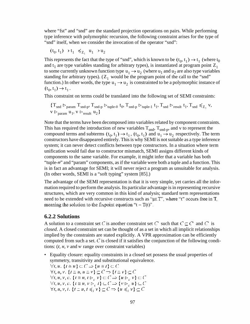
97

where “fst” and “snd” are the standard projection operations on pairs. While performing type inference with polymorphic recursion, the following constraint arises for the type of “snd” itself, when we consider the invocation of the operator “snd”:

This represents the fact that the type of “snd”, which is known to be (where t0 and t1 are type variables standing for arbitrary types), is instantiated at program point to some currently unknown function type (where u1 and u2 are also type variables standing for arbitrary types). ( would be the program point of the call to the “snd” function.) In other words, the type is constrainted to be a polymorphic instance of

.

This constraint on terms could be translated into the following set of SEMI constraints:

Note that the terms have been decomposed into variables related by component constraints. This has required the introduction of new variables Tsnd, Tsnd-p, and v to represent the compound terms and subterms , and respectively. The term constructors have disappeared entirely. This is why SEMI is not suitable as a type inference system; it can never detect conflicts between type constructors. In a situation where term unification would fail due to constructor mismatch, SEMI assigns different kinds of components to the same variable. For example, it might infer that a variable has both “tuple-Q” and “param” components, as if the variable were both a tuple and a function. This is in fact an advantage for SEMI; it will never reject a program as unsuitable for analysis. (In other words, SEMI is a “soft typing” system [85].)

The advantage of the SEMI representation is that it is very simple, yet carries all the infor-mation required to perform the analysis. Its particular advantage is in representing recursive structures, which are very common in this kind of analysis; standard term representations need to be extended with recursive constructs such as ³mt�7´��ZKHUH�³t”�RFFXUV�IUHH�LQ�7��PHDQLQJ�WKH�VROXWLRQ�WR�WKH�IL[SRLQW�HTXDWLRQ�“t� �7�t�´�

6.2.2 SolutionsA solution to a constraint set & is another constraint set such that and is closed. A closed constraint set can be thought of as a set in which all implicit relationships implied by the constraints are stated explicitly. A VPR approximation can be efficiently computed from such a set. & is closed if it satisfies the conjunction of the following condi-tions: (W, X, Y and Z range over constraint variables)

• Equality closure: equality constraints in a closed set possess the usual properties of symmetry, transitivity and substitutional equivalence.

t0 t1,( ) t1� )Z1 u1 u2�

t0 t1,( ) t1�Z1

u1 u2�Z1

u1 u2�t0 t1,( ) t1�

Tsnd Eparam Tsnd-p Tsnd-p Etuple-0 t0 Tsnd-p Etuple-1 t1 Tsnd Eresult t1 Tsnd )Z1 v

v Eparam u1 v Eresult u2

, , , , ,

,

{

}

t0 t1,( ) t1� t0 t1,( ) u1 u2�

&� & &�² &�

W X, . W @ X{ } &² X @ W{ } &²Ã"W X Y, , . W @ X X @ Y,{ } &² W @ Y{ } &²Ã"W X Y F, , , . W @ X W EF Y,{ } &² X EF Y{ } &²Ã"W X Y F, , , . W @ X Y EF W,{ } &² Y EF X{ } &²Ã"W X Y L, , , . W @ X W )L Y,{ } &² X )L Y{ } &²Ã"

98

Equality is meant to be reflexive, but it is troublesome to require reflexivity constraints as explicit elements of the constraint set. The obvious rule is unde-sirable because it requires & to contain an infinite number of constraints. A more com-plex definition is possible, but in fact there is no need for explicit reflexivity constraints, so they are not required to be in the set.

• Component uniqueness: a variable has at most one distinct component with a given label.

• Instance uniqueness: a variable has at most one distinct instance with a given label.

• Component propagation: if a variable has a component Y, then its instances also have the component.

• Instance propagation: instance relationships propagate to matching components.

Given any finite set of constraints &, there is always a finite solution set such that and is closed. For example, the set could be & with equality constraints

added between all variables mentioned in &, and all instance and component relationships holding between all the variables. This would be a correct solution, but not a very useful one because the induced value-point relation would relate every pair of bytecode expres-sions.

A more realistic strategy is to interpret the closure rules as production rules. At each step, if the set of constraints is not closed, the algorithm selects a rule whose hypothesis is satisfied but whose consequent is not and adds the constraint required to satisfy the conse-quent. Unfortunately, this algorithm does not terminate for practical examples.

Discussion of the actual SEMI algorithm is deferred to Chapter 7. In this chapter, I treat it as a black box and show that given an appropriate set of initial constraints, any closed solution gives rise to a conservative approximation of the value-point relation.

6.2.3 RemarksSimplifications of the closure rules give rise to a number of previously studied analyses. For example, if one takes only the equality closure rules plus two rules below forcing components and instances to be degenerate, one obtains a simple monomorphic, struc-tureless type inference analysis similar to Steensgard’s [72]:

If one takes only the equality rules and the component uniqueness rule, and forces instances to be degenerate, then one obtains a monomorphic type inference analysis with structures. This system essentially performs simple term unification. Cycles in the graph of component constraints are allowed, and correspond to recursive type terms.

W X Y L, , , . W @ X Y )L W,{ } &² Y )L X{ } &²Ã"

X. X @ X{ } &²"

W X Y F, , , . W EF X W EF Y,{ } &² X @ Y{ } &²Ã"

W X Y L, , , . W )L X W )L Y,{ } &² X @ Y{ } &²Ã"

W X Y F L, , , , . W EF X W )L Y,{ } &² Z . Y EF Z{ } &²$Ã"

W X Y Z F L, , , , , . W EF X W )L Y Y EF Z, ,{ } &² X )L Z{ } &²Ã"

&�& &�² &� &�

W X Y F, , , . W EF X{ } &² X @ W{ } &²Ã"

W X Y L, , , . W )L X{ } &² X @ W{ } &²Ã"

99

With the full treatment of polymorphic instance constraints as described, the system corre-sponds to type inference with polymorphic recursion using semiunification, again with recursive terms allowed. (The term “polymorphic recursion” means that cycles in the graph of instance constraints are allowed, such as when a polymorphic function recursively calls itself and passes in one of its original parameters.)

In general it is not possible to compute a “most general” or “principal” closed constraint set. This is discussed further in Section 7.1.2.

6.3 The Encoding

6.3.1 IntroductionSEMI generates a set of initial constraints directly from a bytecode program and then solves them to find a closed form. However, the procedure can be viewed conceptually as a trans-lation from the bytecode language into an extended lambda calculus, followed by gener-ation of type constraints for the translated code, followed by solution of the type constraints to yield inferred types. Here I provide an informal description of SEMI from the latter point of view.

6.3.2 MethodsEach Java bytecode method declaration is translated to a function declaration. Each function can take multiple parameters directly — no currying is used. The implicit “this” parameter of non-static methods becomes an explicit parameter in the translation. Functions return two values: the value returned normally by the method, and the thrown exception, if any. Methods that return nothing (“void”) have a return value in the trans-lation, but the value is always ignored. (In the formal MJBC semantics, every function returns a value, so this issue does not arise.)

Therefore this method that adds 3 to [

LQW�DGG��LQW�[��^�ORDG�[��ELSXVK��LDGG��LUHWXUQ��`

translates to the equivalent of

IXQ�DGG��WKLV��[�� [��«�

The “«” indicates that there is no value for the exception; its type is unconstrained. This means that, after type inference, the type of the exception will be a unique type variable. SEMI will conclude that the exception is not related in the VPR to any other value, as one would hope, since there is in fact no exception. (Obviously “«” precludes the translated code from being executable, but that is not a problem.) (A sum type could be used instead of a pair, to indicate that only one of the alternatives is possible, but this leads to essentially the same type constraints.)

Methods are assigned function types. The above method would be assigned the following “type”:

DGG�: "D��E��H. (D) � (E, e)

100

The intuition behind the interpretation of these types is that if two variables can be inferred to have different types, then they cannot be aliased in the VPR sense. If they are always inferred to have the same type, then they may be aliased.

Even though the [ parameter’s real type is LQW, we assign it a type variable so that we can compare its type meaningfully with the types of other variables which also hold integers. For example, here we can see that the value returned by DGG� is a new integer, different from the parameter. (We can also see that the parameter and result are both different from whatever exception may be thrown by DGG�.)

In SEMI, these inferred types become atomic constraint variables connected by component constraints as discussed in Section 6.2.1.2. For example, the above type would be repre-sented as

DGG�: T, where the constraint set contains{ 7 Eparam-0�a, T Eresult�b, T Eexn e `

6.3.3 Global VariablesGlobal variables (Java “static fields”) are passed into all functions in an extra record parameter. Each slot of the record corresponds to one global variable. For example, the method

LQW�JHW*OREDO��^��JHWVWDWLF�JOREDO9DU��LUHWXUQ�`

translates to the equivalent of

IXQ�JHW*OREDO�JOREDOV�� JOREDOV�JOREDO9DU��«�

The function simply performs the assignment and then returns no result and no exception. The following type signature would be inferred for this function:

JHW*OREDO: "D, H, r. ({ globalVar: D; r }) � (D, e)

This signature requires JOREDOV to have a field JOREDO9DU of type D, which must be the same type as the result. The polymorphic type variable r, sometimes referred to as a “row variable”, represents the types of an unknown set of other fields of JOREDOV (i.e., other global variables). This signature allows the other global variables to have any type.

This treatment of globals means that all function bodies are closed, i.e., refer only to variables defined locally or available as parameters, or to other functions. Therefore, in the type inferred for each function, every type variable can be polymorphically generalized. (In the language of Hindley-Milner type inference, every type variable is free in the enclosing type environment.)

If global variables were instead declared as variables in the enclosing environment, e.g.,

OHW�JOREDO9DU� �UHI��LQ��IXQ�JHW*OREDO�� JOREDO9DU��«�

then the type signatures would be

101

JOREDO9DU: D

JHW*OREDO: "H. () � (D, H)

The expression UHI�� indicates that JOREDO9DU is mutable and therefore its type cannot be polymorphically generalized; usage of JOREDO9DU in different contexts may refer to the same runtime value, and therefore JOREDO9DU must have the same type D in all contexts. Similarly, in the type inferred for JHW*OREDO, D cannot be polymorphically generalized because it is constrained to the type of JOREDO9DU.

The two strategies actually produce the same analysis results, because even when each function takes the global variable record as a polymorphic parameter, there is really only one global variable record in the program and one “canonical” type for this record (its type in the program’s PDLQ function). This “top level” type is a polymorphic instance of every other type for the global variable record. Lemma 6-21 below and Section 7.6 explain this in more detail.

For simplicity, SEMI uses explicit global variable passing, so that every type variable in a function signature is polymorphically generalized. The implementation performs optimiza-tions for types (such as the types of global variables) that have only one meaningful instance; this is discussed in Section 7.6. In the rest of this section the global variable passing is ignored for the sake of brevity.

The “row variables” do not occur in SEMI’s constraints. They are implicit. For example, the above method would be given the following constraints:

JHW*OREDO: Twhere the constraint set contains{ 7 Eglobals�Tglobals, Tglobals EglobalVar�a, T Eresult�a, T Eexn e `

6.3.4 Object EncodingJava objects are treated as extensible records, each similar to the “global variables” record. Each slot of the record contains either a field or a method. For example, the code

LQW�JHW;��^��ORDG�WKLV��JHWILHOG�ILHOG;��UHWXUQ�`

would translate to (ignoring the globals object for now)

IXQ�JHW;�WKLV�� WKLV�ILHOG;��«�

This would get type signature

JHW;: "D, G, r. ({ fieldX: D; r }) � (D, G)

Here WKLV is deconstructed into a record containing field ILHOG; of type D and some set of other fields of types r. Effectively, this function and its type say nothing about what other fields of WKLV there may be. Any object containing a ILHOG; can be passed in. In fact, any object at all can be passed in, and the type inference algorithm will infer that it contains ILHOG;. This “row polymorphism” avoids any need for subtype polymorphism in this type system. (This complete reliance on row polymorphism distinguishes this type

102

system from the type system of O’Caml [65], where row polymorphism is available but explicit classes and subtyping are usually used instead.) It also helps reduce the sizes of types inferred for functions, because only fields actually used by the function are given types in the function’s signature.

Field names are always fully qualified with the name of the class in which they are declared, so two fields of different classes which happen to have the same name are never confused in the translation.

The Java class of an object is never represented in the translation or in the type inference system. The implications of this are discussed in the following sections. Tools based on SEMI can recover class information using the VPR; this is discussed in Chapter 10 and elsewhere.

6.3.5 Method Encoding

6.3.5.1 Static MethodsStatic methods are treated as normal functions. A call to a static method is translated into a direct call to the appropriate function. For example, the code in Figure 6-1 would be trans-lated to the equivalent of the code in Figure 6-2.

Because the function DGG2QH is a polymorphic value, its use in DGG2QH:UDSSHU is assigned a fresh polymorphic instance of the type of DGG2QH. All calls to static methods are treated polymorphically. (In other words, static method calls are analyzed with calling-context sensitivity.) Intuitively, this is safe because (being closed) distinct calls to DGG2QH are completely independent and cannot communicate except through the caller’s environment.

6.3.5.2 Nonstatic MethodsNonstatic methods — that is, methods involved in dynamic dispatch — are encoded by treating them as functions assigned to the slots of objects when those objects are created. For example, the code in Figure 6-3 would be translated to the equivalent of the code in Figure 6-4.

VWDWLF�LQW�DGG2QH�LQW�[��^��ORDG�[��ELSXVK��LDGG��LUHWXUQ�`VWDWLF�LQW�DGG2QH:UDSSHU�LQW�\��^��ORDG�\��LQYRNHVWDWLF�DGG2QH��LUHWXUQ�`

Figure 6-1. Static Method Example

IXQ�DGG2QH�[�� [��«�IXQ�DGG2QH:UDSSHU�\�� DGG2QH�\��«�

Figure 6-2. Static Method Translation

103

The following types are inferred:

0\2EMBJHW;: "D, H, r. ({ MyObj_fieldX: D; r }) � (D, H)JHWWHU: "E, H, r. (W) � (E, H) where W = { getX: (W) � (E, H); r }REM (in PDLQ): u where u = { getX: (X) � (F, H); MyObj_fieldX: F; r }

(for some F,�H, r)

Note that objects containing methods usually have recursive types, because the type of the WKLV parameter in each method type is usually the same as the object type.

Another example of the treatment of virtual method calls, expressed directly in the constraint language of SEMI, is given below in Section 6.4.7.

6.3.5.3 Type Checking/Inference For Nonstatic MethodsGiven the above types and assuming standard type checking rules, it is straightforward to show that the types are consistent with the code and each other.

For example, to typecheck JHWWHU, we observe that the type of R is W, and therefore the type of R�JHW; is (W) � (E, H). In the call to R�JHW;, we indeed pass in a parameter of type W (R). Furthermore, the result returned from JHW; has type (E, H), which correctly matches the return type of JHWWHU.

Note that JHWWHU is typechecked (and can have its type inferred) independently of any information about the callee in the call to JHW; (0\2EMBJHW;). All that is required is that the type of the JHW; method recorded in the type of JHWWHU’s R parameter is consistent with the actual usage of that method within JHWWHU. The type information recorded for

FODVV�0\2EM�^��LQW�ILHOG;��LQW�0\2EMBJHW;�0\2EM�WKLV��^��ORDG�WKLV��JHWILHOG�0\2EMBILHOG;��LUHWXUQ��``VWDWLF�LQW�JHWWHU�2EMHFW�R��^��ORDG�R��LQYRNHYLUWXDO�JHW;��LUHWXUQ�`VWDWLF�LQW�PDLQ��^��QHZ�0\2EM��LQYRNHVWDWLF�JHWWHU��LUHWXUQ�`

Figure 6-3. Nonstatic Method Example

IXQ�0\2EMBJHW;�WKLV�� WKLV�0\2EMBILHOG;��«�IXQ�JHWWHU�R�� R�JHW;��R�IXQ�PDLQ�� OHW�REM� �^�JHW;��0\2EMBJHW;��0\2EMBILHOG;��`��LQ�JHWWHU�REM�

Figure 6-4. Nonstatic Method Translation

104

JHW; in the type signature of JHWWHU effectively describes how the method is used by JHWWHU.

To check the type of REM in PDLQ, observe that it constrained both by the initialization of REM as a new 0\2EM object and by REM being passed as a parameter to JHWWHU. The initialization of REM requires REM’s type u to be the type of an object containing a JHW; method and a 0\2EMBILHOG; field. Furthermore, the type of the JHW; method within u must be a polymorphic instance of the type of 0\2EMBJHW; (which is “"D, H, r. ({ MyObj_fieldX: D; r }) � (D, H)”). If no method call was made on the object, we could therefore just set u = { getX: ({ MyObj_fieldX: F, r }) � (F, H); MyObj_fieldX: G; r' } (for some F, d, e, r, r').

However, the type of REM is also constrained by the call to JHWWHU�REM�. This call requires u to be some polymorphic instance of JHWWHU’s parameter type t, where W = { getX: (W) � (E, H); r }. Because the parameter type of t’s JHW; method is t itself, the parameter type of u’s JHW; method is also required to be u itself. Unifying this constraint with the constraints mentioned above requires u to be of the form { getX: (X) � (F, H); MyObj_fieldX: F; r }.

Note also that the type signature of JHWWHU promises that its result has the same type (b) as the result of its object parameter’s JHW; method. Therefore in PDLQ we learn that the result of the call to JHWWHU will have type c.

6.3.5.4 Treatment Of PolymorphismThe call to JHWWHU in PDLQ is treated polymorphically; the caller’s parameter and result types are required to be some polymorphic instance of the callee’s types. On the other hand the call to JHW; from JHWWHU is not treated polymorphically; the caller and callee types must be identical.

The technical reason for this distinction is that we can only polymorphically generalize type variables that are not bound in the current type environment. All the type variables in the type assigned to JHWWHU are polymorphically generalized, because they do not occur anywhere outside the definition of JHWWHU. (Intuitively, this means that the assignment of types to these variables is independent of anything outside JHWWHU, and therefore different types can be chosen for each use of JHWWHU.) On the other hand, in JHWWHU, the type variables in the type of the callee R�JHW; are bound in the type environment; in particular they occur inside JHWWHU’s parameter type. (Intuitively, this means that the assignment of types to these type variables is constrained by the caller of JHWWHU. For example, the caller of JHWWHU might pass in an object whose JHW; method always returns an integer. Obviously it would be unsafe to allow JHWWHU to choose different return types for each call to JHW;.)

6.3.5.5 Polymorphism In Object CreationWhen an object is created, such as when REM is created in PDLQ, its field and method slots are always iniitalized with constant values — either zero scalar values, or the functions that implement the methods supported by the object. The usage of these constant values is always treated polymorphically. Therefore if a method implementation is inherited into multiple classes, which are instantiated at multiple sites, the references to the method

105

implementation at each site can be given distinct types. Similarly, fields of objects of the same class created at different sites can be given distinct types.

6.3.6 Extensible Records and Object ClassesConsider the code in Figure 6-5. This example demonstrates the use of subclass polymor-phism with subclasses having distinct fields.

The following types are inferred:

0\2EMBJHW;: "D, H, r. ({ MyObj_fieldX: D; r }) � (D, H)<RXU2EMBJHW;:"E, H, r. ({ YourObj_otherX: E; r }) � (E, H)JHWWHU: "F, H, r. (W) � (F, H) where W = { getX: (W) � (F, H); r }object in PDLQ: u where u = { getX: (X) � (F, H); MyObj_fieldX: F;

YourObj_otherX: F; r } (for some F,�H, r)

In general, if Java declares a variable to be of class C (here, 6XSHU2EM), then any fields and methods belonging to C or any subclass of C (here, 0\2EM and <RXU2EM) can appear in the type inferred for the variable. This can lead to the slightly counterintuitive situation where variables having the least constraining Java types (e.g., variables of type 2EMHFW) have the most complex inferred types.

FODVV�6XSHU2EM�^��DEVWUDFW�LQW�JHW;�6XSHU2EM�WKLV��`FODVV�0\2EM�^��LQW�ILHOG;��LQW�JHW;�0\2EM�WKLV��^��ORDG�WKLV��JHWILHOG�0\2EMBILHOG;��LUHWXUQ��``FODVV�<RXU2EM�^��LQW�RWKHU;��LQW�JHW;�<RXU2EM�WKLV��^��ORDG�WKLV��JHWILHOG�<RXU2EMBRWKHU;��LUHWXUQ��``VWDWLF�LQW�JHWWHU�6XSHU2EM�REM��^��ORDG�REM��LQYRNHYLUWXDO�JHW;��LUHWXUQ�`VWDWLF�LQW�PDLQ��^��LI�«�WKHQ�QHZ�0\2EM�HOVH�QHZ�<RXU2EM��LQYRNHYLUWXDO�JHW;��LUHWXUQ�`

Figure 6-5. Extensible Record Example

106

6.3.7 MutabilityGlobal variables and fields of objects are mutable. However, in the type system I have not distinguished mutable and immutable slots of records. The distinction is irrelevant because whenever a slot of a record is accessed, the record has a monomorphic type and therefore the type of the slot is monomorphic. Thus two accesses to the same slot of a record, whether reads or writes, always get the same type for the slot. (The fatal error would be to treat a mutable slot of a record as polymorphic; we might store a value in the slot with one type, retrieve the value with another type, and thus destroy soundness.)

6.3.8 Control FlowInternally, a Java bytecode method is simply an array of bytecode instructions with arbitrary control flow between them. SEMI treats each bytecode instruction as a local function which takes the values of the current working stack and local variables as param-eters, and calls the successor instruction(s) as tail calls. Each local function returns the final result of the method and its thrown exception.

The stack is passed as a list, so that “push” operations become “cons” and “pop” operations become “head/tail”. Local variables are passed in a record.

A method executes by calling the local function for the first instruction, with method parameters placed into local variables (as required by the Java bytecode semantics).

)RU�H[DPSOH��WKH�PHWKRG

LQW�DGG��LQW�[��^�ORDG�[��ELSXVK��LDGG��UHWXUQ��`

translates to

IXQ�DGG��WKLV��[�� OHW�IXQ�IB��VW��Y��Y�� IB��Y��VW��Y��Y��DQG�IXQ�IB��VW��Y��Y�� IB��VW��Y��Y��DQG�IXQ�IB��D��E��VW��Y��Y�� IB��D�E��VW��Y��Y��DQG�IXQ�IB��Y��VW��Y��Y�� Y��«��LQ�IB��>@��^��WKLV��[`�

The encoding is simple and regular.

All kinds of control flow are easily handled. The method

VWDWLF�LQW�LVHTXDO�LQW�[��LQW�\��^��ORDG��ORDG��LIBFPSHT��ELSXVK��VWRUH��JRWR��ELSXVK��VWRUH��ORDG��UHWXUQ��`

translates to

107

IXQ�LVHTXDO�[��\�� OHW�IXQ�IB��VW��Y��Y��Y�� IB��Y��VW��Y��Y��Y��DQG�IXQ�IB��VW��Y��Y��Y�� IB��Y��VW��Y��Y��Y��DQG�IXQ�IB��Y��Y��VW��OV�� LI�Y�� Y��WKHQ�IB��VW��OV��HOVH�IB��VW��OV��DQG�IXQ�IB��VW��OV�� IB��VW��OV��DQG�IXQ�IB��D��VW��Y��Y��Y�� IB��VW��Y��Y��D��DQG�IXQ�IB��VW��OV�� IB��VW��OV��DQG�IXQ�IB��VW��OV�� IB��VW��OV��DQG�IXQ�IB��E��VW��Y��Y��Y�� IB��VW��Y��Y��E��DQG�IXQ�IB��VW��Y��Y��Y�� IB��Y��VW��Y��Y��Y��DQG�IXQ�IB��Y��VW�� Y��«�

These calls between instructions could be treated polymorphically. In theory some accuracy might be gained because at control flow merge points, the state along each incoming control flow edge could be given a different type, each an instance of the type of the state at the destination instruction. In practice this increased accuracy has not proved useful, and even with some obvious optimizations (e.g., only allow polymorphism for calls to instructions representing control flow merge points), it has proved prohibitively expensive. Therefore in practice SEMI treats these transfers monomorphically (making the types of the actual parameters and results equal to the types of the formal parameters and results, rather than instances of those types). However, in the description below, I use polymorphic constraints for instruction transfers to show that they are sound.

However, even under monomorphism it is still the case that a stack location or local variable can be given different types at different program points. For example, local variable #2 is has a different type after it is assigned to the type it had before assignment. This has the same effect as translating the program into Single Static Assignment form before performing the analysis, but it arises naturally from the encoding.

6.3.9 Exception HandlingException handling is performed in a way similar to other control transfers. In each method, every instruction which might throw an exception, or receive a propagated exception (which is actually all instructions, because the virtual machine can throw an “internal error” exception at any instruction), can transfer control to any applicable exception handlers defined in the method. The translation does not specify when an exception is thrown; for a given instruction, the choice of whether to throw an exception or continue normal execution is always considered to be nondeterministic (unless the instruction is an unconditional DWKURZ instruction). Control transfer to an exception handler puts the current exception object onto the top of the working stack, as specified by the Java bytecode semantics.

Most methods do not have any explicit exception handlers. However, all methods must be able to propagate thrown exceptions to the caller. Each instruction which can throw an exception (or receive a propagated exception) can nondeterministically choose to return the exception value immediately as the method result, thus propagating the exception. The following code shows an example of such behavior:

108

IXQ�FDOO$OO�� OHW��UHVXOW��H[Q�� FDOO��LQ�LI�"�WKHQ��«��H[Q��HOVH��OHW��UHVXOW��H[Q�� FDOO��UHVXOW��LQ�LI�"�WKHQ��«��H[Q��HOVH��UHVXOW��«�

6.4 Initial Constraint SetConsider a program P in the Micro Java Bytecode language, as defined in Section 3.2.2.

6.4.1 Constraint VariablesThe set of initial constraints for P makes use of the following variables:

• SSF: the variable for the working stack on entry to instruction SFThe stack is a list, so its variable can have two components: “head”, representing the top of the stack, and “tail”, representing the rest of the stack.

• LSF: the variable for the local variable file on entry to instruction SFThe local variables are indexed by number, so LSF has numbered components, one for each local variable used.

• XSF: the variable for the exception thrown by the code starting at SF

• GSF: the variable for the global variables on entry to instruction SFThis variable has one component for each static field in the program.

• RSF: the variable for the value that the code at SF eventually returns from the method

• S�SF, L�SF: the variables for the state on leaving instruction SF

• NFODVV,': the variable representing the prototypical object of class FODVV,'

• MPHWKRG,PSO: the variable representing the type of the method PHWKRG,PSO

• TSF,ODEHO: variables used by the instruction at SF for internal purposes

• NFODVV,',PHWKRG,': the variable representing the type of inherited method PHWKRG,' in class FODVV,'

• NFODVV,',ILHOG,': the variable representing the type of field ILHOG,' in class FODVV,'

• NILHOG,': the variable representing the type of static field ILHOG,'

• Err: the variable representing the exceptions which may be thrown spontaneously by the virtual machine

• S�exn-SF�FODVV,': these variables represent the new stack on transfer to an exception han-dler when exception FODVV,' is thrown at SF

6.4.2 Instance LabelsSEMI uses the following instance labels:

109

• SF-SF�: an instance representing the use of (transfer of control to) one instruction from another.SEMI treats each instruction as a function; transferring control from one instruction to another corresponds a call to the destination instruction’s function, passing in the cur-rent local variables, working stack elements and global variables as parameters. These “functions” do not return until the entire method returns; the returned value is the result of the method. The functions are treated as polymorphic, so different information can be inferred for an instruction for each incoming control path.

• SF: an instance representing the use of a static method (when SF corresponds to an LQYRNHVWDWLF instruction) or the creation of a new object (when SF corresponds to a QHZ instruction).A method can be thought of as a polymorphic function. Note that global variables are treated as the fields of a “globals object” which is passed as a parameter to every such function, so every such function is self-contained and has no references to any environ-ment. A static call to a method is a direct invocation of the function, and so gets a new polymorphic instance. Creation of an object can be thought of as cloning a prototype object, and also gets a new polymorphic instance.

• FODVV,'-PHWKRG,': an instance representing the inheritance of a method implementa-tion by a class.Each prototype object for a class can be thought of as a record, with one slot for each signature of the methods implemented by the class. The putative definition of the proto-type assigns the function associated with each inherited method implementation to the slot for its signature. Since one method implementation can be inherited into multiple classes, each class which uses a method implementation gets a new polymorphic instance of the method.

• err-SF: an instance representing the creation of a spontaneously thrown exception at a particular program point.This is similar to the instance induced when an object is created by QHZ.

• err-FODVV,': an instance representing the creation of a new object when a spontaneous exception is thrown.A spontaneous exception creates an object which has one of many possible classes. The variable “Err” represents the type of an object which could be any one of these classes, and therefore “Err” is an instance of the object prototype for each spontaneous excep-tion class. Each of these instances needs a different label, err-FODVV,'.

6.4.3 Component LabelsI make use of the following component labels:

• param-L: a parameter to a method.

• globals: the global variables passed into a method.

• result: the result returned by a method.

• exn: the exception thrown by a method (essentially, an alternative result).

• L: a local variable index.

110

• ILHOG,': a field slot of an object.

• PHWKRG,': a method slot of an object.

• head: the head element of a stack, treated as a list.

• tail: the tail of a stack.

6.4.4 Program ConstraintsThe set of initial constraints assigned to an MJBC program is given as

InitialConstraints(P) =( { IConstraints(SF) | SF ³ dom Instruction })

( { MInvocation(PHWKRG,PSO) | (PHWKRG,PSO, 0) ³ dom Instruction })

( { MDispatch(FODVV,', PHWKRG,') | (FODVV,', PHWKRG,') ³ dom Dispatch })

( { IFields(FODVV,') | FODVV,' ³ dom InitFields }) ( { CatchConstraints(SF, FODVV,') | (SF, FODVV,') ³ dom

CatchBlockOffset }) ( { { *�0DLQ�� EILHOG,' 1ILHOG,' } | ILHOG,' ³

dom InitStaticFields }) ( { { Err�)err-SF XSF } | SF ³ dom Instruction }) ( { { NFODVV,'�)err-FODVV,' Err } | FODVV,' ³

ErrorClassIDs })

This definition uses several functions:

• IConstraints(SF) is a partial function that assigns to each SF the initial constraints induced by the instruction at SF. IConstraints is defined by the rules in Table 6-1.

• MInvocation computes the constraints needed to hook up the type of a method body P to the types at the method definition.

• MDispatch computes the constraints needed to implant the type of the method imple-mentation PHWKRG,' into the type of the prototype object for class FODVV,'.

MDispatch(FODVV,', PHWKRG,') ={ MDispatch(FODVV,', PHWKRG,')�)FODVV,'�PHWKRG,'�1FODVV,',PHWKRG,'�

1FODVV,' EPHWKRG,' 1FODVV,',PHWKRG,' }

• IFields computes constraints ensuring that every object field has a type.

IFields(FODVV,') ={ 1FODVV,' EILHOG,' 1FODVV,',ILHOG,' | ILHOG,' ³ dom InitFields(FODVV,') }

MInvocation P( ) MP Eparam-0 TP p0, MP Eparam-1 TP p1, MP Eglobals G P 0,( ), ,{ }MP Eexn X P 0,( ) MP Eresult R P 0,( ) L P 0,( ) E0 7P p0, L P 0,( ) E1 TP p1,, , ,{ }

=

111

Instruction(SF) IConstraints(SF)

DFRQVWBQXOO { S�SF Etail�6SF,�SSF+1 Ehead�TSF,v�`

Succ(SF, SF+1, S�SF, LSF)

ELSXVK byte { S�SF Etail�6SF,�SSF+1 Ehead�TSF,v�`


LDGG { 6SF Etail�TSF,t1, TSF,t1 Etail�TSF,t2, S�SF Etail TSF,t2,�SSF+1 Ehead�TSF,v `


ORDG index { LSF ELQGH[ 7SF�Y��S�SF Etail�6SF��S�SF Ehead�7SF�Y�`


VWRUH index { 6SF Etail�S�SF, SSF Ehead�7SF�Y� L�SF ELQGH[ 7SF�Y�` { L�SF EL 7SF�L | L ³ LocalNames(SF) ¾ L � LQGH[ } { LSF EL 7SF�L | L ³ LocalNames(SF) ¾ L � LQGH[ } Succ(SF, SF+1, S�SF, L�SF)

LIBFPSHT offset { 6SF Etail�S�SF ` Succ(SF, SF+1, S�SF, LSF, GSF, XSF, RSF) Succ(SF, (CodeLocMethod(SF), RIIVHW), S�SF, LSF)

JRWR offset Succ(SF, (CodeLocMethod(SF), RIIVHW), SSF, LSF)

UHWXUQ { SSF Ehead�5SF�`

QHZ classID { S�SF Etail�6SF��SSF+1 Ehead�7SF�Y��NFODVV,'�)SF�7SF�Y�`

Succ(SF, SF+1, S�SF, LSF)a

JHWILHOG fieldID { 6SF Etail�TSF,t, 6SF Ehead�TSF,obj, TSF,obj EILHOG,'�TSF,v, S�SF Ehead TSF,v, S�SF Etail TSF,t `


SXWILHOG fieldID { 6SF Etail�TSF,t, 6SF Ehead�TSF,v,�TSF,t Etail�S�SF, TSF,t Ehead TSF,obj, TSF,obj EILHOG,' TSF,v ` Succ(SF, SF+1, S�SF, LSF)

JHWVWDWLF fieldID { GSF EILHOG,' 7SF�Y��S�SF Etail�6SF��S�SF Ehead�7SF�Y�`


SXWVWDWLF fieldID { 6SF Etail�S�SF, SSF Ehead�7SF�Y� GSF EfieldID 7SF�Y�`


LQYRNHYLUWXDO methodID

{ 6SF Etail�TSF,t1, 6SF Ehead�TSF,v1,�TSF,t1 Etail�TSF,t2, TSF,t1 Ehead TSF,v0, TSF,v0�EPHWKRG,'�7SF�P�

6�SF Etail�TSF,t2, 6�SF Ehead�TSF,r ` MethodCall(7SF�P, TSF,v0, TSF,v1, GSF, XSF, 7SF�U) Succ(SF, SF+1, S�SF, LSF)

Table 6-1. Instruction Constraints

112

• CatchConstraints gives constraints capturing the control flow for exceptions of class FODVV,' thrown at SF and caught in the method.

CatchConstraints(SF, FODVV,') =Succ(SF, (CodeLocMethod(SF), CatchBlockOffset(SF, FODVV,')), S�exn-SF�FODVV,', LSF) { S�exn-SF�FODVV,' Ehead�;SF }

The last three sets of constraints are:

• Constraints ensuring that every static field has a type.

• Constraints expressing the possibility that an exception may be spontaneously thrown from at any instruction.

• Constraints specifying that the spontaneously thrown exceptions are objects of the classes found in the ErrorClassIDs.

The rules in Table 6-1 use the following functions:

• LocalNames computes the indices of the local variables used in PHWKRG. LocalNames is used to make sure the values of all local variables are carried forward correctly when one of them is overwritten by a VWRUH instruction.

• Succ computes the constraints that arise along control flow paths within a method, when one instruction is a successor of another in the control flow graph. Succ treats the transfer of control from one instruction to the next as if it were a function call, so that

LQYRNHVWDWLF methodImpl

{ 6SF Etail�TSF,t1, 6SF Ehead�TSF,v1,�TSF,t1 Etail�TSF,t2, TSF,t1 Ehead TSF,v0, MPHWKRG,PSO�)SF�7SF�P��

6�SF Etail�TSF,t2, 6�SF Ehead�TSF,r ` MethodCall(7SF�P, TSF,v0, TSF,v1, GSF, XSF, 7SF�U) Succ(SF, SF+1, S�SF, LSF)

FKHFNFDVW classID Succ(SF, SF�1, SSF, LSF)

LQVWDQFHRI classID { 6SF Etail�TSF,t, S�SF Etail TSF,t,�SSF+1 Ehead�TSF,v `


DWKURZ { SSF Ehead�;SF�`

a. The object’s type variable is plugged into SSF+1 instead of S�SF, because for the proofs, we need the field and method components of the variable to appear at SSF+1. The implementation instead has S�SF Ehead�7SF�Y��7KH�GLVFUHSDQF\�FDQ�SUREDEO\�EH�FRUUHFWHG�E\�DGGLQJ�³SRVW�VWDWH´�H[SUHVVLRQV�WR�WKH�H[SUHVVLRQ�V\QWD[�DQG�H[WHQG�LQJ�WKH�VRXQGQHVV�SURRI�WR�FRYHU�WKHP�

Instruction(SF) IConstraints(SF)

Table 6-1. Instruction Constraints

LocalNames PHWKRG( )LQGH[ L. Instruction PHWKRG L,( ) ORDG �LQGH[ VWRUH�LQGH[,{ }³$|{ }

=

113

the instruction at IURP performs a “tail call” to the instruction at WR to do the rest of the computation for the current method. 6 and / are the types for the working stack and the local variables respectively that are passed into WR.

• MethodCall computes the constraints needed to hook up a method call at a call site. 0 is the type for the method being called. 3� and 3� are the types of the parameters being passed in. * is the type of the globals object being passed in. ; and 5 are the types of the exception and normal result returned, respectively.

6.4.5 Query ConstraintsAdditional constraints must be added to the set & to support queries over arbitrary bytecode expressions. These constraints depend on the queried expressions, and are detailed below in Section 6.5.3.2.

6.4.6 Canonical Constraint Set& is a canonical constraint set if

.

Given a closed constraint set 1,

/HPPD��/HW�D�FORVHG�FRQVWUDLQW�VHW�1�EH�JLYHQ��/HW�0�EH�D�PDS�IURP�YDULDEOHV�WR�

YDULDEOHV�VXFK�WKDW

0 selects one representative element from each equivalence class. Such a map exists for any choice of N, because the closure of 1 implies the relation is an equivalence relation in 1 (lacking only reflexivity, which I restore with the disjunction).

Let & be defined as:

�& replaces each variable in 1 with the representative of its equivalence class.) 7KHQ�&�LV�WULYLDOO\�FDQRQLFDO��)XUWKHUPRUH��&�LV�FORVHG�

Proof: I prove the closure condition that implies .

Suppose . Then

Succ IURP WR 6 /, , ,( )SWR )IURP-WR �6 LWR )IURP-WR�/ GWR )IURP-WR �GIURP XWR )IURP-WR�XIURP, , ,{ }RWR ) IURP-WR�RIURP{ }

=

MethodCall 0 3� 3� * ; 5, , , , ,( )0 Eparam-0 3� 0 Eparam-1 3� 0 Eglobals * 0 Eexn�; 0 Eresult�5, , , ,{ }

=

X Y, . X @ Y{ } &² XÃ" Y=

X Y, . X @ Y{ } 1² X Y=¿ 0 X( )À" 0 Y( )=

@

& 0 W( ) EF 0 X( ) W EF X{ } 1²|{ }

0 W( ) )L 0 X( ) W )L X{ } 1²|{ }

0 W( ) @ 0 W( ) W dom 0³|{ }

=

W EF X W EF Y,{ } &² X @ Y{ } &²

W EF X W EF Y,{ } &²

114

. where

By definition of 0,

In either case of the disjunction,

By closure of N,

This gives

, i.e., and therefore

The other closure conditions follow similarly. n

The remainder of this chapter deals with canonical closed constraint sets. This eliminates the need to explicitly deal with equivalence constraints.

6.4.7 ExampleThe Java code in Figure 6-6 would generate bytecode as shown in Table 6-2.

)RU�WKLV�SURJUDP��RQH�PLJKW�DVN�³FDQ�PDLQ¶V�UHVXOW�HTXDO�WKH�QHZ�;�REMHFW�LW�FUHDWHV"´�:H�VKDOO�VHH�KRZ�WKLV�TXHVWLRQ�LV�DQVZHUHG�E\�FRPSXWLQJ�LQLWLDO�FRQVWUDLQWV��VKRZQ�LQ�Table 6-2��DQG�WKHQ�ILQGLQJ�D�FORVHG�IRUP�

6.4.7.1 Initial ConstraintsThe constraints shown in Table 6-2 have been simplified from the real constraints in order to make the example simultaneously tractable and interesting. In particular, all the “successor instance” constraints have been replaced with equalities, which have then been eliminated by substitution. All of the constraints within methods relating to the stack (S) and local variable (L) variables have been solved and eliminated. All constraints relating to global variables and exceptions are irrelevant and have been elided.

6.4.7.2 Finding a Closed FormSEMI would close the constraint set by generating additional constraints, as follows:

The equality constraints within I give

^�0I�EUHVXOW�7I�S��`�

FODVV�;�^��;�I�;�D��^�UHWXUQ�WKLV��`��VWDWLF�;�J�;�F��;�G��^�UHWXUQ�F�I�G��`��VWDWLF�;�PDLQ�;�E��^�UHWXUQ�J�QHZ�;��E��``

Figure 6-6. A Simple Java Program

W$ � W�� X� Y�, , , W 0 W�( )= X 0 X�( )= W 0 W��( )= Y 0 Y�( )=¾ ¾ ¾

W� EF X� W�� EF Y�,{ } 1²

0 W�( ) 0 W��( )= W� @ W��{ } 1² W� W��=¿Ã

W� EF X� W� EF Y�,{ } 1²

X� @ Y�{ } 1²

0 X�( ) 0 Y�( )= X Y= X @ Y{ } &²

115

We propagate components of Mf to NX,f (using 0I�);�I�1;�I), getting

^�1;�I�ESDUDP��Y��1;�I�EUHVXOW�Y�`��IRU�VRPH�Y�ZKHUH�7I�S��);�I�Y��

Now we propagate NX,f and its components to the instance of CX in PDLQ (using &; )�PDLQ��7�PDLQ��Y), yielding

{ 7�PDLQ��Y EI V ��V�ESDUDP��Y��V�EUHVXOW�Y `��IRU�VRPH�V�DQG�Y�ZKHUH�NX,f�)�PDLQ��V�

DQG��Y )�PDLQ��Y��

In other words, we know in PDLQ that the object’s I method aliases its first parameter and result. Now we need to work on J. The constraints for J contain { 7J�S��EI�7�J��P��

7�J��P ESDUDP��7J�S��7�J��P�EUHVXOW�5�J��`��So inside J, we know that we pass S� into S�’s I method, and the result of that method is returned from J. We do not assume anything else about I here.

We propagate J’s constraints to PDLQ, obtaining

{ 7J�S��)�PDLQ��7�PDLQ��Y��5�J�� )�PDLQ�� 5�PDLQ��`

From here we get

%\WHFRGH ,QGXFHG�,QLWLDO�&RQVWUDLQWVFODVV�;�^ 0I�);�I�1;�I &;�EI�1;�I��I�WKLV��S��^ 0I�ESDUDP��7I�S��

0I�EUHVXOW�5�I��

0I�ESDUDP��7I�S�

�� ORDG�WKLV�� UHWXUQ� 5�I�� 7I�S�

��`��VWDWLF�J�S��S��^

0J�ESDUDP��7J�S�0J�EUHVXOW�5�J��

0J�ESDUDP��7J�S�

�� ORDG�S�� ORDG�S�

��LQYRNHYLUWXDO�I�

7J�S��EI�7�J��P�

7�J��P�ESDUDP��7J�S�

7�J��P�ESDUDP��7J�S�

�� UHWXUQ� 7�J��P�EUHVXOW�5�J��`��VWDWLF�PDLQ�S��^

0PDLQ�ESDUDP��7PDLQ�S�� 0PDLQ�EUHVXOW�5�PDLQ��

�� QHZ�;� &;�)�PDLQ��7�PDLQ��Y�� ORDG�S��

��LQYRNHVWDWLF�J�

0J�)�PDLQ��7�PDLQ��P

7�PDLQ��P�ESDUDP��7PDLQ�S�

7�PDLQ��P�ESDUDP��7�PDLQ��Y

�� UHWXUQ� 7�PDLQ��P�EUHVXOW�5�PDLQ��``

Table 6-2. A Simple Bytecode Program and its Constraints

116

{ 7�PDLQ��Y�EI�X��X�ESDUDP��7�PDLQ��Y��X EUHVXOW�5�PDLQ��`��IRU�VRPH�X�ZKHUH�

7�J��P )�PDLQ�� X��

1RZ�7�PDLQ��Y�EI�X�DQG�7�PDLQ��Y�EI�V�UHTXLUH�XV�WR�VHW

{ }

,Q�RWKHU�ZRUGV��ZH�KDYH�³GLVFRYHUHG´�WKH�LPSOHPHQWDWLRQ�RI�I�WKDW�J�XVHV�

From the param-0 components of u and s, we get

{ , }

Thus

{ }.

%HFDXVH�WKH�UHVXOW�RI�QHZ�;�LQ�PDLQ�LV�DVVLJQHG�W\SH� ��WKH�FRQFOXVLRQ�LV�WKDW�WKH�

UHVXOW�RI�PDLQ�PD\�EH�WKH�QHZ�;�

6.5 Extracting the VPR ApproximationIn this section, I consider a canonical closed constraint set &��ZLWK�DVVRFLDWHG�PDS�0�PDSSLQJ�IURP�WKH�RULJLQDO�YDULDEOHV�WR�WKH�YDULDEOHV�RI�&��DQG�D�SDLU�RI�E\WHFRGH�H[SUHV�VLRQV�H��DQG�H��DQG�VKRZ�KRZ�6(0,�GHFLGHV�ZKHWKHU�H��DQG�H��DUH�UHODWHG�LQ�WKH�935�DSSUR[LPDWLRQ�

6.5.1 OverviewBelow, I define a judgement �WKDW�UHODWHV�D�E\WHFRGH�H[SUHVVLRQ�H�LQ�VRPH�FRQWH[W� �WR�D�6(0,�YDULDEOH�X with some “leftover context” ��ZKLFK�LV�D�VXIIL[�RI� ��$�FRQWH[W�LV�D�VHTXHQFH�RI�LQVWDQFH�ODEHOV��)RU�ILUVW�RUGHU�FRGH��LW�FRUUHVSRQGV�WR�D�FDOO�VWDFN��HDFK�ODEHO�QDPLQJ�D�PHWKRG�FDOO�VLWH�RU�DQ�LQVWUXFWLRQ�WUDQVLWLRQ��UHFDOO�WKDW�LQVWUXFWLRQ�WUDQVLWLRQV�DUH�WUHDWHG�DV�WDLO�FDOOV��

The SEMI variable X is referred to as the ground type of the expression in the context. A ground type is obtained by first ignoring the context and computing the base type t assigned to the expression by SEMI, for example, the type variable assigned to a local variable. Then we follow the chain of instances starting at W and labelled by the instance labels in the context as far as possible, to obtain X, the “most specific” instance of t in context .

The “leftover context” �LV�WKH�VXIIL[�RI� �WKDW�ZDV�QRW�GHUHIHUHQFHG��LW�UHSUHVHQWV�WKH�RXWHUPRVW�FRQWH[W�DW�ZKLFK�VRPH�LQVWDQFH�RI�W appears. For example, when X occurs as part of the type of a global variable, the leftover context is empty because an instance of u will occur at the top level.

The analysis concludes H��H��LI�DQG�RQO\�LI

The idea is that X is the type of a witness value that causes H��DQG�H��WR�EH�UHODWHG��7KH�H[SUHVVLRQV�DUH�UHODWHG�LI�WKHUH�LV�VRPH�SODXVLEOH�W\SH�X�WKDW�LV�DQ�LQVWDQFH��LQ�DQ\�FRQWH[WV��RI�ERWK�RI�WKH�EDVH�W\SHV�RI�H��DQG�H��

X @ V

v� @ T(main,0),v v� @ R(main,0)

R(main,0) @ T(main,0),v

T(main,0),v

H [,( ) X [�,( )�[ [� [

[ [

[� [

X [1 [2 [1� [2�, , , , . H1 [1,( ) X [1�,( )� H2 [2,( ) X [2�,( )�¾$

117

6.5.2 Relating Bytecode Expressions to Variables7KH�LQIHUHQFH�UXOHV�LQ�)LJXUHV��DQG��GHILQH�MXGJHPHQWV�RI�WKH�IRUP�³ ´��WKH�³H[SUHVVLRQ�GHFRPSRVLWLRQ´�UHODWLRQ��³ ´��WKH�³FRPSRQHQW�HYDOXDWLRQ´�UHODWLRQ��DQG�³ ´��WKH�³LQVWDQFH�HYDOXDWLRQ´�UHODWLRQ��7KHVH�MXGJHPHQWV�DUH�FRPELQHG�LQ�)LJXUH ��WR�IRUP�WKH�MXGJHPHQW�³ ´��,Q�WKLV�VHFWLRQ�,�SURYH�D�QXPEHU�RI�VLPSOH�VWUXFWXUDO�SURSHUWLHV�RI�WKHVH�UHODWLRQV�

7KH�H[SUHVVLRQ�GHFRPSRVLWLRQ�UHODWLRQ�PDSV�D�E\WHFRGH�H[SUHVVLRQ�H�WR�D�UHSUHVHQWDWLRQ�RI�LWV�EDVH�W\SH��JLYHQ�DV�D�EDVLF�W\SH�YDULDEOH�X��RQH�RI�6SF��*SF��;SF��RU�/SF��IRU�VRPH�SF��DQG�D�VHTXHQFH�RI�FRPSRQHQW�ODEHOV� �WKDW�PXVW�EH�IROORZHG�IURP�X�WR�UHDFK�WKH�EDVH�W\SH�IRU�H��7KH�FRPSRQHQW�HYDOXDWLRQ�UHODWLRQ�WKHQ�WDNHV�X�DQG�GHUHIHUHQFHV�WKH�FKDLQ�RI�FRPSRQHQW�ODEHOV�WR�UHDFK�D�YDULDEOH� �FRUUHVSRQGLQJ�WR�WKH�DFWXDO�EDVH�W\SH�RI�H��)LQDOO\�WKH�LQVWDQFH�HYDOXDWLRQ�UHODWLRQ�ILQGV�WKH�PRVW�VSHFLILF�LQVWDQFH�RI� �LQ�FRQWH[W� �

7KH�UHVW�RI�WKLV�VXEVHFWLRQ�SURYHV�VHYHUDO�IRUPDO�SURSHUWLHV�RI�WKHVH�HYDOXDWLRQ�UHODWLRQV��0DQ\�RI�WKHP�DUH�JHQHUDOL]DWLRQV�RI�WKH�FORVXUH�SURSHUWLHV�RI�FRQVWUDLQW�VHWV�

Figure 6-7. Rules defining the mapping from bytecode expressions to constraint variables and components

Figure 6-8. Rules defining evaluation through components

H X FÆ Ö�X FÆ Ö X��

X� [,( ) Y [�,( )�H [,( ) Y [�,( )�

SF�VWDFN�0 SSF head e::Æ Ö�----------------------------------------------------------------------------

SF�H[Q XSF eÆ Ö�----------------------------------------------

SF�VWDFN� Q 1–( ) SSF F�Æ Ö� Q 0>

SF�VWDFN�Q SSF tail F�::Æ Ö�-----------------------------------------------------------------------------------------------------

SF�ORFDO�Q LSF Q e::Æ Ö�--------------------------------------------------------------------

SF�staticField GSF VWDWLF)LHOG e::Æ Ö�----------------------------------------------------------------------------------------------

SF�exp X F1 ... FN e:: :: ::Æ Ö�

SF�exp�field X F1 ... FN ILHOG e:: :: :: ::Æ Ö�--------------------------------------------------------------------------------------------------------

X eÆ Ö X�-----------------------

X EF X��{ } &² X�� FÆ Ö X��

X F F::Æ Ö X��--------------------------------------------------------------------------

F

X�X� [�

118

Lemma 6-2. Existence property. Instance evaluation is total:

Proof: The proof is by induction on the length of . The base case is trivial with and . For the induction step, suppose ; either or

. In the former case, the result is trivial with , . In the latter case, the induction hypothesis gives for some , and the result follows. n

Lemma 6-3. Uniqueness properties. Each of the relations is a (partial) function.

Proof: It is clear that exactly one rule from Figure 6-7 applies for each bytecode expression H. Therefore:

Exactly one rule from Figure 6-8 applies for each . (Note that if and then by closure of &, and hence .) Therefore:

Exactly one rule from Figure 6-9 applies for each . (Note that if and then by closure of &, and hence .) Therefore:

3XWWLQJ�WKHVH�WRJHWKHU�JLYHV�

n

Lemma 6-4. Component transitivity property. Component evaluation respects concatenation of component lists.

Figure 6-9. Rules defining evaluation through instances

Figure 6-10. Rule assigning a ground variable to an expression in a given context

X )L X��{ } &² X�� [,( ) X� [�,( )�

X L [::,( ) X� [�,( )�----------------------------------------------------------------------------------------

X�. X )L X� &´"

X L [::,( ) X L [::,( )�----------------------------------------------------

X e,( ) X e,( )�-----------------------------------

H X FÆ Ö� 0 X( ) FÆ Ö X�� X� [,( ) Y [�,( )�H [,( ) Y [�,( )�

-------------------------------------------------------------------------------------------------------------------------

X [, . Y [�, . X [,( ) Y [�,( )�$"

[ [ e=Y X= [ L [��::= X�. X )L X� &´"

X�. X )L X�{ } &²$ Y X= [� [=X� [��,( ) Y [�,( )� Y [�

H X X� F F�, , , , . H X FÆ Ö� H X� F�Æ Ö�¾ XÃ" X� F¾ F�= =

X FÆ Ö X EF X�{ } &²

X EF X��{ } &² X� @ X��{ } &² X� X��=

X F Y Y�, , , . X FÆ Ö Y� X FÆ Ö Y��¾ YÃ" Y�=

X [,( ) X )L X�{ } &²

X )L X��{ } &² X� @ X��{ } &² X� X��=

X [ Y Y�, , , . X [,( ) Y [�,( )� X [,( ) Y� [��,( )�¾ Y Y�= [� [��=¾Ã"

H [ Y Y�, , , . H [,( ) Y [�,( )� H [,( ) Y� [��,( )�¾ Y Y�= [� [��=¾Ã"

119

Proof: The proof is by induction on the length of . The base case is trivial, with . For the induction step, suppose . In the forward direction, we have

. This requires By the induction hypothesis, . But then , as required.

In the reverse direction, we have . This requires . By the induction hypothesis, . Then

, as required. n

Lemma 6-5. Instance suffix property. In instance evaluation, the leftover context is a suffix of the initial context. When the difference between those contexts is itself used as the context for evaluation, the resulting leftover context is empty.

Proof: The proof is by induction on the length of . For the base case , the result is trivial, with and . For the induction step, suppose . Then either

or . In the former case, the result is trivial with , and . In the latter case, we have . The induction

hypothesis gives . Then , as required (substituting for ). n

Lemma 6-6. Component propagation property. Components propagate along instance chains.

This property can be illustrated using the following diagram. In all the illustrations repre-senting constraint sets, nodes represent variables. A dashed edge represents an instance constraint, or (as in this case) a sequence of instance constraints. A solid edge represents a component constraint, or a sequence of component constraints. The edges are labelled with their instance or component labels; the nodes are labelled with the names of the variables.

Any closed set containing the left-hand component must also contain the right-hand component.

Proof: The proof is by induction on the length of . For the base case , the result is trivial, with and . For the induction step, suppose . Then for some , and . By closure of &, there exists such that

X F F� Y, , , . X F F�ªÆ Ö Y� W. X FÆ Ö W� W F�Æ Ö Y�¾$À"

F F e=W X= F F F��::=X F F��:: F�ªÆ Ö Y� X EF X�{ } & X� F�� F�ªÆ Ö Y�¾²

W. X� F��Æ Ö W� W F�Æ Ö Y�¾$ X F F��::Æ Ö W�

W. X F F��::Æ Ö W� W F�Æ Ö Y�¾$

X EF X�{ } & X� F��Æ Ö W�¾² X� F�� F�ªÆ Ö Y�

X F F��:: F�ªÆ Ö Y�

X [ X� [�, , , . X [,( ) X� [�,( )� Y \, . [ \ [�ª= X \,( ) Y e,( )�¾$( )Ã"

[ [ e=Y X= \ e= [ L [��::=

X��. X )L X�� &´" X��. X )L X��{ } &²$

Y X= [� [= \ e= X�� [��,( ) X� [�,( )�

Y \, . [�� \ [�ª= X�� \,( ) Y e,( )�¾$

[ L \::( ) [�ª= X L \::,( ) Y e,( )�¾ L \:: \

X [ X� Y F, , , , . X [,( ) Y e,( )� X EF X�{ } &²¾Y�. X� [,( ) Y� e,( )� Y EF Y�{ } &²¾$( )

Ã"

X Y

F F

X� Y�

[

[ [ e=Y X= Y� X�= [ L [��::=

W X )L W{ } &² W [��,( ) Y e,( )� W�

120

and . By the induction hypothesis, . It follows immediately that ,

as required. n

Lemma 6-7. Instance transitivity property.

This property can be illustrated using the following diagram:

The small indicates that the instance chains converge at Y, in both cases yielding the same leftover instances .

Proof: The proof is by induction on the length of . For the base case , the result is trivial, with . For the induction step, suppose . Then for some ,

and . By the induction hypothesis, . Suppose ; then

and hence , as required. On the other hand, suppose ; then as required. n

Lemma 6-8. Instance convergence property. Suppose that are given such that . Suppose also that , , and

, for some given . Then .

This can be illustrated as follows:

Note how the instance evaluations of and in contexts and terminate at Y with leftover instances , but evaluation of and in the same contexts may “go past” Y’s corresponding component. (This can happen because may have some instances that Y does not have. Conceptually, Y could be the type of something that is local to a function, but which has a component that escapes to a wider context.) The important result here is that even though the evaluations of and do not necessarily yield , they do yield the same result.

W EF W�{ } &² X� )L W�{ } &²

Y�. W� [��,( ) Y� e,( )� Y EF Y�{ } &²¾$ X� L [��::,( ) Y� e,( )�

X [ X�, , . X [,( ) X� e,( )� [� Y Z, , . X [ [�ª,( ) Y Z,( )� X� [�,( ) Y Z,( )�À"( )Ã"

X

X�[�

Y[

[ [�ªZ

Z

Z

[ [ e=X X�= [ L [��::= W

X )L W{ } &² W [��,( ) X� e,( )�

[� Y Z, , . W [�� [�ª,( ) Y Z,( )� X� [�,( ) Y Z,( )�À" X� [�,( ) Y Z,( )�

W [�� [�ª,( ) Y Z,( )� X L [��:: [�ª,( ) Y Z,( )�

W [�� [�ª,( ) Y Z,( )� X� [�,( ) Y Z,( )�

X X� V V� F, , , ,

X EF V X� EF V�,{ } &² X [,( ) Y Z,( )� X� [�,( ) Y Z,( )�

V [,( ) W Z�,( )� Y Z W Z�, , , V� [�,( ) W Z�,( )�

X

F

F

V

V�

X�

Y[

[�

[W

[�

F

Z

Y�Z�

X X� [ [�

Z V V�

Y�

Y�

V V� Y�

121

Proof: The proof is as follows: By Lemma 6-5 (instance suffix), there exist such that and . By Lemma 6-6

(component propagation), . Then by Lemma 6-7 (instance transitivity), . This implies

.

By another application of component propagation, . Because C is closed and canonical,

(being matching components of ). Thus . Invoking instance transitivity, . But and therefore

, i.e. as required. n

Lemma 6-9. Generalized instance convergence property.

Suppose that are given such that . Suppose also that , , and for some given . Then .

Proof: The proof is by induction on the length of . The base case is vacuous with and . For the induction step, suppose . Then

. By the existence property (Lemma 6-2), . Applying Lemma 6-8 (instance convergence),

. Then applying the induction hypothesis, . n

Lemma 6-10. Instance propagation property.

Proof: The proof is by induction on the length of . It is trivially true for , with and . Suppose . Then for some we have and

. By closure of &, . The induction hypothesis yields . Then as required. n

\ \�,

[ \ Zª= X \,( ) Y e,( )�¾ [� \� Zª= X� \�,( ) Y e,( )�¾

Y�. V \,( ) Y� e,( )� Y EF Y�{ } &²¾$

U ], . V \ Zª,( ) U ],( )� Y� Z,( ) U ],( )�À"

Y� Z,( ) W Z�,( )�

Y��. V� \�,( ) Y�� e,( )� Y EF Y��{ } &²¾$ Y�� Y�=Y V� \�,( ) Y� e,( )�

U ], . V� \� Zª,( ) U ],( )� Y� Z,( ) U ],( )�À" Y� Z,( ) W Z�,( )�

V� \� Zª,( ) W Z�,( )� V� [�,( ) W Z�,( )�

X X� V V� F, , , , X FÆ Ö V� X� FÆ Ö V��¾

X [,( ) Y Z,( )� X� [�,( ) Y Z,( )� V [,( ) W Z�,( )� Y Z W Z�, , ,

V� [�,( ) W Z�,( )�

X

V

V�

X�

Y[

[�

[W

[�

Z

Y�Z�

F

F

F

F X V=X� V�= F F F�::=

U U�, . X EF U X� EF U�,{ } &² U F�Æ Ö V� U� F�Æ Ö V��¾ ¾$

Y� Z��, . U [,( ) Y� Z��,( )�$

U� [�,( ) Y� Z��,( )� V� [�,( ) W Z�,( )�

X F Y X�, , , . X FÆ Ö Y� X )L X�{ } &²¾ Y�. X� FÆ Ö Y�� Y ) L Y�{ } &²¾$( )Ã"

X X�

Y�

L

F

Y

FL

F F e=Y X= Y� X�= F F F�::= X�� X EF X��{ } &²

X�� F�Æ Ö Y� W. X�� )L W X� EF W,{ } &²$

Y�. W F�Æ Ö Y�� Y )L Y�{ } &²¾$ X� FÆ Ö Y��

122

6.5.3 Constraints to Support Query Expressions

6.5.3.1 Inadequacy of Program ConstraintsThe analysis requires variables to be associated with arbitrary bytecode expressions. This may not be possible using only the constraints that are derived from the program.

For example, consider the following method P:

VWDWLF�YRLG�P�)RR�I��^�6\VWHP�RXW�SULQWOQ�³+HOOR�.LWW\´��`

Suppose some tool requires SEMI to decide whether P��I�ILHOG$ � P��I�ILHOG% is in the VPR. (The syntax “P��” denotes bytecode offset 0 in method P.) The method P does not mention I, and therefore there are no constraints naming the components of I in the context of P. Therefore, although one can show , does not evaluate to any ground variable. If this situation were to stand, then the analysis would incorrectly deduce that the two expressions are not related, when in fact they may be.

6.5.3.2 Query ConstraintsTo solve this problem, SEMI takes as input a set 4 of bytecode expressions required for the query, and decides only for those in 4. For each expression H in 4, constraints are added to the constraint set &, ensuring that for any context , holds for some , .

Formally, for each H in 4, compute X and such that . Choose fresh variables , and add the constraints

to 1. Then . (If , then set and the result holds.) Thus we have, for any context , and for all

H in 4, and for some . From above, . Therefore, in summary:

6.6 Implementing the Ajax InterfaceThe previous section specifies the approximation to the value-point relation computed by SEMI. This section describes an efficient implementation of the Ajax interface using this approximation. I describe how the Ajax interface is implemented in terms of a given closed constraint set; SEMI’s algorithm for computing a closed constraint set is described in the next chapter.

Recall that the Ajax API specifies the following parameters to the analysis:

• A type D of intermediate data to be propagated

• A type R of tool target data

• An associative, commutative, idempotent binary “merge” operator DM : D � D � D with identity element DE

P��I�ILHOG$ LP�� 0 ILHOG$::Æ Ö� LP�� 0 ILHOG$::Æ Ö

H1 H2� HL[ H [,( ) X� [�,( )�

X� [�

F1 ... FN, , H X F1 ... FN e:: :: ::Æ Ö�

Y1 ... YN, ,

X EF1 Y1 Y1 EF2

Y2 ... YN 1– EFN YN, , ,{ } 0 X( ) F1 ... FN e:: :: ::Æ Ö 0 YN( )�

N 0= YN X= [

H X FÆ Ö� X FÆ Ö Y� X F Y, , [. W [�, . Y [,( ) W [�,( )�$"

H 4 . [" . W [�, . H [,( ) W [�,( )�$³"

123

• A set S of source value-points from which data will be propagated

• A set T of target value-points to which data will be propagated

• An initial assignment of intermediate data to source value-points DI : S � D

• A map from target expressions to tool target data TR : T � R

The analysis computes:

This is computed efficiently using a graph, similar to the method used by RTA (Section 5.3).

Note that the set of bytecode expressions Q used above in Section 6.5.3.2 can be taken simply as the union of S and T.

Multiple queries are treated separately. The intermediate data computations described below are local to each query.

6.6.1 The GraphSEMI constructs a propagation graph with nodes

and edges

Lemma 6-11. Path invariant. SEMI relates if and only if there is a path from In-u to Out-v where� �� DQG� �IRU�VRPH� ��

�� .

Intuitively, the two base types for the expressions have a common instance type if and only if there is a path from one base type to the other in the propagation graph (which is essen-tially two copies of the instance graph pasted together).

Proof: Suppose that SEMI relates . Then

From the uniqueness properties of the relations, we have and . (The existence of �� IROORZV�IURP�WKH�DGGHG�TXHU\�

FRQVWUDLQWV��DV�GLVFXVVHG�DERYH�LQ�Section 6.4.5�) It follows that there is a path in the graph from In-X to In-W and from Out-W to Out-Y. There is an edge from In-W to Out-W. Therefore, there is a path from In-X to Out-Y.

Conversely, suppose there is a path from In-X to Out-Y. There must exist an edge in the path connecting to for some t and . All such edges are of the form ,

lt 7³ . '0 '6 s( ) s 6³ s t� ¾|{ }

31 In-t t Variables &( )³|{ } Out-t t Variables &( )³|{ }=

3( In-X In-Y,( ) L. X )L Y{ } &²$|{ }

Out-Y Out-X,( ) L. X )L Y{ } &²$|{ }

In-W Out-W,( ) t Variables &( )³|{ }

=

H1 H2�

H1 X� FÆ Ö� X� FÆ Ö X� H2 Y� GÆ Ö� Y� GÆ Ö Y� X Y

X� Y� F G

H1 H2�

W [1 [2 [1� [2�, , , , . H1 [1,( ) W [1�,( )� H2 [2,( ) W [2�,( )�¾$

X [1,( ) W [1�,( )�

Y [2,( ) W [2�,( )� X Y X� Y� F G

In-W Out-W� W� In-W Out-W,( )

124

therefore . Furthermore there is a path from In-u to In-t; this path passes only through In nodes (because there are no edges from any Out node back to an In node). This implies that for some sequence of instances , . Similarly there is path from Out-W to Out-Y and for some , . Therefore

and SEMI will conclude . n

6.6.2 Computing Analysis ResultsThe results are computed efficiently over the graph using almost exactly the same algorithm as for RTA (Section 5.3.2). The only difference is the way in which expressions are mapped to nodes in the graph.

The assignment A over graph nodes is computed iteratively as follows:

The algorithm terminates when . The result of the analysis is then:

6.6.3 IncrementalityThe algorithm for computing the closed constraint set is incremental, in the sense that adding new constraints to the initial set (e.g., in response to changes in the input program) will cause new constraints to be added to the closed result set. This process is discussed further in Chapter 7.

This means that new edges and nodes are added to an existing propagation graph. The results are updated incrementally in response to changes in the graph and in the analysis parameters, in much the same way as the RTA implementation operates (Section 5.3.5).

Because incremental extensions to the initial constraints are supported, there is actually no need to know the set 4 of query expressions in advance. Whenever a new query expression is encountered, it is added to 4 and everything is updated appropriately.

6.7 Proving Soundness

6.7.1 Overview

6.7.1.1 StrategySuppose a tagged trace 7� ��X0��«��XQ!�LV�JLYHQ�

In Section 6.7.2 below, we define a function Creation(Y) mapping each tagged value Y occurring in the trace to a pair . The idea is that the first occurrence of Y is in state XL, and can be obtained by evaluating in that state.

In Section 6.7.4 we define a function Context(L), mapping each state index L to a context associated with state XL. This context can be thought of as identifying, for each method in the call stack, which of the polymorphic instances of the method is active. The definition

W� W=

[1 X [1,( ) W e,( )�

[2 Y [2,( ) W e,( )�

H1 [1,( ) W e,( )� H2 [2,( ) W e,( )�¾ s t�

$0 y( ) '0 '6 s( ) s 6³ X F X�, , . V X� FÆ Ö� X� FÆ Ö X� \ In-X=¾ ¾$( )¾|{ }=$n 1+ y( ) '0 $n p( ) p y,( ) 3(³|{ } $n y( ){ }( )=

$n 1+ y( ) $n y( )=

G F A MW( ) W T³ .TR W( ) G= W:MW¾$|{ }[ ],( ) G range TR³|{ }

L H�,( )

H�

125

of the Context function requires an auxiliary CallerState function, defined in Section 6.7.3. CallerState(N) finds the state at which the “current method” executing in state XN was invoked.

Section 6.7.5 proves the following conformance lemma:

The idea is that given an expression evaluating to a value in a particular state, we can look back to where the value was created and determine the expression’s ground type in terms of that creation state.

Soundness is a corollary of this lemma. By definition, two expressions related by the VPR must give the same value when evaluated in some pair of states. Applying the conformance lemma twice, once for each expression in its associated state, we show that the ground types of the expressions are both equal to the ground type of the value, and therefore equal to each other. Thus we can be sure that SEMI relates the two expressions.

Formally, suppose where . Then by definition there�LV�D�WDJJHG�WUDFH�7�DQG�VWDWHV�XL�DQG�XM�LQ�7�VXFK�WKDW� �DQG� �IRU�VRPH�WDJJHG�Y.

Choose , such that and , such that (they must exist according to Section 6.5.3.2). Then by the

conformance lemma,

In Section 6.7.2.1 below, I show that Creation is a function — i.e., and . Therefore and (Lemma 6-3). Thus the analysis concludes .

6.7.1.2 Note: Unique Justification for TransitionsMany of the proofs perform a case analysis of a transition . This depends on the fact that, given two states related in this way, there is always exactly one inference rule justifying the transition.

To see that this is so consider the mode fields of the states and . There are four possibilities:

“Exception return” is the only applicable rule.

“Exception catch” is the only applicable rule.

“Spontaneous exception throw” is the only applicable rule.

The applicable rule is uniquely determined by the value of.

L H Y X [�, , , , . X L H,( ) YÄ H Context L( ),( ) X [�,( )�¾

L� H�, . Creation Y( ) L� H�,( )= L� L� H� Context L�( ),( ) X [�,( )�¾ ¾$

Ã"

H1 H2� H1 H2, 4³

X L H1,( ) YÄ X M H2,( ) YÄ

X1 [1� H1 Context L( ),( ) X1 [1�,( )� X2 [2�

H2 Context M( ),( ) X2 [2�,( )�

L� H�, . Creation Y( ) L� H�,( )= L� L� H� Context L�( ),( ) X1 [1�,( )�¾ ¾$

L�� H��, . Creation Y( ) L�� H��,( )= L�� M� H�� Context L��( ),( ) X2 [2�,( )�¾ ¾$

L� L��= H� H��=X1 X2= [1� [2�= H1 H2�

X L X L 1+ã

X L X L 1+

Mode X L( ) Mode X L 1+( )

THROWING THROWING

THROWING RUNNING

RUNNING THROWING

RUNNING RUNNING

Instruction PC X L( )( )

126

6.7.2 The Creation FunctionThe creation function is defined by the rules given in Figure 6-11��,�GHPRQVWUDWH�WZR�LPSRUWDQW�SURSHUWLHV��WKDW�LW�LV�D�IXQFWLRQ��DQG�WKDW�LW�LV�GHILQHG�IRU�DOO�WDJJHG�YDOXHV�WKDW�

DSSHDU�LQ�WKH�WUDFH�

6.7.2.1 “Creation” Is a FunctionLemma 6-12. For some arbitrary Y, suppose that and

. We show that and .

Proof: From the definition of the Creation function, and .

If , then H must be of the form and of the form . Then ,

hence by the fact that InitialTag is defined to be a bijection.

If but , then , and then , since . this fact is easily observed from the transition rules.

But given that , for each rule that can justify , there is a constraint that . Therefore this situation is impossible. Similar reasoning excludes with .

Consider and . Then , but , therefore for all and . Therefore and

, i.e., .

Now consider the transition . If it is justified by one of the rules for DFRQVWBQXOO, ELSXVK, LDGG, or LQVWDQFHRI, then .

If the transition is justified by the rule for QHZ, and , then one of or must be of the form . Without loss of generality, suppose

. Then there are two cases, or where . Consulting the transition rule, the

former case is impossible because violates the condition . The latter case is impossible because

violates the condition that WDJV is a bijection.

The same reasoning applies to the case in which the transition is justified by the rule for spontaneous exception throws, except that and or . n

6.7.3 The CallerState Function

6.7.3.1 DefinitionThe CallerState function determines at which state in a trace a method invocation began:

Creation Y( ) L H,( )=Creation Y( ) L� H�,( )= L L�= H H�=

X L H,( ) YÄ X L� H�,( ) YÄ

L L� 0= = Main 0,( )�VWDWLF)LHOG H�

Main 0,( )�VWDWLF)LHOG� Tag Y( ) InitalTag VWDWLF)LHOG( ) InitalTag VWDWLF)LHOG�( )= =VWDWLF)LHOG VWDWLF)LHOG�=

L 0= L� 0> Tag Y( ) Used X 0( )³ Tag Y( ) Used X L� 1–( )³

L L�, . L L�� Used X L( ) Used X L�( )²Ã"

Creation Y( ) L� H�,( )= X L� 1– X L�ã

Tag Y( ) Used X L� 1–( )´

L� 0= L 0>

L 0> L� 0> Tag Y( ) Used X L 1–( )´ Tag Y( ) Used X L� 1–( )´¾

Tag Y( ) Used X L( )³ Tag Y( ) Used X L�( )³¾

Tag Y( ) Used X M( )³ Tag Y( ) Used X L�( )³¾ M L� M L�� L� 1– L<

L 1– L�< L L�=

X L 1– X Lã

H H� PC X L( )�VWDFN��= =

H H�� H H�

PC X L( )�VWDFN��ILHOGH PC X L( )�VWDFN��ILHOG= H� PC X L( )�VWDFN��=H� PC X L( )�VWDFN��ILHOG�= ILHOG ILHOG��

Tag Y( ) W WDJV ILHOG( )= =W range WDJV´ Tag Y( ) WDJV ILHOG( ) WDJV ILHOG�( )= =

H PC X L( )�H[Q�ILHOG= H� PC X L( )�H[Q=H� PC X L( )�H[Q�ILHOG�=

CallerState N( ) max L L N IUDPH . MStack X N( ) IUDPH MStack X L( )::=$¾<|{ }=

127

Figure 6-11. Rules defining the Creation function

X L 1– X Lã justified by rule for DFRQVWBQXOO

X L PC X L( )�VWDFN��,( ) YÄ

Creation Y( ) L PC X L( )�VWDFN��,( )=-------------------------------------------------------------------------------------------------------------------------

X L 1– X Lã justified by rule for ELSXVK byte


Creation Y( ) L PC X L( )�VWDFN��,( )=---------------------------------------------------------------------------------------------------------------------

X L 1– X Lã justified by rule for LDGG


Creation Y( ) L PC X L( )�VWDFN��,( )=--------------------------------------------------------------------------------------------------

X L 1– X Lã justified by rule for QHZ classID


Creation Y( ) L PC X L( )�VWDFN��,( )=-------------------------------------------------------------------------------------------------------------------

X L 1– X Lã justified by rule for QHZ classID

X L PC X L( )�VWDFN�� ILHOG,( ) YÄ

Creation Y( ) L PC X L( )�VWDFN��ILHOG,( )=-------------------------------------------------------------------------------------------------------------------

X L 1– X Lã justified by rule for LQVWDQFHRI classID


Creation Y( ) L PC X L( )�VWDFN��,( )=------------------------------------------------------------------------------------------------------------------------------------------

X L 1– X Lã justified by rule for spontaneous exception throw

X L PC X L( )�H[Q,( ) YÄ

Creation Y( ) L PC X L( )�H[Q,( )=-----------------------------------------------------------------------------------------------------------------------------------------------------------

128

It computes the state number L which called into the method active at state N, by finding the most recent state at which the call stack was one element shorter than the current call stack.

This function is used below to define the Context function. Here we prove some “obvious” but useful properties of the CallerState function that are required below. These properties are really invariants of the MJBC semantics ensuring that the call stack and the program counter behave in a disciplined way.

6.7.3.2 Scope of DefinitionCallerState is defined whenever the run time stack is nonempty (i.e., the current method was called by some other method).

Lemma 6-13. The function CallerState is defined for all N such that .

Proof: To prove this, it suffices to prove that the set

is nonempty if . This is shown by induction on N.

For , .

For , consider the transition . If the transition was not justified by a rule for method invocation, method return, or exception return, then

and the result follows from the induction hypothesis.

If the transition was a method return or exception return, then for some I, and therefore . Applying

the induction hypothesis, is defined. Therefore there exists an M such that

Hence . Then, using the induction hypothesis again, if , then

If the transition was a method invocation, then for some I , . Then the set

Figure 6-11. Rules defining the Creation function

X L 1– X Lã justified by rule for spontaneous exception throw

X L PC X L( )�H[Q�ILHOG,( ) YÄ

Creation Y( ) L PC X L( )�H[Q�ILHOG,( )=-----------------------------------------------------------------------------------------------------------------------------------------------------------

X 0 Main 0,( )�VWDWLF)LHOG,( ) YÄ

Creation Y( ) 0 Main 0,( )�VWDWLF)LHOG,( )=--------------------------------------------------------------------------------------------------------

MStack X N( ) e�

L L N IUDPH. MStack X N( ) IUDPH MStack X L( )::=$¾<|{ }

MStack X N( ) e�

N 0= MStack X N( ) e=

N 0> X N 1– X Nã

MStack X N 1–( ) MStack X N( )=

MStack X N 1–( ) I MStack X N( )::= MStack X N 1–( ) e�

CallerState N 1–( )

M N 1– IUDPH . MStack X N 1–( ) IUDPH MStack X M( )::=$¾<

MStack X M( ) MStack X N( )=MStack X N( ) MStack X M( )= e�

L L M IUDPH. MStack X M( ) IUDPH MStack X L( )::=$¾<|{ } «�

L L N IUDPH. MStack X N( ) IUDPH MStack X L( )::=$¾<|{ } «�

MStack X N( ) I MStack X N 1–( )::=

129

contains and is nonempty. n

6.7.3.3 Nested Call StackThe call stack for the current state is a suffix of the call stack in every state during the lifetime of the current method invocation. In other words, the call stack may grow downward due to this method calling into another method, but the current activation record and the records above it on the stack are not popped or modified. We only need to prove this for states between the current state and the invocation of the current method.

Lemma 6-14. If then .

Proof: The proof is by induction on .

For , the result is trivial.

Now consider where the induction hypothesis holds for . That is, assume and . Consider the transition

.

If the transition is not justified by a rule for method invocation, method return, or exception return, then and it follows immediately that

.

If the transition is a method return or exception return, then for some I, and again the result follows immediately.

If the transition is a method invocation, then for some I, . By the induction hypothesis, either or is a proper suffix of . In the latter case, . In the former case, one obtains . But then L is an element of the set and , contradicting the definition of F. n

6.7.3.4 Preservation of Caller StateThe activation record on top of the call stack reflects the state just before we began the current method invocation.

Lemma 6-15. If and then for some value of .

Proof: By the nested call stack lemma, . By the definition of F, . Therefore is a proper suffix of , implying that the transition must be a method call. The method call rules guarantee that where

. Since and is a suffix of , it follows that .n

L L N IUDPH. MStack X N( ) IUDPH MStack X L( )::=$¾<|{ } N 1–

F CallerState N( )=L. F L N�< MStack X N( ) is a suffix of MStack X L( )( )Ã"

N L–

N L– 0=

N L– S= N L– S 1–=F L N< < MStack X N( ) is a suffix of MStack X L 1+( )

X L X L 1+ã

MStack X L( ) MStack X L 1+( )=MStack X N( ) is a suffix of MStack X L( )

MStack X L( ) I MStack X L 1+( )::=

MStack X L 1+( ) I MStack X L( )::=MStack X L 1+( ) MStack X N( )= MStack X N( )

MStack X L 1+( ) MStack X N( ) is a suffix of MStack X L( )MStack X N( ) I MStack X L( )::=

L� L� N IUDPH. MStack X N( ) IUDPH MStack X L�( )::=$¾<|{ } L F>

F CallerState N( )= MStack X N( ) pc 6 / , ,( ) - ::=X F pc: pc wstack: 6 locals: / mstack: - r, , , ,[ ]= r

MStack X N( ) is a suffix of MStack X F 1+( )IUDPH. MStack X N( ) IUDPH MStack X F( )::=$ MStack X F( )

MStack X F 1+( ) X F X F 1+ã

MStack X F 1+( ) pc 6 / , ,( ) - ::=X F pc: pc wstack: 6 locals: / mstack: - r, , , ,[ ]= MStack X N( ) IUDPH - ::=MStack X N( ) pc 6 / , ,( ) - :: MStack X N( ) pc 6 / , ,( ) - ::=

130

6.7.3.5 Method Entry CorrespondenceOn beginning the current method invocation, the program counter was set to bytecode offset zero of the current method. The important thing to prove is that the method invocation actually invoked the same method as the current method.

Lemma 6-16. If then .

Proof: The proof is by induction on . Since , the base case is . Let . Then . Furthermore the

transition is a method call, and therefore , as required.

Now suppose and consider the transition . Whenever then the transition rule also requires

, and then the result follows from the induction hypothesis.

If the transition was a method invocation, then for some I . But that implies , which

only occurs in the base case.

If the transition was a method return or exception return, then for some , where for

exceptional returns and for normal returns. Let . By preser-vation of caller state (Lemma 6-15), and

. This also gives . Furthermore, by the nested call

stack lemma (Lemma 6-14),

Therefore

But and therefore

That is, . Now we appeal to the induction hypothesis applied to . n

6.7.4 The Context FunctionThe Context function maps a state index to a list of instance labels, identifying exactly which polymorphic instance of each currently active method was invoked.

F CallerState N( )= PC X F 1+( ) CodeLocMethod PC X N( )( ) 0,( )=

N F– N F> N F 1+=P RIIVHW,( ) PC X F 1+( )= CodeLocMethod PC X N( )( ) P=

X F X F 1+ã RIIVHW 0=

F CallerState N( )= X N 1– X Nã

MStack X N 1–( ) MStack X N( )=CodeLocMethod PC X N 1–( )( ) CodeLocMethod PC X N( )( )=

MStack X N( ) I MStack X N 1–( )::= F CallerState N( ) N 1–= =

MStack X N 1–( ) PC X N( ) [– 6 / , ,( ) MStack X N( )::= 6 / , [ 0=[ 1= G CallerState N 1–( )=

PC X G( ) PC X N( ) [–=MStack X G( ) MStack X N( )=CodeLocMethod PC X G( )( ) CodeLocMethod PC X N( )( )=

L. G L N 1–�< MStack X N( ) is a suffix of MStack X L( )Ã"

CallerState N( ) max L L N IUDPH . MStack X N( ) IUDPH MStack X L( )::=$¾<|{ }

max L L G IUDPH. MStack X N( ) IUDPH MStack X L( )::=$¾�|{ }

=

=

MStack X G( ) MStack X N( )=

CallerState N( ) max L L G IUDPH. MStack X N( ) IUDPH MStack X L( )::=$¾<|{ }=

CallerState N( ) CallerState G( ) F= =G

131

6.7.4.1 Definition of the Context FunctionThe Context function is defined inductively as follows:

For , Context(L) depends on the form of the transition .

Case: The transition is justified by the rule for LQYRNHVWDWLF.

Case: The transition is justified by the rule for LQYRNHYLUWXDO.

Then is of the form , and . Let and

. Now consider the transition . If it is justified by the rule for QHZ, set

Otherwise it is justified by the rule for spontaneous exception throws, since that is the only other creating rule which adds a mapping for to . Set

Case: The transition is justified by the rule for UHWXUQ.

is well-defined because must be nonempty for the UHWXUQ to execute successfully.

Case: The transition is justified by the rule for exceptional returns.

The reason for the asymmetry between normal and exceptional returns is that a normal return transfers control to the instruction following the method invocation, but an excep-tional return does not.

Case: The transition is justified by a rule for exception throws (either an execution of DWKURZ or a spontaneous exception throw)..

Exception throw transitions simply change the state from RUNNING to THROWING and do not themselves transfer control.

Case: All other transitions induce the following rule:

Context 0( ) e=

L 0> X L 1– X Lã

Context L( ) PC X L 1–( ) Context L 1–( )::=

X L 1– pc: pc wstack: Y1 Y0 6 :: :: locals: / mstack: - heap: + r, , , , ,[ ]

Instruction pc( ) LQYRNHYLUWXDO�PHWKRG,'= L� H,( ) Creation Y0( )=FODVV,' HeapObjClass + Val Y0( )( )( )= X L� 1– X L�ã

Context L( ) FODVV,'-PHWKRG,' PC X L� 1–( ) Context L�( ):: ::=

Val Y0( ) +

Context L( ) FODVV,'-PHWKRG,' err-FODVV,' err-PC X L� 1–( ) Context L�( ):: :: ::=

Context L( ) PC X L( ) 1–( )-PC X L( ) Context CallerState L 1–( )( )::=

CallerState L 1–( ) MStack X L 1–( )

Context L( ) Context CallerState L 1–( )( )=

Context L( ) Context L 1–( )=

Context L( ) PC X L 1–( )-PC X L( ) Context L 1–( )::=

132

6.7.4.2 Preservation of Return TypesThis lemma proves that the return type Rpc and the type Xpc of any thrown exception at some instruction pc map correctly to the actual return type and exception type of the method.

Lemma 6-17. The return type and thrown exception type inferred for a method correspond to the return type and exception type actually used in all contexts.

Proof: The proof is by induction on .

The fact implies . Therefore the base case is . Set , and the result is trivial, noting by the method entry corre-

spondence lemma (Lemma 6-16).

Now consider the transition .

Case: The transition is an exception throw. Then and . Also implying

. We apply the induction hypothesis to get

This is equivalent to the desired result.

Case: The transition is the normal execution of an instruction other than LQYRNHVWDWLF, LQYRNHYLUWXDO or UHWXUQ. Then let and ; then

, and . Also implying

. We apply the induction hypothesis to get

The executed instruction induces the constraints Succ(SF, , V, O) for some V and O. Therefore . Set . Then and

as required.

Case: The transition was a method invocation. Then for some I . But that implies , which

only occurs in the base case, so this case cannot occur.

L P F, , . P CodeLocMethod PC X L( )( )= F CallerState L( )=¾

Z . Context L( ) Z Context F 1+( )ª=0 RPC X L( )( ) Z,( ) 0 R P 0,( )( ) e,( )� 0 XPC X L( )( ) Z,( ) 0 X P 0,( )( ) e,( )�¾ ¾

$

Ã"

L F–

F CallerState L( )= F L< L F 1+=Z e= PC X F 1+( ) P 0,( )=

X L 1– X Lã

PC X L 1–( ) PC X L( )=Context L( ) Context L 1–( )= MStack X L 1–( ) MStack X L( )=F CallerState L( ) CallerState L 1–( )= =

Z . Context L 1–( ) Z Context F 1+( )ª=0 RPC X L 1–( )( ) Z,( ) 0 R P 0,( )( ) e,( )� 0 XPC X L 1–( )( ) Z,( ) 0 X P 0,( )( ) e,( )�¾ ¾

$

SF PC X L 1–( )= SF� PC X L( )=CodeLocMethod SF( ) CodeLocMethod SF�( )=Context L( ) SF-SF� Context L 1–( )::= MStack SF( ) MStack SF�( )=F CallerState L( ) CallerState L 1–( )= =

Z�. Context L 1–( ) Z� Context F 1+( )ª=0 RSF( ) Z�,( ) 0 R P 0,( )( ) e,( )� 0 XSF( ) Z�,( ) 0 X P 0,( )( ) e,( )�¾ ¾

$

SF�

0 RSF�( ) )SF-SF� 0 RSF( ) 0 XSF�( ) )SF-SF� 0 XSF( ),{ } &² Z SF-SF� Z�::=Context L( ) Z Context F 1+( )ª=

0 RSF�( ) Z,( ) 0 R P 0,( )( ) e,( )� 0 XSF�( ) Z,( ) 0 X P 0,( )( ) e,( )�¾

MStack X L( ) I MStack X L 1–( )::= F CallerState L( ) L 1–= =

133

Case: The transition was a method return or exceptional return. Then for some , where for

exceptional returns and for normal returns. Let . By preser-vation of caller state, and . This also gives . Furthermore, by the nested call stack lemma, . Therefore . Now we appeal to the induction hypothesis applied to , yielding

If the transition was an exceptional return, then and ; the required result is obtained by setting .

Otherwise the transition was a normal return. Then and . The method invocation

instruction at induces the constraints Succ( , , V, O) for some V and O. Therefore

Set . Then

n

6.7.5 Proving the Conformance LemmaLemma 6-18. To reprise Section 6.7.1.1, the conformance lemma states:

The proof is by induction on L. The induction hypothesis is strengthened to note that, in every state, the ground type for the global variable record is the type given to it at the beginning of Main:

The base case is proved in Section 6.7.5.1. It is trivial.

For the induction step, I assume the hypothesis is true for and prove it true for .

MStack X L 1–( ) PC X L( ) [– 6 / , ,( ) MStack X L( )::= 6 / , [ 0=[ 1= G CallerState L 1–( )=

PC X G( ) PC X L( ) [–= MStack X G( ) MStack X L( )=P CodeLocMethod PC X L( )( ) CodeLocMethod PC X G( )( )= =

L�. G L� N 1–�< MStack X L( ) is a suffix of MStack X L�( )Ã"

F CallerState L( ) CallerState G( )= =G

Z�. Context G( ) Z� Context F 1+( )ª=0 RPC X GL( )( ) Z�,( ) 0 R P 0,( )( ) e,( )� 0 XPC X G( )( ) Z�,( ) 0 X P 0,( )( ) e,( )�¾ ¾

$

PC X G( ) PC X L( )=Context L( ) Context G( )= Z Z�=

PC X G( ) PC X L( ) 1–=Context L( ) PC X L( ) 1–( )-PC X L( ) Context CallerState L 1–( )( )::=

G PC X G( ) PC X L( )

0 RPC X L( )( ) ) PC X L( ) 1–( )-PC X L( ) 0 RPC X L( ) 1–( )0 XPC X L( )( ) ) PC X L( ) 1–( )-PC X L( ) 0 XPC X L( ) 1–( )

,{

} &²

Z PC X L( ) 1–( )-PC X L( ) Z�::=

Context L( ) Z Context F 1+( )ª=0 RPC X L( )( ) Z,( ) 0 R P 0,( )( ) e,( )� 0 XPC X L( )( ) Z,( ) 0 X P 0,( )( ) e,( )�¾

L H Y X [�, , , , . X L H,( ) YÄ H Context L( ),( ) X [,( )�¾

L� H�, . Creation Y( ) L� H�,( )= L� L� H� Context L�( ),( ) X [,( )�¾ ¾$

Ã"

L. 0 GPC X L( )( ) Context L( ),( ) 0 G Main 0,( )( ) e,( )�

H Y X [�, , , . X L H,( ) YÄ H Context L( ),( ) X [,( )�¾

L� H�, . Creation Y( ) L� H�,( )= L� L� H� Context L�( ),( ) X [,( )�¾ ¾$

Ã"¾

(

)

"

L N�

L N 1+=

134

The basic strategy to prove the induction result is to show that most transitions “preserve types” by extending the context with an instance label (corresponding to method call or intra-method control flow) and by making the types of local variables (and stack locations) at the old code location appropriate instances of the types of local variables (and stack locations) at the new code location. This ensures that the ground type obtained for e evaluated in is the same as when it is evaluated in , and we can appeal to the induction hypothesis to show that it is the correct .

This is not possible for all transitions, because most transitions change the program state, and therefore for some expressions H the value obtained by evaluating H in the new state differs from the result of evaluating H in the old state. Typically these cases are proved by showing that the initial constraints require the type of H to be related to the type of some other expression , where in the old state evaluates to the same value as H in the new state. This allows us to again appeal to the induction hypothesis.

Some other cases require different techniques. For example, transitions that create new values prove the result by appealing directly to the definition of Creation, without resorting to the induction hypothesis. As another example, the return instruction truncates the Context for the current state back to the Context of the caller; this case requires the “preser-vation of return types” Lemma 6-17 from above, as well as other machinery.

In Section 6.7.5.3 we prove the first part of the induction result itself: . The proof is relatively simple because it

does not depend on and only requires a case analysis of the transition . Furthermore, only a few transitions modify global variables.

Section 6.7.5.4 proves the rest of the induction result for expressions H of the form , assuming it holds for . This step also requires case

analysis of . Again, most of the cases are easy because most transitions do not modify object fields.

Section 6.7.5.5 proves the result for expressions of the form . Again, only a few transitions modify static fields.

The simple expressions referring to stack and local variables require the most work, and are handled in Section 6.7.5.6 and following sections. For these expressions, we perform a case analysis of the form of the transition and then break down the expression type within each transition, according to the manner in which stack and local variables are modified by the transition. (Almost every transition modifies the working stack or local variables in some way.)

The proof is simplified by codifying the strategy described above (which relates the expression H to some expression , where in the old state evaluates to the same value as H in the new state) using a “reduction function” (Section 6.7.5.7) mapping H to . The proof also uses a “succession lemma” (Section 6.7.5.8), which captures the invariants

X N X N 1+ã

Context N 1+( ) Context N( )X [,( )

H� H�

0 GPC X N 1+( )( ) Context L( ),( ) 0 G Main 0,( )( ) e,( )�

H X N X N 1+ã

PC X N 1+( )�H[S�I PC X N 1+( )�H[SX N X N 1+ã

PC X N 1+( )�VWDWLF)LHOG

H� H�

H�

135

induced by the use of the Succ function in the initial constraints. Nevertheless for each transition, some case analysis of the form of H is required.

One key supporting lemma is proved in the context of the induction hypothesis: Lemma 6-19 in Section 6.7.5.2. This lemma shows that at the invocation of a virtual method, the type of the method body actually invoked matches the type assigned to the method at the invocation site, in the sense that they have the same set of ground types. (It is not neces-sarily the case that one is an instance of the other.) This is used to show that virtual method calls and returns preserve types. This lemma follows by showing that the type assigned to the object at the invocation site matches the object’s type at its creation, which is a conse-quence of the induction hypothesis.

6.7.5.1 Base CaseThe base case is . Suppose . By the definition of a trace,

X0 = >mode��RUNNING��pc��(Main, 0)��wstack��e, locals: [], mstack: e, heap: [], globals: InitStaticFields, used: range InitialTags]

In this state, expressions of the form SF�VWDFN�Q and SF�ORFDO�Q do not evaluate to anything. Also, since the heap is empty, expressions of the form SF�H[S�ILHOG do not evaluate to anything. Therefore H must be of the form (Main, 0):VWDWLF)LHOG. Therefore

, i.e. and ; noting that and gives the induction result.

6.7.5.2 Preservation of Virtual Call TypesLemma 6-19. The types inferred for a virtual method implementation match up with the types inferred at each call site.

Proof: Then is of the form . Let and . We then let

, where .

Let . Consider the transition . The transition adds a mapping for in the heap, therefore the transition is either an execution of QHZ or a spontaneous exception throw. In Lemma 6-20 below, we show that in either case, for some

, , , and

L 0= X 0 H,( ) YÄ

Creation Y( ) 0 H,( )= L� 0 L= = H� H= PC X 0( ) Main 0,( )=Context 0( ) e=

L PHWKRG,' PHWKRG,PSO F Y Y� X [, , , , , , , .

X L X L 1+ã L N�¾ Instruction PC X L( )( ) LQYRNHYLUWXDO�PHWKRG,'=

PC X L 1+( ) PHWKRG,PSO 0,( )= Mode X L( ) Mode X L 1+( ) RUNNING= =

0 TPC X L( ) v0,( ) PHWKRG,' F e:: ::Æ Ö Y� 0 MPHWKRG,PSO( ) EF Y�{ } &²

¾

¾ ¾

¾ ¾

Y Context L( ),( ) X [,( )� Y� Context L 1+( ),( ) X [,( )�À( )

Ã

"

X L pc: pc wstack: Y1 Y0 6 :: :: locals: / mstack: - heap: + r, , , , ,[ ]

L� H�,( ) Creation Y0( )= FODVV,' HeapObjClass + Val Y0( )( )( )=pc� PC X L 1+( ) PHWKRG,PSO 0,( )= =PHWKRG,PSO Dispatch FODVV,' methodID,( )=

SF�� PC X L� 1–( )= X L� 1– X L�ã

Y0

Z V V� V�� F, , , , H� V� FÆ Ö� V� FÆ Ö V�� V�� PHWKRG,' F e:: ::Æ Ö V� Y� Z,( ) V e,( )�

136

where . This means that the created object, in the context in which it is created, has a type s for the given component c of the object’s method methodID, and s is an instance of the type we observe for the method’s component in state .

The constraints for the LQYRNHYLUWXDO instruction include

{ 6SF Etail�TSF,t1,�6SF Ehead TSF,v1,�TSF,t1 Etail�TSF,t2, TSF,t1 Ehead TSF,v0, TSF,v0 EPHWKRG,'�7SF�P�� `

:H�KDYH� �� DQG�

��1RZ��IRU�VRPH� ��

�DQG�WKHQ� ��%\�WKH�

LQGXFWLRQ�K\SRWKHVLV�� L�H�� ,W�LV�

YDOLG�WR�DSSO\�WKH�LQGXFWLRQ�K\SRWKHVHV�EHFDXVH� .

Now assume . $SSO\LQJ�WKH�JHQHUDOL]HG�LQVWDQFH�FRQYHUJHQFH�SURSHUW\�ZLWK� �JLYHV� ��7KHQ��UHFDOOLQJ�

��ZH�KDYH� ��L�H��

�

Conversely, assuming , i.e. , and knowing , the instance transitivity property shows

. Applying the generalized instance convergence property with gives . n

Lemma 6-20. Sub-lemma of Lemma 6-19: For some : , , and where

.

Proof: The proof is by a case analysis of the transition , introduced above.

Case: The transition is justified by the rule for QHZ. Then and

The constraints for QHZ give

{ S�SF�� Etail�6SF��SSF��+1 Ehead�7SF��Y��NFODVV,' )SF�� 7SF��Y `

Succ(SF��, SF��+1, S�SF��, LSF��)

We also have the initial constraints

{ MPHWKRG,PSO )FODVV,'�PHWKRG,'�1FODVV,',PHWKRG,'��1FODVV,' EPHWKRG,' 1FODVV,',PHWKRG,' }

Because has a mapping in the heap, (the other expressions created by QHZ do not have heap mappings.). Now

and .

Context L 1+( ) Z Context L�( )ª=

Y�

X L 1+

TSF m, Eglobals GSF

X N SF�VWDFN��,( ) Y0Ä SF�VWDFN�� SSF tail head e:: ::,( )�

0 SSF( ) tail head e:: ::,( ) 0 TSF v0,( )� X� [�,

0 TSF v0,( ) Context L( ),( ) X� [�,( )� SF�VWDFN�� Context L( ),( ) X� [�,( )�

H� Context L�( ),( ) X� [�,( )� V�� Context L�( ),( ) X� [�,( )�

L N�

Y Context L( ),( ) X [,( )�

F PHWKRG,' F e:: ::= V Context L�( ),( ) X [,( )�

Y� Z,( ) V e,( )� Y� Z Context L�( )ª,( ) X [,( )�

Y� Context L 1+( ),( ) X [,( )�

Y� Context L 1+( ),( ) X [,( )� Y� Z Context L�( )ª,( ) X [,( )�

Y� Z,( ) V e,( )�

V Context L�( ),( ) X [,( )�

F PHWKRG,' F e:: ::= Y Context L( ),( ) X [,( )�

Z V V� V�� F, , , , H� V� FÆ Ö�

V� FÆ Ö V�� V�� PHWKRG,' F e:: ::Æ Ö V� Y� Z,( ) V e,( )�

Context L 1+( ) Z Context L�( )ª=

X L� 1– X L�ã

X L� 1– X L�ã PC X L�( ) SF�� 1+=Context L 1+( ) FODVV,'-PHWKRG,' SF�� Context L�( ):: ::=

Y0 H� PC X L�( )�VWDFN��=

PC X L�( )�VWDFN�� SSF�� 1+ head e::Æ Ö� 0 SSF�� 1+( ) head e::Æ Ö TSF�� v,�

137

From the program constraints and the assumption , we get for some , where

.

So we set , , , and .

Case: The transition is justified by the rule for spontaneous exception throws. Then and

.

The relevant initial constraints are

{ Err�)err-SF�� XSF��, NFODVV,' )err-FODVV,' Err, MDispatch(FODVV,', PHWKRG,') )FODVV,'�

PHWKRG,'�1FODVV,',PHWKRG,'��1FODVV,' EPHWKRG,' 1FODVV,',PHWKRG,' }

Thus for some , where .

Because has a mapping in the heap, (the other expressions created do not have heap mappings.). Now and .

From the program constraints and the assumption , we get for some , where

.

So we set , , and . n

6.7.5.3 Globals HypothesisHere we prove the global variables “ground type” invariant that we used to strengthen the induction hypothesis

Lemma 6-21. Consider the cases governing the form of . For each case we show

.

Proof: The proof is by a case analysis of the form of the transition .

Case: The transition is justified by the rule for LQYRNHVWDWLF.

Then

Let . By the induction hypothesis, . The LQYRNHVWDWLF instruction induces the

constraints in 1:

0 MPHWKRG,PSO( ) EF Y�{ } &²

Y� FODVV,'-PHWKRG,' SF�� e:: ::,( ) V e,( )� V

0 TSF�� v,( ) PHWKRG,' F e:: ::Æ Ö V�

Z FODVV,'-PHWKRG,' SF�� e:: ::= F head e::= V� SSF�� 1+=V�� TSF�� v,=

X L� 1– X L�ã

PC X L�( ) SF��=

Context L 1+( ) FODVV,'-PHWKRG,' err-FODVV,' err-SF�� Context L�( ):: :: ::=

0 GPC X N 1+( )( ) FODVV,'-PHWKRG,' err-FODVV,' err-PC X L� 1–( ) e:: :: ::,( ) V e,( )�

V 0 XSF��( ) PHWKRG,' globals e:: ::Æ Ö V�

Y0 H� PC X L�( )�H[Q=PC X L�( )�H[Q XSF�� eÆ Ö� XSF�� eÆ Ö XSF��

0 MPHWKRG,PSO( ) EF Y�{ } &²

Y� FODVV,'-PHWKRG,' err-FODVV,' err-PC X L� 1–( ) e:: :: ::,( ) V e,( )� V

XSF�� PHWKRG,' F e:: ::Æ Ö V�

Z FODVV,'-PHWKRG,' err-FODVV,' err-PC X L� 1–( ) e:: :: ::= F e=V� V�� XSF��= =

Context N 1+( )

0 GPC X N 1+( )( ) Context N 1+( ),( ) 0 G Main 0,( )( ) e,( )�

X N X N 1+ã

X N X N 1+ã

Context N 1+( ) PC X N( ) Context N( )::=

PHWKRG,PSO CodeLocMethod PC X N 1+( )( )=0 GPC X N( )( ) Context N( ),( ) G Main 0,( ) e,( )�

138

{ , , `

%\�FORVXUH�RI�&��

Therefore

.

Case: The transition is justified by the rule for LQYRNHYLUWXDO.

Choose PHWKRG,' such that , and PHWKRG,PSO such that . Set , ,

and . The intial constraints contain

Also, by the induction hypothesis, .

Now we appeal to the preservation of virtual call types (Lemma 6-19) to obtain

Case: The transition is justified by the rule for UHWXUQ.

Then

Let . The rule for UHWXUQ implies , using an application of Lemma 6-15 regarding preservation of caller state.

By the induction hypothesis, . The method invocation instructions both induce the constraints Succ(SF, SF+1, S�SF, LSF), which include

Therefore

Case: The transition is justified by the rule for exceptional returns.

Then

Let . The rule for exceptional returns implies . But then ; applying the induction hypothesis gives

This is identical to the required result, taking the equalities into account.

Case: The transition is justified by a rule for exception throws.

MPHWKRG,PSO )PC X M( ) TPC X N( ) m, MPHWKRG,PSO Eglobals GPC X N 1+( )

TPC X N( ) m, Eglobals GPC X N( )

0 GPC X N 1+( )( ) )PC X M( ) 0 GPC X N( )( ){ } &²


Instruction PC X N( )( ) LQYRNHYLUWXDO�PHWKRG,'=PC X N 1+( ) PHWKRG,PSO 0,( )= F globals= L N=

Y� 0 GPC X N 1+( )( )= Y 0 GPC X N( )( )=

MPHWKRG,PSO Eglobals GPC X N 1+( ) TPC X N( ) m, Eglobals GPC X N( ) TPC X N( ) v0, EPHWKRG,' GPC X N( ), ,{ }

0 GPC X N( )( ) Context N( ),( ) 0 G Main 0,( )( ) e,( )�


Context N 1+( ) PC X N 1+( ) 1–( )-PC X N 1+( ) Context CallerState N( )( )::=

SF PC X CallerState N( )( )= PC X N 1+( ) SF 1+=

0 GSF( ) Context CallerState N( )( ),( ) 0 G Main 0,( )( ) e,( )�

GSF 1+ ) PC X N 1+( ) 1–( )-PC X N 1+( ) GSF{ }


Context N 1+( ) Context CallerState N( )( )=

SF PC X CallerState N( )( )= PC X N 1+( ) SF=0 GPC X N 1+( )( ) 0 GPC X CallerState N( )( )( )=

0 GPC X CallerState N( )( )( ) Context CallerState N( )( ),( ) 0 G Main 0,( )( ) e,( )�

139

Then

The two exception throw transition rules guarantee . Therefore applying the induction hypothesis gives

Case: All other transitions induce the following rule:

Let and .

By the induction hypothesis, . The rules for these transitions all require the execution of an instruction which induces the constraints Succ(SF, SF�, S�SF, LSF) — except for the rule for exception catch. The exception catch rule requires where

and for some . But then the constraints Succ(SF, SF�, S�exn-SF�FODVV,', LSF) are in the initial constraints. In either case,

and therefore

n

6.7.5.4 Field DereferencesNow we prove Lemma 6-18 for expressions H of the form .

The rules for expression evaluation require that for some value of UHI, and . Let S

be defined as

Note that because is empty, and . Therefore . Inspection of the tagged transition rules

shows that there are three rules that could change the mapping for from state to state : the rule for QHZ, the rule for spontaneous exception throws, and the rule

for SXWILHOG. In each case, the changed field(s) require

.

Let .

We can use the induction hypothesis to obtain

Context N 1+( ) Context N( )=

PC X N( ) PC X N 1+( )=

0 GPC X N( )( ) Context N( ),( ) 0 G Main 0,( )( ) e,( )�

Context N 1+( ) PC X N( )-PC X N 1+( ) Context N( )::=

SF PC X N( )= SF� PC X N 1+( )=

0 GSF( ) Context N( ),( ) 0 G Main 0,( )( ) e,( )�

handler CatchBlockOffset method offset,( ) HeapObjClass + ref( )( ),( )=SF� method handler,( )= SF method RIIVHW,( )= RIIVHW

0 GSF�( ) )SF-SF� 0 GSF( ){ } &²

0 GSF�( ) Context N 1+( ),( ) 0 G Main 0,( )( ) e,( )�

PC X N 1+( )�H[S�I

X N 1+ PC X N 1+( )�H[S,( ) UHIÄ Y HeapObjFields Heap X N 1+( ) Val UHI( )( )( ) I( )=

S min L Y HeapObjFields Heap X L( ) Val UHI( )( )( ) I( )=|{ }=

S 0> Heap X 0( ) S N 1+�

Y HeapObjFields Heap X S 1–( ) Val UHI( )( )( ) I( )�

Val UHI( )X S 1– X S

I dom InitFields HeapObjClass + Val ref( )( )( )( )³

SF PC X S 1–( )=

Y� X�, . X N 1+ PC X N 1+( )�H[S,( ) Y�Ä PC X N 1+( )�H[S Context N 1+( ),( ) X� [�,( )�¾

L� H�, . Creation Y�( ) L� H�,( )= L� N 1+� H� Context L�( ),( ) X� [�,( )�¾ ¾$

Ã"

140

We have . Also, requires, for some ,

where , , and .

By Lemma 6-6, there exists such that and , i.e. . By Lemma 6-2, there exist , such that

. Thus and for some .

The rest of the induction hypothesis is proven using a case split on the form of the transition .

Case: is justified by the rule for QHZ FODVV,', where .

Then and , giving and

by definition.

It remains to be shown that . From above, we have for some . But because Creation is a function (Lemma 6-12), we have and

, giving . Therefore for some V, and .

The QHZ instruction induces these constraints in 1:

{ S�SF Etail�6SF�� `

{ 7SF�Y EI 7SF�I } Succ(SF, SF+1, S�SF, LSF)

These imply , which in turn imply . Clearly

Thus all that remains to be proved is .

The facts and give and

. Above we showed , , , and . Now

we can invoke the instance convergence property (Lemma 6-8) to obtain the required

Case: is justified by the rule for SXWILHOG I.

X N 1+ PC X N 1+( )�H[S,( ) UHIÄ

PC X N 1+( )�H[S�I Context N 1+( ),( ) X [,( )� W F W�, ,

PC X N 1+( )�H[S�I W F I e::( )ªÆ Ö� PC X N 1+( )�H[S W FÆ Ö�

0 W( ) F I e::( )ªÆ Ö W�� W� Context N 1+( ),( ) X [,( )�

W�� 0 W( ) FÆ Ö W�� W�� I e::Æ Ö W��

W�� EI W�{ } &² X�� [��

W�� Context N 1+( ),( ) X�� [��,( )� PC X N 1+( )�H[S X�� [��,( )�

Creation UHI( ) L� H�,( )= L� N 1+� H� Context L�( ),( ) X�� [��,( )�¾ ¾ L� H�,

X S 1– X Sã

X S 1– X Sã

FODVV,' HeapObjClass + Val ref( )( )( )=

X S PC X S( )�VWDFN��,( ) UHIÄ X S PC X S( )�VWDFN��I,( ) YÄ

Creation Y( ) S PC X S( )�VWDFN��I,( )= Creation UHI( ) S PC X S( )�VWDFN��,( )=

PC X S( )�VWDFN��I Context S( ),( ) X [,( )�


L� S=H� PC X S( )�VWDFN��= PC X S( )�VWDFN�� Context S( ),( ) X�� [��,( )�

0 SSF 1+( ) Ehead V{ } &² V Context S( ),( ) X�� [��,( )�

SSF 1+ Ehead TSF v, NFODVV,' )SF TSF v,

SSF 1+ Ehead TSF v, TSF v, EI TSF I,,{ } 1²

0 SSF 1+( ) Ehead 0 TSF v,( ) 0 TSF v,( ) EI 0 TSF I,( ),{ } &²

PC X S( )�VWDFN��I SSF 1+ head I e:: ::Æ Ö�

0 SSF 1+( ) head I e:: ::Æ Ö 0 TSF I,( )�

0 TSF I,( ) Context S( ),( ) X [,( )�

0 SSF 1+( ) Ehead V{ } &²

0 SSF 1+( ) Ehead 0 TSF v,( ) 0 TSF v,( ) EI 0 TSF I,( ),{ } &² V 0 TSF v,( )=V EI 0 TSF I,( ){ } &² V Context S( ),( ) X�� [��,( )�

W� Context N 1+( ),( ) X [,( )� W�� Context N 1+( ),( ) X�� [��,( )� W�� EI W�{ } &²

0 TSF I,( ) Context S( ),( ) X [,( )�

X S 1– X Sã

141

Then and . We show that ; the main result then follows immediately by appealing to the induction hypothesis.

The SXWILHOG instruction induces these constraints in 1:

{ 6SF Etail�TSF,t, 6SF Ehead�TSF,v,�TSF,t Etail�S�SF, TSF,t Ehead TSF,obj, TSF,obj EI TSF,v ` Succ(SF, SF+1, S�SF, LSF)

Clearly then, and . Therefore for some , , we have

, and . By the induction hypothesis,

. But then and , and indeed , .

Let . Then and . From the preamble to this section (6.7.5.4), ,

, and . The instance convergence property gives . The SXWILHOG constraints show

and . Putting these together gives

Case: is justified by the rule for spontaneous exception throw.

Then and , giving and by

definition.

It remains to be shown that . From above, we have for some . But

because Creation is a function (Lemma 6-12), we have and , giving . Therefore

.

The initial constraints require of 1:

{ Err�)err-SF WSF, WSF�)exn-SF XSF } { NFODVV,'�)err-FODVV,' Err }

{ 1FODVV,' EI 1FODVV,',I }

Therefore for some some , . Clearly and . Thus all that remains to be proved is .

To recap, I have , , , , and . Now

X S 1– PC X S 1–( )�VWDFN��,( ) UHIÄ X S 1– PC X S 1–( )�VWDFN��,( ) YÄ

PC X S 1–( )�VWDFN�� Context S 1–( ),( ) X [,( )�

PC X S 1–( )�VWDFN�� SSF tail head e:: ::Æ Ö�

0 SSF( ) tail head e:: ::Æ Ö 0 TSF obj,( )� U ]

0 TSF obj,( ) Context S 1–( ),( ) U ],( )�

PC X S 1–( )�VWDFN�� Context S 1–( ),( ) U ],( )�

L�� H��, . Creation UHI( ) L�� H��,( )= L�� L� H�� Context L��( ),( ) U ],( )�¾ ¾$ L�� L�=H�� H�= U X��= ] [��=

V 0 TSF obj,( )= V EI 0 TSF v,( ){ } &² V Context S 1–( ),( ) X�� [��,( )�

W� Context N 1+( ),( ) X [,( )�

W�� Context N 1+( ),( ) X�� [��,( )� W�� EI W�{ } &²

0 TSF v,( ) Context S 1–( ),( ) X [,( )�

PC X S 1–( )�VWDFN�� SSF head e::Æ Ö� 0 SSF( ) head e::Æ Ö 0 TSF v,( )�

PC X S 1–( )�VWDFN�� X [,( )�

X S 1– X Sã

X S PC X S( )�H[Q,( ) UHIÄ X S PC X S( )�H[Q�I,( ) YÄ

Creation Y( ) S PC X S( )�H[Q�I,( )= Creation UHI( ) S PC X S( )�H[Q,( )=

PC X S( )�H[Q�I Context S( ),( ) X [,( )�


L� S= H� PC X S( )�H[Q=PC X S( )�H[Q Context S( ),( ) X�� [��,( )�

0 WSF( ) Context S( ),( ) X�� [��,( )�

V� 0 WSF( ) EI V�{ } &² PC X S( )�H[Q�I WSF I e::Æ Ö�

0 WSF( ) I e::Æ Ö V�� V� Context S( ),( ) X [,( )�

0 WSF( ) EI V�{ } &² 0 WSF( ) Context S( ),( ) X�� [��,( )�

W� Context N 1+( ),( ) X [,( )� W�� Context N 1+( ),( ) X�� [��,( )� W�� EI W�{ } &²

142

I can invoke the instance convergence property (Lemma 6-8) to obtain , as required.

6.7.5.5 Static Field ExpressionsSuppose H is of the form . Then the rules for expression evaluation require . We also have the assumption

, implying for some , , ,

and .

We have already proven that . Then by the component propagation property,

This implies and .

Let S be defined as

Clearly .

If then, by the definition of Creation and the initial state , . Now

, and ; therefore, as required,

Suppose . Then . The only transition which can change the mapping of is the execution of a SXWVWDWLF VWDWLF)LHOG instruction. The rule for that instruction requires for some . Therefore .

This instruction induces the constraints

{ 6SF Etail�S�SF, SSF Ehead�7SF�Y� GSF EfieldID 7SF�Y�`

7KHUHIRUH� �DQG� �

$SSO\LQJ�WKH�LQGXFWLRQ�K\SRWKHVLV�JLYHV� � Then applying the component propagation property with

gives

Therefore . Combining the above gives . Now we appeal to the induction hypothesis at to directly obtain the required result.

V� Context S( ),( ) X [,( )�

PC X N 1+( )�VWDWLF)LHOGY Globals X N 1+( ) VWDWLF)LHOG( )=

PC X N 1+( )�VWDWLF)LHOG Context N 1+( ),( ) X [,( )� W

PC X N 1+( )�VWDWLF)LHOG GPC X N 1+( ) VWDWLF)LHOG e::Æ Ö� 0 GPC X N 1+( )( ) VWDWLF)LHOG e::Æ Ö W�

W Context N 1+( ),( ) X [,( )�


Y�. W Context N 1+( ),( ) Y� e,( )� 0 G Main 0,( )( ) EVWDWLF)LHOG Y�{ } &²¾$

X Y�= [ e=

S min L Y Globals X L( ) VWDWLF)LHOG( )=|{ }=

0 S N 1+� �

S 0= X 0Creation Y( ) Main 0,( )�VWDWLF)LHOG( )=

Main 0,( )�VWDWLF)LHOG( ) 0 G Main 0,( )( ) VWDWLF)LHOG e::Æ Ö�

0 G Main 0,( )( ) VWDWLF)LHOG e::Æ Ö Y�� Y� e,( ) Y� e,( )�

Main 0,( )�VWDWLF)LHOG Context 0( ),( ) Y� e,( )�

S 0> Globals X S 1–( ) VWDWLF)LHOG( ) Y�

*

X S 1– pc: pc wstack: Y 6 :: r, ,[ ]= pc r 6 , ,

X S 1– SF�VWDFN��,( ) YÄ

SF�VWDFN�� SSF head e::Æ Ö� 0 SSF( ) head e::Æ Ö 0 TSF v,( )�

0 GSF( ) Context S 1–( ),( ) 0 G Main 0,( )( ) e,( )�

0 GSF( ) EVWDWLF)LHOG 0 TSF v,( ){ } &²

Y��. 0 TSF v,( ) Context S 1–( ),( ) Y�� e,( )� 0 G Main 0,( )( ) EVWDWLF)LHOG Y��{ } &²¾$

Y�� Y�= SF�VWDFN�� Context S 1–( ),( ) Y� e,( )�

S 1–

143

6.7.5.6 Cases For Simple ExpressionsThe remaining cases prove the induction result for the simple expressions of the form

, and , for each form of transition. The rest of this chapter proves those cases, ordered by the form of the transition. For most instructions, the strategy is to map the expression evaluated after transition to an expression evaulated before transition, and show that their values are the same and their types are suitably related.

6.7.5.7 Reduction FunctionFor each case, I define a partial function R : BExpRoot V BExpRoot satisfying the following conditions:

For those H[S on which R is defined, we immediately obtain and ; the required result follows immediately from the

induction hypothesis.

In all the cases, we set .

6.7.5.8 Succession LemmaLemma 6-22. This lemma is very helpful for showing the preservation of types during normal control flow. It states that if an instruction does not modify the value of a stack variable or local variable (implying that it only transfers control within the current method), then the type is preserved.

Here F is defined as follows:

Note that F is not defined for the expression H[Q; the expression H[S can only be H[Q when the abstract machine is in exception-handling mode.

Proof: By definition, requires , and

for some .

VWDFN�P ORFDO�P H[Q

H[S Y, . X N 1+ PC X N 1+( )�H[S,( ) YÄ X N PC X N( )�R H[S( ),( ) YÄÃ"

H[S X [, , . PC X N 1+( )�H[S Context N 1+( ),( ) X [,( )� PC X N( )�H[S Context N( ),( ) X [,( )�Ã

"

X N PC X N( )�R H[S( ),( ) YÄ

PC X N( )�H[S Context N( ),( ) X [,( )�

SF PC X N( )=

H[S M 6� /�, , , . PC X N 1+( )�H[S PC X M( )-PC X N 1+( ) Context M( )::,( ) X [,( )�

H[S H[Q� Succ PC X M( ) PC X N 1+( ) 6� /�, ,,( ) 1²¾

W F V W�, , , . PC X N 1+( )�H[S W FÆ Ö� V FÆ Ö W�� W� Context M( ),( ) X [,( )�

V 0 F H[S 6� /�, ,( )( )=¾ ¾

¾

$Ã

¾

"

F VWDFN�P 6� /�, ,( ) 6�SF=

F ORFDO�P 6� /�, ,( ) /�SF=

PC X N 1+( )�H[S PC X M( )-PC X N 1+( ) Context N( )::,( ) X [,( )�

PC X N 1+( )�H[S W FÆ Ö� 0 W( ) FÆ Ö W��

W�� PC X M( )-PC X N 1+( ) Context N( )::,( ) X [,( )� W F W��, ,

144

Consider the two cases for H[S; we show that in both cases, where .

Case: . Then and . We have

Case: . Then and . We have

Now by the instance propagation property (Section 6-10), there exists such that and . This implies , as

required. n

6.7.5.9 Step: ORDG ruleThe rule for ORDG gives

.

The function R is:

Now consider the different cases for H[S. Because R is defined for all and , this proof suffices to guarantee the induction hypothesis. Note that H[S cannot

be H[Q since the machine is in state RUNNING.

1 contains the constraints

{ LSF ELQGH[ 7SF�Y��S�SF Etail�6SF��S�SF Ehead�7SF�Y�`� Succ(SF, SF+1, S�SF, LSF)

We also have and therefore . This implies that

Case: , . Then .

The evaluation rules show is of the form where . Therefore and , as required.

In this case we apply the succession lemma (6-22) with and , with P occurrences of “tail”. Also, . Therefore

where ; this implies , where . The sequence has tails, therefore

W )PC X M( )�PC X N 1+( ) V{ } 1²

V 0 F H[S 6�SF /�SF, ,( )( )=

H[S VWDFN�P= W SPC X N 1+( )= V 0 6�SF( )=SPC X N 1+( ) )PC X M( )�PC X N 1+( ) 6�{ } Succ PC X M( ) PC X N 1+( ) 6� /�, ,,( )²

H[S ORFDO�P= W LSF= V 0 /�SF( )=LPC X N 1+( ) )PC X M( )�PC X N 1+( ) /�{ } Succ PC X M( ) PC X N 1+( ) 6� /�, ,,( )²

W�

V FÆ Ö W�� W�� )PC X M( )�PC X N 1+( ) W�{ } &² W� Context N( ),( ) X [,( )�

Instruction pc( ) ORDG index=X N pc: pc wstack: 6 locals: / r, , ,[ ]=X N 1+ pc: pc 1+ wstack: / index( ) 6 :: locals: / r, , ,[ ]=

R VWDFN�P( ) VWDFN� P 1–( )= P 0>

R VWDFN��( ) ORFDO�LQGH[=

R ORFDO�Q( ) ORFDO�Q=

VWDFN�P

ORFDO�Q

Context N 1+( ) SF- SF 1+( ) Context N( )::=PC X N 1+( )�H[S SF- SF 1+( ) Context N( )::,( ) X [,( )�

W F V W�, , , . PC X N 1+( )�H[S W FÆ Ö� V FÆ Ö W�� W� Context N( ),( ) X [,( )�V 0 F H[S S�SF LSF GSF, , ,( )( )=

¾ ¾¾

$

H[S VWDFN�P= P 0> R H[S( ) VWDFN� P 1–( )=

/ index( ) 6 :: Y0 ... YP 6 �:: :: :: YP Y=6 Y1 ... YP 6 �:: :: ::= X N SF�VWDFN� P 1–( ),( ) YPÄ Y=

W SSF 1+=F tail ... tail head e:: :: :: ::= V 0 S�SF( )=0 S�SF( ) FÆ Ö W�� W� Context N( ),( ) X [,( )� 0 SSF( ) F�Æ Ö W��

F tail F�::= F� P 1–

145

. All together then, as required.

Case: . Then .

The evaluation rules show is of the form where . Therefore , as required.

In this case and . Also, . Therefore , i.e. . This, plus the constraints in 1, implies

. Also, ; all together then, as required.

Case: . Then .

The evaluation rules show . Therefore , as required.

In this case and . Also, . Therefore . Also, ; all together then,

as required.

6.7.5.10 Induction Step: VWRUH ruleThe rule for VWRUH gives

.

The function R is:

Now consider the different cases for H[S. Because R is defined for all BExpRoots other than H[Q, this proof suffices to guarantee the induction hypothesis.

1 contains the constraints

{ 6SF Etail�S�SF, SSF Ehead�7SF�Y� L�SF ELQGH[ 7SF�Y�`

{ L�SF EL 7SF�L | L ³ LocalNames(SF) ¾ L � LQGH[ }

{ LSF EL 7SF�L | L ³ LocalNames(SF) ¾ L � LQGH[ } Succ(SF, SF+1, S�SF, L�SF)

We also have and therefore . This implies that

PC X N( )�VWDFN� P 1–( ) 0 SSF 1+( ) F�Æ Ö�

PC X N( )�VWDFN� P 1–( ) Context N( ),( ) X [,( )�

H[S VWDFN�0= R H[S( ) ORFDO�LQGH[=

/ index( ) 6 :: Y0 ... YP 6 �:: :: ::Y0 Y / index( )= = X N SF�ORFDO�LQGH[,( ) / index( )Ä Y=

W SSF 1+= F head e::= V 0 S�SF( )=0 S�SF( ) FÆ Ö 0 TSF v,( )� W� 0 TSF v,( )=0 LSF( ) LQGH[Æ Ö W�� PC X N( )�ORFDO�LQGH[ 0 LSF( ) LQGH[ e::Æ Ö�

PC X N( )�ORFDO�LQGH[ Context N( ),( ) X [,( )�

H[S ORFDO�Q= R H[S( ) ORFDO�Q=

/ Q( ) Y= X N SF�ORFDO�Q,( ) / Q( )Ä Y=

W LSF 1+= F Q e::= V 0 LSF( )= 0 LSF( ) FÆ Ö W��

PC X N( )�ORFDO�Q 0 LSF( ) FÆ Ö�

PC X N( )�ORFDO�Q Context N( ),( ) X [,( )�

Instruction pc( ) VWRUH index=X N pc: pc wstack: Y� 6 :: locals: / r, , ,[ ]=X N 1+ pc: pc 1+ wstack: 6 locals: / index: v�[ ] r, , ,[ ]=

5 VWDFN�P( ) VWDFN� P 1+( )=

5 ORFDO�LQGH[( ) VWDFN��=

5 ORFDO�Q( ) ORFDO�Q= Q LQGH[�

Context N 1+( ) SF- SF 1+( ) Context N( )::=PC X N 1+( )�H[S SF- SF 1+( ) Context N( )::,( ) X [,( )�

W F V W�, , , . PC X N 1+( )�H[S W FÆ Ö� V FÆ Ö W�� W� Context N( ),( ) X [,( )�V 0 F H[S S�SF LSF GSF, , ,( )( )=

¾ ¾¾

$

146

Case: . Then .

The evaluation rules show is of the form where . Therefore and , as required.

In this case I apply the succession lemma (6-22) with and , with P occurrences of “tail”. Also, . Therefore

; this implies , where . The sequence has tails, therefore . All together then,

as required.

Case: . Then .


I apply the succession lemma (6-22) with and . Also, . Therefore , i.e. . This, plus the constraints in

1, implies . Also, ; all together then, as required.

Case: , where . Then .


In this case and . Also, . Therefore and . This, plus the constraints in 1, implies Also,

; all together then, as required.

6.7.5.11 Induction Step: QHZ ruleThe rule for QHZ gives

The function R is:

For the expressions on which R is defined, the proof of R’s correctness is identical to the cases for ORDG, and is not repeated here.

For , by the definition of Creation; thus the induction result is trivially satisfied.

is undefined

H[S VWDFN�P= R H[S( ) VWDFN� P 1+( )=

6 Y0 ... YP 6 �:: :: :: YP Y=Stack X N( ) Y� Y0 ... YP 6 �:: :: :: ::= X N SF�VWDFN� P 1+( ),( ) YPÄ Y=

W SSF 1+=F tail ... tail head e:: :: :: ::= V 0 S�SF( )=0 S�SF( ) FÆ Ö W�� 0 SSF( ) F�Æ Ö W�� F� tail F::= F

P 1+ PC X N( )�VWDFN� P 1+( ) 0 SSF 1+( ) F�Æ Ö�

PC X N( )�VWDFN� P 1+( ) Context N( ),( ) X [,( )�

H[S ORFDO�LQGH[= R H[S( ) VWDFN��=

v� Y= X N SF�VWDFN��,( ) v�Ä Y=

W LSF 1+= F LQGH[ e::=V 0 L�SF( )= 0 L�SF( ) FÆ Ö W�� W� 0 TSF v,( )=

0 SSF( ) KHDG e::Æ Ö W�� PC X N( )�SF�VWDFN�� 0 SSF( ) KHDG e::Æ Ö�

PC X N( )�SF�VWDFN�� Context N( ),( ) X [,( )�

H[S ORFDO�Q= Q LQGH[� R H[S( ) ORFDO�Q=

/ Q( ) Y= X N SF�ORFDO�Q,( ) / Q( )Ä Y=

W LSF 1+= F Q e::= V 0 L�SF( )= 0 L�SF( ) FÆ Ö W��

W� 0 TSF Q,( )= 0 LSF( ) Q e::Æ Ö W��

PC X N( )�ORFDO�Q 0 LSF( ) Q e::Æ Ö�


Instruction pc( ) QHZ classID=X N pc: pc wstack: 6 locals: / r, , ,[ ]=X N 1+ pc: pc 1+ wstack: UHI 6 :: locals: / r, , ,[ ]=

5 VWDFN�P( ) VWDFN� P 1–( )= P 0>

5 VWDFN��( )

5 ORFDO�Q( ) ORFDO�Q=

H[S VWDFN��= Creation Y( ) N 1+ SF 1+( )�VWDFN��,( )=

147

6.7.5.12 Induction Step: DFRQVWBQXOO ruleThe proof for this case is the same as for the QHZ rule.

6.7.5.13 Induction Step: ELSXVK ruleThe proof for this case is the same as for the QHZ rule.

6.7.5.14 Induction Step: rule for spontaneous exception throwThe rule for spontaneous exception throw gives

.

Furthermore .

The function R is:

Case: .

This case cannot occur because stack expressions do not evaluate to anything in the THROWING state.

Case: . Then .

The evaluation rules show . Therefore . Furthermore, since and ,

. The result then follows from the induction hypothesis.

Case: .

R is undefined for . However implies ; thus the induction result is trivially satisfied.

6.7.5.15 Induction Step: LQYRNHVWDWLF ruleThe rule for LQYRNHVWDWLF gives

Furthermore, . The induced constraints include

is undefined

is undefined


X N mode: RUNNING pc: pc wstack: 6 locals: / r, , , ,[ ]=X N 1+ mode: THROWING pc: pc wstack: UHI e:: locals: / r, , , ,[ ]=

Context N( ) Context N 1+( )=

5 VWDFN�P( )

5 H[Q( )


H[S VWDFN�P=

H[S ORFDO�Q= R H[S( ) ORFDO�Q=

/ Q( ) Y= X N SF�ORFDO�Q,( ) / Q( )Ä Y=PC X N( ) SF PC X N 1+( )= = Context N( ) Context N 1+( )=


H[S H[Q=

SF�H[Q X N 1+ SF�H[Q,( ) YÄ

Creation Y( ) N 1+ SF�H[Q,( )=

Instruction pc( ) LQYRNHVWDWLF methodImpl=X N pc: pc wstack: Y1 Y0 6 :: :: locals: / mstack: - r, , , ,[ ]=X N 1+ pc: pc� wstack: e locals: [0: Y0, 1: Y1] mstack: pc 6 / , ,( ) - :: r, , , ,[ ]=pc� methodImpl 0,( )=

Context N 1+( ) pc Context N( )::=

148

{ 6SF Etail�TSF,t1, 6SF Ehead�TSF,v1,�TSF,t1 Etail�TSF,t2, TSF,t1 Ehead TSF,v0, MPHWKRG,PSO )SF 7SF�P�� , }

The initial constraints also contain

The function R is:

Case: . This case cannot occur because .

Case: . Then .

In this case Q must be 0 or 1 and . Then the evaluation rules show that .

Now, implies that . Combining this with

gives . Therefore .

If then and . Otherwise , and . Either way,

. The result then follows directly from the induction hypothesis.

6.7.5.16 Induction Step: LQYRNHYLUWXDO ruleThe rule for LQYRNHYLUWXDO gives

where .

The induced constraints include

{ 6SF Etail�TSF,t1, 6SF Ehead�TSF,v1,�TSF,t1 Etail�TSF,t2, TSF,t1 Ehead TSF,v0, TSF,v0�

EPHWKRG,'�7SF�P��6�SF Etail�TSF,t2, 6�SF Ehead�TSF,r�� , }

is undefined otherwise

TSF m, Eparam-0 TSF v0, TSF m, Eparam-1 TSF v1,

MmethodImpl Eparam-0 TmethodImpl p0, MmethodImpl Eparam-1 TmethodImpl p1,Lpc� E0 TmethodImpl p0, Lpc� E1 TmethodImpl p1,

, ,,

{}

5 ORFDO�Q( ) VWDFN� 1 Q–( )= 0 Q 1� �

5 H[S( )

H[S VWDFN�P= WStack X N 1+( ) e=

H[S ORFDO�Q= R H[S( ) VWDFN� 1 Q–( )=

Y YQ=X N SF�VWDFN� 1 Q–( ),( ) YQÄ Y=

pc��ORFDO�Q Context N 1+( ),( ) X [,( )�

0 TmethodImpl pQ,( ) pc Context N( )::,( ) X [,( )�

0 MmethodImpl( ) Eparam-Q 0 TmethodImpl pQ,( ) 0 MmethodImpl( ) )SF 0 TSF m,( )0 TSF m,( ) Eparam-0 0 TSF vQ,( )

, ,{} &²

0 TmethodImpl pQ,( ) )SF 0 TSF vQ,( ){ } &²

0 TSF vQ,( ) Context N( ),( ) X [,( )�

Q 0= pc�VWDFN� 1 Q–( ) SSF tail head e:: ::Æ Ö�

0 SSF( ) tail head e:: ::Æ Ö 0 TSF v0,( )� Q 1=pc�VWDFN� 1 Q–( ) SSF head e::Æ Ö� 0 SSF( ) head e::Æ Ö 0 TSF v1,( )�

pc�VWDFN� 1 Q–( ) Context N( ),( ) X [,( )�

Instruction pc( ) LQYRNHYLUWXDO methodID=X N pc: pc wstack: Y1 Y0 6 :: :: locals: / mstack: - r, , , ,[ ]=X N 1+ pc: pc� wstack: e locals: [0: Y0, 1: Y1] mstack: pc 6 / , ,( ) - :: r, , , ,[ ]=


TSF m, Eparam-0 TSF v0,

TSF m, Eparam-1 TSF v1,

149

The initial constraints also contain

The function R is:

Case: . This case cannot occur because .

Case: . Then .

In this case Q must be 0 or 1 and . Then the evaluation rules show that .

Now, implies that . Apply the preservation of virtual call types

lemma, setting , and , giving .

If then and . Otherwise , and . Either way,

. The result then follows directly from the induction hypothesis.

6.7.5.17 Induction Step: UHWXUQ ruleThe rule for UHWXUQ gives

Let and . The transition must be an appli-cation of LQYRNHVWDWLF or LQYRNHYLUWXDO, because only those rules extend . Therefore or

. In the latter case, ; in the former case, define .

In either case, 1 contains the constraints

{ 6SF� Etail TSF�,t1, 6SF� Ehead�TSF�,v1,�TSF�,t1 Etail�TSF�,t2, TSF�,t1 Ehead TSF�,v0, 6�SF� Etail TSF�,t2, 6�SF� Ehead�TSF�,r ` MethodCall(7SF�P, TSF,v0, TSF,v1, GSF, WSF, 7SF�U)

is undefined otherwise

MmethodImpl Eparam-0 TmethodImpl p0, MmethodImpl Eparam-1 TmethodImpl p1,Lpc� E0 TmethodImpl p0, Lpc� E1 TmethodImpl p1,

, ,,

{}

5 ORFDO�Q( ) VWDFN� 1 Q–( )= 0 Q 1� �

5 H[S( )

H[S VWDFN�P= WStack X N 1+( ) e=

H[S ORFDO�Q= R H[S( ) VWDFN� 1 Q–( )=

Y YQ=X N SF�VWDFN� 1 Q–( ),( ) YQÄ Y=

pc��ORFDO�Q Context N 1+( ),( ) X [,( )�

0 TmethodImpl pQ,( ) Context N 1+( ),( ) X [,( )�

F param-Q= Y TSF vQ,= Y� TmethodImpl pQ,=0 TSF vQ,( ) Context N( ),( ) X [,( )�

Q 0= pc�VWDFN� 1 Q–( ) SSF tail head e:: ::Æ Ö�

0 SSF( ) tail head e:: ::Æ Ö 0 TSF v0,( )� Q 1=pc�VWDFN� 1 Q–( ) SSF head e::Æ Ö� 0 SSF( ) head e::Æ Ö 0 TSF v1,( )�

pc�VWDFN� 1 Q–( ) Context N( ),( ) X [,( )�

Instruction pc( ) UHWXUQ=X N pc: SF wstack: Y� 6 :: locals: / mstack: pc�� 6 � / �, ,( ) - :: r, , , ,[ ]=X N 1+ pc: pc�� 1+ wstack: Y� 6 �:: locals: / � mstack: - r, , , ,[ ]=

F CallerState N( )= pc� PC X F( )= X F X F 1+ã

-

Instruction pc�( ) LQYRNHYLUWXDO�PHWKRG,'=Instruction pc�( ) LQYRNHVWDWLF�PHWKRG,PSO=PHWKRG,PSO CodeLocMethod PC X F 1+( )( )=PHWKRG,PSO CodeLocMethod PC X F 1+( )( )=

Succ pc� pc� 1 S�SF� LSF�, ,+,( )

150

Note also that .

By the lemma governing preservation of caller state (Lemma 6-15), . This implies .

Case: for some .

Then , and therefore .

In this case I apply the succession lemma (6-22) at with and . Also, . Therefore . Also, ; all together then, . Applying the induction hypothesis setting gives the required result.

Case: for some .

The evaluation rules show is of the form where . Therefore . Now

; therefore .

We apply the succession lemma (6-22) at with and and , with P occurrences of “tail”. Also, .

Therefore . This implies , where . Therefore . All together then,

.

Applying the induction hypothesis setting gives the required result.

Case: .

Then , and therefore . I will prove that ; the correctness of this case then follows immedi-

ately using the induction hypothesis.

From and the induced constraints, it follows that , and

, for some W.

We also have by the induced constraints. Therefore and then

.

We apply the preservation of return types lemma (Section 6.7.4.2) at , obtaining .

Now . The constraint induced by the return instruction is , i.e. . We just obtained

. All that remains to be shown is .

Context N 1+( ) pc�- pc� 1+( ) Context F( )::=

X F pc: pc�� wstack: Y�1 Y�0 6�:: :: locals: / � mstack: - r, , , ,[ ]= pc� pc��=

H[S ORFDO�Q= Q

Y / � Q( )= X F pc��H[S,( ) YÄ

M F= W LSF� 1+= F Q e::=V 0 LSF�( )= 0 LSF�( ) FÆ Ö W�� PC X F( )�ORFDO�Q 0 LSF�( ) FÆ Ö�

PC X F( )�ORFDO�Q Context F( ),( ) X [,( )�

L F=

H[S VWDFN�P= P 0>

Y� 6 �:: Y0 ... YP 6 ��:: :: :: YP Y=6 � Y1 ... YP 6 ��:: :: ::=

MStack X F( ) Y�1 Y�0 6�:: :: Y�1 Y�0 Y1 ... YP 6 ��:: :: :: :: ::= =X F pc��VWDFN� P 1+( ),( ) YPÄ Y=

M F= W SSF� 1+=F tail ... tail head e:: :: :: ::= V 0 S�SF�( )=

0 S�SF�( ) FÆ Ö W�� 0 SSF�( ) F�Æ Ö W�� F� tail F::=PC X F( )�VWDFN� P 1+( ) 0 SSF�( ) F�Æ Ö�

PC X F( )�VWDFN� P 1+( ) Context F( ),( ) X [,( )�

L F=

H[S VWDFN��=

Y Y�= X N SF�VWDFN��,( ) YÄ

SF�VWDFN�� Context N( ),( ) X [,( )�

PC X N 1+( )�VWDFN�� Context N 1+( ),( ) X [,( )�

PC X N 1+( )�VWDFN�� SSF� 1+ head e::Æ Ö� 0 SSF� 1+( ) head e::Æ Ö W�

W Context N 1+( ),( ) X [,( )�

0 SSF� 1+( ) )SF�� SF� 1+( ) 0 SSF�( ) 0 SSF�( ) Ehead 0 Tpc� r,( ),{ } &²

W )SF�� SF� 1+( ) 0 Tpc� r,( ){ } &²

0 Tpc� r,( ) Context F( ),( ) X [,( )�

L N=Z . Context N( ) Z Context F 1+( )ª= 0 RSF( ) Z,( ) 0 R PHWKRG,PSO 0,( )( ) e,( )�¾$

SF�VWDFN�� SSF head e::Æ Ö�

0 SSF( ) Ehead 0 RSF( ){ } &² 0 SSF( ) head e::Æ Ö 0 RSF( )�

0 RSF( ) Z,( ) 0 R PHWKRG,PSO 0,( )( ) e,( )�

0 R PHWKRG,PSO 0,( )( ) Context F 1+( ),( ) X [,( )�

151

Consider the case in which the method was invoked by LQYRNHVWDWLF. Then . The constraints { MPHWKRG,PSO�)pc��7SF��P��

�`�DUH�LQGXFHG�E\�WKH�UXOH�IRU�LQYRNHVWDWLF��7KHUHIRUH�

��&RPELQLQJ�WKLV�ZLWK�

gives as required.

Consider the case in which the method was invoked by LQYRNHYLUWXDO. Choose PHWKRG,' such that . Set ,

, and . The intial constraints contain . Now

we appeal to the preservation of virtual call types (Lemma 6-19), applied to , to obtain ,

as required.

6.7.5.18 Induction Step: exceptional returnsThe rule for exceptional returns gives

Let and . The transition must be an appli-cation of LQYRNHVWDWLF or LQYRNHYLUWXDO, because only those rules extend . Therefore or

. In the latter case, ; in the former case, define . In either case, 1 contains

{ 6SF� Etail TSF�,t1, 6SF¶ Ehead�TSF�,v1,�TSF�,t1 Etail�TSF�,t2, TSF�,t1 Ehead TSF�,v0, 6�SF� Etail TSF�,t2, 6�SF� Ehead�TSF�,r `

MethodCall(7SF�P, TSF,v0, TSF,v1, GSF, WSF, 7SF�U)

Note also that .

By the lemma governing preservation of caller state (Lemma 6-15), . This implies .

Case: .


Case: for some .

Then , and therefore . From , and observing that

and , clearly

Context F 1+( ) SF� Context F( )::=TSF� m, Eresult TSF� r,0 R PHWKRG,PSO 0,( )( ) )SF� 0 TSF� r,( ){ } &²

0 TSF� r,( ) Context F( ),( ) X [,( )� 0 R PHWKRG,PSO 0,( )( ) Context F 1+( ),( ) X [,( )�

Instruction pc�( ) LQYRNHYLUWXDO�PHWKRG,'= F result=L F= Y� 0 R PHWKRG,PSO 0,( )( )= Y 0 Tpc� r,( )=

MPHWKRG,PSO Eresult R PHWKRG,PSO 0,( ) Tpc� m, Eresult Tpc� r, Tpc� v0, EPHWKRG,' Tpc� m,, ,{ }

0 Tpc� r,( ) Context F( ),( ) X [,( )� 0 R PHWKRG,PSO 0,( )( ) Context F 1+( ),( ) X [,( )�

X N mode: THROWING pc: pc wstack: ref e:: locals: / mstack: pc�� 6 � / �, ,( ) - :: r, , , , ,[ ]=X N 1+ mode: THROWING pc: pc�� wstack: ref e:: locals: / � mstack: - r, , , , ,[ ]=

F CallerState N( )= pc� PC X F( )= X F X F 1+ã

-

Instruction pc�( ) LQYRNHYLUWXDO�PHWKRG,'=Instruction pc�( ) LQYRNHVWDWLF�PHWKRG,PSO=PHWKRG,PSO CodeLocMethod PC X F 1+( )( )=PHWKRG,PSO CodeLocMethod PC X F 1+( )( )=

Context N 1+( ) err-SF Context F( )::=

X F pc: pc�� wstack: Y�1 Y�0 6�:: :: locals: / � mstack: - r, , , ,[ ]= pc�� pc�=

H[S VWDFN�P=

H[S ORFDO�Q= Q

Y / � Q( )= X F pc��H[S,( ) YÄ

PC X N 1+( )�ORFDO�Q Context N 1+( ),( ) X [,( )�

Context N 1+( ) Context F( )= PC X N 1+( ) PC X F( )=

152

. Applying the induction hypothesis setting gives the required result.

Case: .

Then , and therefore . I will prove that ; the correctness of this case then follows immediately

using the induction hypothesis.

From and the induced constraints, it follows that where .

I apply the preservation of return types lemma (Section 6.7.4.2) at , obtaining .

Now . All that remains to be shown is .

Consider the case in which the method was invoked by LQYRNHVWDWLF. Then . The constraints { MPHWKRG,PSO�)pc��7SF��P��

�`�DUH�LQGXFHG�E\�WKH�UXOH�IRU�LQYRNHVWDWLF��7KHUHIRUH�

��&RPELQLQJ�WKLV�ZLWK�

gives as required.

Consider the case in which the method was invoked by LQYRNHYLUWXDO. Choose PHWKRG,' such that . Set ,

, and . The intial constraints contain . Now I

appeal to the preservation of virtual call types, applied to , to obtain , as required.

6.7.5.19 Induction Step: DWKURZ ruleThe rule for DWKURZ gives

Furthermore , and the induced constraint is .

The function R is:

is undefined

PC X F( )�ORFDO�Q Context F( ),( ) X [,( )�

L F=

H[S H[Q=

Y ref= X N SF�H[Q,( ) YÄ

SF�H[Q Context N( ),( ) X [,( )�

PC X N 1+( )�H[Q Context N 1+( ),( ) X [,( )�

PC X N 1+( )�H[Q XSF� eÆ Ö� 0 XSF�( ) Context N 1+( ),( ) X [,( )�

L N=Z . Context N( ) Z Context F 1+( )ª= 0 XSF( ) Z,( ) 0 X PHWKRG,PSO 0,( )( ) e,( )�¾$

SF�H[Q XSF eÆ Ö�

0 X PHWKRG,PSO 0,( )( ) Context F 1+( ),( ) X [,( )�

Context F 1+( ) SF� Context F( )::=TSF� m, Eexn XSF�0 X PHWKRG,PSO 0,( )( ) )SF� 0 XSF�( ){ } &²

0 XSF�( ) Context F( ),( ) X [,( )� 0 X PHWKRG,PSO 0,( )( ) Context F 1+( ),( ) X [,( )�

Instruction pc�( ) LQYRNHYLUWXDO�PHWKRG,'= F exn=L F= Y� 0 X PHWKRG,PSO 0,( )( )= Y 0 Xpc�( )=

MPHWKRG,PSO Eexn X PHWKRG,PSO 0,( ) Tpc� m, Eexn Xpc� Tpc� v0, EPHWKRG,' Tpc� m,, ,{ }

0 Xpc�( ) Context F( ),( ) X [,( )�

0 X PHWKRG,PSO 0,( )( ) Context F 1+( ),( ) X [,( )�

Instruction pc( ) DWKURZ=X N mode: RUNNING pc: pc wstack: Y� 6 :: locals: / r, , , ,[ ]=X N 1+ mode: THROWING pc: pc wstack: Y� e:: locals: / r, , , ,[ ]=

Context N( ) Context N 1+( )=SSF Ehead XSF{ }

5 VWDFN�P( )

5 H[Q( ) VWDFN��=


153

Case: . Then .


Case: . Then .

The evaluation rules show and therefore .

Now, implies that . But since , it follows that . The result then follows directly from the induction hypothesis.

Case: .

The proof for this case is identical to the proof for the corresponding case for spontaneous exception throws.

6.7.5.20 Induction Step: rule for exception catchingThe rule for exception catching gives

where for some FODVV,', .

The the initial constraints contain

Succ((PHWKRG, RIIVHW), (PHWKRG, KDQGOHU), S�exn-(PHWKRG, RIIVHW)�FODVV,', L(PHWKRG, RIIVHW))

{ S�exn-(PHWKRG, RIIVHW)�FODVV,' Ehead�;(PHWKRG, RIIVHW) }.

The function R is:

We also have .

Case: .

Since , and . Then . The rules for evaluation give .

Now, implies that for some , and

. We also have .

Therefore, for some , . Indeed,

is undefined

H[S VWDFN�P= R H[S( ) VWDFN�P=

H[S H[Q= R H[S( ) VWDFN��=

Y Y�= X N SF�VWDFN��,( ) Y�Ä Y=

SF�H[Q Context N 1+( ),( ) X [,( )� XSF Context N( ),( ) X [,( )�

0 SSF( ) Ehead 0 XSF( ){ } &² SF�VWDFN�� Context N( ),( ) X [,( )�

H[S ORFDO�Q=

X N mode: THROWING pc: method offset,( ) wstack: ref e:: locals: / r, , , ,[ ]=X N 1+ mode: RUNNING pc: method handler,( ) wstack: ref e:: locals: / r, , , ,[ ]=

KDQGOHU CatchBlockOffset method offset,( ) FODVV,',( )=

5 VWDFN�P( ) P 0>

5 VWDFN��( ) H[Q=


Context N 1+( ) method offset,( )- method handler,( ) Context N( )::=

H[S VWDFN�P=

X N 1+ method handler,( )�VWDFN�P,( ) YÄ Y ref= P 0=R H[S( ) H[Q= X N method offset,( )�H[Q,( ) YÄ

method handler,( )�VWDFN�� Context N 1+( ),( ) X [,( )� W

0 S method handler,( )( ) Ehead W{ } &²

W method offset,( )- method handler,( ) Context N( )::,( ) X [,( )�

0 S method handler,( )( ) ) method offset,( )- method handler,( ) 0 S�exn- method offset,( )-FODVV,'( ){ } &²

W�

W ) method offset,( )- method handler,( ) W� 0 S�exn- method offset,( )-FODVV,'( ) Ehead W�,{ } &²

154

. Therefore . This implies . The result then follows from the induction

hypothesis.

Case: .

The proof of this case is identical to that for the corresponding case for ORDG.

6.7.5.21 Induction Step: JHWILHOG ruleThe rule for JHWILHOG gives

Also, the induced constraints are

{ 6SF Etail�TSF,t, 6SF Ehead�TSF,obj, TSF,obj EILHOG,'�TSF,v, S�SF Ehead TSF,v, S�SF Etail TSF,t ` Succ(SF, SF+1, S�SF, LSF, GSF, XSF, RSF)

The function R is:

Case: , . Then .

The evaluation rules show is of the form where . Therefore

and , as required.

In this case I apply the succession lemma (6-22) with and , with occurrences of “tail”. Also, .

Therefore where ; this implies , where . Then . Also

. All together then, ; the result follows immediately from the


Case: . Then .

The evaluation rules give and .

In this case I apply the succession lemma (6-22) with and . Also, . Therefore where ; this

implies . Furthermore,

W� 0 X method offset,( )( )= 0 X method offset,( )( ) Context N( ),( ) X [,( )�

method offset,( )�H[Q Context N( ),( ) X [,( )�

H[S ORFDO�Q=

Instruction pc( ) JHWILHOG fieldID=X N pc: pc wstack: ref 6 :: heap: + locals: / r, , , ,[ ]=X N 1+ pc: pc 1+ wstack: HeapObjFields + Val ref( )( )( ) fieldID( ) 6 :: heap: + locals: / r, , , ,[ ]=

5 VWDFN�P( ) VWDFN�P= P 0>

5 VWDFN��( ) VWDFN��ILHOG,'=


H[S VWDFN�P= P 0> R H[S( ) VWDFN�P=

HeapObjFields + Val ref( )( )( ) fieldID( ) 6 ::Y0� Y1� ... YP� 6 �:: :: :: :: YP� Y=MStack X N( ) ref Y1� ... YP� 6 �:: :: :: ::= X N SF�VWDFN�P,( ) YP�Ä Y=

W SSF 1+=F tail ... tail head e:: :: :: ::= P 0> V 0 S�SF( )=

0 S�SF( ) FÆ Ö W�� W� Context N( ),( ) X [,( )�

0 TSF t,( ) F�Æ Ö W�� F tail F�::= 0 SSF( ) FÆ Ö W��

PC X N( )�VWDFN�P 0 SSF( ) FÆ Ö�

PC X N( )�VWDFN�P Context N( ),( ) X [,( )�

H[S VWDFN��= R H[S( ) VWDFN��ILHOG,'=

Y HeapObjFields + Val ref( )( )( ) fieldID( )=X N SF�VWDFN��ILHOG,',( ) YÄ

W SSF 1+= F head e::=V 0 S�SF( )= 0 S�SF( ) head e::Æ Ö W�� W� Context N( ),( ) X [,( )�

W� 0 TSF v,( )=

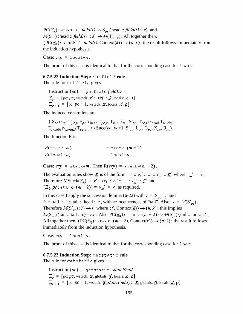
155

and . All together then,

; the result follows immediately from the induction hypothesis.

Case: .


6.7.5.22 Induction Step: SXWILHOG ruleThe rule for SXWILHOG gives

The induced constraints are

{ 6SF Etail�TSF,t, 6SF Ehead�TSF,v,�TSF,t Etail�S�SF, TSF,t Ehead TSF,obj,TSF,obj EILHOG,' TSF,v ` Succ(SF, SF+1, S�SF, LSF, GSF, XSF, RSF)

The function R is:

Case: . Then .

The evaluation rules show is of the form where . Therefore and

, as required.


Therefore where ; this implies . Also .

All together then, ; the result follows immediately from the induction hypothesis.

Case: .


6.7.5.23 Induction Step: JHWVWDWLF ruleThe rule for JHWVWDWLF gives

PC X N( )�VWDFN��ILHOG,' SSF head ILHOG,' e:: ::Æ Ö�

0 SSF( ) head ILHOG,' e:: ::Æ Ö 0 TSF v,( )�

PC X N( )�VWDFN��ILHOG,' Context N( ),( ) X [,( )�

H[S ORFDO�Q=

Instruction pc( ) SXWILHOG fieldID=X N pc: pc wstack: Y� ref 6 :: :: locals: / r, , ,[ ]=X N 1+ pc: pc 1+ wstack: 6 locals: / r, , ,[ ]=




6 Y0� Y1� ... YP� 6 �:: :: :: :: YP� Y=MStack X N( ) Y� ref Y0� ... YP� 6 �:: :: :: :: ::=

X N SF�VWDFN� P 2+( ),( ) YP�Ä Y=

W SSF 1+=F tail ... tail head e:: :: :: ::= P V 0 S�SF( )=


0 SSF( ) tail tail F:: ::Æ Ö W�� PC X N( )�VWDFN� P 2+( ) 0 SSF( ) tail tail F:: ::Æ Ö�


H[S ORFDO�Q=

Instruction pc( ) JHWVWDWLF�VWDWLF)LHOG=X N pc: pc wstack: 6 globals: * locals: / r, , , ,[ ]=X N 1+ pc: pc 1+ wstack: * VWDWLF)LHOG( ) 6 :: globals: * locals: / r, , , ,[ ]=

156


{ GSF EVWDWLF)LHOG 7SF�Y��S�SF Etail�6SF��S�SF Ehead�7SF�Y�`

Succ(SF, SF+1, S�SF, LSF, GSF, XSF, RSF).

The function R is:

Case: , . Then .

The proof for this case is identical to that for the corresponding case for ORDG.

Case: . Then .

The evaluation rules give and therefore .

In this case I apply the succession lemma (6-22) with and . Also, . Therefore where ; this

implies . Furthermore, and . All together then,


Case: .


6.7.5.24 Induction Step: SXWVWDWLF ruleThe rule for SXWVWDWLF gives


{ 6SF Etail�S�SF, SSF Ehead�7SF�Y� GSF EfieldID 7SF�Y�`

Succ(SF, SF+1, S�SF, LSF, GSF, XSF, RSF).

The function R is:

Case: . Then .

The proof for this case is identical to that for the corresponding case for VWRUH.

5 VWDFN�P( ) VWDFN� P 1–( )= P 0>

5 VWDFN��( ) VWDWLF)LHOG=



H[S VWDFN��= R H[S( ) VWDWLF)LHOG=

Y * VWDWLF)LHOG( )= X N SF�VWDWLF)LHOG,( ) YÄ

W SSF 1+= F head e::=V 0 S�SF( )= 0 S�SF( ) head e::Æ Ö W�� W� Context N( ),( ) X [,( )�

W� 0 TSF v,( )= PC X N( )�VWDWLF)LHOG GSF VWDWLF)LHOG e::Æ Ö�

0 GSF( ) VWDWLF)LHOG e::Æ Ö 0 TSF v,( )�

PC X N( )�VWDWLF)LHOG Context N( ),( ) X [,( )�

H[S ORFDO�Q=

Instruction pc( ) SXWVWDWLF fieldID=X N pc: pc wstack: Y� 6 :: locals: / r, , ,[ ]=X N 1+ pc: pc 1+ wstack: 6 locals: / r, , ,[ ]=




157

Case: .


6.7.5.25 Induction Step: LDGG ruleThe rule for LDGG gives


{ 6SF Etail�TSF,t1, TSF,t1 Etail�TSF,t2, S�SF Etail TSF,t2,�S�SF Ehead TSF,v `�

Succ(SF, SF+1, S�SF, LSF, GSF, XSF, RSF)

The function R is:

Case: . Then .

The evaluation rules show is of the form where . Therefore

and , as required.


Therefore where . This implies that is of the form where . This in turn implies . Also . All together then,


Case: .

Then by the definition of Creation, so the induction result is satisfied.

Case: .


6.7.5.26 Induction Step: LIFPSHT rulesThe rules for LIFPSHT give

is undefined

H[S ORFDO�Q=

Instruction pc( ) LDGG classID=X N pc: pc wstack: v1 v2 6 :: :: locals: / r, , ,[ ]=X N 1+ pc: pc 1+ wstack: Val v1( ) Val v2( )+ W,( ) 6 :: locals: / r, , ,[ ]=

5 VWDFN�P( ) VWDFN� P 1+( )= P 0>

5 VWDFN��( )



Val v1( ) Val v2( )+ W,( ) 6 ::Y0� Y1� ... YP� 6 �:: :: :: :: YP� Y=MStack X N( ) v1 v2 Y1� ... YP� 6 �:: :: :: :: ::= X N SF�VWDFN� P 1+( ),( ) YP�Ä Y=

W SSF 1+=F tail ... tail head e:: :: :: ::= P 0> V 0 S�SF( )=

0 S�SF( ) FÆ Ö W�� W� Context N( ),( ) X [,( )� F

tail F�:: 0 TSF t2,( ) F�Æ Ö W�� 0 SSF( ) tail tail F�:: ::Æ Ö W��

PC X N( )�VWDFN� P 1+( ) 0 SSF( ) tail F::Æ Ö�


H[S VWDFN��=

Creation Y( ) N 1+ SF 1+( )�VWDFN��,( )=

H[S ORFDO�Q=

158

where either or .


{ 6SF Etail�S�SF ` Succ(SF, SF+1, S�SF, LSF, GSF, XSF, RSF) Succ(SF, (CodeLocMethod(SF), RIIVHW), S�SF, LSF, GSF, XSF, RSF).

The function R is:

Case: .

The proof for this case is identical to that for the corresponding case for VWRUH. The successor lemma is applicable regardless of which branch is taken.

Case: .

The proof of this case is identical to that for the corresponding case for ORDG. The successor lemma is applicable regardless of which branch is taken.

6.7.5.27 Induction Step: JRWR ruleThe rules for JRWR give


Succ(SF, (CodeLocMethod(SF), RIIVHW), SSF, LSF, GSF, XSF, RSF)

The function R is:

Case: .

The evaluation rules show is of the form where . Therefore , as required.


Therefore where . Also

Instruction pc( ) LIBFPSHT offset=X N pc: pc wstack: Y� 6 :: locals: / r, , ,[ ]=X N 1+ pc: pc� wstack: 6 locals: / r, , ,[ ]=

pc� SF 1+= pc� CodeLocMethod pc( ) RIIVHW,( )=



H[S VWDFN�P=

H[S ORFDO�Q=

Instruction pc( ) JRWR offset=X N pc: pc wstack: 6 locals: / r, , ,[ ]=X N 1+ pc: CodeLocMethod pc( ) RIIVHW,( ) wstack: 6 locals: / r, , ,[ ]=

5 VWDFN�P( ) VWDFN�P( )=


H[S VWDFN�P=

6 Y0� Y1� ... YP� 6 �:: :: :: :: YP� Y=X N SF�VWDFN�P,( ) YP�Ä Y=

W SSF 1+=F tail ... tail head e:: :: :: ::= P V 0 S�SF( )=


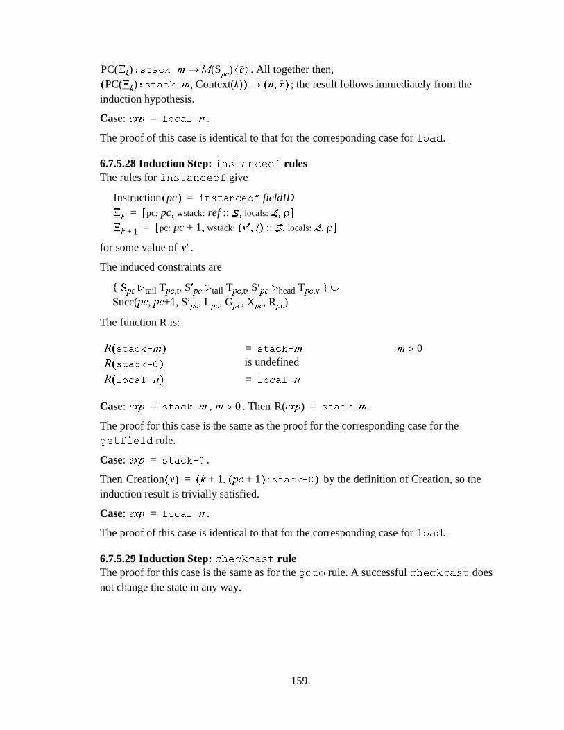
159

. All together then, ; the result follows immediately from the


Case: .


6.7.5.28 Induction Step: LQVWDQFHRI rulesThe rules for LQVWDQFHRI give

for some value of .


{ 6SF Etail�TSF,t, S�SF Etail TSF,t,�S�SF Ehead�TSF,v `

Succ(SF, SF+1, S�SF, LSF, GSF, XSF, RSF)

The function R is:

Case: , . Then .

The proof for this case is the same as the proof for the corresponding case for the JHWILHOG rule.

Case: .

Then by the definition of Creation, so the induction result is trivially satisfied.

Case: .


6.7.5.29 Induction Step: FKHFNFDVW ruleThe proof for this case is the same as for the JRWR rule. A successful FKHFNFDVW does not change the state in any way.

is undefined

PC X N( )�VWDFN�P 0 SSF( ) FÆ Ö�

PC X N( )�VWDFN�P Context N( ),( ) X [,( )�

H[S ORFDO�Q=

Instruction pc( ) LQVWDQFHRI fieldID=X N pc: pc wstack: ref 6 :: locals: / r, , ,[ ]=X N 1+ pc: pc 1+ wstack: Y� W,( ) 6 :: locals: / r, , ,[ ]=

Y�

5 VWDFN�P( ) VWDFN�P= P 0>

5 VWDFN��( )



H[S VWDFN��=

Creation Y( ) N 1+ SF 1+( )�VWDFN��,( )=

H[S ORFDO�Q=

160

161

7 SEMI Implementation

7.1 IntroductionChapter 6 describes the SEMI constraint system and how it is used to derive safe approxi-mations to the value-point relation. That chapter assumes the existence of an algorithm for deriving a closed set of constraints from a given initial set. In this chapter, I describe such an algorithm, as implemented in Ajax’s SEMI analysis engine.

First I describe the basic algorithm, and then I present a series of improvements to the algorithm that improve its performance. I also discuss some changes to the algorithm that I tried and rejected because they decreased performance.

Finally, I discuss some changes to the constraint generation phase that simplify the initial constraint set while leading to the same results.

7.1.1 Solver SpecificationGiven an initial constraint set CI, the job of the solver is simply to find a closed set C containing CI.

CI represents constraints induced by the program under analysis. C represents an extension of those constraints into a complete and consistent description of the “types” in the program.

Note that such a C always exists. For example, given CI, we can add constraints making all variables equal and making all component and instance relationships hold between all variables. (The resulting set is finite because only the variables, component labels and instance labels that occur in CI need be considered.) Effectively this gives all expressions the same type. In practice this result would not be useful — it is preferable to retain distinc-tions between types whenever possible. However, this example illustrates that implemen-tations of the specification can trade off accuracy for performance.

7.1.2 Decidability and PerformanceHenglein [42] shows that the problem of finding a principal (i.e., most general) type is undecidable in the general setting of polymorphic recursion. However, in practice all examples seem tractable. In fact, Henglein’s algorithm is reported to be quite efficient at inferring types for functional programs.

SEMI is similar to Henglein’s algorithm and likewise has no guarantee of termination. (In fact, because SEMI can infer recursive types, the situation is theoretically even more dire than for Henglein’s algorithm: typable programs exist that have no principal types. See Appendix A for details.) However, nonterminating cases have always been traced back to errors in the solver implementation. Because the worst cases may not even terminate,

162

efficiency depends on the characteristics of “average case” programs. Therefore we must measure performance and precision empirically.

In fact, the problem of finding a closed constraint set is not the same problem as finding principal types. As noted above, there is no unique solution to the problem of finding a closed set, and a trivial closed set can always be found.1 However, for the sake of precision we want the analysis to distinguish types whenever possible, just as we do when inferring principal types.

7.1.3 Refined SpecificationThe SEMI analysis engine extracts an approximate value-point relation from the closed set C. This relation is the only function of C that is used. Therefore we can relax the specifi-cation of the engine to allow it to produce any set C' that (for a given set Q of query expres-sions) gives the same relation as that derived from a closed set C. I will call such a set C' quasi-closed with respect to Q. This relaxation enables many optimizations.

The analysis engine actually computes a propagation graph from the constraint set and not a direct approximation to the value-point relation (see Section 6.6.1). However, as shown in Section 6.6, the results computed over the graph are completely determined by the approximate value-point relation defined for the constraint set. Therefore if C' induces the same approximate relation, the results obtained from the propagation graph on C' will be be the same as the results for C’s graph.

From the definition of the approximate value-point relation in Section 6.5.1, the analysis concludes H��H��LI�DQG�RQO\�LI

By the instance transitivity property (Lemma 6-7), this is equivalent to

Let M be a map from bytecode expressions to constraint variables, defined as where . is defined for all expressions in the query set Q; this is guaranteed by the precautions in Section 6.4.5. Then the analysis concludes H� � H��LI�DQG�RQO\�LI

From these definitions, it follows that C' is quasi-closed if there exists a C such that

• C is closed

• C contains CI

• "W��Y�³�9DULDEOHV�&,�� LQ�&�LI�DQG�RQO\�LI��LQ�C'�

1. For this reason, we could guarantee termination by timing out and falling back to an algorithm that is guaranteed to terminate. SEMI does not do this, however; choosing a suitable timeout interval and selecting an algorithm to fall back on appear to be rather complex problems.

X [1 [2 [1� [2�, , , , . H1 [1,( ) X [1�,( )� H2 [2,( ) X [2�,( )�¾$

X [1 [2, , . H1 [1,( ) X e,( )� H2 [2,( ) X e,( )�¾$

M H( ) X=F X�, . H X� FÆ Ö� X� FÆ Ö X�¾$ M H( )

X [1 [2, , . M H1( ) [1,( ) X e,( )� M H2( ) [2,( ) X e,( )�¾$

X [1 [2, , . W [1,( ) X e,( )� Y [2,( ) X e,( )�¾$X [1 [2, , . W [1,( ) X e,( )� Y [2,( ) X e,( )�¾$

163

7.1.4 Basic StructureThis chapter describes a series of algorithms leading up to the full SEMI algorithm, each more sophisticated than the last. All the algorithms commence with the initial constraint set CI and add constraints to the set until it is closed (or quasi-closed).

Because the addition of new constraints to the set is a fundamental operation in the algorithms, it is not difficult to extend these algorithms to be incremental. One can add to the initial constraint set CI at any time and then continue to add derived constraints until reaching (quasi-) closure.

7.2 Basic AlgorithmThe basic algorithm presented in this section corresponds to Henglein’s type inference procedure [42].

The general procedure is to start with a set of initial constraints (the input) and repeatedly add constraints to the set until it reaches closed form (the output). This is complicated by the fact that the initial constraint set can increase during processing, and the new constraints can be observed by tools as soon as they are added (i.e., the results are reported incremen-tally).

Therefore, in reality, the SEMI solver takes a set of constraints as input. If the set is already in closed form, it reports termination, otherwise it adds some constraints to the set and reports the changes in the output of the analysis. The added constraints are chosen to move the set “closer” to closure; that is, if the constraint set output by one step is always used as the input to the next step, the algorithm should terminate (although as discussed above, we cannot guarantee that it will terminate).

7.2.1 Representation of EqualityLike every algorithm of this kind, the SEMI solver uses a representation of the constraint set that avoids explicit equality constraints. Whenever a constraint of the form “ ” is encountered or produced, it is discarded, and the solver substitutes b for a (or a for b) in all other constraints. This can be implemented efficiently by treating each variable as an equiv-alence class and employing the union-find algorithm to merge equivalence classes.

7.2.2 Functional Representation of Components and Instances7KH�FRPSRQHQW�FRQVLVWHQF\�UXOH�JXDUDQWHHV�WKDW�IRU�D�JLYHQ�YDULDEOH�W�DQG�FRPSRQHQW�ODEHO�F��WKHUH�LV�DW�PRVW�RQH�Y�VXFK�WKDW� ��DIWHU�WDNLQJ�LQWR�DFFRXQW�HTXLYDOHQFLHV��7KXV�WKH�FRPSRQHQW�FRQVWUDLQWV�DUH�UHSUHVHQWHG�DV�D�FXUULHG�SDUWLDO�IXQFWLRQ�)

E��9 � /V 9�

/LNHZLVH�WKH�LQVWDQFH�FRQVWUDLQWV�DUH�UHSUHVHQWHG�DV�))��9 � ,V 9�

,Q�WKH�LPSOHPHQWDWLRQ��HDFK�YDULDEOH�Y�KDV�WZR�KDVK�WDEOHV�DVVRFLDWHG�ZLWK�LW��RQH�UHSUH�VHQWLQJ�)

E�Y��DQG�WKH�RWKHU�))�Y��

:KHQ�D�YDULDEOH�Y�LV�VXEVWLWXWHG�IRU�X�EHFDXVH�X�DQG�Y�KDYH�EHHQ�PDGH�HTXDO��X¶V�/�V�9�FRPSRQHQW�PDS�LV�PHUJHG�LQWR�Y¶V�/�V�9�FRPSRQHQW�PDS��7KH�WULFN\�SDUW�RI�WKLV�SURFHVV�LV�WKDW�IRU�HDFK�O�LQ�WKH�LQWHUVHFWLRQ�RI�WKHLU�GRPDLQV��WKH�YDULDEOH�)

E�X��O��LV�PDGH�HTXDO�WR�

D @ E

W EF Y

164

WKH�YDULDEOH�))�Y��O��WKXV��WKH�PHUJH�SURFHGXUH�FDQ�LQYRNH�LWVHOI�UHFXUVLYHO\��7KH�SURFHGXUH�FRUUHVSRQGV�WR�WHUP�XQLILFDWLRQ�

7KH�DOJRULWKP�DOVR�PHUJHV�X¶V�,�V�9�LQVWDQFH�PDS�LQWR�Y¶V�,�V�9�LQVWDQFH�PDS��7KLV�LV�VLPLODU�WR�WKH�FDVH�RI�WKH�FRPSRQHQW�PDSV��DQG�FDQ�DOVR�UHVXOW�LQ�UHFXUVLYH�PHUJH�FDOOV�

7.2.3 Component PropagationThe above normalization procedures ensure that the constraint set is always closed under all rules except for the component and instance propagation rules.

We treat the remaining rules as production rules:

• Component propagation

8SRQ�GHWHFWLQJ�^�W�)L�X��W EF Y `�²�&�IRU�VRPH�W��X��Y��L�DQG�F��DGG�D�QHZ�YDULDEOH�Z�DQG�FRQVWUDLQW�X�EF�Z��XQOHVV�WKHUH�LV�DOUHDG\�D�Z�VXFK�WKDW�X�EF�Z��

• Instance propagation

Upon detecting { t )i u, t Ec v, u Ec w } ² C for some t, u, v, w, i and c, add a constraint v )i w (if not already present).

7KHVH�DUH�LPSOHPHQWHG�XVLQJ�D�ZRUNOLVW��7KH�DOJRULWKP�PDLQWDLQV�D�OLVW�RI�³GLUW\´�FRPSRQHQW�FRQVWUDLQWV��H�J��³W EF Y´��WKDW�PXVW�EH�FKHFNHG�E\�WKH�FRPSRQHQW�SURSDJDWLRQ�UXOH��$OO�FRPSRQHQW�FRQVWUDLQWV�LQ�&,�VWDUW�RII�LQ�WKH�GLUW\�OLVW��:KHQHYHU�D�QHZ�FRPSRQHQW�FRQVWUDLQW�LV�DGGHG�WR�&,��LW�LV�DGGHG�WR�WKH�GLUW\�OLVW��:KHQHYHU�D�YDULDEOH�W�LV�VXEVWLWXWHG�IRU�DQRWKHU�YDULDEOH�Z��DOO�WKH�FRPSRQHQWV�RI�W�WKDW�GR�QRW�DOUHDG\�DSSHDU�LQ�Z�DUH�PDGH�GLUW\��DQG�OLNHZLVH�DOO�WKH�FRPSRQHQWV�RI�Z�WKDW�GR�QRW�DOUHDG\�DSSHDU�LQ�W�DUH�PDGH�GLUW\��)RUPDOO\�

^�W EF Y�_�^�W EF Y�`�²�&�¾��¤$X��^�Z EF X�`�²�&��`�

^�Z EF Y�_�^�Z EF Y�`�²�&�¾��¤$X��^�W EF X�`�²�&��`

$OVR��ZKHQHYHU�DQ�LQVWDQFH�FRQVWUDLQW�W�)L�X�LV�DGGHG��DOO�WKH�FRPSRQHQWV�RI�W�DQG�X�DUH�PDGH�GLUW\�

'XULQJ�HDFK�LWHUDWLRQ�RI�WKH�VROYHU��LW�SXOOV�RQH�GLUW\�FRPSRQHQW�FRQVWUDLQW�W EF Y�IURP�WKH�GLUW\�OLVW��7KHQ�IRU�HDFK�X�DQG�L�VXFK�WKDW�^�W�)L�X�`�²�&��WKH�WZR�SURGXFWLRQ�UXOHV�DUH�FKHFNHG��$OVR��IRU�HDFK�X�DQG�L�VXFK�WKDW�^�X�)L�W�`�²�&��WKH�VHFRQG�SURGXFWLRQ�UXOH�LV�FKHFNHG��VZDSSLQJ�X�ZLWK�W�DQG�Y�ZLWK�Z so that the actual rule checked is

• Upon detecting { u )i t, u Ec w, t Ec v } ² C for some t, u, v, w, i and c, add a constraint w )i v (if not already present).

Note that when checking this rule, since u and c are known, there can be at most one appli-cable w.

Iteration continues until the worklist of dirty component constraints is empty. Upon termi-nation, the constraint set is closed.

When an equality constraint is processed by applying a substitution to the entire constraint set, the same substitution is applied to the elements of the worklist. Of course, this is done efficiently using a union-find data structure.

165

7.2.4 Saving Time By Recording Additional Dirtiness Information)RU�VRPH�YDULDEOHV�W�WKHUH�PD\�EH�PDQ\�X�VXFK�WKDW�W�)L�X�RU�X�)L�W��:KHQ�D�GLUW\�FRPSRQHQW�W EF Y�LV�EHLQJ�SURFHVVHG��LW�FDQ�EH�VORZ�WR�VFDQ�DOO�WKH�LQVWDQFHV�X�VXFK�WKDW�W )L�X�DQG�DOO�WKH�VRXUFHV�X�VXFK�WKDW�X�)L�W��7KHUHIRUH�IRU�HDFK�GLUW\�FRPSRQHQW�W EF Y��ZH�PDLQWDLQ�D�OLVW�RI�DOO�WKH�W )L�X�DQG�X�)L�W�WKDW�QHHG�WR�EH�LQVSHFWHG�LQ�FRQMXQFWLRQ�ZLWK�WKH�W EF Y�FRQVWUDLQW��)RU�HYHU\�VLWXDWLRQ�LQ�ZKLFK�D�FRPSRQHQW�FRQVWUDLQW�PD\�EHFRPH�GLUW\��WKHUH�LV�DQ�DVVRFLDWHG�VHW�RI�LQVWDQFH�DQG�VRXUFH�FRQVWUDLQWV�WKDW�ZLOO�QHHG�WR�EH�LQVSHFWHG�

:KHQ�D�QHZ�FRPSRQHQW�FRQVWUDLQW�W EF Y�LV�DGGHG��DOO�FRQVWUDLQWV�RI�WKH�IRUP�W )L�X�DQG�X )L W�QHHG�WR�EH�LQVSHFWHG�LQ�FRQMXQFWLRQ�ZLWK�W EF Y�

:KHQ�D�YDULDEOH�W�LV�VXEVWLWXWHG�IRU�YDULDEOH�Z��WKHQ�IRU�HDFK�W EF Y�VXFK�WKDW�̂ W EF Y�`�² &�¾��¤$X��^�Z EF X�̀ �²�&��DOO�FRQVWUDLQWV�RI�WKH�IRUP�Z )L�X�DQG�X )L Z�QHHG�WR�EH�LQVSHFWHG�LQ�FRQMXQFWLRQ�ZLWK�W EF Y��/LNHZLVH��IRU�HDFK�Z EF Y�VXFK�WKDW�^ Z EF Y�`�²�&�¾��¤$X� ^ W EF X�`�²�&��DOO�FRQVWUDLQWV�RI�WKH�IRUP�W )L�X�DQG�X )L W�QHHG�WR�EH�LQVSHFWHG�LQ�FRQMXQFWLRQ�ZLWK�Z EF Y�

:KHQHYHU�DQ�LQVWDQFH�FRQVWUDLQW�W�)L�X�LV�DGGHG��WKHQ�IRU�HDFK�W EF Y�LQ�&��WKH�LQVWDQFH�FRQVWUDLQW�W�)L�X�PXVW�EH�LQVSHFWHG�LQ�FRQMXQFWLRQ�ZLWK�W EF Y��$OVR��IRU�HDFK�X EF Y�LQ�&��WKH�VRXUFH�FRQVWUDLQW�W�)L�X�PXVW�EH�LQVSHFWHG�LQ�FRQMXQFWLRQ�ZLWK�X EF Y�

This additional bookkeeping greatly improves runtime, while adding some space overhead.

7.2.5 Overview of an Algorithm StepAn iteration of the solver proceeds as follows:

1. Remove a dirty component constraint W EF Y�from the worklist, with its associated sets of dirty source constraints S and dirty instance constraints I.

2. For each dirty source constraint X�)L�W�in S, we have ^ X�)L�W, W EF Y�`�²�&��(DFK�SURGXF�WLRQ�UXOH�KDV�SUHPLVHV�RI�WKH�IRUP�3�²�&��)RU�HDFK�UXOH��DQG�IRU�HDFK�LQVWDQWLDWLRQ�RI�WKH�IUHH�YDULDEOHV�RI�3�VXFK�WKDW�^ X�)L�W, W EF Y�`�²�3 and 3�²�&, SEMI applies the rule to obtain a set of constraints that must be included in the new constraint set. Each new constraint not already in the set is added and the dirty worklist is updated appropriately.

3. For each dirty instance constraint W�)L�X�in I, we have ^ W�)L�X, W EF Y�`�²�&��)RU�HDFK�SURGXFWLRQ�UXOH��DQG�IRU�HDFK�LQVWDQWLDWLRQ�RI�WKH�IUHH�YDULDEOHV�RI�WKH�UXOH¶V�SUHPLVHV�3�VXFK�WKDW�^ W�)L�X, W EF Y�`�²�3 and 3�²�&, SEMI applies the rule to obtain a set of con-straints to add, as above.

For each rule, it is easy to determine the possible values of P given that ^ X�)L�W, W EF Y�`�²�3 or ^ W�)L�X, W EF Y�`�²�3.

Consider the component propagation rule. P is of the form ̂ T�)L�U, T EF V `. When checking dirty instances, we have ^ W�)L�X, W EF Y�`�²�3. The only possibility is 3� �^ W�)L�X, W EF Y `��VR�WKH�FRQVHTXHQFH�RI�WKH�UXOH�LV� ��:KHQ�FKHFNLQJ�GLUW\�VRXUFHV��ZH�KDYH�^ X�)L�W, W EF Y�`�²�3.�7KH�RQO\�SRVVLELOLW\�LV�3� �^ X�)L�W, W EF Y `��EXW�WKHQ�VLQFH�3�LV�RI�WKH�IRUP�^ T�)L�U, T EF V `��ZH�PXVW�KDYH�X = W and 3� �^ W�)L�W, W EF Y `��,Q�WKLV�FDVH�WKH�FRQVHTXHQFH�RI�WKH�UXOH�� LV�DOUHDG\�VDWLVILHG�ZLWK�Z� �Y��DQG�VR�WKLV�FDVH�QHHG�QRW�EH�FKHFNHG�

Z . X EF Z{ } &²$

Z . W EF Z{ } &²$

166

Consider the instance propagation rule. 3 is of the form�^ T�)L�U, T EF V, r Ec z `��When checking dirty instances, we have ^ W�)L�X, W EF Y�`�²�3. The only possibility is that 3� �^ W )L X, W EF Y, u Ec z `�IRU�VRPH�]��6LQFH�X�DQG�F�DUH�NQRZQ��WKHUH�FDQ�RQO\�EH�RQH�SRVVLEOH�YDOXH�IRU�Z�DQG�LW�FDQ�EH�IRXQG�E\�LQVSHFWLQJ�&��L�H��3�LV�FRPSOHWHO\�GHWHUPLQHG��:KHQ�FKHFNLQJ�GLUW\�VRXUFHV��ZH�KDYH�^ X�)L�W, W EF Y�`�²�3�and WKH�RQO\�SRVVLELOLW\�LV�WKDW�3� �^ X )L�W, u Ec s, W EF Y `�IRU�VRPH�V. Again X and F are known, so the value of V is determined.

Subsequent sections describe enhancements to the basic algorithm which introduce new rules, but in each case it is just as easy to determine how the variables of the rules are to be instantiated.

7.2.6 The Extended Occurs CheckIt is easy to construct constraint sets for which this algorithm does not terminate. Furthermore, these sets do arise in practice.

)RU�H[DPSOH��FRQVLGHU�WKH�VHW�̂ 7I EUHVXOW 7U� 7I )L 7U `��7KLV�FRXOG�DULVH�IURP�DQ�DQDO\VLV�RI�WKH�IROORZLQJ�SURJUDP�

I��^�UHWXUQ�I��`

I¶V�UHVXOW�LV�DQ�LQVWDQFH�RI�I��7KLV�LV�D�FRQWULYHG�H[DPSOH��5HDO�H[DPSOHV�LQ�-DYD�DUH�PRUH�FRPSOLFDWHG��H�J��D�PHWKRG�0�WKDW�UHWXUQV�D�UHIHUHQFH�WR�D�QHZ�REMHFW�ZKLFK�FRQWDLQV�0��

Suppose we apply the above algorithm to this constraint set:

• $SSO\�FRPSRQHQW�SURSDJDWLRQ�WR�^�7I EUHVXOW 7U� 7I )L 7U�`�DGG�7��DQG�FRQVWUDLQW�^�7U�EUHVXOW 7��`

• $SSO\�LQVWDQFH�SURSDJDWLRQ�WR�^�7I EUHVXOW 7U� 7I )L 7U��7U�EUHVXOW 7��`�DGG�FRQVWUDLQW�^�7U�)L 7��`

• $SSO\�FRPSRQHQW�SURSDJDWLRQ�WR�^�7U EUHVXOW 7�� 7U )L 7��`�DGG�7��DQG�FRQVWUDLQW�^�7��EUHVXOW7��`

• $SSO\�LQVWDQFH�SURSDJDWLRQ�WR�^�7U EUHVXOW 7�� 7U )L 7��7��EUHVXOW 7��`�DGG�FRQVWUDLQW�^�7��)L 7��`

• …

,Q�W\SH�LQIHUHQFH��WKH�W\SH�RI�I�ZRXOG�EH�DQ�LQILQLWH�WHUP�

YRLG��YRLG��YRLG � «��

This recursive type is not valid in Henglein’s scheme; therefore his algorithm detects this situation and reports failure. He calls this detection the “extended occurs check”. (It is analogous to the occurs check performed during term unification.) In terms of the SEMI formalism, the extended occurs check fires whenever, for some sets of variables ti and ui:

^�W��)L��X��«��XQ��)LQ�XQ��W��EFRPS��W��«��WP�EFRPSQ�XQ�`�²�&

This means that the extended occurs check is applicable whenever we have a variable t1 with a transitive instance un which is also transitively a component of t1.

When the extended occurs check fires in SEMI, the solver simply forms a recursive type by adding the constraint , and continues. In the example, the extended occurs check W1 @ XQ

167

detects the constraints ^�7I EUHVXOW 7U� 7I )L 7U�̀ and adds the constraint , halting the expansion.

Note that adding this equality forces variables to be equal that do not necessarily need to be equal according to the initial constraints. This is why SEMI does not compute a most general (i.e., principal) solution. The demonstration of non-existence of principal types in Appendix A is based on a similar example.

7KH�LPSOHPHQWDWLRQ�RI�WKH�6(0,�VROYHU�SHUIRUPV�DQ�H[WHQGHG�RFFXUV�FKHFN�ZKHQHYHU�WKH�LQVWDQFH�SURSDJDWLRQ�UXOH�DGGV�D�QHZ�LQVWDQFH�FRQVWUDLQW�W�)L�X�WR�&��,W�VHWV�XQ�� W��XQ X��DQG�LQ� �L��DQG�WKHQ�VHDUFKHV�WKH�FRPSRQHQW�DQG�LQVWDQFH�JUDSKV�IRU�D�YDULDEOH�W��VDWLVI\LQJ�WKH�FKHFN��$Q\�VXFK�YDULDEOHV�IRXQG�DUH�ERXQG�WR�X��7KH�VHDUFK�SURFHHGV�E\�ILUVW�VFDQQLQJ�WKH�LQVWDQFH�JUDSK�EDFNZDUGV��ILQGLQJ�DOO�FDQGLGDWH�W�V�WKDW�DUH�WUDQVLWLYH�VRXUFHV�RI�W��LQFOXGLQJ�W�LWVHOI��DQG�IRU�HDFK�FDQGLGDWH��VFDQQLQJ�LWV�FRPSRQHQWV�WUDQVLWLYHO\�ORRNLQJ�IRU�X�

This check could easily be changed from worst case O(N2) time, where N is the number of variables, to O(N) time, simply by finding all transitive sources of t first, storing them in a hashtable-based set, then scanning all of t’s transitive parents (variables that have t as a transitive component) and testing for membership in the set. In practice, however, the average numbers of transitive instances, sources, components or parents that a variable has are all very large, and a check that is linear time in any of these quantities is prohibitively expensive (since the extended occurs check is performed frequently). Therefore SEMI uses a more complex approach, described below, which builds on the basic algorithm above. It turns out that with the help of those optimizations, the worst case O(N2) version performs significantly better.

7.2.7 NondeterminismThe algorithm presented here is nondeterministic, as are all the following elaborations and the implementation itself. There is always flexibility in choosing the order in which to remove constraints from the worklist. Different orderings can lead to different results of the algorithm, because the extended occurs check may fire at different times and induce different equality constraints.

The implementation also produces non-deterministic results because it is written in Java, and Java’s semantics does not fully define the behavior of the implementation. In particular, the “identity hash code” of an object is not defined by the Java language speci-fication. The identity hash code is returned by the default implementation of 2EMHFW�KDVK&RGH��; the only requirement is that it always return the same value for any given object. When the same program is run multiple times on the same Java virtual machine implementation, the identity hash codes assigned to its objects are often observed to vary between runs. This leads to observable variations in behavior, because the enumer-ation order of the elements of hash tables and related data structures depends on the values of the identity hash codes.

In practice, Ajax almost always returns the same results for multiple runs of a given query.

Tr @ Tf

168

7.3 Optimizing the Occurs Check: ClustersThe naïve approach to performing the extended occurs check can be sped up by exploiting the structure of constraints induced by a Java program (or any program that has layers in its architecture, i.e., almost all programs).

7.3.1 Constraint StructureSEMI generates instance constraints from a Java program in the following situations:

• A method body M1 makes a “static” call to another method M2 (M1 depends on M2).

• A method body M1 creates a new object of a class C (M1 depends on C).

• A method body M1 is installed in the dynamic dispatch table of a class C (C depends on M1).

Due to the layered structure of most programs, the graph of dependencies is “mostly” acyclic. (However, the JDK class library itself contains a number of surprisingly complex cycles, so it is important to be able to handle cycles well.)

7.3.2 ClustersNormally (i.e., in the absence of a cycle of mutually recursive dependencies), the variables associated with parameters, local variables, results, and intermediate values within a given method, and variables which are components of those variables, are related only by component constraints. Instance constraints (and only instance constraints) relate these variables to variables associated with other methods. Similarly, in a class there are variables associated with the method slots, and a variable for the prototype object of the class, which are related to each other by component constraints only. Instance constraints relate these variables to variables in the methods that create objects of the class, and to variables in the method bodies used by the class.

7KH�6(0,�VROYHU�H[SOLFLWO\�FDSWXUHV�WKLV�VWUXFWXUH��7KH�YDULDEOHV�DUH�SDUWLWLRQHG�LQWR�DEVWUDFW�FOXVWHUV��WKH�SDUWLWLRQ�LV�ZULWWHQ�5��9 � ;��ZKHUH�;�LV�WKH�VHW�RI�FOXVWHU�ODEHOV��7KH�RQO\�UHTXLUHG�SURSHUW\�RI�5�LV�WKDW�LI�W�EF�X�LV�D�FRQVWUDLQW��WKHQ�5�W�� 5�X��,Q�RWKHU�ZRUGV��DOO�YDULDEOHV�UHODWHG�E\�RQO\�FRPSRQHQW�FRQVWUDLQWV�DUH�LQ�WKH�VDPH�FOXVWHU��7\SLFDOO\��-DYD�SURJUDPV�JLYH�ULVH�WR�D�ODUJH�QXPEHU�RI�VPDOO�FOXVWHUV��RQH�FOXVWHU�SHU�PHWKRG��

,W�LV�QRW�VWULFWO\�QHFHVVDU\�WR�KDYH�5�EH�WKH�PRVW�UHILQHG�SDUWLWLRQ�SRVVLEOH��EXW�WKDW�LV�HDV\�WR�LPSOHPHQW�DQG�JLYHV�WKH�EHVW�UHVXOWV��7KDW�LV��LI�W�DQG�X�DUH�QRW�UHODWHG�E\�DQ\�FKDLQ�RI�FRPSRQHQW�FRQVWUDLQWV��LJQRULQJ�GLUHFWLRQ��WKHQ�5�W��5�X��

The implementation maintains the cluster map dynamically, taking account of variable merging and the introduction of new constraints.

7.3.3 Optimizing the Extended Occurs Check Using Clusters7KH�FOXVWHU�PDS�LV�XVHG�WR�VKRUW�FLUFXLW�WKH�VXEURXWLQH�WKDW�FRPSXWHV�³,V�X�D�WUDQVLWLYH�FRPSRQHQW�RI�W�"´�,I�5�X��5�W��WKHQ�WKH�UHVXOW�PXVW�EH�IDOVH��6LQFH�FOXVWHUV�DUH�JHQHUDOO\�VPDOO�DQG�QXPHURXV��DQG�IROORZLQJ�DQ�LQVWDQFH�FRQVWUDLQW�XVXDOO\�OHDGV�WR�DQRWKHU�

169

�GLIIHUHQW��FOXVWHU��5�X��5�W��DOPRVW�DOZD\V�KROGV�GXULQJ�WKH�H[WHQGHG�RFFXUV�FKHFN�VHDUFK�

7.3.4 Cluster LevelsUnfortunately, even scanning all transitive sources of a variable and performing a constant-time check for each is too expensive, given the frequency with which extended occurs checks are performed.

6(0,�UHVROYHV�WKLV�SUREOHP�E\�H[SOLFLWO\�FDSWXULQJ�WKH�³PRVWO\�DF\FOLF´�VWUXFWXUH�RI�WKH�LQWHU�FOXVWHU�LQVWDQFH�JUDSK��7KH�LQVWDQFH�FRQVWUDLQWV�DUH�SURMHFWHG�RQWR�WKH�FOXVWHUV��L�H��WKH�FOXVWHUV�DUH�DVVHPEOHG�LQWR�D�GLUHFWHG�JUDSK�*�VXFK�WKDW�IRU�HDFK�W�)L�X��5�W��5�X��LV�DQ�HGJH�LQ�*��7KHQ�WKH�JUDSK�LV�SDUWLWLRQHG�LQWR�VWURQJO\�FRQQHFWHG�FRPSRQHQWV��FDOOHG�FOXVWHU�OHYHOV��7KLV�SDUWLWLRQ�LV�ZULWWHQ�6��; � =��ZKHUH�=�LV�WKH�VHW�RI�FOXVWHU�OHYHO�ODEHOV��%\�GHILQLWLRQ��*�SURMHFWHG�RQWR�FOXVWHU�OHYHOV�LV�DF\FOLF��H[FOXGLQJ�VHOI�ORRSV��7KH�IDFW�WKDW�*�LWVHOI�LV�³PRVWO\�DF\FOLF´�PHDQV�WKDW�PRVW�FOXVWHU�OHYHOV�FRQWDLQ�MXVW�RQH�FOXVWHU�

The implementation maintains the cluster levels dynamically, as the underlying constraint system changes. SEMI does this efficiently, but the implementation is tricky because detecting cycles can be expensive. It is helpful to delay cycle detection until the cluster levels are required to be in a consistent (acyclic) state (i.e., until the next extended occurs check). SEMI maintains a “dirty” bit for each cluster level, indicating that it may be part of a cycle of cluster levels because of the addition of new instance constraints incident to the cluster level. When acyclicity is required, the algorithm performs a worst-case linear time traversal of the cluster level graph — a depth-first search backwards along the instance edges, starting from the dirty cluster levels. Any cycles found are recorded. Finally, the cluster levels in each cycle are merged. It requires care to make sure that all cycles are detected, since the straightforward depth-first search algorithm for cycle detection is only guaranteed to find one cycle (assuming a cycle exists).

In SEMI, the cost of maintaining the cluster levels is usually negligible and never the performance bottleneck.

7.3.5 Optimizing the Extended Occurs Check Using Cluster LevelsThe cluster level map is used to optimize the subroutine that scans the source graph for all candidate t1s that are transitive sources of t.

7KH�H[WHQGHG�RFFXUV�FKHFN�VXEURXWLQH�UHFHLYHV�W�DQG�X�ZKHUH�X�LV�DQ�LQVWDQFH�RI�W��7KHUHIRUH�HYHU\�FDQGLGDWH�W��KDV�X�DV�D�WUDQVLWLYH�LQVWDQFH��1RZ�VXSSRVH�IRU�VRPH�FDQGLGDWH�t1��6�5�X��6�5�W��7KHUH�PXVW�EH�D�SDWK�IURP�6�5�W��WR�6�5�X��LQ�WKH�LQVWDQFH�JUDSK�SURMHFWHG�RQWR�WKH�FOXVWHU�OHYHOV��EHFDXVH�WKHUH�LV�D�SDWK�IURP�W��WR�X�LQ�WKH�LQVWDQFH�JUDSK��%HFDXVH�WKH�FOXVWHU�OHYHO�LQVWDQFH�JUDSK�LV�DF\FOLF��WKHUH�FDQQRW�EH�D�SDWK�IURP�6�5�X��WR�6�5�W��7KHUHIRUH��IRU�DOO�WUDQVLWLYH�VRXUFHV�V�RI�W��6�5�V��6�5�X��DQG�WKHUHIRUH�5�V� � 5�X��EHFDXVH�RWKHUZLVH�ZH�ZRXOG�KDYH�DQ�LQVWDQFH�SDWK�IURP�6�5�V�� 6�5�X��WR�6�5�W��

7KHUHIRUH��ZKHQHYHU�WKH�H[WHQGHG�RFFXUV�FKHFN�VXEURXWLQH�GHWHFWV�6�5�X��6�5�W��W�¶V�VRXUFHV�QHHG�QRW�EH�VHDUFKHG��,Q�SUDFWLFH�WKLV�SUXQHV�WKH�VHDUFK�WUHPHQGRXVO\��,Q�SDUWLFXODU��LI�6�5�X��6�5�W��WKHQ�QHLWKHU�W�QRU�LWV�VRXUFHV�QHHG�EH�FKHFNHG��WKH�HQWLUH�FKHFN�WDNHV�FRQVWDQW�WLPH�

170

In the special case in which there are no recursive dependencies in the original program, the instance graph projected onto clusters is acyclic, i.e., S is one-to-one. Then the extended occurs check always completes in constant time. In other words, this optimization ensures that the extended occurs check only incurs a cost (apart from the cost of maintaining the clusters and cluster levels) when polymorphic recursion is actually being used.

7.3.6 Replacing the Extended Occurs Check with a Conservative Approximation,Q�WKH�FDVH�6�5�X�� 6�5�W��LQVWHDG�RI�SHUIRUPLQJ�WKH�UHVW�RI�WKH�H[WHQGHG�RFFXUV�FKHFN��RQH�FRXOG�VLPSO\�DGG�WKH�HTXDOLW\�FRQVWUDLQW� ��7KH�QHZ�LQVWDQFH�FRQVWUDLQW�W�)L�X�LV�UHGXFHG�WR�D�VHOI�ORRS�LQ�WKH�LQVWDQFH�JUDSK��ZKLFK�IRUHVWDOOV�WKH�QRQWHUPLQDWLQJ�EHKDYLRU�WKDW�WKH�H[WHQGHG�RFFXUV�FKHFN�LV�GHVLJQHG�WR�SUHYHQW��7KLV�DSSURDFK�LV�VLPLODU�WR�WKH�+LQGOH\�0LOQHU�DOJRULWKP��ZKLFK��LQWHUSUHWHG�LQ�WKLV�FRQWH[W��SURKLELWV�DQ\�SRO\PRUSKLVP�FRQVWUDLQWV�ZLWKLQ�D�FOXVWHU�OHYHO��7KLV�EHKDYLRU�FDQ�OHDG�WR�VPDOOHU�FRQVWUDLQW�VHWV�EHFDXVH�RI�WKH�³XQQHFHVVDU\´�HTXDOLWLHV�WKDW�DUH�LQWURGXFHG��ZKLFK�LPSURYHV�SHUIRUPDQFH�EXW�GRHV�\LHOG�D�QRWLFHDEOH�GHFUHDVH�LQ�DFFXUDF\�IRU�VRPH�DSSOLFDWLRQV�RI�WKH�DQDO\VLV�

7.4 Scheduling the Worklist Using Cluster LevelsIt turns out that the acyclic cluster level graph is useful for tasks other than optimizing the extended occurs check.

7.4.1 The Scheduling ProblemComponents propagate from sources to instances, but not the other way around. Therefore as changes are made to constraints at the “bottom” of the instance graph, they tend to “bubble up” to instances. It improves performance to do as much work as possible at the bottom of the instance graph before making changes further up the graph, by reducing the number of times each component is visited or examined.

7.4.2 Using Cluster Levels$�FOXVWHU�OHYHO�O�LV�³GLUW\´�LI�WKHUH�LV�D�FRPSRQHQW�FRQVWUDLQW�LQ�WKH�ZRUNOLVW�RI�WKH�IRUP�W EF X��ZKHUH�6�5�W�� O�

:KHQHYHU�6(0,�FKRRVHV�D�FRPSRQHQW�FRQVWUDLQW�IURP�WKH�ZRUNOLVW��LW�FKRRVHV�D�FRQVWUDLQW�W EF X�ZKHUH�WKH�FOXVWHU�OHYHO�6�5�W��KDV�QR�GLUW\�FOXVWHU�OHYHOV�EHORZ�LW�LQ�WKH�LQVWDQFH�JUDSK�SURMHFWHG�RQWR�WKH�FOXVWHU�OHYHOV��6XFK�D�FRQVWUDLQW�LV�JXDUDQWHHG�WR�H[LVW�EHFDXVH�WKH�FOXVWHU�OHYHO�LQVWDQFH�JUDSK�LV�DF\FOLF�

Making this choice efficiently is tricky, but requires negligible time and space in the SEMI implementation. The dirty component constraints are stored on the worklist indexed by cluster levels; the problem reduces to finding an appropriate cluster level to work on. SEMI explicitly records the dirtiness of each cluster level. It also caches two facts in each cluster level: whether it is known that there is at least one dirty cluster level below it in the cluster level instance graph, and whether it is known that there are no dirty cluster levels below it in the graph. In practice, this cache can be updated and invalidated efficiently in response to changes in dirty state and changes in the underlying constraint set.

W @ X

171

The system keeps a list of dirty cluster levels, separated into two parts: the set of dirty cluster levels that are known to have no dirty cluster levels below them on the projected instance graph (the “ready list”), and the rest (the “blocked list”). When a constraint is selected from the worklist, if the ready list is non-empty then a cluster level is chosen from it and one of the cluster level’s dirty constraints is selected.

If the ready list is empty, then a cluster level l is chosen from the blocked list. The algorithm performs a depth-first search of the cluster level instance graph, backwards from l, from instances to sources. During this search, each visited cluster level is marked as either having dirty cluster levels below it, or not. If not, then the visited cluster level is moved from the blocked list to the ready list. The acyclicity of the cluster level instance graph guarantees that after this procedure, at least one dirty cluster level will be found with no dirty cluster levels below it (unless there are no dirty cluster levels left, in which case the algorithm terminates).

7.5 Suppressing Components: Advertisements

7.5.1 Useless Component Propagation6XSSRVH�)�LV�D�IXQFWLRQ�LQ�WKH�SURJUDP�IRU�ZKLFK�ZH�LQIHU�D�ODUJH�³W\SH´��7)��7KLV�PHDQV�WKDW�7)�LV�WKH�URRW�RI�D�ODUJH�JUDSK�RI�FRPSRQHQW�FRQVWUDLQWV��$W�HYHU\�XVH�RI�)��D�GLUHFW�FDOO�RU�WKH�XVH�RI�)�WR�ILOO�D�VORW�LQ�D�PHWKRG�WDEOH��D�QHZ�LQVWDQFH�L�RI�7)�LV�FUHDWHG��DQG�D�FRQVWUDLQW�7)�)L�W�LV�DGGHG��7KH�FRPSRQHQW�SURSDJDWLRQ�UXOH�ZLOO�HIIHFWLYHO\�FRS\�WKH�WUDQVLWLYH�FRPSRQHQWV�RI�7)��L�H��WKH�FRPSRQHQW�JUDSK�XQGHU�7)��WR�WKH�LQVWDQFH��2IWHQ��KRZHYHU��PXFK�RI�WKLV�VWUXFWXUH�ZLOO�QRW�EH�XVHG��)RU�H[DPSOH��FRQVLGHU�WKLV�-DYD�FRGH�

)RR�[� �EDU��

SULQWOQ�[�NLWW\��

*LYHQ�WKH�FRGH�IRU�EDU��WKH�DQDO\VLV�PD\�ZRUN�RXW�VRPH�FRPSOH[�W\SH�VWUXFWXUH�IRU�LWV�UHWXUQ�YDOXH��LQFOXGLQJ�LQIRUPDWLRQ�DERXW�WKH�YDULRXV�PHWKRGV�DQG�ILHOGV�RI�[��$OO�WKLV�LQIRUPDWLRQ�ZLOO�EH�SURSDJDWHG�WR�WKH�FDOOHU��EXW�RQO\�RQH�ILHOG�LV�XVHG��DQG�WKHUHIRUH�WKH�UHVW�RI�WKH�LQIRUPDWLRQ�LV�LUUHOHYDQW�

)XUWKHUPRUH��VXSSRVH�EDU�LV�LPSOHPHQWHG�DV�D�ZUDSSHU�

)RR�EDU��^�UHWXUQ�ED]��`

Such constructs are common, and defeat purely local schemes for suppressing useless structure.

7.5.2 Illustration&RQVLGHU�WKH�FRQVWUDLQW�VHW�4�VKRZQ�LQ�)LJXUH ��7KLV�GLDJUDP�DQG�WKH�GLDJUDPV�WKDW�IROORZ�UHSUHVHQW�FRQVWUDLQW�VHWV�DV�JUDSKV��1RGHV�FRUUHVSRQG�WR�YDULDEOHV��$�FRQVWUDLQW�RI�WKH�IRUP�W�EF X�LV�GLVSOD\HG�DV�D�VROLG�HGJH�IURP�W¶V�QRGH�WR�X¶V�QRGH�ODEHOOHG�ZLWK�EF��$�FRQVWUDLQW�RI�WKH�IRUP�W )L X�LV�GLVSOD\HG�DV�D�GRWWHG�HGJH�IURP�W¶V�QRGH�WR�X¶V�QRGH�ODEHOOHG�ZLWK�)L�

172

T represents the type of some compound object with an instance i and further instances j and k. Assume Q contains the initial constraint set, CI. The basic algorithm extends Q to the closed set C shown in Figure 7-2�

The basic algorithm reaches C by copying T’s component tree to all the instances, and connecting the components with instance relationships.

7.5.3 Quasi-closure ConditionsThese new components are all unnecessary — Q is, in fact, quasi-closed. To see this, consider two variables in CI, u and v. We must show that u and v are related in Q if and only if they are related in C.

Figure 7-1. Initial constraint set

Figure 7-2. Closed constraint set

EF EG

EH EI EJ EK

)L

)M

)NT

EF EG

EH EI EJ EK

EF EG

EH EI EJ EK

EF EG

EH EI EJ EK

EF EG

EH EI EJ EK

)L

)M

)NT

173

The notation “X ) Y” means that there is a chain of instance constraints from X to Y.

There are two cases:

• 6XSSRVH�X�DQG�Y�DUH�QRW�UHODWHG�LQ�&��7KHQ�½$[��X�)&�[�¾�Y�)&�[��,W�IROORZV�WKDW�½$[� X )4�[�¾�Y�)4�[��VLQFH�&�LV�D�VXSHUVHW�RI�4��7KHUHIRUH�X�DQG�Y�DUH�QRW�UHODWHG�LQ�4�

• 6XSSRVH�X�DQG�Y�DUH�UHODWHG�DFFRUGLQJ�WR�&��7KHQ�$[��X�)&�[�¾�Y�)&�[��:H�VKRZ�WKDW�$S� X )4�S�¾�Y�)4�S��E\�LQGXFWLRQ�RQ�WKH�OHQJWK�RI�WKH�VKRUWHVW�FKDLQ�RI�LQVWDQFHV�MXVW�IL\LQJ�X )& [�5HJDUGOHVV�RI�WKH�OHQJWK�RI�WKH�FKDLQ��LI�[�RFFXUV�LQ�4��WKHQ�X�)4�[�¾�Y�)4�[��VLQFH�WKH�FKDLQV�RI�LQVWDQFHV�MXVWLI\LQJ�X�)&�[�DQG�Y�)&�[�DUH�DOVR�LQ�4��,Q�RWKHU�ZRUGV��HYHU\�LQVWDQFH�FRQVWUDLQW�LQ�&�WKDW�KROGV�EHWZHHQ�YDULDEOHV�LQ�4�LV�LV�DOUHDG\�LQ�4��7KXV�WKH�LQGXFWLRQ�K\SRWKHVLV�KROGV��VHWWLQJ�S� �[�,I�WKH�OHQJWK�RI�WKH�FKDLQ�LV�]HUR��WKHQ�[� �X��KHQFH�[�LV�LQ�4�DQG�WKH�K\SRWKHVLV�KROGV�,I�[�LV�QRW�LQ�4��WKHQ�LW�PXVW�EH�D�FKLOG�YDULDEOH�RI�RQH�RI�WKH�QHZ�FRPSRQHQW�FRQ�VWUDLQWV��(DFK�VXFK�YDULDEOH�KDV�D�XQLTXH�SUHGHFHVVRU�3[�LQ�&�VXFK�WKDW�3[�)�[��7KH�FKDLQV�X )&�[�DQG�Y�)&�[�PXVW�KDYH�OHQJWK�DW�OHDVW�RQH��VLQFH�[�LV�QRW�LQ�4�DQG�WKHUHIRUH�GRHV�QRW�HTXDO�X�RU�Y��7KHUHIRUH�WKH�ODVW�OLQN�RI�HDFK�FKDLQ�PXVW�EH�3[�)�[��7KHUHIRUH��X )&�3[�¾�Y�)&�3[�also holds��%\�WKH�LQGXFWLRQ�K\SRWKHVLV��$S� X )4 S�¾�Y�)4�S�

This argument can be generalized. A general set Q is quasi-closed over CI if:

1. Equalities have been eliminated from Q, and it is closed under the instance and compo-nent consistency rules (guaranteed by my representation).

2. Q contains CI.

3. Q is closed under the instance propagation rule.

4. )RU�DOO�W��X��Y��F��[��\��LI�W�)4�X�¾�X�)4�Y�¾�^�W�EF�[��Y�EF�\�`�²�4��WKHQ�WKHUH�LV�D�Z�VXFK�WKDW�^�X�EF�Z�`�²�4�

5. )RU�DOO�W��X��F��Y��LI�W�)4�X�¾�^�W�EF�Y�`�²�4�EXW�^�X�EF�Z�`�is not in�4�IRU�DQ\�Z��WKHQ�WKH�VHW�^ [ _ $M��Z��\��\�)4�X�¾�^�[�)M�\��[�EF�Z�`�²�4�¾�½�$]��^�\�EF�]�`�²�4��`� �^�W�`�

Conditions 1 and 2 are fundamental. Conditions 3 and 4 are required to justify the “x in Q” part of the proof; they require Q to be closed except possibly for some unexpanded instances of compound structures. Condition 5 is required to justify the “x not in Q” part of the proof; it ensures that if a component c is not propagated to u, then there is a unique instance-chain predecessor that has a real component that we can fall back to.

7.5.4 Advertisements7KH�V\VWHP�UHDFKHV�WKLV�VWDWH�E\�SURSDJDWLQJ�FRPSRQHQWV�OD]LO\��:KHQ�WKH�FRPSRQHQW�SURSDJDWLRQ�UXOH�ILUHV��LW�DFWXDOO\�SURSDJDWHV�DQ�DGYHUWLVHPHQW��UHSUHVHQWLQJ�WKH�SRVVLELOLW\�RI�D�FRPSRQHQW�EHLQJ�SUHVHQW�LQ�WKH�LQVWDQFH��$Q�DGYHUWLVHPHQW�LV�D�SDLU��WKH�SDUHQW�YDULDEOH��Y��DQG�D�FRPSRQHQW�ODEHO��F��ZULWWHQ�Y�FF��7KHVH�DGYHUWLVHPHQWV�DUH�SURSDJDWHG�DORQJ�WKH�LQVWDQFH�JUDSK�XVLQJ�WZR�UXOHV�

• Advertisement propagation from component8SRQ�GHWHFWLQJ�^�W�)L�X��W EF Y `�²�&�IRU�VRPH�W��X��Y��L�DQG�F��DGG�X FF�

174

• Advertisement propagation from advertisement8SRQ�GHWHFWLQJ�^�W�)L�X��W FF `�²�&�IRU�VRPH�W��X��L�DQG�F��DGG�X FF�

If a variable t already has a component c, then it does not need an advertisement for the same component.

• Redundant advertisement suppression8SRQ�GHWHFWLQJ�^�W FF��W EF Y `�²�&�IRU�VRPH�W��Y�DQG�F��GHOHWH�W FF�

These rules replace the component propagation rule. They guarantee that quasi-closure conditions 1, 2 and 3 hold upon termination.

7.5.5 ExampleConsider Figure 7-3. Instead of copying T’s entire component tree, we have added adver-tisements for T’s immediate components.

7.5.6 Ensuring Quasi-closure: Fill-inTo satisfy quasi-closure condition 4, the algorithm “fills in” an advertisement that has a real component above it in the instance graph:

• Advertisement fill-in8SRQ�GHWHFWLQJ�^�W�)L�X��W�FF��X EFZ `�²�&�IRU�VRPH�W��X�DQG�Z��DGG�W EF Y��ZKHUH�Y�LV�D�IUHVK�YDULDEOH�

For example, consider the initial set shown in Figure 7-4.

SEMI adds an advertisement between T and U, as shown in Figure 7-5. The fill-in rule will ensure that the advertisement is replaced with a real component, as shown in Figure 7-6. The instance propagation rule will then ensure that the instance chain from Tc to Uc is completed, as shown in Figure 7-7.

Figure 7-3. Use of advertisements

EF EG

EH EI EJ EK

)L

)M

)NTFF FG

FF FG

FF FG

175

7.5.7 Ensuring Quasi-closure: Detecting Conflicting Sources7R�VDWLVI\�TXDVL�FORVXUH�FRQGLWLRQ��HDFK�DGYHUWLVHPHQW�LV�DVVRFLDWHG�ZLWK�DQ�DGYHU�WLVHPHQW�VRXUFH��V��WKDW�UHFRUGV�WKH�YDULDEOH�WKH�DGYHUWLVHPHQW�LV�GHULYHG�IURP��7KH�DGYHU�

Figure 7-4. Initial constraint set before fill-in

Figure 7-5. Advertisement constructed before fill-in

Figure 7-6. Advertisement replaced with component

Figure 7-7. After fill-in

EF

)L )MT

EF

Tc

U

Uc

EF

)L )MT

EF

Tc

U

Uc

FF

EF

)L )MT

EF

Tc

U

Uc

EF

EF

)L )MT

EF

Tc

U

Uc

EF

176

WLVHPHQW�LV�ZULWWHQ�W FF�>V@��4XDVL�FORVXUH�FRQGLWLRQ��EHFRPHV�WKH�³XQLTXH�VRXUFH�FRQGLWLRQ´�

,I�WKH�DGYHUWLVHPHQW�X FF�>V@�H[LVWV��WKHQ

^�[�_�$M��Z��\��^�[�)M�\��\�)&�X��[�EF�Z�`�²�&�¾��"]��³\�EF�]´�´�&��`� �^�V�`�

The advertisement rules are extended:

• Advertisement propagation from component8SRQ�GHWHFWLQJ�^�W�)L�X��W EF Y `�²�&�IRU�VRPH�W��X��Y��L�DQG�F��DGG�X FF�>W@�

• Advertisement propagation from advertisement8SRQ�GHWHFWLQJ�^�W�)L�X��W FF >V@�`�²�&�IRU�VRPH�W��X��V��L�DQG�F��DGG�X FF�>V@�

• Redundant advertisement suppression8SRQ�GHWHFWLQJ�^�W FF�>V@��W EF Y `�²�&�IRU�VRPH�W��Y��V�DQG�F��GHOHWH�W FF�>V@�

• Advertisement fill-in8SRQ�GHWHFWLQJ�̂ �W�)L�X��W�FF�>V@��X EF Z `�²�&�IRU�VRPH�W��X��V�DQG�Z��DGG�W EF Y��ZKHUH�Y�LV�D�IUHVK�YDULDEOH�

When a conflict arises — two advertisements for the same component show different sources — we collapse the advertisements and make a real component.

• Conflicting advertisement detection8SRQ�GHWHFWLQJ�^�W FF�>V@��W FF�>U@ `�²�&�IRU�VRPH�W��V��F�DQG�U��ZKHUH�U��V��FUHDWH�D�QHZ�Z�DQG�DGG�W EF�Z�

This rule tests for the inequality of two variables. This can be tricky because variables can become equal during the run of the algorithm, but in fact it only means that conflicts may be detected that in the end may not be “true” conflicts. Since replacing an advertisement with a real component is always a conservative operation (possibly hurting performance, but never correctness), this is not a problem.

The conflicting advertisement rule guarantees that upon termination, the unique source condition is satisfied.

7.5.8 Simple ExampleFor example, consider the CI in Figure 7-8.

7KH�DOJRULWKP�SURSDJDWHV�DGYHUWLVHPHQWV�IURP�8�DQG�7�WR�9��EXW�VLQFH�8��7��WKH�FRQIOLFW�GHWHFWLRQ�UXOH�ILUHV�DQG�D�UHDO�FRPSRQHQW�LV�FUHDWHG�IRU�9��7KLV�LV�QHFHVVDU\�WR�PDNH�WKH�UHVXOW�TXDVL�FORVHG�

7.5.9 Advertisement Source UpdatesThe conflicting advertisement detection rule alone is not satisfactory, however. Consider the example in Figure 7-9.

Suppose the algorithm propagates an advertisement from T to V and then W, and then propagates an advertisement from U to V. (This schedule might be chosen because of additional constraints not shown.) Now at V there are conflicting advertisements, with sources U and T. The algorithm creates a real component at V. The resulting state is shown

177

in Figure 7-10. Next the algorithm propagates an advertisement for that component to W. Now there are conflicting advertisements at W, with sources T and V, so a new component must also be created at W. This is suboptimal because W could simply have an adver-tisement with source V.

To avert such situations, it suffices to destroy the advertisements that could be affected by a new component; they will be regenerated with correct source information, if possible.

• Advertisement source update8SRQ�GHWHFWLQJ�^�W FF�>V@��\�EF�]�̀ �²�&�IRU�VRPH�W��V��\��]�DQG�F��ZKHUH�V�)&�\��\�)&�W�DQG�V � \��GHOHWH�³W FF�>V@´�

7.5.10 ImplementationAdvertisement constraints are easily added by treating them as a degenerate kind of component. Propagation and fill-in detection are implemented by allowing advertisements as well as components to be on the dirty worklist. Conflicting advertisement detection is straightforward to implement and is done eagerly.

Figure 7-8. Initial constraints leading to advertisement source conflict

Figure 7-9. Initial constraints requiring advertisement source update

EF

)L

)M

T

Tc

U

Uc

EF V

EF

)L

)M

T

Tc

U

Uc

EF V

W

)N

178

The advertisement source update is difficult to implement efficiently. The straightforward implementation can destroy and recreate many advertisements each time a component is added. SEMI uses an alternative representation for the source field of an advertisement. An advertisement for c at t records a “bottleneck variable” v such that every instance chain from the true source s to t passes through v. v may be s, or it may be some instance of s, in which case v also has an advertisement for c (and its own bottleneck variable, etc). The true source s for t can be found quickly; it is either v, or it is v’s true source. When v is not s, components may be added along the path from s to v without having to update the infor-mation cached in the advertisement at t.

7.6 Globals

7.6.1 Handling Program Global VariablesIt is straightforward to encode a program’s global variables (“static fields” in Java) in the constraint system presented. They can be treated as a single “globals” object with one field for each variable, which is passed into each function as a parameter. However, this is not very efficient because globals information must be copied into each method type. It is much more efficient, and no less accurate, to have just one variable representing the globals object and one copy of the information for the global variables. Lemma 6-21 shows that this is no less accurate. The lemma states that the information inferred for the globals object in any context is always the same.

7.6.2 Characterization of Constraints for Globals,Q�WHUPV�RI�WKH�FRQVWUDLQWV��D�FRQVWUDLQW�YDULDEOH�Y�LQ�DQ�LQLWLDO�VHW�&,�FDQ�EH�VDLG�WR�EH�JOREDO�LI��IRU�DOO�FORVHG�VHWV�&�FRQWDLQLQJ�&,��$J�"\��Y�)&�\�Ã�\�)&�J��7KLV�PHDQV�WKDW�WKHUH�LV�D�³WRS�OHYHO´�FRQVWUDLQW�YDULDEOH�J�UHSUHVHQWLQJ�DOO�LQVWDQFHV�RI�WKH�JOREDO�GDWD��Lemma 6-21 shows that the constraint variables corresponding to static fields in the bytecode have this property.

Figure 7-10. Initial constraints requiring advertisement source update

EF

)L

)M

T

Tc

U

Uc

EF V

W

)N

FF�>8@

EF

179

It is easy to see that an instance of a global constraint variable is also global. Furthermore, a component of a global constraint variable is also global, because all instance chains propagate down the component constraint.

6XSSRVH�WKDW�JOREDO�FRQVWUDLQW�YDULDEOHV�W�DQG�X�DUH�UHODWHG�DFFRUGLQJ�WR�WKH�935�DSSUR[L�PDWLRQ�GHULYHG�IURP�D�TXDVL�FORVHG�FRQVWUDLQW�VHW��6HFWLRQ ��7KHQ�$[� W )&�[�¾�X�)& [��&KRRVH�J such that�"\��W�)&�\�Ã�\�)&�J.�7KHQ�[�)&�J, and therefore�X�)& J��7KLV�LPSOLHV�WKDW�J�DQG�X�DUH�UHODWHG�DFFRUGLQJ�WR�WKH�935��7KXV��W¶V�JOREDO�UHSUHVHQWDWLYH�J�EHKDYHV�LGHQWLFDOO\�WR�W�LQ�WKH�935��:H�FDQ�XQLI\�DOO�JOREDO�FRQVWUDLQW�YDULDEOHV�ZLWK�WKHLU�JOREDO�UHSUHVHQWDWLYHV�ZLWKRXW�FKDQJLQJ�WKH�GHULYHG�935�

7.6.3 ImplementationSEMI marks constraint variables corresponding to static Java variables as global and gives these constraint variables special treatment:

• ,I�W EF Y�DQG�W�LV�JOREDO�WKHQ�Y�LV�PDUNHG�JOREDO�

• When a global constraint variable is unified with another constraint variable, the result-ing variable is marked global.

• ,I�W�)L�X�DQG�W�LV�JOREDO��WKHQ�WKH�DOJRULWKP�VHWV� �DQG�GHOHWHV�WKH�LQVWDQFH�FRQVWUDLQW��7KLV�OHDGV�WR�X�EHLQJ�PDUNHG�JOREDO�

• *OREDO�YDULDEOHV�GR�QRW�EHORQJ�WR�DQ\�FOXVWHU�RU�FOXVWHU�OHYHO��7KH�FOXVWHU�LQYDULDQW�LV�PRGLILHG�WR�³LI�W EF Y�DQG�Y�LV�QRW�JOREDO�WKHQ�W�DQG�Y�EHORQJ�WR�WKH�VDPH�FOXVWHU´��7KH�VFKHGXOHU�NHHSV�D�VHSDUDWH�OLVW�RI�GLUW\�FRQVWUDLQWV�RQ�JOREDO�YDULDEOHV�DQG�DOZD\V�SUR�FHVVHV�WKHP�ODVW��ZKHQ�QR�GLUW\�FOXVWHUV�DUH�DYDLODEOH�

7.6.4 ExceptionsSEMI encodes exceptions thrown by methods as auxiliary result components of method types. In real Java programs, as far as SEMI can tell any exception thrown by a method may propagate to the top level. (This is because catch clauses that catch all exceptions always rethrow the caught exception, and in the case of selective catch clauses SEMI cannot distin-guish between the exceptions that are caught and the exceptions that are not caught.) This means that variables corresponding to thrown exceptions (or their components) satisfy the same constraint property given above for variables corresponding to global data. Therefore SEMI uses the “globalization” optimization for variables corresponding to thrown excep-tions. This technique causes no loss of precision, and in practice the savings in space and time are significant.

7.7 A Failed Optimization: Cut-throughs

7.7.1 ExampleConsider the following program:

W @ X

180

)RR�I��^�UHWXUQ�QHZ�)RR��`)RR�I��^�UHWXUQ�I��`)RR�I��^�UHWXUQ�I��`«�I��«

$Q\�QHFHVVDU\�FRPSRQHQWV�RI�WKH�QHZ�)RR�ZLOO�EH�SURSDJDWHG�WR�WKH�FDOO�VLWH�IRU�I��7KH�YDULDEOHV�FRUUHVSRQGLQJ�WR�WKH�UHVXOWV�RI�I��DQG�I��ZLOO�DOVR�JHW�FRSLHV�RI�WKH�FRPSRQHQWV��7KLV�LV�XQVDWLVI\LQJ�EHFDXVH�KDQGOLQJ�WKHVH�VHPDQWLFDOO\�PHDQLQJOHVV�OD\HUV�RI�DEVWUDFWLRQ�FRXOG�H[DFW�D�VLJQLILFDQW�FRVW�LQ�WLPH�DQG�VSDFH�IRU�WKH�VROYHU�

7.7.2 Cut-throughs,�DWWHPSWHG�WR�UHVROYH�WKLV�SUREOHP�E\�LQWURGXFLQJ�D�QRWLRQ�RI�D�³FXW�WKURXJK�LQVWDQFH´��D�VLQJOH�LQVWDQFH�FRQVWUDLQW�WKDW�VXPPDUL]HV�D�FKDLQ�RI�LQVWDQFH�FRQVWUDLQWV��,Q�WKH�H[DPSOH��D�VLQJOH�FXW�WKURXJK�LQVWDQFH�FRXOG�FRQQHFW�WKH�UHVXOW�RI�³QHZ�)RR´�ZLWK�WKH�UHVXOW�RI�I��7KLV�PHDQW�WKDW�WKH�FRPSRQHQWV�RI�WKH�REMHFW�QHHG�QRW�EH�H[SDQGHG�LQ�WKH�UHVXOWV�RI�I��DQG�I��

It was very difficult to implement. A large amount of bookkeeping was required to ensure consistency, and it was tricky to implement efficiently. To make the implementation tractable, I had to carefully restrict the circumstances in which cut-through edges could be used. Unfortunately, experiments showed that on real examples cut-through instances were hardly ever being used. I do not recommend introducing this style of optimization, and SEMI does not perform it.

7.8 Reducing the Number of Initial Constraints

7.8.1 Dynamic Method Call ResolutionIn SEMI, “virtual” method calls are usually more costly to treat than static method calls because the inferred type of the method will often be copied into the types of many objects. Therefore it is advantageous to apply a preprocessing step to reduce as many dynamic method calls as possible to static ones. This is implemented in SEMI by allowing an Ajax analysis to be specified as an optional parameter; SEMI will issue a query using this analysis, and use the results to resolve as many dynamic method calls as possible.

For this strategy to be useful, the subordinate analysis should be significantly cheaper than SEMI. My experiments use RTA++ for this purpose.

Ajax provides incremental updates to the results of an analysis. For a dynamic method call resolution query, this means that a call site with multiple possible callees will initially be reported as “dead” (callee set is empty), then reported as “statically resolvable” (callee set is a singleton), and then reported as “unresolvable” (callee set has two or more elements). Because SEMI does not support revocation of constraints, if it were to observe the “stati-cally resolvable” state and immediately add appropriate constraints for static method invocation, it would then not be able to revoke them if the state changed in the future to indicate “unresolvable”. This would not harm correctness, but it would reduce accuracy. To avoid this problem, the subordinate analysis is run to completion before SEMI uses its results.

181

This technique also improves both performance and accuracy. Accuracy improves because the statically resolved method call is treated polymorphically rather than monomorphically.

7.8.2 Lazy Method Slot StuffingThe initial constraints install an instance of each method implementation’s signature into the signature for each class C which uses that method implementation. The SEMI imple-mentation delays installing such an instance until it has been determined that that class’s method slot may actually be used, i.e., an LQYRNHYLUWXDO instruction calls the appro-priate method on a class that is a superclass of (or equal to) C. Thus, nonstatic methods of a class which are not actually called will usually not contribute to C’s inferred type infor-mation; this vastly reduces the amount of work for SEMI.

The determination of which nonstatic methods may actually be called takes advantage of the information recovered for dynamic method call resolution.

7.8.3 Instance SuppressionIf a polymorphic value in the program has only one instance, one loses no accuracy by treating it as if it were not polymorphic. Suppose the label for the instance is L. Then all instance constraints labelled L can be replaced with equality constraints. This can greatly reduce the number of variables and constraints in the system. This optimization is used in the following situations:

• Instructions with only one predecessor in the control-flow graph for their method need not be treated polymorphically. This provides a vast saving.

• Methods called from only one call site, where the callee is statically known, need not be treated polymorphically. The information required to implement this is gathered in much the same way as for dynamic method call resolution, discussed above.

• Classes created at only one site need not be treated polymorphically.

7.8.4 Disabling Intra-method PolymorphismAs mentioned in Section 6.3.8, control transfers within a method are modelled as function calls, and instructions at control flow merge points can be treated as polymorphic functions with multiple callers (one caller for each incoming control flow path). In practice, however, allowing such instructions to be treated polymorphically provides little or no accuracy benefit, and imposes a significant burden on performance. Therefore I have turned this option off for all my experiments; all control transfers are treated non-polymorphically.

7.8.5 Structural ShortcutsIn the formal presentation, I have sets of variables for the stack (S), local variable file (L), and global variable table (G). The former two sets of variables can be (and are) eliminated, along with the component constraints binding them to particular stack and local variable elements, by “pre-solving” those constraints. In the implementation this amounts to a form of def-use analysis, and greatly reduces the number of constraints generated. (However, since these constraints are always local to a method, the overall performance impact may be limited.) This optimization is performed even when intra-method polymorphism is

182

enabled; in that case, the constraint generator “manually” adds the correct instance constraints that would have been propagated from the constraints on the Ss and Ls.

The globalization optimization described above in Section 7.6 facilitates the removal of explicit variables and constraints for the global variable table. Variables for individual globals are resolved directly to their top-level variables, and no constraints involving the Gs need be recorded.

7.9 Reducing the Number of Inferred Constraints

7.9.1 Component PartitioningConsider a Java class C with a number of (possibly inherited) fields or methods, and a constraint variable Y, which in some traces corresponds to objects of class C. The variable Y may have a number of component constraints, as illustrated in Figure 7-11. Each component constraint generates an advertisement at each instance.

Suppose we partition the fields of C. We then replace a direct component constraint for a field with a pair of constraints, one identifying the partition, and one identifying the actual field within the partition. Continuing the above example, suppose that there are two equal-sized partitions. The result is shown in Figure 7-12.

If a single partitioning scheme is used consistently everywhere, the results obtained will be identical to those obtained by the simple constraint system. As this example shows, the partitioned component constraints may require fewer advertisements to be generated, although more component constraints are required.

A simple and natural partitioning scheme is to have one partition for each Java class and assign the component constraint for a field or method to the class in which that field or method is declared. A more elaborate scheme would be to form a hierarchy of partitions corresponding to the class hierarchy of the program.

Section 9.5.4 compares performance results for the different schemes. The simple parti-tioning scheme is superior to the elaborate scheme, and is also superior to no partitioning.

Figure 7-11. Advertisement proliferation

Y

183

7.10 Suppressing Components: Modality

7.10.1 ExampleConsider the following Java code:

)RR�[� �E�"�QHZ�%DU��QHZ�%D]��

SULQWOQ�[�NLWW\��

7KH�DGYHUWLVHPHQW�DOJRULWKP�GRHV�QRW�SHUIRUP�ZHOO�RQ�WKLV�FRGH��&RQVLGHU�)LJXUH ��6XSSRVH�7x�LV�WKH�FRQVWUDLQW�YDULDEOH�DVVRFLDWHG�ZLWK�[��)RU�HDFK�G\QDPLFDOO\�GLVSDWFKHG�PHWKRG�P�GHILQHG�LQ�ERWK�FODVVHV�%DU�DQG�%D]��7[�ZLOO�JHW�WZR�DGYHUWLVHPHQWV�IRU�FRPSRQHQW�P��RQH�IURP�%DU�DQG�RQH�IURP�%D]��,I�WKH�PHWKRG�LPSOHPHQWDWLRQV�DUH�GLIIHUHQW��WKHQ�WKH�DGYHUWLVHPHQWV�ZLOO�KDYH�FRQIOLFWLQJ�VRXUFHV��VR�WKH�VWUXFWXUH�RI�WKH�PHWKRG¶V�LQIHUUHG�W\SH�ZLOO�EH�H[SDQGHG��IRUPLQJ�WKH�XQLILFDWLRQ�RI�WKH�W\SHV�RI�%DU’s�P�DQG�%D]¶V�P��7KLV�FDQ�UHVXOW�LQ�D�ODUJH�QXPEHU�RI�XQQHFHVVDU\�FRQVWUDLQWV�

7.10.2 Approach6(0,�DQQRWDWHV�FRPSRQHQW�FRQVWUDLQWV�ZLWK�PRGH�LQIRUPDWLRQ�LQGLFDWLQJ�KRZ�WKDW�FRPSRQHQW�LV�XVHG��$�FRPSRQHQW�FRQVWUDLQW�LV�ZULWWHQ�W�EF

��X��W�EFF�X��W�EF

G�X��RU�W�EFFG�X��

7KH�VXSHUVFULSW�³F´�PHDQV�WKDW�WKH�FRPSRQHQW�LV�XVHG�LQ�³FRQVWUXFWRU´�PRGH��7KH�VXSHU�VFULSW�³G´�PHDQV�WKDW�WKH�FRPSRQHQW�LV�XVHG�LQ�³GHVWUXFWRU´�PRGH��7KH�VXSHUVFULSW�³�³�PHDQV�WKDW�WKH�FRPSRQHQW�LV�QRW�XVHG�LQ�DQ\�PRGH��³FG´�PHDQV�WKDW�WKH�FRPSRQHQW�LV�XVHG�LQ�ERWK�PRGHV�

The idea comes from the realm of functional languages. In that domain, component constraints are associated with the use of type constructors, such as the arrow type for functions. The type rules for these languages have two forms: one form that introduces a new occurrence of the constructor (“constructor mode”), e.g., the “lambda” rule for creating a new function, and another form that eliminates an occurrence of the constructor and uses the components (“destructor mode”), e.g., the “app” rule for applying a function. The intuition I rely on is that if a component is not used in both constructor and destructor modes, then no useful information is transmitted through it. For example, if a function type

Figure 7-12. Advertisement proliferation averted

Y

184

is introduced through the “lambda” rule but is never subject to the “app” rule, then it does not matter what its components are. Similarly, if there is an “app” with no corresponding “lambda” then the components do not matter. (In this case, the code performing the appli-cation must be dead.)

When SEMI gathers constraints from the original Java bytecode program, it adds mode annotations to the component constraints as follows:

• Installing a method implementation into a new object type adds a component constraint in constructor mode.

• Calling a virtual method in an object type adds a component constraint in destructor mode.

• Writing a field of an object type adds a component constraint in constructor mode.

• Reading a field of an object type adds a component constraint in destructor mode.

• Calling a method adds parameter and result component constraints to the method type in destructor mode.

• Declaring a method adds parameter and result component constraints to the method type in constructor mode.

This mode information changes the interface to the solver and its specification. The relevant change is in the definition of closure. The following parts of the definition of closure are altered:

• &RPSRQHQW�SURSDJDWLRQ�UXOH&RPSRQHQWV�SURSDJDWH�WKURXJK�LQVWDQFHV��ZLWK�QRQGHFUHDVLQJ�PRGHV��^�W�)L�X��W�EF

P�Y�`�²�&�Ã�$Z��P��^�X�EFP�Z�¾�P�²�P�`�²�&

The benefit of modes is that we can safely inhibit some instance propagation.

Figure 7-13. Constraint Structures Leading to Excessive Merging

)L

)M

TBaz

TBar

EP

TxEargs Eresult

EP

Eargs Eresult

185

• ,QVWDQFH�SURSDJDWLRQ�UXOH^�W�)L�X��W EF

P Y��X�EFP¶�Z `�²�&�¾��$\��]��X�)&�\�¾�^�\ EF

FG ]�`�²�&��Ã�^�Y�)L�Z�`�²�&7KH�LQVWDQFH�FRQVWUDLQW�LV�RQO\�SURSDJDWHG�WR�WKH�FRPSRQHQW�LI�WKHUH�LV�VRPH�WUDQVLWLYH�LQVWDQFH�RI�WKH�FRPSRQHQW�FRQVWUDLQW�WKDW�LV�XVHG�LQ�ERWK�FRQVWUXFWRU�DQG�GHVWUXFWRU�PRGH��2WKHUZLVH�WKH�LQVWDQFH�FRQVWUDLQW�QHHG�QRW�EH�SURSDJDWHG�

7.10.3 Solver RulesThe solver rules given in previous sections remain in force. Rules that match a component constraint match any mode annotation. Rules that add component constraints add constraints with the “no mode” annotation. We introduce a separate rule to propagate annotation information:

• 0RGH�SURSDJDWLRQ8SRQ�GHWHFWLQJ�^�W�)L�X��W EF

P Y��X EFPZ `�²�&�IRU�VRPH�W��X��Y��L��F��Z��P�DQG�P��

UHSODFH�³X EFP Z´�ZLWK�³X EF

P��PZ´�

• ,QVWDQFH�SURSDJDWLRQ8SRQ�GHWHFWLQJ�^�W�)L�X��W EF

P Y��X�EF�Z `�²�&�IRU�VRPH�W��X��Y��Z��L��F��DQG�P�LI�$\��]��X�)&�\�¾�\ EF

FG ]��WKHQ�DGG�FRQVWUDLQW�Y�)L�Z��LI�QRW�DOUHDG\�SUHVHQW��

7.10.4 ExampleThe example above is transformed to the following:

7.10.5 Implementation7KHVH�UXOHV�DUH�QRW�GLIILFXOW�WR�LPSOHPHQW��DQG�FRVW�YHU\�OLWWOH�LQ�WLPH�DQG�VSDFH��0RGH�SURSDJDWLRQ�WDNHV�SODFH�DORQJ�ZLWK�WKH�RWKHU�ZRUN�RQ�HDFK�GLUW\�FRQVWUDLQW�IURP�WKH�ZRUNOLVW��7KH�LQVWDQFH�SURSDJDWLRQ�FKHFN�LV�SHUIRUPHG�YHU\�HIILFLHQWO\�E\�WUDFNLQJ��IRU�HDFK�

Figure 7-14. Modal Annotations

)L

)M

TBaz

TBar

EPc

TxEargsc Eresult

c

EPc

Eargsc Eresult

c

EPc

186

W EF Y��ZKHWKHU�WKHUH�LV�DQ�LQVWDQFH�RI�WKH�FRPSRQHQW�ZLWK�WKH�³FG´�DQQRWDWLRQ��WKLV�³LQVWDQFH�PRGH´�LQIRUPDWLRQ�LV�SURSDJDWHG�IURP�LQVWDQFHV�WR�VRXUFHV�

7.10.6 Detecting Unused FieldsSuppose that F is a field of some class, and H is a bytecode expression, where in some traces H evaluates to real objects, but none of those objects ever have the field F. Because SEMI is sound, it will determine that the relation “H��H” holds. This means that SEMI has a translation for H into some constraint variable X. Now consider checking the relation “H.F � H.F”. SEMI will translate both occurrences of “H.F” into some constraint variable Y such that X EF Y. SEMI will therefore conclude that “H.F � H.F” holds, even though it does not hold in the true relation (because the assumptions indicate that “H.F” never evaluates to any value). For some analyses, such as object modelling (see Chapter 11), it is important to be able to detect that such fields are actually unused.

The SEMI solution is illustrated in Figure 7-15.

Suppose that we have two expressions H1 and H2, where H1 maps to constraint variable X and H2 maps to constraint variable Y. The two expressions are related because X and Y have a common instance W. However, instead of taking X and Y to be the constraint variables for the expressions, I insert the “Q-d-constraints” indicated in boxes, and assign and as the constraint variables for the expressions. Also, for each constraint variable NFODVV,' repre-senting the prototypical object of each class, I insert the “Q-c-constraints” indicated in the box. Q is a single predefined component and instance label.

Now if, in fact, H1 and H2 can both evaluate to a single real object, then the soundness of SEMI guarantees that for some FODVV,' there will be a chain of instances leading from NFODVV,' to the common instance W. Therefore W will have a component “W E4

FG�Z´�IRU�VRPH�Z��DQG�LQVWDQFH�FKDLQV�ZLOO�EH�FUHDWHG�OHDGLQJ�IURP� to Z and from to Z. Therefore SEMI’s analysis of the instance graph will deduce that H1 and H2 are related.

On the other hand, if H1 and H2 do not evaluate to any actual objects, then there may be no such FODVV,' such that W is transitively an instance of NFODVV,'. In that case W will have the component “W E4

G�Z´��L�H��WKH�FRQVWUXFWRU�PRGH�ZLOO�QRW�EH�SUHVHQW��7KHUHIRUH�LQVWDQFH�

Figure 7-15. Query widget

...

...

X

Y

E4G

E4G

)4

)4X�

Y�

NFODVV,'

E4F

)4 ...

W

X� Y�

X� Y�

187

FKDLQV�ZLOO�QRW�EH�FUHDWHG�OHDGLQJ�IURP� to Z or from to Z, and SEMI will not deduce that H1 and H2 are related.

7.11 Nondeterministic Virtual Method CallsA large contributor to the size of the constraint sets is the presence of structures corre-sponding to “method types” in the signatures of objects. This is a direct consequence of the way SEMI encodes virtually-invoked methods: as first-class functions carried in the slots of objects. The burden of having method types in object signatures can be eliminated by encoding each virtual method call as a nondeterministic call to one of the possible callees for that call site. The set of callees at each call site can be determined by some simpler algorithm (e.g., RTA++).

This transformation effectively reduces the program to first-order code, and allows Ajax to handle significantly larger examples. Of course, the penalty is that the analysis results may be of lower quality because higher-order control flow is not tracked as effectively. On the other hand, accuracy can improve for some examples, because at each virtual call site we can use a fresh polymorphic instance of the type of the callee. In the standard mode, because the callee is extracted from a slot of an object passed in as a parameter, its type cannot be used polymorphically. In practice we find that accuracy does decrease somewhat. The effects are quantified in Chapter 9.

Ajax does not actually generate transformed representations of programs. SEMI is configured with an arbitrary “preparatory” analysis, and then issues queries against the perparatory analysis to compute the sets of possible callees at each call site.

7.12 Future Work and Related WorkEach of these optimizations (except for cut-throughs) made significant improvements to the performance of Ajax. However, there are additional possibilities for optimizing the system.�)RU�H[DPSOH��WKHUH�VHHP�WR�EH�IXUWKHU�RSSRUWXQLWLHV�WR�UHGXFH�VSDFH�E\�LPSOLFLWO\�UHSUH�VHQWLQJ�VRPH�LQVWDQFH�FRPSRQHQW�FRQVWUDLQWV�DQG�UHFRQVWUXFWLQJ�WKHP�RQ�GHPDQG��+RZHYHU��6(0,�DOUHDG\�VHHPV�WRR�FRPSOH[��DQG�WKH�JHQHUDOLW\�RI�WKH�FRQVWUDLQW�V\VWHP�VHHPV�WR�VORZ�LW�GRZQ��HVSHFLDOO\�FRPSDUHG�WR�QRQ�FRQVWUDLQW�EDVHG�SRO\PRUSKLF�W\SH�LQIHUHQFH�V\VWHPV�>��@�>��@��,W�UHPDLQV�XQFOHDU�ZKLFK�VWUDWHJLHV�RIIHU�WKH�EHVW�RSSRUWXQLWLHV�IRU�IXWXUH�SHUIRUPDQFH�LPSURYHPHQWV�

Other researchers [31] have described how to improve the accuracy of this kind of analysis by labelling polymorphic instance constraints as “positive” and/or “negative”, encoding a simple kind of directionality information. For example, function results are instantiated with “positive” instance constraints, and function arguments are instantiated with “negative” instance constraints. This feature could easily be added to SEMI.

The SEMI algorithm is superficially similar to other analysis engines based on polymorphic recursion [31], since they are all based on Henglein’s algorithm. However, SEMI is the only engine that attempts to combine polymorphic recursion with handling of structures with multiple fields. The presence of types with a high degree of “fan-out” in their representation graphs motivates many of the improvements to SEMI.

X� Y�

188

189

8 Analyzing The Inscrutable

8.1 IntroductionThis chapter discusses several features of Java that pose fundamental problems to practical, sound, whole-program static analysis, and presents Ajax’s strategies for dealing with them:

• Foreign and unknown code

• Reflection and serialization

• The Java 6WULQJ “constant pool”

8.2 Foreign and Unknown Code

8.2.1 Foreign CodeOne goal of Ajax is to produce sound results: The results of an analysis must account for all possible runtime behaviors of the program. I have described methods for such analysis of programs which are completely described by Java bytecode. However, all real Java programs depend on the behavior of components that are not described by Java code. For example, the standard Java class library depends on “native code” libraries for some of its functionality.

In many languages and environments foreign code is essentially subservient, providing support to the main system but influencing it only in limited ways. For example, all realistic languages provide input and output routines. However, the effects of simple routines like “print a string” and “read a string” are easily accounted for: “print a string” can be ignored, and “read a string” can be treated as code that creates a String object and fills it with an unknown number of unknown characters.

In Java, interaction between foreign code and Java code is much richer. Foreign code in standard libraries such as the Abstract Window Toolkit modifies Java-visible data (including variables holding object references, affecting aliasing), calls Java methods, and creates new Java objects. If these behaviors are ignored, then some of the program’s live methods will appear to be dead, and some of the program’s instantiated classes will appear not to be instantiated.

Foreign code also initializes the Java environment and transfers control to the Java program in an appropriate state. This code can be complex for programs packaged as “applets” or “servlets”.

190

8.2.2 Unknown CodeThe question of how to handle “foreign code” generalizes immediately to the question of how to handle “unknown code,” which may be foreign or may simply be Java code that is inaccessible to the analysis. For example, some tasks require that an application be analyzed independently of the implementation of the Java libraries. One such task is stripping dead code from an application being packaged for execution on multiple different Java virtual machines, each with its own implementation of the standard libraries [79].

Ajax requires access to all Java bytecode for a program. The solutions that I discuss in this chapter are only applied to foreign code. However, the techniques and most of the discussion are certainly applicable to unknown code and modular analysis in general.

8.2.3 Possible ApproachesOne approach is simply to make “worst case” assumptions about foreign code. Unfortu-nately, foreign code is almost all-powerful in Java. Most foreign code interacts with the Java virtual machine through the prescribed “Java Native Interface”, but that interface allows the code to do almost anything. Some foreign code bypasses JNI and accesses Java program state directly. Therefore, if one makes worst case assumptions about the behavior of foreign code, little can be known about the behavior of Java programs.

Another approach is to make pessimistic assumptions about foreign code, tempered with “realistic” assumptions limiting the code’s behavior. For example, we may assume that the foreign code used by the standard Java libraries has no knowledge of user application code, and will therefore not create application objects, modify the state of such objects or directly call methods on those objects. However, this assumption does not help us analyze the standard Java libraries. It is also possible for applications to pass knowledge — such as the names of application classes and methods — down into the standard libraries, that can then be used to violate assumptions about reasonableness.

The latter approach is feasible, but very conservative, making it difficult to evaluate the effectiveness of the actual analysis engines and Ajax tools. Therefore I have taken a third approach: manual specification of the behavior of all foreign code.

8.3 Salamis: A Specification Language for Foreign Code

8.3.1 The Need For A Separate Specification LanguageOne way to specify foreign code is to write a Java bytecode “dummy implementation” of each foreign subroutine. My previous system, Lackwit, took this approach of writing dummy implementations in C. This has the advantage of requiring little or no work on the part of the analysis implementor, and providing a familiar language to the specification writer.

Experience with Lackwit revealed a serious problem with this approach: it is difficult to write dummy implementations, because it is unclear which implementation details are relevant to the analysis and which are not. This is true even when the specification writer is the same person who implemented the analysis. Use of multiple complex analyses exacerbates the problem.

191

Therefore I created a dedicated specification language for foreign code, called Salamis1. Salamis has limited expressivity; for example, there is no arithmetic, and conditional branches are completely nondeterministic. The specification writer is forced to abstract away from details which are irrelevant to most large scale analyses.

To reduce the effort required for parsing and analysis, I made the language as simple as possible.

8.3.2 Example and OverviewConsider the Java code fragment in Figure 8-1.

Suppose the programmer wishes to find code that modifies her )LOH'HVFULSWRU object. The )LOH'HVFULSWRU is modified by the native method )LOH,QSXW6WUHDP�RSHQ, but this knowledge is only available in native code specifications.

Figure 8-2 shows some code from the standard library code specification that defines the behavior of the native method RSHQ in the class MDYD�LR�)LOH,QSXW6WUHDP.

Each block delimited by braces defines a Salamis function. Each Salamis function either defines a native method with a fully qualified method name, such as

1. “Salamis” is the name of the island on which Ajax is said to have been buried.

��)LOH'HVFULSWRU�P\)'� �QHZ�)LOH'HVFULSWRU��)LOH,QSXW6WUHDP�VWUHDP� �QHZ�)LOH,QSXW6WUHDP�P\)'��VWUHDP�RSHQ��

Figure 8-1. Application code using using native methods

BVWULQJFRQVW��^��UHWXUQ� �MDYD�ODQJ�6WULQJ�LQWHUQVWU�`PDNH,2([FHSWLRQ��^��675� �BVWULQJFRQVW��(;1� �QHZ�MDYD�LR�,2([FHSWLRQ��MDYD�LR�,2([FHSWLRQ��LQLW!�(;1��MDYD�LR�,2([FHSWLRQ��LQLW!�(;1��675��UHWXUQ� �FKRRVH�(;1�`

MDYD�LR�)LOH,QSXW6WUHDP�RSHQ�7+,6��1$0(��^��)'� �7+,6�MDYD�LR�)LOH,QSXW6WUHDP�IG��1(:B26B)'� �FKRRVH��)'�MDYD�LR�)LOH'HVFULSWRU�IG�� 1(:B26B)'��WKURZ� �PDNH,2([FHSWLRQ��`

Figure 8-2. Specification for MDYD�LR�)LOH,QSXW6WUHDP�RSHQ

192

“MDYD�LR�)LOH,QSXW6WUHDP�RSHQ”, or defines an internal function, such as “PDNH,2([FHSWLRQ”, to be used by other specifications.

Statements within blocks are delimited by semicolons. Each statement evaluates a simple expression, with the result optionally assigned to some local variable (using the syntax “A = B”).

The expression “)'� �7+,6�MDYD�LR�)LOH,QSXW6WUHDP�IG” reads the contents of the IG field declared in MDYD�LR�)LOH,QSXW6WUHDP from the object referred to by 7+,6, and stores the resulting reference in local variable )'. Note that in Salamis all “this” parameters are explicit. There is no syntactic distinction between static and non-static methods. Note also that all method and field names are fully qualified with the name of their class; this avoids the need to have any static type information associated with Salamis local variables.

The statement “1(:B26B)'� �FKRRVH�” creates an undetermined scalar value and stores it in the local variable 1(:B26B)'. This statement models the retrieval of some unknown file descriptor value from the operating system.

The statement “)'�MDYD�LR�)LOH'HVFULSWRU�IG�� 1(:B26B)'�” stores the value of 1(:B26B)' into the IG field of the object referenced by )'. Syntactically, this is actually an “store expression” that is not assigned into any local variable. Note that the IG field here is different to the field read above. Also note that writing “)'�MDYD�LR�)LOH'HVFULSWRU�IG�� FKRRVH�” directly would be syntactically invalid, because every statement has exactly one expression.

The constructor of )LOH,QSXW6WUHDP called in Figure 8-1 internally sets the stream’s IG field to P\)'. Static analysis then reveals that P\)'’s own IG field can be modified by the call to )LOH,QSXW6WUHDP�RSHQ. This information is reported to the programmer.

8.3.3 Salamis SyntaxThe grammar of Salamis is presented in Figure 8-3. Apart from the literal strings shown in the grammer, the only tokens are Identifiers and quoted Strings.

The core of the language is the expressions:

• Object creation, e.g.,QHZ�MDYD�LR�,2([FHSWLRQ

The object constructor must be called explicitly in a separate statement.

• Nondeterministic choice, e.g.,FKRRVH�(;1

The result of the expression is chosen nondeterministically from the comma-separated list of operands. In this example there is only one operand, so the expression simply evaluates to the value of (;1. If the list is empty, then the result is a fresh, unknown scalar value.

193

• Object field access, e.g.,7+,6�MDYD�LR�)LOH,QSXW6WUHDP�IG

This expression extracts the value of the named field from the object referred to by the operand. The first operand is omitted if and only if the field is static.

• Object field assignment, e.g.,)'�MDYD�LR�)LOH'HVFULSWRU�IG�� 1(:B26B)'

The value of the field is set to the second operand. The first operand is omitted if and only if the field is static.

• Method call, e.g.,MDYD�LR�,2([FHSWLRQ��LQLW!�(;1�

The named method is called with the provided parameters. If the method is VWDWLF, SULYDWH, a constructor (method named �LQLW!), or ILQDO, then a static method call is used, otherwise a dynamic method call is used. The result of the expression is the value returned by the method, if any.An optional quoted string is allowed. This string contains the Java type signature of the method to call, in Java bytecode format (e.g., ��>&�9� for a method taking an array of characters and returning void). Using this signature, Salamis can unambiguously call overloaded methods. Note that the JVM requires native methods to be uniquely named, so there is no need to define overloaded methods in Salamis.

CompilationUnit::=Function*

Function ::= Name � Identifiers � ^ Statement `

Name ::= Identifier| Identifier � Name| Identifier � Name

Identifiers ::= Identifier| Identifier � Identifiers

Statement ::= Label? JRWR Identifiers �| Label? Definition? Expression �

Label ::= Identifier �

Definition ::= Identifier

Expression ::= QHZ Name| FKRRVH Identifiers?| Identifier? Name| Identifier? Name � Identifier| Name � Identifiers? � String?| FDWFK � Name? � Identifiers

Figure 8-3. Salamis grammar

194

• Salamis function call, e.g.,BVWULQJFRQVW��

This is syntactically the same as a method call, but no class name is present in the method name. All Salamis function calls are static (i.e., Salamis functions are not first-class).

• Exception catching, e.g.,%<7(� �MDYD�LR�2EMHFW,QSXW6WUHDP�UHDG%\WH�7+,6��FDWFK��MDYD�ODQJ�7KURZDEOH��%<7(This expression catches exceptions which are subclasses of 7KURZDEOH and thrown by the statement assigning %<7(. The result of the expression is any caught exception. If not caught, exceptions are not propagated through Salamis code; they are simply ignored. Therefore exceptions must be explicitly propagated from callee to caller. If no class bound is given, all exceptions are caught.

• There is one kind of statement that is not an expression: “goto”, e.g.,JRWR�%��6��&��,��-��=��)��'��/Control is transferred to one of the labelled statements. Statements are labelled by prepending them with the label name and a colon.

8.3.4 Other Salamis FeaturesThe value of the special local variable “return” is returned by each function or method. The value of the local variable “throw” is the thrown exception, if any. Salamis specifications do not specify whether an exception is thrown or the method (or function) returns normally.

Every statement that does not assign to a local variable is conditional; it may or may not actually execute. Therefore in PDNH,2([FHSWLRQ, it is unspecified whether one, both, or none of the ,2([FHSWLRQ constructors (methods named �LQLW!) are executed.

Sometimes it is necessary to associate values with objects that do not belong in the fields declared for the object in Java. One example is the lengths of arrays. For such cases, Salamis supports synthetic “specification only” fields (called “spec fields”). Static spec fields are also supported, e.g., MDYD�ODQJ�6WULQJ�LQWHUQVWU above refers to the global spec variable “internstr”. This fields are not declared anywhere; conceptually, they are simply created as needed when accessed.

All updates to object fields in Salamis are treated as conditional; The previous value of the field may persist. Thus many of the Salamis specifications use a single object reference in a spec field to refer to a whole collection of objects. For example, MDYD�ODQJ�6WULQJ�LQWHUQVWU refers to one of the entire collection of interned string objects; whether there is one or many is irrelevant to any analysis, because the semantics of Salamis are the same in either case.

Array accesses are treated by identifying the elements of an array object with special spec fields of the object, depending on the type of the array: �LQWDUUD\HOHPHQW, �ORQJDUUD\HOHPHQW, �IORDWDUUD\HOHPHQW, �GRXEOHDUUD\HOHPHQW, and �DUUD\HOHPHQW (for arrays of object references). Arrays of bytes, shorts, and characters have their contents mapped to �LQWDUUD\HOHPHQW.

195

Sometimes it is necessary to refer to the names of array classes. These are given the internal Java Virtual Machine names (e.g., >, for an array of integers, >/MDYD�ODQJ�2EMHFW� for an array of objects).

8.3.5 ImplementationSalamis code is compiled into Java data structures by a simple front end. The data structures are then serialized into “specification resources” that are located and loaded by Ajax at analysis time.

When an analysis encounters live foreign code, it looks up the specification and then analyzes the specification directly. In other words, all analyses have to be able to analyze Java code and also Salamis specifications. In practice this is not too difficult, although it is rather cumbersome and leads to some duplication of code.

This approach also requires the language of bytecode expressions to be extended to include Salamis variables. Tools also have to be extended to scan Salamis specifications as well as Java bytecode.

8.4 Salamis SpecificationsAppendix B presents the Salamis specifications for the portion of the JVM class library used by my examples.

8.4.1 OmissionsThe specifications cover only the foreign code exercised by my test applications, which includes the example applications for my thesis plus some other applications. Also, they specify the code used by only the Windows implementation of the Sun JDK 1.1. Other JDK versions and implementations on other platforms use different Java libraries, which rely on different foreign code, and may therefore need different Salamis specifications. Even given these limitations, there are over 2,500 lines of specifications covering such complex areas as the Java Abstract Window Toolkit, which manages the interaction between Java and the underlying Windows graphical user interface toolkit.

There are a few places where it is impossible or undesirable to specify the foreign code adequately. The most important such area is the reflection services, which are discussed below.

8.4.2 RisksThe behavior of foreign code used by the Java libraries is difficult to deduce. Much of it is internal to the library implementation, and much of the rest is under-documented. I have proceeded by reverse-engineering the Java library bytecode, and by observing the behavior of the Java Virtual Machine. This approach is difficult and error-prone. Even with access to the JVM source code, this task would still be difficult; the JVM and its libraries are large and complicated pieces of code.

It is impossible in principle to rigorously prove that the specifications actually match the behavior of the foreign code. In practice it is also difficult to test for conformance. My testing consisted of running live code analyses using the specifications and comparing the

196

results to profile data gathered by running the example programs in the JVM; profiled methods that are declared dead by the analysis clearly indicate bugs, either in the specifi-cations or the analysis itself. I found many incomplete specifications this way. However, it is difficult to achieve high confidence in the completeness of the specifications.

8.4.3 Handling StringsOne quirk in the semantics of the JVM shows up in the specification of certain 6WULQJ methods. The JVM maintains a set of 6WULQJ objects called “interned 6WULQJs”: at runtime, each possible string of characters has at most one corresponding “interned 6WULQJ” object. When a JVM instruction accesses a string constant, it returns a reference to the interned 6WULQJ for that string of characters. Also, it is possible to obtain the interned 6WULQJ for an arbitary string, by calling the method 6WULQJ�LQWHUQ��. This facility is provided to save space, and to allow interned 6WULQJs to be compared for string equality merely be comparing the object references.

The unfortunate result in Ajax is that every object reference that could refer to a 6WULQJ constant must be related in the VPR to every other object reference that could refer to a 6WULQJ constant. I model this behavior faithfully in order to satisfy the definition of the VPR. Furthermore, some programs can depend on it in practice, for example when object references are compared. This is why the Salamis example above gets 6WULQJ constants from the global �LQWHUQVWU spec field. The bytecode instructions that fetch references to 6WULQJ constants also get the reference from this field. In many cases it would make sense to relax this behavior and support unsound handling of Strings.

8.4.4 Other Areas Of InterestThe Salamis code for VXQ�DZW�ZLQGRZV�:7RRONLW�HYHQW/RRS is particularly interesting. This method runs indefinitely on a special AWT thread, pulling events from the Windows event queue and processing them. It responds to the native Windows events by calling methods on Java “peer” objects associated with each underlying Windows interface object. If the callbacks are not modelled correctly, then the peer object methods appear never to be invoked, and large chunks of a program’s code may never be triggered.

Much of the Salamis code is devoted to ensuring that appropriate exceptions are potentially thrown by each method. Also, there is a special function BPDJLFH[Q, which returns one of the exceptions which may be raised at any time by the Java Virtual Machine (e.g., 9LUWXDO0DFKLQH(UURU). This function is used by the analyses to ensure that code which can catch such exceptions is handled soundly; the result of this function is added to the set of objects which may be caught by the code. The BPDJLFH[Q function also includes exceptions for run-time errors that can occur so commonly that they might as well be thrown anywhere, such as $UUD\,QGH[2XW2I%RXQGV([FHSWLRQ, 1XOO3RLQWHU([FHSWLRQ and &ODVV&DVW([FHSWLRQ. (These are the exceptions belonging to the set ErrorClassIDs in the MJBC language; see Section 3.2.5.) This results in no loss of accuracy with the existing Ajax analyses, because they do not accurately capture which exceptions can be thrown by which methods.

197

8.5 Reflection And Serialization

8.5.1 IntroductionAn especially interesting application of foreign code is the standard Java reflection library. It allows programs to query and manipulate the elements of a Java program at run time. For example, a program can obtain, as a string, the name of the class of any object. Conversely, given the name of a class as a string, it can create an object of the class. It can obtain a list of the names of the fields and methods of an object, and other information about those members. It can even call the methods and modify the fields by name.

Reflection is extremely powerful and useful, and it is widely used by real programs. Many important Java programming paradigms depend on it (for example, Java Beans). Unfortu-nately, it is almost completely impervious to static analysis.

A specialized form of reflection is Java serialization — a facility for storing and retrieving object structures from a byte stream. Serialization uses reflection to traverse the contents of objects without requiring the user to write traversal code for each class.

8.5.2 The Reflection ServicesReflection is not an esoteric feature used by just a few applications. In fact, the Java libraries themselves depend on it. For example, the Sun JDK library reads the name of the current locale from a text file, prepends it with the string VXQ�LR�&KDU7R%\WH&RQYHUWHU, and then loads the class with that name and creates an object of the class.

Many applications, including some of the applications I chose for my benchmark suite, also depend on reflection internally. (The benchmark applications are described in the next chapter, in Section 9.2.2.) For example, the Ladybug specification checker tool [44] has a user interface shell wrapped around an abstract formula solution engine. The UI shell accesses the engine through a Java interface, and has no compile-time dependence on any particular implementation of the interface. At run time, Ladybug uses reflection to load the engine class by name and create an object of that class. The object is downcast into a reference to the engine interface, and can then be used by the user interface shell. This pattern of using reflection to break compile-time dependencies is quite common.

Another interesting use of reflection is in the Jess expert system shell [35]. Jess interprets rule sets, which are essentially programs. These programs can contain directives to create and manipulate Java objects; these directives are interpreted by Jess by simply passing them down to the Java reflection API (along with some wrapping and unwrapping between Java object references and Jess data). By this simple mechanism, the full power of the Java platform is available to Jess programs. Clearly, static analysis of Jess alone in the presence of these directives is no longer possible; one would have to analyze Jess in combination with the Jess rules being interpreted. When I use Jess as one of my example programs for this thesis, I assume that these particular directives are not used.

Of course, Java’s original source of popularity was that it can dynamically load and run code from arbitrary sources. This ability depends on the use of reflection. It also requires

198

the use of ClassLoaders, but ClassLoaders do not present any real problems for Ajax above and beyond the difficulties of reflection.

Another, rather obscure, use of reflection is built into the Java compiler. The Java language construct &ODVV1DPH�FODVV obtains the metaclass &ODVV object for the class named “&ODVV1DPH”. The Sun Java compiler implements this feature by compiling in a call to &ODVV�IRU1DPH�³&ODVV1DPH´�, along with some caching of the return value to speed up cases where the expression is evaluated frequently.

8.5.3 Reflection SpecificationsAjax allows the programmer to manually provide specifications describing how a program uses reflection, e.g., which classes it can create instances of and which methods it can call using the reflection API. Appendix C gives the actual specifications used in the experi-ments.

Reflection specifications describe a set of UHIOHFWLYH�PHWKRGV, the methods that perform reflection operations. For each reflective method, the specifications list the caller methods, and for each caller, the specifications enumerate the classes, methods or fields it may access through the callee reflection method. For example, consider Figure 8-4.

Figure 8-4 specifies that &RQVWUXFWRU�QHZ,QVWDQFH is reflective. (This method creates a new object using a constructor chosen at run time.) The specification states that there are only two callers of this reflective method. The first caller, KDQGOH&RPPDQG&DOOEDFN, only uses the method to create objects of classes whose fully qualified names start with “MDYDILJ�FRPPDQGV�” The second caller uses it only to create objects of class MDYD�LR�3ULQW6WUHDP. Note that once again every class, method and field name is fully qualified with the declaring class name and package.

This specification format has two advantages. Ajax can check during analysis that every caller to a reflective method is actually listed in the specifications, and issue warnings when unknown callers are found. This is an essential aid to locating all uses of reflection in a program. Also, the usage of reflection can be computed based on the methods that Ajax finds to be live; dead code that uses reflection does not impact the analysis. This means that one specification file can describe the reflection behavior of the Java libraries and a set of user applications. The only other analysis system with documented support for reflection specifications, Jax [79], only allows the programmer to specify one list of methods and classes accessed via reflection, and does not allow the programmer to specify which program methods perform reflective actions; thus it does not have these advantages.

MDYD�ODQJ�UHIOHFW�&RQVWUXFWRU�QHZ,QVWDQFH�>��MDYDILJ�JXL�0RGXODU(GLWRU�KDQGOH&RPPDQG&DOOEDFN�^��FODVV MDYDILJ�FRPPDQGV� ��`��DMD[�WRROV�EHQFKPDUNV�*HQHUDO%HQFKPDUN�PDNH3ULQW6LQN6WUHDP�^��FODVV MDYD�LR�3ULQW6WUHDP��`@

Figure 8-4. Sample reflection specification

199

Another advantage of this format is that wrappers around reflective methods can be added to the specifications as a new reflective method. This allows its callers to be easily located and reported by Ajax.

Ajax has a separate mechanism to handle the compiler generated use of &ODVV�IRU1DPH discussed above. During analysis, it detects when &ODVV�IRU1DPH is called with a constant string parameter, and adds the named class to the list of classes which are reflected. Therefore uses of the &ODVV1DPH�FODVV expression do not need to be listed in the reflection specifications.

8.5.4 Reflection Specification SyntaxThe syntax is very simple. The example above demonstrates almost all the syntactic features of the language. A reflective method can have an arbitrary number of callees, and each callee can specify an arbitrary number of “reflection targets”. A reflective method and its callees are specified as fully qualified method names; if disambiguation of overloaded methods is required, the method name can be extended with a list of parameter types and quoted as a string. The grammar is given in Figure 8-5. As for Salamis, the tokens are the literal strings occuring in the grammer, plus Identifiers and quoted Strings.

ReflectionSpec::= ReflectiveMethod*

ReflectiveMethod::=MethodName ^ Caller* `

MethodName::= Name| String

Name ::= Identifier| Identifier � Name

Caller ::= Name ^ ReflectionTarget* `

ReflectionTarget::=TargetType TargetSpec

TargetType ::= FODVV| ILHOG| PHWKRG| VHULDOL]HG

TargetSpec ::= WildcardName| WildcardName � Name

WildcardName::= Name| Name �? | �? Name

Figure 8-5. Reflection specification grammar

200

Reflection targets identify the classes, methods or fields that may be referenced by the reflective operation. There are four kinds of reflection targets:

• Classes

• Methods

• Fields

• Serialized Classes

None of the examples I have analyzed use field reflection.

The “serialized class” targets are used to specify which classes of objects may be read from storage using the 2EMHFW,QSXW6WUHDP deserialization machinery. If a class is a “serialized class” target, then instances of that class may be returned from calls to 2EMHFW,QSXW6WUHDP�UHDG2EMHFW. The 2EMHFW,QSXW6WUHDP constructor is treated as a reflective method; callers of the constructor specify which classes they will deserialize using the stream. Strictly speaking the constructor is not a reflective method, because objects are not deserialized and created until UHDG2EMHFW is called on the stream. However it is more helpful to identify creators of object input streams than readers of objects from those streams.

The language supports two shorthand ways to specify reflection targets, corresponding to ways that reflection is frequently used in practice:

• Wildcard names, e.g.,MDYDILJ�FRPPDQGV�

This means any class (or method) whose fully qualified name starts with “MDYDILJ�FRPPDQGV�” Wildcards need not be in trailing positions, e.g., “ �+DQGOHU” is allowed. Ajax searches through all the available classes, methods or fields to find the ones whose names match the pattern. These patterns are very useful because programs often prepend or append some constant string to a variable before passing a name to the reflection API.

• Interface constraints, e.g.,MHVV� �MHVV�7HVWThis means any class matching the pattern “MHVV� ” which implements the named interface MHVV�7HVW. This is also very useful because programs creating objects via reflection usually require those objects to satisfy some known interface.

Serialized class targets undergo additional processing. Every serialized class target must implement the MDYD�LR�6HULDOL]DEOH interface, or it will be ignored. Also, for every field of a serialized class which is not marked WUDQVLHQW, the field’s declared class is added as a serialized class target. (This is because Java serialization automatically serializes such fields.) Similarly, if an array class is serialized, then the array content class is also serialized.

8.5.5 Creating The SpecificationsWriting reflection specifications requires some reverse engineering of the reflection-using code. I used a combination of dynamic and static methods. I ran the example programs and noted which classes were loaded and which methods were called. I also examined the

201

bytecode (and source code, when available) and determined which classes and methods could be accessed.

The specifications I produced use two simplifications to reduce the number of possible classes that may be loaded. First, the character set locale name is assumed to be “Cp1252”, the Windows Latin character set. Secondly, the locale is assumed to be US English. If all available character sets and locales are allowed, the very large amount of code loaded to support them totally dominates the size of my example programs, and most configurations of SEMI are quite impractical.

8.5.6 Using Reflection SpecificationsReflective methods ultimately depend on foreign code. (The reflective methods that appear in the Java library are actually wrappers around foreign methods that do the real work.) I have written Salamis specifications for those foreign methods that take care of mundane aspects such as throwing exceptions, and delegate the essential reflective operations to a special set of foreign functions. These functions are:

• 5HIOHFWLRQ+DQGOHUBPDNH2EMHFW$QG&DOO=HUR$UJ&RQVWUXFWRUCreates an instance of some reflected class with a constructor that takes no arguments, and invokes that constructor on the object.

• 5HIOHFWLRQ+DQGOHUBPDNH2EMHFW$QG&DOO$UELWUDU\&RQVWUXFWRUCreates an instance of some reflected class and invokes one of the constructors on the object; the parameters to the constructor are passed to this function as an array.

• 5HIOHFWLRQ+DQGOHUBFDOO$UELWUDU\0HWKRGCalls a reflected method on some object. The parameters are passed into this function as an array.

• 5HIOHFWLRQ+DQGOHUBPDNH6HULDOL]HG2EMHFWCreates an instance of a serialized non-array class. No constructor is invoked.

• 5HIOHFWLRQ+DQGOHUBPDNH6HULDOL]HG$UUD\Creates an instance of a serialized array class.

• 5HIOHFWLRQ+DQGOHUBDVVLJQ6HULDOL]HG)LHOGThis is actually a family of functions, one per primitive type and one for 2EMHFW. Given an object and a value of the appropriate type, it sets one of the serialized fields of the object to the given value.

• 5HIOHFWLRQ+DQGOHUBJHW6HULDOL]HG)LHOGThis is actually a family of functions, one per primitive type and one for 2EMHFW. Given an object, it returns the value of one of the serialized fields of the object with the appropriate type.

• 5HIOHFWLRQ+DQGOHUBLQYRNHBUHDG2EMHFWGiven an object which has a SULYDWH UHDG2EMHFW method implementing custom serialization behavior, this function calls that method on the object.

202

• 5HIOHFWLRQ+DQGOHUBLQYRNHBZULWH2EMHFWGiven an object which has a SULYDWH ZULWH2EMHFW method implementing custom serialization behavior, this function calls that method on the object.

Since none of my examples use reflection to modify object fields (other than for serial-ization), I did not build support for that functionality.

These functions cannot be specified statically in Salamis code because they depend on knowing the set of reflected classes, methods, and serialized classes. Instead, their specifi-cations are generated dynamically. As analysis progresses and live methods are discovered, they are looked up in the reflection specification. Any induced reflected classes, methods or serialized classes are added to a global list of reflected entities. Whenever this list is updated, Ajax generates new specifications for the primitive reflection functions. (Ajax analyses support code mutation, so they can handle changes in the specifications even if the reflection functions have already been analyzed.)

8.6 ConclusionsJava programs have rich interactions with their environment. These interactions must be modelled accurately to achieve sound and accurate analysis. Unfortunately, this is very difficult to do; the details of the environment are inaccessible, incomprehensible, and subject to change. Even worse, the environment provides reflection facilities allowing Java programs to modify their own behavior in ways that are opaque to static analysis.

Ajax addresses these concerns by providing ways to specify the environment and a program’s reflective behavior. These mechanisms work, but they can be laborious for both the tool implementor and user. More seriously, any attempt to specify the environment and reflective behavior seems doomed to be fragile, for the reasons explained above.

Although these concerns can be tightly constrained or eliminated in some domains (e.g., embedded systems), general purpose systems design is moving in the direction of more of these kinds of problems. Distributed systems, dynamism and introspection are increasingly likely to be the norm. Even embedded systems are increasingly likely to be attached to networks and to exhibit these features — for example, the Jini “smart devices” framework depends on them. Static analysis cannot ignore this challenge.

203

9 Performance

9.1 IntroductionThis chapter describes the resource consumption and accuracy of the basic analyses RTA++ and SEMI for some simple applications: resolving virtual method calls and identi-fying each program’s live code. The focus is on measured performance rather than theoretical estimates or bounds, because performance depends crucially on the character-istics of the programs being analyzed.

The results report accuracy in terms of application metrics (e.g., the number of virtual call sites successfully resolved to a single callee). Metrics internal to an analysis algorithm (e.g., the average size of points-to sets) can be useful for diagnosing the behavior of a particular algorithm, but are not as useful for comparing different analysis algorithms.

Before I describe the performance of the algorithms, I describe the suite of example programs and the test setup. It is difficult to measure the sizes of the programs, partly because it is difficult to describe precisely what code constitutes each program. This is interesting because it also makes whole-program static analysis hard.

One goal of this thesis was to test the scalability of SEMI-style analysis applied to Java programs. My results show that treating methods as functions passed around in records imposes a significant penalty, and prevents the largest examples from being treated within the resource limits I have set. However, this treatment can handle some large and inter-esting programs, including the Ajax system itself with all the libraries on which it depends.

Ajax has many tunable parameters that can alter the accuracy and resource consumption of the sytem. In my results here, and in subsequent chapters, I focus on proving or disproving specific hypotheses rather than attempting to characterize completely the performance of the system in all possible configurations.

9.2 Benchmark Environment

9.2.1 SystemTable 9-1 gives the specifications of the machine running the test.

9.2.2 Benchmark ExamplesI use a suite of ten benchmark programs, described in Table 9-2. Each program is analyzed in conjunction with the libraries provided in Sun’s JDK 1.1.7. These programs cover a range of sizes and programming styles.

204

Table 9-3 records the program sizes. Measuring the size of a program in this context is perplexing. The first difficulty is that only four of the programs — Ajax, CTAS, Jess and Java2HTML — come with complete source code, so measures such as “lines of code” are inapplicable.

More seriously, for each example, the code actually analyzed is neither a superset nor a subset of the code comprising the “application.” (By “application,” I mean a body of code that one downloads and installs as a unit.) In most cases the analyzed code is much larger than the application code, because Ajax analyzes all libraries on which the application depends, as well as the application itself. On the other hand, Ajax only analyzes the code that it detects to be live. Some applications, such as Ajax and JavaFIG, consist of several independently runnable programs; therefore, whichever program is analyzed, a significant amount of the application code falls outside the program. For Jar, JavaP and JavaC there is no clear boundary between the application and the JDK libraries, and the separation into application and library code is somewhat arbitrary.

CPU 500MHz Pentium II

RAM 256MB

Swap Space 600MB

Java VM Sun JDK 1.3.0, Hotspot Client VM

Java Heap Size 192MB

Operating System Windows NT 4.0, Service Pack 5Table 9-1. Environment specifications

Program Name Description

Ajax The downcast checking tool of my analysis system

CTAS The Connection Manager for a prototype air traffic control system, in a test harness, from Daniel Jackson’s group at MIT [43]

Jar The JAR compressed archive manager from Sun’s JDK 1.1.7

Java2HTML Converts Java source code to pretty HTML, from Rustan Leino at DEC/Compaq SRC

JavaC The Java source-to-bytecode compiler from Sun’s JDK 1.1.7

JavaCC The Java Compiler Compiler from Sun Labs, version 0.8pre1 (similar to Yacc)

JavaFIG The JavaFIG 1.3.4 drawing editor from Universitaet Hamburg

JavaP The Java bytecode disassembler supplied with Sun’s JDK 1.1.7

Jess Java Expert System Shell version 4.4, from Sandia National Labs [35]

Ladybug The Ladybug specification checker, by Craig Damon at CMU [44]Table 9-2. The example programs

205

Some features of the example programs skew these statistics. Ajax and JavaCC contain JavaCC-generated code, although Ajax’s generated code is not actually analyzed. Ladybug contains code generated by a different parser generator, JavaCUP. Thus, the characteristics of these programs are partly determined by the design of the parser generator. These characteristics may be different to the characteristics of “handwritten” code, but it is important and interesting to examine both handwritten and machine generated code.

Another problem is that static “class initializer” methods are often unlike other methods in the program. The Java bytecode format has no way to represent an initialized array; therefore all constant arrays are constructed at run time within the class’ static initializer. Usually at least five bytes of bytecode instructions are required per array element. Thus, many class initializer methods are huge compared to other methods, and in some programs they dominate the overall bytecode instruction count. All results in this thesis exclude static class initializer methods from statistics about methods. In particular, the method counts and bytecode byte counts in Table 9-3 exclude static class initializer methods. This does mean that some legitimate code is excluded from the reports, but it improves the meaningfulness of the results overall. These omissions are only in the reporting of results — the analyses take the behavior of the static class initializers fully into account.

In Table 9-3, the “Total Live Classes” number is simply the number of classes containing at least one method body which Ajax determines to be live. The “Total Live Methods” records the number of method bodies determined to be live (excluding static class initial-izers), and the “Total Live Bytecode Bytes” is the sum of the sizes of those methods. Here the set of live methods was computed using the “RTA++” analysis. (Other analyses compute smaller sets of live methods.)

JavaFIG and Ladybug are the only two applications that use the AWT user interface library, and that library accounts for much of the code that is pulled in from outside the application.

Name App.Source Lines

App.Classes

App.Methods

App.BytecodeBytes

Total LiveClasses

Total LiveMethods

Total LiveBytecodeBytes

Ajax 45,086 505 3,145 171,237 537 3,463 197,398

CTAS 6,909 60 365 17,350 283 1,527 86,523

Jar N/A 8 85 6,142 304 1,752 104,979

Java2HTML 543 5 32 2,498 101 388 12,316

JavaC N/A 122 948 68,859 417 2,817 192,528

JavaCC N/A 134 1,975 250,653 161 1,322 170,741

JavaFIG N/A 175 2,139 170,655 496 3,902 250,725

JavaP N/A 58 577 52,215 143 705 32,026

Jess 36,366 173 821 51,468 383 1,854 110,526

Ladybug ~57,000 389 3,109 238,755 731 5,277 346,491Table 9-3. Size statistics for the example programs

206

Figure 9-1 shows the size of each example program, as the number of live methods. Figures 9-2 and 9-3 show that the number of live methods is a reasonably good measure of program size, being well correlated with the number of classes and number of bytes of bytecode instructions for each program. This correlation is improved by the fact that the programs share a great deal of code (the JDK libraries).

Figure 9-4 shows that, considering only code outside the JDK library, the correlation between bytecode bytes and number of methods is still nearly linear, except that Ajax has unusually small methods and JavaCC has unusually large ones.

Figure 9-5 shows that for application code, the number of methods per class varies greatly.

9.3 ToolsIn this chapter, I consider two tools: virtual method call resolution and live code identifi-cation. Other tools and their performance are discussed in later chapters. Here I focus on comparing the performance of different algorithms and configurations.

9.3.1 Virtual Call ResolutionVirtual call resolution is the problem of determining, for each virtual method invocation site, a superset of the actual method bodies that may be invoked by the call. This chapter examines the performance of the virtual call resolution technique described in Section 4.3.4.

Figure 9-1. Example program sizes

�

��

��

��

��

��

��

$MD[

&7$6 -D

U

-DYD�+70/

-DYD&

-DYD&&

-DYD),*

-DYD3

-HVV

/DG\EXJ

([DPSOH�3URJUDP

1XPEHU�RI�0HWKRGV

207

The virtual call resolution tool scans each live method found by the analysis and identifies the occurrences of LQYRNHYLUWXDO and LQYRNHLQWHUIDFH instructions. Each such

Figure 9-2. Correlation between number of methods and number of classes

Figure 9-3. Correlation between bytecode bytes and number of methods

\� ��[

�

��

��

��

��

��

��

� ��

&ODVV�&RXQW

0HWKRG�&RXQW

\� ��[

�

��

��

��

��

��

��

��

��

� ��

0HWKRG�&RXQW

%\WHFRGH�&RXQW

208

Figure 9-4. Correlation between bytecode bytes and number of methods, for application code

Figure 9-5. Correlation between number of methods and number of classes, for application code

\� ��[

�

��

��

��

��

��

��

��

��

� ��

0HWKRG�&RXQW

%\WHFRGH�&RXQW

Ajax

\� ��[

�

��

��

��

��

��

��

��

��

� ��

0HWKRG�&RXQW

%\WHFRGH�&RXQW

Ajax

JavaCC

\� ��[

�

��

��

��

��

��

��

� ��

&ODVV�&RXQW

0HWKRG�&RXQW

209

instruction is considered a “virtual method invocation site”, unless the callee method is declared ILQDO or its declaring class is ILQDO, in which case it is ignored (being trivial to resolve statically). For each site, the tool collects and outputs the set of possible callee method implementations. Section 4.3.4 describes how sets with more than one element are abstracted to a single “many” value. In the implementation, the threshold is configurable; the entire set of possible callees can be retrieved by setting it to a large integer.

Note that calls to SULYDWH methods, constructors, VWDWLF methods, and superclass methods (via VXSHU) all use the LQYRNHVWDWLF or LQYRNHVSHFLDO instructions and so are ignored by the virtual call resolver.

The tool summarizes its results by reporting three numbers:

• The number of virtual method invocation sites found.

• The number of sites resolved, i.e., the number of sites with zero or one possible callees.

• The number of sites dead, i.e., the number of sites with zero callees. A dead site is either never executed or else, whenever it is executed, the object reference used for dis-patch is always null (and therefore an exception is thrown).

The key accuracy metric is the ratio of the first two numbers: the percentage of sites resolved.

As discussed above, because of the frequently anomalous nature of class initializer methods, sites within class initializer methods are not included in the statistics.1

9.3.2 Live Code IdentificationLive code identification is the task of determining a set of method bodies that is a superset of the actual method bodies that may be executed by the program. (Alternatively, it can be thought of as the task of determining a set of method bodies that are guaranteed never to be executed by the program.) This chapter benchmarks the VPR-based technique described in Section 4.3.5.

The tool summarizes its results by reporting two numbers:

• The number of dead method bodies found in the application code

• The total number of method bodies found in the application code

The ratio of these two numbers is the key accuracy metric here: the percentage of methods in the application found to be dead.

Class initializer methods are counted in these statistics because they cannot significantly skew the results.

The results for this task do not vary much across analyses. A simple analysis such as RTA seems to get close to the “true” set of live methods, so there is little room for improvement.

1. One example is the class initializer for the class VXQ�LR�&KDUDFWHU(QFRGLQJ, which contains 411 virtual calls to +DVKWDEOH�SXW. This would account for more than half of the virtual call sites in some examples.

210

9.4 Performance of RTA++Figure 9-6 shows the memory required for Ajax to analyze the example programs with RTA++ for the two tasks of virtual method call resolution and live code identification. Figure 9-7 shows the time taken. RTA++ is fast in each case. The two tasks have similar resource requirements.

The quality of the RTA++ results is presented later, in comparison with the results for SEMI.

9.5 Performance of SEMI

9.5.1 OverviewFigure 9-8 shows the amount of memory used by SEMI in a “high accuracy” configuration, for both the virtual call resolution and live code identification tasks. Figure 9-9 shows the time taken. The missing bars indicate that the analysis did not terminate within three hours.

All configurations of SEMI presented in this chapter use RTA++ to resolve virtual method invocations where possible before applying SEMI (see Section 7.8.1). In this “high accuracy” configuration, SEMI performs precise analysis for the remaining virtual method calls but turns off full polymorphic recursion; this decision is explained below.

These results also show that using SEMI, differences in the resource requirements of the two tools are more pronounced. The reason is that the tool-specific data are propa-gated over much larger graphs for SEMI than for RTA++.

Figure 9-6. Memory consumption of RTA++

�

�

��

��

��

��

��

��

��

$MD[

&7$6 -D

U

-DYD�+70/

-DYD&

-DYD&&

-DYD),*

-DYD3

-HVV

/DG\EXJ

([DPSOH�3URJUDP

0D[�+HDS�6L]H��0%�

/LYH0HWKRG'HWHFWRU 9LUWXDO&DOO5HVROYHU

211

Figure 9-7. Time consumption of RTA++

Figure 9-8. Space consumption of SEMI configured for high accuracy

�

��

��

��

��

��

��

��

$MD[

&7$6 -D

U

-DYD�+70/

-DYD&

-DYD&&

-DYD),*

-DYD3

-HVV

/DG\EXJ

([DPSOH�3URJUDP

(ODSVHG�7LPH��V�


�

��

��

��

��

��

��

��

$MD[

&7$6 -D

U

-DYD�+70/

-DYD&

-DYD&&

-DYD),*

-DYD3

-HVV

/DG\EXJ

([DPSOH�3URJUDP

D�HDS�LH��

�


212

9.5.2 Performance of SEMI in Different ConfigurationsNow I consider configuring SEMI for reduced accuracy but greater efficiency. Figure 9-10 shows the memory consumption for live method detection using all combinations of the PolyRec and HighOrder options. Figure 9-11 shows the time used.

• When PolyRec is enabled, full polymorphic recursion is used. Otherwise polymorphic recursion is mostly suppressed (see Section 7.3.6).

• When HighOrder is enabled, virtual method calls are analyzed by the precise tech-niques described in Chapter 6, otherwise the program is treated as first-order by SEMI, using RTA++ to compute all the possible callees of each virtual call site (see Section 7.11).

The technique described in Section 7.11 for transforming the programs to first-order code significantly reduces the resource usage, making some large examples tractable that were previously intractable. Abandoning full polymorphic recursion reduces resource requirements with HighOrder enabled, but gives mixed results with HighOrder disabled.

9.5.3 Accuracy of SEMI in Different ConfigurationsThe settings of the PolyRec and HighOrder options affect the accuracy of the analysis. Figure 9-12 shows results for live method detection. Figure 9-13 shows results for virtual call resolution.

Figure 9-9. Time consumption of SEMI configured for high accuracy

�

��

��

��

��

��

��

$MD[

&7$6 -D

U

-DYD�+70/

-DYD&

-DYD&&

-DYD),*

-DYD3

-HVV

/DG\EXJ

([DPSOH�3URJUDP



213

Figure 9-10. Space consumption of SEMI in four configurations, for live method detection

Figure 9-11. Time consumption of different SEMI configurations, for live method detection

��

$MD[

&7$6 -D

U

-DYD�+70/

-DYD&

-DYD&&

-DYD),*

-DYD3

-HVV

/DG\EXJ

([DPSOH�3URJUDP

0D[�+HDS�6L]H��0%�

1RQH 3RO\5HF +LJK2UGHU +LJK2UGHU�3RO\5HF

��

$MD[

&7$6 -D

U

-DYD�+70/

-DYD&

-DYD&&

-DYD),*

-DYD3

-HVV

/DG\EXJ

([DPSOH�3URJUDP



214

Figure 9-12. Accuracy of SEMI configurations for live method detection

Figure 9-13. Accuracy of SEMI configurations for virtual method call resolution

��

��

��

��

��

��

��

��

$MD[

&7$6 -D

U

-DYD�+70/

-DYD&

-DYD&&

-DYD),*

-DYD3

-HVV

/DG\EXJ

([DPSOH�3URJUDP

'HDG�0HWKRGV�)RXQG


��

��

��

��

��

��

��

��

��

$MD[

&7$6 -D

U

-DYD�+70/

-DYD&

-DYD&&

-DYD),*

-DYD3

-HVV

/DG\EXJ

([DPSOH�3URJUDP

9LUWXDO�&DOO�6LWHV�5HVROYHG


Anomaly

215

A large number of dead methods are found in the application code of Ajax, CTAS, Jar, JavaCC, JavaFIG and JavaP. In these examples, the “application code” actually comprises several different programs, only one of which is analyzed by Ajax.

The results for virtual call resolution show a slight anomaly: turning off full polymorphic recursion actually improves accuracy for Jess. Normally, restricting polymorphic recursion can only decrease accuracy. In this case, slight variations in the order of constraint processing determine whether calls to 6\VWHP�HUU�SULQWOQ are resolved or not.

Restricting polymorphic recursion does not significantly affect accuracy for either live method detection or virtual call resolution.

Different SEMI configurations produce little variation in the results for live method detection.

For virtual call resolution, enabling HighOrder significantly improves accuracy. Many virtual method call sites do have more than one possible callee, so even an oracle would resolve fewer than 100% of virtual call sites. Therefore, an improvement from (for example) 88% to 89% of call sites resolved is significant, as it should be considered a reduction of at least 10% in the number of resolvable but unresolved call sites.

Using HighOrder never decreases accuracy in practice. Section 7.11 explains why this might not necessarily be so.

9.5.4 Component Partitioning in SEMIIn Section 7.9.1, I claimed that component partitioning improved the performance of SEMI, in particular when object field components were partitioned according to the declaring class of each field. Figure 9-14 shows the memory consumption of three different configurations of SEMI applied to the live method detection problem. Figure 9-15 shows the time consumption. The configurations all use PolyRec but not HighOrder, and each configuration uses a different partitioning scheme.

Clearly, “by class” uses about the same amount of memory as having no partitioning. “By hierarchy” (see Section 7.9) uses substantially more in most cases. Furthermore, “by hierarchy” is often much slower and “by class” is usually fastest, sometimes significantly faster than “none”.

These results verify the claim that partitioning object field components according to the declaring class of each field is a good idea.

9.6 RTA++ and SEMI Intersection

9.6.1 Basic ResultsAjax can be configured to compute the intersection of the results of two analyses, and the result is guaranteed to be at least as accurate as each analysis applied separately. Because RTA++ is cheap, intersecting it with SEMI is not much more expensive than running SEMI alone. The resulting analysis is denoted “SEMI & RTA++”.

Figure 9-17 compares the accuracy of SEMI & RTA++, SEMI, and RTA++, using neither HighOrder nor PolyRec, for virtual call resolution. The results show that SEMI &

216

RTA++ is significantly more accurate than SEMI for this task, and SEMI is usually more accurate than RTA++.

Figure 9-14. Memory consumption for different component partitioning schemes

Figure 9-15. Time consumption for different component partitioning schemes

��

$MD[

&7$6 -D

U

-DYD�+70/

-DYD&

-DYD&&

-DYD),*

-DYD3

-HVV

/DG\EXJ

([DPSOH�3URJUDP

0D[�+HDS�6L]H��0%�

1RQH %\�FODVV %\�KLHUDUFK\

��

��

$MD[

&7$6 -D

U

-DYD�+70/

-DYD&

-DYD&&

-DYD),*

-DYD3

-HVV

/DG\EXJ

([DPSOH�3URJUDP

(DSH�7LPH��

1RQH %\�FODVV %\�KLHUDUFK\

217

RTA++ improves on SEMI because RTA++ can use information about downcasts that SEMI ignores. For example, consider the code in Figure 9-16. SEMI cannot accurately encode the downcast in the type system; downcasts are treated as identity functions. Therefore SEMI infers the same type for V, L, the contents of Y, and V�, and SEMI concludes that V� and L may be aliased. However, using the Java type information with RTA++, it is clear that V� and L are not aliased.

Figure 9-18 gives the same results for live method detection. This task has the same pattern as virtual call resolution but, as before, the differences are much smaller. v

Figure 9-19 gives the time used for virtual call resolution, for the three analysis. Figure 9-20 gives the space consumed. SEMI & RTA++ is not much more expensive than running SEMI alone.

YRLG�P\0HWKRG�9HFWRU�Y��6WULQJ�V��,QWHJHU�L��^��Y�DGG(OHPHQW�«�"�V��L��«��LI��«��^��6WULQJ�V�� 6WULQJ�Y�HOHPHQW$W��«��``

Figure 9-16. Example Of RTA++ Improving SEMI

Figure 9-17. Accuracy of three different analyses for virtual call resolution

��

� ��

� ��

��

��

� ��

� ��

��

��

$MD[

&7$6 -D

U

-DYD�+70/

-DYD&

-DYD&&

-DYD),*

-DYD3

-HVV

/DG\EXJ

([DPSOH�3URJUDP

LD�D�6LH�H

H

7$ 6(0, 6(0,�� 7$

218

Figure 9-18. Accuracy of three different analyses for live method detection

Figure 9-19. Time required by three different analyses for virtual call resolution

� ��

��

��

��

��

� ��

��

� ��

$MD[

&7$6 -D

U

-DYD�+70/

-DYD&

-DYD&&

-DYD),*

-DYD3

-HVV

/DG\EXJ

([DPSOH�3URJUDP

HD�0H

�

7$ 6(0, 6(0,�� 7$

�

��

��

��

��

��

��

$MD[

&7$6 -D

U

-DYD�+70/

-DYD&

-DYD&&

-DYD),*

-DYD3

-HVV

/DG\EXJ

([DPSOH�3URJUDP

$QD\L�7LPH��

7$ 6(0, 6(0,�� 7$

219

9.6.2 Set SizesAs discussed in Section 4.3.4 and Section 4.4.5, the accuracy of an intersection-based analysis can depend on the maximum size of the data sets allowed by the set abstraction function. Figure 9-21 shows the results of SEMI & RTA++ using different set sizes. Changing the set size has no practical effect on the accuracy of SEMI & RTA++.

9.7 Summary of Ajax Performance

9.7.1 Algorithm SelectionBased on the results above, it is clear that the intersection analysis SEMI & RTA++ is preferred over SEMI. It is also clear that, for these tools, polymorphic recursion can be turned off (Section 7.3.6) with little accuracy penalty. SEMI’s handling of higher-order code should be enabled if the program being analyzed is not too large.

9.7.2 Summary ResultsNow I compare the three algorithms RTA++, SEMI & RTA++ with HighOrder, and SEMI & RTA++ without HighOrder. Figure 9-22 shows the accuracy results for virtual call resolution. Figure 9-23 shows the space requirements and Figure 9-24 shows the time used. SEMI is far more expensive than RTA++ for large programs, but produces much better results.

Figure 9-20. Space required by three different analyses for virtual call resolution

�

��

��

��

��

��

��

��

$MD[

&7$6 -D

U

-DYD�+70/

-DYD&

-DYD&&

-DYD),*

-DYD3

-HVV

/DG\EXJ

([DPSOH�3URJUDP

0HPRU\��0%�

57$�� 6(0, 6(0,��57$��

220

9.7.3 ConclusionsClearly, SEMI is not scalable enough to handle very large programs. The limiting factor is time. However, it does handle realistically-sized programs, and it provides a major

Figure 9-21. Effect of different set sizes on virtual call resolution accuracy

Figure 9-22. Accuracy of the three contending algorithms

��

��

��

��

��

��

��

��

��

$MD[

&7$6 -D

U

-DYD�+70/

-DYD&&

-DYD3

-HVV

([DPSOH�3URJUDP


6HW�6L]H�� 6HW�6L]H�� 6HW�6L]H�� 6HW�6L]H��

��

��

��

��

��

��

��

��

��

$MD[

&7$6 -D

U

-DYD�+70/

-DYD&

-DYD&&

-DYD),*

-DYD3

-HVV

/DG\EXJ

([DPSOH�3URJUDP


57$�� 6(0,��57$�� 6(0,�+LJK2UGHU��57$��

221

Figure 9-23. Time consumption of the three contending algorithms

Figure 9-24. Space consumption of the three contending algorithms

�

��

��

��

��

��

��

$MD[

&7$6 -D

U

-DYD�+70/

-DYD&

-DYD&&

-DYD),*

-DYD3

-HVV

/DG\EXJ

([DPSOH�3URJUDP

$QDO\VLV�7LPH��V�

57$�� 6(0,��57$�� 6(0,�+LJK2UGHU��57$��

�

��

��

��

��

��

��

��

$MD[

&7$6 -D

U

-DYD�+70/

-DYD&

-DYD&&

-DYD),*

-DYD3

-HVV

/DG\EXJ

([DPSOH�3URJUDP

0HPRU\�8VHG��0%�

57$�� 6(0,��57$�� 6(0,�+LJK2UGHU��57$��

222

improvement over RTA for resolving virtual method calls. The task of identifying dead application code is well solved by RTA and little improvement seems to be possible there.

223

10 Proving Downcast Safety

10.1 Introduction

10.1.1 Parametric Polymorphism and DowncastsJava lacks parametric polymorphism. Data structures such as containers, which would be parametrically polymorphic if the language permitted, are usually implemented by replacing the parameter type with some “generic” type which is a supertype of the possible instantiations of the parameter type. For example, a Java container class usually holds refer-ences to objects of class 2EMHFW. Methods to insert objects into the collection take a parameter of class 2EMHFW, and methods to extract objects return a value of class 2EMHFW.

For example, consider Figure 10-1. The class MDYD�XWLO�9HFWRU declares the methods DGG(OHPHQW and HOHPHQW$W, among others. To store and retrieve objects of a particular known class, such as String in this case, one must use downcasts.

Without the downcast to 6WULQJ, the code will not compile because the result of HOHPHQW$W is not known to be assignable to a 6WULQJ object reference. The information needed to prove the assignment safe without the downcast would normally be expressed using parametric polymorphism, but cannot be expressed in Java’s type system.

10.1.2 Using SEMI To Prove Downcasts CorrectSEMI is effectively a type inference system with parametric polymorphism. SEMI can reconstruct type parametricity information that Java’s type system cannot express. The most straightforward application is to prove that certain downcasts will always succeed. In the example above, Ajax will prove that the downcast to 6WULQJ always succeeds. A

FODVV�9HFWRU�^��SXEOLF�9HFWRU��^��`��SXEOLF�ILQDO�V\QFKURQL]HG�YRLG�DGG(OHPHQW�2EMHFW�REM��^��`��SXEOLF�ILQDO�V\QFKURQL]HG�2EMHFW�HOHPHQW$W�LQW�LQGH[��^��`��`��VWDWLF�YRLG�PDLQ�6WULQJ>@�DUJV��^��9HFWRU�Y� �QHZ�9HFWRU��Y�DGG(OHPHQW�DUJV>�@��6WULQJ�V� ��6WULQJ�Y�HOHPHQW$W��`

Figure 10-1. Example of a Java generic container requiring downcasts

224

compiler or run-time system could use this information to eliminate run-time checks associated with the downcast. The programmer is assured that the types of elements in the container are consistent with expectations.

The rest of this chapter presents the design of the Ajax downcast checking tool, which is simple given the Ajax infrastructure. I present some quantitative results on the efficacy of the downcast checker on my example programs. These results also include some interesting comparisons between different analysis configurations. I also discuss some of the especially interesting or problematic pieces of code in the examples. I conclude with a comparison of Ajax downcast checking to support for parametric polymorphism in the language, and a discussion of some other similar ways to use Ajax.

10.2 The Downcast Checking Tool

10.2.1 Interface to the VPRSection 4.3.3 presents the design of a VPR-based tool for proving downcasts safe. The tool selects a set of occurrences of downcast instructions for analysis; by default, it chooses all the downcasts in the program code found to be live. Then, using the VPR, for each downcast instruction it computes an upper bound in the Java class hierarchy for the classes of all objects that occur as operands to the downcast instruction. This bound is compared to the class specified by the downcast; if the bound is equal to or is a subclass of the specified class, the downcast is reported to be safe.

10.2.2 User InterfaceThe downcast checking tool is exceptionally simple to use. The user specifies the program to be analyzed by giving a “class path” and the name of the “main” class. The tool then prints out a list of all the downcasts that were found in live code. For each downcast, the tool prints out the location (method name and instruction offset), the class specified by the instruction, the bound actually detected by the analysis, and whether or not the downcast is proven safe.

10.3 Quantitative Results

10.3.1 Proving Downcasts Safe Using RTA++Section 5.4 describes how RTA is extended with intraprocedural flow analysis to track the use of LQVWDQFHRI in conditional expressions, in order to refine the type information known about variables at certain program points. This information can be used to prove the downcast safe in the common “typecase” idiom in Java. For example, given the code

��LI��[�LQVWDQFHRI�&��^��&�F� ��&�[��`

225

it is easy for the Ajax downcast checking tool, using RTA++, to prove that the downcast is safe. While this technique has been used by others [18], its effectiveness has not previously been published.

Figure 10-2 shows the percentage of live downcasts proven safe using basic RTA and the RTA++ extension. The results indicate that RTA++ is effective for many programs. Note that even basic RTA can sometimes prove a downcast safe, for example when an abstract class has only one concrete subclass and we downcast from the abstract class to the subclass.

10.3.2 Proving Downcasts Safe Using SEMIFigure 10-3 shows the results of using SEMI in its four configurations (with or without HighOrder and PolyRec).

In most cases, SEMI alone is able to prove more downcasts safe than RTA++, although we will see below that the downcasts it proves safe are different from the ones RTA++ can prove safe. As shown for the tools in the previous chapter, unrestricted polymorphic recursion is not helpful if HighOrder is enabled. However, when HighOrder is disabled, the situation is different: unrestricted polymorphic recursion significantly improves downcast checking.

10.3.3 Proving Downcasts Safe Using SEMI with RTA++Taking the intersection of the information obtained by SEMI with that obtained by RTA++, as described in Section 4.4.5, gives the best of both worlds. Figure 10-4 shows the results of using SEMI & RTA++ (with full polymorphic recursion) compared to SEMI or RTA++ alone.

Figure 10-2. Downcasts proven safe using RTA and RTA++

��

��

��

��

��

��

��

��

$MD[

&7$6 -D

U

-DYD�+70/

-DYD&

-DYD&&

-DYD),*

-DYD3

-HVV

/DG\EXJ

([DPSOH�3URJUDP

'RZQFDVWV�3URYHQ�6DIH

57$ 57$��

226

Figure 10-3. Downcasts proven safe using SEMI

Figure 10-4. Downcasts proven safe using SEMI & RTA++

��

��

��

��

��

��

��

$MD[

&7$6 -D

U

-DYD�+70/

-DYD&

-DYD&&

-DYD),*

-DYD3

-HVV

/DG\EXJ

([DPSOH�3URJUDP


57$�� 6(0,�1RQH�

6(0,�3RO\5HF� 6(0,�+LJK2UGHU�

6(0,�3RO\5HF�+LJK2UGHU�

��

��

��

��

��

��

��

��

$MD[

&7$6 -D

U

-DYD�+70/

-DYD&

-DYD&&

-DYD),*

-DYD3

-HVV

/DG\EXJ

([DPSOH�3URJUDP


57$�� 6(0,�3RO\5HF� 6(0,�3RO\5HF��57$��

Anomaly

227

One can see that the number of downcasts proven safe by SEMI & RTA++ is close to the sum of the downcasts proven safe by SEMI and RTA++. This is unsurprising. To a rough approximation, RTA++ resolves downcasts introduced because Java lacks sum types (see Section 5.4.1), and SEMI resolves downcasts introduced because Java lacks type parametricity.

There is an oddity in the results for the Java2HTML example: SEMI & RTA++ obtains a worse percentage of downcasts proven safe than RTA++ alone. This is because Java2HTML is a very small program; RTA++ finds only fifteen live downcasts and proves four of them safe, but SEMI & RTA++ finds only thirteen live downcasts, proving two of them safe. That is, SEMI & RTA++ proved that two of RTA++’s safe downcasts are actually dead code, and excluded them from its results.

10.3.4 SummaryFigure 10-5 shows the overall results using the best analyses available. The results for SEMI(HighOrder+PolyRec) & RTA++ are almost identical to those for SEMI(HighOrder) & RTA++.

For some large, realistic programs — Jar, JavaCC, and JavaP — Ajax is able to prove the safety of more than 50% of the downcasts.

Unfortunately, the accuracy seems to deteriorate as programs get larger. Many fewer downcasts are resolved in JavaC, JavaFIG and Ladybug than in the other programs. From these results, it is hard to tell whether this is because of the kind of code people write in larger programs, or whether there is some more subtle reason. Anecdotal evidence suggests

Figure 10-5. Overall results

��

��

��

��

��

��

��

��

$MD[

&7$6 -D

U

-DYD�+70/

-DYD&

-DYD&&

-DYD),*

-DYD3

-HVV

/DG\EXJ

([DPSOH�3URJUDP


57$�� 6(0,�3RO\5HF��57$�� 6(0,�+LJK2UGHU��57$��

228

that larger programs are more likely to contain sections of “difficult” code that destroy the quality of the analysis results in a non-local way. This is discussed further below.

10.4 Unresolvable DowncastsI have already mentioned the kind of code for which SEMI & RTA++ can prove downcast safety. In this section I focus on some negative examples — usage patterns for downcasts that SEMI & RTA++ is unable to handle.

10.4.1 Confusion Involving Sum TypesA useful example is Sun’s Java disassembler JavaP. Analyzed by SEMI & RTA++ with polymorphic recursion and higher-order treatment, it is found to have 38 live downcasts of which 21 are proven safe.

One of the downcasts not proven safe is at offset 8 in VXQ�WRROV�XWLO�/RDG(QYLURQPHQW�JHW&ODVV'HFODUDWLRQ. This downcast is applied after extracting an object from a +DVKWDEOH containing &ODVV'HFODUDWLRQs. The problem is that the same &ODVV'HFODUDWLRQ objects are also placed into a container of general “constant pool items”, which include 6WULQJV, ,QWHJHUV and other constants. The unification behavior of SEMI leads it to conclude that those other constants may also be present in the +DVKWDEOH. This is one example of a common class of problems: the use of sum types in one context causes inaccuracy in another context. Most of the failures to resolve downcasts in JavaP can be traced back to this problem with the “constant pool”.

Flow sensitive analysis techniques could help to reduce the damage caused by the use of such sums.

10.4.2 “Out Of Band” Dynamic Type KnowledgeAnother generally common problem that occurs in JavaP is the use of special knowledge to discriminate sum types. For example, JavaP code often assumes that certain constant pool items have certain types, based on arithmetic invariants governing indices into the constant pool array (e.g., two halves of a 64-bit value are always stored at consecutive locations in the array). It then downcasts to the known type without any guarding LQVWDQFHRI check.

Another example is the method

VXQ�WRROV�MDYD�0HWKRG7\SH�HTXDO$UJXPHQWV�VXQ�WRROV�MDYD�7\SH�

The parameter is downcast to a 0HWKRG7\SH without checking, because other code estab-lishes a precondition that the parameter is indeed a 0HWKRG7\SH. Propagating such invariants interprocedurally would require more sophisticated analysis than that provided by Ajax.

229

10.5 Conclusions

10.5.1 SummaryThe Ajax downcast checking tool is able to prove more than half of the downcasts correct for some real programs. However, as programs get larger the accuracy decreases. This appears to be because as the program gets larger, there is an increasing chance of encoun-tering some code idiom that pollutes the results for a large fraction of the program. The use of sums is often the culprit.

10.5.2 Other ApplicationsProving the safety of downcasts could be useful for Java run-time systems as well as programmers. Many Java programs could be sped up by eliminating the run-time checks.

Another use of this technology would be to reverse engineer type parametricity in existing Java programs, in order to translate them into a language that supports parametericity such as Generic Java [13]. It would not be difficult to implement such a tool based on the tools I have already built.

10.5.3 Limitations of Downcast CheckingChecking downcasts is not the only use of type parametricity information, and checking downcasts does not produce all the benefits that a language with parametric polymorphism provides. For example, in Java it is common to implement a set using a +DVKWDEOH where objects are put into the +DVKWDEOH, and the presence of keys is tested using a method returning a boolean value, but no object extraction (and downcasting) ever occurs. Downcast checking will say that everything is safe even if all sorts of different objects are added to the set. In a language with parametric polymorphism, the user could declare the desired element type and the language would detect any usage inconsistent with the decla-ration.

A completely automatic tool cannot detect such errors. Without user annotations, or at least some heuristics, it is impossible to determine the intended type parametricity of a data structure. If such annotations were available, then it would be easy to design an Ajax tool to check them.

230

231

11 Ajax Object Models

11.1 IntroductionIn this chapter, I describe what object models mean in Ajax, and how Ajax can construct them. Then I present examples taken from real programs, and discuss the advantages and disadvantages of using Ajax to construct these object models.

11.1.1 Overview of Object ModelsAn object model is a graph-based abstraction of a set of program states. In this thesis, each node represents a collection of runtime objects that occur in the states. Edges represent relationships between the collections, such as class inheritance and field reference.

For example, Figure 11-1 shows an object model for the program in Figure 11-2. A dotted edge indicates an inheritance relationship. A solid line represents a field edge, labelled with the name of the referring field. Each node is labelled with the class name of the objects it represents. For example, from this diagram we can see at a glance that ; has two fields referring to < objects, some of which may actually be of class =.

This object model was obtained directly from the program’s class declarations. However, more elaborate object models are possible and useful. For example, Figure 11-3 shows another object model for the same program. This object model reveals more information, such as the fact that ;’s \� and \� fields both refer specifically to objects of class < and not =. This information cannot be obtained from the class declarations alone; different objects of class < must be represented by different nodes.

Figure 11-1. A class hierarchy object model

2EMHFW

; <

\�

\�

FRQWHQWV

=

6WULQJ

V

232

An object model is a directed graph. Each node in the graph is associated with a set of runtime objects. There are two kinds of edges: field edges, labelled with field names, and inheritance edges, which are unlabelled. A field edge from A to B labelled F indicates that at least one of A’s objects has a field F containing a reference to an object in B. An inher-itance edge from A to B indicates that B’s objects are a subset of A’s objects.

FODVV�;�^��<�\��<�\��;��^��\�� QHZ�<�WKLV��\�� QHZ�<��"�QHZ�=��WKLV��`��VWDWLF�YRLG�PDLQ�6WULQJ>@�DUJV��^��;�[� �QHZ�;��``

FODVV�<�^��2EMHFW�FRQWHQWV��<�2EMHFW�S��^��FRQWHQWV� �S��``

FODVV�=�H[WHQGV�<�^��6WULQJ�V� �³)RRWEDOO´��=��^��VXSHU�V��``

Figure 11-2. An example Java program

Figure 11-3. A richer object model

\�\�

FRQWHQWV

s

6WULQJ

<¶

<¶¶

FRQWHQWV

FRQWHQWV

2EMHFW

<

= ;

233

The class hierarchy of a Java program can be interpreted as an object model. Each node corresponds to a class C, and is associated with the set of objects of class C or some subclass of C. Field edges are drawn from C’s node to the nodes corresponding to the declared class types of the object reference fields declared in C. Inheritance edges are drawn from each class to its subclasses.

Object models visualize the structure of a program’s data. In object-oriented programs, the structure of the data reflects the overall organization of the program. Programmers can use object models to capture this organization graphically.

An object model can be thought of as a static projection of all possible runtime heap states of a program.

11.1.2 A Definition of Object ModelsThe following definition is as flexible as possible to accommodate various ideas about what an object model is, how it can be constructed, and how it can be used.

The class hierarchy object model has the following properties:

1. The field edges are sound; field relationships in all program states are reflected in the model. Formally, if in some program state an object O1 has a field F containing a refer-ence to object O2, and O1 and O2 are represented in the model (i.e., they are associated with at least one node), then there are nodes A and B and a field edge from A to B labelled F such that O1 is associated with A and O2 is associated with B.

For example, in Figure 11-3, in the final program state, [�\� refers to an object associ-ated with the <¶¶ node. Since the object [ is associated with node X, an edge labelled \� must be drawn from node ; (or node 2EMHFW) to node <¶¶.

2. Inheritance edges obey the subset relationship: if O1 is associated with node A, and there is an inheritance edge from A to B, then O1 is associated with node B.

In Figure 11-3, all objects associated with node = must also be associated with the < node and the 2EMHFW node.

3. Every object has a “most specific” node: if O is associated with nodes A and B, then there is a node C such that O is associated with C and there is a path in the inheritance edges from A to C and from B to C

The most specific node for [ in the example is the node labelled ;. There is a path from the other node associated with [ (2EMHFW) to the most specific node.

4. If there is a field edge E from A to B labelled F, and a node C such that there is a path in the inheritance edges from C to A, and C has an outgoing field edge labelled F, then A equals C and that edge is E itself.

For example, it would not be permissible to have an edge emanating from node < labelled V, unless the V-edge emanating from node = was deleted.

234

We take these properties as definitional, and call any graph satisfying them an object model. Property 1 is useful because it assigns meaning to the field edges of the graph — more precisely, it assigns meaning to the absence of field edges in the graph. Properties 2 and 3 impose structure on the associations between nodes and objects; in particular property 3 means that given a map from each object to its “most specific” node (e.g., its class), we can find all the nodes associated with any given object. Property 4 guarantees that each field of an object maps to at most one edge in the model.

The class hierarchy model has the following additional “completeness” properties:

5. Objects are complete: given an object O1 containing a field F, a node A such that O1 is associated with node A, and an object O2 such that O1.F = O2, then for some node B there is an edge in the model from A to B labelled F.

6. All objects are included: given an object O1, there is a node A such that O1 is associated with node A.

A useful object model need not satisfy these properties. The object models created by Ajax satisfy property 5 but not property 6.

11.2 Computing Object Models with AjaxAjax includes an object modelling tool based on the VPR. Building object models requires extensive post-processing of the raw value-point relation. This section describes this processing, first giving the series of steps required, and then elaborating on the difficult steps.

11.2.1 OverviewPrevious work on object model construction [46] starts with a class hierarchy and applies transformations to obtain more refined models. In contrast, Ajax builds a refined object model and then applies transformations to simplify the model.

• Ajax first constructs a simple model that uses no inheritance edges and does not obey property 4 (unique field edges). The model associates each object with at most one node. This model is simply a conservative static approximation to the heap graph reachable from a given set of “root objects”, specified by bytecode expressions pro-vided by the user. Property 5 (“object completeness”) is obeyed, but not property 6 (because not all objects are included). The construction of this heap graph is described in more detail in Section 11.2.2.

Figure 11-4 gives this basic model for the program in Figure 11-2. The root objects are the objects evaluated to by the expression [ in the PDLQ method. Note that the node “some other <” has two outgoing edges labelled FRQWHQWV, violating property 4.

• Next, a simple object model is obtained from the heap graph by merging nodes in order to satisfy property 4. That is, whenever we have a node A with two outgoing field edges labelled F to nodes B and C, we merge nodes B and C and delete one of the field edges.

In the example, Ajax merges the ; and = nodes; see Figure 11-5.

235

• In the next pass, each node explodes into a set of subnodes, one for each class of objects associated with the node and one for each of their superclasses. An inheritance edge is introduced between each class and its superclass. The origin of each field edge is set to the subnode for the class in which the field is declared. The target is the subnode of the original target node for the class the field is declared as.

See Figure 11-6. The rounded boxes group the subnodes extracted from each original node. For example, the node “some =, some ;” is exploded into four nodes: one for class =, one for class ;, and one each for their superclasses < and 2EMHFW. The edge for field \� has its origin at the subnode for ;, because field \� is declared in class ;. The edge points to the subnode for class < because \� is declared as class <.

• Sometimes the target of a field edge is known to be of a more specific class than the declared class. (This information is obtained by a separate Ajax query to compute the most specific common superclass of the target objects.) The field edge is retargeted to the more specific class.

For example, in Figure 11-6, =’s field FRQWHQWV is known to contain only 6WULQJV. The edge is updated to point to the 6WULQJ node.

Figure 11-4. Ajax heap graph

Figure 11-5. Ajax heap graph with unique field edges (simple object model)

\�

\�

FRQWHQWV

V FRQWHQWV

some 6WULQJ some <some ;

some other <

some =

FRQWHQWV FRQWHQWV

Root

\�

\�

FRQWHQWV

s

some 6WULQJ some <

some ;

some other <

some =

FRQWHQWVFRQWHQWV

236

• In Figure 11-6, three of the 2EMHFW nodes are not useful because the only edges inci-dent to them are outgoing inheritance edges. All such nodes are deleted, giving Figure 11-7. Since this can create more nodes incident only to outgoing inheritance edges, the operation is repeated until no applicable nodes remain. Other pruning can also be performed at this stage; this is discussed in more detail in Section 11.2.3.

Figure 11-6. Ajax object model with classes and inheritance

Figure 11-7. Ajax object model with superclass suppression

\�\�

FRQWHQWV

V

6WULQJ

<

<

FRQWHQWV

contents

2EMHFW

2EMHFW

2EMHFW

2EMHFW<

= ;

\�\�

FRQWHQWV

V

6WULQJ

<

<

FRQWHQWV

FRQWHQWV

2EMHFW

<

= ;

237

In a final (optional) pass, Ajax identifies isomorphic subgraphs within the model and merges them to save space. Figure 11-7 does not contain any isomorphic subgraphs; therefore it is the graph produced by Ajax for the example program. This is the same model shown in Figure 11-3.

11.2.2 Computing Heap Graphs With The VPRThe first step is to construct a heap graph. Clearly the VPR is not a natural encoding of a heap graph; we must extract a heap graph using Ajax queries.

11.2.2.1 ApproachSuppose a “root expression” H[S is given. This expression can be chosen by the user as described in Section 11.2.4.

Ajax constructs a heap graph with a root node representing the objects to which H[S evaluates. Then, for each field name F in the program, it checks whether H[S�F � H[S�F. If not, then the objects for the root node never have a field F, or their F fields always contain null. Otherwise Ajax adds a field edge labelled F, emanating from the root node and pointing to a new node — the node representing objects evaluated to by “H[S.F”. We repeat this procedure, taking each new node and adding outgoing edges for its fields, building a tree representing the objects reachable from the root objects.

Many nodes in the tree may correspond to overlapping (or identical) sets of objects. Therefore we test, for each pair of nodes, whether the expressions associated with the nodes are related by the value-point relation. If the expressions are related then we merge the nodes. This means that the tree may become a general graph.

11.2.2.2 MethodThe procedure is shown in Figure 11-8.

It is impractical to build such a tree and then subsequently merge the nodes. The initial tree is simply too large, and in the case of cyclic data structures, it may even be infinite. Instead, before creating a new node (label �), Ajax checks to see whether the node’s expression is related to any of the expressions associated with already existing nodes (label �). If so then the new node need not be created; the matching existing node is used instead (label �).

11.2.2.3 CorrectnessUsing the standard value-point relation, the above procedure is not sound. It assumes that when two nodes are related in the VPR, they have exactly the same behavior. More precisely, the algorithm above is only correct if the VPR has the VXEVWLWXWDELOLW\�SURSHUW\:

This means that if H1 and H2 are related, substitution of one for the other does not change whether an expression pair is in the VPR.

This property is not implied by the definition of the VPR. Consider the example in Figure 11-9. According to the VPR, and . However, substituting [ for \, does not hold. Informally, the reason is that

H1 H2, . H1 H2� H . H" 1 H� H2 H�À( ) H ), . H" 1.) H� H2.) H�À( )¾Ã"

I�[ I�\� I�\�OHQJWK I�OHQ�

I�[�OHQJWK I�OHQ�

238

the two antecedent relation pairs hold in different contexts, so no conclusion can be drawn from their conjunction.

11.2.2.4 SolutionTherefore, the object modelling tool notifies the analysis that it must produce a VPR approximation satisfying the substitutability property. For increased flexibility, the tool specifies a program point O at which expressions must be substitutable; all other expressions need not be substitutable. The exact property demanded is:

This suffices because all queries required to build the heap graph are based on one or more root expressions, which are all at the same program point. Limiting the property to one program point means that other queries using the same VPR approximation (e.g., the liveness query used to limit the scope of the analysis) are not seriously impacted.

,QLWLDOL]H�WKH�JUDSK�*�WR�FRQWDLQ�D�VLQJOH�QRGH��WKH�URRW/HW�0�EH�D�PDS�IURP�*¶V�QRGHV�WR�H[SUHVVLRQV,QLWLDOL]H�WKH�PDS�0�WR�PDS�WKH�URRW�QRGH�WR�H[S5HSHDW�^��)RU�HDFK�ILHOG�)�LQ�WKH�SURJUDP�^��)RU�HDFK�QRGH�1��LQ�*�^��,I�0�1��)��!�0�1��)�LV�LQ�WKH�935�^��)RU�HDFK�QRGH�1��LQ�*�^��,I�0�1��)��!�0�1��LV�LQ�WKH�935�^��,I�WKHUH�LV�QR�HGJH�IURP�1��WR�1��ODEHOOHG�)�^��$GG�WR�*�DQ�HGJH�IURP�1��WR�1��ODEHOOHG�)��`��`��`��,I�1��KDV�QR�RXWJRLQJ�HGJH�ODEHOOHG�)�^��&UHDWH�D�QHZ�QRGH�1��([WHQG�0�ZLWK�D�PDSSLQJ�IURP�1�WR�0�1��)��$GG�WR�*�DQ�HGJH�IURP�1��WR�1�ODEHOOHG�)��`��`��`��``�8QWLO�*�GRHV�QRW�FKDQJH

Figure 11-8. Basic heap graph construction algorithm

VWDWLF�YRLG�I�2EMHFW�[��2EMHFW�\��LQW�OHQ��^`VWDWLF�YRLG�PDLQ�6WULQJ>@�DUJV��^��6WULQJ>@�]RR� �^�³OLRQ´��³WLJHU´�`��I�]RR��]RR��DUJV�OHQJWK��I�]RR��DUJV��DUJV�OHQJWK��

`

Figure 11-9. Example of substitutability violation

H1 H2, . O:H1 O:H2�

H ), . O:H1" .) H� O:H2.) H�À( ) H . O:H1" H� O:H2 H�À( )¾

Ã"

239

11.2.2.5 Implementing Substitutability In RTA++It is easy to enforce substitutability in RTA++. We simply assign the static bytecode type TOP to any expression of the form , where O is the program point where substitutability is required. This ensures that every such expression is related to all other expressions in the computed VPR.

This approximation is not particularly useful, because it implies regardless of the values of and , so using RTA++ alone, the heap graph will collapse to a point. Unfortunately it is necessary. For suppose that for some , has Java type 2EMHFW. (The existence of such an is almost certain in practice.) Then for any and such that

and have Java class types, RTA++ will give and . The substitutability property then requires that .

Therefore RTA++ alone is not suitable as the analysis engine for the Ajax object modeling tool.

11.2.2.6 Implementing Substitutability In SEMISuppose that and both map to SEMI constraint variables that have no instance constraints emanating from them. Then in SEMI, if and only if and map to the same constraint variable. If indeed they map to the same constraint variable, the substitutability property is satisfied for and , because SEMI’s VPR is a function of the constraint variables mapped to by the expressions.

Therefore, to enforce the substitutability property in SEMI, I force all expressions of the form to have no instance constraints emanating from them, by forcing their constraint variables to be global (see Section 7.6.3).

11.2.2.7 Improving The Heap Graph AlgorithmThe algorithm described above is rather inefficient. The implementation of the object modelling tool speeds it up by exploiting the power of the Ajax interface. The algorithm is presented in Figure 11-10.

The improved algorithm uses a series of iterations. It maintains a set of “fringe” nodes, the nodes added in the last iteration (set 7). At each step, the fields of the fringe nodes are examined and potential new target nodes for those fields are created (label �). A new node that is related to an existing node is merged into the existing node (label �). New nodes that are related to each other are merged (label �). New nodes that are not even related to themselves are deleted (label �). (The field never refers to any objects.) Surviving new nodes are added to the graph (label �) and become the new fringe set.

11.2.2.8 Reducing Space ConsumptionThe above algorithm exploits the Ajax interface, but peak memory usage can still be very large: accumulating the complete set of source nodes matching each target node can require space quadratic in the number of candidate new nodes.

Another improvement to the algorithm reduces peak space consumption. The basic idea is to compute just one or two elements of the set of source nodes reaching each target node. This is enough information to merge nodes. The query repeats several times, merging nodes

O:H

O:H1 O:H2�

H1 H2H O:H

H H1 H2O:H1 O:H2 O:H O:H1� O:H O:H2�

O:H1 O:H2�

O:H1 O:H2O:H1 O:H2� O:H1 O:H2

O:H1 O:H2

O:H

240

,QLWLDOL]H�WKH�JUDSK�*�WR�FRQWDLQ�D�VLQJOH�QRGH��WKH�URRW/HW�6��WKH�IULQJH�VHW��FRQWDLQ�WKH�URRW�QRGH/HW�0�EH�D�PDS�IURP�*¶V�QRGHV�WR�H[SUHVVLRQV,QLWLDOL]H�WKH�PDS�0�WR�PDS�WKH�URRW�QRGH�WR�H[S:KLOH�6�LV�QRQHPSW\�^��/HW�7�EH�WKH�QHZ�IULQJH�VHW��LQLWLDOO\�HPSW\��/HW�7B0�EH�DQ�HPSW\�PDS�IURP�7¶V�QRGHV�WR�H[SUHVVLRQV��/HW�3�EH�DQ�HPSW\�PDS�IURP�QRGHV�WR�VHWV�RI��QRGH��ILHOG��SDLUV��3�Q��UHFRUGV�HGJHV�WR�EH�FUHDWHG�SRLQWLQJ�LQWR�QRGH�Q

��)RU�HDFK�QRQVWDWLF�ILHOG�)�LQ�WKH�SURJUDP�^��)RU�HDFK�HOHPHQW�6BH�RI�6�^��&UHDWH�D�QHZ�QRGH�1��$GG�1�WR�7��([WHQG�7B0�ZLWK�D�PDSSLQJ�IURP�1�WR�0�6BH��)��([WHQG�3�ZLWK�D�PDSSLQJ�IURP�1�WR�^�6BH��)�`��`��`

��%HJLQ�TXHU\�SURFHVVLQJ��5XQ�D�TXHU\�ZLWK�WKH�IROORZLQJ�SDUDPHWHUV��VRXUFHV� �7B0��WDUJHWV� �0�8�7B0��5� �UHVXOWV� �IRU�HDFK�WDUJHW�QRGH��WKH�VHW�RI�VRXUFH�QRGHVZKRVH�H[SUHVVLRQV�DUH�UHODWHG�WR�WKH�WDUJHW�QRGH¶V�H[SUHVVLRQ��$Q\�QHZ�QRGHV�WKDW�DUH�UHODWHG�WR�H[LVWLQJ�QRGHV�DUH��UHSODFHG�E\�WKH�H[LVWLQJ�QRGHV��)RU�HDFK�QRGH�*BH�LQ�*�^��([WHQG�3�ZLWK�D�PDSSLQJ�IURP�*BH�WR�^`��)RU�HDFK�HOHPHQW�7BH�RI�5�*BH��^��,I�7BH�LV�VWLOO�LQ�7�WKHQ�^��([WHQG�3�ZLWK�D�PDSSLQJ�IURP�*BH�WR�3�7BH��8�3�*BH��'HOHWH�WKH�PDSSLQJ�IRU�7BH�IURP�3��'HOHWH�7BH�IURP�7�DQG�7B0��`��`��`

Figure 11-10. More efficient heap graph construction algorithm

241

after each iteration, until the algorithm converges to the same state it would have reached in one step of the previous algorithm.

There are two kinds of queries. Each query is parameterized by a set of source expressions and a set of target expressions. For each target expression , the first kind of query computes and returns a source expression such that , or returns “unknown” if no such exists. The second kind of query computes and returns two distinct source expressions and such that and (it may also return just one expression or “unknown” if two such expressions do not exist). These queries are imple-mented in the Ajax framework similarly to the abstract set query in Section 4.3.4, except that when a set overflows its bound, its current contents are remembered and propagated. For example, for the second kind of query, the result of { } merged with { , } could be abstracted to “at least { , }”.

Note that if intersection operations are applied to this “bounded set” query data, we may have a result consisting of an “overflowing” set but with no elements known to be in the set. (For example, consider the intersection of the abstract set “at least { }” with the abstract set “at least { }”; the result can only be “at least {}”.) This information is not useful to the heap graph algorithm. Therefore this implementation of the object modeling tool does not work with multiple intersecting analyses.

The query processing of the above algorithm is modified as shown in Figure 11-11. In practice few iterations of the inner loop are required.

��)RU�HDFK�QRGH�7BH�LQ�7�^��1HZ�QRGHV�WKDW�DUHQ¶W�HYHQ�UHODWHG�WR�WKHPVHOYHV�DUH�GHDG��,I�5�7BH��LV�HPSW\�WKHQ�^��'HOHWH�7BH�IURP�7�DQG�7B0��'HOHWH�WKH�PDSSLQJ�IRU�7BH�IURP�3��`�HOVH�^��)RU�HDFK�HOHPHQW�7BU�RI�5�7BH��^��,I�7BU�LV�VWLOO�LQ�7�DQG�7BU�LV�QRW�HTXDO�WR�7BH�^��0HUJH�7BU�LQWR�7BH�EHFDXVH�WKH\¶UH�UHODWHG��([WHQG�3�ZLWK�D�PDSSLQJ�IURP�7BH�WR�3�7BH��8�3�7BU��'HOHWH�WKH�PDSSLQJ�IRU�7BU�IURP�3��'HOHWH�7BU�IURP�7�DQG�7B0��`��`��`��`��(QG�TXHU\�SURFHVVLQJ

��/HW�6� �7��)RU�HDFK�QRGH�1�LQ�WKH�GRPDLQ�RI�3�^��([WHQG�0�ZLWK�D�PDSSLQJ�IURP�1�WR�7B0�1��)RU�HDFK�HOHPHQW��6BH��)��RI�3�1��^��$GG�DQ�HGJH�WR�*�IURP�6BH�WR�1�ODEHOOHG�)��`��``

Figure 11-10. More efficient heap graph construction algorithm

H1H2 H1 H2�

H2H2 H3 H1 H2� H1 H3�

H2 H3 H4H2 H3

H1H2

242

��%HJLQ�TXHU\�SURFHVVLQJ��5XQ�D�TXHU\�RI�WKH�ILUVW�NLQG�ZLWK�WKH�IROORZLQJ�SDUDPHWHUV��VRXUFHV� �7B0��WDUJHWV� �0�8�7B0��5� �UHVXOWV� �IRU�HDFK�WDUJHW�QRGH��VRXUFH�QRGHVZKRVH�H[SUHVVLRQV�DUH�UHODWHG�WR�WKH�WDUJHW�QRGH¶V�H[SUHVVLRQ��$Q\�QHZ�QRGHV�WKDW�DUH�UHODWHG�WR�H[LVWLQJ�QRGHV�DUH��UHSODFHG�E\�WKH�H[LVWLQJ�QRGHV��)RU�HDFK�QRGH�*BH�LQ�*�^��([WHQG�3�ZLWK�D�PDSSLQJ�IURP�*BH�WR�^`��)RU�HDFK�HOHPHQW�7BH�RI�5�*BH��^��,I�7BH�LV�VWLOO�LQ�7�WKHQ�^��([WHQG�3�ZLWK�D�PDSSLQJ�IURP�*BH�WR�3�7BH��8�3�*BH��'HOHWH�WKH�PDSSLQJ�IRU�7BH�IURP�3��'HOHWH�7BH�IURP�7�DQG�7B0��`��`��`

��)RU�HDFK�QRGH�7BH�LQ�7�^��1HZ�QRGHV�WKDW�DUHQ¶W�HYHQ�UHODWHG�WR�WKHPVHOYHV�DUH�GHDG��,I�5�7BH��LV�HPSW\�WKHQ�^��'HOHWH�7BH�IURP�7�DQG�7B0��'HOHWH�WKH�PDSSLQJ�IRU�7BH�IURP�3��`�HOVH�^��)RU�HDFK�HOHPHQW�7BU�RI�5�7BH��^��,I�7BU�LV�VWLOO�LQ�7�DQG�7BU�LV�QRW�HTXDO�WR�7BH�^��0HUJH�7BU�LQWR�7BH�EHFDXVH�WKH\¶UH�UHODWHG��([WHQG�3�ZLWK�D�PDSSLQJ�IURP�7BH�WR�3�7BH��8�3�7BU��'HOHWH�WKH�PDSSLQJ�IRU�7BU�IURP�3��'HOHWH�7BU�IURP�7�DQG�7B0��`��`��`��`

Figure 11-11. Heap graph construction algorithm with reduced peak space consumption

243

11.2.3 Lossless Improvement to the ModelAfter constructing the heap graph and elaborating it with class and field information, the object model may contain superfluous nodes that can be eliminated.

11.2.3.1 Superflous Leaf ClassesField edges can be retargeted from their declared classes to some actual class that is more specific than the declared class. In the example of Figure 11-12, the analysis engine may suggest that the QDPH field refers to an abstract object which could be an ,QWHJHU or a 6WULQJ, but since the QDPH field is declared to be a 6WULQJ and no other fields reference the abstract object, the QDPH field is retargeted to 6WULQJ. This can leave nodes such as ,QWHJHU which are not reachable, i.e., no field edge points to the class or any of its super-classes or subclasses.

Such nodes can never correspond to real objects in the program, so they can be deleted. In the example, the ,QWHJHU subclass can be removed. (The 2EMHFW superclass can then also be hidden.) These nodes can occur because of inaccuracy in the underlying analysis engine.

11.2.3.2 Merging Identical SubgraphsConsider the example on the left hand side of Figure 11-13. Suppose a programmer is inter-ested in discovering the Java types of the objects that may be (indirectly) referenced by 2UE, and which field dereference paths are involved.

Clearly it is unnecessary to distinguish the two 9HFWRUV for this task — the fact that the two 9HFWRUV are not aliased is not important. In this case, one can save space in the model by merging identical subgraphs. The Ajax object modeling tool provides this as an option. The above example would be reduced as shown in Figure 11-13.

��5HSHDW�^��5XQ�D�TXHU\�RI�WKH�VHFRQG�NLQG��VRXUFHV� �7B0��WDUJHWV� �7B0��5� �UHVXOWV� �IRU�HDFK�WDUJHW�QRGH��VRXUFH�QRGHVZKRVH�H[SUHVVLRQV�DUH�UHODWHG�WR�WKH�WDUJHW�QRGH¶V�H[SUHVVLRQ��)RU�HDFK�QRGH�7BH�LQ�7�^��)RU�HDFK�HOHPHQW�7BU�RI�5�7BH��^��,I�7BU�LV�VWLOO�LQ�7�DQG�7BU�LV�QRW�HTXDO�WR�7BH�^��0HUJH�7BU�LQWR�7BH�EHFDXVH�WKH\¶UH�UHODWHG��([WHQG�3�ZLWK�D�PDSSLQJ�IURP�7BH�WR�3�7BH��8�3�7BU��'HOHWH�WKH�PDSSLQJ�IRU�7BU�IURP�3��'HOHWH�7BU�IURP�7�DQG�7B0��`��`��`��`�XQWLO�5�7BH�� ^�7BH�`�IRU�HYHU\�7BH�LQ�7��(QG�TXHU\�SURFHVVLQJ

Figure 11-11. Heap graph construction algorithm with reduced peak space consumption

244

11.2.4 User InterfaceThe Ajax object modeling tool has a simple user interface. The user specifies the program to be analyzed by giving the “class path” and the name of the “main” class. By default, the tool uses as root expressions all the local variables at the last instruction in the main class reachable by non-exceptional control flow. The user can specify an explicit root expression instead, if desired. The tool computes the model and outputs the results in a format suitable for processing by AT&T’s GRW tool for graph layout [36].

11.3 Examples

11.3.1 JavaP ExampleFigure 11-14 shows the object model produced by Ajax applied to Sun’s JavaP disas-sembler tool. Isomorphic subgraphs have not been merged. This example clearly shows the strengths and limitations of the Ajax object modeling tool.

This model uses the default set of root expressions — all the local variables at the last instruction in -DYD3�PDLQ reachable by non-exceptional control flow. The tool uses the SEMI analysis.

Figure 11-12. Example of field retargeting leaving unreachable nodes

Figure 11-13. Example of merging duplicate subgraphs

,QWHJHU

2EMHFW

3DFNDJH

6WULQJ

QDPH

,QWHJHU

2EMHFW

3DFNDJH

6WULQJ

QDPH

6WULQJ

9HFWRU

2UE

6WULQJ

9HFWRU%R[

6WULQJ

%R[9HFWRU

2UE

FODVV�3DFNDJH�^��6WULQJ�QDPH��`

245

Figure 11-14. JavaP object model

FKDU>@

&KDU7R%\WH'HIDXOW

+DVKWDEOH

+DVKWDEOH(QWU\>@

WDEOH

$UUD\7\SH

7\SH

HOHP7\SH

%LQDU\&RQVWDQW3RRO

2EMHFW>@

FSRRO

E\WH>@

W\SHV

+DVKWDEOH

+DVKWDEOH(QWU\>@

WDEOH

E\WH>@

6WULQJ

FKDU>@

YDOXH

%LQDU\$WWULEXWH

QH[W

,GHQWLILHU

QDPH

E\WH>@

GDWD

2XWSXW6WUHDP:ULWHU

3ULQW6WUHDP

RXW

E\WH>@

EE

&KDU7R%\WH&RQYHUWHU

FWE

QDPH

YDOXH

1XPEHU

)ORDW

'RXEOH

,QWHJHU

/RQJ

2EMHFW

DUUD\HOHPHQW

)LOH'HVFULSWRU

3ULQW:ULWHU

OLQH6HSDUDWRU

RXW

9HFWRU

2EMHFW>@

HOHPHQW'DWD

+DVKWDEOH(QWU\

QH[W

NH\

6WULQJ>@

YDOXH

=LS(QWU\

QDPH

E\WH>@

H[WUD

6WULQJ

FRPPHQW

+DVKWDEOH(QWU\

DUUD\HOHPHQW

+DVKWDEOH(QWU\>@

+DVKWDEOH(QWU\

DUUD\HOHPHQW

%LQDU\&ODVV

FSRRO

DWWV

9HFWRU

GHSHQGHQFLHV

7\SH>@

DUUD\HOHPHQW

&KDU7R%\WH&RQYHUWHU

VXE%\WHV

&KDU7R%\WH6LQJOH%\WH

6WULQJ

YDOXH

3DFNDJH

SNJ

&ODVV3DWK

SDWK

0RGLILHU)LOWHU

2XWSXW6WUHDP:ULWHU

FWE

RXW

EE

FKDU2XW

%XIIHUHG:ULWHU

WH[W2XW

=LS)LOH

QDPH

5DQGRP$FFHVV)LOH

UDI

+DVKWDEOH

HQWULHV

)LOH'HVFULSWRU

+DVKWDEOH

+DVKWDEOH(QWU\>@

WDEOH

)LHOG'HILQLWLRQ

QDPH

LQQHU&ODVV

FOD]]

QH[W)LHOG

QH[W0DWFK

W\SH

,GHQWLILHU7RNHQ>@

H[S,GV

%LQDU\)LHOG

LQGH[�

&KDU7R%\WH&S��

VKRUW>@

LQGH[�

6WULQJ>@

ORFDO��

DUUD\HOHPHQW

2EMHFW>@

DUUD\HOHPHQW

(QYLURQPHQW

-DYD3(QYLURQPHQW

HQY

/RDG(QYLURQPHQW

VKRZ$FFHVV

:ULWHU

ORFN

&ODVV7\SH

FODVV1DPH

W\SH6LJ

0HWKRG7\SH

+DVKWDEOH

+DVKWDEOH(QWU\>@

WDEOH

+DVKWDEOH(QWU\

NH\

QH[W

YDOXH

)LOWHU2XWSXW6WUHDP

%XIIHUHG2XWSXW6WUHDP

RXW

&ODVV'HFODUDWLRQ>@

&ODVV'HFODUDWLRQ

DUUD\HOHPHQW

&KDU7R%\WH6LQJOH%\WH

LQGH[�

LQGH[�

&KDU7R%\WH&S��

NH\

YDOXH

QH[W

GHILQLWLRQ

W\SH

&ODVV3DWK(QWU\

VXEGLUV

]LS

)LOH

GLU

&ODVV'HILQLWLRQ

ORFDO1DPH

RXWHU&ODVV

ILHOG+DVK

RXWHU)LHOG

ILUVW)LHOG

ODVW)LHOG

LQWHUIDFHV

VXSHU&ODVV

GHFODUDWLRQ

VRXUFH

6WULQJ

GRFXPHQWDWLRQ

DUUD\HOHPHQW

FKDU>@

+DVKWDEOH(QWU\

NH\Q

H[W

YDOXH

EXI

SDFNDJHV

RXWSXW

FODVVHV

SDWK

&ODVV3DWK(QWU\>@

DUUD\HOHPHQW

YDOXH

NH\

QH[W

DUUD\HOHPHQW

YDOXH

IG

DUJ7\SHV

UHWXUQ7\SH

%LQDU\$WWULEXWH

DWWV

:ULWHU

ORFN

)LOH2XWSXW6WUHDP

IG

:ULWHU

ORFN

HOHPHQW'DWD

FKDU>@

-DYD3

ORFDO��

RXWSXW

FODVV/LVW

HQY

E\WH>@

QDPH

GDWD

QH[W

:ULWHU

ORFDO��

ORFN

YDOXH

OLQH6HSDUDWRU

RXW

FKDU>@

FE

VXE%\WHV

&KDU7R%\WH'HIDXOW

SDWKVWU

ILOH6HSDUDWRU&KDU

SDWK D

UUD\HOHPHQW

WDEOH

)LOWHU2XWSXW6WUHDP

RXW

DUUD\HOHPHQW

DUUD\HOHPHQW

SDWK

246

The figure shows multiple occurrences of the +DVKWDEOH class. Each +DVKWDEOH has an array of +DVKWDEOH(QWULHV, and each +DVKWDEOH(QWU\ has a key and value. In Java, the keys and values are declared as 2EMHFWV, but in most cases Ajax has been able to resolve them to specific classes, revealing the actual keys and values of each Hashtable. For example, we can see that /RFDO(QYLURQPHQW�SDFNDJHV is a Hashtable mapping ,GHQWLILHUV to 3DFNDJHV (in the dashed outline).

On the left hand side of the model are a number of occurrences of stream-related classes. This part of the model reveals, for example, that the -DYD3 object’s RXWSXW field is a 3ULQW:ULWHU wrapping an 2XWSXW6WUHDP:ULWHU wrapping a 3ULQW6WUHDP wrapping a %XIIHUHG2XWSXW6WUHDP wrapping a )LOH2XWSXW6WUHDP (as indicated by the fat dashed arrows). Each of these Writer or Stream objects contains an RXW field referencing the Writer or Stream it wraps. None of these relationships are apparent from the Java class declarations alone, because the RXW fields are simply declared as :ULWHU or 2XWSXW6WUHDP.

On the right hand side of the model is an 2EMHFW node with many edges leading into it, e.g., from the NH\ and YDOXH fields of several Hashtables. Here the analysis was not powerful enough to distinguish the objects referenced by the incoming fields or to precisely determine their classes. The model reveals only that the referenced objects are either 6WULQJV, 1XPEHUV, )LHOG'HILQLWLRQV, &ODVV'HFODUDWLRQV, or subclasses of one of those classes. This is a problem that becomes increasingly severe as the analyzed programs grow: imprecision in the analysis leads to a few nodes covering a very large number of different kinds of run-time objects. Field edges that lead to such nodes do not convey much useful information.

A fundamental problem revealed by this example is that this graph is about as large as one can usefully lay out and read. It has 96 nodes and 157 edges, and JavaP is a relatively small Java program. As graphs get larger, it becomes rapidly more difficult to visualize them in a reasonable way.

11.3.2 CTAS ExampleFigure 11-15 shows the object model produced by Ajax applied to the CTAS example. The setup is the same as for the previous example. This graph has 122 nodes and 166 edges.

This model reveals some interesting facts, e.g., that the SRVW5HFY+DQGOHUV, VHQG+DQGOHUV and PDLQ5HFY+DQGOHUV of +DQGOHU0DQDJHU are all empty. (They are used by other applications based on this code, but not by the test program under analysis.) The model reveals that &RQQHFWLRQ0DQDJHU�VRFNHW4XHXH is a 9HFWRU of 6RFNHWV, and is able to distinguish many different uses of CTAS’s +DQGOHU7DEOH class.

On the negative side, again there is an 2EMHFW node covering a large number of different kinds of objects, that seem to be unrelated but which are not being distinguished by the analysis.

247

Figure 11-15. CTAS object model

String

char[

]

value

char[

]Fil

eDesc

riptor

Vecto

r Objec

t[]

eleme

ntData

Queu

eOutp

utStre

am

Queu

e

q

String

value

char[

]

Clien

tTyp

eFilte

r

Aircr

aftTa

ble

Hasht

able

aircra

fts

Queue

InputS

tream

Queu

e

q

Hasht

ableE

ntry[]

Hash

tableE

ntry

array

eleme

nt

Clien

tFilte

r

Vecto

r

Objec

t[]

eleme

ntData

Clien

tFilte

r$OrH

elper

Clien

tFilte

r

one

two

Serve

rSocke

t

PlainS

ocke

tImpl

impl

PlainS

ocke

tImpl

Hasht

able

Hasht

ableE

ntry[]

table

Clien

tTyp

eFilte

r

Vecto

r

Objec

t[]

eleme

ntData

Hasht

ableE

ntry[]

Hash

tableE

ntry

array

eleme

nt

RAM

anage

r$1

RAM

anage

r

this$0

Main

$1$B

alanc

eRAs

Time

dEve

nt

ramgr

Hasht

ableE

ntry

next

Objec

t

value

key

array

eleme

nt

String

value

Hasht

ableE

ntry

next

Objec

t

key

value

Blocke

d_slo

t_flig

ht_inf

o_st_

obj

Hasht

able

Hash

tableE

ntry[]

table

Main$

1

RAM

anage

r$2

this$0

FileD

escrip

torby

te[]

String

value

Hasht

able Ha

shtabl

eEntr

y[]

table

Meter

_fix_

id_st_

obj

Hash

tableE

ntry[]

String

value

RAs

unass

igned

acidR

As

Defau

ltMess

ageP

rocess

or

messa

gePro

cessor

Hasht

able

RALo

ads

Hand

lerTa

ble

Hasht

able

handle

rs

Objec

t[]

Sock

et

arraye

lement

Hand

lerTa

ble

Hasht

able

hand

lers

Hasht

ableE

ntry[]

Sock

etImp

l

fd

Hasht

ableE

ntry

next

Hasht

able

value

Integ

er

key

InetA

ddres

s

String

value

Messa

gePro

cesso

r

aircra

ftTab

le

raMan

ager

Client

Grou

pclien

tGrou

p

array

eleme

nt

Meter

_fix_

id_st_

obj

String

value

Cm_ac

_st_o

bj

String

id

Hasht

ableE

ntry

next

key

value

Sche

duler

local-

1loc

al-3

local-

2

Vecto

r

even

ts

Hash

tableE

ntry[]

array

eleme

nt

Integ

er

Con

nect

ionM

anag

er

local-

1loc

al-3

local-

2

server

sched

uler

clien

tGrou

p

Threa

d

t

Vecto

r

socke

tQue

ue

Clien

tTyp

eFilte

r

Hasht

able

Hasht

ableE

ntry[]

table

Objec

t

Sock

etImp

l

fdadd

ress

Main$

1$CG

Status

cg

value

next

keyHa

shtab

leEntr

y

arraye

lemen

t

String

value

Hasht

ableE

ntry[]

array

eleme

nt

Aircr

aft

Aircr

aftId

Clien

tTim

edEv

ent

Objec

t

Date

table

Clien

tFilte

r

Hold_

flight_

info_

st_ob

j

Hand

lerTa

ble

Hash

table

hand

lers

crosse

d_fid

state

id

Fligh

t_plan

_st_o

bj

fpCT

AS_fl

ight_i

nfo_st

_obj

fi

id

String

value

route

destin

ation

_fix

atc_ty

pefid

aka_

id

String

coord

inatio

n_frd

String

coord

inatio

n_fix

String

id

String

depa

rture_

fix

String

type

table

Mft_

st_ob

j

Mete

r_fix_

id_st_

obj

fid

String

id

table

table

client

scli

entD

elHan

dlers

clien

tAdd

Hand

lers

Hand

lerMa

nager

hand

lerM

gr

socke

tOut

sock

etIn

clien

tGrou

p

socke

t

Messa

ge

curM

sg

byte[

]

value

value

activa

tionT

ime

Main

$1$C

heckIn

active

TimedE

vent

table

byte[

]

buffe

r

meter

_list_

indica

torblo

cked_

slot_i

nfoho

st_ak

_route

_strin

gid

hold_

info

meter

ing_fi

x_tim

eim

pl

name

Conn

ectio

nMan

ager$

1

targe

t

char[

]value

eleme

ntData

value

array

eleme

nt

this$

0

mainR

ecvHa

ndler

spre

Recv

Hand

lers

sendH

andle

rspo

stRec

vHan

dlers

Main$

defHa

ndler

defau

ltRecv

Hand

ler

table

key

value

next

buffe

r

clien

t

array

eleme

nt

Objec

t[]

eleme

ntData

mp

array

eleme

nt

array

eleme

nt

String

[]loc

al-0

arra

yele

men

t

value

value

buffe

r

actab

le

raman

ager

value

key

value

next

248

11.3.3 Improving The Model By Discarding Information

11.3.3.1 Removing “Lumps”Ajax object models for large programs are often crippled by the “large lump” problem, where the analysis creates one or more 2EMHFW nodes covering a large number of different kinds of objects that are not truly related. These “lumps” cause the model’s graph to be overconstrained, making it difficult to lay out and obscuring useful information.

One way to extract some useful information from these models is to detect and remove inaccurate “lumps” from the model graph. A useful heuristic is to remove nodes corre-sponding to abstract objects whose most specific known superclass is 2EMHFW and which have many incoming edges. The field edges leading to such nodes are annotated to indicate that the referent of the field is not known. Nodes with many incoming edges especially impede comprehensible graph layout using hierarchy-based layout tools such as GRW, so it is especially advantageous to remove them.

This approach sacrifices some information in the hope that some of the remaining infor-mation may still be useful to the user. A model that presents some information in a usable form is more useful than an incomprehensibly large model.

11.3.3.2 Hiding Strings And Other ClassesAs described in Section 8.4.3, most references to 6WULQJ objects are aliased because they may refer to 6WULQJ objects extracted from the “constant pool”. Thus, in an object model, most fields of type 6WULQJ lead to a common node. This clutters the graph layout with a large number of long edges. Furthermore, few programmers are interested in disambigu-ating 6WULQJ references even when this is possible. Therefore the Ajax object modeling tool can optionally remove the common 6WULQJ node and annotate relevant field edges to indicate that the referent is some unknown 6WULQJ.

The same technique can also be useful for other classes. The Ajax object modeling tool allows the user to explicitly specify an arbitrary set of classes to be elided; optionally, all subclasses of a specified class can be elided.

11.3.4 Jess ExampleFigure 11-16 illustrates these techniques applied to an object model for the Java Expert System Shell example. To produce a model of manageable size, the details of the stream-related classes are elided by the tool using the techniques described in Section 11.3.3.2. The rules for elision are specified manually. In this case the rules are:

249

250

Figure 11-16. Jess object model

Ob

ject

Jess

To

kenS

trea

m

Sta

ck

m_s

tack

Str

ing

Buf

fer

m_

stri

ng

To

keni

zer

m_

stre

amO

bjec

t

Str

ing

Has

htab

leE

ntr

y[]

Has

htab

leE

ntry

arra

yel

emen

t

next

Ob

ject

valu

e

Obj

ect

key

Has

htab

l

Has

hta

bleE

nt

tab

le

Def

tem

p

Str

ing

m_d

ocst

rin

g

Val

ueV

ecto

r

m_

deft

Str

ing

m_

nam

e

Vec

tor

Ob

ject

[]

elem

entD

ata

Has

htab

leE

ntr

yn

ext

Obj

ect

key

Obj

ect

val

ue

Obj

ect

Ret

e

Has

hta

bleE

ntr

y[]

Has

htab

leE

ntr

y

arra

yele

men

t

Str

ing

Has

hta

bleE

ntry

nex

t

Bo

olea

n

valu

e

Ob

ject

key

Has

hta

ble

Ent

ry[]

Has

htab

leE

ntr

y

arra

yel

emen

t

m_

docs

trin

g

Has

hta

m_b

ind

ings

Vec

tor

m_p

atts

m_

Str

ing

m_

nam

e

m_

sali

ence

Val

Ob

serv

able

Ob

serv

er[]

arr

Vec

torob

s

Nu

llD

ispl

ay

Ob

ject

arra

yele

men

t

Vec

tor

Ob

ject

[]

elem

entD

ata

Has

htab

leE

ntr

y[

tabl

e

Buf

fere

dInp

utS

trea

m

Has

hta

ble

Has

hta

bleE

ntr

y[]

tab

le

Jesp

m_e

ngin

e

Str

ing

JAV

AC

AL

L

Jess

To

kenS

trea

m

m_j

ts

Has

hta

bleE

ntr

yn

ext Obj

ect

val

ue

Obj

ect

key

Has

hta

ble

Ent

ry[]

arra

yele

men

t

Tes

t1[]

[]

Has

htab

leE

ntr

next

valu

Ob

ject

key

Has

htab

le

table

Ob

ject

[]

Def

glo

bal

Bin

din

g

m_b

ind

ing

m_e

ngi

ne

Str

ing

Has

htab

leE

val

ue

key

nex

t

Ob

ject

[]

Pat

tern

arra

yele

men

t

arra

yele

men

t

Has

hta

ble

tabl

e

Has

hta

ble

Ent

ryne

xt Obj

ect

val

ue

Obj

ect

key

char

[]

valu

e

elem

entD

ata

Obj

ect[

]

Sta

ckO

bje

ct[]

Jess

To

ken

arra

yel

emen

t

m_

ios

Str

ing

Has

htab

leE

ntr

y[]

arra

yele

men

t

m_

test

s

Str

ing

m_c

lass

int[

]

m_s

lotL

eng

ths

m_d

eft

Ret

eCom

pile

r

m_

engi

ne

Str

ing

arra

yele

men

t

Has

hta

ble

tabl

e

m_v

al

Str

ing

m_n

ame

Obj

ect[

]

Jess

To

ken

arra

yele

men

t

m_

deft

emp

late

sm

_fa

cts

m_i

nM

ode

sm

_jes

pm

_def

glo

bal

sm

_in

Wra

pper

sm

_com

pile

rm

_ru

les

Ob

ject

m_s

trat

egy

Has

hta

ble

m_o

utR

out

ers

Has

hta

ble

m_

fun

ctio

ns

Has

htab

le

m_

inR

out

ers

Vec

tor

m_c

lear

able

s

Tex

tInp

utS

trea

m

m_

tis

m_

disp

lay

Has

htab

le

m_d

effa

cts

Vec

tor

m_r

eset

able

s

valu

e

nex

t

Ob

ject

key

Has

htab

leE

ntr

y[]

arra

yel

emen

t

Has

htab

leE

ntr

y[]

tab

leta

ble

m_

sval

Has

htab

leE

ntry

arra

yele

men

t

tabl

e

arra

yele

men

t

elem

entD

ata

el

arra

yele

men

t

elem

entD

ata

Obj

ect

Ou

tput

Str

eam

Str

ing

Str

ingB

uff

er

val

ue

tab

le

key

val

ue

next

m_s

tack

m_s

trea

m

m_

stri

ng

m_

sval

Jesp

loca

l-9

m_j

ts

JAV

AC

AL

Lm

_en

gin

e

m_v

Def

fact

s

m_

fact

sm

_doc

stri

ng

m_e

ngin

e

m_

nam

e

Ob

ject

[]

elem

entD

ata

arra

yel

emen

t

ar

Vec

tor

elem

entD

ata

key

valu

e

nex

t

Vec

tor

elem

entD

ata

251

Figure 11-16. Jess object model

Vec

tor

Obj

ect[

]

elem

entD

ata

Val

ue[]

Val

ue

arra

yele

men

t

Tok

enm

_par

ent

m_

next

Val

ueV

ecto

r

m_

fact

Fu

ncal

l

Ob

ject

m_

fun

call

Has

htab

le Has

htab

leE

ntr

y[]

tab

le

ash

tabl

e

able

Ent

ry[]

le

No

de1

TN

EQ

efte

mp

late

Ob

ject

Nod

e

Suc

cess

or[]

m_l

oca

lSuc

cm

_en

gine

No

deT

erm

No

deT

est

Vec

tor

m_

succ

No

de1

Eva

lCac

he

m_c

ach

e

Suc

cess

or

arra

yele

men

t

Vec

tor

Obj

ect[

]

elem

entD

ata

m_n

ode

Vec

tor

Obj

ect[

]

elem

entD

ata

Nod

e1T

EQ

Vec

tor

Ob

ject

[]

elem

entD

ata

Ob

ject

Def

rule

m_n

odes

Has

hta

ble

gs

m_e

ngin

e

Vec

tor

m_a

ctio

ns

Fun

call

[]

m_l

oca

lAct

ion

s

Val

ueeE

ntr

y[]

e

Fun

call

Sta

ck

Fun

call

[]

m_

v

Fun

call

[]

Fu

ncal

l

arra

yel

emen

t

Ob

ject

[]

Act

ivat

ion

arra

yel

emen

t

Str

ing

Tes

t1

Val

ue

m_

slot

Val

ue

Val

ueV

ecto

r Val

ue[]

m_v

Obj

ect

No

de1T

EL

NV

ecto

r

elem

entD

ata

Str

ing

able

Ent

ry

Ob

ject

valu

e

bjec

t

Obj

ect

m_o

bjec

tval

Def

rule m_

node

sm

_bi

ndi

ngs

m_n

ame

m_p

atts

m_

engi

ne

Str

ing

m_d

ocst

ring

m_

acti

ons

m_

loca

lAct

ions

m_

sali

ence

Val

No

de1

NO

NE

Co

ntex

t

m_b

ind

ing

s

m_

pare

ntm

_eng

ine

m_r

etv

al

No

de1T

EC

T

To

kenT

ree

m_t

oke

n

m_r

ight

m_l

eft

Has

hta

bleE

ntry

[]

Has

htab

leE

ntry

arra

yele

men

t

arra

yel

emen

t

arra

yele

men

t

htab

leE

ntr

y

alu

e

Ob

ject

arra

yele

men

t

arra

yel

emen

t

Has

htab

leE

ntr

y

arra

yele

men

t

No

de1T

NE

V1

valu

e

next

Obj

ect

key

m_

roo

ts

Obj

ect[

]

arra

yel

emen

t

ent

Bin

din

g

m_n

ame

m_v

al

Val

ueS

tack

m_

v

tes

m_

acti

vati

ons

m_

glo

balC

ont

ext

Has

htab

le

m_s

tora

ge

Obj

ect

m_

idL

ock

No

de1T

MF

Val

ueS

tack

Val

ue[]

m_

v

arra

yel

emen

t

Nod

e1T

EV

1

m_a

ctiv

atio

nsm

_ru

le

m_

test

s

Nod

e2T

est[

]

m_

loca

lTes

ts

Ob

ject

m_

tok

en

m_r

ule

m_

nt

t

Nod

eNo

t2

Obj

ect[

]

elem

entD

ata

elem

entD

ata

m_

v

No

de1M

TN

EQ

No

de1M

TM

FN

ode1

MT

EL

N

m_

valu

e No

de1M

TE

Q

Ob

ject

arra

yele

men

t

Fun

call

Sta

ck

m_v

To

kenT

ree

m_

tok

en

m_r

ight

m_

left

arra

yel

emen

t

tab

le

m_

righ

tm

_le

ft

Val

ue[]

arra

yele

men

t

m_o

bjec

tval

_v

valu

ek

ey

next

Obj

ect

arra

yele

men

t

m_

new

Fm

_us

edV

m_n

ewV

m_u

sed

F

arra

yele

men

t

arra

yel

emen

t

Ob

ject

m_

func

all

m_o

bjec

tval

252

• Elide all lumps with more than seven incoming edges.

• Elide all 6WULQJV.

• Elide all subclasses of ,QSXW6WUHDP.

• Elide all subclasses of 2XWSXW6WUHDP.

As in the previous examples, this example reveals the contents of many of the container objects. It also reveals some information that may be surprising; for example, the 5HWH’s PBFOHDUDEOHV 9HFWRU is always empty. Also, there are (at least) two distinct instances of the -HVS engine object.

This graph contains 189 nodes and 243 edges. The corresponding complete graph (without any node elision) contains 885 nodes and 1173 edges. The complete graph is much too complex to be automatically laid out in a comprehensible way. Therefore, although this reduced graph contains less information, in practice it is much more useful because its information is much more accessible.

This example shows one remaining problem with Ajax object models: it reveals unimportant implementation details of library classes. For example, the details of the implementation of +DVKWDEOH are revealed, when it would be better to simply show that +DVKWDEOHV contain keys and values.

11.4 Conclusions

11.4.1 ContributionsUsing the Ajax VPR, it is possible to construct heap graphs and object models. However, inaccuracies in the analysis and the sheer size of the graphs produced can cripple the usefulness of these graphs. Simple pruning countermeasures result in graphs that contain accessible, useful and surprising information, even for large programs. This information cannot be easily automatically obtained using other techniques, especially those that rely on declared class information.

The Ajax VPR is not the ideal abstraction to use for computing heap graphs. Extensive postprocessing is required. A tool with direct access to SEMI’s constraint structures would be more efficient. Given the Ajax infrastructure, however, it seemed to be less work to compute the heap graphs from the VPR than to bypass the VPR and hook into the SEMI implementation.

11.4.2 Future WorkOne major remaining problem with these models is that they have no notion of scope. In particular, they expose the implementation of library data structures. Instead it would be preferable to only show classes and fields visible to the user. On the other hand, sometimes information about private fields is useful to the user — for example, the NH\ and YDOXH fields of +DVKWDEOH(QWU\ convey very useful information. Heuristics or other techniques to resolve this problem are an interesting area for future inquiry.

253

12 A Scanning Tool

12.1 IntroductionProgrammers are adept at using simple tools such as “grep” to scan programs. More advanced cross-referencing and scanning tools such as class browsers, indexed full-text search engines, and hyperlinked source browsers such as LXR [91], are also very popular. However, none of these tools are semantics-based; they use syntactic or lexical infor-mation.

Using the Ajax analysis toolkit, it is not difficult to build similar tools that utilize semantic information about the program. To demonstrate this, I built a simple example called “JGrep”, and used it to reverse engineer some of the example programs.

12.2 The JGrep Tool

12.2.1 User InterfaceJGrep has a simple “command line” interface, although it would be trivial to incorporate it into a graphical or Web-based interface such as LXR. The user specifies the program to analyze, and a program expression (including a code location). The expression need not actually occur in the program text. JGrep reports information about all the objects which might be returned as the result of the expression at the given location.

Four kinds of information are returned:

• New sites: all program locations where the objects are created.

• Call sites: all program locations where one of the objects is passed as the “this” param-eter to a method call.

• Read sites: all program locations where a field of one of the objects is read.

• Write sites: all program locations where a field of one of the objects is written.

Since Ajax performs conservative analysis, some spurious sites may be returned along with the true sites.

The user can control which kinds of sites are returned, using command line options.

12.2.2 ImplementationJGrep is easy to implement using the Ajax toolkit. It comprises 462 lines of code. Collecting the sets of sites is a simple application of the value-point relation. The source set S is a singleton set containing the user-specified expression, and the target set T contains expressions for all the sites the user is interested in:

254

• New: The results of all “new” instructions, i.e., the top of the operand stack at the instruction after each QHZ, QHZDUUD\, DQHZDUUD\ and PXOWLQHZDUUD\ instruc-tion.

• Call: The stack element representing the “this” operand at every LQYRNHYLUWXDO, LQYRNHVSHFLDO and LQYRNHLQWHUIDFH instruction.

• Read: The top of the operand stack at each JHWILHOG instruction.

• Write: The top of the operand stack at each SXWILHOG instruction.

The “intermediate data” propagated by the analysis are boolean values, initially set to false and then set to true for the solitary source expression and all expressions reachable from it in the analyzer’s graph. For each target expression receiving the value “true”, the tool prints out the code location associated with that expression — i.e., the location of the “new” instruction, the “call” instruction, the JHWILHOG instruction or the SXWILHOG instruction.

JGrep currently accepts and prints code locations as the fully qualified name of a method and a bytecode offset within that method, e.g., “MHVV�0DLQ�PDLQ��ORFDO��” — local variable 9 in class MHVV�0DLQ, method PDLQ, bytecode offset 373. It would be easy — and highly desirable — to input and output source line numbers and source-level expres-sions instead.

JGrep currently reanalyzes the program for every query, which means that there is a large delay between posing a query and receiving an answer. However, it would be easy to have JGrep run the analysis engine once and then answer a succession of queries.

12.3 Examples

12.3.1 Checking an AnomalyThe object model for Jess presented in Section 11.3.4 shows that the 5HWH’s PBFOHDUDEOHV Vector is always empty. To investigate further, one simply submits to JGrep an expression corresponding to a path to the desired node in the object model:

MHVV�0DLQ�PDLQ��ORFDO��MHVV�-HVS�PBHQJLQH�

MHVV�5HWH�PBFOHDUDEOHV

This expression specifes local variable 9 at offset 373 in the method PDLQ in class MHVV�0DLQ, a reference to the Jesp application object, followed by two field derefer-ences: first, the dereference of field PBHQJLQH declared in class MHVV�-HVS, to get the Rete engine, and then the dereference of field PBFOHDUDEOHV in class MHVV�5HWH.

The “New” and “Call” sites output are shown in Figure 12-1.

The single “NEW” site reveals immediately that the 9HFWRU is created in 5HWH’s constructor (MHVV�5HWH��LQLW!). The call to MDYD�XWLO�9HFWRU�HOHPHQWV shows that the 9HFWRU’s elements are scanned in the method 5HWH�FOHDU��. The call to MDYD�XWLO�9HFWRU�UHPRYH$OO(OHPHQWV indicates that it is emptied in 5HWH�FOHDU��. There are no calls to methods that add elements to the 9HFWRU.

255

This information is helpful because it indicates to the programmer that if there were any elements in the 9HFWRU, they could only be used in the method 5HWH�FOHDU. Therefore further investigation of this anomaly should focus on that method. If such investigation proves that an empty PBFOHDUDEOHV is benign, then the entire field can be removed and we can be sure that no other code will be affected.

This example illustrates the power of the SEMI analysis; a simpler analysis such as RTA would not have been able to distinguish the different 9HFWRUV used in the program. Running “grep” over the Jess sources finds 43 occurrences of the name 9HFWRU, 5 occur-rences of the name UHPRYH$OO(OHPHQWV, 27 occurrences of the name HOHPHQWV, 34 occurrences of the name HOHPHQW$W, and 22 occurrences of the name DGG(OHPHQW. It would require significant effort to sort through these occurrences to find the three sites specifically operating on the PBFOHDUDEOHV 9HFWRU.

12.3.2 Checking Field AccessesIn JavaC, there is a class %DWFK(QYLURQPHQW with a public IODJV field. It is natural to wonder whether and how this field is accessed — is there an abstraction violation occurring, and in what form? JGrep provides the answer, using a query for the read and write accesses to the objects denoted by the expression:

VXQ�WRROV�MDYDF�%DWFK(QYLURQPHQW��LQLW!

�MDYD�LR�2XWSXW6WUHDP��VXQ�WRROV�MDYD�&ODVV3DWK��

VXQ�WRROV�MDYDF�(UURU&RQVXPHU��

�ORFDO��

This expression denotes the “this” objects of the most general constructor for %DWFK(QYLURQPHQW. The results for the IODJV field are shown in Figure 12-2.

All the accesses are from one of three methods:

VXQ�WRROV�MDYDF�0DLQ�FRPSLOH (read and written)

VXQ�WRROV�MDYDF�%DWFK(QYLURQPHQW�JHW)ODJV (read only)

VXQ�WRROV�MDYDF�%DWFK(QYLURQPHQW�UHSRUW(UURU (read and written)

&$//�WR�PHWKRG�YRLG�MDYD�ODQJ�2EMHFW��LQLW!��2IIVHW��LQ�PHWKRG�YRLG�MDYD�XWLO�9HFWRU��LQLW!�LQW��LQW�&$//�WR�PHWKRG�YRLG�MDYD�XWLO�9HFWRU��LQLW!�LQW��LQW��2IIVHW��LQ�PHWKRG�YRLG�MDYD�XWLO�9HFWRU��LQLW!�LQW�&$//�WR�PHWKRG�YRLG�MDYD�XWLO�9HFWRU��LQLW!�LQW��2IIVHW��LQ�PHWKRG�YRLG�MDYD�XWLO�9HFWRU��LQLW!��1(:�RI�FODVV�MDYD�XWLO�9HFWRU��2IIVHW��LQ�PHWKRG�YRLG�MHVV�5HWH��LQLW!�MHVV�5HWH'LVSOD\�&$//�WR�PHWKRG�YRLG�MDYD�XWLO�9HFWRU��LQLW!��2IIVHW��LQ�PHWKRG�YRLG�MHVV�5HWH��LQLW!�MHVV�5HWH'LVSOD\�&$//�WR�PHWKRG�MDYD�XWLO�(QXPHUDWLRQ�MDYD�XWLO�9HFWRU�HOHPHQWV��2IIVHW��LQ�PHWKRG�YRLG�MHVV�5HWH�FOHDU��&$//�WR�PHWKRG�YRLG�MDYD�XWLO�9HFWRU�UHPRYH$OO(OHPHQWV��2IIVHW��LQ�PHWKRG�YRLG�MHVV�5HWH�FOHDU��

Figure 12-1. Output of the creation sites and method calls on the PBFOHDUDEOHV object

256

Note that this example does not particularly benefit from SEMI. The same results are obtained using Ajax’s RTA engine, because there is really only one instance of %DWFK(QYLURQPHQW used in the program.

12.4 ConclusionsUsing the alias information obtained by Ajax, it is easy to write simple and useful search tools. These tools improve on the functionality available from lexical and syntactic tools in a natural way. Additional postprocessing could improve the utility of the results, but even the simplest approaches are useful. There is significant scope for new searching and visual-ization tools based on these techniques.

5($'�IURP�ILHOG��IODJV��RI�FODVV�VXQ�WRROV�MDYDF�%DWFK(QYLURQPHQW��2IIVHW��LQ�PHWKRG�ERROHDQ�VXQ�WRROV�MDYDF�0DLQ�FRPSLOH�MDYD�ODQJ�6WULQJ>@�

:5,7(�WR�ILHOG��IODJV��RI�FODVV�VXQ�WRROV�MDYDF�%DWFK(QYLURQPHQW��2IIVHW��LQ�PHWKRG�ERROHDQ�VXQ�WRROV�MDYDF�0DLQ�FRPSLOH�MDYD�ODQJ�6WULQJ>@�

:5,7(�WR�ILHOG��IODJV��RI�FODVV�VXQ�WRROV�MDYDF�%DWFK(QYLURQPHQW��2IIVHW��LQ�PHWKRG�ERROHDQ�VXQ�WRROV�MDYDF�0DLQ�FRPSLOH�MDYD�ODQJ�6WULQJ>@�

5($'�IURP�ILHOG��IODJV��RI�FODVV�VXQ�WRROV�MDYDF�%DWFK(QYLURQPHQW��2IIVHW��LQ�PHWKRG�ERROHDQ�VXQ�WRROV�MDYDF�0DLQ�FRPSLOH�MDYD�ODQJ�6WULQJ>@�

5($'�IURP�ILHOG��IODJV��RI�FODVV�VXQ�WRROV�MDYDF�%DWFK(QYLURQPHQW��2IIVHW��LQ�PHWKRG�LQW�VXQ�WRROV�MDYDF�%DWFK(QYLURQPHQW�JHW)ODJV��

5($'�IURP�ILHOG��IODJV��RI�FODVV�VXQ�WRROV�MDYDF�%DWFK(QYLURQPHQW��2IIVHW��LQ�PHWKRG�YRLG�VXQ�WRROV�MDYDF�%DWFK(QYLURQPHQW�UHSRUW(UURU�MDYD�ODQJ�2EMHFW��LQW��MDYD�ODQJ�6WULQJ��MDYD�ODQJ�6WULQJ�

:5,7(�WR�ILHOG��IODJV��RI�FODVV�VXQ�WRROV�MDYDF�%DWFK(QYLURQPHQW��2IIVHW��LQ�PHWKRG�YRLG�VXQ�WRROV�MDYDF�%DWFK(QYLURQPHQW�UHSRUW(UURU�MDYD�ODQJ�2EMHFW��LQW��MDYD�ODQJ�6WULQJ��MDYD�ODQJ�6WULQJ�

:5,7(�WR�ILHOG��IODJV��RI�FODVV�VXQ�WRROV�MDYDF�%DWFK(QYLURQPHQW��2IIVHW��LQ�PHWKRG�YRLG�VXQ�WRROV�MDYDF�%DWFK(QYLURQPHQW�UHSRUW(UURU�MDYD�ODQJ�2EMHFW��LQW��MDYD�ODQJ�6WULQJ��MDYD�ODQJ�6WULQJ�

5($'�IURP�ILHOG��IODJV��RI�FODVV�VXQ�WRROV�MDYDF�%DWFK(QYLURQPHQW��2IIVHW��LQ�PHWKRG�YRLG�VXQ�WRROV�MDYDF�%DWFK(QYLURQPHQW�UHSRUW(UURU�MDYD�ODQJ�2EMHFW��LQW��MDYD�ODQJ�6WULQJ��MDYD�ODQJ�6WULQJ�

Figure 12-2. Accesses to the IODJV field of %DWFK(QYLURQPHQW

257

13 Conclusions

13.1 SummaryAjax demonstrates that sound, static, global alias analysis can be used as the basis for a variety of software engineering tools. These tools produce interesting and nontrivial results that cannot be obtained by other existing methods.

The Ajax design shows that it is practical to separate analysis implementations from tools that consume alias information. The specification for an analysis engine is semantically simple, as defined by the value-point relation, but powerful enough to enable cheap construction of a wide range of tools. The interface is also efficient; for most configura-tions, the scalability of the system is constrained by the scalability of the underlying analysis and not by the overhead of the VPR interface. The exception is the object modelling tool. It takes a significant amount of code and execution resources to reconstruct a “heap graph” from the VPR, and also requires a strengthened definition of the VPR.

Ajax also shows that it is possible to implement the VPR interface using very different analyses — RTA, based on declared language types, SEMI, based on polymorphic type inference, and a hybrid analysis based on the “intersection” of these two analysis engines. The strong separation between analyses and tools ensures that all tools work correctly regardless of the analysis configuration. The analysis technique can be selected at run time according to the desired accuracy for the task at hand and the execution resources available. For example, for finding the set of possibly live methods, RTA is usually good enough, but SEMI is much better for resolving virtual method calls, albeit more expensive.

The VPR interface also enables easy composition of analyses. It is trivial to build an analysis that computes the intersection of the results of two or more other analyses. Ajax can also provide “sequential composition”; for example, SEMI can use some other arbitrary analysis to compute the call graph it uses to reduce programs to first order.

SEMI shows that type inference with polymorphic recursion can usefully be applied to large Java programs, especially if the program is conservatively reduced to first-order code before the application of SEMI. I have proven SEMI sound with respect to a simplified — but still very rich — model of the Java bytecode, and shown that SEMI can even analyze programs which do not conform to the static safety checks usually performed by Java. SEMI provides a significant improvement in accuracy over a wide range of tools and example programs, and well captures implicit type parametricity in Java programs, proving a large percentage of downcasts safe in most programs. However, SEMI is less accurate in larger programs, because imprecision in analyzing one part of the code spills over into other parts of the code. Although SEMI can indeed analyze some large programs (Ladybug having over 5,000 methods), its scalability in terms of resource consumption and accuracy still leaves much to be desired.

258

Polymorphic recursion plays an interesting role in SEMI. I have described several techniques required to make the SEMI implementation of polymorphic recursion practical. The benefits of polymorphic recursion vary by tool: in the virtual call resolution tool, polymorphic recursion improves accuracy only a little, but for checking downcasts, unrestricted polymorphic recursion improves accuracy a great deal — but only when the program is initially reduced to first order. The generality of the SEMI constraint solving engine seems to limit its performance compared to other systems based on Hindley-Milner type inference [54] [69].

My work shows that composing RTA and SEMI by intersection is very useful. RTA is so cheap that performance is not noticeably affected, and for many tools the combined analyses are significantly more accurate than either analysis alone.

Most of the Ajax tools were easy and cheap to build. Of all the tools, I personally feel that the most immediately useful is “JGrep”, having used it myself to reverse-engineer some of the example programs for which source code is not available. It is very useful to be able to track down all accesses to one instance of a commonly reused class. The object modelling tool demonstrates that starting with alias information and transforming it into an object model can produce more precise models than existing techniques, which start with a class hierarchy model and improve its precision using heuristics or other analysis [46].

Accounting for the behavior of non-Java code — i.e., native code and reflection — required a great deal of work. This is an important problem because real programs (especially the standard Java libraries) use these features often, and in a variety of ways. Ajax provides thorough handling of non-Java code by accepting specifications describing how non-Java code is used by the application. However, unavailability of the whole program remains a fundamental problem.

13.2 OutlookThere are many possible future directions for this work:

• SEMI is too slow at analyzing very large programs. It may be possible to reimplement a similar analysis to achieve much higher performance, perhaps using a design similar to Ruf’s escape analysis for Java [69]. Alternatively, it may be possible to design a sim-pler analysis with some of the desirable features of SEMI.

• SEMI’s accuracy degrades as program size increases. Addressing this may required improved analysis techniques. Some limited flow-sensitive analysis might improve accuracy, as might tighter integration of language type information into SEMI’s com-putations. One improvement that would be almost certain to provide increased accu-racy would be the introduction and use of “parity annotations” on instance constraints, as described by Fähndrich, Rehof and Das [31].

• It would be very interesting to implement more analyses in the Ajax framework. Ajax provides a great deal of infrastructure to make it easier to implement analyses. Ajax also provides a tool suite; once an analysis has been implemented, it can be immedi-ately applied to a wide range of problems. Analysis composition is also very easy in Ajax, and can compensate for weaknesses in one particular analysis technique. Also,

259

because Ajax provides a single description of the behavior of non-Java code and a fixed specification of sound analysis results, it is both easy and fair to compare the accuracy and performance of different analyses implemented in Ajax.

• The VPR is not the ultimate abstraction of program behavior. It has very limited expression of context: for example, it is impossible to ask whether two expressions in a method get the same value during the same invocation of the method. It is also impossi-ble to specify that an expression should apply not just at a particular program point, but also when its method has a particular caller. SEMI can capture some of this informa-tion. The VPR could be extended to allow this information to be communicated to tools.

• The VPR could also be extended to accomodate different behaviors of tags in the tagged bytecode semantics. For example, one might wish to have addition take two operands with the same tag and return a result with the same tag as the operands. Thus an expression referring to the result of an addition would match an expression referring to one of the operands. This would allow Ajax to address additional tasks.

• More tools could easily be built in the Ajax framework. Accessible alias analysis opens up many possibilities for new tools for various programmer tasks.

• Sound, global, static analysis of Java programs is inherently difficult because Java pro-grams use Java features that are not amenable to static analysis, such as reflection. Fur-thermore, modern software environments consist of dynamically configured components, often interacting over channels not amenable to static analysis, e.g., by exchanging XML data. Thus many applications are not amenable to sound global static analysis.

• It may be necessary to perform local static analysis. In particular, it would be inter-esting to make “worst case” assumptions about missing code and then measure the accuracy of the resulting analyses. It would also be interesting to introduce “reason-able” heuristics to approximate the behavior of missing code and then measure anal-ysis accuracy.

• It is easy to change the definition of the VPR to quantify over some fixed finite set of program traces (e.g., some program traces that have actually been obtained by run-ning the program) instead of all traces. An Ajax analysis could compute a precise VPR for a program by running it on test data and recording the execution. The exist-ing Ajax tools would be immediately usable with this dynamic analysis.

I predict that in the forseeable future, tasks such as program understanding, which do not absolutely require sound static analysis of code, will best be addressed by other means, such as dynamic analysis or unsound static analysis. Tasks which do require sound static analysis, such as compilers or verification tools, will need to perform local analysis of individual components, relying on whatever explicit (run time checkable) annotations exist at component boundaries to specify the behavior of “external” code.

260

261

Bibliography

[1] O. Agesen. The Cartesian Product Algorithm: Simple And Precise Type Inference Of Parametric Polymorphism. Proceedings of the 9th European Conference on Object-Oriented Programming, Åarhus, Denmark, August 1995, Springer-Verlag LNCS 952, pp. 2-26.

[2] A. Aiken, M. Fähndrich, J. Foster and Z. Su. A Toolkit For Constructing Type- And Constraint-Based Program Analyses. Proceedings of the Second International Workshop on Types in Compilation, Kyoto, Japan, March 1998, Springer-Verlag LNCS 1473, pp. 78-96.

[3] A. Aiken and E. Wimmers. Type Inclusion Constraints And Type Inference. Pro-ceedings of the International Conference on Functional Programming Languages and Computer Architecture, Copenhagen, Denmark, June 1993, pp. 31-41.

[4] J. Aldrich, C. Chambers, E. Gun Sirer, and S. Eggers. Static Analyses For Eliminat-ing Unnecessary Synchronization From Java Programs. Proceedings of the 6th International Static Analysis Symposium, September 1999, Springer-Verlag LNCS 1694, pp. 19-38.

[5] L. Andersen. Program Analysis and Specialization For The C Programming Lan-guage. Technical Report 94-19, University of Copenhagen, Copenhagen, Denmark, 1994.

[6] J. Ashley and R. Dybvig. A Practical And Flexible Flow Analysis For Higher-Order Languages. ACM Transactions on Programming Languages and Systems, Volume 20, No. 4, July 1998, pp. 845-868.

[7] R. Bowdidge and W. Griswold. Automated Support For Encapsulating Abstract Data Types. Proceedings of the ACM Conference On Foundations of Software Engineering, New Orleans, USA, December 1994, pp. 97-110.

[8] A. Bondorf and J. Jørgensen. Efficient Analyses For Realistic Off-line Partial Eval-uation. Journal of Functional Programming, Volume 3, No. 3, July 1993, pp. 315-346.

262

[9] D. Bacon and P. Sweeney. Fast Static Analysis Of C++ Virtual Function Calls. Pro-ceedings of the ACM SIGPLAN ’96 Conference on Object-Oriented Programming Systems, Languages and Applications, San Jose, USA, October 1996, pp. 324-341.

[10] B. Blanchet. Escape Analysis For Object-Oriented Languages: Application To Java. Proceedings of the ACM SIGPLAN ’99 Conference on Object-Oriented Program-ming Systems, Languages and Applications, Denver, USA, November 1999, pp. 20-34.

[11] J. Bogda and U. Hölzle. Removing Unnecessary Synchronization In Java. Proceed-ings of the ACM SIGPLAN '99 Conference on Object-Oriented Programming Sys-tems, Languages and Applications, Denver, USA, November 1999, pp. 35-46.

[12] J. Boyland and A. Greenhouse. May Equal: A New Alias Question. Presented at the Intercontinental Workshop on Aliasing in Object Oriented Systems, Lisbon, Portu-gal, June 1999.

[13] G. Bracha, M. Odersky, D. Stoutamire and P. Wadler. Making The Future Safe For The Past: Adding Genericity To The Java Programming Language. Proceedings of the ACM SIGPLAN '98 Conference on Object-Oriented Programming Systems, Languages and Applications, Vancouver, Canada, October 1998, pp. 183-200.

[14] R. Chatterjee, B. Ryder and W. Landi. Relevant Context Inference. Proceedings of the 26th Annual ACM SIGPLAN-SIGACT Symposium on Principles of Program-ming Languages, San Antonio, USA, January 1999, pp. 133-146.

[15] Y.-F. Chen, M. Nishimoto, and C. Ramamoorthy. The C Information Abstraction System. IEEE Transactions on Software Engineering, Volume 16, No. 3, March 1990, pp. 325-334.

[16] B. Cheng and W. Hwu. Modular Interprocedural Pointer Analysis Using Access Paths: Design, Implementation, And Evaluation. Proceedings of the ACM SIG-PLAN ’00 Conference on Programming Language Design and Implementation, Vancouver, Canada, June 2000, p. 57-69.

[17] J. Choi, M. Gupta, M. Serrano, V. Sreedhar and S. Midkiff. Escape Analysis For Java. Proceedings of the ACM SIGPLAN '99 Conference on Object-Oriented Pro-gramming Systems, Languages and Applications, Denver, USA, November 1999, pp. 1-19.

263

[18] M. Cierniak, G. Lueh and J. Stichnoth. Practicing JUDO: Java Under Dynamic Optimizations. Proceedings of the ACM SIGPLAN ’00 Conference on Program-ming Language Design and Implementation, Vancouver, Canada, June 2000, pp. 13-26.

[19] M. Das. Unification-Based Pointer Analysis With Directional Assignments. Pro-ceedings of the ACM SIGPLAN ’00 Conference on Programming Language Design and Implementation, Vancouver, Canada, June 2000, pp. 35-46.

[20] J. Dean, D. Grove, and C. Chambers. Optimization Of Object-Oriented Programs Using Static Class Hierarchy Analysis. Proceedings of the 9th European Conference on Object-Oriented Programming, Åarhus, Denmark, August 1995, Springer-Verlag LNCS 952, pp. 77-101.

[21] G. DeFouw, D. Grove and C. Chambers. Fast Interprocedural Class Analysis. Pro-ceedings of the 25th Annual ACM SIGPLAN-SIGACT Symposium on Principles of Programming Languages, San Diego, USA, January 1998, pp. 222-236.

[22] A. Diwan, J. Moss, and K. McKinley. Simple And Effective Analysis Of Statically-Typed Object-Oriented Programs. Proceedings of the ACM SIGPLAN '96 Confer-ence on Object-Oriented Programming Systems, Languages and Applications, San Jose, USA, October 1996, pp. 292-305.

[23] A. Diwan, J. Moss, and K. McKinley. Type-Based Alias Analysis. Proceedings of the ACM SIGPLAN ’98 Conference on Programming Language Design and Imple-mentation, Montreal, Canada, June 1998, pp. 106-117.

[24] J. Dolby and A. Chien. An Automatic Object Inlining Optimization And Its Evalua-tion. Proceedings of the ACM SIGPLAN ’00 Conference on Programming Lan-guage Design and Implementation, Vancouver, Canada, June 2000, pp. 345-357.

[25] D. Duggan. Modular Type-Based Reverse Engineering Of Parameterized Types In Java Code. Proceedings of the ACM SIGPLAN '99 Conference on Object-Oriented Programming Systems, Languages and Applications, Denver, USA, November 1999, pp. 97-113.

[26] P. Eidorff, F. Henglein, C. Mossin, H. Niss, M. Sørensen and M. Tofte. AnnoDomini: From Type Theory To Year 2000 Conversion Tool. Proceedings of the 26th Annual ACM SIGPLAN-SIGACT Symposium on Principles of Programming Languages, San Antonio, USA, January 1999, pp. 1-14.

264

[27] J. Eifrig, S. Smith, and V. Trifonov. Sound Polymorphic Type Inference For Objects. Proceedings of the ACM SIGPLAN ’95 Conference on Object-Oriented Program-ming Systems, Languages and Applications, Austin, USA, October 1995, pp. 169-184.

[28] M. Fähndrich. BANE: A Library for Scalable Constraint-Based Program Analysis. PhD Thesis, Computer Science Division, University of California, Berkeley, USA, March 1999.

[29] M. Fähndrich and A. Aiken. Program Analysis Using Mixed Term And Set Con-straints. Proceedings of the 4th International Static Analysis Symposium, September 1997, Springer-Verlag LNCS 1302, pp. 114-126.

[30] M. Fähndrich, J. Foster, Z. Su and A. Aiken. Partial Online Cycle Elimination In Inclusion Constraint Graphs. Proceedings of the ACM SIGPLAN ’98 Conference on Programming Language Design and Implementation, Montreal, Canada, June 1998, pp. 85-96.

[31] M. Fähndrich, J. Rehof and M. Das. Scalable Context-Sensitive Flow Analysis Using Instantiation Constraints. Proceedings of the ACM SIGPLAN ’00 Conference on Programming Language Design and Implementation, Vancouver, Canada, June 2000, pp. 253-263.

[32] M. Fernandez, Simple And Effective Link-Time Optimization Of Modula-3 Pro-grams. Proceedings of the ACM SIGPLAN '95 Conference on Programming Lan-guage Design and Implementation, La Jolla, USA, June 1995, pp. 103-115.

[33] C. Flanagan and M. Felleisen. Componential Set-Based Analysis. ACM Transac-tions on Programming Languages and Systems, Volume 21, No. 2, March 1999, pp. 370-416.

[34] J. Foster, M. Fähndrich and A. Aiken. Polymorphic Versus Monomorphic Flow-Insensitive Points-To Analysis For C. Proceedings of the 7th International Static Analysis Symposium, September 2000, Springer-Verlag LNCS 1824, pp. 175-198.

[35] E. Friedman-Hill. Jess, The Java Expert System Shell. Technical Report SAND98-8206 (revised), Distributed Computing Systems, Sandia National Laboratories, Liv-ermore, California, January 2000.

265

[36] E. Gansner and S. North. An Open Graph Visualization System And Its Applica-tions To Software Engineering. Software Practice and Experience, Volume 30, No. 11, September 2000, pp. 1203-1233.

[37] D. Grove, G. DeFouw, J. Dean and C. Chambers. Call Graph Construction In Object-Oriented Languages. Proceedings of the ACM SIGPLAN ’97 Conference on Object-Oriented Programming Systems, Languages and Applications, Atlanta, USA, October 1997, pp. 108-124.

[38] D. Gifford, P. Jouvelot, J. Lucassen, and M. Sheldon. FX-87 Reference Manual. Technical Report MIT/LCS/TR-407, MIT Laboratory for Computer Science, Bos-ton, USA, September 1987.

[39] N. Heintze. Set-Based Analysis Of ML Programs. Proceedings of the ACM Confer-ence on Lisp and Functional Programming, Orlando, USA, June 1994, pp. 306-317.

[40] N. Heintze. Control-Flow Analysis And Type Systems. Proceedings of the 2nd Static Analysis Symposium, September 1995, Springer-Verlag LNCS 983, pp. 189-206.

[41] N. Heintze and D. McAllester. Linear-Time Subtransitive Control Flow Analysis. Proceedings of the ACM SIGPLAN ’97 Conference on Programming Language Design and Implementation, Las Vegas, USA, June 1997, pp. 261-272.

[42] F. Henglein. Type Inference With Polymorphic Recursion. ACM Transactions on Programming Languages and Systems, Volume 15, No. 2, April 1993, pp. 253-289.

[43] D. Jackson and J. Chapin. Redesigning Air-Traffic Control: A Case Study In Soft-ware Design. IEEE Software, Volume 17, No. 3, May/June 2000, pp. 63-70.

[44] D. Jackson, S. Jha and C. Damon. Isomorph-Free Model Enumeration. ACM Trans-actions on Programming Languages and Systems, Volume 20, No. 2, March 1998, pp. 302-343.

[45] D. Jackson and E. Rollins. Abstractions Of Program Dependencies For Reverse Engineering. Proceedings of the ACM Conference On Foundations of Software Engineering, New Orleans, USA, December 1994, pp. 2-10.

[46] D. Jackson and A. Waingold. Lightweight Extraction Of Object Models From Byte-code. Proceedings of the 1999 International Conference on Software Engineering, Los Angeles, USA, May 1999, pp. 194-202.

266

[47] S. Jagannathan and S. Weeks. A Unified Treatment Of Flow Analysis In Higher-Order Languages. Proceedings of the 22nd Annual ACM SIGPLAN-SIGACT Sym-posium on Principles of Programming Languages, San Francisco, USA, January 1995, pp. 393-407.

[48] T. Lindholm and F. Yellin. The Java Virtual Machine Specification, Second Edition. Addison Wesley, 1997.

[49] R. Milner. A Theory Of Type Polymorphism In Programming. Journal of Computer and System Sciences, Volume 17, 1978, pp. 348-375.

[50] R. Milner, M. Tofte and R. Harper. The Definition Of Standard ML. MIT Press, 1990.

[51] G. Murphy and D. Notkin. Lightweight Source Model Extraction. Proceedings of the ACM Conference On Foundations of Software Engineering, Washington DC, USA, October 1995, pp. 116-127.

[52] G. Murphy and D. Notkin. Software Reflexion Models: Bridging The Gap Between Source And High-Level Models. Proceedings of the ACM Conference On Founda-tions of Software Engineering, Washington DC, USA, October 1995, pp. 18-28.

[53] R. O’Callahan. A Simple, Comprehensive Type System For Java Bytecode Subrou-tines. Proceedings of the 26th Annual ACM SIGPLAN-SIGACT Symposium on Principles of Programming Languages, San Antonio, USA, January 1999, pp. 70-78.

[54] R. O'Callahan and D. Jackson. Lackwit: A Program Understanding Tool Based On Type Inference. Proceedings of the 1997 International Conference on Software Engineering, Boston, USA, 1997, p. 338-348.

[55] R. O'Callahan and D. Jackson. Lackwit: Large-Scale Analysis Of C Programs Using Type Inference. Technical Report CMU-CS-96-130, Carnegie Mellon University Computer Science Department, 1996.

[56] N. Oxhøj, J. Palsberg and M. Schwartzbach. Making Type Inference Practical. Pro-ceedings of the 6th European Conference on Object-Oriented Programming, Utre-cht, The Netherlands, June 1992, Springer-Verlag LNCS 615, pp. 329-349.

[57] J. Palsberg. Efficient Inference Of Object Types. Information and Computation, Vol-ume 123, No. 2, 1995, pp. 198-209.

267

[58] J. Palsberg and P. O’Keefe. A Type System Equivalent To Flow Analysis. ACM Transactions on Programming Languages and Systems, Volume 17, No. 4, July 1995, pp. 576-599.

[59] J. Palsberg and C. Pavlopoulou. From Polyvariant Flow Information To Intersection And Union Types. Proceedings of the 25th Annual ACM SIGPLAN-SIGACT Sym-posium on Principles of Programming Languages, San Diego, USA, January 1998, pp. 197-208.

[60] J. Palsberg and M. Schwartzbach. Object-Oriented Type Inference. Proceedings of the ACM SIGPLAN ’91 Conference on Object-Oriented Programming Systems, Languages and Applications, Phoenix, USA, October 1991, pp. 146-161.

[61] X. Leroy and F. Pessaux. Type-Based Analysis Of Uncaught Exceptions. ACM Transactions on Programming Languages and Systems, Volume 22, No. 2, March 2000, pp. 340-377.

[62] D. Liang and M. Harrold. Efficient Points-to Analysis For Whole-Program Analy-sis. Proceedings of the ACM Conference On Foundations of Software Engineering, Toulouse, France, September 1999, Springer-Verlag LNCS 1687, pp. 199-215.

[63] J. Plevyak. Optimization Of Object-Oriented And Concurrent Programs. PhD The-sis, University of Illinois at Urbana-Champaign, Urbana, Illinois, 1996.

[64] Z. Qian. A Formal Specification Of Java Virtual Machine Instructions. Technical Report, Universitat Bremen, Bremen, Germany, November 1997.

[65] D. Rémy and J. Vouillon. Objective ML: A Simple Object-Oriented Extension Of ML. Proceedings of the 24th Annual ACM SIGPLAN-SIGACT Symposium on Principles of Programming Languages, Paris, France, January 1997, pp. 40-53.

[66] A. Rountev, A. Milanova, and B. Ryder. Points-to Analysis For Java Using Anno-tated Inclusion Constraints. Technical Report DCS-TR-417, Department of Com-puter Science, Rutgers University, Piscataway, USA, July 2000.

[67] E. Ruf. Context-Insensitive Alias Analysis Reconsidered. Proceedings of the ACM SIGPLAN '95 Conference on Programming Language Design and Implementation, La Jolla, USA, June 1995, pp. 13-22.

268

[68] E. Ruf. Partitioning Data Flow Analysis Using Types. Proceedings of the 24th Annual ACM SIGPLAN-SIGACT Symposium on Principles of Programming Lan-guages, Paris, France, January 1997, pp. 15-26.

[69] E. Ruf. Effective Synchronization Removal For Java. Proceedings of the ACM SIG-PLAN ’00 Conference on Programming Language Design and Implementation, Van-couver, Canada, June 2000, pp. 208-218.

[70] J. Rumbaugh, M. Blaha, W. Premerlani, F. Eddy and W. Lorensen. Object Oriented Modeling And Design, Prentice Hall, 1991.

[71] O. Shivers. Control Flow Analysis In Scheme. Proceedings of the ACM SIGPLAN ’88 Conference on Programming Language Design and Implementation, Atlanta,, USA, June 1988, pp. 164-174.

[72] B. Steensgaard. Points-To Analysis In Almost Linear Time. Proceedings of the 23rd Annual ACM SIGPLAN-SIGACT Symposium on Principles of Programming Lan-guages, St. Petersburg Beach, USA, January 1996, pp. 32-41.

[73] B. Steensgaard. Points-To Analysis By Type Inference Of Programs With Structures And Unions. Proceedings of the 1996 International Conference on Compiler Con-struction, Springer-Verlag LNCS 1060, April 1996, pp. 136-150.

[74] P. Stocks, B. Ryder, and W. Landi. Comparing Flow- And Context-Sensitivity On The Modification-Side-Effects Problem. Technical Report DCS-TR-335, Depart-ment of Computer Science, Rutgers University, August 1997.

[75] Z. Su, M. Fähndrich and A. Aiken. Projection Merging: Reducing Redundancies In Inclusion Constraint Graphs. Proceedings of the 27th Annual ACM SIGPLAN-SIGACT Symposium on Principles of Programming Languages, Boston, USA, Jan-uary 2000, pp. 81-95.

[76] V. Sundaresan, L. Hendren, C. Razafimahefa, R Vallee-Rai, P. Lam, E. Gagnon, C. Godin. Practical Virtual Method Call Resolution For Java. Proceedings of the ACM SIGPLAN '00 Conference on Object-Oriented Programming Systems, Languages and Applications, Minneapolis, USA, October 2000, pp. 264-280.

[77] J.-P. Talpin and P. Jouvelot. The Type And Effect Discipline. Proceedings of the 7th IEEE Symposium on Logic in Computer Science, IEEE Computer Society Press, Santa Cruz, USA, 1992, pp. 162-173.

269

[78] F. Tip. A Survey Of Program Slicing Techniques. Journal of Programming Lan-guages, Vol. 3, No. 3, September 1995, pp. 121-189.

[79] F. Tip, C. Laffra, P. Sweeney and D. Streeter. Practical Experience With An Applica-tion Extractor For Java. Proceedings of the ACM SIGPLAN ’99 Conference on Object-Oriented Programming Systems, Languages and Applications, Denver, USA, November 1999, p. 292-305.

[80] F. Tip and J. Palsberg. Scalable Propagation-Based Call Graph Construction Algo-rithms. Proceedings of the ACM SIGPLAN ’00 Conference on Object-Oriented Pro-gramming Systems, Languages and Applications, Minneapolis, USA, October 2000, pp. 281-293.

[81] M. Tofte and J.-P. Taplin. Implementation Of The Typed Call-By-Value l-Calculus Using A Stack of Regions. Proceedings of the 21st Annual ACM SIGPLAN-SIGACT Symposium on Principles of Programming Languages, Portland, USA, January 1994, pp. 188-201.

[82] M. Weiser. Program Slicing. IEEE Transactions on Software Engineering, Volume 10, No. 7, July 1984, pp. 352-357.

[83] J. Whaley and M. Rinard. Compositional Pointer And Escape Analysis For Java Programs. Proceedings of the ACM SIGPLAN ’99 Conference on Object-Oriented Programming Systems, Languages and Applications, Denver, USA, November 1999, pp. 187-206.

[84] R. Wilson and M. Lam. Efficient Context-Sensitive Pointer Analysis For C Pro-grams. Proceedings of the ACM SIGPLAN ’95 Conference on Programming Lan-guage Design and Implementation, La Jolla, USA, June 1995, pp. 1-12.

[85] A. Wright and R. Cartwright. A Practical Soft Type System For Scheme. Proceed-ings of the 1994 ACM Conference on Lisp and Functional Programming, Orlando, Florida, June 1994, pp. 250-262.

[86] S. Zhang, B. Ryder, and W. Landi. Program Decomposition For Pointer Aliasing: A Step Towards Practical Analyses. Proceedings of the 4th Annual ACM Symposium on the Foundations of Software Engineering, San Francisco, USA, October 1996, pp. 81-92.

270

[87] S. Zhang, B. Ryder and W. Landi. Experiments With Combined Analysis For Pointer Aliasing. Proceedings of the ACM SIGPLAN Workshop on Program Analy-sis for Software Tools and Engineering, Montreal, Canada, June 1998, pp. 11-18.

[88] Bugzilla Project Home Page.KWWS��ZZZ�PR]LOOD�RUJ�SURMHFWV�EXJ]LOOD

[89] CodeSurfer Home Page.KWWS��ZZZ�FRGHVXUIHU�FRP

[90] Imagix Corporation Home PageKWWS��ZZZ�LPDJL[�FRP

[91] Linux Cross ReferenceKWWS��O[U�OLQX[�QR

271

Appendix A: Polymorphic Recursion, Unrestricted Recursive Types and Principal Types&RQVLGHU�D�VWDQGDUG�ODPEGD�ODQJXDJH�ZLWK�D�W\SH�V\VWHP�KDYLQJ�SRO\PRUSKLF�UHFXUVLRQ�DQG�XQUHVWULFWHG��m��UHFXUVLYH�W\SHV��,�SURYH�WKDW�WKHUH�H[LVW�W\SDEOH�SURJUDP�WHUPV�WKDW�KDYH�QR�SULQFLSDO�W\SH�

A.1 Intuition,Q�WKH�VHWWLQJ�RI�m�UHFXUVLYH�W\SHV��D�W\SH�7�IRU�D�WHUP�I�LV�SULQFLSDO�LII�7�LV�D�W\SH�RI�I�DQG�HYHU\�W\SH�RI�I�LV�HTXLYDOHQW�WR�DQ�LQVWDQFH�RI�7��ZKHUH�W\SH�HTXLYDOHQFH�PHDQV�WKDW�WKH��SRVVLEO\�LQILQLWH��UHJXODU�ODEHOOHG�WUHHV�FRUUHVSRQGLQJ�WR�WKH�W\SHV�DUH�LGHQWLFDO�

Consider the following function, written in ML-like syntax:

IXQ�I��D��E�� I�E

This function is typable using polymorphic recursion and unrestricted recursive types, but there is no principal type. A list of valid types is below. All free variables are assumed to be universally quantified.

�mW��Y��W��X

Z��mW��Y��W��X

[��Z��mW��Y��W��X

,QIRUPDOO\�ZH�FRXOG�ZULWH�WKHVH�W\SHV�DV�³�Y��Y��Y��«��X´��³�Z� �Y� �Y� �Y� «�� X´��DQG�³�[��Z� �Y� �Y� �Y� «�� X´��7KLV�OHDGV�WR�WKH�LQWXLWLRQ�WKDW�WKH�SULQFLSDO�W\SH�ZRXOG�QHHG�WR�KDYH�DQ�XQERXQGHG�QXPEHU�RI�TXDQWLILHG�YDULDEOHV�²�EXW�VXFK�W\SHV�GR�QRW�H[LVW�

A.2 ProofMore formally, suppose T is the principal type of the function I given above. We show that this leads to a contradiction.

Let m be the number of free variables in T. Define

-�� mW��Y��W

-Q� �Z

Q��-

Q�� Q�!��

)RU�DOO�Q��-Q��X�LV�D�W\SH�RI�I��7KLV�LV�HDVLO\�VKRZQ�E\�LQGXFWLRQ�RQ�Q�

7KHUHIRUH�WKHUH�LV�D�VXEVWLWXWLRQ�6�VXFK�WKDW�6�7��LV�HTXLYDOHQW�WR�-P� X��-

P��X�KDV�PRUH�

IUHH�YDULDEOHV�WKDQ�7��WKHUHIRUH��WKHUH�LV�D�IUHH�YDULDEOH�RI�7��UHIHUUHG�WR�DV�H��VXFK�WKDW�6�PDSV�H�WR�D�WHUP�HTXLYDOHQW�WR�D�VXEWHUP�RI�-P� X�FRQWDLQLQJ�DW�OHDVW�WZR�IUHH�YDULDEOHV��,�ZLOO�UHIHU�WR�WKH�ODWWHU�VXEWHUP�DV�WKH�³H[SDQVLRQ�WHUP´��7KHVH�DUH�WKH�VXEWHUPV�RI�-

P��X��

PRGXOR�HTXLYDOHQFH�

1. -P��X

2. X

3. -L��L��P�

272

4. ZL��L��P�

5. Y

6. mW��Y��W

&DVHV��DQG��GR�QRW�FRQWDLQ�DW�OHDVW�WZR�IUHH�YDULDEOHV��KHQFH�FDQQRW�EH�WKH�H[SDQVLRQ�WHUP��&DVH��FDQQRW�EH�WKH�H[SDQVLRQ�WHUP��IRU�WKHQ�7� �H, a single free variable,�ZKLFK�LV�QRW�D�W\SH�RI�I��7KHUHIRUH�WKH�H[SDQVLRQ�WHUP�LV�-L��IRU�VRPH�L��L��P��

/HW�6�EH�WKH�VDPH�VXEVWLWXWLRQ�DV�6�H[FHSW�WKDW�H�LV�PDSSHG�WR�³LQW´��6�7��LV�HTXLYDOHQW�WR�WKH�WUHH�IRU�-

P� X�ZLWK�RQH�RU�PRUH�VXEWUHHV�HTXLYDOHQW�WR�-

L�UHSODFHG�E\�³LQW´��%XW�VLQFH�

ZL�RFFXUV�MXVW�RQFH�LQ�WKH�WUHH�IRU�³-P� X´��WKHUH�LV�RQO\�RQH�VXFK�VXEWUHH�²�WKH�DFWXDO�RFFXUUUHQFH�RI�-

L�LQWURGXFHG�E\�WKH�SURGXFWLRQ�UXOHV��7KHUHIRUH�6�7�� .

P��X�ZKHUH

Ki = int.Q� �Z

Q��.

Q�� Q�!��

,W�LV�HDV\�WR�VHH�WKDW�WKLV�LV�QRW�D�W\SH�RI�I��YLRODWLQJ�WKH�DVVXPSWLRQ�WKDW�7�LV�D�SULQFLSDO�W\SH�

A.3 CommentsThe principal type T of a term in Henglein’s type system is also a valid type of the term when the type system has recursive types. The reason that principal typing fails is because the addition of recursive types may allow new types for the term which are not instances of T.

273

274

275

Appendix B: Ajax Foreign Code SpecificationsI provide the complete text of the foreign code specifications used by Ajax. They cover a large part of the JDK 1.1 class library for Windows, but not all of the library. I provide the specifications to indicate how extensive they are and how much modelling is required. Also, the curious reader can see how I modelled the behavior of specific functions.

� �6SHFLDO�GHILQLWLRQV�XVHG�E\�WKH�6(0,�DQDO\]HU��7KHVH�GHILQLWLRQV�DUH�XVHG�E\�WKH�6(0,�DQDO\]HU�DQG�E\�RWKHU�QDWLYH�FRGH�VSHFLILFDWLRQV��7KHVH�PD\�QRW�KDYH�FRQVWUDLQWV�JHQHUDWHG�IRU�WKHP�XVLQJ�WKH�QRUPDO�SDWK��JXLGHG�E\�WKH�OLYHQHVV�TXHU\��6(0,�PD\�MXVW�GHFLGH�WR�JHQHUDWH�LWV�RZQ�FRQVWUDLQWV�IRU�WKHP�DV�QHHGHG��:H�GR�WKLV�VR�WKDW�WKH�GHWDLOV�RI�KRZ�WKH\�DUH�XVHG�DUH�NHSW�LQWHUQDO�WR�6(0,� �

PDNH&KDU$UUD\��^��9$/8(� �QHZ�>&��MDYD�ODQJ�2EMHFW��LQLW!�9$/8(��/(1� �FKRRVH��9$/8(�MDYD�ODQJ�2EMHFW�DUUD\OHQJWK�� /(1�

/��&+� �FKRRVH��9$/8(�MDYD�ODQJ�2EMHFW�LQWDUUD\HOHPHQW�� &+��JRWR�/��1��1��UHWXUQ� �FKRRVH�9$/8(�`

DFFHVV6WULQJ&KDUV�675��^��675�MDYD�ODQJ�6WULQJ�YDOXH��675�MDYD�ODQJ�6WULQJ�RIIVHW��675�MDYD�ODQJ�6WULQJ�FRXQW�`

PDNH,QW$UUD\��^��9$/8(� �QHZ�>,��MDYD�ODQJ�2EMHFW��LQLW!�9$/8(��/(1� �FKRRVH��9$/8(�MDYD�ODQJ�2EMHFW�DUUD\OHQJWK�� /(1�

/��,� �FKRRVH��9$/8(�MDYD�ODQJ�2EMHFW�LQWDUUD\HOHPHQW�� ,��JRWR�/��1��1��UHWXUQ� �FKRRVH�9$/8(�`

PDNH%\WH$UUD\��^��9$/8(� �QHZ�>%��MDYD�ODQJ�2EMHFW��LQLW!�9$/8(��/(1� �FKRRVH��9$/8(�MDYD�ODQJ�2EMHFW�DUUD\OHQJWK�� /(1�

/��%� �FKRRVH��9$/8(�MDYD�ODQJ�2EMHFW�LQWDUUD\HOHPHQW�� %��JRWR�/��1��1��UHWXUQ� �FKRRVH�9$/8(�`

PDNH6WULQJ��^��9$/8(� �PDNH&KDU$UUD\��675� �QHZ�MDYD�ODQJ�6WULQJ��MDYD�ODQJ�6WULQJ��LQLW!�675��9$/8(��>&�9��UHWXUQ� �FKRRVH�675�`

PXQJH6WULQJV�675��675��^��9$/8(� �PDNH&KDU$UUD\��JRWR�/��/��1��/��&+$56� �675��MDYD�ODQJ�6WULQJ�YDOXH��JRWR�5��/��&+$56� �675��MDYD�ODQJ�6WULQJ�YDOXH��5��&+� �&+$56�MDYD�ODQJ�2EMHFW�LQWDUUD\HOHPHQW�

��9$/8(�MDYD�ODQJ�2EMHFW�LQWDUUD\HOHPHQW�� &+��JRWR�/��/��1��1��675� �QHZ�MDYD�ODQJ�6WULQJ��MDYD�ODQJ�6WULQJ��LQLW!�675��9$/8(��>&�9��UHWXUQ� �FKRRVH�675��675��675��`

LQLW6WULQJFRQVW��^��675� �PDNH6WULQJ��MDYD�ODQJ�6WULQJ�LQWHUQVWU�� 675�`

� �([FHSWLRQ�IXQFWLRQV� �

� �BVWULQJFRQVW�LV�LQYRNHG�WR�JHQHUDWH�D�6WULQJ�FRQVWDQW�XVHG�E\�RQH�RI�WKH�OGF �LQVWUXFWLRQV��,WV�DOVR�XVHG�LQ�QDWLYH�FRGH�VSHFLILFDWLRQV�� BVWULQJFRQVW��^��UHWXUQ� �MDYD�ODQJ�6WULQJ�LQWHUQVWU�`

� �BPDJLFH[Q�LV�LQYRNHG�DW�WKH�VWDUW�RI�D�FDWFK�EORFN�WR�JHQHUDWH�DOO�WKH�H[FHSWLRQV�WKDW�FRXOG�EH�FDXJKW�WKHUH�� BPDJLFH[Q��^��JRWR�/��/��/��/��/��/��/��/��/��/��/��/��/��/��/��/��/��/��/��/��/��/��/��/��/��/��675� �BVWULQJFRQVW��(;1� �QHZ�MDYD�ODQJ�9LUWXDO0DFKLQH(UURU��MDYD�ODQJ�9LUWXDO0DFKLQH(UURU��LQLW!�(;1��MDYD�ODQJ�9LUWXDO0DFKLQH(UURU��LQLW!�(;1��675��JRWR�/�/��675� �BVWULQJFRQVW��(;1� �QHZ�MDYD�ODQJ�/LQNDJH(UURU��MDYD�ODQJ�/LQNDJH(UURU��LQLW!�(;1��MDYD�ODQJ�/LQNDJH(UURU��LQLW!�(;1��675��JRWR�/�/��675� �BVWULQJFRQVW��(;1� �QHZ�MDYD�ODQJ�1XOO3RLQWHU([FHSWLRQ��MDYD�ODQJ�1XOO3RLQWHU([FHSWLRQ��LQLW!�(;1��MDYD�ODQJ�1XOO3RLQWHU([FHSWLRQ��LQLW!�(;1��675��JRWR�/�/��675� �BVWULQJFRQVW��(;1� �QHZ�MDYD�ODQJ�$UUD\,QGH[2XW2I%RXQGV([FHSWLRQ��,17� �FKRRVH��QRW�OLQNHG�WR�WKH�DFWXDO�DUUD\��LQGH[�XVHG��MDYD�ODQJ�$UUD\,QGH[2XW2I%RXQGV([FHSWLRQ��LQLW!�(;1��MDYD�ODQJ�$UUD\,QGH[2XW2I%RXQGV([FHSWLRQ��LQLW!�(;1��,17��,�9��MDYD�ODQJ�$UUD\,QGH[2XW2I%RXQGV([FHSWLRQ��LQLW!�(;1��675��/MDYD�ODQJ�6WULQJ��9��JRWR�/�/��675� �BVWULQJFRQVW��(;1� �QHZ�MDYD�ODQJ�$UUD\6WRUH([FHSWLRQ��MDYD�ODQJ�$UUD\6WRUH([FHSWLRQ��LQLW!�(;1��MDYD�ODQJ�$UUD\6WRUH([FHSWLRQ��LQLW!�(;1��675��JRWR�/�/��675� �BVWULQJFRQVW��(;1� �QHZ�MDYD�ODQJ�$ULWKPHWLF([FHSWLRQ��MDYD�ODQJ�$ULWKPHWLF([FHSWLRQ��LQLW!�(;1��MDYD�ODQJ�$ULWKPHWLF([FHSWLRQ��LQLW!�(;1��675��JRWR�/�/��675� �BVWULQJFRQVW��

276

��(;1� �QHZ�MDYD�ODQJ�1HJDWLYH$UUD\6L]H([FHSWLRQ��MDYD�ODQJ�1HJDWLYH$UUD\6L]H([FHSWLRQ��LQLW!�(;1��MDYD�ODQJ�1HJDWLYH$UUD\6L]H([FHSWLRQ��LQLW!�(;1��675��JRWR�/�/��675� �BVWULQJFRQVW��(;1� �QHZ�MDYD�ODQJ�&ODVV&DVW([FHSWLRQ��MDYD�ODQJ�&ODVV&DVW([FHSWLRQ��LQLW!�(;1��MDYD�ODQJ�&ODVV&DVW([FHSWLRQ��LQLW!�(;1��675��JRWR�/�/��675� �BVWULQJFRQVW��(;1� �QHZ�MDYD�ODQJ�,OOHJDO0RQLWRU6WDWH([FHSWLRQ��MDYD�ODQJ�,OOHJDO0RQLWRU6WDWH([FHSWLRQ��LQLW!�(;1��MDYD�ODQJ�,OOHJDO0RQLWRU6WDWH([FHSWLRQ��LQLW!�(;1��675��JRWR�/�/��(;1� �QHZ�MDYD�ODQJ�7KUHDG'HDWK��MDYD�ODQJ�7KUHDG'HDWK��LQLW!�(;1��JRWR�/�/��675� �BVWULQJFRQVW��(;1� �QHZ�MDYD�ODQJ�,QWHUQDO(UURU��MDYD�ODQJ�,QWHUQDO(UURU��LQLW!�(;1��MDYD�ODQJ�,QWHUQDO(UURU��LQLW!�(;1��675��JRWR�/�/��675� �BVWULQJFRQVW��(;1� �QHZ�MDYD�ODQJ�2XW2I0HPRU\(UURU��MDYD�ODQJ�2XW2I0HPRU\(UURU��LQLW!�(;1��MDYD�ODQJ�2XW2I0HPRU\(UURU��LQLW!�(;1��675��JRWR�/�/��675� �BVWULQJFRQVW��(;1� �QHZ�MDYD�ODQJ�6WDFN2YHUIORZ(UURU��MDYD�ODQJ�6WDFN2YHUIORZ(UURU��LQLW!�(;1��MDYD�ODQJ�6WDFN2YHUIORZ(UURU��LQLW!�(;1��675��JRWR�/�/��675� �BVWULQJFRQVW��(;1� �QHZ�MDYD�ODQJ�8QNQRZQ(UURU��MDYD�ODQJ�8QNQRZQ(UURU��LQLW!�(;1��MDYD�ODQJ�8QNQRZQ(UURU��LQLW!�(;1��675��JRWR�/�/��675� �BVWULQJFRQVW��(;1� �QHZ�MDYD�ODQJ�$EVWUDFW0HWKRG(UURU��MDYD�ODQJ�$EVWUDFW0HWKRG(UURU��LQLW!�(;1��MDYD�ODQJ�$EVWUDFW0HWKRG(UURU��LQLW!�(;1��675��JRWR�/�/��675� �BVWULQJFRQVW��(;1� �QHZ�MDYD�ODQJ�&ODVV&LUFXODULW\(UURU��MDYD�ODQJ�&ODVV&LUFXODULW\(UURU��LQLW!�(;1��MDYD�ODQJ�&ODVV&LUFXODULW\(UURU��LQLW!�(;1��675��JRWR�/�/��675� �BVWULQJFRQVW��(;1� �QHZ�MDYD�ODQJ�&ODVV)RUPDW(UURU��MDYD�ODQJ�&ODVV)RUPDW(UURU��LQLW!�(;1��MDYD�ODQJ�&ODVV)RUPDW(UURU��LQLW!�(;1��675��JRWR�/�/��675� �BVWULQJFRQVW��(;1� �QHZ�MDYD�ODQJ�,OOHJDO$FFHVV(UURU��MDYD�ODQJ�,OOHJDO$FFHVV(UURU��LQLW!�(;1��MDYD�ODQJ�,OOHJDO$FFHVV(UURU��LQLW!�(;1��675��JRWR�/�/��675� �BVWULQJFRQVW��(;1� �QHZ�MDYD�ODQJ�,QFRPSDWLEOH&ODVV&KDQJH(UURU��MDYD�ODQJ�,QFRPSDWLEOH&ODVV&KDQJH(UURU��LQLW!�(;1��MDYD�ODQJ�,QFRPSDWLEOH&ODVV&KDQJH(UURU��LQLW!�(;1��675��JRWR�/�/��675� �BVWULQJFRQVW��(;1� �QHZ�MDYD�ODQJ�,QVWDQWLDWLRQ(UURU��MDYD�ODQJ�,QVWDQWLDWLRQ(UURU��LQLW!�(;1��MDYD�ODQJ�,QVWDQWLDWLRQ(UURU��LQLW!�(;1��675��JRWR�/�/��675� �BVWULQJFRQVW��(;1� �QHZ�MDYD�ODQJ�1R&ODVV'HI)RXQG(UURU��MDYD�ODQJ�1R&ODVV'HI)RXQG(UURU��LQLW!�(;1��MDYD�ODQJ�1R&ODVV'HI)RXQG(UURU��LQLW!�(;1��675��JRWR�/�/��675� �BVWULQJFRQVW��(;1� �QHZ�MDYD�ODQJ�1R6XFK)LHOG(UURU�

��MDYD�ODQJ�1R6XFK)LHOG(UURU��LQLW!�(;1��MDYD�ODQJ�1R6XFK)LHOG(UURU��LQLW!�(;1��675��JRWR�/�/��675� �BVWULQJFRQVW��(;1� �QHZ�MDYD�ODQJ�1R6XFK0HWKRG(UURU��MDYD�ODQJ�1R6XFK0HWKRG(UURU��LQLW!�(;1��MDYD�ODQJ�1R6XFK0HWKRG(UURU��LQLW!�(;1��675��JRWR�/�/��675� �BVWULQJFRQVW��(;1� �QHZ�MDYD�ODQJ�8QVDWLVILHG/LQN(UURU��MDYD�ODQJ�8QVDWLVILHG/LQN(UURU��LQLW!�(;1��MDYD�ODQJ�8QVDWLVILHG/LQN(UURU��LQLW!�(;1��675��JRWR�/�/��675� �BVWULQJFRQVW��(;1� �QHZ�MDYD�ODQJ�9HULI\(UURU��MDYD�ODQJ�9HULI\(UURU��LQLW!�(;1��MDYD�ODQJ�9HULI\(UURU��LQLW!�(;1��675��JRWR�/�/��UHWXUQ� �FKRRVH�(;1�`

� �BZUDSFODVVLQLWLDOL]HUH[Q�LV�LQYRNHG�ZKHQ�D�FODVV�LQLWLDOL]HU�PHWKRG��FOLQLW!�LV��FDOOHG��$Q\�H[FHSWLRQ�WKURZQ�E\��FOLQLW!�LV�SDVVHG�WKURXJK�KHUH�WR�VLPXODWH�WKH��IDFW�WKDW�WKH�90�WUDQVODWHV�LW�WR�DQ�([FHSWLRQ,Q,QLWLDOL]HU(UURU�� BZUDSFODVVLQLWLDOL]HUH[Q�5($/(;1��^��675� �BVWULQJFRQVW��(;1� �QHZ�MDYD�ODQJ�([FHSWLRQ,Q,QLWLDOL]HU(UURU��MDYD�ODQJ�([FHSWLRQ,Q,QLWLDOL]HU(UURU��LQLW!�(;1��MDYD�ODQJ�([FHSWLRQ,Q,QLWLDOL]HU(UURU��LQLW!�(;1��5($/(;1��/MDYD�ODQJ�7KURZDEOH��9��MDYD�ODQJ�([FHSWLRQ,Q,QLWLDOL]HU(UURU��LQLW!�(;1��675��/MDYD�ODQJ�6WULQJ��9��UHWXUQ� �FKRRVH�(;1�`

PDNH,2([FHSWLRQ��^��675� �BVWULQJFRQVW��(;1� �QHZ�MDYD�LR�,2([FHSWLRQ��MDYD�LR�,2([FHSWLRQ��LQLW!�(;1��MDYD�LR�,2([FHSWLRQ��LQLW!�(;1��675��UHWXUQ� �FKRRVH�(;1�`

� �MDYD�LR�2EMHFW,QSXW6WUHDP� �

MDYD�LR�2EMHFW,QSXW6WUHDP�ORDG&ODVV��&��1$0(��^��UHWXUQ� �MDYD�ODQJ�&ODVV�IRU1DPH�1$0(��`

PDNH,QYDOLG&ODVV([FHSWLRQ�&/$66��^��675� �BVWULQJFRQVW��&1$0(� �BVWULQJFRQVW��(;1� �QHZ�MDYD�LR�,QYDOLG&ODVV([FHSWLRQ��MDYD�LR�,QYDOLG&ODVV([FHSWLRQ��LQLW!�(;1��&1$0(��MDYD�LR�,QYDOLG&ODVV([FHSWLRQ��LQLW!�(;1��&1$0(��675��UHWXUQ� �FKRRVH�(;1�`

PDNH6WUHDP&RUUXSWHG([FHSWLRQ��^��675� �BVWULQJFRQVW��(;1� �QHZ�MDYD�LR�6WUHDP&RUUXSWHG([FHSWLRQ��MDYD�LR�6WUHDP&RUUXSWHG([FHSWLRQ��LQLW!�(;1��MDYD�LR�6WUHDP&RUUXSWHG([FHSWLRQ��LQLW!�(;1��675��UHWXUQ� �FKRRVH�(;1�`

MDYD�LR�2EMHFW,QSXW6WUHDP�LQSXW&ODVV)LHOGV�7+,6��2%-��&/$66��),(/'6��^��),(/'� �),(/'6�MDYD�ODQJ�2EMHFW�DUUD\HOHPHQW��JRWR�%��6��&��,��-��=��)��'��/��%��%<7(� �MDYD�LR�2EMHFW,QSXW6WUHDP�UHDG%\WH�7+,6��(;1�� FDWFK��MDYD�ODQJ�7KURZDEOH��%<7(��5HIOHFWLRQ+DQGOHUBDVVLJQ6HULDOL]HG)LHOG%<7(�2%-��&/$66��%<7(��JRWR�'21(��6��6+257� �MDYD�LR�2EMHFW,QSXW6WUHDP�UHDG6KRUW�7+,6��(;1�� FDWFK��MDYD�ODQJ�7KURZDEOH��6+257��5HIOHFWLRQ+DQGOHUBDVVLJQ6HULDOL]HG)LHOG6+257�2%-��&/$66��6+257��JRWR�'21(��&��&+$5� �MDYD�LR�2EMHFW,QSXW6WUHDP�UHDG&KDU�7+,6��

277

��(;1�� FDWFK��MDYD�ODQJ�7KURZDEOH��&+$5��5HIOHFWLRQ+DQGOHUBDVVLJQ6HULDOL]HG)LHOG&+$5�2%-��&/$66��&+$5��JRWR�'21(��,��,17� �MDYD�LR�2EMHFW,QSXW6WUHDP�UHDG,QW�7+,6��(;1�� FDWFK��MDYD�ODQJ�7KURZDEOH��,17��5HIOHFWLRQ+DQGOHUBDVVLJQ6HULDOL]HG)LHOG,17�2%-��&/$66��,17��JRWR�'21(�

-��/21*� �MDYD�LR�2EMHFW,QSXW6WUHDP�UHDG/RQJ�7+,6��(;1�� FDWFK��MDYD�ODQJ�7KURZDEOH��/21*��5HIOHFWLRQ+DQGOHUBDVVLJQ6HULDOL]HG)LHOG/21*�2%-��&/$66��/21*��JRWR�'21(�

=��%22/� �MDYD�LR�2EMHFW,QSXW6WUHDP�UHDG%RROHDQ�7+,6��(;1�� FDWFK��MDYD�ODQJ�7KURZDEOH��%22/��5HIOHFWLRQ+DQGOHUBDVVLJQ6HULDOL]HG)LHOG%22/�2%-��&/$66��%22/��JRWR�'21(�

)��)/2$7� �MDYD�LR�2EMHFW,QSXW6WUHDP�UHDG)ORDW�7+,6��(;1�� FDWFK��MDYD�ODQJ�7KURZDEOH��)/2$7��5HIOHFWLRQ+DQGOHUBDVVLJQ6HULDOL]HG)LHOG)/2$7�2%-��&/$66��)/2$7��JRWR�'21(�

'��'28%/(� �MDYD�LR�2EMHFW,QSXW6WUHDP�UHDG'RXEOH�7+,6��(;1�� FDWFK��MDYD�ODQJ�7KURZDEOH��'28%/(��5HIOHFWLRQ+DQGOHUBDVVLJQ6HULDOL]HG)LHOG'28%/(�2%-��&/$66��'28%/(��JRWR�'21(�

/��2%-(&7� �MDYD�LR�2EMHFW,QSXW6WUHDP�UHDG2EMHFW�7+,6��(;1�� FDWFK��MDYD�ODQJ�7KURZDEOH��2%-(&7��5HIOHFWLRQ+DQGOHUBDVVLJQ6HULDOL]HG)LHOG2%-(&7�2%-��&/$66��2%-(&7��'21(��(;1�� PDNH&ODVV1RW)RXQG([FHSWLRQ��(;1�� PDNH,QYDOLG&ODVV([FHSWLRQ�&/$66��(;1�� PDNH6WUHDP&RUUXSWHG([FHSWLRQ��WKURZ� �FKRRVH�(;1��(;1��(;1��(;1��`

MDYD�LR�2EMHFW,QSXW6WUHDP�DOORFDWH1HZ2EMHFW�$&/$66��,1,7&/$66��^��2%-� �5HIOHFWLRQ+DQGOHUBPDNH6HULDOL]HG2EMHFW�$&/$66��(;1�� PDNH,QVWDQWLDWLRQ([FHSWLRQ��(;1�� PDNH,OOHJDO$FFHVV([FHSWLRQ��WKURZ� �FKRRVH�(;1��(;1��UHWXUQ� �FKRRVH�2%-�`

MDYD�LR�2EMHFW,QSXW6WUHDP�DOORFDWH1HZ$UUD\�$55$<&/$66��/(1*7+��^��2%-� �5HIOHFWLRQ+DQGOHUBPDNH6HULDOL]HG$UUD\�$55$<&/$66��UHWXUQ� �FKRRVH�2%-�`

MDYD�LR�2EMHFW,QSXW6WUHDP�LQYRNH2EMHFW5HDGHU�7+,6��2%-��&/$66��^��,2� �5HIOHFWLRQ+DQGOHUBLQYRNHBUHDG2EMHFW�2%-��&/$66��7+,6��(;1�� FDWFK��MDYD�ODQJ�7KURZDEOH��,2��(;1�� PDNH&ODVV1RW)RXQG([FHSWLRQ��(;1�� PDNH,QYDOLG&ODVV([FHSWLRQ�&/$66��(;1�� PDNH6WUHDP&RUUXSWHG([FHSWLRQ��WKURZ� �FKRRVH�(;1��(;1��(;1��(;1��`

� �MDYD�LR�2EMHFW2XWSXW6WUHDP� �

MDYD�LR�2EMHFW2XWSXW6WUHDP�RXWSXW&ODVV)LHOGV�7+,6��2%-��&/$66��),(/'6��^��),(/'� �),(/'6�MDYD�ODQJ�2EMHFW�DUUD\HOHPHQW�

��JRWR�%��6��&��,��-��=��)��'��/��%��%<7(� �5HIOHFWLRQ+DQGOHUBJHW6HULDOL]HG)LHOG%<7(�2%-��&/$66��,2� �MDYD�LR�2EMHFW2XWSXW6WUHDP�ZULWH%\WH�7+,6��%<7(��(;1�� FDWFK��MDYD�ODQJ�7KURZDEOH��,2��JRWR�'21(��6��6+257� �5HIOHFWLRQ+DQGOHUBJHW6HULDOL]HG)LHOG6+257�2%-��&/$66��

��,2� �MDYD�LR�2EMHFW2XWSXW6WUHDP�ZULWH6KRUW�7+,6��6+257��(;1�� FDWFK��MDYD�ODQJ�7KURZDEOH��,2��JRWR�'21(��&��&+$5� �5HIOHFWLRQ+DQGOHUBJHW6HULDOL]HG)LHOG&+$5�2%-��&/$66��,2� �MDYD�LR�2EMHFW2XWSXW6WUHDP�ZULWH&KDU�7+,6��&+$5��(;1�� FDWFK��MDYD�ODQJ�7KURZDEOH��,2��JRWR�'21(�

,��,17� �5HIOHFWLRQ+DQGOHUBJHW6HULDOL]HG)LHOG,17�2%-��&/$66��,2� �MDYD�LR�2EMHFW2XWSXW6WUHDP�ZULWH,QW�7+,6��,17��(;1�� FDWFK��MDYD�ODQJ�7KURZDEOH��,2��JRWR�'21(��-��/21*� �5HIOHFWLRQ+DQGOHUBJHW6HULDOL]HG)LHOG/21*�2%-��&/$66��,2� �MDYD�LR�2EMHFW2XWSXW6WUHDP�ZULWH/RQJ�7+,6��/21*��(;1�� FDWFK��MDYD�ODQJ�7KURZDEOH��,2��JRWR�'21(�

=��%22/� �5HIOHFWLRQ+DQGOHUBJHW6HULDOL]HG)LHOG%22/�2%-��&/$66��,2� �MDYD�LR�2EMHFW2XWSXW6WUHDP�ZULWH%RROHDQ�7+,6��%22/��(;1�� FDWFK��MDYD�ODQJ�7KURZDEOH��,2��JRWR�'21(�

)��)/2$7� �5HIOHFWLRQ+DQGOHUBJHW6HULDOL]HG)LHOG)/2$7�2%-��&/$66��,2� �MDYD�LR�2EMHFW2XWSXW6WUHDP�ZULWH)ORDW�7+,6��)/2$7��(;1�� FDWFK��MDYD�ODQJ�7KURZDEOH��,2��JRWR�'21(�

'��'28%/(� �5HIOHFWLRQ+DQGOHUBJHW6HULDOL]HG)LHOG'28%/(�2%-��&/$66��,2� �MDYD�LR�2EMHFW2XWSXW6WUHDP�ZULWH'RXEOH�7+,6��'28%/(��(;1�� FDWFK��MDYD�ODQJ�7KURZDEOH��,2��JRWR�'21(�

/��2%-(&7� �5HIOHFWLRQ+DQGOHUBJHW6HULDOL]HG)LHOG2%-(&7�2%-��&/$66��,2� �MDYD�LR�2EMHFW2XWSXW6WUHDP�ZULWH2EMHFW�7+,6��2%-(&7��(;1�� FDWFK��MDYD�ODQJ�7KURZDEOH��,2��'21(��(;1�� PDNH,QYDOLG&ODVV([FHSWLRQ�&/$66��WKURZ� �FKRRVH�(;1��(;1��`

MDYD�LR�2EMHFW2XWSXW6WUHDP�LQYRNH2EMHFW:ULWHU�7+,6��2%-��&/$66��^��,2� �5HIOHFWLRQ+DQGOHUBLQYRNHBZULWH2EMHFW�2%-��&/$66��7+,6��WKURZ� �FDWFK��MDYD�ODQJ�7KURZDEOH��,2�`

� �MDYD�LR�2EMHFW6WUHDP&ODVV� �

MDYD�LR�2EMHFW6WUHDP&ODVV�JHW&ODVV$FFHVV�&��^��UHWXUQ� �MDYD�ODQJ�&ODVV�JHW0RGLILHUV�&��`

MDYD�LR�2EMHFW6WUHDP&ODVV�JHW0HWKRG6LJQDWXUHV�&��^��UHWXUQ� �PDNH&RQVW6WULQJ$UUD\��`

MDYD�LR�2EMHFW6WUHDP&ODVV�JHW0HWKRG$FFHVV�&��6,*��^��UHWXUQ� �FKRRVH�`

MDYD�LR�2EMHFW6WUHDP&ODVV�JHW)LHOG6LJQDWXUHV�&��^��UHWXUQ� �PDNH&RQVW6WULQJ$UUD\��`

MDYD�LR�2EMHFW6WUHDP&ODVV�JHW)LHOG$FFHVV�&��6,*��^��UHWXUQ� �FKRRVH�`

MDYD�LR�2EMHFW6WUHDP&ODVV�JHW)LHOGV��&��^��/,67� �QHZ�>/MDYD�LR�2EMHFW6WUHDP)LHOG��MDYD�ODQJ�2EMHFW��LQLW!�/,67��/(1� �FKRRVH��/,67�MDYD�ODQJ�2EMHFW�DUUD\OHQJWK�� /(1�

278

/��9$/8(� �QHZ�MDYD�LR�2EMHFW6WUHDP)LHOG��1$0(� �BVWULQJFRQVW��7� �FKRRVH��2� �FKRRVH��76� �BVWULQJFRQVW��MDYD�LR�2EMHFW6WUHDP)LHOG��LQLW!�9$/8(��1$0(��7��2��76��/,67�MDYD�ODQJ�2EMHFW�DUUD\HOHPHQW�� 9$/8(��JRWR�/��1��1��UHWXUQ� �FKRRVH�/,67�`

MDYD�LR�2EMHFW6WUHDP&ODVV�JHW6HULDO9HUVLRQ8,'�&��^��UHWXUQ� �FKRRVH�`

MDYD�LR�2EMHFW6WUHDP&ODVV�KDV:ULWH2EMHFW�&��^��UHWXUQ� �FKRRVH�`

� �MDYD�LR�)LOH'HVFULSWRU� �

MDYD�LR�)LOH'HVFULSWRU�LQLW6\VWHP)'�)'��'(6&��^��)'�MDYD�LR�)LOH'HVFULSWRU�IG�� '(6&��UHWXUQ� �FKRRVH�)'�`

MDYD�LR�)LOH'HVFULSWRU�YDOLG��^��UHWXUQ� �FKRRVH�`

MDYD�LR�)LOH'HVFULSWRU�V\QF��^��(;1� �QHZ�MDYD�LR�6\QF)DLOHG([FHSWLRQ��675� �BVWULQJFRQVW��MDYD�LR�6\QF)DLOHG([FHSWLRQ��LQLW!�(;1��675��WKURZ� �FKRRVH�(;1�`

� �MDYD�LR�)LOH,QSXW6WUHDP� �

MDYD�LR�)LOH,QSXW6WUHDP�RSHQ�7+,6��1$0(��^��)'� �7+,6�MDYD�LR�)LOH,QSXW6WUHDP�IG��1(:)'� �FKRRVH��)'�MDYD�LR�)LOH'HVFULSWRU�IG�� 1(:)'��WKURZ� �PDNH,2([FHSWLRQ��`

PDNH,QWHUUXSWHG,2([FHSWLRQ��^��675� �BVWULQJFRQVW��(;1� �QHZ�MDYD�LR�,QWHUUXSWHG,2([FHSWLRQ��MDYD�LR�,QWHUUXSWHG,2([FHSWLRQ��LQLW!�(;1��MDYD�LR�,QWHUUXSWHG,2([FHSWLRQ��LQLW!�(;1��675��180� �FKRRVH��(;1�MDYD�LR�,QWHUUXSWHG,2([FHSWLRQ�E\WHV7UDQVIHUUHG�� 180��UHWXUQ� �FKRRVH�(;1�`

MDYD�LR�)LOH,QSXW6WUHDP�UHDG�7+,6��^��UHWXUQ� �FKRRVH��(;1�� PDNH,2([FHSWLRQ��(;1�� PDNH,QWHUUXSWHG,2([FHSWLRQ��WKURZ� �FKRRVH�(;1��(;1��)'� �7+,6�MDYD�LR�)LOH2XWSXW6WUHDP�IG��26)'� �)'�MDYD�LR�)LOH'HVFULSWRU�IG�`

MDYD�LR�)LOH,QSXW6WUHDP�UHDG%\WHV�7+,6��%��2))��/(1��^��UHWXUQ� �FKRRVH�/(1��(;1�� PDNH,2([FHSWLRQ��(;1�� PDNH,QWHUUXSWHG,2([FHSWLRQ��WKURZ� �FKRRVH�(;1��(;1��)'� �7+,6�MDYD�LR�)LOH2XWSXW6WUHDP�IG��26)'� �)'�MDYD�LR�)LOH'HVFULSWRU�IG�`

MDYD�LR�)LOH,QSXW6WUHDP�VNLS�7+,6��1��^��UHWXUQ� �FKRRVH�1��WKURZ� �PDNH,2([FHSWLRQ��)'� �7+,6�MDYD�LR�)LOH2XWSXW6WUHDP�IG��26)'� �)'�MDYD�LR�)LOH'HVFULSWRU�IG�`

MDYD�LR�)LOH,QSXW6WUHDP�DYDLODEOH�7+,6��^��UHWXUQ� �FKRRVH��WKURZ� �PDNH,2([FHSWLRQ��)'� �7+,6�MDYD�LR�)LOH2XWSXW6WUHDP�IG��26)'� �)'�MDYD�LR�)LOH'HVFULSWRU�IG�`

MDYD�LR�)LOH,QSXW6WUHDP�FORVH�7+,6��^��WKURZ� �PDNH,2([FHSWLRQ��)'� �7+,6�MDYD�LR�)LOH2XWSXW6WUHDP�IG��26)'� �)'�MDYD�LR�)LOH'HVFULSWRU�IG�`

� �MDYD�LR�)LOH2XWSXW6WUHDP� �

MDYD�LR�)LOH2XWSXW6WUHDP�RSHQ�7+,6��1$0(��^��)'� �7+,6�MDYD�LR�)LOH2XWSXW6WUHDP�IG��1(:)'� �FKRRVH��)'�MDYD�LR�)LOH'HVFULSWRU�IG�� 1(:)'��WKURZ� �PDNH,2([FHSWLRQ��`

MDYD�LR�)LOH2XWSXW6WUHDP�RSHQ$SSHQG�7+,6��1$0(��^��)'� �7+,6�MDYD�LR�)LOH2XWSXW6WUHDP�IG��1(:)'� �FKRRVH��)'�MDYD�LR�)LOH'HVFULSWRU�IG�� 1(:)'��WKURZ� �PDNH,2([FHSWLRQ��`

MDYD�LR�)LOH2XWSXW6WUHDP�ZULWH�7+,6��%��^��(;1�� PDNH,2([FHSWLRQ��(;1�� PDNH,QWHUUXSWHG,2([FHSWLRQ��WKURZ� �FKRRVH�(;1��(;1��)'� �7+,6�MDYD�LR�)LOH2XWSXW6WUHDP�IG��26)'� �)'�MDYD�LR�)LOH'HVFULSWRU�IG�`

MDYD�LR�)LOH2XWSXW6WUHDP�ZULWH%\WHV�7+,6��%��2))��/(1��^��(;1�� PDNH,2([FHSWLRQ��(;1�� PDNH,QWHUUXSWHG,2([FHSWLRQ��WKURZ� �FKRRVH�(;1��(;1��)'� �7+,6�MDYD�LR�)LOH2XWSXW6WUHDP�IG��26)'� �)'�MDYD�LR�)LOH'HVFULSWRU�IG�`

MDYD�LR�)LOH2XWSXW6WUHDP�FORVH�7+,6��^��WKURZ� �PDNH,2([FHSWLRQ��)'� �7+,6�MDYD�LR�)LOH2XWSXW6WUHDP�IG��26)'� �)'�MDYD�LR�)LOH'HVFULSWRU�IG�`

� �MDYD�LR�)LOH� �

MDYD�LR�)LOH�ODVW0RGLILHG��7+,6��^��UHWXUQ� �FKRRVH�`

MDYD�LR�)LOH�OHQJWK��7+,6��^��UHWXUQ� �FKRRVH�`

MDYD�LR�)LOH�H[LVWV��7+,6��^��UHWXUQ� �FKRRVH�`

MDYD�LR�)LOH�FDQ:ULWH��7+,6��^��UHWXUQ� �FKRRVH�`

MDYD�LR�)LOH�FDQ5HDG��7+,6��^��UHWXUQ� �FKRRVH�`

MDYD�LR�)LOH�LV)LOH��7+,6��^��UHWXUQ� �FKRRVH�`

MDYD�LR�)LOH�LV'LUHFWRU\��7+,6��^��UHWXUQ� �FKRRVH�`

MDYD�LR�)LOH�PNGLU��7+,6��^��UHWXUQ� �FKRRVH�`

MDYD�LR�)LOH�GHOHWH��7+,6��^��UHWXUQ� �FKRRVH�`

MDYD�LR�)LOH�UPGLU��7+,6��^��UHWXUQ� �FKRRVH�`

MDYD�LR�)LOH�UHQDPH7R��7+,6��'(67��^��3$7+� �'(67�MDYD�LR�)LOH�SDWK��7+,6�MDYD�LR�)LOH�SDWK�� 3$7+��UHWXUQ� �FKRRVH�`

279

PDNH'\QDPLF6WULQJ$UUD\��^��/,67� �QHZ�>/MDYD�ODQJ�6WULQJ��MDYD�ODQJ�2EMHFW��LQLW!�/,67��/(1� �FKRRVH��/,67�MDYD�ODQJ�2EMHFW�DUUD\OHQJWK�� /(1�

/��675� �PDNH6WULQJ��/,67�MDYD�ODQJ�2EMHFW�DUUD\HOHPHQW�� 675��JRWR�/��1��1��UHWXUQ� �FKRRVH�/,67�`

PDNH&RQVW6WULQJ$UUD\��^��/,67� �QHZ�>/MDYD�ODQJ�6WULQJ��MDYD�ODQJ�2EMHFW��LQLW!�/,67��/(1� �FKRRVH��/,67�MDYD�ODQJ�2EMHFW�DUUD\OHQJWK�� /(1�

/��675� �BVWULQJFRQVW��/,67�MDYD�ODQJ�2EMHFW�DUUD\HOHPHQW�� 675��JRWR�/��1��1��UHWXUQ� �FKRRVH�/,67�`

MDYD�LR�)LOH�OLVW��7+,6��^��UHWXUQ� �PDNH'\QDPLF6WULQJ$UUD\��`

MDYD�LR�)LOH�FDQRQ3DWK�7+,6��^��&853$7+� �7+,6�MDYD�LR�)LOH�SDWK��675� �PDNH6WULQJ��UHWXUQ� �PXQJH6WULQJV�&853$7+��675��`

MDYD�LR�)LOH�LV$EVROXWH�7+,6��^��UHWXUQ� �FKRRVH�`

� �MDYD�LR�5DQGRP$FFHVV)LOH� �

MDYD�LR�5DQGRP$FFHVV)LOH�RSHQ�7+,6��1$0(��:5,7($%/(��^��)'� �7+,6�MDYD�LR�5DQGRP$FFHVV)LOH�IG��1(:)'� �FKRRVH��)'�MDYD�LR�)LOH'HVFULSWRU�IG�� 1(:)'��WKURZ� �PDNH,2([FHSWLRQ��`

MDYD�LR�5DQGRP$FFHVV)LOH�UHDG�7+,6��^��UHWXUQ� �FKRRVH��(;1�� PDNH,2([FHSWLRQ��(;1�� PDNH,QWHUUXSWHG,2([FHSWLRQ��WKURZ� �FKRRVH�(;1��(;1��`

MDYD�LR�5DQGRP$FFHVV)LOH�UHDG%\WHV�7+,6��%��2))��/(1��^��UHWXUQ� �FKRRVH�/(1��(;1�� PDNH,2([FHSWLRQ��(;1�� PDNH,QWHUUXSWHG,2([FHSWLRQ��WKURZ� �FKRRVH�(;1��(;1��`

MDYD�LR�5DQGRP$FFHVV)LOH�ZULWH�7+,6��%��^��(;1�� PDNH,2([FHSWLRQ��(;1�� PDNH,QWHUUXSWHG,2([FHSWLRQ��WKURZ� �FKRRVH�(;1��(;1��`

MDYD�LR�5DQGRP$FFHVV)LOH�ZULWH%\WHV�7+,6��%��2))��/(1��^��(;1�� PDNH,2([FHSWLRQ��(;1�� PDNH,QWHUUXSWHG,2([FHSWLRQ��WKURZ� �FKRRVH�(;1��(;1��`

MDYD�LR�5DQGRP$FFHVV)LOH�JHW)LOH3RLQWHU�7+,6��^��UHWXUQ� �FKRRVH��WKURZ� �PDNH,2([FHSWLRQ��`

MDYD�LR�5DQGRP$FFHVV)LOH�VHHN�7+,6��326��^��WKURZ� �PDNH,2([FHSWLRQ��`

MDYD�LR�5DQGRP$FFHVV)LOH�OHQJWK�7+,6��^��UHWXUQ� �FKRRVH��WKURZ� �PDNH,2([FHSWLRQ��`

MDYD�LR�5DQGRP$FFHVV)LOH�FORVH�7+,6��^��WKURZ� �PDNH,2([FHSWLRQ��`

� �MDYD�ODQJ�2EMHFW� �

MDYD�ODQJ�2EMHFW�KDVK&RGH�7+,6��^��+$6+� �7+,6�MDYD�ODQJ�2EMHFW�LGHQWLW\��UHWXUQ� �FKRRVH�+$6+�`

MDYD�ODQJ�2EMHFW�JHW&ODVV�7+,6��^��UHWXUQ� �PDNH&ODVV��`

MDYD�ODQJ�2EMHFW�FORQH�7+,6��^��675� �BVWULQJFRQVW��(;1�� QHZ�MDYD�ODQJ�&ORQH1RW6XSSRUWHG([FHSWLRQ��MDYD�ODQJ�&ORQH1RW6XSSRUWHG([FHSWLRQ��LQLW!�(;1��MDYD�ODQJ�&ORQH1RW6XSSRUWHG([FHSWLRQ��LQLW!�(;1��675��WKURZ� �FKRRVH�(;1��UHWXUQ� �FKRRVH�7+,6�`

PDNH,OOHJDO0RQLWRU6WDWH([FHSWLRQ��^��675� �BVWULQJFRQVW��(;1� �QHZ�MDYD�ODQJ�,OOHJDO0RQLWRU6WDWH([FHSWLRQ��MDYD�ODQJ�,OOHJDO0RQLWRU6WDWH([FHSWLRQ��LQLW!�(;1��MDYD�ODQJ�,OOHJDO0RQLWRU6WDWH([FHSWLRQ��LQLW!�(;1��675��UHWXUQ� �FKRRVH�(;1�`

MDYD�ODQJ�2EMHFW�QRWLI\�7+,6��^��WKURZ� �PDNH,OOHJDO0RQLWRU6WDWH([FHSWLRQ��`

MDYD�ODQJ�2EMHFW�QRWLI\$OO�7+,6��^��WKURZ� �PDNH,OOHJDO0RQLWRU6WDWH([FHSWLRQ��`

MDYD�ODQJ�2EMHFW�ZDLW�7+,6��7,0(287��^��WKURZ� �PDNH,OOHJDO0RQLWRU6WDWH([FHSWLRQ��`

MDYD�ODQJ�2EMHFW�ZDLW�7+,6��7,0(287��^��(;1�� PDNH,OOHJDO0RQLWRU6WDWH([FHSWLRQ��675� �BVWULQJFRQVW��(;1�� QHZ�MDYD�ODQJ�,OOHJDO$UJXPHQW([FHSWLRQ��MDYD�ODQJ�,OOHJDO$UJXPHQW([FHSWLRQ��LQLW!�(;1��MDYD�ODQJ�,OOHJDO$UJXPHQW([FHSWLRQ��LQLW!�(;1��675��675� �BVWULQJFRQVW��(;1�� QHZ�MDYD�ODQJ�,QWHUUXSWHG([FHSWLRQ��MDYD�ODQJ�,QWHUUXSWHG([FHSWLRQ��LQLW!�(;1��MDYD�ODQJ�,QWHUUXSWHG([FHSWLRQ��LQLW!�(;1��675��WKURZ� �FKRRVH�(;1��(;1��(;1��`

� �MDYD�ODQJ�0DWK� �

MDYD�ODQJ�0DWK�VLQ�$��^��UHWXUQ� �FKRRVH�`

MDYD�ODQJ�0DWK�FRV�$��^��UHWXUQ� �FKRRVH�`

MDYD�ODQJ�0DWK�WDQ�$��^��UHWXUQ� �FKRRVH�`

MDYD�ODQJ�0DWK�DVLQ�$��^��UHWXUQ� �FKRRVH�`

MDYD�ODQJ�0DWK�DFRV�$��^��UHWXUQ� �FKRRVH�`

MDYD�ODQJ�0DWK�DWDQ�$��^��UHWXUQ� �FKRRVH�`

MDYD�ODQJ�0DWK�H[S�$��^��UHWXUQ� �FKRRVH�`

MDYD�ODQJ�0DWK�ORJ�$��^��UHWXUQ� �FKRRVH�`

MDYD�ODQJ�0DWK�VTUW�$��^��UHWXUQ� �FKRRVH�

280

`

MDYD�ODQJ�0DWK�,(((5HPDLQGHU�)��)��^��UHWXUQ� �FKRRVH�`

MDYD�ODQJ�0DWK�FHLO�$��^��UHWXUQ� �FKRRVH�`

MDYD�ODQJ�0DWK�IORRU�$��^��UHWXUQ� �FKRRVH�`

MDYD�ODQJ�0DWK�ULQW�$��^��UHWXUQ� �FKRRVH�`

MDYD�ODQJ�0DWK�DWDQ��$��%��^��UHWXUQ� �FKRRVH�`

MDYD�ODQJ�0DWK�SRZ�$��%��^��UHWXUQ� �FKRRVH�`

� �MDYD�ODQJ�)ORDW� �

MDYD�ODQJ�)ORDW�IORDW7R,QW%LWV�)/2$7��^��UHWXUQ� �FKRRVH�`

MDYD�ODQJ�)ORDW�LQW%LWV7R)ORDW�%,76��^��UHWXUQ� �FKRRVH�`

� �MDYD�ODQJ�'RXEOH� �

MDYD�ODQJ�'RXEOH�GRXEOH7R/RQJ%LWV�'28%/(��^��UHWXUQ� �FKRRVH�`

MDYD�ODQJ�'RXEOH�ORQJ%LWV7R'RXEOH�%,76��^��UHWXUQ� �FKRRVH�`

MDYD�ODQJ�'RXEOH�YDOXH2I��6��^��(;1� �QHZ�MDYD�ODQJ�1XPEHU)RUPDW([FHSWLRQ��675� �BVWULQJFRQVW��MDYD�ODQJ�1XPEHU)RUPDW([FHSWLRQ��LQLW!�(;1��MDYD�ODQJ�1XPEHU)RUPDW([FHSWLRQ��LQLW!�(;1��675��WKURZ� �FKRRVH�(;1��UHWXUQ� �FKRRVH�`

� �MDYD�ODQJ�7KURZDEOH� �

MDYD�ODQJ�7KURZDEOH�ILOO,Q6WDFN7UDFH�7+,6��^��75$&(� �FKRRVH��7+,6�MDYD�ODQJ�7KURZDEOH�EDFNWUDFH�� 75$&(��UHWXUQ� �FKRRVH�7+,6�`

� �7KLV�GRHVQW�UHDOO\�ZRUN��7KH�SULQW6WDFN7UDFH��GRFXPHQWDWLRQ�VD\V�WKDW�WKH�675($0�VKRXOG�KDYH�D�SULQWOQ�FKDU>@��PHWKRG��EXW�ZH�GRQW�NQRZ�ZKDW�FODVV�LWV�LQ��VR�KRZ�FDQ�ZH�FDOO�LW"�:H�SUREDEO\�QHHG�ORWV�RI�H[WUD�XJO\�VXSSRUW�WR�JHW�WKLV�UHDOO\�ULJKW��)RU�QRZ�ZH�MXVW�LJQRUH�WKH�675($0�� MDYD�ODQJ�7KURZDEOH�SULQW6WDFN7UDFH��7+,6��675($0��^`

� �MDYD�ODQJ�7KUHDG� �

MDYD�ODQJ�7KUHDG�FXUUHQW7KUHDG��^��7� �MDYD�ODQJ�7KUHDG�FXUUHQWWKUHDG��UHWXUQ� �FKRRVH�7�`

MDYD�ODQJ�7KUHDG�\LHOG��^`

MDYD�ODQJ�7KUHDG�VOHHS�0,//,6��^��(;1� �QHZ�MDYD�ODQJ�,QWHUUXSWHG([FHSWLRQ��675� �BVWULQJFRQVW��MDYD�ODQJ�,QWHUUXSWHG([FHSWLRQ��LQLW!�(;1��MDYD�ODQJ�,QWHUUXSWHG([FHSWLRQ��LQLW!�(;1��675��WKURZ� �FKRRVH�(;1�`

MDYD�ODQJ�7KUHDG�VWDUW�7+,6��^��(;1� �QHZ�MDYD�ODQJ�,OOHJDO7KUHDG6WDWH([FHSWLRQ�

��675� �BVWULQJFRQVW��MDYD�ODQJ�,OOHJDO7KUHDG6WDWH([FHSWLRQ��LQLW!�(;1��MDYD�ODQJ�,OOHJDO7KUHDG6WDWH([FHSWLRQ��LQLW!�(;1��675��WKURZ� �FKRRVH�(;1��MDYD�ODQJ�7KUHDG�UXQ�7+,6��`

��QRW�VXUH�ZKDW�WKLV�GRHVMDYD�ODQJ�7KUHDG�LV,QWHUUXSWHG�7+,6��&/($5��^��UHWXUQ� �FKRRVH�`

MDYD�ODQJ�7KUHDG�LV$OLYH�7+,6��^��UHWXUQ� �FKRRVH�`

MDYD�ODQJ�7KUHDG�FRXQW6WDFN)UDPHV�7+,6��^��UHWXUQ� �FKRRVH�`

MDYD�ODQJ�7KUHDG�VHW3ULRULW\��7+,6��35,25,7<��^`

MDYD�ODQJ�7KUHDG�VWRS��7+,6��^`

MDYD�ODQJ�7KUHDG�VXVSHQG��7+,6��^`

MDYD�ODQJ�7KUHDG�UHVXPH��7+,6��^`

MDYD�ODQJ�7KUHDG�LQWHUUXSW��7+,6��^`

� �MDYD�ODQJ�&RPSLOHU� �

MDYD�ODQJ�&RPSLOHU�LQLWLDOL]H��^`

MDYD�ODQJ�&RPSLOHU�FRPSLOH&ODVV�&��^��UHWXUQ� �FKRRVH�`

MDYD�ODQJ�&RPSLOHU�FRPSLOH&ODVVHV�&6��^��UHWXUQ� �FKRRVH�`

MDYD�ODQJ�&RPSLOHU�FRPPPDQG�&��^��UHWXUQ� �FKRRVH�`

MDYD�ODQJ�&RPSLOHU�HQDEOH��^`

MDYD�ODQJ�&RPSLOHU�GLVDEOH��^`

� �MDYD�ODQJ�:LQ��3URFHVV� �

MDYD�ODQJ�:LQ��3URFHVV�H[LW9DOXH��^��UHVXOW� �FKRRVH�`

MDYD�ODQJ�:LQ��3URFHVV�ZDLW)RU��^��UHVXOW� �FKRRVH�`

MDYD�ODQJ�:LQ��3URFHVV�GHVWUR\��^`

MDYD�ODQJ�:LQ��3URFHVV�FUHDWH�&0'��(19��^��DFFHVV6WULQJ&KDUV�&0'��DFFHVV6WULQJ&KDUV�(19��`

MDYD�ODQJ�:LQ��3URFHVV�FORVH��^`

� �MDYD�ODQJ�5XQWLPH� �

MDYD�ODQJ�5XQWLPH�H[LW,QWHUQDO�7+,6��67$786��^`

MDYD�ODQJ�5XQWLPH�UXQ)LQDOL]HUV2Q([LW��7+,6��9$/8(��^`

MDYD�ODQJ�5XQWLPH�H[HF,QWHUQDO�7+,6��&0'$55$<��(193��^��352&(66� �QHZ�MDYD�ODQJ�:LQ��3URFHVV��MDYD�ODQJ�:LQ��3URFHVV��LQLW!�352&(66��&0'$55$<��(193��

281

��UHWXUQ� �FKRRVH�352&(66�`

MDYD�ODQJ�5XQWLPH�IUHH0HPRU\�7+,6��^��UHWXUQ� �FKRRVH�`

MDYD�ODQJ�5XQWLPH�WRWDO0HPRU\�7+,6��^��UHWXUQ� �FKRRVH�`

MDYD�ODQJ�5XQWLPH�JF�7+,6��^`

MDYD�ODQJ�5XQWLPH�UXQ)LQDOL]DWLRQ�7+,6��^`

MDYD�ODQJ�5XQWLPH�WUDFH,QVWUXFWLRQV�7+,6��21��^`

MDYD�ODQJ�5XQWLPH�WUDFH0HWKRG&DOOV�7+,6��21��^`

MDYD�ODQJ�5XQWLPH�LQLWLDOL]H/LQNHU,QWHUQDO�7+,6��^��UHWXUQ� �MDYD�ODQJ�6WULQJ�LQWHUQVWU�`

MDYD�ODQJ�5XQWLPH�EXLOG/LE1DPH�7+,6��3$7+1$0(��),/(1$0(��^��%8)� �QHZ�MDYD�ODQJ�6WULQJ%XIIHU��MDYD�ODQJ�6WULQJ%XIIHU��LQLW!�%8)��3$7+1$0(��/MDYD�ODQJ�6WULQJ��9��675� �MDYD�ODQJ�6WULQJ�LQWHUQVWU��MDYD�ODQJ�6WULQJ%XIIHU�DSSHQG�%8)��675��/MDYD�ODQJ�6WULQJ��/MDYD�ODQJ�6WULQJ%XIIHU��MDYD�ODQJ�6WULQJ%XIIHU�DSSHQG�%8)��),/(1$0(��/MDYD�ODQJ�6WULQJ��/MDYD�ODQJ�6WULQJ%XIIHU��675� �MDYD�ODQJ�6WULQJ�LQWHUQVWU��MDYD�ODQJ�6WULQJ%XIIHU�DSSHQG�%8)��675��/MDYD�ODQJ�6WULQJ��/MDYD�ODQJ�6WULQJ%XIIHU��UHWXUQ� �MDYD�ODQJ�6WULQJ%XIIHU�WR6WULQJ�%8)��`

MDYD�ODQJ�5XQWLPH�ORDG)LOH,QWHUQDO�7+,6��),/(1$0(��^��UHWXUQ� �FKRRVH�`

� �MDYD�ODQJ�6WULQJ� �MDYD�ODQJ�6WULQJ�LQWHUQ�7+,6��^��JRWR�<��1��<��MDYD�ODQJ�6WULQJ�LQWHUQVWU�� 7+,6�

1��UHWXUQ� �MDYD�ODQJ�6WULQJ�LQWHUQVWU�`

� �MDYD�ODQJ�6\VWHP� �

MDYD�ODQJ�6\VWHP�FXUUHQW7LPH0LOOLV��^��WKLV�MXVW�UHWXUQV�DQ�DUELWUDU\�IUHVK�YDOXH��UHWXUQ� �FKRRVH�`

MDYD�ODQJ�6\VWHP�LGHQWLW\+DVK&RGH�2%-��^��+$6+� �2%-�MDYD�ODQJ�2EMHFW�LGHQWLW\��UHWXUQ� �FKRRVH�+$6+�`

��7KLV�RQH�PLJKW�QHHG�WR�EH�FKDQJHG��,Q�SDUWLFXODU��LW�PLJKW�FDOO��3URSHUWLHV�UHDGMDYD�ODQJ�6\VWHP�LQLW3URSHUWLHV�35236��^��3523� �PDNH6WULQJ��675� �PDNH6WULQJ��MDYD�XWLO�+DVKWDEOH�SXW�35236��3523��675��UHWXUQ� �FKRRVH�35236�`

MDYD�ODQJ�6\VWHP�VHW,Q��,1��^��MDYD�ODQJ�6\VWHP�LQ�� ,1�`

MDYD�ODQJ�6\VWHP�VHW2XW��287��^��MDYD�ODQJ�6\VWHP�RXW�� 287�`

MDYD�ODQJ�6\VWHP�VHW(UU��(55��^��MDYD�ODQJ�6\VWHP�HUU�� (55�`

MDYD�ODQJ�6\VWHP�VHW,Q��,1��^��MDYD�ODQJ�6\VWHP�LQ�� ,1�

`

MDYD�ODQJ�6\VWHP�DUUD\FRS\�)520��)5202))��72��722))��/(1��^��9$/� �)520�MDYD�ODQJ�2EMHFW�DUUD\HOHPHQW��72�MDYD�ODQJ�2EMHFW�DUUD\HOHPHQW�� 9$/��9$/� �)520�MDYD�ODQJ�2EMHFW�LQWDUUD\HOHPHQW��72�MDYD�ODQJ�2EMHFW�LQWDUUD\HOHPHQW�� 9$/��9$/� �)520�MDYD�ODQJ�2EMHFW�IORDWDUUD\HOHPHQW��72�MDYD�ODQJ�2EMHFW�IORDWDUUD\HOHPHQW�� 9$/��9$/� �)520�MDYD�ODQJ�2EMHFW�ORQJDUUD\HOHPHQW��72�MDYD�ODQJ�2EMHFW�ORQJDUUD\HOHPHQW�� 9$/��9$/� �)520�MDYD�ODQJ�2EMHFW�GRXEOHDUUD\HOHPHQW��72�MDYD�ODQJ�2EMHFW�GRXEOHDUUD\HOHPHQW�� 9$/�`

� �MDYD�ODQJ�&ODVV� �

PDNH&ODVV��^��&/$66� �QHZ�MDYD�ODQJ�&ODVV��MDYD�ODQJ�&ODVV��LQLW!�&/$66��MDYD�ODQJ�&ODVV�LQWHUQFODVV�� &/$66��UHWXUQ� �MDYD�ODQJ�&ODVV�LQWHUQFODVV�`

PDNH6LJQHU��^��UHWXUQ� �MDYD�ODQJ�&ODVV�LQWHUQVLJQHU�`

PDNH&ODVV$UUD\��^��&6� �QHZ�>/MDYD�ODQJ�&ODVV��MDYD�ODQJ�2EMHFW��LQLW!�&6��/(1� �FKRRVH��&6�MDYD�ODQJ�2EMHFW�DUUD\OHQJWK�� /(1��/��&� �PDNH&ODVV��&6�MDYD�ODQJ�2EMHFW�DUUD\HOHPHQW�� &��JRWR�/��1�

1��UHWXUQ� �FKRRVH�&6�`

PDNH)LHOG�&/$66��^��),(/'� �QHZ�MDYD�ODQJ�UHIOHFW�)LHOG��MDYD�ODQJ�UHIOHFW�)LHOG��LQLW!�),(/'��),(/'�MDYD�ODQJ�UHIOHFW�)LHOG�FOD]]�� &/$66��6/27� �FKRRVH��),(/'�MDYD�ODQJ�UHIOHFW�)LHOG�VORW�� 6/27��1$0(� �BVWULQJFRQVW��),(/'�MDYD�ODQJ�UHIOHFW�)LHOG�QDPH�� 1$0(��7<3(� �PDNH&ODVV��),(/'�MDYD�ODQJ�UHIOHFW�)LHOG�W\SH�� 7<3(��MDYD�ODQJ�)LHOG�LQWHUQILHOG�� ),(/'��UHWXUQ� �MDYD�ODQJ�)LHOG�LQWHUQILHOG�`

PDNH0HWKRG�&/$66��^��0(7+2'� �QHZ�MDYD�ODQJ�UHIOHFW�0HWKRG��MDYD�ODQJ�UHIOHFW�0HWKRG��LQLW!�0(7+2'��0(7+2'�MDYD�ODQJ�UHIOHFW�0HWKRG�FOD]]�� &/$66��6/27� �FKRRVH��0(7+2'�MDYD�ODQJ�UHIOHFW�0HWKRG�VORW�� 6/27��1$0(� �BVWULQJFRQVW��0(7+2'�MDYD�ODQJ�UHIOHFW�0HWKRG�QDPH�� 1$0(��5(78517<3(� �PDNH&ODVV��0(7+2'�MDYD�ODQJ�UHIOHFW�0HWKRG�UHWXUQ7\SH�� 5(78517<3(��3$5$0(7(57<3(6� �PDNH&ODVV$UUD\��0(7+2'�MDYD�ODQJ�UHIOHFW�0HWKRG�SDUDPHWHU7\SHV�� 3$5$0(7(57<3(6��(;&(37,217<3(6� �PDNH&ODVV$UUD\��0(7+2'�MDYD�ODQJ�UHIOHFW�0HWKRG�H[FHSWLRQ7\SHV�� (;&(37,217<3(6��02'6� �FKRRVH��0(7+2'�MDYD�ODQJ�UHIOHFW�&RQVWUXFWRU�PRGV�� 02'6��MDYD�ODQJ�UHIOHFW�0HWKRG�LQWHUQPHWKRG�� 0(7+2'��UHWXUQ� �MDYD�ODQJ�UHIOHFW�0HWKRG�LQWHUQPHWKRG�`

PDNH&RQVWUXFWRU�&/$66��^��&216758&725� �QHZ�MDYD�ODQJ�UHIOHFW�&RQVWUXFWRU��MDYD�ODQJ�UHIOHFW�&RQVWUXFWRU��LQLW!�&216758&725��&216758&725�MDYD�ODQJ�UHIOHFW�&RQVWUXFWRU�FOD]]�� &/$66��6/27� �FKRRVH��&216758&725�MDYD�ODQJ�UHIOHFW�&RQVWUXFWRU�VORW�� 6/27��3$5$0(7(57<3(6� �PDNH&ODVV$UUD\��

282

��&216758&725�MDYD�ODQJ�UHIOHFW�&RQVWUXFWRU�SDUDPHWHU7\SHV�� 3$5$0(7(57<3(6��(;&(37,217<3(6� �PDNH&ODVV$UUD\��&216758&725�MDYD�ODQJ�UHIOHFW�&RQVWUXFWRU�H[FHSWLRQ7\SHV�� (;&(37,217<3(6��02'6� �FKRRVH��&216758&725�MDYD�ODQJ�UHIOHFW�&RQVWUXFWRU�PRGV�� 02'6�

��MDYD�ODQJ�UHIOHFW�&RQVWUXFWRU�LQWHUQFRQVWUXFWRU�� &216758&725��UHWXUQ� �MDYD�ODQJ�UHIOHFW�&RQVWUXFWRU�LQWHUQFRQVWUXFWRU�`

PDNH,QVWDQWLDWLRQ([FHSWLRQ��^��675� �BVWULQJFRQVW��(;1� �QHZ�MDYD�ODQJ�,QVWDQWLDWLRQ([FHSWLRQ��MDYD�ODQJ�,QVWDQWLDWLRQ([FHSWLRQ��LQLW!�(;1��MDYD�ODQJ�,QVWDQWLDWLRQ([FHSWLRQ��LQLW!�(;1��675��UHWXUQ� �FKRRVH�(;1�`

PDNH,OOHJDO$FFHVV([FHSWLRQ��^��675� �BVWULQJFRQVW��(;1� �QHZ�MDYD�ODQJ�,OOHJDO$FFHVV([FHSWLRQ��MDYD�ODQJ�,OOHJDO$FFHVV([FHSWLRQ��LQLW!�(;1��MDYD�ODQJ�,OOHJDO$FFHVV([FHSWLRQ��LQLW!�(;1��675��UHVXOW� �FKRRVH�(;1�`

PDNH,OOHJDO$UJXPHQW([FHSWLRQ��^��675� �BVWULQJFRQVW��(;1� �QHZ�MDYD�ODQJ�,OOHJDO$UJXPHQW([FHSWLRQ��MDYD�ODQJ�,OOHJDO$UJXPHQW([FHSWLRQ��LQLW!�(;1��MDYD�ODQJ�,OOHJDO$UJXPHQW([FHSWLRQ��LQLW!�(;1��675��UHVXOW� �FKRRVH�(;1�`

PDNH,QYRFDWLRQ7DUJHW([FHSWLRQ�&$7&+��^��675� �BVWULQJFRQVW��(;1� �QHZ�MDYD�ODQJ�UHIOHFW�,QYRFDWLRQ7DUJHW([FHSWLRQ��MDYD�ODQJ�UHIOHFW�,QYRFDWLRQ7DUJHW([FHSWLRQ��LQLW!�(;1��MDYD�ODQJ�UHIOHFW�,QYRFDWLRQ7DUJHW([FHSWLRQ��LQLW!�(;1��&$7&+��MDYD�ODQJ�UHIOHFW�,QYRFDWLRQ7DUJHW([FHSWLRQ��LQLW!�(;1��&$7&+��675��UHVXOW� �FKRRVH�(;1�`

PDNH&ODVV1RW)RXQG([FHSWLRQ��^��675� �BVWULQJFRQVW��(;1� �QHZ�MDYD�ODQJ�&ODVV1RW)RXQG([FHSWLRQ��MDYD�ODQJ�&ODVV1RW)RXQG([FHSWLRQ��LQLW!�(;1��MDYD�ODQJ�&ODVV1RW)RXQG([FHSWLRQ��LQLW!�(;1��675��UHWXUQ� �FKRRVH�(;1�`

MDYD�ODQJ�&ODVV�IRU1DPH�1$0(��^��WKURZ� �PDNH&ODVV1RW)RXQG([FHSWLRQ��UHWXUQ� �PDNH&ODVV��`

MDYD�ODQJ�&ODVV�QHZ,QVWDQFH�&/$66��^��2%-� �5HIOHFWLRQ+DQGOHUBPDNH2EMHFW$QG&DOO=HUR$UJ&RQVWUXFWRU�&/$66��(;1�� PDNH,QVWDQWLDWLRQ([FHSWLRQ��(;1�� PDNH,OOHJDO$FFHVV([FHSWLRQ��WKURZ� �FKRRVH�(;1��(;1��UHWXUQ� �FKRRVH�2%-�`

MDYD�ODQJ�&ODVV�LV,QVWDQFH�&��^��UHWXUQ� �FKRRVH�`

MDYD�ODQJ�&ODVV�LV$VVLJQDEOH)URP�&��^��UHWXUQ� �FKRRVH�`

MDYD�ODQJ�&ODVV�LV,QWHUIDFH�&��^��UHWXUQ� �FKRRVH�`

MDYD�ODQJ�&ODVV�LV$UUD\�&��^

��UHWXUQ� �FKRRVH�`

MDYD�ODQJ�&ODVV�LV3ULPLWLYH�&��^��UHWXUQ� �FKRRVH�`

MDYD�ODQJ�&ODVV�JHW1DPH�&��^��675� �BVWULQJFRQVW��UHWXUQ� �FKRRVH�675�`

MDYD�ODQJ�&ODVV�JHW&ODVV/RDGHU�&��^��UHWXUQ� �PDNH&ODVV/RDGHU��`

MDYD�ODQJ�&ODVV�JHW6XSHUFODVV�&��^��UHWXUQ� �PDNH&ODVV��`

MDYD�ODQJ�&ODVV�JHW,QWHUIDFHV�&��^��UHWXUQ� �PDNH&ODVV$UUD\��`

MDYD�ODQJ�&ODVV�JHW&RPSRQHQW7\SH�&��^��UHWXUQ� �PDNH&ODVV��`

MDYD�ODQJ�&ODVV�JHW0RGLILHUV�&��^��UHWXUQ� �FKRRVH�`

MDYD�ODQJ�&ODVV�JHW6LJQHUV�&��^��26� �QHZ�>/MDYD�ODQJ�2EMHFW��MDYD�ODQJ�2EMHFW��LQLW!�26��/(1� �FKRRVH��26�MDYD�ODQJ�2EMHFW�DUUD\OHQJWK�� /(1��/��2� �PDNH6LJQHU��26�MDYD�ODQJ�2EMHFW�DUUD\HOHPHQW�� 2��JRWR�/��1�

1��UHWXUQ� �FKRRVH�26�`

MDYD�ODQJ�&ODVV�VHW6LJQHUV�26��^/��2� �26�MDYD�ODQJ�2EMHFW�DUUD\HOHPHQW��MDYD�ODQJ�&ODVV�LQWHUQVLJQHU�� 2��JRWR�/��1�

1��UHWXUQ� �FKRRVH�`

MDYD�ODQJ�&ODVV�JHW3ULPLWLYH&ODVV�1$0(��^��UHWXUQ� �PDNH&ODVV��`

MDYD�ODQJ�&ODVV�JHW'HFODULQJ&ODVV�&��^��UHWXUQ� �PDNH&ODVV��`

MDYD�ODQJ�&ODVV�JHW&ODVVHV�&��^��UHWXUQ� �PDNH&ODVV$UUD\��`

MDYD�ODQJ�&ODVV�JHW)LHOGV��7+,6��:+,&+��^��)6� �QHZ�>/MDYD�ODQJ�UHIOHFW�)LHOG��MDYD�ODQJ�2EMHFW��LQLW!�)6��/(1� �FKRRVH��)6�MDYD�ODQJ�2EMHFW�DUUD\OHQJWK�� /(1��/��)� �PDNH)LHOG�7+,6��)6�MDYD�ODQJ�2EMHFW�DUUD\HOHPHQW�� )��JRWR�/��1�

1��UHWXUQ� �FKRRVH�)6�`

MDYD�ODQJ�&ODVV�JHW)LHOG��7+,6��1$0(��:+,&+��^��675� �BVWULQJFRQVW��(;1� �QHZ�MDYD�ODQJ�1R6XFK)LHOG([FHSWLRQ��MDYD�ODQJ�1R6XFK)LHOG([FHSWLRQ��LQLW!�(;1��MDYD�ODQJ�1R6XFK)LHOG([FHSWLRQ��LQLW!�(;1��675��WKURZ� �FKRRVH�(;1��UHWXUQ� �PDNH)LHOG�7+,6��`

MDYD�ODQJ�&ODVV�JHW0HWKRGV��7+,6��:+,&+��^��06� �QHZ�>/MDYD�ODQJ�UHIOHFW�0HWKRG��MDYD�ODQJ�2EMHFW��LQLW!�06��/(1� �FKRRVH�

283

��06�MDYD�ODQJ�2EMHFW�DUUD\OHQJWK�� /(1��/��0� �PDNH0HWKRG�7+,6��06�MDYD�ODQJ�2EMHFW�DUUD\HOHPHQW�� 0��JRWR�/��1�

1��UHWXUQ� �FKRRVH�06�`

PDNH1R6XFK0HWKRG([FHSWLRQ��^��675� �BVWULQJFRQVW��(;1� �QHZ�MDYD�ODQJ�1R6XFK0HWKRG([FHSWLRQ��MDYD�ODQJ�1R6XFK0HWKRG([FHSWLRQ��LQLW!�(;1��MDYD�ODQJ�1R6XFK0HWKRG([FHSWLRQ��LQLW!�(;1��675��UHWXUQ� �FKRRVH�(;1�`

MDYD�ODQJ�&ODVV�JHW0HWKRG��7+,6��1$0(��3$5$0(7(57<3(6��:+,&+��^��WKURZ� �PDNH1R6XFK0HWKRG([FHSWLRQ��UHWXUQ� �PDNH0HWKRG�7+,6��`

MDYD�ODQJ�&ODVV�JHW&RQVWUXFWRUV��7+,6��:+,&+��^��&6� �QHZ�>/MDYD�ODQJ�UHIOHFW�&RQVWUXFWRU��MDYD�ODQJ�2EMHFW��LQLW!�&6��/(1� �FKRRVH��&6�MDYD�ODQJ�2EMHFW�DUUD\OHQJWK�� /(1��/��&� �PDNH&RQVWUXFWRU�7+,6��&6�MDYD�ODQJ�2EMHFW�DUUD\HOHPHQW�� &��JRWR�/��1�

1��UHWXUQ� �FKRRVH�&6�`

MDYD�ODQJ�&ODVV�JHW&RQVWUXFWRU��7+,6��3$5$0(7(57<3(6��:+,&+��^��WKURZ� �PDNH1R6XFK0HWKRG([FHSWLRQ��UHWXUQ� �PDNH&RQVWUXFWRU�7+,6��`

� �MDYD�ODQJ�&ODVV/RDGHU� �

PDNH&ODVV/RDGHU��^��UHWXUQ� �MDYD�ODQJ�&ODVV/RDGHU�LQWHUQORDGHU�`

MDYD�ODQJ�&ODVV/RDGHU�LQLW�7+,6��^��MDYD�ODQJ�&ODVV/RDGHU�LQWHUQORDGHU�� 7+,6�`

MDYD�ODQJ�&ODVV/RDGHU�GHILQH&ODVV��7+,6��1$0(��'$7$��2))6(7��/(1*7+��^��UHWXUQ� �PDNH&ODVV��`

MDYD�ODQJ�&ODVV/RDGHU�UHVROYH&ODVV��7+,6��&��^`

MDYD�ODQJ�&ODVV/RDGHU�ILQG6\VWHP&ODVV��7+,6��1$0(��^��WKURZ� �PDNH&ODVV1RW)RXQG([FHSWLRQ��UHWXUQ� �PDNH&ODVV��`

MDYD�ODQJ�&ODVV/RDGHU�JHW6\VWHP5HVRXUFH$V6WUHDP��7+,6��1$0(��^��85/� �MDYD�ODQJ�&ODVV/RDGHU�JHW6\VWHP5HVRXUFH�1$0(��UHWXUQ� �MDYD�QHW�85/�RSHQ6WUHDP�85/��`

MDYD�ODQJ�&ODVV/RDGHU�JHW6\VWHP5HVRXUFH$V1DPH��7+,6��1$0(��^��UHWXUQ� �BVWULQJFRQVW��`

� �MDYD�ODQJ�UHIOHFW�&RQVWUXFWRU� �

MDYD�ODQJ�UHIOHFW�&RQVWUXFWRU�JHW0RGLILHUV�7+,6��^��UHWXUQ� �7+,6�MDYD�ODQJ�UHIOHFW�&RQVWUXFWRU�PRGV�`

MDYD�ODQJ�UHIOHFW�&RQVWUXFWRU�QHZ,QVWDQFH�7+,6��$5*6��^��$5*6�MDYD�ODQJ�2EMHFW�DUUD\OHQJWK��2%-� �5HIOHFWLRQ+DQGOHUBPDNH2EMHFW$QG&DOO$UELWUDU\&RQVWUXFWRU�$5*6��&$7&+� �FDWFK��MDYD�ODQJ�7KURZDEOH��2%-��(;1�� PDNH,QVWDQWLDWLRQ([FHSWLRQ��(;1�� PDNH,OOHJDO$FFHVV([FHSWLRQ��(;1�� PDNH,OOHJDO$UJXPHQW([FHSWLRQ��(;1�� PDNH,QYRFDWLRQ7DUJHW([FHSWLRQ�&$7&+��

��WKURZ� �FKRRVH�(;1��(;1��(;1��(;1��UHWXUQ� �FKRRVH�2%-�`

� �MDYD�ODQJ�UHIOHFW�0HWKRG� �

MDYD�ODQJ�UHIOHFW�0HWKRG�JHW0RGLILHUV�7+,6��^��UHWXUQ� �7+,6�MDYD�ODQJ�UHIOHFW�0HWKRG�PRGV�`

MDYD�ODQJ�UHIOHFW�0HWKRG�LQYRNH�7+,6��7$5*(7��$5*6��^��$5*6�MDYD�ODQJ�2EMHFW�DUUD\OHQJWK��2%-� �5HIOHFWLRQ+DQGOHUBFDOO$UELWUDU\0HWKRG�7$5*(7��$5*6��&$7&+� �FDWFK��MDYD�ODQJ�7KURZDEOH��2%-��(;1�� PDNH,OOHJDO$FFHVV([FHSWLRQ��(;1�� PDNH,OOHJDO$UJXPHQW([FHSWLRQ��(;1�� PDNH,QYRFDWLRQ7DUJHW([FHSWLRQ�&$7&+��WKURZ� �FKRRVH�(;1��(;1��(;1��UHWXUQ� �FKRRVH�2%-�`

� �MDYD�XWLO�5HVRXUFH%XQGOH� �

MDYD�XWLO�5HVRXUFH%XQGOH�JHW&ODVV&RQWH[W��^��UHWXUQ� �PDNH&ODVV$UUD\��`

� �MDYD�XWLO�]LS�,QIODWHU� �

MDYD�XWLO�]LS�,QIODWHU�VHW'LFWLRQDU\�7+,6��%��2))��/(1��^��7+,6�MDYD�XWLO�]LS�,QIODWHU�VWUP��1(:1(('',&7� �FKRRVH��7+,6�MDYD�XWLO�]LS�,QIODWHU�QHHGV'LFWLRQDU\�� 1(:1(('',&7�`

MDYD�XWLO�]LS�,QIODWHU�LQIODWH�7+,6��%��2))��/(1��^��7+,6�MDYD�XWLO�]LS�,QIODWHU�VWUP��9$/� �FKRRVH��%�MDYD�ODQJ�2EMHFW�LQWDUUD\HOHPHQW�� 9$/��1(:/(1� �FKRRVH��7+,6�MDYD�XWLO�]LS�,QIODWHU�OHQ�� 1(:/(1��1(:727$/,1� �FKRRVH��7+,6�MDYD�XWLO�]LS�,QIODWHU�WRWDO,Q�� 1(:727$/,1��1(:727$/287� �FKRRVH��7+,6�MDYD�XWLO�]LS�,QIODWHU�WRWDO2XW�� 1(:727$/287��1(:2))� �FKRRVH��7+,6�MDYD�XWLO�]LS�,QIODWHU�RII�� 1(:2))��1(:),1,6+('� �FKRRVH��7+,6�MDYD�XWLO�]LS�,QIODWHU�ILQLVKHG�� 1(:),1,6+('��1(:1(('',&7� �FKRRVH��7+,6�MDYD�XWLO�]LS�,QIODWHU�QHHGV'LFWLRQDU\�� 1(:1(('',&7�

��(;1� �QHZ�MDYD�XWLO�]LS�'DWD)RUPDW([FHSWLRQ��675� �BVWULQJFRQVW��MDYD�XWLO�]LS�'DWD)RUPDW([FHSWLRQ��LQLW!�(;1��MDYD�XWLO�]LS�'DWD)RUPDW([FHSWLRQ��LQLW!�(;1��675��WKURZ� �FKRRVH�(;1�`

MDYD�XWLO�]LS�,QIODWHU�JHW$GOHU�7+,6��^��7+,6�MDYD�XWLO�]LS�,QIODWHU�VWUP��UHWXUQ� �FKRRVH�`

MDYD�XWLO�]LS�,QIODWHU�JHW7RWDO,Q�7+,6��^��7+,6�MDYD�XWLO�]LS�,QIODWHU�VWUP�

��UHWXUQ� �7+,6�MDYD�XWLO�]LS�,QIODWHU�WRWDO,Q�`

MDYD�XWLO�]LS�,QIODWHU�JHW7RWDO2XW�7+,6��^��7+,6�MDYD�XWLO�]LS�,QIODWHU�VWUP�

��UHWXUQ� �7+,6�MDYD�XWLO�]LS�,QIODWHU�WRWDO2XW�`

MDYD�XWLO�]LS�,QIODWHU�UHVHW�7+,6��^��7+,6�MDYD�XWLO�]LS�,QIODWHU�VWUP�

��1(:727$/,1� �FKRRVH��7+,6�MDYD�XWLO�]LS�,QIODWHU�WRWDO,Q�� 1(:727$/,1��1(:727$/287� �FKRRVH��7+,6�MDYD�XWLO�]LS�,QIODWHU�WRWDO2XW�� 1(:727$/287��1(:),1,6+('� �FKRRVH��7+,6�MDYD�XWLO�]LS�,QIODWHU�ILQLVKHG�� 1(:),1,6+('��1(:1(('',&7� �FKRRVH�

284

��7+,6�MDYD�XWLO�]LS�,QIODWHU�QHHGV'LFWLRQDU\�� 1(:1(('',&7�`

MDYD�XWLO�]LS�,QIODWHU�HQG�7+,6��^��7+,6�MDYD�XWLO�]LS�,QIODWHU�VWUP�`

MDYD�XWLO�]LS�,QIODWHU�LQLW�7+,6��12:5$3��^��6750� �FKRRVH��7+,6�MDYD�XWLO�]LS�,QIODWHU�VWUP�� 6750��MDYD�XWLO�]LS�,QIODWHU�UHVHW�7+,6��`

� �MDYD�XWLO�]LS�'HIODWHU� �

DFFHVV'HIODWHU�7+,6��^��7+,6�MDYD�XWLO�]LS�'HIODWHU�VHW3DUDPV��7+,6�MDYD�XWLO�]LS�'HIODWHU�VWUP��7+,6�MDYD�XWLO�]LS�'HIODWHU�ILQLVK��7+,6�MDYD�XWLO�]LS�'HIODWHU�OHYHO��7+,6�MDYD�XWLO�]LS�'HIODWHU�VWUDWHJ\��)$/6(� �FKRRVH��7+,6�MDYD�XWLO�]LS�'HIODWHU�VHW3DUDPV�� )$/6(�`

MDYD�XWLO�]LS�'HIODWHU�VHW'LFWLRQDU\�7+,6��%��2))��/(1��^��DFFHVV'HIODWHU�7+,6��`

MDYD�XWLO�]LS�'HIODWHU�GHIODWH�7+,6��%��2))��/(1��^��DFFHVV'HIODWHU�7+,6��9$/� �FKRRVH��%�MDYD�ODQJ�2EMHFW�LQWDUUD\HOHPHQW�� 9$/��1(:/(1� �FKRRVH��7+,6�MDYD�XWLO�]LS�'HIODWHU�OHQ�� 1(:/(1��1(:727$/,1� �FKRRVH��7+,6�MDYD�XWLO�]LS�'HIODWHU�WRWDO,Q�� 1(:727$/,1��1(:727$/287� �FKRRVH��7+,6�MDYD�XWLO�]LS�'HIODWHU�WRWDO2XW�� 1(:727$/287��1(:2))� �FKRRVH��7+,6�MDYD�XWLO�]LS�'HIODWHU�RII�� 1(:2))��1(:),1,6+('� �FKRRVH��7+,6�MDYD�XWLO�]LS�'HIODWHU�ILQLVKHG�� 1(:),1,6+('��UHWXUQ� �FKRRVH�`

MDYD�XWLO�]LS�'HIODWHU�JHW$GOHU�7+,6��^��DFFHVV'HIODWHU�7+,6��UHWXUQ� �FKRRVH�`

MDYD�XWLO�]LS�'HIODWHU�JHW7RWDO,Q�7+,6��^��DFFHVV'HIODWHU�7+,6��

��UHWXUQ� �7+,6�MDYD�XWLO�]LS�'HIODWHU�WRWDO,Q�`

MDYD�XWLO�]LS�'HIODWHU�JHW7RWDO2XW�7+,6��^��DFFHVV'HIODWHU�7+,6��

��UHWXUQ� �7+,6�MDYD�XWLO�]LS�'HIODWHU�WRWDO2XW�`

MDYD�XWLO�]LS�'HIODWHU�UHVHW�7+,6��^��DFFHVV'HIODWHU�7+,6��

��1(:727$/,1� �FKRRVH��7+,6�MDYD�XWLO�]LS�'HIODWHU�WRWDO,Q�� 1(:727$/,1��1(:727$/287� �FKRRVH��7+,6�MDYD�XWLO�]LS�'HIODWHU�WRWDO2XW�� 1(:727$/287��1(:),1,6+('� �FKRRVH��7+,6�MDYD�XWLO�]LS�'HIODWHU�ILQLVKHG�� 1(:),1,6+('�`

MDYD�XWLO�]LS�'HIODWHU�HQG�7+,6��^��DFFHVV'HIODWHU�7+,6��`

MDYD�XWLO�]LS�'HIODWHU�LQLW�7+,6��12:5$3��^��6750� �FKRRVH��7+,6�MDYD�XWLO�]LS�'HIODWHU�VWUP�� 6750��MDYD�XWLO�]LS�'HIODWHU�UHVHW�7+,6��`

� �MDYD�XWLO�]LS�&5&��

MDYD�XWLO�]LS�&5&��XSGDWH�7+,6��%��2))��/(1��^

��9$/� �FKRRVH��7+,6�MDYD�XWLO�]LS�&5&��FUF�� 9$/��%�MDYD�ODQJ�2EMHFW�LQWDUUD\HOHPHQW�`

MDYD�XWLO�]LS�&5&��XSGDWH��7+,6��%��^��9$/� �FKRRVH��7+,6�MDYD�XWLO�]LS�&5&��FUF�� 9$/�`

� �MDYD�DZW�LPDJH�&RORU0RGHO� �

MDYD�DZW�LPDJH�&RORU0RGHO�GHOHWHS'DWD�7+,6��^`

� �VXQ�DZW�ZLQGRZV�:7RRONLW� �

VXQ�DZW�ZLQGRZV�:7RRONLW�LQLW�7+,6��(9(177+5($'�� MDYD�ODQJ�7KUHDG� ��^`

VXQ�DZW�ZLQGRZV�:7RRONLW�HYHQW/RRS�7+,6��^7��JRWR�($��(%��(&��('��((��()��(*��(+��(,��(-��(.��(/��(0��(1��(<��(=��(��(��(��(��(��(��(��(;,7�

($��7$5*(7� �VXQ�DZW�ZLQGRZV�:&RPSRQHQW3HHU�DOO3HHUV��$&7,21� �FKRRVH��VXQ�DZW�ZLQGRZV�:&KRLFH3HHU�KDQGOH$FWLRQ�7$5*(7��$&7,21��JRWR�7�

(%��7$5*(7� �VXQ�DZW�ZLQGRZV�:&RPSRQHQW3HHU�DOO3HHUV��VXQ�DZW�ZLQGRZV�:%XWWRQ3HHU�KDQGOH$FWLRQ�7$5*(7��JRWR�7�

(&��7$5*(7� �VXQ�DZW�ZLQGRZV�:&RPSRQHQW3HHU�DOO3HHUV��$07� �FKRRVH��VXQ�DZW�ZLQGRZV�:6FUROOEDU3HHU�OLQH8S�7$5*(7��$07��JRWR�7�

('��7$5*(7� �VXQ�DZW�ZLQGRZV�:&RPSRQHQW3HHU�DOO3HHUV��$07� �FKRRVH��VXQ�DZW�ZLQGRZV�:6FUROOEDU3HHU�OLQH'RZQ�7$5*(7��$07��JRWR�7�

((��7$5*(7� �VXQ�DZW�ZLQGRZV�:&RPSRQHQW3HHU�DOO3HHUV��$07� �FKRRVH��VXQ�DZW�ZLQGRZV�:6FUROOEDU3HHU�SDJH8S�7$5*(7��$07��JRWR�7�

()��7$5*(7� �VXQ�DZW�ZLQGRZV�:&RPSRQHQW3HHU�DOO3HHUV��$07� �FKRRVH��VXQ�DZW�ZLQGRZV�:6FUROOEDU3HHU�SDJH'RZQ�7$5*(7��$07��JRWR�7�

(*��7$5*(7� �VXQ�DZW�ZLQGRZV�:&RPSRQHQW3HHU�DOO3HHUV��$07� �FKRRVH��VXQ�DZW�ZLQGRZV�:6FUROOEDU3HHU�GUDJ%HJLQ�7$5*(7��$07��JRWR�7�

(+��7$5*(7� �VXQ�DZW�ZLQGRZV�:&RPSRQHQW3HHU�DOO3HHUV��$07� �FKRRVH��VXQ�DZW�ZLQGRZV�:6FUROOEDU3HHU�GUDJ$EVROXWH�7$5*(7��$07��JRWR�7�

(,��7$5*(7� �VXQ�DZW�ZLQGRZV�:&RPSRQHQW3HHU�DOO3HHUV��$07� �FKRRVH��VXQ�DZW�ZLQGRZV�:6FUROOEDU3HHU�GUDJ(QG�7$5*(7��$07��JRWR�7�

(-��7$5*(7� �VXQ�DZW�ZLQGRZV�:0HQX,WHP3HHU�PHQX,WHP3HHUV��&2'(� �FKRRVH��VXQ�DZW�ZLQGRZV�:0HQX,WHP3HHU�KDQGOH$FWLRQ�7$5*(7��&2'(��JRWR�7�

(.��7$5*(7� �VXQ�DZW�ZLQGRZV�:&RPSRQHQW3HHU�DOO3HHUV��VXQ�DZW�ZLQGRZV�:)LOH'LDORJ3HHU�KDQGOH&DQFHO�7$5*(7��JRWR�7�

(/��7$5*(7� �VXQ�DZW�ZLQGRZV�:&RPSRQHQW3HHU�DOO3HHUV��675� �PDNH6WULQJ��VXQ�DZW�ZLQGRZV�:)LOH'LDORJ3HHU�KDQGOH6HOHFWHG�7$5*(7��675��JRWR�7�

(0��7$5*(7� �VXQ�DZW�ZLQGRZV�:&RPSRQHQW3HHU�DOO3HHUV�

285

��VXQ�DZW�ZLQGRZV�::LQGRZ3HHU�SRVW)RFXV2Q$FWLYDWH�7$5*(7��JRWR�7�

(1��7$5*(7� �VXQ�DZW�ZLQGRZV�:&RPSRQHQW3HHU�DOO3HHUV��VXQ�DZW�ZLQGRZV�:7H[W)LHOG3HHU�KDQGOH$FWLRQ�7$5*(7��JRWR�7�

(<��7$5*(7� �VXQ�DZW�ZLQGRZV�:&RPSRQHQW3HHU�DOO3HHUV��;� �FKRRVH��<� �FKRRVH��:� �FKRRVH��+� �FKRRVH��VXQ�DZW�ZLQGRZV�:&RPSRQHQW3HHU�KDQGOH5HSDLQW�7$5*(7��;��<��:��+��JRWR�7�

(=��7$5*(7� �VXQ�DZW�ZLQGRZV�:&RPSRQHQW3HHU�DOO3HHUV��;� �FKRRVH��<� �FKRRVH��:� �FKRRVH��+� �FKRRVH��VXQ�DZW�ZLQGRZV�:&RPSRQHQW3HHU�KDQGOH([SRVH�7$5*(7��;��<��:��+��JRWR�7�

(��7$5*(7� �VXQ�DZW�ZLQGRZV�:&RPSRQHQW3HHU�DOO3HHUV��;� �FKRRVH��<� �FKRRVH��:� �FKRRVH��+� �FKRRVH��VXQ�DZW�ZLQGRZV�:&RPSRQHQW3HHU�KDQGOH3DLQW�7$5*(7��;��<��:��+��JRWR�7�

(��&/,3%2$5'� �VXQ�DZW�ZLQGRZV�:7RRONLW�WKH&OLSERDUG��VXQ�DZW�ZLQGRZV�:&OLSERDUG�ORVW6HOHFWLRQ2ZQHUVKLS�&/,3%2$5'��JRWR�7��(��(97� �QHZ�MDYD�DZW�HYHQW�.H\(YHQW��7$5*(7� �VXQ�DZW�ZLQGRZV�:&RPSRQHQW3HHU�DOO3HHUV��7$5*(7� �7$5*(7�VXQ�DZW�ZLQGRZV�:2EMHFW3HHU�WDUJHW��,'� �FKRRVH��:+(1� �FKRRVH��02'6� �FKRRVH��.(<&2'(� �FKRRVH��.(<&+$5� �FKRRVH��MDYD�DZW�HYHQW�.H\(YHQW��LQLW!�(97��7$5*(7��,'��:+(1��02'6��.(<&2'(��.(<&+$5��JRWR�3267�

(��(97� �QHZ�MDYD�DZW�HYHQW�0RXVH(YHQW��7$5*(7� �VXQ�DZW�ZLQGRZV�:&RPSRQHQW3HHU�DOO3HHUV��7$5*(7� �7$5*(7�VXQ�DZW�ZLQGRZV�:2EMHFW3HHU�WDUJHW��,'� �FKRRVH��:+(1� �FKRRVH��02'6� �FKRRVH��;� �FKRRVH��<� �FKRRVH��&/,&.6� �FKRRVH��32383� �FKRRVH��MDYD�DZW�HYHQW�0RXVH(YHQW��LQLW!�(97��7$5*(7��,'��:+(1��02'6��;��<��&/,&.6��32383��JRWR�3267�

(��(97� �QHZ�MDYD�DZW�HYHQW�:LQGRZ(YHQW��7$5*(7� �VXQ�DZW�ZLQGRZV�:&RPSRQHQW3HHU�DOO3HHUV��7$5*(7� �7$5*(7�VXQ�DZW�ZLQGRZV�:2EMHFW3HHU�WDUJHW��,'� �FKRRVH��MDYD�DZW�HYHQW�:LQGRZ(YHQW��LQLW!�(97��7$5*(7��,'��JRWR�3267�

(��7$5*(7� �VXQ�DZW�ZLQGRZV�:&RPSRQHQW3HHU�DOO3HHUV��VXQ�DZW�ZLQGRZV�:7H[W&RPSRQHQW3HHU�YDOXH&KDQJHG�7$5*(7��JRWR�7�

(��(97� �QHZ�MDYD�DZW�HYHQW�)RFXV(YHQW��7$5*(7� �VXQ�DZW�ZLQGRZV�:&RPSRQHQW3HHU�DOO3HHUV��7$5*(7� �7$5*(7�VXQ�DZW�ZLQGRZV�:2EMHFW3HHU�WDUJHW��,'� �FKRRVH��,6703� �FKRRVH��MDYD�DZW�HYHQW�)RFXV(YHQW��LQLW!�(97��7$5*(7��,'��,6703��JRWR�3267�

3267��VXQ�DZW�ZLQGRZV�:7RRONLW�SRVW(YHQW�(97��JRWR�7�

(;,7��FKRRVH�`

VXQ�DZW�ZLQGRZV�:7RRONLW�JHW&RPER+HLJKW2IIVHW��^��UHWXUQ� �FKRRVH�� LQW� �`

VXQ�DZW�ZLQGRZV�:7RRONLW�PDNH&RORU0RGHO��^��%,76� �FKRRVH��50$6.� �FKRRVH��*0$6.� �FKRRVH��%0$6.� �FKRRVH��$0$6.� �FKRRVH��0�� QHZ�MDYD�DZW�LPDJH�'LUHFW&RORU0RGHO��MDYD�DZW�LPDJH�'LUHFW&RORU0RGHO��LQLW!�0��%,76��50$6.��*0$6.��%0$6.��$0$6.��6,=(� �FKRRVH��&0$3� �PDNH%\WH$UUD\��67$57� �FKRRVH��+$6$/3+$� �FKRRVH��75$16� �FKRRVH��0�� QHZ�MDYD�DZW�LPDJH�,QGH[&RORU0RGHO��MDYD�DZW�LPDJH�,QGH[&RORU0RGHO��LQLW!�0��%,76��6,=(��&0$3��67$57��+$6$/3+$��75$16��,,>%,=,�9��UHWXUQ� �FKRRVH�0��0��`

VXQ�DZW�ZLQGRZV�:7RRONLW�JHW6FUHHQ5HVROXWLRQ�7+,6��^��UHWXUQ� �FKRRVH�� LQW� �`

VXQ�DZW�ZLQGRZV�:7RRONLW�JHW6FUHHQ:LGWK�7+,6��^��UHWXUQ� �FKRRVH�� LQW� �`

VXQ�DZW�ZLQGRZV�:7RRONLW�JHW6FUHHQ+HLJKW�7+,6��^��UHWXUQ� �FKRRVH�� LQW� �`

VXQ�DZW�ZLQGRZV�:7RRONLW�V\QF�7+,6��^`

VXQ�DZW�ZLQGRZV�:7RRONLW�EHHS�7+,6��^`

VXQ�DZW�ZLQGRZV�:7RRONLW�ORDG6\VWHP&RORUV�7+,6��&2/25$55$<�� LQW>@� ��^��&2/25$55$<�MDYD�ODQJ�2EMHFW�DUUD\OHQJWK��9$/� �FKRRVH��&2/25$55$<�MDYD�ODQJ�2EMHFW�LQWDUUD\HOHPHQW�� 9$/�`

� �VXQ�DZW�ZLQGRZV�:2EMHFW3HHU� �

VXQ�DZW�ZLQGRZV�:2EMHFW3HHU�LQLW,'V��^`

� �VXQ�DZW�ZLQGRZV�:&RPSRQHQW3HHU� �

PDNH3RLQW�;��<��^��;� �FKRRVH��<� �FKRRVH��3� �QHZ�MDYD�DZW�3RLQW��MDYD�DZW�3RLQW��LQLW!�3��;��<��UHWXUQ� �FKRRVH�3�`

VXQ�DZW�ZLQGRZV�:&RPSRQHQW3HHU�BEHJLQ9DOLGDWH�7+,6��^`

VXQ�DZW�ZLQGRZV�:&RPSRQHQW3HHU�HQG9DOLGDWH�7+,6��^`

VXQ�DZW�ZLQGRZV�:&RPSRQHQW3HHU�VWDUW�7+,6��^��;� �FKRRVH��<� �FKRRVH��7+,6�VXQ�DZW�ZLQGRZV�:&RPSRQHQW3HHU�;�� ;��7+,6�VXQ�DZW�ZLQGRZV�:&RPSRQHQW3HHU�<�� <��VXQ�DZW�ZLQGRZV�:&RPSRQHQW3HHU�DOO3HHUV�� 7+,6�`

VXQ�DZW�ZLQGRZV�:&RPSRQHQW3HHU�BGLVSRVH�7+,6��^`

VXQ�DZW�ZLQGRZV�:&RPSRQHQW3HHU�GLVDEOH�7+,6��^`

VXQ�DZW�ZLQGRZV�:&RPSRQHQW3HHU�HQDEOH�7+,6��^

286

`

VXQ�DZW�ZLQGRZV�:&RPSRQHQW3HHU�KLGH�7+,6��^`

VXQ�DZW�ZLQGRZV�:&RPSRQHQW3HHU�VKRZ�7+,6��^`

VXQ�DZW�ZLQGRZV�:&RPSRQHQW3HHU�UHVKDSH�7+,6��;��<��:��+��^��7+,6�VXQ�DZW�ZLQGRZV�:&RPSRQHQW3HHU�;�� ;��7+,6�VXQ�DZW�ZLQGRZV�:&RPSRQHQW3HHU�<�� <�`

VXQ�DZW�ZLQGRZV�:&RPSRQHQW3HHU�JHW/RFDWLRQ2Q6FUHHQ�7+,6��^��;� �7+,6�VXQ�DZW�ZLQGRZV�:&RPSRQHQW3HHU�;��<� �7+,6�VXQ�DZW�ZLQGRZV�:&RPSRQHQW3HHU�<��3� �QHZ�MDYD�DZW�3RLQW��MDYD�DZW�3RLQW��LQLW!�3��;��<��UHWXUQ� �FKRRVH�3�`

VXQ�DZW�ZLQGRZV�:&RPSRQHQW3HHU�VHW&XUVRU�7+,6��&85625��^`

VXQ�DZW�ZLQGRZV�:&RPSRQHQW3HHU�VHW)RQW�7+,6��)217��^`

VXQ�DZW�ZLQGRZV�:&RPSRQHQW3HHU�VHW=2UGHU3RVLWLRQ�7+,6��&20321(17��^`

VXQ�DZW�ZLQGRZV�:&RPSRQHQW3HHU�BVHW%DFNJURXQG�7+,6��&2/25��^`

VXQ�DZW�ZLQGRZV�:&RPSRQHQW3HHU�BVHW)RUHJURXQG�7+,6��&2/25��^`

VXQ�DZW�ZLQGRZV�:&RPSRQHQW3HHU�DGG1DWLYH'URS7DUJHW�7+,6��^`

VXQ�DZW�ZLQGRZV�:&RPSRQHQW3HHU�UHPRYH1DWLYH'URS7DUJHW�7+,6��^`

VXQ�DZW�ZLQGRZV�:&RPSRQHQW3HHU�QDWLYH+DQGOH(YHQW�7+,6��(9(17��^`

VXQ�DZW�ZLQGRZV�:&RPSRQHQW3HHU�UHTXHVW)RFXV�7+,6��^`

� �VXQ�DZW�ZLQGRZV�::LQGRZ3HHU� �

VXQ�DZW�ZLQGRZV�::LQGRZ3HHU�FUHDWH�7+,6��3$5(17��^��3'$7$� �FKRRVH��7+,6�VXQ�DZW�ZLQGRZV�:2EMHFW3HHU�S'DWD�� 3'$7$�`

VXQ�DZW�ZLQGRZV�::LQGRZ3HHU�BVHW5HVL]DEOH�7+,6��%22/��^`

VXQ�DZW�ZLQGRZV�::LQGRZ3HHU�BVHW7LWOH�7+,6��675��^`

VXQ�DZW�ZLQGRZV�::LQGRZ3HHU�WR%DFN�7+,6��^`

VXQ�DZW�ZLQGRZV�::LQGRZ3HHU�WR)URQW�7+,6��^`

VXQ�DZW�ZLQGRZV�::LQGRZ3HHU�XSGDWH,QVHWV�7+,6��,16(76��^`

VXQ�DZW�ZLQGRZV�::LQGRZ3HHU�JHW&RQWDLQHU(OHPHQW�7+,6��&217$,1(5��,1'(;��^��UHWXUQ� �MDYD�DZW�&RQWDLQHU�JHW&RPSRQHQW�&217$,1(5��,1'(;��`

� �VXQ�DZW�ZLQGRZV�:)UDPH3HHU� �

VXQ�DZW�ZLQGRZV�:)UDPH3HHU�FUHDWH�7+,6��3$5(17��^��3'$7$� �FKRRVH��7+,6�VXQ�DZW�ZLQGRZV�:2EMHFW3HHU�S'DWD�� 3'$7$��67$7(� �FKRRVH��7+,6�VXQ�DZW�ZLQGRZV�:)UDPH3HHU�VWDWH�� 67$7(�`

VXQ�DZW�ZLQGRZV�:)UDPH3HHU�JHW6WDWH�7+,6��^��UHWXUQ� �7+,6�VXQ�DZW�ZLQGRZV�:)UDPH3HHU�VWDWH�`

VXQ�DZW�ZLQGRZV�:)UDPH3HHU�BVHW,FRQ,PDJH�7+,6��5(3��^`

VXQ�DZW�ZLQGRZV�:)UDPH3HHU�JHW6\V,FRQ+HLJKW�7+,6��^��UHWXUQ� �FKRRVH�`

VXQ�DZW�ZLQGRZV�:)UDPH3HHU�JHW6\V,FRQ:LGWK�7+,6��^��UHWXUQ� �FKRRVH�`

VXQ�DZW�ZLQGRZV�:)UDPH3HHU�S6HW,002SWLRQ�7+,6��675��^`

VXQ�DZW�ZLQGRZV�:)UDPH3HHU�UHVKDSH�7+,6��;��<��:��+��^��VXQ�DZW�ZLQGRZV�:&RPSRQHQW3HHU�UHVKDSH�7+,6��;��<��:��+��`

VXQ�DZW�ZLQGRZV�:)UDPH3HHU�VHW,FRQ,PDJH)URP,QW5DVWHU'DWD�7+,6��%,76��'$7$:,'7+��3,;+(,*+7��3,;:,'7+��^`

VXQ�DZW�ZLQGRZV�:)UDPH3HHU�VHW0HQX%DU��7+,6��0(18%$5��^`

VXQ�DZW�ZLQGRZV�:)UDPH3HHU�VHW6WDWH�7+,6��67$7(��^��7+,6�VXQ�DZW�ZLQGRZV�:)UDPH3HHU�VWDWH�� 67$7(�`

� �VXQ�DZW�ZLQGRZV�:'LDORJ3HHU� �

VXQ�DZW�ZLQGRZV�:'LDORJ3HHU�FUHDWH�7+,6��3$5(17��^��3'$7$� �FKRRVH��7+,6�VXQ�DZW�ZLQGRZV�:2EMHFW3HHU�S'DWD�� 3'$7$�`

VXQ�DZW�ZLQGRZV�:'LDORJ3HHU�VKRZ0RGDO�7+,6��^`

VXQ�DZW�ZLQGRZV�:'LDORJ3HHU�HQG0RGDO�7+,6��^`

VXQ�DZW�ZLQGRZV�:'LDORJ3HHU�S6HW,002SWLRQ�7+,6��675��^`

� �VXQ�DZW�ZLQGRZV�:)LOH'LDORJ3HHU� �

VXQ�DZW�ZLQGRZV�:)LOH'LDORJ3HHU�LQLW,'V��^`

VXQ�DZW�ZLQGRZV�:)LOH'LDORJ3HHU�VKRZ�7+,6��^`

VXQ�DZW�ZLQGRZV�:)LOH'LDORJ3HHU�WDUJHW6HW'LUHFWRU\B1R&OLHQW&RGH�7+,6��',$/2*��675��^��',$/2*�MDYD�DZW�)LOH'LDORJ�ILOH�� 675�`

VXQ�DZW�ZLQGRZV�:)LOH'LDORJ3HHU�WDUJHW6HW)LOHB1R&OLHQW&RGH�7+,6��',$/2*��675��^��',$/2*�MDYD�DZW�)LOH'LDORJ�GLU�� 675�`

� �VXQ�DZW�ZLQGRZV�:&DQYDV3HHU� �

VXQ�DZW�ZLQGRZV�:&KRLFH3HHU�FUHDWH�7+,6��3$5(17��^��3'$7$� �FKRRVH��7+,6�VXQ�DZW�ZLQGRZV�:2EMHFW3HHU�S'DWD�� 3'$7$�`

VXQ�DZW�ZLQGRZV�:&KRLFH3HHU�DGG,WHP�7+,6��675��,1'(;��^`

VXQ�DZW�ZLQGRZV�:&KRLFH3HHU�UHPRYH�7+,6��,1'(;��^`

VXQ�DZW�ZLQGRZV�:&KRLFH3HHU�VHOHFW�7+,6��,1'(;��^`

VXQ�DZW�ZLQGRZV�:&KRLFH3HHU�UHVKDSH�7+,6��;��<��:��+��^��VXQ�DZW�ZLQGRZV�:&RPSRQHQW3HHU�UHVKDSH�7+,6��;��<��:��+��`

� �VXQ�DZW�ZLQGRZV�:&DQYDV3HHU� �

287

VXQ�DZW�ZLQGRZV�:&DQYDV3HHU�FUHDWH�7+,6��3$5(17��^��3'$7$� �FKRRVH��7+,6�VXQ�DZW�ZLQGRZV�:2EMHFW3HHU�S'DWD�� 3'$7$�`

� �VXQ�DZW�ZLQGRZV�:0HQX,WHP3HHU� �

VXQ�DZW�ZLQGRZV�:0HQX,WHP3HHU�FUHDWH�7+,6��0(18��^��3'$7$� �FKRRVH��7+,6�VXQ�DZW�ZLQGRZV�:2EMHFW3HHU�S'DWD�� 3'$7$��VXQ�DZW�ZLQGRZV�:0HQX,WHP3HHU�PHQX,WHP3HHUV�� 7+,6�`

VXQ�DZW�ZLQGRZV�:0HQX,WHP3HHU�BGLVSRVH�7+,6��^`

VXQ�DZW�ZLQGRZV�:0HQX,WHP3HHU�BVHW/DEHO�7+,6��675��^`

VXQ�DZW�ZLQGRZV�:0HQX,WHP3HHU�HQDEOH�7+,6��%22/��^`

VXQ�DZW�ZLQGRZV�:0HQX,WHP3HHU�LQLW,'V��^`

� �VXQ�DZW�ZLQGRZV�:0HQX3HHU� �

VXQ�DZW�ZLQGRZV�:0HQX3HHU�FUHDWH0HQX�7+,6��0(18%$5��^��3'$7$� �FKRRVH��7+,6�VXQ�DZW�ZLQGRZV�:2EMHFW3HHU�S'DWD�� 3'$7$�`

VXQ�DZW�ZLQGRZV�:0HQX3HHU�FUHDWH6XE0HQX�7+,6��0(18��^��3'$7$� �FKRRVH��7+,6�VXQ�DZW�ZLQGRZV�:2EMHFW3HHU�S'DWD�� 3'$7$�`

VXQ�DZW�ZLQGRZV�:0HQX3HHU�DGG6HSDUDWRU�7+,6��^`

VXQ�DZW�ZLQGRZV�:0HQX3HHU�GHO,WHP�7+,6��,1'(;��^`

� �VXQ�DZW�ZLQGRZV�:0HQX%DU3HHU� �

VXQ�DZW�ZLQGRZV�:0HQX%DU3HHU�FUHDWH�7+,6��)5$0(��^��3'$7$� �FKRRVH��7+,6�VXQ�DZW�ZLQGRZV�:2EMHFW3HHU�S'DWD�� 3'$7$�`

VXQ�DZW�ZLQGRZV�:0HQX%DU3HHU�DGG0HQX�7+,6��0(18��^`

VXQ�DZW�ZLQGRZV�:0HQX%DU3HHU�GHO0HQX�7+,6��,1'(;��^`

� �VXQ�DZW�ZLQGRZV�:&KHFNER[0HQX,WHP3HHU� �

VXQ�DZW�ZLQGRZV�:&KHFNER[0HQX,WHP3HHU�VHW6WDWH�7+,6��%22/��^`

� �VXQ�DZW�ZLQGRZV�:7H[W&RPSRQHQW3HHU� �

VXQ�DZW�ZLQGRZV�:7H[W&RPSRQHQW3HHU�HQDEOH(GLWLQJ�7+,6��%22/��^`

VXQ�DZW�ZLQGRZV�:7H[W&RPSRQHQW3HHU�JHW6HOHFWLRQ6WDUW�7+,6��^��UHWXUQ� �7+,6�VXQ�DZW�ZLQGRZV�:7H[W&RPSRQHQW3HHU�VHOHFWIURP�`

VXQ�DZW�ZLQGRZV�:7H[W&RPSRQHQW3HHU�JHW6HOHFWLRQ(QG�7+,6��^��UHWXUQ� �7+,6�VXQ�DZW�ZLQGRZV�:7H[W&RPSRQHQW3HHU�VHOHFWWR�`

VXQ�DZW�ZLQGRZV�:7H[W&RPSRQHQW3HHU�VHOHFW�7+,6��)520��72��^��7+,6�VXQ�DZW�ZLQGRZV�:7H[W&RPSRQHQW3HHU�VHOHFWIURP�� )520��7+,6�VXQ�DZW�ZLQGRZV�:7H[W&RPSRQHQW3HHU�VHOHFWWR�� 72�`

VXQ�DZW�ZLQGRZV�:7H[W&RPSRQHQW3HHU�JHW7H[W�7+,6��^��UHWXUQ� �7+,6�VXQ�DZW�ZLQGRZV�:7H[W&RPSRQHQW3HHU�WH[W�`

VXQ�DZW�ZLQGRZV�:7H[W&RPSRQHQW3HHU�VHW7H[W�7+,6��675��^��7+,6�VXQ�DZW�ZLQGRZV�:7H[W&RPSRQHQW3HHU�WH[W�� 675�`

VXQ�DZW�ZLQGRZV�:7H[W&RPSRQHQW3HHU�LQLW,'V��^`

� �VXQ�DZW�ZLQGRZV�:7H[W$UHD3HHU� �

VXQ�DZW�ZLQGRZV�:7H[W$UHD3HHU�FUHDWH�7+,6��3$5(17��^��3'$7$� �FKRRVH��7+,6�VXQ�DZW�ZLQGRZV�:2EMHFW3HHU�S'DWD�� 3'$7$�`

VXQ�DZW�ZLQGRZV�:7H[W$UHD3HHU�LQVHUW7H[W�7+,6��675��326��^��7(;7� �7+,6�VXQ�DZW�ZLQGRZV�:7H[W&RPSRQHQW3HHU�WH[W��1(:7(;7� �PXQJH6WULQJV�7(;7��675��7+,6�VXQ�DZW�ZLQGRZV�:7H[W&RPSRQHQW3HHU�WH[W�� 1(:7(;7�`

VXQ�DZW�ZLQGRZV�:7H[W$UHD3HHU�UHSODFH7H[W�7+,6��675��)520��72��^��7(;7� �7+,6�VXQ�DZW�ZLQGRZV�:7H[W&RPSRQHQW3HHU�WH[W��1(:7(;7� �PXQJH6WULQJV�7(;7��675��7+,6�VXQ�DZW�ZLQGRZV�:7H[W&RPSRQHQW3HHU�WH[W�� 1(:7(;7�`

� �VXQ�DZW�ZLQGRZV�:7H[W)LHOG3HHU� �

VXQ�DZW�ZLQGRZV�:7H[W)LHOG3HHU�FUHDWH�7+,6��3$5(17��^��3'$7$� �FKRRVH��7+,6�VXQ�DZW�ZLQGRZV�:2EMHFW3HHU�S'DWD�� 3'$7$�`

VXQ�DZW�ZLQGRZV�:7H[W)LHOG3HHU�VHW(FKR&KDUDFWHU�7+,6��&+��^`

� �VXQ�DZW�ZLQGRZV�:/DEHO3HHU� �

VXQ�DZW�ZLQGRZV�:/DEHO3HHU�FUHDWH�7+,6��3$5(17��^��3'$7$� �FKRRVH��7+,6�VXQ�DZW�ZLQGRZV�:2EMHFW3HHU�S'DWD�� 3'$7$�`

VXQ�DZW�ZLQGRZV�:/DEHO3HHU�VHW$OLJQPHQW�7+,6��$/,*1��^`

VXQ�DZW�ZLQGRZV�:/DEHO3HHU�VHW7H[W�7+,6��675��^`

� �VXQ�DZW�ZLQGRZV�:&KHFNER[3HHU� �

VXQ�DZW�ZLQGRZV�:&KHFNER[3HHU�FUHDWH�7+,6��3$5(17��^��3'$7$� �FKRRVH��7+,6�VXQ�DZW�ZLQGRZV�:2EMHFW3HHU�S'DWD�� 3'$7$�`

VXQ�DZW�ZLQGRZV�:&KHFNER[3HHU�VHW&KHFNER[*URXS�7+,6��*5283��^`

VXQ�DZW�ZLQGRZV�:&KHFNER[3HHU�VHW/DEHO�7+,6��675��^`

VXQ�DZW�ZLQGRZV�:&KHFNER[3HHU�VHW6WDWH�7+,6��%22/��^`

� �VXQ�DZW�ZLQGRZV�:%XWWRQ3HHU� �

VXQ�DZW�ZLQGRZV�:%XWWRQ3HHU�FUHDWH�7+,6��3$5(17��^��3'$7$� �FKRRVH��7+,6�VXQ�DZW�ZLQGRZV�:2EMHFW3HHU�S'DWD�� 3'$7$�`

VXQ�DZW�ZLQGRZV�:%XWWRQ3HHU�LQLW,'V��^`

VXQ�DZW�ZLQGRZV�:%XWWRQ3HHU�VHW/DEHO�7+,6��675��^`

� �VXQ�DZW�ZLQGRZV�:/LVW3HHU� �

VXQ�DZW�ZLQGRZV�:/LVW3HHU�FUHDWH�7+,6��3$5(17��^��3'$7$� �FKRRVH��7+,6�VXQ�DZW�ZLQGRZV�:2EMHFW3HHU�S'DWD�� 3'$7$��0$;:,'7+� �FKRRVH��7+,6�VXQ�DZW�ZLQGRZV�:/LVW3HHU�PD[ZLGWK�� 0$;:,'7+�

288

`

VXQ�DZW�ZLQGRZV�:/LVW3HHU�BDGG,WHP�7+,6��675��,1'(;��:,'7+��^��JRWR�<��1��<��7+,6�VXQ�DZW�ZLQGRZV�:/LVW3HHU�PD[ZLGWK�� :,'7+�

1��FKRRVH�`

VXQ�DZW�ZLQGRZV�:/LVW3HHU�DGG,WHP��7+,6��675��,1'(;��:,'7+��^��JRWR�<��1��<��7+,6�VXQ�DZW�ZLQGRZV�:/LVW3HHU�PD[ZLGWK�� :,'7+�

1��FKRRVH�`

VXQ�DZW�ZLQGRZV�:/LVW3HHU�GHO,WHPV�7+,6��)520��72��^`

VXQ�DZW�ZLQGRZV�:/LVW3HHU�VHW0XOWLSOH6HOHFWLRQV�7+,6��%22/��^`

VXQ�DZW�ZLQGRZV�:/LVW3HHU�VHOHFW�7+,6��,1'(;��^`

VXQ�DZW�ZLQGRZV�:/LVW3HHU�GHVHOHFW�7+,6��,1'(;��^`

VXQ�DZW�ZLQGRZV�:/LVW3HHU�LV6HOHFWHG�7+,6��,1'(;��^��UHWXUQ� �FKRRVH�`

VXQ�DZW�ZLQGRZV�:/LVW3HHU�PDNH9LVLEOH�7+,6��,1'(;��^`

VXQ�DZW�ZLQGRZV�:/LVW3HHU�XSGDWH0D[,WHP:LGWK�7+,6��^`

VXQ�DZW�ZLQGRZV�:/LVW3HHU�JHW0D[:LGWK�7+,6��:,'7+��^��UHWXUQ� �7+,6�VXQ�DZW�ZLQGRZV�:/LVW3HHU�PD[ZLGWK�`

� �VXQ�DZW�ZLQGRZV�:&OLSERDUG� �

VXQ�DZW�ZLQGRZV�:&OLSERDUG�JHW&OLSERDUG7H[W�7+,6��^��JRWR�1��5��1��675� �PDNH6WULQJ��7+,6�VXQ�DZW�ZLQGRZV�:&OLSERDUG�WH[W�� 675�

5��UHWXUQ� �7+,6�VXQ�DZW�ZLQGRZV�:&OLSERDUG�WH[W�`

VXQ�DZW�ZLQGRZV�:&OLSERDUG�LQLW��^`

VXQ�DZW�ZLQGRZV�:&OLSERDUG�VHW&OLSERDUG2EMHFW�7+,6��2%-��^��VXQ�DZW�ZLQGRZV�:7RRONLW�WKH&OLSERDUG�� 7+,6��7+,6�VXQ�DZW�ZLQGRZV�:&OLSERDUG�WH[W�� 2%-�`

VXQ�DZW�ZLQGRZV�:&OLSERDUG�VHW&OLSERDUG7H[W�7+,6��6756(/��^��VXQ�DZW�ZLQGRZV�:7RRONLW�WKH&OLSERDUG�� 7+,6��'$7$� �6756(/�MDYD�DZW�GDWDWUDQVIHU�6WULQJ6HOHFWLRQ�GDWD��7+,6�VXQ�DZW�ZLQGRZV�:&OLSERDUG�WH[W�� '$7$�`

� �VXQ�DZW�ZLQGRZV�:&RORU� �

VXQ�DZW�ZLQGRZV�:&RORU�JHW'HIDXOW&RORU�,1'(;��^��UHWXUQ� �FKRRVH�`

� �VXQ�DZW�ZLQGRZV�:)RQW0HWULFV� �

VXQ�DZW�ZLQGRZV�:)RQW0HWULFV�LQLW,'V��^`

VXQ�DZW�ZLQGRZV�:)RQW0HWULFV�LQLW�7+,6��^��,176� �PDNH,QW$UUD\��7+,6�VXQ�DZW�ZLQGRZV�:)RQW0HWULFV�ZLGWKV�� ,176��9� �FKRRVH��7+,6�VXQ�DZW�ZLQGRZV�:)RQW0HWULFV�DVFHQW�� 9��9� �FKRRVH�

��7+,6�VXQ�DZW�ZLQGRZV�:)RQW0HWULFV�GHVFHQW�� 9��9� �FKRRVH��7+,6�VXQ�DZW�ZLQGRZV�:)RQW0HWULFV�OHDGLQJ�� 9��9� �FKRRVH��7+,6�VXQ�DZW�ZLQGRZV�:)RQW0HWULFV�KHLJKW�� 9��9� �FKRRVH��7+,6�VXQ�DZW�ZLQGRZV�:)RQW0HWULFV�PD[$VFHQW�� 9��9� �FKRRVH��7+,6�VXQ�DZW�ZLQGRZV�:)RQW0HWULFV�PD['HVFHQW�� 9��9� �FKRRVH��7+,6�VXQ�DZW�ZLQGRZV�:)RQW0HWULFV�PD[+HLJKW�� 9��9� �FKRRVH��7+,6�VXQ�DZW�ZLQGRZV�:)RQW0HWULFV�PD[$GYDQFH�� 9�`

VXQ�DZW�ZLQGRZV�:)RQW0HWULFV�E\WHV:LGWK�7+,6��%<7(6��,1'(;��/(1��^��UHWXUQ� �FKRRVH�`

VXQ�DZW�ZLQGRZV�:)RQW0HWULFV�FKDUV:LGWK�7+,6��&+$56��,1'(;��/(1��^��UHWXUQ� �FKRRVH�`

VXQ�DZW�ZLQGRZV�:)RQW0HWULFV�VWULQJ:LGWK�7+,6��675��^��UHWXUQ� �FKRRVH�`

VXQ�DZW�ZLQGRZV�:)RQW0HWULFV�QHHGV&RQYHUVLRQ�)217��)217'(6&��^��UHWXUQ� �FKRRVH�`

VXQ�DZW�ZLQGRZV�:)RQW0HWULFV�JHW0)&KDU6HJPHQW:LGWK�7+,6��)217��)217'(6&��%22/��&+$56��)520��72��6(*6��/(1��^��UHWXUQ� �FKRRVH�`

� �VXQ�DZW�ZLQGRZV�:'HIDXOW)RQW&KDUVHW� �

VXQ�DZW�ZLQGRZV�:'HIDXOW)RQW&KDUVHW�LQLW,'V��^`

VXQ�DZW�ZLQGRZV�:'HIDXOW)RQW&KDUVHW�FDQ&RQYHUW�7+,6��&+��^��UHWXUQ� �FKRRVH�`

� �VXQ�DZW�ZLQGRZV�:3ULQW-RE� �

VXQ�DZW�ZLQGRZV�:3ULQW-RE�LQLW,'V��^`

VXQ�DZW�ZLQGRZV�:3ULQW-RE�QHZ3DJH�7+,6��^`

VXQ�DZW�ZLQGRZV�:3ULQW-RE�IOXVK3DJH,PSO�7+,6��^`

VXQ�DZW�ZLQGRZV�:3ULQW-RE�HQG,PSO�7+,6��^`

� �VXQ�DZW�ZLQGRZV�:*UDSKLFV� �

VXQ�DZW�ZLQGRZV�:*UDSKLFV�LQLW,'V��^`

VXQ�DZW�ZLQGRZV�:*UDSKLFV�FKHFN1R''UDZ��^��UHWXUQ� �FKRRVH�`

VXQ�DZW�ZLQGRZV�:*UDSKLFV�FUHDWH)URP&RPSRQHQW�7+,6��&203��^��3'$7$� �FKRRVH��7+,6�VXQ�DZW�ZLQGRZV�:*UDSKLFV�S'DWD�� 3'$7$�`

VXQ�DZW�ZLQGRZV�:*UDSKLFV�FUHDWH)URP*UDSKLFV�7+,6��*��^��3'$7$� �FKRRVH��7+,6�VXQ�DZW�ZLQGRZV�:*UDSKLFV�S'DWD�� 3'$7$�`

VXQ�DZW�ZLQGRZV�:*UDSKLFV�FUHDWH)URP+'&�7+,6��+'&��^��3'$7$� �FKRRVH��7+,6�VXQ�DZW�ZLQGRZV�:*UDSKLFV�S'DWD�� 3'$7$�`

VXQ�DZW�ZLQGRZV�:*UDSKLFV�FUHDWH)URP3ULQW-RE�7+,6��-2%��^��3'$7$� �FKRRVH��7+,6�VXQ�DZW�ZLQGRZV�:*UDSKLFV�S'DWD�� 3'$7$�`

289

VXQ�DZW�ZLQGRZV�:*UDSKLFV�GLVSRVH,PSO�7+,6��^`

VXQ�DZW�ZLQGRZV�:*UDSKLFV�:��/RFN9LHZ5HVRXUFHV�7+,6��'$7$��9,(:;��9,(:<��9,(::��9,(:+��/2&.0(7+2'��^��UHWXUQ� �FKRRVH�`

VXQ�DZW�ZLQGRZV�:*UDSKLFV�:��8Q/RFN9LHZ5HVRXUFHV�7+,6��'$7$��^��UHWXUQ� �FKRRVH�`

VXQ�DZW�ZLQGRZV�:*UDSKLFV�JHW&OLS%RXQGV�7+,6��^��;� �FKRRVH��<� �FKRRVH��:� �FKRRVH��+� �FKRRVH��5(&7� �QHZ�MDYD�DZW�5HFWDQJOH��MDYD�DZW�5HFWDQJOH��LQLW!�5(&7��;��<��:��+��UHWXUQ� �FKRRVH�5(&7�`

VXQ�DZW�ZLQGRZV�:*UDSKLFV�FKDQJH&OLS�7+,6��;��<��:��+��%22/��^`

VXQ�DZW�ZLQGRZV�:*UDSKLFV�UHPRYH&OLS�7+,6��^`

VXQ�DZW�ZLQGRZV�:*UDSKLFV�FOHDU5HFW�7+,6��;��<��:��+��^`

VXQ�DZW�ZLQGRZV�:*UDSKLFV�GUDZ5HFW�7+,6��;��<��:��+��^`

VXQ�DZW�ZLQGRZV�:*UDSKLFV�ILOO5HFW�7+,6��;��<��:��+��^`

VXQ�DZW�ZLQGRZV�:*UDSKLFV�GUDZ/LQH�7+,6��;��<��;��<��^`

VXQ�DZW�ZLQGRZV�:*UDSKLFV�FRS\$UHD�7+,6��;��<��:��+��';��'<��^`

VXQ�DZW�ZLQGRZV�:*UDSKLFV�GUDZ$UF�7+,6��;��<��:��+��)520��72��^`

VXQ�DZW�ZLQGRZV�:*UDSKLFV�ILOO$UF�7+,6��;��<��:��+��)520��72��^`

VXQ�DZW�ZLQGRZV�:*UDSKLFV�GUDZ2YDO�7+,6��;��<��:��+��^`

VXQ�DZW�ZLQGRZV�:*UDSKLFV�ILOO2YDO�7+,6��;��<��:��+��^`

VXQ�DZW�ZLQGRZV�:*UDSKLFV�GUDZ3RO\JRQ�7+,6��;6��<6��&2817��^`

VXQ�DZW�ZLQGRZV�:*UDSKLFV�ILOO3RO\JRQ�7+,6��;6��<6��&2817��^`

VXQ�DZW�ZLQGRZV�:*UDSKLFV�GUDZ3RO\OLQH�7+,6��;6��<6��&2817��^`

VXQ�DZW�ZLQGRZV�:*UDSKLFV�GUDZ5RXQG5HFW�7+,6��;��<��:��+��5;��5<��^`

VXQ�DZW�ZLQGRZV�:*UDSKLFV�ILOO5RXQG5HFW�7+,6��;��<��:��+��5;��5<��^`

VXQ�DZW�ZLQGRZV�:*UDSKLFV�SULQW�7+,6��&20321(17��^`

VXQ�DZW�ZLQGRZV�:*UDSKLFV�GHY&OHDU5HFW�7+,6��;��<��:��+��^`

VXQ�DZW�ZLQGRZV�:*UDSKLFV�GHY&RS\$UHD�7+,6��;��<��:��+��';��'<��^`

VXQ�DZW�ZLQGRZV�:*UDSKLFV�GHY'UDZ$UF�7+,6��;��<��:��+��)520��72��^`

VXQ�DZW�ZLQGRZV�:*UDSKLFV�GHY)LOO$UF�7+,6��;��<��:��+��)520��72��^`

VXQ�DZW�ZLQGRZV�:*UDSKLFV�GHY'UDZ/LQH�7+,6��;��<��;��<��^`

VXQ�DZW�ZLQGRZV�:*UDSKLFV�GHY'UDZ2YDO�7+,6��;��<��:��+��^`

VXQ�DZW�ZLQGRZV�:*UDSKLFV�GHY)LOO2YDO�7+,6��;��<��:��+��^`

VXQ�DZW�ZLQGRZV�:*UDSKLFV�GHY'UDZ3RO\JRQ�7+,6��;6��<6��&2817��^`

VXQ�DZW�ZLQGRZV�:*UDSKLFV�GHY)LOO3RO\JRQ�7+,6��;6��<6��&2817��^`

VXQ�DZW�ZLQGRZV�:*UDSKLFV�GHY'UDZ3RO\OLQH�7+,6��;6��<6��&2817��^`

VXQ�DZW�ZLQGRZV�:*UDSKLFV�GHY'UDZ5HFW�7+,6��;��<��:��+��^`

VXQ�DZW�ZLQGRZV�:*UDSKLFV�GHY)LOO5HFW�7+,6��;��<��:��+��^`

VXQ�DZW�ZLQGRZV�:*UDSKLFV�GHY'UDZ5RXQG5HFW�7+,6��;��<��:��+��5;��5<��^`

VXQ�DZW�ZLQGRZV�:*UDSKLFV�GHY)LOO5RXQG5HFW�7+,6��;��<��:��+��5;��5<��^`

VXQ�DZW�ZLQGRZV�:*UDSKLFV�GHY)LOO6SDQV�7+,6��,7(5$725��/21*��^`

VXQ�DZW�ZLQGRZV�:*UDSKLFV�GHY3ULQW�7+,6��&20321(17��^`

VXQ�DZW�ZLQGRZV�:*UDSKLFV�GUDZ6)&KDUV�7+,6��&+$56��)520��72��;��<��^`

VXQ�DZW�ZLQGRZV�:*UDSKLFV�GUDZ0)&KDUV6HJPHQW�7+,6��)217��)217'(6&��&+$56��)520��72��;��<��^��UHWXUQ� �FKRRVH�`

VXQ�DZW�ZLQGRZV�:*UDSKLFV�GUDZ0)&KDUV&RQYHUWHG6HJPHQW�7+,6��)217��)217'(6&��%<7(6��/(1��;��<��^��UHWXUQ� �FKRRVH�`

VXQ�DZW�ZLQGRZV�:*UDSKLFV�GUDZ%\WHV�7+,6��%<7(6��)520��72��;��<��^��UHWXUQ� �FKRRVH�`

VXQ�DZW�ZLQGRZV�:*UDSKLFV�GUDZ%\WHV:LGWK�7+,6��%<7(6��)520��72��;��<��^��UHWXUQ� �FKRRVH�`

VXQ�DZW�ZLQGRZV�:*UDSKLFV�GUDZ&KDUV:LGWK�7+,6��&+$56��)520��72��;��<��^��UHWXUQ� �FKRRVH�`

VXQ�DZW�ZLQGRZV�:*UDSKLFV�GUDZ6WULQJ:LGWK�7+,6��675��;��<��^��UHWXUQ� �FKRRVH�`

VXQ�DZW�ZLQGRZV�:*UDSKLFV�S6HW)RQW�7+,6��)217��^`

VXQ�DZW�ZLQGRZV�:*UDSKLFV�S6HW)RUHJURXQG�7+,6��&2/25��^`

VXQ�DZW�ZLQGRZV�:*UDSKLFV�VHW3DLQW0RGH�7+,6��^

290

`

VXQ�DZW�ZLQGRZV�:*UDSKLFV�S6HW3DLQW0RGH�7+,6��^`

VXQ�DZW�ZLQGRZV�:*UDSKLFV�VHW;250RGH�7+,6��&2/25��^`

VXQ�DZW�ZLQGRZV�:*UDSKLFV�S6HW;250RGH�7+,6��&2/25��^`

VXQ�DZW�ZLQGRZV�:*UDSKLFV�VHW2ULJLQ�7+,6��;��<��^`

VXQ�DZW�ZLQGRZV�:*UDSKLFV�LPDJH&UHDWH�7+,6��,0$*(��^`

� �VXQ�DZW�LPDJH�,PDJH5HSUHVHQWDWLRQ� �

VXQ�DZW�LPDJH�,PDJH5HSUHVHQWDWLRQ�RIIVFUHHQ,QLW�7+,6��&2/25��^`

VXQ�DZW�LPDJH�,PDJH5HSUHVHQWDWLRQ�GLVSRVH,PDJH�7+,6��^`

FRQYHUW3L[HO�&0��'$7$��^��3,;(/� �'$7$�MDYD�ODQJ�2EMHFW�LQWDUUD\HOHPHQW��MDYD�DZW�LPDJH�&RORU0RGHO�JHW$OSKD�&0��3,;(/��MDYD�DZW�LPDJH�&RORU0RGHO�JHW5HG�&0��3,;(/��MDYD�DZW�LPDJH�&RORU0RGHO�JHW*UHHQ�&0��3,;(/��MDYD�DZW�LPDJH�&RORU0RGHO�JHW%OXH�&0��3,;(/��`

VXQ�DZW�LPDJH�,PDJH5HSUHVHQWDWLRQ�VHW%\WH3L[HOV�7+,6��;��<��:��+��&0��%<7(6��2))��/(1��^��FRQYHUW3L[HO�&0��%<7(6��`

VXQ�DZW�LPDJH�,PDJH5HSUHVHQWDWLRQ�VHW,QW3L[HOV�7+,6��;��<��:��+��&0��,176��2))��/(1��^��FRQYHUW3L[HO�&0��,176��`

VXQ�DZW�LPDJH�,PDJH5HSUHVHQWDWLRQ�ILQLVK�7+,6��%22/��^`

VXQ�DZW�LPDJH�,PDJH5HSUHVHQWDWLRQ�LPDJH'UDZ�7+,6��*��;��<��&2/25��^`

VXQ�DZW�LPDJH�,PDJH5HSUHVHQWDWLRQ�LPDJH6WUHWFK�7+,6��*��;��<��:��+��)520;��)520<��)520:��)520+��&2/25��^`

� �VXQ�DZW�LPDJH�2II6FUHHQ,PDJH6RXUFH� �

VXQ�DZW�LPDJH�2II6FUHHQ,PDJH6RXUFH�VHQG3L[HOV�7+,6��^��&21680(5� �7+,6�VXQ�DZW�LPDJH�2II6FUHHQ,PDJH6RXUFH�WKH&RQVXPHU��/��;� �FKRRVH��<� �FKRRVH��:� �FKRRVH��+� �FKRRVH��&0� �VXQ�DZW�ZLQGRZV�:7RRONLW�PDNH&RORU0RGHO��%<7(6� �PDNH%\WH$UUD\��2))� �FKRRVH��/(1� �FKRRVH��MDYD�DZW�LPDJH�,PDJH&RQVXPHU�VHW3L[HOV�&21680(5��;��<��:��+��&0��%<7(6��2))��/(1��,,,,/MDYD�DZW�LPDJH�&RORU0RGHO�>%,,�9��JRWR�/��(;��(;��FKRRVH�`

� �VXQ�DZW�LPDJH�-3(*,PDJH'HFRGHU� �

VXQ�DZW�LPDJH�-3(*,PDJH'HFRGHU�UHDG,PDJH�7+,6��675($0��%<7(6��^1��,1387� �PDNH%\WH$UUD\��2))� �FKRRVH��/(1� �FKRRVH��%<7(� �MDYD�LR�,QSXW6WUHDP�UHDG�675($0��%<7(6��2))��/(1��(;1�� FDWFK��MDYD�ODQJ�7KURZDEOH��%<7(��'$7$� �FKRRVH��%<7(6�MDYD�ODQJ�2EMHFW�LQWDUUD\HOHPHQW�� '$7$��JRWR�1��(;�

��(;��675� �BVWULQJFRQVW��(55� �VXQ�DZW�LPDJH�-3(*,PDJH'HFRGHU�HUURU�675��(;1�� FDWFK��MDYD�ODQJ�7KURZDEOH��(55��WKURZ� �FKRRVH�(;1��(;1��`

� �VXQ�DZW�LPDJH�*LI,PDJH'HFRGHU� �

VXQ�DZW�LPDJH�*LI,PDJH'HFRGHU�SDUVH,PDJH�7+,6��;��<��:��+��%22/��)/$*6��+($'(5��287387��&0��^1��,1387� �PDNH%\WH$UUD\��2))� �FKRRVH��/(1� �FKRRVH��5(68/7� �VXQ�DZW�LPDJH�*LI,PDJH'HFRGHU�UHDG%\WHV�7+,6��,1387��2))��/(1��'$7$� �FKRRVH��287387�MDYD�ODQJ�2EMHFW�LQWDUUD\HOHPHQW�� '$7$��JRWR�1��(;��(;��UHWXUQ� �FKRRVH�`

291

Appendix C: Ajax Reflection SpecificationsHere I provide the complete text of the reflection specifications used by Ajax. They cover the examples I used for this thesis.

MDYD�ODQJ�&ODVV�QHZ,QVWDQFH�>��DMD[�DQDO\]HU�WHVW�5HIOHFWLRQ7HVW�PDLQ�^��FODVV DMD[�DQDO\]HU�WHVW�5HIOHFWLRQ7HVW��`��VXQ�LR�&KDU7R%\WH&RQYHUWHU�JHW'HIDXOW�^��FODVV VXQ�LR�&KDU7R%\WH&S��VXQ�LR�&KDU7R%\WH ��`��VXQ�LR�%\WH7R&KDU&RQYHUWHU�JHW'HIDXOW�^��FODVV VXQ�LR�%\WH7R&KDU&S��VXQ�LR�%\WH7R&KDU ��`��VXQ�LR�%\WH7R&KDU&RQYHUWHU�JHW&RQYHUWHU�^��FODVV VXQ�LR�%\WH7R&KDU&S��VXQ�LR�%\WH7R&KDU ��`��MDYD�QHW�85/�JHW85/6WUHDP+DQGOHU�^��FODVV �+DQGOHU��`��MDYD�QHW�,QHW$GGUHVV��FOLQLW!�^��FODVV MDYD�QHW� ,QHW$GGUHVV,PSO��`��MDYD�VHFXULW\�6HFXULW\�JHW,PSO�^��FODVV VXQ�VHFXULW\�SURYLGHU� ��`��MDYD�VHFXULW\�3URYLGHU�ORDG3URYLGHU�^��FODVV VXQ�VHFXULW\�SURYLGHU�6XQ��`��MDYD�XWLO�5HVRXUFH%XQGOH�ILQG%XQGOH�^��FODVV MDYD�WH[W�UHVRXUFHV�'DWH)RUPDW=RQH'DWD��MDYD�WH[W�UHVRXUFHV�'DWH)RUPDW=RQH'DWD ��FODVV MDYD�WH[W�UHVRXUFHV�'DWH)RUPDW=RQH'DWDBHQ��FODVV MDYD�WH[W�UHVRXUFHV�/RFDOH(OHPHQWV��MDYD�WH[W�UHVRXUFHV�/RFDOH(OHPHQWV ��FODVV MDYD�WH[W�UHVRXUFHV�/RFDOH(OHPHQWVBHQ��`��VXQ�VHFXULW\�[��$OJRULWKP,G�EXLOG$OJRULWKP,G�^��FODVV VXQ�VHFXULW\� �VXQ�VHFXULW\�[��$OJRULWKP,G��`��VXQ�VHFXULW\�[��;��.H\�EXLOG;��.H\�^��FODVV VXQ�VHFXULW\�[��;��.H\��`��MDYD�DZW�7RRONLW�JHW'HIDXOW7RRONLW�^��FODVV VXQ�DZW�ZLQGRZV�:7RRONLW��`��ODG\EXJ�HQJLQH�)RUPXOD6ROYHU�FUHDWH6ROYHU�^��FODVV ODG\EXJ�VHOHQXP�FUHDWH6ROYHU��`��VXQ�DZW�6XQ7RRONLW��LQLW!�^��FODVV MDYD�DZW�(YHQW4XHXH��`��VXQ�DZW�ZLQGRZV�:)RQW3HHU�JHW)RQW&KDUVHW�^��FODVV VXQ�LR�&KDU7R%\WH&S��`��VXQ�DZW�ZLQGRZV�:)RQW0HWULFV�JHW0)6WULQJ:LGWK�^��FODVV VXQ�LR�&KDU7R%\WH&S��`��VXQ�DZW�ZLQGRZV�:*UDSKLFV�GUDZ0)&KDUV�^��FODVV VXQ�LR�&KDU7R%\WH&S��`��ODG\EXJ�SDUVH�)RUPXOD�FUHDWH3HHU�^��`��ODG\EXJ�SDUVH�7HUP�FUHDWH3HHU�^��`��MHVV�0DLQ�PDLQ�^��FODVV MHVV�6WULQJ)XQFWLRQV��FODVV MHVV�3UHG)XQFWLRQV��FODVV MHVV�0XOWL)XQFWLRQV��FODVV MHVV�0LVF)XQFWLRQV��FODVV MHVV�0DWK)XQFWLRQV��FODVV MHVV�%DJ)XQFWLRQV��FODVV MHVV�UHIOHFW�5HIOHFW)XQFWLRQV��FODVV MHVV�YLHZ�9LHZ)XQFWLRQV��`��MHVV�)XQFDOO�ORDG,QWULQVLFV�^��FODVV MHVV�$VVHUW��FODVV MHVV�5HWUDFW

��FODVV MHVV�5HWUDFW6WULQJ��FODVV MHVV�3ULQWRXW��FODVV MHVV�([WUDFW*OREDO��FODVV MHVV�2SHQ��FODVV MHVV�&ORVH��FODVV MHVV�)RUHDFK��FODVV MHVV�5HDG��FODVV MHVV�5HDGOLQH��FODVV MHVV�*HQV\P6WDU��FODVV MHVV�:KLOH��FODVV MHVV�,I��FODVV MHVV�%LQG��FODVV MHVV�0RGLI\��FODVV MHVV�$QG��FODVV MHVV�1RW��FODVV MHVV�2U��FODVV MHVV�(T��FODVV MHVV�(T6WDU��FODVV MHVV�(TXDOV��FODVV MHVV�1RW(TXDOV��FODVV MHVV�*W��FODVV MHVV�/W��FODVV MHVV�*W2U(T��FODVV MHVV�/W2U(T��FODVV MHVV�1HT��FODVV MHVV�0RG��FODVV MHVV�3OXV��FODVV MHVV�7LPHV��FODVV MHVV�0LQXV��FODVV MHVV�'LYLGH��FODVV MHVV�6\P&DW��FODVV MHVV�/RDG)DFWV��FODVV MHVV�6DYH)DFWV��FODVV MHVV�$VVHUW6WULQJ��FODVV MHVV�8Q'HIUXOH��FODVV MHVV�7U\��`��MHVV�/RDG3NJ�FDOO�^��FODVV MHVV� �MHVV�8VHUSDFNDJH��`��MHVV�/RDG)Q�FDOO�^��FODVV MHVV� �MHVV�8VHUIXQFWLRQ��`��MHVV�6HW6WUDWHJ\�FDOO�^��FODVV MHVV� �MHVV�6WUDWHJ\��`��MHVV�1RGH7HVW�DGG7HVW�LQW�LQW�LQW�MHVV�9DOXH��^��FODVV MHVV� �MHVV�7HVW��`��MHVV�5HWH��LQLW!�^��FODVV MHVV�GHSWK��`@

MDYD�ODQJ�&ODVV�IRU1DPH�>��DMD[�DQDO\]HU�WHVW�5HIOHFWLRQ7HVW�PDLQ�^��FODVV DMD[�DQDO\]HU�WHVW�5HIOHFWLRQ7HVW��`��DMD[�WRROV�EHQFKPDUNV�*HQHUDO%HQFKPDUN�PDNH3ULQW6LQN6WUHDP�^��FODVV MDYD�LR�2XWSXW6WUHDP��FODVV MDYD�LR�3ULQW6WUHDP��`��VXQ�LR�&KDU7R%\WH&RQYHUWHU�JHW&RQYHUWHU&ODVV�^��FODVV VXQ�LR�&KDU7R%\WH&S��VXQ�LR�&KDU7R%\WH ��`��VXQ�LR�%\WH7R&KDU&RQYHUWHU�JHW&RQYHUWHU&ODVV�^��FODVV VXQ�LR�%\WH7R&KDU&S��VXQ�LR�%\WH7R&KDU ��`��MDYD�LR�2EMHFW6WUHDP&ODVV��FOLQLW!�^��FODVV MDYD�LR�6HULDOL]DEOH��FODVV MDYD�LR�([WHUQDOL]DEOH��`��MDYD�QHW�85/�JHW85/6WUHDP+DQGOHU�^��FODVV �+DQGOHU

292

��`��MDYD�QHW�,QHW$GGUHVV��FOLQLW!�^��FODVV MDYD�QHW� ,QHW$GGUHVV,PSO��`��MDYD�VHFXULW\�6HFXULW\�JHW,PSO�^��FODVV VXQ�VHFXULW\�SURYLGHU� ��`��MDYD�VHFXULW\�3URYLGHU�ORDG3URYLGHU�^��FODVV VXQ�VHFXULW\�SURYLGHU�6XQ��`��VXQ�VHFXULW\�[��$OJRULWKP,G�EXLOG$OJRULWKP,G�^��FODVV VXQ�VHFXULW\� �VXQ�VHFXULW\�[��$OJRULWKP,G��`��VXQ�VHFXULW\�[��;��.H\�EXLOG;��.H\�^��FODVV VXQ�VHFXULW\�[��;��.H\��`��MDYD�DZW�7RRONLW�JHW'HIDXOW7RRONLW�^��FODVV VXQ�DZW�ZLQGRZV�:7RRONLW��`��ODG\EXJ�HQJLQH�6FKHPD6ROYHU�VROYHU&ODVVHV�^��FODVV ODG\EXJ�VHOHQXP�6HO(QXP6ROYHU��`��VXQ�DZW�6XQ7RRONLW��LQLW!�^��FODVV MDYD�DZW�(YHQW4XHXH��`��VXQ�DZW�ZLQGRZV�:)RQW3HHU�JHW)RQW&KDUVHW�^��FODVV VXQ�LR�&KDU7R%\WH&S��`��MDYDILJ�REMHFWV�)LJ$WWULEV��FOLQLW!�^��FODVV MDYD�DZW�JHRP�$IILQH7UDQVIRUP��`��MHVV�0DLQ�PDLQ�^��FODVV MHVV�6WULQJ)XQFWLRQV��FODVV MHVV�3UHG)XQFWLRQV��FODVV MHVV�0XOWL)XQFWLRQV��FODVV MHVV�0LVF)XQFWLRQV��FODVV MHVV�0DWK)XQFWLRQV��FODVV MHVV�%DJ)XQFWLRQV��FODVV MHVV�UHIOHFW�5HIOHFW)XQFWLRQV��FODVV MHVV�YLHZ�9LHZ)XQFWLRQV��`��MHVV�)XQFDOO�ORDG,QWULQVLFV�^��FODVV MHVV�$VVHUW��FODVV MHVV�5HWUDFW��FODVV MHVV�5HWUDFW6WULQJ��FODVV MHVV�3ULQWRXW��FODVV MHVV�([WUDFW*OREDO��FODVV MHVV�2SHQ��FODVV MHVV�&ORVH��FODVV MHVV�)RUHDFK��FODVV MHVV�5HDG��FODVV MHVV�5HDGOLQH��FODVV MHVV�*HQV\P6WDU��FODVV MHVV�:KLOH��FODVV MHVV�,I��FODVV MHVV�%LQG��FODVV MHVV�0RGLI\��FODVV MHVV�$QG��FODVV MHVV�1RW��FODVV MHVV�2U��FODVV MHVV�(T��FODVV MHVV�(T6WDU��FODVV MHVV�(TXDOV��FODVV MHVV�1RW(TXDOV��FODVV MHVV�*W��FODVV MHVV�/W��FODVV MHVV�*W2U(T��FODVV MHVV�/W2U(T��FODVV MHVV�1HT��FODVV MHVV�0RG��FODVV MHVV�3OXV��FODVV MHVV�7LPHV��FODVV MHVV�0LQXV��FODVV MHVV�'LYLGH��FODVV MHVV�6\P&DW��FODVV MHVV�/RDG)DFWV��FODVV MHVV�6DYH)DFWV��FODVV MHVV�$VVHUW6WULQJ��FODVV MHVV�8Q'HIUXOH��FODVV MHVV�7U\��`��MHVV�/RDG3NJ�FDOO�^��FODVV MHVV� �MHVV�8VHUSDFNDJH��`��MHVV�/RDG)Q�FDOO�^��FODVV MHVV� �MHVV�8VHUIXQFWLRQ��`��MHVV�6HW6WUDWHJ\�FDOO�^��FODVV MHVV� �MHVV�6WUDWHJ\��`��MHVV�1RGH7HVW�DGG7HVW�LQW�LQW�LQW�MHVV�9DOXH��^

��FODVV MHVV� �MHVV�7HVW��`��MHVV�5HWH��LQLW!�^��FODVV MHVV�GHSWK��`@

MDYD�ODQJ�&ODVV�JHW&RQVWUXFWRU�>��MDYDILJ�JXL�0RGXODU(GLWRU�KDQGOH&RPPDQG&DOOEDFN�^��`��DMD[�WRROV�EHQFKPDUNV�*HQHUDO%HQFKPDUN�PDNH3ULQW6LQN6WUHDP�^��`@

MDYD�ODQJ�UHIOHFW�&RQVWUXFWRU�QHZ,QVWDQFH�>��MDYDILJ�JXL�0RGXODU(GLWRU�KDQGOH&RPPDQG&DOOEDFN�^��FODVV MDYDILJ�FRPPDQGV� ��`��DMD[�WRROV�EHQFKPDUNV�*HQHUDO%HQFKPDUN�PDNH3ULQW6LQN6WUHDP�^��FODVV MDYD�LR�3ULQW6WUHDP��`@

MDYD�ODQJ�&ODVV�JHW0HWKRG�>��DMD[�DQDO\]HU�WHVW�5HIOHFWLRQ7HVW�PDLQ�^��PHWKRG DMD[�DQDO\]HU�WHVW�5HIOHFWLRQ7HVW� ��`��DMD[�DQDO\]HU�WHVW�5HIOHFWLRQ7HVW�KHOOR�^��PHWKRG DMD[�DQDO\]HU�WHVW�5HIOHFWLRQ7HVW� ��`��MDYDILJ�JXL�0RGXODU(GLWRU�FDOO�^��PHWKRG MDYDILJ�JXL�0RGXODU(GLWRU�GR&DQFHO��PHWKRG MDYDILJ�JXL�0RGXODU(GLWRU�GR8QGR��PHWKRG MDYDILJ�JXL�0RGXODU(GLWRU�GR5HGR��PHWKRG MDYDILJ�JXL�0RGXODU(GLWRU�GR)OXVK8QGR6WDFN��PHWKRG MDYDILJ�JXL�0RGXODU(GLWRU�GR'HOHWH$OO��PHWKRG MDYDILJ�JXL�0RGXODU(GLWRU�GR&RS\7R&OLSERDUG��PHWKRG MDYDILJ�JXL�0RGXODU(GLWRU�GR&XW7R&OLSERDUG��PHWKRG MDYDILJ�JXL�0RGXODU(GLWRU�GR3DVWH)URP&OLSERDUG��PHWKRG MDYDILJ�JXL�0RGXODU(GLWRU�GR&UHDWH&LUFOH��PHWKRG MDYDILJ�JXL�0RGXODU(GLWRU�GR&UHDWH(OOLSVH��PHWKRG MDYDILJ�JXL�0RGXODU(GLWRU�GR&UHDWH5HFWDQJOH��PHWKRG MDYDILJ�JXL�0RGXODU(GLWRU�GR&UHDWH5RXQG5HFWDQJOH��PHWKRG MDYDILJ�JXL�0RGXODU(GLWRU�GR&UHDWH3RO\OLQH��PHWKRG MDYDILJ�JXL�0RGXODU(GLWRU�GR&UHDWH3RO\JRQ��PHWKRG MDYDILJ�JXL�0RGXODU(GLWRU�GR&UHDWH6SOLQH��PHWKRG MDYDILJ�JXL�0RGXODU(GLWRU�GR&UHDWH&ORVHG6SOLQH��PHWKRG MDYDILJ�JXL�0RGXODU(GLWRU�GR&UHDWH%H]LHU��PHWKRG MDYDILJ�JXL�0RGXODU(GLWRU�GR&UHDWH&ORVHG%H]LHU��PHWKRG MDYDILJ�JXL�0RGXODU(GLWRU�GR&UHDWH$UF��PHWKRG MDYDILJ�JXL�0RGXODU(GLWRU�GR&UHDWH,PDJH��PHWKRG MDYDILJ�JXL�0RGXODU(GLWRU�GR&UHDWH7H[W��PHWKRG MDYDILJ�JXL�0RGXODU(GLWRU�GR&UHDWH/LQN��PHWKRG MDYDILJ�JXL�0RGXODU(GLWRU�GR&UHDWH&RPSRXQG��PHWKRG MDYDILJ�JXL�0RGXODU(GLWRU�GR%UHDN&RPSRXQG��PHWKRG MDYDILJ�JXL�0RGXODU(GLWRU�GR0RYH2EMHFW��PHWKRG MDYDILJ�JXL�0RGXODU(GLWRU�GR&RS\2EMHFW��PHWKRG MDYDILJ�JXL�0RGXODU(GLWRU�GR'HOHWH2EMHFW��PHWKRG MDYDILJ�JXL�0RGXODU(GLWRU�GR0RYH3RLQW��PHWKRG MDYDILJ�JXL�0RGXODU(GLWRU�GR,QVHUW3RLQW��PHWKRG MDYDILJ�JXL�0RGXODU(GLWRU�GR&XW3RLQW��PHWKRG MDYDILJ�JXL�0RGXODU(GLWRU�GR0LUURU;2EMHFW��PHWKRG MDYDILJ�JXL�0RGXODU(GLWRU�GR0LUURU<2EMHFW��PHWKRG MDYDILJ�JXL�0RGXODU(GLWRU�GR6FDOH2EMHFW��PHWKRG MDYDILJ�JXL�0RGXODU(GLWRU�GR$OLJQ2EMHFWV��PHWKRG MDYDILJ�JXL�0RGXODU(GLWRU�GR6QDS2EMHFW7R*ULG��PHWKRG MDYDILJ�JXL�0RGXODU(GLWRU�GR&RQYHUW2EMHFW��PHWKRG MDYDILJ�JXL�0RGXODU(GLWRU�GR5HVL]H7H[W��PHWKRG MDYDILJ�JXL�0RGXODU(GLWRU�GR8SGDWH��PHWKRG MDYDILJ�JXL�0RGXODU(GLWRU�GR&DQFHO8SGDWH��PHWKRG MDYDILJ�JXL�0RGXODU(GLWRU�HQDEOH8SGDWH$OO��PHWKRG MDYDILJ�JXL�0RGXODU(GLWRU�HQDEOH8SGDWH1RQH��PHWKRG MDYDILJ�JXL�0RGXODU(GLWRU�HQDEOH8SGDWH,QYHUW��PHWKRG MDYDILJ�JXL�0RGXODU(GLWRU�GR(GLW2EMHFW��PHWKRG MDYDILJ�JXL�0RGXODU(GLWRU�GR(GLW*OREDO$WWULEXWHV��PHWKRG MDYDILJ�JXL�0RGXODU(GLWRU�GR=RRP5HJLRQ��PHWKRG MDYDILJ�JXL�0RGXODU(GLWRU�GR=RRP,Q��PHWKRG MDYDILJ�JXL�0RGXODU(GLWRU�GR=RRP2XW��PHWKRG MDYDILJ�JXL�0RGXODU(GLWRU�GR=RRP��

293

��PHWKRG MDYDILJ�JXL�0RGXODU(GLWRU�GR3DQ+RPH��PHWKRG MDYDILJ�JXL�0RGXODU(GLWRU�GR3DQ/HIW��PHWKRG MDYDILJ�JXL�0RGXODU(GLWRU�GR3DQ5LJKW��PHWKRG MDYDILJ�JXL�0RGXODU(GLWRU�GR3DQ8S��PHWKRG MDYDILJ�JXL�0RGXODU(GLWRU�GR3DQ'RZQ��PHWKRG MDYDILJ�JXL�0RGXODU(GLWRU�GR6HW*ULG1RQH��PHWKRG MDYDILJ�JXL�0RGXODU(GLWRU�GR6HW*ULG&RDUVH��PHWKRG MDYDILJ�JXL�0RGXODU(GLWRU�GR6HW*ULG0HGLXP��PHWKRG MDYDILJ�JXL�0RGXODU(GLWRU�GR6HW*ULG)LQH��PHWKRG MDYDILJ�JXL�0RGXODU(GLWRU�GR6HW1R6QDS��PHWKRG MDYDILJ�JXL�0RGXODU(GLWRU�GR6HW6QDS��PHWKRG MDYDILJ�JXL�0RGXODU(GLWRU�GR6HW6QDS��PHWKRG MDYDILJ�JXL�0RGXODU(GLWRU�GR6HW6QDS��PHWKRG MDYDILJ�JXL�0RGXODU(GLWRU�GR6HW8QLWV,QFKHV��PHWKRG MDYDILJ�JXL�0RGXODU(GLWRU�GR6HW8QLWV0LOOLPHWHU��PHWKRG MDYDILJ�JXL�0RGXODU(GLWRU�GR6HW8QLWV;ILJ0LOOLPHWHU��PHWKRG MDYDILJ�JXL�0RGXODU(GLWRU�GR6QDS$OO2EMHFWV7R*ULG��PHWKRG MDYDILJ�JXL�0RGXODU(GLWRU�GR&OHDU8VHU&RORUV��PHWKRG MDYDILJ�JXL�0RGXODU(GLWRU�GR:ULWH+DGHV5HVRXUFH��PHWKRG MDYDILJ�JXL�0RGXODU(GLWRU�GR5HGUDZ��PHWKRG MDYDILJ�JXL�0RGXODU(GLWRU�GR6WDUW1HZ'UDZLQJ��PHWKRG MDYDILJ�JXL�0RGXODU(GLWRU�GR6HOHFW)LOH��PHWKRG MDYDILJ�JXL�0RGXODU(GLWRU�GR0HUJH)LOH��PHWKRG MDYDILJ�JXL�0RGXODU(GLWRU�GR6HOHFW85/��PHWKRG MDYDILJ�JXL�0RGXODU(GLWRU�GR0HUJH85/��PHWKRG MDYDILJ�JXL�0RGXODU(GLWRU�KDQGOH3DUVHU&DOOEDFN��PHWKRG MDYDILJ�JXL�0RGXODU(GLWRU�KDQGOH3DUVHU0HUJH&DOOEDFN��PHWKRG MDYDILJ�JXL�0RGXODU(GLWRU�KDQGOH&RPPDQG&DOOEDFN��PHWKRG MDYDILJ�JXL�0RGXODU(GLWRU�GR4XLW��PHWKRG MDYDILJ�JXL�0RGXODU(GLWRU�GR6DYH)LOH��PHWKRG MDYDILJ�JXL�0RGXODU(GLWRU�GR6DYH)LOH$V��PHWKRG MDYDILJ�JXL�0RGXODU(GLWRU�GR6DYH7R&RQVROH��PHWKRG MDYDILJ�JXL�0RGXODU(GLWRU�GR3ULQW9LD$:7��PHWKRG MDYDILJ�JXL�0RGXODU(GLWRU�GR3ULQW8QGR6WDFN��PHWKRG MDYDILJ�JXL�0RGXODU(GLWRU�GR3ULQW&OLSERDUG��PHWKRG MDYDILJ�JXL�0RGXODU(GLWRU�GR3ULQW2EMHFWV��PHWKRG MDYDILJ�JXL�0RGXODU(GLWRU�GR6KRZ0HVVDJHV��PHWKRG MDYDILJ�JXL�0RGXODU(GLWRU�GR6KRZ$ERXW'LDORJ��PHWKRG MDYDILJ�JXL�0RGXODU(GLWRU�GR6KRZ/LFHQVH'LDORJ��PHWKRG MDYDILJ�JXL�0RGXODU(GLWRU�GR6KRZ'HDGORFN'LDORJ��PHWKRG MDYDILJ�JXL�0RGXODU(GLWRU�GR6KRZ&KDQJHV'LDORJ��PHWKRG MDYDILJ�JXL�0RGXODU(GLWRU�GR6KRZ0RXVH%XWWRQ'LDORJ��PHWKRG MDYDILJ�JXL�0RGXODU(GLWRU�GR6KRZ6KRUWFXW.H\V'LDORJ��PHWKRG MDYDILJ�JXL�0RGXODU(GLWRU�GR6KRZ)DT'LDORJ��PHWKRG MDYDILJ�JXL�0RGXODU(GLWRU�GR6KRZ+HOS'LDORJ��PHWKRG MDYDILJ�JXL�0RGXODU(GLWRU�GR6KRZ'HPR*ROG��PHWKRG MDYDILJ�JXL�0RGXODU(GLWRU�GR6KRZ'HPR+RXVH��PHWKRG MDYDILJ�JXL�0RGXODU(GLWRU�GR6KRZ'HPR:DWFK��PHWKRG MDYDILJ�JXL�0RGXODU(GLWRU�GR6KRZ'HPR&LUFXLW��PHWKRG MDYDILJ�JXL�0RGXODU(GLWRU�GR6KRZ'HPR/D\RXW��PHWKRG MDYDILJ�JXL�0RGXODU(GLWRU�GR6KRZ'HPR3LFWXUHV��PHWKRG MDYDILJ�JXL�0RGXODU(GLWRU�GR6KRZ'HPR5RWDWHG��PHWKRG MDYDILJ�JXL�0RGXODU(GLWRU�GR6KRZ'HPR8QLFRGH��PHWKRG MDYDILJ�JXL�0RGXODU(GLWRU�GR6KRZ'HPR:HOFRPH��`��MDYDILJ�JXL�(GLW7H[W'LDORJ�JHW6WDWXV0HVVDJH�^��PHWKRG MDYDILJ� �JHW6WDWXV0HVVDJH��`��MDYDILJ�JXL�(GLW3RO\OLQH'LDORJ�JHW6WDWXV0HVVDJH�^��PHWKRG MDYDILJ� �JHW6WDWXV0HVVDJH��`��MDYDILJ�JXL�(GLW(OOLSVH'LDORJ�JHW6WDWXV0HVVDJH�^��PHWKRG MDYDILJ� �JHW6WDWXV0HVVDJH��`��MDYDILJ�JXL�(GLW7ULJJHU'LDORJ�JHW6WDWXV0HVVDJH�^��PHWKRG MDYDILJ� �JHW6WDWXV0HVVDJH��`��MDYDILJ�JXL�(GLW,PDJH'LDORJ�JHW6WDWXV0HVVDJH�^��PHWKRG MDYDILJ� �JHW6WDWXV0HVVDJH��`��MDYDILJ�JXL�(GLW5HFWDQJOH'LDORJ�JHW6WDWXV0HVVDJH�^

��PHWKRG MDYDILJ� �JHW6WDWXV0HVVDJH��`��MDYDILJ�JXL�(GLW*OREDO$WWULEXWHV'LDORJ�JHW6WDWXV0HVVDJH�^��PHWKRG MDYDILJ� �JHW6WDWXV0HVVDJH��`��MDYDILJ�FRPPDQGV�=RRP5HJLRQ&RPPDQG�H[HFXWH�^��PHWKRG MDYDILJ� �GR=RRP5HJLRQ��`@

MDYD�ODQJ�UHIOHFW�0HWKRG�LQYRNH�>��DMD[�DQDO\]HU�WHVW�5HIOHFWLRQ7HVW�PDLQ�^��PHWKRG DMD[�DQDO\]HU�WHVW�5HIOHFWLRQ7HVW� ��`��DMD[�DQDO\]HU�WHVW�5HIOHFWLRQ7HVW�KHOOR�^��PHWKRG DMD[�DQDO\]HU�WHVW�5HIOHFWLRQ7HVW� ��`��MDYDILJ�JXL�0RGXODU(GLWRU�FDOO�^��PHWKRG MDYDILJ�JXL�0RGXODU(GLWRU�GR&DQFHO��PHWKRG MDYDILJ�JXL�0RGXODU(GLWRU�GR8QGR��PHWKRG MDYDILJ�JXL�0RGXODU(GLWRU�GR5HGR��PHWKRG MDYDILJ�JXL�0RGXODU(GLWRU�GR)OXVK8QGR6WDFN��PHWKRG MDYDILJ�JXL�0RGXODU(GLWRU�GR'HOHWH$OO��PHWKRG MDYDILJ�JXL�0RGXODU(GLWRU�GR&RS\7R&OLSERDUG��PHWKRG MDYDILJ�JXL�0RGXODU(GLWRU�GR&XW7R&OLSERDUG��PHWKRG MDYDILJ�JXL�0RGXODU(GLWRU�GR3DVWH)URP&OLSERDUG��PHWKRG MDYDILJ�JXL�0RGXODU(GLWRU�GR&UHDWH&LUFOH��PHWKRG MDYDILJ�JXL�0RGXODU(GLWRU�GR&UHDWH(OOLSVH��PHWKRG MDYDILJ�JXL�0RGXODU(GLWRU�GR&UHDWH5HFWDQJOH��PHWKRG MDYDILJ�JXL�0RGXODU(GLWRU�GR&UHDWH5RXQG5HFWDQJOH��PHWKRG MDYDILJ�JXL�0RGXODU(GLWRU�GR&UHDWH3RO\OLQH��PHWKRG MDYDILJ�JXL�0RGXODU(GLWRU�GR&UHDWH3RO\JRQ��PHWKRG MDYDILJ�JXL�0RGXODU(GLWRU�GR&UHDWH6SOLQH��PHWKRG MDYDILJ�JXL�0RGXODU(GLWRU�GR&UHDWH&ORVHG6SOLQH��PHWKRG MDYDILJ�JXL�0RGXODU(GLWRU�GR&UHDWH%H]LHU��PHWKRG MDYDILJ�JXL�0RGXODU(GLWRU�GR&UHDWH&ORVHG%H]LHU��PHWKRG MDYDILJ�JXL�0RGXODU(GLWRU�GR&UHDWH$UF��PHWKRG MDYDILJ�JXL�0RGXODU(GLWRU�GR&UHDWH,PDJH��PHWKRG MDYDILJ�JXL�0RGXODU(GLWRU�GR&UHDWH7H[W��PHWKRG MDYDILJ�JXL�0RGXODU(GLWRU�GR&UHDWH/LQN��PHWKRG MDYDILJ�JXL�0RGXODU(GLWRU�GR&UHDWH&RPSRXQG��PHWKRG MDYDILJ�JXL�0RGXODU(GLWRU�GR%UHDN&RPSRXQG��PHWKRG MDYDILJ�JXL�0RGXODU(GLWRU�GR0RYH2EMHFW��PHWKRG MDYDILJ�JXL�0RGXODU(GLWRU�GR&RS\2EMHFW��PHWKRG MDYDILJ�JXL�0RGXODU(GLWRU�GR'HOHWH2EMHFW��PHWKRG MDYDILJ�JXL�0RGXODU(GLWRU�GR0RYH3RLQW��PHWKRG MDYDILJ�JXL�0RGXODU(GLWRU�GR,QVHUW3RLQW��PHWKRG MDYDILJ�JXL�0RGXODU(GLWRU�GR&XW3RLQW��PHWKRG MDYDILJ�JXL�0RGXODU(GLWRU�GR0LUURU;2EMHFW��PHWKRG MDYDILJ�JXL�0RGXODU(GLWRU�GR0LUURU<2EMHFW��PHWKRG MDYDILJ�JXL�0RGXODU(GLWRU�GR6FDOH2EMHFW��PHWKRG MDYDILJ�JXL�0RGXODU(GLWRU�GR$OLJQ2EMHFWV��PHWKRG MDYDILJ�JXL�0RGXODU(GLWRU�GR6QDS2EMHFW7R*ULG��PHWKRG MDYDILJ�JXL�0RGXODU(GLWRU�GR&RQYHUW2EMHFW��PHWKRG MDYDILJ�JXL�0RGXODU(GLWRU�GR5HVL]H7H[W��PHWKRG MDYDILJ�JXL�0RGXODU(GLWRU�GR8SGDWH��PHWKRG MDYDILJ�JXL�0RGXODU(GLWRU�GR&DQFHO8SGDWH��PHWKRG MDYDILJ�JXL�0RGXODU(GLWRU�HQDEOH8SGDWH$OO��PHWKRG MDYDILJ�JXL�0RGXODU(GLWRU�HQDEOH8SGDWH1RQH��PHWKRG MDYDILJ�JXL�0RGXODU(GLWRU�HQDEOH8SGDWH,QYHUW��PHWKRG MDYDILJ�JXL�0RGXODU(GLWRU�GR(GLW2EMHFW��PHWKRG MDYDILJ�JXL�0RGXODU(GLWRU�GR(GLW*OREDO$WWULEXWHV��PHWKRG MDYDILJ�JXL�0RGXODU(GLWRU�GR=RRP5HJLRQ��PHWKRG MDYDILJ�JXL�0RGXODU(GLWRU�GR=RRP,Q��PHWKRG MDYDILJ�JXL�0RGXODU(GLWRU�GR=RRP2XW��PHWKRG MDYDILJ�JXL�0RGXODU(GLWRU�GR=RRP��PHWKRG MDYDILJ�JXL�0RGXODU(GLWRU�GR3DQ+RPH��PHWKRG MDYDILJ�JXL�0RGXODU(GLWRU�GR3DQ/HIW��PHWKRG MDYDILJ�JXL�0RGXODU(GLWRU�GR3DQ5LJKW��PHWKRG MDYDILJ�JXL�0RGXODU(GLWRU�GR3DQ8S��PHWKRG MDYDILJ�JXL�0RGXODU(GLWRU�GR3DQ'RZQ��PHWKRG MDYDILJ�JXL�0RGXODU(GLWRU�GR6HW*ULG1RQH��PHWKRG MDYDILJ�JXL�0RGXODU(GLWRU�GR6HW*ULG&RDUVH��PHWKRG MDYDILJ�JXL�0RGXODU(GLWRU�GR6HW*ULG0HGLXP��PHWKRG MDYDILJ�JXL�0RGXODU(GLWRU�GR6HW*ULG)LQH��PHWKRG MDYDILJ�JXL�0RGXODU(GLWRU�GR6HW1R6QDS��PHWKRG MDYDILJ�JXL�0RGXODU(GLWRU�GR6HW6QDS��PHWKRG MDYDILJ�JXL�0RGXODU(GLWRU�GR6HW6QDS��PHWKRG MDYDILJ�JXL�0RGXODU(GLWRU�GR6HW6QDS��PHWKRG MDYDILJ�JXL�0RGXODU(GLWRU�GR6HW8QLWV,QFKHV��PHWKRG MDYDILJ�JXL�0RGXODU(GLWRU�GR6HW8QLWV0LOOLPHWHU

294

��PHWKRG MDYDILJ�JXL�0RGXODU(GLWRU�GR6HW8QLWV;ILJ0LOOLPHWHU��PHWKRG MDYDILJ�JXL�0RGXODU(GLWRU�GR6QDS$OO2EMHFWV7R*ULG��PHWKRG MDYDILJ�JXL�0RGXODU(GLWRU�GR&OHDU8VHU&RORUV��PHWKRG MDYDILJ�JXL�0RGXODU(GLWRU�GR:ULWH+DGHV5HVRXUFH��PHWKRG MDYDILJ�JXL�0RGXODU(GLWRU�GR5HGUDZ��PHWKRG MDYDILJ�JXL�0RGXODU(GLWRU�GR6WDUW1HZ'UDZLQJ��PHWKRG MDYDILJ�JXL�0RGXODU(GLWRU�GR6HOHFW)LOH��PHWKRG MDYDILJ�JXL�0RGXODU(GLWRU�GR0HUJH)LOH��PHWKRG MDYDILJ�JXL�0RGXODU(GLWRU�GR6HOHFW85/��PHWKRG MDYDILJ�JXL�0RGXODU(GLWRU�GR0HUJH85/��PHWKRG MDYDILJ�JXL�0RGXODU(GLWRU�KDQGOH3DUVHU&DOOEDFN��PHWKRG MDYDILJ�JXL�0RGXODU(GLWRU�KDQGOH3DUVHU0HUJH&DOOEDFN��PHWKRG MDYDILJ�JXL�0RGXODU(GLWRU�KDQGOH&RPPDQG&DOOEDFN��PHWKRG MDYDILJ�JXL�0RGXODU(GLWRU�GR4XLW��PHWKRG MDYDILJ�JXL�0RGXODU(GLWRU�GR6DYH)LOH��PHWKRG MDYDILJ�JXL�0RGXODU(GLWRU�GR6DYH)LOH$V��PHWKRG MDYDILJ�JXL�0RGXODU(GLWRU�GR6DYH7R&RQVROH��PHWKRG MDYDILJ�JXL�0RGXODU(GLWRU�GR3ULQW9LD$:7��PHWKRG MDYDILJ�JXL�0RGXODU(GLWRU�GR3ULQW8QGR6WDFN��PHWKRG MDYDILJ�JXL�0RGXODU(GLWRU�GR3ULQW&OLSERDUG��PHWKRG MDYDILJ�JXL�0RGXODU(GLWRU�GR3ULQW2EMHFWV��PHWKRG MDYDILJ�JXL�0RGXODU(GLWRU�GR6KRZ0HVVDJHV��PHWKRG MDYDILJ�JXL�0RGXODU(GLWRU�GR6KRZ$ERXW'LDORJ��PHWKRG MDYDILJ�JXL�0RGXODU(GLWRU�GR6KRZ/LFHQVH'LDORJ��PHWKRG MDYDILJ�JXL�0RGXODU(GLWRU�GR6KRZ'HDGORFN'LDORJ��PHWKRG MDYDILJ�JXL�0RGXODU(GLWRU�GR6KRZ&KDQJHV'LDORJ��PHWKRG MDYDILJ�JXL�0RGXODU(GLWRU�GR6KRZ0RXVH%XWWRQ'LDORJ��PHWKRG MDYDILJ�JXL�0RGXODU(GLWRU�GR6KRZ6KRUWFXW.H\V'LDORJ��PHWKRG MDYDILJ�JXL�0RGXODU(GLWRU�GR6KRZ)DT'LDORJ��PHWKRG MDYDILJ�JXL�0RGXODU(GLWRU�GR6KRZ+HOS'LDORJ��PHWKRG MDYDILJ�JXL�0RGXODU(GLWRU�GR6KRZ'HPR*ROG��PHWKRG MDYDILJ�JXL�0RGXODU(GLWRU�GR6KRZ'HPR+RXVH��PHWKRG MDYDILJ�JXL�0RGXODU(GLWRU�GR6KRZ'HPR:DWFK��PHWKRG MDYDILJ�JXL�0RGXODU(GLWRU�GR6KRZ'HPR&LUFXLW��PHWKRG MDYDILJ�JXL�0RGXODU(GLWRU�GR6KRZ'HPR/D\RXW��PHWKRG MDYDILJ�JXL�0RGXODU(GLWRU�GR6KRZ'HPR3LFWXUHV��PHWKRG MDYDILJ�JXL�0RGXODU(GLWRU�GR6KRZ'HPR5RWDWHG��PHWKRG MDYDILJ�JXL�0RGXODU(GLWRU�GR6KRZ'HPR8QLFRGH��PHWKRG MDYDILJ�JXL�0RGXODU(GLWRU�GR6KRZ'HPR:HOFRPH��`��MDYDILJ�JXL�(GLW7H[W'LDORJ�JHW6WDWXV0HVVDJH�^��PHWKRG MDYDILJ� �JHW6WDWXV0HVVDJH��`��MDYDILJ�JXL�(GLW3RO\OLQH'LDORJ�JHW6WDWXV0HVVDJH�^��PHWKRG MDYDILJ� �JHW6WDWXV0HVVDJH��`��MDYDILJ�JXL�(GLW(OOLSVH'LDORJ�JHW6WDWXV0HVVDJH�^��PHWKRG MDYDILJ� �JHW6WDWXV0HVVDJH��`��MDYDILJ�JXL�(GLW7ULJJHU'LDORJ�JHW6WDWXV0HVVDJH�^��PHWKRG MDYDILJ� �JHW6WDWXV0HVVDJH��`��MDYDILJ�JXL�(GLW,PDJH'LDORJ�JHW6WDWXV0HVVDJH�^��PHWKRG MDYDILJ� �JHW6WDWXV0HVVDJH��`��MDYDILJ�JXL�(GLW5HFWDQJOH'LDORJ�JHW6WDWXV0HVVDJH�^��PHWKRG MDYDILJ� �JHW6WDWXV0HVVDJH��`��MDYDILJ�JXL�(GLW*OREDO$WWULEXWHV'LDORJ�JHW6WDWXV0HVVDJH�^��PHWKRG MDYDILJ� �JHW6WDWXV0HVVDJH��`��MDYDILJ�FRPPDQGV�=RRP5HJLRQ&RPPDQG�H[HFXWH�^��PHWKRG MDYDILJ� �GR=RRP5HJLRQ��`@

�MDYD�ODQJ�&ODVV/RDGHU�GHILQH&ODVV�MDYD�ODQJ�6WULQJ�E\WH>@�LQW�LQW��>@

MDYD�ODQJ�&ODVV/RDGHU�ILQG6\VWHP&ODVV�>

��MDYD�XWLO�6\VWHP&ODVV/RDGHU�ORDG&ODVV�^��`@

MDYD�XWLO�6\VWHP&ODVV/RDGHU�ORDG&ODVV�>@

MDYD�LR�2EMHFW,QSXW6WUHDP��LQLW!�>��DMD[�MEF�XWLO�VDODPLV�6DODPLV&RGH/RDGHU�UHDG&RGH�^��VHULDOL]HG DMD[�MEF�XWLO�VDODPLV� ��VHULDOL]HG DMD[�MEF�XWLO� ��VHULDOL]HG MDYD�XWLO�+DVKWDEOH��`��VXQ�VHFXULW\�SURYLGHU�,GHQWLW\'DWDEDVH�IURP6WUHDP�^��VHULDOL]HG VXQ�VHFXULW\� ��VHULDOL]HG MDYD�VHFXULW\� ��`@

VXQ�DZW�ZLQGRZV�:)RQW3HHU�JHW)RQW&KDUVHW�>@

Generalized Aliasing as a Basis for Program Analysis Tools

Documents