arXiv:1111.5551v1 [stat.AP] 23 Nov 2011 Generalized Admixture Mapping for Complex Traits Bin Zhu 1,2,* , Allison E. Ashley-Koch 1 and David B. Dunson 2 1 Center for Human Genetics, Duke University Medical Center, Durham, North Carolina 27710, U.S.A. 2 Department of Statistical Science, Duke University, Durham, North Carolina 27708, U.S.A. * Correspondence: [email protected] 1

Welcome message from author
This document is posted to help you gain knowledge. Please leave a comment to let me know what you think about it! Share it to your friends and learn new things together.
Transcript

arX
iv:1
111.
5551
v1 [
stat
.AP]
23
Nov
201
1
Generalized Admixture Mapping for Complex Traits
Bin Zhu1,2,∗, Allison E. Ashley-Koch1 and David B. Dunson2
1 Center for Human Genetics, Duke University Medical Center, Durham, North Carolina 27710, U.S.A.
2 Department of Statistical Science, Duke University, Durham, North Carolina 27708, U.S.A.
∗ Correspondence: [email protected]
1
Generalized Admixture Mapping for Complex Traits 1
Abstract
Admixture mapping is a popular tool to identify regions of the genome associated with
traits in a recently admixed population. Existing methods have been developed primarily for
identification of a single locus influencing a dichotomous trait within a case-control study
design. We propose a generalized admixture mapping (GLEAM) approach, a flexible and
powerful regression method for both quantitative and qualitative traits, which is able to test
for association between the trait and local ancestries in multiple loci simultaneously and
adjust for covariates. The new method is based on the generalized linear model and utilizes
a quadratic normal moment prior to incorporate admixture prior information. Through
simulation, we demonstrate that GLEAM achieves lower type I error rate and higher power
than existing methods both for qualitative traits and more significantly for quantitative
traits. We applied GLEAM to genome-wide SNP data from the Illumina African American
panel derived from a cohort of black woman participating in the Healthy Pregnancy, Healthy
Baby study and identified a locus on chromosome 2 associated with the averaged maternal
mean arterial pressure during 24 to 28 weeks of pregnancy.
2
Introduction
Admixture mapping, also known as mapping by admixture linkage disequilibrium (MALD),
has become an important tool for localizing disease genes. A number of admixture mapping
studies, focused on primarily on African American populations, have successfully identified
candidate loci associated with common complex traits and biomarkers. Examples include
hypertension,1, 2 multiple sclerosis,3 cardiovascular disease,4 prostate cancer,5, 6 interleukin
6 levels,7 end-stage renal disease,8, 9 white blood cell counts,10 blood lipid levels,11 obe-
sity,12 retinal vascular caliber,13 peripheral arterial disease,14 blood pressure15 and acute
lymphoblastic leukemia.16 Among these new found susceptibility loci, the association between
end-stage renal disease and the region harboring MYH9 gene has been reported by multiple
independent studies.8, 9, 17 The 8q24 prostate cancer locus5 has been confirmed by a series of
follow-up admixture mapping and genome-wide association studies (GWAS);6, 18–21 and the
locus on 5p13 contributing to inter-individual blood pressure variation1 has been verified by
multiple large-scale GWAS.15
Admixture mapping is a genome-wide association approach to identify susceptibility loci
which confer risk or are linked with other loci harboring risk variants for complex-traits which
have different prevalences between ancestral populations.22–29 In recently admixed popula-
tions, such as African Americans or Hispanic Americans, the chromosome resembles a mosaic
of ancestry blocks, with alleles inherited together from one ancestral population within each
block. The ancestral populations have different risks for the trait, which is assumed to be due
in part to frequency differences in risk variants. For the ancestry block containing the risk
variant, it is more likely to have originated from the high risk ancestral population than the
low risk ancestral population. Hence, detecting the association between ancestry block and
trait helps us to localize the susceptibility loci. The ancestral status of a block at a specific
genomic region, or local ancestry, is unobserved and can be estimated based on ancestry
Generalized Admixture Mapping for Complex Traits 3
informative markers (AIMs), such as single nucleotide polymorphisms (SNPs), which vary in
frequency across ancestral populations. AIMs tag the status of an ancestry block, similar to
that of tagSNPs, which are used to characterize common haplotypes in a chromosomal region.
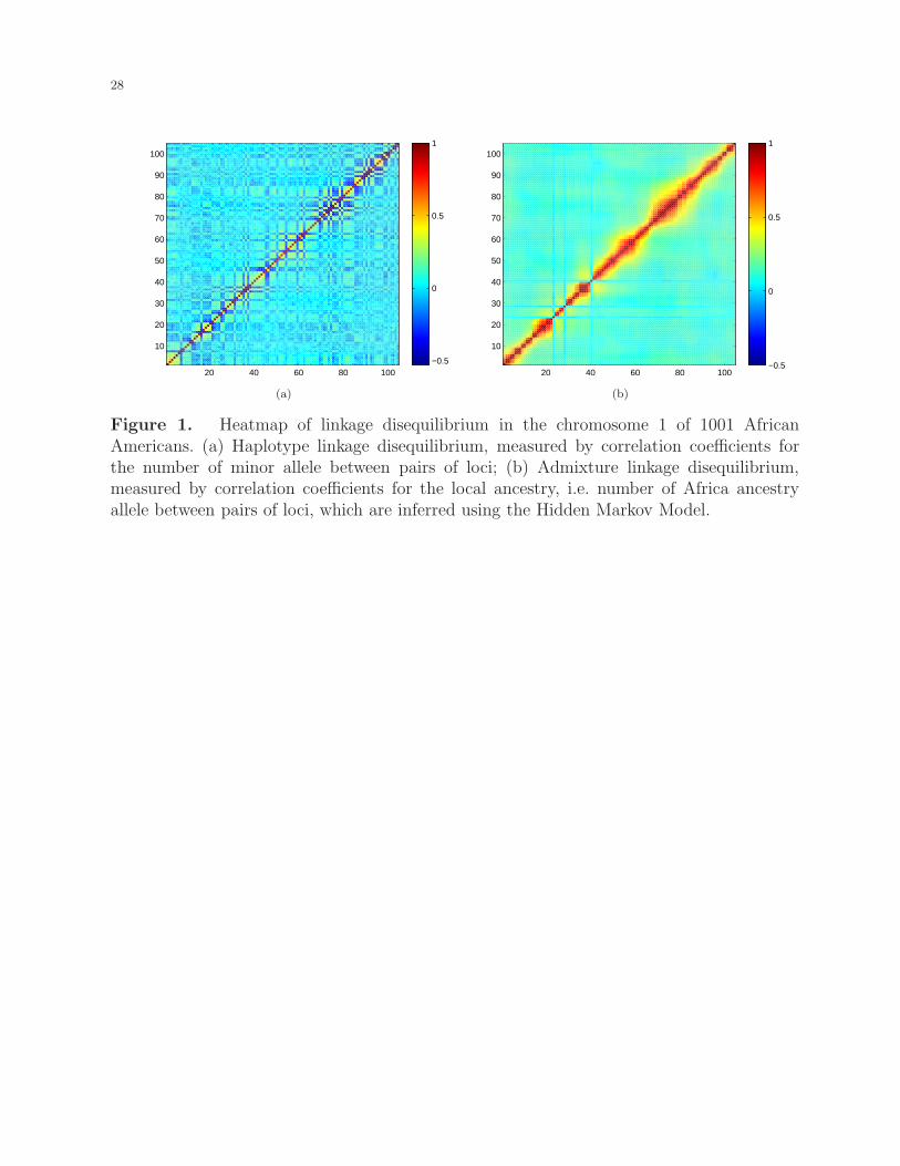
In the African American population, the linkage disequilibrium due to admixture extends for
a much wider region than the linkage disequilibrium between haplotypes,30, 31 which is also
illustrated in Figure 1. Hence, compared to the tagSNP-based GWAS, admixture mapping
requires many fewer markers to tag the whole genome and therefore increases the detection
power at a reduced resolution, which is still higher than linkage analysis.25, 28, 31 Moreover,
admixture mapping is less vulnerable to allelic heterogeneity,26, 32 since it relies on local
ancestry instead of alleles directly.
[Figure 1 about here.]
Given the local ancestries of each individual,33–37 several hypothesis testing-based ap-
proaches have been proposed to test, one locus at a time, the null hypothesis that the
AIM is unlinked to the complex-trait/disease. McKeigue38 first applied the transmission-
disequilibrium test39 to explore the excess transmission of a risk variant from the high risk
ancestral population at an AIM locus, and later40 proposed a test for gametic disequilibrium
between an AIM locus and the trait locus, conditional on the parental admixture. Patterson
et al.31 suggested a Bayesian likelihood ratio test, comparing the likelihood under the alter-
native hypothesis (a given AIM locus is associated with the trait) versus the one under the
null hypothesis, for cases and controls respectively. Zhu et al.41 described a Z-score statistic,
similar to one proposed by Montana and Pritchard,42 for testing the estimated local ancestry
proportion is equal to one under the null hypothesis for case-control and case-only studies.
Although considerable research has been devoted to single locus admixture mapping fo-
cused on dichotomous traits, less attention has been paid to admixture mapping for quan-
titative traits and to considering multiple loci simultaneously while adjusting for other risk
4
factors. Quantitative traits have been the focus in many admixture mapping studies, such
as lnterleukin 6 levels as inflammatory biomarkers for cardiovascular disease risk,7 ankle-
arm index for peripheral arterial disease,14 central retinal artery equivalent level for retinal
vascular caliber,13 and white cell count for acute inflammation.10 To apply existing admixture
methods, the common practice has been to dichotomize subjects with the lowest and highest
q% (e.g. 20%) of the quantitative trait value as cases and controls. The remaining subjects
with in-between quantitative trait values are discarded,7, 13, 14 resulting in reduced power. In
addition, complex traits are commonly caused by joint effects of the multiple genes and other
risk factors, such as age, sex and smoking status. Investigating the association between AIM
loci and a trait, one locus a time, without considering other loci or risk factors may capture a
rather small proportion of joint effects and will possibly lead to inconsistent conclusions.1, 2, 43
With these motivations we propose regression-based generalized admixture mapping (GLEAM)
for both quantitative and qualitative traits with the ability to examine the association
between the complex trait and single or multiple loci simultaneously while also adjusting for
other risk factors. The new approach is based on generalized linear models (GLMs),44 with
linear regression for continuous traits, logistic regression for binary (e.g. case-control) traits
and Poisson regression for count traits. The predictors in GLM include local ancestries at the
given AIM loci and other risk factors. The local ancestry is defined as the number of alleles
from the high risk ancestral population, for example, 0, 1 or 2 alleles from African ancestry
at a given AIM locus. The association examined in GLEAM can be adjusted by other risk
factors. A related approach has been considered by Hoggart et al.45 for single locus without
adjustment for other factors. We assume for complex genetic traits that most loci have no
association with the trait, a few loci may have small to modest association (e.g. odds ratio
< 2 for binary traits), and the loci with higher proportions of disease-causing alleles from
the high-risk population would possibly have stronger association with the traits.25, 28 This
Generalized Admixture Mapping for Complex Traits 5
prior knowledge is incorporated into GLEAM by using a quadratic normal moment (QNM)
prior46 for the coefficients in GLM (See more details in “Material and Methods” section)
with the benefit of reducing the type I error while increasing the power, as demonstrated by
the simulations in “Results” section.
The number of AIMs (1500 ∼ 3000)30 is usually larger than the number of study sub-
jects, and keeps increasing ( >4000)47, 48 with advances due to the HapMap project49, 50
and commercially available genome-wide SNP arrays. It is not feasible to consider loci all
together simultaneously due to the “curse of dimensionality”. Rather, we propose a two-stage
approach: in the first stage, we examine the association between local ancestries with the
trait for one locus at a time and select a small subset of susceptibility loci; in the second
stage, the associations between the various combinations of these selected loci and the trait
are evaluated and the most significant ones are reported. The associations in both steps are
assessed by the Bayes factor (BF), the ratio between the likelihood of observed traits under
the alternative hypothesis (presence of association between single or multiple loci with traits)
and that under the null hypothesis (lack of association).51,52
The local ancestries are unobserved and will be inferred based on the AIMs using the
Hidden Markov Model (HMM),53, 54 with the focus on two-population admixture similar to
that of Falush et al.33 and Patterson et al.31 with one key difference: the recombination
process is modeled non-parametrically. At each AIM locus, the number of alleles from the
high risk ancestral population will be imputed multiple times for every subject, using an
Markov chain Monte Carlo (MCMC) algorithm. Existing approaches only record the imputed
frequency of the number of alleles from the high risk ancestral population individually33 or
across the population without accounting for imputation uncertainty.31 In contrast, our
approach imputes multiple datasets of local ancestries, from which we are able to assess
the association between the traits and local ancestries directly, while taking imputation
6
uncertainty into account through Bayesian averaging. Importantly, the admixture linkage
disequilibrium between the AIM loci is preserved in our multiple imputation approach, which
is crucial for multilocus admixture mapping.
The remainder of paper is organized as follows. In Material and Methods, we first present
the HMM for imputing the local ancestries, followed by the specification of the generalized
linear model for quantitative and qualitative traits with QNM prior density. In Results,
through the simulations we show that the new approach increases the power of admixture
mapping while reducing the type I error rates compared to the popular method by Patterson
et al.31 . The new approach is applied to data from a large cohort study, the Healthy
Pregnancy, Healthy Baby (HPHB) Study, and further extensions are considered in Discussion
section.
Material and Methods
Hidden Markov Model
For a population-based design, suppose we have I unrelated subjects, each of which has the
same set of J AIMs recorded. The local ancestry is measured by Sij ∈ {0, 1, 2}, the number
of alleles from the high risk population A (e.g. African) for the ith subject and the jth AIM.
Sij is unknown and will be imputed using the HMM. For African Americans with African
and European ancestral populations, HMM assumes that given the Sij, the distribution of
Xij ∈ {0, 1, 2}, the number of variant alleles, is independent of other Sij′ and Xij′ with
j′ 6= j and is specified by the observation probability mass matrix P j = {pj(m,n)}3×3 with
pj(m,n) = Prob(Xij = n | Sij = m) and
P j =
Xij = 0 Xij = 1 Xij = 2
Sij = 0 (1− pBj )(1− pBj ) 2pBj (1− pBj ) pBj pBj
Sij = 1 (1− pAj )(1− pBj ) pAj (1− pBj ) + pBj (1− pAj ) pAj pBj
Sij = 2 (1− pAj )(1− pAj ) 2pAj (1− pAj ) pAj pAj
,
where pAj is the minor allele probability at loci j in the high risk population A andpBj is the
corresponding probability in the low risk population B.
The latent states Si = {Sij}1×J , tagging the status of the ancestry blocks, are unobserved
and modeled by an Markov chain which considers the genetic recombination events. Let ρi
Generalized Admixture Mapping for Complex Traits 7
denote the genome-wide proportion of alleles from the high risk population A for subject
i, Qi0 = [(1 − ρi)2, 2ρi(1 − ρi), ρ
2i ]′ initial state vector, Rij ∈ {0, 1, 2} the number of
recombination events between AIM loci j − 1 and j, Q(r)i = {q
(r)i (m,n)}3×3 the conditional
state transition matrix given r recombination events between the neighboring AIM loci with
q(r)i (m,n) = Prob
(Sij = n | Si(j−1) = m,Rij = r
). The Markov chain Si is governed by the
state transition matrix Qij = {qij(m,n)}3×3 with qij(m,n) = Prob(Sij = n | Si(j−1) = m
).
Qij =∑2
r=0Q(r)i Prob(Rij = r), where Q
(0)i , Q
(1)i and Q
(2)i are specified as
Q(0)i =
Sij = 0 Sij = 1 Sij = 2
Si(j−1) = 0 1 0 0
Si(j−1) = 1 0 1 0
Si(j−1) = 2 0 0 1
,
Q(1)i =
Sij = 0 Sij = 1 Sij = 2
Si(j−1) = 0 1− ρi ρi 0
Si(j−1) = 1 12(1− ρi)
12
12ρi
Si(j−1) = 2 0 1− ρi ρi
,
Q(2)i =
Sij = 0 Sij = 1 Sij = 2
Si(j−1) = 0 (1− ρi)2 2ρi(1− ρi) ρ2i
Si(j−1) = 1 (1− ρi)2 2ρi(1− ρi) ρ2i
Si(j−1) = 2 (1− ρi)2 2ρi(1− ρi) ρ2i
,
and Rij ∼ Bin(2, γj) a binomial distribution with γj the probability that a recombination
event occurs between the neighboring AIM loci in a single chromosome. Consequently, we
can get,
Qij =
Sij = 0 Sij = 1 Sij = 2
Si(j−1) = 0 (1− γjρi)2 2γjρi(1− γjρi) γ2
j ρ2i
Si(j−1) = 1 γj(1− ρi)(1− γjρi) {1− γj(1− ρi)}(1− γjρi) + γ2j ρi(1− ρi) γjρi{1− γj(1− ρi)}
Si(j−1) = 2 γ2j (1− ρi)
2 2γj(1− ρi){1− γj(1− ρi)} {1− γj(1− ρi)}2
We further specify informative prior distributions for the parameters pAj , pBj , γj and ρi
involved in the HMM. Although the pAj of the high risk population A is unknown, we have
information on pA0j , the proportion of the variant allele j in a subpopulation of high risk
population A (e.g. YRI for African), from the HapMap or 1000 genome projects. Hence,
we expect that pAj would be close to pA0j and specify pAj ∼ Beta(τApA0j , τ
A(1− pA0j))with
8
the expectation E(pAj ) = pA0j and τA ∼ U[50, 1000] a uniform distribution to reflect the
uncertainty in borrowing the subpopulation information. A similar specification is chosen
for pBj based on the proportion of the variant allele j in a subpopulation of low risk pop-
ulation B (e.g. CEU for European). As for γj, it is well known that the recombination
probability is roughly proportional to dj the genetic distance between (j − 1)th and jth
AIM loci. A common choice is γj = 1− exp(−λdj) with λ = 6 the number of recombination
events per Morgan since admixture.31, 33 However, recombination ‘hotspots’ can occur along
the chromosomes where the recombination probabilities are much higher than the other
regions.55–58 For this reason, we avoid the above parametric specification of γj. Instead,
we let γj ∼ Beta (τγγ0j, τγ(1− γ0j)) with the expectation E(γj) = γ0j = 1 − exp(−λdj).
Hence, on average the probability of recombination is proportional to the genetic distance
while allowing significant deviation (e.g. ‘hotspots’ ) from the average. The deviation is
measured by τγ with V ar(γj) =γ0j(1−γ0j )
τγ+1= µ0. Additionally, for the admixed population,
we often have knowledge about the proportions of ancestral populations at the population
level. For example, the African American population in general consists of 80% African
ancestral population and 20% European ancestral population.25, 28 We borrow this popula-
tion level information to specify ρi, the subject specific proportion of high risk population
A, by letting ρi ∼ Beta (τρρ0i, τρ(1− ρ0i)) with ρ0i (e.g. 0.8 for African American) and
V ar(ρi) =ρ0i(1−ρ0i)
τρ+1= ν0.
We use an MCMC algorithm to sample the local ancestries Si for i = 1, 2, . . . , I, along
with other parameters. The details of MCMC are given in the Appendix.
Generalized linear model with QNM prior
GLEAM is a regression method that extends the current approaches in various ways. The
most obvious extension is to accommodate both quantitative and qualitative traits yi through
a generalized linear model with the ability to adjust for covariates Ei = (Ei1, Ei2, . . . , Eiq)′.
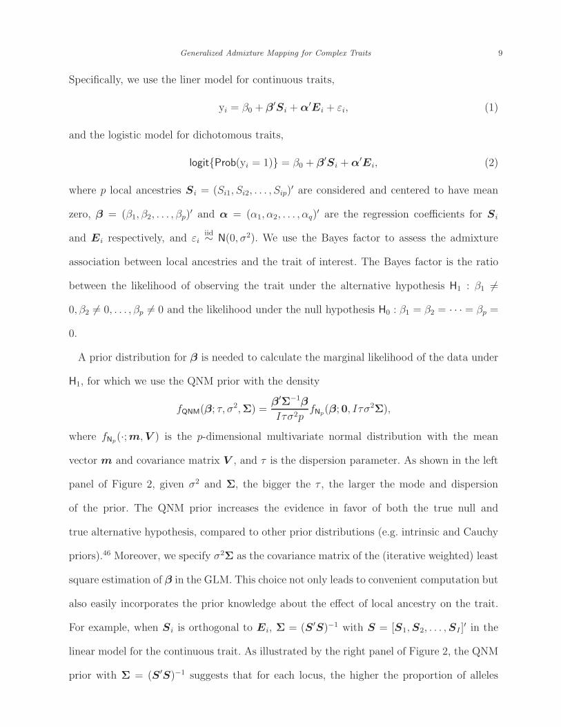
Generalized Admixture Mapping for Complex Traits 9
Specifically, we use the liner model for continuous traits,
yi = β0 + β′Si +α′Ei + εi, (1)
and the logistic model for dichotomous traits,
logit{Prob(yi = 1)} = β0 + β′Si +α′Ei, (2)
where p local ancestries Si = (Si1, Si2, . . . , Sip)′ are considered and centered to have mean
zero, β = (β1, β2, . . . , βp)′ and α = (α1, α2, . . . , αq)
′ are the regression coefficients for Si
and Ei respectively, and εiiid∼ N(0, σ2). We use the Bayes factor to assess the admixture
association between local ancestries and the trait of interest. The Bayes factor is the ratio
between the likelihood of observing the trait under the alternative hypothesis H1 : β1 6=
0, β2 6= 0, . . . , βp 6= 0 and the likelihood under the null hypothesis H0 : β1 = β2 = · · · = βp =
0.
A prior distribution for β is needed to calculate the marginal likelihood of the data under
H1, for which we use the QNM prior with the density
fQNM(β; τ, σ2,Σ) =
β′Σ−1β
Iτσ2pfNp(β; 0, Iτσ
2Σ),
where fNp(·;m,V ) is the p-dimensional multivariate normal distribution with the mean
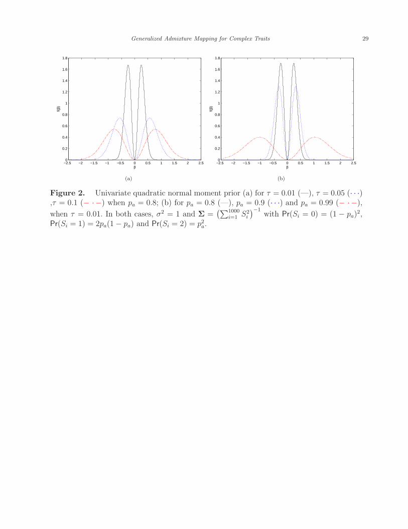
vector m and covariance matrix V , and τ is the dispersion parameter. As shown in the left
panel of Figure 2, given σ2 and Σ, the bigger the τ , the larger the mode and dispersion
of the prior. The QNM prior increases the evidence in favor of both the true null and
true alternative hypothesis, compared to other prior distributions (e.g. intrinsic and Cauchy
priors).46 Moreover, we specify σ2Σ as the covariance matrix of the (iterative weighted) least
square estimation of β in the GLM. This choice not only leads to convenient computation but
also easily incorporates the prior knowledge about the effect of local ancestry on the trait.
For example, when Si is orthogonal to Ei, Σ = (S ′S)−1 with S = [S1,S2, . . . ,SI ]′ in the
linear model for the continuous trait. As illustrated by the right panel of Figure 2, the QNM
prior with Σ = (S′S)−1 suggests that for each locus, the higher the proportion of alleles
10
from the high risk population (pa), on average the larger the risk effect of local ancestry.
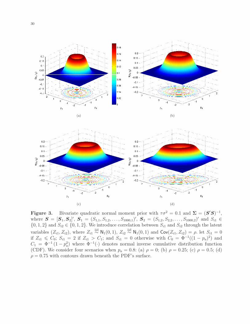
Such relationships are frequently observed in admixture mapping. More importantly, when
we investigate multiple loci simultaneously, it is crucial to take the correlation (linkage
disequilibrium, LD) between the local ancestries into consideration. Figure 3 plots several
volcano-shaped bivariate QNM densities for various correlations between two local ancestries.
It is clear that for two loci with admxiture linkage equilibrium (as shown in panel (a)), such
as two loci on different chromosomes, their risk effects would be independent; and that for
two loci with high admixture LD (as shown in panel (d)), usually located in the same gene,
they would have similar risk effects.
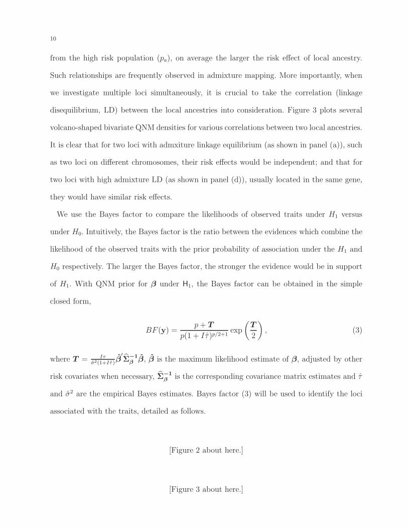
We use the Bayes factor to compare the likelihoods of observed traits under H1 versus
under H0. Intuitively, the Bayes factor is the ratio between the evidences which combine the
likelihood of the observed traits with the prior probability of association under the H1 and
H0 respectively. The larger the Bayes factor, the stronger the evidence would be in support
of H1. With QNM prior for β under H1, the Bayes factor can be obtained in the simple
closed form,
BF (y) =p+ T
p(1 + Iτ̂)p/2+1exp
(T
2
), (3)
where T = Iτσ̂2(1+Iτ̂ )
β̂′Σ̂
−1
β β̂, β̂ is the maximum likelihood estimate of β, adjusted by other
risk covariates when necessary, Σ̂−1
β is the corresponding covariance matrix estimates and τ̂
and σ̂2 are the empirical Bayes estimates. Bayes factor (3) will be used to identify the loci
associated with the traits, detailed as follows.
[Figure 2 about here.]
[Figure 3 about here.]
Generalized Admixture Mapping for Complex Traits 11
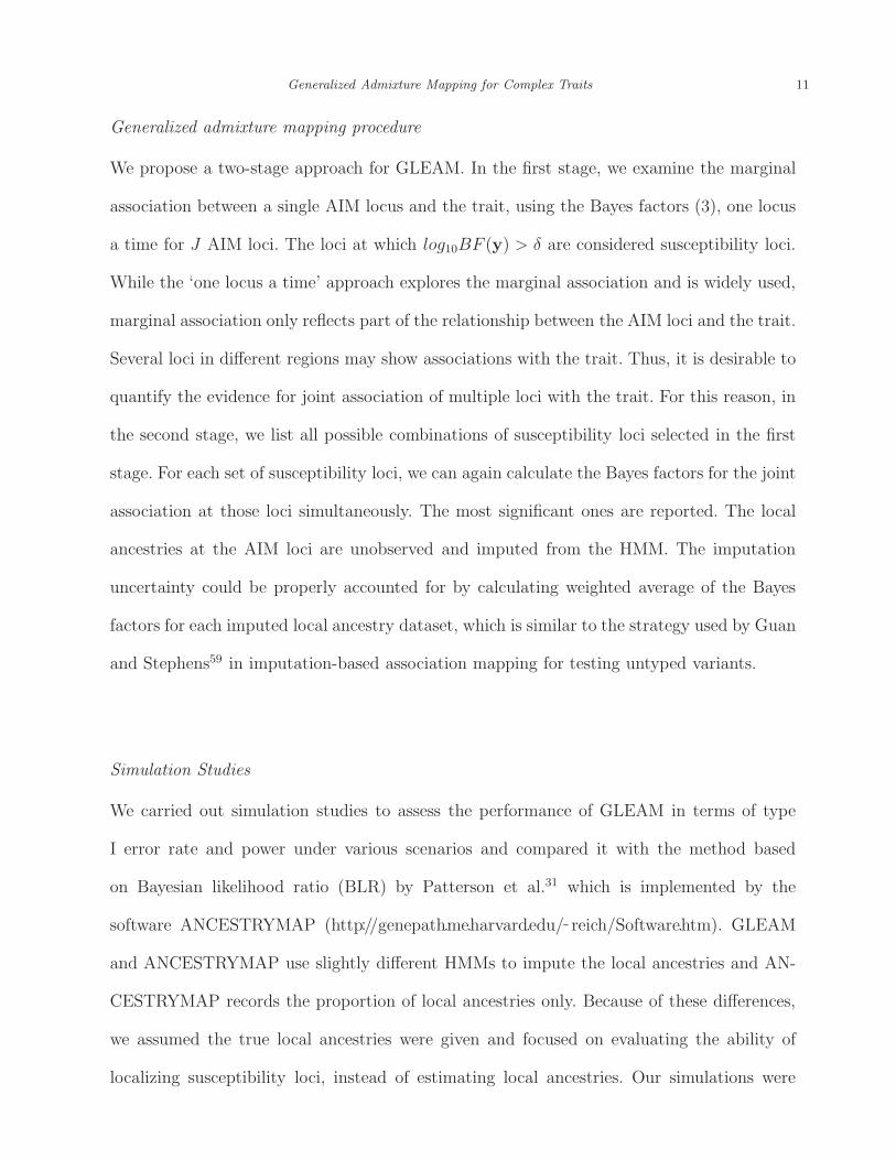
Generalized admixture mapping procedure
We propose a two-stage approach for GLEAM. In the first stage, we examine the marginal
association between a single AIM locus and the trait, using the Bayes factors (3), one locus
a time for J AIM loci. The loci at which log10BF (y) > δ are considered susceptibility loci.
While the ‘one locus a time’ approach explores the marginal association and is widely used,
marginal association only reflects part of the relationship between the AIM loci and the trait.
Several loci in different regions may show associations with the trait. Thus, it is desirable to
quantify the evidence for joint association of multiple loci with the trait. For this reason, in
the second stage, we list all possible combinations of susceptibility loci selected in the first
stage. For each set of susceptibility loci, we can again calculate the Bayes factors for the joint
association at those loci simultaneously. The most significant ones are reported. The local
ancestries at the AIM loci are unobserved and imputed from the HMM. The imputation
uncertainty could be properly accounted for by calculating weighted average of the Bayes
factors for each imputed local ancestry dataset, which is similar to the strategy used by Guan
and Stephens59 in imputation-based association mapping for testing untyped variants.
Simulation Studies
We carried out simulation studies to assess the performance of GLEAM in terms of type
I error rate and power under various scenarios and compared it with the method based
on Bayesian likelihood ratio (BLR) by Patterson et al.31 which is implemented by the
software ANCESTRYMAP (http://genepath.me.harvard.edu/̃ reich/Software.htm). GLEAM
and ANCESTRYMAP use slightly different HMMs to impute the local ancestries and AN-
CESTRYMAP records the proportion of local ancestries only. Because of these differences,
we assumed the true local ancestries were given and focused on evaluating the ability of
localizing susceptibility loci, instead of estimating local ancestries. Our simulations were
12
based on empirical data of local ancestries for 1001 African Americans from the HPHB
Study,60 with 1296 AIM loci measured across the genome.
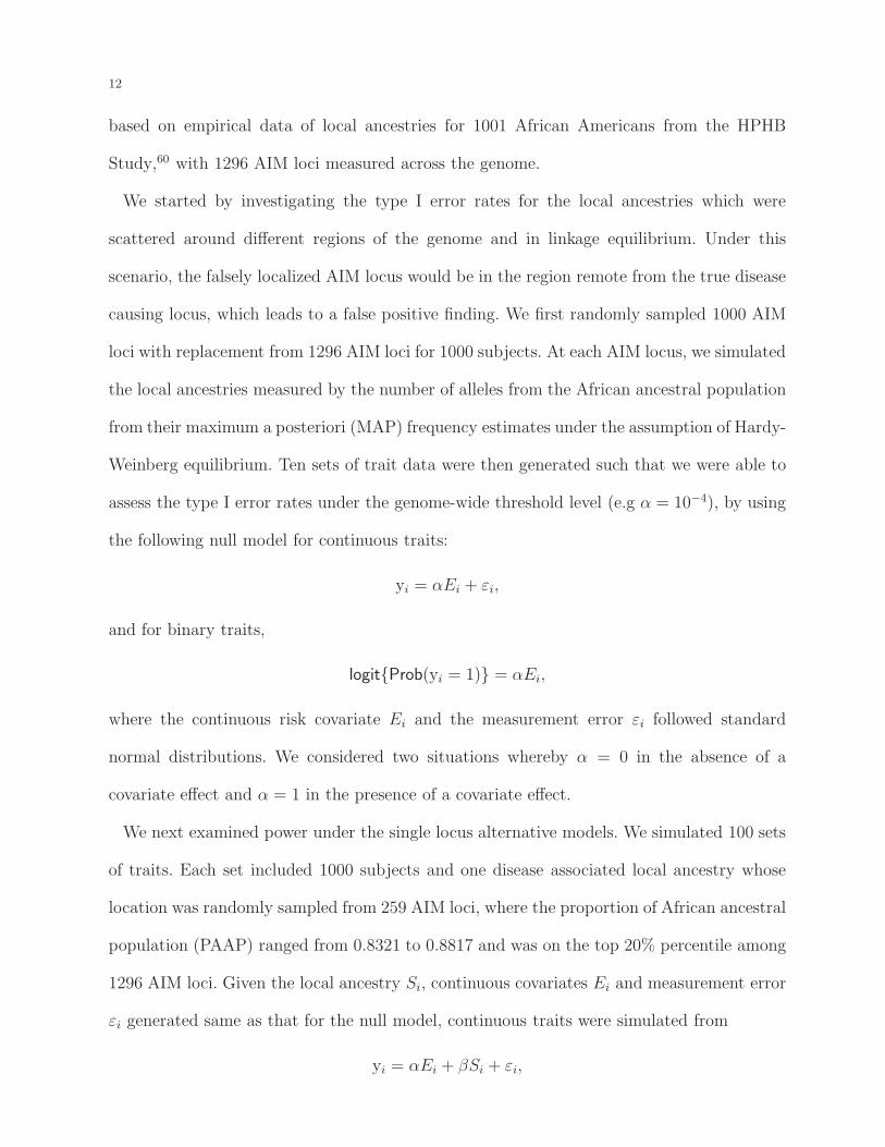
We started by investigating the type I error rates for the local ancestries which were
scattered around different regions of the genome and in linkage equilibrium. Under this
scenario, the falsely localized AIM locus would be in the region remote from the true disease
causing locus, which leads to a false positive finding. We first randomly sampled 1000 AIM
loci with replacement from 1296 AIM loci for 1000 subjects. At each AIM locus, we simulated
the local ancestries measured by the number of alleles from the African ancestral population
from their maximum a posteriori (MAP) frequency estimates under the assumption of Hardy-
Weinberg equilibrium. Ten sets of trait data were then generated such that we were able to
assess the type I error rates under the genome-wide threshold level (e.g α = 10−4), by using
the following null model for continuous traits:
yi = αEi + εi,
and for binary traits,
logit{Prob(yi = 1)} = αEi,
where the continuous risk covariate Ei and the measurement error εi followed standard
normal distributions. We considered two situations whereby α = 0 in the absence of a
covariate effect and α = 1 in the presence of a covariate effect.
We next examined power under the single locus alternative models. We simulated 100 sets
of traits. Each set included 1000 subjects and one disease associated local ancestry whose
location was randomly sampled from 259 AIM loci, where the proportion of African ancestral
population (PAAP) ranged from 0.8321 to 0.8817 and was on the top 20% percentile among
1296 AIM loci. Given the local ancestry Si, continuous covariates Ei and measurement error
εi generated same as that for the null model, continuous traits were simulated from
yi = αEi + βSi + εi,
Generalized Admixture Mapping for Complex Traits 13
and binary traits from,
logit{Prob(yi = 1)} = αEi + βSi.
Under both models, the β was specified as β = c × PAAP which reflected the a priori
observation that the locus with the larger proportion of the high risk ancestral (here African
American) population usually demonstrated stronger association with the traits. For con-
tinuous traits, we chose the values of effect size multiplier c as 0.2, 0.25, 0.3, 0.35 and 0.4
respectively, with the largest possible effect size equal to 0.3527. Similarly, we picked the
values of c’s as 0.4, 0.5, 0.6, 0.7 and 0.8 for binary traits with the largest possible odds ratio
(OR) equal to 1.8537.
We further considered a multilocus alternative model where two local ancestries were
associated with the traits and there existed admixture linkage disequilibrium. To do so,
we generated an artificial chromosome composed of two pieces from chromosome 1 and
chromosome 4 with the length 139.50Mb and 114.88Mb respectively for 1000 subjects, based
on empirical data on local ancestries from HPHB study. In the middle of each chromosome
piece with 51 loci, there is one locus whose proportion of African ancestry population was
among the highest in all 1296 AIM loci. In the simulations, those two loci are assumed to be
associated with traits. We generated 100 sets of continuous and binary traits respectively,
each of which was simulated similarly to the single locus alternative model except with two
local ancestries involved and both effect size multiplier c’s set at 0.7 for continuous traits
and 0.35 for binary traits.
The simulated datasets were analyzed by the GLEAM and the BLR method. Since the BLR
method was primarily developed for binary traits, the BLR method required transformation
of continuous traits into binary ones, such as defining the subjects with top 20% traits as
the cases and the one with bottom 20% traits as controls.
14
Results
Simulation Studies
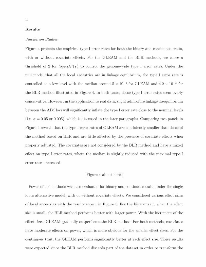
Figure 4 presents the empirical type I error rates for both the binary and continuous traits,
with or without covariate effects. For the GLEAM and the BLR methods, we chose a
threshold of 2 for log10BF (y) to control the genome-wide type I error rates. Under the
null model that all the local ancestries are in linkage equilibrium, the type I error rate is
controlled at a low level with the median around 5 × 10⁻⁴ for GLEAM and 4.2 × 10⁻³ for
the BLR method illustrated in Figure 4. In both cases, those type I error rates seem overly
conservative. However, in the application to real data, slight admixture linkage disequilibrium
between the AIM loci will significantly inflate the type I error rate close to the nominal levels
(i.e. α = 0.05 or 0.005), which is discussed in the later paragraphs. Comparing two panels in
Figure 4 reveals that the type I error rates of GLEAM are consistently smaller than those of
the method based on BLR and are little affected by the presence of covariate effects when
properly adjusted. The covariates are not considered by the BLR method and have a mixed
effect on type I error rates, where the median is slightly reduced with the maximal type I
error rates increased.
[Figure 4 about here.]
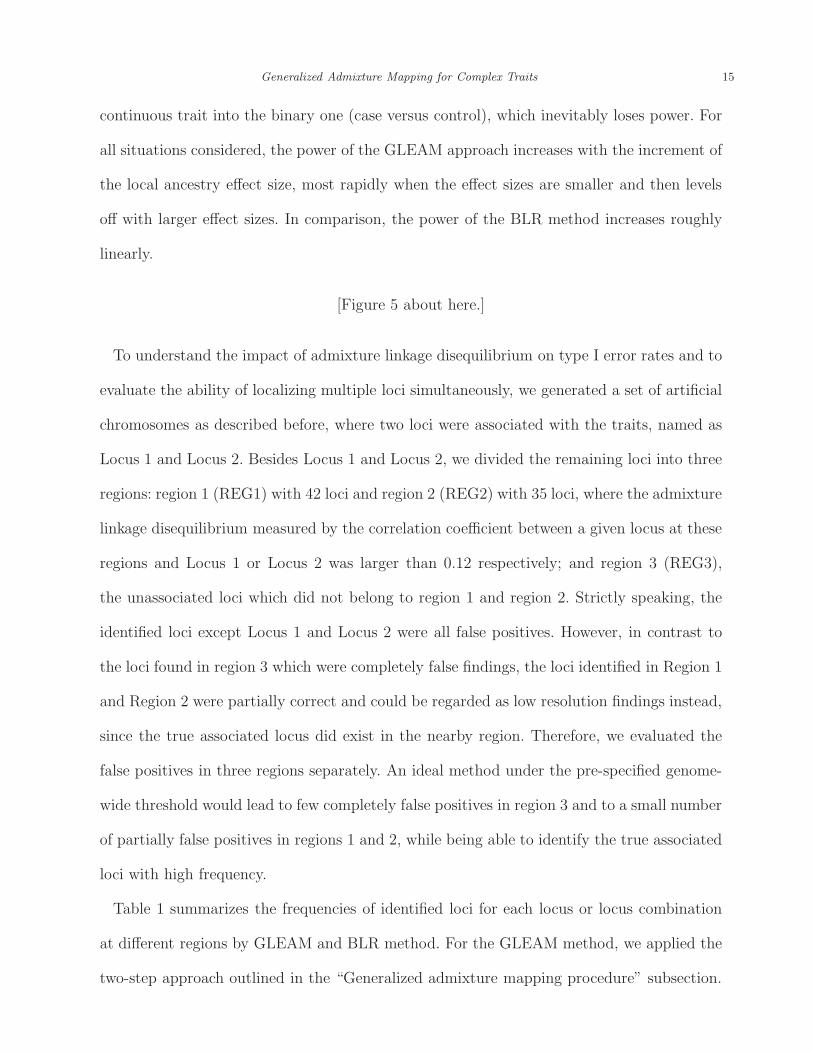
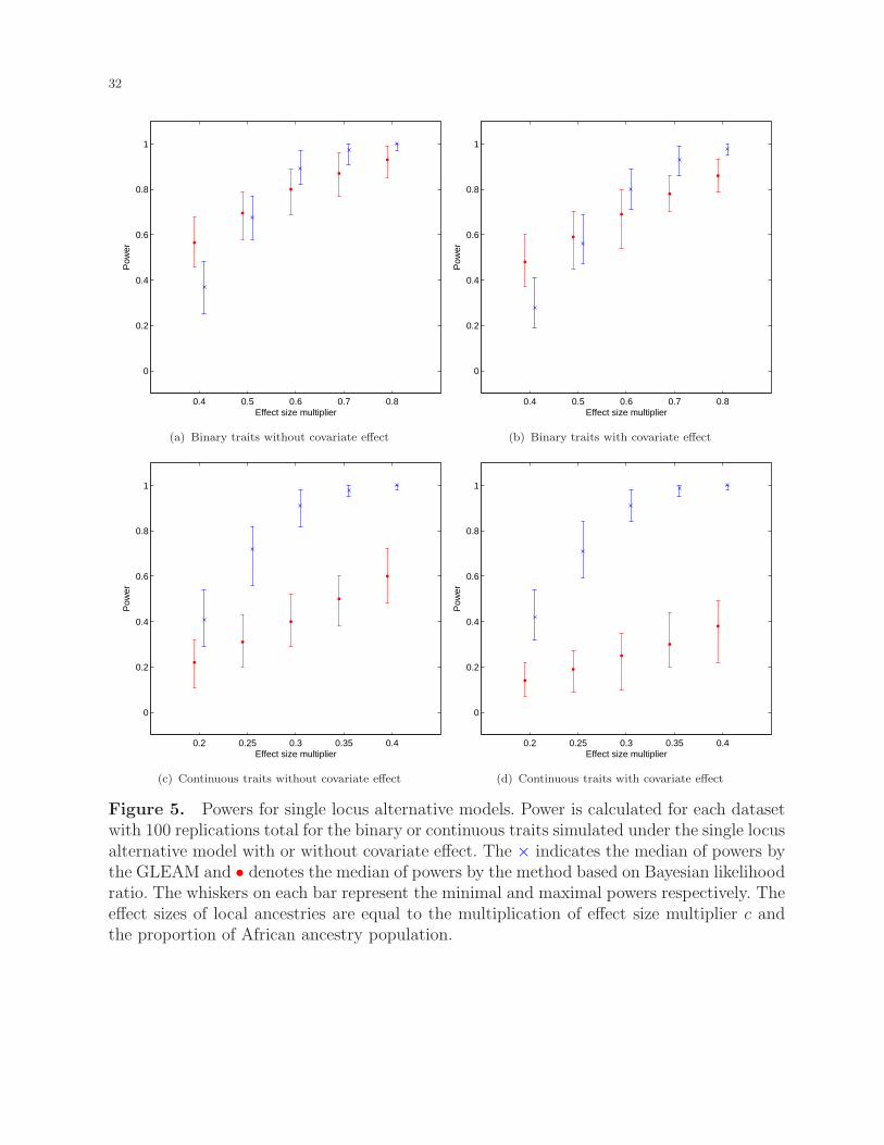
Power of the methods was also evaluated for binary and continuous traits under the single
locus alternative model, with or without covariate effects. We considered various effect sizes
of local ancestries with the results shown in Figure 5. For the binary trait, when the effect
size is small, the BLR method performs better with larger power. With the increment of the
effect sizes, GLEAM gradually outperforms the BLR method. For both methods, covariates
have moderate effects on power, which is more obvious for the smaller effect sizes. For the
continuous trait, the GLEAM performs significantly better at each effect size. These results
were expected since the BLR method discards part of the dataset in order to transform the
Generalized Admixture Mapping for Complex Traits 15
continuous trait into the binary one (case versus control), which inevitably loses power. For
all situations considered, the power of the GLEAM approach increases with the increment of
the local ancestry effect size, most rapidly when the effect sizes are smaller and then levels
off with larger effect sizes. In comparison, the power of the BLR method increases roughly
linearly.
[Figure 5 about here.]
To understand the impact of admixture linkage disequilibrium on type I error rates and to
evaluate the ability of localizing multiple loci simultaneously, we generated a set of artificial
chromosomes as described before, where two loci were associated with the traits, named as
Locus 1 and Locus 2. Besides Locus 1 and Locus 2, we divided the remaining loci into three
regions: region 1 (REG1) with 42 loci and region 2 (REG2) with 35 loci, where the admixture
linkage disequilibrium measured by the correlation coefficient between a given locus at these
regions and Locus 1 or Locus 2 was larger than 0.12 respectively; and region 3 (REG3),
the unassociated loci which did not belong to region 1 and region 2. Strictly speaking, the
identified loci except Locus 1 and Locus 2 were all false positives. However, in contrast to
the loci found in region 3 which were completely false findings, the loci identified in Region 1
and Region 2 were partially correct and could be regarded as low resolution findings instead,
since the true associated locus did exist in the nearby region. Therefore, we evaluated the
false positives in three regions separately. An ideal method under the pre-specified genome-
wide threshold would lead to few completely false positives in region 3 and to a small number
of partially false positives in regions 1 and 2, while being able to identify the true associated
loci with high frequency.
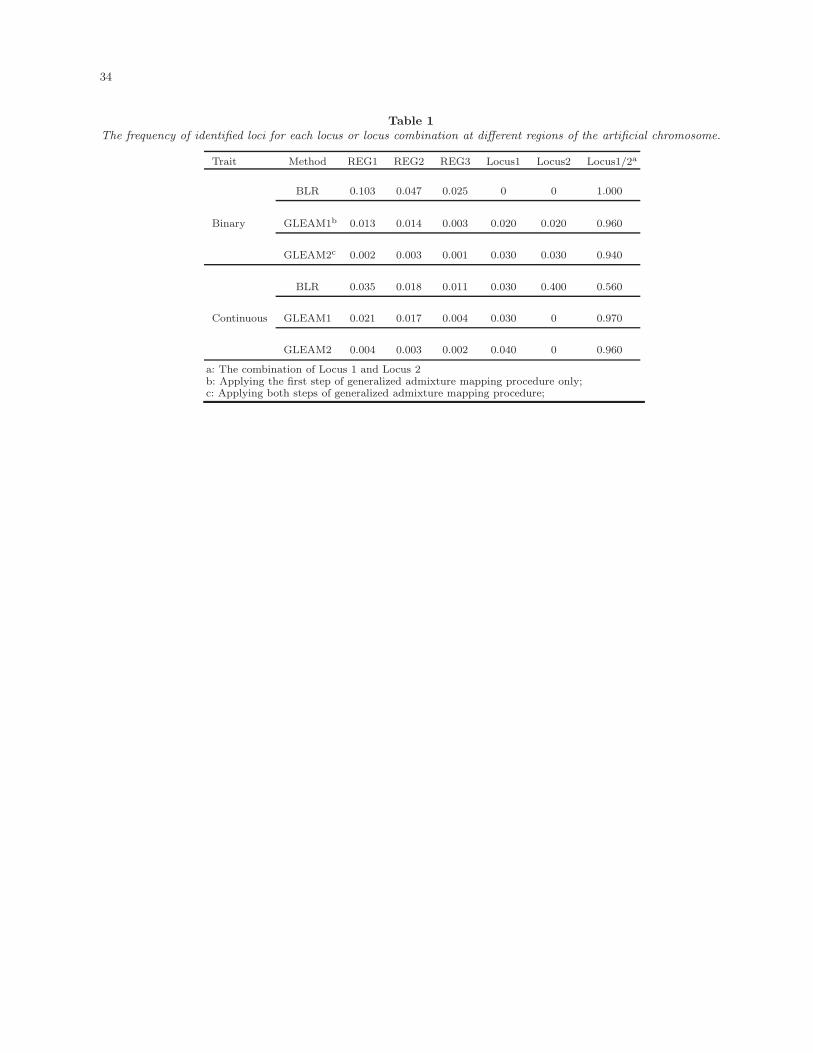
Table 1 summarizes the frequencies of identified loci for each locus or locus combination
at different regions by GLEAM and BLR method. For the GLEAM method, we applied the
two-step approach outlined in the “Generalized admixture mapping procedure” subsection.
16
The results by applying the first step only (GLEAM1) and by applying the two-step approach
(GLEAM2) were both presented. For binary traits, both the BLR method and GLEAM1
could localize both Locus 1 and Locus 2 with high power. The type I error rates in region 1
were around the nominal level (0.025 and 0.003 respectively). The type I error rates in region
1 and region 2 were higher than the ones in region 3, which would decrease the resolution
of the finding. Compared to GLEAM1, further applying the second step of generalized
admixture mapping procedure (GLEAM2) could significantly improve the resolution by
reducing the type I errors in region 1 (from 0.013 to 0.002) and region 2 (from 0.014 to
0.003). For continuous traits, GLEAM2 also performed best with much higher power and
lower type I rate than the BLR method.
[Table 1 about here.]
Application
This methodological work was motivated by real data from the Healthy Pregnancy, Healthy
Baby (HPHB) study, which is a prospective cohort study of pregnant women aimed at
identifying genetic, social and environmental contributors to disparities in adverse birth
outcomes in the US south.60 Consistent with previous studies, African American women
in HPHB have higher risk for maternal hypertension than Caucasian women during the
pregnancy, which contributes to the poor birth outcomes.61 Even within the African Amer-
ican subpopulation, some African American women have much higher blood pressures, and
we hypothesize that one possible contributor may be the percentage of African ancestry.
To explore this hypothesis, we applied GLEAM to investigate the association between the
averaged maternal mean arterial pressure (MAP), defined as (1/3×systolic blood pressure)+
(2/3 × diastolic blood pressure), during 24 to 28 weeks of pregnancy and local ancestries
among these pregnant African American women. Clinical and genetic data were available for
1004 nonHispanic Black (NHB) women. 1509 SNP AIMs were genotyped using the Illumina
Generalized Admixture Mapping for Complex Traits 17
African American admixture panel. After quality control measures described previously,62
the dataset consisted of 1001 NHB women with 1296 AIMs.
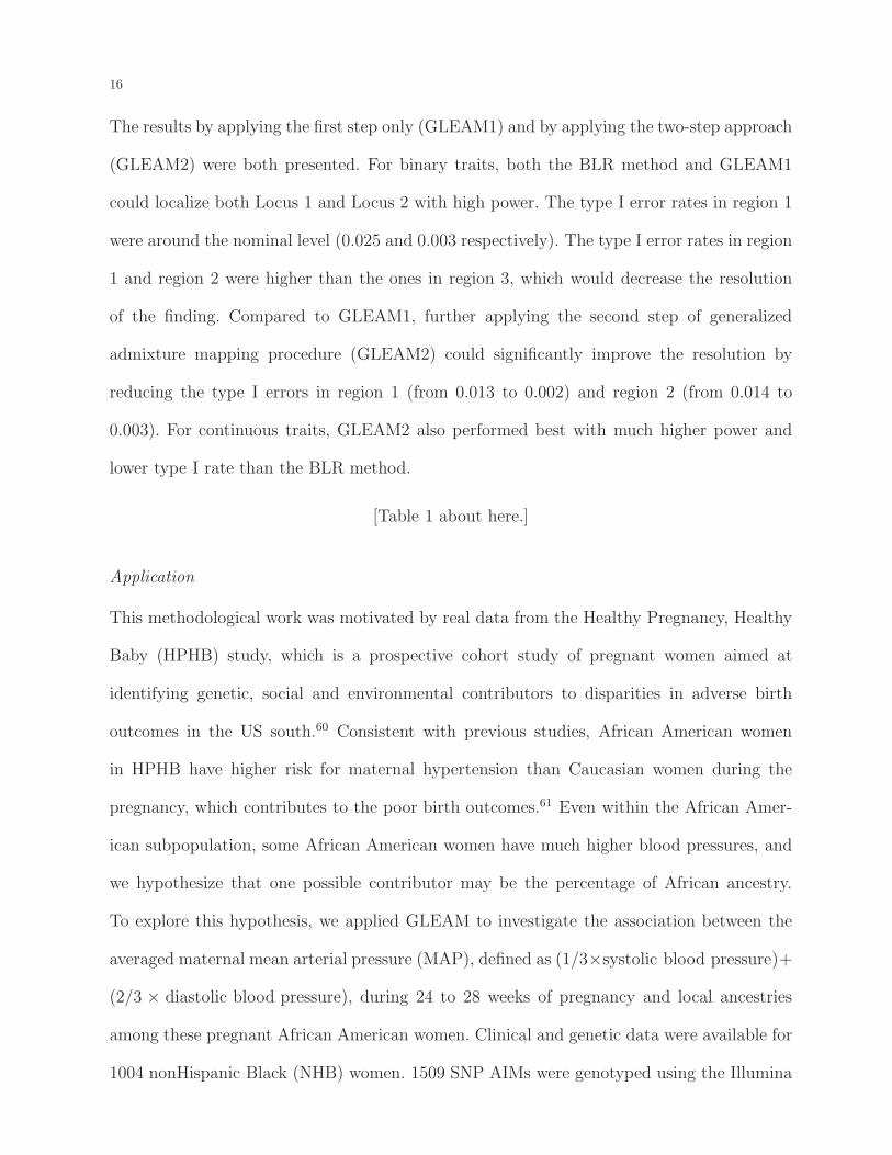
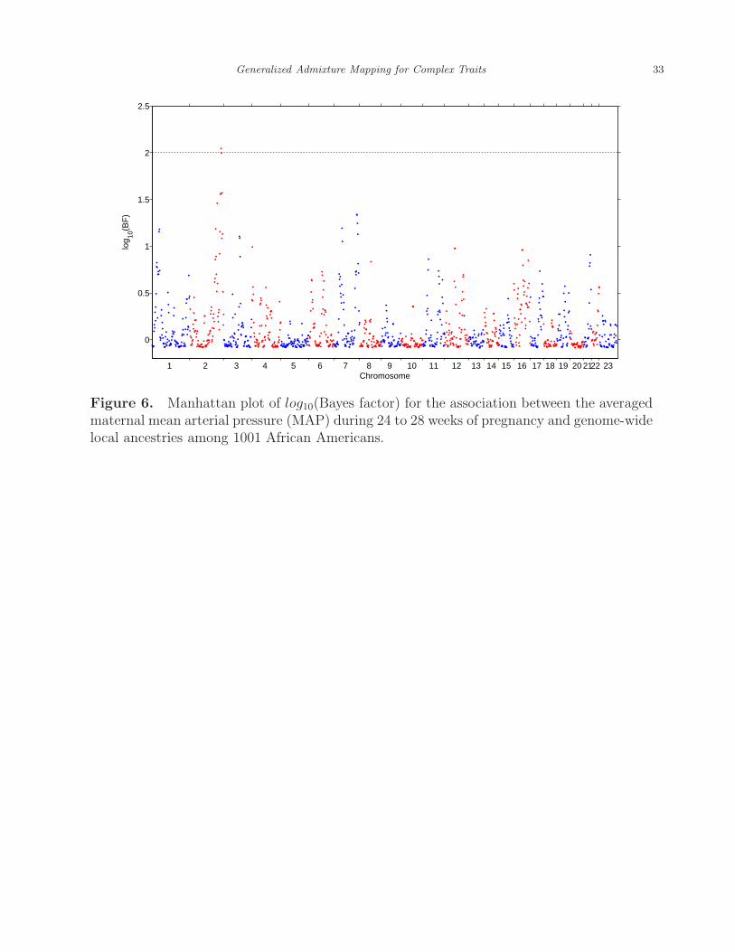
The proposed GLEAM approach was applied to this dataset to identify the local ancestry
associated with the averaged maternal MAP, a continuous trait, while adjusting for mother’s
age. The local ancestries were multiply imputed based on the HMM. We first examined the
marginal association between the trait and local ancestries, one locus a time. The results were
summarized in Figure 6, where one local ancestry on the chromosome 2 was identified with its
log10(Bayes factor) = 2.05 exceeding the threshold 2. With only one local ancestry localized,
the second step of the generalized admixture mapping procedure was unnecessary. The same
data were analyzed by the BLR method, which treated the subjects with averaged maternal
MAP more than 93.67 (top 20% quantile) as cases and the ones with averaged maternal
MAP less than 79.33 (bottom 20% quantile) as control. No local ancestry was identified as
being associated with the averaged maternal MAP with this approach, presumably due to
its relatively low power compared with the GLEAM approach.
[Figure 6 about here.]
Discussion
By utilizing admixture linkage disequilibrium, admixture mapping is an indispensable tool to
localize the alleles which are associated with the qualitative or quantitative traits and diseases
that vary in prevalence across the ancestral populations. The available methods are most
suitable for dichotomous traits in a case-control study and do not allow for adjustment for
other risk covariates. In this article, we propose a flexible and powerful generalized admixture
mapping approach, which is based on the generalized linear model and is able to incorporate
admixture prior information by using the quadratic normal moment prior and to adjust for
covariates. The proposed method is applicable to both qualitative and quantitative traits

18
with satisfactory power while controlling the type I error rates at a low level, and is able to
be easily implemented as we demonstrated with our HPHB example.
In addition to the flexibility to handle different types of traits, other attractive general-
izations include consideration of multiple loci simultaneously. As illustrated in Figure 1, ad-
mixture linkage disequilibrium extends much further than haplotype linkage disequilibrium.
Consequently, if we only examine one locus a time, the local ancestries which are highly
correlated to the true disease associated local ancestry tend to be identified as significant
ones as well. As demonstrated by the simulations, those false positives can be significantly
reduced by considering multiple susceptible loci simultaneously, which reduce the type I
error rates and improve the mapping resolution. In addition, GLEAM specifies a hidden
Markov model treating the recombination rates varying across the genome, which allows
us to infer the recombination “hotspots” in admixture population. Moreover, within the
generalized linear model framework, it is straightforward to extend the current method to
populations with more than to two ancestral populations, such as Hispanic populations,
by adding extra ancestry population covariates. It is also easy to consider the interaction
between the local ancestries and covariates with the properly specification of the priors on
interaction coefficients.
Acknowledgments
This work was supported by Award Number R01ES017436 from the National Institute of
Environmental Health Sciences, and by funding from the National Institutes of Health
(5P2O-RR020782-O3) and the U.S. Environmental Protection Agency (RD-83329301-0).
The content is solely the responsibility of the authors and does not necessarily represent
the official views of the National Institute of Environmental Health Sciences, the National
Institutes of Health or the U.S. Environmental Protection Agency.
Generalized Admixture Mapping for Complex Traits 19
Appendices
MCMC algorithm for HMM
We propose an MCMC algorithm for posterior computation of HMM as follows.
(1) Impute the missing AIM Xmij . Given the P j and Sij , X
mij ∈ {0, 1, 2} can be easily
sampled with probability mass pj(Sij, Xmij ).
(2) Update the latent states Si for i = 1, 2, · · · , I. Given the Qi0, Q(r)i and Ri = {Rij}1×J ,
we will use the forward filtering backward sampling (FFBS) algorithm54 to sample the
Si in one block. The FFBS algorithm mixes more rapidly comparing to the direct
Gibbs sampler which samples one Sij a time conditional on the remains of Si. Let
Xji1 = [Xi1, Xi2, · · · , Xij]
′ and Ri = [Ri1, Ri2, · · · , RiJ ]′. We begin the FFBS algorithm
by calculating QFij = {qFij(m,n)}3×3 with qFij(m,n) = Prob(Si(j−1) = m,Sij = n |
Xji1,Ri) recursively for j = 1, 2, · · · , J as
qFij(m,n) = Prob(Si(j−1) = m,Sij = n | Xji1,Ri)
=Prob(Si(j−1) = m,Sij = n,Xij | X
j−1i1 ,Ri)
Prob(Xij | Xj−1i1 ,Ri)
=qFi(j−1)(m)q
(r)i (m,n)pj(n,Xij)
Prob(Xij | Xj−1i1 ,Ri)
,
where qFi0(m) = Qi0, Prob(Xij | Xj−1i1 ,Ri) =
∑2m=0
∑2n=0 Prob(Si(j−1) = m,Sij =
n,Xij | Xj−1i1 ,Ri), and qFij(n) =
∑2m=0 q
Fij(m,n).
We can then sample the Si backward from SiJ to Si1 with
Prob(Si | X i,Ri) = Prob(SiJ | X i,Ri)J−1∏
j=1
Prob(Si(J−j) | SJi(J−j+1),X i,Ri),
where
Prob(SiJ | X i,Ri) = qFiJ(SiJ),
Prob(Si(J−j) | SJi(J−j+1),X i,Ri) = Prob(Si(J−j) | Si(J−j+1),X
J−j+1i1 ,Ri)
=qFi(J−j+1)(Si(J−j), Si(J−j+1))
qFi(J−j+1)(Si(J−j+1)).
20
The initial state Si0 will be sampled with Prob(Si0 | Si,Xi,Ri) =qFi1(Si0,Si1)
qFi1(Si1).
(3) Update the recombination count Ri = {Rij}1×J for i = 1, 2, · · · , I. Rij is sampled with
full conditional probability mass function
Prob(Rij | Si(j−1) = m,Sij = n,Q(0)i ,Q
(1)i ,Q
(2)i , γj) =
q(Rij)i (m,n)
(2
Rij
)γRij
j (1− γj)2−Rij
∑2r=0 q
(r)i (m,n)
(2r
)γrj (1− γj)2−r
(4) Update recombination probability γj from Beta(τγγ0j +
∑Ii=1Rij , τ
γ(1− γ0j) + 2I −∑I
i=1Rij
)
for j = 1, 2, · · · , J .
(5) Update the proportion ancestry from population A ρi from
Bin(τρρ0i + n
(1)01 + n
(1)12 + n
(1)22 + n
(2)·1 + 2n
(2)·2 , τρ(1− ρ0i) + n
(1)00 + n
(1)10 + n
(1)21 + n
(2)·1 + 2n
(2)·0
),
where n(1)kl =
∑Jj=1 I(Si(j−1) = k and Sij = l and Rij = 1) and n
(2)·l =
∑Jj=1 I(Sij =
l and Rij = 2).
(6) Update Q(0)i , Q
(1)i , Q
(2)i and Qi0 based on last ρi for i = 1, 2, · · · , I.
(7) Update pAj and pBj for j = 1, 2, · · · , J . Let nkl =∑I
i=1 I(Sij = k and Xij = l) and nV A11
denotes the case that the allele from population A is variant allele when Sij = 1 and
Xij = 1. nV A11 is unobserved and can be imputed from Bin
(n11,
pAj (1−pBj )
pAj (1−pBj )+pBj (1−pAj )
). pAj is
then sampled from Beta(τApA0j + n21 + 2n22 + nV A
11 , τA(1− pA0j) + n21 + 2n20 + n11 − nV A11
);
pBj is sampled from Beta(τBpB0j + n01 + 2n02 + n11 − nV A
11 , τB(1− pB0j) + n01 + 2n00 + nV A11
)
(8) Update P j based on last pAj and pBj for j = 1, 2, · · · , J .
(9) Update τA and τB using Random-Walk Metropolis-Hasting. For τA, we propose the
new τA∗ = τA + ǫ where ǫ ∼ N1(0, σ2mh). The posterior distribution of τA, f(τA |
pA) ∝∏J
j=1 fBeta
(PAj | τApA0j , τ
A(1− pA0j))I(50 < τA < 1000). Then, α(τA, τA∗) =
min{
f(τA∗|pA)f(τA|pA)
, 1}. We draw µA ∼ U[0, 1]. If µA < α(τA, τA∗), then τA is replaced by
τA∗; otherwise, τA is unchanged. Similar update is conducted for τB.
Generalized Admixture Mapping for Complex Traits 21
References
1. Zhu, X., Luke, A., Cooper, R.S., Quertermous, T., Hanis, C., Mosley, T., C.C, G., Tang,
H., Rao, D.C., Risch, N., et al. (2005). Admixture mapping for hypertension loci with
genome-scan markers. Nature Genet. 37, 177–181.
2. Zhu, X. and Cooper, R.S. (2007). Admixture mapping provides evidence of association of
the vnn1 gene with hypertension. PLoS One 2, e1244.
3. Reich, D., Patterson, N., De Jager, P.L., McDonald, G.J., Waliszewska, A., Tandon, A.,
Lincoln, R.R., DeLoa, C., Fruhan, S.A., Cabre, P., et al. (2005). A whole-genome admixture
scan finds a candidate locus for multiple sclerosis susceptibility. Nature Genet. 37, 1113–
1118.
4. Reiner, A.P., Ziv, E., Lind, D., Nievergelt, C.M., Schork, N.J., Cummings, S.R., Phong, A.,
Burchard, E.G., Harris, T.B., Psaty, B.M., et al. (2005). Population structure, admixture,
and aging-related phenotypes in african american adults: the cardiovascular health study.
Am. J. Hum. Genet. 76, 463–477.
5. Freedman, M.L., Haiman, C.A., Patterson, N., McDonald, G.J., Tandon, A., Waliszewska,
A., Penney, K., Steen, R.G., Ardlie, K., John, E.M., et al. (2006). Admixture mapping
identifies 8q24 as a prostate cancer risk locus in african-american men. Proc. Natl. Acad.
Sci. U.S.A. 103, 14068.
6. Bock, C.H., Schwartz, A.G., Ruterbusch, J.J., Levin, A.M., Neslund-Dudas, C., Land, S.J.,
Wenzlaff, A.S., Reich, D., McKeigue, P., Chen, W., et al. (2009). Results from a prostate
cancer admixture mapping study in african-american men. Hum. Genet. 126, 637–642.
7. Reich, D., Patterson, N., Ramesh, V., De Jager, P.L., McDonald, G.J., Tandon, A., Choy,
E., Hu, D., Tamraz, B., and Pawlikowska, L. (2007). Admixture mapping of an allele
affecting interleukin 6 soluble receptor and interleukin 6 levels. Am. J. Hum. Genet. 80,
716–726.

22
8. Kao, W.H.L., Klag, M.J., Meoni, L.A., Reich, D., Berthier-Schaad, Y., Li, M., Coresh, J.,
Patterson, N., Tandon, A., Powe, N.R., et al. (2008). MYH9 is associated with nondiabetic
end-stage renal disease in african americans. Nature Genet. 40, 1185–1192.
9. Kopp, J.B., Smith, M.W., Nelson, G.W., Johnson, R.C., Freedman, B.I., Bowden, D.W.,
Oleksyk, T., McKenzie, L.M., Kajiyama, H., Ahuja, T.S., et al. (2008). MYH9 is a
major-effect risk gene for focal segmental glomerulosclerosis. Nature Genet. 40, 1175.
10. Nalls, M.A., Wilson, J.G., Patterson, N.J., Tandon, A., Zmuda, J.M., Huntsman, S.,
Garcia, M., Hu, D., Li, R., Beamer, B.A.., et al. (2008). Admixture mapping of white
cell count: genetic locus responsible for lower white blood cell count in the health abc and
jackson heart studies. Am. J. Hum. Genet. 82, 81–87.
11. Basu, A., Tang, H., Lewis, C., North, K., Curb, J., Quertermous, T., Mosley, T.,
Boerwinkle, E., Zhu, X., and Risch, N. (2009). Admixture mapping of quantitative trait
loci for blood lipids in african-americans. Hum. Mol. Genet. 18, 2091.
12. Cheng, C.Y., Kao, W.H.L., Patterson, N., Tandon, A., Haiman, C.A., Harris, T.B., Xing,
C., John, E.M., Ambrosone, C.B., Brancati, F.L., et al. (2009). Admixture mapping of
15,280 african americans identifies obesity susceptibility loci on chromosomes 5 and x.
PLoS Genet. 5, e1000490.
13. Cheng, C.Y., Reich, D., Wong, T.Y., Klein, R., Klein, B.E.K., Patterson, N., Tandon, A.,
Li, M., Boerwinkle, E., Sharrett, A.R., et al. (2010). Admixture mapping scans identify a
locus affecting retinal vascular caliber in hypertensive african americans: the atherosclerosis
risk in communities (aric) study. PLoS Genet. 6, e1000908.
14. Scherer, M.L., Nalls, M.A., Pawlikowska, L., Ziv, E., Mitchell, G., Huntsman, S., Hu,
D., Sutton-Tyrrell, K., Lakatta, E.G., Hsueh, W.C., et al. (2010). Admixture mapping
of ankle–arm index: identification of a candidate locus associated with peripheral arterial
disease. J. Med. Genet. 47, 1.
Generalized Admixture Mapping for Complex Traits 23
15. Zhu, X., Young, J.H., Fox, E., Keating, B.J., Franceschini, N., Kang, S., Tayo, B.,
Adeyemo, A., Sun, Y.V., Li, Y., et al. (2011). Combined admixture mapping and
association analysis identifies a novel blood pressure genetic locus on 5p13: contributions
from the care consortium. Hum. Mol. Genet. 20, 2285–2295.
16. Yang, J.J., Cheng, C., Devidas, M., Cao, X., Fan, Y., Campana, D., Yang, W., Neale, G.,
Cox, N.J., Scheet, P., et al. (2011). Ancestry and pharmacogenomics of relapse in acute
lymphoblastic leukemia. Nature Genet. 43, 237–241.
17. Ashley-Koch, A.E., Okocha, E.C., Garrett, M.E., Soldano, K., De Castro, L.M., Jonas-
saint, J.C., Orringer, E.P., Eckman, J.R., and Telen, M.J. (In Press 2011). MYH9
and apol1 are both associated with sickle cell disease nephropathy. British Journal of
Haematology.
18. Gudmundsson, J., Sulem, P., Manolescu, A., Amundadottir, L.T., Gudbjartsson, D.,
Helgason, A., Rafnar, T., Bergthorsson, J.T., Agnarsson, B.A., Baker, A., et al. (2007).
Genome-wide association study identifies a second prostate cancer susceptibility variant
at 8q24. Nature Genet. 39, 631–637.
19. Haiman, C.A., Patterson, N., Freedman, M.L., Myers, S.R., Pike, M.C., Waliszewska, A.,
Neubauer, J., Tandon, A., Schirmer, C., McDonald, G.J., et al. (2007). Multiple regions
within 8q24 independently affect risk for prostate cancer. Nature Genet. 39, 638–644.
20. Schumacher, F.R., Feigelson, H.S., Cox, D.G., Haiman, C.A., Albanes, D., Buring, J.,
Calle, E.E., Chanock, S.J., Colditz, G.A., Diver, W.R., et al. (2007). A common 8q24
variant in prostate and breast cancer from a large nested case-control study. Cancer Res.
67, 2951.
21. Wang, L., McDonnell, S.K., Slusser, J.P., Hebbring, S.J., Cunningham, J.M., Jacobsen,
S.J., Cerhan, J.R., Blute, M.L., Schaid, D.J., and Thibodeau, S.N. (2007). Two common
chromosome 8q24 variants are associated with increased risk for prostate cancer. Cancer
24
Res. 67, 2944.
22. Stephens, J.C., Briscoe, D., and O’Brien, S.J. (1994). Mapping by admixture linkage
disequilibrium in human populations: limits and guidelines. Am. J. Hum. Genet. 55, 809.
23. McKeigue, P.M. (2005). Prospects for admixture mapping of complex traits. Am. J.
Hum. Genet. 76, 1–7.
24. Reich, D. and Patterson, N. (2005). Will admixture mapping work to find disease genes?
Phil. Trans. R. Soc. B 360, 1605.
25. Smith, M.W. and O’Brien, S.J. (2005). Mapping by admixture linkage disequilibrium:
advances, limitations and guidelines. Nature Rev. Genet. 6, 623–632.
26. Darvasi, A. and Shifman, S. (2005). The beauty of admixture. Nature Genet. 37, 118–119.
27. Zhu, X., Tang, H., and Risch, N. (2008). Admixture mapping and the role of population
structure for localizing disease genes. Adv. Genet. 60, 547–569.
28. Winkler, C.A., Nelson, G.W., and Smith, M.W. (2010). Admixture mapping comes of
age. Annu. Rev. Genomics Hum. Genet. 11, 65–89.
29. Chanock, S.J. (2011). A twist on admixture mapping. Nature Genet. 43, 178–179.
30. Smith, M.W., Patterson, N., Lautenberger, J.A., Truelove, A.L., McDonald, G.J., Wal-
iszewska, A., Kessing, B.D., Malasky, M.J., Scafe, C., Le, E., et al. (2004). A high-density
admixture map for disease gene discovery in african americans. Am. J. Hum. Genet. 74,
1001–1013.
31. Patterson, N., Hattangadi, N., Lane, B., Lohmueller, K.E., Hafler, D.A., Oksenberg, J.R.,
Hauser, S.L., Smith, M.W., O’Brien, S.J., Altshuler, D., et al. (2004). Methods for high-
density admixture mapping of disease genes. Am. J. Hum. Genet. 74, 979–1000.
32. Weiss, K.M. and Terwilliger, J.D. (2000). How many diseases does it take to map a gene
with SNPs? Nature Genet. 26, 151–158.
33. Falush, D., Stephens, M., and Pritchard, J.K. (2003). Inference of population structure
Generalized Admixture Mapping for Complex Traits 25
using multilocus genotype data: linked loci and correlated allele frequencies. Genetics 164,
1567.
34. Tang, H., Coram, M., Wang, P., Zhu, X., and Risch, N. (2006). Reconstructing genetic
ancestry blocks in admixed individuals. Am. J. Hum. Genet. 79, 1–12.
35. Zhu, X., Zhang, S., Tang, H., and Cooper, R. (2006). A classical likelihood based approach
for admixture mapping using EM algorithm. Hum. Genet. 120, 431–445.
36. Sankararaman, S., Sridhar, S., Kimmel, G., and Halperin, E. (2008). Estimating local
ancestry in admixed populations. Am. J. Hum. Genet. 82, 290–303.
37. Price, A.L., Tandon, A., Patterson, N., Barnes, K.C., Rafaels, N., Ruczinski, I., Beaty,
T.H., Mathias, R., Reich, D., and Myers, S. (2009). Sensitive detection of chromosomal
segments of distinct ancestry in admixed populations. PLoS Genet. 5, e1000519.
38. McKeigue, P.M. (1997). Mapping genes underlying ethnic differences in disease risk by
linkage disequilibrium in recently admixed populations. Am. J. Hum. Genet. 60, 188.
39. Ewens, W.J. and Spielman, R.S. (1995). The transmission/disequilibrium test: history,
subdivision, and admixture. Am. J. Hum. Genet. 57, 455–464.
40. McKeigue, P.M. (1998). Mapping genes that underlie ethnic differences in disease
risk: methods for detecting linkage in admixed populations, by conditioning on parental
admixture. Am. J. Hum. Genet. 63, 241–251.
41. Zhu, X., Cooper, R.S., and Elston, R.C. (2004). Linkage analysis of a complex disease
through use of admixed populations. Am. J. Hum. Genet. 74, 1136–1153.
42. Montana, G. and Pritchard, J.K. (2004). Statistical tests for admixture mapping with
case-control and cases-only data. Am. J. Hum. Genet. 75, 771–789.
43. Deo, R.C., Patterson, N., Tandon, A., McDonald, G.J., Haiman, C.A., Ardlie, K.,
Henderson, B.E., Henderson, S.O., and Reich, D. (2007). A high-density admixture scan
in 1,670 african americans with hypertension. PLoS Genet. 3, e196.
26
44. McCullagh, P. and Nelder, J.A. (1989). Generalized linear models. (London: Chapman
& Hall/CRC).
45. Hoggart, C.J., Shriver, M.D., Kittles, R.A., Clayton, D.G., and McKeigue, P.M. (2004).
Design and analysis of admixture mapping studies. Am. J. Hum. Genet. 74, 965–978.
46. Johnson, V.E. and Rossell, D. (2010). On the use of non-local prior densities in Bayesian
hypothesis tests. J. R. Stat. Soc. Ser. B Stat. Methodol. 72, 143–170.
47. Tian, C., Hinds, D.A., Shigeta, R., Kittles, R., Ballinger, D.G., and Seldin, M.F. (2006).
A genomewide single-nucleotide-polymorphism panel with high ancestry information for
african american admixture mapping. Am. J. Hum. Genet. 79, 640–649.
48. Tandon, A., Patterson, N., and Reich, D. (2011). Ancestry informative marker panels
for African Americans based on subsets of commercially available SNP arrays. Genet.
Epidemiol. 35, 80–83.
49. Gibbs, R.A., Belmont, J.W., Hardenbol, P., Willis, T.D., Yu, F., Yang, H., Ch’ang, L.Y.,
Huang, W., Liu, B., Shen, Y., et al. (2003). The international hapmap project. Nature
426, 789–796.
50. The International HapMap Consortium. (2005). A haplotype map of the human genome.
Nature 437, 1299–1320.
51. Kass, R.E. and Raftery, A.E. (1995). Bayes factors. J. Am. Stat. Assoc. pp. 773–795.
52. Stephens, M. and Balding, D.J. (2009). Bayesian statistical methods for genetic
association studies. Nature Rev. Genet. 10, 681–690.
53. Rabiner, L.R. (1989). A tutorial on hidden Markov models and selected applications in
speech recognition. Proc. IEEE 77, 257–286.
54. Scott, S.L. (2002). Bayesian methods for hidden Markov models. J. Am. Stat. Assoc. 97,
337–351.
55. Stumpf, M.P.H. and McVean, G.A.T. (2003). Estimating recombination rates from

Generalized Admixture Mapping for Complex Traits 27
population-genetic data. Nature Rev. Genet. 4, 959–968.
56. Myers, S., Bottolo, L., Freeman, C., McVean, G., and Donnelly, P. (2005). A fine-scale
map of recombination rates and hotspots across the human genome. Science 310, 321.
57. Kong, A., Thorleifsson, G., Gudbjartsson, D.F., Masson, G., Sigurdsson, A., Jonasdottir,
A., Walters, G.B., Jonasdottir, A., Gylfason, A., Kristinsson, K.T., et al. (2010). Fine-
scale recombination rate differences between sexes, populations and individuals. Nature
467, 1099–1103.
58. Hinch, A.G., Tandon, A., Patterson, N., Song, Y., Rohland, N., Palmer, C.D., Chen, G.K.,
Wang, K., Buxbaum, S.G., Akylbekova, E.L., et al. (2011). The landscape of recombination
in African Americans. Nature advance online publication.
59. Guan, Y. and Stephens, M. (2008). Practical issues in imputation-based association
mapping. PLoS genetics 4, e1000279.
60. Miranda, M.L., Maxson, P., and Edwards, S. (2009). Environmental contributions to
disparities in pregnancy outcomes. Epidemiologic Reviews 31, 67.
61. Allen, V., Joseph, K.S., Murphy, K., Magee, L., and Ohlsson, A. (2004). The effect of
hypertensive disorders in pregnancy on small for gestational age and stillbirth: a population
based study. BMC Pregnancy and Childbirth 4, 17.
62. Ashley-Koch, A.E., Garrett, M.E.., Edwards, S., Quinn, K.S., Swamy, G.K., and Miranda,
M.L. (Submitted 2011). Maternal genetic variation in genes involved in the inflammatory
response interact with measures of air pollution exposure to affect infant birthweight among
non-Hispanic black women.
28
20 40 60 80 100
10
20
30
40
50
60
70
80
90
100
−0.5
0
0.5
1
(a)
20 40 60 80 100
10
20
30
40
50
60
70
80
90
100
−0.5
0
0.5
1
(b)
Figure 1. Heatmap of linkage disequilibrium in the chromosome 1 of 1001 AfricanAmericans. (a) Haplotype linkage disequilibrium, measured by correlation coefficients forthe number of minor allele between pairs of loci; (b) Admixture linkage disequilibrium,measured by correlation coefficients for the local ancestry, i.e. number of Africa ancestryallele between pairs of loci, which are inferred using the Hidden Markov Model.
Generalized Admixture Mapping for Complex Traits 29
−2.5 −2 −1.5 −1 −0.5 0 0.5 1 1.5 2 2.50
0.2
0.4
0.6
0.8
1
1.2
1.4
1.6
1.8
β
f(β)
(a)
−2.5 −2 −1.5 −1 −0.5 0 0.5 1 1.5 2 2.50
0.2
0.4
0.6
0.8
1
1.2
1.4
1.6
1.8
β
f(β)
(b)
Figure 2. Univariate quadratic normal moment prior (a) for τ = 0.01 (—), τ = 0.05 (· · ·),τ = 0.1 (− ·−) when pa = 0.8; (b) for pa = 0.8 (—), pa = 0.9 (· · ·) and pa = 0.99 (− ·−),
when τ = 0.01. In both cases, σ2 = 1 and Σ =(∑1000
i=1 S2i
)−1with Pr(Si = 0) = (1 − pa)
2,Pr(Si = 1) = 2pa(1− pa) and Pr(Si = 2) = p2a.
30
(a) (b)
(c) (d)
Figure 3. Bivariate quadratic normal moment prior with τσ2 = 0.1 and Σ = (S ′S)−1,where S = [S1,S2]
′, S1 = (S1,1, S1,2, . . . , S1000,1)′, S2 = (S1,2, S2,2, . . . , S1000,2)
′ and Si1 ∈{0, 1, 2} and Si2 ∈ {0, 1, 2}. We introduce correlation between Si1 and Si2 through the latent
variables (Zi1, Zi2), where Zi1iid∼ N1(0, 1), Zi2
iid∼ N1(0, 1) and Cov(Zi1, Zi2) = ρ. let Si1 = 0
if Zi1 6 C0; Si1 = 2 if Zi1 > C1; and Si1 = 0 otherwise with C0 = Φ−1((1 − pa)2) and
C1 = Φ−1 (1− p2a) where Φ−1(·) denotes normal inverse cumulative distribution function(CDF). We consider four scenarios when pa = 0.8: (a) ρ = 0; (b) ρ = 0.25; (c) ρ = 0.5; (d)ρ = 0.75 with contours drawn beneath the PDF’s surface.

Generalized Admixture Mapping for Complex Traits 31
2
4
6
8
10
12
x 10−4
Binary E0 Binary E1 Continuous E0 Continuous E1
Typ
e I e
rror
rat
es
(a) Generalized admixture mapping
2.5
3
3.5
4
4.5
5
5.5
6
x 10−3
Binary E0 Binary E1 Continuous E0 Continuous E1
Typ
e I e
rror
rat
es
(b) Method based on BLR
Figure 4. The type I error rates under the null model (Note the different scaling of theY-axis for panels a and b). The type I error rates are presented for both the binary andcontinuous traits respectively, with or without covariate effect. For each simulated dataset,we calculate one type I error rate under the genome-wide threshold level 2 for both methods.The results for 100 replications are summarized by the boxplots, where the center bar ismedian, bottom and top of the box are the 25th and 75th percentile and the whiskersstretch out till the extreme values.
32
0.4 0.5 0.6 0.7 0.8
0
0.2
0.4
0.6
0.8
1
Effect size multiplier
Pow
er
(a) Binary traits without covariate effect
0.4 0.5 0.6 0.7 0.8
0
0.2
0.4
0.6
0.8
1
Effect size multiplier
Pow
er
(b) Binary traits with covariate effect
0.2 0.25 0.3 0.35 0.4
0
0.2
0.4
0.6
0.8
1
Effect size multiplier
Pow
er
(c) Continuous traits without covariate effect
0.2 0.25 0.3 0.35 0.4
0
0.2
0.4
0.6
0.8
1
Effect size multiplier
Pow
er
(d) Continuous traits with covariate effect
Figure 5. Powers for single locus alternative models. Power is calculated for each datasetwith 100 replications total for the binary or continuous traits simulated under the single locusalternative model with or without covariate effect. The × indicates the median of powers bythe GLEAM and • denotes the median of powers by the method based on Bayesian likelihoodratio. The whiskers on each bar represent the minimal and maximal powers respectively. Theeffect sizes of local ancestries are equal to the multiplication of effect size multiplier c andthe proportion of African ancestry population.
Generalized Admixture Mapping for Complex Traits 33
1 2 3 4 5 6 7 8 9 10 11 12 13 14 15 16 17 18 19 20 2122 23
0
0.5
1
1.5
2
2.5
Chromosome
log 10
(BF
)
Figure 6. Manhattan plot of log10(Bayes factor) for the association between the averagedmaternal mean arterial pressure (MAP) during 24 to 28 weeks of pregnancy and genome-widelocal ancestries among 1001 African Americans.
34
Table 1
The frequency of identified loci for each locus or locus combination at different regions of the artificial chromosome.
Trait Method REG1 REG2 REG3 Locus1 Locus2 Locus1/2a
BLR 0.103 0.047 0.025 0 0 1.000
Binary GLEAM1b 0.013 0.014 0.003 0.020 0.020 0.960
GLEAM2c 0.002 0.003 0.001 0.030 0.030 0.940
BLR 0.035 0.018 0.011 0.030 0.400 0.560
Continuous GLEAM1 0.021 0.017 0.004 0.030 0 0.970
GLEAM2 0.004 0.003 0.002 0.040 0 0.960
a: The combination of Locus 1 and Locus 2b: Applying the first step of generalized admixture mapping procedure only;c: Applying both steps of generalized admixture mapping procedure;
Related Documents