INTL JOURNAL OF ELECTRONICS AND TELECOMMUNICATIONS, 2014, VOL. 60, NO. 1, PP. 47–60 Manuscript received December 16, 2013; revised February, 2014. DOI: 10.2478/eletel-2014-0005 Generalization of Linear Rosenstark Method of Feedback Amplifier Analysis to Nonlinear One Andrzej Borys and Zbigniew Zakrzewski Abstract—This paper deals with an extension of the Rosen- stark’s linear model of an amplifier to a nonlinear one for the purpose of performing nonlinear distortion analysis. Contrary to an approach using phasors, our method uses the Volterra series. Relying upon the linear model mentioned above, we define first a set of the so-called amplifier’s constitutive equations in an op- erator form. Then, we expand operators using the Volterra series truncated to the first three components. This leads to getting two representations in the time domain, called in-network and input- output type descriptions of an amplifier. Afterwards, both of these representations are transferred into the multi-frequency domains. Their usefulness in calculations of any nonlinear distortion measure as, for example, harmonic, intermodulation, and/or cross-modulation distortion is demonstrated. Moreover, we show that they allow a simple calculation of the so-called nonlinear transfer functions in any topology as, for example, of cascade and feedback structures and their combinations occurring in single-, two-, and three-stage amplifiers. Examples of such calculations are given. Finally in this paper, we comment on usage of such notions as nonlinear signals, intermodulation nonlinearity, and on identification of transfer function poles and zeros lying on the frequency axis with related real-valued frequencies. Keywords—weakly nonlinear amplifiers, nonlinear Rosenstark model, nonlinear distortion analysis, harmonic distortion, consti- tutive equations, Volterra series I. I NTRODUCTION I N his well known paper [1] and a book [2], Rosenstark developed an unconventional means of analysis of linear feedback amplifiers in the frequency domain. This approach became recently very popular among designers of amplifiers implemented in CMOS and related technologies, see for exam- ple [3], [4], [5]. The original Rosenstark’s amplifier model is a linear one. So, in such a form, it cannot be used in evaluation of nonlinear distortion occurring in weakly (mildly) nonlinear amplifiers – that is in amplifiers which are not strictly linear ones. Nevertheless, it has been used in [5] as a heuristic tool for developing a specific nonlinear model for calculation of harmonic distortions. Correctness of the so-called nonlinear coefficients of the first-, second-, and third-order calculated with its help has been checked in [5] by confronting them with their counterparts evaluated in the analysis using phasors. In this paper, we extend the original linear Rosenstark’s model to a fully nonlinear one, presenting its general form using operators working on continuous time signals. This A. Borys and Z. Zakrzewski are with the Faculty of Telecommunications, Computer Science, and Electrical Engineering, University of Technology and Life Sciences (UTP), 85-789 Bydgoszcz, Poland; (e-mails: {andrzej.borys; zbigniew.zakrzewski}@utp.edu.pl). operator model exploits four linear operators and two nonlinear ones. Further, the nonlinear operators are assumed to have ex- pansions of a polynomial type, which are afterwards truncated to the first three components. All the operators mentioned above are used in a set of three equations. This set constitutes the so-called weakly nonlinear amplifier description – accord- ing to the ideas of Rosenstark [1], [2]. It builds a model called weakly nonlinear one because it involves only nonlinearities of the polynomial type which are of the highest order of three. Further, in this form, the model formulation is in the time domain. After Chua [6], the aforementioned set is a set of con- stitutive relations (equations) describing a weakly nonlinear amplifier as a two-port (shortly 2-port). More precisely, it is a simplified set of constitutive equations because it in- volves only two port variables from the whole number of four occurring in this case. Moreover, it is such a set of relations which contains also (two) internal variables, besides the port ones mentioned above. Further, consistently with the above simplification, none of the six aforementioned operators describes any 2-port circuit element of which the amplifier model is built. Each of them describes a two-terminal (shortly 2-terminal) circuit element independently of weather it is in fact such an element (as for example a nonlinear amplifier conductance) or not (as for instance a nonlinear voltage controlled current source). For those amplifier model com- ponents which are 2-ports, these descriptions form equivalent 2-terminal circuit element representations. We can view them as 2-port-like-2-terminal or block-like-2-terminal descriptions, and name simply a generalized 2-terminal representation. In this context, observe that amplifier’s description that relates its output voltage with its input voltage – without involving in this description amplifier’s output and input currents – can be viewed as a type of a generalized 2-terminal circuit element representation. So, such an amplifier model is one of the forms the generalized 2-terminal device can assume. In this paper, we assume that terminal, port or internal variables occurring in the set of constitutive equations de- scribing a weakly nonlinear amplifier are related to the input signal applied to the whole circuit through Volterra series. Furthermore, we assume here that these Volterra series can be truncated to the first three components. In other words, we assume that neglecting components of orders higher than three in all of the above series do not influence significantly accuracy of the results obtained. By the way, note also that fulfillment of the above assumption can be used as another

Welcome message from author
This document is posted to help you gain knowledge. Please leave a comment to let me know what you think about it! Share it to your friends and learn new things together.
Transcript
INTL JOURNAL OF ELECTRONICS AND TELECOMMUNICATIONS, 2014, VOL. 60, NO. 1, PP. 47–60
Manuscript received December 16, 2013; revised February, 2014. DOI: 10.2478/eletel-2014-0005
Generalization of Linear Rosenstark Method
of Feedback Amplifier Analysis
to Nonlinear OneAndrzej Borys and Zbigniew Zakrzewski
Abstract—This paper deals with an extension of the Rosen-stark’s linear model of an amplifier to a nonlinear one for thepurpose of performing nonlinear distortion analysis. Contrary toan approach using phasors, our method uses the Volterra series.Relying upon the linear model mentioned above, we define firsta set of the so-called amplifier’s constitutive equations in an op-erator form. Then, we expand operators using the Volterra seriestruncated to the first three components. This leads to getting tworepresentations in the time domain, called in-network and input-output type descriptions of an amplifier. Afterwards, both of theserepresentations are transferred into the multi-frequency domains.Their usefulness in calculations of any nonlinear distortionmeasure as, for example, harmonic, intermodulation, and/orcross-modulation distortion is demonstrated. Moreover, we showthat they allow a simple calculation of the so-called nonlineartransfer functions in any topology as, for example, of cascade andfeedback structures and their combinations occurring in single-,two-, and three-stage amplifiers. Examples of such calculationsare given. Finally in this paper, we comment on usage of suchnotions as nonlinear signals, intermodulation nonlinearity, andon identification of transfer function poles and zeros lying on thefrequency axis with related real-valued frequencies.
Keywords—weakly nonlinear amplifiers, nonlinear Rosenstarkmodel, nonlinear distortion analysis, harmonic distortion, consti-tutive equations, Volterra series
I. INTRODUCTION
IN his well known paper [1] and a book [2], Rosenstark
developed an unconventional means of analysis of linear
feedback amplifiers in the frequency domain. This approach
became recently very popular among designers of amplifiers
implemented in CMOS and related technologies, see for exam-
ple [3], [4], [5]. The original Rosenstark’s amplifier model is
a linear one. So, in such a form, it cannot be used in evaluation
of nonlinear distortion occurring in weakly (mildly) nonlinear
amplifiers – that is in amplifiers which are not strictly linear
ones. Nevertheless, it has been used in [5] as a heuristic tool
for developing a specific nonlinear model for calculation of
harmonic distortions. Correctness of the so-called nonlinear
coefficients of the first-, second-, and third-order calculated
with its help has been checked in [5] by confronting them with
their counterparts evaluated in the analysis using phasors.
In this paper, we extend the original linear Rosenstark’s
model to a fully nonlinear one, presenting its general form
using operators working on continuous time signals. This
A. Borys and Z. Zakrzewski are with the Faculty of Telecommunications,Computer Science, and Electrical Engineering, University of Technology andLife Sciences (UTP), 85-789 Bydgoszcz, Poland; (e-mails: {andrzej.borys;zbigniew.zakrzewski}@utp.edu.pl).
operator model exploits four linear operators and two nonlinear
ones. Further, the nonlinear operators are assumed to have ex-
pansions of a polynomial type, which are afterwards truncated
to the first three components. All the operators mentioned
above are used in a set of three equations. This set constitutes
the so-called weakly nonlinear amplifier description – accord-
ing to the ideas of Rosenstark [1], [2]. It builds a model called
weakly nonlinear one because it involves only nonlinearities of
the polynomial type which are of the highest order of three.
Further, in this form, the model formulation is in the time
domain.
After Chua [6], the aforementioned set is a set of con-
stitutive relations (equations) describing a weakly nonlinear
amplifier as a two-port (shortly 2-port). More precisely, it
is a simplified set of constitutive equations because it in-
volves only two port variables from the whole number of
four occurring in this case. Moreover, it is such a set of
relations which contains also (two) internal variables, besides
the port ones mentioned above. Further, consistently with the
above simplification, none of the six aforementioned operators
describes any 2-port circuit element of which the amplifier
model is built. Each of them describes a two-terminal (shortly
2-terminal) circuit element independently of weather it is in
fact such an element (as for example a nonlinear amplifier
conductance) or not (as for instance a nonlinear voltage
controlled current source). For those amplifier model com-
ponents which are 2-ports, these descriptions form equivalent
2-terminal circuit element representations. We can view them
as 2-port-like-2-terminal or block-like-2-terminal descriptions,
and name simply a generalized 2-terminal representation. In
this context, observe that amplifier’s description that relates
its output voltage with its input voltage – without involving in
this description amplifier’s output and input currents – can be
viewed as a type of a generalized 2-terminal circuit element
representation. So, such an amplifier model is one of the forms
the generalized 2-terminal device can assume.
In this paper, we assume that terminal, port or internal
variables occurring in the set of constitutive equations de-
scribing a weakly nonlinear amplifier are related to the input
signal applied to the whole circuit through Volterra series.
Furthermore, we assume here that these Volterra series can
be truncated to the first three components. In other words,
we assume that neglecting components of orders higher than
three in all of the above series do not influence significantly
accuracy of the results obtained. By the way, note also that
fulfillment of the above assumption can be used as another
48 A. BORYS, Z. ZAKRZEWSKI
definition of the notion of a weakly (mildly) nonlinear circuit
(amplifier); it is of course closely related to that presented just
before, however, not identical with.
The set of constitutive equations describing a weakly non-
linear amplifier in the time domain builds the basis for
development of amplifier’s so-called in-network and input-
output representations (in the aforementioned domain). On
this occasion, note that the existence in fact of two kinds
of descriptions for nonlinear circuit elements in nonlinear
analysis using Volterrra series (the same regards also nonlinear
analysis exploiting phasors) has been pointed out for the first
time in [7]; obviously – for linear elements – these descriptions
are identical. In [7], they have been named in-network and
input-output descriptions.
In derivation of the in-network representation (model) of
a weakly nonlinear circuit element, being a part of a larger
circuit, one assumes that the input signal is not applied directly
to a terminal (or port) of this element. Opposite to this, in
derivation of its input-output representation, one assumes that
the input signal is applied directly to one of its terminals
(or ports). Obviously, these two circuit or circuit element
descriptions differ from each other, see for example [7]; this
fact will be also evident in the course of this paper.
Here, we derive first generic formulas in the time domain
for the aforementioned descriptions, valid for any real or
equivalent two-terminal nonlinear circuit element and also
for two-terminal equivalents of whole circuits consisting of
linear and nonlinear elements. Afterwards, these formulas
are transferred into the multi-frequency domains using the
multidimensional Fourier transforms [8], [9]. Further analyses
are performed exclusively in the multi-frequency domains,
which are, as well known, easier to carry out. And at the first
instance, using the above generic formulas for elements which
are the nonlinear Rosenstark amplifier model components, we
derive its in-network and input-output descriptions. Next, we
show that the amplifier’s input-output representation provides
immediately its so-called nonlinear transfer functions of the
first (linear), second, and third order – named in such a way,
for example, in [8]–[11]. These nonlinear transfer functions
specialized for harmonic distortion analysis [12] are identical
with the so-called nonlinear coefficients [3], [5], [13], which
one obtains in the nonlinear analysis using phasors. The above
fact has been pointed out for the first time in [14].
In other words, the nonlinear transfer functions used in
harmonic distortion analysis can be viewed as being functions
of a single frequency, as is the case in symbolic analysis
presented in [3], [5], [13]. Furthermore, as it has been said
above, these transfer functions are then identical with the so-
called nonlinear coefficients introduced in [3], [13]. That is,
nonlinear coefficients are nonlinear transfer functions special-
ized exclusively for performing harmonic distortion analysis
– and nothing more. For calculations of more advanced
nonlinear distortion measures as, for example, intermodulation
and cross-modulation distortions [15], nonlinear coefficients
are useless. In these cases, a more general approach using
general forms of nonlinear transfer functions, which are not
achievable in symbolic analysis [3], [5], [13], must be used.
Such a general framework is presented in this paper.
It is also worth noting that the general formulas of in-
network and input-output representations derived here – for
the use according to the simplified convention of modelling
all the circuit elements as equivalent two-terminal ones –
allow a simple calculation of nonlinear transfer functions of
any circuit topology, as for example, cascade and feedback
structures and their combinations occurring in single-, two-,
and three-stage amplifiers analysed intensively in the literature
recently [3], [5], [13].
This paper is structured as follows: Generalization of the
Rosenstark’s linear model of an amplifier to a nonlinear one
– exploiting operators in the time domain – is developed in
Section 2. Furthermore, in this section, it is shown how to
describe the components of the above model as equivalent two-
terminal circuit elements. Also, a graph visualizing their con-
nections, which will prove to be very useful in further analysis,
is developed. In the next section, the in-network and input-
output representations of the generic nonlinear two-terminal
circuit element described by a truncated Volterra series are
derived. Afterwards these representations are transformed into
the frequency domain (precisely, multi-frequency domains),
and the resulting generic expressions are used in Section 4
to get a general form of the nonlinear Rosenstark’s model in
this domain. Section 4 is also devoted to the specialization
of the nonlinear Rosenstark’s model in the frequency domain
to harmonic distortion analysis. In Section 5, we present an
illustrative but a little bit more advanced example of the
usage of the theory developed in derivation of the in-network
model of two-stage amplifier as a component of three-stage
one. Some remarks on such questionable notions as nonlinear
signals, intermodulation nonlinearity, making identity between
the transfer function poles and zeros lying on the real axis of
the complex plane with the related positive-valued frequencies,
and on other ones are presented in Section 6. The next section
concludes the paper.
II. NONLINEAR ROSENSTARK’S MODEL AND NONLINEAR
EQUIVALENT TWO-TERMINAL CIRCUIT ELEMENTS
The linear Rosenstark model of an amplifier [1], [2], [5]
has been formulated in the frequency domain, using such
notions as transfer functions and Fourier transform. Obviously,
using the reverse Fourier transform, this model can put into
an equivalent form that exploits linear operators working on
continuous time signals. The latter is the basis for general-
ization undertaken in this section. Simply, we assume now
occurrence of nonlinear operators in places of linear ones.
Using the version of the Rosenstark’s model presented in [5]
with the nonlinear voltage controlled current source (NVCCS),
the similar notation for signal variables as therein, and naming
the operators here similarly as the transfer functions in [5], we
write
x̃o (t) = H1 (xs) (t) +HF (xn) (t)xo (t) = HD (xs) (t) +H2 (xn) (t)xn (t) = gm (x̃o) (t) + go (xo) (t)
(1)
where xs (t) and xo (t) mean the amplifier’s input and output
voltage (input and output signal), respectively. Further, x̃o (t)and xn (t) are the internal signals in the model. More precisely,
GENERALIZATION OF LINEAR ROSENSTARK METHOD OF FEEDBACK AMPLIFIER ANALYSIS TO NONLINEAR ONE 49
H
v1
i1
v2
i2
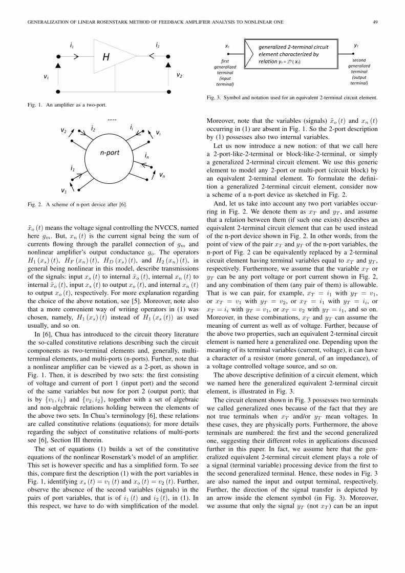
Fig. 1. An amplifier as a two-port.
i2
i1
v1
v2
n-port
device
…..
ii
in
vi
vn
Fig. 2. A scheme of n-port device after [6].
x̃o (t) means the voltage signal controlling the NVCCS, named
here gm. But, xn (t) is the current signal being the sum of
currents flowing through the parallel connection of gm and
nonlinear amplifier’s output conductance go. The operators
H1 (xs) (t), HF (xn) (t), HD (xs) (t), and H2 (xn) (t), in
general being nonlinear in this model, describe transmissions
of the signals: input xs (t) to internal x̃o (t), internal xn (t) to
internal x̃o (t), input xs (t) to output xo (t), and internal xn (t)to output xo (t), respectively. For more explanation regarding
the choice of the above notation, see [5]. Moreover, note also
that a more convenient way of writing operators in (1) was
chosen, namely, H1 (xs) (t) instead of H1 (xs (t)) as used
usually, and so on.
In [6], Chua has introduced to the circuit theory literature
the so-called constitutive relations describing such the circuit
components as two-terminal elements and, generally, multi-
terminal elements, and multi-ports (n-ports). Further, note that
a nonlinear amplifier can be viewed as a 2-port, as shown in
Fig. 1. Then, it is described by two sets: the first consisting
of voltage and current of port 1 (input port) and the second
of the same variables but now for port 2 (output port); that
is by {v1, i1} and {v2, i2}, together with a set of algebraic
and non-algebraic relations holding between the elements of
the above two sets. In Chua’s terminology [6], these relations
are called constitutive relations (equations); for more details
regarding the subject of constitutive relations of multi-ports
see [6], Section III therein.
The set of equations (1) builds a set of the constitutive
equations of the nonlinear Rosenstark’s model of an amplifier.
This set is however specific and has a simplified form. To see
this, compare first the description (1) with the port variables in
Fig. 1, identifying xs (t) = v1 (t) and xo (t) = v2 (t). Further,
observe the absence of the second variables (signals) in the
pairs of port variables, that is of i1 (t) and i2 (t), in (1). In
this respect, we have to do with simplification of the model.
xT yT
first
generalized
terminal
(input
terminal)
generalized 2-terminal circuit
element characterized by
relation yT = D ( xT) second
generalized
terminal
(output
terminal)
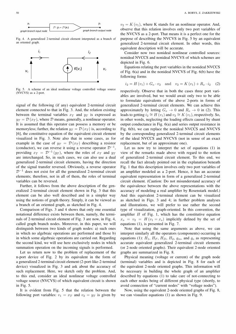
Fig. 3. Symbol and notation used for an equivalent 2-terminal circuit element.
Moreover, note that the variables (signals) x̃o (t) and xn (t)occurring in (1) are absent in Fig. 1. So the 2-port description
by (1) possesses also two internal variables.
Let us now introduce a new notion: of that we call here
a 2-port-like-2-terminal or block-like-2-terminal, or simply
a generalized 2-terminal circuit element. We use this generic
element to model any 2-port or multi-port (circuit block) by
an equivalent 2-terminal element. To formulate the defini-
tion a generalized 2-terminal circuit element, consider now
a scheme of a n-port device as sketched in Fig. 2.
And, let us take into account any two port variables occur-
ring in Fig. 2. We denote them as xT and yT , and assume
that a relation between them (if such one exists) describes an
equivalent 2-terminal circuit element that can be used instead
of the n-port device shown in Fig. 2. In other words, from the
point of view of the pair xT and yT of the n-port variables, the
n-port of Fig. 2 can be equivalently replaced by a 2-terminal
circuit element having terminal variables equal to xT and yT ,
respectively. Furthermore, we assume that the variable xT or
yT can be any port voltage or port current shown in Fig. 2,
and any combination of them (any pair of them) is allowable.
That is we can pair, for example, xT = i1 with yT = v1,
or xT = v1 with yT = v2, or xT = i1 with yT = ii, or
xT = ii with yT = v1, or xT = v2 with yT = i1, and so on.
Moreover, in these combinations, xT and yT can assume the
meaning of current as well as of voltage. Further, because of
the above two properties, such an equivalent 2-terminal circuit
element is named here a generalized one. Depending upon the
meaning of its terminal variables (current, voltage), it can have
a character of a resistor (more general, of an impedance), of
a voltage controlled voltage source, and so on.
The above descriptive definition of a circuit element, which
we named here the generalized equivalent 2-terminal circuit
element, is illustrated in Fig. 3.
The circuit element shown in Fig. 3 possesses two terminals
we called generalized ones because of the fact that they are
not true terminals when xT and/or yT mean voltages. In
these cases, they are physically ports. Furthermore, the above
terminals are numbered: the first and the second generalized
one, suggesting their different roles in applications discussed
further in this paper. In fact, we assume here that the gen-
eralized equivalent 2-terminal circuit element plays a role of
a signal (terminal variable) processing device from the first to
the second generalized terminal. Hence, these nodes in Fig. 3
are also named the input and output terminal, respectively.
Further, the direction of the signal transfer is depicted by
an arrow inside the element symbol (in Fig. 3). Moreover,
we assume that only the signal yT (not xT ) can be an input
50 A. BORYS, Z. ZAKRZEWSKI
xT yT
graph branch input node graph branch output node
D : yT = D (xT)
Fig. 4. A generalized 2-terminal circuit element interpreted as a branch ofan oriented graph.
K(v1) v1
i1
v2
i2
Fig. 5. A scheme of an ideal nonlinear voltage controlled voltage source(NVCVS) as a 2-port.
signal of the following (if any) equivalent 2-terminal circuit
element connected to that in Fig. 3. And, the relation existing
between the terminal variables xT and yT is expressed as
yT = D (xT ), where D means, generally, a nonlinear operator.
It is assumed that this operator can possess a memory or be
memoryless; further, the relation yT = D (xT ) is, according to
[6], the constitutive equation of the equivalent circuit element
visualized in Fig. 3. Note also that in some cases, as for
example in the case of yT = D (xT ) describing a resistor
(conductor), we can reverse it using a reverse operator D−1,
providing xT = D−1 (yT ), where the roles of xT and yTare interchanged. So, in such cases, we can also use a dual
generalized 2-terminal circuit elements, having the direction
of the signal transfer reversed. Obviously, a reverse operator
D−1 does not exist for all the generalized 2-terminal circuit
elements; therefore, not in all of them, the roles of terminal
variables can be reversed.
Further, it follows from the above description of the gen-
eralized 2-terminal circuit element shown in Fig. 3 that this
element can be also well described and in a simpler way
using the notions of graph theory. Simply, it can be viewed as
a branch of an oriented graph, as sketched in Fig. 4.
Comparison of Figs. 3 and 4 shows that only one essential
notational difference exists between them, namely, the termi-
nals of 2-terminal circuit element of Fig. 3 are now, in Fig. 4,
called graph branch nodes. Moreover, in this paper, we will
distinguish between two kinds of graph nodes: a) such ones
in which no algebraic operations are performed and those b)
in which some algebraic operations are carried out. Regarding
the second kind, we will use here exclusively nodes in which
summation operation on the incoming signals is performed.
Let us return now to the problem of replacement of the
n-port device of Fig. 2 by its equivalent in the form of
a generalized 2-terminal circuit element (2-port-like-2-terminal
device) visualized in Fig. 3 and ask about the accuracy of
such replacement. Here, we sketch only the problem. And,
to this end, consider an ideal nonlinear voltage controlled
voltage source (NVCVS) of which equivalent circuit is shown
in Fig. 5.
It is evident from Fig. 5 that the relation between the
following port variables: v1 = xT and v2 = yT is given by
v2 = K (v1), where K stands for an nonlinear operator. And,
observe that this relation involves only two port variables of
the NVCVS as a 2-port. That means it is a perfect one for the
purpose of describing the NVCVS in Fig. 5 by an equivalent
generalized 2-terminal circuit element. In other words, this
equivalent description will be accurate.
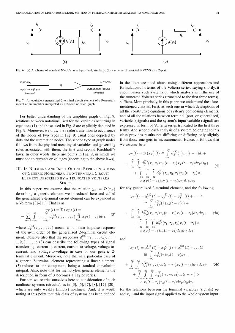
Consider now two nonideal nonlinear controlled sources:
nonideal NVCCS and nonideal NVCVS of which schemes are
depicted in Fig. 6.
Equations relating the port variables in the nonideal NVCCS
of Fig. 6(a) and in the nonideal NVCVS of Fig. 6(b) have the
following forms
i2 = H (v1) +Go · v2 and v2 = K (v1) +Ro · i2 (2)
respectively. Observe that in both the cases three port vari-
ables are involved, but we would await only two to be able
to formulate equivalents of the above 2-ports in forms of
generalized 2-terminal circuit elements. We can achieve this
approximately by letting Go → 0 and Ro → 0 in (2). This
leads to getting i2 ∼= H (v1) and v2 ∼= K (v1), respectively. So,
in other words, neglecting the loading effects caused by shunt
output conductance in Fig. 6(a) and series output resistance in
Fig. 6(b), we can replace the nonideal NVCCS and NVCVS
by the corresponding generalized 2-terminal circuit elements
of the ideal NVCCS and NVCVS (not in sense of an exact
replacement, but of an approximate one).
Let us now try to interpret the set of equations (1) in
view of the remarks made above with regard to the notion
of generalized 2-terminal circuit element. To this end, we
recall the fact already pointed out in the explanation beneath
Fig. 1 that this description involves only two port variables of
an amplifier modeled as a 2-port. Hence, it has an accurate
equivalent representation in form of a generalized 2-terminal
circuit element. (Caution: Do not misunderstand accuracy of
the equivalence between the above representations with the
accuracy of modeling a real amplifier by Rosenstark model.)
And this equivalent 2-terminal element can be visualized
as sketched in Figs. 3 and 4; in further problem analyses
and illustrations, we will prefer to use rather the second
type of visualization, graph-oriented. In this convention, the
amplifier H of Fig. 1, which has the constitutive equation
xo = v2 = H (v1 = xs) implicitly defined by the set of
equations (1), is presented in Fig. 7.
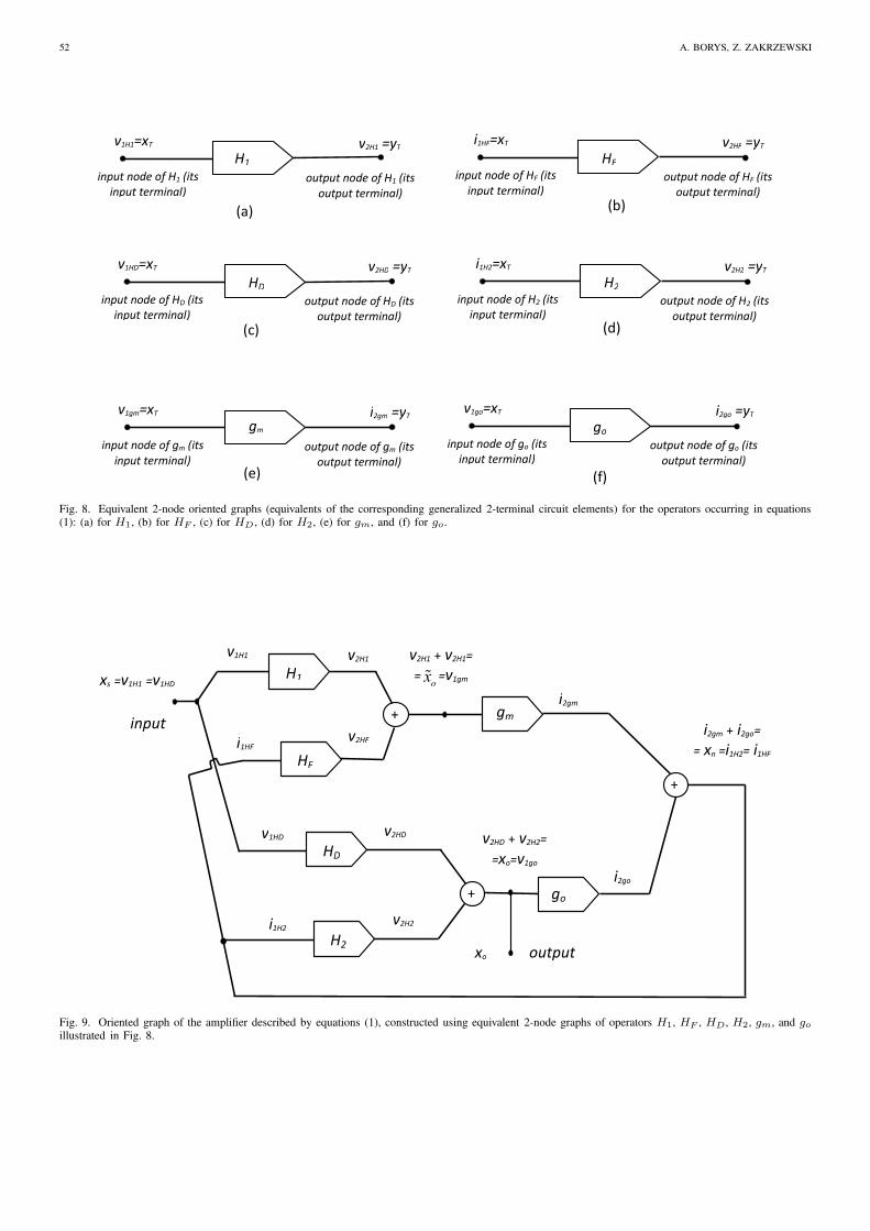
Note that using the same arguments as above, we can
interpret similarly all the operators (components) occurring in
equations (1): H1, HF , HD , H2, gm, and go as representing
accurate equivalent generalized 2-terminal circuit elements
(or 2-node oriented graphs). Their equivalent 2-node oriented
graphs are summarized in Fig. 8.
Physical meaning (voltage or current) of the graph node
(terminal) variables and is depicted in Fig. 8 for each of
the equivalent 2-node oriented graphs. This information will
be necessary in building the whole graph of an amplifier
described by equations (1) to take care of not-connecting to
each other nodes being of different physical type (shortly, to
avoid connection of “current nodes” with “voltage nodes”).
Now, using the equivalent 2-node oriented graphs of Fig. 8,
we can visualize equations (1) as shown in Fig. 9.
GENERALIZATION OF LINEAR ROSENSTARK METHOD OF FEEDBACK AMPLIFIER ANALYSIS TO NONLINEAR ONE 51
H(v1) v1
i1
v2
i2
K(v1) v1
i1
v2
i2
Go
Ro
(a) (b)
Fig. 6. (a) A scheme of nonideal NVCCS as a 2-port and, similarly, (b) a scheme of nonideal NVCVS as a 2-port.
v1=xT =xs v2 =yT=xo
input node (input
terminal)
output node (output
terminal)
H
Fig. 7. An equivalent generalized 2-terminal circuit element of a Rosenstarkmodel of an amplifier interpreted as a 2-node oriented graph.
For better understanding of the amplifier graph of Fig. 9,
relations between notations used for the variables occurring in
equations (1) and those used in Fig. 8 are explicitly depicted in
Fig. 9. Moreover, we draw the reader’s attention to occurrence
of the nodes of two types in Fig. 9: usual ones depicted by
dots and the summation nodes. The second type of graph nodes
follows from the physical meaning of variables and governing
rules associated with them: the first and second Kirchhoff’s
laws. In other words, there are points in Fig. 9, in which we
must add to currents or voltages (according to the above laws).
III. IN-NETWORK AND INPUT-OUTPUT REPRESENTATIONS
OF GENERIC NONLINEAR TWO-TERMINAL CIRCUIT
ELEMENT DESCRIBED BY A TRUNCATED VOLTERRA
SERIES
In this paper, we assume that the relation yT = D (xT )describing a generic element we introduced here and called
the generalized 2-terminal circuit element can be expanded in
a Volterra [8]–[11]. That is as
yT (t) = D (xT ) (t) =
=∞∑
n=1
∞∫
−∞
· · ·∞∫
−∞
d(n)T (τ1, . . . , τn)
n
Πk=1
xT (t− τk)dτk(3)
where d(n)T (τ1, . . . , τn) means a nonlinear impulse response
of the n-th order of the generalized 2-terminal circuit ele-
ment. Observe also that the responses d(n)T (τ1, . . . , τn), n =
1, 2, 3, . . ., in (3) can describe the following types of signal
transferring: current-to-current, current-to-voltage, voltage-to-
current, and voltage-to-voltage in case of our generic 2-
terminal element. Moreover, note that in a particular case of
a generic 2-terminal element representing a linear element,
(3) reduces to one component, being a standard convolution
integral. Also, note that for memoryless generic elements the
description in form of 3 becomes a Taylor series.
Further, we restrict ourselves here to consideration of such
nonlinear systems (circuits), as in [3], [5], [7], [8], [12]–[20],
which are only weakly (mildly) nonlinear. And, it is worth
noting at this point that this class of systems has been defined
in the literature cited above using different approaches and
formulations. In terms of the Volterra series, saying shortly, it
encompasses such systems of which analysis with the use of
the truncated Volterra series (truncated to the first three terms),
suffices. More precisely, in this paper, we understand the afore-
mentioned class as: First, as such one in which descriptions of
all the constitutive equations of system’s composing elements,
and of all the relations between terminal (port, or generalized)
variables (signals) and the system’s input variable (signal) are
expressed in form of Volterra series truncated to the first three
terms. And second, each analysis of a system belonging to this
class provides results not differing or differing only slightly
from those one gets in measurements. Hence, it follows that
we assume here
yT (t) = D (xT ) (t) ∼=∞∫
−∞
d(1)T (τ)xT (t− τ)dτ+
+∞∫
−∞
∞∫
−∞
d(2)T (τ1, τ2)xT (t− τ1)xT (t− τ2)dτ1dτ2+
+∞∫
−∞
∞∫
−∞
∞∫
−∞
d(3)T (τ1, τ2, τ3)xT (t− τ1)×
× xT (t− τ2)xT (t− τ3)dτ1dτ2dτ3
(4)
for any generalized 2-terminal element, and the following
yT (t) = y(1)T (t) + y
(2)T (t) + y
(3)T (t) + . . . ∼=
∼=∞∫
−∞
h(1)To(τ)xs(t− τ)dτ+
+∞∫
−∞
∞∫
−∞
h(2)To(τ1, τ2)xs(t− τ1)xs(t− τ2)dτ1dτ2+
+∞∫
−∞
∞∫
−∞
∞∫
−∞
h(3)To(τ1, τ2, τ3)xs(t− τ1)×
× xs(t− τ2)xs(t− τ3)dτ1dτ2dτ3
(5a)
and
xT (t) = x(1)T (t) + x
(2)T (t) + x
(3)T (t) + . . . ∼=
∼=∞∫
−∞
h(1)Ti (τ)xs(t− τ)dτ+
+∞∫
−∞
∞∫
−∞
h(2)Ti (τ1, τ2)xs(t− τ1)xs(t− τ2)dτ1dτ2+
+∞∫
−∞
∞∫
−∞
∞∫
−∞
h(3)Ti (τ1, τ2, τ3)xs(t− τ1) ×
× xs(t− τ2)xs(t− τ3)dτ1dτ2dτ3
(5b)
for the relations between the terminal variables (signals) yTand xT , and the input signal applied to the whole system input.
52 A. BORYS, Z. ZAKRZEWSKI
v1H1=xT v2H1 =yT
input node of H1 (its
input terminal)
output node of H1 (its
output terminal)
H1
(a)
i1HF=xT v2HF =yT
input node of HF (its
input terminal)
output node of HF (its
output terminal)
HF
(b)
i1H2=xT v2H2 =yT
input node of H2 (its
input terminal)
output node of H2 (its
output terminal)
H2
(d)
v1HD=xT v2HD =yT
input node of HD (its
input terminal)
output node of HD (its
output terminal)
HD
(c)
v1gm=xT i2gm =yT
input node of gm (its
input terminal)
output node of gm (its
output terminal)
gm
(e)
v1go=xT i2go =yT
input node of go (its
input terminal)
output node of go (its
output terminal)
go
(f)
Fig. 8. Equivalent 2-node oriented graphs (equivalents of the corresponding generalized 2-terminal circuit elements) for the operators occurring in equations(1): (a) for H1, (b) for HF , (c) for HD , (d) for H2, (e) for gm, and (f) for go.
xs =v1H1 =v1HD
v2H1 + v2H1=
=oxɶ =v1gm H1
v2H1
HF
v2HF
v2HD
HD
i1HF
H2
v2H2
v1HD
go
gm +
+
+
output
input
v1H1
i1H2
v2HD + v2H2=
=xo=v1go
xo
i2gm
i2go
i2gm + i2go=
= xn =i1H2= i1HF
Fig. 9. Oriented graph of the amplifier described by equations (1), constructed using equivalent 2-node graphs of operators H1, HF , HD , H2, gm, and goillustrated in Fig. 8.
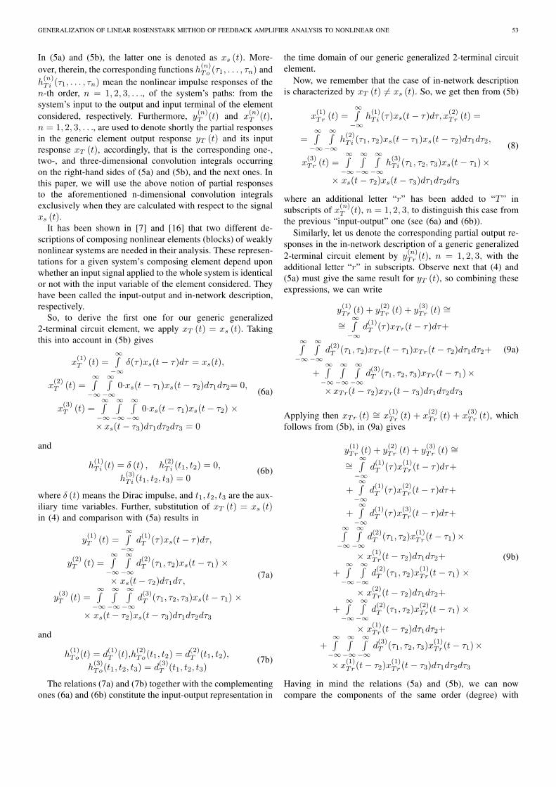
GENERALIZATION OF LINEAR ROSENSTARK METHOD OF FEEDBACK AMPLIFIER ANALYSIS TO NONLINEAR ONE 53
In (5a) and (5b), the latter one is denoted as xs (t). More-
over, therein, the corresponding functions h(n)To (τ1, . . . , τn) and
h(n)Ti (τ1, . . . , τn) mean the nonlinear impulse responses of the
n-th order, n = 1, 2, 3, . . ., of the system’s paths: from the
system’s input to the output and input terminal of the element
considered, respectively. Furthermore, y(n)T (t) and x
(n)T (t),
n = 1, 2, 3, . . ., are used to denote shortly the partial responses
in the generic element output response yT (t) and its input
response xT (t), accordingly, that is the corresponding one-,
two-, and three-dimensional convolution integrals occurring
on the right-hand sides of (5a) and (5b), and the next ones. In
this paper, we will use the above notion of partial responses
to the aforementioned n-dimensional convolution integrals
exclusively when they are calculated with respect to the signal
xs (t).It has been shown in [7] and [16] that two different de-
scriptions of composing nonlinear elements (blocks) of weakly
nonlinear systems are needed in their analysis. These represen-
tations for a given system’s composing element depend upon
whether an input signal applied to the whole system is identical
or not with the input variable of the element considered. They
have been called the input-output and in-network description,
respectively.
So, to derive the first one for our generic generalized
2-terminal circuit element, we apply xT (t) = xs (t). Taking
this into account in (5b) gives
x(1)T (t) =
∞∫
−∞
δ(τ)xs(t− τ)dτ = xs(t),
x(2)T (t) =
∞∫
−∞
∞∫
−∞
0·xs(t− τ1)xs(t− τ2)dτ1dτ2= 0,
x(3)T (t) =
∞∫
−∞
∞∫
−∞
∞∫
−∞
0·xs(t− τ1)xs(t− τ2) ×
× xs(t− τ3)dτ1dτ2dτ3 = 0
(6a)
and
h(1)Ti (t) = δ (t) , h
(2)Ti (t1, t2) = 0,
h(3)Ti (t1, t2, t3) = 0
(6b)
where δ (t) means the Dirac impulse, and t1, t2, t3 are the aux-
iliary time variables. Further, substitution of xT (t) = xs (t)in (4) and comparison with (5a) results in
y(1)T (t) =
∞∫
−∞
d(1)T (τ)xs(t− τ)dτ,
y(2)T (t) =
∞∫
−∞
∞∫
−∞
d(2)T (τ1, τ2)xs(t− τ1) ×
× xs(t− τ2)dτ1dτ,
y(3)T (t) =
∞∫
−∞
∞∫
−∞
∞∫
−∞
d(3)T (τ1, τ2, τ3)xs(t− τ1) ×
× xs(t− τ2)xs(t− τ3)dτ1dτ2dτ3
(7a)
and
h(1)To(t) = d
(1)T (t),h
(2)To(t1, t2) = d
(2)T (t1, t2),
h(3)To(t1, t2, t3) = d
(3)T (t1, t2, t3)
(7b)
The relations (7a) and (7b) together with the complementing
ones (6a) and (6b) constitute the input-output representation in
the time domain of our generic generalized 2-terminal circuit
element.
Now, we remember that the case of in-network description
is characterized by xT (t) 6= xs (t). So, we get then from (5b)
x(1)Tr (t) =
∞∫
−∞
h(1)Ti (τ)xs(t− τ)dτ, x
(2)Tr (t) =
=∞∫
−∞
∞∫
−∞
h(2)Ti (τ1, τ2)xs(t− τ1)xs(t− τ2)dτ1dτ2,
x(3)Tr (t) =
∞∫
−∞
∞∫
−∞
∞∫
−∞
h(3)Ti (τ1, τ2, τ3)xs(t− τ1)×
× xs(t− τ2)xs(t− τ3)dτ1dτ2dτ3
(8)
where an additional letter “r” has been added to “T ” in
subscripts of x(n)T (t), n = 1, 2, 3, to distinguish this case from
the previous “input-output” one (see (6a) and (6b)).
Similarly, let us denote the corresponding partial output re-
sponses in the in-network description of a generic generalized
2-terminal circuit element by y(n)Tr (t), n = 1, 2, 3, with the
additional letter “r” in subscripts. Observe next that (4) and
(5a) must give the same result for yT (t), so combining these
expressions, we can write
y(1)Tr (t) + y
(2)Tr (t) + y
(3)Tr (t)
∼=
∼=∞∫
−∞
d(1)T (τ)xTr(t− τ)dτ+
∞∫
−∞
∞∫
−∞
d(2)T (τ1, τ2)xTr(t− τ1)xTr(t− τ2)dτ1dτ2+
+∞∫
−∞
∞∫
−∞
∞∫
−∞
d(3)T (τ1, τ2, τ3)xTr(t− τ1)×
× xTr(t− τ2)xTr(t− τ3)dτ1dτ2dτ3
(9a)
Applying then xTr (t) ∼= x(1)Tr (t) + x
(2)Tr (t) + x
(3)Tr (t), which
follows from (5b), in (9a) gives
y(1)Tr (t) + y
(2)Tr (t) + y
(3)Tr (t)
∼=
∼=∞∫
−∞
d(1)T (τ)x
(1)Tr (t− τ)dτ+
+∞∫
−∞
d(1)T (τ)x
(2)Tr (t− τ)dτ+
+∞∫
−∞
d(1)T (τ)x
(3)Tr (t− τ)dτ+
∞∫
−∞
∞∫
−∞
d(2)T (τ1, τ2)x
(1)Tr (t− τ1)×
× x(1)Tr (t− τ2)dτ1dτ2+
+∞∫
−∞
∞∫
−∞
d(2)T (τ1, τ2)x
(1)Tr (t− τ1) ×
× x(2)Tr (t− τ2)dτ1dτ2+
+∞∫
−∞
∞∫
−∞
d(2)T (τ1, τ2)x
(2)Tr (t− τ1) ×
× x(1)Tr (t− τ2)dτ1dτ2+
+∞∫
−∞
∞∫
−∞
∞∫
−∞
d(3)T (τ1, τ2, τ3)x
(1)Tr (t− τ1)×
× x(1)Tr (t− τ2)x
(1)Tr (t− τ3)dτ1dτ2dτ3
(9b)
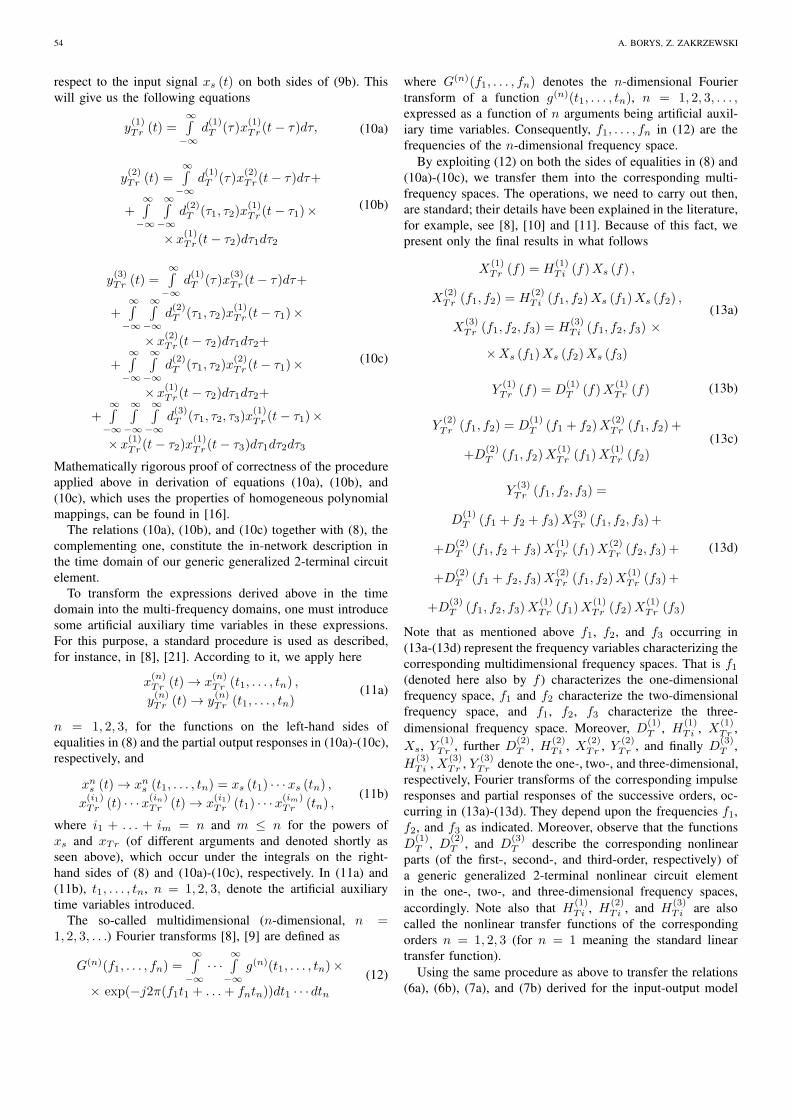
Having in mind the relations (5a) and (5b), we can now
compare the components of the same order (degree) with
54 A. BORYS, Z. ZAKRZEWSKI
respect to the input signal xs (t) on both sides of (9b). This
will give us the following equations
y(1)Tr (t) =
∞∫
−∞
d(1)T (τ)x
(1)Tr (t− τ)dτ, (10a)
y(2)Tr (t) =
∞∫
−∞
d(1)T (τ)x
(2)Tr (t− τ)dτ+
+∞∫
−∞
∞∫
−∞
d(2)T (τ1, τ2)x
(1)Tr (t− τ1)×
× x(1)Tr (t− τ2)dτ1dτ2
(10b)
y(3)Tr (t) =
∞∫
−∞
d(1)T (τ)x
(3)Tr (t− τ)dτ+
+∞∫
−∞
∞∫
−∞
d(2)T (τ1, τ2)x
(1)Tr (t− τ1)×
× x(2)Tr (t− τ2)dτ1dτ2+
+∞∫
−∞
∞∫
−∞
d(2)T (τ1, τ2)x
(2)Tr (t− τ1)×
× x(1)Tr (t− τ2)dτ1dτ2+
+∞∫
−∞
∞∫
−∞
∞∫
−∞
d(3)T (τ1, τ2, τ3)x
(1)Tr (t− τ1)×
× x(1)Tr (t− τ2)x
(1)Tr (t− τ3)dτ1dτ2dτ3
(10c)
Mathematically rigorous proof of correctness of the procedure
applied above in derivation of equations (10a), (10b), and
(10c), which uses the properties of homogeneous polynomial
mappings, can be found in [16].
The relations (10a), (10b), and (10c) together with (8), the
complementing one, constitute the in-network description in
the time domain of our generic generalized 2-terminal circuit
element.
To transform the expressions derived above in the time
domain into the multi-frequency domains, one must introduce
some artificial auxiliary time variables in these expressions.
For this purpose, a standard procedure is used as described,
for instance, in [8], [21]. According to it, we apply here
x(n)Tr (t) → x
(n)Tr (t1, . . . , tn) ,
y(n)Tr (t) → y
(n)Tr (t1, . . . , tn)
(11a)
n = 1, 2, 3, for the functions on the left-hand sides of
equalities in (8) and the partial output responses in (10a)-(10c),
respectively, and
xns (t) → xn
s (t1, . . . , tn) = xs (t1) · · ·xs (tn) ,
x(i1)Tr (t) · · ·x
(in)Tr (t) → x
(i1)Tr (t1) · · ·x
(im)Tr (tn) ,
(11b)
where i1 + . . . + im = n and m ≤ n for the powers of
xs and xTr (of different arguments and denoted shortly as
seen above), which occur under the integrals on the right-
hand sides of (8) and (10a)-(10c), respectively. In (11a) and
(11b), t1, . . . , tn, n = 1, 2, 3, denote the artificial auxiliary
time variables introduced.
The so-called multidimensional (n-dimensional, n =1, 2, 3, . . .) Fourier transforms [8], [9] are defined as
G(n)(f1, . . . , fn) =∞∫
−∞
· · ·∞∫
−∞
g(n)(t1, . . . , tn)×
× exp(−j2π(f1t1 + . . .+ fntn))dt1 · · · dtn
(12)
where G(n)(f1, . . . , fn) denotes the n-dimensional Fourier
transform of a function g(n)(t1, . . . , tn), n = 1, 2, 3, . . . ,expressed as a function of n arguments being artificial auxil-
iary time variables. Consequently, f1, . . . , fn in (12) are the
frequencies of the n-dimensional frequency space.
By exploiting (12) on both the sides of equalities in (8) and
(10a)-(10c), we transfer them into the corresponding multi-
frequency spaces. The operations, we need to carry out then,
are standard; their details have been explained in the literature,
for example, see [8], [10] and [11]. Because of this fact, we
present only the final results in what follows
X(1)Tr (f) = H
(1)Ti (f)Xs (f) ,
X(2)Tr (f1, f2) = H
(2)Ti (f1, f2)Xs (f1)Xs (f2) ,
X(3)Tr (f1, f2, f3) = H
(3)Ti (f1, f2, f3) ×
×Xs (f1)Xs (f2)Xs (f3)
(13a)
Y(1)Tr (f) = D
(1)T (f)X
(1)Tr (f) (13b)
Y(2)Tr (f1, f2) = D
(1)T (f1 + f2)X
(2)Tr (f1, f2) +
+D(2)T (f1, f2)X
(1)Tr (f1)X
(1)Tr (f2)
(13c)
Y(3)Tr (f1, f2, f3) =
D(1)T (f1 + f2 + f3)X
(3)Tr (f1, f2, f3) +
+D(2)T (f1, f2 + f3)X
(1)Tr (f1)X
(2)Tr (f2, f3)+
+D(2)T (f1 + f2, f3)X
(2)Tr (f1, f2)X
(1)Tr (f3)+
+D(3)T (f1, f2, f3)X
(1)Tr (f1)X
(1)Tr (f2)X
(1)Tr (f3)
(13d)
Note that as mentioned above f1, f2, and f3 occurring in
(13a-(13d) represent the frequency variables characterizing the
corresponding multidimensional frequency spaces. That is f1(denoted here also by f ) characterizes the one-dimensional
frequency space, f1 and f2 characterize the two-dimensional
frequency space, and f1, f2, f3 characterize the three-
dimensional frequency space. Moreover, D(1)T , H
(1)Ti , X
(1)Tr ,
Xs, Y(1)Tr , further D
(2)T , H
(2)Ti , X
(2)Tr , Y
(2)Tr , and finally D
(3)T ,
H(3)Ti , X
(3)Tr , Y
(3)Tr denote the one-, two-, and three-dimensional,
respectively, Fourier transforms of the corresponding impulse
responses and partial responses of the successive orders, oc-
curring in (13a)-(13d). They depend upon the frequencies f1,
f2, and f3 as indicated. Moreover, observe that the functions
D(1)T , D
(2)T , and D
(3)T describe the corresponding nonlinear
parts (of the first-, second-, and third-order, respectively) of
a generic generalized 2-terminal nonlinear circuit element
in the one-, two-, and three-dimensional frequency spaces,
accordingly. Note also that H(1)Ti , H
(2)Ti , and H
(3)Ti are also
called the nonlinear transfer functions of the corresponding
orders n = 1, 2, 3 (for n = 1 meaning the standard linear
transfer function).
Using the same procedure as above to transfer the relations
(6a), (6b), (7a), and (7b) derived for the input-output model
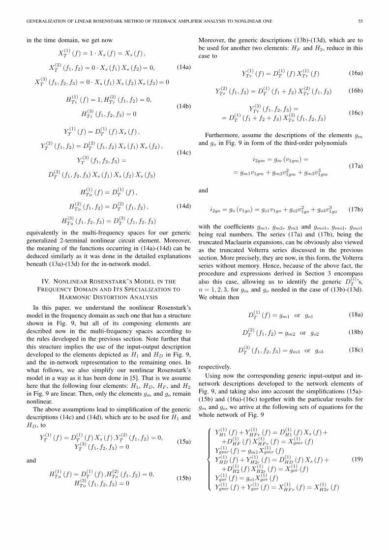
GENERALIZATION OF LINEAR ROSENSTARK METHOD OF FEEDBACK AMPLIFIER ANALYSIS TO NONLINEAR ONE 55
in the time domain, we get now
X(1)T (f) = 1 ·Xs (f) = Xs (f) ,
X(2)T (f1, f2) = 0 ·Xs (f1)Xs (f2)= 0,
X(3)T (f1, f2, f3) = 0 ·Xs (f1)Xs (f2)Xs (f3)= 0
(14a)
H(1)Ti (f) = 1, H
(2)Ti (f1, f2) = 0,
H(3)Ti (f1, f2, f3) = 0
(14b)
Y(1)T (f) = D
(1)T (f)Xs (f) ,
Y(2)T (f1, f2) = D
(2)T (f1, f2)Xs (f1)Xs (f2) ,
Y(3)T (f1, f2, f3) =
D(3)T (f1, f2, f3)Xs (f1)Xs (f2)Xs (f3)
(14c)
H(1)To (f) = D
(1)T (f) ,
H(2)To (f1, f2) = D
(2)T (f1, f2) ,
H(3)To (f1, f2, f3) = D
(3)T (f1, f2, f3)
(14d)
equivalently in the multi-frequency spaces for our generic
generalized 2-terminal nonlinear circuit element. Moreover,
the meaning of the functions occurring in (14a)-(14d) can be
deduced similarly as it was done in the detailed explanations
beneath (13a)-(13d) for the in-network model.
IV. NONLINEAR ROSENSTARK’S MODEL IN THE
FREQUENCY DOMAIN AND ITS SPECIALIZATION TO
HARMONIC DISTORTION ANALYSIS
In this paper, we understand the nonlinear Rosenstark’s
model in the frequency domain as such one that has a structure
shown in Fig. 9, but all of its composing elements are
described now in the multi-frequency spaces according to
the rules developed in the previous section. Note further that
this structure implies the use of the input-output description
developed to the elements depicted as H1 and HD in Fig. 9,
and the in-network representation to the remaining ones. In
what follows, we also simplify our nonlinear Rosenstark’s
model in a way as it has been done in [5]. That is we assume
here that the following four elements: H1, HD, HF , and H2
in Fig. 9 are linear. Then, only the elements gm and go remain
nonlinear.
The above assumptions lead to simplification of the generic
descriptions (14c) and (14d), which are to be used for H1 and
HD , to
Y(1)T (f) = D
(1)T (f)Xs (f) ,Y
(2)T (f1, f2) = 0,
Y(3)T (f1, f2, f3) = 0
(15a)
and
H(1)To (f) = D
(1)T (f) ,H
(2)To (f1, f2) = 0,
H(3)To (f1, f2, f3) = 0
(15b)
Moreover, the generic descriptions (13b)-(13d), which are to
be used for another two elements: HF and H2, reduce in this
case to
Y(1)Tr (f) = D
(1)T (f)X
(1)Tr (f) (16a)
Y(2)Tr (f1, f2) = D
(1)T (f1 + f2)X
(2)Tr (f1, f2) (16b)
Y(3)Tr (f1, f2, f3) =
= D(1)T (f1 + f2 + f3)X
(3)Tr (f1, f2, f3)
(16c)
Furthermore, assume the descriptions of the elements gmand go in Fig. 9 in form of the third-order polynomials
i2gm = gm (v1gm) =
= gm1v1gm + gm2v21gm + gm3v
31gm
(17a)
and
i2go = go (v1go) = go1v1go + go2v21go + go3v
31go (17b)
with the coefficients gm1, gm2, gm3 and gmo1, gmo1, gmo1
being real numbers. The series (17a) and (17b), being the
truncated Maclaurin expansions, can be obviously also viewed
as the truncated Volterra series discussed in the previous
section. More precisely, they are now, in this form, the Volterra
series without memory. Hence, because of the above fact, the
procedure and expressions derived in Section 3 encompass
also this case, allowing us to identify the generic D(i)T ’s,
n = 1, 2, 3, for gm and go needed in the case of (13b)-(13d).
We obtain then
D(1)T (f) = gm1 or go1 (18a)
D(2)T (f1, f2) = gm2 or go2 (18b)
D(3)T (f1, f2, f3) = gm3 or go3 (18c)
respectively.
Using now the corresponding generic input-output and in-
network descriptions developed to the network elements of
Fig. 9, and taking also into account the simplifications (15a)-
(15b) and (16a)-(16c) together with the particular results for
gm and go, we arrive at the following sets of equations for the
whole network of Fig. 9
Y(1)H1 (f) + Y
(1)HFr (f) = D
(1)H1 (f)Xs (f)+
+D(1)HF (f)X
(1)HFr (f) = X
(1)gmr (f)
Y(1)gmr (f) = gm1X
(1)gmr (f)
Y(1)HD (f) + Y
(1)H2r (f) = D
(1)HD (f)Xs (f)+
+D(1)H2 (f)X
(1)H2r (f) = X
(1)gor (f)
Y(1)gor (f) = go1X
(1)gor (f)
Y(1)gmr (f) + Y
(1)gor (f) = X
(1)HFr (f) = X
(1)H2r (f)
(19)
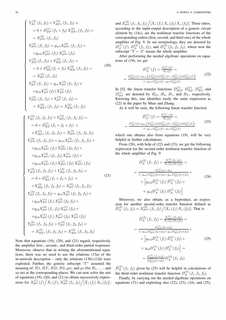
56 A. BORYS, Z. ZAKRZEWSKI
Y(2)H1 (f1, f2) + Y
(2)HFr (f1, f2) =
= 0 +D(1)HF (f1 + f2)X
(2)HFr (f1, f2) =
= X(2)gmr (f1, f2)
Y(2)gmr (f1, f2) = gm1X
(2)gmr (f1, f2)+
+gm2X(1)gmr (f1)X
(1)gmr (f2)
Y(2)HD (f1, f2) + Y
(2)H2r (f1, f2) =
= 0 +D(1)H2 (f1 + f2)X
(2)H2r (f1, f2) =
= X(2)gor (f1, f2)
Y(2)gor (f1, f2) = go1X
(2)gor (f1, f2)+
+go2X(1)gor (f1)X
(1)gor (f2)
Y(2)gmr (f1, f2) + Y
(2)gor (f1, f2) =
= X(2)HFr (f1, f2) = X
(2)H2r (f1, f2)
(20)
Y(3)H1 (f1, f2, f3) + Y
(3)HFr (f1, f2, f3) =
= 0 +D(1)HF (f1 + f2 + f3) ×
×X(3)HFr (f1, f2, f3) = X
(3)gmr (f1, f2, f3)
Y(3)gmr (f1, f2, f3) = gm1X
(3)gmr (f1, f2, f3) +
+gm2X(1)gmr (f1)X
(2)gmr (f2, f3)+
+gm2X(2)gmr (f1, f2)X
(1)gmr (f3)+
+gm3X(1)gmr (f1)X
(1)gmr (f2)X
(1)gmr (f3)
Y(3)HD (f1, f2, f3) + Y
(3)H2r (f1, f2, f3) =
= 0 +D(1)H2 (f1 + f2 + f3) ×
×X(3)H2r (f1, f2, f3) = X
(3)gor (f1, f2, f3)
Y(3)gor (f1, f2, f3) = go1X
(3)gor (f1, f2, f3)+
+go2X(1)gor (f1)X
(2)gor (f2, f3)+
+go2X(2)gor (f1, f2)X
(1)gor (f3)+
+go3X(1)gor (f1)X
(1)gor (f2)X
(1)gor (f3)
Y(3)gmr (f1, f2, f3) + Y
(3)gor (f1, f2, f3) =
= X(3)HFr (f1, f2, f3) = X
(3)H2r (f1, f2, f3)
(21)
Note that equations (19), (20), and (21) regard, respectively,
the amplifier first-, second-, and third-order partial responses.
Moreover, observe that in writing the aforementioned equa-
tions, there was no need to use the relations (13a) of the
in-network description – only the relations (13b)-(13d) were
exploited. Further, the generic subscript “T ” assumed the
meaning of: H1, HF , HD, H2, gm, and go (for H1, . . . , and
so on) at the corresponding places. We can now solve the sets
of equations (19), (20), and (21) to obtain successively expres-
sions for X(1)gor (f)
/
Xs (f), X(2)gor (f1, f2)
/
[Xs (f1)Xs (f2)],
and X(3)gor (f1, f2, f3)
/
[Xs (f1)Xs (f2)Xs (f3)]. These ratios,
according to the input-output description of a generic circuit
element by (14c), are the nonlinear transfer functions of the
corresponding orders (first, second, and third one) of the whole
amplifier of Fig. 9. In our terminology, they are denoted by
D(1)A (f), D
(2)A (f1, f2), and D
(3)A (f1, f2, f3), where now the
subscript “T = A” means the whole amplifier.
After performing the needed algebraic operations on equa-
tions of (19), we get
D(1)A (f) =
X(1)gor(f)
Xs(f)=
=D
(1)HD
(f)+gm1
(
D(1)H2(f)D
(1)H1(f)−D
(1)HF
(f)D(1)HD
(f))
1−gm1D(1)HF
(f)−go1D(1)H2(f)
(22)
In [5], the linear transfer functions D(1)HD , D
(1)H2, D
(1)H1, and
D(1)HF are denoted by HD, H2, H1, and HF , respectively.
Knowing this, one identifies easily the same expression as
(22) in the paper by Miao and Zhang.
As it will be seen, the following linear transfer function
D̃(1)A (f) =
X(1)gmr(f)
Xs(f)=
=D
(1)H1(f)+go1
(
D(1)HF
(f)D(1)HD
(f)−D(1)H2(f)D
(1)H1(f)
)
1−gm1D(1)HF
(f)−go1D(1)H2(f)
(23)
which one obtains also from equations (19), will be very
helpful in further calculations.
From (20), with help of (22) and (23), we get the following
expression for the second-order nonlinear transfer function of
the whole amplifier of Fig. 9
D(2)A (f1, f2) =
X(2)gor(f1,f2)
Xs(f1)Xs(f2)=
=D
(1)H2(f1+f2)
1−gm1D(1)HF
(f1+f2)−go1D(1)H2(f1+f2)
×
×[
gm2D̃(1)A (f1) D̃
(1)A (f2)+
+ go2D(1)A (f1)D
(1)A (f2)
]
(24)
Moreover, we also obtain, as a byproduct, an expres-
sion for another second-order transfer function defined as
D̃(2)A (f1, f2) = X
(2)gmr (f1, f2)
/
[Xs (f1)Xs (f2)]. That is
D̃(2)A (f1, f2) =
X(2)gmr(f1,f2)
Xs(f1)Xs(f2)=
=D
(1)HF
(f1+f2)
1−gm1D(1)HF
(f1+f2)−go1D(1)H2(f1+f2)
×
×[
gm2D̃(1)A (f1) D̃
(1)A (f2)+
+ go2D(1)A (f1)D
(1)A (f2)
]
=
=D
(1)HF (f1+f2)
D(1)H2(f1+f2)
D(2)A (f1, f2)
(25)
D̃(2)A (f1, f2) given by (25) will be helpful in calculations of
the third-order nonlinear transfer function D(3)A (f1, f2, f3).
Finally, by carrying out the needed algebraic operations on
equations (21) and exploiting also (22), (23), (24), and (25),
GENERALIZATION OF LINEAR ROSENSTARK METHOD OF FEEDBACK AMPLIFIER ANALYSIS TO NONLINEAR ONE 57
we arrive at
D(3)A (f1, f2, f3) =
X(3)gor(f1,f2,f3)
Xs(f1)Xs(f2)Xs(f3)=
=D
(1)H2(f1+f2+f3)
1−gm1D(1)HF
(f1+f2+f3)−go1D(1)H2(f1+f2+f3)
×
×[
gm2
(
D̃(1)A (f1) D̃
(2)A (f2, f3)+
+D̃(2)A (f1, f2) D̃
(1)A (f3)
)
+
+gm3D̃(1)A (f1) D̃
(1)A (f2) D̃
(1)A (f3) +
+go2
(
D(1)A (f1)D
(2)A (f2, f3)+
+D(2)A (f1, f2)D
(1)A (f3)
)
+
+go3D(1)A (f1)D
(1)A (f2)D
(1)A (f3)
]
(26)
Expression (26) provides us a formula for calculation of the
third-order nonlinear transfer function of the whole amplifier
structure shown in Fig. 9.
Note now that the expressions (22), (24), and (26) for the
amplifier nonlinear transfer functions we derived in this section
are more general than their harmonic distortion counterparts
called nonlinear coefficients (of the corresponding orders),
developed in [5]. The latter ones are useless in evaluations
of such nonlinear distortion measures as, for example, the
intermodulation distortion coefficients of the second- and
third-order [8], [12], [18] or the cross-modulation index [10],
[15], calculated in such situations in which the input signal
consists of two or more sinusoids of different frequencies.
Then, as shown in the literature cited above, more general
schemes are to be used, which exploit the notion of nonlinear
transfer functions derived from the Volterra series.
We complement the material of this section by showing
how to get the nonlinear coefficients presented in [5] using
our expressions found for the amplifier nonlinear transfer
functions. To this end, note that to perform the above task we
must proceed according to the rules explained, for example,
in [8], [12], [18]. That is, having the input signal of the form
xs (t) = Ao exp (j2πfot) ⇔ Xs (f) = Aoδ (f − fo) (27)
where Ao and fo mean the amplitude and frequency of the
complex harmonic signal xs (t), and δ stands for the Dirac
impulse, we need only to substitute f = f1 = fo, f2 = fo,
and f3 = fo in (22), (24), and (26). Then, we get successively
D(1)A (fo) =
=D
(1)HD
(fo)+gm1
(
D(1)H2(fo)D
(1)H1(fo)−D
(1)HF
(fo)D(1)HD
(fo))
1−gm1D(1)HF (fo)−go1D
(1)H2(fo)
(28a)
D(2)A (fo, fo) =
=D
(1)H2(2fo)
[
gm2
(
D̃(1)A (fo)
)2+go2
(
D(1)A (fo)
)2]
1−gm1D(1)HF (2fo)−go1D
(1)H2(2fo)
(28b)
A2
yA1= xA2 yA2
xs= xA1= vA1
A1
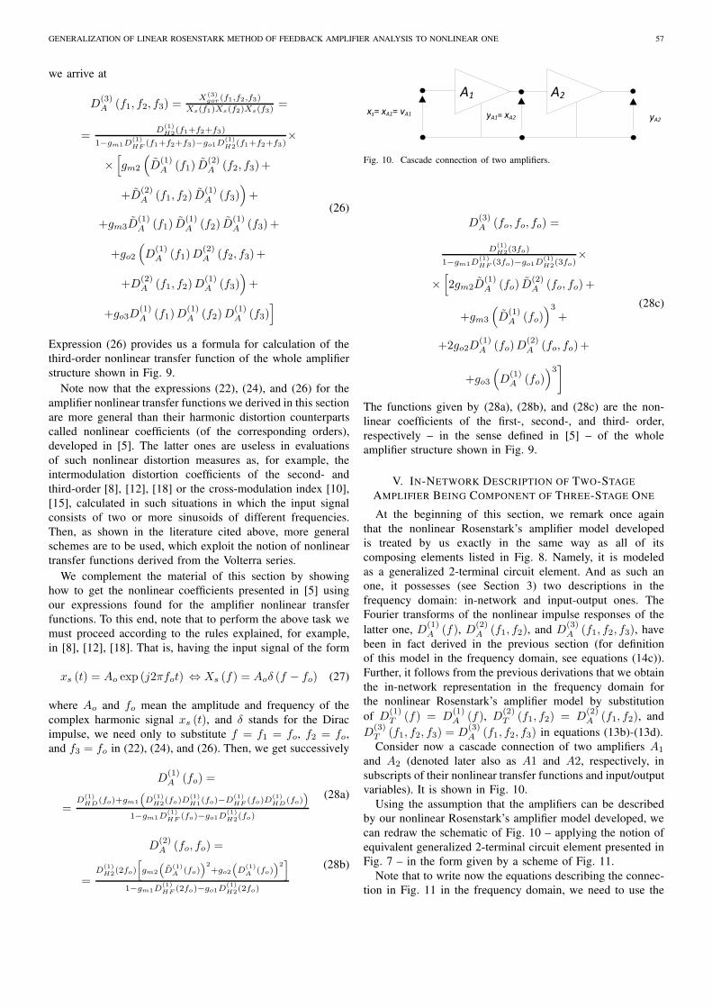
Fig. 10. Cascade connection of two amplifiers.
D(3)A (fo, fo, fo) =
D(1)H2(3fo)
1−gm1D(1)HF (3fo)−go1D
(1)H2(3fo)
×
×[
2gm2D̃(1)A (fo) D̃
(2)A (fo, fo) +
+gm3
(
D̃(1)A (fo)
)3
+
+2go2D(1)A (fo)D
(2)A (fo, fo)+
+go3
(
D(1)A (fo)
)3]
(28c)
The functions given by (28a), (28b), and (28c) are the non-
linear coefficients of the first-, second-, and third- order,
respectively – in the sense defined in [5] – of the whole
amplifier structure shown in Fig. 9.
V. IN-NETWORK DESCRIPTION OF TWO-STAGE
AMPLIFIER BEING COMPONENT OF THREE-STAGE ONE
At the beginning of this section, we remark once again
that the nonlinear Rosenstark’s amplifier model developed
is treated by us exactly in the same way as all of its
composing elements listed in Fig. 8. Namely, it is modeled
as a generalized 2-terminal circuit element. And as such an
one, it possesses (see Section 3) two descriptions in the
frequency domain: in-network and input-output ones. The
Fourier transforms of the nonlinear impulse responses of the
latter one, D(1)A (f), D
(2)A (f1, f2), and D
(3)A (f1, f2, f3), have
been in fact derived in the previous section (for definition
of this model in the frequency domain, see equations (14c)).
Further, it follows from the previous derivations that we obtain
the in-network representation in the frequency domain for
the nonlinear Rosenstark’s amplifier model by substitution
of D(1)T (f) = D
(1)A (f), D
(2)T (f1, f2) = D
(2)A (f1, f2), and
D(3)T (f1, f2, f3) = D
(3)A (f1, f2, f3) in equations (13b)-(13d).
Consider now a cascade connection of two amplifiers A1
and A2 (denoted later also as A1 and A2, respectively, in
subscripts of their nonlinear transfer functions and input/output
variables). It is shown in Fig. 10.
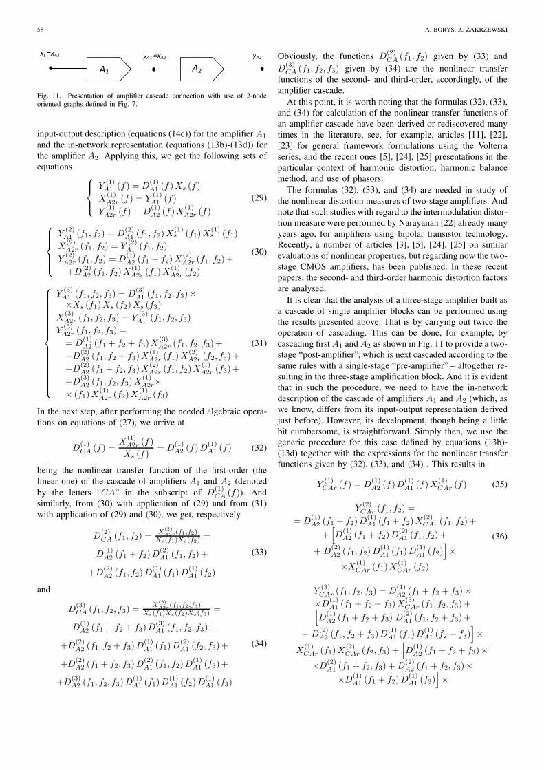
Using the assumption that the amplifiers can be described
by our nonlinear Rosenstark’s amplifier model developed, we
can redraw the schematic of Fig. 10 – applying the notion of
equivalent generalized 2-terminal circuit element presented in
Fig. 7 – in the form given by a scheme of Fig. 11.
Note that to write now the equations describing the connec-
tion in Fig. 11 in the frequency domain, we need to use the
58 A. BORYS, Z. ZAKRZEWSKI
xs =xA1 yA2
A1
yA1 =xA2
A2
Fig. 11. Presentation of amplifier cascade connection with use of 2-nodeoriented graphs defined in Fig. 7.
input-output description (equations (14c)) for the amplifier A1
and the in-network representation (equations (13b)-(13d)) for
the amplifier A2. Applying this, we get the following sets of
equations
Y(1)A1 (f) = D
(1)A1 (f)Xs (f)
X(1)A2r (f) = Y
(1)A1 (f)
Y(1)A2r (f) = D
(1)A2 (f)X
(1)A2r (f)
(29)
Y(2)A1 (f1, f2) = D
(2)A1 (f1, f2)X
(1)s (f1)X
(1)s (f1)
X(2)A2r (f1, f2) = Y
(2)A1 (f1, f2)
Y(2)A2r (f1, f2) = D
(1)A2 (f1 + f2)X
(2)A2r (f1, f2)+
+D(2)A2 (f1, f2)X
(1)A2r (f1)X
(1)A2r (f2)
(30)
Y(3)A1 (f1, f2, f3) = D
(3)A1 (f1, f2, f3)×
×Xs (f1)Xs (f2)Xs (f3)
X(3)A2r (f1, f2, f3) = Y
(3)A1 (f1, f2, f3)
Y(3)A2r (f1, f2, f3) =
= D(1)A2 (f1 + f2 + f3)X
(3)A2r (f1, f2, f3)+
+D(2)A2 (f1, f2 + f3)X
(1)A2r (f1)X
(2)A2r (f2, f3)+
+D(2)A2 (f1 + f2, f3)X
(2)A2r (f1, f2)X
(1)A2r (f3)+
+D(3)A2 (f1, f2, f3)X
(1)A2r×
× (f1)X(1)A2r (f2)X
(1)A2r (f3)
(31)
In the next step, after performing the needed algebraic opera-
tions on equations of (27), we arrive at
D(1)CA (f) =
X(1)A2r (f)
Xs (f)= D
(1)A2 (f)D
(1)A1 (f) (32)
being the nonlinear transfer function of the first-order (the
linear one) of the cascade of amplifiers A1 and A2 (denoted
by the letters “CA” in the subscript of D(1)CA (f)). And
similarly, from (30) with application of (29) and from (31)
with application of (29) and (30), we get, respectively
D(2)CA (f1, f2) =
X(2)A2r(f1,f2)
Xs(f1)Xs(f2)=
D(1)A2 (f1 + f2)D
(2)A1 (f1, f2)+
+D(2)A2 (f1, f2)D
(1)A1 (f1)D
(1)A1 (f2)
(33)
and
D(3)CA (f1, f2, f3) =
X(3)A2r(f1,f2,f3)
Xs(f1)Xs(f2)Xs(f3)=
D(1)A2 (f1 + f2 + f3)D
(3)A1 (f1, f2, f3)+
+D(2)A2 (f1, f2 + f3)D
(1)A1 (f1)D
(2)A1 (f2, f3)+
+D(2)A2 (f1 + f2, f3)D
(2)A1 (f1, f2)D
(1)A1 (f3)+
+D(3)A2 (f1, f2, f3)D
(1)A1 (f1)D
(1)A1 (f2)D
(1)A1 (f3)
(34)
Obviously, the functions D(2)CA (f1, f2) given by (33) and
D(3)CA (f1, f2, f3) given by (34) are the nonlinear transfer
functions of the second- and third-order, accordingly, of the
amplifier cascade.
At this point, it is worth noting that the formulas (32), (33),
and (34) for calculation of the nonlinear transfer functions of
an amplifier cascade have been derived or rediscovered many
times in the literature, see, for example, articles [11], [22],
[23] for general framework formulations using the Volterra
series, and the recent ones [5], [24], [25] presentations in the
particular context of harmonic distortion, harmonic balance
method, and use of phasors.
The formulas (32), (33), and (34) are needed in study of
the nonlinear distortion measures of two-stage amplifiers. And
note that such studies with regard to the intermodulation distor-
tion measure were performed by Narayanan [22] already many
years ago, for amplifiers using bipolar transistor technology.
Recently, a number of articles [3], [5], [24], [25] on similar
evaluations of nonlinear properties, but regarding now the two-
stage CMOS amplifiers, has been published. In these recent
papers, the second- and third-order harmonic distortion factors
are analysed.
It is clear that the analysis of a three-stage amplifier built as
a cascade of single amplifier blocks can be performed using
the results presented above. That is by carrying out twice the
operation of cascading. This can be done, for example, by
cascading first A1 and A2 as shown in Fig. 11 to provide a two-
stage “post-amplifier”, which is next cascaded according to the
same rules with a single-stage “pre-amplifier” – altogether re-
sulting in the three-stage amplification block. And it is evident
that in such the procedure, we need to have the in-network
description of the cascade of amplifiers A1 and A2 (which, as
we know, differs from its input-output representation derived
just before). However, its development, though being a little
bit cumbersome, is straightforward. Simply then, we use the
generic procedure for this case defined by equations (13b)-
(13d) together with the expressions for the nonlinear transfer
functions given by (32), (33), and (34) . This results in
Y(1)CAr (f) = D
(1)A2 (f)D
(1)A1 (f)X
(1)CAr (f) (35)
Y(2)CAr (f1, f2) =
= D(1)A2 (f1 + f2)D
(1)A1 (f1 + f2)X
(2)CAr (f1, f2)+
+[
D(1)A2 (f1 + f2)D
(2)A1 (f1, f2)+
+ D(2)A2 (f1, f2)D
(1)A1 (f1)D
(1)A1 (f2)
]
×
×X(1)CAr (f1)X
(1)CAr (f2)
(36)
Y(3)CAr (f1, f2, f3) = D
(1)A2 (f1 + f2 + f3)×
×D(1)A1 (f1 + f2 + f3)X
(3)CAr (f1, f2, f3)+
[
D(1)A2 (f1 + f2 + f3) D
(2)A1 (f1, f2 + f3)+
+ D(2)A2 (f1, f2 + f3)D
(1)A1 (f1)D
(1)A1 (f2 + f3)
]
×
X(1)CAr (f1)X
(2)CAr (f2, f3) +
[
D(1)A2 (f1 + f2 + f3)×
×D(2)A1 (f1 + f2, f3) +D
(2)A2 (f1 + f2, f3)×
×D(1)A1 (f1 + f2)D
(1)A1 (f3)
]
×
GENERALIZATION OF LINEAR ROSENSTARK METHOD OF FEEDBACK AMPLIFIER ANALYSIS TO NONLINEAR ONE 59
×X(2)CAr (f1, f2)X
(1)CAr (f3)+
+[
D(1)A2 (f1 + f2 + f3)D
(3)A1 (f1, f2, f3) +
+D(2)A2 (f1, f2 + f3)D
(1)A1 (f1)D
(2)A1 (f2, f3)+
+D(2)A2 (f1 + f2, f3)D
(2)A1 (f1, f2)D
(1)A1 (f3)+
+D(3)A2 (f1, f2, f3)×
×D(1)A1 (f1)D
(1)A1 (f2)D
(1)A1 (f3)
]
×
×X(1)CAr (f1)X
(1)CAr (f2)X
(1)CAr (f3)
(37)
with, obviously, X(i)CAr = X
(i)CA1, Y
(i)CAr = Y
(i)A2r, i = 1, 2, 3,
and X(1)CAr 6= Xs.
Finally in this section, we draw the reader’s attention to
the fact that the in-network description of the cascade of two
amplifiers, given by equations (35), (36), and (37), has been
developed here for the first time in the literature.
VI. REMARKS ON SOME QUESTIONABLE NOTIONS
In the paper [5], Miao and Zhang use some specific notions
and concepts, which are highly questionable as, for example,
the following ones:
1) nonlinear signals,
2) intermodulation nonlinearity,
3) second-order intermodulation nonlinearity,
4) nonlinear gain function at fundamental frequency,
5) identification of transfer function poles and zeros lying
on the real axis of the complex plane with the related
frequencies, being positive real numbers.
Let us explain here in more detail their incorrectness and recall
the proper names and their usage.
With regard to nonlinear signals: Note that signals are neither
linear nor nonlinear. After performing any nonlinear process-
ing on a signal, it remains still a signal, assuming only another
form. Linear or nonlinear can be systems, not signals.
With regard to intermodulation nonlinearity: Such notions as,
for example, intermodulation, harmonic or cross-modulation
nonlinearities do not make sense. We explain this point on an
example of a circuit element realizing a quadratic nonlinearity
yT (t) = a · x2T (t), with the coefficient “a” being a real
number. Applying input signal xT (t) = Ao exp (j2πfot) (as
described by (27)) to it, we get the output signal in the form:
yT (t) = a · A2o exp (j2π (2fo) t). Observe that this resulting
signal is a pure harmonic one at the product frequency 2fo.
Next, using another input signal xT (t) = Ao1 exp (j2πfo1t)+Ao2 exp (j2πfo2t), being a sum of the two previous signals
at different frequencies fo1 and fo2, in the above quadratic
nonlinearity, we obtain yT (t) = a · A2o1 exp (j2π (2fo1) t) +
a·A2o2 exp (j2π (2fo2) t)+2a·Ao1Ao2 exp (j2π (fo1 + fo2) t)
in this case. And note that the output signal consists now of
two harmonics of frequencies 2fo1 and 2fo2, respectively, and
of the intermodulation product at frequency fo1 + fo2.
Comparison of the above two results leads to the conclusion
that the quadratic nonlinearity considered can produce both the
harmonic as well as the intermodulation products (depending
upon the form of the input signal). So, therefore, it is nei-
ther harmonic nor intermodulation nonlinearity. It is simply
a quadratic nonlinearity – and this is its proper name.
With regard to second-order intermodulation nonlinearity:
This notion is also flawed. To see this, recall the example
of quadratic nonlinearity from the previous point with the
input signal xT (t) = Ao1 exp (j2πfo1t) +Ao2 exp (j2πfo2t)applied to it. This results, as shown above, in yT (t) =a · A2
o1 exp (j2π (2fo1) t) + a · A2o2 exp (j2π (2fo2) t) + 2a ·
Ao1Ao2 exp (j2π (fo1 + fo2) t), that is in two second-order
harmonic distortion components a · A2o1 exp (j2π (2fo1) t)
and a · A2o2 exp (j2π (2fo2) t), and the second-order inter-
modulation distortion one 2a ·Ao1Ao2 exp (j2π (fo1 + fo2) t).Therefore, the above nonlinearity cannot be solely named as
a second-order intermodulation one.
With regard to nonlinear gain function at fundamental fre-
quency: The above notion is conceptually false because there
exists no such a single nonlinear gain function, which enables
calculation of the gains for the corresponding harmonics
and the frequencies of intermodulation products, and for the
fundamental frequency. For calculation of the gain at the fun-
damental frequency, one has to use a separate function called
in the literature the describing function [10], [26]. Further, for
evaluation of the gain of the second-order harmonic, another
function must be used – and so on – for other harmonics and
frequencies of intermodulation products.
With regard to making identity between the transfer function
poles and zeros, and the related frequencies: One calculates
single poles and zeros of the transfer functions by equating to
zero the polynomials of the form (s+ ap) and (s+ az), with
ap and az being real positive numbers. Hence, the pole and
zero positions are given by sp = −ap and sz = −az , which
lie on the real axis of the complex s-plane in its left-hand side.
These positions are identified in [5] with the related angular
frequencies, which are obviously positive numbers. Correctly,
the related pole and zero frequencies should be written as
ωp = |sp| = ap and ωz = |sz| = az , respectively.
Furthermore, it should be stressed that the use of the notion
of poles and zeros of the nonlinear coefficients and harmonic
distortion factors of the second- and third-order, as done in
[5], cannot be extended to the other areas as, for instance, to
stability issues (at least in the form presented in [5]).
VII. CONCLUSION
In this paper, a thorough and mathematically rigorous ex-
tension of the linear Rosenstark amplifier model to a weakly
nonlinear one has been presented. It has been also demon-
strated that our model exploiting the Volterra series and the
notion of generalized two-terminal nonlinear circuit elements
is more general than the one using phasors [5], and that it
assumes two forms, named here in-network and input-output
type descriptions of an amplifier. In the paper, the relations
describing these forms have been derived in the time as well
as in the frequency domain. Moreover, it has been shown
how to use them in calculations of any nonlinear distortion
measure. In contrast to this, note that the method of phasors
enables calculations of harmonic distortion only. Furthermore,
note likewise that the descriptions developed enable simple
calculation of the nonlinear transfer functions of any amplifier
topology as, for example, cascade and feedback structures and
their combinations occurring in single-, two-, and three-stage
60 A. BORYS, Z. ZAKRZEWSKI
amplifiers. Two examples presented illustrate details of such
calculations. Finally, we draw the reader’s attention to the fact
that many outcomes of this paper systematize, in some aspects,
the results achieved recently with the use of the symbolic
analysis applied to harmonic distortion analyses of CMOS
amplifiers [3], [5], [13], [24], [25].
REFERENCES
[1] S. Rosenstark, “A simplified method of feedback amplifier analysis,”IEEE Transactions on Education, vol. E-17, pp. 192–198, November1974.
[2] ——, Feedback Amplifier Principles. New York: Macmillan PublishingCompany, 1986.
[3] G. Palumbo and S. Pennisi, “High-frequency harmonic distortion infeedback amplifiers: analysis and applications,” IEEE Transactions on
Circuits and Systems-I: Fundamental Theory and Applications, vol. 50,pp. 328–340, March 2003.
[4] ——, Feedback Amplifiers: Theory and Design. Norwell, MA: Kluwer,2002.
[5] Y. Miao and Y. Zhang, “Distortion modeling of feedback two-stageamplifier compensated with Miller capacitor and nulling resistor,” IEEE
Transactions on Circuits and Systems-I: Regular Papers, vol. 59, pp.93–105, January 2012.
[6] L. O. Chua, “Device modeling via basic nonlinear circuit elements,”IEEE Transactions on Circuits Systems, vol. CAS-27, pp. 1014–1044,November 1980.
[7] A. Borys, “On in-network and other types of amplifier descriptions fornonlinear distortion analysis,” International Journal of Electronics and
Telecommunications, vol. 56, no. 2, pp. 177–184, 2010.[8] J. J. Bussgang, L. Ehrman, and J. W. Graham, “Analysis of nonlinear
systems with multiple inputs,” Proceedings of the IEEE, vol. 62, pp.1088–1119, 1974.
[9] E. Bedrosian and S. O. Rice, “The output properties of Volterra systems(nonlinear systems with memory) driven by harmonic and Gaussianinputs,” Proceedings of the IEEE, vol. 59, pp. 1688–1707, December1971.
[10] L. O. Chua and C. Ng, “Frequency domain analysis of nonlinear sys-tems: general theory,” IEE Journal of Electronic Circuits and Systems,vol. 3, pp. 165–185, 1979.
[11] ——, “Frequency domain analysis of nonlinear systems: formulationof transfer functions,” IEE Journal of Electronic Circuits and Systems,vol. 3, pp. 257–269, 1979.
[12] A. Borys, “A simplified analysis of nonlinear distortion in analogelectronic circuits using the Volterra-Wiener series,” Scientia Electrica,vol. 30, no. 3, pp. 78–103, 1984.
[13] S. O. Cannizzaro, G. Palumbo, and S. Pennisi, “Effects of nonlinearfeedback in the frequency domain,” IEEE Transactions on Circuits and
Systems-I: Fundamental Theory and Applications, vol. 53, pp. 225–234,February 2006.
[14] A. Borys, “On correctness of the basics of Palumbo and Pennisi’s meansof harmonic distortion calculation in analog integrated circuits,” Zeszyty
Naukowe Wyszej Szkoy Informatyki w Ł odzi: Teoria i zastosowaniainformatyki, vol. 8, no. 2, pp. 5–16, 2009.
[15] R. G. Meyer, M. J. Shensa, and R. Eschenbach, “Crossmodulation andintermodulation in amplifiers at high frequencies,” IEEE Journal of
Solid-State Circuits, vol. SC-7, pp. 16–23, February 1972.[16] A. Borys, “Exploiting admittance formalism in the nonlinear analysis,”
Zeszyty Naukowe Wyszej Szkoy Informatyki w Ł odzi: Teoria i zastosowa-
nia informatyki, vol. 8, no. 2, pp. 17–39, 2009.[17] G. Palumbo, M. Pennisi, and S. Pennisi, “Miller theorem for weakly
nonlinear feedback circuits and application to CE amplifier,” IEEE
Transactions on Circuits and Systems-II: Express Briefs, vol. 55, pp.991–995, October 2008.
[18] S. Narayanan, “Application of Volterra series to intermodulation distor-tion analysis of transistor feedback amplifiers,” IEEE Transactions on
Circuit Theory, vol. CT-17, pp. 518–527, November 1970.[19] P. Wambacq, G. Gielen, P. Kinget, and W. Sansen, “High-frequency
distortion analysis of analog integrated circuits,” IEEE Transactions on
Circuits and Systems II: Analog and Digital Signal Processing, vol. 46,no. 3, pp. 335–344, March 1999.
[20] B. Hernes and W. Sansen, “Distortion in single-, two- and three-stageamplifiers,” IEEE Transactions on Circuits and Systems I: Regular
Papers, vol. 52, no. 5, pp. 846–856, May 2005.[21] M. Fliess, M. Lamnabhi, and F. Lamnabhi-Lagarrigu, “An algebraic
approach to nonlinear functional expansions,” IEEE Transactions on
Circuits and Systems, vol. 30, no. 8, pp. 554–570, 1983.[22] S. Narayanan, “Intermodulation distortion of cascaded transistors,” IEEE
Journal of Solid-State Circuits, vol. SC-4, no. 3, pp. 97–106, June 1969.[23] Y. L. Kuo, “Frequency-domain analysis of weakly nonlinear networks.
“Canned” Volterra analysis, part 1,” IEEE Circuits and Systems Maga-
zine, vol. 11, no. 4, pp. 2–8, August 1977.[24] S. O. Cannizzaro, G. Palumbo, and S. Pennisi, “Distortion analysis
of Miller-compensated three-stage amplifiers,” IEEE Transactions on
Circuits and Systems I: Regular Papers, vol. 53, no. 5, pp. 961–976,May 2006.
[25] ——, “An approach to model high-frequency distortion in negative-feedback amplifiers,” International Journal of Circuit Theory and Ap-
plications, vol. 36, pp. 3–18, 2008.[26] A. Gelb and W. E. Vander Velde, Multiple-Input Describing Functions
and Nonlinear System Design. New York: McGraw-Hill, 1968.
Related Documents