Welcome message from author
This document is posted to help you gain knowledge. Please leave a comment to let me know what you think about it! Share it to your friends and learn new things together.
Transcript
Generalised Interaction Mining:
Probabilistic, Statistical and Vectorised
Methods in High Dimensional or
Uncertain Databases
Florian Verhein
Dr. rer. nat. Dissertation
Faculty of Mathematics, Informatics and Statistics
Ludwig-Maximilians-Universität, Munich, Germany
2010

ii
Generalised Interaction Mining:Probabilistic, Statistical and Vectorised
Methods in High Dimensional orUncertain Databases
Dissertation zum Erreichen des Doktorgrades
an der Fakultät für Mathematik, Informatik und Statistik
der Ludwig-Maximilians-Universität München
vorgelegt von
Florian Verhein
Tag der Einreichung: 28.10.2010
Tag der mündlichen Prüfung: 15.12.2010
Berichterstatter:
Prof. Dr. Hans-Peter Kriegel, Ludwig-Maximilians-Universität München, Deutschland
Prof. Dr. Jian Pei, Simon Fraser University, Burnaby, Canada.
iii

c© Copyright 2010 Florian Verhein.
http://www.florian.verhein.com
Note: Errata and/or an ammended version may be available from
http://www.florian.verhein.com/publications
iv

für Brigitte, Martin, Mundi & Michael
v

vi
Abstract
Knowledge Discovery in Databases (KDD) is the non-trivial process of identifying
valid, novel, useful and ultimately understandable patterns in data. The core step
of the KDD process is the application of Data Mining (DM) algorithms to e�ciently
�nd interesting patterns in large databases. This thesis concerns itself with three
inter-related themes: Generalised interaction and rule mining; the incorporation
of statistics into novel data mining approaches; and probabilistic frequent pattern
mining in uncertain databases.
An interaction describes an e�ect that variables have � or appear to have � on each
other. Interaction mining is the process of mining structures on variables describing
their interaction patterns � usually represented as sets, graphs or rules. Interac-
tions may be complex, represent both positive and negative relationships, and the
presence of interactions can in�uence another interaction or variable in interesting
ways. Finding interactions is useful in domains ranging from social network analysis,
marketing, the sciences, e-commerce, to statistics and �nance. Many data mining
tasks may be considered as mining interactions, such as clustering; frequent itemset
mining; association rule mining; classi�cation rules; graph mining; �ock mining; etc.
Interaction mining problems can have very di�erent semantics, pattern de�nitions,
interestingness measures and data types. Solving a wide range of interaction mining
problems at the abstract level, and doing so e�ciently � ideally more e�ciently than
with specialised approaches, is a challenging problem.
This thesis introduces and solves the Generalised Interaction Mining (GIM) and
Generalised Rule Mining (GRM) problems. GIM and GRM use an e�cient and in-
tuitive computational model based purely on vector valued functions. The semantics
of the interactions, their interestingness measures and the type of data considered
are �exible components of vectorised frameworks. By separating the semantics of
a problem from the algorithm used to mine it, the frameworks allow both to vary
independently of each other. This makes it easier to develop new methods by fo-
cusing purely on a problem's semantics and removing the burden of designing an
vii
viii
e�cient algorithm. By encoding interactions as vectors in the space (or a sub-space)
of samples, they provide an intuitive geometric interpretation that inspires novel
methods. By operating in time linear in the number of interesting interactions that
need to be examined, the GIM and GRM algorithms are optimal. The use of GRM
or GIM provides e�cient solutions to a range of problems in this thesis, including
graph mining, counting based methods, itemset mining, clique mining, a clustering
problem, complex pattern mining, negative pattern mining, solving an optimisation
problem, spatial data mining, probabilistic itemset mining, probabilistic association
rule mining, feature selection and generation, classi�cation and multiplication rule
mining.
Data mining is a hypothesis generating endeavour, examining large databases for
patterns suggesting novel and useful knowledge to the user. Since the database is a
sample, the patterns found should describe hypotheses about the underlying process
generating the data. In searching for these patterns, a DM algorithm makes addi-
tional hypothesis when it prunes the search space. Natural questions to ask then,
are: �Does the algorithm �nd patterns that are statistically signi�cant?� and �Did
the algorithm make signi�cant decisions during its search?�. Such questions address
the quality of patterns found though data mining and the con�dence that a user can
have in utilising them. Finally, statistics has a range of useful tools and measures
that are applicable in data mining. In this context, this thesis incorporates statis-
tical techniques � in particular, non-parametric signi�cance tests and correlation �
directly into novel data mining approaches. This idea is applied to statistically signif-
icant and relatively class correlated rule based classi�cation of imbalanced data sets;
signi�cant frequent itemset mining; mining complex correlation structures between
variables for feature selection; mining correlated multiplication rules for interaction
mining and feature generation; and conjunctive correlation rules for classi�cation.
The application of GIM or GRM to these problems lead to e�cient and intuitive
solutions.
Frequent itemset mining (FIM) is a fundamental problem in data mining. While it is
usually assumed that the items occurring in a transaction are known for certain, in
many applications the data is inherently noisy or probabilistic; such as adding noise
in privacy preserving data mining applications, aggregation or grouping of records
leading to estimated purchase probabilities, and databases capturing naturally un-
certain phenomena. The consideration of existential uncertainty of item(sets) makes
traditional techniques inapplicable. Prior to the work in this thesis, itemsets were
mined if their expected support is high. This returns only an estimate, ignores the
probability distribution of support, provides no con�dence in the results, and can
ix
lead to scenarios where itemsets are labeled frequent even if they are more likely
to be infrequent. Clearly, this is undesirable. This thesis proposes and solves the
Probabilistic Frequent Itemset Mining (PFIM) problem, where itemsets are consid-
ered interesting if the probability that they are frequent is high. The problem is
solved under the possible worlds model and a proposed probabilistic framework for
PFIM. Novel and e�cient methods are developed for computing an itemset's exact
support probability distribution and frequentness probability, using the Poisson bi-
nomial recurrence, generating functions, or a Normal approximation. Incremental
methods are proposed to answer queries such as �nding the top-k probabilistic fre-
quent itemsets. A number of specialised PFIM algorithms are developed, with each
being more e�cient than the last: ProApriori is the �rst solution to PFIM and is
based on candidate generation and testing. ProFP-Growth is the �rst probabilistic
FP-Growth type algorithm and uses a proposed probabilistic frequent pattern tree
(Pro-FPTree) to avoid candidate generation. Finally, the application of GIM leads to
GIM-PFIM; the fastest known algorithm for solving the PFIM problem. It achieves
orders of magnitude improvements in space and time usage, and leads to an intuitive
subspace and probability-vector based interpretation of PFIM.

x
Zusammenfassung
Knowledge Discovery in Datenbanken (KDD) ist der nicht-triviale Prozess, gültiges,
neues, potentiell nützliches und letztendlich verständliches Wissen aus groÿen Daten-
sätzen zu extrahieren. Der wichtigste Schritt im KDD Prozess ist die Anwendung
e�zienter Data Mining (DM) Algorithmen um interessante Muster (�Patterns�) in
Datensätzen zu �nden. Diese Dissertation beschäftigt sich mit drei verwandten
Themen: Generalised Interaction und Rule Mining, die Einbindung von statistis-
chen Methoden in neue DM Algorithmen und Probabilistic Frequent Itemset Mining
(PFIM) in unsicheren Daten.
Eine Interaktion (�Interaction�) beschreibt den Ein�uss, den Variablen aufeinander
haben. Interaktionsmining ist der Prozess, Strukturen zwischen Variablen zu �nden,
die Interaktionsmuster beschreiben. Diese werden gewöhnlicherweise als Mengen,
Graphen oder Regeln repräsentiert. Interaktionen können komplex sein und sowohl
positive als auch negative Beziehungen repräsentieren. Auÿerdem kann das Vorhan-
densein von Interaktionen andere Interaktionen oder Variablen beein�ussen. Interak-
tionen stellen in Bereichen wie Soziale Netzwerk Analyse, Marketing, Wissenschaft,
E-commerce, Statistik und Finanz wertvolle Information dar. Viele DM Methoden
können als Interaktionsmining betrachtet werden: Zum Beispiel Clustering, Frequent
Itemset Mining, Assoziationsregeln, Klassi�kationsregeln, Graph Mining, Flock Min-
ing, usw. Interaktionsmining-Probleme können sehr unterschiedliche Semantik, Mus-
terde�nitionen, Interessantheitsmaÿe und Datentypen erfordern. Interaktionsmining-
Probleme auf breiter und abstrakter Basis e�zient � und im Idealfall e�zienter als
mit spezialisierten Methoden � zu lösen, ist ein herausforderndes Problem.
Diese Dissertation führt das Generalised Interaction Mining (GIM) und das Gener-
alised Rule Mining (GRM) Problem ein und beschreibt Lösungen für diese. GIM
und GRM benutzen ein e�zientes und intuitives Berechnungsmodell, das einzig
und allein auf vektorbasierten Funktionen beruht. Die Semantik der Interaktionen,
ihre Interessantheitsmaÿe und die Datenarten, sind Komponenten in vektorisierten
Frameworks. Die Frameworks ermöglichen die Trennung der Problemsemantik vom
xi
xii
Algorithmus, so dass beide unabhängig voneinander geändert werden können. Die
Entwicklung neuer Methoden wird dadurch erleichtert, da man sich völlig auf die
Problemsemantik fokussieren kann und sich nicht mit der Entwicklung problemspez-
i�scher Algorithmen befassen muss. Die Kodierung der Interaktionen als Vektoren
im gesamten Raum (oder Teilraum) der Stichproben stellt eine intuitive geometrische
Interpretation dar, die neuartige Methoden inspiriert. Die GRM- und GIM- Algo-
rithmen haben lineare Laufzeit in der Anzahl der Interaktionen die geprüft werden
müssen und sind somit optimal. Die Anwendung von GRM oder GIM in dieser
Dissertation ermöglicht e�ziente Lösungen für eine Reihe von Problemen, wie zum
Beispiel Graph Mining, Aufzählungsmethoden, Itemset Mining, Clique Mining, ein
Clusteringproblem, das Finden von komplexen und negativen Mustern, die Lösung
von Optimierungsproblemen, Spatial Data Mining, probabilistisches Itemset Min-
ing, probabilistisches Mining von Assoziationsregel, Selektion und Erzeugung von
Features, Mining von Klassi�kations- und Multiplikationsregel, u.v.m.
Data Mining ist ein Verfahren, das Hypothesen produziert, indem es in groÿen
Datensätzen Muster �ndet und damit für den Anwender neues und nützliches Wis-
sen vorschlägt. Da die untersuchte Datenbank ein Resultat des datenerzeugenden
Prozesses ist, sollten die gefundenen Muster Erkenntnisse über diesen Prozess liefern.
Bei der Suche nach diesen Mustern macht ein DM Algorithmus zusätzliche Hypothe-
sen, wenn Teile des Suchraums ausgeschlossen werden. Die folgenden Fragen sind
dabei wichtig: �Findet der Algorithmus statistisch signi�kante Muster?� und �Hat
der Algorithmus während des Suchprozesses signi�kante Entscheidungen getro�en?�.
Diese Fragen beein�ussen die Qualität der Muster und die Sicherheit die der An-
wender in ihrer Benutzung haben kann. Da die Statistik auch eine Reihe von nüt-
zlichen Methoden bereitstellt, die für DM anwendbar sind, kombiniert diese Dis-
sertation einige statistische Methoden mit neuen DM Algorithmen, insbesondere
nicht-parametrische Signi�kanztests und Korrelation. Diese Idee wird für die folgen-
den Probleme angewandt: Signi�kante und "relatively class correlated" regelbasierte
Klassi�kation in unsymmetrischen Datensätzen, signi�kantes Frequent Itemset Min-
ing, Mining von komplizierten Korrelationsstrukturen zwischen Variablen zum Zweck
der Featureselektion, Mining von korrelierten Multiplikationsregeln zum Zwecke des
Interaktionsminings und Featureerzeugung und konjunktive Korrelationsregeln für
die Klassi�kation. Die Anwendung von GIM und GRM auf diese Probleme führt zu
e�zienten und intuitiven Lösungen.
Frequent Itemset Mining (FIM) ist ein fundamentales Problem im Data Mining.
Obwohl allgemein die Annahme gilt, dass in einer Transaktion enthaltene Items
bekannt sind, sind die Daten in vielen Anwendungen unsicher oder probabilistisch.
xiii
Beispiele sind das Hinzufügen von Rauschen zu Datenschutzzwecken, die Grup-
pierung von Datensätzen die zu geschätzten Kaufwahrscheinlichkeiten führen und
Datensätze deren Herkunft von Natur aus unsicher sind. Die Berücksichtigung von
unsicheren Datensätzen verhindert die Anwendung von traditionellen Methoden. Vor
der Arbeit in dieser Dissertation wurden Itemsets gesucht, deren erwartetes Vorkom-
men hoch ist. Diese Methode produziert jedoch nur Schätzwerte, vernachlässigt
die Wahrscheinlichkeitsverteilung der Vorkommen, bietet keine Sicherheit für die
Genauigkeit der Ergebnisse und kann zu Szenarien führen in denen das Vorkommen
als häu�g eingestuft wird, obwohl die Wahrscheinlichkeit höher ist, dass sie nur selten
vorkommen. Solche Ergebnisse sind natürlich unerwünscht. Diese Dissertation führt
das Probabilistic Frequent Itemset Mining (PFIM) ein. Diese Lösung betrachtet
Itemsets als interessant, wenn die Wahrscheinlichkeit groÿ ist, dass sie häu�g vorkom-
men. Die Problemlösung besteht aus der Anwendung des Possible Worlds Models und
dem vorgeschlagenen probabilistisches Framework für PFIM. Es werden neue und ef-
�ziente Methoden entwickelt um die Wahrscheinlichkeitsverteilung des Vorkommens
und die Häu�gkeitsverteilung eines Itemsets zu berechnen. Dazu werden die Poisson
Binomial Recurrence, Generating Functions, oder eine normalverteilte Annäherung
verwendet. Inkrementelle Methoden werden vorgeschlagen um Fragen wie "Finde
die top-k Probabilistic Frequent Itemsets" zu beantworten. Mehrere PFIM Algorith-
men werden entwickelt, wobei die E�zienz von Algorithmus zu Algorithmus steigt:
ProApriori ist die erste Lösung für PFIM und basiert auf erzeugen und testen von
Kandidaten. ProFP-Growth ist der erste probabilistische FP-Growth Algorithmus.
Er schlägt einen Probabilistic Frequent Pattern Tree (Pro-FPTree) vor, der Kan-
didatenerzeugung über�üssig macht. Die Anwendung von GIM führt schlieÿlich zu
GIM-PFIM, dem schnellsten bekannten Algorithmus zur Lösung des PFIM Prob-
lems. Dieser Algorithmus resultiert in einem um Gröÿenordnungen besseren Zeit-
und Speicherbedarf, und führt zu einer intuitiven Interpretation von PFIM, basierend
auf Unterräumen und Wahrscheinlichkeitsvektoren.

xiv
Acknowledgments
I would like to acknowledge all the people who supported me during the development
of this thesis. I can only mention some of them here, but my thanks go to all.
First I would like to express my sincere gratitude to my supervisor and �rst referee,
Professor Hans-Peter Kriegel, for his encouragement and advice. He also has a special
talent for creating an inspiring, supportive and productive environment within his
database systems research group. I would also like to thank Professor Jian Pei for
his enthusiastic willingness to be the second referee of this thesis.
This thesis bene�ted greatly from my colleagues at the database research group, who
I thank not only for the great teamwork, advice, productive discussions and exchange
of ideas, but also the fun we had. In no particular order then, my warmest thanks
go to: Dr. Matthias Renz, Andreas Zü�e, Tobias Emrich, Thomas Bernecker, Dr.
Peer Kröger, Dr. Matthias Schubert, Marisa Thoma, Franz Graf, Erich Schubert,
Dr. Arthur Zimek, Dr. Irene Ntoutsi and Dr. Elke Achtert. I am also grateful to
Susanne Grienberger and Franz Krojer for their organisational and technical support.
Some of the research in this thesis was performed while at the University of Sydney,
Australia. I would particularly like to thank my former colleagues Dr. Ghazi Al-
Naymat and Dr. Bavani Arunasalam for fruitful discussions and input.
Last but de�nitely not least, I am very grateful for the support of my family � and
in particular my parents for their never ending encouragement.
xv

xvi
Publications
Publications during the author's Doctoral and PhD candidatures are listed below.
[18] and [19] were joint work with the team in Professor Hans-Peter Kriegel's database
systems group in the Ludwig-Maximilians-Universität, Munich, Germany. [94] was
joint work with Ghazi Al-Naymat at the University of Sydney.
Publications Contributing to this Thesis
The following publications contributed to this thesis, as will be described in sec-
tion 1.2.
• [19] Thomas Bernecker, Hans-Peter Kriegel, Matthias Renz, Florian Verhein,
Andreas Zü�e: Probabilistic Frequent Pattern Growth for Itemset Mining in
Uncertain Databases
Technical report, arXiv.org, arXiv:1008.2300v1, Fri, 13 Aug 2010.
• [93] Florian Verhein: Generalised Rule Mining
The 15th International Conference on Database Systems for Advanced Appli-
cations (DASFAA'2010), 1 � 4 April 2010, Tsukuba, Japan. Lecture Notes in
Computer Science, Volume 5981/2010, pp. 85-92, Springer, 2010.
• [18] Thomas Bernecker, Hans-Peter Kriegel, Matthias Renz, Florian Verhein,
Andreas Zü�e: Probabilistic Frequent Itemset Mining in Uncertain Databases
The 15th ACM SIGKDD Conference on Knowledge Discovery and Data Mining
(SIGKDD'2009). Paris, France, June 28 � July 1 2009. pp. 119-128, ACM
Press, 2009.
• [91] Florian Verhein: Mining Complete Complex Maximal Sets of Correlated
Variables with Applications to Feature Subset Selection
2008 SIAM International Conference on Data Mining (SDM'2008). April 24-26
2008, Atlanta, Georgia, USA. pp. 597-608, SIAM, 2008.
xvii
xviii
• [94] Florian Verhein, Ghazi Al-Naymat: Fast Mining of Complex Spatial Co-
location Patterns using GLIMIT
IEEE International Conference on Data Mining Workshops (ICDM-W'2007).
28 � 31 October 2007, Omaha NE, USA. pp. 679-684, IEEE Computer Society,
2007.
• [98] Florian Verhein, Sanjay Chawla: Using Signi�cant, Positively Associated
and Relatively Class Correlated Rules For Associative Classi�cation of Imbal-
anced Datasets
IEEE International Conference on Data Mining (ICDM'2007). 28 � 31 October
2007, Omaha NE, USA. pp. 679-684, IEEE Computer Society, 2007.
• [96] Florian Verhein, Sanjay Chawla: Geometrically Inspired Itemset Mining
IEEE International Conference on Data Mining (ICDM'2006). 18 � 22 Decem-
ber 2006, Hong Kong. pp. 655-666, IEEE Computer Society, 2006.
Other Publications
The following publications constitute research performed by the author in spatio-
temporal data mining. They contributed to the author's PhD in the Faculty of
Engineering and Information Technology at The University of Sydney, Australia.
The thesis was titled �Mining Complex Spatio-Temporal Movement Patterns�.
• [92] Florian Verhein. Mining Complex Spatio-Temporal Sequence Patterns.
2009 SIAM International Conference on Data Mining (SDM'2009). April 30 �
May 2 2009, Sparks, Nevada, USA. pp. 605-616, SIAM, 2009.
• [99] Florian Verhein, Sanjay Chawla. Mining Spatio-Temporal Patterns in Ob-
ject Mobility Databases
Data Mining and Knowledge Discovery Journal (DMKD), Volume 16, Number
1 / February, 2008 (online 2007). Springer.
• [90] Florian Verhein: k-STARs: Sequences of Spatio-Temporal Association
Rules
IEEE International Conference on Data Mining Workshops (ICDM-W'2006).
18 � 22 December 2006, Hong Kong. pp. 387-394, IEEE Computer Society,
2006.
• [97] Florian Verhein, Sanjay Chawla: Mining Spatio-temporal Association Rules,
Sources, Sinks, Stationary Regions and Thoroughfares in Object Mobility Databases
xix
The 11th International Conference on Database Systems for Advanced Appli-
cations (DASFAA'2006). 12 � 15 April 2006, Singapore. Lecture Notes in
Computer Science, Volume 3882, pp. 187-201, Springer, 2006.
• [95] Florian Verhein, Sanjay Chawla. Mining Spatio-Temporal Association
Rules, Sources, Sinks, Stationary Regions and Thoroughfares in Object Mo-
bility Databases
IEEE International Conference on Data Mining Workshops (ICDM-W'2005).
Publication Outlet Ranking
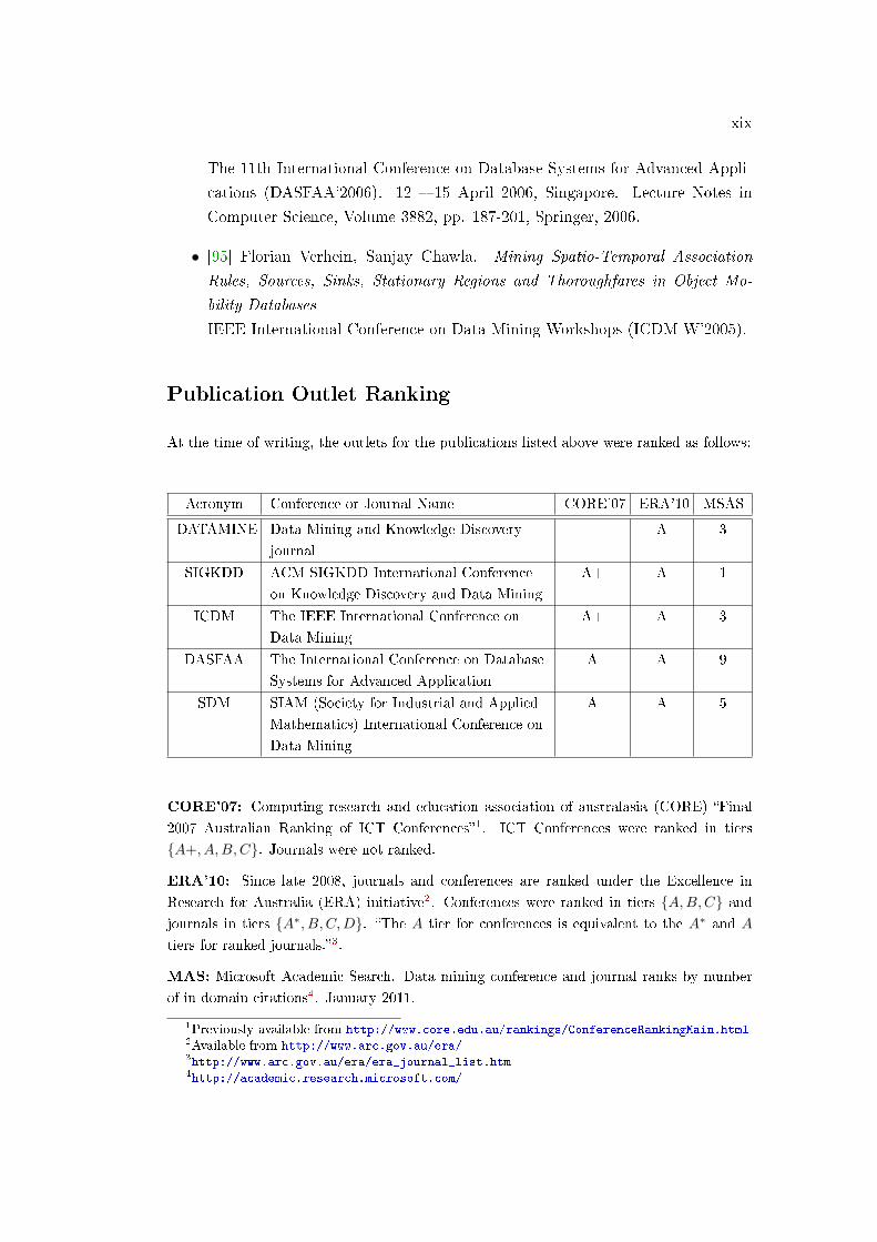
At the time of writing, the outlets for the publications listed above were ranked as follows:
Acronym Conference or Journal Name CORE'07 ERA'10 MSAS
DATAMINE Data Mining and Knowledge Discovery
journal
A 3
SIGKDD ACM SIGKDD International Conference
on Knowledge Discovery and Data Mining
A+ A 1
ICDM The IEEE International Conference on
Data Mining
A+ A 3
DASFAA The International Conference on Database
Systems for Advanced Application
A A 9
SDM SIAM (Society for Industrial and Applied
Mathematics) International Conference on
Data Mining
A A 5
CORE'07: Computing research and education association of australasia (CORE) �Final
2007 Australian Ranking of ICT Conferences�1. ICT Conferences were ranked in tiers
{A+, A,B,C}. Journals were not ranked.
ERA'10: Since late 2008, journals and conferences are ranked under the Excellence in
Research for Australia (ERA) initiative2. Conferences were ranked in tiers {A,B,C} andjournals in tiers {A∗, B, C,D}. �The A tier for conferences is equivalent to the A∗ and A
tiers for ranked journals.�3.
MAS: Microsoft Academic Search. Data mining conference and journal ranks by number
of in domain citations4. January 2011.
1Previously available from http://www.core.edu.au/rankings/ConferenceRankingMain.html2Available from http://www.arc.gov.au/era/3http://www.arc.gov.au/era/era_journal_list.htm4http://academic.research.microsoft.com/

xx
Chapter Summary
Abstract vii
Zusammenfassung xi
Aknowledgements xv
Publications xvii
Chapter Summary xxii
Contents xxxii
List of Figures xxxvi
I Preliminaries xxxvii
1 Introduction 1
2 Background 13
II Generalised Interaction Mining 21
3 Generalised Interaction Mining 23
4 Geometrically Inspired Itemset Mining in the Transpose 65
5 Fast Mining of Complex Spatial Co-location Patterns 97
xxi
xxii CHAPTER SUMMARY
6 Generalised Rule Mining 113
7 Correlated Multiplication Rules with Applications 141
III Statistical Data Mining Methods 155
8 Classi�cation of Imbalanced Databases using Signi�cant Rules 157
9 Mining Complex Correlation Structures 183
IV Mining Uncertain and Probabilistic Databases 207
10 Probabilistic Frequent Itemset Mining 209
11 Signi�cant Frequent Itemset Mining 235
12 Probabilistic Frequent Pattern Growth 251
13 Vectorised Probabilistic Frequent Itemset Mining 279
V Conclusions 291
14 Conclusions and Future Work 293
Bibliography 311
Contents
Abstract vii
Zusammenfassung xi
Aknowledgements xv
Publications xvii
Chapter Summary xxii
Contents xxxii
List of Figures xxxvi
I Preliminaries xxxvii
1 Introduction 1
1.1 Research Problems and Thesis Overview . . . . . . . . . . . . . . . . 2
1.1.1 Generalised Interaction Mining . . . . . . . . . . . . . . . . . 2
1.1.2 Statistical Approaches in Interaction Mining . . . . . . . . . 5
1.1.3 Probabilistic Frequent Itemset Mining in Uncertain Databases 7
1.1.4 Summary of Data Mining Problems Addressed in this Thesis 9
1.2 Publications Contributing to Chapters of this Thesis . . . . . . . . . 9
xxiii
xxiv CONTENTS
2 Background 13
2.1 Knowledge Discovery in Databases . . . . . . . . . . . . . . . . . . . 14
2.2 Data Mining . . . . . . . . . . . . . . . . . . . . . . . . . . . . . . . . 17
II Generalised Interaction Mining 21
3 Generalised Interaction Mining 23
3.1 Introduction . . . . . . . . . . . . . . . . . . . . . . . . . . . . . . . . 24
3.1.1 Relationship to other Chapters . . . . . . . . . . . . . . . . . 26
3.1.2 Contributions . . . . . . . . . . . . . . . . . . . . . . . . . . . 27
3.1.3 Organisation . . . . . . . . . . . . . . . . . . . . . . . . . . . 27
3.2 Generalised Interaction Mining Framework . . . . . . . . . . . . . . . 27
3.3 Generalised Interaction Mining Algorithm . . . . . . . . . . . . . . . 32
3.3.1 Pre�x Tree . . . . . . . . . . . . . . . . . . . . . . . . . . . . 32
3.3.2 Algorithm . . . . . . . . . . . . . . . . . . . . . . . . . . . . . 34
3.3.3 Complexity . . . . . . . . . . . . . . . . . . . . . . . . . . . . 36
3.4 Counting Based Approaches: The Simplest Example . . . . . . . . . 37
3.5 Mining Maximal Interactions . . . . . . . . . . . . . . . . . . . . . . 38
3.6 Including Negative Patterns . . . . . . . . . . . . . . . . . . . . . . . 40
3.7 Solving Top-Down or Monotonic Problems with GIM . . . . . . . . . 42
3.8 Graph Mining: When the Input is an Adjacency or Distance Matrix 44
3.8.1 Clique Mining . . . . . . . . . . . . . . . . . . . . . . . . . . . 44
3.8.2 Mining Maximal Cliques . . . . . . . . . . . . . . . . . . . . . 47
3.8.3 Solving the Independent Set Problem . . . . . . . . . . . . . . 48
3.9 Clustering . . . . . . . . . . . . . . . . . . . . . . . . . . . . . . . . . 49
3.10 Mining Uncertain or Probabilistic Databases . . . . . . . . . . . . . . 50
3.11 Complex (�Non-Trivial�) Interestingness Measures . . . . . . . . . . 52
3.11.1 Complexity . . . . . . . . . . . . . . . . . . . . . . . . . . . . 53
3.12 Weak Anti-monotonicity and when Order is Important . . . . . . . . 55
CONTENTS xxv
3.12.1 Maximum Participation Index (maxPI) . . . . . . . . . . . . 55
3.13 Forced Anti-monotonicity . . . . . . . . . . . . . . . . . . . . . . . . 58
3.14 High Dimensional Data and Dimensionality Reduction . . . . . . . . 59
3.15 Vector Representations and Subspace Projections . . . . . . . . . . . 59
3.15.1 Subspaces, Projections and Geometric Interaction Mining . . 60
3.16 Applications and Examples in Other Chapters . . . . . . . . . . . . . 61
3.16.1 Mining Complex, Maximal and Complete Sub-graphs and Sets
of Correlated Variables . . . . . . . . . . . . . . . . . . . . . . 61
3.16.2 Geometric Itemset Mining, Frequent Itemset Mining . . . . . 62
3.16.3 Mining Complex Spatial Co-location Patterns . . . . . . . . . 62
3.16.4 Probabilistic Itemset Mining in Uncertain Databases . . . . . 62
3.17 Conclusion . . . . . . . . . . . . . . . . . . . . . . . . . . . . . . . . . 62
4 Geometrically Inspired Itemset Mining in the Transpose 65
4.1 Introduction . . . . . . . . . . . . . . . . . . . . . . . . . . . . . . . . 66
4.1.1 Contributions . . . . . . . . . . . . . . . . . . . . . . . . . . . 69
4.1.2 Organisation . . . . . . . . . . . . . . . . . . . . . . . . . . . 69
4.2 Some Challenges and Important Concepts . . . . . . . . . . . . . . . 69
4.2.1 The Transposed View . . . . . . . . . . . . . . . . . . . . . . 70
4.2.2 Number of Item-vectors Used . . . . . . . . . . . . . . . . . . 70
4.3 Related Work . . . . . . . . . . . . . . . . . . . . . . . . . . . . . . . 71
4.4 Item-vector Framework . . . . . . . . . . . . . . . . . . . . . . . . . . 76
4.5 Algorithm . . . . . . . . . . . . . . . . . . . . . . . . . . . . . . . . . 80
4.5.1 Data Structures . . . . . . . . . . . . . . . . . . . . . . . . . . 80
4.5.2 Important Facts and Properties . . . . . . . . . . . . . . . . . 81
4.5.3 Algorithm Example . . . . . . . . . . . . . . . . . . . . . . . 83
4.5.4 Algorithm Complexity . . . . . . . . . . . . . . . . . . . . . . 83
4.5.5 Algorithm Details . . . . . . . . . . . . . . . . . . . . . . . . 87
4.6 Mining Association Rules . . . . . . . . . . . . . . . . . . . . . . . . 88
4.7 Experiments . . . . . . . . . . . . . . . . . . . . . . . . . . . . . . . . 91
4.8 Conclusion and Future Work . . . . . . . . . . . . . . . . . . . . . . 96
xxvi CONTENTS
5 Fast Mining of Complex Spatial Co-location Patterns 97
5.1 Introduction . . . . . . . . . . . . . . . . . . . . . . . . . . . . . . . . 98
5.1.1 Problem Statement . . . . . . . . . . . . . . . . . . . . . . . . 101
5.1.2 Contributions . . . . . . . . . . . . . . . . . . . . . . . . . . . 101
5.1.3 Organisation . . . . . . . . . . . . . . . . . . . . . . . . . . . 102
5.2 Complex Spatial Co-location Pattern Discovery Process . . . . . . . 102
5.3 Maximal Cliques . . . . . . . . . . . . . . . . . . . . . . . . . . . . . 103
5.4 Extracting Complex Relationships . . . . . . . . . . . . . . . . . . . 103
5.5 Mining Interesting Complex Relationships . . . . . . . . . . . . . . . 104
5.5.1 Mapping the Problem to GLIMIT . . . . . . . . . . . . . . . 105
5.6 Mapping the Problem to GIM . . . . . . . . . . . . . . . . . . . . . . 106
5.7 Experiments . . . . . . . . . . . . . . . . . . . . . . . . . . . . . . . . 106
5.8 Related Work . . . . . . . . . . . . . . . . . . . . . . . . . . . . . . . 109
5.9 Conclusion . . . . . . . . . . . . . . . . . . . . . . . . . . . . . . . . . 111
6 Generalised Rule Mining 113
6.1 Introduction . . . . . . . . . . . . . . . . . . . . . . . . . . . . . . . . 114
6.1.1 Contributions . . . . . . . . . . . . . . . . . . . . . . . . . . . 115
6.1.2 Organisation . . . . . . . . . . . . . . . . . . . . . . . . . . . 116
6.2 Related Work . . . . . . . . . . . . . . . . . . . . . . . . . . . . . . . 116
6.3 Novel and Motivational Methods Solved Using GRM . . . . . . . . . 118
6.3.1 Probabilistic Association Rule Mining (PARM) . . . . . . . . 118
6.3.2 Conjunctive Correlation Rules for Classi�cation (CCRules) . 119
6.3.3 Directing the Search by Correlation Improvement . . . . . . 121
6.3.3.1 CCRules for Classi�cation . . . . . . . . . . . . . . . 122
6.4 Generalised Rule Mining (GRM) Framework . . . . . . . . . . . . . . 123
6.5 Generalised Rule Mining Algorithm . . . . . . . . . . . . . . . . . . . 127
6.5.1 Mutual Exclusion Constraints . . . . . . . . . . . . . . . . . . 127
6.5.2 Categorized Pre�x Tree . . . . . . . . . . . . . . . . . . . . . 128
CONTENTS xxvii
6.5.3 Generalized Rule Mining Algorithm . . . . . . . . . . . . . . 129
6.5.4 Complexity . . . . . . . . . . . . . . . . . . . . . . . . . . . . 131
6.6 Experiments . . . . . . . . . . . . . . . . . . . . . . . . . . . . . . . . 133
6.6.1 Complexity Experiments . . . . . . . . . . . . . . . . . . . . . 134
6.6.2 CCRules for Classi�cation . . . . . . . . . . . . . . . . . . . . 136
6.7 Conclusion . . . . . . . . . . . . . . . . . . . . . . . . . . . . . . . . . 137
6.8 Appendix: Notes on using Pearson's Correlation for the Evaluation of
Rules . . . . . . . . . . . . . . . . . . . . . . . . . . . . . . . . . . . . 138
7 Correlated Multiplication Rules with Applications 141
7.1 Introduction . . . . . . . . . . . . . . . . . . . . . . . . . . . . . . . . 142
7.1.1 Contributions . . . . . . . . . . . . . . . . . . . . . . . . . . . 142
7.1.2 Organisation . . . . . . . . . . . . . . . . . . . . . . . . . . . 143
7.2 Related Work . . . . . . . . . . . . . . . . . . . . . . . . . . . . . . . 143
7.2.1 Rule Mining . . . . . . . . . . . . . . . . . . . . . . . . . . . . 143
7.2.2 Correlation Rules . . . . . . . . . . . . . . . . . . . . . . . . . 144
7.3 Correlated Multiplication Rules (CMRules) . . . . . . . . . . . . . . 144
7.3.1 Directing the Search by Correlation Improvement . . . . . . 146
7.4 CMRules for Feature Selection and Generation . . . . . . . . . . . . 148
7.5 Mining CMRules . . . . . . . . . . . . . . . . . . . . . . . . . . . . . 148
7.6 Experiments . . . . . . . . . . . . . . . . . . . . . . . . . . . . . . . . 151
7.6.1 E�ectiveness . . . . . . . . . . . . . . . . . . . . . . . . . . . 151
7.6.2 E�ciency . . . . . . . . . . . . . . . . . . . . . . . . . . . . . 152
7.7 Conclusion . . . . . . . . . . . . . . . . . . . . . . . . . . . . . . . . . 153
III Statistical Data Mining Methods 155
8 Classi�cation of Imbalanced Databases using Signi�cant Rules 157
8.1 Introduction . . . . . . . . . . . . . . . . . . . . . . . . . . . . . . . . 158
8.1.1 Contributions . . . . . . . . . . . . . . . . . . . . . . . . . . . 158
xxviii CONTENTS
8.1.2 Organisation . . . . . . . . . . . . . . . . . . . . . . . . . . . 159
8.2 Background: Associative Classi�cation . . . . . . . . . . . . . . . . . 159
8.2.1 Association Rule Mining . . . . . . . . . . . . . . . . . . . . . 159
8.2.2 Associative Classi�cation . . . . . . . . . . . . . . . . . . . . 159
8.2.3 Associative Classi�cation Rule Mining . . . . . . . . . . . . . 160
8.3 Signi�cance and Class Correlation Ratio for Rules . . . . . . . . . . . 160
8.3.1 Fisher's Exact Test . . . . . . . . . . . . . . . . . . . . . . . . 160
8.3.2 Correlation (Interest Factor) . . . . . . . . . . . . . . . . . . 161
8.3.3 Class Correlation Ratio . . . . . . . . . . . . . . . . . . . . . 162
8.4 Relative Correlation Bias of Con�dence (and Support) on Imbalanced
Data sets . . . . . . . . . . . . . . . . . . . . . . . . . . . . . . . . . 163
8.5 SPARCCC . . . . . . . . . . . . . . . . . . . . . . . . . . . . . . . . . 166
8.5.1 Interestingness and Rule Ranking . . . . . . . . . . . . . . . . 166
8.5.1.1 Interestingness . . . . . . . . . . . . . . . . . . . . . 166
8.5.1.2 Rule Ranking . . . . . . . . . . . . . . . . . . . . . . 167
8.5.2 Search and Pruning Strategies . . . . . . . . . . . . . . . . . . 168
8.5.3 Rule Selection Method . . . . . . . . . . . . . . . . . . . . . . 170
8.5.4 Classi�cation Method . . . . . . . . . . . . . . . . . . . . . . 170
8.5.5 A Note on Interpreting the Rules . . . . . . . . . . . . . . . . 171
8.6 Mining SPARCCC Rules using GRM . . . . . . . . . . . . . . . . . . 172
8.7 Experiments . . . . . . . . . . . . . . . . . . . . . . . . . . . . . . . . 174
8.7.1 Original (Balanced) Data sets . . . . . . . . . . . . . . . . . . 174
8.7.2 Imbalanced Data sets . . . . . . . . . . . . . . . . . . . . . . 177
8.8 Related Work . . . . . . . . . . . . . . . . . . . . . . . . . . . . . . . 179
8.9 Conclusion . . . . . . . . . . . . . . . . . . . . . . . . . . . . . . . . . 181
9 Mining Complex Correlation Structures 183
9.1 Introduction . . . . . . . . . . . . . . . . . . . . . . . . . . . . . . . . 184
9.1.1 Motivations . . . . . . . . . . . . . . . . . . . . . . . . . . . . 185
CONTENTS xxix
9.1.2 Contributions . . . . . . . . . . . . . . . . . . . . . . . . . . . 186
9.1.3 Organisation . . . . . . . . . . . . . . . . . . . . . . . . . . . 187
9.2 Complete, Complex Variable Sub-graphs, Sets and Correlation . . . . 187
9.2.1 Highly Correlated, Complex Variable Sets . . . . . . . . . . . 188
9.2.2 Uncorrelated Variable Sets . . . . . . . . . . . . . . . . . . . . 191
9.3 Mining Complex Maximal Sets: Algorithm . . . . . . . . . . . . . . . 192
9.3.1 Algorithm . . . . . . . . . . . . . . . . . . . . . . . . . . . . . 192
9.3.2 Complex Sets . . . . . . . . . . . . . . . . . . . . . . . . . . . 193
9.3.3 Maximal Complex Sets . . . . . . . . . . . . . . . . . . . . . 194
9.3.4 Mining Uncorrelated Sets . . . . . . . . . . . . . . . . . . . . 194
9.3.5 Complexity . . . . . . . . . . . . . . . . . . . . . . . . . . . . 196
9.4 Mining the Patterns using GIM . . . . . . . . . . . . . . . . . . . . . 197
9.5 Selecting a Representative Set: an Application to Feature Subset Se-
lection . . . . . . . . . . . . . . . . . . . . . . . . . . . . . . . . . . . 197
9.6 Experiments . . . . . . . . . . . . . . . . . . . . . . . . . . . . . . . . 200
9.6.1 Run Time Performance . . . . . . . . . . . . . . . . . . . . . 200
9.6.2 Feature Selection Performance . . . . . . . . . . . . . . . . . 203
9.7 Related Work . . . . . . . . . . . . . . . . . . . . . . . . . . . . . . . 204
9.7.1 Clique and Set Mining . . . . . . . . . . . . . . . . . . . . . . 204
9.7.2 Feature Subset Selection . . . . . . . . . . . . . . . . . . . . . 205
9.8 Conclusion . . . . . . . . . . . . . . . . . . . . . . . . . . . . . . . . . 206
IV Mining Uncertain and Probabilistic Databases 207
10 Probabilistic Frequent Itemset Mining 209
10.1 Introduction . . . . . . . . . . . . . . . . . . . . . . . . . . . . . . . . 210
10.1.1 Uncertain Data Model . . . . . . . . . . . . . . . . . . . . . . 211
10.1.2 Problem De�nition . . . . . . . . . . . . . . . . . . . . . . . . 214
10.1.3 Contributions . . . . . . . . . . . . . . . . . . . . . . . . . . . 214
xxx CONTENTS
10.1.4 Organisation . . . . . . . . . . . . . . . . . . . . . . . . . . . 215
10.2 Related Work . . . . . . . . . . . . . . . . . . . . . . . . . . . . . . . 215
10.3 Probabilistic Frequent Itemsets . . . . . . . . . . . . . . . . . . . . . 217
10.3.1 Probabilistic Support . . . . . . . . . . . . . . . . . . . . . . . 218
10.3.2 Frequentness Probability . . . . . . . . . . . . . . . . . . . . . 220
10.4 E�cient Computation of Probabilistic Frequent Itemsets . . . . . . . 221
10.4.1 E�cient Computation of Probabilistic Support . . . . . . . . 221
10.4.1.1 Certainty Optimisation or �0-1-Optimisation� . . . . 223
10.4.2 Probabilistic Filter Strategies . . . . . . . . . . . . . . . . . . 224
10.4.2.1 Monotonicity Criteria . . . . . . . . . . . . . . . . . 224
10.4.2.2 Pruning Criterion . . . . . . . . . . . . . . . . . . . 225
10.5 Probabilistic Frequent Itemset Mining (PFIM) . . . . . . . . . . . . 226
10.6 Incremental Probabilistic Frequent Itemset Mining (I-PFIM) . . . . . 227
10.6.1 Incremental Probabilistic Frequent Itemset Mining Algorithm 227
10.6.2 Top-k Probabilistic Frequent Itemsets Query . . . . . . . . . 228
10.7 Experimental Evaluation . . . . . . . . . . . . . . . . . . . . . . . . . 229
10.7.1 Evaluation of the Frequentness Probability Calculations . . . 229
10.7.1.1 Scalability . . . . . . . . . . . . . . . . . . . . . . . 229
10.7.1.2 E�ect of the Density . . . . . . . . . . . . . . . . . . 231
10.7.1.3 E�ect of minSup . . . . . . . . . . . . . . . . . . . . 231
10.7.2 Evaluation of the Probabilistic Frequent Itemset Mining Algo-
rithms . . . . . . . . . . . . . . . . . . . . . . . . . . . . . . . 231
10.8 Conclusion . . . . . . . . . . . . . . . . . . . . . . . . . . . . . . . . . 234
11 Signi�cant Frequent Itemset Mining 235
11.1 Introduction . . . . . . . . . . . . . . . . . . . . . . . . . . . . . . . . 236
11.1.1 Problem De�nition . . . . . . . . . . . . . . . . . . . . . . . . 236
11.1.2 Contributions . . . . . . . . . . . . . . . . . . . . . . . . . . . 237
11.1.3 Organisation . . . . . . . . . . . . . . . . . . . . . . . . . . . 238
CONTENTS xxxi
11.2 Related Work . . . . . . . . . . . . . . . . . . . . . . . . . . . . . . . 238
11.3 Signi�cant Frequent Itemsets . . . . . . . . . . . . . . . . . . . . . . 239
11.3.1 Discussion of the Independence Assumption . . . . . . . . . . 240
11.3.2 Parametric Computation of the p-value . . . . . . . . . . . . 241
11.3.3 Non-Parametric Calculation of the (Exact) p-value . . . . . . 243
11.4 Incremental Signi�cant Frequent Itemset Mining . . . . . . . . . . . 244
11.5 Experimental Evaluation . . . . . . . . . . . . . . . . . . . . . . . . . 245
11.5.1 Expected vs. Signi�cant Frequent Itemsets . . . . . . . . . . 245
11.5.2 Evaluation of the Parametric Test . . . . . . . . . . . . . . . 247
11.5.3 Evaluating the Independence Assumption . . . . . . . . . . . 249
11.6 Conclusion . . . . . . . . . . . . . . . . . . . . . . . . . . . . . . . . . 250
12 Probabilistic Frequent Pattern Growth 251
12.1 Introduction . . . . . . . . . . . . . . . . . . . . . . . . . . . . . . . . 252
12.1.1 Problem De�nition and Data Model . . . . . . . . . . . . . . 253
12.1.2 Contributions . . . . . . . . . . . . . . . . . . . . . . . . . . . 254
12.1.3 Organisation . . . . . . . . . . . . . . . . . . . . . . . . . . . 254
12.2 Related Work . . . . . . . . . . . . . . . . . . . . . . . . . . . . . . . 254
12.3 Probabilistic Frequent-Pattern Tree (ProFP-Tree) . . . . . . . . . . . 255
12.3.1 ProFP-Tree Construction . . . . . . . . . . . . . . . . . . . . 257
12.3.1.1 Example . . . . . . . . . . . . . . . . . . . . . . . . 258
12.3.2 Complexity . . . . . . . . . . . . . . . . . . . . . . . . . . . . 259
12.4 Extracting Certain and Uncertain Support Probabilities . . . . . . . 262
12.5 E�cient Computation of Probabilistic Frequent Itemsets . . . . . . . 263
12.5.1 E�cient Computation of Probabilistic Support . . . . . . . . 264
12.5.1.1 Pruning using a Lower Bound . . . . . . . . . . . . 266
12.5.1.2 Pruning using an Upper Bound . . . . . . . . . . . . 267
12.5.1.3 Certainty Optimisation . . . . . . . . . . . . . . . . 267
12.5.1.4 Discussion . . . . . . . . . . . . . . . . . . . . . . . 268
xxxii CONTENTS
12.6 Extracting Conditional ProFP-Trees . . . . . . . . . . . . . . . . . . 269
12.7 ProFP-Growth Algorithm . . . . . . . . . . . . . . . . . . . . . . . . 269
12.8 Experimental Evaluation . . . . . . . . . . . . . . . . . . . . . . . . . 272
12.8.1 Number of Transactions . . . . . . . . . . . . . . . . . . . . . 272
12.8.2 Number of Items . . . . . . . . . . . . . . . . . . . . . . . . . 274
12.8.3 E�ect of Uncertainty and Certainty . . . . . . . . . . . . . . . 275
12.8.4 E�ect of MinSup . . . . . . . . . . . . . . . . . . . . . . . . . 276
12.9 Conclusion . . . . . . . . . . . . . . . . . . . . . . . . . . . . . . . . . 277
13 Vectorised Probabilistic Frequent Itemset Mining 279
13.1 Introduction . . . . . . . . . . . . . . . . . . . . . . . . . . . . . . . . 280
13.1.1 Research Problem and Data Model . . . . . . . . . . . . . . . 280
13.1.2 Contributions . . . . . . . . . . . . . . . . . . . . . . . . . . . 281
13.1.3 Organisation . . . . . . . . . . . . . . . . . . . . . . . . . . . 281
13.2 Related Work . . . . . . . . . . . . . . . . . . . . . . . . . . . . . . . 282
13.3 Solving PFIM with GIM . . . . . . . . . . . . . . . . . . . . . . . . . 282
13.4 Experiments . . . . . . . . . . . . . . . . . . . . . . . . . . . . . . . . 284
13.4.1 Arti�cial Data Sets . . . . . . . . . . . . . . . . . . . . . . . . 284
13.4.2 Well Known and Real World Databases . . . . . . . . . . . . 286
13.5 Conclusion . . . . . . . . . . . . . . . . . . . . . . . . . . . . . . . . . 290
V Conclusions 291
14 Conclusions and Future Work 293
Bibliography 311
List of Figures
1.1 A summary of problems addressed in this thesis. . . . . . . . . . . . 10
2.1 The classic view of the Knowledge Discovery in Databases (KDD)
process. . . . . . . . . . . . . . . . . . . . . . . . . . . . . . . . . . . 16
3.1 An interaction V ′ visualised as a vector xV ′ in the space X of (3)
samples. . . . . . . . . . . . . . . . . . . . . . . . . . . . . . . . . . 28
3.2 Pre�x tree examples. . . . . . . . . . . . . . . . . . . . . . . . . . . . 34
3.3 The fringe of a pre�x tree. . . . . . . . . . . . . . . . . . . . . . . . . 41
3.4 Clique mining example. . . . . . . . . . . . . . . . . . . . . . . . . . 45
4.1 Running item-vector example . . . . . . . . . . . . . . . . . . . . . . 67
4.2 A complete pre�x tree. . . . . . . . . . . . . . . . . . . . . . . . . . . 81
4.3 Complete pre�x tree (when all itemsets are interesting). . . . . . . . 84
4.4 GLIMIT itemset mining example part 1. . . . . . . . . . . . . . . . . 85
4.5 GLIMIT itemset mining example part 1. . . . . . . . . . . . . . . . . 86
4.6 Maximum number of item-vectors needed. . . . . . . . . . . . . . . . 87
4.7 Run time results. Apriori, FP-Growth and GLIMIT. . . . . . . . . . 92
4.8 Run time results. FP-Growth and GLIMIT. . . . . . . . . . . . . . . 93
4.9 Number of item-vectors needed and maximum frontier size. . . . . . 94
5.1 Clique example. . . . . . . . . . . . . . . . . . . . . . . . . . . . . . . 98
5.2 The complete mining process. . . . . . . . . . . . . . . . . . . . . . 102
5.3 Computational Performance. The minPI threshold was changed in
increments of 0.05. . . . . . . . . . . . . . . . . . . . . . . . . . . . . 108
xxxiii
xxxiv LIST OF FIGURES
5.4 The run time of GLIMIT on complex maximal cliques with negative
patterns, versus the number of interesting patterns found. . . . . . . 109
5.5 Number of interesting patterns found. . . . . . . . . . . . . . . . . . 109
6.1 Contingency table for a rule A′ → c. . . . . . . . . . . . . . . . . . . 121
6.2 The rule A′ → c viewed geometrically. . . . . . . . . . . . . . . . . . 123
6.3 Example of a Complete (full) Categorized Pre�x Tree. . . . . . . . . . 129
6.4 Run time comparison of support based conjunctive rules. . . . . . . . 135
6.5 Run time comparison of Probabilistic Association Rule Mining (PARM).135
7.1 Accuracy results when Correlated Multiplication Rules are used as
composite features. . . . . . . . . . . . . . . . . . . . . . . . . . . . 151
7.2 Number of CMRules mined vs minCI on the Arrhythmia data set. . 152
7.3 Run time in comparison to the number of rules mined on the Arrhyth-
mia data set. . . . . . . . . . . . . . . . . . . . . . . . . . . . . . . . 153
8.1 2× 2 Contingency Table for X → y. . . . . . . . . . . . . . . . . . . 163
8.2 Statements for lemma 8.5. ¬y means all class attribute-values other
than y. . . . . . . . . . . . . . . . . . . . . . . . . . . . . . . . . . . 163
8.3 The contingency table [a, b; c, d] used to test for the signi�cance of the
rule X → y in comparison to one of its generalizations X − {z} → y. 169
8.4 Accuracy on original data sets. . . . . . . . . . . . . . . . . . . . . . 175
8.5 True positive rate (recall, sensitivity) of the minority class on imbal-
anced versions of the data sets. . . . . . . . . . . . . . . . . . . . . . 176
8.6 Computational performance on original and imbalanced data sets. . 177
9.1 Simple Example of the lemma and corrolaries for sub-graphs of size 3. 189
9.2 Example of corrolary 9.3 . . . . . . . . . . . . . . . . . . . . . . . . . 191
9.3 Data set properties. . . . . . . . . . . . . . . . . . . . . . . . . . . . 200
9.4 Run time results part 1. . . . . . . . . . . . . . . . . . . . . . . . . . 201
9.5 Run time results part 2. . . . . . . . . . . . . . . . . . . . . . . . . . 202
9.6 Accuracy results for various Classi�ers on the Arrhythmia data set. 203
LIST OF FIGURES xxxv
10.1 Example of a small uncertain transaction database and the possible
worlds it generates. . . . . . . . . . . . . . . . . . . . . . . . . . . . . 212
10.2 Example of a larger uncertain transaction database. . . . . . . . . . 213
10.3 Summary of notations. . . . . . . . . . . . . . . . . . . . . . . . . . . 218
10.4 Probabilistic support of itemset X = {D} in the uncertain database
of �gure 10.2. . . . . . . . . . . . . . . . . . . . . . . . . . . . . . . . 220
10.5 Dynamic computation scheme. . . . . . . . . . . . . . . . . . . . . . 224
10.6 Visualisation of the pruning criterion. . . . . . . . . . . . . . . . . . 225
10.7 Run time evaluation of the frequentness probability computation al-
gorithms with respect to the database size. . . . . . . . . . . . . . . . 230
10.8 Run time evaluation of frequentness probability calculations with re-
spect to the database's density. . . . . . . . . . . . . . . . . . . . . . 232
10.9 Run time evaluation with respect to minSup. . . . . . . . . . . . . . 233
10.10E�ectiveness of the Incremental PFIM approach. . . . . . . . . . . . 233
11.1 Additional notation introduced in this chapter. . . . . . . . . . . . . 239
11.2 Number of itemsets mined and run time of the expected frequent
itemsets and signi�cant frequent itemsets methods. . . . . . . . . . 246
11.3 Convergence of the p-value on synthetic data sets (part 1). Continued
in �gure 11.4. . . . . . . . . . . . . . . . . . . . . . . . . . . . . . . . 247
11.4 Convergence of the p-valueon synthetic data sets (part 2). . . . . . . 248
11.5 Real (retail) database, minSup = 2 . . . . . . . . . . . . . . . . . . . 249
11.6 Independence experiment. . . . . . . . . . . . . . . . . . . . . . . . . 249
12.1 An uncertain transaction database that will be used as a running
example. . . . . . . . . . . . . . . . . . . . . . . . . . . . . . . . . . . 253
12.2 ProFP-Tree generated from the uncertain transaction database given
in �gure 12.1. . . . . . . . . . . . . . . . . . . . . . . . . . . . . . . 257
12.3 Uncertain item pre�x tree after insertion of the �rst transactions. . . 259
12.4 Visualisation of the frequentness probability computation using the
generating function coe�cient method. . . . . . . . . . . . . . . . . . 266
12.5 Upper bound pruning in the computation of the frequentness proba-
bility using generating functions. . . . . . . . . . . . . . . . . . . . . 267
xxxvi LIST OF FIGURES
12.6 Total run time and time required to build the ProFP-Tree in compar-
ison the the database size (number of transactions). . . . . . . . . . . 273
12.7 Tree size in comparison to database size for two databases. . . . . . 274
12.8 E�ect of minSup. . . . . . . . . . . . . . . . . . . . . . . . . . . . . . 275
12.9 Scalability with respect to the number of items. . . . . . . . . . . . . 276
12.10E�ect of uncertainty on the tree size . . . . . . . . . . . . . . . . . . 277
13.1 Example uncertain transaction database in terms of vectors. . . . . 282
13.2 Run time results on arti�cial data sets. . . . . . . . . . . . . . . . . . 285
13.3 Run time results on the uncertain T10I4D100K data set. . . . . . . . 287
13.4 Run time results on the uncertain T10I4D100K data set, showing each
setting for palter1. . . . . . . . . . . . . . . . . . . . . . . . . . . . . . 288
13.5 Run time results on the full uncertain retail data set. . . . . . . . . . 289

Part I
Preliminaries
xxxvii

Chapter 1
Introduction
This chapter introduces and motivates the three main research themes:
Generalised interaction mining, statistical approaches in data mining, and
mining probabilistic or uncertain databases. These high level research
problems are closely linked to each other, primarily through introduction
and development of the generalised interaction and rule mining problems
and the vectorised computational model and abstract frameworks which
can solve a wide range of data mining problems. This chapter provides an
overview of this thesis, explains how the problems are linked and how they
contribute to the thesis as a whole.
Note: Chapter 2 provides a background on knowledge discovery in
databases (KDD) and data mining (DM), and highlights some issues rel-
evant to this thesis.
1
2 1.1. RESEARCH PROBLEMS AND THESIS OVERVIEW
1.1 Research Problems and Thesis Overview
The research problems addressed in this thesis can be grouped into three main re-
search themes. These are organised into three parts: Part II considers interaction
mining problems and proposes novel solutions at the abstract level via generalised
frameworks and an e�cient vectorised computation model, part III considers the
integration of rigorous statistical approaches in novel data mining methods, and
part IV proposes and solves the problem of mining probabilistic frequent itemsets
in uncertain databases. The sections below introduce and motivate these problems,
describe the ways in which they are related to each other as well as providing an
overview of the thesis. The primary thread that draws the entire thesis together
is the generalised notion of interaction mining: All problems in this thesis can be
considered as interaction mining problems. Furthermore, the two main abstract com-
putational frameworks and algorithms � Generalised Interaction Mining (GIM) and
Generalised Rule Mining (GRM) � can be used to solve these problems. In fact, they
also turn out to be the most e�cient solutions.
1.1.1 Generalised Interaction Mining
An interaction is a broad term used in this thesis to describe an e�ect that variables
have on each other, or appear to have on each other. Interaction mining is the
process of mining structures on these variables that describe interaction patterns.
Usually, these structures can be represented as sets or graphs; where each variable
interacts, to some degree, with other variables in the structure. Interactions need
not be symmetric or two-way. They may also be complex, which generally means
being able to represent both positive and negative relationships, and can include
negative patterns. Furthermore, the presence of particular interactions can in�uence
another interaction or variable in interesting ways. These latter kinds of interactions
can be expressed as rules � a special type of interaction where an interaction in
the antecedent a�ects a variable in the consequent. Note that interaction mining is
unrelated to the research �eld of human-computer interaction.
Interactions are of interest in domains including social network analysis, marketing,
the sciences, to statistics and �nance. Furthermore, many data mining tasks can
be considered interaction mining, such as clustering (similar objects may be seen to
be �interacting�), frequent itemset mining (items bought frequently together suggest
these are used together), classi�cation (interactions amongst variables are exploited
for prediction or predictive rules capture potentially causal interactions), graph min-
ing (relationships between vertices can be considered interactions) etc.
Dr. rer. nat. Dissertation
CHAPTER 1. INTRODUCTION 3
The Generalised Interaction Mining (GIM) and Generalised Rule Mining (GRM)
problems introduced in this thesis are to solve a wide range of interaction mining
problems at the abstract level, and to do so very e�ciently. This means the prob-
lems must be solved at a general level, requiring the development of frameworks and
a consistent and e�cient computational model that can capture diverse interaction
mining problems. This is a challenging task since such problems have very di�er-
ent semantics governing the interactions, their structures and their interpretation.
For example, frequent itemset mining, graph mining, �nding correlation structures
between variables, clustering, rule based classi�cation, mining uncertain databases
and mining relationships in social networks (to name a few) have very di�erent prob-
lem de�nitions: The pattern de�nitions and semantics are di�erent; what makes an
interaction pattern interesting is di�erent and how the search should progress is dif-
ferent. The data is also very di�erent; for example, real valued records, a set of time
series, transaction databases, probabilistic databases, attribute value pairs produced
by discretization, instances and adjacency matrices. Finally, solving interaction min-
ing problems usually requires the simultaneous and interdependent development of
new pattern semantics and specialist algorithms for mining the respective pattern.
One may therefore conclude that it is not easy to develop a model abstract enough
to capture this variation in interaction mining problems, while at the same time
enabling the development of an equally abstract algorithm that also solves them
e�ciently � ideally, more e�ciently than specialist algorithms. Doing so is very ben-
e�cial however; it can separate the semantics of a problem from the algorithm used
to mine it. This makes it easier to develop new methods by allowing the data miner
to focus only on their problem's semantics and then plug them into a framework.
Furthermore, by removing the burden of designing an e�cient algorithm, this can
make it easier for end users to design custom data mining methods.
Solving interaction mining problems at the abstract level, as well as applications of
this to speci�c problems, is the primary focus of part II in this thesis.
Chapter 3 introduces and solves the GIM problem. GIM1 uses an e�cient and intu-
itive computational model based purely on vectors and vector valued functions. The
semantics of the interactions, their interestingness measures and the type of data
considered are all �exible components. Intuitively, each interaction is represented by
a vector in a space typically spanned by the samples in the database. The search pro-
gresses by performing functions on these vectors. By providing a layer of abstraction
between a problems semantics and the algorithm used to mine it, the computa-
tional model allows both to vary independently of each other. It also encourages
1Note that the term �GIM� refers both to the problem, as well as the model, framework andalgorithm proposed to solve interaction mining problems at the abstract level.
Florian Verhein
4 1.1. RESEARCH PROBLEMS AND THESIS OVERVIEW
an interesting geometric way of thinking about pattern mining problems in terms
of vector operations � especially when an interestingness measure has a geometric
interpretation. The GIM algorithm runs in linear time in the number of interesting
interactions and uses little space. Chapter 3 also shows how GIM can be applied to
a wide range of problems, including graph mining, counting based methods, itemset
mining, clique mining, clustering, complex pattern mining, negative pattern mining,
solving an optimisation problem, etc.
Chapter 4 presents a vectorised framework and novel algorithm called GLIMIT for
solving itemset mining problems from a geometric perspective in a transposed trans-
action database. It is shown to outperform FP-Growth and Apriori on the frequent
itemset mining task. An e�cient method for generating association rules is also
presented.
Chapter 5 considers the problem of mining complex co-location patterns between
di�erent types of objects in a real world spatial database. When applied to a large
astronomy database, this mines relationships � including negative relationships and
the e�ect of multiple occurrences � between di�erent types of galaxies. Part of this
problem can be solved e�ciently with GIM or GLIMIT.
Chapter 6 introduces and solves the Generalised Rule Mining (GRM) problem. Rules
are an important interaction pattern but existing approaches are limited to conjunc-
tions of binary literals, �xed measures and counting based algorithms. Rules can be
much more diverse, useful and interesting! The chapter rede�nes rule mining in terms
of a vectorised computational model similar to that used in GIM. This abstraction
is motivated through the introduction of three novel methods addressing problems
including correlation based classi�cation, �nding interactions for improving regres-
sion models and �nding probabilistic association rules in uncertain databases. Two
of these methods are introduced in chapter 6 (Probabilistic Association Rule Mining
(PARM) in uncertain databases and Conjunctive Correlation Rules (CCRules) for
classi�cation), while one is introduced in chapter 7.
Since interactions between variables in a database are often unknown to the detriment
of further analysis, classi�cation or mining tasks, chapter 7 proposes Correlated Mul-
tiplication Rules (CMRules). These capture interactions predictive of a dependent
variable and are the �rst rules with multiplicative semantics. Furthermore, a feature
selection and dimensionality reduction method is described whereby CMRules are
used to generate composite features. One advantage of this is that it enables linear
models to learn non-linear decision boundaries with respect to the original features.
As described in detail below, part II has a strong link to the problems considered in
Dr. rer. nat. Dissertation
CHAPTER 1. INTRODUCTION 5
parts III and IV of this thesis. The methods in part III can be solved2 e�ciently with
GIM and GRM: Chapter 8 with GRM and chapter 9 with GIM. Furthermore, GIM
turns out to be the most e�cient known solution to the probabilistic frequent itemset
mining problem considered in part IV. This thesis as a whole therefore validates GIM
and GRM's broad applicability, their ability to inspire novel approaches through the
vectorised model, the e�ciency of their algorithms � even when compared to state
of the art approaches for speci�c problems, and the usefulness of solving problems
at the abstract level.
1.1.2 Statistical Approaches in Interaction Mining
Data mining is a hypothesis generating endeavor. DM examines a large database
for patterns or interactions that suggest novel and useful knowledge to the user, as
de�ned by a pre-speci�ed interestingness measure. The database itself is a sample
drawn or generated from a process, therefore the patterns found should describe
hypotheses about the underlying process that generated the data. Furthermore,
in searching for these patterns, an algorithm usually makes additional hypothesis
pruning the search space as a result of evaluating patterns that the interestingness
measure did not rate high enough. Natural questions to ask then, are:
• Does the algorithm �nd patterns that are signi�cant? That is, are the patterns
unlikely to have occurred by chance or sampling e�ects? Patterns that have a
high probability of occurring by chance are misleading since they would not be
considered interesting in di�erent samples of the process under consideration.
Therefore, decisions based on them cannot be expected to add value to an
application relying on that process.
• Did the algorithm make a signi�cant decision during its search? That is, is a
decision to prune away part of the search justi�ed or could it have occurred by
chance alone?
These questions are often ignored in data mining. It is desirable to provide some
minimal level of con�dence that the patterns are in fact signi�cant, and do not
occur by chance. Even if the data set is not uncertain, it is still a sample generated
by a process about which the user wishes to discover knowledge. The knowledge
discovered should apply to the process, not the sample database. Nor should it be
a�ected adversely by noise in the database. Furthermore, post processing is not an
e�ective solution to this problem for two reasons: First, it does not address the second
2retrospectively
Florian Verhein
6 1.1. RESEARCH PROBLEMS AND THESIS OVERVIEW
question above. Secondly it means that what the user is ultimately interested in (the
knowledge provided at the output of post-processing) is not what the data mining
algorithm is searching for. At best, this is very ine�cient. At worst, the algorithm
never �nds those patterns that the post-processing task would rate most highly. In
addition to the issue of signi�cant decisions and results, statistics has a range of
useful tools and measures that are applicable in data mining. Again, these should
be embedded directly into the algorithm rather than applied in post-processing.
Hence, part of this thesis incorporates statistical techniques into novel data mining
approaches. The majority of this work is located in part III of this thesis, but some
methods are covered in parts II or IV for presentation purposes.
One method employed in this thesis to mine signi�cant patterns is to use signi�cance
tests within the interestingness measure. This approach is used in chapter 8, where
statistics oriented techniques are combined with a new measure � the Class Corre-
lation Ratio (CCR), for associative classi�cation of standard, and imbalanced data
sets3. Rules are interesting if they have a positive CCR, are statistically signi�cant
and positively associated. The search also progresses based on a signi�cance test and
mines signi�cant rules directly. Mining data sets with an imbalanced class distribu-
tion is more challenging than in standard data sets, but is required in applications
such as medical diagnosis and fraud detection.
A second method to deliver only signi�cant results is to mine patterns that are
interesting with a high probability; that is, to generate a signi�cance test around
an existing interestingness measure. This approach is taken in chapter 11, where
itemsets are mined if they are signi�cantly frequent. This is explained further in the
next section.
Due to the inability to make normality (or other) assumptions in many contexts,
the focus in this thesis is on non-parametric methods. For example, chapter 8 uses
Fisher's exact test, and in chapter 11 calculates the exact probability distribution of
support.
Pearson's product moment correlation coe�cient is a common statistical tool and is
used in a number of novel methods in this thesis. Chapter 9 considers the problem
of mining complex maximal cliques of correlated variables (attributes) for the pur-
pose of feature selection, meaningful dimensionality reduction, and as a data mining
3Imbalanced data sets have a skewed class distributions. This generally means that there is alarge di�erence in the frequency with which di�erent classes occur. For example, in a database ofmedical tests, a disease may be present in 5% of cases. In fraud detection, only very few transactionsare fraudulent. Despite these low occurrences, it is clearly very important to predict these minorityclasses. Standard DM and ML approaches generally do not perform well in imbalanced data setsand developing learning algorithms that do is non-trivial.
Dr. rer. nat. Dissertation
CHAPTER 1. INTRODUCTION 7
technique in its own right. Complex interactions consider both positive and negative
relationships.
Parts II and III of the thesis are linked in two ways. First, GIM and GRM can be
applied to solve parts of the problems in part III; GIM can be applied to mine complex
correlation structures and GRM can be used to mine rules based on signi�cance.
Secondly, when correlation is incorporated into the vectorised frameworks of GIM
and GRM, it has a geometric interpretation as the angle between interaction vectors.
This leads to an intuitive method for predictive rule mining where the search causes
the antecedent interaction vector to move closer to the vector for the variable to be
predicted. This is used in the methods of chapters 6 and 7. Part III is linked to part
IV through the development of signi�cant frequent itemset mining in chapter 11.
1.1.3 Probabilistic Frequent Itemset Mining in Uncertain Databases
Association analysis is one of the most important �elds in data mining. It is tra-
ditionally applied to market-basket databases for analysis of consumer purchasing
behaviour, but is much more widely applicable. Such databases consist of a set of
`transactions', each containing the `items' a customer `purchased'. The database can
be analyzed to discover frequent patterns and associations among di�erent sets of
items. The most important step in the mining process is the extraction of frequent
itemsets � sets of items that occur in at least minSup transactions. It is generally
assumed that the items occurring in a transaction are known for certain, but this
is not always the case. In many applications the data is inherently noisy, such as
data collected by sensors or in satellite images. In privacy protection applications,
arti�cial noise can be added deliberately in order to prevent reverse engineering of
the data through pattern analysis. Data sets may also be aggregated: For exam-
ple, by aggregating transactions by customer, it is possible to mine patterns across
customers instead of transactions. The resulting probabilistic database shows the
estimated purchase probabilities per item per customer rather than certain items
per transaction.
In such applications, the information captured in transactions is uncertain since the
existence of an item is associated with a probability. Given an uncertain or prob-
abilistic transaction database, it is not obvious how to identify whether an itemset
is frequent because we usually cannot say for certain whether an itemset actually
appears in a transaction. This makes the problem challenging.
Prior to the work in this thesis, the expected support was used to solve this problem;
an itemset was considered interesting if the expectation of it's support was above
Florian Verhein
8 1.1. RESEARCH PROBLEMS AND THESIS OVERVIEW
minSup. This approach returns an estimate of whether an object is frequent or not
with no indication of how good this estimate is. Since it ignores the probability
distribution of support, it can lead to itemsets being labeled frequent even if the
probability that they are frequent is less than the probability that they are not
frequent. Clearly, this is a problem.
This thesis tackles the problem from a new direction: itemsets are considered inter-
esting if the probability that they are frequent is above a user speci�ed threshold τ .
This is known as the frequentness probability. Accordingly, a Probabilistic Frequent
Itemset (PFI) is de�ned as an itemset with a frequentness probability of at least τ .
This creates two main problems:
1. Given the existential probabilities of an itemset in all transactions, how can
one e�ciently calculate the probability distribution of the support and hence
the frequentness probability of the given itemset?
2. How can one mine all itemsets that satisfy the frequentness probability con-
straints e�ciently? This is called the Probabilistic Frequent Itemset Mining
(PFIM) problem. A PFIM algorithm has three main tasks: E�ciently search-
ing through the space of uncertain itemsets; e�ciently calculating the required
probabilities for 1 for each itemset that must be examined; and then using 1
to determine whether an itemset is interesting.
These problems are considered in part IV of this thesis:
Chapter 10 introduces and motivates the PFIM problem as an important research
direction. It also solves both parts of the problem: E�cient calculation of the fre-
quentness probability is achieved by employing the Poisson binomial recurrence re-
lation and using a divide and conquer scheme in a possible worlds model. Mining
the PFIs is achieved by developing ProApriori; an algorithm based on the Apriori
method with candidate generation and testing. An incremental algorithm solving
the top k PFI problem is also presented.
Chapter 12 improves on this by developing a probabilistic pattern growth approach
inspired by the FP-Growth [47] method. Here, a compact data structure called the
probabilistic frequent pattern tree (ProFP-tree) compresses probabilistic databases
and allows the e�cient extraction of the existence probabilities required for part 1
of the problem. The ProFP-Growth algorithm is subsequently proposed for mining
all PFIs without candidate generation and solves the PFIM problem an order of
magnitude faster than ProApriori. Part 1 of the problem is solved in a more intuitive
manner by employing generating functions.
Dr. rer. nat. Dissertation
CHAPTER 1. INTRODUCTION 9
Chapter 11 considers the problem of signi�cant frequent itemset mining (SiFIM).
Recall from section 1.1.2 that one method of incorporating a statistical test into a
data mining algorithm is to test whether the level of interestingness (here, support),
is high enough that it is unlikely to have occurred by chance. Both a parametric and
an exact method are developed. Additionally, the independence assumption used
in PFIM is validated experimentally. Recall that this chapter also provides a link
between part IV and III of this thesis.
Chapter 13 shows that the PFIM and SiFIM problems can be solved most intuitively
and (by far) most e�ciently by employing the GIM framework and algorithm of chap-
ter 3, resulting in the GIM-PFIM algorithm. In particular, the problem naturally
maps to the GIM framework by associating a probability vector with each itemset
that exists in the subspace spanned by the transactions in which the itemset could
exist. This provides an intuitive vectorised view of PFIM. When applied to PFIM,
the GIM algorithm solves it orders of magnitude faster, and with an order of magni-
tude less space than the specialised techniques ProApriori and ProFP-Growth. The
evaluation takes place on large, commonly used arti�cial and real databases. This
not only provides the best known solution to PFIM, but further validates the use-
fulness of the GIM idea and provides a solid link between parts IV and II of this
thesis.
1.1.4 Summary of Data Mining Problems Addressed in this Thesis
Within the themes of the above research directions, various data mining problems
are considered in this thesis to varying extents. Figure 1.1 provides an overview.
1.2 Publications Contributing to Chapters of this Thesis
This section provides a brief mapping between the chapters in this thesis and the
author's relevant publications. Where work is collaborative, it is acknowledged be-
low.
Part I
Chapter 2 contains background material on KDD and DM that is in part
derived from the author's PhD thesis at the University of Sydney.
Part II
Florian Verhein
10 1.2. PUBLICATIONS CONTRIBUTING TO CHAPTERS OF THIS THESIS
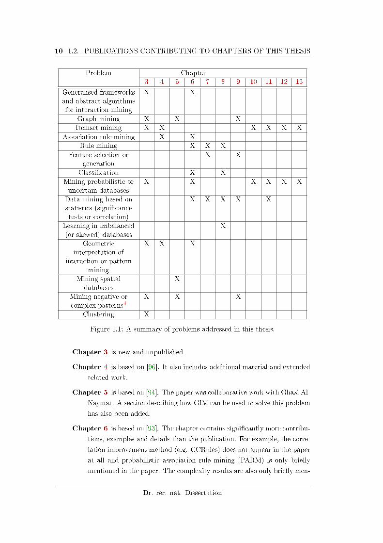
Problem Chapter3 4 5 6 7 8 9 10 11 12 13
Generalised frameworksand abstract algorithmsfor interaction mining
X X
Graph mining X X X
Itemset mining X X X X X X
Association rule mining X X
Rule mining X X X
Feature selection orgeneration
X X
Classi�cation X X
Mining probabilistic oruncertain databases
X X X X X X
Data mining based onstatistics (signi�cancetests or correlation)
X X X X X
Learning in imbalanced(or skewed) databases
X
Geometricinterpretation of
interaction or patternmining
X X X
Mining spatialdatabases
X
Mining negative orcomplex patterns4
X X X
Clustering X
Figure 1.1: A summary of problems addressed in this thesis.
Chapter 3 is new and unpublished.
Chapter 4 is based on [96]. It also includes additional material and extended
related work.
Chapter 5 is based on [94]. The paper was collaborative work with Ghazi Al-
Naymat. A section describing how GIM can be used to solve this problem
has also been added.
Chapter 6 is based on [93]. The chapter contains signi�cantly more contribu-
tions, examples and details than the publication. For example, the corre-
lation improvement method (e.g. CCRules) does not appear in the paper
at all and probabilistic association rule mining (PARM) is only brie�y
mentioned in the paper. The complexity results are also only brie�y men-
Dr. rer. nat. Dissertation
CHAPTER 1. INTRODUCTION 11
tioned in the paper. Furthermore, the framework has been generalised
slightly by allowing multiple measures (adding the k > 1 and l > 1 in
section 6.4).
Chapter 7 is new and unpublished. It is closely linked to chapter 6.
Part III
Chapter 8 is based on an extended version of [98]. An analysis of how GRM
can be used to solve part of this problem has also been added.
Chapter 9 is based on an extended version of [91]. A section describing how
GIM can be used to solve this problem has also been added.
Part IV
Chapter 10 is based on [18] and has been corrected, expanded, reorganised
and a uniform terminology introduced. The paper was collaborative work
with Thomas Bernecker, Dr. Matthias Renz and Andreas Zü�e in Prof.
Hans-Peter Kriegel's research group.
Chapter 11 is new and unpublished. It is based on collaborative work with
Thomas Bernecker, Dr. Matthias Renz and Andreas Zü�e in Prof. Hans-
Peter Kriegel's research group.
Chapter 12 is based on [19], which was collaborative work with Thomas
Bernecker, Dr. Matthias Renz and Andreas Zü�e in Prof. Hans-Peter
Kriegel's research group. Additional material has been added and a num-
ber of corrections made. For example, the overall ProFP-growth algorithm
is included and described. The generating function method for computing
frequentness probability was corrected, expanded and new computation
and pruning results added.
Chapter 13 is new and unpublished.
Florian Verhein

12 1.2. PUBLICATIONS CONTRIBUTING TO CHAPTERS OF THIS THESIS
Dr. rer. nat. Dissertation
Chapter 2
Background
Data is generated from a large number of diverse sources. This data is in-
creasingly being captured with the hope of generating value from the knowl-
edge hidden within it, be this for commercial, scienti�c, predictive or de-
scriptive purposes. The challenge is how to extract valid, novel, useful and
valuable knowledge from the data, do this e�ciently and � as much as pos-
sible � automatically. Every type of data, as well as the type of knowledge
sought from that data, presents its own speci�c challenges and requirements.
This chapter provides a brief background in Knowledge Discovery in
Databases (KDD) and Data Mining (DM) and highlights some issues rele-
vant to this thesis.
13
14 2.1. KNOWLEDGE DISCOVERY IN DATABASES
2.1 Knowledge Discovery in Databases
Data is increasingly being captured because it can � and is � used to better under-
stand the wants and needs of customers; to discover new ways of improving existing
practices, products and services; to discover and evaluate new opportunities; to help
make better decisions on anything from recommending products to medical diagno-
sis; to detect and prevent fraud or threats; to automate or make business or other
processes more e�cient and to help generate, develop and test theories about phe-
nomena. Furthermore, it is becoming established that collected data has value not
only for current applications, but also for future but as yet unknown purposes. That
is, data is collected for the purpose of obtaining value from the knowledge hidden
within it, including for as yet not envisioned applications. The challenge is how to
extract this knowledge.
Knowledge Discovery in Databases (KDD) attempts to solve the problem of ex-
tracting knowledge from data (typically stored in databases) and to provide valuable
information to the user. It aims to do this � as much as possible � automatically.
This information should be �valid, novel, potentially useful, and ultimately under-
standable� [36]: It should capture valid information and be applicable to new data,
rather than capturing an artifact that occurred by chance. It should be non-obvious
and represent new information for the user. It should also be understandable and
ultimately usable to improve a given application, system or process. Extracting this
sort of information from large quantities of data is a valuable but often di�cult
proposition.
While KDD concerns itself with information discovery, not all information discov-
ery tasks constitute KDD. For example, retrieving individual customer records or
querying a database management system or search engine are primarily Information
Retrieval (IR) problems. IR is the science of searching for information to answer
speci�c queries. Since the information being sought is well de�ned and typically
understood, the problem is to e�ciently search for those documents or records that
contain the desired information. KDD on the other hand, aims to �nd knowledge
that the user did not know existed or does not yet understand. Furthermore, this
knowledge is typically more structured, complex and abstract. For example, rather
than �nding web pages on a particular topic, KDD and data mining applied to the
world wide web (known as �web mining�) may �nd information such as a hierarchical
description or taxonomy of topics and their relationships to each other, the structure
of web pages or patterns in the way web pages are used and how this changes over
time. On the other hand, similarity search is a key component in both information
retrieval and clustering, the latter being a data mining method that �nds groupings
Dr. rer. nat. Dissertation
CHAPTER 2. BACKGROUND 15
of objects that are similar to each other. KDD is a multi-disciplinary �eld and often
overlaps IR, Machine Learning (ML), statistics, algorithms, databases, probability
theory and theoretical computer science. Some aspects which di�erentiate it from
other �elds are its attention to exploratory analysis, the ability to �nd and evaluate
complex patterns, its usefulness for hypothesis generation and its applicability to
massive data sets.
Knowledge Discovery in Databases has many challenges including:
• Data sets are typically large which makes e�ciency and scalability important
in order to deliver results to the user in an acceptable time frame. In particular,
the data sets considered in KDD are typically much larger than those consid-
ered in ML. This often makes non-trivial problems that overlap the database
�eld important, such as the storage, e�cient access to and indexing of data.
• Data sets often have a high dimensionality. Methods developed for low di-
mensional data are usually not applicable to high dimensional data since data
becomes sparse, distances between data points become similar and the e�ect
of noise is ampli�ed. Furthermore, the computational cost of many analysis
methods increases rapidly with the number of dimensions.
• Data is becoming increasingly complex and heterogeneous. For example, data
instances may be graphs or multi-instance objects and attributes may be a mix
of continuous, discrete, and semi-structured data.
• It is typically not known what information is sought prior to the application
of KDD. Hence KDD is hypothesis generating and exploratory in nature, in
comparison to traditional statistics for instance where an important task is
testing hypotheses constructed by a knowledgeable user.
• The type of knowledge sought by KDD is non-trivial and often involves complex
structures, descriptions and relationships. This leads to large search spaces
which demands e�cient solutions, as will be discussed in section 2.2. OLAP, in
contrast, is suited to computing and visualising the entire data set or relatively
simple aggregates, projections and groupings of records to �nd things such as
customer purchasing trends. Similarly, hypotheses in statistics are typically
simpler.
• Since KDD is a practical endeavor, it must consider real world issues such as
noise, uncertainty and faults within the data. Ignoring these can adversely
impact the ability to extract valid knowledge or lead to misleading results.
Florian Verhein
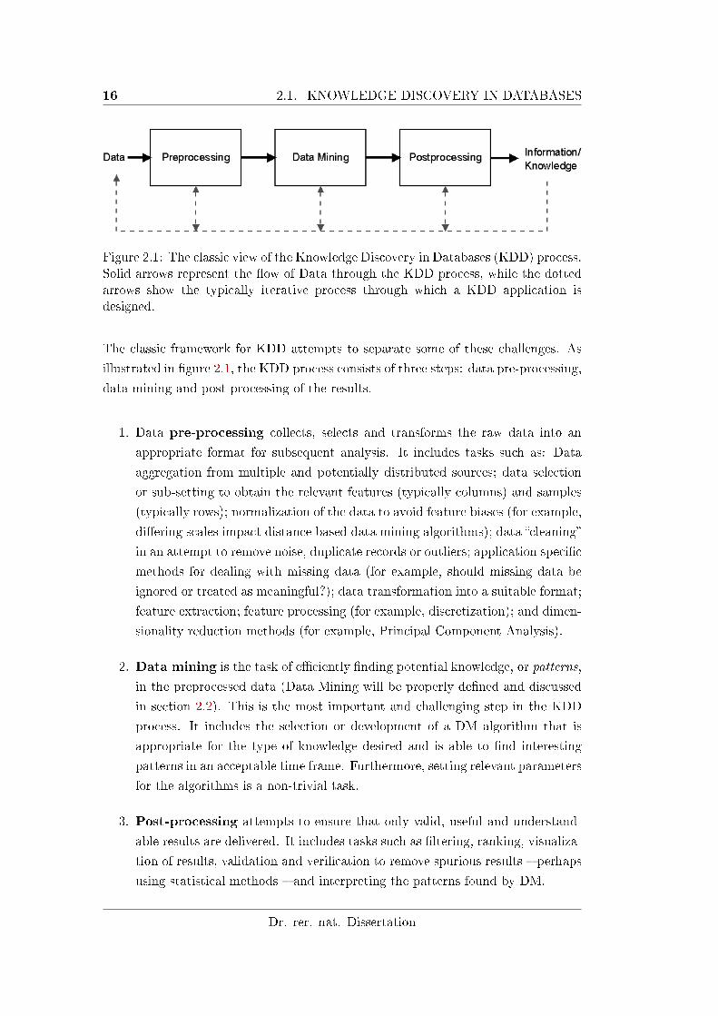
16 2.1. KNOWLEDGE DISCOVERY IN DATABASES
Figure 2.1: The classic view of the Knowledge Discovery in Databases (KDD) process.Solid arrows represent the �ow of Data through the KDD process, while the dottedarrows show the typically iterative process through which a KDD application isdesigned.
The classic framework for KDD attempts to separate some of these challenges. As
illustrated in �gure 2.1, the KDD process consists of three steps: data pre-processing,
data mining and post-processing of the results.
1. Data pre-processing collects, selects and transforms the raw data into an
appropriate format for subsequent analysis. It includes tasks such as: Data
aggregation from multiple and potentially distributed sources; data selection
or sub-setting to obtain the relevant features (typically columns) and samples
(typically rows); normalization of the data to avoid feature biases (for example,
di�ering scales impact distance based data mining algorithms); data �cleaning�
in an attempt to remove noise, duplicate records or outliers; application speci�c
methods for dealing with missing data (for example, should missing data be
ignored or treated as meaningful?); data transformation into a suitable format;
feature extraction; feature processing (for example, discretization); and dimen-
sionality reduction methods (for example, Principal Component Analysis).
2. Data mining is the task of e�ciently �nding potential knowledge, or patterns,
in the preprocessed data (Data Mining will be properly de�ned and discussed
in section 2.2). This is the most important and challenging step in the KDD
process. It includes the selection or development of a DM algorithm that is
appropriate for the type of knowledge desired and is able to �nd interesting
patterns in an acceptable time frame. Furthermore, setting relevant parameters
for the algorithms is a non-trivial task.
3. Post-processing attempts to ensure that only valid, useful and understand-
able results are delivered. It includes tasks such as �ltering, ranking, visualiza-
tion of results, validation and veri�cation to remove spurious results � perhaps
using statistical methods � and interpreting the patterns found by DM.
Dr. rer. nat. Dissertation
CHAPTER 2. BACKGROUND 17
While DM itself is automated, many of the pre- and post-processing tasks require
some human input and domain knowledge in order for the KDD process to be success-
ful. For example, domain knowledge is often required for e�ective feature selection.
Similarly, the output of data mining algorithms cannot simply be assumed to be
valid. The additional steps in the KDD process are essential to ensure that use-
ful and valid knowledge is derived from the data. Blind application of data-mining
methods is a dangerous activity and easily leads to the discovery of meaningless or
outright invalid patterns [35]. The reason for this is that one can �nd, for example,
statistically signi�cant patterns in any data set � even a randomly generated one
� if one searches long enough. Other problems such as noise, incorrect or lack of
normalization, careless selection of features or failing to consider outliers can also
lead to invalid patterns being found. These di�culties typically lead to an iterative
KDD process, illustrated in �gure 2.1 by the dotted arrows, where the results of all
three steps in the KDD process feed back into the decisions made in the previous
stages.
The interested reader is directed to [35] for a more in depth introduction to the high
level KDD process. While as of this writing the article is over 13 years old and
the �eld has progressed considerably, it provides a good overview and de�nitions
of KDD, the classic KDD process, its relationship to longer established �elds like
arti�cial intelligence, machine learning, statistics and databases, as well as some
early real world applications. For more concrete information about the various tasks
and algorithms in the KDD process, the reader is directed to [88] and [46] which
provide excellent introductions.
2.2 Data Mining
Data Mining (DM) is the most important and complex component of the KDD
process. There are a number of �de�nitions� of data mining. The following is most
closely related to that of [88], with the primary di�erence being the use of the term
pattern instead of information1.
1This is for two reasons: First, the author prefers the more concrete term �pattern� since, as shallhopefully become clear in the text, this leads to a natural way of explaining and understanding thedata mining process. Secondly, the author doesn't think that patterns (or to be more speci�c, pat-tern instances in the terminology introduced here) necessarily qualify as information or knowledge.Patterns are the output of an automated process which together, perhaps after post processing,visualization, validation or human interaction, may become information. It should be noted that�pattern� is usually used in the literature in the context of association rules and itemset mining, forexample �frequent pattern mining�, but that patterns are not restricted to this sub-�eld. Pattern isalso used in the de�nition of data mining by [35].
Florian Verhein
18 2.2. DATA MINING
De�nition 2.1. Data mining is the automated process of extracting useful patterns
from typically large quantities of data.
Di�erent types of patterns capture di�erent types of structures in the data: A pattern
may be in the form of a rule, cluster, set, sequence, graph, tree, etc. and each of these
pattern types is able to express di�erent structures and relationships present in the
data. For example, a rule may tell a marketer about strong relationships between
purchased goods or services, predict customer `churn' or be used as the basis of
recommender systems. A set can indicate products that customers are purchasing
together and a cluster might tell him or her about groups of customers that have
similar purchasing patterns. These may be used as the basis for a marketing scheme
that aims to maximize response rates and sales for a given investment. A graph may
tell a biologist about strong and previously unknown gene or protein interactions
present in their experiments, or a security agent about suspicious communication
structures between potential criminals. A tree or a set of rules may describe the
decision structure that can be used to accurately predict medical conditions, perhaps
based on patient records or medical imaging data. As suggested by these examples,
patterns can be descriptive or predictive (or both). That is, they can be used to
describe, model and help better understand a process or phenomena or to predict
future events. In this work, many new types of patterns are introduced. Some are
purely descriptive and some are explicitly used for prediction purposes.
Once a pattern type has been de�ned based on the problem at hand and the structure
of the information sought, the goal � and challenge � is to automatically �nd those
pattern instances2 in the data that are interesting to the end user. That is, pattern
instances providing both useful and previously unknown (novel) information. This is
done by evaluating pattern instances for interestingness according to some measure
that, ideally, should model the value that the user obtains from being made aware of
the pattern. An interestingness measure measures how interesting a pattern instance
is expected to be. These measures must balance three important characteristics:
1. The utility that a user is expected to receive by exploiting the pattern instance.
For example; the value, �nancial gain, increase in accuracy or e�ciency or
2In the terminology used here, a pattern type describes the structure or schema of the pattern.For example, an itemset can be de�ned as a non-empty subset of all items that may be purchasedin a supermarket. This speci�es its type. A pattern instance on the other hand is a particularinstantiation of that type. For example, {bread, butter, jam}. A pattern therefore has one typebut many instances, and these instances are �found� in the data set. This distinction between typeand instance is rarely made explicit but helps to describe the data mining process in terms of thede�nition used in this thesis. In the literature and common usage, the term �pattern� is inherentlyambiguous and refers to both or either the type or instance, depending on the context. Outsidethis section, the term will typically refer to the pattern instance of the type being discussed.
Dr. rer. nat. Dissertation
CHAPTER 2. BACKGROUND 19
ability to understand a phenomena. Modeling utility directly is usually too
di�cult in practice and simpler but objective measures are used instead, ideally
with reasoning linking them back to the users expected utility.
An important in�uence on the utility of pattern instances is how many of
them are labeled as interesting. The utility that a user gains from the results
of data mining � namely, the set of all pattern instances mined � can easily
fall if too many results are delivered, especially if many of them are similar.
One way of combating this problem is post-processing the results. Another
method, favoured in this thesis, is to mine interesting patterns directly, mine
only statistically signi�cant patterns or patterns with a high probability of
being interesting.
Finally, utility should also attempt to capture valid patterns, as opposed to
spurious ones. This is a motivation for the probabilistic and statistical methods
employed in parts of this thesis.
2. The novelty of the pattern instance. For example, simple patterns may be
useful or describe a strong relationship but if they are already known or obvious
then they provide no added value. Novelty is di�cult to take into account, but
a simple method to counter obviousness is perhaps to ensure that a user is
directed to larger or more complex patterns in favour of simple ones.
3. The complexity of calculating the measure and searching for those pattern
instances that have a high interestingness value. Usually, the goal is to develop
a complete algorithm (if possible) so that all patterns satisfying a particular
interestingness criteria will be found. Sometimes this is possible even in very
large databases as some measures allow a suitably developed algorithm to prune
away most of the search space. However, in other cases it is intractable to �nd
all interesting results. In such cases, it is possible that approximate, heuristic
or probabilistic methods can be employed. These limit the search space and
complexity while still delivering useful results. The downside is that the user is
never completely sure that all pattern instances that may be of interest to him
or her are found, or that the best or optimal pattern is found. On the other
hand, this is usually better than not being able to deliver any results. The
complexity of the resulting algorithm and properties that may be exploited are
therefore an important consideration in designing an interestingness measure.
One of the results of this thesis is that forcing good quality interestingness mea-
sures (that correlate with the users utility) to be anti-monotonic (this enables
e�cient pruning) when they do not naturally have pruning friendly proper-
ties gives much better results than using interestingness measures that allow
Florian Verhein
20 2.2. DATA MINING
pruning but are not directly related to the users utility.
With a type of pattern and interestingness measure de�ned, the challenge is to
develop an e�cient algorithm to �nd the interesting pattern instances in large data
sets. Of course, as hinted above, this may be an iterative process where the design
of the algorithm and interestingness measures a�ect each other.
One of the contributions in this thesis is the development of generalised algorithms,
frameworks and a computational model that separates the semantics of the patterns
and interestingness measures from the algorithm used to mine them. This makes the
design process much easier, as both problems can be solved independently. Further-
more, the ability to plug in interestingness measures into an e�cient framework and
algorithm allows the data miner to focus on the semantics of the problem.
Dr. rer. nat. Dissertation

Part II
Generalised Interaction Mining
21

Chapter 3
Generalised Interaction Mining
Interaction mining is the process of mining structures on variables that de-
scribe how they interact (or appear to interact) with each other. Generalised
Interaction Mining (GIM) is a model, framework and algorithm that solves
interaction mining problems at the abstract level. The semantics of the in-
teractions, their interestingness measures and the type of data considered are
�exible components. An e�cient and intuitive computational model based
on vectors and vector valued functions is developed. This functions as a
layer of abstraction between a problems semantics and the algorithm used
to mine it; allowing both to vary independently. It encourages a geometric
way of thinking about pattern mining problems in terms of vector operations
and subspaces. It allows new methods to be developed by focusing purely
on the problem's semantics. The GIM algorithm requires minimal space and
runs in linear time in the number of interesting interactions found.
The GIM framework and algorithm are a cumulative result of many problems
that the author has solved. In addition to introducing GIM, this chapter
demonstrates the breadth of problems that are solvable with GIM by showing
how it can be applied in diverse applications.
23
24 3.1. INTRODUCTION
3.1 Introduction
An interaction is a broad term used in this thesis to describe an e�ect that variables
have on each other, or appear to have on each other. Interaction mining is the process
of mining structures on these variables that describe interaction patterns. Usually,
these structures are represented sets or graphs; where each variable interacts, to some
degree, with other variables in the structure.
Many domains can bene�t from the application of interaction mining. In social
networks people interact with each other through personal contact, email, instant
messaging, telephone and social network applications. Social network analysis is
used in applications such as understanding how patterns of human contact a�ects
the spread of diseases, surveillance and counter intelligence operations, understand-
ing the spread of ideas and for marketing and promotion. In marketing, di�erent
promotional campaigns and customer facing services interact to a�ect customer re-
tention and the bottom line. In pharmacology, drugs may interact with each other.
In genetics, genes interact with each other to a�ect the phenotype (observable char-
acteristics) of organisms. In statistics, interactions between variables create e�ects
greater than the individual variables would, or may be measured by correlation or
signi�cance tests. In �nance, equities interact (or appear to interact) with each other
as re�ected by similarities in the time series of their prices. In ecology, movement
of animals over time may show behavioural interactions. Such interactions may be
complex and include both positive and negative interactions. For example, signed
graphs in social network analysis can show friendship or aversion; there are additive
or suppressive actions between drugs or genes; and mining positive an negative cor-
relations between variables could reveal useful patterns in a range of applications.
Furthermore, many data mining tasks can be considered as mining interactions, such
as clustering (similar objects may be seen to be �interacting�), frequent itemset min-
ing (items bought frequently together suggest these are used together), classi�cation
(interactions amongst variables are exploited for prediction), spatio-temporal data
mining techniques (�ocks and other co-location patterns describe interactions be-
tween objects), etc. Mining interactions between variables is therefore a general
data mining concept that covers a range of problems.
However, these problems have very di�erent semantics governing the interactions,
their structures and their interpretation. Naturally, these problems all have di�erent
de�nitions of what it means for an interaction pattern to be interesting or useful. The
Dr. rer. nat. Dissertation
CHAPTER 3. GENERALISED INTERACTION MINING 25
problems also have very di�erent types of data, such a real valued records, a set of
time series, transaction databases, attribute value pairs produced by discretization,
instances and adjacency matrices. Usually, solving such problems requires the simul-
taneous and interdependent development of new pattern semantics and specialist
algorithms for mining the respective pattern.
Generalised Interaction Mining (GIM) is a framework and method for mining inter-
actions at the abstract level. It does this by leaving the semantics of the interactions,
the interestingness measures used to evaluate the interactions and the data types in
which the interactions are to be mined as �exible components. This creates a layer of
abstraction between a problem's de�nition/semantics and the algorithm used to solve
it. Instantiations of GIM solving speci�c problems need only specify these abstract
components, and the GIM algorithm can be used to mine all interesting interactions
satisfying these constraints. This is achieved by developing a consistent but general
computation model based on vectors and vector valued functions, where each inter-
action is represented by an interaction vector in some space X. This framework is
able to capture a wide range of interaction mining problems simply by instantiating
these functions in di�erent ways. Since the framework operates as an interface be-
tween the semantics of a problem and the algorithm used to mine it, this abstraction
layer enables the problem's semantics and algorithm to vary independently of each
other. This means that new methods can be developed by focusing on the semantics
of the problem, without being concerned with how these semantics are mapped to
a new algorithm. As long as the semantics of the problem can be mapped to the
framework � and it will be shown in this chapter and thesis that many can � the
GIM algorithm can solve it e�ciently. Similarly, since the algorithm depends only
on a set of abstract vector valued functions, it is independent of the semantics of the
particular instantiation and can be swapped out � for example should a more e�-
cient one become available, to cater for di�erent trade-o�s between time and space
resources or to leverage di�erent computation architectures.
GIM's computational model also provides an intuitive �geometric� way of thinking
about problems, as it requires them to be cast into vectors and vector valued func-
tions. Every interaction is represented by a vector, called an interaction vector,
in a high dimensional space X typically spanned by the samples recorded in the
database. By combining such vectors, larger interactions can be built, with vectors
typically existing in subspaces of X. By evaluating functions over these vectors, the
interestingness of interactions can be computed.
The GIM algorithm operates purely by using these functions on interaction vectors,
and searches the space of possible interactions in the most space and time e�cient
Florian Verhein
26 3.1. INTRODUCTION
method possible. This means that interaction vectors are never created more than
once but are reused, while at the same time ensuring that the minimum number
of interaction vectors are in memory at one time. The space required is provably
linear in the size of the data set. The run-time is provably linear in the number
of interactions that need to be examined. These properties allow it to outperform
specialist algorithms when applied to speci�c interaction mining problems, such as
frequent itemset mining and probabilistic frequent itemset mining. Furthermore, the
vectorization inherent in the framework's functions provides additional avenues for
reducing the run time: On single processor architectures, vectorization allows auto-
matic parallelisation and exploitation of machine level operations for bit-vectors. On
multiprocessor architectures, vectorization also provides a point for concurrentisa-
tion [105] while on supercomputer architectures, single instruction vector processing
is directly supported [105].
3.1.1 Relationship to other Chapters
The approach described in this chapter was developed over an extended period of
time while solving other research problems e�ciently and discovering similarities in
the way these problems could be solved. While other chapters in this thesis present
problems that can be solved (retrospectively) using the GIM framework, this may
not have been done at the time. This is also one of the last chapters that was
written and therefore also functions as a broad treatment of interaction mining and
generalised pattern mining. Accordingly, the emphasis is on the abstract framework,
the GIM algorithm and presenting a sample of the many problems to which it can
be applied. Other chapters evaluate some of these problems in depth and therefore
demonstrate the superiority of applying GIM to speci�c research problems. This is
described in section 3.16.
Chapter 6 extends the concept of interaction mining to rules, introducing and de�ne-
ing the generalised rule mining (GRM) problem. This allows the capture of patterns
where an interaction in the antecedent a�ects a variable in the consequent. This can
be used to �nd patterns where interactions have seemingly causal e�ects on other
variables, in particular enabling predictive patterns to be found. For example, in
marketing, various promotions, incentive programs and media coverage interact to
a�ect consumer behaviour, such as the number of new customers, customer churn or
customer spend. Like GIM, GRM solves problems at the abstract level.
Dr. rer. nat. Dissertation
CHAPTER 3. GENERALISED INTERACTION MINING 27
3.1.2 Contributions
This chapter makes the following contributions:
• It introduces the Generalised Interaction Mining (GIM) problem and presents
an abstract framework that allows interaction mining problems to be speci�ed
in terms of functions on interaction vectors. This framework separates the
semantics of interaction mining problems from the algorithms used to mine
them, provides a generic computational model for solving GIM problems and
a useful geometric way of considering these problems in terms of vectors and
subspaces.
• It presents the GIM algorithm, which is able to solve any problems expressed
in the GIM framework e�ciently. It is proved to have linear run time in the
interesting interactions found and uses space linear in the size of the database
(usually less). Extensions are also developed for solving a range of complex
problems.
• It shows that GIM can be applied to solve a wide variety of existing and novel
problems.
• Section 3.12.1 proves that the maxPI measure, used in spatial data mining, is
anti-monotonic under an ordering of variables. Previously this was thought to
be weakly anti-monotonic. This leads to an more e�cient solution using GIM.
3.1.3 Organisation
The remainder of this chapter is organised as follows. Section 3.2 presents the Gener-
alised Interaction Mining (GIM) framework. Section 3.3 presents the GIM algorithm.
Subsequent sections show how diverse problems can be mapped to the framework
and solved by GIM; and how, through various extensions, GIM is able to solve more
complicated problems.
3.2 Generalised Interaction Mining Framework
This section presents the vectorised GIM framework. Let V = {v1, v2, ..., vm} be theset of variables about which interaction information is desired. The data is said to
consist of a set of samples {s1, s2, ..., sn} capturing the variable's values. The goal
is to �nd interesting subsets of V , where these subsets V ′ ⊆ V � corresponding to
Florian Verhein
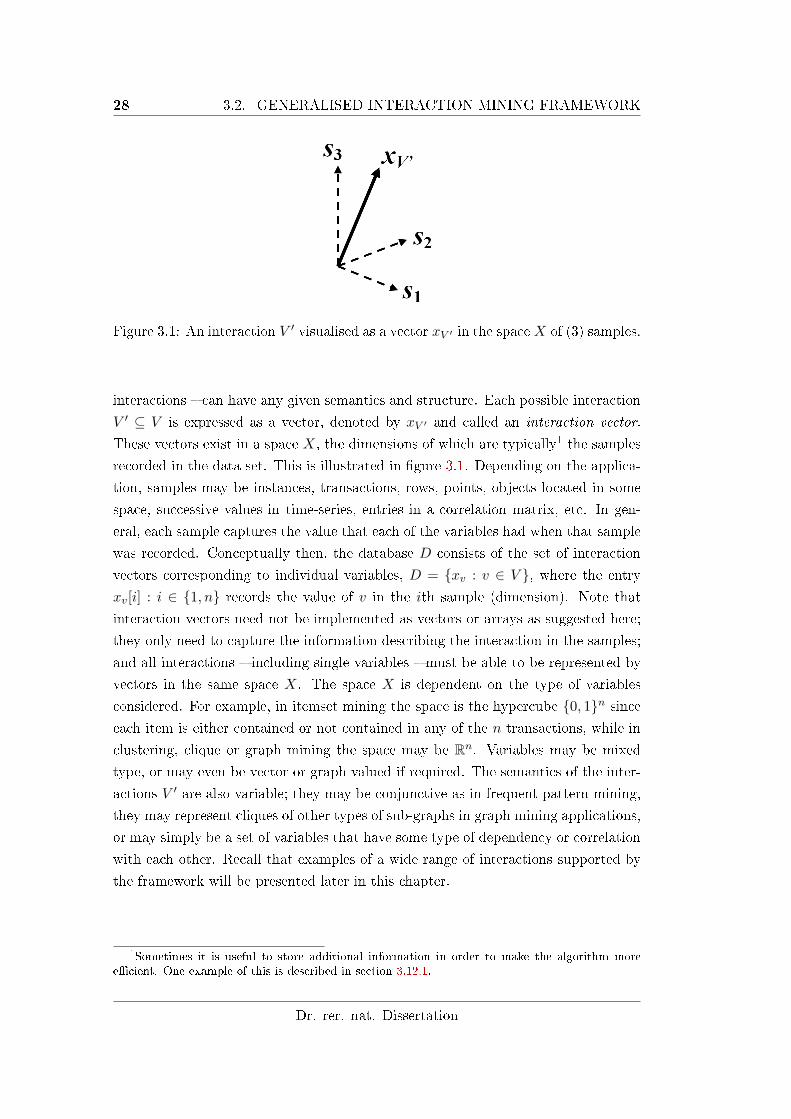
28 3.2. GENERALISED INTERACTION MINING FRAMEWORK
Figure 3.1: An interaction V ′ visualised as a vector xV ′ in the spaceX of (3) samples.
interactions � can have any given semantics and structure. Each possible interaction
V ′ ⊆ V is expressed as a vector, denoted by xV ′ and called an interaction vector.
These vectors exist in a space X, the dimensions of which are typically1 the samples
recorded in the data set. This is illustrated in �gure 3.1. Depending on the applica-
tion, samples may be instances, transactions, rows, points, objects located in some
space, successive values in time-series, entries in a correlation matrix, etc. In gen-
eral, each sample captures the value that each of the variables had when that sample
was recorded. Conceptually then, the database D consists of the set of interaction
vectors corresponding to individual variables, D = {xv : v ∈ V }, where the entry
xv[i] : i ∈ {1, n} records the value of v in the ith sample (dimension). Note that
interaction vectors need not be implemented as vectors or arrays as suggested here;
they only need to capture the information describing the interaction in the samples;
and all interactions � including single variables � must be able to be represented by
vectors in the same space X. The space X is dependent on the type of variables
considered. For example, in itemset mining the space is the hypercube {0, 1}n since
each item is either contained or not contained in any of the n transactions, while in
clustering, clique or graph mining the space may be Rn. Variables may be mixed
type, or may even be vector or graph valued if required. The semantics of the inter-
actions V ′ are also variable; they may be conjunctive as in frequent pattern mining,
they may represent cliques of other types of sub-graphs in graph mining applications,
or may simply be a set of variables that have some type of dependency or correlation
with each other. Recall that examples of a wide range of interactions supported by
the framework will be presented later in this chapter.
1Sometimes it is useful to store additional information in order to make the algorithm moree�cient. One example of this is described in section 3.12.1.
Dr. rer. nat. Dissertation
CHAPTER 3. GENERALISED INTERACTION MINING 29
The �rst component of the framework is an order on the variables.
De�nition 3.1. The variables v ∈ V have a strict total order < de�ned on them.
Write vi < vj ⇐⇒ i < j.
This is trivially satis�ed in most applications as variables occur in some arbitrary
order in the data set, and the order does not impact on the resulting patterns. In
some applications a particular order is important. For example, section 3.12 shows
that the maxPI measure is anti-monotonic provided that variables have a particular
order.
Since each interaction V ′ is represented by a vector xV ′ in X, the evaluation of that
interaction is performed with a vector valued function mI(·).
De�nition 3.2. mI : X → Rk is a measure on a vector xV ′ . mI(xV ′) evaluates the
quality of the interaction V ′. k is �xed.
That is, mI evaluates an interaction based only on the information available in that
interaction's vector. k ≥ 1 allows the function to evaluate V ′ according to multiple
criteria.
.
In order to evaluate an interaction with mI(·), its interaction vector must �rst be
built. Recall that the data set contains all xv where v ∈ V are the single vari-
ables. The interaction vectors xV ′ with |V ′| > 1 are built incrementally using the
aggregation function aR(·), which maps two vectors in X onto X:
De�nition 3.3. aI : X2 → X operates on interaction vectors so that xV ′∪v =
aI(xV ′ , xv) where V ′ ⊂ V , v ∈ (V − V ′), and v occurs prior to all elements in V ′.
That is, v < v′∀v′ ∈ V ′.
In other words, aI(·) combines the vector xV ′ for an existing interaction V ′ ⊂ V with
the vector xv for a new variable v ∈ V − V ′. The resulting vector xV ′∪v represents
the larger interaction V ′ ∪ v. In this way, vectors representing interactions can be
built incrementally. Note that the resulting vector is the same as if it were calculated
Florian Verhein
30 3.2. GENERALISED INTERACTION MINING FRAMEWORK
from the original data set, but rather than examining the original data set for all
v′ ∈ V ′ ∪ v, it requires only one of the vectors (xv) as the information from the
rest is already represented in xV ′ . This is exploited by the GIM algorithm, allowing
it to e�ciently evaluate interactions without recomputing vectors or scanning the
data set. Note that aI(·) need not be commutative, even though the subscript xV ′∪v
uses set notation for simplicity. Furthermore, note that the order can be used in
applications for semantic purposes, as it is guaranteed that interaction vectors are
built in a particular and �xed order.
Note that implicitly, aI(·) de�nes the semantics of the interaction. By de�ning
how xV ′∪v is built, it must implicitly de�ne the semantics between variables in the
interaction. That is, what it means to add a variable to the existing interaction V ′.
Example 3.4. The simplest interaction mining approaches counts the number of
samples that exhibit an interaction V ′. In these cases, the interaction vector seman-
tically consists of the set of samples that contain the interaction and mI(·) is simply
the size of this set. aI(·) is the intersection operation, so that all variables must be
present in a sample for it to be counted. This leads to conjunctive semantics.
While mI(·) and aI(·) are su�cient in a number of applications, it sometimes occurs
that an interaction V ′ needs to be compared with its sub-interactions V ” : V ” ⊂ V ′
in order to compute an interestingness measure. There are a number of problems
in this thesis where this is required, including mining spatial co-location patterns.
Furthermore, it allows the explicit measurement of how much an interaction V ′
improves over its more general sub-interactions V ” : V ” ⊂ V ′, a topic that will be
considered in depth in section 3.21. The following function supports such behaviour.
De�nition 3.5. MI : Rk×|P(V ′)| → Rl is a measure that evaluates an interaction V ′
based on the values computed by mI(·) for V ′ or any sub-interaction V ′′ : V ′′ ⊂ V ′.l is �xed.
Like mI(·), MI(·) may compute multiple values. MI(·) does not take vectors as
arguments � it evaluates a rule based on values that have already been calculated
by mI(·). This is for algorithmic e�ciency purposes and does not limit the scope of
the framework. If MI(·) does not need access to any sub-interactions to perform its
evaluation, it is called trivial since mI(·) can perform the function instead. A trivial
MI(·) simply returns mI(·) and leads to reduced run time and space usage by the
algorithm, as will be described in section 3.3.
Dr. rer. nat. Dissertation
CHAPTER 3. GENERALISED INTERACTION MINING 31
The �nal component of the framework de�nes what interactions are interesting. In-
teresting interactions are
1. Desirable and should therefore be output to the user and
2. Should be further expanded in the sense that additional variable should be
added in order to grow the interaction.
For �exibility, these two concepts may be separated.
De�nition 3.6. SI : Rl+k → {true, false} determines whether an interaction V ′
should be expanded or the search should stop at this interaction. This is determined
based on the values previously computed by mR(·) and MR(·).
In other words, more speci�c interactions � That is, larger interactions with more
variables � will only be considered if SI(·) returns true. Independently, the interest-ingness to the user is de�ned as follows;
De�nition 3.7. II : Rl+k → {true, false} determines whether an interaction V ′
is interesting based on the values computed by mR(·) and MR(·). Only interesting
rules are output by the algorithm.
Note that an interaction may be interesting according to II(·) but not according to
SI(·). This means the interaction will be output, but no larger interaction will ever
be examined or output. Conversely, an interaction may not be interesting according
to II(·) but if SI(·) returns true, then larger interactions will be examined, some
of which may be interesting according to II(·). Of course II(·) and SI(·) may be
identical. The simplest implementation of either function is to return true if one of
the values computed by MI(·) or mI(·) is above a threshold.
Note that this framework accommodates approaches where an interaction V ′ is ex-
amined after its sub-interactions V ′′ ⊂ V ′. That is, bottom up approaches. It is pos-
sible to accommodate top-down approaches be inverting the problem, as described
in section 3.7.
An additional function PI(xV ′ , v) (de�nition 3.17) that allows early pruning and thus
avoids computing vectors in some applications will be considered in section 3.8. An
additional function N(·) (de�nition 3.13) can be included for supporting negative
patterns and will be discussed in section 3.6. The subscripts I in the functions in
this framework is used to di�erentiate them from related functions in the Generalised
Rule Mining (GRM) framework, covered in chapter 6.
Florian Verhein
32 3.3. GENERALISED INTERACTION MINING ALGORITHM
3.3 Generalised Interaction Mining Algorithm
This section presents the Generalised Interaction Mining (GIM) algorithm, which
solves any problem expressible in the GIM framework e�ciently. First, an important
data structure is presented.
3.3.1 Pre�x Tree
In order to make the algorithm easy to understand, a pre�x tree will be used to help
describe it, prove properties, and in some cases, to store a collection of interactions
in compressed form.
Since all variables v ∈ V have a strict total order (de�nition 3.1), they can be
mapped to the set of integers. Without loss of generality therefore, assume the
variables are integers V = {1, 2, ..., |V |}. An interaction can therefore be represented
as a sequence of integers, ordered in decreasing order according to < (de�nition 3.1).
A space e�cient way to store a collection of interactions (in those cases when this is
necessary) is to share common pre�xes in a tree structure. An example of a pre�x
tree is shown in �gure 3.2(b).
In a pre�x tree (PrefixTree), each node � called a PrefixNode � has a label
corresponding to a variable v ∈ V (this will be called variableId in algorithm 3.1).
The root node is special, and is labeled with∞. The tree is constructed so that each
node can only have a parent with a label greater than it's own label. Each node has
a reference to its parent, but not to its children. Maintaining only parent links is
used to increase the run time and space e�ciency of the algorithm. It also sets it
apart from a Trie [66] data structure. In particular, in many instantiations of the
framework, only a single branch (path toward the root) of a pre�x tree must ever
be retained in memory at one time. In a pre�x tree, two nodes are called siblings
if they share the same parent. Each PrefixNode represents a distinct subset of
the variables and as such represents a unique interaction. The interaction can be
re-constructed e�ciently by traversing toward the root. The root node corresponds
to the empty interaction. Each node also contains the values computed by mI(·)(called valuem), MI(·) (called valueM ) and II(·) (called interestingness). It is notnecessary to store the result of SI(·).
A �complete� pre�x tree is a tree containing all possible interactions. Therefore, it
also represents the worst case search space of GIM and contains exactly 2|V | nodes.
An example of a complete PrefixTree is given in �gure 3.2(a).
Dr. rer. nat. Dissertation
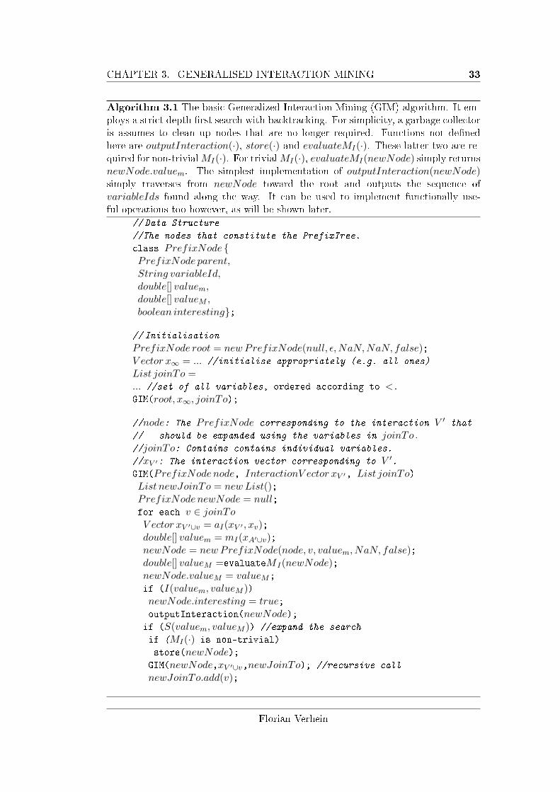
CHAPTER 3. GENERALISED INTERACTION MINING 33
Algorithm 3.1 The basic Generalized Interaction Mining (GIM) algorithm. It em-ploys a strict depth �rst search with backtracking. For simplicity, a garbage collectoris assumes to clean up nodes that are no longer required. Functions not de�nedhere are outputInteraction(·), store(·) and evaluateMI(·). These latter two are re-quired for non-trivialMI(·). For trivialMI(·), evaluateMI(newNode) simply returnsnewNode.valuem. The simplest implementation of outputInteraction(newNode)simply traverses from newNode toward the root and outputs the sequence ofvariableIds found along the way. It can be used to implement functionally use-ful operations too however, as will be shown later.
// Data Structure
//The nodes that constitute the PrefixTree.
class PrefixNode {PrefixNode parent,String variableId,double[] valuem,double[] valueM ,boolean interesting};
// Initialisation
PrefixNode root = new PrefixNode(null, ε,NaN,NaN, false);V ector x∞ = ... //initialise appropriately (e.g. all ones)
List joinTo =... //set of all variables, ordered according to <.GIM(root, x∞, joinTo);
//node: The PrefixNode corresponding to the interaction V ′ that// should be expanded using the variables in joinTo.//joinTo: Contains contains individual variables.
//xV ′: The interaction vector corresponding to V ′.GIM(PrefixNode node, InteractionV ector xV ′, List joinTo)List newJoinTo = newList();PrefixNode newNode = null;for each v ∈ joinToV ector xV ′∪v = aI(xV ′ , xv);double[] valuem = mI(xA′∪v);newNode = new PrefixNode(node, v, valuem, NaN, false);double[] valueM =evaluateM I(newNode);newNode.valueM = valueM;
if (I(valuem, valueM ))newNode.interesting = true;outputInteraction(newNode);if (S(valuem, valueM )) //expand the search
if (MI(·) is non-trivial)
store(newNode);GIM(newNode,xV ′∪v,newJoinTo); //recursive call
newJoinTo.add(v);
Florian Verhein
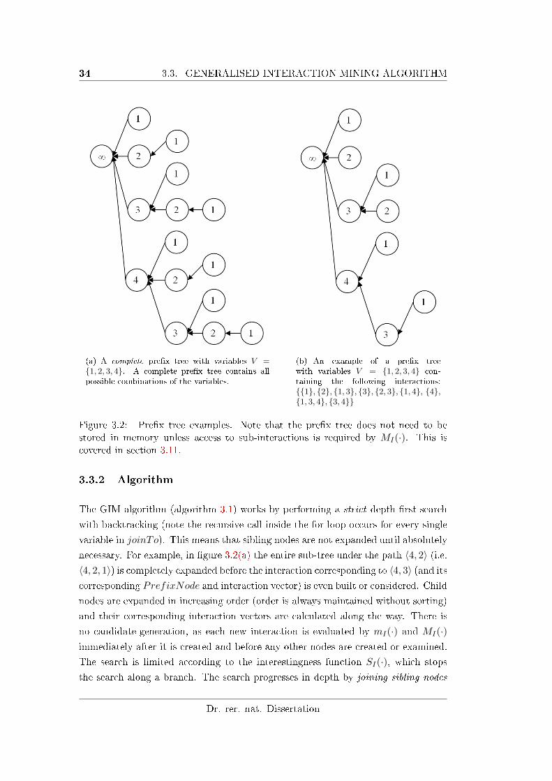
34 3.3. GENERALISED INTERACTION MINING ALGORITHM
(a) A complete pre�x tree with variables V ={1, 2, 3, 4}. A complete pre�x tree contains allpossible combinations of the variables.
(b) An example of a pre�x treewith variables V = {1, 2, 3, 4} con-taining the following interactions:{{1}, {2}, {1, 3}, {3}, {2, 3}, {1, 4}, {4},{1, 3, 4}, {3, 4}}
Figure 3.2: Pre�x tree examples. Note that the pre�x tree does not need to bestored in memory unless access to sub-interactions is required by MI(·). This iscovered in section 3.11.
3.3.2 Algorithm
The GIM algorithm (algorithm 3.1) works by performing a strict depth �rst search
with backtracking (note the recursive call inside the for loop occurs for every single
variable in joinTo). This means that sibling nodes are not expanded until absolutely
necessary. For example, in �gure 3.2(a) the entire sub-tree under the path 〈4, 2〉 (i.e.〈4, 2, 1〉) is completely expanded before the interaction corresponding to 〈4, 3〉 (and itscorresponding PrefixNode and interaction vector) is even built or considered. Child
nodes are expanded in increasing order (order is always maintained without sorting)
and their corresponding interaction vectors are calculated along the way. There is
no candidate-generation, as each new interaction is evaluated by mI(·) and MI(·)immediately after it is created and before any other nodes are created or examined.
The search is limited according to the interestingness function SI(·), which stops
the search along a branch. The search progresses in depth by joining sibling nodes
Dr. rer. nat. Dissertation
CHAPTER 3. GENERALISED INTERACTION MINING 35
in the PrefixTree, so to speak. This means that an interaction 〈4, 3, 2〉 is createdby joining the siblings 〈4, 3〉 and 〈4, 2〉. Note however that while joinTo contains
individual variables, it only contains those that correspond to the last variable in
siblings of the node being expanded. This auto-prunes the search, since 〈4, 3, 2〉 canonly be created if the sibling 〈4, 2〉 exists (is was found to be interesting according
to SI(·)). If 〈4, 2〉 was not found to be interesting, then 〈4, 3, 2〉 would never be
considered. This auto pruning is useful for measures that are anti-monotonic or
weakly anti-monotonic. Should this be undesirable, it can be easily disabled by
placing the last line of the algorithm outside the if (S(valuem, valueM )) statement.
Vectors are calculated incrementally along a path in the search using aI(·). This
is done in a way so that there are never any vector re-computations while at the
same time maintaining optimal memory usage. To appreciate this, consider the
alternatives: One option is to calculate each interaction vector from the vectors
for single variables when it is needed. While this requires no additional space, it
requires |V ′| applications of aI(·) to create xV ′ and many re-computations of the
same vector (vectors for pre�xes would need to be recomputed), which is clearly
undesirable. Another alternative is to keep many interaction vectors in memory
and add variables to these with aI(·) when needed, so that it is guaranteed that
only one application of aI(·) is required to create any required xV ′ . The downside
of this is the space required to store these vectors. The GIM algorithm stores the
fewest interactions necessary in order to avoid any re-computations by only ever
storing vectors along the current path of the search, and performing a strict depth
�rst search. For example, the interaction vector x{4,3,2} is created by a(x{4,3}, x2),
where x{4,3} was just previously created in the search. Since the sub-tree under
〈4, 2〉 must have been completely examined before this is done, the vector x{4,2} is no
longer in memory (it is no longer needed since x{4,2,1}, for example, has already been
considered). Since x{4,3} is only created and tested once the entire search space under
x{4,2} has been completely examined, the search is said to be strictly depth �rst.
As the search progresses in depth, x{4,3,2,1} is created by a(x{4,3,2}, x1), utilising the
already computed x{4,3,2}. Note that one interaction expansion � where an additional
variable is added to the interaction � therefore requires only one application of aI(·)to create its corresponding interaction vector. Furthermore, the only interaction
vectors that need to remain in memory are those on the current path of the search
(due to the recursive implementation, this corresponds to the stack). Since the search
is strictly depth �rst, there will never be a case where vectors corresponding to sibling
nodes are in memory at the same time. For example, only one of x{4,1}, x{4,2}, x{4,3}
is ever in memory at one time, even though they are siblings. There are ways to
slightly reduce this space usage further; interaction vectors for sibling nodes that
Florian Verhein
36 3.3. GENERALISED INTERACTION MINING ALGORITHM
are expanded last can be deleted as soon as their last child is created. For example,
〈4, 3〉 can be deleted as soon as x{4,3,2} is created (even though it is on the same
path) because no other variable that has not previously been added can be added to
{4, 3} without violating the order requirement of de�nition 3.1. For simplicity, this
is not implemented here but it may be adapted from the itemset mining algorithm
in chapter 4.
3.3.3 Complexity
Theorem 3.8. The run time complexity is O(|I| · |V | · (t(mI) + t(MI) + t(aI) +
t(SI) + t(II)), where I is the number of interactions for which SI(·) returns true andt(X) is the time taken to compute function X from the framework.
Proof. For a node corresponding to an interaction V ′ to be expanded (to search for
larger interactions), SI(·) must return true for it and there must be siblings to join
to, otherwise the branch of the search space is pruned. In the worst case, each child
V ′∪v : v ∈ (V−V ′) must be examined, with none of the interactions V ′∪v found to beinteresting according to SI(·). This takes at worst O(|V |) time; for each interaction
mined, at worst O(|V |) larger interactions may have to be examined. Finally, the
processing of each interaction requires one application of each of the functions mI ,
MI , aI , II and SI . Note that |I|·|V | is an upper-bound on the number of interactionsthat must be examined.
In most applications, t(aI) and t(mI) require at most O(n) time (often less if sub-
spaces can be exploited), since the operate on interaction vectors of at most length n
and t(MI) = t(SI) = t(II) = O(1). Note that if SI = II , then the run time is linear
in the number of interesting interactions found. The requirement for completeness
requires that children be examined, leading to the |V | in the run time. The algorithm
is said to be optimal in the sense that it takes time linear in the number of patterns it
�nds to be interesting. Since each interaction must be generated or output, it is not
possible to improve the run time beyond a constant factor. In practice, the algorithm
is therefore theoretically as e�cient as possible, given the frameworks functions. Of
course it should be clear that |I| is at worst 2|V |. In practical applications only a
small proportion of these interactions are interesting however. Also, note that in the
worst case, the |V | component in the run time is super�uous as there exists no inter-
action that is not interesting � |V | was included in the bound to cover interactions
that were examined but not found to be interesting. Since this does not occur in
the worst case, the algorithm is even optimal in the worst case. Interactions may
Dr. rer. nat. Dissertation
CHAPTER 3. GENERALISED INTERACTION MINING 37
be output in time linear in their length, or in constant time if they are output in
compressed format as a pre�x tree.
If MI(·) is trivial, t(MI) = O(1) and the pre�x tree is never kept in memory, leading
to low space usage. The e�ect of non-trivialMI(·) is discussed in section 3.11, where
the pre�x tree allows compression.
Theorem 3.9. The space usage is O(|V | · vs+ |V |2) if MI is trivial, where vs is the
space required by a single interaction vector.
Proof. In the worst case (all single variables are interesting interactions), all individ-
ual variables' interaction vectors must remain in memory at one point. The search
is depth �rst, and so the depth is at most |V |. At each node along the current path
of the search, a list (joinTo) of at most size |V | is kept (containing references to
objects already in memory), as well as at most one additional vector (the vector
corresponding to xV ′ required to build vectors for longer antecedents). Therefore,
at most O(|V | + |V |) = O(|V |) vectors each requiring vs space are in memory, and
O(|V |2) references to existing objects already counted.
In most applications, vs is at worst n, the number of samples. Since most databases
are sparse, sparse methods can be used to simultaneously reduce the space required
by interaction vectors and the run time of functions on them. Furthermore, the
search can often progress in subspaces. This will be described in section 3.15. Note
the order in which the xv are used. xv will only ever be needed by the algorithm
once all possible interactions that can be created from {v′ ∈ V : v′ < v} have beenmined. This means the vector will only need to be loaded into memory at this point.
Furthermore, for any variable v that is not interesting, it's vector xv is not required.
This means that the entire data set need never be in memory unless all single-variable
interactions are interesting. It is worth highlighting the fact that there will only ever
be a single interaction vector in memory at any level (depth) in the search, with the
exception of depth 1 of course. This is an important advantage of the algorithm.
A treatment of related algorithmic approaches and their key di�erences is given in
section 4.3 of chapter 4.
3.4 Counting Based Approaches: The Simplest Example
In data sets where a variable is either present or absent in a sample, the simplest
operation is to count how many times an interaction pattern occurs in the samples.
Florian Verhein
38 3.5. MINING MAXIMAL INTERACTIONS
This can be used as the basis of of more complex methods. Frequent itemset mining
(FIM) (or more generally, frequent pattern mining) is perhaps the simplest and most
widespread instance of interaction mining and aims to �nd all sets of items in a
transaction database that occur in at least minSup transactions [10]. A survey of
such methods may be found in [43] and chapter 4 considers this problem in depth.
Since FIM aims to �nd items that occur frequently together, it can be assumed that
there is some interaction between these variables in the process generating the data;
for example, an unseen variable � the human purchaser � tends to like particular
combinations of items.
FIM can be implemented e�ciently in the GIM framework as follows: Each item is
a variable, and each transaction is a sample. The database consists of the xv : v ∈ Vwhere each xv encodes the set of transactions in which it exists. Geometrically
then, items exist in the space spanned by the transaction identi�ers. This idea
will be covered in more detail in chapter 4. Interaction vectors xV ′ encode the
set of transaction IDs whose corresponding transactions contain V ′. One e�cient
implementation uses bit-vectors so that xV ′ [i] is 1 if the ith transaction contains V ′
and 0 otherwise2. With this encoding, a(xV ′ , xv) = xV ′ ANDxv, the bit-wise AND
operation. Since xv encodes those transaction ids for transactions containing v, and
xV ′ those containing V ′, xV ′∪v therefore encodes those transactions containing all
items in V ′ and the item v. Note that this would be the induction step in a proof of
correctness. mI(xV ′) = |xV ′ |, the number of set bits. Note that this is the supportof the itemset V ′. MI(·) is trivial. Finally, SI(·) = II(·) and returns true if and only
if the value computed by mI(xV ′) is at least minSup. Note that the pre�x tree is
not kept in memory in this application since MI(·) is trivial.
3.5 Mining Maximal Interactions
Interactions often overlap each other, and if an interaction is interesting then its
sub-interactions are usually also interesting. In a number of applications then, only
the maximal interaction is of interest. For example, this is useful in some graph
mining problems and the maximal frequent itemset mining problem.
De�nition 3.10. A maximal interaction V ′ ⊆ V is an interaction for which no
super-interaction V ′′ exists so that V ′ ⊂ V ′′ and V ′′ is interesting.
2A compressed �TID-set� or �TID-list� may also be used, which lists only the identi�ers of thetransactions containing V ′.
Dr. rer. nat. Dissertation
CHAPTER 3. GENERALISED INTERACTION MINING 39
Mining maximal interactions can be e�ciently performed in GIM through detecting
and processing �fringe� nodes.
De�nition 3.11. The fringe of a pre�x tree is the set of PrefixNodes that corre-
spond to interesting interactions and are not pre�xes of any other interesting inter-
action. Nodes in the fringe are called fringe nodes.
Note that if SI(·) = II(·) then the fringe is identical to the set of leaf nodes. Figure
3.3 shows examples of fringe nodes.
The following lemmas are useful for mining maximal interactions:
Lemma 3.12. The set of all maximal interactions is contained in the fringe of a
Prefix Tree.
Proof. If this were not the case, there would exist a maximal interesting interaction
that were a pre�x of another interesting interaction, providing a contradiction.
It will be shown later that the GIM algorithm generates all sub-interactions V ′′ ⊂ V ′
before generating V ′ (lemma 3.18). As a consequence of lemmas 3.12 and 3.18, all
maximal interactions can be mined by iterating over the fringe and discarding all
those interactions that are subsets of nodes mined later in the algorithms process.
Algorithm 3.2 shows an (on-line) incremental algorithm that performs this task as
the interactions are mined. Note that the subset checking must be done in one
direction only thanks to lemma 3.18. Furthermore, note that a new fringe node is
guaranteed to be maximal, and may only be rendered a non-maximal interaction if
a subsequently mined interesting interaction exists that subsumes it. In algorithm
3.2, addFringeNode(·) is called with the fringe nodes as they are generated. These
nodes are a subset of the nodes output by outputInteraction(·) in algorithm 3.1,
and it is not di�cult to modify algorithm 3.1 to be able to determine and hence
provide a signal to outputInteraction(·) when a node is a fringe node. This can
be done in constant time. Details are omitted here for clarity. Note that the maximal
interactions are stored e�ciently through the pre�x sharing of the pre�x tree.
The issues of mining maximal interactions e�ciently is central to the patterns mined
in chapter 9 and will be discussed in more detail there.
Florian Verhein
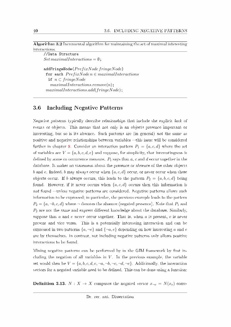
40 3.6. INCLUDING NEGATIVE PATTERNS
Algorithm 3.2 Incremental algorithm for maintaining the set of maximal interestinginteractions.
//Data Structure
SetmaximalInteractions = ∅;
addFringeNode(PrefixNode fringeNode)for each PrefixNode n ∈ maximalInteractionsif n ⊂ fringeNodemaximalInteractions.remove(n);
maximalInteractions.add(fringeNode);
3.6 Including Negative Patterns
Negative patterns typically describe relationships that include the explicit lack of
events or objects. This means that not only is an objects presence important or
interesting, but so is its absence. Such patterns are (in general) not the same as
positive and negative relationships between variables � this issue will be considered
further in chapter 9. Consider an interaction pattern P1 = {a, c, d} where the set
of variables are V = {a, b, c, d, e} and suppose, for simplicity, that interestingness is
de�ned by some co-occurrence measure. P1 says that a, c and d occur together in the
database. It makes no statement about the presence or absence of the other objects
b and e. Indeed, b may always occur when {a, c, d} occur, or never occur when these
objects occur. If b always occurs, this leads to the pattern P2 = {a, b, c, d} beingfound. However, if it never occurs when {a, c, d} occurs then this information is
not found � unless negative patterns are considered. Negative patterns allows such
information to be expressed; in particular, the previous example leads to the pattern
P2 = {a,¬b, c, d} where ¬ denotes the absence (negated presence). Note that P1 and
P2 are not the same and express di�erent knowledge about the database. Similarly,
suppose that a and e never occur together. That is, when a is present, e is never
present and vice versa. This is a potentially interesting interaction and can be
expressed in two patterns {a,¬e} and {¬a, e} depending on how interesting a and e
are by themselves. In contrast, not including negative patterns only allows positive
interactions to be found.
Mining negative patterns can be performed by in the GIM framework by �rst in-
cluding the negation of all variables in V . In the previous example, the variable
set would then be V = {a, b, c, d, e,¬a,¬b,¬c,¬d,¬e}. Additionally, the interactionvectors for a negated variable need to be de�ned. This can be done using a function:
De�nition 3.13. N : X → X computes the negated vector x¬v = N(xv) corre-
Dr. rer. nat. Dissertation
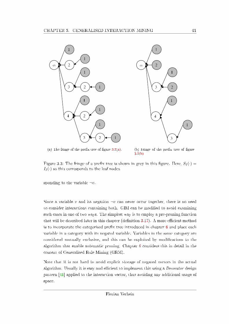
CHAPTER 3. GENERALISED INTERACTION MINING 41
(a) The fringe of the pre�x tree of �gure 3.2(a). (b) Fringe of the pre�x tree of �gure3.2(b)
Figure 3.3: The fringe of a pre�x tree is shown in grey in this �gure. Here, SI(·) =II(·) so this corresponds to the leaf nodes.
sponding to the variable ¬v.
Since a variable v and its negation ¬v can never occur together, there is no need
to consider interactions containing both. GIM can be modi�ed to avoid examining
such cases in one of two ways. The simplest way is to employ a pre-pruning function
that will be described later in this chapter (de�nition 3.17). A more e�cient method
is to incorporate the categorised pre�x tree introduced in chapter 6 and place each
variable in a category with its negated variable. Variables in the same category are
considered mutually exclusive, and this can be exploited by modi�cations to the
algorithm that enable automatic pruning. Chapter 6 considers this in detail in the
context of Generalised Rule Mining (GRM).
Note that it is not hard to avoid explicit storage of negated vectors in the actual
algorithm. Usually it is easy and e�cient to implement this using a Decorator design
pattern [41] applied to the interaction vector, thus avoiding any additional usage of
space.
Florian Verhein
42 3.7. SOLVING TOP-DOWN OR MONOTONIC PROBLEMS WITH GIM
Example 3.14. In frequent itemset mining using bit-vectors as interaction vectors,
N(·) simple �ips all bits. Note that the anti-monotonic property holds when negative
items are included and as such the pruning technique functions identically to the
positive item case.
Example 3.15. A real world example where negative patterns are of interest is
presented in chapter 5. In that chapter, complex spatial co-location patterns were
sought.
Example 3.16. In a toy example, suppose we wish to �nd all possible algebraic
expressions with operators − and + over the set of variables so that the expression
has a value in [a, b] and holds in at least minSup samples. For example, such an
interaction may look like v1 + v2 − v3, and if this is evaluated over all samples
/ instances in the database, and evaluates to a value in [a, b] in at least minSup
samples, then it is an interesting pattern. This can be solved in the GIM framework
using an aggregation function aI(xV ′ , xv) de�ned so that xV ′∪v[i] = xV ′ [i] + xv[i],
using the variable set that includes both the positive and negated variables (where
N(xv)[i] = −xv[i]), mI(xV ′) = |{i : xV ′ [i] ∈ [a, b]}|, MI(·) is trivial, II(·) returns
true if the number computed by mI(·) is at least minSup, and SI(·) always returnstrue (note that this means there is no pruning3).
3.7 Solving Top-Down or Monotonic Problems with GIM
Due to the bottom up nature of the algorithm, where interactions are grown by
adding additional variables to them, GIM is most suited to methods where the in-
terestingness measure is anti-monotonic or partially anti-monotonic, as this enables
e�cient pruning of the search space � particularly in sparse databases: if an inter-
action is not interesting, larger interactions need not be considered. This section
describes how monotonic problems can also be solved using GIM.
It is possible to solve monotonic problems in GIM by �inverting� the original problem,
thus producing an anti-monotonic problem. This means that rather than mining the
interaction itself, the GIM algorithm mines the �inverted� pattern, from which the
actual pattern sought can be recovered.
To illustrate this method, for simplicity consider the problem of mining infrequent
patterns in a database where the absence of objects is meaningful. That is, �nd
3This is just a toy example, where the primary goal it to illustrate a negative pattern, not how tomine it e�ciently. There are methods to solve this problem more e�ciently in the GIM framework.
Dr. rer. nat. Dissertation
CHAPTER 3. GENERALISED INTERACTION MINING 43
all sets of objects that occur at most maxSup times. It should be clear that this
interestingness concept is monotonic. For example, if the set {1, 2, 3} is interesting,then so is {1, 2, 3, 4} and any other super-set of {1, 2, 3}. Conversely, if {1, 2, 3} is notinteresting, then neither is {1, 3} or any other subset. This problem can be solved
by starting with the interaction {1, 2, 3, 4, 5} and removing variables from it. That
is, a top down approach where branches of the search may be pruned accordingly.
This can be achieved in GIM through inverting the problem and mining the inverted
problem in a bottom up manner, therefore implicitly performing the same function
as an explicitly top down algorithm. The main task is to count the occurrences of
interactions in samples. That is, to count how often the pattern ∧v∈V ′v occurs in
the rows (records, samples) r ∈ D of the database D:
count(V ′) = |{r ∈ D : v ∈ r}|
Let us skip straight into how this can be solved in the GIM framework. De�ne an
interaction vector xV ′ as an integer valued vector where xV ′ [i] is the number of times
that any v ∈ V ′ occurs in the ith sample. That is, xV ′ [i] =∑
v∈V ′ I(v ∈ si) where siis the ith sample and I(expr) has value 1 if expr is true, and 0 otherwise. This may
also be expressed as xV ′ [i] =∑
v∈V ′ xv[i] where xv[i] has value 1 if v is contained in
the ith sample and 0 otherwise. Using this representation,
count(V ′) =∑i
I(xV ′ [i] = |V ′|)
That is, all those entries in xV ′ are counted if they match the size of V ′. The integer
vector representation of these interactions allows not only the addition of variables
to an interaction, but also (crucially) their removal. For example, xV ′−v[i] = xV ′ [i]−xv[i]. Since GIM is based on the notion of growing interactions, it is necessary to
invert the problem so that adding variables using aI(·) in the framework semantically
corresponds to removing variables from the actual interaction being sought. This can
be done using the above observations.
Therefore, the infrequent pattern mining problem can be solved in the GIM frame-
work as follows, where i ∈ [1, n] and n is the number of samples / rows / instances.
• x∞[i] =∑
v∈V xv[i] is the vector corresponding to the root node (the empty
interaction V ′ = ∅). Note however that due to the inversion of the problem,
the interpretation of this node is actually the set of all variables V .
• aI(xV ′ , xv) is de�ned so that xV ′∪v[i] = xV ′ [i]− xv[i]. Note that the interpre-
Florian Verhein
443.8. GRAPH MINING: WHEN THE INPUT IS AN ADJACENCY OR
DISTANCE MATRIX
tation of V ′ ∪ v is actually the set of variables except those in V ′ ∪ v. That is,V − (V ′∪ v). In other words, the node in the pre�x tree corresponding to V ′ is
interpreted as the interaction V − V ′. By performing the aI(·) operation, thealgorithm will e�ectively remove the variable v from the interaction V − V ′.
• mI(xV ′) =∑
i I(xV ′ [i] = |V |−|V ′|), that is, the number of entries in the vectorxV ′ that match the size of the desired interaction |V |− |V ′|. Here, I(expr) has
value 1 if expr is true, and 0 otherwise.
• MI(·) is trivial, therefore simply returning the result provided by mI(·).
• SI(·) = II(·) and these return true if the result of mI(·) is less than or equal to
maxSup. Note that the inversion of the problem results in an anti-monotonic
interestingness measure as far as the algorithm is concerned, and therefore the
search space is correctly pruned.
• outputInteraction(PrefixNode node) in algorithm 3.1 outputs the set of vari-
ables not present in the traversal from node to the root.
It has now been shown how a monotonic problem can be inverted and mapped to
an anti-monotonic problem and solved in the GIM framework. This is possible with
any monotonic problem � it is simply a matter of �nding the appropriate inversion.
The reader should note that this inversion is not related to the problem of �nding
negative patterns. Of course, mining positive and negative patterns with a monotonic
measure is also possible using the techniques in this section.
3.8 Graph Mining: When the Input is an Adjacency or
Distance Matrix
This section shows how problems can be solved in GIM that do not require measures
between more than two variables at a time, however still mine interactions of any size.
The result is that the input is a pre-computed adjacency matrix, which describes all
pairwise interactions between variables. The task then is to use this to �nd larger
structural interactions using this data. This is useful in clustering, clique mining and
correlation analysis for example.
3.8.1 Clique Mining
For simplicity, consider the problem of �nding all cliques in a given graph. A clique
is a fully connected sub-graph (a sub-graph where every vertex is connected to every
Dr. rer. nat. Dissertation
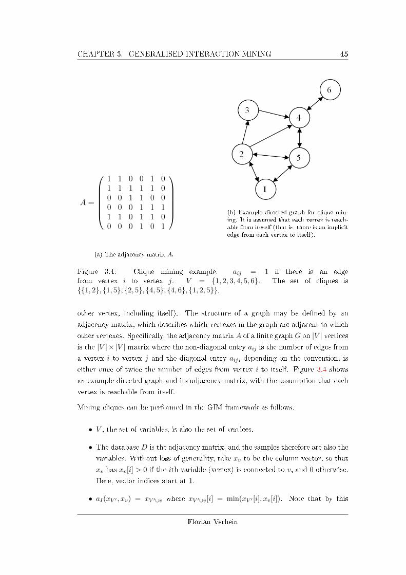
CHAPTER 3. GENERALISED INTERACTION MINING 45
A =
1 1 0 0 1 01 1 1 1 1 00 0 1 1 0 00 0 0 1 1 11 1 0 1 1 00 0 0 1 0 1
(a) The adjacency matrix A.
(b) Example directed graph for clique min-ing. It is assumed that each vertex is reach-able from iteself (that is, there is an implicitedge from each vertex to itself).
Figure 3.4: Clique mining example. aij = 1 if there is an edgefrom vertex i to vertex j. V = {1, 2, 3, 4, 5, 6}. The set of cliques is{{1, 2}, {1, 5}, {2, 5}, {4, 5}, {4, 6}, {1, 2, 5}}.
other vertex, including itself). The structure of a graph may be de�ned by an
adjacency matrix, which describes which vertexes in the graph are adjacent to which
other vertexes. Speci�cally, the adjacency matrix A of a �nite graph G on |V | verticesis the |V |× |V | matrix where the non-diagonal entry aij is the number of edges from
a vertex i to vertex j and the diagonal entry aij , depending on the convention, is
either once of twice the number of edges from vertex i to itself. Figure 3.4 shows
an example directed graph and its adjacency matrix, with the assumption that each
vertex is reachable from itself.
Mining cliques can be performed in the GIM framework as follows.
• V , the set of variables, is also the set of vertices.
• The database D is the adjacency matrix, and the samples therefore are also the
variables. Without loss of generality, take xv to be the column vector, so that
xv has xv[i] > 0 if the ith variable (vertex) is connected to v, and 0 otherwise.
Here, vector indices start at 1.
• aI(xV ′ , xv) = xV ′∪v where xV ′∪v[i] = min(xV ′ [i], xv[i]). Note that by this
Florian Verhein
463.8. GRAPH MINING: WHEN THE INPUT IS AN ADJACENCY OR
DISTANCE MATRIX
construction, xV ′ [i] is non-zero if vertex i is connected to all other vertices in V′.
For example, consider x1, x4 and x5 from �gure 3.4(a). x{1,5} = [1, 1, 0, 0, 1, 0]T ,
showing that 1 and 5 are incident on each other, and 2 is incident on both.
x{1,4} = [0, 1, 0, 0, 1, 0]T , showing that 2 and 5 are both incident on 1 and 4.
If the adjacency matrix is binary, then the xV ′ are binary vectors and aI(·) isthe bit-wise AND operation.
• mI(xV ′) = [∑
v∈V ′ I(xV ′ [v] > 0),∑
v 6∈V ′ I(xV ′ [v] > 0)], an array of two values
where∑
v∈V ′ I(xV ′ [v] > 0) is the number of vertices in V ′ that are reachable
from all other vertices in V ′, and∑
v 6∈V ′ I(xV ′ [v] > 0) are those vertices not
in V ′ that are reachable from all other vertices in V ′. I(expr) is the indicator
variable whose value is 1 if expr is true, and 0 otherwise. Note that by the
construction of xV ′ by aI(·), mI(xV ′)[1] (the �rst value computed by mI(·)),this is precisely the number of vertices in V ′ that are connected to all vertices
in V ′. If this value is equal to |V ′| then V ′ is a clique. Note the maximum
value it can take is |V ′|.
• MI(·) is trivial.
• II(·) returns true if and only if valuem[1] = |V ′|, where valuem are the values
computed by mI(·) and V ′ is the interaction being examined. Recall that if
valuem[1] < V ′ then V ′ is not a clique as it is not completely connected.
• SI(·) returns true if and only if valuem[1] = |V ′| ∧ valuem[2] > 0. If an
interaction vector does not indicate that there are any other vertices incident
on all vertices in V ′ (that is, valuem[2] > 0), then there is no point continuing
the search by expanding V ′. Therefore the search can be pruned at this point.
Note that the above approach works for both directed and undirected graphs. For
a directed graph, only cliques will be mined where each vertex is connected to each
other vertex so that all edges in such a clique are bi-directional. If it is known
that the graph is undirected then the approach can be streamlined to make it more
e�cient since the adjacency matrix is symmetric. Furthermore, note that only one
direction needs to be checked while the above method checks both (as it must for a
directed graph).
The above method can be improved slightly. Note that given an interaction vector
xV ′ , it is possible to determine exactly which variables are potential candidates, and
which are not. In particular {v 6∈ V ′ : xV ′ [v] > 0} is the set of vertices that are
incident on all vertices in V ′. Any vertices not in this set need not be examined and
can be pruned. Note however that through the operation of GIM whereby siblings
Dr. rer. nat. Dissertation
CHAPTER 3. GENERALISED INTERACTION MINING 47
are joined, some of this pruning is performed automatically. Furthermore, any nodes
passing through this automated pruning will be discarded after one application of
aI(·) and mI(·). That is, O(|V |) time. Assuming the interaction vectors are imple-
mented so that the xV ′ [v] look-up can be performed in O(1) time, it is possible to
obtain a run time improvement in cases where pruning can be applied by inserting
the following line into algorithm 3.1:
...
for each v ∈ joinToif (xV ′ [v] = 0) continue; //additional line
V ector xV ′∪v = aI(xV ′ , xv);
...
Where continue skips the remainder of the loop's current iteration. This is a small
check that allows the generation and evaluation of xV ′∪v to be avoided. It is possible
to include an additional function in the framework that generalises this and allows
such e�ciency improvements:
De�nition 3.17. PI(xV ′ , v) returns true if V ′ ∪ v should be examined.
With this additional function, algorithm 3.1 would look like:
...
for each v ∈ joinToif (PI(xV ′ , v)) continue; //additional line
V ector xV ′∪v = aI(xV ′ , xv);
...
Finally, note that the vectors need not be implemented as an explicit vector / array.
An ordered list is more space e�cient and depending on the sparsity of the graph,
may also be faster. A general discussion of vector representations is presented in
section 3.15.
3.8.2 Mining Maximal Cliques
Maximal cliques are those cliques that are not contained inside any larger clique.
Maximal cliques can be mined using GIM by using the method described in section
Florian Verhein
483.8. GRAPH MINING: WHEN THE INPUT IS AN ADJACENCY OR
DISTANCE MATRIX
3.5 in addition to that described above. In �gure 3.4, the maximal cliques are {4, 5},{4, 6} and {1, 2, 5}.
A real world example where maximal cliques are useful is presented in chapter 5. In
that chapter, a specialist method for mining maximal cliques is used that functions
only on two dimensional data. That is, xv = (xi, yi). It is not e�cient for high
dimensional data as it scans over the dimensions. The method described above
can be used as an alternative, and is applicable to high dimensional data. Mining
maximal cliques is also part of the problem considered in chapter 9.
3.8.3 Solving the Independent Set Problem
The independent set problem (ISP) is not a data mining problem, but a well known
problem in algorithms. It encodes situations in which one tries to choose objects
from a collection in which there are pairwise con�icts between some of the objects.
The con�icts are encoded by edges between objects, which become the nodes in the
graph. One wishes to �nd the largest set without con�icts (the largest independent
set). Formally, given a graph G = (V,E), a set of nodes S ⊆ V is said to be
independent if no two nodes in S are joined by an edge. The ISP is stated as
follows: Given G, �nd an independent set that is as large as possible. In �gure
3.4 (note that a con�ict is an undirected concept), the largest independent sets are
{6, 3, 5} and {6, 3, 1}. The ISP is a general problem and subsumes problems such
as interval scheduling (where the goal is to schedule a resource optimally given a
set of requests) and bipartite matching. Since the ISP is NP-Complete, no e�cient
algorithm is known for solving it [51]. As a consequence, it is considered unlikely that
an algorithm exists which can solve it more quickly that an enumeration approach.
GIM can be applied to solve the ISP problem as e�ciently as can be expected by
noting that ISP can be mapped to the clique mining problem above. In clique mining,
sets of vertices are desired where every vertex is connected to every other, while in the
ISP problem, sets of vertices are desired where none of the vertices are connected to
each other. Adding a vertex that is connected to any other violates the independence
property, just like adding a vertex that is not connected to all others violates the
clique property. Therefore, de�ne a graph G∗ = (V,E∗) where an edge exists between
vertices in G∗ if and only if no edge existed in G. Hence E∗ = V × V − E and the
adjacency matrix of G∗ is the result of applying the logical NOT operation to every
entry in the adjacency matrix of G. By mining a clique V ′ in G∗, one is mining a
set of variables V ′ where all variables in V ′ are not connected to all other variables
in V ′; an independent set in G. Therefore, to solve the ISP problem with GIM, V
is the set of vertices and D is the adjacency matrix of G with all bits �ipped so
Dr. rer. nat. Dissertation
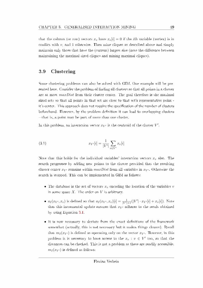
CHAPTER 3. GENERALISED INTERACTION MINING 49
that the column (or row) vectors xv have xv[i] = 0 if the ith variable (vertex) is in
con�ict with v, and 1 otherwise. Then mine cliques as described above and simply
maintain only those that have the (current) largest size (note the di�erence between
maintaining the maximal sized cliques and mining maximal cliques).
3.9 Clustering
Some clustering problems can also be solved with GIM. One example will be pre-
sented here. Consider the problem of �nding all clusters so that all points in a cluster
are at most maxDist from their cluster center. The goal therefore is the maximal
sized sets so that all points in that set are close to that set's representative point -
it's center. This approach does not require the speci�cation of the number of clusters
beforehand. However, by the problem de�nition it can lead to overlapping clusters
� that is, a point may be part of more than one cluster.
In this problem, an interaction vector xV ′ is the centroid of the cluster V ′.
(3.1) xV ′ [i] =1
|V ′|∑v∈V ′
xv[i]
Note that this holds for the individual variables' interaction vectors xv also. The
search progresses by adding new points to the cluster provided that the resulting
cluster center xV ′ remains within maxDist from all variables in xV ′ . Otherwise the
search is stopped. This can be implemented in GIM as follows:
• The database is the set of vectors xv encoding the location of the variables v
in some space X. The order on V is arbitrary.
• aI(xV ′ , xv) is de�ned so that aI(xV ′ , xv)[i] = 1|V ′|+1(|V ′| · xV ′ [i] + xv[i]). Note
that this incremental update ensures that xV ′ adheres to the result obtained
by using Equation 3.1.
• It is now necessary to deviate from the exact de�nitions of the framework
somewhat (actually, this is not necessary but it makes things clearer). Recall
that mI(xV ′) is de�ned as operating only on the vector xV ′ . However, in this
problem it is necessary to have access to the xv : v ∈ V ′ too, so that the
distances can be checked. This is not a problem as these are readily accessible.
mI(xV ′) is de�ned as follows:
Florian Verhein
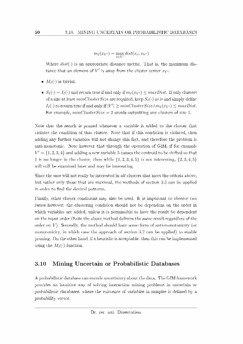
50 3.10. MINING UNCERTAIN OR PROBABILISTIC DATABASES
mI(xV ′) = maxv∈V ′
dist(xv, xV ′)
Where dist(·) is an appropriate distance metric. That is, the maximum dis-
tance that an element of V ′ is away from the cluster center xV ′ .
• MI(·) is trivial.
• SI(·) = II(·) and return true if and only ifmI(xV ′) ≤ maxDist. If only clustersof a size at leastminClusterSize are required, keep SI(·) as is and simply de�ne
II(·) to return true if and only if |V ′| ≥ minClusterSize∧mI(xV ′) ≤ maxDist.For example, minClusterSize = 2 avoids outputting any clusters of size 1.
Note that the search is pruned whenever a variable is added to the cluster that
violates the condition of that cluster. Note that if this condition is violated, then
adding any further variables will not change this fact, and therefore the problem is
anti-monotonic. Note however that through the operation of GIM, if for example
V ′ = {1, 2, 3, 4} and adding a new variable 5 causes the centroid to be shifted so that
1 is no longer in the cluster, then while {1, 2, 3, 4, 5} is not interesting, {2, 3, 4, 5}will still be examined later and may be interesting.
Since the user will not really be interested in all clusters that meet the criteria above,
but rather only those that are maximal, the methods of section 3.5 can be applied
in order to �nd the desired patterns.
Finally, other cluster conditions may also be used. It is important to observe two
issues however; the clustering condition should not be dependent on the order in
which variables are added, unless it is permissible to have the result be dependent
on the input order (Note the above method delivers the same result regardless of the
order on V ). Secondly, the method should have some form of anti-monotonicity (or
monotonicity, in which case the approach of section 3.7 can be applied) to enable
pruning. On the other hand, if a heuristic is acceptable, then this can be implemented
using the MI(·) function.
3.10 Mining Uncertain or Probabilistic Databases
A probabilistic database can encode uncertainty about the data. The GIM framework
provides an intuitive way of solving interaction mining problems in uncertain or
probabilistic databases, where the existence of variables in samples is de�ned by a
probability vector.
Dr. rer. nat. Dissertation
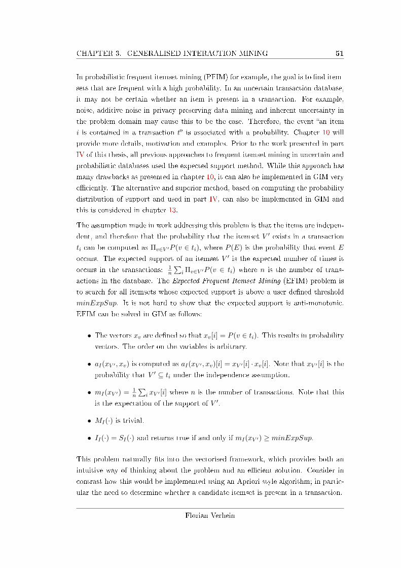
CHAPTER 3. GENERALISED INTERACTION MINING 51
In probabilistic frequent itemset mining (PFIM) for example, the goal is to �nd item-
sets that are frequent with a high probability. In an uncertain transaction database,
it may not be certain whether an item is present in a transaction. For example,
noise, additive noise in privacy preserving data mining and inherent uncertainty in
the problem domain may cause this to be the case. Therefore, the event �an item
i is contained in a transaction t� is associated with a probability. Chapter 10 will
provide more details, motivation and examples. Prior to the work presented in part
IV of this thesis, all previous approaches to frequent itemset mining in uncertain and
probabilistic databases used the expected support method. While this approach has
many drawbacks as presented in chapter 10, it can also be implemented in GIM very
e�ciently. The alternative and superior method, based on computing the probability
distribution of support and used in part IV, can also be implemented in GIM and
this is considered in chapter 13.
The assumption made in work addressing this problem is that the items are indepen-
dent, and therefore that the probability that the itemset V ′ exists in a transaction
ti can be computed as Πv∈V ′P (v ∈ ti), where P (E) is the probability that event E
occurs. The expected support of an itemset V ′ is the expected number of times it
occurs in the transactions: 1n
∑i Πv∈V ′P (v ∈ ti) where n is the number of trans-
actions in the database. The Expected Frequent Itemset Mining (EFIM) problem is
to search for all itemsets whose expected support is above a user de�ned threshold
minExpSup. It is not hard to show that the expected support is anti-monotonic.
EFIM can be solved in GIM as follows:
• The vectors xv are de�ned so that xv[i] = P (v ∈ ti). This results in probability
vectors. The order on the variables is arbitrary.
• aI(xV ′ , xv) is computed as aI(xV ′ , xv)[i] = xV ′ [i] · xv[i]. Note that xV ′ [i] is theprobability that V ′ ⊆ ti under the independence assumption.
• mI(xV ′) = 1n
∑i xV ′ [i] where n is the number of transactions. Note that this
is the expectation of the support of V ′.
• MI(·) is trivial.
• II(·) = SI(·) and returns true if and only if mI(xV ′) ≥ minExpSup.
This problem naturally �ts into the vectorised framework, which provides both an
intuitive way of thinking about the problem and an e�cient solution. Consider in
contrast how this would be implemented using an Apriori style algorithm; in partic-
ular the need to determine whether a candidate itemset is present in a transaction.
Florian Verhein
52 3.11. COMPLEX (�NON-TRIVIAL�) INTERESTINGNESS MEASURES
3.11 Complex (�Non-Trivial�) Interestingness Measures
So far in this chapter, all problems considered had a trivial MI(·). This section
will consider the case when MI(·) is non-trivial. Recall from section 3.2 that this
means that sub-interactions must be examined in order to calculate a measure on
the interaction and to determine whether of not an interaction is interesting. This
requires a way to store and quickly retrieve PrefixNodes given the interaction they
represent, in order to obtain the valuem and valueM values stored within the node.
This is done using a map that maps a given sequence of variables to the corresponding
PrefixNode. Such a map is called a SequenceMap and provides constant time look-
up for the required values. An e�cient method for implementing this is to use aMap
or Hashtable that maps PrefixNodes to themselves, with identity based solely on
the sequence of variables encountered in a traversal towards the root. That is, the
hashCode() and equality is dependent solely on the variableId sequence represented
by the PrefixNode and not on the values. This allows an arbitrary sequence of
variables to be created (for example, as a chain of PrefixNodes � e�ectively a
singly linked list), and the values of that interaction can be retrieved by retrieving
the PrefixNode that the algorithm created earlier via the Map's get(·) operation.In the worst case, this look-up operation requires O(|V ′|) time, where |V ′| is the sizeof the interaction (in the case of a collision, checking if two sequences are identical
requires at most a scan over them).
The additional space used by this method is only the bucket array of the HashTable.
However, recall that algorithm 3.1 assumes a garbage collector, and hence if PrefixNodes
are not explicitly stored, they will be deleted. Storing them, as is required by a non-
trivial MI(·), leads to the pre�x tree remaining in memory. Conversely, note that
for trivial MI(·), only a single path in the pre�x tree is retained in memory and fur-
thermore, a sequence map is not required. Insertion into this map is performed by
the store(·) function in algorithm 3.1. Depending on the measure to be evaluated,
store(·) may only need to store selected nodes. For example, some measures like
minPI and maxPI require only that interactions of size 1 remain in memory for
later use by MI(·). In these cases, the memory requirement is the same as for a
trivial MI(·).
Algorithm 3.3 shows how the sequence map and the pre�x tree nodes can be used to
e�ciently retrieve all immediate sub-interactions {V ′− v : v ∈ V ′} of V ′. Of course,non-immediate sub-interactions can also be retrieved.
The following lemma proves that all sub-interactions will be available, provided they
are interesting. This is important for two reasons:
Dr. rer. nat. Dissertation
CHAPTER 3. GENERALISED INTERACTION MINING 53
1. It proves correctness, and
2. It allows interestingness to be forced to be anti-monotonic simply by checking
whether sub-interactions of V ′ exist. If they do not exist, then they are not
interesting and neither can V ′ be if the measure is anti-monotonic. Hence,
the search may be pruned at V ′. This e�ect can be achieved by examining
only immediate sub-interaction (that is, sub-interactions of size |V ′| − 1). By
induction, this then holds over all sub-interactions. Forcing a measure to be
anti-monotonic is a heuristic that is useful in some applications and is discussed
in section 3.21.
Lemma 3.18. Algorithm 3.1 generates all sub-interactions V ′′ before generating V ′.
Proof. The algorithm progresses through the search space by joining existing Pre-
�xNode siblings together, creating interactions that are one variable larger than the
two original sibling nodes. Suppose for the purpose of contradiction that an inter-
action V ′ exists but a sub-interaction of it is mined later. Proceed by showing that
each immediate sub-interaction V ′ − v : v ∈ V ′ has already been mined, so that the
result follows by induction. First, note that each interaction can be represented by a
sequence of Pre�xNodes, which can be constructed in reverse by traversal from the
node for V ′ towards the root. The immediate sub-interactions of V ′ can be obtained
by removing one variable from V ′ at a time. Suppose v ∈ V ′ is removed, so that
V ′ = Sp∪ v∪Ss where Sp and Ss are the pre�x and su�x (either potentially empty)
of the interaction (sequence) respectively. Since the expansion of the search is done
in depth �rst fashion and with increasing order amongst the siblings (according to
their variables), Sp ∪ Ss must be expanded �rst, since by de�nition the sequences in
the Pre�xTree appear in decreasing order. Since this is true for all v ∈ V ′, the resultfollows by induction and contradiction.
3.11.1 Complexity
The run time complexity is altered only by the evaluation of MI(·), as taken into
account in theorem 3.8. Clearly, computingMI(·) for measures that require compari-
son to immediate sub-interactions requires at most O(|V |) extra time per interaction.
Hence t(MI) = |V | at worst.
The space complexity is altered signi�cantly, as the PrefixNodes must be stored
in order for the algorithm to retrieve the valuems of sub-interactions at a later
Florian Verhein
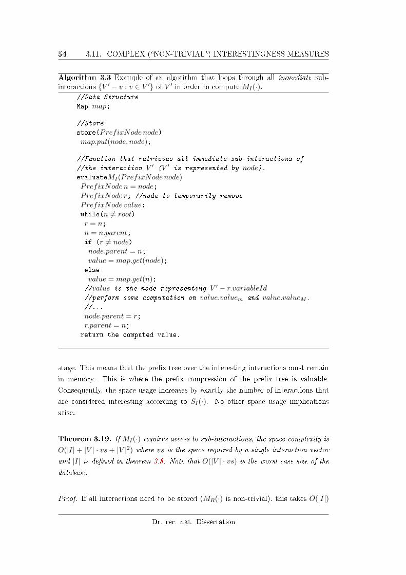
54 3.11. COMPLEX (�NON-TRIVIAL�) INTERESTINGNESS MEASURES
Algorithm 3.3 Example of an algorithm that loops through all immediate sub-interactions {V ′ − v : v ∈ V ′} of V ′ in order to compute MI(·).
//Data Structure
Map map;
//Store
store(PrefixNode node)map.put(node, node);
//Function that retrieves all immediate sub-interactions of
//the interaction V ′ (V ′ is represented by node).evaluateMI(PrefixNode node)PrefixNode n = node;PrefixNode r; //node to temporarily remove
PrefixNode value;while(n 6= root)r = n;n = n.parent;if (r 6= node)node.parent = n;value = map.get(node);else
value = map.get(n);//value is the node representing V ′ − r.variableId//perform some computation on value.valuem and value.valueM.
//...
node.parent = r;r.parent = n;
return the computed value.
stage. This means that the pre�x tree over the interesting interactions must remain
in memory. This is where the pre�x compression of the pre�x tree is valuable.
Consequently, the space usage increases by exactly the number of interactions that
are considered interesting according to SI(·). No other space usage implications
arise.
Theorem 3.19. If MI(·) requires access to sub-interactions, the space complexity is
O(|I| + |V | · vs + |V |2) where vs is the space required by a single interaction vector
and |I| is de�ned in theorem 3.8. Note that O(|V | · vs) is the worst case size of the
database.
Proof. If all interactions need to be stored (MR(·) is non-trivial), this takes O(|I|)
Dr. rer. nat. Dissertation
CHAPTER 3. GENERALISED INTERACTION MINING 55
space at worst as each interaction corresponds to a single pre�x node. The remaining
complexity is the same (see theorem 3.9).
3.12 Weak Anti-monotonicity and when Order is Impor-
tant
This �xed order in variables within the GIM framework and algorithm can be ex-
ploited. While in many applications this order is arbitrary, in some it can be used
to implement a useful heuristic (for example, by expanding the most promising in-
teractions �rst), while in others is can be central to the e�cient mining of patterns.
This section gives an example of a measure that was previously considered weakly
anti-monotonic, but is actually completely anti-monotonic provided the variables are
ordered in a certain fashion. Since GIM supports such an ordering, it can be used
to implement weakly anti-monotonic measures very e�ciently.
3.12.1 Maximum Participation Index (maxPI)
A sub-�eld of Data Mining concerns itself with spatial data. One problem in spatial
data mining is �nding co-location patterns. That is, sets of objects that are located
close to each other in many instances. The minimum participation index , orminPI,
is a commonly used measure in co-location mining:
(3.2) minPI(V ′) = minv∈V ′{count(V ′)/count({v})}
where count(V ′) is the number of occurrences of the interaction V ′ in the database.
For example, minPI will be used in chapter 5 for mining complex spatial co-location
patterns amongst the set of all complex maximal cliques in a real world astronomy
database. It is popular because it is anti-monotonic and therefore allows easy pruning
of the search space: If V ” ⊆ V ′ then minPI(V ′) ≤ minPI(V ”). This is well
known in the literature and follows readily from Equation 3.2 since support is anti-
monotonic, as is the min function. This means that if an interaction V ” is found
not to be interesting (minPI is too low) then the search can avoid considering every
super-set of V ′ and thus prune a large part of the search space.
An alternative to minPI is the maximum participation index [49], or maxPI mea-
sure, de�ned as follows:
Florian Verhein
563.12. WEAK ANTI-MONOTONICITY AND WHEN ORDER IS IMPORTANT
maxPI(V ′) = maxv∈V ′{count(V ′)/count({v})}
This measure is not anti-monotonic due to the max function (which by itself is mono-
tonic) as can be demonstrated with a simple counterexample: With the addition of
an extra variable v to V ′ so that v occurs only with the other variables in V ′, the
ratio count(V ′)/count({v}) = 1; the maximum value. Previous work has assumed
that maxPI is only weakly anti-monotonic [16, 49]. However it is shown here that it
can be completely anti-monotonic provided the data is appropriately pre-processed.
This improves the ability to use this measure to mine patterns, simpli�es the al-
gorithms and increases the e�ciency of mining algorithms. It turns out that if an
order is imposed on the variables, so that in the mining process only those variables
are added to an existing interaction if their count(·) is greater than those previously
added, maxPI becomes anti-monotonic:
Lemma 3.20. If V ′ = V ”∪v and count(v) ≥ maxj∈V ”(count(j)) thenmaxPI(V ′) ≤maxPI(V ”).
Proof. [Sketch] The numerator remains anti-monotonic, and any additional variable
v added will generate a smaller ratio count(V ′)/count({v}) than any existing variablev′ ∈ V ”.
With this result, it is possible to use maxPI anti-monotonically by ordering all
variables by their count(·) values before engaging in the mining process. Recall
that since the GIM algorithm maintains this order throughout its operation, the
requirement of 3.20 is always satis�ed. Hence, the correct result will be mined using
GIM while the search space can be pruned as much as possible. The use of lemma
3.20 results in an O(|V |) factor reduction in computation time over previous methods
based on the weak anti-monotonic result.
The maxPI method can be implemented anti-monotonically in the GIM framework
as follows:
• Supposing we are concerned with a clique mining problem and the database
consists of sub-graph instances. An interaction vector xV ′ has xV ′ [i] = 1 if the
ith instance in the database contains the clique V ′.
• The strict total order < is such that vi < vj ⇐⇒ count(vi) > count(vj). This
means that variables will be added to interactions in increasing count(·) order,
Dr. rer. nat. Dissertation
CHAPTER 3. GENERALISED INTERACTION MINING 57
as required to make maxPI anti-monotonic. This ordering is performed as a
pre-processing step.
• aI(·) and mI(·) are implemented as in a counting approach (see section 3.4 for
example).
• MI(·) can evaluate the maxPI measure by using the result of mI(·) (i.e.
count(V ′)) and looking up the values previously computed by mI(·) for indi-
vidual variables (i.e. count(v) : v ∈ V ′), but this is naive. Note that due to theorder on the variables, it is guaranteed that count(v) ≥ maxj∈V ”(count(j)),
where v is the last variable added to V ′. Hence MI(·) need only compute
count(V ′)/count(v).
• II(·) = SI(·) and return true if and only if the result of MI(·), maxPI, is atleast a user de�ned threshold.
The above approach requires a non-trivial MI(·) and an evaluation ofMI(·) requires|V ′| operations using the naive method and O(1) otherwise. It turns out that there is
an even more e�cient implementation in GIM using a trick on the encoding of the vec-
tors xv. In particular, let xv[0] be |xv| = count(v). And xV ′ [0] = maxv∈V ′{count(v)}.That is, the otherwise binary valued vector has an additional �eld storing the max-
imum count(·) of all variables in V ′. The following instantiation makes this work:
• The order is as above, and so are vectors xv except that the additional �eld xv[0]
exists that is initiated to count(v) =∑n
i=1 xv[i]. x∞, the vector corresponding
to the root, has x∞[0] = 0 for the below to work.
• aI(xV ′ , xv)[i] = xV ′ [i]ANDxv[i] when i ≥ 1 and max{xV ′ [0], xv[0]} when
i = 0. Note that this maintains the desired property of xV ′∪v[0] being the
maximal count(v′) : v′ ∈ V ′ ∪ v as required.
• mI(xV ′) = |xV ′ |/xV ′ [0] where |xV ′ | is the number of set bits, that is count(V ′) =∑ni=1 xV ′ [i]. mI(·) therefore evaluates maxPI.
• MI(·) is trivial. The de�nitions of SI(·) and II(·) are as before.
This is a more e�cient approach and additionally uses a trivial MI(·). It also func-
tions as an example where a clever choice for the interaction vector xV ′ leads to a
more e�cient algorithm.
Florian Verhein
58 3.13. FORCED ANTI-MONOTONICITY
3.13 Forced Anti-monotonicity
Work in this thesis will demonstrate that it can be desirable to force anti-monotonicity,
and consequently encourages the use of this technique over selecting low quality but
anti-monotonic measures. Forcing anti-monotonicity is useful when a measure exists
that correlates highly with the concept of interestingness in the user's domain, but
does not have any properties that can be exploited for pruning. Without searching
the entire pattern space (intractable in anything but the most trivial problems) there
is no way to guarantee a complete solution. An alternative is to combine the measure
with a second measure that can be used for pruning, such as the number of instances
that match the pattern, but then the search is determined completely by the second
measure, which is usually not correlated with what the user wants. A number of con-
crete problems solved in this thesis demonstrate that forcing anti-monotonicity on
a good interestingness measure leads to much better quality results and much more
e�cient algorithms than relying on measures that have natural anti-monotonicity.
In particular, chapters 6, 7 and 8 use this idea for rules. This idea proved to be
especially useful when mining statistically signi�cant patterns.
Forcing anti-monotonicity generates a heuristic. Suppose we have a measure of in-
terestingness M(X) on a set X, and that higher values of M(·) are desirable. Anti-monotonicity means that X ⊆ Y =⇒ M(X) ≥ M(Y ), therefore allowing the
pruning of a search space; if X is not interesting, we need never consider any of its
super-sets. The following can be used to force any non-anti-monotonic measure M ′
to be anti-monotonic.
Lemma 3.21. Suppose M ′ is an arbitrary (not anti-monotonic) measure. The com-
posite measure M” is anti-monotonic:
M”(X) = M ′(X)−maxx∈X
(M ′(X − x))
Proof. By induction.
M” is therefore the improvement inM ′ achieved by the addition of an extra variable
to the interaction, since it is the di�erence between the interestingness of X and
the most interesting immediate subset. When used in GIM, M” therefore greedily
searches for new interactions that have a higher interestingness.
Implementing M” in GIM is easily achieved using the MI(·) function in the frame-
work: set mI(·) = M ′ and have MI(·) compute the equation in lemma 3.21. Recall
that algorithm 3.3 showed how to access the immediate sub-interactions.
Dr. rer. nat. Dissertation
CHAPTER 3. GENERALISED INTERACTION MINING 59
3.14 High Dimensional Data and Dimensionality Reduc-
tion
GIM is designed for high dimensional data. In particular, note from section 3.8
that it scales linearly with the dimensionality of the vectors, since the framework is
based purely on vector valued functions. Since GIM operates on vectors existing in
some space X, it is possible to reduce the dimensionality of those vectors without
a�ecting the operation of GIM. Furthermore, the semantics and scrutability of the
pattern do not change. That is, the results are still an interaction expressed as a
subset of V . For example, the clustering approach considered in section 3.9 may
easily have dimensionality reduction methods applied, since the distance measure is
usually preserved quite well in the reduced space. For dimensionality reduction to
be applicable in a GIM method, the result of mI(·) in the reduced space should be
su�ciently similar to the results when they are applied in the original space, and
aI(·) must lead to the same semantics in the reduced space as in the original space.
Chapter 4 provides some discussion on the use of Singular Value Decomposition to
reduce the space in the context of itemset mining.
3.15 Vector Representations and Subspace Projections
This section brie�y discusses the importance of di�erent vector representations in
GIM and the ability for them to exploit subspace projections. Examples in this
chapter have had real valued vectors (for example in section 3.6 and 3.10), integer
valued vectors (for example in section 3.8 and section 3.7) and of course binary valued
vectors (for example, any counting approach and some graph based approaches).
Since the GIM framework operates using only functions on vectors, the way these
vectors are implemented has a signi�cant impact on the run time of these operations
and hence the algorithm. Di�erent instantiations of functions also favour di�erent
vector implementations. While it is beyond the scope of this section to give a detailed
analysis, a few examples will be shown to demonstrate the issue and provide practical
advice.
The most basic task in interaction mining is often determining in which samples
an interaction exists. Measures on the interaction typically require only the values
corresponding to these samples. First, suppose that we are interested only in the
presence or absence and not the values. Then interaction vectors are (logically) sets
containing those sample ids that contain the interaction. There are multiple ways
to implement this. One method is to use a standard set implementation for xV ′ .
Florian Verhein
60 3.15. VECTOR REPRESENTATIONS AND SUBSPACE PROJECTIONS
This has the advantage that aI(xV ′ , xv) operates in O(max{|xV ′ |, |xv|}) time (set
intersection) and mI(xV ′) operates in O(|xV ′ |) time, where |xV ′ | is the set size andis typically much less than the number of samples, n. A disadvantage is that such
sets have considerable computational and space overhead. A better alternative is to
use bit-vectors, where a bit xV ′ [i] is set if the ith sample contains the interaction
V ′. This has the advantage that aI(·) is the bit-wise AND operation, which is a
machine level operation and can thus be performed quickly. Also, the space usage
per sample is low. Despite fast execution times and low space per sample, the run-
time of aI(·) and mI(·) are typically O(n) and space usage is O(n) regardless of the
logical size of the set. Another e�cient method, particularly when the data is sparse,
is to use an integer array storing the indexes of those samples containing V ′. If this
array is sorted by sample id, then intersection can be implemented very quickly and
thus aI(xV ′ , xv) operates in O(max{|xV ′ |, |xv|}) time (while still maintaining the
order). mI(xV ′) can be implemented to operate in the same time and the space
usage depends on the number of non-zero values; O(|xV ′ |).
As a rule of thumb, the bit-vector approach is much faster than a set implementation.
Similarly, using one bit per sample per variable uses less space in practice than
a set-based implementation. The sparse method using a sorted integer array is
sometimes faster than the bit-vector approach, and sometimes slower. This seems
to be determined primarily by the platform used (processor and OS) and less to by
the density of the vectors. The majority of the work in this thesis uses bit-vectors,
as the sparse method was investigated only toward the end of the PhD.
The sparse vector method is easily extended to problems where the value of a variable
or interaction is required too. For example, the problems presented in sections 3.8
and 3.7 can be expected to have sparse integer vectors and mining expected or
probabilistic frequent itemsets have sparse real valued vectors. Rather than using
arrays of length n, it is only necessary to store the (index, value) pairs of the non-
zero elements. This reduces the space required and improves the computation time of
mI(xV ′) to O(|xV ′ |), where |xV ′ | is the number of non-sparse values in the interactionvector. aI(xV ′ , xv) operates in O(max{|xV ′ |, |xv|}). Experiments have shown that
this sparse approach not only uses much less space than a full array implementation,
but is also signi�cantly faster (for example, experiments in chapter 13 demonstrate
this).
3.15.1 Subspaces, Projections and Geometric Interaction Mining
Geometrically, the sparse vector method records only those dimensions (samples)
spanning the subspace of X where the current interaction V ′ has a presence. Let
Dr. rer. nat. Dissertation
CHAPTER 3. GENERALISED INTERACTION MINING 61
π(V ′) denote this subspace. Recall that as the search progresses and the interaction
is re�ned, additional variables are added to V ′ via aI(xV ′ , xv). Note that V ′ ∪ vexists only in the subspace formed by the intersection of the two spaces π(V ′) and
π(v), since V ′ ∪ v is present only in the space where both V ′ and v both exist.
Usually, both π(V ′) and π(v) are much smaller than the entire space X and in many
cases their intersection is much smaller again. Therefore, as the search progresses
the functions operate on smaller and smaller subspaces and become more and more
e�cient. aI(xV ′ , xv) can also be thought of as a projection of xv onto the dimensions
of xV ′ and vice versa. With this observation, GIM obtains a further geometric
interpretation: Not only is the vectorised computational model inherently geometric,
but the search progresses in terms of projections between subspaces. This observation
also has a very practical consequence: each interaction vector provides an extremely
fast way to �nd precisely the subspace containing the interaction, and hence the
records / samples containing the interaction (since these records / samples span that
space).
3.16 Applications and Examples in Other Chapters
This section brie�y describes other problems in this thesis that have or can be solved
using the GIM framework and algorithm. While the approaches described above
demonstrate the breadth in the applicability of the GIM framework, the speci�c
examples in other parts of this thesis solve problems in depth and also demonstrate
the e�ciency and superiority of GIM when experimentally compared to state of the
art approaches for the respective problems. Performing an experimental evaluation
of all the methods described above is beyond the scope of this thesis.
3.16.1 Mining Complex, Maximal and Complete Sub-graphs and
Sets of Correlated Variables
Chapter 9 considers a special structural interaction capturing the complex correlation
structures amongst variables. Part of the problem in chapter 9 can be solved by
adapting GIM. Indeed, that problem inspired a large part of the generalised approach
in this section; in particular the ability to mine maximal interactions, graphs and
cliques.
Florian Verhein
62 3.17. CONCLUSION
3.16.2 Geometric Itemset Mining, Frequent Itemset Mining
An itemset is a particular type of interaction. Chapter 4 considers the problem of
frequent itemset mining (FIM) and generalises this to interesting itemset mining,
providing a geometrically inspired framework and a algorithm (GLIMIT) also based
on vectors. It is shown to be faster than commonly used algorithms on the FIM
problem. Again, GIM drew from the authors experience in solving that problem.
3.16.3 Mining Complex Spatial Co-location Patterns
Chapter 5 considers the problem of mining complex spatial co-locations. This prob-
lem can be solved using the GIM approach. Furthermore, the maxPI method de-
scribed in section 3.12.1 can now also be applied, allowing an improved interesting-
ness measure.
3.16.4 Probabilistic Itemset Mining in Uncertain Databases
Part IV of this thesis considers the problem of mining probabilistic frequent itemsets
in uncertain or probabilistic databases, including mining the probability distribution
of support. One challenge is to compute the probability distribution e�ciently. The
other challenge is to mine probabilistic frequent itemsets using this computation.
Chapter 10 uses an Apriori style algorithm for the itemset mining task. Chapter 12
introduces the �rst algorithm based on the FP-Growth idea that is able to handle
probabilistic data. It solves the problem much faster than the Apriori style approach.
Finally, chapter 13 shows how the problem can be solved in the GIM framework, lead-
ing to the GIM-PFIM algorithm. This improves the run time by orders of magnitude,
reduces the space usage and also allows the problem to be viewed more naturally
as a vector based problem. The vectors are real valued probability vectors and the
search can bene�t from subspace projections.
3.17 Conclusion
This chapter introduced the Generalised Interaction Mining (GIM) method for solv-
ing interaction mining problems at the abstract level. Since GIM leaves the semantics
of the interactions, their interestingness measures and the space in which the interac-
tions are to be mined as �exible components; it creates a layer of abstraction between
a problem's de�nition/semantics and the algorithm used to solve it; allowing both
to vary independently of each other. This was achieved by developing a consistent
Dr. rer. nat. Dissertation

CHAPTER 3. GENERALISED INTERACTION MINING 63
but general geometric computation model based on vectors and vector valued func-
tions. The GIM algorithm presented in this chapter can solve all problems that can
be expressed in this framework. For most problems, the space required is provably
linear in the size of the data set. The run-time is provably linear in the number of
interactions that need to be examined. These properties allow it to outperform spe-
cialist algorithms when applied to speci�c interaction mining problems. This chapter
demonstrated that GIM is able to solve a wide range of useful interaction mining
problems � from itemset mining, to graph mining to optimisation and clustering �
simply by instantiating the framework's functions in di�erent ways. Other chapters
in this thesis will consider speci�c interaction mining problems in depth, complete
with experimental evaluations and comparisons to specialist algorithms.
Florian Verhein

64 3.17. CONCLUSION
Dr. rer. nat. Dissertation
Chapter 4
Geometrically Inspired Itemset
Mining in the Transpose
An important interaction in data mining is the itemset pattern. In the geo-
metric view, an itemset is a vector (item vector) in the space of transactions.
Linear and potentially non-linear transformations can be applied to the item
vectors before mining patterns. Aggregation functions and interestingness
measures can be applied to the transformed vectors and pushed inside the
mining process. This chapter shows that interesting itemset mining can be
carried out by instantiating four abstract functions: a transformation (g),
an algebraic aggregation operator (◦) and measures (f and F ). For Frequent
Itemset Mining (FIM), g and F are identity transformations, ◦ is intersectionand f is the cardinality.
Based on this geometric view, a novel algorithm is presented that uses space
linear in the number of 1-itemsets to mine all interesting itemsets in a single
pass over the data, with no candidate generation. It scales (roughly) linearly
in running time with the number of interesting itemsets found. Experiments
on the frequent itemset mining problem show that it outperforms FP-Growth
on realistic data sets above a small support threshold (0.29% and 1.2% in
the experiments). It always outperforms Apriori.
65
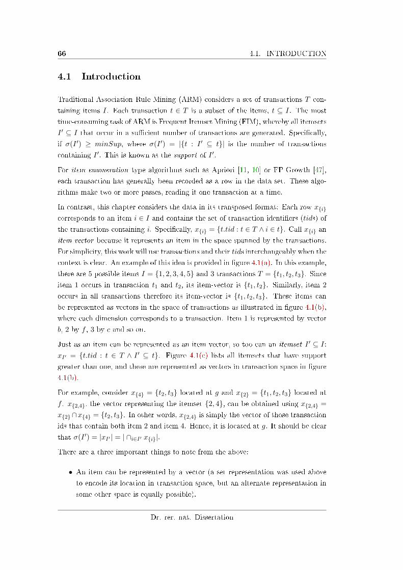
66 4.1. INTRODUCTION
4.1 Introduction
Traditional Association Rule Mining (ARM) considers a set of transactions T con-
taining items I. Each transaction t ∈ T is a subset of the items, t ⊆ I. The most
time-consuming task of ARM is Frequent Itemset Mining (FIM), whereby all itemsets
I ′ ⊆ I that occur in a su�cient number of transactions are generated. Speci�cally,
if σ(I ′) ≥ minSup, where σ(I ′) = |{t : I ′ ⊆ t}| is the number of transactions
containing I ′. This is known as the support of I ′.
For item enumeration type algorithms such as Apriori [11, 10] or FP-Growth [47],
each transaction has generally been recorded as a row in the data set. These algo-
rithms make two or more passes, reading it one transaction at a time.
In contrast, this chapter considers the data in its transposed format: Each row x{i}
corresponds to an item i ∈ I and contains the set of transaction identi�ers (tids) of
the transactions containing i. Speci�cally, x{i} = {t.tid : t ∈ T ∧ i ∈ t}. Call x{i} anitem vector because it represents an item in the space spanned by the transactions.
For simplicity, this work will use transactions and their tids interchangeably when the
context is clear. An example of this idea is provided in �gure 4.1(a). In this example,
there are 5 possible items I = {1, 2, 3, 4, 5} and 3 transactions T = {t1, t2, t3}. Sinceitem 1 occurs in transaction t1 and t2, its item-vector is {t1, t2}. Similarly, item 2
occurs in all transactions therefore its item-vector is {t1, t2, t3}. These items can
be represented as vectors in the space of transactions as illustrated in �gure 4.1(b),
where each dimension corresponds to a transaction. Item 1 is represented by vector
b, 2 by f , 3 by c and so on.
Just as an item can be represented as an item vector, so too can an itemset I ′ ⊆ I:
xI′ = {t.tid : t ∈ T ∧ I ′ ⊆ t}. Figure 4.1(c) lists all itemsets that have support
greater than one, and these are represented as vectors in transaction space in �gure
4.1(b).
For example, consider x{4} = {t2, t3} located at g and x{2} = {t1, t2, t3} located at
f . x{2,4}, the vector representing the itemset {2, 4}, can be obtained using x{2,4} =
x{2}∩x{4} = {t2, t3}. In other words, x{2,4} is simply the vector of those transaction
ids that contain both item 2 and item 4. Hence, it is located at g. It should be clear
that σ(I ′) = |xI′ | = | ∩i∈I′ x{i}|.
There are a three important things to note from the above:
• An item can be represented by a vector (a set representation was used above
to encode its location in transaction space, but an alternate representation in
some other space is equally possible).
Dr. rer. nat. Dissertation
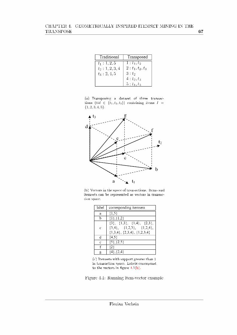
CHAPTER 4. GEOMETRICALLY INSPIRED ITEMSET MINING IN THETRANSPOSE 67
(a) Transposing a dataset of three transac-tions (tid ∈ {t1, t2, t3}) containing items I ={1, 2, 3, 4, 5}.
(b) Vectors in the space of transactions. Items anditemsets can be represented as vectors in transac-tion space.
(c) Itemsets with support greater than 1in transaction space. Labels correspondto the vectors in �gure 4.1(b).
Figure 4.1: Running item-vector example
Florian Verhein
68 4.1. INTRODUCTION
• Item vectors can be created that represent itemsets by performing a simple
operation on the item vectors (in the case above, set intersection was used).
• A measure can be evaluated using a function on the vectors (in the above case,
set size was used and the measure was support). Note that only a single vector
must be examined to do this.
These fundamental operations are all that are required for an itemset mining algo-
rithm. In section 4.4 they are generalised to a function g(·), operator ◦ and function
f(·) respectively. An additional function F (·) is added for more complicated mea-
sures. This generalisation allows the framework and algorithm to be applied to many
other itemset mining problems, and indeed opens the door for novel approaches in-
spired by the geometric view that cannot be solved with existing algorithms. For
example, while frequent itemset mining leads to binary values vectors, the frame-
work could well be used for itemset mining problems that require non-binary vectors
and/or measures other than support. One possible example where real vectors may
be useful is the use of Singular Value Decomposition or Principle Component Anal-
ysis to reduce the dimensionality of the data set and noise prior to mining frequent
itemsets. The result of such a transformation produces real valued vectors. Chap-
ter 5 will show how the framework and algorithm presented in this chapter can be
applied with a di�erent interestingness measure in the spatio-temporal domain.
While this novel approach has many theoretical and practical bene�ts, it is important
to note that there are a number of challenges in exploiting these ideas. The primary
challenge is to compute item-vectors e�ciently, and to avoid recomputing them even
though they are needed at multiple points in the search. This would typically lead
to a trade o� between space and time. However, it turns out that this challenge can
be solved using some important observations, leading to an algorithm that avoids
all re-computations while maintaining minimal space usage. This challenge will be
further discussed in section 4.2.
This chapter presents a single pass algorithm that uses time roughly linear in the
number of interesting itemsets and at worst n′ + dl/2e item-vectors of space, where
n′ ≤ n is the number of interesting 1-itemsets and l is the size of the largest interesting
itemset. This worst case scenario is only reached with extremely low support, and
most practical situations require only a small fraction of n′. Based on these facts
and the geometric inspiration provided by the item-vectors, the algorithm is called
Geometrically inspired Linear Itemset Mining In the Transpose (GLIMIT ).
FP-Growth type algorithms are often the fastest FIM algorithms. Experiments show
that GLIMIT outperforms FP-Growth [47] when the support is above a small thresh-
Dr. rer. nat. Dissertation
CHAPTER 4. GEOMETRICALLY INSPIRED ITEMSET MINING IN THETRANSPOSE 69
old. GLIMIT is more than �just another FIM/ARM algorithm� and support is just
one of many possible interestingness measures it can use. It is a new, and fast,
class of algorithm. Furthermore, it opens possibilities for useful pre-processing tech-
niques based on the item vector framework, as well as new geometrically inspired
interestingness measures.
4.1.1 Contributions
This chapter makes the following contributions:
• An interesting consequences of viewing transaction data as item vectors in
transaction-space is introduced. A theoretical framework for operating on item
vectors is subsequently developed. This abstraction allows a new class of algo-
rithm to be developed, gives great �exibility in the measures used, inspires new
geometric based interestingness measures and opens up the potential for use-
ful transformations (such as pre-processing) on the data that were previously
impossible.
• GLIMIT, a new, e�cient and fast class of algorithm that uses the framework
to mine interesting itemsets in one pass without candidate generation is in-
troduced. It uses linear space and (roughly) time linear in the number of
interesting itemsets. It signi�cantly departs from existing algorithms. Experi-
ments show it beats FP-Growth above small support thresholds when used for
frequent itemset mining. It also beats Apriori.
4.1.2 Organisation
Section 4.3 places GLIMIT and the associated framework in the context of previous
work. Section 4.4 presents the item-vector framework. Section 4.5.1 gives the the
two data structures that can be used by GLIMIT. Section 4.5 gives the main facts
exploited by GLIMIT and follows up with a comprehensive example. The space
complexity is proved and pseudo-code provided. Section 4.6 shows how association
rules can be mined e�ciently using the output of GLIMIT. Section 4.7 presents
experimental results and this chapter is concluded in section 4.8.
4.2 Some Challenges and Important Concepts
This section brie�y discusses some challenges and important concepts that will aid
in understanding this chapter.
Florian Verhein
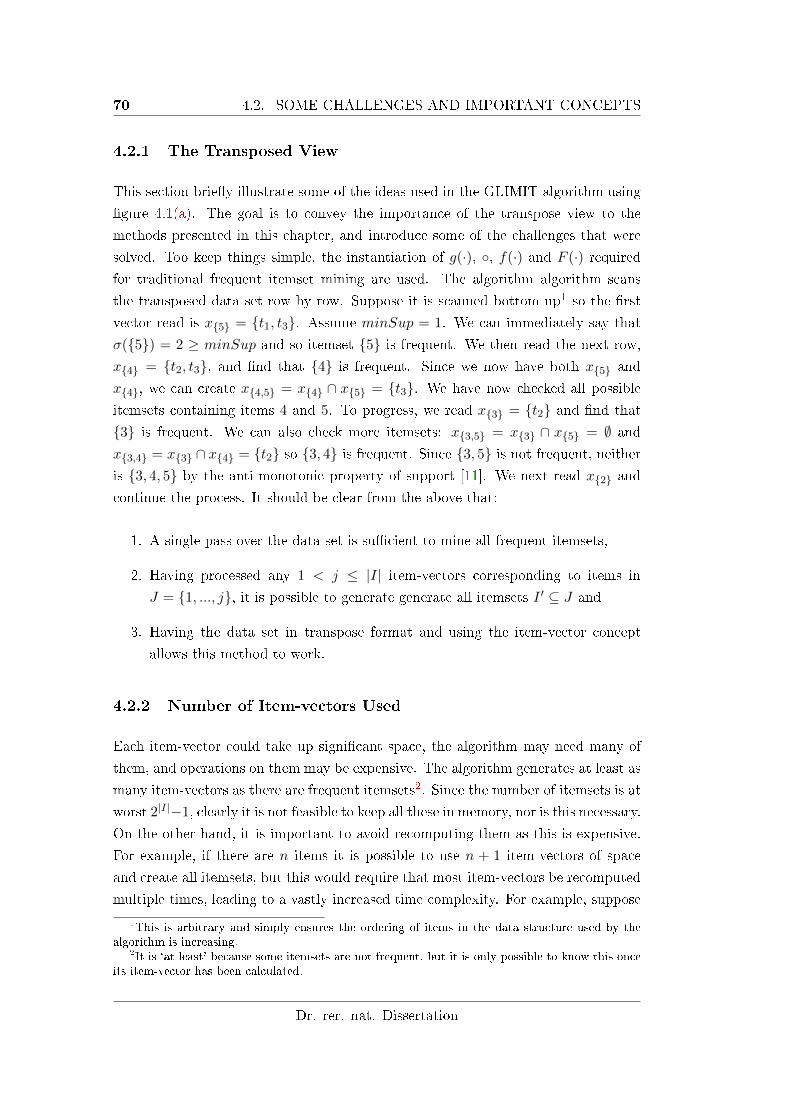
70 4.2. SOME CHALLENGES AND IMPORTANT CONCEPTS
4.2.1 The Transposed View
This section brie�y illustrate some of the ideas used in the GLIMIT algorithm using
�gure 4.1(a). The goal is to convey the importance of the transpose view to the
methods presented in this chapter, and introduce some of the challenges that were
solved. Too keep things simple, the instantiation of g(·), ◦, f(·) and F (·) required
for traditional frequent itemset mining are used. The algorithm algorithm scans
the transposed data set row by row. Suppose it is scanned bottom up1 so the �rst
vector read is x{5} = {t1, t3}. Assume minSup = 1. We can immediately say that
σ({5}) = 2 ≥ minSup and so itemset {5} is frequent. We then read the next row,
x{4} = {t2, t3}, and �nd that {4} is frequent. Since we now have both x{5} and
x{4}, we can create x{4,5} = x{4} ∩ x{5} = {t3}. We have now checked all possible
itemsets containing items 4 and 5. To progress, we read x{3} = {t2} and �nd that
{3} is frequent. We can also check more itemsets: x{3,5} = x{3} ∩ x{5} = ∅ and
x{3,4} = x{3} ∩ x{4} = {t2} so {3, 4} is frequent. Since {3, 5} is not frequent, neitheris {3, 4, 5} by the anti-monotonic property of support [11]. We next read x{2} and
continue the process. It should be clear from the above that:
1. A single pass over the data set is su�cient to mine all frequent itemsets,
2. Having processed any 1 < j ≤ |I| item-vectors corresponding to items in
J = {1, ..., j}, it is possible to generate generate all itemsets I ′ ⊆ J and
3. Having the data set in transpose format and using the item-vector concept
allows this method to work.
4.2.2 Number of Item-vectors Used
Each item-vector could take up signi�cant space, the algorithm may need many of
them, and operations on them may be expensive. The algorithm generates at least as
many item-vectors as there are frequent itemsets2. Since the number of itemsets is at
worst 2|I|−1, clearly it is not feasible to keep all these in memory, nor is this necessary.
On the other hand, it is important to avoid recomputing them as this is expensive.
For example, if there are n items it is possible to use n + 1 item-vectors of space
and create all itemsets, but this would require that most item-vectors be recomputed
multiple times, leading to a vastly increased time complexity. For example, suppose
1This is arbitrary and simply ensures the ordering of items in the data structure used by thealgorithm is increasing.
2It is `at least' because some itemsets are not frequent, but it is only possible to know this onceits item-vector has been calculated.
Dr. rer. nat. Dissertation
CHAPTER 4. GEOMETRICALLY INSPIRED ITEMSET MINING IN THETRANSPOSE 71
we have created x{1,2,3}. When we later need x{1,2,3,4}, we do not want to have to
recalculate it as x{1}∩x{2}∩x{3}∩x{4}. Instead, we would like to use the previously
calculated x{1,2,3}: one option is to compute x{1,2,3,4} = x{1,2,3}∩x{4}. The challengeis to use as little space as necessary, while avoiding all re-computations.
4.3 Related Work
Many itemset mining algorithms have been proposed since association rules were
introduced [11, 10]. Advances can be found in [37] and [38] and a survey of frequent
itemset mining can be found in [43]. Most algorithms can be broadly classi�ed
into two groups, the item enumeration (such as [11, 47, 74, 71, 5, 6, 73, 81, 111,
113, 72, 112]) which operate with a general-to-speci�c search strategy, and the row
enumeration (such as [69, 100]) techniques which �nd speci�c itemsets �rst. Broadly
speaking, item enumeration algorithms are most e�ective for data sets where |T | >>|I|, while row enumeration algorithms are e�ective for data sets where |T | << |I|,such as for micro-array data [69]. Furthermore, a speci�c to general strategy can be
useful for �nding maximal frequent itemsets in dense databases [88].
Item enumeration algorithms mine subsets of an itemset I ′ before mining the more
speci�c itemset I ′. Only those itemsets for which all (or some) subsets are frequent
are generated � making use of the anti-monotonic property of support. This property
is also known as the Apriori property. Apriori-like algorithms [11] search for frequent
itemsets in a breadth �rst generate-and-test manner, where all itemsets of length k
are generated before those of length k+1. In the candidate generation step, possibly
frequent k + 1 itemsets are generated from the already mined k-itemsets prior to
counting items, making use of the Apriori property. This creates a high memory
requirement, as all candidates must remain in main memory. For support counting
(the test step), a pass is made over the database while checking whether the candidate
itemsets occur in at least minSup transactions. This requires subset checking � a
computationally expensive task especially when the transaction width is high. While
methods such as hash-trees [88] or bitmaps have been used to accelerate this step,
candidate checking remains expensive. Various improvements have been proposed
to speed up aspects of Apriori. For example, [71] proposed a hash based method for
candidate generation that reduces the number of candidates generated, thus saving
considerable space and time. [20] argues for the use of the Trie data structure for the
subset checking step, improving on the hash tree approach. Apriori style algorithms
make multiple passes over the database, at least equal to the length of the longest
frequent itemset, which incurs considerable I/O cost. GLIMIT does not perform
Florian Verhein
72 4.3. RELATED WORK
candidate generation or subset enumeration, and generates itemsets in a depth �rst
fashion using a single pass over the transposed data set.
Frequent pattern growth (FP-Growth) type algorithms are often regarded as the
fastest item enumeration algorithms. FP-Growth [47, 74] generates a compressed
summary of the data set using two passes in a cross referenced tree, the FP-tree,
before mining itemsets by traversing the tree and recursively projecting the database
into sub-databases using conditional FP-Trees. In the �rst database pass, infrequent
items are discarded, allowing some reduction in the database size. In the the second
pass, the complete FP-Tree is built by collecting common pre�xes of transactions
and incrementing support counts at the nodes. at the same time, a header table
and node links are maintained, which allow easy access to all nodes given an item.
The mining step operates by following these node links and creating (projected) FP-
Trees that are conditional on the presence of an item(set), from which the support
can be obtained by a traversal of the leaves. Like GLIMIT, it does not perform
any candidate generation and mines the itemsets in a depth �rst manner while still
mining all subsets of an itemset I ′ before mining I ′. FP-Growth is very fast at reading
from the FP-tree, but the downside is that the FP-tree can become very large and
is expensive to generate, so this investment does not always pay o�. Further, the
FP-Tree may not �t into memory. In contrast, GLIMIT uses only as much space as
is required and is based on vector operations, rather than tree projections. It also
uses a purely depth �rst search.
Many other item enumeration methods exist. [5, 6] uses a lexicographic tree and
database projections in order to reduce the CPU time for counting frequent itemsets,
and combine this with a depth �rst search. The tree is based on storing itemsets at
nodes in such a way that parent nodes represent itemsets that are lexicographically
before the present node. The approach uses the concept of projected transactions at
nodes in the tree, observing that these projections fall in size as one descends deeper
into the tree. Nevertheless, the projections must still be stored or read from disk and
the frequency of lexicographic extensions counted within the projection. A matrix
based method is used for support counting, requiring an additional matrix at each
node. The work explores depth and breadth �rst methods for constructing the tree
and mining frequent itemsets, as well as discussing the trade-o�s that these o�er.
H-Mine [73] is another projection based pattern generation approach, proposing a
data structure called a H-struct to store frequent item projections of the database.
The H-struct is composed of a header table for each item, and a set of hyperlinks
between arrays where each array corresponds to a transaction in the current pro-
jected database. The core idea is that these hyperlinks make it easy to obtain those
Dr. rer. nat. Dissertation
CHAPTER 4. GEOMETRICALLY INSPIRED ITEMSET MINING IN THETRANSPOSE 73
transactions containing an item of interest. In many ways, this is similar to the core
idea behind the conditional trees of FP-Growth. The downside of the H-struct is its
potential space requirement however, as the frequent item projections and header
tables must remain in memory. To overcome this, a database partitioning technique
is used. Furthermore, in dense databases a hybrid approach is proposed where H-
struct is combined with FP-Growth in order to take advantage of the transaction
pre�x sharing of FP-Trees.
Another class of item enumeration algorithm is based on the vertical approach. For
example, [111] uses a vertical TID-list database format, where each item is associ-
ated with the list of transactions in which it occurs. In contrast to the traditional
horizontal layout where rows are scanned, vertical methods consider columns in the
database. The idea behind the vertical approach is that TID-list intersections of two
itemsets X and Y give the TID-list of their union X ∪ Y . By observing that in a
lexicographic tree over the itemsets, each node corresponds not only to an itemset X
but also de�nes an equivalence class for all itemsets with the pre�x X, the search can
be decomposed. This is very similar to the decomposition and database projection
idea used in pattern generating approaches. Various algorithms are proposed based
on di�erent search strategies. For frequent itemset mining, Eclat is developed. It is
based on a breadth or depth �rst traversal of the itemset lattice. The downside of
this approach is that many TID-lists � in the worst case an exponential number �
must remain in memory since these are required to create the TID-lists for the next
level in the search.
In [112], the argument is made that vertical methods can use too much space due to
the use of TID lists. To reduce this, in particular for dense data sets, the di�set is
proposed. Here, it is observed that in a lexicographic tree over the itemsets, rather
than storing the entire TID list for an itemset X ∪ i, it is only necessary to store
the di�erence in TIDs of X ∪ i and it's pre�x X. The di�erence in the cardinality of
these sets is the reduction in support of X∪ i compared to X. Under the assumption
that the database is relatively dense, this achieves a reduction in space required.
Furthermore, since smaller sets are faster to intersect, this reduces the run time in
such databases.
[81] presents another vertical approach, called VIPER. Viper uses a vertical TID-
vector (VTV) format to represent an itemset's occurrence in transactions, encoding
this in a compressed binary vector. It uses the disk to temporarily store these
vectors for frequent itemsets and employs temporary horizontal tuples in counting the
support of candidates. It operates in a breadth �rst, level wise manner; necessitating
the disk based approach in order to reduce the the memory requirement.
Florian Verhein
74 4.3. RELATED WORK
CHARM [113] considers the closed itemset mining problem and uses a breadth or
depth depth �rst approach in an Itemset-Tidset tree (IT-Tree). This tree is also a
lexicographic tree, storing both the itemset and the TID-set at the nodes. An itemset
X is closed if there exists no proper super-set Y : X ⊂ Y such that support(X) =
support(Y ) [72]. Closed itemsets are a loss-less way of reducing the itemsets that
need to be mined while still allowing the the support of all itemsets to be calculated;
for instance in the association rule discovery task. Other work on frequent closed
itemsets includes [69, 74, 29, 101]. Another vertical approach is [52], where VB-FT
Mine is introduced in order to mine fault tolerant frequent patterns.
[23] Introduce an e�cient algorithm called MAFIA for maximal frequent pattern
mining when the entire database can �t into memory, and in particular when maximal
frequent itemsets are long. By using a depth �rst search that begins along the
longest branch of a lexicographic tree, MAFIA can quickly reach the frequent itemset
boundary and may thus prune away other parts of the search for maximal frequent
itemsets. The approach uses the vertical layout and bitmaps instead of TID-lists.
A problem with most vertical approaches is that they keep the TID lists for sibling
nodes. For example, given a node for itemset X, even when the overall search
progresses in a depth �rst fashion (and except for maximal and closed approaches,
they use a breadth �rst search), the child nodes and TID lists corresponding to
{X ∪ i : i ∈ I −X} are generated and stored in memory before the search progresses
in depth to one of these. This is a form of candidate generation. This is done
since the fundamental operation in vertical approaches is the intersection of these
TID lists. This is a signi�cant downside, as it requires many TID lists to remain
in memory. For breadth �rst searches, this is even worse, since the TID-lists for all
frequent itemsets at the same level must me maintained � either in memory (which
is not feasible in realistic databases) or on disk.
In comparison to all itemset mining algorithms, GLIMIT has most in common with
vertical approaches since it also views the database column wise, by traversing the
transposed database row-wise. In contrast to these vertical approaches, GLIMIT
does not store vectors for siblings at any time. In the language of TID-lists, the
intermediate TID-lists would not need to be stored in memory, except for those on
the current path (of which there are at most l, where l is the length of the longest
frequent itemset). Indeed, an entire sub-tree under X ∪ i is completely examined
before X ∪ j is ever examined. This is termed the strict depth �rst search in this
work. Furthermore, GLIMIT can mine all frequent itemsets in typically less space
than the database (as shown in the experiments), while making only one pass over
the data. Vertical approaches typically make multiple passes. While it addresses
Dr. rer. nat. Dissertation
CHAPTER 4. GEOMETRICALLY INSPIRED ITEMSET MINING IN THETRANSPOSE 75
the maximal frequent itemset mining problem (thus attempting to avoid as many
frequent itemsets as possible), MAFIA [23] is perhaps the most related work to
GLIMIT on the FIM problem due to the combination of a depth �rst search and use
of bitmaps. The depth �rst search in MAFIA is di�erent for two important reasons
however: In MAFIA the longest branch is searched �rst (which aids in pruning the
search for maximal frequent itemsets early), while in GLIMIT the shortest is searched
�rst (this enables the required property that subsets are examined prior to super-sets
and also allows GLIMIT to avoid loading the entire data set into memory). Secondly,
child nodes are expanded before the depth is increased in MAFIA (leading to the
downside mentioned above), while GLIMIT is strictly depth �rst. The solving of
the maximal problem using various pruning techniques also requires that maximal
frequent itemsets and various data structures remain in memory in MAFIA.
Row enumeration techniques e�ectively intersect transactions and generate super-
sets of I ′ before mining I ′. Although it is much more di�cult for these algorithms
to make use of the anti-monotonic property for pruning, they exploit the fact that
searching the row space in data with |T | << |I| becomes cheaper than searching the
itemset-space. GLIMIT is similar to row enumeration algorithms since both search
using the transpose of the data set. However, where row enumeration intersects
transactions (rows), GLIMIT e�ectively intersect item-vectors (columns). But this
similarity is tenuous at best. Furthermore, existing algorithms use the transpose for
counting convenience rather than for any insight into the data, as is done in the
framework in this chapter. Since GLIMIT searches through the itemset space, it is
classi�ed as an item enumeration technique and is suited to the same types of data.
The transpose has never, to the best of the author's knowledge, been used in an item
enumeration algorithm.
E�orts to create a framework for support exist. Steinbach et al. [86] present one
such generalisation, but their goal is to extend support to cover continuous data.
This is very di�erent to transforming the original (non-continuous) data into a real
vector-space (which is one possibility presented by the framework). Their work is
geared toward existing item enumeration algorithms and so their �pattern evaluation
vector � summarises transactions (that is, rows). The framework presented in this
chapter operates on columns of the original data matrix. Furthermore, rather than
generalising the support measures so as to cover more types of data sets, it generalises
the operations on item-vector and the transformations on the same data set that can
be used to enable a wide range of measures, not just support.
To the author's best knowledge, Ratio Rules are the closest attempt at combining
SVD (or similar techniques such as Principal Component Analysis) and rule mining.
Florian Verhein
76 4.4. ITEM-VECTOR FRAMEWORK
Korn et al. [53] consider transaction data where items have continuous values as-
sociated with them, such as price. A transaction is considered a point in the space
spanned by the items. By performing SVD on such data sets, they observe that the
axes (orthogonal basis vectors) produced de�ne ratios between single items. The
ideas in this chapter di�er in a number of ways. This work considers items (and
itemsets) in transaction space (not the other way around) so when SVD is consid-
ered, the new axes are linear combinations of transactions � not items. Hence I is
unchanged. Secondly, this work considers mining itemsets, not just ratios between
single items. Finally, SVD is just one possible instantiation of g(·).
As shown in this work, by considering items as vectors in transaction space, it is
possible to interpret itemsets geometrically. To the author's knowledge this has not
been considered previously. As well as inspiring the algorithm, this geometric view
has the potential to lead to useful pre-processing techniques, such as dimensionality
reduction of the transactions space. Since GLIMIT uses only this framework, it
should enable the use of such techniques � which are not possible using existing FIM
algorithms.
4.4 Item-vector Framework
In section 4.1, the example of frequent itemset mining (FIM) was used to intro-
duce the ideas behind this work. However, the work in this chapter is more general
than this and the instantiations of g(·), ◦ and f(·) are straightforward for FIM. The
functions and operator formally described in this section de�ne the form of interest-
ingness measures and data-set transformations that are supported by the GLIMIT
algorithm. Not only can existing measures be mapped to this framework, but it
is the author's hope that the geometric interpretation will inspire new interesting
itemset mining approaches.
Recall that xI′ is the set of transaction identi�ers of the transactions containing
the itemset I ′ ⊆ I. Call X the space spanned by all possible xI′ . Speci�cally,
X = P({t.tid : t ∈ T}).
De�nition 4.1. g : X → Y is a transformation on the original item-vector to a
di�erent representation yI′ = g(xI′) in a new space Y .
Even though g(·) is a transformation, it's output still `represents' the item vector.
To avoid too many terms therefore, yI′ will also be referred to as an item vector.
Dr. rer. nat. Dissertation
CHAPTER 4. GEOMETRICALLY INSPIRED ITEMSET MINING IN THETRANSPOSE 77
De�nition 4.2. ◦ is an operator on the transformed item-vectors so that yI′∪I” =
yI′ ◦ yI” = yI” ◦ yI′ .
That is, ◦ is a commutative operator for combining item vectors to create item vectors
representing larger itemsets. It is not required that yI′ = yI′ ◦ yI′ 3.
De�nition 4.3. f : Y → R is a measure on itemsets, evaluated on transformed
item-vectors. Write valueI′ = f(yI′).
De�nition 4.4. interestingness : P(I)→ R is an interestingness measure (order)
on all itemsets.
Suppose a measure of interestingness of an itemset depends only on that itemset.
The simplest example is support. It is possible to represent this as follows, where
I ′ = {i1, ..., iq} and k = 1:
(4.1) interestingness(I ′) = f(g(x{i1}) ◦ ... ◦ g(x{iq}))
So the challenge is, given an interestingness measure, �nd suitable and useful g,◦and f so that the above holds. For support, ◦ = ∩, f = | · | and g as the identity
function. Let us return to the frequent itemset mining motivation. First assume that
g(·) trivially maps xI′ to a binary vector. Using x{1} = {t1, t2} and x{5} = {t1, t3}from �gure 4.1(a) we have y{1} = g(x{1}) = 110 and y{5} = g(x{5}) = 101. It should
be clear that using bit-wise AND as ◦ and f = sum() � the number of set bits �
gives the requires semantics for frequent itemset mining.
To give a motivation for these ideas, notice that sum(y{1}AND y{2}) = sum(y{1}. ∗y{2}) = y{1} · y{2}, the dot product (.∗ is the element-wise product4). That is, the
dot product of two item-vectors is the support of the the 2-itemset. What makes
this interesting is that this holds for any rotation about the origin. Suppose we have
an arbitrary 3 × 3 matrix R de�ning a rotation about the origin. This means we
can de�ne g(x) = RxT because the dot product is preserved by R (hence g(·)). Forexample, σ({1, 5}) = y{1}·y{5} = (RxT{1})·(Rx
T{5}). Therefore, it's possible to perform
an arbitrary rotation of the item-vectors before mining itemsets of size 2. Of course
3Equivalently, ◦ may have the restriction that I ′ ∩ I” = ∅.4(a. ∗ b)[i] = a[i] ∗ b[i] for all i, where [] indexes the vectors.
Florian Verhein
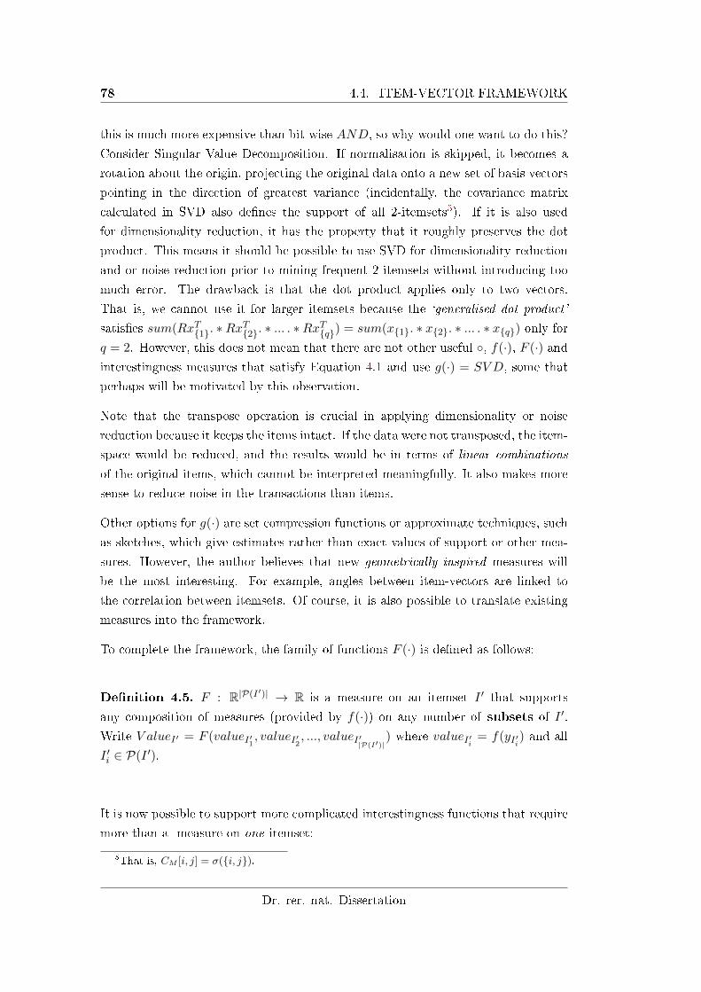
78 4.4. ITEM-VECTOR FRAMEWORK
this is much more expensive than bit-wise AND, so why would one want to do this?
Consider Singular Value Decomposition. If normalisation is skipped, it becomes a
rotation about the origin, projecting the original data onto a new set of basis vectors
pointing in the direction of greatest variance (incidentally, the covariance matrix
calculated in SVD also de�nes the support of all 2-itemsets5). If it is also used
for dimensionality reduction, it has the property that it roughly preserves the dot
product. This means it should be possible to use SVD for dimensionality reduction
and or noise reduction prior to mining frequent 2-itemsets without introducing too
much error. The drawback is that the dot product applies only to two vectors.
That is, we cannot use it for larger itemsets because the `generalised dot product'
satis�es sum(RxT{1}. ∗RxT{2}. ∗ ... . ∗Rx
T{q}) = sum(x{1}. ∗ x{2}. ∗ ... . ∗ x{q}) only for
q = 2. However, this does not mean that there are not other useful ◦, f(·), F (·) andinterestingness measures that satisfy Equation 4.1 and use g(·) = SV D, some that
perhaps will be motivated by this observation.
Note that the transpose operation is crucial in applying dimensionality or noise
reduction because it keeps the items intact. If the data were not transposed, the item-
space would be reduced, and the results would be in terms of linear combinations
of the original items, which cannot be interpreted meaningfully. It also makes more
sense to reduce noise in the transactions than items.
Other options for g(·) are set compression functions or approximate techniques, such
as sketches, which give estimates rather than exact values of support or other mea-
sures. However, the author believes that new geometrically inspired measures will
be the most interesting. For example, angles between item-vectors are linked to
the correlation between itemsets. Of course, it is also possible to translate existing
measures into the framework.
To complete the framework, the family of functions F (·) is de�ned as follows:
De�nition 4.5. F : R|P(I′)| → R is a measure on an itemset I ′ that supports
any composition of measures (provided by f(·)) on any number of subsets of I ′.
Write V alueI′ = F (valueI′1 , valueI′2 , ..., valueI′|P(I′)|) where valueI′i = f(yI′i) and all
I ′i ∈ P(I ′).
It is now possible to support more complicated interestingness functions that require
more than a measure on one itemset:
5That is, CM [i, j] = σ({i, j}).
Dr. rer. nat. Dissertation
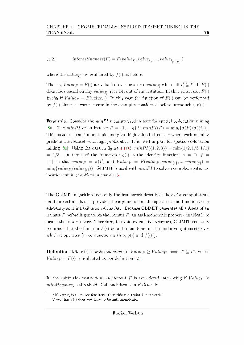
CHAPTER 4. GEOMETRICALLY INSPIRED ITEMSET MINING IN THETRANSPOSE 79
(4.2) interestingness(I ′) = F (valueI′1 , valueI′2 , ..., valueI′|P(I′)|)
where the valueI′i are evaluated by f(·) as before.
That is, V alueI′ = F (·) is evaluated over measures valueI′i where all I′i ⊆ I ′. If F (·)
does not depend on any valueI′i , it is left out of the notation. In that sense, call F (·)trivial if V alueI′ = F (valueI′). In this case the function of F (·) can be performed
by f(·) alone, as was the case in the examples considered before introducing F (·).
Example. Consider the minPI measure used in part for spatial co-location mining
[80]: The minPI of an itemset I ′ = {1, ..., q} is minPI(I ′) = mini{σ(I ′)/σ({i})}.This measure is anti-monotonic and gives high value to itemsets where each member
predicts the itemset with high probability. It is used in part for spatial co-location
mining [80]. Using the data in �gure 4.1(a), minPI({1, 2, 3}) = min{1/2, 1/3, 1/1}= 1/3. In terms of the framework g(·) is the identity function, ◦ = ∩, f =
| · | so that valueI′ = σ(I ′) and V alueI′ = F (valueI′ , value{1}, ..., value{q}) =
mini{valueI′/value{i})}. GLIMIT is used with minPI to solve a complex spatio-co-
location mining problem in chapter 5.
The GLIMIT algorithm uses only the framework described above for computations
on item-vectors. It also provides the arguments for the operators and functions very
e�ciently so it is �exible as well as fast. Because GLIMIT generates all subsets of an
itemset I' before it generates the itemset I ′, an anti-monotonic property enables it to
prune the search space. Therefore, to avoid exhaustive searches, GLIMIT generally
requires6 that the function F (·) be anti-monotonic in the underlying itemsets over
which it operates (in conjunction with ◦, g(·) and f(·)7).
De�nition 4.6. F (·) is anti-monotonic if V alueI′ ≥ V alueI” ⇐⇒ I ′ ⊆ I”, where
V alueI′ = F (·) is evaluated as per de�nition 4.5.
In the spirit this restriction, an itemset I ′ is considered interesting if V alueI′ ≥minMeasure, a threshold. Call such itemsets F-itemsets.
6Of course, it there are few items then this constraint is not needed.7Note that f(·) does not have to be anti-monotonic.
Florian Verhein
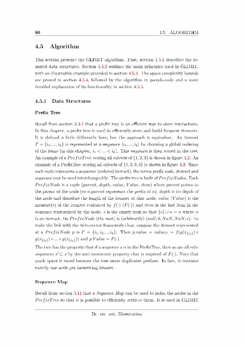
80 4.5. ALGORITHM
4.5 Algorithm
This section presents the GLIMIT algorithm. First, section 4.5.1 describes the re-
quired data structures. Section 4.5.2 outlines the main principles used in GLIMIT,
with an illustrative example provided in section 4.5.3. The space complexity bounds
are proved in section 4.5.4, followed by the algorithm in pseudo-code and a more
detailed explanation of its functionality in section 4.5.5.
4.5.1 Data Structures
Pre�x Tree
Recall from section 3.3.1 that a pre�x tree is an e�cient way to store interactions.
In this chapter, a pre�x tree is used to e�ciently store and build frequent itemsets.
It is de�ned a little di�erently here, but the approach is equivalent. An itemset
I ′ = {i1, ..., ik} is represented as a sequence 〈i1, ..., ik〉 by choosing a global ordering
of the items (in this chapter, i1 < ... < ik). This sequence is then stored in the tree.
An example of a PrefixTree storing all subsets of {1, 2, 3} is shown in �gure 4.2. Anexample of a Pre�xTree storing all subsets of {1, 2, 3, 4} is shown in �gure 4.3. Since
each node represents a sequence (ordered itemset), the terms pre�x node, itemset and
sequence may be used interchangeably. The pre�x tree is built of PrefixNodes. Each
PrefixNode is a tuple (parent, depth, value, V alue, item) where parent points to
the parent of the node (so n.parent represents the pre�x of n), depth is its depth of
the node and therefore the length of the itemset at that node, value (V alue) is the
measure(s) of the itemset evaluated by f(·) (F (·)) and item is the last item in the
sequence represented by the node. ε is the empty item so that {ε} ∪ α = α where α
is an itemset. Its PrefixNode (the root) is (arbitrarily) (null, 0, NaN,NaN, ε). To
make the link with the item-vector framework clear, suppose the itemset represented
at a PrefixNode p is I ′ = {i1, i2, .., ik}. Then p.value = valueI′ = f(g(x{i1}) ◦g(x{i2}) ◦ ... ◦ g(x{ik})) and p.V alue = F (·).
The tree has the property that if a sequence s is in the Pre�xTree, then so are all sub-
sequences s′ @ s by the anti-monotonic property that is required of F (·). Note thatmuch space is saved because the tree never duplicates pre�xes. In fact, it contains
exactly one node per interesting itemset.
Sequence Map
Recall from section 3.11 that a Sequence Map can be used to index the nodes in the
PrefixTree so that it is possible to e�ciently retrieve them. It is used in GLIMIT
Dr. rer. nat. Dissertation
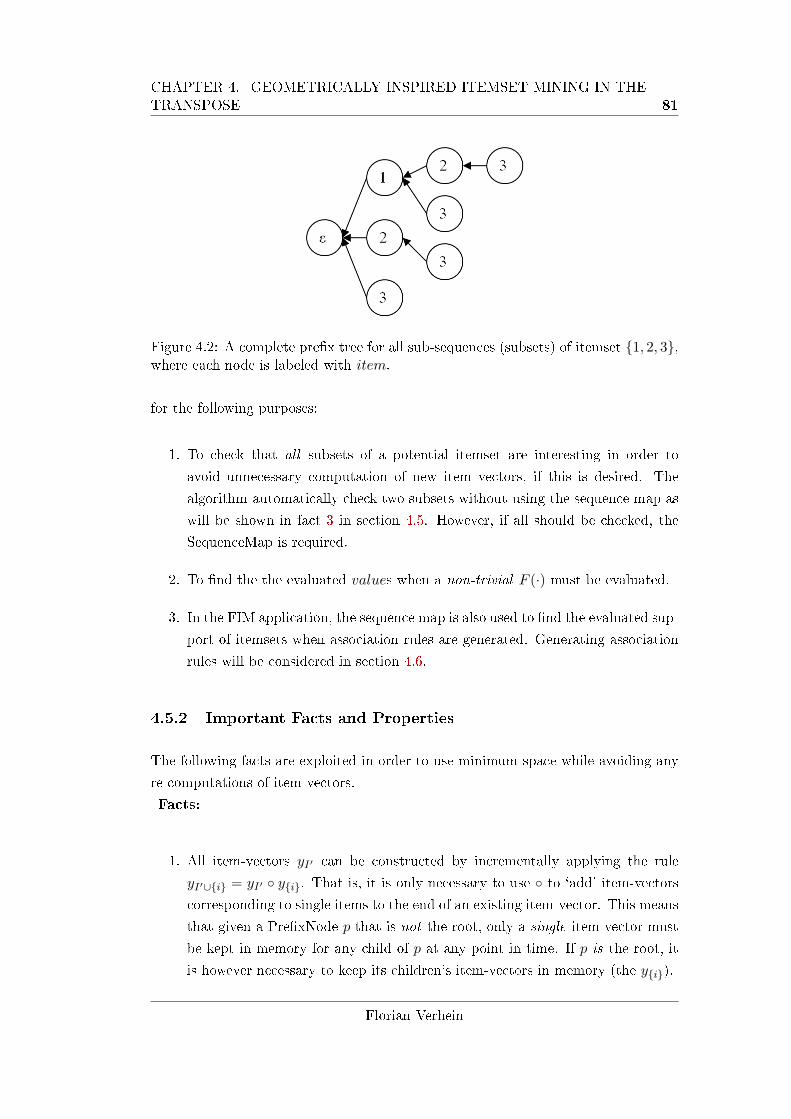
CHAPTER 4. GEOMETRICALLY INSPIRED ITEMSET MINING IN THETRANSPOSE 81
Figure 4.2: A complete pre�x tree for all sub-sequences (subsets) of itemset {1, 2, 3},where each node is labeled with item.
for the following purposes:
1. To check that all subsets of a potential itemset are interesting in order to
avoid unnecessary computation of new item vectors, if this is desired. The
algorithm automatically check two subsets without using the sequence map as
will be shown in fact 3 in section 4.5. However, if all should be checked, the
SequenceMap is required.
2. To �nd the the evaluated values when a non-trivial F (·) must be evaluated.
3. In the FIM application, the sequence map is also used to �nd the evaluated sup-
port of itemsets when association rules are generated. Generating association
rules will be considered in section 4.6.
4.5.2 Important Facts and Properties
The following facts are exploited in order to use minimum space while avoiding any
re-computations of item-vectors.
Facts:
1. All item-vectors yI′ can be constructed by incrementally applying the rule
yI′∪{i} = yI′ ◦ y{i}. That is, it is only necessary to use ◦ to `add' item-vectors
corresponding to single items to the end of an existing item-vector. This means
that given a Pre�xNode p that is not the root, only a single item-vector must
be kept in memory for any child of p at any point in time. If p is the root, it
is however necessary to keep its children's item-vectors in memory (the y{i}).
Florian Verhein
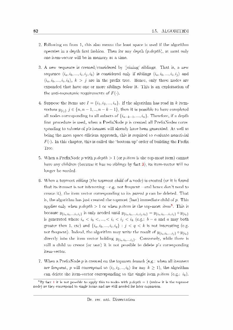
82 4.5. ALGORITHM
2. Following on from 1, this also means the least space is used if the algorithm
operates in a depth �rst fashion. Then for any depth (p.depth), at most only
one item-vector will be in memory at a time.
3. A new sequence is created/considered by `joining' siblings. That is, a new
sequence 〈ia, ib, ..., ii, ij , ik〉 is considered only if siblings 〈ia, ib, ..., ii, ij〉 and〈ia, ib, ..., ii, ik〉, k > j are in the pre�x tree. Hence, only those nodes are
expanded that have one or more siblings below it. This is an exploitation of
the anti-monotonic requirements of F (·).
4. Suppose the items are I = {i1, i2, ..., in}. If the algorithm has read in k item-
vectors y{ij} j ∈ {n, n− 1, .., n− k − 1}, then it is possible to have completed
all nodes corresponding to all subsets of {in−k−1, ..., in}. Therefore, if a depth
�rst procedure is used, when a Pre�xNode p is created all Pre�xNodes corre-
sponding to subsets of p's itemset will already have been generated. As well as
being the most space e�cient approach, this is required to evaluate nontrivial
F (·). In this chapter, this is called the `bottom up' order of building the Pre�x
Tree.
5. When a Pre�xNode p with p.depth > 1 (or p.item is the top-most item) cannot
have any children (because it has no siblings by fact 3), its item-vector will no
longer be needed.
6. When a topmost sibling (the topmost child of a node) is created (or it is found
that its itemset is not interesting � e.g. not frequent � and hence don't need to
create it), the item-vector corresponding to its parent p can be deleted. That
is, the algorithm has just created the topmost (last) immediate child of p. This
applies only when p.depth > 1 or when p.item is the top-most item8. This is
because y{ia,ib,...,ii,ij} is only needed until y{ia,ib,...,ii,ij ,ik} = y{ia,ib,...,ii,ij} ◦ y{ik}is generated where ia < ib <, ..., < ii < ij < ik (e.g.: b − a and a may both
greater then 1, etc) and {ia, ib, ..., ii, iq} : j < q < k is not interesting (e.g.
not frequent). Indeed, the algorithm may write the result of y{ia,ib,...,ij} ◦ y{ik}directly into the item-vector holding y{ia,ib,...,ij}. Conversely, while there is
still a child to create (or test) it is not possible to delete p's corresponding
item-vector.
7. When a Pre�xNode p is created on the topmost branch (e.g.: when all itemsets
are frequent, p will correspond to 〈i1, i2, .., ik〉 for any k ≥ 1), the algorithm
can delete the item-vector corresponding to the single item p.item (e.g.: ik).
8By fact 1 it is not possible to apply this to nodes with p.depth = 1 (unless it is the topmostnode) as they correspond to single items and are still needed for later expansion.
Dr. rer. nat. Dissertation
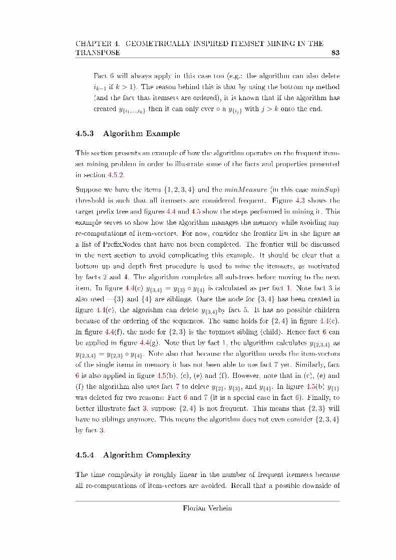
CHAPTER 4. GEOMETRICALLY INSPIRED ITEMSET MINING IN THETRANSPOSE 83
Fact 6 will always apply in this case too (e.g.: the algorithm can also delete
ik−1 if k > 1). The reason behind this is that by using the bottom up method
(and the fact that itemsets are ordered), it is known that if the algorithm has
created y{i1,...,ik} then it can only ever ◦ a y{ij} with j > k onto the end.
4.5.3 Algorithm Example
This section presents an example of how the algorithm operates on the frequent item-
set mining problem in order to illustrate some of the facts and properties presented
in section 4.5.2.
Suppose we have the items {1, 2, 3, 4} and the minMeasure (in this case minSup)
threshold is such that all itemsets are considered frequent. Figure 4.3 shows the
target pre�x tree and �gures 4.4 and 4.5 show the steps performed in mining it. This
example serves to show how the algorithm manages the memory while avoiding any
re-computations of item-vectors. For now, consider the frontier list in the �gure as
a list of Pre�xNodes that have not been completed. The frontier will be discussed
in the next section to avoid complicating this example. It should be clear that a
bottom up and depth �rst procedure is used to mine the itemsets, as motivated
by facts 2 and 4. The algorithm completes all sub-trees before moving to the next
item. In �gure 4.4(c) y{3,4} = y{3} ◦ y{4} is calculated as per fact 1. Note fact 3 is
also used � {3} and {4} are siblings. Once the node for {3, 4} has been created in
�gure 4.4(c), the algorithm can delete y{3,4}by fact 5. It has no possible children
because of the ordering of the sequences. The same holds for {2, 4} in �gure 4.4(e).
In �gure 4.4(f), the node for {2, 3} is the topmost sibling (child). Hence fact 6 can
be applied in �gure 4.4(g). Note that by fact 1, the algorithm calculates y{2,3,4} as
y{2,3,4} = y{2,3} ◦ y{4}. Note also that because the algorithm needs the item-vectors
of the single items in memory it has not been able to use fact 7 yet. Similarly, fact
6 is also applied in �gure 4.5(b), (c), (e) and (f). However, note that in (c), (e) and
(f) the algorithm also uses fact 7 to delete y{2}, y{3}, and y{4}. In �gure 4.5(b) y{1}
was deleted for two reasons: Fact 6 and 7 (it is a special case in fact 6). Finally, to
better illustrate fact 3, suppose {2, 4} is not frequent. This means that {2, 3} willhave no siblings anymore. This means the algorithm does not even consider {2, 3, 4}by fact 3.
4.5.4 Algorithm Complexity
The time complexity is roughly linear in the number of frequent itemsets because
all re-computations of item-vectors are avoided. Recall that a possible downside of
Florian Verhein
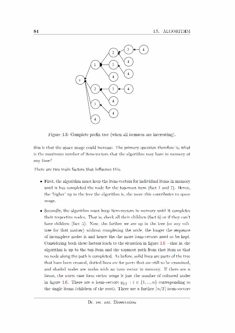
84 4.5. ALGORITHM
Figure 4.3: Complete pre�x tree (when all itemsets are interesting).
this is that the space usage could increase. The primary question therefore is; what
is the maximum number of item-vectors that the algorithm may have in memory at
any time?
There are two main factors that in�uence this.
• First, the algorithm must keep the item-vectors for individual items in memory
until it has completed the node for the top-most item (fact 1 and 7). Hence,
the `higher' up in the tree the algorithm is, the more this contributes to space
usage.
• Secondly, the algorithm must keep item-vectors in memory until it completes
their respective nodes. That is, check all their children (fact 6) or if they can't
have children (fact 5). Now, the further we are up in the tree (or any sub-
tree for that matter) without completing the node, the longer the sequence
of incomplete nodes is and hence the the more item-vectors need to be kept.
Considering both these factors leads to the situation in �gure 4.6 � that is, the
algorithm is up to the top item and the topmost path from that item so that
no node along the path is completed. As before, solid lines are parts of the tree
that have been created, dotted lines are for parts that are still to be examined,
and shaded nodes are nodes with an item-vector in memory. If there are n
items, the worst case item-vector usage is just the number of coloured nodes
in �gure 4.6. There are n item-vectors y{i} : i ∈ {1, ..., n} corresponding to
the single items (children of the root). There are a further dn/2e item-vectors
Dr. rer. nat. Dissertation
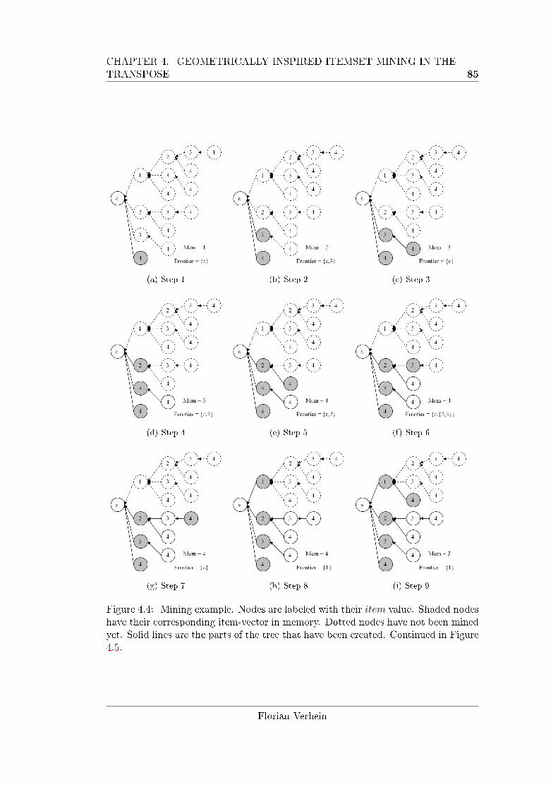
CHAPTER 4. GEOMETRICALLY INSPIRED ITEMSET MINING IN THETRANSPOSE 85
(a) Step 1 (b) Step 2 (c) Step 3
(d) Step 4 (e) Step 5 (f) Step 6
(g) Step 7 (h) Step 8 (i) Step 9
Figure 4.4: Mining example. Nodes are labeled with their item value. Shaded nodeshave their corresponding item-vector in memory. Dotted nodes have not been minedyet. Solid lines are the parts of the tree that have been created. Continued in Figure4.5.
Florian Verhein
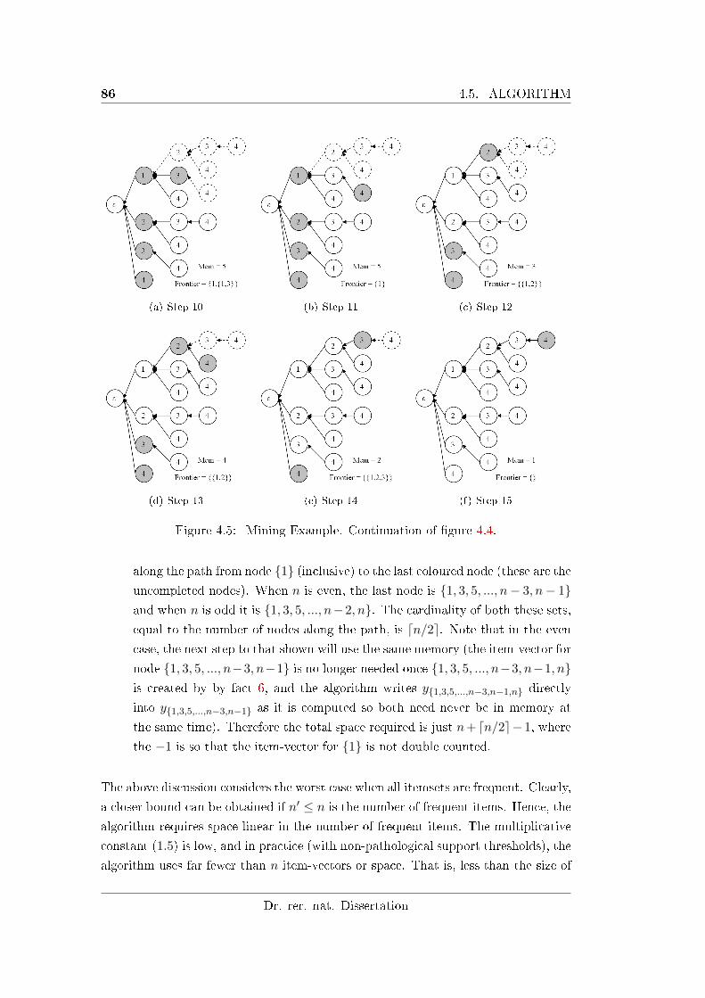
86 4.5. ALGORITHM
(a) Step 10 (b) Step 11 (c) Step 12
(d) Step 13 (e) Step 14 (f) Step 15
Figure 4.5: Mining Example. Continuation of �gure 4.4.
along the path from node {1} (inclusive) to the last coloured node (these are theuncompleted nodes). When n is even, the last node is {1, 3, 5, ..., n− 3, n− 1}and when n is odd it is {1, 3, 5, ..., n−2, n}. The cardinality of both these sets,
equal to the number of nodes along the path, is dn/2e. Note that in the even
case, the next step to that shown will use the same memory (the item-vector for
node {1, 3, 5, ..., n−3, n−1} is no longer needed once {1, 3, 5, ..., n−3, n−1, n}is created by by fact 6, and the algorithm writes y{1,3,5,...,n−3,n−1,n} directly
into y{1,3,5,...,n−3,n−1} as it is computed so both need never be in memory at
the same time). Therefore the total space required is just n+ dn/2e−1, where
the −1 is so that the item-vector for {1} is not double counted.
The above discussion considers the worst case when all itemsets are frequent. Clearly,
a closer bound can be obtained if n′ ≤ n is the number of frequent items. Hence, the
algorithm requires space linear in the number of frequent items. The multiplicative
constant (1.5) is low, and in practice (with non-pathological support thresholds), the
algorithm uses far fewer than n item-vectors or space. That is, less than the size of
Dr. rer. nat. Dissertation
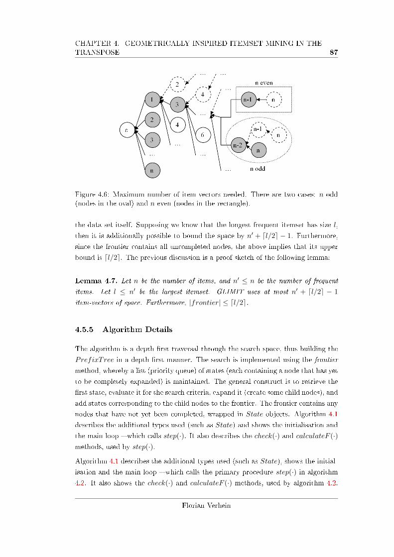
CHAPTER 4. GEOMETRICALLY INSPIRED ITEMSET MINING IN THETRANSPOSE 87
Figure 4.6: Maximum number of item-vectors needed. There are two cases: n odd(nodes in the oval) and n even (nodes in the rectangle).
the data set itself. Supposing we know that the longest frequent itemset has size l,
then it is additionally possible to bound the space by n′ + dl/2e − 1. Furthermore,
since the frontier contains all uncompleted nodes, the above implies that its upper
bound is dl/2e. The previous discussion is a proof sketch of the following lemma:
Lemma 4.7. Let n be the number of items, and n′ ≤ n be the number of frequent
items. Let l ≤ n′ be the largest itemset. GLIMIT uses at most n′ + dl/2e − 1
item-vectors of space. Furthermore, |frontier| ≤ dl/2e.
4.5.5 Algorithm Details
The algorithm is a depth �rst traversal through the search space, thus building the
PrefixTree in a depth �rst manner. The search is implemented using the frontier
method, whereby a list (priority queue) of states (each containing a node that has yet
to be completely expanded) is maintained. The general construct is to retrieve the
�rst state, evaluate it for the search criteria, expand it (create some child nodes), and
add states corresponding to the child nodes to the frontier. The frontier contains any
nodes that have not yet been completed, wrapped in State objects. Algorithm 4.1
describes the additional types used (such as State) and shows the initialisation and
the main loop � which calls step(·). It also describes the check(·) and calculateF (·)methods, used by step(·).
Algorithm 4.1 describes the additional types used (such as State), shows the initial-
isation and the main loop � which calls the primary procedure step(·) in algorithm
4.2. It also shows the check(·) and calculateF (·) methods, used by algorithm 4.2.
Florian Verhein
88 4.6. MINING ASSOCIATION RULES
The pseudo-code is java-like, a garbage collector is assumed which simpli�es it, in-
dentation de�nes blocks and type casts are ignored.
Let α be the itemset of length k represented at node node (assuming node is not
the root). node.item is the last element of α. The check(node, item) method in
algorithm 4.1 checks whether α ∪ {item} can be frequent � in the sense that all its
subsets have already been found to be frequent. This is true if and only if all subsets
of size k are frequent. Note that it is already known that α and (α−{node.item()})∪{item} (the itemset of the sibling of node) are frequent. Hence the method must
just check the other
(k + 1
k
)− 2 subsets. It does this by �rst traversing from
node back toward the root to obtain the itemset, and then looking up the subsets
in the SequenceMap to see if the corresponding Pre�xNode exists. By the bottom
up construction, all the required subsets have already been generated and added to
the SequenceMap (HashTree) using hashtree.add(node). It should be noted that the
correctness does not depend on check() being called. Indeed, check() can do nothing
and the correct results will still be delivered. This decision is a trade o� between
checking if subsets exist or calculating the vectors for new sets. In other words, it is
a heuristic.
It has been explicitly shown when extra item-vectors are required (allocated) and
when they are deleted through the use of the global variable totalMem that tracks the
amount of item-vectors of space needed. Note that the algorithm prepares buffer for
all the subsequent calls to step(·). Normally (when it.hasNext()), buffer cannot
be modi�ed by the receiving method as it is required again for subsequent calls.
However, then it has progressed to the 'top' of the list of siblings (it.hasNext() =
false), the receiving method can modify buffer � and will e�ectively `steal' the
item-vectors from it to reuse (reducing the size of buffer). From then on it will
be responsible for decrementing totalMem when these 'stolen' item-vectors are no
longer used. This explains the last line of the algorithm.
Finally, a few minor points: If node is the root, the algorithm is has not been
called from itself and so has not already put the item-vectors over which it iterates
in memory. Hence the memory required to read from �le must be counted. Also,
it.remove() is ignored if the Iterator is reading from �le.
4.6 Mining Association Rules
This section describes how association rules can be generated very e�ciently. Algo-
rithm 4.3 presents the method, and the following lemma describes it and proves its
Dr. rer. nat. Dissertation
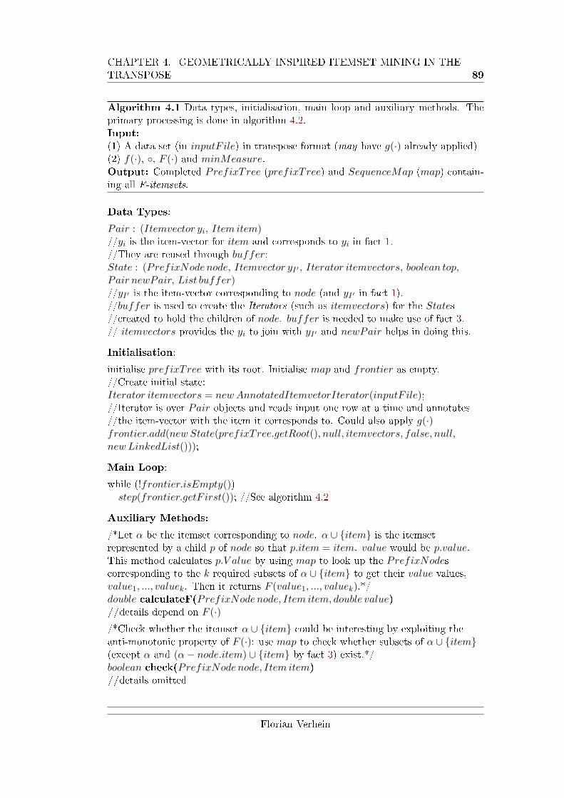
CHAPTER 4. GEOMETRICALLY INSPIRED ITEMSET MINING IN THETRANSPOSE 89
Algorithm 4.1 Data types, initialisation, main loop and auxiliary methods. Theprimary processing is done in algorithm 4.2.Input:(1) A data set (in inputF ile) in transpose format (may have g(·) already applied)(2) f(·), ◦, F (·) and minMeasure.Output: Completed PrefixTree (prefixTree) and SequenceMap (map) contain-ing all F-itemsets.
Data Types:
Pair : (Itemvector yi, Item item)//yi is the item-vector for item and corresponds to yi in fact 1.//They are reused through buffer:State : (PrefixNode node, Itemvector yI′ , Iterator itemvectors, boolean top,Pair newPair, List buffer)//yI′ is the item-vector corresponding to node (and yI′ in fact 1).//buffer is used to create the Iterators (such as itemvectors) for the States//created to hold the children of node. buffer is needed to make use of fact 3.// itemvectors provides the yi to join with yI′ and newPair helps in doing this.
Initialisation:
initialise prefixTree with its root. Initialise map and frontier as empty.//Create initial state:Iterator itemvectors = newAnnotatedItemvetorIterator(inputF ile);//Iterator is over Pair objects and reads input one row at a time and annotates//the item-vector with the item it corresponds to. Could also apply g(·)frontier.add(new State(prefixTree.getRoot(), null, itemvectors, false, null,new LinkedList()));
Main Loop:
while (!frontier.isEmpty())step(frontier.getF irst()); //See algorithm 4.2
Auxiliary Methods:
/*Let α be the itemset corresponding to node. α ∪ {item} is the itemsetrepresented by a child p of node so that p.item = item. value would be p.value.This method calculates p.V alue by using map to look up the PrefixNodescorresponding to the k required subsets of α ∪ {item} to get their value values,value1, ..., valuek. Then it returns F (value1, ..., valuek).*/double calculateF(PrefixNode node, Item item, double value)//details depend on F (·)/*Check whether the itemset α ∪ {item} could be interesting by exploiting theanti-monotonic property of F (·): use map to check whether subsets of α ∪ {item}(except α and (α− node.item) ∪ {item} by fact 3) exist.*/boolean check(PrefixNode node, Item item)//details omitted
Florian Verhein
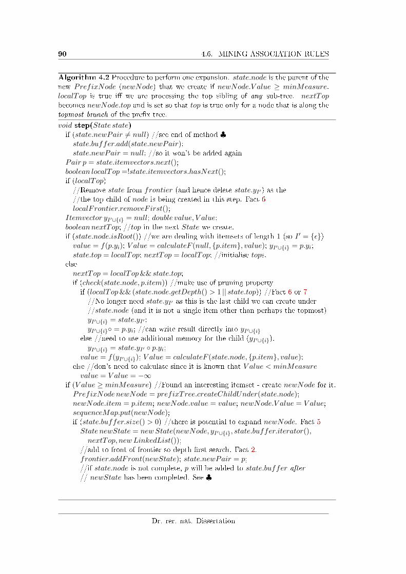
90 4.6. MINING ASSOCIATION RULES
Algorithm 4.2 Procedure to perform one expansion. state.node is the parent of thenew PrefixNode (newNode) that we create if newNode.V alue ≥ minMeasure.localTop is true i� we are processing the top sibling of any sub-tree. nextTopbecomes newNode.top and is set so that top is true only for a node that is along thetopmost branch of the pre�x tree.
void step(State state)if (state.newPair 6= null) //see end of method ♣state.buffer.add(state.newPair);state.newPair = null; //so it won't be added again
Pair p = state.itemvectors.next();boolean localTop =!state.itemvectors.hasNext();if (localTop)//Remove state from frontier (and hence delete state.yI′) as the//the top child of node is being created in this step. Fact 6localFrontier.removeF irst();
Itemvector yI′∪{i} = null; double value, V alue;
booleannextTop; //top in the next State we create.if (state.node.isRoot()) //we are dealing with itemsets of length 1 (so I ′ = {ε})value = f(p.yi); V alue = calculateF (null, {p.item}, value); yI′∪{i} = p.yi;
state.top = localTop; nextTop = localTop; //initialise tops.elsenextTop = localTop&& state.top;if (check(state.node, p.item)) //make use of pruning propertyif (localTop&& (state.node.getDepth() > 1 || state.top)) //Fact 6 or 7//No longer need state.yI′ as this is the last child we can create under//state.node (and it is not a single item other than perhaps the topmost)yI′∪{i} = state.yI′ ;
yI′∪{i}◦ = p.yi; //can write result directly into yI′∪{i}else //need to use additional memory for the child (yI′∪{i}).
yI′∪{i} = state.yI′ ◦ p.yi;value = f(yI′∪{i}); V alue = calculateF (state.node, {p.item}, value);
else //don't need to calculate since it is known that V alue < minMeasurevalue = V alue = −∞
if (V alue ≥ minMeasure) //Found an interesting itemset - create newNode for it.PrefixNode newNode = prefixTree.createChildUnder(state.node);newNode.item = p.item; newNode.value = value; newNode.V alue = V alue;sequenceMap.put(newNode);if (state.buffer.size() > 0) //there is potential to expand newNode. Fact 5State newState = new State(newNode, yI′∪{i}, state.buffer.iterator(),
nextTop, new LinkedList());//add to front of frontier so depth �rst search. Fact 2.frontier.addFront(newState); state.newPair = p;//if state.node is not complete, p will be added to state.buffer after// newState has been completed. See ♣
Dr. rer. nat. Dissertation
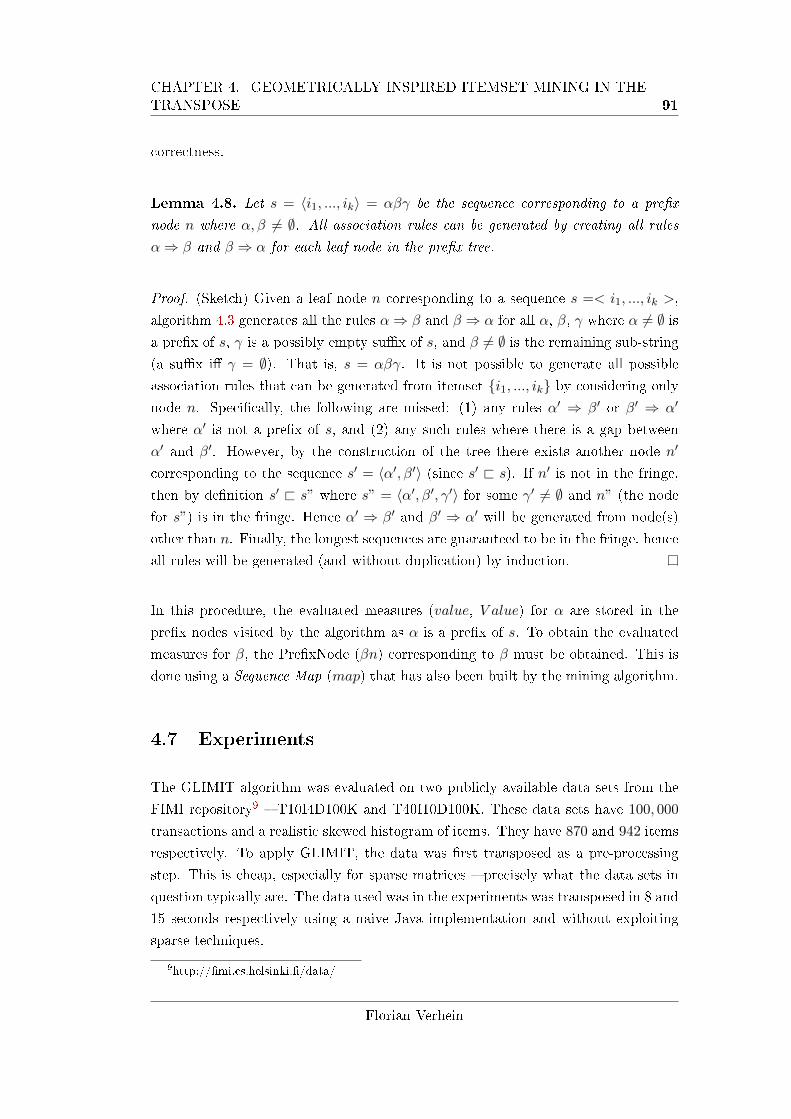
CHAPTER 4. GEOMETRICALLY INSPIRED ITEMSET MINING IN THETRANSPOSE 91
correctness.
Lemma 4.8. Let s = 〈i1, ..., ik〉 = αβγ be the sequence corresponding to a pre�x
node n where α, β 6= ∅. All association rules can be generated by creating all rules
α⇒ β and β ⇒ α for each leaf node in the pre�x tree.
Proof. (Sketch) Given a leaf node n corresponding to a sequence s =< i1, ..., ik >,
algorithm 4.3 generates all the rules α⇒ β and β ⇒ α for all α, β, γ where α 6= ∅ isa pre�x of s, γ is a possibly empty su�x of s, and β 6= ∅ is the remaining sub-string
(a su�x i� γ = ∅). That is, s = αβγ. It is not possible to generate all possible
association rules that can be generated from itemset {i1, ..., ik} by considering only
node n. Speci�cally, the following are missed: (1) any rules α′ ⇒ β′ or β′ ⇒ α′
where α′ is not a pre�x of s, and (2) any such rules where there is a gap between
α′ and β′. However, by the construction of the tree there exists another node n′
corresponding to the sequence s′ = 〈α′, β′〉 (since s′ @ s). If n′ is not in the fringe,
then by de�nition s′ @ s” where s” = 〈α′, β′, γ′〉 for some γ′ 6= ∅ and n” (the node
for s”) is in the fringe. Hence α′ ⇒ β′ and β′ ⇒ α′ will be generated from node(s)
other than n. Finally, the longest sequences are guaranteed to be in the fringe, hence
all rules will be generated (and without duplication) by induction.
In this procedure, the evaluated measures (value, V alue) for α are stored in the
pre�x nodes visited by the algorithm as α is a pre�x of s. To obtain the evaluated
measures for β, the Pre�xNode (βn) corresponding to β must be obtained. This is
done using a Sequence Map (map) that has also been built by the mining algorithm.
4.7 Experiments
The GLIMIT algorithm was evaluated on two publicly available data sets from the
FIMI repository9 � T10I4D100K and T40I10D100K. These data sets have 100, 000
transactions and a realistic skewed histogram of items. They have 870 and 942 items
respectively. To apply GLIMIT, the data was �rst transposed as a pre-processing
step. This is cheap, especially for sparse matrices � precisely what the data sets in
question typically are. The data used was in the experiments was transposed in 8 and
15 seconds respectively using a naive Java implementation and without exploiting
sparse techniques.
9http://�mi.cs.helsinki.�/data/
Florian Verhein
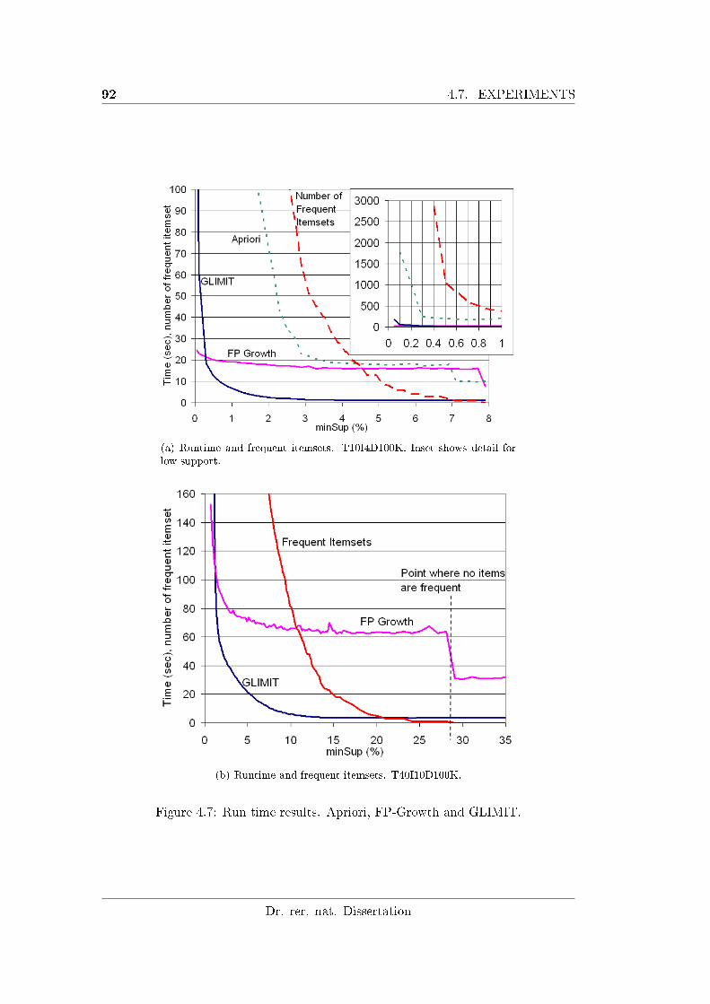
92 4.7. EXPERIMENTS
(a) Runtime and frequent itemsets. T10I4D100K. Inset shows detail forlow support.
(b) Runtime and frequent itemsets. T40I10D100K.
Figure 4.7: Run time results. Apriori, FP-Growth and GLIMIT.
Dr. rer. nat. Dissertation
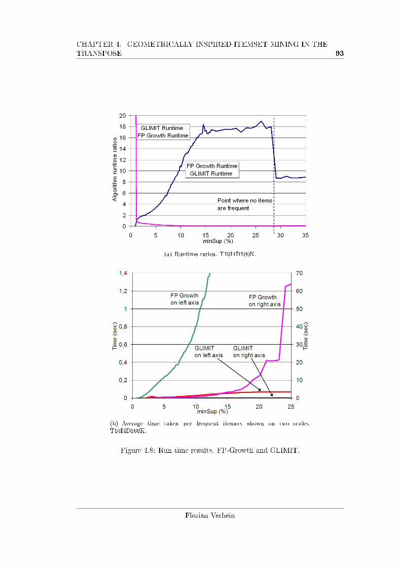
CHAPTER 4. GEOMETRICALLY INSPIRED ITEMSET MINING IN THETRANSPOSE 93
(a) Runtime ratios. T10I4D100K.
(b) Average time taken per frequent itemset shown on two scales.T10I4D100K.
Figure 4.8: Run time results. FP-Growth and GLIMIT.
Florian Verhein
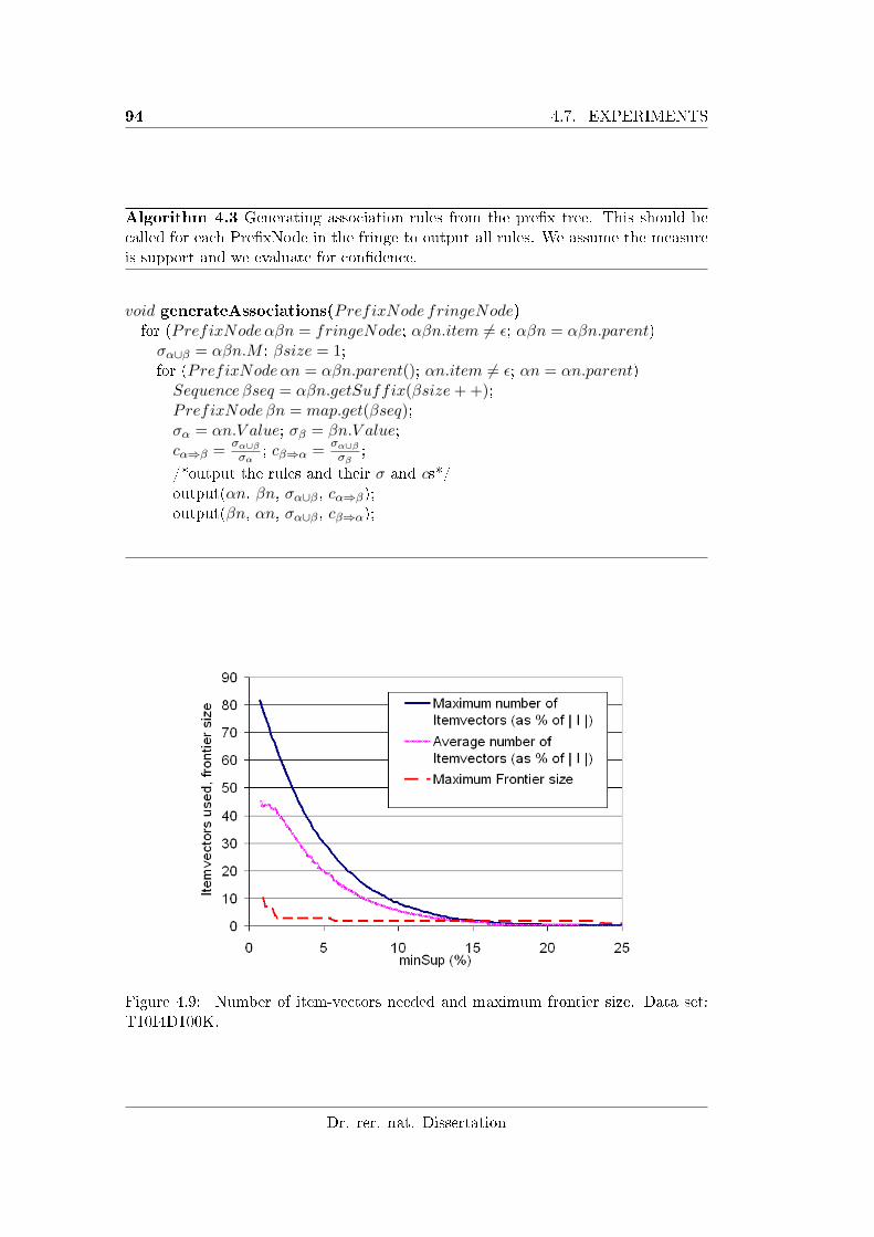
94 4.7. EXPERIMENTS
Algorithm 4.3 Generating association rules from the pre�x tree. This should becalled for each Pre�xNode in the fringe to output all rules. We assume the measureis support and we evaluate for con�dence.
void generateAssociations(PrefixNode fringeNode)for (PrefixNodeαβn = fringeNode; αβn.item 6= ε; αβn = αβn.parent)σα∪β = αβn.M ; βsize = 1;for (PrefixNodeαn = αβn.parent(); αn.item 6= ε; αn = αn.parent)Sequence βseq = αβn.getSuffix(βsize+ +);PrefixNode βn = map.get(βseq);σα = αn.V alue; σβ = βn.V alue;cα⇒β =
σα∪βσα
; cβ⇒α =σα∪βσβ
;
/*output the rules and their σ and cs*/output(αn, βn, σα∪β , cα⇒β);output(βn, αn, σα∪β , cβ⇒α);
Figure 4.9: Number of item-vectors needed and maximum frontier size. Data set:T10I4D100K.
Dr. rer. nat. Dissertation
CHAPTER 4. GEOMETRICALLY INSPIRED ITEMSET MINING IN THETRANSPOSE 95
GLIMIT was compared to a publicly available implementation of FP-Growth and
Apriori. The algorithms used were from ARtool10 as it is also written in Java and
has been available for some time. The algorithms were not used via the supplied
GUI, but rather the underlying classes were invoked directly to avoid overheads.
The primary goal of this section is to show that GLIMIT is fast and e�cient when
compared to existing algorithms on the traditional FIM problem. Recall that a
major contribution of this chapter however is the item-vector framework that allows
operations that previously could not be considered, and a �exible and new class of
algorithm that uses this framework to e�ciently mine data cast into di�erent and
useful spaces. The fact that it is also very fast when applied to traditional FIM is a
consequence of this. To represent item-vectors for traditional FIM, bit-vectors were
used11 so that each bit is set if the corresponding transaction contains the item(set).
Therefore g creates the bit-vector, ◦ = AND, f(·) = sum(·) and F (m) = m.
Figure 4.7(a) shows the run time12 of FP-Growth, GLIMIT and Apriori13 on T10I4D100K,
as well as the number of frequent items. The analogous graph for T40I10D100K is
shown in �gure 4.7(b). Apriori was not run in this experiment as it is too slow. These
graphs clearly show that when the support threshold is below a small value (about
0.29% and 1.2% for the respective data sets), FP-Growth is superior to GLIMIT.
However, above this threshold GLIMIT outperforms FP-Growth signi�cantly. Figure
4.8(a) shows this more explicitly by presenting the run time ratios for T40I10D100K.
FP-Growth takes at worst 19 times as long as GLIMIT. These results indicate that
GLIMIT is superior above a threshold. Furthermore, this threshold is very small and
practical applications usually mine with much larger thresholds than these.
GLIMIT scales roughly linearly in the number of frequent itemsets. Figure 4.8(b)
demonstrates this experimentally by showing the average time to mine a single fre-
quent itemset. The value for GLIMIT is quite stable, rising slowly toward the end
(as in these cases GLIMIT must still check itemsets, but very few of them turn out
to be frequent). FP-Growth on the other hand, clearly does not scale linearly. The
reason behind these di�erences is that FP-Growth �rst builds an FP-tree. This ef-
fectively stores the entire Data set (minus infrequent single items) in memory. The
FP-tree is also highly cross-referenced so that searches are fast. The downside is that
this takes signi�cant time and a lot of space. This pays o� extremely well when the
support threshold is very low, as the frequent itemsets can read from the tree very
10http://www.cs.umb.edu/ laur/ARtool/.11The Colt (http://dsd.lbl.gov/~hoschek/colt/) BitVector implementation was used.12Pentium 4, 2.4GHz with 1GB RAM running WindowsXP Pro.13Apriori was not run for extremely low support as it took longer than 30 minutes for minSup ≤
0.1%
Florian Verhein
96 4.8. CONCLUSION AND FUTURE WORK
quickly. However, when minSup is larger, much of the time and space is wasted.
GLIMIT uses time and space as needed, so it does not waste as many resources,
making it fast. The downside is that the operations on bit-vectors (in our experi-
ments, of length 100, 000) can be time consuming when compared to the search on
the FP-tree, which is why GLIMIT cannot keep up when minSup is very small.
Figure 4.9 shows the maximum and average14 number of item vectors our algorithm
uses as a percentage of the number of items. At worst, this can be interpreted as the
percentage of the data set in memory. Although the worst case space is 1.5 times
the number of items, n (lemma 4.7), the �gure clearly shows this is never reached in
these experiments. The maximum was approximately 0.82n. By the time it were to
get close to 1.5n, minSup would be so small that the run time would be unfeasibly
large anyhow. Furthermore, the space required drops quite quickly as minSup is
increased (and hence the number of frequent items decreases). Figure 4.9 also shows
that the maximum frontier size is very small. (recall from lemma 4.7 it is bounded
above by dl/2e. Finally, recall that the algorithm can avoid using the pre�x tree and
sequence map on the FIM problem, so the only space required are the item vectors
and the frontier. That is, the space required is truly linear.
4.8 Conclusion and Future Work
This chapter showed interesting consequences of viewing transaction data as item-
vectors in transaction-space and developed a framework for operating on item-vectors.
This abstraction gives great �exibility in the measures used and opens up the poten-
tial for useful transformations on the data. Future work may involve �nding useful
geometric measures and transformations for itemset mining. One particular problem
of interest is to �nd a way to use SVD prior to mining for itemsets larger than 2.
This chapter also presented GLIMIT, a novel algorithm that uses the framework
and signi�cantly departs from existing algorithms. GLIMIT mines itemsets in one
pass without candidate generation, in linear space and time linear in the number
of interesting itemsets. Experiments showed that it beats FP-Growth above small
support thresholds and is always faster than Apriori.
14over the calls to step(·).
Dr. rer. nat. Dissertation
Chapter 5
Fast Mining of Complex Spatial
Co-location Patterns
Most algorithms for mining interesting spatial co-locations integrate the co-
location / clique generation task with the interesting pattern mining task
and are usually based on the Apriori algorithm. This has two downsides:
First, it makes it di�cult to meaningfully include certain types of complex
relationships � especially negative relationships � in the patterns. Secondly,
the Apriori algorithm is slow.
This work mines complex co-location relationships between object types; a
special type of interaction between variables. It considers maximal cliques of
galaxies in an astronomy dataset which are used to extract complex maximal
cliques. These are subsequently mined for interesting sets of object (galaxy)
types, including complex types such as absence and multiple occurences. It
is shown that the GLIMIT itemset mining algorithm can be applied to this
problem, leading to far superior performance than using an Apriori style
approach.
The problem may be solved directly using the GIM framework.
97
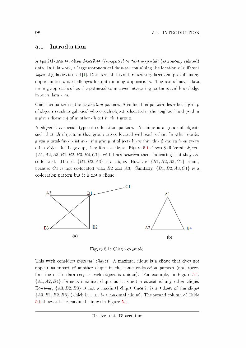
98 5.1. INTRODUCTION
5.1 Introduction
A spatial data set often describes Geo-spatial or �Astro-spatial� (astronomy related)
data. In this work, a large astronomical data-set containing the location of di�erent
types of galaxies is used [1]. Data sets of this nature are very large and provide many
opportunities and challenges for data mining applications. The use of novel data
mining approaches has the potential to uncover interesting patterns and knowledge
in such data sets.
One such pattern is the co-location pattern. A co-location pattern describes a group
of objects (such as galaxies) where each object is located in the neighborhood (within
a given distance) of another object in that group.
A clique is a special type of co-location pattern. A clique is a group of objects
such that all objects in that group are co-located with each other. In other words,
given a prede�ned distance, if a group of objects lie within this distance from every
other object in the group, they form a clique. Figure 5.1 shows 8 di�erent objects
{A1, A2, A3, B1, B2, B3, B4, C1}, with lines between them indicating that they are
co-located. The set {B1, B2, A3} is a clique. However, {B1, B2, A3, C1} is not,
because C1 is not co-located with B2 and A3. Similarly, {B1, B2, A3, C1} is a
co-location pattern but it is not a clique.
Figure 5.1: Clique example.
This work considers maximal cliques. A maximal clique is a clique that does not
appear as subset of another clique in the same co-location pattern (and there-
fore the entire data set, as each object is unique). For example, in Figure 5.1,
{A1, A2, B4} forms a maximal clique as it is not a subset of any other clique.
However, {A3, B2, B3} is not a maximal clique since it is a subset of the clique
{A3, B1, B2, B3} (which in turn is a maximal clique). The second column of Table
5.1 shows all the maximal cliques in Figure 5.1.
Dr. rer. nat. Dissertation
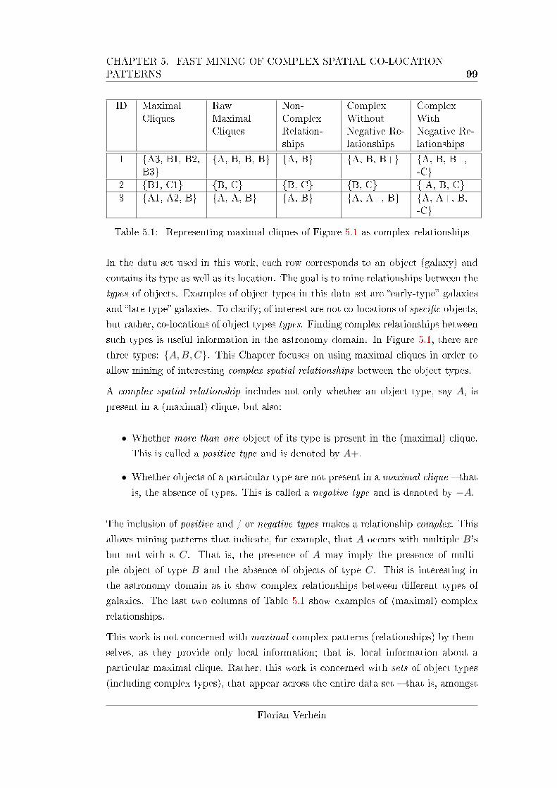
CHAPTER 5. FAST MINING OF COMPLEX SPATIAL CO-LOCATIONPATTERNS 99
ID MaximalCliques
RawMaximalCliques
Non-ComplexRelation-ships
ComplexWithoutNegative Re-lationships
ComplexWithNegative Re-lationships
1 {A3, B1, B2,B3}
{A, B, B, B} {A, B} {A, B, B+} {A, B, B+,-C}
2 {B1, C1} {B, C} {B, C} {B, C} {-A, B, C}
3 {A1, A2, B} {A, A, B} {A, B} {A, A+, B} {A, A+, B,-C}
Table 5.1: Representing maximal cliques of Figure 5.1 as complex relationships
In the data set used in this work, each row corresponds to an object (galaxy) and
contains its type as well as its location. The goal is to mine relationships between the
types of objects. Examples of object types in this data set are �early-type� galaxies
and �late-type� galaxies. To clarify; of interest are not co-locations of speci�c objects,
but rather, co-locations of object types types. Finding complex relationships between
such types is useful information in the astronomy domain. In Figure 5.1, there are
three types: {A,B,C}. This Chapter focuses on using maximal cliques in order to
allow mining of interesting complex spatial relationships between the object types.
A complex spatial relationship includes not only whether an object type, say A, is
present in a (maximal) clique, but also:
• Whether more than one object of its type is present in the (maximal) clique.
This is called a positive type and is denoted by A+.
• Whether objects of a particular type are not present in a maximal clique � that
is, the absence of types. This is called a negative type and is denoted by −A.
The inclusion of positive and / or negative types makes a relationship complex. This
allows mining patterns that indicate, for example, that A occurs with multiple B's
but not with a C. That is, the presence of A may imply the presence of multi-
ple object of type B and the absence of objects of type C. This is interesting in
the astronomy domain as it show complex relationships between di�erent types of
galaxies. The last two columns of Table 5.1 show examples of (maximal) complex
relationships.
This work is not concerned with maximal complex patterns (relationships) by them-
selves, as they provide only local information; that is, local information about a
particular maximal clique. Rather, this work is concerned with sets of object types
(including complex types), that appear across the entire data set � that is, amongst
Florian Verhein
100 5.1. INTRODUCTION
many maximal cliques. In other words, the goal is to �nd interesting complex spatial
relationships (sets), where �interesting� is de�ned by a global measure. Returning
to the astronomy data set, this means patterns will be found showing complex rela-
tionships between galaxy types that reoccur throughout the data set.
The global measure of interestingness used in this work is a variation of the minPI
[80] measure:
(5.1) minPI(P ) = mint∈P{N(P )/N({t})}
Here, P is a set of complex types being evaluated and N(·) is the number of maximal
cliques that contain the set of complex types. Note that the occurrences of the
pattern (set of complex types) are counted only in the maximal cliques. This means
that if the minPI of a pattern is above α, then it is possible to say that whenever
any type t ∈ P occurs in a maximal clique, the entire pattern P will occur in at least
a fraction alpha of those maximal cliques. minPI is superior to simply using N(P )
because it scales by the occurrences of the individual object types, thus reducing
the impact of a non-uniform distribution on the object types. This is important, as
otherwise those object types that occur frequently dominate the results.
This work focuses on maximal cliques for the following reasons:
• The process of forming complex positive relationships only makes sense in
maximal cliques. Suppose we extract a clique that is not maximal, such as
{A1, B4} from Figure 5.1. We would not generate the positive relationship
{A+, B} from this, even though each of {A1, B4} are co-located with {A2}.The correct pattern emerges only once maximal cliques are considered.
• Negative relationships are possible. For example, consider the maximal clique
in row 1 of Table 5.1. If maximal cliques were not used, then we would also con-
sider {B1, B2, B3}, and from this we would incorrectly infer that the complex
relationship {B,B+,−A} exists. However, this is not true because A is co-
located with each of {B1, B2, B3}. Therefore, using non-maximal cliques will
generate incorrect negative patterns because negative types cannot be inferred
until the maximum clique is mined.
• Each maximal clique will be considered as a single instance (transaction) for
the purposes of counting. In other words, using maximal cliques automatically
avoids counting the same objects within a maximal clique multiple times.
Dr. rer. nat. Dissertation
CHAPTER 5. FAST MINING OF COMPLEX SPATIAL CO-LOCATIONPATTERNS 101
• Using maximal cliques reduces the total number of cliques by removing all
redundancy. So not only does this lead to better quality results as outlined
above, but it also reduces the computational cost of the subsequent mining
process. Furthermore, since it is possible to mine maximal cliques directly
without �rst considering all sub-cliques, this leads to a further computational
advantage.
5.1.1 Problem Statement
Problem Statement: Given the set of maximal cliques, �nd all interesting and
complex patterns that occur amongst that set of maximal cliques. More speci�cally,
�nd all sets of object types, including positive and negative (complex) types that
have a minPI above a user de�ned threshold.
It will be shown that this problem can be mapped to an itemset mining task with
minPI used as an interestingness measure. In order to solve it very quickly, the
GLIMIT algorithm of Chapter 4 is applied, as will be described in Section 5.5.
Including negative types makes the problem much more di�cult, as it is typical for
spatial data to be sparse. This means that the absence of a type amongst maximal
cliques is very common. This is analogous to having a very large transaction width in
frequent itemset mining, which is known to be very challenging for mining algorithms.
In contrast to standard approaches relying on an Apriori style algorithm that �nd this
very di�cult, it will be shown that this is not a problem for the approach described
in this Chapter.
5.1.2 Contributions
This Chapter makes the following contributions:
• It introduces maximal cliques and describes how they make more sense than
simply using cliques in co-location mining. Furthermore, it is shown that they
allow the use of negative patterns.
• A general and modular Knowledge Discovery in Databases (KDD) process is
introduced that splits the maximal clique generation, complex pattern extrac-
tion and interesting pattern mining tasks into independent components.
• It shows that GLIMIT can be used to mine complex, interesting co-location
patterns very e�ciently in very large real world data sets. Indeed, it is demon-
Florian Verhein
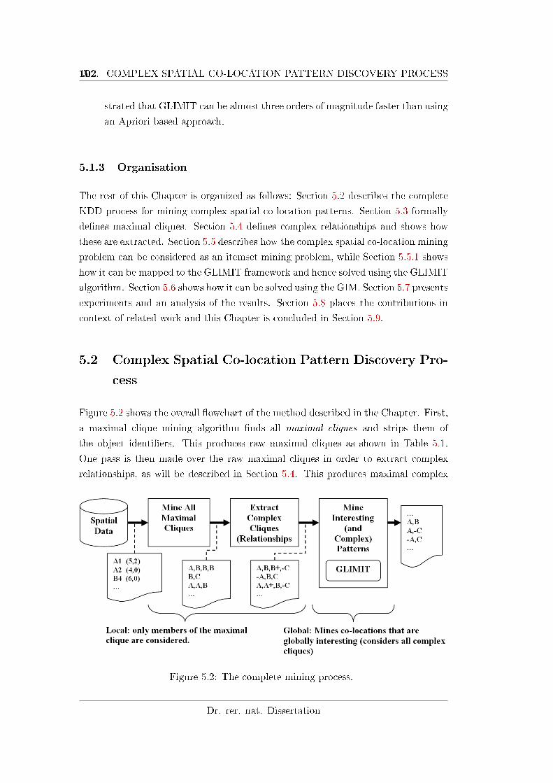
1025.2. COMPLEX SPATIAL CO-LOCATION PATTERN DISCOVERY PROCESS
strated that GLIMIT can be almost three orders of magnitude faster than using
an Apriori based approach.
5.1.3 Organisation
The rest of this Chapter is organized as follows: Section 5.2 describes the complete
KDD process for mining complex spatial co-location patterns. Section 5.3 formally
de�nes maximal cliques. Section 5.4 de�nes complex relationships and shows how
these are extracted. Section 5.5 describes how the complex spatial co-location mining
problem can be considered as an itemset mining problem, while Section 5.5.1 shows
how it can be mapped to the GLIMIT framework and hence solved using the GLIMIT
algorithm. Section 5.6 shows how it can be solved using the GIM. Section 5.7 presents
experiments and an analysis of the results. Section 5.8 places the contributions in
context of related work and this Chapter is concluded in Section 5.9.
5.2 Complex Spatial Co-location Pattern Discovery Pro-
cess
Figure 5.2 shows the overall �owchart of the method described in the Chapter. First,
a maximal clique mining algorithm �nds all maximal cliques and strips them of
the object identi�ers. This produces raw maximal cliques as shown in Table 5.1.
One pass is then made over the raw maximal cliques in order to extract complex
relationships, as will be described in Section 5.4. This produces maximal complex
Figure 5.2: The complete mining process.
Dr. rer. nat. Dissertation
CHAPTER 5. FAST MINING OF COMPLEX SPATIAL CO-LOCATIONPATTERNS 103
cliques. Each of these complex, maximal cliques is then considered as a transaction,
and an interesting itemset mining algorithm, using minPI as the interestingness
measure, is used to extract the interesting complex relationships. This is described
in Sections 5.5 and 5.5.1.
As shown in Figure 5.2, the clique generation and complex relationship extraction are
local procedures, in the sense that they deal only with individual maximal cliques.
In contrast, the interesting pattern mining is global � it �nds patterns that occur
across the entire space. Secondly, subsets of maximal cliques are only considered in
the last step � that is, after the complex patterns have been extracted.
5.3 Maximal Cliques
Consider a set of objects O with �xed locations. Given an appropriate distance
measure d : O×O → R, de�ne a graph G as follows; let O be the set of vertices and
construct an edge between two objects o1 ∈ O and o2 ∈ O if d(o1, o2) ≤ τ , where τ
is a chosen distance.
De�nition 5.1. A co-location pattern is a connected sub graph in G.
De�nition 5.2. A clique C ∈ O is any fully connected sub graph of G. That is,
d(o1, o2) ≤ τ ∀{o1, o2} ∈ C × C.
As was mentioned in Section 5.1, maximal cliques are used in this work so that
complex patterns can be meaningfully de�ned and used, and to avoid double counting
which would heavily skew the results towards large cliques.
De�nition 5.3. A maximal clique CM is a clique that is not a subset (sub-graph)
of any other clique.
The mining of maximal cliques is done directly � it does not require mining all sub-
cliques �rst in an enumeration style approach. The maximal clique mining algorithm
is described in [12].
5.4 Extracting Complex Relationships
A relationship is called complex if it consists of complex types as de�ned in Section
5.1.
Florian Verhein
104 5.5. MINING INTERESTING COMPLEX RELATIONSHIPS
Extracting a complex relationship R from a maximal clique CM involves using the
following rules for every type t:
1. If CM contains an object with type t, R = R ∪ t.
2. If CM contains more than one object of type t, R = R ∪ t+.
3. If CM does not contain an object of type t, R = R ∪ −t.
Note that if R includes a positive type A+, it will also always include the basic
type A. This is necessary so that maximal cliques that contain A+ will also be
counted as containing A when they are mined for interesting patterns. Recall that
the negative type only makes sense if maximal cliques are used. The last three
columns of Table 5.1 show the result of applying Rule 1, Rule 1 and then Rule 2,
and all three rules, respectively.
5.5 Mining Interesting Complex Relationships
The complex relationships considered in this chapter are speci�c types of interac-
tions between variables, and hence can be solved using the GIM framework and
algorithm. At the time this work was performed, GIM had not been developed.
Instead, the problem is mapped to itemset mining. Solving the problem directly in
GIM is described in section 5.6.
In itemset mining, the data set consists of a set of transactions T , where each trans-
action t ∈ T is a subset of a set of items I; that is, t ⊆ I. In order to map complex
spatial co-location mining to the itemset mining task, the set of complex maximal
cliques (relationships) become the set of transactions T . The items are the object
types � including the complex types such as A+ and −A. For example, if the object
types are {A,B,C}, and each of these types is present and absent in at least one
maximal clique, then I = {A,A+,−A,B,B+,−B}. An interesting itemset mining
algorithm mines T for interesting itemsets. The support of an itemset I ′ ⊆ I is the
number of transactions containing the itemset: support(I ′) = |{t ∈ T : I ′ ⊆ t}|. Socalled frequent itemset mining uses the support as the measure of interestingness.
For reasons described in Section 5.1, this work uses minPI (see Equation 5.1) which,
under the mapping described above, is equivalent to
(5.2) minPI(I ′) = mini∈I′{support(I ′)/support({i})}
Dr. rer. nat. Dissertation
CHAPTER 5. FAST MINING OF COMPLEX SPATIAL CO-LOCATIONPATTERNS 105
Since minPI is anti-monotonic, the search space for interesting patterns can easily
be pruned.
5.5.1 Mapping the Problem to GLIMIT
Recall from Chapter 4 that GLIMIT is a fast and e�cient itemset mining algorithm
that has been shown to outperform Apriori [11] and FP-Growth [47]. Since it is based
on a framework of functions (Section 4.4), new measures can easily be incorporated.
In particular, the minPI measure can be build on top of the frequent itemset mining
approach: Recall from example 4.4 on page 79 that it can be incorporated into
GLIMIT as follows (let I ′ = {1, 2, ..., q} for simplicity): g(·) is the identity function
(there is no transformation on the data set), ◦ = ∩ (intersection) and f(·) = | · |(the set size). Let mI′ be the result computed by f(·) on the itemset I ′. This means
that mI′ = support(I ′), as is the case for FIM. To evaluate minPI, F (·) is used:
F (mI′ ,m1, ...,mq) = mini∈I′{mI′/mi}.
GLIMIT is used with the above instantiations of its framework to mine interesting
complex co-locations, as shown in Figure 5.2. For comparison, an Apriori [11] style
implementation will be used in the experiments.
The Apriori [11] and Apriori-like algorithms are bottom up item enumeration type
itemset mining algorithms. Apriori works in a breadth �rst fashion, making one pass
over the data set for each level expanded. This is in contrast to GLIMIT, which
makes only one pass over the entire data set. In Apriori, a candidate generation step
generates candidate itemsets (itemsets that may be interesting) for the next level,
followed by a data set pass (support counting) where each candidate itemset is either
con�rmed as interesting, or discarded. The support counting step is computationally
intensive as subsets of the transactions need to be generated. This is particularly
problematic when the transaction width is large, as is the case for spatial co-location
data that includes complex relationships. GLIMIT operates on completely di�erent
principles and does not have these drawbacks.
It is also worth noting that since all single itemsets are always interesting (by def-
inition, their minPI has the maximum value of 1), they cannot be discarded from
the search. Note that were an FP-Growth style algorithm developed for this mining
task, it would need to build an FP-Tree for the entire data set without any pruning.
Hence, it is not a practical choice for this problem.
Florian Verhein
106 5.6. MAPPING THE PROBLEM TO GIM
5.6 Mapping the Problem to GIM
GIM is more abstract than GLIMIT (which focuses only on itemset mining) and
operates on a di�erent (but related) framework and algorithm. Furthermore, while
GLIMIT performs subset checking and requires that the entire Pre�xTree remain
in memory, both of these can be avoided in GIM; saving space and time. This was
brie�y discussed in section 3.11.
While the experiments in this chapter were performed using GLIMIT, it is worth
showing how the problem can be solved directly in GIM:
• Each complex type is a variable, and complex maximal clique is a sample.
• Interaction vectors xV ′ contain the set of complex maximal clique IDs that
contain V ′, where V ′ is a complex spatial co-location pattern. Suppose xV ′ is
implemented as a bit vector.
• a(xV ′ , xv) = xV ′ ANDxv, the bit-wise AND operation.
• mI(xV ′) = |xV ′ |, the number of set bits. This is the support of the interactionV ′
• MI(·) evaluates minPI of V ′ by using the result of mI(xV ′) and looking up
the mI(xv) : v ∈ V ′ using the sequence map. As explained in section 3.11,
store(·) only needs to store PrefixNodes corresponding to single variables.
Hence, the pre�x tree is not stored in memory.
• SI(·) = II(·) and returns true i� the value computed by MI(·) is at least equalto the minPI threshold.
Recall that mining maximal cliques is performed using a specialist algorithm [12].
This step can also be performed using GIM, as described in Section 3.8.2.
5.7 Experiments
To evaluate the process presented in this Chapter, a real life two dimensional as-
tronomy data set from the the Sloan Sky Digital Survey (SDSS) [1] was used. All
galaxies from this data set were extracted, giving a total of 365, 425 objects. There
were 12 types of galaxies. The distance threshold used for generating the maximal
cliques was 1 Mega-parsec1.
1The mega-parsec is an astronomical distance measure. Seehttp://csep10.phys.utk.edu/astr162/lect/distances/distscales.html for details.
Dr. rer. nat. Dissertation
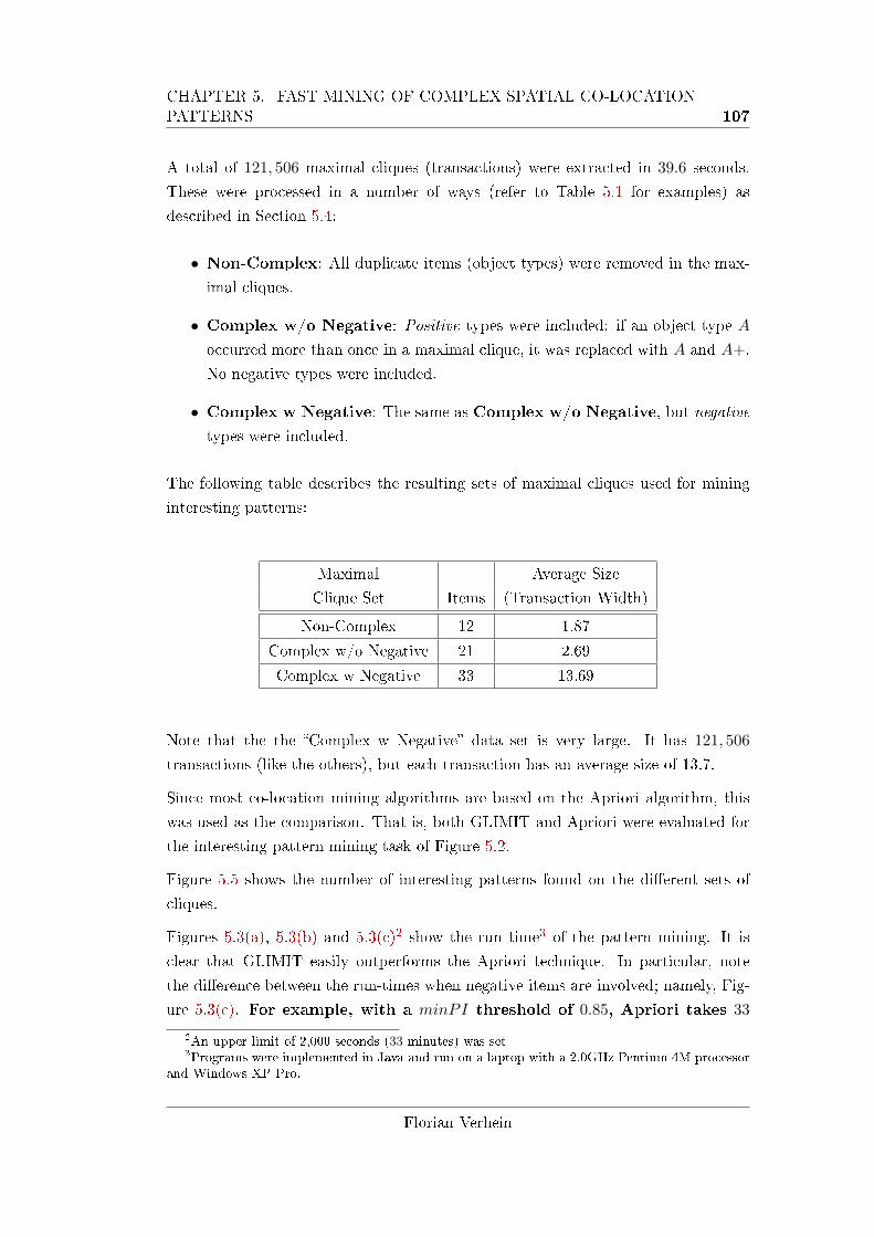
CHAPTER 5. FAST MINING OF COMPLEX SPATIAL CO-LOCATIONPATTERNS 107
A total of 121, 506 maximal cliques (transactions) were extracted in 39.6 seconds.
These were processed in a number of ways (refer to Table 5.1 for examples) as
described in Section 5.4:
• Non-Complex: All duplicate items (object types) were removed in the max-
imal cliques.
• Complex w/o Negative: Positive types were included: if an object type A
occurred more than once in a maximal clique, it was replaced with A and A+.
No negative types were included.
• Complex w Negative: The same as Complex w/o Negative, but negative
types were included.
The following table describes the resulting sets of maximal cliques used for mining
interesting patterns:
Maximal Average Size
Clique Set Items (Transaction Width)
Non-Complex 12 1.87
Complex w/o Negative 21 2.69
Complex w Negative 33 13.69
Note that the the �Complex w Negative� data set is very large. It has 121, 506
transactions (like the others), but each transaction has an average size of 13.7.
Since most co-location mining algorithms are based on the Apriori algorithm, this
was used as the comparison. That is, both GLIMIT and Apriori were evaluated for
the interesting pattern mining task of Figure 5.2.
Figure 5.5 shows the number of interesting patterns found on the di�erent sets of
cliques.
Figures 5.3(a), 5.3(b) and 5.3(c)2 show the run time3 of the pattern mining. It is
clear that GLIMIT easily outperforms the Apriori technique. In particular, note
the di�erence between the run-times when negative items are involved; namely, Fig-
ure 5.3(c). For example, with a minPI threshold of 0.85, Apriori takes 33
2An upper limit of 2,000 seconds (33 minutes) was set3Programs were implemented in Java and run on a laptop with a 2.0GHz Pentium 4M processor
and Windows XP Pro.
Florian Verhein
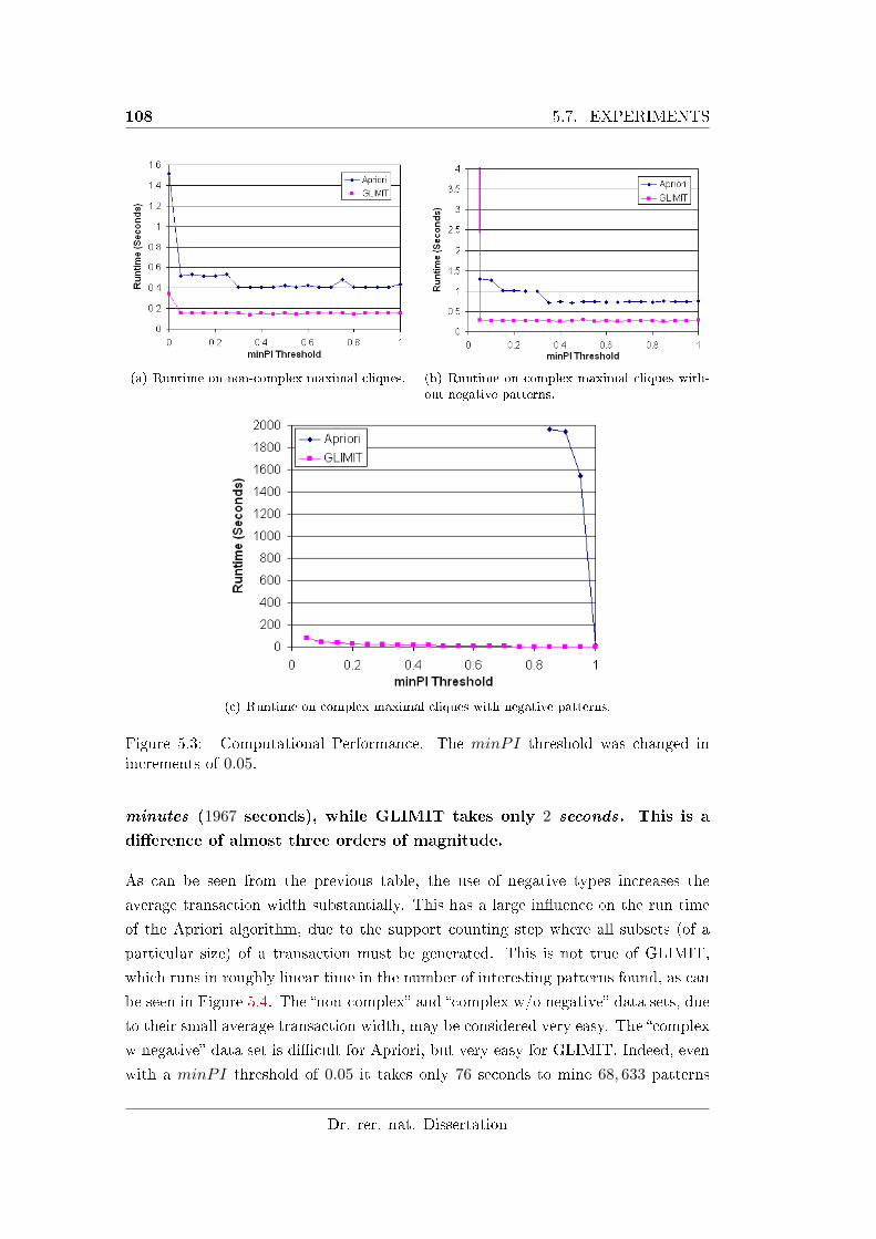
108 5.7. EXPERIMENTS
(a) Runtime on non-complex maximal cliques. (b) Runtime on complex maximal cliques with-out negative patterns.
(c) Runtime on complex maximal cliques with negative patterns.
Figure 5.3: Computational Performance. The minPI threshold was changed inincrements of 0.05.
minutes (1967 seconds), while GLIMIT takes only 2 seconds. This is a
di�erence of almost three orders of magnitude.
As can be seen from the previous table, the use of negative types increases the
average transaction width substantially. This has a large in�uence on the run time
of the Apriori algorithm, due to the support counting step where all subsets (of a
particular size) of a transaction must be generated. This is not true of GLIMIT,
which runs in roughly linear time in the number of interesting patterns found, as can
be seen in Figure 5.4. The �non-complex� and �complex w/o negative� data sets, due
to their small average transaction width, may be considered very easy. The �complex
w negative� data set is di�cult for Apriori, but very easy for GLIMIT. Indeed, even
with a minPI threshold of 0.05 it takes only 76 seconds to mine 68, 633 patterns
Dr. rer. nat. Dissertation
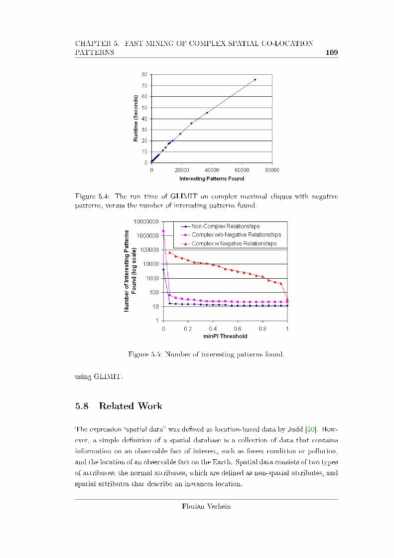
CHAPTER 5. FAST MINING OF COMPLEX SPATIAL CO-LOCATIONPATTERNS 109
Figure 5.4: The run time of GLIMIT on complex maximal cliques with negativepatterns, versus the number of interesting patterns found.
Figure 5.5: Number of interesting patterns found.
using GLIMIT.
5.8 Related Work
The expression �spatial data� was de�ned as location-based data by Judd [50]. How-
ever, a simple de�nition of a spatial database is a collection of data that contains
information on an observable fact of interest, such as forest condition or pollution,
and the location of an observable fact on the Earth. Spatial data consists of two types
of attributes; the normal attributes, which are de�ned as non-spatial attributes, and
spatial attributes that describe an instances location.
Florian Verhein
110 5.8. RELATED WORK
Huang et al. [49] de�ne the co-location pattern as the presence of a spatial feature in
the neighborhood of instances of other spatial features. They develop an algorithm
for mining valid rules in spatial databases using an Apriori based approach. Their
algorithm does not separate the co-location mining and interesting pattern mining
steps like the KDD process in this Chapter. Also, they do not consider complex
relationships or patterns. Speci�cally, their method cannot mine give complex rules
such as A→ B+ or B → −C and they do not allow cliques to be connected to each
other, which can lead to some cliques being ignored.
Monroe et al. [64] use cliques as a co-location patterns. Similar to the approach
in this chapter, they separated the clique mining from the pattern mining stages.
However, they do not use maximal cliques. They treat each clique as a transaction
and use an Apriori based technique for mining association rules. Since they used
cliques (rather than maximal cliques) as transactions, the counting of pattern in-
stances is very di�erent. They consider complex relationships within the pattern
mining stage. However, their de�nition of negative patterns is di�erent � they use
infrequent types while the work in this Chapter is based on the concept of absence
in maximal cliques. Therefore, in [64] a negative pattern does not necessarily mean
that type is not present. Monroe et al. also used a di�erent measure; maxPI. Fur-
thermore, they de�ne the positive relationship as a set of features that co-locates
in a ratio greater than prede�ned threshold. Perhaps a method based on maximal
cliques, as introduced in this Chapter, is simpler, leads to more useful semantics and
avoids the problems caused by the fact that large cliques have many sub-cliques.
Arunasalam et al. [16] use a similar approach to [64]. They propose an algorithm
called NP_maxPI which also uses the maxPI measure. The proposed algorithm
prunes the candidate itemsets using the weak anti-monotonic property of maxPI.
They also use an Apriori based technique to mine complex patterns. A primary goal
of their work is to mine patterns which have low support and high con�dence. As
with the work of [64], they did not use maximal cliques.
Zhang et al. [116] enhanced the algorithm proposed in [49] and used it to mine
special types of co-location relationships in addition to cliques, namely; the spatial
star, and generic patterns. Most related work makes use of anti-monotonic or weakly
anti-monotonic measures. Morimoto [62], however, used a measure that is not anti-
monotonic to mine a co-location pattern called the k-neighboring class set.
To the best of the authors knowledge, all previous work has used Apriori type algo-
rithms for mining interesting co-location patterns. This work uses GLIMIT as the
underlying pattern mining algorithm as already discussed in Section 5.5. Further-
more, this is the �rst work to apply GLIMIT on spatial data and with a measure
Dr. rer. nat. Dissertation
CHAPTER 5. FAST MINING OF COMPLEX SPATIAL CO-LOCATIONPATTERNS 111
other than support.
5.9 Conclusion
This Chapter introduced the idea of using maximal cliques for complex pattern
mining, which is fundamental to the approaches presented in this work. It was argued
that complex patterns only make sense in the context of maximal cliques. Using
maximal cliques also allowed the clique generation step to be split from the interesting
pattern mining tasks and avoided the problem of redundant cliques. This Chapter
presented a complete KDD process for the problem of mining complex spatial co-
location patterns. This Chapter showed that the complex spatial co-location pattern
mining problem can be mapped to the GLIMIT algorithm, and that this is a far more
e�cient solution than using the traditional Apriori style of algorithm, especially when
complex patterns are involved. Previous work in co-location mining used Apriori
style algorithms.
Since the problem in this chapter was one of the many in�uences in developing the
generalised interaction mining (GIM) approach of Chapter 3, the problem can also be
solved directly using GIM. Furthermore, recall that Chapter 3 showed how maxPI
can be applied to this problem e�ciently using GIM (see section 3.12.1).
Florian Verhein

112 5.9. CONCLUSION
Dr. rer. nat. Dissertation
Chapter 6
Generalised Rule Mining
Rules are an important interaction pattern in data mining, but existing ap-
proaches are limited to conjunctions of binary literals, �xed measures and
counting based algorithms. Rules can be much more diverse, useful and
interesting! This work introduces and solves the Generalised Rule Mining
(GRM) problem, which removes restrictions on the semantics of rules and
rede�nes rule mining by functions on vectors. This abstraction is moti-
vated through the introduction of three diverse and novel methods address-
ing problems including correlation based classi�cation, �nding interactions
for improving regression models and �nding probabilistic association rules in
uncertain databases. Two of these methods are introduced in this chapter,
while one is introduced in chapter 7. Furthermore, this approach can be
applied to other methods, such in chapter 8.
The proposed GRM framework and algorithm allow methods not possible
with existing algorithms, speed up existing methods, separate rule semantics
from algorithmic considerations and lend an interesting geometric interpre-
tation to the rule mining problem. The GRM algorithm scales linearly in
the number of rules found and provides orders of magnitude speed up over
fast candidate generation type approaches when these are applicable.
113
114 6.1. INTRODUCTION
6.1 Introduction
Rules are an important pattern in data mining due to their ease of interpretation and
usefulness for prediction. They have been heavily explored as association patterns
[11, 22, 81, 47, 84], �correlation� rules [22, 108] and for associative classi�cation [61,
60, 100]. These approaches consider only conjunctions of binary valued variables1,
use �xed measures of interestingness and counting based algorithms2. The rule
mining problem can be generalised by relaxing the restrictions on the semantics of
the antecedent as well as the variable types, and supporting any measure on rules.
A generalised rule A′ → c describes a relationship between a set of variables in the
antecedent A′ ⊆ A and a variable in the consequent c ∈ C, where A is the set of
possible antecedent variables and C is the set of possible consequent variables3. The
goal in Generalised Rule Mining (GRM) is to �nd useful rules A′ → c : A′ ⊆ A∧ c ∈C ∧ c 6∈ A′ given functions de�ning the measures and semantics of the variables and
rules. Unlike in existing methods, variables do not need to be binary valued. Unlike
in existing methods, semantics are not limited to conjunction.
This work introduces and solves the Generalised Rule Mining problem by propos-
ing a vectorized framework and algorithm that are applicable to general-to-speci�c
methods4. The framework is composed of �ve functions;
1. Rules are evaluated using a vector valued distance functionmR(xA′ , xc) applied
to the vectors corresponding to the antecedent (xA′) and the consequent (xc)
of the rule A′ → c.
2. An aggregation function aR(·) incrementally builds xA′ and implicitly de�nes
the semantics of the rule.
3. MR(·) allows complex evaluations requiring comparisons to less speci�c rules,
4. IR(·) de�nes the interestingness of rules and search expansion criteria and
5. IA(xA′) allows (pre-emptive) antecedent pruning when possible.
Rule mining is a challenging problem due to its exponential search space in A ∪ C.At best, an algorithm's run time is linear in the number of interesting rules it �nds,
1The antecedent and consequent consist of a conjunction of literals that are either true or false.2Such algorithms explicitly count instances/transactions that apply to a rule, typically through
explicit counting, subset operations or tree/trie/graph traversals.3Note that A and C do not need to be mutually exclusive.4That is, methods where a less speci�c rule A”→ c : A” ⊂ A′ is mined before the more speci�c
one A′ → c.
Dr. rer. nat. Dissertation
CHAPTER 6. GENERALISED RULE MINING 115
and the GRM algorithm is provably optimal in this sense. It also scales linearly in
the dimensionality of the vectors, and can use space linear in the size of the database.
The GRM algorithm in itself is very fast. It completely avoids �candidate generation�
and does not build a compressed version of the data set � thus setting it apart from
Apriori and FP-Growth. Instead it operates directly on vectors. Furthermore, the
vectorization inherent in the framework's functions provides additional avenues for
reducing the run time: On single processor architectures, vectorization allows au-
tomatic parallelisation and exploitation of machine level operations for bit-vectors,
and optimizations for operations on �oating point arrays (real vectors). On multipro-
cessor architectures, vectorization also provides a point for concurrentisation [105]
while on supercomputer architectures, single instruction vector processing is directly
supported [105].
By abstracting rule mining, the GRM framework separates the semantics and mea-
sures of rules from the algorithm used to mine them. The GRM algorithm can
be exploited for any methodology map-able to the frameworks functions, such as
[61, 60, 98, 103], especially generalized associative type patterns and mining classi�-
cation rules. For example, methods based on counting such as support, con�dence,
lift, interest factor, all-con�dence, correlation, signi�cance tests and entropy. In par-
ticular, complete contingency tables can be calculated, including columns for sub-
rules as required by complex, statistically signi�cant rule mining methods [98, 103].
More interestingly though, it supports novel approaches including those with seman-
tics unlike any existing method.
6.1.1 Contributions
The contributions of this work are as follows:
• It de�nes the Generalized Rule Mining (GRM) problem and proposes a vec-
torised framework that solves GRM using only functions on vectors. As a side
e�ect, this provides a natural geometric interpretation of rule mining, which is
very di�erent to the counting interpretation in previous work. Together with
the algorithm, this solves the generalized rule mining problem for general-to-
speci�c rule mining with one variable in the consequent.
• It introduces the vectorized GRM algorithm, which e�ciently solves any rule
mining problem expressible in the GRM framework. It is not based on Apriori
or FP-Growth or any other counting based algorithm. It also supports/exploits
any mutual exclusion constraints on variables.
Florian Verhein
116 6.2. RELATED WORK
• To motivate and demonstrate GRM, two novel rule mining approaches are
introduced:
� First, Probabilistic Association Rule Mining (PARM) tackles association
analysis in uncertain or probabilistic transaction databases. The required
probability computations naturally �t into the vectorised GRM frame-
work.
� Secondly, Conjunctive Correlation Rules (CCRules) are used for an asso-
ciative classi�er. It uses the proposed Correlation Improvement technique
to direct the search, which also has an interesting geometric interpreta-
tion.
Aside: In addition to the motivational methods above, another technique
called Correlated Multiplication Rules (CMRules) is developed in chapter 7.
It �nds multiplicative interactions and a method is presented for mining the
best interaction terms for inclusion in linear (especially regression) models.
This enables linear models to achieve non-linear decision boundaries by using
the antecedents of CMRules as composite features and is the �rst rule mining
approach with multiplication semantics.
6.1.2 Organisation
The remainder of this chapter is organised as follows: Section 6.2 places the this
work in context of related work. Section 6.3 presents two novel techniques that are
solved e�ciently using GRM. Section 6.4 presents the GRM framework. Section 6.5
describes the GRM algorithm. Section 6.6 presents experimental results and the
chapter is concluded in section 6.7.
6.2 Related Work
Most existing rule mining methods are used for associative pattern mining or classi-
�cation. These only consider rules with conjunctive semantics of binary literals and
use counting approaches in their algorithms. Other than border traversal based tech-
niques for maximal or closed item-sets, they use general-to-speci�c searches. Associ-
ation rule mining methods [11, 47, 81] typically mine item-sets before mining rules.
Unlike GRM, they do not mine rules directly. Itemset mining methods are often ex-
tended to rule based classi�cation [110, 61, 100]. The algorithms can be categorized
into Apriori-like approaches [11] characterized by a breadth �rst search through the
Dr. rer. nat. Dissertation
CHAPTER 6. GENERALISED RULE MINING 117
item lattice and multiple database scans, tree based approaches [47] characterized
by a traversal over a pre-built compressed representation of the database, projec-
tion based approaches [100] characterised by depth �rst projection based searches
and vertical approaches [81, 34, 96] that operate on columns. Vertical bit-map ap-
proaches [81, 96] have received considerable interest due to their ability to outperform
horizontal based techniques. Of existing work, the vectorized approach in GRM is
most similar to the vertical approach. However, GRM is not limited to bitmaps or
support based techniques; for example, unlike any previous work it can usefully and
meaningfully handle real vectors as demonstrated by PARM and CMRules. It also
solves a di�erent problem, namely, the generalised rule mining problem, and mines
rules directly � without �rst mining sets. It also runs in provably linear time in the
number of interesting rules output.
Rule based classi�cation is a major application area for rules with one variable in the
consequent [110, 60, 61, 100]. Approaches in literature are speci�c to one measure
or approach, do not generalize well and are based on the above association / item
set mining algorithms. Rules based on decision trees [76] or rule induction [27] have
di�erent mining approaches generally not compatible with those considered here.
The �generalisation� of rules in this paper applies to the ability to support many
di�erent semantics, variable types and interestingness measures. This is di�erent to
the �generalization� of association rules in the literature, where it refers to quanti-
tative rules [84, 78], correlations [22] or hierarchical rules. Quantitative rules [84]
consider the number of items bought in a transaction and mine rules with quantity
ranges. More recently, the term has referred to relationships between weighted sums
of variables [78], though this is an optimisation problem rather than a rule mining
problem. Within the GRM framework, such databases correspond to integer valued
variable vectors. However, the rules are still conjunctions of binary valued literals.
Correlation rules [22] are �general� in that they use a di�erent measure on rules;
thus �generalizing� association rules from support and con�dence to correlation. But
like other approaches, this just uses another, �xed, measure. Since GRM is a true
framework, unlike existing approaches it avoids limiting the rule de�nition and solves
the problem at the abstract level. As far as the author is aware, no existing rule
mining approach considers real valued vectors, expands the rule de�nition to non-
conjunctive semantics, allows a wide range of measures, or attempts to solve the
problem at this abstracted level.
The mutually exclusive constraints considered in this paper are not hierarchical [85]
and are primarily used for classi�cation using conjunctive rules where values have
been discretised. No work was found that considers rule mining geometrically. Re-
Florian Verhein
118 6.3. NOVEL AND MOTIVATIONAL METHODS SOLVED USING GRM
lated work pertaining to the motivational methods introduced in this chapter (that
is, PARM and CCRules) is covered in the corresponding sections.
6.3 Novel and Motivational Methods Solved Using GRM
This section presents two very di�erent and novel techniques that are solved e�-
ciently using GRM. These problems can be solved orders of magnitude faster with
GRM than using a suitable alternative method. Furthermore, chapter 7 will intro-
duce another novel technique that can only be solved with GRM. In addition to these
novel methods, section 6.4 will show how existing techniques such as support based
rules are solved using the GRM framework.
6.3.1 Probabilistic Association Rule Mining (PARM)
In a probabilistic database D, each row rj contains a set of observations about
variables A∪C together with their probabilities of being observed in rj . Probabilistic
databases arise whenever there is uncertainty or noise in the data. For example, in
the medical domain each row may correspond to a patient, the variables are medical
conditions and the probabilities capture the likelihood that the patient has (or will
get) the condition based on risk factors or tests. For instance, prenatal tests to
determine chromosomal or genetic disorders in the fetus, such as cystic �brosis, return
probabilities. Risk factors such as smoking, sex, family history, etc can also provide
probability estimates of diseases. In such databases, Probabilistic Association Rules
can show interesting patterns while taking into account the uncertainty of the data.
Traditional association analysis cannot deal with probabilistic databases. Previous
work such as [25, 26, 58, 7, 57] has examined expected frequent itemsets, that is,
the itemset mining task where itemsets with an expected support above minSup are
mined. These do not consider rules. Furthermore, previous work has used Apriori
[26, 25] or FP-Growth style approaches [58, 7, 57]. No previous work that the author
is aware of has cast probabilistic pattern mining in terms of vectors.
Problem De�nition: Probabilistic Association Rule Mining (PARM): �nd
probabilistic association rules A′ → c where the expected support E(s(A′ → c)) =1n
∑nj=1 P (A′ → c ⊆ rj) and expected con�dence exp_conf(A′ → c) (de�ned later)
are above thresholds minExpSup and minExpConf respectively. Under the as-
sumption that the variables' existential probabilities in the rows are determined
under independent observations, P (A′ → c ⊆ rj) = Πa∈A′P (a ∈ rj) · P (c ∈ rj).
Dr. rer. nat. Dissertation
CHAPTER 6. GENERALISED RULE MINING 119
The PARM problem could be solved using an Apriori style algorithm adapted for
rules (this is not straightforward) and where subset checking is replaced by proba-
bility evaluation. However, this leads either to large space requirements or repeated
work in the probability calculations (consider how P (A′ → c ⊆ rj) is calculated whenone adds a variable to the antecedent). It also has the usual run time disadvantages
of Apriori.
In the GRM model however, each variable is represented by a probability vector xi
expressing the probabilities xi[j] = P (i ∈ rj) : j ∈ {1, n}. That is, the probabilitiesthat the variable i exists in row j of the database. As will be further explained in
section 6.4, all the {P (A′′ → c ⊆ rj) : rj ∈ D : A′′ ⊆ A′} can be calculated easily
and e�ciently by incremental element-wise multiplication of individual vectors using
an appropriate aR(·) function. The GRM algorithm's use of aR(·) ensures that thereis no duplication of calculations throughout the mining process while keeping space
usage to a minimum through its depth �rst approach.
By the de�nition of P (A′ → c ⊆ rj), adding variables to A′ increases the number of
probabilities multiplied together. Hence, it can easily be shown that the following
lemma holds.
Lemma 6.1. expected support is downwards closed (anti-monotonic): E(s(A′ →c)) ≤ E(s(A′′ → c)) : A′′ ⊆ A′
To complete the PARM method, de�ne the expected con�dence of a rule A′ → c as
exp_conf(A′ → c) = E(s(A′ → c))/E(s(A′)) where E(s(A′)) = 1n
∑nj=1 P (A′ ⊆
rj) and �lter out all rules not meeting the minExpConf threshold. The expected
con�dence measures the degree of association between A′ and c5. Note that the
expected support and expected con�dence reduce to the usual de�nitions of support
and con�dence [88] when the database has no uncertainty.
6.3.2 Conjunctive Correlation Rules for Classi�cation (CCRules)
This section presents a rule mining method that �nds conjunctive rules where the
antecedent is highly correlated with the consequent, and uses these rules in a classi-
�cation method. These rules, together with the method by which they are mined �
called Correlation Improvement � also have an interesting geometric interpretation
5Note that de�ning the expected con�dence as the expectation (over all rows rj) of the proba-
bilistic con�dences P (A′ → c ⊆ rj)/P (A′ ⊆ rj) is pointless under the independence assumption, asP (A′→c⊆rj)P (A′⊆rj)
= P (c ⊆ rj).
Florian Verhein
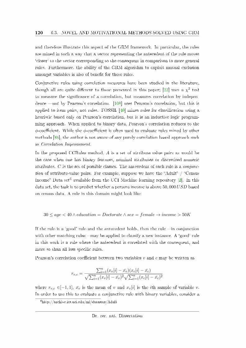
120 6.3. NOVEL AND MOTIVATIONAL METHODS SOLVED USING GRM
and therefore illustrate this aspect of the GRM framework. In particular, the rules
are mined in such a way that a vector representing the antecedent of the rule moves
`closer' to the vector corresponding to the consequent in comparison to more general
rules. Furthermore, the ability of the GRM algorithm to exploit mutual exclusion
amongst variables is also of bene�t for these rules.
Conjunctive rules using correlation measures have been studied in the literature,
though all are quite di�erent to those presented in this paper; [22] uses a χ2 test
to measure the signi�cance of a correlation, but measures correlation by indepen-
dence � not by Pearson's correlation. [108] uses Pearson's correlation, but this is
applied to item pairs, not rules. FOSSIL [40] mines rules for classi�cation using a
heuristic based only on Pearson's correlation, but it is an inductive logic program-
ming approach. When applied to binary data, Pearson's correlation reduces to the
φ-coe�cient. While the φ-coe�cient is often used to evaluate rules mined by other
methods [88], the author is not aware of any purely correlation based approach such
as Correlation Improvement.
In the proposed CCRules method, A is a set of attribute-value pairs as would be
the case when one has binary features, nominal attributes or discretised numeric
attributes. C is the set of possible classes. The antecedent of each rule is a conjunc-
tion of attribute-value pairs. For example, suppose we have the �Adult� / �Census
Income� Data set6 available from the UCI Machine learning repository [2]. In this
data set, the task is to predict whether a persons income is above 50, 000USD based
on census data. A rule in this domain might look like:
30 ≤ age < 40 ∧ education = Doctorate ∧ sex = female→ income > 50K
If the rule is a `good' rule and the antecedent holds, then the rule � in conjunction
with other matching rules � may be applied to classify a new instance. A `good' rule
in this work is a rule where the antecedent is correlated with the consequent, and
more so than all less speci�c rules.
Pearson's correlation coe�cient between two variables v and c may be written as
rv,c =
∑ni=1(xv[i]− xv)(xc[i]− xc)√∑n
i=1(xv[i]− xv)2√∑n
i=1(xc[i]− xc)2
where rv,c ∈[−1, 1], xv is the mean of v and xv[i] is the ith sample of variable v.
In order to use this to evaluate a conjunctive rule with binary variables, consider a
6http://archive.ics.uci.edu/ml/datasets/Adult
Dr. rer. nat. Dissertation
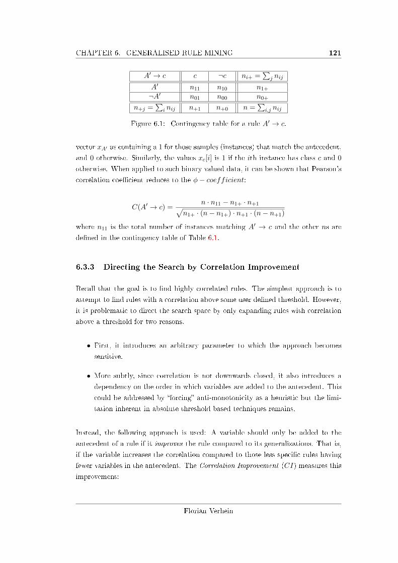
CHAPTER 6. GENERALISED RULE MINING 121
A′ → c c ¬c ni+ =∑
j nij
A′ n11 n10 n1+¬A′ n01 n00 n0+
n+j =∑
i nij n+1 n+0 n =∑
i,j nij
Figure 6.1: Contingency table for a rule A′ → c.
vector xA′ as containing a 1 for those samples (instances) that match the antecedent,
and 0 otherwise. Similarly, the values xc[i] is 1 if the ith instance has class c and 0
otherwise. When applied to such binary valued data, it can be shown that Pearson's
correlation coe�cient reduces to the φ− coefficient:
C(A′ → c) =n · n11 − n1+ · n+1√
n1+ · (n− n1+) · n+1 · (n− n+1)
where n11 is the total number of instances matching A′ → c and the other ns are
de�ned in the contingency table of Table 6.1.
6.3.3 Directing the Search by Correlation Improvement
Recall that the goal is to �nd highly correlated rules. The simplest approach is to
attempt to �nd rules with a correlation above some user de�ned threshold. However,
it is problematic to direct the search space by only expanding rules with correlation
above a threshold for two reasons.
• First, it introduces an arbitrary parameter to which the approach becomes
sensitive.
• More subtly, since correlation is not downwards closed, it also introduces a
dependency on the order in which variables are added to the antecedent. This
could be addressed by �forcing� anti-monotonicity as a heuristic but the limi-
tation inherent in absolute threshold based techniques remains.
Instead, the following approach is used: A variable should only be added to the
antecedent of a rule if it improves the rule compared to its generalizations. That is,
if the variable increases the correlation compared to those less speci�c rules having
fewer variables in the antecedent. The Correlation Improvement (CI) measures this
improvement;
Florian Verhein
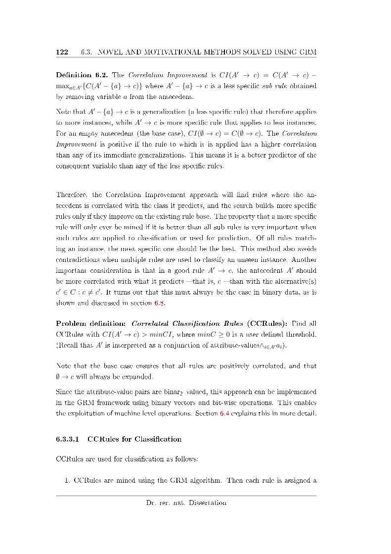
122 6.3. NOVEL AND MOTIVATIONAL METHODS SOLVED USING GRM
De�nition 6.2. The Correlation Improvement is CI(A′ → c) = C(A′ → c) −maxa∈A′{C(A′ − {a} → c)} where A′ − {a} → c is a less speci�c sub rule obtained
by removing variable a from the antecedent.
Note that A′−{a} → c is a generalization (a less speci�c rule) that therefore applies
to more instances, while A′ → c is more speci�c rule that applies to less instances.
For an empty antecedent (the base case), CI(∅ → c) = C(∅ → c). The Correlation
Improvement is positive if the rule to which it is applied has a higher correlation
than any of its immediate generalizations. This means it is a better predictor of the
consequent variable than any of the less speci�c rules.
Therefore, the Correlation Improvement approach will �nd rules where the an-
tecedent is correlated with the class it predicts, and the search builds more speci�c
rules only if they improve on the existing rule base. The property that a more speci�c
rule will only ever be mined if it is better than all sub rules is very important when
such rules are applied to classi�cation or used for prediction. Of all rules match-
ing an instance, the most speci�c one should be the best. This method also avoids
contradictions when multiple rules are used to classify an unseen instance. Another
important consideration is that in a good rule A′ → c, the antecedent A′ should
be more correlated with what it predicts � that is, c � than with the alternative(s)
c′ ∈ C : c 6= c′. It turns out that this must always be the case in binary data, as is
shown and discussed in section 6.8.
Problem de�nition: Correlated Classi�cation Rules (CCRules): Find all
CCRules with CI(A′ → c) > minCI, where minC ≥ 0 is a user de�ned threshold.
(Recall that A′ is interpreted as a conjunction of attribute-values∧i∈A′ai).
Note that the base case ensures that all rules are positively correlated, and that
∅ → c will always be expanded.
Since the attribute-value pairs are binary valued, this approach can be implemented
in the GRM framework using binary vectors and bit-wise operations. This enables
the exploitation of machine level operations. Section 6.4 explains this in more detail.
6.3.3.1 CCRules for Classi�cation
CCRules are used for classi�cation as follows:
1. CCRules are mined using the GRM algorithm. Then each rule is assigned a
Dr. rer. nat. Dissertation
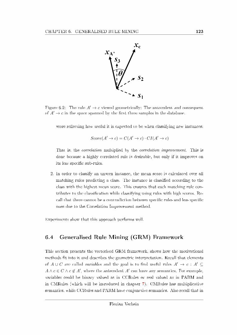
CHAPTER 6. GENERALISED RULE MINING 123
Figure 6.2: The rule A′ → c viewed geometrically: The antecedent and consequentof A′ → c in the space spanned by the �rst three samples in the database.
score re�ecting how useful it is expected to be when classifying new instances:
Score(A′ → c) = C(A′ → c) · CI(A′ → c)
That is, the correlation multiplied by the correlation improvement. This is
done because a highly correlated rule is desirable, but only if it improves on
its less speci�c sub-rules.
2. In order to classify an unseen instance, the mean score is calculated over all
matching rules predicting a class. The instance is classi�ed according to the
class with the highest mean score. This ensures that each matching rule con-
tributes to the classi�cation while classifying using rules with high scores. Re-
call that there cannot be a contradiction between speci�c rules and less speci�c
ones due to the Correlation Improvement method.
Experiments show that this approach performs well.
6.4 Generalised Rule Mining (GRM) Framework
This section presents the vectorised GRM framework, shows how the motivational
methods �t into it and describes the geometric interpretation. Recall that elements
of A ∪ C are called variables and the goal is to �nd useful rules A′ → c : A′ ⊆A ∧ c ∈ C ∧ c 6∈ A′, where the antecedent A′ can have any semantics. For example,
variables could be binary valued as in CCRules or real valued as in PARM and
in CMRules (which will be introduced in chapter 7). CMRules has multiplicative
semantics, while CCRules and PARM have conjunctive semantics. Also recall that in
Florian Verhein
124 6.4. GENERALISED RULE MINING (GRM) FRAMEWORK
the GRM framework, each possible antecedent A′ ⊆ A and each possible consequent
c ∈ C are expressed as vectors, denoted by xA′ and xc respectively. As indicated in
�gure 6.2, these vectors exist in the space X, the dimensions of which are samples
{s1, s2, ..., sn} � depending on the application these may be instances, transactions,
rows, etc. The database is the set of vectors corresponding to individual variables,
D = {xv : v ∈ A∪C}. The space X is dependent on the type of variables considered.
This work presents techniques with variables in Rn and in {0, 1}n.
Good rules have high prediction power. Geometrically, in such rules the antecedent
vector is �close� to the consequent vector.
De�nition 6.3. mR : X2 → Rk is a set of k distance measures between the an-
tecedent and consequent vectors xA′ and xc. mR(xA′ , xc) evaluates the quality of
the rule A′ → c. k is �xed.
That is, it is some form of distance metric (or metrics) that evaluate how useful the
rule is expected to be.
In PARM (section 6.3.1), mR(·) is the expectation function and calculates the ex-
pected support: mR(A′ → c) = 1n
∑nj=1 xA′ [j]∗xc[j]. Geometrically, this is the scaled
dot product of xA′ and xc: mR(A′ → c) =|xA′ ||xc|
n xA′ · xc. CCRules (section 6.3.2)
uses Pearson's correlation coe�cient. Geometrically, this is the cosine of the angle θ
between xA′ and xc (see �gure 6.2). In CCRules the attribute-value pairs are binary
valued variables. It this case, recall that C(A′ → c) = n·n11−n1+·n+1√n1+·(n−n1+)·n+1·(n−n+1)
(the
φ-coe�cient), where n11 is the number of instances matching A′ → c and the other
ns are de�ned in the contingency table of �gure 6.1. This is advantageous since these
are counts (a.k.a frequencies). Any method based on counting can be implemented
using bit-vectors in the GRM framework (sparse methods outlined in section 3.15
can of course also be applied). Each variable corresponds to a binary literal that
is true or false in the samples (instances, records, etc). A bit is set in xA′ (xc) if
the corresponding sample contains A′ (c). Then, the number of samples contain-
ing A′, A′ → c and c are simply the number of set bits in xA′ , xA′ ANDxc and
xc respectively. From these counts (n1+, n11 and n+1 respectively) and the length
of the vector, n, a complete contingency table can be constructed as in �gure 6.1.
Using this, mR can evaluate a wide range of measures such as con�dence, interest
factor, lift, φ-coe�cient and even statistical signi�cance tests. For example, all as-
sociation rules with a single variable in the consequent can be mined and evaluated
with any of these measures. Geometrically, in counting based applications mR is the
dot-product; mR(A′ → c) = xA′ · xc = n11.
Dr. rer. nat. Dissertation
CHAPTER 6. GENERALISED RULE MINING 125
Since xc corresponds to a single variable it is readily available as xc ∈ D. This is
also the case for all xa : a ∈ A. However, the xA′ : A′ ⊂ A ∧ |A′| > 1 required for
the evaluation of mR(·) on rules with |A′| > 1 must be calculated. These are built
incrementally from vectors xa ∈ D using the aggregation function aR(·):
De�nition 6.4. aR : X2 → X operates on vectors of the antecedent so that xA′∪a =
aR(xA′ , xa) where A′ ⊆ A and a ∈ (A−A′).
In other words, aR(·) combines the vector xA′ for an existing antecedent A′ ⊆ A
with the vector xa for a new antecedent element a ∈ A − A′. The resulting vector
xA′∪a represents the larger antecedent A′ ∪ a. In this way, the vector representing
the antecedent can be built incrementally. This is equivalent to the aI(·) function
in the GIM framework of chapter 3. Note that this vector is the same as if it were
calculated from the original data set, but rather than examining the original data
set, it requires only one of the vectors (xa) since the information from the rest is
already represented in xA′ . This property can be exploited to allow the algorithm to
e�ciently evaluate the rules without recomputing vectors or scanning the data set
to construct xA′∪a.
More importantly however, note that aR(·) also de�nes the semantics of the an-
tecedent of the rule. By de�ning how xA′∪a is built, it must implicitly de�ne the
semantics between elements of A′ ∪ a. That is, what it means to add a variable to
the antecedent of a rule.
For rules with a conjunction of binary valued variables such as CCRules and associa-
tion rules, vectors are represented as bit-vectors and hence aR(xA′ , xa) = xA′ ANDxa
de�nes the required semantics; bits will be set in xA′∪a corresponding to those sam-
ples that are matched by the conjunction ∧ai∈A′ ∧ a. In PARM (section 6.3.1),
the vectors contain probabilities. Since the antecedent vector is de�ned by xA′ =
Πa∈A′P (a ∈ rj), aR(·) is de�ned by element-wise multiplication: aR(xA′ , aa)[j] =
xA′ [j] ∗ xa[j]. PARM is interpreted using conjunctive semantics.
While mR(·) and aR(·) su�ce for many measures, it often occurs that a rule A′ → c
needs to be compared with its sub-rules A” → c : A” ⊂ A′. This is particularly
useful in order to �nd more speci�c rules that improve on their less speci�c sub-
rules. Geometrically, this means the antecedent of a rule can be built by adding
more variables in such a way that the corresponding vector xA′ moves closer to the
vector representing the consequent of the rule xc. This is exactly what the Correlation
Improvement technique does. Examples from the literature that require comparison
to sub-rules include [103, 98]. The following function supports such behaviour.
Florian Verhein
126 6.4. GENERALISED RULE MINING (GRM) FRAMEWORK
De�nition 6.5. MR : Rk×|P(A′)| → Rl is a measure that evaluates a rule A′ → c
based on the value computed by mR(·) for any rule A′′ → c : A′′ ⊆ A′. l is �xed.
MR(·) does not take vectors as arguments � it evaluates a rule based on values
that have already been calculated. This is important as it enables the algorithm
to perform only one vector calculation per rule. Not that this is for algorithmic
e�ciency purposes only and does not limit the scope of the framework in any way.
If MR(·) does not need access to any sub-rules to perform its evaluation, it is called
trivial since mR(·) can perform the function instead. A trivial MR(·) simply returns
mR(·) and has advantages in terms of space and time complexity (section 6.5).
In PARM, MR(·) is trivial. The Correlation Improvement method is implemented
usingMR(·) according to de�nition 6.2. Geometrically, since C(A′ → c) =cos(θ) and
CI(·) must be positive, the search progresses by adding variables to the antecedent
in a way that the antecedent vector moves closer to the consequent vector in terms
of the subtended angle θ. In CCRules, variables will only be added if they improve
the correlation with the class to be predicted. For counting based approaches,MR(·)can be used to evaluate measures on more complex contingency tables such as those
in [103, 98] and chapter 8. For example, to evaluate whether a rule signi�cantly
improves on its less speci�c sub-rules by using Fisher's Exact Test (see chapter 8).
Together with IR below, it can also be used to direct and prune the search space �
even `forcing' a measure implemented in mR to be downward closed.
The �nal component of the framework de�nes what rules are interesting. Interesting
rules are those that are
1. desirable and should therefore be output and
2. should be further improved in the sense that more speci�c rules should be
mined by the GRM algorithm.
De�nition 6.6. IR : Rk+l → {true, false} determines whether a rule A′ → c is
interesting based on the values produced by mR(·) and MR(·). Only interesting
rules are further expanded and output.
In other words, more speci�c rules (i.e. with more variables in the antecedent) will
only be considered if IR(·) returns true. The simplest implementation of IR(·) is toreturn true ifMR(·) is above (below) a threshold. For simplicity, both interestingness
Dr. rer. nat. Dissertation
CHAPTER 6. GENERALISED RULE MINING 127
concepts have been combined in IR(·). Separating them, as is done in GIM with II(·)and SI(·) (section 3.2) is of course also possible.
In PARM, the search space can be pruned by the expected support (lemma 6.1).
Hence IR(A′ → c) returns true if and only if mR(A′ → c) ≥ minExpSup. For
Correlation Improvement, the desired search strategy is achieved when IR returns
true for A′ → c if and only if CI(A′ → c) > minCI.
Sometimes it is possible to determine that a rule is not interesting based purely on
the antecedent. For example, in PARM the expected support of the antecedent is
always less than that of the rule and so we can avoid unnecessary computation of
rules. This pre-emptive pruning is de�ned by IA(·):
De�nition 6.7. IA : X → {true, false}. IA(xA) = false implies IR(·) = false for
all A′ → c : c ∈ C.
The framework can accommodate any approach where a rule can (or must) be exam-
ined after its generalizations are examined. In other words, it accommodates bottom
up approaches. Beyond that, the order in which rules are examined is up to the
algorithm and complexity considerations.
6.5 Generalised Rule Mining Algorithm
The GRM algorithm e�ciently solves any problem that can be expressed in the
framework. It is optimal in the sense that it uses time linear in the number of rules
found. It also uses space linear in the size of the data set. To understand the
algorithm, it is necessary to understand the The Categorised Pre�x Tree �rst, part
of which involves the ability to exploit mutual exclusion constraints.
6.5.1 Mutual Exclusion Constraints
Often, groups of variables are mutually exclusive. For instance, when numeric at-
tributes have been discretised, an attribute can take on only one of a set of values
and each of these attribute-value pairs becomes a binary variable. The reader may
recall the example for CCRules in section 6.3.2, where for example an attribute age
is split into di�erent ranges. Of course a person can only have an age in one range,
and therefore the di�erent ranges are mutually exclusive. It is pointless to check
rules which contain the same attribute but with di�erent values if these are mutually
Florian Verhein
128 6.5. GENERALISED RULE MINING ALGORITHM
exclusive, as no instances can exist with this property. Avoiding such unnecessary
computation saves computational resources. A second source of mutual exclusion oc-
curs when a user does not require certain combinations of variables to be examined
as they are not interested them.
Such intrinsic and extrinsic constraints can be expressed through a categoriza-
tion where variables in the same category are mutually exclusive. For example, all
attribute-value pairs with the same attribute will correspond to one category. Vari-
ables that have no constraints are simply placed in categories by themselves. Exploit-
ing such constraints reduces the search space from O(2|A| ·|C|) to O(|C|·Πmi=1(ni+1)),
where ni is the number of variables in the ith category. The GRM algorithm fully
and implicitly exploits all constraints expressible by mutual exclusion through the
use of a Categorised Pre�x Tree.
6.5.2 Categorized Pre�x Tree
The Categorized Pre�x Tree (CPT) can e�ciently store rules in a compressed format.
The reader should keep in mind however, that depending on the requirements of MR,
the Categorized Pre�x Tree often does not need to be stored at all.
The CPT is an important concept in the algorithm. The following rules de�ne
it: First, an arbitrary but �xed order is chosen on the variables � in this chapter,
ascending order will be used. Variables in C must always be �rst in the order. Each
node in the CPT (a Pre�xNode) has a label corresponding to a variable v ∈ A ∪ C.The root node is special, and is labeled with ∞. The CPT is constructed so that
each node can only have a parent with a label greater than it's own label and not in
its category.
Figure 6.3 shows a `full' CPT in that it contains all possible rules given the set
of variables and categories. In the �gure, the variables {a, b}, {1, 2} and {3, 4} aremutually exclusive so the categorization is {{a, b}, {1, 2}, {3, 4}}. Each non-leaf node
in a complete tree represents an antecedent A′ ∈ A and each leaf node (grey in the
�gure) represents a complete rule A′ → c : c ∈ C. Then rules can be reconstructed
by traversal toward the root, which corresponds to the empty antecedent A′ = ∅.WhenMR(·) is non-trivial, the CPT can e�ciently store rules in a compressed format
through pre�x sharing. Otherwise, only the current path the algorithm is processing
is in memory. A Complete Categorized Pre�x Tree (CCPT) such as shown in �gure
6.3 is a `full' CPT in that it contains all possible rules given the set of variables and
categories. A complete CPT therefore also represents the worst case search space of
the rule mining problem (when categories are exploited).
Dr. rer. nat. Dissertation
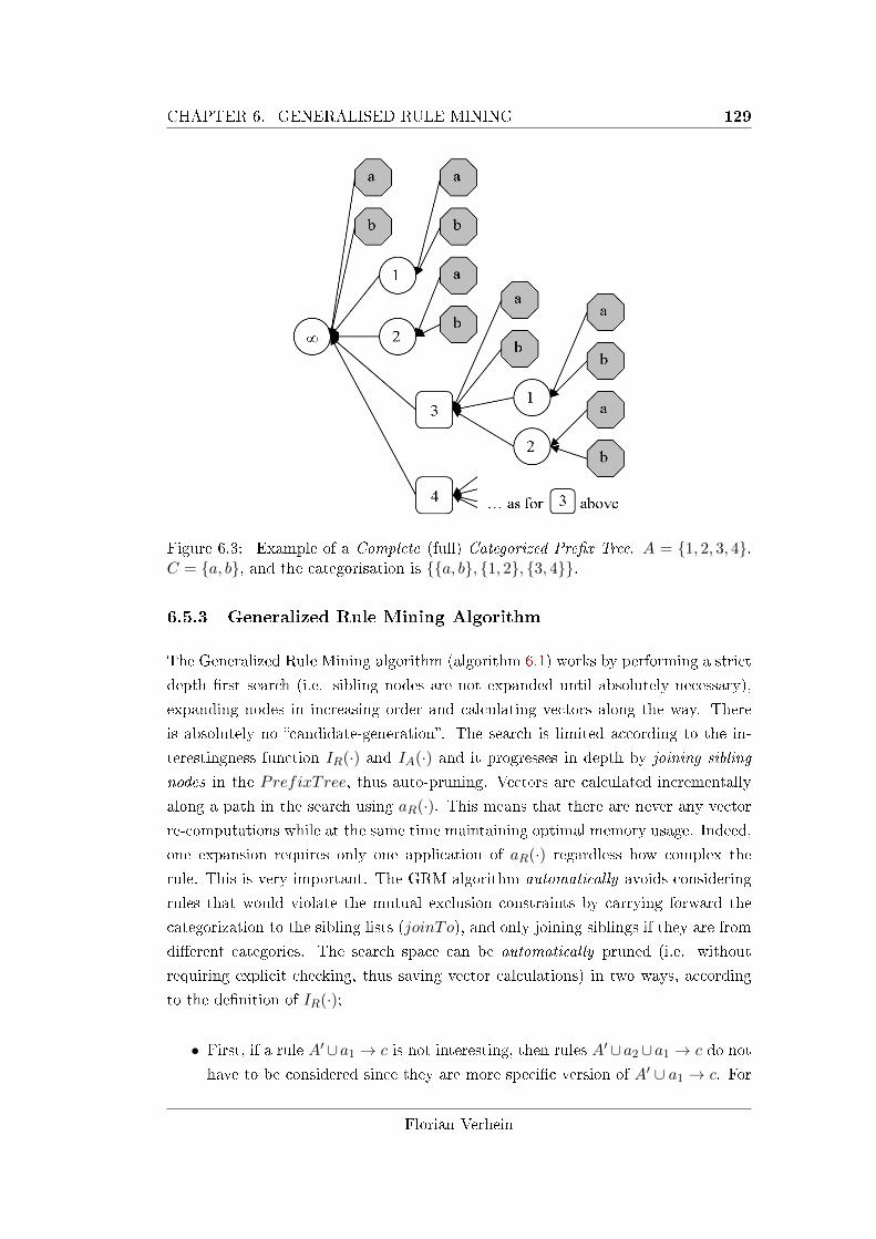
CHAPTER 6. GENERALISED RULE MINING 129
Figure 6.3: Example of a Complete (full) Categorized Pre�x Tree. A = {1, 2, 3, 4},C = {a, b}, and the categorisation is {{a, b}, {1, 2}, {3, 4}}.
6.5.3 Generalized Rule Mining Algorithm
The Generalized Rule Mining algorithm (algorithm 6.1) works by performing a strict
depth �rst search (i.e. sibling nodes are not expanded until absolutely necessary),
expanding nodes in increasing order and calculating vectors along the way. There
is absolutely no �candidate-generation�. The search is limited according to the in-
terestingness function IR(·) and IA(·) and it progresses in depth by joining sibling
nodes in the PrefixTree, thus auto-pruning. Vectors are calculated incrementally
along a path in the search using aR(·). This means that there are never any vector
re-computations while at the same time maintaining optimal memory usage. Indeed,
one expansion requires only one application of aR(·) regardless how complex the
rule. This is very important. The GRM algorithm automatically avoids considering
rules that would violate the mutual exclusion constraints by carrying forward the
categorization to the sibling lists (joinTo), and only joining siblings if they are from
di�erent categories. The search space can be automatically pruned (i.e. without
requiring explicit checking, thus saving vector calculations) in two ways, according
to the de�nition of IR(·);
• First, if a rule A′∪a1 → c is not interesting, then rules A′∪a2∪a1 → c do not
have to be considered since they are more speci�c version of A′ ∪ a1 → c. For
Florian Verhein
130 6.5. GENERALISED RULE MINING ALGORITHM
example, in �gure 6.3, if 1 → a was not interesting, then 3, 1 → a would not
need to be examined by the de�nition of IR(·). This is automatically achieved
by maintaining a list of siblings (joinTo), and only joining sibling nodes. Note
that A′ ∪ a2 → c and A′ ∪ a1 → c are siblings in the CPT. Recall that only
interesting rules as speci�ed by IR(·) are to be expanded, and therefore only
interesting rules become siblings, achieving this pruning automatically.
• Secondly, if no rules with the antecedent A′ are interesting, then that node is
not further expanded. For example, if neither 3 → a or 3 → b are interesting
in �gure 6.3, then the complete sub-tree rooted at 3 can be pruned. This is
called prune early functionality and implements the semantics of IR(·).
In algorithm 6.1, evaluateAndSetMR(·) evaluates MR and sets valueM of the Pre-
�xNode. Recall that if MR is non-trivial, its evaluation requires the valuems of sub
rules. In this case, store(·) stores the PrefixNode in an index structure for later use
by evaluateAndSetMR(·). This means that the CPT will be built in memory as refer-
ences to its leaf nodes is maintained. A suitable index structure would be a hash-table
due to the constant look-up time that can be exploited by evaluateAndSetMR(·). IfMR is trivial, store(·) does nothing and rules (and hence the entire Categorized Pre-
�x Tree) are not kept in memory7. The outputRule(·) function provides rules (as
PrefixNodes) to client code. For example, to output the rule to a �le or to maintain
the top k-rules.
Despite the search being depth �rst, the following holds, proving correctness.
Lemma 6.8. All sub-rules A′′ → c : A′′ ⊂ A′ are examined before A′ → c is
examined.
Proof. The algorithm progresses through the search space by joining existing Pre-
�xNode siblings together, creating antecedents or complete rules that are one variable
larger than the two original sibling nodes. Suppose for the purpose of contradiction
that a rule r = A′ → c exists but a sub-rule of it is mined later. Proceed by showing
that each sub-rule A′ − a → c : a ∈ A′ has already been mined, so that the result
follows by induction. First, note that each rule can be represented by a sequence of
Pre�xNodes, which can be constructed in reverse by traversal from c towards the
root. The immediate sub-rules of r can be obtained by removing one variable from
the antecedent at a time. Suppose a ∈ A′ is removed, so that r = Sp ∪ a ∪ Ss → c
7algorithm 6.1 assumes a garbage collector, so such rules � and hence the entire CPT except forthe current search path � are garbage collected.
Dr. rer. nat. Dissertation
CHAPTER 6. GENERALISED RULE MINING 131
where Sp and Ss are the pre�x and su�x (either potentially empty) of the antecedent
(sequence) respectively. Since the expansion of the search is done in depth �rst fash-
ion and with increasing order amongst the siblings (according to their variables),
Sp ∪ Ss must be expanded �rst, since by de�nition the sequences in the Pre�xTree
appear in decreasing order. Since this is true for all a ∈ A′, the result follows by
induction and contradiction.
6.5.4 Complexity
Theorem 6.9. The run time complexity is at worst O(R · |A| · |C| ·(t(mR)+ t(MR)+
t(aR) + t(IR)), where R is the number of rules mined by the algorithm and t(X) is
the time taken to compute function X from the framework.
Proof. For a node corresponding to A′ to be expanded to search for more speci�c
rules, (for more variables to be added to it in an attempt to �nd larger rules), at least
one rule A′ → c : c ∈ C must have been mined, otherwise the branch of the search
space is pruned. In the worst case, each child A′∪a : a ∈ (A−A′) must be examined,
with none of the rules A′∪a→ c : c ∈ C found to be interesting. This takes at worst
O(|A| · |C|) time. Therefore, for each rule mined, at worst O(|A| · |C|) more speci�c
but non-interesting rules may have to be examined. Finally, the processing of each
rule requires one application of each of the functions mR, MR, aR and IR.
This theorem states that the performance is linear in the number of interesting rules
found by the algorithm (the number of rules for which IR(·) returns true). It is
therefore not possible to improve the algorithm other than by a constant factor since
each interesting rule must at least be output by the algorithm. Note that this result
is not the same as saying that the run time is linear in the size of the search space.
The search space is known beforehand, but the required rules are not. The search
space may be O(2|A∪C|) but if only R of these rules are interesting (and typically
R << 2|A∪C|), then the run time of GRM is linear in R, not 2|A∪C|. It is not
possible to improve on the |A| · |C| without sacri�cing completeness in a general-to-
speci�c type algorithm. The proof of theorem 6.9 implies that the number of rules
that must be examined to guarantee completeness is O(R · |A| · |C|). The cost of
garbage collection execution does not alter the complexity and the algorithm can be
implemented with the same complexity without one.
Corollary 6.10. PARM takes O(R·|A|·|C|·n) time. CCRules takes O(R·|A|2·|C|·n)
time, where n is the number of samples (instances). Mining association rules with a
Florian Verhein
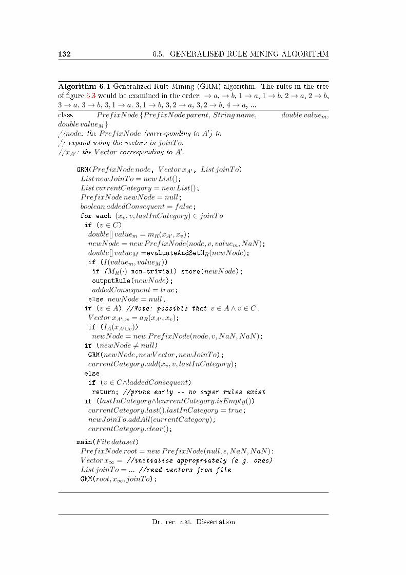
132 6.5. GENERALISED RULE MINING ALGORITHM
Algorithm 6.1 Generalized Rule Mining (GRM) algorithm. The rules in the treeof �gure 6.3 would be examined in the order: → a,→ b, 1→ a, 1→ b, 2→ a, 2→ b,3→ a, 3→ b, 3, 1→ a, 3, 1→ b, 3, 2→ a, 3, 2→ b, 4→ a, ...
class PrefixNode {PrefixNode parent, String name, double valuem,double valueM}//node: the PrefixNode (corresponding to A′) to// expand using the vectors in joinTo.//xA′: the V ector corresponding to A
′.
GRM(PrefixNode node, V ector xA′, List joinTo)List newJoinTo = newList();List currentCategory = newList();PrefixNode newNode = null;boolean addedConsequent = false;for each (xv, v, lastInCategory) ∈ joinToif (v ∈ C)double[] valuem = mR(xA′ , xv);newNode = new PrefixNode(node, v, valuem, NaN);double[] valueM =evaluateAndSetMR(newNode);if (I(valuem, valueM ))if (MR(·) non-trivial) store(newNode);outputRule(newNode);addedConsequent = true;else newNode = null;if (v ∈ A) //Note: possible that v ∈ A ∧ v ∈ C.V ector xA′∪v = aR(xA′ , xv);if (IA(xA′∪v))newNode = new PrefixNode(node, v,NaN,NaN);
if (newNode 6= null)GRM(newNode,newV ector,newJoinTo);currentCategory.add(xv, v, lastInCategory);else
if (v ∈ C∧!addedConsequent)return; //prune early -- no super rules exist
if (lastInCategory∧!currentCategory.isEmpty())currentCategory.last().lastInCategory = true;newJoinTo.addAll(currentCategory);currentCategory.clear();
main(File dataset)PrefixNode root = new PrefixNode(null, ε,NaN,NaN);V ector x∞ = //initialise appropriately (e.g. ones)
List joinTo = ... //read vectors from file
GRM(root, x∞, joinTo);
Dr. rer. nat. Dissertation
CHAPTER 6. GENERALISED RULE MINING 133
single variable in the consequent takes O(R · |A| · |C| · n) time. R is the number of
rules mined.
Proof. For all instantiations considered in this paper, t(mR) = t(aR) = O(n) where n
is the number of samples, since all functions require examining vectors. t(IR) = O(1).
For CCRules, t(MR) = O(|A|) since MR examines immediate sub-rules. For PARM
and association rule mining, t(MR) = O(1) and MR is trivial, as sub-rules do not
need to be examined due to the anti-monotonicity of support.
The complexity of outputRule(·) is dependent on the application and what is done
with the rules. Outputting a single rule can be done in O(|A|) time, storing it
in memory for later use can be done in O(1) time (add operation in a hash table
prevents garbage collection), �nding the top k rules can be done in O(k log(k)) time,
etc.
Theorem 6.11. The space usage is O(|A ∪ C| · n + |A|2) if MR is trivial, and
O(R+ |A∪C| ·n+ |A|2) if MR requires access to sub-rules8. Note that O(|A∪C| ·n)
is the size of the database.
Proof. In the worst case (all elements in A induce at least one interesting rule), all
variables' vectors must remain in memory. The search is depth �rst, and so the depth
is at most |A|+1. At each node along the current path of the search, a list of at most
size |A| is kept (containing references to objects already in memory), as well as at
most one additional vector (the vector corresponding to xA′ required to build vectors
for longer antecedents). Therefore, at most O(|A ∪ C| + |A|) = O(|A ∪ C|) vectors
of length n are in memory, and O(|A|2) references to existing objects. If all mined
rules need to be stored (MR(·) is non-trivial), this takes O(R) space at worst.
6.6 Experiments
The primary purpose of the experiments is to demonstrate and validate the run-time
complexity of the GRM algorithm and its superiority in comparison to alternative
approaches. It also provides initial e�ectivity results for the CCRule and CMRule
methods.
8Note that if the rules need to be stored, common pre�xes are shared in the Categorized Pre�x
Tree and so in practice the space usage of the rules is much less than O(R · |A ∪ C|) � at best it isO(R). The worst case is only possible for trivial cases involving small R.
Florian Verhein
134 6.6. EXPERIMENTS
6.6.1 Complexity Experiments
GRM's run time is evaluated here for conjunctive rules with bit-vectors (therefore
covering any counting based approach) and multiplicative rules with real valued
vectors. Unfortunately, there are no existing or suitable algorithms for compar-
ison. For example, recall that previous work on uncertain transaction databases
[25, 26, 58, 7, 57] considers only itemsets, not rules. Itemset mining is very dif-
ferent to the direct mining of rules. For comparison therefore, an fast �Apriori�
style method for mining rules was developed, called FastAprioriRules. It is based
on the candidate generation and testing methodology that is common in literature.
However, it mines rules directly � that is, it does not mine sets �rst and then gen-
erate rules form these as this would be ine�cient. FastAprioriRules also exploits
the mutual exclusion optimisation which greatly reduces the number of candidates
generated, preemptively prunes by antecedents when possible and incorporates the
pruneEarly concept. Hence FastAprioriRules evaluates exactly the same number of
rules as GRM so that the comparison is fair and evaluates the characteristics of the
underlying algorithms. To check if a rule matches an instance in the counting phase,
a set based method is used, which proved to be much quicker than enumerating the
sub-rules in an instance and using hash tree based look-up methods to �nd matching
candidates. This is not surprising as instances in classi�cation data sets are large.
The data set is kept in memory to avoid Apriori's downsides of multiple passes, and
unlike the GRM experiments, I/O time is not included. The general idea was to err
on the side of giving FastAprioriRules the advantage. Two approaches were imple-
mented using the FastAprioriRule method; a generic counting method, and PARM.
Note that the latter operates on uncertain transactions.
Most rule mining methods require frequency counts. Hence, the algorithms are
compared on the task of mining all conjunctive rules A′ → c that are satis�ed by (i.e.
classify correctly) at least minCount instances. By varying minCount, the number
of interesting rules mined can be plotted against the run time. The UCI [2] Mushroom
and the 2006 KDD Cup data sets were used as they are relatively large. Figure 6.4(a)
clearly shows the linear relationship of theorem 6.9 for over three orders of magnitude
before the experiments were stopped (this also holds in linear-linear scale). When
few rules are found, setup factors dominate. More importantly, GRM is consistently
more than two orders of magnitude faster than FastAprioriRules. It is also very
insensitive to the data set characteristics, unlike FastAprioriRules. Results on
smaller data sets (UCI data sets Cleve and Heart) lead to identical conclusions and
are omitted for clarity.
PARM is evaluated in a similar fashion by varyingminExpSup. Here, the Mushroom
Dr. rer. nat. Dissertation
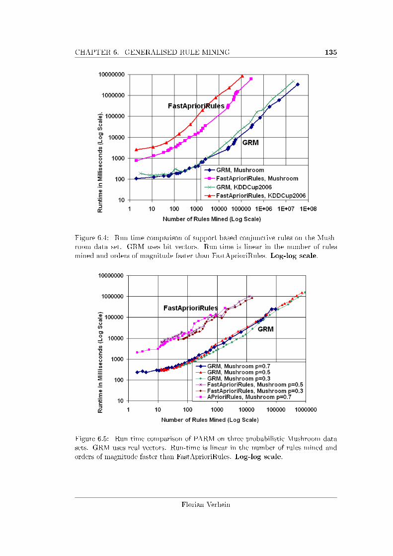
CHAPTER 6. GENERALISED RULE MINING 135
Figure 6.4: Run time comparison of support based conjunctive rules on the Mush-room data set. GRM uses bit vectors. Run-time is linear in the number of rulesmined and orders of magnitude faster than FastAprioriRules. Log-log scale.
Figure 6.5: Run time comparison of PARM on three probabilistic Mushroom datasets. GRM uses real vectors. Run-time is linear in the number of rules mined andorders of magnitude faster than FastAprioriRules. Log-log scale.
Florian Verhein
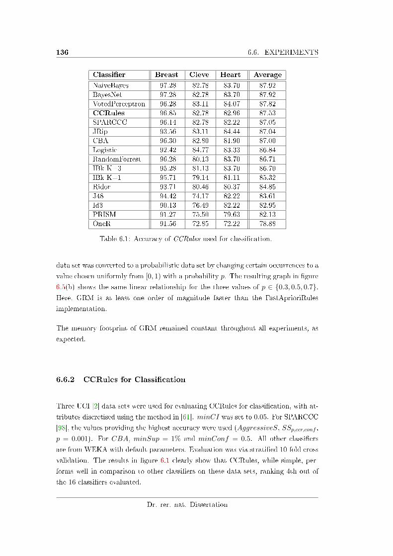
136 6.6. EXPERIMENTS
Classi�er Breast Cleve Heart Average
NaiveBayes 97.28 82.78 83.70 87.92
BayesNet 97.28 82.78 83.70 87.92
VotedPerceptron 96.28 83.11 84.07 87.82
CCRules 96.85 82.78 82.96 87.53
SPARCCC 96.14 82.78 82.22 87.05
JRip 93.56 83.11 84.44 87.04
CBA 96.30 82.80 81.90 87.00
Logistic 92.42 84.77 83.33 86.84
RandomForrest 96.28 80.13 83.70 86.71
IBk K=3 95.28 81.13 83.70 86.70
IBk K=1 95.71 79.14 81.11 85.32
Ridor 93.71 80.46 80.37 84.85
J48 94.42 74.17 82.22 83.61
Id3 90.13 76.49 82.22 82.95
PRISM 91.27 75.50 79.63 82.13
OneR 91.56 72.85 72.22 78.88
Table 6.1: Accuracy of CCRules used for classi�cation.
data set was converted to a probabilistic data set by changing certain occurrences to a
value chosen uniformly from [0, 1) with a probability p. The resulting graph in �gure
6.5(b) shows the same linear relationship for the three values of p ∈ {0.3, 0.5, 0.7}.Here, GRM is at least one order of magnitude faster than the FastAprioriRules
implementation.
The memory footprint of GRM remained constant throughout all experiments, as
expected.
6.6.2 CCRules for Classi�cation
Three UCI [2] data sets were used for evaluating CCRules for classi�cation, with at-
tributes discretised using the method in [61]. minCI was set to 0.05. For SPARCCC
[98], the values providing the highest accuracy were used (AggressiveS, SSp,ccr,conf ,
p = 0.001). For CBA, minSup = 1% and minConf = 0.5. All other classi�ers
are from WEKA with default parameters. Evaluation was via strati�ed 10-fold cross
validation. The results in �gure 6.1 clearly show that CCRules, while simple, per-
forms well in comparison to other classi�ers on these data sets, ranking 4th out of
the 16 classi�ers evaluated.
Dr. rer. nat. Dissertation

CHAPTER 6. GENERALISED RULE MINING 137
6.7 Conclusion
This work introduced the Generalized Rule Mining problem and solved it with the
combination of a novel vectorised framework and algorithm. The usefulness of this
abstraction was demonstrated by solving two very di�erent and novel rule mining
approaches. The next chapter shows a further approach. GRM was also demon-
strated to be orders of magnitude faster than a fast candidate generation and testing
approach on methods were this comparison is possible. Rules with novel semantics
(perhaps inspired by the geometric interpretation) that are now solvable using GRM
provide fertile avenues for future work.
Florian Verhein
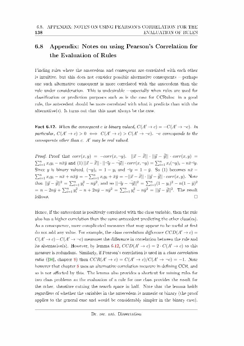
1386.8. APPENDIX: NOTES ON USING PEARSON'S CORRELATION FOR THE
EVALUATION OF RULES
6.8 Appendix: Notes on using Pearson's Correlation for
the Evaluation of Rules
Finding rules where the antecedent and consequent are correlated with each other
is intuitive, but this does not consider possible alternative consequents � perhaps
one such alternative consequent is more correlated with the antecedent than the
rule under consideration. This is undesirable � especially when rules are used for
classi�cation or prediction purposes such as is the case for CCRules: in a good
rule, the antecedent should be more correlated with what it predicts than with the
alternative(s). It turns out that this must always be the case.
Fact 6.12. When the consequent c is binary valued, C(A′ → c) = −C(A′ → ¬c). Inparticular, C(A′ → c) > 0 ⇐⇒ C(A′ → c) > C(A′ → ¬c). ¬c corresponds to the
consequents other than c. A′ may be real valued.
Proof. Proof that corr(x, y) = −corr(x,¬y). ||~x − ~x|| · ||~y − ~y|| · corr(x, y) =∑ni=1 xiyi − nxy and (1) ||~x− ~x|| · || ~¬y − ¬~y|| · corr(x,¬y) =
∑ni=1 xi(¬y)i − nx¬y.
Since y is binary valued, (¬y)i = 1 − yi and ¬y = 1 − y. So (1) becomes nx −∑ni=1 xiyi − nx + nxy = −
∑ni=1 xiyi + xy = −||~x − ~x|| · ||~y − ~y|| · corr(x, y). Note
that ||~y − ~y||2 =∑n
i=1 y2i − ny2, and so || ~¬y − ¬~y||2 =
∑ni=1(1 − yi)2 − n(1 − y)2
= n − 2ny +∑n
i=1 y2i − n + 2ny − ny2 =
∑ni=1 y
2i − ny2 = ||~y − ~y||2. The result
follows.
Hence, if the antecedent is positively correlated with the class variable, then the rule
also has a higher correlation than the same antecedent predicting the other class(es).
As a consequence, more complicated measures that may appear to be useful at �rst
do not add any value. For example, the class correlation di�erence CCD(A′ → c) =
C(A′ → c)−C(A′ → ¬c) measures the di�erence in correlation between the rule and
its alternative(s). However, by lemma 6.12, CCD(A′ → c) = 2 · C(A′ → c) so this
measure is redundant. Similarly, if Pearson's correlation is used in a class correlation
ratio ([98], chapter 8) then CCR(A′ → c) = C(A′ → c)/C(A′ → ¬c) = −1. Note
however that chapter 8 uses an alternative correlation measure in de�ning CCR, and
so is not a�ected by this. The lemma also provides a shortcut for mining rules for
two class problems as the evaluation of a rule for one class provides the result for
the other, therefore cutting the search space in half. Note that the lemma holds
regardless of whether the variables in the antecedent is numeric or binary (the proof
applies to the general case and would be considerably simpler in the binary case).
Dr. rer. nat. Dissertation

CHAPTER 6. GENERALISED RULE MINING 139
As far as the author is aware, previous work (e.g. [40]) has noted and used this
relationship for binary valued antecedents only.
Florian Verhein

1406.8. APPENDIX: NOTES ON USING PEARSON'S CORRELATION FOR THE
EVALUATION OF RULES
Dr. rer. nat. Dissertation
Chapter 7
Correlated Multiplication Rules
with Applications to Feature
Selection and Generation
Often, interactions between variables in a database are unknown to the
detriment of further analysis, classi�cation and mining tasks. This chapter
proposes Correlated Multiplication Rules (CMRules) which capture interac-
tions predictive of a dependent variable. CMRules are the �rst rules with
multiplicative semantics. Furthermore, a feature selection and dimensional-
ity reduction method is described whereby CMRules are used to generate
composite features. One advantage of this approach is that it allows linear
models to learn non-linear decision boundaries with respect to the original
variables. Unlike other methods, the resulting features are easy to under-
stand and initial experiments show that the proposed method can improve
classi�cation accuracy compared both to the original database and PCA
projections. Finally, it is shown that the CMRule mining problem can be
solved using the Generalised Rule Mining (GRM) framework of chapter 6.
141
142 7.1. INTRODUCTION
7.1 Introduction
Feature selection and generation is an important part of the Knowledge Discovery
process. This chapter proposes a data mining technique that �nds rules that are able
to capture interactions amongst variables that are highly correlated with a variable
of interest. In contrast to other rule mining methods, the variables may be real
valued or binary valued.
Rules are an important pattern in data mining due to their ease of interpretation and
usefulness for prediction. They have been heavily explored as association patterns
[11, 22, 81, 47, 84], �correlation� rules [22, 108] and for associative classi�cation
[61, 60, 100]. These approaches consider only conjunctions of binary valued variables
� which means that the antecedent and consequent consist of a conjunction of literals
that are either true or false [11, 22, 81, 47, 84, 108, 61].
Correlated Multiplication Rules (CMRules) consist of a set of real valued variables
multiplied together in the antecedent, and predict a variable c in the consequent:
vi ∗ vj ∗ ... ∗ vk → c. Rules with multiplication semantics and real valued variable
types are novel in the literature. CMRules �nd interactions between variables and
are successfully used as composite features, enabling linear models to learn non-linear
decision boundaries. Mixed variable types pose no problems.
Rule mining is a challenging problem due to its exponential search space in A ∪ C,where A is the set of variables that may be in the antecedent and C is the set of
variables that may be in the consequent. At best, an algorithms run time is linear
in the number of interesting rules it �nds, and the CMRules algorithm is provably
optimal in this sense. It also scales linearly in the dimensionality of the vectors, and
can use space linear in the size of the database. The algorithm uses a depth �rst
vectorized search approach, therefore avoiding the �candidate generation� problem
inherent with Apriori style algorithms.
7.1.1 Contributions
The contributions of this work are as follows:
• A new rule pattern, Correlated Multiplication Rules (CMRules) is introduced.
It is able to �nd multiplicative interactions amongst features that predict a
dependent variable; such as a class if used for classi�cation. In a descriptive
data mining approach, it helps �nd those features that interact to a�ect the
variable being studied. Unlike other rule mining methods, it can handle real
Dr. rer. nat. Dissertation
CHAPTER 7. CORRELATED MULTIPLICATION RULES WITHAPPLICATIONS 143
valued data. An e�cient algorithm is proposed based on the Generalised Rule
Mining methodology of chapter 6.
• A feature selection, generation and reduction method is introduced whereby
the antecedent of CMRules are used as composite features. This improves the
�t and classi�cation accuracy of other algorithms by explicitly allowing them
to capture interactions. In particular, this enables linear models to achieve
non-linear decision boundaries in the original features and thus improves the
classi�cation accuracy of such models. Since the composite features are rule
antecedents, which in turn are multiplications of attributes, the approach has
the advantage that the features are still interpretable. This contrasts methods
like Principle Component Analysis (PCA).
7.1.2 Organisation
The remainder of this chapter is organised as follows: Section 7.2 places this work in
the context of existing literature, section 7.3 presents the Correlated Multiplication
Rules technique. Section 7.4 describes the method whereby CMRules can be used
for composite feature generation and selection. Section 7.5 describes the CMRules
algorithm. Experimental results are presented in section 7.6 and this chapter is
concluded in section 7.7.
7.2 Related Work
7.2.1 Rule Mining
Most existing rule mining methods are used for associative pattern mining or clas-
si�cation. These only consider rules with conjunctive semantics of binary literals
and use counting approaches in their algorithms. Association rule mining meth-
ods [11, 47, 81] typically mine item-sets before mining rules, rather than mining
rules directly. Itemset mining methods are often extended to rule based classi�ca-
tion, which consider one variable in the consequent [110, 61, 100]. The algorithms
can be categorized into Apriori-like approaches [11] characterized by a breadth �rst
search through the item lattice and multiple database scans, tree based approaches
[47] characterized by a traversal over a pre-built compressed representation of the
database, projection based approaches [100] characterised by depth �rst projection
based searches and vertical approaches [81, 34, 96] that operate on columns. However,
CMRules does not use a support based technique, requires rules rather than sets,
Florian Verhein
144 7.3. CORRELATED MULTIPLICATION RULES (CMRULES)
and most importantly; does not have conjunctive semantics and requires handling
of real valued variables. Therefore, the Generalised Rule Mining (GRM) approach
(chapter 6, [93]), is exploited. GRM abstracts rule mining and mines rules directly
and very e�ciently
7.2.2 Correlation Rules
Conjunctive rules using correlation measures have been studied in the literature,
though all are quite di�erent to those presented in this paper; [22] uses a χ2 test to
measure the signi�cance of a correlation, but measures correlation by independence
� not by Pearson's correlation. [108] uses Pearson's correlation, but this is applied to
item pairs, not rules. FOSSIL [40] mines rules for classi�cation using a heuristic based
only on Pearson's correlation, but it is an inductive logic programming approach.
While the φ-coe�cient is often used to evaluate rules mined by other methods [88],
the author is not aware of any purely correlation based approach such as Correlation
Improvement. Furthermore, note that no previous rule mining approach applied to
real valued vectors in the context of rule mining, as is done in the CMRules method.
Existing rule mining techniques are exclusively conjunctive and include association
analysis and prediction or rule based classi�cation [11, 103, 110].
7.3 Correlated Multiplication Rules (CMRules)
Linear models such as regression are important for modeling [44] and classi�cation
[104], but their power is limited by their linear decision boundary. They can be
used to model non-linearities (in terms of the original variables) by using non-linear
functions on existing variables as regressors (or `features' in machine learning). Fur-
thermore, when such functions are applied to multiple variables at a time, they
generate composite variables capable of capturing non-linear interactions between
variables. These can replace existing variables or function as additional variables in
a linear model. The use of such composite variables transforms the space in which
the (linear) model is built. If the composite features are non-linear in the original
features, the model becomes non-linear in the original variables1. This is analogous
to using kernel functions to map the space so that a non-linear decision boundary is
achieved using linear models.
Good candidates for composite variables are multiplications of sets of variables. For
example, the regression/decision problem y = α1v1 +α2v2 +α3v3 +α1,2v1v2 +β can
1Of course, it remains linear in the (composite) variables used in the model.
Dr. rer. nat. Dissertation
CHAPTER 7. CORRELATED MULTIPLICATION RULES WITHAPPLICATIONS 145
capture non linearities in v1 and v2 as well as capturing an interaction between v1
and v2 since it includes the term α1,2v1v2. Finding the right variables to multiply
together in order to achieve a better �t is a challenging problem. The best composite
variables are highly correlated with the dependent variable; they capture the non-
linearities and interactions well and therefore allow a better �t. This is a simple
but powerful idea. However, if there are m variables, there are O(mk) composite
feature size to k and, in general, there are O(2m). Therefore, an intelligent search
with pruning is required.
Example 7.1. Suppose we have the regression/decision problem P : y = α1v1 +
α2v2+β. We can add an extra (composite) variable v1v2: P′ : y = α1v1+α2v2+β+
α1,2v1v2. This model is now capable of expressing a non-linear decision boundary
in terms of v1 and v2 and can also capture a multiplicative interaction between v1
and v2. If there are no such patterns, α1,2 will be found to be 0. If there are non-
linearities or interactions in the problem that can be approximated by v1v2 then P′
will have α1,2 6= 0 and will �t better than P .
Correlated Multiplication Rules (CMRules) are rules of the form vi ∗ vj∗, ..., ∗vk → c,
where the vi ∈ A are observed variables and c is the dependent variable to be
predicted. Based on the above discussion, the antecedents of rules with the highest
correlations de�ne ideal composite variables and capture interactions explaining the
dependent variable c. Furthermore, such rules are easy to interpret and understand
and can therefore provide useful information to help explain interactions in the data.
The data set consists of a set of variables A and a dependent variable c. Each row in
the data set consists of samples of these variables. Each column therefore contains all
samples for a particular variable v ∈ A or c. Consider these columns as vectors and
denote these by xv and xc respectively. xv[i] is therefore the ith sample of variable
v.
The CMRules presented in this chapter use Pearson's product moment correlation
coe�cient, although other measures can easily be used in its place. Pearson's corre-
lation coe�cient between two variables v and c may be written as
rv,c =
∑ni=1(xv[i]− xv)(xc[i]− xc)√∑n
i=1(xv[i]− xv)2√∑n
i=1(xc[i]− xc)2
where rv,c ∈[−1, 1] and xv is the mean of v. If all variables are binary valued, it
reduces to the φ coe�cient.
Florian Verhein
146 7.3. CORRELATED MULTIPLICATION RULES (CMRULES)
The correlation C(A′ → c) of a rule A′ → c is de�ned as the Pearson's product
moment correlation coe�cient between the antecedent and the consequent of the
rule. Let the vector corresponding to the antecedent be denoted xA′ . C(A′ → c)
may then be written as:
C(A′ → c) =(xA′ − xA′) · (xc − xc)||xA′ − xA′ ||||xc − xc||
Since CMRules have multiplication semantics, the vector xA′ is de�ned by
xA′ [i] = Πv∈A′xv[i]
That is, for each sample / row in the database, the values of the variables in the
antecedent of the rule are multiplied together. Accordingly, CMRules with a high
correlation show those variables that, when multiplied together in all the samples,
are highly correlated with the dependent variable c.
7.3.1 Directing the Search by Correlation Improvement
Recall that the goal is to �nd highly correlated CMRules. The simplest approach
is to attempt to �nd rules with a correlation above some user de�ned threshold.
However, it is problematic to direct the search space by only expanding rules with
correlation above a threshold for two reasons.
• First, it introduces an arbitrary parameter to which the approach becomes
sensitive.
• More subtly, since correlation is not downwards closed, it also introduces a
dependency on the order in which variables are added to the antecedent. This
could be addressed by �forcing� anti-monotonicity as a greedy heuristic but the
limitation inherent in absolute threshold based techniques remains.
Instead, the following approach is used: A variable should only be added to the
antecedent of a rule if it improves the rule compared to its generalizations. That
is, if the variable improves the rule compared to those less speci�c rules having
fewer variables in the antecedent. The Correlation Improvement (CI) measures this
improvement in terms of correlation;
De�nition 7.2. The Correlation Improvement is
CI(A′ → c) = C(A′ → c)−maxa∈A′{C(A′ − {a} → c)}
Dr. rer. nat. Dissertation
CHAPTER 7. CORRELATED MULTIPLICATION RULES WITHAPPLICATIONS 147
where A′ − {a} → c is a less speci�c sub rule obtained by removing variable a from
the antecedent. Note that A′ − {z} → c is a generalization (a less speci�c rule) that
therefore applies to more samples, while A′ → c is more speci�c and applies to less
samples. For an empty antecedent (the base case), CI(∅ → c) = C(∅ → c) where x∅
is a vector of 1s.
The Correlation Improvement is positive if the rule to which it is applied has a
higher correlation than any of its immediate generalizations. This means it is a bet-
ter predictor of the consequent variable than any of the less speci�c rules. This also
has a geometric interpretation: Since correlation is the cosine of the angle between
vectors (Recall �gure 6.2), using the correlation improvement technique means the
antecedent is built so that it moves closer to the consequent (in terms of the sub-
tended angle) in comparison to the immediate sub-rules.
The following lemma shows that Correlation Improvement is downward closed.
Lemma 7.3. If A′ → c is expanded (and considered interesting) only when CI(A′ →c) ≥ 0 then Correlation Improvement is downwards closed: If A′ → c is interesting,
then so are all sub-rules.
Proof. This follows by induction over all sub-rules.
This means that A′ → c is not only more correlated than all immediate sub-rules,
but indeed all sub-rules. Consequently, Correlation Improvement is a useful method
to direct the search for CMRules.
It is now possible to de�ne the CMRule problem:
Problem de�nition: Correlated Multiplication Rules (CMRules): Find all
CMRules with CI(A′ → c) > minCI, a threshold. (Recall that A′ is interpreted as
a multiplication of variables; Πvi∈A′vi).
Note that if minCI > 0, only variable interactions that predict the dependent vari-
able better than all individual variables are found.
Finally, note that CMRules with a single variable in the antecedent are also useful �
they can (trivially) be used to select a good subset of variables (features) to use since
they simple variables that are highly correlated with the dependent variable. Recall
that CMRules can be used for automated supervised variable (feature) selection and
composite variable generation � in particular, for generating composite variables that
allow a non-linear interactions to be captured in the model.
Florian Verhein
148 7.4. CMRULES FOR FEATURE SELECTION AND GENERATION
7.4 CMRules for Feature Selection and Generation
Recall that the antecedents of CMRules are ideal candidates for composite features,
and CMRules with only a single variable in the antecedent are also useful for fea-
ture selection. This is because the interactions de�ned by the antecedent variables
are highly correlated with the dependent variable to be predicted, and since the
antecedent is the product of variables, it introduces introduces non-linearity.
In order to use CMRules for feature selection and composite feature generation,
this chapter proposes the Top Correlated Multiplication Rules (TCMR) method as
follows:
1. First, all CMRules are mined using the correlation improvement method.
2. Then, the rules are sorted according to their C(A′ → c) values and the top
ranked rules selected.
3. Finally, the antecedents of the selected rules are used as (composite) variables
in the model. This means the vectors xA′ of the selected rules A′ → c become
the new values of the composite features A′.
This simple procedure works well, as will be shown in section 7.6.
7.5 Mining CMRules
This chapter adopts the Generalised Rule Mining (GRM) method proposed in chap-
ter 6. GRM is a combination of a framework of functions on vectors and an e�cient
algorithm for mining rules directly. It solves rule mining at the abstract level. It is
used for the following reasons:
• GRM proved to be easy to apply to the problem addressed in this paper. Since
GRM solves rule mining at the abstract level, the CMRules problem can be
solved by instantiating the functions in the framework appropriately (below)
and using the GRM algorithm.
• GRM supports real valued variables and any rule semantics. Since CMRules
is the �rst rule based method with multiplicative semantics and real valued
variables, other algorithms are not applicable.
• The GRM algorithm is e�cient and uses linear time in the rules mined. It does
not use �candidate generation�, does not require multiple scans and does not
generate a compressed version of the database.
Dr. rer. nat. Dissertation
CHAPTER 7. CORRELATED MULTIPLICATION RULES WITHAPPLICATIONS 149
The core of GRM is its framework, which abstracts and vectorises rule mining. Re-
call that A is the set of variables that may be in the antecedent, and C is the set of
variables that may be in the consequent. In CMRules, C = {c}, the dependent vari-able to be predicted. As an aside, supposing there are multiple dependent variables,
one may have |C| > 1. This is equivalent to mining CMRules for each dependent
variable separately, however the separation method takes O(|C|) times longer than
if they are mined together in one go.
In the GRM framework, each possible antecedent A′ ⊆ A and each possible conse-
quent c ∈ C are expressed as vectors, denoted by xA′ and xc respectively. Recall
that these were already de�ned in section 7.3. The GRM framework is composed of
�ve functions, which can be instantiated in the following way to solve the CMRules
problem:
1. mR : X2 → R is a distance measure between the antecedent and consequent
vectors xA′ and xc. mR(xA′ , xc) evaluates the quality of the rule A′ → c.
In CMRules, mR(xA′ , xc) = C(A′ → c), Pearson's correlation coe�cient as per
section 7.3. Geometrically, in CMRules �close� means the angle between xA′
and xc is small (�gure 6.2 on page 123).
2. aR : X2 → X operates on vectors of the antecedent so that xA′∪a = aR(xA′ , xa)
where A′ ⊆ A and a ∈ (A−A′). This means aR(·) combines the vector xA′ foran existing antecedent A′ ⊆ A with the vector xa for a new antecedent element
a ∈ A−A′. The resulting vector xA′∪a represents the larger antecedent A′ ∪ a.Therefore, aR(·) allows the antecedent vector required by mR(·) to be built
incrementally. Since aR(·) de�nes how the vectors are built, it also � implicitly
� de�nes the semantics of the rule.
In CMRules, aR(·) is the element-wise multiplication of (typically) real val-
ued vectors: aR(xA′ , aa)[j] = xA′ [j] ∗ xa[j]. The semantics of CMRules are
multiplicative.
3. MR : R|P(A′)| → R is a measure that evaluates a rule A′ → c based on the
value computed by mR(·) for any sub-rule A′′ → c : A′′ ⊆ A′. This supports
interestingness measures where a rule A′ → c needs to be compared with some
or all of its sub-rules.
Recall that in CMRules, the Correlation Improvement method ensures rules
are mined that are more correlated with c than their immediate sub-rules. The
Correlation Improvement method is implemented using MR(·) according to
de�nition 7.2.
Florian Verhein
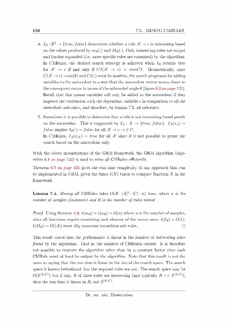
150 7.5. MINING CMRULES
4. IR : R2 → {true, false} determines whether a rule A′ → c is interesting based
on the values produced by mR(·) and MR(·). Only interesting rules are output
and further expanded (i.e. more speci�c rules are examined) by the algorithm.
In CMRules, the desired search strategy is achieved when IR returns true
for A′ → c if and only if CI(A′ → c) > minCI. Geometrically, since
C(A′ → c) =cos(θ) and CI(·) must be positive, the search progresses by addingvariables to the antecedent in a way that the antecedent vector moves closer to
the consequent vector in terms of the subtended angle θ (�gure 6.2 on page 123).
Recall that this means variables will only be added to the antecedent if they
improve the correlation with the dependent variable c in comparison to all the
immediate sub-rules, and therefore, by lemma 7.3, all sub-rules.
5. Sometimes it is possible to determine that a rule is not interesting based purely
on the antecedent. This is supported by IA : X → {true, false}. IA(xA) =
false implies IR(·) = false for all A′ → c : c ∈ C.In CMRules, IA(xA′) = true for all A′ since it is not possible to prune the
search based on the antecedent only.
With the above instantiations of the GRM framework, the GRM algorithm (algo-
rithm 6.1 on page 132) is used to mine all CMRules e�ciently.
Theorem 6.9 on page 131 gives the run time complexity of any approach that can
be implemented in GRM, given the times t(X) taken to compute function X in the
framework.
Lemma 7.4. Mining all CMRules takes O(R · |A|2 · |C| · n) time, where n is the
number of samples (instances) and R is the number of rules mined.
Proof. Using theorem 6.9; t(mR) = t(aR) = O(n) where n is the number of samples,
since all functions require examining each element of the vector once. t(IR) = O(1).
t(MR) = O(|A|) since MR examines immediate sub-rules.
This result states that the performance is linear in the number of interesting rules
found by the algorithm. That is, the number of CMRules output. It is therefore
not possible to improve the algorithm other than by a constant factor since each
CMRule must at least be output by the algorithm. Note that this result is not the
same as saying that the run time is linear in the size of the search space. The search
space is known beforehand, but the required rules are not. The search space may be
O(2|A∪C|) but if only R of these rules are interesting (and typically R << 2|A∪C|),
then the run time is linear in R, not 2|A∪C|.
Dr. rer. nat. Dissertation
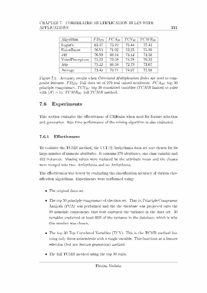
CHAPTER 7. CORRELATED MULTIPLICATION RULES WITHAPPLICATIONS 151
Algorithm FD279 PCA30 TCV30 TCMR30
Logistic 63.27 75.22 75.44 77.43
NaiveBayes 76.55 71.02 73.23 75.89
J48 76.99 68.14 74.12 74.56
VotedPerceptron 75.22 70.58 74.78 76.33
Jrip 75.22 68.58 72.79 73.67
Average 73.45 70.71 74.07 75.58
Figure 7.1: Accuracy results when Correlated Multiplication Rules are used as com-posite features. FD279: Full data set of 279 real valued attributes. PCA30: top 30principle components. TCV30: top 30 correlated variables (TCMR limited to ruleswith |A′| = 1). TCMR30: full TCMR method.
7.6 Experiments
This section evaluates the e�ectiveness of CMRules when used for feature selection
and generation. Run time performance of the mining algorithm is also evaluated.
7.6.1 E�ectiveness
To evaluate the TCMR method, the UCI [2] Arrhythmia data set was chosen for its
large number of numeric attributes. It contains 279 attributes, one class variable and
452 instances. Missing values were replaced by the attribute mean and the classes
were merged into two: Arrhythmia and no Arrhythmia.
The e�ectiveness was tested by evaluating the classi�cation accuracy of various clas-
si�cation algorithms. Experiments were performed using:
• The original data set.
• The top 30 principle components of the data set. That is, Principle Component
Analysis (PCA) was performed and the the database was projected onto the
30 principle components that best captured the variance in the data set. 30
variables explained at least 95% of the variance in the database, which is why
this number was chosen.
• The top 30 Top Correlated Variables (TCV). This is the TCMR method but
using only those antecedents with a single variable. This functions as a feature
selection (but not feature generation) method.
• The full TCMR method using the top 30 rules.
Florian Verhein
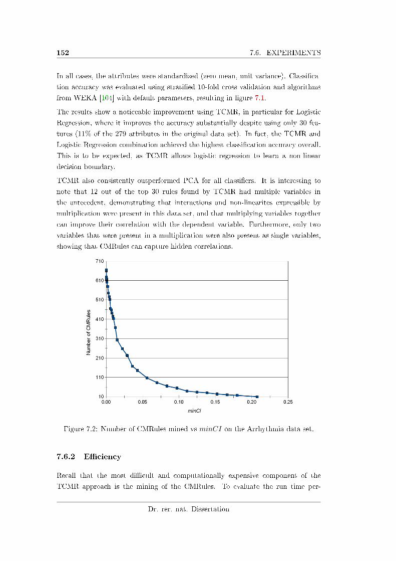
152 7.6. EXPERIMENTS
In all cases, the attributes were standardized (zero mean, unit variance). Classi�ca-
tion accuracy was evaluated using strati�ed 10-fold cross validation and algorithms
from WEKA [104] with default parameters, resulting in �gure 7.1.
The results show a noticeable improvement using TCMR, in particular for Logistic
Regression, where it improves the accuracy substantially despite using only 30 fea-
tures (11% of the 279 attributes in the original data set). In fact, the TCMR and
Logistic Regression combination achieved the highest classi�cation accuracy overall.
This is to be expected, as TCMR allows logistic regression to learn a non-linear
decision boundary.
TCMR also consistently outperformed PCA for all classi�ers. It is interesting to
note that 12 out of the top 30 rules found by TCMR had multiple variables in
the antecedent, demonstrating that interactions and non-linearites expressible by
multiplication were present in this data set, and that multiplying variables together
can improve their correlation with the dependent variable. Furthermore, only two
variables that were present in a multiplication were also present as single variables,
showing that CMRules can capture hidden correlations.
Figure 7.2: Number of CMRules mined vs minCI on the Arrhythmia data set.
7.6.2 E�ciency
Recall that the most di�cult and computationally expensive component of the
TCMR approach is the mining of the CMRules. To evaluate the run time per-
Dr. rer. nat. Dissertation
CHAPTER 7. CORRELATED MULTIPLICATION RULES WITHAPPLICATIONS 153
Figure 7.3: Run time in comparison to the number of rules mined on the Arrhythmiadata set.
formance, the minCI parameter was varied and all CMRules mined that setting.
Figure 7.2 shows the number of rules mined for various minCI settings. Figure 7.3
shows the run time in comparison to the number of rules mined in log-log scale.
Above about the �rst 10 rules, it is clear to see that the run time is linear in the
number of rules mined.
7.7 Conclusion
Often, interactions between variables in a database are unknown to the detriment
of further analysis, classi�cation and mining tasks. This paper proposed Correlated
Multiplication Rules (CMRules) which are able to capture interactions predictive
of a dependent variable. CMRules are the �rst rules with multiplicative semantics
and are applied to feature selection and dimensionality reduction. This method uses
CMRules to generate composite features, enabling linear models to learn non-linear
decision boundaries with respect to the original variables. The resulting features are
easy to understand and initial experiments showed that the proposed method can
improve classi�cation accuracy compared both to the original database and PCA
projections. Finally, it is shown that the CMRule mining problem can be solved
e�ciently using the Generalised Rule Mining (GRM) framework.
Florian Verhein

154 7.7. CONCLUSION
Dr. rer. nat. Dissertation
Part III
Statistical Data Mining Methods
155

Chapter 8
Using Signi�cant, Positively
Associated and Relatively Class
Correlated Rules for Classi�cation
of Imbalanced Databases
The application of association rule mining to classi�cation has led to a new
family of classi�ers which are often referred to as Associative Classi�ers
(ACs). The advantage of using rule based approaches is that they are easy
to interpret and perform a global search, compared to many other rule based
approaches that use a greedy search strategy.
Rule-based classi�ers can play an important role in applications such as
medical diagnosis and fraud detection where data sets are almost always
imbalanced. The focus of this chapter is to extend ACs for classi�cation on
imbalanced data sets using statistics based techniques.
This work combines the use of statistically signi�cant rules with a new mea-
sure, the Class Correlation Ratio (CCR), to build an AC called SPARCCC.
A detailed set of experiments show that in terms of classi�cation quality,
SPARCCC performs comparably on balanced data sets and greatly outper-
forms other AC techniques on imbalanced data sets. It also has a signif-
icantly smaller rule base and is more computationally e�cient than tradi-
tional support-con�dence based associative classi�ers.
157
158 8.1. INTRODUCTION
8.1 Introduction
Since the introduction of CBA [61] many variations on Associative Classi�ers (ACs)
have been proposed in the literature [60, 13, 110, 100, 28, 30, 15, 89]. Most of the
ACs are based on rules discovered using the support-con�dence paradigm and the
classi�er itself is a collection of rules ranked using con�dence or variation thereof.
In many application domains, the data sets are imbalanced, i.e., the proportion
of samples from one class is much smaller than the other class(es). Additionally,
the smaller class is the class of interest. For example; fraud detection and medical
diagnoses. Unfortunately, the support-con�dence framework does not perform well
in such cases.
Many of the rules mined using support-con�dence are spurious and are irregularities
in the data rather than properties of the underlying population or process, motivating
the statistically signi�cant rules proposed by Webb [103]. The same holds true of
rules used for classi�cation. It is also well known that con�dence has non-intuitive
properties in imbalanced data sets. For example, high con�dence rules can also be
negatively correlated. This chapter combines statistically signi�cant rules with a
new measure, the Class Correlation Ratio (CCR), which leads to a better classi�er.
Furthermore, the proposed method does not use the support-con�dence paradigm.
8.1.1 Contributions
This chapter makes the following contributions:
• It proposes the Class Correlation Ratio (CCR), which measures the relative
class correlation of a rule. A high CCR is desirable because it means the rule
is more positively correlated with the class it predicts than the alternative(s).
CCR also forms the basis of an e�ective rule ranking method that does not
require con�dence.
• It proves that con�dence and support are biased toward the majority class
in imbalanced data sets in the context of CCR. This result also motivates a
correction for con�dence's bias, and is a key component in making the classi�er
perform well on both balanced and imbalanced data sets.
• An associative classi�er is proposed that is based on statistical techniques. The
method is called Signi�cant, Positively Associated and Relatively Class Corre-
Dr. rer. nat. Dissertation
CHAPTER 8. CLASSIFICATION OF IMBALANCED DATABASES USINGSIGNIFICANT RULES 159
lated Classi�cation (SPARCCC) because it uses only rules that are statistically
signi�cant and positively associated, and where the antecedent is more corre-
lated with the class it predicts than with the other class(es). It also searches
directly for signi�cant rules and uses this to prune the search space. SPARCCC
outperforms support-con�dence based associative classi�ers on balanced data
sets in terms of computational performance, and on imbalanced data sets in
both computational and classi�cation performance. SPARCCC is parameter-
free, in the sense that it does not use thresholds � except standard levels of
signi�cance � to prune rules. Finally, since the rules are statistically signi�cant
and relatively class correlated, they may be examined for insights into the data.
8.1.2 Organisation
The the remainder of this chapter is organised as follows: Section 8.2 gives a brief
background in associative classi�cation. Section 8.3 describes the class correlation
ratio and the signi�cance test used. Section 8.4 proves that con�dence (and support)
are biased against the minority class under CCR. Section 8.5 describes the SPARCCC
technique. Section 8.7 contains experimental results. Related work is surveyed in
section 8.8 and this chapter concludes in section 8.9.
8.2 Background: Associative Classi�cation
8.2.1 Association Rule Mining
In Association Rule Mining (ARM), the data is a set of transactions T = {t1, ..., t|T |},each of which is a subset of the set of items: ti ⊆ I, I = {i1, ..., i|I|}. The support
of an itemset X ⊆ I is sup(X) = |{ti : X ⊆ ti ∧ ti ∈ T}|. An association rule
X → Y is an implication between two mutually exclusive itemsets X and Y . The
support of X → Y is sup(X → Y ) = sup(X ∪ Y ) and its confidence, an estimate
of the probability that Y occurs given that X occurs, is conf(X → Y ) = sup(X →Y )/sup(X).
8.2.2 Associative Classi�cation
This chapter assumes a discrete data set D with attributes A = {a1, a2, ..., a|A|},one of which is the class attribute ac. In every instance d ∈ D, each attribute
ai ∈ A takes one of a �nite number of possible values Vi = {vi,1, ..., vi,|Vi|} so that
d = [v1,j , v2,k, ..., v|A|,l] (for some j, k, ..., l). As an ARM task, the attribute-value
Florian Verhein
160 8.3. SIGNIFICANCE AND CLASS CORRELATION RATIO FOR RULES
pairs become items (Namely, i|V1|+...+|Vi−1|+j ≡ (ai = vi,j)) and the instances become
corresponding transactions. The previous instance d then becomes a transaction
t = {(a1 = v1,i), (a2 = v2,j), ..., (a|A| = v|A|,k)}. Clearly, there will be∑|A|
i=1 |Vi| = |I|items and each transaction will have size |A|. Since the described mapping is a
bijection, one can freely interchange instances and transactions when convenient.
8.2.3 Associative Classi�cation Rule Mining
The Associative Classi�cation Rule Mining (ACRM) task is to �nd interesting rules
X → y whereX is a set of legal (an attribute cannot occur more than once) attribute-
value pairs and y is one of the class attribute-value pairs. �Interesting� rules are rules
that, in conjunction with other mined rules, are likely to perform well for classi�cation
of unseen data.
8.3 Signi�cance and Class Correlation Ratio for Rules
8.3.1 Fisher's Exact Test
There are strong arguments for mining statistically signi�cant rules [103]. These
also hold true when the rules are used for classi�cation, as one would like to make a
decision based on signi�cant evidence.
Support is often used as a measure of �signi�cance�, the reasoning being that rules
that have high support are �intuitively� more likely to capture the underlying process
generating the data, rather than being artifacts of the data set or generated by noise.
However, this is simply not the case and one can easily generate counterexamples
showing insigni�cant high support or signi�cant low support rules.
This work considers rules X → y that are statistically signi�cant in the positively
associated direction. Toward that end, Fisher's Exact Test (FET) is used on contin-
gency tables of the form of �gure 8.11.
1Statistical tests on such tables determine whether there is a signi�cant association betweenthe variables, compared to the null hypothesis of no association. If the sampling scheme is suchthat only the total (n) is �xed (or it is unrestricted), then the null hypothesis is that the variablesare independent of each other, in the sense that the probability of falling into a particular rowis independent of the column a particular subject is in, and vice versa (This symmetry meansthat the tests give the same result for [a, b; c, d] as they do for [a, c; b, d].) [31]. For example,P (V1, V2) = P (V1) · P (V2). Statistical tests compute the probability (the p-value) of obtaining atable at least as unusual as the observed table. If the p-value is below a level of signi�cance, thenthere is assumed to be su�cient evidence to reject the null hypothesis and therefore we can saywith some con�dence level that the variables are correlated.
Dr. rer. nat. Dissertation
CHAPTER 8. CLASSIFICATION OF IMBALANCED DATABASES USINGSIGNIFICANT RULES 161
FET is an exact test (permutation test) that computes the p-value of an observed
contingency table by explicitly calculating the probability of di�erent table con�gu-
rations, rather than using an approximate or limiting distribution. This work uses
the positive one sided FET to test whether rules are signi�cant in the positive direc-
tion. Given a table [a, b; c, d], FET will �nd the probability (p-value) of obtaining the
given table or a table where X and y are more positively associated under the null
hypothesis that {X,¬X} and {y,¬y} are independent, and that the margin sums
are �xed. The p-value is given by:
p([a, b; c, d]) =
min(b,c)∑i=0
(a+ b)!(c+ d)!(a+ c)!(b+ d)!
n!(a+ i)!(b− i)!(c− i)!(d+ i)!
Only rules whose p-values are below the level of signi�cance desired are used, as they
are statistically signi�cant in the positively associated direction.
FET's continuous approximation � the χ2 test � could also be used, but since it is a
two sided test it cannot distinguish positive associations and is thus less desirable.
8.3.2 Correlation (Interest Factor)
Correlation also forms an important component of the technique in this work. This
chapter proposes that rules X → y should be used when X is more positively corre-
lated with y than it is with ¬y. The following de�nition of correlation2 is used:
ˆcorr(X → y) =sup(X ∪ y) · |D|sup(X) · sup(y)
=a · n
(a+ c) · (a+ b)
X and y are positively (negatively) correlated if ˆcorr(X → y) > 1 (< 1), and
independent otherwise. Note that ˆcorr(X → y) = I(X, y), where I(X, y) is the
Interest Factor [88]. This measure has downsides when used by itself. It is clear to
see that increasing the size of the data set by increasing d (refer to �gure 8.1) will
increase the correlation between X and y � even though it is actually increasing the
association between ¬X and ¬y. The reverse holds for decreasing d.
Example 8.1. Consider the table T1 = [100, 20; 20, 10] where X and y are have a
strong association but ˆcorr(X → y) = 1.04 (almost independent). If d is increased
to get T2 = [100, 20; 20, 200], then clearly ¬X and ¬y are strongly associated, but
ˆcorr(¬X → ¬y) = 1.4 while now ˆcorr(X → y) = 2.36. This is clearly undesirable.
2To be more precise, ˆcorr(X → y) this is the estimate of corr(X → y) = P (X∪y⊆t)P (X⊂t)·P (y∈t) , where
corr(X → y) is de�ned over the underlying process that generates the data.
Florian Verhein
162 8.3. SIGNIFICANCE AND CLASS CORRELATION RATIO FOR RULES
This problem arises only in imbalanced data sets; note that changing d alters the
class distribution.
Therefore, SPARCCC does not search for positively correlated rules using ˆcorr.
When a rule is described as being positively associated or correlated, the author
means using the one sided test of signi�cance using FET. FET does not have the
downside described above because of the constant margin sum restriction. Indeed,
p(T1) = 0.041 (signi�cant at the 0.05 level) and p(T2) = 1.07 · 10−44 (highly signi�-
cant).
8.3.3 Class Correlation Ratio
SPARCCC uses ˆcorr(·) to measure how correlated X is with y compared to ¬y usingthe proposed Class Correlation Ratio (CCR):
De�nition 8.2. The Class Correlation Ratio (CCR) is de�ned as:
CCR(X → y) =ˆcorr(X → y)
ˆcorr(X → ¬y)=a · (b+ d)
b · (a+ c)
The CCR measures how much more positively the antecedent is correlated with
the class it predicts, relative to the alternative class(es). This avoids the downsides
of using an absolute correlation measure � indeed, terms cancel out. Furthermore,
intuitively one would not want to use a rule that is more correlated with classes other
than the one it predicts!
Example 8.3. Returning to Example 8.1, CCR(X → y) = 1.25 for T1 and CCR(X →y) = 9.17 for T2. This also says that X → y is a better rule under T2 than under
T1. This is true � it is much more discriminative because under T1, y is already the
majority class and therefore the rule does not provide much additional information.
In fact, the information gain of using X → y over ∅ → y is only 0.072 bits under T1
but is 0.215 bits under T2. Recall also that the rule was much more signi�cant under
T2.
SPARCCC uses only rules with CCR > 1, so that no rules are used that are more
positively associated with the classes they do not predict. Furthermore, CCR is also
used in the strength score � which used to rank rules for classi�cation � in order to
correct for the bias of con�dence. This will be covered shortly.
Dr. rer. nat. Dissertation
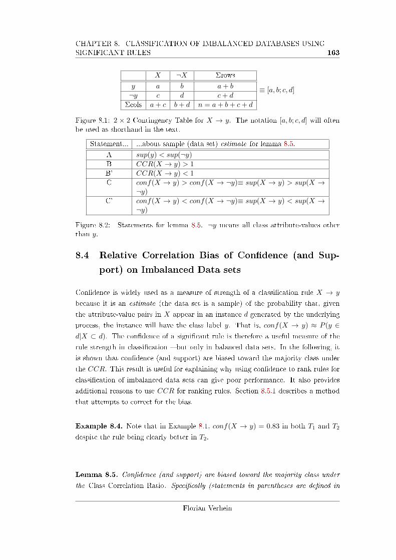
CHAPTER 8. CLASSIFICATION OF IMBALANCED DATABASES USINGSIGNIFICANT RULES 163
X ¬X Σrows
y a b a+ b
¬y c d c+ d
Σcols a+ c b+ d n = a+ b+ c+ d
≡ [a, b; c, d]
Figure 8.1: 2 × 2 Contingency Table for X → y. The notation [a, b; c, d] will oftenbe used as shorthand in the text.
Statement... ...about sample (data set) estimate for lemma 8.5.
A sup(y) < sup(¬y)
B CCR(X → y) > 1
B' CCR(X → y) < 1
C conf(X → y) > conf(X → ¬y)≡ sup(X → y) > sup(X →¬y)
C' conf(X → y) < conf(X → ¬y)≡ sup(X → y) < sup(X →¬y)
Figure 8.2: Statements for lemma 8.5. ¬y means all class attribute-values otherthan y.
8.4 Relative Correlation Bias of Con�dence (and Sup-
port) on Imbalanced Data sets
Con�dence is widely used as a measure of strength of a classi�cation rule X → y
because it is an estimate (the data set is a sample) of the probability that, given
the attribute-value pairs in X appear in an instance d generated by the underlying
process, the instance will have the class label y. That is, conf(X → y) ≈ P (y ∈d|X ⊂ d). The con�dence of a signi�cant rule is therefore a useful measure of the
rule strength in classi�cation � but only in balanced data sets. In the following, it
is shown that con�dence (and support) are biased toward the majority class under
the CCR. This result is useful for explaining why using con�dence to rank rules for
classi�cation of imbalanced data sets can give poor performance. It also provides
additional reasons to use CCR for ranking rules. Section 8.5.1 describes a method
that attempts to correct for the bias.
Example 8.4. Note that in Example 8.1, conf(X → y) = 0.83 in both T1 and T2
despite the rule being clearly better in T2.
Lemma 8.5. Con�dence (and support) are biased toward the majority class under
the Class Correlation Ratio. Speci�cally (statements in parentheses are de�ned in
Florian Verhein
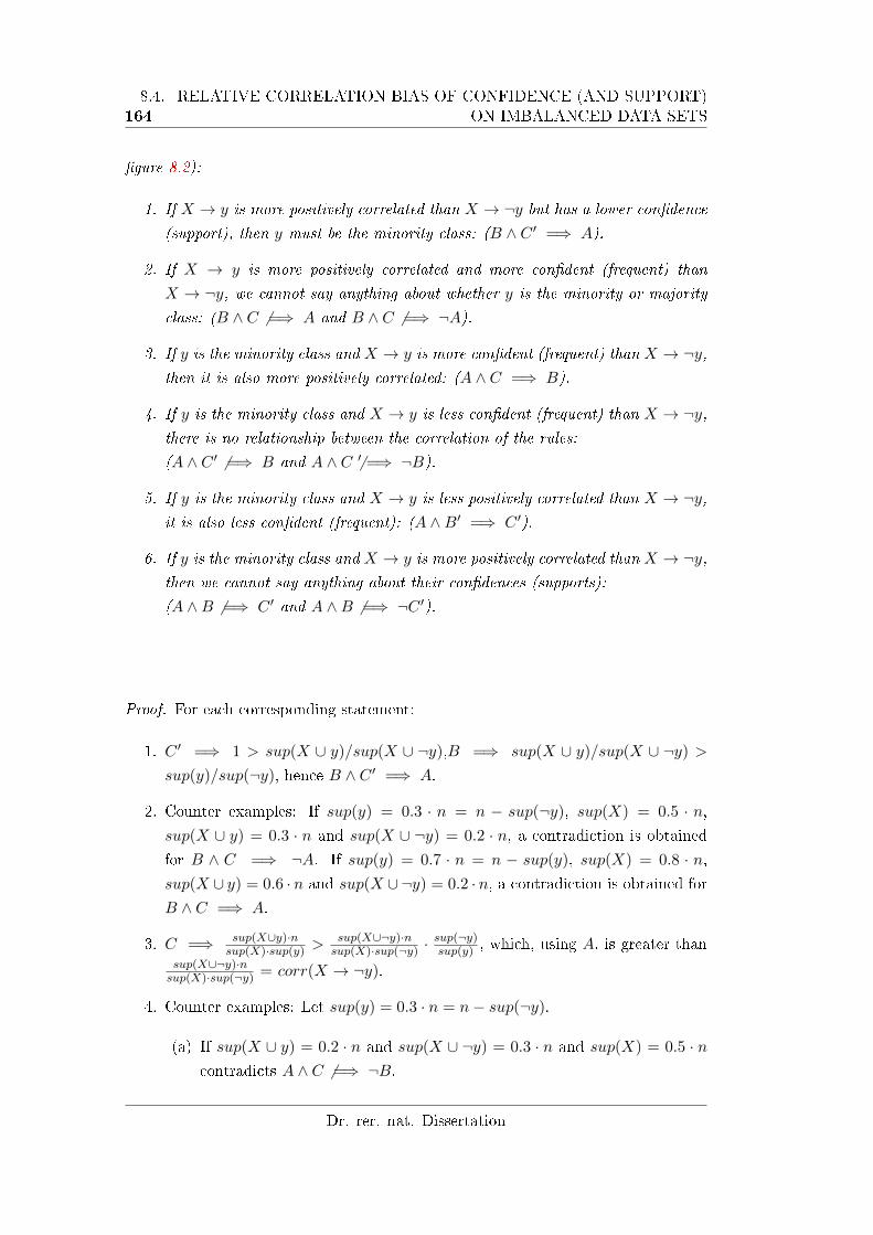
1648.4. RELATIVE CORRELATION BIAS OF CONFIDENCE (AND SUPPORT)
ON IMBALANCED DATA SETS
�gure 8.2):
1. If X → y is more positively correlated than X → ¬y but has a lower con�dence(support), then y must be the minority class: (B ∧ C ′ =⇒ A).
2. If X → y is more positively correlated and more con�dent (frequent) than
X → ¬y, we cannot say anything about whether y is the minority or majority
class: (B ∧ C 6 =⇒ A and B ∧ C 6 =⇒ ¬A).
3. If y is the minority class and X → y is more con�dent (frequent) than X → ¬y,then it is also more positively correlated: (A ∧ C =⇒ B).
4. If y is the minority class and X → y is less con�dent (frequent) than X → ¬y,there is no relationship between the correlation of the rules:
(A ∧ C ′ 6 =⇒ B and A ∧ C 6′ =⇒ ¬B).
5. If y is the minority class and X → y is less positively correlated than X → ¬y,it is also less con�dent (frequent): (A ∧B′ =⇒ C ′).
6. If y is the minority class and X → y is more positively correlated than X → ¬y,then we cannot say anything about their con�dences (supports):
(A ∧B 6 =⇒ C ′ and A ∧B 6 =⇒ ¬C ′).
Proof. For each corresponding statement:
1. C ′ =⇒ 1 > sup(X ∪ y)/sup(X ∪ ¬y),B =⇒ sup(X ∪ y)/sup(X ∪ ¬y) >
sup(y)/sup(¬y), hence B ∧ C ′ =⇒ A.
2. Counter examples: If sup(y) = 0.3 · n = n − sup(¬y), sup(X) = 0.5 · n,sup(X ∪ y) = 0.3 · n and sup(X ∪ ¬y) = 0.2 · n, a contradiction is obtained
for B ∧ C =⇒ ¬A. If sup(y) = 0.7 · n = n − sup(y), sup(X) = 0.8 · n,sup(X ∪ y) = 0.6 · n and sup(X ∪¬y) = 0.2 · n, a contradiction is obtained for
B ∧ C =⇒ A.
3. C =⇒ sup(X∪y)·nsup(X)·sup(y) >
sup(X∪¬y)·nsup(X)·sup(¬y) ·
sup(¬y)sup(y) , which, using A, is greater than
sup(X∪¬y)·nsup(X)·sup(¬y) = corr(X → ¬y).
4. Counter examples: Let sup(y) = 0.3 · n = n− sup(¬y).
(a) If sup(X ∪ y) = 0.2 · n and sup(X ∪ ¬y) = 0.3 · n and sup(X) = 0.5 · ncontradicts A ∧ C 6 =⇒ ¬B.
Dr. rer. nat. Dissertation
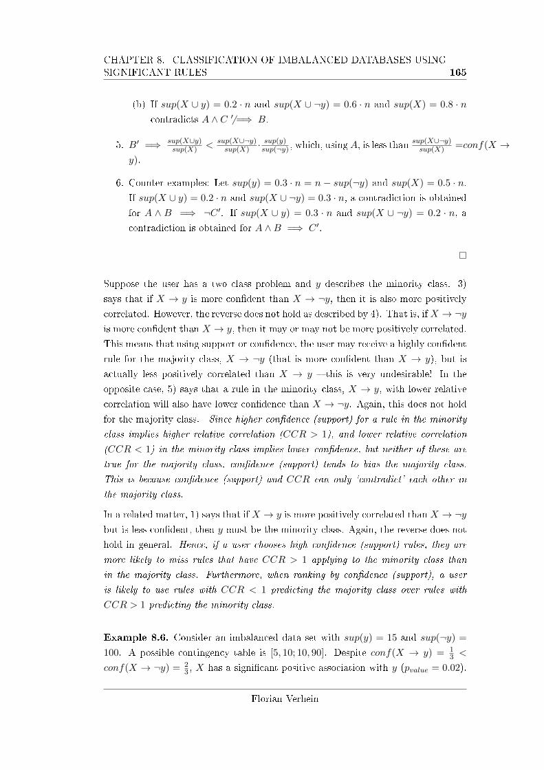
CHAPTER 8. CLASSIFICATION OF IMBALANCED DATABASES USINGSIGNIFICANT RULES 165
(b) If sup(X ∪ y) = 0.2 · n and sup(X ∪ ¬y) = 0.6 · n and sup(X) = 0.8 · ncontradicts A ∧ C 6′ =⇒ B.
5. B′ =⇒ sup(X∪y)sup(X) < sup(X∪¬y)
sup(X) ·sup(y)sup(¬y) , which, usingA, is less than
sup(X∪¬y)sup(X) =conf(X →
y).
6. Counter examples: Let sup(y) = 0.3 · n = n − sup(¬y) and sup(X) = 0.5 · n.If sup(X ∪ y) = 0.2 · n and sup(X ∪ ¬y) = 0.3 · n, a contradiction is obtained
for A ∧ B =⇒ ¬C ′. If sup(X ∪ y) = 0.3 · n and sup(X ∪ ¬y) = 0.2 · n, acontradiction is obtained for A ∧B =⇒ C ′.
Suppose the user has a two class problem and y describes the minority class. 3)
says that if X → y is more con�dent than X → ¬y, then it is also more positively
correlated. However, the reverse does not hold as described by 4). That is, ifX → ¬yis more con�dent than X → y, then it may or may not be more positively correlated.
This means that using support or con�dence, the user may receive a highly con�dent
rule for the majority class, X → ¬y (that is more con�dent than X → y), but is
actually less positively correlated than X → y � this is very undesirable! In the
opposite case, 5) says that a rule in the minority class, X → y, with lower relative
correlation will also have lower con�dence than X → ¬y. Again, this does not holdfor the majority class. Since higher con�dence (support) for a rule in the minority
class implies higher relative correlation (CCR > 1), and lower relative correlation
(CCR < 1) in the minority class implies lower con�dence, but neither of these are
true for the majority class, con�dence (support) tends to bias the majority class.
This is because con�dence (support) and CCR can only `contradict' each other in
the majority class.
In a related matter, 1) says that if X → y is more positively correlated than X → ¬ybut is less con�dent, then y must be the minority class. Again, the reverse does not
hold in general. Hence, if a user chooses high con�dence (support) rules, they are
more likely to miss rules that have CCR > 1 applying to the minority class than
in the majority class. Furthermore, when ranking by con�dence (support), a user
is likely to use rules with CCR < 1 predicting the majority class over rules with
CCR > 1 predicting the minority class.
Example 8.6. Consider an imbalanced data set with sup(y) = 15 and sup(¬y) =
100. A possible contingency table is [5, 10; 10, 90]. Despite conf(X → y) = 13 <
conf(X → ¬y) = 23 , X has a signi�cant positive association with y (pvalue = 0.02).
Florian Verhein
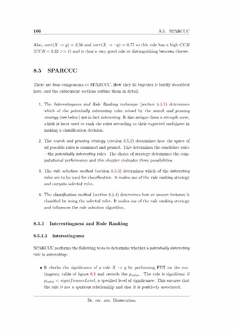
166 8.5. SPARCCC
Also, corr(X → y) = 2.56 and corr(X → ¬y) = 0.77 so this rule has a high CCR
(CCR = 3.32 >> 1) and is thus a very good rule at distinguishing between classes.
8.5 SPARCCC
There are four components to SPARCCC. How they �t together is brie�y described
here, and the subsequent sections outline them in detail.
1. The Interestingness and Rule Ranking technique (section 8.5.1) determines
which of the potentially interesting rules mined by the search and pruning
strategy (see below) are in fact interesting. It also assigns them a strength score,
which is later used to rank the rules according to their expected usefulness in
making a classi�cation decision.
2. The search and pruning strategy (section 8.5.2) determines how the space of
all possible rules is examined and pruned. This determines the candidate rules
� the potentially interesting rules. The choice of strategy determines the com-
putational performance and this chapter evaluates three possibilities.
3. The rule selection method (section 8.5.3) determines which of the interesting
rules are to be used for classi�cation. It makes use of the rule ranking strategy
and outputs selected rules.
4. The classi�cation method (section 8.5.4) determines how an unseen instance is
classi�ed by using the selected rules. It makes use of the rule ranking strategy
and in�uences the rule selection algorithm.
8.5.1 Interestingness and Rule Ranking
8.5.1.1 Interestingness
SPARCCC performs the following tests to determine whether a potentially interesting
rule is interesting:
• It checks the signi�cance of a rule X → y by performing FET on the con-
tingency table of �gure 8.1 and records the pvalue. The rule is signi�cant if
pvalue < significanceLevel, a speci�ed level of signi�cance. This ensures that
the rule is not a spurious relationship and that it is positively associated.
Dr. rer. nat. Dissertation
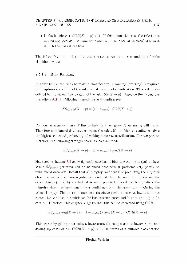
CHAPTER 8. CLASSIFICATION OF IMBALANCED DATABASES USINGSIGNIFICANT RULES 167
• It checks whether CCR(X → y) > 1. If this is not the case, the rule is not
interesting because it is more correlated with the alternative class(es) than it
is with the class it predicts.
The interesting rules � those that pass the above two tests � are candidates for the
classi�cation task.
8.5.1.2 Rule Ranking
In order to use the rules to make a classi�cation, a ranking (ordering) is required
that captures the ability of the rule to make a correct classi�cation. This ordering is
de�ned by the Strength Score (SS) of the rule: SS(X → y). Based on the discussions
in sections 8.3 the following is used as the strength score:
SSp,CCR(X → y) = (1− pvalue) · CCR(X → y)
Con�dence is an estimate of the probability that, given X occurs, y will occur.
Therefore in balanced data sets, choosing the rule with the highest con�dence gives
the highest expected probability of making a correct classi�cation. For comparison
therefore, the following strength score is also evaluated:
SSp,conf (X → y) = (1− pvalue) · conf(X → y)
However, as lemma 8.5 showed, con�dence has a bias toward the majority class.
While SSp,conf performs well on balanced data sets, it performs very poorly on
imbalanced data sets. Recall that a) a highly con�dent rule predicting the majority
class may in fact be more negatively correlated than the same rule predicting the
other class(es), and b) a rule that is more positively correlated but predicts the
minority class may have much lower con�dence than the same rule predicting the
other class(es). The interestingness criteria above excludes case a), but it does not
correct for the bias in con�dence for less extreme cases and it does nothing to �x
case b). Therefore, this chapter suggests that this can be corrected using CCR:
SSp,conf,CCR(X → y) = (1− pvalue) · conf(X → y) · CCR(X → y)
This works by giving poor rules a lower score (in comparison to better rules) and
scaling up cases of b): CCR(X → y) > 1. In terms of a suitable classi�cation
Florian Verhein
168 8.5. SPARCCC
performance P (·), experiments show that on relatively balanced data sets:
P (SSp,CCR) ≈ P (SSp,conf,CCR) ≈ P (SSp,conf )
While on imbalanced data sets (as would be expected):
P (SSp,CCR) >> P (SSp,conf,CCR) >> P (SSp,conf )
That is, the use of CCR achieves the highest performance on imbalanced data sets
while performing comparably on balanced data sets. As expected, this agrees nicely
with the discussions and theoretical results in sections 8.3 and 8.4. Furthermore,
note that in a completely balanced data set, CCR(X → y) reduces to sup(X→y)sup(X→¬y) =
conf(X→y)conf(X→¬y) which shall be called the Class Support Ratio and the Class Con�dence
Ratio respectively. E�ectively, the more imbalanced the data set, the higher the e�ect
of CCR. Finally, note that the pvalue has little impact in the �nal score, because it
varies at most by the signi�cance level. It's inclusion therefore favors more signi�cant
rules only if the other components of SS are similar. Based on both the theory and
the experimental results, the author recommends the use of SSp,c,CCR.
Example 8.7. Recall Example 8.6 where a highly positively correlated and signi�-
cant rule had a very low con�dence of 13 , so SSp,conf = 0.33. However, CCR(X →
y) = 2.560.77 = 3.33. Inclusion of this in the strength score raises it from 0.33 to
SSp,conf,CCR = 0.33 · 3.33 = 1.09. In comparison, if the classes had been equally dis-
tributed, the rule would have been negatively correlated, insigni�cant and CCR(X →y) would have been 1
2 . This demonstrates how CCR can be used to counteract the
bias of conf(·) in imbalanced data sets. Clearly, SSp,CCR = 3.27.
8.5.2 Search and Pruning Strategies
This section describes the techniques used to prune the search space for classi�cation
rules. The overall strategy is a bottom up enumeration technique, as all the less
speci�c rules X ′ → y : X ′ ⊂ X will be examined before a more speci�c rule X → y
is generated and examined. The underlying algorithm used to perform this search is
beyond the scope of this chapter. A number of approaches may be applied, however,
the author recommends the use of GRM (chapter 6) due to its space and run time
advantages.
The idea of a rule being statistically signi�cant is not anti-monotonic. To avoid exam-
ining all rules, search strategies are used that ensure the concept of being potentially
Dr. rer. nat. Dissertation
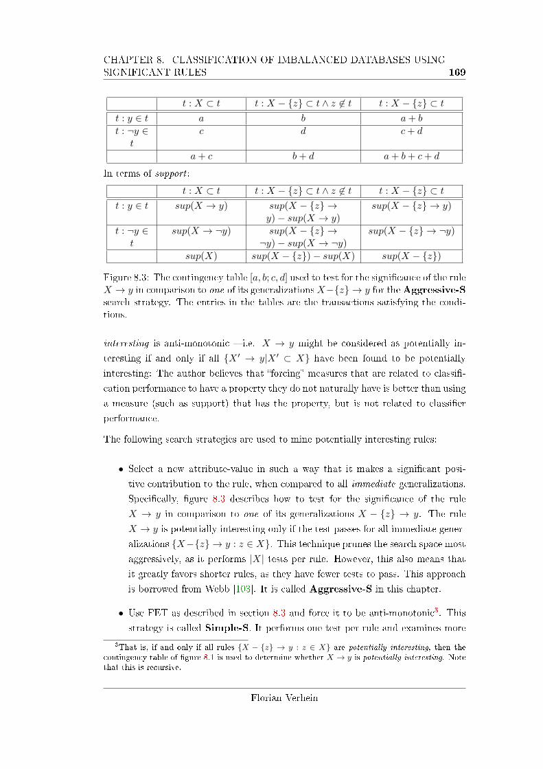
CHAPTER 8. CLASSIFICATION OF IMBALANCED DATABASES USINGSIGNIFICANT RULES 169
t : X ⊂ t t : X − {z} ⊂ t ∧ z 6∈ t t : X − {z} ⊂ tt : y ∈ t a b a+ b
t : ¬y ∈t
c d c+ d
a+ c b+ d a+ b+ c+ d
In terms of support :
t : X ⊂ t t : X − {z} ⊂ t ∧ z 6∈ t t : X − {z} ⊂ tt : y ∈ t sup(X → y) sup(X − {z} →
y)− sup(X → y)sup(X − {z} → y)
t : ¬y ∈t
sup(X → ¬y) sup(X − {z} →¬y)− sup(X → ¬y)
sup(X − {z} → ¬y)
sup(X) sup(X − {z})− sup(X) sup(X − {z})
Figure 8.3: The contingency table [a, b; c, d] used to test for the signi�cance of the ruleX → y in comparison to one of its generalizationsX−{z} → y for theAggressive-Ssearch strategy. The entries in the tables are the transactions satisfying the condi-tions.
interesting is anti-monotonic � i.e. X → y might be considered as potentially in-
teresting if and only if all {X ′ → y|X ′ ⊂ X} have been found to be potentially
interesting: The author believes that �forcing� measures that are related to classi�-
cation performance to have a property they do not naturally have is better than using
a measure (such as support) that has the property, but is not related to classi�er
performance.
The following search strategies are used to mine potentially interesting rules:
• Select a new attribute-value in such a way that it makes a signi�cant posi-
tive contribution to the rule, when compared to all immediate generalizations.
Speci�cally, �gure 8.3 describes how to test for the signi�cance of the rule
X → y in comparison to one of its generalizations X − {z} → y. The rule
X → y is potentially interesting only if the test passes for all immediate gener-
alizations {X−{z} → y : z ∈ X}. This technique prunes the search space most
aggressively, as it performs |X| tests per rule. However, this also means that
it greatly favors shorter rules, as they have fewer tests to pass. This approach
is borrowed from Webb [103]. It is called Aggressive-S in this chapter.
• Use FET as described in section 8.3 and force it to be anti-monotonic3. This
strategy is called Simple-S. It performs one test per rule and examines more
3That is, if and only if all rules {X − {z} → y : z ∈ X} are potentially interesting, then thecontingency table of �gure 8.1 is used to determine whether X → y is potentially interesting. Notethat this is recursive.
Florian Verhein
170 8.5. SPARCCC
of the search space.
• For comparison, a minimum support threshold strategy is also used. All rules
with supp(X → y) ≥ minSup are potentially interesting. This strategy is
called Support in the experiments.
For Aggressive-S and simple-S, de�ne sup(∅) = |D| so that it is possible to evaluate
a pvalue (usually high) for so-called �default rules� � rules with no antecedent that
can be applied when no other rules match an instance.
8.5.3 Rule Selection Method
The rule selection algorithm (algorithm 8.1) returns the set of highest ranking rules
so that each training instance is covered by (and correctly classi�ed by) enough rules
for it to have minGroups groups of rules, where each group is made up of rules with
the same scores. This is a type of covering technique. The concept of groups is
required by the classi�cation method used.
8.5.4 Classi�cation Method
The classi�cation algorithm (algorithm 8.2) classi�es an unseen instance based on
the highest ranked (according to the strength score) matching rules. If there is one
rule with the highest score, or multiple rules with the same score but predicting the
same class, then the choice is straightforward � simply pick the class predicted by
the rules. However, if there are multiple rules with the same score but predicting
di�erent classes, then the class is picked that is predicted by the majority of the
rules in the group. In cases where there is no single majority, �rst remove from
consideration any classes that are not in the majority. Then, the next group of rules
is used to make a decision between the remaining classes. This process is continued
until there is a majority in a group. If the rules run out, a random choice is made
between the remaining classes4.
4SPARCCC ensures that it does not make a decision due to running out of rules for any of theseclasses. For example, suppose there are 3 matching rules, and further suppose there are two rulespredicting di�erent classes in the top group. It is not possible to make a decision based on the topgroup alone. Hence, the next group is considered. Suppose a decision were to be made based onthe single remaining rule even though the other class is not represented in this group (recall therules for it have run out, and there was a higher ranked rule for that class in the previous group).Note also that the single rule used may have a very low score. This were to create a bias toward theclass that has the most rules, even if they are of poor quality. This is not fair to the class for whichfewer rules were found (for whatever reason � for example, this could happen if it was the minorityclass). So in this case, a random choice is made in place of relying on left over rules. Indeed, it
Dr. rer. nat. Dissertation
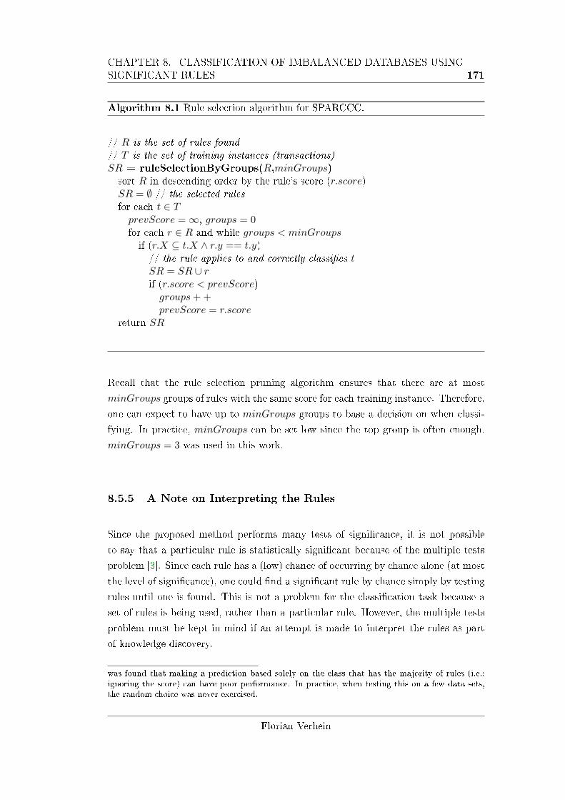
CHAPTER 8. CLASSIFICATION OF IMBALANCED DATABASES USINGSIGNIFICANT RULES 171
Algorithm 8.1 Rule selection algorithm for SPARCCC.
// R is the set of rules found// T is the set of training instances (transactions)SR = ruleSelectionByGroups(R,minGroups)sort R in descending order by the rule's score (r.score)SR = ∅ // the selected rulesfor each t ∈ TprevScore =∞, groups = 0for each r ∈ R and while groups < minGroupsif (r.X ⊆ t.X ∧ r.y == t.y)// the rule applies to and correctly classi�es tSR = SR ∪ rif (r.score < prevScore)groups+ +prevScore = r.score
return SR
Recall that the rule selection pruning algorithm ensures that there are at most
minGroups groups of rules with the same score for each training instance. Therefore,
one can expect to have up to minGroups groups to base a decision on when classi-
fying. In practice, minGroups can be set low since the top group is often enough.
minGroups = 3 was used in this work.
8.5.5 A Note on Interpreting the Rules
Since the proposed method performs many tests of signi�cance, it is not possible
to say that a particular rule is statistically signi�cant because of the multiple tests
problem [3]. Since each rule has a (low) chance of occurring by chance alone (at most
the level of signi�cance), one could �nd a signi�cant rule by chance simply by testing
rules until one is found. This is not a problem for the classi�cation task because a
set of rules is being used, rather than a particular rule. However, the multiple tests
problem must be kept in mind if an attempt is made to interpret the rules as part
of knowledge discovery.
was found that making a prediction based solely on the class that has the majority of rules (i.e.:ignoring the score) can have poor performance. In practice, when testing this on a few data sets,the random choice was never exercised.
Florian Verhein
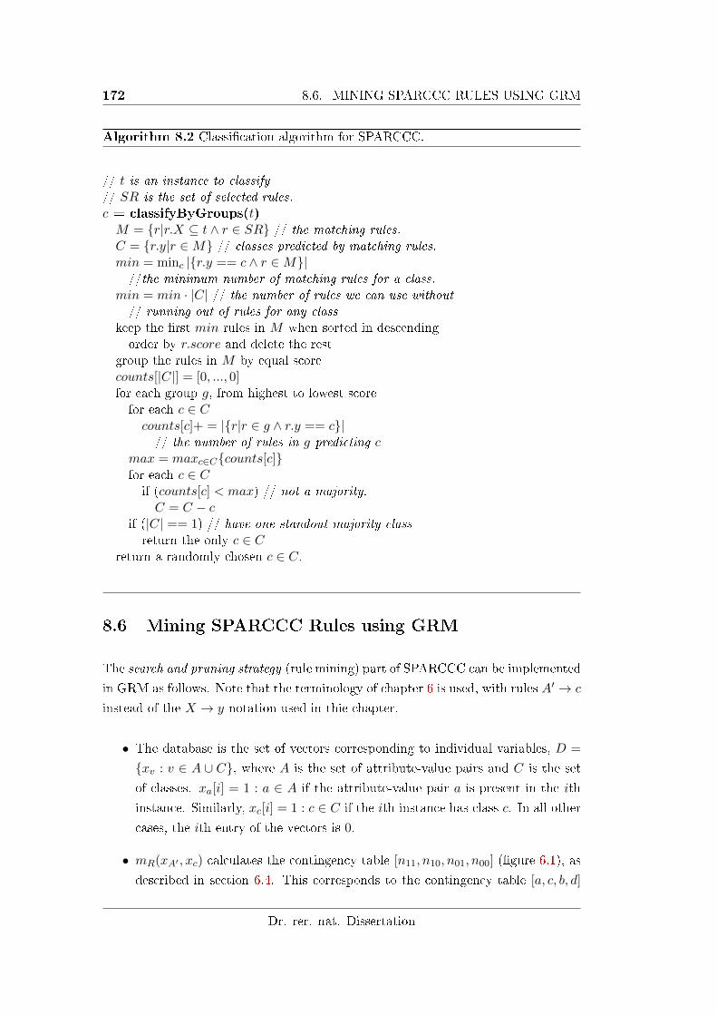
172 8.6. MINING SPARCCC RULES USING GRM
Algorithm 8.2 Classi�cation algorithm for SPARCCC.
// t is an instance to classify// SR is the set of selected rules.c = classifyByGroups(t)M = {r|r.X ⊆ t ∧ r ∈ SR} // the matching rules.C = {r.y|r ∈M} // classes predicted by matching rules.min = minc |{r.y == c ∧ r ∈M}|//the minimum number of matching rules for a class.
min = min · |C| // the number of rules we can use without// running out of rules for any class
keep the �rst min rules in M when sorted in descendingorder by r.score and delete the rest
group the rules in M by equal scorecounts[|C|] = [0, ..., 0]for each group g, from highest to lowest scorefor each c ∈ Ccounts[c]+ = |{r|r ∈ g ∧ r.y == c}|// the number of rules in g predicting c
max = maxc∈C{counts[c]}for each c ∈ Cif (counts[c] < max) // not a majority.C = C − c
if (|C| == 1) // have one standout majority classreturn the only c ∈ C
return a randomly chosen c ∈ C.
8.6 Mining SPARCCC Rules using GRM
The search and pruning strategy (rule mining) part of SPARCCC can be implemented
in GRM as follows. Note that the terminology of chapter 6 is used, with rules A′ → c
instead of the X → y notation used in thie chapter.
• The database is the set of vectors corresponding to individual variables, D =
{xv : v ∈ A ∪ C}, where A is the set of attribute-value pairs and C is the set
of classes. xa[i] = 1 : a ∈ A if the attribute-value pair a is present in the ith
instance. Similarly, xc[i] = 1 : c ∈ C if the ith instance has class c. In all other
cases, the ith entry of the vectors is 0.
• mR(xA′ , xc) calculates the contingency table [n11, n10, n01, n00] (�gure 6.1), as
described in section 6.4. This corresponds to the contingency table [a, c, b, d]
Dr. rer. nat. Dissertation
CHAPTER 8. CLASSIFICATION OF IMBALANCED DATABASES USINGSIGNIFICANT RULES 173
of �gure 8.1 in this chapter (note the di�erent order due the di�erent table
headings). n11 = xA′ · xc; the dot-product of the two vectors. Note that
this is the number of instances in which the rule A′ → c holds (it's support).
n10 = |xA′ |−n11, n01 = |xc|−n11 and n00 can be calculated as n−n11−n01−n10where n is the length of the vectors. From this, it can calculate the p value
(pvalue) of the rule, it's CCR and it's con�dence (conf) as described in this
chapter. Let the result of mR(·) evaluated on the rule A′ → c be the array
valuem(A′ → c) = [n11, n10, n01, n00, pvalue, CCR, conf ]. For simplicity, let the
notation valuem(A′ → c).n11 refer to the n11 entry, etc.
• aR(xA′ , xa) is de�ned so that xA′∪a[i] = xA′ [i]ANDxa[i]. Hence, xA′∪a[i] = 1
if the antecedent A′ ∪ a matches the ith instance.
• MR(·) is de�ned di�erently, depending on the search and pruning strategy used.
� For Agressive-S, it must evaluate the signi�cance of A′ → c in com-
parison to all the rule's immediate generalisations. The contingency table
[a, b, c, d] of �gure 8.3 can be obtained as follows: a = valuem(A′ → c).n11,
b = valuem(A′− x→ c).n11− a (where A′− z → c is a subrule of A′ → c
obtained by removing z ∈ A′), c = valuem(A′ → c).n10 (the number of in-
stances supporting the rule A′ → ¬c), and d = valuem(A′−z → c).n10−c.By constructing this table for all immediate sub-rules and testing the
signi�cance as described in this chapter, MR(·) can determine whether
the A′ → c signi�cantly improves on it's immediate generalisations. Let
AggresiveS.pvalue be the maximum pvalue of all these tests. Of course,
the computation can be aborted early one any of the tests deliver an
insigni�cant pvalue, in which case set AggresiveS.pvalue = 1.
� For Simple-S, M(·) must check to see if A′ → c as well as all it's imme-
diate sub-rules are signi�cant as determined by the signi�cance test imple-
mented inmR(·). Let SimpleS.pvalue = max{valuem(A′ → c).pvalue,maxz∈A′(valuem(A′−z → c).pvalue)}.
� For Support, M(·) is trivial.
• IR(·) determines which rules are interesting and should be expanded. Again,
this is determined by the strategy used:
� For Agressive-S, IR(·) returns true if and only if AggresiveS.pvalue <
significanceLevel.
� For Simple-S, IR(·) returns true if and only if SimpleS.pvalue < significanceLevel.
Florian Verhein
174 8.7. EXPERIMENTS
� For Support, IR(·) returns true if and only if valuem.n11 ≥ minSup.
• IA(·) can only be exploited in the Support method, in which case it returns
false if |xA′ | ≤ minSup. In all other methods, IA(·) is always true.
The above instantiation of GRM e�ciently mines all potentially interesting rules. It
also calculates all the values required by the interestingness and rule ranking strategy.
8.7 Experiments
Experiments were performed5on relatively balanced well known UCI data sets [65] as
well as imbalanced variations of them. The data sets used were {Australia, breast,
Cleve, Diabetes, Heart, Horse}6.
In the tables, the proposed methods are denoted by �SPARCCC� with the search
strategy in parentheses. For comparison, a purely support and con�dence based
technique was also used, denoted by �Support-Con�dence�. It �nds all rules satisfying
the support and con�dence thresholds and uses con�dence as the strength score7.
Any techniques using a support based search (such as CBA and CMAR) have exactly
the same search space (and at least the same run time) as �Support-Con�dence�.
Hence these are not reported separately.
8.7.1 Original (Balanced) Data sets
This section presents experiments on the original data sets, where the class distribu-
tions are roughly balanced. Figure 8.4 shows that (on average) SPARCCC performs
comparably to CBA, CMAR and C4.58, and is insensitive to the choice of SS. How-
ever, there are large di�erences in the search space examined and hence the run
times, as shown in �gures 8.6(a) and 8.6(b). Also, much fewer rules are found as can
be seen in �gure 8.6(d). Despite having very similar accuracy, the search space ex-
plored by �Aggressive-S� is {1.6%, 1.4%, 1.3%} (for signi�cances of {0.05, 0.01, 0.001}respectively) of that explored using a support based technique with minSup = 1%9.
For the less aggressively pruned search, �Simple-S�, it is {18.9%, 10%, 6%}.5The experiments were performed on an laptop with: Intel Pentium M 2.0GHz, 1GB of RAM,
Windows XP Professional. Programs written in Java. Strati�ed 10-fold cross validation was usedfor measuring all performance indicators.
6Continuous variables were discretised using the technique of [61]7That is, there is no use of signi�cance tests or correlation at all. The rule selection and classi-
�cation procedure is as described in this paper.8The reported accuracy levels for C4.5, CBA and CMAR were obtained from [60].9It should be noted that minSup = 1% is usually recommended. minSup = 5% performs worse,
and as will be shown, is terrible on skewed data sets.
Dr. rer. nat. Dissertation
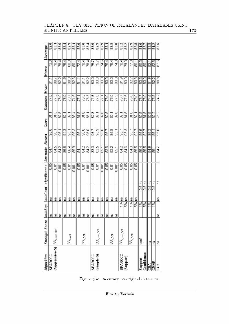
CHAPTER 8. CLASSIFICATION OF IMBALANCED DATABASES USINGSIGNIFICANT RULES 175
Figure 8.4: Accuracy on original data sets.
Florian Verhein
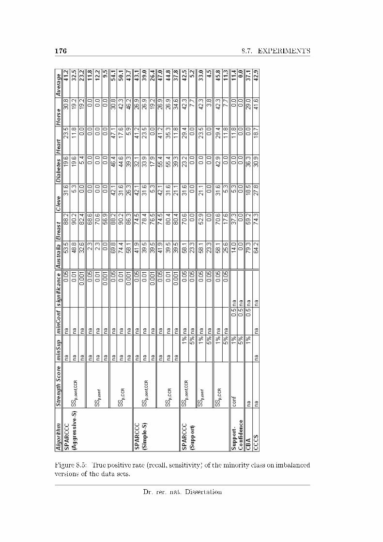
176 8.7. EXPERIMENTS
Figure 8.5: True positive rate (recall, sensitivity) of the minority class on imbalancedversions of the data sets.
Dr. rer. nat. Dissertation
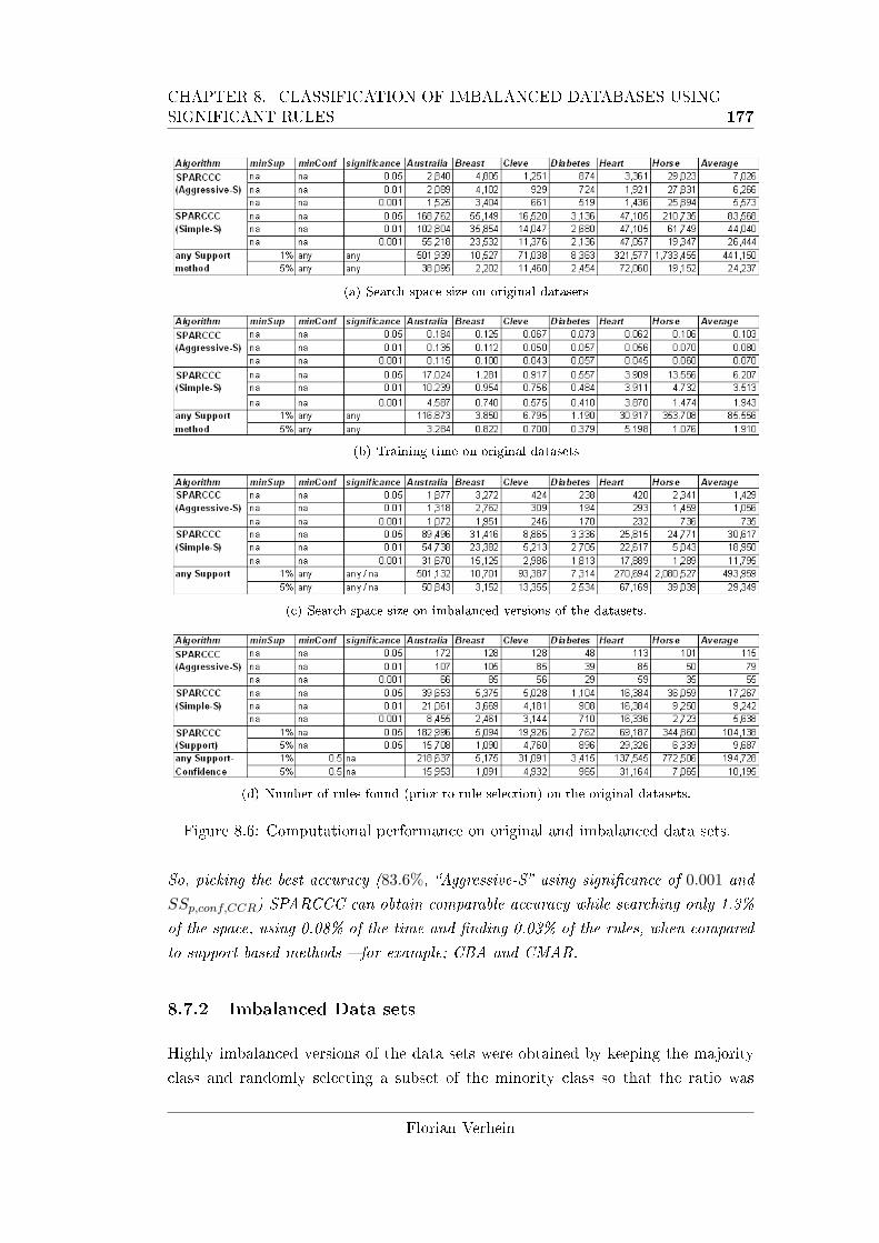
CHAPTER 8. CLASSIFICATION OF IMBALANCED DATABASES USINGSIGNIFICANT RULES 177
(a) Search space size on original datasets
(b) Training time on original datasets
(c) Search space size on imbalanced versions of the datasets.
(d) Number of rules found (prior to rule selection) on the original datasets.
Figure 8.6: Computational performance on original and imbalanced data sets.
So, picking the best accuracy (83.6%, �Aggressive-S� using signi�cance of 0.001 and
SSp,conf,CCR) SPARCCC can obtain comparable accuracy while searching only 1.3%
of the space, using 0.08% of the time and �nding 0.03% of the rules, when compared
to support based methods � for example; CBA and CMAR.
8.7.2 Imbalanced Data sets
Highly imbalanced versions of the data sets were obtained by keeping the majority
class and randomly selecting a subset of the minority class so that the ratio was
Florian Verhein
178 8.7. EXPERIMENTS
1 : 9. That is, the percentage of instances with the minority class was 10%. Figure
8.5 shows the True Positive Rate (TPR) of the minority class. Note that accuracy
is a poor performance measure for imbalanced data sets because one can obtain
high (at least 90%) accuracy by predicting the majority class. TPR (also known
as sensitivity and recall) is a much better performance indicator. The accuracy is
therefore not shown for space reasons. It remains high however.
The e�ect of using CCR in the SS is large. One can clearly see the following rela-
tionship:
TPR(SSp,CCR) >> TPR(SSp,conf,CCR) >> TPR(SSp,conf )
For example, when using �Aggressive-S�, SSp,conf,CCR is on average (over data sets
and signi�cance levels) 2.87 times better than SSp,conf and SSp,CCR is 1.58 times
better than SSp,conf,CCR and 4.44 times better than SSp,conf . A similar, though
slightly smaller e�ect occurs for �Simple-S� and �Support-S�.
The proposed methods also score much higher than other rule based techniques such
as CBA and CCCS, the latter of which was designed speci�cally for imbalanced data
sets. The highest average TPR overall is for �Aggressive-S� with a signi�cance level
of 0.05. This was 45.8% better than CBA and 26.1% better than CCCS. Unlike for
the original data sets, the signi�cance level has a large impact on the classi�cation
performance on imbalanced data sets, likely due to the pruning of the search space.
Interestingly, the use of CCR had the unexpected bene�t of reducing this e�ect. It
was also noticed that much fewer rules were generated overall. Finally, the compu-
tational performance favors the proposed techniques even more on imbalanced data
sets. Figure 8.6(c) for example shows that �Aggressive-S�, at a signi�cance level of
0.05, explores only 0.29% of the space considered by a support based method with
minSup = 1% � and the training time is even less. For �Simple-S� it is 6.2%. Note
also that the performance of any support based technique with minSup = 5% is
very poor, as is to be expected on such an imbalanced data set.
Overall, the experiments show that, by using SPARCCC with a signi�cance based
search strategy, one can achieve much better classi�cation performance on skewed
data sets than techniques such as CBA (which is outperformed it by up to 45.8%
when using a signi�cance level of 0.05) while using dramatically fewer computational
resources (0.29% of those used by support based methods).
Dr. rer. nat. Dissertation
CHAPTER 8. CLASSIFICATION OF IMBALANCED DATABASES USINGSIGNIFICANT RULES 179
8.8 Related Work
CBA [61] was the �rst Associative Classi�er (AC) proposed and most other ACs
are variations on the original CBA design which consists of three components: 1)
rule mining, 2) rule selection (classi�er building) and 3) classi�cation. For rule
mining, CBA mines all rules passing support and con�dence thresholds (minSup
and minConf). Additionally, it ignores rules based on a �pessimistic error based
pruning method� borrowed from C4.5 [76]. Unfortunately, minSup and minConf
need to be set very low for decent accuracy, generating tens of thousands of rules
� most of which perform poorly. Therefore, a rule selection process is needed to
select a small subset likely to perform well. Rules are selected so that each training
instance is covered by the highest ranked rule that matches the instance, and each
rule, when considered together with the others, will be used to correctly classify at
least one training instance. New instances are classi�ed according to the highest
ranked rule that is applicable. Rules are ranked according to con�dence, support,
and size.
CMAR [60] has many similarities to CBA. The main di�erences10 are the use of
a χ2 test instead of the error based pruning and a more complicated classi�cation
procedure involving an empirically chosen weighted χ2 measure applied to multiple
matching rules. CMAR uses the same contingency table (�gure 8.1) as one of the
interestingness criteria proposed in this chapter. However, the χ2 test does not
distinguish between directions of association and therefore the claim in [60] that only
positively correlated rules are found is not necessarily correct. Negatively associated
rules are just as likely to pass the test as positively associated ones. For example,
the table [4, 25; 12, 15] is signi�cant at the 0.05 level but X is negatively associated
(correlated) with y. Though CMAR checks for signi�cance, it is still based on the
support-con�dence framework.
In general, rules with CCR(·) < 1 will incorrectly classify the training data. The
above techniques still work because, in balanced data sets, choosing high support
and con�dence rules tends to favor positively correlated rules, but this is not the
case in imbalanced data sets as lemma 8.5 shows.
CBA, CMAR and related techniques rely heavily on support and con�dence for
searching, pruning and ranking rules. While popular and convenient, there is little
evidence to suggest they are any good at �nding useful classi�cation rules. Indeed,
both CMAR and CBA need to use minSup = 1% and minConf = 0.5 in their
10We note that CBA is based on the Apriori algorithm, while CMAR is based on FP-Growth.Such di�erences do not change the rules that are found, just the way in which they are found, andhence are irrelevant for this discussion.
Florian Verhein
180 8.8. RELATED WORK
experiments to beat C4.5 [61, 60], generating tens of thousands of rules. Note that
CMAR's χ2 test, CBA's error rate pruning and the use of con�dence does not reduce
the search space. A large number of rules found, many of which are poor, dictates
the requirement of often complex rule selection methods. It is not uncommon for
these to discard 99% of the mined rules [61, 60] � meaning the search by support
and con�dence has an e�ective precision of only 1%.
It is not surprising then, that techniques using the support-con�dence framework
perform poorly on imbalanced data sets. The approach in this chapter is much sim-
pler: the rule mining method �nds statistically signi�cant and positively associated
rules. Since the number of rules found is typically very small, and SPARCCC directly
mines for rules that are expected to perform well for classi�cation, there is no need for
rule selection. SPARCCC has a very simple classi�cation method; a simple strength
score is used to rank the rules and the highest ranked matching rule is used. This
straightforward technique performs comparably on balanced data sets, much better
on imbalanced data sets and has greatly reduced computational requirements.
The CCCS [15] technique was proposed to �nd positively correlated rules. It takes
into account imbalanced class distributions, enabling it to outperform other tech-
niques on imbalanced data sets while performing competitively on balanced data
sets. Another upside is that it is relatively parameter free. It does not rely on sup-
port to prune the search space, but instead forces correlation to be locally monotonic
and uses a top down row enumeration algorithm. However, there is no guarantee that
the rules found are statistically signi�cant, and this algorithm generates many thou-
sands of rules. It is also very computationally intensive an does not scale well for
traditional data sets where there are more instances than attributes.
Morishita et al. [63] use the same test as CMAR but �nd upper-bounds on χ2 for
search space pruning. It is an association rule mining technique and is not used for
classi�cation.
Webb [103] proposed the use of Fisher's Exact Test (FET) to examine the signif-
icance of association rules in more detail than [60, 63]. The technique is used in
the Aggressive-S search strategy employed in this chapter for pruning the search
space. Webb does not use the rules for classi�cation � instead it is used for knowl-
edge discovery. This requires consideration of the issue of multiple tests. Since the
mined rules are not validated, it is very di�cult to determine whether the rules are
useful. This chapter mines signi�cant rules under a number of di�erent strategies
and uses them for classi�cation � which also requires additional work such as rule
selection, ranking and classi�cation. This gives a very good performance indicator �
performance on unseen data in comparison to other algorithms. As a side e�ect, the
Dr. rer. nat. Dissertation
CHAPTER 8. CLASSIFICATION OF IMBALANCED DATABASES USINGSIGNIFICANT RULES 181
author believes that this also provides extra weight to the method proposed in [103].
8.9 Conclusion
The traditional measures of support and con�dence are fundamental in association
rule mining and associative classi�ers. However, they have many downsides, espe-
cially when used for classi�cation of imbalanced data sets. Many rules found under
such schemes are statistically insigni�cant, negatively correlated, the antecedent and
consequent are independent of each other, or the antecedent is more positively corre-
lated with the alternate classes than the class it predicts. Furthermore, in imbalanced
data sets these measures favor the majority class, and in this chapter this was proved
in the context of the Class Correlation Ratio. If this is not corrected, classi�cation
performance su�ers. There is also little evidence that support is good for anything
other than pruning the search space, and even then, it must be set to very low values
in order to capture useful rules. However, at this point many thousands of rules
can be generated � most of which will be discarded (sometimes even 99% [60]). The
author believes this support and con�dence approach is ine�cient and that there is
an over-reliance on these measures for historical or simplicity reasons.
This chapter makes the case that searching directly for signi�cant rules is more appro-
priate. From a theoretical standpoint, it makes sense to use statistically signi�cant
and positively correlated rules, and additionally require that they are more positively
correlated with the class they predict than with the alternatives. This has been val-
idated by experiments on the novel associative classi�er introduced in this chapter �
SPARCCC. The experiments showed similar classi�cation performance on balanced
data sets, and higher classi�cation performance on imbalanced data sets compared
to other ACs. Furthermore, by searching directly for signi�cant rules, SPARCCC is
faster as it does not need to explore as much of the search space. Finally, it also
uses much fewer rules, suggesting that it is much better at �nding quality predictive
rules.
The author feels that this work lends some weight to the argument that it is better to
focus on measures that are statistically sound and are linked to classi�er performance,
and if necessary, force these to be anti-monotonic for computational e�ciency � than
to use approaches which are not directly related to classi�er accuracy but have an
inherent anti-monotonic property.
Florian Verhein

182 8.9. CONCLUSION
Dr. rer. nat. Dissertation
Chapter 9
Mining Complex Sub-graphs of
Correlated Variables with
Applications to Feature Selection
Finding interactions between variables is a fundamental concept in Data
Mining. This chapter considers correlations between variables using Pear-
son's product moment correlation coe�cient and mines complex, complete,
and maximal sub-graphs describing the correlation structure between vari-
ables. Both positive and negative (complex) correlations are considered. It is
proved that under a constraint on the minimum level of correlation desired,
there are useful guarantees on the graph's structure; the sign of the correla-
tion between vertices can be mapped to the vertices themselves, leading to
complex sets. Therefore, complex interactions become simpler to understand
and a novel algorithm is presented that mines complex interactions in the
same run time as if negative correlations were not considered.
The approach is useful for examining complex correlation structures in
databases and mining representative subsets. The latter idea is extended
to a feature subset selection method that gives guarantees on the minimum
correlation required for features to be considered interchangeable (redun-
dant), while guaranteeing that the selected features are not correlated with
each other. Experiments show the approach performs well.
183
184 9.1. INTRODUCTION
9.1 Introduction
Finding interactions between variables is a fundamental concept in Data Mining.
This chapter investigates the correlation structure between variables. In the graph
view, each variable is a vertex, and an edge exists between vertices if the magnitude
of the correlation between the corresponding variables exceeds a threshold. Graphs
de�ned by a lack of correlation are also brie�y considered. The sign of the correlation
(positive or negative) is taken into account and the edge labeled accordingly.
In this work, completely connected sub-graphs (cliques) are of interest because these
guarantee that every variable in the sub-graph is highly correlated with each other
variable, therefore describing a strong symmetric relationship. An application of
this structure is to use one variable in place of the variables in the sub-graph. Being
completely connected is useful here; the user may de�ne a level of correlation over
which the variables are considered to be equivalent � or more precisely; of insu�cient
di�erence to warrant inclusion of more than one of them. This is the basis for
applying the approach to feature subset selection in section 9.5.
It is important to consider both positive and negative correlations � that is, �com-
plex� sub-graphs. If only positive or high magnitude correlations are considered,
much of the structure will be missed as negative correlations will not be included.
For example, A may be highly correlated with D, but both of these may also be
negatively correlated with B and C. This methods in this chapter mine complete
and complex sub-graphs capturing such a structure. The goal is to represent these
as complex sets of variables � sets of variables that may include negated variables �
that are all highly positively correlated with each other. For instance, the complex
set {A,−B,−C,D} indicates that A, −B (negative B), −C and D are highly pos-
itively correlated, describing the above-mentioned pattern. Without consideration
for complex relationships, either a) two separate sets {A,B} and {C,D} would be
mined instead or b) the set {A,B,C,D} would be mined � in both cases failing to
show the complete structure of the interaction.
This chapter shows that under a practical constraint on the correlation coe�cient,
mining complex sub-graphs can be reduced to mining complex sets of variables, as
a majority of the edge combinations are impossible. Furthermore, the positive and
negative labeling of variables in the sets can be achieved for free. This achieves
signi�cant computational savings and makes complex interaction patterns easier to
understand: Suppose there is a complete sub-graph G′ on the variables V ′ ⊆ V ,
where V is the set of all variables. There are |V ′|2/2 edges in G′ and therefore
2|V′|2/2 possible labellings of edges as either positive or negative. Hence, there are
Dr. rer. nat. Dissertation
CHAPTER 9. MINING COMPLEX CORRELATION STRUCTURES 185
2|V′|2/2 di�erent complex correlation structures. The results in this chapter show
that under the constraint, only 2|V′| of these are possible. This is precisely the
number of labellings of vertices in G′, which means that instead of mining and
reporting entire sub-graphs including edge labels � and incurring the correspondingly
higher complexity � the same problem can be solved by mining complex sets of
variables. Furthermore, of the 2|V′| possibilities, half are the negation of all variables
in another combination, leaving 2|V′|−1 con�gurations. Finally, it will be shown
that the labellings can be achieved for free using the proposed algorithm: searching
through all possible subsets of all vertices V takes O(2|V |) time, but the algorithm
also labels the variables within this time. Therefore, the results in this chapter reduce
the complexity of the problem from O(2|V′|2/2) to O(2|V
′|).
Since mining these complex sets creates the problem of redundancy (each set of size
k will contain 2k − 1 subsets), this work focuses on mining maximal sets (maximal
complete sub-graphs).
9.1.1 Motivations
Each maximal complex set of variables indicates that all the variables in that set
are highly positively correlated with every other variable. Furthermore, no other
variable (or its negation) can be added to the set without breaking this property.
Such correlation structures are interesting in their own right and can indicate near
duplicate variables or �ag previously unknown complex interactions. By comparison,
analysing or graphing a correlation matrix usually hides interactions that involve
more than two variables at a time.
Each maximal complex set can also be thought of as capturing an underlying fea-
ture, or �factor�, in the process captured by the data set. Of course, there are other
approaches for doing this, namely Principle Component Analysis (PCA) [44], Sin-
gular Value Decomposition (SVD) � which is related to PCA � and Factor Analysis
[44] � which uses PCA. In these approaches, each principle component capture a
source of variability in the data � that is, a factor. While it is possible to examine
the coe�cients of a principle component in order to determine what variables are
associated with it, it is a technique that does not provide the type of guarantees on
the correlation structure that the approach in this chapter does. It also becomes
di�cult to do when many variables are involved. The advantages of the proposed
technique are that it gives guarantees on the correlations in a set, it maintains the
actual variables (unlike PCA), and the resulting patterns are easy to interpret.
A concrete application of this idea is to provide suggestions for selecting a represen-
Florian Verhein
186 9.1. INTRODUCTION
tative set of features. It is therefore applied to the problem of feature subset selection
[88] using a three stage �lter [88] approach: First, maximal complex sets of variables
(features) are mined. The variables in such a set are considered interchangeable,
as they are highly correlated with each other. Then, a representative variable for
each set is found, taking account the overlap between other sets. This is intended
to remove from consideration any redundant, duplicate, or otherwise unnecessary
variables while capturing the primary factors in the underlying process. Finally, a
subset of the representative variables is chosen so that none of them are correlated
with each other.
The approach allows the user to de�ne the minimal correlation required for fea-
tures to be considered interchangeable, and provides a guarantee that the features
selected will not be correlated. Another advantage is that a subset of the original
features are used as selected features. This means models such as trees and rules
built on these remain highly interpretable, contrasting approaches such as PCA or
SVD which produce features that are linear combinations of all original features.
Linear combinations as features make the resulting models very di�cult to interpret.
Furthermore, they do not reduce the number of attributes that need to be collected
in future: The principle components are only orthogonal if the linear combination is
not truncated. This means that while the algorithm uses fewer features, the features
used are still a function of all the original features.
9.1.2 Contributions
This chapter makes the following contributions:
• Complete, complex and maximal sub-graphs (sets) of correlated variables are
proposed as useful patterns for describing complicated correlation structures
in an easily understood manner.
• It is proved that under a constraint on the minimum correlation desired, there
is a speci�c structure on the correlations between variables that allows edge
relationships to be mapped to the vertices, and thus allows complex sets to
capture the same information as complete complex sub-graphs.
• An algorithm is developed that mines all complex maximal sets of variables.
This is a data mining technique, where the patterns mined highlight interesting
and complex interactions between variables that would otherwise be hidden.
Experiments show the algorithm is very e�cient at mining such sets, due also
in part to the extensive pruning it employs.
Dr. rer. nat. Dissertation
CHAPTER 9. MINING COMPLEX CORRELATION STRUCTURES 187
• The approach is further developed for mining a representative subset of the
variables and in particular, for the feature subset selection problem. As a result,
an unsupervised feature subset selection method is proposed. Experiments on
the UCI cardiac arrhythmia data set show that it outperforms PCA when used
for feature selection.
9.1.3 Organisation
The remainder of this chapter is organised as follows: Section 9.2 presents the theory,
section 9.3 describes the data mining algorithm, section 9.5 describes the feature
subset selection algorithm, section 9.6 provides experimental results, section 9.7 puts
the contributions in the context of previous work, and section 9.8 concludes this
chapter.
9.2 Complete, Complex Variable Sub-graphs, Sets and
Correlation
Recall that the graph on the variables was de�ned as follows: each variable is a vertex
and there is an edge between vertices if the corresponding variables are correlated:
Given a threshold t, an edge exists between two variables A and B if |ρA,B| ≥ t.
The weight of the edge is ρA,B and of speci�c interest is whether ρA,B is positive or
negative � called the label of the edge. Later, the problem of mining uncorrelated
sets is also considered, where |ρA,B| ≤ t.
Pearson's correlation coe�cient between two random variables A and B is
ρA,B =cov(A,B)
σAσB=E((A− µA)(B − µB))
σAσB
If the data is centered, that is, E(A) = E(B) = 0, then
ρA,B =~a ·~b||~a|| ||~b||
= corr(~a,~b)
where ~a and ~b are the vectors of samples for the variables A and B. In this work,
corr(~a,~b) is used, and the data is assumed to be centered1. The use of the dot
1Centering the data is not necessary, and this is sometimes preferred in practice, but in thatcase it does not equal ρA,B .
Florian Verhein
1889.2. COMPLETE, COMPLEX VARIABLE SUB-GRAPHS, SETS AND
CORRELATION
product also means that the kernel trick is applicable � potentially allowing non-
linear correlations to be used. However, this is not explored in this chapter.
Recall that the goal is to mine complete, complex and maximal sub-graphs of vari-
ables, and to be able to represent these as complex maximal sets. Recall that a
sub-graph is complete if it is completely connected. A set will only ever be used to
describe a complete sub-graph. Recall that the term complex describes the inclusion
of negative and positive relationships (labellings of edges or variables). Recall that
a complete sub-graph is called maximal if no other complete sub-graph subsumes it.
Equivalently, a set is maximal if no super-set exists.
Section 9.2.1 considers the problem of mining maximal and complex sets of highly
correlated variables � which is the focus of this paper. Section 9.2.2 brie�y considers
the problem of mining uncorrelated variables.
9.2.1 Highly Correlated, Complex Variable Sets
This section develops the theory required to mine highly correlated, complex variable
sets.
Lemma 9.1. corr(~a,~b) > t ∧ corr(~b,~c) > t ∧ |corr(~a,~c)| > t =⇒ corr(~a,~c) > t if
and only if t ≥ 0.5. In other words, if (~a,~b) are highly positively correlated and (~b,~c)
are highly positively correlated and (~a,~c) are highly positively or negatively correlated,
then (~a,~c) are in fact highly positively correlated. In this case, �highly� means with a
correlation coe�cient above 0.5.
Proof. Without loss of generality, assume {~a,~b,~c} are all unit vectors (this does notchange the correlation: ~a·~b
||~a|| ||~b||= ( ~a
||~a|| ·~b
||~b||)/(|| ~a||~a|| || ||
~b
||~b||||)). Then corr(~a,~b) = ~a ·~b �
the dot product. The following identity is used:∑
i(ai+ci−bi)2 =∑
i[(a2i +b2i +c2i )+
2(aici−bici−aibi)] = 3+2(~a·~c−~b·~c−~a·~b). The last equality follows as the vectors areunit vectors (i.e. ||~a|| = 1 =⇒
∑i a
2i = 1). Using the thresholds ~a ·~b > t and ~b ·~c > t
and the fact that∑
i(ai+ci−bi)2 ≥ 0 gives: 0 ≤ 3+2(~a·~c−~b·~c−~a·~b) < 3+2~a·~c−4t.
To avoid a contradiction we must therefore have ~a · ~c ≥ 2t − 1.5 If ~a · ~c < −t then−t > 2t − 1.5 ⇐⇒ t < 0.5. Therefore, when t ≥ 0.5, a · c < −t provides a
contradiction and therefore we must have ~a · ~c > t.
In the reverse direction, we have ~a ·~c > t (as the implication is true). Suppose for the
purpose of a contradiction that t < 0.5. Then we can see from ~a · ~c ≥ 2t − 1.5 that
it is possible to have ~a ·~c < −t � providing the contradiction (for example substitute
any value t < 0.5).
Dr. rer. nat. Dissertation
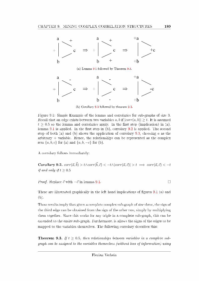
CHAPTER 9. MINING COMPLEX CORRELATION STRUCTURES 189
(a) Lemma 9.1 followed by Theorem 9.3.
(b) Corollary 9.2 followed by theorem 9.3.
Figure 9.1: Simple Example of the lemma and corrolaries for sub-graphs of size 3.Recall that an edge exists between two variables a, b if |corr(a, b)| ≥ t. It is assumedt ≥ 0.5 so the lemma and corrolaries apply. In the �rst step (implication) in (a),lemma 9.1 is applied. In the �rst step in (b), corrolary 9.2 is applied. The secondstep of both (a) and (b) shows the application of corrolary 9.3, choosing a as thearbitrary + variable. Hence, the relationships can be represented as the complexsets {a, b, c} for (a) and {a, b,−c} for (b).
A corrolary follows immediately:
Corollary 9.2. corr(~a,~b) > t∧corr(~b,~c) < −t∧|corr(~a,~c)| > t =⇒ corr(~a,~c) < −tif and only if t ≥ 0.5
Proof. Replace ~c with −~c in lemma 9.1.
These are illustrated graphically in the left hand implications of �gures 9.1 (a) and
(b).
These results imply that given a complete complex sub-graph of size three, the sign of
the third edge can be obtained from the sign of the other two, simply by multiplying
them together. Since this works for any triple in a complete sub-graph, this can be
extended to the entire sub-graph. Furthermore, it allows the signs of the edges to be
mapped to the variables themselves. The following corrolary describes this:
Theorem 9.3. If t ≥ 0.5, then relationships between variables in a complete sub-
graph can be assigned to the variables themselves (without loss of information) using
Florian Verhein
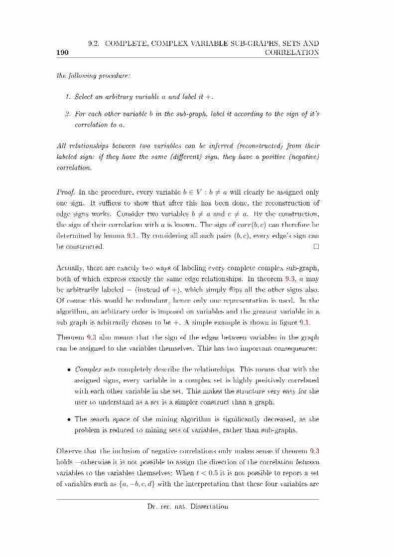
1909.2. COMPLETE, COMPLEX VARIABLE SUB-GRAPHS, SETS AND
CORRELATION
the following procedure:
1. Select an arbitrary variable a and label it +.
2. For each other variable b in the sub-graph, label it according to the sign of it's
correlation to a.
All relationships between two variables can be inferred (reconstructed) from their
labeled sign: if they have the same (di�erent) sign, they have a positive (negative)
correlation.
Proof. In the procedure, every variable b ∈ V : b 6= a will clearly be assigned only
one sign. It su�ces to show that after this has been done, the reconstruction of
edge signs works. Consider two variables b 6= a and c 6= a. By the construction,
the sign of their correlation with a is known. The sign of corr(b, c) can therefore be
determined by lemma 9.1. By considering all such pairs (b, c), every edge's sign can
be constructed.
Actually, there are exactly two ways of labeling every complete complex sub-graph,
both of which express exactly the same edge relationships. In theorem 9.3, a may
be arbitrarily labeled − (instead of +), which simply �ips all the other signs also.
Of course this would be redundant, hence only one representation is used. In the
algorithm, an arbitrary order is imposed on variables and the greatest variable in a
sub-graph is arbitrarily chosen to be +. A simple example is shown in �gure 9.1.
Theorem 9.3 also means that the sign of the edges between variables in the graph
can be assigned to the variables themselves. This has two important consequences:
• Complex sets completely describe the relationships. This means that with the
assigned signs, every variable in a complex set is highly positively correlated
with each other variable in the set. This makes the structure very easy for the
user to understand as a set is a simpler construct than a graph.
• The search space of the mining algorithm is signi�cantly decreased, as the
problem is reduced to mining sets of variables, rather than sub-graphs.
Observe that the inclusion of negative correlations only makes sense if theorem 9.3
holds � otherwise it is not possible to assign the direction of the correlation between
variables to the variables themselves: When t < 0.5 it is not possible to report a set
of variables such as {a,−b, c, d} with the interpretation that these four variables are
Dr. rer. nat. Dissertation
CHAPTER 9. MINING COMPLEX CORRELATION STRUCTURES 191
(a) A con�guration likethis is possible onlywhen t < 0.5. It cannotbe mapped to a com-plex set.
(b) When t ≥ 0.5, any complete complex sub-graph can be mapped to a complex set. Thesigns on the dotted edges can be inferred fromthe others.
Figure 9.2: Example of corrolary 9.3
highly positively correlated with each other, since it is possible that corr(a, b) < −t,corr(a, c) > t but corr(b, c) > t. In this case there exists no labeling of variables
that can produce a set so that each element is positively correlated with the others.
Accordingly, complex sets are not meaningful when t < 0.5. The reader may like to
try this on the example in �gure 9.2(a). Following the procedure of theorem 9.3 does
not work as the edges cannot be reconstructed, so it is impossible to map the complex
sub-graph it to a complex set. On the other hand, the example in �gure 9.2(b) does
work and demonstrates the procedure.
In section 9.3, a method of enumerating the possible sets will be presented that, in
conjunction with theorem 9.3, means that all complex complete variable sets can
be mined and labeled in O(2|V |) time � the same complexity as without considering
the sign of the correlations. For comparison, note that a naive approach would be
to enumerate possible sets, and for each, apply corrolary 9.3. This would require
O(|V | · 2|V |) time due to the O(|V |) operations used for labeling the extra O(|V |)edges added whenever another variable is added in the search.
9.2.2 Uncorrelated Variable Sets
An interesting but simpler problem is to �nd maximal sets of variables that are
pairwise uncorrelated, in the sense that the absolute correlation is below a threshold.
That is, an edge exists between two variables A and B if |corr(A,B)| ≤ t, where t
is a (usually small) threshold. This mines sets of uncorrelated variables. Of course,
complex relationships don't make sense for these.
Florian Verhein
192 9.3. MINING COMPLEX MAXIMAL SETS: ALGORITHM
9.3 Mining Complex Maximal Sets: Algorithm
9.3.1 Algorithm
Recall from section 3.3.1 that a PrefixTree can be used to represent the search
space for mining interactions. Here, each node in the pre�x tree (called a Node in
algorithm 9.1) corresponds to a complete set of variables. Without loss of generality,
assume the variables are integers V = {1, 2, ..., n}. The only information stored
at each node is a variable (v) and a sign label (sign). For ease of presentation,
consideration of the sign is deferred for the moment.
The algorithm (algorithm 9.1) works by performing a depth �rst traversal of the
search space, expanding sibling nodes in increasing order � which is important as
described later � and pruning the search as soon as possible.
Speci�cally, the following properties are exploited. Here, a set is called complete if
the corresponding sub-graph is complete. Elsewhere in the paper this is implicit.
1. Whenever a new variable v2 is considered to be added to a complete set C, and
v2 is not highly correlated with each variable in C, then neither C ∪ v2 or anysuper-set of C ∪ v2 can be complete. That is, the corresponding sub-graphs
will also be missing at least one edge. One consequence of this is the following:
Since by construction v2 < v1∀v1 ∈ C, the entire sub-tree rooted at the node
corresponding to C ∪ v2 may be pruned. The case C = ∅ holds trivially by
de�ning it as complete.
2. When checking whether a new variable v2 can be added to a complete set C∪v1,the algorithm only needs to consider those v2 for which C ∪ v2 is complete, by
property 1. That is, if C ∪ v2 is not complete, then neither can its super-set
C∪v1∪v2 be. Now, if C∪v1 and C∪v2 are complete, then C∪v1∪v2 is complete
if and only if v1 ∪ v2 is complete (that is, if and only if v1 and v2 are highly
positively or negatively correlated). The reason for this is straightforward: the
only edge that can be missing in the sub-graph de�ned by C∪v1∪v2 is (v1, v2),
as the existence of all the other edges has already been established. Translated
to the pre�x tree and the algorithm, this means that only siblings need to be
considered � note that C∪v1 and C∪v2 will become siblings in the pre�x tree,
with common pre�x C. The algorithm is said to progress by joining siblings.
3. The above two properties also work in combination. If C ∪ v2 is not complete,
then neither can C ∪ v1 ∪ v2 be. By never creating the node for C ∪ v2 (recall
Dr. rer. nat. Dissertation
CHAPTER 9. MINING COMPLEX CORRELATION STRUCTURES 193
this part of the search space is pruned), C ∪ v1 will have one less sibling that
must be considered.
In algorithm 9.1, properties 2 and 3 are achieved using the newSiblings list, which
is used as the siblings list for expanding new child nodes in the depth �rst search.
Property 1 is achieved by not adding the corresponding node or expanding the search
(no recursive call). Note that the for loop in algorithm 9.1 traverses the siblings in
increasing order.
It can be of use to report the minimum correlation between any pair or variables in
a set. This is useful, as it provides a bound that is generally higher than t. This can
be achieved by storing the minimum at the corresponding node, and computing the
new minimum for a new node as the minimum over the siblings and the additional
link.
Note that the algorithm works by growing sets, and using heavy pruning. This
approach is appropriate when the graph of correlations is sparse � precisely what
happens when high correlations are desired.
9.3.2 Complex Sets
The only thing left in the search part of the algorithm is to label the variables.
Accordingly, recall that each node also has a sign associated with it � either + or
− (in the algorithm, Node.sign). The sign corresponds to the relationship that the
node's variable has to the �rst node in the sequence � the node whose parent is the
root.
Without loss of generality2, the children of the root are labeled +. The sign of a
new node is calculated as follows. When joining the siblings corresponding to C ∪ v1and C ∪ v2, the sign of C ∪ v1 ∪ v2 is the sign of C ∪ v1 multiplied by the sign of
the correlation between v1 and v2. This is a direct consequence of lemma 9.1 and
corrolary 9.2 applied to the variables v1, v2 and x, where x is the �rst node in the
sequence (the �rst element of C). Note that this is the application of the procedure
in theorem 9.3. Furthermore, by that theorem, the signs of the relationships between
any of the variables can be derived from the sign of the node (variable). When the
sets are output by a traversal toward the root, the sign also becomes the sign of the
variable.
2There are two equivalent labellings for variables in complex sets � just �ip the sign of eachvariable.
Florian Verhein
194 9.3. MINING COMPLEX MAXIMAL SETS: ALGORITHM
9.3.3 Maximal Complex Sets
The algorithm must also calculate the maximal complex sets. It does this by main-
taining the current maximal sets, and as new sets are added, deleting any subsets.
Labels can be ignored during this process. The following lemma makes this easier.
Lemma 9.4. Subsets of a set represented by a node currently being examined can
only occur in a part of the tree that has already been examined by the algorithm.
Proof. This can be proved analogously to lemma 3.18.
Note that this is why the order of expansion of siblings is important. More speci�-
cally, maintaining a consistent (but possibly arbitrary) order is important.
The algorithm only updates the maximalSets list with sets (nodes) that are known
to be maximal so far and in the near future in the search. The �rst constraint
is trivially met by lemma 9.4. The second constraint is met by adding those sets
(nodes) that have no children when that path is complete, as such a set may only
be a subset of a node on a di�erent path of the search, which occurs later (that is,
only after the current path is completed). Because of lemma 9.4, new maximal sets
can only replace existing ones, and therefore only sets that have been mined earlier
must be checked for being subsets of a new one.
Finally, note that since the Pre�x-Tree shares as many nodes as possible, the space
of the collection of maximal sets is minimized since pre�xes of the stored maximal
sets are shared.
Considering all of the above, the resulting algorithm can be written surprisingly
simply � especially in recursive form as shown in algorithm 9.1.
9.3.4 Mining Uncorrelated Sets
In order to mine sets where each variable is uncorrelated with every other, algo-
rithm 9.1 is modi�ed as follows. �|corr(v1, v2)| ≥ t� in mine( , , ) is replaced with
�|corr(v1, v2)| ≤ t�, and �return 1� in corr( , ) is replaced with �return 0�. The sign
of the variables should also be ignored, as they cannot represent all relationships.
However, it should be pointed out that data sets generally have many uncorrelated
variables, so using the enumeration approach of algorithm 9.1 is not the most prac-
tical method as it is designed for mining sets de�ned by high correlations, as this
allows it to take maximum advantage of the pruning abilities.
Dr. rer. nat. Dissertation
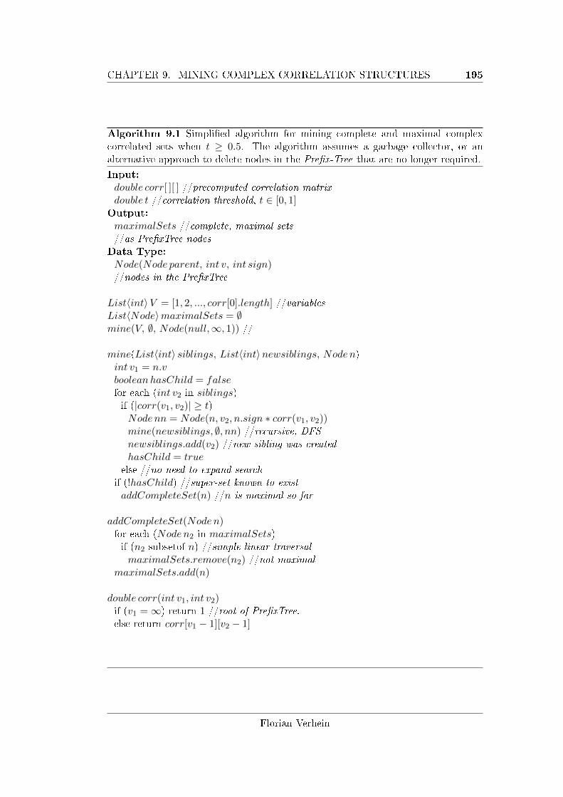
CHAPTER 9. MINING COMPLEX CORRELATION STRUCTURES 195
Algorithm 9.1 Simpli�ed algorithm for mining complete and maximal complexcorrelated sets when t ≥ 0.5. The algorithm assumes a garbage collector, or analternative approach to delete nodes in the Pre�x-Tree that are no longer required.
Input:double corr[ ][ ] //precomputed correlation matrixdouble t //correlation threshold, t ∈ [0, 1]
Output:maximalSets //complete, maximal sets//as Pre�xTree nodes
Data Type:Node(Node parent, int v, int sign)//nodes in the Pre�xTree
List〈int〉V = [1, 2, ..., corr[0].length] //variablesList〈Node〉maximalSets = ∅mine(V, ∅, Node(null,∞, 1)) //
mine(List〈int〉 siblings, List〈int〉newsiblings, Node n)int v1 = n.vbooleanhasChild = falsefor each (int v2 in siblings)if (|corr(v1, v2)| ≥ t)Nodenn = Node(n, v2, n.sign ∗ corr(v1, v2))mine(newsiblings, ∅, nn) //recursive, DFSnewsiblings.add(v2) //new sibling was createdhasChild = true
else //no need to expand searchif (!hasChild) //super-set known to existaddCompleteSet(n) //n is maximal so far
addCompleteSet(Noden)for each (Noden2 in maximalSets)if (n2 subsetof n) //simple linear traversalmaximalSets.remove(n2) //not maximal
maximalSets.add(n)
double corr(int v1, int v2)if (v1 =∞) return 1 //root of Pre�xTree.else return corr[v1 − 1][v2 − 1]
Florian Verhein
196 9.3. MINING COMPLEX MAXIMAL SETS: ALGORITHM
9.3.5 Complexity
For completeness, this section brie�y considers the worst case complexity of the
algorithm and can be skipped without loosing the �ow of the chapter.
Lemma 9.5. The time complexity of algorithm 9.1 is at most O(|V |2 ·|S|)+O(2|V |)+
O(|V | · 22|V |) = O(|V | · 22|V |), where |S| is the number of samples.
Proof. Calculating the correlations is done in O(|V |2 · |S|), enumerating the sets
takes at worst O(2|V |) (the number of nodes in the search), since there are a constant
number of operations per node (recall this is a consequence of exploiting the theory
in this chapter). The maximum number of maximal sets is bounded above by 2|V |,
and computing the maximal sets given m candidates takes m2/2 comparisons, each
of which is O(|V |) (traversal of the node sequence to check whether one is a subset).
Hence this part is O(|V | · 22|V |).
In practice, due to the nature of real data sets and the pruning used, this is not
a realistic re�ection of run time performance. In particular, the computation of
maximal sets generally takes less time that the enumeration of sets, despite having
higher worst case complexity. This is because the set of maximal sets is continually
reduced as the algorithm progresses (which is not re�ected in the worst case), and the
number of candidate maximal sets is much fewer that the number of sets enumerated
by the search. Finally, the worst case occurs when every variable is highly correlated
with every other variable, which generally does not happen in practice.
Lemma 9.6. The space complexity is at most O(|V |2)+O(|V |2)+O(
(|V ||V |/2
)) <
O(2|V |)
Proof. This is simply the space of the correlation matrix, plus the space of a depth
�rst search including the sibling list (the maximum depth and sibling list size is
|V |), plus the maximum number of maximal item-sets at any one time. It can be
shown that the latter is
(|V ||V |/2
), since this is the maximum number of subsets
of equal size, and the maximum number of maximal sets must all have equal size
(proof omitted). A bound on this is 2|V |.
Again, in practice this is misleading since computing the maximal sets continuously
Dr. rer. nat. Dissertation
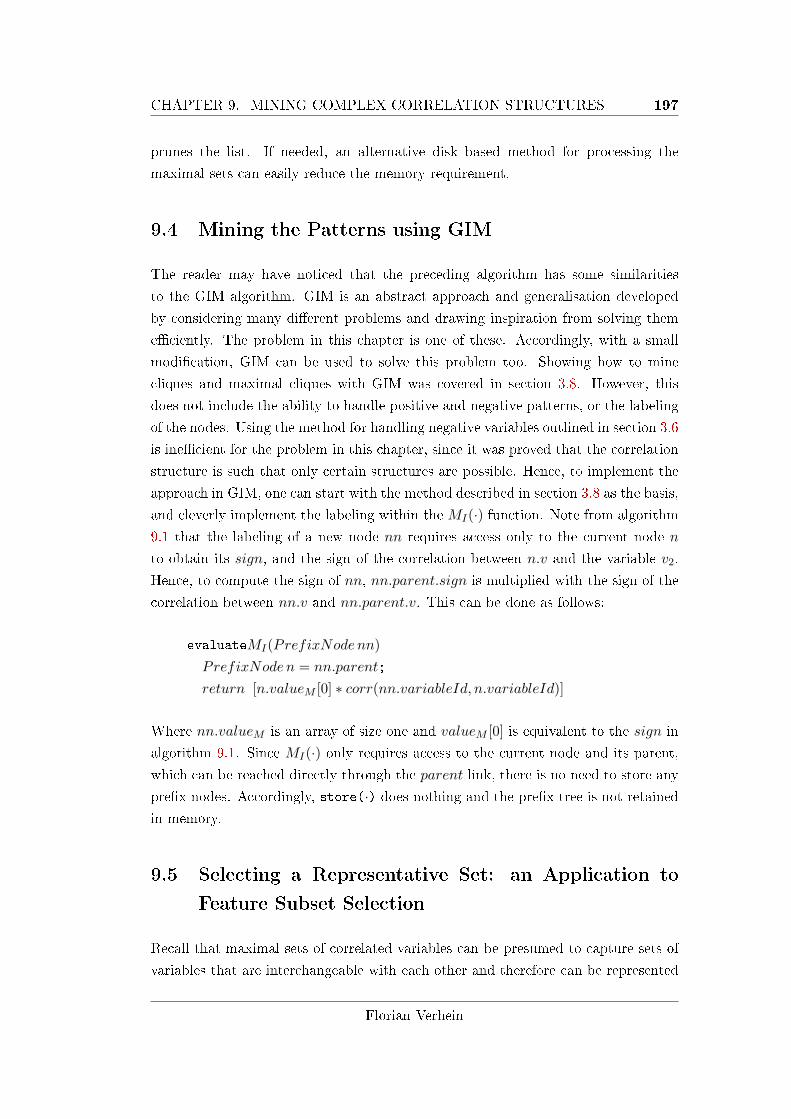
CHAPTER 9. MINING COMPLEX CORRELATION STRUCTURES 197
prunes the list. If needed, an alternative disk based method for processing the
maximal sets can easily reduce the memory requirement.
9.4 Mining the Patterns using GIM
The reader may have noticed that the preceding algorithm has some similarities
to the GIM algorithm. GIM is an abstract approach and generalisation developed
by considering many di�erent problems and drawing inspiration from solving them
e�ciently. The problem in this chapter is one of these. Accordingly, with a small
modi�cation, GIM can be used to solve this problem too. Showing how to mine
cliques and maximal cliques with GIM was covered in section 3.8. However, this
does not include the ability to handle positive and negative patterns, or the labeling
of the nodes. Using the method for handling negative variables outlined in section 3.6
is ine�cient for the problem in this chapter, since it was proved that the correlation
structure is such that only certain structures are possible. Hence, to implement the
approach in GIM, one can start with the method described in section 3.8 as the basis,
and cleverly implement the labeling within the MI(·) function. Note from algorithm
9.1 that the labeling of a new node nn requires access only to the current node n
to obtain its sign, and the sign of the correlation between n.v and the variable v2.
Hence, to compute the sign of nn, nn.parent.sign is multiplied with the sign of the
correlation between nn.v and nn.parent.v. This can be done as follows:
evaluateMI(PrefixNode nn)
PrefixNode n = nn.parent;
return [n.valueM [0] ∗ corr(nn.variableId, n.variableId)]
Where nn.valueM is an array of size one and valueM [0] is equivalent to the sign in
algorithm 9.1. Since MI(·) only requires access to the current node and its parent,
which can be reached directly through the parent link, there is no need to store any
pre�x nodes. Accordingly, store(·) does nothing and the pre�x tree is not retained
in memory.
9.5 Selecting a Representative Set: an Application to
Feature Subset Selection
Recall that maximal sets of correlated variables can be presumed to capture sets of
variables that are interchangeable with each other and therefore can be represented
Florian Verhein
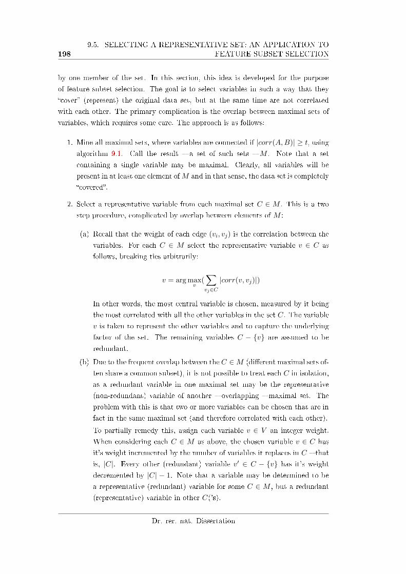
1989.5. SELECTING A REPRESENTATIVE SET: AN APPLICATION TO
FEATURE SUBSET SELECTION
by one member of the set. In this section, this idea is developed for the purpose
of feature subset selection. The goal is to select variables in such a way that they
�cover� (represent) the original data set, but at the same time are not correlated
with each other. The primary complication is the overlap between maximal sets of
variables, which requires some care. The approach is as follows:
1. Mine all maximal sets, where variables are connected if |corr(A,B)| ≥ t, usingalgorithm 9.1. Call the result � a set of such sets � M . Note that a set
containing a single variable may be maximal. Clearly, all variables will be
present in at least one element ofM and in that sense, the data set is completely
�covered�.
2. Select a representative variable from each maximal set C ∈ M . This is a two
step procedure, complicated by overlap between elements of M :
(a) Recall that the weight of each edge (vi, vj) is the correlation between the
variables. For each C ∈ M select the representative variable v ∈ C as
follows, breaking ties arbitrarily:
v = arg maxv
(∑vj∈C
|corr(v, vj)|)
In other words, the most central variable is chosen, measured by it being
the most correlated with all the other variables in the set C. The variable
v is taken to represent the other variables and to capture the underlying
factor of the set. The remaining variables C − {v} are assumed to be
redundant.
(b) Due to the frequent overlap between the C ∈M (di�erent maximal sets of-
ten share a common subset), it is not possible to treat each C in isolation,
as a redundant variable in one maximal set may be the representative
(non-redundant) variable of another � overlapping � maximal set. The
problem with this is that two or more variables can be chosen that are in
fact in the same maximal set (and therefore correlated with each other).
To partially remedy this, assign each variable v ∈ V an integer weight.
When considering each C ∈ M as above, the chosen variable v ∈ C has
it's weight incremented by the number of variables it replaces in C � that
is, |C|. Every other (redundant) variable v′ ∈ C − {v} has it's weight
decremented by |C| − 1. Note that a variable may be determined to be
a representative (redundant) variable for some C ∈ M , but a redundant
(representative) variable in other C('s).
Dr. rer. nat. Dissertation
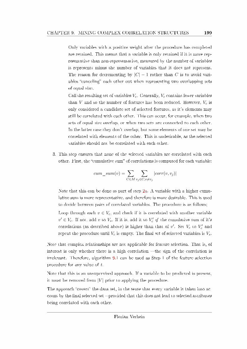
CHAPTER 9. MINING COMPLEX CORRELATION STRUCTURES 199
Only variables with a positive weight after the procedure has completed
are retained. This means that a variable is only retained if it is more rep-
resentative than non-representative, measured by the number of variables
it represents minus the number of variables that it does not represent.
The reason for decrementing by |C| − 1 rather than C is to avoid vari-
ables �canceling� each other out when representing two overlapping sets
of equal size.
Call the resulting set of variables Vc. Generally, Vc contains fewer variables
than V and so the number of features has been reduced. However, Vc is
only considered a candidate set of selected features, as it's elements may
still be correlated with each other. This can occur, for example, when two
sets of equal size overlap, or when two sets are connected to each other.
In the latter case they don't overlap, but some elements of one set may be
correlated with elements of the other. This is undesirable, as the selected
variables should not be correlated with each other.
3. This step ensures that none of the selected variables are correlated with each
other. First, the �cumulative sum� of correlations is computed for each variable:
cum_sum(v) =∑C∈M
∑vj∈C,v 6=vj
|corr(v, vj)|
Note that this can be done as part of step 2a. A variable with a higher cumu-
lative sum is more representative, and therefore is more desirable. This is used
to decide between pairs of correlated variables. The procedure is as follows;
Loop through each v ∈ Vc, and check if it is correlated with another variable
v′ ∈ Vc. If not, add v to Vs. If it is, add it to V ′c if the cumulative sum of it's
correlations (as described above) is higher than that of v′. Set Vc to V′c and
repeat the procedure until Vc is empty. The �nal set of selected variables is Vs.
Note that complex relationships are not applicable for feature selection. That is, of
interest is only whether there is a high correlation � the sign of the correlation is
irrelevant. Therefore, algorithm 9.1 can be used as Step 1 of the feature selection
procedure for any value of t.
Note that this is an unsupervised approach. If a variable to be predicted is present,
it must be removed from |V | prior to applying the procedure.
The approach �covers� the data set, in the sense that every variable is taken into ac-
count by the �nal selected set � provided that this does not lead to selected attributes
being correlated with each other.
Florian Verhein
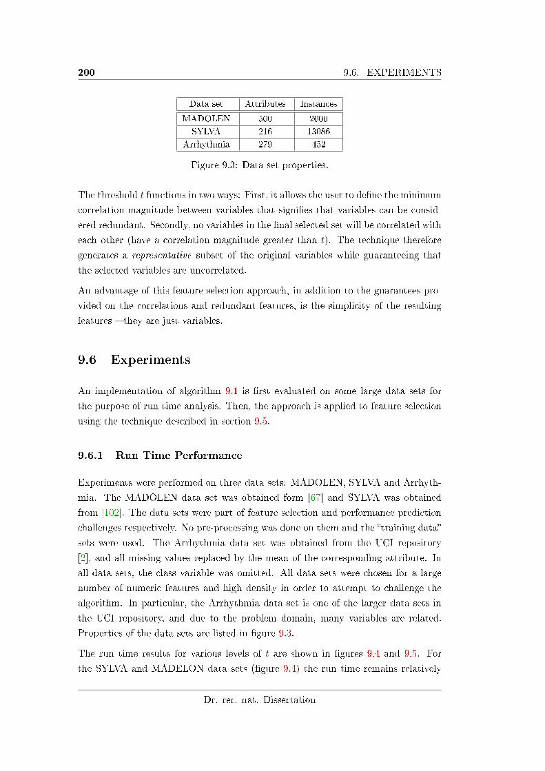
200 9.6. EXPERIMENTS
Data set Attributes Instances
MADOLEN 500 2000
SYLVA 216 13086
Arrhythmia 279 452
Figure 9.3: Data set properties.
The threshold t functions in two ways: First, it allows the user to de�ne the minimum
correlation magnitude between variables that signi�es that variables can be consid-
ered redundant. Secondly, no variables in the �nal selected set will be correlated with
each other (have a correlation magnitude greater than t). The technique therefore
generates a representative subset of the original variables while guaranteeing that
the selected variables are uncorrelated.
An advantage of this feature selection approach, in addition to the guarantees pro-
vided on the correlations and redundant features, is the simplicity of the resulting
features � they are just variables.
9.6 Experiments
An implementation of algorithm 9.1 is �rst evaluated on some large data sets for
the purpose of run time analysis. Then, the approach is applied to feature selection
using the technique described in section 9.5.
9.6.1 Run Time Performance
Experiments were performed on three data sets: MADOLEN, SYLVA and Arrhyth-
mia. The MADOLEN data set was obtained form [67] and SYLVA was obtained
from [102]. The data sets were part of feature selection and performance prediction
challenges respectively. No pre-processing was done on them and the �training data�
sets were used. The Arrhythmia data set was obtained from the UCI repository
[2], and all missing values replaced by the mean of the corresponding attribute. In
all data sets, the class variable was omitted. All data sets were chosen for a large
number of numeric features and high density in order to attempt to challenge the
algorithm. In particular, the Arrhythmia data set is one of the larger data sets in
the UCI repository, and due to the problem domain, many variables are related.
Properties of the data sets are listed in �gure 9.3.
The run time results for various levels of t are shown in �gures 9.4 and 9.5. For
the SYLVA and MADELON data sets (�gure 9.4) the run time remains relatively
Dr. rer. nat. Dissertation
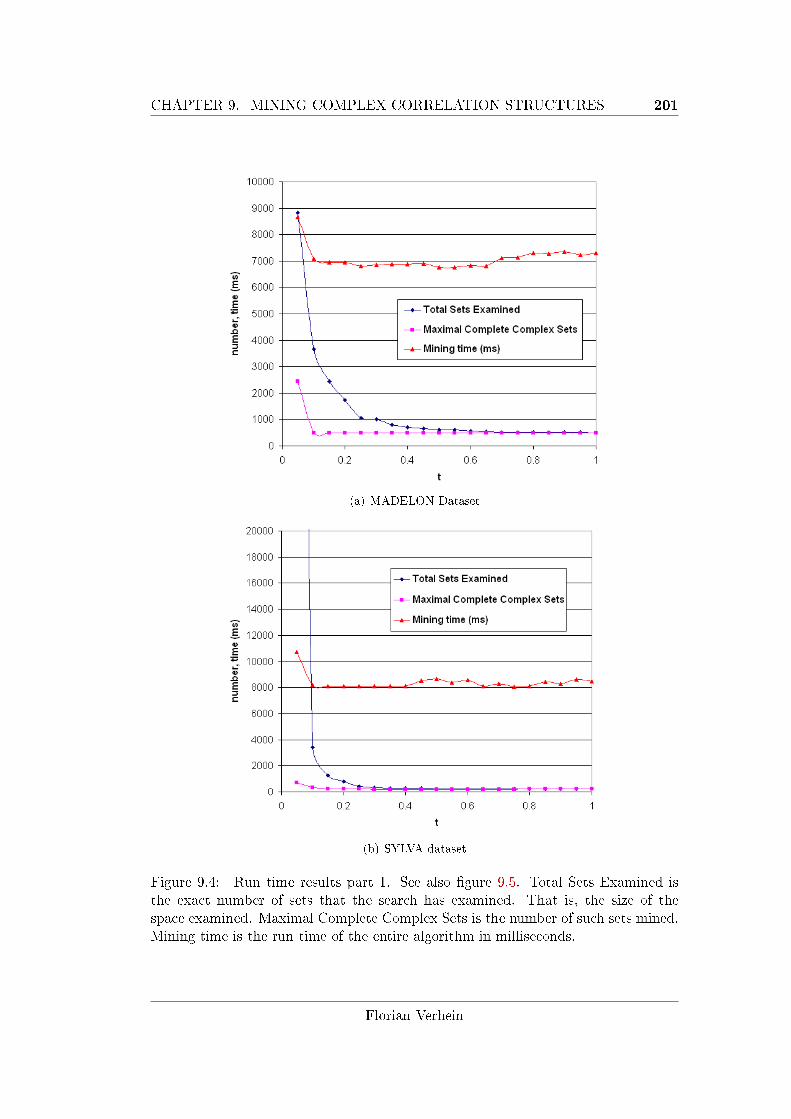
CHAPTER 9. MINING COMPLEX CORRELATION STRUCTURES 201
(a) MADELON Dataset
(b) SYLVA dataset
Figure 9.4: Run time results part 1. See also �gure 9.5. Total Sets Examined isthe exact number of sets that the search has examined. That is, the size of thespace examined. Maximal Complete Complex Sets is the number of such sets mined.Mining time is the run time of the entire algorithm in milliseconds.
Florian Verhein
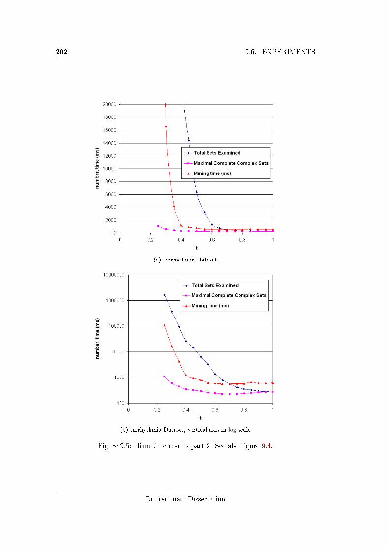
202 9.6. EXPERIMENTS
(a) Arrhythmia Dataset
(b) Arrhythmia Dataset, vertical axis in log scale
Figure 9.5: Run time results part 2. See also �gure 9.4.
Dr. rer. nat. Dissertation
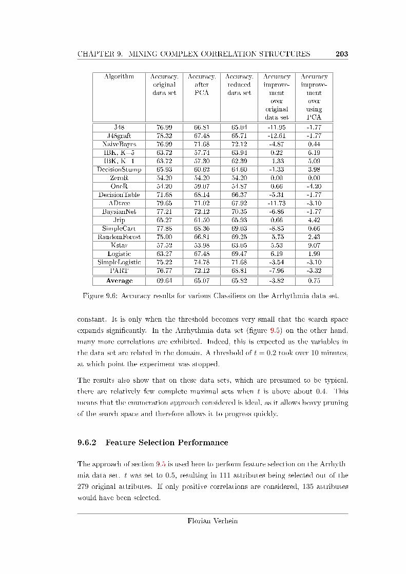
CHAPTER 9. MINING COMPLEX CORRELATION STRUCTURES 203
Algorithm Accuracy,originaldata set
Accuracy,afterPCA
Accuracy,reduceddata set
Accuracyimprove-mentover
originaldata set
Accuracyimprove-mentoverusingPCA
J48 76.99 66.81 65.04 -11.95 -1.77
J48graft 78.32 67.48 65.71 -12.61 -1.77
NaiveBayes 76.99 71.68 72.12 -4.87 0.44
IBK, K=5 63.72 57.74 63.94 0.22 6.19
IBK, K=1 63.72 57.30 62.39 -1.33 5.09
DecisionStump 65.93 60.62 64.60 -1.33 3.98
ZeroR 54.20 54.20 54.20 0.00 0.00
OneR 54.20 59.07 54.87 0.66 -4.20
DecisionTable 71.68 68.14 66.37 -5.31 -1.77
ADtree 79.65 71.02 67.92 -11.73 -3.10
BaysianNet 77.21 72.12 70.35 -6.86 -1.77
Jrip 65.27 61.50 65.93 0.66 4.42
SimpleCart 77.88 68.36 69.03 -8.85 0.66
RandomForest 75.00 66.81 69.25 -5.75 2.43
Kstar 57.52 53.98 63.05 5.53 9.07
Logistic 63.27 67.48 69.47 6.19 1.99
SimpleLogistic 75.22 74.78 71.68 -3.54 -3.10
PART 76.77 72.12 68.81 -7.96 -3.32
Average 69.64 65.07 65.82 -3.82 0.75
Figure 9.6: Accuracy results for various Classi�ers on the Arrhythmia data set.
constant. It is only when the threshold becomes very small that the search space
expands signi�cantly. In the Arrhythmia data set (�gure 9.5) on the other hand,
many more correlations are exhibited. Indeed, this is expected as the variables in
the data set are related in the domain. A threshold of t = 0.2 took over 10 minutes,
at which point the experiment was stopped.
The results also show that on these data sets, which are presumed to be typical,
there are relatively few complete maximal sets when t is above about 0.4. This
means that the enumeration approach considered is ideal, as it allows heavy pruning
of the search space and therefore allows it to progress quickly.
9.6.2 Feature Selection Performance
The approach of section 9.5 is used here to perform feature selection on the Arrhyth-
mia data set. t was set to 0.5, resulting in 111 attributes being selected out of the
279 original attributes. If only positive correlations are considered, 135 attributes
would have been selected.
Florian Verhein
204 9.7. RELATED WORK
In addition to comparing classi�cation results on the reduced data set to the original
data set, a comparison to PCA was also performed. PCA was performed using the
algorithm from WEKA [104], and options were set so the same number of attributes
� 111 � were chosen. The 111 principle components cover 96% of the variance of the
data set.
Figure 9.6 shows the results on various classi�ers in WEKA [104] (version 3.5.7),
evaluated over the original data set, the data set with features extracted using PCA,
and the subset of the attributes selected using the approach in section 9.5. Unless
otherwise stated, default values were used in the ML algorithms. The 16 classes
in the original data set were amalgamated into two classes, representing normal
heart rhythms (245 instances) and cardiac arrhythmia (207 instances). 10-fold cross
validation was used for the evaluation of classi�cation accuracy in all cases. The
approach in this paper performs comparably to PCA, having only 0.75 percentage
points better accuracy on average. On average, the accuracy is 3.82% lower than on
the original data set. Therefore, not only can this approach compete well against
PCA, but it maintains the interpretability of the model. That is, the rules and
decision trees built on the data set retain the actual attributes, in contrast to when
PCA is used.
9.7 Related Work
9.7.1 Clique and Set Mining
A complete set and a clique are equivalent. The latter is often used in social network
situations or in spatial data sets. In spatial applications, the space in which variables
exist is usually low dimensional so enumeration approaches to mine them are not
appropriate. Also, distances are used, rather than correlations (angles). �Complex�
cliques have been considered [64], but this is in relation to absence of objects.
Graph based clustering approaches are also related. In some sense, the approach
described in this paper is related to agglomerative clustering [88]. The desire for
complete sub-graphs (sets) is the same as the clique pattern, or in distance based
approaches, the MAX approach [88]. The maximal set idea could be considered as
the highest level in a hierarchy de�ned over subsets, but the method does not �t into
hierarchical clustering. In particular, the threshold is �xed. The approach in this
paper is not really a clustering method. It is best described as a method of mining
interactions between variables, with those interactions having a speci�c structure and
being de�ned by correlation. The consideration of complex interactions in particular
Dr. rer. nat. Dissertation
CHAPTER 9. MINING COMPLEX CORRELATION STRUCTURES 205
sets it well apart from clustering approaches.
The algorithmic approach has a closer relationship to itemset mining than it does
to clustering. Items are a special type of variable, and itemsets are sets of vari-
ables possessing some interesting property � usually that they occur frequently. The
similarity to item enumeration approaches is that the enumeration is over sets of
variables, from the bottom up. The fundamental di�erence to itemset mining is that
the itemset mining problem cannot be mapped to graph mining, as it cannot be
reduced to pairwise relationships. Complex relationships therefore also don't mean
the same thing. While the absence of an item can be considered, this is di�erent
to the complex relationships (both negative and positive correlations) considered in
this chapter.
It should also be emphasised that the use of correlation is a core component of
this work, in particular, the lemma and corollaries that are developed under the
completely connected sub-graph structure. Correlation is generally not used for
clustering, and it cannot be used for itemset mining, as it does not translate to
more than two variables at a time. Unlike distance measures, it has both positive
and negative values � therefore techniques based on it necessarily have di�erent
semantics.
9.7.2 Feature Subset Selection
Feature subset selection comes in three �avours; wrapper, embedded or �lter [88]. In
the wrapper or embedded approaches, it is used in conjunction with a data mining or
machine learning algorithm in some form of supervised or semi-supervised process.
The wrapper approach uses the DM or ML algorithm as an objective function, while
in the embedded approach the DM or ML algorithm decides what features to discard
as part of its operation. The �lter approach selects a subset independently of the
subsequent DM/ML algorithm. It may or may not be supervised. The approach
described in section 9.5 �ts into the unsupervised �lter category. One �lter approach
using correlation for feature subset selection is presented in [45]. However, this is
a hill climbing, supervised, optimizing approach. It is also based on entropy � not
statistical correlation.
Finding representative sets is considered in [70] using an entropy based approach on
binary data. The algorithm in [70] also mines a representative set directly (this work
performs it as a second step).
As earlier mentioned, the idea of maximal complex sets representing underlying
factors of the data set has similarities to the way principle components can be applied.
Florian Verhein
206 9.8. CONCLUSION
But as also mentioned earlier, these are very di�erent approaches.
In summary, the work in this paper is related to various bodies of work in Data
Mining, but to the author's knowledge, is quite di�erent to each.
9.8 Conclusion
This chapter presented and exploited useful results about the correlation structures
between variables. Additionally, it proposed the `complete, complex and maximal
sub-graphs or sets of highly correlated variables' pattern. This approach is useful as
a data mining technique in its own right, or, as also demonstrated in this paper, as
the core component of an unsupervised feature subset selection procedure.
Solving the problem considered in this chapter was one of the many inspirations
behind developing the generalised interaction mining approach introduced in this
thesis.
A useful avenue of future work is to consider only signi�cant patterns. For example,
considering correlation graphs de�ned by signi�cant correlation, in order to reduce
the e�ects of noise and the probability that seemingly interesting patterns are found
by chance alone.
Dr. rer. nat. Dissertation
Part IV
Mining Uncertain and
Probabilistic Databases
207

Chapter 10
Probabilistic Frequent Itemset
Mining in Uncertain Databases
Probabilistic frequent itemset mining in uncertain transaction databases
semantically and computationally di�ers from traditional frequent itemset
mining techniques applied to standard �certain� transaction databases. The
consideration of existential uncertainty of item(sets), indicating the proba-
bility that an item(set) occurs in a transaction, makes traditional techniques
inapplicable. This chapter introduces new probabilistic formulations of fre-
quent itemsets based on possible world semantics. In this probabilistic con-
text, an itemset X is called frequent if the probability that X occurs in at
least minSup transactions is above a given threshold τ . This is the �rst ap-
proach addressing this problem and does so under possible worlds semantics.
In consideration of the probabilistic formulations, a framework is presented
which is able to solve the Probabilistic Frequent Itemset Mining (PFIM)
problem e�ciently. An extensive experimental evaluation investigates the
impact of the proposed techniques and shows that the approach is orders of
magnitude faster than straight-forward approaches.
209
210 10.1. INTRODUCTION
10.1 Introduction
Association rule analysis is one of the most important �elds in data mining. It is
commonly applied to market-basket databases for analysis of consumer purchasing
behaviour. Such databases consist of a set of transactions, each containing the items
a customer purchased. The database can be analyzed to discover associations among
di�erent sets of items. The most important and computationally intensive step in
the mining process is the extraction of frequent itemsets � sets of items that occur
in at least minSup transactions.
It is generally assumed that the items occurring in a transaction are known for
certain. However, this is not always the case. For instance;
• In many applications the data is inherently noisy, such as data collected by
sensors or in satellite images.
• In privacy protection applications, arti�cial noise can be added deliberately in
order to prevent reverse engineering of the data through pattern analysis [107].
Finding patterns despite this noise is a challenging problem.
• Data sets may also be aggregated. By aggregating transactions by customer,
it is possible to mine patterns across customers instead of transactions. In the
resulting database, this produces estimated purchase probabilities per item per
customer rather than certain items per transaction. This application is used
as an example later.
In such applications, the information captured in transactions is uncertain since the
existence of an item is associated with a likelihood measure or existential probability.
Given an uncertain transaction database, it is not obvious how to identify whether
an item or itemset is frequent because we generally cannot say for certain whether
an itemset appears in a transaction. In a traditional (certain) transaction database,
one can simply perform a database scan and count the transactions that include the
itemset. This does not work in an uncertain transaction database.
Dealing with such databases is a di�cult but interesting problem. While a naive
approach might transform uncertain items into certain ones by thresholding the
probabilities 1, this loses useful information and leads to inaccuracies. Existing ap-
proaches in the literature are based on expected support, �rst introduced in [26].
Chui et. al. [25, 26] take the uncertainty of items into account by computing the
1For example, by treating all uncertain items with a probability value higher than 0.5 as beingpresent, and all others as being absent.
Dr. rer. nat. Dissertation
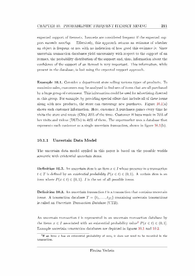
CHAPTER 10. PROBABILISTIC FREQUENT ITEMSET MINING 211
expected support of itemsets. Itemsets are considered frequent if the expected sup-
port exceeds minSup. E�ectively, this approach returns an estimate of whether
an object is frequent or not with no indication of how good this estimate is. Since
uncertain transaction databases yield uncertainty with respect to the support of an
itemset, the probability distribution of the support and, thus, information about the
con�dence of the support of an itemset is very important. This information, while
present in the database, is lost using the expected support approach.
Example 10.1. Consider a department store selling various types of products. To
maximize sales, customers may be analysed to �nd sets of items that are all purchased
by a large group of customers. This information could be used for advertising directed
at this group. For example, by providing special o�ers that include all of these items
along with new products, the store can encourage new purchases. Figure 10.1(a)
shows such customer information. Here, customer A purchases games every time he
visits the store and music (CDs) 20% of the time. Customer B buys music in 70% of
her visits and videos (DVDs) in 40% of them. The supermarket uses a database that
represents each customer as a single uncertain transaction, shown in �gure 10.1(b).
10.1.1 Uncertain Data Model
The uncertain data model applied in this paper is based on the possible worlds
semantic with existential uncertain items.
De�nition 10.2. An uncertain item is an item x ∈ I whose presence in a transactiont ∈ T is de�ned by an existential probability P (x ∈ t) ∈ (0, 1). A certain item is an
item where P (x ∈ t) ∈ {0, 1}. I is the set of all possible items.
De�nition 10.3. An uncertain transaction t is a transaction that contains uncertain
items. A transaction database T = {t1, . . . , t|T |} containing uncertain transactions
is called an Uncertain Transaction Database (UTB).
An uncertain transaction t is represented in an uncertain transaction database by
the items x ∈ I associated with an existential probability value2 P (x ∈ t) ∈ (0, 1].
Example uncertain transaction databases are depicted in �gures 10.1 and 10.2.
2If an item x has an existential probability of zero, it does not need to be recorded in thetransaction.
Florian Verhein
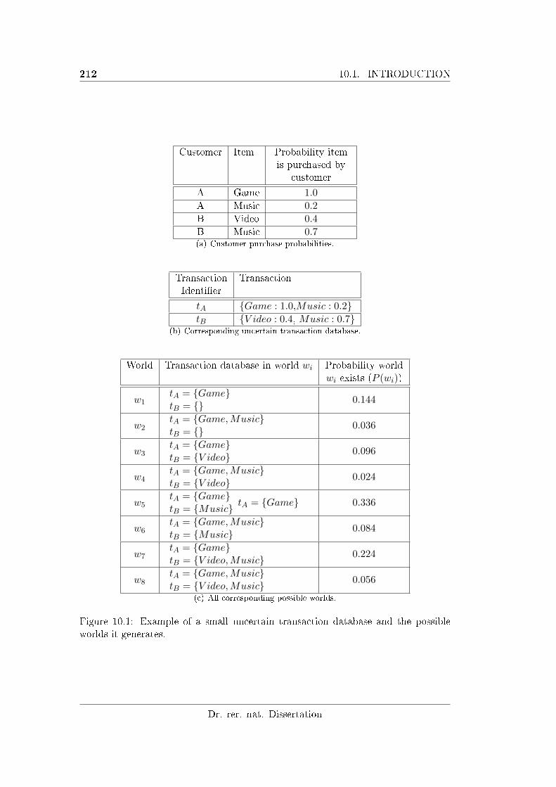
212 10.1. INTRODUCTION
Customer Item Probability itemis purchased by
customer
A Game 1.0
A Music 0.2
B Video 0.4
B Music 0.7(a) Customer purchase probabilities.
TransactionIdenti�er
Transaction
tA {Game : 1.0,Music : 0.2}tB {V ideo : 0.4, Music : 0.7}
(b) Corresponding uncertain transaction database.
World Transaction database in world wi Probability worldwi exists (P (wi))
w1tA = {Game}tB = {} 0.144
w2tA = {Game,Music}tB = {} 0.036
w3tA = {Game}tB = {V ideo} 0.096
w4tA = {Game,Music}tB = {V ideo} 0.024
w5tA = {Game}tB = {Music} tA = {Game} 0.336
w6tA = {Game,Music}tB = {Music} 0.084
w7tA = {Game}tB = {V ideo,Music} 0.224
w8tA = {Game,Music}tB = {V ideo,Music} 0.056
(c) All corresponding possible worlds.
Figure 10.1: Example of a small uncertain transaction database and the possibleworlds it generates.
Dr. rer. nat. Dissertation
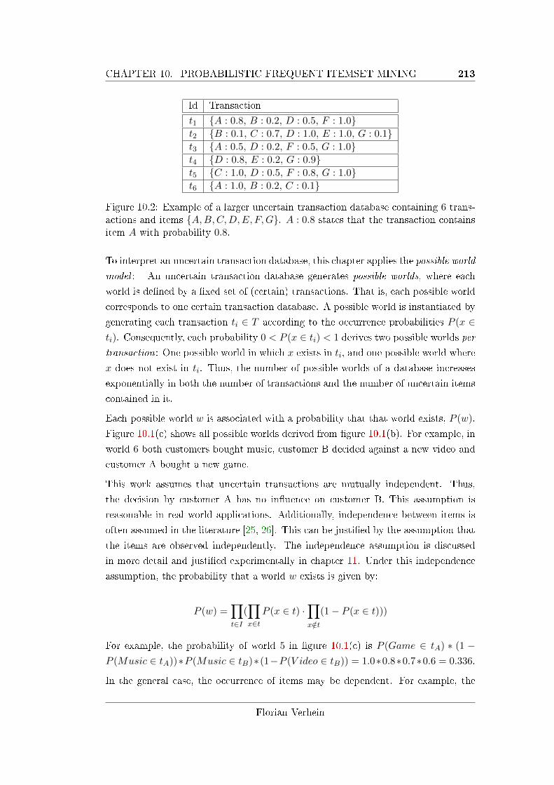
CHAPTER 10. PROBABILISTIC FREQUENT ITEMSET MINING 213
Id Transaction
t1 {A : 0.8, B : 0.2, D : 0.5, F : 1.0}t2 {B : 0.1, C : 0.7, D : 1.0, E : 1.0, G : 0.1}t3 {A : 0.5, D : 0.2, F : 0.5, G : 1.0}t4 {D : 0.8, E : 0.2, G : 0.9}t5 {C : 1.0, D : 0.5, F : 0.8, G : 1.0}t6 {A : 1.0, B : 0.2, C : 0.1}
Figure 10.2: Example of a larger uncertain transaction database containing 6 trans-actions and items {A,B,C,D,E, F,G}. A : 0.8 states that the transaction containsitem A with probability 0.8.
To interpret an uncertain transaction database, this chapter applies the possible world
model : An uncertain transaction database generates possible worlds, where each
world is de�ned by a �xed set of (certain) transactions. That is, each possible world
corresponds to one certain transaction database. A possible world is instantiated by
generating each transaction ti ∈ T according to the occurrence probabilities P (x ∈ti). Consequently, each probability 0 < P (x ∈ ti) < 1 derives two possible worlds per
transaction: One possible world in which x exists in ti, and one possible world where
x does not exist in ti. Thus, the number of possible worlds of a database increases
exponentially in both the number of transactions and the number of uncertain items
contained in it.
Each possible world w is associated with a probability that that world exists, P (w).
Figure 10.1(c) shows all possible worlds derived from �gure 10.1(b). For example, in
world 6 both customers bought music, customer B decided against a new video and
customer A bought a new game.
This work assumes that uncertain transactions are mutually independent. Thus,
the decision by customer A has no in�uence on customer B. This assumption is
reasonable in real world applications. Additionally, independence between items is
often assumed in the literature [25, 26]. This can be justi�ed by the assumption that
the items are observed independently. The independence assumption is discussed
in more detail and justi�ed experimentally in chapter 11. Under this independence
assumption, the probability that a world w exists is given by:
P (w) =∏t∈I
(∏x∈t
P (x ∈ t) ·∏x/∈t
(1− P (x ∈ t)))
For example, the probability of world 5 in �gure 10.1(c) is P (Game ∈ tA) ∗ (1 −P (Music ∈ tA))∗P (Music ∈ tB)∗(1−P (V ideo ∈ tB)) = 1.0∗0.8∗0.7∗0.6 = 0.336.
In the general case, the occurrence of items may be dependent. For example, the
Florian Verhein
214 10.1. INTRODUCTION
decision to purchase a new music video DVD may mean they are unlikely to purchase
a music CD by the same artist. Alternatively, some items must be bought together.
If these conditional probabilities are known, they can be used in the methods in this
thesis. For example, the probability that both a video and music are purchased by
customer B is P ({V ideo,Music} ∈ tB) = P (V ideo ∈ tB) ∗ P (Music ∈ tB|V ideo ∈tB).
10.1.2 Problem De�nition
An itemset is a frequent itemset if it occurs in at least minSup transactions, where
minSup is a user speci�ed parameter. In uncertain transaction databases however,
the support of an itemset is uncertain; it is de�ned by a discrete probability distri-
bution function (p.d.f). Therefore, each itemset has a frequentness probability3 � the
probability that it is frequent (de�ned formally in de�nition 10.10). This chapter
focuses on the problem of e�ciently calculating this p.d.f. (called the support prob-
ability distribution function and de�ned formally in de�nition 10.8) and extracting
all probabilistic frequent itemsets:
De�nition 10.4 (Probabilistic Frequent Itemset). A Probabilistic Frequent Itemset
(PFI) is an itemset with a frequentness probability of at least τ .
The parameter τ is the user speci�ed minimum con�dence in the frequentness of an
itemset. If τ is set close to 1 then the user is interested only in itemsets that have a
very high probability of being frequent, while a small value for τ (close to 0) would
lead to results that also include itemsets which are frequent in very few possible
worlds � that is, that have a very low probability of being frequent.
The problem may now be de�ned as follows:
De�nition 10.5 (Probabilistic Frequent Itemset Mining). Given an uncertain trans-
action database T , a minimum support scalar minSup and a frequentness probabil-
ity threshold τ , Probabilistic Frequent Itemset Mining (PFIM) problem is to �nd all
probabilistic frequent itemsets.
10.1.3 Contributions
This chapter makes the following contributions:
3Frequentness is the rarely used word describing the property of being frequent.
Dr. rer. nat. Dissertation
CHAPTER 10. PROBABILISTIC FREQUENT ITEMSET MINING 215
• It proposes a probabilistic framework for frequent itemset mining in uncertain
transaction databases, based on the possible worlds model. Furthermore, it
proposes the probabilistic frequent itemset mining (PFIM) problem.
• It presents a dynamic computation method for computing the probability that
an itemset is frequent (the frequentness probability), as well as the entire prob-
ability distribution function of the support of an itemset, in O(|T |) time4.
Without this technique, it would run in exponential time in the number of
transactions. Using this approach, the algorithm has the same time complex-
ity as methods based on the expected support [25, 26, 58] but yields much
better e�ectiveness.
• It proposes an algorithm � ProApriori � to mine all itemsets that are frequent
with a probability of at least τ . This chapter also proposes an additional
algorithm that incrementally outputs the probabilistic frequent itemsets in the
order of their frequentness probability. This ensures that itemsets with the
highest probability of being frequent are output �rst. This has two additional
advantages; �rst, it makes the approach free of the parameter τ . Secondly, it
solves the top k itemsets problem in uncertain databases.
10.1.4 Organisation
The remainder of this chapter is organised as follows: Section 10.2 surveys related
work. Section 10.3 presents the probabilistic support framework. Section 10.4 shows
how to compute the frequentness probability in O(|T |) time. Section 10.5 presents
ProApriori � a probabilistic frequent itemset mining algorithm. Section 10.6 presents
the incremental algorithm. Experiments are presented in section 10.7 and this chap-
ter concludes in section 10.8.
10.2 Related Work
There is a large body of research on Frequent Itemset Mining (FIM), a survey can
be found in [43]. Recall also that section 4.3 provided an overview of FIM. However,
very little work addresses FIM in uncertain databases [25, 26, 58]. Indeed, the
problem is a recent one. The approach proposed by Chui et. al [26] computes the
expected support of itemsets by summing all itemset probabilities in their U-Apriori
algorithm. Later, in [25], they additionally proposed a probabilistic �lter in order
4Assuming minSup is a constant.
Florian Verhein
216 10.2. RELATED WORK
to prune candidates early. In [58], the UF-growth algorithm is proposed. Like U-
Apriori, UF-growth computes frequent itemsets by means of the expected support,
but it uses the FP-tree [48, 47] approach in order to avoid expensive candidate
generation. In contrast to the probabilistic approach in this chapter, itemsets are
considered frequent if the expected support exceeds minSup. The main drawback of
this estimator is that information about the uncertainty of the expected support is
lost; [25, 26, 58] ignore the number of possible worlds in which an itemsets is frequent.
[114] proposes exact and sampling-based algorithms to �nd likely frequent items in
streaming probabilistic data. However, they do not consider itemsets with more than
one item. Finally, except for [96], existing FIM algorithms assume binary valued
items which precludes simple adaptation to uncertain databases. The approach in
this thesis is the �rst that is able to �nd frequent itemsets in an uncertain transaction
database in a probabilistic way.
Existing approaches in the �eld of uncertain data management and mining can be
categorized into a number of research directions. Most related to the work in this
chapter are the two categories �probabilistic databases� [17, 77, 79, 14] and �proba-
bilistic query processing� [32, 54, 109, 83].
The uncertainty model used in this chapter is very close to the model used for proba-
bilistic databases. A probabilistic database denotes a database composed of relations
with uncertain tuples [32], where each tuple is associated with a probability denoting
the likelihood that it exists in the relation. This model, called �tuple uncertainty�,
adopts the possible worlds semantics [14]. A probabilistic database represents a set
of possible �certain� database instances (worlds), where a database instance corre-
sponds to a subset of uncertain tuples. Each instance (world) is associated with the
probability that the world is �true�. The probabilities re�ect the probability distri-
bution of all possible database instances. In the general model description [79], the
possible worlds are constrained by rules that are de�ned on the tuples in order to
incorporate object (tuple) correlations. The ULDB model proposed in [17], which is
used in Trio[9], supports uncertain tuples with alternative instances which are called
x-tuples. Relations in ULDB are called x-relations containing a set of x-tuples. Each
x-tuple corresponds to a set of tuple instances which are assumed to be mutually ex-
clusive, i.e. no more than one instance of an x-tuple can appear in a possible world
instance at the same time. Probabilistic top-k query approaches [83, 109, 77] are
usually associated with uncertain databases using the tuple uncertainty model. The
approach proposed in [109] was the �rst approach able to solve probabilistic queries
e�ciently under tuple independency by means of dynamic programming techniques.
This chapter adopts the dynamic programming technique for the e�cient computa-
Dr. rer. nat. Dissertation
CHAPTER 10. PROBABILISTIC FREQUENT ITEMSET MINING 217
tion of probabilistic frequent itemsets (PFIs).
Another uncertainty model also exists, called attribute uncertainty [24]. In this
model, each tuple is assumed to be �certainly� existent, but their attributes are un-
certain. Therefore, each attribute is instantiated by a range of values associated with
a probability distribution. This model is often used in the context of probabilistic
similarity queries over uncertain vector data [24, 54].
While managing uncertain data has been studied for a considerable time [115], re-
cently there has been an increasing interest in algorithms and applications on un-
certain data. [8, 115] provide surveys and categorise the three main research areas
in this �eld: Modeling uncertain data, which considers the process of capturing the
uncertainties in the data while keeping the data useful for database management ap-
plications; uncertain data management / analysing uncertain data, which considers
the issue of incorporating uncertain data semantics into database management sys-
tem and problems such as query processing, joins and indexing; and mining uncertain
data, which develops data mining techniques that take into account the uncertainty
of the data. A tutorial on mining uncertain and probabilistic data may be found
in [75]. The work in this chapter falls primarily into the third category, since it
proposes a new approach to frequent itemset mining that explicitly and e�ectively
deals with a database's uncertainty. The solution to the top-k probabilistic frequent
itemset query falls into the second category, while the probabilistic framework for
itemset mining based on possible world semantics falls into the �rst.
10.3 Probabilistic Frequent Itemsets
Recall that previous work was based on the expected support [25, 26, 58].
De�nition 10.6. Given an uncertain transaction database T , the expected support
E(X) of an itemset X is de�ned as E(X)=∑
t∈T P (X ⊆ t).
Considering an itemset frequent if its expected support is above minSup has a ma-
jor drawback. Uncertain transaction databases involve uncertainty concerning the
support of an itemset. It is important to consider this when evaluating whether an
itemset is frequent or not. However, this information is forfeited when using the
expected support approach. Returning to the example shown in �gure 10.2, the ex-
pected support of the itemset {D} is E({D}) = 3.0. The fact that {D} occurs forcertain in one transaction, namely in t2, and that there is at least one possible world
Florian Verhein
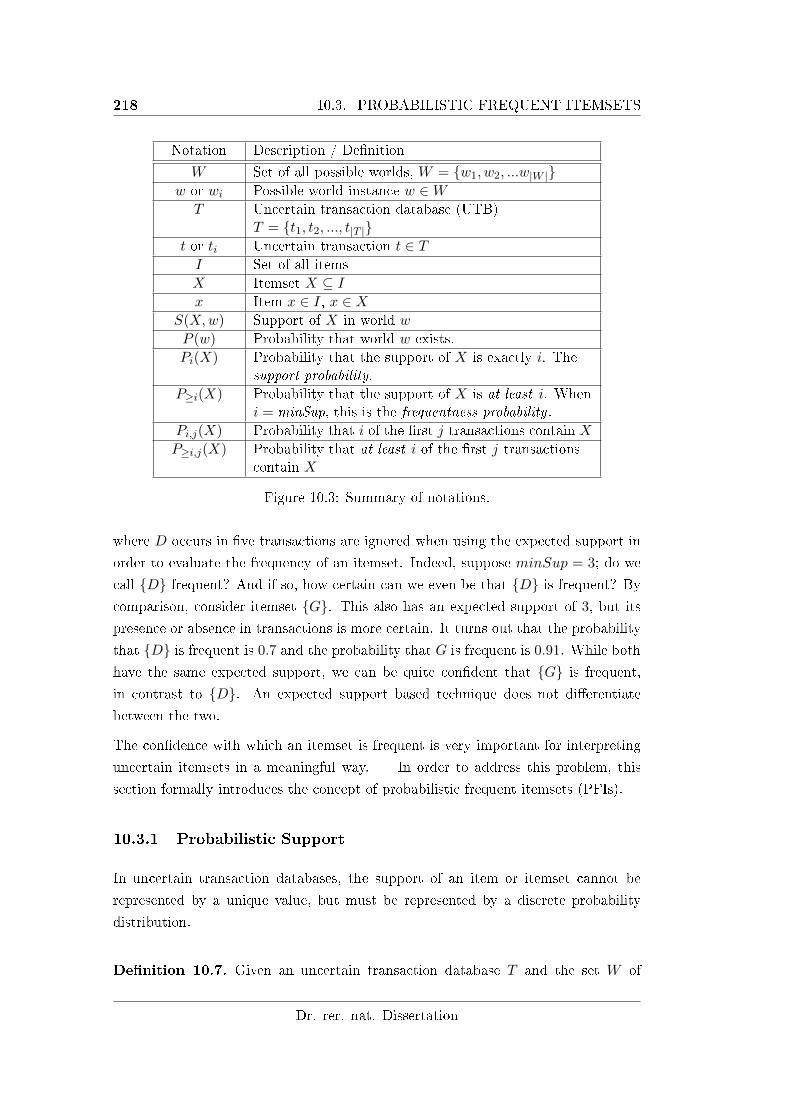
218 10.3. PROBABILISTIC FREQUENT ITEMSETS
Notation Description / De�nition
W Set of all possible worlds, W = {w1, w2, ...w|W |}w or wi Possible world instance w ∈WT Uncertain transaction database (UTB)
T = {t1, t2, ..., t|T |}t or ti Uncertain transaction t ∈ TI Set of all items
X Itemset X ⊆ Ix Item x ∈ I, x ∈ X
S(X,w) Support of X in world w
P (w) Probability that world w exists.
Pi(X) Probability that the support of X is exactly i. Thesupport probability.
P≥i(X) Probability that the support of X is at least i. Wheni = minSup, this is the frequentness probability .
Pi,j(X) Probability that i of the �rst j transactions contain X
P≥i,j(X) Probability that at least i of the �rst j transactionscontain X
Figure 10.3: Summary of notations.
where D occurs in �ve transactions are ignored when using the expected support in
order to evaluate the frequency of an itemset. Indeed, suppose minSup = 3; do we
call {D} frequent? And if so, how certain can we even be that {D} is frequent? By
comparison, consider itemset {G}. This also has an expected support of 3, but its
presence or absence in transactions is more certain. It turns out that the probability
that {D} is frequent is 0.7 and the probability that G is frequent is 0.91. While both
have the same expected support, we can be quite con�dent that {G} is frequent,
in contrast to {D}. An expected support based technique does not di�erentiate
between the two.
The con�dence with which an itemset is frequent is very important for interpreting
uncertain itemsets in a meaningful way. In order to address this problem, this
section formally introduces the concept of probabilistic frequent itemsets (PFIs).
10.3.1 Probabilistic Support
In uncertain transaction databases, the support of an item or itemset cannot be
represented by a unique value, but must be represented by a discrete probability
distribution.
De�nition 10.7. Given an uncertain transaction database T and the set W of
Dr. rer. nat. Dissertation
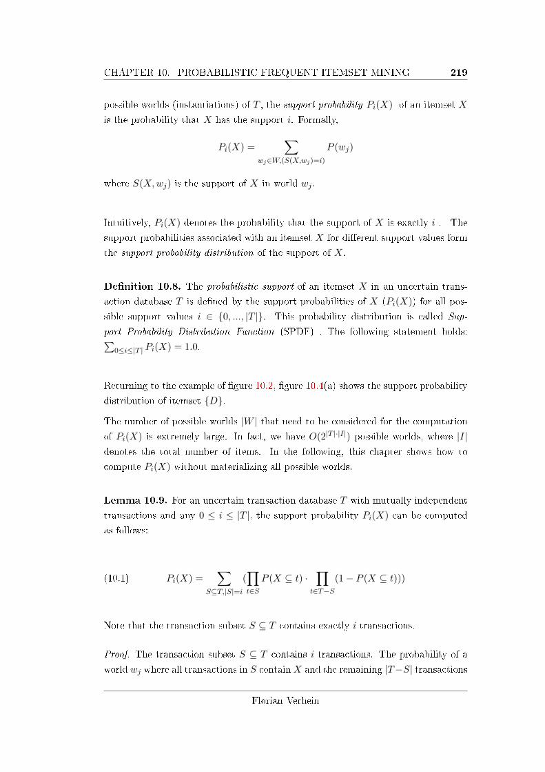
CHAPTER 10. PROBABILISTIC FREQUENT ITEMSET MINING 219
possible worlds (instantiations) of T , the support probability Pi(X) of an itemset X
is the probability that X has the support i. Formally,
Pi(X) =∑
wj∈W,(S(X,wj)=i)
P (wj)
where S(X,wj) is the support of X in world wj .
Intuitively, Pi(X) denotes the probability that the support of X is exactly i . The
support probabilities associated with an itemset X for di�erent support values form
the support probability distribution of the support of X.
De�nition 10.8. The probabilistic support of an itemset X in an uncertain trans-
action database T is de�ned by the support probabilities of X (Pi(X)) for all pos-
sible support values i ∈ {0, ..., |T |}. This probability distribution is called Sup-
port Probability Distribution Function (SPDF) . The following statement holds:∑0≤i≤|T | Pi(X) = 1.0.
Returning to the example of �gure 10.2, �gure 10.4(a) shows the support probability
distribution of itemset {D}.
The number of possible worlds |W | that need to be considered for the computation
of Pi(X) is extremely large. In fact, we have O(2|T |·|I|) possible worlds, where |I|denotes the total number of items. In the following, this chapter shows how to
compute Pi(X) without materializing all possible worlds.
Lemma 10.9. For an uncertain transaction database T with mutually independent
transactions and any 0 ≤ i ≤ |T |, the support probability Pi(X) can be computed
as follows:
(10.1) Pi(X) =∑
S⊆T,|S|=i
(∏t∈S
P (X ⊆ t) ·∏
t∈T−S(1− P (X ⊆ t)))
Note that the transaction subset S ⊆ T contains exactly i transactions.
Proof. The transaction subset S ⊆ T contains i transactions. The probability of a
world wj where all transactions in S containX and the remaining |T−S| transactions
Florian Verhein
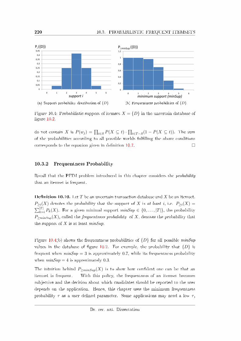
220 10.3. PROBABILISTIC FREQUENT ITEMSETS
0 35
0,4
0,45
Pi ({D})
0,2
0,25
0,3
0,35
0
0,05
0,1
0,15
support i
0
0 1 2 3 4 5 6
(a) Support probability distribution of {D}
P minSup ({D})
1,2
0 6
0,8
1
0,2
0,4
0,6
minimum support (minSup)
0
0 1 2 3 4 5 6
(b) Frequentness probabilities of {D}
Figure 10.4: Probabilistic support of itemset X = {D} in the uncertain database of�gure 10.2.
do not contain X is P (wj) =∏t∈S P (X ⊆ t) ·
∏t∈T−S(1 − P (X ⊆ t)). The sum
of the probabilities according to all possible worlds ful�lling the above conditions
corresponds to the equation given in de�nition 10.7.
10.3.2 Frequentness Probability
Recall that the PFIM problem introduced in this chapter considers the probability
that an itemset is frequent.
De�nition 10.10. Let T be an uncertain transaction database and X be an itemset.
P≥i(X) denotes the probability that the support of X is at least i, i.e. P≥i(X) =∑|T |k=i Pk(X). For a given minimal support minSup ∈ {0, . . . , |T |}, the probability
P≥minSup(X), called the frequentness probability of X, denotes the probability that
the support of X is at least minSup.
Figure 10.4(b) shows the frequentness probabilities of {D} for all possible minSup
values in the database of �gure 10.2. For example, the probability that {D} is
frequent when minSup = 3 is approximately 0.7, while its frequentness probability
when minSup = 4 is approximately 0.3.
The intuition behind P≥minSup(X) is to show how con�dent one can be that an
itemset is frequent. With this policy, the frequentness of an itemset becomes
subjective and the decision about which candidates should be reported to the user
depends on the application. Hence, this chapter uses the minimum frequentness
probability τ as a user de�ned parameter. Some applications may need a low τ ,
Dr. rer. nat. Dissertation
CHAPTER 10. PROBABILISTIC FREQUENT ITEMSET MINING 221
while in other applications only highly con�dent results should be reported (high
τ).
In the possible worlds model, P≥i(X) =∑
wj∈W :(S(X,wj)≥i) P (wj). This can be
computed according to Equation 10.1 by
(10.2) P≥i(X) =∑
S⊆T,|S|≥i
(∏t∈S
P (X ⊆ t) ·∏
t∈T−S(1− P (X ⊆ t))).
Hence, the frequentness probability can be calculated by enumerating all possible
worlds satisfying the minSup condition through the direct application of Equation
10.2. This naive approach is very ine�cient however and can be sped up signi�cantly.
First, note that typically minSup << |T | and the number of worlds with support i
is at most
(|T |i
). Hence, enumeration of all worlds w in which the support of X is
greater than minSup is much more expensive than enumerating those where the sup-
port is less than minSup. Using the following easily veri�ed lemma, the frequentness
probability can be computed exponentially in minSup << |T |.
Lemma 10.11. P≥i(X) = 1−∑
S⊆T :|S|<i(∏t∈S P (X ⊆ t) ·
∏t∈T−S(1−P (X ⊆ t))).
Despite this improvement, the complexity of the above approach, called Basic in the
experiments, is still exponential with respect to the number of transactions. Section
10.4 describes this can be reduced to linear time.
10.4 E�cient Computation of Probabilistic Frequent Item-
sets
This section presents the dynamic programming approach, which avoids the enu-
meration of possible worlds in calculating the frequentness probability and the sup-
port distribution. It is based on the Poisson binomial recurrence. This section also
presents probabilistic �lter and pruning strategies which further improve the run
time.
10.4.1 E�cient Computation of Probabilistic Support
The key to calculating the frequentness probability e�ciently is to consider the prob-
lem in terms of sub-problems. First, appropriate de�nitions are required;
Florian Verhein
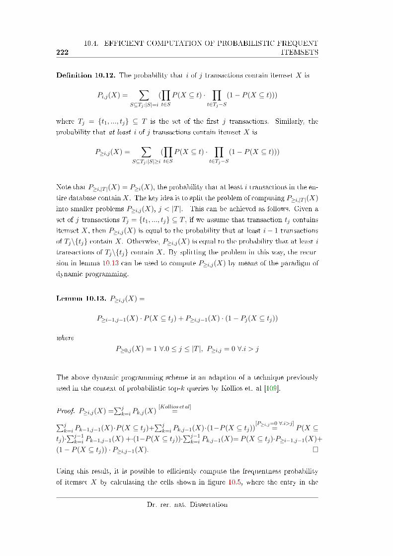
22210.4. EFFICIENT COMPUTATION OF PROBABILISTIC FREQUENT
ITEMSETS
De�nition 10.12. The probability that i of j transactions contain itemset X is
Pi,j(X) =∑
S⊆Tj :|S|=i
(∏t∈S
P (X ⊆ t) ·∏
t∈Tj−S(1− P (X ⊆ t)))
where Tj = {t1, ..., tj} ⊆ T is the set of the �rst j transactions. Similarly, the
probability that at least i of j transactions contain itemset X is
P≥i,j(X) =∑
S⊆Tj :|S|≥i
(∏t∈S
P (X ⊆ t) ·∏
t∈Tj−S(1− P (X ⊆ t)))
Note that P≥i,|T |(X) = P≥i(X), the probability that at least i transactions in the en-
tire database containX. The key idea is to split the problem of computing P≥i,|T |(X)
into smaller problems P≥i,j(X), j < |T |. This can be achieved as follows. Given a
set of j transactions Tj = {t1, ..., tj} ⊆ T , if we assume that transaction tj contains
itemset X, then P≥i,j(X) is equal to the probability that at least i− 1 transactions
of Tj\{tj} contain X. Otherwise, P≥i,j(X) is equal to the probability that at least i
transactions of Tj\{tj} contain X. By splitting the problem in this way, the recur-
sion in lemma 10.13 can be used to compute P≥i,j(X) by means of the paradigm of
dynamic programming.
Lemma 10.13. P≥i,j(X) =
P≥i−1,j−1(X) · P (X ⊆ tj) + P≥i,j−1(X) · (1− Pj(X ⊆ tj))
where
P≥0,j(X) = 1 ∀.0 ≤ j ≤ |T |, P≥i,j = 0 ∀.i > j
The above dynamic programming scheme is an adaption of a technique previously
used in the context of probabilistic top-k queries by Kollios et. al [109].
Proof. P≥i,j(X) =∑j
k=i Pk,j(X)[Kollios et al]
=∑jk=i Pk−1,j−1(X)·P (X ⊆ tj)+
∑jk=i Pk,j−1(X)·(1−P (X ⊆ tj))
[P≥i,j=0 ∀.i>j]= P (X ⊆
tj)·∑j−1
k=i Pk−1,j−1(X) +·(1−P (X ⊆ tj))·∑j−1
k=i Pk,j−1(X)= P (X ⊆ tj)·P≥i−1,j−1(X)+
(1− P (X ⊆ tj)) · P≥i,j−1(X).
Using this result, it is possible to e�ciently compute the frequentness probability
of itemset X by calculating the cells shown in �gure 10.5, where the entry in the
Dr. rer. nat. Dissertation
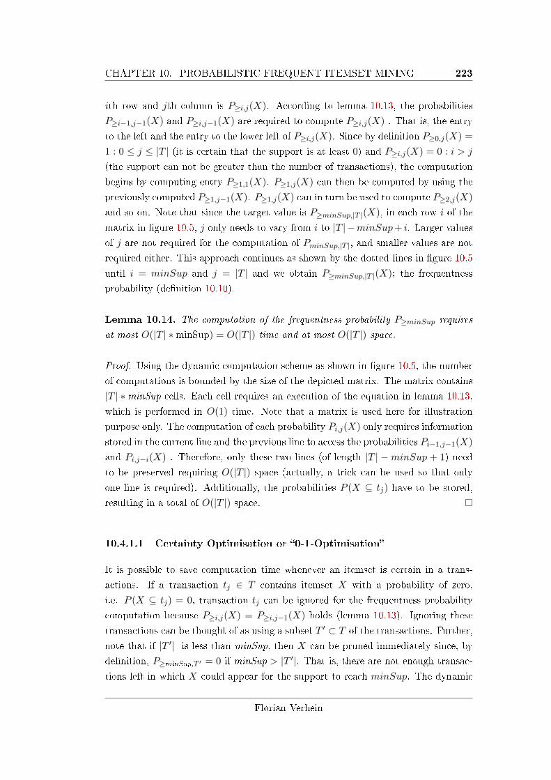
CHAPTER 10. PROBABILISTIC FREQUENT ITEMSET MINING 223
ith row and jth column is P≥i,j(X). According to lemma 10.13, the probabilities
P≥i−1,j−1(X) and P≥i,j−1(X) are required to compute P≥i,j(X) . That is, the entry
to the left and the entry to the lower left of P≥i,j(X). Since by de�nition P≥0,j(X) =
1 : 0 ≤ j ≤ |T | (it is certain that the support is at least 0) and P≥i,j(X) = 0 : i > j
(the support can not be greater than the number of transactions), the computation
begins by computing entry P≥1,1(X). P≥1,j(X) can then be computed by using the
previously computed P≥1,j−1(X). P≥1,j(X) can in turn be used to compute P≥2,j(X)
and so on. Note that since the target value is P≥minSup,|T |(X), in each row i of the
matrix in �gure 10.5, j only needs to vary from i to |T | −minSup+ i. Larger values
of j are not required for the computation of PminSup,|T |, and smaller values are not
required either. This approach continues as shown by the dotted lines in �gure 10.5
until i = minSup and j = |T | and we obtain P≥minSup,|T |(X); the frequentness
probability (de�nition 10.10).
Lemma 10.14. The computation of the frequentness probability P≥minSup requires
at most O(|T | ∗minSup) = O(|T |) time and at most O(|T |) space.
Proof. Using the dynamic computation scheme as shown in �gure 10.5, the number
of computations is bounded by the size of the depicted matrix. The matrix contains
|T | ∗minSup cells. Each cell requires an execution of the equation in lemma 10.13,
which is performed in O(1) time. Note that a matrix is used here for illustration
purpose only. The computation of each probability Pi,j(X) only requires information
stored in the current line and the previous line to access the probabilities Pi−1,j−1(X)
and Pi,j−i(X) . Therefore, only these two lines (of length |T | −minSup + 1) need
to be preserved requiring O(|T |) space (actually, a trick can be used so that only
one line is required). Additionally, the probabilities P (X ⊆ tj) have to be stored,
resulting in a total of O(|T |) space.
10.4.1.1 Certainty Optimisation or �0-1-Optimisation�
It is possible to save computation time whenever an itemset is certain in a trans-
actions. If a transaction tj ∈ T contains itemset X with a probability of zero,
i.e. P (X ⊆ tj) = 0, transaction tj can be ignored for the frequentness probability
computation because P≥i,j(X) = P≥i,j−1(X) holds (lemma 10.13). Ignoring these
transactions can be thought of as using a subset T ′ ⊂ T of the transactions. Further,
note that if |T ′| is less than minSup, then X can be pruned immediately since, by
de�nition, P≥minSup,T ′ = 0 if minSup > |T ′|. That is, there are not enough transac-
tions left in which X could appear for the support to reach minSup. The dynamic
Florian Verhein
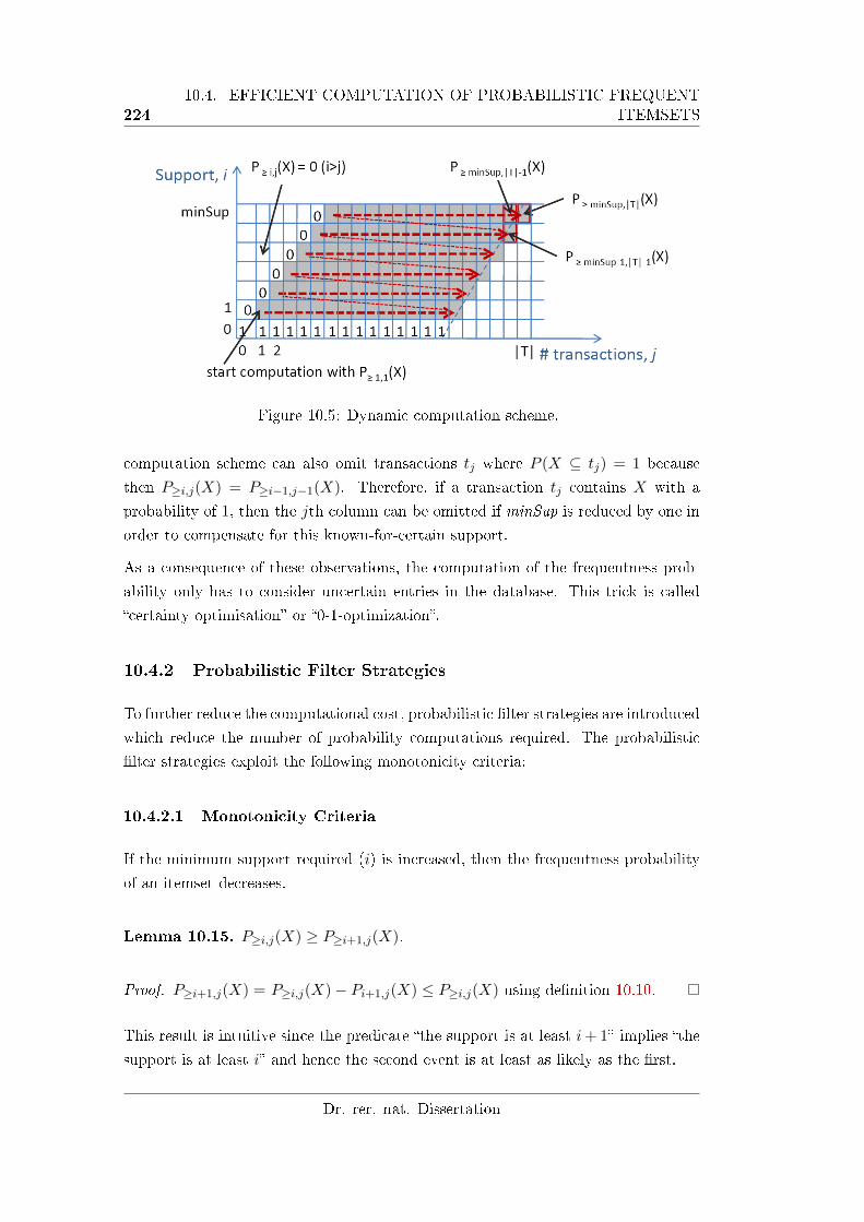
22410.4. EFFICIENT COMPUTATION OF PROBABILISTIC FREQUENT
ITEMSETS
Figure 10.5: Dynamic computation scheme.
computation scheme can also omit transactions tj where P (X ⊆ tj) = 1 because
then P≥i,j(X) = P≥i−1,j−1(X). Therefore, if a transaction tj contains X with a
probability of 1, then the jth column can be omitted if minSup is reduced by one in
order to compensate for this known-for-certain support.
As a consequence of these observations, the computation of the frequentness prob-
ability only has to consider uncertain entries in the database. This trick is called
�certainty optimisation� or �0-1-optimization�.
10.4.2 Probabilistic Filter Strategies
To further reduce the computational cost, probabilistic �lter strategies are introduced
which reduce the number of probability computations required. The probabilistic
�lter strategies exploit the following monotonicity criteria:
10.4.2.1 Monotonicity Criteria
If the minimum support required (i) is increased, then the frequentness probability
of an itemset decreases.
Lemma 10.15. P≥i,j(X) ≥ P≥i+1,j(X).
Proof. P≥i+1,j(X) = P≥i,j(X)− Pi+1,j(X) ≤ P≥i,j(X) using de�nition 10.10.
This result is intuitive since the predicate �the support is at least i+ 1� implies �the
support is at least i� and hence the second event is at least as likely as the �rst.
Dr. rer. nat. Dissertation
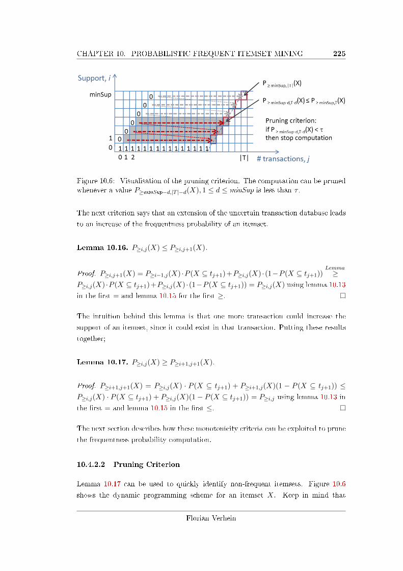
CHAPTER 10. PROBABILISTIC FREQUENT ITEMSET MINING 225
Figure 10.6: Visualisation of the pruning criterion. The computation can be prunedwhenever a value P≥minSup−d,|T |−d(X), 1 ≤ d ≤ minSup is less than τ .
The next criterion says that an extension of the uncertain transaction database leads
to an increase of the frequentness probability of an itemset.
Lemma 10.16. P≥i,j(X) ≤ P≥i,j+1(X).
Proof. P≥i,j+1(X) = P≥i−1,j(X) ·P (X ⊆ tj+1)+P≥i,j(X) ·(1−P (X ⊆ tj+1))Lemma≥
P≥i,j(X) ·P (X ⊆ tj+1)+P≥i,j(X) ·(1−P (X ⊆ tj+1)) = P≥i,j(X) using lemma 10.13
in the �rst = and lemma 10.15 for the �rst ≥.
The intuition behind this lemma is that one more transaction could increase the
support of an itemset, since it could exist in that transaction. Putting these results
together;
Lemma 10.17. P≥i,j(X) ≥ P≥i+1,j+1(X).
Proof. P≥i+1,j+1(X) = P≥i,j(X) · P (X ⊆ tj+1) + P≥i+1,j(X)(1 − P (X ⊆ tj+1)) ≤P≥i,j(X) · P (X ⊆ tj+1) + P≥i,j(X)(1− P (X ⊆ tj+1)) = P≥i,j using lemma 10.13 in
the �rst = and lemma 10.15 in the �rst ≤.
The next section describes how these monotonicity criteria can be exploited to prune
the frequentness probability computation.
10.4.2.2 Pruning Criterion
Lemma 10.17 can be used to quickly identify non-frequent itemsets. Figure 10.6
shows the dynamic programming scheme for an itemset X. Keep in mind that
Florian Verhein
226 10.5. PROBABILISTIC FREQUENT ITEMSET MINING (PFIM)
the goal is to compute P≥minSup,|T |(X). Lemma 10.17 states that the probabilities
P≥minSup−d,|T |−d(X), 1 ≤ d ≤ minSup (highlighted in �gure 10.6), are conservative
bounds of P≥minSup,|T |(X). Thus, if any of the probabilities P≥minSup−d,|T |−d(X), 1 ≤d ≤ minSup is lower than the user speci�ed parameter τ , then the computation can
be immediately pruned since it is already clear that X cannot be a PFI.
10.5 Probabilistic Frequent Itemset Mining (PFIM)
The previous section section showed how to e�ciently identify whether a given item-
set X is a probabilistic frequent itemset (PFI). This section shows how to �nd all
probabilistic frequent itemsets in an uncertain transaction database. Traditional fre-
quent itemset mining is based on support pruning by exploiting the anti-monotonic
property of support: S(X) ≤ S(Y ) where S(X) is the support of X and Y ⊆ X. In
uncertain transaction databases however, support is de�ned by a probability distri-
bution and itemsets are mined according to their frequentness probability. It turns
out that the frequentness probability is anti-monotonic:
Lemma 10.18. ∀Y ⊆ X : P≥minSup(X) ≤ P≥minSup(Y ). In other words, all subsets
of a probabilistic frequent itemset are also probabilistic frequent itemsets.
Proof. P≥i(X) = 1|W |∑|W |
i=1 P (wi) · IS(X,wi)≥minSup, since the probability is de�ned
over all possible worlds. Here, IZ is an indicator variable that is 1 when z = true
and 0 otherwise. In other words, P≥i(X) is the relative number of worlds in which
S(X) ≥ minSup holds, where each occurrence is weighted by the probability of
the world occurring. Since world wi corresponds to a normal transaction database
with no uncertainty, S(X,wi) ≤ S(Y,wi)∀Y ⊆ X due to the anti-monotonicity of
support. Therefore, IS(X,wi)≥minSup ≤ IS(Y,Wi)≥minSup∀i ∈ |W |, ∀Y ⊆ X and, thus,
P≥i(X) ≤ P≥i(Y ), ∀Y ⊆ X.
The contra-positive of lemma 10.18 can be used to prune the search space for PFIs.
That is, if an itemset Y is not a PFI (P≥minSup(Y ) < τ), then all itemsets X ⊇ Y
cannot be probabilistic frequent itemsets either.
The �rst algorithm presented in this chapter is based on the combination of tradi-
tional frequent itemset mining methods and the PFI identi�cation method described
earlier. In particular, a probabilistic frequent itemset mining (PFIM) approach is
proposed based on the Apriori algorithm ([11]). Like Apriori, the method iteratively
generates the PFIs using a bottom-up strategy. Each iteration is performed in two
Dr. rer. nat. Dissertation
CHAPTER 10. PROBABILISTIC FREQUENT ITEMSET MINING 227
steps, a join step for generating new candidate PFIs and a pruning step for calculat-
ing the frequentness probabilities and identifying the PFIs from the set of candidates.
In turn, these are used to generate candidates in the next iteration. Lemma 10.18 is
exploited to prune the search space. The data set is stored in memory in a way that
allows fast access to the P (xi ∈ tj); in particular the vertical database layout [88] canbe exploited e�ectively. This avoids the subset checking problem in the traditional
Apriori algorithm. The algorithm is called ProApriori in this thesis.
10.6 Incremental Probabilistic Frequent Itemset Mining
(I-PFIM)
Probabilistic frequent itemset mining (PFIM) allows the user to control the con�-
dence of the results using τ . However, since the number of results also depends on τ ,
it may prove di�cult for a user to correctly specify this parameter without additional
domain knowledge. Furthermore, it can be expected that the user is interested in
receiving the best results �rst. Therefore, this section shows how to e�ciently solve
the following problems, which do not require the speci�cation of τ ;
• Top-k probabilistic frequent itemsets query: return the k itemsets that have the
highest frequentness probability, where k is speci�ed by the user.
• Incremental ranking queries: successively return the itemsets with the highest
frequentness probability, one at a time.
The problems are collectively called incremental PFIM (I-PFIM).
10.6.1 Incremental Probabilistic Frequent Itemset Mining Algo-
rithm
The I-PFIM method computes the next most probable frequent itemset in each
step, as shown in algorithm 10.1. The algorithm keeps an Active Itemsets Queue
(AIQ) that is initialized with all one-item sets. The AIQ is sorted by frequentness
probability in descending order. Without loss of generality, itemsets are represented
in lexicographical order to avoid generating them more than once. In each iteration
of the algorithm, i.e. each call of the getNext()-function, the �rst itemset X in the
queue is removed. X is the next most probable frequent itemset because all other
itemsets in the AIQ have a lower frequentness probability due to the order on the
AIQ, and all of X's super-sets (which have not yet been generated) cannot have a
Florian Verhein
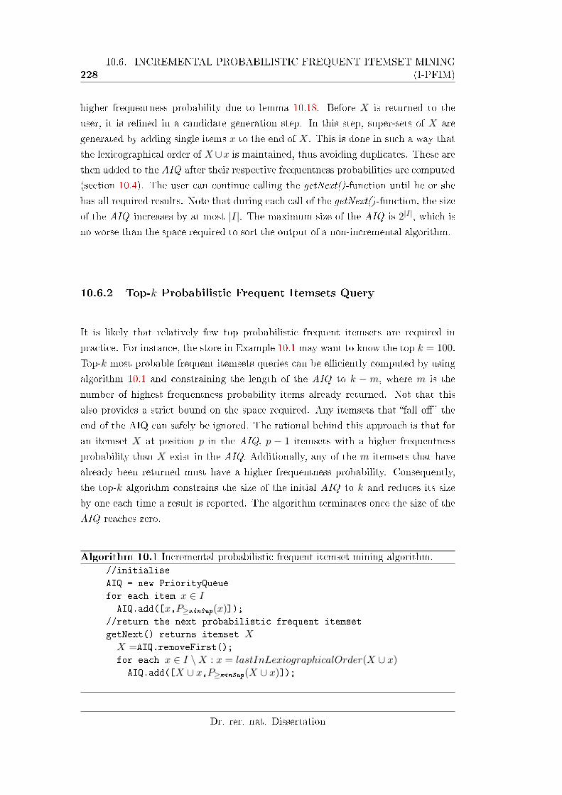
22810.6. INCREMENTAL PROBABILISTIC FREQUENT ITEMSET MINING
(I-PFIM)
higher frequentness probability due to lemma 10.18. Before X is returned to the
user, it is re�ned in a candidate generation step. In this step, super-sets of X are
generated by adding single items x to the end of X. This is done in such a way that
the lexicographical order of X ∪x is maintained, thus avoiding duplicates. These are
then added to the AIQ after their respective frequentness probabilities are computed
(section 10.4). The user can continue calling the getNext()-function until he or she
has all required results. Note that during each call of the getNext()-function, the size
of the AIQ increases by at most |I|. The maximum size of the AIQ is 2|I|, which is
no worse than the space required to sort the output of a non-incremental algorithm.
10.6.2 Top-k Probabilistic Frequent Itemsets Query
It is likely that relatively few top probabilistic frequent itemsets are required in
practice. For instance, the store in Example 10.1 may want to know the top k = 100.
Top-k most probable frequent itemsets queries can be e�ciently computed by using
algorithm 10.1 and constraining the length of the AIQ to k − m, where m is the
number of highest frequentness probability items already returned. Not that this
also provides a strict bound on the space required. Any itemsets that �fall o�� the
end of the AIQ can safely be ignored. The rational behind this approach is that for
an itemset X at position p in the AIQ, p − 1 itemsets with a higher frequentness
probability than X exist in the AIQ. Additionally, any of the m itemsets that have
already been returned must have a higher frequentness probability. Consequently,
the top-k algorithm constrains the size of the initial AIQ to k and reduces its size
by one each time a result is reported. The algorithm terminates once the size of the
AIQ reaches zero.
Algorithm 10.1 Incremental probabilistic frequent itemset mining algorithm.
//initialise
AIQ = new PriorityQueue
for each item x ∈ IAIQ.add([x,P≥minSup(x)]);
//return the next probabilistic frequent itemset
getNext() returns itemset XX =AIQ.removeFirst();
for each x ∈ I \X : x = lastInLexiographicalOrder(X ∪ x)AIQ.add([X ∪ x,P≥minSup(X ∪ x)]);
Dr. rer. nat. Dissertation
CHAPTER 10. PROBABILISTIC FREQUENT ITEMSET MINING 229
10.7 Experimental Evaluation
This section present e�ciency and e�cacy experiments. First, the algorithm and
all optimisations and variations for computing the frequentness probability (sections
10.3 and 10.4) are evaluated and compared. Then, the performance and utility of
the PFIM algorithm (ProApriori) and the incremental PFIM algorithm (sections
10.5 and 10.6) are evaluated.
Additional experiments can be found in chapter 13, where ProApriori is compared
to algorithms developed in subsequent chapters on large, well known arti�cial and
real databases.
10.7.1 Evaluation of the Frequentness Probability Calculations
The frequentness probability calculation methods were evaluated on several arti�cial
data sets with varying database sizes |T | (up to 10, 000, 000) and densities. The
density of an item denotes the expected number of transactions in which an item
may be present (i.e. where its existence probability is in (0, 1]). The probabilities
themselves were drawn from a uniform distribution. Note that the density is directly
related to the degree of uncertainty. If not stated otherwise, a database consisting of
10, 000 uncertain transactions, 20 items, a density of 0.5 and frequentness probability
threshold τ = 0.9 were used.
The following notations are used for the frequentness probability calculation algo-
rithms:
Basic: basic probability computation (section 10.3.2)
Dynamic: dynamic probability computation (section 10.4.1)
Dynamic+P: dynamic probability computation with pruning (section 10.4.2)
DynamicOpt: dynamic probability computation utilizing certainty optimisation;
�0-1-optimization� (section 10.4.1) and
DynamicOpt+P: 0-1-optimized dynamic probability computation method with
pruning.
10.7.1.1 Scalability
Figure 10.7 shows the scalability of the frequentness probability calculation ap-
proaches when the number of transactions, |T |, are varied. The run time of the
Florian Verhein
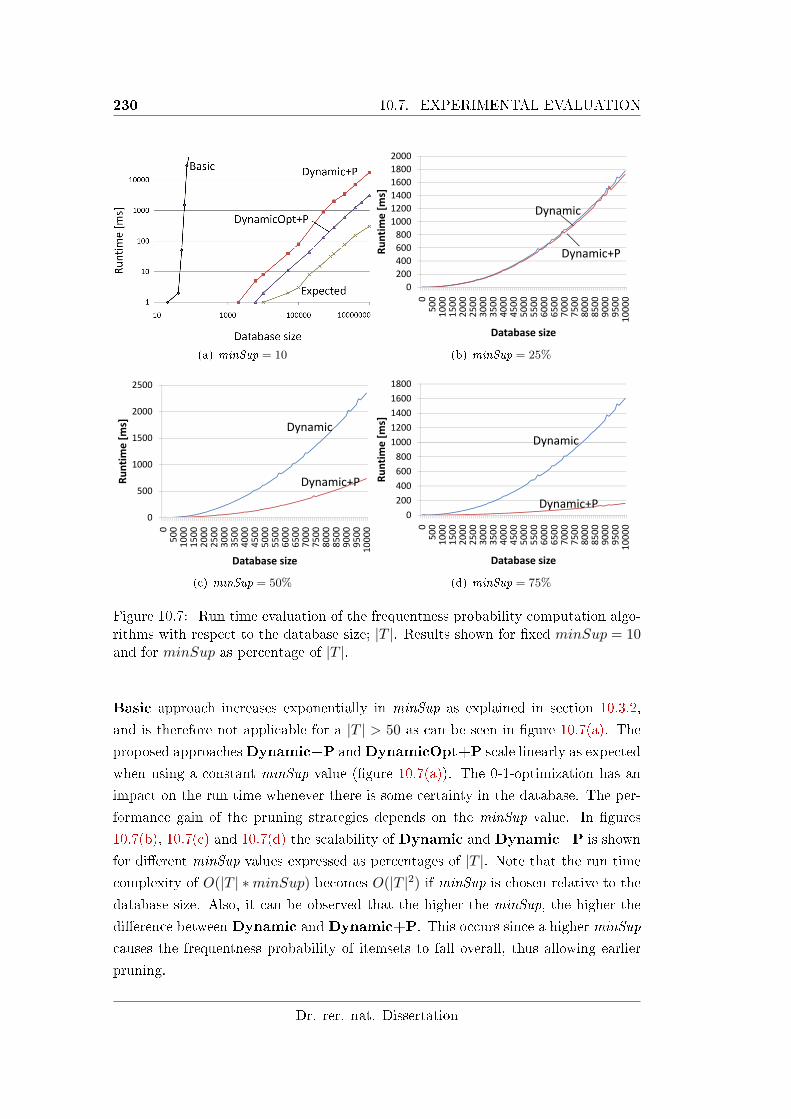
230 10.7. EXPERIMENTAL EVALUATION
(a) minSup = 10
0
200
400
600
800
1000
1200
1400
1600
1800
2000
0500
1000
1500
2000
2500
3000
3500
4000
4500
5000
5500
6000
6500
7000
7500
8000
8500
9000
9500
10000
Runtime
[ms]
Database size
Dynamic
Dynamic+P
(b) minSup = 25%
0
500
1000
1500
2000
2500
0500
1000
1500
2000
2500
3000
3500
4000
4500
5000
5500
6000
6500
7000
7500
8000
8500
9000
9500
10000
Runtime
[ms]
Database size
Dynamic
Dynamic+P
(c) minSup = 50%
0
200
400
600
800
1000
1200
1400
1600
1800
0500
1000
1500
2000
2500
3000
3500
4000
4500
5000
5500
6000
6500
7000
7500
8000
8500
9000
9500
10000
Runtime
[ms]
Database size
Dynamic
Dynamic+P
(d) minSup = 75%
Figure 10.7: Run time evaluation of the frequentness probability computation algo-rithms with respect to the database size; |T |. Results shown for �xed minSup = 10and for minSup as percentage of |T |.
Basic approach increases exponentially in minSup as explained in section 10.3.2,
and is therefore not applicable for a |T | > 50 as can be seen in �gure 10.7(a). The
proposed approachesDynamic+P andDynamicOpt+P scale linearly as expected
when using a constant minSup value (�gure 10.7(a)). The 0-1-optimization has an
impact on the run time whenever there is some certainty in the database. The per-
formance gain of the pruning strategies depends on the minSup value. In �gures
10.7(b), 10.7(c) and 10.7(d) the scalability of Dynamic and Dynamic+P is shown
for di�erent minSup values expressed as percentages of |T |. Note that the run time
complexity of O(|T | ∗minSup) becomes O(|T |2) if minSup is chosen relative to the
database size. Also, it can be observed that the higher the minSup, the higher the
di�erence between Dynamic and Dynamic+P. This occurs since a higher minSup
causes the frequentness probability of itemsets to fall overall, thus allowing earlier
pruning.
Dr. rer. nat. Dissertation
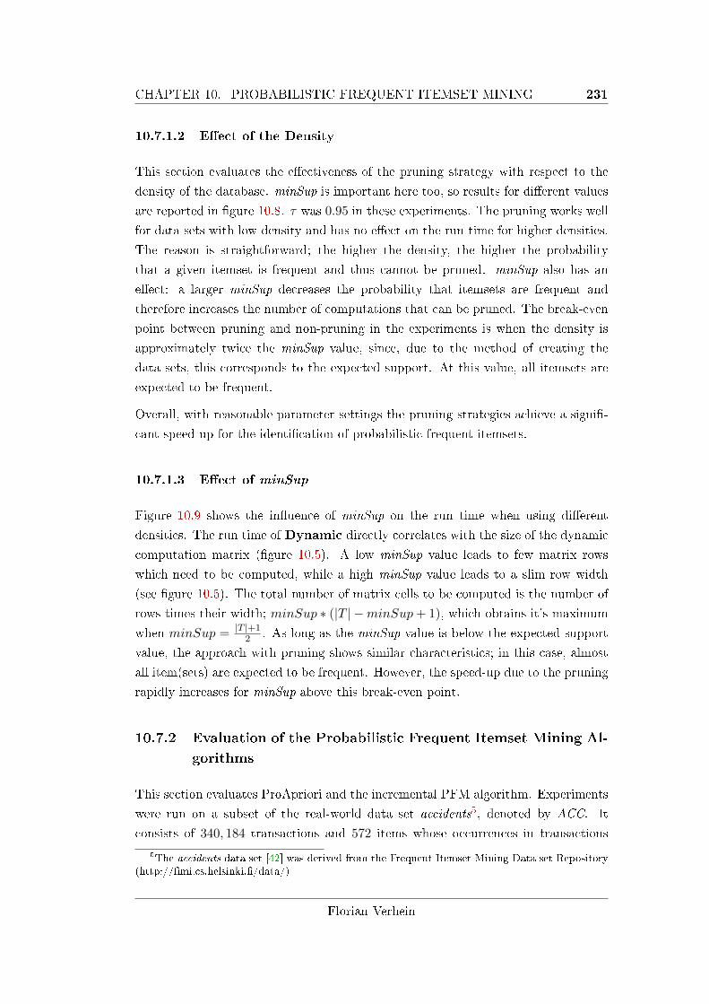
CHAPTER 10. PROBABILISTIC FREQUENT ITEMSET MINING 231
10.7.1.2 E�ect of the Density
This section evaluates the e�ectiveness of the pruning strategy with respect to the
density of the database. minSup is important here too, so results for di�erent values
are reported in �gure 10.8. τ was 0.95 in these experiments. The pruning works well
for data sets with low density and has no e�ect on the run time for higher densities.
The reason is straightforward; the higher the density, the higher the probability
that a given itemset is frequent and thus cannot be pruned. minSup also has an
e�ect: a larger minSup decreases the probability that itemsets are frequent and
therefore increases the number of computations that can be pruned. The break-even
point between pruning and non-pruning in the experiments is when the density is
approximately twice the minSup value, since, due to the method of creating the
data sets, this corresponds to the expected support. At this value, all itemsets are
expected to be frequent.
Overall, with reasonable parameter settings the pruning strategies achieve a signi�-
cant speed-up for the identi�cation of probabilistic frequent itemsets.
10.7.1.3 E�ect of minSup
Figure 10.9 shows the in�uence of minSup on the run time when using di�erent
densities. The run time of Dynamic directly correlates with the size of the dynamic
computation matrix (�gure 10.5). A low minSup value leads to few matrix rows
which need to be computed, while a high minSup value leads to a slim row width
(see �gure 10.5). The total number of matrix cells to be computed is the number of
rows times their width; minSup ∗ (|T | −minSup+ 1), which obtains it's maximum
when minSup = |T |+12 . As long as the minSup value is below the expected support
value, the approach with pruning shows similar characteristics; in this case, almost
all item(sets) are expected to be frequent. However, the speed-up due to the pruning
rapidly increases for minSup above this break-even point.
10.7.2 Evaluation of the Probabilistic Frequent Itemset Mining Al-
gorithms
This section evaluates ProApriori and the incremental PFM algorithm. Experiments
were run on a subset of the real-world data set accidents5, denoted by ACC. It
consists of 340, 184 transactions and 572 items whose occurrences in transactions
5The accidents data set [42] was derived from the Frequent Itemset Mining Data set Repository(http://�mi.cs.helsinki.�/data/)
Florian Verhein
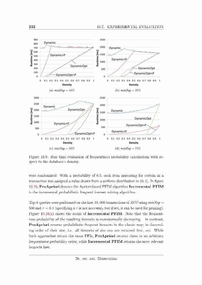
232 10.7. EXPERIMENTAL EVALUATION
0
100
200
300
400
500
600
700
800
900
0 0.1 0.2 0.3 0.4 0.5 0.6 0.7 0.8 0.9 1
Runtime
[ms]
Density
Dynamic
Dynamic+P
DynamicOpt+P
DynamicOpt
(a) minSup = 10%
0
500
1000
1500
2000
2500
0 0.1 0.2 0.3 0.4 0.5 0.6 0.7 0.8 0.9 1
Runtime
[ms]
Density
Dynamic
Dynamic+P
DynamicOpt+P
DynamicOpt
(b) minSup = 25%
Dynamic
Dynamic+P
DynamicOpt+P
DynamicOpt
0
500
1000
1500
2000
2500
3000
0 0.1 0.2 0.3 0.4 0.5 0.6 0.7 0.8 0.9 1
Runtime
[ms]
Density
(c) minSup = 50%
0
500
1000
1500
2000
2500
0 0.1 0.2 0.3 0.4 0.5 0.6 0.7 0.8 0.9 1
Runtime
[ms]
Density
Dynamic
Dynamic+P
DynamicOpt+P
DynamicOpt
(d) minSup = 75%
Figure 10.8: Run time evaluation of frequentness probability calculations with re-spect to the database's density.
were randomized: With a probability of 0.5, each item appearing for certain in a
transaction was assigned a value drawn from a uniform distribution in (0, 1]. In �gure
10.10, ProApriori denotes the Apriori-based PFIM algorithm Incremental PFIM
is the incremental probabilistic frequent itemset mining algorithm.
Top-k queries were performed on the �rst 10, 000 transactions of ACC usingminSup =
500 and τ = 0.1 (specifying a τ is not necessary but if set, it can be used for pruning).
Figure 10.10(a) shows the result of Incremental PFIM. Note that the frequent-
ness probability of the resulting itemsets is monotonically decreasing. In contrast,
ProApriori returns probabilistic frequent itemsets in the classic way; in descend-
ing order of their size, i.e. all itemsets of size one are returned �rst, etc. While
both approaches return the same PFIs, ProApriori returns them in an arbitrary
frequentness probability order, while Incremental PFIM returns the most relevant
itemsets �rst.
Dr. rer. nat. Dissertation
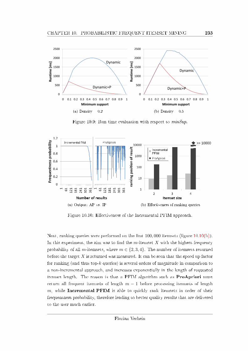
CHAPTER 10. PROBABILISTIC FREQUENT ITEMSET MINING 233
0
500
1000
1500
2000
2500
0 0.1 0.2 0.3 0.4 0.5 0.6 0.7 0.8 0.9 1
Runtime
[ms]
Minimum support
Dynamic
Dynamic+P
(a) Density = 0.2
0
500
1000
1500
2000
2500
0 0.1 0.2 0.3 0.4 0.5 0.6 0.7 0.8 0.9 1
Runtime
[ms]
Minimum support
Dynamic
Dynamic+P
(b) Density = 0.5
Figure 10.9: Run time evaluation with respect to minSup.
(a) Output: AP vs. IP (b) E�ectiveness of ranking queries
Figure 10.10: E�ectiveness of the Incremental PFIM approach.
Next, ranking queries were performed on the �rst 100, 000 itemsets (�gure 10.10(b)).
In this experiment, the aim was to �nd the m-itemset X with the highest frequency
probability of all m-itemsets, where m ∈ {2, 3, 4}. The number of itemsets returned
before the target X is returned was measured. It can be seen that the speed up factor
for ranking (and thus top-k queries) is several orders of magnitude in comparison to
a non-incremental approach, and increases exponentially in the length of requested
itemset length. The reason is that a PFIM algorithm such as ProApriori must
return all frequent itemsets of length m − 1 before processing itemsets of length
m, while Incremental PFIM is able to quickly rank itemsets in order of their
frequentness probability, therefore leading to better quality results that are delivered
to the user much earlier.
Florian Verhein
234 10.8. CONCLUSION
10.8 Conclusion
The Probabilistic Frequent Itemset Mining (PFIM) problem is to �nd itemsets in
an uncertain transaction database that are (highly) likely to be frequent. The work
in this chapter (and the paper it is based on, [18]) is the �rst to address this prob-
lem, and does so using a framework built on possible world semantics. This chapter
theoretically and experimentally showed that the proposed dynamic computation
technique is able to compute the exact support probability distribution and the fre-
quentness probability of an itemset in linear time in the number of transactions.
This is in comparison to the exponential run time of a non-dynamic approach. Fur-
thermore, it was demonstrated that various probabilistic pruning strategies further
improved the run time. In addition, a PFIM algorithm � ProApriori � was presented
to mine all probabilistic frequent itemsets (PFIs). Finally, the incremental PFIM
problem was introduced, where the most likely frequent itemsets are mined and re-
ported incrementally. This was used to solve problems such as querying the top-k
PFIs.
Dr. rer. nat. Dissertation
Chapter 11
Signi�cant Frequent Itemset
Mining
Frequent itemset mining in uncertain transaction databases (UTDBs) se-
mantically and computationally di�ers from traditional techniques applied
to standard �certain� databases since the support of an itemset is de�ned by
a probability distribution rather than a single scalar.
This chapter introduces and solves the Signi�cant Frequent Itemset Mining
(SiFIM) problem for UTDBs. An itemset X is signi�cantly frequent if,
given a desired level of signi�cance, we can reject the null hypothesis that
its support is below minSup. This chapter formulates both a parametric and
a non-parametric (exact) test to achieve this. The non-parametric approach
is an adaptation of the PFIM method in chapter 10.
An incremental signi�cant frequent itemset mining method is also proposed,
which may help reduce the e�ects of the multiple tests problem. An extensive
experimental analysis evaluates all methods. Furthermore, the independence
assumption used in PFIM and SiFIM is validated and a demonstration of the
the downsides of the Expected Frequent Itemset Mining (EFIM) method is
provided.
235
236 11.1. INTRODUCTION
11.1 Introduction
It is usually assumed that the items in a transaction are �certain�, that is; an item
is either present or absent. In practice this is not always the case � the presence of
an item may be uncertain. Recall from section 10.1 that such situations may occur
due to inherently noisy data, the addition of noise for privacy protection purposes
[107] or through aggregation of records in order to produce purchase probabilities.
Furthermore, data sets are generated from observations of a process and, even when
the results of those observations are known for certain, they implicitly contain noise
when the underlying process is noisy.
Dealing with uncertain databases is a di�cult but interesting problem. Prior to the
work in chapter 10 ([18]), existing approaches in the literature were based on the
expected support, �rst introduced in [26]. Recall that in this method, itemsets are
considered frequent if the expected support exceeds minSup [25, 26]. Also recall
that this approach e�ectively returns an estimate of whether an object is frequent or
not with no indication of how good this estimate is � in fact, an expected frequent
itemset can be infrequent with high probability.
This chapter builds on chapter 10 and introduces the concept of signi�cant frequent
itemsets. A signi�cant frequent itemset is an itemset where, given a desired level
of signi�cance, we can reject the null hypothesis that its support is below minSup.
This chapter develops the theory and method for both a parametric and a non-
parametric test for determining whether an arbitrary itemset is signi�cantly frequent.
By building on this, it introduces the �rst signi�cant frequent itemset mining (SiFIM)
method that can be used for uncertain, probabilistic or noisy data. The advantage
of this approach is that the user can be con�dent that the reported itemsets are
indeed frequent, thus greatly reducing the risk that frequent itemsets are reported in
error. This can be achieved without much computation overhead in comparison to
the expectation approach. The approach is also used to demonstrate the downsides
of the expected frequent itemset approach; in particular, most expected frequent
itemsets are insigni�cant and can occur by chance alone.
11.1.1 Problem De�nition
An itemset is a frequent itemset if it occurs in at least minSup transactions, where
minSup is a user speci�ed parameter. In uncertain or noisy transaction databases
however, an itemset's support is a probability distribution and in general, one cannot
be sure whether an itemset is frequent or whether it just appears to be frequent by
chance, due to the noise or uncertainty in the database.
Dr. rer. nat. Dissertation
CHAPTER 11. SIGNIFICANT FREQUENT ITEMSET MINING 237
De�nition 11.1. A Signi�cant Frequent Itemset (SFI) is an itemset where we can
reject, at a desired signi�cance level α, the null hypothesis that the support is less
than minSup.
The signi�cance level α is typically 0.05 or 0.01. Intuitively, a signi�cant frequent
itemset has a very high (statistically signi�cant) probability of being frequent (fre-
quentness probability). The problem de�nition is as follows:
De�nition 11.2. Given an uncertain transaction database T , a minimum support
scalar minSup and a signi�cance level α, the Signi�cant Frequent Itemset Mining
Problem (SiFIM) is to �nd all SFIs.
The development of signi�cance tests requires an appropriate probability model to
derive the required approximate and exact distributions. The possible worlds model
introduced in chapter 10 is used for this purpose. The reader may like to refer back
to section 10.1.1 for an explanation and the de�nitions applying to this model, and
�gure 10.3 for a summary of the notation.
11.1.2 Contributions
This chapter makes the following contributions:
• It formally introduces and e�ciently solves the Signi�cant Frequent Itemset
Mining (SiFIM) problem.
• A parametric signi�cance test for �nding signi�cant frequent itemsets is de-
veloped, and its advantages and limitations are investigated. As a side e�ect,
this approach can be adapted to approximately solve the probabilistic frequent
itemset mining problem of chapter 10 in O(|T |) time.
• An e�cient non-parametric signi�cance test is developed. No assumptions
about the distribution of item and itemsets are made, leading to exact p-values.
Exact tests are usually much slower than their parametric counterparts. In-
deed, a straightforward implementation would run in exponential time in the
number of transactions |T |. However, based on the work in chapter 10, a
method is developed that runs in O(|T | ·minSup) time.
• All methods are evaluated experimentally. Furthermore, it is shown that de-
spite the independence assumption made in this and previous work, dependent
Florian Verhein
238 11.2. RELATED WORK
itemsets can still be mined. The shortcomings of the expected support method
is also demonstrated experimentally.
11.1.3 Organisation
The remainder of this chapter is organised as follows: Section 11.2 brie�y surveys
related work and puts the contributions in context. Section 11.3 introduces the model
and signi�cance tests. Section 11.3.1 discusses the independence assumption. Section
11.3.2 presents the parametric signi�cance test, while section 11.3.3 presents the non
parametric (exact) test. An incremental mining method, useful in overcoming the
multiple tests problem, is discussed in section 11.4. Experiments are presented in
section 11.5 and this chapter concludes in section 11.6.
11.2 Related Work
Recall that section 10.2 provided a discussion of work related to frequent itemset
mining in uncertain and probabilistic databases. This section brie�y covers work
speci�c to signi�cant itemset mining, of which there seems to be little.
[114] proposes exact and sampling-based algorithms to �nd likely frequent items in
streaming probabilistic data. In [114], an e�cient approach is presented to �nd
signi�cant frequent items (that is, itemsets of size one) in uncertain databases and
is based on the possible worlds semantics and the X-Relation model. [114] also
proposes sampling-based algorithms to �nd signi�cantly frequent items in streaming
data. The main restriction of [114] is that it is only applicable for itemsets of size
one.
While it is a separate research problem and does not consider uncertain or proba-
bilistic databases, several approaches have been proposed to de�ne and measure the
signi�cance of association rules. For example, [98, 103] �nd signi�cant association
and classi�cation rules based on Fisher's exact test. The approach proposed in [82]
measures the signi�cance of association rules via the chi-squared test of independence
to evaluate correlations among items. Itemsets can be called signi�cant if both the
minimum support and minimum correlation criteria are met. Testing for signi�cant
correlations is a well-known statistical problem, and the reader is referred to to [55]
which gives a closer insight into the theory. In [61] the chi-squared tests are used
for pruning and summarizing association rules. In order to e�ectively prune and
extract meaningful association rules, [87] presents three adaptive Apriori association
rule mining methods. These methods are able to discover itemsets with low and
Dr. rer. nat. Dissertation
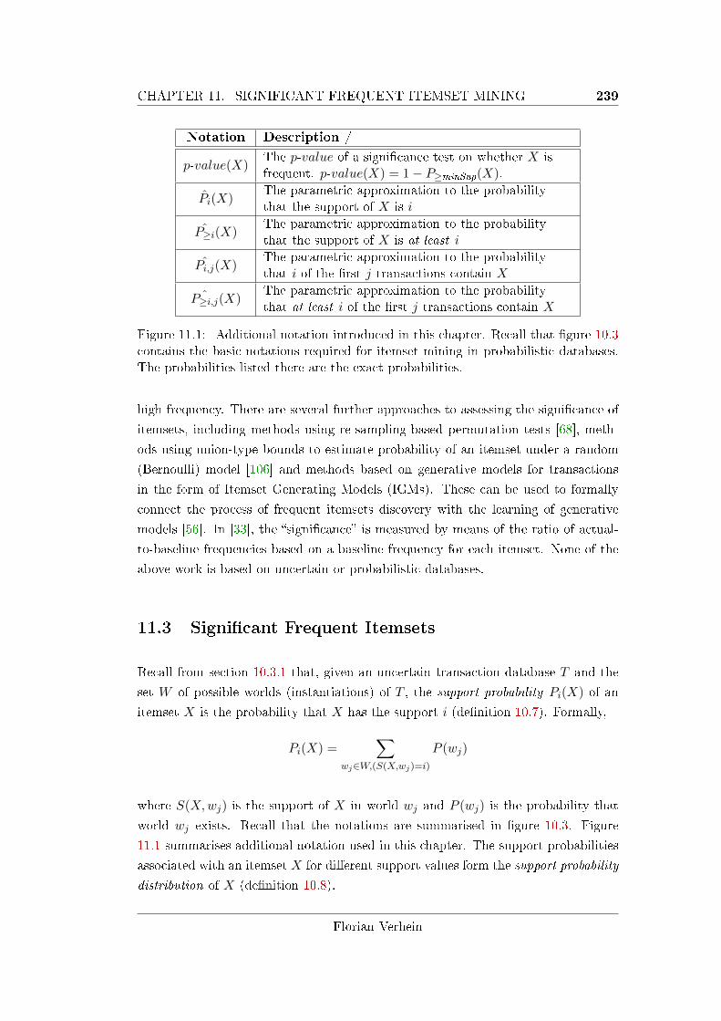
CHAPTER 11. SIGNIFICANT FREQUENT ITEMSET MINING 239
Notation Description /
p-value(X)The p-value of a signi�cance test on whether X isfrequent. p-value(X) = 1− P≥minSup(X).
Pi(X)The parametric approximation to the probabilitythat the support of X is i
P≥i(X)The parametric approximation to the probabilitythat the support of X is at least i
Pi,j(X)The parametric approximation to the probabilitythat i of the �rst j transactions contain X
ˆP≥i,j(X)The parametric approximation to the probabilitythat at least i of the �rst j transactions contain X
Figure 11.1: Additional notation introduced in this chapter. Recall that �gure 10.3contains the basic notations required for itemset mining in probabilistic databases.The probabilities listed there are the exact probabilities.
high frequency. There are several further approaches to assessing the signi�cance of
itemsets, including methods using re-sampling-based permutation tests [68], meth-
ods using union-type bounds to estimate probability of an itemset under a random
(Bernoulli) model [106] and methods based on generative models for transactions
in the form of Itemset Generating Models (IGMs). These can be used to formally
connect the process of frequent itemsets discovery with the learning of generative
models [56]. In [33], the �signi�cance� is measured by means of the ratio of actual-
to-baseline frequencies based on a baseline frequency for each itemset. None of the
above work is based on uncertain or probabilistic databases.
11.3 Signi�cant Frequent Itemsets
Recall from section 10.3.1 that, given an uncertain transaction database T and the
set W of possible worlds (instantiations) of T , the support probability Pi(X) of an
itemset X is the probability that X has the support i (de�nition 10.7). Formally,
Pi(X) =∑
wj∈W,(S(X,wj)=i)
P (wj)
where S(X,wj) is the support of X in world wj and P (wj) is the probability that
world wj exists. Recall that the notations are summarised in �gure 10.3. Figure
11.1 summarises additional notation used in this chapter. The support probabilities
associated with an itemset X for di�erent support values form the support probability
distribution of X (de�nition 10.8).
Florian Verhein

240 11.3. SIGNIFICANT FREQUENT ITEMSETS
In order to test whether an itemset is signi�cantly frequent, the following method-
ology is used. The Null Hypothesis states that an itemset X is not frequent under
the assumption that the items of X are mutually independent. The probability that
the null hypothesis holds is then calculated � p-value(X). The null hypothesis can
be rejected if p-value(X) is low enough. More formally, we have the following two
hypotheses:
• Null hypothesis H0: the support of itemset X is less than minSup.
• Alternative hypothesis H1: the support of itemset X is at least minSup.
The null hypothesis is rejected if the probability is at most α that the itemset X has
a support value at most minSup− 1. Therefore;
De�nition 11.3. The p-value for the signi�cance test on an itemset X under H0 is
p-value(X) = P<minSup(X) :=∑minSup−1
k=0 Pk(X).
H0 is rejected for itemset X in favour of H1 if p-value(X) < α. If H0 is rejected, X
is called a Signi�cant Frequent Itemset (de�nition 11.1).
11.3.1 Discussion of the Independence Assumption
In previous literature, independence between items is assumed [25, 26] and is justi�ed
by the assumption that the items are observed independently. This chapter considers
this issue more thoroughly.
Under the independence assumption, the probability that an itemset X is contained
in a transaction t ∈ T is
P (X ⊆ t) = Πx∈XP (x ∈ t).
If dependency information among items is supplied, then the corresponding condi-
tional probabilities can be used in the method considered in this chapter1. However,
1For example, assume that two items x and y are mutually dependent and this dependency isknown in advance. Then the probability that the itemset X = {x, y} is contained in a transactiont ∈ T is
P (X ⊆ t) = P (y ∈ t|x ∈ t) · P (x ∈ t),where P (y ∈ t|x ∈ t) is the conditional probability that item y is in transaction t under theassumption that item x is in t.
Dr. rer. nat. Dissertation
CHAPTER 11. SIGNIFICANT FREQUENT ITEMSET MINING 241
it is not practical or necessary. By de�nition, an uncertain transaction databases
lacks the ability to represent dependency information since it records the existence
probability per item per transaction (see de�nitions 10.2 and 10.3). Even if the def-
inition were extended, two problems arise: First, dependency information is di�cult
to collect. Secondly, capturing it would require exponential space, since there are an
exponential number of conditional probabilities amongst a set of items. Hence, in
practice, we have little choice but to assume independence.
The signi�cance test based on the independence assumption helps identify dependen-
cies between items that are inherent in the data. For example, if customers typically
buy a set of products together and do so frequently, then one might expect a de-
pendency between those products for that customer. It actually makes sense that
under the null hypothesis, the occurrence of items in transactions are assumed to
be independent for the purpose of calculating the p-value, since the signi�cance test
methodology involves assuming no relationship between items, but proving other-
wise.
Finally, and perhaps most importantly, the experimental evaluation in section 11.5.3
shows that the dependencies between items are found accurately, despite the use of
the independence assumption. This validates the assumption in practice.
In addition to the assumption that uncertain items in a transaction are mutually in-
dependent, it is also assumed that uncertain transactions are mutually independent.
This is valid in practice. For instance, in a UTDB containing aggregated customer
data, this means that a decision by one customer has no in�uence on another cus-
tomers decisions. In transaction databases without such aggregation, it simply means
the transactions are independent.
11.3.2 Parametric Computation of the p-value
In the possible world model, the occurrence of itemsets are implicitly modeled as
Bernoulli random variables, with the existence probability as the mean of these.
That is, the existence probability �generates� the possible worlds according to the
Bernoulli distribution. Conversely, for the parametric computation the existence
probability is treated as the expected number of worlds in which the itemset is
present.
Therefore, in the model for the parametric test, the occurrence of an itemset X in
transaction t is a Bernoulli random variable with an expected value of P (X ⊆ t)
Florian Verhein
242 11.3. SIGNIFICANT FREQUENT ITEMSETS
and variance P (X ⊆ t) · (1 − P (X ⊆ t)). Note that while these random variables
are independent due to the independence of uncertain transactions, they are not
identically distributed.
The support of an itemset X is simply the sum of these |T | independent (but notidentically distributed) Bernoulli random variables. Call this sum S|T |(X). Since the
expectation of a sum is the sum of the expectations, and the variance of the sum of
uncorrelated variables is the sum of the variances, the following holds:
µX = E(S|T |(X)) =∑t∈T
P (X ⊆ t)
σ2X = V ar(S|T |(X)) =∑t∈T
P (X ⊆ t) · (1− P (X ⊆ t))
Under the Central Limit Theorem, provided |T | is large enough, S|T |(X) converges
to the Normal distribution. With a continuity correction, this provides a good ap-
proximation. Note that the number of transactions |T | is very large in transaction
databases. In summary:
Lemma 11.4. The support probability distribution of an itemset X is approximated
by the Normal distribution with mean µX and variance σ2X as de�ned above. There-
fore,
P≤i(X) =1
σX√
2π
∫ i+0.5
−∞e− (x−µX )2
2σ2X
where the i+ 0.5 is the continuity correction to compensate for the fact that S|T |(X)
is discrete.
The p-value is therefore p-value(X) = P<minSup(X).
Since the cumulative Normal has no closed form solution, this work uses the Abro-
mowitz and Stegun approximation [4] to evaluate it quickly. The result is a fast
parametric signi�cance test for determining whether an itemset is a signi�cant fre-
quent itemset.
Lemma 11.5. The run time of the parametric test is O(|T |)
Proof. The method requires only the computation of the mean, variance and then the
Abromowitz and Stegun approximation to the cumulative normal distribution.
Dr. rer. nat. Dissertation
CHAPTER 11. SIGNIFICANT FREQUENT ITEMSET MINING 243
While this parametric test works on average and converges as expected, its drawback
is that it can lead to errors in comparison to the exact method for individual itemsets.
These errors can be larger than α, which is problematic. Furthermore, it may not
be strictly anti-monotonic when applied to itemset mining. In the next section, the
non-parametric (exact) method is presented. The advantages of this are that there
is no need to make any assumptions or arguments based on limiting distributions.
The downside is that it takes longer to compute. By adapting the method in chapter
10 however, this chapter shows how to achieve it in O(|T | ·minSup) time.
11.3.3 Non-Parametric Calculation of the (Exact) p-value
In order to calculate the exact (non-parametric) p-value, the possible worlds model
is used. There are no additional assumptions to those in section 11.3.
Recall from section 11.3 that the support probability distribution was de�ned by the
probabilities Pi(X). From de�nition 10.7 we know that these can be calculated by
enumerating the possible worlds P (w). Recall that under the independence assump-
tion, the probability that a w exists is given by:
P (w) =∏t∈I
(∏x∈t
P (x ∈ t) ∗∏x/∈t
(1− P (x ∈ t)))
To compute p-value(X), it is possible to simply sum the probabilities of all the
worlds where support of itemset X is at most i:
p-value(X) = P<minSup(X) =∑
w∈W :(S(X,w)<i)
P (w)
Unfortunately, the number of possible worlds |W | that need to be considered using
this enumeration approach is large since there are O(2|T |·|I|) possible worlds, where
I is the set of items.
Note that computing the p-value is equivalent to computing P≥minSup(X) since
p-value(X) = P<minSup(X) = 1 − P≥minSup(X). It is therefore possible to apply
the results of chapter 10: P≥i(X) can be computed very e�ciently in O(|T |) using
an adaption of the Poisson Binomial Recurrence.
P≥i(X) = P≥i,T (X) = P≥i−1,T\t(X) · P (X ⊆ t) + P≥i,T\t(X) · (1− P (X ⊆ t))
Florian Verhein
244 11.4. INCREMENTAL SIGNIFICANT FREQUENT ITEMSET MINING
P≥0,T ′(X) = 1, P≥i,T ′(X) = 0 ∀.i > |T ′|∀.T ′ ⊆ T
where P≥i,T ′(X) denotes the probability that the support of itemset X is at least i
in the set of transactions T ′ ⊆ T .
As a consequence of this adaptation of PFIM, it should also be clear that the SiFIM
problem is anti-monotonic.
11.4 Incremental Signi�cant Frequent Itemset Mining
The SiFIM approach allows the user to control the level of signi�cance required by
using the parameter α. However, since the number of results also depends on α,
it may prove di�cult for a user to correctly specify this parameter; depending on
minSup, even a reasonable α = 0.01 may yield too many results.
More importantly, if the user wishes to take the multiple tests problem into account
to keep the false positive rate constant (according to their experimental conditions),
for instance by adjusting α using the Bonferroni adjustment [3], then the number of
itemsets tested is critical. When one performs more than a single hypothesis test,
α can no longer be interpreted as the probability that the test reports a signi�cant
result by chance. The more tests one performs, the higher the likelihood that one
of those tests will report a signi�cant result by chance and therefore the lower the
signi�cance of the hypothesis that was labeled signi�cant.
Solving the following problems do not require the speci�cation of α and limit the
e�ect of the multiple tests problem by allowing the user complete control over the
number of signi�cant itemsets mined. The number of itemsets tested (which enables
adjustment for the multiple tests problem) can also be output.
• Top-k signi�cant frequent itemsets query: return the k itemsets that are fre-
quent at the highest level of signi�cance, where k is speci�ed by the user.
• Incremental ranking queries: successively return the itemsets in increasing or-
der of their p-value. That is, return the most signi�cant frequent itemsets one
at a time.
Both these problems can be solved by adapting the methods in section 10.6. In
particular, the AIQ is now sorted by the p-value of the corresponding SiFIMs in
increasing order.
Please note that a complete treatment of the multiple tests problem and how to
overcome it is beyond the scope of this chapter and depends on the users needs
Dr. rer. nat. Dissertation
CHAPTER 11. SIGNIFICANT FREQUENT ITEMSET MINING 245
and experimental setup. However, the Bonferroni adjustment is a commonly used
method that is applicable to the current problem.
11.5 Experimental Evaluation
The evaluation begins by demonstrating the problems with using expected frequent
itemsets in UTDBs, which contributes to the motivation for this chapter and indeed
all the chapters in part IV of this thesis. Then, the e�cacy of the parametric method
is evaluated by comparing its calculated p-values to those of the exact method. While
the parametric method is e�ective on average and converges, the convergence can
sometimes be slow and errors larger than α = 0.05 can occur. This motivates the
exact method, which is a little slower. Subsequently, all methods are evaluated in
terms of database properties and sensitivity to parameter settings. Then, the useful-
ness of the incremental signi�cant frequent itemset mining algorithm is demonstrated
using the exact method. Finally, it is demonstrated that the independence assump-
tion does not prevent the method from �nding dependent itemsets. This experiment
therefore validates the independence assumption in part IV of this thesis.
The underlying itemset mining algorithm used is based on Apriori, as was the case
in chapter 10. A number of experiments were performed on arti�cial data sets with
varying database sizes and levels of uncertainty. The degree of uncertainty in is
expressed by the �density� of uncertain items. The density denotes the relative
number of transactions in which the items are uncertain, i.e. have a probability
between zero and one. Unless otherwise stated, these probabilities were drawn from
a uniform distribution. The real data sets is introduced when needed.
11.5.1 Expected vs. Signi�cant Frequent Itemsets
Recall that prior to the work in this thesis, existing approaches dealing with itemset
mining in UTDBs were based on expected support. This section demonstrates that
mining expected frequent itemsets (EFI) returns many insigni�cant itemsets: While
the itemsets have expected support above minSup, the probability that this is the
case can often be so low that it can easily have occurred by chance alone. Indeed, it
is even possible that an itemset with expected support above minSup has a greater
probability of having support below minSup than above it! This can occur when
the support probability distribution is skewed. Usually, with typical values for α, a
Florian Verhein
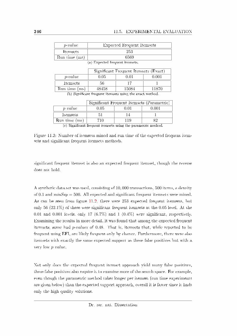
246 11.5. EXPERIMENTAL EVALUATION
p-value Expected Frequent Itemsets
Itemsets 253
Run time (ms) 6569(a) Expected frequent itemsets.
Signi�cant Frequent Itemsets (Exact)
p-value 0.05 0.01 0.001
Itemsets 56 17 1
Run time (ms) 48458 15084 11870(b) Signi�cant frequent itemsets using the exact method.
Signi�cant Frequent Itemsets (Parametric)
p-value 0.05 0.01 0.001
Itemsets 51 14 1
Run time (ms) 710 119 82(c) Signi�cant frequent itemsets using the parametric method.
Figure 11.2: Number of itemsets mined and run time of the expected frequent item-sets and signi�cant frequent itemsets methods.
signi�cant frequent itemset is also an expected frequent itemset, though the reverse
does not hold.
A synthetic data set was used, consisting of 10, 000 transactions, 500 items, a density
of 0.1 and minSup = 500. All expected and signi�cant frequent itemsets were mined.
As can be seen from �gure 11.2, there were 253 expected frequent itemsets, but
only 56 (22.1%) of these were signi�cant frequent itemsets at the 0.05 level. At the
0.01 and 0.001 levels, only 17 (6.7%) and 1 (0.4%) were signi�cant, respectively.
Examining the results in more detail, it was found that among the expected frequent
itemsets, some had p-values of 0.48. That is, itemsets that, while reported to be
frequent using EFI, are likely frequent only by chance. Furthermore, there were also
itemsets with exactly the same expected support as these false positives but with a
very low p-value.
Not only does the expected frequent itemset approach yield many false positives,
these false positives also require it to examine more of the search space. For example,
even though the parametric method takes longer per itemset (run time experiments
are given below) than the expected support approach, overall it is faster since it �nds
only the high quality solutions.
Dr. rer. nat. Dissertation
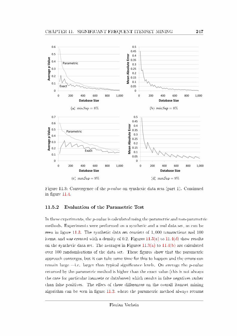
CHAPTER 11. SIGNIFICANT FREQUENT ITEMSET MINING 247
0
0.1
0.2
0.3
0.4
0.5
0.6
0 200 400 600 800 1,000
Average
p!Value
Database Size
Exact
Parametric
(a) minSup = 8%
0
0.05
0.1
0.15
0.2
0.25
0.3
0.35
0.4
0.45
0.5
0 200 400 600 800 1,000
Mean
Absolute
Error
Database Size
(b) minSup = 8%
0
0.1
0.2
0.3
0.4
0.5
0.6
0.7
0 200 400 600 800 1,000
Average
p!Value
Database Size
Exact
Parametric
(c) minSup = 9%
0
0.05
0.1
0.15
0.2
0.25
0.3
0.35
0.4
0.45
0.5
0 200 400 600 800 1,000
Mean
Absolute
Error
Database Size
(d) minSup = 9%
Figure 11.3: Convergence of the p-value on synthetic data sets (part 1). Continuedin �gure 11.4.
11.5.2 Evaluation of the Parametric Test
In these experiments, the p-value is calculated using the parametric and non-parametric
methods. Experiments were performed on a synthetic and a real data set, as can be
seen in �gure 11.3. The synthetic data set consists of 1, 000 transactions and 100
items, and was created with a density of 0.2. Figures 11.3(a) to 11.4(d) show results
on the synthetic data set. The averages in Figures 11.3(a) to 11.4(b) are calculated
over 100 randomisations of the data set. These �gures show that the parametric
approach converges, but it can take some time for this to happen and the errors can
remain large � i.e. larger than typical signi�cance levels. On average the p-value
returned by the parametric method is higher than the exact value (this is not always
the case for particular itemsets or databases) which results in false negatives rather
than false positives. The e�ect of these di�erences on the overall itemset mining
algorithm can be seen in �gure 11.2, where the parametric method always returns
Florian Verhein
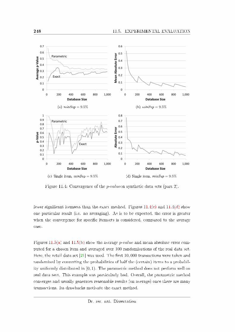
248 11.5. EXPERIMENTAL EVALUATION
0
0.1
0.2
0.3
0.4
0.5
0.6
0.7
0 200 400 600 800 1,000
Average
p!Value
Database Size
Exact
Parametric
(a) minSup = 9.5%
0
0.1
0.2
0.3
0.4
0.5
0.6
0 200 400 600 800 1,000
Mean
Absolute
Error
Database Size
(b) minSup = 9.5%
0
0.1
0.2
0.3
0.4
0.5
0.6
0.7
0.8
0.9
1
0 200 400 600 800 1,000
p Value
Database!Size
Exact
Parametric
(c) Single item, minSup = 9.5%
0
0.1
0.2
0.3
0.4
0.5
0.6
0.7
0.8
0 200 400 600 800 1,000
Absolute
Error
Database Size
(d) Single item, minSup = 9.5%
Figure 11.4: Convergence of the p-valueon synthetic data sets (part 2).
fewer signi�cant itemsets than the exact method. Figures 11.4(c) and 11.4(d) show
one particular result (i.e. no averaging). As is to be expected, the error is greater
when the convergence for speci�c itemsets is considered, compared to the average
case.
Figures 11.5(a) and 11.5(b) show the average p-value and mean absolute error com-
puted for a chosen item and averaged over 100 randomisations of the real data set.
Here, the retail data set [21] was used. The �rst 10, 000 transactions were taken and
randomised by converting the probabilities of half the (certain) items to a probabil-
ity uniformly distributed in [0, 1). The parametric method does not perform well on
real data sets. This example was particularly bad. Overall, the parametric method
converges and usually generates reasonable results (on average) once there are many
transactions. Its drawbacks motivate the exact method.
Dr. rer. nat. Dissertation
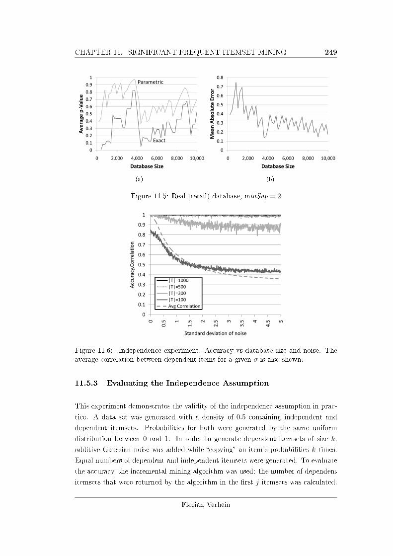
CHAPTER 11. SIGNIFICANT FREQUENT ITEMSET MINING 249
0
0.1
0.2
0.3
0.4
0.5
0.6
0.7
0.8
0.9
1
0 2,000 4,000 6,000 8,000 10,000
Average
p!Value
Database Size
Exact
Parametric
(a)
0
0.1
0.2
0.3
0.4
0.5
0.6
0.7
0.8
0 2,000 4,000 6,000 8,000 10,000
Mean
Absolute
Error
Database Size
(b)
Figure 11.5: Real (retail) database, minSup = 2
0
0.1
0.2
0.3
0.4
0.5
0.6
0.7
0.8
0.9
1
0
0.5 1
1.5 2
2.5 3
3.5 4
4.5 5
Accuracy,Co
rrelation
Standard deviation of noise
|T|=1000|T|=500|T|=300|T|=100Avg Correlation
Figure 11.6: Independence experiment. Accuracy vs database size and noise. Theaverage correlation between dependent items for a given σ is also shown.
11.5.3 Evaluating the Independence Assumption
This experiment demonstrates the validity of the independence assumption in prac-
tice. A data set was generated with a density of 0.5 containing independent and
dependent itemsets. Probabilities for both were generated by the same uniform
distribution between 0 and 1. In order to generate dependent itemsets of size k,
additive Gaussian noise was added while �copying� an item's probabilities k times.
Equal numbers of dependent and independent itemsets were generated. To evaluate
the accuracy, the incremental mining algorithm was used: the number of dependent
itemsets that were returned by the algorithm in the �rst j itemsets was calculated,
Florian Verhein
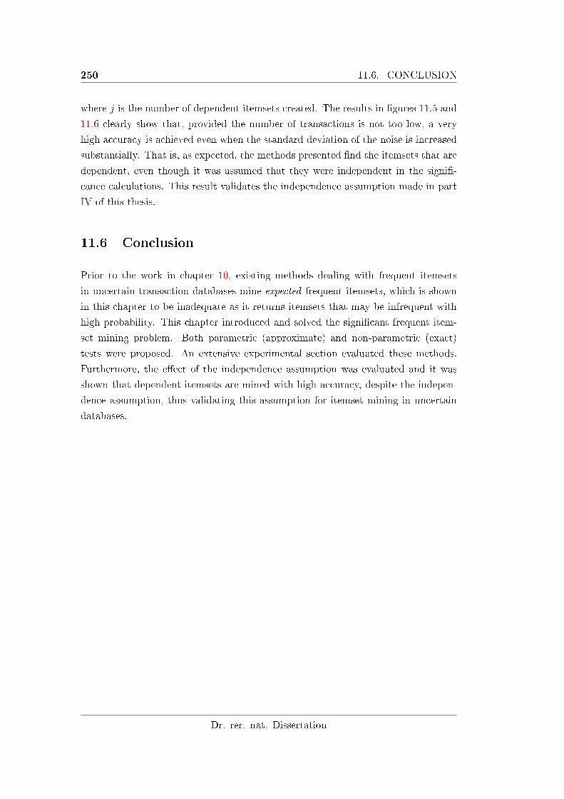
250 11.6. CONCLUSION
where j is the number of dependent itemsets created. The results in �gures 11.5 and
11.6 clearly show that, provided the number of transactions is not too low, a very
high accuracy is achieved even when the standard deviation of the noise is increased
substantially. That is, as expected, the methods presented �nd the itemsets that are
dependent, even though it was assumed that they were independent in the signi�-
cance calculations. This result validates the independence assumption made in part
IV of this thesis.
11.6 Conclusion
Prior to the work in chapter 10, existing methods dealing with frequent itemsets
in uncertain transaction databases mine expected frequent itemsets, which is shown
in this chapter to be inadequate as it returns itemsets that may be infrequent with
high probability. This chapter introduced and solved the signi�cant frequent item-
set mining problem. Both parametric (approximate) and non-parametric (exact)
tests were proposed. An extensive experimental section evaluated these methods.
Furthermore, the e�ect of the independence assumption was evaluated and it was
shown that dependent itemsets are mined with high accuracy, despite the indepen-
dence assumption, thus validating this assumption for itemset mining in uncertain
databases.
Dr. rer. nat. Dissertation
Chapter 12
Probabilistic Pattern Growth for
Itemset Mining in Uncertain
Databases
Uncertain transaction databases (UTDBs) consist of sets of existentially
uncertain items. The uncertainty of items in transactions makes traditional
frequent itemset mining techniques inapplicable. This chapter tackles the
Probabilistic Frequent Itemset Mining (PFIM) problem, where all Proba-
bilistic Frequent Itemsets (PFIs) are mined e�ciently.
In this context, this chapter makes the following contributions: The �rst
probabilistic FP-Growth (ProFP-Growth) algorithm and associated proba-
bilistic FP-Tree (ProFP-Tree) are proposed. It is used to mine all probabilis-
tic frequent itemsets in uncertain transaction databases without candidate
generation, resulting in a faster algorithm than the previous state of the
art algorithm proposed in chapter 10. In addition, this chapter proposes
an e�cient technique to compute the support probability distribution of an
itemset using the concept of generating functions. This is an alternative,
and more intuitive approach to the method proposed in chapter 10. An
extensive experimental section evaluates the impact of the proposed tech-
niques and shows that the ProFP-Growth approach is much faster than the
Apriori based algorithm.
251
252 12.1. INTRODUCTION
12.1 Introduction
Mining probabilistic frequent itemsets is a recent and challenging problem [18]. Re-
call that in an uncertain transaction database, the information captured in transac-
tions is uncertain as the existence of an item is associated with a likelihood measure
or existential probability. An example of a small uncertain transaction database is
given in �gure 12.1. This data set will be used as a running example in this chapter.
Recall from section 10.1 that given an uncertain transaction database, it is generally
not possible to determine whether an item or itemset is frequent because it is not cer-
tain whether or not it appears in transactions. In a traditional (certain) transaction
database on the other hand, an algorithm can simply perform a database scan and
count the transactions that include the itemset. Since this approach does not work
in an uncertain transaction database, traditional frequent itemset mining methods
cannot be applied to uncertain databases.
Prior to [18] (on which chapter 10 is based), expected support was used to deal with
uncertain databases [25, 26, 58]. It was shown in chapters 10 and 11 that the use
of expected support in probabilistic databases has signi�cant drawbacks that can
lead to misleading and even incorrect results. The proposed alternative was based
on computing the entire probability distribution of itemsets' support and mining
probabilistic frequent itemsets � itemsets where the probability of being frequent is
high. In chapter 10, this was achieved this in linear time by employing the Poisson
binomial recurrence relation. Chapter 10 adopted an Apriori-like approach to the
PFIM problem, which was based on an anti-monotone Apriori property1 [11] and
candidate generation. However, it is well known that Apriori-like algorithms su�er a
number of disadvantages. First, all candidates generated must �t into main memory
and the number of candidates can become prohibitively large. Secondly, checking
whether a candidate is a subset of a transaction is non-trivial. Finally, the entire
database needs to be scanned multiple times. In uncertain databases, the e�ective
transaction width is typically larger than in a certain transaction database which in
turn can increase the number of candidates generated as well as the resulting space
and time costs.
In certain transaction databases, the FP-Growth algorithm [47, 48] has become the
established alternative. By building an FP-Tree � e�ectively a compressed and highly
indexed structure storing the information in the database � candidate generation
and multiple database scans can be avoided. However, extending this idea to mine
probabilistic frequent patterns in uncertain transaction databases is non-trivial. It
1If if an itemset X is not frequent, then any itemset X ∪ Y is not frequent.
Dr. rer. nat. Dissertation
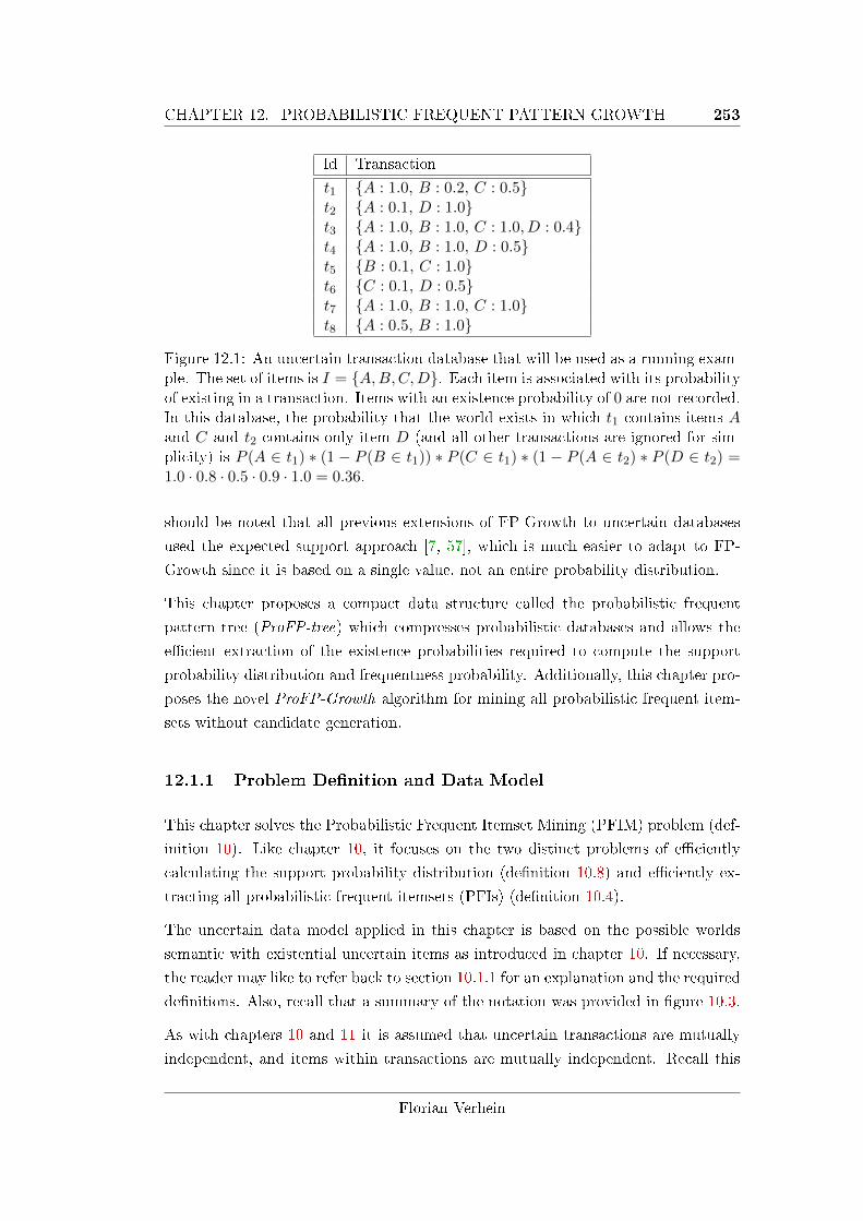
CHAPTER 12. PROBABILISTIC FREQUENT PATTERN GROWTH 253
Id Transaction
t1 {A : 1.0, B : 0.2, C : 0.5}t2 {A : 0.1, D : 1.0}t3 {A : 1.0, B : 1.0, C : 1.0, D : 0.4}t4 {A : 1.0, B : 1.0, D : 0.5}t5 {B : 0.1, C : 1.0}t6 {C : 0.1, D : 0.5}t7 {A : 1.0, B : 1.0, C : 1.0}t8 {A : 0.5, B : 1.0}
Figure 12.1: An uncertain transaction database that will be used as a running exam-ple. The set of items is I = {A,B,C,D}. Each item is associated with its probabilityof existing in a transaction. Items with an existence probability of 0 are not recorded.In this database, the probability that the world exists in which t1 contains items Aand C and t2 contains only item D (and all other transactions are ignored for sim-plicity) is P (A ∈ t1) ∗ (1 − P (B ∈ t1)) ∗ P (C ∈ t1) ∗ (1 − P (A ∈ t2) ∗ P (D ∈ t2) =1.0 · 0.8 · 0.5 · 0.9 · 1.0 = 0.36.
should be noted that all previous extensions of FP-Growth to uncertain databases
used the expected support approach [7, 57], which is much easier to adapt to FP-
Growth since it is based on a single value, not an entire probability distribution.
This chapter proposes a compact data structure called the probabilistic frequent
pattern tree (ProFP-tree) which compresses probabilistic databases and allows the
e�cient extraction of the existence probabilities required to compute the support
probability distribution and frequentness probability. Additionally, this chapter pro-
poses the novel ProFP-Growth algorithm for mining all probabilistic frequent item-
sets without candidate generation.
12.1.1 Problem De�nition and Data Model
This chapter solves the Probabilistic Frequent Itemset Mining (PFIM) problem (def-
inition 10). Like chapter 10, it focuses on the two distinct problems of e�ciently
calculating the support probability distribution (de�nition 10.8) and e�ciently ex-
tracting all probabilistic frequent itemsets (PFIs) (de�nition 10.4).
The uncertain data model applied in this chapter is based on the possible worlds
semantic with existential uncertain items as introduced in chapter 10. If necessary,
the reader may like to refer back to section 10.1.1 for an explanation and the required
de�nitions. Also, recall that a summary of the notation was provided in �gure 10.3.
As with chapters 10 and 11 it is assumed that uncertain transactions are mutually
independent, and items within transactions are mutually independent. Recall this
Florian Verhein
254 12.2. RELATED WORK
was justi�ed theoretically in chapters 10 and 11 and experimentally in chapter 11.
12.1.2 Contributions
This chapter makes the following contributions:
• It introduces the Probabilistic Frequent Pattern Tree (ProFP-Tree) and shows
how it is built e�ciently. This is the �rst FP-Tree type approach for han-
dling uncertain or probabilistic data. This tree e�ciently stores a probabilistic
database and enables e�cient extraction of itemset occurrence probabilities
and database projections (conditional ProFP-Trees).
• It proposes ProFP-Growth, an algorithm based on the ProFP-Tree which mines
all PFIs without using expensive candidate generation.
• It presents an intuitive and e�cient method for computing the frequentness
probability, as well as the entire support probability distribution, in O(|T | ·minSup) time. This has the same time complexity as the approach based on
Poisson binomial recurrence / dynamic programming technique in chapter 10,
but it is more intuitive and thus o�ers advantages.
12.1.3 Organisation
The remainder of this chapter is organized as follows; section 12.2 surveys related
work. Section 12.3 presents the ProFP-Tree, explains how it is constructed and
brie�y introduces the concept of conditional ProFP-Trees. Section 12.4 describes
how probability information is extracted from a (conditional) ProFP-Tree. Section
12.5 introduces the generating function approach for computing the frequentness
probability and the support probability distribution in linear time. Section 12.6 de-
scribes how conditional ProFP-Trees are built. Finally, section 12.7 describes the
ProFP-Growth algorithm by drawing together the previous sections. The experi-
mental evaluation is presented in section 12.8 and this chapter concludes in section
12.9.
12.2 Related Work
Recall that section 10.2 provided an in depth discussion of work related to frequent
itemset mining in uncertain and probabilistic databases. This also applies to the
work in this chapter.
Dr. rer. nat. Dissertation
CHAPTER 12. PROBABILISTIC FREQUENT PATTERN GROWTH 255
Prior to the work in this chapter, state-of-the-art (and only) approach for probabilis-
tic frequent itemset mining (PFIM) in uncertain databases was proposed in chapter
10 (and the associated publication [18]). That approach used an Apriori-like algo-
rithm to mine all probabilistic frequent itemsets and the Poisson binomial recurrence
to compute the support probability distribution function (SPDF). This chapter pro-
vides a faster solution by proposing the �rst probabilistic frequent pattern growth
approach (ProFP-Growth), thus avoiding expensive candidate generation and al-
lowing PFIM to be performed in large databases. Furthermore, a more intuitive
generating function method is proposed in order to compute the SPDF.
Previous methods extending FP-Growth [47] to uncertain databases (such as the UF-
Growth algorithm in [58]) use the expected support method, which is much simpler
to apply but has signi�cant disadvantages which were outlined in chapters 10 and
11.
FP-Growth is based on the idea of generating a compact in memory tree structure
that captures the support information of the entire database. When this tree � the
FP-Tree � �ts in memory, the candidate generation and multiple database passes of
the Apriori method are avoided. Furthermore, the FP-Growth algorithm avoids the
subset-checking that makes Apriori sensitive to databases with a wide transaction
width. A good introduction to the FP-Growth method can be found in [88].
12.3 Probabilistic Frequent-Pattern Tree (ProFP-Tree)
This section introduces a novel pre�x-tree structure that enables fast detection of
probabilistic frequent itemsets without the costly candidate generation or multiple
database scans that plague Apriori style algorithms. By itself, it functions as an
e�cient compressed data structure that allows the fast retrieval of all item probabil-
ities. The proposed structure is based on the frequent-pattern tree (FP-Tree [47]).
In contrast to the FP-tree, the ProFP-tree has the ability to compress uncertain and
probabilistic transactions. If a data set contains no uncertainty it reduces to the
(certain) FP-Tree.
De�nition 12.1. A Probabilistic Frequent Pattern Tree (ProFP-Tree) is composed
of the following three components:
1. Uncertain item pre�x tree : A root labeled �null� pointing to a set of pre�x
trees each associated with uncertain item sequences. Each node n in a pre�x
tree is associated with an (uncertain) item ai and consists of �ve �elds:
Florian Verhein
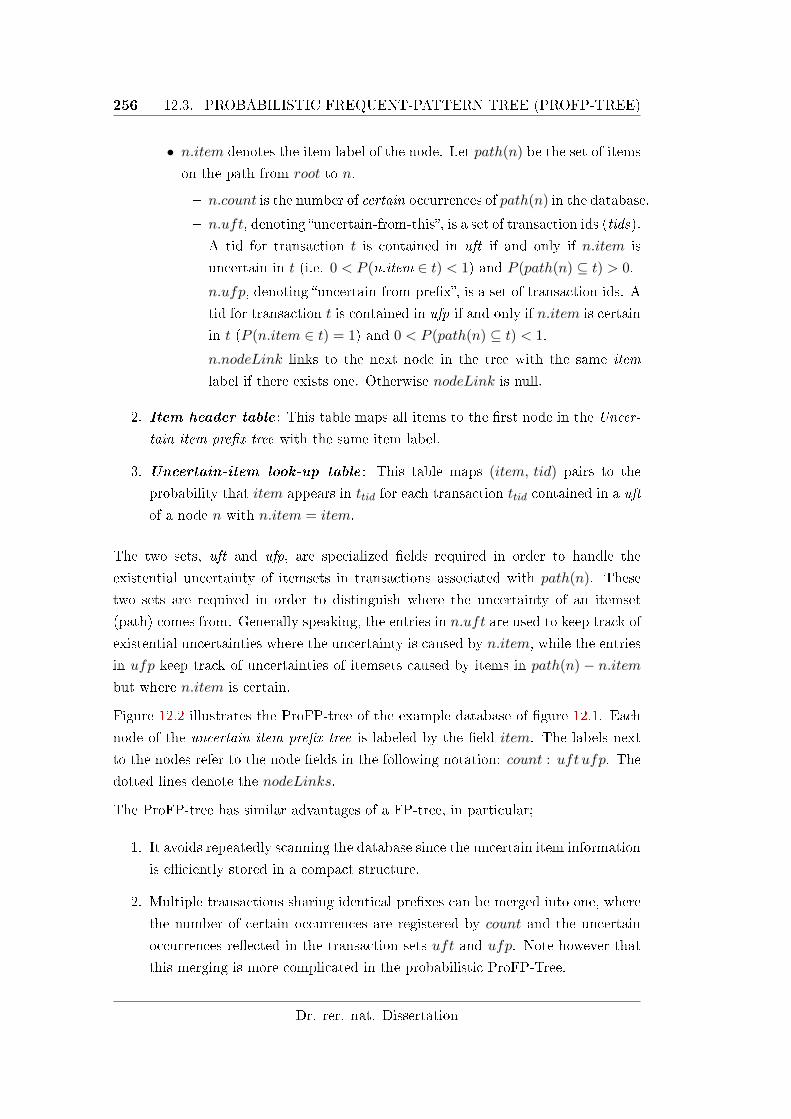
256 12.3. PROBABILISTIC FREQUENT-PATTERN TREE (PROFP-TREE)
• n.item denotes the item label of the node. Let path(n) be the set of items
on the path from root to n.
� n.count is the number of certain occurrences of path(n) in the database.
� n.uft, denoting �uncertain-from-this�, is a set of transaction ids (tids).
A tid for transaction t is contained in uft if and only if n.item is
uncertain in t (i.e. 0 < P (n.item ∈ t) < 1) and P (path(n) ⊆ t) > 0.
� n.ufp, denoting �uncertain-from-pre�x�, is a set of transaction ids. A
tid for transaction t is contained in ufp if and only if n.item is certain
in t (P (n.item ∈ t) = 1) and 0 < P (path(n) ⊆ t) < 1.
� n.nodeLink links to the next node in the tree with the same item
label if there exists one. Otherwise nodeLink is null.
2. Item header table : This table maps all items to the �rst node in the Uncer-
tain item pre�x tree with the same item label.
3. Uncertain-item look-up table : This table maps (item, tid) pairs to the
probability that item appears in ttid for each transaction ttid contained in a uft
of a node n with n.item = item.
The two sets, uft and ufp, are specialized �elds required in order to handle the
existential uncertainty of itemsets in transactions associated with path(n). These
two sets are required in order to distinguish where the uncertainty of an itemset
(path) comes from. Generally speaking, the entries in n.uft are used to keep track of
existential uncertainties where the uncertainty is caused by n.item, while the entries
in ufp keep track of uncertainties of itemsets caused by items in path(n) − n.itembut where n.item is certain.
Figure 12.2 illustrates the ProFP-tree of the example database of �gure 12.1. Each
node of the uncertain item pre�x tree is labeled by the �eld item. The labels next
to the nodes refer to the node �elds in the following notation: count : uft ufp. The
dotted lines denote the nodeLinks.
The ProFP-tree has similar advantages of a FP-tree, in particular;
1. It avoids repeatedly scanning the database since the uncertain item information
is e�ciently stored in a compact structure.
2. Multiple transactions sharing identical pre�xes can be merged into one, where
the number of certain occurrences are registered by count and the uncertain
occurrences re�ected in the transaction sets uft and ufp. Note however that
this merging is more complicated in the probabilistic ProFP-Tree.
Dr. rer. nat. Dissertation
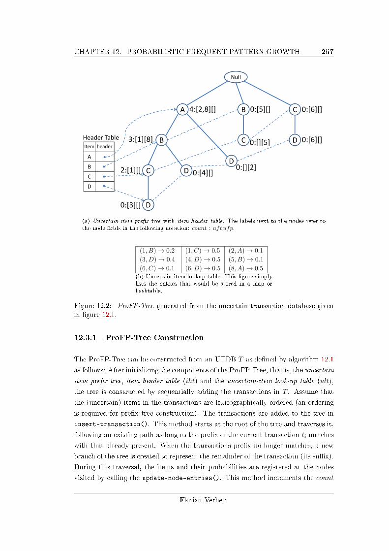
CHAPTER 12. PROBABILISTIC FREQUENT PATTERN GROWTH 257
Null
A B C4 [2 8][] 0 [5][] 0 [6][]A B C4:[2,8][] 0:[5][] 0:[6][]
C DB3:[1][8] 0:[][5] 0:[6][]Header TableItem header
DC D2:[1][] 0:[4][]
0:[][2]A
B
C [ ][]C
D
D0:[3][]
(a) Uncertain item pre�x tree with item header table. The labels next to the nodes refer tothe node �elds in the following notation: count : uft ufp.
(1, B)→ 0.2 (1, C)→ 0.5 (2, A)→ 0.1
(3, D)→ 0.4 (4, D)→ 0.5 (5, B)→ 0.1
(6, C)→ 0.1 (6, D)→ 0.5 (8, A)→ 0.5(b) Uncertain-item lookup table. This �gure simplylists the entries that would be stored in a map orhashtable.
Figure 12.2: ProFP-Tree generated from the uncertain transaction database givenin �gure 12.1.
12.3.1 ProFP-Tree Construction
The ProFP-Tree can be constructed from an UTDB T as de�ned by algorithm 12.1
as follows: After initializing the components of the ProFP-Tree, that is, the uncertain
item pre�x tree, item header table (iht) and the uncertain-item look-up table (ult),
the tree is constructed by sequentially adding the transactions in T . Assume that
the (uncertain) items in the transactions are lexicographically ordered (an ordering
is required for pre�x tree construction). The transactions are added to the tree in
insert-transaction(). This method starts at the root of the tree and traverses it,
following an existing path as long as the pre�x of the current transaction ti matches
with that already present. When the transactions pre�x no longer matches, a new
branch of the tree is created to represent the remainder of the transaction (its su�x).
During this traversal, the items and their probabilities are registered at the nodes
visited by calling the update-node-entries(). This method increments the count
Florian Verhein
258 12.3. PROBABILISTIC FREQUENT-PATTERN TREE (PROFP-TREE)
of a node if the current item and all preceding items are certain in ti. If the current
item is certain but one of its preceding items not, then ti is registered in ufp. If
the current item is uncertain, then ti is registered in uft. This insertion process is
repeated until all transactions are added to the tree.
12.3.1.1 Example
For further illustration, refer to the example database of �gure 12.1 and the corre-
sponding ProFP-tree in �gure 12.2.
The algorithm �rst creates the root of the uncertain item pre�x tree labeled �null �.
It then reads the uncertain transactions one at a time. While scanning the �rst
transaction t1, the �rst branch of the tree can be generated leading to the �rst path
composed of entries of the form (item, count, uft, ufp, node− link). In the example,
the �rst branch of the tree is built by the following path:
〈root, (A, 1, [], [], null), (B, 0, [1], [], null), (C, 0, [1], [], null)〉
Note that the entry �1� in the �eld uft of the nodes associated with B and C indicate
that item B and C are existentially uncertain in t1. Next, the second transaction
(t2) is scanned and the tree structure is updated accordingly. Since t2 shares a pre�x
with t1, the algorithm follows the existing path in the tree starting at the root and
updates this path. Since the �rst item A in t2 is existentially uncertain � that is,
it exists in t2 with a probability of 0.1 � the count of the �rst node in the path is
not incremented. Instead, t2 is added to uft of this node. The next item D in t2
does not match the next node on the existing path and thus a new branch leading
to a new leaf node n with entry (D, 0, [], [2], null) is added. Although item D is
existentially certain in t2, the count of n is initialized with zero because n represents
the set {A,D} and this path from the root to node n is existentially uncertain in t2
due to the existential uncertainty of item A. Hence, transaction t2 is counted in the
uncertain-from-pre�x (ufp) �eld of n. This results in the ProFP-Tree illustrated in
�gure 12.3(a).
The next transaction to be scanned is t3. Again, due to matching pre�xes the
algorithm follows the already existing path 〈A,B,C〉2 while scanning the (uncertain)items in t3. The resulting tree is illustrated in �gure 12.3(b). Since the �rst item A
exists for certain, count of the �rst node in the pre�x path is incremented by one.
2To simplify matters, the item �elds are used to address the nodes in a path. That is, the valuesof the nodes are omitted.
Dr. rer. nat. Dissertation
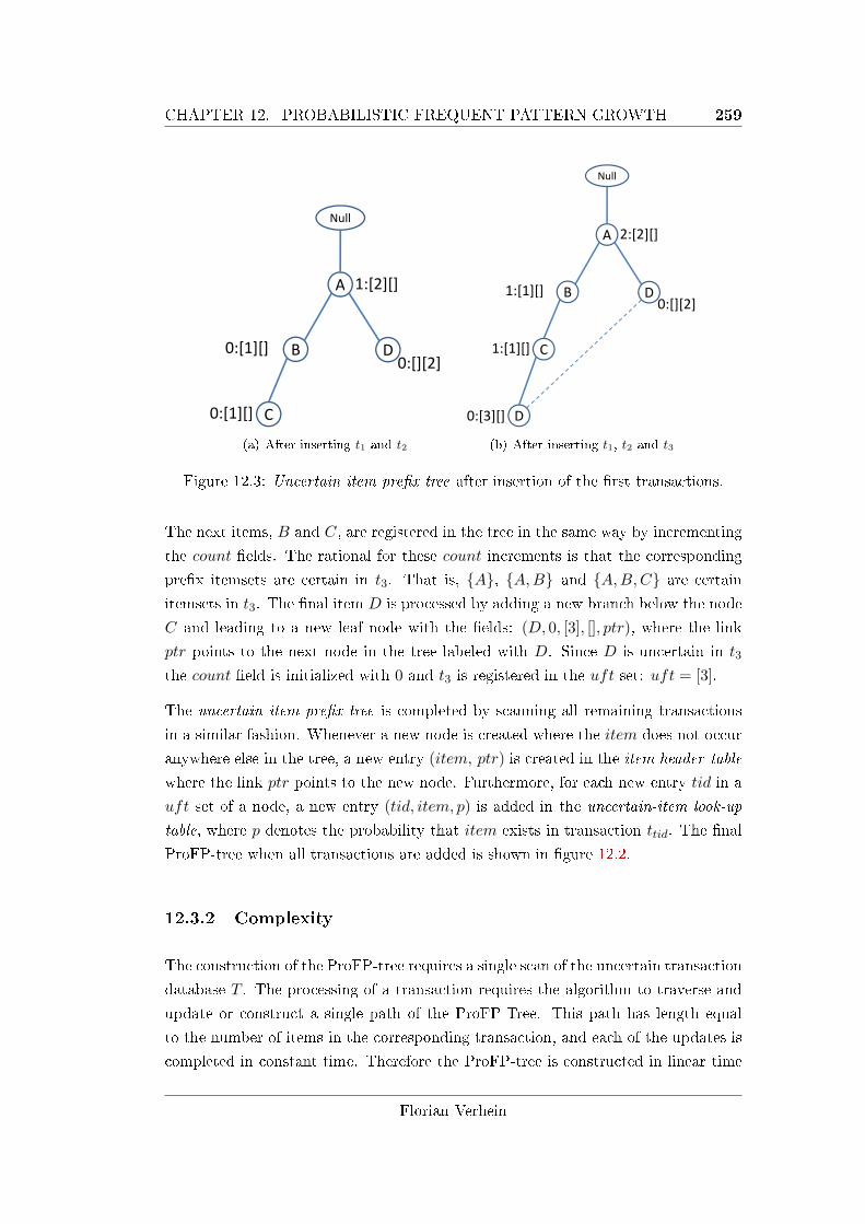
CHAPTER 12. PROBABILISTIC FREQUENT PATTERN GROWTH 259
Null
A 1:[2][]A 1:[2][]
DB0:[1][]0:[][2]
C0:[1][]
(a) After inserting t1 and t2
Null
A 2:[2][]A 2:[2][]
DB1:[1][]0:[][2]
C1:[1][]
D0:[3][]
(b) After inserting t1, t2 and t3
Figure 12.3: Uncertain item pre�x tree after insertion of the �rst transactions.
The next items, B and C, are registered in the tree in the same way by incrementing
the count �elds. The rational for these count increments is that the corresponding
pre�x itemsets are certain in t3. That is, {A}, {A,B} and {A,B,C} are certain
itemsets in t3. The �nal item D is processed by adding a new branch below the node
C and leading to a new leaf node with the �elds: (D, 0, [3], [], ptr), where the link
ptr points to the next node in the tree labeled with D. Since D is uncertain in t3
the count �eld is initialized with 0 and t3 is registered in the uft set: uft = [3].
The uncertain item pre�x tree is completed by scanning all remaining transactions
in a similar fashion. Whenever a new node is created where the item does not occur
anywhere else in the tree, a new entry (item, ptr) is created in the item header table
where the link ptr points to the new node. Furthermore, for each new entry tid in a
uft set of a node, a new entry (tid, item, p) is added in the uncertain-item look-up
table, where p denotes the probability that item exists in transaction ttid. The �nal
ProFP-tree when all transactions are added is shown in �gure 12.2.
12.3.2 Complexity
The construction of the ProFP-tree requires a single scan of the uncertain transaction
database T . The processing of a transaction requires the algorithm to traverse and
update or construct a single path of the ProFP-Tree. This path has length equal
to the number of items in the corresponding transaction, and each of the updates is
completed in constant time. Therefore the ProFP-tree is constructed in linear time
Florian Verhein
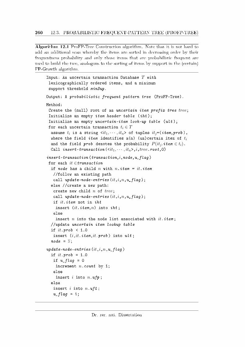
260 12.3. PROBABILISTIC FREQUENT-PATTERN TREE (PROFP-TREE)
Algorithm 12.1 ProFP-Tree Construction algorithm. Note that it is not hard toadd an additional scan whereby the items are sorted in decreasing order by theirfrequentness probability and only those items that are probabilistic frequent areused to build the tree, analogous to the sorting of items by support in the (certain)FP-Growth algorithm.
Input: An uncertain transaction Database T with
lexicographically ordered items, and a minimum
support threshold minSup.
Output: A probabilistic frequent pattern tree (ProFP-Tree).
Method:
Create the (null) root of an uncertain item prefix tree tree;Initialize an empty item header table (iht );
Initialize an empty uncertain-item look-up table (ult );
for each uncertain transaction ti ∈ Tassume ti is a string <it1, · · · , itn> of tuples itj=(item,prob ),where the field item identifies a(n) (un)certain item of tiand the field prob denotes the probability P (itj .item ∈ ti).Call insert-transaction (<it1, · · · , itn>,i,tree.root,0)
insert-transaction (transaction,i,node,u_flag )for each it ∈transactionif node has a child n with n.item = it.item//follow an existing path
call update-node-entries (it,i,n,u_flag );else //create a new path:
create new child n of tree;call update-node-entries (it,i,n,u_flag );if it.item not in iht
insert (it.item,n) into iht ;
else
insert n into the node list associated with it.item ;//update uncertain item lookup table
if it.prob < 1.0
insert (i,it.item,it.prob ) into ult ;
node = N;
update-node-entries (it,i,n,u_flag )if it.prob = 1.0
if u_flag = 0
increment n.count by 1;
else
insert i into n.ufp ;else
insert i into n.uft ;u_flag = 1;
Dr. rer. nat. Dissertation
CHAPTER 12. PROBABILISTIC FREQUENT PATTERN GROWTH 261
with respect to the size of the database � O(|T | · |I|) where |T | is the number of
transactions and |I| is the number of items.
Since the ProFP-Tree is based on the original FP-Tree (that is, the pre�x-tree part
has the same structure), it inherits its compactness properties. In particular, the size
of a ProFP-Tree is bounded by the overall occurrences of the items in the database
and its height is bounded by the maximal number of items in a transaction.
For any transaction ti in T , there exists exactly one path in the ProFP-Tree starting
below the root node. Each item within a transaction in the transaction database
can create no more than one node in the tree and the height of the tree is bounded
by the number of items in a transaction (path). Note that as with the FP-Tree, the
compression is obtained by sharing common pre�xes.
It is now shown that the values stored at the nodes do not a�ect the bound on the
size of the tree. In particular, the following lemma bounds the uncertain-from-this
(uft) and uncertain-from-pre�x (ufp) sets. Note that count and nodeLink have
constant size.
Lemma 12.2. Let tree be the ProFP-Tree generated from an uncertain transaction
database T . The total space required by all the transaction-id sets (uft and ufp) in
all nodes in tree is bounded by the the total number of entries in transactions with
an existential probability in (0, 1). That is, the number of probabilities in (0, 1) in T .
Proof. Each occurrence of an uncertain item (with existence probability in (0, 1))
in the database yields at most one transaction-id entry in one of the transaction-id
sets assigned to a node in the tree. In general there are three update possibilities for
a node n: If the current item and all pre�x items in the current transaction ti are
certain, there is no new entry in uft or ufp as count is incremented. ti is registered
in n.uft if and only if n.item is existentially uncertain in ti while ti is registered in
n.ufp if and only if n.item is existentially certain in in ti but at least one of the
pre�x items in ti is existentially uncertain. Therefore each occurrence of an item in
T leads to either a count increment (which does not require additional space) or one
new entry in uft or ufp.
Finally, it should be clear that the size of the uncertain item look-up table is bounded
by the number of uncertain (non zero and non 1) entries in the database.
This section showed that the ProFP-Tree inherits the compactness of the original FP-
tree. The next section shows that the information stored in the ProFP-Tree su�ces to
retrieve all probabilistic information required for PFIM, thus proving completeness.
Florian Verhein
26212.4. EXTRACTING CERTAIN AND UNCERTAIN SUPPORT
PROBABILITIES
12.4 Extracting Certain and Uncertain Support Proba-
bilities
Unlike the (certain) FP-Growth approach where it is easy to extract the support of
an itemset X by summing the support counts along the node-links for X in a suitable
conditional ProFP-Tree, this chapter is concerned with the support distribution of
X in the probabilistic case. Before this can be computed however, both the number
of certain occurrences as well as the probabilities 0 < P (X ∈ ti) < 1 are required.
Both can be e�ciently obtained using the ProFP-Tree as follows:
• To obtain the certain support of an item x, the algorithm follows the node-links
from the item header table and accumulates both the counts and the number
of transactions in which x is uncertain-from-pre�x. The latter is counted since
the support of x is required and by construction, transactions in ufp are known
to be certain for x (but uncertain from the pre�x).
• To �nd the set of transaction ids in which x is uncertain, the algorithm fol-
lows the node-links as above and accumulate all transactions that are in the
uncertain-from-this (uft) list.
Example 12.3. Consider item C in the ProFP-Tree of �gure 12.2. By traversing
the node-list for C, we can reach three nodes which are accumulated as follows in
order to calculate the certain support: (2 + |∅|) + (0 + |{t5}|) + (0 + |∅|) = 3. Note
there is one transaction in which C is uncertain-from-pre�x (t5). Similarly, in this
same traversal it is easy to obtain the transaction ids for the transactions in which
C is uncertain: [1] ∪ ∅ ∪ [6] = [1, 6]. That is, the only transactions in which C is
uncertain are t1 and t6. The exact appearance probabilities in these transactions can
be obtained from the uncertain-item look-up table (�gure 12.2(b)): the probabilities
of C appearing in transactions t1 and t6 are 0.5 and 0.4, respectively. By comparing
these results to the original database in �gure 12.1), it is easy to see that the tree
allows the certain support as well as the transaction ids where C is uncertain to be
found e�ciently.
To compute the support of an itemset X = {B,C,D, ...,K}, the conditional tree for{C,D, ...,K} is required, from which the certain support and uncertain transaction
ids for the nodes labeled B can be obtained. These implicitly correspond to the
entire itemset X. Since it is somewhat involved, the construction of conditional
ProFP-Trees is deferred to section 12.6. For now it su�ces to state that by using
Dr. rer. nat. Dissertation
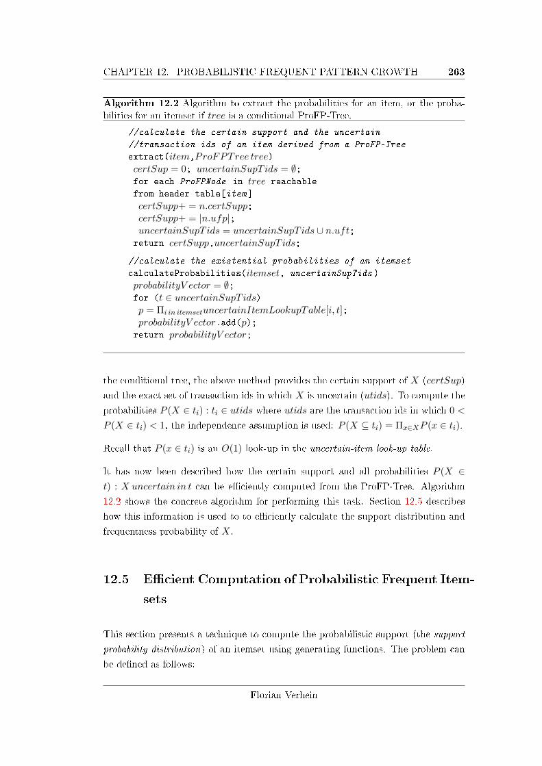
CHAPTER 12. PROBABILISTIC FREQUENT PATTERN GROWTH 263
Algorithm 12.2 Algorithm to extract the probabilities for an item, or the proba-bilities for an itemset if tree is a conditional ProFP-Tree.
//calculate the certain support and the uncertain
//transaction ids of an item derived from a ProFP-Tree
extract(item,ProFPTree tree)certSup = 0; uncertainSupT ids = ∅;for each ProFPNode in tree reachable
from header table[item ]
certSupp+ = n.certSupp;certSupp+ = |n.ufp|;uncertainSupT ids = uncertainSupT ids ∪ n.uft;return certSupp,uncertainSupT ids;
//calculate the existential probabilities of an itemset
calculateProbabilities(itemset, uncertainSupTids )
probabilityV ector = ∅;for (t ∈ uncertainSupT ids)p = Πi in itemsetuncertainItemLookupTable[i, t];probabilityV ector.add(p);return probabilityV ector;
the conditional tree, the above method provides the certain support of X (certSup)
and the exact set of transaction ids in which X is uncertain (utids). To compute the
probabilities P (X ∈ ti) : ti ∈ utids where utids are the transaction ids in which 0 <
P (X ∈ ti) < 1, the independence assumption is used: P (X ⊆ ti) = Πx∈XP (x ∈ ti).
Recall that P (x ∈ ti) is an O(1) look-up in the uncertain-item look-up table.
It has now been described how the certain support and all probabilities P (X ∈t) : X uncertain in t can be e�ciently computed from the ProFP-Tree. Algorithm
12.2 shows the concrete algorithm for performing this task. Section 12.5 describes
how this information is used to to e�ciently calculate the support distribution and
frequentness probability of X.
12.5 E�cient Computation of Probabilistic Frequent Item-
sets
This section presents a technique to compute the probabilistic support (the support
probability distribution) of an itemset using generating functions. The problem can
be de�ned as follows:
Florian Verhein
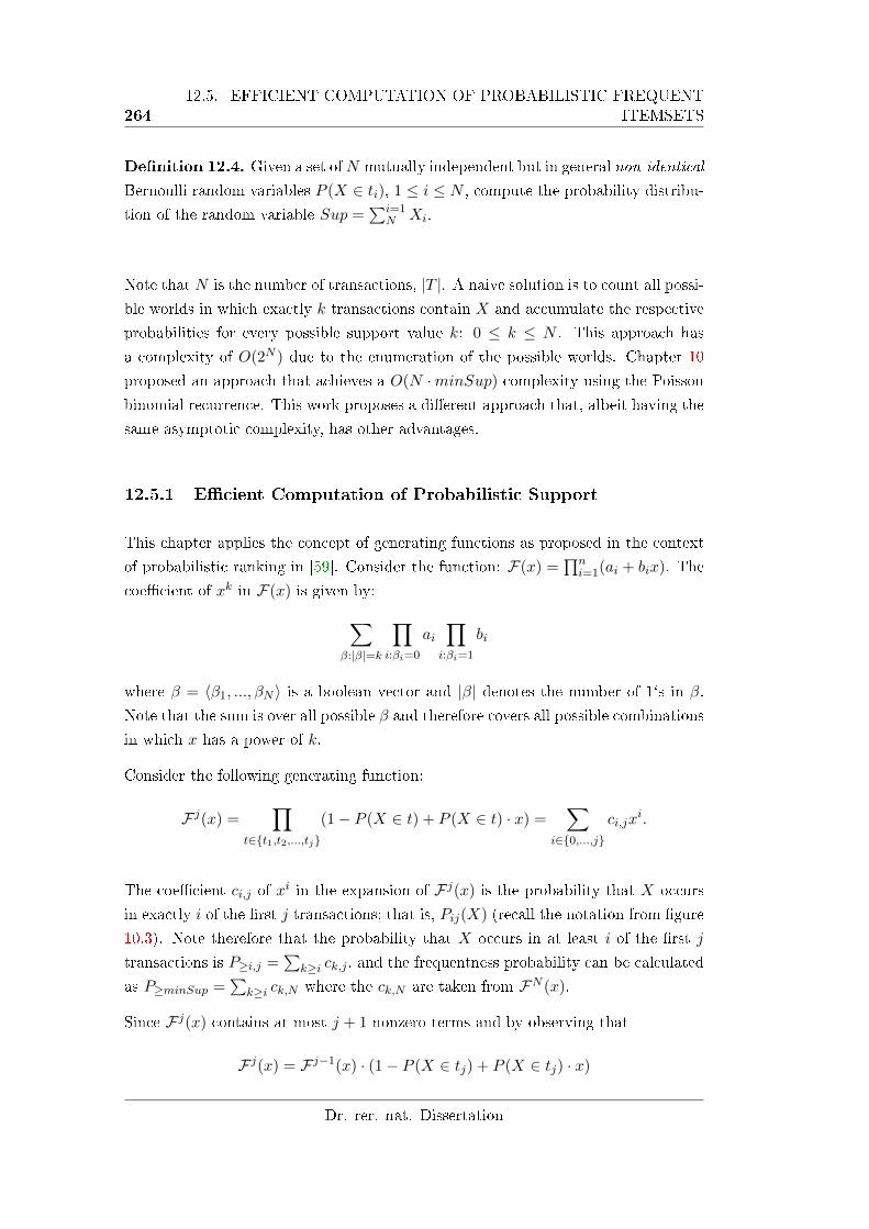
26412.5. EFFICIENT COMPUTATION OF PROBABILISTIC FREQUENT
ITEMSETS
De�nition 12.4. Given a set ofN mutually independent but in general non-identical
Bernoulli random variables P (X ∈ ti), 1 ≤ i ≤ N , compute the probability distribu-
tion of the random variable Sup =∑i=1
N Xi.
Note that N is the number of transactions, |T |. A naive solution is to count all possi-
ble worlds in which exactly k transactions contain X and accumulate the respective
probabilities for every possible support value k: 0 ≤ k ≤ N . This approach has
a complexity of O(2N ) due to the enumeration of the possible worlds. Chapter 10
proposed an approach that achieves a O(N ·minSup) complexity using the Poisson
binomial recurrence. This work proposes a di�erent approach that, albeit having the
same asymptotic complexity, has other advantages.
12.5.1 E�cient Computation of Probabilistic Support
This chapter applies the concept of generating functions as proposed in the context
of probabilistic ranking in [59]. Consider the function: F(x) =∏ni=1(ai + bix). The
coe�cient of xk in F(x) is given by:∑β:|β|=k
∏i:βi=0
ai∏i:βi=1
bi
where β = 〈β1, ..., βN 〉 is a boolean vector and |β| denotes the number of 1`s in β.
Note that the sum is over all possible β and therefore covers all possible combinations
in which x has a power of k.
Consider the following generating function:
F j(x) =∏
t∈{t1,t2,...,tj}
(1− P (X ∈ t) + P (X ∈ t) · x) =∑
i∈{0,...,j}
ci,jxi.
The coe�cient ci,j of xi in the expansion of F j(x) is the probability that X occurs
in exactly i of the �rst j transactions; that is, Pij(X) (recall the notation from �gure
10.3). Note therefore that the probability that X occurs in at least i of the �rst j
transactions is P≥i,j =∑
k≥i ck,j , and the frequentness probability can be calculated
as P≥minSup =∑
k≥i ck,N where the ck,N are taken from FN (x).
Since F j(x) contains at most j + 1 nonzero terms and by observing that
F j(x) = F j−1(x) · (1− P (X ∈ tj) + P (X ∈ tj) · x)
Dr. rer. nat. Dissertation
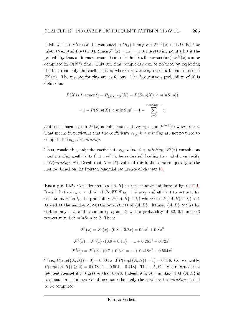
CHAPTER 12. PROBABILISTIC FREQUENT PATTERN GROWTH 265
it follows that F j(x) can be computed in O(j) time given F j−1(x) (this is the time
taken to expand the terms). Since F0(x) = 1x0 = 1 is the starting point (this is the
probability that an itemset occurs 0 times in the �rst 0 transactions), FN (x) can be
computed in O(N2) time. This run time complexity can be reduced by exploiting
the fact that only the coe�cients ci where i < minSup need to be considered in
FN (x). The reasons for this are as follows: The frequentness probability of X is
de�ned as
P (X is frequent) = P≥minSup(X) = P (Sup(X) ≥ minSup))
= 1− P (Sup(X) < minSup) = 1−minSup−1∑
i=0
ci
and a coe�cient ci,j in F j(x) is independent of any ck,j−1 in F j−1(x) where k > i.
That means in particular that the coe�cients ck,j , k ≥ minSup are not required to
compute the ci,j , i < minSup.
Thus, considering only the coe�cients ci,j where i < minSup, F j(x) contains at
most minSup coe�cients that need to be evaluated, leading to a total complexity
of O(minSup ·N). Recall that N = |T | and that this is the same complexity as the
method based on the Poisson binomial recurrence of chapter 10.
Example 12.5. Consider itemset {A,B} in the example database of �gure 12.1.
Recall that using a conditional ProFP-Tree, it is easy and e�cient to extract, for
each transaction ti, the probability P ({A,B} ∈ ti) where 0 < P ({A,B} ∈ ti) < 1
as well as the number of certain occurrences of {A,B}. Itemset {A,B} occurs forcertain only in t4 and occurs in t1, t2 and t3 with a probability of 0.2, 0.1, and 0.3
respectively. Let minSup be 2. Then:
F1(x) = F0(x) · (0.8 + 0.2x) = 0.2x1 + 0.8x0
F2(x) = F1(x) · (0.9 + 0.1x) = ...+ 0.26x1 + 0.72x0
F3(x) = F2(x) · (0.7 + 0.3x) = ...+ 0.418x1 + 0.504x0
Thus, P (sup({A,B}) = 0) = 0.504 and P (sup({A,B}) = 1) = 0.418. Consequently,
P (sup({A,B}) ≥ 2) = 0.078 (1 − 0.504 − 0.418). Thus, A,B is not returned as a
frequent itemset if τ is greater than 0.078. Indeed, it is very unlikely that {A,B} isfrequent. In the above Equations, note that only the ci where i < minSup needed
to be computed.
Florian Verhein
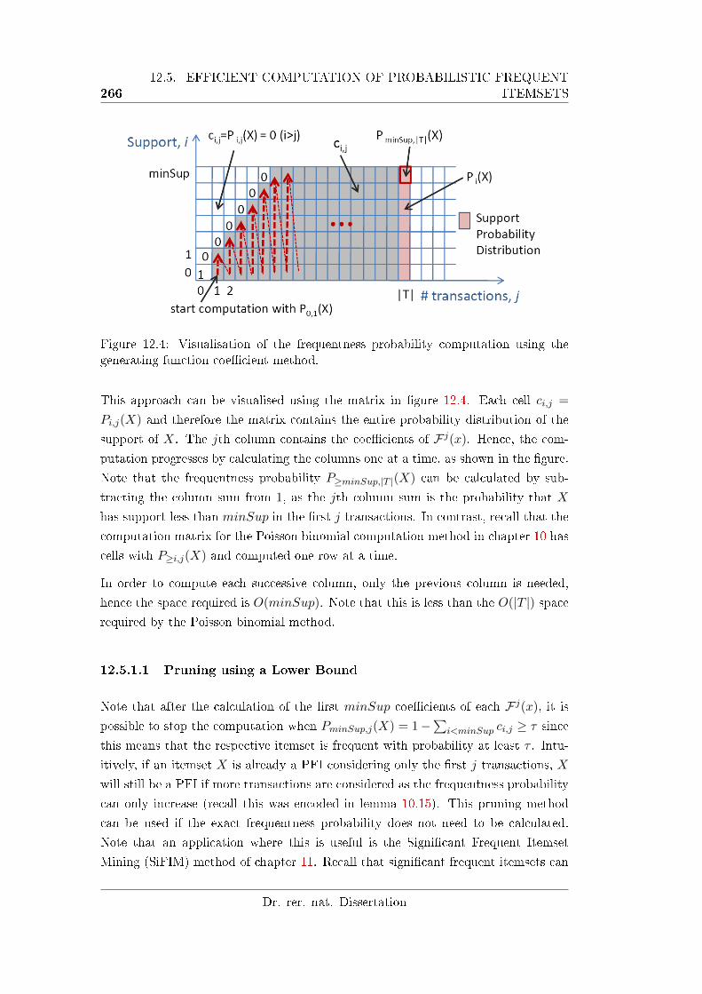
26612.5. EFFICIENT COMPUTATION OF PROBABILISTIC FREQUENT
ITEMSETS
Figure 12.4: Visualisation of the frequentness probability computation using thegenerating function coe�cient method.
This approach can be visualised using the matrix in �gure 12.4. Each cell ci,j =
Pi,j(X) and therefore the matrix contains the entire probability distribution of the
support of X. The jth column contains the coe�cients of F j(x). Hence, the com-
putation progresses by calculating the columns one at a time, as shown in the �gure.
Note that the frequentness probability P≥minSup,|T |(X) can be calculated by sub-
tracting the column sum from 1, as the jth column sum is the probability that X
has support less than minSup in the �rst j transactions. In contrast, recall that the
computation matrix for the Poisson binomial computation method in chapter 10 has
cells with P≥i,j(X) and computed one row at a time.
In order to compute each successive column, only the previous column is needed,
hence the space required is O(minSup). Note that this is less than the O(|T |) spacerequired by the Poisson binomial method.
12.5.1.1 Pruning using a Lower Bound
Note that after the calculation of the �rst minSup coe�cients of each F j(x), it is
possible to stop the computation when PminSup,j(X) = 1−∑
i<minSup ci,j ≥ τ since
this means that the respective itemset is frequent with probability at least τ . Intu-
itively, if an itemset X is already a PFI considering only the �rst j transactions, X
will still be a PFI if more transactions are considered as the frequentness probability
can only increase (recall this was encoded in lemma 10.15). This pruning method
can be used if the exact frequentness probability does not need to be calculated.
Note that an application where this is useful is the Signi�cant Frequent Itemset
Mining (SiFIM) method of chapter 11. Recall that signi�cant frequent itemsets can
Dr. rer. nat. Dissertation
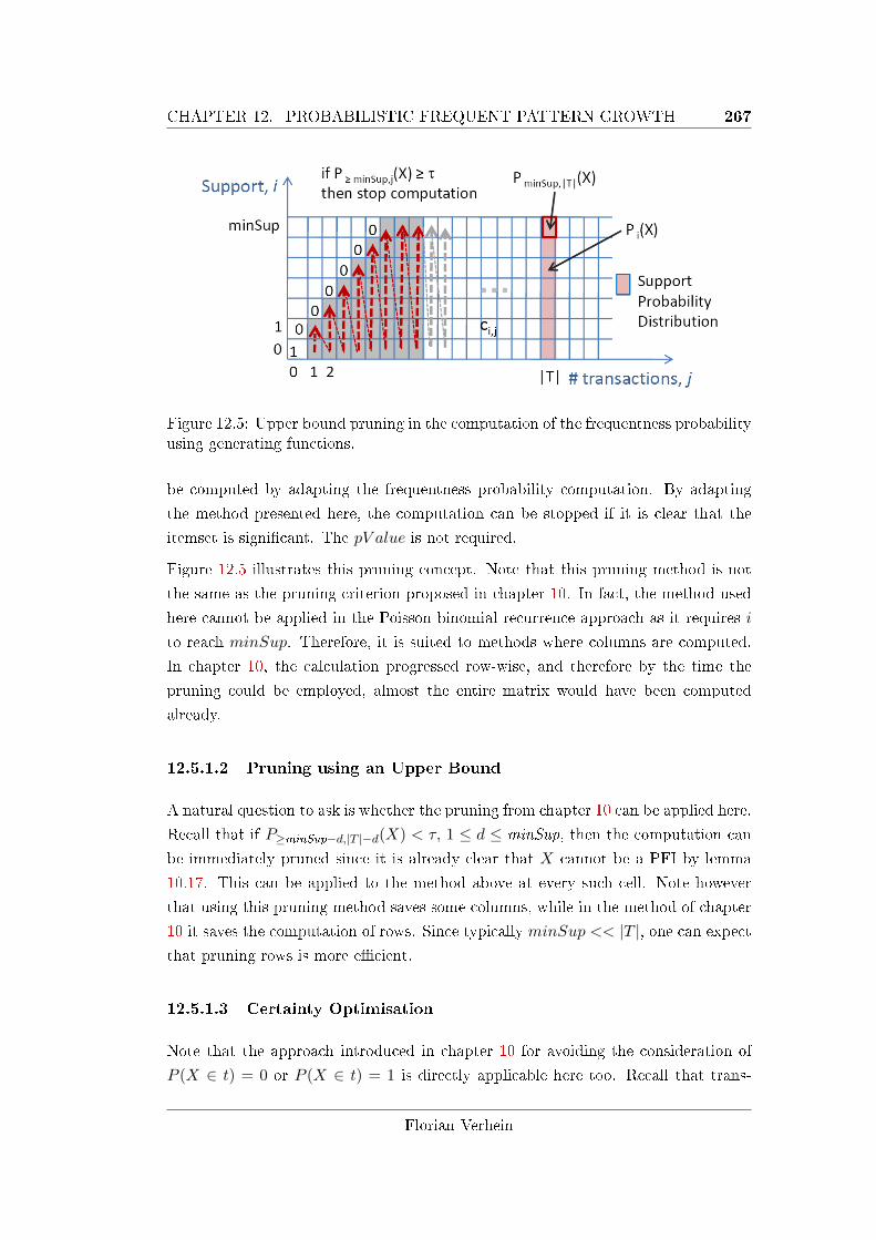
CHAPTER 12. PROBABILISTIC FREQUENT PATTERN GROWTH 267
Figure 12.5: Upper bound pruning in the computation of the frequentness probabilityusing generating functions.
be computed by adapting the frequentness probability computation. By adapting
the method presented here, the computation can be stopped if it is clear that the
itemset is signi�cant. The pV alue is not required.
Figure 12.5 illustrates this pruning concept. Note that this pruning method is not
the same as the pruning criterion proposed in chapter 10. In fact, the method used
here cannot be applied in the Poisson binomial recurrence approach as it requires i
to reach minSup. Therefore, it is suited to methods where columns are computed.
In chapter 10, the calculation progressed row-wise, and therefore by the time the
pruning could be employed, almost the entire matrix would have been computed
already.
12.5.1.2 Pruning using an Upper Bound
A natural question to ask is whether the pruning from chapter 10 can be applied here.
Recall that if P≥minSup−d,|T |−d(X) < τ, 1 ≤ d ≤ minSup, then the computation can
be immediately pruned since it is already clear that X cannot be a PFI by lemma
10.17. This can be applied to the method above at every such cell. Note however
that using this pruning method saves some columns, while in the method of chapter
10 it saves the computation of rows. Since typically minSup << |T |, one can expect
that pruning rows is more e�cient.
12.5.1.3 Certainty Optimisation
Note that the approach introduced in chapter 10 for avoiding the consideration of
P (X ∈ t) = 0 or P (X ∈ t) = 1 is directly applicable here too. Recall that trans-
Florian Verhein
26812.5. EFFICIENT COMPUTATION OF PROBABILISTIC FREQUENT
ITEMSETS
actions t where P (X ∈ t) = 0 can be ignored, and transactions with P (X ∈ t) = 1
can be ignored by decrementing minSup. Note that the �rst optimisation is done
automatically when one used the ProFP-Tree, and the second one is made much
easier with the ProFP-Tree as it stores the certain support separately.
12.5.1.4 Discussion
The generating function technique is di�erent to the Poisson binomial recurrence
method, but has the same run time complexity. This section weights up their re-
spective bene�ts and downsides.
Using generating functions instead of the recursion formula gives a di�erent and
intuitive view of the problem. It can be argued that it is clearer, since the coe�cients
correspond to the support distribution. It also leads to a method for computing the
frequentness probability in less space. The column wise computation method allows a
new pruning method that cannot be applied to the recurrence method. An additional
advantage of this approach is that it allows an iterative database scan in a candidate
generation type method. By storing an array of length minSup for each candidate,
one can scan the database one transaction at a time and update all the coe�cients per
transaction. In one scan, all the probabilities for all candidates can be incrementally
computed. As described above, itemsets can be pruned before all transactions are
considered using both a lower bound and an upper bound. In contrast, the row
based method does not lend itself to such a method, because probabilities in all
transactions are required to compute the �rst � and all subsequent � rows. While
this observation is not an advantage in the ProFP-Growth algorithm, it could be
an advantage in ProApriori � allowing it to use less space and avoid keeping the
database in memory.
In addition, the generating function approach allows the support probability density
function to be updated easily if the probability that a transaction ti contains an
itemset X changes. That is, if the probability p = P (X ∈ ti) changes to p′, then it
is possible to update the support probability distribution by dividing the generating
function by px + (1 − p) (using polynomial division) in order to remove the e�ect
of ti, and subsequently, multiplying this result by p′x + (1 − p′) to incorporate the
new probability p′. That is, F j′(x) = F j(x) : (px + 1 − p) × (p′x + 1 − p′), whereF j′ is the generating function for the support probability distribution of X in the
�rst j transactions in the altered database. Note that this chapter does not consider
transactions as mutable, but this possibility may be useful in some other applications.
Dr. rer. nat. Dissertation
CHAPTER 12. PROBABILISTIC FREQUENT PATTERN GROWTH 269
12.6 Extracting Conditional ProFP-Trees
This section describes how conditional ProFP-Trees are constructed from other (po-
tentially conditional) ProFP-Trees. The method for doing this is more involved than
the analogous operation for the certain FP-Growth algorithm, since the information
capturing the source of the uncertainty must remain correct. That is, whether the
uncertainty at that node comes from the pre�x or from the present node. Recall from
section 12.4 that this is required in order to extract the correct probabilities from
the tree. A conditional ProFP-Tree for itemset X (treeX) is equivalent to a ProFP-
Tree built on only those transactions in which X occurs with a non-zero probability.
In order to generate a conditional ProFP-Tree for itemset X ∪ i (treeX∪i) where
i occurs lexicographically prior to any item in X, �rst begin with the conditional
ProFP-Tree for X. When X = ∅, treeX is simply the complete ProFP-Tree. treeX∪i
is constructed by propagating the values at the nodes for i upwards and accumulat-
ing these at the nodes closer to the root as listed in algorithm 12.3. Let Ni be the
set of nodes with item label i (These are obtained by following the links from the
header table). The values for every node n in treeX∪i are calculated as follows:
• n.count =∑
ni∈Ni ni.count since these represent certain transactions.
• n.uft = ∪ni∈Nini.uft since treeX∪i conditions on an item that is uncertain in
these transactions and hence any node in the �nal conditional tree will also be
uncertain for these transactions.
• When collecting transactions for n that are uncertain from the pre�x (i.e.
t ∈ ufp), it is necessary to determine whether the item n.item caused this
uncertainty. If the corresponding node in treeX contained transaction t in
ufp, then t is also in n.ufp (n.item was not uncertain in t). If n.item was
uncertain in t, then the corresponding node in treeX would have t listed in
uft and this must also remain the case for the conditional tree. If t ∈ n.ufp isneither in the corresponding ufp nor uft in treeX , then it must be certain for
n.item and n.count is incremented.
12.7 ProFP-Growth Algorithm
This chapter has described four fundamental operations required for the ProFP-
Growth algorithm; building the ProFP-Tree (section 12.3); e�ciently extracting
the certain support and uncertain transaction probabilities from it (section 12.4);
Florian Verhein
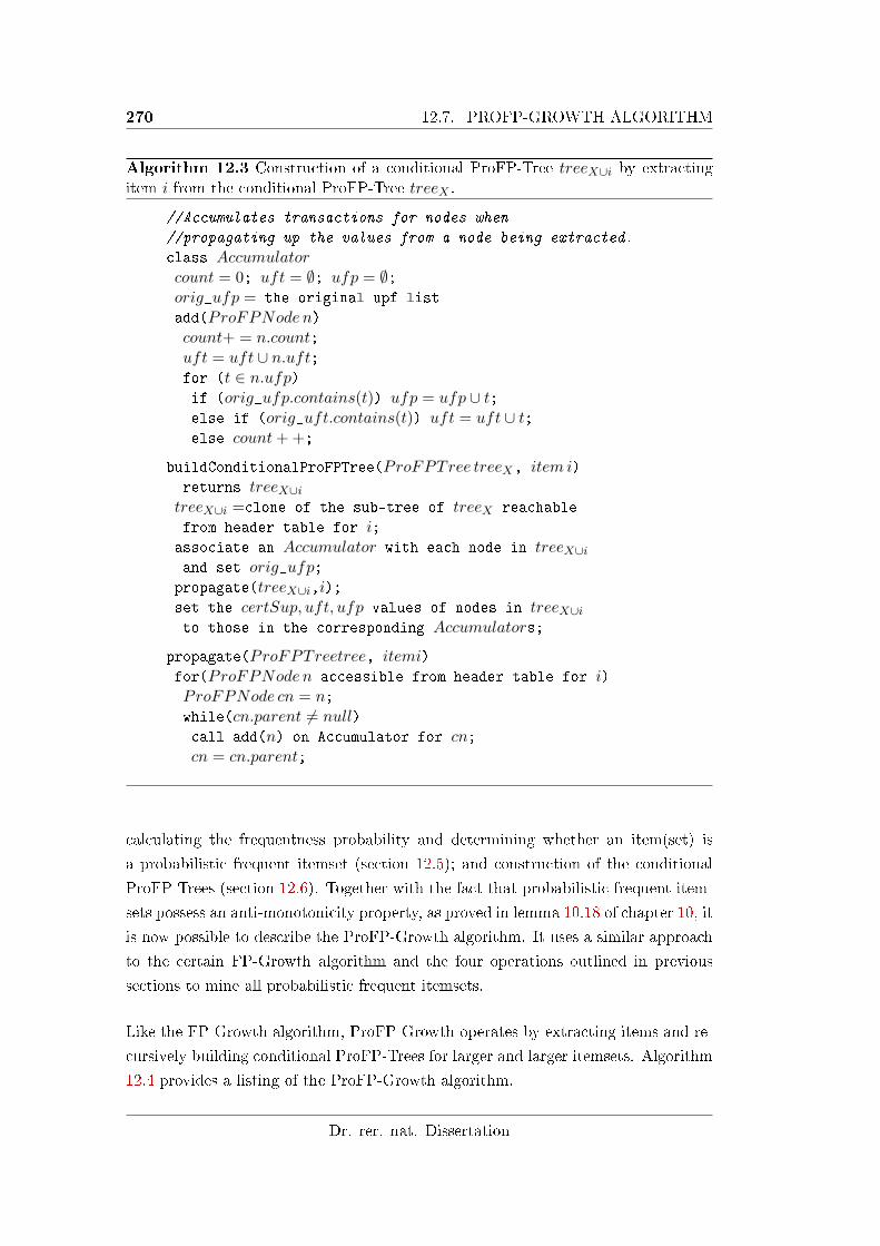
270 12.7. PROFP-GROWTH ALGORITHM
Algorithm 12.3 Construction of a conditional ProFP-Tree treeX∪i by extractingitem i from the conditional ProFP-Tree treeX .
//Accumulates transactions for nodes when
//propagating up the values from a node being extracted.
class Accumulatorcount = 0; uft = ∅; ufp = ∅;orig_ufp = the original upf list
add(ProFPNode n)count+ = n.count;uft = uft ∪ n.uft;for (t ∈ n.ufp)if (orig_ufp.contains(t)) ufp = ufp ∪ t;else if (orig_uft.contains(t)) uft = uft ∪ t;else count+ +;
buildConditionalProFPTree(ProFPTree treeX, item i)returns treeX∪itreeX∪i =clone of the sub-tree of treeX reachable
from header table for i;associate an Accumulator with each node in treeX∪iand set orig_ufp;
propagate(treeX∪i,i);set the certSup, uft, ufp values of nodes in treeX∪ito those in the corresponding Accumulators;
propagate(ProFPTreetree, itemi)for(ProFPNode n accessible from header table for i)ProFPNode cn = n;while(cn.parent 6= null)call add(n) on Accumulator for cn;cn = cn.parent;
calculating the frequentness probability and determining whether an item(set) is
a probabilistic frequent itemset (section 12.5); and construction of the conditional
ProFP-Trees (section 12.6). Together with the fact that probabilistic frequent item-
sets possess an anti-monotonicity property, as proved in lemma 10.18 of chapter 10, it
is now possible to describe the ProFP-Growth algorithm. It uses a similar approach
to the certain FP-Growth algorithm and the four operations outlined in previous
sections to mine all probabilistic frequent itemsets.
Like the FP-Growth algorithm, ProFP-Growth operates by extracting items and re-
cursively building conditional ProFP-Trees for larger and larger itemsets. Algorithm
12.4 provides a listing of the ProFP-Growth algorithm.
Dr. rer. nat. Dissertation
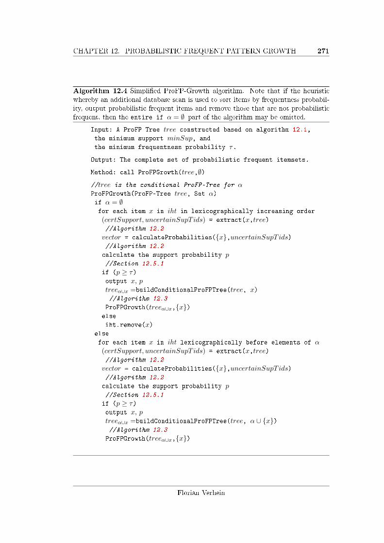
CHAPTER 12. PROBABILISTIC FREQUENT PATTERN GROWTH 271
Algorithm 12.4 Simpli�ed ProFP-Growth algorithm. Note that if the heuristicwhereby an additional database scan is used to sort items by frequentness probabil-ity, output probabilistic frequent items and remove those that are not probabilisticfrequent, then the entire if α = ∅ part of the algorithm may be omitted.
Input: A ProFP-Tree tree constructed based on algorithm 12.1,
the minimum support minSup, and
the minimum frequentness probability τ.
Output: The complete set of probabilistic frequent itemsets.
Method: call ProFPGrowth(tree,∅)
//tree is the conditional ProFP-Tree for αProFPGrowth(ProFP-Tree tree, Set α)if α = ∅for each item x in iht in lexicographically increasing order
(certSupport, uncertainSupT ids) = extract(x,tree)//Algorithm 12.2
vector = calculateProbabilities({x},uncertainSupT ids)//Algorithm 12.2
calculate the support probability p//Section 12.5.1
if (p ≥ τ)output x, ptreeα∪x =buildConditionalProFPTree(tree, x)//Algorithm 12.3
ProFPGrowth(treeα∪x,{x})else
iht.remove(x)else
for each item x in iht lexicographically before elements of α(certSupport, uncertainSupT ids) = extract(x,tree)//Algorithm 12.2
vector = calculateProbabilities({x},uncertainSupT ids)//Algorithm 12.2
calculate the support probability p//Section 12.5.1
if (p ≥ τ)output x, ptreeα∪x =buildConditionalProFPTree(tree, α ∪ {x})//Algorithm 12.3
ProFPGrowth(treeα∪x,{x})
Florian Verhein
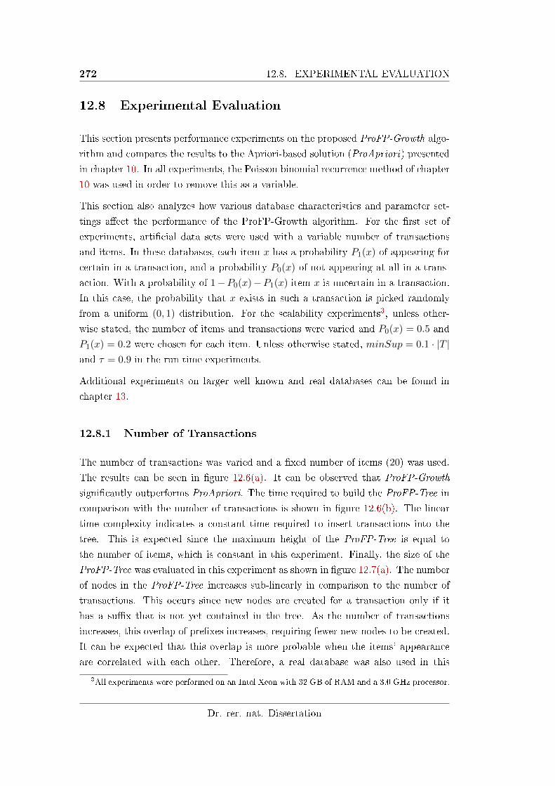
272 12.8. EXPERIMENTAL EVALUATION
12.8 Experimental Evaluation
This section presents performance experiments on the proposed ProFP-Growth algo-
rithm and compares the results to the Apriori-based solution (ProApriori) presented
in chapter 10. In all experiments, the Poisson binomial recurrence method of chapter
10 was used in order to remove this as a variable.
This section also analyzes how various database characteristics and parameter set-
tings a�ect the performance of the ProFP-Growth algorithm. For the �rst set of
experiments, arti�cial data sets were used with a variable number of transactions
and items. In these databases, each item x has a probability P1(x) of appearing for
certain in a transaction, and a probability P0(x) of not appearing at all in a trans-
action. With a probability of 1−P0(x)−P1(x) item x is uncertain in a transaction.
In this case, the probability that x exists in such a transaction is picked randomly
from a uniform (0, 1) distribution. For the scalability experiments3, unless other-
wise stated, the number of items and transactions were varied and P0(x) = 0.5 and
P1(x) = 0.2 were chosen for each item. Unless otherwise stated, minSup = 0.1 · |T |and τ = 0.9 in the run time experiments.
Additional experiments on larger well known and real databases can be found in
chapter 13.
12.8.1 Number of Transactions
The number of transactions was varied and a �xed number of items (20) was used.
The results can be seen in �gure 12.6(a). It can be observed that ProFP-Growth
signi�cantly outperforms ProApriori. The time required to build the ProFP-Tree in
comparison with the number of transactions is shown in �gure 12.6(b). The linear
time complexity indicates a constant time required to insert transactions into the
tree. This is expected since the maximum height of the ProFP-Tree is equal to
the number of items, which is constant in this experiment. Finally, the size of the
ProFP-Tree was evaluated in this experiment as shown in �gure 12.7(a). The number
of nodes in the ProFP-Tree increases sub-linearly in comparison to the number of
transactions. This occurs since new nodes are created for a transaction only if it
has a su�x that is not yet contained in the tree. As the number of transactions
increases, this overlap of pre�xes increases, requiring fewer new nodes to be created.
It can be expected that this overlap is more probable when the items' appearance
are correlated with each other. Therefore, a real database was also used in this
3All experiments were performed on an Intel Xeon with 32 GB of RAM and a 3.0 GHz processor.
Dr. rer. nat. Dissertation
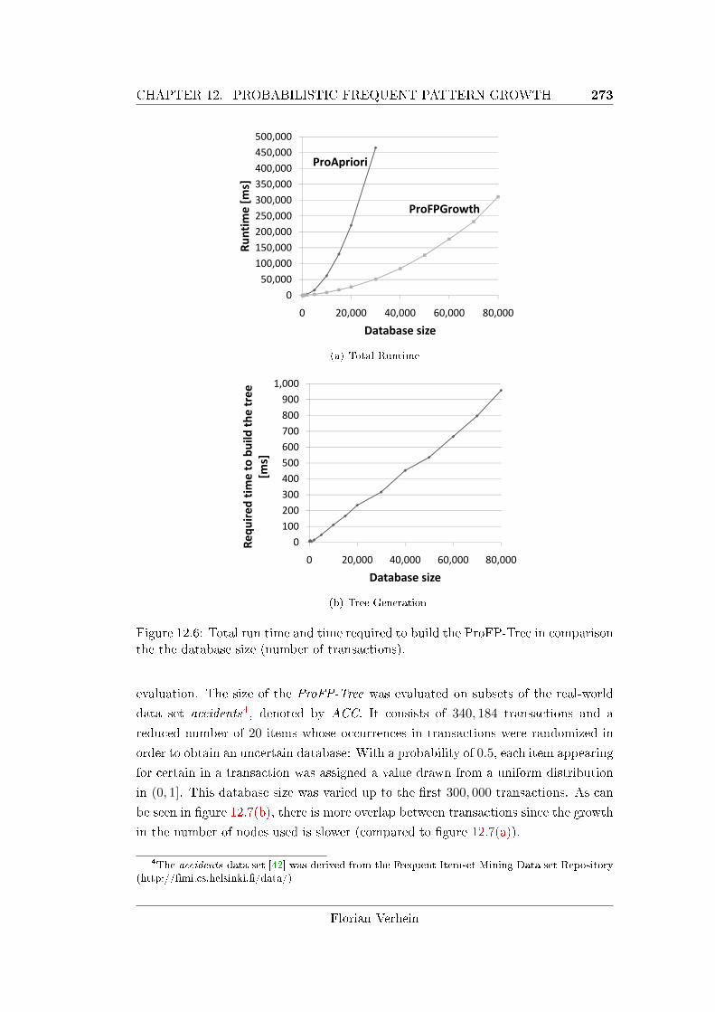
CHAPTER 12. PROBABILISTIC FREQUENT PATTERN GROWTH 273
050,000100,000150,000200,000250,000300,000350,000400,000450,000500,000
0 20,000 40,000 60,000 80,000
Runtim
e [m
s]
Database size
ProApriori
ProFPGrowth
(a) Total Runtime
0100200300400500600700800900
1,000
0 20,000 40,000 60,000 80,000
Requ
ired
tim
e to build the
tree
[ms]
Database size
(b) Tree Generation
Figure 12.6: Total run time and time required to build the ProFP-Tree in comparisonthe the database size (number of transactions).
evaluation. The size of the ProFP-Tree was evaluated on subsets of the real-world
data set accidents4, denoted by ACC. It consists of 340, 184 transactions and a
reduced number of 20 items whose occurrences in transactions were randomized in
order to obtain an uncertain database: With a probability of 0.5, each item appearing
for certain in a transaction was assigned a value drawn from a uniform distribution
in (0, 1]. This database size was varied up to the �rst 300, 000 transactions. As can
be seen in �gure 12.7(b), there is more overlap between transactions since the growth
in the number of nodes used is slower (compared to �gure 12.7(a)).
4The accidents data set [42] was derived from the Frequent Itemset Mining Data set Repository(http://�mi.cs.helsinki.�/data/)
Florian Verhein
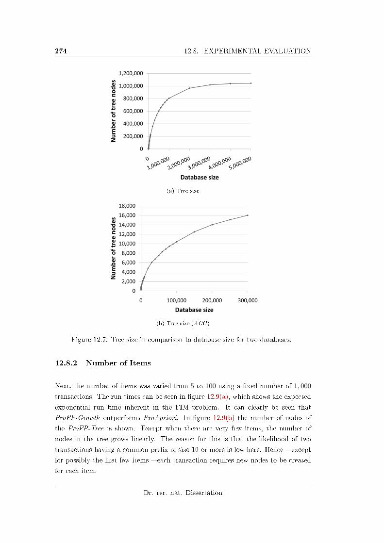
274 12.8. EXPERIMENTAL EVALUATION
0
200,000
400,000
600,000
800,000
1,000,000
1,200,000
Num
ber of tree
nod
es
Database size
(a) Tree size
0
2,000
4,000
6,000
8,000
10,000
12,000
14,000
16,000
18,000
0 100,000 200,000 300,000
Num
ber of tree
nod
es
Database size
(b) Tree size (ACC )
Figure 12.7: Tree size in comparison to database size for two databases.
12.8.2 Number of Items
Next, the number of items was varied from 5 to 100 using a �xed number of 1, 000
transactions. The run times can be seen in �gure 12.9(a), which shows the expected
exponential run time inherent in the FIM problem. It can clearly be seen that
ProFP-Growth outperforms ProApriori. In �gure 12.9(b) the number of nodes of
the ProFP-Tree is shown. Except when there are very few items, the number of
nodes in the tree grows linearly. The reason for this is that the likelihood of two
transactions having a common pre�x of size 10 or more is low here. Hence � except
for possibly the �rst few items � each transaction requires new nodes to be created
for each item.
Dr. rer. nat. Dissertation
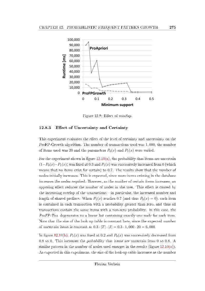
CHAPTER 12. PROBABILISTIC FREQUENT PATTERN GROWTH 275
010,00020,00030,00040,00050,00060,00070,00080,00090,000100,000
0 0.1 0.2 0.3 0.4 0.5
Runtim
e [m
s]
Minimum support
ProApriori
ProFPGrowth
Figure 12.8: E�ect of minSup.
12.8.3 E�ect of Uncertainty and Certainty
This experiment evaluates the e�ect of the level of certainty and uncertainty on the
ProFP-Growth algorithm. The number of transactions used was 1, 000, the number
of items used was 20 and the parameters P0(x) and P1(x) were varied.
For the experiment shown in �gure 12.10(a), the probability that items are uncertain
(1−P0(x)−P1(x)) was �xed at 0.3 and P1(x) was successively increased from 0 (which
means that no items exist for certain) to 0.7. The results show that the number of
nodes initially increases. This is expected, since more items existing in the database
increases the nodes required. However, as the number of certain items increases, an
opposing e�ect reduces the number of nodes in the tree. This e�ect is caused by
the increasing overlap of the transactions � in particular, the increased number and
length of shared pre�xes. When P1(x) reaches 0.7 (and thus P0(x) = 0), each item
is contained in each transaction with a probability greater than zero, and thus all
transactions contain the same items with a non-zero probability. In this case, the
ProFP-Tree degenerates to a linear list containing exactly one node for each item.
Note that the size of the look-up table is constant here, since the expected number
of uncertain items is constant at 0.3 · |T | · |I| = 0.3 · 1, 000 · 20 = 6, 000.
In �gure 12.10(b), P1(x) was �xed at 0.2 and P0(x) was successively decreased from
0.8 to 0. This increases the probability that items are uncertain from 0 to 0.8. A
similar pattern in the number of nodes used emerges in the results (�gure 12.10(a)).
As expected in this experiment, the size of the look-up table increases as the number
Florian Verhein
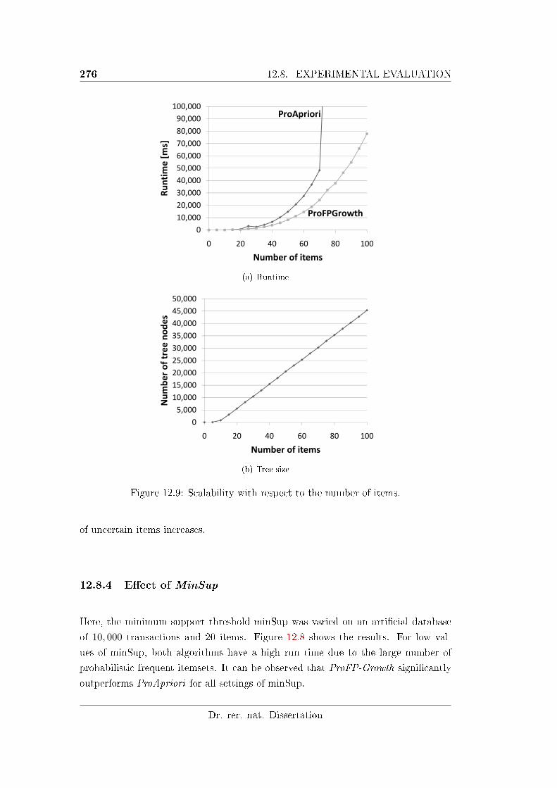
276 12.8. EXPERIMENTAL EVALUATION
010,00020,00030,00040,00050,00060,00070,00080,00090,000100,000
0 20 40 60 80 100
Runtim
e [m
s]
Number of items
ProApriori
ProFPGrowth
(a) Runtime
05,00010,00015,00020,00025,00030,00035,00040,00045,00050,000
0 20 40 60 80 100
Num
ber of tree
nod
es
Number of items
(b) Tree size
Figure 12.9: Scalability with respect to the number of items.
of uncertain items increases.
12.8.4 E�ect of MinSup
Here, the minimum support threshold minSup was varied on an arti�cial database
of 10, 000 transactions and 20 items. Figure 12.8 shows the results. For low val-
ues of minSup, both algorithms have a high run time due to the large number of
probabilistic frequent itemsets. It can be observed that ProFP-Growth signi�cantly
outperforms ProApriori for all settings of minSup.
Dr. rer. nat. Dissertation
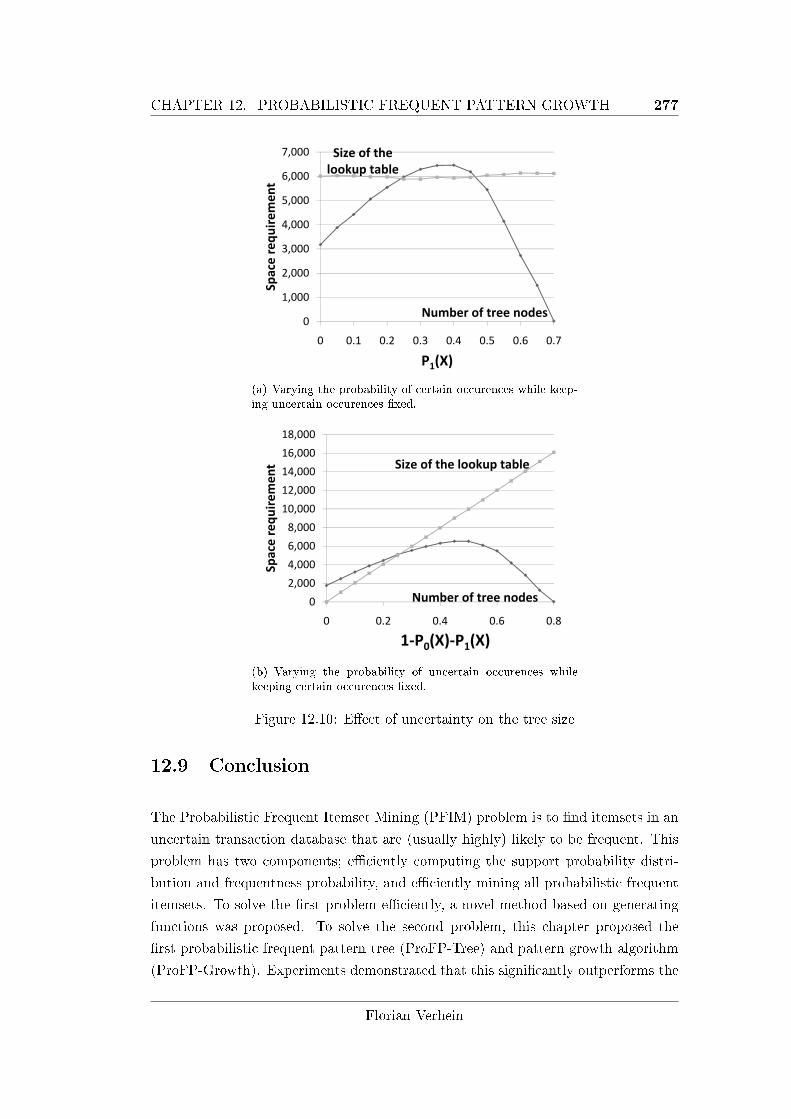
CHAPTER 12. PROBABILISTIC FREQUENT PATTERN GROWTH 277
7,000 Size of thelookup table
5 000
6,000
ent
lookup table
4,000
5,000
uireme
3,000
,
e requ
2,000Space
1,000
S
Number of tree nodes0
0 0.1 0.2 0.3 0.4 0.5 0.6 0.7
u be o t ee odes
P1(X)
(a) Varying the probability of certain occurences while keep-ing uncertain occurences �xed.
16 000
18,000
14,000
16,000
ent Size of the lookup table
10,000
12,000
uirem
8,000
10,000
e requ
4,000
6,000
Space
0
2,000
S
Number of tree nodes0
0 0.2 0.4 0.6 0.8
Number of tree nodes
1‐P0(X)‐P1(X)
(b) Varying the probability of uncertain occurences whilekeeping certain occurences �xed.
Figure 12.10: E�ect of uncertainty on the tree size
12.9 Conclusion
The Probabilistic Frequent Itemset Mining (PFIM) problem is to �nd itemsets in an
uncertain transaction database that are (usually highly) likely to be frequent. This
problem has two components; e�ciently computing the support probability distri-
bution and frequentness probability, and e�ciently mining all probabilistic frequent
itemsets. To solve the �rst problem e�ciently, a novel method based on generating
functions was proposed. To solve the second problem, this chapter proposed the
�rst probabilistic frequent pattern tree (ProFP-Tree) and pattern growth algorithm
(ProFP-Growth). Experiments demonstrated that this signi�cantly outperforms the
Florian Verhein

278 12.9. CONCLUSION
previous state of the art ProApriori approach to PFIM (presented in chapter 10).
Dr. rer. nat. Dissertation
Chapter 13
Vectorised Probabilistic Frequent
Itemset Mining using GIM
Uncertain transaction databases consist of sets of existentially uncertain
items. The uncertainty of items in transactions makes traditional frequent
itemset mining techniques inapplicable. This chapter tackles the Probabilis-
tic Frequent Itemset Mining (PFIM) problem.
In this context, this chapter makes the following contributions: The �rst
vectorised algorithm for solving the PFIM problem is proposed, resulting in a
much faster algorithm than the previous state of the art algorithms proposed
in chapters 10 and 12. In particular, it is shown that the PFIM problem
can be solved by the Generalised Interaction Mining (GIM) framework and
algorithm of chapter 3. An extensive experimental section evaluates GIM-
PFIM and shows that it is orders of magnitude faster and used orders of
magnitude less space than ProFP-Growth and Pro-Apriori.
279
280 13.1. INTRODUCTION
13.1 Introduction
Mining probabilistic frequent itemsets is a recent and challenging problem [18]. Re-
call from chapter 10 that in an Uncertain Transaction Database (UTDB), the infor-
mation captured in transactions is uncertain as the existence of an item is associated
with a likelihood measure or existential probability. Figure 12.1 shows the UTDB
that will be used as a running example in this chapter.
Recall from section 10.1 that given an uncertain transaction database, it is generally
not possible to determine whether an item or itemset is frequent because it is not
certain whether or not it appears in transactions. Consequently, traditional frequent
itemset mining methods cannot be applied to UTDBs.
Prior to the work in chapters 10, 11 and 12, expected support was used to deal with
uncertain databases [25, 26]. This method was shown to have signi�cant drawbacks,
causing misleading and even incorrect results. The proposed alternative is based on
computing the entire support probability distribution, but doing so very e�ciently.
Subsequently, either probabilistic frequent itemsets (chapters 10 and 12) or signi�cant
frequent itemsets (chapter 11) were mined.
However, the algorithm in which these methods were embedded has a large impact
on the run time of the overall mining algorithm. Chapter 10 developed ProApriori;
an Apriori style algorithm which is based on candidate generation and checking of
PFIMs. Chapter 12 improved on this by developing a probabilistic pattern growth
approach inspired by the FP-Growth method. Here, a compact representation of
the data set as an interlinked tree storing both certain and uncertain occurrences
enables faster run times than ProApriori. This chapter uses the GIM framework and
algorithm by casting the PFIM problem in terms of vectors and functions of vectors.
This mapping is both intuitive and allows the application of the GIM algorithm.
The resulting approach, called GIM-PFIM, is shown to be signi�cantly faster and
use much less memory than both ProApriori and ProFP-Growth. The improvement
in space usage and run time is about an order of magnitude better than ProFP-
Growth.
13.1.1 Research Problem and Data Model
This chapter solves the Probabilistic Frequent Itemset Mining (PFIM) problem (def-
inition 10) and the Signi�cant Frequent Itemset Mining (SiFIM) e�ciently. There
are two parts to these problems:
Dr. rer. nat. Dissertation
CHAPTER 13. VECTORISED PROBABILISTIC FREQUENT ITEMSETMINING 281
1. Given the existential probabilities of an itemset in all transactions, calculating
the support probability distribution and hence the frequentness probability or
the signi�cance of the given itemset.
2. Mine all itemsets that satisfy the frequentness or signi�cance constraints by
(a) Searching through the space of uncertain itemsets,
(b) Calculating the required probabilities for 1. and
(c) Using 1. to determine whether an itemset is interesting (a PFI or a SFI).
This chapter focuses on solving the second part of the problem very e�ciently. The
PFIM problem is solved by plugging in the methods for computing the frequentness
probability (either the Poisson binomial recurrence method of chapter 10 or equiv-
alently the generating function method of chapter 12). The SiFIM problem can be
solved by plugging in either of the two signi�cance tests proposed in chapter 11.
The uncertain data model applied in this chapter is based on the possible worlds
semantic with existential uncertain items as introduced in chapter 10.
13.1.2 Contributions
This chapter makes the following contributions:
• It shows that the PFIM problem can be cast into the vectorised GIM frame-
work, and hence that it can be solved using the GIM algorithm. The resulting
method for solving the PFIM problem, called GIM-PFIM, is orders of magni-
tude faster and requires orders of magnitude less space than the previous state
of the art algorithms for solving PFIM. This chapter is also the �rst work to
evaluate and compare all solutions to PFIM on well known and full sized real
world data sets.
• As a side e�ect, this work strengthens the argument for solutions at the abstract
level and further validates the �exibility, e�ciency and e�ectiveness of the GIM
framework and algorithm.
13.1.3 Organisation
The remainder of this chapter is organised as follows: Section 13.2 brie�y puts this
chapter in context, section 13.3 shows how the PFIM problem can be solved with
GIM, section 13.4 presents in depth experiments and this chapter concludes in section
13.5.
Florian Verhein
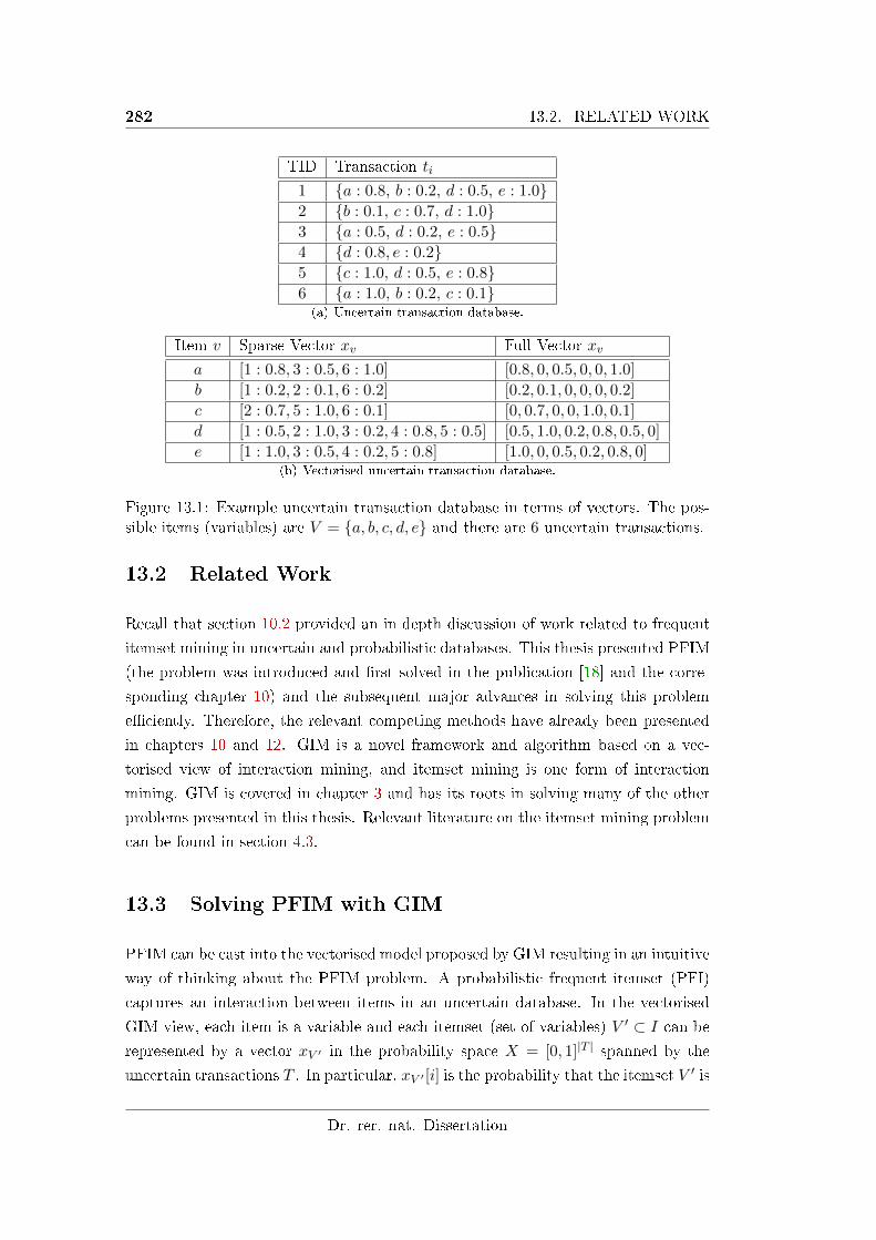
282 13.2. RELATED WORK
TID Transaction ti
1 {a : 0.8, b : 0.2, d : 0.5, e : 1.0}2 {b : 0.1, c : 0.7, d : 1.0}3 {a : 0.5, d : 0.2, e : 0.5}4 {d : 0.8, e : 0.2}5 {c : 1.0, d : 0.5, e : 0.8}6 {a : 1.0, b : 0.2, c : 0.1}(a) Uncertain transaction database.
Item v Sparse Vector xv Full Vector xv
a [1 : 0.8, 3 : 0.5, 6 : 1.0] [0.8, 0, 0.5, 0, 0, 1.0]
b [1 : 0.2, 2 : 0.1, 6 : 0.2] [0.2, 0.1, 0, 0, 0, 0.2]
c [2 : 0.7, 5 : 1.0, 6 : 0.1] [0, 0.7, 0, 0, 1.0, 0.1]
d [1 : 0.5, 2 : 1.0, 3 : 0.2, 4 : 0.8, 5 : 0.5] [0.5, 1.0, 0.2, 0.8, 0.5, 0]
e [1 : 1.0, 3 : 0.5, 4 : 0.2, 5 : 0.8] [1.0, 0, 0.5, 0.2, 0.8, 0](b) Vectorised uncertain transaction database.
Figure 13.1: Example uncertain transaction database in terms of vectors. The pos-sible items (variables) are V = {a, b, c, d, e} and there are 6 uncertain transactions.
13.2 Related Work
Recall that section 10.2 provided an in depth discussion of work related to frequent
itemset mining in uncertain and probabilistic databases. This thesis presented PFIM
(the problem was introduced and �rst solved in the publication [18] and the corre-
sponding chapter 10) and the subsequent major advances in solving this problem
e�ciently. Therefore, the relevant competing methods have already been presented
in chapters 10 and 12. GIM is a novel framework and algorithm based on a vec-
torised view of interaction mining, and itemset mining is one form of interaction
mining. GIM is covered in chapter 3 and has its roots in solving many of the other
problems presented in this thesis. Relevant literature on the itemset mining problem
can be found in section 4.3.
13.3 Solving PFIM with GIM
PFIM can be cast into the vectorised model proposed by GIM resulting in an intuitive
way of thinking about the PFIM problem. A probabilistic frequent itemset (PFI)
captures an interaction between items in an uncertain database. In the vectorised
GIM view, each item is a variable and each itemset (set of variables) V ′ ⊂ I can be
represented by a vector xV ′ in the probability space X = [0, 1]|T | spanned by the
uncertain transactions T . In particular, xV ′ [i] is the probability that the itemset V ′ is
Dr. rer. nat. Dissertation
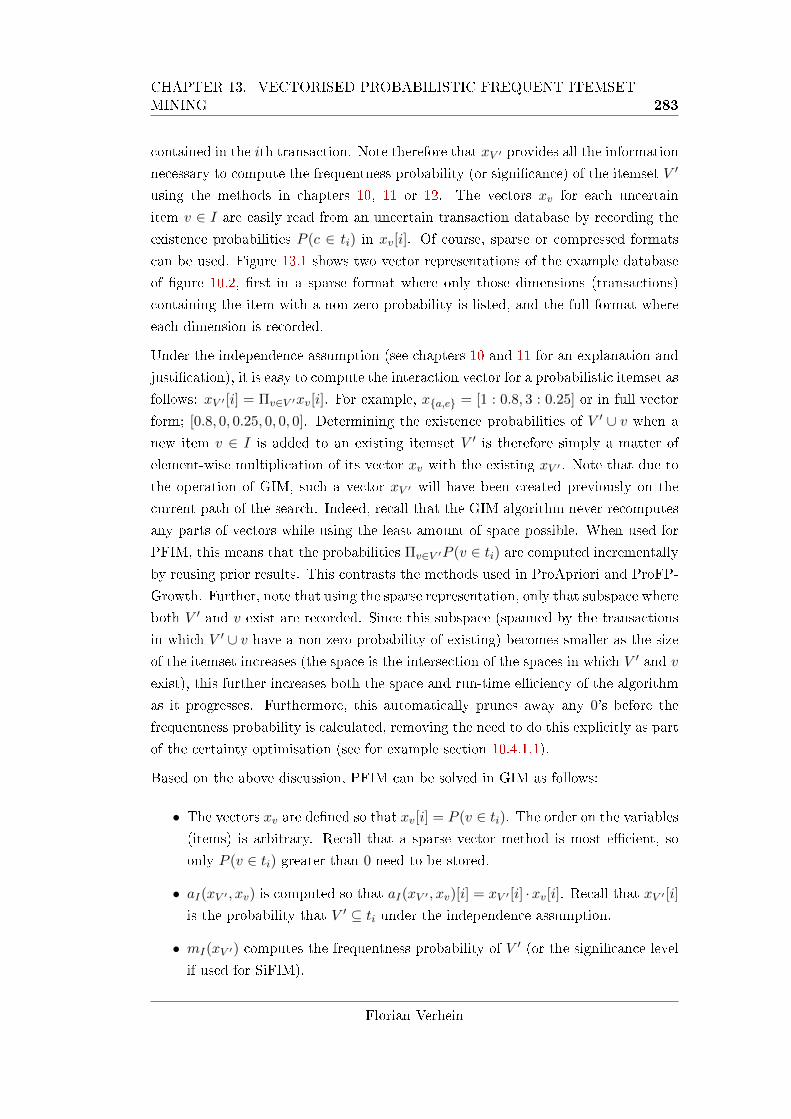
CHAPTER 13. VECTORISED PROBABILISTIC FREQUENT ITEMSETMINING 283
contained in the ith transaction. Note therefore that xV ′ provides all the information
necessary to compute the frequentness probability (or signi�cance) of the itemset V ′
using the methods in chapters 10, 11 or 12. The vectors xv for each uncertain
item v ∈ I are easily read from an uncertain transaction database by recording the
existence probabilities P (c ∈ ti) in xv[i]. Of course, sparse or compressed formats
can be used. Figure 13.1 shows two vector representations of the example database
of �gure 10.2, �rst in a sparse format where only those dimensions (transactions)
containing the item with a non-zero probability is listed, and the full format where
each dimension is recorded.
Under the independence assumption (see chapters 10 and 11 for an explanation and
justi�cation), it is easy to compute the interaction vector for a probabilistic itemset as
follows: xV ′ [i] = Πv∈V ′xv[i]. For example, x{a,e} = [1 : 0.8, 3 : 0.25] or in full vector
form; [0.8, 0, 0.25, 0, 0, 0]. Determining the existence probabilities of V ′ ∪ v when a
new item v ∈ I is added to an existing itemset V ′ is therefore simply a matter of
element-wise multiplication of its vector xv with the existing xV ′ . Note that due to
the operation of GIM, such a vector xV ′ will have been created previously on the
current path of the search. Indeed, recall that the GIM algorithm never recomputes
any parts of vectors while using the least amount of space possible. When used for
PFIM, this means that the probabilities Πv∈V ′P (v ∈ ti) are computed incrementally
by reusing prior results. This contrasts the methods used in ProApriori and ProFP-
Growth. Further, note that using the sparse representation, only that subspace where
both V ′ and v exist are recorded. Since this subspace (spanned by the transactions
in which V ′ ∪ v have a non-zero probability of existing) becomes smaller as the size
of the itemset increases (the space is the intersection of the spaces in which V ′ and v
exist), this further increases both the space and run-time e�ciency of the algorithm
as it progresses. Furthermore, this automatically prunes away any 0's before the
frequentness probability is calculated, removing the need to do this explicitly as part
of the certainty optimisation (see for example section 10.4.1.1).
Based on the above discussion, PFIM can be solved in GIM as follows:
• The vectors xv are de�ned so that xv[i] = P (v ∈ ti). The order on the variables(items) is arbitrary. Recall that a sparse vector method is most e�cient, so
only P (v ∈ ti) greater than 0 need to be stored.
• aI(xV ′ , xv) is computed so that aI(xV ′ , xv)[i] = xV ′ [i] ·xv[i]. Recall that xV ′ [i]is the probability that V ′ ⊆ ti under the independence assumption.
• mI(xV ′) computes the frequentness probability of V ′ (or the signi�cance level
if used for SiFIM).
Florian Verhein
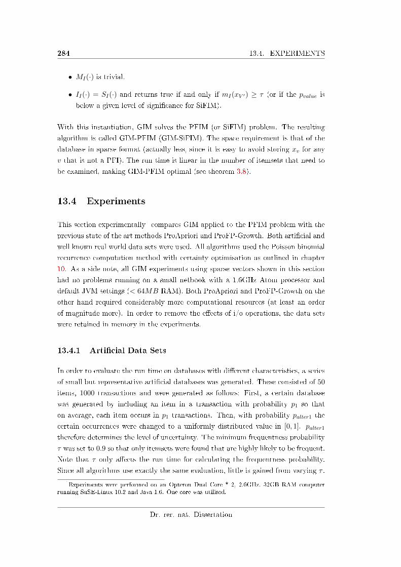
284 13.4. EXPERIMENTS
• MI(·) is trivial.
• II(·) = SI(·) and returns true if and only if mI(xV ′) ≥ τ (or if the pvalue is
below a given level of signi�cance for SiFIM).
With this instantiation, GIM solves the PFIM (or SiFIM) problem. The resulting
algorithm is called GIM-PFIM (GIM-SiFIM). The space requirement is that of the
database in sparse format (actually less, since it is easy to avoid storing xv for any
v that is not a PFI). The run time is linear in the number of itemsets that need to
be examined, making GIM-PFIM optimal (see theorem 3.8).
13.4 Experiments
This section experimentally1 compares GIM applied to the PFIM problem with the
previous state of the art methods ProApriori and ProFP-Growth. Both arti�cial and
well known real world data sets were used. All algorithms used the Poisson binomial
recurrence computation method with certainty optimisation as outlined in chapter
10. As a side note, all GIM experiments using sparse vectors shown in this section
had no problems running on a small netbook with a 1.6GHz Atom processor and
default JVM settings (< 64MB RAM). Both ProApriori and ProFP-Growth on the
other hand required considerably more computational resources (at least an order
of magnitude more). In order to remove the e�ects of i/o operations, the data sets
were retained in memory in the experiments.
13.4.1 Arti�cial Data Sets
In order to evaluate the run time on databases with di�erent characteristics, a series
of small but representative arti�cial databases was generated. These consisted of 50
items, 1000 transactions and were generated as follows: First, a certain database
was generated by including an item in a transaction with probability p1 so that
on average, each item occurs in p1 transactions. Then, with probability palter1 the
certain occurrences were changed to a uniformly distributed value in [0, 1]. palter1
therefore determines the level of uncertainty. The minimum frequentness probability
τ was set to 0.9 so that only itemsets were found that are highly likely to be frequent.
Note that τ only a�ects the run time for calculating the frequentness probability.
Since all algorithms use exactly the same evaluation, little is gained from varying τ .
1Experiments were performed on an Opteron Dual Core * 2, 2.6GHz, 32GB RAM computerrunning SuSE-Linux 10.2 and Java 1.6. One core was utilised.
Dr. rer. nat. Dissertation
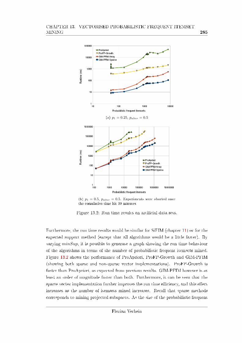
CHAPTER 13. VECTORISED PROBABILISTIC FREQUENT ITEMSETMINING 285
(a) p1 = 0.25, palter = 0.5
(b) p1 = 0.5, palter = 0.5. Experiments were aborted oncethe comulative time hit 30 minutes.
Figure 13.2: Run time results on arti�cial data sets.
Furthermore, the run time results would be similar for SiFIM (chapter 11) or for the
expected support method (except that all algorithms would be a little faster). By
varying minSup, it is possible to generate a graph showing the run time behaviour
of the algorithms in terms of the number of probabilistic frequent itemsets mined.
Figure 13.2 shows the performance of ProApriori, ProFP-Growth and GIM-PFIM
(showing both sparse and non-sparse vector implementations). ProFP-Growth is
faster than ProApriori, as expected from previous results. GIM-PFIM however is at
least an order of magnitude faster than both. Furthermore, it can be seen that the
sparse vector implementation further improves the run time e�ciency, and this e�ect
increases as the number of itemsets mined increases. Recall that sparse methods
corresponds to mining projected subspaces. As the size of the probabilistic frequent
Florian Verhein
286 13.4. EXPERIMENTS
itemsets increase, they de�ne smaller and smaller subspaces that need to be mined.
Hence the vectors become smaller and operations on these become faster.
The wave like e�ect that can be observed over the orders of magnitude is likely due
to the way the data sets were generated2.
13.4.2 Well Known and Real World Databases
The algorithms were also evaluated on two large, publicly available data sets: The
well known FIM database (T10I4D100K) consisting of 870 items and 100, 000 trans-
actions; and the real world retail data set with 16, 470 items and 88, 162 transactions.
Both are available from the FIM data set repository [39]. Being certain data sets,
these were altered as above to generate various uncertain databases. palter1 was var-
ied to values in {0, 0.25, 0.5, 0.75, 1}, where palter1 = 0 corresponds to the data set
remaining certain, and palter1 = 1 corresponding to a completely uncertain database
where no item exists for certain in any transaction. In the graphs, palter1 is denoted
by P (Alter1). GIM was used with sparse real vectors only.
T10I4D100K
Figures 13.3 and 13.4 show the results on the T10I4D100K data set. Again, minSup
was varied from 1000 to 2 to obtain the graph. The total time allowed for each
series of experiments (line in the graph) was limited however; 30 minutes for GIM,
and 2 hours for ProFP-Growth and ProApriori. In the completely uncertain data
set and for the lowest minSup setting (minSup = 2), ProFP-Growth achieves the
same run time as GIM. However, this setting corresponds to a support of only 2
out of the 100, 000 transactions, or 0.002%. Furthermore, it generates far too many
probabilistic frequent itemsets to be useful. When there is less uncertainty, this
crossover point increases to minSup = 17, or 0.017%. Such settings are pointless in
practice, where higher support is desired. It can clearly be seen that regardless of the
level of uncertainty in the data set, GIM outperforms ProFP-Growth for practical
levels of minSup, usually by one order of magnitude. ProApriori is over an order of
magnitude slower than ProFP-Growth, and at least two orders of magnitude slower
than GIM.2Since the probabilities were generated from the same distribution, all itemsets of size k can
be expected to have similar probabilities of being frequent but the larger the itemsets become, thesmaller their existence probabilities but the more of them there are. Further, the random numbergenerator is not a particularly robust. These e�ects lead to ranges for minSup where many itemsetsmust be examined while few are interesting, and other settings (when minSup is increased abovea certain threshold) where suddenly a higher percentage of the itemsets examined end up beingprobabilistically frequent.
Dr. rer. nat. Dissertation
CHAPTER 13. VECTORISED PROBABILISTIC FREQUENT ITEMSETMINING 287
Figure 13.3: Run time results on the uncertain T10I4D100K data set. The resultsare split up by palter1 value in �gure 13.4.
There is also a large di�erence in memory required between GIM and ProFP-Growth.
All the GIM experiments ran on the default JVM settings and required at most 48MB
of RAM. ProFP-Growth on the other hand, required up to about 7.4GB of RAM
� over one order of magnitude more. ProApriori generally used a few GB of RAM.
Incidentally, all GIM experiments happily run on a small netbook with the same run
time characteristics, albeit at a constant factor slower due to the slower CPU.
Florian Verhein
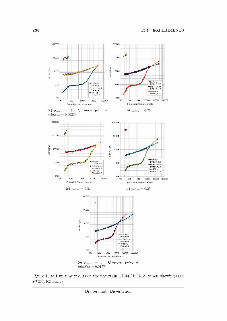
288 13.4. EXPERIMENTS
(a) palter = 1. Crossover point atminSup = 0.002%
(b) palter = 0.75.
(c) palter = 0.5. (d) palter = 0.25.
(e) palter = 0. Crossover point atminSup = 0.017%
Figure 13.4: Run time results on the uncertain T10I4D100K data set, showing eachsetting for palter1.
Dr. rer. nat. Dissertation
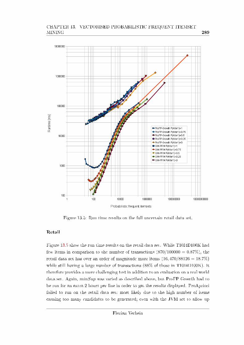
CHAPTER 13. VECTORISED PROBABILISTIC FREQUENT ITEMSETMINING 289
Figure 13.5: Run time results on the full uncertain retail data set.
Retail
Figure 13.5 show the run time results on the retail data set. While T10I4D100K had
few items in comparison to the number of transactions (870/100000 = 0.87%), the
retail data set has over an order of magnitude more items (16, 470/88126 = 18.7%)
while still having a large number of transactions (88% of those in T10I4D100K). It
therefore provides a more challenging test in addition to an evaluation on a real world
data set. Again, minSup was varied as described above, but ProFP-Growth had to
be run for an extra 2 hours per line in order to get the results displayed. ProApriori
failed to run on the retail data set; most likely due to the high number of items
causing too many candidates to be generated; even with the JVM set to allow up
Florian Verhein
290 13.5. CONCLUSION
to 20GB or RAM. The results clearly show that GIM-PFIM is superior to ProFP-
Growth for all minSup settings and all levels of uncertainty. The improvement
ranges up to over 2 orders of magnitude.
13.5 Conclusion
Probabilistic frequent itemset mining (PFIM) is a challenging problem, requiring
both e�cient computation of the support probability distribution, and algorithms
able to mine all probabilistic itemsets e�ciently. This chapter presented the fastest
and most e�cient algorithm to date for PFIM. It beats the previous state of the art
algorithms by at least an order of magnitude. In addition, the results in this chapter
lend weight to the wide ranging applicability, e�ectiveness and e�ciency of the GIM
framework and algorithm.
Dr. rer. nat. Dissertation

Part V
Conclusions
291

Chapter 14
Conclusions and Future Work
This thesis was organised into three main research themes: Part II considered vari-
ous interaction mining problems and proposed novel solutions at the abstract level
via generalised frameworks and an e�cient vectorised computation model. Part III
considered the integration of rigorous statistical approaches in novel data mining
methods, and part IV proposed and solved the problem of mining probabilistic fre-
quent itemsets in uncertain databases.
Uncertain or probabilistic databases pose signi�cant challenges for the KDD process.
They require the development of specialist algorithms that take into account the
probability distributions of the data in order to deliver useful results to the user.
This was demonstrated in the context of frequent itemset mining, where existing
work treated itemsets as being interesting if their expected support was high. This
is known as the expected FIM (EFIM) problem. While the EFIM approach lead to
the relatively easy extension of FIM algorithms, it has the fundamental �aw that
it provides no con�dence in the result. Indeed, it was shown in this thesis that it
leads to scenarios where itemsets are labeled frequent even if they are actually more
likely to be infrequent. It was also demonstrated that the expected support approach
labeled many patterns interesting in a random database, even though these patterns
were statistically insigni�cant. Clearly, this is undesirable.
In response to these problems, part IV of this thesis proposed and solved the Prob-
abilistic Frequent Itemset Mining (PFIM) problem, where itemsets are considered
interesting if the probability that they are frequent is high. PFIM delivers high qual-
ity patterns and does not su�er the downsides of EFIM since it uses the probability
distribution of an itemset's support. This methodology made the problem much
more challenging however. In particular, two problems needed to be addressed:
293
294
First, an e�cient method was required to calculate an itemset's support probabil-
ity distribution (SPDF) and frequentness probability. This thesis used the possible
worlds model and a proposed probabilistic framework to solve this problem in var-
ious ways: Novel methods based on the Poisson binomial recurrence (chapter 10)
and generating functions (chapter 12) were developed. Despite calculating the ex-
act SPDF and frequentness probability, these avoided the exponential run time of
naive solutions and had run times close to the EFIM method. Approximate results
using a Normal approximation are also investigated (chapter 11). Secondly, novel
algorithms needed to be developed in order to e�ciently calculate and feed itemsets'
existence probabilities to the frequentness probability computation method, and in
turn search through the space of itemsets. Since more probability information is re-
quired in comparison to EFIM, specialist algorithms had to be developed. This thesis
�rst developed ProApriori, which is based on the candidate generation and testing
framework (chapter 10). Then, ProFP-Growth was proposed in chapter 12. This was
the �rst probabilistic FP-Growth type algorithm and used a proposed probabilistic
frequent pattern tree (Pro-FPTree) to avoid candidate generation, while being able
to compress the uncertain transaction database in a loss-less manner. Finally, the
PFIM problem was mapped to the GIM framework, casting PFIM as a vectorised
interaction mining problem in chapter 13. The resulting GIM-PFIM algorithm is
the current fastest known algorithm for solving the PFIM problem. In comparison
to ProApriori and ProFP-Growth, it achieved orders of magnitude improvements in
space and time usage. Furthermore, it lead to an intuitive subspace and probability-
vector based interpretation of PFIM. Incremental methods were also proposed to
answer queries such as �nding the top-k probabilistic frequent itemsets.
This thesis identi�ed a fundamental problem with the prior state of the art approach
to mining itemsets in uncertain databases, proposed an alternative approach that
overcame these problems and examined it in depth. This demonstrates the need
and advantages of developing specialist algorithms that take account the probability
distribution of the target measure in uncertain or probabilistic databases. It also
showed that doing so can not only lead to higher quality output for the user, but very
e�cient algorithms. This thesis contributed a range of methods that e�ciently �nd
high quality probabilistic frequent patterns in uncertain or probabilistic databases,
potentially rendering the previous expectation based method obsolete.
Another hypothesis considered in this thesis was that statistical techniques embedded
within data mining and machine learning methods lead to better descriptive and
predictive outcomes. Therefore, signi�cance tests and Pearson's correlation were
used to develop various novel data mining approaches. The use of signi�cance tests
Dr. rer. nat. Dissertation
CHAPTER 14. CONCLUSIONS AND FUTURE WORK 295
was based on the observation that data mining is a hypothesis generating endeavour,
and that DM algorithms make decisions in their search for interesting patterns. Since
the database is a sample, the patterns found should describe hypotheses about the
underlying process that generated the data. Furthermore, a DM algorithm should
ideally deliver patterns that are statistically signi�cant, so that they are unlikely to
have occurred by chance, noise or sampling e�ects. Finally, the decisions made by an
algorithm during its search should ideally also be signi�cant, so that the search itself
is not sensitive to `chance'. These issues are often ignored. It is desirable to provide
some minimal level of con�dence that the patterns found are in fact signi�cant, and
that the algorithm does not make decisions likely to have occurred by chance. Post
processing is not an e�ective solution to these problem for two reasons: First, it
cannot address the issue of signi�cant algorithmic decisions. Secondly, it means that
what the user is ultimately interested in (the knowledge provided at the output of
post-processing) is not what the data mining algorithm is actually searching for. At
best, this is very ine�cient. At worst, the algorithm never �nds those patterns that
the post-processing task would rate most highly.
One method used in this thesis to mine signi�cant patterns is to use signi�cance
tests within the search and interestingness measures themselves. This means that
both the decisions made by the search, as well as the patterns found, have high con-
�dence. This approach was used in chapter 8, which addressed the problem of rule
based classi�cation of standard and in particular, highly imbalanced (skewed) data
sets. Mining data sets with an imbalanced class distribution is challenging and is re-
quired in applications such as medical diagnosis and fraud detection. In the proposed
SPARCCC method, rules are interesting if they have a positive class correlation ratio,
are statistically signi�cant based on Fisher's exact test and are positively associated.
The search also progresses based on signi�cance tests and therefore mines signi�cant
rules directly. In contrast, many other associative classi�cation methods were based
on the support framework and subsequent �ltering. This was found to lead to rules
with a bias against the minority class, rules that were statistically insigni�cant or
could be correlated more highly with an alternative class to the one they predict.
By relying on the popular support-con�dence framework and �ltering the results in
post processing, these methods were also very ine�cient; requiring that many rules
be mined but discarding up to 99% of them in order to achieve acceptable classi�-
cation performance. SPARCCC on the other hand achieved the same accuracy on
balanced data sets and much higher classi�cation performance on imbalanced data
sets, discovered orders of magnitude fewer � but high quality � rules and discarded
none of them.
Florian Verhein
296
A second method to deliver only signi�cant results is to mine patterns that are in-
teresting with a high probability; that is, to generate a signi�cance test around an
existing interestingness measure. This approach is taken in chapter 11, where item-
sets are mined if they are signi�cantly frequent. Again, a non-parametric method was
used and the results had a higher quality than the alternative expectation approach.
Finally, Pearson's product moment correlation coe�cient was used in a number of
novel methods in this thesis. Chapter 9 considered the problem of mining complex
maximal cliques of correlated variables (attributes) for the purpose of feature selec-
tion, meaningful dimensionality reduction, and as an interaction mining technique
in its own right. An e�cient algorithm was developed based on a proven structural
constraint on complex correlation graphs. Correlation was also used successfully for
mining correlated multiplication rules for interaction mining and feature generation;
and conjunctive correlation rules for classi�cation.
Together then, these results support the hypothesis that better predictive and de-
scriptive patterns are mined by the incorporation of statistical techniques embedded
directly within novel data mining methods.
This thesis developed a range of data mining methods that can be covered by the
term interaction mining. While solving these problems, it was discovered that many
aspects were similar when regarded from a suitably abstracted view: In general, a
data set can be considered as a set of variables about which one has samples. In-
teraction mining is the process of mining structures on these variables that describe
interaction patterns. Usually, these structures can be represented as sets or graphs;
where each variable interacts, to some degree, with other variables in the structure.
Such interactions can also be complex, representing both positive and negative rela-
tionships, and can include negative patterns. Furthermore, the presence of particular
interactions can in�uence another interaction or variable in interesting ways. These
latter kinds of interactions can be expressed as rules. Recall that interactions are
of interest in many domains, ranging from social network analysis, marketing, the
sciences, to statistics and �nance. Furthermore, many data mining tasks can be
considered as mining interactions, such as clustering, frequent itemset mining, rule
based classi�cation, graph mining, etc.
Therefore, the research problem was to develop abstract frameworks, a computational
model and algorithms capable of modeling, capturing and solving a wide range of
such interaction mining problems at the abstract level, and to do so very e�ciently.
This was a challenging task since such problems have very di�erent semantics govern-
ing the interactions, their structures and their interpretation: The pattern de�nitions
Dr. rer. nat. Dissertation
CHAPTER 14. CONCLUSIONS AND FUTURE WORK 297
and semantics are di�erent; what makes an interaction pattern interesting is di�er-
ent; how the search should progress is di�erent and the data is also very di�erent.
Finally, solving interaction mining problems usually requires the simultaneous and
interdependent development of new pattern semantics and specialist algorithms for
mining the respective pattern. One can therefore conclude that it is not easy to
develop models abstract enough to capture this variation in interaction mining prob-
lems, while at the same time enabling the development of equally abstract algorithms
that also solves them e�ciently � ideally, more e�ciently than specialist algorithms.
But this is what part II of this thesis achieved:
Chapter 3 introduced and solved the GIM problem. GIM uses an e�cient and
intuitive computational model based purely on vectors and vector valued functions.
The semantics of the interactions, their interestingness measures and the type of data
considered are all �exible components. Intuitively, each interaction is represented by
a vector in a space typically spanned by the samples in the database. The search
progresses by performing functions on these vectors. The GIM algorithm runs in
linear time in the number of interesting interactions and uses little space. Chapter 3
showed how GIM can be applied to a wide range of problems, including graph mining,
counting based methods, itemset mining, clique mining, clustering, complex pattern
mining, negative pattern mining, solving an optimisation problem, etc. Later, it was
shown that it can solve many of the problems considered in other parts of this thesis.
For example, it turns out to be the most e�cient solution to the PFIM problem
considered in part IV. It can also solve the problems considered in chapter 9 and 5.
Other interaction mining problems considered in this thesis are covered in chapters
4 and 5. Chapter 4 presented a vectorised framework and novel algorithm called
GLIMIT for solving abstract itemset mining problems from a geometric perspective
in a transposed database. It is shown to outperform FP-Growth and Apriori on
the frequent itemset mining task. An e�cient method for generating association
rules was also presented. Chapter 5 considered the problem of mining complex co-
location patterns between di�erent types of objects in a real world spatial database.
When applied to a large astronomy database, this mines relationships � including
negative relationships and the e�ect of multiple occurrences � between di�erent types
of galaxies. Part of this problem was solved with GLIMIT but can be solved directly
with GIM.
Chapter 6 introduced and solved the Generalised Rule Mining (GRM) problem.
Rules are an important interaction pattern but existing approaches were limited to
conjunctions of binary literals, �xed measures and counting based algorithms. Rules
can be much more diverse, useful and interesting! The chapter rede�ned rule mining
Florian Verhein
298
in terms of a similar vectorised computational model to that used in GIM. This ab-
straction was motivated through the introduction of three diverse and novel methods
addressing problems including correlation based classi�cation, �nding interactions for
improving regression models and �nding probabilistic association rules in uncertain
databases. Two of these methods were introduced in chapter 6 (Probabilistic As-
sociation Rule Mining (PARM) in uncertain databases and Conjunctive Correlation
Rules (CCRules) for classi�cation), while one was introduced in chapter 7. Fur-
thermore, the SPARCCC method can also be solved with GRM, as was outlined in
chapter 8. Since interactions between variables in a database are often unknown to
the detriment of further analysis, classi�cation or mining tasks, chapter 7 proposes
Correlated Multiplication Rules (CMRules). These capture interactions predictive
of a dependent variable and are the �rst rules with multiplicative semantics. Fur-
thermore, a feature selection and dimensionality reduction method was described
whereby CMRules are used to generate composite features. One advantage of this is
that it enables linear models to learn non-linear decision boundaries with respect to
the original variables.
In summary then, in addition to proposing and solving the PFIM problem and
developing useful methods based on statistical approaches in data mining, this the-
sis successfully abstracted and solved the problem of mining interactions between
variables. The interaction mining problem was solved through the development of
abstract frameworks and algorithms operating on a vectorised computational model.
By doing this, one can separate the semantics of an interaction mining problem from
the algorithm used to mine it, allowing both to vary independently of each other.
This makes it easier to develop new methods by allowing the data miner to focus
only on their problem's semantics and then plug them into a framework. Further-
more, the frameworks make it easy to push good interestingness measures (such as
signi�cance tests and correlation) directly into the mining process. This leads to
higher quality results, more e�cient solutions and less reliance on measures that are
traditionally easier to implement but are not necessarily correlated with predictive
or descriptive performance (for example, support). Examples where these aspects
were demonstrated in this thesis include chapters 3, 5, 6, 7, 8, 9 and 13. Results
in this thesis also suggest that forcing good quality interestingness measures (that
correlate with the user's utility) to be anti-monotonic to allow for e�ective pruning
when they do not naturally have pruning friendly properties (for example, using the
improvement methods described in chapter 3 and 6), gives much better results than
using interestingness measures that are not directly related to the users utility, but
allow good pruning.
Dr. rer. nat. Dissertation
CHAPTER 14. CONCLUSIONS AND FUTURE WORK 299
By removing the burden of designing an e�cient algorithm, it is also easier for end
users to design custom data mining algorithms. By allowing the algorithms to vary
independently of the problem, new ones can be developed that can be immediately
be applied to solve many problems. Since it was shown that all problems considered
in this thesis can (at least retrospectively) be mapped to and solved by GIM or GRM,
any new GIM or GRM algorithm can immediately speed up all of these problems
without specialisation or modi�cation. This property is particularly advantageous
when DM is embedded into practical applications. The GIM and GRM algorithms
are already e�cient however, achieving the asymptotically optimal linear run time
in the number of interactions that must be examined and using little space. When
applied to speci�c problems, they turned out to be most e�cient. For example, the
PFIM problem was solved not only most e�ciently, but also most intuitively using
the GIM framework.
The vectorised computational model introduced in this thesis also encourages an
interesting geometric way of thinking about pattern mining problems in terms of
vector operations and subspaces � especially when an interestingness measure has
a geometric interpretation. Such a geometric interpretation leads to new insights
and can inspire new methods. For example, mining rules based on reducing the
angle between a vector representing the antecedent and the vector representing the
consequent. This idea was used successfully in chapters 6 and 7. Developing methods
that are now possible are also fruitful avenues for future work. For example, prior to
the development of GRM, multiplication rules were never considered and could not be
mined with existing methods. However, their use in chapter 7 turned out to be useful
for feature generation and interaction mining. Evaluating this application further
is a candidate for future work. GIM also provided a novel vector and subspace-
search interpretation of the search for interesting patterns. For example, this was
discussed in the context of probabilistic databases. There is plenty of scope for the
evaluation of other existing or novel methods using the GIM and GRM frameworks.
For example, recall that it was shown in chapter 3 that GIM may be used to solve a
wide range of problems, from itemset mining to complex pattern mining to clustering
to graph mining to optimisation. Later in the thesis, a number of these problems
were considered in detail, together with experimental evaluations and comparison to
the state of the art where applicable. Evaluating the others in depth, or developing
new methods inspired by the vectorised framework are also promising directions for
future work.
Florian Verhein

300
Dr. rer. nat. Dissertation
Bibliography
[1] Sloan digital sky survey / skyserver, http://cas.sdss.org/dr6/en/.
[2] D.J. Newman A. Asuncion. UCI machine learning repository, 2007.
[3] Herve Abdi. Bonferroni and sidak corrections for multiple comparisons. 2007.
[4] Abramowitz and Stegun. Handbook of Mathematical Functions With Formulas,
Graphs, and Mathematical Tables. 10 edition, 1972.
[5] Ramesh C. Agarwal, Charu C. Aggarwal, and V. V. V. Prasad. Depth �rst
generation of long patterns. In ACM SIGKDD international conference on
Knowledge discovery and data mining, pages 108�118. ACM Press, 2000.
[6] Ramesh C. Agarwal, Charu C. Aggarwal, and V. V. V. Prasad. A tree pro-
jection algorithm for generation of frequent itemsets. Journal of Parallel and
Distributed Computing, 61:350�371, 2000.
[7] Charu C. Aggarwal, Yan Li, Jianyong Wang, and Jing Wang. Frequent pattern
mining with uncertain data. In Proc. of the 15th ACM SIGKDD international
conference on Knowledge discovery and data mining, 2009.
[8] Charu C. Aggarwal and Philip S. Yu. A survey of uncertain data algorithms
and applications. IEEE Trans. on Knowl. and Data Eng., 21(5):609�623, 2009.
[9] Parag Agrawal, Omar Benjelloun, Anish Das Sarma, Chris Hayworth, Shubha
Nabar, Tomoe Sugihara, and Jennifer Widom. Trio: A system for data, un-
certainty, and lineage. In 32nd International Conference on Very Large Data
Bases. VLDB 2006 (demonstration description), 2006.
[10] Rakesh Agrawal, Tomasz Imielinsk, and Arun Swami. Mining association rules
between sets of items in large databases. In SIGMOD '93: Proceedings of the
1993 ACM SIGMOD international conference on Management of data, pages
207�216. ACM Press, 1993.
301
302 BIBLIOGRAPHY
[11] Rakesh Agrawal and Ramakrishnan Srikant. Fast algorithms for mining asso-
ciation rules. In Proceedings of 20th International Conference on Very Large
Data Bases VLDB, pages 487�499. Morgan Kaufmann, 1994.
[12] Ghazi Al-Naymat, Sanjay Chawla, and Bavani Arunasalam. Enumeration of
maximal clique for mining spatial co-location patterns. tr 615. Technical report,
School of Information Technologies, University of Sydney, Australia, 2007.
[13] Maria-Luiza Antonie and Osmar R. Zaiane. An associative classi�er based on
positive and negative rules. In 9th ACM SIGMOD workshop on Research Issues
in Data Mining and Knowledge Discovery(DMKD-04), pages 64�69, 2004.
[14] L. Antova, T. Jansen, C. Koch, and D Olteanu. Fast and simple relational
processing of uncertain data. In IEEE International Conference on Data En-
gineering (ICDE08), pages 983 � 992. IEEE, 2008.
[15] Bavani Arunasalam and Sanjay Chawla. Cccs: a top-down associative classi�er
for imbalanced class distribution. In Proceedings of the 12th ACM SIGKDD
international conference on Knowledge discovery and data mining, pages 517�
522, New York, NY, USA, 2006. ACM Press.
[16] Bavani Arunasalam, Sanjay Chawla, and Pei Sun. Striking two birds with
one stone: Simultaneous mining of positive and negative spatial patterns. In
Proceedings of the Fifth SIAM International Conference on Data Mining, pages
173�182, 2005.
[17] Omar Benjelloun, Anish Das Sarma, Alon Halevy, and Jennifer Widom. Uldbs:
databases with uncertainty and lineage. In VLDB '06: Proceedings of the
32nd international conference on Very large data bases, pages 953�964. VLDB
Endowment, 2006.
[18] Thomas Bernecker, Hans-Peter Kriegel, Matthias Renz, Florian Verhein, and
Andreas Zü�e. Probabilistic frequent itemset mining in uncertain databases. In
Proceedings of the 15th ACM SIGKDD International Conference on Knowledge
Discovery and Data Mining (SIGKDD'09), pages 119�128. ACM, 2009.
[19] Thomas Bernecker, Hans-Peter Kriegel, Matthias Renz, Florian Verhein, and
Andreas Zü�e. Probabilistic frequent pattern growth for itemset mining in
uncertain databases (technical report). CoRR, abs/1008.2300, 2010.
[20] Ferenc Bodon. A fast apriori implementation. In In Proceedings of the IEEE
ICDM Workshop on Frequent Itemset Mining Implementations, 2003.
Dr. rer. nat. Dissertation
BIBLIOGRAPHY 303
[21] Tom Brijs, Gilbert Swinnen, Koen Vanhoof, and Geert Wets. Using association
rules for product assortment decisions: A case study. In Knowledge Discovery
and Data Mining, pages 254�260, 1999.
[22] Sergey Brin, Rajeev Motwani, and Craig Silverstein. Beyond market baskets:
generalizing association rules to correlations. In ACM SIGMOD International
Conference on Management of Data, pages 265�276. ACM, 1997.
[23] Doug Burdick, Manuel Calimlim, and Johannes Gehrke. Ma�a: A maximal
frequent itemset algorithm for transactional databases. In In International
Conference on Data Engineering, pages 443�452, 2001.
[24] Reynold Cheng, Dmitri V. Kalashnikov, and Sunil Prabhakar. Evaluating
probabilistic queries over imprecise data. In SIGMOD '03: Proceedings of the
2003 ACM SIGMOD international conference on Management of data, pages
551�562. ACM, 2003.
[25] Chun Kit Chui and Ben Kao. A decremental approach for mining frequent
itemsets from uncertain data. In The 12th Paci�c-Asia Conference on Knowl-
edge Discovery and Data Mining (PAKDD), pages 64�75, 2008.
[26] Chun Kit Chui, Ben Kao, and Edward Hung. Mining frequent itemsets from
uncertain data. In 11th Paci�c-Asia Conference on Advances in Knowledge
Discovery and Data Mining, PAKDD 2007, Nanjing, China, pages 47�58, 2007.
[27] William W. Cohen. Fast e�ective rule induction. In International Conference
on Machine Learning. Morgan Kaufmann, 1995.
[28] Gao Cong, Anthony K.H.Tung, Xin Xu, Feng Pan, and Jiong Yang. Farmer:
Finiding interesting rule groups in microarray datasets. In 23rd ACM SIGMOD
International Conference on Management of Data Proceedings, pages 145�154,
2004.
[29] Gao Cong, Kian-Lee Tan, Anthony K.H.Tung, and Feng Pan. Mining frequent
closed patterns in microarray data. In 2004 IEEE International Conference on
Data Mining (ICDM'04) Proceedings, pages 363�366, 2004.
[30] Gao Cong, Kian-Lee Tan, Anthony K.H.Tung, and Xin Xu. Mining top-k
covering rule groups for gene expression data. In ACM SIGMOD/PODS 2005
Proceedings, pages 670�681, 2005.
[31] Gerard E. Dallal. The little handbook of statistical practice.
http://www.statisticalpractice.com.
Florian Verhein
304 BIBLIOGRAPHY
[32] N. Dalvi and D. Suciu. E�cient query evaluation on probabilistic databases.
The VLDB Journal, 16(4):523�544, 2007.
[33] William DuMouchel and Daryl Pregibon. Empirical bayes screening for multi-
item associations. In KDD '01: Proceedings of the seventh ACM SIGKDD
international conference on Knowledge discovery and data mining, pages 67�
76. ACM, 2001.
[34] Brian Dunkel and Nandit Soparkar. Data organization and access for e�cient
data mining. In International Conference on Data Engineering (ICDE99),
pages 522�529, 1999.
[35] Usama Fayyad, Gregory Piatetsky-shapiro, and Padhraic Smyth. From data
mining to knowledge discovery in databases. AI Magazine, 17:37�54, 1996.
[36] Usama M. Fayyad, Gregory Piatetsky-Shapiro, and Padhraic Smyth. From
data mining to knowledge discovery: an overview. Advances in knowledge
discovery and data mining, pages 1�34, 1996.
[37] Workshop on frequent itemset mining implementations 2003.
http://�mi.cs.helsinki.�/�mi03.
[38] Workshop on frequent itemset mining implementations 2004.
http://�mi.cs.helsinki.�/�mi04.
[39] Frequent itemset mining dataset repository. http://�mi.cs.helsinki.�/data/.
[40] Johannes Fürnkranz. Fossil: A robust relational learner. In Machine Learning:
ECML94, volume 784 of Lecture Notes in Computer Science, pages 122�137.
Springer Berlin / Heidelberg, 1994.
[41] Erich Gamma, Richard Helm, Ralph Johnson, and John Vlissides. Design
Patterns: Elements of Reusable Object-Oriented Software. Addison Wesley
Professional, 1994.
[42] Karolien Geurts, Geert Wets, Tom Brijs, and Koen Vanhoof. Pro�ling high
frequency accident locations using association rules. In Proceedings of the 82nd
Annual Transportation Research Board, Washington DC. (USA), January 12-
16, page 18pp, 2003.
[43] B. Goethals. "Survey on frequent pattern mining.". In Technical report,
Helsinki Institute for Information Technology, 2003.
Dr. rer. nat. Dissertation
BIBLIOGRAPHY 305
[44] Joseph Hair, Bill Black, Barry Babin, Rolph Anderson, and Ronald Tatham.
Multivariate Data Analysis (6th Edition). Pearson, November 2005.
[45] M.A. Hall and L.A. Smith. Feature subset selection: a correlation based �lter
approach. In N. Kasabov and et al., editors, Proc Fourth International Con-
ference on Neural Information Processing and Intelligent Information Systems,
pages 855�858, Dunedin, New Zealand, 1997.
[46] Jiawei Han and Micheline Kamber. Data Mining: Concepts and Techniques.
Morgan Kaufmann Publishers, 2000.
[47] Jiawei Han, Jian Pei, and Yiwen Yin. Mining frequent patterns without candi-
date generation. In ACM SIGMOD International Conference on Management
of Data (SIGMOD'00). ACM Press, 2000.
[48] Jiawei Han, Jian Pei, Yiwen Yin, and Runying Mao. Mining frequent patterns
without candidate generation: A frequent-pattern tree approach. Data Mining
and Knowledge Discovery, pages 53�87, 2004.
[49] Yan Huang, Hui Xiong, Shashi Shekhar, and Jian Pei. Mining con�dent co-
location rules without a support threshold. In Proceedings of the 18th ACM
Symposium on Applied Computing ACM SAC, 2003.
[50] Damon D. Judd. What's so special about spatial data? Earth Observation
Magazine, 2005.
[51] Jon Kleinberg and Eva Tardos. Algorithm Design. Addison Wesley, 2006.
[52] Jia-Ling Koh and Pei-Wy Yo. An e�cient approach for mining fault-tolerant
frequent patterns based on bit vector representations. In Lecture Notes in
Computer Science: DASFAA05: Database Systems for Advanced Applications.
Springer-Verlag, 2005.
[53] Flip Korn, Alexandros Labrinidis, Yannis Kotidis, and Christos Faloutsos.
Quanti�able data mining using ratio rules. VLDB Journal: Very Large Data
Bases, 8(3�4):254�266, 2000.
[54] H.-P. Kriegel, P. Kunath, M. Pfei�e, and M. Renz. "Probabilistic Similarity
Join on Uncertain Data". In Proc. 11th Int. Conf. on Database Systems for
Advanced Applications, Singapore, pp. 295-309, 2006.
[55] H.O. Lancaster. The chi-squared distribution. In John Wiley & Sons Ltd,
1969.
Florian Verhein
306 BIBLIOGRAPHY
[56] Srivatsan Laxman, Prasad Naldurg, Raja Sripada, and Ramarathnam Venkate-
san. Connections between mining frequent itemsets and learning generative
models. In ICDM '07: Proceedings of the 2007 Seventh IEEE International
Conference on Data Mining, pages 571�576, Washington, DC, USA, 2007.
IEEE Computer Society.
[57] Carson Leung, Mark Mateo, and Dale Brajczuk. A tree-based approach for
frequent pattern mining from uncertain data. In Advances in Knowledge Dis-
covery and Data Mining, volume 5012 of Lecture Notes in Computer Science,
pages 653�661. Springer Berlin / Heidelberg, 2008.
[58] Carson Kai-Sang Leung, Christopher L. Carmichael, and Boyu Hao. E�cient
mining of frequent patterns from uncertain data. In ICDMW '07: Proceedings
of the Seventh IEEE International Conference on Data Mining Workshops,
pages 489�494, 2007.
[59] Jian Li, Barna Saha, and Amol Deshpande. A uni�ed approach to ranking in
probabilistic databases. Proceedings of the VLDB Endowment, 2(1):502�513,
2009.
[60] Wenmin Li, Jiawei Han, and Jian Pei. Cmar: Accurate and e�cient classi-
�cation based on multiple class-association rules. In Proceedings of the 2001
IEEE International Conference on Data Mining (ICDM01), pages 369�376.
IEEE Computer Society, 2001.
[61] Bing Liu, Wynne Hsu, and Yiming Ma. Integrating classi�cation and asso-
ciation rule mining. In Knowledge Discovery and Data Mining, pages 80�86,
1998.
[62] Yasuhiko Morimoto. Mining frequent neighboring class sets in spatial
databases. In Proceedings of the Seventh ACM SIGKDD international confer-
ence on Knowledge discovery and data mining, pages 353 � 358. ACM Press-
New York, 2001.
[63] Shinichi Morishita and Jun Sese. Traversing itemset lattice with statistical
metric pruning. In Symposium on Principles of Database Systems, pages 226�
236, 2000.
[64] Rob Munro, Sanjay Chawla, and Pei Sun. Complex spatial relationships. In
Proceedings of the 3rd IEEE International Conference on Data Mining, ICDM
2003, pages 227�234. IEEE Computer Society, 2003.
Dr. rer. nat. Dissertation
BIBLIOGRAPHY 307
[65] P. M. Murphy and D. W. Aha. UCI repository of machine learning databases.
Machine-readable data repository, University of California, Department of In-
formation and Computer Science, Irvine, CA, 1992.
[66] Gonzalo Navarro and Veli Mäkinen. Compressed full-text indexes. ACM Com-
puting Surveys, 39(1):2, 2007.
[67] Nips 2003 workshop on feature extraction.
http://clopinet.com/isabelle/projects/nips2003.
[68] Balaji Padmanabhan and Alexander Tuzhilin. On characterization and discov-
ery of minimal unexpected patterns in rule discovery. IEEE Trans. on Knowl.
and Data Eng., 18(2):202�216, 2006.
[69] F. Pan, G. Cong, A. Tung, J. Yang, and M. Zaki. Carpenter: Finding closed
patterns in long biological datasets. In Proceedings of the Ninth ACM SIGKDD
International Conference on Knowledge Discovery and Data Mining. Morgan
Kaufmann, 2003.
[70] Feng Pan, Wei Wang, Anthony K. H. Tung, and Jiong Yang. Finding repre-
sentative set from massive data. In ICDM '05: Proceedings of the Fifth IEEE
International Conference on Data Mining, pages 338�345, Washington, DC,
USA, 2005. IEEE Computer Society.
[71] Jong Soo Park, Ming-Syan Chen, and Philip S. Yu. An e�ective hash-based
algorithm for mining association rules. In SIGMOD '95: Proceedings of the
1995 ACM SIGMOD international conference on Management of data, pages
175�186, New York, NY, USA, 1995. ACM.
[72] Nicolas Pasquier, Yves Bastide, Ra�k Taouil, and Lot� Lakhal. Discovering
frequent closed itemsets for association rules. In Database Theory (ICDT99),
volume 1540 of Lecture Notes in Computer Science, pages 398�416. Springer,
1999.
[73] Jian Pei, Jiawei Han, Hongjun Lu, Shojiro Nishio, Shiwei Tang, and Dongqing
Yang. H-mine: Hyper-structure mining of frequent patterns in large databases.
In IEEE International Conference on Data Mining (ICDM01), pages 441�448,
2001.
[74] Jian Pei, Jiawei Han, and Runying Mao. CLOSET: An e�cient algorithm for
mining frequent closed itemsets. In ACM SIGMOD Workshop on Research
Issues in Data Mining and Knowledge Discovery, pages 21�30, 2000.
Florian Verhein
308 BIBLIOGRAPHY
[75] Jian Pei and Ming Hua. Mining uncertain and probabilistic data: prob-
lems, challenges, methods, and applications. In Proceeding of the 14th ACM
SIGKDD international conference on Knowledge discovery and data mining
(SIGKDD08), New York, NY, USA, 2008. ACM.
[76] Ross Quinlan. C4.5: Programs for Machine Learning. Morgan Kaufmann,
1993.
[77] Christopher Ré, Nilesh Dalvi, and Dan Suciu. E�cient top-k query evaluation
on probalistic databases. In International Conference on Data Engineering
(ICDE07), pages 886�895, 2007.
[78] Ulrich Ruckert, Lothar Richter, and Stefan Kramer. Quantitative association
rules based on half-spaces: An optimization approach. In International Con-
ference on Data Mining (ICDM04), pages 507�510. IEEE Computer Society,
2004.
[79] P. Sen and A. Deshpande. Representing and querying correlated tuples in
probabilistic databases. In International Conference on Data Engineering
(ICDE07), 2007.
[80] Shashi Shekhar and Yan Huang. Discovering spatial co-location patterns: A
summary of results. Lecture Notes in Computer Science, 2121:236+, 2001.
[81] Pradeep Shenoy, Gaurav Bhalotia, Jayant R. Haritsa T, Mayank Bawa,
S. Sudarshan, and Devavrat Shah. Turbo-charging vertical mining of large
databases. In ACM SIGMOD International Conference on Management of
Data, pages 22�33, 2000.
[82] Craig Silverstein, Sergey Brin, and Rajeev Motwani. Beyond market baskets:
Generalizing association rules to dependence rules. Data Mining and Knowl-
edge Discovery, 2(1):39�68, 1998.
[83] M.A. Soliman, I.F. Ilyas, and K. Chen-Chuan Chang. Top-k query process-
ing in uncertain databases. In International Conference on Data Engineering
(ICDE07), pages 896�905, 2007.
[84] Ramakrishnan Srikant and Rakesh Agrawal. Mining quantitative association
rules in large relational tables. In ACM SIGMOD International Conference on
Management of Data, pages 1�12. ACM, 1996.
[85] Ramakrishnan Srikant, Quoc Vu, and Rakesh Agrawal. Mining association
rules with item constraints. In International Conference on Knowledge Discov-
ery in Databases (KDD97), pages 67�73. AAAI Press, 1997.
Dr. rer. nat. Dissertation
BIBLIOGRAPHY 309
[86] Michael Steinbach, Pang-Ning Tan, Hui Xiong, and Vipin Kumar. Generalizing
the notion of support. In The Tenth ACM SIGKDD International Conference
on Knowledge Discovery and Data Mining KDD'04, 2004.
[87] Rani J. Swargam and Mathew J. Palakal. The role of least frequent item sets
in association discovery. In International Conference on Digital Information
Management (ICDIM07), pages 217�223. IEEE, 2007.
[88] Pang-Ning Tan, Michael Steinbach, and Vipin Kumar. Introduction to Data
Mining. Addison Wesley, 2006.
[89] Adriano Veloso, Wagner Meira Jr., and Mohammed J. Zaki. Lazy associative
classi�cation. In IEEE International Conference on Data Mining (ICDM06),
pages 645�654. IEEE Computer Society, 2006.
[90] Florian Verhein. k-stars: Sequences of spatio-temporal association rules. In
The 1st Workshop on Spatial and Spatio-temporal Data Mining (SSTDM'06),
Workshops Proceedings of the 6th IEEE International Conference on Data Min-
ing (ICDM 2006), pages 387�394. IEEE Computer Society, 2006.
[91] Florian Verhein. Mining complex, maximal and complete sub-graph and sets of
correlated variables with applications to feature subset selection. In Proceedings
of the SIAM International Conference on Data Mining, SDM 2008, April 24-
26, 2008, Atlanta, Georgia, USA, pages 597�608, 2008.
[92] Florian Verhein. Mining complex spatio-temporal sequence patterns. In Pro-
ceedings of the SIAM International Conference on Data Mining (SDM 2009),
pages 605�616. SIAM, 2009.
[93] Florian Verhein. Generalised rule mining. In Proceedings of the 15th Inter-
national Conference on Database Systems for Advanced Applications (DAS-
FAA'06), Lecture Notes in Computer Science. Springer, 2010.
[94] Florian Verhein and Ghazi Al-Naymat. Fast mining of complex spatial co-
location patterns using glimit. In Workshops Proceedings of the 7th IEEE
International Conference on Data Mining (ICDM'07). IEEE Computer Society,
2007.
[95] Florian Verhein and Sanjay Chawla. Mining spatio-temporal association
rules, sources, sinks, stationary regions and thoroughfares in object mobility
databases. InWorkshops Proceedings of the 5th IEEE International Conference
on Data Mining (ICDM 2005), pages 41�52. IEEE Computer Society, 2005.
Florian Verhein
310 BIBLIOGRAPHY
[96] Florian Verhein and Sanjay Chawla. Geometrically inspired itemset min-
ing. In Proceedings of the 6th IEEE International Conference on Data Mining
(ICDM'06), pages 655�666. IEEE Computer Society, 2006.
[97] Florian Verhein and Sanjay Chawla. Mining spatio-temporal association
rules, sources, sinks, stationary regions and thoroughfares in object mobility
databases. In The 11th International Conference on Database Systems for Ad-
vanced Applications (DASFAA'06), volume 3882 of Lecture Notes in Computer
Science, pages 187�201. Springer, 2006.
[98] Florian Verhein and Sanjay Chawla. Using signi�cant, positively and rela-
tively class correlated rules for associative classi�cation of imbalanced datasets.
In Proceedings of the 7th IEEE International Conference on Data Mining
(ICDM'07). IEEE Computer Society, 2007.
[99] Florian Verhein and Sanjay Chawla. Mining spatio-temporal patterns in object
mobility databases. Data Mining and Knowledge Discovery, 2008.
[100] Jianyong Wang and George Karypis. Harmony: E�ciently mining the best
rules for classi�cation. In SIAM International Conference on Data Mining
(SDM05), 2005.
[101] Jianyong Wang and Jian Pei. Closet+: searching for the best strategies for
mining frequent closed itemsets. In ACM SIGKDD International Conference
on Knowledge Discovery in Databases, pages 236�245, 2003.
[102] Performance prediction challenge, wcci model selection workshop, 2006.
http://www.modelselect.inf.ethz.ch/datasets.php.
[103] Geo�rey I. Webb. Discovering signi�cant rules. In 12th ACM SIGKDD Inter-
national Conference on Knowledge Discovery and Data Mining (SIGKDD06),
pages 434�443. ACM Press, 2006.
[104] Ian H. Witten and Eibe Frank. Data Mining: Practical machine learning tools
and techniques, 2nd Edition. Morgan Kaufmann, 2005.
[105] Michael Wolfe. Vector optimization vs. vectorization. In Supercomputing, Lec-
ture Notes in Computer Science. Springer, 1988.
[106] Sun X. and A.B. Nobel. Signi�cance and recovery of block structures in bi-
nary matrices with noise. In Technical report, pages 217�223. Department of
Statistics and Operations Research, UNC Chapel Hill, 2005.
Dr. rer. nat. Dissertation
BIBLIOGRAPHY 311
[107] Yi Xia, Yirong Yang, and Yun Chi. Mining association rules with non-uniform
privacy concerns. In DMKD '04: Proceedings of the 9th ACM SIGMOD work-
shop on Research issues in data mining and knowledge discovery, pages 27�34,
2004.
[108] Hui Xiong, Shashi Shekhar, Pang-Ning Tan, and Vipin Kumar. Exploiting a
support-based upper bound of pearson's correlation coe�cient for e�ciently
identifying strongly correlated pairs. In ACM SIGKDD International Confer-
ence on Knowledge Discovery in Databases, pages 334�343. ACM, 2004.
[109] K. Yi, F. Li, G. Kollios, and D. Srivastava. E�cient processing of top-k queries
in uncertain databases. In 24th International Conference on Data Engineering
(ICDE'08), 2008.
[110] Xiaoxin Yin and Jiawei Han. CPAR: Classi�cation based on predictive asso-
ciation rules. In Proceedings of the Third SIAM International Conference on
Data Mining. SIAM, 2003.
[111] Mohammed J. Zaki. Scalable algorithms for association mining. IEEE Trans-
actions on Knowledge and Data Engineering, 12:372�390, 2000.
[112] Mohammed J. Zaki and Karam Gouda. Fast vertical mining using di�sets.
In 9th ACM SIGKDD International Conference on Knowledge Discovery and
Data Mining (SIGKDD'03), pages 326�335, 2003.
[113] Mohammed J. Zaki and Ching jui Hsiao. Charm: An e�cient algorithm for
closed itemset mining. In In 2nd SIAM International Conference on Data
Mining, pages 457�473, 2002.
[114] Qin Zhang, Feifei Li, and Ke Yi. Finding frequent items in probabilistic data.
In Jason Tsong-Li Wang, editor, SIGMOD Conference, pages 819�832. ACM,
2008.
[115] Wenjie Zhang, Xuemin Lin, Jian Pei, and Ying Zhang. Managing uncertain
data: Probabilistic approaches. In The Ninth International Conference on
Web-Age Information Management (WAIM '08), 2008.
[116] Xin Zhang, Nikos Mamoulis, David W. Cheung, and Yutao Shou. Fast mining
of spatial collocations. In Proceedings of the tenth ACM SIGKDD international
conference on Knowledge discovery and data mining, pages 384 � 393. ACM
Press-New York, 2004.
Florian Verhein
Related Documents