MNRAS 000, 1–55 (2021) Preprint February 23, 2021 Compiled using MNRAS L A T E X style file v3.0 General-relativistic hydrodynamics of non-perfect fluids: 3+1 conservative formulation and application to viscous black-hole accretion Michail Chabanov 1 , Luciano Rezzolla 1,2,3 and Dirk H. Rischke 1 1 Institut für Theoretische Physik, Goethe-Universität, Max-von-Laue-Str. 1, 60438 Frankfurt am Main, Germany 2 Frankfurt Institute for Advanced Studies, Ruth-Moufang-Str. 1, 60438 Frankfurt am Main, Germany 3 School of Mathematics, Trinity College, Dublin 2, Ireland Accepted XXX. Received YYY; in original form ZZZ ABSTRACT We consider the relativistic hydrodynamics of non-perfect fluids with the goal of de- termining a formulation that is suited for numerical integration in special-relativistic and general-relativistic scenarios. To this end, we review the various formulations of relativistic second-order dissipative hydrodynamics proposed so far and present in detail a particular formulation that is fully general, causal, and can be cast into a 3+1 flux-conservative form as the one employed in modern numerical-relativity codes. As an example, we employ a variant of this formulation restricted to a relaxation- type equation for the bulk viscosity in the general-relativistic magnetohydrodynam- ics code BHAC. After adopting the formulation for a series of standard and non- standard tests in 1+1-dimensional special-relativistic hydrodynamics, we consider a novel general-relativistic scenario, namely, the stationary, spherically symmetric vis- cous accretion onto a black hole. The newly developed solution – which can exhibit even considerable deviations from the inviscid counterpart – can be used as a testbed for numerical codes simulating non-perfect fluids on curved backgrounds. Key words: hydrodynamics, shock waves, accretion 1 INTRODUCTION The detection of the first binary neutron-star (BNS) merger event, GW170817 (Abbott et al. 2017a) has provided a new valuable tool to study matter and gravity under extreme conditions. Espe- cially the detection of electromagnetic counterparts in form of a short gamma-ray burst (Abbott © 2021 The Authors arXiv:2102.10419v1 [gr-qc] 20 Feb 2021

Welcome message from author
This document is posted to help you gain knowledge. Please leave a comment to let me know what you think about it! Share it to your friends and learn new things together.
Transcript
MNRAS 000, 1–55 (2021) Preprint February 23, 2021 Compiled using MNRAS LATEX style file v3.0
General-relativistic hydrodynamics of non-perfect fluids: 3+1
conservative formulation and application to viscous black-hole
accretion
Michail Chabanov1, Luciano Rezzolla1,2,3 and Dirk H. Rischke11Institut für Theoretische Physik, Goethe-Universität, Max-von-Laue-Str. 1, 60438 Frankfurt am Main, Germany
2Frankfurt Institute for Advanced Studies, Ruth-Moufang-Str. 1, 60438 Frankfurt am Main, Germany
3School of Mathematics, Trinity College, Dublin 2, Ireland
Accepted XXX. Received YYY; in original form ZZZ
ABSTRACTWe consider the relativistic hydrodynamics of non-perfect fluids with the goal of de-
termining a formulation that is suited for numerical integration in special-relativistic
and general-relativistic scenarios. To this end, we review the various formulations of
relativistic second-order dissipative hydrodynamics proposed so far and present in
detail a particular formulation that is fully general, causal, and can be cast into a 3+1
flux-conservative form as the one employed in modern numerical-relativity codes.
As an example, we employ a variant of this formulation restricted to a relaxation-
type equation for the bulk viscosity in the general-relativistic magnetohydrodynam-
ics code BHAC. After adopting the formulation for a series of standard and non-
standard tests in 1+1-dimensional special-relativistic hydrodynamics, we consider a
novel general-relativistic scenario, namely, the stationary, spherically symmetric vis-
cous accretion onto a black hole. The newly developed solution – which can exhibit
even considerable deviations from the inviscid counterpart – can be used as a testbed
for numerical codes simulating non-perfect fluids on curved backgrounds.
Key words: hydrodynamics, shock waves, accretion
1 INTRODUCTION
The detection of the first binary neutron-star (BNS) merger event, GW170817 (Abbott et al. 2017a)
has provided a new valuable tool to study matter and gravity under extreme conditions. Espe-
cially the detection of electromagnetic counterparts in form of a short gamma-ray burst (Abbott
© 2021 The Authors
arX
iv:2
102.
1041
9v1
[gr
-qc]
20
Feb
2021
2 M. Chabanov, L. Rezzolla and D.H. Rischke
et al. 2017b) and of a kilonova (Drout et al. 2017; Cowperthwaite et al. 2017) accompanying
GW170817, has made this event an incredibly rich laboratory for physics, providing a number of
constraints on the equation of state (EOS) of nuclear matter (see, e.g., Margalit & Metzger 2017;
Bauswein et al. 2017; Rezzolla et al. 2018; Ruiz et al. 2018; Annala et al. 2018; Radice et al.
2018b; Most et al. 2018; De et al. 2018; Abbott et al. 2018; Montaña et al. 2019; Raithel et al.
2018; Tews et al. 2018; Malik et al. 2018; Koeppel et al. 2019; Shibata et al. 2019).
BNS mergers are highly dynamical and nonlinear phenomena especially during the first few
milliseconds after merger, (see, e.g., Baiotti & Rezzolla 2017; Paschalidis 2017; Burns 2020, for
some reviews). As has been shown recently, harmonic density oscillations in this violent phase
could be damped significantly due to bulk-viscosity dissipation coming from modified Urca pro-
cesses (Alford et al. 2018, 2020; Alford & Haber 2020). Thus, bulk viscosity might lead to modifi-
cations in the post-merger gravitational-wave signal. Furthermore, it was shown in high-resolution
general-relativistic magnetohydrodynamic (GRMHD) calculations that the matter after merger is
unstable to MHD instabilities, e.g., the Kelvin-Helmholtz instability (Baiotti et al. 2008; Radice &
Rezzolla 2012) and the magnetorotational instability (Siegel et al. 2013; Kiuchi et al. 2018). Due
to these instabilities, turbulence can develop and be maintained, which will ultimately influence
BNS-merger observables such as the gravitational-wave signal and the ejected matter.
The emergence of turbulence clearly represents a challenge for numerical-relativity simula-
tions, which can only be performed with limited resolutions and are normally carried out with
resolutions that are well above the scale at which turbulence is physically quenched off. As a re-
sult, a number of studies have employed effective shear-viscous models in order to capture the
effects of magneto-turbulent motion in the remnant of BNS mergers. An approach to handle this
problem has been suggested with the use of general-relativistic large-eddy simulations (LES) in
pure hydrodynamics. This method maps effects from numerical calculations with high resolution
to simulations with lower resolution, which would otherwise disappear in an implicit filtering
procedure (Radice 2017; Radice et al. 2018a,c; Radice 2020). The same method has been system-
atically extended to the full set GRMHD equations to study the amplification of the magnetic field
shortly after merger (Viganò et al. 2020; Aguilera-Miret et al. 2020). In this way, it was shown that
by considering the subgrid-scale model for the induction equation only, and suitably increasing
(well above the expected value of order one) the phenomenological coefficients associated with
the LES terms, magnetic-field strengths comparable to an high-resolution direct simulation can be
achieved.
While the robustness and universality – i.e., their effectiveness to capture multi-scale turbu-
MNRAS 000, 1–55 (2021)
GRHD of non-perfect fluids 3
lence without expensive fine tuning – remains to be assessed (see Duez et al. 2020, for a careful
comparison of momentum transport models for numerical relativity), the inclusion of genuinely
dissipative effects already in the general-relativistic hydrodynamics or MHD equations offers the
possibility to study a variety of physical phenomena on more robust grounds, where the much
larger computational costs can be compensated by the use of high-order methods [see, e.g., Radice
& Rezzolla 2012; Most et al. 2019 for standard finite-volume/difference methods, and Fambri et al.
2018; Hebert et al. 2018 for more advanced approaches]. A first attempt in the direct solution of
the dissipative hydrodynamics equations has been made by Duez et al. (2004), who has performed
simulations in full general relativity of a differentially rotating star, although employing an acausal
formulation of the equations of dissipative hydrodynamics. More recently, Shibata et al. (2017)
and Fujibayashi et al. (2018) have employed an incomplete but causal viscous model motivated by
the work of Israel & Stewart (1979) to assess the effects of turbulence in long-term evolutions of
BNS-merger remnants. In this way, it was found that viscous effects can significantly change the
amount and composition of the matter outflow from BNS mergers, altering the electromagnetic
signal and nucleosynthetic yields (Baiotti & Rezzolla 2017; Shibata & Hotokezaka 2019; Burns
2020). These studies, together with the prospects suggested by the microphysical investigations of
Alford et al. (2018) clearly motivate a more comprehensive and mathematically complete use of
general-relativistic hydrodynamics of non-perfect fluids to study BNS mergers.
Although the use of dissipative relativistic-hydrodynamics effects has only just started in the
modelling of BNS mergers, this is not the case when describing the special-relativistic evolution of
hot and dense strongly interacting matter created in heavy-ion collisions (HICs). In this case, a vast
literature has been developed on the optimal way to model dissipative effects in such collisions
(see, e.g., Romatschke & Romatschke 2019; Busza et al. 2018, for some recent reviews) and
extract from them the imprint of the shear and bulk viscosity to be compared with the experimental
data (Bernhard et al. 2019).
We here make use of the bulk of knowledge developed to model numerically dissipative ef-
fects in HICs (see McNelis et al. 2021 for some very recent overview) to propose a comprehensive
description of general-relativistic dissipative hydrodynamics (GRDHD) to be used for modelling
dissipative effects in BNS mergers. In particular, we propose a complete formulation of the equa-
tions of GRDHD based on a second-order description of relativistic dissipative effects and cast
them into a 3+1 split of spacetime, in which they can then be coupled to the solution of the Ein-
stein equations. More specifically, we choose the equations first derived by Israel (1976), in the
notation of Hiscock & Lindblom (1983) (from now on denoted as HL83), to serve as our reference
MNRAS 000, 1–55 (2021)
4 M. Chabanov, L. Rezzolla and D.H. Rischke
second-order theory. We discuss the properties of this formulation and provide a comprehensive
comparison with other and equivalent formulations of relativistic dissipative hydrodynamics that
have been proposed and employed in the literature. In addition, we discuss the implementation of
this formulation in the general-relativistic magnetohydrodynamics code BHAC, where it is subject
to a number of tests in special and general relativity.
The structure of the paper is as follows. In Section 2 we first provide a brief review of rela-
tivistic dissipative hydrodynamics mostly to recall definitions and conventions, while Section 3 is
dedicated to the presentation of the set of the HL83 equations in a general four-dimensional man-
ifold. Extending the work of Peitz & Appl (1997) and Peitz & Appl (1999), in Section 4 we derive
a 3+1 decomposed version of HL83, including all source terms and gradients of fluid variables,
which are separately listed in Section 4.3, such that the coupling to a numerical-relativity code
becomes possible. In Section 5 we use this formulation to implement a simplified version for bulk
viscosity in the GRMHD code BHAC (Porth et al. 2017) and perform tests in special relativity in
Section 6. As a first but rigorous test in general relativity, we consider in Section 7 the problem
of stationary, spherically symmetric viscous accretion onto a black hole. We conclude this work
in Section 8, where we also comment on future developments. A number of Appendices is also
used to provide additional information on the currently available second-order descriptions of rel-
ativistic dissipative effects and the differences among them. In addition, details are provided on
the numerical solution of the viscous accretion problem, which is less trivial than may appear at
first sight.
Unless stated otherwise, we use geometrised units, where the speed of light c = 1 and the
gravitational constant G = 1. Greek letters denote spacetime indices, i.e., µ = 0, 1, 2, 3, while
Roman letters cover spatial indices only, i.e., i = 1, 2, 3. Also, we make use of Einstein’s summa-
tion convention and choose the metric signature to be (−,+,+,+). Bold symbols such as g refer
to tensors of generic rank while the symbol ∇ denotes the covariant derivative with respect to g
and we use the following definitions for the components of a symmetric and antisymmetric rank-2
tensor: T (µν) := 12
(T µν + T νµ), T [µν] := 12
(T µν − T νµ).
2 RELATIVISTIC DISSIPATIVE HYDRODYNAMICS: A BRIEF OVERVIEW
A large portion of the theory of relativistic dissipative hydrodynamics dates back to the 70’s and is
both vast and somewhat confusing, with multiple formulations having been produced, often with-
out a clear demarcation or obvious guidance on which formulation may be seen as the most robust.
MNRAS 000, 1–55 (2021)
GRHD of non-perfect fluids 5
For this reason, we use this Section to provide a very brief overview of the formulations proposed
and of the terminology that has been introduced with them (see also Rezzolla & Zanotti 2013, for
a more systematic introduction to the relativistic hydrodynamics of non-perfect fluids). We start
by recalling that, in general, one distinguishes between first-order and second-order relativistic
dissipative hydrodynamics. “First-order” theories are relativistic extensions of the Navier-Stokes
(NS) equations, in which the dissipative quantities are directly related to first-order gradients of
the primary fluid variables appearing in perfect-fluid hydrodynamics, such as e.g., pressure, rest-
mass density and fluid velocity1. However, already early on (Hiscock & Lindblom 1985; Hiscock
& Lindblom 1987), it was shown that a large class of first-order theories suffer from instability
as well as acausal behaviour due to their parabolic nature (Hiscock & Lindblom 1985; Hiscock &
Lindblom 1987; Denicol et al. 2008a). Because of this drawback, “second-order” theories were
developed, which extend first-order theories by including terms of second order in quantities which
describe deviations from perfect-fluid hydrodynamics. On the one hand, these are dissipative cur-
rents like bulk-viscosity pressure, heat current (also referred to as heat flux) or shear-stress tensor.
On the other hand, these are gradients of the primary fluid variables, which are in principle inde-
pendent from the dissipative currents.
While this can be done in different ways, here we focus on three conceptually rather differ-
ent approaches. The first approach was suggested originally by Israel (1976) and it extends the
definition of the entropy current by all terms of second order in the dissipative currents allowed
by symmetry. The second-law of thermodynamics then leads to relaxation-type equations for the
dissipative currents (see also Hiscock & Lindblom 1983; Muronga 2004; Jaiswal et al. 2013).
The second approach, instead, adds to the definitions of the dissipative currents all terms of
second order in gradients of the primary fluid variables that are allowed by symmetry. This ap-
proach follows in spirit that of a systematic gradient expansion and was first suggested by Baier
et al. (2008). Unfortunately, second-order (spatial) gradients usually destroy the hyperbolic nature
of a partial differential equation. To counter this problem and obtain a hyperbolic formulation –
that can therefore be solved numerically – an amendment to the gradient expansion was proposed
by Baier et al. (2008), where gradients of primary fluid variables were replaced by dissipative
currents, using the first-order Navier-Stokes relation. This effectively leads to a resummation of
gradients and, ultimately, to relaxation-type equations for the dissipative currents.
1 The large majority of these works concentrate on single-fluid scenarios, but valuable work has been done also when considering dissipative
hydrodynamics of multi-fluids [see, e.g., Carter 1989; Andersson & Comer 2015, but also Andersson & Comer 2020 for a recent review].
MNRAS 000, 1–55 (2021)
6 M. Chabanov, L. Rezzolla and D.H. Rischke
Finally, the third approach considers hydrodynamics as an effective theory in the long-wavelength,
low-frequency limit of an underlying microscopic theory. Taking kinetic theory for the latter, it is
possible to derive hydrodynamics from the relativistic Boltzmann equation and the method of
moments (Israel & Stewart 1979; Betz et al. 2009; Denicol et al. 2012a,b; Jaiswal 2013). This
approach leads to an infinite system of coupled equations of motion for the moments of the devia-
tion of the single-particle distribution function from local equilibrium. In particular, Denicol et al.
(2012b) have proposed a systematic power-counting scheme in Knudsen and inverse Reynolds
numbers that allows for a truncation of the infinite set of moment equations at an arbitrary order
in these quantities (Denicol et al. 2014).
The stability and causality of second-order theories has been studied in a series of works.
In particular, stability and causality were analysed in a linear regime using the rest frame of the
fluid (Hiscock & Lindblom 1983), with the extension to a moving frame in the case of either bulk
viscosity (Denicol et al. 2008a), or of shear viscosity (Pu et al. 2010). In this way, it was found that
stability implies causality and vice-versa, but only if the relaxation times are larger than a certain
timescale. These studies were recently extended to include heat flow (Brito & Denicol 2020) and
a magnetic field (Biswas et al. 2020).
While most of these works have considered either a flat Minkowski background or a fixed
curved background, recent works have studied the coupling of Einstein equations to second-order
dissipative hydrodynamics. This has been done by Bemfica et al. (2019b) when considering only
the effects of bulk viscosity and by Bemfica et al. (2020) when including also shear viscosity. These
second-order formulations – that are shown to be causal and to admit unique solutions under rather
reasonable conditions – effectively pave the way for applications in numerical relativity and hence
for the modelling of BNS mergers.
We conclude this overview Section by remarking that it has become clear recently that the
unstable and acausal behaviour of first-order theories discussed above is actually related to the
particular choice of rest frame of the fluid, for instance the particle frame proposed by Eckart
(1940) or the energy-density frame proposed by Landau & Lifshitz (2004). As a result, new causal
and stable formulations of first-order theories have been found by choosing different rest frames
(Van & Biro 2012; Disconzi et al. 2017; Bemfica et al. 2019a; Kovtun 2019; Hoult & Kovtun
2020; Taghinavaz 2020). The prospects of using these theories, that are in principle easier to solve
numerically, are very good but no concrete application to HICs or BNS mergers has been presented
yet.
MNRAS 000, 1–55 (2021)
GRHD of non-perfect fluids 7
3 A COMPREHENSIVE FORMULATION OF GRDHD VIA THE ENTROPY
CURRENT
In this Section, we briefly review the phenomenological approach to second-order GRDHD lead-
ing to the HL83 formulation in a generic four-dimensional manifold. The first assumption made
is that the rest-mass2 current Jµ and the energy-momentum tensor T µν continue to provide a
valid description for fluids which are out of thermodynamical equilibrium. Fluids in such an off-
equilibrium state show dissipative effects, which characterize them as non-perfect fluids. Hereafter,
we will distinguish perfect fluids from generic (non-perfect) fluids, by using the lower index “PF”.
The conservation of rest mass (or some associated conserved number density), energy, and
momentum, is expressed by the five conservation equations
∇µJµ = 0 , (1)
∇µTµν = 0 , (2)
where Jµ = JµPF
and T µν = T µνPF
. These equations can be complemented by one equation of state
(EOS) of the form
ePF = ePF (ρPF , pPF) , (3)
so that perfect fluids need only five independent variables to be described. However, under more
general conditions, i.e., for non-perfect fluids, Jµ and T µν = T νµ contain 14 independent vari-
ables. The physical meaning of the nine additional degrees of freedom for non-perfect fluids can
be made transparent in a tensor decomposition with respect to the fluid velocity uµ. Choosing the
Eckart frame (Eckart 1940; Rezzolla & Zanotti 2013), where uµ is the velocity of the flow of rest
mass, the energy-momentum tensor reads
T µν = euµuν + (p+ Π)hµν + 2q(µuν) + πµν , (4)
while Jµ = ρuµ maintains the form of the rest-mass current of a perfect fluid, where ρ is the
rest-mass density.
In Eq. (4), e and p + Π are the energy density and the total isotropic pressure, Π is the bulk-
viscosity pressure and hµν := gµν + uµuν is the projector orthogonal to uµ, respectively. Further-
more, qµ is the heat current, which is orthogonal to the fluid four-velocity, i.e., qµuµ = 0. Finally,
πµν is the shear-stress tensor with the following properties: it is symmetric πµν = πνµ, purely
spatial πµνuµ = 0, and trace-free πµµ = 0.
2 Hereafter we will always refer to rest mass as this is a quantity normally conserved in simulations of neutron stars. However, the rest mass here
can be replaced by any other conserved charge, e.g., baryon number.
MNRAS 000, 1–55 (2021)
8 M. Chabanov, L. Rezzolla and D.H. Rischke
As a result of the additional degrees of freedom, the bulk-viscosity pressure adds one, the
heat current three and the shear-stress tensor five independent variables to the non-perfect energy-
momentum tensor. Note that one can define the temperature T and the baryon chemical potential
µ by matching the energy density e and the number density n to the corresponding values of a
fictitious equilibrium state, i.e., e = ePF , n = nPF , such that p = pPF , and then from well-known
thermodynamical relations also T and µ, can be determined from the EOS (3):
1
T=
(∂s
∂e
)n
, µ = −T(∂s
∂n
)e
, s =e+ p− µn
T, (5)
where s denotes the entropy density. We also remark that in the Landau frame (Landau & Lifshitz
2004; Rezzolla & Zanotti 2013), where the fluid four-velocity is the timelike eigenvector of the
energy-momentum tensor, the heat current is absent in the tensor decomposition (4), but its three
independent degrees of freedom reappear in the form of a diffusion current as part of the non-
perfect rest-mass current.
Hereafter, we will make use of the Eckart frame because it is more intuitive to relate the
fluid four-velocity to the motion of particles in astrophysical scenarios. In contrast to that, one
often chooses the Landau frame in the context of heavy-ion collisions, because baryon chemical
potentials are typically small in the center of the collision zone.
To close the system (1)–(2), we need therefore nine additional equations which determine
the evolution of the dissipative currents Π, qµ and πµν . Following Israel (1976) and Hiscock &
Lindblom (1983), such relations are obtained by ensuring the positivity of entropy production.
The entropy current depends quadratically on the dissipative currents and reads:
Sµ = suµ +qµ
T−(β0Π2 + β1qαq
α + β2παβπαβ) uµ
2T+ α0
Πqµ
T+ α1
qαπαµ
T, (6)
where the physical meaning of the coefficients α0, α1, β0, β1, β2 will become clear below. From
the second law of thermodynamics, i.e.
∇µSµ ≥ 0 , (7)
MNRAS 000, 1–55 (2021)
GRHD of non-perfect fluids 9
the following set of constitutive equations is obtained
τΠΠ = Π
NS− Π− 1
2ζΠT∇µ
(τ
Πuµ
ζT
)+ α0ζ∇µq
µ + γ0ζTqµ∇µ
(α0
T
), (8)
τqq〈µ〉 = q µ
NS− qµ − 1
2κT 2qµ∇ν
(τqu
ν
κT 2
)+ κT
[α0∇〈µ〉Π + α1∇νπ
ν〈µ〉
+ (1− γ0)ΠT∇〈µ〉(α0
T
)+ (1− γ1)Tπµν∇ν
(α1
T
)], (9)
τππ〈µν〉 = π µν
NS− πµν − 1
2ηTπµν∇λ
(τπu
λ
ηT
)+ 2α1η∇〈µqν〉 + 2γ1ηTq
〈µ∇ν〉(α1
T
), (10)
where we have introduced two new coefficients, γ0 and γ1, whose existence is due to the ambiguity
when factoring out the terms which involve the products Πqµ and qαπαµ. Also, note in the expres-
sions above the introduction of an operator we will often employ, i.e., the “comoving derivative”
A := (u ·∇)A = uµ∇µA, where A can be an arbitrary tensor field. The comoving derivative is
naturally accompanied by “relaxation times” for the bulk-viscosity pressure, the heat current, and
shear-stress tensor, that are respectively defined as
τΠ
:= β0ζ , τq := β1κT , τπ := 2β2η . (11)
where ζ is the bulk viscosity, κ the heat conductivity, and η the shear viscosity, respectively. All of
these coefficients are by definition non-negative and they essentially set the timescales over which
non-equilibrium effects act to push the equations of GRDHD towards the NS solution. Clearly, an
inviscid fluid has zero relaxation times.
A physically intuitive interpretation of the bulk-viscosity pressure, of the heat current, and
of the shear-stress tensor comes from the naive extensions of the non-relativistic NS equations
(Landau & Lifshitz 2004), which leads to the NS expressions of these quantities as3
ΠNS
= −ζΘ , (12)
q µNS
= −κT(∇〈µ〉 lnT + aµ
), (13)
π µνNS
= −2ησµν , (14)
Furthermore, we define b〈µ〉 := hµνbν the projection of an arbitrary vector bµ onto the direction
orthogonal to uµ, while b〈µν〉 := (hα(µhν)
β − 13hµνhαβ)bαβ denotes the symmetric and trace-free
3 Note that after using the conservation equations (2) for perfect fluids, which read mnhaµ = −∇〈µ〉p – where h is the specific enthalpy and
m the rest mass of the particles constituting the fluid – and using the Gibbs-Duhem relation, i.e., dp = sdT + ndµ, the NS value of the heat
current (13) can also be approximated by the expression q µNS = (κT 2/mh)∇〈µ〉(µ/T ). This expression is an identity at first order in gradients
of primary fluid variables and in dissipative currents in the sense that if higher-order terms would be used in the form of the acceleration, then terms
of orderO2K orO2R orORK would appear [see Eq. (A4) in Appendix A for the definitions of the symbolsO2K ,O2R andORK ].
MNRAS 000, 1–55 (2021)
10 M. Chabanov, L. Rezzolla and D.H. Rischke
projection of an arbitrary tensor bµν orthogonal uµ. It is then easy to show that when the entropy
current contains only first-order dissipative currents, i.e., β0 = β1 = β2 = α0 = α1 = 0, then
(Rezzolla & Zanotti 2013):
Π = ΠNS, (15)
qµ = q µNS
, (16)
πµν = π µνNS
, (17)
As anticipated in Sec. 2, Eqs. (15)–(17) are acausal and fall into the class of equations investigated
by Hiscock & Lindblom (1985) that were shown to be unstable around hydrostatic equilibrium
states.
4 GENERAL-RELATIVISTIC DISSIPATIVE HYDRODYNAMICS: 3+1
CONSERVATIVE FORMULATION
We next derive a general-relativistic 3+1 flux-conservative (or simply “conservative”) formulation
of the dissipative-hydrodynamics Eqs. (8) – (10) so as to provide a comprehensive and complete
way of including causal dissipative effects in general-relativistic calculations.
4.1 3+1 decomposition of spacetime
As customary in the so-called 3+1 decomposition of spacetime, we decompose the four-dimensional
manifold such that notions of time and space reappear. This can be achieved by foliating spacetime
in terms of a set of non-intersecting spacelike hypersurfaces. On each hypersurface a unit timelike
four-vector field n can be defined such that n is normal to its corresponding hypersurface. As we
have nµnµ = −1, its trajectory can also be interpreted as a reference observer, called “normal” or
“Eulerian” observer. In this way, it is possible represent physical laws in terms of projections ei-
ther parallel or orthogonal to n. For a detailed description of this formalism we refer to Alcubierre
(2008), Gourgoulhon (2012), and Rezzolla & Zanotti (2013).
The generic line-element in a 3+1 decomposition can be written as
ds2 = −(α2 − βiβi)dt2 + 2βidxidt+ γijdx
idxj , (18)
where α is the so-called lapse function, the purely spatial vector β, i.e., βµ = (0, βi)T , is the shift
vector and γij denotes the components of the purely spatial metric γ, defined as
γµν := gµν + nµnν , (19)
which acts as the projection operator onto spatial hypersurfaces. Note that the following identities
MNRAS 000, 1–55 (2021)
GRHD of non-perfect fluids 11
then follow: βi := γijβj ,√−g = α
√γ, where g := det (gµν) and γ := det (γij). The components
of n and its dual are given by:
nµ =1
α(1,−βi)T , nµ = (−α, 0, 0, 0) . (20)
Having a timelike unit four-vector n, we can use it to decompose any tensor into a part that is
parallel (‖) and perpendicular (⊥) to it. We start from the four-velocity uµ, which can then be
written as:
uµ = uµ‖ + u µ
⊥ := (−nνuν)nµ + γµνuν = W (nµ + vµ) , (21)
where W := (1 − vivi)−1/2 is the Lorentz factor and vµ := (0, vi)T the fluid velocity measured
by the normal observer. Analogously, we can decompose the heat current qµ and the shear-stress
tensor πµν into components relative to n:
qµ = qµ‖ + q µ
⊥ := (−nνqν)nµ + γµνqν , (22)
πµν = πµν‖ + π×
µν + π νµ× + π µν
⊥
: =(nαnβπ
αβ)nµnν +
(−nαγνβπαβ
)nµ +
(−nβγµαπαβ
)nν + γµαγ
νβπ
αβ . (23)
Additionally, since the time components of the parallel projections are effectively scalar functions,
we treat them as such after the following definitions
q : = −nµqµ , (24)
π : = nµnνπµν , (25)
πλ : = −nµγλνπµν . (26)
Note that the parallel and perpendicular components are not independent and indeed the following
identities can be obtained and will be used hereafter
q = viqi⊥ , πi = vjπ
ij⊥ , π = viπ
i = π i⊥ i . (27)
Note that expressions (27) imply that the knowledge of q i⊥ and π ij
⊥ suffices to fully reconstruct
qµ and πµν if the fluid three-velocity vi and the full metric gµν is known.
The projections (27) turn out to be helpful in the 3+1 decomposition of the non-perfect energy-
momentum tensor (4)
T µν = Enµnν + Sµnν + Sνnµ + Sµν , (28)
MNRAS 000, 1–55 (2021)
12 M. Chabanov, L. Rezzolla and D.H. Rischke
where
E := nµnνTµν = (e+ p+ Π)W 2 + 2qW − (p+ Π− π) , (29)
Sµ := −nνγµαTαν = (e+ p+ Π)W 2vµ +W(qvµ + q µ
⊥
)+ πµ , (30)
Sµν := γµαγνβT
αβ = (e+ p+ Π)W 2vµvν +W(q µ⊥ vν + q ν
⊥ vµ)
+ (p+ Π) γµν + π µν⊥ , (31)
are: the energy density, the momentum density, and the purely spatial part of the energy-momentum
tensor, respectively. Additionally, we will make use of the acceleration of the normal observer and
the extrinsic curvature given by
aµ := nν∇νnµ = γµν∂ν lnα , (32)
Kµν := −1
2Lnγµν = −γµλ∇λnν = −∇µnν − nµaν , (33)
respectively, where Ln denotes the Lie derivative along n. Finally, we recall two important four-
dimensional tensor identities that will be useful later on to to obtain a flux-conservative formulation
for the conservation of rest mass (1) and energy-momentum (2), namely,
∇µJµ =
∂µ (√−gJµ)√−g
, (34)
∇µTµν = gνλ
[∂µ (√−gT µλ)√−g
− 1
2Tαβ∂λgαβ
]. (35)
4.2 3+1, flux-conservative formulation of HL83: general expressions
We next rewrite the full set of general-relativistic dissipative hydrodynamics, i.e., Eqs. (1), (2),
and (8) – (10), and which essentially represent the equations of the HL83 formulation, in a 3+1
flux-conservative form. We start by recalling that a system of partial differential equations is said
to be flux-conservative (or simply “conservative”) if it can be written as
∂tU + ∂iFi(U ) = S , (36)
whereU is the “state vector”, F i are the “flux vectors” and S is the “source vector”. Employing
now Eq. (34) it is possible to rewrite Eq. (1) as
∂t (√γD) + ∂i
[√γD(αvi − βi
)]= 0 , (37)
where D := ραut = ρW is the conserved rest mass. Similarly, we use equations (28) and (35) to
obtain a flux-conservative form of the equations for the conservation of energy and momentum (2)
∂t (√γSj) + ∂i
[√γ(αSij − βiSj
)]=√γ
(1
2αSik∂jγik + Si∂jβ
i − E∂jα),
(38)
∂t [√γ(E −D)] + ∂i
√γ[α(Si − viD
)− βi (E −D)
]=√γ(αSijKij − Sj∂jα
). (39)
MNRAS 000, 1–55 (2021)
GRHD of non-perfect fluids 13
Note that we use E − D rather than simply E in equation (39) because the conservation of
E − D is more accurate than that of E only. Comparing Eqs. (36)–(39) we can now read off the
components of U , F i and S corresponding to the conservation equations. We will write them
down explicitly in the next Section, after we have reformulated the constitutive equations (8)–(10)
in conservative form. In order to do this, we consider the evolution equation for the heat current
(9) as an example and extend the treatment to the other equations afterwards. We start with the
term
q〈µ〉 = hµνuλ∇λq
ν = uλ∇λqµ − aνqνuµ , (40)
where we used the fact that q · u = 0 and have introduced the kinematic acceleration a – not to
be confused with the acceleration of normal observers a – with components aµ := uλ∇λuµ. Our
goal is to obtain evolution equations in a conservative form for state variables that are orthogonal
to n. Thus, we project Eq. (40) by multiplying with γiµ:
γiµq〈µ〉 = uλ∇λq
i⊥ − qµuν∇νγ
iµ − aνqνγiµuµ
= uλ∂λqi⊥ − G i
q −H iq , (41)
where, upon using Eq. (33) and the definition of the covariant derivative, we have introduced the
new quantities
G iq :=
W
α
(Kkjv
k − aj)q j⊥ β
i + qWvjKij − qW ai − W
αΓi0jq
j⊥ −
W
αΓijkq
j⊥ V
k , (42)
H iq :=
(a⊥jq
j⊥ − aq
)Wvi . (43)
The right-hand sides of Eqs. (42) and (43) also contain other new quantities, namely, the “co-
ordinate velocity” V j := uj/ut = αvj − βj and the 3+1 split of the kinematic acceleration
aµ := aµ‖ + a µ
⊥ = anµ + a µ⊥ , whose explicit components are given by
a i⊥ = Ai +WΛi − 2W 2vjK
ij , (44)
a = viai⊥ = viA
i +WviΛi − 2W 2vivjK
ij , (45)
with
Ai := WvjDj
(Wvi
), (46)
Λi :=1
α(∂t −Lβ)Wvi +Wai . (47)
and Dj being the fully spatial part of the covariant derivative ∇, i.e., Djvi := ∂jv
i + 3Γijkvk,
where 3Γijk represent the Christoffel symbols related to the three-metric γ (see Gourgoulhon
2012; Rezzolla & Zanotti 2013, for details)
3Γijk := 12γil (∂jγlk + ∂jγlk − ∂lγjk) . (48)
MNRAS 000, 1–55 (2021)
14 M. Chabanov, L. Rezzolla and D.H. Rischke
Note that the vector G iq captures the influence of the choice of spacetime foliation as well as
the curvature of spacetime itself on the transport of heat on each hypersurface. On the other hand,
the tensorH iq is a correction term that arises from the projection operator hµν , which ensures that
heat transport occurs always orthogonal to u. Notice that at this point G iq and H i
q are not fully
3+1 decomposed due to a, q and the corresponding Christoffel symbols not yet being fully split.
Their full 3+1 decomposition will be given in Section 4.3 as both terms belong to the source terms.
Now we exploit the continuity equation in the form (34) in order to modify the first term on
the right-hand side of Eq. (41):
α√γρuλ∂λq
i⊥ = ∂λ
(α√γρq i
⊥ uλ)
= ∂t(√
γDq i⊥)
+ ∂j(√
γDV jq i⊥). (49)
Using this equation, as well as Eq. (41), and projecting Eq. (9) with γiµ, we obtain
∂t(√
γDq i⊥)
+ ∂j(√
γDV jq i⊥)
=α√γD
τqW
γiµq
µNS− q i
⊥ −1
2κT 2q i
⊥ ∇ν
(τqu
ν
κT 2
),
+ κT
[α0γ
iµ∇〈µ〉Π + α1γ
iµ∇νπ
ν〈µ〉
+ (1− γ0)ΠTγiµ∇〈µ〉(α0
T
)+ (1− γ1)Tγiµπ
µν∇ν
(α1
T
)],
+ τq
[G i
q +H iq
]. (50)
Proceeding in a similar way, we find that the projected version of equation (10) is given by
∂t
(√γDπ ij
⊥
)+ ∂k
(√γDV iπ ij
⊥
)=α√γD
τπW
γiµγ
jνπ
µνNS− π ij
⊥ −1
2ηTπ ij
⊥ ∇λ
(τπu
λ
ηT
),
+ 2α1ηγiµγ
jν∇〈µqν〉 + 2γ1ηTγ
jνγ
iµq〈µ∇ν〉
(α1
T
),
+ τπ[G ijπ +H ij
π
], (51)
with
G ijπ :=
W
α
(Klkv
l − ak) (π ki⊥ βj + π kj
⊥ βi)
+Wvl(K liπj +K ljπi
)−W
(aiπj + ajπi
),
− W
α
(Γi0kπ
kj⊥ + Γj0kπ
ki⊥
)− W
α
(Γiklπ
kj⊥ V l + Γjklπ
ki⊥ V l
), (52)
H ijπ := Wa⊥k
(π ki⊥ vj + π kj
⊥ vi)−Wa
(πivj + πjvi
). (53)
Finally, since the bulk-viscosity pressure Π is a scalar quantity, there are no projections that
have to be performed in order to write a 3+1 split version of Eq. (8):
∂t (√γDΠ) + ∂i
(√γDV iΠ
)=α√γD
τΠW
[Π
NS− Π− 1
2ζΠT∇µ
(τ
Πuµ
ζT
),
+ α0ζ∇µqµ + γ0ζTq
µ∇µ
(α0
T
)]. (54)
In summary, Eqs. (37)–(39), (50), (51) and (54) can be combined into the flux-conservative
MNRAS 000, 1–55 (2021)
GRHD of non-perfect fluids 15
form (36), with the following expressions for the quantities U , F i and S
U =√γ
D
Sj
E −D
DΠ
Dq j⊥
Dπ jk⊥
=√γ
ρW
(e+ p+ Π)W 2vj +W(qvj + q j
⊥
)+ πj
(e+ p+ Π)W 2 + 2qW − (p+ Π− π)− ρW
ρWΠ
ρWq j⊥
ρWπ jk⊥
, (55)
F i =√γ
DV i
αSij − βiSj
α (Si − viD)− βi (E −D)
DV iΠ
DV iq j⊥
DV iπ jk⊥
, (56)
S =√γ
0
12αSik∂jγik + Si∂jβ
i − E∂jα
αSijKij − Sj∂jα
(αD/τΠW ) (Π
NS− Π + ∆
Π)
(αD/τqW )(γjµq
µNS− q j
⊥ + ∆ jq + τqG j
q + τqH jq
)(αD/τπW )
(γjµγ
kνπ
µνNS− π jk
⊥ + ∆ jkπ + τπG jk
π + τπH jkπ
)
, (57)
MNRAS 000, 1–55 (2021)
16 M. Chabanov, L. Rezzolla and D.H. Rischke
where we have introduced the following new quantities:
∆Π
:= −1
2ζΠT∇µ
(τ
Πuµ
ζT
)+ α0ζ∇µq
µ + γ0ζTqµ∇µ
(α0
T
), (58)
∆ jq := −1
2κT 2q j
⊥ ∇ν
(τqu
ν
κT 2
)+ κT
[α0γ
jµ∇〈µ〉Π + α1γ
jµ∇νγ
jµ∇〈µ〉
(α0
T
)+ (1− γ1)Tγjµπ
µν∇ν
(α1
T
)], (59)
∆ jkπ := −1
2ηTπ jk
⊥ ∇λ
(τπu
λ
ηT
)+ 2α1ηγ
jµγ
kν∇〈µqν〉 + 2γ1ηTγ
kµγ
jνq〈µ∇ν〉
(α1
T
). (60)
The evolution equations (36) for the fifteen components of the state vector (57), with fluxes given
by the vectors (56), and source terms (57) represent the 3+1 flux-conservative formulation of the
HL83 system.
A few considerations are worth making at this point. First, although the whole solution of
the set of partial differential equations becomes computationally more expensive, the conversion
from the conserved to the primitive variables does not gain complexity, at least not beyond what is
already encountered in GRMHD. We recall that such a conversion, which needs to be performed
numerically at each grid cell and on each timelevel of the solution, requires the solution of a set
of nonlinear equations to obtain the values of the primitive variables from the newly computed
conserved ones. Fortunately, the extension of the set of equations in GRDHD does not require new
root-finding steps to obtain the ten new primitive variables, i.e., Π, q i⊥ , π
ij⊥ , as these are related
algebraically with the corresponding components of the state vector U . Second, the way in which
the new conversion from the conserved to the primitive variables differs from the perfect-fluid
case is in the appearance of the three-velocities vi in the definitions of the conserved variables,
i.e., Eqs. (29) – (30), as well as in the contractions with the projected dissipative currents q i⊥
and π ij⊥ . While the latter are related algebraically with the corresponding conserved variables,
the three-velocity vi still requires a numerical root-finding and hence a continuous update in the
root-finding process. Ultimately, this leads to a numerical matrix inversion or additional root-
finding steps in the conversion when compared to the perfect-fluid case. Second, a different choice
of second-order theory will only change the explicit expressions for ∆Π
, ∆ jq and ∆ jk
π . Stated
differently, ∆Π
, ∆ jq and ∆ jk
π contain off-equilibrium contributions that are not captured by simple
relaxation-type equations and typically contain contributions that are of second and even higher
order. A few examples of other second-order GRDHD equations are presented in Appendix A,
where we compare HL83 to other dissipative-hydrodynamics formulations. Finally, we remark
that the sources for the dissipative quantities in Eqs. (57) are not yet fully 3+1 decomposed and
their explicit expressions will be presented in the following Section.
MNRAS 000, 1–55 (2021)
GRHD of non-perfect fluids 17
4.3 3+1, flux-conservative formulation of HL83: source terms
As mentioned above, in order to provide complete expressions for the 3+1, flux-conservative for-
mulation of Eqs. (36) we need to obtain right-hand sides that only contain fully spatial quantities,
both for the ordinary variables – i.e., ρ, p, vi, α, βi, γij , Kij , as well as their spatial (partial) deriva-
tives – and for the dissipative ones, as well as their temporal and spatial (partial and covariant)
derivatives – i.e., Π, q i⊥ and π ij
⊥ .
To accomplish this second goal, we need to project the corresponding evolution equations –
and corresponding right-hand sides – onto spatial hypersurfaces via the metric γ. However, since
many terms in the source terms involve covariant derivatives [cf., Eqs. (58)–(60)], the resulting
3+1 decomposed expressions are inevitably very complicated and lengthy, so that it is difficult to
reconstruct the origin of the various source terms. To avoid this, and hence make the calculations
more transparent and easy to follow, we collect the relevant source terms in the following classes:
1. Intrinsically spatial terms. These are terms containing only quantities which are originally
defined on a spatial hypersurface, i.e., ρ, p, vi, Π, q i⊥ and π ij
⊥ , as well as spatial partial or covariant
derivatives of these quantities. Also part of this class are terms proportional to γij and its spatial
partial derivatives. We have marked these terms in green.
2. Terms not containing the extrinsic curvature Kij . These are terms involving temporal deriva-
tives, spatial derivatives involving α or βi, as well as terms containing projections parallel to the
unit normal n, e.g., q. We have marked these terms in orange.
3. Terms containing the extrinsic curvatureKij . These are terms linear in the extrinsic curvature,
its trace, K := γijKij , but not containing spatial derivatives of Kij . We have marked these terms
in light blue.
However, before proceeding to this classification, we recall a number of useful identities that
will be exploited in the derivation of the source terms and that are associated to gradients of the
fluid four-velocity; in doing so we are following in part the convention introduced by Peitz & Appl
(1997, 1999). We first recall that the covariant derivative of the four-velocity can be decomposed
in terms of tensors that describe its properties in terms of changes in volumes, shape and vorticity,
i.e., as (Rezzolla & Zanotti 2013)
∇µuν = ωµν + σµν +1
3Θhµν − uµaν , (61)
where Θ is the “expansion” and is defined as
Θ : = ∇µuµ = ϑ+ Λ−KW , (62)
MNRAS 000, 1–55 (2021)
18 M. Chabanov, L. Rezzolla and D.H. Rischke
and where we have introduced
ϑ := Di
(Wvi
)=∂i(√
γWvi)
√γ
, (63)
Λ :=1
α(∂t −Lβ)W +Wvia
i . (64)
Similarly, the “shear tensor” can be written as:
σµν : = ∇〈µuν〉 = σnµnν + σµnν + σνnµ + σ µν⊥ , (65)
where
σ ij⊥ = γiµγ
jν∇〈µuν〉 = Σij + Λij −WKij , (66)
with
Σij :=1
2
[Di(Wvj
)+Dj(Wvi)
]+
1
2W(Aivj + Ajvi
)− 1
3
(γij +W 2vivj
)ϑ , (67)
Λij :=1
2W 2
(Λivj + Λjvi
)− 1
3Λ(γij +W 2vivj
), (68)
Kij := Kij +W 2vk(Kikvj +Kjkvi
)− 1
3K(γij +W 2vivj
), (69)
σi = vjσij⊥ , (70)
σ = γijσij⊥ = σ⊥i
i . (71)
Finally, the “kinematic vorticity” has the form:
ωµν : = ∇[µuν] + u[µaν] = ωµnν − ωνnµ + ω µν⊥ , (72)
where
ω ij⊥ = Ωij − 1
2W 2
(Λivi − Λjvi
)+W 3vk
(Kikvj −Kjkvi
), (73)
with
Ωij := D[iWvj] −WA[ivj] , and ωi := −nνγiλωλν = vjωij⊥ . (74)
MNRAS 000, 1–55 (2021)
GRHD of non-perfect fluids 19
4.3.1 Sources for the evolution of the bulk-viscosity pressure
Listed below are all the spatial source terms [6-th component of the vector S in (57)] appearing in
the evolution equation for the bulk-viscosity pressure, i.e., ∂t(√
γDΠ)
= . . .
ΠNS
= −ζ (ϑ+ Λ−KW ) , (75)
1
2ζΠT∇µ
(τ
Πuµ
ζT
)=
1
2τ
ΠΠϑ+
1
2ζΠTWvi∂i
(τ
Π
ζT
)+
1
2τ
ΠΠΛ +
ζΠTW
2α(∂t −Lβ)
(τ
Π
ζT
)− 1
2τ
ΠΠWK , (76)
∇µqµ = Diq
i⊥ +
1
α(∂t −Lβ) q + aiq
i⊥ − qK , (77)
qµ∇µ
(α0
T
)= q i
⊥ ∂i
(α0
T
)+q
α(∂t −Lβ)
(α0
T
). (78)
4.3.2 Sources for the evolution of the heat current
Similarly, listed below are all the spatial source terms [components 7-9 in Eq. (57)] appearing in the
evolution equation for the components of the perpendicular heat current, i.e., ∂t(√
γDq i⊥)
= . . .
γiµqµ
NS= −κT
[(γij +W 2vivj
)∂j ln (T ) + Ai
+W 2
αvi (∂t −Lβ) ln (T ) +WΛi − 2W 2Ki
jvj
], (79)
1
2κT 2q i
⊥ ∇ν
(τqu
ν
κT 2
)=
1
2τqq
i⊥ ϑ+
1
2κT 2q i
⊥ Wvj∂j
( τq
κT 2
)+
1
2τqq
i⊥ Λ +
κT 2q i⊥ W
2α(∂t −Lβ)
( τq
κT 2
)− 1
2τqq
i⊥ WK , (80)
γiµhµν∇νΠ =
(γij +W 2vivj
)∂jΠ +
W 2
αvi (∂t −Lβ) Π , (81)
γiµ∇νπν〈µ〉 = Djπ
ij⊥ +W 2vivkDjπ
jk⊥
−W 2viDjπj +
1
α(∂t −Lβ) πi − ajπ ij
⊥ − πai
+Wvi[vkα
(∂t −Lβ) πk − 1
α(∂t −Lβ) π − 3ajπ
j − πvkak]
− 2Kijπ
j −W 2vi(
2Kjkπjvk −Kjkπ
jk⊥ − πK
), (82)
(1− γ0)ΠTγiµ∇〈µ〉(α0
T
)= (1− γ0)ΠT
[γij∂j +W 2vivj∂j +
W 2
α(∂t −Lβ)
](α0
T
), (83)
(1− γ1)Tγiµπµν∇ν
(α1
T
)= (1− γ1)Tπ ij
⊥ ∂j
(α1
T
)+
(1− γ1)T πi
α(∂t −Lβ)
(α1
T
), (84)
MNRAS 000, 1–55 (2021)
20 M. Chabanov, L. Rezzolla and D.H. Rischke
Hiq = Wvi
(Ajq
j⊥ +WΛjq
j⊥ − qWvjΛ
j − qvjAj
− 2W 2Kkjqk⊥ vj + 2qW 2Kkjv
kvj), (85)
Giq = −W 3Γijkqj⊥ v
k − qW ai − W
αq j⊥ ∂jβ
i + qWvjKij +WKi
jqj⊥ . (86)
4.3.3 Sources for the evolution of the shear-stress tensor
Finally, listed below are all the spatial source terms [components 10-15 in Eq. (57)] appearing in
the evolution equation for the components of the perpendicular shear-stress tensor, i.e., ∂t(√
γDπ ij⊥
)=
. . .
γiµγjνπ
µνNS
= −2η(Σij + Λij −WKij
), (87)
1
2ηTπ ij
⊥ ∇λ
(τπu
λ
ηT
)=
1
2τππ
ij⊥ ϑ+
1
2ηTπ ij
⊥ Wvi∂i
(τπηT
)+
1
2τππ
ij⊥ Λ +
ηTπ ij⊥ W
2α(∂t −Lβ)
(τπηT
)− 1
2τππ
ij⊥ WK , (88)
γiµγjν∇〈µqν〉 = D(iq
j)⊥ +
1
2W 2vi
(vkDkq
j⊥ + vkD
jq k⊥
)+
1
2W 2vj
(vkDkq
i⊥ + vkD
iq k⊥)
−W 2vivjAkqk⊥ −
1
3
(γij +W 2vivj
) (Dkq
k⊥ − Akq k
⊥)
+1
2W 2vi
[1
α(∂t −Lβ) q j
⊥ + qaj − γjk∂kq]
+1
2W 2vj
[1
α(∂t −Lβ) q i
⊥ + qai − γik∂kq]
−W 2vivj(WΛkq
k⊥ − qWΛkv
k − qAkvk)
−1
3
(γij +W 2vivj
) [ 1
α(∂t −Lβ) q −WΛkq
k⊥ + akq
k⊥ + qWΛkv
k + qAkvk
]− qKij − qW 2vk
(Kikvj +Kjkvi
)+ 2W 4vivjKkl
(q k⊥ vl − qvkvl
)+
1
3
(γij +W 2vivj
)Kkl
(2qW 2vkvl − 2W 2q k
⊥ vl + qγkl), (89)
γjνγiµq〈µ∇ν〉
(α1
T
)=
1
2
[q i⊥
(γjk∂k +W 2vjvk∂k +
W 2vj
α(∂t −Lβ)
)+ q j
⊥
(γik∂k +W 2vivk∂k +
W 2vi
α(∂t −Lβ)
)]− 1
3
(γij +W 2vivj
)(q k⊥ ∂k +
q
α(∂t −Lβ)
)(α1
T
), (90)
MNRAS 000, 1–55 (2021)
GRHD of non-perfect fluids 21
Hijπ = WAk
(π ik⊥ vj + π jk
⊥ vi)
+W 2Λk
(π ik⊥ vj + π jk
⊥ vi)−W
(vlA
l +WvlΛl) (πivj + πjvi
)− 2W 3Klkv
l(π ik⊥ vj + π jk
⊥ vi)
+ 2W 3Klkvlvk(πivj + πjvi
), (91)
Gijπ = −Wvl(
3Γiklπkj⊥ + 3Γjklπ
ki⊥
)−W
(πiaj + πj ai
)− W
α
(π ik⊥ ∂kβ
j + π jk⊥ ∂kβ
i)
+Wvl(Kl
iπj +Kljπi)
+W(Ki
lπlj⊥ +Kj
lπli⊥
). (92)
4.3.4 Corollary: explicit expressions for the Christoffel symbols
As a corollary to the lengthy expressions provided above and as a way to help in the actual numeri-
cal implementation of Eqs. (36), we provide below also the explicit expressions for the Christoffel
symbols appearing in the source terms (57)
Γ000 = ∂t lnα + aiβ
i − 1
αKijβ
iβj , (93)
Γ00i = ai −
1
αKijβ
j , (94)
Γ0ij = − 1
αKij , (95)
Γi00 = ∂tβi − βi∂t lnα + βj∂jβ
i +1
2γij∂jα
2 − βiβj∂j lnα + 3Γijkβjβk
− 2αKijβ
j +1
αβiKjkβ
jβk , (96)
Γi0j = ∂jβi − βi∂j lnα + 3Γijkβ
k +1
αβiKjkβ
k − αKij , (97)
Γijk = 3Γijk +1
αβiKjk . (98)
In summary, the 3+1 flux-conservative formulation of the general-relativistic Eqs. (36), com-
bined with the explicit components Eqs. (55)–(57) and Eqs. (58)–(60), provides a complete and
ready-to-use set of equations for the numerical evaluation of dissipative effects in special-relativistic
simulations of colliding heavy ions as well as in general-relativistic simulations of compact ob-
jects. In Appendix A we provide a detailed comparison of the system presented here with that of
other formulations (see Table A2).
MNRAS 000, 1–55 (2021)
22 M. Chabanov, L. Rezzolla and D.H. Rischke
5 GENERAL-RELATIVISTIC DISSIPATIVE HYDRODYNAMICS: NUMERICAL
IMPLEMENTATION
After having presented a fully general, causal, 3+1 split, and flux-conservative formulation of the
equations of general-relativistic dissipative hydrodynamics, i.e., Eqs. (36) with explicit compo-
nents (55)–(57), we now turn to a numerical implementation and the strategy that needs to be
developed when these equations have to be cast within an already developed GRHD or GRMHD
code. For simplicity, but also because the issues that will be discussed below would apply also for
more complicated (and complete) forms of the equations, hereafter we concentrate on a reduced
set after neglecting the heat current and the shear-stress tensor in Eqs. (55)–(57), i.e., after setting
q i⊥ = 0 = π ij
⊥4. Furthermore, we will also assume that the off-equilibrium contributions to the
source terms are very small, i.e., ∆Π ' 0, or, equivalently, that Π relaxes towards its NS-value
only, ignoring corrections coming from terms of order higher than one in Knudsen number. As a
result, the evolution equation for the bulk-viscosity pressure (54) reduces to
∂t (√γDΠ) + ∂i
(√γDV iΠ
)=α√γD
τΠW
(ΠNS− Π) = −
α√γD
τΠW
[ζ (ϑ+ Λ−KW ) + Π] , (99)
which is a relaxation-type equation, describing the evolution of the bulk-viscosity pressure such
that causality is not violated and stability is guaranteed.
The specific implementation discussed here refers to the one made within the Black Hole Ac-
cretion Code BHAC (Porth et al. 2017). The code, which solves the equations of GRMHD by means
of a finite-volume approach and high-resolution shock-capturing (HRSC) methods, assumes a sta-
tionary but curved background, and it has been employed in a number of studies of accretion onto
supermassive black holes (Mizuno et al. 2018; Event Horizon Telescope Collaboration et al. 2019;
Olivares et al. 2020). Of course, in our present implementation all of the electromagnetic fields are
set to zero so that the various terms in Eqs. (36) reduce to
U =√γ
D
Sj
E −D
DΠ
=√γ
ρW
(e+ p+ Π)W 2vj
(e+ p+ Π)W 2 − (p+ Π)− ρW
ρWΠ
, (100)
4 Note that setting to zero the spatial components of the heat current and of the shear-stress tensor implies that also the time components are zero
[cf., Eq. (27)].
MNRAS 000, 1–55 (2021)
GRHD of non-perfect fluids 23
F i =√γ
V iD
αSij − βiSj
α(Si − viD)− βi(E −D)
V iDΠ
, (101)
S =√γ
0
12αSik∂jγik + Si∂jβ
i − E∂jα
12Sikβj∂jγik + Si
j∂jβi − Sj∂jα
−(αD/τΠW ) [ζ (ϑ+ Λ−KW ) + Π]
. (102)
Clearly, the extra terms that need to be handled in Eqs. (99) either involve divergences or
partial derivatives, which can be evaluated using the standard differential operators available within
BHAC. For example, the divergence appearing in the term ϑ is discretised at second order as
ϑ =∂i(√γWvi)√γ
=
∫V∂i(√γWvi)dV∫
V
√γdV
=1
∆V
3∑i=1
[(Wvi∆Si
)(xi+∆xi/2)
−(Wvi∆Si
)(xi−∆xi/2)
],
(103)
where the cell volume and cell surfaces are defined respectively as (Porth et al. 2017)
∆V :=
∫V
√γ dV , ∆Si(xi+∆xi/2) :=
∫(xi+∆xi/2)
√γ dSi , (104)
Each integral is performed over one cell, where the coordinate volume and surface are given by
dV := dx1dx2dx3 and dSi := sidxj 6=idxk 6=i, respectively. The co-vector si is the ith component
of the unit normal with respect to the boundary of the cell. In addition, we calculate the boundary
data through averages; for example, given a scalar function φ, we compute φ(xi+∆xi/2) := (φ(xi +
∆xi) + φ(xi))/2, φ(xi−∆xi/2) := (φ(xi −∆xi) + φ(xi))/2, and φ := φ(xi).
Similarly, the volume-averaged partial derivative of a scalar function φ (e.g., W )
∂iφ =
∫V
√γ∂iφ dV∫
V
√γ dV
=1
∆V
[(φ∆Si
)(xi+∆xi/2)
−(φ∆Si
)(xi−∆xi/2)
− φ(∆Si
)(xi+∆xi/2)
+ φ(∆Si
)(xi−∆xi/2)
].
(105)
Also, the time derivative, such as the one appearing in the term Λ, (∂t − βi∂i)W , is calculated
MNRAS 000, 1–55 (2021)
24 M. Chabanov, L. Rezzolla and D.H. Rischke
using central second-order finite differences and a two-step predictor-corrector time evolution
(∂tW )c ≈W (t+ ∆t/2)−W (t−∆t/2)
∆t, (106)
where W (t−∆t/2) is saved from the previous timestep and is also used to calculate the predictor
step via first-order backward differences (∂tW )p ≈ [W (t)−W (t−∆t/2)]/(∆t/2), with W (t+
∆t/2) being the Lorentz factor after the predictor step. Finally, for stationary spacetimes, as the
one considered here, the trace of the extrinsic curvature can be computed as
K =1
α∂iβ
i +1
2αγijβk∂kγij . (107)
Note that the newly evolved bulk-viscosity pressure appears also in the definitions of E, Sj , Sij ,
which need to be suitably updated. Fortunately, Π only appears as a correction to the equilibrium
pressure p in the total pressure of the fluid pt = p+ Π. Therefore, we can rewrite equation (100)–
(102) in terms of pt, of the total specific enthalpy
ht := h+Π
ρ=e+ p+ Π
ρ. (108)
and of an effective EOS, pt = pt(ρ, e,Π). As a result, when considering a simple ideal-gas EOS,
where the pressure is given by
p = (e− ρ)(γ − 1) , (109)
and γ is the adiabatic index, the new effective EOS would then read
pt = (e− ρ)(γ − 1) + Π , (110)
Note that for a generic EOS p = p(n, e) and particle rest mass m, the effective sound speed in the
presence of bulk viscosity is given by (Bemfica et al. 2019b)
c2s,t :=
(∂p
∂e
)n
+1
mht
(∂p
∂n
)e
+ζ
τΠ
1
ρht, (111)
where n is the number density and ρ = nm. Clearly, c2s,t > c2
s and so the correct characteristic
wave-speeds need to be updated in the presence of bulk viscosity.
As a result, in the code we make use only of the total pressure, of the total specific enthalpy,
and of the corresponding sound speed. In other words, in the recovery of the primitive variables
from the conserved ones, we perform the following mapping
ρh = ρ+γ
γ − 1p → ρht = ρ+
γ
γ − 1pt −
1
γ − 1Π , (112)
p =γ − 1
γ(ρh− ρ) → pt = ρ
(γ − 1
γ
)(ht − 1) +
Π
γ, (113)
c2s = (γ − 1)
h− 1
h→ c2
s,t = (γ − 1)ht − 1
ht+
ζ
τΠ
1
ρht. (114)
MNRAS 000, 1–55 (2021)
GRHD of non-perfect fluids 25
Finally, we note that hereafter we will concentrate on a reduced set of equations, namely, the one
obtained after neglecting the heat current and the shear-stress tensor in Eqs. (55)–(57).
6 NUMERICAL TESTS: FLAT SPACETIME
In this Section we present the application of the relativistic dissipative-hydrodynamics Eqs. (100)–
(102) described in Section 5 to two 1+1-dimensional tests in special relativity. The time integration
is carried out explicitly by using a two-step predictor-corrector scheme. Furthermore, we employ
the so-called Rusanov (Rusanov 1961) or “TVDLF” flux at the cell boundaries, with wave-speed
given by the expression for cs,t in Eq. (114), although the differences when using instead the
expressions for cs are at most of the order of 0.6% for the cases considered here. Furthermore,
we use the “minmod” reconstruction scheme to compute state variables at cell boundaries (see,
e.g., Rezzolla & Zanotti 2013); for more details on the numerical schemes we refer the interested
reader to Porth et al. (2017).
6.1 Bjorken flow
We first consider the time-honoured Bjorken-flow (Bjorken 1983) when bulk viscosity is present,
which still represents a well-known and often-used test in relativistic dissipative hydrodynamics
(see, e.g., Del Zanna et al. 2013; Inghirami et al. 2016, 2018) and MHD with transverse magnetic
fields (Roy et al. 2015; Pu et al. 2016). We recall that the Bjorken flow is the idealised repre-
sentation of a one-dimensional, longitudinally boost-invariant motion of a fluid, such as the one
produced in an ultrarelativistic collision of two ions.
As usual for the Bjorken-flow scenario, it is convenient to make use of the so-called Milne
coordinates, which are given by
cτ :=√
(ct)2 − z2 , η := artanh( zct
)=
1
2ln
(1 + z/(ct)
1− z/(ct)
), (115)
t = τ cosh η , z = cτ sinh η , (116)
where τ and η are defined as the proper time and space-time rapidity, respectively. In our setup,
the evolution starts at τ = 1 fm c−1 and ends at τ = 15 fm c−1. The initial conditions are given by
( ρ, p, v, Π ) =(
10−7 GeV c−2 fm−3 , 10.0 GeV fm−3, 0.0, 0.0). (117)
As the solution does not depend on the coordinate η, all solutions are taken at η = 0.0. Finally, we
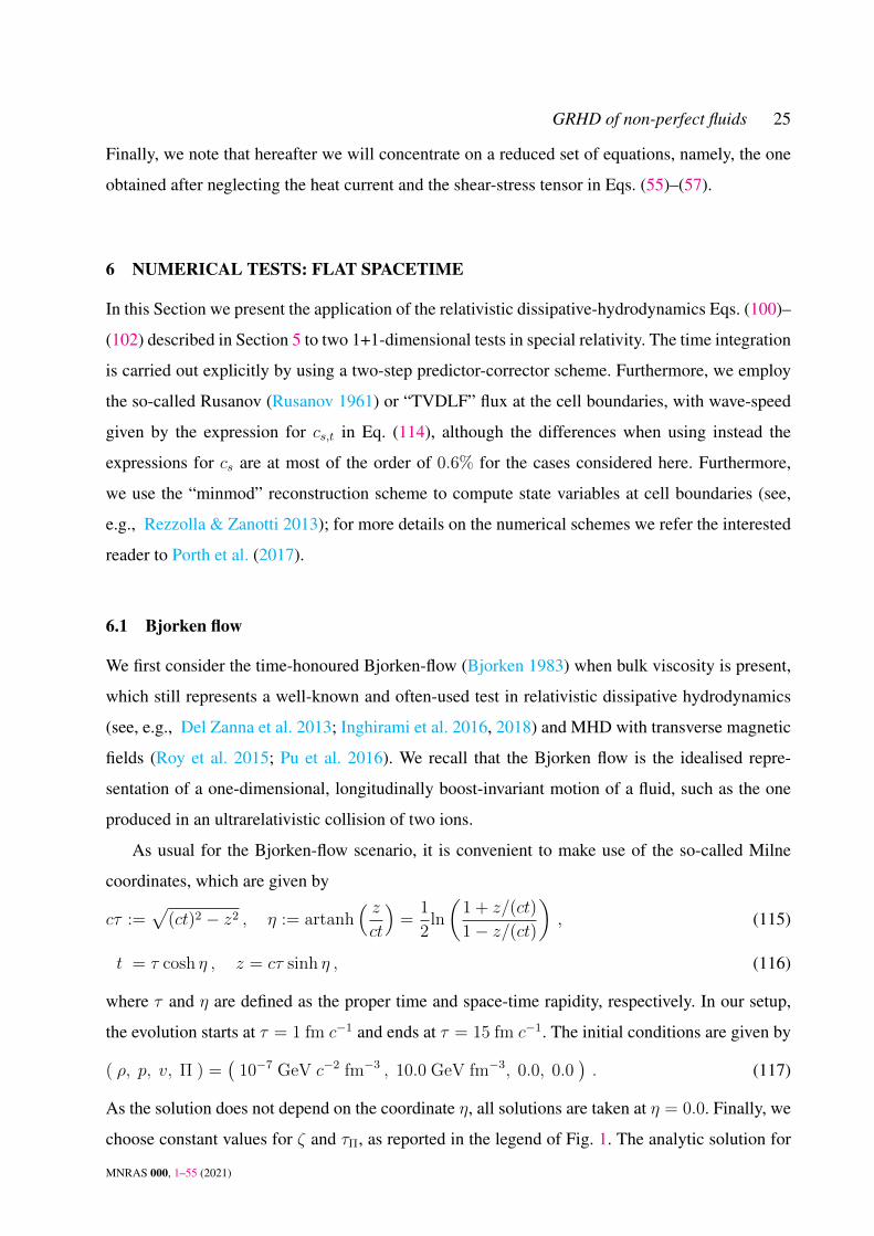
choose constant values for ζ and τΠ, as reported in the legend of Fig. 1. The analytic solution for
MNRAS 000, 1–55 (2021)
26 M. Chabanov, L. Rezzolla and D.H. Rischke
2 4 6 8 10 12 14τ [fm c−1]
−0.05
−0.04
−0.03
−0.02
−0.01
0.00
Π[G
eVfm−3
]
τΠ
= 1.0 fm c−1, ζ = 0.01 GeV fm−2
analyticΠ
NS
τΠ
= 1.0 fm c−1, ζ = 0.05 GeV fm−2
analyticΠ
NS
Figure 1. Evolution of the bulk-viscosity pressure in a Bjorken flow. Solid lines show the analytic solution, while dashed lines the solution in theNS approximation. Filled circles report instead the numerical solution from BHAC.
this problem is given by
Π (τ) = Π (τ0) exp [− (τ − τ0) /τΠ] +
ζ
cτΠ
exp (−τ/τΠ) [Ei (τ0/τΠ
)− Ei (τ/τΠ)] , (118)
where Ei (x) is the exponential integral function (see, e.g., Del Zanna et al. 2013, for more details).
Figure 1 shows the evolution of the bulk-viscosity pressure Π for the initial data given by
Eq. (117) (the changes in the other hydrodynamical quantities are very small and not particularly
interesting). As it can be seen, the numerical solutions agree very well with the analytical ones.
Also, note that with time, Π converges towards its NS value ΠNS
= −ζΘ = −ζ/(cτ) (dashed
lines in Fig. 1). At any time during the evolution, the relative difference between the analytic
and numerical solution is 10−7 at most, confirming the correct implementation of the relativis-
tic dissipative-hydrodynamics equations for smooth flows in a flat spacetime. Furthermore, our
choices for the pair (ζ, τ) lie well within the range of applicability for the equations of GRDHD.
This can be seen by calculating the effective speed of sound which is given byc2s,t
c2=
1
3+
ζ
cτΠ
1
4p+ Π, (119)
Requiring causality, i.e., cs,t/c < 1, and expressing p through the perfect-fluid solution p(τ) =
p(τ0) (τo/τ)4/3 we obtain that
τ <
(8
3cτ
Π
p(τ0)
ζ
)3/4
τ0 , (120)
when p |Π|.
For our choices (ζ, τΠ) = (0.01 GeV fm−2, 1.0 fm c−1) and (ζ, τ
Π) = (0.05 GeV fm−2, 1.0 fm c−1)
MNRAS 000, 1–55 (2021)
GRHD of non-perfect fluids 27
the dimensionless ratio |Π|/p remains below 1% and 5%, respectively, up to the time τ = 400 fm c−1.
Hence, we apply Eq. (120) and find τ < 371 fm c−1 as well as τ < 110 fm c−1, respectively. Both
values agree very well with the ones obtained from the exact solution and lie clearly above the end
of the simulation at τ = 15 fm c−1.
6.2 Shock-tube test
We next explore the solution of a shock-tube problem for an ultra-relativistic gas of gluons. While
this is a standard 1+1-dimensional test scenario, we here use the same setup implemented by
(Bouras et al. 2009a; Gabbana et al. 2020), i.e., we consider the ideal-gas EOS relative to an ultra-
relativistic fluid (i.e., γ = 4/3). Adopting Cartesian coordinates, the spatial domain ranges from
x = −3.5 fm to x = 3.5 fm and the initial discontinuity in pressure and density is located at
x = 0.0 fm, while the velocity and bulk-viscosity pressure are assumed to be zero initially. In
other words, the initial conditions are given by5
( T, p, v, Π ) =
(
0.4 GeV k−1B , 5.43 GeV fm−3, 0.0, 0.0
)x < 0.0 fm ,(
0.2 GeV k−1B , 0.33 GeV fm−3, 0.0, 0.0
)x ≥ 0.0 fm .
(121)
On the other hand, we parametrize the bulk-viscosity coefficient ζ in terms of the entropy density
of the fluid, namely,
s = ρkB
m
[4− ln
(π2ρ
m dFT 3
c3~3
k3B
)], (122)
where dF denotes the number of degrees of freedom and is set to 16 for gluons, such that
ζ =4
3
kB
c~ζ0 s , (123)
The coefficient ζ0 is a non-negative number, for which we choose the values ζ0 = 0.002, 0.01, 0.1
to obtain a direct comparison with the data from Gabbana et al. (2020). Note that the equations
describing the shock-tube problem with bulk viscosity in one dimension take the same form as
the corresponding equations with shear viscosity; the latter has been investigated in the work of
Bouras et al. (2010), as well as more recently by Gabbana et al. (2020). This leads to the mapping
ζ = 4/3 η between the bulk viscosity employed in this work and the shear viscosity used in Bouras
et al. (2010) and Gabbana et al. (2020). Furthermore, to obtain the correct rest-mass density we
assume a single-particle rest mass m = 0.5 MeV c−2, so that ρ e, as required by wanting to
consider an ultra-relativistic limit. Finally, the relaxation time used by Gabbana et al. (2020) is
5 In this Section, to facilitate the comparison with codes designed for describing HICs (Gabbana et al. 2020) we adopt physical units, where kB
and ~ are the Boltzmann and reduced Planck constants, respectively.
MNRAS 000, 1–55 (2021)
28 M. Chabanov, L. Rezzolla and D.H. Rischke
given in terms of the bulk viscosity by
τΠ
=15
16
ζ
pc. (124)
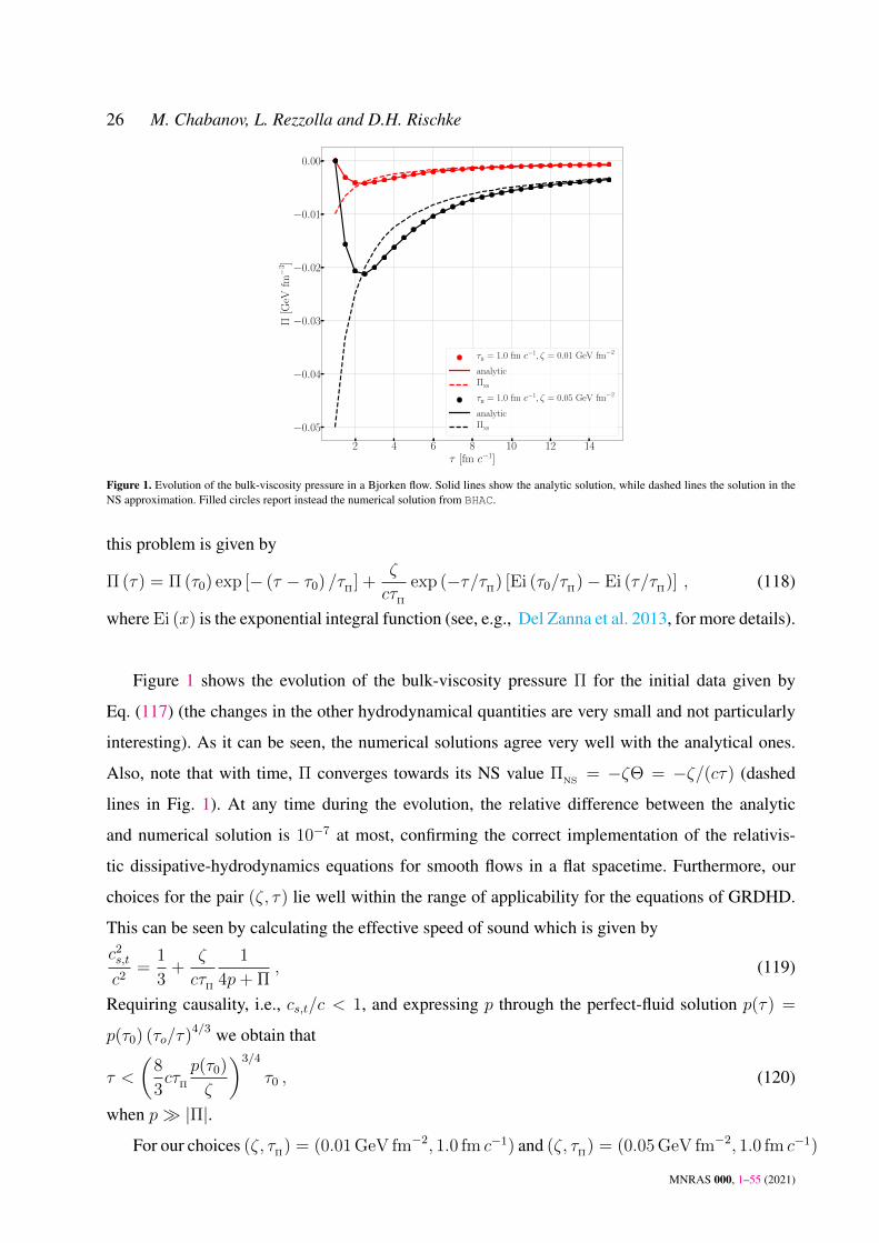
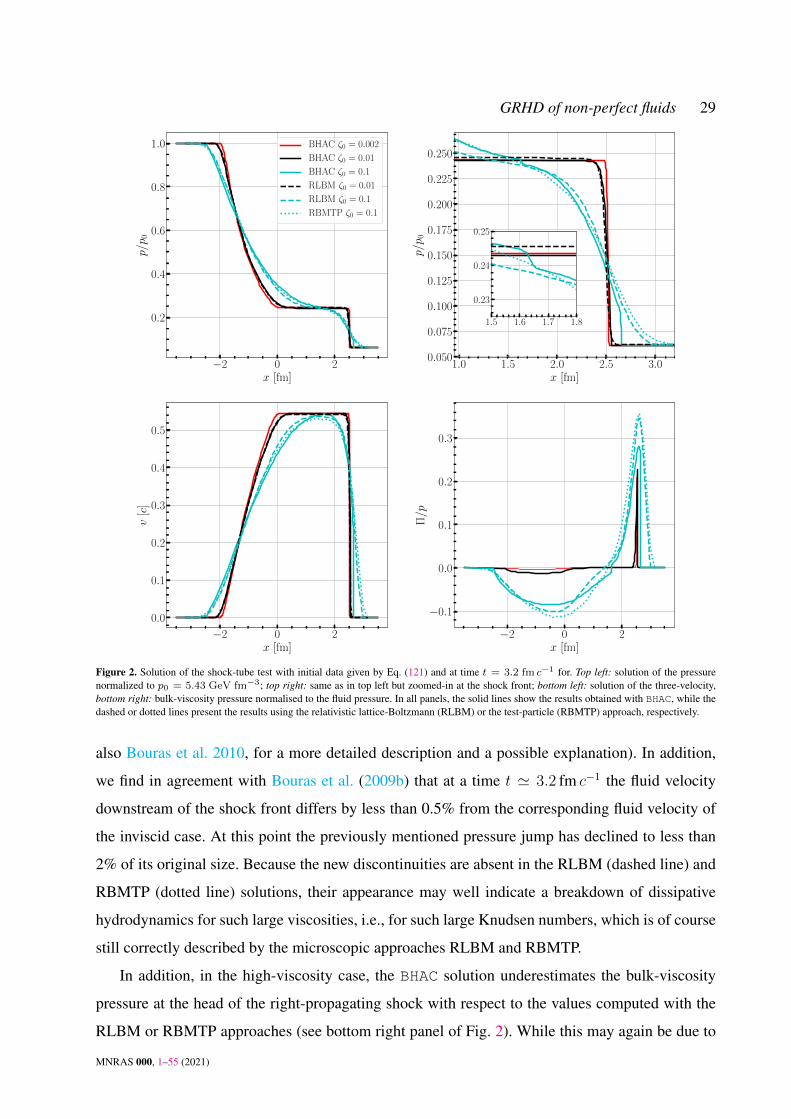
The numerical solution of the shock-tube problem at time t = 3.2 fm c−1 is shown in Fig. 2,
whose upper panels report the behaviour of the pressure normalized to p0 := 5.43 GeV fm−3 (the
top right panel is a magnification of the top left panel), while the bottom panels show the solution
of the velocity and bulk-viscosity pressure normalized to the fluid pressure. Different lines refer
either to solutions obtained with BHAC for different values of ζ0, or to solutions obtained with a
relativistic lattice-Boltzmann (RLBM) approach (dashed lines) or to solutions of the relativistic
Boltzmann equation via the test-particle (RBMTP) approach (dotted lines). Note that the case
ζ0 = 0.002 is essentially indistinguishable from an inviscid solution with the precision shown in
the figure and hence can be taken as the perfect-fluid reference.
Figure 2 highlights how the strong spatial gradients present in the initial conditions tend to
be washed out by the presence of bulk viscosity and that this smearing of the discontinuities is
larger with increasing bulk viscosity. Note that the wave-pattern of perfect-fluid hydrodynamics
– which consists of a rarefaction wave and of a shock wave – can still be clearly identified if the
bulk viscosity is not too large, i.e., ζ0 . 0.01 (see, e.g., the pressure in the upper left panel of Fig.
2). Furthermore, the solution behaviour is in good agreement with the results obtained by using
the RLBM approach. However, in the case of high bulk-viscosity, i.e., ζ0 = 0.1, the wave-pattern
of perfect-fluid hydrodynamics is so strongly smeared out that it is difficult to clearly distinguish
the rarefaction wave from the shock wave. This is not surprising, since such large values of the
bulk viscosity effectively correspond to a regime of large Knudsen number, which is where the
hydrodynamical approach – and hence the formation of shock waves – is expected to fail.
Interestingly, and as pointed out by Denicol et al. (2008b) and Bouras et al. (2010), three
additional discontinuities are present in the high-viscosity, ζ0 = 0.1, case, two of which can be seen
in the upper right panel of Fig. 2, where one is located at the head of the right-propagating shock,
while the other near the contact discontinuity of the corresponding inviscid (ζ0 = 0.002) case6. The
third additional discontinuity is located at the head of the left-propagating rarefaction fan which is
not shown here. However, all discontinuities transition smoothly into the wave-pattern of perfect-
fluid hydrodynamics at later times; indeed, the pressure jump located near the contact discontinuity
decays to less than 10% of its initial size of ' 2.4 GeV fm−3 by a time of t ' 1.8 fm c−1 (see
6 Obviously the contact discontinuity cannot be seen in the pressure profile, but it is apparent in the rest-mass density profile, which is not shown
in Fig. 2.
MNRAS 000, 1–55 (2021)
GRHD of non-perfect fluids 29
−2 0 2x [fm]
0.2
0.4
0.6
0.8
1.0p/p 0
BHAC ζ0 = 0.002
BHAC ζ0 = 0.01
BHAC ζ0 = 0.1
RLBM ζ0 = 0.01
RLBM ζ0 = 0.1
RBMTP ζ0 = 0.1
1.0 1.5 2.0 2.5 3.0x [fm]
0.050
0.075
0.100
0.125
0.150
0.175
0.200
0.225
0.250
p/p 0
−2 0 2x [fm]
0.0
0.1
0.2
0.3
0.4
0.5
v[c
]
−2 0 2x [fm]
−0.1
0.0
0.1
0.2
0.3
Π/p
1.5 1.6 1.7 1.8
0.23
0.24
0.25
Figure 2. Solution of the shock-tube test with initial data given by Eq. (121) and at time t = 3.2 fm c−1 for. Top left: solution of the pressurenormalized to p0 = 5.43 GeV fm−3; top right: same as in top left but zoomed-in at the shock front; bottom left: solution of the three-velocity,bottom right: bulk-viscosity pressure normalised to the fluid pressure. In all panels, the solid lines show the results obtained with BHAC, while thedashed or dotted lines present the results using the relativistic lattice-Boltzmann (RLBM) or the test-particle (RBMTP) approach, respectively.
also Bouras et al. 2010, for a more detailed description and a possible explanation). In addition,
we find in agreement with Bouras et al. (2009b) that at a time t ' 3.2 fm c−1 the fluid velocity
downstream of the shock front differs by less than 0.5% from the corresponding fluid velocity of
the inviscid case. At this point the previously mentioned pressure jump has declined to less than
2% of its original size. Because the new discontinuities are absent in the RLBM (dashed line) and
RBMTP (dotted line) solutions, their appearance may well indicate a breakdown of dissipative
hydrodynamics for such large viscosities, i.e., for such large Knudsen numbers, which is of course
still correctly described by the microscopic approaches RLBM and RBMTP.
In addition, in the high-viscosity case, the BHAC solution underestimates the bulk-viscosity
pressure at the head of the right-propagating shock with respect to the values computed with the
RLBM or RBMTP approaches (see bottom right panel of Fig. 2). While this may again be due to
MNRAS 000, 1–55 (2021)
30 M. Chabanov, L. Rezzolla and D.H. Rischke
the breakdown of the hydrodynamical description, part of the error may also originate from the
truncation of the relativistic evolution equation for Π [we recall that we have set ∆Π = 0 in Eq.
(57)]. As remarked by Bouras et al. (2010), the inclusion of additional source terms, as well as of
a coupling to a heat current, generally yields a better description of the corresponding dissipative
current (see Fig. 10 of Bouras et al. 2010). We expect the same to be true here and hence that a
smaller deviation would be obtained with a more sophisticated source term for Eq. (99).
Overall, Fig. 2 shows that our numerical implementation of the relativistic dissipative-hydrody-
namics equations leads to solutions that are in very good agreement with the reference solutions
obtained by the direct solution of the relativistic Boltzmann equation in regimes that are mildly
dissipative, i.e., ζ0 . 0.01, and in regimes that are highly dissipative, i.e., ζ0 . 0.1. The relative
differences remain below 8% for p/p0 where we only considered the region x ∈ [−2.5, 2.6] fm. In
this way we exclude rightmost shock wave and the head of the left-propagating rarefaction wave.
Due to the fact that the solution obtained by BHAC reaches its unperturbed initial state at lower |x|
than the solutions obtained by RLBM and RBMTP, the relative difference starts growing outside
of [−2.5, 2.6] fm and can reach values close to 45%. Note that this relative difference depends
solely on the value of p in the unperturbed initial states, for instance if the pressure of the right
initial state was close to zero then the relative difference would be close to 100% at the rightmost
shock wave. Furthermore, we similarly calculate the relative differences for Π/p and obtain values
below a maximum of ∼ 60% which is reached at x ∼ 2 fm. Note that Π/p passes through zero
such that the corresponding region is excluded, too.
7 NUMERICAL TESTS: CURVED SPACETIME
In this Section we present a stationary solution of the spherically symmetric equations of GRDHD
in a Schwarzschild spacetime. In the following, we return to using geometrised units. For perfect
fluids, the fully general-relativistic solution is known as the so-called “Michel solution” (Michel
1972) and, together with the “Bondi-Hoyle” solution (Bondi 1952), serves as the reference solution
for models of accreting nonrotating black holes in spherical symmetry, (see e.g., Nobili et al.
1991, and references therein) as well as serves as a testbed for GRHD and GRMHD codes (see,
e.g., Hawley et al. 1984; Porth et al. 2017; Weih et al. 2020).
The effects of shear viscosity – such as the one arising from turbulent motion – have first been
considered by Turolla & Nobili (1989), who however adopted a description in terms of the general-
relativistic NS equations. However, already in this simplified setup, Turolla & Nobili (1989) have
MNRAS 000, 1–55 (2021)
GRHD of non-perfect fluids 31
pointed out the numerous subtleties and highly nontrivial behaviour of the problem of stationary
viscous accretion onto a black hole. Hence, to the best of our knowledge, the problem of sta-
tionary, spherically symmetric accretion of bulk viscous fluids onto nonrotating black holes using
second-order dissipative-hydrodynamics framework has not been considered before. We here use
the solution of this problem obtained from the corresponding system of ordinary differential equa-
tions (ODEs) to test our implementation of bulk viscosity in BHAC in a curved spacetime geometry.
Details on the derivation and solution of the ODEs can be found in Appendix B.
We assume the fluid to be a mixture of ionised non-relativistic hydrogen coupled to photons
by employing the following EOS (see, e.g., Rezzolla & Zanotti 2013)
p = pM
(1 + α) . (125)
Here, pM
denotes the pressure of the matter component, which is assumed to be an ideal gas, while
the contribution from the radiation component is fixed using the parameter α. By rearranging Eq.
(125), we find that the EOS of the total mixture takes the same form as the EOS for an ideal gas
having an effective adiabatic index γe:
p = (γe − 1)(e− ρ) , (126)
where γe = 1 + 2(1 +α)/[3(1 + 2α)]. Note that e is the total energy density of the mixture while ρ
denotes the rest-mass density of the hydrogen ions. The effective adiabatic index γe should not be
confused with the generalized adiabatic exponent Γ1 which instead is defined through a thermo-
dynamic relation: Γ1 := (∂ ln p/∂ ln ρ)s = (5/2 + 20α + 16α2) / [(3/2 + 12α)(1 + α)] , where s
denotes the specific entropy (see, e.g., Mihalas & Mihalas 1984; Rezzolla & Zanotti 2013). In
addition, the effective adiabatic index γe can be expressed through the well-known generalized
adiabatic exponent Γ3 which is defined by Γ3 − 1 := (∂ lnT/∂ ln ρ)s = (1 + 4α) / (3/2 + 12α):
γe = 1 +9− 7Γ3
11− 9Γ3
. (127)
The temperature can be obtained from the ideal-fluid law for the matter component pM = 2(kB/mp)ρT
which yields:
T =1
2(1 + α)
mp
kB
p
ρ, (128)
where mp denotes the proton mass. Note the appearance of a factor 2 in the denominator coming
from the electrons in our charge-neutral plasma. Furthermore, we use a modification of the formula
for radiative bulk viscosity given by Weinberg (1971) and Sawyer (2006)
ζ = 4ζ0σSBT 4τmfp
(4
3− γe
)2
, (129)
where σSB
is the Stefan-Boltzmann constant and τmfp := mpρ−1σ−1
T the mean free time for a
MNRAS 000, 1–55 (2021)
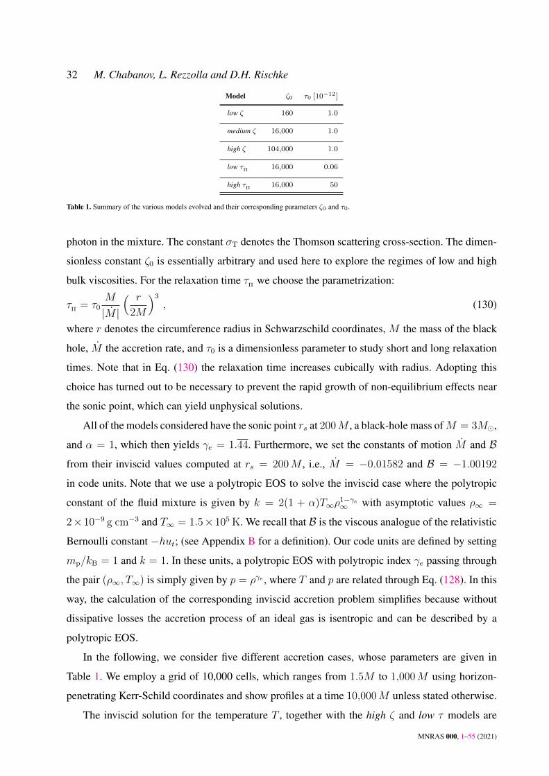
32 M. Chabanov, L. Rezzolla and D.H. Rischke
Model ζ0 τ0 [10−12]
low ζ 160 1.0
medium ζ 16,000 1.0
high ζ 104,000 1.0
low τΠ 16,000 0.06
high τΠ 16,000 50
Table 1. Summary of the various models evolved and their corresponding parameters ζ0 and τ0.
photon in the mixture. The constant σT denotes the Thomson scattering cross-section. The dimen-
sionless constant ζ0 is essentially arbitrary and used here to explore the regimes of low and high
bulk viscosities. For the relaxation time τΠ
we choose the parametrization:
τΠ
= τ0M
|M |
( r
2M
)3
, (130)
where r denotes the circumference radius in Schwarzschild coordinates, M the mass of the black
hole, M the accretion rate, and τ0 is a dimensionless parameter to study short and long relaxation
times. Note that in Eq. (130) the relaxation time increases cubically with radius. Adopting this
choice has turned out to be necessary to prevent the rapid growth of non-equilibrium effects near
the sonic point, which can yield unphysical solutions.
All of the models considered have the sonic point rs at 200M , a black-hole mass ofM = 3M,
and α = 1, which then yields γe = 1.44. Furthermore, we set the constants of motion M and B
from their inviscid values computed at rs = 200M , i.e., M = −0.01582 and B = −1.00192
in code units. Note that we use a polytropic EOS to solve the inviscid case where the polytropic
constant of the fluid mixture is given by k = 2(1 + α)T∞ρ1−γe∞ with asymptotic values ρ∞ =
2× 10⁻⁹ g cm−3 and T∞ = 1.5× 10⁵ K. We recall that B is the viscous analogue of the relativistic
Bernoulli constant −hut; (see Appendix B for a definition). Our code units are defined by setting
mp/kB = 1 and k = 1. In these units, a polytropic EOS with polytropic index γe passing through
the pair (ρ∞, T∞) is simply given by p = ργe , where T and p are related through Eq. (128). In this
way, the calculation of the corresponding inviscid accretion problem simplifies because without
dissipative losses the accretion process of an ideal gas is isentropic and can be described by a
polytropic EOS.
In the following, we consider five different accretion cases, whose parameters are given in
Table 1. We employ a grid of 10,000 cells, which ranges from 1.5M to 1,000M using horizon-
penetrating Kerr-Schild coordinates and show profiles at a time 10,000M unless stated otherwise.
The inviscid solution for the temperature T , together with the high ζ and low τ models are
MNRAS 000, 1–55 (2021)
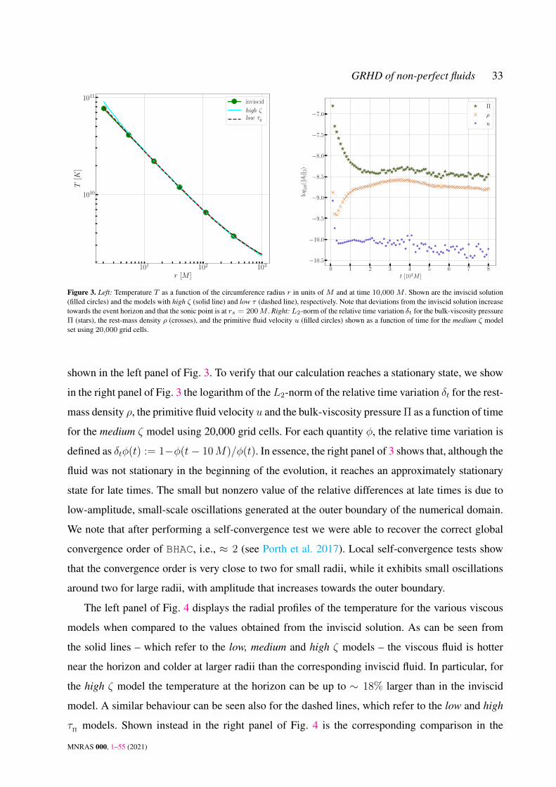
GRHD of non-perfect fluids 33
101 102 103
r [M ]
1010
1011
T[K
]
inviscid
high ζlow τ
Π
0 1 2 3 4 5 6 7 8t [104M ]
−10.5
−10.0
−9.5
−9.0
−8.5
−8.0
−7.5
−7.0
log 1
0(||δ t|| 2
)
Π
ρ
u
Figure 3. Left: Temperature T as a function of the circumference radius r in units of M and at time 10,000 M . Shown are the inviscid solution(filled circles) and the models with high ζ (solid line) and low τ (dashed line), respectively. Note that deviations from the inviscid solution increasetowards the event horizon and that the sonic point is at rs = 200M . Right:L2-norm of the relative time variation δt for the bulk-viscosity pressureΠ (stars), the rest-mass density ρ (crosses), and the primitive fluid velocity u (filled circles) shown as a function of time for the medium ζ modelset using 20,000 grid cells.
shown in the left panel of Fig. 3. To verify that our calculation reaches a stationary state, we show
in the right panel of Fig. 3 the logarithm of the L2-norm of the relative time variation δt for the rest-
mass density ρ, the primitive fluid velocity u and the bulk-viscosity pressure Π as a function of time
for the medium ζ model using 20,000 grid cells. For each quantity φ, the relative time variation is
defined as δtφ(t) := 1−φ(t− 10M)/φ(t). In essence, the right panel of 3 shows that, although the
fluid was not stationary in the beginning of the evolution, it reaches an approximately stationary
state for late times. The small but nonzero value of the relative differences at late times is due to
low-amplitude, small-scale oscillations generated at the outer boundary of the numerical domain.
We note that after performing a self-convergence test we were able to recover the correct global
convergence order of BHAC, i.e., ≈ 2 (see Porth et al. 2017). Local self-convergence tests show
that the convergence order is very close to two for small radii, while it exhibits small oscillations
around two for large radii, with amplitude that increases towards the outer boundary.
The left panel of Fig. 4 displays the radial profiles of the temperature for the various viscous
models when compared to the values obtained from the inviscid solution. As can be seen from
the solid lines – which refer to the low, medium and high ζ models – the viscous fluid is hotter
near the horizon and colder at larger radii than the corresponding inviscid fluid. In particular, for
the high ζ model the temperature at the horizon can be up to ∼ 18% larger than in the inviscid
model. A similar behaviour can be seen also for the dashed lines, which refer to the low and high
τΠ
models. Shown instead in the right panel of Fig. 4 is the corresponding comparison in the
MNRAS 000, 1–55 (2021)
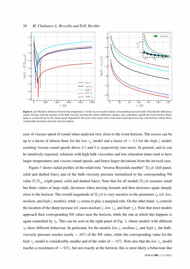
34 M. Chabanov, L. Rezzolla and D.H. Rischke
0 200 400 600 800 1000r [M ]
−9
−8
−7
−6
−5
−4
−3
−2
−1
log(|1−T/T
invis
cid|)
low ζ
med . ζ
high ζlow τ
Π
high τΠ
0 20 40 60 80 100 120r [M ]
−6
−5
−4
−3
−2
−1
0
log(|1−c s,t/c
s|) 2.5 5.0 7.5
0.2
0.4
c s,t
[c]
inviscid
Figure 4. Left: Relative difference between the temperature T of the viscous models and the corresponding inviscid model. Note that the differencesclearly increase with the increase of the bulk viscosity and that the relative difference changes sign somewhere outside the event horizon. Right:Same as on the left but for the sound speed. Reported in the inset is the actual value of the total sound speed near the event horizon, which showsconsiderable deviations from the inviscid solution.
case of viscous speed of sound when analysed very close to the event horizon. The excess can be
up to a factor of almost three for the low τΠ
model and a factor of ∼ 2.3 for the high ζ model,
reaching viscous sound speeds above 0.5 and 0.4, respectively (see inset). In general, and as can
be intuitively expected, solutions with high bulk viscosities and low relaxation times tend to have
larger temperatures and viscous sound speeds, and hence larger deviations from the inviscid case.
Figure 5 shows radial profiles of the relativistic “inverse Reynolds number” Π/ρh (left panel,
solid and dashed lines) and of the bulk-viscosity pressure normalized to the corresponding NS
value Π/ΠNS
(right panel, solid and dashed lines). Note that for all models Π/ρh assumes small
but finite values at large radii, decreases when moving inwards and then increases again sharply
close to the horizon. The overall magnitude of Π/ρh is very sensitive to the parameter ζ0 (cf. low,
medium, and high ζ models), while τ0 seems to play a marginal role. On the other hand, τ0 controls
the location of the sharp increase (cf. cases medium ζ , low τΠ
, and high τΠ
). Note that most models
approach their corresponding NS values near the horizon, while the rate at which this happens is
again controlled by τ0. This can be seen in the right panel of Fig. 5, where models with different
τ0 show different behaviour. In particular, for the models low ζ , medium ζ , and high ζ , the bulk-
viscosity pressure reaches nearly ∼ 80% of the NS value, while the corresponding value for the
high τΠ
model is considerably smaller and of the order of ∼ 10%. Note also that the low τΠ
model
reaches a maximum of ∼ 92%, but not exactly at the horizon; this is most likely a behaviour due
MNRAS 000, 1–55 (2021)
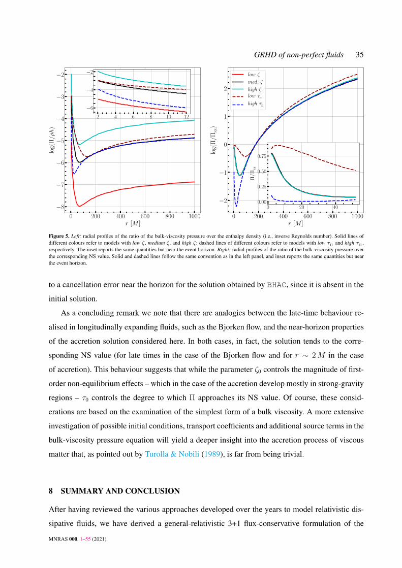
GRHD of non-perfect fluids 35
0 200 400 600 800 1000r [M ]
−8
−7
−6
−5
−4
−3
−2
log(
Π/ρh
)
0 200 400 600 800 1000r [M ]
−2
−1
0
1
2
log(
Π/Π
NS)
low ζ
med . ζ
high ζlow τ
Π
high τΠ
2 4 6 8 10 12
−6
−4
−2
0 20 400.00
0.25
0.50
0.75
Π/Π
NS
Figure 5. Left: radial profiles of the ratio of the bulk-viscosity pressure over the enthalpy density (i.e., inverse Reynolds number). Solid lines ofdifferent colours refer to models with low ζ, medium ζ, and high ζ; dashed lines of different colours refer to models with low τΠ and high τΠ ,respectively. The inset reports the same quantities but near the event horizon. Right: radial profiles of the ratio of the bulk-viscosity pressure overthe corresponding NS value. Solid and dashed lines follow the same convention as in the left panel, and inset reports the same quantities but nearthe event horizon.
to a cancellation error near the horizon for the solution obtained by BHAC, since it is absent in the
initial solution.
As a concluding remark we note that there are analogies between the late-time behaviour re-
alised in longitudinally expanding fluids, such as the Bjorken flow, and the near-horizon properties
of the accretion solution considered here. In both cases, in fact, the solution tends to the corre-
sponding NS value (for late times in the case of the Bjorken flow and for r ∼ 2M in the case
of accretion). This behaviour suggests that while the parameter ζ0 controls the magnitude of first-
order non-equilibrium effects – which in the case of the accretion develop mostly in strong-gravity
regions – τ0 controls the degree to which Π approaches its NS value. Of course, these consid-
erations are based on the examination of the simplest form of a bulk viscosity. A more extensive
investigation of possible initial conditions, transport coefficients and additional source terms in the
bulk-viscosity pressure equation will yield a deeper insight into the accretion process of viscous
matter that, as pointed out by Turolla & Nobili (1989), is far from being trivial.
8 SUMMARY AND CONCLUSION
After having reviewed the various approaches developed over the years to model relativistic dis-
sipative fluids, we have derived a general-relativistic 3+1 flux-conservative formulation of the
MNRAS 000, 1–55 (2021)

36 M. Chabanov, L. Rezzolla and D.H. Rischke
second-order dissipative-hydrodynamics equations first suggested by Israel (1976) and Hiscock
& Lindblom (1983) (i.e., the HL83 set of GRDHD equations). The new set of equations derived
in this way provides a comprehensive and complete way of including causal dissipative effects in
general-relativistic calculations.
Although a 3+1 formulation of a reduced version of the HL83 set of GRDHD equations was
already proposed by Peitz & Appl (1997) and Peitz & Appl (1999)7 , the work presented here
extends the results of Peitz and Appl in three important ways. First, our set of equations is complete
and does not neglect terms that are considered to play a less significant role (see Appendix A
for a comparison of the system presented here with other formulations). Second, the equations
presented are cast into a flux-conservative form suitable for numerical implementation. Finally,
also the coupling terms between the different dissipative currents are rewritten a 3+1 form. As a
result, the full system given in Hiscock & Lindblom (1983) can now be readily implemented in
modern numerical-relativity codes and evolved numerically.
As a way to test the new set of equations, we have proceeded with the implementation in the
GRMHD code BHAC of a reduced version of the equations describing fluids with zero shear and
heat currents, and used them against a number of tests in flat and curved background metrics.
In the first case, we have first considered the one-dimensional, longitudinally boost-invariant
motion of a viscous fluid, such as the one produced in an ultrarelativistic collision of two ions. This
expansion, first proposed by Bjorken for an inviscid fluid, is a standard testbed and can be solved
analytically. Overall, we find that the numerical solutions agree well with the analytical solutions,
with a relative difference that is∼ 10−7 for all the values of viscosity considered. As an additional
flat-spacetime test, we have explored the solution of a shock-tube problem for an ultra-relativistic
gas of gluons for different values of the ratio ζ/s, with ζ and s being bulk-viscosity coefficient
and the entropy density, respectively. Also in this case, when comparing the solutions with those
obtained with methods based on the direct solution of the relativistic Boltzmann equation, we
find a very good agreement up to a ratio of ζ/s . 0.133, which is already in a regime where a
dissipative-hydrodynamics framework breaks down.
Finally, as a general-relativistic test we have considered for the first time the problem of sta-
tionary, spherically symmetric accretion of bulk viscous fluids onto nonrotating black holes within
a second-order dissipative-hydrodynamics framework. Starting from initial conditions obtained
7 In Peitz & Appl (1997) and Peitz & Appl (1999), all terms including products of dissipative currents, i.e., Π, q and π, and first-order gradients
of the primary fluid variables are set to zero in Eqs. (8) – (10).
MNRAS 000, 1–55 (2021)
GRHD of non-perfect fluids 37
from the solution of a non-trivial set of ODEs (see Appendix B for details), we evolve the fluid
with different values of the bulk-viscosity coefficient and of the relaxation time. Given the non-
triviality of this testbed, we recommend it as a standard benchmark for those codes wishing to
include dissipative effects in the general-relativistic modelling of compact objects. Overall, we
find that the solution obtained by BHAC can deviate from the corresponding inviscid solution with
differences . 19% for the temperature and ∼ 200% for the sound speed. In addition, the bulk-
viscosity pressure is highly sensitive to the bulk-viscosity coefficient, exhibiting deviations of up
to three orders of magnitude near the event horizon depending on whether the viscosity is large or
small. We also show that, although BHAC is able to maintain a quasi-stationarity in the solution
and shows global second-order convergence, it does not converge to the reference solution with
increasing grid resolution because of the influence of a finite-size computational domain. Interest-
ingly, we note analogies between the late-time behaviour in the Bjorken and accretion flows. In
both cases, in fact, the solution tends to the corresponding NS value, with this happening at late
times in the Bjorken flow, and near the horizon in the case of accretion onto a black hole.
As a concluding remark we note that although the 3+1 formulation presented here, and its
corresponding discretisation, offers a viable path to the inclusion of non-equilibrium effects in
general-relativistic simulations of compact objects, short relaxation times as well as the required
temporal and spatial discretization of the source terms in the full system may lead to stiff equations,
whose solution will not be feasible with simple explicit schemes. We leave the examination of
more sophisticated numerical techniques for future work, where mixed explicit-implicit (IMEX)
time integrators (see, e.g., Palenzuela et al. 2009; Dionysopoulou et al. 2013; Weih et al. 2020)
will be considered.
ACKNOWLEDGEMENTS
We thank Masoud Shokri, Elias Most, Hector Olivares and Lukas Weih for useful discussions. Sup-
port comes in part from HGS-HIRe for FAIR; the LOEWE-Program in HIC for FAIR; “PHAROS”,
COST Action CA16214; the ERC Synergy Grant “BlackHoleCam: Imaging the Event Horizon
of Black Holes” (Grant No. 610058); the Deutsche Forschungsgemeinschaft (DFG, German Re-
search Foundation) through the CRC-TR 211 “Strong-interaction matter under extreme condi-
tions” - project number 315477589 - TRR 211.
MNRAS 000, 1–55 (2021)
38 M. Chabanov, L. Rezzolla and D.H. Rischke
References
Abbott B. P., et al., 2017a, Phys. Rev. Lett., 119, 161101
Abbott B. P., et al., 2017b, Astrophys. J. Lett., 848, L13
Abbott B. P., et al., 2018, Physical Review Letters, 121, 161101
Afshordi N., Paczynski B., 2003, Astrophys. J., 592, 354
Aguilera-Miret R., Viganò D., Carrasco F., Miñano B., Palenzuela C., 2020, Phys. Rev. D, 102, 103006
Alcubierre M., 2008, Introduction to 3 + 1 Numerical Relativity. Oxford University Press, Oxford, UK,
doi:10.1093/acprof:oso/9780199205677.001.0001
Alford M. G., Haber A., 2020, arXiv e-prints, p. arXiv:2009.05181
Alford M. G., Bovard L., Hanauske M., Rezzolla L., Schwenzer K., 2018, Phys. Rev. Lett., 120, 041101
Alford M., Harutyunyan A., Sedrakian A., 2020, Particles, p. arXiv:2006.07975
Andersson N., Comer G. L., 2015, Classical and Quantum Gravity, 32, 075008
Andersson N., Comer G. L. C., 2020, arXiv e-prints, p. arXiv:2008.12069
Annala E., Gorda T., Kurkela A., Vuorinen A., 2018, Phys. Rev. Lett., 120, 172703
Baier R., Romatschke P., Son D. T., Starinets A. O., Stephanov M. A., 2008, Journal of High Energy Physics, 2008, 100
Baiotti L., Rezzolla L., 2017, Rept. Prog. Phys., 80, 096901
Baiotti L., Giacomazzo B., Rezzolla L., 2008, Phys. Rev. D, 78, 084033
Bauswein A., Just O., Janka H.-T., Stergioulas N., 2017, Astrophys. J. Lett., 850, L34
Bemfica F. S., Disconzi M. M., Noronha J., 2019a, Phys. Rev. D, 100, 104020
Bemfica F. S., Disconzi M. M., Noronha J., 2019b, Phys. Rev. Lett., 122, 221602
Bemfica F. S., Disconzi M. M., Hoang V., Noronha J., Radosz M., 2020, arXiv e-prints, p. arXiv:2005.11632
Bernhard J. E., Moreland J. S., Bass S. A., 2019, Nature Physics, 15, 1113
Betz B., Henkel D., Rischke D. H., 2009, Progress in Particle and Nuclear Physics, 62, 556
Betz B., Denicol G., Koide T., Molnar E., Niemi H., Rischke D., 2011, EPJ Web Conf., 13, 07005
Biswas R., Dash A., Haque N., Pu S., Roy V., 2020, Journal of High Energy Physics, 2020, 171
Bjorken J. D., 1983, Phys. Rev. D, 27, 140
Bondi H., 1952, Mon. Not. R. Astron. Soc., 112, 195
Bouras I., Molnar E., Niemi H., Xu Z., El A., Fochler O., Greiner C., Rischke D. H., 2009a, Phys. Rev. Lett., 103, 032301
Bouras I., Molnár E., Niemi H., Xu Z., El A., Fochler O., Greiner C., Rischke D. H., 2009b, Nuclear Phys. A, 830, 741
Bouras I., Molnar E., Niemi H., Xu Z., El A., Fochler O., Greiner C., Rischke D. H., 2010, Phys. Rev., C82, 024910
Brito C. V., Denicol G. S., 2020, Phys. Rev. D, 102, 116009
Burns E., 2020, Living Reviews in Relativity, 23, 4
Busza W., Rajagopal K., van der Schee W., 2018, Annual Review of Nuclear and Particle Science, 68, 339
Carter B., 1989, in Anile A., Choquet-Bruhat Y., eds, Lecture Notes in Mathematics, Vol. 1385, Relativistic Fluid Dynamics. Springer Berlin /
Heidelberg, pp 1–64, http://dx.doi.org/10.1007/BFb0084028
Cowperthwaite P. S., et al., 2017, Astrophys. J. Lett., 848, L17
De S., Finstad D., Lattimer J. M., Brown D. A., Berger E., Biwer C. M., 2018, Physical Review Letters, 121, 091102
Del Zanna L., et al., 2013, European Physical Journal C, 73, 2524
Denicol G. S., Kodama T., Koide T., Mota P., 2008a, Journal of Physics G: Nuclear and Particle Physics, 35, 115102
Denicol G. S., Kodama T., Koide T., Mota P., 2008b, Phys. Rev. C, 78, 034901
Denicol G. S., Molnár E., Niemi H., Rischke D. H., 2012a, The European Physical Journal A, 48, 170
Denicol G. S., Niemi H., Molnár E., Rischke D. H., 2012b, Phys. Rev. D, 85, 114047
Denicol G., Niemi H., Bouras I., Molnar E., Xu Z., Rischke D., Greiner C., 2014, Phys. Rev. D, 89, 074005
Dionysopoulou K., Alic D., Palenzuela C., Rezzolla L., Giacomazzo B., 2013, Phys. Rev. D, 88, 044020
Disconzi M. M., Kephart T. W., Scherrer R. J., 2017, International Journal of Modern Physics D, 26, 1750146
MNRAS 000, 1–55 (2021)
GRHD of non-perfect fluids 39
Drout M. R., et al., 2017, Science, 358, 1570
Duez M. D., Liu Y. T., Shapiro S. L., Stephens B. C., 2004, Phys. Rev. D, 69, 104030
Duez M. D., et al., 2020, Phys. Rev. D, 102, 104050
Eckart C., 1940, Phys. Rev., 58, 919
Event Horizon Telescope Collaboration et al., 2019, Astrophys. J. Lett., 875, L1
Fambri F., Dumbser M., Köppel S., Rezzolla L., Zanotti O., 2018, Mon. Not. R. Astron. Soc., 477, 4543
Fujibayashi S., Kiuchi K., Nishimura N., Sekiguchi Y., Shibata M., 2018, The Astrophysical Journal, 860, 64
Gabbana A., Plumari S., Galesi G., Greco V., Simeoni D., Succi S., Tripiccione R., 2020, Phys. Rev. C, 101, 064904
Gourgoulhon E., 2012, 3+1 Formalism in General Relativity. Lecture Notes in Physics, Berlin Springer Verlag Vol. 846, Springer, doi:10.1007/978-
3-642-24525-1
Hairer E., Wanner G., 1996, Solving Ordinary Differential Equations II - Stiff and Differential-Algebraic Problems, 2nd edn. Springer
Hawley J. F., Smarr L. L., Wilson J. R., 1984, Astrophys. J., 277, 296
Hebert F., Kidder L. E., Teukolsky S. A., 2018, Phys. Rev. D, 98, 044041
Hiscock W. A., Lindblom L., 1983, Annals of Physics, 151, 466
Hiscock W. A., Lindblom L., 1985, Phys. Rev. D, 31, 725
Hiscock W. A., Lindblom L., 1987, Phys. Rev. D, 35, 3723
Hoult R. E., Kovtun P., 2020, Journal of High Energy Physics, 2020, 67
Inghirami G., Del Zanna L., Beraudo A., Moghaddam M. H., Becattini F., Bleicher M., 2016, European Physical Journal C, 76, 659
Inghirami G., Del Zanna L., Beraudo A., Haddadi Moghaddam M., Becattini F., Bleicher M., 2018, in Journal of Physics Conference Series. p.
012043, doi:10.1088/1742-6596/1024/1/012043
Israel W., 1976, Annals of Physics, 100, 310
Israel W., Stewart J. M., 1979, Annals of Physics, 118, 341
Jaiswal A., 2013, Phys. Rev. C, 87, 051901
Jaiswal A., Bhalerao R. S., Pal S., 2013, Phys. Rev. C, 87, 021901
Jordan D. W., Smith P., 2007, Nonlinear Ordinary Differential Equations : An Introduction for Scientists and Engineers. Oxford University Press,
Oxford, UK
Kiuchi K., Kyutoku K., Sekiguchi Y., Shibata M., 2018, Phys. Rev. D, 97, 124039
Koeppel S., Bovard L., Rezzolla L., 2019, Astrophys. J. Lett., 872, L16
Kovtun P., 2019, Journal of High Energy Physics, 2019, 34
Landau L. D., Lifshitz E. M., 2004, Fluid Mechanics, Course of Theoretical Physics, Volume 6. Elsevier Butterworth-Heinemann, Oxford
Malik T., Alam N., Fortin M., Providência C., Agrawal B. K., Jha T. K., Kumar B., Patra S. K., 2018, Physical Review C, 98, 035804
Mandal I., Ray A. K., Das T. K., 2007, Mon. Not. R. Astron. Soc., 378, 1400
Margalit B., Metzger B. D., 2017, Astrophys. J. Lett., 850, L19
McNelis M., Bazow D., Heinz U., 2021, arXiv e-prints, p. arXiv:2101.02827
Michel F. C., 1972, Ap&SS, 15, 153
Mihalas D., Mihalas B., 1984, Foundations of radiation hydrodynamics
Mizuno Y., et al., 2018, Nature Astronomy,
Montaña G., Tolós L., Hanauske M., Rezzolla L., 2019, Phys. Rev. D, 99, 103009
Most E. R., Weih L. R., Rezzolla L., Schaffner-Bielich J., 2018, Phys. Rev. Lett., 120, 261103
Most E. R., Papenfort L. J., Rezzolla L., 2019, Mon. Not. R. Astron. Soc., 490, 3588
Muronga A., 2004, Phys. Rev. C, 69, 034903
Nobili L., Turolla R., Zampieri L., 1991, Astrophys. J., 383, 250
Olivares H., et al., 2020, MNRAS, 497, 521
Palenzuela C., Lehner L., Reula O., Rezzolla L., 2009, Mon. Not. R. Astron. Soc., 394, 1727
Paschalidis V., 2017, Classical and Quantum Gravity, 34, 084002
MNRAS 000, 1–55 (2021)
40 M. Chabanov, L. Rezzolla and D.H. Rischke
Peitz J., Appl S., 1997, Mon. Not. R. Astron. Soc., 286, 681
Peitz J., Appl S., 1999, Class. Quantum Grav., 16, 979
Porth O., Olivares H., Mizuno Y., Younsi Z., Rezzolla L., Moscibrodzka M., Falcke H., Kramer M., 2017, Computational Astrophysics and
Cosmology, 4, 1
Pu S., Koide T., Rischke D. H., 2010, Phys. Rev. D, 81, 114039
Pu S., Roy V., Rezzolla L., Rischke D. H., 2016, Phys. Rev. D, 93, 074022
Radice D., 2017, Astrophys. J. Lett., 838, L2
Radice D., 2020, Symmetry, 12, 1249
Radice D., Rezzolla L., 2012, Astron. Astrophys., 547, A26
Radice D., Perego A., Bernuzzi S., Zhang B., 2018a, Mon. Not. R. Astron. Soc., 481, 3670
Radice D., Perego A., Zappa F., Bernuzzi S., 2018b, Astrophys. J. Lett., 852, L29
Radice D., Perego A., Hotokezaka K., Fromm S. A., Bernuzzi S., Roberts L. F., 2018c, Astrophys. J., 869, 130
Raithel C., Özel F., Psaltis D., 2018, Astrophys. J., 857, L23
Ray A. K., Bhattacharjee J. K., 2002, Phys. Rev. E, 66, 066303
Rezzolla L., Zanotti O., 2013, Relativistic Hydrodynamics. Oxford University Press, Oxford, UK,
doi:10.1093/acprof:oso/9780198528906.001.0001
Rezzolla L., Most E. R., Weih L. R., 2018, Astrophys. J. Lett., 852, L25
Romatschke P., Romatschke U., 2019, Relativistic Fluid Dynamics In and Out of Equilibrium: And Applications to Relativistic Nuclear Collisions.
Cambridge Monographs on Mathematical Physics, Cambridge University Press, doi:10.1017/9781108651998
Roy V., Pu S., Rezzolla L., Rischke D., 2015, Physics Letters B, 750, 45
Ruiz M., Shapiro S. L., Tsokaros A., 2018, Phys. Rev. D, 97, 021501
Rusanov V. V., 1961, J. Comput. Math. Phys. USSR, 1, 267
Sawyer R. F., 2006, Phys. Rev. D, 74, 043527
Shibata M., Hotokezaka K., 2019, Annual Review of Nuclear and Particle Science, 69, 41
Shibata M., Kiuchi K., Sekiguchi Y.-i., 2017, Phys. Rev. D, 95, 083005
Shibata M., Zhou E., Kiuchi K., Fujibayashi S., 2019, Phys. Rev. D, 100, 023015
Siegel D. M., Ciolfi R., Harte A. I., Rezzolla L., 2013, Phys. Rev. D R, 87, 121302
Taghinavaz F., 2020, JHEP, 08, 119
Tews I., Margueron J., Reddy S., 2018, Physical Review C, 98, 045804
Turolla R., Nobili L., 1989, Astrophys. J., 342, 982
Van P., Biro T., 2012, Phys. Lett. B, 709, 106
Viganò D., Aguilera-Miret R., Carrasco F., Miñano B., Palenzuela C., 2020, Phys. Rev. D, 101, 123019
Weih L. R., Olivares H., Rezzolla L., 2020, Mon. Not. R. Astron. Soc., 495, 2285
Weinberg S., 1971, Astrophys. J., 168, 175
Wolfram Research I., 2020, Mathematica, Version 12.1, https://www.wolfram.com/mathematica
APPENDIX A: REVIEW OF SECOND-ORDER RELATIVISTIC DISSIPATIVE
HYDRODYNAMICS
This Appendix serves the scope of providing a guidance in comparing our reference second-order
formulation of general-relativistic dissipative hydrodynamics originally suggested by Hiscock &
Lindblom (1983) with other formulations that have appeared in the literature, i.e., the formulations
MNRAS 000, 1–55 (2021)
GRHD of non-perfect fluids 41
by Israel & Stewart (1979) (hereafter IS79), by Denicol et al. (2012a) (hereafter DMNR12)8, and
by Baier et al. (2008) (hereafter rBRSSS08). Since these formulations often adopt different no-
tations that makes it hard to compare them, we introduce a generalized notation for the various
transport coefficients, whose terminology is given in Table A1. Furthermore, since the equations
of HL83 are chosen as our reference equations, we use upper-case letters for transport coefficients
appearing in HL83; the only exception to this rule will be made for the relaxation times. Further-
more, since the comparison needs to distinguish terms of first and second order, we introduce the
following dimensionless numbers: the Knudsen number
Kn :=lmicro
Lmacro
, (A1)
where lmicro and Lmacro are the microscopic lengthscale given by the mean-free-path of the mi-
croscopic constituents of the fluid and the macroscopic lengthscale given by the distance over
which gradients of primary fluid variables appear, respectively. Furthermore, the inverse Reynolds
numbers are given by
R−1Π :=
|Π|p+ e
, R−1n :=
|nµ|n, R−1
π :=|πµν |p+ e
. (A2)
Note that in the Eckart frame the inverse Reynolds number R−1n is replaced by
R−1q :=
|qµ|p+ e
∼ O(R−1n
). (A3)
Using these dimensionless numbers, we can identify the order of the terms given in Table A2
according to the following classification:
O(R−1i ,Kn
):= O1 , O
(R−1i Kn
):= O
RK, O
(R−1i R−1
j
):= O
2R, O
(Kn2
):= O
2K.
(A4)
In this way, following the convention of Denicol et al. (2012b), we refer to terms of order O1 as
being of first order, while all other terms are referred to as being of second order.
With these definitions made, we next proceed to the actual comparison which will take place
by first briefly reviewing each of the formulations considered (Sec. A1–A4) and then proceeds
with the actual comparison (Sec. A5).
8 Note that there is another frequently used second-order GRDHD formulation proposed by Denicol et al. (2012b) and often referred to as the
“DNMR” formulation. We will not use this formulation for our comparison here since the formulation by Denicol et al. (2012b) is in the Landau
frame and we instead consider the formulations adopting the Eckart frame for our comparison.
MNRAS 000, 1–55 (2021)
42 M. Chabanov, L. Rezzolla and D.H. Rischke
transport coefficients description
τΠ , τq , τπ relaxation times for bulk viscosity, heat conduction and shear viscosity, respectivelyδij or ∆i
j transport coefficients for gradients of the fluid velocity ulij or Lij transport coefficients for gradients of the dissipative currentsλij or Λij transport coefficients for the contribution of gradients of ρ and pϕij transport coefficients for the contribution of contracted dissipative currentsgij transport coefficients in front of geometrical quantities, i.e. Rµνλρ, Rµν or R
Table A1. Generalized notation for the transport coefficients. Shown on the left are the newly introduced symbols, while a description of whichfluid field it appears in combination with is shown on the right. The upper index indicates which dissipative current the transport coefficient belongsto, e.g., δ
Π
2 is the second transport coefficient expressing the coupling to a gradient of the fluid velocity in the constitutive equation for the bulk-viscosity pressure. Upper-case letters indicate that the corresponding transport coefficient occurs in the HL83 formulation, while lower case lettersindicate that it is set to zero in HL83.
A1 Israel and Stewart 1979 (IS79)
The equations for the dissipative currents of IS79 read as follows
τΠ
Π = ΠLNS− Π + δ
Π
1 qµaµ + L
Π
1 ∇µqµ , (A5)
τq q〈µ〉 = q µ
NS− qµ + δq1 Πaµ + δq2 π
µνaν + δq3 ωµνqν + Lq1 ∇〈µ〉Π + Lq2 ∇νπ
〈µ〉ν , (A6)
τπ π〈µν〉 = π µν
LNS− πµν + δπ1 q
〈µaν〉 + δπ2 πλ〈µω ν〉
λ + Lπ1 ∇〈µ q ν〉 . (A7)
Here, ΠLNS
and π µνLNS
denote the NS values of the dissipative currents evaluated in the Landau
frame. Equations (A5), (A6) and (A7) correspond to equations (7.1a), (7.1b) and (7.1c) of Israel
& Stewart (1979), respectively. This set of equations was derived using the Boltzmann equation
for the single-particle distribution function f , parametrized in the form
y(xµ, pi) := ln
[f (xµ, pi)
A1
], (A8)
y(xµ, pi) :=µ
T+ ε+
(uλT
+ελm
)pλ +
1
m2ελρp
λpρ , (A9)
A1 := 1 + A2f(xµ, pi
), A2 ∈ −1, 0,+1 , (A10)
where p0 = p0(pi,m) is the on-shell energy of the particles, A2 = −1(+1) refers to fermions
(bosons) so that A2 → 0 corresponds to the limit yielding the Boltzmann distribution, and m is
the mass of the particles.
The functions ε, ελ and ελρ are off-equilibrium corrections. Note that we recover the standard
Fermi, Bose and Boltzmann local-equilibrium distributions for ε, ελ, ελρ = 0. The single-particle
distribution f contains 14 independent variables (T, µ, the three independent components of uµ and
the nine independent components of the functions ε, ελ and ελρ). These are one-to-one matched
to the components of Jµ and T µν . The system of conservation equations, corresponding to the
equations of motion for the first and second moment of f , is closed by employing the equation of
motion for the third moment of f , leading to relaxation-type equations for the dissipative currents.
MNRAS 000, 1–55 (2021)
GRHD of non-perfect fluids 43
The fact that 14 independent variables occur in the equations of motion is also referred to as the
“14-moment approximation”.
We should recall that in the derivation of IS79 two approximations are made. First, they ne-
glected second-order terms proportional to ∇µρ and Θ. Following the derivation from the second
law of thermodynamics, these terms arise from gradients of the transport coefficients and are gen-
erally of the form (see, e.g., the equation for the shear-stress tensor) ∝ πµνuλIλ
and ∝ q〈µIν〉
,
where Iµ
is a linear combination of gradients of transport coefficients that can be related to gradi-
ents of the chosen pair of thermodynamical variables T, µ or ρ, p. In general, these terms can
be further decomposed by using the first-order version of the conservation laws (1) and (2):
ρ ∝ Θ , (A11)
aµ ∝ ∇〈µ〉p , (A12)
e ∝ Θ , (A13)
where, again, A := (u ·∇)A = uµ∇µA. By choosing the pair ρ, p as our thermodynamical
variables and exploiting Eqs. (A11) – (A13), the following relations are valid to second-order
πµνuλIλ ∝ πµνΘ , (A14)
q〈µIν〉 ∝ b1q
〈µaν〉 + b2q〈µ∇ν〉ρ , (A15)
where b1 and b2 denote scalar functions of the pair ρ, p. Hence, the missing terms in IS79
proportional to ∇µρ and Θ are of the form ∝ πµνΘ and ∝ q〈µ∇ν〉ρ, while the term b1q〈µaν〉 could
be absorbed in the transport coefficient δπ1 .
Second, there are terms of the form ∝ πλ〈µσν〉λ and ∝ Πσµν , appearing for instance in the
equation for the shear-stress tensor that are also apparently missing in the IS79 formulation. The
existence of these terms was first pointed out by Betz et al. (2011), which were subsequently
included in the DMNR12 formulation (see below).
A2 Hiscock and Lindblom 1983 (HL83)
When using a generalized notation, the evolution equations (8)–(10) for the dissipative currents in
the HL83 formulation can be written as
τΠ
Π = ΠNS− Π + ∆
Π
1 ΠΘ + LΠ
1 ∇µqµ + Λ
Π
1 ΠuµI1µ + Λ
Π
2 qµI2µ , (A16)
τq q〈µ〉 = qµ
NS− qµ + ∆q
1 qµΘ + Lq1 ∇〈µ〉Π + Lq2 ∇νπ
〈µ〉ν + Λq1 q
µuνI3ν
+ Λq2 ΠI2
〈µ〉 + Λq3 π
µνI4
ν , (A17)
τπ π〈µν〉 = πµν
NS− πµν + ∆π
1 πµνΘ + Lπ1 ∇〈µ q ν〉 + Λπ
1 πµνuλI5
λ + Λπ2 q〈µI4
ν〉 . (A18)
MNRAS 000, 1–55 (2021)
44 M. Chabanov, L. Rezzolla and D.H. Rischke
where the currents Iiµ are given by
I1µ := ∇µ (τ
Π/ζT ) , (A19)
I2µ := ∇µ (α0/T ) , (A20)
I3µ := ∇µ
(τq/κT
2), (A21)
I4µ := ∇µ (α1/T ) , (A22)
I5µ := ∇µ (τπ/ηT ) . (A23)
In similarity with Sec. A1, we can use the first-order relations (A11)–(A13) to further decom-
pose the terms in (A16)–(A18) that include the currents Iiµ and obtain
ΠuµI1µ ∝ ΠΘ , (A24)
qµI2µ ∝ b3qµa
µ + b4qµ∇µρ , (A25)
qµuνI3ν ∝ qµΘ , (A26)
ΠI2〈µ〉 ∝ b4Πaµ + b5Π∇〈µ〉ρ , (A27)
πµνI4ν ∝ b6π
µνa
ν + b7πµν∇νρ , (A28)
πµνuλI5λ ∝ πµνΘ , (A29)
q〈µI4ν〉 ∝ b8q
〈µaν〉 + b9q〈µ∇ν〉ρ , (A30)
where, again, the quantities b3-b9 are scalar functions of ρ and p.
A3 Denicol et al. 2012a (DMNR12)
The equations for the dissipative currents of the DMNR12 formulation are
τΠ
Π = ΠNS− Π + ∆
Π
1 ΠΘ + δΠ
1 qµaµ + δ
Π
2 πµνσµν + L
Π
1 ∂µqµ + Λ
Π
2 qµI6µ , (A31)
τq q〈µ〉 = qµ
NS− qµ + ∆q
1 qµΘ + δq1 Πaµ + δq2 π
µνaν + δq3 ωµνqν + δq4 σ
µνqν
+ Lq1 ∂〈µ〉Π + Lq2 ∂νπ
〈µ〉ν + Λq2 ΠI6
〈µ〉 + Λq3 π
µνI6
ν , (A32)
τπ π〈µν〉 = πµν
NS− πµν + ∆π
1 πµνΘ + δπ1 q
〈µaν 〉 + δπ2 πλ〈µων 〉λ + δπ3 π
λ〈µσν 〉λ
+ δπ4 Πσµν + Lπ1 ∂〈µqν 〉 + Λπ
2 q〈µ I6
ν〉 . (A33)
Equations (A31), (A32) and (A33) correspond to equations (128), (138) and (153) of Denicol
et al. (2012a), respectively, when the Eckart frame is chosen as the frame of reference, i.e., when
MNRAS 000, 1–55 (2021)
GRHD of non-perfect fluids 45
V µ = 0 and W µ = qµ. Notice that the terms including the current I6µ can be decomposed as
qµI6µ ∝ b10qµa
µ + b11qµ∇µρ , (A34)
ΠI6〈µ〉 ∝ b10Πaµ + b11Π∇〈µ〉ρ , (A35)
πµνI6ν ∝ b10π
µνa
ν + b11πµν∇νρ , (A36)
q〈µI6ν〉 ∝ b10q
〈µaν〉 + b11q〈µ∇ν〉ρ , (A37)
where I6µ := ∂µ
(µT
)and b10, b11 are scalar functions of ρ and p.
Note that Eqs. (A31)–(A33) have been derived for a flat spacetime with signature (+,−,−,−)9,
so that the comoving derivative is A = uµ∂µA. Hence, in the comparison we will carry out in Sec.
A5 the covariant derivatives in our general-relativistic formulation have to be replaced with a sim-
ple partial derivative when comparing to DMNR12.
We recall that in the derivation of the DMNR12 formulation, the full off-equilibrium distribu-
tion function is decomposed as
f(xµ, pi) = f0(xµ, pi) + δf(xµ, pi) , (A38)
where f0 is the local-equilibrium distribution function and δf denotes the deviation from it. One
then defines the so-called generalized irreducible moments of order r of δf as
ρµ1···µlr :=
∫gd3p
(2π)3p0(E)rp〈µ1 · · · pµl〉δf , (A39)
where g is the number of internal degrees of freedom and E is defined by pµ =: Euµ + p〈µ〉. The
full off-equilibrium distribution function can now be expanded in momentum space in a basis of
irreducible tensors p〈µ1 · · · pµl〉 and orthogonal polynomials inE, where the generalized irreducible
moments appear as coefficients. Some of these moments are directly connected to the dissipative
currents, e.g.,
Π = −m2
3ρ0 = −m
2
3
∫gd3p
(2π)3p0δf , (A40)
qµ = ρµ1 =
∫gd3p
(2π)3p0Epµδf, (A41)
πµν = ρµν0 =
∫gd3p
(2π)3p0p〈µpν〉δf . (A42)
Inserting Eq. (A38) into the special-relativistic version of the Boltzmann equation leads to an
equation of motion for δf ,
δf = −f0 −1
Ep〈µ〉∂µ (f0 + δf) . (A43)
This equation is then used to evaluate the comoving derivatives of the generalized irreducible
9 This choice introduces a sign difference in some quantities, e.g., π µνNS , which are instead computed with the signature (−,+,+,+).
MNRAS 000, 1–55 (2021)
46 M. Chabanov, L. Rezzolla and D.H. Rischke
moments (A39) and leads to an infinite set of evolution equations for the latter. When this infinite
system is truncated at the lowest order – corresponding to the 14-moment approximation – it leads
to the IS79-like equations, which have been given above by Eqs. (A31)–(A33).
However, this procedure is ambiguous because, once the 14-moment approximation is applied,
it is possible to obtain a closed evolution equation of the desired dissipative current from any choice
of r in Eq. (A39), for the irreducible moment of tensor rank corresponding to that of the respective
dissipative current10. This can be seen from the r-dependence of the transport coefficients in Tables
A3 and A4, which reflects the choice of the moment equation. The transport coefficients of IS79
are obtained if one sets r = 3 for the scalar moment, r = 2 for the vector moment and r =
1 for the tensor moment. Microphysical properties of the system are encoded in the transport
coefficients obtained from a moment expansion of the collision integral of the Boltzmann equation.
Instead of applying the 14-moment approximation, a power-counting scheme in Knudsen and
inverse Reynolds numbers is used by Denicol et al. (2012b) to truncate the system.
A4 Baier et al. 2008 (rBRSSS08)
The equations for the dissipative currents of the rBRSSS08 formulation read as follows [here
we use the version presented by Romatschke & Romatschke (2019), where they appear as Eq.
(2.122)]11
τΠ
Π = ΠNS− Π + δ
Π
3 ωµνωµν + λ
Π
1 I7〈µ〉I7〈µ〉 + ϕ
Π
1 πµνπµν + ϕ
Π
2 Π2
+ gΠ
1 R + gΠ
2 uµuνRµν , (A44)
τπ π〈µν〉 = πµν
NS− πµν + ∆π
1 πµνΘ + δπ2 π
λ〈µων 〉λ + δπ5 ω〈µλω
ν 〉λ + λπ1 I7〈µ I7
ν〉
+ ϕπ1 πλ〈µπν 〉λ + gπ1 R
〈µν〉 + gπ2 uλuρRλ〈µν〉ρ . (A45)
Note that we have defined I7µ := ∇µ ln e and that the heat current is absent because these ex-
pressions refer to the Landau frame as the reference frame, where the heat currents are zero by
definition.
As for the previous formulations, we can use the first-order relations (A11)–(A13) to further
10 Stated differently, it is possible to derive a relationship between the dissipative currents Π, qµ, and πµν , which are essentially the irreducible
moments ρ0, ρµ1 , and ρµν0 , and all the other ρr, ρ
µr , and ρµνr , for any index r. As a result, there is ambiguity because it is possible to derive an
equation of motion for Π, etc. from the equation of motion for ρr , etc. for any r and not only for r = 0.11 In Baier et al. (2008) the equations for the dissipative currents have been derived for the case of conformal fluids. Here we present their complete
extension to the case of non-conformal fluids.
MNRAS 000, 1–55 (2021)
GRHD of non-perfect fluids 47
decompose the terms in Eqs. (A44), (A45) that include the current I7µ as
I7〈µ〉I7〈µ〉 = I7µI7
µ + uµI7µuνI7
ν
∝ (b12aµ + b13∇µρ)(b12aµ + b13∇µρ) + b14Θ2
∝ (b12)2aµaµ + 2b12b13a
µ∇µρ+ (b13)2∇µρ∇µρ+ b14Θ2 , (A46)
I7〈µ I7
ν〉 ∝ (b12)2a〈µaν〉 + 2b12b13a〈µ∇ν〉ρ+ (b13)2∇〈µρ∇ν〉ρ , (A47)
where, again, the quantities b12,b13 and b14 are scalar functions of ρ and p.
The rBRSSS08 formulation is based on a systematic expansion in terms of gradients of the
fluid variables in equilibrium and of the metric gµν , hence inheriting purely geometric terms in-
volving the Ricci tensor Rµν and the Ricci scalar R := Rµµ. The dissipative currents are then
written as a power series in such gradients up to a given order. The individual terms for the shear-
stress tensor respect its properties, namely that it is symmetric, trace-free and orthogonal to u.
A resummation procedure is then applied to obtain relaxation-type equations, e.g., for the
shear-stress tensor the first-order relation πµν = −2ησµν is used to derive
uλ∇λπ〈µν〉 ∝ −2ηuλ∇λσ
〈µν〉 − b15σµνΘ , (A48)
which then leads to hyperbolic equations of motion if the term uλ∇λσ〈µν〉 is substituted using
(A48) in the corresponding parabolic equations of motion. Note that b15 is a scalar function of ρ
and p, and can be absorbed in the definitions of the transport coefficients. In addition, Eq. (A48)
is accurate to second order in the gradients. In this way, the previously acausal behaviour is cured
and causality is recovered.
A5 Comparing different GRDHD formulations
After having introduced and reviewed four different second-order formulations of the equations of
GRDHD, namely, IS79, HL83, DMNR12 and rBRSSS08, we next proceed with a comparison of
the sets of evolution equations for the dissipative currents. In order to facilitate the identification
of the transport coefficients in our notation with the transport coefficients in the original notations,
we have distinguished between the different currents Iiµ, as well as the kinematic acceleration aµ
so far. However, as one can see from the first-order relations (A11)–(A13), a further reduction is
possible by using equations (A24)–(A30), (A34)–(A37) and (A46), (A47), respectively. To this
scope, we choose the pair ρ, p as our thermodynamical variables and write every gradient as
a linear combination of the pair aµ, ∂〈µ〉ρ. We apply this reduction in order to compare IS79,
DMNR12 and rBRSSS08 with HL83 in Table A2. Thus, it is convenient to introduce the new
MNRAS 000, 1–55 (2021)
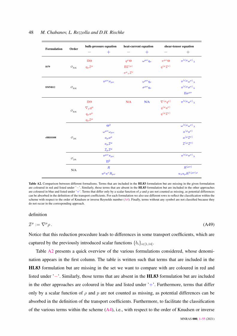
48 M. Chabanov, L. Rezzolla and D.H. Rischke
Formulation Orderbulk-pressure equation heat-current equation shear-tensor equation
− + − + − +
IS79 ORK
ΠΘ qµΘ ωµνqν πµνΘ πλ〈µων〉λ
qµIµ ΠI〈µ〉 q〈µIν〉
πµνIν
DMNR12 ORK
πµνσµν ωµνqν πλ〈µων〉λ
σµνqν πλ〈µσν〉λ
Πσµν
rBRSSS08
ORK
ΠΘ N/A N/A ∇〈µqν〉 πλ〈µων〉λ
∇µqµ q〈µaν〉
qµaµ q〈µIν〉
qµIµ
O2K
Θ2 ωλ〈µων〉λ
ωµνωµν a〈µaν〉
aµaµ a〈µIν〉
aµIµ I〈µIν〉
IµIµ
O2R
πµνπµν πλ〈µπν〉λ
Π2
N/AR R〈µν〉
uµuνRµν uλuρRλ〈µν〉ρ
Table A2. Comparison between different formalisms. Terms that are included in the HL83 formulation but are missing in the given formulationare coloured in red and listed under ’−’. Similarly, those terms that are absent in the HL83 formulation but are included in the other approachesare coloured in blue and listed under ’+’. Terms that differ only by a scalar function of ρ and p are not counted as missing, as potential differencescan be absorbed in the definition of the transport coefficients. For each formulation we also use different rows to reflect the classification within thescheme with respect to the order of Knudsen or inverse Reynolds number (A4). Finally, terms without any symbol are not classified because theydo not occur in the corresponding approach.
definition
Iµ := ∇µρ . (A49)
Notice that this reduction procedure leads to differences in some transport coefficients, which are
captured by the previously introduced scalar functions bii∈[1,14].
Table A2 presents a quick overview of the various formulations considered, whose denomi-
nation appears in the first column. The table is written such that terms that are included in the
HL83 formulation but are missing in the set we want to compare with are coloured in red and
listed under ’−’. Similarly, those terms that are absent in the HL83 formulation but are included
in the other approaches are coloured in blue and listed under ’+’. Furthermore, terms that differ
only by a scalar function of ρ and p are not counted as missing, as potential differences can be
absorbed in the definition of the transport coefficients. Furthermore, to facilitate the classification
of the various terms within the scheme (A4), i.e., with respect to the order of Knudsen or inverse
MNRAS 000, 1–55 (2021)
GRHD of non-perfect fluids 49
Reynolds number O1, ORK, O2R, and O2K, they are collected on different rows. Finally, terms
without any symbol are not classified because they do not occur in the corresponding approach.
Note that the rBRSSS08 formulation includes second-order terms, but does not distinguish
between ησµνΠ and ζπµνΘ. However, these are not the only second-order terms present in the
rBRSSS08 formulation. Another difference is of course the presence of terms associated with the
curvature of spacetime, which are absent in DMNR12. Clearly, these terms cannot be classified
by a certain order within the scheme (A4). However, if gµν is considered as an equilibrium fluid
variable, then these terms can be seen as of second order in Knudsen number. Finally, we recall
that the rBRSSS08 formulation is derived in the Landau frame, where the heat currents are zero.
As a corollary to this comparison, we report in Tables A3 and A4 a list of all the transport
coefficients in our and in the original notation, while the definition of all Iiµ is given in Table A5.
APPENDIX B: DETAILS ON VISCOUS BLACK-HOLE ACCRETION
Given the very limited use and knowledge of the stationary solution of the spherically symmet-
ric equations of GRDHD in a Schwarzschild spacetime, we here review the basic mathematical
expressions and the strategy employed to obtain a numerical solution in the presence of a critical
point.
B1 Equations of GRDHD
We recall that the equations of GRDHD are given by Eqs. (1), (2) where Jµ = JµPF
, and T µν is
given by Eq. (4), together with Eq. (99) in the case in which the heat current and the shear-stress
tensor are set to zero. By demanding the equations to be stationary and spherically symmetric,
i.e., all state variables are functions of the circumference radius r only and the fluid four-velocity
has the form uµ = (ut, u, 0, 0)T , it is possible to obtain the following coupled, nonlinear system
MNRAS 000, 1–55 (2021)
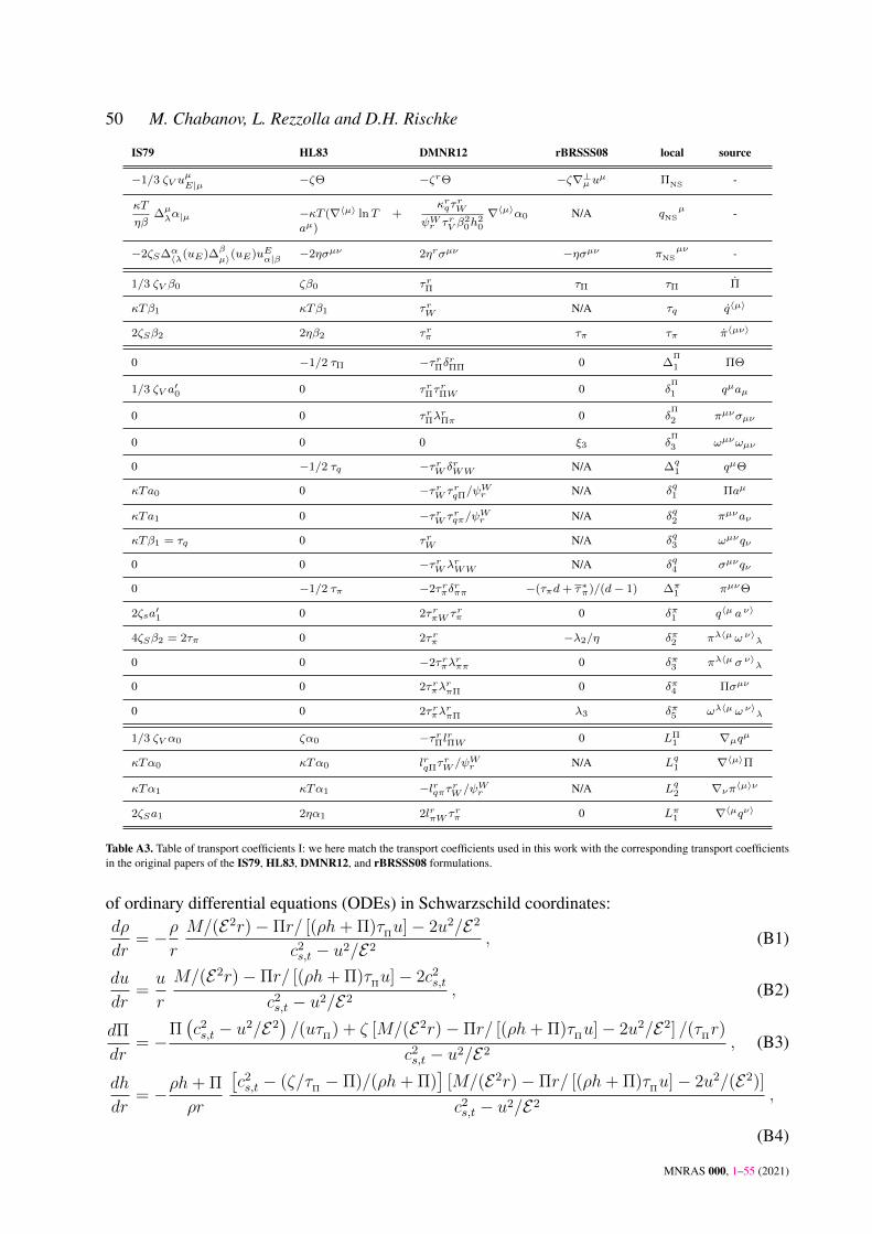
50 M. Chabanov, L. Rezzolla and D.H. Rischke
IS79 HL83 DMNR12 rBRSSS08 local source
−1/3 ζV uµE|µ −ζΘ −ζrΘ −ζ∇⊥µ uµ ΠNS -
κT
ηβ∆µλα|µ −κT (∇〈µ〉 lnT +
aµ)
κrqτrW
ψWr τrV β20h
20
∇〈µ〉α0 N/A qµ
NS -
−2ζS∆α〈λ(uE)∆β
µ〉(uE)uEα|β −2ησµν 2ηrσµν −ησµν π
µνNS -
1/3 ζV β0 ζβ0 τrΠ τΠ τΠ Π
κTβ1 κTβ1 τrW N/A τq q〈µ〉
2ζSβ2 2ηβ2 τrπ τπ τπ π〈µν〉
0 −1/2 τΠ −τrΠδrΠΠ 0 ∆
Π
1 ΠΘ
1/3 ζV a′0 0 τrΠτ
rΠW 0 δ
Π
1 qµaµ
0 0 τrΠλrΠπ 0 δ
Π
2 πµνσµν
0 0 0 ξ3 δΠ
3 ωµνωµν
0 −1/2 τq −τrW δrWW N/A ∆q1 qµΘ
κTa0 0 −τrW τrqΠ/ψWr N/A δq1 Πaµ
κTa1 0 −τrW τrqπ/ψWr N/A δq2 πµνaν
κTβ1 = τq 0 τrW N/A δq3 ωµνqν
0 0 −τrWλrWW N/A δq4 σµνqν
0 −1/2 τπ −2τrπδrππ −(τπd+ τ∗π)/(d− 1) ∆π
1 πµνΘ
2ζsa′1 0 2τrπW τrπ 0 δπ1 q〈µ a ν〉
4ζSβ2 = 2τπ 0 2τrπ −λ2/η δπ2 πλ〈µ ω ν〉λ
0 0 −2τrπλrππ 0 δπ3 πλ〈µ σ ν〉λ
0 0 2τrπλrπΠ 0 δπ4 Πσµν
0 0 2τrπλrπΠ λ3 δπ5 ωλ〈µ ω ν〉λ
1/3 ζV α0 ζα0 −τrΠlrΠW 0 LΠ
1 ∇µqµ
κTα0 κTα0 lrqΠτrW /ψWr N/A Lq1 ∇〈µ〉Π
κTα1 κTα1 −lrqπτrW /ψWr N/A Lq2 ∇νπ〈µ〉ν
2ζSa1 2ηα1 2lrπW τrπ 0 Lπ1 ∇〈µqν〉
Table A3. Table of transport coefficients I: we here match the transport coefficients used in this work with the corresponding transport coefficientsin the original papers of the IS79, HL83, DMNR12, and rBRSSS08 formulations.
of ordinary differential equations (ODEs) in Schwarzschild coordinates:dρ
dr= −ρ
r
M/(E2r)− Πr/ [(ρh+ Π)τΠu]− 2u2/E2
c2s,t − u2/E2
, (B1)
du
dr=u
r
M/(E2r)− Πr/ [(ρh+ Π)τΠu]− 2c2
s,t
c2s,t − u2/E2
, (B2)
dΠ
dr= −
Π(c2s,t − u2/E2
)/(uτ
Π) + ζ [M/(E2r)− Πr/ [(ρh+ Π)τ
Πu]− 2u2/E2] /(τ
Πr)
c2s,t − u2/E2
, (B3)
dh
dr= −ρh+ Π
ρr
[c2s,t − (ζ/τ
Π− Π)/(ρh+ Π)
][M/(E2r)− Πr/ [(ρh+ Π)τ
Πu]− 2u2/(E2)]
c2s,t − u2/E2
,
(B4)
MNRAS 000, 1–55 (2021)
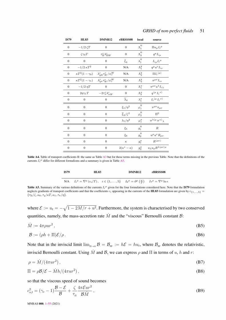
GRHD of non-perfect fluids 51
IS79 HL83 DMNR12 rBRSSS08 local source
0 −1/2 ζT 0 0 ΛΠ
1 ΠuµIiµ
0 ζγ0T τrΠλrΠW 0 Λ
Π
2 qµIiµ
0 0 0 ξ4 λΠ
1 IiµIiµ
0 −1/2 κT 2 0 N/A Λq1 qµuνIiν
0 κT 2(1− γ0) λrqΠτrW /ψWr N/A Λq2 ΠIi
〈µ〉
0 κT 2(1− γ1) λrqπτrW /ψWr N/A Λq3 πµνIiν
0 −1/2 ηT 0 0 Λπ1 πµνuλIiλ
0 2ηγ1T −2τrπλrπW 0 Λπ2 q〈µ Ii
ν〉
0 0 0 λ4 λπ1 Ii〈µ Ii
ν〉
0 0 0 ξ1/η2 ϕΠ
1 πµνπµν
0 0 0 ξ2/ζ2 ϕ
Π
2 Π2
0 0 0 λ1/η2 ϕπ1 πλ〈µ π ν〉λ
0 0 0 ξ5 gΠ
1 R
0 0 0 ξ6 gΠ
2 uµuνRµν
0 0 0 κ gπ1 R〈µν〉
0 0 0 2(κ∗ − κ) gπ2 uλuρRλ〈µν〉ρ
Table A4. Table of transport coefficients II: the same as Table A3 but for those terms missing in the previous Table. Note that the definitions of thecurrents Iiµ differ for different formalisms and a summary is given in Table A5.
IS79 HL83 DMNR12 rBRSSS08
N/A Iiµ = ∇µ (ci/T ) , i ∈ 1, . . . , 5 I6
µ = ∂µ( µT
)I7µ = ∇µ ln e
Table A5. Summary of the various definitions of the currents Iiµ given for the four formulations considered here. Note that the IS79 formulationneglects gradients of transport coefficients and that the coefficients ci appearing in the currents of the HL83 formulation are given by c1,...,5 =τΠ/ζ, α0, τq/κT, α1, τπ/η.
where E := ut = −√
1− 2M/r + u2. Furthermore, the system is characterised by two conserved
quantities, namely, the mass-accretion rate M and the “viscous” Bernoulli constant B:
M := 4πρur2 , (B5)
B := (ρh+ Π)E/ρ . (B6)
Note that in the inviscid limit limΠ→0B = BPF := hE = hut, where BPF denotes the relativistic,
inviscid Bernoulli constant. Using M and B, we can express ρ and Π in terms of u, h and r:
ρ = M/(4πur2) , (B7)
Π = ρB/E − Mh/(4πur2) , (B8)
so that the viscous speed of sound becomes
c2s,t = (γe − 1)
B − EB
+ζ
τΠ
4πEur2
BM, (B9)
MNRAS 000, 1–55 (2021)
52 M. Chabanov, L. Rezzolla and D.H. Rischke
and Eqs. (B2) and (B4) simplify todu
dr=u
r
M/(E2r)− (B − Eh)r/ (BτΠu)− 2c2
s,t
c2s,t − u2/E2
, (B10)
dh
dr= −1
r
[(γe − 1)(B − E)/E + (B − hE)/E ] [M/(E2r)− (B − Eh)r/ (BτΠu)− 2u2/E2]
c2s,t − u2/E2
.
(B11)
Equations (B10)–(B11) do not have an analytic solution and their non-trivial numerical solution is
discussed in more detail in the next section.
B2 Singular point analysis and integration
The first step in the solution of Eqs. (B10), (B11) is to choose the location of the sonic point rs,
which is defined as the radial coordinate where u2/E2 = c2s,t. This corresponds to the position
where the infalling fluid velocity equals that of the speed of sound as observed at rest from spatial
infinity, and where Eqs. (B10), (B11) become singular. Because of that, we choose to start the
numerical integration procedure directly at rs and integrate inward (i.e., supersonic portion) and
outward (i.e., subsonic portion) from there. In this way, we can make use of exact results for the
states and their first derivatives at the sonic point in order to initialise numerical integration. In
the following we will elaborate on the exact method. Using the inviscid solution with a polytropic
constant (see discussion in Sec. 7), it is possible to obtain values for M and BPF . In the inviscid
case, all state variables at the sonic point are automatically determined by choosing rs (see Hawley
et al. 1984, for details).
Setting B = BPF and using the value for M found for the inviscid case, we can compute our
initial values at rs for the viscous case. As in the inviscid case, we demand that the derivatives at
the sonic point constitute a removable singularity. Hence, from equations (B10) and (B11) we find
the conditions
0 =M
E2r− B − Eh
Br
τΠu− 2c2
s,t , (B12)
0 = c2s,t −
u2
E2. (B13)
Numerical root finding via Mathematica (Wolfram Research 2020) yields the values of the radial
four-velocity component and of the specific enthalpy at the sonic radius, us and hs. Because multi-
ple solutions exist, we select the solution satisfying the conditions: us < 0 and hs > 1, which was
found to be unique for the choice of constant ζ and τΠ
. Next, accurate values for the derivatives
du/dr and dh/dr are needed at the sonic point because we would otherwise rely on the evaluation
of the right-hand side of Eqs. (B10) and (B11) at rs for the first step of the integration procedure.
MNRAS 000, 1–55 (2021)
GRHD of non-perfect fluids 53
Even though the singularity is removable, numerical errors cause singular behaviour and unreliable
values for the derivatives.
Hence, following Mandal et al. (2007) (but see also Ray & Bhattacharjee 2002; Afshordi &
Paczynski 2003) we can treat Eqs. (B10)–(B11) assuming that each function u, r, and h can be
expressed in terms of a parameter ξ, i.e., u = u(ξ), r = r(ξ), h = h(ξ), such that when writing
Eqs. (B10)–(B11) symbolically as du/dr = A/B and dh/dr = C/B, they can be effectively
rewritten as du/dξ = A, dr/dξ = B, and dh/dξ = C. More specifically, we express Eqs. (B10)–
(B11) symbolically as
dr
dξ= r
(c2s,t −
u2
E2
), (B14)
du
dξ= u
(M
E2r− B − Eh
Br
τΠu− 2c2
s,t
), (B15)
dh
dξ= −
[(γe − 1)
B − EE
+B − hEE
] [M
E2r− B − Eh
Br
τΠu− 2
u2
E2
]. (B16)
Note that ξ does not have a physical interpretation and should be seen simply as a mathematical
parameter. However, with this parameterisation, each of the solutions r(ξ), u(ξ), and h(ξ) can be
thought as consisting of two branches on either side of the sonic point: i.e., one branch for r < rs
and one for r > rs. In this way, and as will be found later, the solution at the sonic point can be
obtained in the limit ξ → ±∞12.
Hence, Eqs. (B14)–(B16) effectively represent an independent system whose paths in the
(u, h, r)-space, i.e., the phase space of Eqs. (B14)–(B16), correspond to solutions of the origi-
nal system, i.e., Eqs. (B10) and (B11). Thus, the original system can be viewed as differential
equations for the phase paths of Eqs. (B14)– (B16). The solution (us, hs) at the sonic point rs
constitutes a solution (us, hs, rs) of Eqs. (B14)–(B16) at the so-called equilibrium point, where
du/dξ = dh/dξ = dr/dξ = 0. Notice the dependence on the specific choice of ζ = ζ(u, h, r) and
τΠ
= τΠ(u, h, r).
Equations (B14)–(B16) can can be linearised at the sonic point, i.e., u ≈ us + δu, h ≈ hs + δh
and r ≈ rs + δr, to obtain a local solution (Jordan & Smith 2007). This linearisation procedure
and the ansatz δu = δu exp(λξ), δh = δh exp(λξ) and δr = δr exp(λξ) leads to a an eigenvalue
problem, which can be solved numerically (Wolfram Research 2020). The outcome is a set of three
eigenvalues λ1, λ2, λ3 and eigenvectors with the properties λ1 < 0, λ2 > 0 and λ3 ≈ 0. The
12 This condition follows from the requirement that the perturbation behaves as∼ eλξ , where λ is a constant eigenvalue that can be either positive
or negative, and that it vanishes at the sonic point; see also below.
MNRAS 000, 1–55 (2021)
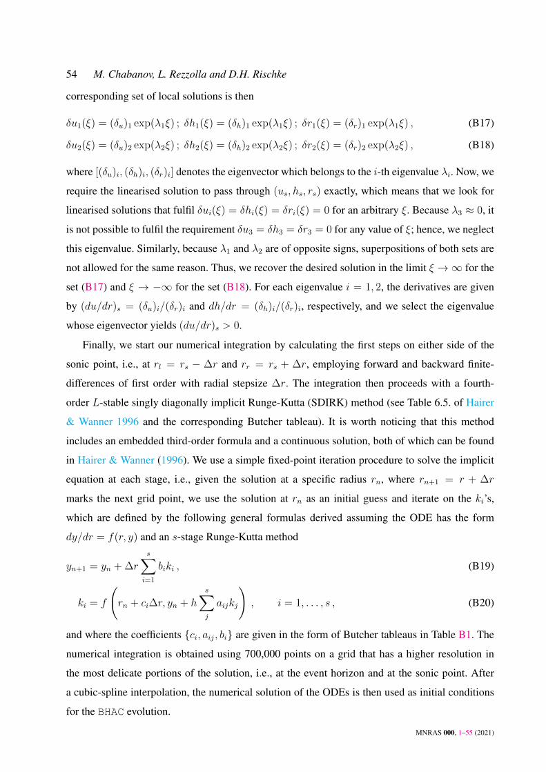
54 M. Chabanov, L. Rezzolla and D.H. Rischke
corresponding set of local solutions is then
δu1(ξ) = (δu)1 exp(λ1ξ) ; δh1(ξ) = (δh)1 exp(λ1ξ) ; δr1(ξ) = (δr)1 exp(λ1ξ) , (B17)
δu2(ξ) = (δu)2 exp(λ2ξ) ; δh2(ξ) = (δh)2 exp(λ2ξ) ; δr2(ξ) = (δr)2 exp(λ2ξ) , (B18)
where [(δu)i, (δh)i, (δr)i] denotes the eigenvector which belongs to the i-th eigenvalue λi. Now, we
require the linearised solution to pass through (us, hs, rs) exactly, which means that we look for
linearised solutions that fulfil δui(ξ) = δhi(ξ) = δri(ξ) = 0 for an arbitrary ξ. Because λ3 ≈ 0, it
is not possible to fulfil the requirement δu3 = δh3 = δr3 = 0 for any value of ξ; hence, we neglect
this eigenvalue. Similarly, because λ1 and λ2 are of opposite signs, superpositions of both sets are
not allowed for the same reason. Thus, we recover the desired solution in the limit ξ →∞ for the
set (B17) and ξ → −∞ for the set (B18). For each eigenvalue i = 1, 2, the derivatives are given
by (du/dr)s = (δu)i/(δr)i and dh/dr = (δh)i/(δr)i, respectively, and we select the eigenvalue
whose eigenvector yields (du/dr)s > 0.
Finally, we start our numerical integration by calculating the first steps on either side of the
sonic point, i.e., at rl = rs − ∆r and rr = rs + ∆r, employing forward and backward finite-
differences of first order with radial stepsize ∆r. The integration then proceeds with a fourth-
order L-stable singly diagonally implicit Runge-Kutta (SDIRK) method (see Table 6.5. of Hairer
& Wanner 1996 and the corresponding Butcher tableau). It is worth noticing that this method
includes an embedded third-order formula and a continuous solution, both of which can be found
in Hairer & Wanner (1996). We use a simple fixed-point iteration procedure to solve the implicit
equation at each stage, i.e., given the solution at a specific radius rn, where rn+1 = r + ∆r
marks the next grid point, we use the solution at rn as an initial guess and iterate on the ki’s,
which are defined by the following general formulas derived assuming the ODE has the form
dy/dr = f(r, y) and an s-stage Runge-Kutta method
yn+1 = yn + ∆rs∑i=1
biki , (B19)
ki = f
(rn + ci∆r, yn + h
s∑j
aijkj
), i = 1, . . . , s , (B20)
and where the coefficients ci, aij, bi are given in the form of Butcher tableaus in Table B1. The
numerical integration is obtained using 700,000 points on a grid that has a higher resolution in
the most delicate portions of the solution, i.e., at the event horizon and at the sonic point. After
a cubic-spline interpolation, the numerical solution of the ODEs is then used as initial conditions
for the BHAC evolution.
MNRAS 000, 1–55 (2021)
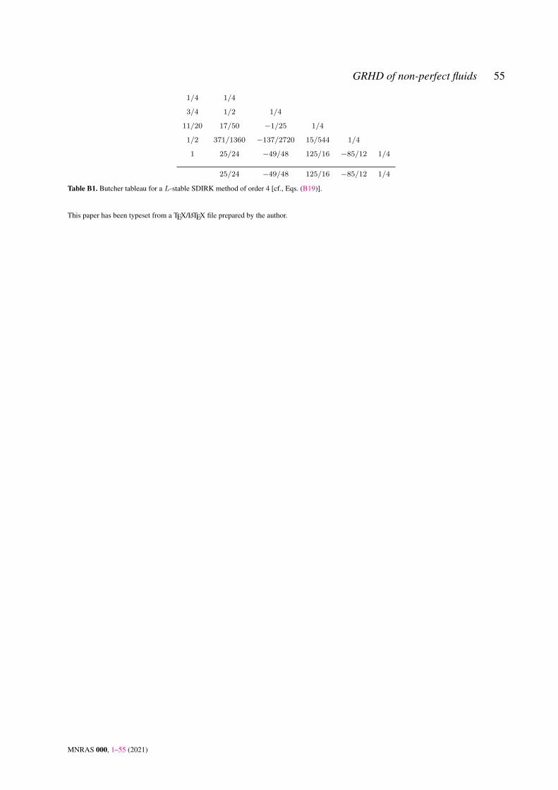
GRHD of non-perfect fluids 55
1/4 1/4
3/4 1/2 1/4
11/20 17/50 −1/25 1/4
1/2 371/1360 −137/2720 15/544 1/4
1 25/24 −49/48 125/16 −85/12 1/4
25/24 −49/48 125/16 −85/12 1/4
Table B1. Butcher tableau for a L-stable SDIRK method of order 4 [cf., Eqs. (B19)].
This paper has been typeset from a TEX/LATEX file prepared by the author.
MNRAS 000, 1–55 (2021)
Related Documents


