General methods for evolutionary quantitative genetic inference from generalised mixed models Pierre de Villemereuil * , Holger Schielzeth †,‡ , Shinichi Nakagawa § , and Michael Morrissey ** * Laboratoire d’ ´ Ecologie Alpine, CNRS UMR 5553 Universit´ e Joseph Fourier , BP53, 38041 Grenoble, Cedex 9, France [email protected] † Department of Evolutionary Biology Bielefeld University, Bielefeld, Germany ‡ Institute of Ecology Dornburger Str. 159, 07743 Jena [email protected] § Evolution and Ecology Research Centre University of New South Wales, Sydney, NSW 2052, Australia [email protected] ** School of Evolutionary Biology University of St Andrews, St Andrews, UK, KY16 9TH [email protected] May 18, 2016 Keywords: quantitative genetics, generalised linear model, statistics, theory, evolution, addi- tive genetic variance, G matrix 1 . CC-BY 4.0 International license not peer-reviewed) is the author/funder. It is made available under a The copyright holder for this preprint (which was . http://dx.doi.org/10.1101/026377 doi: bioRxiv preprint first posted online Sep. 8, 2015;

Welcome message from author
This document is posted to help you gain knowledge. Please leave a comment to let me know what you think about it! Share it to your friends and learn new things together.
Transcript

General methods for evolutionary quantitative genetic inference from
generalised mixed models
Pierre de Villemereuil*, Holger Schielzeth†,‡, Shinichi Nakagawa§, and Michael Morrissey**
*Laboratoire d’Ecologie Alpine, CNRS UMR 5553Universite Joseph Fourier , BP53, 38041 Grenoble, Cedex 9, France
†Department of Evolutionary BiologyBielefeld University, Bielefeld, Germany
‡Institute of EcologyDornburger Str. 159, 07743 [email protected]
§Evolution and Ecology Research CentreUniversity of New South Wales, Sydney, NSW 2052, Australia
**School of Evolutionary BiologyUniversity of St Andrews, St Andrews, UK, KY16 9TH
May 18, 2016
Keywords: quantitative genetics, generalised linear model, statistics, theory, evolution, addi-tive genetic variance, G matrix
1
.CC-BY 4.0 International licensenot peer-reviewed) is the author/funder. It is made available under aThe copyright holder for this preprint (which was. http://dx.doi.org/10.1101/026377doi: bioRxiv preprint first posted online Sep. 8, 2015;
Quantitative genetic inference with GLMMs 2
Abstract1
Methods for inference and interpretation of evolutionary quantitative genetic pa-2
rameters, and for prediction of the response to selection, are best developed for traits3
with normal distributions. Many traits of evolutionary interest, including many life4
history and behavioural traits, have inherently non-normal distributions. The gen-5
eralised linear mixed model (GLMM) framework has become a widely used tool for6
estimating quantitative genetic parameters for non-normal traits. However, whereas7
GLMMs provide inference on a statistically-convenient latent scale, it is sometimes8
desirable to express quantitative genetic parameters on the scale upon which traits9
are expressed. The parameters of a fitted GLMMs, despite being on a latent scale,10
fully determine all quantities of potential interest on the scale on which traits are11
expressed. We provide expressions for deriving each of such quantities, including12
population means, phenotypic (co)variances, variance components including additive13
genetic (co)variances, and parameters such as heritability. We demonstrate that fixed14
effects have a strong impact on those parameters and show how to deal for this effect15
by averaging or integrating over fixed effects. The expressions require integration of16
quantities determined by the link function, over distributions of latent values. In gen-17
eral cases, the required integrals must be solved numerically, but efficient methods are18
available and we provide an implementation in an R package, QGglmm. We show19
that known formulae for quantities such as heritability of traits with Binomial and20
Poisson distributions are special cases of our expressions. Additionally, we show how21
fitted GLMM can be incorporated into existing methods for predicting evolutionary22
trajectories. We demonstrate the accuracy of the resulting method for evolution-23
ary prediction by simulation, and apply our approach to data from a wild pedigreed24
vertebrate population.25
.CC-BY 4.0 International licensenot peer-reviewed) is the author/funder. It is made available under aThe copyright holder for this preprint (which was. http://dx.doi.org/10.1101/026377doi: bioRxiv preprint first posted online Sep. 8, 2015;

Quantitative genetic inference with GLMMs 3
Introduction26
Additive genetic variances and covariances of phenotypic traits determine the response to se-27
lection, and so are key determinants of the processes of adaptation in response to natural28
selection and of genetic improvement in response to artificial selection (Fisher, 1918; Falconer,29
1960; Lynch and Walsh, 1998; Walsh and Lynch, forthcoming). While the concept of additive30
genetic variance (Fisher, 1918; Falconer, 1960) is very general, being applicable to any type of31
character with any arbitrary distribution, including, for example, fitness (Fisher, 1930), tech-32
niques for estimating additive genetic variances and covariances are best developed for Gaussian33
traits (i.e., traits that follow a normal distribution; Henderson 1950; Lynch and Walsh 1998).34
Furthermore, quantitative genetic theory for predicting responses to selection are also best35
developed and established for Gaussian characters (Walsh and Lynch, forthcoming), but see36
Morrissey (2015). Consequently, although many characters of potential evolutionary interest37
are not Gaussian (e.g. survival or number of offspring), they are not well-handled by existing38
theory and methods. Comprehensive systems for estimating genetic parameters and predict-39
ing evolutionary trajectories of non-Gaussian traits will hence be very useful for quantitative40
genetic studies of adaptation.41
For the analysis of Gaussian traits, linear mixed model-based (LMM) inferences of genetic42
parameters, using the ‘animal model’, have become common practice in animal and plant43
breeding (Thompson, 2008; Hill and Kirkpatrick, 2010), but also in evolutionary studies on44
wild populations (Kruuk, 2004; Wilson et al., 2010). Recently, the use of generalised linear45
mixed models (GLMMs) to analyse non-Gaussian traits has been increasing (e.g. Milot et al.,46
2011; Wilson et al., 2011; Morrissey et al., 2012; de Villemereuil et al., 2013; Ayers et al.,47
2013). Whereas LMM analysis directly estimates additive genetic parameters on the scale on48
which traits are expressed and selected, and upon which we may most naturally consider their49
evolution, this is not the case for GLMMs. In this paper, we offer a comprehensive description50
of the assumptions of GLMMs and their consequences in terms of quantitative genetics and a51
framework to infer quantitative genetic parameters from GLMMs output. This work applies and52
extends theory in Morrissey (2015), to handle the effects of (non-linear) relationships among the53
scale upon which inference is conducted in a GLMM and the scale of data, and to accommodate54
.CC-BY 4.0 International licensenot peer-reviewed) is the author/funder. It is made available under aThe copyright holder for this preprint (which was. http://dx.doi.org/10.1101/026377doi: bioRxiv preprint first posted online Sep. 8, 2015;

Quantitative genetic inference with GLMMs 4
the error structures that arise in GLMM analysis. These results generalise existing expressions55
for specific models (threshold model and Poisson with a log-link, Dempster and Lerner, 1950;56
Robertson, 1950; Foulley and Im, 1993). We show that fixed effects in GLMMs raise special57
complications and we offer some efficient approaches for dealing with this issue.58
While it will undoubtedly be desirable to develop a comprehensive method for making data-59
scale inferences of quantitative genetic parameters with GLMMs, such an endeavour will not60
yield a system for predicting evolution in response to natural or artificial selection, even if a61
particular empirical system is very well served by the assumptions of a GLMM. This is because62
systems for evolutionary prediction, specifically the Breeder’s equation (Lush, 1937; Fisher,63
1924) and the Lande equation (Lande, 1979; Lande and Arnold, 1983), assume that breeding64
values (and in most applications, phenotypes) are multivariate normal or make assumptions65
such as linearity of the parent-offspring regression, which are unlikely to hold for non-normal66
traits (Walsh and Lynch, forthcoming). Even if it is possible to estimate additive genetic vari-67
ances of traits on the scale upon which traits are expressed, we will show that these quantities68
will not strictly be usable for evolutionary prediction. However, we will see that the scale on69
which estimation is performed in a GLMM does, by definition, satisfy the assumptions of the70
Breeder’s and Lande equations. Thus, for the purpose of predicting evolution, it may be useful71
to be able to express selection of non-Gaussian traits on this scale. Such an approach will yield72
a system for evolutionary prediction of characters that have been modelled with a GLMM,73
requiring no more assumptions than those that are already made in applying the statistical74
model.75
The main results in this paper are arranged in four sections. First, we describe the GLMM76
framework: its relationship to the more general (Gaussian) LMM and especially to the Gaussian77
animal model (Henderson, 1973; Kruuk, 2004; Wilson et al., 2010), how GLMMs can be usefully78
viewed as covering three scales and how some special interpretational challenges arise and are79
currently dealt with. Second, we propose a system for making inferences of quantitative genetic80
parameters on the scale upon which traits are expressed for arbitrary GLMMs. We show how81
to estimate genotypic and additive genetic variances and covariances on this scale, accounting82
for fixed effects as necessary. We lay out the formal theory underlying the system, apply it to83
an empirical dataset. The relationships between existing analytical formulae and our general84
.CC-BY 4.0 International licensenot peer-reviewed) is the author/funder. It is made available under aThe copyright holder for this preprint (which was. http://dx.doi.org/10.1101/026377doi: bioRxiv preprint first posted online Sep. 8, 2015;
Quantitative genetic inference with GLMMs 5
framework are also highlighted. Third, we illustrate the issues when inferring quantitative85
genetic parameters using a GLMM with an empirical example on Soay sheep (Ovis aries) and86
how our framework can help to overcome them. Fourth, we outline a system of evolutionary87
prediction for non-Gaussian traits that capitalises on the fact that the latent scale in a GLMM88
satisfies the assumptions of available equations for the prediction of evolution. We show in89
a simulation study that (i) evolutionary predictions using additive genetic variances on the90
observed data scale represent approximations, and can, in fact, give substantial errors, and91
(ii) making inferences via the latent scale provides unbiased predictions, insofar as a GLMM92
may provide a pragmatic model of variation in non-Gaussian traits. The framework introduced93
here (including both quantitative genetic parameters inference and evolutionary prediction) has94
been implemented in a package for the R software (R Core Team, 2015) available at https:95
//github.com/devillemereuil/qgglmm.96
The generalised linear mixed model framework97
Linear mixed models for Gaussian traits98
For Gaussian traits, a linear mixed model allows various analyses of factors that contribute to99
the mean and variance of phenotype. In particular, a formulation of a linear mixed model called100
the ‘animal model’ provides a very general method for estimating additive genetic variances and101
covariances, given arbitrary pedigree data, and potentially accounting for a range of different102
types of confounding variables, such as environmental effects, measurement error or maternal103
effects. A general statement of an animal model analysis decomposing variation in a trait, z,104
into additive genetic and other components would be105
z = µ+ Xb + Zaa + Z1u1 + ...+ Zkuk + e, (1)
where µ is the model intercept, b is a vector of fixed effects such as sex and age, relating106
potentially both continuous and categorical effects to observations via the fixed effects design107
matrix X, just as in an ordinary linear model, and e is the vector of normally-distributed108
residuals. An arbitrary number of random effects can be modelled, with design matrices Z,109
.CC-BY 4.0 International licensenot peer-reviewed) is the author/funder. It is made available under aThe copyright holder for this preprint (which was. http://dx.doi.org/10.1101/026377doi: bioRxiv preprint first posted online Sep. 8, 2015;

Quantitative genetic inference with GLMMs 6
where effects (a, u1...uk) are assumed to be drawn from normal distributions with variances110
to be estimated. The key feature of the animal model is that it includes individual additive111
genetic effects, or breeding values, conventionally denoted a. These additive genetic effects112
and, critically, their variance, are estimable given relatedness data, which can be derived from113
pedigree data, or, more recently, from genomic estimates of relatedness (Sillanpaa, 2011). The114
covariances of breeding values among individuals can be modelled according to115
a ∼ N (0,AVA) , (2)
where A is the additive genetic relatedness matrix derived from the pedigree and VA is the116
genetic additive variance.117
Common issues with non-Gaussian traits118
Many non-Gaussian traits, however, cannot be strictly additive on the scale on which they are119
expressed. Consider, for example, survival probability that is bounded at 0 and 1 so that effects120
like the substitution effect of one allele for another necessarily must be smaller when expressed121
in individuals that otherwise have expected values near zero or one. In such a scenario, it may122
be reasonable to assume that there exists an underlying scale, related to survival probability,123
upon which genetic and other effects are additive.124
In addition to inherent non-additivity, many non-Gaussian traits will have complex patterns125
of variation. Over and above sources of variation that can be modelled with fixed and random126
effects, as in a LMM (e.g., using Eqs. 1 and 2), residual variation may include both inherently127
stochastic components, and components that correspond to un-modelled systematic differences128
among observations. In a LMM, such differences are not distinguished, but contribute to resid-129
ual variance. However, for many non-Gaussian traits it may be desirable to treat the former130
as arising from some known statistical distribution, such as the binomial or Poisson distribu-131
tion, and to deal with additional variation via a latent-scale residual (i.e. an overdispersion132
term). Separation of these two kinds of variation in residuals may be very generally useful in133
evolutionary quantitative genetic studies.134
.CC-BY 4.0 International licensenot peer-reviewed) is the author/funder. It is made available under aThe copyright holder for this preprint (which was. http://dx.doi.org/10.1101/026377doi: bioRxiv preprint first posted online Sep. 8, 2015;

Quantitative genetic inference with GLMMs 7
The scales of the generalised linear mixed model135
Generalised linear mixed model (GLMM) analysis can be used for inference of quantitative136
genetic parameters, and provides pragmatic ways of dealing with inherent non-additivity and137
with complex sources of variation. The GLMM framework can be thought of as consisting of138
three distinct scales on which we can think of variation in a trait occurring (see Fig. 1). A latent139
scale is assumed (Fig. 1, top), on which effects on the propensity for expression of some trait140
are assumed to be additive. A function, called a ‘link function’ is applied that links expected141
values for a trait to the latent scale. For example, a trait that is expressed in counts, say,142
number of behaviours expressed in a unit time, is a strictly non-negative quantity. As depicted143
in Fig. 1, a strictly positive distribution of expected values may related to latent values ranging144
from −∞ to +∞ by a function such as the log link. Finally, a distribution function (e.g.145
Binomial, Poisson, etc.) is required to model the “noise” of observed values around expected146
value (Fig. 1, bottom). Different distributions are suitable for different traits. For example,147
with a count trait such as that depicted in Fig. 1, observed values may be modelled using the148
Poisson distribution, with expectations related to the latent scale via the log link function.149
More formally, these three scales of the GLMM can be written:150
` = µ+ Xb + Zaa + Z1u1 + ...+ Zkuk + o, (3a)
151
η = g−1(`), (3b)152
z ∼ D(η,θ), (3c)
where Eq. 3a is just as for a LMM (Eq. 1), except that it describes variation on the latent153
scale `, rather than the response directly. Note that we now refer to the “residual” (noted e in154
Eq. 1) as “overdispersion” (denoted o, with a variance denoted VO), since residuals (variation155
around expected values) are defined by the distribution function, D, in this model. Just as for156
the LMM (Eq. 1), all random effects are assumed to follow normal distributions with variances157
to be estimated on the latent scale. Particularly, the variance of additive genetic effects a is158
assumed to follow Eq. 2 on the latent scale.159
Eq. 3b formalises the idea of the link function. Any link function has an associated inverse160
.CC-BY 4.0 International licensenot peer-reviewed) is the author/funder. It is made available under aThe copyright holder for this preprint (which was. http://dx.doi.org/10.1101/026377doi: bioRxiv preprint first posted online Sep. 8, 2015;

Quantitative genetic inference with GLMMs 8
link function, g−1, which is often useful for converting specific latent values to expected values.161
The expected values η constitute what we call the expected data scale. For example, where162
the log link function translates expected values to the latent scale, its inverse, the exponential163
function, translates latent values to expected values. Finally, Eq. 3c specifies the distribution164
by which the observations z scatter around the expected values according to some distribution165
function, that may involve parameters (denoted θ) other than the expectation. We call this166
the observed data scale. Some quantities of interest, such as the mean, are the same on the167
expected data scale and on the observed data scale. When parameters are equivalent on these168
two scales, we will refer to them together as the data scales.169
The distinction we make between the expected and observed data scales is one of convenience170
as they are not different scales per se. However, this distinction allows for more biological171
subtlety when interpreting the output of a GLMM. The expected data scale can be thought172
of as the “intrinsic” value of individuals (shaped by both the genetic and the environment),173
but this intrinsic value can only be studied through random realisations. As we will see,174
because breeding values are intrinsic individual values, the additive genetic variance is the175
same for both scales, but, due to the added noise in observed data, the heritabilities are not.176
Upon which scale to calculate heritability depends on the underlying biological question. For177
example, individuals (given their juvenile growth and genetic value) might have an intrinsic178
annual reproductive success of 3.4, but can only produce a integer number of offspring each179
year (say 2, 3, 4 or 5): heritabilities of both intrinsic expectations and observed numbers can180
be computed, but their values and interpretations will differ.181
Current practices and issues to compute genetic quantitative parameters from182
GLMM outputs183
Genetic variance components estimated in a generalised animal model are obtained on the184
latent scale. Hence, the “conventional” formula to compute heritability:185
h2lat =VA,`
VA,` + VRE + VO, (4)
.CC-BY 4.0 International licensenot peer-reviewed) is the author/funder. It is made available under aThe copyright holder for this preprint (which was. http://dx.doi.org/10.1101/026377doi: bioRxiv preprint first posted online Sep. 8, 2015;

Quantitative genetic inference with GLMMs 9
where VRE is the summed variance of all random effects apart from the additive genetic variance,186
and VO is the overdispersion variance, is the heritability on the latent scale, not on the observed187
data scale (Morrissey et al., 2014). Here, and throughout this paper, VA,` stands for the additive188
genetic variance on the latent scale. Although it might sometimes be sensible to measure the189
heritability of a trait on the latent scale (for example, in animal breeding, where selection might190
be based on latent breeding values), it is natural to seek inferences on the scale upon which the191
trait is expressed, and on which we may think of selection as acting. Some expressions exist192
by which various parameters can be obtained or approximated on the observed data scale. For193
example, various expressions for the intra-class correlation coefficients on the data scale exist194
(reviewed in Nakagawa and Schielzeth, 2010), but, contrary to LMM, heritabilities on the data195
scales within a GLMM framework cannot be considered as intra-class correlation coefficients.196
Exact analytical expressions exist for the additive genetic variance and heritability on the197
observed data scale for two specific and important families of GLMMs (i.e. combinations of198
link functions and distribution functions): for a binomial model with a probit link function (i.e.,199
the “threshold model,” Dempster and Lerner, 1950) and for a Poisson model with a logarithm200
link function (Foulley and Im, 1993). A general system for calculating genetic parameters on201
the expected and observed data scales for arbitrary GLMMs is currently lacking.202
In addition to handling the relationship between observed data and the latent trait via203
the link and distribution functions, any system for expected and observed scale quantitative204
genetic inference with GLMMs will have to account for complex ways in which fixed effects205
can influence quantitative genetic parameters. It is currently appreciated that fixed effects206
in LMMs explain variance, and that variance associated with fixed effects can have a large207
influence on summary statistics such as repeatability (Nakagawa and Schielzeth, 2010) and208
heritability (Wilson, 2008). This principle holds for GLMMs as well, but fixed effects cause209
additional, important complications for interpreting GLMMs. While random and fixed effects210
are independent in a GLMM on the latent scale, the non-linearity of the link function renders211
them inter-related on the expected and observed scales. Consequently, and unlike in a LMM212
or in a GLMM on the latent scale, variance components on the observed scale in a GLMM213
depend on the fixed effects. Consider, for example, a GLMM with a log link function. Because214
the exponential is a convex function, the influence of fixed and random effects will create more215
.CC-BY 4.0 International licensenot peer-reviewed) is the author/funder. It is made available under aThe copyright holder for this preprint (which was. http://dx.doi.org/10.1101/026377doi: bioRxiv preprint first posted online Sep. 8, 2015;

Quantitative genetic inference with GLMMs 10
variance on the expected and observed data scales for larger values than for smaller values.216
Quantitative genetic parameters in GLMMs217
Although all examples and most equations in this article are presented in a univariate form, all218
our results are applicable to multivariate analysis, which is implemented in our software. Unless219
stated otherwise, the equations below assume that no fixed effect (apart from the intercept)220
were included in the GLMM model.221
Phenotypic mean and variances222
Expected population mean The expected mean phenotype z on the data scale (i.e., applying223
to both the mean expected value and mean observed value) is given by224
z =
∫g−1(`)fN (`, µ, VA,` + VRE + VO)d`, (5)
where fN (`, µ, VA,` + VRE + VO) is the probability density of a Normal distribution with mean225
µ and variance VA,` + VRE + VO evaluated at `.226
Expected-scale phenotypic variance Phenotypic variance on the expected data scale can be227
obtained analogously to the data scale population mean. Having obtained z, the phenotypic228
variance is229
VP,exp =
∫ (g−1(`)− z
)2fN (`, µ, VA,` + VRE + VO)d`. (6)
Observed-scale phenotypic variance Phenotypic variance of observed values is the sum of the230
variance in expected values and variance arising from the distribution function. Since these231
variances are independent by construction in a GLMM, they can be summed. This distribution232
variance is influenced by the latent trait value, but might also depend on additional distribution233
parameters included in θ (see Eq. 3c). Given a distribution-specific variance function v:234
VP,obs = VP,exp +
∫v(`,θ)fN (`, µ, VA,` + VRE + VO)d`. (7)
.CC-BY 4.0 International licensenot peer-reviewed) is the author/funder. It is made available under aThe copyright holder for this preprint (which was. http://dx.doi.org/10.1101/026377doi: bioRxiv preprint first posted online Sep. 8, 2015;
Quantitative genetic inference with GLMMs 11
Genotypic variance on the data scales, arising from additive genetic variance on235
the latent scale236
Because the link function is non-linear, additive genetic variance on the latent scale is manifested237
as a combination of additive and non-additive variance on the data scales. Following Falconer238
(1960) the total genotypic variance on the data scale is the variance of genotypic values on239
that scale. Genotypic values are the expected data scale phenotypes, given latent scale genetic240
values. The expected phenotype of an individual with a given latent genetic value a, i.e., its241
genotypic value on the data scales E[z|a], is given by242
E[z|a] =
∫g−1(`)fN (`, µ+ a, VRE + VO)d`. (8)
The total genotypic variances on the expected and observed data scales are the same, since243
genotypic values are expectations that do not change between the expected and observed scales.244
The total genotypic variance on both the expected and observed data scales is then245
V (E[z|a]) =
∫(E[z|a]− z)2 fN (a, 0, VA,`)da. (9)
This is the total genotypic variance on the data scale, arising from strictly additive genetic246
variance on the latent scale. If non-additive genetic effects are modelled on the latent scale,247
they would be included in the expectations and integrals in Eqs. 8 and 9.248
Additive genetic variance on the data scales249
The additive variance on the data scales is the variance of breeding values computed on the250
data scales. Following Robertson (1950; see also Fisher 1918), breeding values on the data251
scales, i.e., aexp and aobs, are the part of the phenotype z that depends linearly on the latent252
breeding values. The breeding values on the datas scale can then be defined as the predictions253
of a least-squares regression of the observed data on the latent breeding values,254
aobs = z|a = m+ ba, (10)
.CC-BY 4.0 International licensenot peer-reviewed) is the author/funder. It is made available under aThe copyright holder for this preprint (which was. http://dx.doi.org/10.1101/026377doi: bioRxiv preprint first posted online Sep. 8, 2015;
Quantitative genetic inference with GLMMs 12
where z is the value of z predicted by the regression, a the latent breeding value and m and b255
the parameters of the regression. Thus, we have VA,obs = b2VA,` and, from standard regression256
theory:257
b =cov(z, a)
VA,`
. (11)
Because of the independence between the expected values of z (i.e. the expected data scale258
g−1(`)) and the distribution “noise” (see Eq. 7), we can obtain the result that cov(z, a) =259
cov(g−1(`), a), hence:260
b =cov(g−1(`), a)
VA,`
. (12)
Stein’s (1973) lemma states that ifX and Y are bivariate normally distributed random variables,261
then the covariance of Y and some function of X, f(X), is equal to the expected value of f ′(X)262
times the covariance between X and Y , so,263
cov(g−1(`), a) = E
[dg−1(`)
d`
]cov(`, a) = E
[dg−1(`)
d`
]VA,`, (13)
noting that the covariance of latent breeding values and latent values is the variance of latent264
breeding values. Finally, combining Eq. 12 with Eq. 13, we obtain:265
b = E
[dg−1(`)
d`
]. (14)
To avoid confusion with various uses of b as other forms of regression coefficients, and for266
consistency with Morrissey (2015), we denote the average derivative of expected value with267
respect to latent value as Ψ:268
Ψ = E
[dg−1(`)
d`
]=
∫dg−1(`)
d`fN (`, µ, VA,` + VRE + VO)d`. (15)
The additive genetic variance on the expected and observed scales are still the same and are269
given by270
VA,obs = VA,exp = Ψ2VA,`. (16)
.CC-BY 4.0 International licensenot peer-reviewed) is the author/funder. It is made available under aThe copyright holder for this preprint (which was. http://dx.doi.org/10.1101/026377doi: bioRxiv preprint first posted online Sep. 8, 2015;
Quantitative genetic inference with GLMMs 13
Including fixed effects in the inference271
General issues Because of the non-linearity introduced by the link function in a GLMM, all272
quantitative genetic parameters are directly influenced by the presence of fixed effects. Hence,273
when fixed effects are included in the model, it will often be important to marginalise over them274
to compute accurate population parameters. There are different approaches to do so. We will275
first describe the simplest approach (i.e. directly based on GLMM assumptions).276
Averaging over predicted values In a GLMM, no assumption is made about the distribution of277
covariates in the fixed effects. Given this, we can marginalise over fixed effects by averaging over278
predicted values (marginalised over the random effects, i.e. Xb, where b are the fixed effects279
estimates). Note that, doing so, we implicitly make the assumption that our sample is repre-280
sentative of the population of interest. Using this approach, we can compute the population281
mean in Eq. 5 as:282
z =1
N
N∑i=1
∫g−1(`)fN (`, µ+ ˆ
i, VA,` + VRE + VO)d`, (17)
where N is the number of predicted latent values in ˆ = Xb. Typically, X will be the fixed283
effects design matrix used when fitting the generalised animal model (Eqs. 1, 2, and 3), and284
N will be the number of data observations. Furthermore, this assumes that all fixed effects285
represent biologically relevant variation, rather than being corrections for the observation pro-286
cess or experimental condition. From this estimate of z, we can compute the expected-scale287
phenotypic variance:288
VP,exp =1
N
N∑i=1
∫ (g−1(`)− z
)2fN (`, µ+ ˆ
i, VA,` + VRE + VO)d`. (18)
Note that we are not averaging over variances computed for each predicted values, since the289
value of the mean z is the same across the computation. Eqs. 7, 8, 9 and 15 are to be modified290
accordingly to compute all parameters, including Ψ. This approach has the advantages of being291
simple and making a direct use of the GLMM inference without further assumptions.292
.CC-BY 4.0 International licensenot peer-reviewed) is the author/funder. It is made available under aThe copyright holder for this preprint (which was. http://dx.doi.org/10.1101/026377doi: bioRxiv preprint first posted online Sep. 8, 2015;

Quantitative genetic inference with GLMMs 14
Sampled covariates are not always representative of the population The distribution of covariate293
values in X may not be representative of the population being studied. In such cases, integration294
over available values of fixed effects may be inappropriate. For example, a population may be295
known (or assumed) to have an equal sex ratio, but one sex may be easier to catch, and296
therefore over-represented in any given dataset. In such a situation, incorporation of additional297
assumptions or data about the distribution of covariates (e.g., of sex ratio) may be useful.298
A first approach is to predict values according to a new set of covariates constructed to be299
representative of the population (e.g. with balanced sex ratio). Given these new predicted300
values, the above approach can readily be used to compute quantitative genetic parameters301
of interest. A drawback of this approach is that it requires one to create a finite sample of302
predicted values instead of a full distribution of the covariates. A second approach will require303
one to specify such a distribution for fixed covariates, here noted fX(X). In that case, Eq. 17304
can be modified as follows305
z =
∫∫g−1(`)fN (`, µ+ Xb, VA,` + VRE + VO)fX(X)dXd`. (19)
All relevant equations (Eqs. 6, 7, 8, 9 and 15) are to be modified accordingly. This approach is306
the most general one, but requires the ability to compute fX(X). Note that this distribution307
should also account for potential covariance between covariates.308
Summary statistics and multivariate extensions309
Eqs. 5 through 16 give the values of different parameters that are useful for deriving other310
evolutionary quantitative genetic parameters on the observed data scale. Hence, from them,311
other parameters can be computed. The narrow-sense heritability on the observed data scale312
can be written as313
h2obs =VA,obs
VP,obs. (20)
Replacing VP,obs by VP,exp will lead to the heritability on the expected data scale h2exp:314
h2exp =VA,exp
VP,exp. (21)
.CC-BY 4.0 International licensenot peer-reviewed) is the author/funder. It is made available under aThe copyright holder for this preprint (which was. http://dx.doi.org/10.1101/026377doi: bioRxiv preprint first posted online Sep. 8, 2015;

Quantitative genetic inference with GLMMs 15
Recalling that VA,obs = VA,exp, but VP,obs 6= VP,exp, note that the two heritabilities above differ.315
Parameters such as additive genetic coefficient of variance and evolvability (Houle, 1992) can316
be just as easily derived. The coefficient of variation on the expected and observed data scales317
are identical and can be computed as318
CVA,obs = CVA,exp = 100
√VA,obs
z, (22)
and the evolvability on the expected and observed data scales will be319
IA,obs = IA,exp =VA,obs
z2. (23)
The multivariate genetic basis of phenotypes, especially as summarised by the G matrix,320
is also often of interest. For simplicity, all expressions considered to this point have been pre-321
sented in univariate form. However, every expression has a fairly simple multivariate extension.322
Multivariate phenotypes are typically analysed by multi-response GLMMs. For example, the323
vector of mean phenotypes in a multivariate analysis on the expected data scale is obtained by324
defining the link function to be a vector-valued function, returning a vector of expected values325
from a vector of values on the latent scale. The phenotypic variance is then obtained by inte-326
grating the vector-valued link function times the multivariate normal distribution total variance327
on the latent scale, as in Eq. 5 and Eq. 7. Integration over fixed effects for calculation of the328
multivariate mean is directly analogous to either of the extensions of Eq. 5 given in Eqs. 17329
or 19. Calculation of other parameters, such as multivariate genotypic values, additive-derived330
covariance matrices, and phenotypic covariance matrices, have directly equivalent multivariate331
versions as well. The additive genetic variance-covariance matrix (the G matrix) on the ob-332
served scale is simply the multivariate extension of Eq. 16, i.e., Gobs = ΨG`ΨT . Here, G` is the333
latent G matrix and Ψ is the average gradient matrix of the vector-valued link function, which334
is a diagonal matrix of Ψ values for each trait (simultaneously computed from a multivariate335
version of Eq. 15).336
.CC-BY 4.0 International licensenot peer-reviewed) is the author/funder. It is made available under aThe copyright holder for this preprint (which was. http://dx.doi.org/10.1101/026377doi: bioRxiv preprint first posted online Sep. 8, 2015;
Quantitative genetic inference with GLMMs 16
Relationships with existing analytical formulae337
Binomial distribution and the threshold model338
Heritabilities of binary traits have a long history of analysis with a threshold model (Wright,339
1934; Dempster and Lerner, 1950; Robertson, 1950), whereby an alternate trait category is340
expressed when a trait on a latent “liability scale” exceeds a threshold. Note that this liability341
scale is not the same as the latent scale hereby defined for GLMM (see Fig. S1 in Supplementary342
Information). However, it can be shown (see Supplementary Information, section A) that343
a GLMM with a binomial distribution and a probit link function is exactly equivalent to344
such a model, only with slightly differently defined scales. For threshold models, heritability345
can be computed on this liability scale by using adding a so-called “link variance” VL to the346
denominator (see for example Nakagawa and Schielzeth, 2010; de Villemereuil et al., 2013):347
h2liab =VA,`
VA,` + VRE + VO + VL. (24)
Because the probit link function is the inverse of the cumulative standard normal distribution348
function, the “link variance” VL is equal to one in this case. One can think of the “link variance”349
as arising in this computation because of the reduction from three scales (in case of a GLMM)350
to two scales (liability and observed data in the case of a threshold model): the liability scale351
includes the link function.352
When the heritability is computed using the threshold model, Dempster and Lerner (1950)353
and Robertson (1950) derived an exact analytical formula relating this estimate to the observed354
data scale:355
h2obs =t2
p(1− p)h2liab, (25)
where p is the probability of occurrence of the minor phenotype and t is the density of a356
standard normal distribution at the pth quantile (see also Roff, 1997). It can be shown (see357
SI, section A) that this formula is an exact analytical solution to Eqs. 5 to 21 in the case of358
a GLMM with binomial distribution and a probit link. When fixed effects are included in the359
model, it is still possible to use these formulae by integration over the marginalised predictions360
(see SI, section A). Note that Eq. 25 applies only to analyses conducted with a probit link, it361
.CC-BY 4.0 International licensenot peer-reviewed) is the author/funder. It is made available under aThe copyright holder for this preprint (which was. http://dx.doi.org/10.1101/026377doi: bioRxiv preprint first posted online Sep. 8, 2015;
Quantitative genetic inference with GLMMs 17
does not apply to a binomial model with a logit link function.362
Poisson distribution with a logarithm link363
For a log link function and a Poisson distribution, both the derivative of the inverse link function,364
and the variance of the distribution, are equal to the expected value. Consequently, analytical365
results are obtainable for a log/Poisson model for quantities such as broad- and narrow-sense366
heritabilities. Foulley and Im (1993) derived an analytical formula to compute narrow-sense367
heritability on the observed scale:368
h2obs =λ2 VA,`
λ2 [exp(VA,` + VRE + VO)− 1] + λ=
λVA,`
λ [exp(VA,` + VRE + VO)− 1] + 1, (26)
where λ is the data scale phenotypic mean, computed analytically as:369
λ = exp
(µ+
VA,` + VRE + VO2
). (27)
Again, it can be shown (see SI, section B) that these formulae are exact solutions to Eq. 5 to370
21 when assuming a Poisson distribution with a log link. The inclusion of fixed effects in the371
model make the expression slightly more complicated (see SI, section B). These results can also372
be extended to the Negative-Binomial distribution with log link with slight modifications of373
the analytical expressions (see SI, section B).374
The component of the broad-sense heritability on the observed data scale that arises from375
additive genetic effects on the latent scale can be computed as an intra-class correlation coeffi-376
cient (i.e. repeatability) for this kind of model (Foulley and Im, 1993; Nakagawa and Schielzeth,377
2010):378
H2obs =
V (E[z|a])
VP,obs=
λ(exp(VA,`)− 1)
λ [exp(VA,` + VRE + VO)− 1] + 1. (28)
If non-additive genetic component were fitted in the model (e.g. dominance variance), they379
should be added to VA,` in Eq. 28 to constitute the total genotypic variance, and thus obtain380
the actual broad-sense heritability. Note that the Eqs. 28 and 26 converge together for small381
values of VA,`.382
.CC-BY 4.0 International licensenot peer-reviewed) is the author/funder. It is made available under aThe copyright holder for this preprint (which was. http://dx.doi.org/10.1101/026377doi: bioRxiv preprint first posted online Sep. 8, 2015;

Quantitative genetic inference with GLMMs 18
Example analysis: quantitative genetic parameters of a non-normal383
character384
We modelled the first year survival of Soay sheep (Ovis aries) lambs on St Kilda, Outer He-385
brides, Scotland. The data are comprised of 3814 individuals born between 1985 and 2011,386
and that are known to either have died in their first year, defined operationally as having died387
before the first of April in the year following their birth, or were known to have survived be-388
yond their first year. Months of mortality for sheep of all ages are generally known from direct389
observation, and day of mortality is typically known. Furthermore, every lamb included in this390
analysis had a known sex and twin status (whether or not it had a twin), and a mother of a391
known age.392
Pedigree information is available for the St Kilda Soay sheep study population. Maternal393
links are known from direct observation, with occasional inconsistencies corrected with genetic394
data. Paternal links are known from molecular data. Most paternity assignments are made395
with very high confidence, using a panel of 384 SNP markers, each with high minor allele396
frequencies, and spread evenly throughout the genome. Details of marker data and pedigree397
reconstruction are given in Berenos et al. (2014). The pedigree information was pruned to398
include only phenotyped individuals and their ancestors. The pedigree used in our analyses399
thus included 4687 individuals with 4165 maternal links and 4054 paternal links.400
We fitted a generalised linear mixed model of survival, with a logit link function and a401
binomial distribution function. We included fixed effects of individual’s sex and twin status,402
and linear, quadratic, and cubic effects of maternal age (matAgei). Maternal age was mean-403
centred by subtracting the overall mean. We also included an interaction of sex and twin status,404
and an interaction of twin status with maternal age. We included random effects of breeding405
value (as for Eq. 2), maternal identity, and birth year. Because the overdispersion variance VO406
in a binomial GLMM is unobservable for binary data, we set its variance to one. The model was407
fitted in MCMCglmm (Hadfield, 2010), with diffuse independent normal priors on all fixed408
effects, and parameter-expanded priors for the variances of all estimated random effects.409
We identified important effects on individual survival probability, i.e., several fixed effects410
were substantial, and also, each of the additive genetic, maternal, and among-year random411
.CC-BY 4.0 International licensenot peer-reviewed) is the author/funder. It is made available under aThe copyright holder for this preprint (which was. http://dx.doi.org/10.1101/026377doi: bioRxiv preprint first posted online Sep. 8, 2015;
Quantitative genetic inference with GLMMs 19
effects explained appreciable variance (Table 1). The model intercept corresponds to the ex-412
pected value on the latent scale of a female singleton (i.e. not a twin) lamb with an average413
age (4.8 years) mother. Males have lower survival than females, and twins have lower survival414
than singletons. There were also substantial effects of maternal age, corresponding to a rapid415
increase in lamb survival with maternal age among relatively young mothers, and a negative416
curvature, such that the maximum survival probabilities occur among offspring of mothers aged417
6 or 7 years. The trajectory of maternal age effects in the cubic model are similar to those418
obtained when maternal age is fitted as a multi-level effect.419
To illustrate the consequences of accounting for different fixed effects on expected and ob-420
served data scale inferences, we calculated several parameters under a series of different treat-421
ments of the latent scale parameters of the GLMM. We calculated the phenotypic mean, the422
additive genetic variance, the total variance of expected values, the total variance of observed423
values, and the heritability of survival on the expected and observed scales.424
First, we calculated parameters using only the model intercept (µ in Eq. 1 and 3a). This425
intercept, under default settings, is arbitrarily defined by the linear modelling software imple-426
mentation and is thus software-dependent. In the current case, due to the details of how the427
data were coded, the intercept is the latent scale prediction for female singletons with average428
aged (4.8 years) mothers. In an average year, singleton females with average aged mothers have429
a probability of survival of about 80%. The additive genetic variance VA,obs, calculated with430
Eq. 16 is about 0.005, and corresponds to heritabilities on the expected and observed scales of431
0.115 and 0.042 (Table 2).432
In contrast, if we wanted to calculate parameters using a different (but equally arbitrary)433
intercept, corresponding to twin males, we would obtain a mean survival rate of 0.32, an additive434
genetic variance that is twice as large, but similar heritabilities (Table 1). Note that we have435
not modelled any systematic differences in genetic parameters between females and males, or436
between singletons and twins. These differences in parameter estimates arise from the exact437
same estimated variance components on the latent scale, as a result of different fixed effects.438
This first comparison has illustrated a major way in which the fixed effects in a GLMM439
influence inferences on the expected and observed data scales. For linear mixed models, it440
has been noted that variance in the response is explained by the fixed predictors, and that441
.CC-BY 4.0 International licensenot peer-reviewed) is the author/funder. It is made available under aThe copyright holder for this preprint (which was. http://dx.doi.org/10.1101/026377doi: bioRxiv preprint first posted online Sep. 8, 2015;
Quantitative genetic inference with GLMMs 20
this may inappropriately reduce the phenotypic variance and inflate heritability estimates for442
some purposes (Wilson, 2008). However, in the example so far, we have simply considered two443
different intercepts (i.e. no difference in explained variance): female singletons vs male twins,444
in both cases, assuming focal groups of individuals are all born to average aged mothers. Again445
these differences in phenotypic variances and heritabilities arise from differences in intercepts,446
not any differences in variance explained by fixed effects. All parameters on the expected and447
observed value scales are dependent on the intercept, including the mean, the additive genetic448
variance and the total variance generated from random effects. Heritability is modestly affected449
by the intercept, because additive genetic and total variances are similarly, but not identically,450
influenced by the model intercept.451
Additive genetic effects are those arising from the average effect of alleles on phenotype,452
integrated over all background genetic and environmental circumstances in which alternate453
alleles might occur. Fixed effects, where they represent biologically-relevant variation, are454
part of this background. Following our framework (see Eq. 17), we can solve the issue of the455
influence of the intercept by integrating our calculation of Ψ and ultimately VA,obs over all fixed456
effects. This approach has the advantage of being consistent for any chosen intercept, as the457
value obtained after integration will not depend on that intercept. Considering all fixed and458
random effects, quantitative genetic parameters on the expected and observed scales are given459
in table 2, third column. Note that additive genetic variance is not intermediate between the460
two extremes (concerning sex and twin status), that we previously considered. The calculation461
of VA,obs now includes an average slope calculated over a wide range of the steep part of the462
inverse-link function (near 0 on the latent scale, and near 0.5 on the expected data scale), and so463
is relatively high. The observed total phenotypic variance VP,obs is also quite high. The increase464
in VP,obs has two causes. First the survival mean is closer to 0.5, so the random effects variance465
is now manifested as greater total variance on the expected and observed scales. Second, there466
is now variance arising from fixed effects that is included in the total variance.467
Given this, which estimates should be reported or interpreted? We have seen that when468
fixed effects are included in a GLMM, the quantitative genetic parameters calculated without469
integration are sensitive to an arbitrary parameter: the intercept. Hence integration over fixed470
effects may often be the best strategy for obtaining parameters that are not arbitrary. In471
.CC-BY 4.0 International licensenot peer-reviewed) is the author/funder. It is made available under aThe copyright holder for this preprint (which was. http://dx.doi.org/10.1101/026377doi: bioRxiv preprint first posted online Sep. 8, 2015;
Quantitative genetic inference with GLMMs 21
the case of survival analysed here, h2obs is the heritability of realised survival, whereas h2exp is472
the heritability of “intrinsic” individual survival. Since realised survival is the one “visible”473
by natural selection, h2obs might be a more relevant evolutionary parameter. Nonetheless, we474
recommend that VP,exp and VP,obs are both reported.475
Evolutionary prediction476
Systems for predicting adaptive evolution in response to phenotypic selection assume that the477
distribution of breeding values is multivariate normal, and in most applications, that the joint478
distribution of phenotypes and breeding values is multivariate normal (Lande, 1979; Lande and479
Arnold, 1983; Morrissey, 2014; Walsh and Lynch, forthcoming). The distribution of breeding480
values is assumed to be normal on the latent scale in a GLMM analysis, and therefore the481
parent-offspring regression will also be normal on that scale, but not necessarily on the data482
scale. Consequently, evolutionary change predicted directly using data-scale parameters may483
be distorted. The Breeder’s and Lande equations may hold approximately, and may perhaps be484
useful. However, having taken up the non-trivial task of pursuing GLMM-based quantitative485
genetic analysis, the investigator has at their disposal inferences on the latent scale. On this486
scale, the assumptions required to predict the evolution of quantitative traits hold. In this487
section we will first demonstrate by simulation how application of the Breeder’s equation will488
generate biased predictions of evolution. We then proceed to an exposition of some statistical489
machinery that can be used to predict evolution on the latent scale (from which evolution on490
the expected and observed scale can subsequently be calculated, using Eq. 5), given inference491
of the function relating traits to fitness.492
Direct application of the Breeder’s and Lande equations on the data scale493
In order to explore the predictions of the Breeder’s equation applied at the level of observed494
phenotype, we conducted a simulation in which phenotypes were generated according to a495
Poisson GLMM (Eq. 3a to 3c, with a Poisson distribution function and a log link function), and496
then selected the largest observed count values (positive selection) with a range of proportions497
of selected individuals (from 5% to 95%, creating a range of selection differentials), a range498
.CC-BY 4.0 International licensenot peer-reviewed) is the author/funder. It is made available under aThe copyright holder for this preprint (which was. http://dx.doi.org/10.1101/026377doi: bioRxiv preprint first posted online Sep. 8, 2015;

Quantitative genetic inference with GLMMs 22
of latent-scale heritabilities (0.1, 0.3, 0.5 and 0.8, with a latent phenotypic variance fixed to499
0.1), and a range of latent means µ (from 0 to 3). We simulated 10,000 replicates of each500
scenario, each composed of a different array of 10,000 individuals. For each simulation, we501
simulated 10,000 offspring. For each offspring, a breeding value was simulated according to502
a`,i ∼ N ((a`,d + a`,s)/2, VA,`/2), where a`,i is the focal offspring’s breeding value, a`,d and a`,s are503
the breeding values of simulated dams and sires and VA,`/2 represents the segregational variance504
assuming parents are not inbred. Dams and sires were chosen at random with replacement505
from among the pool of simulated selected individuals. For each scenario, we calculated the506
realised selection differential arising from the simulated truncation selection, Sobs, and the507
average evolutionary response across simulations, Robs. For each scenario, we calculated the508
heritability on the observed scale using Eq. 20. If the Breeder’s equation was strictly valid for509
a Poisson GLMM on the observed scale, the realised heritability Robs/Sobs would be equal to510
the observed-scale heritability h2obs.511
The correspondence between Robs/Sobs and h2obs is approximate (Fig. 2), and strongly de-512
pends on the selection differential (controlled here by the proportion of selected individuals).513
Note that, although the results presented here depict a situation where the ratio Robs/Sobs is514
very often larger than h2obs, this is not a general result (e.g. this is not the case when using515
negative instead of positive selection, data not shown). In particular, evolutionary predictions516
are poorest in absolute terms for large µ and large (latent) heritabilities. However, because517
we were analysing simulation data, we could track the selection differential of latent value (by518
calculating the difference in its mean between simulated survivors and the mean simulated be-519
fore selection). We can also calculate the mean latent breeding value after selection. Across all520
simulation scenarios, the ratio of the change in breeding value after selection, to the change in521
breeding value before selection was equal to the latent heritability (see Fig. 2), showing that522
evolutionary changes could be accurately predicted on the latent scale.523
Evolutionary change on the latent scale, and associated change on the expected524
and observed scales525
In an analysis of real data, latent (breeding) values are, of course, not measured. However,526
given an estimate of the effect of traits on fitness, say via regression analysis, we can derive527
.CC-BY 4.0 International licensenot peer-reviewed) is the author/funder. It is made available under aThe copyright holder for this preprint (which was. http://dx.doi.org/10.1101/026377doi: bioRxiv preprint first posted online Sep. 8, 2015;

Quantitative genetic inference with GLMMs 23
the parameters necessary to predict evolution on the latent scale. The idea is thus to relate528
measured fitness on the observed data scale to the latent scale, compute the evolutionary529
response on the latent scale and finally compute the evolutionary response on the observed530
data scale.531
To relate the measured fitness on the observed scale to the latent scale, we need to compute532
the expected fitness Wexp given latent trait value `, which is533
Wexp(`) =∑k
WP (k)P (Z = k|`), (29)
where WP (k) is the measure of fitness for the kth data scale category (assuming the observed534
data scale is discrete as in most GLMMs). Population mean fitness, can then be calculated in535
an analogous way to Eq. 5:536
W =
∫Wexp(`)fN (`, µ, VA,` + VRE + VO)d`. (30)
These expressions comprise the basic functions necessary to predict evolution. Given a fitted537
GLMM, and a given estimate of the fitness function WP (k), each of several approaches could538
give equivalent results. For simplicity, we proceed via application of the breeder’s equation at539
the level of the latent scale.540
The change in the mean genetic value of any character due to selection is equal to the541
covariance of breeding value with relative fitness (Robertson, 1966, 1968). Using Stein’s (1973)542
lemma once more, this covariance can be obtained as the product of the additive genetic variance543
of latent values and the average derivative of expected fitness with respect to latent value, i.e.,544
E[dWexp
d`
]. Evolution on the latent scale can therefore be predicted by545
∆µ = VAE
[dWexp
d`
]1
W. (31)
In the case of a multivariate analysis, note that the derivative above should be a vector of546
partial derivatives (partial first order derivative with respect to latent value for each trait) of547
fitness.548
If fixed effects need to be considered, the approach can be modified in the same way as549
.CC-BY 4.0 International licensenot peer-reviewed) is the author/funder. It is made available under aThe copyright holder for this preprint (which was. http://dx.doi.org/10.1101/026377doi: bioRxiv preprint first posted online Sep. 8, 2015;

Quantitative genetic inference with GLMMs 24
integration over fixed effects is accomplished for calculating other quantities, i.e. the expression550
W =1
N
N∑i=1
∫Wexp(`)fN (`, µ+ ˆ
i, VA,` + VRE + VO)d` (32)
would be used in calculations of mean fitness and the average derivative of expected fitness551
with respect to latent value.552
Phenotypic change caused by changes in allele frequencies in response to selection is calcu-553
lated as554
∆z =
∫g−1(`)fN (`, µ+ ∆µ, VA,` + VRE + VO)d`− z. (33)
Or, if fixed effects are included in the model:555
∆z =1
N
N∑i=1
∫g−1(`)fN (`, µ+ ˆ
i + ∆µ, VA,` + VRE + VO)d`− z. (34)
Note that, in this second equation, z must be computed as in Eq. 17 and that this equation556
assumes that the distribution of fixed effects for the offspring generation is the same as for the557
parental one.558
Another derivation of the expected evolutionary response using the Price-Robertson identity559
(Robertson, 1966; Price, 1970) is given in the Supplementary Information (section C).560
The simulation study revisited561
Using the same replicates as in the simulation study above, we used Eqs. 29 to 34 to predict562
phenotypic evolution. This procedure provides greatly improved predictions of evolutionary563
change on the observed scale (Fig. 3, top row). However, somewhat less response to selection is564
observed than is predicted. This deviation occurs because, in addition to producing a perma-565
nent evolutionary response in the mean value on the latent scale, directional selection creates566
a transient reduction of additive genetic variance due to linkage disequilibrium. Because the567
link function is non-linear, this transient change in the variance on the latent scale generates568
a transient change in the mean on the expected and observed scales. Following several genera-569
tions of random mating, the evolutionary change on the observed scale would converge on the570
predicted values. We simulated such a generation at equilibrium by simply drawing breeding571
.CC-BY 4.0 International licensenot peer-reviewed) is the author/funder. It is made available under aThe copyright holder for this preprint (which was. http://dx.doi.org/10.1101/026377doi: bioRxiv preprint first posted online Sep. 8, 2015;

Quantitative genetic inference with GLMMs 25
values for the post-selection sample from a distribution with the same variance as in the parental572
generation. This procedure necessarily generated a strong match between predicted and simu-573
lated evolution (Fig. 3, bottom row). Additionally, the effects of transient reduction in genetic574
variance on the latent scale could be directly modelled, for example, using Bulmer’s (1971)575
approximations for the transient dynamics of the genetic variance in response to selection.576
Discussion577
The general approach outlined here for quantitative genetic inference with GLMMs has several578
desirable features: (i) it is a general framework, which should work with any given GLMM579
and especially, any link and distribution function, (ii) provides mechanisms for rigorously han-580
dling fixed effects, which can be especially important in GLMMs, and (iii) it can be used for581
evolutionary prediction under standard GLMM assumptions about the genetic architecture of582
traits.583
Currently, with the increasing applicability of GLMMs, investigators seem eager to convert584
to the observed data scale. It seems clear that conversions between scales are generally useful.585
However, it is of note that the underlying assumption when using GLMMs for evolutionary586
prediction is that predictions hold on the latent scale. Hence, some properties of heritabilities587
for additive Gaussian traits, particularly the manner in which they can be used to predict588
evolution, do not hold on the data scale for non-Gaussian traits, even when expressed on the589
data scale. Yet, given an estimate of a fitness function, no further assumptions are necessary to590
predict evolution on the data scale, via the latent scale (as with Eqs. 29, 31, and 33), over and591
above those that are made in the first place upon deciding to pursue GLMM-based quantitative592
genetic analysis. Hence we recommend using this framework to produce accurate predictions593
about evolutionary scenarios.594
We have highlighted important ways in which fixed effects influence quantitative genetic in-595
ferences with GLMMs, and developed an approach for handling these complexities. In LMMs,596
the main consideration pertaining to fixed effects is that they explain variance, and some or all597
of this variance might be inappropriate to exclude from an assessment of VP when calculating598
heritabilities (Wilson, 2008). This aspect of fixed effects is relevant to GLMMs, but further-599
.CC-BY 4.0 International licensenot peer-reviewed) is the author/funder. It is made available under aThe copyright holder for this preprint (which was. http://dx.doi.org/10.1101/026377doi: bioRxiv preprint first posted online Sep. 8, 2015;

Quantitative genetic inference with GLMMs 26
more, all parameters on the expected and observed scales, not just means, are influenced by600
fixed effects in GLMMs; this includes additive genetic and phenotypic variances. This fact601
necessitates particular care in interpreting GLMMs. Our work clearly demonstrates that con-602
sideration of fixed effects is essential, and the exact course of action needs to be considered603
on a case-by-case basis. Integrating over fixed effects would solve, in particular, the issue of604
intercept arbitrariness illustrated with the Soay sheep example. Yet cases may often arise where605
fixed effects are fitted, but where one would not want to integrate over them (e.g. because they606
represent experimental rather than natural variability). In such cases, it will be important to607
work with a biologically meaningful intercept, which can be achieved for example by centring608
covariates on relevant values (Schielzeth, 2010). Finally, note that this is not an all-or-none609
alternative: in some situations, it could be relevant to integrate over some fixed effects (e.g. of610
biological importance) while some other fixed effects (e.g. those of experimental origins) would611
be left aside.612
One of the most difficult concepts in GLMMs seen as a non-linear developmental model613
(Morrissey, 2015) is that an irreducible noise is attached to the observed data. This is the614
reason why we believe that distinguishing between expected and observed data scale does have615
a biological meaning. Researchers using GLMMs need to realise that this kind of model can616
assume a large variance in the observed data with very little variance on the latent and expected617
data scales. For example, a Poisson/log GLMM with a latent mean µ = 0 and a total latent618
variance of 0.5 will result in observed data with a variance VP,obs = 2.35. Less than half of this619
variance lies in the expected data scale (VP,exp = 1.07), the rest is residual Poisson variation.620
Our model hence assumes that more than half of the measured variance comes from totally621
random noise. Hence, even assuming that the whole latent variance is composed of additive622
genetic variance, the heritability will never reach a value above 0.5. Whether this random noise623
should be accounted for when computing heritabilities (i.e. whether we should compute h2exp624
or h2obs) depends on the evolutionary question under study. In many instances, it is likely that625
natural selection will act directly on realised values rather than their expectations, in which case626
h2obs should be preferred. We recommend however, that, along with VA,obs, all other variances627
(including VO, VP,exp and VP,obs) are reported by researchers.628
The expressions given here for quantitative genetic parameters on the expected and ob-629
.CC-BY 4.0 International licensenot peer-reviewed) is the author/funder. It is made available under aThe copyright holder for this preprint (which was. http://dx.doi.org/10.1101/026377doi: bioRxiv preprint first posted online Sep. 8, 2015;

Quantitative genetic inference with GLMMs 27
served data scales are exact, given the GLMM model assumptions, in two senses. First, they630
are not approximations, such as might be obtained by linear approximations (Browne et al.,631
2005). Second, they are expressions for the parameters of direct interest, rather than convenient632
substitutes. For example, the calculation (also suggested by Browne et al. 2005) of variance633
partition coefficients (i.e. intraclass correlations) on an underlying scale only provides a value634
of the broad-sense heritability (e.g. using the genotypic variance arising from additive genetic635
effects on the latent scale).636
The framework developed here (including univariate and multivariate parameters computa-637
tion and evolutionary predictions on the observed data scale) is implemented in the R package638
QGglmm available at https://github.com/devillemereuil/qgglmm. Note that the package639
does not perform any GLMM inference but only implements the hereby introduced framework640
for analysis posterior to a GLMM inference. While the calculations we provide will often (i.e.641
when no analytical formula exists) be more computationally demanding than calculations on642
the latent scale, they will be direct ascertainments of specific parameters of interest, since the643
scale of evolutionary interest is likely to be the observed data scale, rather than the latent644
scale (unless some artificial selection is applied to predicted latent breeding values as in mod-645
ern animal breeding). Most applications should not be onerous. Computations of means and646
(additive genetic) variances took less than a second on a 1.7 GHz processor when using our647
R functions on the Soay sheep data set. Summation over fixed effects, and integration over648
1000 posterior samples of the fitted model took several minutes. When analytical expressions649
are available (e.g. for Poisson/log, Binomial/probit and Negative-Binomial/log, see the sup-650
plementary information and R package documentation), these computations are considerably651
accelerated.652
Acknowledgements653
PdV was supported by a doctoral studentship from the French Ministere de la Recherche et de654
l’Enseignement Superieur. HS was supported by an Emmy Noether fellowship from the German655
Research Foundation (DFG; SCHI 1188/1-1). SN is supported by a Future Fellowship, Aus-656
tralia (FT130100268). MBM is supported by a University Research Fellowship from the Royal657
.CC-BY 4.0 International licensenot peer-reviewed) is the author/funder. It is made available under aThe copyright holder for this preprint (which was. http://dx.doi.org/10.1101/026377doi: bioRxiv preprint first posted online Sep. 8, 2015;

Quantitative genetic inference with GLMMs 28
Society (London). The Soay sheep data were provided by Josephine Pemberton and Loeske658
Kruuk, and were collected primarily by Jill Pilkington and Andrew MacColl with the help of659
many volunteers. The collection of the Soay sheep data is supported by the National Trust660
for Scotland and QinetQ, with funding from NERC, the Royal Society, and the Leverhulme661
Trust. We thank Kerry Johnson, Paul Johnson, Alastair Wilson, Loeske Kruuk and Josephine662
Pemberton for valuable discussions and comments on this manuscript.663
References664
Ayers, D. R., R. J. Pereira, A. A. Boligon, F. F. Silva, F. S. Schenkel, V. M. Roso, and L. G.665
Albuquerque, 2013 Linear and Poisson models for genetic evaluation of tick resistance in666
cross-bred Hereford x Nellor cattle. Journal of Animal Breeding and Genetics 130: 417–424.667
Browne, W. J., S. V. Subramanian, K. Jones, and H. Goldstein, 2005 Variance partitioning668
in multilevel logistic models that exhibit overdispersion. Journal of the Royal Statistical669
Society 168: 599–613.670
Bulmer, M. G., 1971 The effect of selection on genetic variability. The American Natural-671
ist 105: 201–211.672
Berenos, C., P. A. Ellis, J. G. Pilkington, and J. M. Pemberton, 2014 Estimating quantitative673
genetic parameters in wild populations: a comparison of pedigree and genomic approaches.674
Molecular Ecology 23: 3434–3451.675
de Villemereuil, P., O. Gimenez, and B. Doligez, 2013 Comparing parent–offspring regression676
with frequentist and Bayesian animal models to estimate heritability in wild populations: a677
simulation study for Gaussian and binary traits. Methods in Ecology and Evolution 4(3):678
260–275.679
Dempster, E. R. and I. M. Lerner, 1950 Heritability of Threshold Characters. Genetics 35(2):680
212–236.681
Falconer, D. S., 1960 Introduction to Quantitative Genetics. Oliver and Boyd.682
.CC-BY 4.0 International licensenot peer-reviewed) is the author/funder. It is made available under aThe copyright holder for this preprint (which was. http://dx.doi.org/10.1101/026377doi: bioRxiv preprint first posted online Sep. 8, 2015;

Quantitative genetic inference with GLMMs 29
Fisher, R. A., 1918 The correlation between relatives on the supposition of Mendelian inheri-683
tance. Transactions of the Royal Society of Edinburgh 52: 399–433.684
Fisher, R. A., 1924 The biometrical study of heredity. Eugenics Review 16: 189–210.685
Fisher, R. A., 1930 The Genetical Theory of Natural Selection. Oxford: Clarendon Press.686
Foulley, J. L. and S. Im, 1993 A marginal quasi-likelihood approach to the analysis of Poisson687
variables with generalized linear mixed models. Genetics Selection Evolution 25(1): 101.688
Hadfield, J., 2010 MCMC Methods for Multi-Response Generalized Linear Mixed Models:689
The MCMCglmm R Package. Journal of Statistical Software 33(2): 1–22.690
Henderson, C. R., 1950 Estimation of genetic parameters. Annals of Mathematical Statis-691
tics 21: 309–310.692
Henderson, C. R., 1973 Proceedings of the Animal Breeding and Genetics Symposium in693
Honour of Dr. Jay L. Lush, Chapter Sire evaluation and genetic trends. Published by the694
American Society of Animal Science and the American Dairy Science Association.695
Hill, W. G. and M. Kirkpatrick, 2010 What animal breeding has taught us about evolution.696
Annual Review of Ecology, Evolution, and Systematics 41: 1–19.697
Houle, D., 1992 Comparing evolvability and variability of quantitative traits. Genetics 130(1):698
195–204.699
Kruuk, L. E. B., 2004 Estimating genetic parameters in natural populations using the ‘animal700
model’. Philosophical Transactions of the Royal Society of London B 359: 873–890.701
Lande, R., 1979 Quantitative genetic analysis of multivariate evolution, applied to brain:body702
size allometry. Evolution 33: 402–416.703
Lande, R. and S. J. Arnold, 1983 The measurement of selection on correlated characters.704
Evolution 37: 1210–1226.705
Lush, J. L., 1937 Animal breeding plans. Ames, Iowa: Iowa State College Press.706
Lynch, M. and B. Walsh, 1998 Genetics and analysis of quantitative traits. Sunderland, MA:707
Sinauer.708
.CC-BY 4.0 International licensenot peer-reviewed) is the author/funder. It is made available under aThe copyright holder for this preprint (which was. http://dx.doi.org/10.1101/026377doi: bioRxiv preprint first posted online Sep. 8, 2015;

Quantitative genetic inference with GLMMs 30
Milot, E., F. M. Mayer, D. H. Nussey, M. Boisvert, F. Pelletier, and D. Reale, 2011 Evidence for709
evolution in response to natural selection in a contemporary human population. Proceedings710
of the National Academy of Sciences 108(41): 17040–17045.711
Morrissey, M. B., 2014 In search of the best methods for multivariate selection analysis.712
Methods in Ecology and Evolution 5: 1095–1109.713
Morrissey, M. B., 2015 Evolutionary quantitative genetics of non-linear developmental systems.714
Evolution 69: 2050–2066.715
Morrissey, M. B., P. de Villemereuil, B. Doligez, and O. Gimenez, 2014 Bayesian approaches to716
the quantitative genetic analysis of natural populations. In A. Charmantier, D. Garant, and717
L. E. Kruuk (Eds.), Quantitative Genetics in the Wild, pp. 228–253. Oxford (UK): Oxford718
University Press.719
Morrissey, M. B., C. A. Walling, A. J. Wilson, J. M. Pemberton, T. H. Clutton-Brock, and720
L. E. B. Kruuk, 2012 Genetic Analysis of Life-History Constraint and Evolution in a Wild721
Ungulate Population. The American Naturalist 179(4): E97–E114.722
Nakagawa, S. and H. Schielzeth, 2010 Repeatability for Gaussian and non Gaussian data: a723
practical guide for biologists. Biological Reviews 85(4): 935–956.724
Price, G. R., 1970 Selection and covariance. Nature 227: 520–521.725
R Core Team, 2015 R: A Language and Environment for Statistical Computing. Vienna,726
Austria: R Foundation for Statistical Computing.727
Robertson, A., 1950 Heritability of threshold characters. Genetics 35(2): 212–236.728
Robertson, A., 1966 A mathematical model of the culling process in dairy cattle. Animal729
Production 8: 95–108.730
Robertson, A., 1968 Population Biology and Evolution, Chapter The spectrum of genetic731
variation, pp. 5–16. New York: Syracuse University Press.732
Roff, D. A., 1997 Evolutionary quantitative genetics. New York (US): Chapman & Hall.733
.CC-BY 4.0 International licensenot peer-reviewed) is the author/funder. It is made available under aThe copyright holder for this preprint (which was. http://dx.doi.org/10.1101/026377doi: bioRxiv preprint first posted online Sep. 8, 2015;
Quantitative genetic inference with GLMMs 31
Schielzeth, H., 2010 Simple means to improve the interpretability of regression coefficients.734
Methods in Ecology and Evolution 1(2): 103–113.735
Sillanpaa, M. J., 2011 On statistical methods for estimating heritability in wild populations.736
Molecular Ecology 20(7): 1324–1332.737
Stein, C. M., 1973 Estimation of the mean of a multivariate normal distribution. Proceedings738
of the Prague Sumposium on Asymptotic Statistics 1: 345–381.739
Thompson, R., 2008 Estimation of quantitative genetic parameters. Proceedings of the Royal740
Society B: Biological Sciences 275(1635): 679 –686.741
Walsh, B. and M. Lynch, forthcoming Evolution and selection of quantitative traits. Sinauer.742
Wilson, A. J., 2008 Why h2 does not always equal VA/VP? Journal of Evolutionary Biol-743
ogy 21(3): 647–650.744
Wilson, A. J., M. B. Morrissey, M. J. Adams, C. A. Walling, F. E. Guinness, J. M. Pemberton,745
T. H. Clutton-Brock, and L. E. B. Kruuk, 2011 Indirect genetics effects and evolutionary746
constraint: an analysis of social dominance in red deer, Cervus elaphus. Journal of Evolu-747
tionary Biology 24(4): 772–783.748
Wilson, A. J., D. Reale, M. N. Clements, M. B. Morrissey, C. A. W. E. Postma, L. E. B.749
Kruuk, and D. H. Nussey, 2010 An ecologist’s guide to the animal model. Journal of Animal750
Ecology 79: 13–26.751
Wright, S., 1934 An analysis of variability in number of digits in an inbred strain of Guinea752
pigs. Genetics 19(6): 506–536.753
.CC-BY 4.0 International licensenot peer-reviewed) is the author/funder. It is made available under aThe copyright holder for this preprint (which was. http://dx.doi.org/10.1101/026377doi: bioRxiv preprint first posted online Sep. 8, 2015;

Quantitative genetic inference with GLMMs 32
Table 1: Parameters from the GLMM-based quantitative genetic analysis of Soay sheep (Ovis aries) lamb first-year survival. All estimates are reported as posterior modes with 95% credible intervals. The intercept in thismodel is arbitrarily defined for female lambs without twins, born to average age (4.8 years) mothers.
Parameter Posterior mode with 95% CI(a) Fixed effectsIntercept 2.686 (1.631 – 3.299)Sex (male vs. female) -1.185 (-1.436 – -0.932)Twin (twin vs. singleton) -2.383 (-3.315 – -1.760)Maternal age, linear term 0.238 (0.092 – 0.384)Maternal age, quadratic term -0.169 (-0.196 – -0.148)Maternal age, cubic term 0.014 (0.010 – 0.019)Sex-twin interaction 0.497 (0.016 – 1.016)Sex-maternal age interaction -0.020 (-0.103 – 0.070)(b) Random effectsVA,` 0.882 (0.256 – 1.542)Vmother 0.467 (0.213 – 0.876)Vyear 3.062 (1.814 – 5.635)
Table 2: Estimates of expected and observed scale phenotypic mean and variances, and additive genetic variance,for three different treatments of the fixed effects, as modelled on the linear scale with a GLMM, and reported intable 1. Additive genetic variance and heritability on the latent scales are also reported for comparison. Notethat h2lat is slightly lower when averaging over fixed effects, since the variance they explain is then accountedfor.
Quantity Arbitrary intercept Arbitrary intercept Averaging over all fixed effects(singleton female) (twin male)
VA,` 0.915 (0.275 – 1.66) 0.915 (0.275 – 1.66) 0.915 (0.275 – 1.66)h2lat 0.159 (0.056 – 0.27) 0.159 (0.056 – 0.27) 0.117 (0.0417 – 0.194)z 0.838 (0.721 – 0.887) 0.352 (0.220 – 0.474) 0.446 (0.334 – 0.511)VA, obs 0.006 (0.002 – 0.015) 0.011 (0.005 – 0.023) 0.013 (0.005 – 0.021)VP, exp 0.060 (0.034 – 0.095) 0.098 (0.072 – 0.124) 0.123 (0.106 – 0.137)VP, obs 0.136 (0.108 – 0.206) 0.250 (0.183 – 0.250) 0.250 (0.227 – 0.250)h2exp 0.109 (0.043 – 0.201) 0.122 (0.054 – 0.227) 0.102 (0.039 – 0.166)h2obs 0.047 (0.017 – 0.085) 0.051 (0.022 – 0.101) 0.043 (0.020 – 0.087)
.CC-BY 4.0 International licensenot peer-reviewed) is the author/funder. It is made available under aThe copyright holder for this preprint (which was. http://dx.doi.org/10.1101/026377doi: bioRxiv preprint first posted online Sep. 8, 2015;
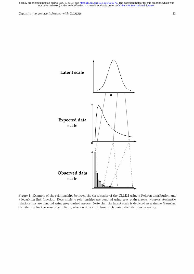
Quantitative genetic inference with GLMMs 33
Latent scale
Expected datascale
Observed datascale
0
0
Figure 1: Example of the relationships between the three scales of the GLMM using a Poisson distribution anda logarithm link function. Deterministic relationships are denoted using grey plain arrows, whereas stochasticrelationships are denoted using grey dashed arrows. Note that the latent scale is depicted as a simple Gaussiandistribution for the sake of simplicity, whereas it is a mixture of Gaussian distributions in reality.
.CC-BY 4.0 International licensenot peer-reviewed) is the author/funder. It is made available under aThe copyright holder for this preprint (which was. http://dx.doi.org/10.1101/026377doi: bioRxiv preprint first posted online Sep. 8, 2015;

Quantitative genetic inference with GLMMs 34
Latent scale
µ = 0
Latent scale
µ = 1
Latent scale
µ = 2
Latent scale
µ = 3
Observed scale
µ = 0
Observed scale
µ = 1
Observed scale
µ = 2
Observed scale
µ = 3
0.2
0.4
0.6
0.8
0.2
0.4
0.6
0.8
0.2
0.4
0.6
0.8
0.2
0.4
0.6
0.8
0.02
0.04
0.06
0.08
0.05
0.10
0.15
0.20
0.1
0.2
0.3
0.1
0.2
0.3
0.4
0.5
0.2 0.4 0.6 0.8 0.2 0.4 0.6 0.8 0.2 0.4 0.6 0.8 0.2 0.4 0.6 0.8
0.02 0.04 0.06 0.05 0.10 0.15 0.1 0.2 0.3 0.1 0.2 0.3 0.4 0.5
Heritability
Sim
ulat
ed R
/S ra
tio
0.05
0.50
0.95
Proportionof selected
Figure 2: Simulated R/S (evolutionary response over selection differential, or the realised heritability) on thelatent (upper panels) or observed data (lower panels) scales against the corresponding-scale heritabilities. Eachdata point is the average over 10,000 replicates of 10,000 individuals for various latent heritabilities h2lat (0.1,0.3, 0.5, 0.8), latent population mean (µ from 0 to 3, from left to right) and proportion of selected individuals(5%, 10%, 20%, 30%, 50%, 70%, 80%, 90%, 95%, varying from black to blue). The 1:1 line is plotted in black.The breeder’s equation is predictive on the latent scale (upper panels), but approximate on the observed datascale (lower panels), because phenotypes and breeding values are not jointly multivariate normal on that scale.
.CC-BY 4.0 International licensenot peer-reviewed) is the author/funder. It is made available under aThe copyright holder for this preprint (which was. http://dx.doi.org/10.1101/026377doi: bioRxiv preprint first posted online Sep. 8, 2015;

Quantitative genetic inference with GLMMs 35
Immediate
µ = 0
Immediate
µ = 1
Immediate
µ = 2
Immediate
µ = 3
Permanent
µ = 0
Permanent
µ = 1
Permanent
µ = 2
Permanent
µ = 3
0.00
0.05
0.10
0.15
0.20
0.0
0.2
0.4
0.6
0.8
01
23
03
69
12
0.00
0.05
0.10
0.15
0.20
0.0
0.2
0.4
0.6
0.8
01
23
0.0
2.5
5.0
7.5
10.0
12.5
0.00 0.05 0.10 0.15 0.20 0.0 0.2 0.4 0.6 0.8 0 1 2 3 0.0 2.5 5.0 7.5 10.0
0.00 0.05 0.10 0.15 0.20 0.0 0.2 0.4 0.6 0.8 0 1 2 3 0.0 2.5 5.0 7.5 10.0 12.5
Predicted evolutionary response
Sim
ulat
ed e
volu
tiona
ry re
spon
se
0.05
0.50
0.95
Proportionof selected
Figure 3: Predicted Robs (phenotypic evolutionary response on the observed scale, see Eq. 34) against thesimulated Robs, via evolutionary predictions applied on the latent scale. Each data point is the average over10,000 replicates of 10,000 individuals for various latent heritabilities h2lat (0.1, 0.3, 0.5, 0.8), latent populationmean (µ from 0 to 3) and proportion of selected individuals (5%, 10%, 20%, 30%, 50%, 70%, 80%, 90%, 95%,varying from black to blue). The 1:1 line is plotted in black. The upper panels (“Immediate”) show simulationsfor the response after a single generation, which include both a permanent and transient response to selectionarising from linkage disequilibrium. The bottom panels (“permanent”) show simulation results modified toreflect only the permanent response to selection.
.CC-BY 4.0 International licensenot peer-reviewed) is the author/funder. It is made available under aThe copyright holder for this preprint (which was. http://dx.doi.org/10.1101/026377doi: bioRxiv preprint first posted online Sep. 8, 2015;
Related Documents