Gene set enrichment and network analyses of high ... · high-throughput screen data set we use here results from a genome-wide RNAi analysis of growth and viability in Drosophila

Gene set enrichment and network analyses of

high-throughput screens using HTSanalyzeR

Xin Wang †, Camille Terfve †, John Rose and Florian Markowetz

October 29, 2019

Contents

1 Introduction 2

2 An overview of HTSanalyzeR 2

3 Preprocessing of high-throughput screens (HTS) 4

4 Gene set overrepresentation and enrichment analysis 64.1 Prepare the input data . . . . . . . . . . . . . . . . . . . . . . 64.2 Initialize and preprocess . . . . . . . . . . . . . . . . . . . . . 74.3 Perform analyses . . . . . . . . . . . . . . . . . . . . . . . . . 84.4 Summarize results . . . . . . . . . . . . . . . . . . . . . . . . 94.5 Plot significant gene sets . . . . . . . . . . . . . . . . . . . . . 104.6 Enrichment map . . . . . . . . . . . . . . . . . . . . . . . . . 114.7 Report results and save objects . . . . . . . . . . . . . . . . . 15

5 Network analysis 155.1 Prepare the input data . . . . . . . . . . . . . . . . . . . . . . 165.2 Initialize and preprocess . . . . . . . . . . . . . . . . . . . . . 175.3 Perform analysis . . . . . . . . . . . . . . . . . . . . . . . . . 185.4 Summarize results . . . . . . . . . . . . . . . . . . . . . . . . 185.5 Plot subnetworks . . . . . . . . . . . . . . . . . . . . . . . . . 205.6 Report results and save objects . . . . . . . . . . . . . . . . . 21

6 Appendix A: HTSanalyzeR4cellHTS2–A pipeline for cell-HTS2 object 21

7 Appendix B: Using MSigDB gene set collections 22

1

8 Appendix C: Performing gene set analysis on multiple phe-notypes 23

1 Introduction

In recent years several technological advances have pushed gene perturbationscreens to the forefront of functional genomics. Combining high-throughputscreening (HTS) techniques with rich phenotypes enables researchers to ob-serve detailed reactions to experimental perturbations on a genome-widescale. This makes HTS one of the most promising tools in functional ge-nomics.

Although the phenotypes in HTS data mostly correspond to single genes,it becomes more and more important to analyze them in the context of cellu-lar pathways and networks to understand how genes work together. Networkanalysis of HTS data depends on the dimensionality of the phenotypic read-out [9]. While specialised analysis approaches exist for high-dimensionalphenotyping [5], analysis approaches for low-dimensional screens have so farbeen spread out over diverse softwares and online tools like DAVID [7] orgene set enrichment analysis [14]).

Here we provide a software to build integrated analysis pipelines forHTS data that contain gene set and network analysis approaches commonlyused in many papers (as reviewed by [9]). HTSanalyzeR is implementedby S4 classes in R [11] and freely available via the Bioconductor project[6]. The example pipeline provided by HTSanalyzeR interfaces directly withexisting HTS pre-processing packages like cellHTS2 [4] or RNAither [12].Additionally, our software will be fully integrated in a web-interface for theanalysis of HTS data [10] and thus be easily accessible to non-programmers.

2 An overview of HTSanalyzeR

HTSanalyzeR takes as input HTS data that has already undergone prepro-cessing and quality control (e.g. by using cellHTS2). It then functionallyannotates the hits by gene set enrichment and network analysis approaches(see Figure 1 for an overview).

Gene set analysis. HTSanalyzeR implements two approaches: (i) hyper-geometric tests for surprising overlap between hits and gene sets, and (ii)gene set enrichment analysis to measure if a gene set shows a concordanttrend to stronger phenotypes. HTSanalyzeR uses gene sets from MSigDB

2

Hypergeometric test

Gene set enrichment analysis (GSEA)

Rich subnetworks

High-throughputScreen

Preprocessing& Quality control

Network and pathway analysis

3HTSanalyzeR

Gene setse.g. MSigDB, GO, KEGG

Networkse.g. BioGRID

Outputreport

HTMLLinks to databasesNetwork �guresEnrichment Map

42cellHTS21HTS

Di�erential GSEA

Figure 1: HTSanalyzeR takes as input HTS data that has already been pre-processed, normalized and quality checked, e.g. by cellHTS2. HTSanalyzeRthen combines the HTS data with gene sets and networks from freely avail-able sources and performs three types of analysis: (i) hypergeometric testsfor overlap between hits and gene sets, (ii) gene set enrichment analysis(GSEA) for concordant trends of a gene set in one phenotype, (iii) differen-tial GSEA to identify gene sets with opposite trends in two phenotypes, and(iv) identification of subnetworks enriched for hits. The results are providedto the user as figures and HTML tables linked to external databases forannotation.

[14], Gene Ontolology [1], KEGG [8] and others. The accompanying vi-gnette explains how user-defined gene sets can easily be included. Resultsare visualized as an enrichment map [15].

Network analysis. In a complementary approach strong hits are mappedto a network and enriched subnetworks are identified. Networks can comefrom different sources, especially protein interaction networks are often used.In HTSanalyzeR we use networks defined in the BioGRID database [13], butother user-defined networks can easily be included in the analysis. To iden-tify rich subnetworks, we use the BioNet package [2], which in its heuristicversion is fast and produces close-to-optimal results.

Comparing phenotypes. A goal we expect to become more and moreimportant in the future is to compare phenotypes for the same genes indifferent cellular conditions. HTSanalyzeR supports comparative analysesfor gene sets and networks. Differentially enriched gene sets are computedby comparing GSEA enrichment scores or alternatively by a Wilcoxon teststatistic. Subnetworks rich for more than one phenotype can be found withBioNet [2].

As a demonstration, in this vignette, we introduce how to perform these

3

analyses on an RNAi screen data set in cellHTS2 format. For other biologicaldata sets, the users can design their own classes, methods and pipelines veryeasily based on this package.

The packages below need to be loaded before we start the demonstration:

> library(HTSanalyzeR)

> library(GSEABase)

> library(cellHTS2)

> library(org.Dm.eg.db)

> library(GO.db)

> library(KEGG.db)

3 Preprocessing of high-throughput screens (HTS)

In this section, we use RNA interference screens as an example to demon-strate how to prepare data for the enrichment and network analyses. Thehigh-throughput screen data set we use here results from a genome-wideRNAi analysis of growth and viability in Drosophila cells [3]. This data setcan be found in the package cellHTS2 ([4]). Before the high-level functionalanalyses, we need a configured, normalized and annotated cellHTS objectthat will be used for the networks analysis. This object is then scored tobe used in the gene set overrepresentation part of this analysis. Briefly, thedata consists in a series of text files, one for each microtiter plate in the ex-periment, containing intensity reading for a luciferase reporter of ATP levelsin each well of the plate.

The first data processing step is to read the data files and build a cellHTSobject from them (performed by the readPlateList function).

> experimentName <- "KcViab"

> dataPath <- system.file(experimentName, package = "cellHTS2")

> x <- readPlateList("Platelist.txt", name = experimentName,

+ path = dataPath,verbose=TRUE)

Then, the object has to be configured, which involves describing theexperiment and, more importantly in our case, the plate configuration (i.e.indicating which wells contain samples or controls and which are empty orflagged as invalid).

> x <- configure(x, descripFile = "Description.txt", confFile =

+ "Plateconf.txt", logFile = "Screenlog.txt", path = dataPath)

4

Following configuration, the data can be normalized, which is done inthis case by substracting from each raw intensity measurement the medianof all sample measurements on the same plate.

> xn <- normalizePlates(x, scale = "multiplicative", log = FALSE,

+ method = "median", varianceAdjust = "none")

In order to use this data in HTSanalyzeR, we need to associate eachmeasurement with a meaningful identifier, which can be done by the an-notate function. In this case, the function will associate with each samplewell a flybaseCG identifier, which can be converted subsequently into anyidentifiers that we might want to use. There are many ways to perform thistask, for example using our preprocess function (in the next section), us-ing a Bioconductor annotation package or taking advantage of the bioMaRtpackage functionalities. These normalized and annotated values can then beused for the network analysis part of this vignette.

> xn <- annotate(xn, geneIDFile = "GeneIDs_Dm_HFA_1.1.txt",

+ path = dataPath)

For the gene set overrepresentation part of this vignette, we choose towork on data that has been scored and summarized. These last process-ing steps allow us to work with values that have been standardized acrosssamples, resulting in a robust z-score which is indicative of how much thephenotype associated with one condition differs from the bulk. This scoreeffectively quantifies how different a measurement is from the median ofall measurements, taking into account the variance (or rather in this casethe median absolute deviation) across measurements, therefore reducing thespread of the data. This seems like a sensible measure to be used in geneset overrepresentation, especially for the GSEA, since it is more readily in-terpretable and comparable than an absolute phenotype.

> xsc <- scoreReplicates(xn, sign = "-", method = "zscore")

Moreover the summarization across replicates produces only one valuefor each construct tested in the screen, which is what we need for the over-representation analysis.

> xsc <- summarizeReplicates(xsc, summary = "mean")

> xsc

5

cellHTS (storageMode: lockedEnvironment)

assayData: 21888 features, 1 samples

element names: Channel 1

phenoData

sampleNames: 1

varLabels: replicate assay

varMetadata: labelDescription channel

featureData

featureNames: 1 2 ... 21888 (21888 total)

fvarLabels: plate well ... GeneID (5 total)

fvarMetadata: labelDescription

experimentData: use 'experimentData(object)'

state: configured = TRUE

normalized = TRUE

scored = TRUE

annotated = TRUE

Number of plates: 57

Plate dimension: nrow = 16, ncol = 24

Number of batches: 1

Well annotation: sample other neg pos

pubMedIds: 14764878

For a more detailed description of the preprocessing methods below,please refer to the cellHTS2 vignette.

4 Gene set overrepresentation and enrichment anal-ysis

4.1 Prepare the input data

To perform gene set enrichment analysis, one must first prepare three inputs:

1. a named numeric vector of phenotypes,

2. a character vector of hits, and

3. a list of gene set collections.

First, the phenotype associated with each gene must be assembled into anamed vector, and entries corresponding to the same gene must be summa-rized into a unique element.

6

> data4enrich <- as.vector(Data(xsc))

> names(data4enrich) <- fData(xsc)[, "GeneID"]

> data4enrich <- data4enrich[which(!is.na(names(data4enrich)))]

Then we define the hits as targets displaying phenotypes more than 2standard deviations away from the mean phenotype, i.e. abs(z-score) > 2.

> hits <- names(data4enrich)[which(abs(data4enrich) > 2)]

Next, we must define the gene set collections. HTSanalyzeR providesfacilities which greatly simplify the creation of up-to-date gene set collec-tions. As a simple demonstration, we will test three gene set collections forDrosophila melanogaster (see help(annotationConvertor) for details aboutother species supported): KEGG and two GO gene set collections. To workproperly, these gene set collections must be provided as a named list.

For details on downloading and utilizing gene set collections from Molec-ular Signatures Database[14], please refer to Appendix B.

> GO_MF <- GOGeneSets(species="Dm", ontologies=c("MF"))

> GO_BP <- GOGeneSets(species="Dm", ontologies=c("BP"))

> PW_KEGG <- KeggGeneSets(species="Dm")

> ListGSC <- list(GO_MF=GO_MF, GO_BP=GO_BP, PW_KEGG=PW_KEGG)

4.2 Initialize and preprocess

An S4 class GSCA (Gene Set Collection Analysis) is developed to do hyper-geometric tests to find gene sets overrepresented among the hits and alsoperform gene set enrichment analysis (GSEA), as described by Subramanianand colleagues[14].

To begin, an object of class GSCA needs to be initialized with a list ofgene set collections, a vector of phenotypes and a vector of hits. A prepro-cessing step including input data validation, duplicate removing, annotationconversion and phenotype ordering can be conducted by the method pre-process. An example of such a case is when the input data is not associatedwith Entrez identifiers (which is the type of identifiers expected for the sub-sequent analyses). The user can also build their own preprocessing functionspecifically for their data sets. For example, the current method preprocessranks the phenotype vector decreasingly, which may not fit the users’ re-quirements. At this time, the user can develop a new function to order theirphenotypes and simply couple it with the functions annotationConvertor,duplicateRemover, etc. in our package to create their own preprocessingpipeline.

7

> gsca <- new("GSCA", listOfGeneSetCollections=ListGSC,

+ geneList=data4enrich, hits=hits)

> gsca <- preprocess(gsca, species="Dm", initialIDs="FlybaseCG",

+ keepMultipleMappings=TRUE, duplicateRemoverMethod="max",

+ orderAbsValue=FALSE)

4.3 Perform analyses

Having obtained a preprocessed GSCA object, the user now proceed to dothe overrepresentation and enrichment analyses using the function analyze.This function needs an argument called para, which is a list of parametersrequired to run these analyses including:

� minGeneSetSize: a single integer or numeric value specifying the min-imum number of elements in a gene set that must map to elements ofthe gene universe. Gene sets with fewer than this number are removedfrom both hypergeometric analysis and GSEA.

� nPermutations: a single integer or numeric value specifying the num-ber of permutations for deriving p-values in GSEA.

� exponent: a single integer or numeric value used in weighting pheno-types in GSEA (see help(gseaScores) for more details)

� pValueCutoff : a single numeric value specifying the cutoff for ad-justed p-values considered significant.

� pAdjustMethod: a single character value specifying the p-value adjust-ment method to be used.

> gsca<-analyze(gsca, para=list(pValueCutoff=0.05, pAdjustMethod

+ ="BH", nPermutations=100, minGeneSetSize=180, exponent=1))

In the above example, we set a very large minGeneSetSize just for afast compilation of this vignette. In real applications, the user may want amuch smaller threshold (e.g. 15).

During the enrichment analysis of gene sets, the function evaluates thestatistical significance of the gene set scores by performing a large number ofpermutations. This package supports parallel computing to promote speedbased on the snow package. To do this, the user simply needs to set a clustercalled cluster before running analyze.

8

> library(snow)

> options(cluster=makeCluster(4, "SOCK"))

Please do make sure to stop this cluster and assign ‘NULL’ to it afterthe enrichment analysis.

> if(is(getOption("cluster"), "cluster")) {

+ stopCluster(getOption("cluster"))

+ options(cluster=NULL)

+ }

The output of all analyses stored in slot result of the object containsdata frames displaying the results for hypergeometric testing and GSEA foreach gene set collection, as well as data frames showing the combined resultsof all gene set collections. Additionally, the output contains data frames ofgene sets exhibiting significant p-values (and significant adjusted p-values)for enrichment from both hypergeometric testing and GSEA.

4.4 Summarize results

A summary method is provided to print summary information about inputgene set collections, phenotypes, hits, parameters for hypeogeometric testsand GSEA and results.

> summarize(gsca)

-No of genes in Gene set collections:

input above min size

GO_MF 2358 10

GO_BP 5061 8

PW_KEGG 127 1

-No of genes in Gene List:

input valid duplicate removed converted to entrez

Gene List 13546 13525 12151 11063

-No of hits:

input preprocessed

Hits 1230 1065

9

-Parameters for analysis:

minGeneSetSize pValueCutoff pAdjustMethod

HyperGeo Test 180 0.05 BH

minGeneSetSize pValueCutoff pAdjustMethod nPermutations exponent

GSEA 180 0.05 BH 100 1

-Significant gene sets (adjusted p-value< 0.05 ):

GO_MF GO_BP PW_KEGG

HyperGeo 6 3 0

GSEA 9 5 0

Both 5 3 0

The function getTopGeneSets is desinged to retrieve all or top signif-icant gene sets from results of overrepresentation or GSEA analysis. Ba-sically, the user need to specify the name of results–“HyperGeo.results” or“GSEA.results”, the name(s) of the gene set collection(s) as well as the typeof selection– all (by argument allSig) or top (by argument ntop) significantgene sets.

> topGS_GO_MF <- getTopGeneSets(gsca, "GSEA.results", c("GO_MF",

+ "PW_KEGG"), allSig=TRUE)

> topGS_GO_MF

$GO_MF

GO:0003674 GO:0003677 GO:0003700 GO:0003723 GO:0005515

"GO:0003674" "GO:0003677" "GO:0003700" "GO:0003723" "GO:0005515"

GO:0043565 GO:0004252 GO:0003676 GO:0005524

"GO:0043565" "GO:0004252" "GO:0003676" "GO:0005524"

$PW_KEGG

named character(0)

4.5 Plot significant gene sets

To help the user view GSEA results for a single gene set, the functionviewGSEA is developed to plot the positions of the genes of the gene setin the ranked phenotypes and the location of the enrichment score.

10

−5

05

10

Phe

noty

pes

0 2000 4000 6000 8000 10000

−0.

25−

0.10

0.00

Position in the ranked list of genes

Run

ning

enr

ichm

ent s

core

Figure 2: Plot of GSEA result of the most significant gene set of the Molec-ular Function collection

> viewGSEA(gsca, "GO_MF", topGS_GO_MF[["GO_MF"]][1])

A plot method (the function plotGSEA) is also available to plot andstore GSEA results of all significant or top gene sets in specified gene setcollections in ‘pdf’ or ‘png’ format.

> plotGSEA(gsca, gscs=c("GO_BP","GO_MF","PW_KEGG"),

+ ntop=1, filepath=".")

4.6 Enrichment map

An enrichment map is a network facillitating the visualization and interpre-tation of Hypergeometric test and GSEA results. In an enrichment map,the nodes represent gene sets and the edges denote the Jaccard similarity

11

coefficient between two gene sets. Node colors are scaled according to theadjusted p-values (the darker, the more significant). In the enrichment mapfor GSEA, nodes are colored by the sign of the enrichment scores (red:+,blue: -). The sizes of nodes are in proportion to the sizes of gene sets, whilethe width of edges are proportionate to Jaccard coefficients.

The method viewEnrichMap of class GSCA is developed to view an en-richment map for Hypergeometric or GSEA results over one or multiple geneset collections. As an example, here we use the sample data in the packageto plot enrichment maps for a KEGG gene set collection.

> data("KcViab_GSCA")

> viewEnrichMap(KcViab_GSCA, resultName="HyperGeo.results",

+ gscs=c("PW_KEGG"), allSig=FALSE, ntop=30, gsNameType="id",

+ displayEdgeLabel=FALSE, layout="layout.fruchterman.reingold")

> data("KcViab_GSCA")

> viewEnrichMap(KcViab_GSCA, resultName="GSEA.results",

+ gscs=c("PW_KEGG"), allSig=FALSE, ntop=30, gsNameType="id",

+ displayEdgeLabel=FALSE, layout="layout.fruchterman.reingold")

To make the map more readable, we can first append gene set terms tothe GSEA results using the method appendGSTerms of class GSCA, andthen call the function viewEnrichMap.

> KcViab_GSCA<-appendGSTerms(KcViab_GSCA, goGSCs=c("GO_BP",

+ "GO_MF","GO_CC"), keggGSCs=c("PW_KEGG"))

> viewEnrichMap(KcViab_GSCA, resultName="HyperGeo.results",

+ gscs=c("PW_KEGG"), allSig=FALSE, ntop=30, gsNameType="term",

+ displayEdgeLabel=FALSE, layout="layout.fruchterman.reingold")

> KcViab_GSCA<-appendGSTerms(KcViab_GSCA, goGSCs=c("GO_BP",

+ "GO_MF","GO_CC"), keggGSCs=c("PW_KEGG"))

> viewEnrichMap(KcViab_GSCA, resultName="GSEA.results",

+ gscs=c("PW_KEGG"), allSig=FALSE, ntop=30, gsNameType="term",

+ displayEdgeLabel=FALSE, layout="layout.fruchterman.reingold")

In figure 4, there are considerable coefficients between metabolism-relatedgene sets, suggesting that the significance of these gene sets is probably dueto a group of genes shared by them.

Similarly, the enrichment map can be generated and saved to a file in‘pdf’ or ‘png’ format.

12

●

●

●

●

●

●

●

●

●

●

●●

● ●

●

●

●

●

●

●

●

●

●

●

●

●

●●

●

dme03010

dme03050

dme03040

dme04320

dme00600dme04144

dme00410

dme00565

dme00650

dme00071

dme03018dme01040

dme04330 dme03430

dme04013

dme04310

dme04914

dme00230

dme00260

dme00280

dme00310

dme00380

dme00561

dme00564

dme00640

dme03020

dme03022

dme04130dme04150

dme04340

Enrichment Map of Hypergeometric tests on "PW_KEGG"

0

0.010.05

1

Adjustedp−values

(a) Hypergeometric tests

●

●

● ●●

●

●

●

●

●

●

●

●

●

●

●

●

●

●

●

●●

●

●●

●

●

●

●

dme00565

dme01040

dme03010dme03040

dme03050

dme00564

dme00600

dme00051

dme00561

dme04330

dme00190

dme00500

dme04320

dme03022

dme00830

dme03018

dme00040

dme00071

dme00053

dme03410

dme04013

dme00903dme00350

dme04080

dme00980

dme04630

dme04350

dme04340

dme00982

dme00052

Enrichment Map of GSEA on "PW_KEGG"

0

0.010.05

1

0.050.01

0

Adjustedp−values

(b) GSEA

Figure 3: Enrichment map for the GSEA results of a KEGG gene set col-lection (using gene set id as node labels)

13

●●

●●

●

●

●

●

●●

●

●

●

●

●●

●

●

●●

●

●

●

●

●

●

●

●

●

RibosomeProteasome

Spliceosome

Dorso−ventral axis formation

Sphingolipid metabolism

Endocytosis

beta−Alanine metabolism

Ether lipid metabolism

Butanoate metabolismFatty acid degradation

RNA degradation

Biosynthesis of unsaturatedfatty acids

Notch signaling pathway

Mismatch repair

MAPK signaling pathway − flyWnt signaling pathway

Progesterone−mediated oocytematuration

Purine metabolism

Glycine, serine and threoninemetabolism

Valine, leucine and isoleucinedegradationLysine degradation

Tryptophan metabolism

Glycerolipid metabolism

Glycerophospholipid metabolism

Propanoate metabolism

RNA polymerase

Basal transcription factors

SNARE interactions in vesiculartransport

mTOR signaling pathway

Hedgehog signaling pathway

Enrichment Map of Hypergeometric tests on "PW_KEGG"

0

0.010.05

1

Adjustedp−values

(a) Hypergeometric tests

●

●

●

●

●

●

●

●●

●

●

●●

●

●

●

●

●

●●

●●

●

●

●

● ●

●

●

Ether lipid metabolism

Biosynthesis of unsaturatedfatty acids

Ribosome

Spliceosome

Proteasome

Glycerophospholipid metabolism

Sphingolipid metabolism

Fructose and mannose metabolismGlycerolipid metabolism

Notch signaling pathway

Oxidative phosphorylation

Starch and sucrose metabolism

Dorso−ventral axis formationBasal transcription factors

Retinol metabolism

RNA degradation

Pentose and glucuronateinterconversions

Fatty acid degradation

Ascorbate and aldaratemetabolism

Base excision repairMAPK signaling pathway − fly

Limonene and pinene degradation

Tyrosine metabolism

Neuroactive ligand−receptorinteraction

Metabolism of xenobiotics bycytochrome P450

Jak−STAT signaling pathway

TGF−beta signaling pathwayHedgehog signaling pathway

Drug metabolism − cytochromeP450

Galactose metabolism

Enrichment Map of GSEA on "PW_KEGG"

0

0.010.05

1

0.050.01

0

Adjustedp−values

(b) GSEA

Figure 4: Enrichment map for the GSEA results of a KEGG gene set col-lection (using gene set terms as node labels)

14

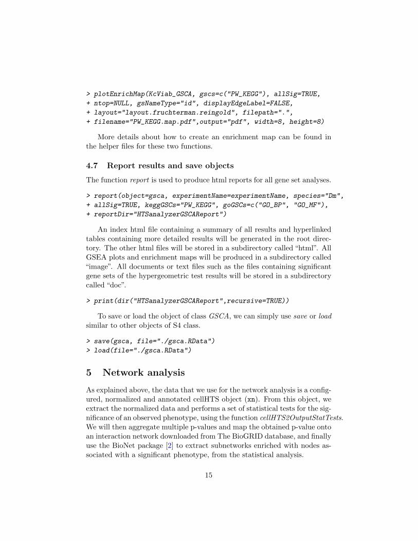
> plotEnrichMap(KcViab_GSCA, gscs=c("PW_KEGG"), allSig=TRUE,

+ ntop=NULL, gsNameType="id", displayEdgeLabel=FALSE,

+ layout="layout.fruchterman.reingold", filepath=".",

+ filename="PW_KEGG.map.pdf",output="pdf", width=8, height=8)

More details about how to create an enrichment map can be found inthe helper files for these two functions.

4.7 Report results and save objects

The function report is used to produce html reports for all gene set analyses.

> report(object=gsca, experimentName=experimentName, species="Dm",

+ allSig=TRUE, keggGSCs="PW_KEGG", goGSCs=c("GO_BP", "GO_MF"),

+ reportDir="HTSanalyzerGSCAReport")

An index html file containing a summary of all results and hyperlinkedtables containing more detailed results will be generated in the root direc-tory. The other html files will be stored in a subdirectory called “html”. AllGSEA plots and enrichment maps will be produced in a subdirectory called“image”. All documents or text files such as the files containing significantgene sets of the hypergeometric test results will be stored in a subdirectorycalled “doc”.

> print(dir("HTSanalyzerGSCAReport",recursive=TRUE))

To save or load the object of class GSCA, we can simply use save or loadsimilar to other objects of S4 class.

> save(gsca, file="./gsca.RData")

> load(file="./gsca.RData")

5 Network analysis

As explained above, the data that we use for the network analysis is a config-ured, normalized and annotated cellHTS object (xn). From this object, weextract the normalized data and performs a set of statistical tests for the sig-nificance of an observed phenotype, using the function cellHTS2OutputStatTests.We will then aggregate multiple p-values and map the obtained p-value ontoan interaction network downloaded from The BioGRID database, and finallyuse the BioNet package [2] to extract subnetworks enriched with nodes as-sociated with a significant phenotype, from the statistical analysis.

15

5.1 Prepare the input data

In the following example, we perform a one sample t-test which tests whetherthe mean of the observations for each construct is equal to the mean of allsample observations under the null hypothesis. This amounts to testingwhether the phenotype associated with a construct is significantly differentfrom the bulk of observations, with the underlying assumption that in alarge scale screen (i.e. genome-wide in this case) most constructs are notexpected to show a significant effect. We also perform a two-sample t-test,which tests the null hypothesis that two populations have the same mean,where the two populations are a set of observations for each construct anda set of observations for a control population.

To perform those tests, it is mandatory that the samples and controls arelabelled in the column controlStatus of the fData(xn) data frame as sam-ple and a string specified by the control argument of the networkAnalysisfunction, respectively. Non-parametric tests, such as the Mann-Whitney Utest and the Rank Product test, can also be performed. Both the two samplesand the one sample tests are automatically produced, in the case of the t-testand the Mann-Withney U test, by the function cellHTS2OutputStatTests inthe package.

Please be aware that the t-test works under the assumption that theobservations are normally distributed and that all of these tests are lessreliable when the number of replicates is small. The user should also keepin mind that the one sample t-test assumes that the majority of conditionsare not expected to show any significant effect, which is likely to be a dodgyassumption when the size of the screen is small. This test is also to beavoided when the data consists of pre-screened conditions, i.e. constructsthat have been selected specifically based on a potential effect.

All three kind of tests can be performed with the ‘two sided’, ‘less’ or‘greater’ alternative, corresponding to population means (or ranking in thecase of the rank product) expected to be different, smaller of larger thanthe null hypothesis, respectively. For example if your phenotypes consist ofcell number and you are looking for constructs that impair cell viability, youmight be looking for phenotypes that are smaller than the mean. The anno-tationcolumn argument is used to specify which column of the fData(xn)data frame contains identifiers for the constructs.

> test.stats <- cellHTS2OutputStatTests(cellHTSobject=xn,

+ annotationColumn="GeneID", alternative="two.sided",

+ tests=c("T-test"))

16

> library(BioNet)

> pvalues <- aggrPvals(test.stats, order=2, plot=FALSE)

5.2 Initialize and preprocess

After the p-values associated with the node have been aggregated into a sin-gle value for each node, an object of class NWA can be created. If phenotypesfor genes are also available, they can be inputted during the initializationstage. The phenotypes can then be used to highlight nodes in different col-ors in the identified subnetwork. When initializing an object of class NWA,the user also has the possibility to specify the argument interactome whichis an object of class graphNEL. If it is not available, the interactome can beset up later.

> data("Biogrid_DM_Interactome")

> nwa <- new("NWA", pvalues=pvalues, interactome=

+ Biogrid_DM_Interactome, phenotypes=data4enrich)

In the above example, the interactome was built from the BioGRIDinteraction data set for Drosophila Melanogaster (version 3.1.71, accessedon Dec. 5, 2010).

The next step is preprocessing of input p-values and phenotypes. Similarto class GSCA, at the preprocessing stage, the function will also check thevalidity of input data, remove duplicated genes and convert annotations toEntrez ids. The type of initial identifiers can be specified in the initialIDs

argument, and will be converted to Entrez gene identifiers which can bemapped to the BioGRID interaction data.

> nwa <- new("NWA", pvalues=pvalues, phenotypes=data4enrich)

> nwa <- preprocess(nwa, species="Dm", initialIDs="FlybaseCG",

+ keepMultipleMappings=TRUE, duplicateRemoverMethod="max")

To create an interactome for the network analysis, the user can eitherspecify a species to download corresponding network database from Bi-oGRID, or input an interaction matrix if the network is already availableand in the right format: a matrix with a row for each interaction, and atleast the three columns “InteractorA”, “InteractorB” and “InteractionType”,where the interactors are specified by Entrez identifiers..

> nwa<-interactome(nwa, species="Dm", reportDir="HTSanalyzerReport",

+ genetic=FALSE)

17

> data("Biogrid_DM_Mat")

> nwa<-interactome(nwa, interactionMatrix=Biogrid_DM_Mat,

+ genetic=FALSE)

> nwa@interactome

A graphNEL graph with undirected edges

Number of Nodes = 7163

Number of Edges = 21599

5.3 Perform analysis

Having preprocessed the input data and created the interactome, the net-work analysis can then be performed by calling the method analyze. Thefunction will plot a figure showing the fitting of the BioNet model to yourdistribution of p-values, which is a good plot to check the choice of statisticsused in this function. The argument fdr of the method analyze is the falsediscovery rate for BioNet to fit the BUM model. The parameters of thefitted model will then be used for the scoring function, which subsequentlyenables the BioNet package to search the optimal scoring subnetwork (see[2] for more details).

> nwa<-analyze(nwa, fdr=0.001, species="Dm")

The plotSubNet function produces a figure of the enriched subnetwork,with symbol identifiers as labels of the nodes (if the argument species hasbeen inputted during the initialization step).

5.4 Summarize results

Similar to class GSCA, a summary method is also available for objects ofclass NWA. The summary includes information about the size of the p-valueand phenotype vectors before and after preprocessing, the interactome used,parameters and the subnetwork identified by BioNet.

> summarize(nwa)

-p-values:

input valid duplicate removed

12170 12170 12170

converted to entrez in interactome

18

Histogram of p−values

P−values

Den

sity

0.0 0.2 0.4 0.6 0.8 1.0

05

1015

π

0.0 0.2 0.4 0.6 0.8 1.0

0.0

0.2

0.4

0.6

0.8

1.0

QQ−Plot

Estimated p−value

Obs

erve

d p−

valu

e

Figure 5: Fitting BUM model to p-values by BioNet.

11081 6303

-Phenotypes:

input valid duplicate removed

12170 12170 12170

converted to entrez in interactome

11081 6303

-Interactome:

name species genetic node No edge No

Interaction dataset User-input <NA> FALSE 7163 21599

-Parameters for analysis:

FDR

Parameter 0.001

-Subnetwork identified:

node No edge No

Subnetwork 95 102

19

●

●

●

●

●

●●

●

●

●

●●

●●

●●

●●

●

●

●● ●

●

●●

●

●

●

●

●

●

●

●

●

●

●

●

●

●

●

●

●

●

●●

●

● ●

●

●

●

●

●●

●

●

●●

●

●

●● ●

●

●

●

● ●

●

●

●

●

●●

●

●

●●● ●

●

●

● ●

●

●

●

●

●

●

●●

●

●

Mdr65

Nup98−96

RpS26

Tailor

CG11581

SkpC

p130CAS

CG12470

CG13005

Rpb10

Pldn

Mer

COX6B

CG15109

SpindlyCG15561

RpS20

drl

Act87E

Rad23

CG2091

RpS3A vilya

nito

tinc

CenG1A

geminin

crn

CG31999

rols

CG32104

CG3281

CG33017

YME1L

RpL23

hoip

eIF4E1

vret

pins

Mst33A

Dysb

CG9674

TRAM

RpL8

CG13220

CG13526

CG14689

PPYR1 CG15545

c−cup

Rop

RpL10

CG18088

GstT1Sp7

CG31482

dsx−c73A

RpS16

Bap60

bnl

Tctp

CG4820

CG4853 RpL3

imd

par−6

Desat1

CG6230 RpS3

CG7656

strat

RpS8

BubR1

Rexo5

exd

sona

TSG101

CG33095Lztr1

CG9951 PK2−R1

E(Pc)

E5

CG9986 P58IPK

Sf3b1

CG4702

Pp4−19C

dom

CG7556

Fad2

stau

Msh6

CG5439

SLIRP2

−4−2.9−1.7

−0.991.72.93.95

5.88.610

Figure 6: Enriched subnetwork identified by BioNet.

5.5 Plot subnetworks

The identified enriched subnetwork can be viewed using the function view-SubNet.

> viewSubNet(nwa)

As we can see in figure 6, the nodes of the enriched submodule arecolored in red and green according to the phenotype (positive or negative).Rectangle nodes correspond to negative scores while circles depict positivescores.

To plot and save the subnetwork, we can use the function plotSubNetwith filepath and filename specified accordingly.

> plotSubNet(nwa, filepath=".", filename="subnetwork.png")

20

5.6 Report results and save objects

The results of network analysis can be written into an html report into auser-defined directory, using the the function report. An index html filecontaining a brief summary of the analyses will be generated in the rootdirectory. Another html file including more detailed results will be storedin a subdirectory called “html”. One subnetwork figure will be produced ina subdirectory called “image”. In addition, a text file containing the Entrezids and gene symbols for the nodes included in the identified subnetworkwill be stored in subdirectory “doc”.

> report(object=nwa, experimentName=experimentName, species="Dm",

+ allSig=TRUE, keggGSCs="PW_KEGG", goGSCs=c("GO_BP", "GO_MF"),

+ reportDir="HTSanalyzerNWReport")

To report both results of the enrichment and network analyses, we canuse function reportAll :

> reportAll(gsca=gsca, nwa=nwa, experimentName=experimentName,

+ species="Dm", allSig=TRUE, keggGSCs="PW_KEGG", goGSCs=

+ c("GO_BP", "GO_MF"), reportDir="HTSanalyzerReport")

An object of class NWA can be saved for reuse in the future followingthe same procedure used with GSCA objects:

> save(nwa, file="./nwa.RData")

> load("./nwa.RData")

6 Appendix A: HTSanalyzeR4cellHTS2–A pipelinefor cellHTS2 object

All of the above steps can be performed with a unique pipeline function,starting from a normalized, configured and annotated cellHTS object.

First, we need to prepare input data required for analyses just as weintroduced in section 3.

> data("KcViab_Norm")

> GO_CC<-GOGeneSets(species="Dm",ontologies=c("CC"))

> PW_KEGG<-KeggGeneSets(species="Dm")

> ListGSC<-list(GO_CC=GO_CC,PW_KEGG=PW_KEGG)

21

Then we simply call the function HTSanalyzeR4cellHTS2. This will pro-duce a full HTSanalyzeR report, just as if the above steps were performedseparately. All the parameters of the enrichment and network analysis stepscan be specified as input of this function (see help(HTSanalyzeR4cellHTS2)).Since they are given sensible default values, a minimal set of input parame-ters is actually required.

> HTSanalyzeR4cellHTS2(

+ normCellHTSobject=KcViab_Norm,

+ annotationColumn="GeneID",

+ species="Dm",

+ initialIDs="FlybaseCG",

+ listOfGeneSetCollections=ListGSC,

+ cutoffHitsEnrichment=2,

+ minGeneSetSize=200,

+ keggGSCs=c("PW_KEGG"),

+ goGSCs=c("GO_CC"),

+ reportDir="HTSanalyzerReport"

+ )

7 Appendix B: Using MSigDB gene set collections

For experiments in human cell lines, it is often useful to test the geneset collections available at the Molecular Signatures Database (MSigDB;http://www.broadinstitute.org/gsea/msigdb/)[14].

In order to download the gene set collections available through MSigDB,one must first register. After registration, download the desired gmt files intothe working directory. Using the getGmt and mapIdentifiers functions fromGSEABase importing the gene set collection and mapping the annotationsto Entrez IDs is relatively straightforward.

> c2<-getGmt(con="c2.all.v2.5.symbols.gmt.txt",geneIdType=

+ SymbolIdentifier(), collectionType=

+ BroadCollection(category="c2"))

Once again, for many of the functions in this package to work properly,all gene identifiers must be supplied as Entrez IDs.

> c2entrez<-mapIdentifiers(c2, EntrezIdentifier('org.Hs.eg.db'))

To create a gene set collection for an object of class GSCA, we need toconvert the ”GeneSetCollection” object to a list of gene sets.

22

> collectionOfGeneSets<-geneIds(c2entrez)

> names(collectionOfGeneSets)<-names(c2entrez)

8 Appendix C: Performing gene set analysis onmultiple phenotypes

When performing high-throughput screens in cell culture-based assays, it isincreasingly common that multiple phenotypes would be recorded for eachcondition (such as e.g. number of cells and intensity of a reporter). In thesecases, you can perform the enrichment analysis separately on the differentlists of phenotypes and try to find gene sets enriched in all of them. In suchcases, our package comprises a function called aggregatePvals that allowsyou to aggregate p-values obtained for the same gene set from an enrichmentanalysis on different phenotypes. This function simply inputs a matrix ofp-values with a row for each gene set, and returns aggregated p-values,obtained using either the Fisher or Stouffer methods. The Fisher methodcombines the p-values into an aggregated chi-squared statistic equal to -2*sum(log(Pk)) were we have k=1,..,K p-values independently distributedas uniform on the unit interval under the null hypothesis. The resulting p-values are calculated by comparing this chi-squared statistic to a chi-squareddistribution with 2K degrees of freedom. The Stouffer method computes az-statistic assuming that the sum of the quantiles (from a standard normaldistribution) corresponding to the p-values are distributed as N(0,K).

However, it is possible that the phenotypes that are measured are ex-pected to show opposite behaviors (e.g. when measuring the number ofcells and a reporter for apoptosis). In these cases, we provide two meth-ods to detect gene sets that are associated with opposite patterns of a pairof phenotypic responses. The first method (implemented in the functionspairwiseGsea and pairwiseGseaPlot) is a modification of the GSEA methodby [14]. Briefly, the enrichment scores are computed separately on bothphenotype lists, and the absolute value of the difference between the two en-richment scores is compared to permutation-based scores obtained by com-puting the difference in enrichment score between the two lists when thegene labels are randomly shuffled. This method can only be applied if bothphenotypes are measured on the same set of conditions (i.e. the gene labelsare the same in both lists, although their associated phenotypes might bevery different).

The second method, implemented in the function pairwisePhenoMan-nWhit, performs a Mann-Whitney test for shift in location of genes from gene

23

sets, on a pair of phenotypes. The Mann-Whitney test is a non-parametricalequivalent to a two samples t-test (equivalent to a Wilcoxon rank sum test).It looks for gene sets with a phenotye distribution located around two differ-ent values in the two phenotypes list, rather than spread on the whole list inboth lists. Please be aware that this test should be applied on phenotypesthat are on the same scale. If you compare a number of cells (e.g. thousandsof cells) to a percentage of cells expressing a marker for example, you willalways find a difference in the means of the two populations of phenotypes,whatever the genes in those populations. However, it is very common in highthroughput experiments that some sort of internal control is available (e.g.phenotype of the wild type cell line, with no RNAi). A simple way to obtainthe different phenotypes on similar scales is therefore to use as phenotypesthe raw measurements divided by their internal control counterpart.

Session info

This document was produced using:

> toLatex(sessionInfo())

� R version 3.6.1 (2019-07-05), x86_64-pc-linux-gnu

� Locale: LC_CTYPE=en_US.UTF-8, LC_NUMERIC=C,LC_TIME=en_US.UTF-8, LC_COLLATE=C, LC_MONETARY=en_US.UTF-8,LC_MESSAGES=en_US.UTF-8, LC_PAPER=en_US.UTF-8, LC_NAME=C,LC_ADDRESS=C, LC_TELEPHONE=C, LC_MEASUREMENT=en_US.UTF-8,LC_IDENTIFICATION=C

� Running under: Ubuntu 18.04.3 LTS

� Matrix products: default

� BLAS: /home/biocbuild/bbs-3.10-bioc/R/lib/libRblas.so

� LAPACK:/home/biocbuild/bbs-3.10-bioc/R/lib/libRlapack.so

� Base packages: base, datasets, grDevices, graphics, grid, methods,parallel, stats, stats4, utils

� Other packages: AnnotationDbi 1.48.0, BioNet 1.46.0,Biobase 2.46.0, BiocGenerics 0.32.0, GO.db 3.10.0, GSEABase 1.48.0,

24

HTSanalyzeR 2.38.0, IRanges 2.20.0, KEGG.db 3.2.3, RBGL 1.62.0,RColorBrewer 1.1-2, S4Vectors 0.24.0, XML 3.98-1.20,annotate 1.64.0, cellHTS2 2.50.0, genefilter 1.68.0, graph 1.64.0,hwriter 1.3.2, igraph 1.2.4.1, locfit 1.5-9.1, org.Dm.eg.db 3.10.0,splots 1.52.0, vsn 3.54.0

� Loaded via a namespace (and not attached): BiocFileCache 1.10.0,BiocManager 1.30.9, Category 2.52.0, DBI 1.0.0, DEoptimR 1.0-8,MASS 7.3-51.4, Matrix 1.2-17, R6 2.4.0, RCurl 1.95-4.12,RSQLite 2.1.2, RankProd 3.12.0, Rcpp 1.0.2, Rmpfr 0.7-2,affy 1.64.0, affyio 1.56.0, askpass 1.1, assertthat 0.2.1,backports 1.1.5, biomaRt 2.42.0, bit 1.1-14, bit64 0.9-7, bitops 1.0-6,blob 1.2.0, cluster 2.1.0, colorspace 1.4-1, compiler 3.6.1, crayon 1.3.4,curl 4.2, dbplyr 1.4.2, digest 0.6.22, dplyr 0.8.3, ggplot2 3.2.1,glue 1.3.1, gmp 0.5-13.5, gtable 0.3.0, hms 0.5.1, httr 1.4.1,lattice 0.20-38, lazyeval 0.2.2, limma 3.42.0, magrittr 1.5,memoise 1.1.0, munsell 0.5.0, mvtnorm 1.0-11, openssl 1.4.1,pcaPP 1.9-73, pillar 1.4.2, pkgconfig 2.0.3, prada 1.62.0,preprocessCore 1.48.0, prettyunits 1.0.2, progress 1.2.2, purrr 0.3.3,rappdirs 0.3.1, rlang 0.4.1, robustbase 0.93-5, rrcov 1.4-7, scales 1.0.0,splines 3.6.1, stringi 1.4.3, stringr 1.4.0, survival 2.44-1.1, tibble 2.1.3,tidyselect 0.2.5, tools 3.6.1, vctrs 0.2.0, xtable 1.8-4, zeallot 0.1.0,zlibbioc 1.32.0

References

[1] Ashburner, M., Ball, C. A., Blake, J. A., Botstein, D., et al (2000).Gene ontology: tool for the unification of biology. the gene ontologyconsortium. Nat Genet , 25(1), 25–29. 3

[2] Beisser, D., Klau, G. W., Dandekar, T., Muller, T., Dittrich, M. T.(2010) BioNet: an R-Package for the functional analysis of biologicalnetworks. Bioinformatics, 26, 1129-1130 3, 15, 18

[3] Boutros, M., Kiger, A. A., Armknecht, S., Kerr, K., Hild, M., et al(2004). Genome-wide RNAi analysis of growth and viability in drosophilacells. Science, 303(5659), 832–835. 4

[4] Boutros, M., Bras, L. P., and Huber, W. (2006). Analysis of cell-basedRNAi screens. Genome Biol , 7(7), R66. 2, 4

25

[5] Frohlich, H., Beissbarth, T., Tresch, A., Kostka, D., Jacob, J., Spang,R., and Markowetz, F. (2008). Analyzing gene perturbation screens withnested effects models in R and Bioconductor. Bioinformatics, 24(21),2549–2550. 2

[6] Gentleman, R. C., Carey, V. J., Bates, D. M., Bolstad, B., Dettling, M.,et al (2004). Bioconductor: open software development for computa-tional biology and bioinformatics. Genome Biol , 5(10), R80. 2

[7] Huang, D. W., Sherman, B. T., and Lempicki, R. A. (2009). Systematicand integrative analysis of large gene lists using DAVID bioinformaticsresources. Nat Protoc, 4(1), 44–57. 2

[8] Kanehisa, M., Goto, S., Hattori, M., Aoki-Kinoshita, K. F., et al. (2006).From genomics to chemical genomics: new developments in KEGG. Nu-cleic Acids Res, 34(Database issue), D354–D357. 3

[9] Markowetz, F. (2010). How to understand the cell by breaking it: net-work analysis of gene perturbation screens. PLoS Comput Biol , 6(2),e1000655. 2

[10] Pelz, O., Gilsdorf, M., and Boutros, M. (2010). web-cellHTS2: a web-application for the analysis of high-throughput screening data. BMCBioinformatics, 11, 185. 2

[11] R Development Core Team (2009). R: A Language and Environment forStatistical Computing . R Foundation for Statistical Computing, Vienna,Austria. ISBN 3-900051-07-0. 2

[12] Rieber, N., Knapp, B., Eils, R., and Kaderali, L. (2009). RNAither, anautomated pipeline for the statistical analysis of high-throughput RNAiscreens. Bioinformatics, 25(5), 678–679. 2

[13] Stark, C., Breitkreutz, B.-J., Reguly, T., Boucher, L., Breitkreutz, A.,and Tyers, M. (2006). BioGRID: a general repository for interactiondatasets. Nucleic Acids Res, 34(Database issue), D535–D539. 3

[14] Subramanian, A., Tamayo, P., Mootha, V. K., Mukherjee, S., Ebert,B. L., et al. (2005). Gene set enrichment analysis: a knowledge-basedapproach for interpreting genome-wide expression profiles. Proc NatlAcad Sci U S A, 102(43), 15545–15550. 2, 3, 7, 22, 23

26

[15] Merico D, Isserlin R, Stueker O, Emili A, Bader GD (2010). EnrichmentMap: A Network-Based Method for Gene-Set Enrichment Visualizationand Interpretation. PLoS One 5(11):e13984 3

27