Gene regulated car driving: using a gene regulatory network to drive a virtual car

Page 1

Gene Regulated Car Driving:

Using a Gene Regulatory Network to Drive a

Virtual Car

Stephane Sanchez and Sylvain Cussat-BlancUniversity of Toulouse - IRIT - CNRS UMR 5505

[email protected]@irit.fr

Abstract

This paper presents a virtual racing car controller based on an artificialgene regulatory network. Usually used to control virtual cells in devel-opmental models, recent works showed that gene regulatory networks arealso capable to control various kinds of agents such as foraging agents, polecart, swarm robots, etc. This paper details how a gene regulatory networkis evolved to drive on any track through a 3-stages incremental evolution.To do so, the inputs and outputs of the network are directly mapped tothe car sensors and actuators. To make this controller a competitive racer,we have distorted its inputs online to make it drive faster and to avoid op-ponents. Another interesting property emerges from this approach: theregulatory network is naturally resistant to noise. To evaluate this ap-proach, we participated to The 2013 Simulated Racing Car competition(SRC) against eight other evolutionary and scripted approaches. After itsfirst participation, this approach finished at the third place of the compe-tition.

1

Page 2

1 Introduction

The Simulated Racing Car competition (SRC) aims to design a controller in or-der to race competitors on various unknown tracks. This competition is basedon The Open-source Racing Car Simulator (TORCS1). Both scripted and evo-lutionary approaches can be used to control the virtual car. Within the frameof this competition, we have proposed a new approach based on gene regula-tion evolved with a genetic algorithm to produce a virtual car controller. Generegulatory networks are bio-inspired approaches usually used to control virtualcells in developmental models. However, over the past few years, they havebeen found to be competitive approaches to control agents that have to dealwith uncertainty. To our knowledge, this work is the first attempt to use sucha controller to drive a virtual car. The competition offers a very unique frameto compare this approach to other ones within a common benchmark. The re-mainder of this section presents the existing approaches based on an evolution-ary process. Further details about them, and about other fully hand scripted,supervised learning or imitation based controllers can be found in [24, 23]

Amongst the existing controllers for virtual car racing games that use anevolutionary process to optimize the driver behavior, we can broadly considertwo kind of controllers. The first kind are indirect controllers where the inputsare not directly linked to the outputs of the virtual racing car. The inputs, suchas track sensors, angle sensors, and speed sensors, are computed and transmittedto driving policies based on hand-coded rules or heuristics that manage steeringand throttle controls. Usually, these controllers already know how to drive butan evolutionary algorithm is used to improve and tune the driving policies inorder to obtain a competitive driver. They learn how, or are evolved, to drivebetter than their initial design. The driver presented in [5], COBOSTAR, issuch a controller. It is based on two hand coded driving strategies, one foron-track driving and the other for off-track driving. The parameters of thesestrategies are then optimized with CMA-ES. The controllers Autopia in [26] andMr. Driver in [29, 30] are both based on a modular architecture. The modulesare hand-coded heuristics or sets of rules in charge of the basic control of the car(gear, steering wheel, opponents management, etc.). A learning module thendetects the segments of the track and adapts the target speed of the car to driveas fast as possible. These kind of controllers are efficient and they have been atthe top of the SRC competition since 2009.

The second kind of controllers are direct controllers where sensors are directlymapped to the car effectors. These direct controllers actually learn how to drivethe car using its sensors and actuators. These direct controllers can be based onevolved artificial neural networks [34, 2], genetic programming [1] or the NEATalgorithm [33, 32, 6, 8]. These methods have produced controllers that arespecialized and efficient on one specific track. The one in [32] approaches curvesfrom the outside and then cuts inside to reach the curve apex and maximizeits speed. However, they can also produce more generalized controllers that

1http://torcs.sourceforge.net/

2

Page 3

drive on most of the tracks but on a safer race line rather than on the optimalrace line of the tracks [6]. Because evolving a direct controller from scratchthat can drive on-track and manage all car controls and race events is difficult,these controllers are sometimes mixed with hand-coded policies that modifythe controller outputs to handle crash recovery or opponents, or that managespecific controls such as gear handling.

The controller we present in this paper is a direct controller. Instead ofdesigning complex hand-coded heuristics, we prefer to evolve the controller todrive the car by using a standard genetic algorithm. In this work, the controlleris based on a Gene Regulatory Network (GRN). In order to optimize this GRN,we have used an incremental evolution (as in [34, 5]) based on different fitnessesthat gradually refine the controller’s behavior. The experiments presented inthis paper show that this controller is able to drive on every kind of track.The performance of the GRN has also been improved by the means of hand-coded contextual modifications of its inputs to make it drive faster and overtakeopponents.

The paper is organized as follows. Section 2 presents gene regulatory net-works in general, describing the existing computational models and the prob-lems they are currently handling. This section also introduces the computationalmodel we have used in this work. Section 3 describes how the GRN is connectedto the car sensors and actuators and how the GRN is incrementally trained witha genetic algorithm to produce a basic driver. This section also demonstratesthe capacity of the GRN to naturally handle noisy sensors without any noisefilter in-between the GRN and the sensors. Then, section 4 shows how we biasedthe GRN’s inputs to improve its capacity to drive fast and avoid opponents. Acomparitive study follows, showing how the GRN performs in comparison toother approaches involved in the past years competition. A discussion abouthow the obtained GRN works and about the advantages and the weaknesses ofour approach is provided in section 6. Finally, the paper concludes how thisapproach could be improved to produce a more efficient car controller and howthe GRNs are becoming a competitive alternative to other common evolutionaryapproaches.

2 Gene regulatory network

Gene Regulatory Networks (GRN) are biological structures that control the in-ternal behavior of living cells. They regulate gene expression by enhancing andinhibiting the transcription of certain parts of the DNA. For this purpose, thecells use protein sensors dispatched on their membranes; these provide crucialinformation to guide the cells through their cycle. Figure 1 presents the func-tioning of the network. Many modern computational models of these networksexist. They are used both to simulate real gene regulatory networks [31, 3, 14]and to control agents [13, 16, 25, 19, 12, 10].

When used for simulation purpose, a GRN is usually encoded within a bitstring, as DNA is encoded within a nucleotid string. As in real DNA, a gene

3

Page 4

Protein sensors

Regulation

Regulation sites

Target gene

Transcription

Produced protein

Proteins

Expression Cellfunctions

Figure 1: In real cells, the gene regulatory network uses external signals toenhance or inhibit the transcription of target genes. The expression of thesegenes will determine the final behavior of the cell.

sequence starts with a particular sequence, called the promoter in biology [21].In the real DNA, this sequence is represented with a set of four protein: TATAwhere T represents the thymine and A the Adenine. In [31], Torsten Reil is oneof the first to propose a biologically plausible model of gene regulatory networks.The model is based on a sequence of bits in which the promoter is composed ofthe four bits 1010. The gene is coded directly after this promoter whereas theregulatory elements are coded before the promoter. To visualize the propertiesof these networks, he uses graph visualization to observe the concentration vari-ation of the different proteins of the system. He points out three different kindsof behavior from randomly generated gene regulatory networks: stable, chaoticand cyclic. He also observes that these networks are capable of recovering fromrandom alterations of the genome, producing the same pattern when they arerandomly mutated. In 2003, Wolfgang Banzhaf formulates a new gene regula-tory network heavily inspired from biology [3]. He uses a genome composed ofmultiple 32-bit integers encoded as a bit string. Each gene starts with a pro-moter coded by any integer ending with the sequence “XYZ01010101“. Thissequence occurs with a 2−8 probability (0.39%). The gene following this pro-moter is then coded in five 32-bits integers (160 bit) and the regulatory elementsare coded upstream to the promotor by two integers, one for the enhancing andone for the inhibiting kinetics. Banzhaf’s model confirms the hypothesis pointedout by Reil’s one; the same properties emerges from his model.

From these seminal models, many computational models have been initiallyused to control the cells of artificial developmental models [14, 13, 19]. Theysimulate the very first stage of the embryogenesis of living organisms and moreparticularly the cell differentiation mechanisms. One of the initial problem ofthis field of research is the French Flag problem [36] in which a virtual or-ganism has to produce a rectangle that contains three strips of different colors(blue, white and red). This simulates the capacity of differentiation in a spatialenvironment of the cells. Many models addressed this benchmark with cells

4

Page 5

controlled by a gene regulatory network [20, 19, 9]. More recently, gene reg-ulatory networks have proven their capacity to regulate complex behaviors invarious situations: they have been used to control virtual agents [25, 18, 12] orreal swarm or modular robots [16, 10].

2.1 Our model

The gene regulatory network used to control a virtual car in this paper is a sim-plified model based on Banzhaf’s model. It has already been successfully usedin other applications. It is capable of developing modular robot morphologies[10], producing 2-D images [11], controlling cells designed to optimize a windfarm layout [35] and controlling reinforcement learning parameters in [17]. Thismodel has been designed for computational purpose only and not to simulate abiological network.

This model is composed of a set of abstract proteins. A protein a is composedof three tags:

• the protein tag ida that identifies the protein,

• the enhancer tag enha that defines the enhancing matching factor betweentwo proteins, and

• the inhibitor tag inha that defines the inhibiting matching factor betweentwo proteins.

These tags are coded with an integer in [0, p] where the upper bound p canbe tuned to control the precision of the network. In addition to these tags,a protein is also defined by its concentration that will vary over time withparticular dynamics described later. A protein can be of three different types:

• input, a protein whose concentration is provided by the environment,which regulates other proteins but is not regulated,

• output, a protein with a concentration used as output of the network,which is regulated but does not regulate other proteins, and

• regulatory, an internal protein that regulates and is regulated by othersproteins.

With this structure, the dynamics of the GRN are computed by using theprotein tags. They determine the productivity rate of pairwise interaction be-tween two proteins. For this, the affinity of a protein a for another protein bis given by the enhancing factor u+ab and the inhibiting factor u−ab calculated asfollows:

u+ab = p− |enha − idb| ; u−ab = p− |inha − idb| (1)

The proteins are then compared pairwise according to their enhancing andinhibiting factors. For a protein a, the total enhancement ga and inhibition ha

5

Page 6

P1id=8

enh=25inh=4

P2id=15enh=6inh=23

P3id=24enh=6inh=4

P4id=2

enh=15inh=30

P5id=6enh=2inh=24

P6id=19enh=14inh=1

P1id=8

enh=25inh=4

P4id=2

enh=15inh=30

P6id=19enh=14inh=1

Input proteinRegulatoryproteinOutput protein

Enhances

Inhibits

Figure 2: Graphical representation of a GRN: the nodes are the proteins andthe edges represents the enhancing and inhibiting affinity between two proteins.The bigger the edges, the closer the proteins.

are given by:

ga =1

N

N∑b

cbeβu+

ab−u+max ; hi =

1

N

N∑b

cbeβu−

ab−u−max (2)

where N is the number of proteins in the network, cb is the concentration ofthe protein b, u+max is the maximum observed enhancing factor, u−max is themaximum observed inhibiting factor and β is a control parameter which will bedetailed hereafter. At each timestep, the concentration of a protein a changeswith the following differential equation:

dcadt

=δ(ga − ha)

Φ

where Φ is a normalization factor to ensure that the total sum of the outputand regulatory protein concentrations is equal to 1. β and δ are two constantsthat influence the reaction rates of the network. β affects the importance of thematching factors and δ is used to modify the production level of the proteins inthe differential equation. In summary, the lower both values are, the smootherthe regulation is; the higher the values are, the more sudden the regulation is.

Figure 2 summarizes how the model functions. The edges represent theenhancing (in green) and inhibiting (in red) matching factors between two pro-teins. Their thickness represents the distance value: the thicker the line, thecloser the proteins.

3 Using a GRN to drive a virtual car

3.1 Linking the GRN to the car sensors and actuators

The GRN can be seen as any kind of computational controller: it computesinputs provided by the problem it is applied to and it returns values to solve

6

Page 7

the problem. To use the gene regulatory network to control a virtual car, ourmain wish is to keep the connection between the GRN and the car sensors andactuators as simple as possible. In our opinion, the approach should be able tohandle the reactivity necessary to drive a car, the possible noise of the sensorsand unexpected situations. The car simulator provides 18 track sensors spaced10◦ apart and many other sensors such as car fuel, race position, motor speed,distance to opponents, etc. However, in our opinion, all of the sensors are notrequired to drive the car. Reducing the number of inputs directly reduces thecomplexity of the GRN optimization. Therefore, we have selected the followingsubset of sensors provided by the TORCS simulator:

• 9 track sensors that provide the distance to the track border in 9 differentdirections,

• longitudinal speed and transversal speed of the car.

Figure 3 represents the sensors used by the GRN to drive the car. Beforebeing computed by the GRN, each sensor value is normalized to [0, 1] with thefollowing formula:

norm(v(s)) =v(s)−minsmaxs −mins

(3)

where v(s) is the value of sensor s to normalize, mins is the minimum value ofthe sensor and maxs is the maximum value of the sensor.

Once the GRN input protein concentrations are updated, the GRN’s dy-namics are run one time in order to propagate the concentration modificationto the whole network. The concentrations of the output proteins are then usedto regulate the car actuators. Four output proteins are necessary: two proteinsol and or for steering (left and right), one protein oa for the accelerator and oneob for the brake. The final values provided to the car simulator are computedas follow:

steer =c(ol)− c(or)c(ol) + c(or)

(4)

accel =

{0 if ab <= 0

ab otherwise(5)

brake =

{−ab if ab <= 0

0 otherwise(6)

with ab =c(oa)− c(ob)c(oa) + c(ob)

where steer is the final steering value of the car in [−1, 1], accel is the finalacceleration value in [0, 1], brake is the final brake value in [0, 1], c(o∗) is theconcentration of the output protein o∗. Figure 4 shows the connection of theGRN to the virtual car.

Finally, the gear value is hand-written as it is a very simple script to develop;when the motor is over a given threshold that depends of the current gear,

7

Page 8

the driver shifts up. Under another threshold, the driver shifts down. Thethresholds are detailed in table 1.

Current gear Shift down threshold Shift up threshold1 - 9500 rpm2 4000 rpm 9500 rpm3 6300 rpm 9500 rpm4 7000 rpm 9500 rpm5 7300 rpm 9000 rpm6 7300 rpm -

Table 1: Motor speed thresholds to shift down and up a gear.

Whereas other approaches use a noise reduction filter in addition to thestandard anti-locking braking system (ABS) and the traction control systems(TCS), the GRN approach does not need any noise filter: it is naturally noise-resistant. The ABS and TCS are switched on because they provide a largesupport in the braking and acceleration zones. The impact of noise on the GRNreaction is detailed in section 3.4. The code of the GRNDriver is avalailable on-line on the SRC competition http://scr.geccocompetitions.com. However,some improvements (minor bug corrections) have been made for this particularpaper.

Speed X

Spee

d Y

31

GR

N D

river

GR

N D

river

Figure 3: Sensors of the car connectedto the GRN. The red plain arrows areused track sensors whereas the graydashed ones are the track sensors alsoavailable in the simulator but not usedby the GRN. The plain arrows SpeedX and Speed Y are respectively thelongitudinal and the transversal carspeeds.

...9 track sensors

Longitudinal speedTransversal speed

P1id=8

enh=25inh=4

P2id=15enh=6inh=23

P3id=24enh=6inh=4

P4id=2

enh=15inh=30

P5id=6enh=2inh=24

P6id=19enh=14inh=1

GRNLeft steeringRight steering

AcceleratorBrake

Figure 4: The GRN uses 9 tracksensors and the longitudinal andtransversal speeds to compute thesteering, the acceleration and thebrake of the car.

8

Page 9

3.2 GRN genome

Before it can drive, the regulatory network needs to be optimized. In this work,we use a standard genetic algorithm to optimize the GRN’s protein tags, en-hancing tags and inhibiting tags. The GRN can be easily encoded in a genome.The genome contains two independent chromosomes. The first one is defined asa variable length chromosome of indivisible proteins. Each protein is encodedwith three integers between 0 and p that correspond to the three tags. In thisparticular work, p is set at 32 and the genome proteins are organized with theinput proteins first, followed by the output proteins and then regulatory pro-teins. The inputs and outputs presented in the previous section will be alwaysbe linked to the same protein, as represented in figure 5.

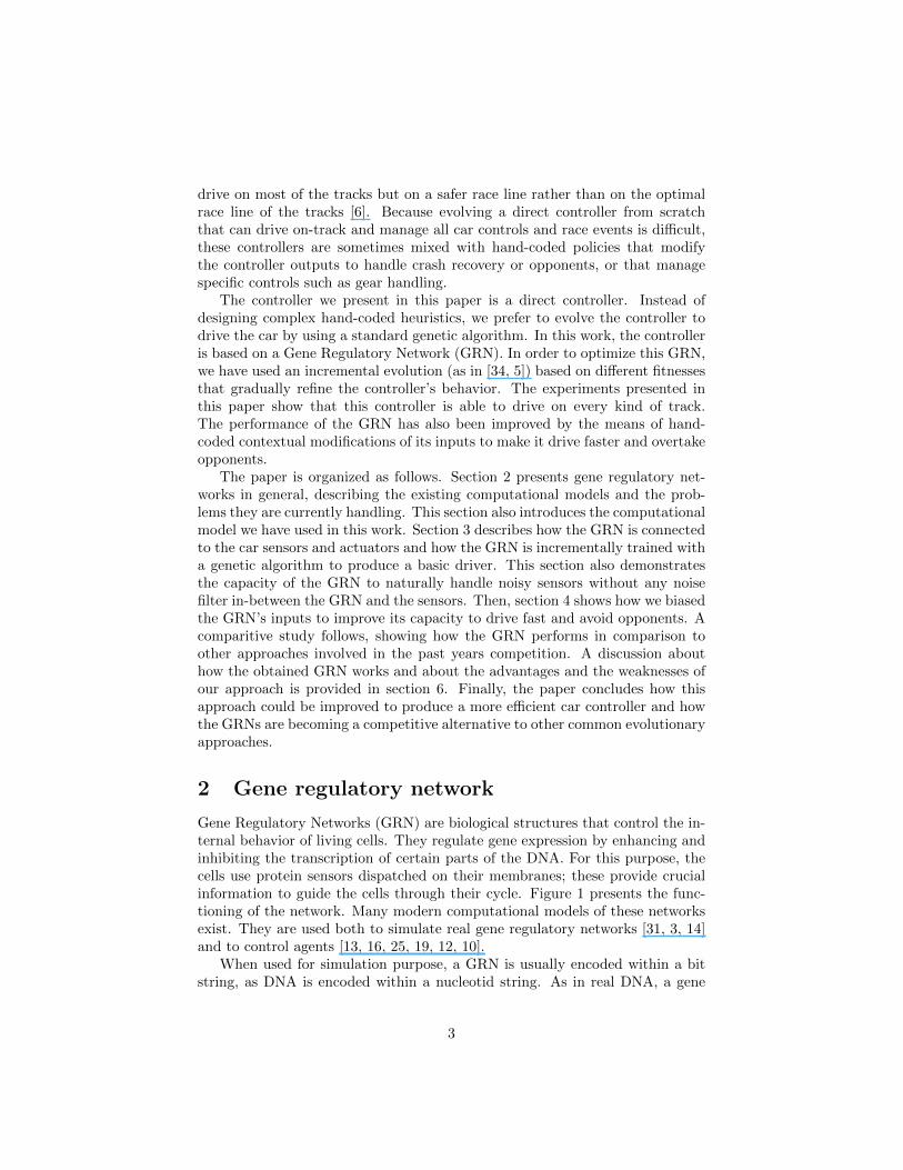
This chromosome requires particular crossover and mutation operators (rep-resented in figure 6):

• a crossover can only occur between two proteins and never between twotags of the same protein. This ensures the integrity of both subnetworkswhen the GRN is subdivided into two networks. When assembling an-other GRN, local connections are kept with this operator and only newconnections between the two networks are created.

• three mutations can be equiprobably used: add a new random regulatoryprotein, remove one protein randomly selected in the set of regulatoryproteins, or mutate a tag within a randomly selected protein.

A second chromosome is used to evolve the dynamics variables β and δ. Thischromosome consists of two double-precision floating point values and uses thestandard mutation and crossover methods. These variables are evolved in the

Car actuators

Car sensors

Protein ChromosomeProtein 1id: [0,32]

enh: [0,32]inh: [0,32]type: input

...

Protein 9id: [0,32]

enh: [0,32]inh: [0,32]type: input

Protein 10id: [0,32]

enh: [0,32]inh: [0,32]type: input

Protein 11id: [0,32]

enh: [0,32]inh: [0,32]type: input

Protein Nid: [0,32]

enh: [0,32]inh: [0,32]type: regul.

...

Left Right Accel. Brake

...Track

sensor 1Track

sensor 9 Speed X Speed Y

Protein 12id: [0,32]

enh: [0,32]inh: [0,32]

type: output

Protein 13id: [0,32]

enh: [0,32]inh: [0,32]

type: output

Protein 14id: [0,32]

enh: [0,32]inh: [0,32]

type: output

Protein 15id: [0,32]

enh: [0,32]inh: [0,32]

type: output

Protein 16id: [0,32]

enh: [0,32]inh: [0,32]type: regul.

Figure 5: Organization of the protein chromosome and link to the car sensorsand actuators: the tags (in red) are evolved by the genetic algorithm whereasthe types (in green) are fixed and always plugged to the same car sensors (forinput proteins) and the same car actuators (for output proteins).

9

Page 10

Protein chromosome A

Prot a1

Prot a2

Prot a3

Prot a4

Prot a5

Prot a6

Protein chromosome B

Prot b1

Prot b2

Prot b3

Prot b4

Prot b5

Crossover

Protein chromosome C

Prot a1

Prot a2

Prot a3

Prot b5

Protein chromosome D

Prot b1

Prot b2

Prot b3

Prot b4

Prot a4

Prot a5

Prot a6

Protein chromosome X

Protein 1id=10enh=7inh=14

type=input

Protein iid=8enh=3inh=6

type=regulatory ......

Protein chromosome X'

Protein 1id=10enh=7inh=14

type=input

Protein iid=8

enh=31inh=6

type=output ......

Protein chromosome Z

Protein 1id=10enh=7inh=14

type=input

Protein iid=8enh=3inh=6

type=regulatory ......

Protein chromosome Z'

Protein 1id=10enh=7inh=14

type=input

Protein n-1id=23enh=14inh=18

type=regulatory...

Mutate:remove a protein

Mutate:modify a protein

Protein chromosome Y'

Protein 1id=10enh=7inh=14

type=input

Protein n+1id=19enh=1inh=4

type=regulatory...

Protein chromosome Y

Protein 1id=10enh=7inh=14

type=input

Protein nid=7

enh=13inh=18

type=regulatory...

Mutate:add a protein

Figure 6: Crossover and mutation operators applied to the protein chromosome.A crossover (on the left-hand side) can only occur between two proteins and amutation (on the right-hand side) consists of adding, removing or changing aprotein.

interval [0.5, 2]. Values under 0.5 produce unreactive networks whereas valuesover 2 produce very unstable networks. These values are chosen empiricallythrough a series of test cases.

3.3 Incremental evolution

In order to optimize the GRN to drive a car, we use an incremental evolutionin three stages2. During these stages, the same parameters have been used totune the genetic algorithm. Only the fitness function is modified. The geneticalgorithm parameters are:

• Population size: 500,

• Mutation rate: 15%,

• Crossover rate: 75%,

• GRN Size: [4, 20] regulatory proteins plus inputs and outputs.

3.3.1 Stage 1: learning to drive on one simple track

The first stage consists of training the GRN to drive as far as possible, with aminimum speed, on one track. We use CGSpeedway, the left-hand side track offigure 7, which is simple with long turns and straight lines. In our opinion, thistrack is interesting for learning to drive. It is a relatively easy track with longfast turns and with fast straight lines to learn how to steer and to accelerate,and with more difficult short turns to learn how to slow down and to brake.Each GRN is tested on this track for 31 kilometers (about 10 laps) maximum.The simulation is stopped as soon as the car leaves the track or gets damaged(by hitting a rail for example). To ensure the car is driving fast enough, weuse a ticket system in which the GRN must cover 500 ∗ nLap meters per 1000

2Videos of this evolution are available online: http://www.irit.fr/~Sylvain.

Cussat-Blanc/GRNDriver/index_en.php.

10

Page 11

simulation steps, where nLap is the current lap number. This pushes the GRNsthat go far to accelerate. If a GRN cannot reach this objective, the simulation isstopped. When the simulation ends, the fitness function is given by the distancecovered by the GRN along the central line of the track. If a GRN has traveledall 31 kilometers, a bonus is added. The bonus is inversely proportional to thenumber of simulation steps needed to completed the race.

The top curve in figure 8 presents convergence of the genetic algorithm withthis fitness. In order to avoid plateauing, we have implemented a restart functionwhich renews the entire population with the best individual, 25 individualsmutated from the best one and 474 new genomes. The effects of the restartfunction can clearly be seen on the convergence curve with a drastic drop of thefitness average, pointed by the symbol (a).

In this convergence curve, five stages clearly appear. The first stage, denoted(b), represents the time to learn to accelerate and to steer to avoid the trackborder of the very first turn (turn 1 on figure 7). The second stage, denoted(c), represents the time needed to learn to steer in order to go through turn 2.Once this is done, the GRN can go through the complex series of turns 3, 4 and5. At the third stage, denoted (d), the best GRN can finish one lap, but theGRN stops in the second lap between turn 4 and turn 8. The GRN is too slowand is eliminated from the race by the ticket system. The GRN then learns todrive faster until it can finish the second lap. At this point, the ticket systemincreases the speed pressure on the GRN and the evolution reaches a new stage(e). The best GRNs are once again stuck in turns 3 to 5 part of the circuit. Asmooth optimization of the GRN is observable in stage (f): the GRN optimizesthe trajectory in order to increase the car speed and go further. However, it isnot sufficient to finish the third lap.

At this point of the evolution, two GRNs are remarkable:

• the best GRN of stage (e) is able to drive endlessly on this track, withoutthe speed pressure. It is a safe driver that regulates its speed so that itcan go through all the turns of this track.

• the best GRN of stage (f) is able to drive faster than the previous one but

CGSpeedway Alpine

Street

Turn3

Turn4

Turn6

Turn8

Turn9

Turn1 Turn2

Turn7

Turn5

Figure 7: Tracks used to train the GRN. All of them are provided by TORCS.

11

Page 12

!1000$

0$

1000$

2000$

3000$

4000$

5000$

6000$

0$ 50$ 100$ 150$ 200$ 250$ 300$ 350$ 400$ 450$

First optimization on 1 track

(c)(d) (e) (a)

— Max - - Average - - Min (f)

!2000$

0$

2000$

4000$

6000$

8000$

10000$

12000$

14000$

16000$

18000$

20000$

0$ 10$ 20$ 30$ 40$

Second optimization on 3 tracks

0"

1"

2"

3"

4"

5"

6"

7"

8"

9"

0" 5" 10" 15" 20" 25" 30" 35"

Final optimization

Generalization

Cleaning

(b)

— Max - - Average - - Min

— Max - - Average - - Min

Figure 8: Evolution of the fitnesses over the three evolution stages of the GRN.First, the GRN is evolved on one track to learn to drive. Then, the GRN isgeneralized on three different tracks. Then, the GRN behavior is cleaned up inorder to reduce oscillatory issues.

12

Page 13

-1

0

1

0 500 1000 1500 2000

CGSpeedway (Asphalt) - Trajectory

Stage 1 Stage 2 Stage 3-1

-0.5

0

0.5

1

0 500 1000 1500 2000

CGSpeedway (Asphalt) - Steering

Stage 1 Stage 2 Stage 3

Turns 4 to 8 Turns 9 and 1Turn 2 Turn 3

Figure 9: Evolution of the car behavior during the three different stages ofevolution. The left-hand side plot represents the track position of the car alongthe distance from the start line: 0 means the car is on the track centerline, -1means the car is on the right edge of the track and 1 means the car is on the leftone. The right-hand side plot is the steering output value along the distancefrom start. -1 means the steer is fully rotated to the right and 1 means fullyrotated to the left.

takes more risks. It optimizes the trajectories specifically to this track. Inour opinion, this controller is overspecialized: whereas the first one cancover some other easy tracks, this one cannot.

Moreover, as presented on Figure 9, the car is slightly shifted to the right sideof the track. That might explains why the GRN cannot generalize its drivingto other tracks: most of the turns on the training track are to the left. Thus,staying on the right side is better. However, on tracks with hard right turns,this position can be dangerous, the angle for right turns being closed. Moreover,some significant oscillations on the steering can be noticed. Even if they do notimply oscillations on the car track position, this behavior is unwanted and canbe harmfull in a car race. The aim of the next evolution stages is to correctthese defects.

3.3.2 Stage 2: generalization on three tracks

From the previous observation, we want a GRN able to safely cover all possibletracks, with all possible kinds of turns. With this aim in mind, we evolved thetwo previous GRNs a second time with the same evolutionary process but onthree different tracks. The tracks used are CGSpeedway (in order not to losethe driving capacity of the previous GRN), Alpine and Street, whose layoutsare presented in figure 7. The fitness function consists of summing the fitnessesof the first evolution stage successively applied to the three tracks.

The middle curve of figure 8 plots the evolution of the population’s best,worst and average fitnesses. The restart mechanisms has also been applied: thisexplains the average fitness drops on the blue curve. Plateauing can be noticed

13

Page 14

during this evolution. It also corresponds to the successive difficulties of thetracks:

• the beginning hair pins of Alpine,

• the three turns at the top of Street,

• the very slow hair pin at the end of the long straight line of Street.

At the end of this evolution, the best GRN is able to drive on every possibletrack. It drives very safely, going at a suitable speed to go through every kindof turn and braking when it detects a turn. However, the best GRN has anoscillatory behavior and is slightly shifted to the right hand side of the track.Whereas oscillatory behaviors are common in gene regulatory networks, boththese issues could be harmful during a car race. This oscillation can be observedin Figure 9 where the trajectories and the steering of the car are plotted duringthe second lap on the learning track (CGSpeedway). This oscillatory behaviorcan still be noticed on the steering plot in which the blue curve, which representsthe second stage of evolution, strongly oscillates. The result is some parasiticbehavior of the car on the trajectory, especially at the end of the turns. Thefinal cleaning stage aims to reduce these parasitic behaviors.

3.3.3 Stage 3: cleaning the GRN’s imperfections

To minimize the oscillatory behavior, we evolve the best GRN one last time.This time we add to the fitness function another test case that penalizes thecontinuous oscillations of the car on straight lines and long turns or fast mul-tiple steering changes from full right to full left. As with the ticket system orthe damage control used in the previous fitness functions, we simply stop theevaluation if we detect oscillatory behavior.

The detection routine proceeds as follows. A potential oscillatory behavioris detected when the steering wheel crosses its neutral position (i.e. if goes fromleft to right or from right to left). This initiates a countdown of 50 simulationsteps. Within this 50 simulation steps, if the steering wheel crosses the neutralposition more than three times and the sum of the steering variations is greaterthan a specified threshold (here empirically set up to 2.0, which correspondsto one steering switch from full right to full left), the oscillatory behavior isconfirmed and the evaluation stops.

The green line on figure 9 shows the steering values of the best GRN on theCGSpeedway track at the end of this evolution stage. The steering spikiness ofthe previous evolution (blue curve) that is visible in the first two fast curves issmoothed and the steering does not oscillate anymore from full right to full leftin the track section from turn 4 to turn 8 and from turn 9 to turn 1 (see figure7).

It can be noted that this last evolution stage reinforces the generalizationstage by improving the central position of the car. The GRN is also faster thanbefore because the oscillations reduce the car speed in general. These multiple

14

Page 15

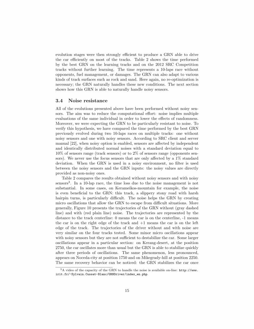
evolution stages were then strongly efficient to produce a GRN able to drivethe car efficiently on most of the tracks. Table 2 shows the time performedby the best GRN on the learning tracks and on the 2012 SRC Competitiontracks without further learning. The time represents a 10-laps race withoutopponents, fuel management, or damages. The GRN can also adapt to variouskinds of track surfaces such as rock and sand. Here again, no re-optimization isnecessary; the GRN naturally handles these new conditions. The next sectionshows how this GRN is able to naturally handle noisy sensors.

3.4 Noise resistance

All of the evolutions presented above have been performed without noisy sen-sors. The aim was to reduce the computational effort: noise implies multipleevaluations of the same individual in order to lower the effects of randomness.Moreover, we were expecting the GRN to be particularly resistant to noise. Toverify this hypothesis, we have compared the time performed by the best GRNpreviously evolved during two 10-laps races on multiple tracks: one withoutnoisy sensors and one with noisy sensors. According to SRC client and servermanual [22], when noisy option is enabled, sensors are affected by independentand identically distributed normal noises with a standard deviation equal to10% of sensors range (track sensors) or to 2% of sensors range (opponents sen-sors). We never use the focus sensors that are only affected by a 1% standarddeviation. When the GRN is used in a noisy environment, no filter is usedbetween the noisy sensors and the GRN inputs: the noisy values are directlyprovided as non-noisy ones.

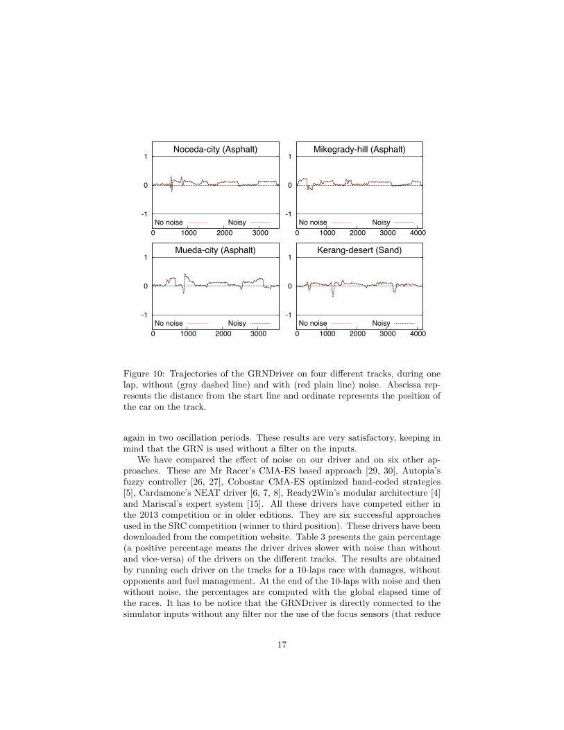
Table 2 compares the results obtained without noisy sensors and with noisysensors3. In a 10-lap race, the time loss due to the noise management is notsubstantial. In some cases, on Kerameikos-mountain for example, the noiseis even beneficial to the GRN: this track, a slippery stony road with harshhairpin turns, is particularly difficult. The noise helps the GRN by creatingmicro oscillations that allow the GRN to escape from difficult situations. Moregenerally, Figure 10 presents the trajectories of the GRN without (gray dashedline) and with (red plain line) noise. The trajectories are represented by thedistance to the track centerline: 0 means the car is on the centerline, -1 meansthe car is on the right edge of the track and +1 means the car is on the leftedge of the track. The trajectories of the driver without and with noise arevery similar on the four tracks tested. Some minor micro oscillations appearwith noisy sensors but they are not sufficient to destabilize the car. Some largeroscillations appear in a particular section: on Kerang-desert, at the position2750, the car oscillates more than usual but the GRN is able to stabilize quicklyafter three periods of oscillations. The same phenomenon, less pronounced,appears on Noceda-city at position 1750 and on Mikegrady-hill at position 2250.The same recovery behavior can be noticed: the GRN stabilizes the car once

3A video of the capacity of the GRN to handle the noise is available on-line: http://www.irit.fr/~Sylvain.Cussat-Blanc/GRNDriver/index_en.php.

15

Page 16

Tra

ckn

ame

Tra

ckty

pe

Tim

ew

ith

ou

tT

ime

wit

hD

iffer

ence

nois

yse

nso

rsn

ois

yse

nso

rsA

lpin

eA

sph

alt

28:5

4.9

829:0

2.5

5+

00:0

7.5

7(+

0.4

%)

CG

Sp

eed

way

Asp

halt

07:3

4.0

907:3

5.2

3+

00:0

1.1

4(+

0.2

%)

Str

eet

Asp

halt

16:0

0.2

516:2

1.6

8+

00:2

1.4

3(+

2.2

%)

Em

ero-

city

Asp

halt

12:3

1.3

512:3

7.3

5+

00:0

6.0

0(+

0.8

%)

Ills

chw

ang-

des

ert

San

d15:4

0.5

114:4

4.4

8-0

0:5

6.0

3(-

6.0

%)

Ker

amei

kos-

mou

nta

inR

ock

s20:3

6.4

018:4

3.2

2-0

1:5

3.1

8(-

9.1

%)

Ker

ang-

des

ert

San

d14:0

3.4

214:0

8.6

5+

00:0

5.2

3(+

0.6

%)

Mik

egra

dy-h

ill

Asp

halt

14:5

3.5

614:5

9.4

7+

00:0

5.9

1(+

0.7

%)

Mu

eda-

city

Asp

halt

12:5

6.0

513:0

4.5

4+

00:0

8.4

9(+

1.1

%)

Noce

da-

city

Asp

halt

12:0

2.7

912:0

5.8

0+

00:0

3.0

1(+

0.4

%)

Sen

hor

-hil

lA

sph

alt

17:4

6.2

018:3

2.0

3+

00:4

5.8

3(+

4.3

%)

Zvo

len

ovic

e-m

ounta

inR

ock

s13:1

4.0

813:2

0.6

6+

00:0

6.5

8(+

0.8

%)

Ave

rage

-00:0

4.8

4(-

0.3

%)

Tab

le2:

Tim

eof

the

GR

ND

rive

ron

vari

ous

track

sw

ith

an

dw

ith

ou

tn

ois

yse

nso

rs(e

lap

sed

tim

eof

a10-l

ap

race

wit

hout

opp

onen

ts,

fuel

man

agem

ent,

ord

amag

es).

Tim

efo

rmat:

mm

:ss.

ms.

16

Page 17

-1

0

1

0 1000 2000 3000

Noceda-city (Asphalt)

No noise Noisy-1

0

1

0 1000 2000 3000 4000

Mikegrady-hill (Asphalt)

No noise Noisy

-1

0

1

0 1000 2000 3000

Mueda-city (Asphalt)

No noise Noisy-1

0

1

0 1000 2000 3000 4000

Kerang-desert (Sand)

No noise Noisy

Figure 10: Trajectories of the GRNDriver on four different tracks, during onelap, without (gray dashed line) and with (red plain line) noise. Abscissa rep-resents the distance from the start line and ordinate represents the position ofthe car on the track.

again in two oscillation periods. These results are very satisfactory, keeping inmind that the GRN is used without a filter on the inputs.

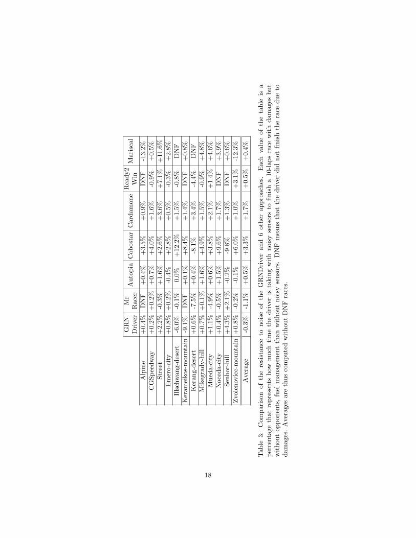
We have compared the effect of noise on our driver and on six other ap-proaches. These are Mr Racer’s CMA-ES based approach [29, 30], Autopia’sfuzzy controller [26, 27], Cobostar CMA-ES optimized hand-coded strategies[5], Cardamone’s NEAT driver [6, 7, 8], Ready2Win’s modular architecture [4]and Mariscal’s expert system [15]. All these drivers have competed either inthe 2013 competition or in older editions. They are six successful approachesused in the SRC competition (winner to third position). These drivers have beendownloaded from the competition website. Table 3 presents the gain percentage(a positive percentage means the driver drives slower with noise than withoutand vice-versa) of the drivers on the different tracks. The results are obtainedby running each driver on the tracks for a 10-laps race with damages, withoutopponents and fuel management. At the end of the 10-laps with noise and thenwithout noise, the percentages are computed with the global elapsed time ofthe races. It has to be notice that the GRNDriver is directly connected to thesimulator inputs without any filter nor the use of the focus sensors (that reduce

17

Page 18

GR

NM

rA

uto

pia

Cob

ost

ar

Card

am

on

eR

ead

y2

Mari

scal

Dri

ver

Race

rW

inA

lpin

e+

0.4%

DN

F+

0.4

%+

3.5

%+

0.9

%D

NF

-13.2

%C

GS

pee

dw

ay+

0.2%

+0.2

%+

0.7

%+

4.0

%+

1.6

%-0

.9%

+0.5

%S

tree

t+

2.2%

-0.3

%+

1.6

%+

2.6

%+

3.6

%+

7.1

%+

11.6

%E

mer

o-ci

ty+

0.8%

+0.2

%-0

.4%

+2.8

%+

0.5

%-0

.3%

+2.8

%Il

lsch

wan

g-d

eser

t-6

.0%

-0.1

%0.0

%+

12.2

%+

1.5

%-0

.8%

DN

FK

eram

eiko

s-m

ounta

in-9

.1%

DN

F+

0.1

%+

8.4

%+

1.4

%D

NF

+0.8

%K

eran

g-d

eser

t+

0.6%

-7.5

%+

0.4

%-8

.1%

+3.4

%-4

.4%

DN

FM

ikeg

rad

y-h

ill

+0.

7%+

0.1

%+

1.6

%+

4.9

%+

1.5

%-0

.9%

+4.8

%M

ued

a-ci

ty+

1.1%

-4.9

%+

0.6

%+

3.8

%+

2.1

%+

1.4

%+

4.6

%N

oce

da-

city

+0.

4%-0

.5%

+1.5

%+

9.6

%+

1.7

%D

NF

+3.9

%S

enh

or-h

ill

+4.

3%+

2.1

%-0

.2%

-9.8

%+

1.3

%D

NF

+0.6

%Z

vole

nov

ice-

mou

nta

in+

0.8%

-0.2

%-0

.1%

+6.0

%+

1.0

%+

3.1

%-1

2.3

%

Ave

rage

-0.3

%-1

.1%

+0.5

%+

3.3

%+

1.7

%+

0.5

%+

0.4

%

Tab

le3:

Com

par

ison

ofth

ere

sist

ance

ton

oise

of

the

GR

ND

rive

ran

d6

oth

erap

pro

ach

es.

Each

valu

eof

the

tab

leis

ap

erce

nta

geth

atre

pre

sents

how

mu

chti

me

the

dri

ver

ista

kin

gw

ith

nois

yse

nso

rsto

fin

ish

a10-l

ap

sra

cew

ith

dam

ages

bu

tw

ith

out

opp

onen

ts,

fuel

man

agem

ent

than

wit

hou

tn

ois

yse

nso

rs.

DN

Fm

ean

sth

at

the

dri

ver

did

not

fin

ish

the

race

du

eto

dam

ages

.A

vera

ges

are

thu

sco

mp

ute

dw

ith

out

DN

Fra

ces.

18

Page 19

the noise in one chosen direction). Actually, few drivers use a noise reductionsystem: only Mr Racer uses a quadratic regression to handle the noise [28] andReady2Win use a simple noise remover method based on averaging values thatare 5% higher or lower than the 5 past averaged values. As the GRNDriver,all other drivers have a direct connection of the inputs to the control systems.Comparing the average values, the GRNDriver and Mr Racer are the only twodrivers to gain time with the noise. Whereas Mr Racer’s quadratic noise reduc-tion system provides it a strong advandage, the GRNDriver is not really affectedby the noise and even gain few seconds avoiding crashes as stated previously.In comparison, other approaches loose few seconds handling noise. Three otherapproaches handle the noise quite well: Autopia, Ready2Win and Mariscal arealmost unsensitive to the noise with an average gain percentage lower than0.5%. In conclusion, GRNDriver handles the noise well in comparison to otherapproaches without noise resistance systems.

4 Optimizing the GRN for racing

4.1 Learning to drive fast

The gene regulatory network optimized with the previous method is a safedriver, able to finish almost any kind of tracks, with or without noisy sensors.However, this GRN is not fast enough to compete with opponents. In orderto make it drive the car faster, we have distorted the GRN longitudinal speed.The idea is to trick the GRN about its speed to make it accelerate and brakein particular areas of the track. To do so, the speed sensor value is multipliedby a coefficient. The bigger the coefficient is, the faster the GRN thinks the caris going and the most it tries to slow down by braking. Actually, this provesthe GRN perfectly correlates its speed and the dangerousness of the current carstate (track sensors, lateral speed, etc.). This coefficient is calculated accordingto a target speed learned during the warm-up stage of the race4. The GRNspeed perception is distorted in order to reach the target speed as follows:

• If the car speed is 10 km/h under the target speed, the GRN’s speed sensoris set to zero in order to make it accelerate as much as it can handle it.

• If the car speed is 10km/h over the target speed, the speed sensor providedto the GRN is multiplied by 1 + ds/50 where ds is the difference betweenthe current speed and the target speed. The GRN is then pushed to reduceits speed but not too drastically. For example, if the car is in a turn, itwould be counter-productive to brake (the car will spin).

To learn the target speeds, we use a scripted approach. This approachis comparable to Butz et al. method [5] in which crash points are detectedduring the race and the car is slowed down in these areas in order to secure the

4The warm-up stage consists of 100,000 timesteps that can be used by the competitors inorder to collect data about an unknown track.

19

Page 20

Tra

ckn

ame

Tra

ckty

pe

Tim

ew

ith

ou

tT

ime

wit

hD

iffer

ence

targ

etsp

eed

sta

rget

spee

dE

mer

o-ci

tyA

sph

alt

12:3

7.3

510:5

1.8

5-0

1:4

5.5

0(-

13.9

%)

Ills

chw

ang-

des

ert

San

d14:4

4.4

811:0

8.0

5-0

3:36.4

3(-

24.5

%)

Ker

amei

kos-

mou

nta

inR

ock

s18:4

3.2

214:4

3.7

7-0

3:59.4

5(-

21.3

%)

Ker

ang-

des

ert

San

d14:0

8.6

512:3

2.1

0-0

1:3

4.5

5(-

11.1

%)

Mik

egra

dy-h

ill

Asp

halt

14:5

9.4

713:0

0.8

7-0

1:5

8.6

0(-

13.2

%)

Mu

eda-

city

Asp

halt

13:0

4.5

410:4

6.4

8-0

2:1

8.0

6(-

17.6

%)

Noce

da-

city

Asp

halt

12:0

5.8

009:3

5.9

8-0

2:2

9.8

2(-

20.6

%)

Sen

hor

-hil

lA

sph

alt

18:3

2.1

813:2

6.1

8-0

5:05.8

5(-

27.5

%)

Ave

rage

-02:5

1.0

3(-

18.7

%)

Tab

le4:

Com

par

ison

ofth

eb

est

lap

out

ofth

ree

wit

han

dw

ith

ou

tta

rget

spee

dopti

miz

ati

on.

Form

at

ofth

ela

pti

me:

mm

:ss.

ms.

20

Page 21

car behavior. In our approach, this optimization is made during the warm-upstage. To do so, the track is first divided into 25 meters long sectors. The targetspeeds are all initialized to 300 km/h in order to push the GRN to drive as fastas possible. When the GRNDriver spins or leaves the track, the sectors of azone which contain the current sector and the 5 sectors upstream are marked as“reducing”. When marked, the target speeds of these sectors are reduced by 125km/h. When the target speeds of this zone reach a minimal value of 50 km/h,one sector is added to the zone and its target speed is decreased. With thismethod, we can guarantee that the GRN can handle every kind of turns, evenwhen it approaches very fast and has to brake quickly. Once the zone is passed,all sectors of the zone are marked as “increasing” and the target speeds of allsectors are gradually increased by 20 km/h until the GRNDriver crashes againin this zone. When this happens, the previously added 20 km/h is subtractedand the sectors are marked as “braking”. The final step consists of reducing

Downgrading target speed of 5 sectors

Downgrading target speed of the entire zone

Upgrading the zone until the car crashed

Reducing the braking zone until the car crashes

Backtrack on the braking zone and Lock the zone

25m long sector with its target speed

Locked sector

GR

N D

GR

N D Car trajectory

Car crash

300 km/h

175 km/h

50 km/h

110 km/h

Target speeds:

S1

S2

S3

S4

S5

S6

S7 S8 S9

GRN D

GRN D

Stage 1

S1

S2

S3

S4

S5

S6

S7 S8 S9

GRN D

GRN D

Stage 2

S1

S2

S3

S4

S5

S6

S7 S8 S9

GRN D

GRN D

Stage 3

S1

S2

S3

S4

S5

S6

S7 S8 S9

GRN D

GRN D

Stage 4

S1

S2

S3

S4

S5

S6

S7 S8 S9

GRN D

GRN D

Stage 6

S1

S2

S3

S4

S5

S6

S7 S8 S9

GRN D

GRN D

Stage 7

S1

S2

S3

S4

S5

S6

S7 S8 S9

GRN D

GRN D

Stage 5

Backtracking (removing 20 km/h)

Figure 11: Example of target speed optimization on one turn: the target speed isfirst initialized to maximum speed (300km/h). If the GRN cannot go through aturn, the speed is gradually reduced by 125km/h until reaching 50km/h (Stages1 and 3). When the car can manage the turn, the target speed is graduallyincreased by 20 km/h until the car crashes again (Stage 3 and 4, here onlyrepresented on one picture). Then, the braking zone is reduced as much aspossible (Stages 5 and 6). When the car crashes again, the braking zone isbacktracked to the previous size and all sectors are locked (Stage 7).

21

Page 22

the possibly too long braking zone. To do so, the target speed of the zone’sfirst sector is set to 300 km/h: the braking zone will be reduced each time theGRNDriver is able to go through the modified zone. When the GRNDrivercrashes once again in this zone, the previous target speed is restored and thezone is marked as “locked”. When locked, the GRNDriver can still crash becauseof the noise. If this happens, the target speeds are reduced by 5 km/h to securethe zone. Figure 11 presents an example of the optimization mechanism.

The process can be pipelined along multiple runs: if the car crashes on thethird zone, it means that the third zone must be modified but it also implies thatthe GRN was able to handle the first two zones. Thus, they can be optimizedby potentially going to the next step. The marking process is linear per zone(a mark of a zone can only be increased, never downgraded to a previous stage)expect for the first zone which can be marked as “reducing” when the car crashesin this zone after it finishes a lap. This ensures that the first turn is perfectlycovered, even if it is after a long straight line.

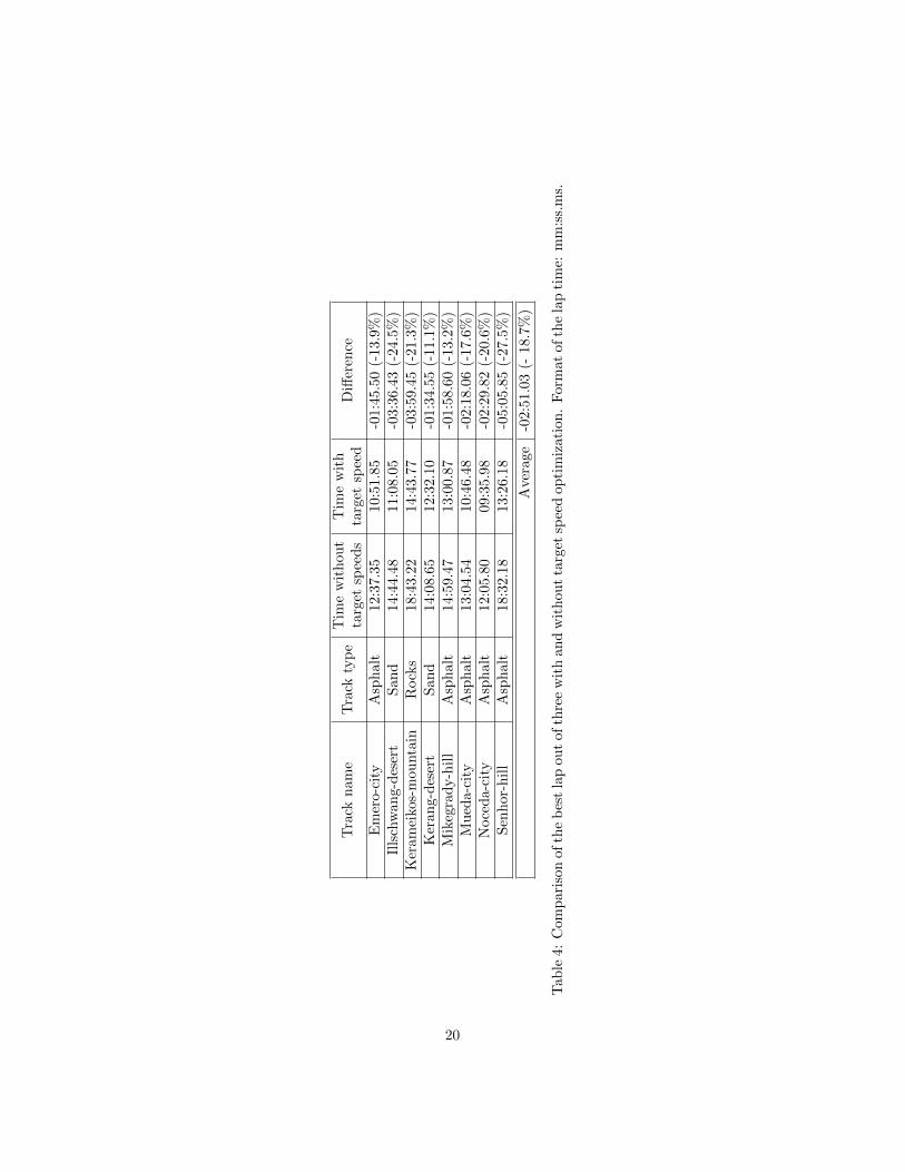
Table 4 presents the time performed by the best GRN on various tracks takenfrom the 2012 competition with and without this speed optimization. To do so,the GRN is tested without target speed and with target speed on all tracks withnoisy sensors. For the target speed optimization, we use the standard warm-up procedure that consists of running the optimization for 100,000 simulationsteps; then the GRN with the optimized target speed vector is run in race modewithout opponents for 10 laps. Damages and fuel are disabled but the GRN hasto handle the noise, as in the competition. By learning the target speed for thedifferent sectors of the track, the GRN runs on average 2 minutes 51 seconds or18.7% faster than the default GRN. The gain is significant in all tested tracks.

Figure 12 presents the track position and the longitudinal speed of the caron 4 different tracks, with and without target speed optimization. The speedgain of this approach is undeniable in all the sectors of the tracks. The GRN isaccelerating earlier and stronger and brakes later. Moreover, it may be notedthat the increase of the speed drives the GRN to use the full width of the track,the speed dragging the car to the outside edge of the track.

4.2 Avoiding opponents

In order to compete efficiently, the driver must avoid or overtake opponents.The GRN controller has learned to drive without such considerations and, evenif it can be fast using the “target speeds” method, it needs to be able to changetrajectories in order to avoid or to overtake opponents. The GRN controller wechose to compete presents an interesting and usable feature: two track sensors,one on each side of the car, are linked to the steering actuators in order to keepthe car on the centerline of the track. This characteristic is common to almostevery GRN that was evolved through the process previously described, althoughthe track sensors used to center the car on the track might differ and are notnecessarily symmetric. In order to modify the car trajectory toward the left orthe right hand side of the track, we can alter both sensors as we altered thelongitudinal speed sensor to make the GRN drive faster in the previous section.

22

Page 23

-1

0

1

0 1000 2000 3000

Noceda-city (Asphalt) - Trajectory

Optimized Basic-1

0

1

0 1000 2000 3000 4000

Mikegrady-hill (Asphalt) - Trajectory

Optimized Basic

-1

0

1

0 1000 2000 3000

Mueda-city (Asphalt) - Trajectory

Optimized Basic-1

0

1

0 1000 2000 3000 4000

Kerang-desert (Sand) - Trajectory

Optimized Basic

0

100

200

300

0 1000 2000 3000

Noceda-city (Asphalt) - Speed

Optimized Basic 0

100

200

300

0 1000 2000 3000 4000

Mikegrady-hill (Asphalt) - Speed

Optimized Basic

0

100

200

300

0 1000 2000 3000

Mueda-city (Asphalt) - Speed

Optimized Basic 0

100

200

300

0 1000 2000 3000 4000

Kerang-desert (Sand) - Speed

Optimized Basic

Figure 12: Trajectories (top) and longitudinal speed (bottom) of the car on 4different tracks with and without target speed optimization.

23

Page 24

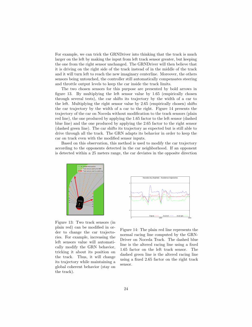
For example, we can trick the GRNDriver into thinking that the track is muchlarger on the left by making the input from left track sensor greater, but keepingthe one from the right sensor unchanged. The GRNDriver will then believe thatit is driving on the right side of the track instead of in the middle of the trackand it will turn left to reach the new imaginary centerline. Moreover, the otherssensors being untouched, the controller still automatically compensates steeringand throttle output levels to keep the car inside the track limits.

The two chosen sensors for this purpose are presented by bold arrows infigure 13. By multiplying the left sensor value by 1.65 (empirically chosenthrough several tests), the car shifts its trajectory by the width of a car tothe left. Multiplying the right sensor value by 2.65 (empirically chosen) shiftsthe car trajectory by the width of a car to the right. Figure 14 presents thetrajectory of the car on Noceda without modification to the track sensors (plainred line), the one produced by applying the 1.65 factor to the left sensor (dashedblue line) and the one produced by applying the 2.65 factor to the right sensor(dashed green line). The car shifts its trajectory as expected but is still able todrive through all the track. The GRN adapts its behavior in order to keep thecar on track even with the modified sensor inputs.

Based on this observation, this method is used to modify the car trajectoryaccording to the opponents detected in the car neighborhood. If an opponentis detected within a 25 meters range, the car deviates in the opposite direction

31

GRN Driver

GRN Driver

Unused track sensorsTrack sensors used by the GRNTrack sensors used for positioning

Figure 13: Two track sensors (inplain red) can be modified in or-der to change the car trajecto-ries. For example, increasing theleft sensors value will automati-cally modify the GRN behavior,tricking it about its position onthe track. Thus, it will changeits trajectory while maintaining aglobal coherent behavior (stay onthe track).

-1

0

1

0 1000 2000

Noceda-city (Asphalt) - Avoidence trajectories

Original Avoid left Avoid right

Figure 14: The plain red line represents thenormal racing line computed by the GRN-Driver on Noceda Track. The dashed blueline is the altered racing line using a fixed1.65 factor on the left track sensor. Thedashed green line is the altered racing lineusing a fixed 2.65 factor on the right tracksensor.

24

Page 25

GRN Driver

GRN Driver

X 1.

Overtaking done!Go back to

standard trajectory ...GRN Driver

GRN Driver

X 1.65

Overtaking left side!

GRN Driver

GRN Driver

X 1.65

Overtake left side! (a) (b) (c)

Figure 15: Three phases in avoidance routine: (a) The GRNDriver detects acar on the right and begins to overtake on the left side. (b) The GRNDriverovertakes, keeping the car on the left of the track. (c) Overtaking is done,the GRNDriver resumes its normal racing behavior. The blue and red angularsectors represent the opponent sensors as described in the SRC competitionclient. Only the useful sensors are represented for clarity matters.

Figure 16: The GRNDriver avoids the red car. The plain line is the normaltrajectory, the dotted line is the altered trajectory using a 2.65 factor on theright track sensor used to position the car in the middle of the track.

to the one the opponent is detected in. This procedure only applies if the fronttrack sensor value is greater than 50 meters. If it’s not, overtaking is detected asunsafe and the car will stay behind the opponent car with a procedure describedhereafter. If overtaking occurs, the opponent car is tracked during the wholeoperation and the track sensors return to their real value when the front andside opponent sensors do not detect any opponent nearby. Figure 15 shows thisprocedure and figure 16 shows the trajectory taken by the car in a real situationextracted from TORCS.

If opponents are detected on both sides of the car or if the distance ahead isnot sufficient, the GRNDriver will stay behind the closest opponent ahead (figure17). To keep the GRNDriver behind an opponent, we adjust the speed of thecar using the same method we used in section 4.1. In this case, the longitudinalspeed sensor is adjusted according to the speed of the closest opponent as follows:

25

Page 26

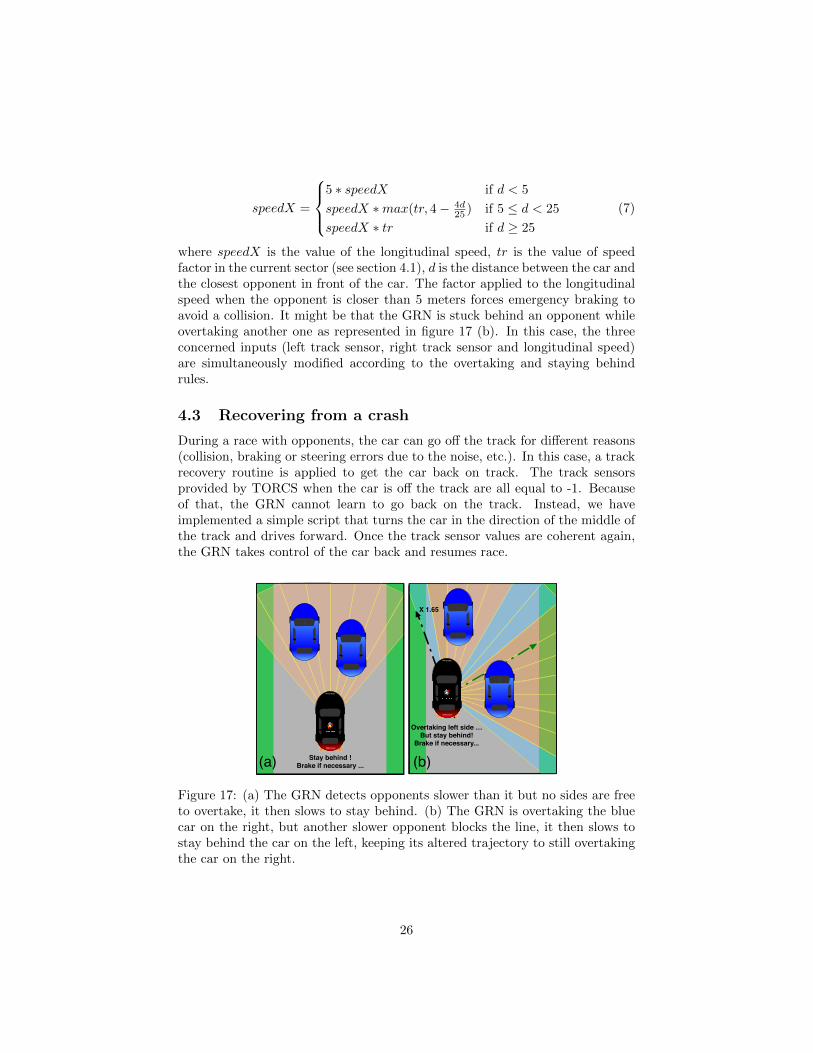
speedX =

5 ∗ speedX if d < 5

speedX ∗max(tr, 4− 4d25 ) if 5 ≤ d < 25

speedX ∗ tr if d ≥ 25

(7)

where speedX is the value of the longitudinal speed, tr is the value of speedfactor in the current sector (see section 4.1), d is the distance between the car andthe closest opponent in front of the car. The factor applied to the longitudinalspeed when the opponent is closer than 5 meters forces emergency braking toavoid a collision. It might be that the GRN is stuck behind an opponent whileovertaking another one as represented in figure 17 (b). In this case, the threeconcerned inputs (left track sensor, right track sensor and longitudinal speed)are simultaneously modified according to the overtaking and staying behindrules.

4.3 Recovering from a crash

During a race with opponents, the car can go off the track for different reasons(collision, braking or steering errors due to the noise, etc.). In this case, a trackrecovery routine is applied to get the car back on track. The track sensorsprovided by TORCS when the car is off the track are all equal to -1. Becauseof that, the GRN cannot learn to go back on the track. Instead, we haveimplemented a simple script that turns the car in the direction of the middle ofthe track and drives forward. Once the track sensor values are coherent again,the GRN takes control of the car back and resumes race.

GRN Driver

GRN Driver

X 1.65

Overtaking left side …But stay behind!

Brake if necessary...GRN Driver

GRN Driver

Stay behind !Brake if necessary ...(a) (b)

Figure 17: (a) The GRN detects opponents slower than it but no sides are freeto overtake, it then slows to stay behind. (b) The GRN is overtaking the bluecar on the right, but another slower opponent blocks the line, it then slows tostay behind the car on the left, keeping its altered trajectory to still overtakingthe car on the right.

26

Page 27

5 Comparative study

To evaluate the model presented in this paper, we have compared the GRN-Driver with other approaches that have competed during the past SimulatedCar Racing competitions. As in section 3.4, the selected drivers for this com-parative study are Mr Racer, Autopia, Cobostar, Cardamone, Ready2Win andMariscal. The comparative study is based upon:

• the best lap times in qualification mode,

• the elapsed times on a 10-laps race with noise, damages and without fuelmanagement nor opponents,

• the final positions on 10-laps races with all the opponents, with noise,damages and without fuel management.

All these comparison have been made after independent warm-up stages foreach driver on each track. These results might differ from the results obtainedduring the competition due to minor bug resolution in our code for this paper.The three next sections present these comparisons.

5.1 Qualifications: best lap comparison

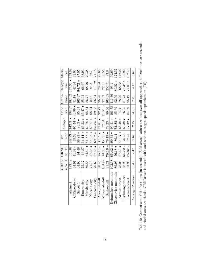
In this first comparison, the drivers are alone on a track and are running for10-laps. Fifteen tracks have been selected to have various types of coatings(asphalt, rock and sand) and different profiles (city, mountain, etc.). Table 5presents the best lap of each driver at the end of these 10 laps.

In this table, the GRNDriver is compared before and after the target speedoptimization presented in section 4.1. Without target speeds optimization, theGRNDriver competes with the slowest drivers with an average final positionof 6.40 over 8 participants. The main observation that can be made is thatthe GRNDriver can drive on any kind of tracks, without prior learning on thesetracks. However, it has a safe driving behavior that does not allow it to competewith the best approaches.

With target speed optimization, the GRNDriver is still not the fastest driverbut it is usually well ranked: it finishes amongst the first three fastest drivers13 times out of 15. The GRNDriver competes particularly well on slipperytracks such as mountain (rocks) and desert (sand) tracks. We can note that theGRNDriver has only been trained on asphalt tracks (CGSpeedway, Alpine andStreet) and never on slippery tracks. Moreover, there is no specific parametersor sub-routines to handle slippery tracks. The GRN controller is used as is.This emphasizes the capacity of the GRN to adapt its behavior under unknownconditions.

5.2 10-laps races without opponents

In this second comparison, the drivers are running for a 10-laps race with noiseand damages and without fuel management or opponents. Prior to each race, a

27

Page 28

GR

ND

.G

RN

D.

Mr

Au

top

iaC

ob

oC

ard

a-

Rea

dy2

Mari

s-w

/oT

Sw

.T

SR

ace

rst

ar

mon

ew

inca

lA

lpin

e1

173.

49156.6

7147.9

3◦142.3?

199.3

7182.0

2147.3

4•

153.6

9C

GS

pee

dw

ay44

.97

41.0

2◦

49.3

940.54?

40.9

9•

51.1

842.9

443.0

3S

tree

t1

94.9

291.4

686.8

5◦

86.3•

95.4

9106.9

784.72?

87.0

5E

mer

o-ci

ty75

.17

66.8

764.11?

66.5

3◦

65.4

7•

85.9

266.6

768.9

3M

ued

a-ci

ty89

.55

64.5

9•

64.55?

64.7

8◦

65.5

486.7

768.7

670.3

8N

oce

da-

city

71.7

357.3

5•

56.95?

59.7

7◦

68.6

480.6

85.3

62.7

San

cass

a-ci

ty76

.69

67.6

8•

69.0

2◦

65.85?

89.5

886.8

4119.7

271.1

8A

lsou

jlak

-hil

l90

.45

75.1

3◦

73.5?

74.8

1•

92.7

995.2

678.8

478.6

5M

ikeg

rad

y-h

ill

104.

9974.3

6•

72.66?

77.0

476.5

1◦

97.8

277.3

180.5

5S

enh

or-h

ill

91.2

179.16?

79.1

9•

79.2

3◦

80.4

6100.6

5256.7

183.6

Kei

ram

ekos

-mou

nta

in10

2.38

85.42?

90.3

8•

90.5

1◦

101.7

8111.3

693.1

99.6

9Z

love

nov

ice-

mou

nta

in89

.93

76.1

8•

86.1

175.85?

85.3

992.5

980.5

2◦

124.5

7A

rrai

as-d

eser

t78

.06

67.6

9•

65.07?

68.4

8◦

73.4

78.2

668.6

8142.2

2Il

lsch

wan

g-d

eser

t88

.23

64.72?

76.4

668.3

8•

76.0

581.7

372.3

8◦

98.9

2K

eran

g-d

eser

t83

.93

75.37?

82.4

477.3

2•

84.8

995.1

977.8

5◦

102.4

8

Ave

rage

Pos

itio

n6.

402.4

72.6

72.2

74.9

37.2

04.4

75.6

7

Tab

le5:

Com

par

ison

ofth

eb

est

lap

s(i

nse

con

ds)

.B

old

-sta

red

valu

esare

bes

tov

erall

ap

pro

ach

es,

bu

llet

edones

are

seco

nd

san

dci

rcle

don

esar

eth

ird

s.G

RN

Dri

ver

iste

sted

wit

han

dw

ithou

tta

rget

spee

ds

op

tim

izati

on

(TS

).

28

Page 29

GR

ND

.G

RN

D.

Mr

Au

top

iaC

ob

oC

ard

a-

Rea

dy2

Mari

s-w

/oT

Sw

.T

SR

ace

rst

ar

mon

ew

inca

lA

lpin

e1

29:0

026:1

9•

DN

F23:54?

34:2

330:2

6D

NF

27:0

6◦

CG

spee

dw

ay07

:35

06:5

5•

08:1

806:51?

07:2

108:3

907:1

607:1

2◦

Str

eet

116

:07

15:2

2◦

14:36?

14:5

2•

16:1

118:2

315:3

816:0

1E

mer

o-ci

ty12

:37

11:1

711:01?

11:1

3•

11:2

614:3

411:1

6◦

11:3

8M

ued

a-ci

ty15

:00

10:52?

11:1

3◦

10:5

5•

11:2

314:3

411:4

911:5

2N

oce

da-

city

12:0

509:3

9•

09:38?

10:0

5◦

11:3

813:4

5D

NF

10:3

5S

anca

ssa-

city

12:5

311:2

1•

11:4

6◦

11:08?

15:0

514:4

3D

NF

12:0

4A

lsou

jlak

-hil

l15

:10

12:3

7◦

12:32?

12:3

6•

15:4

415:5

913:2

313:2

0M

ikeg

rad

y-h

ill

17:3

512:3

1•

12:11?

12:5

8◦

13:0

816:2

512:5

913:4

9S

enh

or-h

ill

16:0

013:18?

13:3

3◦

13:2

3•

14:1

016:5

4D

NF

14:0

9K

eira

mek

os-m

ounta

in17

:38

14:28?

DN

F15:2

3•

17:0

9◦

19:1

3D

NF

21:4

5Z

love

nov

ice-

mou

nta

in15

:08

12:52?

15:1

312:5

4•

14:2

115:3

413:5

6◦

34:3

3A

rrai

as-d

eser

t13

:09

11:26?

13:3

611:5

6◦

12:3

314:1

011:4

9•

DN

FIl

lsch

wan

g-d

eser

t14

:49

10:57?

12:5

711:3

6•

13:2

113:4

512:1

6◦

18:1

7K

eran

g-d

eser

t14

:08

12:41?

16:0

913:1

7◦

14:5

016:1

413:1

7•

DN

F

Ave

rage

Pos

itio

n5.

801.8

02.0

73.8

05.1

36.8

75.0

05.5

3

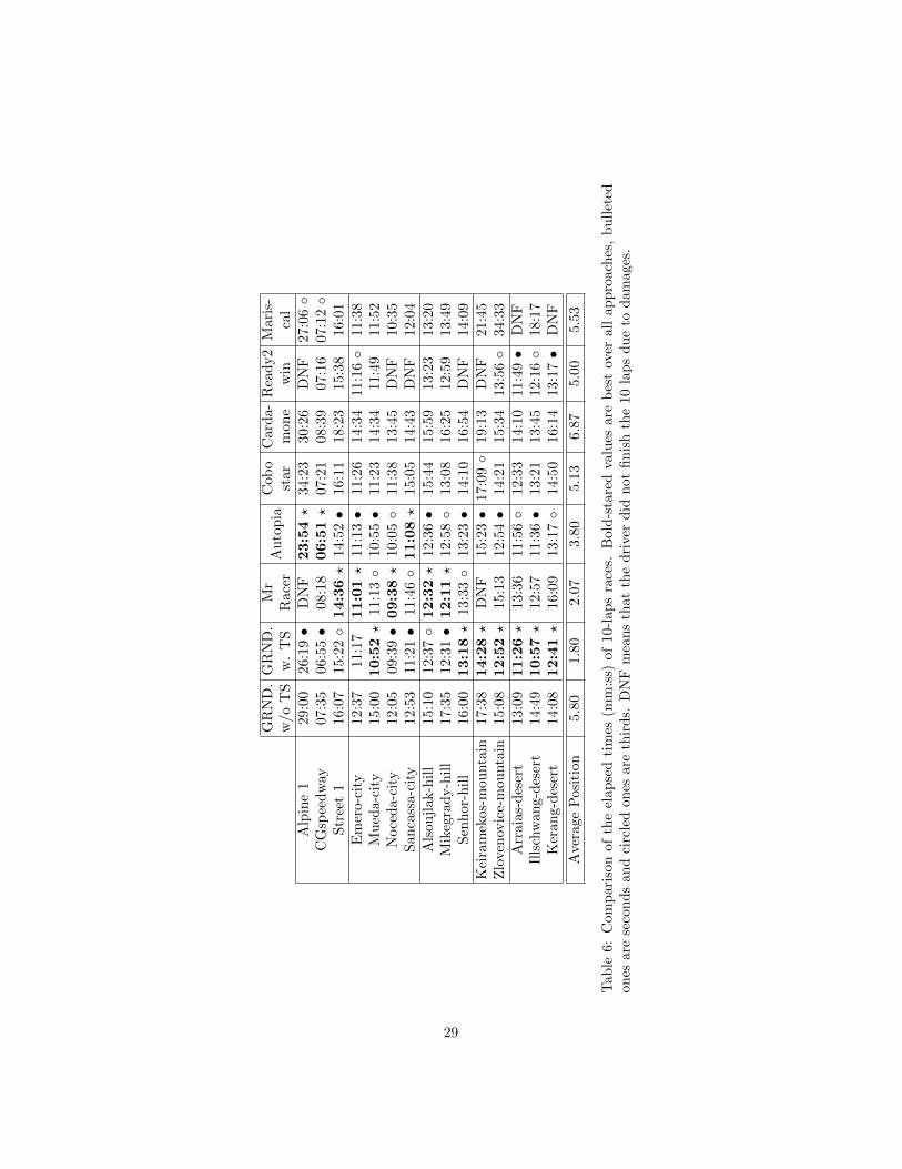
Tab

le6:

Com

par

ison

ofth

eel

apse

dti

mes

(mm

:ss)

of

10-l

ap

sra

ces.

Bold

-sta

red

valu

esare

bes

tov

erall

ap

pro

ach

es,

bu

llet

edon

esar

ese

con

ds

and

circ

led

ones

are

thir

ds.

DN

Fm

ean

sth

at

the

dri

ver

did

not

fin

ish

the

10

lap

sd

ue

tod

am

ages

.

29

Page 30

warm-up has been run so that each driver starts on a fresh learning basis. Table6 presents the results of each driver on 15 different tracks.

The GRNDriver without target speed is evaluated first. Whereas somedrivers cannot reach the finish line of the race (see DNF signs in the table)even after a warm-up session, the GRNDriver without target speed optimiza-tion, and thus without any a-priori knowledge of the tracks, finishes all tracks.Moreover, GRNDriver is faster than one of the opponent (Cardamone): itsaverage final position is 5.8 in comparison to 6.87 for Cardamone.

With the target speed optimization, the GRNDriver still finishes all the racesand it is very competitive: its average final position is 1.80 and it finishes 14races out of 15 in the top three pilots. Whereas other approaches defeats theGRNDriver on a one-lap race, the GRNDriver is more competitive on longerruns. This shows the capacity of the GRN to keep a stable behavior on longnoisy runs. Once again, we can notice that the GRNDriver beats all other driverswhen the track conditions become slippery (mountains and desert). That showsthe capacity of the GRN to adapt to the changing track conditions withoutfurther learning.

5.3 10-laps races with opponents

In this last comparison, all the drivers compete against each other in 10-lapsraces on three different tracks. Each race is run nine times: 3 times with thesame initial starting grid based on the 10-Laps races results presented in table6 and 6 times with different starting positions (based on a circular rotation ofall the drivers). For computational reasons, the three tracks of the 2013 SRCcompetition have been selected: one on asphalt (Sancassa-city), one on sand(Arraias-desert) and one in mountain (Alsoujlak-hill). Only the GRNDriverwith target speed optimization and with the opponent management is evaluatedin this section. Table 7 shows the starting and final position of the drivers forall the runs on these three tracks. Runs a − c are runs starting with the best10-laps solo races positions and runs d − i are the one with circular startingpositions.

Globally, the GRNDriver is very competitive with an average finishing po-sition of 1.67. In comparison, the second best driver, Autopia, finishes at anaverage finish position of 1.89. This shows the capacity of the GRN to usemodified inputs to handle opponents. Even if the GRNDriver is starting on theback of the grid, it is able to gain positions, because it is fast on long run races(see table 6) and because the modification of the inputs is well managed bythe GRN. In comparison to modifying the outputs, modifying the inputs allowsthe GRN to keep its regulatory ability. Thus, the GRN adapts its outputs tospecific situations such as overtaking an opponent, but its driving behavior re-mains globally the same and the GRNDriver almost never goes out of track. Forexample, it can slow down if the car state becomes dangerous while overtakingan opponent in a turn to make its behavior more conservative to avoid a colli-sion or going out of track. Locally, we can notice that in most cases (the onlycounter example being run d on Alsoujlak-hill), the GRNDriver always gains

30

Page 31

San

cass

a-ci

tyA

rraia

s-d

eser

tA

lsou

jlak-h

ill

Avg

abcdefghi

avgabcdefghi

avgabcdefghi

avg

GR

ND

rive

rG

rid

22

21

76

54

31

11

76

54

32

33

32

17

65

4w

ith

TS

Fin

ish

12

21

22

21

11.

561

11

11

31

11

1.2

23

22

32

22

13

2.2

1.6

7

Au

top

iaG

rid

11

17

65

43

23

33

21

76

54

22

21

76

54

3F

inis

h2

11

21

11

22

1.44

24

23

32

42

22.6

72

31

11

11

22

1.5

61.8

9

Mr

Rac

erG

rid

33

32

17

65

45

55

43

21

76

11

17

65

43

2F

inis

h4

44

63

45

54

4.33

56

66

76

66

45.7

81

13

23

43

31

2.3

34.1

5

Cob

osta

rG

rid

66

65

43

21

74

44

32

17

65

66

65

43

21

7F

inis

h6

56

55

54

45

53

33

22

12

36

2.7

86

66

66

66

56

5.8

94.5

6

Car

dam

one

Gri

d5

55

43

21

76

66

65

43

21

77

77

65

43

21

Fin

ish

56

54

66

66

75.

676

55

44

43

43

4.2

25

77

75

75

67

6.2

25.3

7

Rea

dy2w

inG

rid

77

76

54

32

12

22

17

65

43

55

54

32

17

6F

inis

h7

77

77

77

76

6.89

42

45

55

55

54.4

44

54

44

34

74

4.3

35.2

2

Mar

isca

lG

rid

44

43

21

76

57

77

65

43

21

44

43

21

76

5F

inis

h3

33

34

33

33

3.11

77

77

67

77

76.8

97

45

57

57

45

5.4

45.1

5

Tab

le7:

Sim

ula

ted

race

sb

etw

een

the

opp

onen

ts.

Race

sta

ggeda−c

are

race

sw

ith

ast

art

ing

posi

tion

from

bes

tla

pco

mp

ari

son

(see

tab

le5)

and

race

sd−i

are

race

sw

ith

circ

ula

rst

art

ing

gri

ds,

equ

ivale

nt

toth

eon

eu

sed

inth

eco

mp

etit

ion

.G

raye

dce

lls

are

un

fin

ish

edra

ces

du

eto

dam

ages

.A

vera

ges

are

the

aver

aged

fin

al

posi

tion

over

the

9ru

ns

an

dth

ela

stco

lum

nre

pre

sents

the

glob

alav

erag

edfi

nal

pos

itio

ns.

31

Page 32

positions and finishes all the races. That shows its capacity to avoid opponentsand dangerous situations in order to keep its damage level low and thus finishthe race.

6 Discussion and analysis of the GRN

After the comparison with all the other approaches, this section discusses theGRN used in this work. Since it is obtained through evolution, we discuss theglobal regulation flows to explain the global functioning of the GRN. In a secondpart, we also discuss the advantages and weaknesses of this approach.

6.1 Analysis of the GRN

Figure 18 represents proteins and enhancement and inhibition bends of the GRNcontroller that competed in 2013 SRC competion.

The first observation is that all the evolved networks, as well as the onepresented in this paper, contain few proteins. As a matter of fact, most of theGRN that are able to drive a car in TORCS present five to fifteen regulatoryproteins. However, analyzing how the GRN works can be complex: a protein en-hances and inhibits the linked proteins accordingly to the sum of enhancementsand inhibitions it receives from other proteins in the GRN (see section 2). Thestronger an enhancement is (or the stronger an input is), the more it enhancesand inhibits the linked proteins. A protein that is totally inhibited or that isnot enhanced (an input with no signal) does not enhance nor inhibit the linkedproteins. Moreover, according to the equations that compute enhancements andinhibitions in section 2, and considering the control parameters β = 1.07965 andδ = 0.712952 of this particular network, a protein in the presented GRN cansignificantly enhance or inhibit neighbor proteins until ±3 around its tag value(some of the evolved GRN present a significant influential range of ±5 aroundthe protein tag value with a greater β value). Thus, the dynamics of enhance-ment and inhibition flows can become extremely complex inside a GRN. At thetime of this paper, we are still investigating how to represent and to analyzeaccurately how a GRN works. This study will be the subject of future scien-tific publications. Nevertheless, the figure 18 gives an insight of how the GRNpresumably works.

6.1.1 General structure

The presented GRN shows several interesting structural features. Firstly, theGRN can duplicate a protein in order to amplify (by addition) its enhancing andinhibiting strengths. It is the case in this GRN of proteins R6 and R7 that areboth duplicated (represented on figure 18 by the black background). Secondly,this network contains regulatory proteins with same tag values but differentproteins to enhance and to inhibit. The aim is to extend their enhancing and/orinhibiting influential ranges. In the presented GRN, the regulatory proteins R6

32

Page 33

and R7 combine their actions, having the same tag value (15) but differentproteins to enhance (tags 17 and 22), extending the enhancement range from 14to 25. Thirdly, some proteins such as R8 or R11 enhance themselves and amplifyenhancement and inhibition of linked proteins. In contrast, some proteins suchas R7 inhibit themselves when enhanced. This gives them a special role : aprotein needs two steps to inhibit itself because the effect on the concentrationis only visible at the next regulatory step. In other words, this protein willregulates on one step before inhibiting itself on the next step. That producesan oscillatory behavior. Finally, the protein R9 is only regulated but does notregulated any other proteins within a ±3 identifier range. We can consider thisprotein as a evolutionary side effect since this protein does not participate tothe regulatory process.

ISx

R4 R5 R6 R7 R8 R10 R11

OL OR OB OA

Longitudinal speed sub regulatory network

IM30 2 17

IL42 13 12

IL324 30 3

IL29 6 29

IL122 5 29

IR129 21 7

IR213 15 9

IR310 2 8

IR47 17 25

ISx26 27 18

ISy19 8 4

R14 31 14

R213 3 30

R35 24 3

R424 16 17

R520 18 15

R615 17 12

R715 22 15

R822 22 13

R917 8 10

R1027 20 8

R1128 30 4

OL24 7 0

OR19 9 11

OB25 26 29

OA0 22 25

IX

Ri

OX

Input proteinRegulatoryproteinOutput protein

Enhances

Inhibits

Figure 18: Graphical representation of the GRN obtained through evolution.Nodes are the proteins (renamed Ix for input, Ri for regulatory and Ox foroutput proteins) and edges represent the affinity between the two proteins forenhancement (in plain green) and for inhibition (in dashed red).

33

Page 34

6.1.2 Steering regulation

An interesting spatialization of the network can also be observed with half theregulatory proteins mostly regulating left steering output protein OL and theother half mostly regulating right steering output protein OR. Proteins repre-sented with a gray background activates principally left steering. White onesactivates principally right steering. Gray proteins are mostly enhanced by leftinput proteins (named from IL1 to IL4) and enhances output protein OL. Theseproteins also inhibit white regulatory proteins that activate right steer. Sym-metrically, right input proteins (named from IR1 to IR4) enhance mostly reg-ulatory proteins R5, R6, R7 and R8 that directly enhance right steer outputprotein OR, or that enhance protein R10 that enhances output protein OR.They also directly inhibits gray regulatory proteins that activate left steer orenhance white regulatory protein R11 that inhibit gray ones. This means thatif left track sensors indicates a farther distance than right side sensors, the GRNenhances steering to the left and inhibits the regulatory proteins that enhancesteering to the right. If right track sensors indicates a farther distance than lefttrack sensors, the opposite effect occurs. If sensors from both sides sense closeor equal distances, left and right outputs are equals, steering wheel is in middleposition.

The role of the lateral speed input protein ISy is also important in thesteering regulation. When the car slides, ISy concentration increases. Theinteresting fact is that this protein inhibits proteins R1 and R4, which areproteins involved in the left steering behavior. The effect is to reduce the leftsteering, and consequently reduces the global use of right steering as well bypropagation in the whole network in the very few next regulatory steps. Thismights explain the capacity of the GRN to properly drive the car in varioustrack coating such as sand or rock.

6.1.3 Thrust regulation

The braking output protein OB is linked to regulatory proteins R3, R5 and R8and thus to track sensors from left and right sides of the car. This providesa constant, seemingly weak, enhancement. However, right input protein IR4

directly provides a strong inhibition to the brake output OB . The farther thedistance sensed by input protein IR4 (rightmost track sensor) is, the less theGRNDriver brakes (and vice versa).

The acceleration output protein OA is directly enhanced by the middle tracksensor (input protein IM ) and the second rightmost sensor (input protein IR3):the farther the sensed distance is, the more GRNDriver accelerates. Left sidesensors seems to have a lesser influence: second leftmost sensor (input proteinIR3) and regulatory proteins R2 and R3 (linked to left side sensors) inhibit andenhance the accelerate output protein, possibly canceling their mutual actions.

Another important protein for thrust regulation is the longitudinal speedinput protein, named ISx. For better understanding, we have zoomed the graphof figure 18 with the only significant regulation proteins involved directly or

34

Page 35

indirectly with this protein (see bottom-right box). Firstly, the steering is notaffected by input ISx, since ISx inhibits OR and enhances OR through R10.Therefore, the regulation flows negate each other. All other enhancing flows toboth steering output proteins are inhibited by the inputs. However, concerningthe car thrust, this input protein enhances R10 (both directly and throughR11) that enhances R8 and that finally enhances slightly OB . However, sincethe R8 is self-catalyzed, the final reaction can be substantial. In summary, thelongitudinal speed protein ISx enhances the brake so that when the car goestoo fast, the driver speeds down.

6.2 Advantages and weaknesses of the approach

In this paper, we showed that the GRN is suitable to drive efficiently a simulatedracing car. We proved the GRN naturally handles noisy sensors as well on-the-flymodification of its inputs with the aim to improve its behavior. Since the innerdynamics of the GRN can be compared to neural network with inter-connectedneurons activated and inhibited by a given function, the main advantage of thisapproach is the compact structure of genomes. Whereas each neuron and eachconnection between two neurons have to be encoded in a neural network, theencoding of the GRN builds all protein interactions with only three numbers.Modifying the architecture of the protein network is therefore easier: a simplemutation on any tag value in a protein globally modify the structure of the GRN.Moreover, when subject to evolution, crossing two networks is extremely simpleand efficient since all connections are coded within the proteins. However, thisadvantage has a side effect: some regulatory flows are hard to dissociate, dueto the low number of available protein tags. For example, in figure 18, leftsteering output protein OL and braking out protein OB have respectively 24and 25 tag values. This means that every protein that influences OL influencesOB as well (and vice versa). In order to avoid that the GRNDriver brakeseach time it turns left (or turns left each time it brakes), the evolutionaryprocess has produced complex enhancement and inhibition flows to compensatethis default. Unfortunately, our GA-based evolution is not always so effectiveand dissociation artifacts can remain. This is particularly the case with morecomplex problems that involves large networks. We are currently working onmodifying the protein affinity formula (distance between the protein tag values)so that more regulation channels can be added by only modifying a variable(that could be subject to evolution too).

Another evolutionary side effect is the global imperfection of produced solu-tions: most evolved GRN present contradictory regulation flows. For example,in the GRN presented in figure 18, IL4 is enhancing and inhibiting R2 in thesame time and we can notice that the enhancer identifier of IL4 (which is 13) isalmost equal to its inhibiting identifier (equal to 12). This means that almostall proteins enhanced by this protein will be also inhibited. This behavior is notefficient and could be improved by defining new mutation operator that wouldcheck this kind of inconsistency and solve them adequately (by generating anidentifier out of the range for example).

35

Page 36

One more advantage of the GRN is that all the GRN’s variables are sub-ject to evolution and thus do not have to be set up. The only parameters thatneed a set up are the ones involved in the evolutionary algorithm used to op-timize the network, such as the crossover and mutation rates, the populationsize, the selection algorithm, etc. Using a GRN is then very easy for peoplewith experience in evolutionary algorithms: the main difficult aspect of usinga evolutionary algorithm to evolve a GRN is the formulation of the adequatefitness. But this is a usual difficulty with problems that involve an evolutionaryalgorithm.

However, the GRN still has weaknesses that should be addressed in orderto make them more efficient or easier to use. The main difficulty about using aGRN is the connection of the input and output proteins to the problem it hasto solve. As presented in this paper, since the sum of the regulatory and outputprotein concentrations is always equal to 1, it is usually necessary to have twooutputs to obtain a continuous values: one is used as a self-adjusted thresholdand the second is used to evaluate the final value according to the threshold.We are currently working on this negative aspect of the regulation by modifyingthe network dynamics.

7 Conclusion

In this paper, we have showed how to used a gene regulatory network to drivea virtual car. The connection between the car and the GRN have been kept assimple as possible. The GRN has been naturally resistant to sensor noise: theimpact of noise on the GRN’s capacity to drive the car is very low. Moreover,the GRN is able to generalize a behavior learned on asphalt tracks to other typeof surfaces such as sandy and rocky tracks. The GRN evolved through a 3-stepsevolutionary process has been found to be a safe driver. To make it become areal racer, we have distorded the GRN inputs to make it more aggressive withthe break and accelerator and to create multiple trajectories in order to make itovertake or avoid other cars. A recovery procedure has also been implementedin order to put the car back on track when the GRN fails to handle a complexsituation.

To improve this work, multiple options have to been investigated. Our goalis to design a driver with as much automatic learning as possible. First, the useof the GRN as a racing driver requires the design of a track learning methodto speed up the wise GRNs we generally obtain by evolution. We would like toteach the GRN to go faster by the use of a hierarchical architecture: a secondGRN, pre-optimized on multiple tracks and reoptimized during the warm-upstage, could modify the inputs and/or the outputs of the driving GRN accordingto the current car state. The specialization capacity of the GRN observed inthe first evolutionary step could be helpful during this warm-up stage.

This GRN must also been improved in order to correctly handle opponents.For now, the perception of the GRN is modified by a hand-written script in orderto overtake or avoid an opponent detected to close to the car. This approach is

36

Page 37

innovative in comparison to most other approaches because they usually directlyimpact the car actuators. Modifying the inputs instead of the output keeps thecontroller as the center piece of the algorithm. However, we want the GRN tolearn to handle this move by itself because most overruns are currently due tothis script. Having all the information the car can detect and letting the GRNdecide the best move could reduce this issue.

A full detailed study on how the GRN actually handles noise could be in-teresting to conduct. Our first hypothesis is that the granularity between theprotein affinities helps the network to compensate input distortions. Studyingthis phenomenon precisely could help us to better understand the dynamics ofthe evolved GRNs and possibly to prove their capacity to handle noisy inputs.

According to past experiences using the GRN as an agent controller (in de-velopmental models, foraging agents, pole carts, etc.), we believe this approachis now ready to be used in a wide range of agent-based problems. This methodcan handle uncertainty because of the kinetics of the network. The GRN isthus easy to plug to any kind of agent; the only requirement is being ableto convert the input and output signals into normalized concentration values.The strength of the GRN is also handling cooperative and conflicting behaviorwithin the same network. In our opinion, this method can compete with neuralnetworks, genetic programming, and other evolutionary approaches on multipledomains.

References

[1] Agapitos, A., Togelius, J., Lucas, S.M.: Evolving controllers for simulatedcar racing using object oriented genetic programming. In: Proceedings ofthe 9th annual conference on Genetic and evolutionary computation, pp.1543–1550. ACM (2007)

[2] Athanasiadis, C., Galanopoulos, D., Tefas, A.: Progressive neural networktraining for the open racing car simulator. In: Computational Intelligenceand Games (CIG), 2012 IEEE Conference on, pp. 116–123. IEEE (2012)

[3] Banzhaf, W.: Artificial Regulatory Networks and Genetic Programming.In: R.L. Riolo, B. Worzel (eds.) Genetic Programming Theory and Practice,chap. 4, pp. 43–62 (2003)

[4] Bednar, M., Brcek, A., Marek, B., Florek, M., Juhasz, V., Kosmel’, J.,Valencık, I.: The modular architecture of an autonomous vehicle controller

[5] Butz, M.V., Lonneker, T.D.: Optimized sensory-motor couplings plusstrategy extensions for the torcs car racing challenge. In: Proceedings ofthe 5th international conference on Computational Intelligence and Games,CIG’09, pp. 317–324. IEEE Press, Piscataway, NJ, USA (2009)

[6] Cardamone, L., Loiacono, D., Lanzi, P.L.: Evolving competitive car con-trollers for racing games with neuroevolution. In: Proceedings of the 11th

37

Page 38

Annual conference on Genetic and evolutionary computation, GECCO ’09,pp. 1179–1186. ACM, New York, NY, USA (2009)

[7] Cardamone, L., Loiacono, D., Lanzi, P.L.: On-line neuroevolution appliedto the open racing car simulator. In: Proceedings of the Eleventh conferenceon Congress on Evolutionary Computation, CEC’09, pp. 2622–2629. IEEEPress, Piscataway, NJ, USA (2009)

[8] Cardamone, L., Loiacono, D., Lanzi, P.L.: Learning to drive in the openracing car simulator using online neuroevolution. Computational Intelli-gence and AI in Games, IEEE Transactions on 2(3), 176–190 (2010)

[9] Cussat-Blanc, S., Bredeche, N., Luga, H., Duthen, Y., Schoenauer, M.:Artificial gene regulatory networks and spatial computation: A case study.In: Proceedings of the European Conference on Artificial Life (ECAL’11).MIT Press, Cambridge, MA (2011)

[10] Cussat-Blanc, S., Pollack, J.: A cell-based developmental model to generaterobot morphologies. In: Proceedings of the 14th annual conference onGenetic and evolutionary computation. ACM New York, NY, USA (2012)

[11] Cussat-Blanc, S., Pollack, J.: Using pictures to visualize the complexity ofgene regulatory networks. In: Artificial Life, vol. 13, pp. 491–498 (2012)

[12] Cussat-Blanc, S., Sanchez, S., Duthen, Y.: Simultaneous cooperative andconflicting behaviors handled by a gene regulatory network. In: Evolution-ary Computation (CEC), 2012 IEEE Congress on, pp. 1–8. IEEE (2012)

[13] Doursat, R.: Organically grown architectures: Creating decentralized, au-tonomous systems by embryomorphic engineering. Organic Computing pp.167–200 (2008)

[14] Eggenberger Hotz, P.: Combining developmental processes and theirphysics in an artificial evolutionary system to evolve shapes. On Growth,Form and Computers p. 302 (2003)

[15] Fernandez, D.M., Fernandez-Leiva, A.J.: Una experiencia de diseno decontroladores en juegos de carreras de coche mediante algoritmos evolutivosmultiobjetivos y sistemas expertos

[16] Guo, H., Meng, Y., Jin, Y.: A cellular mechanism for multi-robot con-struction via evolutionary multi-objective optimization of a gene regulatorynetwork. BioSystems 98(3), 193–203 (2009)

[17] Harrington, K.I., Awa, E., Cussat-Blanc, S., Pollack, J.: Robot CoverageControl by Evolved Neuromodulation. In: IJCNN 2013, p. accepted (2013)

[18] Joachimczak, M., Wrobel, B.: Evolving Gene Regulatory Networks forReal Time Control of Foraging Behaviours. In: Proceedings of the 12thInternational Conference on Artificial Life (2010)

38

Page 39

[19] Joachimczak, M., Wrobel, B.: Evolution of the morphology and patterningof artificial embryos: scaling the tricolour problem to the third dimension.In: Advances in Artificial Life. Darwin Meets von Neumann, pp. 35–43.Springer (2011)

[20] Knabe, J., Schilstra, M., Nehaniv, C.: Evolution and morphogenesis ofdifferentiated multicellular organisms: autonomously generated diffusiongradients for positional information. Artificial Life XI 11, 321 (2008)

[21] Lifton, R., Goldberg, M., Karp, R., Hogness, D.: The organization of the hi-stone genes in drosophila melanogaster: functional and evolutionary impli-cations. In: Cold Spring Harbor symposia on quantitative biology, vol. 42,pp. 1047–1051. Cold Spring Harbor Laboratory Press (1978)

[22] Loiacono, D., Cardamone, L., Lanzi, P.L.: Simulated car racing champi-onship: Competition software manual. CoRR (2013)

[23] Loiacono, D., Lanzi, P.L., Togelius, J., Onieva, E., Pelta, D.A., Butz, M.V.,Lonneker, T.D., Cardamone, L., Perez, D., Saez, Y., et al.: The 2009simulated car racing championship. Computational Intelligence and AI inGames, IEEE Transactions on 2(2), 131–147 (2010)

[24] Loiacono, D., Togelius, J., Lanzi, P.L., Kinnaird-Heether, L., Lucas, S.M.,Simmerson, M., Perez, D., Reynolds, R.G., Saez, Y.: The wcci 2008 simu-lated car racing competition. In: Computational Intelligence and Games,2008. CIG’08. IEEE Symposium On, pp. 119–126. IEEE (2008)

[25] Nicolau, M., Schoenauer, M., Banzhaf, W.: Evolving genes to balance apole. In: A.I. Esparcia-Alcazar, A. Ekart, S. Silva, S. Dignum, A.S. Uyar(eds.) Proceedings of the 13th European Conference on Genetic Program-ming, EuroGP 2010, LNCS, vol. 6021, pp. 196–207 (2010)

[26] Onieva, E., Pelta, D.A., Alonso, J., Milanes, V., Perez, J.: A modularparametric architecture for the torcs racing engine. In: Proceedings of the5th international conference on Computational Intelligence and Games,CIG’09, pp. 256–262. IEEE Press, Piscataway, NJ, USA (2009)

[27] Onieva, E., Pelta, D.A., Godoy, J., Milanes, V., Perez, J.: An evolutionarytuned driving system for virtual car racing games: The autopia driver.International Journal of Intelligent Systems 27(3), 217–241 (2012)

[28] Preuss, M., Quadflieg, J., Rudolph, G.: Torcs sensor noise removal andmulti-objective track selection for driving style adaptation. In: Computa-tional Intelligence and Games (CIG), 2011 IEEE Conference on, pp. 337–344. IEEE (2011)

[29] Quadflieg, J., Preuss, M., Kramer, O., Rudolph, G.: Learning the track andplanning ahead in a car racing controller. In: Computational Intelligenceand Games (CIG), 2010 IEEE Symposium on, pp. 395–402. IEEE (2010)

39

Page 40

[30] Quadflieg, J., Preuss, M., Rudolph, G.: Driving faster than a human player.In: Proceedings of the 2011 international conference on Applications of evo-lutionary computation-Volume Part I, pp. 143–152. Springer-Verlag (2011)

[31] Reil, T.: Dynamics of gene expression in an artificial genome-implicationsfor biological and artificial ontogeny. Lecture notes in computer science pp.457–466 (1999)

[32] Stanley, K., Sherony, R., Kohl, N., Miikkulainen, R.: Neuroevolution of anautomobile crash warning system. In: In Proceedings of the Genetic andEvolutionary Computation Conference (GECCO) (2005)

[33] Stanley, K.O., Miikkulainen, R.: Evolving neural networks through aug-menting topologies. Evolutionary Computation 10 (2002)

[34] Togelius, J., Lucas, S.M.: Evolving robust and specialized car racing skills.In: Evolutionary Computation, 2006. CEC 2006. IEEE Congress on, pp.1187–1194. IEEE

[35] Wilson, D., Awa, E., Cussat-Blanc, S., Veeramachaneni, K., O’Reilly, U.M.:On learning to generate wind farm layouts. In: Proceeding of the fifteenthannual conference on Genetic and evolutionary computation conference,pp. 767–774. ACM (2013)

[36] Wolpert, L.: Positional information and the spatial pattern of cellular dif-ferentiation. Journal of theoretical biology 25(1), 1 (1969)

40