Gradient Boosting Method Venkat Reddy

Welcome message from author
This document is posted to help you gain knowledge. Please leave a comment to let me know what you think about it! Share it to your friends and learn new things together.
Transcript

Gradient Boosting MethodVenkat Reddy

Statinfer.comData Science Training and R&D
statinfer.com
2
Corporate Training
Classroom Training
Online Training
Contact us

Note
•This presentation is just my class notes. The course notes for data science training is written by me, as an aid for myself.
•The best way to treat this is as a high-level summary; the actual session went more in depth and contained detailed information and examples
•Most of this material was written as informal notes, not intended for publication
•Please send questions/comments/corrections to [email protected]
•Please check our website statinfer.com for latest version of this document
-Venkata Reddy Konasani(Cofounder statinfer.com)
statinfer.com
3

Contents
Contents
•What is boosting
•Boosting algorithm
•Building models using GBM
•Algorithm main Parameters
•Finetuning models
•Hyper parameters in GBM
•Validating GBM models
5
statinfer.com

Boosting
•Boosting is one more famous ensemble method
•Boosting uses a slightly different techniques to that of bagging.
•Boosting is a well proven theory that works really well on many of the
machine learning problems like speech recognition
•If bagging is wisdom of crowds then boosting is wisdom of crowds
where each individual is given some weight based on their expertise
6
statinfer.com

Boosting
•Boosting in general decreases the bias error and builds strong
predictive models.
•Boosting is an iterative technique. We adjust the weight of the
observation based on the previous classification.
•If an observation was classified incorrectly, it tries to increase the
weight of this observation and vice versa.
7
statinfer.com

Boosting Main idea
8
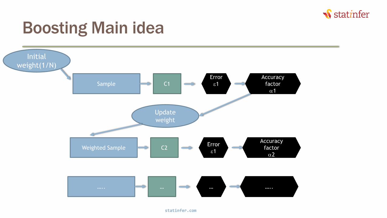
Take a random sample from population of size N
Each record has 1/N Chance of picking
Let 1/N be the weight w
Build a classifier Note down the accuracy
The Classifier may misclassify some of the records. Note them down
Take a weighted sample
This time give more weight to misclassified records from previous model
Update the weight w accordingly to pick the misclassified records
Build a new classifier on the reweighted sample
Since we picked many previously misclassified records, we expect this model to build a better model for those records
Check the error and resample
Does this classifier still has some misclassifications
If yes, then re-sample
Final Weighted Classifier C = ∑𝛼𝑖𝑐𝑖
statinfer.com
Boosting Main idea
9
Sample C1
Accuracy
factor
a1
Update
weight
Error
e1
Weighted Sample C2
Accuracy
factor
a2
Error
e1
Initial
weight(1/N)
….. … …..…
statinfer.com

How weighted samples are taken
Data 1 2 3 4 5 6 7 8 9 10
Class - - + + - + - - + +
Predicted Class M1 - - - - - - - - + +
M1 Result a a r r a r a a a a
10
Weighted Sample1 1 2 3 4 5 6 7 4 3 6
Class - - + + - + - + + +
Predicted Class M2 - - + + + + + + + +
M2 Result a a a a r a r a a a
Weighted Sample2 6 5 3 4 5 6 7 7 5 7
Class + - + + - + - - - -
Predicted Class M3 + - + + - + - - - -
M3 Result a a a a a a a a a a
statinfer.com

Boosting illustration
Boosting illustration
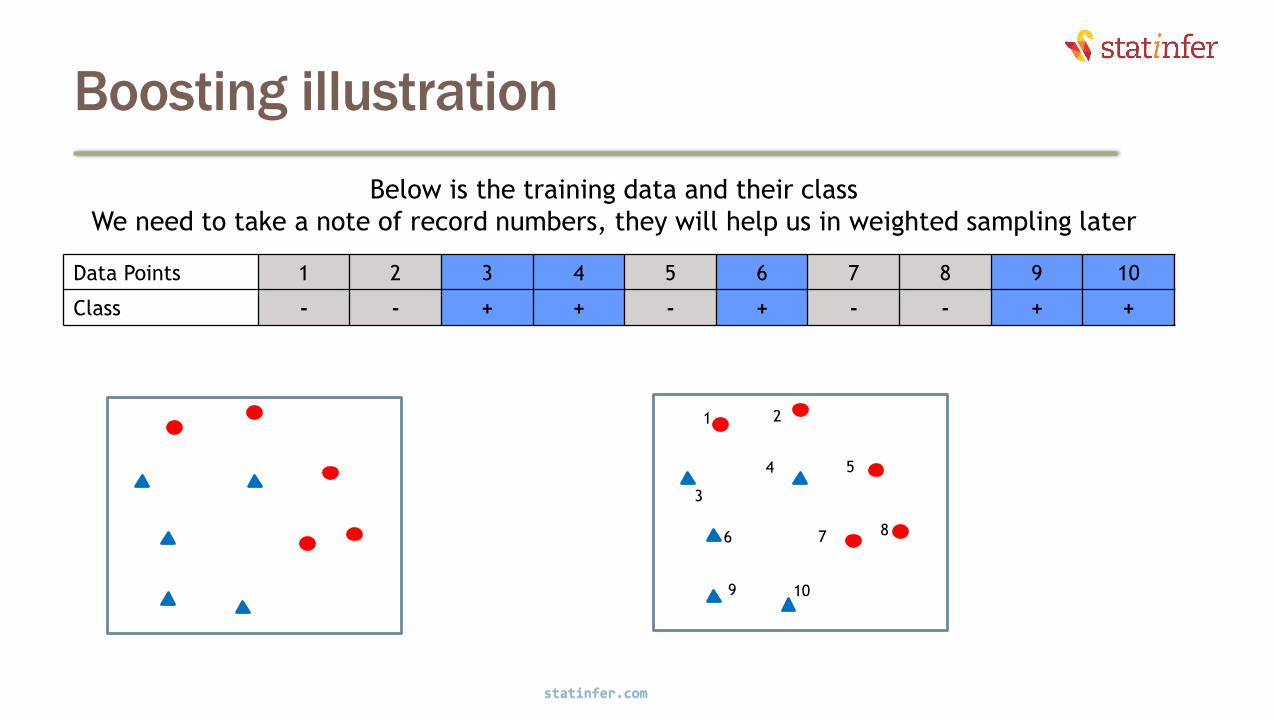
Data Points 1 2 3 4 5 6 7 8 9 10
Class - - + + - + - - + +
12
1 2
3
4 5
6 7 8
9 10
Below is the training data and their class
We need to take a note of record numbers, they will help us in weighted sampling later
statinfer.com

Boosting illustration
Data 1 2 3 4 5 6 7 8 9 10
Class - - + + - + - - + +
Predicted Class M1 - - - - - - - - + +
M1 Result a a r r a r a a a a
13
• Model M1 is built, anything above
the line is – and below the line is +
• 3 out of 10 are misclassified by the
model M1
• These data points will be given
more weight in the re-sampling step
• We may miss out on some of the
correctly classified records
statinfer.com
Boosting illustration
14
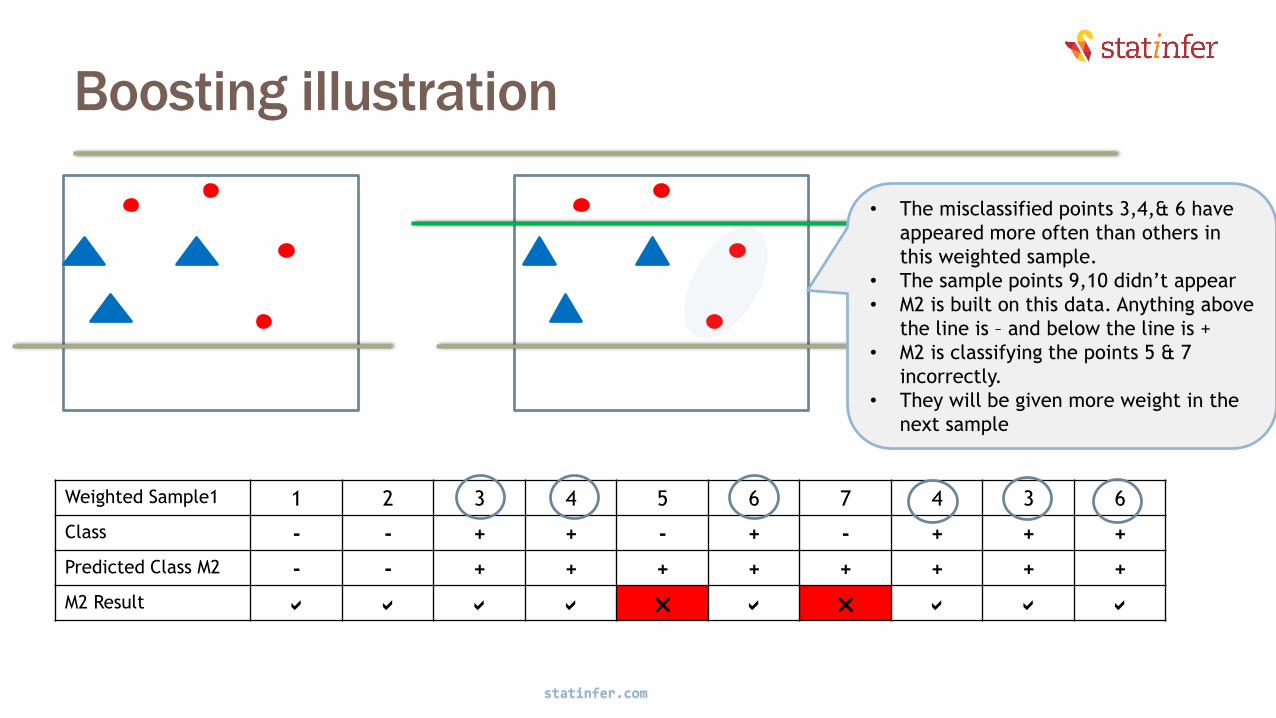
Weighted Sample1 1 2 3 4 5 6 7 4 3 6
Class - - + + - + - + + +
Predicted Class M2 - - + + + + + + + +
M2 Result a a a a r a r a a a
• The misclassified points 3,4,& 6 have
appeared more often than others in
this weighted sample.
• The sample points 9,10 didn’t appear
• M2 is built on this data. Anything above
the line is – and below the line is +
• M2 is classifying the points 5 & 7
incorrectly.
• They will be given more weight in the
next sample
statinfer.com
Boosting illustration
15
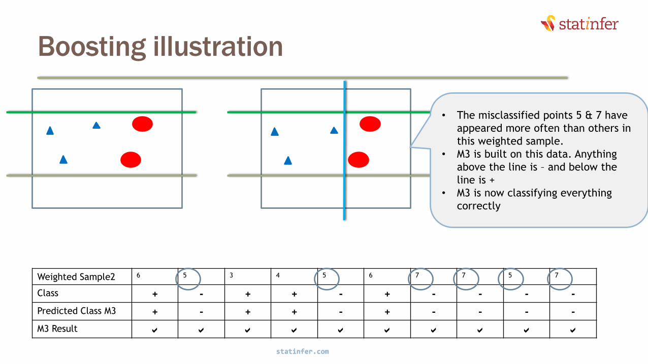
Weighted Sample2 6 5 3 4 5 6 7 7 5 7
Class + - + + - + - - - -
Predicted Class M3 + - + + - + - - - -
M3 Result a a a a a a a a a a
• The misclassified points 5 & 7 have
appeared more often than others in
this weighted sample.
• M3 is built on this data. Anything
above the line is – and below the
line is +
• M3 is now classifying everything
correctly
statinfer.com
Boosting illustration
16
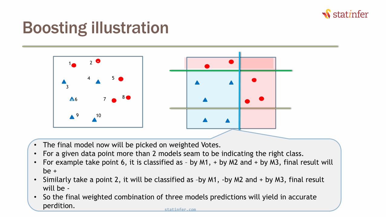
• The final model now will be picked on weighted Votes.
• For a given data point more than 2 models seam to be indicating the right class.
• For example take point 6, it is classified as – by M1, + by M2 and + by M3, final result will
be +
• Similarly take a point 2, it will be classified as –by M1, -by M2 and + by M3, final result
will be -
• So the final weighted combination of three models predictions will yield in accurate
perdition.
+
-1 2
3
4 5
6 7 8
9 10
statinfer.com

Theory behind Boosting
Algorithm
Theory behind Boosting Algorithm
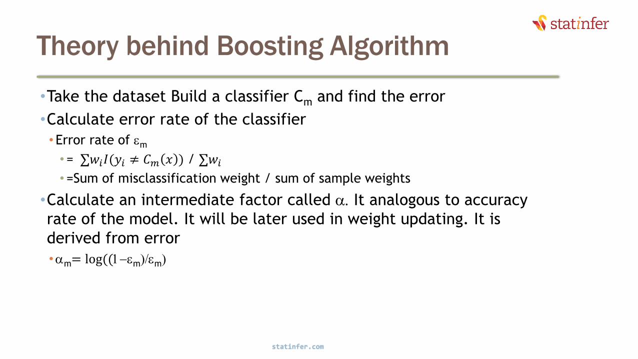
•Take the dataset Build a classifier Cm and find the error
•Calculate error rate of the classifier
•Error rate of em
• = ∑𝑤𝑖𝐼(𝑦𝑖 ≠ 𝐶𝑚 𝑥 ) / ∑𝑤𝑖
• =Sum of misclassification weight / sum of sample weights
•Calculate an intermediate factor called a. It analogous to accuracy
rate of the model. It will be later used in weight updating. It is
derived from error
•am= log((1-em)/em)
18
statinfer.com

Theory behind Boosting Algorithm..contd
•Update weights of each record in the sample using the a factor. The indicator
function will make sure that the misclassifications are given more weight
• For i=1,2….N
•𝑤𝑖+1 = 𝑤𝑖𝑒am𝐼(𝑦𝑖≠𝐶𝑚 𝑥 )
• Renormalize so that sum of weights is 1
•Repeat this model building and weight update process until we have no
misclassification
•Final collation is done by voting from all the models. While taking the votes,
each model is weighted by the accuracy factor a
• C = 𝑠𝑖𝑔𝑛(∑𝛼𝑖𝐶𝑖(𝑥))
statinfer.com
19
Gradient Boosting
•Ada boosting
•Adaptive Boosting
•Till now we discussed Ada boosting technique. Here we give high weight to
misclassified records.
•Gradient Boosting
• Similar to Ada boosting algorithm.
•The approach is same but there are slight modifications during re-weighted
sampling.
•We update the weights based on misclassification rate and gradient
•Gradient boosting serves better for some class of problems like regression.
20
statinfer.com
GBM- Parameters
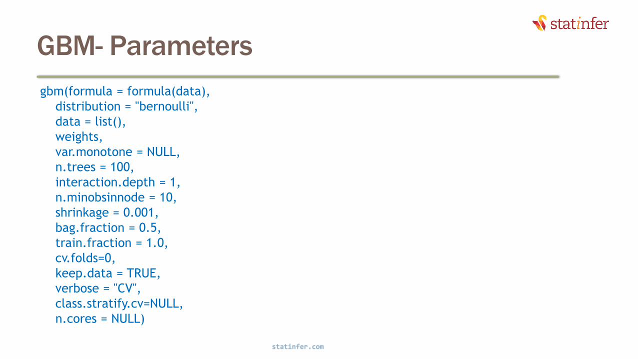
gbm(formula = formula(data),
distribution = "bernoulli",
data = list(),
weights,
var.monotone = NULL,
n.trees = 100,
interaction.depth = 1,
n.minobsinnode = 10,
shrinkage = 0.001,
bag.fraction = 0.5,
train.fraction = 1.0,
cv.folds=0,
keep.data = TRUE,
verbose = "CV",
class.stratify.cv=NULL,
n.cores = NULL)
statinfer.com
21
GBM- Parameters verbose
•If TRUE, gbm will print out progress and performance indicators.
statinfer.com
22

GBM- Parameters distribution
•"multinomial" for classification when there are more than 2 classes
•"bernoulli" for logistic regression for 0-1 outcomes
•If not specified, gbm will try to guess:
• if the response has only 2 unique values, bernoulli is assumed;
•otherwise, if the response is a factor, multinomial is assumed;
statinfer.com
23

GBM- Parameters n.trees = 100
•The number of steps
•the total number of trees to fit.
•This is equivalent to the number of iterations
•Default value is 100
statinfer.com
24

Code n.trees
statinfer.com
25
Number of
trees/iterations
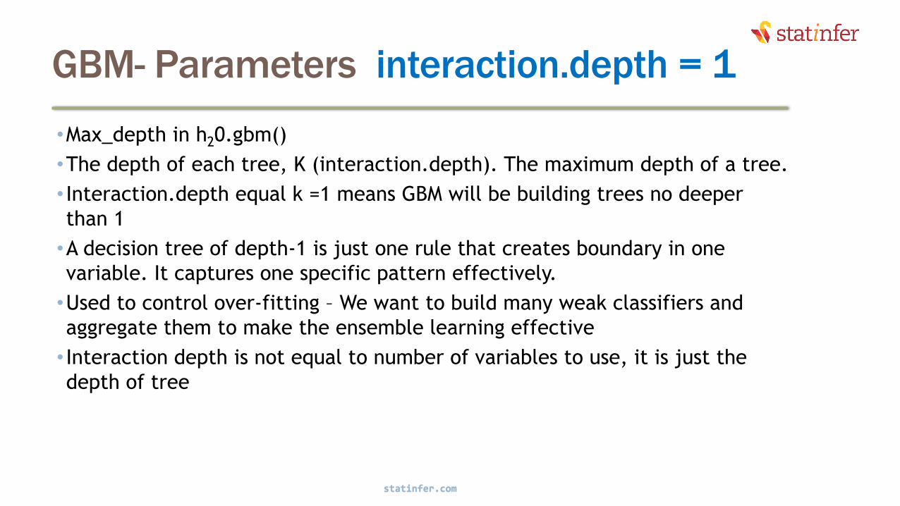
GBM- Parameters interaction.depth = 1
•Max_depth in h20.gbm()
•The depth of each tree, K (interaction.depth). The maximum depth of a tree.
• Interaction.depth equal k =1 means GBM will be building trees no deeper
than 1
•A decision tree of depth-1 is just one rule that creates boundary in one
variable. It captures one specific pattern effectively.
•Used to control over-fitting – We want to build many weak classifiers and
aggregate them to make the ensemble learning effective
• Interaction depth is not equal to number of variables to use, it is just the
depth of tree
statinfer.com
26

GBM- Parameters interaction.depth = 1
•Tuning:
•Have interaction depth as 1 to reduce overfitting. Simpler models are always less
likely to overfit.
•But if the depth of the tree is 1 then it takes of time to execute. You can try any
value between 2-5 to reduce computation time
statinfer.com
27
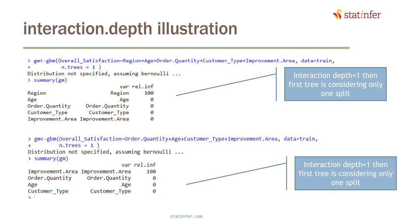
interaction.depth illustration
statinfer.com
28
Interaction depth=1 then
first tree is considering only
one split
Interaction depth=1 then
first tree is considering only
one split

interaction.depth illustration
statinfer.com
29
Interaction depth=2 then
first tree is going up to two
splits
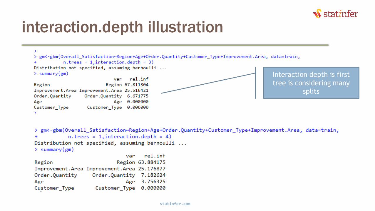
interaction.depth illustration
statinfer.com
30
Interaction depth is first
tree is considering many
splits

n.minobsinnode
•minimum number of observations in the trees terminal nodes.
•n.minobsinnode = 10 by default.
•Finetuning:
•A really high value might lead to underfitting
•A really low value might lead to overfitting
•You can try 30-100 depending on dataset size
•Interaction depth and minimum number of samples per node are
connected.
•If we take care of any one of them then the other one will adjust
automatically
statinfer.com
31

LAB: n.minobsinnode
statinfer.com
32
Too few observations in
terminal nodes can lead to
overfitting
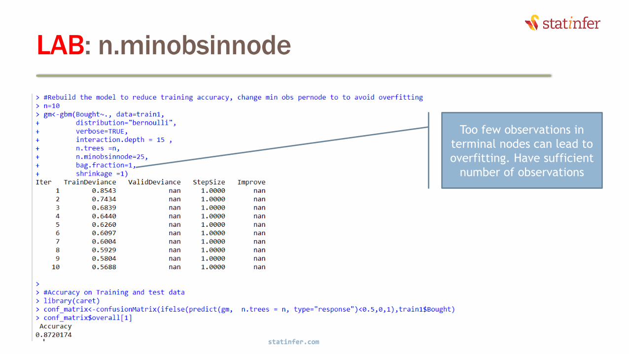
LAB: n.minobsinnode
statinfer.com
33
Too few observations in
terminal nodes can lead to
overfitting. Have sufficient
number of observations

Shrinkage
•Learn_rate in h20
•The learning rate is a multiplier fraction in gradient boosting algorithm before updating the learning function in each iteration
•This fraction restricts the algorithm’s speed in reaching optimum values
•The direct empirical analogy of this parameter is not very obvious
•You can understand this as reduction in the weights of misclassification sample(before preparing for sampling in next step).
•It is also known as gradient descent step size
•a shrinkage parameter applied to each tree in the expansion.
•Also known as the learning rate or step-size reduction.
•Default value Shrinkage = 0.001
statinfer.com
34
Shrinkage
statinfer.com
35
Learning rate
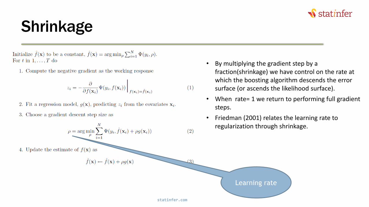
• By multiplying the gradient step by a fraction(shrinkage) we have control on the rate at which the boosting algorithm descends the error surface (or ascends the likelihood surface).
• When rate= 1 we return to performing full gradient steps.
• Friedman (2001) relates the learning rate to regularization through shrinkage.
Shrinkage - Illustration
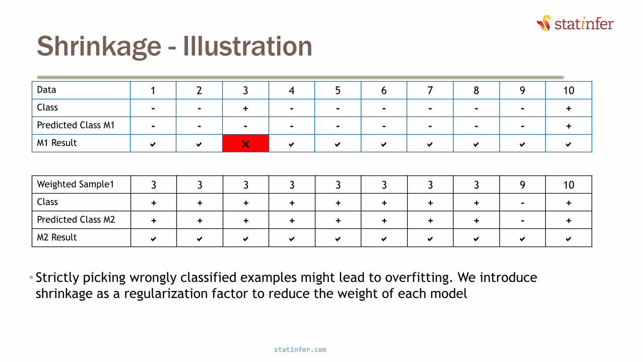
• Strictly picking wrongly classified examples might lead to overfitting. We introduce
shrinkage as a regularization factor to reduce the weight of each model
statinfer.com
36
Data 1 2 3 4 5 6 7 8 9 10
Class - - + - - - - - - +
Predicted Class M1 - - - - - - - - - +
M1 Result a a r a a a a a a a
Weighted Sample1 3 3 3 3 3 3 3 3 9 10
Class + + + + + + + + - +
Predicted Class M2 + + + + + + + + - +
M2 Result a a a a a a a a a a

Shrinkage
•Being conservative while picking up new sample, instead of strictly
picking just the misclassified observations we would like to pickup a
good portion of rightly classified observations as well to capture the
right patterns
•A high shrinkage value gives high weight to each step/tree.
•A high shrinkage value makes the overall algorithm exit faster –
Underfitting till a step and overfitting right after that
•There is a trade-off between learning rate and n.tree
•Even if the number of trees is set to a high number, if the
shrinkage/learning rate is high then iterations after a limit will have
no impact
statinfer.com
37

Shrinkage - Illustration
statinfer.com
38
High shrinkage will lead to
early exit of the algorithm.
There is a risk of underfitting
The whole algorithm
converged in just two trees
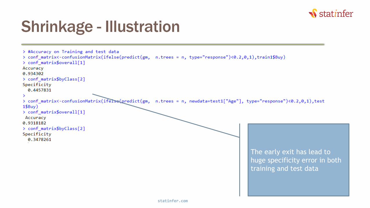
Shrinkage - Illustration
statinfer.com
39
The early exit has lead to
huge specificity error in both
training and test data
Shrinkage tuning
•If shrinkage is high then algorithm exists early. There is a risk of
underfitting
•If shrinkage is low then algorithm will need lot of iterations. If number
of tree is less then it might also lead to underfitting
•If shrinkage is less then ntree should be high.
•Having a high ntree might take lot of execution time.
•What is the optimal shrinkage and ntree combination?
statinfer.com
40

Shrinkage - Illustration
statinfer.com
41
User defined function for
shrinkage vs n-tree fine tuning
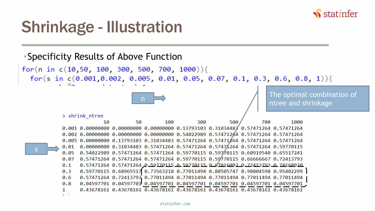
Shrinkage - Illustration
•Specificity Results of Above Function
statinfer.com
42
n
s
The optimal combination of
ntree and shrinkage

bag.fraction
•The fraction of the training set observations randomly selected to
propose the next tree in the expansion.
•According to algorithm we should pick complete sample based on the
weights, but what if we pick a fraction of the data instead of complete
sample
•This introduces randomness into the model fit. The errors will reduce
by introducing randomness and averaging out(the spirit of ensemble
method)
•Use set.seed to ensure that the model can be reconstructed as it is
statinfer.com
43
bag.fraction
•The remaining fraction helps in validation
•The out of bag also used in internal cross validation
•It also helps identifying the number of iterations
•Default value is bag.fraction = 0.5
statinfer.com
44

train.fraction
•The first train.fraction * nrows(data) observations are used to fit the gbm
•The remainder are used for computing out-of-sample estimates of the loss function.
•If you do-not choose train.fraction then ValidDeviance will be missingfrom output
•Note that if the data are sorted in a systematic way (such as cases for which y = 1 come first), then the data should be shuffled before running gbm.
•Do not confuse this with bag.fraction parameter. Bag fraction is for randomly picking up samples in each step.
•This parameter can also be used for deciding the right number of trees for a given learning rate
statinfer.com
45

train.fraction- illustration
statinfer.com
46
Train fraction gives valid
deviance

train.fraction- illustration
•The same model on ordered data.
statinfer.com
47
You need to shuffle the
data. Train fraction
considers strictly initial
few records

Finding the right number of iterations.
•There are two ways
•Using the bag fraction and calculating OOB. This doesn’t work if bag fraction =1
•Using test data and validation error. This doesn’t work if train.fraction is not set
statinfer.com
48
OOB generally underestimates
the optimal number of iterations

Variable Importance
statinfer.com
49
VarImp in GBM
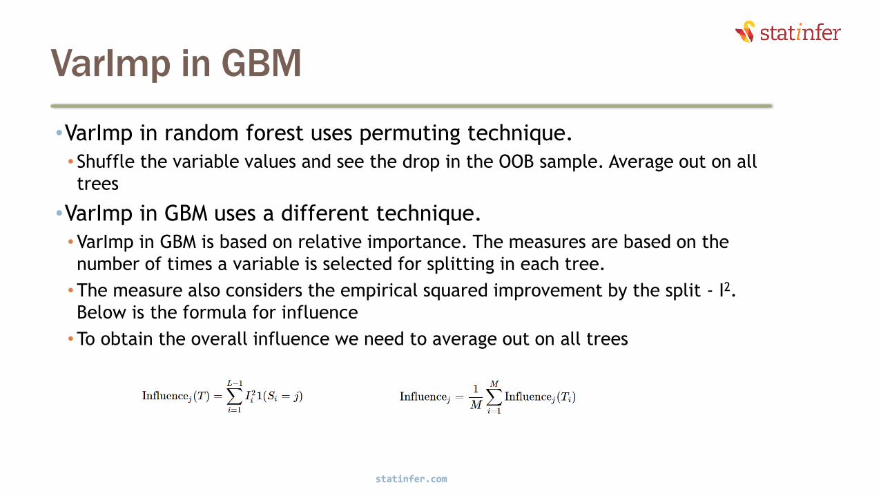
•VarImp in random forest uses permuting technique.
• Shuffle the variable values and see the drop in the OOB sample. Average out on all
trees
•VarImp in GBM uses a different technique.
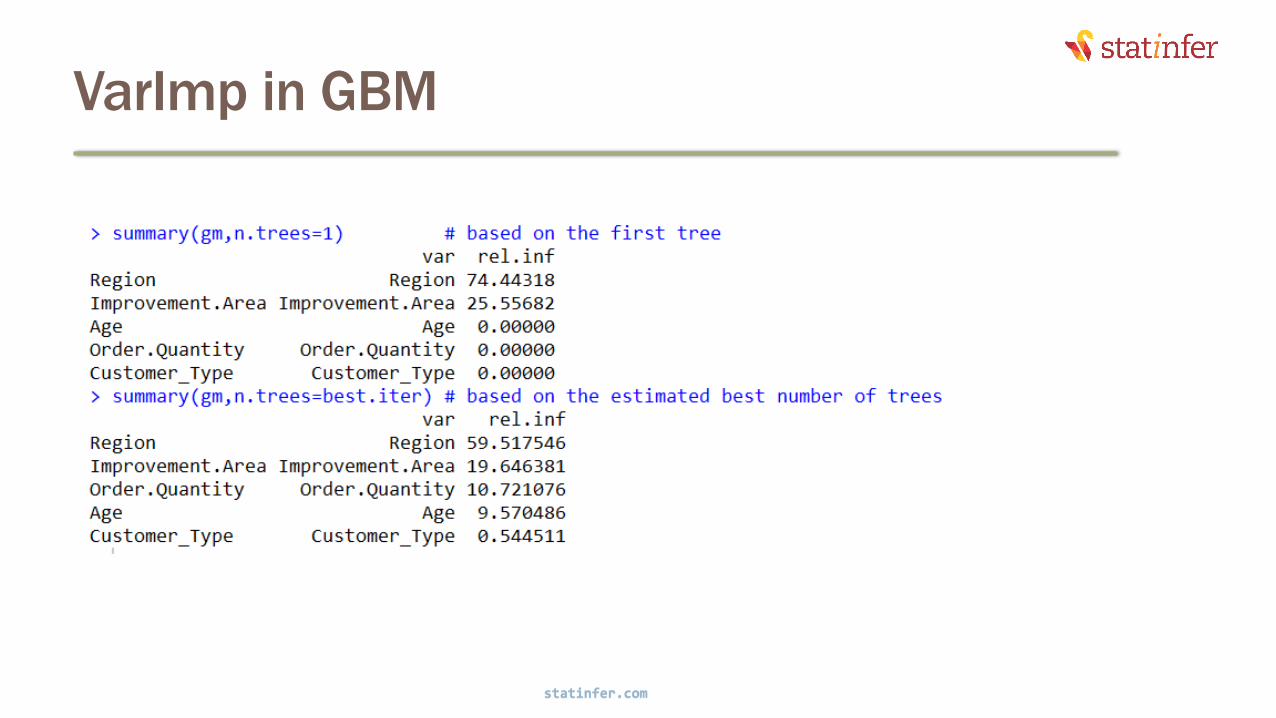
•VarImp in GBM is based on relative importance. The measures are based on the
number of times a variable is selected for splitting in each tree.
•The measure also considers the empirical squared improvement by the split - I2.
Below is the formula for influence
•To obtain the overall influence we need to average out on all trees
statinfer.com
50
VarImp in GBM
statinfer.com
51
Partial dependence plots
•Partial dependence plots show us the impact of a variable on the
modelled response after marginalizing out(averaging out) all other
explanatory variables.
•We marginalize the rest of the variables by substituting their average
value(or integrating them).
•Partial plots tell us the exact impact of x variable and its impact on
Y(positive or negative) at every point of x
statinfer.com
52
LAB: Boosting
•Import Credit Risk Data
•Create a balanced sample
•Build GBM tree
•What are the important variables
•Draw the partial dependency plots.
statinfer.com
53
Code: Boosting
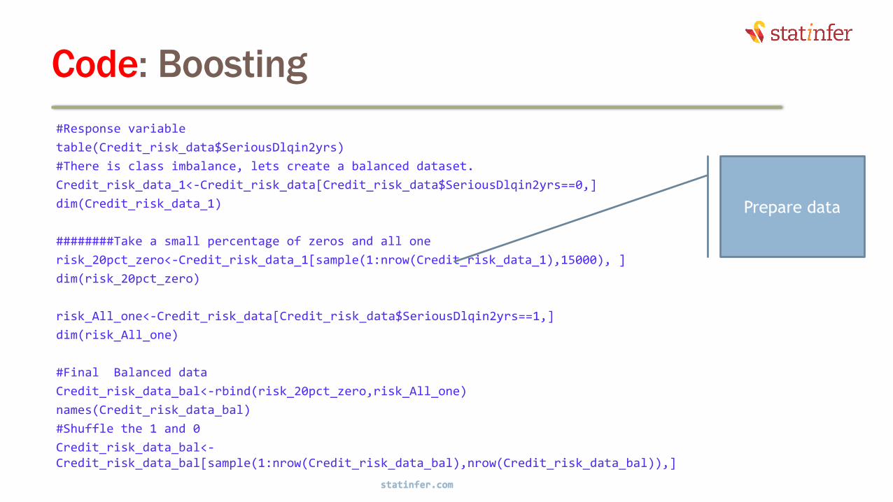
#Response variable
table(Credit_risk_data$SeriousDlqin2yrs)
#There is class imbalance, lets create a balanced dataset.
Credit_risk_data_1<-Credit_risk_data[Credit_risk_data$SeriousDlqin2yrs==0,]
dim(Credit_risk_data_1)
########Take a small percentage of zeros and all one
risk_20pct_zero<-Credit_risk_data_1[sample(1:nrow(Credit_risk_data_1),15000), ]
dim(risk_20pct_zero)
risk_All_one<-Credit_risk_data[Credit_risk_data$SeriousDlqin2yrs==1,]
dim(risk_All_one)
#Final Balanced data
Credit_risk_data_bal<-rbind(risk_20pct_zero,risk_All_one)
names(Credit_risk_data_bal)
#Shuffle the 1 and 0
Credit_risk_data_bal<-Credit_risk_data_bal[sample(1:nrow(Credit_risk_data_bal),nrow(Credit_risk_data_bal)),]
statinfer.com
54
Prepare data

Code: Boosting
statinfer.com
55
Build GBM Model

Code: Boosting
statinfer.com
56
Accuracy and
VarImp

Code: Boosting
statinfer.com
57
Partial
Dependency
plots
Negative
influence on
class 1
Influence on
class 1 at
different values
of X

Case Study: Direct Mail
Marketing Response Model
statinfer.com
58

LAB: Direct Mail Marketing Response
Model•Large Marketing Response Data/train.csv
•How many variables are there in the dataset?
•Take a one third of the data as training data and one third as test data
•Look at the response rate from target variables
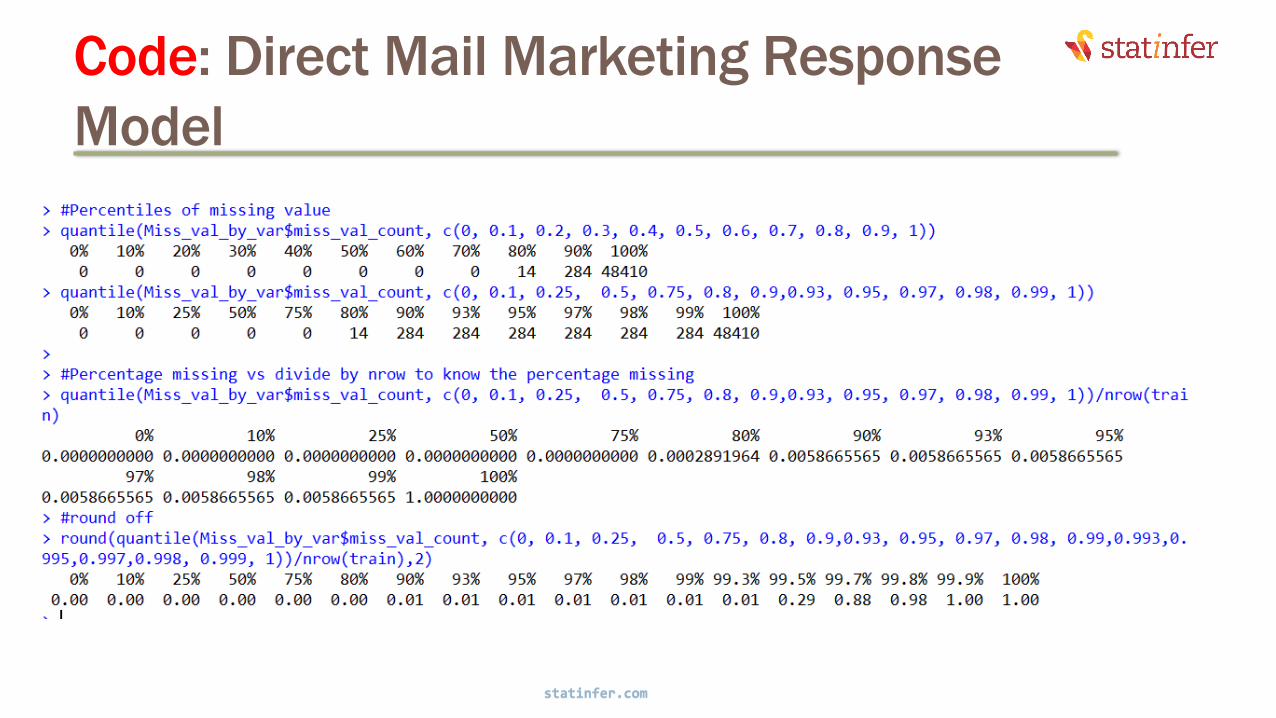
•Find out the overall missing values and missing values by variables
•Do the missing value and outlier treatment, prepare data for analysis
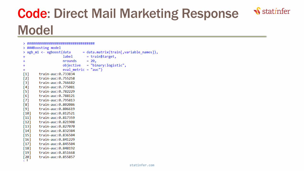
•Build a boosting model
•Find the training data accuracy
•Find the accuracy on test data
statinfer.com
59

Code: Direct Mail Marketing Response
Model#####Boosting modeln=100gbm_m1<-gbm(target~., data=train[,-1],
distribution="bernoulli", verbose=T, interaction.depth = 2 , n.trees = n,n.minobsinnode=5,bag.fraction=0.5,set.seed(125),shrinkage = 0.1,train.fraction = 0.5)
# plot the performance # plot variable influenceimp_var<-summary(gbm_m1,n.trees=1) # based on the first treeimp_var[1:10,]
imp_var<-summary(gbm_m1,n.trees=best.iter) # based on the estimated best number of treesimp_var[imp_var$rel.inf>1,]
statinfer.com
60

Code: Direct Mail Marketing Response
Model###Boosting model-2 with scale_pos_weight For Class imbalance
#Create model weights first
table(train$target)/nrow(train)
model_weights <- ifelse(train$target ==0, 0.2,0.8)
table(model_weights)
n=300
gbm_m1<-gbm(target~., data=train[,-1],
distribution="bernoulli",
verbose=T,
interaction.depth = 2 ,
n.trees = n,
n.minobsinnode=5,
bag.fraction=0.5,set.seed(125),
shrinkage = 0.1,
weights = model_weights)
statinfer.com
61

Conclusion
statinfer.com
62

Conclusion
•GBM is one of the mot widely used machine learning technique in
business
•GBM is less prone to overfitting when compared to other techniques
like Neural nets
•We need to be patient, GBM might take a lot of time for execusion.
statinfer.com
63

Thank you
statinfer.com
64

Appendix
statinfer.com
65

Xgboosting
statinfer.com
66

Xgboost parameters
statinfer.com
67

GBM vs Xgboost
1. Extreme Gradient Boosting – XGBoost
2. Both xgboost and gbm follows the principle of gradient boosting.
3. There are however, the difference in modelling & performance
details.
4. xgboost used a more regularized model formalization to control
over-fitting, which gives it better performance.
5. Improved convergence techniques, vector and matrix type data
structures for faster results
6. Unlike GBM XGBoost package is available in C++, Python, R, Java,
Scala, Julia with same parameters for tuning
statinfer.com
68

Xgboost Advantages
1. Developers of xgboost have made a number of important
performance enhancements.
2. Xgboost and GBM have big difference in speed and memory
utilization
3. Code modified for better processor cache utilization which makes it
faster.
4. Better support for multicore processing which reduces overall
training time.
statinfer.com
69

GBM vs Xgboost
•Most importantly, the memory error is somewhat resolved in xgboost
•For a given dataset, you are less likely to get memory error while using
xgboost when compared to GBM
statinfer.com
70
Xgboost parameters
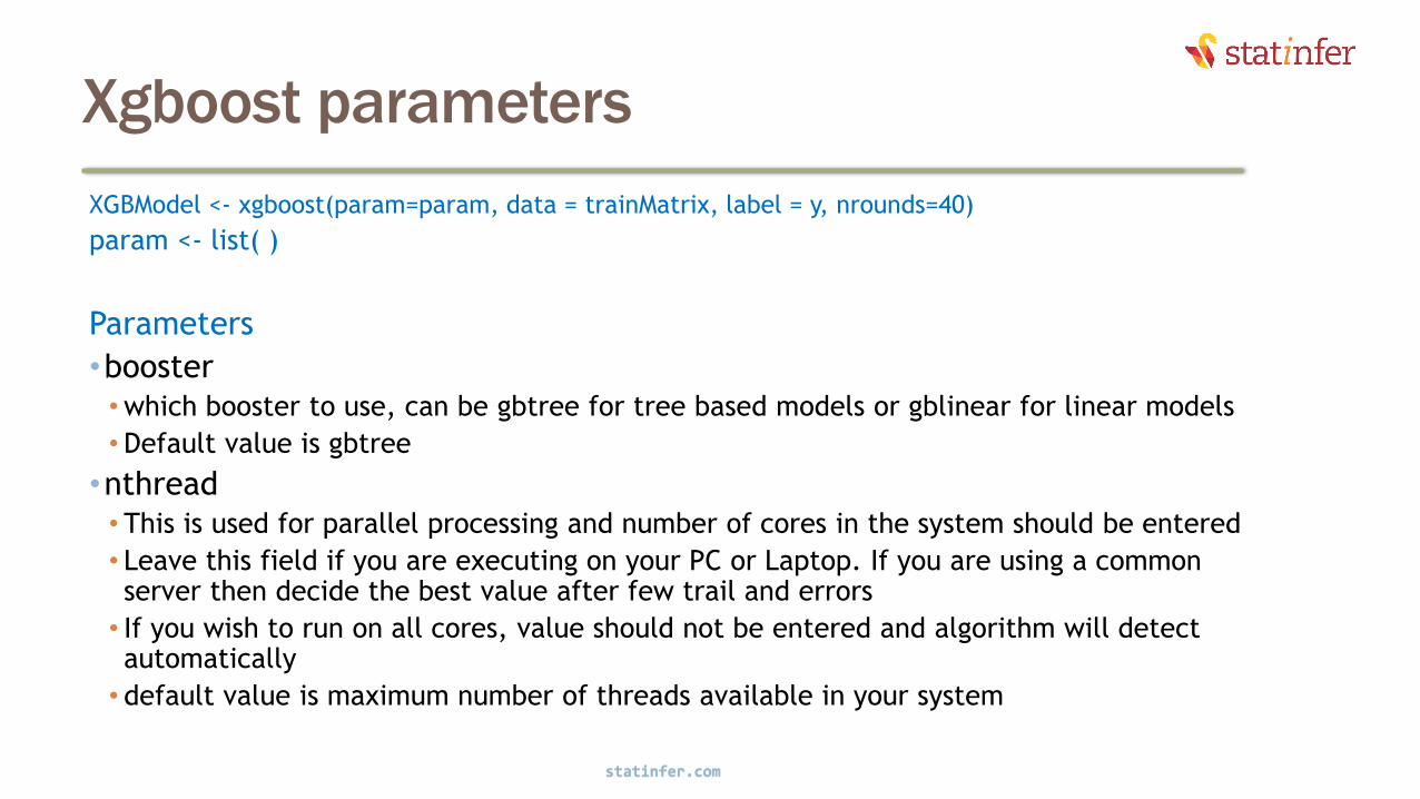
XGBModel <- xgboost(param=param, data = trainMatrix, label = y, nrounds=40)
param <- list( )
Parameters
•booster •which booster to use, can be gbtree for tree based models or gblinear for linear models
• Default value is gbtree
•nthread• This is used for parallel processing and number of cores in the system should be entered
• Leave this field if you are executing on your PC or Laptop. If you are using a common server then decide the best value after few trail and errors
• If you wish to run on all cores, value should not be entered and algorithm will detect automatically
• default value is maximum number of threads available in your system
statinfer.com
71

Xgboost parameters
•objective • default=reg:linear
• This defines the type of problem that we are solving and the loss function to be minimized.
• reg:logistic - logistic regression.
• binary:logistic –logistic regression for binary classification, returns predicted probability (not class)
• binary:logitraw logistic regression for binary classification, output score before logistic transformation.
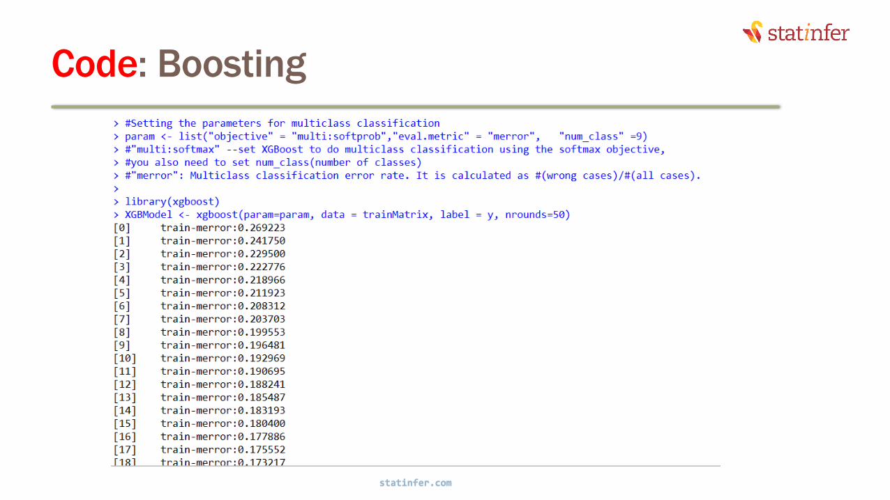
•multi:softmax –multiclass classification using the softmax objective
• returns predicted class (not probabilities).
• you also need to set an additional num_class (number of classes) parameter defining the number of unique classes. Class is represented by a number and should be from 0 to (num_class – 1).
•multi:softprob –same as softmax, but returns predicted probability of each data point belonging to each class.
•Note: num_class set the number of classes. To use only with multiclass objectives.
statinfer.com
72
Xgboost parameters
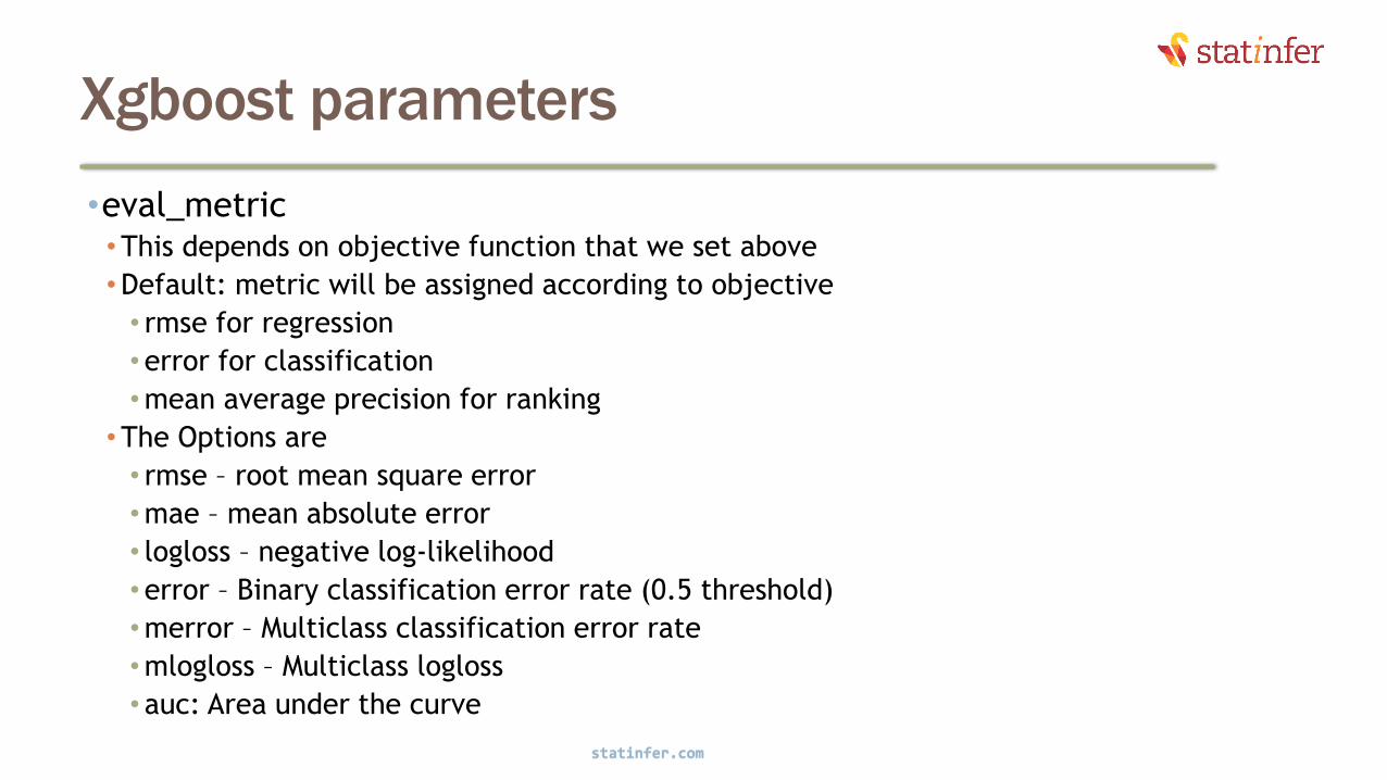
•eval_metric•This depends on objective function that we set above
•Default: metric will be assigned according to objective
• rmse for regression
•error for classification
•mean average precision for ranking
•The Options are
• rmse – root mean square error
•mae – mean absolute error
• logloss – negative log-likelihood
•error – Binary classification error rate (0.5 threshold)
•merror – Multiclass classification error rate
•mlogloss – Multiclass logloss
• auc: Area under the curve
statinfer.com
73

Xgboost parameters
•eta
•eta controls the learning rate, Analogous to learning rate in GBM
•As you know boosting uses ensemble algorithm. Larger number models will ensure
more robust model.
•Right after every boosting step you have each feature and their weights, eta shrinks
the feature weights the boosting process more conservative.
• Instead of considering each model as it is, we will give it less weight. We use eta to
reduce the contribution of each tree
• If eta is low then we will have larger value for nrounds.
• low eta value means model more robust to overfitting but slower to compute
•eta scales the contribution of each tree by a factor of 0 < eta < 1 when it is added
to the current approximation.
•Default value is 0.3. Typical final values to be used: 0.01-0.2
statinfer.com
74
More on eta
•For example you need 10 rounds for a best model
•The learning rate is the shrinkage you do at every step you are
making.
•If eta is 1.00, the step weight is 1.00. You will end up with 10 rounds
only.
•If you make 1 step at eta = 0.25, the step weight is 0.25. you will end
up in 40 steps
•If you decrease learning rate, you need to increase number of
iterations in same proportion.
statinfer.com
75
Xgboost parameters
•min_child_weight [default=1]
•min_child_weight minimum sum of instance weight (hessian) needed in a child. If
the tree partition step results in a leaf node with the sum of instance weight less
than min_child_weight, then the building process will give up further partitioning.
• In simple terms you can see this minimum number of instances needed to be in
each node.
•This is similar to min_child_leaf in GBM with a slght change. Here it refers to min
“sum of weights” of observations while GBM has min “number of observations”.
•Used to control over-fitting. Higher values prevent a model from learning relations
which might be highly specific to the particular sample selected for a tree.
•Too high values can lead to under-fitting hence, it should be tuned using CV.
•Default value is : 1
•Try to tune it by looking at results of CV.
statinfer.com
76
Xgboost parameters
•max_depth• The maximum depth of a tree, same as GBM.
•Used to control over-fitting as higher depth will allow model to learn relations very specific to a particular sample.
• Default value is 6
• Try to tune it by looking at results of CV. Typical values:5-10
•gamma • A node is split only when the resulting split gives a positive reduction in the loss function. Gamma specifies the minimum loss reduction required to make a split.
•Makes the algorithm conservative and reduces overfitting. The values can vary depending on the loss function and should be tuned.
• A larger value of gamma reduces runtime.
• Try to tune it by looking at results of CV. Start with very low values
• Leave it as it is if you have no idea on the data
• Default value is 0
statinfer.com
77
Xgboost parameters
•subsample
• Same as the subsample of GBM.
• subsample ratio of the training instance. Denotes the fraction of observations to be
randomly samples for each tree.
• Setting it to 0.5 means that xgboost randomly collected half of the data instances
to grow trees and this will prevent overfitting.
• It makes computation shorter (because less data to analyse).
• It is advised to use this parameter with eta and increase nround.
• Lower values make the algorithm more conservative(less accurate) and prevents
overfitting but too small values might lead to under-fitting.
•Default value is 1 - gathers complete data
•Typical values: 0.2-0.8 depending on size of data
statinfer.com
78
Xgboost parameters
•scale_pos_weight, [default=1]
•Control the balance of positive and negative weights
•useful for unbalanced classes.
•A typical value to consider: sum(negative cases) / sum(positive cases)
statinfer.com
79
Xgboost parameters
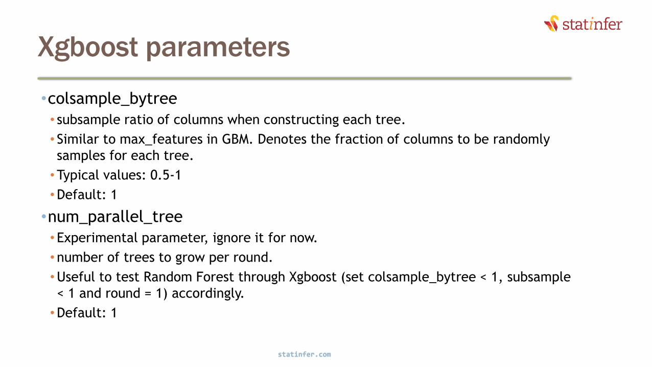
•colsample_bytree
• subsample ratio of columns when constructing each tree.
• Similar to max_features in GBM. Denotes the fraction of columns to be randomly
samples for each tree.
•Typical values: 0.5-1
•Default: 1
•num_parallel_tree
•Experimental parameter, ignore it for now.
•number of trees to grow per round.
•Useful to test Random Forest through Xgboost (set colsample_bytree < 1, subsample
< 1 and round = 1) accordingly.
•Default: 1
statinfer.com
80

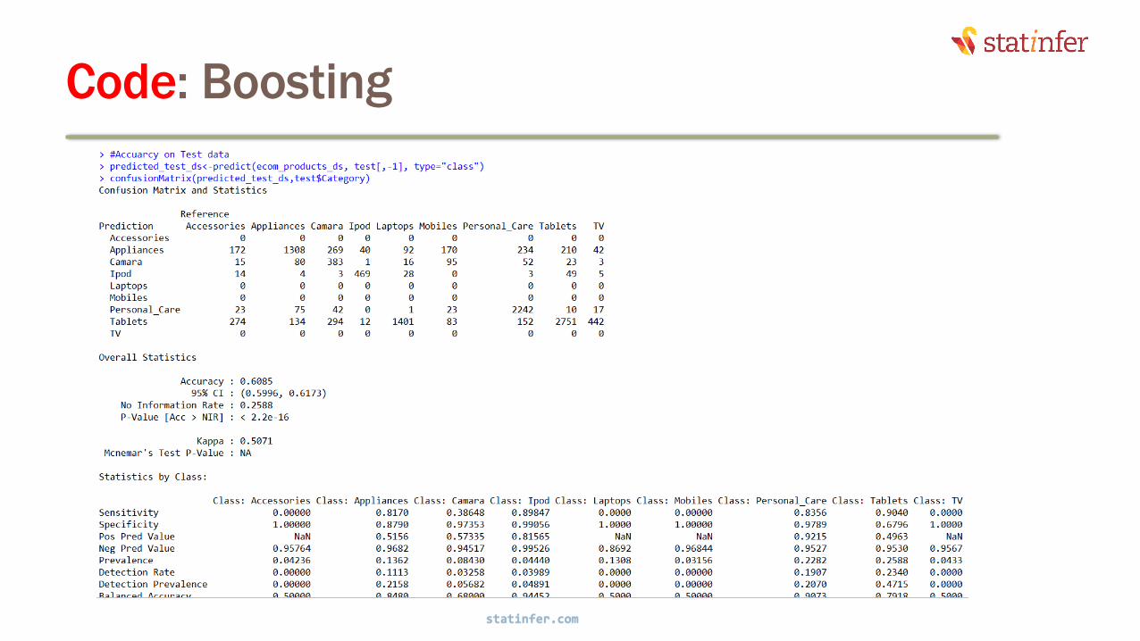
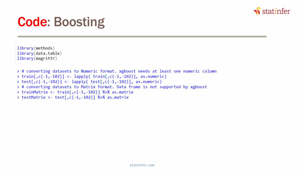
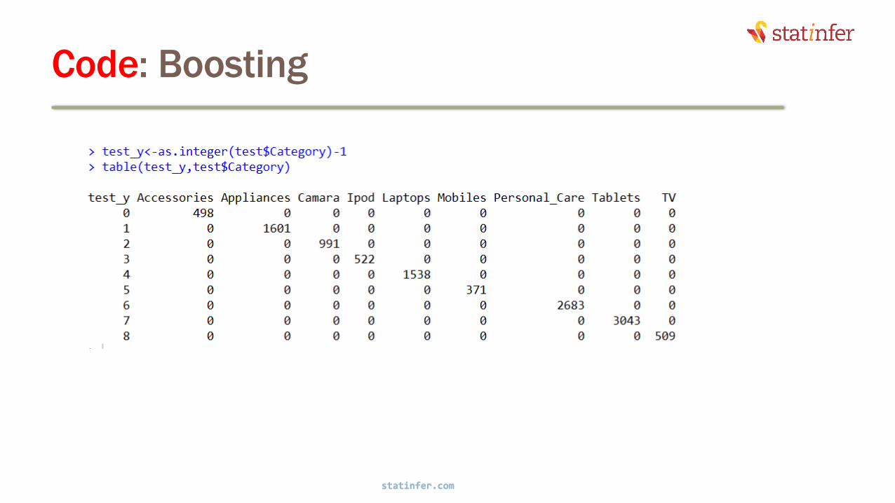
LAB: Boosting
•Ecom products classification. Rightly categorizing the items based on
their detailed feature specifications. More than 100 specifications
have been collected.
•Data: Ecom_Products_Menu/train.csv
•Build a decision tree model and check the training and testing
accuracy
•Build a boosted decision tree.
•Is there any improvement from the earlier decision tree
81
statinfer.com

Code: Boosting
statinfer.com
82

Code: Boosting
statinfer.com
83
Code: Boosting
statinfer.com
84
Code: Boosting
statinfer.com
85

Code: Boosting
statinfer.com
86
Code: Boosting
statinfer.com
87
Code: Boosting
statinfer.com
88
Code: Boosting
statinfer.com
89

Code: Boosting
statinfer.com
90

Code: Boosting
statinfer.com
91

Code: Boosting
statinfer.com
92

Case Study: Direct Mail
Marketing Response Model
statinfer.com
93

LAB: Direct Mail Marketing Response
Model•Large Marketing Response Data/train.csv
•How many variables are there in the dataset?
•Take a one third of the data as training data and one third as test data
•Look at the response rate from target variables
•Find out the overall missing values and missing values by variables
•Do the missing value and outlier treatment, prepare data for analysis
•Build a boosting model
•Find the training data accuracy
•Find the accuracy on test data
statinfer.com
94

Code: Direct Mail Marketing Response
Model
statinfer.com
95
Note: This code is to create initial benchmark model only. You need to spend some
time and finetune it to create the final model

Code: Direct Mail Marketing Response
Model
statinfer.com
96

Code: Direct Mail Marketing Response
Model
statinfer.com
97

Code: Direct Mail Marketing Response
Model
statinfer.com
98

Code: Direct Mail Marketing Response
Model
statinfer.com
99
Code: Direct Mail Marketing Response
Model
statinfer.com
100

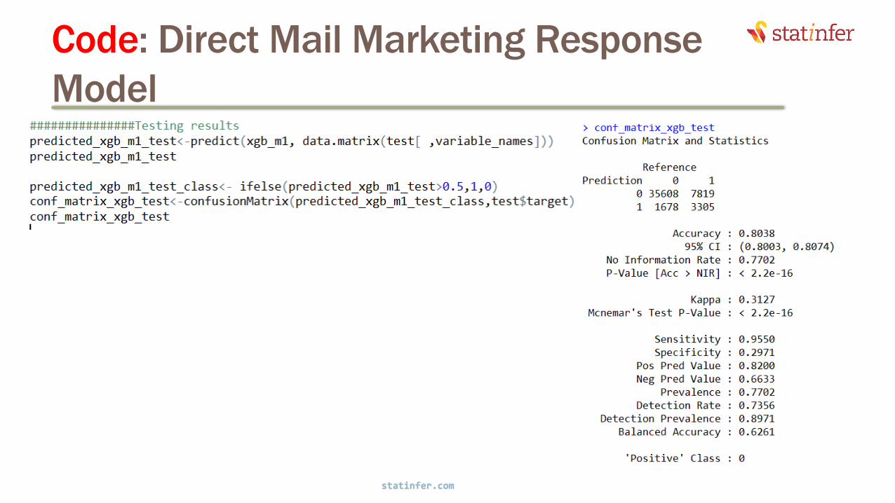
Code: Direct Mail Marketing Response
Model
statinfer.com
101
Code: Direct Mail Marketing Response
Model
statinfer.com
102

Code: Direct Mail Marketing Response
Model
statinfer.com
103
Code: Direct Mail Marketing Response
Model
statinfer.com
104

Code: Direct Mail Marketing Response
Model
statinfer.com
105

Code: Direct Mail Marketing Response
Model
statinfer.com
106

Code: Direct Mail Marketing Response
Model
statinfer.com
107
GBM Reference
• Y. Freund and R.E. Schapire (1997) “A decision-theoretic generalization of on-line learning and an application to boosting,” Journal of Computer and System Sciences, 55(1):119-139.
• G. Ridgeway (1999). “The state of boosting,” Computing Science and Statistics 31:172-181.
• J.H. Friedman, T. Hastie, R. Tibshirani (2000). “Additive Logistic Regression: a Statistical View of Boosting,” Annals of Statistics 28(2):337-374.
• J.H. Friedman (2001). “Greedy Function Approximation: A Gradient Boosting Machine,” Annals of Statistics 29(5):1189-1232.
• J.H. Friedman (2002). “Stochastic Gradient Boosting,” Computational Statistics and Data Analysis 38(4):367-378.
• B. Kriegler (2007). Cost-Sensitive Stochastic Gradient Boosting Within a Quantitative Regression Framework. PhD dissertation, UCLA Statistics.
• C. Burges (2010). “From RankNet to LambdaRank to LambdaMART: An Overview,” Microsoft Research Technical Report MSR-TR-2010-82.
statinfer.com
108

Thank you

Statinfer.com
statinfer.com
110
Download the course videos and handouts from the
below link
https://statinfer.com/course/machine-learning-
with-r-2/curriculum/?c=b433a9be3189
Related Documents