Gauge Mean Field Theory in a Highly Frustrated Ferromagnet

Master Science de la matiere Stage 2011–2012

Ecole Normale Superieure de Lyon Begue FredericUniversite Claude Bernard Lyon I M2 Physique

Gauge Mean Field Theory in aHighly Frustrated Ferromagnet

Resume : This paper enters into the spirit of the “second ice age” in which weconsider the effect of quantum fluctuations on classical spin ice systems. The “spinice” state ground found in rare earth pyrochlore magnets such has Dy2Ti2O7 exhibitsclassical analogues magnetic monopoles which are excitations out of this ground state[1], whose dynamics has been studied in ref. [2]. It has been argued [3] that in “quan-tum spin ice” materials this spin ice state is replaced by a “quantum spin liquid”state which realizes an emergent gauge theory, lattice-analogue of quantum electro-magnetism, with both electric and magnetic monopoles-like quasi-particles [4]. Sinceusual mean field theory has a tendency to wash out the behavior of these particles [5],we will present here a gauge mean field theory, first developed by Savary and cowork-ers [6], which attemps to retain some of the fluctuation properties, and use it to getsome dynamical properties of magnetic monopoles in such systems.

key-words: frustrated magnetism on a pyrochlore lattice, gauge mean field theory

Director :Pr. Peter [email protected] / tel. 04 72 72 84 49Ecole Normale superieure de Lyon45 allee d’Italie 69364 Lyon Francehttp://www.ens-lyon.fr/PHYSIQUE/Institut Universitaire de France (IUF)http://iuf.amue.fr

August 19,2011

Contents

I Introduction 1

1 The pyrochlore lattice 1

2 Classical Spin Ice 2

3 Magnetic Monopoles and Spinons 4

4 Transverse fluctuations 5

II Introduction to the Gauge Mean Field Theory 5

5 Gauge mean field Hamiltonian 8

6 The gauge field Hamiltonian: Hs 10

7 The gauge charge Hamiltonian: HΦ 11

8 Variational Energy Method 11

III A detailed example of the application of the meanfield gauge theory 13

9 Computation of the Green’s function 14

10 Computation of the Lagrange multiplier λ 15

11 Energy of the system 16

12 Quantum Spin Liquid Phase 17

13 Condensation and Anti-ferromagnetic phase 18

IV Conclusion and Perspective 20

1

Part I

IntroductionSystems made of ferromagnetic spins on a pyrochlore lattice are of great inter-est for several reasons. Indeed, from a classical point of view, since they arehighly frustrated systems, they have an extensive ground state entropy and so,violate the third principle of thermodynamics [7]. Moreover, they exhibit quasi-particles excitations that interact via Coulomb’s law, are of magnetic originand behave exactly as magnetic dipoles deconfined into free magnetic charges(magnetic monopoles)[1][8]. The classical ensemble of low energy states hasan internal constraint, a divergence free condition on the spin field, leading tothe description of the ground state manyfold in terms of an emergent classicalgauge field and classical magnetostatics, including monopoles. Adding quan-tum fluctuations, one gets a conjugate “electric” field and a complete analogywith quantum electrodynamics. In this project, we attempt to understand thissystem in more details. In the first part, after presenting the pyrochlore lat-tice, we will look at classical spin systems and show how magnetics monopolescan appear. Then we will see how one can add quantum fluctuation on suchsystems, which will be the starting point for the second part.

1 The pyrochlore lattice

We work with spins on a pyrochlore lattice which is a three dimensional latticemade of corner-sharing tetrahedra whose centers form a diamond lattice andwith spins at the edges of each tetrahedron. Since a diamond lattice can beseparated in two FCC sublattices, there are two kind of tetrahedron that weshall call up and down and that live on each of the FCC sublattice (that weshall call respectively A and B). Each up tetrahedron is connected to four downones, and vice-versa.(see Fig.1)

We define:e0 =

a

4(1, 1, 1)

e1 =a

4(1,−1−, 1)

e2 =a

4(−1, 1,−1)

e3 =a

4(−1,−1, 1) (1)

where a is the usual FCC lattice spacing, then the FCC primitive lattice vectorsare Ai = e0−ei, i = 1, ..., 3, and the four pyrochlore sites of an up tetrahedronplaced at the origin will be located at eµ/2, µ = 0, ..., 3 while the four nearestdown tetrahedra’s center will be located at eµ, µ = 0, ..., 3. We can now define

four local sets of unit vectors with cubic symmetry, (aµ, bµ, eµ), µ = 0, ..., 3,with:

a0 = (−2, 1, 1)/√

6

a1 = (−2,−1,−1)/√

6

a2 = (2, 1,−1)/√

6

a3 = (2,−1, 1)/√

6 (2)

2 CLASSICAL SPIN ICE 2

Figure 1: The spins are located on the corner of each tetrahedra. There are twokind of tetrahedron that we shall call down (bottom left with the four spins)and up tetrahedra and that live on each of the FCC sublattice (that we shallcall respectively A and B). Each up tetrahedron is connected to four down ones,and vice-versa. a is the usual FCC lattice spacing. The [100](x), [010](y) and[001](z) axes define the global basis. The distance between nearest neighbors

is rnn =√

24 a. The distance between the center of two connected tetrahedron

is rd =√

34 a. The smallest close loop encompasses 6 spins (see green loop).

(extracted from [9])

and also, eµ = eµ/||eµ|| and bµ = eµ × aµ so that a spin Sµ on site µ of a up

tetrahedron is Sµ = Sxµaµ + Syµbµ + Szµeµ. As we shall see, it is useful to definea pseudo-spin Sµ by Sµ = Sxµx + Syµy + Szµz where (x, y, z) is the global basisin which we define the FCC lattice vectors. This means that pseudo-spins arespins rotated in a way that the four local [111] axis (which are the directions ofquantization for the spins in spin ice materials) are now align along the globalz axis.

We also define the reciprocal FCC lattice by, as usual, B1 = 2π A2×A3

A1 · (A2×A3)

and its cyclic permutations. Then, if we define the qi’s such that

k =

3∑i=1

qiBi (3)

the first Brillouin zone is for −1/2 < qi < 1/2.

2 Classical Spin Ice

In compounds like Dy2Ti2O7 (or Ho2Ti2O7), the ions of Dy3+ (respectivelyHo3+) are placed on the sites of the pyrochlore lattice described earlier. Herethe total angular momentum J = L + S is a good quantum number and wehave JDy3+ = 15/2 and JHo3+ = 8. The free ion Dy3+ (resp. Ho3+) thenhave a 16-fold (resp. 17-fold) degeneracy which is lifted by the surroundingcrystal field. In both cases, the ground state becomes the doublet of fullypolarised spin along the local [111] axis (which join the center of two nearestneighbors tetrahedra and corrspond to the e axis defines in the last section),and

2 CLASSICAL SPIN ICE 3

the energy distance to the first excited state is sufficiently important (380 Kfor Dy2Ti2O7 and 240 K for Ho2Ti2O7) to approximate the low temperaturebehavior of these materials by classical Ising spins. So we will call these twostates in or out if the spin is pointing in or out of a tetrahedra in the spinlanguage and up or down depending on the magnetization on the z axis in thepseudo-spin language. Hence the pseudo-spins describe the Ising like projectionalong the principle [111] axis of classical spin ice physics. It should be notedthat these spins have a very large magnetic moment of approximately 10 Bohr’smagneton (µB). Despite this, the srongly Ising nature allows us to treat themas effective S = 1/2 moments. What is interesting is that, as we will see,Ho2Ti2O7 appeared as the first example of a frustrated ferromagnet. Indeed,if we consider the nearest neighbors spin ice Hamiltonian to be

H = −J∑〈i,j〉

Si · Sj (4)

with J a positive constant, and add to this the constraint that all spins liveonly along their local [111] axis, we can rewrite the Hamiltonian as [10]:

H =J

3

∑〈i,j〉

Szi Szj (5)

Hence, if we look at only one tetrahedron, this Hamiltonian favors stateswith two spins pointing inward and two spin pointing outward (that we willcall 2 in-2 out state), or two up and two down in the pseudo-spin language (seeFig.2). Among the 24 = 16 possible states for a single tetrahedron, there are 6

Figure 2: The ground state for a single tetrahedron in a spin ice system is atwo up and two down state in the pseudo-spin language, as it is represented onthe first picture, or a 2 in-2 out state in the spin language, as it is representedin the second picture. (extracted from [9])

such states. In the entire system, the ground states will be composed only of 2in-2 out tetrahedra. It will then be a highly degenerated ground state which willlead to a non zero entropy at zero temperature, in apparent opposition with thethird law of thermodynamics, but in complete agreement with experiments onspin ice materials [7]. We can have an idea of the value of this zero point entropyby considering that there are twice as many spins as there are tetrahedra in asystem. Moreover,only 6 of the 16 possible configurations for a tetrahedra areallowed in the ground state. So, if we consider a system of N spins, we willhave [9]

S(T = 0) ≈ kB ln

(2N(

6

16

)N/2)=N

2kB ln

(3

2

)(6)

3 MAGNETIC MONOPOLES AND SPINONS 4

This result, the so-called Pauling entropy, is in agreement (at a few per-cent) with experimental results for Dy2Ti2O7 by Ramirez and collaborators [7],confirming the Spin Ice nature of this material.

3 Magnetic Monopoles and Spinons

So far we have seen that in materials like Dy2Ti2O7, the ground state is highlydegenerated and is made of all states that respect the ice-rules, which meansthat each tetrahedron is in a 2 in-2 out state. This can be represented by adivergence free condition of the magnetization on each tetrahedron, but ther-mal fluctuations can break this divergence free condition by creating defects.Indeed, starting with a 2 in-2 out configuration and flipping a single spin willlead to the creation of a pair of defects by creating a 3 in-1 out and a 3 out-1 intetrahedron. These defects can be separated at zero energy cost by flipping astring of spins in a nearest neighbors spin ice description (see Fig.3). If we adddipolar interactions, the long range part is screened to an excellent approx-imation in the Pauling states, but leads to an effective Coulomb interactionbetween defects[1]. Since the two defects are deconfined, spin ice is the first ex-

Figure 3: Starting from a 2in-2 out state and flipping a single spin (the redone in the first picture) leads to the creation of a pair of defects (the red andblue balls). These defects can then be moved at zero energy cost in the nearestneighbors spin ice model by flipping other spins. In the second picture, theblue defect has been moved by flipping a second spin.(extracted from [9])

ample of fractionalisation in a 3d system [9]. These defects are called magneticmonopoles [1] because they lead to a non zero divergence of the magnetization.That is, in the same way that an electric dipole can be separated in two electriccharges of opposite charge, here the system decomposes a spin in two magneticmonopoles. The monopoles sit on the sites of the dual lattice of the pyrochlorelattice, which is a diamond lattice with sites at the center of each tetrahedron.In the third part of this report we will be interested in the behavior of thesedefects in the presence of quantum fluctuations.

The historical context is such that these excitation carry different namesin the literature. In spin ice, the relevant dipolar interaction means that theirtopological charge is also a magnetic charge [3], while in the context of nearest

4 TRANSVERSE FLUCTUATIONS 5

neighbors modeles and quantum fluctuations these objects have become knownas spinons [4]. In the rest of this article, we will refer to them as spinons.

4 Transverse fluctuations

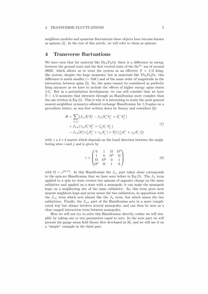
We have seen that for material like Dy2Ti2O7 there is a difference in energybetween the ground state and the first excited state of the Dy3+ ion of around380K, which allows us to treat the system as an effective S = 1/2 Ising-like system, despite the large moments; but in materials like Tb2Ti2O7, thisdifference is much smaller (∼ 10K) and of the same order of magnitude as theinteraction between spins [5]. So, the spins cannot be considered as perfectlyIsing anymore as we have to include the effects of higher energy spins states[11]. But in a perturbation development, we can still consider that we haveS = 1/2 moments that interacts through an Hamiltonian more complex thanthe one written in Eq.(5). This is why it is interesting to study the most generalnearest-neigbhbor symmetry-allowed exchange Hamiltonian for 1/2-spins on apyrochlore lattice, as was first written down by Savary and coworkers [6]:

H =∑〈i,j〉

JzzSzi Szj − J±(S+i S−j + S−i S

+j )

+ J±±(γijS+i S

+j + γ∗ijS

−i S−j )

− Jz±[Szi (γ∗ijS+j + γijS

−j ) + Szj (γ∗jiS

+i + γjiS

−i )]

(7)

with γ a 4× 4 matrix which depends on the bond direction between the neigh-boring sites i and j and is given by

γ =

0 1 Ω Ω2

1 0 Ω2 ΩΩ Ω2 0 1Ω2 Ω 1 0

(8)

with Ω = e2πi/3. In this Hamiltonian the Jzz part taken alone correspondsto the spin-ice Hamiltonian that we have seen before in Eq.(5). The J± termapplied to a spin ice state creates two spinons of opposite charge on the samesublattice and applied on a state with a monopole, it can make the monopolehope on a neighboring site of the same sublattice. So, this term gives nextnearest neighbors hops and never mixes the two sublattices, in opposition withthe Jz± term which acts almost like the J± term, but which mixes the twosublattices. Finally, the J±± part of the Hamiltonian acts in a more compli-cated way but always involves several monopoles, and can then be seen as aclose ranged interaction term between monopoles.

Here we will not try to solve this Hamiltonian directly, rather we will sim-plify by taking one or two parameters equal to zero. In the next part we willpresent the gauge mean field theory first developed in [6], and we will use it ona “simple” example in the third part.

6

Part II

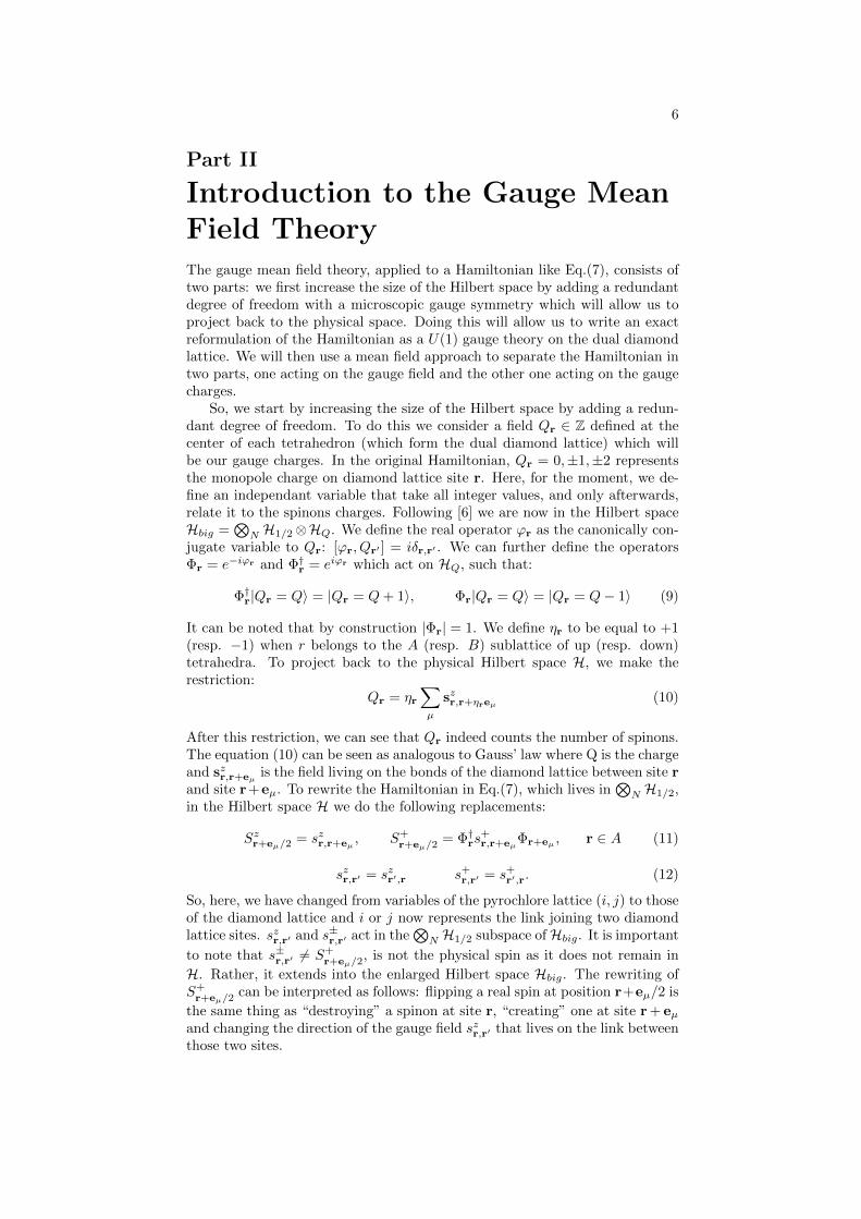
Introduction to the Gauge MeanField TheoryThe gauge mean field theory, applied to a Hamiltonian like Eq.(7), consists oftwo parts: we first increase the size of the Hilbert space by adding a redundantdegree of freedom with a microscopic gauge symmetry which will allow us toproject back to the physical space. Doing this will allow us to write an exactreformulation of the Hamiltonian as a U(1) gauge theory on the dual diamondlattice. We will then use a mean field approach to separate the Hamiltonian intwo parts, one acting on the gauge field and the other one acting on the gaugecharges.

So, we start by increasing the size of the Hilbert space by adding a redun-dant degree of freedom. To do this we consider a field Qr ∈ Z defined at thecenter of each tetrahedron (which form the dual diamond lattice) which willbe our gauge charges. In the original Hamiltonian, Qr = 0,±1,±2 representsthe monopole charge on diamond lattice site r. Here, for the moment, we de-fine an independant variable that take all integer values, and only afterwards,relate it to the spinons charges. Following [6] we are now in the Hilbert spaceHbig =

⊗N H1/2⊗HQ. We define the real operator ϕr as the canonically con-

jugate variable to Qr: [ϕr, Qr′ ] = iδr,r′ . We can further define the operatorsΦr = e−iϕr and Φ†r = eiϕr which act on HQ, such that:

Φ†r|Qr = Q〉 = |Qr = Q+ 1〉, Φr|Qr = Q〉 = |Qr = Q− 1〉 (9)

It can be noted that by construction |Φr| = 1. We define ηr to be equal to +1(resp. −1) when r belongs to the A (resp. B) sublattice of up (resp. down)tetrahedra. To project back to the physical Hilbert space H, we make therestriction:

Qr = ηr∑µ

szr,r+ηreµ (10)

After this restriction, we can see that Qr indeed counts the number of spinons.The equation (10) can be seen as analogous to Gauss’ law where Q is the chargeand szr,r+eµ is the field living on the bonds of the diamond lattice between site rand site r+eµ. To rewrite the Hamiltonian in Eq.(7), which lives in

⊗N H1/2,

in the Hilbert space H we do the following replacements:

Szr+eµ/2= szr,r+eµ , S+

r+eµ/2= Φ†rs

+r,r+eµΦr+eµ , r ∈ A (11)

szr,r′ = szr′,r s+r,r′ = s+

r′,r. (12)

So, here, we have changed from variables of the pyrochlore lattice (i, j) to thoseof the diamond lattice and i or j now represents the link joining two diamondlattice sites. szr,r′ and s±r,r′ act in the

⊗N H1/2 subspace ofHbig. It is important

to note that s±r,r′ 6= S+r+eµ/2

, is not the physical spin as it does not remain in

H. Rather, it extends into the enlarged Hilbert space Hbig. The rewriting ofS+r+eµ/2

can be interpreted as follows: flipping a real spin at position r+eµ/2 is

the same thing as “destroying” a spinon at site r, “creating” one at site r + eµand changing the direction of the gauge field szr,r′ that lives on the link betweenthose two sites.

7

After noticing that

∑r∈A∪B

3∑µ,ν=0µ<ν

Szr+ηreµ/2Szr+ηreν/2

=1

2

∑r∈A∪B

Q2r −

1

2

∑r∈A∪B

3∑µ=0

(Szr+eµ/2)2 (13)

one can rewrite H in Eq.(7) as

HU(1) =Jzz2

∑r

Q2r − J±

∑r

∑µ6=ν

Φ†r+ηreµΦr+ηreνs−ηrr,r+ηreµs

+ηrr,r+ηreν

+J±±

2

∑r

∑µ6=ν

(γ−2ηrµν Φ†rΦ

†rΦr+ηreµΦr+ηreνs

+ηrr,r+ηreµs

+ηrr,r+ηreν + h.c.)

− Jz±∑r

∑µ 6=ν

szr,r+ηreµ(γ−ηrµν Φ†rΦr+ηreνs+ηrr,r+ηreν + h.c.)

(14)

after dropping a constant equal to −Nu.c.Jzz, where Nu.c. = N/4 is the numberof unit cells and N is the number of spins (in a unit cell there are 2 tetrahedra,one up and one down).It can be noted that the constant we dropped is equalto the energy of a spin ice state with all the interaction parameters except Jzztaken equal to zero. One can see that this Hamiltonian really is the Hamiltonianof a U(1) gauge theory because it is invariant under the gauge transformation:

Φr → Φreiχr

s±r∈A,r′∈B → s±r,r′e±i(χ′r−χr) (15)

with arbitrary χr.Before applying the mean field theory, it is worth pausing to give more

details on the algebra of our operators:

• s±r,r′ and szr′′,r′′′ follow the same algebra as normal spins when on thesame link, and commute if not

• [Φr, Qr′ ] = Φrδr,r′ and [Φ†r, Qr′ ] = −Φ†rδr,r′

• [Φ†r,Φ†r′ ] = [Φ†r,Φr′ ] = [Φr,Φr′ ] = 0

• [Qr, Qr′ ] = 0

• [Φ†r, sαr′,r′′ ] = [Φr, s

αr′,r′′ ] = [Qr, s

αr′,r′′ ] = 0

To get the mean field Hamiltonian we proceed to the following kind of replace-ments:

Φ†r,µΦr,νs−r,µs

+r,ν → (Φ†r,µΦr,ν − 〈Φ†r,µΦr,ν〉)〈s−r,µ〉〈s+

r,ν〉+(〈Φ†r,µΦr,ν〉)

(〈s−r,µ〉s+

r,ν + 〈s−r,µ〉s+r,ν − 〈s−r,µ〉〈s+

r,ν〉)

(16)Φ†rΦ

†rΦr,µΦr,νs

+r,µs

+r,ν → 〈s+

r,µ〉〈s+r,ν〉[Φ†rΦ†r〈Φr,µΦr,ν〉+ 〈Φ†rΦ†r〉Φr,µΦr,ν − 2〈Φ†rΦ†r〉〈Φr,µΦr,ν〉

+2(Φ†rΦr,µ〈Φ†rΦr,ν〉+ 〈Φ†rΦr,µ〉Φ†rΦr,ν − 2〈Φ†rΦr,µ〉〈Φ†rΦr,ν〉)]+(〈Φ†rΦ†r〉〈Φr,µΦr,ν〉+ 2〈Φ†rΦr,µ〉〈Φ†rΦr,ν〉)×(〈s+

r,µ〉s+r,ν + 〈s+

r,µ〉s+r,ν − 〈s+

r,µ〉〈s+r,ν〉)

(17)where we used the notation

sr,µ = sr,r+ηreµ

Φr,µ = Φr+ηreµ(18)

5 GAUGE MEAN FIELD HAMILTONIAN 8

Doing this will separate the Hamiltonian in two parts, one acting on the gaugefield, and the other one acting on the gauge charges. This is the most importantdifference with normal mean field theory. Indeed normal mean field theorywashes out the dynamics of spinons [5], but here as we have first increasedthe Hilbert space’s size, we get a Hamiltonian which governs the behavior ofspinons, and this Hamiltonian will depend on the organization of the gaugefield through the value of the mean field parameters.

5 Gauge mean field Hamiltonian

Before writing the mean field Hamiltonian, we should first introduce the dif-ferent mean field parameter that we get, and so we define:

Zr,µ = 〈szr,µ〉,∆r,µ = 〈s+

r,µ〉,χA/Br,µν = 〈ΦrΦr+eµ−eν 〉, µ, ν = 0...3, r ∈ A/B,εA/Br,µν = 〈Φ†rΦr+eµ−eν 〉, µ, ν = 0...3, r ∈ A/B,ξr,µ = 〈Φ†rΦr+eµ〉, µ = 0...3, r ∈ A,

(19)

We will often assume translational invariance at the scale of the unit cells forthe mean field parameters, which will allow us to drop the r indices. Afterthe replacement proposed in Eq. (16) and (17), and using the notations of Eq.(19) one gets:

Hm.f. = Hs +HΦ (20)

withHs =

∑r∈A

∑µ

αr,µs+r,µ + α∗r,µs

−r,µ + βr,µs

zr,µ + γr,µ (21)

where

αr,µ =∑ν 6=µ −J±(∆∗r+eµ,νε

Ar,µν + ∆∗r,νε

Br+eν ,µν)

−Jz±ξr,µ(Zr,ν + Zr+eµ,ν)γ∗µν+J±±γµν(∆r,νχ

A∗r,00χ

Br+eµ,νµ + ∆r+eµ,νχ

Br+eµ,00χ

A∗r,µν

+ 2∆r,νξr,µξr,ν + 2∆r+eµ,νξr,µξr+eµ−eν ,ν)

βr,µ =∑ν 6=µ −Jz±(γµν∆∗r+eµ,νξ

∗r+eµ−eν ,ν + γ∗µν∆r,νξr,ν) + c.c.

γr,µ =∑ν 6=µ 2J±(εB∗r+eν ,νµ∆r,µ∆∗r,ν + εAr,µν∆r,µ∆∗r+eµ,ν)

+2Jz±[γ∗µνZr,µ(ξr,ν∆r,ν + ξ∗r+eµ−eν ,µ∆∗r+eµ,ν) + c.c.]

−J±±2 ([3γµν∆r,µ(∆r,νχA∗r,00χ

Br+eµ,νµ + ∆r+eµ,νχ

Br+eµ,00χ

A∗r,µν

+ 2∆r,νξr,µξr,ν + 2∆r+eµ,νξr,µξr+eµ−eν ,ν)] + c.c)(22)

5 GAUGE MEAN FIELD HAMILTONIAN 9

and

HΦ =∑r

Jzz2Q2

r

−∑r∈A

∑µ6=ν

J±∆∗r,µ∆r,νΦ†r+eµΦr+eν

−∑r∈B

∑µ6=ν

J±∆r,µ∆∗r,νΦ†r−eµΦr−eν

+∑r∈A

∑µ6=ν

2J±±γµν∆r,µ∆r,νξr,νΦ†rΦr+eν + h.c.

+∑r∈B

∑µ6=ν

2J±±γ∗µν∆∗r,µ∆∗r,νξ

∗r−eν ,νΦ†rΦr−eν + h.c.

−∑r∈A

∑µ6=ν

Jz±γ∗µν∆r,µZr,νΦ†rΦr+eν + h.c.

−∑r∈B

∑µ6=ν

Jz±γµν∆∗r,µZr,νΦ†rΦr−eν + h.c.

+∑r∈A

∑µ6=ν

J±±2γµν∆r,µ∆r,νχ

Br+eµ,νµΦ†rΦ

†r + h.c.

+∑r∈B

∑µ6=ν

J±±2γ∗µν∆∗r,µ∆∗r,νχ

Ar−eµ,µνΦ†rΦ

†r + h.c.

+∑r∈A

∑µ6=ν

J±±2γ∗µν∆∗r,µ∆∗r,νχ

Ar,00Φ†r+eµΦ†r+eν + h.c.

+∑r∈B

∑µ6=ν

J±±2γµν∆r,µ∆r,νχ

Br,00Φ†r−eµΦ†r−eν + h.c.

(23)

If we assume translationnal invariance at the scales of the unit cells, we canthen simply apply a Fourier transformation on HΦ using

ΦA/Br,τ =1

2πNu.c.

∑k

∫dωΦ

A/Bk,ω ei(kr−ωτ) (24)

and we get:

HΦ =∑r

Jzz2Q2

r +1

2πNu.c.

∑k>0

∫dω~Φ∗k,ωMk

~Φk,ω (25)

where

~Φk,ω =

ΦAk,ω

ΦA−k,ω∗ΦBk,ω

ΦB−k,ω∗

(26)

and

Mk =

A11(k) A12(k) C(k) 0A∗12(k) A11(−k) 0 C∗(−k)C∗(k) 0 B11(k) B12(k)

0 C(−k) B∗12(k) B11(−k)

(27)

6 THE GAUGE FIELD HAMILTONIAN: HS 10

where we defined

A11(k) = B11(k) = −J±∆µ∆∗νeik(eµ−eν)

A12(k) = J±±2

∑µ6=ν γµν∆µ∆ν(χBµν + χB00e

ik(eµ−eν))

B12(k) = J±±2

∑µ6=ν γ

∗µν∆∗µ∆∗ν(χAµν + χA00e

ik(eµ−eν))

C(k) =∑µ6=ν(4J±±γµν∆µ∆νξν − 2Jz±γ

∗µν∆µZν)eikeµ

(28)

In this section we have writtenHm.f. in different ways depending on whetherwe assume translationnal invariance of the mean field parameters or not. Wehave combined the work of both ref. [6] and [12] and have written down theexpressions that one would get in more details in order to have a clear start-ing point for further works. From the size of the different expressions and thenumber of mean field parameters one can see why it is so difficult to solve thisHamiltonian directly and why one has to take one or more interaction param-eters equal to zero in order to solve it. In the two next sections we will take acloser look at the two parts of Hm.f.: Hs and HΦ.

6 The gauge field Hamiltonian: Hs

We will first take a closer look at Hs (Eq.(21)). This part is pretty simple tosolve as it can be seen as the Hamiltonian of spins in a magnetic field with nointeractions between them. We find the ground state to be

|G.S.〉 =⊗r∈A

⊗µ

1

Nr,µ

| ↑〉 −√|αr,µ|2 + β2

r,µ/4 + βr,µ/2

αr,µ| ↓〉

(29)

with the normalization constant

Nr,µ =1

|αr,µ|

√√|αr,µ|2 + β2

r,µ/4(

2√|αr,µ|2 + β2

r,µ/4− βr,µ)

(30)

and the energy of the ground state is:

Es =∑r∈A

∑µ

γµ −√|αr,µ|2 + β2

r,µ/4 (31)

Thanks to this we can write down the two first self-consistent equations of thismean field theory, which are:

Zr,µ = 〈szr,µ〉 = − βr,µ

4√|αr,µ|2 + β2

r,µ/4(32)

∆r,µ = 〈s+r,µ〉 = −

α∗r,µ

4√|αr,µ|2 + β2

r,µ/4(33)

We now have to look at the self consistent equations which will give us infor-

mation on mean field parameters of the form 〈Φ(†)r,µΦ

(†)r′,ν〉, and for this we have

to study the spinon Hamiltonian.

7 THE GAUGE CHARGE HAMILTONIAN: HΦ 11

7 The gauge charge Hamiltonian: HΦ

We have a Hamiltonian for the spinons, HΦ, which howeveris not yet writtenwith conjugate variables. In order to solve it, we have to do this[6]. There aretwo ways to solve this problem: we can either write Φ in term of the conjugatevariable of Q (which is ϕ), or write Q in term of the conjugate variable ofΦ. The first solution is easy to implement, since Φr = e−iϕr but the secondsolution needs a little more work.

Since Φr = e−iϕr we can think of ϕr as the position of a particle on a circleof unit size and of Φr as the corresponding position on the complex plan. Hence,we can write Φr = xr + iyr once we enforce the condition that the particle liveson a circle of unit size, which can be done thanks to a lagrange multiplier,by adding a term like

∑r λr(Φ

†rΦr − 1). We can then define a new operator,

Πr = pxr + ipyr where pxr and pyr are the momenta canonically conjugate tothe positions xr and yr. Doing this we get:

[Π(†)r ,Π

(†)r′ ] = 0

[Φ(†)r ,Φ

(†)r′ ] = 0

[Φr,Πr′ ] = [Φ†r,Π†r′ ] = 0

[Φ†r,Πr′ ] = [Φ†r,Πr′ ] = 2δr,r′

(34)

It follows that the conjugate operator of Φ is Π†/2, and the conjugate operatorof Φ† is Π/2. What remains to do, is to write

∑rQ

2r in terms of Π and Π†. To

do this, one can notice that

Π†rΠr = p2xr

+ p2yr = −∆xr,yr (35)

Then, by writing the Laplace operator in the polar coordinates |Φr| and ϕr onegets

Π†rΠr = − 1

|Φr|∂

∂|Φr|

(|Φr|

∂

∂|Φr|

)− 1

|Φr|2∂2

∂ϕ2r

(36)

As ϕr and Qr are canonically conjugate variables, − ∂2

∂ϕ2r

= Q2r. If we also use

the fact that we work with the constraint |Φr| = 1 we can finally write:

Π†rΠr = Q2r (37)

and then get a Hamiltonian as a function of Φr, Φ†r, Πr and Π†r. It can be notedthat the local constraint expressed by the term

∑r λr(Φ

†rΦr − 1) will usually

be relaxed, and we will only use the global constraint λr∑

r(Φ†rΦr − 1), in a

kind of Gaussian approximation.It is principally this second method that has been used and will be used

here, but as we will see below, the first method can still give useful information.

8 Variational Energy Method

A couple of papers ([6],[12]) have been interested in the phase diagram that onewould get by using the gauge mean field theory, but the problem is that sincewe have a lot of mean field parameters it is rarely possible to completely solveall the self-consistent equations of the theory. So what has been done is to firstreduce the number of parameters by using different approximations, and thenget an approximate form for the ground state by looking for the minimum ofthe energy as a function of the remaining parameters. Here we will take a look

8 VARIATIONAL ENERGY METHOD 12

at these different approximations. In their paper [6], Savary and collaboratorsstudy the Hamiltonian of equation (7) with the following constraints on theinteraction parameters:

Jzz > 0, J± > 0, J±± = 0 (38)

and they use the following ansatz:

〈szµ〉 =1

2sin θεµ, 〈s+

µ 〉 =1

2cos θ, µ = 0, ..., 3 (39)

with ε = (1, 1,−1,−1). This ansatz assumes translational invariance of thesystem at the scale of the unit cells (we drop the r indices) and fully polarized“spins” s, which seems correct if we look at equation (21). But this ansatz alsoassumes that the components sz are always in a 2 in-2 out states (ε imposesthe 2 in-2 out structure), and that the planar components, if they are not equalto zero, are always aligned along the x axis, and cannot have a dependence onµ as could be the casein a phase that breaks the gauge symmetry. The lasttwo assumptions could be correct but they seem less realistic that the first twoassumptions, even if they simplify the calculation a lot.

In the second paper [12], Lee and collaborators study the same Hamiltonianwith different constraints on the interaction parameter, which are:

Jzz > 0, J± > 0, Jz± = 0 (40)

and:Jzz > 0, J± < 0, Jz± = 0, J±± = 0 (41)

Here, they reduce the number of mean field parameters using an alternativemethod. Indeed, they use results from a non-mean-field but pertubative theorywhich goes as follows:

First, we should notice that when Jz± = 0, βµ = 0 and so, we get 〈szµ〉 = 0.So, if we assume fully polarized spins, we get

〈s±r,r′〉 = |〈s±r,r′〉|e±iAr,r′ (42)

Moreover, if we take J±± . J± Jzz, the leading term in the perturbationtheory that can lift the degeneracy between the 2 in-2 out states is the thirdorder term in J± and corresponds to the flip of 6 spins circulating around ahexagon of the diamond lattice (See Fig. 1). It can be written as:

Hring ∼ J3±/J

2zz

∑

cos(∇×A) (43)

where (∇×A) ≡∑i∈hexagonAri,ri+1

ηri denotes the flux through the hexagonscontaining the sites i. So, depending on the sign of J±, there will be differentorganizations of the ground state. Indeed, if J± > 0, the ground state will bea 0-flux state with cos(∇ × A) = 1, but if J± < 0, the ground state will bea π-flux state with cos(∇ × A) = −1. In their article, Lee and collaboratorschose a particular realization of a 0-flux and a π-flux states, and thanks to this,fix the value of 〈s±r,r′〉 (to be 0 on each link in the 0-flux state, and to be 0or π, in a way that each hexagon possesses three 0-links and three π-links, inthe π-flux state), but in both cases, there are many other possibilities for thechoice of the 0- or π-flux states.

Thanks to these two approximations, Savary and collaborators in [6] andLee and collaborators in [12], managed to draw a part of the phase diagram

13

of a spin-1/2 system on a pyrochlore lattice. However, in both articles, theywere more interested in the position of the transition line than in a quantitativedescription of each phase. In the last part of this report we will present sucha quantitative description for a single set of parameters: Jz± = 0, J±± = 0andJ± > 0

Part III

A detailed example of theapplication of the mean fieldgauge theoryIn this part we will take Jz± = 0, J±± = 0 andJ± > 0. So, the Hamiltonian issimply (as first studied in [4]):

HJ± =∑〈i,j〉

[JzzSzi S

zj − J±(S+

i S−j + S−i S

+j )]. (44)

Doing the same manipulations as before one gets:

Hm.f. = Hs +HΦ (45)

withHs =

∑r∈A

∑µ

αr,µs+r,µ + α∗r,µs

−r,µ + βr,µs

zr,µ + γr,µ (46)

where

αr,µ =∑ν 6=µ −J±(∆∗r+eµ,νε

Ar,µν + ∆∗r,νε

Br+eν ,µν)

βr,ν = 0

γr,ν =∑ν 6=µ 2J±(εB∗r+eν ,νµ∆r,µ∆∗r,ν + εAr,µν∆r,µ∆∗r+eµ,ν)

(47)

and

HΦ =∑r

Jzz2Q2

r

−∑r∈A

∑µ6=ν

J±∆∗r,µ∆r,νΦ†r+eµΦr+eν

−∑r∈B

∑µ 6=ν

J±∆r,µ∆∗r,νΦ†r−eµΦr−eν

(48)

The first thing to notice is that here, thanks to βµ = 0, we have, fromEq.(32), Zµ = 〈szµ〉 = 0, so that we can write

∆r,µ = 〈s+r,µ〉 =

1

2eiθr,µ (49)

And from Eq.(33) we get

θr,µ = π −Arg(αr,µ) (50)

9 COMPUTATION OF THE GREEN’S FUNCTION 14

So here, if we could get the value of εA/Br,µν , from solving the HΦ Hamiltonian,

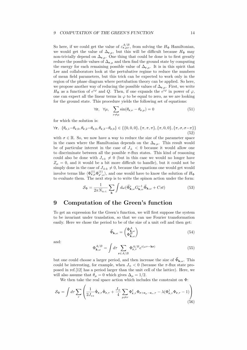
we would get the value of ∆r,µ, but this will be difficult because HΦ maynon-trivially depend on ∆r,µ. One thing that could be done is to first greatlyreduce the possible values of ∆r,µ and then find the ground state by computingthe energy for each remaining possible value of ∆r,µ. It is in this spirit thatLee and collaborators look at the pertubative regime to reduce the numbersof mean field parameters, but this trick can be expected to work only in theregion of the phase diagram where pertubation theory can be applied. So here,we propose another way of reducing the possible values of ∆r,µ. First, we writeHΦ as a function of eiϕ and Q. Then, if one expands the eiϕ in power of ϕ,one can expect all the linear terms in ϕ to be equal to zero, as we are lookingfor the ground state. This procedure yields the following set of equations:

∀r, ∀µ,∑ν 6=µ

sin(θr,ν − θr,µ) = 0 (51)

for which the solution is:

∀r, θr,1−θr,0, θr,2−θr,0, θr,3−θr,0 ∈ 0, 0, 0, π, π, π, π, 0, 0, π, σ, σ−π(52)

with σ ∈ R. So, we now have a way to reduce the size of the parameter spacein the cases where the Hamiltonian depends on the ∆r,µ. This result wouldbe of particular interest in the case of J± < 0 because it would allow oneto discriminate between all the possible π-flux states. This kind of reasoningcould also be done with Jz± 6= 0 (but in this case we would no longer haveZµ = 0, and it would be a bit more difficult to handle), but it could not besimply done in the case of J±± 6= 0, because the equations one would get would

involve terms like 〈Φ(†)r,µΦ

(†)r′,ν〉, and one would have to know the solution of HΦ

to evaluate them. The next step is to write the spinon action under the form:

SΦ =1

2πNu.c.

∑k

∫dω(~Φ∗k,ωG

−1k,ω

~Φk,ω + Cst) (53)

9 Computation of the Green’s function

To get an expression for the Green’s function, we will first suppose the systemto be invariant under translation, so that we can use Fourier transformationeasily. Here we chose the period to be of the size of a unit cell and then get:

~Φk,ω =

(ΦAk,ωΦBk,ω

)(54)

and:

ΦA/Bk,ω =

∫dτ

∑r∈A/B

ΦA/Br,τ ei(ωτ−kr) (55)

but one could choose a larger period, and then increase the size of ~Φk,ω. Thiscould be interesting, for example, when J± < 0 (because the π-flux state pro-posed in ref.[12] has a period larger than the unit cell of the lattice). Here, wewill also assume that θµ = 0 which gives ∆µ = 1/2.

We then take the real space action which includes the constraint on Φ:

SΦ =

∫dτ∑r

1

2JzzΦr,τ Φr,τ +

J±4

∑µ 6=ν

Φ†r,τΦr+eµ−eν ,τ − λ(Φ†r,τΦr,τ − 1)

(56)

10 COMPUTATION OF THE LAGRANGE MULTIPLIER λ 15

and Fourier transform. One gets:

G−1k,ω =

1

2Jzz

(ω2 − ω2

k 00 ω2 − ω2

k

), Cst = 2πλ (57)

with:

ωk =

√2Jzzλ− JzzJ±

∑µ,ν<µ

cos(k(eµ − eν)) (58)

We then integrate Gk,ω over ω to get the equal-time Green function. To dothis integration we use Feynmann’s prescription and replace ωk by ωk− iε. Weget:

GFk =

√Jzz2

1√λ− J±2

∑µ,ν<µ cos(k(eµ−eν))

0

0 1√λ− J±2

∑µ,ν<µ cos(k(eµ−eν))

(59)

GFk =

(Jzzωk

0

0 Jzzωk

)(60)

So, we now have an expression for the Green functions but we still need tocompute the value of λ and that will be done in the next section.

10 Computation of the Lagrange multiplier λ

To get an expression for λ, we need to use the constraint 〈Φ†rΦr〉 = 1, whichcan be rewritten as:

1

Nu.c.

∑k

[GFk]11 = 1 (61)

and so:1

Nu.c.

∑k

1√λ− J±

2

∑µ,ν<µ cos(k(eµ − eν))

= 1 (62)

Rewriting the sum as an integral one gets:∫∫∫ 1/2

−1/2

d3q√λJ±− 1

2

∑µ,ν<µ cos(2π(qµ − qν))

=

√2J±Jzz

(63)

where q0 = 0 and qi i = 1..3 have been define in Eq.(3). At this point westarted to use mathematica to solve this kind of equations. After noticingthat λ/J± has to be greater than 3 in order to have a real value for ωk onecan compute the integral for several values of λ/J± and get the correspondingvalue of J±/Jzz (see Fig.4)

Two things can be noticed here: firstly, when λ/J± = 3, we find J±/Jzz =(J±/Jzz)lim ≈ 0.192, so we can expect a transition to occur at this point, intotal agreement with ref. [6]. This will be discussed in another section and forthe moment we will restrain ourselves to the study of J±/Jzz < (J±/Jzz)limwhich correspond to the quantum spin liquid phase. Secondly, when J±/Jzzgoes to zero, the value of λ/Jzz goes to 1/2, which is what is expected whenwe directly take J± = 0 in Eq.(62).

11 ENERGY OF THE SYSTEM 16

0.00 0.05 0.10 0.150.50

0.52

0.54

0.56

J±

Jzz

Λ

Jzz

0.00 0.05 0.10 0.150

10

20

30

40

J±

Jzz

Λ

J±

Figure 4: λ/Jzz and λ/J± as a function of J±/Jzz. On the first graph, we canobserve that the value of λ/Jzz goes to 1/2, which is what is expected whenwe directly take J± = 0 in Eq.(62). On the second graph, we can see thatthe value of λ/J± decreases as the value of J±/Jzz increases, and stopped atλ/J± = 3, for J±/Jzz = (J±/Jzz)lim ≈ 0.192, in total agreement with ref. [6]

11 Energy of the system

We now have almost everything we need to solve the problem, except the values

of the εA/Br,µν , that are given by:

εA/Br,µν = 〈Φ†rΦr+eµ−eν 〉

= 1Nu.c.

∑k[GFk]11e

ik(eµ−eν)

=∫∫∫ 1/2

−1/2d3qei2π(qµ−qν )√

λJ±− 1

2

∑ρ,σ<ρ cos(2π(qρ−qσ))

(64)

Knowing the value of λ/J± as a function of J±/Jzz we can compute the value

of εA/Br,µν for different values of J±/Jzz using mathematica. It can be noticed

that εA/Br,µν will depend neither on µ and ν nor on the choice of the sublattice,

not because we chose this parameter to be translationally invariant, but as adirest consequence of the calculation.

What remains to be done is to put together all the terms that contributeto the total energy per unit cell of the system, in units of Jzz. Doing this weget the graph in Fig.5. If we take a closer look at the behavior of the energy

0.00 0.05 0.10 0.15

-0.15

-0.10

-0.05

0.00

J±

Jzz

etot

Jzz

+

+

++

++

++

++

+++++++++++++++++++++

++++++++++++++++++++++++++++++++++++++++++++

0.00 0.01 0.02 0.03 0.04 0.05 0.06 0.07

-0.015

-0.010

-0.005

0.000

J±

Jzz

etot

Jzz

Figure 5: The total energy etot in units of Jzz as a function of J±/Jzz. Thesecond picture is a zoom of the first one near J±/Jzz = 0 fitted by etot =−3J2

±/Jzz − 6J3±/J

2zz (red curve).

at low J±/Jzz we find that the energy can be fitted by etot = Etot/Nu.c. =

12 QUANTUM SPIN LIQUID PHASE 17

−3J2±/Jzz − 6J3

±/J2zz. This is in qualitative agreement with the perturbation

theory developed by Hermele, Fisher and Balents in ref.[4] in that we havecorrections to the energy to order J2

±/Jzz and J3±/J

2zz. It can be noted that in

ref. [4], the authors are mainly interested in the third order term, J3±/J

2zz, as it

is the one that lift the degeneracy between the spin ice states, but the secondorder term also give a correction to the energy, even if it is the same correctionfor all spin ice states. There is an anology between the perturbation theoryused here and the strong coupling Hubbard model [13], in the way that theperturbation correction that we have correspond only to virtual return pathand ring exchange terms.

However even though the prefactor we found are of the same order of mag-nitude than those predicted by the perturbation theory, they are not perfectlyequal.This is not the first time that the gauge mean field theory and the pertur-bation theory are in partial disagreement. Indeed in ref.[6] the phase diagramfor gauge mean field theory obtained by Savary and coworkers had to be cor-rected by results coming from a perturbation theory in the case of low Jz±/Jzz.There are three possible explanations for why the coefficients of Jn±/J

n−1zz are

not in agreement with perturbation theory: firstly, the gauge mean field theoryis intrinsically wrong; secondly, the calculation in one or the other theory iswrong; finaly, there are other terms related to deconfinement that are not takenin account in the perturbation theory. Indeed, the perturbation theory onlylook at short path terms for the virtual spinons, but if we assume deconfinedspinons, the perturbation theory may not converge. In other words, as thecreation of a spinon needs an energy of order Jzz, a density of spinons thatvaries as Jn±/J

nzz would also lead to a correcting term in the energy of order

Jn±/Jn−1zz .

We now have numerical access to the value of the energy and of the dis-persion relation of the spinons in the quantum spin liquid phase, and this isprobably one of the main achievements of this internship. We will now take acloser look to the description of this quantum spin liquid phase.

12 Quantum Spin Liquid Phase

In this section we will try to give some more details on the quantum spinliquid state. The most interesting thing to look at is the value of 〈Sr+eµ/2〉.Indeed, as noticed following equation (47), we have βµ = 0 for all µ and so,〈Szr+eµ/2

〉 = 〈szr,r+eµ〉 = 0. But also, even if 〈s±µ 〉 6= 0 we have to remember

that S±r+eµ/26= s±r,r+eµ . We instead have:

S+r+eµ/2

= Φ†rs+r,r+eµΦr+eµ , r ∈ A (65)

and so we can write

〈S+r+eµ/2

〉 = 〈s+r,r+eµ〉〈Φ

†rΦr+eµ〉, r ∈ A (66)

As the Green function written in equation (59) directly give 〈Φ†rΦr+eµ〉 = 0,we

have 〈S+r+eµ/2

〉 = 0 giving us 〈Sr+eµ/2〉 = 0, which is the signature of a quantum

spin liquid phase. Indeed, to get 〈Sr+eµ/2〉 = 0, we can imagine the quantumspin liquid state to be a macroscopic superposition of 2 in- 2 out states (possiblymixed with others states) that would be the quantum analog of the extensivelydegenerated ground states that we found in the classical case.

13 CONDENSATION AND ANTI-FERROMAGNETIC PHASE 18

To do this calculation, we have chosen the solution for θµ from Eq.(50) to beθµ = 0, but other choices could have been made. In this section, we will showthat this choice is not important and does not change the results thanks tothe local U(1) symmetry (represented by Eq.(15)) of the quantum spin liquid.Indeed, if we do not make such a choice, the

∑µ,ν<µ cos(k(eµ − eν)) that

appears in Eq.(58) has to be changed in∑µ,ν<µ cos(k(eµ − eν) + (θµ − θν)).

Then, to get λ, we have to compute the value of:∫∫∫ 1/2

−1/2

d3q√λJ±− 1

2

∑µ,ν<µ cos(2π(qµ − qν) + (θµ − θν))

=

√2J±Jzz

(67)

and we get the same result as before if we do the change of variable qi →qi − θi−θ0

2π . The only thing that will change, is the value of εA/Br,µν . Indeed, we

now have to compute

εA/Br,µν = 〈Φ†rΦr+eµ−eν 〉

=∫∫∫ 1/2

−1/2d3qei2π(qµ−qν )√

λJ±− 1

2

∑ρ,σ<ρ cos(2π(qρ−qσ)+(θρ−θσ))

(68)

and doing the same change of variable we get:

εA/Br,µν =(εA/Br,µν

)θσ=0,∀σ

e−i(θµ−θν) (69)

As εA/Br,µν only appears in terms like ε

A/Br,µν∆r,µ∆∗r,ν or |

∑ν 6=µ ε

A/Br,µν∆∗r,ν | the

phases in θµ or θν disappear and do not play any role. This can be linked withthe U(1) invariance of Eq.(15) by saying that if this invariance is not broken(and it is not in the quantum spin liquid state), when we change the phaseof ∆µ the phase of Φ will be adapted in a way that will not change the finalresult.

13 Condensation and Anti-ferromagnetic phase

We will now take a look at what happens when J±/Jzz > (J±/Jzz)lim. Wehave seen that λ has to be greater than 3J± in order to have ωk ∈ R. Whenλ = 3J±, we get ωk=0 = 0 (see Fig.6) and so the spinons can condensed atk = 0 in both sublattices. To treat this case, we follow what was done bySavary and coworkers in ref.[6], and write λ as

λ = λlim +δ2

N2u.c.

(70)

with δ > 0, and also change the rules of the conversion of a sum in an integralin:

1

Nu.c.

∑k

f(k)→ f(k = 0)

Nu.c.+

1

VBZ

∫k

f(k) (71)

where VBZ is the volume of the Brillouin zone. Then, we define the condensatedensity ρ as the part of 〈Φ†rΦr〉 that comes from the condensed fraction, andwe have:

ρ =[GFk=0]11

Nu.c.=

√Jzz2

1

δ= 1−

√JzzJ±

√(JpmJzz

)lim

(72)

13 CONDENSATION AND ANTI-FERROMAGNETIC PHASE 19

-3 -2 -1 1 2 3

k1

3 a

0.2

0.4

0.6

0.8

1.0

Ωk

Jzz

-3 -2 -1 1 2 3

k1

3 a

0.2

0.4

0.6

0.8

1.0

Ωk

Jzz

-3 -2 -1 1 2 3

k1

3 a

0.2

0.4

0.6

0.8

1.0

Ωk

Jzz

Figure 6: Dispersion relation of the spinons as a function of k1, for k2 = k3 = 0and λ/J± = 4, 3.5 and 3. We can see that as the value of λ/J± decreases(J±/Jzz increases), the minimum value of ωk decreases, until we reach λ/J± =3 (J±/Jzz = (J±/Jzz)lim) where the minimum value of ωk is given for k = 0and equals 0, allowing the condensation of spinons.

The uncondensed part here, will behave as the quantum spin liquid of theprevious part and will still be U(1) invariant, but the condensed part willchange behavior, and in particular, it will break the U(1) symmetry. Indeed, ifthe spinons condensed at a wave vector k,we will have:

〈Φr〉 = 〈Φk〉eikr (73)

In our case, using the definition of ρ and the fact that the condensation occursat k = 0, we get:

〈Φr∈A/B〉 = 〈ΦA/Bk=0 〉 =√ρ eiφA/B (74)

Because of this, the condensed part of εA/Br,µν = 〈Φ†rΦr+eµ−eν 〉 = ρ will

always be real (and positive), and won’t be able to compensate an arbitrarychoice of θµ. So we have to look at the dependence of the energy in θµ to fixtheir value. We find that we have to minimize

∑µ

J±ε

∑ν 6=µ

1

2cos(θµ − θν)− |

∑ν 6=µ

eiθν |

(75)

and this happens to be minimum for θ0 = θ1 = θ2 = θ3 = θ. So here the systembreaks local U(1) symmetry but still keep a global U(1) symmetry (which isthe choice of θ). This is an explicit difference with the spin liquid phase.

If we want to described the organization of this phase more precisely, wecan notice that we still have 〈Szr+eµ/2

〉 = 0, but as φA/B can arbitrarily be

20

taken equal to zero, we now have:

〈S+r+eµ/2

〉 = 〈s+r,r+eµ〉〈Φ

†r〉〈Φr+eµ〉 =

ρ

2eiθ, r ∈ A (76)

which means that as the value of J±/Jzz increases, the tangential part of thespin increases. In the pseudo-spin language, this phase looks like a ferromag-netic XY ordered state with spins pointing in an arbitrary but fixed directionin the (x,y) plan. But real spins are different from pseudo-spins, and if weget back to the local basis define in Part.1, section.1, this state of mattercorresponds to spins living in the plan tangential to the local [111] and withantiferromagnetic order, hence the name antiferromagnetic phase.

Part IV

Conclusion and PerspectiveThe two main achievements of this internship, after getting a better under-standing of a field of condensed matter that was totally unknown to me, werefirst to get the full gauge mean field Hamiltonian of equation (20), by combin-ing the methods of both the articles by Savary and coworkers [6], and by Leeand coworkers [12], in order to have a good starting point for further works.The second main achievement, was to get a better description of the quantumspin liquid state that appears in the context of the gauge mean field theorywith only J± > 0 as an interaction parameter. Particularly, the obtention (nu-merically) of the ground state energy of the quantum spin liquid and of thedispersion relation for the spinons may be used to get some understanding ofthe behavior of such systems at small but non-zero temperature. But manythings have yet to be done, among which trying to use the method of the thirdpart in cases where Jz±, or J±± (or both) are non-zero may be the most impor-tant, but there will obviously be new difficulties as the number of mean fieldparameters will increase. But questions like the effect of different choices ofperiod for the translational invariance (particularly in the case of J± < 0), orthe reasons for the apparent quantitative disagreement between perturbationtheory and gauge mean field theory may also be of some interest.

To complete this work, I would like to use the last lines of this reportto thank my advisor Peter Holdsworth for those four months of work whichwere really interesting, and those two weeks of scientific tourism in Dresden.I am ready to travel again in his luggage whenever he wants. I also want tothank Tommaso Roscilde and Louis-Paul Henry for their help on this work,and Lucille Savary, for the time she gave me during her holidays. Finally, Iwant to thanks all the Laboratoire de Physique de L’ENS de Lyon for the greattime I have spent there.

REFERENCES 21

References

[1] C. Castelnovo, R. Moessner, and Sondhi S.L. Magnetic monopoles in spinice. Nature, 451:42–45, Jan 2008.

[2] L.D.C. Jaubert and P.C.W Holdsworth. Signature of magnetic monopoleand dirac string dynamics in spin ice. Nature Physics, 5:258–261, Mar2009.

[3] O. Benton, O. Sikora, and N. Shannon. Seeing the light : experimentalsignatures of emergent electromagnetism in a quantum spin ice. ArXive-prints, April 2012.

[4] Michael Hermele, Matthew P. A. Fisher, and Leon Balents. Pyrochlorephotons: The u(1) spin liquid in a s = 1

2 three-dimensional frustratedmagnet. Phys. Rev. B, 69:064404, Feb 2004.

[5] M. J. P. Gingras, B. C. den Hertog, M. Faucher, J. S. Gardner, S. R.Dunsiger, L. J. Chang, B. D. Gaulin, N. P. Raju, and J. E. Greedan.Thermodynamic and single-ion properties of tb3+ within the collectiveparamagnetic-spin liquid state of the frustrated pyrochlore antiferromag-net tb2ti2o7. Phys. Rev. B, 62:6496–6511, Sep 2000.

[6] Lucile Savary and Leon Balents. Coulombic quantum liquids in spin-1/2pyrochlores. Phys. Rev. Lett., 108:037202, Jan 2012.

[7] Ramirez A.P., Hayashi A., Cava R.J., Siddharthan R., and Shastry B.S.Zero-point entropy in ’spin ice’. Nature, 399:333–335, May 1999.

[8] I. Ryzhkin. Magnetic relaxation in rare-earth oxide pyrochlores.Journal of Experimental and Theoretical Physics, 101:481–486, 2005.10.1134/1.2103216.

[9] L.D.C. Jaubert. Topological Constraints and Defects in Spin Ice. These,Ecole Normale Superieure de Lyon, September 2009.

[10] R. Moessner. Relief and generation of frustration in pyrochlore magnetsby single-ion anisotropy. Phys. Rev. B, 57:R5587–R5589, Mar 1998.

[11] Hamid R. Molavian, Michel J. P. Gingras, and Benjamin Canals. Dynami-cally induced frustration as a route to a quantum spin ice state in tb2ti2o7

via virtual crystal field excitations and quantum many-body effects. Phys.Rev. Lett., 98:157204, Apr 2007.

[12] S. Lee, S. Onoda, and L. Balents. Generic quantum spin ice. ArXiv e-prints, April 2012.

[13] J.-Y. P. Delannoy, M. J. P. Gingras, P. C. W. Holdsworth, and A.-M. S.Tremblay. Neel order, ring exchange, and charge fluctuations in the half-filled hubbard model. Phys. Rev. B, 72:115114, Sep 2005.