HAL Id: hal-03042226 https://hal.archives-ouvertes.fr/hal-03042226 Submitted on 6 Dec 2020 HAL is a multi-disciplinary open access archive for the deposit and dissemination of sci- entific research documents, whether they are pub- lished or not. The documents may come from teaching and research institutions in France or abroad, or from public or private research centers. L’archive ouverte pluridisciplinaire HAL, est destinée au dépôt et à la diffusion de documents scientifiques de niveau recherche, publiés ou non, émanant des établissements d’enseignement et de recherche français ou étrangers, des laboratoires publics ou privés. Gathering and Analyzing Surface Parameters for Diet Identification Purposes Arthur Francisco, Noël Brunetière, Gildas Merceron To cite this version: Arthur Francisco, Noël Brunetière, Gildas Merceron. Gathering and Analyzing Surface Parameters for Diet Identification Purposes. Technologies , MDPI, 2018, 6 (3), pp.75. 10.3390/technologies6030075. hal-03042226

Welcome message from author
This document is posted to help you gain knowledge. Please leave a comment to let me know what you think about it! Share it to your friends and learn new things together.
Transcript
HAL Id: hal-03042226https://hal.archives-ouvertes.fr/hal-03042226
Submitted on 6 Dec 2020
HAL is a multi-disciplinary open accessarchive for the deposit and dissemination of sci-entific research documents, whether they are pub-lished or not. The documents may come fromteaching and research institutions in France orabroad, or from public or private research centers.
L’archive ouverte pluridisciplinaire HAL, estdestinée au dépôt et à la diffusion de documentsscientifiques de niveau recherche, publiés ou non,émanant des établissements d’enseignement et derecherche français ou étrangers, des laboratoirespublics ou privés.
Gathering and Analyzing Surface Parameters for DietIdentification Purposes
Arthur Francisco, Noël Brunetière, Gildas Merceron
To cite this version:Arthur Francisco, Noël Brunetière, Gildas Merceron. Gathering and Analyzing Surface Parameters forDiet Identification Purposes. Technologies , MDPI, 2018, 6 (3), pp.75. �10.3390/technologies6030075�.�hal-03042226�
technologies
Article
Gathering and Analyzing Surface Parameters for DietIdentification Purposes
Arthur Francisco 1,* ID , Noël Brunetière 1 ID and Gildas Merceron 2,* ID
1 Institut Prime, CNRS, Université de Poitiers, ISAE-ENSMA, F-86962 Futuroscope Chasseneuil, France;[email protected]
2 PALEVOPRIM UMR 7262, CNRS, Université de Poitiers, 86073 Poitiers Cedex 9, France* Correspondence: [email protected] (A.F.); [email protected] (G.M.);
Tel.: +33-5-45-25-19-79 (A.F.); +33-5-49-36-63-05 (G.M.)
Received: 20 May 2018; Accepted: 9 August 2018; Published: 11 August 2018�����������������
Abstract: Modern surface acquisition devices, such as interferometers and confocal microscopes,make it possible to have accurate three-dimensional (3D) numerical representations of real surfaces.The numerical dental surfaces hold details that are related to the microwear that is caused by foodprocessing. As there are numerous surface parameters that describe surface properties and knowingthat a lot more can be built, is it possible to identify the ones that can separate taxa based on theirdiets? Until now, the candidates were chosen from among those provided by metrology software,which often implements International Organization for Standardization (ISO) parameters. Moreover,the way that a parameter is declared as diet-discriminative differs from one researcher to another.The aim of the present work is to propose a framework to broaden the investigation of relevantparameters and subsequently a procedure that is based on statistical tests to highlight the best ofthem. Many parameters were tested in a previous study. Here, some were dropped and othersadded to the classical ones. The resulting set is doubled while considering two derived surfaces: theinitial one minus a second order and an eighth order polynomial. The resulting surfaces are thensampled—256 samples per surface—making it possible to build new derived parameters that arebased on statistics. The studied dental surfaces belong to seven sets of three or more groups withknown differences in diet. In almost all cases, the statistical procedure succeeds in identifying themost relevant parameters to reflect the group differences. Surprisingly, the widely used Area-scalefractal complexity (Asfc) parameter—despite some improvements—cannot differentiate the groupsas accurately. The present work can be used as a standalone procedure, but it can also be seen as afirst step towards machine learning where a lot of training data is necessary, thus making the humanintervention prohibitive.
Keywords: dental microwear analysis; sampling method; statistical tests; surface parameters
1. Introduction
Fundamentally, dental microwear analysis involves gathering as many dental surface details thatare related to wear as possible to aid in its characterization. It is a generic expression referring to thestudy of the patterns on teeth left by the processing of food.
Researchers have long acknowledged this technique as a means of providing information aboutthe diet in the days or weeks prior to death. This way of inferring a diet is widespread and can bequalified as mature. Numerous works have been and are still published on the matter and championthe efficiency of the method in distinguishing some diets from others. In particular, depending onthe mechanical properties of the foodstuff, scratches or pits are left on human or other animal teeth,thus making it possible to guess the predominant diet before death. The clearer the signal strength,
Technologies 2018, 6, 75; doi:10.3390/technologies6030075 www.mdpi.com/journal/technologies
Technologies 2018, 6, 75 2 of 21
the more certain the conclusions. For a less abbreviated history of dental microwear analysis, thereader is referred to Ungar et al. [1] (pp. 389–425), in which the authors describe dental microwearanalysis from the early thirties up to the beginning of the 2000s. Ungar and DeSantis [2,3] providemore recent conclusions that were collected from works on mammals. As a novel approach to themethod of analyzing the dental microwear data is presented here, only some recent works are cited togive a snapshot of the current uses.
Depending on the researcher’s habits, needs, equipment, etc., different ways of dealing withdental microwear analysis can be distinguished. Three kinds of devices are used today to analyzethe tooth surfaces: three-dimensional (3D) optical profilers, two-dimensional (2D) Scanning ElectronMicroscopes (SEM), and 2D low-magnification light microscopes.
Light microscopes involved in stereomicroscopic microwear analysis are used to count the pitsand scratches. The scratches are recognized as being characteristic of tough food, like mature grassand pits, are markers of brittle food, like fruit, seeds, some leaves, etc. The relative proportion of pitsand scratches is then often used as an indicator of grazing or browsing habits. The efficacy of thismethod relies heavily on the observer experience, which explains the variability in the results: differentoperators count surface features differently and may tune the light orientation differently, highlightingmore or fewer features on the surface [4,5]. However, this method is still in use and it proves to beefficient [6–9]. SEM is used less than before because it has been advantageously replaced by 3D opticalprofilers, such as confocal or interferometer microscopes. The latter are more affordable and easier touse. However, some recent works on dental microwear are based on SEM images, analyzed with thehelp of an image-processing software [10–12].
As for 3D digitized data treatment, Scale Sensitive Fractal Analysis (SSFA) has garnered a lot ofinterest because it uses a few parameters that correlate strongly to characteristic diets and has beensuccessfully applied in numerous works, for which some of the more recent are references in thisstudy [13–18]. Another approach, Surface Texture Analysis (STA), is sometimes used as a complementto SSFA, consists of computing ISO-25178 areal parameters, the extension of classic industrial profileparameters, see [19–21].
As pointed out by DeSantis [3], there are between 20 and 30 ISO-25178 parameters. However, SSFAparameters are more closely linked to the diet. STA parameters can prove to be more discriminantin some cases. As for selecting the relevant parameters, the question has been addressed in anindustrial context by Najjar et al. [22,23], Bigerelle et al. [24], and Deltombe et al. [25], utilizing amethodology that is based on a bootstrap method. First, Najjar et al. [22] searched for the bestcorrelation between a given surface property and roughness parameters. The correlation strength—thelinear regression slope—was then quantified using a bootstrap approach. Then, Najjar et al., Bigerelle etal., and Deltombe et al. [23–25] used analysis of variance (ANOVA) to organize roughness parametersaccording their relevance (F statistics) in discriminating industrial process steps. The bootstrap wasused to quantify the F probability density function. The authors proposed a methodology close to theone developed here that aims to address the following issue: among a given set of parameters, whatare those which discriminate best between different surface types, without any preconceived opinion?Even if the question is the same, some differences lead to different approaches. Here, the surfacesare not presumed homogeneous, which broadens the parameter set. Hence, intensive calculationsare avoided. As a given parameter is naturally supposed to behave as a normal variable among theindividuals of the population, the use of a bootstrap approach is not justified. These two considerations,large parameter sets and no mandatory bootstrap, have lead the authors of this study to parametrictests. It is to be noted, though, that the cited works and the present one share similar methods to orderthe “best parameters” F statistics and p-values.
The first goal of 3D digitized surface analysis should be to determine whether it is better to builda set of parameters that can differentiate between different diet groups, provided that a parameter isnot necessarily associated to a particular diet, or whether it is more desirable to work with a small setof parameters, perhaps less efficient, but more understandable. However, the present study does not
Technologies 2018, 6, 75 3 of 21
aim to answer this question, but rather, to extend the existing parameters and test their ability in orderto separate different groups. Some groups are easily distinguishable, others less so. The methodologyhere, based on surface sampling and automated statistical treatments, has previously been successfullytested and compared to Dental Microwear Texture Analysis (DMTA) results by Francisco et al. [26].The surface sampling relies on a simple observation: some surfaces do not exhibit a given featureacross their entire surface. For instance, a diet that is known to scar the enamel may fail to leavescratches on a part of the digitized surface. Regarding the surface feature analysis, the authors haveproposed a sequence of statistical treatments to identify the meaningful parameters and leave asidethe others. In the final discussion, it has been mentioned that the widely used Asfc parameter hassurprisingly lead to moderate results and that it should be reworked. In addition to that point, it hasalso been concluded that the whole procedure should be applied to other species to confirm or refuteits efficiency.
In the present work, the same methodology is followed, but with modifications. The set ofdiscriminative parameters has been refined, as will be described in Section 2.2.
2. Materials and Methods
2.1. Material
Here, the reliability of new developments in describing dental microwear textures, as introducedin Francisco et al. [26], is tested. To do so, the choice was made to select six sets composed of modernwild species or samples of domesticated animals fed on different diets, issued by the ANR TRIDENTProject [27–29]. The reader will find in the Electronic Supplementary Material (ESM) some illustrationsof the different species. It is important to note that we made the set assumptions before we startedthe simulations. The expectations related to the group separation are based on (from the strongest tothe weakest):
• different tooth microwear textures,• known diet habits of the studied species, and• the confidence in the procedure reliability.
In the first case, it is a question a procedure validation. Even if it is not guaranteed that the resultscorroborates the tooth observations—some visual features may not be caught by the parameters—goodresults are expected. As for the two other cases, there is more uncertainty but the large number ofparameters suggests that there should be interesting findings.
2.1.1. Triplet 1 (T1), “Old World Monkeys”
This triplet is composed of three African species of monkeys with divergent dietary habits andhabitat preferences: 19 specimens of Cercocebus atys (CE), 19 of Papio hamadryas (PA), and 19 of Colobuspolykomos (CO). The first species lives in Central African forest and feeds mostly on hard fruits andseeds [30,31]. The third species also occupies inter-tropical African forest, but differs from Cercocebusatys by being a leaf-eating monkey [32,33]. Papio hamadryas is more plastic in its dietary and habitatpreferences. It mostly occupies wooded to open habitats and its diet varies from one season toanother [34,35].
Testing hypothesis: leaf eating monkeys such as Colobus polykomos display significant differencesin dental microwear textures when compared to seed- and fruit-eating monkeys, such as Cercocebusatys [36]. The wide spectrum of dietary habits for Papio hamadryas suggest a wide range of textures ontooth enamel surfaces overlapping the ecospaces of the two former taxa.
2.1.2. Triplet 2 (T2), “European Ruminants”
The triplet is composed of 20 specimens of Cervus elaphus (CE) from Białowieza, Poland,20 specimens of Bos taurus (BO) from the Camargue, Rhône delta, France, and 20 specimens of chamois
Technologies 2018, 6, 75 4 of 21
Rupicapra rupicapra (RU) from the Bauges National Park, Alps, France. The Polish cervids are forestdwellers and their microwear textures reflect browsing habits [37]. The semi-wild cattle from theCamargue displays dental microwear textures suggesting a high amount of herbaceous dicots. Thechamois is a mountain species with a diet that is composed of dicots and monocots.
Testing hypothesis: to be able to discriminate the browsing red deer from the grazing wild cattle isonly to be expected. Here, the question is how best to discriminate the chamois, a mixed feedingspecies, from the two other dietary categories.
2.1.3. Triplet 3 (T3), “African Ruminants”
The triplet is composed of African species represented by 15 specimens each: the grazing antelopeAlcelaphus buselaphus (AB), the browsing Tragelaphus scriptus (TS), and the fruit-eating Cephalophussilvicultor (CS).
Testing hypothesis: simply put, to be able to discriminate between the three dietary categories hereis expected.
2.1.4. Quadruplet (Q1), “Cervus”
The set is composed of four populations of red deer (Cervus elaphus) with contrasted habitatsand diets. 15 specimens of red deer come from the Scottish highlands. They include high amounts ofherbaceous monocots (GR) in their diet. A second 15-individual group comes from the BiałowiezaNational Park, Poland. This group is composed of browsers (BR). Two 15-individual groups of reddeer occupying woodland from Central France are representative of mixed feeding species (I1 and I2).
Testing hypothesis: the red deer is known to be plastic in its feeding preferences. The authorshypothesize that its diet and notably the amount of herbaceous monocots that is consumed correlatesto the tree cover. The expectation here is that dietary differences can be detected and so too canpreferences in habitat.
2.1.5. Triplet 4 (T4), “Three Cervids”
This triplet is composed of 15 moose Alces alces (AA) from Bierzba, Poland, 15 roe deer Capreoluscapreolus (CC) from the Dourdan forest in France, and 15 red deer Cervus elaphus (CE) from southernSpain. The sample of red deer is known to be one of the larger grazing populations of red deer inEurope. Alces alces mostly browse on leaves, buds, shoots and the bark of bushes, shrubs, and trees.The roe deer (Capreolus capreolus), however, is a selective browser, avoiding ligneous (woody) parts,but including in its diet a lot of forbs and leaves of variable toughness depending on the season.
Testing hypothesis: the challenge is multiple here.
• Although the red deer in southern Spain is highly engaged in grazing and the roe deer fromDourdan in France is a selective browser, many specimens share high anisotropy. The challengehere is to be able to distinguish between the two dietary habits, and thus, to find out whichparameters are relevant for that purpose.
• Roe deer and moose are both browsers. However, they differ significantly in the widely usedparameter epLsar (exact proportion length–scale anisotropy of relief, an anisotropy marker). Theauthors of this study hypothesize that it could be linked to the differences in the amount ofligneous material (woody parts), which is greater for the moose. So, the challenge is to be able tounite them and thus differentiate them from the grazing deer (Cervus elaphus).
2.1.6. Quintet (Q2), “Browse, Grass and Dust” (Sheep Experiment)
This set of five 10-ewe samples is issued from the ANR TRIDENT project (ANR-13-JSV7-0008-01).The first 10-ewe sample (L1) was fed with an assemblage dominated by ray grass. Sheep from samples
Technologies 2018, 6, 75 5 of 21
L5 and L6 were fed with silage dominated by red clover. The ray grass and red clover were bothsowed in September 2014 and were mowed in June 2015. Sheep from the samples L7 and L8 were fedwith a grass-dominated silage. This multi-specific grass assemblage comes from a 15 year old pasturemowed and grazed by livestock every year. The silage given to samples L6 and L8 were laden dailywith 13.2 g/ewe of fine quartz-dominated dust (under 100 µm). This simulates windblown depositson vegetation in the West African Guinean savannah during the five-month long Harmattan windseason [27].
Testing hypothesis: herbaceous monocots, including grasses, are richer in biosilica phytoliths thanherbaceous dicots, such as the red clover. These plants also differ in inner structure and thus onmechanical properties. Furthermore, fresh grasses are less likely to scar enamel than mature grassesfrom old pastures [38]. Exogenous particles are also responsible for the loss of dental tissue. Thedifferences in dietary bolus will probably generate significant differences between these samples.
2.1.7. Triplet 5 (T5), “Seeds, Browse, and Grass” (Sheep Experiment)
This set of three 10-ewe samples is issued from the ANR TRIDENT project (ANR-13-JSV7-0008-01).The first 10-ewe sample, L5 was fed with a red clover-dominated silage. Sheep from sample L7 werefed with a grass-dominated silage. A final 10-ewe sample, LO, was fed with a red clover-dominatedsilage supplemented by 25% of barley kernels.
Testing hypothesis: herbaceous monocots including grasses are richer in biosilica phytoliths thanherbaceous dicots, such as the red clover. Barley kernels are hard and brittle and their shells are rich insilica. The differences in dietary bolus, and notably the presence of seeds, should generate significantdifferences between these samples.
2.2. Methods
The primary extracted surfaces are obtained, as follows. First, the tooth surface is cleaned ofany foreign items and a silicon polyvinylsiloxane elastomer is utilized to mold the surface (RegularBody President, ref. 6015—ISO 4823, medium consistency, polyvinylsiloxane addition type; ColteneWhaledent). Finally, the mold surface is digitized with a confocal, white light profilometer (LeicaMicrosystem DCM8; 100 × magnification lens, Numerical Aperture = 0.9; Working Distance = 0.9 mm,Lateral Resolution up to 140 nm, Vertical Resolution up to 2 nm).
2.2.1. Surface Treatment and Sampling
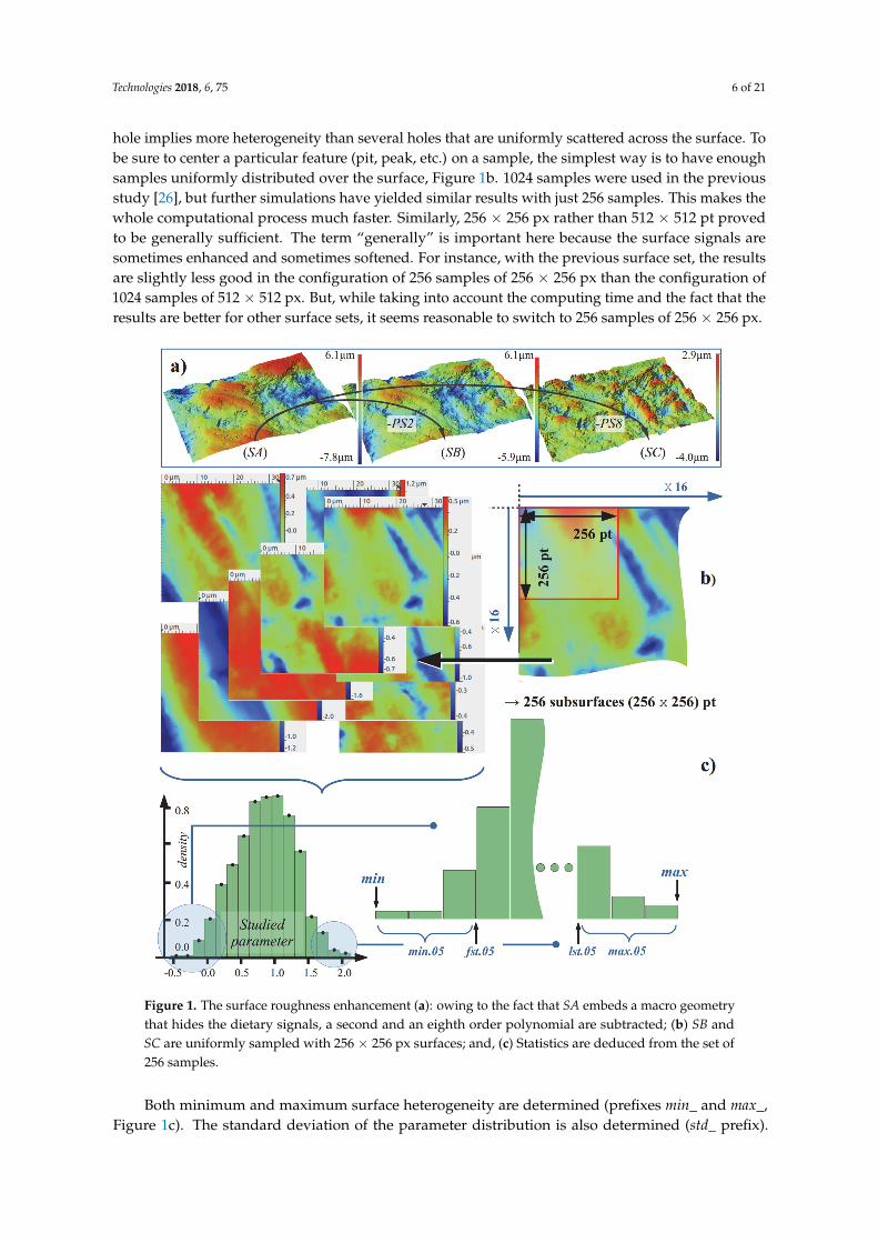
Following the procedure that is defined by Francisco et al. [26], the primary extracted surface S1is first numerically cleaned of any abnormal peaks. The resulting surface is called SA. Then, Figure 1a,considering the tooth surface geometry as a second order polynomial (PS2), the latter is subtracted viaa least square approximation, yielding the surface SB. PS2 could be deemed sufficient due to the smallarea measured (0.2 mm), as dental facets are concave or convex with a single preferred axis. However,in order to enhance the finest scale roughness, the same operation is applied to SA with an eighthorder polynomial (PS8), which creates SC. It must be noted that the order of the polynomial appliesto each direction, and it must not be confused with the maximum polynomial order as proposed bysome software.
The authors of this study have investigated all of the orders, from one to nine, for a wide rangeof surfaces and the analysis revealed no clear advantage in using a second order polynomial ratherthan a third order for SB. The same goes for SC, a ninth or seventh order polynomial is sometimesbetter. Therefore, the authors chose to keep the two orders, two and eight. Working on SC is possiblysufficient because it makes the roughness clearer, however an eighth order polynomial can erase wavyfeatures from SA, which is a loss of information.
Following the SSFA parameters HAsfc(n2) (Asfc heterogeneity through n2 cells), as proposed byScott et al. [39], the heterogeneity of a surface is related to the spatial distribution of its features: a single
Technologies 2018, 6, 75 6 of 21
hole implies more heterogeneity than several holes that are uniformly scattered across the surface. Tobe sure to center a particular feature (pit, peak, etc.) on a sample, the simplest way is to have enoughsamples uniformly distributed over the surface, Figure 1b. 1024 samples were used in the previousstudy [26], but further simulations have yielded similar results with just 256 samples. This makes thewhole computational process much faster. Similarly, 256 × 256 px rather than 512 × 512 pt provedto be generally sufficient. The term “generally” is important here because the surface signals aresometimes enhanced and sometimes softened. For instance, with the previous surface set, the resultsare slightly less good in the configuration of 256 samples of 256 × 256 px than the configuration of1024 samples of 512 × 512 px. But, while taking into account the computing time and the fact that theresults are better for other surface sets, it seems reasonable to switch to 256 samples of 256 × 256 px.
Technologies 2018, 6, x FOR PEER REVIEW 6 of 21
have enough samples uniformly distributed over the surface, Figure 1b. 1024 samples were used in
the previous study [26], but further simulations have yielded similar results with just 256 samples.
This makes the whole computational process much faster. Similarly, 256 × 256 px rather than 512 ×
512 pt proved to be generally sufficient. The term “generally” is important here because the surface
signals are sometimes enhanced and sometimes softened. For instance, with the previous surface set,
the results are slightly less good in the configuration of 256 samples of 256 × 256 px than the
configuration of 1024 samples of 512 × 512 px. But, while taking into account the computing time and
the fact that the results are better for other surface sets, it seems reasonable to switch to 256 samples
of 256 × 256 px.
Figure 1. The surface roughness enhancement (a): owing to the fact that SA embeds a macro geometry
that hides the dietary signals, a second and an eighth order polynomial are subtracted; (b) SB and SC
are uniformly sampled with 256 × 256 px surfaces; and, (c) Statistics are deduced from the set of 256
samples.
Both minimum and maximum surface heterogeneity are determined (prefixes min_ and max_,
Figure 1c). The standard deviation of the parameter distribution is also determined (std_ prefix). The
“central” values, or mean and median, being an entire surface signature, are also determined (mean_
and med_ prefixes).
Figure 1. The surface roughness enhancement (a): owing to the fact that SA embeds a macro geometrythat hides the dietary signals, a second and an eighth order polynomial are subtracted; (b) SB andSC are uniformly sampled with 256 × 256 px surfaces; and, (c) Statistics are deduced from the set of256 samples.
Both minimum and maximum surface heterogeneity are determined (prefixes min_ and max_,Figure 1c). The standard deviation of the parameter distribution is also determined (std_ prefix).
Technologies 2018, 6, 75 7 of 21
The “central” values, or mean and median, being an entire surface signature, are also determined(mean_ and med_ prefixes).
In order to be more robust when defining the extrema of the parameter distribution, the quantile5% is used. fst.05_ refers to the 5% quantile and lst.05_ to the 95% quantile. However, the robustnessmust not hide extreme values that might not be outliers. That is why min.05_ and max.05_ areintroduced. They are the mean of the values below (and respectively above) the quantile 5% (and95%, respectively), Figure 1c. As a trade-off between 5% and 50%, the quantile 25% is also used:fst.25_ stands for the first quartile and lst.25_ stands for the last quartile. In the same way as before,min.25_ and max.25_ are also used. In the eventuality that the parameter distribution shape couldbe the signature of a particular diet, the skewness and kurtosis (skw_ and kurt_ respectively) arealso calculated.
To conclude on the statistics that are deduced from the 256 samples of a given surface, eachparameter generates 15 “sub-parameters”. It is obvious that some of them are strongly correlated, butit does not affect the process of finding those that are the most discriminative.
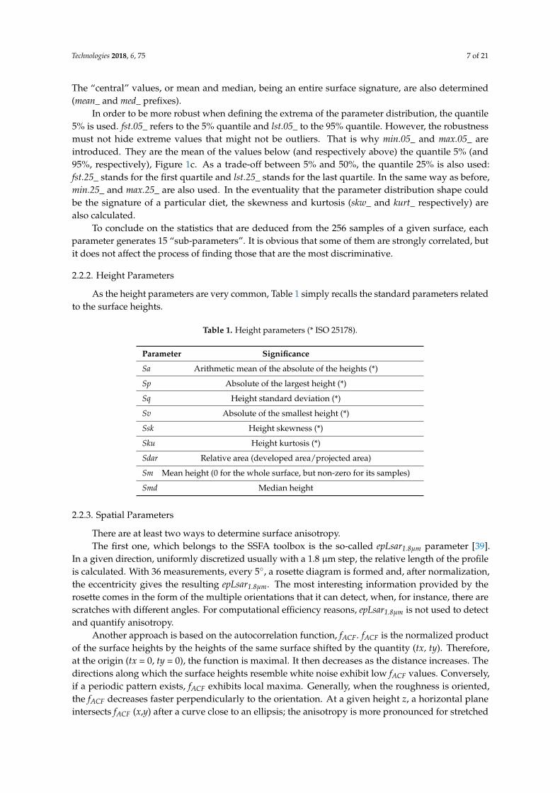
2.2.2. Height Parameters
As the height parameters are very common, Table 1 simply recalls the standard parameters relatedto the surface heights.
Table 1. Height parameters (* ISO 25178).
Parameter Significance
Sa Arithmetic mean of the absolute of the heights (*)
Sp Absolute of the largest height (*)
Sq Height standard deviation (*)
Sv Absolute of the smallest height (*)
Ssk Height skewness (*)
Sku Height kurtosis (*)
Sdar Relative area (developed area/projected area)
Sm Mean height (0 for the whole surface, but non-zero for its samples)
Smd Median height
2.2.3. Spatial Parameters
There are at least two ways to determine surface anisotropy.The first one, which belongs to the SSFA toolbox is the so-called epLsar1.8µm parameter [39].
In a given direction, uniformly discretized usually with a 1.8 µm step, the relative length of the profileis calculated. With 36 measurements, every 5◦, a rosette diagram is formed and, after normalization,the eccentricity gives the resulting epLsar1.8µm. The most interesting information provided by therosette comes in the form of the multiple orientations that it can detect, when, for instance, there arescratches with different angles. For computational efficiency reasons, epLsar1.8µm is not used to detectand quantify anisotropy.
Another approach is based on the autocorrelation function, fACF. fACF is the normalized productof the surface heights by the heights of the same surface shifted by the quantity (tx, ty). Therefore,at the origin (tx = 0, ty = 0), the function is maximal. It then decreases as the distance increases. Thedirections along which the surface heights resemble white noise exhibit low fACF values. Conversely,if a periodic pattern exists, fACF exhibits local maxima. Generally, when the roughness is oriented,the fACF decreases faster perpendicularly to the orientation. At a given height z, a horizontal planeintersects fACF (x,y) after a curve close to an ellipsis; the anisotropy is more pronounced for stretched
Technologies 2018, 6, 75 8 of 21
ellipses. Three parameters are hence defined: Rmax the major ellipsis radius, Sal the minor ellipsisradius, and Str−1 the ratio Rmax/Sal. An illustration is provided in ESM, Figure S1.
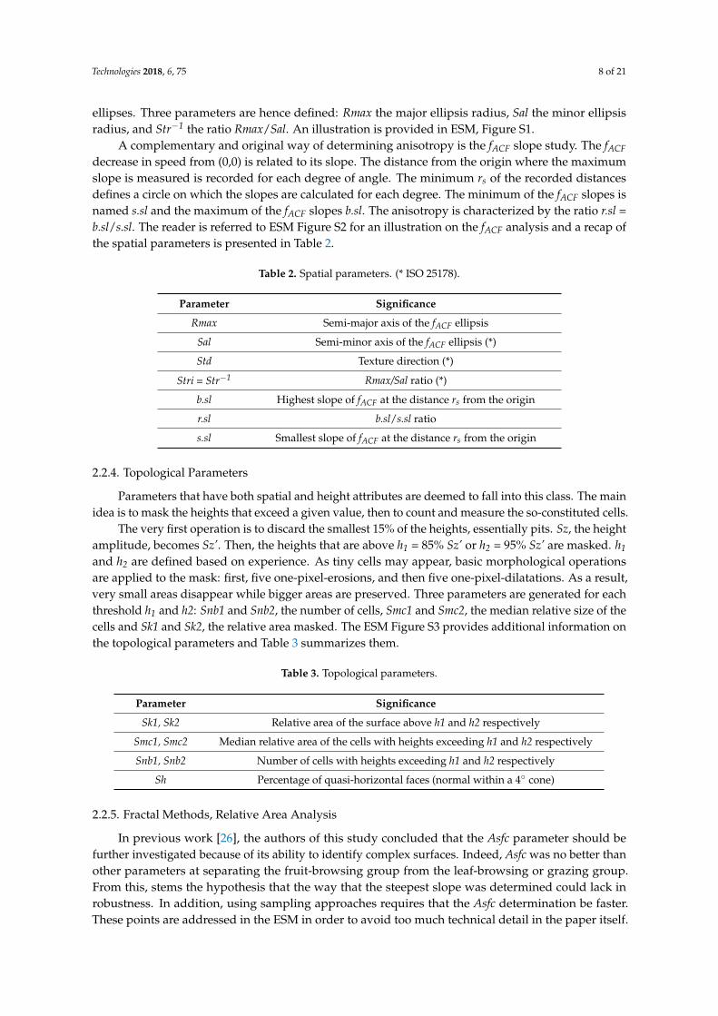
A complementary and original way of determining anisotropy is the fACF slope study. The fACFdecrease in speed from (0,0) is related to its slope. The distance from the origin where the maximumslope is measured is recorded for each degree of angle. The minimum rs of the recorded distancesdefines a circle on which the slopes are calculated for each degree. The minimum of the fACF slopes isnamed s.sl and the maximum of the fACF slopes b.sl. The anisotropy is characterized by the ratio r.sl =b.sl/s.sl. The reader is referred to ESM Figure S2 for an illustration on the fACF analysis and a recap ofthe spatial parameters is presented in Table 2.
Table 2. Spatial parameters. (* ISO 25178).
Parameter Significance
Rmax Semi-major axis of the fACF ellipsis
Sal Semi-minor axis of the fACF ellipsis (*)
Std Texture direction (*)
Stri = Str−1 Rmax/Sal ratio (*)
b.sl Highest slope of fACF at the distance rs from the origin
r.sl b.sl/s.sl ratio
s.sl Smallest slope of fACF at the distance rs from the origin
2.2.4. Topological Parameters
Parameters that have both spatial and height attributes are deemed to fall into this class. The mainidea is to mask the heights that exceed a given value, then to count and measure the so-constituted cells.
The very first operation is to discard the smallest 15% of the heights, essentially pits. Sz, the heightamplitude, becomes Sz’. Then, the heights that are above h1 = 85% Sz’ or h2 = 95% Sz’ are masked. h1and h2 are defined based on experience. As tiny cells may appear, basic morphological operationsare applied to the mask: first, five one-pixel-erosions, and then five one-pixel-dilatations. As a result,very small areas disappear while bigger areas are preserved. Three parameters are generated for eachthreshold h1 and h2: Snb1 and Snb2, the number of cells, Smc1 and Smc2, the median relative size of thecells and Sk1 and Sk2, the relative area masked. The ESM Figure S3 provides additional information onthe topological parameters and Table 3 summarizes them.
Table 3. Topological parameters.
Parameter Significance
Sk1, Sk2 Relative area of the surface above h1 and h2 respectively
Smc1, Smc2 Median relative area of the cells with heights exceeding h1 and h2 respectively
Snb1, Snb2 Number of cells with heights exceeding h1 and h2 respectively
Sh Percentage of quasi-horizontal faces (normal within a 4◦ cone)
2.2.5. Fractal Methods, Relative Area Analysis
In previous work [26], the authors of this study concluded that the Asfc parameter should befurther investigated because of its ability to identify complex surfaces. Indeed, Asfc was no better thanother parameters at separating the fruit-browsing group from the leaf-browsing or grazing group.From this, stems the hypothesis that the way that the steepest slope was determined could lack inrobustness. In addition, using sampling approaches requires that the Asfc determination be faster.These points are addressed in the ESM in order to avoid too much technical detail in the paper itself.
Technologies 2018, 6, 75 9 of 21
As a result of the study, an efficient procedure for the determination of Asfc is proposed along with thesampling characteristics: 256 samples of 512 × 512 px subsurfaces.
2.2.6. The Automatic Discriminative Procedure
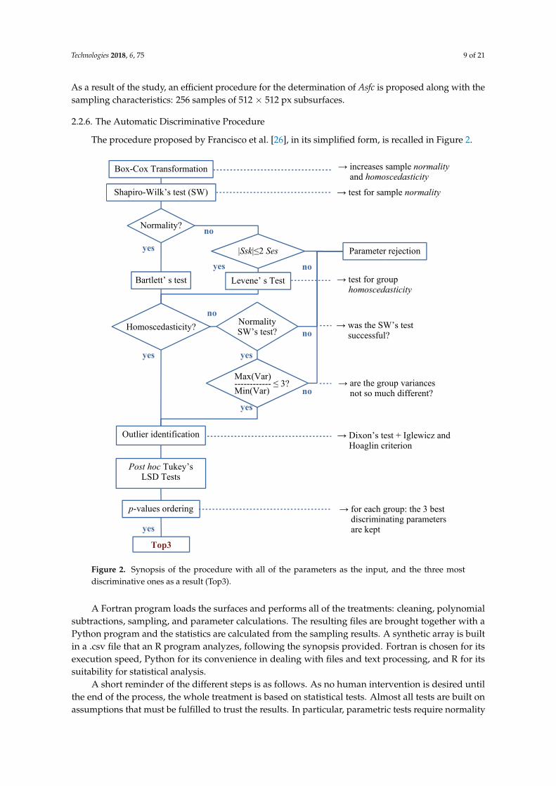
The procedure proposed by Francisco et al. [26], in its simplified form, is recalled in Figure 2.
Technologies 2018, 6, x FOR PEER REVIEW 9 of 21
itself. As a result of the study, an efficient procedure for the determination of Asfc is proposed along
with the sampling characteristics: 256 samples of 512 × 512 px subsurfaces.
2.2.6. The Automatic Discriminative Procedure
The procedure proposed by Francisco et al. [26], in its simplified form, is recalled in Figure 2.
Figure 2. Synopsis of the procedure with all of the parameters as the input, and the three most
discriminative ones as a result (Top3).
A Fortran program loads the surfaces and performs all of the treatments: cleaning, polynomial
subtractions, sampling, and parameter calculations. The resulting files are brought together with a
Python program and the statistics are calculated from the sampling results. A synthetic array is built
in a .csv file that an R program analyzes, following the synopsis provided. Fortran is chosen for its
execution speed, Python for its convenience in dealing with files and text processing, and R for its
suitability for statistical analysis.
A short reminder of the different steps is as follows. As no human intervention is desired until
the end of the process, the whole treatment is based on statistical tests. Almost all tests are built on
assumptions that must be fulfilled to trust the results. In particular, parametric tests require normality
and homoscedasticity properties. To maximize the chance of being eligible for the tests, the
parameters are Box‐Cox transformed instead of systematically log‐transformed. What differs from
the norm is the presence of retrieval steps: when tests reject a parameter, that parameter can be called
Box-Cox Transformation
Shapiro-Wilk’s test (SW)
Normality?
Bartlett’ s test Levene’ s Test
Post hoc Tukey’sLSD Tests
p-values ordering
Homoscedasticity?
→ test for sample normality
→ increases sample normality and homoscedasticity
→ test for group homoscedasticity
yes
no
→ for each group: the 3 best discriminating parameters are kept
Top3
|Ssk|≤2 Ses Parameter rejection
yes no
Max(Var) ------------ ≤ 3? Min(Var)
NormalitySW’s test?
no
yes yes
no
no
yes
→ was the SW’s test successful?
→ are the group variances not so much different?
yes
Outlier identification → Dixon’s test + Iglewicz and Hoaglin criterion
Figure 2. Synopsis of the procedure with all of the parameters as the input, and the three mostdiscriminative ones as a result (Top3).
A Fortran program loads the surfaces and performs all of the treatments: cleaning, polynomialsubtractions, sampling, and parameter calculations. The resulting files are brought together with aPython program and the statistics are calculated from the sampling results. A synthetic array is builtin a .csv file that an R program analyzes, following the synopsis provided. Fortran is chosen for itsexecution speed, Python for its convenience in dealing with files and text processing, and R for itssuitability for statistical analysis.
A short reminder of the different steps is as follows. As no human intervention is desired untilthe end of the process, the whole treatment is based on statistical tests. Almost all tests are built onassumptions that must be fulfilled to trust the results. In particular, parametric tests require normality
Technologies 2018, 6, 75 10 of 21
and homoscedasticity properties. To maximize the chance of being eligible for the tests, the parametersare Box-Cox transformed instead of systematically log-transformed. What differs from the norm is thepresence of retrieval steps: when tests reject a parameter, that parameter can be called into questionregarding the tests that follow. Rules of thumb, based on expert experience, are introduced to softentest rigidity. Once the parameters are declared to be test-compliant, questions arise about post hocanalyses and the necessity of a preceding ANOVA test. However, based on the previous work by theauthors of this study, a post hoc analysis is carried out directly. Because Fisher’s Least SignificantDifference (LSD) test is less conservative than Tuckey’s Honest Significant Difference (HSD) version,the former is preferred.
The choice of parametric tests is justified in Francisco et al. [26], and is recapped hereafter. Basedon experience, the parametric tests are quiet robust to non-normality. Moreover, non-parametric tests,such as Kruskal-Wallis’, sometimes reveal to be less robust against heteroscedasticity. It is nonethelessto be acknowledged that, for very small samples, non parametric tests are better suited. But where isthe frontier between ‘small’ and ‘very small’? We suppose here that 10 individuals is indeed a smallsample but still acceptable for parametric tests. To conclude on this point, the methodology that isproposed here ends with a graphical representation of the sets, which limits erroneous conclusions.
Another debate is about the p-value meaning and how best to draw conclusions about it. Onceagain, the choice is made from experience: until now, the lowest p-values have provided the mostdiscriminating parameters. Therefore, the Top3 parameters will be selected based upon their p-value.In most cases treated below, three parameters appear to be enough to choose two low-correlatedparameters for a biplot. The procedure aims to assist the researcher in finding the most discriminatingparameters rather than be a substitute for him. Therefore, if the three proposed parameters are toogreatly correlated, the next parameters in the p-value ordered list should be considered.
3. Results
The graphs present back-transformed data. Indeed, to increase the eligibility for F-tests, theparameters are all Box-Cox transformed. However, once the parameter selection has ended, there is noneed to keep the transformation. When points are circled and labeled with a letter on the graphs, thereader is referred to the ESM to see the corresponding surface.
3.1. T1, Old World Monkeys
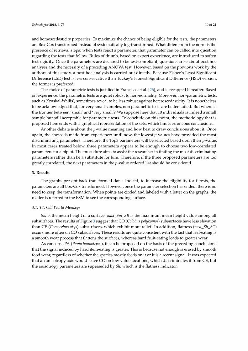
Sm is the mean height of a surface. max_Sm_SB is the maximum mean height value among allsubsurfaces. The results of Figure 3 suggest that CO (Colobus polykomos) subsurfaces have less elevationthan CE (Cercocebus atys) subsurfaces, which exhibit more relief. In addition, flatness (med_Sh_SC)occurs more often on CO subsurfaces. These results are quite consistent with the fact that leaf-eating isa smooth wear process that flattens the surfaces, whereas hard fruit-eating leads to greater wear.
As concerns PA (Papio hamadryas), it can be proposed on the basis of the preceding conclusionsthat the signal induced by hard item-eating is greater. This is because not enough is erased by smoothfood wear, regardless of whether the species mostly feeds on it or it is a recent signal. It was expectedthat an anisotropy axis would leave CO on low value locations, which discriminates it from CE, butthe anisotropy parameters are superseded by Sh, which is the flatness indicator.
Technologies 2018, 6, 75 11 of 21
Technologies 2018, 6, x FOR PEER REVIEW 10 of 21
into question regarding the tests that follow. Rules of thumb, based on expert experience, are
introduced to soften test rigidity. Once the parameters are declared to be test‐compliant, questions
arise about post hoc analyses and the necessity of a preceding ANOVA test. However, based on the
previous work by the authors of this study, a post hoc analysis is carried out directly. Because Fisher’s
Least Significant Difference (LSD) test is less conservative than Tuckey’s Honest Significant
Difference (HSD) version, the former is preferred.
The choice of parametric tests is justified in Francisco et al. [26], and is recapped hereafter. Based
on experience, the parametric tests are quiet robust to non‐normality. Moreover, non‐parametric
tests, such as Kruskal‐Wallis’, sometimes reveal to be less robust against heteroscedasticity. It is
nonetheless to be acknowledged that, for very small samples, non parametric tests are better suited.
But where is the frontier between ‘small’ and ‘very small’? We suppose here that 10 individuals is
indeed a small sample but still acceptable for parametric tests. To conclude on this point, the
methodology that is proposed here ends with a graphical representation of the sets, which limits
erroneous conclusions.
Another debate is about the p‐value meaning and how best to draw conclusions about it. Once
again, the choice is made from experience: until now, the lowest p‐values have provided the most
discriminating parameters. Therefore, the Top3 parameters will be selected based upon their p‐value.
In most cases treated below, three parameters appear to be enough to choose two low‐correlated
parameters for a biplot. The procedure aims to assist the researcher in finding the most discriminating
parameters rather than be a substitute for him. Therefore, if the three proposed parameters are too
greatly correlated, the next parameters in the p‐value ordered list should be considered.
3. Results
The graphs present back‐transformed data. Indeed, to increase the eligibility for F‐tests, the
parameters are all Box‐Cox transformed. However, once the parameter selection has ended, there is
no need to keep the transformation. When points are circled and labeled with a letter on the graphs,
the reader is referred to the ESM to see the corresponding surface.
3.1. T1, Old World Monkeys
Sm is the mean height of a surface. max_Sm_SB is the maximum mean height value among all
subsurfaces. The results of Figure 3 suggest that CO (Colobus polykomos) subsurfaces have less
elevation than CE (Cercocebus atys) subsurfaces, which exhibit more relief. In addition, flatness
(med_Sh_SC) occurs more often on CO subsurfaces. These results are quite consistent with the fact
that leaf‐eating is a smooth wear process that flattens the surfaces, whereas hard fruit‐eating leads to
greater wear.
(a) (b)
Figure 3. Old World Monkeys, most discriminating parameters. max_Sm_SB p-value for CE-CO:6.95 × 10⁻¹³, and for CO-PA: 1.05 × 10⁻⁹ (a) There is a clear boundary between Colobus (CO) andCercocebus (CE). The surfaces related to the points (A) and (B) are represented in the ESM; (b)Box-whiskers representation of the best parameter (heteroscedasticity is clear, but it must be noted thatthe parameters are back-transformed for the graph presentation).
3.2. T2, European Ruminants
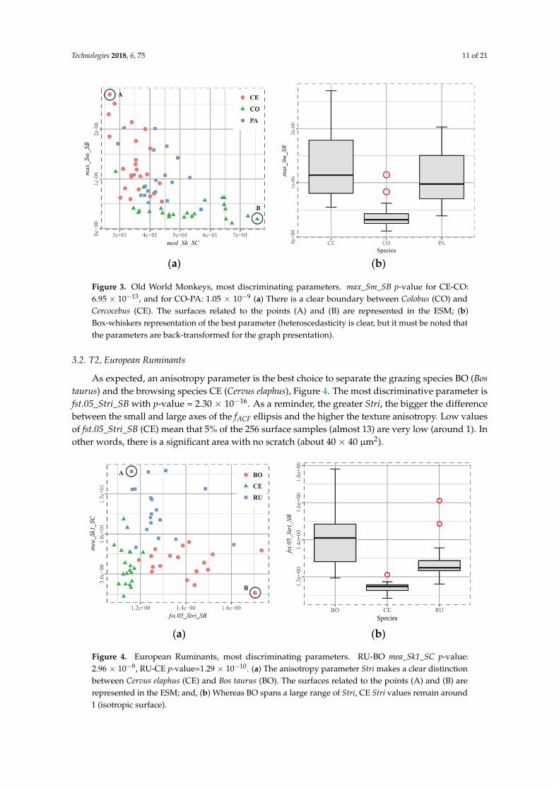
As expected, an anisotropy parameter is the best choice to separate the grazing species BO (Bostaurus) and the browsing species CE (Cervus elaphus), Figure 4. The most discriminative parameter isfst.05_Stri_SB with p-value = 2.30 × 10⁻¹⁶. As a reminder, the greater Stri, the bigger the differencebetween the small and large axes of the fACF ellipsis and the higher the texture anisotropy. Low valuesof fst.05_Stri_SB (CE) mean that 5% of the 256 surface samples (almost 13) are very low (around 1). Inother words, there is a significant area with no scratch (about 40 × 40 µm2).
Technologies 2018, 6, x FOR PEER REVIEW 11 of 21
Figure 3. Old World Monkeys, most discriminating parameters. max_Sm_SB p‐value for CE‐CO: 6.95
× 10−13, and for CO‐PA: 1.05 × 10⁻⁹ (a) There is a clear boundary between Colobus (CO) and Cercocebus
(CE). The surfaces related to the points (A) and (B) are represented in the ESM; (b) Box‐whiskers
representation of the best parameter (heteroscedasticity is clear, but it must be noted that the
parameters are back‐transformed for the graph presentation).
As concerns PA (Papio hamadryas), it can be proposed on the basis of the preceding conclusions
that the signal induced by hard item‐eating is greater. This is because not enough is erased by smooth
food wear, regardless of whether the species mostly feeds on it or it is a recent signal. It was expected
that an anisotropy axis would leave CO on low value locations, which discriminates it from CE, but
the anisotropy parameters are superseded by Sh, which is the flatness indicator.
3.2. T2, European Ruminants
As expected, an anisotropy parameter is the best choice to separate the grazing species BO (Bos
taurus) and the browsing species CE (Cervus elaphus), Figure 4. The most discriminative parameter is
fst.05_Stri_SB with p‐value = 2.30 × 10⁻¹⁶. As a reminder, the greater Stri, the bigger the difference
between the small and large axes of the fACF ellipsis and the higher the texture anisotropy. Low values
of fst.05_Stri_SB (CE) mean that 5% of the 256 surface samples (almost 13) are very low (around 1).
In other words, there is a significant area with no scratch (about 40 × 40 μm²).
The parameter that helps in separating the mixed habit species RU (Rupicapra rupicapra) from
the others is Sk1, which measures the surface above 85% Sz’. It may suggest that significant wear has
created relief on the tooth surface, and that softer wear has occurred, decreasing in this way the peak
heights. Conversely, it could also be that little wear has occurred on the tooth.
(a) (b)
Figure 4. European Ruminants, most discriminating parameters. RU‐BO mea_Sk1_SC p‐value: 2.96 ×
10−9, RU‐CE p‐value=1.29 × 10⁻¹⁰. (a) The anisotropy parameter Stri makes a clear distinction between
Cervus elaphus (CE) and Bos taurus (BO). The surfaces related to the points (A) and (B) are represented
in the ESM; and, (b) Whereas BO spans a large range of Stri, CE Stri values remain around 1 (isotropic
surface).
3.3. T3, African Ruminants
Once again, the anisotropy parameters are good candidates to separate the browsing TS
(Tragelaphus scriptus) and the fruit‐eating CS (Cephalophus silvicultor) from the grazing AB (Alcelaphus
buselaphus) species, Figure 5. It is nonetheless important to note that another discriminative parameter
is the kurtosis Sku, as also found by Francisco et al. [26], with an even better p‐value (3.71 × 10⁻⁷).
However, it separates less clearly AB and CS (p‐value = 4.10 × 10⁻³ vs. 1.27 × 10⁻⁶ for r.sl, the facf slope
ratio).
Figure 4. European Ruminants, most discriminating parameters. RU-BO mea_Sk1_SC p-value:2.96 × 10⁻⁹, RU-CE p-value=1.29 × 10⁻¹⁰. (a) The anisotropy parameter Stri makes a clear distinctionbetween Cervus elaphus (CE) and Bos taurus (BO). The surfaces related to the points (A) and (B) arerepresented in the ESM; and, (b) Whereas BO spans a large range of Stri, CE Stri values remain around1 (isotropic surface).
Technologies 2018, 6, 75 12 of 21
The parameter that helps in separating the mixed habit species RU (Rupicapra rupicapra) fromthe others is Sk1, which measures the surface above 85% Sz’. It may suggest that significant wear hascreated relief on the tooth surface, and that softer wear has occurred, decreasing in this way the peakheights. Conversely, it could also be that little wear has occurred on the tooth.
3.3. T3, African Ruminants
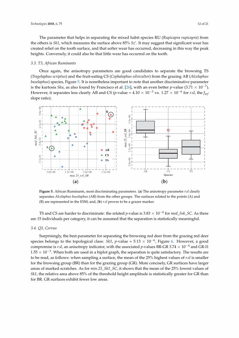
Once again, the anisotropy parameters are good candidates to separate the browsing TS(Tragelaphus scriptus) and the fruit-eating CS (Cephalophus silvicultor) from the grazing AB (Alcelaphusbuselaphus) species, Figure 5. It is nonetheless important to note that another discriminative parameteris the kurtosis Sku, as also found by Francisco et al. [26], with an even better p-value (3.71 × 10⁻⁷).However, it separates less clearly AB and CS (p-value = 4.10 × 10⁻³ vs. 1.27 × 10⁻⁶ for r.sl, the facfslope ratio).
Technologies 2018, 6, x FOR PEER REVIEW 12 of 21
TS and CS are harder to discriminate: the related p‐value is 3.83 × 10⁻⁴ for med_Ssk_SC. As there
are 15 individuals per category, it can be assumed that the separation is statistically meaningful.
(a) (b)
Figure 5. African Ruminants, most discriminating parameters. (a) The anisotropy parameter r.sl
clearly separates Alcelaphus buselaphus (AB) from the other groups. The surfaces related to the points
(A) and (B) are represented in the ESM; and, (b) r.sl proves to be a grazer marker.
3.4. Q1, Cervus
Surprisingly, the best parameter for separating the browsing red deer from the grazing red deer
species belongs to the topological class: Sk1, p‐value = 5.13 × 10⁻⁶, Figure 6. However, a good
compromise is r.sl, an anisotropy indicator, with the associated p‐values BR‐GR 3.74 × 10⁻⁴ and GR‐I1
1.55 × 10⁻³. When both are used in a biplot graph, the separation is quite satisfactory. The results are
to be read, as follows: when sampling a surface, the mean of the 25% highest values of r.sl is smaller
for the browsing group (BR) than for the grazing group (GR). More concisely, GR surfaces have larger
areas of marked scratches. As for min.25_Sk1_SC, it shows that the mean of the 25% lowest values of
Sk1, the relative area above 85% of the threshold height amplitude is statistically greater for GR than
for BR. GR surfaces exhibit fewer low areas.
(a) (b)
Figure 6. Red deer, most discriminating parameters. (a) The anisotropy parameter r.sl together with
the topology parameter Sk1 are able to separate the browsing red deer (BR) from the grazing red deer
(GR). The surfaces related to the points (A) and (B) are represented in the ESM; and, (b) Here, Sk1 is
a browser marker.
Figure 5. African Ruminants, most discriminating parameters. (a) The anisotropy parameter r.sl clearlyseparates Alcelaphus buselaphus (AB) from the other groups. The surfaces related to the points (A) and(B) are represented in the ESM; and, (b) r.sl proves to be a grazer marker.
TS and CS are harder to discriminate: the related p-value is 3.83 × 10⁻⁴ for med_Ssk_SC. As thereare 15 individuals per category, it can be assumed that the separation is statistically meaningful.
3.4. Q1, Cervus
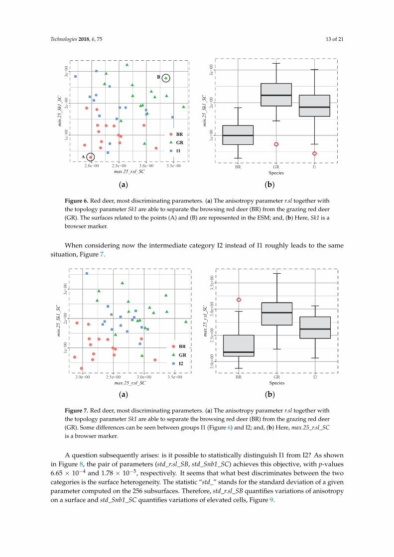
Surprisingly, the best parameter for separating the browsing red deer from the grazing red deerspecies belongs to the topological class: Sk1, p-value = 5.13 × 10⁻⁶, Figure 6. However, a goodcompromise is r.sl, an anisotropy indicator, with the associated p-values BR-GR 3.74 × 10⁻⁴ and GR-I11.55 × 10−3. When both are used in a biplot graph, the separation is quite satisfactory. The results areto be read, as follows: when sampling a surface, the mean of the 25% highest values of r.sl is smallerfor the browsing group (BR) than for the grazing group (GR). More concisely, GR surfaces have largerareas of marked scratches. As for min.25_Sk1_SC, it shows that the mean of the 25% lowest values ofSk1, the relative area above 85% of the threshold height amplitude is statistically greater for GR thanfor BR. GR surfaces exhibit fewer low areas.
Technologies 2018, 6, 75 13 of 21
Technologies 2018, 6, x FOR PEER REVIEW 12 of 21
TS and CS are harder to discriminate: the related p‐value is 3.83 × 10⁻⁴ for med_Ssk_SC. As there
are 15 individuals per category, it can be assumed that the separation is statistically meaningful.
(a) (b)
Figure 5. African Ruminants, most discriminating parameters. (a) The anisotropy parameter r.sl
clearly separates Alcelaphus buselaphus (AB) from the other groups. The surfaces related to the points
(A) and (B) are represented in the ESM; and, (b) r.sl proves to be a grazer marker.
3.4. Q1, Cervus
Surprisingly, the best parameter for separating the browsing red deer from the grazing red deer
species belongs to the topological class: Sk1, p‐value = 5.13 × 10⁻⁶, Figure 6. However, a good
compromise is r.sl, an anisotropy indicator, with the associated p‐values BR‐GR 3.74 × 10⁻⁴ and GR‐I1
1.55 × 10⁻³. When both are used in a biplot graph, the separation is quite satisfactory. The results are
to be read, as follows: when sampling a surface, the mean of the 25% highest values of r.sl is smaller
for the browsing group (BR) than for the grazing group (GR). More concisely, GR surfaces have larger
areas of marked scratches. As for min.25_Sk1_SC, it shows that the mean of the 25% lowest values of
Sk1, the relative area above 85% of the threshold height amplitude is statistically greater for GR than
for BR. GR surfaces exhibit fewer low areas.
(a) (b)
Figure 6. Red deer, most discriminating parameters. (a) The anisotropy parameter r.sl together with
the topology parameter Sk1 are able to separate the browsing red deer (BR) from the grazing red deer
(GR). The surfaces related to the points (A) and (B) are represented in the ESM; and, (b) Here, Sk1 is
a browser marker.
Figure 6. Red deer, most discriminating parameters. (a) The anisotropy parameter r.sl together withthe topology parameter Sk1 are able to separate the browsing red deer (BR) from the grazing red deer(GR). The surfaces related to the points (A) and (B) are represented in the ESM; and, (b) Here, Sk1 is abrowser marker.
When considering now the intermediate category I2 instead of I1 roughly leads to the samesituation, Figure 7.
Technologies 2018, 6, x FOR PEER REVIEW 13 of 21
When considering now the intermediate category I2 instead of I1 roughly leads to the same
situation, Figure 7.
(a) (b)
Figure 7. Red deer, most discriminating parameters. (a) The anisotropy parameter r.sl together with
the topology parameter Sk1 are able to separate the browsing red deer (BR) from the grazing red deer
(GR). Some differences can be seen between groups I1 (Figure 6) and I2; and, (b) Here, max.25_r.sl_SC
is a browser marker.
A question subsequently arises: is it possible to statistically distinguish I1 from I2? As shown in
Figure 8, the pair of parameters (std_r.sl_SB, std_Snb1_SC) achieves this objective, with p‐values 6.65
× 10−4 and 1.78 × 10⁻⁵, respectively. It seems that what best discriminates between the two categories
is the surface heterogeneity. The statistic “std_” stands for the standard deviation of a given
parameter computed on the 256 subsurfaces. Therefore, std_r.sl_SB quantifies variations of
anisotropy on a surface and std_Snb1_SC quantifies variations of elevated cells, Figure 9.
(a) (b)
Figure 8. Red deer I1 and I2, most discriminating parameters. (a) The anisotropy parameter r.sl
together with the topology parameter Snb1 make it possible to separate them; and, (b) std_Snb1_SC is
statistically lower for I2 than for I1.
Figure 7. Red deer, most discriminating parameters. (a) The anisotropy parameter r.sl together withthe topology parameter Sk1 are able to separate the browsing red deer (BR) from the grazing red deer(GR). Some differences can be seen between groups I1 (Figure 6) and I2; and, (b) Here, max.25_r.sl_SCis a browser marker.
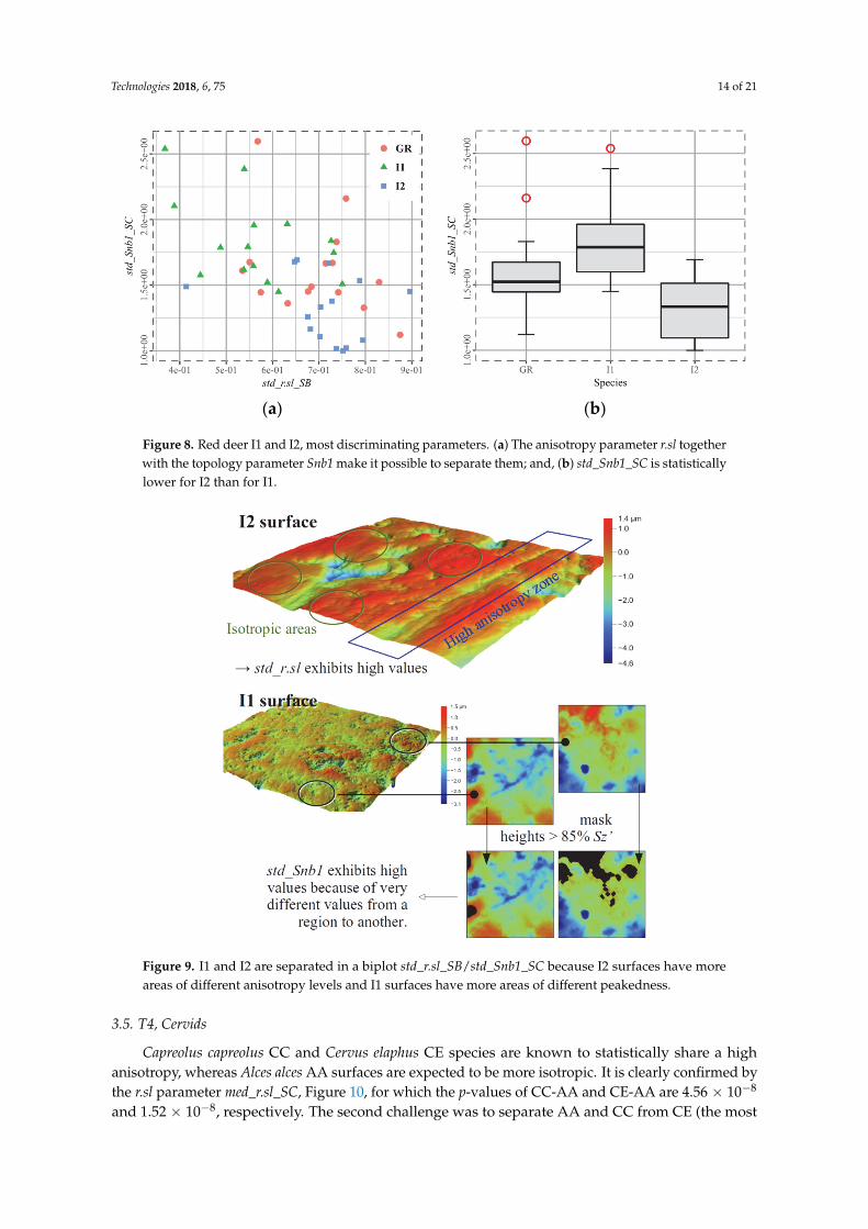
A question subsequently arises: is it possible to statistically distinguish I1 from I2? As shownin Figure 8, the pair of parameters (std_r.sl_SB, std_Snb1_SC) achieves this objective, with p-values6.65 × 10−4 and 1.78 × 10⁻⁵, respectively. It seems that what best discriminates between the twocategories is the surface heterogeneity. The statistic “std_” stands for the standard deviation of a givenparameter computed on the 256 subsurfaces. Therefore, std_r.sl_SB quantifies variations of anisotropyon a surface and std_Snb1_SC quantifies variations of elevated cells, Figure 9.
Technologies 2018, 6, 75 14 of 21
Technologies 2018, 6, x FOR PEER REVIEW 13 of 21
When considering now the intermediate category I2 instead of I1 roughly leads to the same
situation, Figure 7.
(a) (b)
Figure 7. Red deer, most discriminating parameters. (a) The anisotropy parameter r.sl together with
the topology parameter Sk1 are able to separate the browsing red deer (BR) from the grazing red deer
(GR). Some differences can be seen between groups I1 (Figure 6) and I2; and, (b) Here, max.25_r.sl_SC
is a browser marker.
A question subsequently arises: is it possible to statistically distinguish I1 from I2? As shown in
Figure 8, the pair of parameters (std_r.sl_SB, std_Snb1_SC) achieves this objective, with p‐values 6.65
× 10−4 and 1.78 × 10⁻⁵, respectively. It seems that what best discriminates between the two categories
is the surface heterogeneity. The statistic “std_” stands for the standard deviation of a given
parameter computed on the 256 subsurfaces. Therefore, std_r.sl_SB quantifies variations of
anisotropy on a surface and std_Snb1_SC quantifies variations of elevated cells, Figure 9.
(a) (b)
Figure 8. Red deer I1 and I2, most discriminating parameters. (a) The anisotropy parameter r.sl
together with the topology parameter Snb1 make it possible to separate them; and, (b) std_Snb1_SC is
statistically lower for I2 than for I1.
Figure 8. Red deer I1 and I2, most discriminating parameters. (a) The anisotropy parameter r.sl togetherwith the topology parameter Snb1 make it possible to separate them; and, (b) std_Snb1_SC is statisticallylower for I2 than for I1.Technologies 2018, 6, x FOR PEER REVIEW 14 of 21
Figure 9. I1 and I2 are separated in a biplot std_r.sl_SB/std_Snb1_SC because I2 surfaces have more
areas of different anisotropy levels and I1 surfaces have more areas of different peakedness.
3.5. T4, Cervids
Capreolus capreolus CC and Cervus elaphus CE species are known to statistically share a high
anisotropy, whereas Alces alces AA surfaces are expected to be more isotropic. It is clearly confirmed
by the r.sl parameter med_r.sl_SC, Figure 10, for which the p‐values of CC‐AA and CE‐AA are 4.56 ×
10−8 and 1.52 × 10⁻⁸, respectively. The second challenge was to separate AA and CC from CE (the most
prolific grazer). The separation is effective with max_Ssk_SB, for which the p‐values of CE‐AA and
CE‐CC are 7.86 × 10⁻⁵ and 2.68 × 10⁻³, respectively. In addition, CC and CE were not supposed to be
statistically different from an anisotropy viewpoint. This is now confirmed.
(a) (b)
Figure 10. Cervid, most discriminating parameters. (a) The anisotropy parameter r.sl isolates the
browsing moose (AA), the skewness reaches higher values for the red deer (CE); and, (b) med_r.sl_SC
is statistically lower for AA, even if CE spans a wide range of values.
Figure 9. I1 and I2 are separated in a biplot std_r.sl_SB/std_Snb1_SC because I2 surfaces have moreareas of different anisotropy levels and I1 surfaces have more areas of different peakedness.
3.5. T4, Cervids
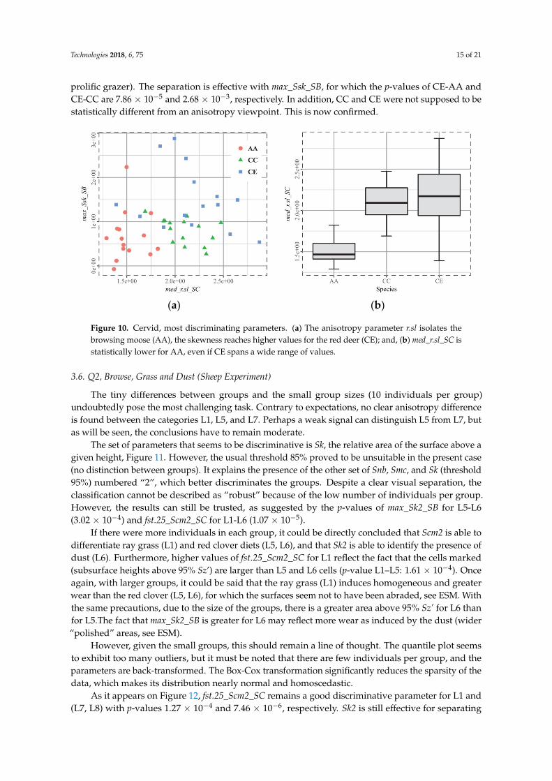
Capreolus capreolus CC and Cervus elaphus CE species are known to statistically share a highanisotropy, whereas Alces alces AA surfaces are expected to be more isotropic. It is clearly confirmed bythe r.sl parameter med_r.sl_SC, Figure 10, for which the p-values of CC-AA and CE-AA are 4.56 × 10⁻⁸
and 1.52 × 10⁻⁸, respectively. The second challenge was to separate AA and CC from CE (the most
Technologies 2018, 6, 75 15 of 21
prolific grazer). The separation is effective with max_Ssk_SB, for which the p-values of CE-AA andCE-CC are 7.86 × 10⁻⁵ and 2.68 × 10⁻³, respectively. In addition, CC and CE were not supposed to bestatistically different from an anisotropy viewpoint. This is now confirmed.
Technologies 2018, 6, x FOR PEER REVIEW 14 of 21
Figure 9. I1 and I2 are separated in a biplot std_r.sl_SB/std_Snb1_SC because I2 surfaces have more
areas of different anisotropy levels and I1 surfaces have more areas of different peakedness.
3.5. T4, Cervids
Capreolus capreolus CC and Cervus elaphus CE species are known to statistically share a high
anisotropy, whereas Alces alces AA surfaces are expected to be more isotropic. It is clearly confirmed
by the r.sl parameter med_r.sl_SC, Figure 10, for which the p‐values of CC‐AA and CE‐AA are 4.56 ×
10−8 and 1.52 × 10⁻⁸, respectively. The second challenge was to separate AA and CC from CE (the most
prolific grazer). The separation is effective with max_Ssk_SB, for which the p‐values of CE‐AA and
CE‐CC are 7.86 × 10⁻⁵ and 2.68 × 10⁻³, respectively. In addition, CC and CE were not supposed to be
statistically different from an anisotropy viewpoint. This is now confirmed.
(a) (b)
Figure 10. Cervid, most discriminating parameters. (a) The anisotropy parameter r.sl isolates the
browsing moose (AA), the skewness reaches higher values for the red deer (CE); and, (b) med_r.sl_SC
is statistically lower for AA, even if CE spans a wide range of values.
Figure 10. Cervid, most discriminating parameters. (a) The anisotropy parameter r.sl isolates thebrowsing moose (AA), the skewness reaches higher values for the red deer (CE); and, (b) med_r.sl_SC isstatistically lower for AA, even if CE spans a wide range of values.
3.6. Q2, Browse, Grass and Dust (Sheep Experiment)
The tiny differences between groups and the small group sizes (10 individuals per group)undoubtedly pose the most challenging task. Contrary to expectations, no clear anisotropy differenceis found between the categories L1, L5, and L7. Perhaps a weak signal can distinguish L5 from L7, butas will be seen, the conclusions have to remain moderate.
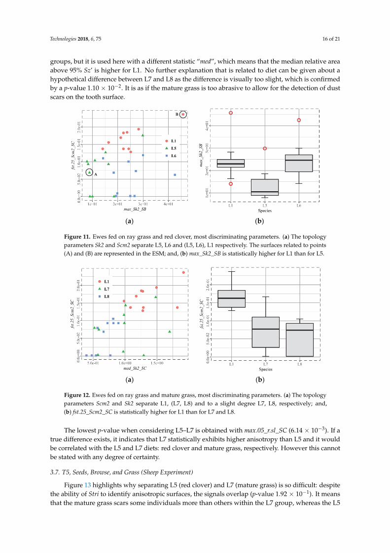
The set of parameters that seems to be discriminative is Sk, the relative area of the surface above agiven height, Figure 11. However, the usual threshold 85% proved to be unsuitable in the present case(no distinction between groups). It explains the presence of the other set of Snb, Smc, and Sk (threshold95%) numbered “2”, which better discriminates the groups. Despite a clear visual separation, theclassification cannot be described as “robust” because of the low number of individuals per group.However, the results can still be trusted, as suggested by the p-values of max_Sk2_SB for L5-L6(3.02 × 10⁻⁴) and fst.25_Scm2_SC for L1-L6 (1.07 × 10⁻⁵).
If there were more individuals in each group, it could be directly concluded that Scm2 is able todifferentiate ray grass (L1) and red clover diets (L5, L6), and that Sk2 is able to identify the presence ofdust (L6). Furthermore, higher values of fst.25_Scm2_SC for L1 reflect the fact that the cells marked(subsurface heights above 95% Sz’) are larger than L5 and L6 cells (p-value L1–L5: 1.61 × 10⁻⁴). Onceagain, with larger groups, it could be said that the ray grass (L1) induces homogeneous and greaterwear than the red clover (L5, L6), for which the surfaces seem not to have been abraded, see ESM. Withthe same precautions, due to the size of the groups, there is a greater area above 95% Sz’ for L6 thanfor L5.The fact that max_Sk2_SB is greater for L6 may reflect more wear as induced by the dust (wider“polished” areas, see ESM).
However, given the small groups, this should remain a line of thought. The quantile plot seemsto exhibit too many outliers, but it must be noted that there are few individuals per group, and theparameters are back-transformed. The Box-Cox transformation significantly reduces the sparsity of thedata, which makes its distribution nearly normal and homoscedastic.
As it appears on Figure 12, fst.25_Scm2_SC remains a good discriminative parameter for L1 and(L7, L8) with p-values 1.27 × 10⁻⁴ and 7.46 × 10⁻⁶, respectively. Sk2 is still effective for separating
Technologies 2018, 6, 75 16 of 21
groups, but it is used here with a different statistic “med”, which means that the median relative areaabove 95% Sz’ is higher for L1. No further explanation that is related to diet can be given about ahypothetical difference between L7 and L8 as the difference is visually too slight, which is confirmedby a p-value 1.10 × 10⁻². It is as if the mature grass is too abrasive to allow for the detection of dustscars on the tooth surface.
Technologies 2018, 6, x FOR PEER REVIEW 15 of 21
3.6. Q2, Browse, Grass and Dust (Sheep Experiment)
The tiny differences between groups and the small group sizes (10 individuals per group)
undoubtedly pose the most challenging task. Contrary to expectations, no clear anisotropy difference
is found between the categories L1, L5, and L7. Perhaps a weak signal can distinguish L5 from L7,
but as will be seen, the conclusions have to remain moderate.
The set of parameters that seems to be discriminative is Sk, the relative area of the surface above
a given height, Figure 11. However, the usual threshold 85% proved to be unsuitable in the present
case (no distinction between groups). It explains the presence of the other set of Snb, Smc, and Sk
(threshold 95%) numbered “2”, which better discriminates the groups. Despite a clear visual
separation, the classification cannot be described as “robust” because of the low number of
individuals per group. However, the results can still be trusted, as suggested by the p‐values of
max_Sk2_SB for L5‐L6 (3.02 × 10⁻⁴) and fst.25_Scm2_SC for L1‐L6 (1.07 × 10⁻⁵).
(a) (b)
Figure 11. Ewes fed on ray grass and red clover, most discriminating parameters. (a) The topology
parameters Sk2 and Scm2 separate L5, L6 and (L5, L6), L1 respectively. The surfaces related to points
(A) and (B) are represented in the ESM; and, (b) max_Sk2_SB is statistically higher for L1 than for L5.
If there were more individuals in each group, it could be directly concluded that Scm2 is able to
differentiate ray grass (L1) and red clover diets (L5, L6), and that Sk2 is able to identify the presence
of dust (L6). Furthermore, higher values of fst.25_Scm2_SC for L1 reflect the fact that the cells marked
(subsurface heights above 95% Sz’) are larger than L5 and L6 cells (p‐value L1–L5: 1.61 × 10⁻⁴). Once
again, with larger groups, it could be said that the ray grass (L1) induces homogeneous and greater
wear than the red clover (L5, L6), for which the surfaces seem not to have been abraded, see ESM.
With the same precautions, due to the size of the groups, there is a greater area above 95% Sz’ for L6
than for L5.The fact that max_Sk2_SB is greater for L6 may reflect more wear as induced by the dust
(wider “polished” areas, see ESM).
However, given the small groups, this should remain a line of thought. The quantile plot seems
to exhibit too many outliers, but it must be noted that there are few individuals per group, and the
parameters are back‐transformed. The Box‐Cox transformation significantly reduces the sparsity of
the data, which makes its distribution nearly normal and homoscedastic.
As it appears on Figure 12, fst.25_Scm2_SC remains a good discriminative parameter for L1 and
(L7, L8) with p‐values 1.27 × 10⁻⁴ and 7.46 × 10⁻⁶, respectively. Sk2 is still effective for separating
groups, but it is used here with a different statistic “med”, which means that the median relative area
above 95% Sz’ is higher for L1. No further explanation that is related to diet can be given about a
hypothetical difference between L7 and L8 as the difference is visually too slight, which is confirmed
by a p‐value 1.10 × 10⁻². It is as if the mature grass is too abrasive to allow for the detection of dust
scars on the tooth surface.
Figure 11. Ewes fed on ray grass and red clover, most discriminating parameters. (a) The topologyparameters Sk2 and Scm2 separate L5, L6 and (L5, L6), L1 respectively. The surfaces related to points(A) and (B) are represented in the ESM; and, (b) max_Sk2_SB is statistically higher for L1 than for L5.
Technologies 2018, 6, x FOR PEER REVIEW 16 of 21
The lowest p‐value when considering L5–L7 is obtained with max.05_r.sl_SC (6.14 × 10⁻³). If a
true difference exists, it indicates that L7 statistically exhibits higher anisotropy than L5 and it would
be correlated with the L5 and L7 diets: red clover and mature grass, respectively. However this cannot
be stated with any degree of certainty.
(a) (b)
Figure 12. Ewes fed on ray grass and mature grass, most discriminating parameters. (a) The topology
parameters Scm2 and Sk2 separate L1, (L7, L8) and to a slight degree L7, L8, respectively; and, (b)
fst.25_Scm2_SC is statistically higher for L1 than for L7 and L8.
3.7. T5, Seeds, Browse, and Grass (Sheep Experiment)
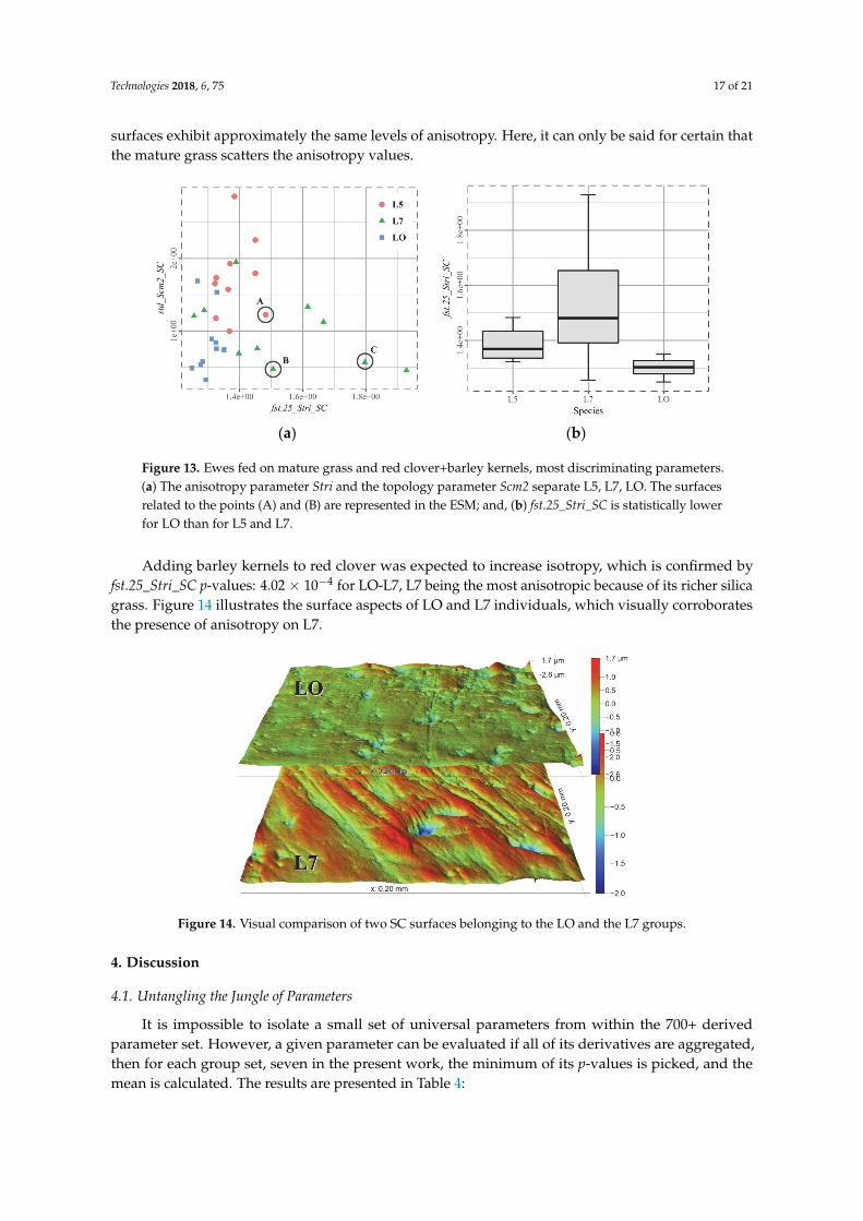
Figure 13 highlights why separating L5 (red clover) and L7 (mature grass) is so difficult: despite
the ability of Stri to identify anisotropic surfaces, the signals overlap (p‐value 1.92 × 10⁻¹). It means
that the mature grass scars some individuals more than others within the L7 group, whereas the L5
surfaces exhibit approximately the same levels of anisotropy. Here, it can only be said for certain that
the mature grass scatters the anisotropy values.
(a) (b)
Figure 13. Ewes fed on mature grass and red clover+barley kernels, most discriminating parameters.
(a) The anisotropy parameter Stri and the topology parameter Scm2 separate L5, L7, LO. The surfaces
related to the points (A) and (B) are represented in the ESM; and, (b) fst.25_Stri_SC is statistically
lower for LO than for L5 and L7.
Figure 12. Ewes fed on ray grass and mature grass, most discriminating parameters. (a) The topologyparameters Scm2 and Sk2 separate L1, (L7, L8) and to a slight degree L7, L8, respectively; and,(b) fst.25_Scm2_SC is statistically higher for L1 than for L7 and L8.
The lowest p-value when considering L5–L7 is obtained with max.05_r.sl_SC (6.14 × 10⁻³). If atrue difference exists, it indicates that L7 statistically exhibits higher anisotropy than L5 and it wouldbe correlated with the L5 and L7 diets: red clover and mature grass, respectively. However this cannotbe stated with any degree of certainty.
3.7. T5, Seeds, Browse, and Grass (Sheep Experiment)
Figure 13 highlights why separating L5 (red clover) and L7 (mature grass) is so difficult: despitethe ability of Stri to identify anisotropic surfaces, the signals overlap (p-value 1.92 × 10⁻¹). It meansthat the mature grass scars some individuals more than others within the L7 group, whereas the L5
Technologies 2018, 6, 75 17 of 21
surfaces exhibit approximately the same levels of anisotropy. Here, it can only be said for certain thatthe mature grass scatters the anisotropy values.
Technologies 2018, 6, x FOR PEER REVIEW 16 of 21
The lowest p‐value when considering L5–L7 is obtained with max.05_r.sl_SC (6.14 × 10⁻³). If a
true difference exists, it indicates that L7 statistically exhibits higher anisotropy than L5 and it would
be correlated with the L5 and L7 diets: red clover and mature grass, respectively. However this cannot
be stated with any degree of certainty.
(a) (b)
Figure 12. Ewes fed on ray grass and mature grass, most discriminating parameters. (a) The topology
parameters Scm2 and Sk2 separate L1, (L7, L8) and to a slight degree L7, L8, respectively; and, (b)
fst.25_Scm2_SC is statistically higher for L1 than for L7 and L8.
3.7. T5, Seeds, Browse, and Grass (Sheep Experiment)
Figure 13 highlights why separating L5 (red clover) and L7 (mature grass) is so difficult: despite
the ability of Stri to identify anisotropic surfaces, the signals overlap (p‐value 1.92 × 10⁻¹). It means
that the mature grass scars some individuals more than others within the L7 group, whereas the L5
surfaces exhibit approximately the same levels of anisotropy. Here, it can only be said for certain that
the mature grass scatters the anisotropy values.
(a) (b)
Figure 13. Ewes fed on mature grass and red clover+barley kernels, most discriminating parameters.
(a) The anisotropy parameter Stri and the topology parameter Scm2 separate L5, L7, LO. The surfaces
related to the points (A) and (B) are represented in the ESM; and, (b) fst.25_Stri_SC is statistically
lower for LO than for L5 and L7.
Figure 13. Ewes fed on mature grass and red clover+barley kernels, most discriminating parameters.(a) The anisotropy parameter Stri and the topology parameter Scm2 separate L5, L7, LO. The surfacesrelated to the points (A) and (B) are represented in the ESM; and, (b) fst.25_Stri_SC is statistically lowerfor LO than for L5 and L7.
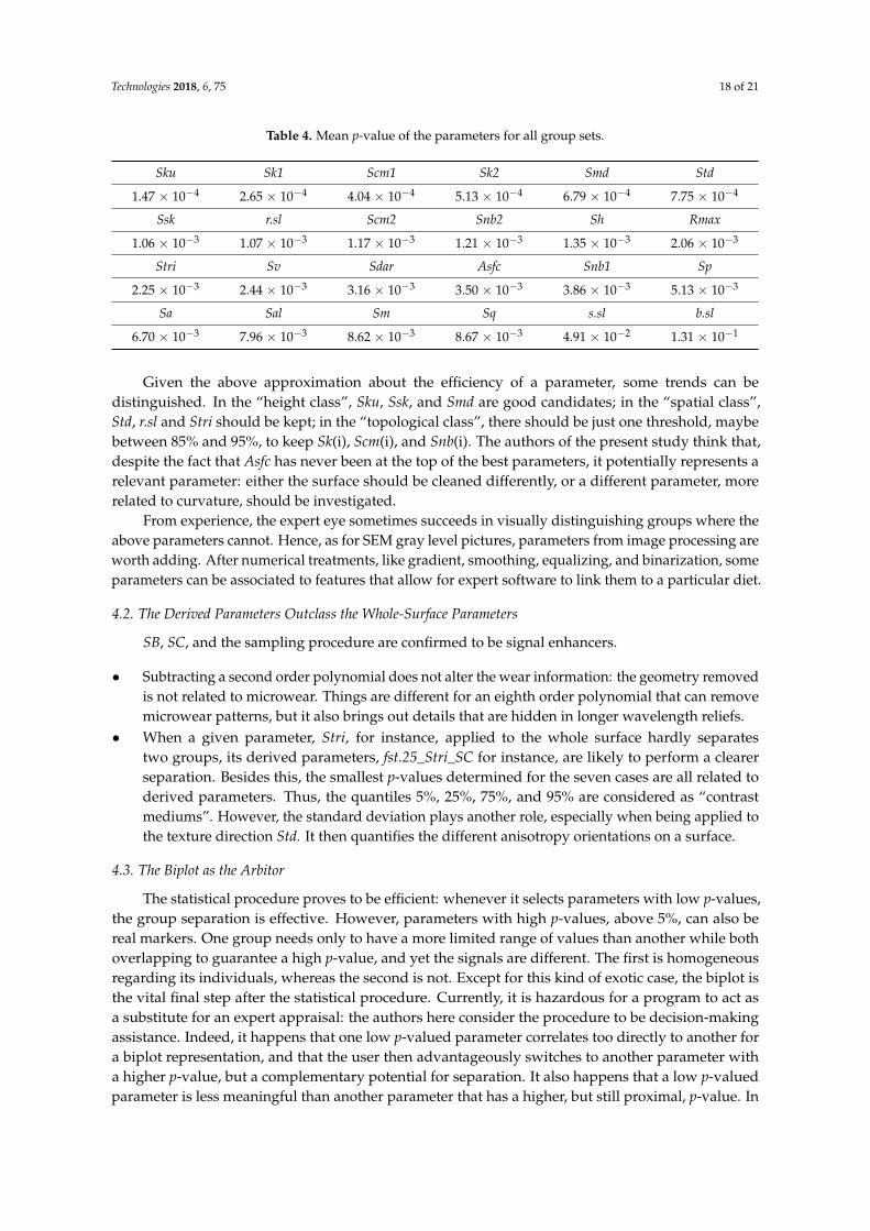
Adding barley kernels to red clover was expected to increase isotropy, which is confirmed byfst.25_Stri_SC p-values: 4.02 × 10⁻⁴ for LO-L7, L7 being the most anisotropic because of its richer silicagrass. Figure 14 illustrates the surface aspects of LO and L7 individuals, which visually corroboratesthe presence of anisotropy on L7.
Technologies 2018, 6, x FOR PEER REVIEW 17 of 21
Adding barley kernels to red clover was expected to increase isotropy, which is confirmed by
fst.25_Stri_SC p‐values: 4.02 × 10⁻⁴ for LO‐L7, L7 being the most anisotropic because of its richer silica
grass. Figure 14 illustrates the surface aspects of LO and L7 individuals, which visually corroborates
the presence of anisotropy on L7.
Figure 14. Visual comparison of two SC surfaces belonging to the LO and the L7 groups.
4. Discussion
4.1. Untangling the Jungle of Parameters
It is impossible to isolate a small set of universal parameters from within the 700+ derived
parameter set. However, a given parameter can be evaluated if all of its derivatives are aggregated,
then for each group set, seven in the present work, the minimum of its p‐values is picked, and the
mean is calculated. The results are presented in Table 4:
Table 4. Mean p‐value of the parameters for all group sets.
Sku Sk1 Scm1 Sk2 Smd Std
1.47 × 10⁻⁴ 2.65 × 10⁻⁴ 4.04 × 10⁻⁴ 5.13 × 10⁻⁴ 6.79 × 10⁻⁴ 7.75 × 10⁻⁴
Ssk r.sl Scm2 Snb2 Sh Rmax
1.06 × 10⁻³ 1.07 × 10⁻³ 1.17 × 10⁻³ 1.21 × 10⁻³ 1.35 × 10⁻³ 2.06 × 10⁻³
Stri Sv Sdar Asfc Snb1 Sp
2.25 × 10⁻³ 2.44 × 10⁻³ 3.16 × 10⁻³ 3.50 × 10⁻³ 3.86 × 10⁻³ 5.13 × 10⁻³
Sa Sal Sm Sq s.sl b.sl
6.70 × 10⁻³ 7.96 × 10⁻³ 8.62 × 10⁻³ 8.67 × 10⁻³ 4.91 × 10⁻² 1.31 × 10⁻¹
Given the above approximation about the efficiency of a parameter, some trends can be
distinguished. In the “height class”, Sku, Ssk, and Smd are good candidates; in the “spatial class”, Std,
r.sl and Stri should be kept; in the “topological class”, there should be just one threshold, maybe
between 85% and 95%, to keep Sk(i), Scm(i), and Snb(i). The authors of the present study think that,
despite the fact that Asfc has never been at the top of the best parameters, it potentially represents a
relevant parameter: either the surface should be cleaned differently, or a different parameter, more
related to curvature, should be investigated.
From experience, the expert eye sometimes succeeds in visually distinguishing groups where
the above parameters cannot. Hence, as for SEM gray level pictures, parameters from image
processing are worth adding. After numerical treatments, like gradient, smoothing, equalizing, and
binarization, some parameters can be associated to features that allow for expert software to link
them to a particular diet.
Figure 14. Visual comparison of two SC surfaces belonging to the LO and the L7 groups.
4. Discussion
4.1. Untangling the Jungle of Parameters
It is impossible to isolate a small set of universal parameters from within the 700+ derivedparameter set. However, a given parameter can be evaluated if all of its derivatives are aggregated,then for each group set, seven in the present work, the minimum of its p-values is picked, and themean is calculated. The results are presented in Table 4:
Technologies 2018, 6, 75 18 of 21
Table 4. Mean p-value of the parameters for all group sets.
Sku Sk1 Scm1 Sk2 Smd Std
1.47 × 10⁻⁴ 2.65 × 10⁻⁴ 4.04 × 10⁻⁴ 5.13 × 10⁻⁴ 6.79 × 10⁻⁴ 7.75 × 10⁻⁴
Ssk r.sl Scm2 Snb2 Sh Rmax
1.06 × 10⁻³ 1.07 × 10⁻³ 1.17 × 10⁻³ 1.21 × 10⁻³ 1.35 × 10⁻³ 2.06 × 10⁻³
Stri Sv Sdar Asfc Snb1 Sp
2.25 × 10⁻³ 2.44 × 10⁻³ 3.16 × 10⁻³ 3.50 × 10⁻³ 3.86 × 10⁻³ 5.13 × 10⁻³
Sa Sal Sm Sq s.sl b.sl
6.70 × 10⁻³ 7.96 × 10⁻³ 8.62 × 10⁻³ 8.67 × 10⁻³ 4.91 × 10⁻² 1.31 × 10⁻¹
Given the above approximation about the efficiency of a parameter, some trends can bedistinguished. In the “height class”, Sku, Ssk, and Smd are good candidates; in the “spatial class”,Std, r.sl and Stri should be kept; in the “topological class”, there should be just one threshold, maybebetween 85% and 95%, to keep Sk(i), Scm(i), and Snb(i). The authors of the present study think that,despite the fact that Asfc has never been at the top of the best parameters, it potentially represents arelevant parameter: either the surface should be cleaned differently, or a different parameter, morerelated to curvature, should be investigated.
From experience, the expert eye sometimes succeeds in visually distinguishing groups where theabove parameters cannot. Hence, as for SEM gray level pictures, parameters from image processing areworth adding. After numerical treatments, like gradient, smoothing, equalizing, and binarization, someparameters can be associated to features that allow for expert software to link them to a particular diet.
4.2. The Derived Parameters Outclass the Whole-Surface Parameters
SB, SC, and the sampling procedure are confirmed to be signal enhancers.
• Subtracting a second order polynomial does not alter the wear information: the geometry removedis not related to microwear. Things are different for an eighth order polynomial that can removemicrowear patterns, but it also brings out details that are hidden in longer wavelength reliefs.
• When a given parameter, Stri, for instance, applied to the whole surface hardly separatestwo groups, its derived parameters, fst.25_Stri_SC for instance, are likely to perform a clearerseparation. Besides this, the smallest p-values determined for the seven cases are all related toderived parameters. Thus, the quantiles 5%, 25%, 75%, and 95% are considered as “contrastmediums”. However, the standard deviation plays another role, especially when being applied tothe texture direction Std. It then quantifies the different anisotropy orientations on a surface.
4.3. The Biplot as the Arbitor
The statistical procedure proves to be efficient: whenever it selects parameters with low p-values,the group separation is effective. However, parameters with high p-values, above 5%, can also bereal markers. One group needs only to have a more limited range of values than another while bothoverlapping to guarantee a high p-value, and yet the signals are different. The first is homogeneousregarding its individuals, whereas the second is not. Except for this kind of exotic case, the biplot isthe vital final step after the statistical procedure. Currently, it is hazardous for a program to act asa substitute for an expert appraisal: the authors here consider the procedure to be decision-makingassistance. Indeed, it happens that one low p-valued parameter correlates too directly to another fora biplot representation, and that the user then advantageously switches to another parameter witha higher p-value, but a complementary potential for separation. It also happens that a low p-valuedparameter is less meaningful than another parameter that has a higher, but still proximal, p-value. In
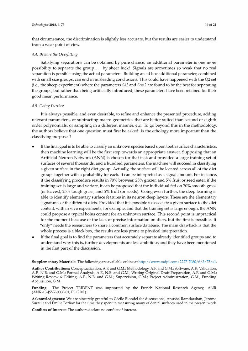
Technologies 2018, 6, 75 19 of 21
that circumstance, the discrimination is slightly less accurate, but the results are easier to understandfrom a wear point of view.
4.4. Beware the Overfitting
Satisfying separations can be obtained by pure chance, an additional parameter is one morepossibility to separate the group . . . by sheer luck! Signals are sometimes so weak that no realseparation is possible using the actual parameters. Building an ad hoc additional parameter, combinedwith small size groups, can end in misleading conclusions. This could have happened with the Q2 set(i.e., the sheep experiment) where the parameters Sk2 and Scm2 are found to be the best for separatingthe groups, but rather than being artificially introduced, these parameters have been retained for theirgood mean performance.
4.5. Going Further
It is always possible, and even desirable, to refine and enhance the presented procedure, addingrelevant parameters, or subtracting macro-geometries that are better suited than second or eighthorder polynomials, or sampling in a different manner, etc. To go beyond this in the methodology,the authors believe that one question must first be asked: is the ethology more important than theclassifying purposes?
• If the final goal is to be able to classify an unknown species based upon tooth surface characteristics,then machine learning will be the first step towards an appropriate answer. Supposing that anArtificial Neuron Network (ANN) is chosen for that task and provided a large training set ofsurfaces of several thousands, and a hundred parameters, the machine will succeed in classifyinga given surface in the right diet group. Actually, the surface will be located across all of the dietgroups together with a probability for each. It can be interpreted as a signal amount. For instance,if the classifying procedure results in 70% browser, 25% grazer, and 5% fruit or seed eater, if thetraining set is large and variate, it can be proposed that the individual fed on 70% smooth grass(or leaves), 25% tough grass, and 5% fruit (or seeds). Going even further, the deep learning isable to identify elementary surface features in its neuron deep layers. These are the elementarysignatures of the different diets. Provided that it is possible to associate a given surface to the dietcontent, with in vivo experiments, for example, and that the training set is large enough, the ANNcould propose a typical bolus content for an unknown surface. This second point is impracticalfor the moment because of the lack of precise information on diets, but the first is possible. It“only” needs the researchers to share a common surface database. The main drawback is that thewhole process is a black box, the results are less prone to physical interpretation.
• If the final goal is to find the parameters that accurately separate already identified groups and tounderstand why this is, further developments are less ambitious and they have been mentionedin the first part of the discussion.
Supplementary Materials: The following are available online at http://www.mdpi.com/2227-7080/6/3/75/s1.
Author Contributions: Conceptualization, A.F. and G.M.; Methodology, A.F. and G.M.; Software, A.F.; Validation,A.F., N.B. and G.M.; Formal Analysis, A.F., N.B. and G.M.; Writing-Original Draft Preparation, A.F. and G.M.;Writing-Review & Editing, A.F., N.B. and G.M.; Supervision, G.M.; Project Administration, G.M.; FundingAcquisition, G.M.
Funding: The Project TRIDENT was supported by the French National Research Agency, ANR(ANR-13-JSV7-0008-01; PI: G.M.).
Acknowledgments: We are sincerely grateful to Cécile Blondel for discussions, Anusha Ramdarshan, JérômeSurault and Emilie Berlioz for the time they spent in measuring many of dental surfaces used in the present work.
Conflicts of Interest: The authors declare no conflict of interest.
Technologies 2018, 6, 75 20 of 21
References
1. Technique and Application in Dental Anthropology; Irish, J.D.; Nelson, G.C., Eds.; Cambridge Studiesin Biological and Evolutionary Anthropology; Cambridge University Press: Cambridge, UK, 2008;ISBN 978-0-521-87061-0.
2. Ungar, P.S. Mammalian dental function and wear: A review. Biosurf. Biotribol. 2015, 1, 25–41. [CrossRef]3. DeSantis, L.R.G. Dental microwear textures: Reconstructing diets of fossil mammals. Surf. Topogr. Metrol.
Prop. 2016, 4, 023002. [CrossRef]4. Mihlbachler, M.C.; Beatty, B.L.; Caldera-Siu, A.; Chan, D.; Lee, R. Error rates and observer bias in dental
microwear analysis using light microscopy. Palaeontol. Electron. 2012, 15, 12A.5. Mihlbachler, M.C.; Beatty, B.L. Magnification and resolution in dental microwear analysis using light
microscopy. Palaeontol. Electron. 2012, 15, 25A.6. Merceron, G.; Costeur, L.; Maridet, O.; Ramdarshan, A.; Göhlich, U.B. Multi-proxy approach detects
heterogeneous habitats for primates during the Miocene climatic optimum in Central Europe. J. Hum. Evol.2012, 63, 150–161. [CrossRef] [PubMed]
7. Ramdarshan, A.; Merceron, G.; Marivaux, L. Spatial and temporal ecological diversity amongst eoceneprimates of France: Evidence from teeth. Am. J. Phys. Anthropol. 2012, 147, 201–216. [CrossRef] [PubMed]
8. Semprebon, G.M.; Solounias, N.; Tao, D. Dietary reconstruction of Hezhengia bohlini (Artiodactyla, Bovidae)from the late Miocene Linxia Basin of China using enamel microwear. Palaeogeogr. Palaeoclimatol. Palaeoecol.2017, 481, 57–63. [CrossRef]
9. Xafis, A.; Nagel, D.; Bastl, K. Which tooth to sample? A methodological study of the utility ofpremolar/non-carnassial teeth in the microwear analysis of mammals. Palaeogeogr. Palaeoclimatol. Palaeoecol.2017, 487, 229–240. [CrossRef]
10. Percher, A.M.; Romero, A.; Galbany, J.; Akoue, G.N.; Pérez-Pérez, A.; Charpentier, M.J.E. Buccaldental-microwear and dietary ecology in a free-ranging population of mandrills (Mandrillus sphinx) fromsouthern Gabon. PLoS ONE 2017, 12, e0186870. [CrossRef] [PubMed]
11. Teaford, M.F.; Ungar, P.S.; Taylor, A.B.; Ross, C.F.; Vinyard, C.J. In vivo rates of dental microwear formationin laboratory primates fed different food items. Biosurf. Biotribol. 2017. [CrossRef]
12. Henton, E.; Martin, L.; Garrard, A.; Jourdan, A.-L.; Thirlwall, M.; Boles, O. Gazelle seasonal mobility inthe Jordanian steppe: The use of dental isotopes and microwear as environmental markers, applied toEpipalaeolithic Kharaneh IV. J. Archaeol. Sci. Rep. 2017, 11, 147–158. [CrossRef]
13. Berlioz, E.; Kostopoulos, D.S.; Blondel, C.; Merceron, G. Feeding ecology of Eucladoceros ctenoides as a proxyto track regional environmental variations in Europe during the early Pleistocene. Comptes Rendus Palevol2017. [CrossRef]
14. Green, J.L.; DeSantis, L.R.G.; Smith, G.J. Regional variation in the browsing diet of Pleistocene Mammutamericanum (Mammalia, Proboscidea) as recorded by dental microwear textures. Palaeogeogr. Palaeoclimatol.Palaeoecol. 2017, 487, 59–70. [CrossRef]
15. Smith, G.J.; Desantis, L.R.G. Dietary ecology of Pleistocene mammoths and mastodons as inferred fromdental microwear textures. Palaeogeogr. Palaeoclimatol. Palaeoecol. 2017. [CrossRef]
16. Zhang, H.; Wang, Y.; Janis, C.M.; Goodall, R.H.; Purnell, M.A. An examination of feeding ecology inPleistocene proboscideans from southern China (Sinomastodon, Stegodon, Elephas), by means of dentalmicrowear texture analysis. Q. Int. 2017, 445, 60–70. [CrossRef]
17. Mahoney, P.; Schmidt, C.W.; Deter, C.; Remy, A.; Slavin, P.; Johns, S.E.; Miszkiewicz, J.J.; Nystrom, P.Deciduous enamel 3D microwear texture analysis as an indicator of childhood diet in medieval Canterbury,England. J. Archaeol. Sci. 2016, 66, 128–136. [CrossRef]
18. De Bonis, L.; Abella, J.; Merceron, G.; Begun, D.R. A new late Miocene ailuropodine (Giant Panda) fromRudabánya (North-central Hungary). Geobios 2017, 50, 413–421. [CrossRef]
19. Calandra, I.; Labonne, G.; Schulz-Kornas, E.; Kaiser, T.M.; Montuire, S. Tooth wear as a means to quantifyintra-specific variations in diet and chewing movements. Sci. Rep. 2016, 6, 34037. [CrossRef] [PubMed]
20. Purnell, M.A.; Goodall, R.H.; Thomson, S.; Matthews, C.J.D. Tooth microwear texture in odontocete whales:Variation with tooth characteristics and implications for dietary analysis. Biosurf. Biotribol. 2017, 3, 184–195.[CrossRef]
Technologies 2018, 6, 75 21 of 21
21. Kubo, M.O.; Yamada, E.; Kubo, T.; Kohno, N. Dental microwear texture analysis of extant sika deer withconsiderations on inter-microscope variability and surface preparation protocols. Biosurf. Biotribol. 2017, 3,155–165. [CrossRef]
22. Najjar, D.; Bigerelle, M.; Iost, A. The computer-based bootstrap method as a tool to select a relevant surfaceroughness parameter. Wear 2003, 254, 450–460. [CrossRef]
23. Najjar, D.; Bigerelle, M.; Migaud, H.; Iost, A. About the relevance of roughness parameters used forcharacterizing worn femoral heads. Tribol. Int. 2006, 39, 1527–1537. [CrossRef]
24. Bigerelle, M.; Najjar, D.; Mathia, T.; Iost, A.; Coorevits, T.; Anselme, K. An expert system to characterise thesurfaces morphological properties according to their tribological functionalities: The relevance of a pair ofroughness parameters. Tribol. Int. 2013, 59, 190–202. [CrossRef]
25. Deltombe, R.; Kubiak, K.J.; Bigerelle, M. How to select the most relevant 3D roughness parameters of asurface. Scanning 2014, 36, 150–160. [CrossRef] [PubMed]
26. Francisco, A.; Blondel, C.; Brunetière, N.; Ramdarshan, A.; Merceron, G. Enamel surface topography analysisfor diet discrimination. A methodology to enhance and select discriminative parameters. Surf. Topogr. Metrol.Prop. 2017. [CrossRef]
27. Merceron, G.; Ramdarshan, A.; Blondel, C.; Boisserie, J.-R.; Brunetiere, N.; Francisco, A.; Gautier, D.;Milhet, X.; Novello, A.; Pret, D. Untangling the environmental from the dietary: Dust does not matter.Proc. Biol. Sci. 2016, 283. [CrossRef] [PubMed]
28. Merceron, G.; Blondel, C.; Brunetiere, N.; Francisco, A.; Gautier, D.; Ramdarshan, A. Dental microwear andcontrolled food testing on sheep: The TRIDENT project. Biosurf. Biotribol. 2017, 3, 174–183. [CrossRef]
29. Ramdarshan, A.; Blondel, C.; Gautier, D.; Surault, J.; Merceron, G. Overcoming sampling issues in dentaltribology: Insights from an experimentation on sheep. Palaeontol. Electron. 2017, 20, 1–19. [CrossRef]
30. Lambert, J.E.; Chapman, C.A.; Wrangham, R.W.; Conklin-Brittain, N.L. Hardness of cercopithecine foods:Implications for the critical function of enamel thickness in exploiting fallback foods. Am. J. Phys. Anthropol.2004, 125, 363–368. [CrossRef] [PubMed]
31. Daegling, D.J.; McGraw, W.S.; Ungar, P.S.; Pampush, J.D.; Vick, A.E.; Bitty, E.A. Hard-object feeding in sootymangabeys (Cercocebus atys) and interpretation of early hominin feeding ecology. PLoS ONE 2011, 6, e23095.[CrossRef] [PubMed]
32. Maisels, F.; Gautier-Hion, A.; Gautier, J.-P. Diets of two sympatric colobines in Zaire: More evidence onseed-eating in forests on poor soils. Int. J. Primatol. 1994, 15, 681. [CrossRef]
33. Daegling, D.J.; McGraw, W.S. Feeding, Diet, and Jaw Form in West African Colobus and Procolobus. Int. J.Primatol. 2001, 22, 1033–1055. [CrossRef]
34. Post, D.G.; Hausfater, G.; McCuskey, S. Feeding Behavior of Yellow Baboons (Papio cynocephalus): Relationshipto Age, Gender and Dominance Rank. Folia Primatol. 1980, 34, 170–195. [CrossRef] [PubMed]
35. Rhine, R.J.; Norton, G.W.; Wynn, G.M.; Wynn, R.D.; Rhine, H.B. Insect and meat eating among infant andadult baboons (Papio cynocephalus) of Mikumi National Park, Tanzania. Am. J. Phys. Anthropol. 1986, 70,105–118. [CrossRef] [PubMed]
36. Scott, R.S.; Teaford, M.F.; Ungar, P.S. Dental microwear texture and anthropoid diets. Am. J. Phys. Anthropol.2012, 147, 551–579. [CrossRef] [PubMed]
37. Merceron, G.; Hofman-Kaminska, E.; Kowalczyk, R. 3D dental microwear texture analysis of feeding habitsof sympatric ruminants in the Białowieza Primeval Forest, Poland. For. Ecol. Manag. 2014, 328, 262–269.[CrossRef]
38. Massey, F.; Smith, M.; Lambin, X.; Hartley, S. Are silica defences in grasses driving vole population cycles?Biol. Lett. 2008, 4, 419–422. [CrossRef] [PubMed]
39. Scott, R.S.; Ungar, P.S.; Bergstrom, T.S.; Brown, C.A.; Childs, B.E.; Teaford, M.F.; Walker, A. Dental microweartexture analysis: Technical considerations. J. Hum. Evol. 2006, 51, 339–349. [CrossRef] [PubMed]
© 2018 by the authors. Licensee MDPI, Basel, Switzerland. This article is an open accessarticle distributed under the terms and conditions of the Creative Commons Attribution(CC BY) license (http://creativecommons.org/licenses/by/4.0/).
Related Documents