Brigham Young University Brigham Young University BYU ScholarsArchive BYU ScholarsArchive Theses and Dissertations 2015-05-01 Gaseous Particulate Interaction in a 3-Phase Granular Simulation Gaseous Particulate Interaction in a 3-Phase Granular Simulation Kevin W. Munns Brigham Young University - Provo Follow this and additional works at: https://scholarsarchive.byu.edu/etd Part of the Computer Sciences Commons BYU ScholarsArchive Citation BYU ScholarsArchive Citation Munns, Kevin W., "Gaseous Particulate Interaction in a 3-Phase Granular Simulation" (2015). Theses and Dissertations. 5261. https://scholarsarchive.byu.edu/etd/5261 This Thesis is brought to you for free and open access by BYU ScholarsArchive. It has been accepted for inclusion in Theses and Dissertations by an authorized administrator of BYU ScholarsArchive. For more information, please contact [email protected], [email protected].

Welcome message from author
This document is posted to help you gain knowledge. Please leave a comment to let me know what you think about it! Share it to your friends and learn new things together.
Transcript

Brigham Young University Brigham Young University
BYU ScholarsArchive BYU ScholarsArchive
Theses and Dissertations
2015-05-01
Gaseous Particulate Interaction in a 3-Phase Granular Simulation Gaseous Particulate Interaction in a 3-Phase Granular Simulation
Kevin W. Munns Brigham Young University - Provo
Follow this and additional works at: https://scholarsarchive.byu.edu/etd
Part of the Computer Sciences Commons
BYU ScholarsArchive Citation BYU ScholarsArchive Citation Munns, Kevin W., "Gaseous Particulate Interaction in a 3-Phase Granular Simulation" (2015). Theses and Dissertations. 5261. https://scholarsarchive.byu.edu/etd/5261
This Thesis is brought to you for free and open access by BYU ScholarsArchive. It has been accepted for inclusion in Theses and Dissertations by an authorized administrator of BYU ScholarsArchive. For more information, please contact [email protected], [email protected].

Gaseous Particulate Interaction in a 3-Phase Granular Simulation
Kevin W. Munns
A thesis submitted to the faculty of Brigham Young University
in partial fulfillment of the requirements for the degree of
Master of Science
Seth Holladay, Chair Parris Egbert
Dennis Ng
Department of Computer Science
Brigham Young University
April 2015
Copyright © 2015 Kevin W. Munns
All Rights Reserved
ABSTRACT
Gaseous Particulate Interaction in a 3-Phase Granular Simulation
Kevin W. Munns Department of Computer Science, BYU
Master of Science
As computer generated special effects play an increasingly integral role in the development of films and other media, simulating granular material continues to be a challenging and resource intensive process. Solutions tend to be pieced together in order to address the complex and different behaviors of granular flow. As such, these solutions tend to be brittle, overly specific, and unnatural. With the introduction of a holistic 3-phase granular simulation, we can now create a reliable and adaptable granular simulation.
Our solution improves upon this hybrid solution by addressing the issue of particle flow and correcting interpenetration amongst particles while maintaining the efficiency of the overall simulation. We achieve this by projecting particles onto a 2D manifold and implementing density correction using a quadratic solver. Particle updates are projected back into 3D to spread the particles apart on each frame.
Keywords: granular simulation, unilateral incompressibility, compression

ACKNOWLEDGEMENTS
I’d like to thank Dr. Holladay and Dr. Egbert for their mentorship and support. I’d also like to thank my wife and family, for whose understanding and support made this workpossible.

iv
Table of Contents
Introduction ............................................................................................................................................................ 1
Related Work .......................................................................................................................................................... 8
2.1 Discrete Element Methods .................................................................................................................... 8
2.2 Height Maps ............................................................................................................................................. 10
2.3 Proxy Methods ........................................................................................................................................ 12
2.4 Sand as a Fluid ......................................................................................................................................... 12
Hybrid Granular Simulation........................................................................................................................... 16
3.1 Solid ............................................................................................................................................................. 17
3.2 Liquid .......................................................................................................................................................... 18
3.3 Gas ................................................................................................................................................................ 18
Particulate Unilateral Incompressibility ................................................................................................... 21
4.1 Compression ............................................................................................................................................ 24
4.2 Volumes and Fields ............................................................................................................................... 25
4.3 Surface construction ............................................................................................................................. 27
4.4 Projection .................................................................................................................................................. 29
4.5 Texture Parameterization .................................................................................................................. 30
v
4.6 Quadratic Minimization ....................................................................................................................... 31
4.7 Gradient ..................................................................................................................................................... 34
4.8 Advection .................................................................................................................................................. 35
Results .................................................................................................................................................................... 37
Discussion and Future Work ......................................................................................................................... 41
Conclusion............................................................................................................................................................. 43
References ............................................................................................................................................................ 44
Image Credits ....................................................................................................................................................... 47
1
Chapter 1
Introduction
Image 1: Close-up of sand from the Coral Pink Sand Dunes State Park in Utah. These grains are rough and misshapen allowing for sand to interlock creating friction, which allows it to form a pile.
As computer-generated special effects become more prevalent in media, more challenging
natural phenomena have been simulated and presented in a believable manner. Simulating
fine particulate systems such as sand, soot, detergent and flour have historically been
difficult as they exhibit a wide variety of behavior that mimic other phenomena. A pile of
volcanic rock may act completely solid at times, then at other times exhibit fluid-like
flowing with rockslides. Flour can pile as it is poured from a sack. Soot can cloud up if
disturbed. Detergent can flow in interesting and unpredictable patterns as it clumps and
breaks up.

2
Sand has received special attention as early as the 1980’s. Its applications range
from modeling natural phenomena such as weathering and erosion to entertainment. Sand
can form piles. Granules can interlock to form micro arches. As sand avalanches certain
granules can actually rise. As sand gets deeper, it doesn’t increase in pressure, as opposed
to water, which is why it can be used in an hourglass: its rate of flow is constant.
Understanding sand can be crucial in assessing the risk of debris flow, which puts
certain populations around the world in danger. Sand’s ability to allow fluid to percolate
through it destabilizes its structure. It can lead to mud slides that flow like a liquid but
behave like cement.
Image 2: Sinkhole in Guatemala.
Observing sand can lead to efficiencies in mineral displacement and energy
exploration. Fracturing, or mining natural gas with the use of high-pressured water, is of
great interest to our energy sector. Environmental hazards like sink holes reveal sand’s
interstitial structure and by understanding sand’s behavior, we can understand the

3
consequences of various displacement techniques in use today. Understanding basic
behaviors can give us insight in preservation of natural phenomena as well as
understanding our geological history.
The simulation of granular materials can also be used in entertainment. This can
add a layer of depth and realism to movies, enabling the audience to more fully experience
emotions. In Pixar’s Toy Story 3, our heroes find themselves helpless as they are drifting
among debris in a garbage incinerator. The audience can relate to the emotion drawing
upon their earlier experience as children in a ball pit. During the making of the film, a ball
pit was set up in Pixar’s main office for the artists and technicians to revisit and explore the
emotion.
Image 3: Still of Woody in the garbage incinerator in Toy Story 3.
The complexity of sand can lead to the effect being avoided in animation all together
make the case for our research into efficient sand simulation. The simulation of sand can
also tie together computer-generated effects with their natural counterparts, though sand
simulations are often left out because they slow production and raise costs. In Michael
Bay’s Transformers, for example, the U.S. military engaged in battle with a scorpion-like
4
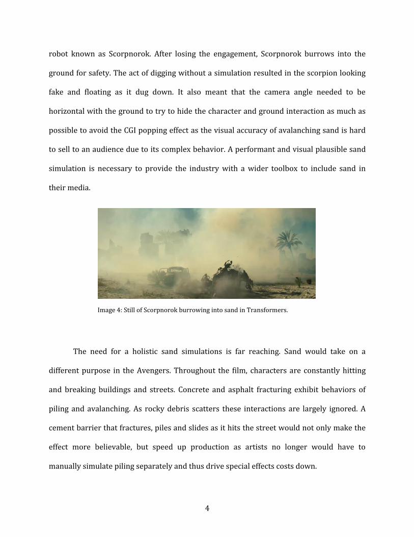
robot known as Scorpnorok. After losing the engagement, Scorpnorok burrows into the
ground for safety. The act of digging without a simulation resulted in the scorpion looking
fake and floating as it dug down. It also meant that the camera angle needed to be
horizontal with the ground to try to hide the character and ground interaction as much as
possible to avoid the CGI popping effect as the visual accuracy of avalanching sand is hard
to sell to an audience due to its complex behavior. A performant and visual plausible sand
simulation is necessary to provide the industry with a wider toolbox to include sand in
their media.
Image 4: Still of Scorpnorok burrowing into sand in Transformers.
The need for a holistic sand simulations is far reaching. Sand would take on a
different purpose in the Avengers. Throughout the film, characters are constantly hitting
and breaking buildings and streets. Concrete and asphalt fracturing exhibit behaviors of
piling and avalanching. As rocky debris scatters these interactions are largely ignored. A
cement barrier that fractures, piles and slides as it hits the street would not only make the
effect more believable, but speed up production as artists no longer would have to
manually simulate piling separately and thus drive special effects costs down.

5
Simulating millions of particles of sand is challenging. Each grain of sand has a
unique material property and shape. Just a handful of sand contains hundreds of thousands
of these particles, all of which collide against each other and interlock in different ways
creating friction and stress while at times allowing movement and collision. These unique
properties give sand the ability to act as a solid at times and flow like a fluid at others.
Holladay and Egbert have addressed the need to have an efficient and visually
compelling granular simulation using a hybrid technique [3] (see image 5). Sand is
comprised of three separate simulations including static geometry, a fluid solver featuring
two-way coupling of friction and pressure, and free flowing particles. The efficiency gains
of having sand that is further from the surface simplified is appealing as it allows artists to
create and iterate granular simulations with greater speed and lower computational costs
resulting in special effects studios saving money.
Image 5: Cutaway of Holladay and Egbert’s hybrid simulation revealing the solid, liquid, and gas states.

6
Our solution builds upon a hybrid simulation of sand which seeks efficiency and
visual plausibility over accuracy. Visual plausibility is necessary for effects to be believable
to a film audience. Accuracy can be slow and costly and is often not necessary in a
cinematic context. The hybrid technique relies on more complex states near the surface to
maintain integrity of the system while keeping simulation frames down.
The most complex state of the hybrid solver is the gaseous state which consists of a
thin layer of particles that glide on top of the fluid simulation below. This state uses
simplified particle physics as physically-based simulation would introduce a computational
bottle neck on the system. The lack of collision or particle-particle interaction on the
surface can lead to undesirable artifacts that detract from the overall simulation. These
special cases are similar to edge cases that appear in general simulation requiring the
programmer to manually patch or deflect them. We propose a general modification to the
gaseous state by introducing a simplified algorithm that addresses the issue when particles
can clump up together and interpenetrate leading to visual flaws in the simulation.
We solve this by adding a density constraint into the system. This constraint is
enforced with a density correction step that uses a quadratic minimization solver to
produce a pressure gradient. Particles are displaced from high pressure into low pressure
zones. A key contribution of our research involves flattening the particles from 3
dimensions into 2 dimensions to linearly reduce the problem space of our solver. This is
possible by acknowledging the tendency of surface particles to flatten out. Particles that
sink too far are converted into the separate liquid phase. The vertical variability of the
particles are not a primary component in the distribution. Applying the density correction
7
step with reduced dimensions means clumping and interpenetrating particles are
prevented in typically what is the most expensive simulation step without creating the
computational bottleneck in other approaches.
The remainder of this thesis is organized as follows: Chapter 2 addresses previous
work and methods for simulating sand efficiently. Chapter 3 reviews the hybrid solution
introduced by Holladay and Egbert that we use as the basis for the work presented here.
Chapter 4 describes our algorithm and how it fits in the context of the hybrid solution.
Chapter 5 demonstrates results of the algorithm. Chapter 6 discusses future work. Chapter
7 provides some concluding remarks relative to this thesis.
8
Chapter 2
Related Work
Sand has been observed and modeled to highlight and simulate varying behaviors. Liu,
Kaplan, and Gray first considered the fractal and recursive behavior of sand, observing how
it can settle, form patterns, bridges and fractal structures that repeat on multiple scales
[17]. Cundall and Strack first developed a discrete numeric model for particles to collide
and were the first to discover the properties of granular assemblies [1]. McCarthy and
Ottino recognized the system-wide behaviors of sand and modeled equations to capture
avalanching, friction, and sliding of sand inside a tumbler [4]. Mehta et al. have revisited the
piling and arching of sand producing a model of sand that takes into consideration the
angle of repose and handles collisions through discrete element methods [20].
2.1 Discrete Element Methods
The most accurate and realistic looking approach to simulating granular phenomena is to
use Discrete Element Methods (DEM). DEM takes an intuitive and straight-forward
approach. Each particle is simulated as a rigid body. A simple piece of geometry stands in
for the particle and simulates its 3-dimensional position, velocity, and momentum. Spheres
are chosen as a proxy because the collision detection is efficient. A particle can be
represented by a small group of spheres, known as an assembly (see image 6), of random
sizes frozen together to mimic interlocking and friction on a particulate basis.

9
Image 6: Granular Assembly comprised of frozen spheres.
The DEM algorithm integrates all Newtonian forces and particles and updates their
velocities and positions. This approach is computationally expensive and necessitates
limitations on either the number of particles in the simulation or the number of frames
simulated, though with some simulations multiple particles track a single near-by particle
to reduce complexity. While DEM solutions work for scenes of small scale, they become
prohibitively expensive as more particles are added.
The discrete element method has been improved upon by Fortin, Millet, and Saxce
through projecting friction onto a cone when dealing with compaction [7]. Irving et al.
revealed a superior method for resolving multiple contact points between non-convex
bodies [11]. When spherical particulate assemblies are used in proxy of granules, they
speed up computation. Particles can even be used as underlying rigid body collision proxies
for any arbitrary geometry [15]. Coarse grain collision detection can be tuned when dealing
with granular flow to find potential collision pairs faster [22]. Liu et al. have found that by
using primary component analysis on the coarse axis sweep step, the complexity of finding
potential collision pairs can be reduced [18]. When colliding thousands of particles, fine-
grained steps can be culled from particles not currently acting upon geometry [19]. Our

10
simulation seeks to avoid paying the high computational cost of simulating individual
granules and their collisions at an individual level. With our work addressing surface
particles, DEM methods would be a computational bottleneck for the simulation, and
therefore unsuitable.
2.2 Height Maps
In order to reduce the number of particles in a scene, height maps [31] are often used.
Discrete 2-dimensional height maps are rectangular columns that stand as proxies for
particles [32]. A pile of granules is mostly solid and therefore can be frozen, or temporarily
removed from computation. Only the surface needs to be simulated to mimic granular
phenomena. In a height map, a 3-dimensional surface is constructed using a 2-dimensional
grid of height values that determine the surface of the solid mesh (see Image 7). The
surface holds the remaining top layer of particles that are simulated with DEM. Height
maps have been constructed together with DEM models so that they can adaptively grow
and replace particles or shrink and produce additional particles.

11
Image 7: A Height Map sliced by a laser engraver.
Although height maps provide some computational relief, they still suffer from
having to provide a thick layer of particles sufficient to cover their surface if particulate
surface detail or granular flow is required, which is computationally expensive. Particulate
flow can mean a majority of the sand has to be solved using DEM while only a small portion
can be culled out. Height maps also suffer from requiring sand to be on flat, horizontal
surfaces [32]. This allows for effects such as foot prints and tracks on a beach [25], but
does not scale well for simulating effects such as sand being poured from a bucket. Height
maps benefit simulations with deep layers of granules. Our particle layer is a thin covering
and thus would not be effective at reducing computation as the surface particles would still
have to be simulated.

12
2.3 Proxy Methods
Other mesh-like algorithms can settle particles in place or replace still particles with proxy
geometry to simplify the number of actors in a scene [33]. While these approaches solve
some of the issues that come with height maps, they still suffer from having to simulate a
large number of particles using DEM. These techniques have allowed detail to be allocated
to where it is most important. Adams et al. have shown that particles can be adaptively
down-sampled while preserving detail in the fluid simulation [16]. Zhang et al. authored a
similar approach that also combines deep-water particles and is GPU friendly. Hsu and
Keyser developed a technique in which as they piled rigid bodies, they would freeze pieces
that have stopped moving and were below the surface to speed up computation [9]. Irving
et al. revealed that by using a grid that was made of tall and thin cells, deep below the
surface, they could use less cells but keep the horizontal grid resolution, which was
responsible for surface wave effects [10]. Recently, Kim et al. have opted to upscale a fluid
simulation by adding detail entirely to the surface wave simulation while on a coarse grid
below [24]. Proxy methods could simplify the simulation of particles by freezing them onto
control particles. Our method, however, seeks to avoid the interpenetration of particles
which previous proxy method fails to address.
2.4 Sand as a Fluid
As sand avalanches and flows, it can be modeled similar to a liquid. Fluid solvers are able to
efficiently simulate fluid behavior through essentially sub-sampling the phenomena. Fluids
can be simulated with either grid-based Eulerian approaches or particle-based Lagrangian
methods. A hybrid or Fluid Implicit Particle (flip) solver uses particles to track the fluid

13
while using a volumetric approach to calculate pressure [13]. As fluids are solved using
pressures and their number of particles are drastically smaller than granules, they provide
a great speed-up over DEM methods. Drawing inspiration from McCarthy and Ottino, Zhu
and Bridson explore the continuum properties of sand by using fluid equations [2] that
Bridson had worked on [14]. They modified an Eulerian grid to only animate cells where
the sand is above the angle of repose and able to overcome frictional forces, otherwise
making them solid.
Chang et al. improve on this approach using smooth particle hydrodynamics (SPH)
allowing for better splash effects [5]. SPH is a Lagrangian approach to fluid solvers where
fluid information is tracked on a particle bases. The movement of particles corresponds to
the movement of the liquid. SPH was first introduced by Monaghan [13] and extended to
account for multi-phase behavior [21]. Alduá and Otaduy also take an SPH approach
eliminating grid-like artifacts from Zhu and Bridson’s earlier work [8]. The SPH approach
has also allowed for fluids and granules to be co-simulated [12]. A drawback of using SPH
to simulate liquid in general is the instability of the system when particles get too close.
Particles that end up too close together explode in all directions as stiff spring forces react
adversely to small floating point values.
Fluid-based methods for simulating granular phenomena in general suffer from
various issues. While granules can take on fluid-like characteristics when avalanching, they
aren’t fundamentally fluids. Granular phenomena simulated as a fluid looks and acts like
quicksand or mud. Fluid based methods suffer from particles that separate from each
other, which makes them look and behave like globs of mud. Fluids also pile fundamentally

14
different as they rely on surface tension instead of friction to hold their material together.
Simulating surface particles as a fluid would result in less surface detail. Fluid simulation
steps smooth over fine movement which would make the surface look artificial. Surface
particles need to be able to break free from the surface when granules avalanche and
splash. Simulating surface particles as a fluid also adds additional computational
complexity. The hybrid solver uses surface particles to add detail. The current work has
issues with clumping on the surface (Image 8). Our solution makes the granules appear less
clumped. This will be covered in more detail in Chapter 4.
Image 8: Surface granules clumping together along an edge
DEM, height maps, and fluids all have major drawbacks that reduce the believability
of the granular phenomena by either making them look less accurate or by reducing the
number of particles as a trade-off to render time. Combining these different approaches can
allow for some better trade-offs in appearance and complexity. Sand is described as three
phases of matter and interstitial fluid is addressed by Forterre and Pouliquen [6]. Holladay
and Egbert developed a hybrid system that allowed underlying particles to solidify and

15
liquefy depending on their motion and how close they are to the surface allowing for a fast
and realistic simulation [3].
Discrete element methods are the most accurate approaches for simulating granular
materials, but their complexity is undesirable for the rapid iteration needed for adding
special effects in movies. Fluid approaches reduce complexity, but at the cost of realistic
behavior. A hybrid approach using both fluid and DEM methods solves the trade-off
between fluid and discrete element methods, but using discrete element methods still
introduces too much complexity. Our approach seeks to replace the standard DEM method
for particles.
All existing methods for simulating sand fall short. Discrete Element Methods are
too computationally expensive. Fluids methods suffer smoothing effects. Proxy methods
cannot be applied to the surface while maintaining detail. Our solution is to address these
short-comings by applying a light-weight density correction step that pushes particles
apart.

16
Chapter 3
Hybrid Granular Simulation
We review the Hybrid simulation by Holladay and Egbert as our research builds upon the
hybrid solution. We propose an algorithm that preserves particulate detail on the surface of
the simulation. We will give sand its characteristic look and feel by introducing particles
that bounce, splash without clumping up or looking like a viscous fluid. In order to describe
our solution, we must first describe the approach we have taken to simulate sand.
In the hybrid solution, granular phenomena can be characterized by 3 distinct
phases: solid, liquid, and gas. Granules are solid-like in their lowest energy state.
Microscopic particles are rough and interlock forming tight and incompressible structures.
Sand can pile up and maintain a slope, something that is impossible in a liquid. As sand is
poured, it will continue to form a bigger pile until the angle of the pile becomes steeper
than the material’s angle of repose. This angle describes the angle in which the forces of
gravity overcome the forces of friction in the material leading to granules breaking off and
sliding down the pile.
While in motion or avalanching, particles tend to stay in motion and mimic
behaviors found in fluids, behaviors such as incompressibility, cohesion, and dispersion.
Particles will flow until the friction of the material overcomes the momentum and
gravitational forces acting on the particle. During particulate flow, particles may collide
with one another and bounce into the air separating entirely from the system.

17
Airborne particles resemble gaseous particulate interactions. These particles are
generally free from interaction with other particles until they either leave the system or fall
back onto the material. In the latter case, they may either rebound or join the majority of
the material. Airborne particles follow gaseous properties and can be modeled with simple
Newtonian forces.
Holladay and Egbert’s hybrid solution describes and implements their simulation in
three states, which characterize the three main approaches to granular simulation.
Particles that are below the surface of the simulation and are not currently in motion are
culled out and are replaced by a proxy geometry in the form of a triangulated mesh whose
collision can be proxied by freezing the particles that border its space. This geometry can
grow as the pile gets deeper or more particles settle. Conversely, when the pile suddenly
shifts or vibrates, an exterior object penetrates or other forces act on the pile, the solid
geometry returns to its particulate state. As our research builds upon the gaseous state of
the hybrid solution, we include relevant details of the hybrid solution in sections 3.1, 3.2,
and 3.3 for completeness.
3.1 Solid
The solid geometry can be carved off and repopulated with granules in preparation for
simulating moving particles [3]. The amount of geometry converted to the fluid state
depends on the magnitude of the force acting upon it. Our simulation handles this situation
by allowing a portion of the material to be in a liquid state. As the simulation proceeds, the
system converts portions of the material between the solid and liquid states, as
circumstances require.
18
3.2 Liquid
The liquid state of matter is simulated with a fluid solver. A fluid implicit grid-based
approach simulates sand as liquid just below the surface of our simulation. The fluid
simulation acts as a buffer between our frozen solid pile of sand and our surface particles.
The fluid part of our simulation is the part that gives us most of the continuum behavior
that is sought after in sand. As such, our solid mesh is now modeled as cells in our fluid
simulation that freeze when the frictional forces are greater than other forces acting upon
it. In the presence of greater external forces, these cells convert from a solid state to a fluid
state and resume participating in the fluid simulation.
3.3 Gas
Our gaseous state refers to the surface of the granular material. The surface contains
individual particles composed of granular assemblies. Aside from texture or describing the
surface of the fluid, particles can detach from the simulation to emulate effects such as
splashing, spilling, scattering, and settling. This overcomes the limitations of our fluid
simulation and gives our sand simulation more believable behavior.
Particles that ride along the surface of the fluid do not collide against one another as
collision is computationally expensive and resembles a DEM solution, which is accurate but
costly. In the 3-phase solver, particles that glide along the surface do so because of state
information sharing. As a particle gets close to the implicit surface of the fluid, it begins to
“borrow” characteristics from the fluid closest to the surface.
Particles are increasingly influenced by the velocities of their fluid counterparts the
closer they are together. Particles that begin to sink into the fluid either condensate and

19
join the fluid state or are pushed back along the tangent of the implicit fluid surface.
Particles that remain buoyant may clump together and form rivers in an avalanching
surface. The extreme overlap of particles may distract the viewer, as particles should not
interpenetrate. This is the current state of sand of a hybrid sand simulation. We will
propose a few different approaches, and then go on to describe one that works best.
The most straightforward approach to increasing realism is to use discrete element
methods for every particle in the simulation. Even with spatial optimization and a reduced
number of particles in the simulation. D.E.M can still be too heavy of a solution as we are
not interested in individual particles colliding. Our solution seeks to highlight the behaviors
of sand as a continuum, which exhibit macro behaviors that are easily recognizable. We do
not need to collide particulate assemblies to achieve that level of detail.
A less complex approach could involve a simplified collision detection model with
the particles represented as spheres. Collision would be detected using a mark-and-sweep
coarse collision detection step, which would identify possible colliding pairs. Those pairs
would be pushed apart to avoid collision. Although this approach would reduce the
complexity greatly, thousands of particles on the screen would still need to be simulated
apart from our fluid simulation. The added complexity of performing a coarse collision
detection step on so many particles can be avoided altogether as our desired behaviors
mostly come from our fluid simulation. The particles serve to decorate the surface as well
as hide the underlying fluid simulation. The solution we propose, and the thrust of the
research in this thesis, is to use a reduced fluid solver to overcome the particle
interpenetration issue.

20
Thesis Statement
On the existing hybrid sand solver there exists an issue where particles on the
surface of the simulation can clump up because there is no collision detection keep them
apart as it is too expensive. We propose to solve this problem by reusing a quadratic solver
that is used for density correction on a 3D volume and repurposing it in a 2D context. We
do this by recognizing that since particles on a surface are mostly flat, they could be
approached as a 2D problem. We build a special surface that we project these particles onto
to flatten them out.
We then perform density correction on this surface, which produces a pressure
gradient that we then take the reverse gradient. All particles lingering around the surface in
3-space are advected by the gradient field that run along the manifold whose shape runs
through 3-space. We build a matrix and constraint vector (that is normally run on a
uniform grid) in a non-uniform context, namely surface mesh. We also perform a gradient
operation on a non-uniform context, again the surface mesh, when gradients are typically
run on uniform grids.
Our major contributions are applying the density correction or quadratic minimizer
to a 2D surface that we construct and project particles to, the building of and
parameterization of such surface, finding the gradient of resulting pressures, and the trade-
off or novel approach in correct the problem of particle clumping without resorting to a
heavy handed approach like collision detection.
Chapter 4
Particulate Unilateral Incompressibility
Our approach in preventing gas-state particles from clumping in an unrealistic manner is to
apply the density-correction step of sand fluids to the gas-state particles. A major
contribution of our work is the restatement of our problem in a lower dimension. Since gas
particles only exist at the surface, we take advantage of the 2D manifold property of
surfaces, projecting the particles to a 2D volume. This is much more efficient than solving a
minimization problem in 3 dimensions, enabling us to address a higher number of
particles.
In fluid solvers there are a wide range of trade-offs involving speed and accuracy.
For the density correction step, speed is a priority and as such, we can run a solver
that estimates the density solution with a few iterations (just enough to push the
particles apart) and then stops, providing a rough solution where pressure doesn’t
necessarily behave in a manner that is physically correct, but where the
most apparent interpenetrations are corrected.
As the fluid is a grid our solution can take advantage of existing structures. Running
the existing fluid solver would result in surface particles dispersing too rapidly and
behaving as a wispy fluid. We don’t want the surface to slosh around as it will distract the
viewer. Instead, we use a light-weight solution that ignores many behaviors typically
associated with fluids.
The fluid will contain a surface of varying height. The difference in height between a
fluid cell and its neighbors cannot exceed a certain threshold that is correlated to the angle
21
22
of repose. With this guarantee, we construct a manifold. Though the normals of the 2-
dimensional grid cells will differ, their underlying pressure solving step will ignore this
entirely while the advection step will use the normal as it advects each particle, pushing
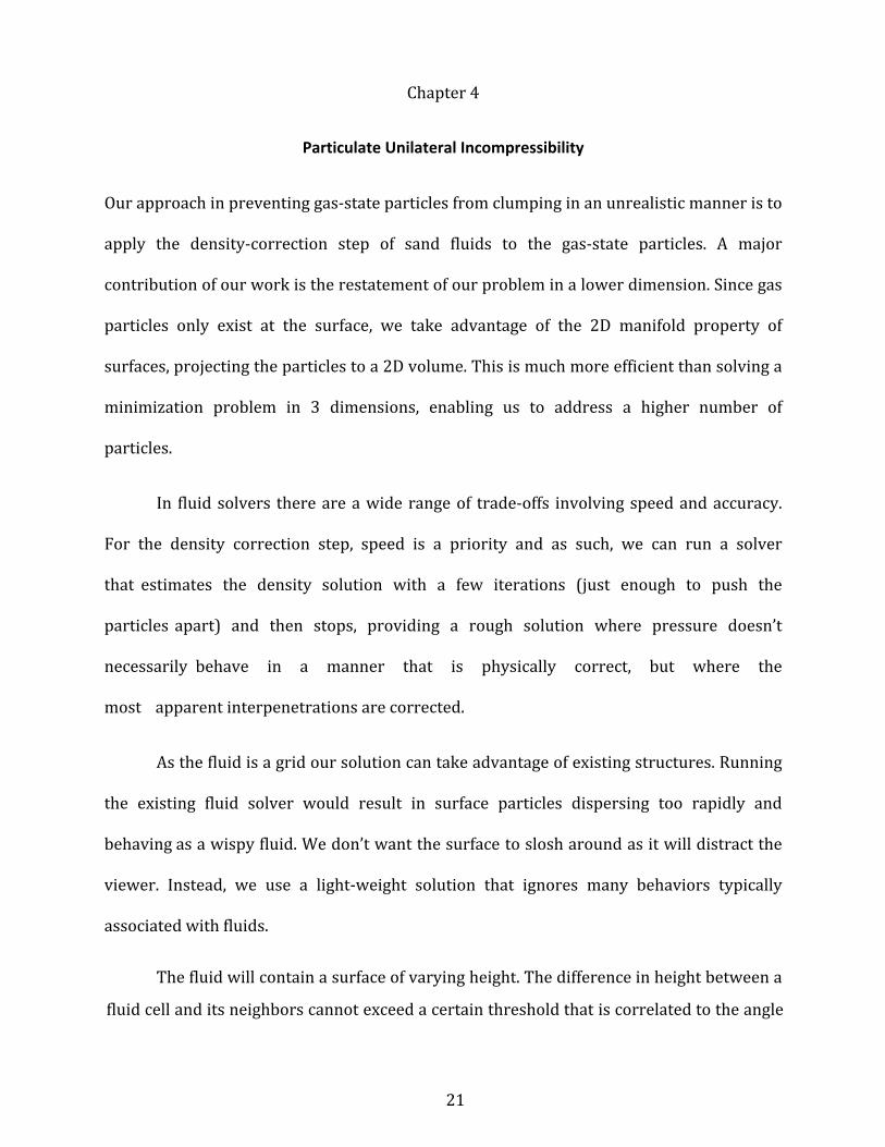
each particle relative to the fluid surface. See Figure 1 for an outline of our approach.
Figure 1: Algorithm Overview
Step 1. Surface construction
Insert primitives between grid points of fluid field.
Add vertices to steep edges.
Flip triangles to normalize surface.
See section 4.3 for details.
Step 2. Project particles
Find closest primitive.
See section 4.4 for details
Step 3. Texturization
Determine adjacent primitives.
Calculate particle density of each primitive.
See section 4.5 for details

23
Step 4. Density Correction
Build Laplacian matrix.
Run density correction solver.
See section 4.6 for details
Step 5. Gradient
Run pressure difference on each primitive pair.
See section 4.7 for details
Step 6. Advection
Interpolate gradient vectors onto particle.
Update particle position.
See section 4.8 for details
Once 2-dimensional projection vectors are resolved, the original particle will project
its velocity vector onto the grid. After the advection step, the particles behave similar to
those might have been colliding. The particles do not interpenetrate as frequently as before
our method was applied nor act as a singularity giving our sand simulation surface
divergence.
Our approach gives the surface of our simulation increased fidelity without the
burden of too much computational complexity added by other methods. By introducing a
simplified fluid simulator that uses a pressure solver to affect the density correction step,
we are able to prevent granular particles from clumping together without introducing the
complexity of collision detection and correction. Our method will allow our tri-state
granular simulation to look as good as discrete element methods while allowing for faster

24
simulation times. Our tool will empower artists to iterate on granular simulations quickly
giving them greater control over their simulation while reducing time and cost.
4.1 Compression
The issue of clumping is directly caused by an artifact in the method chosen in simulating
the liquid layer. We have chosen the fluid-implicit particle method (FLIP) which is a semi-
Lagrangian approach. This class of fluid solvers suffers from a type of numerical error
called compression [29].
Figure 2 Compression can be seen as clumps of particles form solid linesalong the inside of the rim and at points of impact.
Compression is a state when fluid clumps together and resists the pressure solver’s
correction resulting in a high density area. In fluids, this can result in a loss of volume and
produce artifacts in fluid flow. This type of numerical error is acceptable because it is
difficult to notice due to the constant motion and chaos in fluid simulations. When two
particles are close together, they receive the same advection updates and travel together
from the Eulerian solve (see Figure 2). While this works with particles deeply embedded in
a fluid simulation, it can have a popping effect on surface particles. Moving particles apart

25
also does not prevent them from compressing. Density correction prevents clumping and
corrects for areas on the surface where particles gather.
4.2 Volumes and Fields
To understand our manifold construction, we introduce our data structure used in our fluid
simulation. A voxel field is a three-dimensional structure where values are stored at
discreet points along a grid that runs over three axes. Voxel fields are commonly referred to
as fields, grids, and volumes. A fog volume is the simplest version where a value of 1
signifies the voxel contains fluid and a value of 0 signifies the absence of fluid (generally
considered air but in order to realistically capture interaction air requires a 2-phase fluid
simulation). In general, the more (which results in smaller) voxels representing a volume,
the more accurate that representation will be at the penalty of memory and computation
time. Volumes are generally uniformly spaced with uniform dimensions for simplicity,
though they may vary. Non-uniform fields (such as tall cells) [10] must take into account
the different voxel areas in computations and spatial derivatives.
Our solution focuses on building a non-uniform surface that lacks the breadth and
ease of applying algorithms like finite differencing and minimization to accommodate our
2-dimension surface. We introduce major contributions in building these algorithms for a
non-uniform surface of primitives.
26
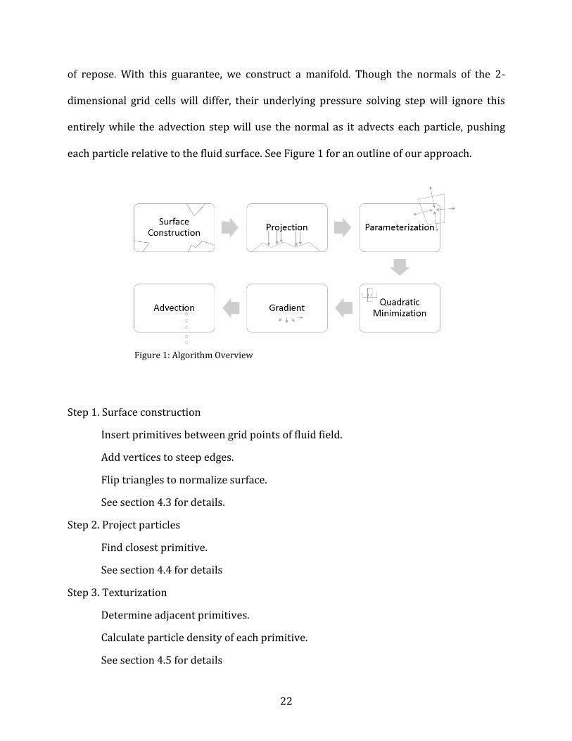
Figure 3: Particles gliding across an implicit volume boundary.
In fog volumes, a surface is built along the border of voxels where 0 meets 1. A
limitation of the fog volume is that surfaces must be constrained to a voxel boundary. A
signed distance field (SDF) corrects for this by allowing for a floating point value to be
stored at the voxel centers which indicate the distance to the closest surface. A negative
value may represent the distance inside the surface while positive values indicate the
distance above the surface. The surface is implicit as it exists on the 0 boundary, though the
boundary value can be set arbitrarily as well. The floating point values allow the surface to
be constructed within voxel boundaries allowing for a more accurate fluid boundary (see
Figure 3). Signed distance fields are the preferred representation for Euclidian fluid
volumes.
Multiple fields can be used to represent different values such as density and
velocity. Staggered grids ease the computation of spatial derivatives. Values on a staggered
grid are represented on the center of the positive axis faces. This allows for the spatial
27
derivative to be computed as a closer central difference, (less smoothed out) which lands
the result in the center of the voxels of the resulting field, which eliminates the need for an
extra trilinear interpolation step. Much research has been put into optimizing grids as a
data structure for fluid simulations.
4.3 Surface construction
A surface is constructed on the implicit the fluid signed distance field. Having a surface
enables us to enforce a density constraint in only 2 dimensions instead of a 3 dimensional
volume. Each voxel is sampled once for the distance to the surface and a point lifted or sunk
from the center of the voxel to sit on the surface. More samples may be used to build a
more accurate surface at the cost of additional complexity (see Figure 4). The set of points
that represent the surface are used to build a mesh. The points act as vertices for the
resulting quadrilaterals. The surface can be further refined by looking for disparity in
height and adding additional vertices along with their resulting triangles in order to get a
more accurate surface.
Inserted vertices that come from the refinement step will fall on an edge and will
gravitate towards the points with the greatest difference. The disparity is measured by
comparing difference in height among the four shared axel points. Like clothes on a
clothing line that is lifted, the point slides closer to the steeper point. If the point slides too
close and creates a sliver (a triangle with a low area to edge length), which is degenerate,
and the point is removed. Small primitives unnecessarily increase the size of our solver
matrix and are avoided. The resulting surface is a combination of triangles and quads.

28
Figure 4: An example of our Surface construction from a signed distance field
Delaunay triangulation can be used to enforce the Delaunay condition minimizing
the maximum angles. A simple triangle soup can be built by of randomly adding a point
from the point set, forming a triangle and flipping if needed. Though the surface used does
not need enforce the Delaunay condition. A balanced algorithm for triangulation is
important to keep the surface as uniform as possible as it gives the solver predictable areas
for pressure to escape to. Delaunay is often the go to algorithm with triangularization. The
surface, however, may also be entirely comprised of triangles by using Catmull-Clark
subdivision if one so chooses. A mixture of polys and triangles will work equally well for
our purposes as our algorithm generalizes to any polygon.
The surface comprises the boundary of a 3-dimensional volume. As we are only
interested in the top surface, a group of polygons is formed by calculating each face normal
29
and filtering out every face that differs from the angle pointing directly upwards by a
maximum of 85 degrees arbitrarily chosen to be near vertical. This constraint means that
the only faces to remain are those that face relatively upwards. Those faces are the most
likely to support the bulk of the gas particles. This filtering is a trade-off that allows for a
smaller problem set.
4.4 Projection
A trade-off between realism and complexity is made with the projection from 3-dimensions
to 2-dimensions. The difference in speed in each frame is justifies the error in accuracy
introduced with projection. As a granular simulation will mostly be viewed from above,
subtle difference in particle height go unnoticed. Taking advantage of this fact we approach
the problem of density correction as a 2-dimensional problem and project particles that are
close to the fluid surface onto the newly created surface.
The particles that represent the gaseous state of the granular simulation are located
on the fluid surface and are allowed to slide along that surface as necessary. As gravity
overcomes the hydrophobic properties of the surface, the particles coalesce and join the
fluid. This results in the majority of the gas particles floating just above the fluid surface. As
particles exit this space, they are either ignored if they travel above or converted below
into the fluid state. In order to spread these particles apart along the surface, they are
projected onto the newly built surface.
Gas particles can be projected onto the surface by using a minimum distance
criteria. Points along the surface and particles can be paired by using a divide and conquer
closest point-pair algorithm. A more straightforward approach involves gas particles using

30
ray-triangle intersection with a downward normal (along gravity). The ray-triangle
intersection can give the point of collision in Barycentric coordinates and ray-polygon
intersection in parametric coordinates.
𝜌𝑓 =∑ f𝑝
𝑛
𝑝=0
𝑎(1)
As each gas particle projects to a single polygon, the relationship becomes a one-to-
many relationship where each polygonal face, f, can have any number of gas particles
project to it. The concentration of particles on each polygon normalized by the area, 𝑎, of
the polygon determines its density, 𝜌 (1). The density of every polygon is needed to enforce
the global density constraint in the density correction step.
4.5 Texture Parameterization
The construction of a fluid surface and filtering out faces by their normals allows for the
planning of a 2-dimensional manifold that can host a lightweight solution to the problem of
interpenetrating particles. Building the surface as a manifold abstracts away 3-dimensional
spatial details in favor of relative position in a 2-dimensional context.
Manifolds are offered referred to as textures and are parameterized along two
dimensions commonly labeled U and V to avoid confusion with Euclidian spaces. Mapping
textures to meshes or subdivision surfaces is a common problem in animation. The ideal
parameterization of this manifold provides a mapping from an individual face to all
neighboring faces that share an edge (see Figure 5). A per-face UV parameterization with

31
adjacency data called Ptex has been developed by Disney Animation for efficient and
general filtering across textures.
Figure 5: Ptex parameterization of neighboring faces establishing adjacency.
Ptex is a per-face parameterization where U and V texture coordinates are local to
the face. Along with individual U and V coordinates, the Ptex texture format also encodes
neighboring (faces that share an edge) faces to allow for easy convolution and
compression. A neighbor or adjacent primitive is determined by a shared edge. There is no
need to parameterize the surface globally.
4.6 Quadratic Minimization
Sand is unilaterally incompressible. This means that while sand cannot be compressed
beyond a certain threshold, it also does not force the system to become divergence free.
Our density correction step is a constraint that enforces unilateral incompressibility.
Though it can be compressed beyond a certain threshold, it may be free to disperse
32
indefinitely, or only experience compression in only one direction. Sand differs from water
in that pressure will not infinitely increase given an infinite force. We determine a
minimum density constraint that each face is bound to in order to avoid excessive particle
overlap as demonstrated in Narain et al [26]. Narain et. al introduces a density constraint to
correct for overly dense conditions on their granular fluid simulation. A unilateral
constraint means that pressure is only applied in areas where density has hit a threshold.
Areas below this threshold are largely unaffected [27]. The constraint is satisfied by
moving particles away from cells that violate it. The minimum amount of movement
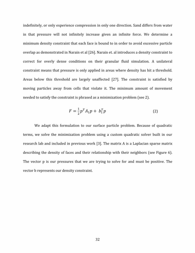
needed to satisfy the constraint is phrased as a minimization problem (see 2).
𝐹 =1
2𝑝𝑇𝐴1𝑝 + 𝑏1
𝑇𝑝 (2)
We adapt this formulation to our surface particle problem. Because of quadratic
terms, we solve the minimization problem using a custom quadratic solver built in our
research lab and included in previous work [3]. The matrix A is a Laplacian sparse matrix
describing the density of faces and their relationship with their neighbors (see Figure 6).
The vector p is our pressures that we are trying to solve for and must be positive. The
vector b represents our density constraint.
33
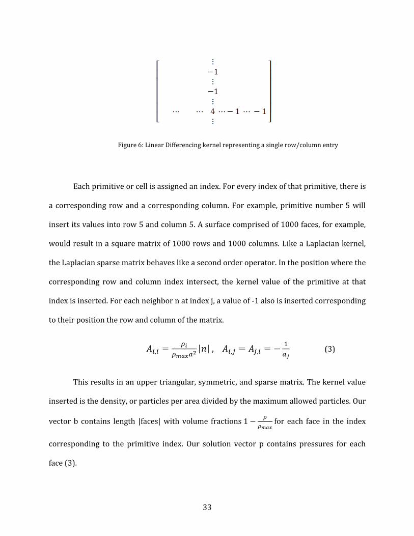
Figure 6: Linear Differencing kernel representing a single row/column entry
Each primitive or cell is assigned an index. For every index of that primitive, there is
a corresponding row and a corresponding column. For example, primitive number 5 will
insert its values into row 5 and column 5. A surface comprised of 1000 faces, for example,
would result in a square matrix of 1000 rows and 1000 columns. Like a Laplacian kernel,
the Laplacian sparse matrix behaves like a second order operator. In the position where the
corresponding row and column index intersect, the kernel value of the primitive at that
index is inserted. For each neighbor n at index j, a value of -1 also is inserted corresponding
to their position the row and column of the matrix.
𝐴𝑖,𝑖 =𝜌𝑖
𝜌𝑚𝑎𝑥𝑎2|𝑛| , 𝐴𝑖,𝑗 = 𝐴𝑗,𝑖 = −
1
𝑎𝑗(3)
This results in an upper triangular, symmetric, and sparse matrix. The kernel value
inserted is the density, or particles per area divided by the maximum allowed particles. Our
vector b contains length |faces| with volume fractions 1 −𝜌
𝜌𝑚𝑎𝑥 for each face in the index
corresponding to the primitive index. Our solution vector p contains pressures for each
face (3).
34
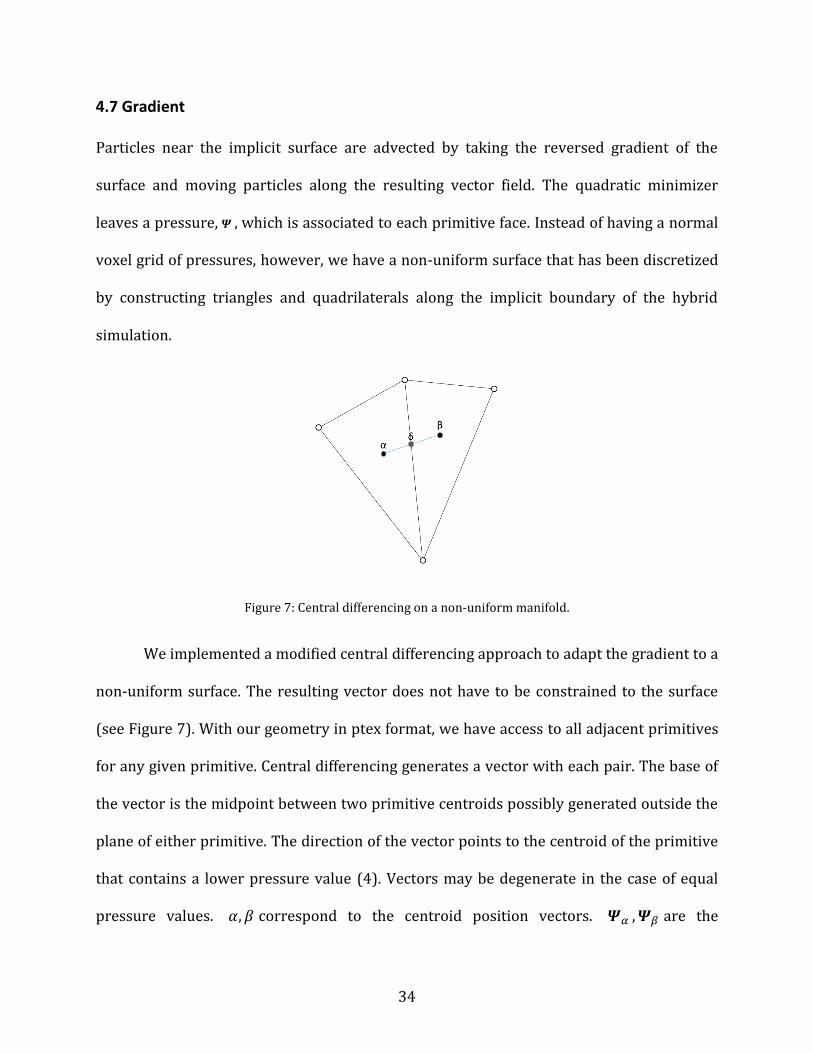
4.7 Gradient
Particles near the implicit surface are advected by taking the reversed gradient of the
surface and moving particles along the resulting vector field. The quadratic minimizer
leaves a pressure, 𝜳 , which is associated to each primitive face. Instead of having a normal
voxel grid of pressures, however, we have a non-uniform surface that has been discretized
by constructing triangles and quadrilaterals along the implicit boundary of the hybrid
simulation.
Figure 7: Central differencing on a non-uniform manifold.
We implemented a modified central differencing approach to adapt the gradient to a
non-uniform surface. The resulting vector does not have to be constrained to the surface
(see Figure 7). With our geometry in ptex format, we have access to all adjacent primitives
for any given primitive. Central differencing generates a vector with each pair. The base of
the vector is the midpoint between two primitive centroids possibly generated outside the
plane of either primitive. The direction of the vector points to the centroid of the primitive
that contains a lower pressure value (4). Vectors may be degenerate in the case of equal
pressure values. 𝛼, 𝛽 correspond to the centroid position vectors. 𝜳𝛼 , 𝜳𝛽 are the
35
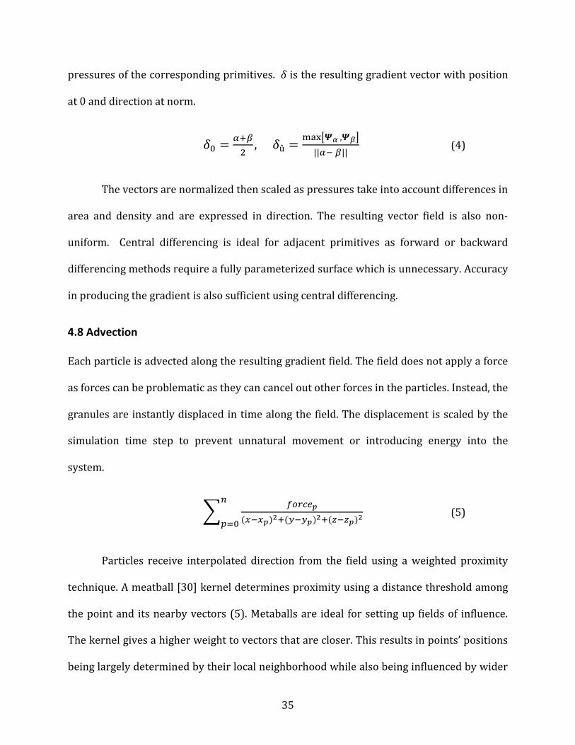
pressures of the corresponding primitives. 𝛿 is the resulting gradient vector with position
at 0 and direction at norm.
𝛿0 =𝛼+𝛽
2, 𝛿û =
max[𝜳𝛼 ,𝜳𝛽]
||𝛼− 𝛽||(4)
The vectors are normalized then scaled as pressures take into account differences in
area and density and are expressed in direction. The resulting vector field is also non-
uniform. Central differencing is ideal for adjacent primitives as forward or backward
differencing methods require a fully parameterized surface which is unnecessary. Accuracy
in producing the gradient is also sufficient using central differencing.
4.8 Advection
Each particle is advected along the resulting gradient field. The field does not apply a force
as forces can be problematic as they can cancel out other forces in the particles. Instead, the
granules are instantly displaced in time along the field. The displacement is scaled by the
simulation time step to prevent unnatural movement or introducing energy into the
system.
∑𝑓𝑜𝑟𝑐𝑒𝑝
(𝑥−𝑥𝑝)2+(𝑦−𝑦𝑝)2+(𝑧−𝑧𝑝)2
𝑛
𝑝=0(5)
Particles receive interpolated direction from the field using a weighted proximity
technique. A meatball [30] kernel determines proximity using a distance threshold among
the point and its nearby vectors (5). Metaballs are ideal for setting up fields of influence.
The kernel gives a higher weight to vectors that are closer. This results in points’ positions
being largely determined by their local neighborhood while also being influenced by wider
36
trends in the system. After particles have been moved along the gradient field, they
continue to run through the hybrid simulation, reacting to external forces, coalescing, and
separating as normal.
37
Chapter 5
Results
We set up a signed distance field volume that was initially 10x10x10. The volume has a
random function that generates interior and exterior volume for our algorithm to run on.
We populated the surface of the volume with 10,000 particles. Particle distribution is
biased to simulate the condition of clumping on a full solver (see Figure 8).
Results of the simulation are run a small grid as well as a higher grid. To render each
frame takes < 1 second on a 4.0 Ghz AMD 8 core machine with 16 Gb of memory on a
virtual machine allotted 50% of those resources. The algorithm is not intended to be real
time. The fluid step on a sand solver can typically take 30 seconds to 3 minutes on a similar
machine and similar grid. On a 1000x1000x1000 volume the simulation takes 3-12 minutes
depending on the initial conditions of the solver. Solving over a 3d volume would take
hours.
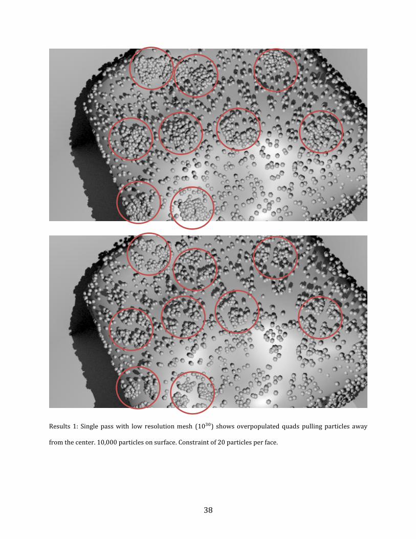
The first set of results shows a volume with particles forming in 9 individual
clusters. In each of these clusters, the algorithm detected violation of the density constraint
and flagged the primitive with a high pressure. Lower pressure primitives surrounding pull
the particles apart. The next set of results were run on a higher voxel grid with more
primitives creating the surface. A cluster of particles is detected and dispersed. The third
set of results is run at the same resolution with different random initial conditions and
shows a more broad resolution of the particles.
38
Results 1: Single pass with low resolution mesh (1030) shows overpopulated quads pulling particles away
from the center. 10,000 particles on surface. Constraint of 20 particles per face.
39
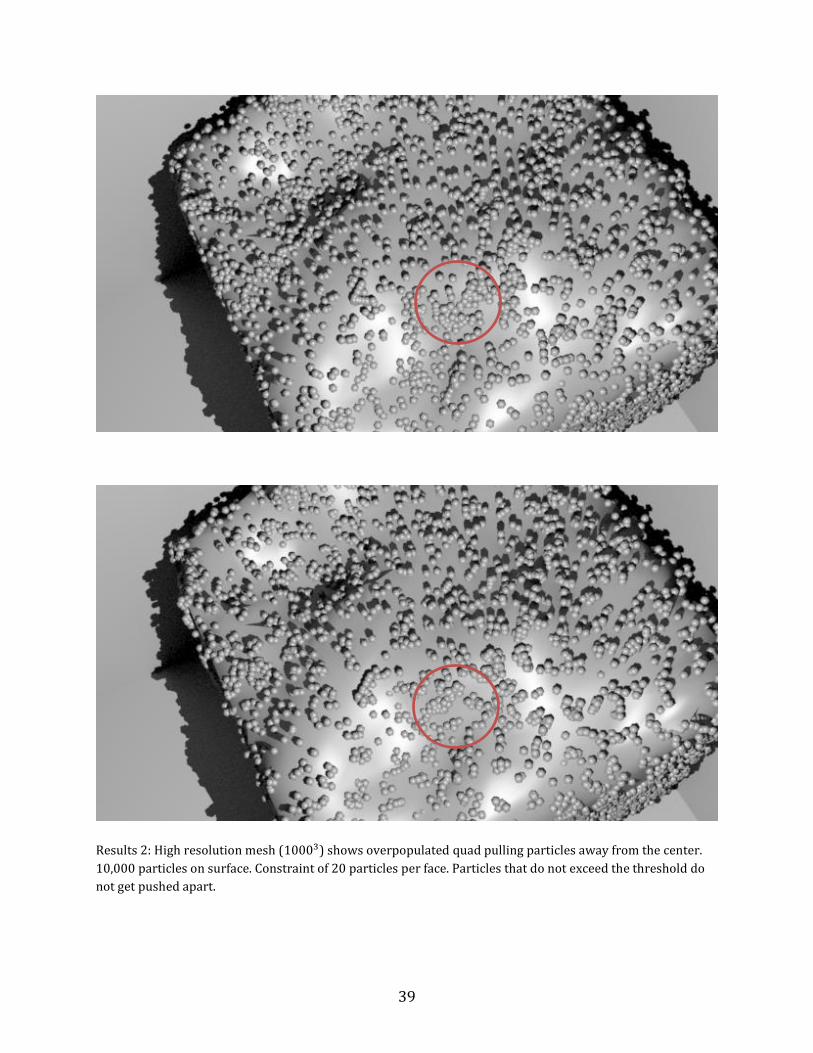
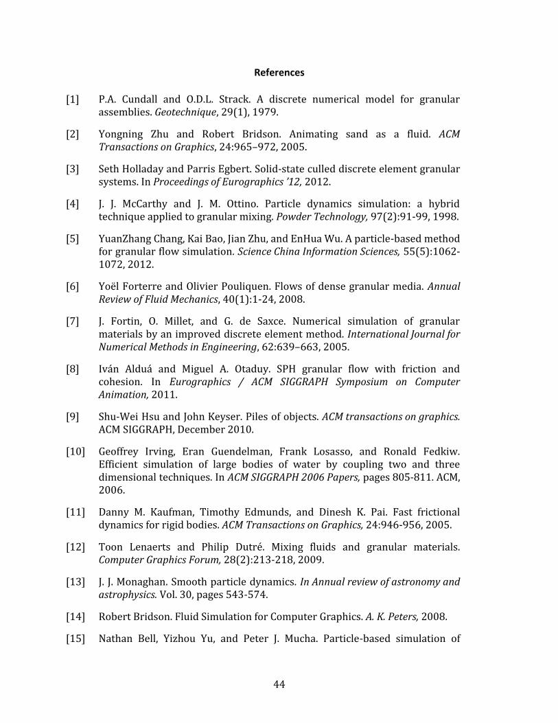
Results 2: High resolution mesh (10003) shows overpopulated quad pulling particles away from the center.
10,000 particles on surface. Constraint of 20 particles per face. Particles that do not exceed the threshold do
not get pushed apart.

40
Results 3: Another high resolution mesh (10003) with a different surface. Constraint of 20 particles per face.
Dispersion of particles in overly dense areas.

41
Chapter 6
Discussion and Future Work
Our solution performs well at breaking apart clumps that upset our predefined density
constraint. In every case where particles violate this constraint, they are globally moved
into lower pressure areas to obey the constraint.
One shortcoming of our algorithm is that our density constraint has to be specified
ahead of time. Future could involve automatically finding a threshold based on the
distribution of the particles at the start of the frame and adjusting to enforce a constraint
on a certain deviation of that density. Another issue is when the constraint is set too high
and the system is too laden with particles to be able to effectively find a solution where the
constraint isn’t violated becomes impossible. This is only avoided through trial and error.
Our formation of the problem was from the primitive or cell point of view. We just
have easily formulated the problem from a vertex point of view, which would allow us to
perform operations like the gradient as a vertex shader potentially speeding up the process
and giving us access to the graphics card for parallel computation.
The construction of the surface from the implicit voxel boundary alternatively could
be dependent upon the density of the particles around it. More triangles and quadrilaterals
under particle-dense areas would allow for more gradient vectors resulting in finer
movement. More computation would be spent on problem areas as opposed to a mostly
uniform advection solution.

42
Another possibility for dispersing patches is to apply more than one pass of our
algorithm relaxing the constraint on each pass in order to get additional smoothness. The
motivated researcher may even apply machine learning to reach a solution that optimizes
for both speed and lower density given the inputs of number of passes, density constraint,
and various scalar values found throughout the equations like advection intensity.

43
Chapter 7
Conclusion
We have demonstrated a superior method for handling surface particles on a hybrid
simulation. Our method solves the issue of particles getting too close together and
clumping unnaturally, distracting from the simulation. We have solved this issue without
adding a computational bottleneck and meeting the performance goals of the hybrid solver.
Our contributions include a unique rephrasing of the problem of running our
density correction step from a 3d volume to a 2d manifold making a very important trade-
off in having a faster density correction step while relenting only slightly on the visual
acuity of the algorithm. As a result, we have extended the 3-phrase hybrid simulation to fix
an artifact on the surface where particles clumped.
44
References
[1] P.A. Cundall and O.D.L. Strack. A discrete numerical model for granularassemblies. Geotechnique, 29(1), 1979.
[2] Yongning Zhu and Robert Bridson. Animating sand as a fluid. ACMTransactions on Graphics, 24:965–972, 2005.
[3] Seth Holladay and Parris Egbert. Solid-state culled discrete element granularsystems. In Proceedings of Eurographics ’12, 2012.
[4] J. J. McCarthy and J. M. Ottino. Particle dynamics simulation: a hybridtechnique applied to granular mixing. Powder Technology, 97(2):91-99, 1998.
[5] YuanZhang Chang, Kai Bao, Jian Zhu, and EnHua Wu. A particle-based methodfor granular flow simulation. Science China Information Sciences, 55(5):1062-1072, 2012.
[6] Yoël Forterre and Olivier Pouliquen. Flows of dense granular media. AnnualReview of Fluid Mechanics, 40(1):1-24, 2008.
[7] J. Fortin, O. Millet, and G. de Saxce. Numerical simulation of granularmaterials by an improved discrete element method. International Journal forNumerical Methods in Engineering, 62:639–663, 2005.
[8] Iván Alduá and Miguel A. Otaduy. SPH granular flow with friction andcohesion. In Eurographics / ACM SIGGRAPH Symposium on ComputerAnimation, 2011.
[9] Shu-Wei Hsu and John Keyser. Piles of objects. ACM transactions on graphics.ACM SIGGRAPH, December 2010.
[10] Geoffrey Irving, Eran Guendelman, Frank Losasso, and Ronald Fedkiw.Efficient simulation of large bodies of water by coupling two and threedimensional techniques. In ACM SIGGRAPH 2006 Papers, pages 805-811. ACM,2006.
[11] Danny M. Kaufman, Timothy Edmunds, and Dinesh K. Pai. Fast frictionaldynamics for rigid bodies. ACM Transactions on Graphics, 24:946-956, 2005.
[12] Toon Lenaerts and Philip Dutré. Mixing fluids and granular materials.Computer Graphics Forum, 28(2):213-218, 2009.
[13] J. J. Monaghan. Smooth particle dynamics. In Annual review of astronomy andastrophysics. Vol. 30, pages 543-574.
[14] Robert Bridson. Fluid Simulation for Computer Graphics. A. K. Peters, 2008.
[15] Nathan Bell, Yizhou Yu, and Peter J. Mucha. Particle-based simulation of

45
granular materials. In ACM SIGGRAPH/Eurographics Symposium on Computer Animation, pages 77-86, 2005.
[16] Bart Adams, Mark Pauly, Richard Keiser, and Leonidas J. Guibas. Adaptivelysampled particle fluids. ACM Transactions on Graphics, 26(3), July 2007.
[17] S. H. Liu, Theodore Kaplan, and L. J. Gray. Geometry and dynamics ofdeterministic sand piles. Physical Review A, 42(6):320703212, 1990.
[18] Fuchang Liu, Takahiro Harada, Youngeum Lee, and Young J. Kim. Real-timecollision culling of a million bodies on graphics processing units. ACMTransaction on Graphics (SIGGRAPH Asia), 2010.
[19] Iván Alduá, Ángel Tena and Miguel A. Otaduy. Simulation of high-resolutiongranular media. In Proceedings of Congreso Español de Informática Gráphica,2009.
[20] Anita Mehta, J. M. Luck, J. M. Berg, and G. C. Barker. Competition andcooperation: Aspects of dynamics in sandpiles. Journal of Physics: CondensedMatter, 17, 2005.
[21] J. J. Monaghan, A. Kocharyan. SPH simulation of multi-phase flow. InComputer Physics Communications, Elsevier 87(2), pages 225-235, May, 1995.
[22] B. C. Vemuri, L. Chen, L. Vu-Quoc, X. Zhang, and O. Walton. Efficient andaccurate collision detection for granular flow simulation. Graphical Models inImage Processing, 60:403-422, 1998.
[23] Yanci Zhang, Barbara Solenthaler, and Renato Pajarola. Adaptive Samplingand rendering of fluids on the gpu. In Proceedings of Volume Graphics, pages137-146, August, 2008.
[24] Theodore Kim, Jerry Tessendorf and Nils Thürey. Closest Point Turbulencefor Liquid Surfaces. ACM Transactions on Graphics. ACM SIGGRAPH, 2013.
[25] Robert W. Summer, James F. O’Brien, Jessica K. Hodgins. Animating Sand,Mud, and Snow. Graphics Interface, 1998.
[26] Rahul Narain, Abhinav Golas, Ming C. Lin. Free-Flowing Granular Materialswith Two-Way Solid Coupling. ACM Trans. Graph. 29, 6, Article 173,December 2010.
[27] Rahul Narain, Abhinav Golas, Sean Curtis, and Ming C. Lin, AggregateDynamics for Dense Crowd Simulation. Siggraph Asia ‘09, 2009.
[28] Brent Burley and Dylan Lacewell. Ptex: Per-Face Texture Mapping forProduction Rendering. Eurographics Symposium on Rendering, pages 1155-1164, 2008.

46
[29] Jens Cornelis, Markus Ihmsen, Andreas Peer, and Matthias Teschner. IISPH-FLIP for incompressible fluids. Computer Graphics Forum 33(2), pages 255-262, 2014.
[30] James F. Blinn. A generalization of algebraic surface drawing. ACM Trans.Graph. 1, 3 (235-256), 1982.
[31] Alain Fournier, Don Fussell, and Loren Carpenter. Computer Rendering ofStochastic Models. Commun. ACM, vol 25, no. 6, pages 371-384, 1982.
[32] Bo Zhu and Xubo Yang. Animating Sand as a Surface Flow. EurographicsShort Papers, 2010.
[33] J.-P. Bouchaud, M. Cates, J. Ravi Prakash, S. Edwards. A model for dynamics ofsandpile surfaces. Journal de Physique I, EDP Sciences, 4 (10), pages 1383-1410, 1994.
47
Image Credits
1. Close-up of sand from Coral Pink Sand Dunes State Park in Utah. Mark A. Wilson,
2008 (Department of Geology, College of Wooster) released to public domain.
2. Guatemala sinkhole 2010. Creative Commons Attribution 2.0 Generic. Photo by
Reuters/Scanpix. Modifications: ratio-locked reduce scale; filter: orange accent color
6 Dark. https://creativecommons.org/licenses/by/2.0.
3. Still of Woody in the garbage incinerator. Toy Story 3, 2010. Pixar Animation Studios
and Walt Disney Pictures. Fair Use.
4. Still of Scorpnorok burrowing into sand in Transformers. Transformers 2007.
Paramount Pictures; Sony/ATV Music Publishing; BMG Rights Management. Fair
Use.
5. Cutaway of Holladay and Egbert’s hybrid simulation revealing the solid, liquid, and
gas state [3]. Copyright 2011. Used with permission. All rights reserved.
6. Granular Assembly comprised of frozen spheres. Author released for public domain,
2015.
7. An example of a height map. Digital elevation model of a landform translated into a
sliced topograph on the laser engraver. Jared Tarbell. Creative Commons Attribution
2.0 Generic. Scaled to fit page.
8. Surface Granules clumping together along an edge. Copyright Seth Holladay and
Parris Egbert 2011 [1]. Used with permission.
Related Documents