Gas CondensateReservoirs

ABSTRACT that occur in the near-well region. The production performance of a gas condensate well is

easy to predict as long as the well’s flowing bottom-hole pres-sure (FBHP) is above the fluid dew point pressure (similar to adry gas well). Once the well’s FBHP falls below the dew point,the well performance starts to deviate from that of a dry gaswell. Condensate begins to drop out first near the wellbore.Immobile initially, the liquid condensate accumulates until thecritical condensate saturation (the minimum condensate satu-ration for mobility) is reached. This rich liquid zone then growsoutward deeper into the reservoir as depletion continues2.

The loss in productivity due to liquid buildup is mostly in-fluenced by the value of gas relative permeability (krg) near thewell when compared with the value of krg in the reservoir fur-ther away. The loss in productivity is more sensitive to theserelative permeability curves than to fluid pressure-volume-temperature (PVT) properties3.

The most accurate way to calculate gas condensate well pro-ductivity is by fine grid numerical simulation, either in single wellmodels with a fine grid near the well or in full field models usinglocal grid refinement. A large part of the pressure drawdownoccurs within 10 ft of the well, so radial models are needed,with the inner grid cell having dimensions of about 1 ft4, 5.

Several investigators have estimated the productivity of gascondensate reservoirs, but none of these methods is simple touse. Some methods require the use of the modification of a finite difference simulation process, whereas other methods usesimplified simulation models5, 6. Our objective is to develop asimple yet accurate analytical procedure to estimate the pro-ductivity of gas condensate reservoirs without having to runsimulations. The only data required by our method is the CCEexperiment results and relative permeability curves. As withother simplified methods, our new technique allows well per-formance to be evaluated quickly without reservoir simulations.A fine grid radial compositional model was built in a commercialflow simulator to validate the results of our analytical approach.

BACKGROUND

A method has been proposed for modeling the deliverability ofgas condensate wells2. Well deliverability is calculated using amodified Evinger-Muskat pseudopressure approach7. The gas-

Gas condensate reservoirs differ from dry gas reservoirs. Anunderstanding of relationships in the phase and fluid flow behavior is essential if we want to make accurate engineeringcomputations for gas condensate systems. That is because con-densate dropout occurs in the reservoir as the pressure falls below the dew point, as a result of which gas phase productiondecreases significantly.

The goal of this study is to understand the multiphase flowbehavior in gas condensate reservoirs, in particular focusing onestimating gas condensate well deliverability. Our new methodanalytically generates inflow performance relationship (IPR)curves for gas condensate wells by incorporating the effect ofcondensate banking as the pressure near the wellbore dropsbelow the dew point. The only information needed to generatethe IPR is the rock relative permeability data and results fromthe constant composition expansion (CCE) experiment.

We have developed a concept of critical oil saturation nearthe wellbore by simulating both lean and rich condensatereservoirs, and we have observed that the loss in productivitydue to condensate accumulation can be closely tied to criticalsaturation. We further are able to reasonably estimate re-evap-oration of the liquid accumulation by knowing the CCE data.

We validated our new method by comparing our analyticalresults with fine scale radial simulation model results. Wedemonstrated that our analytical tool can predict the IPR curveas a function of reservoir pressure. We also developed a methodfor generating an IPR curve by using field data and demonstratedits application. The method is easy to use and can be imple-mented quickly.

INTRODUCTION

Well productivity is an important issue in the development ofmost low and medium permeability gas condensate reservoirs.Liquid buildup around the well can cause a significant reduc-tion in productivity, even in lean gas condensate reservoirswhere the maximum liquid dropout in the constant compositionexpansion (CCE) experiment is as low as 1%1. Subsequently,accurate forecasts of productivity can be difficult because ofthe need to understand and account for the complex processes

A New Method to Predict Performance ofGas Condensate Reservoirs

Ali M. Al-Shawaf, Dr. Mohan Kelkar and Dr. Mohammed Sharifi

SAUDI ARAMCO JOURNAL OF TECHNOLOGY SUMMER 2013 23

64165araD4R1_64165araD4R1 5/29/13 3:52 PM Page 23

24 SUMMER 2013 SAUDI ARAMCO JOURNAL OF TECHNOLOGY

oil ratio (GOR) needs to be known accurately for each reservoirpressure to use the pseudopressure integral method. Equation 12

is employed to calculate the pseudopressure integral in thepseudo steady-state gas rate equation:

qg = CPr

[( Kro] Rs +

Krg )dp (1)Pwf

Bo o Bg g

To apply their method, we need to break the pseudopressureintegral into three parts corresponding to the three flow regionsdiscussed here:

Region 1: In this inner near-wellbore region, Fig. 1, bothcondensate and gas are mobile. It is the most important regionfor calculating condensate well productivity as most of thepressure drop occurs in Region 1. The flowing composition(GOR) within Region 1 is constant throughout and a semisteady-state regime exists. This means that the single-phase gasentering Region 1 has the same composition as the producingwell stream mixture. The dew point of the producing wellstream mixture equals the reservoir pressure at the outer edgeof Region 1.

Region 2: This is the region where the condensate saturationis building up. The condensate is immobile, and only gas isflowing. Condensate saturations in Region 2 are approximatedby the liquid dropout curve from a constant volume depletion(CVD) experiment, corrected for water saturation.

Region 3: This is the region where no condensate phase exists(it is above the dew point). Region 3 only exists in a gas con-densate reservoir that is currently in a single phase. It containsa single-phase (original) reservoir gas.

Another major finding2 is that the primary cause of reducedwell deliverability within Region 1 is krg as a function of relativepermeability ratio (krg/kro). Fevang and Whitson’s approach isapplicable for running coarse simulation studies, where theproducing GOR is available from a prior time step.

An approach to generate inflow performance relationship(IPR) curves for depleting gas condensate reservoirs withoutresorting to the use of simulation has been previously presented6.The producing GOR (Rp) is calculated with an expression

derived from the continuity equations of gas and condensate inRegion 1. But his approach requires an iterative scheme by as-suming Rp at a given reservoir pressure to generate IPR curvesfor rich gas condensate, whereas for lean gas condensates,GOR values from the reservoir material balance (MB) modelare adequate to achieve good results.

Later, Mott (2003) presented a technique that can be imple-mented in an Excel™ spreadsheet model for forecasting theperformance of gas condensate wells4. The calculation uses aMB model for reservoir depletion and a two-phase pseudo-pressure integral for well inflow performance. Mott’s methodgenerates a well’s production GOR by modeling the growth ofcondensate banking without a reservoir simulator.

All these methods do not provide a simple way of generat-ing IPR curves for condensate wells. The IPR curve as a func-tion of reservoir pressure is needed to accurately predict andoptimize the performance of the well.

APPROACH

The pseudo steady-state rate equation for a gas condensatewell in field units is given in Eqn. 28:

qsc =(703x10-6) kh[m(Pr) – m(Pwf)] (2)

T [1n( re ) – 0.75 + S]rw

where qsc = gas flow rate in Mscfd; k = permeability in md; h =thickness in ft; m (p) = pseudopressure in (psi2/cp); T = temper-ature in (ºR), re = drainage radius in ft; and rw = wellbore radius in ft. We can use this equation to estimate the gas pro-duction rate as long as the FBHP is above the dew point of thereservoir fluids. This means that this equation is applicableonly for single-phase gas flow. As soon as the FBHP drops be-low the dew point pressure of the reservoir fluid, condensatebegins to drop out, first near the wellbore, and the well per-formance starts to deviate from that of a dry gas well. Liquidcondensate accumulates until the critical condensate saturation(the minimum condensate saturation for mobility) is reached.This rich liquid bank/zone grows outward deeper into thereservoir as depletion continues.

Liquid accumulation, or condensate banking, causes a reduction in the gas relative permeability and acts as a partialblockage to gas production, which leads to potentially significantreductions in well productivity. To quantify the impact of gascondensation phenomena, we have developed a method togenerate the IPR of gas condensate reservoirs using analyticalprocedures. The main idea is to combine fluid properties (CCEor CVD data) with rock properties (relative permeabilitycurves) to arrive at an analytical solution that is accurateenough to estimate the IPR curves of gas condensate reservoirs.

FLUID DESCRIPTION

Two different synthetic gas condensate compositions were used

Fig. 1. Three regions of flow behavior in a gas condensate well.



to generate the rich, intermediate, and lean fluids representedin Fig. 2. The rich fluid is composed of three components:methane (C1) 89%, butane (C4) 1.55%, and decane (C10)9.45%. A four-component composition was used to generatethe intermediate and lean condensate mixtures at differentreservoir temperatures: methane (C1) 60.5%, ethane (C2)20%, propane (C3) 10%, and decane (C10) 9.5%. The char-acteristics of the condensate mixtures are outlined in Table 1.The Peng-Robinson three parameter equation of state (PR3)was used to simulate phase behavior and laboratory experi-ments, such as CCE and CVD.

RESERVOIR DESCRIPTION

The Eclipse 300 compositional simulator was used. A 1D radialcompositional model with a single vertical layer and 36 gridcells in the radial direction was used as a test case, Fig. 3. Homogeneous properties were used in the fine scale model asdescribed in Table 2.

A single producer well lies at the center of the reservoir. Themodel has been refined near the wellbore to accurately observethe gas condensate dropout effect on production. For that pur-pose, the size of the radial cells were logarithmically distributedwith the innermost grid size at 0.25 ft, according to Eqn. 3:

ri+1 = [re ]

1(3)ri rw

N

where N is the number of radial cells in the model. In additionto having very small grid blocks around the well, the time stepswere refined at initial times, which led to a very smooth satu-ration profile around the well. The fully implicit method waschosen for all the runs.

RELATIVE PERMEABILITY CURVES

It has already been noted in the literature that relative perme-ability curves affect the gas flow significantly in a gas condensatereservoir once the pressure falls below dew point pressure. Accurate knowledge about the relative permeability curves in agas condensate reservoir therefore would be critical information.Unfortunately, the relative permeability curves are rarely knownaccurately. It seemed worthwhile to investigate the effect of dif-ferent relative permeability curves on gas flow and study theuncertainty they bring to the saturation buildup in gas conden-sate reservoirs.

Different sets of relative permeability curves were used inthe study. These curves were generated based on Corey equa-tions, as illustrated in Eqns. 4 and 5:

Krg = Sgn (4)

Kro = (1 – Sg – Sor)m

(5) 1 – Sor

where n is the gas relative permeability exponent, m is the oilrelative permeability exponent, and Sor is the residual oil satu-ration. Fractures (X-curves) and intermediate and tight relativepermeability curves were generated by changing the n and m

Fig. 2. CCE data for synthetic gas condensate compositions.

ParametersR ich Gas

IntermediateGas

Lean Gas

Initial Reservoir Pressure (psia)

7,000 5,500 5,000

Dew Point Pressure (psia)

5,400 3,250 2,715

Reservoir Temperature (ºF)

200 260 340

Maximum Liquid Dropout (%)

26 20 8.5

Table 1. Fluid properties of condensate mixtures

Fig. 3. Fine grid radial model with 36 cells.

Porosity (%) 20

Absolute permeability (md) 10

Reservoir height (ft) 100

Irreducible water saturation (%) 0

Rock compressibility (psi-1) 4.0E-06

T

Table 2. Reservoir properties used in the fine radial model



exponents from 1 to 5 and changing Sor from 0 to 0.60. Figure4 shows three sets of relative permeability curves. Corey-1 (X-curve) was generated based on n=1, m=1, and Sor=0. Corey-14was generated based on n=3, m=4, and Sor=0.20. The thirdcurve, Corey-24, was generated based on n=5, m=4, andSor=0.60.

SENSITIVITY STUDY

In this research, we examined a large number of relative per-meability curves — over 20 sets of curves. The sensitivity studyalso examined the effects of fluid richness on gas productivityby using two fluid compositions (lean fluids and rich fluids).

The results of the sensitivity study were checked againstsimulation results. The simulation runs were done under a con-stant rate mode of production utilizing the fine compositionalradial model. After testing this wide range of relative perme-ability curves, we found that a very strong correlation existsbetween the well’s productivity index (PI) ratio and krg (So*).The value of So* is defined in a later section. Equation 6 definesthe well PI ratio:

PI Ratio = Min Well PI

(6)Max Well PI

Figure 5 shows an example of the well PI as a function oftime for a producing well. The abrupt fall of PI happens imme-diately after the FBHP falls below the Pd. After analyzing severalcases, we found that the PI is very close to krg (So*).

As can be seen from Fig. 5, the well PI drops quickly, theneventually increases slightly before stabilizing; the slight increasein PI is due to re-vaporization of oil. This type of PI behaviorhas been observed in field data where, after the bottom-holepressure (BHP) drops below the dew point pressure, the PI decreases suddenly before stabilizing.

As we can see from Fig. 6, after oil saturation reaches amaximum value, the So drops gradually after a period of pro-duction, which will enhance the gas relative permeability andtherefore the gas productivity. Figures 7 and 8 clearly show thatfor both rich and lean fluids, the relationship between the PIratio and krg (So*) is linear with a strong correlation coefficient.

Another important outcome of this sensitivity analysis is the

Fig. 4. Different sets of Corey relative permeability curves.

Fig. 5. Well PI as a function of time.

Fig. 6. Oil saturation profiles around the well as a function of time.

Fig. 7. Krg (So*) vs. PI ratio for rich fluid.



finding that the loss in productivity is more sensitive to the relative permeability curves than to fluid PVT properties. Figure 9 shows the well PI vs. time for the rich and lean fluids using the same relative permeability set. Figure 9 also demon-strates that the loss in productivity is much more dependent onrelative permeability curves than on the fluid composition.

Figure 10 summarizes the results of the sensitivity studydone on the rich and lean fluids by using the wide range of rel-ative permeability curves. It appears that the loss is similar forboth rich and lean gases so long as the same relative permeabilitycurves are used. The slope is not exactly equal to one, but it isvery close to one.

GENERATION OF IPR CURVES

IPR curves are very important to predicting the performance ofgas or oil wells; however, generating IPR curves using a simula-tor is not straightforward since the IPR represents the instanta-neous response of the reservoir at a given reservoir pressure fora given BHP. This cannot be generated in a single run since, ifwe change the BHP in a simulation run, depending on howmuch oil or gas is produced, the average pressure will change.

To generate IPR curves, we had to use a composite method.For different reservoir pressures, we ran a simulator at a fixedBHP. We then varied the BHP from high to low values. Wegenerated rate profiles for a particular BHP and average reservoirpressure as the reservoir pressure was depleted. Using variousruns, we picked the rate at a given reservoir pressure and agiven BHP and combined them into one curve to generate theIPR curve.

IMPORTANT OBSERVATIONS FROM SIMULATIONSTUDY

We wanted to develop simple relationships for generating theIPR curves under field conditions. We used the following im-portant observations from our simulation study to come upwith our procedure.

1. As already discussed before, we observed that the relative permeability curves have a bigger impact on the loss of productivity than the type of fluid that is produced.

2. The loss of productivity is significant and instantaneous after

Fig. 8. Krg (So*) vs. PI ratio for lean fluid.

Fig. 9. Well PI vs. time for rich and lean fluids (same relative permeability curves).

Fig. 10. Rich vs. lean PI ratio.

Fig. 11. Pseudo-pressure vs. gas rate plot.



the pressure drops below the dew point. After that point, the PI recovers slightly due to re-vaporization of the liquid.

3. The oil saturation profile near the wellbore is a strong func-tion of the average reservoir pressure9. Consequently, for a given reservoir pressure, the oil saturation profile does not change significantly for different BHPs, which will be shown in the next section.

NEW ANALYTICAL APPROACH FOR ESTIMATING GASCONDENSATE WELL PRODUCTIVITY

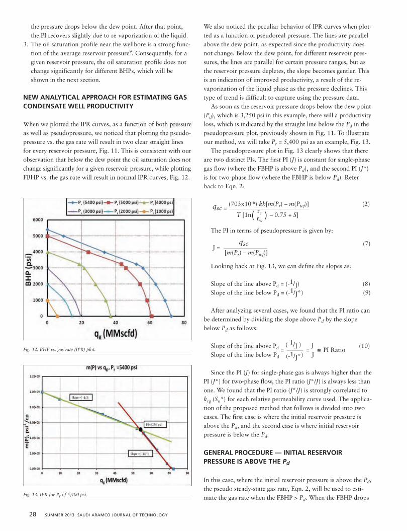
When we plotted the IPR curves, as a function of both pressureas well as pseudopressure, we noticed that plotting the pseudo-pressure vs. the gas rate will result in two clear straight linesfor every reservoir pressure, Fig. 11. This is consistent with ourobservation that below the dew point the oil saturation does notchange significantly for a given reservoir pressure, while plottingFBHP vs. the gas rate will result in normal IPR curves, Fig. 12.

We also noticed the peculiar behavior of IPR curves when plot-ted as a function of pseudoreal pressure. The lines are parallelabove the dew point, as expected since the productivity doesnot change. Below the dew point, for different reservoir pres-sures, the lines are parallel for certain pressure ranges, but asthe reservoir pressure depletes, the slope becomes gentler. Thisis an indication of improved productivity, a result of the re-vaporization of the liquid phase as the pressure declines. Thistype of trend is difficult to capture using the pressure data.

As soon as the reservoir pressure drops below the dew point(Pd), which is 3,250 psi in this example, there will a productivityloss, which is indicated by the straight line below the Pd in thepseudopressure plot, previously shown in Fig. 11. To illustrateour method, we will take Pr = 5,400 psi as an example, Fig. 13.

The pseudopressure plot in Fig. 13 clearly shows that thereare two distinct PIs. The first PI (J) is constant for single-phasegas flow (where the FBHP is above Pd), and the second PI (J*)is for two-phase flow (where the FBHP is below Pd). Referback to Eqn. 2:

qsc =(703x10-6) kh[m(Pr) – m(Pwf)] (2)

T [1n( re ) – 0.75 + S]rw

The PI in terms of pseudopressure is given by:

J = qsc (7)

[m(Pr) – m(Pwf)]

Looking back at Fig. 13, we can define the slopes as:

Slope of the line above Pd = (-1/J) (8)Slope of the line below Pd = (-1/J*) (9)

After analyzing several cases, we found that the PI ratio canbe determined by dividing the slope above Pd by the slope below Pd as follows:

Slope of the line above Pd =(-1/J )

=J

PI Ratio(10)

Slope of the line below Pd (-1/J*) J

Since the PI (J) for single-phase gas is always higher than thePI (J*) for two-phase flow, the PI ratio (J*/J) is always less thanone. We found that the PI ratio (J*/J) is strongly correlated tokrg (So*) for each relative permeability curve used. The applica-tion of the proposed method that follows is divided into twocases. The first case is where the initial reservoir pressure isabove the Pd, and the second case is where initial reservoirpressure is below the Pd.

GENERAL PROCEDURE — INITIAL RESERVOIR PRESSURE IS ABOVE THE Pd

In this case, where the initial reservoir pressure is above the Pd,the pseudo steady-state gas rate, Eqn. 2, will be used to esti-mate the gas rate when the FBHP > Pd. When the FBHP drops

Fig. 12. BHP vs. gas rate (IPR) plot.

Fig. 13. IPR for Pr of 5,400 psi.



below the Pd, we need to estimate (J*) first to be able to calcu-late the gas rate analytically. Since, in this case, initial reservoirpressure is above the Pd, we can estimate the PI (J), which willbe constant for all BHPs above the Pd.

After estimating (J), we use our knowledge of krg (So*) as amultiplier to get (J*) as:

J*=PI Ratio Krg( So*) (11)J

After estimating J*, which has a constant but higher slopethan J, as shown before on the pseudopressure plot, we canuse J* to estimate the gas rate for all BHP below the Pd. Usingthe following equation, we assume:

y = mx+b (12)

m(Pwf) = (- 1 )q+b (13)J*

We can utilize our knowledge of the rate and FBHP at thePd using the pseudo steady-state gas rate equation above thedew point. Then the intercept b can be calculated as:

b=m(Pd)+qd (14)J*

where b in field units is in (psi2/cp).Now, our straight line pseudopressure equation is complete

and able to estimate the gas rate for any FBHP less than the Pdas:

q = [b — m(Pwf)] J* (15)

where q is in (Mscfd), b and m(Piwf ) are in (psi2/cp), and J* isin (Mscfd/psia2/cp).

GENERAL PROCEDURE — INITIAL RESERVOIR PRES-SURE IS BELOW THE Pd

In this case, the pseudopressure vs. rate plot (IPR) will haveonly one straight line. Figure 11 shows three examples of IPRlines where the initial reservoir pressure is below the Pd. To beable to generate the IPR curves for these cases, the followingprocedure should be followed.

Estimate the PI (J)

If an IPR curve is available for the case where reservoir pres-sure is above the Pd, the PI (J) of this case could be used to esti-mate J* as a function of pressure using CCE data, as will beexplained in the next step. For cases above the Pd where IPRcurves are not available, the PI (J) could be estimated using apseudo steady-state gas rate equation, Eqn. 16:

J =qsc

=(703x10-6) kh (16)

[m(Pr) – m(Pwf)] T [1n (re ) – 0.75 + S]rw

Estimate the PI (J*)

As we have stated earlier, the PI ratio (J*/J) is correlated to krg(Sor), but in those cases where initial reservoir pressure is belowPd, liquid re-vaporization plays a very important role in deter-mining the productivity of gas condensate reservoirs. By examiningthe CCE data, as previously shown in Fig. 2, we can see that assoon as the pressure drops below the Pd, liquid saturation imme-diately reaches a maximum value (Max_SoCCE) around the Pd,then it falls gradually as a function of pressure. Our idea of utilizingCCE data in generating the IPR curves is really to account forthis phenomenon of liquid re-vaporization as pressure drops belowthe Pd9. We have found that using a fixed value of krg (Sor) or krg(Max_SoCCE) will underestimate the gas productivity for caseswhere initial reservoir pressure is below the Pd.

Therefore, for any reservoir pressure below Pd, krg needs tobe estimated at the corresponding pressure and oil saturationfrom the CCE data according to Eqn. 17:

J*(Pr) = Productivity Ratio Ratio Krg( Socce) (17)J

Estimate the Gas Rate

Finally, the gas rate can be directly estimated from Eqn. 18:

q = [m(Pr) – m(Pwf)] J* (18)

The above outlined procedure for generating IPR curves assumes that Sor = Max_SoCCE, but that is not always the casein real field applications. Since Sor is a rock property whileMax_SoCCE is a fluid property, we expect them to be differentin most of the field application cases.

For that reason, we have analyzed several cases where Sorcould be equal to, less than, or greater than Max_SoCCE. Basedon our evaluation, we believe that the maximum of the two valuesshould be used to correctly capture the fluid behavior around thewellbore and thereby accurately estimate the gas productivity.

The procedure to estimate PI (J*) here is exactly the same asthe procedure outlined above for the case where Sor =Max_SoCCE, but with some modifications as given by Table 3.This procedure is used for flowing pressure that is less than thedew point. In effect, what we are saying in this table is that, ifwe have reservoir pressure above the dew point, then to calcu-late the IPR curve for the BHP below the dew point, we canuse a constant slope (J*) based on the krg estimate as stated inTable 3. Subsequently, once the reservoir pressure drops belowthe dew point, we will need to use krg as a function of averagereservoir pressure.

IMPORTANCE OF THRESHOLD OIL SATURATION (SO*)

We have found that accurate estimation of gas productivity depends not only on Sor but also on the threshold oil saturation



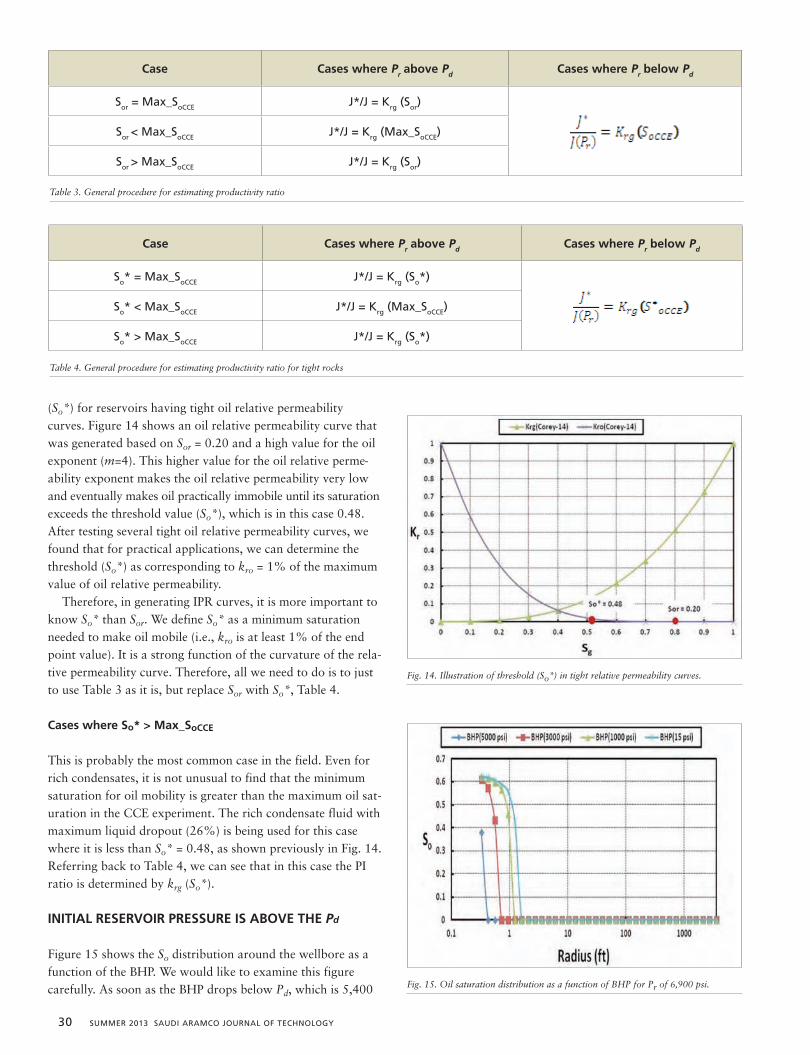
(So*) for reservoirs having tight oil relative permeabilitycurves. Figure 14 shows an oil relative permeability curve thatwas generated based on Sor = 0.20 and a high value for the oilexponent (m=4). This higher value for the oil relative perme-ability exponent makes the oil relative permeability very lowand eventually makes oil practically immobile until its saturationexceeds the threshold value (So*), which is in this case 0.48.After testing several tight oil relative permeability curves, wefound that for practical applications, we can determine thethreshold (So*) as corresponding to kro = 1% of the maximumvalue of oil relative permeability.

Therefore, in generating IPR curves, it is more important toknow So* than Sor. We define So* as a minimum saturationneeded to make oil mobile (i.e., kro is at least 1% of the endpoint value). It is a strong function of the curvature of the rela-tive permeability curve. Therefore, all we need to do is to justto use Table 3 as it is, but replace Sor with So*, Table 4.

Cases where So* > Max_SoCCE

This is probably the most common case in the field. Even forrich condensates, it is not unusual to find that the minimumsaturation for oil mobility is greater than the maximum oil sat-uration in the CCE experiment. The rich condensate fluid withmaximum liquid dropout (26%) is being used for this casewhere it is less than So* = 0.48, as shown previously in Fig. 14.Referring back to Table 4, we can see that in this case the PIratio is determined by krg (So*).

INITIAL RESERVOIR PRESSURE IS ABOVE THE Pd

Figure 15 shows the So distribution around the wellbore as afunction of the BHP. We would like to examine this figurecarefully. As soon as the BHP drops below Pd, which is 5,400

Case Cases where Pr above Pd Cases where Pr below Pd

So* = Max_SoCCE J*/J = Krg (So*)

So* < Max_SoCCE J*/J = Krg (Max_SoCCE)

So* > Max_SoCCE J*/J = Krg (So*)

Table 4. General procedure for estimating productivity ratio for tight rocks

Case Cases where Pr above Pd Cases where Pr below Pd

Sor = Max_SoCCE J*/J = Krg (Sor)

Sor < Max_SoCCE J*/J = Krg (Max_SoCCE)

Sor > Max_SoCCE J*/J = Krg (Sor)

Table 3. General procedure for estimating productivity ratio

Fig. 14. Illustration of threshold (So*) in tight relative permeability curves.

Fig. 15. Oil saturation distribution as a function of BHP for Pr of 6,900 psi.



choose the CCE data is because the accumulation near thewellbore is minimal, which means that near the wellbore regionwhatever flows from the reservoir will flow into the wellborewithout any change in its composition.

Since in this case the threshold (So*) is greater thanMax_SoCCE, our approach is to develop a linear relationshipbetween the So* and the CCE data, Fig. 21. Careful examinationof Fig. 15 and Figs. 18 to 20 tells us that actual liquid dropoutaround the wellbore is much greater than Max_SoCCE and is

psi for this fluid, liquid starts dropping out close to the well-bore first. The radius of oil banking expands inside the reservoir,and oil saturation away from the wellbore increases as theBHP decreases. We can see that at a BHP of 3,000 psi, Soreaches a maximum value of about 0.62, and this value almoststays constant even though the BHP drops to 1,000 psi andthen to atmospheric conditions.

What we want to highlight here is that as long as reservoirpressure is above the Pd, the oil saturation near the wellboreremains reasonably constant irrespective of the BHP. Since inthis case the threshold (So*) is higher than Max_SoCCE, thevalue of So* should be used to get the corresponding krg andtherefore estimate the well productivity for the cases wherereservoir pressure is above Pd. By following the general proce-dure outlined above for the case where initial reservoir pressure is above the Pd, we can generate the IPR curve asshown in Figs. 16 and 17. Just keep in mind that the onlychange you would make for this case where the threshold (So*)> Max_SoCCE is to use the larger value of (So*) or Max_SoCCE,which is in this case the So*.

J*= PI Ratio Krg( So*) (19)J

INITIAL RESERVOIR PRESSURE IS BELOW THE Pd

Now, we will illustrate an example where the IPR is below thePd. To correctly generate the slope of the IPR curve on thepseudopressure plot, we need to account for re-vaporization.Again we need to utilize the fine grid model to capture the condensate behavior near the wellbore.

By examining the three figures, Figs. 18 to 20, which showthe So distribution for saturated reservoirs, one will notice thatSo is decreasing gradually as a function of reservoir pressure,from about 0.62 when Pr = 6,900 psi, Fig. 15, to almost 0.30when Pr = 1,000 psi, Fig. 20. We conclude from this that oil re-vaporization close to the wellbore is a strong function of decreasing reservoir pressure.

For each saturated reservoir pressure, we can see that Sobuilds up to a uniform value close to the wellbore. This uniformSo remains almost constant as BHP decreases. Therefore, avalid assumption for the application of our method is to assumea uniform So for every saturated pressure under consideration.Figure 20 shows an example of an extreme case where all theoil evaporates at a very low flowing pressure.

Once we have understood gas condensate behavior aroundthe wellbore, we see that we really need to use a method thatcan mimic condensate re-vaporization as reservoir pressure depletes. The best tool to use is the CCE or CVD data for eachcondensate fluid being used9. The CCE data of the rich fluidwas previously shown in Fig. 2. Following Fevang and Whitson(1995)2, we will assume that the CCE experiment provides thebest description of fluid near the wellbore. That is, we can useCCE data to predict the re-vaporization of oil. The reason we

Fig. 16. IPR curve for Pr of 6,900 psi.

Fig. 17. Pseudo-pressure vs. gas rate plot for Pr of 6,900 psi..




closer to the threshold So*. We have seen from testing severalcases under this category that using krg (Max_SoCCE) will over-estimate the gas rate since it will not account for the relativepermeability of the oil phase; however, we can use CCE data toaccount for changes in oil saturation as the reservoir pressuredeclines.

It is very clear that condensate banking (accumulation) istied up with two factors. The first factor is fluid properties(Maximum So from CCE), and the second factor is rock prop-erties (Immobile So). Accordingly, we have asked ourselves thisquestion: Although we know that the actual liquid dropoutaround the wellbore is much greater than Max_SoCCE, how canwe still utilize the CCE data along with relative permeabilitycurves to come up with a robust analytical procedure that isaccurate enough to estimate the well productivity?

Other researchers have shown that relative permeability hasa first order effect on condensate banking, greater than thePVT properties3. As we have concluded from the results of thesensitivity study, different fluids will have a similar productivityloss for the same relative permeability curve used, confirmingto us that it is the relative permeability that is the most impor-tant factor in determining the productivity loss.

We used engineering approximation to model the behaviorbelow the dew point pressure. As we have stated before, we

are going to assume that the area around the wellbore behaveslike the CCE data for every designated saturated pressure. Following the general procedure previously outlined for thecase where IPR is below the Pd, we are going to explain ourapproach at Pr = 4,000 psi. After estimating the PI (J) asshown in Step 1 of the procedure, we can estimate PI (J*) as:

J* = Krg(S*oCCE) (20)

J(Pr)

At Pr = 4,000 psi, we should estimate So from the linear relation between the So* and CCE data, Fig. 21. The next stepis to go back to the relative permeability curves to estimate krgat the corresponding So from this linear relation. After that, J*can be calculated directly from Eqn. 20. The last step beforegenerating the IPR curve is to estimate the gas rate directlyfrom Eqn. 18. Just keep in mind that in this case the pseudo-pressure vs. rate plot will have only one straight line as this iswhat we expect to see in saturated reservoirs. The IPR curve isshown in Fig. 22 along with the pseudopressure plot in Fig.23. The complete IPR curves of this case are shown in Fig. 24.

Figure 25 shows the well PI producing at a constant rate. Asexpected, we found that the PI ratio is very close to krg (So*) asfollows:



Fig. 21. Developing linear relation between So* and CCE data.




Min Well PIKrg(So*) = 0.11 (21)

Max Well PI

Based on the PI ratio, we can define the productivity loss as:

Productivity loss = 1 –Min Well PI

(22)Max Well PI

Therefore, in this example, the productivity loss is 0.89. Thismeans that this well will experience an 89% productivity loss assoon as the BHP reaches the Pd. Looking back at Fig. 25, we cansee that the well restores some of its productivity after about 5

years of production. Figure 26 shows the saturation profiles as afunction of time, which shows the re-vaporization process.

FIELD APPLICATIONS

In this section we will show the application of our method to afield case. Both compositional model data and relative perme-ability curves were provided. A nine-component compositionalmodel was used with the PR3 to simulate phase behavior andthe CCE laboratory experiment, Fig. 27. Tables 5 and 6 showfluid properties and composition for the field case, respectively.

Figure 28 shows the relative permeability curves. As is com-mon in field applications, what matters here is the thresholdSo*. Although Sor = 0.20, the threshold So* = 0.32, which corresponds to about kro = 1% as a practical value. As wehave stated before, accurate estimation of gas productivity inthis case depends on the value of krg estimated at the thresholdSo*, which equals 0.32 in this case.

Moving to the production operations view in the field, wewill show that our method can be used to generate IPR curvesbased on production test data in the same way as Vogel’s,Fetkovich’s, and other IPR correlations.

Fig. 23. Pseudo-pressure vs. gas rate plot for Pr of 4,000 psi.

Fig. 24. IPR curves for rich gas (Corey-14).

Fig. 25. Well PI as a function of time.

Fig. 26. Oil saturation profiles around the well as a function of time.

Fig. 27. CCE data for field case fluid.



1. Estimate the PI (J) by utilizing Pr and the test data at the Pdusing Eqn. 7:

J = qsc

(7)[m(Pr) – m(Pwf)]

Or another way to estimate J is to plot the test points abovethe Pd on the pseudopressure plot, Fig. 30. J can then be calcu-lated from Eqn. 8:

slope = – 1 (8) J

2. Using J, you should be able to generate the first portion ofthe IPR curve using Eqn. 7.

3. The same way as we did in Step 1, we need to plot the testpoints below the Pd on the pseudopressure plot, Fig. 31. ThenJ* can be calculated from the slope as:

slope = – 1 (9) J*

4. The intercept of the straight line (b) should be estimated byusing Eqn. 14 as follows:

b = m(Pd) + qd (14)J*

5. Finally, we can estimate the gas rate for any BHP less thanthe Pd using Eqn. 15 as follows:

Assume that we are working in a production environment ina field where we have no knowledge about its relative permeabilitycurves. The only thing that we have is some production data.Since initial reservoir pressure is above the Pd, we know thatthe pseudopressure vs. gas rate plot will have two straightlines, as explained earlier. Therefore, to generate the IPR curvefor a given reservoir pressure, all we need is two test points.One point should be above the Pd and the other point shouldbe below the Pd.

Figure 29 shows an example of data from two productiontests. To explain how our method will work, we have designatedone of the test data to be at the Pd. Otherwise, any availabletest data above the Pd will fit the procedure. Our method usesthe following procedure:

Initial Reservoir Pressure (psia) 9,000

Dew Point Pressure (psia) 8,424

Reservoir Temperature (ºF) 305

Maximum Liquid Dropout (%) 3

Table 5. Fluid properties for the field case

Component Composition (Fraction)

H2S 0

CO2 0.0279

N2 0.0345

C1 0.7798

C2-C3 0.1172

C4-C6 0.0215

C7-C9 0.0132

C10-C19 0.00445

C20+ 0.00145

T Table 6. Fluid composition for the field case

Fig. 28. Relative permeability set of the field case.

Fig. 29. Production data from two tests.

Fig. 30. Pseudo-pressure vs. gas rate plot for points above Pd.



Therefore, in this example, we can conclude that once the FBHP drops below the Pd, the well will lose 70% of itsproductivity. We would like to highlight two major pointshere:1. Having two test points of production data clearly helped us

to characterize one value of relative permeability, which is krg at (So*). By knowing krg (So*), one can easily utilize relative permeability curves (if available) to estimate (So*) ormaximum oil saturation around the well.

2. Although this field case has very lean gas with maximum liquid dropout of only 3%, as previously shown in Fig. 27, the loss in productivity is significant (70%). This clearly tells us that the most important parameter in determining productivity loss is the gas-oil relative permeability curves, expressed in terms of krg estimated at residual (or threshold)oil saturation.We can easily generate the IPR curves for reservoir pressure

above the dew point pressure. The slope of the IPR curvesabove and below the dew point will remain the same, exceptthat the curve will shift downwards as the reservoir pressuredeclines. If the reservoir pressure is below the dew point, togenerate the entire IPR curve, we will just need one observation.

The PI (J*) can be calculated directly based on the test dataand reservoir pressure using Eqn. 16.

J*=qsc (16)

[m(Pr) – m(Pwf)]

After that, the gas rate can be directly estimated from Eqn. 18.

q = [m(Pr) – m(Pwf)]. J* (18)

If we want to predict the future IPR based on the currentIPR curve, we will need to have information about relative per-meability and CCE data. The complete IPR curves for this caseare shown in Fig. 34 where the generated IPR curves are vali-dated with the results of the fine radial compositional model.

Using our methodology, we examined 10 years of the production history of a gas condensate well with known CCEand relative permeability data. We used the initial production

q = [b – m(Pwf)]. J* (15)

The generated IPR curve and the pseudopressure plot areshown in Fig. 32 and Fig. 33, respectively.

We have shown that our method can be used to generateIPR curves based on available test data without any basicknowledge about the relative permeability curves. Before weproceed to an example where initial reservoir pressure is belowthe Pd, we would like to highlight one important thing. Wefound that the PI ratio equals 0.30 by using Eqn. 10:

Slope of the line above Pd=(-1

J )= Productivity Ratio = 0.30 (10)Slope of the line above Pd (-1

J*)

We would have expected this value to be equal to krg (So*),or 0.31, as previously shown in Fig. 28. We can easily quantifythe productivity loss once we have an idea about the PI ratioor krg (So*) using Eqn. 22 as follows:

Productivity loss = 1 – Productivity Ratio (22)

Fig. 31. Pseudo-pressure vs. gas rate plot for points below Pd.


Fig. 33. Pseudo-pressure vs. gas rate plot for Pr of 8,900 psi.



data and calculated the future IPR curves using our methodol-ogy. Figure 35 shows the future IPR curves. Superimposed onthose curves, we also show the actual production data as a func-tion of time as the reservoir pressure has declined. The matchbetween predicted rates and observed rates is quite good, vali-dating our procedure.

CONCLUSIONS

In this article, a new analytical procedure has been proposedto estimate the well deliverability of gas condensate reservoirs.Our new method analytically generates the IPR curves of gascondensate wells by incorporating the effect of condensate

banking as the pressure near the wellbore drops below the dewpoint. Other than basic reservoir properties, the only informa-tion needed to generate the IPR is the rock relative permeabil-ity data and CCE experiment results. In addition to predictingthe IPR curve under current conditions, our method can alsopredict future IPR curves if the CCE data are available.

We found that the most important parameter in determiningproductivity loss is the gas relative permeability at immobileoil saturation. We observed that at low reservoir pressures someof the accumulated liquid near the wellbore re-vaporizes. Thisre-vaporization can be captured by using CCE data. In ourmethod, we propose two ways of predicting the IPR curves:

• Forward Approach: By using the basic reservoirproperties, relative permeability data, and CCEinformation, we can predict the IPR curves for theentire pressure range. Comparison with simulationresults validates our approach.

• Backward Approach: By using field data, we can predictthe IPR curves for the entire pressure range. Thismethod does not require reservoir data; instead, similarto Vogel’s approach, it uses point information from theIPR curve and then predicts the IPR curve for the entireBHP range. Both synthetic and field data validate oursecond approach.

ACKNOWLEDGMENTS

The authors would like to thank Saudi Aramco managementfor permission to present and publish this article. The authorswould also like to acknowledge the support from the ReservoirDescription and Simulation Department at Saudi Aramco andextend thanks to the Tulsa University Center of ReservoirStudies for their support.

This article was presented at the SPE International Petro-leum Exhibition and Conference (ADIPEC), Abu Dhabi,U.A.E., November 11-14, 2012.

NOMENCLATURE

J = productivity index, (Mscfd/psia2/cp)K = absolute rock permeability, mdKrg = gas relative permeabilityKro = oil relative permeabilitym(p) = pseudopressure function, (psi2/cp)Pd = dew point pressure, psiaPr = average reservoir pressure, psiaPwf = flowing bottom-hole pressure, psiaqsc = gas flow rate at standard conditions, Mscfdre = external reservoir radius, ftrw = wellbore radius, ftRp = producing GOR, Scf/STBSg = gas saturation, fractionSo = oil saturation, fraction

Fig. 34. IPR curves for the field case.

Fig. 35. Validation of the new method with field data.


So* = threshold oil saturation, fractionSor = residual oil saturation, fractionSwi = connate water saturation

REFERENCES

1. Afidick, D., Kaczorowski, N.J. and Bette, S.: “ProductionPerformance of a Retrograde Gas Reservoir: A Case Studyof the Arun Field,” SPE paper 28749, presented at the SPEAsia Pacific Oil and Gas Conference, Melbourne,Australia, November 7-10, 1994.

2. Fevang, O. and Whitson, C.H.: “Modeling GasCondensate Well Deliverability,” SPE paper 30714,presented at the SPE Annual Technical Conference andExhibition, Dallas, Texas, October 22-25, 1995.

3. Mott, R.: “Calculating Well Deliverability in GasCondensate Reservoirs,” paper 104, presented at the 10th

European Symposium on Improved Oil Recovery, Brighton,U.K., August 18-20, 1999.

4. Mott, R.: “Engineering Calculations of Gas CondensateWell Productivity,” SPE paper 77551, presented at the SPEAnnual Technical Conference and Exhibition, San Antonio,Texas, September 29 - October 2, 2002.

5. Xiao, J.J. and Al-Muraikhi, A.J.: “A New Method for theDetermination of Gas Condensate Well ProductionPerformance,” SPE paper 90290, presented at the SPEAnnual Technical Conference and Exhibition, Houston,Texas, September 26-29, 2004.

6. Guehria, F.M.: “Inflow Performance Relationships for GasCondensates,” SPE paper 63158, presented at the SPEAnnual Technical Conference and Exhibition, Dallas,Texas, October 1-4, 2000.

7. Evinger, H.H. and Muskat, M.: “Calculation of TheoreticalProductivity Factor,” Transaction of the AIME, Vol. 146,No. 1, December 1942, pp. 126-139.

8. Kelkar, M.: Natural Gas Production Engineering, Tulsa,Oklahoma: PennWell Books, 2008, p. 584.

9. Vo, D.T., Jones, J.R. and Raghavan, R.: “PerformancePrediction for Gas Condensate Reservoir,” SPE FormationEvaluation, Vol. 4, No. 4, December 1989, pp. 576-584.

Engineering Division as a Production Field Engineer in theHaradh Engineering Unit.

In May 2008, Ali joined the Southern Area ReservoirSimulation Division where he conducted several full fieldsimulation models in onshore and offshore developmentand increment fields. His major responsibilities includeworking with a multidisciplinary team in a full IntegratedReservoir Study, which ranges from building staticgeological models to history matching and ends withforecasting full field development plans.

In 2006, Ali received his B.S. degree in PetroleumEngineering from King Fahd University of Petroleum andMinerals (KFUPM), Dhahran, Saudi Arabia. In 2012, hereceived his M.S. degree in Petroleum Engineering from theUniversity of Tulsa, OK, where he developed a new methodto predict the performance of gas condensate wells.

Ali is the author and coauthor of several technicalpapers. He has participated in several regional andinternational technical conferences and symposiums.

Ali is an active member of the Society of PetroleumEngineers (SPE) where he serves on several committees forSPE technical conferences and workshops.

Dr. Mohan Kelkar is the Director ofthe Tulsa University Center forReservoir Studies (TUCRS). He iscurrently working with severalmedium- and small-sized oil and gascompanies in relation to reservoircharacterization and optimization of

tight gas reservoirs. Mohan has published over 50 refereed publications and

has made over 100 technical presentations. He is acoauthor of a bestseller titled Applied Geostatistics forReservoir Characterization, published by the Society ofPetroleum Engineers (SPE) in 2002, and Gas ProductionEngineering, published in 2008 by PennWell Books.

In 1979, Mohan received his B.S. degree in ChemicalEngineering from the University of Bombay, Mumbai,Maharashtra, India. He received his M.S. and Ph.D.degrees in Petroleum Engineering and ChemicalEngineering, respectively, from the University of Pittsburgh,Pittsburgh, PA, in 1982.

Dr. Mohammad Sharifi is a ReservoirSimulation Engineer. His main researchis in the area of bridging static todynamic models through efficientupgrading and upscaling techniques.Mohammad is currently working ondeveloping a fast dynamic method for

ranking multiple reservoir realization models.He received his B.S., M.Eng., and M.S. degrees from the

Petroleum University of Technology (PUT), the Universityof Calgary, and PUT, respectively, all in ReservoirEngineering. Mohammad received his Ph.D. degree in Petroleum Engineering from the University of Tulsa, Tulsa,OK.

BIOGRAPHIES

Ali M. Al-Shawaf is the LeadSimulation Engineer for offshore gasfields in Saudi Aramco’s ReservoirDescription and SimulationDepartment. He joined the company in2006 and began working for theSouthern Area Gas Production

tight gas reservoirs

ki lti l



Gas CondensateReservoirs

Documents

gasgas condensate reservoirs

onestimating gas condensate

gas condensate systems

liquid condensate

adry gas

dry gas reservoirs

gas phase productiondecreases

minimum condensate saturation