Games and Goal-oriented Behavior

Games and Goal-oriented Behavior

Marek Hudík

Habilitation thesis

Faculty of Economics and Administration

Masaryk University

Brno, 2020

2

Abstract

This thesis uses a game-theoretic framework to formalize the Hayekian notion of equilibrium as

the compatibility of plans. In order to do so, it imposes more structure on the conventional model

of strategic games. For each player, it introduces goals, goal-oriented strategies, and the goals’

probabilities of success, from which players’ payoffs are derived. The differences between the

compatibility of plans and Nash equilibrium are identified and discussed. Furthermore, it is

shown that the notion of compatibility of plans, in general, differs from the notion of Pareto

efficiency. Since the compatibility of plans across all players can rarely be achieved in reality, a

measurement is introduced to determine various degrees of plan compatibility. Several possible

extensions and applications of the model are discussed. First, the model is used to account for,

endogenous instability of social norms. Second, a new classification of strategic games, based on

the goal structure of the game, is suggested. Third, the model is used to explain cooperative

behavior in social dilemmas. Finally, it is suggested that the notion of goal-orientedness of

behavior can serve as an unifying principle for behavioral sciences.

Keywords: goals, plans, goal-oriented strategies, Hayekian equilibrium, compatibility of plans,

Nash equilibrium, Pareto efficiency, social norms, classification of games, cooperative behavior,

Prisoner’s Dilemma

Contents

Acknowledgements 1

1 Introduction 2

2 Strategic games with goal-oriented strategies 11

3 Two notions of equilibrium: Hayek and Nash 17

4 Compatibility of plans and Pareto efficiency 29

5 Games with random events 33

6 Degrees of plan compatibility 41

7 Games with multiple goals 44

8 Extensions 51

9 Endogenous instability of Nash equilibrium 63

10 A theory of social norms change 78

11 Goal-oriented behavior and evolution 84

12 Goals and classification of games 92

13 Compatibility of plans and cooperative behavior 104

14 Conclusion 118

Appendix I: Hayek on equilibrium 120

Appendix II: Theories of social norms change 128

Appendix III: Instructions in the Prisoner’s Dilemma experiment 132

References 137

1

Acknowledgments

Various parts of this thesis were presented at the following conferences and workshops: Prague

Conference on Political Economy (April 2014), Center for Theoretical Studies Seminar (June

2014), University of Nottingham Ningbo China Research Seminar (May 2015), Xi’an Jiaotong-

Liverpool University Research Seminar (October 2017), 27th International Conference on Game

Theory at Stony Brook University (July 2018), Prague Conference on Political Economy (April

2019), and the World Interdisciplinary Network for Institutional Research (WINIR) at Lund

University (September 2019). I thank participants at these events, as well as my former and

current colleagues for helpful comments, critiques, encouragement, and inspiration. In particular,

I thank David Andersson, Pert Bartoň, Peter Bolcha, Steven Brams, Benoît Desmarchelier, Lu

Dong, Sailesh Gunessee, Gergely Horvath, Petr Houdek, Mofei Jia, Martin Komrska, Jirka

Lahvička, David Lipka, Shravan Luckraz, Antonín Machač, Pelin Ayan Musil, Pavel Pelikán,

Pavel Potužák, Tony So, David Storch, Dominik Stroukal, Mirek Svoboda, Josef Šíma, Petr

Špecián, Dan Šťastný, and Barnabé Walheer. In addition, I thank Tony So, Jenny Wang,

Yanning Zeng, and Xiyan Cai for excellent help with conducting the experiment reported in

Chapter 13. Chapters 2-5 are based on Hudik (2019), while Appendix I is based on Hudik (2018).

A substantial part of my research was supported by the research grant “Games and Goal-

Oriented Behavior” (RRSC10120160021) from the National Natural Science Foundation of

China. Last but not least, I would also like to thank my family and friends for their

encouragement and support. In particular, I am grateful to my dear wife Edita, who not only

supported me throughout the work but also gave me invaluable feedback.

2

3

1 Introduction

In groups, organizations, and societies, plans of various individuals may or may not be mutually

compatible. Consider the following two examples: A seller intends to sell a loaf of bread for at

least $1, while a buyer wants to buy a loaf of bread for at most $2. A football player performing

a penalty kick plans to kick to the left to score a goal, while a goalie intends to jump to the left to

prevent a goal. In the first example, plans of the two individuals are mutually compatible: The

seller’s plan to sell a loaf of bread for at least $1 and the buyers plan to buy a loaf of bread for at

most $2 can be both successfully carried out at the same time. In the second example, the plans

of the two individuals are not mutually compatible: The players plan to kick to the left to score a

goal, and the goalie’s plan to jump to the left to prevent a goal cannot both be successfully

carried out at the same time.

Intuitively, mutual compatibility of plans across individuals seems to be a characteristic of

equilibrium. Indeed, Hayek (1937, 2007) famously defined equilibrium as the compatibility of

plans. However, conventional equilibrium approaches do not model players’ plans and their

compatibility explicitly. Consider Nash equilibrium, the most commonly used solution concept

in the game theory. Nash equilibrium is based on the idea of payoff maximization rather than

plan compatibility. In fact, it can be shown that in Nash equilibrium, players’ plans may or may

not be compatible. Likewise, the compatibility of plans may not guarantee Nash equilibrium. To

see this, consider two traders who can either be honest, and carry out a transaction they agreed

4

on, or dishonest and try to cheat the other trader. Their situation can be modeled as the Prisoner’s

Dilemma with a unique Nash equilibrium in which both players choose to cheat (see Figure 1.1).

Yet, their plans to cheat are not mutually compatible. Each player’s plan to cheat can be

successfully carried out only if the other player is honest. Now assume that each player plans to

be honest and to carry out the transaction as agreed. Their plans are mutually compatible;

however, the outcome is not a Nash equilibrium because there is a better plan available for each

player, namely, to cheat.

a > 1, b > 0

Figure 1.1: Trade as a Prisoner’s Dilemma

Hayek’s notion of equilibrium as the compatibility of plans1 has never been formalized. In this

work, I fill this gap using the game-theoretic framework. In order to define the compatibility of

plans, a definition of “plan” has to be introduced. According to my approach, the plan is defined

as a “goal-oriented strategy”. For this purpose, I extend the conventional definition of strategic

games by introducing a set of goals for each player and associate them with their actions. The

compatibility of plans in my model means that all players are successful in achieving all the

1 Various terms have been used in the literature to describe the Hayekian notion of equilibrium, such as “maximum

compatibility of plans” (Rizzo 1990), “complete plan coordination” (Lewin 1997), or “Hayek’s compatibility”

(Giocoli 2003).

Honest Cheat

Honest 1, 1 a, –b

Cheat a, –b 0, 0

5

goals that are part of their plan. To formalize this, for each player, I introduce a success function

that determines whether players’ goals are achieved or not in a particular outcome. Players’

payoffs then depend on two characteristics: how successful a strategy is in achieving the goals

that the player has in mind and how valuable are these goals to the player.

Since payoffs are derived from goals and their probabilities of success, my model endogenizes

payoffs of the conventional model. From this perspective, it is related to the model of reason-

based rational choice by Dietrich and List (2013a; 2013b). In their model, players’ payoffs are

derived from their motivational states. If the motivational state changes, then the player’s payoffs

may change as well (see Hudik (2014) for a discussion of this model). I interpret the

motivational state as a set of goals rather than reasons. However, my main purpose is not to

endogenize preferences; instead, endogenization emerges as a byproduct of an attempt to

formalize the compatibility of plans.

Explicit modeling of players’ goals is a natural extension of the conventional model with

exogenous payoffs. This extension is in line with the recent attempts to move towards more

procedural models of decision making, as well as with an introspective observation that players

often think in terms of discrete goals and make plans to achieve them. The advantage of the

framework introduced in this paper is that it is procedural without compromising the

conventional payoff-based approach. The complementarity between my framework and the

conventional approach should be highlighted since several authors suggested the notion of goal-

oriented behavior as an alternative to payoff maximization (Conte and Castelfranchi 1995;

Vanberg 2002; 2004). In my interpretation, the conventional model implicitly aggregates actual

6

players’ motives into payoff maximization.2 My approach disaggregates payoffs into more basic

components.

Explicit modeling of players’ goals also builds a bridge between economics and other disciplines.

The notion of goal-orientedness is already employed in psychology (Locke and Latham 2002,

2013), biology (Mayr 1988, 1992), and it has been traditionally used in cybernetics and systems

theory (Rosenblueth et al. 1943; Ashby 1957; Bertalanffy 1968). In contrast, game-theoretic

literature on modeling players’ goals is small.3 Although various authors do sometimes speak

about goals,4 formal models are usually lacking. One exception proving the rule is Castelfranchi

and Conte (1998), who explore the issue of applicability of game theory to artificial intelligence

problems and propose what they call “goal-based strategy” as an alternative to payoff

maximization. Unfortunately, they do not develop the idea any further. Apart from this proposal,

they also correctly observe that strategies are sometimes (implicitly or explicitly) described as

2 In contrast to my interpretation, payoffs are sometimes treated as actual motives of players. This is justifiable in

case of money payoffs. However, in general, I find no introspective or other evidence that people actually think in

terms of payoffs postulated by the conventional model. Surprisingly, procedural-rationality models often keep the

conventional payoffs-beliefs framework rather than going beyond it. For the criticism along these lines, see Berg

and Gigerenzer (2010). For a discussion of the relationship between the behavioral (procedural) and rational choice

models, see Hudik (2017).

3 This is, however, less true for economics literature in general: Probably the best-known model of purposeful

behavior is Becker’s (1998) model of consumption as the production of commodities. For a survey of this literature,

see e.g., Dietrich and List (2013b). Apart from the references in Dietrich and List (2013b), works by Engliš (1930),

Mises (1996), and Rothbard (2004) are relevant. These works place purposeful behavior at the center of their

approach.

4 For instance, the concept of forward induction of Kohlberg and Mertens (1986) is based on goal-based reasoning.

7

goal-oriented. Thus, for instance, one of the strategies in the Prisoner’s Dilemma is usually

described as “cooperate”, indicating that the outcome aimed at is cooperation.5 My model is

consistent with Castelfranchi and Conte’s (1998) proposal, but contrary to these authors, I argue

that the concept of goal-orientedness is compatible with payoff maximization.

On a general level, my model can be thought of as a contribution to the literature that expresses

dissatisfaction with the Nash equilibrium concept. A prominent example of this literature

includes Brams and Wittman (1981) Brams and Mattli (1993), and Brams (1994), who argue that

Nash equilibrium is “myopic” and propose the “theory of moves” to address this deficiency.

Players in myopic equilibria may be “unhappy” if there exists a Pareto-superior outcome in the

game. The theory of moves elaborates on how players deal with this dissatisfaction by changing

the rules of the play. The notion of compatibility of plans provides another reason why players

may be “unhappy” in Nash equilibria: failure to realize their plans. The complementarity

between my approach and the theory of moves is underlined by the fact that the authors also

derive players’ preferences from goals. However, they assume that players’ goals are

lexicographically ordered. My approach is more general, as it is not restricted to lexicographic

ordering, and also closer to the conventional game theory with respect to formal representation.

1.1 Outline of the work

This thesis is organized as follows.

5 Another example is the Stag Hunt game, where the strategies are typically described with goals that players want

to achieve (i.e., “Stag” and “Hare”). I make extensive use of the Stag Hunt game in this work.

8

Chapter 2 introduces the model of strategic games with goal-oriented strategies. The model is

compared with the conventional model of strategic games.

Chapter 3 defines two solution concepts for the strategic games with goal-oriented strategies:

Nash equilibrium and overall compatibility of plans (OCP). The relationship between these two

solution concepts is discussed.

Chapter 4 discusses the relationship between Pareto efficiency and OCP. In particular, I show

that even if all players are successful in achieving their goals, the outcome may not be Pareto

efficient. The reason is that for each player, there may exist a more valuable goal outside the

OCP. At the same time, Pareto efficiency does not imply compatibility of plans. The fact that a

player does not achieve a particular goal with probability one can be compensated for by a high

value of this goal to him, which is reflected in high payoff (in relative terms).

Chapter 5 explicitly introduces exogenous events in the model. This extension helps to

distinguish mutual compatibility of plans across players and the compatibility of players’ plans

with their environment. Another solution concept is introduced: the mutual compatibility of

plans (MCP). MCP isolates the compatibility of plans across players from compatibility with the

environment.

Chapter 6 acknowledges that both OCP and MCP may be difficult to achieve in reality.

Therefore, measurements are introduced to account for various degrees of plan compatibility.

9

These measurements are used to identify situations “closer to” or “further away from”

equilibrium in the sense of compatibility of plans.

Chapter 7 considers a more general case of the model, in which players’ plans may be associated

with more than one goal.

Chapter 8 discusses two additional extensions of the framework. In particular, I consider that

players have preferences defined on probabilities of success in all feasible outcomes rather than

on overall probabilities of success of their plans. This extension, which elaborates on the model

introduced in Chapter 5, enables players to have different preferences in the case when their

plans were disappointed by the incompatibility of other players’ plans and in the case when their

plans were disappointed by incompatibility with the environment. As a different extension of the

basic model, I explicitly include players’ beliefs. This extension allows players to have

asymmetric beliefs about the realized state of nature.

Chapter 9 starts with the observation that Nash equilibrium and OCP may differ. It is argued that

if an outcome is an OCP but not a Nash equilibrium, then it is intuitively appealing to players

because they are successful in carrying out their plans; however, OCP is unstable within the

game, as the players can profitably deviate from this outcome (i.e., attain a more valuable goal).

If, on the other hand, an outcome is a Nash equilibrium but not an OCP, then this outcome tends

to be endogenously unstable, as players, whose plans are disappointed, have an incentive to

change the game, either by searching for alternative plans or by strategically modifying the game.

10

Chapter 10 applies the notion of endogenous instability of Nash equilibria to account for the

social norms change. As an example, I use the change of medium of exchange from commodity

money to banknotes.

Chapter 11 uses the notion of goal-oriented behavior as a link between payoff maximization and

fitness maximization. It is argued that goal-oriented behavior is a useful tool to model types of

adaptation that rest between natural selection and purposeful behavior. It is also suggested that

the idea of goal-directedness can serve as a unifying concept for various behavioral sciences.

Chapter 12 uses the explicit modeling of players’ goals introduced in previous chapters as a tool

to classify games as pure common-interest, mixed-motive, and pure conflict games. The

difference between the conventional classification and the suggested classification is discussed.

Chapter 13 considers the intuitive appeal of OCP. It argues that OCP may contribute to the

explanation of cooperative behavior in the one-shot Prisoner’s Dilemma. This hypothesis is

tested experimentally.

Chapter 14 concludes with methodological remarks and suggestions for further research.

Appendix I discusses Hayek’s views on equilibrium and compares them to the approach

introduced in this work.

11

Appendix II reviews existing theories of social norms change and compares them to the approach

outlined in Chapters 9 and 10.

Appendix III contains instructions used in the Prisoner’s Dilemma experiment reported in

Chapter 13.

12

2 Strategic games with goal-oriented strategies

2.1 Conventional strategic games

I start with the definition of conventional strategic games, found in virtually all textbooks on

game theory. These games consist of three elements: a finite set of players, N; for each player

i N , a non-empty set of actions, Ai; for each player i N , a preference relation ≿idefined on

the set j N jA A . Preferences are conveniently represented with a payoff function ;iu A as

follows: ( ) ( )i iu a u b whenever a ≿ib.

Definition 2.1. Strategic game is defined as a triple ,( ),iN A ≿ i .

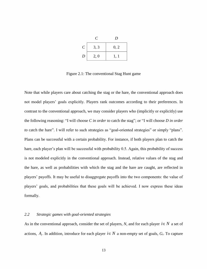
Example 2.1. Consider a simple two-player example of a strategic game known as the Stag Hunt

game. Each of the two players – hunters – chooses between cooperating in pursuing a single stag,

C, and defecting, D, i.e., competing in pursuing a single hare. If both players cooperate, they will

catch the stag with certainty and share it equally; if only one of them cooperates, he will catch

nothing. On the other hand, if a player pursues the hare alone, he will catch it for sure; if both

players pursue the hare, each will catch it with the probability 0.5. Thus we have {1,2}N , and

1 2 { , }A A C D . Payoffs are shown in Figure 2.1. In particular, it is assumed that each player

prefers a share of the stag to the hare, i.e., 1( , ) ( , )C C D C and 2( , ) ( , )C C C D .

13

Figure 2.1: The conventional Stag Hunt game

Note that while players care about catching the stag or the hare, the conventional approach does

not model players’ goals explicitly. Players rank outcomes according to their preferences. In

contrast to the conventional approach, we may consider players who (implicitly or explicitly) use

the following reasoning: “I will choose C in order to catch the stag”; or “I will choose D in order

to catch the hare”. I will refer to such strategies as “goal-oriented strategies” or simply “plans”.

Plans can be successful with a certain probability. For instance, if both players plan to catch the

hare, each player’s plan will be successful with probability 0.5. Again, this probability of success

is not modeled explicitly in the conventional approach. Instead, relative values of the stag and

the hare, as well as probabilities with which the stag and the hare are caught, are reflected in

players’ payoffs. It may be useful to disaggregate payoffs into the two components: the value of

players’ goals, and probabilities that these goals will be achieved. I now express these ideas

formally.

2.2 Strategic games with goal-oriented strategies

As in the conventional approach, consider the set of players, N, and for each player i N a set of

actions, iA . In addition, introduce for each player i N a non-empty set of goals, Gi. To capture

C D

C 3, 3 0, 2

D 2, 0 1, 1

14

the notion of goal-orientedness of behavior, define for each player i N a set of goal-oriented

strategies (or plans) i i iS A G . In words, each action is associated with one (possibly different)

goal. A more general case where an action can be associated with multiple goals is discussed in

Chapter 7. The set of strategy profiles j N jS is denoted by S.

We now want to capture the idea that players’ may or may not be successful in realizing their

plans. In general, whether a player realizes his plan or not depends not only on the strategies

taken by him and others but also on the environment. For instance, a farmer’s plan to produce a

certain amount of corn may be disappointed due to unfavorable weather conditions. For now, I

do not distinguish between the two cases, and I assume that players care only about the overall

probability of achieving their goals. As I demonstrate below, even this simple model gives

interesting results. Nevertheless, in Chapter 5, I consider an extension that allows distinguishing

between incompatibility of a player’s plan with other players’ plans and incompatibility with the

environment.

To account for the compatibility of players’ plans, define for each i N a success function6

: [0,1] iG

ip S which assigns to each strategy profile a iG -tuple of probabilities, ( | )i ip g s . For

each goal i ig G , they specify the probability with which the player i achieves his goal if the

outcome is s. For each player i, denote the set of the probability vectors ( )ip s by Pi.

6 This function is different from the success function used in the contest theory. Nevertheless, it resembles a

consequence function sometimes considered in strategic games (Osborne and Rubinstein 1994).

15

Since each goal may have a different importance to a player, define for each player i N a

complete and transitive preference relation ≿ i on the set Pi. We will assume that preferences are

strongly monotone. That is, if ( ) ( )i ip s p s then ( ) ( )i ip s p s . In words, players prefer higher

probability of achieving their goals to lower probability. 7 As usual, preferences can be

conveniently represented by a payoff function defined in the standard way.8

Definition 2.2. Strategic game with goal-oriented strategies is defined as a sextuple

,( ),( ),( ),( ),i i i iN A G S p ≿ i .

Recall that conventional strategic game (Definition 2.1) is defined as a triple ,( ),iN A ≿ i . This

means that we have introduced three new elements: goals, plans, and probabilities of success.

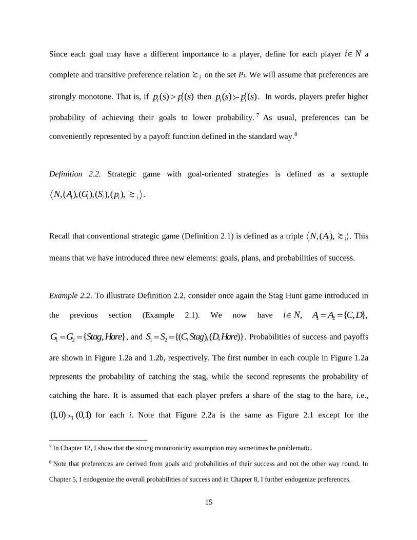
Example 2.2. To illustrate Definition 2.2, consider once again the Stag Hunt game introduced in

the previous section (Example 2.1). We now have ,i N 1 2 { , },A A C D

1 2 { , }G G Stag Hare , and 1 2 {( , ),( , )}S S C Stag D Hare . Probabilities of success and payoffs

are shown in Figure 1.2a and 1.2b, respectively. The first number in each couple in Figure 1.2a

represents the probability of catching the stag, while the second represents the probability of

catching the hare. It is assumed that each player prefers a share of the stag to the hare, i.e.,

(1,0) (0,1)i for each i. Note that Figure 2.2a is the same as Figure 2.1 except for the

7 In Chapter 12, I show that the strong monotonicity assumption may sometimes be problematic.

8 Note that preferences are derived from goals and probabilities of their success and not the other way round. In

Chapter 5, I endogenize the overall probabilities of success and in Chapter 8, I further endogenize preferences.

16

descriptions of the alternatives from which players choose. In the conventional approach, each

player chooses an action; in the present model, each player chooses a goal-oriented strategy, i.e.,

an action associated with a goal. The similarity between Figure 2.1 and Figure 2.2b highlights

the fact that the model with goal-oriented strategies endogenizes payoffs of the conventional

model.

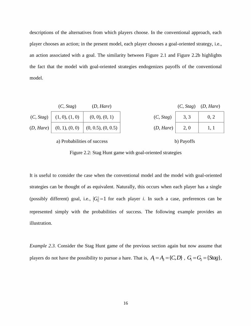
a) Probabilities of success b) Payoffs

Figure 2.2: Stag Hunt game with goal-oriented strategies

It is useful to consider the case when the conventional model and the model with goal-oriented

strategies can be thought of as equivalent. Naturally, this occurs when each player has a single

(possibly different) goal, i.e., 1iG for each player i. In such a case, preferences can be

represented simply with the probabilities of success. The following example provides an

illustration.

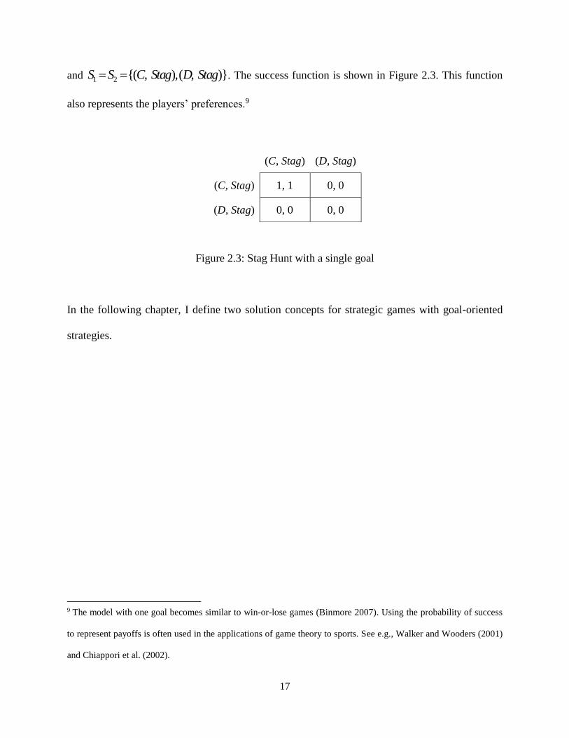
Example 2.3. Consider the Stag Hunt game of the previous section again but now assume that

players do not have the possibility to pursue a hare. That is, 1 2 { , }A A C D , 1 2 { }G G Stag ,

(C, Stag) (D, Hare)

(C, Stag) (1, 0), (1, 0) (0, 0), (0, 1)

(D, Hare) (0, 1), (0, 0) (0, 0.5), (0, 0.5)

(C, Stag) (D, Hare)

(C, Stag) 3, 3 0, 2

(D, Hare) 2, 0 1, 1

17

and 1 2 {( , ),( , )}S S C Stag D Stag . The success function is shown in Figure 2.3. This function

also represents the players’ preferences.9

Figure 2.3: Stag Hunt with a single goal

In the following chapter, I define two solution concepts for strategic games with goal-oriented

strategies.

9 The model with one goal becomes similar to win-or-lose games (Binmore 2007). Using the probability of success

to represent payoffs is often used in the applications of game theory to sports. See e.g., Walker and Wooders (2001)

and Chiappori et al. (2002).

(C, Stag) (D, Stag)

(C, Stag) 1, 1 0, 0

(D, Stag) 0, 0 0, 0

18

3 Two notions of equilibrium: Hayek and Nash

I define two solution concepts for strategic games with goal-oriented strategies: Nash

equilibrium and overall compatibility of plans (OCP). OCP is inspired by Hayek (1937, 2007). I

summarize Hayek’s views on the equilibrium concept in Appendix I.

3.1 Definitions

In Chapter 2, I have argued that the model of games with goal-oriented strategies puts more

structure on the conventional model of strategic games (it specifies what is “behind” the payoffs).

Therefore, solutions used for the latter type of games can also be used for the former type. In

particular, we can still apply Nash equilibrium, although the formal definition is slightly different.

More specifically, in our case, Nash equilibrium is a profile of goal-oriented strategies rather

than actions.

Definition 3.1. A Nash equilibrium of a strategic game with goal-oriented strategies

,( ),( ),( ),( ),i i i iN A G S p ≿ i is a profile *s S of goal-oriented strategies with the property that

for every player i N we have * *( , )i i ip s s ≿ *( , )i i i ip s s for all i is S .10

10 It is assumed throughout the paper that players do not choose mixed strategies. One problem with mixed strategies

is that they allow for multiple interpretations (e.g., Osborne and Rubinstein 1994). A procedural approach, such as

the one proposed in this paper, should either assume mixed strategies away (if they are irrelevant for the issue at

hand) or commit to a specific interpretation. This paper adopts the first route. However, a simple way to account for

mixed strategies in a way consistent with the proposed framework is to consider the possibility that players can

commit to a randomizing device. This possibility can be modeled as a pure strategy.

19

Example 3.1. The Stag Hunt game in Example 2.2 (Figure 2.2) has two Nash equilibria: (C, Stag;

C, Stag) and (D, Hare; D, Hare).

Explicit modeling of players’ goals allows for an additional solution concept, based on the

considerations of whether players are successful in attaining their goals. I first define a perfectly

successful goal-oriented strategy in a given outcome; then, I define as a profile of perfectly

successful goal-oriented strategies. I call this profile the overall compatibility of plans (OCP).

Definition 3.2. Consider a strategic game with goal-oriented strategies. A goal-oriented strategy

j js S is perfectly successful in s if ( | ) 1j jp g s for gj associated with js .

Definition 3.3. Overall compatibility of plans (OCP) in a strategic game with goal-oriented

strategies ,( ),( ),( ),( ),i i i iN A G S p ≿ i is a profile s S of goal-oriented strategies with the

property that for each i N , is is perfectly successful in s .

Example 3.2. The Stag Hunt game in Example 2.2 (Figure 2.2) has one OCP, namely (C, Stag; C,

Stag).

In Chapter 5, I distinguish OCP from the mutual compatibility of plans (MCP). The term

“overall” refers to the fact that in the present model, we do not distinguish between the

compatibility of plans across players and compatibility of plans with the environment. In Chapter

5, I distinguish these two cases. Both OCP and MCP and are derived from Hayek’s notion of

20

equilibrium. However, Hayek was more interested in mutual compatibility of plans across

individuals than in compatibility of an individual’s plans with the nature (see Hayek 1937 and

Appendix I).

Note that unlike Nash equilibrium, OCP is not defined in terms of payoffs. In a sense, the

compatibility of players’ plans is “objective” because it does not depend on players’ preferences

and beliefs.11 Nonetheless, there is a link from goals to payoffs through the strong monotonicity

assumption: Since players seek to realize their plans, a perfectly successful strategy is reflected

in a high payoff (in relative terms). An important implication of the fact that OCP is not defined

in terms of payoffs is that players’ plans can be mutually compatible even if players do not

maximize their payoffs. Conversely, if players maximize their payoffs, they may end up in a

situation where their plans are mutually incompatible. Therefore, while there is a direct link

between maximizing behavior and Nash equilibrium (Aumann 1985), there is no such link

between maximizing behavior and OCP. 12 I now discuss the relationship between the two

concepts of equilibria in more detail.

11 “Objective” here does not refer to physical objectivity but to inter-personal validity. One can think of

compatibility of plans as being “ontologically subjective” but “epistemologically objective” (Searle 2005). Or –

using Popper’s (1979) terminology – it is objectivity in the sense of World 3 rather than World 1. On this issue, see

also Hudik (2011).

12 The issue of whether there is a link between maximizing behavior and equilibrium has been (in a different

context) raised by Boettke and Candela (2017). See also Giocoli (2003).

21

3.2 The relationship between OCP and Nash equilibrium

3.2.1 Games with a single goal

First, consider a game in which each player has only one goal. For this class of games, the

following theorem holds.

Theorem 3.1. Let be Γ be a game with goal-oriented strategies where 1iG for each player i. If

s is an OCP, then it is also a Nash equilibrium.

Proof. Note that since s is an OCP, then ˆ( | ) 1i ip g s for each player i. The strong monotonicity

assumption implies that for every player i N we have ˆ ˆ( , )i i ip s s ≿ ˆ( , )i i i ip s s for all i is S ,

and therefore, s is also a Nash equilibrium.

Example 3.3. Consider again the version of the Stag Hunt in Example 2.3, where players do not

have an option to pursue a hare. In this game, there is a single OCP, (C, Stag; C, Stag), which is

at the same time a Nash equilibrium (see Figure 2.3). The game has another Nash equilibrium,

namely (D, Stag; D, Stag). This second Nash equilibrium is not an OCP as neither player

achieves his goal.

The Example 3.3 shows that even in a game with single goal, Nash equilibrium need not be an

OCP. On the other hand, since by Theorem 3.1 all OCPs in the games with a single goal are at

the same time Nash equilibria, the following corollary holds.

22

Corollary 3.1. Let be Γ be a game with goal-oriented strategies where 1iG for each player i.

If Γ has no Nash equilibrium, then it also has no OCP.

Proof. Directly follows from Theorem 3.1.

Example 3.4. Consider the Matching Pennies game with goal-oriented strategies. Each of the two

players chooses between heads and tails. If both players make the same choice, player 1 wins; if

their choices differ, then player 2 wins. Each player’s goal is to win the game. Thus we have

{1,2}N , 1 2 { , }A A Heads Tails , 1 2 { }G G Win , and S1 = S2 = {(Heads, Win), (Tails, Win)}.

Probabilities of success are shown in Figure 3.1. These probabilities also represent players’

payoffs. The game has no Nash equilibrium because, in each outcome, one player can deviate

and increase his payoff. The game also has no OCP as there is no outcome in which players’

plans to win the game are mutually compatible.13

Figure 3.1: Matching Pennies with goal-oriented strategies

13 The well-known Holmes-Moriarty game is also of this type. In this game, Holmes, trying to escape Moriarty,

considers whether to get off the train in Dover or a station earlier. Moriarty, pursuing Holmes, has to decide at which

station he should wait for Holmes. Note that this game was introduced by Morgenstern (1928) and inspired Hayek’s

work on equilibrium (Giocoli 2003; Leonard 2010). See also Appendix I.

(Heads, Win) (Tails, Win)

(Heads, Win) 1, 0 0, 1

(Tails, Win) 0, 1 1, 0

23

3.2.2 Games with multiple goals

In general, if each player can pursue only one goal, the analysis of the goal structure of the game

adds only little to the conventional approach. More interesting cases emerge when players pursue

multiple goals. Here the conventional analysis collapses potentially complex goal structure into a

single artificially-constructed goal, namely payoff maximization. Consequently, some relevant

information about players’ reasoning may get lost by this aggregation. More specifically, with

multiple goals, there may be OCPs that are not Nash equilibria. This can be seen already in

games where each player has two goals. The following example provides an illustration.

Example 3.5. Consider first the Stag Hunt game in Example 2.2. The outcome (C, Stag; C, Stag)

is an OCP (see Figure 1.1a) and, given the preferences in Figure 1.1b, also a Nash equilibrium.

Now assume that for each player, a hare is preferred to a share of the stag, i.e. (0,1) (1,0)i . At

the same time, continue to assume that (1,0) (0,0.5)i . The probabilities of success are shown in

Figure 3.2a. They are the same as in Figure 2.1a (the “hunting technology” has not changed);

however, payoffs are now different, as shown in Figure 3.2b.


Figure 3.2: Stag Hunt as Prisoner’s Dilemma

(C, Stag) (D, Hare)

(C, Stag) (1, 0), (1, 0) (0, 0), (0, 1)

(D, Hare) (0, 1), (0, 0) (0, 0.5), (0, 0.5)

(C, Stag) (D, Hare)

(C, Stag) 2, 2 0, 3

(D, Hare) 3, 0 1, 1

24

The game now has a structure of the Prisoner’s Dilemma. The outcome (C, Stag; C, Stag) is still

an OCP but not a Nash equilibrium anymore. Each player can achieve a more valuable goal (i.e.,

hare) by deviating. However, their plans to catch the hare are mutually incompatible: The

outcome (D, Hare; D, Hare) is not an OCP (although it is a Nash equilibrium). Players thus may

face a dilemma between the Nash equilibrium and the OCP. Conventional analysis is clear: In

order to maximize his payoff, each player should choose D. However, the outcome (C, Stag; C,

Stag) is appealing to the players because they are successful in attaining the goal they have in

mind. It has been observed that many people actually choose to cooperate in one-shot Prisoner’s

Dilemma both in laboratory experiments (Colman 1995; Sally 1995; Komorita and Parks 1995)

and outside the laboratory (List 2006). The notion of compatibility of plans may contribute to the

explanation of the observed play. I follow this line of reasoning further in Chapter 11.

3.3 A note on the existence of equilibria

As it is clear from the Matching Pennies game in Example 3.4, Nash equilibrium and OCP may

not exist even in the simplest games (recall, that we do not consider mixed strategies). While a

lot of attention is paid to existence theorems in the game-theoretic literature, I argue that the non-

existence of a solution concept for a particular game does not represent a major problem, and in

the case of OCP, it is, in fact, a feature.

Consider that we observe a stable behavior in reality. For instance, real-world hunters always

cooperate in pursuing a stag. In line with the current practice, we attempt to account for this

behavior as a Nash equilibrium phenomenon. Therefore, we construct a game, where pursuing a

stag is a Nash equilibrium. In other words, equilibrium in such a game exists by construction,

25

and games with no Nash equilibria are simply non-applicable to cases of stable and persistent

behavior.

In contrast, OCP can be used to account for changes in behavior. One way to think about this

equilibrium concept is as a “Platonic” ideal, which players attempt to achieve but often may be

out of reach.14 More specifically, players care about the maximum success of their plans and if it

cannot be achieved in a particular game, they would attempt to modify the game. For example,

they may look for alternative plans (this amounts to expanding their action sets), or they may

modify the rules of the play (e.g., transforming a one-shot game into a repeated game, static

game into a dynamic game, or they can apply various commitment strategies). If all players were

successful in achieving their most valued goals, i.e., if OCP in a particular game existed, we

would observe no such activity, except in response to exogenous shocks which disturb OCP. I

pursue this line of reasoning further in Chapter 9.

3.4 Methodological remarks

Having introduced games with goal-oriented strategies and their solution concepts, several

methodological comments are in place.

Firstly, specifying the players’ goals depends on the judgment of the model-builder. Note, that

any outcome of a game can be turned into an OCP by a suitable definition of goals and goal-

oriented strategies. The following example illustrates this point.

14 This is in line with Hayek’s own view of the equilibrium concept. See Appendix I.

26

Example 3.6. Consider the Stag Hunt game in Example 2.2 but with the following modification:

player 1’s goal is to catch nothing yet he is forced to participate in the hunt and has to choose

between cooperating and defecting, and he cannot let the animals escape. Player 2’s goals remain

the same as before. Hence, we have {1,2}N , 1 2 { , }A A C D , 1 { }G Nothing ,

2 { , }G Stag Hare , S1 = {(C, Nothing), (D, Nothing)}, and 2 {( , ),( , )}S C Stag D Hare . The

probabilities of success are shown in Figure 3.3a, while the payoffs are represented in Figure

3.3b. In this game, the outcome (C, Nothing; D, Hare) is an OCP.


Figure 3.3: Stag Hunt as a game with goal-oriented strategies and an ascetic hunter

Example 3.6 shows that OCP depends on the specification of players’ goals, which are not

observable. However, a very similar problem exists with the conventional approach because a

model builder has to make a decision about how to determine players’ payoffs. Consequently,

any outcome can be turned into a Nash equilibrium if payoffs are suitably specified. Indeed,

since, in the goal-based approach, payoffs are derived from goals, these are just two sides of the

same problem—namely, determining what players care about. Therefore, if Player 1’s plan is to

catch nothing, then, by the monotonicity assumption, her payoff in (C, Nothing; D, Hare) will be

higher than in (C, Nothing; C, Stag), and, therefore, (C, Nothing; D, Hare) is also a Nash

(C, Stag) (D, Hare)

(C, Nothing) (0), (1, 0) (1), (0, 1)

(D, Nothing) (0), (0, 0) (0.5), (0, 0.5)

(C, Stag) (D, Hare)

(C, Nothing) 0, 3 2, 2

(D, Nothing) 0, 0 1, 1

27

equilibrium (see Figure 3b). 15 Therefore, from this perspective, both the model of strategic

games, which includes players’ goals, and the conventional model allow for some flexibility

because they rely on unobservable parameters. As argued by Rubinstein (1991, 919), modeling is

akin to art as it requires “intuition, common sense, and empirical data in order to determine the

relevant factors entering into players’ strategic considerations.” This is true both for the

conventional approach and for the goal-based approach.

Given the flexibility regarding the definition of goals, how is it possible to derive empirical

predictions from the model with goal-oriented strategies, given the flexibility regarding the

definition of goals? The crucial restriction of the model is that goals are not defined in

probabilistic terms, such as Hare with probability 0.5. Therefore, the outcome (D, Nothing; D,

Hare) in Example 3.6 cannot be an OCP. First note that allowing for probabilistic goals also

brings some technical complications. Assume that a player catches the Hare with probability

larger than 0.5; in such case, it is unclear what the probability of success of the goal Hare with

probability 0.5 is. A possible interpretation of allowing only for nonprobabilistic goals is that

players do not have a mental model of the game (e.g., they are individuals who make their

choices intuitively) and their goal-oriented strategies are programs (Mayr 1988, 1992; Vanberg

2002, 2004) or heuristics (Gigerenzer 2004). The model with goal-oriented strategies then

analyzes success and mutual compatibility of these programs or heuristics, rather than players’

strategic reasoning about the game. I pursue this line of reasoning in Chapter 11. Nevertheless, it

15 It is assumed that disposal of a hare is not free or that shirking in hunting is costly to player 1. Nevertheless, the

relationship between payoffs and goals could also be shown if these assumptions do not hold. In such case, player 1

would simply catch nothing in all outcomes and so all probabilities of success would be zero and his payoffs in all

outcomes would be equal.

28

is straightforward to include subjective beliefs into the model to model behavior of more

sophisticated players. This is shown in Chapter 8.

Another problematic issue concerns expectations. A usual requirement for any (long run)

equilibrium concept is that expectations are correct. 16 This requirement is also in line with

Hayek’s view that “equilibrium merely means that the foresight of the different members of the

society is in a special sense correct” (Hayek 1937, 41). Nevertheless, Hayek neither specifies the

“special sense” in which expectations are correct nor discusses whether correct expectations

imply compatibility of plans. Although expectations are not explicitly modeled in the present

paper, the correct-expectation requirement holds for OCP: goal-oriented plans are constructed

based on expectations, and a successful plan means that these expectations turned out to be

correct. On the other hand, the correctness of expectations is not a sufficient condition for OCP.

It may be impossible to achieve OCP in a given game, irrespective of players’ expectations.17

Consider the following example.

Example 3.7. Recall again the Stag Hunt example in Example 2.2 (Figure 2.2): If a player

chooses D, the only goal he can achieve is Hare (given the “hunting technology”), and so his

goal-oriented strategy is (D; Hare). Now, if he expects the other player to choose (D, Hare), the

outcome is that each player obtains the hare with probability 0.5, which means that the result is

not an OCP (players’ plans are not compatible), although players’ expectations are correct. The

16 See e.g. Tieben (2012) and Boland (2017) for recent useful reviews of various equilibrium concepts in economics.

17 Regarding the Nash equilibrium, the correctness of expectations is a sufficient but not necessary condition

(Aumann and Brandenburger 1995).

29

reason correct expectations do not imply compatibility of plans is that the model does not allow

players to choose probabilistic goals. Intuitively, undesirable outcomes remain undesirable even

if they are expected. As argued earlier, allowing for probabilistic goals would strip the model of

empirical content. 18

Earlier I have mentioned that OCP as an outcome, in which players achieve their goals, may

have a normative appeal. Indeed, in my approach, players want to carry out their plans with the

highest possible probability of success. However, the traditional normative benchmark is Pareto

efficiency, which is defined in terms of utilities rather than plans. It is, therefore, necessary to

distinguish clearly between the two concepts. I do this in the following chapter.

18 Further chapters offer practical applications of OCP. Chapter 6 discusses the degree of plan compatibility, and

Chapters 9 and 10 apply OCP to account for endogenous instability of some Nash equilibria. These notions would

be lost if goals were defined in probabilistic terms.

30

4 Compatibility of plans and Pareto efficiency

Pareto efficiency and related concepts are defined in the usual way.

Definition 4.1. The outcome s Pareto dominates the outcome s , if, for every player i, we have

( )ip s ≿ ( )i ip s , and there exists at least one player j for whom ( ) ( )j jp s p s .

Definition 4.2. An outcome s is called Pareto efficient if there does not exist any outcome

which Pareto dominates the outcome s .

Definition 4.3. Outcomes s and s are called Pareto non-comparable, if for some player i, we

have ( ) ( )i ip s p s , but for some other player j, we have ( ) ( )j jp s p s .

To compare Pareto considerations with the notion of compatibility of plans, I again start with a

simple case of games in which each player has only one goal. For these games, the following

theorem holds.

Theorem 4.1. Let Γ be a strategic game with goal-oriented strategies where 1iG for each

player i. Assume that the game has one or more OCP. Then s is an OCP, if and only if it is

Pareto efficient.

31

Proof. First, I prove that if an outcome is an OCP, then it is Pareto efficient. Since s is OCP,

then ˆ( | ) 1i ip g s for each player i. The strong monotonicity assumption implies that, for every

player i N , we have ˆ( )ip s ≿ ( )i ip s for all s S . I now prove that if an outcome is Pareto

efficient, then it is an OCP. Assume that s is a Pareto efficient outcome, but it is not an OCP.

Then there exists a player j, for whom ( | ) 1j jp g s . At the same time, for player j, we have

ˆ( | ) 1j jp g s , therefore, by monotonicity assumption ˆ( ) ( )j jp s p s . It follows that s cannot

be Pareto efficient.

I illustrate Theorem 4.1 with the following example.

Example 4.1. Consider once again the version of the Stag Hunt game in Example 2.3. In this

game, players have only a single goal, Stag. That is, we have 1 2 { , }A A C D , 1 2 { }G G Stag ,

and 1 2 {( , ),( , )}S S C Stag D Stag . A unique OCP of the came is (C, Stag; C, Stag). It is also a

unique Pareto efficient outcome.

While for one-goal games the sets of OCPs and Pareto efficient outcomes are identical, this

relationship breaks down once we consider multiple-goal games. The following example shows

that for these games, a Pareto efficient outcome may not be an OCP.

Example 4.2. Consider the version of the Stag Hunt game in Example 3.5. As noted earlier, this

game has a structure of the Prisoner’s Dilemma (see Figure 3.2). (C, Stag; C, Stag) is an OCP.

32

Although this outcome is Pareto efficient, it is not the only Pareto efficient outcome of the game.

The outcomes (D, Hare; C, Stag) and (C, Stag; D, Hare) also belong to the Pareto efficient set.

Example 4.2 shows that in a multi-goal game, there may be Pareto-efficient outcomes that are

not OCPs. The next example shows that there may be OCPs that are not Pareto efficient.

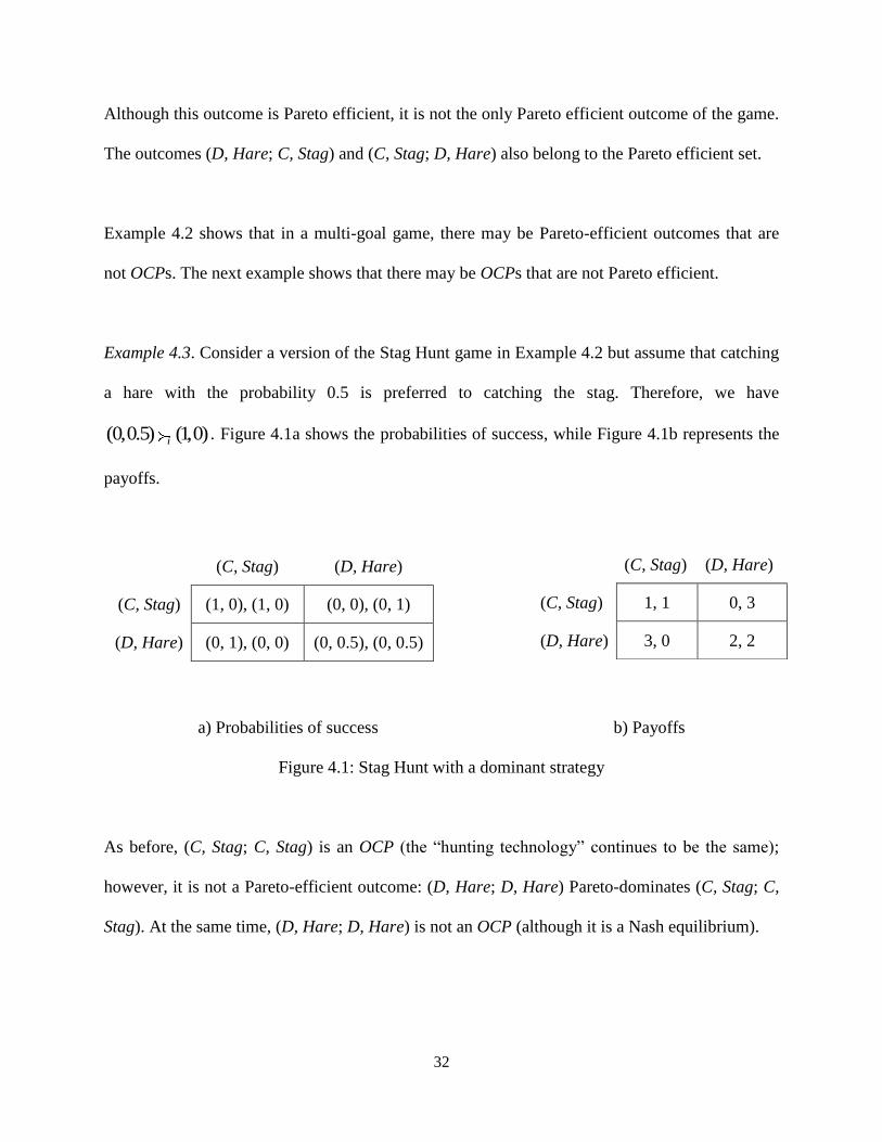
Example 4.3. Consider a version of the Stag Hunt game in Example 4.2 but assume that catching

a hare with the probability 0.5 is preferred to catching the stag. Therefore, we have

(0,0.5) (1,0)i . Figure 4.1a shows the probabilities of success, while Figure 4.1b represents the

payoffs.


Figure 4.1: Stag Hunt with a dominant strategy

As before, (C, Stag; C, Stag) is an OCP (the “hunting technology” continues to be the same);

however, it is not a Pareto-efficient outcome: (D, Hare; D, Hare) Pareto-dominates (C, Stag; C,

Stag). At the same time, (D, Hare; D, Hare) is not an OCP (although it is a Nash equilibrium).

(C, Stag) (D, Hare)

(C, Stag) (1, 0), (1, 0) (0, 0), (0, 1)

(D, Hare) (0, 1), (0, 0) (0, 0.5), (0, 0.5)

(C, Stag) (D, Hare)

(C, Stag) 1, 1 0, 3

(D, Hare) 3, 0 2, 2

33

To summarize, although OCP may seem to have a normative appeal, it should be recalled that it

ignores the value of goals to players. Consequently, one or more players may prefer an outcome,

in which they achieve a higher-valued goal, with a sufficiently high probability, to the outcome

in which they achieved a lower-valued goal with certainty.19

19 For a different (but compatible) argument why the Hayekian notion of equilibrium may not be preferable, see

Rizzo (1990).

34

5 Games with random events

So far, I have considered the overall success of plans. That is, I did not distinguish between the

case when a player’s plan is incompatible with other players’ plans and the case when a player’s

plan is incompatible with the environment. I now generalize the model to distinguish between

these two cases. First, consider the following example.

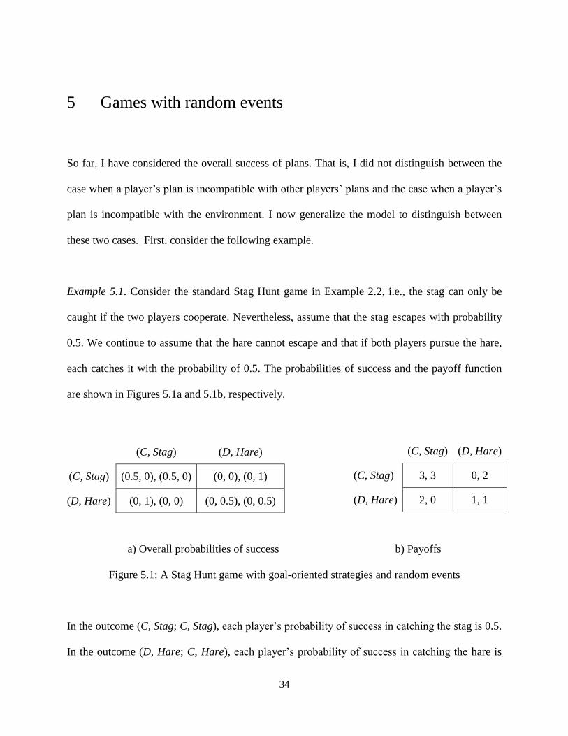
Example 5.1. Consider the standard Stag Hunt game in Example 2.2, i.e., the stag can only be

caught if the two players cooperate. Nevertheless, assume that the stag escapes with probability

0.5. We continue to assume that the hare cannot escape and that if both players pursue the hare,

each catches it with the probability of 0.5. The probabilities of success and the payoff function

are shown in Figures 5.1a and 5.1b, respectively.

a) Overall probabilities of success b) Payoffs

Figure 5.1: A Stag Hunt game with goal-oriented strategies and random events

In the outcome (C, Stag; C, Stag), each player’s probability of success in catching the stag is 0.5.

In the outcome (D, Hare; C, Hare), each player’s probability of success in catching the hare is

(C, Stag) (D, Hare)

(C, Stag) 3, 3 0, 2

(D, Hare) 2, 0 1, 1

(C, Stag) (D, Hare)

(C, Stag) (0.5, 0), (0.5, 0) (0, 0), (0, 1)

(D, Hare) (0, 1), (0, 0) (0, 0.5), (0, 0.5)

35

0.5. Although in both cases the overall probabilities of achieving a given goal are the same, there

is a difference: In the outcome (C, Stag; C, Stag), plans are compatible across players (they can

both achieve their goals at the same time) but are not compatible with the environment (the Stag

may escape). In the outcome (D, Hare; C, Hare), plans are not compatible across players (they

cannot achieve their goals at the same time) but are compatible with the environment (the Hare

cannot escape). I extend the model of games with goal-oriented strategies to account for the

difference between the two cases.

As before, assume the set of players, N, and for each player i, a set of actions, iA , set of goals,

iG , and a set of goal-oriented strategies, iS . To model the compatibility of players’ plans with

the environment, define a finite set of states of nature, , and a probability measure q on . We

now have to assess whether the goals of a player are compatible with the goals of other players in

a given state. In order to do so, define for each i N a success function : {0,1} iG

ir S

which assigns to each strategy profile in every state of nature a iG -tuple of probabilities

( | , )i ir g s specifying for each goal i ig G whether the player i achieves her goal (probability 1)

or not (probability 0), if the outcome is ( , )s .

There are two main differences between the success functions ip and ir . Firstly, the range of the

function ip is S, while the range of the function ir is S . Secondly, the domain of the

function ip is [0,1] iG, while the domain of the function ir is {0,1} iG

. Intuitively, once a certain

state is realized, a player’s goal is either achieved or not; there is no intermediate possibility. As

we will immediately see, the model with random events puts more structure on the original

36

model. Namely, it endogenizes ( )ip s , the overall probability vector that specifies the

probabilities with which a player i achieves his goals.

For each strategy profile s, the success function ir , together with the probability measure q over

the states, generates a bundle ip which assigns to each i ig G an overall probability ( | )i ip g s

that ig is achieved by i given the strategy profile s. This is the probability of success of ig

introduced as a primitive in the simplified model. In the extended model, it is calculated as

( | ) ( ) ( | , )i i i ip g s q r g s

. As before, for each player i, denote the set of the probability

bundles ( )ip s by iP and define a preference relation ≿ i on this set.20

Definition 5.1. The strategic game with goal-oriented strategies and random events is an octuple

, , ,( ),( ),( ),( ),i i i iN q A G S r ≿ i .

Recall that the simple games with game-oriented strategies were defined as a sextuple

,( ),( ),( ),( ),i i i iN A G S p ≿ i (Definition 2.2). We have now introduced two new elements: states

of nature and a probability measure on these states. In addition, we have modified the success

function.

20 Note that it is still assumed that players care about the overall probabilities of success of their goals. In particular,

they do not distinguish between a decrease in the probability of success due to choices of the other players and due

to chance. See Chapter 8 for an elaboration of this point.

37

Two examples will help to illustrate this framework. In the first example, one player plays only

against his environment. The second example involves two players and the environment. While

in the first example, a player’s plans may fail only because of their incompatibility with the

environment, in the second case, they may fail because of their incompatibility with both

environment and other players’ plans.

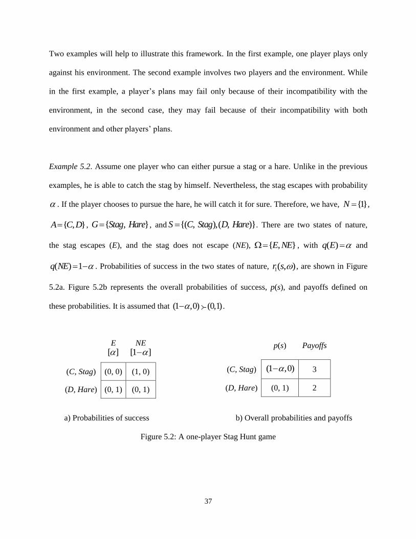
Example 5.2. Assume one player who can either pursue a stag or a hare. Unlike in the previous

examples, he is able to catch the stag by himself. Nevertheless, the stag escapes with probability

. If the player chooses to pursue the hare, he will catch it for sure. Therefore, we have, {1}N ,

{ , }A C D , { , }G Stag Hare , and {( , ),( , )}S C Stag D Hare . There are two states of nature,

the stag escapes (E), and the stag does not escape (NE), { , }E NE , with ( )q E and

( ) 1q NE . Probabilities of success in the two states of nature, 1( , )r s , are shown in Figure

5.2a. Figure 5.2b represents the overall probabilities of success, p(s), and payoffs defined on

these probabilities. It is assumed that (1 ,0) (0,1) .

a) Probabilities of success b) Overall probabilities and payoffs

Figure 5.2: A one-player Stag Hunt game

E

[ ] NE

[1 ]

(C, Stag) (0, 0) (1, 0)

(D, Hare) (0, 1) (0, 1)

p(s)

Payoffs

(C, Stag) (1 ,0) 3

(D, Hare) (0, 1) 2

38

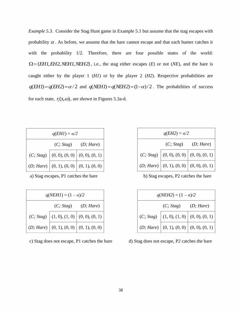
Example 5.3. Consider the Stag Hunt game in Example 5.1 but assume that the stag escapes with

probability . As before, we assume that the hare cannot escape and that each hunter catches it

with the probability 1/2. Therefore, there are four possible states of the world:

{ , , , }EH1 EH2 NEH1 NEH2 , i.e., the stag either escapes (E) or not (NE), and the hare is

caught either by the player 1 (H1) or by the player 2 (H2). Respective probabilities are

( ) ( ) / 2q EH1 q EH2 and ( ) ( ) (1 ) / 2q NEH1 q NEH2 . The probabilities of success

for each state, ( , )ir s , are shown in Figures 5.3a-d.

a) Stag escapes, P1 catches the hare b) Stag escapes, P2 catches the hare

c) Stag does not escape, P1 catches the hare d) Stag does not escape, P2 catches the hare

q(EH1) = α/2

(C; Stag) (D; Hare)

(C; Stag) (0, 0), (0, 0) (0, 0), (0, 1)

(D; Hare) (0, 1), (0, 0) (0, 1), (0, 0)

q(EH2) = α/2

(C; Stag) (D; Hare)

(C; Stag) (0, 0), (0, 0) (0, 0), (0, 1)

(D; Hare) (0, 1), (0, 0) (0, 0), (0, 1)

q(NEH1) = (1 – α)/2

(C; Stag) (D; Hare)

(C; Stag) (1, 0), (1, 0) (0, 0), (0, 1)

(D; Hare) (0, 1), (0, 0) (0, 1), (0, 0)

q(NEH2) = (1 – α)/2

(C; Stag) (D; Hare)

(C; Stag) (1, 0), (1, 0) (0, 0), (0, 1)

(D; Hare) (0, 1), (0, 0) (0, 0), (0, 1)

39

e) Overall probabilities of success f) Payoffs

Figure 5.3: A Stag Hunt game with goal-oriented strategies and random events

Combining the probabilities of success in each state with probabilities of states, we obtain

overall probabilities of success, p(s). These overall probabilities are shown in Figure 5.3e. Note

that if 0 , i.e., the stag cannot escape, the game is identical to the one in Example 2.1 (Figure

2.2). If 0.5 , we obtain the game in Example 5.1 (Figure 5.1). It is assumed that for each

player i, (1 ) (0,1)i . Payoffs representing these preferences are shown in Figure 5.3f. It can

be seen that while the simple model in Chapter 2 endogenizes the payoffs of the conventional

model, the model with exogenous events further endogenizes the probabilities of success of the

simple model.

We now consider definitions of Nash equilibrium and OCP. Since the model with random events

endogenizes the model of Chapter 2, neither the definition of Nash equilibrium nor the definition

of OCP is affected. Nevertheless, in addition to OCP, we may now define the mutual

compatibility of plans (MCP). MCP isolates the compatibility of a player’s plan with other

players’ plans from the compatibility of a player’s plan with nature.

(C, Stag) (D, Hare)

(C, Stag) (1 – α, 0), (1 – α, 0) (0, 0), (0, 1)

(D, Hare) (0, 1), (0, 0) (0, 0.5), (0, 0.5)

(C, Stag) (D, Hare)

(C, Stag) 3, 3 0, 2

(D, Hare) 2, 0 1, 1

40

Definition 5.2. Consider a strategic game with goal-oriented strategies and random events. A

goal-oriented strategy j js S is perfectly successful in ( ; )s if ( | , ) 1i ir g s for gj associated

with js .

Definition 5.3. Mutual compatibility of plans (MCP) in a strategic game with goal-oriented

strategies and random events , , ,( ),( ),( ),( ),i i i iN q A G S r ≿ i is a profile s S of goal-oriented

strategies with the following property: there exists , such that for each i N , is is

perfectly successful in ( , )s S .

Example 5.4. Consider the game in Example 5.3 with 0 1 . The game has two Nash

equilibria, (C, Stag; C, Stag) and (D, Hare; D, Hare), and no OCP. Nevertheless, (C, Stag; C,

Stag) is a MCP.

The following theorem establishes the relationship between OCP and MCP. To put it simply, if

an outcome is an OCP, then players’ plans are both mutually compatible and compatible with all

possible states of nature. Therefore, this outcome has to be also MCP. In contrast, if an outcome

is an MCP, it may or may not be an OCP because players’ plans may be disappointed by nature

(see Example 5.4 above).

Theorem 5.1. If an outcome is an OCP, then it is also MCP.

41

Proof. Assume that the outcome s is an OCP. Then, for each player i, we have ˆ( | ) 1i ip g s for

ig associated with is . Since ˆ ˆ( | ) ( ) ( | , )i i i ip g s q r g s

, we must have ˆ( | , ) 1i ir g s for

each . Therefore, s is also an MCP.

42

6 Degrees of plan compatibility

The compatibility of plans, both in the sense of OCP and MCP, is a state of affairs, which can be

approached but perhaps never achieved in reality. One implication of this observation is that a

particular outcome can be “closer to” or “further away from” the Hayekian equilibrium.

Although the situations “near equilibrium” are mentioned in the literature (Rizzo 1990), they

have not been rigorously defined. The framework introduced in previous chapters allows for

such a definition.

A simple way to measure closeness to OCP is to use the average success of plans. The degree of

overall compatibility of plans (DOCP) in an outcome s can be defined as follows:

1( )

( )

n

i iip g s

DOCP sn

(6.1)

In words, for each player, we consider the probability of the goal he tries to achieve, and we add

these probabilities across players. Then we divide this number with the number of players, n. The

obtained measurement of the degree of plan compatibility is between 1 (perfect compatibility)

and 0 (perfect incompatibility).

Example 6.1. Consider the Stag Hunt model in Example 2.2 (Figure 2.2a). For the outcome (D,

Hare; D Hare), DOCP is equal to 0.5 (each player catches the Hare with the probability 0.5).

43

DOCP has the same value for the outcome (D, Hare; C, Stag): Player 1 catches the Hare with

probability one, while player 2 catches Stag with probability zero.

For the games with random events, DOCP can be derived as follows:

1 1

1

( | , ) ( )( ) ( )

n n

m i i j i ii ijj

r g s p g sDOCP s q

n n

(6.2)

That is, we first calculate the average success of plans for each state of nature, and then we add

these values across all states using the probabilities of each state as weights. Since

1( | , )

n

i i jir g s

also represents the absolute number of successful plans in ( , )s , the average

success of plans in ( , )s can also be interpreted as the proportion of perfectly successful plans

in ( , )s .

Example 6.2. Consider the game in Example 5.3 (Figure 5.3a-d). For the outcome (D, Hare; D

Hare), ( / 2)(0.5) ( / 2)(0.5) [(1 ) / 2](0.5) [(1 ) / 2](0.5) 0.5DOCP .

In games with random events, we can also define the degree of mutual compatibility of plans

(DMCP) in an outcome s:

1( , )

( ) max

n

i iir g s

DMCP sn

(6.3)

44

DMCP is constructed as follows: for a given outcome s, we first calculate the average success of

plans for each state of nature. We then select the maximum value. In other words, we consider

the compatibility of plans under the most favorable state of nature.

Example 6.3. Consider the game in Example 4.3 with 0.5 . For the outcome (C, Stag; C,

Stag), DOCP is equal to 0.5. max{0,1} 1DMCP . In contrast, consider the outcome (D, Hare;

D Hare). For this outcome, both DOCP and DMCP are equal to 0.5.

In the following Chapter, I generalize DOCP and DMCP to games with multiple goals. In

Chapter 9, I apply these two measurements to account for degrees of stability of Nash equilibria.

45

7 Games with multiple goals

We have assumed that each action is associated with exactly one goal. We now extend the

definition of goal-oriented strategy to the cases, when an action is associated with several

independent goals. Formally, a set of goal-oriented strategies can be defined as

(2 \ )iGi iS A . Below is a simple example.21

Example 7.1. Consider the following Battle of Sexes game: Two players choose between opera

and box match. They both primarily want to coordinate on the same activity; however, player 1

prefers to attend opera, while player two prefers to attend the boxing match. Therefore, we have

{1,2}N , 1 2 { , }A A X Y , 1 { , }G M O , and 2 { , }G M B , where X and Y denote two

possible activities, M stands for “meet”, O is “opera”, and B represents “box”. Goal-oriented

strategies are 1 {( ; , ),( ; )}S X M O Y M , and 2 {( ; ),( ; , )}S X M Y M B . The probabilities of

success are shown in Figure 7.1a, and payoffs are shown in Figure 7.1b. It is assumed that (0,1)

~i (0,0) for each i. That is, for both activities (opera or box), each player considers the other

player as an essential input in his consumption technology.

21 This generalized model then becomes similar to games with multiple payoffs (Zeleny 1975; Zhao 1991). See also

Nishizaki and Sakawa (2001) for a review of this literature.

46


Figure 7.1: The Battle of Sexes as a game with goal-oriented strategies

In the game with multiple goals, the notion of perfectly successful goal-oriented strategy has to

be generalized. In particular, the probability of success of all goals associated with an action has

to be equal to one.

Definition 7.1. Consider a strategic game with goal-oriented strategies. A goal-oriented strategy

j js S is perfectly successful in s if ( | ) 1j jp g s for all gj associated with js .

The definitions of Nash equilibrium and OCP remain unchanged.

Example 7.2. Consider the Battle of Sexes in Example 7.1. The game has two Nash equilibria,

both of which are also OCP: (X; M, O; X; M), and (Y; M; Y; M, B).

There is a new result about Pareto efficiency.

(X; M) (Y; M, B)

(X; M, O) 2, 1 0, 0

(Y; M) 0, 0 1, 2

(X; M) (Y; M, B)

(X; M, O) (1, 1), (1, 0) (0, 1), (0, 1)

(Y; M) (0, 0), (0, 0) (1, 0), (1, 1)

47

Theorem 7.1. Let be Γ be a strategic game with goal-oriented strategies with one or more OCP.

Let 1{ ,..., }ii mG g g for each i and assume that 1( , ,..., )

ii i ms a g g for each i is S and each

player i. Then s is an OCP, if and only if it is Pareto efficient.

Proof. First, I prove that if an outcome is an OCP, then it is Pareto efficient. Since s is an OCP,

then ˆ( | ) 1i ip g s for each goal ig and each player i. The strong monotonicity assumption

implies that, for every player i N , we have ˆ( )ip s ≿ ( )i ip s for all s S . I now prove that if an

outcome is Pareto efficient, then it is an OCP. Assume that s is a Pareto efficient outcome, but

it is not an OCP. Then there exists a player j, for whom ( | ) 1j jp g s for some jg . At the same

time, for player j, we have ˆ( | ) 1j jp g s , and therefore, by strong monotonicity assumption

ˆ( ) ( )j jp s p s . It follows that s cannot be Pareto efficient.

Intuitively, if every player achieves all his goals in an outcome of a game, then this game is

Pareto efficient. If an outcome is Pareto efficient, then it is an OCP, provided that OCP exists,

and each plan of every player includes all the player’s goals. Note that Theorem 7.1 generalizes

Theorem 4.1 to cases where 1iG . The following example illustrates Theorem 7.1.

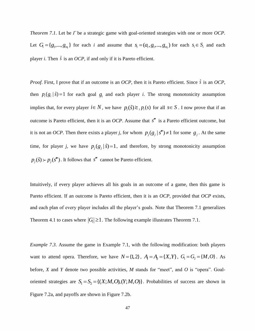
Example 7.3. Assume the game in Example 7.1, with the following modification: both players

want to attend opera. Therefore, we have {1,2}N , 1 2 { , }A A X Y , 1 2 { , }G G M O . As

before, X and Y denote two possible activities, M stands for “meet”, and O is “opera”. Goal-

oriented strategies are 1 2 {( ; , ),( ; , )}S S X M O Y M O . Probabilities of success are shown in

Figure 7.2a, and payoffs are shown in Figure 7.2b.

48



The outcome (X; M, O; X; M, O) is both unique OCP and unique Pareto efficient outcome.

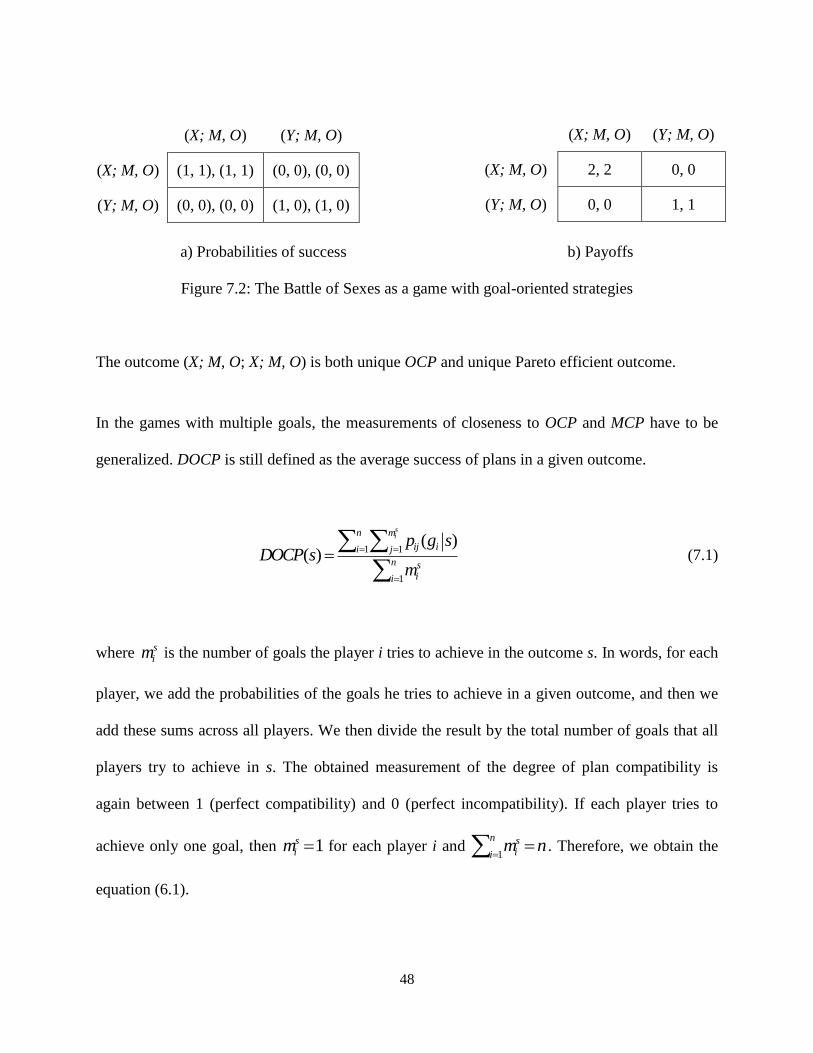
In the games with multiple goals, the measurements of closeness to OCP and MCP have to be

generalized. DOCP is still defined as the average success of plans in a given outcome.

1 1

1

( )( )

sin m

ij ii j

n sii

p g sDOCP s

m

(7.1)

where sim is the number of goals the player i tries to achieve in the outcome s. In words, for each

player, we add the probabilities of the goals he tries to achieve in a given outcome, and then we

add these sums across all players. We then divide the result by the total number of goals that all

players try to achieve in s. The obtained measurement of the degree of plan compatibility is

again between 1 (perfect compatibility) and 0 (perfect incompatibility). If each player tries to

achieve only one goal, then 1sim for each player i and

1

n sii

m n

. Therefore, we obtain the

equation (6.1).

(X; M, O) (Y; M, O)

(X; M, O) (1, 1), (1, 1) (0, 0), (0, 0)

(Y; M, O) (0, 0), (0, 0) (1, 0), (1, 0)

(X; M, O) (Y; M, O)

(X; M, O) 2, 2 0, 0

(Y; M, O) 0, 0 1, 1

49

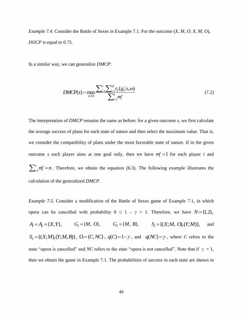
Example 7.4. Consider the Battle of Sexes in Example 7.1. For the outcome (X, M, O; X, M, O),

DOCP is equal to 0.75.

In a similar way, we can generalize DMCP:

1 1

1

( , )( ) max

sin m

ij ii in s

ii

r g sDMCP s

m

(7.2)

The interpretation of DMCP remains the same as before: for a given outcome s, we first calculate

the average success of plans for each state of nature and then select the maximum value. That is,

we consider the compatibility of plans under the most favorable state of nature. If in the given

outcome s each player aims at one goal only, then we have 1sim for each player i and

1

n sii

m n

. Therefore, we obtain the equation (6.3). The following example illustrates the

calculation of the generalized DMCP.

Example 7.5. Consider a modification of the Battle of Sexes game of Example 7.1, in which

opera can be cancelled with probability 0 ≤ 1 – γ < 1. Therefore, we have {1,2},N

1 2 { , },A A X Y 1 { , },G M O 2 { , },G M B 1 {( ; , ),( ; )},S X M O Y M and

2 {( ; ),( ; , )}S X M Y M B , { , }C NC , ( ) 1q C , and ( )q NC , where C refers to the

state “opera is cancelled” and NC refers to the state “opera is not cancelled”. Note that if γ = 1,

then we obtain the game in Example 7.1. The probabilities of success in each state are shown in

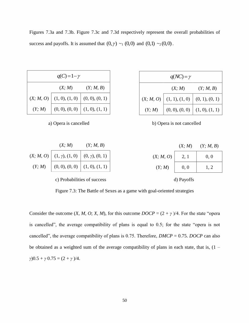
50

Figures 7.3a and 7.3b. Figure 7.3c and 7.3d respectively represent the overall probabilities of

success and payoffs. It is assumed that (0, ) ~1 (0,0) and (0,1) ~2 (0,0) .

a) Opera is cancelled b) Opera is not cancelled

c) Probabilities of success d) Payoffs


Consider the outcome (X, M, O; X, M), for this outcome DOCP = (2 + γ )/4. For the state “opera

is cancelled”, the average compatibility of plans is equal to 0.5; for the state “opera is not

cancelled”, the average compatibility of plans is 0.75. Therefore, DMCP = 0.75. DOCP can also

be obtained as a weighted sum of the average compatibility of plans in each state, that is, (1 –

γ)0.5 + γ 0.75 = (2 + γ )/4.

( ) 1q C

(X; M) (Y; M, B)

(X; M, O) (1, 0), (1, 0) (0, 0), (0, 1)

(Y; M) (0, 0), (0, 0) (1, 0), (1, 1)

( )q NC

(X; M) (Y; M, B)

(X; M, O) (1, 1), (1, 0) (0, 1), (0, 1)

(Y; M) (0, 0), (0, 0) (1, 0), (1, 1)

(X; M) (Y; M, B)

(X; M, O) (1, γ), (1, 0) (0, γ), (0, 1)

(Y; M) (0, 0), (0, 0) (1, 0), (1, 1)

(X; M) (Y; M, B)

(X; M, O) 2, 1 0, 0

(Y; M) 0, 0 1, 2

51

The model with multiple goals is considered in Chapters 10, 11, and 12. Chapter 12 highlights

some difficulties if goals associated with one action are not independent. In such cases, the

strong monotonicity assumption may not be plausible. Considering multiple goals may be

thought of as one possible extension of the basic model introduced in Chapter 5. Two other

possible extensions are considered in the following chapter.

52

8 Extensions

The framework introduced in previous chapters can be further elaborated in various directions.

Below I briefly discuss two simple extensions. In one case, I further endogenize players’ payoffs

to account for the possibility that a player may differently evaluate the failure of their plans due

to incompatibility with other players’ plans and the failure of their plans due to incompatibility

with the environment. In the other case, I explicitly include players’ beliefs in the model.

8.1 Payoffs

In the model with random events (Chapter 5), we assumed that players care about the overall

probabilities of success. Alternatively, we could assume that players care about the probabilities

of success in each of the feasible outcomes, i.e., that they consider each feasible state of nature

separately. Consider the following example.

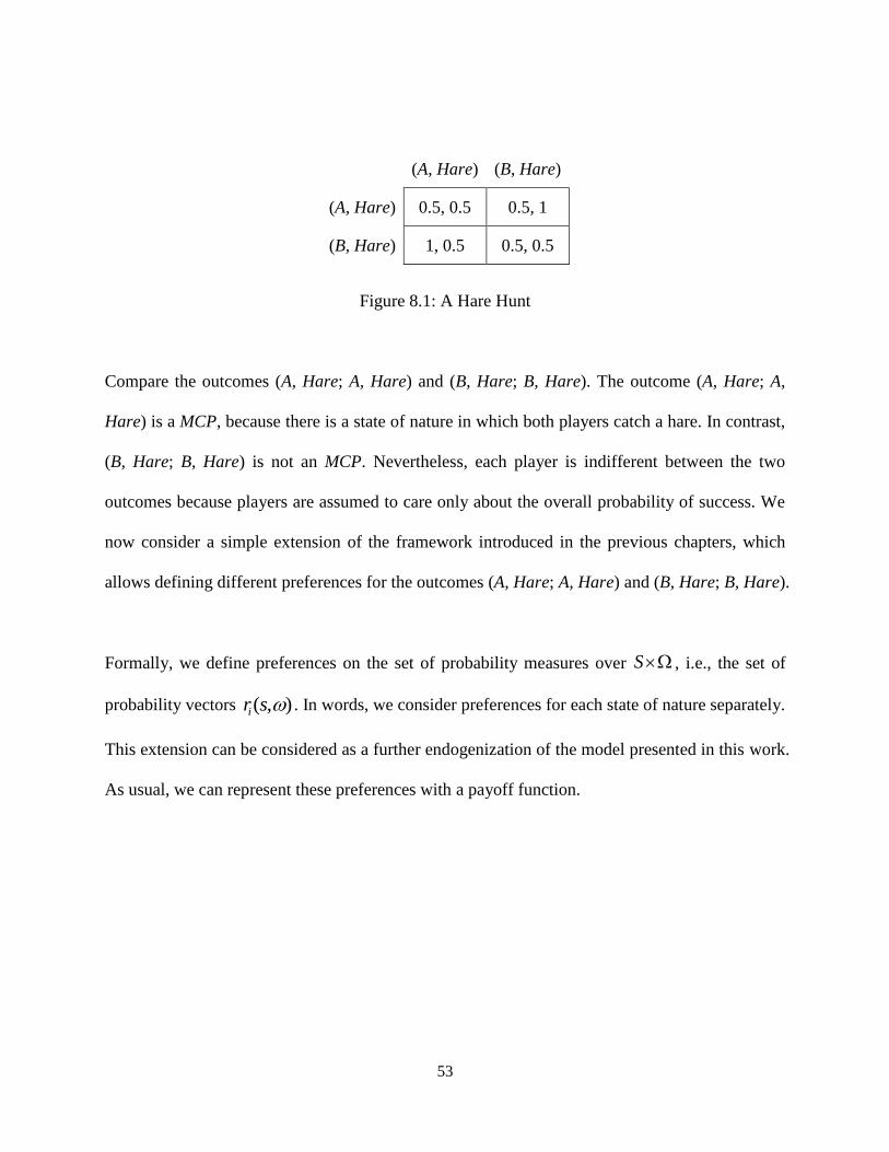
Example 8.1. Two hunters choose between two locations, A and B. In the location A, there are

many hares, but each escapes the hunters with probability 0.5. In the location B, there is only one

hare, who cannot escape the hunters. Figure 8.1 shows the overall probabilities of success. Since

each player pursues only one goal, these probabilities also represent players’ preferences.

53

Figure 8.1: A Hare Hunt

Compare the outcomes (A, Hare; A, Hare) and (B, Hare; B, Hare). The outcome (A, Hare; A,

Hare) is a MCP, because there is a state of nature in which both players catch a hare. In contrast,

(B, Hare; B, Hare) is not an MCP. Nevertheless, each player is indifferent between the two

outcomes because players are assumed to care only about the overall probability of success. We

now consider a simple extension of the framework introduced in the previous chapters, which

allows defining different preferences for the outcomes (A, Hare; A, Hare) and (B, Hare; B, Hare).

Formally, we define preferences on the set of probability measures over S , i.e., the set of

probability vectors ( , )ir s . In words, we consider preferences for each state of nature separately.

This extension can be considered as a further endogenization of the model presented in this work.

As usual, we can represent these preferences with a payoff function.

(A, Hare) (B, Hare)

(A, Hare) 0.5, 0.5 0.5, 1

(B, Hare) 1, 0.5 0.5, 0.5

54

Example 8.2. Consider once again the game in Example 8.1. There are eight states of nature in

this game shown in Figures 8.2a-h. For example, the state E1N2P1 denotes “hare escapes player

1, if player 1 chooses A” (E1), “hare doesn’t escape player 2 if player 2 chooses A”, and “player

1 catches the hare if both players choose B”. The figures in each table represent the players’

payoffs. We again use probabilities of success in each state to represent these payoffs, with one

exception: if a player i does not catch a hare in a state where the hare does not escape him if he

chooses A, then his payoff is -1 rather than 0.22 Specifically, for player 1, it is the states N1E2P2

and N1E2P2, while for player 2, it is in the states E1N2P1 and N1N2P1.

22 We may think about these preferences as including regret. For the regret theory, see Loomes and Sugden (1982.

1987), Sugden (1985, 1993), and Quiggin (1994).

55

a) E1E1P1 b) E1N2P1

c) N1E2P1 d) N1N2P1

e) E1E1P2 f) E1N2P2

g) N1E2P2 h) N1N2P2

Figure 8.2: A Hare Hunt with payoffs over feasible outcomes

q(E1E1P1) = 0.125

(A, Hare) (B, Hare)

(A, Hare) 0, 0 0, 1

(B, Hare) 1, 0 1, 0

q(E1N2P1) = 0.125

(A, Hare) (B, Hare)

(A, Hare) 0, 1 0, 1

(B, Hare) 1, 1 1, -1

q(N1E2P1) = 0.125

(A, Hare) (B, Hare)

(A, Hare) 1, 0 1, 0

(B, Hare) 1, 0 1, 0

q(N1N2P1) = 0.125

(A, Hare) (B, Hare)

(A, Hare) 1, 1 1, 1

(B, Hare) 1, 1 1, -1

q(E1E1P2) = 0.125

(A, Hare) (B, Hare)

(A, Hare) 0, 0 0, 1

(B, Hare) 1, 0 0, 1

q(E1N2P2) = 0.125

(A, Hare) (B, Hare)

(A, Hare) 0, 1 0, 1

(B, Hare) 1, 1 0, 1

q(N1E2P2) = 0.125

(A, Hare) (B, Hare)

(A, Hare) 1, 0 1, 1

(B, Hare) 1, 0 -1, 1

q(N1N2P2) = 0.125

(A, Hare) (B, Hare)

(A, Hare) 1, 1 1, 1

(B, Hare) 1, 1 -1, 1

56

It is useful to combine the preferences in each state to obtain aggregate preferences over

outcomes s. Denote this aggregate payoff function ( )iU s . Let ( )iu r be a payoff function

representing preferences over ( , )ir s . A simple way to obtain the aggregate the payoff function

over s, is to weight ( )iu r with the probability of the respective state of nature. Denoting the

aggregate payoff function ( )iU s , we have

( ) ( ) ( ( | , ))i i i iU s q u r g s

(8.1)

Compare the equation (8.1) with the model of Chapter 4. There, we first derived the aggregate

probability, ( )ip s , as follows:

( | ) ( ) ( | , )i i i ip g s q r g s

(8.2)

Then we defined preferences over ( )ip s . Denote the payoff function representing these

preferences ( ( ))i iV p s . Note that ( )iU s and ( ( ))i iV p s may or may not represent the same

preferences. The following examples illustrate the two approaches.

Example 8.3. Consider the game in Examples 8.1 and 8.2. Figure 8.1 shows the payoff function

( ( ))i iV p s , while Figure 8.2 shows the payoff function ( )iu r . Using equation (8.1), we obtain

( )iU s (see Figure 8.3). Comparing Figures 8.1 and 8.3, we see that ( ( )) ( )i i iV p s U s . In

particular, a player’s payoff is lower, if his plan is disappointed by the other player’s plan rather

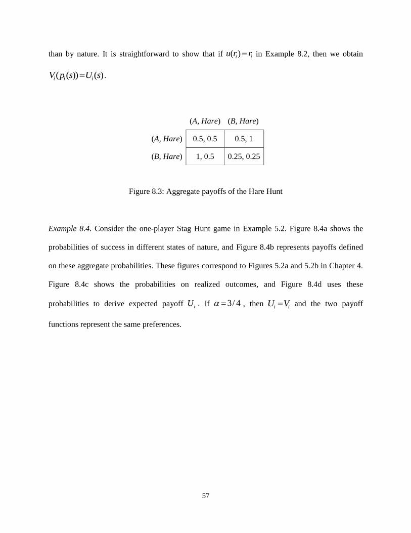
57

than by nature. It is straightforward to show that if ( )i iu r r in Example 8.2, then we obtain

( ( )) ( )i i iV p s U s .

Figure 8.3: Aggregate payoffs of the Hare Hunt

Example 8.4. Consider the one-player Stag Hunt game in Example 5.2. Figure 8.4a shows the

probabilities of success in different states of nature, and Figure 8.4b represents payoffs defined

on these aggregate probabilities. These figures correspond to Figures 5.2a and 5.2b in Chapter 4.

Figure 8.4c shows the probabilities on realized outcomes, and Figure 8.4d uses these

probabilities to derive expected payoff iU . If 3/ 4 , then i iU V and the two payoff

functions represent the same preferences.

(A, Hare) (B, Hare)

(A, Hare) 0.5, 0.5 0.5, 1

(B, Hare) 1, 0.5 0.25, 0.25

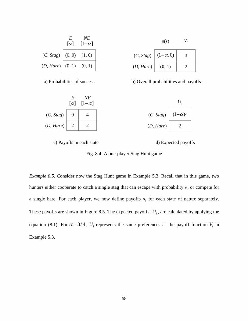
58

a) Probabilities of success b) Overall probabilities and payoffs

c) Payoffs in each state d) Expected payoffs

Fig. 8.4: A one-player Stag Hunt game

Example 8.5. Consider now the Stag Hunt game in Example 5.3. Recall that in this game, two

hunters either cooperate to catch a single stag that can escape with probability α, or compete for

a single hare. For each player, we now define payoffs iu for each state of nature separately.

These payoffs are shown in Figure 8.5. The expected payoffs, iU , are calculated by applying the

equation (8.1). For 3/ 4 , iU represents the same preferences as the payoff function iV in

Example 5.3.

E

[ ] NE

[1 ]

(C, Stag) (0, 0) (1, 0)

(D, Hare) (0, 1) (0, 1)

p(s)

iV

(C, Stag) (1 ,0) 3

(D, Hare) (0, 1) 2

E

[ ] NE

[1 ]

(C, Stag) 0 4

(D, Hare) 2 2

iU

(C, Stag) (1 )4

(D, Hare) 2

59

a) Stag escapes, P1 catches the hare b) Stag escapes, P2 catches the hare

c) Stag doesn’t escape, P1 catches the hare d) Stag doesn’t escape, P2 catches the hare

Figure 8.5: A Stag Hunt game with payoffs over feasible outcomes

Chapter 13 provides empirical evidence that players care about whether their plans fail because

of the incompatibility of other players’ plans or because of incompatibility with the environment.

8.2 Beliefs

The framework introduced in preceding chapters considers the “objective” compatibility of plans,

in the sense that this compatibility is independent of players’ knowledge and beliefs.

Nevertheless, the model introduced in the preceding chapters can be extended to include players’

beliefs. From this perspective, the model with random events considered in Chapter 5 can be

interpreted as a special case in which 1) all players have common prior beliefs, 2) these prior

q(EH2) = α/2

(C, Stag) (D, Hare)

(C, Stag) 0, 0 0, 2

(D, Hare) 2, 0 0, 2

q(EH1) = α/2

(C, Stag) (D, Hare)

(C, Stag) 0, 0 0, 2

(D, Hare) 2, 0 2, 0

q(NEH1) = (1 – α)/2

(C, Stag) (D, Hare)

(C, Stag) 4, 4 0, 2

(D, Hare) 2, 0 2, 0

q(NEH2) = (1 – α)/2

(C, Stag) (D, Hare)

(C, Stag) 4, 4 0, 2

(D, Hare) 2, 0 0, 2

60

beliefs are correct, and 3) all players receive the same signal regardless of the state of the world.

The model can be generalized by considering differences in prior beliefs across players and

explicit introduction of a signal function as in conventional Bayesian games (Osborne and

Rubinstein 1994). This would allow modeling asymmetric information, which is important in

many cases, and indeed, emphasized by Hayek (1945). I now consider this generalization.

Assume the set of players N and for each player i a set of actions, iA , set of goals, iG , and a set

of goal-oriented strategies, iS . As in chapter 4, is the finite set of possible states of nature and

q is the probability measure on , with ( ) 0q for each . We now introduce for each

player i the set of player’s types, iT . Players’ information about the state of nature is modeled

with the signal function :i iT . The posterior belief that about the state that has been

realized is 1( | ) ( ) / ( ( ))i i i it q q t . The overall probability that the goal ig is achieved given

the strategy profile s, is given by: ( | ) ( | ) ( | , )i i i i i ip g s t r g s

. Preferences of each

player are defined on the set of overall probabilities, iP .23

Definition 8.1. A Bayesian game with goal-oriented strategies is a decuple

, , ,( ),( ),( ),( ),( ),( ),i i i i i iN q A G S T r ≿ i .

Note that one can think about this extension as yet another endogenization of conventional

strategic games. In particular, the conventional strategic game can be understood as a Bayesian

game where players do not learn anything about the realized state of nature from their signals.

23 Alternatively, we can define preferences for each state separately. See Section 8.1.

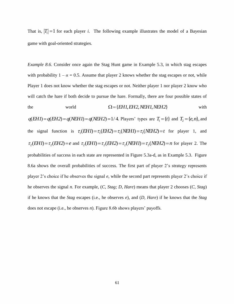
61

That is, 1iT for each player i. The following example illustrates the model of a Bayesian

game with goal-oriented strategies.

Example 8.6. Consider once again the Stag Hunt game in Example 5.3, in which stag escapes

with probability 1 – α = 0.5. Assume that player 2 knows whether the stag escapes or not, while

Player 1 does not know whether the stag escapes or not. Neither player 1 nor player 2 know who

will catch the hare if both decide to pursue the hare. Formally, there are four possible states of

the world { , , , }EH1 EH2 NEH1 NEH2 with

( ) ( ) ( ) ( ) 1/ 4.q EH1 q EH2 q NEH1 q NEH2 Players’ types are 1 { }T t and 2 { , },T e n and

the signal function is 1 1 1 1( ) ( ) ( ) ( )EH1 EH2 NEH1 NEH2 t for player 1, and

2 2( ) ( )EH1 EH2 e and 2 2 2 2( ) ( ) ( ) ( )EH1 EH2 NEH1 NEH2 n for player 2. The

probabilities of success in each state are represented in Figure 5.3a-d, as in Example 5.3. Figure

8.6a shows the overall probabilities of success. The first part of player 2’s strategy represents

player 2’s choice if he observes the signal e, while the second part represents player 2’s choice if

he observes the signal n. For example, (C, Stag; D, Hare) means that player 2 chooses (C, Stag)

if he knows that the Stag escapes (i.e., he observes e), and (D, Hare) if he knows that the Stag

does not escape (i.e., he observes n). Figure 8.6b shows players’ payoffs.

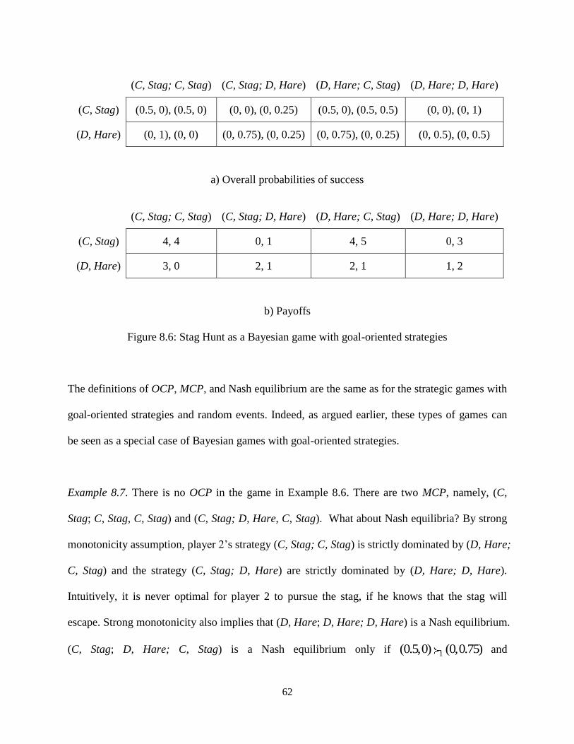
62

a) Overall probabilities of success

b) Payoffs

Figure 8.6: Stag Hunt as a Bayesian game with goal-oriented strategies

The definitions of OCP, MCP, and Nash equilibrium are the same as for the strategic games with

goal-oriented strategies and random events. Indeed, as argued earlier, these types of games can

be seen as a special case of Bayesian games with goal-oriented strategies.

Example 8.7. There is no OCP in the game in Example 8.6. There are two MCP, namely, (C,

Stag; C, Stag, C, Stag) and (C, Stag; D, Hare, C, Stag). What about Nash equilibria? By strong

monotonicity assumption, player 2’s strategy (C, Stag; C, Stag) is strictly dominated by (D, Hare;

C, Stag) and the strategy (C, Stag; D, Hare) are strictly dominated by (D, Hare; D, Hare).

Intuitively, it is never optimal for player 2 to pursue the stag, if he knows that the stag will

escape. Strong monotonicity also implies that (D, Hare; D, Hare; D, Hare) is a Nash equilibrium.

(C, Stag; D, Hare; C, Stag) is a Nash equilibrium only if 1(0.5,0) (0,0.75) and

(C, Stag; C, Stag) (C, Stag; D, Hare) (D, Hare; C, Stag) (D, Hare; D, Hare)

(C, Stag) (0.5, 0), (0.5, 0) (0, 0), (0, 0.25) (0.5, 0), (0.5, 0.5) (0, 0), (0, 1)

(D, Hare) (0, 1), (0, 0) (0, 0.75), (0, 0.25) (0, 0.75), (0, 0.25) (0, 0.5), (0, 0.5)

(C, Stag; C, Stag) (C, Stag; D, Hare) (D, Hare; C, Stag) (D, Hare; D, Hare)

(C, Stag) 4, 4 0, 1 4, 5 0, 3

(D, Hare) 3, 0 2, 1 2, 1 1, 2

63

2(0.5,0.5) (0,1). This is, in fact, what we assume in Figure 8.6b. Intuitively, players will pursue

the stag if the value of the stag is sufficiently high compared to the value of the hare. It is

straightforward to generalize the model to the case when the stag escapes with the probability α.

Players then pursue the stag if α is sufficiently low, given the value of the stag.

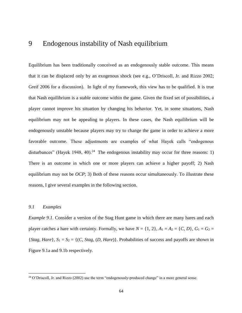
64

9 Endogenous instability of Nash equilibrium

Equilibrium has been traditionally conceived as an endogenously stable outcome. This means

that it can be displaced only by an exogenous shock (see e.g., O’Driscoll, Jr. and Rizzo 2002;

Greif 2006 for a discussion). In light of my framework, this view has to be qualified. It is true

that Nash equilibrium is a stable outcome within the game. Given the fixed set of possibilities, a

player cannot improve his situation by changing his behavior. Yet, in some situations, Nash

equilibrium may not be appealing to players. In these cases, the Nash equilibrium will be

endogenously unstable because players may try to change the game in order to achieve a more

favorable outcome. These adjustments are examples of what Hayek calls “endogenous

disturbances” (Hayek 1948, 40).24 The endogenous instability may occur for three reasons: 1)

There is an outcome in which one or more players can achieve a higher payoff; 2) Nash

equilibrium may not be OCP; 3) Both of these reasons occur simultaneously. To illustrate these

reasons, I give several examples in the following section.

9.1 Examples

Example 9.1. Consider a version of the Stag Hunt game in which there are many hares and each

player catches a hare with certainty. Formally, we have N = {1, 2}, A1 = A2 = {C, D}, G1 = G2 =

{Stag, Hare}, S1 = S2 = {(C, Stag, (D, Hare)}. Probabilities of success and payoffs are shown in

Figure 9.1a and 9.1b respectively.

24 O’Driscoll, Jr. and Rizzo (2002) use the term “endogenously-produced change” in a more general sense.

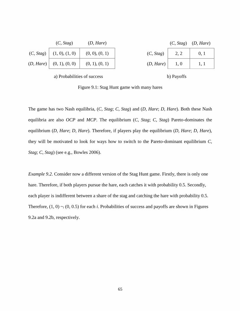
65


Figure 9.1: Stag Hunt game with many hares

The game has two Nash equilibria, (C, Stag; C, Stag) and (D, Hare; D, Hare). Both these Nash

equilibria are also OCP and MCP. The equilibrium (C, Stag; C, Stag) Pareto-dominates the

equilibrium (D, Hare; D, Hare). Therefore, if players play the equilibrium (D, Hare; D, Hare),

they will be motivated to look for ways how to switch to the Pareto-dominant equilibrium C,

Stag; C, Stag) (see e.g., Bowles 2006).

Example 9.2. Consider now a different version of the Stag Hunt game. Firstly, there is only one

hare. Therefore, if both players pursue the hare, each catches it with probability 0.5. Secondly,

each player is indifferent between a share of the stag and catching the hare with probability 0.5.

Therefore, (1, 0) ~i (0, 0.5) for each i. Probabilities of success and payoffs are shown in Figures

9.2a and 9.2b, respectively.

(C, Stag) (D, Hare)

(C, Stag) 2, 2 0, 1

(D, Hare) 1, 0 1, 1

(C, Stag) (D, Hare)

(C, Stag) (1, 0), (1, 0) (0, 0), (0, 1)

(D, Hare) (0, 1), (0, 0) (0, 1), (0, 1)

66


Figure 9.2: Stag Hunt game without Pareto-dominance

There is only one Nash equilibrium, namely, (D, Hare; D, Hare). No outcome Pareto-dominates

the Nash equilibrium outcome. Moreover, the goal-oriented strategy (D, Hare) strictly dominates

the strategy (C, Stag). Each player will, therefore, choose (D, Hare). However, each player can

receive a higher payoff if he is the only one pursuing the hare. That is,

1( , ; , ) ( , ; , )D Hare C Stag D Hare D Hare and 2( , ; , ) ( , ; , )C Stag D Hare D Hare D Hare . Therefore,

each player is motivated to change the game to achieve a higher payoff.

If we look at the game from the perspective of goals, then we conclude that there is only one

OCP (which is at the same time MCP), namely (C, Stag; C, Stag). In particular, the Nash

equilibrium (D, Hare; D, Hare) is neither OCP nor MCP. Therefore, we predict that the Nash

equilibrium will be unstable. The prediction of the conventional (payoff-based) approach and the

goal-based approach are similar. However, there is a subtle difference. Firstly, from the payoff

perspective, the Nash equilibrium is unstable because there are outcomes with a higher payoff

for one of the players. In contrast, from the goal perspective, the Nash equilibrium is unstable

because one of the players fails to achieve his goal. To highlight the difference between the

payoff and goal perspectives, consider the following example.

(C, Stag) (D, Hare)

(C, Stag) (1, 0), (1, 0) (0, 0), (0, 1)

(D, Hare) (0, 1), (0, 0) (0, 0.5), (0, 0.5)

(C, Stag) (D, Hare)

(C, Stag) 2, 2 0, 3

(D, Hare) 3, 0 2, 2

67

Example 9.3. Consider a Hare Hunt game, defined as follows: N = {1, 2}, A1 = A2 = {D}, G1 =

G2 = {Hare}, and ( | ) 0.5ip Hare DD . Each player considers only one action (perhaps due to

strong habit – see Epstein (2001)) and so the game has only a single outcome; this outcome is

trivially a Nash equilibrium but not an OCP as each player catches the hare with the probability

0.5.

The conventional approach has nothing to say about the game in Example 9.3 because players

have no choice within the game, given their actions sets. Moreover, since the game has only one

outcome, there is no payoff-based reason for players to modify the game. Nonetheless, a goal-

based perspective predicts that players will attempt to change the game since their plans are

mutually incompatible. To highlight the fact that the goal-based approach gives empirical

predictions that cannot be derived from the conventional approach, contrast the Hare Hunt in

Example 7.3 with a version of the Stag Hunt in the following example.

Example 9.4. N = {1, 2}, Ai = {C}, Gi = {Stag}, and ( | ) 1ip Stag CC . The single outcome of the

game is both Nash and OCR.

From the point of view of the conventional theory, the games in Examples 9.3 and 9.4, when

considered separately, are equivalent and, in fact, uninteresting. In contrast, according to the

goal-based approach, the two games are different. In the Hare Hunt in Example 9.3, the single

outcome of the game is an OCP, while in the Stag Hunt in Example 9.4, it is not. Consequently,

68

the goal-based approach predicts that the Hare Hunt will be goal-unstable while the Stag Hunt

will be goal-stable because players have no incentive to change the game.

Another advantage of the goal-based approach is that it predicts endogenous instability of Nash

equilibrium ex ante, that is, without identifying an alternative outcome. In the Hare Hunt game in

Example 9.3, we predict that players are motivated to modify the game even without knowing

how exactly they will do it or even without identifying alternative outcomes that the players may

attempt to achieve. In contrast, the conventional approach can reconstruct various game

modifications only ex post, that is, with the knowledge of relevant alternatives and means to

achieve them, so that they can be included in the model.25 For instance, assume that players

attempt to look for an alternative location, where hares could be found. These locations would be

included in the model as possibilities that could be discovered with given probability by players.

Search costs then would be balanced against the benefits of sticking to the status quo. While such

ex post reconstructions are useful (I discuss them in Section 9.3), the ability to predict instability

ex ante seems even more important, even though we may not be able to predict how exactly

players will use their knowledge and resources to modify the game.

Although in this chapter, I emphasize goal considerations, payoff considerations should not be

neglected. Example 9.3 shows that a Nash equilibrium may be endogenously unstable if it is not

an OCP. I call this type of instability goal-instability. Now consider Example 9.1. The outcome

(D, Hare; D, Hare) is an OCP, but it is unstable because there is an outcome where each player

25 This epistemological problem is also mentioned by Hayek (2002).

69

can achieve a higher payoff, namely (C, Stag; C, Stag). I call this type of instability payoff-

instability. In the following section, I give formal definitions.

9.2 Definitions

I start with the definitions of goal-stability and payoff-stability.

Definition 9.1. An outcome s S is goal-stable if it is OCP. An outcome s S is goal-unstable

if it is not goal-stable. That is, if there exists a player i N whose goal-oriented strategy is not

perfectly successful in s .

Definition 9.2. An outcome s S is payoff-stable if it Pareto-dominates all s S . An outcome

s S is payoff-unstable if it is not payoff-stable. That is, if there exists a player i N such that

is s for some s S .

Applying Theorem 4.1, we obtain the following result.

Result 9.1. Let Γ be a strategic game with goal-oriented strategies where 1iG for each player i.

Assume that the game has one or more OCP. Then s is goal-stable if and only if it is payoff-

stable.

Stability is a matter of degree. The degree of goal-stability can be measured with DOCP. The

intuition is that the lower the average success of plans (i.e., the lower DOCP), the less goal-

stable an outcome is. We can also define a measurement of payoff-stability. Note that the crucial

70

difference between the goal-stability and payoff-stability is that from the goal perspective, there

exists an absolute ideal (namely, OCP) to which other outcomes could be compared. In contrast,

payoffs are always relative. Therefore, there is no absolute ideal to which other outcomes could

be compared. A rough and simple way to measure payoff-stability (PS) is to calculate a relative

number of players who cannot increase their payoff within the game:

( )n k

PS sn

(9.1)

where k is the number of players who can achieve a payoff higher than the payoff they receive in

the outcome s, and n is the number of players. This measurement ranges from 0 to 1. Clearly, if s

is payoff-stable (according to the Definition 9.2), then PS(s) = 1. The measurement (9.1) is

illustrated in the following example.

Example 9.5. Consider the games in Figure 9.3a and 9.3b (goals are left out because they are not

relevant in this example).

a) PS(T, I) = 1 b) PS(T', I') = 0.5

Figure 9.3: Payoff stability – illustration

I O

T 3, 3 0, 2

B 2, 0 1, 1

I' O'

T' 3, 2 0, 1

B' 2, 0 1, 3

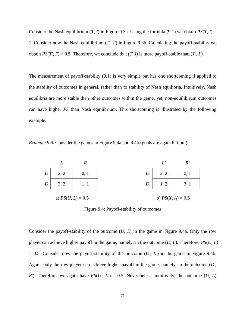
71

Consider the Nash equilibrium (T, I) in Figure 9.3a. Using the formula (9.1) we obtain PS(T, I) =

1. Consider now the Nash equilibrium (T', I') in Figure 9.3b. Calculating the payoff-stability we

obtain PS(T', I') = 0.5. Therefore, we conclude that (T, I) is more payoff-stable than (T', I').

The measurement of payoff-stability (9.1) is very simple but has one shortcoming if applied to

the stability of outcomes in general, rather than to stability of Nash equilibria. Intuitively, Nash

equilibria are more stable than other outcomes within the game, yet, non-equilibirum outcomes

can have higher PS than Nash equilibrium. This shortcoming is illustrated by the following

example.

Example 9.6. Consider the games in Figure 9.4a and 9.4b (goals are again left out).

a) PS(U, L) = 0.5 b) PS(X, A) = 0.5

Figure 9.4: Payoff-stability of outcomes

Consider the payoff-stability of the outcome (U, L) in the game in Figure 9.4a. Only the row

player can achieve higher payoff in the game, namely, in the outcome (D, L). Therefore, PS(U, L)

= 0.5. Consider now the payoff-stability of the outcome (U', L') in the game in Figure 9.4b.

Again, only the row player can achieve higher payoff in the game, namely, in the outcome (D',

R'). Therefore, we again have PS(U', L') = 0.5. Nevertheless, intuitively, the outcome (U, L)

L R

U 2, 2 0, 1

D 3, 2 1, 1

L' R'

U' 2, 2 0, 1

D' 1, 2 3, 1

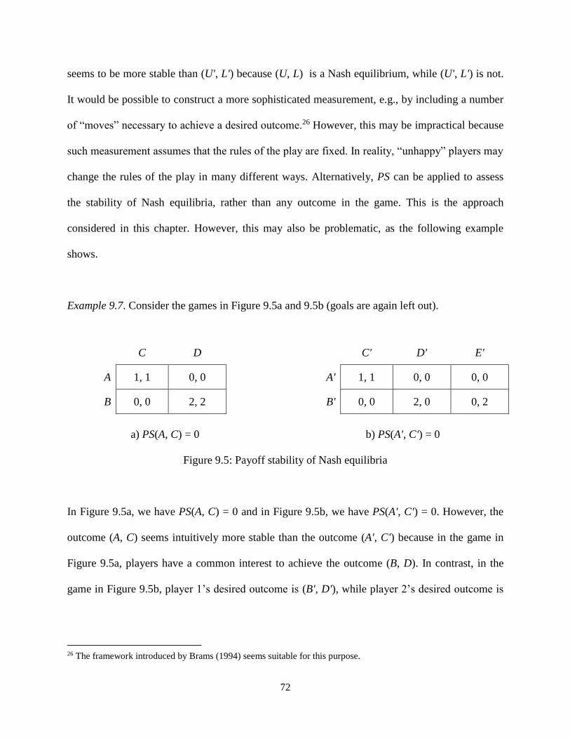
72

seems to be more stable than (U', L') because (U, L) is a Nash equilibrium, while (U', L') is not.

It would be possible to construct a more sophisticated measurement, e.g., by including a number

of “moves” necessary to achieve a desired outcome.26 However, this may be impractical because

such measurement assumes that the rules of the play are fixed. In reality, “unhappy” players may

change the rules of the play in many different ways. Alternatively, PS can be applied to assess

the stability of Nash equilibria, rather than any outcome in the game. This is the approach

considered in this chapter. However, this may also be problematic, as the following example

shows.

Example 9.7. Consider the games in Figure 9.5a and 9.5b (goals are again left out).

a) PS(A, C) = 0 b) PS(A', C') = 0

Figure 9.5: Payoff stability of Nash equilibria

In Figure 9.5a, we have PS(A, C) = 0 and in Figure 9.5b, we have PS(A', C') = 0. However, the

outcome (A, C) seems intuitively more stable than the outcome (A', C') because in the game in

Figure 9.5a, players have a common interest to achieve the outcome (B, D). In contrast, in the

game in Figure 9.5b, player 1’s desired outcome is (B', D'), while player 2’s desired outcome is

26 The framework introduced by Brams (1994) seems suitable for this purpose.

C D

A 1, 1 0, 0

B 0, 0 2, 2

C' D' E'

A' 1, 1 0, 0 0, 0

B' 0, 0 2, 0 0, 2

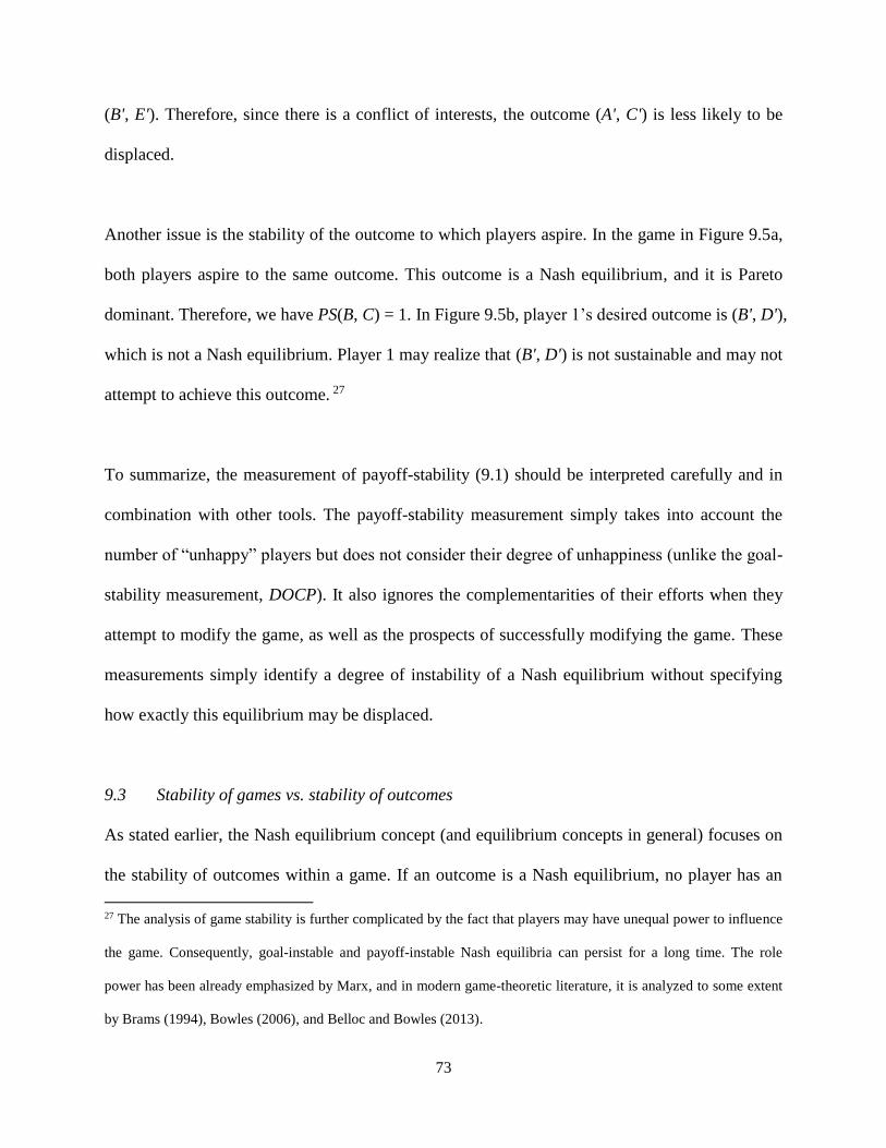
73

(B', E'). Therefore, since there is a conflict of interests, the outcome (A', C') is less likely to be

displaced.

Another issue is the stability of the outcome to which players aspire. In the game in Figure 9.5a,

both players aspire to the same outcome. This outcome is a Nash equilibrium, and it is Pareto

dominant. Therefore, we have PS(B, C) = 1. In Figure 9.5b, player 1’s desired outcome is (B', D'),

which is not a Nash equilibrium. Player 1 may realize that (B', D') is not sustainable and may not

attempt to achieve this outcome. 27

To summarize, the measurement of payoff-stability (9.1) should be interpreted carefully and in

combination with other tools. The payoff-stability measurement simply takes into account the

number of “unhappy” players but does not consider their degree of unhappiness (unlike the goal-

stability measurement, DOCP). It also ignores the complementarities of their efforts when they

attempt to modify the game, as well as the prospects of successfully modifying the game. These

measurements simply identify a degree of instability of a Nash equilibrium without specifying

how exactly this equilibrium may be displaced.

9.3 Stability of games vs. stability of outcomes

As stated earlier, the Nash equilibrium concept (and equilibrium concepts in general) focuses on

the stability of outcomes within a game. If an outcome is a Nash equilibrium, no player has an

27 The analysis of game stability is further complicated by the fact that players may have unequal power to influence

the game. Consequently, goal-instable and payoff-instable Nash equilibria can persist for a long time. The role

power has been already emphasized by Marx, and in modern game-theoretic literature, it is analyzed to some extent

by Brams (1994), Bowles (2006), and Belloc and Bowles (2013).

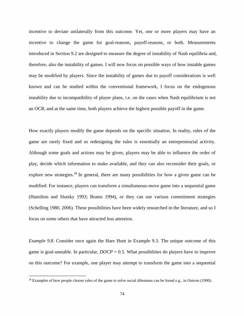
74

incentive to deviate unilaterally from this outcome. Yet, one or more players may have an

incentive to change the game for goal-reasons, payoff-reasons, or both. Measurements

introduced in Section 9.2 are designed to measure the degree of instability of Nash equilibria and,

therefore, also the instability of games. I will now focus on possible ways of how instable games

may be modified by players. Since the instability of games due to payoff considerations is well

known and can be studied within the conventional framework, I focus on the endogenous

instability due to incompatibility of player plans, i.e. on the cases when Nash equilibrium is not

an OCR, and at the same time, both players achieve the highest possible payoff in the game.

How exactly players modify the game depends on the specific situation. In reality, rules of the

game are rarely fixed and so redesigning the rules is essentially an entrepreneurial activity.

Although some goals and actions may be given, players may be able to influence the order of

play, decide which information to make available, and they can also reconsider their goals, or

explore new strategies.28 In general, there are many possibilities for how a given game can be

modified: For instance, players can transform a simultaneous-move game into a sequential game

(Hamilton and Slutsky 1993; Brams 1994), or they can use various commitment strategies

(Schelling 1980, 2006). These possibilities have been widely researched in the literature, and so I

focus on some others that have attracted less attention.

Example 9.8. Consider once again the Hare Hunt in Example 9.3. The unique outcome of this

game is goal-unstable. In particular, DOCP = 0.5. What possibilities do players have to improve

on this outcome? For example, one player may attempt to transform the game into a sequential

28 Examples of how people choose rules of the game to solve social dilemmas can be found e.g., in Ostrom (1990).

75

one: If e.g., player 1 moves first, he will catch the hare with probability 1, while the player 2

catches nothing.29 Nevertheless, the modified game is still not goal-stable because player 2 fails

to achieve her goal (as before the modification, DOCP = 0.5). Player 2 may perhaps try to move

even before the player 1.

Another way how players can modify the game is to expand their action sets; for example, each

player can invest in better hunting technology in an attempt to increase his probability of success.

This will lead to an innovation race, which, however, cannot change the fact that players’ plans

will continue to be mutually incompatible. The following simple example illustrates this logic.

Example 9.8. N = {1, 2}, A1 = A2 = {Invest, Not} G1 = G2 = {Hare}. If a player invests in better

hunting technology and the other player doesn’t, the probability of success for the player who

invests, increases by τ. If both players invest or if both players don’t invest, each of them catches

the hare with probability 0.5.30 The probabilities of success of this modified game are shown in

Figure 9.6. Since each player has only one goal, the probabilities of success can be used to

represent players’ payoffs.

29 Note that transforming the simultaneous game into the sequential one would affect the players’ payoffs. This

would also be the case in the Stag Hunt games in Figs. 1 and 3. In contrast, conventional analysis typically assumes

that the change of the order of play does not affect players’ outcomes (Hamilton and Slutsky 1993).

30 For simplicity, it is assumed that investment in new technology is costless.

76

Figure 9.6: Technological race in the Hare Hunt

Nash equilibrium of the game is (Invest, Hare; Invest, Hare). Yet, this Nash equilibrium is still

goal-unstable. DOCP(Invest, Hare; Invest, Hare) = 0.5, which means that the players are

motivated to modify the game further.

Players can expand their action sets also in different ways: They can search for other locations

where hares can be found. This case is described in the following example.

Example 9.9. N = {1, 2}, A1 = A2 = {Search, Not} G1 = G2 = {Hare}. Assume that if a player

abandons the original location and searches for a new one, he will catch a hare with probability

0.5 < β ≤ 1. This probability is independent of whether the other player searches for a new

location or not. The probabilities of success (also representing players’ payoffs) are shown in

Figure 9.7.

Figure 9.7: Hare Hunt with a search option

(Invest, Hare) (Not, Hare)

(Invest, Hare) 0.5, 0.5 0.5 + τ, 0

(Not, Hare) 0, 0.5 + τ 0.5, 0.5

(Search, Hare) (Not, Hare)

(Search, Hare) β, β β, 1

(Not, Hare) 1, β 0.5, 0.5

77

The Nash equilibria of the game are (Search, Hare; Not, Hare) and (Not, Hare; Search, Hare). In

each of these equilibria we have DOCP = (1 + β)/2 > 0.5. Compared to the original Hare Hunt in

Example 9.3, the goal-stability of Nash equilibrium increases. The payoff stability remains the

same, i.e., PS = 1. If β = 1, another Nash equilibrium emerges, namely, (Search, Hare; Search,

Hare). All the three Nash equilibria are then goal-stable and payoff-stable.31

9.4 Stability of Nash equilibria and MCP

So far, we have focused on goal-stability without considering MCP. From Theorem 5.1, an

outcome can be goal-unstable (i.e., it is not an OCP), and yet it can be an MCP. First, consider

the following example.

Example 9.10. Recall the Stag Hunt game in Example 5.1, where the stag can escape with the

probability α = 0.5. We have shown, that there are two Nash equilibria: (D, Hare; D, Hare) and

(C, Stag; C, Stag). None of these Nash equilibria is an OCP. Consequently, they will be

endogenously goal-unstable. Yet, (C, Stag; C, Stag) is an MCP. Therefore, in the (C, Stag; C,

Stag), the players have a common interest. They are facing a technological problem of how to

improve their hunting efficiency. In contrast, in the Nash equilibrium (D, Hare; D, Hare), their

interests are opposed, and they are facing an institutional problem of making their plans mutually

compatible.32

31 A more realistic example would also incorporate search costs.

32 Although this is an institutional problem, each hunter may attempt to increase his hunting efficiency by investing

in better hunting technology. However, this would not solve the institutional problem of the mutual incompatibility

of plans.

78

In practice, both technological and institutional problems may be involved simultaneously. For

instance, we can consider a case when the hare can escape both hunters. We can use DMCP to

measure the degree of mutual plan incompatibility. The lower the DMCP is, the more serious the

institutional problem is in this particular case. Therefore, DMCP can be used in combination

with DOCP and PS to assess the endogenous instability of a Nash equilibrium in specific

contexts. In the following chapter, I apply these concepts to account for changes in social norms.

79

10 A theory of social norms change

Why do norms change? Several possibilities have been suggested in the literature: They may

change as a result of group selection (Hayek 1973), imitation of more successful groups by less

successful ones (Boyd and Richerson 2002), or change in costs and benefits (Becker and Murphy

2000). Another possibility is that they change from within. The dominant model of such change

is due to Young (1993, 1996, 2001).33 According to his model, changes in norms occur due to

“mistakes”, which in turn result from the bounded rationality of agents. Hence, a change of a

norm is modeled as a move from one equilibrium of a given game to another. Explicit modeling

of goals and probabilities of their success offers another possibility: Individuals may make an

effort to replace a norm by modifying the game, if they sometimes fail to achieve their goals

under the current norm, or alternatively, if a better norm (i.e., a norm which enables to achieve

more valuable set of goals) is available. To use the terminology of the previous chapter, the

norms change if they are goal-unstable and/or payoff-unstable.34 As an example, consider the

change of the medium of exchange from coins to banknotes.

Example 10.1. Consider two players using coins in an exchange. However, coins include positive

transportation costs, c > 0. At the same time, they can be stolen with the probability 0 < 1 – s < 1.

Players want to carry out the desired transaction. If the coins are stolen, the transaction will fail.

Each player values carrying out this transaction at v > 0. Formally, we have N = {1, 2} A1 = A2 =

33 A more detailed survey of the literature can be found in Appendix II.

34 The possibility of an intentional change of a norm via collective action is studied by Bowles (2006). Bowles uses

the conventional approach with players motivated by their payoffs.

80

{Coins}, and G1 = G2 = {T, C}, where T refers to “carry out the transaction”, and C represents

“avoid transportation costs”. There is a single goal-oriented strategy for each player, namely, S1

= S2 = {(Coins; T, C)}. There are two states of the world: { , }R NR with ( ) 1p R s and

( )p NR s , where R denotes “robbery occurs”, and NR refers to “robbery doesn’t occur”.

Figures 10.1a and 10.1b show the probabilities of success for each state, while Figures 10.1c and

10.2d show the overall probabilities and payoffs, respectively.

a) Robbery occurs b) Robbery doesn’t occur

c) Overall probabilities of success d) Payoffs

Figure 10.1: Exchange with coins

Since 0 < s < 1, the unique outcome of the game is not an OCP, with DOCP = s/2. Therefore, the

outcome is goal-unstable. The players are motivated to look for ways how to decrease the

probability of robbery and avoid transportation costs. A major innovation came with paper

( ) 1p R s

(Cash; T, C)

(Cash; T, C) (0, 0), (0, 0)

( )p NR s

(Cash; T, C)

(Cash; T, C) (1, 0), (1, 0)

(Cash; T, C)

(Cash; T, C) (s, 0), (s, 0)

(Cash; T, C)

(Cash; T, C) sv – c, sv – c

81

notes.35 This innovation, which transformed the game in Example 10.1 into a new game, is

described in the following example.

Example 10.2. Consider two players choosing between using coins and notes in a transaction.

For simplicity, it is assumed that they cannot choose both. The transaction only occurs if they

choose to use the same means of exchange. Coins include positive transportation costs, c > 0,

while notes do not. In contrast, notes have no value (because they are either counterfeit or

inflated) with probability 0 < 1 – q < 1, while coins always have a value. Players want to carry

out the desired transaction. If the notes have no value, the transaction will fail. Each player

values carrying out this transaction at v > 0. Formally, we have N = {1, 2} A1 = A2 = {Coins,

Notes}, and G1 = G2 = {T, C}, where T refers to “carry out the transaction”, and C represents

“avoid transportation costs”. There are now four states of the world:

{ , , , }RNV RV NRNV NRV with ( ) (1 )(1 )p RNV s q , ( ) (1 )p RV s q ,

( ) (1 )p NRNV s q , and ( )p NRV sq , where R denotes “robbery occurs”, NR refers to

“robbery doesn’t occur”, NV represents “notes have no value”, and V denotes “notes have a

value”. Probabilities of success in each state are shown in Figures 10.2a-d, while Figures 10.2e

and 10.2f show overall probabilities of success and payoffs, respectively.

35 For evidence that paper money in China was introduced to avoid transportation costs, see e.g., Bowman (2000),

Ebrey, Walthall, and Palais (2006), and Gernet (1962).

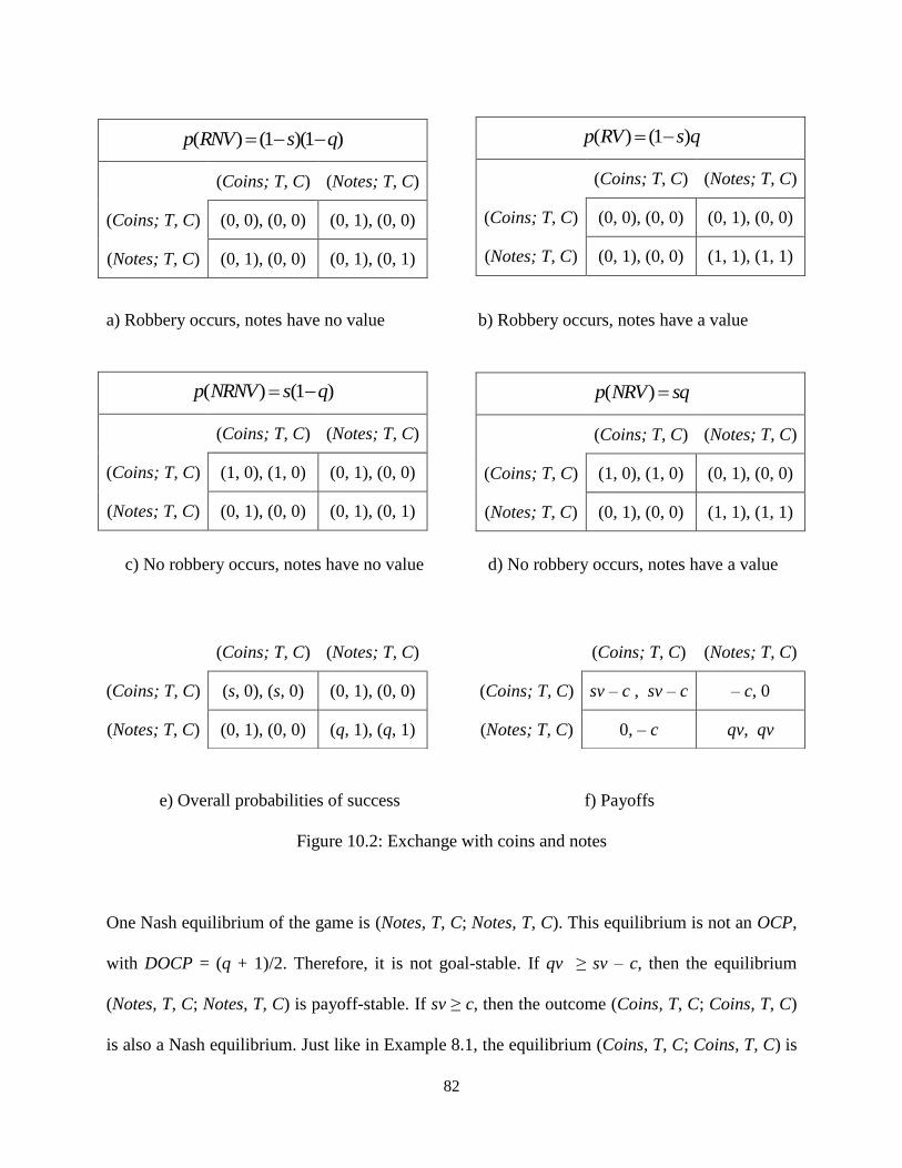
82

a) Robbery occurs, notes have no value b) Robbery occurs, notes have a value

c) No robbery occurs, notes have no value d) No robbery occurs, notes have a value

e) Overall probabilities of success f) Payoffs

Figure 10.2: Exchange with coins and notes

One Nash equilibrium of the game is (Notes, T, C; Notes, T, C). This equilibrium is not an OCP,

with DOCP = (q + 1)/2. Therefore, it is not goal-stable. If qv ≥ sv – c, then the equilibrium

(Notes, T, C; Notes, T, C) is payoff-stable. If sv ≥ c, then the outcome (Coins, T, C; Coins, T, C)

is also a Nash equilibrium. Just like in Example 8.1, the equilibrium (Coins, T, C; Coins, T, C) is

( ) (1 )(1 )p RNV s q

(Coins; T, C) (Notes; T, C)

(Coins; T, C) (0, 0), (0, 0) (0, 1), (0, 0)

(Notes; T, C) (0, 1), (0, 0) (0, 1), (0, 1)

( ) (1 )p RV s q


(Coins; T, C) (0, 0), (0, 0) (0, 1), (0, 0)

(Notes; T, C) (0, 1), (0, 0) (1, 1), (1, 1)

( ) (1 )p NRNV s q


(Coins; T, C) (1, 0), (1, 0) (0, 1), (0, 0)

(Notes; T, C) (0, 1), (0, 0) (0, 1), (0, 1)

( )p NRV sq


(Coins; T, C) (1, 0), (1, 0) (0, 1), (0, 0)

(Notes; T, C) (0, 1), (0, 0) (1, 1), (1, 1)


(Coins; T, C) (s, 0), (s, 0) (0, 1), (0, 0)

(Notes; T, C) (0, 1), (0, 0) (q, 1), (q, 1)


(Coins; T, C) sv – c , sv – c – c, 0

(Notes; T, C) 0, – c qv, qv

83

not an OCP, with DOCP = s/2, and therefore, it is not goal-stable. If qv ≤ sv – c, then this

equilibrium is payoff-stable.

We are concerned with the transition from coins to paper money. One possibility is that sv < c

and therefore, (Coins, T, C; Coins, T, C) is not a Nash equilibrium. In words, the high probability

of robbery and high transportation costs exceed the value of transactions. Therefore, once notes

are introduced, players have a dominant strategy to choose them as a medium of exchange.

Alternatively, (Coins, T, C; Coins, T, C) is a Nash equilibrium, and players are facing an

equilibrium selection problem. In this case, mechanisms analyzed by, for example, Young (1993,

1996, 2001) and Bowles (2006) may apply.36

Recall that the Nash equilibrium (Notes, T, C; Notes, T, C) is not goal-stable, because with a

positive probability, banknotes may be valueless. Therefore, the model predicts players will look

for ways how to increase the success of their plans. For example, they will attempt to increase

the probability q. This fact explains subsequent efforts to decrease counterfeiting (by designing

banknotes that are more difficult to counterfeit or by adopting legislation that would make

counterfeiting less profitable)37 as well as the efforts to design institutions that would tame

excessive inflations. They may also look for a better media of exchange. All these efforts will be

36 For various accounts of the introduction of paper money, see e.g., Graeber (2011), Ferguson (2008), and Shin

(2009).

37 See e.g., Langford (1989), who mentions later 18th-century legislation in England that aimed consumers’

protection against forged notes. See also McGowen (2002, 2005, 2007, 2011), Sharpe (1999), and Mockford (2014).

84

more intensive during periods of high inflation rates or frequent counterfeiting.38 At the same

time, the Nash equilibrium (Notes, T, C; Notes, T, C) is an MCP. Therefore, in this simple setting,

players are motivated to cooperate to increase q, as they would both benefit from the measures

that would take them closer to the idealized state of OCP.39

38 For instance, Hayek’s (1976, 1990) proposal to redesign monetary institutions was written in response to high

inflation rates in the early 1970s. See Komrska and Hudik (2016).

39 A more realistic model would also include an issuing bank as a player.

85

11 Goal-oriented behavior and evolution

So far, I have focused on modeling human behavior. Nevertheless, the notion of goal-oriented

strategy can be used in biology to model the behavior of non-human players. Mayr (1988, 1992)

points out that biology cannot dispense with the notion of goal-directedness, as many processes

or behaviors in nature are characterized by this property. However, these processes or behaviors,

which Mayr calls “teleonomic” (a term first introduced by Pittendrigh (1958)), owe their goal-

directedness to the operation of a program rather than deliberate goal-setting. Fortunately, in the

model introduced in the previous chapters, it is irrelevant whether the goal-orientedness is

programmed or whether purposeful behavior is involved.

In spite of the importance of goal-orientedness in biology, only a few works incorporated this

idea into formal models. One possible exception is Kalmus and Smith’s (1960), who introduce a

model of the sex ratio evolution, according to which sex ratio maximizes the probability that

when two individuals meet, they will have different sexes. Their model can be understood as an

(implicit) coordination game with goal-oriented strategies. Maynard Smith (1978, 34) calls their

model “eccentric” and favors an alternative (more conventional) model according to which the

sex ratio is determined by a gene with natural selection maximizing the number of copies of that

gene in future generations. In my interpretation, the positions of Kalmus and Smith (1960) and

Maynard Smith (1978) are, to some extent, compatible. The former focuses on the problem of

strategies compatibility while the latter emphasizes the mechanism by which the compatibility

problem is solved.

86

11.1 Fitness maximization

In biological applications of game theory, payoffs are interpreted as inclusive or individual

fitness (or its component) of an organism (Smith 1982, Hofbauer and Sigmund 1998). The

crucial aspect of these applications is that a strategy (phenotype) is considered to be a hereditary

trait. This aspect links the frequencies of strategies in a population with the payoffs of a game:

the higher payoffs, the more offspring, and hence the higher frequency of a particular strategy in

the population. This, of course, is the standard mechanism of natural selection, which plays an

important role in the evolution of many phenotypes. There are, however, a couple of problems

when strategies in the games are behavioral traits.

The first problem is that the link between genes and behavior is not clear; for instance, according

to Dawkins (1989), genes influence behavior only in a statistical sense, and this influence can be

modified, overridden, or reversed by other influences. In a similar vein, Buller (2005), points out

that only proximate mechanisms underlying the tendency to exhibit certain behavior are affected

genetically. If this is true, it would be indeed astonishing if fitness was the only thing that

determined frequencies of strategies in a population: to wit, the “other influences” sometimes

change rather quickly, possibly several times during a life of an individual (Stephens and

Clements 2000). Moreover, while paying the lip service to the genetic basis of behavior, the

games usually focus on phenotypic changes only without actually keeping track of underlying

genetics, which would be rather complicated business (Hammerstein 2000).

87

The second problem is that some strategies have minimal fitness consequences, and natural

selection may not be powerful enough to tweak them (Johnstone 2000). Note that this would be

an issue even if strategies were completely genetically determined. It may also be the case that

an individual pursues a strategy yielding low payoff in one type of interaction while pursuing

strategies yielding high payoffs in other types of interactions. Given that fitness is a unique

measure for an individual, such an organism may cross-subsidize low payoffs in one type of

interaction with high payoffs in other interactions. Strategies yielding low payoffs thus may not

be eliminated.40

Based on these arguments – and given the intuitive plausibility and empirical relevance of game-

theoretic models – there seems to be more to payoffs in evolutionary games than just fitness.

Accordingly, natural selection may not be the only mechanism playing a role in the evolution of

behavioral strategies; learning (social and individual) may be another one. Behavior is often

flexible rather than hard-wired. For example, Alexander (1961) has shown that even crickets

adjust their behavior to their past experience (Dawkins 1989). If learning is important, the

challenge is how to relate learning to payoffs in evolutionary games. To account for various

mechanisms of adaptation, Dennett (1995) distinguishes among four types of “creatures”:

Darwinian, Skinnerian, Popperian, and Gregorian. Darwinian creatures reflect the adaptation

through natural selection. These types of creatures are described by the conventional

evolutionary game theory. All living organisms are Darwinian creatures because they are all

subject to natural selection. Skinnerian creatures, a sub-set of Darwinian creatures, represent

adaptation through trial-and-error learning. Several game-theoretic learning models account for

40 Related issue arises in the attributes-approach to behavior in economics (Lancaster 1966, Rosen 1974).

88

this behavior (Young 2004). Popperian creatures, a sub-set of Skinnerian creatures, are capable

of preselection among possible behaviors before they engage in trial-and-error learning. In

conventional game theory, Popperian creatures are able to (repeatedly) eliminate strictly

dominated actions or Bayesian learning. Finally, Gregorian creatures, a sub-set of Popperian

creatures, are those who make use of designed portions of the outer environment. That is, they

are able to use tools (including mind-tools, such as language) to generate possible behaviors as

well as to preselect these behaviors before they try them out. The purpose of this chapter is to

construct a framework that would account for all four types of adaptation.

The main difference between evolutionary game-theoretic models and conventional game-

theoretic models is that in the evolutionary models players maximize their fitness, while in the

conventional models players maximize subjective utility.41 Therefore the challenge is to find the

link between fitness and utility. I argue that the notion of goal-oriented behavior provides this

link. In the following section, I apply the framework introduced in previous chapters to analyze

the behavior of players who may or may not be humans.

11.2 Example

Example 11.1. Consider the following version of the Hawk-Dove game, in which two players,

attacker (player 1) and defender (player 2), aim to obtain a pray. Let {1,2},N

1 2 { , }A A H D , and 1 2 { , }G G GP AC , where H represents Hawk, D, stands for Dove, GP

41 For a discussion on the link between fitness maximization and utility maximization, see e.g., Robson (1996, 2001,

2002), Samuelson and Swinkels (2006), Rayo and Becker (2007), Gintis (2007, 2009) and Sterelny (2012).

89

denotes “Get the prey”, and AC represents “Avoid conflict”. Goal-oriented strategies are the

following: 1 2 {( ; , ),( ; , )}S S H GP AC D GP AC . There are four states of nature, each

occurring with the probability 0.25: {11,12,21,22} . For instance, 12 denotes that the player 1

gets the prey if both choose H and the player 2 gets the prey if both choose D. Compatibility

functions for each state are shown in Figures 11.1a-d, and overall probabilities of success and

payoffs are shown in the Figures 11.1e and 11.1f respectively.

a) 11 b) 12

c) 21 d) 22

(11) 0.25q

(H; GP, AC) (D; GP, AC)

(H; GP, AC) (1, 0), (0, 0) (1, 1), (0, 1)

(D; GP, AC) (0, 1), (1, 1) (1, 1), (0, 1)

(12) 0.25q


(H; GP, AC) (1, 0), (0, 0) (1, 1), (0, 1)

(D; GP, AC) (0, 1), (1, 1) (0, 1), (1, 1)

(21) 0.25q


(H; GP, AC) (0, 0), (1, 0) (1, 1), (0, 1)

(D; GP, AC) (0, 1), (1, 1) (1, 1), (0, 1)

(22) 0.25q


(H; GP, AC) (0, 0), (1, 0) (1, 1), (0, 1)

(D; GP, AC) (0, 1), (1, 1) (0, 1), (1, 1)

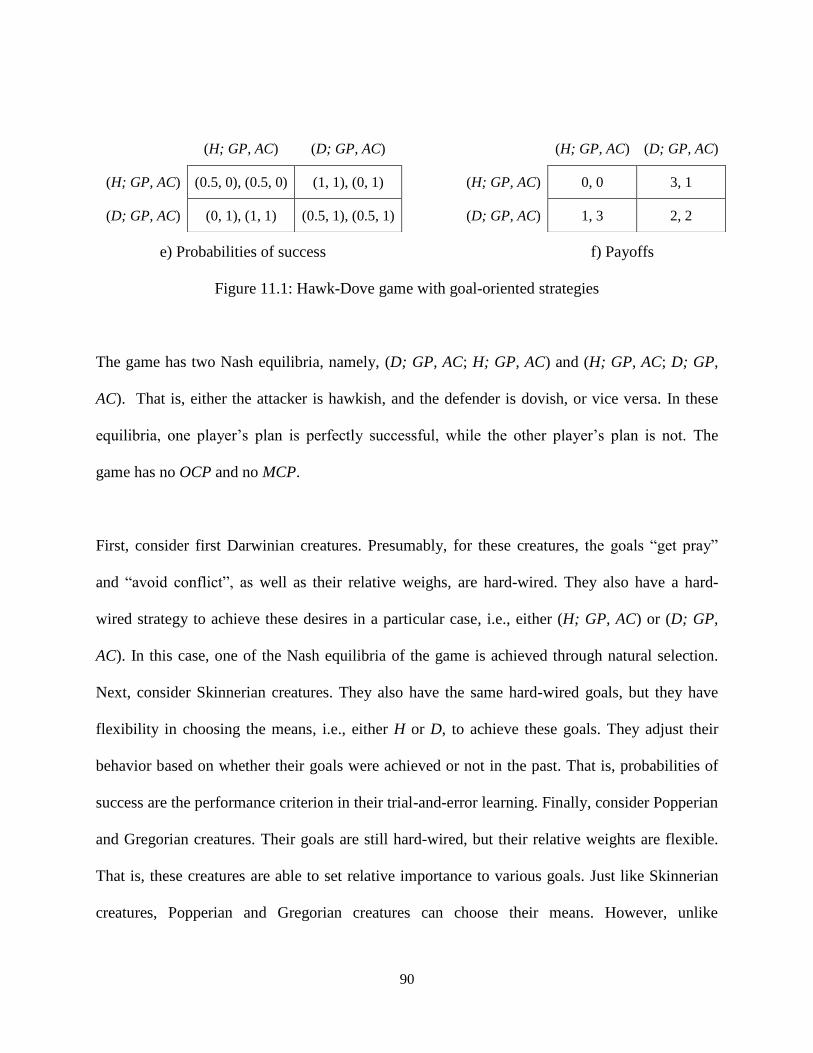
90

e) Probabilities of success f) Payoffs

Figure 11.1: Hawk-Dove game with goal-oriented strategies

The game has two Nash equilibria, namely, (D; GP, AC; H; GP, AC) and (H; GP, AC; D; GP,

AC). That is, either the attacker is hawkish, and the defender is dovish, or vice versa. In these

equilibria, one player’s plan is perfectly successful, while the other player’s plan is not. The

game has no OCP and no MCP.

First, consider first Darwinian creatures. Presumably, for these creatures, the goals “get pray”

and “avoid conflict”, as well as their relative weighs, are hard-wired. They also have a hard-

wired strategy to achieve these desires in a particular case, i.e., either (H; GP, AC) or (D; GP,

AC). In this case, one of the Nash equilibria of the game is achieved through natural selection.

Next, consider Skinnerian creatures. They also have the same hard-wired goals, but they have

flexibility in choosing the means, i.e., either H or D, to achieve these goals. They adjust their

behavior based on whether their goals were achieved or not in the past. That is, probabilities of

success are the performance criterion in their trial-and-error learning. Finally, consider Popperian

and Gregorian creatures. Their goals are still hard-wired, but their relative weights are flexible.

That is, these creatures are able to set relative importance to various goals. Just like Skinnerian

creatures, Popperian and Gregorian creatures can choose their means. However, unlike


(H; GP, AC) (0.5, 0), (0.5, 0) (1, 1), (0, 1)

(D; GP, AC) (0, 1), (1, 1) (0.5, 1), (0.5, 1)


(H; GP, AC) 0, 0 3, 1

(D; GP, AC) 1, 3 2, 2

91

Skinnerian creatures, they can employ more sophisticated methods of learning. In particular, they

may use information about strategies of other individuals, and they may even attempt to modify

the game in ways outlined in Chapter 9.

11.3 Goal-Directedness and Unification of Behavioral Sciences

There have been attempts to construct a unified theory of behavior, integrating insights from

various behavioral sciences. For some authors, maximizing behavior has a place in this unified

theory (Gintis 2007, 2009), while for others, it does not. For example, Vanberg (2002, 2004)

argues that the principle of payoff maximization should be replaced with Mayr’s (1988, 1992)

idea of goal-directed program-based behavior (see also Conte and Castelfranchi 1995).

This chapter shows that these two approaches to behavior are, in fact, compatible. The concept of

goal-oriented strategy does not necessarily presuppose that individuals choose their goals

consciously. Nothing prevents one from interpreting purposive strategies as goal-directed

programs. The preference relation defined on the set of lotteries over player’s goals merely

reflects the unequal importance of various goals to the player (who may be a living or a non-

living system) and is open to various interpretations. It may reflect player’s subjective

preferences (if it is a human being), contributions of player’s goals to its fitness (if it is an

organism), preferences of the engineer who designed the player (if it is a machine), or any other

criterion. If a player has more than one goal, a model of behavior needs to incorporate some sort

of preference relation, which would describe how agents resolve trade-offs between competing

goals. Therefore, the concept of goal-orientedness usually (i.e., if players have more than one

goal) needs to be complemented with the principle of maximizing behavior. But the reverse is

92

also true: the maximization principle sometimes requires the concept of goal-directedness, in

order to analyze processes of learning.

The conventional game-theoretic assumptions allow only for one method of adjusting strategies

to the environment at a time: either natural selection (if payoffs are interpreted as players’

fitness) or learning and reasoning (if payoffs represent subjective preferences). The distinction

between means (actions) and goals enables analysis of various adjustment processes of

adaptation within one framework. For instance, it can be assumed that natural selection operates

on the set of goals (i.e., it determines the payoffs) and learning and reasoning operates on the

level of adjustment of actions to given goals (i.e., it is concerned whether a particular strategy

was successful in achieving a given goal or not) (El Mouden et al. 2012). The model of games

with goal-oriented strategies can thus provide a link between social and biological sciences.

93

12 Goals and classification of games

Since the birth of game-theory, scholars have attempted to classify games according to various

criteria and for various purposes (e.g., Guyer and Hamburger 1968; Rapoport, Guyer, and

Gordon 1967; Kilgour and Fraser 1988). One such classification, introduced by Schelling (1980),

distinguishes among pure conflict (or zero-sum), pure common-interest (or pure-coordination),

and mixed-motive games. The definition of these categories is based on relationships between

payoffs of various players: If players’ payoffs are perfectly positively correlated, then the game

is of pure common-interest; if the payoffs are perfectly negatively correlated, then the game is of

pure conflict game. Mixed-motive games are those in which players’ payoffs are imperfectly

correlated. The following example illustrates this classification.

Example 12.1. Consider the three examples of games in Figure 12.1. The game in Figure 12.1a is

a pure-common interest game (Spearman rank correlation coefficient is equal to 1)42, the game in

Figure 12.1b is a mixed-motive game (Spearman rank correlation coefficient is equal to 0.6), and

the game in Figure 12.1c is a pure-conflict game (Spearman rank correlation coefficient is equal

to –1).

42 I use the rank correlation coefficient because I assume that payoffs are ordinal.

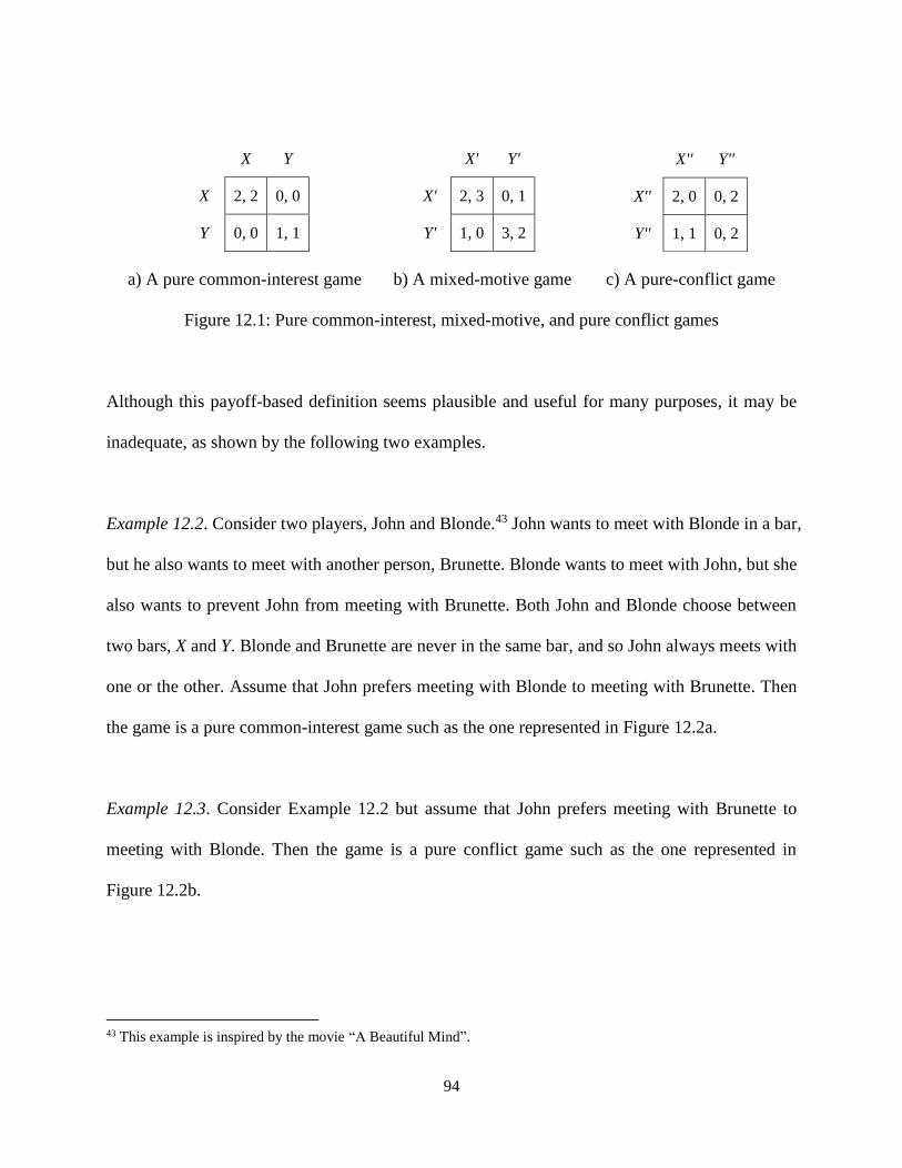
94

a) A pure common-interest game b) A mixed-motive game c) A pure-conflict game

Figure 12.1: Pure common-interest, mixed-motive, and pure conflict games

Although this payoff-based definition seems plausible and useful for many purposes, it may be

inadequate, as shown by the following two examples.

Example 12.2. Consider two players, John and Blonde.43 John wants to meet with Blonde in a bar,

but he also wants to meet with another person, Brunette. Blonde wants to meet with John, but she

also wants to prevent John from meeting with Brunette. Both John and Blonde choose between

two bars, X and Y. Blonde and Brunette are never in the same bar, and so John always meets with

one or the other. Assume that John prefers meeting with Blonde to meeting with Brunette. Then

the game is a pure common-interest game such as the one represented in Figure 12.2a.

Example 12.3. Consider Example 12.2 but assume that John prefers meeting with Brunette to

meeting with Blonde. Then the game is a pure conflict game such as the one represented in

Figure 12.2b.

43 This example is inspired by the movie “A Beautiful Mind”.

X Y

X 2, 2 0, 0

Y 0, 0 1, 1

X' Y'

X' 2, 3 0, 1

Y' 1, 0 3, 2

X'' Y''

X'' 2, 0 0, 2

Y'' 1, 1 0, 2

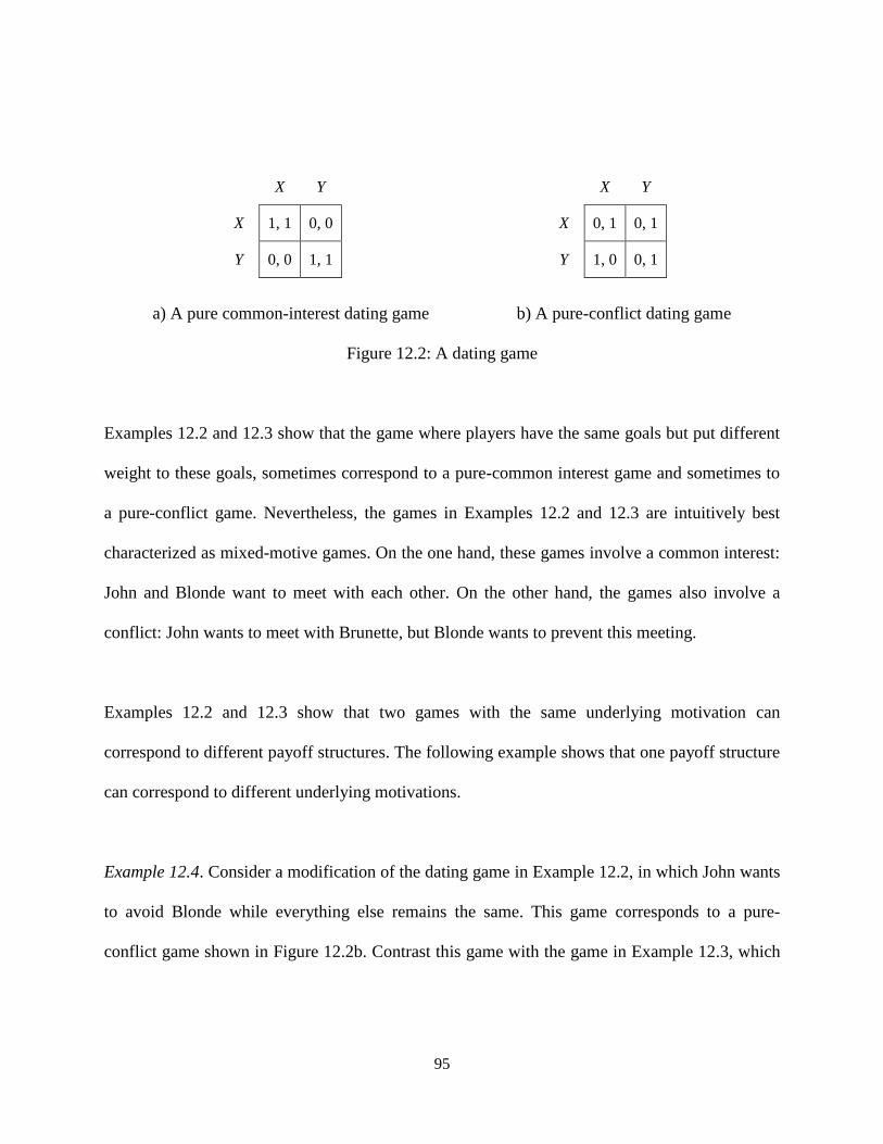
95

a) A pure common-interest dating game b) A pure-conflict dating game

Figure 12.2: A dating game

Examples 12.2 and 12.3 show that the game where players have the same goals but put different

weight to these goals, sometimes correspond to a pure-common interest game and sometimes to

a pure-conflict game. Nevertheless, the games in Examples 12.2 and 12.3 are intuitively best

characterized as mixed-motive games. On the one hand, these games involve a common interest:

John and Blonde want to meet with each other. On the other hand, the games also involve a

conflict: John wants to meet with Brunette, but Blonde wants to prevent this meeting.

Examples 12.2 and 12.3 show that two games with the same underlying motivation can

correspond to different payoff structures. The following example shows that one payoff structure

can correspond to different underlying motivations.

Example 12.4. Consider a modification of the dating game in Example 12.2, in which John wants

to avoid Blonde while everything else remains the same. This game corresponds to a pure-

conflict game shown in Figure 12.2b. Contrast this game with the game in Example 12.3, which

X Y

X 1, 1 0, 0

Y 0, 0 1, 1

X Y

X 0, 1 0, 1

Y 1, 0 0, 1

96

also corresponds to a pure-conflict game but in which John prefers meeting with Brunette to

meeting with Blonde.

Although the games in Examples 12.3 and 12.4 are represented with the same payoffs, there is an

important difference between them. In the game in Example 12.3, Blonde can turn the pure-

conflict game into a pure common-interest game by disposing of Brunette. Note that this fact

cannot be inferred from the standard representation of the game, which does not provide

information about players’ goals. In contrast, Blonde, in Example 12.4, is unable to turn the

pure-conflict game into one of pure common interest: if she disposes of Brunette, the game

continues to be a pure conflict game. This difference between the games in Examples 12.3 and

12.4 again cannot be inferred from the standard representation.

The Examples 12.2-12.4 illustrate the problem with the payoff-based classification of games:

actual complex motives of players are aggregated into a single (artificially constructed) motive –

payoff maximization. As a result, a game involving elements of both conflict and common

interest may sometimes appear as a game of pure conflict and at other times, as a game of pure

common interest, depending on which motive prevails. Hence, for more adequate classification

of games, it seems necessary to disaggregate players’ payoffs and uncover their various motives.

Inspired by the Examples 12.2-12.4, I propose a new definition of pure conflict, pure common-

interest, and mixed-motive games, which involves the standard definition as a special case. At

the same time, the new definition is complementary to the conventional one because it ignores

97

the relative importance of various goals that players consider. This new definition is based on the

mutual compatibility of goals across players introduced in previous chapters.

12.1 Definitions

I formally define a G-pure-common-interest game, G-pure-conflict game, and a G-mixed-motive

game as follows. G denotes that this classification is goal-based rather than payoff-based. The P-

pure-common-interest game, P-pure-conflict game, and a P-mixed-motive game refers to

conventional payoff-based classification.

Definition 12.1. Let be a game with goal-oriented strategies, which allows for multiple goals

and random events. For each i N define the function :iz S 0 that assigns to each

outcome ( , )s a number of successful goals of player i in the outcome ( , )s .

a) is a G-pure-common-interest game, if, for every pair of player ,i j N , we have

( , ) 1i jz z , where ρ is the Pearson correlation coefficient.

b) Let be such that 2N ; is a G-pure-conflict game, for every pair of player ,i j N , we

have ( , ) 1i jz z .

c) is a G-mixed-motive game, if it is neither a pure common-interest nor a pure-conflict game.

A goal-based perspective focuses on the number of successful goals while ignoring their relative

importance. In reality, achieving more goals is not always considered to be better from the

perspective of individuals. For instance, an individual may prefer to achieve one valuable goal to

several less valuable goals. Therefore, goal-based considerations have to be supplemented with

payoff considerations, as in the conventional classification of games. The combination of goal-

98

perspective and payoff-perspective then provides a more complete understanding of interests in a

strategic situation.

Definition 12.2. Let be a game with goal-oriented strategies, which allows for multiple goals

and random events.

a) is a P-pure-common-interest game, if for every pair of players ,i j N , with i j , we have

( , ) 1s i jr u u , where sr is the Spearman’s rank correlation coefficient and ui and uj are payoff

functions representing player i’s and player j’s preferences respectively.

b) Let be such that 2N ; is a P-pure-conflict game, if ( , ) 1s i jr u u .

c) is a P-mixed-motive game, if it is neither P-pure-common-interest nor P-pure-conflict

game.

Definitions 12.1 and 12.2 are illustrated by the following examples.

Example 12.5. Consider Examples 12.2 and 12.3. We now formalize them as games with goal-

oriented strategies. Let N = {John, Blonde}, AJ = AB = {X, Y}, GJ = {MBL, MBR}, GB = {MJ,

PJBR}, where MBL denotes “Meet with Blonde”, MBR represents “Meet with Brunette”, MJ

denotes “Meet with John”, and PJBR represents “Prevent John from Meeting with Brunette”.

Success functions are shown in Figure 12.3a. By strong monotonicity assumption, we have

(1,1) (0,0)B . If (1,0) (0,1)J then the preferences can be represented by payoffs in Figure

12.2a. This case corresponds to the Example 12.2. This game is G-mixed-motive ( 1 2( , ) 0z z )

and P-pure-common-interest ( 1 2( , ) 1sr u u ). If (0,1) (1,0)J , then the preferences can be

99

represented by payoffs in Figure 1b. This case corresponds to the Example 12.3. This game is

again a G-mixed-motive game ( 1 2( , ) 0z z ), the structure of goals is the same as before) and P-

pure-conflict game ( 1 2( , ) 1sr u u ).

Example 12.6. Consider Example 12.4. Let { , },N John Blonde { , },J BA A X Y

{ , },JG ABR MBR { , },BG MJ PJBR where ABR denotes “Avoid Meeting Blonde”. Success

functions are shown in Figure 12.3b. By strong monotonicity assumption we have (1,1) (0,0)B

and (1,1) (0,0)J . These preferences can be represented by payoffs in Figure 12.2b. The game

is a G-pure-conflict game ( 1 2( , ) 1z z ) as well as a P-pure-conflict game ( 1 2( , ) 1sr u u ).

a) John wants to meet Blonde b) John wants to avoid Blonde

Figure 12.3: Two versions of a dating game as strategic games with goals

In the following section, I establish some relationships between goal-based and preference-based

classifications.

12.3 Relationships between goal-based and preference-based classifications

Under what conditions does G-pure-common-interest (G-pure-conflict) correspond to P-pure

common-interest (P-pure-conflict)? The following two theorems address this question.

(X; MJ, PJBR) (Y; MJ, PJBR)

(X; BL, BR) (1, 0), (1, 1) (0, 1), (0, 0)

(Y; BL, BR) (0, 1), (0, 0) (1, 0), (1, 1)

(X; MJ, PJBR) (X; MJ, PJBR)

(X; ABL, BR) (0, 0), (1, 1) (1, 1), (0, 0)

(Y; ABL, BR) (1, 1), (0, 0) (0, 0), (1, 1)

100

Theorem 12.1. Let be a game with goal-oriented strategies such that 1iG for all i N . If

is a G-pure-common-interest (G-pure-conflict) game, then it is also P-pure-common-interest

(P-pure-conflict) game.

Proof. Assume first that is G-pure-common-interest. For each outcome ( , ),s we have

( , ) ( , )i jr s r s for each pair of players ,i j N . Therefore, we also have ( ) ( )i jp s p s for

each pair of players ,i j N . By the strong monotonicity assumption, we can represent payoff of

each player i with the overall probability of success, i.e., ( ) ( )i iu s p s . Therefore, we have

1 2( , ) 1sr u u and so is a P-pure-common-interest game. Assume now that G-pure-conflict.

Therefore, we have 2N . For each outcome ( , )s , we have 1 2( , ) 1 ( , )r s r s . Therefore,

we also have 1 2( ) 1 ( )p s p s . By the strong monotonicity assumption, we can represent the

payoff of each player i with the overall probability of success, i.e., ( ) ( )i iu s p s . Therefore, we

have 1 2( , ) 1sr u u and so is a P-pure-conflict game.

I have argued that the problem with the payoff classification is that payoffs do not provide

information about players’ underlying goals. Hence, if each player has only one goal in mind,

then no information is lost if these goals are not explicitly specified. In this case, the payoff-

based classification of games as pure common-interest, pure conflict, and mixed-motive is the

same as goal-based classification. The payoff-based and goal-based classification is equivalent

also when players have multiple goals, and the probabilities of success of each player’s goals are

perfectly correlated.

101

Theorem 12.2. Let be a game with goal-oriented strategies.

a) If is a G-pure-common-interest game and ( , ) (1,...,1)ir s or ( , ) (0,...,0)ir s for each

player i, then it is also P-pure-common-interest game.

b) If is a G-pure-conflict game and and ( , ) (1,...,1)ir s or ( , ) (0,...,0)ir s for each player

i, then it is also P-pure-conflict game.

Proof. Assume first that is G-pure-common-interest. For each outcome ( , )s , we have

( , ) (1,...,1) ( , ) (1,...,1)i jr s r s and ( , ) (0,...,0) ( , ) (0,...,0)i jr s r s for each pair of

players ,i j N . Therefore, we also have ( | ) ( | ) ( | ) ( | )i i i i j j j jp g s p g s p g s p g s for each

,ig ,jg s, and s', and each pair of players , .i j N It follows that

( )ip s ≿ ( ) ( )i i jp s p s ≿ ( )j jp s and therefore, ( ) ( ) ( ) ( )i i j ju s u s u s u s . This means that

1 2( , ) 1sr u u and so is a P-pure-common-interest game. Assume now that is G-pure-

conflict. Therefore, we have 2.N For each outcome ( , ),s we have

( , ) (0,...,0) ( , ) (1,...,1)i jr s r s for each outcome ( , )s and each pair of players ,i j N .

Therefore, we also have ( | ) ( | ) ( | ) ( | )i i i i j j j jp g s p g s p g s p g s for each ig , jg , s, and s',

and each pair of players ,i j N . It follows that ( )ip s ≿ ( ) ( )i i jp s p s ≿ ( )j jp s and therefore,

( ) ( ) ( ) ( )i i j ju s u s u s u s . This means that 1 2( , ) 1sr u u and so is a P-pure-conflict

game.

102

Theorem 12.2 generalizes Theorem 12.1 to cases when 1iG for all i N . Example 12.6

illustrates Theorem 12.2. In this game, each player has more than one goal. For each player, one

goal is achieved whenever the other goal is achieved. Since the game is G-pure-conflict, it is also

P-pure-conflict.

12.4 Discussion

The way how players’ goals are defined requires some attention. For instance, John of the dating

game considered in Example 12.2, may want to meet with both Blonde and Brunette, but perhaps

he does not want to meet with both of them at the same time. Therefore, contrary to the strong

monotonicity assumption, we may have (1,0) (1,1).J Furthermore, we may even have

(0,0) (1,1).J If such an outcome is feasible, then John’s goals can be more conveniently

defined as “Meet with Blonde alone” and “Meet with Brunette alone”. The general point is that

the specification of goals has to be sufficiently detailed so that all characteristics relevant to

players’ evaluations are included, and the strong monotonicity assumption is met.

12.5 A practical example

To illustrate the practical relevance of the goal-based classification, consider the following

example.

Example 12.7. Two countries, A and B, are negotiating a treaty about import quotas and tariffs. If

the treaty is signed, then tariffs will be reduced, and import quotas will be abolished. If the treaty

is not signed, then the tariffs will be kept at the current level, and the quotas will not be abolished.

Each country chooses between signing the treaty, S, and not signing the treaty, NS. The goals of

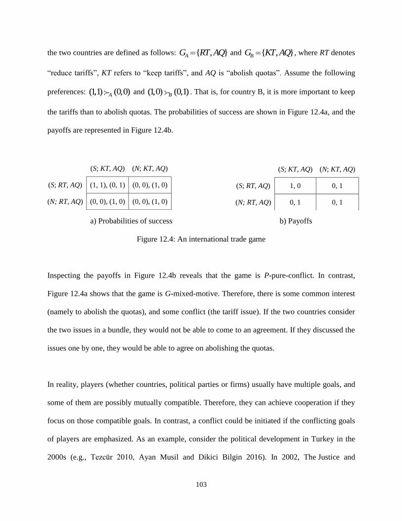
103

the two countries are defined as follows: { , }AG RT AQ and { , }BG KT AQ , where RT denotes

“reduce tariffs”, KT refers to “keep tariffs”, and AQ is “abolish quotas”. Assume the following

preferences: (1,1) (0,0)A and (1,0) (0,1)B . That is, for country B, it is more important to keep

the tariffs than to abolish quotas. The probabilities of success are shown in Figure 12.4a, and the

payoffs are represented in Figure 12.4b.


Figure 12.4: An international trade game

Inspecting the payoffs in Figure 12.4b reveals that the game is P-pure-conflict. In contrast,

Figure 12.4a shows that the game is G-mixed-motive. Therefore, there is some common interest

(namely to abolish the quotas), and some conflict (the tariff issue). If the two countries consider

the two issues in a bundle, they would not be able to come to an agreement. If they discussed the

issues one by one, they would be able to agree on abolishing the quotas.

In reality, players (whether countries, political parties or firms) usually have multiple goals, and

some of them are possibly mutually compatible. Therefore, they can achieve cooperation if they

focus on those compatible goals. In contrast, a conflict could be initiated if the conflicting goals

of players are emphasized. As an example, consider the political development in Turkey in the

2000s (e.g., Tezcür 2010, Ayan Musil and Dikici Bilgin 2016). In 2002, The Justice and

(S; KT, AQ) (N; KT, AQ)

(S; RT, AQ) (1, 1), (0, 1) (0, 0), (1, 0)

(N; RT, AQ) (0, 0), (1, 0) (0, 0), (1, 0)

(S; KT, AQ) (N; KT, AQ)

(S; RT, AQ) 1, 0 0, 1

(N; RT, AQ) 0, 1 0, 1

104

Development Party (AKP), led by Recep Tayyip Erdoğan, was able to attract supporters all over

the political spectrum. Arguably, this was because the party emphasized goals, such as the

expansion of ethnic rights, religious freedoms, economic liberalism, and anti-military attitudes,

that were shared by individuals with diverse political views. In particular, AKP represented an

opposition to the repressive state. Later, when the issue of the repressive state ceased to be

salient, differences among the original supporters of AKP came to the forefront, and AKP lost

the support of some of these voters.

105

13 Compatibility of plans and cooperative behavior

It has been observed that many people cooperate in a one-shot Prisoner’s Dilemma both in

laboratory experiments (Roth 1988; Colman 1995; Sally 1995; Komorita and Parks 1995;

Cooper et al. 1996) and outside the laboratory (List 2006). What explains this behavior?

According to one explanation, individuals care about other things besides material payoffs, such

as some notion of fairness (Rabin 1993; Fehr and Schmidt 1999; Bolton and Ockenfels 2000;

Bicchieri 2005; Falk and Fischbacher 2006). According to other explanations, players employ

various types of (potentially erroneous) reasoning which differ from the conventional rationality,

such as team reasoning (Bacharach 2006; Sugden 2000, 2003), evidential reasoning (Acevedo

and Krueger 2005; Krueger and Acevedo 2007; Krueger, DiDonato, and Freestone 2012), or

sample bias (Chater, Vlaev, and Grinberg 2008).

The framework introduced in previous chapters offers another explanation of the cooperative

behavior. According to this explanation, individuals use goal-based reasoning and identify the

cooperative outcome as an OCP, i.e., as an outcome where their goal-oriented strategies are

compatible.44 At the same time, they, to some extent, ignore the relative value of various goals.

In a way, these types of players think about the Prisoner’s Dilemma (incorrectly, at least from the

44 This explanation of cooperation in the Prisoner’s Dilemma may resemble Howard’s (1966a; 1966b) “meta-game”

approach. Howard introduces strategies conditional on the choices of other players. This, however, involves several

difficulties; above all, it seems inconsistent with the notion of a simultaneous-move game. For criticism of Howard’s

approach, see e.g., Harris (1969; 1970) and Shubik (1970).

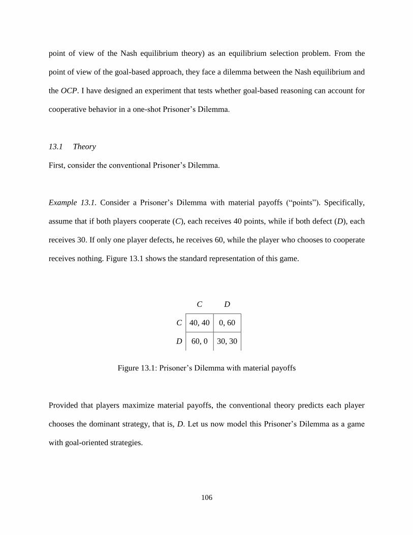
106

point of view of the Nash equilibrium theory) as an equilibrium selection problem. From the

point of view of the goal-based approach, they face a dilemma between the Nash equilibrium and

the OCP. I have designed an experiment that tests whether goal-based reasoning can account for

cooperative behavior in a one-shot Prisoner’s Dilemma.

13.1 Theory

First, consider the conventional Prisoner’s Dilemma.

Example 13.1. Consider a Prisoner’s Dilemma with material payoffs (“points”). Specifically,

assume that if both players cooperate (C), each receives 40 points, while if both defect (D), each

receives 30. If only one player defects, he receives 60, while the player who chooses to cooperate

receives nothing. Figure 13.1 shows the standard representation of this game.

Figure 13.1: Prisoner’s Dilemma with material payoffs

Provided that players maximize material payoffs, the conventional theory predicts each player

chooses the dominant strategy, that is, D. Let us now model this Prisoner’s Dilemma as a game

with goal-oriented strategies.

C D

C 40, 40 0, 60

D 60, 0 30, 30

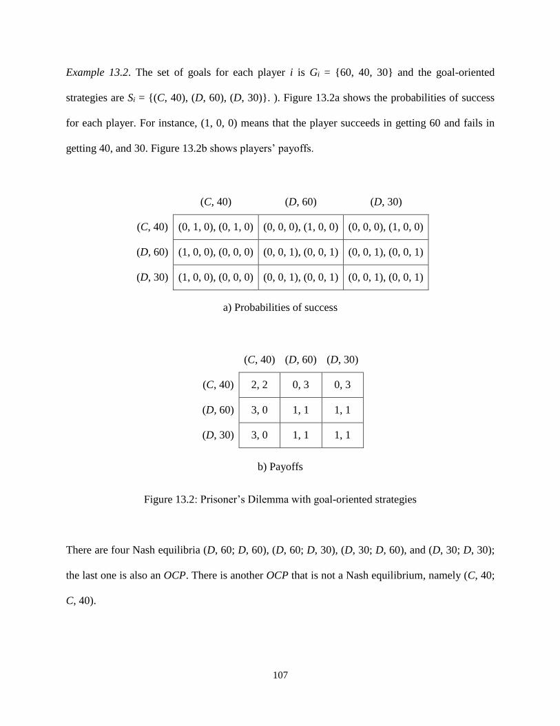
107

Example 13.2. The set of goals for each player i is Gi = {60, 40, 30} and the goal-oriented

strategies are Si = {(C, 40), (D, 60), (D, 30)}. ). Figure 13.2a shows the probabilities of success

for each player. For instance, (1, 0, 0) means that the player succeeds in getting 60 and fails in

getting 40, and 30. Figure 13.2b shows players’ payoffs.

a) Probabilities of success

b) Payoffs

Figure 13.2: Prisoner’s Dilemma with goal-oriented strategies

There are four Nash equilibria (D, 60; D, 60), (D, 60; D, 30), (D, 30; D, 60), and (D, 30; D, 30);

the last one is also an OCP. There is another OCP that is not a Nash equilibrium, namely (C, 40;

C, 40).

(C, 40) (D, 60) (D, 30)

(C, 40) (0, 1, 0), (0, 1, 0) (0, 0, 0), (1, 0, 0) (0, 0, 0), (1, 0, 0)

(D, 60) (1, 0, 0), (0, 0, 0) (0, 0, 1), (0, 0, 1) (0, 0, 1), (0, 0, 1)

(D, 30) (1, 0, 0), (0, 0, 0) (0, 0, 1), (0, 0, 1) (0, 0, 1), (0, 0, 1)

(C, 40) (D, 60) (D, 30)

(C, 40) 2, 2 0, 3 0, 3

(D, 60) 3, 0 1, 1 1, 1

(D, 30) 3, 0 1, 1 1, 1

108

A player may reason as follows: “I may try to achieve the outcome (C, 40; C, 40) where my

strategy is compatible with the other player’s strategy. Hence it’s potentially sustainable.

However, each of us is tempted to aim at a more valuable goal, namely 60. But our plans to

achieve 60 are mutually incompatible and, therefore, potentially unsustainable.” Hence, there is a

dilemma between the OCP, (C, 40; C, 40), and the Nash equilibrium, (D, 30; D, 30). The

reasoning may then continue as follows. “The only stable outcome in the game is when we both

choose D, in which case each of us gets 30.” I should, therefore, choose D and aim at obtaining

30. Nonetheless, even though (D, 30; D, 30) is both Hayek and Nash equilibrium, it is Pareto-

dominated by the Hayek equilibrium (C, 40; C, 40). Hence, there is now another dilemma

between an OCP, which is a Nash equilibrium, (D, 30; D, 30), and an OCP, which Pareto

dominates the first OCP. While this second dilemma is obvious already from the conventional

analysis in terms of players’ payoffs, the first dilemma between OCP and Nash equilibrium can

be only analyzed when players’ goals are explicitly modeled. The question addressed in this

chapter is whether the reasoning in terms of compatibility of plans provides an additional

account of cooperative behavior.

The problem is that in the Prisoner’s Dilemma in Examples 13.1 and 13.2, it is impossible to

determine whether some players cooperate because they use goal-based reasoning or because of

other reasons. Therefore, the Prisoner’s Dilemma has to be modified to isolate goal-based

reasoning. I consider now the following three modifications.

Example 13.3. For each player i, we have Gi = {60, 40} and Si = {(C, 40), (D, 60)}. There are

two states of the world that occurs with equal probability: either player 1 gets 60 ( 1 ), or

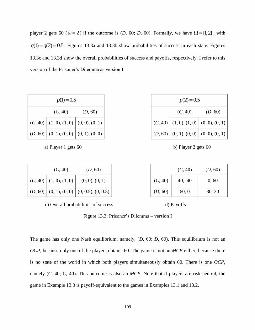
109

player 2 gets 60 ( 2 ) if the outcome is (D, 60; D, 60). Formally, we have {1,2} , with

(1) (2) 0.5q q . Figures 13.3a and 13.3b show probabilities of success in each state. Figures

13.3c and 13.3d show the overall probabilities of success and payoffs, respectively. I refer to this

version of the Prisoner’s Dilemma as version I.

a) Player 1 gets 60 b) Player 2 gets 60


Figure 13.3: Prisoner’s Dilemma – version I

The game has only one Nash equilibrium, namely, (D, 60; D, 60). This equilibrium is not an

OCP, because only one of the players obtains 60. The game is not an MCP either, because there

is no state of the world in which both players simultaneously obtain 60. There is one OCP,

namely (C, 40; C, 40). This outcome is also an MCP. Note that if players are risk-neutral, the

game in Example 13.3 is payoff-equivalent to the games in Examples 13.1 and 13.2.

(1) 0.5p

(C, 40) (D, 60)

(C, 40) (1, 0), (1, 0) (0, 0), (0, 1)

(D, 60) (0, 1), (0, 0) (0, 1), (0, 0)

(2) 0.5p

(C, 40) (D, 60)

(C, 40) (1, 0), (1, 0) (0, 0), (0, 1)

(D, 60) (0, 1), (0, 0) (0, 0), (0, 1)

(C, 40) (D, 60)

(C, 40) (1, 0), (1, 0) (0, 0), (0, 1)

(D, 60) (0, 1), (0, 0) (0, 0.5), (0, 0.5)

(C, 40) (D, 60)

(C, 40) 40, 40 0, 60

(D, 60) 60, 0 30, 30

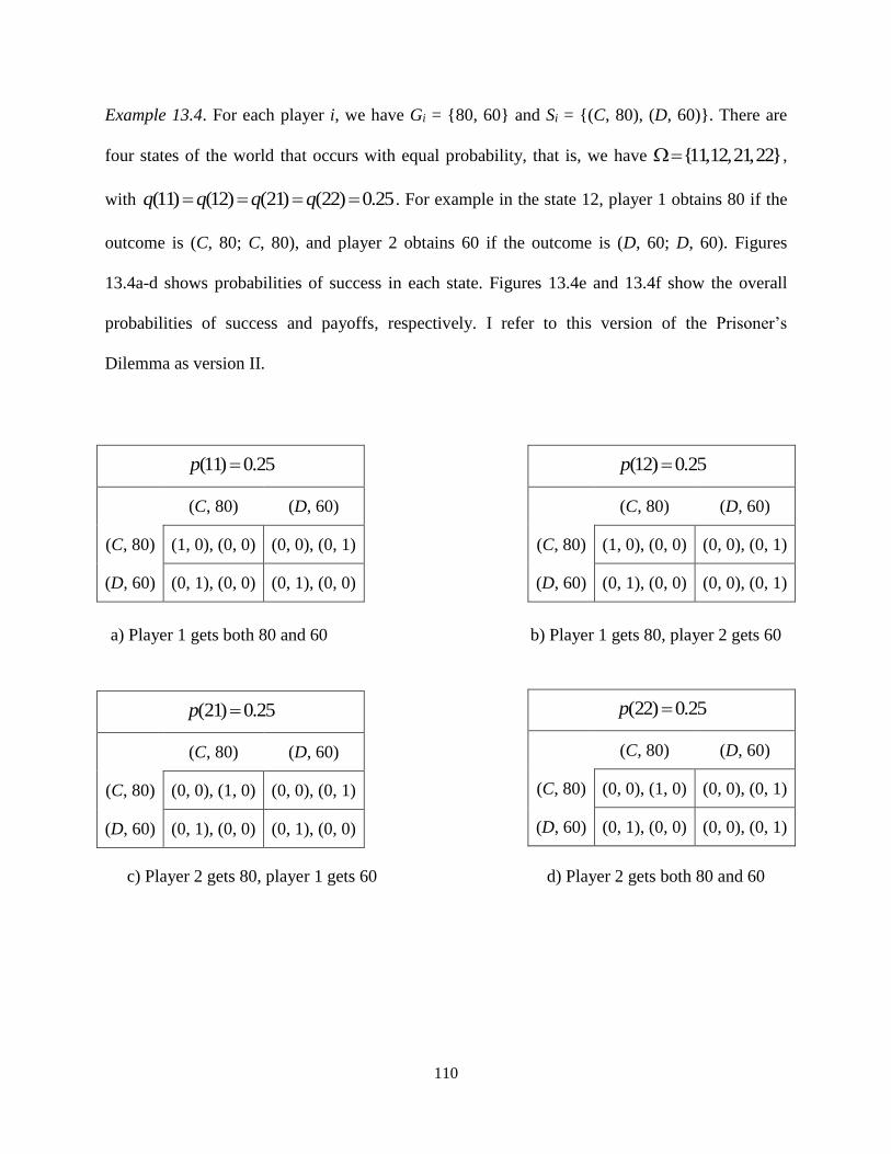
110


four states of the world that occurs with equal probability, that is, we have {11,12,21,22} ,

with (11) (12) (21) (22) 0.25q q q q . For example in the state 12, player 1 obtains 80 if the

outcome is (C, 80; C, 80), and player 2 obtains 60 if the outcome is (D, 60; D, 60). Figures

13.4a-d shows probabilities of success in each state. Figures 13.4e and 13.4f show the overall

probabilities of success and payoffs, respectively. I refer to this version of the Prisoner’s

Dilemma as version II.

a) Player 1 gets both 80 and 60 b) Player 1 gets 80, player 2 gets 60

c) Player 2 gets 80, player 1 gets 60 d) Player 2 gets both 80 and 60

(11) 0.25p

(C, 80) (D, 60)

(C, 80) (1, 0), (0, 0) (0, 0), (0, 1)

(D, 60) (0, 1), (0, 0) (0, 1), (0, 0)

(12) 0.25p

(C, 80) (D, 60)

(C, 80) (1, 0), (0, 0) (0, 0), (0, 1)

(D, 60) (0, 1), (0, 0) (0, 0), (0, 1)

(21) 0.25p

(C, 80) (D, 60)

(C, 80) (0, 0), (1, 0) (0, 0), (0, 1)

(D, 60) (0, 1), (0, 0) (0, 1), (0, 0)

(22) 0.25p

(C, 80) (D, 60)

(C, 80) (0, 0), (1, 0) (0, 0), (0, 1)

(D, 60) (0, 1), (0, 0) (0, 0), (0, 1)

111


Figure 13.4: Prisoner’s Dilemma – version II

Just like in Example 13.3, this game has only one Nash equilibrium, namely, (D, 60; D, 60). This

equilibrium is not an OCP, because only one of the players obtains 60. The outcome is not an

MCP either, because there is no state of the world in which both players simultaneously obtain

60. Unlike the game in Example 11.3, the outcome (C, 40; C, 40) is neither MCP nor OCP. Yet,

if players are risk-neutral, the games in the Examples 13.1-13.4 are equivalent.


four states of the world that occurs with equal probability: { 1, 2, 1, 2}b b n n with

( 1) ( 2) ( 1) ( 2) 0.25q b q b q b q b . For example, in the state b2, both players obtain 80 if the

outcome is (C, 80; C, 80), and player 2 obtains 60 if the outcome is (D, 60; D, 60). The

difference from Example 11.4 is that in the outcome (C, 80; C, 80), either each gets 80 or

nothing. Figures 13.5a-d shows probabilities of success in each state. Figures 13.5e and 13.5f

show the overall probabilities of success and payoffs, respectively. I refer to this version of the

Prisoner’s Dilemma as version III.

(C, 80) (D, 60)

(C, 80) (0.5, 0), (0.5, 0) (0, 0), (0, 1)

(D, 60) (0, 1), (0, 0) (0, 0.5), (0, 0.5)

(C, 80) (D, 60)

(C, 80) 40, 40 0, 60

(D, 60) 60, 0 30, 30

112

a) Both players get 80, Player 1 gets 60 b) Both players get 80, player 2 gets 60

c) Players don’t get 80, player 1 gets 60 d) Players don’t get 80, player 2 gets 60


Figure 13.5: Prisoner’s Dilemma – version III

This game has again only one Nash equilibrium, namely, (D, 60; D, 60), which is neither MCP

nor OCP. As in Example 13.4, the outcome (C, 40; C, 40) is not an OCP. However, unlike in

Example 13.4, it is an MCP. Again, if players are risk-neutral, the games in Example 13.1-13.5

are equivalent.

( 1) 0.25p b

(C, 80) (D, 60)

(C, 80) (1, 0), (1, 0) (0, 0), (0, 1)

(D, 60) (0, 1), (0, 0) (0, 1), (0, 0)

( 2) 0.25p b

(C, 80) (D, 60)

(C, 80) (1, 0), (1, 0) (0, 0), (0, 1)

(D, 60) (0, 1), (0, 0) (0, 0), (0, 1)

( 1) 0.25p b

(C, 80) (D, 60)

(C, 80) (0, 0), (0, 0) (0, 0), (0, 1)

(D, 60) (0, 1), (0, 0) (0, 1), (0, 0)

( 2) 0.25p b

(C, 80) (D, 60)

(C, 80) (0, 0), (0, 0) (0, 0), (0, 1)

(D, 60) (0, 1), (0, 0) (0, 0), (0, 1)

(C, 80) (D, 60)

(C, 80) (0.5, 0), (0.5, 0) (0, 0), (0, 1)

(D, 60) (0, 1), (0, 0) (0, 0.5), (0, 0.5)

(C, 80) (D, 60)

(C, 80) 40, 40 0, 60

(D, 60) 60, 0 30, 30

113

In summary, the conventional approach, which takes payoffs as exogenous, cannot distinguish

among the three versions of the Prisoner’s Dilemma considered in Examples 13.3-13.5. The

goal-based approach can distinguish between these three games and gives different predictions

about behavior in these three versions of the Prisoner’s Dilemma. These predictions are

discussed in the following section.

13.2 Experimental design and hypotheses

The model with goal-oriented strategies generates the following testable hypotheses:

H1: Players choose C more frequently in version I than in version II.

The reason is that in version I of the Prisoner’s Dilemma, the cooperative outcome is both OCP

and MCP, while in version II, the cooperative outcome is neither OCP nor MCP.

H2: Players choose C more frequently in version I than in version III.

In both, version I and version III of the Prisoner’s Dilemma, the cooperative outcome is an MCP,

but only in version I it is an OCP.

We can also use versions II and III of the Prisoner’s Dilemma to test whether players care

whether their plans fail due to the incompatibility with other player’s plans or due to

incompatibility with “nature”. Neither in version II nor in version III is the cooperative outcome

an OCP. However, in version III, the cooperative outcome is an MCP. In other words, in version

III, players’ plans fail due to incompatibility with the “nature”, while in version II their plans fail

114

because they are incompatible with each other. If players do not care whether their plans fail due

to incompatibility with “nature” or with incompatibility with each other, then the following

hypothesis holds:

H3: The frequency of C is the same in version II and version III.

I conducted an experiment where these three hypotheses were tested. Subjects were

undergraduate microeconomics students (n = 85). These subjects were randomly assigned to

three groups, each playing a different version of the Prisoner’s Dilemma, i.e., either version I (n

= 26), II (n = 30), or III (n = 29). Since the three versions of the Prisoner’s Dilemma are payoff-

equivalent only if individuals are risk-neutral, we also elicited their risk preferences. There were

two tasks. In the first one, subjects were offered certain option 60 points and a risky option,

which included either 0 or 60 + y, each with probability 0.5, where {0,10,20,...,190}y .

Therefore, there were twenty pairs of options to choose from. The second task was the same,

except that the certain option was 80 points, and the risky option included either 0 or 80 + y, each

with probability 0.5. (see Appendix III for instructions). After collecting the answers from the

subjects, I excluded those which were incomplete and/or confused.45 I obtained 62 valid answers

in total, out of which 20 for version I, 22 for version II, and 20 for version III. The results of the

experiment are reported in the following section.

45 More specifically, I excluded subjects who chose an outcome in the Prisoner’s Dilemma instead of an action. I

also excluded subjects who, in the risk-question, switched back and forth between the risky and certain options.

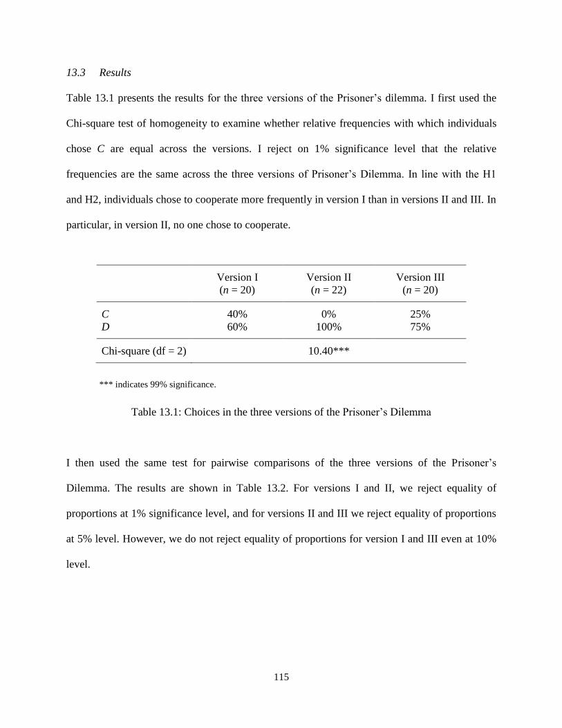
115

13.3 Results

Table 13.1 presents the results for the three versions of the Prisoner’s dilemma. I first used the

Chi-square test of homogeneity to examine whether relative frequencies with which individuals

chose C are equal across the versions. I reject on 1% significance level that the relative

frequencies are the same across the three versions of Prisoner’s Dilemma. In line with the H1

and H2, individuals chose to cooperate more frequently in version I than in versions II and III. In

particular, in version II, no one chose to cooperate.

Version I

(n = 20)

Version II

(n = 22)

Version III

(n = 20)

C 40% 0% 25%

D 60% 100% 75%

Chi-square (df = 2) 10.40***

*** indicates 99% significance.

Table 13.1: Choices in the three versions of the Prisoner’s Dilemma

I then used the same test for pairwise comparisons of the three versions of the Prisoner’s

Dilemma. The results are shown in Table 13.2. For versions I and II, we reject equality of

proportions at 1% significance level, and for versions II and III we reject equality of proportions

at 5% level. However, we do not reject equality of proportions for version I and III even at 10%

level.

116

Versions I and II Version II and III Versions I and III

Chi-square (df = 2) 10.87*** 6.24** 1.03

*** and ** indicate 99% and 95% significance respectively.

Table 13.2: Pairwise comparisons of the three versions of the Prisoner’s Dilemma

The differences in behavior in the three versions may be due to risk aversion. In particular, if

players are risk-averse, then in the versions II and III their payoff from cooperation are lower

than in the version I. Table 13.3 shows players’ risk preferences in the three versions of the game.

Version I Version II Version III Risk-neutrality

Switch (60 p.) 8.30

(std = 2.81)

8.34

(std = 2.77)

9.90*

(std = 4.89) 8.00

Switch (40 p.) 6.90**

(std = 1.83)

6.43

(std = 2.18)

8.25**

(std = 4.62) 6.00

Table 13.2: Risk-aversion in the three groups

By conventional criteria, risk-neutrality is not rejected in three cases out of six. In the other three

cases, players seem to be risk-averse. What matters from the perspective of the hypotheses H1

and H2, is the risk-equivalent to 40 points in versions II and III. We found that in version II, we

do not reject risk-neutrality. Therefore, certain 40 points are equivalent to the lottery 80 points

and 0 with equal probabilities. Consequently, differences in behavior in versions I an II cannot

be explained by risk aversion. In version III, we reject risk-neutrality at 5% significance level.

Therefore, we have u(40) > 0.5u(80) + 0.5u(0). Consequently, potential differences in behavior

117

in versions I and III could be explained by risk aversion. We have found that in version III,

people cooperate less than in version I, which is in line with risk aversion. However, the

differences in behavior between these two versions are statistically insignificant (see Tables 13.1

and 13.2). Finally, we compare risk preferences in versions II and III. In version II we do not

reject risk-neutrality, while in version III we reject risk-neutrality in favor of risk-aversion. This

means that the payoff in the cooperative outcome in version III is lower than in version II.

Therefore, the temptation to defect is higher in version III than in version II. Yet, we observe

significantly more cooperation in version III than in version II. Therefore, although risk

preferences are different in versions II and III, they cannot explain differences in behavior in

these two versions of the Prisoner’s Dilemma.

We now evaluate the hypotheses H1-H3. In line with hypothesis H1, there is significantly more

cooperation in version I of the game than in version II. This result cannot be explained by risk-

aversion. Therefore, H1 cannot be rejected. However, we do reject H2: Although there the

frequency of cooperation is higher in version I than in version III, the difference is not

statistically significant. Moreover, the observed differences may be due to risk-aversion. We also

reject H3: participants cooperated significantly more in version III than in version II, and the

difference cannot be explained by risk preferences. We conclude that MCP may explain

cooperative behavior in Prisoner’s Dilemma. Furthermore, it matters to the individuals whether

their plans are disappointed due to incompatibility with nature or due to incompatibility with

other players’ plans.46 Therefore, the model considered in Chapter 8 may be relevant.

46 Related research supports this view. For instance, in the ultimatum game, players respond differently to unfair

offers from humans than to the same offers from a computer (Sanfrey et al. 2003, Wout et al. 2006). More generally,

118

13.4 Discussion

This experiment has several limitations. Firstly, samples are small and include only

undergraduate economic students. Secondly, the payoffs were abstract points rather than money,

which means that participants may not have been sufficiently motivated to make well-thought

decisions. However, see e.g., Rubinstein (1999) for the view that experimental results without

money incentives may also be useful. Although the non-cooperation in version II is striking,

more tests are needed to establish the relevance of goal-based thinking in decisions.

people seem to care not only about consequences but also intentions (Offerman 2002; Sutter 2007; Cushman et al.

2009; Falk Fehr, and Fischbacher 2008).

119

14 Conclusion

I have attempted to show, that the Hayekian notion of equilibrium as the compatibility of plans

differs from the conventional Nash equilibrium used in many economic models. Moreover, the

Hayekian notion of equilibrium differs from Pareto efficiency. I have explicitly modeled

compatibility of plans in a game-theoretic framework, and I have shown how this notion can be

used in practice to explain some real-world phenomena. In particular, I have shown how

incompatibility of plans may give rise to an endogenous change of social norms. Moreover,

explicit modeling of players’ goals can help to analyze strategic situations involving multiple

goals. Finally, goal-based reasoning may explain cooperative behavior in the Prisoner’s

Dilemma and possibly other types of behavior.

Although the model presented in this paper reflects many Hayek’s ideas, there are aspects of the

Hayekian approach that I neglected. Most importantly, my framework is static. In contrast,

Hayek was mainly concerned with dynamic coordination (Hayek 1937, 2007). Related to the

time point is the issue of uncertainty and learning emphasized in the Hayekian literature (e.g.,

O’Driscoll, Jr. and Rizzo 2002). Although the framework developed in this paper in principle

allows incorporating these additional considerations, they give rise to specific problems that are

beyond the scope of the present work. Therefore, future research can incorporate these

considerations into the current framework.

120

Another possible area for future research is a more detailed analysis of relationships among plans.

The approach presented in this work simply assumes that plans may be compatible or

incompatible. Nevertheless, they may be compatible at least in two different meanings. They

may be compatible and independent and compatible and complementary. If two hunters plan to

catch a hare in an area where hares are abundant, their plans are compatible and independent

because the success of one player’s plan does not depend on the other player’s plan. In contrast,

if two players plan to catch a stag, their plans are compatible and complementary because the

success of one player’s plan depends on the other player’s plan.

The model of goal-based behavior goes beyond the traditional payoff-maximizing approach.

Nevertheless, it can also be understood as supporting the payoff-maximizing approach as a

simple and powerful tool of analysis. As argued, payoff-maximizing greatly simplifies complex

decision processes of real-world individuals. Often this simplification comes at little or no cost.

For instance, as we have seen in Chapter 2, if all players pursue only one goal and have

alternative ways to reach this goal, payoffs can be represented simply by probabilities of success

of achieving this single goal. Even when players have multiple goals in mind, the conventional

approach is often sufficient to capture all the crucial aspects of behavior. Only when the

conventional approach fails to give satisfactory answers, one may need to look “behind” the

payoffs and study actual motivations and decision processes.

121

Appendix I: Hayek on equilibrium

The notion of equilibrium as “compatibility of plans” was introduced by Hayek (1937). 47

According to him, equilibrium means that the “different plans which the individuals composing

[a society] have made for action in time are mutually compatible” (Hayek 1948, 41). 48

Unfortunately, neither Hayek nor his followers clarify in detail how the notions of “plans” and

“compatibility” fit in the conventional conceptual framework used in economics. Regarding the

former term, Hayek emphasizes that his concept of equilibrium refers specifically to actions, and

he contrasts it with approaches that treat equilibrium as a relationship among existing things,

such as quantities of goods—that is, results of past activities (Hayek 2007, 41–42). Therefore, for

Hayek, the terms “plan” and “action” seem closely related. He also uses the term “intention” as a

synonym of “plan” (Hayek 1948, 40). Given Hayek’s emphasis on equilibrium of actions rather

than of quantities, game theory, rather than Marshallian/Walrasian price theory, seems to be a

suitable framework to formalize his views. Moreover, Hayek considers situations in which plans

are chosen “simultaneously but independently by a number of persons” (Hayek, 1948, 38). This

specification directly calls for the use of strategic games.

47 For even earlier Hayek’s discussion of equilibrium, see Hayek (1928).

48 In the original version of Hayek’s essay, the definition is formulated as follows: equilibrium means that the

“compatibility exists between the different plans which the individuals composing [a society] have made for action

in time.” (Hayek 1937, 40). Similar definition can be found in Hayek (2007).

122

However, Hayek does not specify any criterion for how individuals choose a plan from the set of

feasible plans. His discussion implies that expectations about both external events and plans of

others are important in the choice of a particular plan (Hayek 1948, 38), but he never explicitly

considers the value (or profitability) of various feasible plans. While it is plausible that, other

things equal, individuals choose the plan that is most valuable to them, it is not clear how they

resolve the trade-off between value and risk if such a trade-off occurs. For example, do

individuals prefer a plan that promises to achieve a higher-valued but risky goal or a plan that

enables them to achieve a lower-valued goal with certainty? Hayek does not answer this question.

According to my approach, it is assumed that individuals use the conventional expected utility

theory to resolve this trade-off.

Regarding the term “compatibility,” Hayek means that there is a “conceivable set of external

events which allow people to carry out their plans and not cause any disappointments” (Hayek

1948, 40). In Chapter 5, I introduce the concept of the “mutual compatibility of plans,” which is

a formalization of this idea. Although Hayek repeatedly states that equilibrium is a fictitious

concept (Hayek 1948, 44; 2007, 46, 50), he also argues that empirically there is a tendency

toward general equilibrium in a market economy (Hayek 1948, 45, 55; 2007, 50). The main

evidence to support his claim is that prices “tend to correspond to costs” (Hayek 1948, 51; 2007,

50n2). Hence Hayek’s approach differs from the approaches that model phenomena as if they

were always in equilibrium (e.g., Machlup 1958). Compatibility of plans, as formalized in the

present paper, may or may not be considered as a fictitious concept. In large populations, as

considered by Hayek, compatibility of plans may often be difficult or even impossible to achieve.

123

In Chapter 6, measurements are introduced in an attempt to quantify the tendency toward the

compatibility of plans in situations in which the compatibility of all plans cannot be achieved.

Hayek also gives some idea of what happens in a state of disequilibrium. He argues that in such a

situation, “revision of the plans on the part of at least some people is inevitable,” and he refers to

this revision of plans as “endogenous disturbances” (Hayek 1948, 40). I show that Hayekian

“compatibility of plans” and Nash equilibrium may or may not coincide. If they coincide,

Hayek’s statement can be interpreted as follows: individuals choose the Nash equilibrium plans,

which also allows them to carry out their plans. The question is what happens if, in a Nash

equilibrium, one or more individuals fail to carry out their plans. In such a situation, individuals

are already “doing the best they can” given the rules of the game and the choices of others.

Hayek’s “endogenous disturbance” may refer to a search for new, previously unknown, plans or

other modifications of the rules of the game. This issue is discussed in Chapter 9.

Although Hayek himself was not engaged in game-theoretic modeling, the discussion above

suggests that a modified model of a strategic game is a suitable framework to formalize his views.

In fact, early work by Morgenstern (1928) inspired Hayek’s work on equilibrium (Giocoli 2003;

Leonard 2010). Moreover, in his early discussion of the equilibrium concept, Hayek calls for a

systematic attempt to analyze social interactions in terms of compatibility and incompatibility of

plans (Hayek 1937, 38n1). In this context, he refers to the pioneering game-theoretic work of

Menger (1974) as an attempt in this direction. However, he arguably became disappointed with

the later development of game theory (Becchio 2009). Therefore, the model introduced in this

124

thesis can be understood as a response to Hayek’s call and an attempt to develop a game-

theoretic framework along Hayekian lines.

O’Driscoll and Rizzo (2002) also use games (namely, the Keynesian beauty contest and

Morgenstern’s Holmes–Moriarty game) to discuss the Hayekian notion of equilibrium. However,

they do not distinguish between Nash’s and Hayek’s notions of equilibria. In this paper, most

concepts and results are illustrated with various versions of the Stag Hunt game. This game

provides a suitable illustration of Hayek’s views not only because it shows a coordination

problem in a (simple) production process, in which Hayek was interested, but also because it can

be used to represent coordination failure as postulated by Keynesian business cycle theory

(Bryant 1983, 1994; Cooper and John 1988), which stood in opposition to Hayek’s own theory at

the time when he was developing his views on equilibrium (Boettke 2018; Caldwell 2004).

For Hayek, the main purpose of the equilibrium concept is to account for the order that exists in

the society. Nevertheless, the usefulness of the equilibrium concept for him does not end with a

mere description of the social order. As Hayek puts it:

“Its function is simply to serve as a guide to the analysis of concrete situations, showing what their

relations would be under ‘ideal’ conditions, and so helping us to discover cause of impending

changes not yet contemplated by any of the individuals concerned” (Hayek 2007, 51).

For Hayek, the ultimate goal all economic analysis is to provide a causal explanation of

phenomena and equilibrium analysis is merely a stepping stone towards this goal (Hayek 2007,

42-43). However, in order to reach this goal, one has to abandon the concept of a stationary

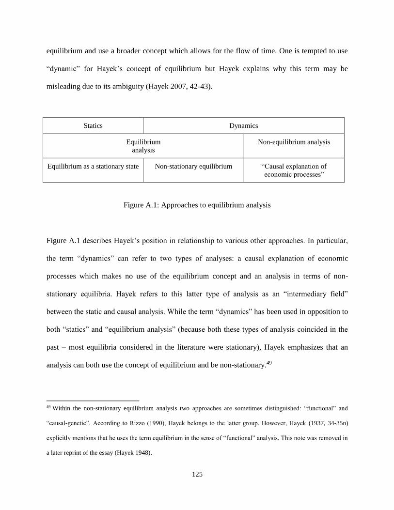
125

equilibrium and use a broader concept which allows for the flow of time. One is tempted to use

“dynamic” for Hayek’s concept of equilibrium but Hayek explains why this term may be

misleading due to its ambiguity (Hayek 2007, 42-43).

Statics Dynamics

Equilibrium

analysis

Non-equilibrium analysis

Equilibrium as a stationary state Non-stationary equilibrium “Causal explanation of

economic processes”

Figure A.1: Approaches to equilibrium analysis

Figure A.1 describes Hayek’s position in relationship to various other approaches. In particular,

the term “dynamics” can refer to two types of analyses: a causal explanation of economic

processes which makes no use of the equilibrium concept and an analysis in terms of non-

stationary equilibria. Hayek refers to this latter type of analysis as an “intermediary field”

between the static and causal analysis. While the term “dynamics” has been used in opposition to

both “statics” and “equilibrium analysis” (because both these types of analysis coincided in the

past – most equilibria considered in the literature were stationary), Hayek emphasizes that an

analysis can both use the concept of equilibrium and be non-stationary.49

49 Within the non-stationary equilibrium analysis two approaches are sometimes distinguished: “functional” and

“causal-genetic”. According to Rizzo (1990), Hayek belongs to the latter group. However, Hayek (1937, 34-35n)

explicitly mentions that he uses the term equilibrium in the sense of “functional” analysis. This note was removed in

a later reprint of the essay (Hayek 1948).

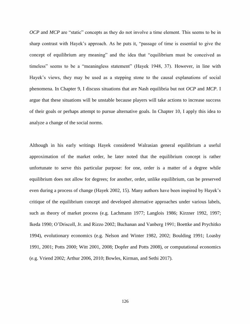
126

OCP and MCP are “static” concepts as they do not involve a time element. This seems to be in

sharp contrast with Hayek’s approach. As he puts it, “passage of time is essential to give the

concept of equilibrium any meaning” and the idea that “equilibrium must be conceived as

timeless” seems to be a “meaningless statement” (Hayek 1948, 37). However, in line with

Hayek’s views, they may be used as a stepping stone to the causal explanations of social

phenomena. In Chapter 9, I discuss situations that are Nash equilibria but not OCP and MCP. I

argue that these situations will be unstable because players will take actions to increase success

of their goals or perhaps attempt to pursue alternative goals. In Chapter 10, I apply this idea to

analyze a change of the social norms.

Although in his early writings Hayek considered Walrasian general equilibrium a useful

approximation of the market order, he later noted that the equilibrium concept is rather

unfortunate to serve this particular purpose: for one, order is a matter of a degree while

equilibrium does not allow for degrees; for another, order, unlike equilibrium, can be preserved

even during a process of change (Hayek 2002, 15). Many authors have been inspired by Hayek’s

critique of the equilibrium concept and developed alternative approaches under various labels,

such as theory of market process (e.g. Lachmann 1977; Langlois 1986; Kirzner 1992, 1997;

Ikeda 1990; O’Driscoll, Jr. and Rizzo 2002; Buchanan and Vanberg 1991; Boettke and Prychitko

1994), evolutionary economics (e.g. Nelson and Winter 1982, 2002; Boulding 1991; Loasby

1991, 2001; Potts 2000; Witt 2001, 2008; Dopfer and Potts 2008), or computational economics

(e.g. Vriend 2002; Arthur 2006, 2010; Bowles, Kirman, and Sethi 2017).

127

My approach acknowledges that the existing equilibrium concepts are inadequate to account for

Hayek views.50 In order to account for Hayek’s observation that an order (in my approach

formalized as OCP or MCP) can be preserved in a disequilibrium, I introduce a measure of order

ranging from 0 (no individual achieves his goal) and 1 (every individual achieves his goal, i.e.

there is a perfect compatibility of plans and the outcome is Hayek equilibrium). This measure

highlights Hayek’s point that the perfect compatibility of plans is a “Platonic” notion that may be

approached but is rarely reached in complex societies.

Hayek’s views of equilibrium have been discussed in various contexts and in various degrees of

depth. Some of these works focus on interpretation and evolution of Hayek’s views in the

context of the Austrian school (Vaughn 1999, 2013), heterodox traditions (Lawson 2005), or

economics in general (Giocoli 2003). Other works are critical and attempt to develop Hayekian

view further (O’Driscoll, Jr. 1977; O’Driscoll, Jr. and Rizzo 2002; Rizzo 1990, 1992; Lewin

1997). Vriend (2002) and Bowles et al. (2017) show the relevance of Hayek’s views for

contemporary economics of complex adaptive systems. Hudik (2018) compares Hayek’s views

on equilibrium with price-theoretic concept of equilibrium represented by Machlup (1958).

Arena (1999) emphasizes the continuity of Hayek’s views on equilibrium. All these and similar

works are useful in interpreting and extending various aspects of Hayek’s views. Yet, with a few

exceptions, they do not attempt to trace differences between Hayek’s concept of equilibrium and

alternative concepts. For example, O’Driscoll and Rizzo ([1985] 2002) also use games (namely,

Keynesian beauty contest and Morgenstern’s Holmes-Moriarty game) to discuss Hayekian

notion of equilibrium. However, they do not distinguish between Nash’s and Hayek’s notions of

50 Yet, they me useful for other purposes. See Hudik (2018).

128

equilibria. Overall, there have been very few attempts to formalize Hayek’s views. One of the

goals of my work is to fill this gap.

129

Appendix II: Theories of social norms change

The question of how social norms change is closely linked to the question of how social norms

are defined.51 Therefore, I first focus on definitions of social norms, and then I discuss several

theories of norms change.

Definitions of social norms

Definitions of social norms can be informal and formal. I first consider informal definitions.

According to Burke (2007) and Burke and Young (2011), social norms are customary rules of

behavior that coordinate interactions with others. This definition is very broad and highlights the

coordinating function of social norms. Another definition emphasizes the role of expectations.

According to this definition, social norms are behavioral rules supported by a combination of

empirical and normative expectations (Bicchieri 2005, 2017). This second definition is narrower

because it distinguishes between social norms and conventions. More specifically, social norms,

unlike conventions, are supported by normative expectations. In contrast, conventions are

supported by empirical expectations and a preference to follow if everyone else follows. A

similar distinction between social norms and conventions is also made by Sugden (1986) and

Coleman (1990). In Chapter 10, I use the term social norm in a broader sense of Burke and

Young’s (2011) definition.

51 Useful surveys of the literature on social norms include Young (2007), Burke and Young (2011), Elster (1989),

and Bergstrom (2002). Posner (2000) studies social norms in relation to law.

130

A different perspective on norms is presented by Becker (1996) and Becker and Murphy (2000),

who define norms as common values of a group internalized as preferences.52 According to this

approach, individuals follow norms irrespectively of their expectations or behavior of others.53

Nevertheless, Becker and Murphy (2000) consider the effect of peer pressure on the stability of

norms. In this view, norms need not necessarily coordinate interactions, but they often reduce

transaction costs (Becker 1996). Becker and Murphy (2000) distinguish social norms from

conventions, such as driving on the right side of the road. Conventions, unlike social norms, need

not have intrinsic value; instead, they depend on the choices of others.

Regarding the formal definitions of social norms (and conventions), we can distinguish between

game-theoretic and price-theoretic definitions. According to the game-theoretic definitions, a

social norm is an equilibrium of a game with multiple equilibria (Burke and Young 2011;

Sugden 1986). Lewis (1969) focuses on equilibria of coordination games, while Vanderschraaf

(1998) extends Lewis’s approach to other games. Vanderschraaf (1998) define social norm as

correlated equilibrium in the sense of Aumann (1974, 1987), whereas Gintis (2009, 2010)

suggests that social norms are correlating devices for a correlated equilibrium. My formal

definition is broader than these definitions. It merely assumes that social norm is a Nash

equilibrium of a game that may or may not have multiple equilibria. Furthermore, my example of

the medium of exchange is a convention in the sense of Becker and Murphy (2000) and Bicchieri

(2017).

52 Internalization of norms is also considered by Young (2007), Coleman (1990), and Elster (1989, 1999).

53 This definition corresponds to what Bicchieri (2017) calls a shared (prudential, moral, or religious) norm.

131

The price-theoretic approach to social norms is exemplified by Becker (1996) and Becker and

Murphy (2000), who model norms simply as arguments in a utility function. These norms may

increase or reduce an individual’s utility, and they may or may not depend on the choices of

others. These choices of others are modeled as social capital. In contrast, conventions are inputs

in the individual’s production function – they do not have intrinsic utility; they have utility only

as instruments. Furthermore, they are complementary to social capital, which also enters an

individual’s production function.

Why do social norms change?

For the approaches where a social norm is an equilibrium of a game with multiple equilibria,

social norms change means a switch from one equilibrium to another. This change may occur

from without, due to exogenous shocks (e.g., Libecap 1989), or from within. A change from

within is analyzed by Young (1993), according to whom players are boundedly rational and

make “mistakes” when choosing their best response. This account of social norms change

emphasizes the independent choices of individuals. Other accounts emphasize collective action

in the change of social norms (Bowles 2006; Libecap 1989). Bicchieri and Mercier (2014) and

Bicchieri (2017) focus on the collective change of expectations. According to this account,

norms change if there is a widespread change in expectations. The change of expectations may

occur bottom-up or top-down.

Approaches that emphasize top-down change of social norms include Belloc and Bowles (2013),

who highlight the role of political power. Becker (1996) and Becker and Murphy (2000) consider

a model where an upper class imposes norms on a lower class. However, the upper class has to

132

compensate the lower class if the norms decrease the utility of the members of the lower class.

Yet other approaches focus on imitation of norms in more successful societies (Robson and

Vega-Redondo 1996; Boyd and Richerson 2001, 2002; Henrich and Boyd 2001) or on a

selection of groups with superior norms through growth or conquest (Hayek 1973).

According to my approach to social norm change outlined in Chapter 10, norms change because

individuals fail to carry out their plans. This corresponds to Bicchieri’s (2017) view that in order

for a norm to change, there must be a shared reason to change. I argue that this aspect is missing

in the current models unless the reason for the change is an attempt to achieve a known outcome

with higher payoff for one or more players. My model does not specify how exactly the change

will occur. In this respect, it is complementary to models that analyze specific mechanisms of

norms change.

133

Appendix III: Instructions in the Prisoner’s Dilemma experiment

Instructions

Welcome to this experiment. You and the other participants are asked to make decisions. Your

decisions as well as the decisions of the other participants will determine the result of the

experiment. Please read the instructions thoroughly and think about your decision carefully.

During the experiment you are not allowed to talk to the other participants or to use cell phones.

The neglect of these rules will lead to the immediate exclusion from the experiment. If you have

any questions, please raise your hand. An experimenter will then come to your seat to answer

your questions. During the experiment we will talk about points instead of money.

The experiment consists of three independent parts in which you can accumulate points. During

the experiment neither you nor the other participants will receive any information on the course

of the experiment (e.g. decisions of other participants or results of a particular part).

Version I

Without showing others what you are doing, write down on a form either the letter x or the letter

y. Think of this as a “point bid”. I will randomly pair your form with one other form. Neither you

nor your pair will ever know with whom you were paired. Here is how points will be assigned

for this activity:

If you put y and your pair puts x, then you will get 60 points, and your pair 0 points.

If both you and your pair put y, then two possibilities may occur:

134

a) you will get 60 points and your pair 0 points, or

b) you will get 0 points and your pair 60 points.

Each possibility occurs with an equal probability, that is, 50%.

If you put x and your pair puts y, then you will get 0 points, and your pair 60 points.

If both you and your pair put x, then you will both get 40 points.

Your answer:

Version II

Without showing others what you are doing, write down on a form either the letter X or the letter

Y. Think of this as a “point bid”. I will randomly pair your form with one other form. Neither you


for this activity:

If you put y and your pair puts X, then you will get 60 points, and your pair 0 points.

If both you and your pair put Y, then two possibilities may occur:




If you put X and your pair puts Y, then you will get 0 points, and your pair 60 points.

If both you and your pair put X, then two possibilities may occur:

a) you will get 80 marks and your pair 0 points, or

b) you will get 0 marks and your pair 80 points.

Each possibility occurs with an equal probability, that is, 50%

Your answer:

135

Version III

Without showing others what you are doing, write down on a form either the letter x or the letter

y. Think of this as a “point bid”. I will randomly pair your form with one other form. Neither you


for this activity:

If you put y and your pair puts x, then you will get 60 points, and your pair 0 points.

If both you and your pair put y, then two possibilities may occur:




If you put x and your pair puts y, then you will get 0 points, and your pair 60 points.

If both you and your pair put x, then two possibilities may occur:

a) you both will get 80 points, or

b) you both will get 0 points.

Each possibility occurs with an equal probability, that is, 50%

Your answer:

Risk preferences

For the ten questions below, we ask you to decide between two options. For each question please

indicate whether you prefer option A or B.

136

Question Option A Option B Your Choice

1 60 points 60 points with a probability of 50%

0 points with a probability of 50%







































For the ten questions below, we ask you to decide between two options. For each question please

indicate whether you prefer option C or D.

137

Question Option C Option D Your Choice









































138

References

Acevedo, Melissa, and Joachim I. Krueger. 2005. “Evidential Reasoning in the Prisoner’s

Dilemma.” The American Journal of Psychology 118 (3): 431–57.

Alexander, Richard D. 1961. “Aggressiveness, Territoriality, and Sexual Behavior in Field

Crickets (Orthoptera: Gryllidae).” Behaviour 17 (2): 130–223.

Arena, Richard. 1999. “Hayek et l’équilibre Économique : Une Autre Interprétation / Hayek and

Equilibrium : An Alternative Interpretation.” Revue d’économie Politique 109 (6): 847–

58.

Arthur, W. Brian. 2006. “Out-of-Equilibrium Economics and Agent-Based Modeling.” In

Handbook of Computational Economics, edited by L. Tesfatsion and K. L. Judd, 2:1551–

64. Elsevier.

Arthur, W. Brian. 2010. “Complexity, the Santa Fe Approach, and Non-Equilibrium

Economics.” History of Economic Ideas 18 (2): 149–66.

Ashby, Ross W. 1957. An Introduction to Cybernetics. London: Chapman & Hall.

Aumann, Robert J. 1974. “Subjectivity and Correlation in Randomized Strategies.” Journal of

Mathematical Economics 1 (1): 67–96.

Aumann, Robert J. 1985. “What Is Game Theory Trying to Accomplish?” In Frontiers of

Economics, K. Arrow and S. Honkapohja, 28–76. Oxford: Basil Blackwell.

Aumann, Robert J. 1987. “Correlated Equilibrium as an Expression of Bayesian Rationality.”

Econometrica 55 (1): 1–18.

139

Aumann, Robert, and Adam Brandenburger. 1995. “Epistemic Conditions for Nash

Equilibrium.” Econometrica 63 (5): 1161–80.

Ayan Musil, Pelin, and Hasret Dikici Bilgin. 2016. “Types of Outcomes in Factional Rivalries:

Lessons from Non-Democratic Parties in Turkey.” International Political Science Review

37 (2): 166–83.

Bacharach, Michael. 2006. Beyond Individual Choice: Teams and Frames in Game Theory.

Edited by Natalie Gold and Robert Sugden. Princeton and Oxford: Princeton University

Press.

Becchio, Giandomenica. 2009. “Ethics and Economics in Karl Menger.” In Unexplored

Dimensions: Karl Menger on Economics and Philosophy (1923-1938), 12:21–35.

Advances in Austrian Economics. Emerald Group Publishing Limited.

Becker, Gary S. 1998. Accounting for Tastes. Cambridge: Harvard University Press.

Becker, Gary S., and Kevin M. Murphy. 2000. Social Economics: Market Behavior in Social

Environment. Cambridge and London: The Belknap Press of Harvard University Press.

Belloc, Marianna, and Samuel Bowles. 2013. “The Persistence of Inferior Cultural-Institutional

Conventions.” American Economic Review 103 (3): 93–98.

Berg, Nathan, and Gerd Gigerenzer. 2010. “As-If Behavioral Economics: Neoclassical

Economics in Disguise?” History of Economic Ideas 18 (1): 133–66.

Bergstrom, Theodore C. 2002. “Evolution of Social Behavior: Individual and Group Selection.”

Journal of Economic Perspectives 16 (2): 67–88.

Bertalanffy, Ludwig von. 1968. General System Theory. New York: George Braziller.

Bicchieri, Cristina. 2005. The Grammar of Society: The Nature and Dynamics of Social Norms.

Cambridge: Cambridge University Press.

140

Bicchieri, Cristina. 2017. Norms in the Wild: How to Diagnose, Measure, and Change Social

Norms. New York: Oxford University Press.

Bicchieri, C. and Mercier, H. 2014. “Norms and beliefs: How change occurs.” In M. Xenitidou

& B. Edmonds (Eds.), The complexity of social norms (pp. 37-54). Switzerland: Springer.

Binmore, K. G. 2007. Playing for Real: A Text on Game Theory. New York: Oxford University

Press.

Boettke, Peter J. 2018. F. A. Hayek: Economics, Political Economy, and Social Philosophy.

Palgrave, Macmillan.

Boettke, Peter J., and Rosolino A. Candela. 2017. “Price Theory as Prophylactic against Popular

Fallacies.” Journal of Institutional Economics, January, 1–28.

Boettke, Peter J., and David L. Prychitko, eds. 1994. The Market Process: Essays in

Contemporary Austrian Economics. Edward Elgar Publishing.

Boland, Lawrence A. 2017. Equilibrium Models in Economics: Purposes and Critical

Limitations. New York: Oxford University Press.

Bolton, Gary E, and Axel Ockenfels. 2000. “ERC: A Theory of Equity, Reciprocity, and

Competition.” The American Economic Review 90 (1): 166–93.

Boulding, K. E. 1991. “What Is Evolutionary Economics?” Journal of Evolutionary Economics 1

(1): 9–17.

Bowles, Samuel. 2006. Microeconomics: Behavior, Institutions, and Evolution. Princeton

University Press.

Bowles, Samuel, Alan Kirman, and Rajiv Sethi. 2017. “Retrospectives: Friedrich Hayek and the

Market Algorithm.” Journal of Economic Perspectives 31 (3): 215–30.

141

Bowman, John S. 2000. Columbia Chronologies of Asian History and Culture. New York:

Columbia University Press.

Boyd, Robert, and Peter J. Richerson. “Norms and bounded rationality.” In: G. Gigerenzer, R.

Selten (Eds.), Bounded Rationality: The Adaptive Toolbox. MIT Press, Cambridge,

London, pp. 281–296.

Boyd, Robert, and Peter J. Richerson. 2002. “Group Beneficial Norms Can Spread Rapidly in a

Structured Population.” Journal of Theoretical Biology 215 (3): 287–96.

Brams, Steven J. 1994. Theory of Moves. Cambridge: Cambridge University Press.

Brams, Steven J., and Walter Mattli. 1993. “Theory of Moves: Overview and Examples.”

Conflict Management and Peace Science 12 (2): 1–39.

Brams, Steven J., and Donald Wittman. 1981. “Nonmyopic Equilibria in 2×2 Games.” Conflict

Management and Peace Science 6 (1): 39–62.

Bryant, John. 1983. “A Simple Rational Expectations Keynes-Type Model.” The Quarterly

Journal of Economics 98 (3): 525–28.

Bryant, John. 1994. “Coordination Theory, the Stag Hunt and Macroeconomics.” In Problems of

Coordination in Economic Activity, edited by James W. Friedman, 207–25. Boston:

Kluwer.

Buchanan, James M., and Viktor J. Vanberg. 1991. “The Market as a Creative Process.”

Economics & Philosophy 7 (2): 167–86.

Buller, David J. 2005. Adapting Minds: Evolutionary Psychology and the Persistent Quest for

Human Nature. MIT Press.

142

Burke, Mary A., and H. Peyton Young. 2011. “Social Norms.” In Handbook of Social

Economics, edited by Jess Benhabib, Alberto Bisin, and Matthew O. Jackson, 1:311–38.

North-Holland.

Caldwell, Bruce. 2004. Hayek’s Challenge: An Intellectual Biography of F. A. Hayek. Chicago

and London: University of Chicago Press.

Castelfranchi, Cristiano, and Rosaria Conte. 1998. “Limits of Economic and Strategic

Rationality for Agents and MA Systems.” Robotics and Autonomous Systems 24 (3–4):

127–39.

Chater, Nick, Ivo Vlaev, and Maurice Grinberg. 2008. “A New Consequence of Simpson’s

Paradox: Stable Cooperation in One-Shot Prisoner’s Dilemma from Populations of

Individualistic Learners.” Journal of Experimental Psychology: General 137 (3): 403–21.

Chiappori, P.-A, S Levitt, and T Groseclose. 2002. “Testing Mixed-Strategy Equilibria When

Players Are Heterogeneous: The Case of Penalty Kicks in Soccer.” American Economic

Review 92 (4): 1138–51.

Coleman, James S. 1990. Foundations of Social Theory. Cambridge MA: Harvard University

Press.

Colman, Andrew M. 1995. Game Theory and Its Applications in the Social and Biological

Sciences. Oxford: Butterworth-Heinemann.

Conte, Rosaria, and Cristiano Castelfranchi. 1995. Cognitive and Social Action. London:

University College London Press.

Cooper, Russell, and Andrew John. 1988. “Coordinating Coordination Failures in Keynesian

Models.” The Quarterly Journal of Economics 103 (3): 441–63.

143

Cooper, Russell, Douglas V. DeJong, Robert Forsythe, and Thomas W. Ross. 1996.

“Cooperation without Reputation: Experimental Evidence from Prisoner’s Dilemma

Games.” Games and Economic Behavior 12 (2): 187–218.

Cushman, Fiery, Anna Dreber, Ying Wang, and Jay Costa. 2009. “Accidental Outcomes Guide

Punishment in a ‘Trembling Hand’ Game.” PLoS ONE 4 (8): 1–7.

Dawkins, Richard. 1989. The Selfish Gene. Oxford University Press.

Dennett, Daniel C. 1995. Darwin’s Dangeorus Idea: Evolution and the Meanings of Life. New

York: Simon and Schuster.

Dietrich, Franz, and Christian List. 2013a. “A Reason-Based Theory of Rational Choice.” Noûs

47 (1): 104–34.

Dietrich, Franz, and Christian List. 2013b. “Where Do Preferences Come From?” International

Journal of Game Theory 42 (3): 613–37.

Dopfer, Kurt, and Jason Potts. 2008. The General Theory of Economic Evolution. London and

New York: Routledge.

Ebrey, P., Walthall, A., and Palais, J. 2006. East Asia: A Cultural, Social, and Political History.

Boston: Houghton Mifflin Company.

El Mouden, Claire, Maxwell Burton-Chellew, Andy Gardner, and Stuart A. West. 2012. “What

Do Humans Maximize?” In Evolution and Rationality, edited by Samir Okasha and Ken

Binmore. Oxford: Cambridge University Press.

Elster, Jon. 1989. Social norms and economic theory. Journal of Economic Perspectives, 3, no. 4,

99-117.

Elster, Jon. 1999. Alchemies of the Mind. Cambridge UK: Cambridge University Press.

144

Engliš, Karel. 1930. Begründung Der Teleologie Als Form Des Empirischen Erkennens. Brno:

Rohrer.

Epstein, Joshua M. 2001. “Learning to Be Thoughtless: Social Norms and Individual

Computation.” Computational Economics 18 (1): 9–24.

Falk, Armin, Ernst Fehr, and Urs Fischbacher. 2008. “Testing Theories of Fairness—Intentions

Matter.” Games and Economic Behavior 62 (1): 287–303.

Falk, Armin, and Urs Fischbacher. 2006. “A Theory of Reciprocity.” Games and Economic

Behavior 54 (2): 293–315.

Fehr, Ernst, and Klaus M. Schmidt. 1999. “A Theory of Fairness, Competition, and

Cooperation.” The Quarterly Journal of Economics 114 (3): 817–68.

Ferguson, Niall. 2008. The Ascent of Money: A Financial History of the World. London: Penguin.

Gernet, Jacques 1962. Daily Life in China on the Eve of the Mongol Invasion, 1250–1276.

Stanford University Press.

Gintis, Herbert. 2007. “A Framework for the Unification of the Behavioral Sciences.” The

Behavioral and Brain Sciences 30 (1): 1–16; discussion 16–61.

Gintis, Herbert. 2009. The Bounds of Reason: Game Theory and the Unification of the

Behavioral Sciences. Princeton: Princeton University Press.

Gintis, Herbert. 2010. “Social Norms as Choreography.” Politics, Philosophy & Economics 9 (3):

251–64.

Giocoli, Nicola. 2003. Modeling Rational Agents: From Interwar Economics to Early Modern

Game Theory. Cheltenham and Northampton: Edward Elgar.

Graeber, David. 2011. Debt: The First 5,000 Years. New York: Melville House.

145

Greif, A. 2006. Institutions and the Path to the Modern Economy, Cambridge: Cambridge

University Press.

Guyer, M. and Hamburger H. 1968. “A note on the enumeration of all 2 x 2 games.” General

Systems 13: 205-208.

Hamilton, Jonathan H., and Steven M. Slutsky. 1993. “Endogenizing the Order of Moves in

Matrix Games.” Theory and Decision 34 (1): 47–62.

Hammerstein, Peter. 2000. “What Is Evolutionary Game Theory?” In Game Theory and Animal

Behavior, edited by Lee Alan Dugatkin and Hudson Kern Reeve, 3–15. New York,

Oxford: Oxford University Press.

Harris, Richard J. 1969. “Note on Howards’’Theory of Meta-Games’.” Psychol Rep.

Harris, Richard J.. 1970. “Paradox Regained.” Psychological Reports 26: 264–66.

Hayek, F. A. 1928. “Das Intertemporale Gleichgewichtssystem Der Preise Und Die Bewegungen

Des ‘Geldwertes.’” Weltwirtschaftliches Archiv 28: 33–76.

Hayek, F. A. 1937. “Economics and Knowledge.” Economica, New Series, 4 (13): 33–54.

Hayek, F. A. 1948. “Economics and Knowledge.” In Individualism and Economic Order, 33–56.

Chicago: The University of Chicago Press.

Hayek, F. A. 1973. Law, Legislation and Liberty, Vol. 1: Rules and Order, Chicago: University

of Chicago Press.

Hayek, F. A. 1976. Choice in currency: a way to stop inflation. London: Institute of Economic

Affairs.

Hayek, F. A. 1990. The Fatal Conceit: The Errors of Socialism. The Collected Works of

Friedrich August Hayek. Volume I. London: Routledge.

146

Hayek, F. A. 1990. Denationalisation of money: The argument refined. London: The Institute of

Economic Affairs.

Hayek, F. A. 2002. “Competition as a Discovery Procedure.” The Quarterly Journal of Austrian

Economics 5 (3): 9–23.

Hayek, F. A. 2007. The Pure Theory of Capital. Edited by Lawrence H. White. The Collected

Works of F. A. Hayek. Volume XII. Chicago: The University of Chicago Press.

Henrich, J., Boyd, R., 2001. “Why people punish defectors: weak conformist transmission can

stabilize costly enforcement of norms in cooperative dilemmas.” Journal of Theoretical

Biology 208, 79–89.

Hofbauer, Josef, and Karl Sigmund. 1998. Evolutionary Games and Population Dynamics.

Cambridge University Press.

Howard, Nigel. 1966a. “The Theory of Meta-Games.” General Systems 11: 167–86.

Howard, Nigel. 1966b. “The Mathematics of Meta-Games.” General Systems 11: 187–200.

Hudik, Marek. 2011. “Why Economics Is Not a Science of Behaviour.” Journal of Economic

Methodology 18 (2): 147–62.

Hudik, Marek. 2014. “A Preference Change or a Perception Change? A Comment on Dietrich

and List.” International Journal of Game Theory 44 (2): 425–31.

Hudik, Marek. 2017. “Rational Choice Theory and Behavioral Economics: Alternatives or

Complements?” SSRN Scholarly Paper ID 2968845. Rochester, NY: Social Science

Research Network.

Hudik, Marek. 2018. “Equilibrium Analysis: Two Austrian Views,” Cosmos + Taxis, 6(1): 3-10.

Hudik, Marek. 2019. “Equilibrium as Compatibility of Plans.” Manuscript.

147

Ikeda, Sanford. 1990. “Market-Process Theory and ‘Dynamic’ Theories of the Market.”

Southern Economic Journal 57 (1): 75–92.

Johnstone, Rufus A. 2000. “Game Theory and Communication.” In Game Theory and Animal

Behavior, edited by Lee Alan Dugatkin and Hudson Kern Reeve, 94–117. New York,

Oxford: Oxford University Press.

Kalmus, H., and C. A. B. Smith. 1960. “Evolutionary Origin of Sexual Differentiation and the

Sex-Ratio.” Nature 186: 1004–6.

Kilgour, D. Marc, and Niall M. Fraser. 1988. “A Taxonomy of All Ordinal 2 × 2 Games.”

Theory and Decision 24 (2): 99–117.

Kirzner, Israel M. 1992. The Meaning of Market Process: Essays in the Development of Modern

Austrian Economics. London and New York: Routledge.

Kirzner, Israel M. 1997. “Entrepreneurial Discovery and the Competitive Market Process: An

Austrian Approach.” Journal of Economic Literature 35 (1): 60–85.

Kohlberg, Elon, and Jean-Francois Mertens. 1986. “On the Strategic Stability of Equilibria.”

Econometrica 54 (5): 1003–37.

Komorita, Samuel S., and Craig D. Parks. 1995. “Interpersonal Relations: Mixed-Motive

Interaction.” Annual Review of Psychology 46 (1): 183–207.

Komrska, Martin, and Marek Hudík. 2016. “Hayek’s Monetary Theory and Policy: A Note on

Alleged Inconsistency.” The Review of Austrian Economics 29 (1): 85–92.

Kresge, Stephen, and Leif Wenar, eds. 1994. Hayek on Hayek; An Autobiographical Dialogue.

London: Routledge.

148

Krueger, Joachim I., and Melissa Acevedo. 2007. “Perceptions of Self and Other in the

Prisoner’s Dilemma: Outcome Bias and Evidential Reasoning.” The American Journal of

Psychology 120 (4): 593–618.

Krueger, Joachim I., Theresa E. DiDonato, and David Freestone. 2012. “Social Projection Can

Solve Social Dilemmas.” Psychological Inquiry 23 (1): 1–27.

Lachmann, Ludwig M. 1977. Capital, Expectations, and the Market Process; Essays on the

Theory of Market Economy. Kansas City: Sheed Andrews and Mc Neel, Inc.

Lancaster, Kelvin J. 1966. “A New Approach to Consumer Theory.” Journal of Political

Economy 74 (2): 132–57.

Langford, P. 1989. A Polite and Commercial People: England, 1727-1783. Oxford: Oxford

University Press.

Langlois, Richard N. 1986. Economics as a Processs: Essays in the New Institutional Economics.


Lawson, Tony. 2005. “The (Confused) State of Equilibrium Analysis in Modern Economics: An

Explanation.” Journal of Post Keynesian Economics 27 (3): 423–44.

Leonard, Robert. 2010. Von Neumann, Morgenstern, and the Creation of Game Theory: From

Chess to Social Science, 1900--1960. Cambridge University Press.

Lewin, Peter. 1997. “Hayekian Equilibrium and Change.” Journal of Economic Methodology 4

(2): 245–66.

Lewis, David. 1969. Convention: A Philosophical Study. Cambridge MA: Harvard University

Press.

Libecap, G. D. 1989. Contracting for Property Rights, Cambridge: Cambridge University Press.

149

List, John A. 2006. “‘Friend or Foe?’ A Natural Experiment of the Prisoner’s Dilemma.” The

Review of Economics and Statistics 88 (3): 463–71.

Loasby, Brian J. 1991. Equilibrium and Evolution: An Exploration of Connecting Principles in

Economics. Manchester: Manchester University Press.

Loasby, Brian J. 2001. “Time, Knowledge and Evolutionary Dynamics: Why Connections

Matter.” Journal of Evolutionary Economics 11 (4): 393–412.

Locke, Edwin A., and Gary P. Latham. 2002. “Building a Practically Useful Theory of Goal

Setting and Task Motivation: A 35-Year Odyssey.” American Psychologist 57 (9): 705–

17.

Locke, Edwin A., and Gary P. Latham, eds. 2013. New Developments in Goal Setting and Task

Performance. New York and London: Routledge.

Loomes, Graham, and Robert Sugden. 1982. “Regret Theory: An Alternative Theory of Rational

Choice Under Uncertainty.” The Economic Journal 92 (368): 805–24.

Loomes, Graham, and Robert Sugden. 1987. “Some Implications of a More General Form of

Regret Theory.” Journal of Economic Theory 41 (2): 270–87.

Machlup, F. 1958. “Equilibrium and Disequilibrium: Misplaced Concreteness and Disguised

Politics.” The Economic Journal 68 (269): 1–24.

Mayr, Ernst. 1988. Toward a New Philosophy of Biology: Observations of an Evolutionist.

Harvard University Press.

Mayr, Ernst. 1992. “The Idea of Teleology.” Journal of the History of Ideas 53 (1): 117–35.

McGowen, R. 2002. “Making the ‘Bloody Code’? Forgery Legislation in Eighteenth Century

England.” In, Landau, N. (ed), Law, Crime and English Society, 1660-1830, Cambridge:

117-138.

150

McGowen, R. 2005. “The Bank of England and the Policing of Forgery 1797-1821.” Past and

Present, 186: 81-116.

McGowen, R. 2007. “Managing the Gallows: The Bank of England and the Death Penalty, 1797-

1821.” Law and History Review, 25 (2): 241-282.

McGowen, R. 2011. “Forgery and the Twelve Judges in Eighteenth-Century England.” Law and

History Review, 29 (1): 221-257.

Menger, Karl. 1974. Morality, Decision, and Social Organization: Toward a Logic of Ethics.

Dordrecht and Boston: D. Reidel Publishing Company.

Mises, Ludwig Von. 1996. Human Action: A Treatise on Economics. Fox & Wilkes.

Mockford, Jack. 2014. They Are Exactly as Banknotes Are: Perceptions and Technologies of

Bank Note Forgery During the Bank Restriction Period, 1797-1821. PhD Thesis,

University of Hertfordshire.

Morgenstern, Oskar. 1928. Wirtschaftsprognose. Wien: Julius Springer.

Nelson, Richard R., and Sidney G. Winter. 1982. An Evolutionary Theory of Economic Change.

Cambridge and London: The Belknap Press of Harvard University Press.

Nelson, Richard R., and Sidney G. Winter. 2002. “Evolutionary Theorizing in Economics.”

Journal of Economic Perspectives 16 (2): 23–46.

Nishizaki, Ichiro, and Masatoshi Sakawa. 2001. Fuzzy and Multiobjective Games for Conflict

Resolution. Heidelberg: Physica-Verlag.

O’Driscoll, Jr., Gerald P. 1977. Economics as a Coordination Problem. Kansas City: Sheed

Andrews and Mc Neel, Inc.

O’Driscoll, Jr., Gerald P., and Mario J. Rizzo. 2002. The Economics of Time and Ignorance:

With a New Introduction. Taylor & Francis.

151

Offerman, Theo. 2002. “Hurting Hurts More than Helping Helps.” European Economic Review

46 (8): 1423–37.

Osborne, Martin J., and Ariel Rubinstein. 1994. A Course in Game Theory. Cambridge, Mass.:

MIT Press.

Ostrom, Elinor. 1990. Governing the Commons: The Evolution of Institutions for Collective

Action. Cambridge: Cambridge University Press.

Pittendrigh, Colin S. 1958. “Adaptation, Natural Selection, and Behavior.” In Behavior and

Evolution, edited by Anne Roe and George Gaylord Simpson, 360–416. New Haven:

Yale University Press.

Popper, Karl R. 1979. Objective Knowledge: An Evolutionary Approach. Oxford: Clarendon

Press.

Posner, Eric. 2000. Law and Social Norms. Cambridge MA: Harvard University Press.

Potts, Jason. 2000. The New Evolutionary Microeconomics: Complexity, Competence and

Adaptive Behaviour. Cheltenham and Northampton: Edward Elgar.

Quiggin, John. 1994. “Regret Theory with General Choice Sets.” Journal of Risk and

Uncertainty 8 (2): 153–65.

Rabin, Matthew. 1993. “Incorporating Fairness into Game Theory and Economics.” The

American Economic Review 83 (5): 1281–1302.

Rapoport, A., M. J. Guyer, and D. G. Gordon. 1967. The 2x2 Game. Ann Arbor: University of

Michigan Press.

Rayo, Luis, and Gary S. Becker. 2007. “Evolutionary Efficiency and Happiness.” Journal of

Political Economy 115 (2): 302–37.

152

Rizzo, Mario J. 1990. “Hayek’s Four Tendencies Toward Equilibrium.” Cultural Dynamics 3 (1):

12–31.

Rizzo, Mario J. 1992. “Equilibrium Visions.” South African Journal of Economics 60 (1): 66–73.

Robson, Arthur J. 1996. “A Biological Basis for Expected and Non-Expected Utility.” Journal of

Economic Theory 68 (2): 397–424.

Robson, Arthur J. 2001. “Why Would Nature Give Individuals Utility Functions?” Journal of

Political Economy 109 (4): 900–914.

Robson, Arthur J. 2002. “Evolution and Human Nature.” The Journal of Economic Perspectives

16 (2): 89–106.

Robson, Arthur and Fernando Vega-Redondo. 1996. Efficient equilibrium selection in

evolutionary games with random matching. Journal of Economic Theory 70, 65-92.

Rosen, Sherwin. 1974. “Hedonic Prices and Implicit Markets: Product Differentiation in Pure

Competition.” Journal of Political Economy 82 (1): 34–55.

Rosenblueth, Arturo, Norbert Wiener, and Julian Bigelow. 1943. “Behavior, Purpose and

Teleology.” Philosophy of Science 10 (1): 18–24.

Roth, Alvin E. 1988. “Laboratory Experimentation in Economics: A Methodological Overview.”

Economic Journal 98 (393): 974–1031.

Rothbard, Murray Newton. 2004. Man, Economy, and State with Power and Market:

Government and Economy. Auburn: Ludwig von Mises Institute.

Rubinstein, Ariel. 1991. “Comments on the Interpretation of Game Theory.” Econometrica 59

(4): 909.

Rubinstein, A. (1999). Experience from a Course in Game Theory: Pre- and Postclass Problem

Sets as a Didactic Device. Games and Economic Behavior, 28, 155-170.

153

Sally, David. 1995. “Conversation and Cooperation in Social Dilemmas: A Meta-Analysis of

Experiments from 1958 to 1992.” Rationality and Society 7 (1): 58–92.

Sanfey, Alan G., James K. Rilling, Jessica A. Aronson, Leigh E. Nystrom, and Jonathan D.

Cohen. 2003. “The Neural Basis of Economic Decision-Making in the Ultimatum

Game.” Science 300 (5626): 1755–58.

Schelling, Thomas C. 1980. The Strategy of Conflict. Cambridge: Harvard University Press.

Schelling, Thomas C. 2006. Strategies of Commitment and Other Essays. Cambridge: Harvard

University Press.

Searle, John R. 2005. “What Is an Institution?” Journal of Institutional Economics 1 (1): 1–22.

Sharpe, James A. 2014. Crime in Early Modern England 1550-1750. London: Routledge.

Shin, H. 2009. The Culture of Paper Money in Britain: The Bank of England During the

Restriction Period, 1797-1821. PhD Thesis, University of Cambridge.

Shubik, Martin. 1970. “Game Theory, Behavior, and the Paradox of the Prisoner’s Dilemma:

Three Solutions.” Journal of Conflict Resolution 14 (2): 181–93.

Smith, John Maynard. 1978. “Optimization Theory in Evolution.” Annual Review of Ecology and

Systematics 9: 31–56.

Smith, John Maynard. 1982. Evolution and the Theory of Games. Cambridge University Press.

Stephens, David W., and Kevin C. Clements. 2000. “Game Theory and Learning.” In Game

Theory and Animal Behavior, edited by Lee Alan Dugatkin and Hudson Kern Reeve,

239–60. New York, Oxford: Oxford University Press.

Sterelny, Kim. 2012. “From Fitness to Utility.” In Evolution and Rationality: Decisions, Co-

Operation and Strategic Behaviour, edited by Samir Okasha and Ken Binmore.


154

Stigler, George J. 1983. The Organization of Industry. Chicago and London: The University of

Chicago Press.

Sugden, Robert. 1985. “Regret, Recrimination and Rationality.” Theory and Decision 19 (1): 77–

99.

Sugden, Robert. 1986. The Economics of Rights, Cooperation and Welfare. Oxford: Basil

Blackwell.

Sugden, Robert. 1993. “An Axiomatic Foundation for Regret Theory.” Journal of Economic

Theory 60 (1): 159–80.

Sugden, Robert. 2000. “Team Preferences.” Economics and Philosophy 16 (02): 175–204.

Sugden, Robert. 2003. “The Logic of Team Reasoning.” Philosophical Explorations 6 (3): 165–

81.

Sutter, Matthias. 2007. “Outcomes versus Intentions: On the Nature of Fair Behavior and Its

Development with Age.” Journal of Economic Psychology 28 (1): 69–78.

Swinkels, Jeroen, and Larry Samuelson. 2006. “Information, Evolution and Utility.” Theoretical

Economics 1 (1): 119–42.

Tezcür, Güneş M. 2010. The Paradox of Moderation: Muslim Reformers in Iran and Turkey.

Austin: University of Texas Press.

Tieben, Bert 2012. The concept of equilibrium in different economic traditions: an historical

investigation. Cheltenham, UK; Northhampton, MA: Edward Elgar.

Vanberg, Viktor J. 2002. “Rational Choice vs. Program-Based Behavior Alternative Theoretical

Approaches and Their Relevance for the Study of Institutions.” Rationality and Society

14 (1): 7–54.

155

Vanberg, Viktor J. 2004. “The Rationality Postulate in Economics: Its Ambiguity, Its Deficiency

and Its Evolutionary Alternative.” Journal of Economic Methodology 11 (1): 1–29.

Vanderschraaf, P. 1998. “Knowledge, Equilibrium and Convention.” Erkenntnis 49 (3): 337–69.

Vaughn, Karen I. 1999. “Hayek’s Implicit Economics: Rules and the Problem of Order.” The

Review of Austrian Economics 11 (1–2): 129.

Vaughn, Karen I. 2013. “Hayek, Equilibrium, and The Role of Institutions in Economic Order.”

Critical Review 25 (3–4): 473–96.

Vriend, Nicolaas J. 2002. “Was Hayek an Ace?” Southern Economic Journal 68 (4): 811–40.

Walker, Mark, and John Wooders. 2001. “Minimax Play at Wimbledon.” American Economic

Review 91 (5): 1521–38.

Witt, Ulrich. 2001. “Evolutionary Economics: An Interpretative Survey.” In Evolutionary

Economics: Program and Scope, 45–88. Recent Economic Thought Series. Springer,

Dordrecht.

Witt, Ulrich. 2008. “What Is Specific about Evolutionary Economics?” Journal of Evolutionary

Economics 18 (5): 547–75.

Wout, Mascha van ’t, René S. Kahn, Alan G. Sanfey, and André Aleman. 2006. “Affective State

and Decision-Making in the Ultimatum Game.” Experimental Brain Research 169 (4):

564–68.

Young, H. Peyton. 1993. “The Evolution of Conventions.” Econometrica 61 (1): 57–84.

Young, H. Peyton. 1996. “The Economics of Convention.” The Journal of Economic

Perspectives 10 (2): 105–22.

Young, H. Peyton. 2001. Individual Strategy and Social Structure: An Evolutionary Theory of

Institutions. Princeton University Press.

156

Young, H. Peyton. 2004. Strategic Learning and Its Limits. Oxford University Press.

Young, H. Peyton. 2007. “Social Norms.” 307. Economics Series Working Papers. University of

Oxford, Department of Economics.

Zeleny, M. 1975. “Games with Multiple Payoffs.” International Journal of Game Theory 4 (4):

179–91.

Zhao, J. 1991. “The Equilibria of a Multiple Objective Game.” International Journal of Game

Theory 20 (2): 171–82.

Games and Goal-oriented Behavior

Documents