GAME THEORY ANALYSIS OF INTRA-DISTRICT WATER TRANSFERS; CASE STUDY OF THE BERRENDA MESA WATER DISTRICT A Thesis presented to the Faculty of California State Polytechnic University, San Luis Obispo In Partial Fulfillment of the Requirements for the Degree Master of Science in Agribusiness by Harry Riordan Ferdon December 2016

Welcome message from author
This document is posted to help you gain knowledge. Please leave a comment to let me know what you think about it! Share it to your friends and learn new things together.
Transcript
GAME THEORY ANALYSIS OF INTRA-DISTRICT WATER TRANSFERS;
CASE STUDY OF THE BERRENDA MESA WATER DISTRICT
A Thesis
presented to
the Faculty of California State Polytechnic University,
San Luis Obispo
In Partial Fulfillment
of the Requirements for the Degree
Master of Science in Agribusiness
by
Harry Riordan Ferdon
December 2016

ii
© 2016 Harry Riordan Ferdon
ALL RIGHTS RESERVED
iii
COMMITTEE MEMBERSHIP
TITLE: Game Theory Analysis of Intra-District Water Transfers;
Case Study of the Berrenda Mesa Water District
AUTHOR: Harry Riordan Ferdon
DATE SUBMITTED: December 2016
COMMITTE CHAIR: Jay Noel, Ph.D.
Professor of Agribusiness
COMMITTE MEMBER: Daniel Howes, Ph.D.
Professor of BioResource & Agricultural Engineering
COMMITTEE MEMBER: Richard Howitt, Ph.D.
Professor of Agricultural & Resource Economics
University of California, Davis
iv
ABSTRACT
Game Theory Analysis of Intra-District Water Transfers;
Case Study of the Berrenda Mesa Water District
Harry Riordan Ferdon
California state officials have continued to warn and encourage preparedness for the growing threats of water scarcity. This puts pressure on water suppliers to develop technological and managerial solutions to alleviate the problems associated with scarcity. A recent popular management strategy for distributing water is encouraging water transfers. While there has been analyses on water transfers between large districts and agencies, little analysis has been completed for smaller scale trades, i.e. between individuals in the same water district. This analysis models an agricultural water district, based on the Berrenda Mesa Water District (BMWD). In the model, the growers in the district have the collective goal of profit maximization, and the district has the goal of maximizing revenue from agriculture. The district decides if either long term or short term transfers are allowed between growers, who themselves decide to either elect to save more water or trade more water. A game theory simulation model is used to determine the best cooperative management strategy (BCSC), which is defined as a strategy combination which is Pareto optimal and a Nash equilibrium, or Pareto optimal and there are no Nash equilibria. Ultimately, the strategy combination of the district allowing short term trades and the growers electing to sell more water is the BCSC in all tested water scarcity scenarios.
v
ACKNOWLEDGMENTS
I would like to thank first and foremost my thesis committee, particularly my advisor
Professor Jay Noel, for their continued support over the past four years as I have completed this
project.
I would also like to thank the other faculty and staff in the Agribusiness Department that I
had the pleasure of working with, particularly Professors Neal MacDougall and James Ahern, as
well as my fellow graduate students in the College of Food, Agriculture, & Environmental
Sciences.
A special thanks to Greg Hammett of BMWD for providing information for completing
this case study analysis.
A very special thanks to Joseph McIlvaine and Kimberly Brown of Wonderful Orchards,
for providing the information and resources necessary for the completion of this study.
vi
TABLE OF CONTENTS
Page
LIST OF TABLES ......................................................................................................................... ix
LIST OF FIGURES ........................................................................................................................ x
LIST OF EQUATIONS ................................................................................................................. xi
I. INTRODUCTION ....................................................................................................................... 1
Problem Statement ...................................................................................................................... 5
Research Question ....................................................................................................................... 5
Hypothesis ................................................................................................................................... 5
Objectives .................................................................................................................................... 5
Contribution ................................................................................................................................ 6
II. LITERATURE REVIEW ........................................................................................................... 7
Supply.......................................................................................................................................... 7
Sources of Water ..................................................................................................................... 7
Water Districts ......................................................................................................................... 8
Climate Change ....................................................................................................................... 9
Demand ..................................................................................................................................... 11
Derived Demand .................................................................................................................... 11
Return on Water ..................................................................................................................... 12
Pricing ....................................................................................................................................... 12
History ................................................................................................................................... 13
Economic Theory .................................................................................................................. 14
Water Trading ........................................................................................................................... 16
Water Markets ....................................................................................................................... 17
Groundwater Banking............................................................................................................ 20
Game Theory ............................................................................................................................. 21
Cooperative Game Theory ..................................................................................................... 22
Non-Cooperative Game Theory ............................................................................................ 24
Simulation Modeling ................................................................................................................. 28
vii
Berrenda Mesa Water District ................................................................................................... 30
III. METHODOLOGY ................................................................................................................. 34
Assumptions .............................................................................................................................. 34
Procedures for Data Analysis .................................................................................................... 35
Game Set-Up ......................................................................................................................... 35
Solution Determination.......................................................................................................... 36
Payoff Variables .................................................................................................................... 39
The Intra-District Water Market ............................................................................................ 41
District Decision .................................................................................................................... 44
Varying Factors ..................................................................................................................... 46
Procedures for Data Collection ................................................................................................. 48
Case Study Interview ............................................................................................................. 48
2013 GIS Analysis ................................................................................................................. 49
University of California Cost & Return Studies .................................................................... 49
U.S. Bureau of Labor Statistics ............................................................................................. 50
USDA NASS ......................................................................................................................... 50
IV. RESULTS & ANALYSIS ...................................................................................................... 52
Scenario of 100% Water Availability ....................................................................................... 52
Scenario of 75% Water Availability ......................................................................................... 52
Scenario of 50% Water Availability ......................................................................................... 53
Scenario of 25% Water Availability ......................................................................................... 53
Scenario of 10% Water Availability ......................................................................................... 53
District Shut-Down ................................................................................................................... 54
Sensitivity Analysis ................................................................................................................... 56
V. SUMMARY, CONCLUSIONS, AND RECOMMENDATIONS ........................................... 59
Summary ................................................................................................................................... 59
Conclusions ............................................................................................................................... 60
Recommendations ..................................................................................................................... 63
REFERENCES ............................................................................................................................. 65
APPENDICES
Appendix A - Crop Cost & Return Summaries ......................................................................... 69
viii
Appendix B - Price Analysis of Agricultural Outputs .............................................................. 74
Appendix C - Sensitivity Analysis Results ............................................................................... 78
ix
LIST OF TABLES
Table Page
1. Acres by Four Major Crop Type & Price Zone, 2013 .......................................................49
2. Average prices received for Alfalfa, Almonds, Pistachios, & Carrots, 1996-2013 ...........51
3. 100% Water Availability Results .......................................................................................52
4. 75% Water Availability Results .........................................................................................52
5. 50% Water Availability Results .........................................................................................53
6. 25% Water Availability Results .........................................................................................53
7. 10% Water Availability Results .........................................................................................54
8. District Shut Down Occurrences by Strategy Combination ..............................................55
9. Summary of Sensitivity Analysis.......................................................................................57
10. Actual Water Availability in BMWD, 2009 - 2015 ...........................................................62
x
LIST OF FIGURES
Figure Page
1. State Water Project Allocations 2003 – Present (BMWD 2016) .......................................10
2. AF demanded at different VMP for fixed pw .....................................................................15
3. VMPtotal as a Decreasing Step Function .............................................................................16
4. Pareto Optimality in a Two Player, Two Strategy Game ..................................................23
5. The Prisoner's Dilemma .....................................................................................................25
6. The Tragedy of the Commons ...........................................................................................26
7. Multistage Game in Extensive Form .................................................................................27
8. Normal Form Game from Figure 7 ....................................................................................28
9. District Growers Game in Extensive Form ........................................................................36
10. District Growers Game in Normal Form ...........................................................................36
xi
LIST OF EQUATIONS
Equation Page
i. Pareto Optimality, Condition 1 ...........................................................................................38
ii. Pareto Optimality, Condition 2 ...........................................................................................38
iii. Pareto Optimality, Condition 3 ...........................................................................................38
I. SPNE, Condition 1 ..............................................................................................................38
II. SPNE, Condition 2 ..............................................................................................................38
1. Economic Size (EStcz) .........................................................................................................39
2. Real Returns (RRtcz) ............................................................................................................39
3. Stand-By Charge (SBt) ........................................................................................................40
4. AF Applied (AFAtcz) ...........................................................................................................40
5. Acres Lost (ALtcz) ...............................................................................................................40
6. Total AF after trades (AFTtcz) .............................................................................................41
7. AF Available before trades (AVtcz) .....................................................................................41
8. Water Bank Water Available (WBtcz) .................................................................................41
9. Willingness To Pay (WTPtcz) ..............................................................................................41
10. Willingness To Accept (WTAtcz) .......................................................................................41
11. Want-to-Buy (WTBtcz) .......................................................................................................42
12. AF Less (AFLtcz) ................................................................................................................42
13. Willingness-to-Trader, Water Trader strategy (WTTtczT) ..................................................42
14. AF Surplus (ASRtcz) ...........................................................................................................42
15. Willingness-to-Trader, Water Saver strategy (WTTtczS) ....................................................42
16. Average Revenue (ARtc) ....................................................................................................42
17. Real Price of Water (PWtcz) ...............................................................................................42
18. Return on Water (RWtc) .....................................................................................................43
19. Total AF Exchanged (TAEt) ..............................................................................................43
20. Full Allocation (FAtcz) .......................................................................................................45
21. Productive Acres (PAtcz) ....................................................................................................45
22. Water Bank AF Sold, Inflexible District strategy (WBSItcz) .............................................45
xii
23. Water Bank AF Bought, Inflexible District strategy (WBBItcz) ........................................45
24. Allocated AF Sold, Inflexible District strategy (AASItcz) ..................................................46
25. Allocated AF Bought, Inflexible District strategy (AABItcz) .............................................46
26. Full Allocation, Inflexible District strategy (FAItcz) ..........................................................46
27. Water Availability Proxy Variable (Yt) .............................................................................47
28. Water Availability (Pt) .......................................................................................................47
1
CHAPTER I
INTRODUCTION
In January 2014, the California Department of Water Resources (DWR) took an
unprecedented step in response to Governor Jerry Brown’s announcement of a drought state of
emergency. For the first time in its history, State Water Project (SWP) allocation expectations
dropped to 0%, with cities, farmers, and the environment all having to suffer through extreme
scarcity (Vogel and Thomas 2014). In 2015, the drought state of emergency continued to get
worse, as the 'Extreme Drought' became an 'Exceptional Drought,' and more historic water
restrictions would impact the state. In April 2015, following the lowest snowpack recorded in
California history, Governor Brown released an executive order mandating a 25 percent
reduction for all water agencies statewide (Governor's Press Office 2015). In June 2015, for the
first time ever, water rights would be curtailed for pre-1914 senior water right holders in the
Delta, San Joaquin, and Sacramento watersheds (Moran and Kostyrko 2015).
In 2016, Governor Brown extended the required 25% reduction mandate, however the
state has experienced some relief in the form of rain and snowfall, and reductions willfully made
by California residents. Although as of April 2016 the state has come just short of the 25 percent
goal, the actual 23.9 percent decrease has saved an estimated 1.19 million acre-feet (AF), enough
to supply nearly 6 million people (Kostryko 2016). Furthermore, El Nino conditions have
brought the largest snowpack and rainfall to the state in five years. Nonetheless, the drought
emergency continues, particularly in the southern part of the state where relief has been less
substantial, and La Nina dry weather expectations for the near future predict prolonged drought
conditions (Rogers 2016).
2
Even before the onset of this historic drought, state officials have warned and encouraged
preparedness for the growing threats of water scarcity. In considering the potential for long term
water scarcity, there are five major physical threats to California’s water supply. These are
periodic droughts, climate change, catastrophic supply disruptions, declining groundwater
basins, and large-scale floods. The most controversial and potentially impactful of these comes
in climate change, as it has the potential to exacerbate each of the other listed threats (Hanak et
al. 2012). Climate change impacts furthermore could lead to larger evapotranspiration for plants,
along with lower crop yields. This, in conjunction with a growing population, value increase for
agricultural products, and larger prevalence of permanent crops, could mean higher overall
demand for water across the state, and less flexibility in reducing usage during dry years (Simon
& Stratton 2008). These threats contribute to the predicted long term average reduction of at least
25% in annual Sierra snowpack (DWR 2014).
The economic devastation as a result of the prolonged drought is a major concern in
many parts of the state, particularly in agriculture. Impacts on California agriculture affect not
only local producers, but also markets globally where the products are sold. In 2014, the
estimated losses as a result of the drought were estimated at $2.2 billion, with an estimated $1.5
billion due to losses in agriculture specifically. This includes a total loss of 17,100 jobs (Howitt
et al. 2014). Therefore, agricultural parts of the state are being hurt the most by this prolonged
drought. One such example is Kern County. Kern County is the second largest agricultural
county in California, with the gross value of agricultural commodities produced in the area
estimated to be in excess of $7.5 billion in 2014 (KEDC 2016). Kern County also faces some of
the most pressing water issues, with a variety of their sources perpetually in jeopardy, including
the SWP, the CVP, the Kern River, and groundwater aquifers. Confounding the water scarcity
3
issue is that Kern County, much like many other parts of California's Central Valley, houses
many permanent crops, such as grapes, almonds, citrus, and other orchard and vine crops
(WAKC 2016). Permanent crops such as these often have higher economic value, and need water
to remain viable for future growing seasons. Therefore growers of these crops may be much less
likely to elect to fallow and sell their water (Mount et al. 2015).
Water transfers have become a very popular management strategy for alleviating the
impacts of the drought. Short term transfers can facilitate emergency sources for cities and other
users during very dry years, whereas long term, or permanent transfers, may occur as a result of
major economic shifts, such as from agriculture to other industries (Hanak et al. 2012). The
economic theory behind water transfers is that they will allocate more water to higher value
applications, such as higher value crops or for urban use (Zilberman and Schoengold 2005).
Trends in the California water market include more transfers from agriculture to cities, and more
localized transfers, i.e. within the same county (Hanak and Stryjewski 2012). Better facilitation
of short term and local transfers may lead to stronger economic efficiency (Regnacq et al. 2016).
Another growing trend in California is transfers for groundwater banking, meaning trading water
in wet years for water in future dry years (Hanak and Stryjewski 2012).
Game theory is often used to model water resource issues as this method of analysis
considers multiple stakeholders, and the multiple combinations of decisions which can be made.
Often times, water resource issues will be considered as cooperative games, where players will
coordinate with one another to reach Pareto-optimal solutions. However, cooperative solutions
can be in jeopardy if one or more parties has the incentive to not cooperate. One such example is
the tragedy of the commons, which demonstrates the incentive for stakeholders not to cooperate
when facing a resource constraint (Madani 2010). Cooperative solutions often are not reached
4
when a resource is constrained, as there is no guarantee that players will not be made worse off
(Madani and Dinar 2012).
For this analysis of intra-district water transfers, the Berrenda Mesa Water District
(BMWD) is analyzed. This district, located in the northwest corner of Kern County, has an
entitlement to 92,800 AF of SWP water (BMWD 2016). BMWD receives its entire supply
through the SWP, with no access to usable groundwater. Growers in the district must pay for
100% of their SWP allocation, regardless of what is actually delivered in any given year.
Growers also pay the energy costs to the district to deliver water, with further-away turnouts
paying more for deliveries. Pricing based on demand would not be feasible at the district level,
however may happen within the district through intra-district water trades (Hammett 2014).
The model for this case study is going to consider there to be two primary stakeholders,
the growers and the district, who will be the two players in the game. Although the district makes
decisions based on its board of directors, which is comprised of representatives of the growers in
the district, it is assumed that the two stakeholders make different decisions, and have different
goals. The district is assumed to want to maximize total revenue for agricultural output, thus
promoting the most possible economic growth through agriculture. The growers, on the other
hand, will have the goal of maximizing total returns, which includes revenue less operating costs,
and profits made on selling water. Both the district and growers have two pure strategies. The
district either will be 'flexible' and allow only for all short term trades, or 'inflexible' and only
allow for permanent trades. The growers will decide to be 'traders,' and opt to trade water any
year that they would have negative returns over operating expenses, or opt to be 'savers,' and
only sell when they would not have the revenue to cover water payments. The model considers
relative water availability scenarios of 100%, 75%, 50%, 25%, and 10%.
5
Problem Statement
Although water transfers may be particularly beneficial at the local level, analyses are not
readily available for trades made within the same district, i.e. intra-district transfers. Long term
transfers from one region to another may create some negative environmental externalities due to
moving surface water out of its natural watershed, however this can be less problematic when
transfers are local. However, the prevalence of permanent crops may reduce growers' willingness
to sell any water, as it may become economical to retain water even if it means experiencing
some temporary financial losses. An economic analysis of short and long term intra-district water
trades in an area featuring both permanent and row crops could begin to indicate an optimal
management strategy.
Research Question
Assuming prolonged water scarcity, what is the optimal management strategy
combination for a district and its growers such that the growers can maximize their returns, while
the district can ensure a large and healthy agricultural economy?
Hypothesis
The strategy combination of 1) the district being more flexible in terms of short term
water transfers, and 2) the growers choosing to trade more, is the most efficient cooperative
solution.
Objectives
1. Determine the prevalence of Pareto optimal solutions under different water
availability scenarios.
6
2. Determine the prevalence of non-cooperative equilibria (i.e. Nash equilibria)
under each scenario.
3. Compute the most likely Best Cooperative Strategy Combination (BCSC) by the
number of occurrences where a strategy combination is Pareto optimal and is a
Nash equilibrium, or is Pareto optimal and there are no Nash equilbiria.
4. Determine if there is a most efficient cooperative solution, i.e. a strategy
combination which is the most likely BCSC in all of the water availability
scenarios.
Contribution
This paper seeks to provide insight on intra-district water trades, which are not
considered in most updated research on water transfers in California. The findings particularly
can apply to other agricultural water districts receiving all or most water from the SWP, and who
house mostly permanent crops. As growers and the district which serves them are comprised of
the same individuals, cooperative solutions which ensure both a strong economy and good
returns for individual growers will be important in light of potentially severe water scarcity. This
analysis could benefit not only suppliers of surface water, as this study will consider, but the
growing number of groundwater agencies in formation, which may want to consider promoting
water transfers as an allocation method in light of realized scarcity.
7
CHAPTER II
LITERATURE REVIEW
Supply
The following section describes how growers in California receive their water, and what
factors threaten the reliability of these sources.
Sources of Water
California farmers get their water from some combination of surface and groundwater
supplies. Groundwater has historically been unregulated in the majority of the state, as
correlative rights allow landowners to pump as much water from under their property as they
physically can gain access to. Surface water, on the other hand, can come from a variety of
sources (including rivers, dams, and major aqueducts), which are diverted to users based on a
diverse structure of rights (riparian, appropriative, etc.). A large amount of surface water is
distributed by government projects, particularly the SWP and the CVP (Littleworth and Garner
2007).
Historically, surface water flows available for environmental and consumptive use in the
state amount to around 78 million acre-feet (AF), although 60 million AF or less is common
during dry years. The amount of this runoff which is captured and consumed is variable;
particularly since approximately 40% of surface water runoff occurs in the scarcely populated
north coast region of the state. The CVP historically delivers about 7 million AF on average each
year. The SWP delivers up to 4.2 million AF per year, though in most years much less. When
surface flows are limited, Californians either take water from storage reservoirs, which
collectively have a capacity of about 43 million AF, or from groundwater. On average, 12
8
million AF of groundwater is pumped per year, which accounts for around 30% of water
distributed for municipal, industrial, and agricultural purposes. In drought years, groundwater
use has been closer to 60% for these purposes. This contributed to the average 1.5 million AF of
groundwater overdraft per year in California from the 1970s into the 2000s (Littleworth and
Garner 2007).
Water Districts
Many farmers have rights to take water directly from these sources; however, surface
water for agriculture is predominately handled by local water districts. These major public
irrigation systems were established by the Wright Act of 1887, with the intention of promoting
economic growth through agriculture. These districts hold the rights to surface supplies, as well
as contracts with federal, state, and local water projects, and have the responsibility to distribute
supplies to the growers in the district, who may also serve as the district's board members
(Littleworth and Garner 2007). In light of the threat of water scarcity to agricultural areas in
California, this puts tremendous pressure on agricultural water districts to remain functional with
a lower water supply.
The California Polytechnic State University Irrigation Training & Research Center
(ITRC) has performed a number of agricultural water district Benchmarking Studies, which
evaluates the level of modernization achieved at various types of agricultural water districts. A
critical part of this analysis is the flexibility achieved by districts in the distribution of water
resources. Their flexibility benchmark of districts is based on a scale from 1-5 on irrigation
frequency, flow rate, and duration, with a score of 1 corresponding to fixed frequency, flow
rates, and durations for deliveries, and 5 implying that changes can be made anytime by the
grower without notification to the district. Based on the survey of sixteen non-federal water
9
districts in California, the average flexibility rating was 10.9, indicating a great deal of effort has
gone toward improvement of district flexibility (Styles and Howes 2002).
Climate Change
Climate change forecasts indicate an expected reduction in water available for human
uses in California in coming years. The California Department of Water Resources (DWR)
anticipates at least a 25% reduction in yearly Sierra mountain snowpack relative to the historic
average (DWR 2014). This decrease in snowpack would significantly reduce the available water
to districts contracted to the SWP. More variability of surface water supplies, and a lower long
run average, would further encourage groundwater use where possible, adding to the growing
threat of groundwater overdraft, and the impending threats of increased regulations and
moratoriums on water use. The potential effects of climate change on rainfall patterns are also
expected to create more frequent and intense droughts. Natural water storage provided by forests
may diminish as forests are expected to experience drier soils and more fires. Water quality
could be threatened both by potential low flow, causing sediment build up, and by increased
flooding, causing greater erosion. In addition to its threats to diminishing water supply, climate
change is also expected to raise the demand for water through increased evapotranspiration rates
and growing season length, implying lower crop yield per unit of water applied (CRNA 2008).
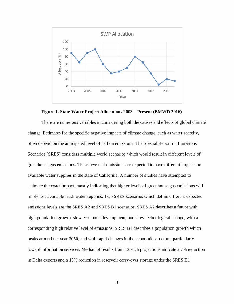
Agricultural water districts, such as BMWD, who receive all of their water from the
SWP, certainly are experiencing reduced water supply already. Figure 1 shows SWP allocation
percentages since 2003 (BMWD 2016). This reflects diminishing fresh water resources available
for growers, one of many predictions made by some climate change experts (CRNA 2008).
10
Figure 1. State Water Project Allocations 2003 – Present (BMWD 2016)
There are numerous variables in considering both the causes and effects of global climate
change. Estimates for the specific negative impacts of climate change, such as water scarcity,
often depend on the anticipated level of carbon emissions. The Special Report on Emissions
Scenarios (SRES) considers multiple world scenarios which would result in different levels of
greenhouse gas emissions. These levels of emissions are expected to have different impacts on
available water supplies in the state of California. A number of studies have attempted to
estimate the exact impact, mostly indicating that higher levels of greenhouse gas emissions will
imply less available fresh water supplies. Two SRES scenarios which define different expected
emissions levels are the SRES A2 and SRES B1 scenarios. SRES A2 describes a future with
high population growth, slow economic development, and slow technological change, with a
corresponding high relative level of emissions. SRES B1 describes a population growth which
peaks around the year 2050, and with rapid changes in the economic structure, particularly
toward information services. Median of results from 12 such projections indicate a 7% reduction
in Delta exports and a 15% reduction in reservoir carry-over storage under the SRES B1
0
20
40
60
80
100
120
2003 2005 2007 2009 2011 2013 2015
Allocation (%)
Year
SWP Allocation
11
scenario, and a 10% reduction in Delta exports and a 19% reduction in reservoir carry-over
storage under the SRES A2 scenario (Mirchi et al. 2013).
Another important consideration with respect to the impacts of climate change on water
resources is also how legislative actions might change water allocations for various uses. Federal
biological opinions to protect endangered fish species under the Endangered Species Act were
issued in February 1993 (by the National Marine Fisheries Service to protect Chinook Salmon)
and in March 1995 (by the U.S. Fish & Wildlife Service to protect the splittail and delta smelt).
These were the first such environmental regulations on the SWP and CVP. More recent
biological opinions were issued in December 2008 to allocate more water for protecting the delta
smelt, and in June 2009 for Chinook salmon. These actions have led to roughly a 10% reduction
in combined deliveries from the SWP and CVP. The impacts of further legislation, particularly
new biological opinions and adoption of the Bay Delta Conservation Plan (BDCP), are likely to
allocate even more water away from agricultural purposes and to environmental purposes (DWR
2014).
Demand
The following section describes some methods economists use to model and estimate
demand for water for agriculture.
Derived Demand
Some analysts consider the demand for agricultural water to be derived from the demand
for the agricultural outputs that the water is used to produce. A production function for an
agricultural product may appear as:
Y = f(W, XE, XM, XL, XK)
12
Where Y is the amount of crop produced (per acre), W is water, and the X’s represent
amounts of energy, materials, labor, and capital, respectively. With a production function set up
in this manner there are two primary methods of estimating the demand for water: (1)
Considering water as a variable input and deriving its value marginal product, or (2) Considering
water as a constrained input, and deriving the profit maximizing input decisions based on input
and output prices. The former of these approaches generally involves statistical analysis of either
field experiments or aggregate data, whereas the latter is generally performed using simulation
modeling and mathematical programming (Scheierling et al. 2006).
Return on Water
Given that the demand for irrigation water is high and sources are limited in California,
models which consider water as a constrained resource are highly prevalent for this region. The
primary function of these models is to maximize total return for farmers, with constraints set by
resource capacities. For derived water demand, the idea is to maximize returns for each unit of
water input (RW):
Rw = Y*PY – (PE*XE + PM*XM + PL*XL + PK*XK)
Where the P’s refer to the respective output and input prices. Using this methodology, the
profit maximizing water quantity choice can be made at various price levels (Scheierling et al.
2006).
Pricing
This section describes some of the many ways to determine pricing for water for
agriculture.
13
History
Agricultural water districts must charge their members to raise revenue to provide funds
for technical and managerial services, even though these districts are not intended to be profiting
enterprises. In the early years of agricultural water districts, fees were assessed by acreage, and
in many instances also varying by crop type (Burt 2006). By 1958, some districts were
employing a “water toll,” used either in combination with or in replacement of per-acre
assessments. The majority of districts employed a fixed, per-unit price for agricultural water, in
conjunction with property taxes. Water prices in this instance were often large enough to
encourage efficient use, while low enough so that users did not opt to pump and use
groundwater. Many districts, however, continued to charge only based on acreage, some based
on acreage and crop type, and others which rationed water and did not employ prices as a means
of allocation and financing (Bain et al. 1966).
From 1975 - 2005, thanks to advancements in metering technology, nearly 80% of
California water districts had switched to volumetric pricing, which is charging per-unit of water
delivered. There are two primary methods for conducting volumetric billing: either a flat rate,
single charge per unit of water delivered, or a tiered structure. Tiered (or block) prices for
irrigation water charge different prices for different amounts of water. They are typically based
on either the amount, with different levels of use costing different amounts, or on the location of
the user, with prices reflecting the costs to move the water. Conservation tiered pricing implies
specifically charging more for larger amounts of usage (Burt 2006).
Recent regulations have further increased the prevalence of advanced metering
technology and volumetric pricing. California’s Water Conservation Act of 2009, SBx7-7,
required that by July 2012, agricultural water suppliers must price their water based at least in
14
part on the quantity delivered. The bill also requires metering with some level of accuracy at
each turnout from the supplier to the individual users (California State Senate 2009). The U.S.
Bureau of Reclamation (USBR) also has encouraged volumetric pricing structures, particularly
those which promote conservation by users. Conservation tiered pricing is believed to offer the
most flexibility and encouragement of efficiency of all the pricing alternatives, as well as
offering the secondary service of consistent water measurement (USBR 1997).
Economic Theory
Economic theory suggests that there are multiple ways to effectively set the price of a
resource, depending on the goal(s) of the participants in the market. If an agricultural water
district’s goal is to cover the full costs of operation in the long run, they must charge at least the
average total cost for the available water. This would be the breakeven price.
The purchasers of water, i.e. the farmers in an agricultural water district, would optimally
pay for water at the point where it is equal to the marginal value created by the last unit of water
applied. That is, they would consume water and produce at the point where the value marginal
product (VMPwy) of water (w) for their product (y) is equal to the marginal cost, or price, of
water (pw). At a fixed price for water, the quantity (Q) demanded by agricultural users is going to
change depending on the value, or price, of the output they are producing (py), and the marginal
product of water applied (MPwy), which is the marginal increase in output with each AF applied.
These establish the value marginal product (VMPwy = py*MPwy) (Doll and Orazem 1984). This
theory is shown in Figure 5, for three different products (y1, y2, y3), such that VMPwy1 < VMPwy2
< VMPwy3. Q1, Q2, and Q3 represent the different number of AF demanded for each of the
products.
15
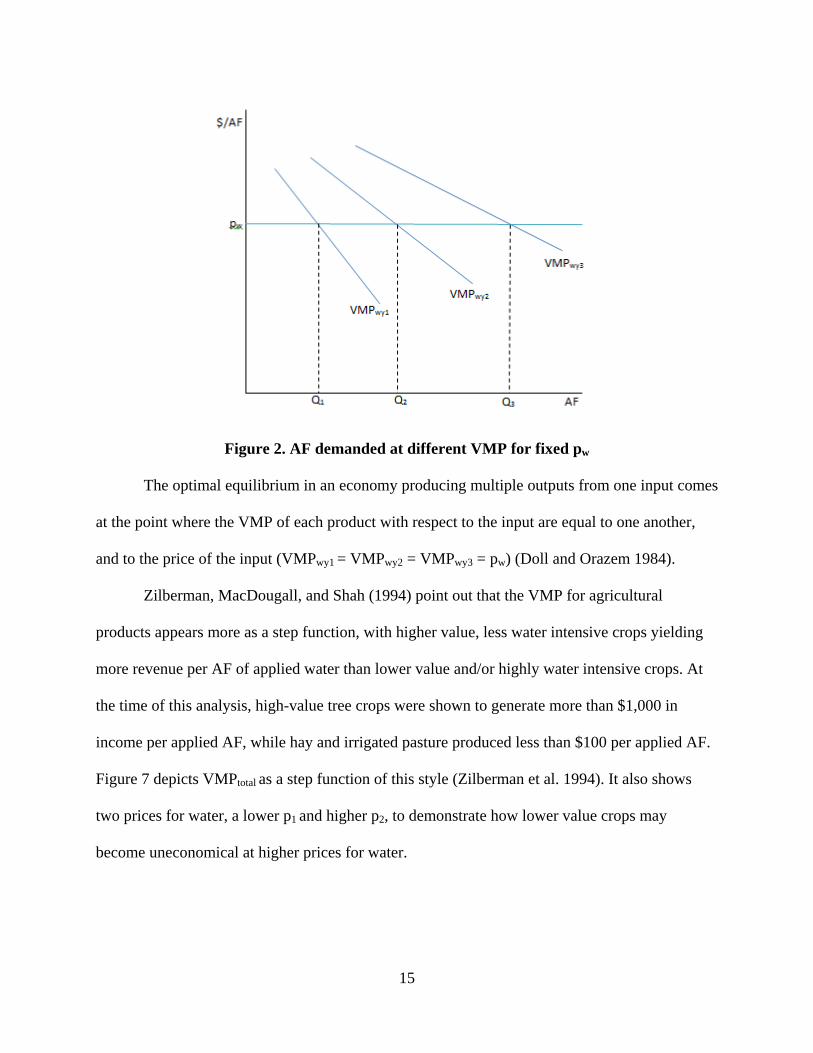
Figure 2. AF demanded at different VMP for fixed pw
The optimal equilibrium in an economy producing multiple outputs from one input comes
at the point where the VMP of each product with respect to the input are equal to one another,
and to the price of the input (VMPwy1 = VMPwy2 = VMPwy3 = pw) (Doll and Orazem 1984).
Zilberman, MacDougall, and Shah (1994) point out that the VMP for agricultural
products appears more as a step function, with higher value, less water intensive crops yielding
more revenue per AF of applied water than lower value and/or highly water intensive crops. At
the time of this analysis, high-value tree crops were shown to generate more than $1,000 in
income per applied AF, while hay and irrigated pasture produced less than $100 per applied AF.
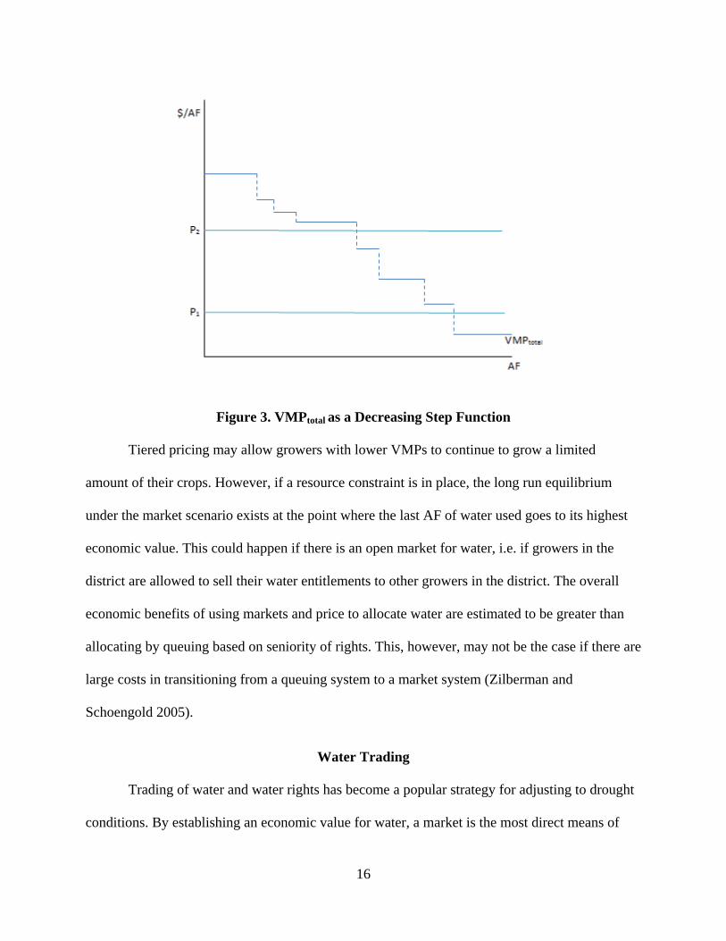
Figure 7 depicts VMPtotal as a step function of this style (Zilberman et al. 1994). It also shows
two prices for water, a lower p1 and higher p2, to demonstrate how lower value crops may
become uneconomical at higher prices for water.
16
Figure 3. VMPtotal as a Decreasing Step Function
Tiered pricing may allow growers with lower VMPs to continue to grow a limited
amount of their crops. However, if a resource constraint is in place, the long run equilibrium
under the market scenario exists at the point where the last AF of water used goes to its highest
economic value. This could happen if there is an open market for water, i.e. if growers in the
district are allowed to sell their water entitlements to other growers in the district. The overall
economic benefits of using markets and price to allocate water are estimated to be greater than
allocating by queuing based on seniority of rights. This, however, may not be the case if there are
large costs in transitioning from a queuing system to a market system (Zilberman and
Schoengold 2005).
Water Trading
Trading of water and water rights has become a popular strategy for adjusting to drought
conditions. By establishing an economic value for water, a market is the most direct means of
17
transferring water from a lower value application to a higher value application (Hanak et al.
2012). The willingness to pay by high value users, the willingness to sell by low value users, and
the distribution costs all affect the prices that water might be sold for (Regnacq et al. 2016). In
the context of water scarcity, a higher economic value of water creates a larger incentive to
conserve water, and invest in ways to reduce distribution losses and increase storage. Water
market trades are generally of two varieties: short term (1 year) or long term (permanent). Short
term transfers become critical during very dry years, whereas long term water right exchanges
are more reflecting of major economic shifts. Another type of water trading, groundwater
banking, allows growers to trade water in wet years for water in dry years (Hanak et al. 2012).
Water Markets
The water market in California became very active during the drought in the late 1980s
and early 1990s, and today it is estimated that roughly 5% of water used in the state annually is
as part of a water transfer. Although initially short term transfers were more popular, long term
and permanent exchanges are becoming more and more prevalent. Farmers are the main
suppliers of water to the market, with cities, environmental causes, and other farmers all active in
purchasing water. Since 2003, as long term exchanges have become the norm, farmers are
buying significantly less water, representing only about one quarter of active market purchases
from 2003 to 2011. It is important to note that this data pertains to exchanges of water from one
water district to another, and not intra-district (Hanak and Stryjewski 2012).
Most demand for water transfers recently comes from cities, with urban agencies
purchasing nearly three times as much water from 2003 to 2011 than during the period 1995-
2002, despite the total volume of water traded not increasing significantly over these two
periods. This trend is expected to continue as cities demand water both for emergency storage for
18
current residents and to allow for development and expansion, which tend to hold a higher direct
value per unit of water used than for agriculture and environmental purposes. Larger demand for
water from urban agencies, coupled with decreasing demand by farmers and steady demand for
environmental purposes, is expected to lead to large scale fallowing of agricultural land, which
would have the secondary effects of higher food costs, less valuable land, and higher
unemployment, particularly in Kern County and other parts of the San Joaquin Valley (Hanak
and Stryjewski 2012).
Another trend in water markets is a shift toward more localization, with nearly half of
recent exchanges occurring within the same county (Hanak and Stryjewski 2012). Although data
on intra-district water transfers are not publicly available, it is reasonable to assume that this
occurs regularly and is facilitated by the district, given the district's decision ultimately is made
by a governing board of the growers.
Generally speaking, California uses water markets as a means of allocation much less
compared to comparable parts of the world. Recent estimates claim about 5% of total water
diverted in California is by way of a water market transfer; by comparison, about one third of
water used in Australia's Murray-Darling Basin is by way of a trade. A major factor that
discourages water markets are transfer costs, which include both the costs of conveyance and the
institutional costs. Institutional costs cover the various administrative costs that must be covered
by the agencies involved in facilitating the trade (Regnacq et al. 2016). Sometimes, part of the
costs of water transfers includes negative externality costs. The presence of externalities can
substantially raise transfer costs, particularly when the trade is going to be permanent. Regions
with larger negative externalities due to water markets generally feature more short term trading
and less permanent trades of water rights (Hansen et al. 2014).
19
Numerous heterogeneous factors lead to the high transfer costs of water, particularly in
California. The volumes traded are generally large, so conveyance costs can be very high, and
will be extremely high if infrastructure for moving water is not already in place. Precipitation
varies both spatially and temporally, making large conveyance costs unavoidable, and often
uneconomical. Another debilitating factor is the effect of fallowed land as a result of transfers
from agricultural applications to non-agricultural operations. A major factor of consideration is
whether or not water will be transferred out of the basin-of-origin. This could prevent re-charge
and introduce the negative externalities associated with groundwater overdraft, especially if the
transfer is long term (Hansen et al. 2014). Due to the larger threat of negative externalities from
long term permanent water trades, better facilitation of short term and local trades may lead to
stronger economic efficiency (Regnacq et al. 2016) (Hansen et al. 2014).
In spite of the negative externalities associated with water markets, exchanges from low
value to high value applications do persist. Water markets most successfully take place when
participants have homogenous rights to the water. This implies that cuts to supply in light of
scarcity are prorated equally to each of the right holders. This reduces the legal hindrances to
agreeing on an exchange value (Hansen et al. 2014). Regnacq et al. (2016), in its analysis of the
friction created in the water market due to high transfer costs, makes three assumptions about the
operation of agricultural water districts within the context of inter-district trade. First, agents in
the water district can only use water supplied from the water district. Second, there is no
asymmetry of power between the different users of water in the district. Third, profit is re-
distributed amongst agents in equal shares. Although the first assumption is not true in reality for
many agricultural water districts, it can be for some, and certainly for many urban water districts.
The second and third assumptions about equality in the district, both with respect to power and
20
total profits, become necessary assumptions for analysis as accurate data for this information is
rarely available in reality (Regnacq et al. 2016).
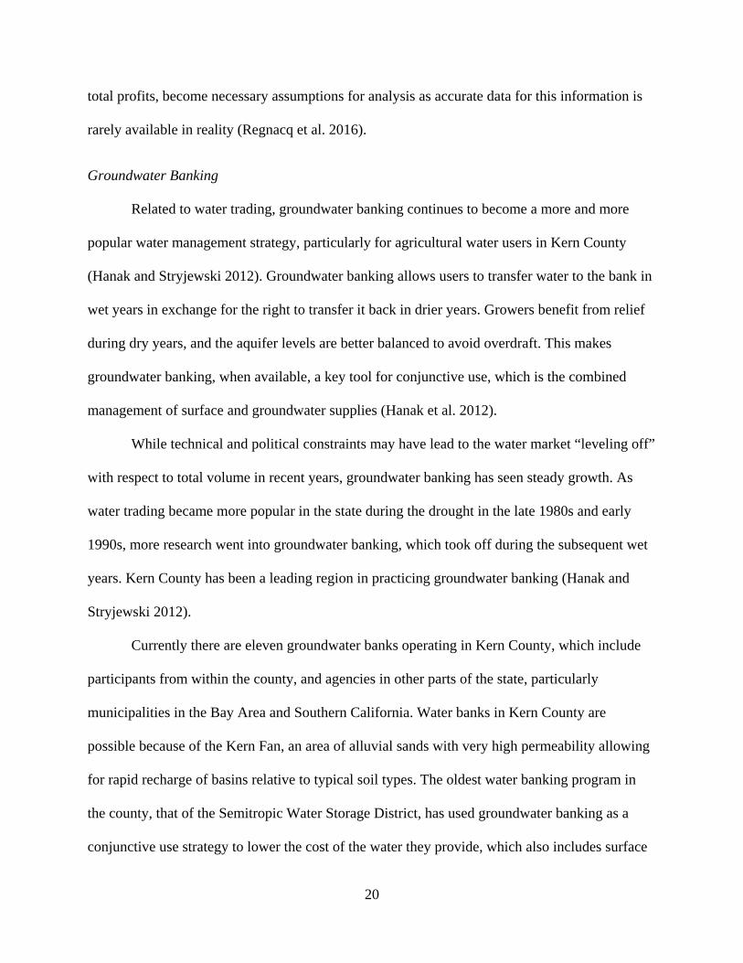
Groundwater Banking
Related to water trading, groundwater banking continues to become a more and more
popular water management strategy, particularly for agricultural water users in Kern County
(Hanak and Stryjewski 2012). Groundwater banking allows users to transfer water to the bank in
wet years in exchange for the right to transfer it back in drier years. Growers benefit from relief
during dry years, and the aquifer levels are better balanced to avoid overdraft. This makes
groundwater banking, when available, a key tool for conjunctive use, which is the combined
management of surface and groundwater supplies (Hanak et al. 2012).
While technical and political constraints may have lead to the water market “leveling off”
with respect to total volume in recent years, groundwater banking has seen steady growth. As
water trading became more popular in the state during the drought in the late 1980s and early
1990s, more research went into groundwater banking, which took off during the subsequent wet
years. Kern County has been a leading region in practicing groundwater banking (Hanak and
Stryjewski 2012).
Currently there are eleven groundwater banks operating in Kern County, which include
participants from within the county, and agencies in other parts of the state, particularly
municipalities in the Bay Area and Southern California. Water banks in Kern County are
possible because of the Kern Fan, an area of alluvial sands with very high permeability allowing
for rapid recharge of basins relative to typical soil types. The oldest water banking program in
the county, that of the Semitropic Water Storage District, has used groundwater banking as a
conjunctive use strategy to lower the cost of the water they provide, which also includes surface
21
water, to discourage growers from over-pumping their groundwater basin. The largest water
bank in Kern County today is the Kern Water Bank, a joint powers authority with both public
and private water agencies within the county participating. The Kern Water Bank began
expanding in the mid-1990s, during the wet years following a major drought period. Total
groundwater bank volume in Kern County hit a peak in 2006 at about 3 million AF, which went
down during the 2007-2009 drought, but was reached again following a wet year in 2011. Of this
total balance, roughly half is held by users within the county, with the remaining split mostly
between municipalities in Southern California and the Bay Area (Hanak and Stryjewski 2012).
Although water markets and groundwater banking have been identified as viable and
effective strategies for agricultural water users in California, ultimately it is up to the discretion
of decisions made by the individual stakeholders, such as when to trade for the growers, and how
trades may be facilitated by the districts.
Game Theory
Game theory approaches to water resource issues demonstrate ways to analyze
stakeholder pay-offs given multiple players and strategy combination alternatives. Since the
players in game theory often receive different individual pay-outs in some or all strategy
combinations, this approach to modeling analyzes the social and political feasibility of water
projects and management strategies. Generally speaking, game theory models reflecting water
resource strategies are assumed to be cooperative games. The decision to cooperate by players
should lead to Pareto-optimal outcomes. However, assuming long-term, self-optimizing
strategies by the players, non-cooperative strategies may become realized equilibria (Madani
2010).
22
Cooperative Game Theory
Decision makers in many games will want to cooperate and form coalitions. In Madani
and Dinar (2012), the researchers identify three important conditions for a successful cooperative
game solution in their analysis of cooperative common pool resource management. The first is
the 'individual rationality condition,' which states that pay-offs under cooperation must be at least
as large or greater than payoffs from non-cooperation for every individual player. The second
condition is the 'group rationality condition,' stating that the sum of total pay-offs for any group
of individual players is greater under total cooperation of all players than it could be under any
other coalition that could be formed from the same pool of players. The third condition, the
'efficiency condition,' states that that the total obtainable benefits under the 'grand coalition,' i.e.
total cooperation by the individual players, must be distributed equally amongst the individual
players (Madani and Dinar 2012).
Madani and Lund (2011) identifies further factors which strengthen the development of
cooperative solutions in their analysis of cooperation and competition over Sacramento and San
Joaquin Delta water exports. The study identifies these five cooperative factors specifically to
demonstrate how Delta management has gone from cooperative to competitive: (1) Homogeneity
of stakeholder interests provides mutual incentive for all players in a game. (2) The availability
of a mutually beneficial solution must be present, as opposed to a zero sum game. (3) Supply
must exceed demands to guarantee cooperation, so that players know that they cannot be made
worse off. (4) Perceived benefits must exceed perceived costs. (5) State and federal funding is
readily available for the development and advancement of cooperative projects (Madani and
Lund 2011).
23
Although in water conflicts the various stakeholders often make different decisions at
different times, they may also decide to cooperate, leading to Pareto optimal decisions. Pareto
optimality exists in strategy combinations in which no individual player could achieve a higher
pay-off in a different strategy combination without making any other player receive a lower pay-
off (Madani 2010). If one player can be made better off without making another player worse
off, this change would be a Pareto Improvement. If the pay-offs are such that no Pareto
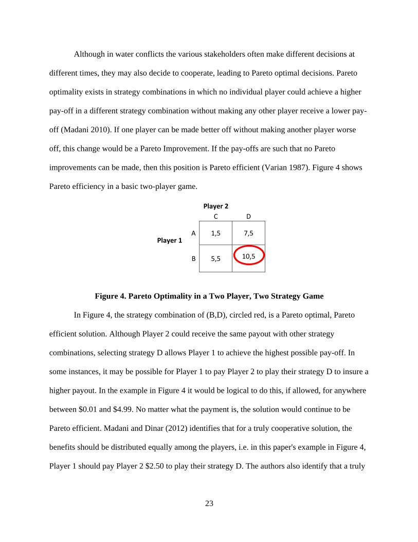
improvements can be made, then this position is Pareto efficient (Varian 1987). Figure 4 shows
Pareto efficiency in a basic two-player game.
Player 2
C D
Player 1A 1,5 7,5
B 5,5 10,5
Figure 4. Pareto Optimality in a Two Player, Two Strategy Game
In Figure 4, the strategy combination of (B,D), circled red, is a Pareto optimal, Pareto
efficient solution. Although Player 2 could receive the same payout with other strategy
combinations, selecting strategy D allows Player 1 to achieve the highest possible pay-off. In
some instances, it may be possible for Player 1 to pay Player 2 to play their strategy D to insure a
higher payout. In the example in Figure 4 it would be logical to do this, if allowed, for anywhere
between $0.01 and $4.99. No matter what the payment is, the solution would continue to be
Pareto efficient. Madani and Dinar (2012) identifies that for a truly cooperative solution, the
benefits should be distributed equally among the players, i.e. in this paper's example in Figure 4,
Player 1 should pay Player 2 $2.50 to play their strategy D. The authors also identify that a truly
24
cooperative solution must have a greater payout for each player than non-cooperation might
have.
Non-Cooperative Game Theory
Although cooperation can lead to Pareto optimal solutions, there are a number of games
in which one player, assuming they want to maximize their individual payout, will logically elect
to choose a strategy which is not cooperative. Normal form game structures, as demonstrated in
Figure 4, allow for consideration of a player's best strategy given the strategy taken by the other
player. Player 1 in this example will receive a higher pay off for selecting strategy B whether
Player 2 plays strategy D or C. This makes strategy B Player 1's dominant strategy. Player 2, on
the other hand, has no dominant strategy. Given that Player 1 plays strategy B, Player 2 can
select strategy C or D and be equally as well off. This makes strategy (B,C) a Nash Equilibrium.
A Nash Equilibrium occurs when each player is playing their best strategy given the strategy
played by the other player (Baye 2010). The (B,C) strategy is not Pareto optimal, because Player
1 could be made better off without making Player 2 worse off. However, if Player 2 is selecting
their strategy based strictly on self-interest, both strategy C and D are their best strategy given
Player 2 plays their dominant strategy. There would need to be some type of intervention or
coordination which would allow Player 2 to realize the benefits of playing strategy D and
achieving the Pareto optimal (B,D) strategy, which is also a Nash Equilibrium.
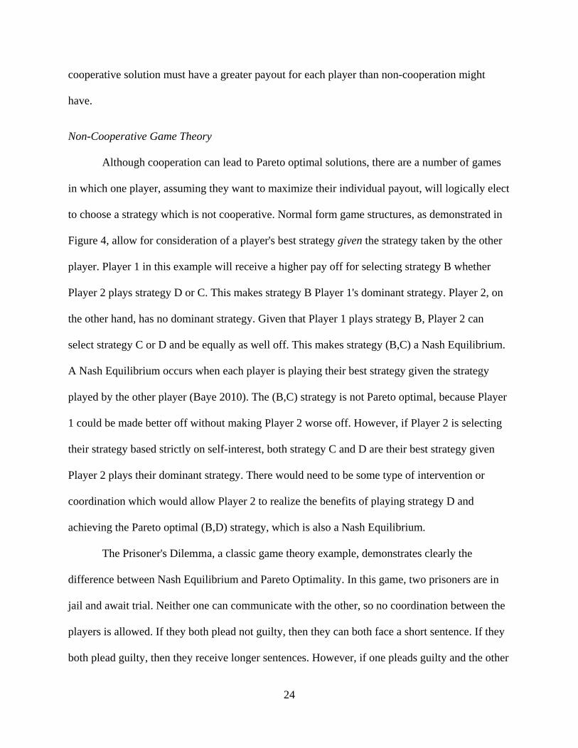
The Prisoner's Dilemma, a classic game theory example, demonstrates clearly the
difference between Nash Equilibrium and Pareto Optimality. In this game, two prisoners are in
jail and await trial. Neither one can communicate with the other, so no coordination between the
players is allowed. If they both plead not guilty, then they can both face a short sentence. If they
both plead guilty, then they receive longer sentences. However, if one pleads guilty and the other
25
pleads not guilty, the former gets off with a plea bargain, and the latter receives the maximum
sentence (Madani 2010). Figure 5 demonstrates this two-by-two game, with higher payouts
correlating to less time served in jail.
Prisoner2
N G
Prisoner1N 3,3 1,4
G 4,1 2,2
Figure 5. The Prisoner's Dilemma
In Figure 5, N corresponds to pleading Not Guilty, G to pleading Guilty. In this game, the
strategy combinations (N,N), (G,N),and (N,G) are all Pareto optimal. In each case, neither could
get a larger pay-off without the other receiving a lower pay-off. However, in this game only one
Nash Equilibrium exists, the (G,G) strategy combination, which is not Pareto optimal. The (N,N)
strategy combination is clearly Pareto superior to the (G,G) combination. However, given
Prisoner 2 pleads not guilty, Prisoner 1 gets a higher payout pleading guilty, and given Prisoner 2
pleads guilty, Prisoner 1 will again get a higher payout pleading guilty. Therefore pleading guilty
is Prisoner 1's strictly dominant strategy, and similarly pleading guilty is Prisoner 2's dominant
strategy as well. Hence, even though it is the only Pareto inferior outcome, the logical outcome
of this game is for both prisoners to confess to their crimes.
A less uplifting application of this game is the "tragedy of the commons." This is the
theory that scarce common pool resources inevitably will become depleted, despite the perceived
benefits of cooperating to save the resource (Madani 2010). Common pool resources are defined
as goods which are non-excludable, meaning anyone is free to pay to take it, and are rival,
26
meaning use by one individual prevents use by another individual. One example of a common
pool resource is California groundwater. Groundwater is a rival good, as pumping from an
aquifer removes water that can be pumped by others over the aquifer, and is also non-excludable,
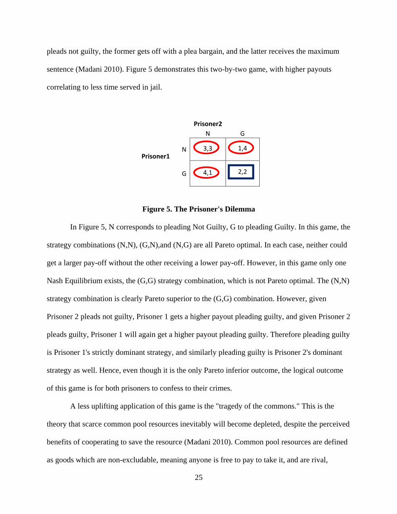
as anyone can buy property and pump as much groundwater as they can access. Figure 6
demonstrates the tragedy of the commons in a two-by-two game, with two growers who pump
water from the same aquifer which faces overdraft. Each can either decide to cooperate by
cutting their water use to allow for necessary recharge, or not cooperate and continue to pump
and overdraft the basin.
Grower 2
C N
Grower 1C 3,3 4,1
N 1,4 2,2
Figure 6. The Tragedy of the Commons
In Figure 6, C corresponds to Cooperating and N to Not Cooperating. This game has the
same dynamics as the Prisoner's Dilemma. One Pareto optimal solution is for both players to
cooperate and cut back their usage to protect the basin. However, the strategy combinations of
one grower cooperating and the other not are also Pareto optimal. In the strategy combination of
(C,N), for example, Grower 1 cooperates and cuts back his production to use less water, however
suffers from the threat of overdraft due to Grower 2's non-cooperation. Meanwhile, Grower 2
benefits from full production, and additionally from the water saved in the aquifer thanks to
Grower 1's decision to cooperate. Grower 2, therefore, would have to be made worse off to make
Grower 1 better off. The tragedy comes in that both growers dominant strategies end up being
not to cooperate. Even though (C,C) is Pareto superior to (N,N), the latter is the only Nash
27
Equilibrium in this game, and therefore overdraft of the basin may be the logical outcome in this
scenario without intervention.
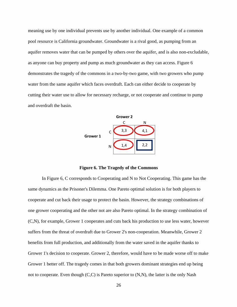
In multi-stage games, players make decisions at different points in time. Although this
type of game could still be represented in the normal form, as in Figures 4, 5, and 6, more often
the extensive form is used to reflect in which stages decisions are made, and by which player.
The different stages are also called 'decision nodes.' (Baye 2010). Figure 7 shows a basic
multistage game in extensive form.
Figure 7. Multistage Game in Extensive Form
In the above game, Player 1 first decides to play top or bottom, and based on that
decision there are two decision nodes in which Player 2 can play one of two strategies, left or
right. This game structure is unique from other two player games, such as the Prisoner's
Dilemma, because Player 1 gets to make a decision knowing that Player 2 must try to get a
higher pay-off given the choice made by Player 1 (Varian 1987). For this reason, backward
induction is used in sequential games to determine the Sub-game Perfect Nash Equilibria
(SPNE). This equilibrium exists with a strategy combination with which neither player could
28
receive a higher payout by changing their strategy at any stage. In a two player, two decision
game such as in Figure 7, the Subgame Perfect Nash Equilibrium exists when Player 1 selects
the best strategy given what Player 2's best strategy is for each of Player 1's potential strategies.
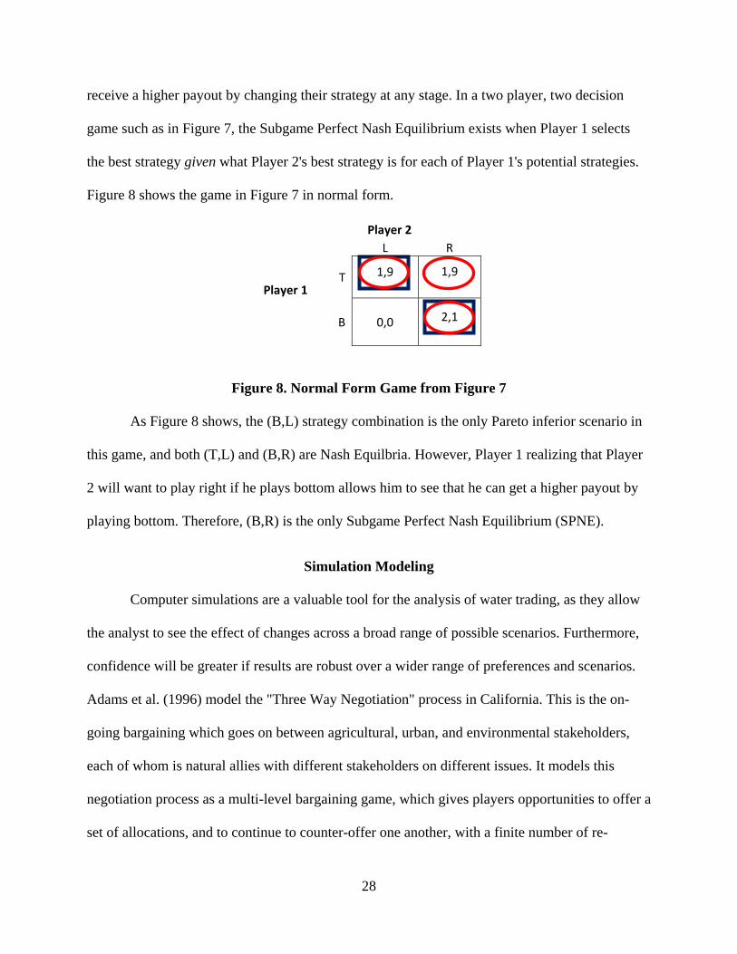
Figure 8 shows the game in Figure 7 in normal form.
Player 2
L R
Player 1T 1,9 1,9
B 0,0 2,1
Figure 8. Normal Form Game from Figure 7
As Figure 8 shows, the (B,L) strategy combination is the only Pareto inferior scenario in
this game, and both (T,L) and (B,R) are Nash Equilbria. However, Player 1 realizing that Player
2 will want to play right if he plays bottom allows him to see that he can get a higher payout by
playing bottom. Therefore, (B,R) is the only Subgame Perfect Nash Equilibrium (SPNE).
Simulation Modeling
Computer simulations are a valuable tool for the analysis of water trading, as they allow
the analyst to see the effect of changes across a broad range of possible scenarios. Furthermore,
confidence will be greater if results are robust over a wider range of preferences and scenarios.
Adams et al. (1996) model the "Three Way Negotiation" process in California. This is the on-
going bargaining which goes on between agricultural, urban, and environmental stakeholders,
each of whom is natural allies with different stakeholders on different issues. It models this
negotiation process as a multi-level bargaining game, which gives players opportunities to offer a
set of allocations, and to continue to counter-offer one another, with a finite number of re-
29
negotiations allowed. The study specifically looks at the effects on changes to the "constitutional
structure" of the multi-level bargaining game. These changes include limits on infrastructure
development opportunities, and diverging positions of sub-groups within the three main groups
(Adams et al. 1996).
This multi-level bargaining game consists of 25 computational solutions to each
simulation, in which one aspect of the bargaining process systematically varies in each solution.
For each of the simulations, the other parameters solving for each player's utility function are
randomized based on pre-specified intervals, although estimated from prior knowledge which
may not be precise. The results of this analysis do suggest significant changes to the results of
this bargaining process under different negotiation structures. For example, lower levels of
opportunity for developing infrastructure offers more bargaining power to environmental
stakeholders, as it limits opportunities for agricultural and urban development. Another example
is diverging opinions within the agricultural stakeholder group on water transfers, which can
create a better position for urban stakeholders. This is because sup-groups within the greater
agriculture group would have the opportunity to create more water transfers to urban growers,
even if this is not the position of the collective agriculture group (Adams et al. 1996).
Computer simulations are also an effective way to analyze the results of simply strategy
alternatives under the same, but varying, exogenous factors. Small and Rimal (1996) use a
simulated irrigated rice system (SIRS) model, which compares the impacts of three possible
distribution outcome strategies: minimum conveyance losses, maximum crop yield, or maximum
economic productivity of water. This study defines the "economic productivity of water" as "the
value of irrigated crop production, net of the costs to society of the inputs used to produce it,
divided by the quantity of water used." The model solves for this strategy as equal marginal
30
products for distributions to each turnout. The model simulates the outcome of these three
different strategies, or "water distribution rules," assuming a SIRS "manager," who has complete
control over the distribution, and that the actual distribution is precisely that called for by the
water distribution rule. The study recognizes that although these assumptions limit the
applicability of the results to real systems, this idealized look at efficient solutions opens the door
to understanding actual potentials and limitations of the different strategy scenarios. Ultimately,
the study concludes that there is no significant difference between the economic efficiency of
water between the minimum conveyance loss and maximum economic productivity distribution
rules (Small and Rimal 1996).
Berrenda Mesa Water District
The Berrenda Mesa Water District (BMWD) began to provide landowners water
deliveries in 1968, after contracting with the Kern County Water Agency to begin providing
irrigation water from the SWP. The district covers the northwest corner of Kern County, about
50 miles from the city of Bakersfield. The total area of the district is 55,440 acres, with about
32,420 acres with crops and 27,200 acres with irrigation systems. BMWD currently has an
entitlement to 92,800 AF of SWP water. In any given year, about 98% of water supplied in the
district is delivered through the Coastal Branch of the California Aqueduct, with the remaining
coming from a single turnout on the main branch of the California Aqueduct. The water is
pumped at Pump Station ‘A’ 225 feet uphill into a regulating reservoir in the northwest part of
the district. From there deliveries are made by gravity, first through a concrete lined main canal,
then through lateral pipelines to specific parcels, most of which are at a lower elevation (BMWD
2015).
31
Although the majority of the water in any given year comes from SWP allocations,
BMWD supplies also come from purchases from other districts, and participation in the Kern
Water Bank. Supplemental supplies are secured both on a larger scale, with multiple districts on
the west side of Kern County working to secure sources pro rata for their growers, and on a
smaller scale by just the district or individual growers within the district. Growers have the
option to, independently, participate in the Kern Water Bank, sending water to the bank in wet
years and retrieving it in dry years. In the case that a grower in the district was to decide to
discontinue paying for and receiving deliveries, their entitlement normally would be allocated
pro rata to others in the district (Hammett 2014).
BMWD uses a pricing method which includes a base price paid per AF, plus an added
price based on a user’s location within the district. The base price covers the costs paid to the
DWR for water deliveries through the SWP, administrative costs, and Operation & Maintenance.
The added-price for deliveries based on grower location is strictly to cover energy costs. BMWD
also charges a per-acre stand-by charge for all acres within the service area. This is designed to
cover the capital costs related to new and upgraded facilities, as well as other programs to benefit
all growers in the district. While the added-price is only charged for water deliveries which are
made, growers are responsible for paying the base price for their full allocation of SWP water,
regardless of what is provided by the SWP in any given year. The district, in turn, must pay for
their full allocation to the SWP regardless of real deliveries. BMWD sets its pricing strictly with
the goal of covering their costs (Hammett 2014).
Technically, the district and its growers use precision technology to be as efficient with
their water as possible. Many of the productive orchards in the district use drip or micro-spray
irrigation, with row crop growers using sprinklers predominately. Many growers within the
32
district have conducted advanced analysis of the effectiveness of their irrigation scheduling,
including soil moisture sensing and plant stress monitoring. The district itself has implemented a
Supervisory Control And Data Acquisition (SCADA) system, which allows for remote
automated control and adjustments of deliveries. The district runs almost completely on gravity
from the regulating reservoir, with upstream control at turnouts allowing for a large amount of
flexibility. BMWD has invested a great deal in modernizing over the years, and continues to
search for opportunities for improvement (Hammett 2014).
BMWD sets its budget based on expected allocations and revenue, and typically does not
make budget cuts, however may make some deferments in the case of very low supply and
corresponding revenue. Costs to the DWR for SWP water and power costs are two that
absolutely must be covered for the district to remain in operation. Maintenance is the easiest cost
to defer to future years, however there are limitations to how much maintenance can be avoided.
In an extreme, prolonged low revenue scenario, labor would be the next to be cut. There may,
alternatively, be opportunities to increase supplies within the district. A potential delta bypass
project could raise the expected average SWP allocations looking forward from 60% to 75%,
although the firm figures on water gains and the costs to contractors will not be known until a
final project is approved. Another option would be to use reverse osmosis to clean and use water
groundwater in the district which currently is not usable for agriculture by standard extraction.
The feasibility of this, however, has yet to be determined as an economically viable solution.
Other potential options include solar and other alternatives to alleviate energy spending.
With regard to future management strategies to alleviate the effects of prolonged drought,
BMWD is limited as their growers are entitled to SWP water at fair and reasonable prices. Water
prices are tiered based on location for energy cost purposes, but conservation tiered pricing
33
would not be feasible given their contracts, and given that the real cost per AF to growers already
does increase in drier years. Although pricing based on demand is not a possibility for the
district, it is possible that this type of pricing could be self-managed within the district if water
gets more scarce and expensive. As the district does allow growers to exchange with one
another, growers could have the ability to purchase additional water at a higher price from other
growers after the allocations have been set. There has been no study on the potential outcomes of
this, particularly with respect to the types of trades and the growers’ willingness to sell water.
34
CHAPTER III
METHODOLOGY
Assumptions
The model for this analysis will be based on BMWD. However, there are several
assumptions for the analysis which simplify the data for the purposes of the model, which may
not be completely true to the real BMWD:
1. There are two primary stakeholders in the model, the growers and the district, who each
make decisions and receive pay-outs as an aggregate, single group.
2. The primary goal of the district is to maximize agricultural revenue in the district.
3. The primary goal of growers in the district is to maximize returns over operating
expenses.
4. Water availability follows the inverse of the lognormal distribution.
5. The district distributes all water applied by growers in the district.
6. Growers can trade water for a fee of 10% of the Base Price.
7. Growers may elect to send water to a water bank in a given year, then retrieve 90% of it
in any future year for the same energy cost paid to the district.
8. Over a seven year period, growers of permanent crops would not be able to discontinue
watering acres in any year and be able to use the land economically in a future year.
9. Growers of row crops, specifically carrots and alfalfa hay, can choose to stop watering
acres in any year and be able to use the land at full production in any future year.
35
10. Any grower after three years of average negative returns will go out of business and
their water allocation will be distributed pro rata to the growers still active in the district
service area.
Procedures for Data Analysis
Game Set-Up
This model considers the decisions which the district and growers could make as a two
player, two decision, multi-stage game. The district decides whether exchanges are short term or
long term. If they accept short term exchanges, and take a 'flexible' strategy, growers can sell
water one year while retaining their rights for future years. The district's 'inflexible' strategy
allows for only long term exchanges, so that sellers of water lose their rights to the buyers of the
water. The grower has two decisions as well, to be a water 'saver' or a water 'trader.' If they elect
to be a 'trader,' they 1) Sell available water whenever opting to use it would result in negative
returns, and 2) Opt to sell water over sending it to the water bank. Alternatively, if they elect to
be a 'saver,' they 1) Only sell water if their total revenue is not enough to cover the costs of
water, and 2) Opt to send water to the water bank over selling it.
The payouts for each player in this game is total agricultural revenue for the district, and
total returns for the growers. This game is assumed to be a two-stage sequential game, with the
district first making their decision, followed by the growers. The payouts will be represented as
the Total Economic Size (TES) for the district and Total Real Returns (TRR) for the growers.
The superscript 'F' refers to Flexible District strategies, 'I' corresponds to Inflexible District, 'T' to
water Trading Growers, and 'S' to water Saving Growers. This game is represented in extensive
form in Figure 9, and in normal form in Figure 10.
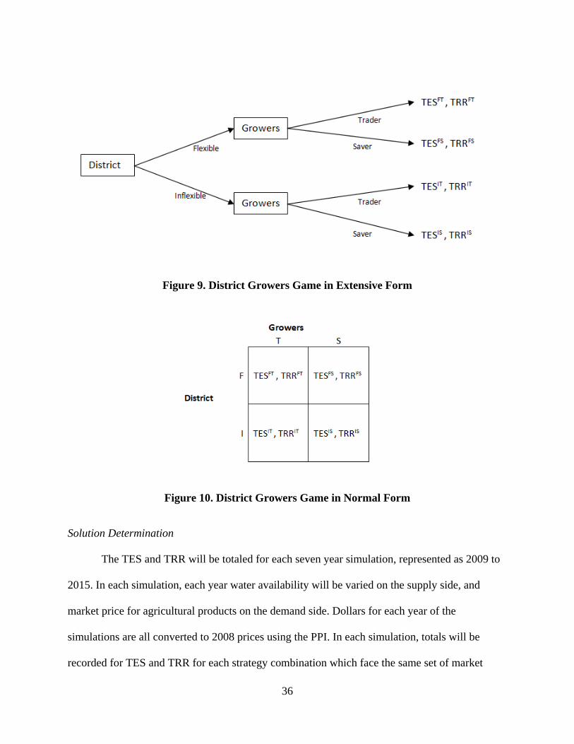
36
Figure 9. District Growers Game in Extensive Form
Figure 10. District Growers Game in Normal Form
Solution Determination
The TES and TRR will be totaled for each seven year simulation, represented as 2009 to
2015. In each simulation, each year water availability will be varied on the supply side, and
market price for agricultural products on the demand side. Dollars for each year of the
simulations are all converted to 2008 prices using the PPI. In each simulation, totals will be
recorded for TES and TRR for each strategy combination which face the same set of market
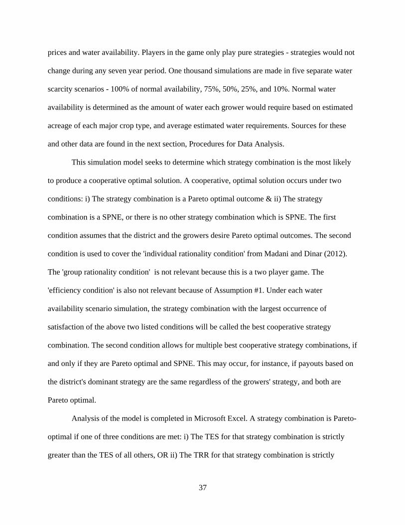
37
prices and water availability. Players in the game only play pure strategies - strategies would not
change during any seven year period. One thousand simulations are made in five separate water
scarcity scenarios - 100% of normal availability, 75%, 50%, 25%, and 10%. Normal water
availability is determined as the amount of water each grower would require based on estimated
acreage of each major crop type, and average estimated water requirements. Sources for these
and other data are found in the next section, Procedures for Data Analysis.
This simulation model seeks to determine which strategy combination is the most likely
to produce a cooperative optimal solution. A cooperative, optimal solution occurs under two
conditions: i) The strategy combination is a Pareto optimal outcome & ii) The strategy
combination is a SPNE, or there is no other strategy combination which is SPNE. The first
condition assumes that the district and the growers desire Pareto optimal outcomes. The second
condition is used to cover the 'individual rationality condition' from Madani and Dinar (2012).
The 'group rationality condition' is not relevant because this is a two player game. The
'efficiency condition' is also not relevant because of Assumption #1. Under each water
availability scenario simulation, the strategy combination with the largest occurrence of
satisfaction of the above two listed conditions will be called the best cooperative strategy
combination. The second condition allows for multiple best cooperative strategy combinations, if
and only if they are Pareto optimal and SPNE. This may occur, for instance, if payouts based on
the district's dominant strategy are the same regardless of the growers' strategy, and both are
Pareto optimal.
Analysis of the model is completed in Microsoft Excel. A strategy combination is Pareto-
optimal if one of three conditions are met: i) The TES for that strategy combination is strictly
greater than the TES of all others, OR ii) The TRR for that strategy combination is strictly
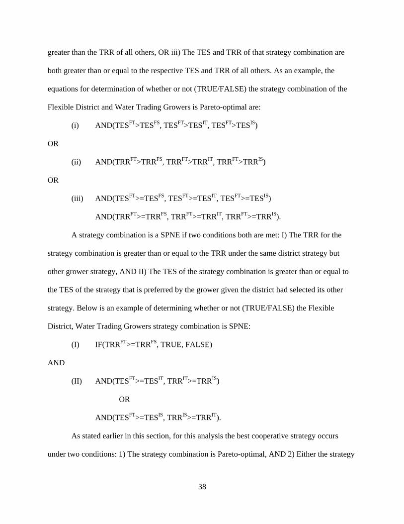
38
greater than the TRR of all others, OR iii) The TES and TRR of that strategy combination are
both greater than or equal to the respective TES and TRR of all others. As an example, the
equations for determination of whether or not (TRUE/FALSE) the strategy combination of the
Flexible District and Water Trading Growers is Pareto-optimal are:
(i) AND(TESFT>TESFS, TESFT>TESIT, TESFT>TESIS)
OR
(ii) AND(TRRFT>TRRFS, TRRFT>TRRIT, TRRFT>TRRIS)
OR
(iii) AND(TESFT>=TESFS, TESFT>=TESIT, TESFT>=TESIS)
AND(TRRFT>=TRRFS, TRRFT>=TRRIT, TRRFT>=TRRIS).
A strategy combination is a SPNE if two conditions both are met: I) The TRR for the
strategy combination is greater than or equal to the TRR under the same district strategy but
other grower strategy, AND II) The TES of the strategy combination is greater than or equal to
the TES of the strategy that is preferred by the grower given the district had selected its other
strategy. Below is an example of determining whether or not (TRUE/FALSE) the Flexible
District, Water Trading Growers strategy combination is SPNE:
(I) IF(TRRFT>=TRRFS, TRUE, FALSE)
AND
(II) AND(TESFT>=TESIT, TRRIT>=TRRIS)
OR
AND(TESFT>=TESIS, TRRIS>=TRRIT).
As stated earlier in this section, for this analysis the best cooperative strategy occurs
under two conditions: 1) The strategy combination is Pareto-optimal, AND 2) Either the strategy
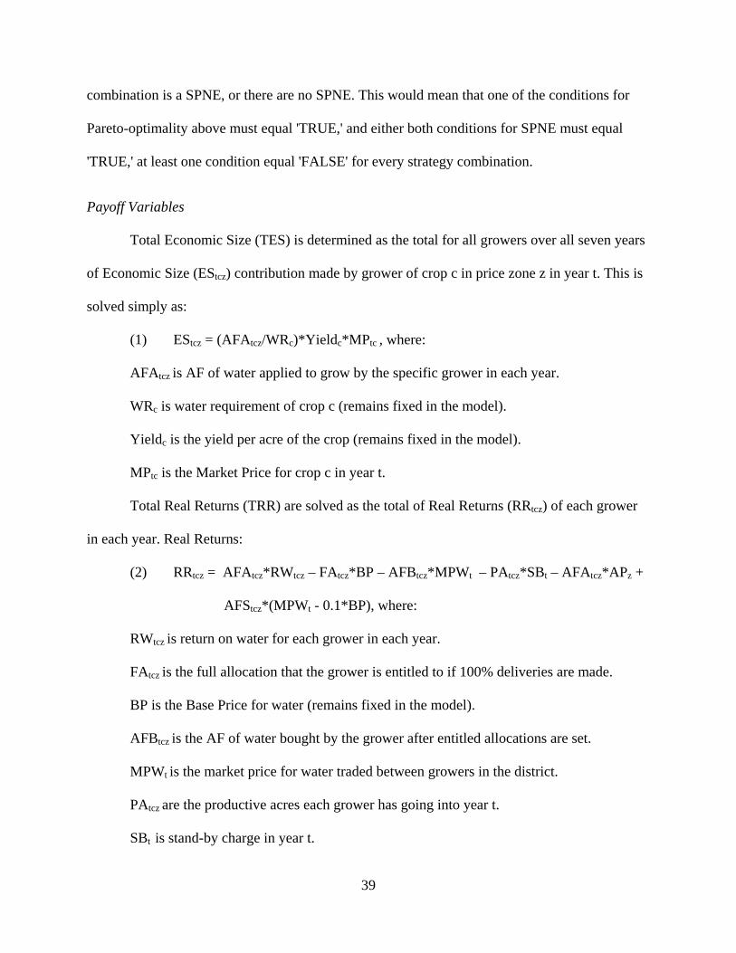
39
combination is a SPNE, or there are no SPNE. This would mean that one of the conditions for
Pareto-optimality above must equal 'TRUE,' and either both conditions for SPNE must equal
'TRUE,' at least one condition equal 'FALSE' for every strategy combination.
Payoff Variables
Total Economic Size (TES) is determined as the total for all growers over all seven years
of Economic Size (EStcz) contribution made by grower of crop c in price zone z in year t. This is
solved simply as:
(1) EStcz = (AFAtcz/WRc)*Yieldc*MPtc , where:
AFAtcz is AF of water applied to grow by the specific grower in each year.
WRc is water requirement of crop c (remains fixed in the model).
Yieldc is the yield per acre of the crop (remains fixed in the model).
MPtc is the Market Price for crop c in year t.
Total Real Returns (TRR) are solved as the total of Real Returns (RRtcz) of each grower
in each year. Real Returns:
(2) RRtcz = AFAtcz*RWtcz – FAtcz*BP – AFBtcz*MPWt – PAtcz*SBt – AFAtcz*APz +
AFStcz*(MPWt - 0.1*BP), where:
RWtcz is return on water for each grower in each year.
FAtcz is the full allocation that the grower is entitled to if 100% deliveries are made.
BP is the Base Price for water (remains fixed in the model).
AFBtcz is the AF of water bought by the grower after entitled allocations are set.
MPWt is the market price for water traded between growers in the district.
PAtcz are the productive acres each grower has going into year t.
SBt is stand-by charge in year t.
40
APz is the Added Price in price zone z (remains fixed in the model).
AFStcz is the AF of water sold by the grower each year.
This equation for Real Returns assumes that the grower who sells water pays the 10% fee
for water trades.
The Stand-By charge (SBt) will increase in years in which the total serviced acres in the
district go down. This happens due to permanent water transfers under the inflexible district
decision, and also as a result of growers in the district going out of production due to prolonged
financial losses. SBt when t=2008, i.e. the first year, is equal to $19.08. In future years, it is equal
to:
(3) SBt = IF(TPAt > 0, $530,812/TPAt, 0)
An 'IF' function is used because if the Total Productive Acres (TPAt), which are acres
active in the service area and able to grow in year t, are equal to zero, than the district is
presumed to 'shut down.' TPAt is divided into $530,812 because this is the total revenue raised
by the district with a stand-by charge of $19.08 when all acres are initially productive. TPAt is
the sum of PAtcz, defined below, for all growers in year t.
The AF Applied (AFAtcz) by each grower in year t is defined as:
(4) AFAtcz = (Atcz – ALtcz)*WRc, where:
Atcz are each grower's allocated acres in year t.
ALtcz are the total acres 'lost' each year by each grower. This determined as:
(5) ALtcz = IF(AFTtcz < FAtcz, (FAtcz – AFTtcz)/WRc, 0), where:
AFTtcz is the Total AF each grower has access to in each year, after water trades have
been completed. This is calculated as:
41
(6) AFTtcz = AVtcz + AFBtcz – AFStcz, where:
AVtcz is the AF Available to each grower in each year before trades have been made. This
is calculated as:
(7) AVtcz = Pt*FAtcz + WB(t-1)cz, where:
Pt is the percent of normal water that is available in year t. The available Water Bank
water available in year t (WBtcz) is:
(8) WBtcz = (AFTtcz – AFAtcz)*0.9.
The Water Bank (WBtcz) amount for each grower for year ending 2008 (the last year
before the model) is assumed to be equal to zero.
The Intra-District Water Market
The water market in this model assumes that the growers with the highest willingness to
pay for water will have the first opportunity to purchase water, and those with the lowest
willingness to accept to not use water will have the first opportunity to sell their water.
Regardless of the willingness to pay for water or to accept to sell, the amount that each grower
will want to buy or sell will be based on the grower's decision variable, which is the Want-to-
Buy, which is computed differently depending on the grower strategy.
The Willingness-to-Pay for water by each grower in each year (WTPtcz) is determined as:
(9) WTPtcz = RWtc – APz + (BP*0.10), where:
RWtc is the return on water for crop c in year t. The Willingness-to-Accept (WTAtcz) is
determined as:
(10) WTAtcz = RWtcz + PWtcz – APz.
Where PWtcz is the perceived Real Price of Water by each grower each year.
42
Although WTPtcz and WTAtcz can be calculated each year by each grower, their decision
on how much to buy will depend on profitability, and on how much to sell will depend on what
strategy they are taking. The amount that each grower Wants-to-Buy (WTBtcz) is:
(11) WTBtcz = IF(RWtc < PWtcz, 0, AFLtcz), where:
AFLtcz is the how many AF Less in year t each grower has relative to their full allocation.
This is determined as:
(12) AFLtcz = IF(AVtcz < FAtcz, FAtcz – AVtcz, 0).
The Willingness-to-Trade by each grower in each year when they take a water Trader
strategy (WTTtczT) is determined as:
(13) WTTtczT = IF(RWtc < PWtcz, AVtcz, ASRtcz), where:
ASRtcz is the amount of AF Surplus each grower has each year. This is solved as:
(14) ASRtcz = IF(AVtcz > FAtcz, AVtcz - FAtcz, 0).
The Willingness-to-Trade by each grower each year when they take a water Saver
strategy (WTTtczS) is:
(15) WTTtczS = IF(ARtc < PWtcz, AVtcz, 0), where:
ARtc is the Average Revenue per AF Applied for crop c in year t. This is determined as:
(16) ARtc = (MPtc*Yieldc)/WRc.
The real price of water (PWtcz) seeks to approximate the average cost per AF that each
grower has per AF available in a given year t, between the stand-by charge, the base price
charges, the added charges for energy for water delivery, and the costs for moving any available
water from the water bank. The equation used to solve is:
(17) PWtcz = IF(RAtcz>0, BP*(FAtcz/RAtcz)*1.37, 0) +IF(AVtcz>0,
(SBt*PAtcz)/AVtcz + APz, 0).
43
The return on water (RWtc) in each year for grower of crop c solves for how much money
each AF of water applied is expected to bring over the other, non-water related variable costs.
This is solved as:
(18) RWtc = (MPtc*Yieldc - CAc)/WRc, where:
CAc is the total, non-water operating costs for crop c (remains fixed in the model).
In any given year, the total amount of water which will be traded, the Total AF
Exchanged (TAEt) is solved as:
(19) TAEt = MIN(TADt, TASt).
Where the Total AF in Demand (TADt) is the sum of WTBtcz for each grower in year t,
and the Total AF in Supply (TASt) is the sum of WTTtcz for each grower in year t (N.B. TASt
will be different given the grower strategy). Except for the unlikely scenario in which TADt =
TASt, this equation for TAEt implies that there will either be growers who want to buy water
who cannot, or those wishing to sell water who do not. In order to determine how much AF each
grower may buy or sell, they are 'queued' based on respective WTP and WTA.
For purposes of exchanging water, the AF Bought (AFBtcz) and the AF Sold (AFStcz) for
growers, which are the amounts actually bought and sold each year by each grower, are based
WTPtcz and WTAtcz rankings (from 1 to 17, the number of crop type and price zone combinations
in the district). The model assumes that growers can purchase their full WTBt if their ranking in
WTPt is such that the sum of their WTBt, and the WTBt of growers with an equal or higher WTPt
ranking, is less than or equal to TAEt. In the instance where this sum is greater than TAEt but the
sum of AF purchased by the previous WTPt ranked growers is less than TAEt, then the grower(s)
of that ranking will be able to buy water pro rata. For the remaining growers, where the sum of
44
WTBt for growers with a higher WTPt is equal to or greater than TAEt, those growers will have
AFBtcz = 0.
Similarly, the model assumes that growers can sell their full WTTt if their ranking in
WTAt is such that the sum of their WTTt and the WTTt of growers with an equal or lower WTAt
ranking is less than or equal to TAEt. In the instance where this sum is greater than TAEt but the
sum sold by the previous WTAt ranked growers is less than TAEt, then the grower(s) of that
ranking will be able to sell their water pro rata. For the remaining growers, where the sum of
WTTt for growers with a lower WTPt is equal to or greater than TAEt, those growers will have
AFStcz = 0.
This model assumes that the Market Price of Water (MPWt), that is the price paid for the
water that is exchanged, is determined as the minimum WTPtcz for growers that are able buy
water in year t. This assumes that all growers who buy and sell water are paying or receiving the
same price per AF, less energy costs which vary by price zone. Although this may not be exactly
true to reality, this model ultimately considers total collective returns for growers in the district,
and therefore the specific price point becomes less important, so long as it is between the
maximum WTAtcz for growers who are able to sell water, and the minimum WTPtcz for growers
who are able to purchase water.
District Decision
The implications of water exchanges depend on whether the District is following their
flexible or inflexible strategy. When the District takes a flexible strategy, growers may make
short term water transfers, meaning growers who sell their water in year t will retain their
entitled allocation in year t+1. That is to say, Growers in year t will have FAtcz equal to FA(t-1)cz,
unless the Grower of crop c in zone z has experienced average RR < 0 in the period from (t – 3)
45
through (t – 1), in which case FAtcz will equal zero. Therefore during the first three years when
the district is flexible, growers will continue to have the same FAcz. If and when growers do have
to relinquish FAtcz due to continued financial loss, this is considered Forgone AF (FAFtcz), which
will be reallocated to the remaining growers based on the proportion of each of the remaining
growers' FAtcz to the total FAt of all remaining growers. In this manner, each grower's Full
Allocation (FAtcz) of AF when the district takes the flexible strategy becomes:
(20) FAFtcz = Atcz*WRc + SUM(FAFt)*(Atcz/SUM(At)).
Due to the dichotomy between permanent crops (i.e. almonds and pistachios) and row
crops (i.e. carrots and pasture), PAtcz when t>0 is determined as:
(21) PAtcz = IF(Atcz>0, PA(t-1)cz - AL(t-1)cz*PCc,
Where PCc is a binary variable such that PCc = 1 for permanent crops and PCc = 0 for
row crops.
When the District takes an inflexible strategy, only long term water transfers are allowed,
and Growers are forced to make permanent exchanges when buying and selling water.
Therefore, in addition to the AFBtcz and AFStcz variables, growers also must consider their
Available AF Bought (AVBtcz) and Available AF Sold (AVStcz). Assuming that a grower would
opt to sell all Water Bank water before any allocated water, the Water Bank AF Sold (WBStcz) is
also considered, and when t>0 solved as:
(22) WBSItcz = IF(AFStcz > WB(t-1)cz, WB(t-1)cz, AFStcz) * IF(AFStcz>0, 1, 0).
The Water Bank AF Bought (WBBtcz) then becomes:
(23) WBBItcz = IF(SUM(AFBt)>0, (AFBtcz/SUM(AFBtcz))*SUM(WBSt), 0).
This calculation assumes that all growers who buy water will purchase an equal
proportion of Water Bank water, regardless of the relative amount sold by those growers who
46
sell water. As the district inflexible strategy assumes that growers who sell water will sell Water
Bank water first and then sell water entitlements, the Allocated AF Sold (AAS) becomes:
(24) AASItcz = IF(Pt>0, (AFStcz – WBSI
tcz)/Pt, 0).
The remaining AFStcz, other than what the grower may have had in the water bank, is
divided by Pt to correspond to the loss from the grower’s Full Allocation, i.e. the entitlement
given the district’s relative equilibrium. Similarly, the Allocated AF Bought (AABItcz) for
growers who buy water is:
(25) AABItcz = IF(Pt>0, (AFBtcz – WBBI
tcz)/Pt, 0).
The Full Allocation for each grower in the years after t=0 then becomes:
(26) FAItcz = Atcz*WRc + SUM(FAFt)*(Atcz/SUM(At)) – AASI
ncz + AABIncz,
Where n = {2009, …, 2015}.
Varying Factors
In each seven year simulation, two variables are randomly selected; water availability
from the SWP on the supply side, and the market price for agricultural outputs on the demand
side. The model assumes that 2009 is a period of “relative equilibrium” in the sample economy,
with farmers realistically expecting their full AF requirement from the district at their 2009
acres. It is important to distinct this from the allocation entitlement from the SWP. In 2009, it
was the case that farmers already were not getting their full allocation from the SWP, with the
average being about 73% from 2003-2008. Therefore, estimates for available water in the district
are assumed to be relative to what growers in this region had come to be used to, and the active
acres that they have. Thus, the Full Allocation of AF each year (FAtcz) is based on the Allocated
Acres (Atcz) that each grower has available to harvest, where FAtcz equals Atcz times WRc when t
= 0, where WRc is the Water Requirement for crop c in feet per acre per year. This also means
47
that FAtcz can be less than the Real Allocation of water in a given year (RAtcz), which is not the
case for the allocations directly from the SWP.
Another important note is that not all deliveries in 2009, nor the years before and after,
come directly from SWP allocations. Although all deliveries to the district come from the state
operated California Aqueduct (specifically the Coastal Branch), some proportion of this typically
will be from a combination of short and long term water exchanges. Therefore, the model
considers relative water scarcity at the aggregate level, rather than from specific sources which
would depend on many exogenous circumstances and decisions. Furthermore, the model is
concerned with analyzing the effects of relative water scarcity, and as different levels of scarcity
are considered, the quantified effects of specific causes of water scarcity to different sources due
to climate change become less important. The established notion that climate change will cause
some level of relative water scarcity is the critical assumption for this model.
The relative level of water scarcity is simulated based on the inverse of the log normal
cumulative distribution. This distribution implies that while the mean of the available water in
each scenario is likely, values greater become exponential less likely, while the likelihood of
values less than the mean has a smoother probability function. The simulation that water
availability follows is calculated with the proxy variable Y in year t:
(27) Yt = LOGNORM.INV( RAND( ), X, 0.28 ).
Where X is the relative scarcity level (i.e. in the 50% scenario, X=0.5). This data is
converted to relative water scarcity percentage P in year t:
(28) Pt = IF(Yt > 137%, 137%, IF(LN( Yt) > 0.05, LN(Yt), 0)).
The “IF” excel functions set the constraints for water allocation to be 5% and 137%. The
upper constraint of 137% is based on the assumption that the “relative equilibrium” for the
48
district is 73% of SWP allocation, making 137% correspond to a SWP allocation of 100%. This
assumption is based on the average percent allocation delivery to the district from the SWP
during the period 2003-2008. The 5% constraint assumes that no allocations will be made if the
available water is less than 5%. This would make sense as typically canals need some water to
continue to operate, and would not be flexible and precise enough to provide such small
amounts.
The market price of agricultural outputs are randomly distributed and based on nationally
aggregated prices. The source for this and other variables is covered in the next section.
Procedures for Data Collection
Case Study Interview
Information about prices for water and SWP obligations come from the case study
interview of Greg Hammett, manager of BMWD. Prices for water in the BMWD are broken
down into the Base Price, Added Price, and Stand-By charge. The Base Price is the price all
growers must pay based on the contractually obligated costs for the district to the State Water
Project. The Base Price is the same for all growers, and must be paid for each AF that the grower
is entitled, regardless of what is delivered. The Added Price of water includes all energy costs for
delivery, and is the price paid per AF of water that is delivered. Growers in the district are in one
of several Price Zones, with the Added Price for the grower dependent on their respective price
zone. The Stand-By charge covers the remaining Overhead & Maintenance and Administrative
costs, as well as per-acre charges to the SWP, that the district must cover each year. This charge
is charged per acre with the same per acre charge to each grower in the district each year.
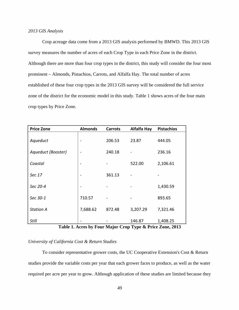
49
2013 GIS Analysis
Crop acreage data come from a 2013 GIS analysis performed by BMWD. This 2013 GIS
survey measures the number of acres of each Crop Type in each Price Zone in the district.
Although there are more than four crop types in the district, this study will consider the four most
prominent – Almonds, Pistachios, Carrots, and Alfalfa Hay. The total number of acres
established of these four crop types in the 2013 GIS survey will be considered the full service
zone of the district for the economic model in this study. Table 1 shows acres of the four main
crop types by Price Zone.
Price Zone Almonds Carrots Alfalfa Hay Pistachios
Aqueduct ‐
206.53
23.87
444.05
Aqueduct (Booster) ‐
240.18
‐
236.16
Coastal ‐
‐
522.00
2,106.61
Sec 17 ‐
361.13
‐
‐
Sec 20‐4 ‐
‐
‐
1,430.59
Sec 30‐1 710.57
‐
‐
893.65
Station A 7,688.62
872.48
3,207.29
7,321.46
Still ‐
‐
146.87
1,408.25
Table 1. Acres by Four Major Crop Type & Price Zone, 2013
University of California Cost & Return Studies
To consider representative grower costs, the UC Cooperative Extension's Cost & Return
studies provide the variable costs per year that each grower faces to produce, as well as the water
required per acre per year to grow. Although application of these studies are limited because they
50
would have to assume conditions that are unchanged spatially and temporally, they do provide
some comparative information for a sample economy. For Almonds, Pistachios, and Alfalfa
Hay, the 2008 studies on the Southern San Joaquin Valley are used. Because there is no 2008
study for carrots in this region, instead the 2004 study from Imperial County is used, with costs
in this analysis converted to 2008 prices using the Producer Price Index (PPI). Furthermore, the
costs to grow and yield for a representative active acre of carrots is divided by three to account
for the usual practice of growing in annual rotation. A summary of these figures are included in
Appendix #1.
U.S. Bureau of Labor Statistics
Data on the Producer Price Index (PPI) come from the U.S. Department of Labor’s
Bureau of Labor Statistics. Data from the period 1996-2013 were collected for this analysis, with
1982 the base year. This PPI data is average, annual in the U.S. for all commodities, and not
seasonally adjusted.
USDA NASS
Estimates for the market prices growers receive for their products come from the
USDA’s National Agricultural Statistics Service. The USDA NASS annual survey estimates the
average annual price received in the United States for various crops and other agricultural
products. These data are available for Almonds, Pistachios, Carrots, and Alfalfa Hay from 1996
to 2013, shown in Table 2.
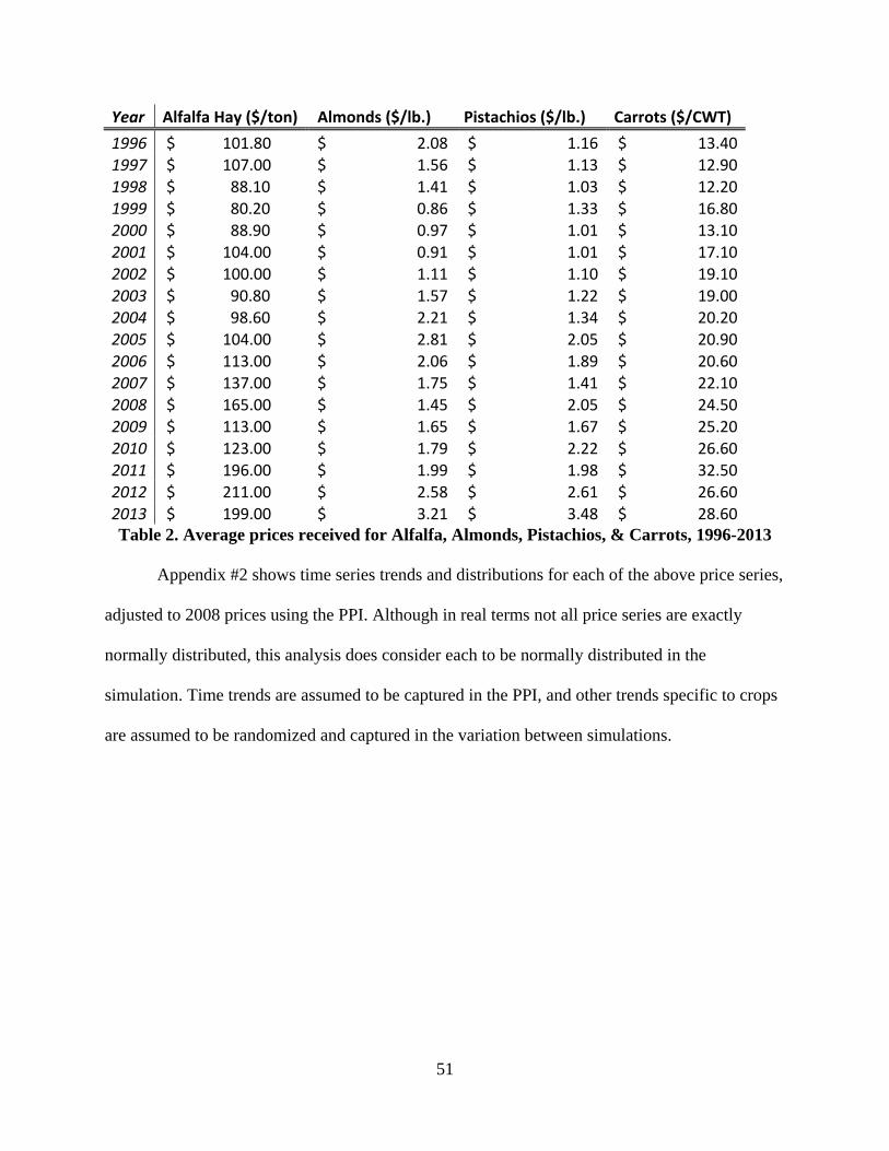
51
Year Alfalfa Hay ($/ton) Almonds ($/lb.) Pistachios ($/lb.) Carrots ($/CWT)
1996 $ 101.80 $ 2.08 $ 1.16 $ 13.40 1997 $ 107.00 $ 1.56 $ 1.13 $ 12.90 1998 $ 88.10 $ 1.41 $ 1.03 $ 12.20 1999 $ 80.20 $ 0.86 $ 1.33 $ 16.80 2000 $ 88.90 $ 0.97 $ 1.01 $ 13.10 2001 $ 104.00 $ 0.91 $ 1.01 $ 17.10 2002 $ 100.00 $ 1.11 $ 1.10 $ 19.10 2003 $ 90.80 $ 1.57 $ 1.22 $ 19.00 2004 $ 98.60 $ 2.21 $ 1.34 $ 20.20 2005 $ 104.00 $ 2.81 $ 2.05 $ 20.90 2006 $ 113.00 $ 2.06 $ 1.89 $ 20.60 2007 $ 137.00 $ 1.75 $ 1.41 $ 22.10
2008 $ 165.00 $ 1.45 $ 2.05 $ 24.50 2009 $ 113.00 $ 1.65 $ 1.67 $ 25.20 2010 $ 123.00 $ 1.79 $ 2.22 $ 26.60 2011 $ 196.00 $ 1.99 $ 1.98 $ 32.50 2012 $ 211.00 $ 2.58 $ 2.61 $ 26.60 2013 $ 199.00 $ 3.21 $ 3.48 $ 28.60
Table 2. Average prices received for Alfalfa, Almonds, Pistachios, & Carrots, 1996-2013
Appendix #2 shows time series trends and distributions for each of the above price series,
adjusted to 2008 prices using the PPI. Although in real terms not all price series are exactly
normally distributed, this analysis does consider each to be normally distributed in the
simulation. Time trends are assumed to be captured in the PPI, and other trends specific to crops
are assumed to be randomized and captured in the variation between simulations.
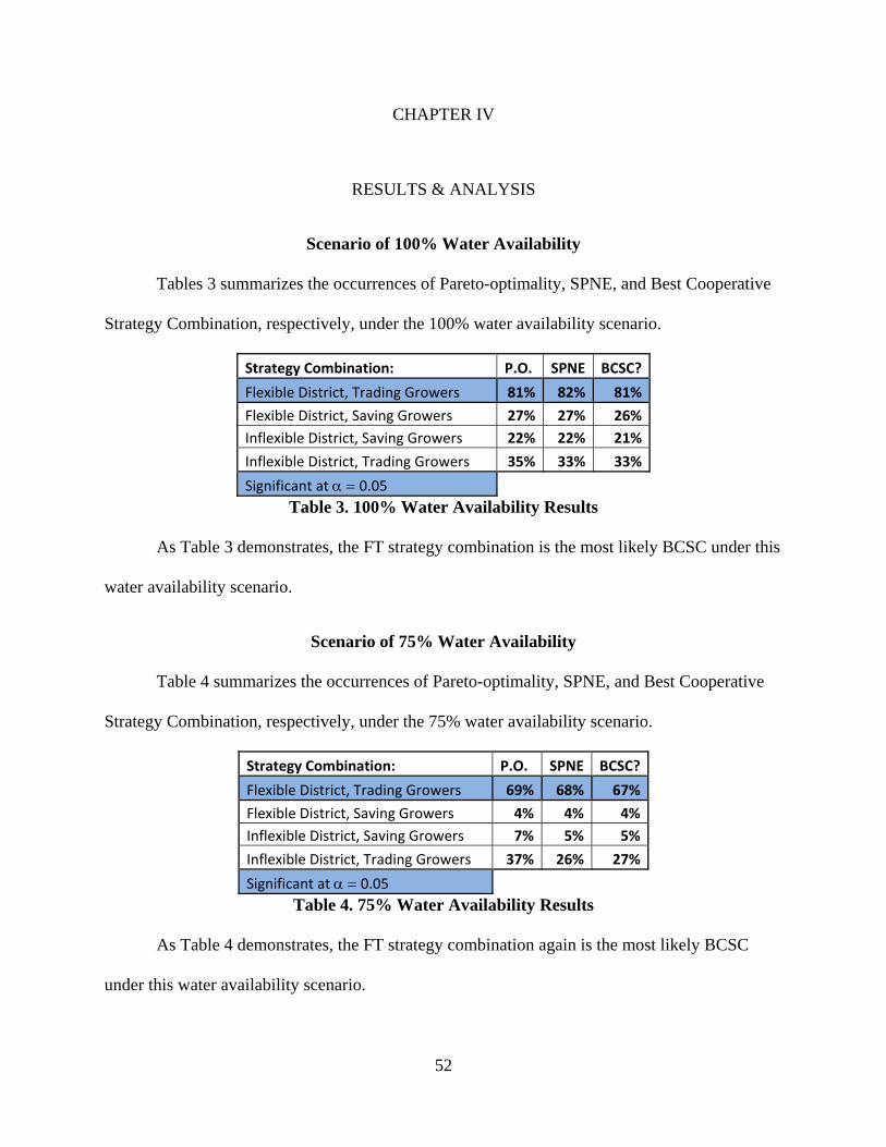
52
CHAPTER IV
RESULTS & ANALYSIS
Scenario of 100% Water Availability
Tables 3 summarizes the occurrences of Pareto-optimality, SPNE, and Best Cooperative
Strategy Combination, respectively, under the 100% water availability scenario.
Strategy Combination: P.O. SPNE BCSC?
Flexible District, Trading Growers 81% 82% 81%
Flexible District, Saving Growers 27% 27% 26%
Inflexible District, Saving Growers 22% 22% 21%
Inflexible District, Trading Growers 35% 33% 33%
Significant at 0.05Table 3. 100% Water Availability Results
As Table 3 demonstrates, the FT strategy combination is the most likely BCSC under this
water availability scenario.
Scenario of 75% Water Availability
Table 4 summarizes the occurrences of Pareto-optimality, SPNE, and Best Cooperative
Strategy Combination, respectively, under the 75% water availability scenario.
Strategy Combination: P.O. SPNE BCSC?
Flexible District, Trading Growers 69% 68% 67%
Flexible District, Saving Growers 4% 4% 4%
Inflexible District, Saving Growers 7% 5% 5%
Inflexible District, Trading Growers 37% 26% 27%
Significant at 0.05Table 4. 75% Water Availability Results
As Table 4 demonstrates, the FT strategy combination again is the most likely BCSC
under this water availability scenario.
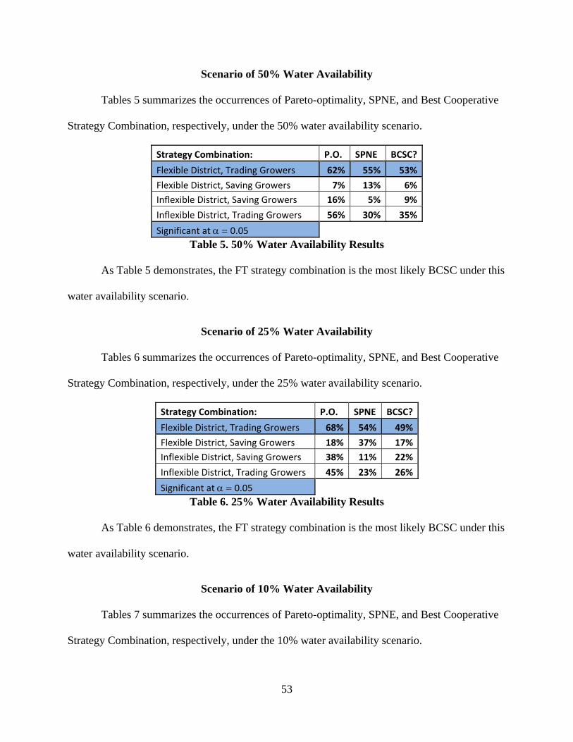
53
Scenario of 50% Water Availability
Tables 5 summarizes the occurrences of Pareto-optimality, SPNE, and Best Cooperative
Strategy Combination, respectively, under the 50% water availability scenario.
Strategy Combination: P.O. SPNE BCSC?
Flexible District, Trading Growers 62% 55% 53%
Flexible District, Saving Growers 7% 13% 6%
Inflexible District, Saving Growers 16% 5% 9%
Inflexible District, Trading Growers 56% 30% 35%
Significant at 0.05Table 5. 50% Water Availability Results
As Table 5 demonstrates, the FT strategy combination is the most likely BCSC under this
water availability scenario.
Scenario of 25% Water Availability
Tables 6 summarizes the occurrences of Pareto-optimality, SPNE, and Best Cooperative
Strategy Combination, respectively, under the 25% water availability scenario.
Strategy Combination: P.O. SPNE BCSC?
Flexible District, Trading Growers 68% 54% 49%
Flexible District, Saving Growers 18% 37% 17%
Inflexible District, Saving Growers 38% 11% 22%
Inflexible District, Trading Growers 45% 23% 26%
Significant at 0.05Table 6. 25% Water Availability Results
As Table 6 demonstrates, the FT strategy combination is the most likely BCSC under this
water availability scenario.
Scenario of 10% Water Availability
Tables 7 summarizes the occurrences of Pareto-optimality, SPNE, and Best Cooperative
Strategy Combination, respectively, under the 10% water availability scenario.
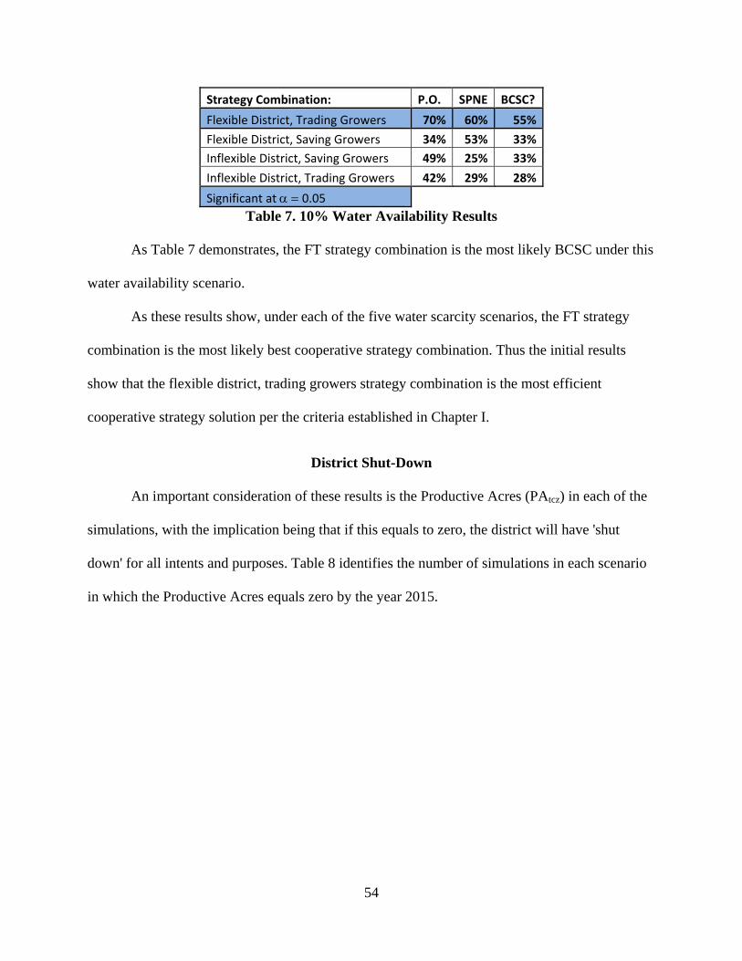
54
Strategy Combination: P.O. SPNE BCSC?
Flexible District, Trading Growers 70% 60% 55%
Flexible District, Saving Growers 34% 53% 33%
Inflexible District, Saving Growers 49% 25% 33%
Inflexible District, Trading Growers 42% 29% 28%
Significant at 0.05Table 7. 10% Water Availability Results
As Table 7 demonstrates, the FT strategy combination is the most likely BCSC under this
water availability scenario.
As these results show, under each of the five water scarcity scenarios, the FT strategy
combination is the most likely best cooperative strategy combination. Thus the initial results
show that the flexible district, trading growers strategy combination is the most efficient
cooperative strategy solution per the criteria established in Chapter I.
District Shut-Down
An important consideration of these results is the Productive Acres (PAtcz) in each of the
simulations, with the implication being that if this equals to zero, the district will have 'shut
down' for all intents and purposes. Table 8 identifies the number of simulations in each scenario
in which the Productive Acres equals zero by the year 2015.
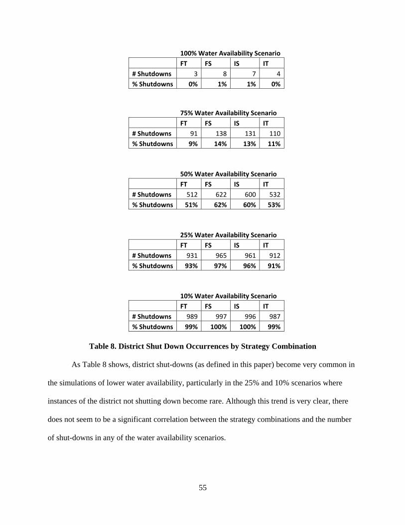
55
100% Water Availability Scenario
FT FS IS IT
# Shutdowns 3 8 7 4
% Shutdowns 0% 1% 1% 0%
75% Water Availability Scenario
FT FS IS IT
# Shutdowns 91 138 131 110
% Shutdowns 9% 14% 13% 11%
50% Water Availability Scenario
FT FS IS IT
# Shutdowns 512 622 600 532
% Shutdowns 51% 62% 60% 53%
25% Water Availability Scenario
FT FS IS IT
# Shutdowns 931 965 961 912
% Shutdowns 93% 97% 96% 91%
10% Water Availability Scenario
FT FS IS IT
# Shutdowns 989 997 996 987
% Shutdowns 99% 100% 100% 99%
Table 8. District Shut Down Occurrences by Strategy Combination
As Table 8 shows, district shut-downs (as defined in this paper) become very common in
the simulations of lower water availability, particularly in the 25% and 10% scenarios where
instances of the district not shutting down become rare. Although this trend is very clear, there
does not seem to be a significant correlation between the strategy combinations and the number
of shut-downs in any of the water availability scenarios.
56
Sensitivity Analysis
To test the strength of the results, a sensitivity analysis is conducted which includes
changes to five different previously fixed variables, a control run which simply is a repeat of the
original model as is, and a full run which varies all five previously fixed variables
simultaneously. SA1 will be the simulation which is the control run.
In SA2, the water requirements for each crop in each year are varied. This simulation
varies both the fixed water requirement, which would remain constant through each of the seven
years, and a variable component, which changes each year. The fixed component is
representative of grower-specific reasons for which water requirements might be different from
grower to grower, such as differing soil water holding capacities, irrigation uniformities, micro-
climates, etc. The variable changes to water requirements would be those to climatic effects on
the whole service area of the district, such as rainfall, evapotranspiration amounts, etc. The fixed
water requirement is randomly selected for each grower for all years of each simulation with the
fixed water requirement used in the initial model set as the mean, and the standard deviation
equal to 0.25 feet for all crops, and assuming normal distribution. The variable factor of the
water requirements is set first as a percentage which applies equally to each grower of each crop.
This is randomized with a mean of 0% and standard deviation of 10%.
SA3 varies the non-water costs assumed in the model based on the UC Cost & Return
studies. This randomization assumes that the mean is set as the fixed amounts from the original
model, and normal distribution. The standard deviation for pistachios and almonds is equal to
15% of the value of the original fixed amounts. The standard deviation for carrots is set to 10%
and alfalfa hay to 25%. The reason for this is the relatively large costs per acre for carrots, and
small for alfalfa hay. SA4 varies the added-price for each year in each price zone. In each year,
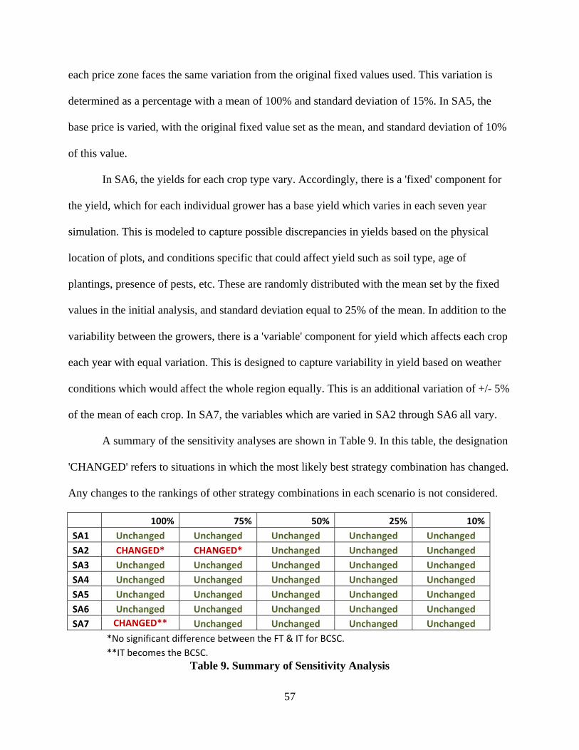
57
each price zone faces the same variation from the original fixed values used. This variation is
determined as a percentage with a mean of 100% and standard deviation of 15%. In SA5, the
base price is varied, with the original fixed value set as the mean, and standard deviation of 10%
of this value.
In SA6, the yields for each crop type vary. Accordingly, there is a 'fixed' component for
the yield, which for each individual grower has a base yield which varies in each seven year
simulation. This is modeled to capture possible discrepancies in yields based on the physical
location of plots, and conditions specific that could affect yield such as soil type, age of
plantings, presence of pests, etc. These are randomly distributed with the mean set by the fixed
values in the initial analysis, and standard deviation equal to 25% of the mean. In addition to the
variability between the growers, there is a 'variable' component for yield which affects each crop
each year with equal variation. This is designed to capture variability in yield based on weather
conditions which would affect the whole region equally. This is an additional variation of +/- 5%
of the mean of each crop. In SA7, the variables which are varied in SA2 through SA6 all vary.
A summary of the sensitivity analyses are shown in Table 9. In this table, the designation
'CHANGED' refers to situations in which the most likely best strategy combination has changed.
Any changes to the rankings of other strategy combinations in each scenario is not considered.
100% 75% 50% 25% 10%
SA1 Unchanged Unchanged Unchanged Unchanged Unchanged
SA2 CHANGED* CHANGED* Unchanged Unchanged Unchanged
SA3 Unchanged Unchanged Unchanged Unchanged Unchanged
SA4 Unchanged Unchanged Unchanged Unchanged Unchanged
SA5 Unchanged Unchanged Unchanged Unchanged Unchanged
SA6 Unchanged Unchanged Unchanged Unchanged Unchanged
SA7 CHANGED** Unchanged Unchanged Unchanged Unchanged
*No significant difference between the FT & IT for BCSC.
**IT becomes the BCSC. Table 9. Summary of Sensitivity Analysis
58
As Table 9 demonstrates, SA1 features no changes in any of the water availability
scenarios, as expected. In fact, the only analyses which feature any changes from the original
simulation are SA2 and SA7. Full results of each sensitivity analysis are summarized in
Appendix #3. The general consistency of the Flexible District, Trading Growers strategy
combination being the BCSC strengthens the argument for hypothesis that this strategy
combination is the most efficient.
59
CHAPTER V
SUMMARY, CONCLUSIONS, AND RECOMMENDATIONS
Summary
The existing problems and impending threats of water scarcity in California calls for not
only technical advancements, which have helped reduce human water use tremendously, but also
progressive management strategies, to figure out how to distribute less water to growing
demands. With regards to agribusiness in California, competition for limited water supply would
seemingly increase the economic value per volume of water tremendously, and create an
incentive for some growers to fallow and sell their water instead. This will depend heavily,
however, on the nature and value of crops grown, and the ability to facilitate transfers by
suppliers of water to agriculture.
Game theory analyses can be insightful tools for determining optimal decision making by
multiple stakeholders. When coordinating decisions, or strategies, the stakeholders, or players,
typically will want to reach Pareto optimal solutions, that is combinations of strategies where no
one could be made better off without someone being made worse off. In water resources, the
general assumption is that stakeholders will want to cooperate, however an efficient cooperative
solution must ensure that no individual stakeholders would be made better off by not
cooperating. A Nash equilibrium in game theory is a strategy combination where each player is
selecting their best strategy combination given the strategy played by the other player. As The
Prisoner's Dilemma and other game theory examples show us, Nash equilibria are not always
Pareto optimal. Therefore, a truly cooperative solution must also be a Nash equilibrium, or a
situation with no Nash equilbiria.
60
This study uses basic information about BMWD to create a two player, two decision
game structure, with one player, the district, selecting their strategy first, then the second player,
the growers, makes theirs. The district has two strategies: be 'flexible,' and allow for short term
trades, or be 'inflexible,' and require that all transfers must be permanent in nature. Growers,
considered as one collective group, will either be 'traders,' and have a propensity to sell water, or
'savers,' and have a propensity to use all of their water, or save in an available groundwater bank.
The pay-off for the district is the total agricultural revenue in the district over a seven year
period, and for growers total real returns, both from their crops and from selling water, over
seven years. The decisions are compared in 1,000 simulations in each of five water scarcity
scenarios: 100%, 75%, 50%, 25%, and 10%.
In order to determine optimal strategy combinations, both Pareto optimality and Nash
equilibria are considered. In the context of this game structure, the best cooperative strategy
combination (BCSC) is considered to be one that is Pareto optimal, and is either a SPNE, or
there are no SPNE. If one strategy combination is the BCSC in significantly more simulations in
all of the water scarcity scenarios, it will be considered the most efficient BCSC. The hypothesis
of this study is that the most efficient BCSC will be that of the district being 'flexible' and the
growers being 'traders.'
Conclusions
The results of this analysis suggest that the hypothesis of this study cannot be rejected.
The 'flexible' district and 'trading' growers did end up being the most likely BCSC in all five
water scarcity scenarios, making it the most efficient BCSC by the definition in this paper. This
matches the literature which suggests the economic efficiency of increased water trading,
particularly in that it will send water to its highest valued economic use. The results also agree
61
with the perceived benefit of short term trades for alleviating the problems of sudden water
scarcity over a shorter period, before longer economic shifts may take effect. A sensitivity
analysis, including one control run and six different iterations with adjustments to some of the
data, were completed for comparative purposes. There were very few changes to the primary
results of the analysis under each of the sensitivity analyses. The three that did have changes
show the 'inflexible' district, 'trading' growers strategy combination to be a BCSC.
An interesting note about the results is that, with the exception of the seemingly
catastrophic scenario of 10% water availability scenario, the 'inflexible' district and 'trading'
growers strategy combination is the second most likely BCSC. This is particularly true for the
50% and 75% water scarcity scenarios, which would hopefully be more likely in reality than the
25% or 10% scenarios, assuming some degree of scarcity is inevitable. This indicates that the
growers' general strategy of trading more, when seemingly advantageous, may be their dominant
strategy. In reality, growers might even want to be more aggressive about trading water than in
this analysis, and trade even if their crops would be profitable if the sale will be more profitable.
Although the results do suggest that short term trades are preferable to long term ones,
intuitively there are certain aspects of long term trades that are more attractive to some growers.
For example, growers who will be purchasing water will likely perceive less risk from a long
term purchase versus a short term one. In reality, the type of trades are going to be dictated by
individual growers themselves for the most part, as most district managers are going to be open
to what growers would like to do, assuming it is fair and feasible. In a district like BMWD,
where both permanent and row crops are present and the real cost per volume of water is highly
correlated to availability, long term transfers which are adjusted yearly in volume and price
depending on realized availability may be the most efficient solution for each party.
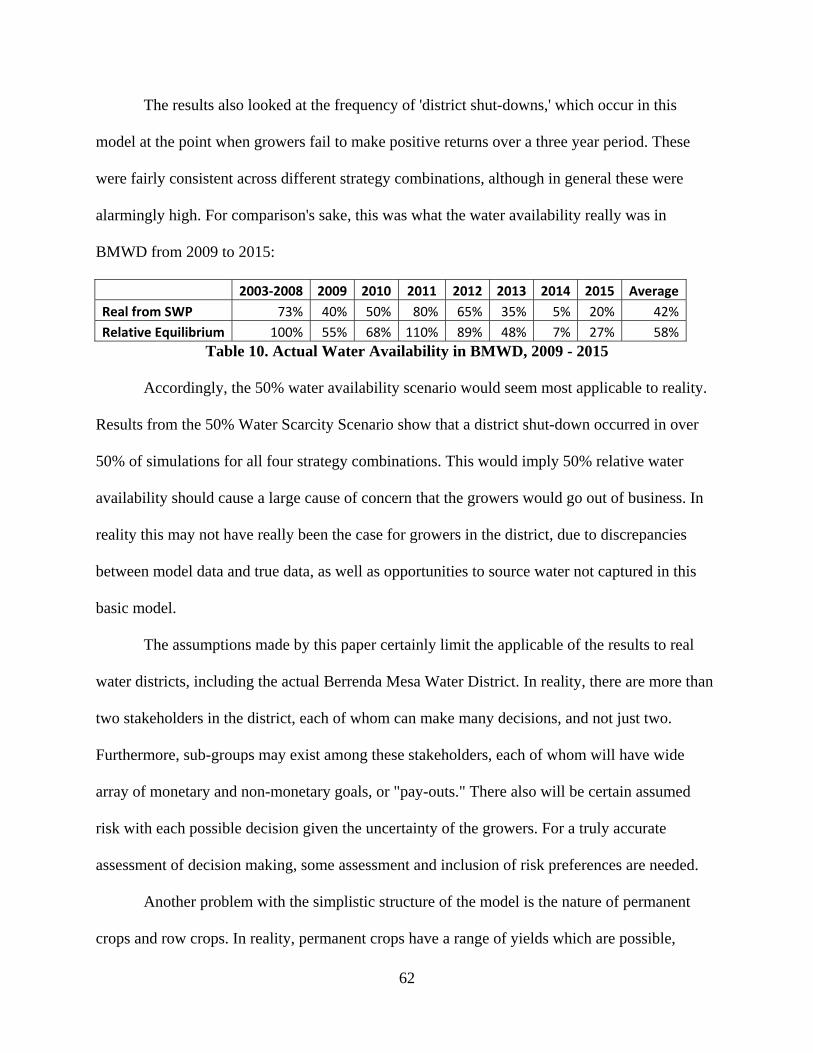
62
The results also looked at the frequency of 'district shut-downs,' which occur in this
model at the point when growers fail to make positive returns over a three year period. These
were fairly consistent across different strategy combinations, although in general these were
alarmingly high. For comparison's sake, this was what the water availability really was in
BMWD from 2009 to 2015:
2003‐2008 2009 2010 2011 2012 2013 2014 2015 Average
Real from SWP 73% 40% 50% 80% 65% 35% 5% 20% 42%
Relative Equilibrium 100% 55% 68% 110% 89% 48% 7% 27% 58%
Table 10. Actual Water Availability in BMWD, 2009 - 2015
Accordingly, the 50% water availability scenario would seem most applicable to reality.
Results from the 50% Water Scarcity Scenario show that a district shut-down occurred in over
50% of simulations for all four strategy combinations. This would imply 50% relative water
availability should cause a large cause of concern that the growers would go out of business. In
reality this may not have really been the case for growers in the district, due to discrepancies
between model data and true data, as well as opportunities to source water not captured in this
basic model.
The assumptions made by this paper certainly limit the applicable of the results to real
water districts, including the actual Berrenda Mesa Water District. In reality, there are more than
two stakeholders in the district, each of whom can make many decisions, and not just two.
Furthermore, sub-groups may exist among these stakeholders, each of whom will have wide
array of monetary and non-monetary goals, or "pay-outs." There also will be certain assumed
risk with each possible decision given the uncertainty of the growers. For a truly accurate
assessment of decision making, some assessment and inclusion of risk preferences are needed.
Another problem with the simplistic structure of the model is the nature of permanent
crops and row crops. In reality, permanent crops have a range of yields which are possible,
63
depending a great deal on the irrigated amount. For example, a grower of almonds or pistachios
could reduce a great deal, although not eliminate, water usage to experience a much lower or no
existent yield, but still be able to grow the following year. Growers of row crops, in reality, are
not able to grow on the same ground every season and therefore may have more variable
requirements based on their crop rotations. This detail may also bias the economic size and
returns contributed by carrots and alfalfa hay in the model.
Recommendations
Although these and other details may cause bias in this study, they also open the door to
advancement of the model for a wider applicability. More strategies may be considered for both
the district and the growers, and the ability to change strategies may be a possibility throughout
simulations. Different pay-outs may be considered for the model to analyze the consistency of
results when different goals are considered. Updated information on the non-water costs for
growing these crops in this area would strengthen the results, as would more detailed information
about the prices received for the quality of products from this region specifically. For a thorough
analysis to be complete, these changes could be incorporated with grower production functions,
identifying what yields are achievable given water applied, with variables including soil type,
irrigation efficiency, evapotranspiration amounts, run-off, etc.
A specific aspect of this analysis which should be analyzed further is the nature of
permanent versus row crops, and this significance when considering water trades. Theoretically,
a good combination of permanent and row crops allows permanent crop growers to purchase
water during dry years. However, in reality there could be contractual obligations for row crop
growers which would force them to continue growing despite potential returns from fallowing
and selling water. Water managers of each crop type may want to consider long-term water
64
transfers which vary in amount and price depending on availability in a given year. This could
ensure growers of permanent crops a more stable supply in light of scarcity, and row crop
growers sure that they will be profitable despite fallowing.
Overall, the determination of a BCSC used in this paper could be applied to a number of
different resource applications and other game theory analyses, including those with more
players and strategies. Although this analysis looks specifically at a district which distributes
only surface water from the SWP, the importance of intra-district trading could become
significant for groundwater districts if groundwater were to become a more excludable good.
Putting restrictions on pumping amounts but allowing growers to trade their rights for pumping
groundwater should help to ensure that the water being used is going to its highest economic use,
providing returns for both the buyer and seller. However, if this type of structure is going to be
implemented, the nature of the crops (row vs. permanent) needs to be considered, as well as the
nature of the trades (long vs. short term), and the growers willingness to buy and sell. Game
theory analyses such as this one could provide insight into optimal management strategies.
65
REFERENCES
Adams, G., Rausser, G., and Simon, L. (1996) Modelling multilateral negotiations: An application to California water policy. Journal of Economic Behavior & Organisation 30, 97-111. Bain, J., Caves, R., & Margolis, J. (1966). Northern California Water Industry: The Competitive Efficiency of Public Enterprise in Developing a Scarce Natural Resource. Baltimore, MD: The Johns Hopkins Press. Baye, M. (2010). Managerial Economics and Business Strategy, 7th Edition. New York, NY: McGraw-Hill. Beede, R., Kallsen, C., Holtz, B., Ferguson, L., Klonsky, K., & DeMoura, R. (2008). Sample Costs to Produce and Establish Market Pistachios - San Joaquin Valley (A report by the University of California Cooperative Extension). Davis, CA. Berrenda Mesa Water District (BMWD). (2013). GIS Analysis of Acreage By Crop (A report by the GIS Department). Lost Hills, CA. Berrenda Mesa Water District (BMWD). (2016). About Us. Retrieved from http://www.bmwd.org/about-us. Burt, C. (2006). Volumetric Pricing Considerations (A report from the Cal Poly Irrigation Training & Research Center). California Polytechnic State University, San Luis Obispo. Burt, C., Mutziger, A., & Cordova, D. (2000). Benchmarking of Flexibility & Needs - Survey of Irrigation Districts - USBR Mid-Pacific Region (A report from the Cal Poly Irrigation Training & Research Center). California Polytechnic State University, San Luis Obispo. California Department of Water Resources (DWR). (2014). California Drought Information. Retreived http://www.water.ca.gov/waterconditions/droughtinfo.cfm California Department of Water Resources (DWR). (2014). Climate Change. Retrieved from http://www.water.ca.gov/climatechange/ California Natural Resources Agency (CRNA). (2008). Managing an Uncertain Future (A report for the CA Department of Water Resources). Sacramento, CA. California State Senate. (2009). Water Conservation Act (SBx7-7). Retrieved February 2, 2014 from http://www.water.ca.gov/wateruseefficiency/sb7/docs/SB7-7-TheLaw.pdf Doll, J., & Orazem, F. (1984). Production Economics, Theory with Applications, 2nd Edition. New York, NY: Wiley.
66
Freeman, M., Viveros, M., Klonsky, K., DeMoura, R. (2008). Sample Costs to Establish an Almond Orchard and Produce Almonds - San Joaquin Valley (A report by the University of California Cooperative Extension). Davis, CA. Governor's Press Office (2015). Governor Brown Directs First Ever Statewide Mandatory Water Reductions. Retrieved from http://drought.ca.gov/topstory/top-story-29.html. Hammett, G. (2014, April 11). Personal Interview. Hanak, E. Lund, J., Gray, B. Houston, D. Howitt, R., Jessoe, K, Thompson, B., Cutter, B.W., Libecap, G., Sumner, D., & Sunding, D. (2012). Water and the California Economy (A report from the Public Policy Institute of California). San Francisco, CA. Hanak, E., & Stryjewski, E. (2012). California's Water Market, By the numbers: Update 2012 (A report from the Public Policy Institute of California). San Francisco, CA. Hansen, K., Howitt, R., & Williams, J. (2014). An econometric test of water market structure in the western United States. Natural Resources Journal 55, 127-152 Howitt, R., Medllin-Azuara, J., MacEwan, D., Lund, J., and Sumner, D. (2014). Economic Analysis of the 2014 Drought for California Agriculture (A report made in collaboration with the Center for Watershed Sceinces, UC Davis, UC Agricultural Issues Center, & ERA Economics). Davis, CA. Kern Economic Development Corporation (KEDC). (2016). Value-Added Agriculture. Retrieved from http://kedc.com/site-selection/target-industries/value-added-agriculture/ Kostyrko, G. (2016). Californians Save 1.19 Million Acre-Feet of Water, Enough to Supply Nearly 6 Million People for a Year. Retrieved from: http://drought.ca.gov/topstory/top- story-57.html Littleworth, A., & Garner, E. (2007). California Water II. Point Arena, CA: Solano Press Books. Madani, K. (2010). Game theory and water resources. Journal of Hydrology 381, 225-238. Madani, K., & Dinar, A. (2012). Non-cooperative institutions for sustainable common pool resource management: Application to groundwater. Journal of Ecological Economics 74, 34-45. Madani K., & Lund, J. (2011). A Monte-Carlo game theoretic approach for Multi-Criteria Decision Making under uncertainty. Advnaces in Water Resources 34, 607-616. Meister, H. (2004). Sample Costs to Produce and Establish Market Carrots - Imperial Valley (A report by the University of California Cooperative Extension). Davis, CA.
67
Mirchi, A., Madani, K., Roos, M., & Watkins, D. (2013). Climate Change Impacts on California’s Water Resources. In K. Schwabe, J. Albiac, J. Connor, R. Hassan, & L. Gonzalez (Eds.), Drought in Arid and Semi-Arid Regions (p. 301-319). New York, NY: Springer. Moran, T., & Kostyrko, G. (2015). Senior Water Rights Curtailed in Delta, San Joaquin & Sacramento Watersheds. Retrieved from http://drought.ca.gov/topstory/top-story-37.html Mount, J., Lund, J., & Hanak, E. (2015). California's Water (A report from the Public Policy Institute of California). San Francisco, CA. Mueller, S., Frate, C., Canevari, M., Campbell-Matthews, M., Klonsky, K., & DeMoura, R. (2008). Sample Costs to Produce and Establish Alfalfa - San Joaquin Valley (A report by the University of California Cooperative Extension). Davis, CA. Regnacq, C., Dinar, A., & Hanak, E. (2016). The gravity of water: Water trade friction in California. In Proceedings of the Meetings of the Allied Soil Science Association, San Francisco, CA, January 2016. Rogers, P. (2016). California drought: Odds of La Niña increase for next winter, bringing concerns the drought may drag on. San Jose Mercury News. Retrieved from http://www.mercurynews.com/drought/ci_29766133/california-drought-odds-la-nina- increase-next-winter Scheierling, S., Loomis, J., & Young, R. (2006). Irrigation water demand: A meta-analysis of price elasticities. Water Resources Research 42, W01411, doi:10.1029/2005WR004009 Small, L., & Rimal, A. (1996). Effects of alternative water distribution rules on irrigation system performance: a simulation analysis. Irrigation and Drainage Systems 10, 25-45. Simon, L., & Stratton, S. (2008). California's Water Problems: Why a Comprehensive Solution Makes Sense. Agricutural & Resource Economics Update 11, 9-11. Styles, S., & Howes, D. (2002). Benchmarking of Flexibility & Needs - Survey of Non-Federal Irrigation Districts (A report from the Cal Poly Irrigation Training & Research Center). California Polytechnic State University, San Luis Obispo. U.S. Bureau of Reclamation. (1997). Incentive Pricing Handbook for Agricultural Water Districts. Washington, D.C.: Hydrosphere Resource Consultants. U.S. Department of Agriculture (2014). Almonds - Prices Received, Measured in $/LB. (A report by the National Agricultural Statistics Service). Washington, D.C. U.S. Department of Agriculture (2014). Carrots, Fresh Market - Prices Received, Measured in $/CWT. (A report by the National Agricultural Statistics Service). Washington, D.C.
68
U.S. Department of Agriculture (2014). Hay, Alfalfa - Prices Received, Measured in $/TON. (A report by the National Agricultural Statistics Service). Washington, D.C. U.S. Department of Agriculture (2014). Pistachios - Prices Received, Measured in $/LB. (A report by the National Agricultural Statistics Service). Washington, D.C. U.S. Department of Labor (2014). Producer Price Index: All Commodities (A report by the Bureau of Labor Statistics). Washington, D.C. Varian, H. (1984). Intermediate Microeconomics: A Modern Approach, 7th Edition. New York, NY: W.W. Norton & Co. Vogel, N., & Thomas, T. (2014). DWR Drops State Water Project Allocation to Zero, Seeks to Preserve Remaining Supply. California Deparment of Water Resources - News for Immediate Release Sacramento, CA. Water Association of Kern County (WAKC). (2016). Sources of Water. Retreived from http://www.wakc.com/index.php/water-overview/sources-of-water Water Association of Kern County (WAKC). (2016). Water Overview. Retreived from http://www.wakc.com/index.php/water-overview/overview Zilberman, D., MacDougall, N., & Shah, F. (1994). Changes in water allocation mechanisms for California agriculture. Contemporary Economic Policy 7, 122-133. Zilberman, D., & Schoengold, K. (2005). The Use of Pricing and Markets for Water Allocation. Canadian Water Resources Journal 30(10), 47-54.
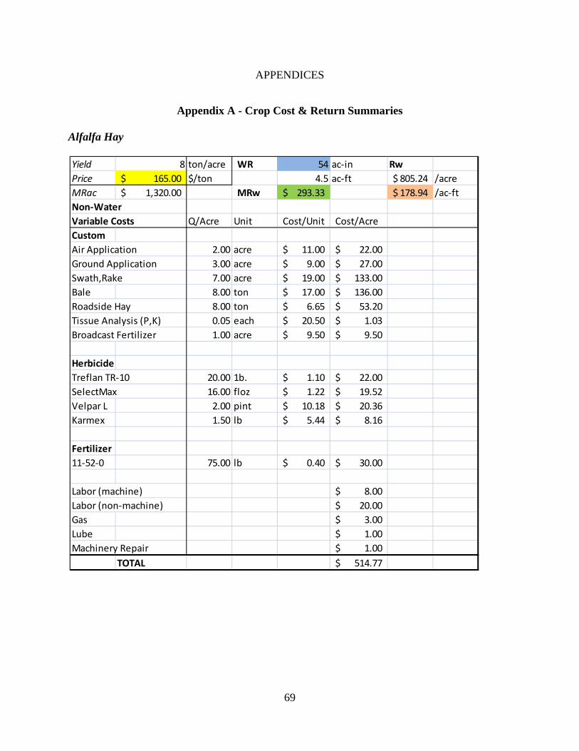
69
APPENDICES
Appendix A - Crop Cost & Return Summaries
Alfalfa Hay
Yield 8 ton/acre WR 54 ac‐in Rw
Price 165.00$ $/ton 4.5 ac‐ft 805.24$ /acre
MRac 1,320.00$ MRw 293.33$ 178.94$ /ac‐ft
Non‐Water
Variable Costs Q/Acre Unit Cost/Unit Cost/Acre
Custom
Air Application 2.00 acre 11.00$ 22.00$
Ground Application 3.00 acre 9.00$ 27.00$
Swath,Rake 7.00 acre 19.00$ 133.00$
Bale 8.00 ton 17.00$ 136.00$
Roadside Hay 8.00 ton 6.65$ 53.20$
Tissue Analysis (P,K) 0.05 each 20.50$ 1.03$
Broadcast Fertilizer 1.00 acre 9.50$ 9.50$
Herbicide
Treflan TR‐10 20.00 1b. 1.10$ 22.00$
SelectMax 16.00 floz 1.22$ 19.52$
Velpar L 2.00 pint 10.18$ 20.36$
Karmex 1.50 lb 5.44$ 8.16$
Fertilizer
11‐52‐0 75.00 lb 0.40$ 30.00$
Labor (machine) 8.00$
Labor (non‐machine) 20.00$
Gas 3.00$
Lube 1.00$
Machinery Repair 1.00$
TOTAL 514.77$
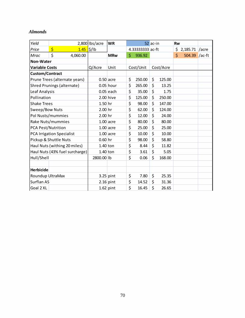
70
Almonds
Yield 2,800 lbs/acre WR 52 ac‐in Rw
Price 1.45$ $/lb 4.33333333 ac‐ft 2,185.71$ /acre
Mrac 4,060.00$ MRw 936.92$ 504.39$ /ac‐ft
Non‐Water
Variable Costs Q/Acre Unit Cost/Unit Cost/Acre
Custom/Contract
Prune Trees (alternate years) 0.50 acre 250.00$ 125.00$
Shred Prunings (alternate) 0.05 hour 265.00$ 13.25$
Leaf Analysis 0.05 each 35.00$ 1.75$
Pollination 2.00 hive 125.00$ 250.00$
Shake Trees 1.50 hr 98.00$ 147.00$
Sweep/Bow Nuts 2.00 hr 62.00$ 124.00$
Pol Nusts/mummies 2.00 hr 12.00$ 24.00$
Rake Nuts/mummies 1.00 acre 80.00$ 80.00$
PCA Pest/Nutrition 1.00 acre 25.00$ 25.00$
PCA Irrigation Specialist 1.00 acre 10.00$ 10.00$
Pickup & Shuttle Nuts 0.60 hr 98.00$ 58.80$
Haul Nuts (withing 20 miles) 1.40 ton 8.44$ 11.82$
Haul Nuts (43% fuel surcharge) 1.40 ton 3.61$ 5.05$
Hull/Shell 2800.00 lb 0.06$ 168.00$
Herbicide
Roundup UltraMax 3.25 pint 7.80$ 25.35$
Surflan AS 2.16 pint 14.52$ 31.36$
Goal 2 XL 1.62 pint 16.45$ 26.65$
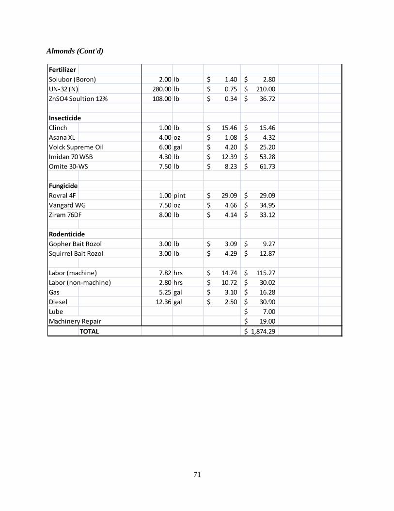
71
Almonds (Cont'd)
Fertilizer
Solubor (Boron) 2.00 lb 1.40$ 2.80$
UN‐32 (N) 280.00 lb 0.75$ 210.00$
ZnSO4 Soultion 12% 108.00 lb 0.34$ 36.72$
Insecticide
Clinch 1.00 lb 15.46$ 15.46$
Asana XL 4.00 oz 1.08$ 4.32$
Volck Supreme Oil 6.00 gal 4.20$ 25.20$
Imidan 70 WSB 4.30 lb 12.39$ 53.28$
Omite 30‐WS 7.50 lb 8.23$ 61.73$
Fungicide
Rovral 4F 1.00 pint 29.09$ 29.09$
Vangard WG 7.50 oz 4.66$ 34.95$
Ziram 76DF 8.00 lb 4.14$ 33.12$
Rodenticide
Gopher Bait Rozol 3.00 lb 3.09$ 9.27$
Squirrel Bait Rozol 3.00 lb 4.29$ 12.87$
Labor (machine) 7.82 hrs 14.74$ 115.27$
Labor (non‐machine) 2.80 hrs 10.72$ 30.02$
Gas 5.25 gal 3.10$ 16.28$
Diesel 12.36 gal 2.50$ 30.90$
Lube 7.00$
Machinery Repair 19.00$
TOTAL 1,874.29$
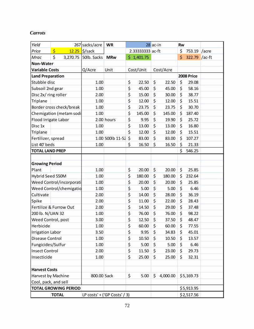
72
Carrots
Yield 267 sacks/acre WR 28 ac‐in Rw
Price 12.25$ $/sack 2.33333333 ac‐ft 753.19$ /acre
Mrac 3,270.75$ 50lb. Sacks MRw 1,401.75$ 322.79$ /ac‐ft
Non‐Water
Variable Costs Q/Acre Unit Cost/Unit Cost/Acre
Land Preparation 2008 Price
Stubble disc 1.00 22.50$ 22.50$ 29.08$
Subsoil 2nd gear 1.00 45.00$ 45.00$ 58.16$
Disc 2x/ ring roller 2.00 15.00$ 30.00$ 38.77$
Triplane 1.00 12.00$ 12.00$ 15.51$
Border cross check/break 1.00 23.75$ 23.75$ 30.70$
Chemigation (metam sodi 1.00 145.00$ 145.00$ 187.40$
Flood Irrigate Labor 2.00 hours 9.95$ 19.90$ 25.72$
Disc 1x 1.00 13.00$ 13.00$ 16.80$
Triplane 1.00 12.00$ 12.00$ 15.51$
Fertilizer, spread 1.00 500lb 11‐52 83.00$ 83.00$ 107.27$
List 40' beds 1.00 16.50$ 16.50$ 21.33$
TOTAL LAND PREP 546.25$
Growing Period
Plant 1.00 20.00$ 20.00$ 25.85$
Hybrid Seed 550M 1.00 180.00$ 180.00$ 232.64$
Weed Control/incorporati 1.00 20.00$ 20.00$ 25.85$
Weed Control/chemigatio 1.00 5.00$ 5.00$ 6.46$
Cultivate 2.00 14.00$ 28.00$ 36.19$
Spike 2.00 11.00$ 22.00$ 28.43$
Fertilize & Furrow Out 2.00 14.50$ 29.00$ 37.48$
200 lb. N/UAN 32 1.00 76.00$ 76.00$ 98.22$
Weed Control, post 3.00 12.50$ 37.50$ 48.47$
Herbicide 1.00 60.00$ 60.00$ 77.55$
Irrigation Labor 3.50 9.95$ 34.83$ 45.01$
Disease Control 1.00 10.50$ 10.50$ 13.57$
Fungicides/Sulfur 1.00 5.00$ 5.00$ 6.46$
Insect Control 2.00 11.50$ 23.00$ 29.73$
Insecticide 1.00 25.00$ 25.00$ 32.31$
Harvest Costs
Harvest by Machine 800.00 Sack 5.00$ 4,000.00$ 5,169.73$
Cool, pack, and sell
TOTAL GROWING PERIOD 5,913.95$
TOTAL LP costs' + ('GP Costs' / 3) 2,517.56$
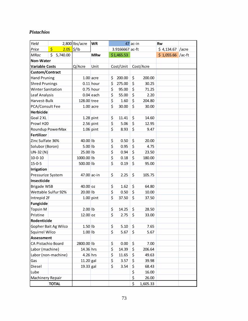
73
Pistachios
Yield 2,800 lbs/acre WR 47 ac‐in Rw
Price 2.05$ $/lb 3.9166667 ac‐ft 4,134.67$ /acre
MRac 5,740.00$ MRw 1,465.53$ 1,055.66$ /ac‐ft
Non‐Water
Variable Costs Q/Acre Unit Cost/Unit Cost/Acre
Custom/Contract
Hand Pruning 1.00 acre 200.00$ 200.00$
Shred Prunings 0.11 hour 275.00$ 30.25$
Winter Sanitation 0.75 hour 95.00$ 71.25$
Leaf Analysis 0.04 each 55.00$ 2.20$
Harvest‐Bulk 128.00 tree 1.60$ 204.80$
PCA/Consult Fee 1.00 acre 30.00$ 30.00$
Herbicide
Goal 2 XL 1.28 pint 11.41$ 14.60$
Prowl H20 2.56 pint 5.06$ 12.95$
Roundup PowerMax 1.06 pint 8.93$ 9.47$
Fertilizer
Zinc Sulfate 36% 40.00 lb 0.50$ 20.00$
Solubor (Boron) 5.00 lb 0.95$ 4.75$
UN‐32 (N) 25.00 lb 0.94$ 23.50$
10‐0‐10 1000.00 lb 0.18$ 180.00$
15‐0‐5 500.00 lb 0.19$ 95.00$
Irrigation
Pressurize System 47.00 ac‐in 2.25$ 105.75$
Insecticide
Brigade WSB 40.00 oz 1.62$ 64.80$
Wettable Sulfur 92% 20.00 lb 0.50$ 10.00$
Intrepid 2F 1.00 pint 37.50$ 37.50$
Fungicide
Topsin M 2.00 lb 14.25$ 28.50$
Pristine 12.00 oz 2.75$ 33.00$
Rodenticide
Gopher Bait Ag Wilco 1.50 lb 5.10$ 7.65$
Squirrel Wilco 1.00 lb 5.67$ 5.67$
Assessment
CA Pistachio Board 2800.00 lb 0.00$ 7.00$
Labor (machine) 14.36 hrs 14.39$ 206.64$
Labor (non‐machine) 4.26 hrs 11.65$ 49.63$
Gas 11.20 gal 3.57$ 39.98$
Diesel 19.33 gal 3.54$ 68.43$
Lube 16.00$
Machinery Repair 26.00$
TOTAL 1,605.33$
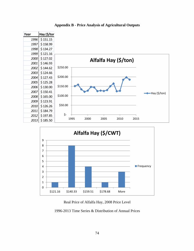
74
Appendix B - Price Analysis of Agricultural Outputs
Real Price of Alfalfa Hay, 2008 Price Level
1996-2013 Time Series & Distribution of Annual Prices
Year Hay ($/ton
1996 151.15$
1997 158.99$
1998 134.27$
1999 121.16$
2000 127.02$
2001 146.93$
2002 144.62$
2003 124.66$
2004 127.43$
2005 125.28$
2006 130.00$
2007 150.41$
2008 165.00$
2009 123.91$
2010 126.26$
2011 184.79$
2012 197.85$
2013 185.50$
$‐
$50.00
$100.00
$150.00
$200.00
$250.00
1995 2000 2005 2010 2015
Alfalfa Hay ($/ton)
Hay ($/ton)
0
1
2
3
4
5
6
7
8
9
$121.16 $140.33 $159.51 $178.68 More
Alfalfa Hay ($/CWT)
Frequency
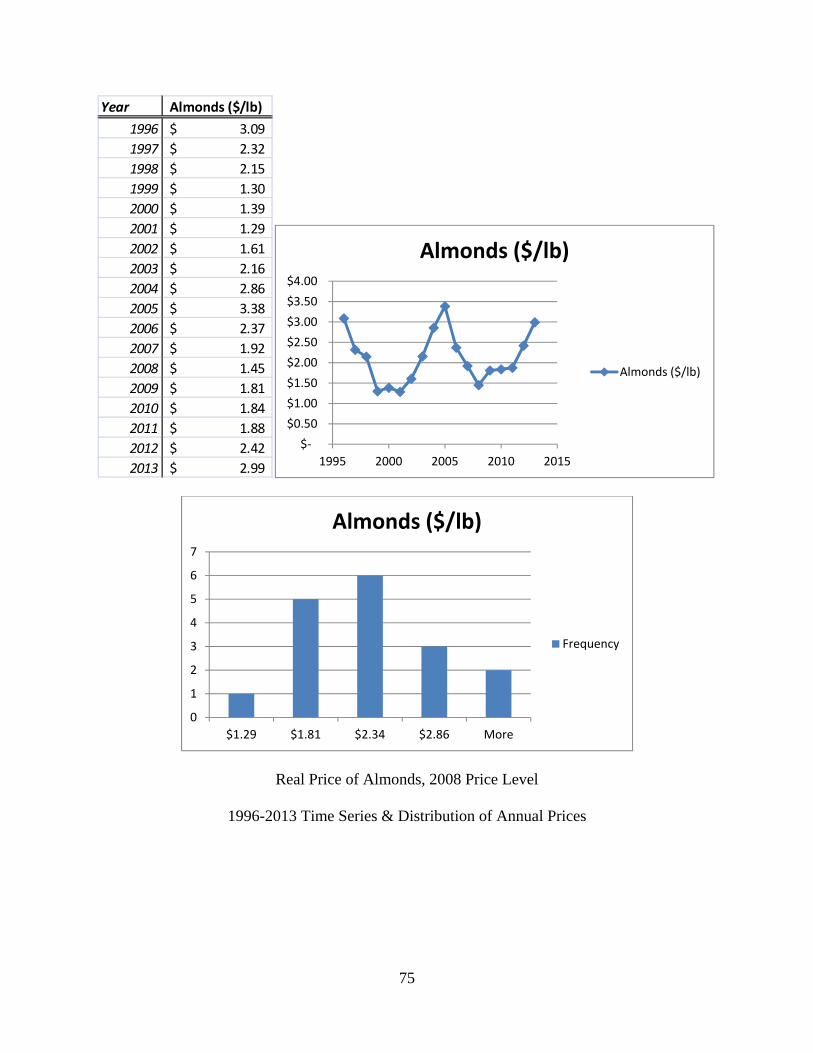
75
Real Price of Almonds, 2008 Price Level
1996-2013 Time Series & Distribution of Annual Prices
Year Almonds ($/lb)
1996 3.09$
1997 2.32$
1998 2.15$
1999 1.30$
2000 1.39$
2001 1.29$
2002 1.61$
2003 2.16$
2004 2.86$
2005 3.38$
2006 2.37$
2007 1.92$
2008 1.45$
2009 1.81$
2010 1.84$
2011 1.88$
2012 2.42$
2013 2.99$
$‐
$0.50
$1.00
$1.50
$2.00
$2.50
$3.00
$3.50
$4.00
1995 2000 2005 2010 2015
Almonds ($/lb)
Almonds ($/lb)
0
1
2
3
4
5
6
7
$1.29 $1.81 $2.34 $2.86 More
Almonds ($/lb)
Frequency
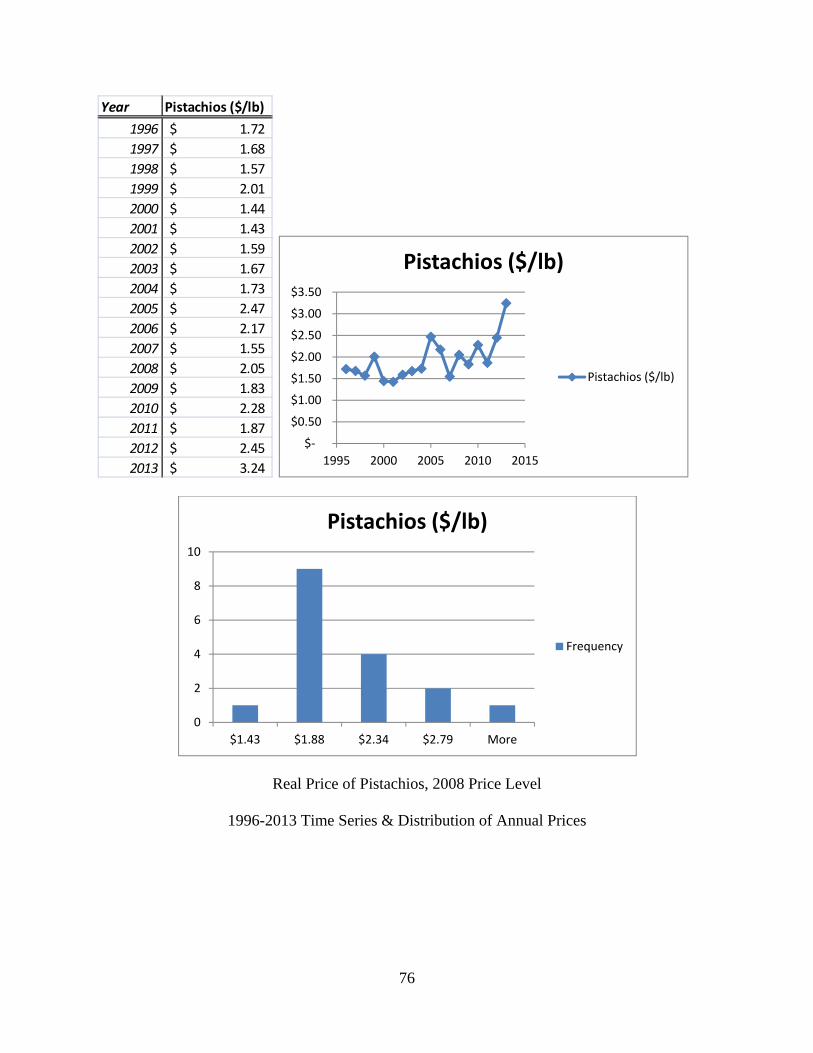
76
Real Price of Pistachios, 2008 Price Level
1996-2013 Time Series & Distribution of Annual Prices
Year Pistachios ($/lb)
1996 1.72$
1997 1.68$
1998 1.57$
1999 2.01$
2000 1.44$
2001 1.43$
2002 1.59$
2003 1.67$
2004 1.73$
2005 2.47$
2006 2.17$
2007 1.55$
2008 2.05$
2009 1.83$
2010 2.28$
2011 1.87$
2012 2.45$
2013 3.24$
$‐
$0.50
$1.00
$1.50
$2.00
$2.50
$3.00
$3.50
1995 2000 2005 2010 2015
Pistachios ($/lb)
Pistachios ($/lb)
0
2
4
6
8
10
$1.43 $1.88 $2.34 $2.79 More
Pistachios ($/lb)
Frequency
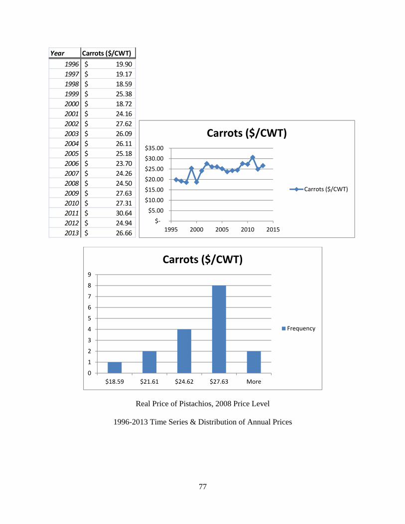
77
Real Price of Pistachios, 2008 Price Level
1996-2013 Time Series & Distribution of Annual Prices
Year Carrots ($/CWT)
1996 19.90$
1997 19.17$
1998 18.59$
1999 25.38$
2000 18.72$
2001 24.16$
2002 27.62$
2003 26.09$
2004 26.11$
2005 25.18$
2006 23.70$
2007 24.26$
2008 24.50$
2009 27.63$
2010 27.31$
2011 30.64$
2012 24.94$
2013 26.66$
$‐
$5.00
$10.00
$15.00
$20.00
$25.00
$30.00
$35.00
1995 2000 2005 2010 2015
Carrots ($/CWT)
Carrots ($/CWT)
0
1
2
3
4
5
6
7
8
9
$18.59 $21.61 $24.62 $27.63 More
Carrots ($/CWT)
Frequency
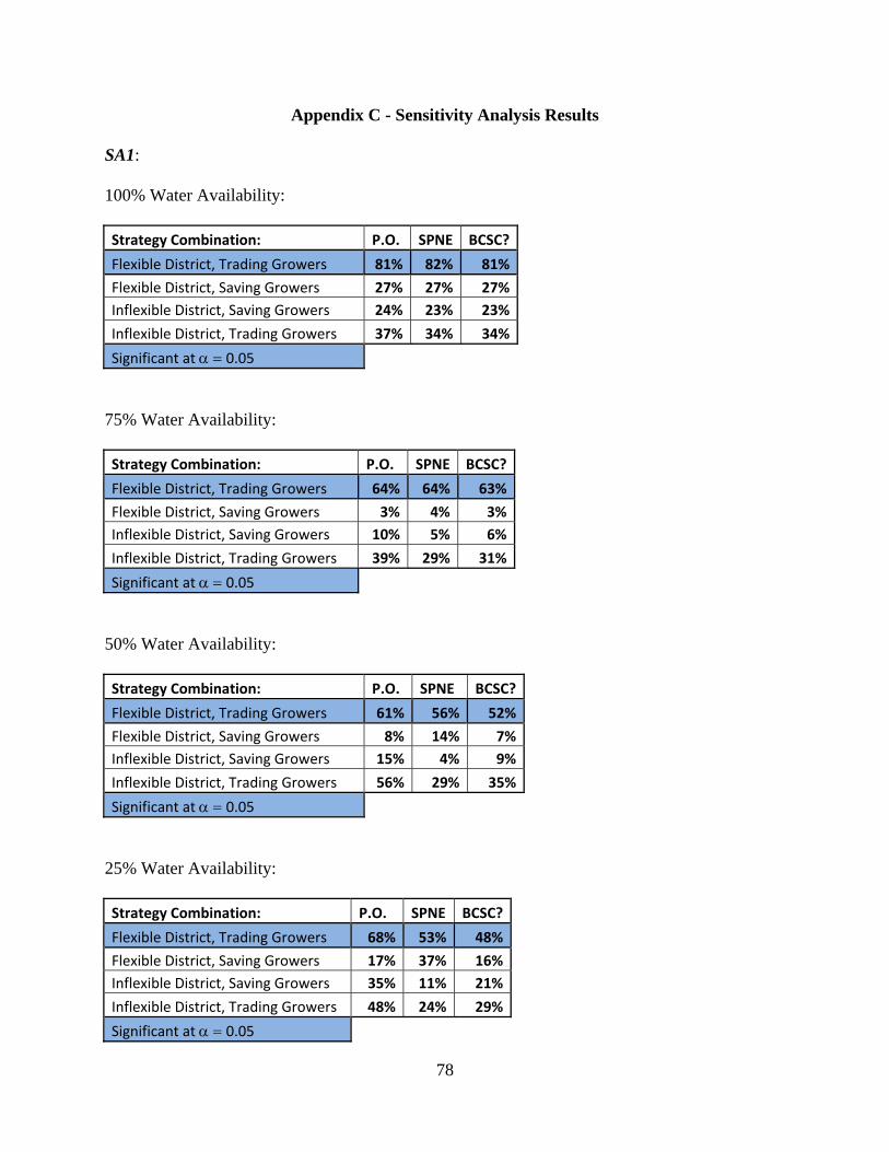
78
Appendix C - Sensitivity Analysis Results
SA1:
100% Water Availability:
Strategy Combination: P.O. SPNE BCSC?
Flexible District, Trading Growers 81% 82% 81%
Flexible District, Saving Growers 27% 27% 27%
Inflexible District, Saving Growers 24% 23% 23%
Inflexible District, Trading Growers 37% 34% 34%
Significant at 0.05
75% Water Availability:
Strategy Combination: P.O. SPNE BCSC?
Flexible District, Trading Growers 64% 64% 63%
Flexible District, Saving Growers 3% 4% 3%
Inflexible District, Saving Growers 10% 5% 6%
Inflexible District, Trading Growers 39% 29% 31%
Significant at 0.05
50% Water Availability:
Strategy Combination: P.O. SPNE BCSC?
Flexible District, Trading Growers 61% 56% 52%
Flexible District, Saving Growers 8% 14% 7%
Inflexible District, Saving Growers 15% 4% 9%
Inflexible District, Trading Growers 56% 29% 35%
Significant at 0.05
25% Water Availability:
Strategy Combination: P.O. SPNE BCSC?
Flexible District, Trading Growers 68% 53% 48%
Flexible District, Saving Growers 17% 37% 16%
Inflexible District, Saving Growers 35% 11% 21%
Inflexible District, Trading Growers 48% 24% 29%
Significant at 0.05
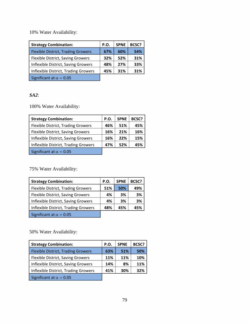
79
10% Water Availability:
Strategy Combination: P.O. SPNE BCSC?
Flexible District, Trading Growers 67% 60% 54%
Flexible District, Saving Growers 32% 52% 31%
Inflexible District, Saving Growers 48% 27% 33%
Inflexible District, Trading Growers 45% 31% 31%
Significant at 0.05
SA2:
100% Water Availability:
Strategy Combination: P.O. SPNE BCSC?
Flexible District, Trading Growers 46% 51% 45%
Flexible District, Saving Growers 16% 21% 16%
Inflexible District, Saving Growers 16% 22% 15%
Inflexible District, Trading Growers 47% 52% 45%
Significant at 0.05
75% Water Availability:
Strategy Combination: P.O. SPNE BCSC?
Flexible District, Trading Growers 51% 50% 49%
Flexible District, Saving Growers 4% 3% 3%
Inflexible District, Saving Growers 4% 3% 3%
Inflexible District, Trading Growers 48% 45% 45%
Significant at 0.05
50% Water Availability:
Strategy Combination: P.O. SPNE BCSC?
Flexible District, Trading Growers 63% 51% 50%
Flexible District, Saving Growers 11% 11% 10%
Inflexible District, Saving Growers 14% 8% 11%
Inflexible District, Trading Growers 41% 30% 32%
Significant at 0.05
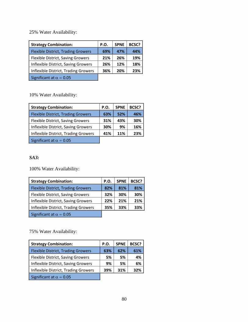
80
25% Water Availability:
Strategy Combination: P.O. SPNE BCSC?
Flexible District, Trading Growers 69% 47% 44%
Flexible District, Saving Growers 21% 26% 19%
Inflexible District, Saving Growers 26% 12% 18%
Inflexible District, Trading Growers 36% 20% 23%
Significant at 0.05
10% Water Availability:
Strategy Combination: P.O. SPNE BCSC?
Flexible District, Trading Growers 63% 52% 46%
Flexible District, Saving Growers 31% 43% 30%
Inflexible District, Saving Growers 30% 9% 16%
Inflexible District, Trading Growers 41% 11% 23%
Significant at 0.05
SA3:
100% Water Availability:
Strategy Combination: P.O. SPNE BCSC?
Flexible District, Trading Growers 82% 81% 81%
Flexible District, Saving Growers 32% 30% 30%
Inflexible District, Saving Growers 22% 21% 21%
Inflexible District, Trading Growers 35% 33% 33%
Significant at 0.05
75% Water Availability:
Strategy Combination: P.O. SPNE BCSC?
Flexible District, Trading Growers 63% 62% 61%
Flexible District, Saving Growers 5% 5% 4%
Inflexible District, Saving Growers 9% 5% 6%
Inflexible District, Trading Growers 39% 31% 32%
Significant at 0.05
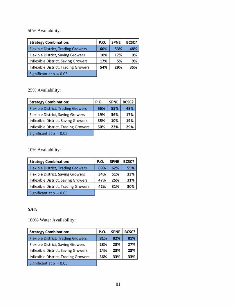
81
50% Availability:
Strategy Combination: P.O. SPNE BCSC?
Flexible District, Trading Growers 60% 53% 48%
Flexible District, Saving Growers 10% 17% 9%
Inflexible District, Saving Growers 17% 5% 9%
Inflexible District, Trading Growers 54% 29% 35%
Significant at 0.05
25% Availability:
Strategy Combination: P.O. SPNE BCSC?
Flexible District, Trading Growers 66% 55% 48%
Flexible District, Saving Growers 19% 36% 17%
Inflexible District, Saving Growers 35% 10% 19%
Inflexible District, Trading Growers 50% 23% 29%
Significant at 0.05
10% Availability:
Strategy Combination: P.O. SPNE BCSC?
Flexible District, Trading Growers 69% 62% 55%
Flexible District, Saving Growers 34% 51% 33%
Inflexible District, Saving Growers 47% 25% 31%
Inflexible District, Trading Growers 42% 31% 30%
Significant at 0.05
SA4:
100% Water Availability:
Strategy Combination: P.O. SPNE BCSC?
Flexible District, Trading Growers 81% 82% 81%
Flexible District, Saving Growers 28% 28% 27%
Inflexible District, Saving Growers 24% 23% 23%
Inflexible District, Trading Growers 36% 33% 33%
Significant at 0.05
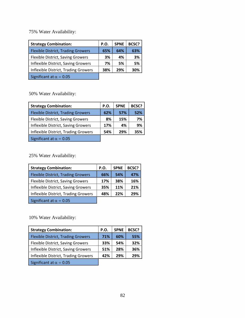
82
75% Water Availability:
Strategy Combination: P.O. SPNE BCSC?
Flexible District, Trading Growers 65% 64% 63%
Flexible District, Saving Growers 3% 4% 3%
Inflexible District, Saving Growers 7% 5% 5%
Inflexible District, Trading Growers 38% 29% 30%
Significant at 0.05
50% Water Availability:
Strategy Combination: P.O. SPNE BCSC?
Flexible District, Trading Growers 62% 57% 52%
Flexible District, Saving Growers 8% 15% 7%
Inflexible District, Saving Growers 17% 4% 9%
Inflexible District, Trading Growers 54% 29% 35%
Significant at 0.05
25% Water Availability:
Strategy Combination: P.O. SPNE BCSC?
Flexible District, Trading Growers 66% 54% 47%
Flexible District, Saving Growers 17% 38% 16%
Inflexible District, Saving Growers 35% 11% 21%
Inflexible District, Trading Growers 48% 22% 29%
Significant at 0.05
10% Water Availability:
Strategy Combination: P.O. SPNE BCSC?
Flexible District, Trading Growers 71% 60% 55%
Flexible District, Saving Growers 33% 54% 32%
Inflexible District, Saving Growers 51% 28% 36%
Inflexible District, Trading Growers 42% 29% 29%
Significant at 0.05
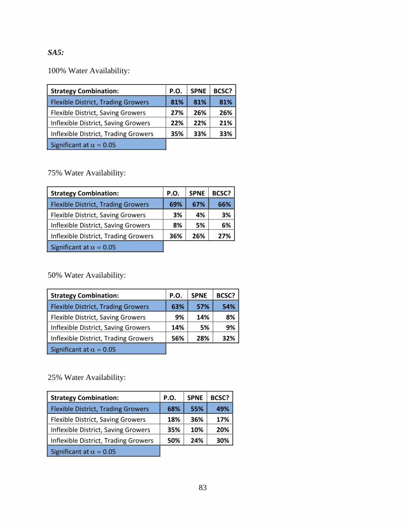
83
SA5:
100% Water Availability:
Strategy Combination: P.O. SPNE BCSC?
Flexible District, Trading Growers 81% 81% 81%
Flexible District, Saving Growers 27% 26% 26%
Inflexible District, Saving Growers 22% 22% 21%
Inflexible District, Trading Growers 35% 33% 33%
Significant at 0.05
75% Water Availability:
Strategy Combination: P.O. SPNE BCSC?
Flexible District, Trading Growers 69% 67% 66%
Flexible District, Saving Growers 3% 4% 3%
Inflexible District, Saving Growers 8% 5% 6%
Inflexible District, Trading Growers 36% 26% 27%
Significant at 0.05
50% Water Availability:
Strategy Combination: P.O. SPNE BCSC?
Flexible District, Trading Growers 63% 57% 54%
Flexible District, Saving Growers 9% 14% 8%
Inflexible District, Saving Growers 14% 5% 9%
Inflexible District, Trading Growers 56% 28% 32%
Significant at 0.05
25% Water Availability:
Strategy Combination: P.O. SPNE BCSC?
Flexible District, Trading Growers 68% 55% 49%
Flexible District, Saving Growers 18% 36% 17%
Inflexible District, Saving Growers 35% 10% 20%
Inflexible District, Trading Growers 50% 24% 30%
Significant at 0.05
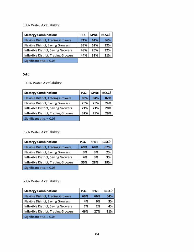
84
10% Water Availability:
Strategy Combination: P.O. SPNE BCSC?
Flexible District, Trading Growers 71% 61% 56%
Flexible District, Saving Growers 33% 52% 32%
Inflexible District, Saving Growers 48% 26% 32%
Inflexible District, Trading Growers 44% 31% 31%
Significant at 0.05
SA6:
100% Water Availability:
Strategy Combination: P.O. SPNE BCSC?
Flexible District, Trading Growers 83% 84% 82%
Flexible District, Saving Growers 25% 25% 24%
Inflexible District, Saving Growers 21% 21% 20%
Inflexible District, Trading Growers 32% 29% 29%
Significant at 0.05
75% Water Availability:
Strategy Combination: P.O. SPNE BCSC?
Flexible District, Trading Growers 69% 68% 67%
Flexible District, Saving Growers 3% 3% 2%
Inflexible District, Saving Growers 4% 3% 3%
Inflexible District, Trading Growers 35% 28% 29%
Significant at 0.05
50% Water Availability:
Strategy Combination: P.O. SPNE BCSC?
Flexible District, Trading Growers 69% 66% 64%
Flexible District, Saving Growers 4% 6% 3%
Inflexible District, Saving Growers 7% 2% 4%
Inflexible District, Trading Growers 46% 27% 31%
Significant at 0.05
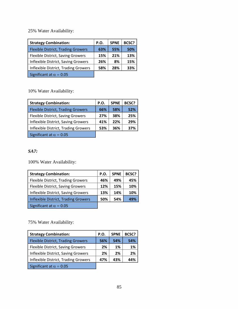
85
25% Water Availability:
Strategy Combination: P.O. SPNE BCSC?
Flexible District, Trading Growers 63% 55% 50%
Flexible District, Saving Growers 15% 21% 13%
Inflexible District, Saving Growers 26% 8% 15%
Inflexible District, Trading Growers 58% 28% 33%
Significant at 0.05
10% Water Availability:
Strategy Combination: P.O. SPNE BCSC?
Flexible District, Trading Growers 66% 58% 52%
Flexible District, Saving Growers 27% 38% 25%
Inflexible District, Saving Growers 41% 22% 29%
Inflexible District, Trading Growers 53% 36% 37%
Significant at 0.05
SA7:
100% Water Availability:
Strategy Combination: P.O. SPNE BCSC?
Flexible District, Trading Growers 46% 49% 45%
Flexible District, Saving Growers 12% 15% 10%
Inflexible District, Saving Growers 13% 14% 10%
Inflexible District, Trading Growers 50% 54% 49%
Significant at 0.05
75% Water Availability:
Strategy Combination: P.O. SPNE BCSC?
Flexible District, Trading Growers 56% 54% 54%
Flexible District, Saving Growers 2% 1% 1%
Inflexible District, Saving Growers 2% 2% 2%
Inflexible District, Trading Growers 47% 43% 44%
Significant at 0.05
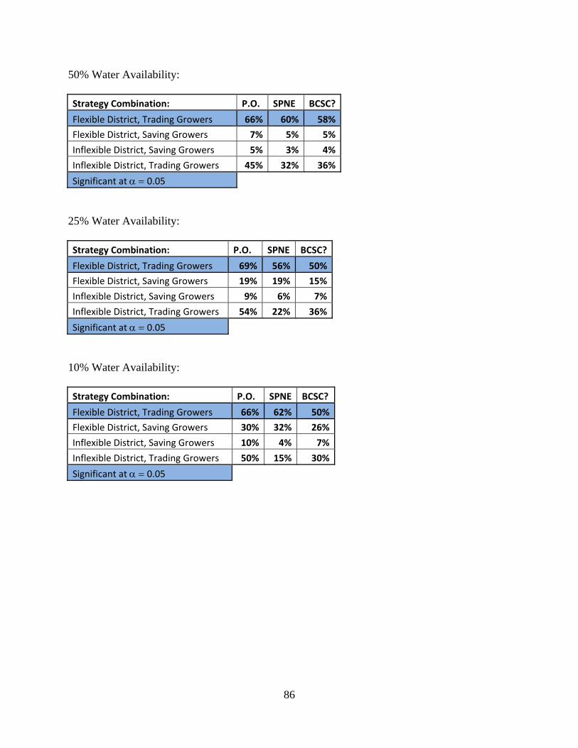
86
50% Water Availability:
Strategy Combination: P.O. SPNE BCSC?
Flexible District, Trading Growers 66% 60% 58%
Flexible District, Saving Growers 7% 5% 5%
Inflexible District, Saving Growers 5% 3% 4%
Inflexible District, Trading Growers 45% 32% 36%
Significant at 0.05
25% Water Availability:
Strategy Combination: P.O. SPNE BCSC?
Flexible District, Trading Growers 69% 56% 50%
Flexible District, Saving Growers 19% 19% 15%
Inflexible District, Saving Growers 9% 6% 7%
Inflexible District, Trading Growers 54% 22% 36%
Significant at 0.05
10% Water Availability:
Strategy Combination: P.O. SPNE BCSC?
Flexible District, Trading Growers 66% 62% 50%
Flexible District, Saving Growers 30% 32% 26%
Inflexible District, Saving Growers 10% 4% 7%
Inflexible District, Trading Growers 50% 15% 30%
Significant at 0.05
Related Documents