1 Galois Fields and Cyclic Codes Phil Lucht Rimrock Digital Technology, Salt Lake City, Utah 84103 last update: Aug 31, 2013 Maple code is available upon request. Comments and errata are welcome. The material in this document is copyrighted by the author. The graphics look ratty in Windows Adobe PDF viewers when not scaled up, but look just fine in this excellent freeware viewer: http://www.tracker-software.com/pdf-xchange-products-comparison-chart . The table of contents has live links. Preface ...................................................................................................................................................... 5 Summary .................................................................................................................................................. 6 Chapter 1: Modern Algebra................................................................................................................ 11 (a) Groups, Fields and Rings............................................................................................................... 11 (b) Groups and Subgroups .................................................................................................................. 15 1. Subgroups, cosets, coset leaders, coset decomposition, N/k = m, normal subgroups................. 15 2. The Factor Group G/H formed from a group G and a normal subgroup H ................................ 15 3. Cyclic Groups and Cyclic Subgroups ......................................................................................... 16 4. Additive Groups and Additive Cyclic Groups : the Vector Space of group elements ............... 18 5. Example of an additive cyclic group: {Mod-n,+}....................................................................... 21 (c) Rings and Ideals ............................................................................................................................ 22 1. Ideals, residue classes, residue class leaders, residue class decomposition, N/n = m ................. 22 2. The Residue Class Ring R/I formed from a ring R and an ideal I .............................................. 23 3. Principle Ideals and Principle Ideal Rings .................................................................................. 24 4. Example of a ring: Z n ≡ {Mod-n,+,•} ; Modulo Arithmetic ....................................................... 24 5. Example of a Residue Class Ring: Z/(n) .................................................................................... 27 6. Some basic facts about the integer ring Z ................................................................................... 29 7. The Residue Class Ring Z/(n) is a field if n is prime .................................................................. 30 Chapter 2: The Galois Fields GF(p) ................................................................................................... 32 (a) More Discussion of Z n = { mod-n,+,•} ......................................................................................... 32 (b) The relation between GF(p) and Z p ............................................................................................... 33 (c) Selected facts about GF(p) = Z p (p = prime) ................................................................................. 35 Chapter 3: Polynomials ....................................................................................................................... 37 (a) Specification of the ring R of polynomials with coefficients in Z p ............................................... 37 (b) Basic facts about polynomials with coefficients in a ring R......................................................... 39 (c) The meaning of a polynomial in R being irreducible in R ............................................................ 41 (d) The Residue Class Decomposition of R ........................................................................................ 43 (e) Comparison Between Chapter 3 and Chapter 1............................................................................. 46

Welcome message from author
This document is posted to help you gain knowledge. Please leave a comment to let me know what you think about it! Share it to your friends and learn new things together.
Transcript

1
Galois Fields and Cyclic Codes Phil Lucht
Rimrock Digital Technology, Salt Lake City, Utah 84103 last update: Aug 31, 2013
Maple code is available upon request. Comments and errata are welcome. The material in this document is copyrighted by the author. The graphics look ratty in Windows Adobe PDF viewers when not scaled up, but look just fine in this excellent freeware viewer: http://www.tracker-software.com/pdf-xchange-products-comparison-chart . The table of contents has live links.
Preface...................................................................................................................................................... 5 Summary.................................................................................................................................................. 6 Chapter 1: Modern Algebra................................................................................................................ 11
(a) Groups, Fields and Rings............................................................................................................... 11 (b) Groups and Subgroups .................................................................................................................. 15
1. Subgroups, cosets, coset leaders, coset decomposition, N/k = m, normal subgroups................. 15 2. The Factor Group G/H formed from a group G and a normal subgroup H ................................ 15 3. Cyclic Groups and Cyclic Subgroups ......................................................................................... 16 4. Additive Groups and Additive Cyclic Groups : the Vector Space of group elements ............... 18 5. Example of an additive cyclic group: {Mod-n,+}....................................................................... 21
(c) Rings and Ideals ............................................................................................................................ 22 1. Ideals, residue classes, residue class leaders, residue class decomposition, N/n = m................. 22 2. The Residue Class Ring R/I formed from a ring R and an ideal I .............................................. 23 3. Principle Ideals and Principle Ideal Rings .................................................................................. 24 4. Example of a ring: Zn ≡ {Mod-n,+,•} ; Modulo Arithmetic....................................................... 24 5. Example of a Residue Class Ring: Z/(n).................................................................................... 27 6. Some basic facts about the integer ring Z ................................................................................... 29 7. The Residue Class Ring Z/(n) is a field if n is prime .................................................................. 30
Chapter 2: The Galois Fields GF(p) ................................................................................................... 32 (a) More Discussion of Zn = { mod-n,+,•} ......................................................................................... 32 (b) The relation between GF(p) and Zp............................................................................................... 33 (c) Selected facts about GF(p) = Zp (p = prime) ................................................................................. 35
Chapter 3: Polynomials ....................................................................................................................... 37 (a) Specification of the ring R of polynomials with coefficients in Zp ............................................... 37 (b) Basic facts about polynomials with coefficients in a ring R......................................................... 39 (c) The meaning of a polynomial in R being irreducible in R ............................................................ 41 (d) The Residue Class Decomposition of R........................................................................................ 43 (e) Comparison Between Chapter 3 and Chapter 1............................................................................. 46
2
Chapter 4: The Galois Fields GF(q=pm ). .......................................................................................... 48 (a) GF(p) is a subfield of GF(q) .......................................................................................................... 48 (b) Representing GF(q) Field Elements as Polynomials and as m-tuples........................................... 49 (c) Extending polynomials from ground field GF(p) to extension field GF(q) .................................. 52 (d) Cyclic Subgroups and GF(q)......................................................................................................... 53 (e) An example of root factorization in GF(22) .................................................................................. 60 (f) Two ways to label elements of GF(q) in the + and • tables........................................................... 61 (g) Selected Facts About GF(q) .......................................................................................................... 62
Chapter 5: The Minimum Polynomial of an element of GF(q)........................................................ 63 (a) The Minimum Polynomial m(x) of an element α in GF(q). .......................................................... 63 (b) Primitive Polynomials and the Period of m(x) .............................................................................. 65 (c) Formula for the Minimum Polynomial m(x) of α : Conjugate Sets ............................................. 66
1. Minimum and primitive polynomials of GF(23) ......................................................................... 70 2. Minimum and primitive polynomials of GF(24) ......................................................................... 71 3. Minimum and primitive polynomials of GF(25) ......................................................................... 73 4. Minimum and primitive polynomials of GF(p) for p = 2,3,5,7................................................... 74
(d) How many primitive elements and primitive polynomials are there for GF(pm)?......................... 76 (e) On finding the minimum and primitive polynomials of GF(pm) expressed over GF(p) ................ 77 (f) Selecting f(x) for GF(q) = R/( f(x) ) ; Classifying Irreducible Polynomials .................................. 81 (g) More facts about conjugate sets and minimum polynomials ........................................................ 82 (h) Cyclotomic Cosets......................................................................................................................... 85 (i) Least Common Multiples of minimum polynomials ..................................................................... 86 (j) Order = Period Theorem for a minimum polynomial .................................................................... 87 (k) Maple code to compute all minimum and primitive polynomials for any GF(pm) ........................ 89
Chapter 6: The GF(q) Enumeration Table........................................................................................ 94 (a) Development History of the Primitive Polynomial ....................................................................... 94 (b) Using a Primitive Polynomial as the f(x) in GF(q) = R/( f(x) )..................................................... 96
Constructing the Enumeration Table for GF(q) .............................................................................. 98 Example GF(23) .............................................................................................................................. 99 Example GF(24) ............................................................................................................................ 102 Example GF(25) ............................................................................................................................ 102 Example GF(32) ............................................................................................................................ 103
(c) Using Maple to build any GF(q) Enumeration Table .................................................................. 104 (d) Using the GF(q) Table to multiply out polynomials factored in GF(q) ...................................... 107
1. Expansion of a factored minimum polynomial: an example..................................................... 107 2. Maple expansion of factored minimum polynomials for GF(23), GF(24), GF(25) ................... 108 3. Factoring polynomials in Maple ............................................................................................... 110 4. Multiplying GF(2) polynomials in Maple................................................................................. 112 5. Finding GF(2) quotients and remainders in Maple ................................................................... 112 6. Finding all Irreducible and Minimum Polynomials of GF(2m) ................................................. 113 7. Connection with Peterson and Weldon Appendix C.................................................................114
(e) Construction of the + and • tables for GF(22) ............................................................................. 115
3
Chapter 7: Linear Block Codes ........................................................................................................ 117 (a) The Basics ................................................................................................................................... 117 (b) Notational Remarks..................................................................................................................... 120 (c) The Perp Space and the Parity Check Matrix H .......................................................................... 122 (d) The Dual Code generated by H ................................................................................................... 123 (e) The Systematic Basis................................................................................................................... 124 (f) The notion of Distance between code words: Error Correction................................................... 126 (g) What does the real code space picture look like?........................................................................ 131 (h) Encoders and Decoders: The Syndrome ..................................................................................... 134 (i) Important codes, code history, and other kinds of codes ............................................................. 134
Chapter 8: Cyclic Codes .................................................................................................................... 136 (a) Definition of a Cyclic Code: The Cyclic Basis ........................................................................... 136 (b) The Systematic Basis versus the Cyclic Basis ............................................................................ 138 (c) Implementation of Encoders and Decoders................................................................................. 139 (d) Cyclic Redundancy Check (CRC)............................................................................................... 141
Example: Ethernet CRC-32 .......................................................................................................... 142 (e) The 1-to-1 relationship between the Cyclic Basis and the Systematic Basis .............................. 143 (f) Why Cyclic Codes are Cyclic ...................................................................................................... 145 (g) A Cyclic Code as an Ideal of the Ring An = Rq / ( xn - 1 ).......................................................... 147 (h) The Standard Array and Cyclic Code Error Correction .............................................................. 150 (i) Galois-Induced Cyclic Codes and the Parity Check Matrix H..................................................... 153 (j) Motivation for g(x) to have coefficients in GF(p)........................................................................155 (k) The Code Word Exhaustion-by-Rotation Theorem .................................................................... 158
Chapter 9: A Small Survey of a few Standard Code Families ....................................................... 161 (a) The BCH Codes........................................................................................................................... 161 (b) The Narrow-Sense BCH Codes................................................................................................... 163 (c) Narrow-Sense BCH Codes with N = 1 and Hamming Codes ..................................................... 168
1. The H matrix for the Narrow-Sense BCH Codes with N = 1 ................................................... 168 2. The H1 Matrix and Hamming Codes ........................................................................................ 170 3. Error Correction capabilities of Hamming Codes..................................................................... 171 4. A Modified Hamming Code ..................................................................................................... 171
(d) The Reed-Solomon Codes........................................................................................................... 174 (e) Galois Field GF(2m) Math compared to Digital Filter Math........................................................ 176
Chapter 10: Matrix Representation of a Galois Field .................................................................... 177 (a) How to construct a matrix representation for GF(q) ................................................................... 177 (b) Specification of the ring Rp
m of matrix polynomials with coefficients in Zp .............................. 181 (c) The Companion Matrix ............................................................................................................... 182 (d) Maple program to construct the matrix representation of GF(pm) ............................................... 187
Appendix A: Proof of Fact 10 (4.29)................................................................................................. 190 Appendix B: The Nature of the Conjugate Set of α ........................................................................ 194 Appendix C: Evaluation of a(x)b(x) ................................................................................................. 197 Appendix D: A Small Collection of Matrix Facts ........................................................................... 199 Appendix E: Existence of g(x) which divides xn- 1 . ........................................................................ 204

4
Appendix F: Cyclic Code Error Detection Theorems (CRC) ........................................................ 209 Appendix G: GCD, mod n, totient φ(n), Euler Theorem, Fermat's Little Theorem ................... 212 Appendix H: Order Reversal Theorems for Irreducible Polynomials.......................................... 220 References ............................................................................................................................................ 226
Preface
5
"Now, what I want is, Facts. Teach these boys and girls nothing but Facts. Facts alone are wanted in life. Plant nothing else, and root out everything else." Charles Dickens, Hard Times Preface This document is written for readers who are non-experts in modern algebra and coding theory. It is mainly a "theory" document, but still contains many down-to-earth examples. There are no discussions of detailed error-correction implementations as are found in books on error correction (e.g., Rhee), but the tight connection between Galois fields and cyclic codes is hopefully made very clear. In some coding texts, the review of modern algebra is so brief and dense that comprehension is quite difficult, especially for someone totally unfamiliar with the subject. Conversely, in some math books the discussion of modern algebra is so comprehensive that one is forced to invest in many concepts unnecessary for Galois field applications We have attempted to bridge this gap. The wonderfully efficient and dense mathematical notations like ∈ ∀ | ∃ ⇔ iff are generally replaced by words. Some well-known theorems are not proved, but those that are proved are treated with a (hopefully) reasonable amount of rigor. Lots of "words" are used to reinforce the various concepts, many examples are provided, and there is constant (perhaps excessive) repetition to grind in definitions and "facts" (Mr. Thomas Gradgrind, schoolmaster, is the character quoted above). After doing manual examples, it is often shown how algorithms can be automated using very simple Maple programs, Maple being a commercial symbolic computer algebra system. Freeware systems exist (see wiki) and our short Maple programs can easily be translated into other languages which support the constructs used. The structure of a document like this one involves certain design issues. On the one hand, if a simple Fact applies to a larger class of objects than we are really interested in, but if proving the Fact for that larger class of objects is no harder than for the smaller class, one might as well prove the Fact in its more general application. The reader is then forced to learn somewhat more than necessary, but this seems fairly harmless. Some Facts are so simple to prove, and perhaps so interesting, that they are included in the forest of Facts, even though they are not directly needed on this particular voyage through the forest. On the other hand, one might argue that the forest then becomes so cluttered with trees that a voyager loses track of where he or she is going, and which trees are important and which are not. The relative importance of various trees only becomes clear later in the trip when certain applications of the Facts are considered. It is useful to pause from time to time and review the trip up to the current point of rest, and that is done in several places in the document. In an earlier version of this document, there were no equation numbers but the Facts in each chapter had Fact numbers starting with Fact 1. Although now redundant, most of these Fact numbers have been retained. One might then see Fact 4 (7.35) as a cross-reference. Equation numbers of the form (3.14) are applied to equations, Facts and certain definitions. When a numbered item is quoted later in the document, the equation number is put in italics. Some proofs end with the letters QED so the reader knows where the text flow continues.

Summary
6
Summary This is a detailed summary. The reader is directed to the Table of Contents for a more concise overview. Chapter 1 [Algebra] is a partial review of Modern Algebra which includes only concepts that will be needed in later sections. The basic subjects here are groups, fields, rings and ideals. The so-called residue class ring is formed as R/I where R is a ring and I is an ideal. In particular, Z/(n) is such a residue class ring where Z are the integers and (n) is the ideal which consists of integers which are multiplies of n. It is shown that this residue class ring is isomorphic to the ring of integers mod n, called Zn. It is then shown that if n is a prime number p, the rings Z/(n) and Zn are fields. Many "facts" are accumulated in this chapter, and most of them have analogs in the polynomial world introduced in Chapter 3. Chapter 2 [GF(p)] provides more information about Zn with a few examples. It then shows that the fields Z/(p) and Zp are isomorphic to the Galois Field GF(p). The field operations of GF(p) = Zp = Z/(p) are here called • and + and we learn how to construct the addition and multiplication tables for GF(p). Various facts about GF(p) are then developed. Some authors refer to Galois Fields simply as finite fields, since that is what they in fact are. The argument of GF(*) denotes the number of elements in the finite field. Two of these elements are always 0 and 1. Chapter 3 [Polynomials] discusses another ring, the ring of polynomials R whose coefficients lie in Zp= GF(p). In this chapter, the operations of GF(p) are called ⊕ and ⊗. Basic facts concerning such polynomials are developed in analogy with similar properties of integers presented back in Chapter 1. Within the polynomial world, the notion of an irreducible polynomial is introduced and is seen to be analogous to the notion of a prime number in the integer world. An ideal within the polynomial ring R, called ( f(x) ), consists of all polynomials which are multiples of a polynomial f(x). Then, just as in Chapter 1 for integers, here the residue class ring R/( f(x) ) is shown to be a field when f(x) is an irreducible polynomial in R. In Chapter 4 [GF(q)] it is shown that, if irreducible polynomial f(x) is of degree m, then the field R/(f(x)) is in fact isomorphic to Galois Field GF(pm). Each element of GF(pm) can be associated with a possible remainder polynomial which is obtainable when a polynomial in R is divided by f(x). Since these remainder polynomials are of degree < m and have coefficients in GF(p) = Zp, there are pm of them. Each remainder polynomial, and thus each element of GF(q), can be represented as an m-tuple of Zp elements which are the remainder polynomial coefficients. Since the only finite fields that exist are these GF(pm) where p is a prime number and m a positive integer, we have at this point a "model" (realization, representation) for all the Galois Fields. A method for determining the + and • tables for any GF(q = pm) is then developed based on this model. There follows a lengthy discussion of the notion of cyclic groups with respect to the GF(q) fields, and after much work it is shown that the non-zero elements of every Galois Field GF(q) form a cyclic group with respect to the • operator. This means that it is possible to find some element in GF(q) (a generator) whose powers enumerate all non-zero elements of the field, an extremely useful fact. This is the "power basis" and serves as a second method of labeling elements of GF(q), the first being the m-tuple basis mentioned above. Each basis leads to a different labeling of the headings of the + and • tables for GF(q).

Summary
7
It is then shown that the polynomial xq - x can be written as a product of q factors of the form (x-ai) where the ai are the q elements of GF(q):
(xq - x ) = (x - a1)•(x - a2)•(x - a3)•(x - a4)•......(x - aq) . In other words, xq - x can be fully factored in GF(q). Another way to say this is that the q elements of GF(q) are all roots of the polynomial xq - x. This implies that αq = α for any α in GF(q). The chapter then closes with a few facts about GF(q) similar to those presented at the end of Chapter 2 for GF(p). It is shown that GF(p) is a subfield of GF(pm) and both these fields have the same 0 and 1 elements. In some ways, this is similar to the real numbers being a subfield of the complex numbers, those two fields of course being infinite fields and thus not Galois fields. Chapter 5 [Minimum and Primitive Polynomials] broaches the topic of the minimum polynomial m(x) of an element α of GF(q). Such a polynomial is simply a portion of the above displayed product of factors (x-ai) which includes (x-α) and includes the smallest set of other (x-ai) factors which, when multiplied out, results in m(x) having coefficients all lying in Zp = GF(p). In general, some arbitrary product of the (x-ai) factors will form a polynomial with coefficients in GF(q) which contains GF(p). Since the factor (x-α) is included, m(α) = 0. It is shown that any minimum polynomial is irreducible in GF(p). It turns out that a given minimum polynomial m(x) is the minimum polynomial of all the GF(q) elements ai that appear in those other (x-ai) factors which make up its portion of the fully factored xq - x. The set of GF(q) elements for which some m(x) is the minimum polynomial is called a conjugate set. If element α of GF(q) is a primitive element of GF(q), meaning its powers can enumerate all the non-zero elements of GF(q) as noted above, then the minimum polynomial of α is called a primitive polynomial of GF(q). We determine exactly how many primitive polynomials GF(q) has. The question of how minimum and primitive polynomials are determined is then discussed with various examples. A primitive polynomial f(x) of GF(q=pm) is always of degree m, and can therefore serve as the f(x) in the residue class ring R/(f(x)) which represents GF(q). It is shown that the conjugate sets partition the elements of GF(q), and this is then related to the subject of cyclotomic cosets. Section (i) discusses certain products of minimum polynomials which will appear later in the theory of BCH codes. Section (j) shows that the order of an element of GF(q) is equal to the period of the corresponding minimum polynomial. Finally, section (k) provides a short Maple program which generates all the minimum polynomials (in factored form) of any Galois Field. Chapter 6 [GF(q) Enumeration Table] shows how one determines the "enumeration table" of any Galois Field GF(q=pm). This table is based on a selected primitive element α and its corresponding primitive polynomial m(x). Since m(α) = 0, this equation gives a way to express αm as a sum of lower powers of α times coefficients. One first enumerates all the non-zero elements of GF(q) as powers of primitive element α up to power αq-2, and then one uses this αm reduction equation to express the higher powers in terms of lesser powers, and the result is the "table" for GF(q). The table is useful because, once it is known, one can immediately obtain the addition table for the field GF(q). The multiplication table in this "powers basis" is completely trivial. In section (c) a very simple Maple program is used to directly construct enumeration tables for several GF(q) fields. Given the enumeration table for a field, section (d) shows how one can then expand the factored minimum polynomials of Chapter 5 to verify that they do indeed have coefficients in GF(p). Along the way we show how Maple can be used to accomplish various tasks like factoring a polynomial
Summary
8
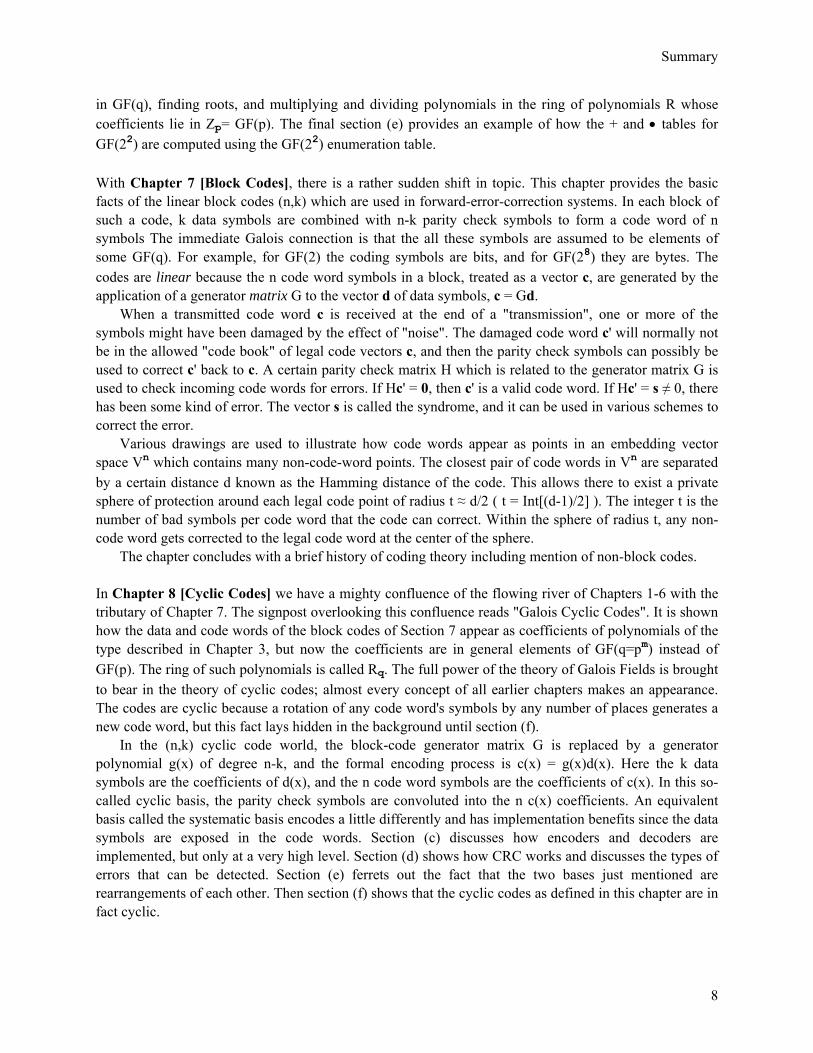
in GF(q), finding roots, and multiplying and dividing polynomials in the ring of polynomials R whose coefficients lie in Zp= GF(p). The final section (e) provides an example of how the + and • tables for GF(22) are computed using the GF(22) enumeration table. With Chapter 7 [Block Codes], there is a rather sudden shift in topic. This chapter provides the basic facts of the linear block codes (n,k) which are used in forward-error-correction systems. In each block of such a code, k data symbols are combined with n-k parity check symbols to form a code word of n symbols The immediate Galois connection is that the all these symbols are assumed to be elements of some GF(q). For example, for GF(2) the coding symbols are bits, and for GF(28) they are bytes. The codes are linear because the n code word symbols in a block, treated as a vector c, are generated by the application of a generator matrix G to the vector d of data symbols, c = Gd. When a transmitted code word c is received at the end of a "transmission", one or more of the symbols might have been damaged by the effect of "noise". The damaged code word c' will normally not be in the allowed "code book" of legal code vectors c, and then the parity check symbols can possibly be used to correct c' back to c. A certain parity check matrix H which is related to the generator matrix G is used to check incoming code words for errors. If Hc' = 0, then c' is a valid code word. If Hc' = s ≠ 0, there has been some kind of error. The vector s is called the syndrome, and it can be used in various schemes to correct the error. Various drawings are used to illustrate how code words appear as points in an embedding vector space Vn which contains many non-code-word points. The closest pair of code words in Vn are separated by a certain distance d known as the Hamming distance of the code. This allows there to exist a private sphere of protection around each legal code point of radius t ≈ d/2 ( t = Int[(d-1)/2] ). The integer t is the number of bad symbols per code word that the code can correct. Within the sphere of radius t, any non-code word gets corrected to the legal code word at the center of the sphere. The chapter concludes with a brief history of coding theory including mention of non-block codes. In Chapter 8 [Cyclic Codes] we have a mighty confluence of the flowing river of Chapters 1-6 with the tributary of Chapter 7. The signpost overlooking this confluence reads "Galois Cyclic Codes". It is shown how the data and code words of the block codes of Section 7 appear as coefficients of polynomials of the type described in Chapter 3, but now the coefficients are in general elements of GF(q=pm) instead of GF(p). The ring of such polynomials is called Rq. The full power of the theory of Galois Fields is brought to bear in the theory of cyclic codes; almost every concept of all earlier chapters makes an appearance. The codes are cyclic because a rotation of any code word's symbols by any number of places generates a new code word, but this fact lays hidden in the background until section (f). In the (n,k) cyclic code world, the block-code generator matrix G is replaced by a generator polynomial g(x) of degree n-k, and the formal encoding process is c(x) = g(x)d(x). Here the k data symbols are the coefficients of d(x), and the n code word symbols are the coefficients of c(x). In this so-called cyclic basis, the parity check symbols are convoluted into the n c(x) coefficients. An equivalent basis called the systematic basis encodes a little differently and has implementation benefits since the data symbols are exposed in the code words. Section (c) discusses how encoders and decoders are implemented, but only at a very high level. Section (d) shows how CRC works and discusses the types of errors that can be detected. Section (e) ferrets out the fact that the two bases just mentioned are rearrangements of each other. Then section (f) shows that the cyclic codes as defined in this chapter are in fact cyclic.
Summary
9
In section (g) the dormant residue-class-ring machinery introduced in Chapter 1 and used in Chapter 3 is powered up again, this time in double overdrive. First, a nameless ring An with qn elements is defined as Rq/(xn-1); its elements are associated with remainder polynomials of degree < n and can be regarded as the points of the code-embedding vector space Vn. This ring An contains the qk code word polynomials c(x) along with the qn-qk "illegal" code word polynomials, all mixed together. In a second residue-class-ring application, the elements of An are used in An/(g(x)) to form what is called the standard array. In this array, all the legal code words are rounded up into one bin which is the ideal ( g(x) ), the first row of the standard array. Then in section (h) it is shown how this standard array "does" error correction. It is a rather amazing logical thread. Section (i) then shows the form of the parity check matrix H for a cyclic code, and gives a top level picture of the code families associated with the names BCH, Hamming and Reed-Solomon. The first and last code families can be designed to correct an arbitrary number t of symbol errors in a code word and are very efficient at doing it. Section (j) explains why one might want the coefficients of the generator polynomial g(x) to lie in G(p) rather than G(q). The reason is that this makes the design of hardware polynomial multipliers and dividers extremely simple. This desire to have g(x) have coefficients in GF(p) is a major driver for all the work of Chapter 5 on minimal polynomials, as is seen in Chapter 9. The final section (k) shows that, for our Galois-induced cyclic codes, one can generate all the code words of the code by rotating any one of them, as long as the generator polynomial is a primitive polynomial. Chapter 9 [Small Code Survey] states the BCH Bound Theorem and defines the BCH cyclic codes as those which optimize this theorem. The theorem provides a floor for distance d and therefore error-correcting ability t. The order of a BCH code with respect to GF(q) is always n = q-1 = pm-1, whereas the k value of the (n,k) code designation is an integer forced by the code. The so-called narrow-sense BCH codes are a special case which have the coefficients of g(x) in GF(p). The generators gN(x) of such codes are the "least common multiples" of N of the minimum polynomials described in Chapter 5. An example with GF(25) is worked out in some detail, providing several BCH codes with code length n = 31. A simple subset of the narrow-sense BCH codes have g(x) = a single minimum polynomial, and from this subset various Hamming codes are derived, though historically the Hamming codes were known before the BCH codes revealed their Galois Field underpinnings. Finally it is shown how the Reed-Solomon codes have g(x) coefficients in GF(q) rather than GF(p) and, despite increased implementation costs, are able to correct the most possible errors that any (n,k) code can correct ; they are maximum-distance separable. The final section (e) comments on how Galois logic uses the algebra of GF(q), whereas digital filters use that of Zq. Chapter 10 [Matrix Representation of GF(q)] is another change of topic. It is shown how one can easily construct a representation of any GF(q=pm) field as a set of q mxm matrices whose elements lie in GF(p). Two critical ingredients are the Cayley-Hamilton Theorem and the notion of a Companion Matrix. A very simple Maple program is then presented which generates a set of q matrices which represent any GF(q) Galois field. (continued on next page)
Summary
10
Appendix A gives a proof of a certain claim (4.29) made in Chapter 4 upon which is based the derivation of the important fact that all Galois fields are cyclic. Appendix B explains the basic nature of the conjugate set of α as encountered in Chapter 5. Appendix C evaluates the polynomial product a(x)b(x). Appendix D is a brief matrix review in support of Chapter 10. Appendix E discusses how cyclic code generators g(x) can be found. Then through a guided thread of Facts, it shows that, for a code using symbols in GF(p) and for code length n ≠ Np, an irreducible g(x) exists and is in fact a minimum polynomial of GF(pφ(n)) where φ(m) is Euler's totient function. Appendix F discusses in detail the nature of the errors that a CRC error detection system system can detect. CRC means Cyclic Redundancy Check and is used for example to protect Ethernet packets. Appendix G is a brief excursion into the dense terrain of Number Theory resulting in the derivation of two classic results: Euler's Theorem and Fermat's Little Theorem. Euler's totient function φ(n) is defined and it is shown how φ(n) determines the number of primitive elements of a Galois Field and also the number of primitive polynomials. A few References are then provided.
Chapter 1: Modern Algebra
11
Chapter 1: Modern Algebra The purpose of this chapter is to point out and give recognizable names to some of the animals which inhabit the landscape of modern algebra. We do so in a non-rigorous manner, because we want to get done as fast as possible. We try to include only those ideas that are necessary for our development to come in later chapters. Not everything is proved, because the proofs all exist in standard texts. We are more interested in showing how things are defined and how they fit together. The reader looking for more on this subject would do well to consult Birkhoff and MacLane (see References). When a word of phrase is being defined, that word or phrase is put in bold font to make the definition easier to locate later on. ( "Now let's see, what exactly was a primitive polynomial?") (a) Groups, Fields and Rings A group G is a set of elements g (a,b,c,...) and an operation * such that the following are true: Closed under Associative Identity exists Inverse exists Commutative * (a*b)*c=a*(b*c) "1": 1*g = g*1 = g "g-1": g*g-1 = g-1*g = 1 a*b = b*a ? GROUP (1.1) Closed under some operation means that if one applies the operation to two elements in some set, the result is also in that set. Associative says (a*b)*c=a*(b*c) regardless of the order in which the pairwise operations are carried out. Notice that the order a,b,c must be the same on both sides. The identity must exist as a "two sided" identity, so that 1*g = g*1 = g . Similarly, the inverse must exist as a two-sided inverse g*g-1 = g-1*g = 1. The notation g-1 for an inverse is written as (-g) if the operation * is "addition", but we can regard g-1 as a generic notation valid for all * cases. Similarly. "1" is written 0 for addition, but again we regard "1" as a valid generic notation for all cases. The power notation g2 means g*g, g3 = g*g*g and so on. According to the associative rule, g2g = gg2 and in general gngm = gmgn = gn+m. A group element g always "commutes with itself". In the case of addition, g3 = g+g+g = 3g, and so we might use the specific notation 3g instead of the generic notation g3. To emphasize that g is the group element and 3 is just an integer, we might sometimes write g3 = 3g in the additive case (g bolded). Sometimes we might informally write g1g2, but this really means g1* g2. Fact: For any group, the identity not only exists, but is unique. (1.2) Proof: Suppose we had two identities 1a and 1b, Since 1a is an identity, we have 1a* 1b = 1b. Since 1b is an identity, we have 1b* 1a = 1a. But since an identity must be two-sided, 1a* 1b = 1b* 1a so 1a= 1b . Examples: Suppose g1*g2 = g2 for some particular g1 and g2. Then it must be that g1 = 1. Suppose g * gm = gm. Then it must be that g = 1. So if g ≠ 1, then gm+1 and gm must be different elements. So for example we know that g3 ≠ g2 and g4 ≠ g3. It might be, however, that g2 = g4.
Chapter 1: Modern Algebra
12
Fact : For any group, the inverse of any element g, called g-1, not only exists, but is unique. (1.3) Proof: Suppose g had two inverses g-1a and g-1b. Then g-1a g = 1. Right multiply by g-1b to get (g-1a * g)* g-1b = 1* g-1b . From associative and identity rules this says g-1a * (g* g-1b) = g-1b. But we know that g* g-1b = 1 so we get g-1a * 1 = g-1b and the identity rule then gives g-1a = g-1b . Finally, if the operation * is commutative, then a*b = b*a for any elements a,b of the group. This property is an optional one. If it is valid, then we have a commutative group, otherwise the group is a non-commutative group. In honor of Norwegian mathematician Niels Henrik Abel (1802-1829), a commutative group is also called an abelian group, and the other a non-abelian group. The number of elements n in a group is called its order. We might denote the above group as {G, *} order n The notation here is { set, list of operations }. Sometimes we will use {a,b,c...} to represent a set of the elements listed, a very traditional notation. In defining fields and rings below, we shall make use of operations called multiplication and addition, with symbols • and +. The reader is warned that these operations are in general not what one is used to for say the integers or real numbers. For addition, the identity element is called "0", with g + 0 = 0 + g = g, and the inverse is called -g, with g + (-g) = (-g) + g = 0. The above little table then becomes these two separate tables: Additive Group (1.1a) Closed under Associative Identity exists Inverse exists Commutative + (a+b)+c=a+(b+c) "0": 0+g = g+0 = g "-g": g+(-g) = (-g)+g = 1 a+b = b+a Multiplicative Group (1.1b) Closed under Associative Identity exists Inverse exists Commutative • (a•b)•c=a•(b•c) "1": 1•g = g•1 = g "g-1": g•g-1 = g-1•g = 1 a•b = b•a ? The idea is that the additive group is some generalization of the additive group of real numbers or of integers or of matrices in linear algebra. In these three cases "addition" is commutative, so by definition the general additive group is specified as commutative, no question mark on the right. Thus, any additive group is abelian. Similarly, the multiplicative group is a generalization of the multiplicative group of real numbers or matrices. Although multiplication of real numbers is commutative, the multiplication of matrices is well known not to be so. For this kind of group the question mark remains. As we shall see later, the set of square matrices forms a group only if the matrices have non-zero determinant, which assures that every matrix has an inverse. Similarly, the integers do not form a group because inverses are not included in the set.

Chapter 1: Modern Algebra
13
Example for • : Consider gθ = Rz(θ), the 3x3 matrix for rotations about the z axis. The set of all such rotations forms an abelian group with an infinite order: θ can be any real number from 0 to 2π, and Rz(θ1)Rz(θ2) = Rz(θ2) Rz(θ1) so that gθ1• gθ2= gθ2• gθ1. Associative is pretty obvious, the inverse is g-1 = Rz(-θ) and identity is 1 = Rz(0) = 3x3 identity matrix. In contrast, the set of arbitrary 3x3 rotation matrices forms a non-abelian group. For example, Rx(θ1)Rz(θ2) ≠ Rz(θ2) Rx(θ1). In these examples, the abstract group elements like gθ are "represented" by 3x3 matrices, and the operation • is represented by the usual multiplication of 3x3 matrices. All rotation matrices have determinant +1. Another Example: In hadron physics, which is the study of strongly interacting particles, the Lagrangian density from which the equations of motion are derived has an internal symmetry group which contains pieces reminiscent of rotations in physical space. Like the group of rotations, this internal symmetry group is not commutative. The symmetry is an extension of a symmetry that arises in electromagnetic theory known as gauge invariance. The resulting class of hadron theories are known as non-abelian gauge theories. A field is a heavier duty algebraic entity since it involves both operations • and + at the same time. A field is a set of elements with the two operations + and • such that the following conditions are valid for all a,b,c,g... in the field: Closed under Associative Identity exists Inverse exists such that: Commutative + (a+b)+c=a+(b+c) "0": 0+g = g+0 = g "-g": g+(-g) = (-g)+g = 1 a+b = b+a • (a•b) •c=a• (b•c) "1": 1•g = g•1 = g "g-1": g•g-1 = g-1•g = 1 a•b = b•a and: a• (b+c) = a•b + a•c (distributive property) FIELD (1.4) A field must be commutative under both the + and • operations, so the • question mark is now gone in the right column. Notice the newly appearing distributive property which involves both operations • and +. The • inverse of the element "0" does not need to exist. Somehow we would have to have some element ∞ such that 0 • ∞ = 1. For a finite field of order n, we might knock out the 0 element when thinking about •, and write these two groups within the field. { F, +} order n {F - 0, •} order n-1 where F - 0 means the that 0 has been deleted from the set F. A ring is a field which has two of the • properties missing, and the • commutative property is optional : Closed under Associative Identity exists Inverse exists such that: Commutative + (a+b)+c=a+(b+c) "0": 0+g = g+0 = g "-g": g+(-g) = (-g)+g = 1 a+b = b+a • (a•b) •c=a• (b•c) [ "1" may exist] [g-1 may exist] a•b = b•a ? and: a• (b+c) = a•b + a•c (distributive property) RING (1.5)
Chapter 1: Modern Algebra
14
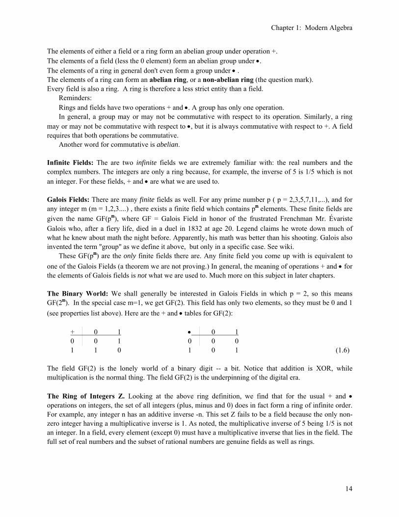
The elements of either a field or a ring form an abelian group under operation +. The elements of a field (less the 0 element) form an abelian group under •. The elements of a ring in general don't even form a group under • . The elements of a ring can form an abelian ring, or a non-abelian ring (the question mark). Every field is also a ring. A ring is therefore a less strict entity than a field. Reminders: Rings and fields have two operations + and •. A group has only one operation. In general, a group may or may not be commutative with respect to its operation. Similarly, a ring may or may not be commutative with respect to •, but it is always commutative with respect to +. A field requires that both operations be commutative. Another word for commutative is abelian. Infinite Fields: The are two infinite fields we are extremely familiar with: the real numbers and the complex numbers. The integers are only a ring because, for example, the inverse of 5 is 1/5 which is not an integer. For these fields, + and • are what we are used to. Galois Fields: There are many finite fields as well. For any prime number p ( p = 2,3,5,7,11,...), and for any integer m (m = 1,2,3....) , there exists a finite field which contains pm elements. These finite fields are given the name GF(pm), where GF = Galois Field in honor of the frustrated Frenchman Mr. Évariste Galois who, after a fiery life, died in a duel in 1832 at age 20. Legend claims he wrote down much of what he knew about math the night before. Apparently, his math was better than his shooting. Galois also invented the term "group" as we define it above, but only in a specific case. See wiki. These GF(pm) are the only finite fields there are. Any finite field you come up with is equivalent to one of the Galois Fields (a theorem we are not proving.) In general, the meaning of operations + and • for the elements of Galois fields is not what we are used to. Much more on this subject in later chapters. The Binary World: We shall generally be interested in Galois Fields in which p = 2, so this means GF(2m). In the special case m=1, we get GF(2). This field has only two elements, so they must be 0 and 1 (see properties list above). Here are the + and • tables for GF(2): + 0 1 • 0 1 0 0 1 0 0 0 1 1 0 1 0 1 (1.6) The field GF(2) is the lonely world of a binary digit -- a bit. Notice that addition is XOR, while multiplication is the normal thing. The field GF(2) is the underpinning of the digital era. The Ring of Integers Z. Looking at the above ring definition, we find that for the usual + and • operations on integers, the set of all integers (plus, minus and 0) does in fact form a ring of infinite order. For example, any integer n has an additive inverse -n. This set Z fails to be a field because the only non-zero integer having a multiplicative inverse is 1. As noted, the multiplicative inverse of 5 being 1/5 is not an integer. In a field, every element (except 0) must have a multiplicative inverse that lies in the field. The full set of real numbers and the subset of rational numbers are genuine fields as well as rings.
Chapter 1: Modern Algebra
15
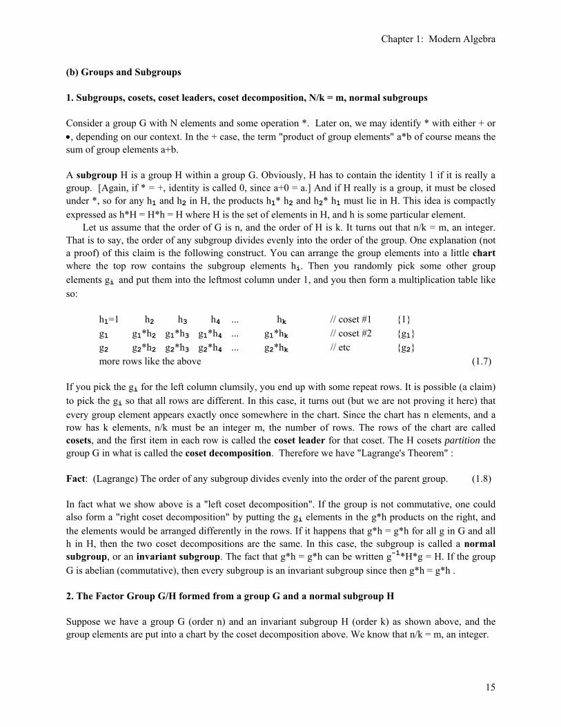
(b) Groups and Subgroups 1. Subgroups, cosets, coset leaders, coset decomposition, N/k = m, normal subgroups Consider a group G with N elements and some operation *. Later on, we may identify * with either + or •, depending on our context. In the + case, the term "product of group elements" a*b of course means the sum of group elements a+b. A subgroup H is a group H within a group G. Obviously, H has to contain the identity 1 if it is really a group. [Again, if * = +, identity is called 0, since a+0 = a.] And if H really is a group, it must be closed under *, so for any h1 and h2 in H, the products h1* h2 and h2* h1 must lie in H. This idea is compactly expressed as h*H = H*h = H where H is the set of elements in H, and h is some particular element. Let us assume that the order of G is n, and the order of H is k. It turns out that n/k = m, an integer. That is to say, the order of any subgroup divides evenly into the order of the group. One explanation (not a proof) of this claim is the following construct. You can arrange the group elements into a little chart where the top row contains the subgroup elements hi. Then you randomly pick some other group elements gi and put them into the leftmost column under 1, and you then form a multiplication table like so: h1=1 h2 h3 h4 ... hk // coset #1 {1} g1 g1*h2 g1*h3 g1*h4 ... g1*hk // coset #2 {g1} g2 g2*h2 g2*h3 g2*h4 ... g2*hk // etc {g2} more rows like the above (1.7) If you pick the gi for the left column clumsily, you end up with some repeat rows. It is possible (a claim) to pick the gi so that all rows are different. In this case, it turns out (but we are not proving it here) that every group element appears exactly once somewhere in the chart. Since the chart has n elements, and a row has k elements, n/k must be an integer m, the number of rows. The rows of the chart are called cosets, and the first item in each row is called the coset leader for that coset. The H cosets partition the group G in what is called the coset decomposition. Therefore we have "Lagrange's Theorem" : Fact: (Lagrange) The order of any subgroup divides evenly into the order of the parent group. (1.8) In fact what we show above is a "left coset decomposition". If the group is not commutative, one could also form a "right coset decomposition" by putting the gi elements in the g*h products on the right, and the elements would be arranged differently in the rows. If it happens that g*h = g*h for all g in G and all h in H, then the two coset decompositions are the same. In this case, the subgroup is called a normal subgroup, or an invariant subgroup. The fact that g*h = g*h can be written g-1*H*g = H. If the group G is abelian (commutative), then every subgroup is an invariant subgroup since then g*h = g*h . 2. The Factor Group G/H formed from a group G and a normal subgroup H Suppose we have a group G (order n) and an invariant subgroup H (order k) as shown above, and the group elements are put into a chart by the coset decomposition above. We know that n/k = m, an integer.

Chapter 1: Modern Algebra
16
It is possible now to define a new group which has m elements. These elements are the rows of the chart! Although each row contains more than one element of group G, we think of the entire row as one element of the new group we are talking about. A standard notation is to label each row by some representative element, like the coset leader, and put this in curly brackets. Thus, the top row of the chart is our first group element which is {1}, and the next row is {g1} and so on. Recall that earlier we used {a,b,c...} to represent a set of elements. One can think of {g1} as a shorthand for {g1, g1*h2, g1*h3 ... } which is indeed the set of elements on a row of the chart. Normally one does not think of a set {...} as being a group element, but here that is exactly the case. Now we have to define what it means to "multiply" two rows of the chart. We write {g1} * {g2} = {g3}, where g3 = g1*g2 . What exactly does this mean? Each row has k elements. Suppose one creates all the products possible by multiplying some element of row 1 by some element of row 2. There are k2 of these products. We claim (without proof) that all of these products will lie in the same row of the chart, and that row will be {g3} where g3 = g1*g2. Obviously, many of these products must be the same, since row 3 only contains k elements. The general idea is that one can represent a row by any of its elements. All the elements of a row have something in common. Notice that the operation * in our new group, whose elements are the rows, is defined in terms of what * does to elements of the underlying group G. Do the m rows {gi} really form a group with m elements? The set of rows is closed under * as shown above since G is closed under *. The other group properties of G are similarly induced into our new group. For example, the inverse of {g1} will be {g1-1}, since {g1} * {g1-1} = { g1g1-1} = {1}. The inverse of the row {1} is itself, which corresponds to H being closed under * (it is, after all, a subgroup). So yes, it is easy to show that G/H is in fact a group with the * operation as shown above. This new group, whose elements are the rows or cosets of the group G with respect to the normal subgroup H, has a special name and notation. It is called the factor group of G with respect to H, and the notation for this new group is G/H. This is just a notation, we are not trying to divide group G by group H. factor group = G/H . // has m = (n/k) elements, the rows (cosets) of the chart.
It is certainly not obvious why anybody in their right mind would have any interest in such a curiosity as this "factor group". Although we won't be applying this construct, we will apply its sister construct called the residue class ring coming up in section (c) below. One never knows what might be useful. 3. Cyclic Groups and Cyclic Subgroups If g is in an element of group G then so is g*g = g2, and (g*g)*g = g3, and so on (because a group is closed under *). If the group has a finite number of elements n, we can write this list of n elements as {g0, g1, g2 .... gn-1} where of course g0 = 1 and g1 = g. If there exists a g in G such that this list of n elements are all distinct, which is to say the list exhausts all elements of G, then G is said to be a cyclic

Chapter 1: Modern Algebra
17
group. If the n elements are not all distinct, then perhaps we find that g5 = g2. We can write this as g3 g2 = g2 which then means that g3 = 1 (identity is unique, or, inverse g-2 exists). Thus, before we discovered that g5 = g2, we would have discovered that g4 = g1 and g3 = 1. In general, if the n elements are not all distinct, we will get gk = 1 for some integer k that is less than n. The smallest k for which gk = 1 is called the order of g because g generates a cyclic subgroup of G which has order k. That is, the number of distinct elements in the subgroup { g0, g1, g2... gk-1) is k. This subgroup is a group because all the group properties are satisfied, notably closure. If it turns out that if k = n, the order of G, then the entire group G is cyclic and that g is a generator. If k = 1, then the cyclic subgroup is just the set {1}. According to Lagrange's Theorem (1.8), we know that k must divide n, so we can write n = Nk. Then since there is some k such that gk = 1 for every g in the group, we know that (gk)N = 1 and thus gn = 1 for every g in the group. We have now proven the following claims: Facts: For finite groups: (a) Any group element g of any group G must be a member of some cyclic subgroup of G. (b) That cyclic subgroup could be the entire group, just the identity, or something in between. (c) For any g in group G there is some minimum exponent k such that gk = 1. We refer to this exponent as the order of g, since it is the order of the cyclic subgroup generated by g. (d) the order k of the cyclic group generated by g must divide the order of G. (e) for any g in G, gn = 1 where n is the order of G. (1.9) To summarize, a cyclic group contains at least one element g such that the powers of g exhaust the group: { 1, g, g2, g3, .....gn-1} = cyclic group, order = n elements, gn = 1 (1.10) Every element of the group can be written as a power of g, for power = 0,1,2....n-1. An element g which allows a cyclic group to be fully enumerated as above is called a generator. In general, not every group element can serve as a generator, certainly not the identity. There may exist several alternative generators of the same cyclic group. The Greatest Common Divisor of two integers i and j, written GCD(i,j), is the largest integer that divides evenly into both numbers. For example GCD(3,7) = 1, GCD(3,6) = 3. An integer is prime (or "a prime", or "a prime number") if its only integer divisors are itself and 1. Two integers i and j are relatively prime (coprime) when GCD(i,j) = 1, an example being GCD(3,8) = 1 (three is prime, eight is not prime, 3 and 8 are relatively prime). If p is a prime and q is any other integer not a multiple of p, then GCD(p,q) = 1 since p has no divisors other than p and 1. In this case, p and q are relatively prime. Fact: If g is a generator of a cyclic group G of order n, then g1 ≡ gi (1 ≤ i ≤ n) is the generator of a cyclic subgroup of order j = n/GCD(n,i). (1.11) Note the validity of the two extreme cases: if i = 1, then j = n which is correct since g is a generator. And if i = n, then j = 1 which is again correct since gn = 1.

Chapter 1: Modern Algebra
18
Proof: The above Fact will be proven as (4.21), where cyclic subgroups of GF(q) are explored in great detail. For now, we state some Corollaries to this Fact, and then prove one of them. Corollary 1: If n is prime and i < n, then in (1.11) j = n/GCD(n,i) = n. In this case, our Fact above says that if g is a generator of a cyclic group, then the group element g1 ≡ gi (1 < i < n) is an alternative generator. Even if n is not prime, such a gi is an alternative generator if GCD(n,i) = 1, which is to say, if n and i are "relatively prime". (1.12a) Corollary 2: All elements (except the identity element) of a cyclic group G of prime order n are alternative generators. This is a direct result of Corollary 1. (1.12b) Corollary 3: If n/i = k for i>1, then g1 = gi is not an alternative generator to g. In this case, g1 generates a smaller cyclic subgroup of order j = n/GCD(n,i) = n/i = k. (1.12c) Proof of Corollary 3: This follows directly from (1.11), but here is a proof anyway. Let n/i = k, an integer. Since i>1, k < n. If one tries to list off the group elements using gi as a generator, one gets {1, gi, g2i,g3i
... g(k-1)i}. The next element in the list would be gki, but gki = gn = 1 (since g is a generator of cyclic group G). The next element would then be g(k+1)i = gi, so we are just repeating elements. We know that the cyclic group G has n elements, but we have only been able to enumerate k of them, and k < n. Example: Let n = 12, i = 3, and k = n/i = 4. Then here is our partial enumeration: { 1, g3, g6, g9 } g12 = 1 // only get 4 elements out of the 12. Fact: A cyclic group is commutative (abelian). (1.13) Proof: Let g1 and g2 be any elements of the group. If g is a generator, then g1 = ga and g2 = gb. It then follows that g1g2 = ga gb = ga+b = gbga = g2g1. Thus any pair of elements commutes. 4. Additive Groups and Additive Cyclic Groups : the Vector Space of group elements Additive Groups By "additive group" we mean a group whose operation * is +. By definition (1.1a), such a group is abelian. For the + operation, the term "powers of g" means "multiples of g", since for example g3 = g*g*g = g+g+g = 3g. The notation "3g" means just the sum shown. The thing "3" is not in the group. The 3 is a scalar multiple of the group element g. It happens that the scalar in question, 3, is a element of the ring of integers. For the moment, we display group elements in bold font just to distinguish them from the integer multipliers as in 3g. Let's now pick some g and try to enumerate the group with it : { 0g = 0, 1g = g, 2g, 3g, 4g, ....}
Chapter 1: Modern Algebra
19
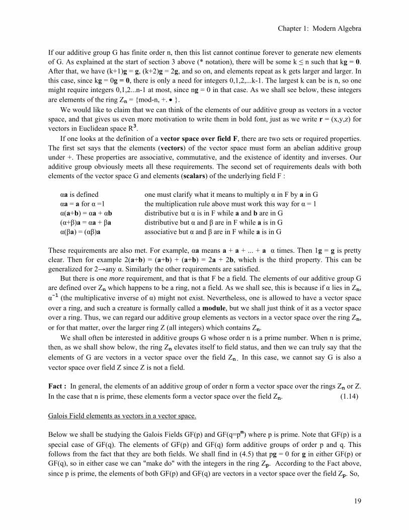
If our additive group G has finite order n, then this list cannot continue forever to generate new elements of G. As explained at the start of section 3 above (* notation), there will be some k ≤ n such that kg = 0. After that, we have (k+1)g = g, (k+2)g = 2g, and so on, and elements repeat as k gets larger and larger. In this case, since kg = 0g = 0, there is only a need for integers 0,1,2,...k-1. The largest k can be is n, so one might require integers 0,1,2...n-1 at most, since ng = 0 in that case. As we shall see below, these integers are elements of the ring Zn = {mod-n, +. • }. We would like to claim that we can think of the elements of our additive group as vectors in a vector space, and that gives us even more motivation to write them in bold font, just as we write r = (x,y,z) for vectors in Euclidean space R3. If one looks at the definition of a vector space over field F, there are two sets or required properties. The first set says that the elements (vectors) of the vector space must form an abelian additive group under +. These properties are associative, commutative, and the existence of identity and inverses. Our additive group obviously meets all these requirements. The second set of requirements deals with both elements of the vector space G and elements (scalars) of the underlying field F : αa is defined one must clarify what it means to multiply α in F by a in G αa = a for α =1 the multiplication rule above must work this way for α = 1 α(a+b) = αa + αb distributive but α is in F while a and b are in G (α+β)a = αa + βa distributive but α and β are in F while a is in G α(βa) = (αβ)a associative but α and β are in F while a is in G These requirements are also met. For example, αa means a + a + ... + a α times. Then 1g = g is pretty clear. Then for example 2(a+b) = (a+b) + (a+b) = 2a + 2b, which is the third property. This can be generalized for 2→any α. Similarly the other requirements are satisfied. But there is one more requirement, and that is that F be a field. The elements of our additive group G are defined over Zn which happens to be a ring, not a field. As we shall see, this is because if α lies in Zn, α-1 (the multiplicative inverse of α) might not exist. Nevertheless, one is allowed to have a vector space over a ring, and such a creature is formally called a module, but we shall just think of it as a vector space over a ring. Thus, we can regard our additive group elements as vectors in a vector space over the ring Zn, or for that matter, over the larger ring Z (all integers) which contains Zn. We shall often be interested in additive groups G whose order n is a prime number. When n is prime, then, as we shall show below, the ring Zn elevates itself to field status, and then we can truly say that the elements of G are vectors in a vector space over the field Zn. In this case, we cannot say G is also a vector space over field Z since Z is not a field. Fact : In general, the elements of an additive group of order n form a vector space over the rings Zn or Z. In the case that n is prime, these elements form a vector space over the field Zn. (1.14) Galois Field elements as vectors in a vector space. Below we shall be studying the Galois Fields GF(p) and GF(q=pm) where p is prime. Note that GF(p) is a special case of GF(q). The elements of GF(p) and GF(q) form additive groups of order p and q. This follows from the fact that they are both fields. We shall find in (4.5) that pg = 0 for g in either GF(p) or GF(q), so in either case we can "make do" with the integers in the ring Zp. According to the Fact above, since p is prime, the elements of both GF(p) and GF(q) are vectors in a vector space over the field Zp. So,

Chapter 1: Modern Algebra
20
Fact: The elements of GF(p) and GF(q) form a vector space over the field Zp . (1.14a) Corollary: The elements of GF(q) form a vector space over the field GF(p). (1.14b) Proof: This is a combination of the (1.14a) and the Super Big Fact (2.5a) to be shown below that GF(p) = Zp , meaning the two fields are isomorphic. Comment: Except in Chapter 10, we don't use a special symbol like =· to indicate isomorphism, we just say the two fields are "the same" with an = sign. Isomorphism means there is a clean one-to-one correspondence between the elements and all properties of the two isomorphic sets. Additive Cyclic Groups If there exists some g ≠ 0 such that the smallest integer k for which kg = 0 is k = n, then our additive group G is an additive cyclic group, according to the cyclic definition of section 3 above. Recall that, for any cyclic group, gn = 1, where 1 is the identity of the group, n is the order of the cyclic group, and g is a generator. For an additive cyclic group, this statement becomes ng = 0, since the nth power of g is ng, and since 0 is the identity for + . Thus, we can enumerate the elements of an additive cyclic group as follows ( if g is a generator) { 0, g, 2g, 3g, ....(n-1)g} = cyclic group, order = n elements, ng = 0 . (1.15) Fact: If the order n of an additive cyclic group G is a prime number, then any element (other than 0) can serve as a generator. In this case, ng = 0 for any element of G. (1.16) Proof: This is just the statement of Corollary 2 (1.12b). Example: If n is prime, we could take h = 3g and enumerate the above as group as { 0, h, 2h, 3h, ....(n-1)h} = cyclic group, order = n elements, nh= 0 Fact: If the order n of an additive cyclic group is a prime number, then -(ig) = (n-i)g . (1.17) Proof: The object -(ig) means the additive inverse of element ig. Since (n-i)g +ig = ng - ig + ig = ng = 0 // since n prime we conclude that (n-i)g must be the inverse of ig. Summary of the properties of an additive cyclic group of finite order n: (1.18) 1) the identity element is 0 2) every element g must have an inverse (-g) such that g + (-g) = 0.

Chapter 1: Modern Algebra
21
3) the group can be enumerated as { 0, g, 2g, 3g, ....(n-1)g } for at least one g // since cyclic 4) such a g is by definition a generator 5) ng = 0 for this generator g // (1.15) 6) if n is prime, then all non-zero group elements are generators // (1.16) 7) if n is prime, then ng = 0 for any g in the group. // (1.15) 8) if n is prime, then n is the smallest positive integer for which ng = 0 for any g 9) if n is prime, then for any g we can write -(ig) = (n-i)g // (1.17) Suppose n = 7. One could perversely enumerate such an additive cyclic group as shown on the left below, instead of as shown on the right : { -3g, -2g, -g, 0, g, 2g, 3g } instead of { 0, g, 2g, 3g, 4g, 5g, 6g } . We know from item 9 above that - 3g = 4g, -2g = 5g, -g = 6g. In section (c) 5 below we shall consider a ring whose order n is infinite. In this case, the idea of (1.17) doesn't work since n = ∞. Then if we enumerate the group as { 0, g, 2g, 3g, 4g, 5g, 6g ....} , the inverse of 3g is not included! In this case, we must enumerate elements in this manner { ... -3g, -2g, -g, 0, g, 2g, 3g, ..... } (1.19) where g is a generator of the infinite additive group. Are Galois Fields cyclic under • or + ? We shall find in (4.30) that both {GF(p)-0} and (GF(q)-0} are cyclic under • . What about under + ? Are GF(p) and GF(q) additive cyclic groups? We shall see in (2.5) that GF(p) is isomorphic to Zp, the field of modulo p integers. Since 1 is a viable additive generator for Zp, that is also true for GF(p). Thus, GF(p) is an additive cyclic group. In fact, since p is prime, any non-zero element g of GF(p) is an additive generator by (1.16), and pg=0. For GF(q=pm) with m > 1 the story is different. We will find in (4.5) that pg = 0 for any element g of GF(q). Since q = pm > p when m>1, we know that GF(q) for m>1 is not an additive cyclic group. We can try to additively enumerate all elements of GF(q) starting with any g, but the farthest we will get is p elements. 5. Example of an additive cyclic group: {Mod-n,+} The "mod-n additive group" has as its elements {0,1,2,3,..n-1}, and the + operation is mod-n addition, which is to say, a + b = Rem[ (a+b)/n] = Rem[ (a+b)/n] 1 . (1.20) Example: Suppose n = 4. Then 2 + 3 = Rem[ (2+3)/4] = Rem[5/4] = 1 = Rem[5/4] 1 = 1 1 = 1. This is certainly a ponderous exercise in using a bold font to represent group elements. Why is {Mod-n,+} an additive cyclic group? It is certainly closed under addition. Element 1 (not the identity) is certainly a generator which enumerates all the elements of the group, so the group is cyclic.

Chapter 1: Modern Algebra
22
Here is a list of observations about the additive cyclic group mod-n: 1) there is no element n. 2) the identity element is 0. 3) the group is cyclic with 1 as a generator, and n1 = 0 4) all non-zero elements can be written as multiples of the generator, m = m1. 5) the inverse of element m must be (-m) ≡ (n-m)1. (Proof: m + (-m) = m1 + (n-m)1 = n1 = 0.) 6) if n is prime, then any element m (other than 0) is a generator, and nm = 0. 7) mod-n forms a "principle ideal" within the integers (see below) (1.21) These facts come from (1.18) which applies to any additive cyclic group. (c) Rings and Ideals 1. Ideals, residue classes, residue class leaders, residue class decomposition, N/n = m We are now going to repeat the above song and dance almost verbatim, but this time for a ring instead of a group. A ring has two operations • and +, whereas a group has only one operation, so things will be just a little different. We started the above harangue by imagining that group G had a subgroup H. Here we might suppose that a ring R has a subring, but this turns out to be not the right thing; the correct sub-thing is called an ideal, and one uses the letter I. So what is an ideal I of ring R? First of all, with respect to the + operation, I must be a subgroup of R. Thus, I must contain the additive identity which we call 0. Secondly, with respect to the • operation, I must have this property: r•I = I•r = I. This means that if you pick any r in R, and any i in I, the product r•i lies somewhere in I, and so does the other product i•r. In particular, we have i•I = I, so I is closed under • as well as +. So an ideal is in fact a subring of R, but it is more specific since r•I = I even for r not in I. (1.22) So let R have n elements, and assume there is an ideal I with k elements. As before, we are going to build a chart, and we will then claim that n/k = m = an integer. We lay down I itself as the top row. Since we are really thinking about the + operation now, the top left element is the + identity 0 ( the thing you put in r + 0 = r). We next start picking random elements of R and plop them down in the left column, then we form rows by doing sums of the left element with the i's along the top. Here is the chart for ring R with respect to ideal I: i1=0 i2 i3 i4 ... ik // residue class #1 r1 r1+ i2 r1+ i3 r1+ i4 ... r1+ ik // residue class #2 r2 r2+ i2 r2+ i3 r2+ i4 ... r2+ ik // etc more rows like the above (1.23) Again, we make the claim that if you pick the left elements right and get things so that you throw out any repeating rows, you end up with a coset decomposition that partitions the ring. Each ring element appears exactly one place in the chart. Thus, as before, we conclude that n/k = m, and integer.

Chapter 1: Modern Algebra
23
Because mathematicians cannot leave well enough alone, they decided that they had to invent a new name for everything since we are doing rings instead of groups. Thus, what was called a coset before is now called a residue class. A residue class is a row of the chart. And the first item in a row is now the residue class leader. Big deal. Note that, although a ring has • and + operations, it is only the + operation we are talking about in the above chart. The ring is a group under +, so this chart really is analogous to our early group chart. 2. The Residue Class Ring R/I formed from a ring R and an ideal I Before, our next step was to claim that you could make a fancy new group by considering each row of the chart to be an element of that new group. This was the factor group of G with respect to H. Here we are going to do the same thing, but as you might expect, the new "thing" which has the rows as elements is going to be a ring, not a group, since R is a ring. Thus, admittedly, we cannot call this thing a factor group. So they make a new name. This new ring with m elements being the rows of the above chart is called the residue class ring, or the quotient ring To be consistent, they should have called the other thing a coset group, but they called it a factor group instead. The notation is pretty much the same: residue class ring = R/I has m = (n/k) elements, the rows (residue classes) of the chart. (1.24a) We now have to say what it means to do the + and • operations on "rows" of the chart. We have two operations to worry about instead of one : {r1} • {r2} = {r3}, where r3 = r1•r2 {r1} + {r2} = {r4}, where r4 = r1+r2 (1.24b) Again, {r2} is an element of the new "residue class ring", and r2 is some representative element of the row of the chart by which this residue class ring element is labeled. We need then to make exactly the same interpretation as before for what the above lines mean, only here we say the same thing for each operator + and •. For example, if you form all k2 products between elements of two rows, the results all lie in the same row of k elements. And the same applies if you make all k2 possible sums. Of course the results row will likely not be the same row for • and +, so we have used r3 and r4 above. We have not proven that the residue class ring is a ring, we are just claiming that it is. You may remember that a ring does not in general have a 1 element for •, but it always has a 0 element. Thus, every row {r1} must have some corresponding "negative" row {r2} such that {r1} + {r2} = {0} . And as before, since our ideal I is a subgroup of R relative to +, we know that the negative of the top row is itself ( the subgroup I is closed so {-ir} and {ir} are in the first row since -ir and ir are in I). This is expressed by the incredibly boring statement: {0} + {0} = {0}. Since we might not have a {1} row, we have nothing to say about {1}. (yet) A quotient ring example is coming very soon, please hold on.

Chapter 1: Modern Algebra
24
3. Principle Ideals and Principle Ideal Rings Now we are ready to pursue the ring analog of the cyclic subgroup discussion above. If i is in an element of ring R, then so is any multiple of i, such as 3i. If the ring has a finite number n of elements, you must, as you keep adding more terms, come to a point where ki = 0 for some k ≤ n. After this point, if you keep adding i, things just repeat, for example, (k+1)i= i. This set of multiples of some ring element i together with 0 forms an additive cyclic group of order k, as discussed in much detail above. We have, { 0, i, 2i, 3i, .....(k-1)i } = additive cyclic group of order k (1.25) If you find that you have exhausted all the elements of the ring in this way, then it must be that k = n, the order of the ring, and i is a generator. The other possibility is that you reach the point ki= 0 before all ring elements have been hit. In this case, you have found an additive cyclic subgroup (order k) of the ring. In the case of rings, we are more interested in ideals than we are in subgroups. The above cyclic subgroup of order k may or may not be an ideal of R. Recall (1.22) that for an ideal, it must be true that r•I = I•r = I for elements r that are outside the ideal as well as inside. The above enumeration and the fact that a set forms an additive cyclic subgroup within R does not guarantee this extra required property to make that subgroup be an ideal. If the subgroup is not an ideal, then we have nothing more to say. But if the subgroup is an ideal, then it is called a principle ideal. Thus, a principle ideal is an ideal whose elements can be fully enumerated as sums of some generator i. Alternatively, a principle ideal is an ideal which is an additive cyclic subgroup of R. (1.26) If every ideal in a ring is a principle ideal, then the ring as a whole is called a principle ideal ring. We can now go back and consider the case we quietly skipped. If you have exhausted all ring elements by taking multiples of some r, then the set of all these multiples is an ideal of the ring. Every ring is an ideal of itself, just look at the definition (1.19) of an ideal. Thus, in this case of exhaustion, you again end up with a principle ideal ring. Fact: The order of any principle ideal of a ring must divide evenly into the order of the ring. (1.27) Proof: We already know from the residue class decomposition that the order of any ideal I of a ring R must divide evenly into the order of R, so saying this for a principle ideal is nothing new. 4. Example of a ring: Zn ≡ {Mod-n,+,•} ; Modulo Arithmetic Earlier we discussed the additive cyclic group {Mod-n,+} which consisted of n elements {0,1,2....n-1} with addition defined by a + b = Rem[(a+b)/n] 1. The additive generator is 1. Any element can be written in the form m = m1, a multiple of the additive generator.

Chapter 1: Modern Algebra
25
In order to have a ring, we need a second operation •. It is defined in a manner similar to +, so here are both operations: a • b = Rem[ab/n] 1 a + b = Rem[(a+b)/n] 1 (1.28) Claim: {Mod-n,+,•} forms a "ring with identity". A standard notation for this ring is Zn, though some authors use the notation Z/nZ. (1.29) Proof: Since this ring is so important, we will make a reasonable attempt to do a real proof: 1) The elements of Mod-n are clearly closed under this •, since ab/n always produces a remainder in the range (0,n-1). 2) Also, ab/n = ba/n so we have a • b = b • a and we have commutative (it's an abelian ring). 3) The associativity proof requires Little Lemma 2 below, then you get:
(a•b)•c = Rem[ab/n] 1 • c = Rem { Rem(ab/n) c
n } 1 = Rem { (abc)/n} 1 .
Since this result is symmetric in a, b and c, it must be equal to any grouping (x•y)•z you want, in particular it is equal then to a•(b•c) so we have associative. 4) The distributive property looks like this:
a•(b+c) = Rem[a(b+c)/n] 1 = Rem[ab + ac
n ] 1
a•b + a•c = Rem(ab/n)1 + Rem(ac/n) 1 = Rem[ Rem(ab/n) + Rem(ac/n)
n ] 1
and these are equal from Little Lemma 3 below. 5) The element 1 is an identity for •, since 1•m = (1m)1 = m 1 = m . Thus, we have shown that {mod-n, + • } has all the properties of a ring, and it has a multiplicative identity as well, so it is a ring with identity. As noted, a common notation for {mod-n, + • } is Zn. Consider the following "little lemmas":
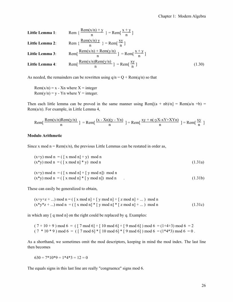
Chapter 1: Modern Algebra
26
Little Lemma 1: Rem { Rem(x/n) + y
n } = Rem[ x + y
n ]
Little Lemma 2: Rem { Rem(x/n) y
n } = Rem[ xyn ]
Little Lemma 3: Rem[ Rem(x/n) + Rem(y/n)
n ] = Rem[ x + y
n ]
Little Lemma 4: Rem[ Rem(x/n)Rem(y/n)
n ] = Rem[ xyn ] (1.30)
As needed, the remainders can be rewritten using q/n = Q + Rem(q/n) so that Rem(x/n) = x - Xn where X = integer Rem(y/n) = y - Yn where Y = integer. Then each little lemma can be proved in the same manner using Rem[(a + nb)/n] = Rem(a/n +b) = Rem(a/n). For example, in Little Lemma 4,
Rem[ Rem(x/n)Rem(y/n)
n ] = Rem[ (x - Xn)(y - Yn)
n ] = Rem[ xy + n(-yX-xY+XYn)
n ] = Rem[ xyn ]
Modulo Arithmetic Since x mod n = Rem(x/n), the previous Little Lemmas can be restated in order as, (x+y) mod n = ( [ x mod n] + y) mod n (x*y) mod n = ( [ x mod n] * y) mod n (1.31a) (x+y) mod n = ( [ x mod n] + [ y mod n]) mod n (x*y) mod n = ( [ x mod n] * [ y mod n]) mod n . (1.31b) These can easily be generalized to obtain, (x+y+z + ...) mod n = ( [ x mod n] + [ y mod n] + [ z mod n] + ... ) mod n (x*y*z + ...) mod n = ( [ x mod n] * [ y mod n] * [ z mod n] + ... ) mod n (1.31c) in which any [ q mod n] on the right could be replaced by q. Examples: ( 7 + 10 + 9 ) mod 6 = ( [ 7 mod 6] + [ 10 mod 6] + [ 9 mod 6] ) mod 6 = (1+4+3) mod 6 = 2 ( 7 * 10 * 9 ) mod 6 = ( [ 7 mod 6] * [ 10 mod 6] * [ 9 mod 6] ) mod 6 = (1*4*3) mod 6 = 0 . As a shorthand, we sometimes omit the mod descriptors, keeping in mind the mod index. The last line then becomes 630 = 7*10*9 = 1*4*3 = 12 = 0 The equals signs in this last line are really "congruence" signs mod 6.

Chapter 1: Modern Algebra
27
5. Example of a Residue Class Ring: Z/(n) Suddenly all of the above obscure residue class business is going to start making sense. The classic example is to let R be Z, the ring of integers -- plain old integers, plus and minus and 0. The + and • operations are the regular operations we are used to. Consider the subset of integers which are multiples of 5. We could pick any integer n, but 5 seems nice: { 0 ±5 ±10 ±15 ±20 ........ } (1.32) This type of list appeared in (1.19) and in that notation we rewrite the members of this ring as { ... -3α, -2α, -α, 0, α, 2α, 3α, ..... } α = 51 (1.33) which is to say { ..... -3(51), - 2(51) , - (51) 1, 0, (51), 2(51), 3(51) ......} . (1.34) The generator is (51), and this ring is formally an additive cyclic group since the generator enumerates all ring elements. The set is closed under either the + or • operations. You cannot, for example, generate a 14 by adding or multiplying two items in the above list. In our former notation, any element of this set can be written as g = n(51) = (5n)1, where n can be any integer, so the elements of the above set form a vector space over the ring (a module) of integers which are multiples of 5. In slightly less formal notation, we write the set as { ..... -3(5), - 2(5) , -(5), 1, 0, (5), 2(5), 3(5) ......} (1.35) or { ..... -15, - 10 , -5, 1, 0, 5, 10, 15 ......} . (1.36) The above list of elements forms an ideal within the full set Z of integers. Why? Because it is first of all an additive subgroup of Z, and second of all, multiplication of any element of this set by any integer gives an element in the set, whether or not that integer is in the set. Thus our additive subgroup fulfills the requirements (1.22) of being an ideal. Since this ideal is a subgroup of Z, it is a principle ideal, (1.26). Fact: The only ideals one can make inside the set of integers are principle ideals like this, so R is a principle ideal ring, see text below (1.26). (no proof) (1.37) The usual notation for this ideal is (5), where the parentheses are supposed to suggest all multiples of the thing inside, as in (1.35). Since the parent ring is Z (all integers), we are now going to form the residue class ring which has the notation Z/(5), or more generally, R/I = Z/(n). [ Later in a different world we will have an ideal ( f(x) ) which consists of all polynomials which are a multiple of some f(x). ] In building the residue class chart, we are going to make a slight change in notation. Instead of putting the residue class leaders on the left edge of our chart as done above, we will put them as the middle column of the chart, and we will mark it with a ** so you can find this column. So here is the chart which is the
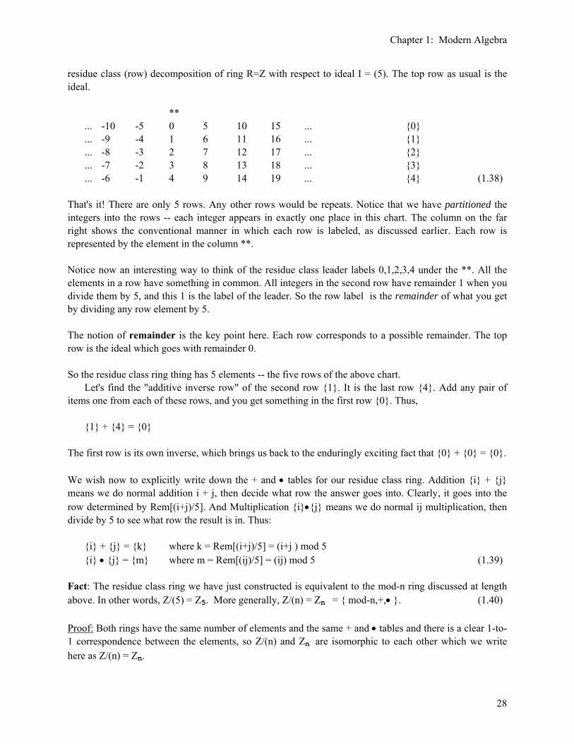
Chapter 1: Modern Algebra
28
residue class (row) decomposition of ring R=Z with respect to ideal I = (5). The top row as usual is the ideal. ** ... -10 -5 0 5 10 15 ... {0} ... -9 -4 1 6 11 16 ... {1} ... -8 -3 2 7 12 17 ... {2} ... -7 -2 3 8 13 18 ... {3} ... -6 -1 4 9 14 19 ... {4} (1.38) That's it! There are only 5 rows. Any other rows would be repeats. Notice that we have partitioned the integers into the rows -- each integer appears in exactly one place in this chart. The column on the far right shows the conventional manner in which each row is labeled, as discussed earlier. Each row is represented by the element in the column **. Notice now an interesting way to think of the residue class leader labels 0,1,2,3,4 under the **. All the elements in a row have something in common. All integers in the second row have remainder 1 when you divide them by 5, and this 1 is the label of the leader. So the row label is the remainder of what you get by dividing any row element by 5. The notion of remainder is the key point here. Each row corresponds to a possible remainder. The top row is the ideal which goes with remainder 0. So the residue class ring thing has 5 elements -- the five rows of the above chart. Let's find the "additive inverse row" of the second row {1}. It is the last row {4}. Add any pair of items one from each of these rows, and you get something in the first row {0}. Thus, {1} + {4} = {0} The first row is its own inverse, which brings us back to the enduringly exciting fact that {0} + {0} = {0}. We wish now to explicitly write down the + and • tables for our residue class ring. Addition {i} + {j} means we do normal addition i + j, then decide what row the answer goes into. Clearly, it goes into the row determined by Rem[(i+j)/5]. And Multiplication {i}•{j} means we do normal ij multiplication, then divide by 5 to see what row the result is in. Thus: {i} + {j} = {k} where k = Rem[(i+j)/5] = (i+j ) mod 5 {i} • {j} = {m} where m = Rem[(ij)/5] = (ij) mod 5 (1.39) Fact: The residue class ring we have just constructed is equivalent to the mod-n ring discussed at length above. In other words, Z/(5) = Z5. More generally, Z/(n) = Zn = { mod-n,+,• }. (1.40) Proof: Both rings have the same number of elements and the same + and • tables and there is a clear 1-to-1 correspondence between the elements, so Z/(n) and Zn are isomorphic to each other which we write here as Z/(n) = Zn.
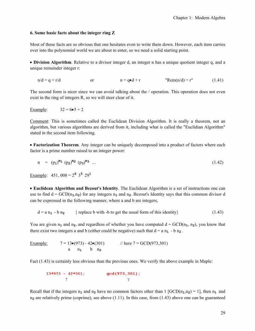
Chapter 1: Modern Algebra
29
6. Some basic facts about the integer ring Z Most of these facts are so obvious that one hesitates even to write them down. However, each item carries over into the polynomial world we are about to enter, so we need a solid starting point. • Division Algorithm. Relative to a divisor integer d, an integer n has a unique quotient integer q, and a unique remainder integer r: n/d = q + r/d or n = q•d + r "Rem(n/d) = r" (1.41) The second form is nicer since we can avoid talking about the / operation. This operation does not even exist in the ring of integers R, so we will steer clear of it. Example: 32 = 6•5 + 2 Comment: This is sometimes called the Euclidean Division Algorithm. It is really a theorem, not an algorithm, but various algorithms are derived from it, including what is called the "Euclidian Algorithm" stated in the second item following. • Factorization Theorem. Any integer can be uniquely decomposed into a product of factors where each factor is a prime number raised to an integer power: n = (p1)m1 (p2)m2 (p3)m3 ... (1.42) Example: 451, 008 = 26 35 291
• Euclidean Algorithm and Bezout's Identity. The Euclidean Algorithm is a set of instructions one can use to find d = GCD(n1,n2) for any integers n1 and n2. Bezout's Identity says that this common divisor d can be expressed in the following manner, where a and b are integers, d = a n1 - b n2 { replace b with -b to get the usual form of this identity} (1.43) You are given n1 and n2, and regardless of whether you have computed d = GCD(n1, n2), you know that there exist two integers a and b (either could be negative) such that d = a n1 - b n2 . Example: 7 = 13•(973) - 42•(301) // here 7 = GCD(973,301) a n1 b n2 Fact (1.43) is certainly less obvious than the previous ones. We verify the above example in Maple:
Recall that if the integers n1 and n2 have no common factors other than 1 [GCD(n1,n2) = 1], then n1 and n2 are relatively prime (coprime), see above (1.11). In this case, from (1.43) above one can be guaranteed

Chapter 1: Modern Algebra
30
of the existence of integers a,b such that 1 = a n1 - b n2. This occurs, for example, if n1 is a prime number and n2 is any integer that is not a multiple of n1. 7. The Residue Class Ring Z/(n) is a field if n is prime We now close this chapter by coming back to the subject of fields. We have seen how one can take a ring R and an ideal I and how one can make a chart whose rows become elements of something called the residue class ring. We did an example Z/(5) which was seen to be equivalent to Z5 ≡ {Mod-5,+,•}. Here is a fundamental new result: Big Fact: If n is a prime number, then the residue class ring Z/(n) above is also a field. Since we have shown already that Z/(n) = Zn , this means that Zn ≡ {Mod-n,+,•} is a field when n is prime. (1.44) Proof: The proof is really the same whether you do it for Z/(n), or for Zn. In the former case, we add a few brackets to talk about residue class rows. In the latter case, we just talk about remainders, not rows. What we need to do is show that the two properties omitted in our ring definition above (compared to the field definition) are present in this case. Those properties are existence of an inverse, and existence of an identity, both relative to •. But we already know that the • identity exists since we showed that {Mod-n,+,•} was a "ring with identity". So all that remains is to show there is a • inverse for any element of Zn when n is prime. Consider an arbitrary row {r} described by remainder r. We need to show that there exists an inverse row {s} under the operation • such that {r}•{s} = 1. Since n is prime, and since r < n, we know that n and r are relatively prime, and their greatest common divisor is 1. Using Bezout's Identity (1.43) above, we claim that integers N and M must exist such that 1 = Nr -Mn. Now take the remainder of both sides of this equation divided by n. This says that there exists an N such that 1 = Rem(Nr/n). Next, use (1.41) to expand N = Kn + s, where s < n. This gives 1 =
Rem(Knr +sr
n ) = Rem(sr/n). Thus, according to the definition of the operation •, we have found s such
that r•s = 1. [ The Zn proof just ended here.] These remainders of course are representative of rows, so this means {r}•{s} = {1}. QED Thus, every row has a multiplicative inverse, and this was the only missing factor which prevents our residue class ring Z/(n) from being a field. The proof required that n be prime. The implication is that some row in the chart must be the identity {1}, and each row must now have an "inverse" row in the multiplicative sense: identity: {r1} • {1} = {r1} inverse: {r1} • {r2} = {1} In our example two sections above, 5 was a prime number, so these things must be true. Identity {1} for • is the second row of our chart (1.38) (the row containing the integer 1), as is easy to verify. The • inverse of row {3} is row {2}. Every row has an inverse row. Recall that the first row is the additive identity {0}, which is different from multiplicative identity {1}.

Chapter 1: Modern Algebra
31
If you try doing the case n = 4 and make the chart, you find a most annoying thing. Yes, the row containing 1 is still the identity {1}, but certain rows don't have any inverses. You multiply some row by all the other rows, and you never get {1} as the answer! The chart is shown below for n=4. Think about the row {2}. It now contains only even numbers. Row {1} contains only odd numbers. What row could there be that such that {2}•{r} = {1} ? We need Rem((2r)/4) = 1, but the remainder of an even number divided by 4 cannot be 1, it can only be 0 or 2. Thus, the row {2} has no inverse. ... -8 -4 0 4 8 12 ... {0} ... -7 -3 1 5 9 13 ... {1} ... -6 -2 2 6 10 14 ... {2} ... -5 -1 3 7 11 15 ... {3} (1.45) So n = 4 does not make a field. Our n must be a prime number, then all the rows will have inverses, and then Z/(n) will be a field.

Chapter 2: GF(p)
32
Chapter 2: The Galois Fields GF(p) Throughout this Chapter, we shall assume that p is some prime number, p = 2,3,5,7,11,13,... (a) More Discussion of Zn = { mod-n,+,•} In Chapter 1 (b) 5 we showed that that the set of numbers {0,1,2,3,...n-1} formed a cyclic additive group which we called {mod-n,+}. A short list of properties was then presented for {mod-n,+} in (1.21). The next step was to upgrade this additive group to ring status by endowing it with the modulo • multiplicative operation. This ring was called Zn = { mod-n,+,•}, and the proof that it really is a ring was presented in full detail below (1.29). In fact, it is a "ring with identity". Finally, at the end of Chapter 1 we showed in (1.44) that Zn is a field when n is prime. This means that all non-zero elements have inverses. This leads to the next claim: Fact: The ring Zn has n elements which are {0,1,2,3...n-1}, and we have modulo-n operations + and •. If we consider the subset of the n-1 non-zero elements {1,2,3...n-1}, this set forms a group under the mod-n • operation, provided that n is a prime number. Although the modulo operation is mod-n, the order of this group is n-1, since order is the number of elements in a group. (2.1) Proof: We already know from (1.29) that Zn is a ring with • identity, so it is just the • inverses that are missing. But since Zn is a field for prime n from (1.44), we know these inverses all exist. QED Fact : The group just mentioned, {1,2,3...n-1} under operation •, is a cyclic group for prime n. It follows from this Fact that there is at least one generator g, so we can write the group as in (1.10) with n→n-1, {1, g, g2, g3, ...gn-2} = cyclic group, order = n-1, where gn-1 = 1 ( gn = g) . (2.2) Proof: It will later be shown that all Galois Fields are cyclic groups under •, and that Zn for n prime is a Galois Field, so Zn is a cyclic group under •. This is the content of Big Theorem 1 (4.30) in Chapter 4. Fact : If n is prime, then for any element a of Zn we have: an = a. (2.3) Proof: According to (2.2), we may write our arbitrary element a as be a = gk. Then an = (gk)n = gkn = (gn)k = (g)k = a , since gn = 1 from (2.2). Example: Let n = 5 = prime, then the 4 elements of our multiplicative group are {1,2,3,4}. These are the non-zero elements of the ring (and field) Z5. An acceptable generator is 2, since (remember mod 5) 21 = 2 22 = 4 23 = 8 = 3 24 = 16 = 1. So we can write out our non-zero Z5 elements using this generator as:
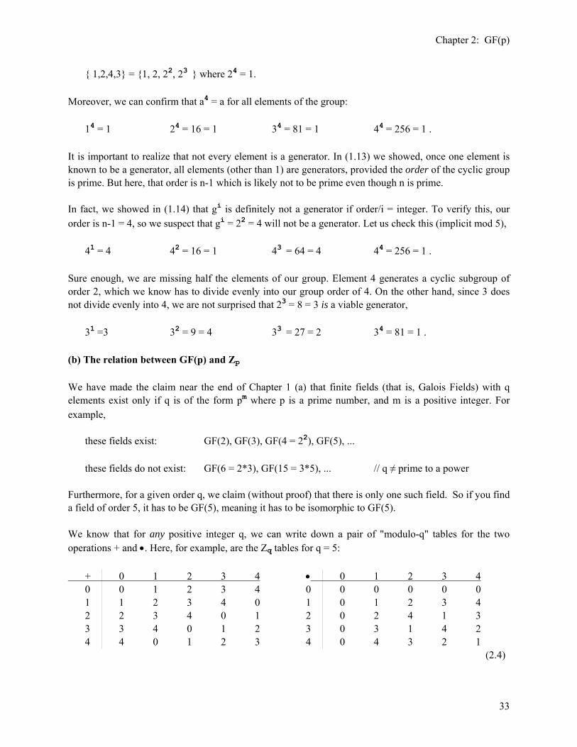
Chapter 2: GF(p)
33
{ 1,2,4,3} = {1, 2, 22, 23 } where 24 = 1. Moreover, we can confirm that a4 = a for all elements of the group: 14 = 1 24 = 16 = 1 34 = 81 = 1 44 = 256 = 1 . It is important to realize that not every element is a generator. In (1.13) we showed, once one element is known to be a generator, all elements (other than 1) are generators, provided the order of the cyclic group is prime. But here, that order is n-1 which is likely not to be prime even though n is prime. In fact, we showed in (1.14) that gi is definitely not a generator if order/i = integer. To verify this, our order is n-1 = 4, so we suspect that gi = 22 = 4 will not be a generator. Let us check this (implicit mod 5), 41 = 4 42 = 16 = 1 43 = 64 = 4 44 = 256 = 1 . Sure enough, we are missing half the elements of our group. Element 4 generates a cyclic subgroup of order 2, which we know has to divide evenly into our group order of 4. On the other hand, since 3 does not divide evenly into 4, we are not surprised that 23 = 8 = 3 is a viable generator, 31 =3 32 = 9 = 4 33 = 27 = 2 34 = 81 = 1 . (b) The relation between GF(p) and Zp We have made the claim near the end of Chapter 1 (a) that finite fields (that is, Galois Fields) with q elements exist only if q is of the form pm where p is a prime number, and m is a positive integer. For example, these fields exist: GF(2), GF(3), GF(4 = 22), GF(5), ... these fields do not exist: GF(6 = 2*3), GF(15 = 3*5), ... // q ≠ prime to a power Furthermore, for a given order q, we claim (without proof) that there is only one such field. So if you find a field of order 5, it has to be GF(5), meaning it has to be isomorphic to GF(5). We know that for any positive integer q, we can write down a pair of "modulo-q" tables for the two operations + and •. Here, for example, are the Zq tables for q = 5: + 0 1 2 3 4 • 0 1 2 3 4 0 0 1 2 3 4 0 0 0 0 0 0 1 1 2 3 4 0 1 0 1 2 3 4 2 2 3 4 0 1 2 0 2 4 1 3 3 3 4 0 1 2 3 0 3 1 4 2 4 4 0 1 2 3 4 0 4 3 2 1 (2.4)

Chapter 2: GF(p)
34
For any integer q, we get similar tables. So we have a set of q elements and two operations + and •, and the set is "closed" under each operation, and distributive holds, and there is an identity, so for any q the set of elements forms a "ring with identity". This is Zq. If every element has an inverse, then the set advances to the front of the class and is proclaimed to be a field. The + table is always boring, since it just contains the q elements cyclically permuted on each new line. The • table is more interesting. Notice in the above • table that a 1 appears in every row except the first row. This means that every element except 0 has an inverse, so Zq is a field when q = 5. Each row except the first is just a reordering of all the elements. Since we have formed a finite field with 5 elements, it must be equivalent to GF(5). More generally, since we have already identified a set of fields Zp for any prime p, these must be the GF(p). Recall from (1.40) that the Zp rings are equivalent also to the residue class rings Z/(p). Thus, we have arrived at the following Super Big Fact: For p = prime, GF(p) = Zp = Z/(p). (2.5) Remember: GF(p) = one of the Galois Fields having p abstract elements Zp = {Mod-p,+,•} having elements 0,1,2..(p-1) Z/(p) = the residue class ring having elements marked by remainders like {2} When we say GF(p) = Zp = Z/(p), we mean these objects are isomorphic to each other. There is a 1-to-1 correspondence between the elements of any two of the three objects, and they all have the same + and • tables. If p is not a prime, this does not work. For example, here is the • table for Z4; • 0 1 2 3 0 0 0 0 0 1 0 1 2 3 2 0 2 0 2 3 0 3 2 1 Notice that the third row does not contain 1, so the element 2 has no multiplicative inverse. This "modulo-4 ring with identity" has four elements, but it is not a field. We know that the field GF(4) = GF(22) exists. So we now know that the + and • tables for GF(4) are not the Z4 modulo-4 arithmetic tables we have been talking about above. The correspondence between GF(p) and Zp only holds when p = a prime number. Just to emphasize this fact, here are the full set of tables for Z4 and GF(4). The former are by inspection, the latter from (6.24) and (6.27) :
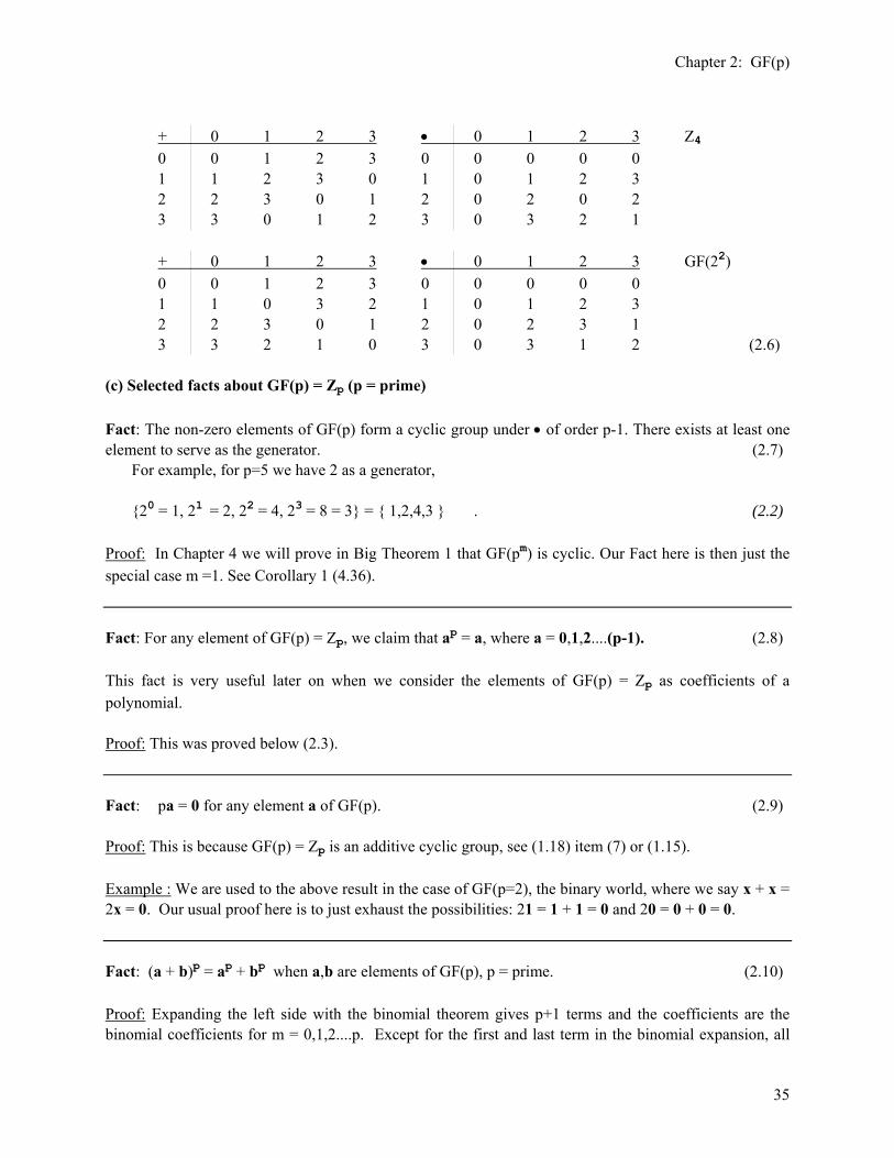
Chapter 2: GF(p)
35
+ 0 1 2 3 • 0 1 2 3 Z4 0 0 1 2 3 0 0 0 0 0 1 1 2 3 0 1 0 1 2 3 2 2 3 0 1 2 0 2 0 2
3 3 0 1 2 3 0 3 2 1 + 0 1 2 3 • 0 1 2 3 GF(22) 0 0 1 2 3 0 0 0 0 0 1 1 0 3 2 1 0 1 2 3 2 2 3 0 1 2 0 2 3 1 3 3 2 1 0 3 0 3 1 2 (2.6) (c) Selected facts about GF(p) = Zp (p = prime) Fact: The non-zero elements of GF(p) form a cyclic group under • of order p-1. There exists at least one element to serve as the generator. (2.7) For example, for p=5 we have 2 as a generator, {20 = 1, 21 = 2, 22 = 4, 23 = 8 = 3} = { 1,2,4,3 } . (2.2) Proof: In Chapter 4 we will prove in Big Theorem 1 that GF(pm) is cyclic. Our Fact here is then just the special case m =1. See Corollary 1 (4.36). Fact: For any element of GF(p) = Zp, we claim that ap = a, where a = 0,1,2....(p-1). (2.8) This fact is very useful later on when we consider the elements of GF(p) = Zp as coefficients of a polynomial. Proof: This was proved below (2.3). Fact: pa = 0 for any element a of GF(p). (2.9) Proof: This is because GF(p) = Zp is an additive cyclic group, see (1.18) item (7) or (1.15). Example : We are used to the above result in the case of GF(p=2), the binary world, where we say x + x = 2x = 0. Our usual proof here is to just exhaust the possibilities: 21 = 1 + 1 = 0 and 20 = 0 + 0 = 0. Fact: (a + b)p = ap + bp when a,b are elements of GF(p), p = prime. (2.10) Proof: Expanding the left side with the binomial theorem gives p+1 terms and the coefficients are the binomial coefficients for m = 0,1,2....p. Except for the first and last term in the binomial expansion, all

Chapter 2: GF(p)
36
these coefficients are proportional to p, and since pn = 0 for any field element n, we see that all the cross terms having these coefficients must vanish. In more detail,
(a + b)p = ap + bp + Σm=1p-1 p (p-1)!
m! (p-m)! apbp-m , but papbp-m = (pa)ap-1bp-m = 0 .
The key thing here is that, since p is prime, it cannot be eliminated by something in the denominator factorial pair, so p survives in every cross term. Admittedly the result above conflicts with our usual intuition (field = reals) about what (a+b)p ought to be. We continue our haphazard notation of sometimes emphasizing group elements with bold font. Example: (a + b)5 = a5 + 5a4b + 10a3b2 + 10a2b3 + 5ab4 + b5 = a5 + b5
Example: (1 + x)p = 1 + xp , where x is some element in GF(p), p = prime. Counterexample: (a + b)4 = a4 + 4a3b + 6a2b2+ 4ab3+ b4 = a4 + b4 + 6a2b2 . The above fact can be generalized as follows: Fact: (a + b + c + d + ... )p = ap + bp + cp +dp +... for a,b,c,d... in GF(p), p = prime (2.11) Proof: Just apply the binomial proof a bunch of times, the first time with b + c + d + ... = B, etc. Conclusion: In this chapter we have identified the Galois Fields GF(p) to be the Zp. We have not yet nailed down the fields GF(pm). This is where the notion of polynomials comes into play. As a hint, we note that if you divide a polynomial by some polynomial of degree m, and this polynomial has coefficients in Zp = GF(p), then there are exactly pm possible remainders you can get. If we can somehow identify each of these remainders with a row of a residue class ring chart, then we may be on our way to constructing a representation of GF(pm) which is analogous to Z/(p) for GF(p). Whereas integers sufficed for GF(p) = Zp and gave us p remainders, we have to go to polynomials to get pm remainders.
Chapter 3: Polynomials
37
Chapter 3: Polynomials (a) Specification of the ring R of polynomials with coefficients in Zp The highest power of x actually appearing in a polynomial f(x) is called the degree of the polynomial. If we have f(x) = Σi=0n fixi, then a(x) has degree n only if fn ≠ 0. For a polynomial written as a sum in this way, the degree m is the value of the largest index i on fi for which fi ≠ 0. Let R be the set of polynomials f(x) whose coefficients lie in Zp. We say nothing about the nature of the variable x. It could lie in Zp or it could lie in some set different from Zp. In a sense, the variable x is just an inert carrier of the coefficients of the polynomial. Let a(x) and b(x) be any two polynomials in R. Symbol Σ used below implies the + operation of ring R. For example, if a(x) = x3 + 2x, the + here is the + operation of the ring R (to be defined just below). The Σi can be thought of as Σi=0∞ and then the degree of a polynomial is determined by its highest-indexed non-zero coefficient. For the moment, the addition and multiplication operators for the field Zp will be written ⊕ and ⊗ . Here then are our two arbitrary such polynomials: a(x) = Σiaixi
b(x) = Σibixi . (3.1) The + and • operations for the ring R are defined by the expressions to the right of ≡ on these two lines: a(x) + b(x) = (Σiaixi) + (Σibixi) ≡ Σi(ai⊕bi)xi
a(x) • b(x) = (Σi aixi) • (Σj bjxj) ≡ Σi,j (ai⊗bj) xi+j . (3.2) Notice that both + and • are commutative because both ⊕ and ⊗ are commutative for Zp. It is clear that if we write a(x) + b(x) = d(x), then di = ai⊕bi . If we write a(x) • b(x) = c(x), then Appendix C shows that the ci are given by
ci = ∑j = max(0,i-A)
min(i, B) ai-j⊗bj (3.3)
where A and B are the upper endpoints of the sums in (3.1). The polynomial a(x) = x has ai = δi,1. If a(x) = b(x) = x, the above definitions result in these intuitively desirable results: x + x = Σi (δi,1⊕ δi,1)xi = 1⊕1 x1 = 2x // assuming p > 2 x • x = Σi,j (δi,1⊗ δj,1) xi+j = 1⊗1 x2 = x2 . Thus, although we have not specified the nature of the polynomial argument x, we have a precise meaning for things like 3x = x+x+x and x3 = x•x•x. In particular, we know that px = 0 :
Chapter 3: Polynomials
38
px = x + x + x +.... + x = (1⊕1⊕1⊕.....⊕1)x = (0)x = 0. (3.4) We know that x is one of the polynomials in our set R. Subtraction of two polynomials in R is just a special case of addition: a(x) – b(x) = (Σiaixi) – (Σibixi) ≡ Σi (ai⊕(p-bi))xi (3.5) where we know that - bi = p - bi in Zp, since then bi + (-bi) = p = 0. We shall now show in full detail that the set R with + and • as defined in (3.2) forms a ring with identity: + associative: [ a(x) + b(x) ] + c(x) = Σi (ai⊕bi)xi + (Σicixi) = Σi (ai⊕bi)⊕ ci xi = Σi ai⊕(bi⊕ ci)xi a(x) + [b(x) + c(x)] = (Σiaixi) + Σi (bi⊕ci)xi = Σi ai⊕(bi⊕ ci)xi QED + identity: i(x) = 0 i(x) + a(x) = (Σi0xi) + (Σiaixi) = Σi (0⊕ai)xi = Σi aixi = a(x) + inverse: -a(x) = Σi([-ai])xi // [-ai] exists since Zp is a field a(x) - a(x) = (Σiaixi) + Σi([-ai])xi = Σi ai⊕[-ai] xi = Σi 0 xi = 0 QED + commutative: a(x) + b(x) = Σi (ai⊕bi)xi = Σi (bi⊕ai)xi b(x) + a(x) = Σi (bi⊕ai)xi QED • associative [a(x) • b(x)] • c(x) = Σi,j (ai⊗bj) xi+j • (Σkckxk) = Σi,j,k(ai⊗bj) ⊗ck xi+j+k = Σi,j,k ai⊗(bj ⊗ck) xi+j+k a(x) • [b(x) • c(x)] = (Σiaixi) • Σj,k (bj⊗ck) xj+k = Σi,j,k ai⊗(bj⊗ck) xi+j+k QED +/• distributive a(x) • [b(x) + c(x)] = (Σiaixi) • Σj (bj⊕cj)xj = Σi,j ai⊗(bj⊕cj) xi+j = Σi,j [ ai⊗bj ⊕ ai⊗cj ] xi+j a(x) • b(x) + a(x) • c(x) = Σi,j (ai⊗bj) xi+j + Σi,j (ai⊗cj) xi+j = Σi,j [(ai⊗bj) ⊕ (ai⊗cj)] xi+j QED • identity: I(x) = 1 => Ii = δi,0 I(x) • a(x) = Σi,j (Ii⊗aj) xi+j = Σj (1⊗aj) xj = Σj (aj) xj = a(x) QED
Chapter 3: Polynomials
39
To summarize, we considered the set of polynomials f(x) having coefficients in Zp and having the variable x in some unspecified set. We defined certain + and • operations for the sum and product of two arbitrary polynomials in our set R. We then showed that with these operations, this set forms a commutative ring with identity. So, Definition: R is the commutative ring of polynomials whose coefficients lie in Zp and whose + and • operations are defined by a(x) + b(x) = (Σiaixi) + (Σibixi) ≡ Σi (ai⊕bi)xi a(x) • b(x) = (Σiaixi) • (Σjbjxj) ≡ Σi,j (ai⊗bj) xi+j (3.2) where ⊕ and ⊗ are the field operations for Zp. The argument x is unspecified. Observation: In all of the above, we could replace Zp with R, where R is some arbitrary ring with identity. Then R becomes the ring of polynomials whose coefficients lie in the ring R, and then ⊕ and ⊗ are the operations which define the ring R. Candidates for R would be the real numbers, the complex numbers, or the integers Z. One could of course select R to be a field F as we did above with R = F = Zp. The point is that there was never any need for a multiplicative inverse in the above discussion. Usually, when one speaks of "polynomials over a ring R" or "polynomials over a field F", one implies that both the variable x and the coefficients lie in R or F, but we do not make that implication for the variable x. (b) Basic facts about polynomials with coefficients in a ring R As just noted, R is really a ring with identity, and it could be a field F. Here we mimic Chapter 1 (c) 6: • Division Algorithm. Relative to a divisor polynomial d(x), a polynomial n(x) has a unique quotient polynomial q(x), and a unique remainder polynomial r(x): n(x)/d(x) = q(x) + r(x)/d(x) "Rem(n(x)/d(x)) = r(x)" n(x) = q(x)•d(x) + r(x) (3.6) The remainder polynomial r(x) has degree less than the divisor polynomial d(x). This algorithm should be compared to (1.41) for integers, where n = q•d + r . Example: Let's work with ring R = F = GF(2), and let n(x) = 1 + x2 + x5 , and let d(x) = 1 + x. It is perhaps useful to remind calculator-era readers how long division works. Recall that in GF(2), the symbols + and – have the same meaning! Also, 2x5 = (2x)x4 = 0x4 = 0, and so on.
Chapter 3: Polynomials
40
x4 + x3 + x2 x + 1 | x5 + x2 + 1 x5 + x4
x4 + x2 + 1 x4 + x3 x3 + x2 + 1 x3 + x2 1 (3.7) So the idea is to put largest powers first in both divisor and dividend, then turn the crank. So here is our result (where now we put the lowest power first),
1 + x2 + x5
1+x = (x2 + x3 + x4) + 1
1+x ,
which can also be expressed in the other forms,
( 1 + x2 + x5) = (x2 + x3 + x4)•(1+x) + 1 Rem[ 1 + x2 + x5
1+x ] = 1
n(x) = q(x) • d(x) + r(x) Rem (n(x)/d(x)) = r(x) . Observation about working with F = GF(p). Suppose the divisor d(x) is a polynomial of degree m. We know that all remainders must have degree less than this. How many possible remainders are there? There are m coefficients in the remainder, and each coefficient must take one of the p values in the field GF(p) = Zp. Thus, there are pm possible remainders of degree m-1 or less, where we have included the possibility that all coefficients are 0. • Factorization Theorem. Any polynomial can be uniquely decomposed into a product of factors where each factor is an "irreducible" (in R) polynomial raised to an integer power: f(x) = [p1(x) ]m1 • [p2(x)]m2 • [p3(x)]m3 ... (3.8) The meaning of the term irreducible will be clarified in section (c) below. Again, notice the powerful analogy with (1.42) which said n = (p1)m1 (p2)m2 (p3)m3 .... . Example: for R = Z (integers) f(x) = x4 - 4x3 + 5x2- 4x + 4 = [x2+1]1• [x-2]2
• Euclidean Algorithm and Bezout's Identity. The Euclidean Algorithm is a set of instructions one can use to find d(x) = GCD(n1(x), n2(x)). Bezout's Identity then says one can write this divisor as a unique linear combination of the two polynomials, where the coefficients are again polynomials: d(x) = a(x)•n1(x) - b(x)•n2(x) // compare to (1.43), d = a n1 - b n2 (3.9)
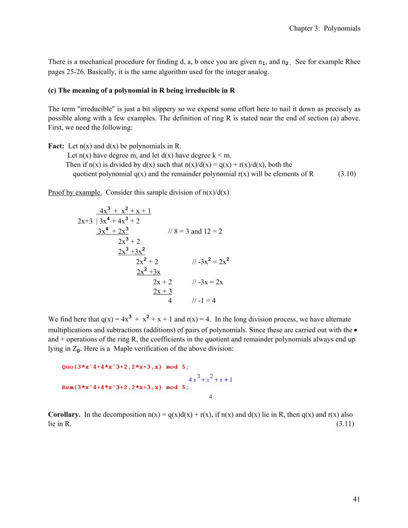
Chapter 3: Polynomials
41
There is a mechanical procedure for finding d, a, b once you are given n1, and n2. See for example Rhee pages 25-26. Basically, it is the same algorithm used for the integer analog. (c) The meaning of a polynomial in R being irreducible in R The term "irreducible" is just a bit slippery so we expend some effort here to nail it down as precisely as possible along with a few examples. The definition of ring R is stated near the end of section (a) above. First, we need the following: Fact: Let n(x) and d(x) be polynomials in R. Let n(x) have degree m, and let d(x) have degree k < m. Then if n(x) is divided by d(x) such that n(x)/d(x) = q(x) + r(x)/d(x), both the quotient polynomial q(x) and the remainder polynomial r(x) will be elements of R (3.10) Proof by example. Consider this sample division of n(x)/d(x) 4x3 + x2 + x + 1 2x+3 | 3x4 + 4x3 + 2 3x4 + 2x3 // 8 = 3 and 12 = 2 2x3 + 2 2x3 +3x2
2x2 + 2 // -3x2 = 2x2 2x2 +3x 2x + 2 // -3x = 2x 2x + 3 4 // -1 = 4 We find here that q(x) = 4x3 + x2 + x + 1 and r(x) = 4. In the long division process, we have alternate multiplications and subtractions (additions) of pairs of polynomials. Since these are carried out with the • and + operations of the ring R, the coefficients in the quotient and remainder polynomials always end up lying in Zp. Here is a Maple verification of the above division:
Corollary. In the decomposition n(x) = q(x)d(x) + r(x), if n(x) and d(x) lie in R, then q(x) and r(x) also lie in R. (3.11)
Chapter 3: Polynomials
42
We now list off several equivalent definitions of the meaning of n(x) in R being reducible in R. It is understood that all f(x) here are polynomials: (3.12) 1. Given n(x) in R of degree m, if there exists some d(x) in R of degree 0 < k < m such that in the known unique expansion n(x) = q(x)d(x) + r(x) one gets r(x) = 0, then n(x) is said to be reducible in R. As noted above, q(x) will also be in R. 2. Given n(x) in R of degree m, if there exists some d(x) in R of degree 0 < k < m such that n(x) = q(x)d(x) where both d(x) and q(x) are in R, then n(x) is reducible in R. 3. If n(x) in R can be factored into a product of factors q(x)d(x) both of which lie in R and both of which have degree > 0, then n(x) is reducible in R. 4. Given n(x) in R of degree m, if GCD(n(x),d(x)) ≠ 1 for some d(x) in R of degree 0 < k < m, then n(x) is reducible in R. Examples: n(x) = (x-a)•(x-b) is reducible since d(x) = (x-a) is a dividing factor with 0 < k < 2 (ie, k= 1). Notice the assumption implicitly made here that both a and b are elements of Zp. If either a or b does not lie in Zp, then at least one of the factors does not lie in R, and in that case this n(x) would not be reducible according to item 2 above. n(x) = x2 + 2x + 1 is reducible since it equals (x+1)•(x+1). n(x) = x2 + 1 is not reducible for Zp with p > 2 because it cannot be factored in such a way that the factors are both in R with the degree of both factors being > 0. For example, (x+i)•(x-i) is not allowed because (x+i) does not lie in R since i does not lie in Zp. However, in the special case of Z2 we can write x2+1 = x2- 1 = (x+1)•(x-1) and then x2 is reducible in this particular R. n(x) = (x-a) is not reducible because no d(x) exists with 0 < k < 1 that could be a divisor. n(x) = (2x-a) is not reducible for the same reason n(x) = 2•(x-a) is not reducible for the same reason. If n(x) in R is not reducible in R, then it is irreducible in R. The last three examples above show n(x) that are irreducible, and x2 + 1 is irreducible for Z2 only. Comment: For the more general R consisting of polynomials with coefficients in a ring-with-identity R, one can define the irreducibility of f(x) exactly as above: just replace Zp with R. The famous example is that x2+1 is irreducible in R(r) (R with R = reals) but is reducible in R(c) (R with R =complex).
Chapter 3: Polynomials
43
(d) The Residue Class Decomposition of R In this section we continue to use • and + to indicate the two operations of the ring R defined at the end of section (a) above. Eventually we will stop displaying • so that a(x) • b(x) will be written as a(x)b(x), but for the present • is retained. Now we are going to repeat exactly the discussion of Chapter 1 (c) 1 about decomposing a ring based on some ideal of the ring. First, we have to find a candidate ideal. We know from the integer ring case that one could make an ideal by taking all multiples of some integer N. In the polynomial case, one can form an ideal within the ring of polynomials R consisting of all polynomials which are multiples of some specified polynomial f(x). We denote by ( f(x) ) the set of all polynomials which are multiples of f. We shall assume that f(x) is some arbitrary polynomial in R of degree m. Proof that ( f(x) ) is an ideal within R: There is nothing mysterious about this. If polynomial F(x) is a multiple of f(x), then there is some q(x) such that F(x) = q(x)f(x). One might have to do a bit of factoring of F(x) to expose the fact that it can be written in this manner. This is trivial, but the point should not be missed. For example, if R = reals, we have (x2 - 1) = (x + 1)•(x - 1) so (x2 - 1) is a "multiple" of either (x + 1) or (x -1) . So we have come up with a claimed ideal I of the ring R of polynomials. The ideal consists of only those polynomials in R which are multiples of f(x). Why is this set an ideal? First of all, it is a ring (and an abelian one at that) because the properties of (1.5) are trivially satisfied, including closure under both + and •. To see this, consider two polynomials in the ideal, F1(x) = f1(x) • f(x) F2(x) = f2(x) • f(x) . Closure under +: F1 + F2 = f1•f + f2•f = (f1+ f2) •f = f3•f = in the ideal since multiple of f Closure under •: F1• F2 = (f1•f)• (f2•f) = (f1•f•f2) •f = f4•f = in the ideal since multiple of f So ( f(x) ) is a subring of the ring of all polynomials. From definition (1.22) we then have to show that for any r(x) in R and i(x) in I, r(x) • i(x) is in I (then i(x)•r(x) will also be in I since • is commutative): i(x)• r(x) = (j(x) • f(x)) • r(x) = (j(x) • r(x)) •f(x) = in the ideal QED Thus, this restricted set of polynomials in R forms an ideal which we call I = ( f(x) ). Now we make the chart, just as before. Here is our Chapter 1 chart for general ring R and ideal I:

Chapter 3: Polynomials
44
i1=0 i2 i3 i4 ... ik // residue class #1 r1 r1+ i2 r1+ i3 r1+ i4 ... r1+ ik // residue class #2 r2 r2+ i2 r2+ i3 r2+ i4 ... r2+ ik // etc more rows like the above (1.23) We now apply this to our polynomial situation (comments below), i1(x)=0 i2(x) = q(x)•f(x) for all possible q(x) r1(x) r1(x) + i2(x) = q(x)•f(x) + r1(x), for all possible q(x) r2(x) r2(x) + i2(x) = q(x)•f(x) + r2(x), for all possible q(x) more rows like the above (3.13) First look at the top row, which is the ideal. We separate out the polynomial 0 and put it first. Then, instead of trying to list off specific elements of the ideal going left to right, we write this list by saying that the polynomial q(x) can be any polynomial in R. As q(x) ranges over all possible polynomials, we get our list for that row. It is of course an infinite list since we can have q(x) of any degree. Now look at the next row. We pick some r1(x) from the ring R of polynomials of degree < m and plop it down in the left column, then we form the row as instructed by the previous prototype chart (1.23). Now suddenly one sees an interesting coincidence of the notation. The polynomials ri(x) which are the residue class (row) leaders, look like "remainder" polynomials, and the q(x) notation suggests "quotient" polynomials. In fact, all polynomials in the second row have r1(x) as their remainder when they are divided by f(x), and q(x) is in fact the quotient polynomial. There are as many polynomials in the second row as there are quotient polynomials q(x). As noted above, this number of quotient polynomials is infinite. [ We can in fact label a chart row by any of the elements in that row, but it is best to use the remainder polynomial as the "residue class leader" . Each row has only one polynomial of degree < m. ] So here is the general idea of the above chart. Across the top you have the ideal which is the set of all polynomials which are multiples of f(x) with no remainder. Then each row is represented by some possible remainder (of degree less than that of f(x)) you could get by dividing f(x) into elements of the polynomial ring. How many rows are there? Since f(x) is of degree m, a remainder polynomial is of degree m-1 or less. A remainder polynomial then has m coefficients. Since each coefficient lies in Zp, there are pm such remainder polynomials, and so there are pm rows in the chart including the first row of the ideal. {} Notation: Recall that we have used the notation {joe} to label the row of a coset chart in the case of groups and subgroups, and to label the row of a residue class ring chart in the case of rings and ideals. The "joe" object in these two cases was the coset leader or the residue class leader. See for example Chapter 1 (b) 2, Chapter 1 (c) 2 or (1.38). This notation continues in the polynomial world, and {rk(x)} denotes the residue class chart row whose remainder function is rk(x). For GF(3m) some sample chart rows would be indicated by {1}, {2}, {x}, {2x}, {x2}, {2x2} and so on. For GF(2m) we have {1}, {x}, {x2}, {x+x2}, etc.
Chapter 3: Polynomials
45
We pause for a moment to note a few facts concerning this notation. We are running out of symbols for multiplication, so we use + and • for both polynomials and chart rows. Facts using {} notation: (3.14) (a) {r1(x)+r2(x)} = {r1(x)} + {r2(x)} (b) {r1(x)•r2(x)} = {r1(x)} • {r2(x)} (c) {c r2(x)} = c{r2(x)} for c in Zp (d) {cxk} = c{xk} for c in Zp (e) {xk} = {x}k (f) {p(x)} = p({x}) where p(x) is a polynomial with coefficients in GF(p) (g) {r1(x)} + {r2(x)} = {r3(x)} where r3(x) = r1(x) + r2(x) (h) {r1(x)} • {r2(x)} = {r4(x)} where r4(x) = Rem[ (r1(x)•r2(x))/f(x) ] Proof: In some proofs we just give examples and the general proof should be obvious. (a) and (b) The equations here are just statements of how elements of a residue class ring are added and multiplied. If the degree of r1(x)•r2(x) > m, it is still OK to label a row as {r1(x)•r2(x)} . (c) for example, {2 r2(x)} = { r2(x) + r2(x)} = {r2(x)} + {r2(x)} = 2 {r2(x)} // used (a) (d) special case of (c) where r2(x) = xk (e) for example, {x3} = {x2}•{x} = {x} • {x} • {x} = {x}3. (f) {p(x)} = {Σiaixi} = Σi{aixi} (a) = Σiai{xi} (c) = Σiai{x}i (e) = p({x}) (g) and (h). Normally we like to label chart rows with remainder polynomials of degree < m, and in these two lines we assume all the ri(x) have degree < m. For addition, the sum of two polynomials of degree < m itself has degree < m, so no remaindering is necessary. For multiplication, it often happens that the degree of the product of two polynomials of degree < m will have degree ≥ m, so in this case we must do the remaindering as shown. The elements of R/(f(x)) can be regarded either as these chart rows, or as the set of remainder polynomials of degree < n which label the chart rows. In the integer world, the analog statements of (g) and (h) are these, from (1.39) where we replace 5 by n, {i} + {j} = {k} where k = Rem[(i+j)/n] = (i+j) mod n {i} • {j} = {m} where m = Rem[(ij)/n] = (ij) mod n (1.39) Since the sum of two integers each of which is < n an exceed n, remaindering here is required for both addition and multiplication, whereas in the polynomial case remaindering is needed only for multiplication. We are now rapidly closing on the target of all our efforts. Admittedly, it has taken a while. We considered our special ring R of polynomials with coefficients in Zp, and we considered an ideal consisting of all polynomials which were multiples of some selected polynomial f(x) of degree m. We then used this ideal to construct the "chart" which partitions the ring into rows of polynomials, the residue classes. There is one row for each possible remainder polynomial, and the polynomials across a row are "indexed" by the quotient polynomial. The number of rows equals the number of possible remainder polynomials pm , and the first row corresponds to remainder 0.
Chapter 3: Polynomials
46
We know from Chapter 1 (c) 2 that these rows can be considered elements of a new ring known as the residue class ring. We indicated this new ring by the notation R/I, residue class ring = R/( f(x) ) If the degree of f(x) is m, the residue class ring has pm elements. Here then comes the grand finale, the analogy to the Big Fact of (1.44): Theorem: If a polynomial f(x) is irreducible in R, then R/( f(x) ) is a field. (3.15) Proof: The proof exactly parallels the proof of (1.44). We have to show that for some {r(x)} we can find an inverse {s(x)} such that {r(x)}• {s(x)} = {1}. We will mimic every statement of the previous proof: We note that, since f(x) is irreducible in R and r(x) has smaller degree than f(x), they cannot be multiples, so their greatest common divisor is 1. Using Bezout's Identity (3.5) above, we claim that polynomials N(x) and M(x) must exist such that 1 = N(x)r(x)-M(x)f(x). This says that there exists an N(x) such that 1 = Rem[N(x)r(x)/f(x)]. Now expand N(x) = K(x)f(x) + s(x), where the degree of s(x) is less than that of
f(x). This gives 1 = Rem(K(x)f(x)r(x) +s(x)r(x)
f(x) ) = Rem[s(x)r(x)/f(x)]. This says that {s(x)r(x)} = 1 and
therefore {r(x)}• {s(x)} = {1}. Thus, if f(x) is irreducible in R then the residue class ring R / ( f(x) ) is a field. QED Implication: Find some irreducible polynomial f(x) of degree m in the ring R. Then the residue class ring R / ( f(x) ) is a field with pm elements, because there are pm rows in the chart (3.6). But, from Chapter 1 we know that all finite fields must be equivalent to the Galois Fields, so we have explicitly constructed a representation of GF(pm) !! (3.16) In ring R, the coefficients of the polynomials are elements of Zp = GF(p), which is the base field or ground field. The elements of the residue class ring R / ( f(x) ) represent GF(pm) which is the extension field. So we now have a method whereby we start with a ground field that we know about, namely GF(p), and we construct a pile of new extension fields GF(pm), where m = any integer. From our construction, we should be able to learn everything about GF(pm) and therefore everything about any finite field. We have arrived at a major waypoint along our little voyage. (e) Comparison Between Chapter 3 and Chapter 1 In Chapter 1 we considered the residue class ring Z/(p) for p = prime and showed it was a field having p elements. This got us used to working with a residue class ring. We knew all along that this field was equivalent to Zp , the modulo-p field, so we didn't really need Z/(p), it was just practice. In Z/(p) the ring Z was integers. We partitioned up the integers into chart rows, where the integers in each row had something in common: some remainder r < p when divided by p. There were p rows.

Chapter 3: Polynomials
47
Here in Chapter 3 we really need the residue class ring. We need something with pm elements, and we realize that a R/( f(x) ) has pm remainders if f(x) is of degree m. If we take f(x) to be irreducible in R, then this residue class ring R/( f(x) ) becomes a field with pm elements, and then GF(pm) = R / ( f(x) ) R = polys with coefficients in Zp=GF(p) f(x) = degree m, irreducible in R . (3.17) Obviously, there are p remainder polynomials which are constants independent of x. One can consider these remainders to be generating GF(p) as a subfield of GF(pm), a subject we examine in the next Chapter.
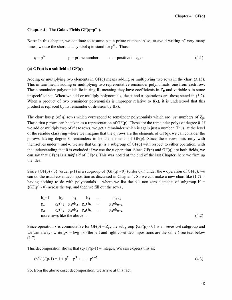
Chapter 4: GF(q)
48
Chapter 4: The Galois Fields GF(q=pm ). Note: In this chapter, we continue to assume p = a prime number. Also, to avoid writing pm very many times, we use the shorthand symbol q to stand for pm . Thus: q = pm p = prime number m = positive integer (4.1) (a) GF(p) is a subfield of GF(q) Adding or multiplying two elements in GF(q) means adding or multiplying two rows in the chart (3.13). This in turn means adding or multiplying two representative remainder polynomials, one from each row. These remainder polynomials lie in ring R, meaning they have coefficients in Zp and variable x in some unspecified set. When we add or multiply polynomials, the + and • operations are those stated in (3.2). When a product of two remainder polynomials is improper relative to f(x), it is understood that this product is replaced by its remainder of division by f(x). The chart has p (of q) rows which correspond to remainder polynomials which are just numbers of Zp. These first p rows can be taken as a representation of GF(p). These are the remainder polys of degree 0. If we add or multiply two of these rows, we get a remainder which is again just a number. Thus, at the level of the residue class ring where we imagine that the q rows are the elements of GF(q), we can consider the p rows having degree 0 remainders to be the elements of GF(p). Since these rows mix only with themselves under + and •, we see that GF(p) is a subgroup of GF(q) with respect to either operation, with the understanding that 0 is excluded if we use the • operation. Since GF(p) and GF(q) are both fields, we can say that GF(p) is a subfield of GF(q). This was noted at the end of the last Chapter, here we firm up the idea. Since {GF(p) - 0} (order p-1) is a subgroup of {GF(q) - 0} (order q-1) under the • operation of GF(q), we can do the usual coset decomposition as discussed in Chapter 1. So we can make a new chart like (1.7) -- having nothing to do with polynomials -- where we list the p-1 non-zero elements of subgroup H = {GF(p) - 0} across the top, and then we fill out the rows , h1=1 h2 h3 h4 ... hp-1 g1 g1•h2 g1•h3 g1•h4 ... g1•hp-1 g2 g2•h2 g2•h3 g2•h4 ... g2•hp-1 more rows like the above . (4.2) Since operation • is commutative for GF(p) = Zp, the subgroup {GF(p) - 0} is an invariant subgroup and we can always write g•h= h•g , so the left and right coset decompositions are the same ( see text below (1.7). This decomposition shows that (q-1)/(p-1) = integer. We can express this as: (pm-1)/(p-1) = 1 + p2 + p3 + .... + pm-1 (4.3)
So, from the above coset decomposition, we arrive at this fact:
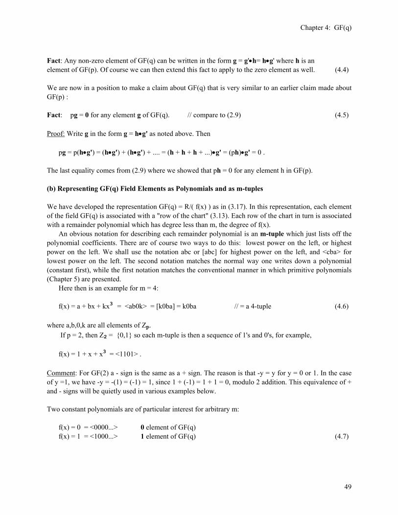
Chapter 4: GF(q)
49
Fact: Any non-zero element of GF(q) can be written in the form g = g'•h= h•g' where h is an element of GF(p). Of course we can then extend this fact to apply to the zero element as well. (4.4) We are now in a position to make a claim about GF(q) that is very similar to an earlier claim made about GF(p) : Fact: pg = 0 for any element g of GF(q). // compare to (2.9) (4.5) Proof: Write g in the form g = h•g' as noted above. Then pg = p(h•g') = (h•g') + (h•g') + .... = (h + h + h + ...)•g' = (ph)•g' = 0 . The last equality comes from (2.9) where we showed that ph = 0 for any element h in GF(p). (b) Representing GF(q) Field Elements as Polynomials and as m-tuples We have developed the representation GF(q) = R/( f(x) ) as in (3.17). In this representation, each element of the field GF(q) is associated with a "row of the chart" (3.13). Each row of the chart in turn is associated with a remainder polynomial which has degree less than m, the degree of f(x). An obvious notation for describing each remainder polynomial is an m-tuple which just lists off the polynomial coefficients. There are of course two ways to do this: lowest power on the left, or highest power on the left. We shall use the notation abc or [abc] for highest power on the left, and <cba> for lowest power on the left. The second notation matches the normal way one writes down a polynomial (constant first), while the first notation matches the conventional manner in which primitive polynomials (Chapter 5) are presented. Here then is an example for m = 4: f(x) = a + bx + kx3 = <ab0k> = [k0ba] = k0ba // = a 4-tuple (4.6) where a,b,0,k are all elements of Zp. If p = 2, then Z2 = {0,1} so each m-tuple is then a sequence of 1's and 0's, for example, f(x) = 1 + x + x3 = <1101> . Comment: For GF(2) a - sign is the same as a + sign. The reason is that -y = y for y = 0 or 1. In the case of y =1, we have -y = -(1) = (-1) = 1, since 1 + (-1) = 1 + 1 = 0, modulo 2 addition. This equivalence of + and - signs will be quietly used in various examples below. Two constant polynomials are of particular interest for arbitrary m: f(x) = 0 = <0000...> 0 element of GF(q) f(x) = 1 = <1000...> 1 element of GF(q) (4.7)

Chapter 4: GF(q)
50
Each element of GF(q) is associated with a particular remainder polynomial of degree less than m, and therefore with a particular m-tuple having m Zp integers. We can therefore use these m-tuples to label the GF(q) field elements in a clear, unambiguous fashion. Now consider two remainder polynomials a(x) and b(x), for some m. The m-tuples are also shown. a(x) = a0 + a1 • x + a2 • x2 + a3 • x3 +... = <a0 a1 a2 a3 ...> b(x) = b0 + b1 • x + b2 • x2 + b3 • x3 +... = <b0 b1 b2 b3 ...> As noted above, adding two GF(q) field elements means adding rows of the chart, and this means adding remainder polynomials. This in turn means adding the coefficients. But the coefficients live in Zp, and addition here is just modulo-p addition. Thus, we can add the above remainder polynomials to get the following result: a(x) + b(x) = c(x) = c0 + c1 • x + c2 • x2 + c3 • x3 +... = <c0 c1 c2 c3 ...> where ci = ai ⊕ bi where ⊕ means addition modulo p (4.8) We have just proven : Fact: If the elements of GF(q) are represented as polynomial coefficient m-tuples, the addition table can be written down immediately with no further ado. One just does a modulo-p addition on each m-tuple position. Knowledge of the defining polynomial f(x) is not even needed. (4.9) Example: Here is the addition table for GF(4) = GF(22) where recall that the unbracketed m-tuple notation means the lowest power on the right. The same table is shown on the right where each element is given a decimal value from the usual binary evaluation of a sequence of 1's and 0's + 00 01 10 11 + 0 1 2 3 00 00 01 10 11 0 0 1 2 3 01 01 00 11 10 1 1 0 3 2 10 10 11 00 01 2 2 3 0 1 11 11 10 01 00 3 3 2 1 0 (4.10) Now what about multiplication? Following the same line of argument, and writing things out in the obvious manner, one can easily show that the product of two field elements, each represented by some remainder ra(x) and rb(x) appearing in the left column of chart (3.13), is a new field element represented by the product of the remainders. However, although each remainder is of degree less than m, it may happen that the product remainder has degree more than m. In this case, as is easily shown, the right thing to do is take this "improper" product remainder, divide it by f(x), and the resulting proper remainder is the remainder you want, call it rc(x). This of course requires a knowledge of f(x).
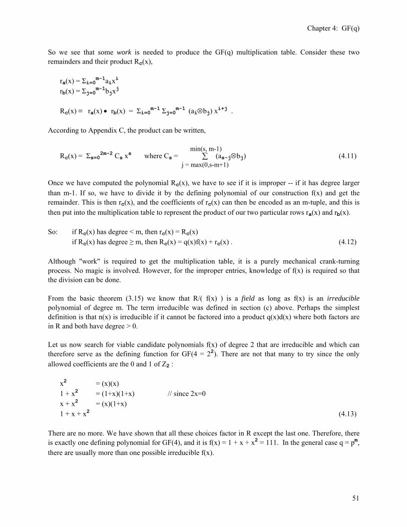
Chapter 4: GF(q)
51
So we see that some work is needed to produce the GF(q) multiplication table. Consider these two remainders and their product Rc(x), ra(x) = Σi=0m-1aixi rb(x) = Σj=0m-1bjxj Rc(x) ≡ ra(x) • rb(x) = Σi=0m-1 Σj=0m-1 (ai⊗bj) xi+j . According to Appendix C, the product can be written,
Rc(x) = Σs=02m-2 Cs xs where Cs = ∑j = max(0,s-m+1)
min(s, m-1) (as-j⊗bj) (4.11)
Once we have computed the polynomial Rc(x), we have to see if it is improper -- if it has degree larger than m-1. If so, we have to divide it by the defining polynomial of our construction f(x) and get the remainder. This is then rc(x), and the coefficients of rc(x) can then be encoded as an m-tuple, and this is then put into the multiplication table to represent the product of our two particular rows ra(x) and rb(x). So: if Rc(x) has degree < m, then rc(x) = Rc(x) if Rc(x) has degree ≥ m, then Rc(x) = q(x)f(x) + rc(x) . (4.12) Although "work" is required to get the multiplication table, it is a purely mechanical crank-turning process. No magic is involved. However, for the improper entries, knowledge of f(x) is required so that the division can be done. From the basic theorem (3.15) we know that R/( f(x) ) is a field as long as f(x) is an irreducible polynomial of degree m. The term irreducible was defined in section (c) above. Perhaps the simplest definition is that n(x) is irreducible if it cannot be factored into a product q(x)d(x) where both factors are in R and both have degree > 0. Let us now search for viable candidate polynomials f(x) of degree 2 that are irreducible and which can therefore serve as the defining function for GF(4 = 22). There are not that many to try since the only allowed coefficients are the 0 and 1 of Z2 : x2 = (x)(x) 1 + x2 = (1+x)(1+x) // since 2x=0 x + x2 = (x)(1+x) 1 + x + x2 (4.13) There are no more. We have shown that all these choices factor in R except the last one. Therefore, there is exactly one defining polynomial for GF(4), and it is f(x) = 1 + x + x2 = 111. In the general case q = pm, there are usually more than one possible irreducible f(x).
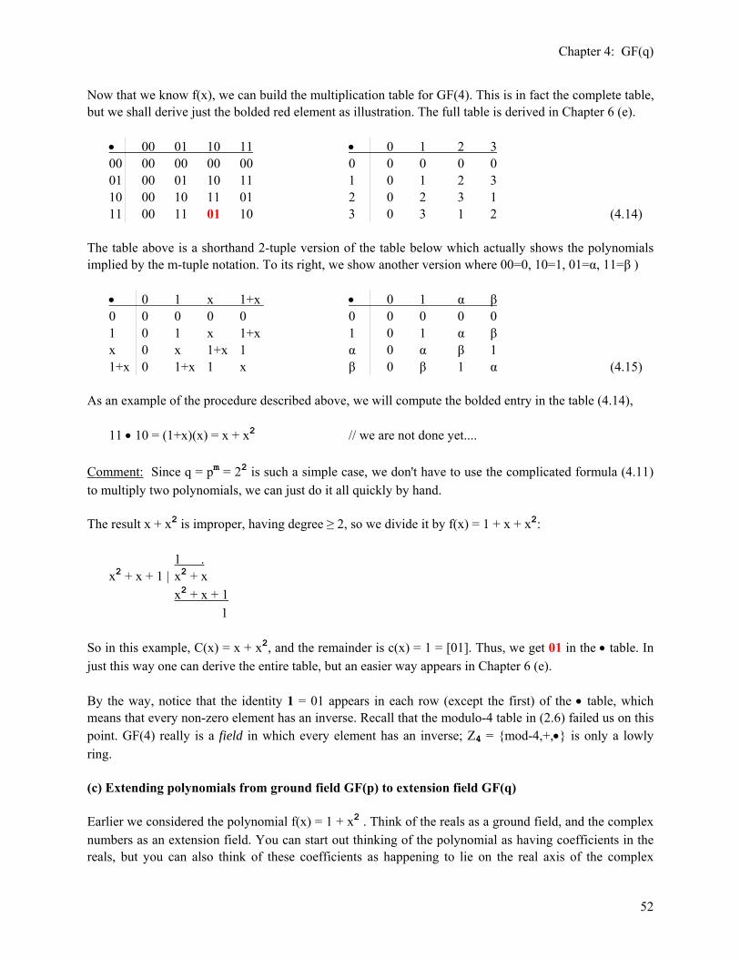
Chapter 4: GF(q)
52
Now that we know f(x), we can build the multiplication table for GF(4). This is in fact the complete table, but we shall derive just the bolded red element as illustration. The full table is derived in Chapter 6 (e). • 00 01 10 11 • 0 1 2 3 00 00 00 00 00 0 0 0 0 0 01 00 01 10 11 1 0 1 2 3 10 00 10 11 01 2 0 2 3 1 11 00 11 01 10 3 0 3 1 2 (4.14) The table above is a shorthand 2-tuple version of the table below which actually shows the polynomials implied by the m-tuple notation. To its right, we show another version where 00=0, 10=1, 01=α, 11=β ) • 0 1 x 1+x • 0 1 α β 0 0 0 0 0 0 0 0 0 0 1 0 1 x 1+x 1 0 1 α β x 0 x 1+x 1 α 0 α β 1 1+x 0 1+x 1 x β 0 β 1 α (4.15) As an example of the procedure described above, we will compute the bolded entry in the table (4.14), 11 • 10 = (1+x)(x) = x + x2 // we are not done yet....
Comment: Since q = pm = 22 is such a simple case, we don't have to use the complicated formula (4.11) to multiply two polynomials, we can just do it all quickly by hand. The result x + x2 is improper, having degree ≥ 2, so we divide it by f(x) = 1 + x + x2: 1 . x2 + x + 1 | x2 + x x2 + x + 1 1 So in this example, C(x) = x + x2, and the remainder is c(x) = 1 = [01]. Thus, we get 01 in the • table. In just this way one can derive the entire table, but an easier way appears in Chapter 6 (e). By the way, notice that the identity 1 = 01 appears in each row (except the first) of the • table, which means that every non-zero element has an inverse. Recall that the modulo-4 table in (2.6) failed us on this point. GF(4) really is a field in which every element has an inverse; Z4 = {mod-4,+,•} is only a lowly ring. (c) Extending polynomials from ground field GF(p) to extension field GF(q) Earlier we considered the polynomial f(x) = 1 + x2 . Think of the reals as a ground field, and the complex numbers as an extension field. You can start out thinking of the polynomial as having coefficients in the reals, but you can also think of these coefficients as happening to lie on the real axis of the complex
Chapter 4: GF(q)
53
number plane. In some sense, then, you are extending the interpretation of your polynomial to a larger world. As noted earlier, a crucial difference is that in the reals, this f(x) cannot be factored and is therefore irreducible, but when extended to the complex numbers, suddenly f(x) is no longer irreducible and can be factored into (x + i)(x - i). The reason that extending the polynomial from the reals to the complex numbers makes sense is that the reals form a subfield of the field of complex numbers. In similar fashion, GF(p) is a subfield of GF(q). Thus, we can take any polynomial having coefficients in GF(p) and then think of this polynomial as being extended so these coefficients are now elements of the larger field GF(q). The polynomial "looks" the same before and after this extension. However, it may turn out that the polynomial is more factorable in GF(q) than it is in GF(p). Note that in general you cannot go the other direction. If you have a polynomial with general coefficients in GF(q), how can you write it in terms of only GF(p) elements? For example, the polynomial over the complex number field f(x) = (x + i) cannot be written over the real number field. (d) Cyclic Subgroups and GF(q) Much of the structure of the Galois Field GF(q) can be brought to light by analyzing its cyclic subgroups under the multiplicative operation •. That is the main subject of this section. A cyclic subgroup was defined in Chapter 1 (b) 3, and a few facts about it derived there. Many of the "facts" below apply to cyclic subgroups in general, or in some cases, to commutative groups in general. However, we will be specific and claim our facts only with respect to the field GF(q). There are 16 Facts presented in this section, all with proofs. The reader is encouraged to read the proofs, since they serve as checks on the previous material. The main conclusions of this section are presented as Big Theorems 1 and 2. This is a long and somewhat tedious development.
Notation: In the following set of fact developments, the term "cyclic subgroup" refers exclusively to a cyclic subgroup of the group {GF(q) - 0,•}. This means the multiplicative group under • of GF(q) where we have excluded the 0 element. The group {GF(q) - 0,•} thus has order q-1. A divides B (sometimes written A|B ) means that there is no remainder when A is divided into B. It means that B is a multiple of A. If A and B are numbers, it means that B= Ak for some integer k = 1,2,3... If A and B are polynomials, it means B(x) = A(x)k(x) for some polynomial k(x). Fact 1: The order n of any cyclic subgroup of {GF(q) - 0,•} divides q-1. (4.16) Proof: The order of any subgroup H divides the order of a group G containing it. This follows from the coset decomposition discussed in Chapter 1 (b) 1.

Chapter 4: GF(q)
54
Fact 2: Start with any α in {GF(q) - 0 ,•}. Start forming a list by taking powers of α: { 1 = α0 , α = α1, α2, α3, ...... } We claim quite a few things in this one "fact" (proofs to follow): (a) there exists an integer n such that αn-1 is the last distinct element of this list. Thus, the complete list has n distinct elements as follows: { 1, α, α2, ...... αn-1 } (b) αn = 1, which repeats the first element of the list (this is the first repeat) (c) all subsequent powers repeat elements of the list. (d) The list of n distinct elements forms a cyclic subgroup of {GF(q) - 0 ,•} of order n. We can denote this as: (α, n, •) = cyclic subgroup of {GF(q) - 0 ,•} = ( generator, order , • operation ) (e) This integer n is called the order of α; α is said to be of order n. [ If α is of order n, it generates a cyclic subgroup within {GF(q) - 0 ,•} of order n. ] (f ) The fact that α has order n does not imply that other elements of the subgroup have order n. (g) α is called a generator of the cyclic subgroup. (h) Any other list element β = αk which, upon taking powers 0 through n-1, yields the same list as α (with a possible reordering of the elements) is also regarded as a generator. Such an alternate generator has order n if α has order n. (i) If βn = 1, it does not follow that n is the order of β.
(j) We have shown in (1.9a) that any element of {GF(q) - 0 ,•} lies in some cyclic subgroup of some order. For example, α lies in (α, n,•). Another example is that 1 lies in (1,1,•). (k) The order of α is the smallest integer n such that αn = 1. (l) The order of α is a divisor of q-1, which is to say, (q-1)/n = integer. (4.17) Proof: (a),(b) All elements in the list are contained in {GF(q) - 0 ,•} which is a finite set. Therefore, there must be a first power where an element of the sequence repeats some earlier element. Suppose this power is n, so that αn-1 is the last distinct item on the list, and suppose αn = αk , some earlier item on the list. If k > 0, then we would have αn-1 = αk-1, which says that the previous power also repeated an item on the list, which is a contradiction. Thus, we must have k=0, so αn = 1. (c) As we build subsequent powers, the list repeats: αn = 1, αn+1 = α, αn+2 = α2 , and so on. (f) Suppose the order of α is 4 so list is {1, α, α2, α3} with α4 = 1. Consider β = α2. The order of β is 2, not 4, since the β list is {1, β = α2, β2 = α4 = 1} Notice that 2 divides 4. (h) Such alternate generators may or may not exist;

Chapter 4: GF(q)
55
(i) Suppose the order of β is 5, so that β5 = 1. It is then certainly true that β10 = 1, but this clearly does not imply that β has order 10. (k) By the definition of n as the order of α above, αn is the first repeat element. There is no earlier repeat element, so there is no smaller subgroup within the one discussed that is generated by α. So for this n which has αn = 1, we know that there is no smaller integer N < n such that αN= 1. (l) This thing (α, n, •) of order n is a cyclic subgroup of {GF(q) - 0 ,•} which has order q-1. According to (1.8), the order of any subgroup divides evenly into the order of the parent group. Fact 3: Let g ∈ {GF(q) - 0 ,•}. If "g has order n" , then gn = 1 and n is the least integer for which gn = 1. (4.18) Proof: This follows from the definition of the order of g. We just want to stress the fact. Fact 4: Let g ∈ {GF(q) - 0 ,•}. If gk = 1, the "order of g" divides k. (4.19) Proof: Let n be the order of g. We know from the definition that n is the smallest power of g such that gn = 1. Consider some higher power that is not a multiple of n: k = qn + r where 0 < r < n. Then gk = gqn gr = gr. But we know that gr ≠ 1 since 0 < r < n. Thus, if k is not a multiple of n, gk ≠ 1. Therefore, if gk = 1, k must be a multiple of n, and n divides k. Look back at the β10 = 1 comment. Fact 5: If β is any element of the cyclic subgroup (α,n,•), then βn = 1. (4.20) Proof: Since β ∈ (α,n,•), we know that β = αk for some k, and αn = 1 . Thus βn = αnk = 1k = 1. Fact 6: If β is any element of (α,n,•), then the order of β divides n, the order of α. More specifically, we claim that [order of β] = n/GCD(k,n) where β = αk. (4.21) Proof: Since β ∈ (α,n,•), we know that β = αk for some k, and αn = 1. Then as we enumerate the subgroup generated by β, we get { 1, β, β2, β3 ... } = { 1, αk , α2k , α3k ...}. If the order of β is m, then βm = 1, and our little cyclic subgroup can be called (β,m,•). This implies that m is the smallest integer such that βm = (αk)m = 1 or α(km) = 1. We now apply Fact 4 with g → α and k → km and "order of g" is "order of α" which is n. Thus, n divides km, so km = nN for some integer N. From the Lemma below, we conclude that m = n/GCD(k,n) so that m = [order of β] = n/GCD(k,n). QED Lemma: The smallest integer m such that km = nN is m = n/GCD(k,n). (4.22) Proof: In (G.21) it is shown that, for ax = by, the smallest-x solution is x = b/d where d = GCD(a,b). We apply that here with a = k, x = m, b = n and y = N to find that the smallest-m solution is m = n/d where d = GCD(k,n).

Chapter 4: GF(q)
56
We now develop some facts which involve polynomials. These polynomials are not restricted to the special ring R of polynomials discussed in Chapter 3 (a). That is, the coefficients are not necessarily elements of Zp. Element a is a root of polynomial f(x) means that f(a) = 0. (4.23) Fact 7: (The Factor Theorem) Polynomial f(x) can be written as f(x) = (x-a)q(x) for some polynomial q(x) if and only if a is a root of f(x). (4.24) Proof: (⇐) Assume a is a root of f(x). By the Division Algorithm, we can expand f(x) = (x-a)q(x) + r(x) where the remainder polynomial r(x) has degree less than (x-a), which means it has degree 0, which means r(x) = constant K. Since f(a) = 0, we see that r(x) = K = 0. (⇒) Assume f(x) = (x-a)q(x). Since q(x) is a polynomial, q(a) is finite, so f(a) = 0. Fact 8: The n elements ai of the cyclic subgroup (α,n,•) are the n roots of the polynomial 1 - xn. This polynomial can be fully factored into a product of n linear factors (x-ai) where the ai are the roots, xn - 1 = (x - a1)• (x - a2)• (x - a3)• ... (x - an) . (4.25) Proof: We know from Fact 5 that (ai)n = 1 for all n elements in the cyclic subgroup. Thus, these n elements are all roots of f(x) = 1 - xn. According to Fact 7, each such root results in a factor (x-ai) in f(x). Since this polynomial has at most n roots and we have found them all, it fully factors as claimed. Fact 9: Consider two cyclic subgroups A = (α,n,•) and B = (β,m,•) of some group. If n=km for some integer k , then A contains B. (4.26) Corollary: If the orders of two cyclic subgroups are the same, then the subgroups are the same. (4.27) Corollary : There can be at most one cyclic subgroup of any given order. (4.28) Proof: Let b ∈ (β,m,•). From Fact 5 , bm = 1. Raise both sides of this last equation to power k to get bmk = 1. If mk=n, we get bn = 1 Thus, b is a root of f(x) = 1 - xn. Since A is a cyclic subgroup of order n, we know by Fact 8 that the n roots of f(x) = 1 - xn are all elements of A. Since b is a root of f(x), b must equal one of the elements of a. Thus, b is contained in A. Since this is true for any b in B, this means all of B is contained in A. Corollaries follow from k=1. The exponent e is the order of the largest cyclic subgroup E in {GF(q) - 0}, •}. Heads Up: This is one of several competing meanings for the word "exponent" in Galois Theory. There are after all quite a few exponents! This particular one is going to end up being the same as q-1 according to Big Theorem 1 below, so its interest does not persist.
Chapter 4: GF(q)
57
Fact 10: The order of any cyclic subgroup of {GF(q)-0,•} divides the exponent e. (4.29) Proof: This Fact 10 looks innocent enough, but it is the real meat and potatoes of this entire section. We are assuming there is some maximal cyclic subgroup called E of order e. As far as we know at this point in the development, E can be less than all of {GF(q)-0,•}. Thus, if there is some cyclic subgroup called G, we do not know that G is contained in E. If we knew that all such G were contained in E, we would immediately know Fact 10, since the order of any subgroup G divides the order of the containing subgroup E. So at this point, as far as we know, G may or may not be contained within E. Thus, we need to find a more general proof of Fact 10. Although this proof is somewhat complicated, it uses only Facts 3, 4 and 5, and the basic properties of integers. The proof is given in Appendix A. Based on Fact 10, we will quickly arrive at Big Theorem 1 below which says that {GF(q) - 0, •} is cyclic. This implies that E must indeed be all of {GF(q) - 0, •}. In retrospect, Fact 10 seems less impressive. But one must remember that the information that E = {GF(q) - 0, •} is not available for the proof of Fact 10. Big Theorem 1: The entire group {GF(q) - 0, •} is cyclic (so exponent e = q-1). (4.30) Proof: Consider any element α of {GF(q) - 0, •}. From Fact 2(j), α must lie in some cyclic subgroup of some order n. From Fact 5 we know α is a solution of 1 = xn. From Fact 10 we know that e, the order of the largest cyclic subgroup, must be a multiple of n, we can write e = kn. Raise both sides of 1 = xn to the kth power then to get 1 = xe. Thus, we have shown that any element α of {GF(q) - 0, •} is a root of 1 - xe. But 1 - xe can have at most e roots. Since all q-1 elements of {GF(q) - 0, •} are roots (like α), we know that q-1 ≤ e. On the other hand, it is clear that e ≤ q-1 since e is the order of a cyclic subgroup contained within {GF(q) - 0, •} . The only possible solution to this dilemma is e = q-1. Thus, the size of the largest cyclic subgroup equals the size of the whole group. Thus, the whole group is cyclic. The structure of this proof and that of Fact 10 in Appendix A were both taken from Bobrow and Arbib. Fact 11: There exists at least one generator α for {GF(q) - 0, •}. In terms of it, the entire group GF(q) can be enumerated as follows: { 0, 1, α, α2, α3 , ...... αq-2 } αq-1 = 1 αq = α (4.31) Proof: Since {GF(q) - 0, •} is cyclic and is of order q-1, it must have a generator α. Then we add back the 0 element to get GF(q). Any generator of {GF(q) - 0, •} is called a primitive element of GF(q). Thus, the α shown above is a primitive element of GF(q). [ Note that a primitive element is not a generator of { GF(q), • }. No power of some α ≠ 0 is going to produce the zero element 0. ]

Chapter 4: GF(q)
58
Fact 12: If α is a primitive element of GF(q) then : (a) order of (αk) = (q-1)/GCD(k,q-1) (b) if GCD(k,q-1) = 1, then αk is also a primitive element of GF(q) (c) if GCD(k,q-1) ≠ 1, then αk is not primitive element of GF(q) (4.32) Proof: Part (a) is just Fact 6 (4.21) applied to the cyclic group {GF(q)-1, • }. For Parts (b) and (c): If GCD(k,q-1) = 1, then (a) says order of (αk) = (q-1) and by the definition of a primitive element of GF(q) we conclude that αk is primitive. Conversely: If GCD(k,q-1) ≠ 1, then GCD(k,q-1) = N > 1, and order of αk = (q-1)/N, so in this case αk is not a primitive element. Fact 13: If q-1 is prime, all elements of {GF(q) - 0 - 1} are primitive elements of GF(q). (4.33) Proof: If q-1 is prime, then any k [in the range 0<k<q-1] and q-1 are relatively prime, so GCD(k,q-1) = 1. Thus, from Fact 12, any power αk of a primitive element α with 0<k<q-1 is a primitive element. Example: GF(4 = 22) has q-1 = 3 = prime. The elements are {0,1,α,β}. Either α or β can serve as a generator, they are both primitive elements. Thus, β = α2 and α = β2. In terms of m-tuple notation and the GF(4) multiplication table given in (4.14), we know that: If α = 10, then β = α2 = 10 • 10 = 11 = β If β = 11, then α = β2 = 11 • 11 = 10 = α Example: GF(8 = 23) has q-1 = 7 = prime: { 0, 1, α, α2, α3, α4, α5, α6 } α7 = 1 This field has 6 distinct primitive elements. Here they are: α, α2, α3, α4, α5, α6. Example: GF(16 = 24) has q-1 = 15 ≠ prime. If α is a primitive element, then β = α3 is not a primitive element. In fact, the order of β's subgroup is 5, not 15: [ From Fact 6, 5 = 15/GCD(3,15) = 15/3 ] GF(16) = { 0, 1, α, α2, α3, α4, α5, α6, α7, α8, α9, α10, α11, α12, α13, α14} α15 = 1 β = α3 β2 = α6 β3 = α9 β3 = α12 β5 = α15 = 1
{ 1, β, β2, β3, β3 } = cyclic subgroup of {GF(16) - 0} of order 5 ⇒ β not a primitive element

Chapter 4: GF(q)
59
Big Theorem 2: We shall state this theorem in five equivalent ways: (4.34) 1) The q-1 elements of {GF(q) - 0, •} are the q-1 roots of the polynomial A(x) ≡ xq-1 - 1 2) The q elements of GF(q) are the q roots of B(x) ≡ xq - x = xA(x) 3) If α is any element of GF(q), then B(α) = 0. 4) If α is any non-zero element of GF(q) , then αq = α and αq-1 = 1.
5) The polynomial xq - x can be fully factored into q linear factors of the form (x - ai). Each factor contains one of the elements of GF(q). There is one factor for each root. Thus:
(xq - x ) = (x - a1)•(x - a2)•(x - a3)•(x - a4)•......(x - aq) . We might as well pick out the field elements that we know must be present, namely 1 and 0. Letting these be a1 and aq , we can rewrite the above factorization as: (xq - x ) = (x - 1)•(x - a2)•(x - a3)•(x - a4)•......(x - aq-1)• (x - 0) . Dividing by x gives (xq-1 - 1 ) = (x - 1)•(x - a2)•(x - a3)•(x - a4)•......(x - aq-1) .
Proof: These results are all trivial once we know that {GF(q) - 0, •} is cyclic. Item #1 is true for any cyclic subgroup, as shown in Fact 8. Item #2 is trivial since we have just added a factor of x to account for the 0 element of GF(q). Item #3 and #4 are a restatements of item #2. Item #5 follows because we know that xq - x has at most q roots, and we have identified all q of them in item #3, so we are just writing them out, as argued in Fact 8. Each form of the above theorem stresses a certain point. Comment: The polynomial xq - x has coefficients in Zp = GF(p) and in general cannot be factored into a product of factors (x-ai) where the roots ai are all in GF(p). But item 5 above says that xq - x can be fully factored if we allow the roots ai to lie in GF(q). Sometimes one then says that GF(q) is an extension of GF(p). Because this allows the above factorization in GF(q), GF(q) is referred to as a splitting field of the polynomial xq - x over GF(p). Fact 14: All facts above apply to GF(p) since this is a special case of GF(q). (4.35) Corollary 1: The group {GF(p) - 0, •} is cyclic, as was claimed without proof in (2.2). (4.36) Corollary 2: Big Theorems 1 and 2 apply to GF(p), replace q with p everywhere. (4.37) Fact 15: {GF(p) - 0, •} is a cyclic subgroup, order p-1, of {GF(q) - 0, •} which has order q-1. (4.38) Proof: If group H is a subset of group G, then H is by definition a subgroup of G. We know that {GF(p) - 0, •} is a group, and we know it is a subset of {GF(q) - 0, •}, so it is a subgroup. We also know that {GF(p) - 0, •} is cyclic, as just stated above. Thus, it is a cyclic subgroup.
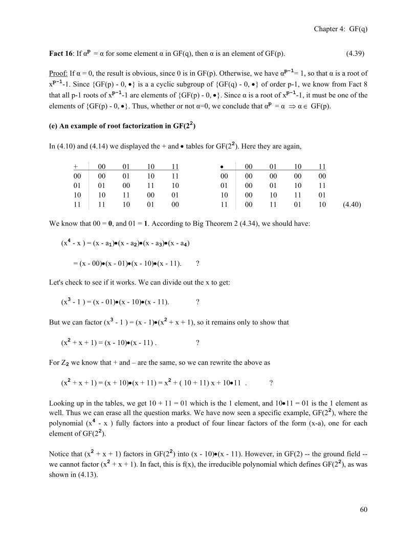
Chapter 4: GF(q)
60
Fact 16: If αp = α for some element α in GF(q), then α is an element of GF(p). (4.39) Proof: If α = 0, the result is obvious, since 0 is in GF(p). Otherwise, we have αp-1= 1, so that α is a root of xp-1-1. Since {GF(p) - 0, •} is a a cyclic subgroup of {GF(q) - 0, •} of order p-1, we know from Fact 8 that all p-1 roots of xp-1-1 are elements of {GF(p) - 0, •}. Since α is a root of xp-1-1, it must be one of the elements of {GF(p) - 0, •}. Thus, whether or not α=0, we conclude that αp = α ⇒ α ∈ GF(p). (e) An example of root factorization in GF(22) In (4.10) and (4.14) we displayed the + and • tables for GF(22). Here they are again, + 00 01 10 11 • 00 01 10 11 00 00 01 10 11 00 00 00 00 00 01 01 00 11 10 01 00 01 10 11 10 10 11 00 01 10 00 10 11 01 11 11 10 01 00 11 00 11 01 10 (4.40) We know that 00 = 0, and 01 = 1. According to Big Theorem 2 (4.34), we should have: (x4 - x ) = (x - a1)•(x - a2)•(x - a3)•(x - a4) = (x - 00)•(x - 01)•(x - 10)•(x - 11). ? Let's check to see if it works. We can divide out the x to get: (x3 - 1 ) = (x - 01)•(x - 10)•(x - 11). ? But we can factor (x3 - 1 ) = (x - 1)•(x2 + x + 1), so it remains only to show that (x2 + x + 1) = (x - 10)•(x - 11) . ? For Z2 we know that + and – are the same, so we can rewrite the above as (x2 + x + 1) = (x + 10)•(x + 11) = x2 + ( 10 + 11) x + 10•11 . ? Looking up in the tables, we get 10 + 11 = 01 which is the 1 element, and 10•11 = 01 is the 1 element as well. Thus we can erase all the question marks. We have now seen a specific example, GF(22), where the polynomial (x4 - x ) fully factors into a product of four linear factors of the form (x-a), one for each element of GF(22). Notice that (x2 + x + 1) factors in GF(22) into (x - 10)•(x - 11). However, in GF(2) -- the ground field -- we cannot factor (x2 + x + 1). In fact, this is f(x), the irreducible polynomial which defines GF(22), as was shown in (4.13).
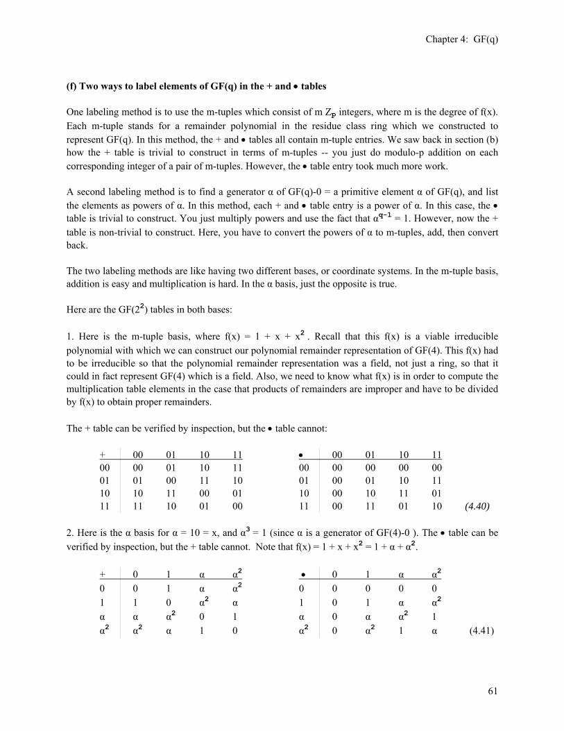
Chapter 4: GF(q)
61
(f) Two ways to label elements of GF(q) in the + and • tables One labeling method is to use the m-tuples which consist of m Zp integers, where m is the degree of f(x). Each m-tuple stands for a remainder polynomial in the residue class ring which we constructed to represent GF(q). In this method, the + and • tables all contain m-tuple entries. We saw back in section (b) how the + table is trivial to construct in terms of m-tuples -- you just do modulo-p addition on each corresponding integer of a pair of m-tuples. However, the • table entry took much more work. A second labeling method is to find a generator α of GF(q)-0 = a primitive element α of GF(q), and list the elements as powers of α. In this method, each + and • table entry is a power of α. In this case, the • table is trivial to construct. You just multiply powers and use the fact that αq-1 = 1. However, now the + table is non-trivial to construct. Here, you have to convert the powers of α to m-tuples, add, then convert back. The two labeling methods are like having two different bases, or coordinate systems. In the m-tuple basis, addition is easy and multiplication is hard. In the α basis, just the opposite is true. Here are the GF(22) tables in both bases: 1. Here is the m-tuple basis, where f(x) = 1 + x + x2 . Recall that this f(x) is a viable irreducible polynomial with which we can construct our polynomial remainder representation of GF(4). This f(x) had to be irreducible so that the polynomial remainder representation was a field, not just a ring, so that it could in fact represent GF(4) which is a field. Also, we need to know what f(x) is in order to compute the multiplication table elements in the case that products of remainders are improper and have to be divided by f(x) to obtain proper remainders. The + table can be verified by inspection, but the • table cannot: + 00 01 10 11 • 00 01 10 11 00 00 01 10 11 00 00 00 00 00 01 01 00 11 10 01 00 01 10 11 10 10 11 00 01 10 00 10 11 01 11 11 10 01 00 11 00 11 01 10 (4.40) 2. Here is the α basis for α = 10 = x, and α3 = 1 (since α is a generator of GF(4)-0 ). The • table can be verified by inspection, but the + table cannot. Note that f(x) = 1 + x + x2 = 1 + α + α2. + 0 1 α α2 • 0 1 α α2 0 0 1 α α2 0 0 0 0 0 1 1 0 α2 α 1 0 1 α α2 α α α2 0 1 α 0 α α2 1 α2 α2 α 1 0 α2 0 α2 1 α (4.41)

Chapter 4: GF(q)
62
(g) Selected Facts About GF(q) We arrange this list in the same order as the list for GF(p) in Chapter 2 (c). Fact: The q-1 non-zero elements of GF(q) form a cyclic group under • of order q-1. The generators of this cyclic group are called primitive elements of GF(q). Thus, GF(q) can be enumerated as : { 0, 1, α, α2, α3 , ...... αq-2 } αq-1 = 1 αq = α (4.42) Saying that the group is cyclic implies that at least one primitive element α exists. If q-1 is prime, then all elements of GF(q) other than 0 and 1 are primitive elements (Fact 13). Proof: See Big Theorem 1, (4.30) and also (4.31). Fact: For any element β of GF(q) , βq = β ( β is a root of βq - β ) (4.43) Proof: See Big Theorem 2 item (4), (4.34). Fact: For any element β of GF(q = pm), pβ = 0. (4.44) Proof: This is just Fact (4.5). Fact: (a + b)p = ap + bp when a,b are elements of GF(q). (4.46) Proof: Same as the proof of (2.7), except here we say that the binomial coefficients of the cross terms vanish because pβ = 0 for any element β of GF(q). Fact: (a + b + c + d + ... )p = ap + bp + cp + dp +... for a,b,c,d... in GF(q). (4.47) Proof: Just apply (4.46) multiple times, as in the proof of (2.8).
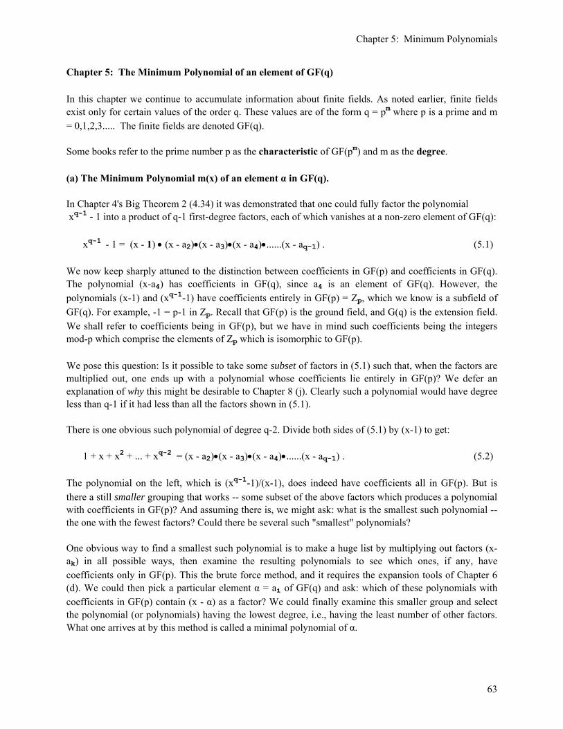
Chapter 5: Minimum Polynomials
63
Chapter 5: The Minimum Polynomial of an element of GF(q) In this chapter we continue to accumulate information about finite fields. As noted earlier, finite fields exist only for certain values of the order q. These values are of the form q = pm where p is a prime and m = 0,1,2,3..... The finite fields are denoted GF(q). Some books refer to the prime number p as the characteristic of GF(pm) and m as the degree. (a) The Minimum Polynomial m(x) of an element α in GF(q). In Chapter 4's Big Theorem 2 (4.34) it was demonstrated that one could fully factor the polynomial xq-1 - 1 into a product of q-1 first-degree factors, each of which vanishes at a non-zero element of GF(q): xq-1 - 1 = (x - 1) • (x - a2)•(x - a3)•(x - a4)•......(x - aq-1) . (5.1) We now keep sharply attuned to the distinction between coefficients in GF(p) and coefficients in GF(q). The polynomial (x-a4) has coefficients in GF(q), since a4 is an element of GF(q). However, the polynomials (x-1) and (xq-1-1) have coefficients entirely in GF(p) = Zp, which we know is a subfield of GF(q). For example, -1 = p-1 in Zp. Recall that GF(p) is the ground field, and G(q) is the extension field. We shall refer to coefficients being in GF(p), but we have in mind such coefficients being the integers mod-p which comprise the elements of Zp which is isomorphic to GF(p). We pose this question: Is it possible to take some subset of factors in (5.1) such that, when the factors are multiplied out, one ends up with a polynomial whose coefficients lie entirely in GF(p)? We defer an explanation of why this might be desirable to Chapter 8 (j). Clearly such a polynomial would have degree less than q-1 if it had less than all the factors shown in (5.1). There is one obvious such polynomial of degree q-2. Divide both sides of (5.1) by (x-1) to get: 1 + x + x2 + ... + xq-2 = (x - a2)•(x - a3)•(x - a4)•......(x - aq-1) . (5.2) The polynomial on the left, which is (xq-1-1)/(x-1), does indeed have coefficients all in GF(p). But is there a still smaller grouping that works -- some subset of the above factors which produces a polynomial with coefficients in GF(p)? And assuming there is, we might ask: what is the smallest such polynomial -- the one with the fewest factors? Could there be several such "smallest" polynomials? One obvious way to find a smallest such polynomial is to make a huge list by multiplying out factors (x-ak) in all possible ways, then examine the resulting polynomials to see which ones, if any, have coefficients only in GF(p). This the brute force method, and it requires the expansion tools of Chapter 6 (d). We could then pick a particular element α = ai of GF(q) and ask: which of these polynomials with coefficients in GF(p) contain (x - α) as a factor? We could finally examine this smaller group and select the polynomial (or polynomials) having the lowest degree, i.e., having the least number of other factors. What one arrives at by this method is called a minimal polynomial of α.
Chapter 5: Minimum Polynomials
64
To recap: a minimum polynomial for some element α of GF(q) is a polynomial which is the product of the smallest set of factors (x - ak) which contains the factor (x - α), and which (when multiplied out) has coefficients only in GF(p). Denote this minimum polynomial for α by the name m(x). Thus, α is a root of m(x) so m(α) = 0. Remember that in general α and the ai are themselves not in GF(p). (5.3) Note: Any minimum polynomial is an element of the ring R defined in Chapter 3 (a) which, recall, was the set of polynomials with coefficients in Zp. Example: The minimum polynomial of the 0 element of GF(q) is m(x) = (x - 0) = x. Comment: One could and probably should write mα(x) to show that m(x) is specific to some α. We don't do this because: (1) more than one α can have the same m(x); (2) we shall be putting subscripts on m(x) in Chapter 8 which have a different though related meaning. If the coefficient of the highest power of a polynomial is 1, the polynomial is said to be monic. As defined above, any minimum polynomial m(x) is always monic, being a product of (x-a) factors. For GF(p) with p>2, one can have coefficients other than 1 and 0. In this case, one can construct several superficially different polynomials which have the same roots, but they differ just by a scale factor. The monic requirement of m(x) then removes these superficial duplications. For example, 2x-2 is not really distinct from x-1 in terms of its roots. It turns out that the minimal polynomial of α is unique, but to show that we first need the following. Fact 1: If p(x) lies in R and p(α) = 0, then p(x) = q(x)m(x) of α . In other words, p(x) having a root α must be a multiple of any minimum polynomial m(x) of α. (5.4) Proof: Expand p(x) = q(x)m(x) + r(x), where m(x) is a minimum polynomial of α, and where the degree of r(x) is less than that of m(x)-- this is the Division Algorithm (3.6). If p(α) = 0, then r(α) = 0, since m(α) = 0. But if r(α) = 0, then m(x) must not be a minimal polynomial because r(x) is a polynomial of lesser degree than m(x), and has α as a root. In other words, then r(x) must be the real minimum polynomial, not m(x). This contradicts the starting assumption, so we must have r(x) = 0 and then we end up with p(x) = q(x)m(x), so p(x) is a "multiple" of m(x). Fact 2: The minimum polynomial m(x) for some element α of GF(q) has these properties: (a) A unique m(x) exists for any given α (b) m(α) = 0 (c) m(x) is irreducible in GF(p) (d) m(x) divides evenly into the polynomial xq-1 - 1 (5.5) Proof: (a) Certainly we know that a minimum polynomial m(x) for any α must exist. If nothing smaller works out, we know that the polynomial shown above, xq-1 - 1, is the final candidate. Suppose there are two different minimum polynomials m1(x) and m(x) for α. Then m1(α) = 0 and m(α) = 0. Both m1(x) and m(x) have the same degree r (since they are both minimum polynomials) and are both monic. By Fact 1 of (5.4) we can write m1(x) = q(x)m(x). Thus we have,
Chapter 5: Minimum Polynomials
65
( xr + lower terms) = q(x) ( xr + other lower terms) . In this equation, if q(x) were of degree s > 0, the right side would generate terms of degree s+r which are not present on the left. Thus q(x) must be of degree 0 -- it is a constant. Only q = 1 can match the coefficients of xr on both sides, so q(x) = 1 and therefore m1(x) = m(x) so there cannot be two different minimum polynomials for an element α of GF(q). (b) That m(α) = 0 follows by definition since m(x) contains (x-α) as a factor. (c) Recall (3.12) item 3 on reducible polynomials. If m(x) were reducible in R, then we could write m(x) = a(x)b(x) where both a(x) and b(x) lie in R and neither a(x) nor b(x) is a constant. Then, since m(α) = 0, we know that either a(α) = 0 or b(α) = 0 (or both). In this case, we would take whichever one of these vanishes at α, and then that one would be a minimum polynomial for α of lower degree than m(x). But this is a contradiction since m(x) is supposed to be the minimum polynomial. Thus, m(x) must be irreducible. (d) Since m(x) contains a subset of the factors than make up xq-1 - 1, it must divide evenly into xq-1 - 1, see (5.1). The quotient is then all the factors of xq-1 - 1 which are not contained in m(x). Fact 3: If monic f(x) in R is irreducible in R and f(α) = 0 for some α in GF(q), then f(x) is the minimum polynomial m(x) of α. (5.6) Proof: If f(x) were reducible in R, one could write f(x) = q(x) d(x) where both q(x) and d(x) lie in R and neither is a constant. In this case, since f(α) = 0, we have q(α) = 0, d(α) = 0, or both. In any case, we know that f(x) is not the minimum polynomial for α since at least one of q(x), d(x) is of lower degree and has root α and so it would then be the minimum polynomial. On the other hand, if f(x) were irreducible in R, then one could not write f(x) = q(x)d(x) for non-constant q(x) and d(x) in R, and then we cannot find a polynomial of degree lower than f(x) which has α as a root. Then f(x) must be the lowest degree polynomial which has α as a root, and then f(x) is the minimum polynomial for α. Corollary: There may exist monic irreducible polynomials which are not minimum polynomials for any α in GF(q). An example is given later in Chapter 6 (d) 3. (b) Primitive Polynomials and the Period of m(x) If α is a primitive element of GF(q), meaning α is a generator of cyclic {GF(q) - 0, •}, then the minimum polynomial m(x) of α is called a primitive polynomial of GF(q). Conversely, if m(x) is a primitive polynomial for GF(q) for α, then α is a primitive element of GF(q). (5.7) Corollary: If monic f(x) in R is irreducible over R and has some primitive element α of GF(q) as a root, then f(x) is a primitive polynomial of GF(q). (5.8) Proof: This is a restatement of Fact 3 (5.6) for α = a primitive element of GF(q).

Chapter 5: Minimum Polynomials
66
From Fact 2(d) we know that a minimal polynomial m(x) for any α in GF(q) divides xq-1 - 1. It may be possible that m(x) also divides xn-1 for some n < q-1. The smallest such power n is called the period of m(x). (5.9) Fact 4: A primitive polynomial p(x) of GF(q) must have the maximal period q-1. (5.10) Proof: We know that p(x) is a minimal polynomial for some primitive element α of GF(q). We know by Fact 2(d) that p(x) divides xn - 1 with n = q-1. Is there some smaller n? Assume there exists some n < q-1 such that p(x) divides xn - 1. Then xn - 1 = p(x)q(x) for some q(x). Since p(α) = 0, we find αn = 1 for n < q-1. But by the definition of a primitive element, the order of α is q-1, and this means that n = q-1 is the smallest integer such that αn = 1. Thus we have a contradiction, so there is no n < q-1 that works. The smallest n that works is then q-1, so this is the period. Fact 5: If the period of some minimum polynomial m(x) of α is q-1, then α must be a primitive element of GF(q), and then by definition m(x) is a primitive polynomial of GF(q). (5.11) Proof: If α is not primitive, then α has some period n < q-1 by Fact 4. Thus, we can consider (α,n,•), the cyclic subgroup generated by α. According to Fact 8 (4.25), the n elements of this subgroup are the n roots of xn -1, and we can factor as follows: xn -1 = (x - a1)• (x - a2)• (x - a3)• ... (x - an), (4.25) where one of the ai is our element α. Since xn -1 has coefficients in GF(p), it is a candidate for the minimum polynomial m(x) of α. The other possibility is that some subset of the factors shown here forms m(x). In either case, m(x) divides xn - 1, so we have period n < q-1. But by hypothesis, the period of m(x) is supposed to be q-1. Thus, α must be a primitive element of GF(q), and by definition, m(x) is then a primitive polynomial of GF(q). (c) Formula for the Minimum Polynomial m(x) of α : Conjugate Sets We would now like to develop an explicit formula for the minimum polynomial m(x) of α. As a very strong hint toward this end, we state and prove the following interesting fact: Lemma 6: If f(x) is in R, then f(xp) = [f(x)]p. (5.12) Proof: Just write out both sides and make use of the expansion formula (2.11). The RHS becomes [f(x)]p = [ a + bx + cx2 + ... ]p = (a)p + (bx)p + (cx2)p + ... = ap + bp(xp) + cp(xp)2 + ... But we also know from (2.8) that ap = a for any coefficient in GF(p), such as the coefficients a,b,c above. Thus we get , [f(x)]p = a + b (xp) + c (xp)2 +....

Chapter 5: Minimum Polynomials
67
But this series is exactly f(xp), so our Lemma is proved. Notice how the nature of variable x plays no role in this Lemma. Fact 6: Let min pol mean "the minimum polynomial ". This Fact then claims that [m(x) = min pol of α] ⇔ [m(x) = min pol of αp] where α is in GF(pm) (5.13) Proof: From Lemma 6 we know that m(xp ) = [m(x)]p. This means that m(αp) = [m(α)]p = 0, since m(x) is the minimum polynomial for α. Since m(x) is already known to be irreducible, and since m(αp) = 0, (5.6) says that m(x) is also the minimum polynomial for αp. Conversely, [m(α)]p = m(αp) = 0 if m(x) is the minimum polynomial for αp, which says m(α) = 0. Since m(x) is already known to be irreducible, and since m(α) = 0, (5.6) says that m(x) is also the minimum polynomial for α. Fact 7: If m(x) is the minimal polynomial of α, then it is the minimal polynomial for all the elements in the following set of m elements (warning: the elements may not be distinct) { α, αp, αp2, αp3 , .... αpm-1 } αpm = αq = α m elements (5.14) This implies that m(αpi) = 0 for any αpi in the set. Big Theorem 2 (4.34) item 4 showed that αq = α for any α in GF(q). For this reason, there can be no elements of the above set beyond those shown -- such extra elements would just be repeats of earlier elements. The set shown nominally has m elements, but they may not all be distinct, a subject discussed soon. Proof: Each element of this set is the previous element raised to the power p, so we just repeatedly apply Fact 6. For example, consider the element αp2 , m(x) = min pol of αp2 ⇔ m(x) = min pol of (αp)p ⇔ m(x) = min pol of (αp) ⇔ m(x) = min pol of(α) . We know from (4.34) item 4 that αpm = αq = α. This is why the list in (5.14) ends as shown. The next element would be a repeat of α, and the one after that would repeat αp and so on. As already noted, there is no guarantee that the elements on the list are all distinct. The distinct members of the set of elements in (5.14) form the conjugate set of α, and the distinct elements other than α are called the conjugates of α. As already noted, each member of the above list is the previous member raised to the power p. Do not confuse this sequence with that of a cyclic group which looks like { α, α2, α3, α4, ...} or maybe like { αp, α2p, α3p, α4p, ...}. This conjugate list is a different beast. Fact 8: If α is a primitive element of GF(pm) , then (5.15) (a) the conjugate set of α contains the full complement of m distinct elements (b) all members of this conjugate set are primitive elements. (c) If any element of a conjugate set is primitive, so are all the other elements in the set (d) The elements of a conjugate set are either all primitive, or they are all non-primitive

Chapter 5: Minimum Polynomials
68
The set of powers of the conjugate set, { 1, p, p2, p3.... pm-1 }, is sometimes called a cyclotomic coset, see Chapter 5 (h) for more on this subject. Proof: (a) If α is a primitive element, then from (4.31) GF(q) contains all powers of α out to a maximum exponent of q-2. In the conjugate list above, the largest conjugate has power pm-1 = pm / p = q/p. Thus, all the conjugate elements hit distinct elements of GF(q) as long as q/p ≤ q-2 which can be rewritten as pm-1(p-1) ≥ 2. For any p>2 this is true for all m. For p=2, it is true for all m>1. We don't care about the case p=1 m=1 since this is GF(2) which we know all about. This field has no powers of α, is just has 0 and 1 as elements. Thus in fact q/p ≤ q-2 and so all m elements of the conjugate set are distinct. (b) If α is a primitive element, we know from (4.32) that αp is also a primitive element since GCD(p,pm-1) = 1. Thus αp is a primitive element, (αp)p = αp2 is a primitive element, and so on. (c) and (d) are just restatements of (b). Fact 9: If α is not a primitive element, then the only possibility is that the first k of the m conjugates of some element α are distinct, where k is very dependent on the field and on the field element selected. In this case, the conjugate set has this form, { α, αp, αp2, αp3 , .... αpk-1 } αpk = α k conjugates k ≤ m (5.16) If α = 1 then only 1 conjugate is distinct. We exclude this trivial case and assume that α ≠ 1. Proof: This is a slightly tricky proof which we defer to Appendix B since it is a little long and takes us off the main line of presentation. It is included in Appendix B because we could not find it in any text and had to do it from scratch. What is happening here is that the conjugates are landing on the elements of a cyclic subgroup { α, α2, α3 .... αn-1} where αn = 1. Since there might not be many elements in such a subgroup, it seems reasonable that the m conjugates in the original list might hit the same elements more than once. What is not obvious is that the first repeated element is α, as implied above. This turns out to be true, and moreover, as higher and higher powers are applied, the same elements in the subgroup are hit in the same order that they were first hit, and this hitting sequence cycles over and over. Furthermore, certain members of the cyclic subgroup may never be hit. Big Theorem 3: The minimum polynomial of an element α of GF(q) may be written as follows: m(x) = (x - α) • (x - αp) • (x - αp2) • (x - αp3) ... .... (x - αpk-1) αpk= α k ≤ m (5.17) In other words, the claim is that the minimum polynomial m(x) of α is the product of (x - α) with linear factors of the form (x-ai), where the ai are all the conjugates of α. The degree of this polynomial is then equal to the number of distinct elements in the conjugate set of α, which we call k, and we know that k ≤ m. Proof: The proof is simple and fascinating. First of all, we already know that m(x) must have at least all the factors shown above -- it can have no smaller number of factors. This is because it needs all these factors in order to vanish at all the conjugate elements, as required by Fact 7 (5.14). If we can show that the coefficients of the m(x) given above are all in GF(p), then we are done.

Chapter 5: Minimum Polynomials
69
Here is the trick. Write the pth power of m(x) in two different ways. First, compute [m(x)]p by raising each linear factor to power p. Then apply the theorem (4.46) that (a+b)p = ap + bp. Here is what happens to one factor: (x - αp2)p = ( xp - αp3) . It becomes the next factor to the right but with x replaced by xp. So what happens to the final factor on the right? (x - αpk-1)p = ( xp - αpk) = ( xp - α). It becomes the factor on the far left, with x replaced by xp. We have thus shown that: [m(x)]p = m(xp) = Σici(xp)i . (5.18)
In the last step we just expanded polynomial m(xp) in terms of its coefficients ci. On the other hand, we could have started with this coefficient expansion of m(x) and raised it to the power p, and then used the generalized theorem (4.47) that (a + b + c + d + ... )p = ap + bp + cp + dp +... to get: [m(x)]p = ( Σicixi )p = Σi(cixi)p = Σi(ci)p(xp)i . (5.19)
For (5.18) and (5.19) to be equal, the coefficients must all match, so we get that (ci)p = ci . According to Fact 16 (4.39) this means all the ci are elements of GF(p). Thus, m(x) as shown has coefficients in GF(p) and has the fewest number of factors possible, so it is in fact the minimum polynomial of α. We have successfully produced a "formula" (5.17) for the minimum polynomial of α. We just keep adding factors until we get a repeat, then we know k. QED Fact 10: The degree of any primitive polynomial of GF(pm) is m. (5.20) Proof: A primitive polynomial is a minimum polynomial m(x) for some primitive element α. According to Fact 8 (5.15) above, the conjugate set of α has m distinct elements if α is primitive. Then according to Big Theorem 3 (5.17), we see that there is one factor (x - a) for each distinct element in the conjugate set of α, so there are m factors. Thus, the degree of m(x) is m in this case. Fact 11: The number of primitive polynomials for GF(pm) is equal to the number of distinct conjugate sets which contain primitive elements. (5.21) Proof: According to Big Theorem 3 (5.17), the number of distinct minimal polynomials must equal the number of distinct conjugate sets. Suppose there are N such sets, and suppose M of these contain primitive elements. Then there are M unique primitive polynomials. For q = pm , we know that each conjugate set has at most m distinct elements. If a conjugate set contains a primitive element, Fact 8 says that all m members of the set must be distinct.

Chapter 5: Minimum Polynomials
70
We now try to bring the above general discussion down to earth with three concrete examples, GF(2m) for m = 3,4,5. In each example we shall construct all minimum polynomials as products of (x-a) factors, and shall show which of these are primitive polynomials. The process is very straightforward, and it would not be hard (see section 5 below) to write a Maple program to find and classify all the minimum polynomials for any field GF(2m) and in fact for any GF(pm). Of course the polynomials so obtained would be in factored form, as in these examples. One then needs the tools of Chapter 6 (d) to expand ("multiply out") these factored forms. 1. Minimum and primitive polynomials of GF(23) We know that from Big Theorem 1 (4.30) that any GF(pm) is cyclic. This means that there must exist a primitive element α whose powers enumerate the non-zero elements of GF(pm). Thus, we may "enumerate" GF(23) as follows: { 0, 1, α, α2, α3, α4, α5, α6 } α7 = 1 α = some primitive element of GF(23) (5.22) Which elements are primitive elements besides α? Fact 12 (4.32) tells us that a power αs is a primitive element if GCD(s,7) = 1. So s = 1,2,3,4,5,6 all define primitive elements. It happens that the number q-1 = 23-1= 7 is prime, so all αs will be primitive elements, a Fact noted earlier in (4.33). Next, let's construct the conjugate sets using the template (5.17). Since all our αs for s in the list are primitive, we know from (5.15) that all the conjugate sets have m=3 elements. So: { α, αp, αp2, αp3 , .... αpm-1 } αpm = αq = α m elements // template { α, α2, α4 } α8 = α8 = α 3 elements // GF(23) Our task now is to replace α by αs in the last line and see if we get a distinct conjugate set. So { α, α2, α4 } // the first conjugate set { αs, α2s, α4s } // is this conjugate set distinct from those previously obtained? Note for example on the last line that (αs)4 = α4s. We can then start with each candidate α1, α2.... α6 and try to build a conjugate set from it. But if we find that some element has already appeared in a set, we skip that one and move to the next candidate. This is because no element of GF(q) can appear in two distinct conjugate sets, a fact we will formally prove below in (5.38). The first set is of course { α, α2, α4 } . Since this includes α2, we skip α2 and move on to α3. This gives{ α3, α6, α5} where the last element is (α3)4 = α5 α7 = α5 1 = α5 . We then skip α4, α5 and α6 and we have run the gamut. So we find these three conjugate sets, {1} being a trivial one : { α, α2, α4 }, { α3, α6, α5 }, {1} (5.23) prim prim Notice that the elements of these three sets partition the field elements {GF(23) - 0}, a fact proven in (5.38) below for any GF(q). In a denser notation, the above partition can be written in terms of just the powers

Chapter 5: Minimum Polynomials
71
{1,2,4}, {3,6,5}, {0} and this grouping is referred to as the set of cyclotomic cosets for GF(23), see Chapter 5 (h). Since all elements of {GF(23)-0-1} are primitive, the first two conjugate sets contains only primitive elements. More generally, we know that from (5.15) that either all elements of a conjugate set are primitive, or they are all not-primitive. Of course 1 is not a primitive element. Here then is a complete list of the minimum polynomials for GF(23). Here we label each polynomial by the lowest appearing power of α. p1(x) = (x - α)(x - α2)(x - α4) p3(x) = (x - α3)(x - α6)(x - α5) m0(x) = (x-α0) = (x-1) mzero(x) = (x-0) = x . (5.24) In the next two examples we won't mention the last two trivial minimum polynomials shown here. They are always present. Fact 11 (5.21) then says there are two distinct primitive polynomials for GF(23), and we see them as the pi(x) in (5.24). So, although there are 6 elements in {GF(23)-0-1}, there are only two minimal polynomials and they are shared by the 6 elements as shown. Both these minimal polynomials are primitive polynomials since α and α3 are primitive elements. Each element of {GF(23)} appears in exactly one (x-a) factor, in line with the partition comment above. We will show in (5.30) below that the first two polynomials in (5.24) must be x3 + x + 1 and x3 + x2 + 1. But how can we verify this? And which one is which? At this point all we know about p1(x) is this: p1(x) = (x - α)(x - α2)(x - α4) = x3 + [α + α2 + α4]x2 + [α3 + α5 + α6]x + α7 . (5.25) The answer to the second question is that it depends on which α you select at the start as your primitive element. As for the first question, in order to multiply things out, we have to have at hand the addition table for GF(23) where the rows and columns are enumerated by powers of α. We showed such a table for GF(22) in (4.41), and we showed how such a table can be created, but we have not yet stated the table for GF(23), so at this point we really don't have the tools needed to multiply out the polynomials in (5.24). There is a circular route at play here. In order to create an addition table, we have to select an α whose powers will enumerate the table's rows and columns. That implicitly means that we have to know and select a specific primitive polynomial. That in turn will determine which pi(x) of (5.24) is x3 + x + 1 and which is x3 + x2 + 1. This subject will be treated in detail in Chapter 6 (d) 2. 2. Minimum and primitive polynomials of GF(24) The reader is assumed to have carefully read through the previous example, so not all the supporting "words" will be repeated here. We first enumerate the field GF(24), having selected α as some primitive element,
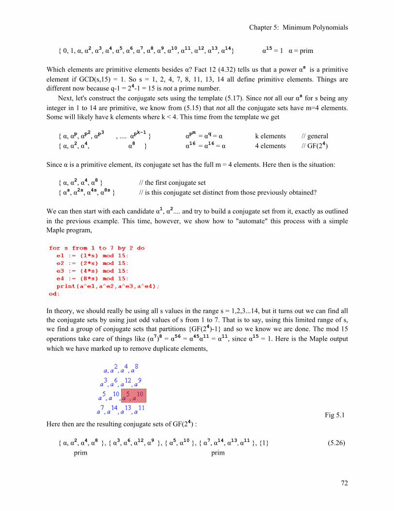
Chapter 5: Minimum Polynomials
72
{ 0, 1, α, α2, α3, α4, α5, α6, α7, α8, α9, α10, α11, α12, α13, α14} α15 = 1 α = prim Which elements are primitive elements besides α? Fact 12 (4.32) tells us that a power αs is a primitive element if GCD(s,15) = 1. So s = 1, 2, 4, 7, 8, 11, 13, 14 all define primitive elements. Things are different now because q-1 = 24-1 = 15 is not a prime number. Next, let's construct the conjugate sets using the template (5.17). Since not all our αs for s being any integer in 1 to 14 are primitive, we know from (5.15) that not all the conjugate sets have m=4 elements. Some will likely have k elements where k < 4. This time from the template we get { α, αp, αp2, αp3 , .... αpk-1 } αpm = αq = α k elements // general { α, α2, α4, α8 } α16 = α16 = α 4 elements // GF(24) Since α is a primitive element, its conjugate set has the full m = 4 elements. Here then is the situation: { α, α2, α4, α8 } // the first conjugate set { αs, α2s, α4s, α8s } // is this conjugate set distinct from those previously obtained? We can then start with each candidate α1, α2.... and try to build a conjugate set from it, exactly as outlined in the previous example. This time, however, we show how to "automate" this process with a simple Maple program,
In theory, we should really be using all s values in the range s = 1,2,3...14, but it turns out we can find all the conjugate sets by using just odd values of s from 1 to 7. That is to say, using this limited range of s, we find a group of conjugate sets that partitions {GF(24)-1} and so we know we are done. The mod 15 operations take care of things like (α7)8 = α56 = α45α11 = α11, since α15 = 1. Here is the Maple output which we have marked up to remove duplicate elements,
Fig 5.1 Here then are the resulting conjugate sets of GF(24) : { α, α2, α4, α8 }, { α3, α6, α12, α9 }, { α5, α10 }, { α7, α14, α13, α11 }, {1} (5.26) prim prim
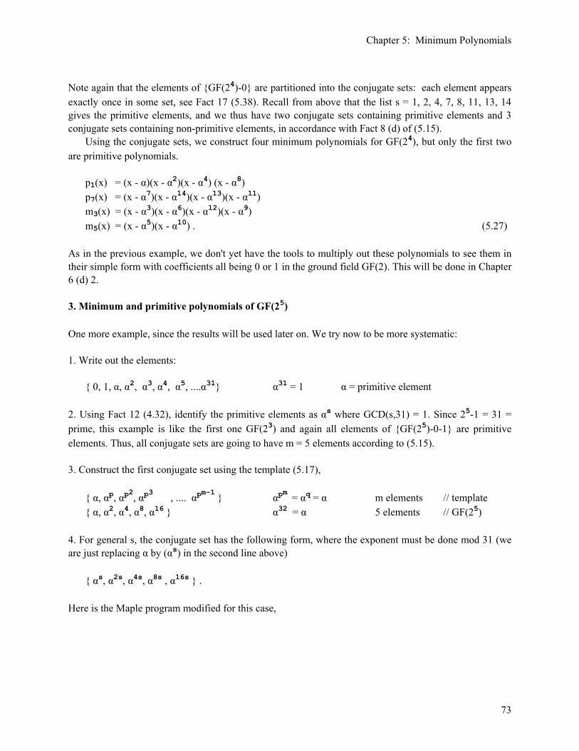
Chapter 5: Minimum Polynomials
73
Note again that the elements of {GF(24)-0} are partitioned into the conjugate sets: each element appears exactly once in some set, see Fact 17 (5.38). Recall from above that the list s = 1, 2, 4, 7, 8, 11, 13, 14 gives the primitive elements, and we thus have two conjugate sets containing primitive elements and 3 conjugate sets containing non-primitive elements, in accordance with Fact 8 (d) of (5.15). Using the conjugate sets, we construct four minimum polynomials for GF(24), but only the first two are primitive polynomials. p1(x) = (x - α)(x - α2)(x - α4) (x - α8) p7(x) = (x - α7)(x - α14)(x - α13)(x - α11) m3(x) = (x - α3)(x - α6)(x - α12)(x - α9) m5(x) = (x - α5)(x - α10) . (5.27) As in the previous example, we don't yet have the tools to multiply out these polynomials to see them in their simple form with coefficients all being 0 or 1 in the ground field GF(2). This will be done in Chapter 6 (d) 2. 3. Minimum and primitive polynomials of GF(25) One more example, since the results will be used later on. We try now to be more systematic: 1. Write out the elements: { 0, 1, α, α2, α3, α4, α5, ....α31} α31 = 1 α = primitive element 2. Using Fact 12 (4.32), identify the primitive elements as αs where GCD(s,31) = 1. Since 25-1 = 31 = prime, this example is like the first one GF(23) and again all elements of {GF(25)-0-1} are primitive elements. Thus, all conjugate sets are going to have m = 5 elements according to (5.15). 3. Construct the first conjugate set using the template (5.17), { α, αp, αp2, αp3 , .... αpm-1 } αpm = αq = α m elements // template { α, α2, α4, α8, α16 } α32 = α 5 elements // GF(25) 4. For general s, the conjugate set has the following form, where the exponent must be done mod 31 (we are just replacing α by (αs) in the second line above) { αs, α2s, α4s, α8s , α16s } . Here is the Maple program modified for this case,
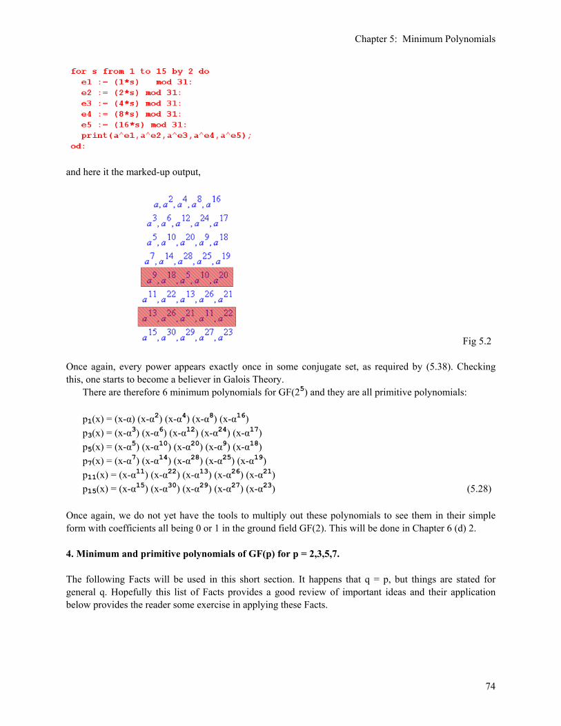
Chapter 5: Minimum Polynomials
74
and here it the marked-up output,
Fig 5.2 Once again, every power appears exactly once in some conjugate set, as required by (5.38). Checking this, one starts to become a believer in Galois Theory. There are therefore 6 minimum polynomials for GF(25) and they are all primitive polynomials: p1(x) = (x-α) (x-α2) (x-α4) (x-α8) (x-α16) p3(x) = (x-α3) (x-α6) (x-α12) (x-α24) (x-α17) p5(x) = (x-α5) (x-α10) (x-α20) (x-α9) (x-α18) p7(x) = (x-α7) (x-α14) (x-α28) (x-α25) (x-α19) p11(x) = (x-α11) (x-α22) (x-α13) (x-α26) (x-α21) p15(x) = (x-α15) (x-α30) (x-α29) (x-α27) (x-α23) (5.28) Once again, we do not yet have the tools to multiply out these polynomials to see them in their simple form with coefficients all being 0 or 1 in the ground field GF(2). This will be done in Chapter 6 (d) 2. 4. Minimum and primitive polynomials of GF(p) for p = 2,3,5,7. The following Facts will be used in this short section. It happens that q = p, but things are stated for general q. Hopefully this list of Facts provides a good review of important ideas and their application below provides the reader some exercise in applying these Facts.

Chapter 5: Minimum Polynomials
75
[0] GF(p) = Mod(p) also called Zp [ (2.5) ] [1] Every GF(q) has at least one primitive element. [ since {GF(q) - 0} is cyclic under • , see (4.31) ] [2] αq-1 = 1 for any non-zero element α of GF(q). [ (4.34) item 4 ] [3] The order of α in GF(q) is the smallest integer n such that αn = 1. [ (4.17) item k ] [4] If α is primitive in GF(q), its order is q-1 and vice versa. [ (4.31) ] [5] The order n of α in GF(q) divides q-1. [ (4.17) item (l) ] [6] The number of primitive elements of GF(q) is φ(q-1) [ Section 5 (d) below, with table of Euler φ. ] In each example, we pay attention to the symmetry of the coefficients of the primitive polynomials obtained, since this will be of interest later. GF(2) { 0, 1 } α = 1 α = prim In this trivial case, since we can enumerate all non-zero elements of GF(2) by powers of 1, element 1 is a primitive element. That will not be true for GF(p) with p > 2 so 1 will never be a primitive element again in this set of examples. For GF(2), the only minimum polynomial is (x-1) and it is primitive. Since + and - are the same for GF(2), we can write this as (x+1) which we note has symmetric coefficients " 11" . GF(3) { 0, 1, α } α2 = 1 α = prim From [1] there must be a primitive element, so it must be α = 2, and indeed 22 = 4 = 1 according to the rule [0] of GP(3) = Mod(3). The only minimum polynomial is (x-2) and it is a primitive polynomial. Since –2 = +1 for GF(3), we can write this as (x+1) and again we have symmetric coefficients "11" . GF(5) { 0, 1, α, α2, α3 } α4 = 1 α = prim From [6] there are φ(p-1) = φ(4) = 2 primitive elements, so in the set {2,3,4} one must not be primitive. They all satisfy α4 = 1 according [2], but 42 = 16 = 1 so [3] says the order of 4 is 2 and not 4 = q-1, so 4 is not primitive by [4]. There are three minimum polynomials (x-2),(x-3),(x-4), and only (x-2),(x-3) are primitive. Just as a check, note that 22 = 4 ≠ 1 and 32 = 9 = 4 ≠ 1, so both 2 and 3 have the full order 4. The two primitive polynomials do not have symmetric coefficients even if written as (x+3), (x+2) = "13" and "12". GF(7) { 0, 1, α, α2, α3, α4, α5 } α6 = 1 α = prim From [6] there are φ(p-1)=φ(6) = 2 primitive elements, so in the set {2,3,4,5,6} only two are primitive. Since q-1 = p-1 = 6, non-primitive elements could have order 2 or 3 according to [5] . For 2 we find 22 = 4, but 23 = 8 = 1 so 2 has order 3 and is non-primitive by [4]. For 3 we find 32 = 9 = 2, 33 = 27 = 6, so only 36 = 1 so 3 is primitive by [4].

Chapter 5: Minimum Polynomials
76
For 4, we find 42= 16 =2, 43 = 64 = 1, so 4 has order 3 and is non-primitive by [4]. For 5, we find 52= 25 = 4, 53 = 25*4 = 4*4 = 16 = 2, so 5 is primitive by [4]. For 6, we find 62 = 36 = 1, 63 = 36*6 = 1*6 = 6, so 6 has order 2 and is non-primitive by [4]. The minimum polynomials are (x-2), (x-3), (x-4), (x-5), (x-6) but only (x-3), (x-5) are primitive. Even when written as (x+4), (x+2), these primitive polynomials "14" and "12" are not symmetric. (d) How many primitive elements and primitive polynomials are there for GF(pm)? According to (4.31) there always exists a primitive element α for GF(q=pm). The 0 and 1 elements are never primitive, and the remaining q-2 elements are enumerated as powers of α : {α, α2, α3.....αq-2}. According to (4.32), a power αk of a known primitive element α is also primitive iff GCD(k,q-1) = 1. Thus, the number of primitive elements must be the number of integers k in the range 0 to q-2 for which GCD(k,q-1) = 1, which recall means that k and q-1 are coprime. The number of coprime integers < n is called φ(n), Euler's "totient function", so the number of primitive elements is φ(q-1). Each primitive polynomial covers m primitive elements of GF(q) as shown in (5.15a), so the number of primitive polynomials is then φ(q-1)/m. These matters are described in more detail in Appendix G and we just quote the two results which, in fact, we have just proven: Fact 13: The number of primitive elements in GF(q=pm) is φ(pm-1). (G.19) Fact 14: The number of primitive polynomials in GF(pm) is φ(pm -1)/m. (G.20) Here is a Maple-generated table of φ(n) for n = 1 to 100 where each bracket is of the form [ n, φ(n)].
and here is a plot of the digital function φ(n) with linear interpolation of the points n = 1 to 100:

Chapter 5: Minimum Polynomials
77
A few examples: GF(pm) # prim elements # prim polys 22 φ(3) = 2 2/2 = 1 // shown in (5.29) 23 φ(7) = 6 6/3 = 2 // listed in (5.24) and (6.20) 24 φ(15) = 8 8/4 = 2 // listed in (5.27) and (6.21) 25 φ(31) = 30 30/5 = 6 // listed in (5.28) and (6.22) 32 φ(8) = 4 4/2 = 2 // quoted below equation (6.15) (e) On finding the minimum and primitive polynomials of GF(pm) expressed over GF(p) In Chapter 6 (d) 2 we will show how to expand all the factored minimum polynomials stated above to obtain their simple forms over GF(2), like x5 + x3 + 1. This requires a priori knowledge of one primitive polynomial. We know in principle how to find such a primitive polynomial by brute force. We need the addition table and that can be obtained from our R/I representation of GF(pm) of (3.17), GF(pm) = R / ( f(x) ) . (3.17) Note that f(x) does not have to be a primitive polynomial, nor does it have even to be a minimum polynomial. It need only be irreducible in R and of degree m. Such a polynomial can easily be found, as in (4.13), and the + and • tables constructed as in (4.10) and (4.14) where the elements are written as m-tuples. Then taking α to be each of these m-tuples one at a time, one can iteratively use the • table to compute the powers of this α. At some point one must find an α of order q-1 since we know such an α must exist for a cyclic group like {GF(q)-0}. In this way one can identify a primitive element α. This does seem like a lot of work. Probably a better way is trial and error, at least for smaller GF(q).

Chapter 5: Minimum Polynomials
78
GF(22): We know from just above that there is exactly one primitive polynomial. All candidates must be of degree m = 2, and must have +1 as the final term. If the +1 were missing, x could be factored out and the candidate would then not be a minimum polynomial. The grand list of candidates is then the following two polynomials : x2 + x + 1 • 111 x2 + 1 = x2- 1 = (x-1)(x+1) = reducible (5.29) Since the second one is reducible, the first one must be the sole primitive polynomial of GF(22). Notice that if you reverse the order of the m-tuple symbols 111 you get the same 111. GF(23): Now there are four polynomial candidates, x3 + x2 + x + 1 = x2 (x + 1) + (x+1) = (x2+1)(x+1) = reducible x3 + x2 + 1 ° 1101 x3 + x + 1 • 1011 x3 + 1 = x3 - 1 = reducible (5.30) Since we know both from the previous section and from (5.23) that there are two primitive polynomials for GF(23), and since we have only two irreducible candidates in the list, they must be the ones! We didn't even have to check that the period of each is 7, we know it must be true. GF(24): Now there are more possibilities to worry about: 1 x4 + x3 + x2 + x + 1 divides into x5 - 1 so flunks period test, not a primitive polynomial 2 x4 + x3 + x2 + 1 3 x4 + x3 + x + 1 = (x3+1)(x+1) = reducible 4 x4 + x2 + x + 1 5 x4 + x3 + 1 ° 11001 6 x4 + x + 1 • 10011 7 x4 + x2 + 1 8 x4 + 1 = x4 - 1 = (x-1)(x3+x2+x+1) = reducible (5.31) We know from (5.27) that there are only three minimum polynomials for GF(24) of degree 4, two of which are primitive polynomials. We can eliminate items 3 and 8 since they are reducible, but this still leaves six candidates (1,2,4,5,6,7), all of which look irreducible. One could apply the period test (5.10) to each to try to eliminate some of the candidates from being the primitive polynomials: which ones (if any) divide into xn - 1 for n less than 15? The first one we can see divides into x5 - 1, so we know it is not a primitive polynomial. The others are less obvious. An excellent test is to see which items on the list divide evenly into x15-1 with no remainder. Any minimum polynomial must divide evenly since it is a product of (x-ai) factors and x15-1 is the product of all such factors according to (4.34). One could manually compute all the remainders for (5.31), but Maple is happy to do it for us:
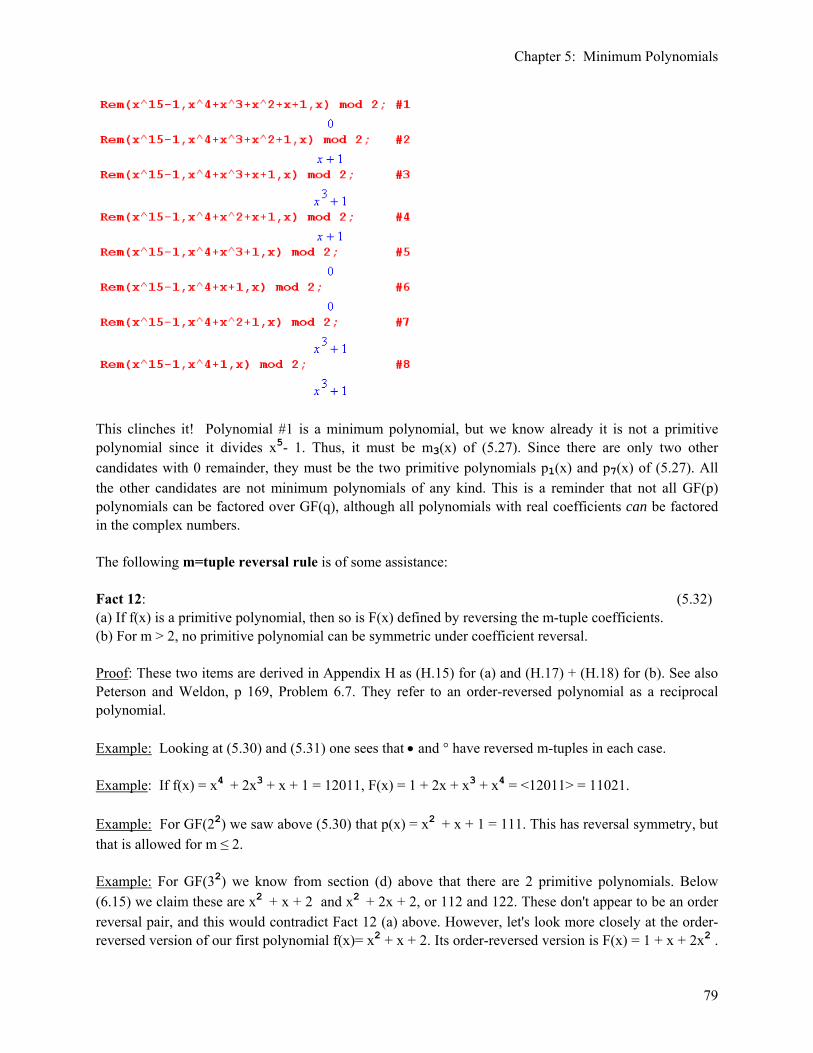
Chapter 5: Minimum Polynomials
79
This clinches it! Polynomial #1 is a minimum polynomial, but we know already it is not a primitive polynomial since it divides x5- 1. Thus, it must be m3(x) of (5.27). Since there are only two other candidates with 0 remainder, they must be the two primitive polynomials p1(x) and p7(x) of (5.27). All the other candidates are not minimum polynomials of any kind. This is a reminder that not all GF(p) polynomials can be factored over GF(q), although all polynomials with real coefficients can be factored in the complex numbers. The following m=tuple reversal rule is of some assistance: Fact 12: (5.32) (a) If f(x) is a primitive polynomial, then so is F(x) defined by reversing the m-tuple coefficients. (b) For m > 2, no primitive polynomial can be symmetric under coefficient reversal. Proof: These two items are derived in Appendix H as (H.15) for (a) and (H.17) + (H.18) for (b). See also Peterson and Weldon, p 169, Problem 6.7. They refer to an order-reversed polynomial as a reciprocal polynomial. Example: Looking at (5.30) and (5.31) one sees that • and ° have reversed m-tuples in each case. Example: If f(x) = x4 + 2x3 + x + 1 = 12011, F(x) = 1 + 2x + x3 + x4 = <12011> = 11021. Example: For GF(22) we saw above (5.30) that p(x) = x2 + x + 1 = 111. This has reversal symmetry, but that is allowed for m ≤ 2. Example: For GF(32) we know from section (d) above that there are 2 primitive polynomials. Below (6.15) we claim these are x2 + x + 2 and x2 + 2x + 2, or 112 and 122. These don't appear to be an order reversal pair, and this would contradict Fact 12 (a) above. However, let's look more closely at the order-reversed version of our first polynomial f(x)= x2 + x + 2. Its order-reversed version is F(x) = 1 + x + 2x2 .
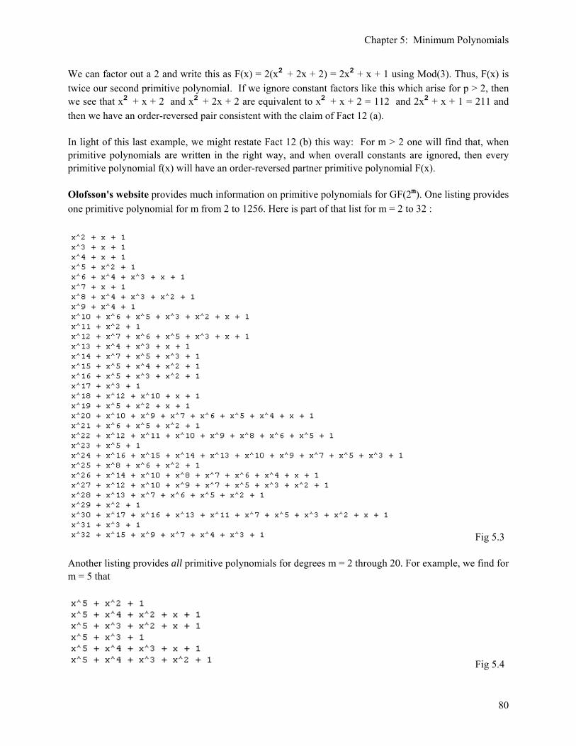
Chapter 5: Minimum Polynomials
80
We can factor out a 2 and write this as F(x) = 2(x2 + 2x + 2) = 2x2 + x + 1 using Mod(3). Thus, F(x) is twice our second primitive polynomial. If we ignore constant factors like this which arise for p > 2, then we see that x2 + x + 2 and x2 + 2x + 2 are equivalent to x2 + x + 2 = 112 and 2x2 + x + 1 = 211 and then we have an order-reversed pair consistent with the claim of Fact 12 (a). In light of this last example, we might restate Fact 12 (b) this way: For m > 2 one will find that, when primitive polynomials are written in the right way, and when overall constants are ignored, then every primitive polynomial f(x) will have an order-reversed partner primitive polynomial F(x). Olofsson's website provides much information on primitive polynomials for GF(2m). One listing provides one primitive polynomial for m from 2 to 1256. Here is part of that list for m = 2 to 32 :
Fig 5.3 Another listing provides all primitive polynomials for degrees m = 2 through 20. For example, we find for m = 5 that
Fig 5.4
Chapter 5: Minimum Polynomials
81
We shall obtain these in Chapter 6 (d) 2. The website does not give minimum polynomials that are not primitive polynomials. A classic 1962 note by E.J. Watson gives a half page summary of his algorithm for doing this, though he did not use Maple. Tables of irreducible polynomials are given in Peterson and Weldon, Appendix C, see Chap 6 (d) 7 below. More extensive tables appear in Lidi and Niederreiter. In section (l) below we present a short Maple program that computes all minimum polynomials for any GF(pm) where the polynomials are in factored form. (f) Selecting f(x) for GF(q) = R/( f(x) ) ; Classifying Irreducible Polynomials In Chapter 3 we were able to construct a representation of GF(pm) by starting with any irreducible polynomial of degree m, q = pm. We made the identification: GF(pm ) = R/( f(x) ) . // irreducible f(x) is of degree m (3.17) As our GF(24) example above shows, even when p=2, there are typically many candidates for f(x), all of which give an equivalent representation of GF(pm). Moreover, for p>2, every candidate has p-2 shadow candidates which are just integer multiples of f(x). By our definition, a primitive polynomial is monic and so the shadow candidates are eliminated. Since a primitive polynomial of degree m is irreducible, it can serve as an f(x) in the construction of GF(pm) as the extension field over GF(p). However, it is not necessary to use a primitive polynomial to accomplish the construction. As we shall see in the next chapter, there is a great advantage to using a primitive polynomial for this purpose. We now look into the classification of the irreducible polynomials of GF(q). We start with: Fact 13: If monic irreducible f(x) is used to construct a representation of GF(q), then f(x) is a minimum polynomial of GF(q) in that representation. Since all representations of GF(q) are equivalent, f(x) is a minimum polynomial of GF(q). (5.33) Proof: In Fact 1 (6.5) we will show that α = {x} is a root of any degree-m polynomial f(x) used to construct a residue class ring representation of GF(q). Since this α = {x} is an element of GF(q) and is a root of f(x), we can apply Fact 3 (5.6) to conclude that f(x) is a minimum polynomial. Fact 14: (a) If monic irreducible f(x) is of degree m, then it is a minimum polynomial for GF(pm) (b) If monic irreducible f(x) is not a minimum polynomial for GF(pm), it must have degree < m. (5.34) These are corollaries to Fact 15. If monic irreducible f(x) has degree m, it can be used in GF(q) = R/(f(x)) and it is therefore a minimum polynomial of GF(q). Then (b) is the contrapositive of (a). Using Fact 14, we can now draw a picture to classify all monic irreducible polynomials of GF(q).
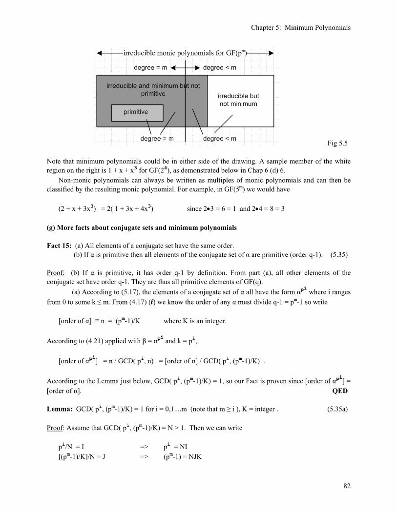
Chapter 5: Minimum Polynomials
82
Fig 5.5 Note that minimum polynomials could be in either side of the drawing. A sample member of the white region on the right is 1 + x + x3 for GF(24), as demonstrated below in Chap 6 (d) 6. Non-monic polynomials can always be written as multiples of monic polynomials and can then be classified by the resulting monic polynomial. For example, in GF(5m) we would have (2 + x + 3x3) = 2( 1 + 3x + 4x3) since 2•3 = 6 = 1 and 2•4 = 8 = 3 (g) More facts about conjugate sets and minimum polynomials Fact 15: (a) All elements of a conjugate set have the same order. (b) If α is primitive then all elements of the conjugate set of α are primitive (order q-1). (5.35) Proof: (b) If α is primitive, it has order q-1 by definition. From part (a), all other elements of the conjugate set have order q-1. They are thus all primitive elements of GF(q). (a) According to (5.17), the elements of a conjugate set of α all have the form αpi where i ranges from 0 to some k ≤ m. From (4.17) (l) we know the order of any α must divide q-1 = pm-1 so write [order of α] ≡ n = (pm-1)/K where K is an integer. According to (4.21) applied with β = αpi and k = pi, [order of αpi] = n / GCD( pi, n) = [order of α] / GCD( pi, (pm-1)/K) . According to the Lemma just below, GCD( pi, (pm-1)/K) = 1, so our Fact is proven since [order of αpi] = [order of α]. QED Lemma: GCD( pi, (pm-1)/K) = 1 for i = 0,1....m (note that m ≥ i ), K = integer . (5.35a) Proof: Assume that GCD( pi, (pm-1)/K) = N > 1. Then we can write pi/N = I => pi = NI [(pm-1)/K]/N = J => (pm-1) = NJK

Chapter 5: Minimum Polynomials
83
where I and J are integers. Write pm = pi pm-i where m-i ≥ 0 so then the last equation above becomes (pi pm-i -1) = NJK . But pi = NI so we have (NI pm-i -1) = NJK N(I pm-i - JK) = 1 (I pm-i - JK) = 1/N . Since the left side is an integer and the right side is a fraction, we have a contradiction, so N = 1. QED Notice that the fact that p = prime was not necessary in the above Lemma proof. It never hurts to test a proof in Maple. Here we let p,m,i,K range from 1 to 25 and look for GCD( pi, (pm-1)/K) ≠ 1 :
Corollary 15: All roots of any minimum polynomial m(x) have the same order, see (5.17). In particular, all roots of a primitive polynomial have order q-1 since any primitive element has order q-1. (5.36) Fact 16: Let { α, αp, αp2, αp3 , .... αpk-1 } be the conjugate set of α of some order k ≤ n. Let β ≡ αpr be any one of these conjugates. Then the exact same set can be written { β, βp, βp2, βp3 , .... βpk-1 }. Thus any element of a conjugate set can be used to generate the conjugate set. (5.37) Proof: Perhaps this seems obvious, but here is a proof. Start with { α, αp, αp2, αp3 , .... αpk-1 } αpk = α k conjugates k ≤ m (5.16) Take α , which is first in the list, and move it to the end of the list, using αpk = α :

Chapter 5: Minimum Polynomials
84
{αp, αp2, αp3 , .... αpk-1, αpk } = {αp, αp2, αp3 , .... αp1+k-1 } Now move αp to the right end and use αpk+1 = αpkp = (αpk)p = αp to get { αp2, αp3 , .... αpk-1, αpk, αpk+1 } = { αp2, αp3 , .... αp2+k-1 } Doing this r times lets us list off the conjugate set as follows { αpr, αpr+1 .... αpr+k-1 } = { [αpr], [αpr]p .... [αpr]k-1 } QED Fact 17: There are several related parts to this Fact: (5.38) (a) No two distinct conjugate sets can have a common element. (b) Each non-zero element of GF(q) appears in exactly one conjugate set. (c) The conjugate sets form a partition of the non-zero elements of GF(q) In these claims we are including the trivial conjugate set { 1 } as a conjugate set. Proof: (a) Consider these two conjugate sets { α, αp, αp2, αp3 , .... αpk-1 } αpk = α k conjugates k ≤ m { β, βp, βp2, βp3 , .... βpk'-1 } βpk' = β k' conjugates k' ≤ m Suppose these sets have some common element a. Then we must have, for some i and j, a = αpi a = βpj Therefore, assuming i ≥ j, we write αpi = βpj => β = α[pi/pj] = αpi-j = αpr where r ≡ i-j But we know from Fact 16 that if β = αpr, then the first conjugate set can be written as the second conjugate set, and therefore the two sets are the same and k' = k. If i < j, repeat the argument reversing the roles of α and β. QED (b) In order to form all the conjugate sets, we consider all powers αs for s = 1,2,3...q-1 and check to see if the conjugate set formed from αs is distinct from all the previous conjugate sets. In theory, one could end up with q-1 different conjugate sets each with one power αs. More likely, however, there will be some number n < q-1 of conjugate sets and some sets will contain multiple elements. According to (a), a given power αs can end up in only one conjugate set, which is the claim of (b). Putting the q-1 powers as into these n conjugate sets is like putting q-1 numbered balls into n ≤ q-1 boxes. Since a ball can only go into one box, the set of numbered balls is naturally partitioned into the n boxes. Thus, the conjugate sets form a partition of the powers αs, which is the claim of (c)

Chapter 5: Minimum Polynomials
85
Corollary 1: Two distinct minimum polynomials can have no roots in common. (5.39) Proof: Minimum polynomials have as their roots the elements of conjugate sets, as in (5.17), and according to (5.38) (a), those conjugate sets can have no elements in common. (h) Cyclotomic Cosets If α is a primitive element of GF(pm), then {GF(pm)-0-1} is enumerated by powers αs for s = 1,2...pm-1. Fact 8 (5.15) tells us that the first conjugate set will have m elements of the form { α, αp, αp2, αp3 , .... αpm-1 }. Subsequent conjugate sets for powers αs will all have some number ks ≤ m elements, and the < can apply only in the case that αs is not a primitive element of GF(q). Here is one of those subsequent sets, { (αs), (αs)p, (αs)p2, (αs)p3 , .... (αs)pk-1 } k ≤ m = { αs, αsp, αsp2, αsp3 , .... αspk-1 } . (5.40) We can think of this as the sth attempted conjugate set. It may end up the same as some other conjugate set. Consider the set of exponents of this attempted conjugate set exponents = { s, sp, sp2, sp3, ..... spk-1 }. (5.41) There is an obvious 1-to-1 correspondence between the conjugate sets and the sets of such exponents. We have already shown in (5.38) (c) that the set of distinct conjugate sets partitions the set of powers αs. Therefore, the corresponding set of distinct sets of exponents partitions the set of exponents 1 to q-1. The set of exponents above Cs = { s, sp, sp2, sp3, ..... spk-1 } is called a cyclotomic coset mod p. We have just noted that the cyclotomic cosets are in 1-to-1 correspondence with the conjugate sets. Just as the distinct conjugate sets partition the q-1 powers αs, so the cyclotomic cosets partition the exponents of those powers which are just integers in the range 1 to q-1. We have just proven : Fact 18: The cyclotomic cosets mod p of GF(pm) partition the integers 1,2....pm-1. (5.42) Example: In (5.26) we saw for GF(24) how the conjugate sets partition the powers α0 through α14.
{ α, α2, α4, α8 }, { α3, α6, α12, α9}, { α5, α10 }, { α7, α14, α13, α11 }, {1} (5.26) prim prim where {1} = {α0} = {α15}. The corresponding cyclotomic coset partitioning of integers 1 to 15 is {1,2,4,8}, {3,6,12,9}, {5,10}, {7,14,13,11}, {15} . Since αpm = αq = α for a primitive element of GF(pm), we know that αq-1 = α0 so that the exponent q-1 is always equivalent to the exponent 0. Thus,

Chapter 5: Minimum Polynomials
86
Corollary: The cyclotomic cosets mod p of GF(pm) partition the integers 0,1....pm-2. (5.43) Example: {1,2,4,8}, {3,6,12,9}, {5,10}, {7,14,13,11}, {0} . (i) Least Common Multiples of minimum polynomials Suppose we multiply together the minimum polynomials of some subset of the elements of GF(q). It is quite possible that the same minimum polynomial will appear more than once in this product. Assume that we remove all duplicate copies and end up with a polynomial of this form, where all the mi are distinct, F(x) = m1(x)m2(x)......mj(x) . This is sometimes written in this notation F(x) = LCM[m1(x)m2(x)......mj(x)] where LCM means Least Common Multiple, which just means duplicate mi are removed. We know from Fact 17 that no root of GF(q) can appear more than once in this product. Therefore, the degree of F(x) must be ≤ q. Recall now the result of Big Theorem 2 (4.34) that the product of all the (x-α) factors of GF(q) is given by
(xq - x ) = (x - a1)•(x - a2)•(x - a3)•(x - a4)•......(x - aq) . Since each mi(x) includes some subset of these (x-ai) factors, if follows that F(x) includes some larger subset of the (x-ai) factors, and therefore both the mi(x) and F(x) must divide evenly into xq - x. We have just proven this Fact: Fact 18: If F(x) = LCM[m1(x)m2(x)......mj(x)] for some subset of the elements of GF(q), then the degree of F(x) is ≤ q, no root of GF(q) is repeated more than once in F(x), and F(x) divides evenly into xq - x, as do each of the mi(x). (5.44) Here is the same Fact restricted to non-zero elements of GF(q): Fact 19: If G(x) = LCM[m1(x)m2(x)......mj(x)] for some subset of the non-zero elements of GF(q), then the degree of G(x) is ≤ q-1, no root of GF(q) is repeated more than once in G(x), and G(x) divides evenly into xq-1 - 1, as do each of the mi(x). (5.45) Proof: According to Corollary 1 (5.39), no root of GF(q) is repeated more than once in G(x), just as with F(x) of Fact 18. The minimum polynomial of α = 0 is just (x-0) = x. If we divide this out of the product shown above, we get
(xq-1 - 1 ) = (x - a1)•(x - a2)•(x - a3)•(x - a4)•......(x - aq-1) ,
Chapter 5: Minimum Polynomials
87
where we have assumed that aq = 0. Since there are now only q-1 roots available for G(x), we know that the degree of G(x) is ≤ q-1. Since all mi(x) as well as G(x) are constructed from subsets of the (x-ai) factors shown, we know that all these mi(x) as well as F(x) divide evenly into xq-1 - 1. Corollary: If F(x) = LCM[m1(x)m2(x)......mj(x)] for all the elements of GF(q), then F(x) = xq - x. If m(x) = x of the 0 element of GF(q) is omitted, then F(x) = xq-1- 1. (5.46) Proof: Each mi(x) includes a factor (x-α) for its own α. If we include all mi(x) in F(x), then all α are included in (x-α) factors, and thus each factor is included once and the product is then xq - x . If F(x) is a product for only non-zero α mi(x), then m(x) = x is omitted, and F(x) is then xq-1- 1. (j) Order = Period Theorem for a minimum polynomial First we set up the context for this theorem. Recall these earlier definitions: order of β in GF(q) = smallest integer N such that βN = 1 (4.17) (k) period of minimum polynomial h(x) = smallest integer n such that (xn-1)/h(x) = g(x) (5.9) Note: Peterson and Weldon use the term "exponent" instead of period. Here is a linguistic translation: n is the period of h(x) ↔ n is the exponent to which h(x) belongs A minimum polynomial h(x) for α in GF(q) of degree k has the form, h(x) = (x-a1)(x-a2)....(x-ak) where α is one of these ai and where the symbols {a1, a2....ak} form the conjugate set of h(x). We know from Fact 15 (5.35) that all elements of a conjugate set have the same order which we shall denote here as N. So here is our claimed theorem: Fact: If h(x) is any minimum polynomial of GF(q) of degree k, then the order of any member of the conjugate set of h(x) equals the period of h(x). (5.47) Proof: As just stated above: (1) All members of a conjugate set have the same order, which we shall call N; (2) The order of some β in GF(q) is the smallest integer N for which βN = 1; (3) The period, on the other hand, is the smallest integer n such that h(x) divides evenly into (xn-1), so (xn-1)/h(x) = some polynomial g(x) with no remainder. The k elements ai of the conjugate set of h(x) comprise all the roots of h(x), so h(ai) = 0 for any conjugate set element. Since these are all the roots of h(x), if one finds that h(β) = 0, then β must be one of the conjugate set elements. We know that h({x}) = 0 because we know {h(x)} = 0 since there is no remainder when h(x) is divided by h(x) in the representation GF(pm) = R/h(x). Since h({x}) = 0, we conclude that {x} must be one of those ai conjugate set elements. Therefore, the order of {x} is N. Since

Chapter 5: Minimum Polynomials
88
the elements of a conjugate set are really all on an equal footing, let's just call this a1 and so we have then α = a1 = {x}. Now consider these steps: g(x)h(x) = (xn-1) // period n is the smallest integer that makes this possible g({x}) h({x}) = ({x}n-1) // apply {...} to both sides and use the rules of (3.14) g(α)h(α) = (αn-1) // {x} has name α 0 = (αn-1) // since h({x}) = h(α) = 0 αn = 1 . Thus, we see that n is a candidate value for N, the order of {x} = α and all other conjugate set elements. Since we are finding here that αn = 1 for period n, we certainly know that the order N ≤ n since N is supposed to be the smallest possible integer for which αN = 1. Thus we have ruled out N > n. We shall now also rule out N < n and conclude therefore that N = n and our Fact is proven. Suppose N = order of α = {x} and n = period of h(x) with N < n. Since the order is less than the period, we must get a non-zero remainder r(x) when (xN-1) is divided by h(x), (xN-1)/h(x) = q(x) + r(x)/h(x) or (xN-1) = q(x)h(x) + r(x) where r(x) ≠ 0. This says that ({x}N-1) = r({x}) or (αN - 1) = r(α) where α = {x}. But since N is the order of α, we know that αN = 1 so we then find that r(α) = 0, but r(x) ≠ 0, and the degree of r(x) is < k. We assumed that h(x) was the minimum polynomial for α. Thus, h(x) has this form: h(x) = (x-α)(x- a2)(x-a3).....(x-ak) h(x) in R, all ai in GF(q), deg h(x) = k, Since r(α) = 0, it has this form: r(x) = (x-α) (x-b1)(x-b2)..... r(x) in R, bj = unknown but in GF(q), deg r(x) < k Both h(x) and r(x) have the form for a minimum polynomial of α, but since r(x) has the lower degree, it must be the true minimum polynomial of α which then has degree < k. But this contradicts our original assumption that h(x) is the minimum polynomial of α and has degree k. Therefore we cannot have N < n. The conclusion is that n = N so the period n of a minimum polynomial is the same as the order N of any of the elements of the conjugate set of that minimum polynomial. QED Comment: If irreducible h(x) in R degree k < m is not a minimum polynomial of GF(q) (white region of Fig 5.5) , then it cannot be written in the usual factored form shown above, and therefore it cannot divide into xn - 1 for any n, even for n = q-1. Such a polynomial therefore has no period whatsoever. Of course it
Chapter 5: Minimum Polynomials
89
also has no conjugate set, so we cannot talk about the order of conjugate set elements. The point is just that if h(x) is not a minimum polynomial, this Fact (5.47) makes no sense at all. Consistency Observation: We showed in (5.35) that all elements of a conjugate set of a minimum polynomial h(x) have the same order. In retrospect, now that we know that the order of an element α of the conjugate set of h(x) is the period of h(x), and since h(x) can only have one period, the elements of the conjugate set must have the same order. (k) Maple code to compute all minimum and primitive polynomials for any GF(pm) Our method has been described in section 5 (c) 3 above. Here then is self-documented Maple code which carries out the method for an arbitrary Galois Field GF(pm). We first show the code and then show the output for all the cases already treated above and a few new cases as well. This code produces output lines like [5,10], (x-α5)(x-α10). It does not multiply out the polynomial to get something like x2 + x + 1. Doing that requires the selection of a specific primitive polynomial as shown later in Section 6 (d) 2. One could modify the code below allowing the user to enter a specific primitive polynomial and then each output line could have the form [5,10], (x-α5)(x-α10), x2 + x + 1 and this could be put into a fancy spreadsheet. For now, we just want to see all the minimum polynomials in their factored form with the primitive ones marked. The code shown happens to have p = 2 and m = 6.

Chapter 5: Minimum Polynomials
90
Here are some sample runs of the above code :
// must be x2+x+1 from Fig 5.29 (5.48)

Chapter 5: Minimum Polynomials
91
// agrees with (5.24) (5.49)
// agrees with (5.27) (5.50)
(5.51) // agrees with (5.28)

Chapter 5: Minimum Polynomials
92
Here is a case we have not done before:
(5.52) Comment: As will be shown in Chapter 6 (d) item 3, it is an easy matter to display a minimum polynomial written in its normal form as a polynomial with coefficients in GF(p). For example, using the primitive polynomial x6+x4+x3+x+1 for GF(26) taken from Fig 5.3, the last polynomial shown above becomes just x6+x5+x2+x+1, appropriately of degree 6 :
Here are some low-m runs with p = 3, 5 and 7. One can compare these results to section 5 (c) 4 above by identifying a primitive element, as shown in the last case below.
(5.53)

Chapter 5: Minimum Polynomials
93
(5.54)
(5.55)
(5.56) For GF(7) we saw in 5 (c) 4 that " The minimum polynomials are (x-2), (x-3), (x-4), (x-5), (x-6) but only (x-3), (x-5) are primitive." and that 3 and 5 are primitive elements. Picking then α = 3 we find : (x-α) = (x-3) Prim (x-α2) = (x-2) since 32 = 9 = 2 (x-α3) = (x-6) since 33 = 9*3 = 2*3 = 6 (x-α4) = (x-4) since 34 = 9*9 = 2*2 = 4 (x-α5) = (x-5) since 35 = 9*9*3 = 2*2*3 = 12 = 5 Prim

Chapter 6: GF(q) Enumeration Table
94
Chapter 6: The GF(q) Enumeration Table In Chapter 5 we spent much time developing the notion of a primitive polynomial. In this chapter, we show why primitive polynomials are useful. They let us make a concise table to enumerate all elements of GF(q) as both powers of some α, and as m-tuples. From this enumeration table, the • and + field operation tables can be immediately derived. We then show how Maple can be harnessed to create the enumeration table for GF(q) and to carry out various other Galois field related tasks. Although the enumeration table can then be used to compute the field + operation table, we do not carry out that task in Maple, we just indicate how it can be done. (a) Development History of the Primitive Polynomial It is now time for a glance back at the development of the previous chapters. We wish here to trace the thread of our voyage through the thick forest of Facts, Theorems, Lemmas, Definitions and Proofs. If the reader is not comfortable with the vocabulary appearing in this section (terms such as group, ring, order, period, cyclic, generator, primitive element, residue class ring, primitive and minimum and irreducible polynomials, etc.) then it is not yet time to proceed. In other words, this is a good time to do a solid review of the first five Chapters before the forest voyage continues. We are almost done with the Theory and we want to apply that theory to some Applications. Chapter 1 provided the underpinning mathematical formalisms, especially the idea of a residue class ring formed as R/I where I is some ideal in a ring R. In Chapter 2 the connection was made between GF(p) and Zp , the field of integers modulo p. Once this connection was made, we knew at once how to construct the + and • operation tables for GF(p). However, some facts about GF(q) which applied to GF(p) as a special case were not yet developed. We knew that the study of GF(pm) required the use of polynomials, so this was the main topic of Chapter 3. The grand connection was made that every extended Galois field could be identified with a certain residue class ring, GF(pm) = R/( f(x) ) (3.17) where f(x) was any irreducible polynomial in R of degree m. We know in retrospect that there are usually many choices for f(x), some of which are primitive polynomials, and some of which are not. We know that changing from one f(x) to another does not change the structure of GF(pm) ( the • and + tables), it just alters the "basis", which is to say, it alters the way the elements are named. Formally speaking, the different versions of GF(pm) obtained by changing f(x) are all isomorphic to each other. The R/I structure with some f(x) is just a representation of the abstract GF(pm) Galois field. Then came Chapter 4 where most of the "facts" about GF(pm) were painfully extracted and proved. It was like pulling teeth. The m-tuple notation was introduced as a convenient way to label the pm remainder polynomials which are in effect the elements of GF(pm) in its R/I representation. It was noted that in the m-tuple basis, the + table is trivial to construct, but the • table is painful to construct, requiring many long divisions to find remainder polynomials.

Chapter 6: GF(q) Enumeration Table
95
We then considered the cyclic subgroups of GF(q) and were able to derive many facts about GF(q). For example, each element of {GF(q) - 0) is in a cyclic subgroup of some order n. We learned that there is always at least one primitive element which has order q-1 and whose powers can be used to enumerate the elements of {GF(q) -0}. In other words, we learned that {GF(q)-0,•} is cyclic. This suggested another "basis" for labeling the elements of {GF(q)-0}, namely, the "powers of α" basis, where α is some primitive element. In this basis, we noted that the • table was trivial to write down, but the + table was painful to develop. We compared the two bases for GF(22) toward the end of Chapter 4. We then learned that the little polynomial xq-1- 1 can be exploded into a product of linear factors, each of which contains an element of GF(q). For the first time, this caused us to think about the idea that a polynomial might have roots in GF(q) due to these factors (x-a). Soon, we became comfortable with the idea of a polynomial having some roots in GF(q). If we look back now at Chapter 3 on polynomials, there was no concept of a polynomial f(x) having an element α of GF(q) as a root, which is to say f(α) = 0. In Chapter 3, polynomials were what lived in the chart rows of the R/I residue class ring. The rows of this chart were the elements of GF(q), but we did not consider to write f(some row) = 0, where "some row" was a root of f. It was not reasonable to think of our defining f(x) as having roots in Chapter 3 because after all, f(x) was supposed to be irreducible over GF(p) which meant you could not factor it, so it seemed there were no roots at all. We later realized that any polynomial f(x) defined over the field GF(p) can be extended to have a definition over GF(q), and it is here that an "irreducible in GF(p)" polynomial might have roots. As will be seen below, it is perfectly reasonable to observe that f({x}) = 0 when f(x) is the R/I defining polynomial, and where {x} is the chart row containing the polynomial x. In Chapter 5 we defined the minimum polynomial m(x) of some α in GF(q) to be the smallest set of (x-a) factors which contains the factor (x-α) and which has coefficients in the ground field GF(p). We then noted that m(x) has several roots in GF(q) -- the elements of the conjugate set of α. The exact number of roots is not known in general, it is some k ≤ m where m is the m of q = pm. Finally, we said that if α is a primitive element of GF(q), then minimum polynomial m(x) gets the special name of being a primitive polynomial of GF(q). We noted several facts about such primitive polynomials p(x) : they are monic and irreducible in GF(p), p(α) = 0 for some primitive element of GF(q), they are of degree m for GF(q=pm), and they have period = q-1. We considered briefly how one might search for the primitive polynomials p(x) of GF(pm). We know for sure that there is at least one primitive polynomial for any choice of p and m, and there are generally more than one. This is simply because there is likely to be more than one cyclic generator of {GF(q)-0}. One got the impression in Chapter 5 that the process of searching for the p(x) for GF(q) could be automated in some way. Figure 5.3 listed one primitive polynomial for p=2 and m = 2 to 32, taken from a web reference that goes up to m = 1256. Having done all this work, the reader must wonder: Why are primitive polynomials useful? Where is the payoff?

Chapter 6: GF(q) Enumeration Table
96
(b) Using a Primitive Polynomial as the f(x) in GF(q) = R/( f(x) ) The material of this section was treated in an introductory fashion in Chapter 4 (b) for the field GF(22). Here we formalize that treatment. Our context is the identification noted above, GF(pm) = R/( f(x) ) (3.17) where f(x) is certainly allowed to be a primitive polynomial of GF(pm), since any primitive polynomial p(x) is irreducible in R and has degree m. We shall now learn that there is a great advantage in making this selection for f(x). We shall show this by first not doing so. f(x) could be a primitive polynomial We know that we can represent the elements of GF(q) as m-tuples consisting of m integers, where each integer lies in Zp = GF(p). And each such m-tuple is a shorthand notation for a GF(q) remainder polynomial of degree less than m (relative to the defining polynomial f(x)) which characterizes a row of the R/I chart, that is to say, which characterizes an element of GF(q). For example, m-tuple = <1ab....> {r(x)} = {1 + ax + b x2 + ...} 1,a,b ∈ Zp . Let us now single out one very simple m-tuple: α = {x} = <0100....> = ...00010 (6.1) Thus, as defined right here, α is the element of GF(q) which corresponds to the R/I chart row {x} which contains the polynomial x. Assume that we use some generic degree-m irreducible f(x) to define our R/I chart. We can then start building a table of powers of α as follows: (assume p = 2, m = 4) 1 {1} 0001 α {x} 0010 α2 {x2} 0100 α3 {x3} 1000 α4 {x4} ???? ..... α15 ??? ???? (6.2) How does this work? Recall from Section 1 (c) 2 that the product of two rows in the R/I chart gives a third row, and that the polynomials in that third row will be the products of the polynomials in the two rows, modulo remaindering which we ignore for the moment, thinking m is large. Thus, if we multiply row {x} which contains the polynomial x by itself, we get a new row, and that new row will be the one which contains x2, which row is {x2}. Therefore if row {x} has the name α, then {x2} is {x}•{x} = {x}2 = α2, where α2 is field element α squared. Thus is built the above table, at least through {x4} since we assumed m = 4 for illustration. See (3.14) for general {} usage. When we reach the power 4, we have to do a remainder calculation. Assume that f(x) = 1 + x2 + x4, which happens not to be a primitive polynomial for GF(24). Then Rem(x4/f) = 1 + x2,

Chapter 6: GF(q) Enumeration Table
97
and this lets us continue with the chart: α4 {x4} = {x2 + 1} 0101 (6.3) The next row will be α5 = α (α4) = {x}•{1+x2} = {x + x3}, so α5 {x5} = {x3 + x} 1010 (6.4) In this manner, we can build up all powers through α15. The job of building the chart is really quite simple and fast. In fact, one does not have to compute any remainders due to the following fact, which may not have been obvious before now: Fact 1: f(α) = 0 for α = {x} . { α may or may not be a primitive element of GF(q) } (6.5) Proof: Assume that f(x) = 1 + x2 + x4 is the polynomial of degree 4 which defines our R/I residue class ring. Then write {f(x)} = { 1 + x2 + x4 }. Since the polynomial 1 + x2 + x4 has no remainder when divided by itself, we must have that { 1 + x2 + x4 } = {0}, which is the first row of the chart (3.13) which contains all polynomials with zero remainder. This row is identified with element 0 of GF(q). Thus we have shown that {f(x)} = {0} = 0. Now, according to (3.14) (f), we know that {f(x)} = f({x}). Therefore we have shown that f({x}) = {f(x)} = {0} = 0 . If we use the name α = {x}, this says f(α) = {0} = 0 = 0 where α = {x} QED It is understood that 0 means 0, the 0 element of the base field GF(p), so we stop bolding it. Perhaps to be more consistent we should be saying f(α) = 0 and f(α) = 0 as the two notational choices. And then since α is an element of GF(q), one might choose to write α instead. The reader was warned earlier about our planned inconsistent use of bolded-font objects. Given this Fact, for our f(x) = 1 + x2 + x4, we have f(α) = 1 + α2 + α4 = 0, so α4 = -α2-1 which is the same as α4 = α2 + 1, since + and - are the same in GF(2). If α = {x}, then this tells us that {x4} = {x2} + {1} = {x2 + 1} which gives (6.3) with no remainder calculations needed. Similarly α5 = α3 + α gives (6.4) {x5} = {x3} + {x} = {x3 + x} // which is (6.4)
Chapter 6: GF(q) Enumeration Table
98
In this way we can quickly finish the table (6.2) started above. Question: Have we in this manner enumerated all elements of GF(q) - 0 ? Answer: No! At least there is no guarantee. How do we know that we "hit" all q-1 = 15 distinct m-tuples by this construction? If α as defined above happens to be a primitive element of GF(q), then all the m-tuples will be hit, because by definition, α would then be a generator of the full group {GF(q) - 0,•}. This is our motivation. f(x) is a primitive polynomial Fact 2: If we choose f(x) to be a primitive polynomial for GF(q), then we can enumerate all elements of the set {GF(q)-0} using any root of f(x), including the root {x}. This is because all roots of f(x) are primitive elements of GF(q). (6.6) Proof: Saying that f(x) is a primitive polynomial says that f(x) is the minimum polynomial for some primitive element α of GF(q), meaning α is a generator of {GF(q)-0}. We know from Big Theorem 3 of (5.17) that all the roots of a minimum polynomial are in the conjugate set of α. But from Fact 8 (b) of (5.15) we know that all elements of the conjugate set of α are primitive elements. Therefore, all the roots of f(x) are primitive elements and any can be used to enumerate {GF(q)-0}. Since f({x}) = 0 by Fact 1, we know that {x} is a primitive element and can therefore be used to enumerate {GF(q)-0}. In general, there is no reason one would imagine that the (row of the) remainder function r(x) = x and its m-tuple representation ...000010 would be a primitive element of GF(q). This would be an amazing coincidence, one would think offhand. It turns out, as shown above, that by using a primitive polynomial as the defining f(x), this is exactly what happens. We have now proved the following claim, which summarizes the content of this section: Fact 3: If the GF(q) = R/( f(x) ) defining polynomial f(x) of degree m is selected to be p(x), a primitive polynomial of GF(q), then the remainder function r(x) = x which belongs to chart row {x}, and which is represented by the m-tuple ...000010 , labels a primitive element α of GF(q). All other elements of {GF(q) - 0} can therefore be represented as powers of this primitive element α. (6.7) Constructing the Enumeration Table for GF(q) We now return to the details of constructing the table. Going back to the general GF(pm), we know that our primitive polynomial p(x) is monic and of degree m, so write it as follows, p(x) = xm + cm-1xm-1 + cm-2xm-2 + ... + c3x3 + c2x2 + c1x + c0 (6.8) where the coefficients ci are elements of GF(p). Note that c0 ≠ 0 because otherwise x could be factored out and p(x) would not be irreducible. We know from (6.5) that p(α) = 0, where α equals {x}, so αm + cm-1αm-1 + cm-2αm-2 + ... + c3α3 + c2α2 + c1α + c0 = 0,

Chapter 6: GF(q) Enumeration Table
99
and we know from (6.6) that α is a primitive element of GF(pm). Solving the above for αm, αm = - [ cm-1αm-1 + cm-2αm-2 + ... + c3α3 + c2α2 + c1α + c0] = (p-cm-1) αm-1 + (p-cm-2) αm-2 + ... + (p-c1) α + (p-c0) . (6.9) In the second line we have used the fact (1.17) that -a = (p-a) for a lying in GF(p). Thus, we are able to replace αm with a sum of lower powers of α. This equation exists in the space GF(q), not GF(p). We are writing the GF(q) element αm as a sum of other elements of GF(q). The coefficients are still in GF(p). To get αm+1 multiply both sides of (6.9) by α, then in the first term on the right use (6.9) to replace αm. Keep going in this manner to obtain all the powers of α. For any power we will therefore obtain a result of the form αn = Am-1 αm-1 + Am-2αm-2 + ... +A1α + A0 = Σi=0m-1 Aiαi . (6.10) So now the construction of a complete table for GF(pm) is a straightforward and fast mechanical procedure once some primitive polynomial p(x) is identified. There are no remainder division computations needed, one just keeps re-using (6.9) to reduce things to degree less than m. Reminder: Equation (6.9) is the statement p(α) = 0 for some known primitive polynomial p(x). Here then is a summary of how to compute an enumeration table for GF(q): • find a primitive element α and its minimum polynomial p(x). You then know the ci in (6.9). • create a table with powers αn going down the left edge • the powers α,α2...αm-1 stand by themselves • use (6.9) to reduce higher powers of α to linear combinations of the first m table entries The case GF(22) is worked out in section (e) below. It seems more useful here to start with a more substantial case. Example GF(23) From the primitive polynomial list in Fig 5.3 we find p(x) = 1 + x + x3. We proved this is a primitive polynomial for GF(8) in (5.30). In terms of (6.8) we have c3 = c1 = c0 = 1. Then (6.9) says that α3 = (2-c2)α2 + (2-c1)α + (2-c0) = (2)α2 + α + 1 = α + 1 since pα = 0, (4.44). So the reduction rule (6.9) states that α3 = α + 1. This is of course totally obvious just setting p(α) = 0 for the above p(x), remembering + and - are the same, but we wanted to see how (6.9) gets the right answer. So we can build the entire enumeration table in 1 minute. We now start using the m-tuple notation <...> which puts the highest power on the left.

Chapter 6: GF(q) Enumeration Table
100
0 000 0 α0 = 1 001 1 α1 = α 010 2 α2 100 4 α3 = α + 1 011 3 α4 = α2 + α 110 6 α4 = α α3 = α(1 + α) = α + α2 α5 = α2 + α + 1 111 7 α5 = α α4 = α2 + α3 = α2 + α + 1 α6 = α2 + 1 101 5 α6 = (α3)2 = (1+α)2 = 1 + α2 (6.11) Notice that all 3-tuples are "hit", as claimed above. We have added some octal/hex numbers to make this fact more obvious. Also we know that α7 = 1, since the non-zero elements of GF(8) form a cyclic group under • for a primitive element like α (which is a root of primitive polynomial p(x)) . This fact α7 = 1 was not needed to build the above table, but it is needed to construct the • table. Question: Why is this construction so useful? Answer: The reason is that it provides an immediate + addition table. Recall from our earlier discussion that in the powers-of-α basis, the • table was trivial, but the + table was difficult to compute. With the above construction, the • table is still trivial, but the + table is now almost as trivial! Here are some sample computations for GF(23) : • table: α5 • α6 = α11 = α4 and so on, not much more to say, α7 = 1 The • table for GF(2m) could be constructed using this trivial function,
+ table: α5 + α6 = (α2 + α + 1) + (α2 + 1) = α // remember that 2g = 0 for g in GF(2m) α5 + α4 = (α2 + α + 1) + (α2 + α) = 1 α5 + α3 = (α2 + α + 1) + (α + 1) = α2 α5 + α2 = (α2 + α + 1) + ( α2) =1 + α = α3 etc. So by choosing a primitive polynomial p(x) to develop the extension field, GF(pm ) = R / ( p(x) ), we can easily construct both the • and + tables for GF(pm ) where elements are listed as powers or α, the primitive element for which p(α) = 0.
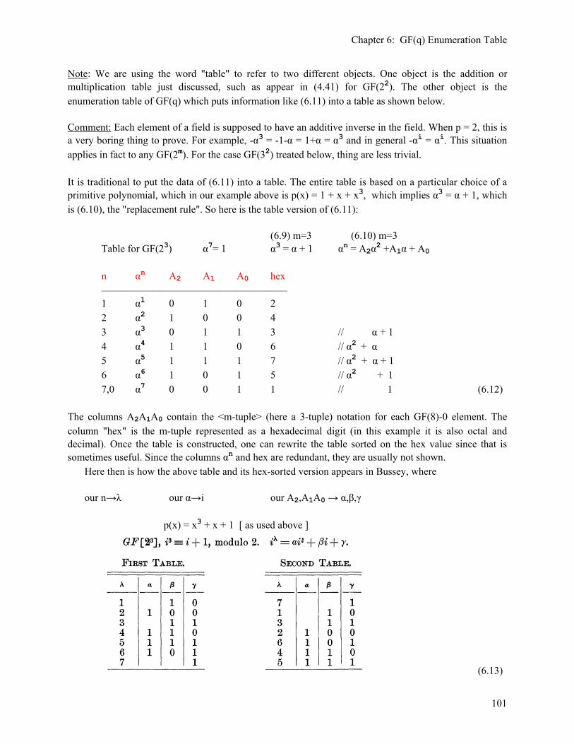
Chapter 6: GF(q) Enumeration Table
101
Note: We are using the word "table" to refer to two different objects. One object is the addition or multiplication table just discussed, such as appear in (4.41) for GF(22). The other object is the enumeration table of GF(q) which puts information like (6.11) into a table as shown below. Comment: Each element of a field is supposed to have an additive inverse in the field. When p = 2, this is a very boring thing to prove. For example, -α3 = -1-α = 1+α = α3 and in general -αi = αi. This situation applies in fact to any GF(2m). For the case GF(32) treated below, thing are less trivial. It is traditional to put the data of (6.11) into a table. The entire table is based on a particular choice of a primitive polynomial, which in our example above is p(x) = 1 + x + x3, which implies α3 = α + 1, which is (6.10), the "replacement rule". So here is the table version of (6.11): (6.9) m=3 (6.10) m=3 Table for GF(23) α7= 1 α3 = α + 1 αn = A2α2 +A1α + A0
n αn A2 A1 A0 hex –––––––––––––––––––––––––––––––––––– 1 α1 0 1 0 2 2 α2 1 0 0 4 3 α3 0 1 1 3 // α + 1 4 α4 1 1 0 6 // α2 + α 5 α5 1 1 1 7 // α2 + α + 1 6 α6 1 0 1 5 // α2 + 1 7,0 α7 0 0 1 1 // 1 (6.12) The columns A2A1A0 contain the <m-tuple> (here a 3-tuple) notation for each GF(8)-0 element. The column "hex" is the m-tuple represented as a hexadecimal digit (in this example it is also octal and decimal). Once the table is constructed, one can rewrite the table sorted on the hex value since that is sometimes useful. Since the columns αn and hex are redundant, they are usually not shown. Here then is how the above table and its hex-sorted version appears in Bussey, where our n→λ our α→i our A2,A1A0 → α,β,γ p(x) = x3 + x + 1 [ as used above ]
(6.13)

Chapter 6: GF(q) Enumeration Table
102
The tables of course get larger as q = pm increases. Example GF(24) p(x) = x4 + x + 1 [ this is p1(x) of (6.21) ]
(6.14) Example GF(25) p(x) = x5 + x3 + x2 + x + 1 [ this is p1(x) of (6.22) ]
(6.15)
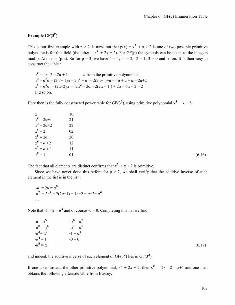
Chapter 6: GF(q) Enumeration Table
103
Example GF(32) This is our first example with p > 2. It turns out that p(x) = x2 + x + 2 is one of two possible primitive polynomials for this field (the other is x2 + 2x + 2). For GF(p) the symbols can be taken as the integers mod p. And -n = (p-n). So for p = 3, we have 4 = 1, -1 = 2, -2 = 1, 3 = 0 and so on. It is then easy to construct the table : α2 = -α - 2 = 2α + 1 // from the primitive polynomial α3 = α2α = (2α + 1)α = 2α2 + α = 2(2α+1)+α = 4α + 2 + α = 2α+2 α4 = α3α = (2α+2)α = 2α2 + 2α = 2(2α + 1 ) + 2α = 6α + 2 = 2 and so on. Here then is the fully constructed power table for GF(32), using primitive polynomial x2 + x + 2: α 10 α2 = 2α+1 21 α3 = 2α+2 22 α4 = 2 02 α5 = 2α 20 α6 = α +2 12 α7 = α + 1 11 α8 = 1 01 (6.16) The fact that all elements are distinct confirms that x2 + x + 2 is primitive. Since we have never done this before for p > 2, we shall verify that the additive inverse of each element in the list is in the list : -α = 2α = α5 -α2 = 2α2 = 2(2α+1) = 4α+2 = α+2= α6 etc. Note that -1 = 2 = α4 and of course -0 = 0. Completing this list we find -α = α5 -α6 = α2 -α2 = α6 -α7 = α3 -α3= α7 -1 = α4 -α4 = 1 -0 = 0 -α5 = α (6.17) and indeed, the additive inverse of each element of GF(32) lies in GF(32). If one takes instead the other primitive polynomial, x2 + 2x + 2, then x2 = -2x - 2 = x+1 and one then obtains the following alternate table from Bussey,
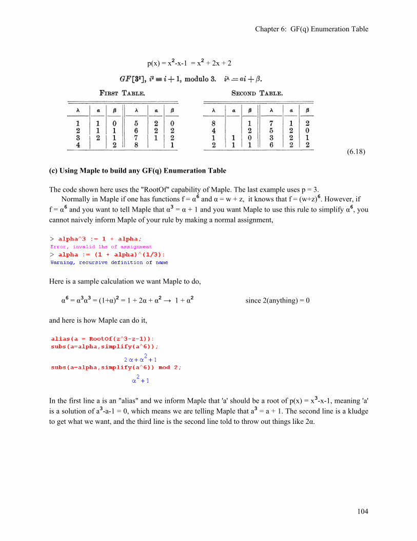
Chapter 6: GF(q) Enumeration Table
104
p(x) = x2-x-1 = x2 + 2x + 2
(6.18) (c) Using Maple to build any GF(q) Enumeration Table The code shown here uses the "RootOf" capability of Maple. The last example uses p = 3. Normally in Maple if one has functions f = α6 and α = w + z, it knows that f = (w+z)6. However, if f = α6 and you want to tell Maple that α3 = α + 1 and you want Maple to use this rule to simplify α6, you cannot naively inform Maple of your rule by making a normal assignment,
Here is a sample calculation we want Maple to do, α6 = α3α3 = (1+α)2 = 1 + 2α + α2 → 1 + α2 since 2(anything) = 0 and here is how Maple can do it,
In the first line a is an "alias" and we inform Maple that 'a' should be a root of p(x) = x3-x-1, meaning 'a' is a solution of a3-a-1 = 0, which means we are telling Maple that a3 = a + 1. The second line is a kludge to get what we want, and the third line is the second line told to throw out things like 2α.
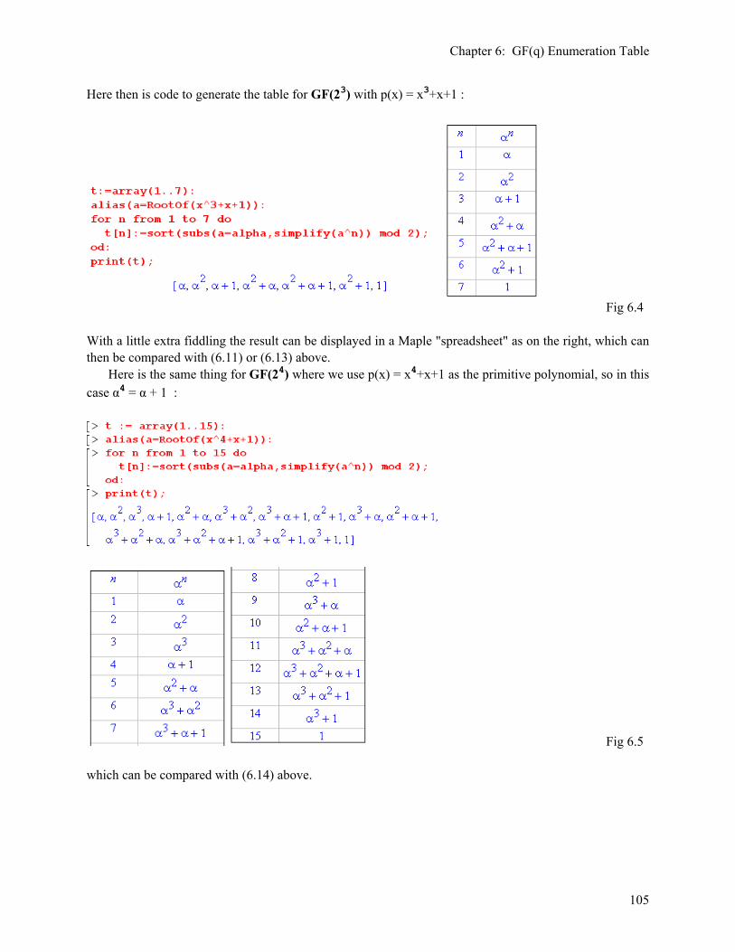
Chapter 6: GF(q) Enumeration Table
105
Here then is code to generate the table for GF(23) with p(x) = x3+x+1 :
Fig 6.4 With a little extra fiddling the result can be displayed in a Maple "spreadsheet" as on the right, which can then be compared with (6.11) or (6.13) above. Here is the same thing for GF(24) where we use p(x) = x4+x+1 as the primitive polynomial, so in this case α4 = α + 1 :
Fig 6.5 which can be compared with (6.14) above.
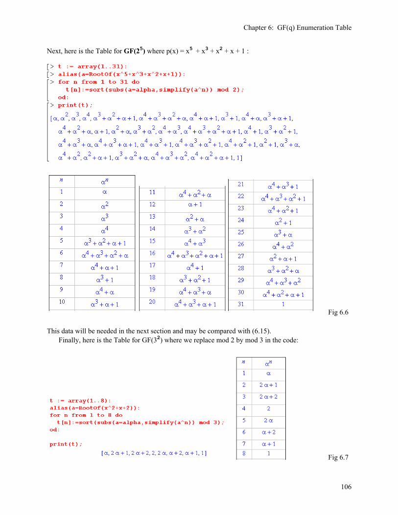
Chapter 6: GF(q) Enumeration Table
106
Next, here is the Table for GF(25) where p(x) = x5 + x3 + x2 + x + 1 :
Fig 6.6
This data will be needed in the next section and may be compared with (6.15). Finally, here is the Table for GF(32) where we replace mod 2 by mod 3 in the code:
Fig 6.7

Chapter 6: GF(q) Enumeration Table
107
Since we used p(x) = x2 + x + 2, this matches our (6.16) rather than Bussey's (6.18). (d) Using the GF(q) Table to multiply out polynomials factored in GF(q) In Big Theorem 3 (5.17) we showed how to obtain all minimum polynomials of some GF(q) in factored form, where α is some element of GF(q), m(x) = (x - α) • (x - αp) • (x - αp2) • (x - αp3) ... .... (x - αpk-1) αpk= α k ≤ m . (5.17) In the examples of Chapter 5 (c) we then explicitly listed all minimal polynomials for GF(2m) for m = 3,4,5. Here we shall show how the GF(q) table constructed above can be used to expand the m(x) into a form which explicitly has coefficients in GF(2), that is, polynomials like x2 + x + 1. We shall first do an example by hand, then show how to automate the process using Maple. 1. Expansion of a factored minimum polynomial: an example For GF(23) one of the minimum polynomials ( in fact a primitive one) was found to be p1(x) = (x - α )(x - α2 )(x - α4) . (5.24) The first step is to expand in the obvious manner, p1(x) = x3 + [α + α2 + α4]x2 + [α3 + α5 + α6]x + [1] 1 . The important information in the above GF(23) table is this α3 = 1 + α α4 = α + α2 α5 = 1 + α + α2 α6 = 1 + α2 which we then use to evaluate each of the non-obvious coefficients coeff of x2 = α + α2 + α4 = α + α2 + (α + α2) = 2α + 2α2 = 0 + 0 = 0 // 2y=0 for any y coeff of x = α3 + α5 + α6 = (1 + α) + ( 1 + α + α2) + (1 + α2) = 3 + 2α + 2α2 = 1
Thus, we find p1(x) = x3 + x + 1 (6.19) This just happens to be the very primitive polynomial with which we built the table. But this method works with any factored polynomial, and we will do them all below.
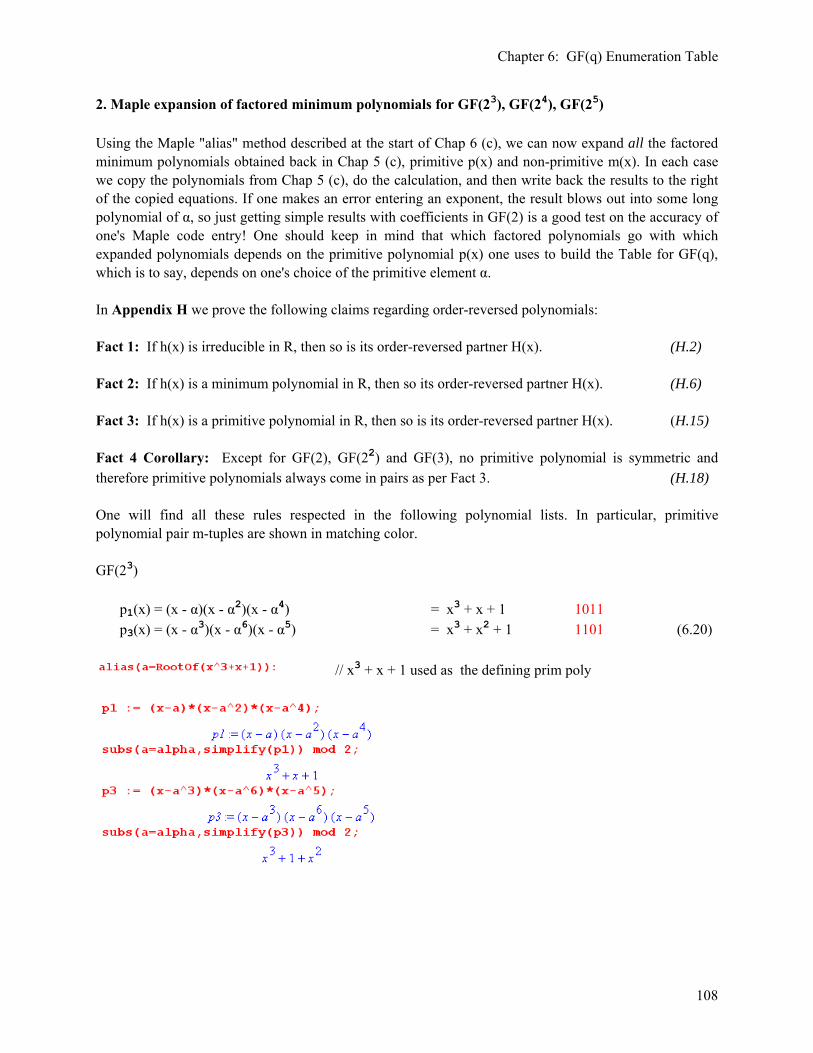
Chapter 6: GF(q) Enumeration Table
108
2. Maple expansion of factored minimum polynomials for GF(23), GF(24), GF(25) Using the Maple "alias" method described at the start of Chap 6 (c), we can now expand all the factored minimum polynomials obtained back in Chap 5 (c), primitive p(x) and non-primitive m(x). In each case we copy the polynomials from Chap 5 (c), do the calculation, and then write back the results to the right of the copied equations. If one makes an error entering an exponent, the result blows out into some long polynomial of α, so just getting simple results with coefficients in GF(2) is a good test on the accuracy of one's Maple code entry! One should keep in mind that which factored polynomials go with which expanded polynomials depends on the primitive polynomial p(x) one uses to build the Table for GF(q), which is to say, depends on one's choice of the primitive element α. In Appendix H we prove the following claims regarding order-reversed polynomials: Fact 1: If h(x) is irreducible in R, then so is its order-reversed partner H(x). (H.2) Fact 2: If h(x) is a minimum polynomial in R, then so its order-reversed partner H(x). (H.6) Fact 3: If h(x) is a primitive polynomial in R, then so is its order-reversed partner H(x). (H.15) Fact 4 Corollary: Except for GF(2), GF(22) and GF(3), no primitive polynomial is symmetric and therefore primitive polynomials always come in pairs as per Fact 3. (H.18) One will find all these rules respected in the following polynomial lists. In particular, primitive polynomial pair m-tuples are shown in matching color. GF(23) p1(x) = (x - α)(x - α2)(x - α4) = x3 + x + 1 1011 p3(x) = (x - α3)(x - α6)(x - α5) = x3 + x2 + 1 1101 (6.20)
// x3 + x + 1 used as the defining prim poly

Chapter 6: GF(q) Enumeration Table
109
GF(24) p1(x) = (x - α)(x - α2)(x - α4) (x - α8) = x4 + x + 1 10011 p7(x) = (x - α7)(x - α14)(x - α13)(x - α11) = x4 + x3 + 1 11001 m3(x) = (x - α3)(x - α6)(x - α12)(x - α9) = x4 + x3 + x2 + x + 1 11111 m5(x) = (x - α5)(x - α10) = x2 + x + 1 111 (6.21)
// x4 + x + 1 used as the defining prim poly
In this example, the non-primitive minimum polynomials are symmetric and so don't appear as "pairs".
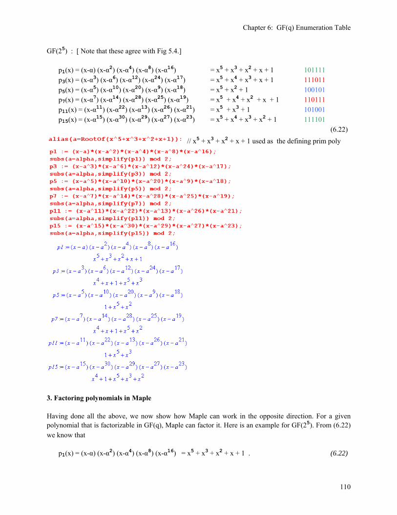
Chapter 6: GF(q) Enumeration Table
110
GF(25) : [ Note that these agree with Fig 5.4.] p1(x) = (x-α) (x-α2) (x-α4) (x-α8) (x-α16) = x5 + x3 + x2 + x + 1 101111 p3(x) = (x-α3) (x-α6) (x-α12) (x-α24) (x-α17) = x5 + x4 + x3 + x + 1 111011 p5(x) = (x-α5) (x-α10) (x-α20) (x-α9) (x-α18) = x5 + x2 + 1 100101 p7(x) = (x-α7) (x-α14) (x-α28) (x-α25) (x-α19) = x5 + x4 + x2 + x + 1 110111 p11(x) = (x-α11) (x-α22) (x-α13) (x-α26) (x-α21) = x5 + x3 + 1 101001 p15(x) = (x-α15) (x-α30) (x-α29) (x-α27) (x-α23) = x5 + x4 + x3 + x2 + 1 111101 (6.22)
// x5 + x3 + x2 + x + 1 used as the defining prim poly
3. Factoring polynomials in Maple Having done all the above, we now show how Maple can work in the opposite direction. For a given polynomial that is factorizable in GF(q), Maple can factor it. Here is an example for GF(25). From (6.22) we know that p1(x) = (x-α) (x-α2) (x-α4) (x-α8) (x-α16) = x5 + x3 + x2 + x + 1 . (6.22)

Chapter 6: GF(q) Enumeration Table
111
So we enter x5 + x3 + x2 + x + 1 and ask Maple if it can factor this into a product of (x-ri) factors where the roots ri all lie in GF(25) . We continue to use alias(a=RootOf(x^5+x^3+x^2+x+1) from earlier.
If we just want the roots,
α16 α4 α α8 α2
In each pair, the second index gives the root multiplicity and here each root occurs only once. Looking in the GF(25) table in Fig 6.6 we find that this root list contains the values added above in black, and these roots agree with those of the factored p1(x) shown above. If Maple is asked to factor something that is not factorable in GF(q) it will go as far as it can,
but there are no roots in GF(25) so the Roots function returns a null set
As shown above, x5 + x4 + 1 is reducible into the product of two factors (x3+x+1)(x2+x+1). Each of these factors is irreducible but is not a minimum polynomial since each cannot be factored into a product of GF(25) elements (otherwise Maple would have done it). Thus, these two polynomials fit into the white region on the right side of Fig 5.5. To be specific, for x3+x+1 we get
Notice the alias 'a' second argument of the Factor and Roots commands above. If one simply wants to factor a polynomial within GF(2) and not GF(q), this argument should be omitted. For example, back in (5.31) we eliminated various polynomials from a list because they were not irreducible. There we had this partially factored result done by hand, x4 + x3 + x + 1 = (x3+1)(x+1) = reducible Maple can check to see if x4 + x3 + x + 1 is factorable in GF(2) as follows,
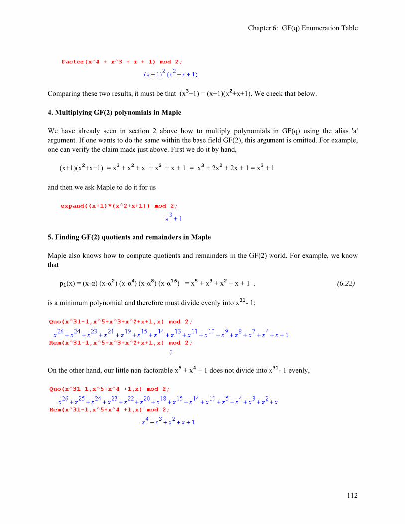
Chapter 6: GF(q) Enumeration Table
112
Comparing these two results, it must be that (x3+1) = (x+1)(x2+x+1). We check that below. 4. Multiplying GF(2) polynomials in Maple We have already seen in section 2 above how to multiply polynomials in GF(q) using the alias 'a' argument. If one wants to do the same within the base field GF(2), this argument is omitted. For example, one can verify the claim made just above. First we do it by hand, (x+1)(x2+x+1) = x3 + x2 + x + x2 + x + 1 = x3 + 2x2 + 2x + 1 = x3 + 1 and then we ask Maple to do it for us
5. Finding GF(2) quotients and remainders in Maple Maple also knows how to compute quotients and remainders in the GF(2) world. For example, we know that p1(x) = (x-α) (x-α2) (x-α4) (x-α8) (x-α16) = x5 + x3 + x2 + x + 1 . (6.22) is a minimum polynomial and therefore must divide evenly into x31- 1:
On the other hand, our little non-factorable x5 + x4 + 1 does not divide into x31- 1 evenly,

Chapter 6: GF(q) Enumeration Table
113
6. Finding all Irreducible and Minimum Polynomials of GF(2m) The simple code below works for GF(2m) but could easily be generalized for GF(pm). The example given is GF(24). We select a GF(24) primitive polyomial p(x) = x4+x+1 as shown in (6.21) and set "a" using the alias method discussed above. Then we exhaust all possible polynomials of degree 4 and less which have constant 1 and have coefficients in GF(2) ( 0 or 1) and we attempt to factor each one:
For each non-trivial polynomial there are four possibilities: (A) factors into unique (x-ai) factors where all ai ≠ 1 irreducible and min poly (maybe prim) (B) has at least one (x+1) factor reducible hence not min poly (C) has a single but non-linear-in-x factor irreducible and not min poly (D) has multiple factors with at least one non-linear-in-x reducible hence not min poly (E) case A but at least one factor appears more than once reducible hence not min poly The irreducible polynomials are all A + C. In terms of Fig 5.5 which we repeat here, the A items go in the gray area (some of them will be primitive, some will not), while the C items go in the white area.
Fig 5.5 Here is the output of the above code where each case is labeled A,B,C,D. The four A items are in (6.21). See Fig 6.5 to find that α2+α = α5 and α2+α +1 = α10 , so the first "A" item is (x-α5)(x-α10) which we know from (6.21) is a non-primitive minimum polynomial.
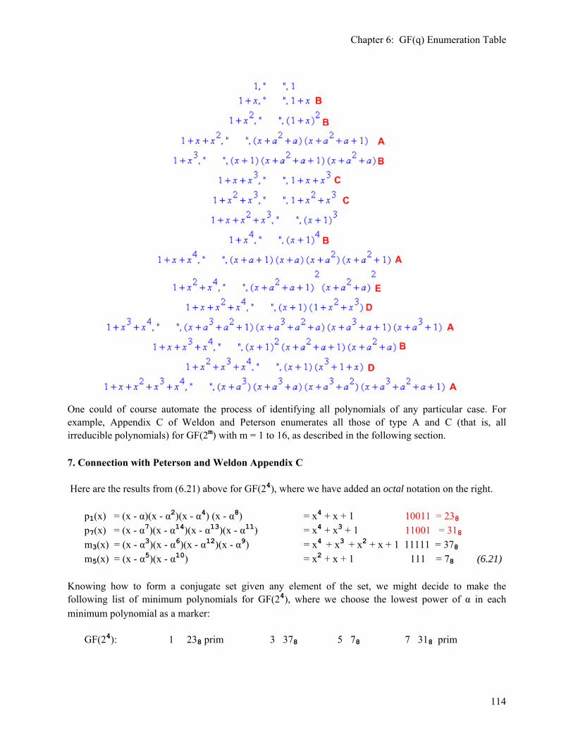
Chapter 6: GF(q) Enumeration Table
114
One could of course automate the process of identifying all polynomials of any particular case. For example, Appendix C of Weldon and Peterson enumerates all those of type A and C (that is, all irreducible polynomials) for GF(2m) with m = 1 to 16, as described in the following section. 7. Connection with Peterson and Weldon Appendix C Here are the results from (6.21) above for GF(24), where we have added an octal notation on the right. p1(x) = (x - α)(x - α2)(x - α4) (x - α8) = x4 + x + 1 10011 = 238 p7(x) = (x - α7)(x - α14)(x - α13)(x - α11) = x4 + x3 + 1 11001 = 318 m3(x) = (x - α3)(x - α6)(x - α12)(x - α9) = x4 + x3 + x2 + x + 1 11111 = 378 m5(x) = (x - α5)(x - α10) = x2 + x + 1 111 = 78 (6.21) Knowing how to form a conjugate set given any element of the set, we might decide to make the following list of minimum polynomials for GF(24), where we choose the lowest power of α in each minimum polynomial as a marker: GF(24): 1 238 prim 3 378 5 78 7 318 prim

Chapter 6: GF(q) Enumeration Table
115
Knowing that primitive polynomials always come in order-reversed pairs according to Fact 3 (H.15), we might save space in the table by not displaying the last item since we know how to order-reverse the first item to obtain the last item. Then we have just GF(24): 1 238 prim 3 378 5 78 This is the basic notation used in the Peterson and Weldon Appendix C,
Primitive polynomials of degree m get suffix letters E,F,G,H while non-minimum polynomials of degree m get suffix letters A,B,C,D and polynmials of degree less than 4 get no suffix. The tables show full results for GF(2m ) with m = 1 through 16. Reduced information is then given form m = 17 through 34. The number of entrees of course can get very large. For example number or primitive polynomials for GF(216) = φ(216-1)/16 = 2048 of which 1024 appear in the table, along with many non-primitive polynomials. (e) Construction of the + and • tables for GF(22) To illustrate the method outlined above, we take this very simple case GF(22). We need the GF(22) enumeration table, which we now obtain by mimicking the GF(23) example above: " From the primitive polynomial list in Fig 5.3 we find p(x) = 1 + x + x2. We proved this is a primitive polynomial for GF(22) in (5.29). In terms of (6.8) we have c2 = c1 = c0 = 1. Then (6.9) says that α2 = (2-c1)α + (2-c0) = α +1. So the reduction rule (6.9) states that α2 = α + 1. This is of course totally obvious just setting p(α) = 0 for the above p(x), remembering + and - are the same, but we wanted to see how (6.9) gets the right answer. So we can build the entire enumeration table in 1 minute. 0 00 0 α0 = 1 01 1 α3 = α2α = (α+1)α = α2+α = α+1+α = 2α +1 = 1 α 10 2 α2 = α + 1 11 3 (6.23) Notice that all 2-tuples are "hit", as claimed above. We have added some octal/hex numbers to make this fact more obvious. We know that α3 = 1, since the non-zero elements of GF(8) form a cyclic group under • for a primitive element like α (which is a root of primitive polynomial p(x)). This fact is verified as shown above on the right. This fact α3 = 1 was not needed to build the above enumeration table, but it is needed to construct the • table. "

Chapter 6: GF(q) Enumeration Table
116
The addition table was already worked out in (4.10) in the m-tuple basis so we just quote that result here, + 00 01 10 11 + 0 1 2 3 00 00 01 10 11 0 0 1 2 3 01 01 00 11 10 1 1 0 3 2 10 10 11 00 01 2 2 3 0 1 11 11 10 01 00 3 3 2 1 0 (6.24) Recall that the table on the left is trivially computed by doing GF(2) addition (XOR) independently on each position of the 2-tuples being added as shown in (4.8). This table can be written in the power basis using (6.23), where on the right we use α + 1 in place of α2, + 0 1 α α2 + 0 1 α α+1 0 1 1 α α2 0 1 1 α α+1 1 1 0 α2 α 1 1 0 α+1 α α α α2 0 1 α α α+1 0 1 α2 α2 α 1 0 α+1 α+1 α 1 0 (6.25) As noted above, the multiplication table is trivial to construct in the power basis using α3 = 1 as shown on the left, • 0 1 α α2 • 0 1 α α+1 0 0 0 0 0 0 0 0 0 0 1 0 1 α α2 1 0 1 α α+1 α 0 α α2 1 α 0 α α+1 1 α2 0 α2 1 α α+1 0 α+1 1 α (6.26) On the right we have just replaced α2 by α + 1. Using the enumeration table above, we can write this multiplication table in these alternate m-tuple basis, • 00 01 10 11 • 0 1 2 3 00 00 00 00 00 0 0 0 0 0 01 00 01 10 11 1 0 1 2 3 10 00 10 11 01 2 0 2 3 1 11 00 11 01 10 3 0 3 1 2 (6.27)

Chapter 7: Linear Block Codes
117
Chapter 7: Linear Block Codes There are many good texts on the theory of error-correcting codes; two are mentioned in the References. It has been our experience that most of the difficulty encountered in reading these texts is not so much with the coding theory itself, but with the underlying theory of Galois Fields. Since we have just finished a long exposition of Galois Field theory, it seems appropriate to make at least a preliminary connection between block codes and Galois Fields. This connection will become much tighter in Chapter 8 on Cyclic Codes. (a) The Basics For our purposes, a symbol, or code symbol, is an element of some Galois field GF(q=pm). For example, if p = 2 and m = 1, a symbol is an element of GF(2). The only elements of GF(2) are 0 and 1, and a symbol that takes these two values is called a bit. If p = 2 and m = 8, a symbol is an element of GF(28), an 8-tuple of bits known as a byte, which symbol can take 256 values. We shall try to keep the discussion as general as possible by using the term symbol in place of bit or byte or some other special case. Vector Space comment Recall from (1.14b) that the elements of GF(q) form a vector space over the field GF(p). Thus, our coding symbols are elements of this vector space, which let us call V. One can then think of an n-tuple of coding symbols like d = (d1, d2, d3) as being an element of a vector space V3 ≡ V ⊕ V ⊕ V which means V3 is a "direct sum" of three copies of the vector space V. When we refer below to the vector spaces like Dk, Ck and Vk, we are referring to direct sum spaces of the type Vk. A direct sum of vector spaces is always itself a vector space because all the axioms of a vector space are fulfilled, as the reader can verify. For example, if d = (d1, d2, d3) and e = (e1, e2, e3), then the addition of two vectors in the V3 space is defined in the very obvious manner: d + e = (d1, d2, d3) + (e1, e2, e3) = (d1+e1, d2+e2, d3+e3), (7.1) and of course a sum of code symbols (elements of GF(q)) like d2+e2 is provided by the + table for GF(q). A vector space in general allows for vectors to be added as above. It says nothing about the possible multiplication of two vectors. We shall in effect be using the following definition of the product of two vectors in V3, d • e = (d1, d2, d3) • (e1, e2, e3) = (d1•e1, d2•e2, d3•e3) , (7.2) where terms like d2•e2 are provided by the • table for GF(q). Notice that the three spaces V which comprise V3 do not interact with each other in any way. A familiar example is a point r = (x,y,z) in 3D Cartesian space R3 = R ⊕ R ⊕ R where R is the real numbers. In linear algebra, a direct sum matrix like V(3) can be thought of as being a large matrix in which the matrices being direct-summed appear as square blocks on the diagonal, surrounded by a sea of zeros. In this situation, a corresponding large vector has a section associated with each smaller matrix, and each section is affected only by its matrix block on the large matrix diagonal.
Chapter 7: Linear Block Codes
118
The direct sum concept is different from the notion of a direct product. In our example above, the direct product space V ⊗ V would have elements of the form [d x e]ij = diej and V ⊗ V ⊗ V elements like [d x e x f]ijk = diejfk . This is not what we are dealing with in our current context. The basic plan of a block code is to take data words of k symbols each, add n-k parity check symbols which are dependent on (computed from) the k data symbols, and end up with code words of n symbols each. Thus, data is encoded in finite blocks consisting of n symbols. Such a code is denoted as (n,k). In some sense the efficiency of a code is indicated by the ratio of data bits k to total bits n, known as the code rate, k/n = the code rate of an (n,k) code . One might be willing to tolerate a lower code rate if the code is good at detecting and/or correcting a certain desired number of errors in the received code words. A subset of block codes are the linear block codes, where the code words are generated by the application of a linear operator onto the data words. Since we are limiting our interest to situations where k and n are finite numbers, such a linear operator is simply a matrix. If we think of data words and code words as row vectors (as opposed to column vectors), then a linear block code is defined by a matrix G (known as the generator matrix) acting to the left on data words d to generate code words c, c = dG . (7.3) The data word d is a k-component row vector, the code word c is an n-component row vector, and therefore G is a matrix with n columns and k rows. It is useful to go immediately to a simple example. For k = 2 and n = 3, so we write d = (d1 d2) and c = (c1 c2 c3) and G as shown [ commas in our row vectors are optional ]
(c1 c2 c3) = (d1 d2) ⎝⎛
⎠⎞ a b c
d e f . (7.4)
The vector d = (d1 d2) lies in a 2 dimensional vector space (called D2, the data space) whose basis vectors we could take to be (1 0) and (0 1). Here, D2 = V ⊕ V. When these basis vector data words are mapped into the code space we get
(a b c) = (1 0) ⎝⎛
⎠⎞ a b c
d e f (d e f) = (0 1) ⎝⎛
⎠⎞ a b c
d e f . (7.5)
Since (1 0) and (0 1) are legal data words, the triplets (a b c) and (d e f) are legal code words. These code words exist in a 3 dimensional vector space (V3) spanned by (1 0 0), (0 1 0) and (0 0 1). We want the two code word vectors (a b c) and (d e f) to be linearly independent so that these vectors span a 2 dimensional subspace (called C2, or the code space) of the 3 dimensional space V3. For that reason, we want the k = 2 rows of the matrix G to be linearly independent. In matrix language, this means that the matrix G has rank k. Since the number of rows k is ≤ the number of columns n, k is the maximum rank that matrix G can possibly have.

Chapter 7: Linear Block Codes
119
If one makes arbitrary linear combinations of (a b c) and (d e f), one exhausts all possible code vectors in V3. There are of course q2 such code words in our example (q from GF(q)) because there are q2 data words we can start with. In general there will be qk such code words in Ck if the symbols all lie in GF(q) and data words have k symbols. Of course qk is also the total number of possible data words in the data space Dk. There are three vector spaces of interest. Think of a word or vector as a "point" in a vector space: data space = Dk (dim = k) which has qk points, all of which are legal data words code space = Ck (dim = k) which has qk legal code word points, spanned by the k rows of G embedding space = Vn (dim = n) which has qn points, many of which are not legal code word points code space Ck is a k dimensional subspace of Vn which is an n dimensional vector space (7.6) The code space Ck is the same as the row space of matrix G (the vector space spanned by the rows of G) and some authors use the term row space instead of code space, but we shall refer to Ck always as the code space, which is a subspace of Vn . Since the code points in Vn all live in the Ck subspace of Vn which has k spanning vectors, we can think of the rest of Vn as being spanned by some set of n-k basis vectors all of which are orthogonal to the k basis vectors which are the rows of G, like (a b c) and (d e f) in the example. We might call this (Ck)⊥ where symbol ⊥ means this space is orthogonal or "perpendicular" to Ck. So we add to our list, perp space = (Ck)⊥ (dim = n-k) which has qn - qk points, all of which are NOT legal code points (7.7) The implication of course is that Vk = Ck + (Ck)⊥ (7.8)
where in this one equation + means the union of the two sets of points Ck and (Ck)⊥. Since the legal code words are all points in the code space Ck we can say linear block code (n,k) = the code space = Ck = the k-dimensional row space of matrix G . (7.9) The components of all vectors referred to above are symbols = elements of GF(q). The elements of the G matrix are symbols, not real numbers. Even the components of vectors in (Ck)⊥ are symbols. It happens that they are combinations of symbols which don't form legal code words. We sometimes like to add the word "legal" when talking about code words, but it is redundant. A code word is a legal code word. The implication is that elements of (Ck)⊥ are illegal code words, meaning they are not code words. As we shall see, noise in data transmission can convert a legal code word into an illegal one (an error).

Chapter 7: Linear Block Codes
120
(b) Notational Remarks (1) The transpose T symbol (some people use other symbols) swaps the columns and rows of a matrix of any dimension n x m. Here are some examples ( ≡ means "is defined as" )
d ≡ (d1 d2) => dT = ⎝⎛
⎠⎞ d1
d2 (7.10)
G ≡ ⎝⎛
⎠⎞ a b c
d e f => GT = ⎝⎜⎛
⎠⎟⎞ a d
b e c f
(7.11)
d ≡ ⎝⎛
⎠⎞ d1
d2 => dT = (d1 d2) . (7.12)
Traditionally linear algebra texts use column vectors like the d on the last line above, but we are perversely using row vectors as on the first line. Coding theory texts often do this as a space-saving measure, since one wastes less vertical line-inches writing out a row vector than a column vector. So far we have indicated row vectors like (a b c) without commas, but (a,b,c) means the same thing. Notice that there are no commas in a column vector or a matrix. Therefore, we could write (7.3) c = dG in the following completely equivalent transposed form cT = GTdT (7.13) where one can easily show that (ABC...)T = ...CTBTAT. Of course if we had decided to start off using column vectors instead of row vectors, we would have redefined everything so this equation would have said c = Gd. (2) Now what happens when we multiply a row vector and a column vector together? There are two ways to do this, known as an inner and outer product,
⎝⎛
⎠⎞ d1
d2 (e1 e2) = ⎝⎛
⎠⎞ d1e1 d1e2
d2e1 d2e2 // outer product , result is a 2x2 matrix
(e1 e2) ⎝⎛
⎠⎞ d1
d2 = e1d1+ e2d2 // inner product, result is a 1x1 matrix (7.14)
The outer product is an example of the direct product concept mentioned above. In our perverse row vector notation of (7.10) these lines would be written
dTe = ⎝⎛
⎠⎞ d1
d2 (e1 e2) = ⎝⎛
⎠⎞ d1e1 d1e2
d2e1 d2e2 // outer product , result is a 2x2 matrix
edT = (e1 e2) ⎝⎛
⎠⎞ d1
d2 = e1d1+ e2d2 // inner product, result is a 1x1 matrix
≡ e • d = "dot product" = (e,d) = inner product = scalar product . (7.15) but in normal linear algebra notation using vectors as in (7.12) one would have
Chapter 7: Linear Block Codes
121
deT = ⎝⎛
⎠⎞ d1
d2 (e1 e2) = ⎝⎛
⎠⎞ d1e1 d1e2
d2e1 d2e2
eTd = (e1 e2) ⎝⎛
⎠⎞ d1
d2 = e1d1+ e2d2
≡ e • d = "dot product" = (e,d) = inner product = scalar product . (7.16) In either notation the inner product is thought of as the "dot product" of two vectors as shown, normally written with some dot symbol and bolded vectors. For a very brief description of inner products (as well as norms, distance, metrics, and Hilbert Spaces) see Section 4 of the author's tensor analysis reference. (3) Looking at (7.4) above, we would write, for example, c2 = d1b + d2e and in (7.16) we wrote eTd = e1d1+ e2d2. One must keep in mind that, since all these symbols are elements of GF(q), the meaning of addition and multiplication is that given by the GF(q) + and • tables. Recall that we showed how to construct such tables in Chapter 6. As a reminder of this, one might write c2 = d1• b + d2 • e (7.17) One must be careful not to use ordinary real-number-field + and • operators. In the matrix and vector formalism, these operators are sort of hidden away, as in the vector/matrix equation (7.3), c = dG . (4) In earlier chapters, we sometimes used bold font to denote elements of GF(q), to distinguish such elements from normal scalars. For example we had ( with p = integer, g = field element, q = pm ) , Fact: pg = 0 for any element g of GF(q=pm). (4.5) In the current context, we are now using bolded font to indicate vectors in Vk type vector spaces, so we shall discontinue randomly using bold font for field elements. The above Fact now says Fact: pg = 0 for any element g of GF(q=pm). (4.5) (5) For all our vectors we have starting the component numbering with 1, as in d = (d1 d2 d3) just because this seems the simplest thing to do. Obviously one could have written d = (d0 d1 d2) as an alternate notation. Later when we start talking about vector components being the coefficients of polynomials, it will be much easier to start the labeling with 0, then we will have for example d(x) = d0 + d1x + d2x2 so the coefficient subscript will match the power. The reader should be aware of which convention is being used in a given section below. (6) There is a semantic question about which symbol is first. When we write d = (d0 d1 d2), we say that the d0 symbol is first just because it is on the left and we read left to right. However, in the next chapter when we come to polynomials like d(x) = d0 + d1x + d2x2, we shall find that it is most convenient in the transmission of data to send the most significant symbol first, so if the coefficients of this polynomial
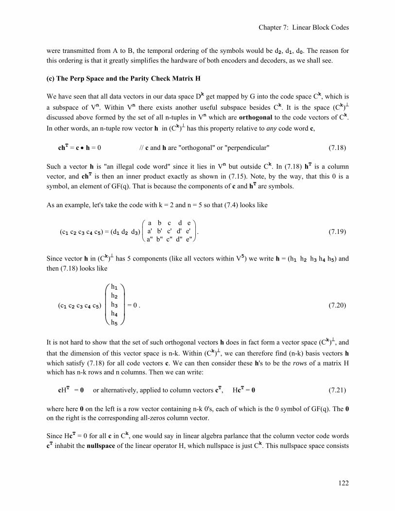
Chapter 7: Linear Block Codes
122
were transmitted from A to B, the temporal ordering of the symbols would be d2, d1, d0. The reason for this ordering is that it greatly simplifies the hardware of both encoders and decoders, as we shall see. (c) The Perp Space and the Parity Check Matrix H We have seen that all data vectors in our data space Dk get mapped by G into the code space Ck, which is a subspace of Vn. Within Vn there exists another useful subspace besides Ck. It is the space (Ck)⊥
discussed above formed by the set of all n-tuples in Vn which are orthogonal to the code vectors of Ck. In other words, an n-tuple row vector h in (Ck)⊥ has this property relative to any code word c, chT = c • h = 0 // c and h are "orthogonal" or "perpendicular" (7.18) Such a vector h is "an illegal code word" since it lies in Vn but outside Ck. In (7.18) hT is a column vector, and chT is then an inner product exactly as shown in (7.15). Note, by the way, that this 0 is a symbol, an element of GF(q). That is because the components of c and hT are symbols. As an example, let's take the code with k = 2 and n = 5 so that (7.4) looks like
(c1 c2 c3 c4 c5) = (d1 d2 d3) ⎝⎜⎛
⎠⎟⎞ a b c d e
a' b' c' d' e' a" b" c" d" e"
. (7.19)
Since vector h in (Ck)⊥ has 5 components (like all vectors within V5) we write h = (h1 h2 h3 h4 h5) and then (7.18) looks like
(c1 c2 c3 c4 c5)
⎝⎜⎜⎛
⎠⎟⎟⎞ h1
h2 h3 h4 h5
= 0 . (7.20)
It is not hard to show that the set of such orthogonal vectors h does in fact form a vector space (Ck)⊥, and that the dimension of this vector space is n-k. Within (Ck)⊥, we can therefore find (n-k) basis vectors h which satisfy (7.18) for all code vectors c. We can then consider these h's to be the rows of a matrix H which has n-k rows and n columns. Then we can write: cHT = 0 or alternatively, applied to column vectors cT, HcT = 0 (7.21) where here 0 on the left is a row vector containing n-k 0's, each of which is the 0 symbol of GF(q). The 0 on the right is the corresponding all-zeros column vector. Since HcT = 0 for all c in Ck, one would say in linear algebra parlance that the column vector code words cT inhabit the nullspace of the linear operator H, which nullspace is just Ck. This nullspace space consists

Chapter 7: Linear Block Codes
123
of all the points in Vn which are hit by the mapping c = dG for all data vectors d. Thus, the range of operator G (all points it hits) = the nullspace of operator H = Ck. In our example, let us call our set of n-k = 5-3 = 2 h vectors by the names h and h'. Then (7.21) reads
cHT = (c1 c2 c3 c4 c5)
⎣⎢⎢⎡
⎦⎥⎥⎤ h1 h'1
h2 h'2 h3 h'3 h4 h'4 h5 h'5
= (0 0) H = ⎝⎛
⎠⎞ h1 h2 h3 h4 h5
h'1 h'2 h'3 h'4 h'5 (7.22)
In coding theory, the matrix H is called the parity check matrix of the (n,k) code. We can "check" that a vector c really is a code word by computing cHT and seeing if the result is 0. If a received code word flunks this test, we know that there has been a transmission error. But all we know, when an error is detected by cHT ≠ 0, is that one or more of the n symbols in that code word are wrong. Since the rows of G are a set of code vectors, it trivially follows from the above that: GHT = 0 or HGT = 0 (7.23) where now each 0 is an all-zeros matrix. (d) The Dual Code generated by H Since matrix H has rank n-k, it can itself be considered as the generator matrix of a new code having data words containing n-k symbols. That is, we can define a code: c' = d'H (7.24) where d' is a (n-k)-tuple and c' is an n-tuple. This code is (n,n-k) and is known as the dual code to (n,k). All code vectors c of the code (n,k) are orthogonal to all code vectors c' of the dual code (n,n-k). Here is a little proof: c'cT = (d'H)(dG)T = (d'H)(GTdT) = d' (HGT)dT = d' (0) dT = 0 . The following drawing illustrates the above discussion:
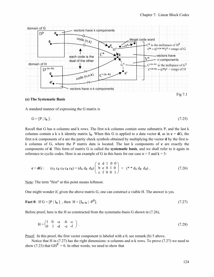
Chapter 7: Linear Block Codes
124
Fig 7.1 (e) The Systematic Basis A standard manner of expressing the G matrix is G = [P | Ik ] . (7.25) Recall that G has n columns and k rows. The first n-k columns contain some submatrix P, and the last k columns contain a k x k identity matrix Ik. When this G is applied to a data vector d, as in c = dG, the first n-k components of c are the parity check symbols obtained by multiplying the vector d by the first n-k columns of G, where the P matrix data is located. The last k components of c are exactly the components of d. This form of matrix G is called the systematic basis, and we shall refer to it again in reference to cyclic codes. Here is an example of G in this basis for our case n = 5 and k = 3:
c = dG : (c1 c2 c3 c4 c5) = (d1 d2 d3) ⎝⎜⎛
⎠⎟⎞ a d 1 0 0
b e 0 1 0 c f 0 0 1
= (* * d1 d2 d3) . (7.26)
Note: The term "first" at this point means leftmost. One might wonder if, given the above matrix G, one can construct a viable H. The answer is yes. Fact 0: If G = [P | Ik ] , then H = [In-k | -PT]. (7.27) Before proof, here is the H so constructed from the systematic-basis G shown in (7.26),
H = ⎝⎛
⎠⎞1 0 -a -b -c
0 1 -d -e -f . (7.28)
Proof: In this proof, the first vector component is labeled with a 0, see remark (b) 5 above. Notice that H in (7.27) has the right dimensions: n columns and n-k rows. To prove (7.27) we need to show (7.23) that GHT = 0. In other words, we need to show that
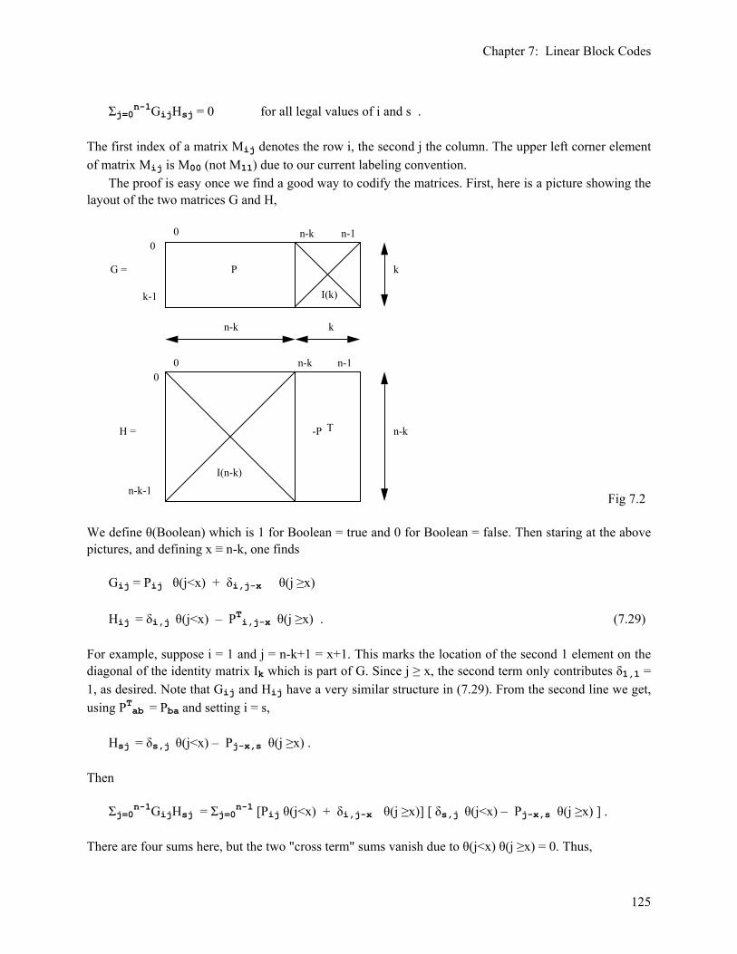
Chapter 7: Linear Block Codes
125
Σj=0n-1GijHsj = 0 for all legal values of i and s . The first index of a matrix Mij denotes the row i, the second j the column. The upper left corner element of matrix Mij is M00 (not M11) due to our current labeling convention. The proof is easy once we find a good way to codify the matrices. First, here is a picture showing the layout of the two matrices G and H,
0 n-k n-1
P
I(k)
G =
0
k-1
0
n-k-1
0 n-k n-1
I(n-k)
H =
k
k
n-k
n-k-P T
Fig 7.2 We define θ(Boolean) which is 1 for Boolean = true and 0 for Boolean = false. Then staring at the above pictures, and defining x ≡ n-k, one finds Gij = Pij θ(j<x) + δi,j-x θ(j ≥x)
Hij = δi,j θ(j<x) – PTi,j-x θ(j ≥x) . (7.29) For example, suppose i = 1 and j = n-k+1 = x+1. This marks the location of the second 1 element on the diagonal of the identity matrix Ik which is part of G. Since j ≥ x, the second term only contributes δ1,1 = 1, as desired. Note that Gij and Hij have a very similar structure in (7.29). From the second line we get, using PTab = Pba and setting i = s, Hsj = δs,j θ(j<x) – Pj-x,s θ(j ≥x) . Then Σj=0n-1GijHsj = Σj=0n-1 [Pij θ(j<x) + δi,j-x θ(j ≥x)] [ δs,j θ(j<x) – Pj-x,s θ(j ≥x) ] . There are four sums here, but the two "cross term" sums vanish due to θ(j<x) θ(j ≥x) = 0. Thus,
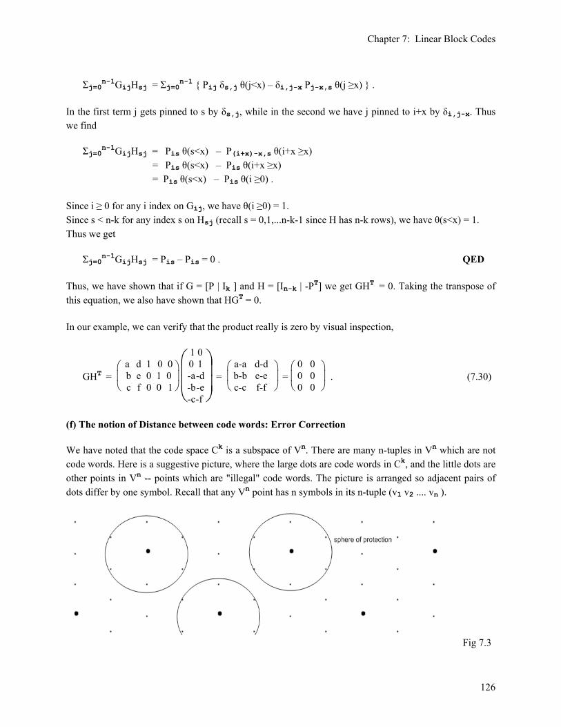
Chapter 7: Linear Block Codes
126
Σj=0n-1GijHsj = Σj=0n-1 { Pij δs,j θ(j<x) – δi,j-x Pj-x,s θ(j ≥x) } . In the first term j gets pinned to s by δs,j, while in the second we have j pinned to i+x by δi,j-x. Thus we find Σj=0n-1GijHsj = Pis θ(s<x) – P(i+x)-x,s θ(i+x ≥x) = Pis θ(s<x) – Pis θ(i+x ≥x) = Pis θ(s<x) – Pis θ(i ≥0) . Since i ≥ 0 for any i index on Gij, we have θ(i ≥0) = 1. Since s < n-k for any index s on Hsj (recall s = 0,1,...n-k-1 since H has n-k rows), we have θ(s<x) = 1. Thus we get Σj=0n-1GijHsj = Pis – Pis = 0 . QED Thus, we have shown that if G = [P | Ik ] and H = [In-k | -PT] we get GHT = 0. Taking the transpose of this equation, we also have shown that HGT = 0. In our example, we can verify that the product really is zero by visual inspection,
GHT = ⎝⎜⎛
⎠⎟⎞ a d 1 0 0
b e 0 1 0 c f 0 0 1
⎝⎜⎜⎛
⎠⎟⎟⎞ 1 0
0 1-a-d-b-e-c-f
= ⎝⎜⎛
⎠⎟⎞ a-a d-d
b-b e-e c-c f-f
= ⎝⎜⎛
⎠⎟⎞ 0 0
0 0 0 0
. (7.30)
(f) The notion of Distance between code words: Error Correction We have noted that the code space Ck is a subspace of Vn. There are many n-tuples in Vn which are not code words. Here is a suggestive picture, where the large dots are code words in Ck, and the little dots are other points in Vn -- points which are "illegal" code words. The picture is arranged so adjacent pairs of dots differ by one symbol. Recall that any Vn point has n symbols in its n-tuple (v1 v2 .... vn ).
Fig 7.3

Chapter 7: Linear Block Codes
127
Suppose an error occurs during the transmission of a code word (•), and a code word is converted into an unused vector (.). It seems reasonable to assume that such an erroneous code word is a mutation of the "nearest" good code word (•). By "error" we mean that one or more symbols of the code word got hammered during transmission. If the number of such symbol alterations in a code word is t, we say that there was a t-symbol random error in that code word. As the picture above suggests, if the bad code word (.) is an immediate neighbor of a good word (•), it seems likely that the bad code word was (•) when it was transmitted, so (.) should be corrected to (•). Conceptually, each legal code word (•) is surrounded by a sphere of protection which contains no other legal code words. Any bad code word in a sphere is corrected to the good code word at the center of the sphere. The radius of the protective sphere is basically t units and in the above drawing t = 1. In the above symbolic picture, the distance between code words is 3. That is, 3 symbols must be changed to get from one (•) to another (•). Thus, if we get some bad code word (.), it is more likely that it represents a 1-symbol error than a 2-symbol error, so the best thing to do is correct it to the nearest neighboring (•). This is illustrated in the next drawing. The transmitted code word is the (•) in the center of the red hexagon. The vertices of this red hexagon show all possible 1-symbol errors (in this schematic example). Suppose one symbol is changed and we end up at the (.) at the end of the 1 arrow. An error in some other symbol of the code word could take us to any point on the perimeter of the dashed blue hexagon, and so on. Three symbols of the code word must get changed in this example to arrive at the good code word at the end of the 3 arrow. Such an error would not detected by the parity matrix method of (7.22) and following discussion.
Fig 7.4 In summary, a code word (•) has some "private region" surrounding it, and all bad code words (.) in this region most likely are mutations of the (•). The larger n is relative to k, and the better "quality" the code has, the larger is this private region surrounding each code word, so more erroneous symbols can be corrected. Of course the larger n is relative to k, the worse the code rate k/n becomes. Not all code words necessarily have the same size private region. The smallest distance between any two code words of a code is called d.

Chapter 7: Linear Block Codes
128
d = smallest distance between any two code words of a code Suppose you wish to be able to "correct" all random errors of t or fewer symbols. t = number of random errors (in symbols per codeword) that a code can "correct" We use the term random error to indicate errors that occur independently on each symbol of a code word during transmission. Another class of errors are burst errors, where there is a coherent destruction of many sequential symbols by a single event (lightning stroke, scratch on a CD). Burst errors are important in coding theory, but we shall have nothing to say about them other than that they exist, and one can calculate their probability and analyze the quality of a code in terms of how well it can correct burst errors. Burst errors can be "spread out" by the use of a transmitting interleaver and a receiving deinterleaver. If d ≥ 2t+1, then one can make a clear presumption that a non-codeword vector that results from some random error is closer to one codeword than to any other, and it would best be corrected to this code word. For example, if there were a 2-symbol error, and if the distance between code words were at least 5 symbols (meaning 5 symbols must be changed to convert one codeword into another), then you would have a choice of making a 2-symbol correction to get to codeword A, or a 3-symbol correction to get to codeword B. Probability favors codeword A. Thus, "error correction" is really a probabilistic process, not a foolproof one. Moreover, it is possible that an error (a 5-symbol error in this example) could convert one code word into another. This would be an undetectable error. If the probability of a random error in a symbol of a code word is very small, like 10-6 , then it is very reasonable to assume that the a (t+1)-symbol random error is less likely than a t-symbol error: Probability of (t+1)-symbol error = (10-6) (t+1)
Probability of (t)-symbol error = (10-6) (t) ratio = 10-6
Thus, in this case, the t+1 symbol error is a million times less likely than a t symbol error. The distance between any two code words is the number of symbols that differ between the two code words. This is the same as the number of non-zero symbols in the code word which is the difference of those two code words (the difference code word is a code word because Ck is a vector space). Usually this distance is called the Hamming distance, but we shall just call it the distance. The minimum distance of a code is defined to be the minimum of the distances between all pairs of code words in the code. The weight of a code word is the number of non-zero symbols in a code word (Hamming weight). Fact 1: The minimum distance d of a code is the minimum of the weights of all the code words. (7.31) To get a large d, you want code word weights to be large, so you don't want lots of 0's in code words.

Chapter 7: Linear Block Codes
129
Proof: Imagine we take a survey of all N2 pairs of code words in our code which contains N code words. Suppose we find that the minimum distance between any pair of code words is d, and this occurs for code words c1 and c2. The difference code word c3 = c1-c2 will therefore have d non-zero symbols, and that means c3 will have weight d. In general, in our list of pairs, we will find that the distance is always ≥ d, which means the weight of the difference code word will be ≥ d. Thus, of all the difference code words generated, the minimum weight will be d. But all code words are difference code words for some pair of code words (just let the second of the pair be the 0 code word). Since all difference code words have weight ≥ d, that means that all code words have weight ≥ d, and that means that d is the minimum weight of all code words. Fact 2: If the minimum distance of a code is d, then the maximum number t of symbol errors per code word that the code can correct (but of course not perfectly) is given by: t = Int[(d-1)/2] ( Int = Integer Part) (7.32) Proof by example: (d odd) If d = 5, then you have (• . . . . • . . . . •), and any bad code word can be unambiguously mapped to a good code word if the error is less than t=2 symbols. If there were a t ≥ 3 symbol error, your correction would fix it as if it were t ≤ 2 symbol error, and the result would be wrong. (d even) If d = 6, then you have (• . . . . . • . . . . . •), and you can still only unambiguously correct t ≤ 2 bit errors. An error of 3 symbols which puts you at a middle (.) cannot be corrected without a 50% chance of doing the wrong thing (in our schematic model). Corollary: The relation between t and d is d = 2t+1 if d is odd, and d = 2t+2 if d is even. (7.33) Fact 3: There is an upper bound on d or t which applies to all block codes. It is this: d ≤ n-k+1 or t ≤ Int[ (n-k)/2 ] . (7.34) Proof: Consider the data unit vector d = (1 0 0 ...). In the systematic basis of (7.26), the weight of the corresponding code vector is at most 1 + (n-k), because at most you might have all n-k parity check symbols non-zero. The minimum weight over all code vectors must certainly be ≤ the maximum weight of this one code vector. Thus, we arrive that the fact that the minimum weight ≤ 1+n-k . According to Fact 1 (7.31), we set the minimum weight equal to the code distance d to get d ≤ (n-k+1) t ≤ Int[(n-k)/2] The rightmost inequality follows from Fact 2 (7.32) above. Obviously, the closer you can come to this bound, the happier you are, since you can correct more errors t for a given number n-k of parity check symbols, that is, for a given code rate k/n. Amazingly, certain high quality codes hit this bound exactly. A code which satisfies the above bound as an equality is called maximum-distance-separable. The Reed-Solomon codes are examples.

Chapter 7: Linear Block Codes
130
Now a set of columns of a matrix are linearly dependent if there exists a linear combination of them that adds to zero. Another way to say this is that any of the columns of a linearly dependent set can be written as a linear combination of the others in the set. For example, three columns C1, C3 and C6 are linearly dependent if αC1 + βC3+ γC6 = 0 for some non-zero α,β,γ. Then C3 = -(α/β)C1 - (γ/β)C6. If two columns are linearly dependent, either can be written as a multiple of the other. We are now ready for: Fact 4: The minimum distance d of a code is equal to the minimum number of columns of the matrix H which are linearly dependent. (7.35) This should not be confused with the rank of H, which is n-k, and which is the maximum number of columns which are linearly independent. Proof by Example: Suppose the minimum distance of a code is d =3. According to Fact 1 (7.31), the minimum weight of all code words is 3. Suppose 3 columns of H are linearly dependent. Linear dependence of 3 columns means that there is a linear combination of the these 3 columns which adds up to 0. According to our known fact (7.21) that HcT = 0, we can interpret the coefficients in any such linear combination as the coefficients of some code word c. For example, in our n=5, k=2 example, suppose the first 3 columns of H are the ones which are linearly dependent. Then we must have
0 = HcT = ⎝⎛
⎠⎞ h1 h2 h3 h4 h5
h'1 h'2 h'3 h'4 h'5
⎝⎜⎜⎛
⎠⎟⎟⎞ c1
c2 c3 0 0
= c1 ⎝⎛
⎠⎞ h1
h'1 + c2 ⎝⎛
⎠⎞ h2
h'2 + c3 ⎝⎛
⎠⎞ h3
h'3 = 0
so the code word c has weight 3 (three non-zero symbols). Fine. Now suppose there were 2 columns of H which were linearly dependent, perhaps the last two. Then we would have, for some code word c,
0 = HcT = ⎝⎛
⎠⎞ h1 h2 h3 h4 h5
h'1 h'2 h'3 h'4 h'5
⎝⎜⎜⎛
⎠⎟⎟⎞ 0
0 0 c4 c5
= c4 ⎝⎛
⎠⎞ h4
h'4 + c5 ⎝⎛
⎠⎞ h5
h'5 = 0 .
But this implies the existence of a code word of weight 2. This contradicts Fact 1 (7.31) which said the minimum weight must be our d=3. Therefore there cannot be any 2 columns which are linearly dependent. Thus in this case the minimum number of dependent columns is 3 which matches the minimum distance of the code. One can repeat the proof for arbitrary d, so the minimum code word weight is d. If one tries to have < d independent columns, one gets a code word of weight < d, which is a contradiction.
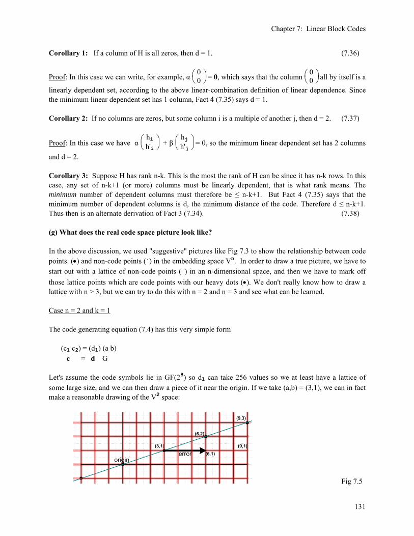
Chapter 7: Linear Block Codes
131
Corollary 1: If a column of H is all zeros, then d = 1. (7.36)
Proof: In this case we can write, for example, α ⎝⎛
⎠⎞ 0
0 = 0, which says that the column ⎝⎛
⎠⎞ 0
0 all by itself is a
linearly dependent set, according to the above linear-combination definition of linear dependence. Since the minimum linear dependent set has 1 column, Fact 4 (7.35) says d = 1. Corollary 2: If no columns are zeros, but some column i is a multiple of another j, then d = 2. (7.37)
Proof: In this case we have α ⎝⎛
⎠⎞ hi
h'i + β ⎝⎛
⎠⎞ hj
h'j = 0, so the minimum linear dependent set has 2 columns
and d = 2. Corollary 3: Suppose H has rank n-k. This is the most the rank of H can be since it has n-k rows. In this case, any set of n-k+1 (or more) columns must be linearly dependent, that is what rank means. The minimum number of dependent columns must therefore be ≤ n-k+1. But Fact 4 (7.35) says that the minimum number of dependent columns is d, the minimum distance of the code. Therefore d ≤ n-k+1. Thus then is an alternate derivation of Fact 3 (7.34). (7.38) (g) What does the real code space picture look like? In the above discussion, we used "suggestive" pictures like Fig 7.3 to show the relationship between code points (•) and non-code points (.) in the embedding space Vn. In order to draw a true picture, we have to start out with a lattice of non-code points (.) in an n-dimensional space, and then we have to mark off those lattice points which are code points with our heavy dots (•). We don't really know how to draw a lattice with n > 3, but we can try to do this with n = 2 and n = 3 and see what can be learned. Case n = 2 and k = 1 The code generating equation (7.4) has this very simple form (c1 c2) = (d1) (a b) c = d G Let's assume the code symbols lie in GF(28) so d1 can take 256 values so we at least have a lattice of some large size, and we can then draw a piece of it near the origin. If we take (a,b) = (3,1), we can in fact make a reasonable drawing of the V2 space:
Fig 7.5

Chapter 7: Linear Block Codes
132
The thin black lines are the lattice and their intersections are the lattice points, mostly illegal code words (.). The legal code words lie on the green line at the large dots (•). The pink bands show the effect of single-symbol errors. For example, suppose the legal code word (3,1) was received as the illegal code word (6,1) due to a single-symbol error in the first symbol of the code word (c1 c2). Since we don't know which symbol is wrong, c1 or c2 (all we know is that cHT = s ≠ 0 ), this received code word could have started life as either (3,1) or (6,2). Both of these legal code words differ from the bad code word (6,1) by a single-symbol error. We then don't know whether to correct this code word to (3,1) or to (6,2). These two code words are separated by distance d = 2, and from (7.32) this means t = 0 and this code cannot correct all single-symbol errors. If the error vector above happened to be one box shorter in length, then the code could conclude that (3,1) was the proper corrected code word. If a code has some t > 0, that code must be able to correct all t-symbol errors. So to get anything reasonable in terms of error correction capability, we have to turn to n > 2. So next we try n = 3. Case n = 3 and k = 1 The code generating equation (7.4) now has this form, (c1 c2 c3) = (d1) (a b c) . c = d G The reader must now imagine a 3D lattice in which the valid code words lie on a skewed green line similar to that shown above. Perhaps we select (a,b,c) = (1,2,3). It is painful to attempt a full rendering of the V3 space as done above, but we can draw a very small piece of this space which shows only two code words (1,2,3) and (2,4,6) lying on the skewed green line. These (•) code words lie on opposite corners of the lattice box shown. Not all lattice lines are drawn.
Fig 7.6 Suppose there is an error in the first symbol of the code word (1,2,3) so it is received as (2,2,3). This then is a single-symbol error. If we could correct it, what would we correct it to? The point (2,2,3) lies on the intersection of three single-symbol-error pink bands. Because our Vn space has more dimension now than it did in the previous example, we have a new situation. If we probe along the vertical pink band through (2,2,3) we find that it hits no code points. The same is true if we probe along the front-to-back pink band. Only the horizontal pink band through (2,2,3) goes through a code word, namely, (1,2,3). So in this example, if we receive the bad code word (2,2,3), and if we assume there has been only a 1-symbol error,

Chapter 7: Linear Block Codes
133
then we know we should correct (2,2,3) to be (1,2,3). In this example we have d = 3 since any two code words differ in all three symbols. Then from (7.32) we have t = Int[(d-1)/2] = Int[2/2] = 1 which agrees with our conclusion just developed. In this example we require a 3-symbol error to get from one legal code word to another. If we pile up several copies of the above box following generally along the green line, we get,
Fig 7.7 where on the right the Vn grid segments have been deleted. The picture on the right at least bears a dim topological resemblance to our symbolic Figures 7.3 and 7.4. The notion of the three numbered arrows in Fig 7.4 (each a single symbol error) to get from one code word to another is also born out in the above drawing. One difference between Fig 7.4 and Fig 7.7 is that the code points (•) are collinear in the latter figure, but in the general case discussed next, the code points will lie on a hyperplane of dimension more than 1, and the code points will then no longer be collinear, and Fig 7.4 becomes more "accurate". General n and k Now we have to first imagine an n-dimensional lattice of (.) points for Vn. In this lattice we then imagine a skewed hyperplane of dimension k (this is Ck) which intersects some of the lattice points which we then mark as (•). Through each such valid code point (•) we then drawn n pink bands parallel to the Vn axes, showing the effect of single-symbol errors. Assume for our selected code that t ≥ 2. This code, of the form (7.4), determines the orientation of that hyperplane in Vn. We will find that, if we start at some bad code word lattice point, and if we trace all double paths first onto one pink band and then from that onto any second pink band, only one such double path will lead to a code word point (•), and that is the code word we want to correct to. In order to get to any other (•) from our bad (.), we will have to travel on at least three different pink bands. These facts are a challenge to illustrate in a drawing. Hopefully this discussion explains why we grudgingly accept schematic representations of the Vn embedding space such as Figure 7.3 and 7.4. The theory of block codes must really be done algebraically without the assistance of precise graphical aids.

Chapter 7: Linear Block Codes
134
(h) Encoders and Decoders: The Syndrome An "encoder" is a piece of hardware or software which in effect applies the matrix G to data words to generate codes words, c = dG as in (7.3). It normally does this in the systematic basis, so G has the form (7.25). The data symbols are passed through and n-k parity check symbols are added, as in (7.26). A "decoder" is a piece of hardware or software which receives the code words, and tries to determine if there have been errors, and may try to correct some errors. When a bad code word is received, that is to say, some c' ≠ c because an error occurred in transmission, the so-called syndrome s is the result of the application of HT to c'. Recall from (7.21) that cHT = 0 for good code words. Thus, the syndrome is defined as s ≡ c' HT . (7.39) One can express the bad code word as a good code word plus an error code word, so c' = c + e . Then s = c' HT = (c + e) HT = e HT . (7.40) Since HT has n-k columns, the syndrome row vector s has n-k components (s = 0 example in (7.22)). A non-vanishing syndrome vector detects an error; good code words always have zero syndrome. An error correcting decoder attempts to look up the most likely e for a given s, and then corrects the error by subtracting the error back out of c' to recover the good code word, c = c' - e where s = e HT (7.41) Exactly how this is done for various specific codes is the subject of error correction texts such as Peterson and Weldon or Rhee. If it happens that the damage to c is enough to knock c' into another good code word, then e ≡ c' - c ≠ 0 but s = 0 and the error goes undetected. (i) Important codes, code history, and other kinds of codes Linear block codes are characterized by their values of n and k, by their d (which is really their ability to correct t-symbol random errors), and by the complexity/expense of the required encoders and decoders. Another factor is the ability to correct burst errors. All these things are measures of the performance of a code. Some of the names of famous block codes are Hamming, Golay, Hadamard, Reed-Muller, Fire, BCH, and Reed-Solomon. There are many more. The study of error-correcting codes is a relatively recent development on the time scale of the supporting math. Although Galois died in 1832, Shannon's famous paper was published in 1948. Golay codes arrived in 1949, then the Hamming codes were discovered in 1950. Fire codes came in 1959, especially formulated to correct long burst errors. In 1960 came the large class of BCH codes (discussed below) that could correct multiple random symbol errors. The Reed-Solomon codes also appeared in 1960. These are BCH codes applied to code symbols in GF(2m) and are thus finding much current use since digital

Chapter 7: Linear Block Codes
135
hardware uses "buses" m bits wide. They have good burst-error-correcting capabilities and are used, for example, in CD recorders and players. Convolution codes are in a completely different class from block codes, and were developed in the 1960's. You produce n code symbols based on k data symbols, but also based on some number m of previous data symbols, so there is no clearly defined "block" that is the basic encoded unit. These systems use encoders which look somewhat like polynomial multipliers in that they store some number of previous data symbols in flip-flops and have lots of feed-forward adders. There is a definite state-machine flavor here, due to the memory of previous symbols. Convolution codes are more complex to analyze than linear block codes, but implementation can be very efficient. Topological methods such as tree or trellis diagrams are used to understand them. One popular decoding method is the Viterbi algorithm associated with Markov chains that appeared in 1967. In contrast, the block codes and especially the cyclic block codes have a strong "algebraic" flavor. For example, they might involve the algebra of Galois Field elements. According to Rhee, the 1970's were spent mostly finding codes of longer length and better performance, while the 1980's concentrated on practical applications. Block and convolution codes were combined in various ways, always seeking better performance. In 1993 turbo codes were discovered which allow very close approach to the Shannon channel-capacity limit in information theory. These codes have somewhat supplanted the older codes in both research and application.

Chapter 8: Cyclic Codes
136
Chapter 8: Cyclic Codes In this section, component numbering of data and code words begins with 0 instead of 1. Cyclic codes are a subset of the linear block codes. The name arises from the fact that, in a cyclic code, any cyclic permutation of a code word is also a code word. For example, with n = 3, if c = (c0 c1 c2) is a code word, then c(1) ≡ (c2 c0 c1) and c(2) ≡ (c1 c2 c0) are also code words. We shall define a cyclic code in (8.1) below. This definition makes no mention of anything being cyclic, but later in section (f) we shall prove that a code defined by (8.1) is in fact a cyclic code. Example : Suppose k = 2 and n = 3 and q = pm = 21 = 2. The embedding space of the code words V3 must contain 2n = 23 = 8 vectors, but only 2k = 22 = 4 of these vectors are code words. We can arrange the 3-tuples of V3 into rows where the elements of each row are cyclically related: (0 0 0) (0 0 0) (0 0 0) 1 (1 0 0) (0 1 0) (0 0 1) 3 (1 1 0) (0 1 1) (1 0 1) 3 (1 1 1) (1 1 1) (1 1 1) 1 Here you see the 8 distinct elements of V3. We know that a (3,2) code only has 2k = 22 = 4 code words, and we know that (0 0 0 ) must be the code word corresponding to d = (0 0 ). Thus, if this is a cyclic code, the code must consist of (0 0 0) and just one of the middle two rows. (a) Definition of a Cyclic Code: The Cyclic Basis A cyclic code is constructed (and therefore defined) by the sequence of instructions given below. All polynomials referred to have coefficients in some field GF(q=pm). The three key polynomials are these : g(x) = Σi=0n-kgixi degree = n-k #coefficients = n-k+1 "generator" d(x) = Σi=0k-1dixi degree ≤ k-1 #coefficients = k "data word" c(x) = Σi=0n-1cixi degree ≤ n-1 #coefficients = n "code word" The code word c = (c0,c1...cn-1) is embedded into the code word polynomial c(x), and similarly d is embedded into d(x). Since there is a 1-to-1 relation between the vectors and the polynomials, we sometimes loosely refer to c(x) as a "code word" and d(x) as a "data word"

Chapter 8: Cyclic Codes
137
Definition of a Cyclic Code (n,k) (8.1)
(a) Select an integer value for n, the desired length of the code words. (b) Find a pair of polynomials g(x) and h(x) such that g(x)h(x) = xn - 1 where the degree of h(x) is k and the degree of g(x) is n-k. The polynomial g(x) is the generator of the (n,k) cyclic code, and h(x) is the generator of the dual code (n,n-k). (c) Let a set of k data symbols (in GF(q)) be the coefficients of a polynomial d(x) of degree ≤ k-1. (d) The code words are then the n coefficients of polynomials c(x) where c(x) = d(x) g(x) . Since d(x) has degree ≤ k-1, and g(x) has degree n-k, c(x) is of degree ≤ n-1, which means it has n coefficients or symbols in GF(q). In fact, [n-k ≤ degree of c(x) ≤ n] since d(x) has degree n-k.
Comment: One might wonder just how one goes about finding polynomials g(x) which divide xn-1 and whether in fact there are any such polynomials for a given n, and if so, what degrees these polynomials have. One way to find viable g(x) is to do a blind search of all possible g(x) of degree < n. This method is illustrated in Appendix E. The main effort of Appendix E, however, is to demonstrate that for any integer n > 1, there does exist at least one g(x) that divides xn-1 and this g(x) happens to be irreducible over GF(p). It turns out that this g(x) is a minimum polynomial of GF(pm) where m = φ(n), Euler's totient function mentioned back in Chap 5 (d) (and also in Appendix G). Fact 0: When one carries out the polynomial multiplication c(x) = d(x) g(x), the coefficients cs of c(x) can be expressed in terms of those of d(x) and g(x) according to,
cs = ∑j = max(0,s-k+1)
min(s, n-k) ds-j gj for s = 0,1...n-1 c(x) = Σs=0n-1cs xs (8.2)
where we have used the result of Appendix C with A = k-1 and B = n-k and A+B = n-1. We will show in the next section how it is possible to simplify the messy convolution of (8.2) by replacing the polynomials c(x) and d(x) with certain C(x) and D(x), a transformation known as going to the systematic basis in the cyclic world. We have already seen the systematic basis at work in the matrix world as in (7.25) and (7.26),
c = dG G = [P | Ik ] (c0 c1 c2 c3 c4) = (d0 d1 d2) ⎝⎜⎛
⎠⎟⎞ a d 1 0 0
b e 0 1 0 c f 0 0 1
= (pc0 pc1 d0 d1 d2)

Chapter 8: Cyclic Codes
138
In this form, or basis, the n-symbol code words ci have their left n-k symbols being parity check symbols pci, and their right k symbols being the data symbols. Recall from Chapter 7 (b) 6 that the symbols are transmitted from right to left, so in the above example d2 is sent first. In the cyclic basis with c(x) = d(x)g(x) these symbols are convoluted together in the n-bit code words according to (8.2). We shall soon show how the systematic and cyclic bases are related. For the moment, imagine working in the cyclic basis. It is not hard (section (j) below) to build a piece of hardware that computes c(x) = d(x)g(x). The circuit is a polynomial multiplier. The code word c(x) is then transmitted over a channel. The receiver, to nobody's great surprise, tries to recover d(x) by dividing c(x) by g(x): d(x) = c(x)/g(x). The hardware for doing this is called a polynomial divider. Example: In a Reed-Solomon code, the code symbols are carried on parallel groups of bits, so the R-S polynomial multipliers and dividers have data paths that are multiple bits wide. They look very much like digital filters, with one significant difference which we will describe in Chapter 9 (e) below. (b) The Systematic Basis versus the Cyclic Basis In practice, one tends to use hardware (or software) which works in the systematic basis rather than the cyclic basis. The reason is that error detection and correction are much easier in the systematic basis, since one knows where the data and parity check symbols are in the code words. We are soon going to show that the two bases have a 1-to-1 relationship. This means that the set of polynomials { c(x) } is simply a rearrangement of a set of polynomials { C(x) }. The theory of cyclic codes (including a heavy dose of Galois Field theory) uses the cyclic basis, whereas the practice of cyclic codes uses the systematic basis. According to our polynomial Division Algorithm (3.6), we can write the following expansion, xn-k d(x) = D(x)g(x) - γ(x) . (8.3) In other words, we multiply d(x) [ which carries our k data symbols as coefficients ] by a power, and then divide this product by the generator polynomial g(x) which, recall, has degree n-k. Then D(x) is the quotient polynomial, and - γ(x) is the remainder. Whatever γ(x) is, it is of degree less than n-k and thus has n-k coefficients. Since the LHS has degree ≤ (n-k) + (k-1) = (n-1), and since g(x) has degree (n-k), D(x) must have degree ≤ (k-1), the same as d(x). Suppose we now define our code word to be C(x) = D(x)g(x) (8.4) = γ(x) + xn-k d(x) . (8.5)
Chapter 8: Cyclic Codes
139
If you write out the coefficients of C(x) (from low to high power), you find from (8.5) that the first n-k of them are the coefficients of γ(x), and the last k of them are the data bits of d(x). For example, if n=5 and k=3, C(x) = (γ0+γ1x) + x2(d0+d1x+d2x2) = γ0+γ1x+d0x2+d1x3+d2x4 → (γ0, γ1, d0, d1, d2) . (8.6) Therefore, the coefficients of γ(x) are precisely the n-k parity check symbols which one combines with the k data symbols to get an n-symbol code word. Thus, we are now in the systematic basis. In the cyclic basis, we had code words c(x) = d(x)g(x), whereas in the systematic basis, we have C(x) = D(x)g(x). Comparing the (γ0, γ1, d0, d1, d2) of (8.6) to the (pc0 pc1 d0 d1 d2) of our example below (8.2), it seems clear that one could come up with a G matrix of the form G = [P | Ik ] which would give the same result as C(x) = D(x)g(x), so there is an alignment between the "systematic basis" c = dG of the matrix world and the "systematic basis" C(x) = D(x)g(x) of the polynomial world. The systematic basis plan will be to multiply polynomials in our transmitting encoder C(x) = D(x)g(x), and to divide polynomials in our receiving decoder D(x) = C(x)/g(x). We have already noted that the coefficients of a polynomial are transmitted most significant symbol first. We certainly know from our pre-calculator experience with long division (see (3.7)) that we start with the most significant digit of a dividend, here C(x). A hardware polynomial divider is no different. Thus, in terms of time ordering, when we think of C(x) as described above, the most significant symbols are the data symbols that come first in time, then the least significant symbols are the parity check symbols which come last in a data stream of coefficients which represents C(x). Also, within each group (data symbols, parity check symbols), the time ordering is most significant first.. In either cyclic or systematic basis, the code word is the product of some sort of data polynomial of degree ≤ k-1 with the generator polynomial of degree n-k to give a code word polynomial of degree ≤ n-1. The construction which led to C(x) = D(x)g(x) is what one needs do to untangle the convolution (8.2) inherent in the cyclic basis method c(x) = d(x)g(x). (c) Implementation of Encoders and Decoders If C(x) is sent through a channel, how do we recover d(x) at the receiving end? We just grab the first (in time) k symbols of C(x) and these make up d(x), according to (8.5) and (8.6). How do we know if there was an error? We set up a polynomial divider to compute C(x)/g(x). The quotient is D(x), and looking at (8.4) the remainder is supposed to be zero! [ Remember that remainder γ(x) comes from a different division, xn-kd(x) by g(x).] That is, true code words C(x) are multiples of g(x), so there should be no remainder. If there is a non-zero remainder, then there has been an error. This remainder is a form of the syndrome referred to earlier. Thus, at the receiver we have: C'(x) = D'(x) g(x) + s(x) s(x) = Rem[C'(x)/g(x)] (8.7) where now s(x) is a syndrome polynomial. Here we indicate by C'(x) a received code word polynomial that has an error. D'(x) and s(x) are the quotient and remainder of C'(x)/g(x). If there was no transmission error, then D'(x) = D(x), C'(x) = C(x) and s(x) = 0. If s(x) ≠ 0, then we have detected an error.
Chapter 8: Cyclic Codes
140
If s(x) ≠ 0, then the coefficients of s(x) can be used to correct the error, provided that the size of the error was less than t symbols and the selected code can correct t-symbol errors. A large fraction of any book on error-correcting codes deals with the details of how this is done for various codes, and this is where implementations can become quite complex. Obviously, it is the fact that there are extra parity check symbols in the code which allows an error to be detected and possibly corrected. Let us take one more look at the encoding and decoding equations for a cyclic code in the systematic basis: encode C(x) = D(x) g(x) = γ(x) + xn-k d(x) (8.8a) decode C'(x) = D'(x) g(x) + s(x) s(x) = Rem[C'(x)/g(x)] (8.8b) error polynomial: E(x) ≡ C'(x) - C(x) (8.8c) In this notation, E(x) ≠ 0 means there was an error, while s(x) ≠ 0 means the error was detected. In the case that C'(x) is another legal code word, we will have E(x) ≠ 0 and s(x) = 0 so the error won't be detected. The dcoder only knows s(x), it doesn't know E(x). We wish to stress the extreme simplicity of implementing these functions in hardware, apart from the error correction. The encoder is a two-stage process. In the first stage, we just bypass through the k data symbols into "the channel" (most significant first), since these are the higher coefficients of C(x) as in (8.6). At the same time, we run these same symbols into a polynomial divider set up do compute [ xn-k d(x) ] / g(x). The factor xn-k is a trivial complication in the implementation of such a divider (it turns out). We then throw out the quotient D(x); it goes into a bit bucket. When the division is done, the flip-flops of the divider contain the remainder -γ(x) as shown in (8.8a). From this γ(x) is obtained and the coefficients of γ(x) are then shifted out into the channel and we are done. C(x) is built and sent. A non-correcting decoder is also a two-stage process. The first k symbols of C'(k) are the data symbols we want. They are received and parked in local memory within the decoder. At the same time, all n symbols of C'(x) are run through a polynomial divider which computes C'(x)/g(x). The quotient is again thrown out, and the remainder is the syndrome s(x), again as shown in (8.8b). If s(x) ≠ 0, an error has been detected. Error correction logic can then attempt to correct the data word that has been temporarily parked in memory before it is sent out from the decoder to the rest of the receiving system. Drawings of hardware polynomial mulitipliers and dividers are shown in Fig 8.2 and Fig 8.3 below. In a practical transmission system, data transmitted may be interleaved just before transmission and then deinterleaved by the receiver, in order to disperse the effect of a possible burst error in the channel. The same system is used on an audio CD to spread out the effect of a surface scratch. The encoder might also encrypt the data being sent, requiring decryption at the receiving end.
Chapter 8: Cyclic Codes
141
(d) Cyclic Redundancy Check (CRC) If we ignore error correction, the circuit described above is exactly how a CRC system works. There is some generator polynomial g(x). The parity check symbols are computed as shown above and are tacked onto the end of the data stream to form C(x). At the receiver, the data symbols are siphoned off as needed. The entire incoming packet (coefficients of C'(x)) is run through a divider and the syndrome remainder is computed. If it is not zero, there was a "CRC error". Of course the number of data symbols k can be somewhat larger than one usually thinks of in a "code". One might have a block of k = 100,000 data symbols followed by some parity check symbols. Although we associate CRC with a cyclic code, it is not required that g(x) divide xn- 1 for an (n,k) code used for CRC purposes. If g(x) does not divide xn- 1, the code words won't be cyclic, but we don't care. Thus, if one first selects a CRC checksum length n - k, which is also the degree of g(x), one can then set either n or k arbitrarily. It is shown below, however, that in order to detect double-bit errors, g(x) must have a period ≥ n for the selected value of n. The probability of detecting an error increases with the degree of g(x) which is the number of parity check symbols n-k. Typical numbers used are n-k = 8, 16 or 32. In Appendix F we derive some classic "facts" about CRC error detection. Here we just quote those facts. The requirement g(0) ≠ 0 just means g(x) is not of the form xi f(x) and g(x) ≠ a constant. The first two Facts are not particularly impressive since they can be achieved for GF(2) by adding a single parity check bit to the end of a data stream. Fact 1: If g(0) ≠ 0, a cyclic code generated by g(x) over GF(p) detects all single-symbol errors. (F.1) Fact 2: If g(x) = (x-1)f(x), a cyclic code generated by g(x) over GF(2) detects all odd-number-bit errors. (F.2) Fact 3: If g(0) ≠ 0 and g(x) has period ≥ n, a cyclic code generated by g(x) over GF(2) detects all double-bit errors and all single-bit errors. (F.3) Fact 4: If g(0) ≠ 0 and g(x) = (x-1)f(x) and g(x) has period ≥ n, a cyclic code generated by g(x) over GF(2) detects all single-bit, double-bit, triple-bit and all other odd-number-bit errors. (F.4) Definition: A burst error of length r refers to an arbitrary amount of damage done to the symbols of a transmitted code word provided this damage is limited to some extent of width r. For example, if symbol c4 is the first damaged symbol and c9 is the last damaged symbol, the following illustrates a burst error of length r = 6. Any or all of the symbols c5 through c8 might also be in error. c' = (c0, c1, c2, c3, c4, c5, c6, c7, c8, c9, c10, c11,c12,c13,c14 ........) The following two facts state quite impressive capabilities of CRC error detection: Fact 5: If g(0) ≠ 0, a cyclic code generated by g(x) over GF(p) detects all burst errors of length n-k or smaller. (F.5)
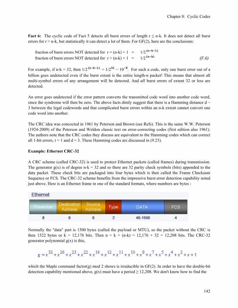
Chapter 8: Cyclic Codes
142
Fact 6: The cyclic code of Fact 5 detects all burst errors of length r ≤ n-k. It does not detect all burst errors for r > n-k, but statistically it can detect a lot of them. For GF(2), here are the conclusions: fraction of burst errors NOT detected for r = (n-k) + 1 = 1/2(n-k-1)
fraction of burst errors NOT detected for r > (n-k) + 1 = 1/2(n-k) (F.6) For example, if n-k = 32, then 1/2(n-k-1) = 1/231 ~ 10-9. For such a code, only one burst error out of a billion goes undetected even if the burst extent is the entire length-n packet! This means that almost all multi-symbol errors of any arrangement will be detected. And all burst errors of extent 32 or less are detected. An error goes undetected if the error pattern converts the transmitted code word into another code word, since the syndrome will then be zero. The above facts dimly suggest that there is a Hamming distance d ~ 3 between the legal codewords and that complicated burst errors within an n-k extent cannot convert one code word into another. The CRC idea was concocted in 1961 by Peterson and Brown (see Refs). This is the same W.W. Peterson (1924-2009) of the Peterson and Weldon classic text on error-correcting codes (first edition also 1961). The authors note that the CRC codes they discuss are equivalent to the Hamming codes which can correct all 1-bit errors, t = 1 and d = 3. These Hamming codes are discussed in (9.23). Example: Ethernet CRC-32 A CRC scheme (called CRC-32) is used to protect Ethernet packets (called frames) during transmission. The generator g(x) is of degree n-k = 32 and so there are 32 parity check symbols (bits) appended to the data packet. These check bits are packaged into four bytes which is then called the Frame Checksum Sequence or FCS. The CRC-32 scheme benefits from the impressive burst error detection capability noted just above. Here is an Ethernet frame in one of the standard formats, where numbers are bytes :
Normally the "data" part is 1500 bytes (called the payload or MTU), so the packet without the CRC is then 1522 bytes or k = 12,176 bits. Then n = k + (n-k) = 12,176 + 32 = 12,208 bits. The CRC-32 generator polynomial g(x) is this,
which the Maple command factor(g) mod 2 shows is irreducible in GF(2). In order to have the double-bit detection capability mentioned above, g(x) must have a period ≥ 12,208. We don't know how to find the
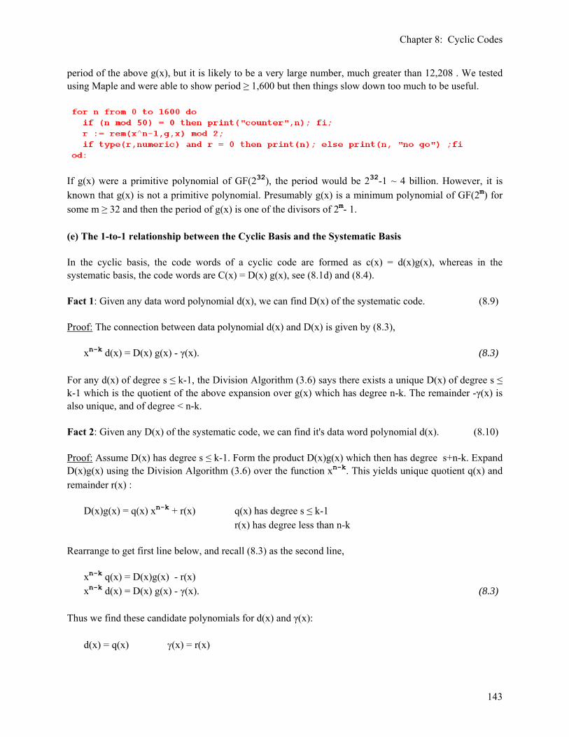
Chapter 8: Cyclic Codes
143
period of the above g(x), but it is likely to be a very large number, much greater than 12,208 . We tested using Maple and were able to show period ≥ 1,600 but then things slow down too much to be useful.
If g(x) were a primitive polynomial of GF(232), the period would be 232-1 ~ 4 billion. However, it is known that g(x) is not a primitive polynomial. Presumably g(x) is a minimum polynomial of GF(2m) for some m ≥ 32 and then the period of g(x) is one of the divisors of 2m- 1. (e) The 1-to-1 relationship between the Cyclic Basis and the Systematic Basis In the cyclic basis, the code words of a cyclic code are formed as c(x) = d(x)g(x), whereas in the systematic basis, the code words are C(x) = D(x) g(x), see (8.1d) and (8.4). Fact 1: Given any data word polynomial d(x), we can find D(x) of the systematic code. (8.9) Proof: The connection between data polynomial d(x) and D(x) is given by (8.3), xn-k d(x) = D(x) g(x) - γ(x). (8.3) For any d(x) of degree s ≤ k-1, the Division Algorithm (3.6) says there exists a unique D(x) of degree s ≤ k-1 which is the quotient of the above expansion over g(x) which has degree n-k. The remainder -γ(x) is also unique, and of degree < n-k. Fact 2: Given any D(x) of the systematic code, we can find it's data word polynomial d(x). (8.10) Proof: Assume D(x) has degree s ≤ k-1. Form the product D(x)g(x) which then has degree s+n-k. Expand D(x)g(x) using the Division Algorithm (3.6) over the function xn-k. This yields unique quotient q(x) and remainder r(x) : D(x)g(x) = q(x) xn-k + r(x) q(x) has degree s ≤ k-1 r(x) has degree less than n-k Rearrange to get first line below, and recall (8.3) as the second line, xn-k q(x) = D(x)g(x) - r(x) xn-k d(x) = D(x) g(x) - γ(x). (8.3) Thus we find these candidate polynomials for d(x) and γ(x): d(x) = q(x) γ(x) = r(x)
Chapter 8: Cyclic Codes
144
Fact 3: The mapping between d(x) and D(x) is one-to-one. Thus, one can regard either set of polynomials as a rearrangement of the other set of polynomials. (8.11) Proof: Suppose different d1(x) and d2(x) both map into the same D(x). Then xn-k d1(x) = D(x) g(x) + γ1(x) xn-k d2(x) = D(x) g(x) + γ2(x) Subtract to get: xn-k [ d1(x) - d2(x) ] = γ1(x) - γ2(x) . The LHS is a polynomial of degree ≥ n-k. The RHS is a polynomial of degree < n-k. This is a contradiction, so one cannot have two different d's which map into the same D. Similarly, suppose different D1(x) and D2(x) map into the same d(x). Then write xn-k d(x) = D1(x) g(x) + γ1(x) xn-k d(x) = D2(x) g(x) + γ2(x) Subtract to get: [ D2(x) - D1(x) ] g(x) = γ1(x) - γ2(x) We make the same argument as above: The LHS is a polynomial of degree ≥ n-k. The RHS is a polynomial of degree < n-k. This is a contradiction, so one cannot have two different D's which map into the same d. Thus, the mapping between the d(x) and D(x) is a 1-to-1 mapping. Fact 4: The mapping between c(x) and C(x) is one-to-one. Thus, one can regard either set of polynomials as a rearrangement of the other set of polynomials. (8.12) Proof: According to Fact 3 (8.11), the mapping between the d(x) and the D(x) is one-to-one. Then, since c(x) = g(x)d(x) C(x) = g(x)D(x) we can make a corresponding one-to-one mapping between the c(x) and the C(x). Corollary: The set of code words of a code in the cyclic basis is a rearrangement of the set of code words of the same code in the systematic basis. (8.13) Comment: The Corollary is true whether or not the generator g(x) divides xn - 1. Nowhere in this section have we made use of this fact. However, this fact is the basis of the next sections.

Chapter 8: Cyclic Codes
145
(f) Why Cyclic Codes are Cyclic In the above discussion of cyclic codes, it was noted that the name arises because all cyclic permutations of code words are also code words. Here we will prove this is so. If we take the coefficients of a polynomial f(x) and "rotate them m places to the right" to form a new polynomial, this new polynomial is called a cyclic permutation of the original polynomial by m places, and is denoted by f(m) (x). Example: (a rotation of one place)
(8.14) Math Lemma 1: Claim that: f(1)(x) = Rem[(x f(x))/(xn - 1)]. (8.15) Proof: Let f(x) = f0 + f1x + f2x2 + ... fn-1xn-1 . Then xf(x) = f0x + f1x2 + f2x3 + ... fn-1xn
= [ fn-1 + f0x + f1x2 + ... fn-2xn-1 ] + fn-1(xn - 1) = [ f(1)(x) ] + fn-1(xn - 1). If we were to expand xf(x) over (xn-1) using the Division Algorithm (3.6), we would recognize the coefficient fn-1 as the quotient polynomial, and [ f(1)(x) ] as the remainder polynomial. QED
Math Lemma 2: Claim that: f(m)(x) = Rem[(xm f(x))/(xn - 1)] or (8.16) xm f(x) = q(x) (xn - 1) + f(m)(x) for some quotient polynomial q(x) Proof: Math Lemma 1 shows this is true for m=1. Then do an induction proof. Assume true for m=k and show that true for m = k+1. For m=k we have the equivalent equations, f(k)(x) = Rem[(xk f(x))/(xn - 1)] (*) xk f(x) = q(x) (xn - 1) + f(k)(x) . (**) Lemma 1 with f = f(k)(x) says that [f(k)(x)](1) = Rem[(x f(k)(x))/(xn - 1)] . But f(k) shifted one to the right is f(k+1). Then insert f(k) from (**) on the right to get

Chapter 8: Cyclic Codes
146
f(k+1)(x) = Rem[(x { xk f(x) – q(x) (xn - 1)})/(xn - 1)] = Rem[(x { xk f(x) })/(xn - 1)] = Rem[(xk+1 f(x))/(xn - 1)] which is (*) for m = k+1. QED Fact 5: For a cyclic code, all cyclic permutations of any code word are also code words. Thus, the k-dimensional vector space Ck spanned by the code words is a cyclic subspace of Vn. (8.17) Proof: We do this proof in the cyclic basis. It then also applies to the systematic basis, since we have just shown above in Corollary (8.13) that the set of code words is the same in either basis (they are just rearranged). Apply Math Lemma 2 (8.16) to f(x) = c(x), a polynomial of degree s ≤ n-1 corresponding to a legal codeword, xm c(x) = q(x) (xn - 1) + c(m)(x) . Make the replacement c(x) = d(x)g(x) to get c(m)(x) = xm d(x)g(x) - q(x)(xn - 1) . Now make the further replacement (xn - 1) = h(x)g(x) from (8.1) (b), c(m)(x) = [ xm d(x) - q(x)h(x) ] g(x) . Since g(x) has degree n-k, and since c(m)(x) has degree s ≤ n-1, the item in brackets [ ] must have degree s-(n-k). But since s ≤ n-1 we have s-(n-k) ≤ (n-1) - (n-k) = k-1 . Thus, the degree of [ xm d(x) - q(x)h(x) ] is ≤ k-1, so this is just some data polynomial we will call dm(x), dm(x) = [ xm d(x) - q(x)h(x) ] . Thus, c(m)(x) = dm(x) g(x). So, the rotated (cyclically permuted) code word c(m)(x) results from encoding the data word dm(x), so c(m)(x) must therefore be a code word. QED

Chapter 8: Cyclic Codes
147
(g) A Cyclic Code as an Ideal of the Ring An = Rq / ( xn - 1 ) In the Observation at the end of Chapter 3 (a) we discussed the commutative ring R of polynomials having coefficients in some arbitrary ring-with-identity R having operations ⊕ and ⊗. The sums and products of polynomials in such a ring R are indicated by operations + and •. Here we consider the case where R = GF(q), and we shall call the corresponding polynomial ring Rq. Consider then the residue class ring, An ≡ Rq / ( xn - 1 ) . (8.18) Here ( xn - 1 ) refers to an ideal consisting of all polynomials which are multiplies of xn-1. We studied this type of R/I structure in detail in Chapter 3 (d). The elements of An are the rows of a chart, and each row can be labeled as {r(x)} where r(x) is a polynomial of degree < n obtained by dividing some polynomial in Rq by xn - 1. Thus, we can think of the elements of An (rows of the chart) as corresponding to the remainder polynomials of degree < n, and we know there are qn such polynomials in Rq. Because xn- 1 is reducible, this residue class ring is not a field, it is just a ring. We have in mind that n is the same n that appears in the (n,k) code designation. A remainder r(x) could for example be a data polynomial d(x), or a code word polynomial c(x), or our cyclic code generator g(x). If we consider the chart row labeled by d(x) and the row labeled by g(x), the ring element product of these two rows must contain d(x) • g(x) [= d(x)g(x)]. In other words, we must have { d(x) • g(x) } = { d(x) } • { g(x) } where the curly bracket notation {...} was discussed in (3.14). But d(x)• g(x) = c(x) so this says { c(x) } = { d(x) } • { g(x) } . (8.19) If we draw a picture of the chart for An similar to (3.13), we get i1(x)=0 i2(x) = q(x)•(xn-1) for all possible q(x) r1(x) r1(x) + i2(x) = q(x)•(xn-1) + r1(x), for all possible q(x) r2(x) r2(x) + i2(x) = q(x)•(xn-1) + r2(x), for all possible q(x) more rows like the above (8.20) We might imagine enumerating the qn remainders ri(x) by increasing degree in some manner, so that the first row in the chart has the remainder ri(x) = 0 which corresponds to the ideal ( xn-1 ). Then the second chart row might have remainder x, and so on. Since c(x) = d(x)g(x), code word polynomials have degree in the range (n-k,n-1), where n-k occurs for d(x) = constant and n-1 for d(x) of maximal degree k-1. Thus, the code word polynomials are dispersed throughout the lower region of the chart, that region where remainders have degree n-k up to n-1. They are dispersed amidst many other chart rows which also correspond to remainders in this range (all corresponding to "illegal" code words). The point is that in the An chart sorted in this manner, the rows corresponding to code polynomials c(x) are not adjacent to each

Chapter 8: Cyclic Codes
148
other but are widely dispersed. Of course there is always the exceptional code word c(x) = 0 which goes in the first row of the chart.
Fig 7.8 Recall the embedding vector space Vn of (7.6) which has qn points and which contains the subspace Ck which contains the qk code words. Each row of the chart An, meaning each element of An , corresponds to one point in Vn. The actual vector in Vn is formed by taking the m-tuple of the coefficients of a polynomial in An. So we can regard Figure 7.8 as a picture of Vn in which the code vectors are dispersed in line with Fig 7.3 showing the (•) in a sea of (.). Fact 6: If g(x) divides xn - 1, the chart rows {c(x)} form an ideal ( g(x) ) within An. (8.21) In other words, the code word polynomials of a cyclic code comprise an ideal within the set of polynomials of degree < n. We shall denote this ideal as ( g(x) ), meaning rows { f(x) } of An where f(x) is any multiple of g(x). Proof: An ideal I of a ring R was defined in (1.22). First of all, the set {c(x)} is an additive subgroup of An, as required. The set contains the additive identity 0 from c(x) = 0 and the other required properties including closure under + : {c1(x)} + {c2(x)} = {c1(x) + c2(x)} = {c3(x)} . // closed under An + operation We then have to show that r•I = I. This means that {r(x)}•{i(x)} = {i'(x)} for any {r(x)} in An and any {i(x)} in the ideal ( g(x) ). Since our candidate ideal is I = {c(x)}, the set of code word polynomials, i(x) is some code word polynomial, call it c(x). We then have to show that {r(x)}•{c(x)} = {c'(x)} where c'(x) is some other code word polynomial, where r(x) is some arbitrary element of An. Setting c(x) = d(x)g(x), this is what we need to show
Chapter 8: Cyclic Codes
149
{r(x)}•{ d(x)g(x)} = {c'(x)} where c'(x) is a code word polynomial . Here is a proof pathway that looks promising, but does not succeed. Rewrite the above as {r(x)d(x)}•{g(x)} = {c'(x)} . If we knew that {r(x)d(x)} = {d1(x)} for some data d1(x) (degree < k), we could write the left side as {r(x)d(x)}•{g(x)} = {d1(x)}•{g(x)} = {d1(x)g(x)} = {c1(x)} where c1(x) ≡ d1(x)g(x) is a code word polynomial, and then our proof that {c(x)} is an ideal would be concluded with c' = c1. But we don't know that such a d1(x) exists with degree < k, so this approach does not work. Here is a viable proof. We know we can write {r(x)}•{d(x)g(x)} = {f(x)} where f(x) has degree < n and is the remainder of r(x)d(x)g(x) divided by xn-1. But this does not tell us that f(x) is a code word. Now we add the assumption that g(x)h(x) = (xn-1). Multiply both sides of the above equation by h(x) and rearrange {r(x)d(x)} • {g(x) h(x)} = {f(x) h(x)} or {r(x)d(x)} • {xn-1} = {f(x) h(x)} or {r(x)d(x)} • 0 = {f(x) h(x)} or {f(x) h(x)} = 0 . This says that
Rem [ f(x) h(x)
xn-1 ] = 0
or f(x)h(x) = q(x)(xn-1) . <n k <k n The degree of quotient q(x) must be < k in order to balance the powers on the two sides of this last equation. Therefore q(x) can be regarded as a data polynomial. Rewrite the above as f(x)h(x) = q(x)g(x)h(x) or f(x) = q(x)g(x).
Chapter 8: Cyclic Codes
150
Since q(x) is a data polynomial, f(x) must be a code polynomial. QED Fact 5 Revisited: If g(x) divides xn - 1, then any cyclic permutation of a code word of the cyclic code generated by g(x) is also a code word. (8.22) Proof: Here we are giving an "alternate proof" of Fact 5 (8.17). Actually, it is the same proof as above, only here it is expressed in the language of rings and ideals. A code word c(x) is a polynomial of degree < n. Thus, according to Math Lemma 2 (8.16), c(m)(x) = Rem[ (xm c(x))/ (xn - 1)] , where c(m)(x) is a cyclic permutation of c(x) by m places. Since c(x) is of degree < n, we know that { c(x) } ∈ An. If m < n, then { xm } ∈ An . Thus, we can rewrite the above equation as { c(m)(x) } = { xm } • { c(x) } . (has qn rows) Because {c(x)} is an element of the ideal ( g(x) ), and because { xm } ∈ An, it follows from the definition of an ideal that { c(m)(x) } is also in the ideal ( g(x) ). Thus, { c(m)(x) } must be some code word. QED So, we have an interesting new way to view a cyclic code: Fact 7 : A cyclic code with symbols in GF(q), and which is generated by some g(x) which divides xn -1, forms an ideal ( g(x) ) of the ring An = Rq / ( xn - 1 ). This ideal consists of the set of qk code words generated by multiplying the qk data polynomials d(x) by g(x), { c(x) } = { d(x) } • { g(x) }. The full An chart has qn rows since there are qn remainder polynomials of degree < n. (8.23) (h) The Standard Array and Cyclic Code Error Correction We now take the qn rows of the An chart shown in Fig 7.8 above and sort them into bins. To start off, we grab all qk code word polynomials and put them into one bin. We realize that this bin must be all the polynomials in An which have remainder 0 when divided by g(x), since c(x) = d(x)g(x). We just showed in Fact 6 (8.21) that this bin is an ideal of An. We shall regard this bin as the first row of a new chart for the residue class ring An/(g(x)) which is built on top of our previous residue class ring An = Rq/(xn - 1). The other, non-ideal bins correspond to non-zero remainders of the An remainders upon division by g(x). Since g(x) has qn-k remainders, there must then be qn-k of these bins. The number of bins times the population of each bin gives qn-k qk = qn, which is the total number of An rows. This is consistent with the fact that the order of An must be integrally divisible by the order of any ideal within An, see (1.27). This set of bins forms our new residue class ring of An with respect to ( g(x) ), and this set of bins has a special name: the standard array : Standard Array = An / ( g(x) ) = [ Rq / ( xn - 1 ) ] / ( g(x) ) , (8.24) which has this row structure,
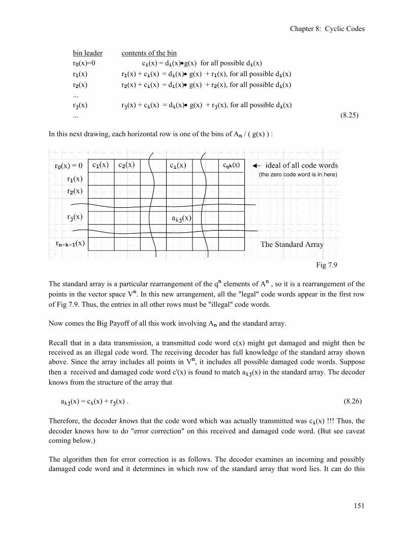
Chapter 8: Cyclic Codes
151
bin leader contents of the bin r0(x)=0 ci(x) = di(x)•g(x) for all possible di(x) r1(x) r1(x) + ci(x) = di(x)• g(x) + r1(x), for all possible di(x) r2(x) r2(x) + ci(x) = di(x)• g(x) + r2(x), for all possible di(x) ... rj(x) rj(x) + ci(x) = di(x)• g(x) + rj(x), for all possible di(x) ... (8.25) In this next drawing, each horizontal row is one of the bins of An / ( g(x) ) :
Fig 7.9 The standard array is a particular rearrangement of the qn elements of An , so it is a rearrangement of the points in the vector space Vn. In this new arrangement, all the "legal" code words appear in the first row of Fig 7.9. Thus, the entries in all other rows must be "illegal" code words. Now comes the Big Payoff of all this work involving An and the standard array. Recall that in a data transmission, a transmitted code word c(x) might get damaged and might then be received as an illegal code word. The receiving decoder has full knowledge of the standard array shown above. Since the array includes all points in Vn, it includes all possible damaged code words. Suppose then a received and damaged code word c'(x) is found to match aij(x) in the standard array. The decoder knows from the structure of the array that aij(x) = ci(x) + rj(x) . (8.26) Therefore, the decoder knows that the code word which was actually transmitted was ci(x) !!! Thus, the decoder knows how to do "error correction" on this received and damaged code word. (But see caveat coming below.) The algorithm then for error correction is as follows. The decoder examines an incoming and possibly damaged code word and it determines in which row of the standard array that word lies. It can do this
Chapter 8: Cyclic Codes
152
since it knows all about the standard array. It then obtains the rj(x) for that row and subtracts it from the word that came in, ci(x) = aij(x) – rj(x) (8.27) which, when written as Vn vectors (coefficient m-tuples), says ci = aij – rj. (8.28) We may compare this with our earlier equation, c = c' - e where s = e HT = c'HT (7.41) Thus, the correcting vector is - e = - rj . Notice that all bad code words in the row with aij have the same correcting vector -rj due to the fact that the standard array is a residue class ring. Thus, all bad code words in that row will generate the same syndrome sj = rjHT . As shown in the example (7.22), there are qn-k possible syndromes sj, and this corresponds to the number of remainders rj so there is a 1-to-1 relation between the rj and the sj. In its initialization sequence (or perhaps this is precomputed into a ROM memory), the decoder can build a lookup table as follows. For each possible rj it computes the corresponding syndrome sj = rj HT . The lookup table then provides r = F(s). Then in operation, when an incoming word c' arrives, the decoder computes s = c'HT, looks up the proper r in this little table, and does the addition c = c' - r. That's it! If the incoming word had no error, the syndrome will be s = 0, and the lookup table puts out r = 0, and this is benignly added to the incoming word. It almost sounds too good to be true. One gets the impression that the standard array can correct any number of symbol errors in an incoming code word, but this is a false impression. The technique can only correct errors for which the error pattern is one of the ri class leaders in the standard array! Since the code words have n symbols, there are qn - qk possible bad code words (all rows of the standard array below the first row), but there are only qn-k correction vectors ri used as residue class leaders. In general qn-k < qn - qk so there are not enough ri to correct all possible errors. So in Fig 7.9, the received word aij(x) might have come from an alteration of some other codeword cr(x) ≠ ci(x) due to an error pattern which does not appear among the listed ri. Recall that in the construction of a coset decomposition or a residue class ring, there is always freedom in choosing the row "leaders". The leaders, which in our case are the ri, can be taken as any element of the row that the leader leads. One wants then to select the leaders to represent error patterns that are most likely to occur, and that means patterns with the largest possible number of zeros, or minimum weight. There are nq patterns with all zeros except a single symbol ( weight 1) and such patterns would represent single-symbol errors which are the most probable errors to occur. So the best use of the standard array is to select the leaders rj to be patterns representing r-symbol errors for small r. Recall from Chapter 7 (f) that an r+1 symbol error might be 10-6 times less likely than an r-symbol error. When an error pattern does occur which is not among the rj, the correction process of course goes ahead, but the corrected code word is wrong.

Chapter 8: Cyclic Codes
153
This concludes our minimal discussion of "error correction" and the reader is directed to the references for more information. (i) Galois-Induced Cyclic Codes and the Parity Check Matrix H So far in this Chapter we have already made a modest connection between cyclic codes and Galois Fields GF(q). We have suggested that code symbols -- the coefficients of the polynomials c(x), d(x), and g(x) -- can be thought of as elements of GF(q). Now we are going to make a much stronger connection between such cyclic codes and the Galois Fields GF(q). This connection is motivated by the following two observations: (1) According to the definition given in (8.1), a cyclic code (n,k) is defined by any polynomial g(x) (degree n-k) which divides evenly into xn - 1. (2) According to Big Theorem 2 (4.34) item 5, the polynomial xq-1 - 1 can be fully factored into linear factors each of which contains an element of Galois Field GF(q). We write this as: (xq-1 - 1 ) = (x - a1)•(x - a2)•(x - a3)•(x - a4)•......(x - aq-1) . (8.29) These two observations scream out the following suggestion: Suggestion: Why not take g(x) to be any subset of n-k of these factors in (8.29). Such a g(x) will then generate a cyclic code (n,k) = (q-1,k) = (pm - 1,k). We shall call this a Galois-induced cyclic code. Let g(x) then have the following form, where the αi are taken from the set {ar} shown above, g(x) = (x - α1)•(x - α2)•(x - α3) ..... (x - αn-k) . What can we say about this particular g(x)? (8.30) (1) it has n-k roots in GF(q), that is, g(α1) = g(α2) = g(α3) ... = 0 (2) it has degree n-k (3) the coefficients of g(x) lie in GF(q) Are there any cyclic codes with polynomial coefficients in GF(q) which are not Galois-induced cyclic codes? Such a code would involve a g(x) which divides xn-1 which g(x) was not formed from a subset of the factors in (8.29). But we know that xn-1 fully factors within GF(q=n+1) as shown in (8.29) ( GF(q) is a "splitting field" for xn - 1), so the only g(x) with coefficients in GF(q) which can divide xn- 1 must be formed from a subset of the (8.29) factors. In other words, if we have xn-1 = h(x) • g(x) and xn-1 = (x - a1)•(x - a2)•(x - a3)•(x - a4)•......(x - an) then h(x) • g(x) = (x - a1)•(x - a2)•(x - a3)•(x - a4)•......(x - an) .

Chapter 8: Cyclic Codes
154
Since h(x) and g(x) are polynomials in x, it must be that both h(x) and g(x) are formed from sets of (x-a) factors which partition the set of all (x-a) factors. Thus, the answer to the question is no, and we conclude that all cyclic codes having coefficients in GF(q) are in fact Galois-induced cyclic codes. According to the definition of a cyclic code, the code word polynomials will be formed as ci(x) = di(x)g(x) i = 1,2,3.... qk . It therefore follows that all the code word polynomials of such a cyclic code will have at least the same GF(q) roots αi that g(x) has. It also follows that the code symbols, being coefficients of ci(x), will lie in GF(q). If we happen to want these coefficients to lie in the ground field GF(p), we would have to take combinations of factors (x - αi) that form the "minimum polynomials" defined in (5.3), and this will be done soon. Fact 8: The viable parity check matrix H for such a cyclic code has the following form: 1 (α1) (α1)2 (α1)3 ... (α1)n-1 1 (α2) (α2)2 (α2)3 ... (α2)n-1 H = 1 (α3) (α3)2 (α3)3 ... (α3)n-1 (8.31) ... ... ... ... ... ... 1 (αn-k) (αn-k)2 (αn-k)2 ... (αn-k)n-1 Proof: First of all, this H has the right number of rows (n-k) and columns (n). Recall from (7.21) that H is a matrix which kills all code vectors, HcT = 0. Think of the components of cT as the coefficients of the polynomial c(x). If we multiply the ith row of the above H matrix by column vector cT, we get: c0 + c1 (αi) + c2 (αi)2 + c3 (αi)3 + ... cn-1 (αi)n-1 . (8.32)
But this is exactly c(αi) which we know is 0 since αi is a root of g(x) and c(x) = d(x)g(x). Thus, the above matrix H has the right property that HcT = 0 for any codeword c. The elements of H are symbols, elements of GF(q). And H is the generator of the dual code (n,n-k) as in (7.24).
There are ⎝⎛
⎠⎞ q-1
n-k ways to construct a g(x) of degree n-k from the factors of (8.29). For q = 2m = 28 = 256
this represents a very large number of possible codes with relatively small n-k. For example, for codes
with n = q-1 = 255 and with n-k = 10 parity check bytes there are ⎝⎛
⎠⎞ 255
10 = 267,934,565,633,045,025
Galois induced codes. It turns out that some of these codes are much more interesting than others because they have better "performance". In particular, as we shall see in the next section, there is a theorem which lets us pick out the codes which have the best random error correction capability. These codes form the so-called BCH code family, which happens to contain the narrow-sense BCH codes as well as the Reed-Solomon codes. A subset of the narrow-sense BCH codes consists of the Hamming Codes. Here is the general relationship:

Chapter 8: Cyclic Codes
155
BCH codes (8.33) The narrow-sense BCH Codes t ≥ 0 GF(q) The Hamming Codes t = 0,1 GF(q) The Reed-Solomon codes t ≥ 0 GF(q) The t column indicates the amount of random error correction possible, and the last column shows the space of the code symbols. Most useful cases have q = pm with p=2, since that is what digital computers deal with most easily ( a flip-flop can be 0 or 1). (j) Motivation for g(x) to have coefficients in GF(p) In our Chapter 5 discussion of minimum polynomials the reader may have wondered why it is useful for the coefficients to lie in GF(p) instead of in GF(q=pm). In Chapter 9 we shall see codes in which g(x) is formed from certain products of minimum polynomials, and therefore the g(x) so formed have coefficients in GF(p). Although Galois theory is always done with a general prime number p as the characteristic, engineers always have in mind the world of binary digital logic where p = 2. In digital logic, a physical wire is either high or low. In early times, a wire was "high" if it was 5 volts, and was "low" if it was 0 volts. The number 5 continues to decrease with the progression of Moore's Law and die shrinkage. Regardless, a traditional digital wire carries an element of GF(2). [ It could carry an element of GF(p) with p discrete voltage levels, but we assume p = 2.] In this section, we want to show why it is useful in practice to have the coefficients of g(x) lie in GF(2). We think here in terms of hardware implementations. By "hardware" we mean an implementation that involves a set of elements which run separate "programs" concurrently. Let's start with the regular block code situation of (7.3) and (7.4) where we had
c = dG : (c1 c2 c3) = (d1 d2) ⎝⎛
⎠⎞ a b c
d e f . (8.34)
The elements of vectors c and d as well as the matrix elements of G were all assumed to be in GF(q). Consider the computation of c2, c2 = b • d1 + e • d2. (8.35) An encoder has to actually compute things like b • d1 using the GF(q) multiplication table. In a hardware implementation, this is a fairly expensive proposition. One needs a black box with two inputs and one output which "looks up" the product of two elements of GF(q). In the real world of digital hardware, we are going to have q = pm = 2m for some power m. Let's just take m = 8 so the symbols of GF(28) are then normal computer bytes of 8 bits each. A typical m-tuple is then [11001010]. In this case, the computation of b • d1 could be implemented in a read-only memory (ROM) with two 8-bit inputs going to a total of 16 address lines, and 8 data outputs. In other words, this is a 216 x 8 = 64K x 8 ROM. This method would be "fast" because the result could be developed in a single "clock". A more practical alternative would be to have the black box compute the GF(28) product in some number of clocks using less hardware than the

Chapter 8: Cyclic Codes
156
ROM requires. If one has a lot of a • b activity going on, one might need many of these black boxes to do things fast, or share black boxes and have things be slower. But suppose we could arrange for the elements of the G matrix to lie in GF(p) = GF(2), the only elements of which are 0 and 1. Then look at b • d1. If b = 0, the product is 0, and if b = 1, the product is d1. The need to actually do multiplication goes away. For each term in (8.35), we either add in one copy of the byte or we don't. Thus, a computation like (8.35) is very easy to do in hardware. Suppose the computation (8.35) had k terms, result = Σi=1k Cidi . Here is a simple hardware circuit which computes this result in k clocks :
Fig 8.1
A line is a wire carrying a 1 or 0 (high or low), but a line marked by 8 is a bus of 8 wires. Such a bus carries an element of GF(q=28) -- a byte. The register is first cleared. Then on each clock, a new di and Ci are presented on the left. The multiplexor, based on Ci, selects either the di input byte or a 0 byte to be added to the current contents of the register which here is being use as an "accumulator". The result is ready in k clocks. Very cheap and very fast. Moreover, the "adder" is a GF(28) adder, not a Z256 adder normally used to add integers. Looking back at the m-tuple notation of Chapter 4 (b) one recalls from (4.8) that the individual "digits" of an m-tuple representing an element of GF(q) are added independently in Zp = GF(p), and here those digits are bits since p=2. There is no "carry" between digits. Thus, the adder shown above is just a set of eight cheap XOR gates, each having 2 bits in and 1 bit out. This XOR gate implements the + function of GF(2), and in particular, 1+1 = 0. To distinguish GF(2) addition from normal integer addition one can use that ⊕ symbol, so then 1⊕1 = 0 . In the world of cyclic codes, a similar simplification is obtained if the coefficients of g(x) lie in GF(2) and not in GF(28). In the cyclic-basis product c(x) = d(x) g(x) we found the need to do the following computation in (8.2),
cs = ∑j = max(0,s-k+1)
min(s, n-k) ds-j gj for s = 0,1...n-1 c(x) = Σs=0n-1cs xs (8.2)
In this sum, if the gj are elements of GF(2), then once again each term in this sum is a situation of either you add di-j or you don't, there is no need for actual multiplication. A circuit similar to that shown above could compute the cs coefficients. In the systematic basis with C(x) = D(x) g(x), things are more difficult. In order to form the code word C(x) = γ(x) + xn-k d(x) in which the data coefficients are "visible", as in (8.5) and (8.6), one must compute the parity check polynomial γ(x) according to (8.3)
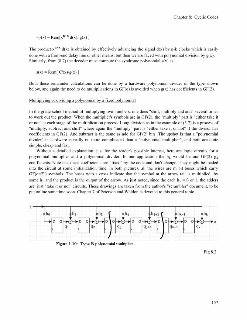
Chapter 8: Cyclic Codes
157
- γ(x) = Rem[xn-k d(x)/ g(x) ] The product xn-k d(x) is obtained by effectively advancing the signal d(x) by n-k clocks which is easily done with a front-end delay line or other means, but then we are faced with polynomial division by g(x). Similarly, from (8.7) the decoder must compute the syndrome polynomial s(x) as s(x) = Rem[ C'(x)/g(x) ] Both these remainder calculations can be done by a hardware polynomial divider of the type shown below, and again the need to do multiplications in GF(q) is avoided when g(x) has coefficients in GF(2). Multiplying or dividing a polynomial by a fixed polynomial In the grade-school method of multiplying two numbers, one does "shift, multiply and add" several times to work out the product. When the multiplier's symbols are in GF(2), the "multiply" part is "either take it or not" at each stage of the multiplication process. Long division as in the example of (3.7) is a process of "multiply, subtract and shift" where again the "multiply" part is "either take it or not" if the divisor has coefficients in GF(2). And subtract is the same as add for GF(2) bits. The upshot is that a "polynomial divider" in hardware is really no more complicated than a "polynomial multiplier", and both are quite simple, cheap and fast. Without a detailed explanation, just for the reader's possible interest, here are logic circuits for a polynomial multiplier and a polynomial divider. In our application the hi would be our GF(2) gi coefficients. Note that these coefficients are "fixed" by the code and don't change. They might be loaded into the circuit at some initialization time. In both pictures, all the wires are m bit buses which carry GF(q=2m) symbols. The buses with a cross indicate that the symbol at the arrow tail is multiplied by some hi and the product is the output of the arrow. As just noted, since the each hi = 0 or 1, the adders are just "take it or not" circuits. These drawings are taken from the author's "scrambler" document, to be put online sometime soon. Chapter 7 of Peterson and Weldon is devoted to this general topic.
Fig 8.2
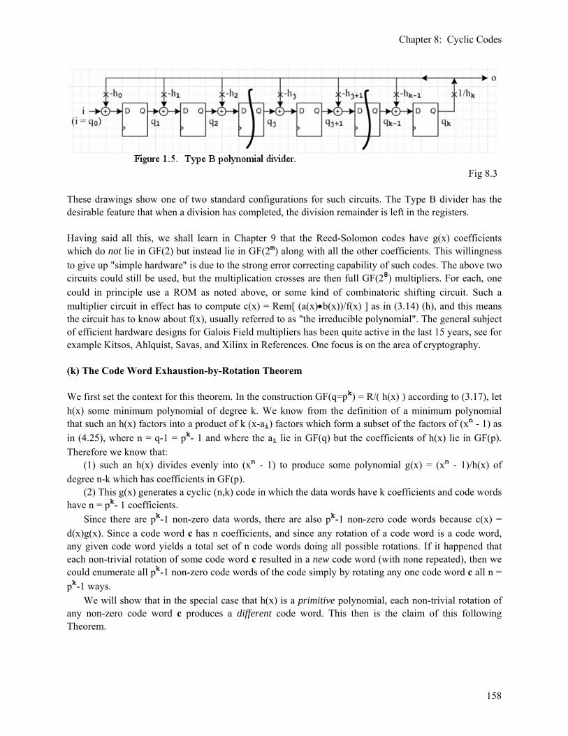
Chapter 8: Cyclic Codes
158
Fig 8.3 These drawings show one of two standard configurations for such circuits. The Type B divider has the desirable feature that when a division has completed, the division remainder is left in the registers. Having said all this, we shall learn in Chapter 9 that the Reed-Solomon codes have g(x) coefficients which do not lie in GF(2) but instead lie in GF(2m) along with all the other coefficients. This willingness to give up "simple hardware" is due to the strong error correcting capability of such codes. The above two circuits could still be used, but the multiplication crosses are then full GF(28) multipliers. For each, one could in principle use a ROM as noted above, or some kind of combinatoric shifting circuit. Such a multiplier circuit in effect has to compute c(x) = Rem[ (a(x)•b(x))/f(x) ] as in (3.14) (h), and this means the circuit has to know about f(x), usually referred to as "the irreducible polynomial". The general subject of efficient hardware designs for Galois Field multipliers has been quite active in the last 15 years, see for example Kitsos, Ahlquist, Savas, and Xilinx in References. One focus is on the area of cryptography. (k) The Code Word Exhaustion-by-Rotation Theorem We first set the context for this theorem. In the construction GF(q=pk) = R/( h(x) ) according to (3.17), let h(x) some minimum polynomial of degree k. We know from the definition of a minimum polynomial that such an h(x) factors into a product of k (x-ai) factors which form a subset of the factors of (xn - 1) as in (4.25), where n = q-1 = pk- 1 and where the ai lie in GF(q) but the coefficients of h(x) lie in GF(p). Therefore we know that: (1) such an h(x) divides evenly into (xn - 1) to produce some polynomial g(x) = (xn - 1)/h(x) of degree n-k which has coefficients in GF(p). (2) This g(x) generates a cyclic (n,k) code in which the data words have k coefficients and code words have n = pk- 1 coefficients. Since there are pk-1 non-zero data words, there are also pk-1 non-zero code words because c(x) = d(x)g(x). Since a code word c has n coefficients, and since any rotation of a code word is a code word, any given code word yields a total set of n code words doing all possible rotations. If it happened that each non-trivial rotation of some code word c resulted in a new code word (with none repeated), then we could enumerate all pk-1 non-zero code words of the code simply by rotating any one code word c all n = pk-1 ways. We will show that in the special case that h(x) is a primitive polynomial, each non-trivial rotation of any non-zero code word c produces a different code word. This then is the claim of this following Theorem.
Chapter 8: Cyclic Codes
159
Exhaustion-by-Rotation Theorem. In the context of the above paragraph, if h(x) is a primitive polynomial, then: (1) each non-trivial rotation of a non-zero code word yields a new and different code word and thus (2) the code words obtained by rotating any given non-zero code word exhaust the set of non-zero code words of the code associated with h(x). (8.36) Proof: Let c(x) be some code word polynomial, and let c(m)(x) be the code word polynomial obtained by rotating the coefficients of c(x) m symbols to the right. It is understood that in such a rotation or "cyclic permutation", symbols wrap around as shown in (8.14). By a non-trivial rotation we mean that 0 < m < n . From Math Lemma 2 of (8.16) we know that c(m)(x) = Rem[(xm c(x))/(xn - 1)] or (8.16) xm c(x) = q(x) (xn - 1) + c(m)(x) for some quotient polynomial q(x) m n-1 m-1 n <n where we have indicated the degree of the various polynomial players. So assume for the moment that the mth rotated codeword polynomial c(m)(x) is identical to the original code word polynomial c(x), c(m)(x) = c(x) for some m in range (1,n-1) . Then (8.16) just above becomes xm c(x) = q(x) (xn - 1) + c(x) for some quotient polynomial q(x) or c(x) (xm - 1) = q(x) (xn- 1) 1 ≤ m ≤ n-1 . (8.37) n-1 m m-1 n Installing into this c(x) = d(x)g(x) and (xn- 1) = h(x)g(x) gives d(x)g(x) (xm - 1) = q(x) h(x)g(x) or d(x) (xm - 1) = q(x) h(x) . (8.38) k-1 m m-1 k Now using the rules shown in (3.14), we put our special Galois brackets {...} around the above equation and drill them inward to get d({x}) ({x}m - 1) = q({x}) {h(x)} (8.39) where recall that {x} represents some element (call it α) of GF(q). Writing {x} = α and recalling that in our remainder construction we must have {h(x)} = 0 (this is the remainder of dividing h(x) by h(x)), we have d(α) (αm - 1) = 0 (8.40)

Chapter 8: Cyclic Codes
160
where the 0 and 1 are the 0 and 1 elements of GF(q). Since we assume that d is some non-zero data word, we know that d(α) ≠ 0 and we conclude that αm = 1 where α = {x} where 1 ≤ m ≤ n-1 . (8.41) Since {h(x)} = 0, we know also that h({x}) = 0 and thus h(α) = 0. We know that the k ai for which h(x) = Π (x-ai) [ and for which therefore h(ai) = 0 ] form the conjugate set of any of these ai. Now we said that h(x) was a primitive polynomial for GF(q). As noted in (5.35), all elements of the conjugate set of a primitive polynomial are primitive elements of GF(q). Since h(α) = 0, we know that our α = {x} is one of these primitive elements, call it aj. Thus, we may regard h(x) as a primitive polynomial for element α = {x} of GF(q). We know from (4.31) and elsewhere that if αm = 1 for a primitive element α of GF(q) then m must be a multiple of q-1, so m = N(q-1). But q-1 is the symbol n of the discussion above, so that we can only have m = Nn for some integer N. But this then rules out all values of m in the range 1 ≤ m ≤ n-1 shown in (8.41) above, so we arrive at a contradiction. Therefore our supposition that it was possible to have some c(m)(x) = c(x) for primitive h(x) was wrong, so we must then have c(m)(x) ≠ c(x) if h(x) is a primitive polynomial. Now consider two rotations of c(x), call them c(m1)(x) and c(m2)(x) and assume m2> m1. Define C(x) ≡ c(m1)(x) . Then C(m2-m1)(x) = c(m2)(x) . In this last line we rotate C(x) m1 symbols to the left ( undoing c(m1)(x) to c(x)) and then we rotate it m2 symbols to the right to get c(m2)(x) . If we now apply our proven Theorem above to C(x) instead of c(x), we conclude that we must have C(m2-m1)(x) ≠ C(x) which then says c(m2)(x) ≠ c(m1)(x). Thus we know that each non-trivial rotation of c(x) gives a new code word polynomial! Then, as noted in the opening paragraph, since all the rotations of c(x) are different, they exhaust the entire set of code word polynomials and thus their coefficients exhaust all the code words c of our cyclic code.
Chapter 9: Code Survey
161
Chapter 9: A Small Survey of a few Standard Code Families (a) The BCH Codes BCH are the initials of Bose and Ray-Chaudhuri (1960) and independently Hocquenghem (1959), see References. The philosophy here is a little different than that of the last two Chapters. There we selected arbitrary values n and k for our (n,k) code and then constructed a code. For a linear block code, that meant selecting a kxn matrix G which had k linearly independent rows -- rank k. For a cyclic code as defined in (8.1) we had to select an h(x) of degree k and g(x) of degree n-k such that their product was xn-1. In contrast, in the BCH discussion below, we specify certain desirable properties of the code (error correcting ability) and then we try to find values for n and k for which such desirable properties are realized. We are forced to a certain set of values for n (usually n = pm - 1) and for each n we are forced to some set of values for k. We end up then with a family of (n,k) BCH codes. Let us return to the Suggestion of Chapter 8 (i). We select g(x) of the form (8.30) so that g(x) has the set of roots α1 , α2, .... αn-k . According to Big Theorem 1 (4.30) we know that GF(q) is cyclic under •, and we can therefore represent all its non-zero elements as powers αk of a primitive element α. Thus, we can rewrite the (8.30) list of roots as: { α1, α2, α3, .... αn-k } = { αe1 , αe2 , αe3 , .... αen-k } (9.1) where the ei are whatever exponents produce α1 , α2, .... αn-k. We now wish to quote a very strange theorem about the minimum distance, hence error correcting ability, of this Galois-induced cyclic code. You will have to read this very carefully. The BCH Bound Context: Any element α of GF(q) has some specific order n, which is the minimum power for which αn = 1. Recall that such an α carves out a cyclic subgroup under • within GF(q) of order n. We first pick an α, and then use its order n to be the length of our cyclic (n,k) code. BCH Bound Theorem. Given some α in GF(q) of order n, the minimum distance d of the cyclic code (n,k) whose generator g(x) has some set of n-k roots in GF(q), namely { αe1, αe2, αe3, .... αen-k }, is greater than the largest number of consecutive integers in the power list: { e1, e2, e3, ....en-k} . (9.2) This theorem provides a lower bound on the minimum distance d of the code, implying a lower limit on t, the number of errors per codeword that can be corrected. Recall from (7.33) that d ~ 2t+1. This suggests that we might be able to find some codes that will correct large numbers of errors in a code word. Proof: Recall Fact 4 of (7.35) that the minimum distance d of a code is equal to the minimum number of columns of the matrix H which are linearly dependent. One proof of the BCH bound theorem involves examining the H matrix shown above in (8.31), and showing that d = (the minimum number of linearly

Chapter 9: Code Survey
162
dependent columns) exceeds the strange count noted in the theorem. This proof is presented in Peterson and Weldon Section 9.1 p 269 and we won't repeat it here since it is a bit involved. From this bound, we are immediately motivated to select powers that are in sequence, rather than some set of random powers of α, due to the word "consecutive" appearing in the theorem. Also, we might like to have n = the order of α be as large as possible, since this increases the size of the pool of roots from which we may select the roots of g(x), and this would increase the chances of having a longer consecutive power sequence. For any GF(q), if we pick α = a primitive element, its order will be n = q-1 which is the most it can be. Of course in this case the code length n must be set to n = q-1 = pm - 1, which is a restriction on the possible values of the code length n. For the binary p=2, one could have n = 3, 7, 15, 31, 63, 127, 255 and so on. Question: Why can't one just pick the roots { αe1, αe2, αe3, .... αen-k } to be { α, α2, α3.... αn-k} for some general n and k, and then the theorem says d > n-k which we can write as d ≥ n-k+1. This would be an interesting situation since we know from (7.34) that d ≤ n-k+1, and therefore we would have to have d = n-k+1, which would be the best d possible. The reason one can't in general do this is that, for n < q-1, the elements of { α, α2, α3.... αn-k}, although roots of xq-1-1 according to (4.34), probably won't all be roots of xn- 1 and therefore can't be used as the roots of g(x) as required by (8.1) g(x)h(x) = xn-1. But if α is taken as a primitive element, then its order is n = q-1 and all powers αs are roots of xn-1 and then we can select the sequence { α, α2, α3.... αn-k} and this does give d = n-k+1. The only problem here is that g(x) = (x-α)(x-α2)(x-α3)....(x-αn-k) likely won't have coefficients in GF(p). For example, this is not the obvious form of a minimum polynomial (5.14) which does have coefficients in GF(p). In Chapter 8 (j) we explained why we want the coefficients of g(x) to be in GF(p): hardware simplification. We have said earlier that k is not yet determined. As we reduce the number k for a given n, the number of roots of g(x) increases. As we add more (x-a) factors to g(x) in this way, maybe at some point g(x) will become a minimal polynomial or a product of minimum polynomials, and then we know g(x) will have GF(p) coefficients. This is precisely the plan that will be pursued below, and this then explains why the value of k gets "forced" on the code designer. In our final section on Reed-Solomon codes, however, we will go ahead and allow g(x) to have coefficients in GF(q), despite the hardware cost, and this will result in the best distance d possible, as suggested above. BCH Bound Corollary : If we can select the roots of g(x) to include { αa, αa+1, αa+2, .... αa+r} for some a and r, then, since this list has r+1 consecutive powers, the minimum code distance will be d > r+1. If we take α as a primitive element, then the order of α is n = q-1, and then all terms shown in the list will be roots of xn-1 and therefore allowable roots for g(x). Such codes are generally called BCH codes. (9.3) At this point then we shall select n = q-1, but we have to hold off on finding a value of k for (n,k) because that is going to be a forced value. The order of g(x) is n-k, but we don't yet have a value for k so we don't yet know the actual order of g(x). Fact: For a BCH code defined on GF(q = pm), the n of (n,k) is set to n = q-1 = pm - 1. Comment: The Corollary above says that the minimum of (the minimum code distance d) is r+2.
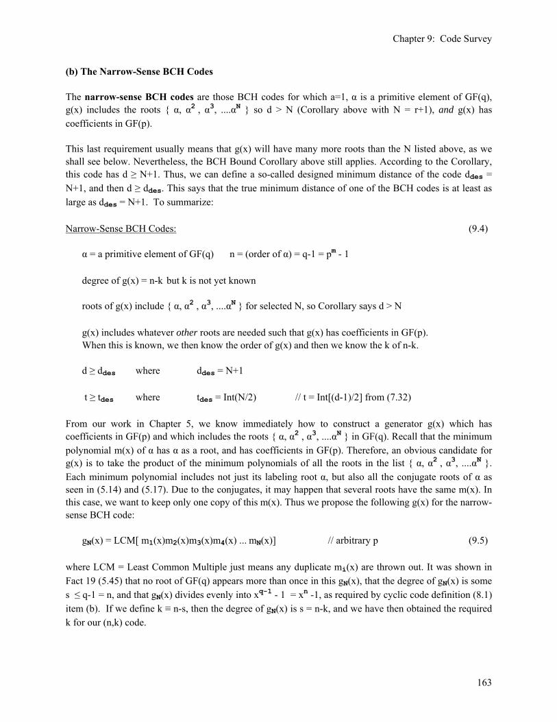
Chapter 9: Code Survey
163
(b) The Narrow-Sense BCH Codes The narrow-sense BCH codes are those BCH codes for which a=1, α is a primitive element of GF(q), g(x) includes the roots { α, α2 , α3, ....αN } so d > N (Corollary above with N = r+1), and g(x) has coefficients in GF(p). This last requirement usually means that g(x) will have many more roots than the N listed above, as we shall see below. Nevertheless, the BCH Bound Corollary above still applies. According to the Corollary, this code has d ≥ N+1. Thus, we can define a so-called designed minimum distance of the code ddes = N+1, and then d ≥ ddes. This says that the true minimum distance of one of the BCH codes is at least as large as ddes = N+1. To summarize: Narrow-Sense BCH Codes: (9.4) α = a primitive element of GF(q) n = (order of α) = q-1 = pm - 1 degree of g(x) = n-k but k is not yet known roots of g(x) include { α, α2 , α3, ....αN } for selected N, so Corollary says d > N g(x) includes whatever other roots are needed such that g(x) has coefficients in GF(p). When this is known, we then know the order of g(x) and then we know the k of n-k. d ≥ ddes where ddes = N+1 t ≥ tdes where tdes = Int(N/2) // t = Int[(d-1)/2] from (7.32) From our work in Chapter 5, we know immediately how to construct a generator g(x) which has coefficients in GF(p) and which includes the roots { α, α2 , α3, ....αN } in GF(q). Recall that the minimum polynomial m(x) of α has α as a root, and has coefficients in GF(p). Therefore, an obvious candidate for g(x) is to take the product of the minimum polynomials of all the roots in the list { α, α2 , α3, ....αN }. Each minimum polynomial includes not just its labeling root α, but also all the conjugate roots of α as seen in (5.14) and (5.17). Due to the conjugates, it may happen that several roots have the same m(x). In this case, we want to keep only one copy of this m(x). Thus we propose the following g(x) for the narrow-sense BCH code: gN(x) = LCM[ m1(x)m2(x)m3(x)m4(x) ... mN(x)] // arbitrary p (9.5) where LCM = Least Common Multiple just means any duplicate mi(x) are thrown out. It was shown in Fact 19 (5.45) that no root of GF(q) appears more than once in this gN(x), that the degree of gN(x) is some s ≤ q-1 = n, and that gN(x) divides evenly into xq-1 - 1 = xn -1, as required by cyclic code definition (8.1) item (b). If we define k ≡ n-s, then the degree of gN(x) is s = n-k, and we have then obtained the required k for our (n,k) code.
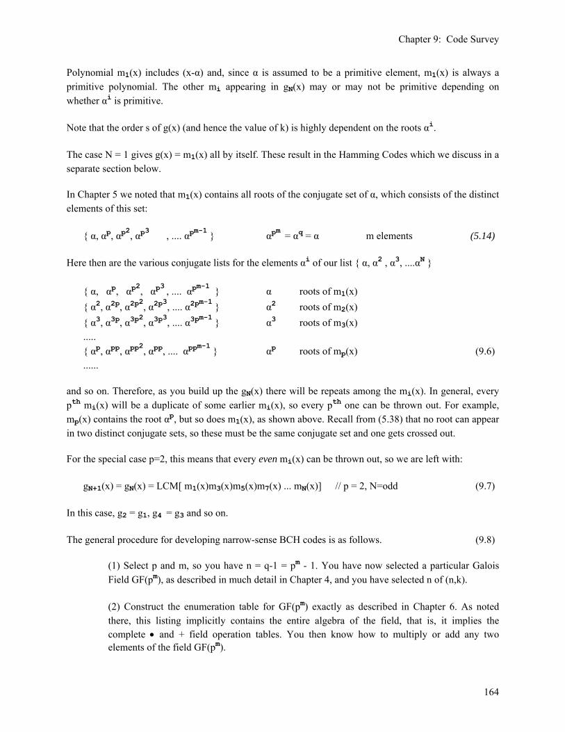
Chapter 9: Code Survey
164
Polynomial m1(x) includes (x-α) and, since α is assumed to be a primitive element, m1(x) is always a primitive polynomial. The other mi appearing in gN(x) may or may not be primitive depending on whether αi is primitive. Note that the order s of g(x) (and hence the value of k) is highly dependent on the roots αi. The case N = 1 gives g(x) = m1(x) all by itself. These result in the Hamming Codes which we discuss in a separate section below. In Chapter 5 we noted that m1(x) contains all roots of the conjugate set of α, which consists of the distinct elements of this set: { α, αp, αp2, αp3 , .... αpm-1 } αpm = αq = α m elements (5.14) Here then are the various conjugate lists for the elements αi of our list { α, α2 , α3, ....αN } { α, αp, αp2, αp3 , .... αpm-1 } α roots of m1(x) { α2, α2p, α2p2, α2p3, .... α2pm-1 } α2 roots of m2(x) { α3, α3p, α3p2, α3p3, .... α3pm-1 } α3 roots of m3(x) ..... { αp, αpp, αpp2, αpp, .... αppm-1 } αp roots of mp(x) (9.6) ...... and so on. Therefore, as you build up the gN(x) there will be repeats among the mi(x). In general, every pth mi(x) will be a duplicate of some earlier mi(x), so every pth one can be thrown out. For example, mp(x) contains the root αp, but so does m1(x), as shown above. Recall from (5.38) that no root can appear in two distinct conjugate sets, so these must be the same conjugate set and one gets crossed out. For the special case p=2, this means that every even mi(x) can be thrown out, so we are left with: gN+1(x) = gN(x) = LCM[ m1(x)m3(x)m5(x)m7(x) ... mN(x)] // p = 2, N=odd (9.7) In this case, g2 = g1, g4 = g3 and so on. The general procedure for developing narrow-sense BCH codes is as follows. (9.8)
(1) Select p and m, so you have n = q-1 = pm - 1. You have now selected a particular Galois Field GF(pm), as described in much detail in Chapter 4, and you have selected n of (n,k). (2) Construct the enumeration table for GF(pm) exactly as described in Chapter 6. As noted there, this listing implicitly contains the entire algebra of the field, that is, it implies the complete • and + field operation tables. You then know how to multiply or add any two elements of the field GF(pm).

Chapter 9: Code Survey
165
(3) for each power αi construct the minimal polynomial mi(x). Chapter 5 showed exactly how this is done. (4) Then for each value of N = 1,2,3,.... compute g(x) exactly as shown above, gN(x) = LCM[ m1(x)m2(x)m3(x)m4(x) ... mN(x)] . For each N, you find that g(x) has some degree n-k, so for each N, you get a value of k.
From the (9.4) root listing { α, α2 , α3, ....αN } we know that N ≤ n, since N cannot be larger than the number of non-zero elements in GF(q). Thus also from (9.4) tdes ≤ Int(n/2). So, N ≤ n tdes ≤ Int(n/2) (9.9) Example: GF(32 = 25). We found all the minimum polynomials in (5.28), then we expanded them later on in (6.22). Since 25-1 = 31 is prime, they are all primitive polynomials of degree m = 5. Here they are. Here we call them mi(x) instead of pi(x), m1(x) = (x-α) (x-α2) (x-α4) (x-α8) (x-α16) = x5 + x3 + x2 + x + 1 m3(x) = (x-α3) (x-α6) (x-α12) (x-α24) (x-α17) = x5 + x4 + x3 + x + 1 m5(x) = (x-α5) (x-α10) (x-α20) (x-α9) (x-α18) = x5 + x2 + 1 m7(x) = (x-α7) (x-α14) (x-α28) (x-α25) (x-α19) = x5 + x4 + x2 + x + 1 m11(x) = (x-α11) (x-α22) (x-α13) (x-α26) (x-α21) = x5 + x3 + 1 m15(x) = (x-α15) (x-α30) (x-α29) (x-α27) (x-α23) = x5 + x4 + x3 + x2 + 1 . (6.22) We can consider the possibilities { α, α2 , α3, ....αN } one at a time: N = 1 {α} g1(x) = LCM[m1(x)] = m1(x) N = 2 {α, α2} g2(x) = LCM[m1(x)m2(x)] = m1(x) N = 3 {α, α2, α3} g3(x) = LCM[m1(x)m2(x)m3(x)] = m1(x) m3(x) N = 4 {α, α2, α3,α4} g4(x) = LCM[m1(x)m2(x)m3(x)m4(x)] = m1(x) m3(x) N = 5 {α, α2, α3,α4,α5} g5(x) = LCM[m1(x)m2(x)m3(x)m4(x)m5(x)] = m1(x) m3(x) m5(x) ..... (9.10) • As just noted, we always have gN+1(x) = gN(x) for any odd N since p = 2. • Since all the mi(x) are of degree 5, all the gi(x) will have a degree that is a multiple of 5. Eventually as N increases, all 6 of the mi form g and then g has degree 30, the most it can be. • For each value of N we know tdes = Int(N/2), we can compute s = n-k, the order of g(x), and thus k, and the code is (31,k). We then arrive at this table, where the gi(x) are expressed in a recursive manner:
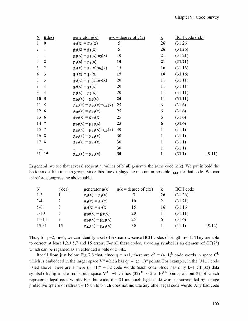
Chapter 9: Code Survey
166
N t(des) generator g(x) n-k = degree of g(x) k BCH code (n,k) 1 0 g1(x) = m1(x) 5 26 (31,26) 2 1 g2(x) = g1(x) 5 26 (31,26) 3 1 g3(x) = g1(x)m3(x) 10 21 (31,21) 4 2 g4(x) = g3(x) 10 21 (31,21) 5 2 g5(x) = g3(x)m5(x) 15 16 (31,16) 6 3 g6(x) = g5(x) 15 16 (31,16) 7 3 g7(x) = g5(x)m7(x) 20 11 (31,11) 8 4 g8(x) = g7(x) 20 11 (31,11) 9 4 g9(x) = g7(x) 20 11 (31,11) 10 5 g10(x) = g9(x) 20 11 (31,11) 11 5 g11(x) = g10(x)m11(x) 25 6 (31,6) 12 6 g12(x) = g11(x) 25 6 (31,6) 13 6 g13(x) = g11(x) 25 6 (31,6) 14 7 g14(x) = g13(x) 25 6 (31,6) 15 7 g15(x) = g13(x)m15(x) 30 1 (31,1) 16 8 g16(x) = g15(x) 30 1 (31,1) 17 8 g17(x) = g15(x) 30 1 (31,1) ..... ..... 30 1 (31,1) 31 15 g31(x) = g29(x) 30 1 (31,1) (9.11) In general, we see that several sequential values of N all generate the same code (n,k). We put in bold the bottommost line in each group, since this line displays the maximum possible tdes for that code. We can therefore compress the above table: N t(des) generator g(x) n-k = degree of g(x) k BCH code 1-2 1 g2(x) = g1(x) 5 26 (31,26) 3-4 2 g4(x) = g3(x) 10 21 (31,21) 5-6 3 g6(x) = g5(x) 15 16 (31,16) 7-10 5 g10(x) = g9(x) 20 11 (31,11) 11-14 7 g14(x) = g13(x) 25 6 (31,6) 15-31 15 g31(x) = g29(x) 30 1 (31,1) (9.12) Thus, for p=2, m=5, we can identify a set of six narrow-sense BCH codes of length n=31. They are able to correct at least 1,2,3,5,7 and 15 errors. For all these codes, a coding symbol is an element of GF(25) which can be regarded as an extended nibble of 5 bits. Recall from just below Fig 7.8 that, since q = n+1, there are qk = (n+1)k code words in space Ck which is embedded in the larger space Vn which has qn = (n+1)n points. For example, in the (31,1) code listed above, there are a mere (31+1)1 = 32 code words (each code block has only k=1 GF(32) data symbol) living in the monstrous space V31 which has (32)31 ~ 5 x 1046 points, all but 32 of which represent illegal code words. For this code, d = 31 and each legal code word is surrounded by a huge protective sphere of radius t ~ 15 units which does not include any other legal code words. Any bad code

Chapter 9: Code Survey
167
word in this sphere is corrected to the center point legal code word, and that is why such a code can correct even a 15 symbol error in the 31 symbol code word. Since this code has the horrible code rate k/n = 1/31 and is overkill on correction, it is often omitted from listings of BCH codes. The (31,6) code puts (32)6= 1,073,741,824 code words in the same huge V31 space and has code rate k/n = 6/31 which is six times better than that of the (31,1) code, and it can still correct up to 7 symbol errors in a 32 symbol code word. The specific generators of the length 31 BCH codes appearing in the above table are g2(x) = m1(x) g4(x) = m1(x) m3(x) g6(x) = m1(x) m3(x) m5(x) g10(x) = m1(x) m3(x) m5(x) m7(x) g14(x) = m1(x) m3(x) m5(x) m7(x) m11(x) g31(x) = m1(x) m3(x) m5(x) m7(x) m11(x) m15(x) . (9.13) We can have Maple compute each of these GF(2) polynomials:
(9.14)
A table of all narrow-sense BCH codes for GF(2m) with m = 1 to 10 appears on pages 274-5 of Pederson and Weldon. The significance of the BCH codes is that they provide clear-cut codes for correcting multi-symbol errors. The Hamming codes for p=2 discussed below only correct single bit errors. We have seen that the BCH codes are completely based on Galois Field theory.
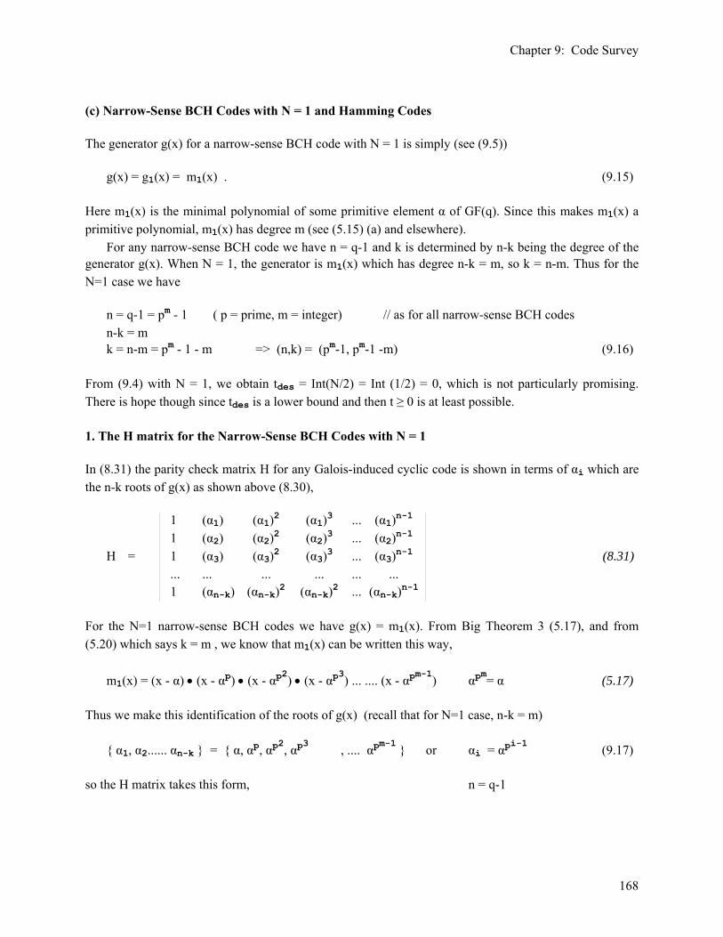
Chapter 9: Code Survey
168
(c) Narrow-Sense BCH Codes with N = 1 and Hamming Codes The generator g(x) for a narrow-sense BCH code with N = 1 is simply (see (9.5)) g(x) = g1(x) = m1(x) . (9.15) Here m1(x) is the minimal polynomial of some primitive element α of GF(q). Since this makes m1(x) a primitive polynomial, m1(x) has degree m (see (5.15) (a) and elsewhere). For any narrow-sense BCH code we have n = q-1 and k is determined by n-k being the degree of the generator g(x). When N = 1, the generator is m1(x) which has degree n-k = m, so k = n-m. Thus for the N=1 case we have n = q-1 = pm - 1 ( p = prime, m = integer) // as for all narrow-sense BCH codes n-k = m k = n-m = pm - 1 - m => (n,k) = (pm-1, pm-1 -m) (9.16) From (9.4) with N = 1, we obtain tdes = Int(N/2) = Int (1/2) = 0, which is not particularly promising. There is hope though since tdes is a lower bound and then t ≥ 0 is at least possible. 1. The H matrix for the Narrow-Sense BCH Codes with N = 1 In (8.31) the parity check matrix H for any Galois-induced cyclic code is shown in terms of αi which are the n-k roots of g(x) as shown above (8.30), 1 (α1) (α1)2 (α1)3 ... (α1)n-1 1 (α2) (α2)2 (α2)3 ... (α2)n-1 H = 1 (α3) (α3)2 (α3)3 ... (α3)n-1 (8.31) ... ... ... ... ... ... 1 (αn-k) (αn-k)2 (αn-k)2 ... (αn-k)n-1
For the N=1 narrow-sense BCH codes we have g(x) = m1(x). From Big Theorem 3 (5.17), and from (5.20) which says k = m , we know that m1(x) can be written this way, m1(x) = (x - α) • (x - αp) • (x - αp2) • (x - αp3) ... .... (x - αpm-1) αpm= α (5.17) Thus we make this identification of the roots of g(x) (recall that for N=1 case, n-k = m) { α1, α2...... αn-k } = { α, αp, αp2, αp3 , .... αpm-1 } or αi = αpi-1 (9.17) so the H matrix takes this form, n = q-1

Chapter 9: Code Survey
169
1 α α2 α3 ... αn-1 1 (αp) (αp)2 (αp)3 ... (αp)n-1 1 (αp2) (αp2)2 (αp2)3 ... (αp2)n-1 H = 1 (αp3) (αp3)2 (αp3)3 ... (αp3)n-1 ... ... ... ... ... ... 1 (αpi-1) (αpi-1)2(αpi-1)3 ... (αpi-1)n-1 ... ... ... ... ... ... 1 (αpm-1) (αpm-1)2(αpm-1)3 ... (αpm-1)n-1 (9.18) As usual, there are n-k (=m) rows and n columns, and the matrix elements are symbols in GF(q=pm). Fact: The first row of H contains all q-1 non-zero elements of GF(q). Proof: Since α is a primitive element of GF(q), it enumerates all non-zero elements. Fact: Each column of H is a conjugate set of GF(q). Proof: See (5.14) and (5.16). Typically most columns include duplicate elements such as the first. The only column that is guaranteed to have m distinct elements is the column headed by α since the conjugate set of a primitive element α always has m distinct elements, according to (5.15). Typically a conjugate set will be repeated multiple times among the columns of H with different ordering of the elements. We know from (3.10) that the elements of GF(q=pm) can be represented by remainder polynomials of degree less than m whose coefficients lie in GF(p), and which coefficients can be represented by an m-tuple as in (4.6). Since each element of the above H matrix (9.18) is an element of GF(q), we can think of each single matrix element (like α2) as an m-tuple column vector. From this point of view, the H matrix then has m2 rows and n columns. This view will come into play in the next section. Recall from (8.1) that c(x) = d(x)g(x) where d(x) is a data polynomial and c(x) is a code word polynomial. Fact: The ith row of H corresponds to c(β) = 0 for β = αpi-1 where c(x) is any code polynomial. Proof: From (7.21) we know that the H matrix kills good code words meaning HcT = 0 where cT is a column vector with coefficients ci of polynomial c(x). When the ith row of H in (8.31) is multiplied by cT the result is 0, as was shown in (8.32), c0 + c1 (αi) + c2 (αi)2 + c3 (αi)3 + ... cn-1 (αi)n-1 = 0 (8.32) Since c(x) = d(x)g(x), g(αi) = 0 => c(αi) = 0, and this is exactly what (8.32) says: all the αi roots of g(x) are passed through to c(x). In the current context we have the same idea, c0 + c1 (αpi-1) + c2 (αpi-1)2 + c3 (αpi-1)3 + ... cn-1 (αpi-1)n-1 = 0 (9.19)
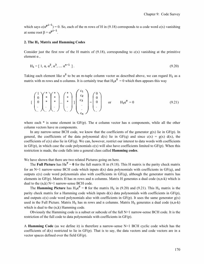
Chapter 9: Code Survey
170
which says c(αpi-1) = 0. So, each of the m rows of H in (9.18) corresponds to a code word c(x) vanishing at some root β = αpi-1. 2. The H1 Matrix and Hamming Codes Consider just the first row of the H matrix of (9.18), corresponding to c(x) vanishing at the primitive element α , H1 = [ 1, α, α2, α3, .... αn-1 ] . (9.20) Taking each element like α2 to be an m-tuple column vector as described above, we can regard H1 as a matrix with m rows and n columns. It is certainly true that H1cT = 0 which then appears this way
[
⎝⎜⎜⎛
⎠⎟⎟⎞ 1
0 0..
⎝⎜⎜⎛
⎠⎟⎟⎞ *
* *..
⎝⎜⎜⎛
⎠⎟⎟⎞ *
* *..
...
⎝⎜⎜⎛
⎠⎟⎟⎞ *
* *..
]
⎝⎜⎜⎛
⎠⎟⎟⎞
c1 c2 c3 . .
cn
=
⎝⎜⎜⎛
⎠⎟⎟⎞ 0
0 0..
or H1cT = 0 (9.21)
where each * is some element in GF(p). The c column vector has n components, while all the other column vectors have m components. In any narrow-sense BCH code, we know that the coefficients of the generator g(x) lie in GF(p). In general, the coefficients of the data polynomial d(x) lie in GF(q) and since c(x) = g(x) d(x), the coefficients of c(x) also lie in GF(q). We can, however, restrict our interest to data words with coefficients in GF(p), in which case the code polynomials c(x) will also have coefficients limited to GF(p). When this restriction is made, the code falls into a general class called Hamming codes. We have shown that there are two related Pictures going on here. The Full Picture has HcT = 0 for the full matrix H in (9.18). This H matrix is the parity check matrix for an N=1 narrow-sense BCH code which inputs d(x) data polynomials with coefficients in GF(q), and outputs c(x) code word polynomials also with coefficients in GF(q), although the generator matrix has elements in GF(p). Matrix H has m rows and n columns. Matrix H generates a dual code (n,n-k) which is dual to the (n,k) N=1 narrow-sense BCH code. The Hamming Picture has H1cT = 0 for the matrix H1 in (9.20) and (9.21). This H1 matrix is the parity check matrix for a Hamming code which inputs d(x) data polynomials with coefficients in GF(p), and outputs c(x) code word polynomials also with coefficients in GF(p). It uses the same generator g(x) used in the Full Picture. Matrix H1 has m rows and n columns. Matrix H1 generates a dual code (n,n-k) which is dual to the (n,k) Hamming code. Obviously the Hamming code is a subset or subcode of the full N=1 narrow-sense BCH code. It is the restriction of the full code to data polynomials with coefficients in GF(p). A Hamming Code (as we define it) is therefore a narrow-sense N=1 BCH cyclic code which has the coefficients of d(x) restricted to lie in GF(p). That is to say, the data vectors and code vectors are in a vector spaces defined over the field GF(p).

Chapter 9: Code Survey
171
Some authors might further restrict Hamming codes to having p = 2 so they are then binary codes -- the data coefficients and code coefficients are bits. In the case from above we have n = q-1 = 2m - 1 (m = integer) // binary Hamming Code n-k = m k = n-m = 2m - 1 - m => (n,k) = (2m-1, 2m-1-m) (9.22) We might call this a binary Hamming code. For m=3 one has (n,k) = (7,4) and this is the specific code that Richard Hamming invented and used in 1950 to deal with punched card reader errors (References). Comment: When one first sees the Hamming Codes, the fact that (n,k) = (2m-1, 2m-1-m) seems very strange. One has no clue as to where these peculiar numbers are coming from. In retrospect, these numbers fall out very naturally from the concept of Galois-induced cyclic codes. The 2m-1 is just the number of non-zero elements in GF(2m), and the generator m1(x) has degree m, so n-k = m and k = n-m. Fact: (9.23) A Hamming code with p = 2 can correct single-symbol errors (t=1). A Hamming code with p > 2 cannot correct any errors (t=0). Proof: This Fact is proved in the following section. 3. Error Correction capabilities of Hamming Codes The Hamming parity check matrix H1 gives us some insight as to why t=0 when p>2. We know that all q-1 elements of {GF(q)-0} must appear in the first row of H, called H1 in (9.20), and that means that every non-zero m-tuple (components in GF(p)) must appear as a column of H1 in (9.21). For p = 2, no m-tuple is a multiple of another m-tuple simply because there are no multiple m-tuples in the set of m-tuples for p = 2. Thus, no pair of columns in H1 is linearly dependent. Since a column of zeros does not appear, no single column is linearly dependent. We know for sure that many columns can be written as a linear combination of two other columns. Thus, the minimum number of dependent columns in H will be 3. According to Fact 4 (7.35), the code must have a minimum distance of d = 3, and then (7.32) says that t = Int[(d-1)/2] = 1. Thus, the p = 2 Hamming code can correct single-symbol errors. When p > 2, we still have all q-1 m-tuples appearing as the columns of H1, but of course q is larger now, being pm instead of 2m. This set of m-tuples includes many multiples, such as (2,0,0...) = 2(1,0,0...). Since at least one pair of columns has one being a multiple of the other (there will be many such pairs), the minimum number of dependent columns is 2, and then (7.35) says that d = 2 and t = Int[(d-1)/2] = 0. That is why Hamming codes for p > 2 cannot correct even single symbol errors. 4. A Modified Hamming Code There are many kinds of modified Hamming codes. Here we describe one which has interesting algebraic properties. It is mentioned on page 221 of Peterson and Weldon. We derive this code using two Lemmas which are then proven below.

Chapter 9: Code Survey
172
It was noted in the previous section that the non-binary Hamming codes (p > 2) cannot correct even 1-symbol errors due to the existence of sets of columns in the H1 matrix which are multiples of each other. This problem can be repaired by eliminating the extra columns and the result is a modified Hamming Code that can in fact correct single-symbol errors for p > 2. Toward this end, we reconsider the (3.16) representation GF(pm ) = R / ( f(x) ) where we have a chart whose rows are labeled by the remainders of polynomials over GF(p) divided by some irreducible f(x). In the resulting chart, one could combine together into one row all rows whose remainders are multiples of each other. For example, the rows {x}, {2x}....{(p-1)x} = {x}, 2{x}....(p-1){x} would be combined into a single row of a new chart which of course then has fewer rows. If we ignore the first row {0}, the original chart has pm -1 non-zero rows, and the new chart then has (pm-1)/(p-1) non-zero rows. As shown in Lemma 1, there is no integer m' such that, given m and p, (pm-1)/(p-1) = pm'-1. Thus, the order of the new chart (including the zero row) is not of the form pm', so the rows in the new chart do not represent a field, since all finite fields have order of the form pm'. The elements of this new chart only form a ring, which we might loosely write as GF(pm)/Zp. So we have constructed GF(pm)/Zp r ≡ (pm-1)/(p-1) = the number of non-zero elements (9.24) Notice that r = pm-1 + pm-2..... + 1 is of course an integer. Each row of the new chart can be represented by a polynomial p(x) which represents not just itself, but all integer multiples of itself by an integer in Zp. If a polynomial is multiplied by k, its remainder is multiplied by k, and so it is associated with the same row of the new chart. In terms of the m-tuple notation for polynomial coefficients, we can regard the non-zero chart rows as being represented by a set of m-tuples none of which are multiples of each other. For example, (2,0,0) = 2(1,0,0) is in the same row as (1,0,0). Since each original m-tuple had m digits, each of the new set of m-tuples obviously also has m digits. Recall that m is the degree of f(x) in GF(pm ) = R /( f(x) ). If α is a primitive element of GF(q=pm), then the order of α is q-1 and we can enumerate the non-zero elements of GF(q) as powers of α. If we define β ≡ αp-1, we find that β is not a primitive element because it's order is less than q-1. In fact, its order is r = (q-1)/(p-1), which is easily shown since αq-1 = 1: βr = (αp-1)[(q-1)/(p-1)] = αq-1 = 1 . In Lemma 2 we show that each element of the subgroup {1, β, β2....βr-1} can be associated with a non-zero row of our new chart which defines GF(pm)/Zp. Thus, each power of β can be represented by one of the m-tuples which label the rows of the new chart. Recall that no m-tuples of this set are multiples of each other. We then define a Hamming type parity check matrix in this way H'1 ≡ [1, β, β2....βr-1 ] . (9.25) The space of code words is the nullspace of H'1, which is to say H'1cT = 0. The H'1 matrix has m rows and r = (q-1)/(p-1)columns. This is similar to the Hamming matrix H1 which had m rows but n = q-1 columns. The difference is that all the "multiple columns" in H1 have been removed in H'1. Therefore, in H'1 no pair of columns is a multiple of each other, and then the minimum number of dependent columns is 3. According to (7.35) this new code has minimum distance d = 3 and then t = Int[(d-1)/2] = 1.
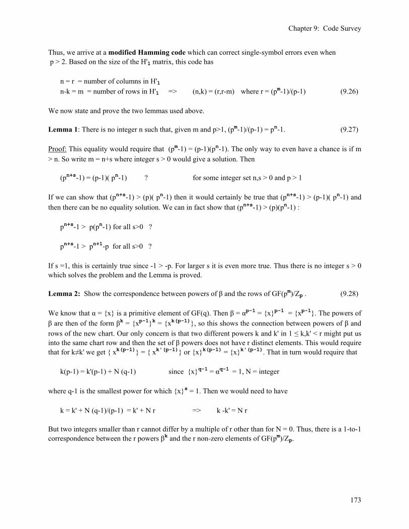
Chapter 9: Code Survey
173
Thus, we arrive at a modified Hamming code which can correct single-symbol errors even when p > 2. Based on the size of the H'1 matrix, this code has n = r = number of columns in H'1 n-k = m = number of rows in H'1 => (n,k) = (r,r-m) where r = (pm-1)/(p-1) (9.26) We now state and prove the two lemmas used above. Lemma 1: There is no integer n such that, given m and p>1, (pm-1)/(p-1) = pn-1. (9.27) Proof: This equality would require that (pm-1) = (p-1)(pn-1). The only way to even have a chance is if m > n. So write m = n+s where integer s > 0 would give a solution. Then (pn+s-1) = (p-1)( pn-1) ? for some integer set n,s > 0 and p > 1 If we can show that (pn+s-1) > (p)( pn-1) then it would certainly be true that (pn+s-1) > (p-1)( pn-1) and then there can be no equality solution. We can in fact show that (pn+s-1) > (p)(pn-1) : pn+s-1 > p(pn-1) for all s>0 ? pn+s-1 > pn+1-p for all s>0 ? If s =1, this is certainly true since -1 > -p. For larger s it is even more true. Thus there is no integer s > 0 which solves the problem and the Lemma is proved. Lemma 2: Show the correspondence between powers of β and the rows of GF(pm)/Zp . (9.28) We know that α = {x} is a primitive element of GF(q). Then β = αp-1 = {x}p-1 = {xp-1}. The powers of β are then of the form βk = {xp-1}k = {xk(p-1)}, so this shows the connection between powers of β and rows of the new chart. Our only concern is that two different powers k and k' in 1 ≤ k,k' < r might put us into the same chart row and then the set of β powers does not have r distinct elements. This would require that for k≠k' we get { xk(p-1)} = { xk'(p-1)} or {x}k(p-1) = {x}k'(p-1). That in turn would require that k(p-1) = k'(p-1) + N (q-1) since {x}q-1 = αq-1 = 1, N = integer where q-1 is the smallest power for which {x}s = 1. Then we would need to have k = k' + N (q-1)/(p-1) = k' + N r => k -k' = N r But two integers smaller than r cannot differ by a multiple of r other than for N = 0. Thus, there is a 1-to-1 correspondence between the r powers βk and the r non-zero elements of GF(pm)/Zp.

Chapter 9: Code Survey
174
(d) The Reed-Solomon Codes We have seen that the narrow-sense BCH codes (9.4) are a special case of the general class of BCH codes (9.3). The Reed-Solomon codes are another special case. Recall that all BCH codes have n = q-1. The reason we chose the minimum polynomials in (9.5) for the narrow-sense BCH codes was to make sure g(x) had coefficients in the field GF(p). Suppose we consider generators g(x) that have coefficients in GF(q) = GF(pm). As noted in Chapter 8 (j), this means we give up a significant amount of design simplicity in coding hardware. In this case, there is no need to fool around with the minimum polynomials, and we have a much simpler expression for a generator containing the desired roots. As with the narrow-sense BCH codes, we set a = 1 in (9.3) and select α to be a primitive element of GF(q). Thus, our candidate g(x) in GF(q) is simply this: gN(x) = (x - α)(x-α2)(x-α3).....(x-αN) g(x) has coefficients in GF(pm) (9.29) Notice that there is no uncertainty about the degree of gN(x) as there is in the narrow-sense BCH codes. The degree here is n-k = N. If g(x) has coefficients in GF(pm), then so do the code polynomials c(x) = g(x)d(x) of (8.1). There is then no motivation to restrict the coefficients of the data polynomials d(x) to GF(p), so they can be in GF(q) as well. The error correcting capability of the above code is exactly the same as for the corresponding narrow sense BCH code expressed at the end of (9.4), and for the same reason: an application of the BCH Bound Corollary (9.3). Thus we have, d ≥ ddes where ddes = N+1 t ≥ tdes where tdes = Int(N/2) // t = Int[(d-1)/2] from (7.32) (9.30) Example: p=2 and m=8, n = q-1 = 28-1 = 255. The data symbols and code symbols are then bytes. Each code word contain 255 bytes. If N=even, then tdes= N/2 and we know that at least N/2 erroneous bytes in such code words can be corrected. Of course k = n-N = 255-N is the size of the data word. Codes with code symbols in pm and with g(x) as shown above are known as Reed-Solomon codes (1960). α is a primitive element of GF(pm) and the code can correct at least t = Int(N/2) bad symbols errors per code word. Thus for even N, the code can correct half the number of parity check symbols (n-k). Note that a single bad symbol error might involved multiple bad bits in that symbol. For the special case p=2, the parameters of a Reed Solomon code are as follows: n = 2m - 1 n-k = N k = 2m - 1 - N = n-N (9.31)
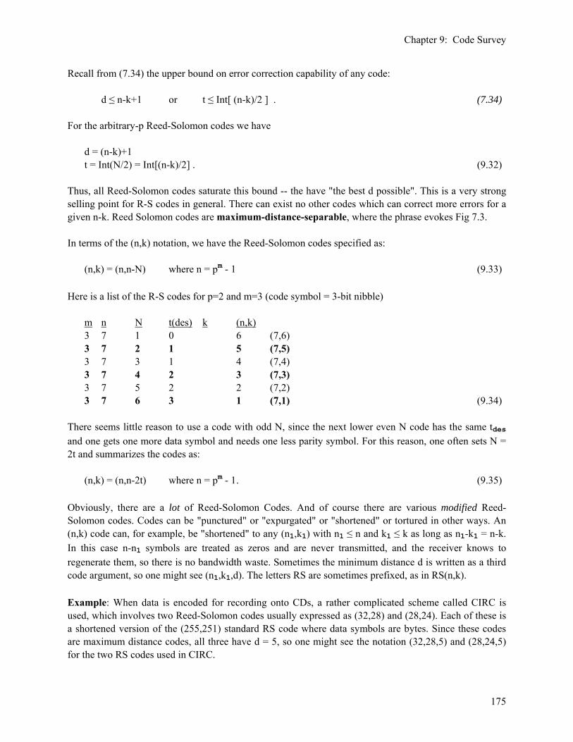
Chapter 9: Code Survey
175
Recall from (7.34) the upper bound on error correction capability of any code: d ≤ n-k+1 or t ≤ Int[ (n-k)/2 ] . (7.34) For the arbitrary-p Reed-Solomon codes we have d = (n-k)+1 t = Int(N/2) = Int[(n-k)/2] . (9.32) Thus, all Reed-Solomon codes saturate this bound -- the have "the best d possible". This is a very strong selling point for R-S codes in general. There can exist no other codes which can correct more errors for a given n-k. Reed Solomon codes are maximum-distance-separable, where the phrase evokes Fig 7.3. In terms of the (n,k) notation, we have the Reed-Solomon codes specified as: (n,k) = (n,n-N) where n = pm - 1 (9.33) Here is a list of the R-S codes for p=2 and m=3 (code symbol = 3-bit nibble) m n N t(des) k (n,k) 3 7 1 0 6 (7,6) 3 7 2 1 5 (7,5) 3 7 3 1 4 (7,4) 3 7 4 2 3 (7,3) 3 7 5 2 2 (7,2) 3 7 6 3 1 (7,1) (9.34) There seems little reason to use a code with odd N, since the next lower even N code has the same tdes and one gets one more data symbol and needs one less parity symbol. For this reason, one often sets N = 2t and summarizes the codes as: (n,k) = (n,n-2t) where n = pm - 1 . (9.35) Obviously, there are a lot of Reed-Solomon Codes. And of course there are various modified Reed-Solomon codes. Codes can be "punctured" or "expurgated" or "shortened" or tortured in other ways. An (n,k) code can, for example, be "shortened" to any (n1,k1) with n1 ≤ n and k1 ≤ k as long as n1-k1 = n-k. In this case n-n1 symbols are treated as zeros and are never transmitted, and the receiver knows to regenerate them, so there is no bandwidth waste. Sometimes the minimum distance d is written as a third code argument, so one might see (n1,k1,d). The letters RS are sometimes prefixed, as in RS(n,k). Example: When data is encoded for recording onto CDs, a rather complicated scheme called CIRC is used, which involves two Reed-Solomon codes usually expressed as (32,28) and (28,24). Each of these is a shortened version of the (255,251) standard RS code where data symbols are bytes. Since these codes are maximum distance codes, all three have d = 5, so one might see the notation (32,28,5) and (28,24,5) for the two RS codes used in CIRC.

Chapter 9: Code Survey
176
CIRC stands for Cross-Interleaved Reed-Solomon Coding. As mentioned earlier, the interleaving aspect shuffles the data so that a physical burst error is widely dispersed into the logical data stream. It is often claimed that CIRC can correct a burst of up to 3500 sequential bad bits which could be caused by a 1/10" wide scratch on a CD. It is impressive that a full CIRC decoder can be implemented in a $9 Walmart portable CD player. (e) Galois Field GF(2m) Math compared to Digital Filter Math Another selling point of p=2 Reed-Solomon codes is that one can work with polynomial multipliers, dividers and related circuits that have data paths that are m-bits wide. Hardware is well geared for doing this and a few circuit examples were shown in Chapter 8 (j). Circuits used in digital filters and related digital applications have a very similar appearance, but there is one major difference that we wish to point out. In an integer-math digital filter with data paths m-bits wide, the + and • tables are those of modulo-q arithmetic where q = 2m. The field in which the numbers reside is Zq. For q=28, an adder does addition then within Z256 and there is carry between the bit lines inside the adder. In a Reed-Solomon polynomial divider or multiplier with data paths m-bits wide ( as one might encounter in an encoder or decoder), the + and • tables are those of the field GF(q=2m). In this case an adder is just a set of m XOR gates and there is no carry between bit lines within the adder. All addition is done within Z2. Earlier it was stressed that the multiplication table for Z4 is different from that of GF(4). This is true in general for any q = 2m (except m=1). In both Zq and GF(q) there is an interaction between all the bit lines during a multiplication. Thus, in building Reed-Solomon circuits, one can use XOR gates for addition independently on the individual bit lines, but multiplication must be done with some kind of lookup or combinatoric/state machine circuit which correctly computes products of GF(2m) symbols. As in a digital filter, multiplication cannot be done independently on the individual bit lines.
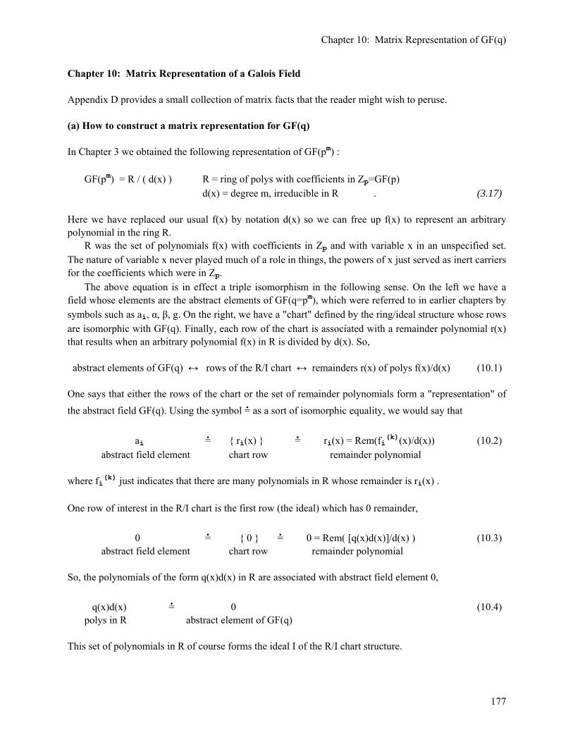
Chapter 10: Matrix Representation of GF(q)
177
Chapter 10: Matrix Representation of a Galois Field Appendix D provides a small collection of matrix facts that the reader might wish to peruse. (a) How to construct a matrix representation for GF(q) In Chapter 3 we obtained the following representation of GF(pm) : GF(pm) = R / ( d(x) ) R = ring of polys with coefficients in Zp=GF(p) d(x) = degree m, irreducible in R . (3.17) Here we have replaced our usual f(x) by notation d(x) so we can free up f(x) to represent an arbitrary polynomial in the ring R. R was the set of polynomials f(x) with coefficients in Zp and with variable x in an unspecified set. The nature of variable x never played much of a role in things, the powers of x just served as inert carriers for the coefficients which were in Zp. The above equation is in effect a triple isomorphism in the following sense. On the left we have a field whose elements are the abstract elements of GF(q=pm), which were referred to in earlier chapters by symbols such as ai, α, β, g. On the right, we have a "chart" defined by the ring/ideal structure whose rows are isomorphic with GF(q). Finally, each row of the chart is associated with a remainder polynomial r(x) that results when an arbitrary polynomial f(x) in R is divided by d(x). So, abstract elements of GF(q) ↔ rows of the R/I chart ↔ remainders r(x) of polys f(x)/d(x) (10.1) One says that either the rows of the chart or the set of remainder polynomials form a "representation" of the abstract field GF(q). Using the symbol =· as a sort of isomorphic equality, we would say that ai =· { ri(x) } =· ri(x) = Rem(fi(k)(x)/d(x)) (10.2) abstract field element chart row remainder polynomial where fi(k) just indicates that there are many polynomials in R whose remainder is ri(x) . One row of interest in the R/I chart is the first row (the ideal) which has 0 remainder, 0 =· { 0 } =· 0 = Rem( [q(x)d(x)]/d(x) ) (10.3) abstract field element chart row remainder polynomial So, the polynomials of the form q(x)d(x) in R are associated with abstract field element 0, q(x)d(x) =· 0 (10.4) polys in R abstract element of GF(q) This set of polynomials in R of course forms the ideal I of the R/I chart structure.

Chapter 10: Matrix Representation of GF(q)
178
Now in what follows we are going the take the unspecified polynomial variable x and specify it to be a square matrix in a certain space of matrices. To stress that x is a matrix, we will write it as X. If we take any polynomial f(x) and evaluate it at x = X, that polynomial evaluates to a matrix, where we assume that the constant term in the polynomial is that constant times the identity matrix I. For example: f(x) = a + bx + cx2 → f(X) = aI + bX + cX2 = a matrix We wish to select a certain set of matrices to be a "representation" of the field GF(q). Thus, we write (10.4) as q(x)d(x) =· 0 =· q(X)d(X) (10.5) polys in R abstract element of GF(q) matrix in the matrix representation We would like the "all-zeros matrix" of the matrix representation to represent the abstract element 0 of the field GF(q). We can achieve this goal for all q(x) by requiring that d(X) = 0. Thus we are led to our first key equation, Fact 1: d(X) = 0 (the all-zeros matrix) (10.6) Another row of interest in the R/I chart is this one, where the remainder is ri(x) = x, α =· { x } =· x (10.7) abstract field element chart row remainder polynomial Recall that if d(x) is a primitive polynomial for element α, then d(x) contains (x-α) as a factor, d(α) = 0, and α is a primitive element of GF(q) whose powers enumerate the non-zero elements of GF(q). We will assume from now on that d(x) is in fact a primitive polynomial for some primitive element α, which in the chart representation we identify with {x} and also with remainder polynomial x. Recall from (6.5) that since d(x) is a primitive polynomial, d(α) = 0 for α = {x} and α is a primitive element of GF(q). We now add our matrix representation item to (10.7) and say α =· { x } = x =· X (10.8) primitive abstract remainder matrix field element chart row polynomial representation Therefore we have the following: Fact 2: The matrix X is a primitive element in the matrix representation of GF(q) and the powers of matrix X enumerate the non-zero elements of GF(q) in the matrix representation. (10.9) This enumeration capability of a primitive element results from our realization in Big Theorem 1 (4.30) that {GF(q) - 0, •} is a cyclic group, and from (1.10) which says that, by the definition of a cyclic group, there is always some element of the group (called a generator) which enumerates the group. Such a generator is called a primitive element and the minimal polynomial of a primitive element is a primitive polynomial.
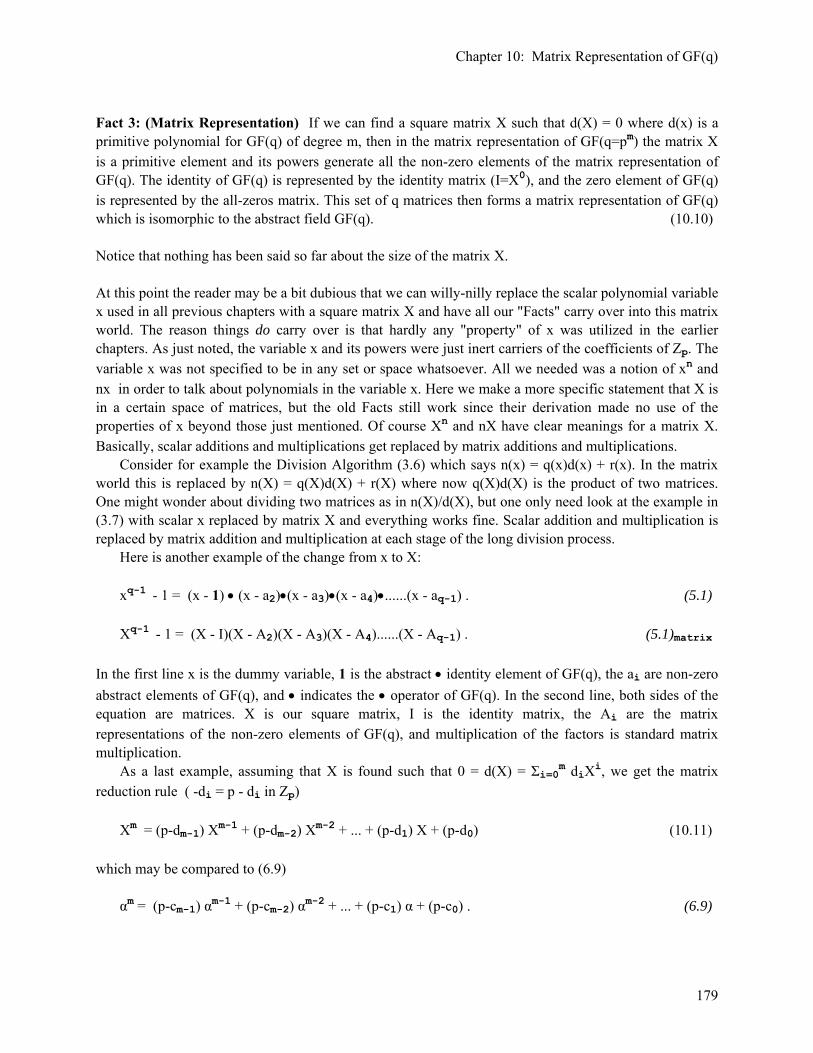
Chapter 10: Matrix Representation of GF(q)
179
Fact 3: (Matrix Representation) If we can find a square matrix X such that d(X) = 0 where d(x) is a primitive polynomial for GF(q) of degree m, then in the matrix representation of GF(q=pm) the matrix X is a primitive element and its powers generate all the non-zero elements of the matrix representation of GF(q). The identity of GF(q) is represented by the identity matrix (I=X0), and the zero element of GF(q) is represented by the all-zeros matrix. This set of q matrices then forms a matrix representation of GF(q) which is isomorphic to the abstract field GF(q). (10.10) Notice that nothing has been said so far about the size of the matrix X. At this point the reader may be a bit dubious that we can willy-nilly replace the scalar polynomial variable x used in all previous chapters with a square matrix X and have all our "Facts" carry over into this matrix world. The reason things do carry over is that hardly any "property" of x was utilized in the earlier chapters. As just noted, the variable x and its powers were just inert carriers of the coefficients of Zp. The variable x was not specified to be in any set or space whatsoever. All we needed was a notion of xn and nx in order to talk about polynomials in the variable x. Here we make a more specific statement that X is in a certain space of matrices, but the old Facts still work since their derivation made no use of the properties of x beyond those just mentioned. Of course Xn and nX have clear meanings for a matrix X. Basically, scalar additions and multiplications get replaced by matrix additions and multiplications. Consider for example the Division Algorithm (3.6) which says n(x) = q(x)d(x) + r(x). In the matrix world this is replaced by n(X) = q(X)d(X) + r(X) where now q(X)d(X) is the product of two matrices. One might wonder about dividing two matrices as in n(X)/d(X), but one only need look at the example in (3.7) with scalar x replaced by matrix X and everything works fine. Scalar addition and multiplication is replaced by matrix addition and multiplication at each stage of the long division process. Here is another example of the change from x to X: xq-1 - 1 = (x - 1) • (x - a2)•(x - a3)•(x - a4)•......(x - aq-1) . (5.1) Xq-1 - 1 = (X - I)(X - A2)(X - A3)(X - A4)......(X - Aq-1) . (5.1)matrix In the first line x is the dummy variable, 1 is the abstract • identity element of GF(q), the ai are non-zero abstract elements of GF(q), and • indicates the • operator of GF(q). In the second line, both sides of the equation are matrices. X is our square matrix, I is the identity matrix, the Ai are the matrix representations of the non-zero elements of GF(q), and multiplication of the factors is standard matrix multiplication. As a last example, assuming that X is found such that 0 = d(X) = Σi=0m diXi, we get the matrix reduction rule ( -di = p - di in Zp) Xm = (p-dm-1) Xm-1 + (p-dm-2) Xm-2 + ... + (p-d1) X + (p-d0) (10.11) which may be compared to (6.9) αm = (p-cm-1) αm-1 + (p-cm-2) αm-2 + ... + (p-c1) α + (p-c0) . (6.9)

Chapter 10: Matrix Representation of GF(q)
180
Nevertheless, for the dubious reader we provide the next section which makes a detailed specification of the new ring of polynomials Rp
m which is appropriate for our new matrix isomorphism GF(pm) = Rp
m/d(X). Everything about this ring Rpm is just an extension of the Chapter 3 (a) scalar ring R where
scalar addition and multiplication is replaced by matrix addition and multiplication. Rather than hold the reader in suspense, we shall right here finish off the logic flow to show exactly how a matrix representation of GF(q) can be constructed in actual practice. Then the following sections can be considered "support material". In the final section we will use Maple to execute our algorithm for creating matrix representations for some sample GF(q) fields. Looking at Fact 3 (10.10) above, we are faced with this problem: given a primitive polynomial d(x) for GF(q) (which we can find from a table, or which we can figure out by some method outlined earlier), how do we find a square matrix X such that d(X) = 0? If we can solve this problem, then Fact 3 gives complete instructions for constructing a matrix representation of GF(q). The following famous theorem comes to the rescue: Theorem: (Cayley-Hamilton). Every square matrix satisfies its own characteristic equation. (10.12) As reviewed in Appendix D, if X is an mxm matrix, then (a) d(x) ≡ det(xI - X) is the characteristic polynomial of matrix X, and it has degree m. (b) the characteristic (secular) equation says d(x) = 0. Normally this equation is solved to find the eigenvalues of matrix X. What Cayley-Hamilton says is simply this: for any square matrix X, d(X) = 0. Proof: See any good linear algebra text. Birkhoff and MacLane give a one page proof on page 341. Wiki has several proofs. Here is a non-proof which involves an equation which does not "carry over" when x goes to matrix X : d(x) = det(xI - X) = 0 =>? d(X) = det(XI - X) = 0 On the right, d(X) = det(XI - X) is completely meaningless since d(X) is a matrix while any determinant is just a number. The proof takes a little more work than that. In order that d(x) ≡ det(xI - X) be a polynomial of degree m, the square matrix X must be an mxm matrix. Then Cayley-Hamilton says d(X) = 0. So if we use this plan to find a matrix X such that d(X)= 0, then our X must be an mxm matrix if we are building a matrix representation for GF(pm). We are now faced with a new problem: given a primitive polynomial d(x) of degree m and which we associate with the characteristic polynomial of matrix X, how to we actually construct a matrix X which has this d(x) as its characteristic polynomial? If we can construct such an X, then d(X) = 0, and then Fact 3 is happy. As shown in the second section following, there is a standard method of constructing a matrix X which has any desired characteristic polynomial. Such a matrix X is called a companion matrix to that

Chapter 10: Matrix Representation of GF(q)
181
polynomial. It is then trivial to write down a matrix X that works, and we are done. In the third section following, we shall have Maple construct some matrix representations using Fact 3 above. (b) Specification of the ring Rp
m of matrix polynomials with coefficients in Zp Let Xp
m denote the set of mxm matrices whose elements lie in Zp. There are exactly pm2 matrices in this set. Let X and Y be elements of Xp
m. With set Xpm we associate + and • operations defined as follows.
First the + operator: Z = X + Y ⇔ Zrs ≡ Xrs ⊕ Yrs (10.13) where, as before, ⊕ and ⊗ refer to the operators of Zp. Thus, addition in Xp
m is normal matrix addition, but matrix elements are added in Zp. Now the • operator : Z = X•Y = XY ⇔ Zrs ≡ Σ⊕
t=1m (Xrt⊗Yts) . (10.14)
Here Xrt and Yts are elements of Zp, so (Xrt⊗Yts) is a well-defined element of Zp and we are adding m such elements with the ⊕ operator, all within Zp. This is the meaning of Σ⊕. Notice that everything is normal matrix addition and matrix multiplication except the only numbers that ever appear lie in Zp. Examples of the above are: Zrs = Xrs⊕ Xrs = 2Xrs => Z = X + X = 2X // assuming p > 2 (10.15) Zrs ≡ Σ⊕
t=1m (Xrt⊗Xts) = (X2)rs => Z = X•X = X2 . (10.16)
Thus any multiple of X or power of X lies in Xp
m and as usual all numbers come out lying in Zp. In particular we have Fact 1: pX = 0: (10.17) Proof: pX = X + X + ... + X ⇔ pXrs= Xrs ⊕ Xrs ⊕ ... ⊕ Xrs = 0 since pa = 0 for any a in Zp . With the + and • operations of (10.13) and (10.14), the set Xp
m forms a ring with identity, the identity being the usual identity matrix with all 1's on the diagonal. The additive identity is the all-zeros matrix. One can go through all the ring properties just as we did in Chapter 3 (a) with the + and • definitions shown here and verify each one. Therefore we have: Fact 2: Let Xp
m denote the set of mxm matrices whose elements lie in Zp, and let the + and • operations for Xp
m be as given in (10.13) and (10.14). Then Xpm is a ring with identity having pm2 elements. (10.18)
Now, let Rp
m be the set of polynomials f(X) whose coefficients lie in Zp and whose variable X lies in Xpm.
It is easy to show that any f(X) is in fact a matrix lying in Xpm. Consider:

Chapter 10: Matrix Representation of GF(q)
182
f(X) = Σi ai Xi ⇔ [f(X)]rs = Σi ai [Xi]rs . (10.19) We know that aiXi = Xi + Xi + .... is in fact a matrix in Xp
m having elements in Zp. And then Σi ai Xi is just a sum of matrices in Xp
m , as defined above. Thus we conclude that f(X) is itself a matrix in Xpm.
Since adding and multiplying polynomials in Rpm is the same as adding and multiplying matrices in Xp
m, the + and • operations for Rp
m are the same as those for Xpm. For example,
a(X) + b(X) = (ΣiaiXi) + (ΣibiXi) ≡ Σi (ai⊕bi)Xi (10.20) a(X) • b(X) = (ΣiaiXi) • (ΣjbjXj) ≡ Σi,j (ai⊗bj) Xi+j . (10.21) In the second line, Xi+j = Xi • Xj is a product of two matrices Xi and Xi using (10.14), so Xi+j then has elements in Zp. Then (ai⊗bj) is some integer multiple of XiXj and we know what that means in Xp
m. Fact 3: Let Rp
m be the set of polynomials f(X) whose coefficients lie in Zp and whose variable X lies in Xm. Let the + and • operations for Rp
m be those of Xpm. Then Rp
m is a ring with identity having an infinite number of elements. (10.22) Proof: The identity polynomial for Rp
m is just f(X) = I, the identity matrix of Xpm. One can go through
each of the ring definition items exactly as done in Chapter 3 (a) with x → X and one finds that each item verifies. Fact 4: The rings Rm and Xp
m are different, although they have the same + and • operations. (10.23) Proof: Rp
m has an infinite number of elements, while Xpm has a finite number of elements pm2. Rp
m has an infinite number of elements because it contains polynomials of arbitrarily high degree. Fact 5: The mapping from Rp
m to Xpm defined by evaluating a polynomial in Rp
m is many-to-one. (10.24) Proof: We know each element of Rp
m evaluates to some element of Xpm and we know that Rp
m has a lot more elements than Xp
m has, so the mapping has to be many-to-one. Fact 6: The ring Rp
1 is exactly the ring R studied above in Chapter 3 (a) if we let x of that section lie in Zp. (10.25) (c) The Companion Matrix In this section we shall explicitly construct forms of the matrix X which satisfy the needs of (10.10).

Chapter 10: Matrix Representation of GF(q)
183
Let d(x) be some monic polynomial of degree m, d(x) = d0 + d1 x + ... + dm-1 xm-1 + xm. (10.26) Consider the following mxm matrix : 0 0 0 0 0 .. 0 -d0 1 0 0 0 0 .. 0 -d1 0 1 0 0 0 .. 0 -d2 X = 0 0 1 0 0 .. 0 -d3 .. .. .. 0 0 0 0 0 .. 1 -dm-1 (10.27)
Note that this matrix X is mxm, where m is the degree of d(x). There are 1's just below the main diagonal all the way through the matrix. The rightmost column contains the negatives of all but the leading coefficient of d(x), which is 1, since d(x) was assumed monic. Notice that tr(X) = -dm-1 and det(X) = (-1)m-1 (-d0) = (-1)md0. (10.28) The X matrix elements can be written using Kronecker deltas. With rows and columns going 1 to m, Xij = δi,j+1 ( 1 ) + δj,m ( -di-1 ) // for example, X2m = δm,m(-d1) = -d1 (10.29) The δi,j+1 says that to get the 1, the row i has to be one more than the column j, while the δj,m term says that, in the last column, row i gets coefficient -di-1. This matrix X is called a companion matrix of the monic polynomial d(x). We now show that: Fact 1: The characteristic polynomial of matrix X is precisely d(x). (10.30) Proof: There are various well-known operations one can perform on rows or columns of a matrix which do not change the determinant, such as adding some multiple of one row to another row. Here then is the basic plan: start with matrix M1 = xI - X (10.31) do rowm-1 := rowm-1 + x • rowm to make matrix M2 do rowm-2 := rowm-2 + x • rowm-1 to make matrix M3 .... do row1 := row1 + x • row2 to make matrix Mm

Chapter 10: Matrix Representation of GF(q)
184
At each level, we add x times some row to the row above. What this does is cancel out the various x elements of the rows of M1, and causes the right column to build up to our polynomial f(x). What you end up with is a matrix with an easily computed determinant. Here is an example for m=4 so M1 = xI - X is a 4x4 matrix: x 0 0 d0 -1 x 0 d1 M1 = 0 -1 x d2 0 0 -1 d3 + x add x times this row to row above
x 0 0 d0 -1 x 0 d1 M2 = 0 -1 0 d2 + d3 x + x2 add x times this row to row above 0 0 -1 d3 +x
x 0 0 d0 -1 0 0 d1 + d2 x + d3 x2 + x3 add x times this row to row above M3 = 0 -1 0 d2 + d3 x + x2 0 0 -1 d3 +x 0 0 0 d0 + d1 x + d2 x2+ d3 x3 + x4 -1 0 0 d1 + d2 x + d3 x2 + x3 M4 = 0 -1 0 d2 + d3 x + x2 0 0 -1 d3 +x At this point, the determinant is (-1) 4-1 [ d0 + d1 x + d2 x2+ d3 x3 + x4 ] det(-I3) = (-1) 4-1 d(x) det(-I3) = (-1) 4-1 d(x) (-1)3det(I3) = (-1) 4-1 d(x) (-1)3 = d(x) . In the general case, where X is an mxm matrix, d(x) = det(xI-X) = det(M1) = det(Mm) = (-1)m-1 d(x) det(-Im-1) = (-1)m-1 d(x) (-1)m-1det(Im-1) = (-1)m-1 d(x) (-1)m-1 = d(x) . QED Fact 2: (a) The eigenvalues of companion matrix X are the roots of d(x) (10.32) (b) The sum of the eigenvalues of companion matrix X is -dm-1 (c) The product of the eigenvalues of companion matrix X is (-1)m d0 Proof: (a) By Fact 1 (10.30), d(x) is the characteristic polynomial of matrix X. Thus, the equation d(x) = 0 determines the eigenvalues of X. Thus, the eigenvalues of X are the roots of d(x). (b) the eigenvalue sum is the trace of X (sum of diagonal elements) which from (10.28) is -dm-1

Chapter 10: Matrix Representation of GF(q)
185
(c) the eigenvalue product of X is det(X) which from (10.28) is (-1)md0 Fact 3: The characteristic polynomial d(x) = det( xI - X) remains unaltered if the matrix X is reflected in either or both diagonals. (10.33) Comment: This is a Fact that would have interested Évariste Galois. We ponder the symmetry group of a physical object in the context of an equation relating to the object. Proof: (1) Consider det(B). Think of the numbers which comprise matrix B as a square sheet of paper aligned with this page. If this piece of paper is rigidly rotated in any way which leaves it aligned with the page, the determinant is unchanged. These transformations include 180° rotation about the x or y axis, or about either diagonal, or various 90° rotations about an axis perpendicular to the page. The reason these operations leave det(B) unchanged is that these transformations by rotations result in B' = RBR-1 where R is a rotation, and det(B') = det(RBR-1) = det(BR-1R) = det(B), as in (D.6). Matrix B' is how matrix B appears in a frame of reference rotated by R from the frame of reference in which B is observed. A similar statement can be made about any tensor of rank n, and this happens to be the statement for the rank 2 tensor B. (2) Not all of these rigid transformations leave the identity matrix I unchanged. The following do: rotation about either diagonal, and thus rotation about one diagonal followed by rotation about the other. This last is the same as a perp-to-page rotation by 180°. The diagonal rotations are the same as reflections in the diagonals. The reflection in the main diagonal gives the transpose of the original matrix. The other two transformations give matrices which don't have standard names. (3) Since the three transformations R just noted leave I intact, we conclude that det(xI - X) = det { R (xI - X) R-1} = det { x RIR-1 - RXR-1} = det { (xI - X'} Thus, these three transforms do not alter the characteristic polynomial. QED Fact 4: Based on Fact 3, we can now write down three alternative forms of the companion matrix. All four forms, including X above, have the same characteristic polynomial: (10.34) To get X1, reflect X in the / diagonal: -dm-1 -dm-2 -dm-3 -dm-4 -dm-5 .. -d1 -d0 1 0 0 0 0 .. 0 0 0 1 0 0 0 .. 0 0 X1 = 0 0 1 0 0 .. 0 0 .. .. .. 0 0 0 0 0 .. 1 0 (10.35)
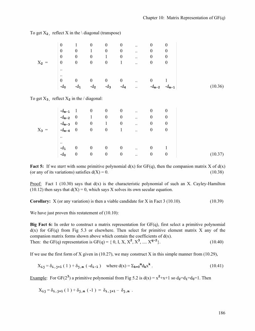
Chapter 10: Matrix Representation of GF(q)
186
To get X2, reflect X in the \ diagonal (transpose) 0 1 0 0 0 .. 0 0 0 0 1 0 0 .. 0 0 0 0 0 1 0 .. 0 0 X2 = 0 0 0 0 1 .. 0 0 .. .. 0 0 0 0 0 .. 0 1 -d0 -d1 -d2 -d3 -d4 .. -dm-2 -dm-1 (10.36) To get X3, reflect X2 in the / diagonal: -dm-1 1 0 0 0 .. 0 0 -dm-2 0 1 0 0 .. 0 0 -dm-3 0 0 1 0 .. 0 0 X3 = -dm-4 0 0 0 1 .. 0 0 .. .. -d1 0 0 0 0 .. 0 1 -d0 0 0 0 0 .. 0 0 (10.37) Fact 5: If we start with some primitive polynomial d(x) for GF(q), then the companion matrix X of d(x) (or any of its variations) satisfies d(X) = 0. (10.38) Proof: Fact 1 (10.30) says that d(x) is the characteristic polynomial of such an X. Cayley-Hamilton (10.12) then says that d(X) = 0, which says X solves its own secular equation. Corollary: X (or any variation) is then a viable candidate for X in Fact 3 (10.10). (10.39) We have just proven this restatement of (10.10): Big Fact 6: In order to construct a matrix representation for GF(q), first select a primitive polynomial d(x) for GF(q) from Fig 5.3 or elsewhere. Then select for primitive element matrix X any of the companion matrix forms shown above which contain the coefficients of d(x). Then: the GF(q) representation is GF(q) = { 0, I, X, X2, X3, .... Xq-2}. (10.40) If we use the first form of X given in (10.27), we may construct X in this simple manner from (10.29), Xij = δi,j+1 ( 1 ) + δj,m ( -di-1 ) where d(x) = Σk=0mdkxk . (10.41) Example: For GF(23) a primitive polynomial from Fig 5.2 is d(x) = x2+x+1 so d2=d1=d0=1. Then Xij = δi,j+1 ( 1 ) + δj,m ( -1 ) = δi,j+1 – δj,m .

Chapter 10: Matrix Representation of GF(q)
187
(d) Maple program to construct the matrix representation of GF(pm) The code is self-documented. The p,m values selected in this code are for GF(23).

Chapter 10: Matrix Representation of GF(q)
188
Example: GF(23) This example uses the numbers shown in the above code. The primitive polynomial d(x) = 1 + x + x3 is the same one used in the example below (6.10). Here are the 8 matrices of our matrix representation of GF(23),
As expected, X7 = I and I does not appear as some lesser power of X. There are 232 = 29 = 512 possible matrices containing 1's and 0's (the ring X2
3), and we have used 8 of them to represent GF(23). Since GF(23) has q-1 = 7 which is prime, any power of X can also serve as the primitive element, and then the matrices above get reordered. Also, the primitive element X can be replaced by any of its reflected versions as noted above in (10.35-37), which set includes the simple transpose of X. Example: GF(32) The primitive polynomial f(x) = x2 + x +2 is the same one quoted below (6.15). Here are the 9 matrices of our matrix representation of GF(32),
As expected, X8 = I and I does not appear as some lesser power of X. Notice that X4 = 2I which is not the same as I. There are 322 = 81 possible matrices containing 0,1,2 (the ring X3
2), and we have used 9 of them to represent GF(32). Example: GF(29) For this example we use the Fig 5.3 primitive polynomial x9 + x4 + 1:
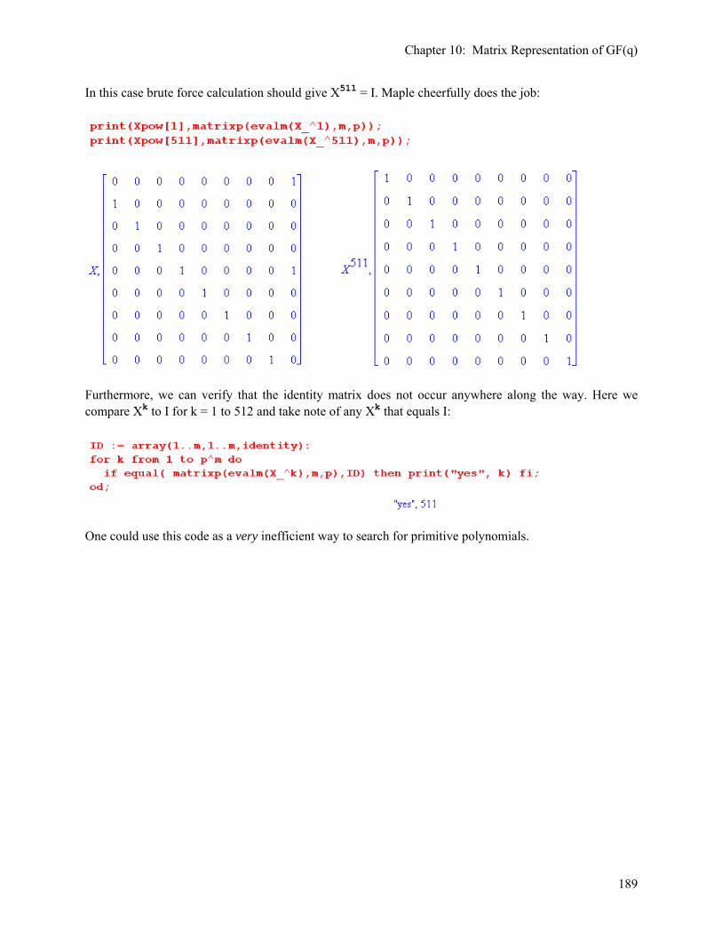
Chapter 10: Matrix Representation of GF(q)
189
In this case brute force calculation should give X511 = I. Maple cheerfully does the job:
Furthermore, we can verify that the identity matrix does not occur anywhere along the way. Here we compare Xk to I for k = 1 to 512 and take note of any Xk that equals I:
One could use this code as a very inefficient way to search for primitive polynomials.
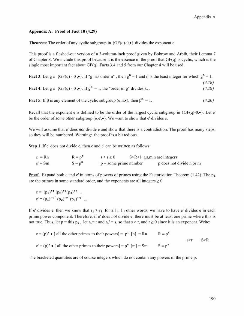
Appendix A
190
Appendix A: Proof of Fact 10 (4.29) Theorem: The order of any cyclic subgroup in {GF(q)-0,•} divides the exponent e. This proof is a fleshed-out version of a 3-column-inch proof given by Bobrow and Arbib, their Lemma 7 of Chapter 8. We include this proof because it is the essence of the proof that GF(q) is cyclic, which is the single most important fact about GF(q). Facts 3,4 and 5 from our Chapter 4 will be used: Fact 3: Let g ∈ {GF(q) - 0 ,•}. If "g has order n" , then gn = 1 and n is the least integer for which gn = 1. (4.18) Fact 4: Let g ∈ {GF(q) - 0 ,•}. If gk = 1, the "order of g" divides k. . (4.19) Fact 5: If β is any element of the cyclic subgroup (α,n,•), then βn = 1. (4.20) Recall that the exponent e is defined to be the order of the largest cyclic subgroup in {GF(q)-0,•}. Let e' be the order of some other subgroup (α,e',•). We want to show that e' divides e. We will assume that e' does not divide e and show that there is a contradiction. The proof has many steps, so they will be numbered. Warning: the proof is a bit tedious. Step 1. If e' does not divide e, then e and e' can be written as follows: e = Rn R = pr s > r ≥ 0 S>R>1 r,s,m,n are integers e' = Sm S = ps p = some prime number p does not divide n or m Proof. Expand both e and e' in terms of powers of primes using the Factorization Theorem (1.42). The pi are the primes in some standard order, and the exponents are all integers ≥ 0. e = (p1)r1 (p2)r2(p3)r3 ... e' = (p1)r1' (p2)r2'(p3)r3' ... If e' divides e, then we know that ri ≥ ri' for all i. In other words, we have to have e' divides e in each prime power component. Therefore, if e' does not divide e, there must be at least one prime where this is not true. Thus, let p = this pi, let ri= r and ri' = s, so that s > r, and r ≥ 0 since it is an exponent. Write: e = (p)r • [ all the other primes to their powers] = pr [n] = Rn R ≡ pr s>r S>R e' = (p)s • [ all the other primes to their powers] = ps [m] = Sm S ≡ ps
The bracketed quantities are of course integers which do not contain any powers of the prime p.

Appendix A
191
Step 2. Consider G = (g,e,•) and G' = (g',e',•). That is, g is a generator of G of order e, and g' is a generator of G' of order e'. Then construct these two elements: g1 = (g)R in G Claim that order of g1= n. (g1, n, •) = G1
g2 = (g')m in G' Claim that order of g2 = S. (g2, S, •) = G2 Proof: Consider these facts: (g1)n = (g)nR = (g)e = 1 (g2)S = (g')Sm = (g')e'= 1 In each line, the last equality is due to fact that e and e' are the orders of the two subgroups G and G'. This is an application of Fact 5. Since (g1)n = 1, according to Fact 4 we know that the order of g1 divides n. So we write both: (g1)n = 1 ⇒ (order of g1) divides n ⇒ (order of g1) = n/d1 (g2)S = 1 ⇒ (order of g2) divides S ⇒ (order of g2) = S/d2 . We now argue that d1 = d2 = 1. If this is not so, then for example get: (g1)n/d1 = (g)nR/d1 = (g)e/d1 = 1 (g2)S/d2 = (g')Sm/d2 = (g')e'/d2 = 1 The top last equality here says (order of g) divides (e/d1 ) for d1>1. This implies that (order of g) < e. This is a contradiction since we assumed at the start that (order of g) = e. Thus d1 = 1. Similarly for the lower line. Therefore: d1 = 1 ⇒ (order of g1) = n d2 = 1 ⇒ (order of g2) = S So now we know the order of our two constructed elements g1 and g2. Step 3. Now construct element g3 = g1g2. Let d = (order of g3) as shorthand, so we have G3 = (g3, d,•). Claim: 1. (g3)d = 1 2. d divides nS. Proof: (1) This follows from Fact 3. (2) Using above facts, we find that: (g3)nS = [(g1)n] S [(g2)S] n = 1S 1n = 1 . Therefore, from Fact 4, we know that (order of g3 ) divides nS, so d divides nS. This result will again be used at the very end of this proof.

Appendix A
192
Step 4. Define h = (g1)d . Claim that h lies in both G1 and G2 . Proof: We know that (g3)d = 1. Therefore, (g1d) (g2d) = 1. Therefore (g1d) = (g2d)-1, the inverse element of (g2d). But the inverse of any element in G2 is in G2, since it is a group. Thus, h = (g1d) lies in G2. Of course it also lies in G1 since it is a power of g1. Step 5: Now consider the subgroup ( h, I, •) generated by h, and let I be its order. We claim that I divides n I divides S Proof: Since h is in G1, we know from Fact 5 that hn = 1 since n is the order of G1. Since I is the order of h, we know from Fact 4 that I divides n. Similarly, since h is in G2, we know from Fact 5 that hS= 1 since S is the order of G2. Since I is the order of h, we know from Fact 4 that I divides S. Step 6: Claim the following sequence of results: 1. I = 1 2. h = 1 3. (g1d) = 1 and (g2d) = 1. 4. n divides d 5. S divides d Proof: (1) We know that S = ps for some prime p, and that n has no powers of p. This means that GCD(n,S) = 1, n and S are "relatively prime". If a number divides into both n and S, that number must be 1. Therefore, from Step 5, I = 1. Thus, our subgroup ( h, I, •) has order I = 1; (2) I=1 means that h1= 1, or simply h = 1. (3) Since (g1d) (g2d) = 1 and h = (g1)d, the last results follows. (4) Since order of g1 is n, and since (g1d) = 1, we know from Fact 4 that n divides d. (5) Since order of g2 is S, and since (g2d) = 1, we know from Fact 4 that S divides d. Step 7: Claim that nS divides d. Proof: We have already noted that n and S are relatively prime. Thus, if these two numbers both divide into a third number, that third number must be a multiple of nS. From Step 6's 4 and 5 above, we know that n and S each divide d, and therefore d must be a multiple of nS. Thus, nS divides d. Step 8: Claim that d = nS. Proof: From Step 3 above, we learned that d divides nS. From Step 7 we learned that nS divides d. The conclusion is that d = nS. Step 9: This leads to the contradiction that d > e, and therefore e' divides e. Proof: Recall that d is the order of field element g3 in G3 = (g3, d,•). We have just shown that d = nS. Since S > R, we know that d > nR. But nR = e, so we have d > e. This is a contradiction because the order of any subgroup is supposed to be less than e -- this was how e was defined.
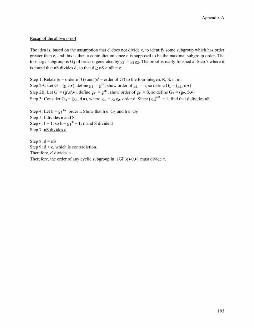
Appendix A
193
Recap of the above proof The idea is, based on the assumption that e' does not divide e, to identify some subgroup which has order greater than e, and this is then a contradiction since e is supposed to be the maximal subgroup order. The too-large subgroup is G3 of order d generated by g3 = g1g2. The proof is really finished at Step 7 where it is found that nS divides d, so that d ≥ nS > nR = e. Step 1: Relate (e = order of G) and (e' = order of G') to the four integers R, S, n, m. Step 2A: Let G = (g,e,•), define g1 = gR , show order of g1 = n, so define G1 = (g1, n,•) Step 2B: Let G' = (g',e',•), define g2 = g'm , show order of g2 = S, so define G2 = (g2, S,•) Step 3: Consider G3 = (g3, d,•), where g3 = g1g2, order d. Since (g3)nS = 1, find that d divides nS. Step 4: Let h = g1d, order I. Show that h ∈ G1 and h ∈ G2 Step 5: I divides n and S Step 6: I = 1, so h = g1d = 1; n and S divide d Step 7: nS divides d Step 8: d = nS Step 9: d > e, which is contradiction. Therefore, e' divides e. Therefore, the order of any cyclic subgroup in {GF(q)-0,•} must divide e.
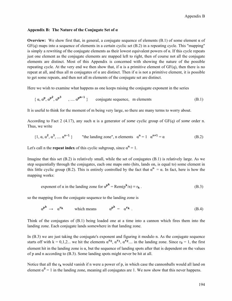
Appendix B
194
Appendix B: The Nature of the Conjugate Set of α Overview: We show first that, in general, a conjugate sequence of elements (B.1) of some element α of GF(q) maps into a sequence of elements in a certain cyclic set (B.2) in a repeating cycle. This "mapping" is simply a rewriting of the conjugate elements as their lowest equivalent powers of α. If this cycle repeats just one element as the conjugate elements are mapped left to right, then of course not all the conjugate elements are distinct. Most of this Appendix is concerned with showing the nature of the possible repeating cycle. At the very end we then show that, if α is a primitive element of GF(q), then there is no repeat at all, and thus all m conjugates of α are distinct. Then if α is not a primitive element, it is possible to get some repeats, and then not all m elements of the conjugate set are distinct. Here we wish to examine what happens as one keeps raising the conjugate exponent in the series { α, αp, αp2, αp3 , .... αpm-1 } conjugate sequence, m elements (B.1) It is useful to think for the moment of m being very large, so there are many terms to worry about. According to Fact 2 (4.17), any such α is a generator of some cyclic group of GF(q) of some order n. Thus, we write {1, α, α2, α3, .... αn-1 } "the landing zone", n elements αn = 1 αn+1 = α (B.2) Let's call n the repeat index of this cyclic subgroup, since αn = 1. Imagine that this set (B.2) is relatively small, while the set of conjugates (B.1) is relatively large. As we step sequentially through the conjugates, each one maps onto (hits, lands on, is equal to) some element in this little cyclic group (B.2). This is entirely controlled by the fact that αn = α. In fact, here is how the mapping works: exponent of α in the landing zone for αpk = Rem(pk/n) ≡ rk . (B.3) so the mapping from the conjugate sequence to the landing zone is αpk → αrk which means αpk = αrk . (B.4) Think of the conjugates of (B.1) being loaded one at a time into a cannon which fires them into the landing zone. Each conjugate lands somewhere in that landing zone. In (B.3) we are just taking the conjugate's exponent and figuring it modulo n. As the conjugate sequence starts off with k = 0,1,2... we hit the elements αr0, αr1, αr2.... in the landing zone. Since r0 = 1, the first element hit in the landing zone is α, but the sequence of landing spots after that is dependent on the values of p and n according to (B.3). Some landing spots might never be hit at all. Notice that all the rk would vanish if n were a power of p, in which case the cannonballs would all land on element α0 = 1 in the landing zone, meaning all conjugates are 1. We now show that this never happens.

Appendix B
195
Fact: Order n is not a power of p. (B.5) Proof: The cyclic group shown in (B.2) has n elements and is certainly a subgroup of { GF(q) - 0} which has q-1 elements. From (1.9d) then we know that n must divide evenly into q-1 = pm - 1. Suppose n were some power of p, n = pk. This value of n does not divide evenly into pm - 1 and in fact there is always a remainder of -1. Thus, the order n cannot be a power of p. Let us now assume there is some minimum k = k0 > 0 such that rk0 = Rem(pk0/n) = 1. This k0 would mark the second cannonball that lands on α (the first was marked with k = 0). For example, if n = 5 and p = 2, we get k0 = 4. If there is no k0 that is less than m (the max number of conjugates), then α is hit only once by the limited set of conjugates shown above. So assume k0 does exist.
Fact: We now claim this to be true: Rem[ pk0+s
n ] = rs, where rs is as in (B.3). (B.6)
We will prove this below, but first, what is this saying? Well, for k = 0,1,2...k0-1, our αpk land on αr0 = α, αr1, αr2.... αrk0-1 in the landing zone, according to (B.4). Then when k=k0 we land on
αrk0 = α1 = α again. Then as s increments and we have k = k0 + s for s = 1,2,... and then our αpk land on αr1, αr2.... all over again, a second time! This is what that above Facts says. So if we have a large number of conjugates (B.1) and a small cyclic group (B.2), this says that as the conjugates are mapped in sequence, they are sprayed into the landing zone in a sequence of landing spots that repeats again and again in the same order. As noted above, this sequence might never hit one or more of the landing spots. Proof: Apply Little Lemma 2 (1.30) ,
Rem[ xyn ] = Rem[
y Rem(x/n) n ] (1.30a)
with x = pk0 and y = ps and xy = pk0+s to get,
Rem[ pk0+s
n ] = Rem [ ps Rem( pk0/n)
n ] = Rem [ ps 1
n ] = rs . QED
Now consider this enhanced version of the previous Fact:
Fact: Rem[ pNk0+s
n ] = rs, the same rs numbers given above, for N = 0,1,2... (B.7)
If we have a large number of conjugates (B.1) and a small cyclic group (B.2), this Fact says that as the conjugates are mapped in sequence, they are sprayed into the landing zone in a sequence of landing spots that repeats again and again in the same order! The first spray sequence has N = 0 and then the Fact just restates (B.3). The second spray sequence has N = 1, which we studied in (B.6). Then N = 2,3,4.. are

Appendix B
196
further repeats of the same spray sequence. As noted above, this sequence might never hit one or more of the landing spots. Proof: We prove this by induction. Assume it is true for some N (we know N=0 and N=1 work), and show true for N+1. Our proof makes two uses of Little Lemma 2 (1.30). In the first use we have
Rem[ xyn ] = Rem[
y Rem(x/n) n ] (1.30a)
with x = pNk0+s and y = pk0 and xy = p(N+1)k0+s to get
Rem[ p(N+1)k0+s
n ] = Rem[ pk0Rem(pNk0+s/n)
n ]
= Rem [ pk0 rs
n ] // induction proof assumes Fact (B.7) is valid for N = N
= Rem [ rs Rem[pk0/n]
n ] // this is (1.30a) applied again with x = pk0 and y = rs
= Rem(rs1 /n) // from Fact (B.6) = rs // Rem(rs/n) = rs
Thus we have shown that Rem[ p(N+1)k0+s
n ] = rs which is our Fact (B.7) for N+1. QED
So the question of whether all m conjugates are distinct in the original set boils down to the question of whether there exists a k0 such that Rem(pk0/n) = 1, where k0 < m. This in turn depends on p and on the order n of the cyclic subgroup which contains element α. If there is some k0 < m, then we get some number of "repeat hits" in the landing zone, which means that some of the conjugate set elements are identical. If α is a primitive element of GF(q), then we know n = q-1 because such an α is a generator of {GF(q)-0} and since this group is cyclic, all group elements can be enumerated as powers of α, see (4.31). In this case, it is easy to see that all m conjugates in the sequence (B.1) are distinct, because there is no k0 < m such that Rem(pk0/n) = 1 since,
Rem [ pk0
n ] = Rem [ pk0
q-1 ] = Rem [ pk0
pm-1 ] = pk0 ≠ 1 .
For the last steps, since k0 < m, the fraction pk0
pm-1 is a proper fraction, so the remainder is pk0 . Since we
assume p ≥ 2 and k0 > 0, we cannot have pk0 = 1. Thus we have proven: Fact: If α is a primitive element of GF(q), then all m conjugates in the conjugate set of α are distinct. Conversely, if α is not a primitive element, it is possible that only the first k0 of the conjugates are in fact distinct, for some k0 < m. (B.8)

Appendix C
197
Appendix C: Evaluation of a(x)b(x) Consider this product of two polynomials c(x) = a(x) b(x) (C.1) where a(x) = Σi=0A aixi b(x) = Σj=0B bjxj (C.2) and where ai and bj lie in Zp whose operations are ⊗ and ⊕. Fact: We will show that
c(x) = Σs=0A+B cs xs where cs = ∑j = max(0,s-A)
min(s, B) (as-j⊗bj) . (C.3)
Proof: Inserting the expansions (C.2) we get a(x) b(x) = (Σi=0A aixi) (Σj=0B bjxj) = Σj=0B Σi=0A (ai⊗bj) xi+j . (C.4) Let s ≡ i+j to get = Σj=0B Σs-j=0A (as-j⊗bj) xs = Σj=0B Σs=0A+j (as-j⊗bj) xs (C.5) We can see that max(s) = A+B, so s ≤ A+B. If we define a function θ(Boolean) such that θ = 1 if the Boolean is true and θ = 0 if it is false, then we are free to insert a factor θ(s ≤ A+B) into our sum to get = Σj=0B Σs=0A+j θ(s ≤ A+B) (as-j⊗bj) xs . (C.6) We can use this same θ function to make explicit the bounds of the subscripts on as-j and bj as-j = {θ(s-j ≥ 0) θ(s-j ≤ A)} as-j = {θ(s ≥ j) θ(s ≤ A+j)} as-j bj = {θ(j ≥ 0) θ(j ≤ B)} bj (C.7) then we have a(x) b(x) = Σj=0B Σs=0A+j {θ(s ≥ j) θ(s ≤ A+j)}{θ(j ≥ 0) θ(j ≤ B)} θ(s ≤ A+B) (as-j⊗bj) xs .
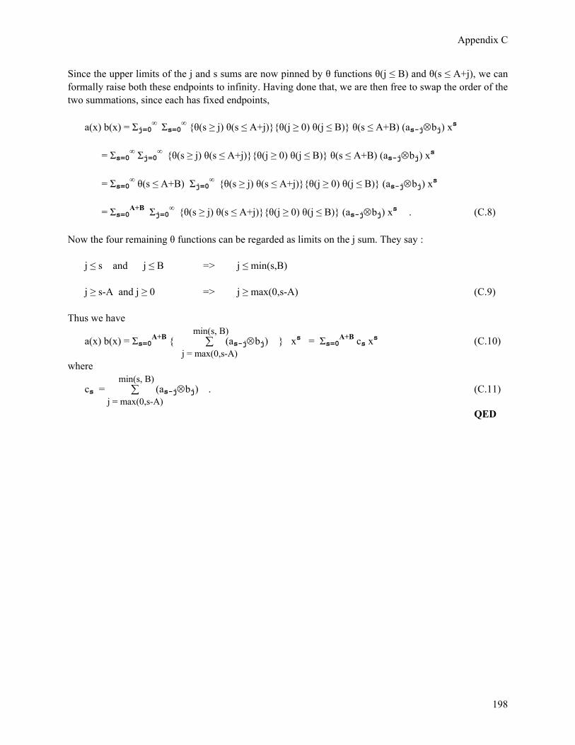
Appendix C
198
Since the upper limits of the j and s sums are now pinned by θ functions θ(j ≤ B) and θ(s ≤ A+j), we can formally raise both these endpoints to infinity. Having done that, we are then free to swap the order of the two summations, since each has fixed endpoints, a(x) b(x) = Σj=0∞ Σs=0∞ {θ(s ≥ j) θ(s ≤ A+j)}{θ(j ≥ 0) θ(j ≤ B)} θ(s ≤ A+B) (as-j⊗bj) xs = Σs=0∞ Σj=0∞ {θ(s ≥ j) θ(s ≤ A+j)}{θ(j ≥ 0) θ(j ≤ B)} θ(s ≤ A+B) (as-j⊗bj) xs = Σs=0∞ θ(s ≤ A+B) Σj=0∞ {θ(s ≥ j) θ(s ≤ A+j)}{θ(j ≥ 0) θ(j ≤ B)} (as-j⊗bj) xs = Σs=0A+B Σj=0∞ {θ(s ≥ j) θ(s ≤ A+j)}{θ(j ≥ 0) θ(j ≤ B)} (as-j⊗bj) xs . (C.8) Now the four remaining θ functions can be regarded as limits on the j sum. They say : j ≤ s and j ≤ B => j ≤ min(s,B) j ≥ s-A and j ≥ 0 => j ≥ max(0,s-A) (C.9) Thus we have
a(x) b(x) = Σs=0A+B { ∑j = max(0,s-A)
min(s, B) (as-j⊗bj) } xs = Σs=0A+B cs xs (C.10)
where
cs = ∑j = max(0,s-A)
min(s, B) (as-j⊗bj) . (C.11)
QED

Appendix D
199
Appendix D: A Small Collection of Matrix Facts If the reader is anything like the author, all these facts are familiar but don't suffer from being refreshed from time to time. The reader may consult any book on matrices to find proofs of things unproven here. All the following facts deal with square matrices. We use an mxm matrix A as our prototype. It is of course assumed that the reader has a basic knowledge of matrices, such as how to multiply them and how to compute a determinant. It is assumed in this section that the elements of the matrix A are just "numbers", meaning complex numbers. More generally, the matrix elements are elements of some field F. In our application in Chapter 10, that field will be Zp= GF(p). It is amazing how the theory of matrices seems to infiltrate every field of human interest in which there is some attempt to calculate something. There are probably a thousand "facts" about matrices which could be listed in an exhaustive treatise, which this small review is not. Convention: For the definitions which follow, we shall assume that the "first" row or column or a matrix is labeled by 1. Labels increase top to bottom for rows, and left to right for columns. If A is a matrix, and its elements are Aij , the first index i is the row index, and the second j is the column index. Thus, the first row of this matrix has elements A11, A12, A13, ... The row index is constant across a row, and serves to define a row. Similarly for the column index. The transpose of a matrix A we shall call AT. It is a new matrix formed by interchanging the rows and columns of A. We have then (AT)ij = Aji. (D.1) A tensor of rank n is a "matrix" with n subscripts instead of 2. For example, Aijk is a rank-3 tensor. A matrix is a rank-2 tensor, a vector is a rank-1 tensor. This is a simplification of the meaning of a tensor; for detail on this subject see the author's reference on tensor analysis or elsewhere. (D.2) The completely antisymmetric tensor εabcde... of rank n is defined as follows. If the subscripts are an even permutation of 123...n, it is (+1). If the subscripts are an odd permutation, it is (-1). If the subscripts are not a permutation, this means some subscripts are repeats, and in this case it is (0). This object is totally antisymmetric because it changes sign when any two indices are swapped. It is also called the permutation tensor. (D.3) Comment: The actual tensor nature of εabcde... is an interesting subject, see the author's tensor analysis reference, Section 7 (h) and Appendix D. The εabcde... object is a tensor density of weight -1. Example : The rank 6 totally antisymmetric tensor. Some sample elements: ε123456 = 1 ε132456= -1 ε132465 = 1 ε123345= 0 The determinant of an mxm matrix A is indicated by det(A) or |A| and is defined as: det(A) = εabcde...A1aA2bA3cA4d ... ( = εabcde...Aa1Ab2Ac3Ad4 .. .) (D.4)

Appendix D
200
where ε is the totally antisymmetric tensor of rank m defined above. In the above formula, each repeated index is implicitly summed from 1 to m. There are a total of m such indices, hence there are a total of m factors of A. This form of the determinant is convenient for making some points below. It is assumed that the reader is familiar with the more normal "recursive" method of computing a determinant in terms of sub-determinants by starting with any row or column. Example: Determinant of a 2x2 matrix: det(A) = εabA1aA2b = ε12A11A22 + ε21 A12A21 = A11 A22 - A12A21 Fact 1: Adding a multiple of one row to another row does not change the determinant of a matrix, although it certainly changes the matrix itself. The same applies for columns. (D.5) Fact 2: det(A) = det(AT) det(AB) = det(A)det(B) det(ABC) = det(A)det(B)det(C) = det(BCA) = det(CAB) det(RR-1) = det(1) = 1 = det(R)det(R-1) (D.6) Fact 3: If A is an mxm matrix, and α is a constant, then det(αA) = αm det(A). (D.7) If A is a square matrix, then the cofactor of a matrix element Aij is denoted by [cof(A)]ij and is equal to (-1)i+j times the determinant of the submatrix obtained by crossing out the row and column which contains Aij. Thus, the cofactor is just some number. Since there is one cofactor for each element of a matrix, we can combine all these cofactors into a new matrix called the cofactor matrix cof(A). Fact 4: The inverse of a square matrix A is given by A-1 = [cof(A)] T / det(A) (D.8) Corollary 4: The inverse A-1 exists if and only if det(A) ≠ 0. (D.9) If det(A) = 0 so this A-1 does not exist, A is said to be singular. The matrix [cof(A)]T is sometimes called the adjoint matrix of A and denoted adj(A). That is , the adjoint is the transpose of the cofactor matrix of A. We will not use this adjoint terminology. The trace of a square matrix A is denoted tr(A) and is defined as the sum of the diagonal elements. (D.10) Peculiar Fact 5: If A is a square matrix, then det(eA) = etr(A). (D.11)

Appendix D
201
The rank of an mxm matrix A is denoted r(A) and is the number of linearly independent rows or columns. It is also the size of the largest non-zero sub-determinant. The size m of a square matrix is called its order. The quantity (order - rank) is called the degeneracy or the nullity of A, denoted by n(A). Thus, n(A) = m - r(A). (D.12) If Ax = 0, the space of solutions x, called the nullspace of A, has dimension n(A). If matrix A has full rank m, then n(A) = m-m = 0 and the nullspace contains only the trivial element x = 0. This is the case in which the inverse A-1 exists and of course then x = A-10 = 0. (D.13) The rank of a matrix has nothing to do with the rank of a tensor mentioned above. It just happens that the same word is used for both concepts. Corollary 5: If an mxm matrix A is invertible, it has full rank m. (D.14) Proof: From Fact 4, A invertible means det(A) ≠ 0, which means rank = m. Peculiar Fact 6: Consider the equation C = AB for three square matrices. It turns out that n(c) ≥ n(a),n(b) but n(c) ≤ n(a) + n(b). This "triangle rule" is called Sylvester's Law of Nullity. (D.15) The characteristic polynomial d(x) of a square matrix A is d(x) ≡ det(xI - A). (D.16) Here, I is the identity matrix. Fact 7: The characteristic polynomial of an mxm matrix A is of degree m. Two of the coefficients of d(x) are known at once: d0 = (-1)mdet(A), and dm = 1. From this last, d(x) is a monic polynomial, meaning the coefficient of the highest power is 1. (D.17) Proof: From the expression (D.4) given for a determinant, it is clear that one term in the determinant is the product of the diagonal elements of the matrix with a (+1) coefficient. If the matrix is (xI-A), then this term has the form ( x - A11) (x-A22).... ( x - Amm) = xm + .... . This shows that the degree is m and the leading coefficient is dm = 1. As for the constant term, d(0) = d0 = det(0I-A) = det(-A) = (-1)mdet(A). The equation det(xI - A) = 0 [ d(x) = 0 ] is called the characteristic equation or sometimes the secular equation. The roots of the characteristic polynomial are thus the solutions to the secular equation. These roots/solutions are called eigenvalues and are often denoted λi. Thus, d(λi) = 0 for any eigenvalue λi. The eigenvalues of A are the solutions to its secular equation. (D.18) Comment: The characteristic equation arises in the calculation of long-term variations in the motion of the planets. Such long term variations are called "secular motions". OED2 gives these distinct definitions of the word secular: I. Of or pertaining to the world (as opposed to the spiritual realm); II Of or pertaining to an age or long period.
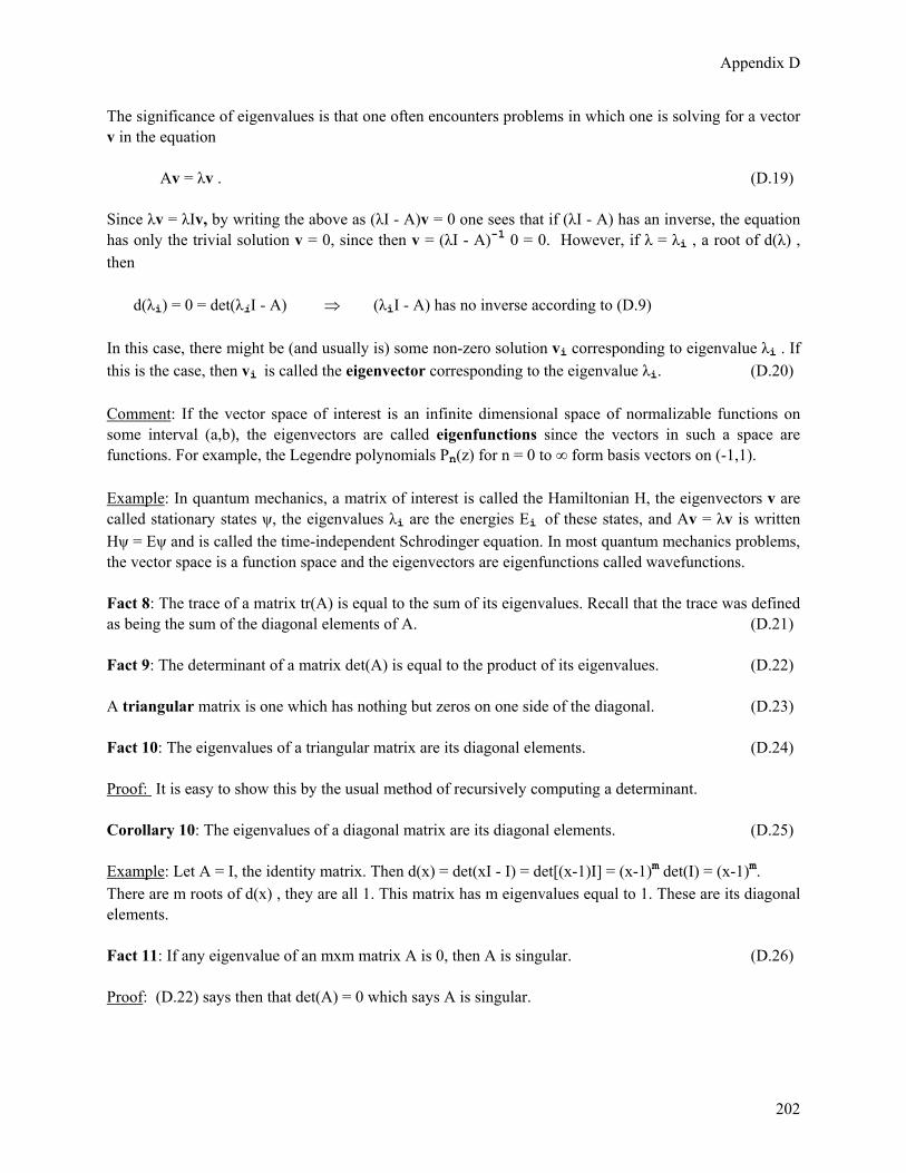
Appendix D
202
The significance of eigenvalues is that one often encounters problems in which one is solving for a vector v in the equation Av = λv . (D.19) Since λv = λIv, by writing the above as (λI - A)v = 0 one sees that if (λI - A) has an inverse, the equation has only the trivial solution v = 0, since then v = (λI - A)-1 0 = 0. However, if λ = λi , a root of d(λ) , then d(λi) = 0 = det(λiI - A) ⇒ (λiI - A) has no inverse according to (D.9) In this case, there might be (and usually is) some non-zero solution vi corresponding to eigenvalue λi . If this is the case, then vi is called the eigenvector corresponding to the eigenvalue λi. (D.20) Comment: If the vector space of interest is an infinite dimensional space of normalizable functions on some interval (a,b), the eigenvectors are called eigenfunctions since the vectors in such a space are functions. For example, the Legendre polynomials Pn(z) for n = 0 to ∞ form basis vectors on (-1,1). Example: In quantum mechanics, a matrix of interest is called the Hamiltonian H, the eigenvectors v are called stationary states ψ, the eigenvalues λi are the energies Ei of these states, and Av = λv is written Hψ = Eψ and is called the time-independent Schrodinger equation. In most quantum mechanics problems, the vector space is a function space and the eigenvectors are eigenfunctions called wavefunctions. Fact 8: The trace of a matrix tr(A) is equal to the sum of its eigenvalues. Recall that the trace was defined as being the sum of the diagonal elements of A. (D.21) Fact 9: The determinant of a matrix det(A) is equal to the product of its eigenvalues. (D.22) A triangular matrix is one which has nothing but zeros on one side of the diagonal. (D.23) Fact 10: The eigenvalues of a triangular matrix are its diagonal elements. (D.24) Proof: It is easy to show this by the usual method of recursively computing a determinant. Corollary 10: The eigenvalues of a diagonal matrix are its diagonal elements. (D.25) Example: Let A = I, the identity matrix. Then d(x) = det(xI - I) = det[(x-1)I] = (x-1)m det(I) = (x-1)m. There are m roots of d(x) , they are all 1. This matrix has m eigenvalues equal to 1. These are its diagonal elements. Fact 11: If any eigenvalue of an mxm matrix A is 0, then A is singular. (D.26) Proof: (D.22) says then that det(A) = 0 which says A is singular.
Appendix D
203
A similarity transformation of a square matrix A is defined by A' = S A S-1 (D.27) where S is any square matrix such that S-1 exists and thus det(S) ≠ 0. One says that A and A' are similar. If we define Q ≡ S–1, then A' =Q-1AQ, another form of a similarity transformation. Observation: Saying that A and A' are similar is like saying that a rotated set of axes (x',y',z') is similar to an unrotated set (x,y,z). Generally speaking, a similarity transformation does not change the nature of what is going on, it just changes how things are labeled. It is a change of basis. The following fact should impress upon the reader how little a similarity transformation changes the nature of a matrix. Fact 12: Similar matrices have the same determinant, the same trace, the same rank, the same characteristic polynomial, and the same eigenvalues. In addition, any equation involving matrices retains its same form after application of a similarity transformation. Such an equation is said to be covariant. (D.28) Example: If AB=C, then apply S .. S-1 to get (S A S-1 )(S B S-1) = (S C S-1 ) or A'B' = C' . Comment: There are certain interesting classes of matrices (Hermitian, real symmetric) which can be brought to diagonal form by a similarity transformation (unitary, real orthogonal). If one can find this similarity transformation, then one at once knows all the eigenvalues of the original matrix, since they are just the diagonal elements of the transformed matrix and since eigenvalues are preserved under any similarity transformation. The process of bringing a matrix to diagonal form is called diagonalization. A notable absence from this Appendix is the Cayley-Hamilton theorem. Since this plays such a key role in Chapter 10, it is stated there in (10.12).
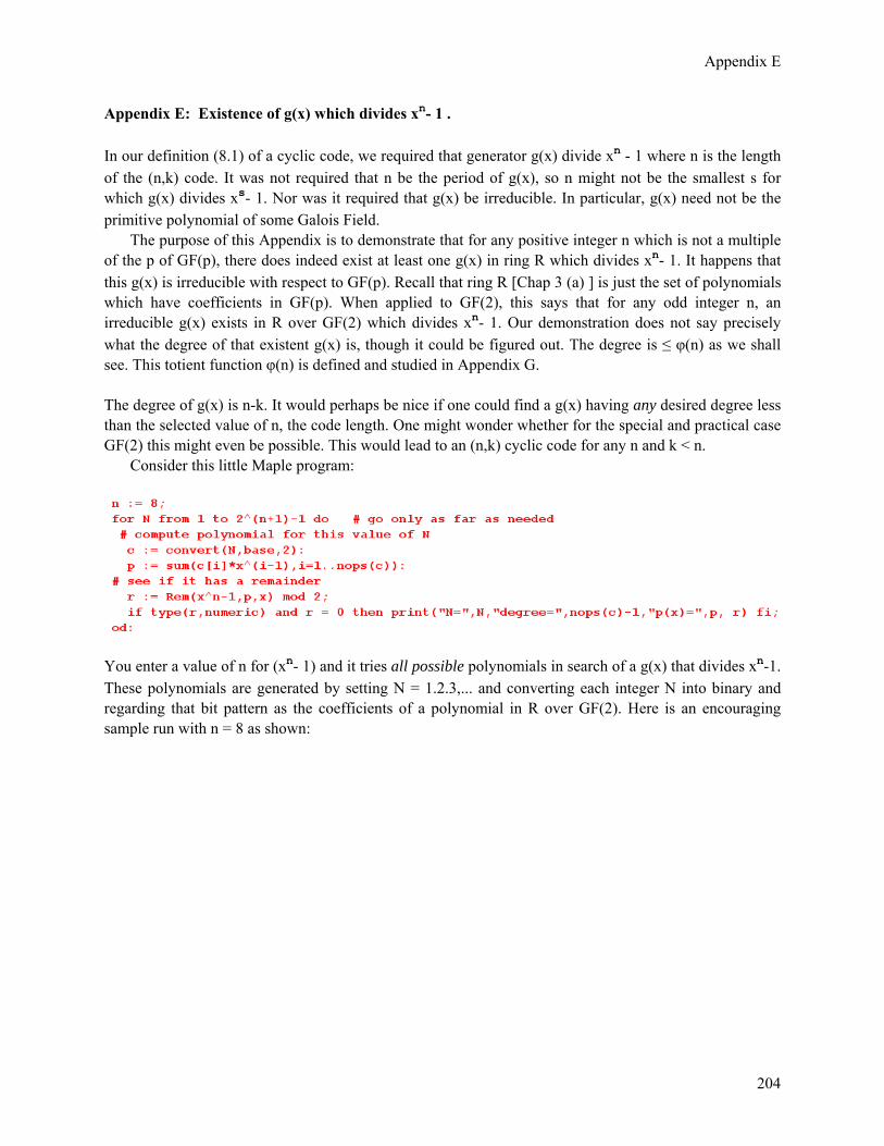
Appendix E
204
Appendix E: Existence of g(x) which divides xn- 1 . In our definition (8.1) of a cyclic code, we required that generator g(x) divide xn - 1 where n is the length of the (n,k) code. It was not required that n be the period of g(x), so n might not be the smallest s for which g(x) divides xs- 1. Nor was it required that g(x) be irreducible. In particular, g(x) need not be the primitive polynomial of some Galois Field. The purpose of this Appendix is to demonstrate that for any positive integer n which is not a multiple of the p of GF(p), there does indeed exist at least one g(x) in ring R which divides xn- 1. It happens that this g(x) is irreducible with respect to GF(p). Recall that ring R [Chap 3 (a) ] is just the set of polynomials which have coefficients in GF(p). When applied to GF(2), this says that for any odd integer n, an irreducible g(x) exists in R over GF(2) which divides xn- 1. Our demonstration does not say precisely what the degree of that existent g(x) is, though it could be figured out. The degree is ≤ φ(n) as we shall see. This totient function φ(n) is defined and studied in Appendix G. The degree of g(x) is n-k. It would perhaps be nice if one could find a g(x) having any desired degree less than the selected value of n, the code length. One might wonder whether for the special and practical case GF(2) this might even be possible. This would lead to an (n,k) cyclic code for any n and k < n. Consider this little Maple program:
You enter a value of n for (xn- 1) and it tries all possible polynomials in search of a g(x) that divides xn-1. These polynomials are generated by setting N = 1.2.3,... and converting each integer N into binary and regarding that bit pattern as the coefficients of a polynomial in R over GF(2). Here is an encouraging sample run with n = 8 as shown:

Appendix E
205
For this value of n, we find a viable g(x) of every degree less than n. Viable just means we could create a cyclic code based on that g(x) (the case g(x) = 1 excluded). Unfortunately, this is true for some values of n and not true for others. There is doubtless some theorem that explains which values of n work and which don't. Here are some values of n which are found not to have g(x) of every possible degree: n = 5,7,9,10,14,15. Some of these are prime, some not, some even, some odd. The run for n = 9 looks like this
so that no g(x) exists of degree 4 or 5. The reason a degree is missing can be analyzed by writing the equation g(x)h(x) = xn-1 where g and h are allowed arbitrary coefficients a,b,c.... For bad values of n, one is led to a set of equations for these coefficients which have no solution. For example, one might end up with the requirement that b + b + 1 = 0 and no b in GF(2) solves that equation. With the above as introduction, we now start into a set of Facts, many of which are quite interesting in their own right. They lead to the final conclusion that some g(x) which divides xn-1 does exist.
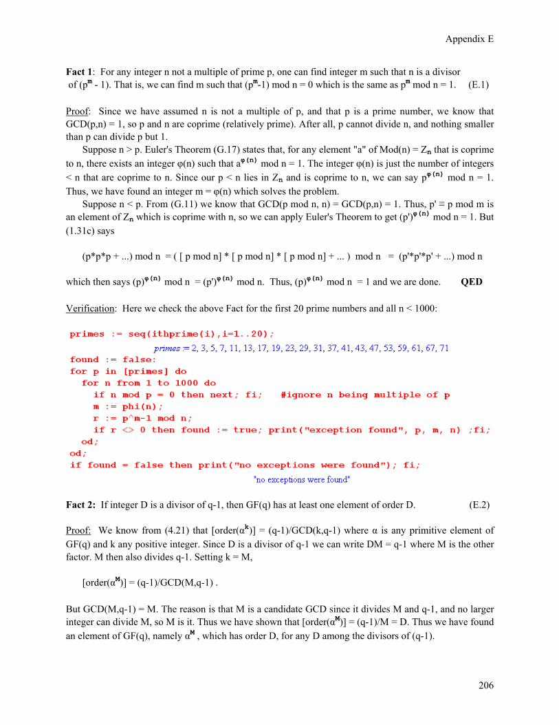
Appendix E
206
Fact 1: For any integer n not a multiple of prime p, one can find integer m such that n is a divisor of (pm - 1). That is, we can find m such that (pm-1) mod n = 0 which is the same as pm mod n = 1. (E.1) Proof: Since we have assumed n is not a multiple of p, and that p is a prime number, we know that GCD(p,n) = 1, so p and n are coprime (relatively prime). After all, p cannot divide n, and nothing smaller than p can divide p but 1. Suppose n > p. Euler's Theorem (G.17) states that, for any element "a" of Mod(n) = Zn that is coprime to n, there exists an integer φ(n) such that aφ(n) mod n = 1. The integer φ(n) is just the number of integers < n that are coprime to n. Since our p < n lies in Zn and is coprime to n, we can say pφ(n) mod n = 1. Thus, we have found an integer m = φ(n) which solves the problem. Suppose n < p. From (G.11) we know that GCD(p mod n, n) = GCD(p,n) = 1. Thus, p' ≡ p mod m is an element of Zn which is coprime with n, so we can apply Euler's Theorem to get (p')φ(n) mod n = 1. But (1.31c) says (p*p*p + ...) mod n = ( [ p mod n] * [ p mod n] * [ p mod n] + ... ) mod n = (p'*p'*p' + ...) mod n which then says (p)φ(n) mod n = (p')φ(n) mod n. Thus, (p)φ(n) mod n = 1 and we are done. QED Verification: Here we check the above Fact for the first 20 prime numbers and all n < 1000:
Fact 2: If integer D is a divisor of q-1, then GF(q) has at least one element of order D. (E.2) Proof: We know from (4.21) that [order(αk)] = (q-1)/GCD(k,q-1) where α is any primitive element of GF(q) and k any positive integer. Since D is a divisor of q-1 we can write DM = q-1 where M is the other factor. M then also divides q-1. Setting k = M, [order(αM)] = (q-1)/GCD(M,q-1) . But GCD(M,q-1) = M. The reason is that M is a candidate GCD since it divides M and q-1, and no larger integer can divide M, so M is it. Thus we have shown that [order(αM)] = (q-1)/M = D. Thus we have found an element of GF(q), namely αM , which has order D, for any D among the divisors of (q-1).

Appendix E
207
Example: For GF(24) we have q-1 = 15 which has divisors 1,3,5 and 15. If α is a primitive element, then we know α15 = 1 since such an element has order q-1. D 1 3 5 15 M 15 5 3 1 βorder=1 (α15)1= 1 (α5)3= 1 (α3)5= 1 (α1)15= 1 order β 1 3 5 15 Here an element β of GF(q) has been found for each divisor of q-1. For D = 1, β = 1 and 11 = 1 so the identity always has an order to match D = 1. For D = 15 we just get the statement that α is a primitive element α15= 1. It is the interior columns that are important. Fact 3: If integer D is a divisor of q -1, then GF(q) has at least one minimum polynomial of period D. (E.3) Proof: From Fact 2, we know that GF(pm) has at least one element (call it α) of order D. This element has a minimum polynomial m(x) of the form (x-α)(other factors). From (5.47) we know that the period of a minimum polynomial is the same as the order of the elements in its conjugate set (here including α), so since α has order D, there exists m(x) of period D. QED Example: Recall this enumeration (6.21) of the minimum polynomials of GF(24), where we have added the two trivial minimum polynomials shown in (5.24) which are always present : p1(x) = (x - α)(x - α2)(x - α4) (x - α8) = x4 + x + 1 10011 p7(x) = (x - α7)(x - α14)(x - α13)(x - α11) = x4 + x3 + 1 11001 m3(x) = (x - α3)(x - α6)(x - α12)(x - α9) = x4 + x3 + x2 + x + 1 11111 m5(x) = (x - α5)(x - α10) = x2 + x + 1 111 (6.21) m0(x) = (x - α0) = (x-1); mzero = (x - 0) = x; We shall now compute the period of each. First the polynomials are entered:
The following procedure scans n downward to find the period of polynomial f(x) :

Appendix E
208
And here are the resulting periods:
As claimed in the Fact, there exists a minimum polynomial of period D for each D that divides pm-1. The function x can never divide any xn- 1 so the procedure sets period = ∞. Fact 4: For any n not a multiple of p, there exists a g(x) which divides xn - 1 and which can therefore be used to construct a cyclic code of length n. This g(x) is irreducible in GF(p). (E.4) Proof: To find a suitable g(x) with coefficients in GF(p), we search through extension fields GF(pm) for m = 1,2,3 ... . We know from Fact 3 that, for any divisor D of pm- 1, GF(pm) has a minimum polynomial m(x) of period D, so that m(x) divides xD-1. If we can find a value of m such that pm - 1 has a divisor D=n then m(x) divides xn - 1 and this m(x) is a viable g(x). But Fact 1 says that we can find m such that n is a divisor of pm -1, namely, m = φ(n). Thus, the field GF(pφ(n)) has a suitable minimum polynomial that can be used for g(x). Corollary: For any n not a multiple of p one can construct a cyclic code of length n whose polynomials have coefficients in GF(p). (E.5) Reminder: It is likely that there are many viable g(x) that divide xn-1 and there will be such viable g(x) even when n is a multiple of p as our examples with GF(2) earlier show (see n = 8 case). It just happens that the g(x) we find here in our existence proof happens to be a minimum polynomial of some Galois extension field GF(q) over GF(p). This g(x) is of course irreducible in GF(p), and may or may not be a primitive polynomial of GF(q).

Appendix F
209
Appendix F: Cyclic Code Error Detection Theorems (CRC) We shall identify the term Cyclic Redundancy Check (CRC) with any error detection system based on an (n,k) cyclic code. The Facts presented in this section are all stated and proved in the original 1961 CRC paper by Peterson and Brown noted in References. The notation used in their paper is the same as ours except for the following differences: us CRC paper generator g(x) P(X) data polynomial D(x) G(X) code polynomial C(x) F(X) semantics g(x) has period n P(X) belongs to exponent n Our proofs are only slightly more general in some cases than those of the paper which deals only with GF(2). We always assume the code length is n and number of data symbols is k. Our definition of a cyclic code includes item (8.1) (b) requiring that g(x) divides xn- 1. If this requirement is ignored, then a "cyclic code" so obtained won't really be cyclic because the proof of Chap 8 (f) fails. Also, the set of code words won't form an ideal in the ring An, and much of the theory of cyclic codes falls apart. Still, the claims below still apply if g(x) does not divide xn- 1. However, in order to detect all double-bit errors, g(x) must divide some xs-1 for some s ≥ n. _____________________________________________________________________________________ Fact 1: If g(0) ≠ 0, a cyclic code generated by g(x) over GF(p) detects all single-symbol errors. (F.1) Proof. Suppose C'(x) and C(x) differ in one symbol position. Then E(x) ≡ C'(x)-C(x) = αxi where i = 0,1..n-1 and α is some non-zero element of GF(p) = Zp. We need to show that in this case the syndrome s(x) will be non-zero so the error will then be detected. But : s(x) = Rem[C'(x)/g(x)] = Rem[{C(x) + E(x)}/g(x)] = Rem[{D(x)g(x) + E(x)}/g(x)] = Rem[E(x)/g(x)] = Rem[α xi/g(x) ] Now: • For i = 0, Rem[αxi/g(x) ] = Rem[α/g(x) ] = α ≠ 0. Note that g(0) ≠ 0 rules out g(x) = constant ≠ 0. • For i > 1, Rem[αxi/g(x) ] ≠ 0 unless g(x) = αxn for n ≤ i, but g(0) ≠ 0 rules out such a g(x). Thus, s(x) ≠ 0 and the error is detected. Notice that it was not required that g(x) divide evenly into xn - 1. _____________________________________________________________________________________ Fact 2: If g(x) = (x-1)f(x), a cyclic code generated by g(x) over GF(2) detects all odd-number-bit errors. (F.2) Comment: x-1 is the same as x+1 for GF(2) since -1 = +1 in GF(2). Proof: In this case, E(x) = C'(x) - C(x) is a polynomial with an odd number of terms. We must show that in this case the syndrome s(x) does not vanish so the error will be detected. But:

Appendix F
210
s(x) = Rem[E(x)/g(x)] = Rem[(poly with odd of terms) /g(x) ] . Assume that this remainder is 0. Then we would have some quotient q(x) = E(x)/g(x) and poly with odd of terms (x) = g(x) q(x) = (x-1)f(x) q(x) . Evaluate at x = 1 to get odd sum of 1's = 1 = (1-1)f(1)q(1) = 0 Since 1 ≠ 0 we have a contradiction, so it must be that s(x) ≠ 0 and the error is detected. Notice that it was not required that g(x) divide evenly into xn - 1. _____________________________________________________________________________________ Fact 3: If g(0) ≠ 0 and g(x) has period ≥ n, a cyclic code generated by g(x) over GF(2) detects all double-bit errors and all single-bit errors. (F.3) Proof: We already know from Fact 1 that single-bit errors are detected. For double-bit errors we have E(x) = xi + xj for some 0 ≤ i ≤ j ≤ n-1 We need to show that the syndrome does not vanish in this case. s(x) = Rem[E(x)/g(x)] = Rem[(xi+xj)/g(x)] = Rem[xi(xj-i+1)/g(x)] . Since g(0) ≠ 0, we know that g(x) has no factors of x so the xi cancels nothing in g(x), so the only way for s(x) to be 0 is if Rem[(xj-i+1)/g(x)] = 0 which we rewrite in GF(2) as Rem[(xj-i - 1)/g(x)] = 0 . (*) The maximum value of j-i is (n-1)-(0) = n-1. If the period of g(x) is ≥ n, then (*) cannot be true, since the period t of g(x) is the smallest t such that (xt-1) is divisible by g(x). Then we get s(x) ≠ 0 and the double-bit error will be detected. Notice that it was not required that g(x) divide evenly into xn - 1. However, it was required that g(x) have a period ≥ n, the length of the code. _____________________________________________________________________________________
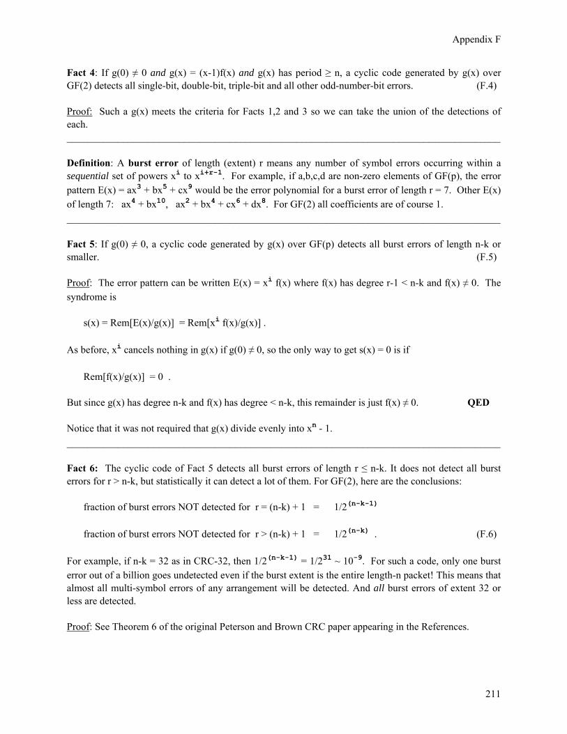
Appendix F
211
Fact 4: If g(0) ≠ 0 and g(x) = (x-1)f(x) and g(x) has period ≥ n, a cyclic code generated by g(x) over GF(2) detects all single-bit, double-bit, triple-bit and all other odd-number-bit errors. (F.4) Proof: Such a g(x) meets the criteria for Facts 1,2 and 3 so we can take the union of the detections of each. _____________________________________________________________________________________ Definition: A burst error of length (extent) r means any number of symbol errors occurring within a sequential set of powers xi to xi+r-1. For example, if a,b,c,d are non-zero elements of GF(p), the error pattern E(x) = ax3 + bx5 + cx9 would be the error polynomial for a burst error of length r = 7. Other E(x) of length 7: ax4 + bx10, ax2 + bx4 + cx6 + dx8. For GF(2) all coefficients are of course 1. _____________________________________________________________________________________ Fact 5: If g(0) ≠ 0, a cyclic code generated by g(x) over GF(p) detects all burst errors of length n-k or smaller. (F.5) Proof: The error pattern can be written E(x) = xi f(x) where f(x) has degree r-1 < n-k and f(x) ≠ 0. The syndrome is s(x) = Rem[E(x)/g(x)] = Rem[xi f(x)/g(x)] . As before, xi cancels nothing in g(x) if g(0) ≠ 0, so the only way to get s(x) = 0 is if Rem[f(x)/g(x)] = 0 . But since g(x) has degree n-k and f(x) has degree < n-k, this remainder is just f(x) ≠ 0. QED Notice that it was not required that g(x) divide evenly into xn - 1. _____________________________________________________________________________________ Fact 6: The cyclic code of Fact 5 detects all burst errors of length r ≤ n-k. It does not detect all burst errors for r > n-k, but statistically it can detect a lot of them. For GF(2), here are the conclusions: fraction of burst errors NOT detected for r = (n-k) + 1 = 1/2(n-k-1)
fraction of burst errors NOT detected for r > (n-k) + 1 = 1/2(n-k) . (F.6) For example, if n-k = 32 as in CRC-32, then 1/2(n-k-1) = 1/231 ~ 10-9. For such a code, only one burst error out of a billion goes undetected even if the burst extent is the entire length-n packet! This means that almost all multi-symbol errors of any arrangement will be detected. And all burst errors of extent 32 or less are detected. Proof: See Theorem 6 of the original Peterson and Brown CRC paper appearing in the References.

Appendix G
212
Appendix G: GCD, mod n, totient φ(n), Euler Theorem, Fermat's Little Theorem Here we take a brief tour of "number theory" with the goal being to arrive at the endpoints of Euler's Theorem (Fact 11) and Fermat's Little Theorem (Fact 12). More trees in the forest. The entire thread presented here (excluding a few references to items in the main document) is completely self-contained, and each Fact has a proof. In our selected pathway, every Fact in this section is required to get the train to the station. No doubt there are shorter paths, but all these Facts are worth stating and proving. If the GCD and Mod concepts are old hat to you, all these Facts will all be familiar. Euler's Theorem is used in Appendix E to prove (E.1). The two Facts 13 and 14 show how the number of primitive elements and the number of primitive polynomials of a Galois Field are related to the totient function φ defined below in (G.15). The final Fact 15 examines the smallest-x solution of the Diophantine equation ax = bx. _____________________________________________________________________________________ Fact 0: These fundamental modulo arithmetic rules were stated and derived in (1.31c) : (x+y+z + ...) mod n = ( [ x mod n] + [ y mod n] +[ z mod n] + ... ) mod n (x*y*z + ...) mod n = ( [ x mod n]* [ y mod n] * [ z mod n] + ... ) mod n (1.31c) _____________________________________________________________________________________ Fact 1: Let d = GCD(c,m). Then by the meaning of "common divisor" there must exist integers N1 and N2 such that c/d = N1 and m/d = N2. The fact claims that GCD(N1,N2) = 1. (G.1) Proof: Suppose GCD(N1,N2) = K > 1. Then there must exist integers M1 and M2 such that N1/K = M1 => N1 = M1K => c/d = M1K => c/(dK) = M1
N2/K = M2 => N2 = M2K => m/d = M2K => m(dK) = M2 . The equations on the right show that then dK > d is a common divisor of c and m which is a contradiction since d is supposed to be the largest common divisor. QED _____________________________________________________________________________________ Fact 2: Suppose GCD(N1,N2) = 1 and N1A = N2B. Then N2 divides A and N1 divides B. (G.2) Proof: • If N1 = 1 then A = N2B so N2 divides A and of course N1 = 1 divides B. • If N2 = 1 then B = N1A so N1 divides B and of course N2 = 1 divides A. • If N1>1 and N2> 1 and if N1A = N2B, then N2 divides N1A (quotient B). But if GCD(N1,N2) = 1, N2 cannot divide N1 because if it did then N2 > 1 would be a common divisor of N1 and N2. Thus, if N2 divides N1A then N2 must be dividing A. Similarly, N1 must divide B. _____________________________________________________________________________________

Appendix G
213
Notation: The notation a = b mod m is a shorthand for a mod m = b mod m, or (a-b) mod m = 0. It means that a and b are congruent mod m. The notation is a little misleading since it seems to say for example 100 = 100 mod 4 = 0 so 100 = 0, but that is not what it means. It means that 100 is congruent with 0 mod 4. A better notation might be a = b (mod m), but that adds clutter. Note then that for a and b integers in Z, there exists an integer I such that a = b mod m ⇔ a mod m = b mod m ⇔ (a-b) mod m = 0 ⇔ (a-b) = I m ⇔ a = b + I m (G.3) _____________________________________________________________________________________
Fact 3: ca = cb mod m ⇔ a = b mod m
GCD(c,m) (G.4)
Proof: Let d ≡ GCD(c,m). As in Fact 1, there exist N1 and N2 such that c = N1d
m = N2d => m
GCD(c,m) = md = N2 = an integer (which is promising!)
Proof in the ⇒ direction:
ca = cb mod m => ca = cb + em => c(a-b) = em => N1d(a-b) = em => a-b = emN1d =
eN1
md .
If we can show that e
N1 is an integer, then we have shown that a = b mod
md as claimed. Go back to
N1d(a-b) = em => N1(a-b) = e md => N1(a-b) = N2 e .
Since GCD(N1,N2) = 1 by Fact 1, Fact 2 says that N2 divides (a-b). Now write the last equation as
e
N1 =
a-bN2
Since we just showed that N2 divides a-b, we have shown that e
N1 is an integer. QED
Proof in the ⇐ direction: If a = b mod N2 then a = b + kN2 and ca = cb + ckN2. But
ckN2 = (N1d)k md = (N1k)m
Thus ca = cb + (N1k)m and so ca = cb mod m. QED
Appendix G
214
_____________________________________________________________________________________ Corollary 3. If GCD(c,m) = 1 then [ ca = cb mod m ⇔ a = b mod m ] . (G.5) In this special case of Fact 3, if we see ca = cb, we can divide both sides by c to get a = b mod m. _____________________________________________________________________________________ Fact 4: (Linear Congruence Theorem). If ax = b mod m and GCD(a,m) = 1, there is a unique mod-m solution x. (G.6) Comment: If a = b mod m, then a and b are said to be congruent mod m. The set of integers a which are congruent to b mod n is called a congruence class. The set of such values was called a residue class in our residue class ring discussion of Chap 1 (c), with an example shown in (1.32). In this Fact our equation to be solved is ax = b which is a linear equation and ax is congruent to b mod m, hence the theorem name. History: An equation of two of more variables, like ax2 + by + cy3 + dz = e, in which all coefficients and variables are restricted to be integers, is called a Diophantine equation, named after a Greek algebra guy Diophantus circa 250 BC. An equation like ax + by = c is a linear Diophantine equation. We saw an example of this in (1.43), Bezout's Identity d = x n1 + y n2 where d = GCD(n1,n2) and we want to solve for integers x and y. In our current Fact 4, we have ax = b mod m which is a "linear Diophantine equation mod m". Hilbert's 10th Problem (1900) was to find an algorithm which could determine whether a given Diophantine equation has a solution or not. The work of several people from 1944 to 1970 showed that such an algorithm does not exist for the general case. Proof of Fact 4: We want to solve ax = b mod m for x. Consider the linear Diophantine equation ay - mz = 1 1 = GCD(a,m) variables y,z Since this is the Bezout Identity (1.43), we know there exists an integer solution for y and z. So we have a specific value of y. Multiply by b to get a(by) = b + m(bz) => a(by) = b mod m Thus our solution is x = by. Suppose there were another solution x'. Then ax = b mod m ax' = b mod m => ax = ax' mod m Since GCD(a,m) = 1, Corollary 3 says that x = x' mod m. Thus our solution x = by is the only solution mod m. QED _____________________________________________________________________________________ Corollary 4: Element a of Zm has an inverse if GCD(a,m) = 1. (G.7) Proof: In Fact 4 we showed that in this case ax = b mod m had a unique solution. Setting b = 1 we find that ax = 1 has a unique solution. But that solution is a-1. [ Zm means Mod(m, +, •) ].
Appendix G
215
_____________________________________________________________________________________ Fact 5: Given a,b > 0, and if x and y exist such that ax+by = 1, then GCD(a,b) = 1. (G.8) Proof: Suppose GCD(a,b) = Q > 1. Then a = QN1 b = QN2 => 1 = ax+by = (QN1)x + (QN2)y = Q (N1x + N2y) => 1/Q = N1x + N2y . But since Q > 1, this says fraction = integer which is a contradiction, so Q = 1. _____________________________________________________________________________________ Fact 6: If GCD(a,m) = 1 and GCD(b,m) = 1, then GCD(ab,m) = 1. (G.9) Proof: From the if conditions we know from Bezout's Identity (1.43) that x,y,x',y' exist such that 1 = ax + my and 1 = bx' + my'. Thus, 1 = (ax + my)( bx' + my') = ab(xx') + m (ybx'+axy'+myy') = ab x" + m y" . From Fact 5, since (ab) x" + m y" = 1 we conclude that GCD(ab,m) = 1. _____________________________________________________________________________________ Fact 7: For any integer I, GCD(a + Im, m) = GCD(a,m). (G.10) Proof: (1) Let s be some common divisor of a and m. Clearly s divides a+Im. Thus, s is a common divisor of the pair a+Im and m. So { common divisors of a and m } ⊂ { common divisors of a+Im and m } . (*) (2) Let s be some common divisor of a+Im and m. Does s divide a? To find out, consider a+Im = s N1
m = s N2
N1 = a+Im
s = as + I
ms =
as + I N2 =>
as = N1 - I N2
Thus, as is an integer so yes, s does divide a. Thus, s is a common divisor of m and a. So
{ common divisors of a+Im and m } ⊂ { common divisors of a and m } (**) (3) We conclude from (*) and (**) that the two common divisor sets are the same set, call it Q.

Appendix G
216
Suppose this set is Q = {1, 5, 17}. Then GCD(a + Im, m) = 17 and GCD(a,m) = 17. In general, we find that both GCD(a + Im, m) and GCD(a,m) will be the largest element of Q, so GCD(a + Im, m) = GCD(a,m). QED _____________________________________________________________________________________ Fact 8: GCD(a mod m, m) = GCD(a,m) (G.11) Proof: We know that a mod m = a + Im for some integer I (I < 0 if a > m). Thus from Fact 7 we have that GCD(a mod m, m) = GCD(a + Im, m) = GCD(a,m). QED _____________________________________________________________________________________ Fact 9: For a,b in Zm (with + and • ), GCD(a•b, m) = GCD(ab mod m, m) = GCD(ab,m). (G.12) Proof: The meaning of a•b is that this product is some element c within Zm which is closed under •. The rule for finding this element c is c = ab mod m, so a•b = ab mod m. Then the last equality shown follows from Fact 8. _____________________________________________________________________________________ Definition: Integers n and m are coprime (relatively prime) iff GCD(n,m) = 1. (G.13) Definition: The set of integers < n which are coprime with n are called the totatives of n. We shall refer to this set as Gn in what follows. (G.14) Example: The totatives of n = 12 are {1,5,7,11} . Definition: Euler's totient function φ(n) is the number of totatives of n. (G.15) Examples: φ(12) = 4 since the set {1,5,7,11} has four elements. φ(7) = 6 since the set {1,2,3,4,5,6} has 6 elements. φ(p) = p-1 if p is prime Comment: It happens that the sum of the totatives of n is (n/2)φ(n), but we shall not prove it since we don't need it. In our example with n = 12, 1+5+7+11 = 24 and (n/2)φ(n) = 6*φ(12) = 6*4 = 24. Here are the first 100 values of φ(n) in the form _____________________________________________________________________________________ Fact 10: The set Gn of the totatives of n forms an abelian group under • within Zn of order φ(n). (G.16) Proof: The properties of a group are shown in (1.1). We know that G is closed under • from Fact 6 which reads " if a and b are in Gn, then ab is in Gn ". We know from (1.29) that Zn forms an abelian ring with identity, so any subset of Zn which includes 1 has the commutative, associative, and identity-exists properties for operator •. What is missing is the existence of a • inverse. When n is a prime p, we showed such an inverse always exists and Zp is then a field GF(p). But for general Zn some inverses do not exist.
Appendix G
217
However, for our set Gn inverses always exist due to Corollary 4 above. Thus Gn is a group of order φ(n). Example: Z8 = {0,1,2,3,4,5,6,7} = Mod(8,+,•) G8 = {1,3,5,7} with • operation of Z8. Note that φ(8) = 4. 3 • 3 = 9 mod 8 = 1 ∈ G8 3-1 = 1 5 • 5 = 15 mod 8 = 7 ∈ G8 5-1= 7 3 • 5 = 15 mod 8 = 7 ∈ G8 5 • 7 = 35 mod 8 = 3 ∈ G8 3 • 7 = 21 mod 8 = 3 ∈ G8 7 • 7 = 49 mod 8 = 1 ∈ G8 7-1 = 1 Thus, G8 is closed under • and all elements have an inverse. _____________________________________________________________________________________ Fact 11: (Euler's Theorem). For any a in Gn, aφ(n) = 1 mod n . (G.17) Proof: Fact (1.9e) says that for any a in group G, an = 1 where n is the order of the group. What that means here is a•a•a...•a = 1 where we have φ(n) factors of a since from Fact 10 the order of Gn is φ(n). The operation • is that of Zn of which Gn is a subset. For elements in Zn we know that a•b= ab mod n. Thus, a•a•a...•a = aφ(n) mod n if we interpret aφ(n) as aaaa..a (integer multiplication). Thus, we have Euler's Theorem: a•a•a...•a = aφ(n) mod n = 1 or aφ(n) = 1 mod n // see (G.3) This theorem was proved by Euler in 1763. The theorem and the totient function φ(n) play a major role in current day RSA public key cryptography. _____________________________________________________________________________________ Fact 12: (Fermat's Little Theorem). If p is prime and a is any integer, then ap = a mod p. (G.18) Proof: For n = prime p, Gp = {1,2,3, .... p-1} = Zp and φ(p) = p-1. Fact 11 then says ap-1 = 1 mod p for any a in Gp. Since any a in Gp and p are coprime, meaning GCD(a,p) =1, we can apply Corollary 3 and multiply both sides of ap-1 = 1 mod p by a to get ap = a mod p for any a in Gp = Zp. We can then extend the theorem to any integer a using Fact 0 to say, ap mod p = {[a mod p] * [a mod p] ...} mod p = [a mod p]p mod p = 1 where the last equality follows since a mod p lies in Gp. There is no restriction to positive integers, since every negative integer is congruent to a positive integer, such as (-19) mod 7 = (-5) mod 7 = 2 mod 7 = 2. Then [(-19)7 - (-19)] mod 7 = (27 - 2) mod 7 = 126 mod 7 = 0. Also, for a = 0, 0p = 0 = 0 mod p = 0. Comments: This theorem was stated by Fermat in 1640 without proof (as was his custom) and was later proved by Euler in 1736. In the Fermat primality test, if one can find an integer a such that ap-1 mod p ≠ 1, one knows that p is not prime. The converse of the theorem is not true: that ap = a mod p for all a => p is prime. This converse fails for integers known as Carmichael numbers (Fermat pseudoprimes), the
Appendix G
218
smallest of which is 561 (found in 1910 by Carmichael). Here we test 561 = 3*11*17 for a = the first 10,000 integers:
There are an infinite number of these pseudoprimes. Fermat's "big" theorem was his Last Theorem which says that the Diophantine equation xn + yn = zn
has no solutions for n > 2 and x,y,x > 0. This theorem was conjectured by Fermat in 1637 in a margin note and was first proved by Andrew Wiles in 1995, some 358 years after the conjecture was made. _____________________________________________________________________________________ Fact 13: The number of primitive elements in Galois Field GF(q=pm) is φ(pm-1). (G.19) Proof: First we quote (4.32): Fact 12: A power αk of a known primitive element α of GF(q) is itself a primitive element if and only if GCD(k,q-1) = 1. (4.32) Since powers of α enumerate all of {GF(q) - 0, • }, we can just try all powers αk for k = 1 to q-2 and see whether or not the condition GCD(k,q-1) = 1 is valid for that power. If the condition is true, αk is a primitive element. Then the number of primitive elements of GF(q) is the number of integers k < q-1 which are coprime to q-1. But this is exactly the set Gq-1 of totatives of q-1 discussed above, a set we showed has φ(q-1) elements. Thus, the number of primitive elements of GF(q) is just φ(q-1). QED _____________________________________________________________________________________ Fact 14: The number of primitive polynomials in Galois Field GF(pm) is φ(pm -1)/m. (G.20) Proof: We know from (5.15) that a primitive polynomial has coefficients which lie in a conjugate set which contains m elements, all of which are primitive elements. The primitive polynomials for all m elements in such a conjugate set are the same primitive polynomial since they have the same roots of GF(q). Thus, we have to divide the total count of primitive elements by m to get the total number of distinct primitive polynomials for GF(q). QED. _____________________________________________________________________________________ (continued next page)
Appendix G
219
_____________________________________________________________________________________ Fact 15: Consider the Diophantine equation ax = by where a,b > 0. Consider the set of solutions (x,y) in which x,y > 0. The solution with the smallest value of x is (x = b/d , y = a/d) where d = GCD(a,b). (G.21) Proof: Let N1, N2 be the positive integers N1 = a/d, N2 = b/d. From Fact 1, GCD(N1,N2) = 1. Also, we see that ax = by ⇔ N1x = N2y. The solutions (x,y) of these two equations are the same, so the smallest-x solution will be the same. We shall now determine the smallest-x solution of N1x = N2y. According to Fact 2 with A = x and B = y, we know, since GCD(N1,N2) = 1 and N1x = N2y, that x/N2 = y/N1 = I, a positive integer. Thus, solutions of N1x = N2y are x = IN2 and y = IN1 where I is a positive integer. The smallest-x solution must then be x = N2 and y = N1. This is then also the smallest-x solution of equation ax = by. Thus, the smallest-x solution of ax = by is x = b/d and y = a/d. QED _____________________________________________________________________________________
Appendix H
220
Appendix H: Order Reversal Theorems for Irreducible Polynomials An order-reversed polynomial is one in which the order of the coefficients is reversed. For example, here H(x) is the order-reversed version of h(x), h(x) = c0 + c1x + c2x2 + c3x3 + ... ck-1xk-1 + ckxk = {c0,c1,c2......ck-1,ck} (H.1) H(x) = ck + ck-1x + ck-2x2 + ck-2x3 + ... + c1xk-1 + c0xk = {ck, ck-1.....c2,c1, c0} Peterson and Weldon refer to such polynomials as being reciprocal. If h(x) and H(x) are the same polynomial, we call it a symmetric polynomial (self-reciprocal). We shall now develop four Facts relating to order-reversed polynomials. Fact 1: If h(x) is irreducible in R, then so is its order-reversed partner H(x). (H.2) Corollary: Irreducible polynomials thus come in pairs as long as h(x) is not symmetric. Often tables of irreducible polynomials only state one of the pair in order to save space. Proof of Fact 1: Let h(x) of degree k be irreducible for GF(pm). We can write (c0 ≠ 0 and ck ≠ 0) h(x) = c0 + c1x + c2x2 + c3x3 + ... + ckxk degree k ≤ m GF(pm) . If c0 were 0, we could factor out x and h(x) would be reducible. If ck were 0, we would not have degree k which we want for this proof. Now consider the order-reversed polynomial, H(x) = ck + ck-1x + ck-2x2 + ck-2x3 + ... + c1xk-1+ c0xk degree k . Notice that H(1/x) = ck + ck-1x-1 + ck-2x-2 + ck-2x-3 + ... + c1x-k+1 c0x-k = x-k [c0 + c1x + c2x2 + c3x3 + ... + ckxk] = x-k h(x) . (H.3) Assume h(x) is irreducible and H(x) is reducible. We will find a contradiction and conclude that if h(x) is irreducible, then the order-reversed H(x) must also be irreducible. If H(x) is reducible then it can be written as the product of two polynomials in R whose degrees add up to the degree of H(x) which is k. So write, H(x) = [gn(x)][fk-n(x)] (H.4) where the gn is of degree n and fk-n is of degree k-n. Values of n range from 1 to k-1, so each factor is at least linear in x, not just a constant. We then find that
Appendix H
221
h(x) = xk H(1/x) = xnxk-n [gn(1/x)][fk-n(1/x)] = { xn gn(1/x) } { xk-n fk-n(1/x) } = { Gn(x) } { Fk-n(x)} (H.5) where Gn(x) and Fk-n(x) are both polynomials in R with 1 ≤ n ≤ k-1 so neither factor is a constant. Then h(x) is reducible, and this is our contradiction. QED Fact 2: If h(x) is a minimum polynomial in R, then so its order-reversed partner H(x). (H.6) Corollary: Minimum polynomials thus come in pairs as long as h(x) is not symmetric. Often tables of minimum polynomials only state one of the pair in order to save space. Proof of Fact 2: If h(x) is a a minimum polynomial in R, we know it is irreducible and it can be factored as h(x) = (x-a1)(x-a2)...... (x-ak) (H.7) where the ai are all elements of GF(pm) and are elements of a conjugate set as defined in Section 5 (c). We already know that H(x) is irreducible from Fact 1, but we need to show that H(x) is a minimum polynomial. From (H.3) , H(1/x) = x-k h(x) . (H.3) so that H(x) = xk h(1/x) = xk(1/x-a1)(1/x-a2)...... (1/x-ak) = (1-a1x) (1-a2x)...... (1-akx) = [(-a1)(x-a1-1)] [(-a2)(x-a2-1)] ... [(-ak)(x-ak-1)] = {(-a1) (-a2) ... (-ak) } {(x-a1-1) (x-a2-1) ... (x-ak-1) . Since any product of field elements is a field element, we can call the first factor γ in GF(q). Then H(x) = γ (x-a1-1) (x-a2-1) ... (x-ak-1) . (H.8) According to following Lemma, we know that the inverses of the elements of a conjugate set form a conjugate set, and therefore H(x) is a minimum polynomial. QED
Appendix H
222
Lemma 1: The set formed by inverting the elements of a conjugate set is a conjugate set. (H.9) Proof: If α is a primitive element of GF(q), then we can enumerate GF(q) this way from (4.31), { 0, 1, α, α2, α3 , ...... αq-2 } αq-1 = 1 αq = α . (4.31) The general form of a conjugate set from (5.40) is { αs, αsp, αsp2, αsp3 , .... αspk-1 } , (5.40) where α is a primitive element of GF(q) and αs is some other element of GF(q) where s is an integer which we normally think of as lying in the range 1 to q-1. If we set s = q-2, we get this conjugate set { α(q-2), α(q-2)p, α(q-2)p2, α(q-2)p3 , .... α(q-2)pk-1 } . (H.10) If α-1 is the inverse of α, then α α-1 =1. On the other hand, we know α αq-2 = αq-1 = 1. Therefore we can identify α-1 = α(q-2) (H.11) and we can write the above conjugate set as { α-1, (α-1)p, (α-1)p2, (α-1)p3 , .... (α-1)pk-1 } . (H.12) We know that in general (αn)-1 = (α α α...)-1 = α-1 α-1 α-1 ... = (α-1)n (H.13) so we can write the above conjugate set as { α-1, (αp)-1, (αp2)-1, (αp3)-1 , .... (αpk-1 )-1} (H.14) Since this is a conjugate set, we have shown that the inverses of the elements of a conjugate set form a conjugate set (in general a different one with the same number of elements). QED Fact 3: If h(x) is a primitive polynomial in R, then so is its order-reversed partner H(x). (H.15) Corollary: Primitive polynomials thus come in pairs as long as h(x) is not symmetric (see Fact 4 below). Often tables of primitive polynomials only state one of the pair in order to save space. Proof of Fact 3: If h(x) is a primitive polynomial of GF(pm) then it is of degree m and from (5.35) all members of its conjugate set ai are primitive elements of GF(q). From (H.10) α-1 = α(q-2). According to (4.32), if α is primitive, α-1 = α(q-2) is also primitive since GCD(q-2,q-1) = 1 (see Lemma 1 below). Now recall from Fact 2 the forms for h(x) and its order-reversed H(x),
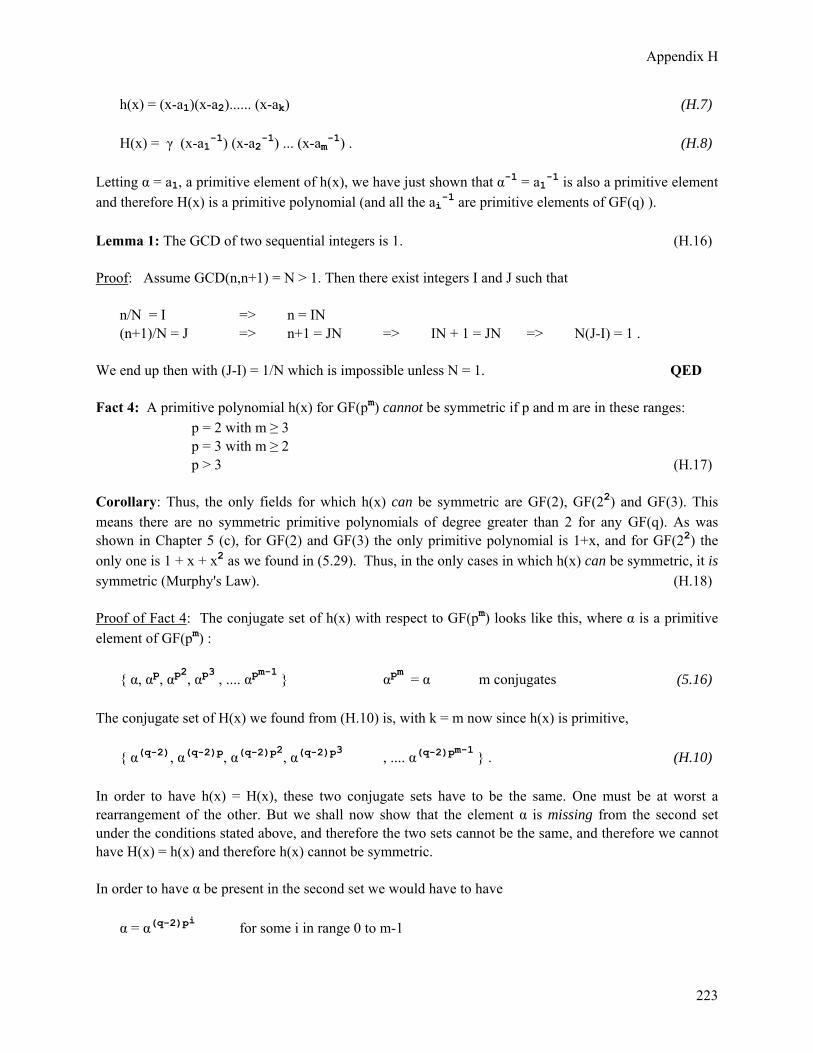
Appendix H
223
h(x) = (x-a1)(x-a2)...... (x-ak) (H.7) H(x) = γ (x-a1-1) (x-a2-1) ... (x-am-1) . (H.8) Letting α = a1, a primitive element of h(x), we have just shown that α-1 = a1-1 is also a primitive element and therefore H(x) is a primitive polynomial (and all the ai-1 are primitive elements of GF(q) ). Lemma 1: The GCD of two sequential integers is 1. (H.16) Proof: Assume GCD(n,n+1) = N > 1. Then there exist integers I and J such that n/N = I => n = IN (n+1)/N = J => n+1 = JN => IN + 1 = JN => N(J-I) = 1 . We end up then with (J-I) = 1/N which is impossible unless N = 1. QED Fact 4: A primitive polynomial h(x) for GF(pm) cannot be symmetric if p and m are in these ranges: p = 2 with m ≥ 3 p = 3 with m ≥ 2 p > 3 (H.17) Corollary: Thus, the only fields for which h(x) can be symmetric are GF(2), GF(22) and GF(3). This means there are no symmetric primitive polynomials of degree greater than 2 for any GF(q). As was shown in Chapter 5 (c), for GF(2) and GF(3) the only primitive polynomial is 1+x, and for GF(22) the only one is 1 + x + x2 as we found in (5.29). Thus, in the only cases in which h(x) can be symmetric, it is symmetric (Murphy's Law). (H.18) Proof of Fact 4: The conjugate set of h(x) with respect to GF(pm) looks like this, where α is a primitive element of GF(pm) : { α, αp, αp2, αp3 , .... αpm-1 } αpm = α m conjugates (5.16) The conjugate set of H(x) we found from (H.10) is, with k = m now since h(x) is primitive, { α(q-2), α(q-2)p, α(q-2)p2, α(q-2)p3 , .... α(q-2)pm-1 } . (H.10) In order to have h(x) = H(x), these two conjugate sets have to be the same. One must be at worst a rearrangement of the other. But we shall now show that the element α is missing from the second set under the conditions stated above, and therefore the two sets cannot be the same, and therefore we cannot have H(x) = h(x) and therefore h(x) cannot be symmetric. In order to have α be present in the second set we would have to have α = α(q-2)pi for some i in range 0 to m-1
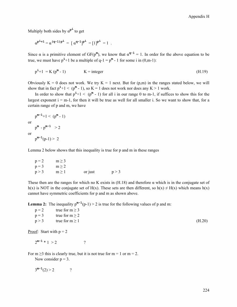
Appendix H
224
Multiply both sides by αpi to get αpi+1 = α(q-1)pi = [ αq-1]pi = [1]pi = 1 . Since α is a primitive element of GF(pm), we know that αq-1 = 1. In order for the above equation to be true, we must have pi+1 be a multiple of q-1 = pm - 1 for some i in (0,m-1): pi+1 = K (pm - 1) K = integer (H.19) Obviously K = 0 does not work. We try K = 1 next. But for (p,m) in the ranges stated below, we will show that in fact pi+1 < (pm - 1), so K = 1 does not work nor does any K > 1 work. In order to show that pi+1 < (pm - 1) for all i in our range 0 to m-1, if suffices to show this for the largest exponent i = m-1, for then it will be true as well for all smaller i. So we want to show that, for a certain range of p and m, we have pm-1+1 < (pm - 1) or pm - pm-1 > 2 or pm-1(p-1) > 2 Lemma 2 below shows that this inequality is true for p and m in these ranges p = 2 m ≥ 3 p = 3 m ≥ 2 p > 3 m ≥ 1 or just p > 3 These then are the ranges for which no K exists in (H.18) and therefore α which is in the conjugate set of h(x) is NOT in the conjugate set of H(x). These sets are then different, so h(x) ≠ H(x) which means h(x) cannot have symmetric coefficients for p and m as shown above. Lemma 2: The inequality pm-1(p-1) > 2 is true for the following values of p and m: p = 2 true for m ≥ 3 p = 3 true for m ≥ 2 p > 3 true for m ≥ 1 (H.20) Proof: Start with p = 2 2m-1 * 1 > 2 ? For m ≥3 this is clearly true, but it is not true for m = 1 or m = 2. Now consider p = 3. 3m-1(2) > 2 ?
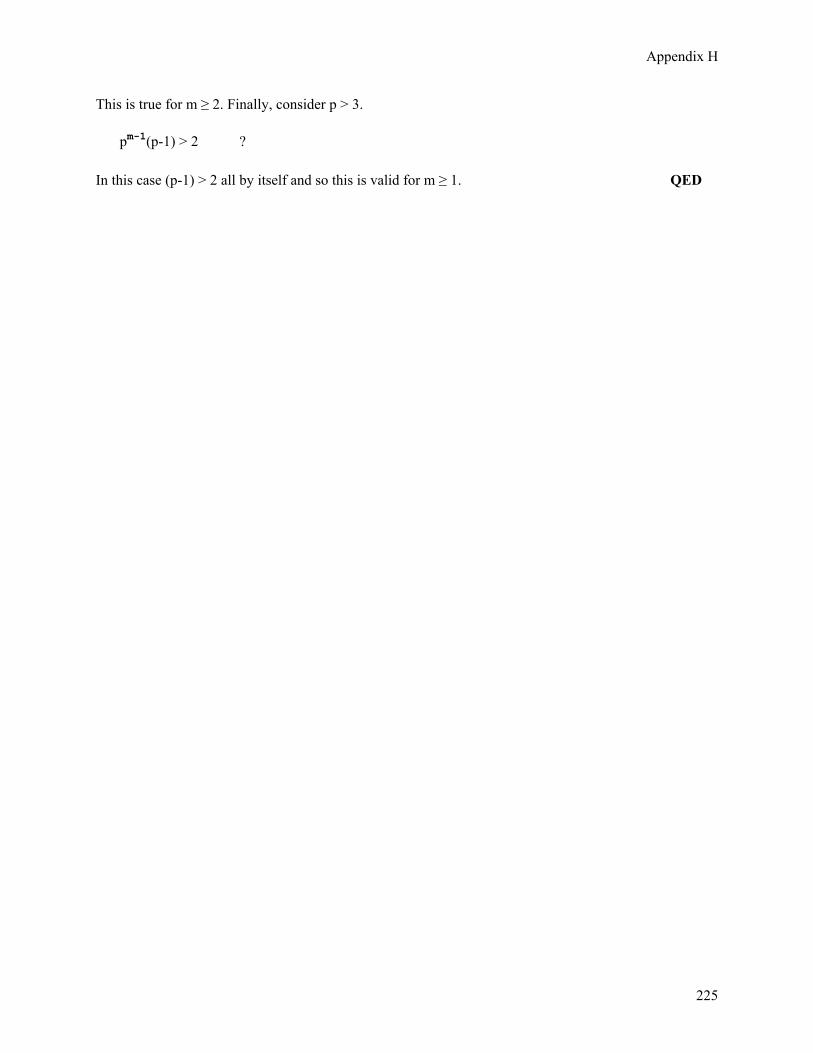
Appendix H
225
This is true for m ≥ 2. Finally, consider p > 3. pm-1(p-1) > 2 ? In this case (p-1) > 2 all by itself and so this is valid for m ≥ 1. QED

References
226
References There are many modern books on the subjects of Galois fields (finite fields) and error-correcting codes, as a quick scan of Amazon will attest. Below we list only a few, including some "classics". The list below is alphabetical by first author. Bad links can be often be replaced by a web search on title or author. G.C. Ahlquist, B. Nelson and M. Rice, "Optimal Finite Field Multipliers for FPGAs", Lecture Notes in Computer Science Vol. 1673, 1999, pp 51.60. http://splish.ee.byu.edu/docs/ffmult.fpl99.pdf BBC: The link below contains a fascinating 14 minute podcast on the short life of Évariste Galois. http://www.bbc.co.uk/podcasts/series/maths G. Birkhoff and S. MacLane, Survey of Modern Algebra, 4th. Ed (Macmillan, New York, 1977). This is an excellent and classic text. Earlier editions were 1941, 1953, and 1965. A paperback printing was published by A.K. Peters in 2008. L.S. Bobrow and M.A. Arbib, Discrete Mathematics: Applied Algebra for Computer and Information Science (W.B. Saunders, Philadelphia, 1974). R.C. Bose and D.K. Ray-Chaudhuri "On a class of error-correcting binary codes", Information and control, 3, (1960), 68–79. Also "Further results on error-correcting binary group codes", Information and control, 3, (1960), 279–290. W.H. Bussey, "Galois Field Tables for pn ≤ 169", Bull. Amer. Math. Soc, Vol 12, Num 1 (1905), 22-38. For each Galois Field with pn ≤169, the author provides one primitive polynomial along with a table of the type we show in (6.12). This paper is freely available as a PDF at http://projecteuclid.org . W.H. Bussey, "Tables of Galois Fields of order less than 1000", Bull. Amer. Math. Soc, Vol 16, Num 4 (1910), 188-206. This paper is an extension of the previous one and is also available at Project Euclid. R.W. Hamming, Error Detecting and Error Correcting Codes, Bell System Technical Journal, Vol XXIX No.2 April 1950. (Try www.lee.eng.uerj.br/~gil/redesII/hamming.pdf .) A. Hocquenghem. "Codes correcteurs d'erreurs", Chiffres (Paris), 2:147–156, September 1959. Try http://kom.aau.dk/~heb/kurser/NOTER/KOFA02.pdf for the first few pages of this paper. P. Kitsos, G. Theodoridis, and O. Koufopavlou, " An efficient reconfigurable multiplier architecture for Galois field GF(2m) ", Microelectronics Journal 34 (2003) 975-980. http://dsmc.eap.gr/members/pkitsos/papers/Kitsos_j02.pdf R. Lidi and H. Niederreiter, Finite Fields, 2nd Ed., Volume 20 of The Encyclopedia of Mathematics and Its Applications (Cambridge University Press, 2008). The original Volume 20 was published in 1983, and a slightly reduced separate edition appeared in 1986. The Encyclopedia now has 142 volumes!

References
227
P. Lucht, Tensor Analysis and Curvilinear Coordinates (2012, http://user.xmission.com/~rimrock/). This document is segmented into two PDF files, the second containing a set of Appendices. If link is bad, search on . M. Olofsson (Linkoping University, Sweden), lists of primitive polynomials over GF(2). http://www.commsys.isy.liu.se/en/staff/mikael/polynomials/primpoly W.W. Peterson and D.T. Brown, "Cyclic Codes for Error Detection", Proc. IRE, 49, 228-235 (1961). This classic paper can be found online as well. W.W. Peterson and E.J. Weldon, Error Correcting Codes, 2nd Ed. (The MIT Press, Cambridge, 1972). M.Y. Rhee, Error Correcting Coding Theory (McGraw-Hill, New York, 1989). E. Savas, A.F. Tenca and C.K. Koc, "A Scalable and Unified Multiplier Architecture for Finite Fields GF(p) and GF(2m) ", Lecture Notes in Computer Science Vol. 1965, 2000, pp 277-292. http://cryptocode.net/docs/c19.pdf E.J. Watson, "Primitive Polynomials (Mod 2)", Math. Comp. 16 (1962), 368-369. Try www.ams.org/journals/...16.../S0025-5718-1962-0148256-1.pdf Xilinx Corp., "CoolRunner-II CPLD Galois Field GF(2m) Multiplier", XAPP371 (v1.0) Sept. 26, 2003. www.xilinx.com/support/documentation/application_notes/xapp371.pdf
Related Documents


