arXiv:astro-ph/0410341v1 13 Oct 2004 Galactic Bulge Microlensing Events from the MACHO Collaboration C.L. Thomas 1 , K. Griest 1 , P. Popowski 2 , K.H. Cook 3 , A.J. Drake 4 , D. Minniti 4 , C. Alcock 5 , R.A. Allsman 6 , D.R. Alves 7 , T.S. Axelrod 8 , A.C. Becker 9 , D.P. Bennett 10 , K.C. Freeman 11 , M. Geha 12 , M.J. Lehner 13 , S.L. Marshall 14 , D.G. Myer 1 , C.A. Nelson 3 , B.A. Peterson 11 , P.J. Quinn 15 , C.W. Stubbs 5 , W. Sutherland 16 , T. Vandehei 1 , D.L. Welch 17 (The MACHO Collaboration) Abstract We present a catalog of 450 high signal-to-noise microlensing events observed by the MA- CHO collaboration between 1993 and 1999. The events are distributed throughout our fields and, as expected, they show clear concentration toward the Galactic center. No optical depth is given for this sample since no blending efficiency calculation has been performed, and we find evidence for substantial blending. In a companion paper we give optical depths for the sub-sample of events on clump giant source stars, where blending is not a significant effect. Several events with sources that may belong to the Sagittarius dwarf galaxy are identified. For these events even relatively low dispersion spectra could suffice to classify these events as either consistent with Sagittarius membership or as non-Sagittarius sources. Several unusual events, such as microlensing of periodic variable source stars, binary lens events, and an event showing extended source effects are identified. We also identify a number of contaminating background events as cataclysmic variable stars. Subject headings: catalogs, gravitational lensing, Galaxy: bulge, Galaxy: structure, stars: dwarf novae, stars: variables: other 1 Department of Physics, University of California, San Diego, CA 92093, USA Email: clt, kgriest, [email protected], [email protected] 2 Max-Planck-Institute for Astrophysics, Karl- Schwarzschild-Str. 1, Postfach 1317, 85741 Garching bei M¨ unchen, Germany Email: [email protected] 3 Lawrence Livermore National Laboratory, Livermore, CA 94550, USA Email: kcook, [email protected] 4 Departmento de Astronomia, Pontifica Universidad Catolica, Casilla 104, Santiago 22, Chile Email: dante, [email protected] 5 Harvard-Smithsonian Center for Astrophysics, 60 Garden St., Cambridge, MA 02138, USA Email: calcock, [email protected] 6 NOAO, 950 North Cherry Ave., Tucson, AZ 85719, USA Email: [email protected] 7 Laboratory for Astronommy & Solar Physics, Goddard Space Flight Center, Code 689, Greenbelt, MD 20781, USA Email: [email protected] 8 Steward Observatory, University of Arizona, Tucson, AZ 85721, USA Email: [email protected] 9 Astronomy Department, University of Washington, Seat- tle, WA 98195, USA Email: [email protected] 10 Department of Physics, University of Notre Dame, IN 46556, USA Email: [email protected] 11 Research School of Astronomy and Astrophysics, Can- berra, Weston Creek, ACT 2611, Australia Email: kcf, [email protected] 12 Carnegie Observatories, 813 Santa Barbara Street, Pasadena, CA 91101, USA 1

Welcome message from author
This document is posted to help you gain knowledge. Please leave a comment to let me know what you think about it! Share it to your friends and learn new things together.
Transcript

arX
iv:a
stro
-ph/
0410
341v
1 1
3 O
ct 2
004
Galactic Bulge Microlensing Events from the MACHO Collaboration
C.L. Thomas1, K. Griest1, P. Popowski2, K.H. Cook3, A.J. Drake4, D. Minniti4,C. Alcock5, R.A. Allsman6, D.R. Alves7, T.S. Axelrod8, A.C. Becker9, D.P. Bennett10,
K.C. Freeman11, M. Geha12, M.J. Lehner13, S.L. Marshall14, D.G. Myer1, C.A. Nelson3,B.A. Peterson11, P.J. Quinn15, C.W. Stubbs5, W. Sutherland16, T. Vandehei1, D.L. Welch17
(The MACHO Collaboration)
AbstractWe present a catalog of 450 high signal-to-noise microlensing events observed by the MA-
CHO collaboration between 1993 and 1999. The events are distributed throughout our fieldsand, as expected, they show clear concentration toward the Galactic center. No optical depthis given for this sample since no blending efficiency calculation has been performed, and wefind evidence for substantial blending. In a companion paperwe give optical depths for thesub-sample of events on clump giant source stars, where blending is not a significant effect.
Several events with sources that may belong to the Sagittarius dwarf galaxy are identified.For these events even relatively low dispersion spectra could suffice to classify these events aseither consistent with Sagittarius membership or as non-Sagittarius sources. Several unusualevents, such as microlensing of periodic variable source stars, binary lens events, and an eventshowing extended source effects are identified. We also identify a number of contaminatingbackground events as cataclysmic variable stars.
Subject headings: catalogs, gravitational lensing, Galaxy: bulge, Galaxy: structure, stars: dwarf novae,stars: variables: other
1Department of Physics, University of California, SanDiego, CA 92093, USAEmail: clt, kgriest, [email protected],[email protected]
2Max-Planck-Institute for Astrophysics, Karl-Schwarzschild-Str. 1, Postfach 1317, 85741 Garchingbei Munchen, GermanyEmail: [email protected]
3Lawrence Livermore National Laboratory, Livermore,CA 94550, USAEmail: kcook, [email protected]
4Departmento de Astronomia, Pontifica UniversidadCatolica, Casilla 104, Santiago 22, ChileEmail: dante, [email protected]
5Harvard-Smithsonian Center for Astrophysics, 60 GardenSt., Cambridge, MA 02138, USAEmail: calcock, [email protected]
6NOAO, 950 North Cherry Ave., Tucson, AZ 85719, USA
Email: [email protected] for Astronommy & Solar Physics, Goddard
Space Flight Center, Code 689, Greenbelt, MD 20781, USAEmail: [email protected]
8Steward Observatory, University of Arizona, Tucson, AZ85721, USAEmail: [email protected]
9Astronomy Department, University of Washington, Seat-tle, WA 98195, USAEmail: [email protected]
10Department of Physics, University of Notre Dame, IN46556, USAEmail: [email protected]
11Research School of Astronomy and Astrophysics, Can-berra, Weston Creek, ACT 2611, AustraliaEmail: kcf, [email protected]
12Carnegie Observatories, 813 Santa Barbara Street,Pasadena, CA 91101, USA
1

1. Introduction
The structure and composition of our Galaxyis one of the outstanding problems in contem-porary astrophysics. While inventories of brightstars have been made, it is known that the bulkof the material in our Galaxy is dark. In addi-tion, the number and mass distribution of stellarremnants such as white dwarfs, neutron stars andblack holes is quite uncertain, as is the numberof faint stars, brown dwarfs and extra-solar plan-ets. Gravitational microlensing was suggested asa probe to detect compact objects including darkmatter (Paczynski 1986, Griest 1991a, Nemiroff1991) and was observationally discovered in 1993(Alcock et al. 1993; Aubourg et al. 1993; Udalskiet al. 1993). The line-of-sight towards the LargeMagellanic Cloud (LMC) is best for dark mat-ter detection, but as a probe of faint objects fromplanets to black holes, the line-of-sight towardsthe Galactic bulge is superior (Griest et al. 1991b;Paczynski 1991). The high density of stars in thedisk and bulge means that the vast majority ofevents detected by microlensing experiments arein this direction.
The amount of lensing matter between asource and the observer is typically describedusing the optical depth to microlensing,τ , de-fined as the probability that a given source starwill be magnified by any lens by more than afactor of 1.34. Early predictions (Griest et al.1991b; Paczynski 1991) of the optical depth
Email: [email protected] of Physics and Astronomy, University of
Pennsylvania, PA 19104, USAEmail: [email protected]
14SLAC/KIPAC, 2575 Sand Hill Rd., MS 29, Menlo Park,CA 94025, USAEmail: [email protected]
15European Southern Observatory, Karl-Schwarzchild-Str.2, 85748 Garching bei Munchen, GermanyEmail: [email protected]
16Institute of Astronomy, University of Cambridge, Madin-gley Road, Cambridge. CB3 0HA, U.K.Email: [email protected]
17McMaster University, Hamilton, Ontario Canada L8S4M1Email: [email protected]
towards the Galactic center included only disklenses and found values nearτ = 0.5 × 10⁻⁶.The early detection rate (Udalski et al. 1993,1994a) seemed higher than this, and further cal-culations (Kiraga & Paczynski 1994) added bulgestars to bring the prediction up to0.85 × 10−6.The first measurements were substantially higherthan this,τ ≥ 3.3 ± 1.2 × 10⁻⁶ (Udalski et al.1994b) based upon 9 events andτ = 3.9+1.8
−1.2
(Alcock et al. 1997) based upon an efficiency cal-culation and 13 clump-giant events taken fromtheir 45 candidates. Many additional calculationsensued, including additional effects, especiallynon-axisymmetric components such as a bar (e.g.Zhao, Spergel & Rich 1995; Metcalf 1995; Zhao& Mao 1996; Bissantz et al. 1997; Gyuk 1999;Nair & Miralda-Escude 1999; Binney, Bissantz &Gerhard 2000; Sevenster & Kalnajs 2001; Evans& Belokurov 2002; Han & Gould 2003). Val-ues in the range0.8 × 10−6 to 2 × 10⁻⁶ werepredicted for various models, and values as largeτ = 4 × 10⁻⁶ were found to be inconsistent withalmost any model.
More recent measurements have all used ef-ficiency calculations and have found values ofτ = 3.2 ± 0.5 × 10⁻⁶ from 99 events in 8 fieldsusing difference imaging (Alcock et al. 2000b),τ = 2.0±0.4×10⁻⁶ from around 50 clump-giantevents in a preliminary version of the companionpaper (Popowski et al. 2001a),τ = 0.94±0.29×10⁻⁶ from 16 clump-giant events (Afonso et al.2003), andτ = 3.36+1.11
−0.81 from 28 events (Sumiet al. 2003).
In releases similar in spirit to our catalog hereUdalski et al. (2000) presented a catalog of 214microlensing events from the 3 seasons of theOGLE-II bulge observation, and Wozniak et al.(2001) presented a catalog of 520 events, mainlyfrom difference imaging.
In this work we present our complete catalogof high signal-to-noise microlensing events thatwere found with point spread function fitting pho-tometry. In the companion paper (Popowski etal. 2004), we make an accurate determination ofthe bulge optical depth using the 62 clump gi-ant events (60 unique) listed here and findτ =
2

2.17+0.47−0.38 × 10⁻⁶ at (l, b) = (1.◦50,−2.◦68). We
do not calculate an optical depth for our entiresample of microlensing events since a completeblending efficiency calculation has not been per-formed, and we caution against using the entiresample of events for such purposes.
Initially envisioned as a probe of dark mat-ter, microlensing has evolved into a more gen-eral astronomical tool, useful for several distinctpurposes. For example, since the duration of themicrolensing event is proportional to the squareroot of the lens mass, microlensing is sensitive tocompact objects in the10−7M⊙ to101M⊙ range,independent of the object’s luminosity, so it facil-itates inventories of brown dwarfs, white dwarfs,and black holes. However, the lens mass mea-surement is degenerate with the lens distance andspeed, severely limiting the accuracy of the massdistribution measurement. Our catalog includesseveral long duration events that may be massiveblack holes and several short duration events thatmay be brown dwarfs.
In order to break the mass/distance/speed de-generacy several techniques have been appliedto rare classes of events such as those with bi-nary lenses, binary sources, large annual paral-laxes, etc. Our catalog lists events which maybe members of exotic microlensing classes. Fi-nally microlensing has emerged as a powerfulmethod of detecting or constraining the existenceof extra-solar planets orbiting the lens (Mao &Paczynski 1991; Gould & Loeb 1992; Griest &Safizadeh 1998; Rhie et al. 2000; Gaudi et al.2002). A key for these searches is careful follow-up on microlensing events, almost all of whichare towards the Galactic bulge. Our catalog canbe used to determine the frequencies of detectablelensing in various directions towards the bulge.
For comparison with other works we note thatour definition of microlensing event duration,t,is the Einstein ring diameter crossing time, twicethe more commonly used Einstein ring radiuscrossing time.
2. Data
The MACHO Project had full-time use of the1.27 meter telescope at Mount Stromlo Obser-vatory, Australia1 from July 1992 until Decem-ber 1999. Details of the telescope system aregiven by Hart et al. (1996), and details of thecamera system by Stubbs et al. (1993) and Mar-shall et al. (1994). Briefly, corrective optics anda dichroic were used to give simultaneous imag-ing of a 43’× 43’ field in two non-standard filterbands, using eight20482 pixel CCD’s. A totalof 32700 exposures were taken in 94 fields to-wards the Milky Way bulge, resulting in around 3Tbytes of raw image data and photometry on 50.2million stars. The location of the centers of thebulge fields are shown in Figure1 and the loca-tion and number of exposures taken of each fieldare given in Table1. Table1 also gives the num-ber of stars in each field, the number of clump gi-ants, the number of microlensing events, and thesampling efficiency at event durations oft = 50and t = 200 days. This latter numbers can beused as a rough indication of the relative sensi-tivity to microlensing in each field, but should beused for quantitative work only with the clumpgiant sample of events (see the companion paperby Popowski et al. 2004). The coverage of fieldsvaries greatly from 12 observations of field 106to 1815 observations of field 119. Note that theobserving strategy changed several times duringthe project, so even in a given field the frequencyof observations changed from year to year. Inaddition, there are gaps between November andFebruary as the bulge was not observed duringprime LMC observing times.
The photometric reduction used here is a vari-ation of the DOPHOT (Schechter, Mateo, & Saha1993) point spread function (PSF) fitting method(Alcock et al. 1999). Briefly, a good-quality im-age of each field is chosen as a template and usedto generate a list of stellar positions and magni-tudes. The templates are used to “warm-start” all
1A fire tragically razed Mount Stromlo Observatory in Januaryof 2003.
3

Fig. 1.— Location of the bulge fields in galacticcoordinates
subsequent photometric reductions, and for eachstar we record information on the flux, an errorestimate, the object type, theχ2 of the PSF fit,a crowding parameter, a local sky level, and thefraction of the star’s flux rejected due to bad pix-els and cosmic rays. The resulting data are re-organized into lightcurves, and searched for vari-able stars and microlensing events. The photo-metric data base used here is about 450 Gbytesin size. We report magnitudes using a global,chunk-uncorrected photometric relations that ex-press JohnsonsV and Kron-CousinsR in termsof the MACHO intrinsic magnitudesbM andrM
as:
V = bM − 0.18(bM − rM ) + 23.70 (1)
R = rM + 0.18(bM − rM ) + 23.41. (2)
For more details see Alcock et al. (1999).
3. Event selection
The data set used here consists of about 19 bil-lion individual photometric measurements. Dis-criminating genuine microlensing from stellar
Fig. 2.— Spatial distribution of microlensingevents.
variability, systematic photometry errors, andother astronomical events is difficult, and the sig-nificance of the results depend upon the eventselection criteria. The selection criteria are basedon cuts made on a set of over 150 statistics cal-culated for each lightcurve. First a smaller setof “level 1” statistics is calculated for every starin the data base. Based on variability criteria,a few percent of the lightcurves are advanced tolevel 1 and the complete set of statistics, includingnon-linear fits to microlensing lightcurve shape,are calculated. Using these a broad selection ofevents is advanced to level 1.5 and output. Finallya fine-tuned set of selection criteria is used to se-lect the level 2 candidates. From a total of 50.2million lightcurves, around 90000 were advancedto level 1.5, and 337 to level 2. In addition, duringthis procedure, lightcurves are tagged as variablestars for inclusion in our variable star catalog.
If the goal is to measure the optical depth ormicrolensing rate, then great care must taken inthe selection of candidate microlensing events. Itis crucial that the same selection method be per-formed on the actual data and on the artificial dataused to calculate the detection efficiency. A cer-
4

tain fraction of “good” microlensing events willbe missed by any set of selection criteria, and itis important to not include these events in anycalculation of optical depth. For more discus-sion, the reader is referred to the companion paper(Popowski et al. 2004) that derives the microlens-ing optical depth toward the Galactic bulge basedon clump giant events.
The basic cuts of selection criteria C are givenin Table 2. A more thorough description of themost useful statistics is given in Alcock et al.(2000c). Note that Table 2 below is not in-tended to fully inform about the selection of bulgeevents; instead it is supposed to document thelevel 2 selection criteria used. Nevertheless incolumn 2 we offer a rough guide to what a givencut or class of cuts is intended to achieve.
In this paper, however, since no estimate of op-tical depth is being made, we can augment thecomputer selected (criteria C) events with “good”events found by other methods such as our alertsystem (Alcock et al. 1996) or even a search byeye over a larger set of candidates. In Figure 2 weshow the position of the microlensing events onthe sky. In Figure 10 we display the lightcurvesof events we selected, organized by field.tile.seqidentification number. In Tables 3 and 4 we de-scribe the source stars corresponding to the se-lected events, and also give the microlensing fitparameters. Table 3 contains the events we sub-jectively regard as likely microlensing candidates,while Table 4 shows the events we think are prob-ably not microlensing. Column 10 of Tables 3and 4 shows our subjective “grade” of the eventdata quality (A-F). Column 11 shows the methodor methods by which each event was selected (‘c’7→ “criteria C”, ‘a’ 7→ “alert system”, ‘b’ 7→ “bi-nary search”, ‘e’ 7→ “by eye selection” out ofan expanded set of events from a ‘C’-like selec-tion). Column 12 shows our subjective deter-mination of event type (‘CV’7→ suspected cata-clysmic variable or supernova, ‘var’7→ suspectedvariable star, ‘bin’ 7→ suspected binary lensingevent, ‘R 6= B’ 7→ red and blue lightcurves differin shape and/or amplitude indicating a possibleblend or systematic error). In column 1 we also
mark events identified as lensed clump giants inthe companion paper with a† flag. We also in-clude OGLE event identifications in Table 5 forevents found at the same position in both surveys.
Note, that for the clump giant subsampleused to calculate optical depth it is importantthat very few non-microlensing events are se-lected by the “C” criteria. However, when weapply the “C” criteria to non-clump areas of thecolor-magnitude diagram a few non-microlensingevents are selected. This is not a problem for op-tical depth calculation but may be of interest. Welist the entire set of events that pass criteria C,including 5 events which we subjectively gradedas probably non-microlensing (quality D or F orsuspected variable) in Table 4.
In summary we show the lightcurves of 252grade “A” (very good signal-to-noise) candi-date microlensing events, 198 grade “B” (goodquality) events, and 76 grade “C” (poor quality)events. Of the grade “A” events 220 were se-lected with criteria C, 6 from the alert system, 4from our binary search, and 22 by eye. Of thegrade “B” events 97 were found with criteria C,15 with the alert system, 2 from the binary search,and 84 by eye. Of the grade “C” events 11 wereselected with criteria C, 12 by the alert system, 1from our binary search, and 52 by eye. We alsoidentify 32 pairs of candidates at the same loca-tion on the sky and one triplet of events. Theseare either the same physical events reported intwo overlapping fields (14 cases) or two stars soclose on the sky that they both receive the fluxfrom the actual event (20 cases). This latter effectresults from the photometry code and not the mi-crolensing of two separate sources. In such caseswe move the worse of the two events into Table4, and recommend ignoring it.
4. Special events
4.1. Binaries
Alcock et al. (2000a) described 17 binaries inthe Galactic bulge. We include these events in thelightcurve figures and in the tables. We also mark
5

24 additional events as potential binaries. Theseare events that have deviations from the standardlightcurve shape and may be better fit with a bi-nary lens or source lightcurve. We have not donethis fitting in this paper, and it is also possible thatthese are not microlensing or have larger than nor-mal measurement errors.
4.2. Lensing of variable stars
Several of the good quality microlensingevents occurred on periodic, or nearly periodicvariable stars. These include events: 108.18689.1979,108.19602.415,118.18009.35,and 403.47848.35.
These events are useful because the measuredamplitude of the stellar variation allows one to de-termine the amount of blending. If the variabilitycan be used to learn more about these stars (suchas their distance or radius) then in some cases thedegeneracy between lens mass, distance, and ve-locity may be partly broken.
4.3. Other exotic events
Event 121.22423.1032 seems to display ex-tended source effects.
5. Supernovae and Cataclysmic Variables
Supernova (SN) explosions in galaxies behindthe microlensing source stars have been shown tocontribute a significant background to the LMCand SMC microlensing searches (Alcock et al.2000c). We do not expect SN to be as impor-tant in this search towards the Galactic bulge dueto the large extinction through the disk and bulge,but we did a search for SN-like lightcurves, andhave marked a number of events that we think arenot microlensing. In fact, most of these eventsare probably cataclysmic variables (CV), e.g., no-vae or dwarf novae (DNe), so we mark them as‘CV’. Of the 16 events we identify in this way,7 repeat, i.e. show more than one brightening.Most of these events exhibit a rapid rise (∼ 4days) followed by a more gradual decline (∼ 20days). The peak is typically about 4 magnitudesbrighter inV and 2.7 magnitudes brighter inR
than the baseline, consistent with the CV classi-fication (Sterken & Jaschek, 1996). We identifythese events as CV’s rather than SNe because thedecline after peak is too fast over the first 20 daysas compared with typical SN.
The lightcurves of the repeating CV’s can beseen in Figure 10. We classify these as long pe-riod dwarf novae, since the periods seem to bebetween 300 and 700 days. In particular note:event 113.18676.5195 with 7 outbursts and a pe-riod of around 400 days, event 114.19842.2283with 5 outbursts and a period of around 340days, event 115.22695.3361 with 3 outbursts, aswell events with two outbursts: 178.23266.2918,178.24048.3166, and 311.37730.4143.
Since our photometry points are generally sep-arated by at least one day, no flickering analysisis done. In dwarf novae one expects flickeringon time scales of minutes to hours, so further ob-servations are needed to positively identify thesesource as DNe. The 9 events with single excur-sions are more difficult to identify; possibilitiesinclude long duration DNe, or heavily blendedclassical novae. They are unlikely to be SNe.
6. The significance of blending
The photometry code measures the light com-ing from stars within the seeing disk, and forbulge stars and conditions at Mt. Stromlo Ob-servatory this means there are usually manystars contained within each photometric “object”.However, in almost all cases only the light fromone of these stars is lensed and gives rise to thetransient microlensing lightcurve. The light fromthe non-lensed source therefore “blends” withthe light from the lensed source distorting thelightcurve from its theoretical shape. In partic-ular the event durationt derived from a fit toa blended lightcurve can be shortened and themagnification decreased. Since the microlensingoptical depth is proportional to the durations ofthe events, blending must be taken into accountwhen trying to measure an optical depth.
In the companion paper (Popowski et al.2004), we show that when using clump giant stars
6

as sources the problem of blending is much alle-viated. In the events on non-clump giant starslisted in this paper, however, blending is expectedto be quite significant. One signature of a heavilyblended event is a large difference between themagnification in the red and blue filter bands. InTables 3 and 4 we label events which have such alarge difference as “R 6= B”. These differencesmay be due to blending, or especially for thelower quality events (grade C) these differencesmay just be indicating that the event is not mi-crolensing. Because of this effect it is importantto use only the clump giants for any quantitativework.
7. Signatures of Sagittarius dwarf galaxy
Sagittarius dwarf galaxy (Ibata, Gilmore, & Ir-win 1995) is the closest satellite galaxy to theMilky Way at a distance of about 25 kpc fromthe Sun. It is centered at the globular cluster M54at (l, b) = (5.◦6,−14.◦0), and extends over sev-eral degrees perpendicular to the Galactic plane.Traces of Sgr dwarf structure can be seen behindthe MACHO fields that lie at negative Galacticlatitudes. Therefore, we expect that some mi-crolensing events may originate in Sgr dwarf.The identification of events with sources in theSgr dwarf serves several goals: 1. it removesthe contaminating sources from the map of themicrolensing optical depth toward the Galacticbulge and thus improves the determination of barparameters; 2. it probes the inner 25 kpc of theGalaxy for massive dark structures; 3. it helpsto constrain the mass function of the lenses. Wediscuss these points in more detail below.
To fully explore the results of the microlens-ing surveys, we would like to better understandthe lens population. In particular, we want to as-sign the lenses to different Galactic populations.However, because most of the lenses are too faintto be directly observed, we attempt to use thelocation of the sources to constrain the locationof the lenses. We can assume that the sourcesin the Galactic bulge imply that the lenses areeither in the bulge or in the disk and that the
sources in the Sagittarius dwarf galaxy shouldtypically have lenses in the bulge. By findingevents that have Sgr sources, we can make bet-ter maps of the microlensing optical depth towardthe sources in the bulge. Such improved mapswill provide crucial constraints in constructingbetter models of the Galactic bar. It is even pos-sible that a detailed analysis of events with Sgrsources could reveal a lens populationbehind theGalactic bulge. Such a population could be partof the warped or flared disk or even of a new, asyet undiscovered streamer of stars. In brief, Sgrevents probe the inner 25 pc of the Galaxy forintervening structures in a way not possible withmicrolensing events with sources in the bulge.
A separate goal is to constrain the masses ofthe lenses. The distribution of the durations ofevents contains the information about the massesof the lenses and the kinematics of the objects in-volved in the lensing process. However, a char-acteristic time of microlensing event is a degener-ate combination of several parameters, includingthe geometry of the system and the relative trans-verse velocity. The better constraints we have onthe kinematics, the better we can understand themasses of the lenses. For example, Gould (2000)showed that the bulge velocity dispersion intro-duces so much scatter to the duration distributionthat lenses in the form of brown dwarfs cannotbe distinguished from those in the form of neu-tron stars on an event-by-event basis. Therefore,the situations where kinematics is additionallyconstrained are very valuable. There are a fewgeneric cases that help to determine the massesof the lenses: 1) the parallax effect, which placesconstraints on the combination of the relative ve-locity and distances (Bennett et al. 2002), 2) themeasurement of the relative proper motion of thelens with respect to the source, which is partic-ularly powerful if coupled with a parallax mea-surement (Alcock et al. 2001), 3) the possibil-ity to assign a source to a system with distinctbulk velocity and negligible velocity dispersion(e.g., Sagittarius dwarf galaxy). We think the timeis ripe to explore this third option. The extentto which the identification of the microlensing
7

events with sources in Sagittarius dwarf galaxywould improve the determination of the masses ofthe lenses can be judged from Fig. 8 by Cseres-njes & Alard (2001). Moreover, such events canprobe a different lens population than all the othertechniques used thus far. Cases 1) and 2) arebiased toward detecting the lenses in the disk,whereas the lenses for Sgr events would likely bein the Galactic bulge or may even be behind thebulge.
Is it possible to select Sgr events based on theirexpected location on a color-magnitude diagram(CMD) from the MACHO survey? This is illus-trated in Figure 3, where we show the sources ofmicrolensing events detected by the MACHO col-laboration on aV0 versus(V − R)0 CMD. TheCMD was dereddened using the extinction mapby Popowski, Cook, & Becker (2003) [extinctionAV was taken from column 4 of their Table 3]. Inpanel a) we plot the microlensing events togetherwith a ridge-line (bold lines) of the Sgr dwarfgalaxy taken from Bellazzini et al. (1999). Theridge-line has been adjusted to the dereddenedquantities usingE(V − I) = 0.22 and AV =0.55. The ridge-line in(V − R)0 color has beenderived assuming that(V −R)0 = 0.5 (V − I)0,which according to Padova isochrones (Girardi etal. 2002: the tables provided on their web page:http://pleiadi.pd.astro.it) is accu-rate to within a few percent. The intrinsic widthof the observed stellar distribution in Sgr dwarfis visualized with thin solid lines (only for thebluer branch of the Bellazzini et al. 1999 track).The errors of(V − R)0 color of the MACHOevents are of order of at least 0.05 mag. We con-clude that many microlensing events could havesources in Sgr dwarf galaxy. In panel b) we su-perpose relevant Padova isochrones on the samecollection of events. The blue isochrone is for anage of 12.6 Gyr and metallicity [M/H] of−1.7,the green one for an age of 10.0 Gyr and metal-licity −1.3, and the red one for an age of 6.3Gyr and metallicity of−0.4 (which is claimed tobe the dominant population according to Monacoet al. 2002). We shifted the isochrones assum-ing the distance modulus,(m − M)Sgr = 17.0.
Again, many microlensing events are consistentwith having sources in the Sgr dwarf galaxy.Therefore, the location of events on the(V, V −
R) color-magnitude diagram does not facilitatethe identification of Sgr sources.
Is there any way to narrow the list of possibleSgr events? Kunder, Popowski, & Cook (2004,in preparation) analyzed a set of almost 4000 RRLyrae stars in the MACHO bulge fields. Theyseparated the stars into the bulge and Sgr groupswith high confidence. The Sgr RR Lyrae starsdominate over the bulge ones for Galactic lati-tudesb < −6.0. This suggests that Sgr sourcescan make a detectable contribution to the mi-crolensing optical depth at these latitudes, whichis in qualitative agreement with conclusions fromCseresnjes & Alard (2001). In panel c) of Fig-ure 3, the microlensing events with the Galacticlatitudeb < −6.0 are marked as solid magentadots. Their distribution on a CMD is not identicalto the other events, which is apparent from thedistribution of their dereddenedV0 magnitudes(Figure 4). In addition, many of those events arein the vicinity of the Sgr ridgeline suggesting thatthey are more consistent with Sgr membership.These 34 events are our Sgr dwarf candidates. Welist their main parameters in Table 6.
The Sagittarius dwarf galaxy has a distinct he-liocentric radial velocity of140±10 km/s, differ-ent from the bulk of bulge stars (see e.g. Figure 4by Ibata et al. 1995). The Sgr membership cannotbe assigned in a robust way based on the mea-surement of radial velocities alone, but such mea-surements are very powerful in eliminating bulgeor disk events. In addition, radial velocity can beobtained long after the event. Our 34 candidatesare the recommended targets for such an investi-gation2.
Our selection of Sgr microlensing candi-dates should enable the first systematic search
2Ideally, one would like to perform such a radial velocity testfor all microlensing candidates from all microlensing surveys,especially the ones with negative Galactic latitudeb. Due tothe location of the MACHO fields, the MACHO data are themost suitable for the search for events with Sgr sources.
8

Fig. 3.— In panel a) we plot the events together with a ridge-line (bold lines) of the Sgr dwarf galaxy takenfrom Bellazzini et al. (1999). The intrinsic width of the observed stellar distribution in Sgr dwarf is visualizedwith thin solid lines (only for the bluer branch of the Bellazzini et al. 1999 track). The errors of(V − R)0color of the MACHO events are of order of at least 0.05 mag. In panel b) we superpose relevant Padovaisochrones on the same collection of events. The blue isochrone is for an age of 12.6 Gyr and metallicity[M/H] of −1.7, the green one for an age of 10.0 Gyr and metallicity−1.3, and the red one for an age of 6.3Gyr and metallicity of−0.4. We shifted the isochrones assuming the distance modulus,(m−M)Sgr = 17.0.From panels a) and b) we conclude that many microlensing events are consistent with having sources in theSgr dwarf galaxy. Therefore, the location of events on the(V, V − R) color-magnitude diagram does notfacilitate the identification of Sgr sources. In panel c), the events with the Galactic latitudeb < −6.0 aremarked as solid magenta dots. Their distribution on a CMD is not identical to the other events and many ofthem are more consistent with Sgr membership. Again we over-plotted a ridge-line from Bellazzini et al.(1999) for reference.
9

Fig. 4.— The histogram ofV0 magnitudes for aset of all 511 unique microlensing events and 34Sagittarius candidates. The difference in magni-tude distribution is very significant.
for such stars by the means of radial veloci-ties. There are two recent spectroscopic stud-ies of microlensing events toward the Galacticbulge by Cavallo et al. (2002) and Kane & Sahu(2003). The first investigates 6 and the second17 events. Most of the events studied by thosegroups are rather bright and neither of the abovestudies specifically targeted the microlensingsources in the Sgr dwarf galaxy. An example of136.27650.2370/142.27650.6057, which is not aSgr member, shows that spectroscopic follow-upis essential. Event 136.27650.2370/142.27650.6057is in our candidate list but was measured by Cav-allo et al. (2002) to have the radial velocity of60 ± 2km s−1, inconsistent with the velocity ofSgr dwarf. On the other hand, there may be Sagit-tarius events hiding among bulge events closer tothe Galactic plane. Cook et al. (2004) claim adetection of two likely Sgr events that are distinctthrough their radial velocity, metallicity and loca-tion on the(K, J − K) CMD. Determination ofradial velocities of our candidate Sgr events asks
Fig. 5.— Spatial distribution of events (dots) inthe MACHO fields (squares) most distant fromthe Galactic plane. The filled dots represent Sgrcandidates. The strip of empty fields atb ≈ −6 iscaused by very low detection efficiency in thosefields and unrelated to the existence of differentevent populations.
for observations on an 8m class telescope. Un-fortunately, these observations cannot be sped upwith currently available multi-object instruments,because the candidate Sgr events are distributedover a large area. Their spatial distribution isshown in Figure 5.
As many as five methods to identify Sagittar-ius events are discussed by Popowski (2004)3.
8. Statistical properties of the events
8.1. Clustering of microlensing events
Figure 2 shows the position of the events onthe sky. The events are noticably concentrated to-ward the Galactic center and toward the Galac-tic plane as expected. Examination of the fig-ure shows some apparent clustering of events
3See:http://www.stelab.nagoya-u.ac.jp/hawaii/Popowski/hawaii2004.html
10

on the sky, in particular in fields 108, 104, and113. If microlensing events are clustered on thesky above random chance it has important con-sequences. It could indicate clustering of lenses,perhaps in some bound Galactic substructure. Wetested for the significance of the clustering in ourdata by simulating 10000 microlensing experi-ments each of which found 318 criteria “C” se-lected unique microlensing events (as in the cur-rent data set). The Monte Carlo is described inmore detail in the companion paper (Popowski etal. 2004). The result is that we find no strongevidence for clustering beyond random chance.The probability of finding by chance a cluster of3 events as dense as in the data is betwen 7 and36% depending on the assumed optical depth gra-dient. The chance of finding a 4-event cluster asdense as in the data varies between 4 and 32%depending on the assumed optical depth gradient.
8.2. Impact Parameters
One test of microlensing is the distribution ofimpact parameters,umin. The impact parame-ter umin is the distance of closest approach be-tween the lens and the source in units of the Ein-stein ring radius, and it is completely determinedby the maximum magnification. If the efficiencywere independent of the magnification one wouldexpect a uniform distribution ofumin’s since ev-ery impact parameter is equally likely. In thatcase, a cumulative distribution of impact parame-ters should be a straight line from 0 up to the max-imum impact parameter allowed by our cuts (thecutAmax >= 1.5 corresponds toumin < 0.826.)In Figure 6, we plot the cumulative distributionsof impact parameters for unique events selectedby the ‘C’ criteria for both clump giants events(60 events) and non-clump events (258 events). Inboth cases no correction is made for microlensingefficiency, though this correction is made (withlittle effect) for the clump giant events in the com-panion paper (Popowski et al. 2004).
For the clump events, the resulting Kolmogorov-Smirnov (KS) statistic shows excellent agreementwith the microlensing hypothesis:D = 0.081
with 60 events, with a probability of 81% to find avalue ofD this large or larger. For the non-clumpevents, the agreement is marginal:D = 0.091with 258 events, for a probability of 2.5% of find-ing a value ofD this large. This deviation fromuniformity can be caused by blending (which canlower the measured maximum amplification andtherefore increase the measuredumin), by a lowerefficiency at larger impact parameter, or by inclu-sion of non-microlensing events in the sample.
8.3. Distributions
Figure 7 shows the distribution of lensing du-rationst for both the clump giant and non-clumpgiant events. Only events grade A and B eventsare included. The average value oft for thenon-clump sample is
⟨
t⟩
= 49 ± 62 days. Forcomparison note that the clump giant events have⟨
t⟩
= 56±64 days. Because the distributions arenot gaussian we also give the median and quar-tiles for non-clump A and B events 31.1, 17.4, &57.0, and clump events 30.8, 15.9, & 60.9. Theseresults are consistent with partial blending of thenon-clump sample discussed in§ 6 but they do notprovide any additional support for this hypothe-sis.
Figure 8 shows the distribution of the timesof microlensing peaks, mostly showing when ob-servations took place, but is consistent with uni-formity when this is taken into account. Figure9 shows the CMD of the microlensing events,which, as expected, is a reasonable sample of theCMD of the Galactic bulge. The location on aCMD is used in the companion paper to selectclump giants.
9. Conclusions
In conclusion, light curves and parameters of528 microlensing events found by the MachoProject (1993-1999) are presented. Included are5 events on variable stars, 17 binary events, 24potential binary events, and 1 extended sourceevent. Also included is a representative sampleof 36 contaminant events, consisting of 16 cat-aclysmic variables, and 20 duplicate events. In
11

(a) (b)
Fig. 6.— Cumulative distribution of impact parameter for clump events (a) and non-clump, selection criteriaC events (b).
addition we select 37 (34 unique) events that arepotentially lensed Sagittarius sources. The sam-ple of over 500 events presented here is effectedsignificantly by blending and should not be usedfor quantitative studies. We present light curvesfor all 564 microlensing and non-microlensingevents. Data and figures will be available athttp://wwwmacho.mcmaster.ca uponacceptance of this paper.
This work was performed under the auspicesof the U.S. Department of Energy, National Nu-clear Security Administration by the Universityof California, Lawrence Livermore National Lab-oratory under contract No. W-7405-Eng-48. KGand CT were supported in part by the DoE undergrant DEFG0390ER40546. DM is supported byFONDAP Center for Astrophysics 15010003.
12

(a) (b)
Fig. 7.— Distribution of event durations for clumps giants (a) and non-clump giants (b).
13

Fig. 8.— Histogram oft0 of events. The peaksand troughs are due to the lack of observationsform November through February. The smallnumber of events in the second year is due tofewer observations in that period.
Fig. 9.— Color-magnitude diagram of events(black triangles) and a representative sample ofall stars in our fields (yellow dots).
14

TABLE 1
DATA ON THE 94 BULGE FIELDS.
field l b nstars
100
nclumps
100nevents nexposures ǫ(50days.) ǫ(200days)
101 3.73 −3.02 6284 629.5 30 804 0.41 0.61102 3.77 −4.11 6545 444 15 421 0.24 0.46103 4.31 −4.62 6349 368 5 331 0.21 0.36104 3.11 −3.01 5813 652 28 1639 0.40 0.59105 3.23 −3.61 6375 539 21 640 0.39 0.52106 3.59 −4.78 6648 346 0 12 < 0.003 < 0.003107 4.00 −5.31 6159 269 0 51 0.007 < 0.003108 2.30 −2.65 6498 790 32 1031 0.49 0.75109 2.45 −3.20 6926 661 19 761 0.35 0.60110 2.81 −4.48 6649 408 11 650 0.32 0.57111 2.99 −5.14 6036 298 5 305 0.21 0.34112 3.40 −5.53 5147 246.5 0 43 < 0.003 < 0.003113 1.63 −2.78 6252 834 31 1127 0.51 0.72114 1.81 −3.50 6665 617 20 776 0.39 0.59115 2.04 −4.85 5756 325.5 9 357 0.24 0.35116 2.38 −5.44 5812 268.5 4 314 0.21 0.38117 2.83 −6.00 5185 198 0 39 0.006 < 0.003118 0.83 −3.07 6347 741.5 29 1053 0.44 0.74119 1.07 −3.83 7454 542.5 27 1815 0.45 0.68120 1.64 −4.42 5599 394 9 676 0.35 0.54121 1.20 −4.94 5855 344 10 352 0.22 0.37122 1.57 −5.45 4890 266 3 186 0.15 0.23123 1.95 −6.05 5119 210.5 1 40 0.006 < 0.003124 0.57 −5.28 5716 265.5 3 337 0.22 0.39125 1.11 −5.93 5839 189 1 287 0.21 0.37126 1.35 −6.40 4789 182 0 36 < 0.003 < 0.003127 0.28 −5.91 4975 192 0 178 0.13 0.24128 2.43 −4.03 6160 516.5 9 711 0.35 0.55129 4.58 −5.93 5123 234.5 0 31 0.006 < 0.003130 5.11 −6.49 4864 169.5 2 20 0.02 0.02131 4.98 −7.33 4256 130 1 106 0.12 0.22132 5.44 −7.91 4533 102 2 180 0.17 0.33133 6.05 −8.40 4174 70.5 0 176 0.15 0.17134 6.34 −9.07 3370 46.5 1 197 0.08 0.14135 3.89 −6.26 5476 179 0 30 0.004 < 0.003136 4.42 −6.82 5623 137.5 1 207 0.17 0.25137 4.31 −7.60 4488 101 4 193 0.15 0.36138 4.69 −8.20 4380 95.5 0 201 0.16 0.21139 5.35 −8.65 4112 81 1 191 0.11 0.10140 5.71 −9.20 3723 64 0 209 0.12 0.24141 3.26 −6.59 5001 159 0 28 0.03 0.02142 3.81 −7.08 4985 126.5 2 218 0.15 0.35143 3.80 −8.00 4767 97 0 210 0.17 0.25144 4.68 −9.02 3798 50.5 1 210 0.10 0.18145 5.20 −9.50 3385 49.5 1 210 0.12 0.23146 3.26 −7.54 3798 106 0 207 0.19 0.33
15
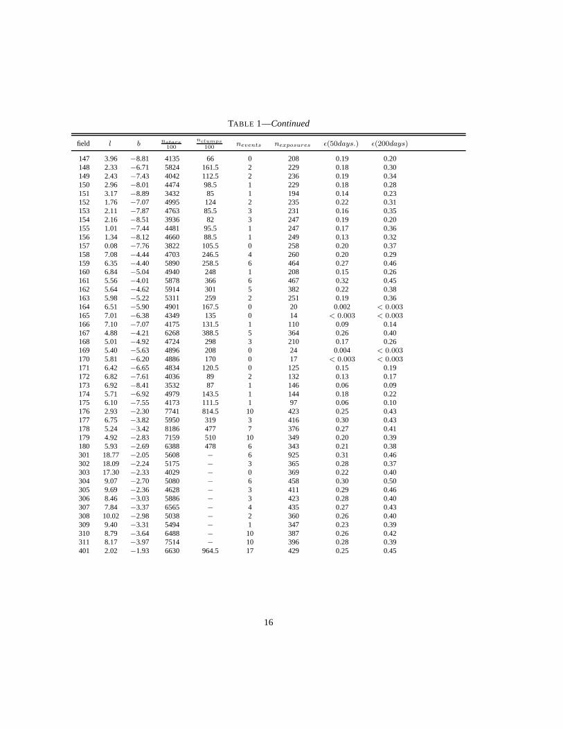
TABLE 1—Continued
field l b nstars
100
nclumps
100nevents nexposures ǫ(50days.) ǫ(200days)
147 3.96 −8.81 4135 66 0 208 0.19 0.20148 2.33 −6.71 5824 161.5 2 229 0.18 0.30149 2.43 −7.43 4042 112.5 2 236 0.19 0.34150 2.96 −8.01 4474 98.5 1 229 0.18 0.28151 3.17 −8.89 3432 85 1 194 0.14 0.23152 1.76 −7.07 4995 124 2 235 0.22 0.31153 2.11 −7.87 4763 85.5 3 231 0.16 0.35154 2.16 −8.51 3936 82 3 247 0.19 0.20155 1.01 −7.44 4481 95.5 1 247 0.17 0.36156 1.34 −8.12 4660 88.5 1 249 0.13 0.32157 0.08 −7.76 3822 105.5 0 258 0.20 0.37158 7.08 −4.44 4703 246.5 4 260 0.20 0.29159 6.35 −4.40 5890 258.5 6 464 0.27 0.46160 6.84 −5.04 4940 248 1 208 0.15 0.26161 5.56 −4.01 5878 366 6 467 0.32 0.45162 5.64 −4.62 5914 301 5 382 0.22 0.38163 5.98 −5.22 5311 259 2 251 0.19 0.36164 6.51 −5.90 4901 167.5 0 20 0.002 < 0.003165 7.01 −6.38 4349 135 0 14 < 0.003 < 0.003166 7.10 −7.07 4175 131.5 1 110 0.09 0.14167 4.88 −4.21 6268 388.5 5 364 0.26 0.40168 5.01 −4.92 4724 298 3 210 0.17 0.26169 5.40 −5.63 4896 208 0 24 0.004 < 0.003170 5.81 −6.20 4886 170 0 17 < 0.003 < 0.003171 6.42 −6.65 4834 120.5 0 125 0.15 0.19172 6.82 −7.61 4036 89 2 132 0.13 0.17173 6.92 −8.41 3532 87 1 146 0.06 0.09174 5.71 −6.92 4979 143.5 1 144 0.18 0.22175 6.10 −7.55 4173 111.5 1 97 0.06 0.10176 2.93 −2.30 7741 814.5 10 423 0.25 0.43177 6.75 −3.82 5950 319 3 416 0.30 0.43178 5.24 −3.42 8186 477 7 376 0.27 0.41179 4.92 −2.83 7159 510 10 349 0.20 0.39180 5.93 −2.69 6388 478 6 343 0.21 0.38301 18.77 −2.05 5608 − 6 925 0.31 0.46302 18.09 −2.24 5175 − 3 365 0.28 0.37303 17.30 −2.33 4029 − 0 369 0.22 0.40304 9.07 −2.70 5080 − 6 458 0.30 0.50305 9.69 −2.36 4628 − 3 411 0.29 0.46306 8.46 −3.03 5886 − 3 423 0.28 0.40307 7.84 −3.37 6565 − 4 435 0.27 0.43308 10.02 −2.98 5038 − 2 360 0.26 0.40309 9.40 −3.31 5494 − 1 347 0.23 0.39310 8.79 −3.64 6488 − 10 387 0.26 0.42311 8.17 −3.97 7514 − 10 396 0.28 0.39401 2.02 −1.93 6630 964.5 17 429 0.25 0.45
16
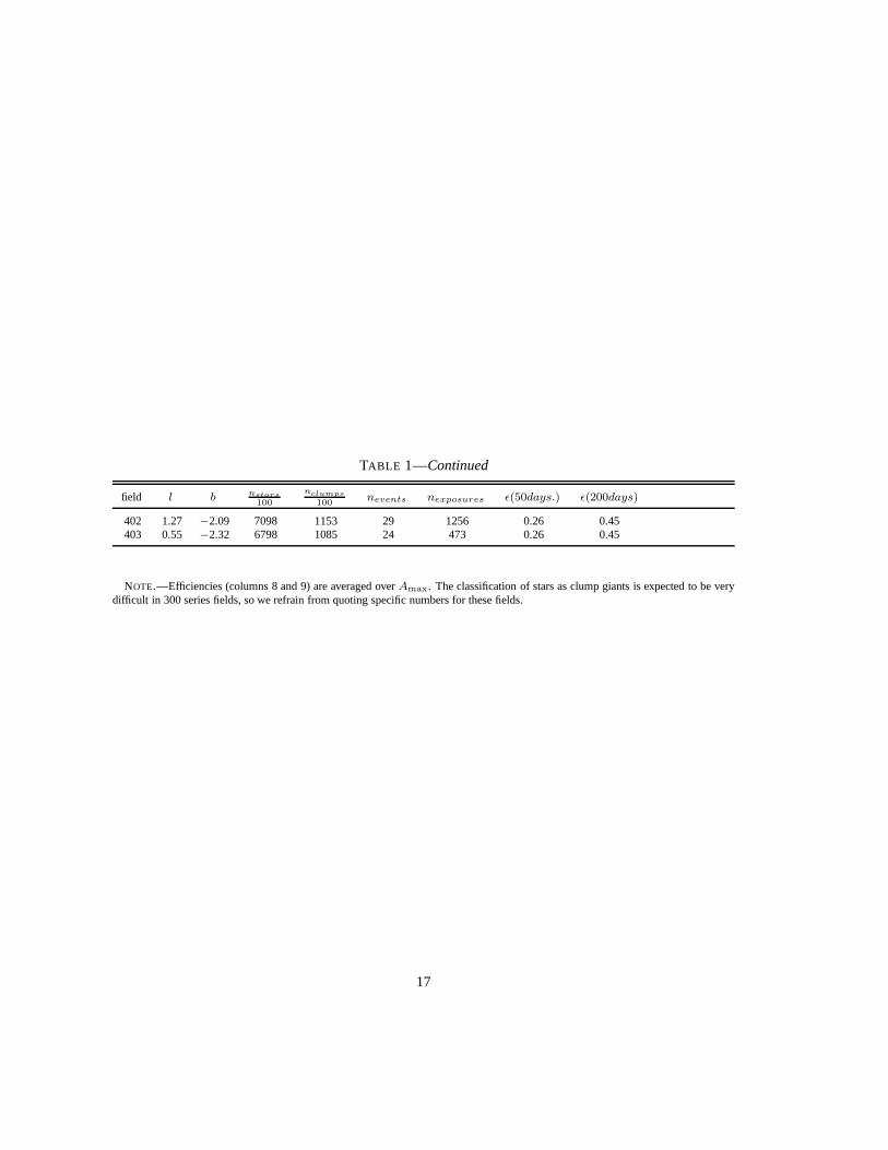
TABLE 1—Continued
field l b nstars100
nclumps
100nevents nexposures ǫ(50days.) ǫ(200days)
402 1.27 −2.09 7098 1153 29 1256 0.26 0.45403 0.55 −2.32 6798 1085 24 473 0.26 0.45
NOTE.—Efficiencies (columns 8 and 9) are averaged overAmax. The classification of stars as clump giants is expected to beverydifficult in 300 series fields, so we refrain from quoting specific numbers for these fields.
17

TABLE 2
SELECTION CRITERIA
Selection Description
microlensing fit parameter cuts:N(V −R) > 0 require color informationχ2
out < 3.0, χ2out > 0.0 require high quality baselines
Namp ≥ 8 require 8 points in the amplified regionNrising ≥ 1, Nfalling ≥ 1 require at least one point in the rising and falling part of the peakAmax > 1.5 magnification threshold(Amax − 1) > 2.0(σR + σB) signal to noise cut on amplification(σR + σB) < (0.05 δχ2)/(Namp χ2
in χ2out)
(Namp χ2out fchrom)/(befaft δχ2) < 0.0003
(Namp χ2in)/(befaft δχ2) < 0.00004
remove spurious photometric signals caused by nearby saturated stars
δχ2/fc2 > 320.0 good overall fit to microlensing lc shapeδχ2/χ2
peak ≥ 400.0 same quality fit in peak as whole lc0.5(rcrda + bcrda) ≤ 143.0 source star not too crowdedξautoB /ξauto
R < 2.0 remove long period variablest0 > 419.0, t0 < 2850.0 constrain the peak to period of observationst < 1700 limit event duration to∼half the span of observationsclump giant cuts:V ≥ 15, V ≤ 20.5 select bright stars with reliabale photometryV ≥ 4.2(V − R) + 12.4 define bright boundary of extinction stripV ≤ 4.2(V − R) + 14.2 define faint boundry of extinction strip(V − R) ≥ (V − R)boundary avoid main sequence contaminationexclude fields300 − 311 avoid disk contamination
18

TABLE 3
EVENT PARAMETERS
field.tile.seq α (2000) δ (2000) V V − R t0 t Amaxχ2
ndofGr. Sel. Notes
101.20650.1216a 18 04 20.25 −27 24 45.3 18.01 0.67 1971.8 10.3 2.19 1.09 A cb bin101.20658.2639 18 04 22.39 −26 53 15.3 20.73 0.97 1204.7 22.3 7.66 0.84 A c101.20908.1433 18 04 57.68 −27 33 18.4 18.57 0.82 1598.6 14.1 1.41 0.46 C a bin101.20910.2922b 18 04 54.54 −27 25 50.0 19.43 0.74 2265.9 243 9.12 1.03 A c101.20913.2158 18 04 56.18 −27 13 40.0 19.56 0.92 2484.9 57.0 4.91 0.88 B a101.20914.3873 18 04 56.32 −27 10 41.3 20.06 0.94 2008.8 33.8 1.85 1.74 B c101.21042.5059c 18 05 28.27 −27 16 21.3 20.14 0.84 2805.4 44.0 4.45 0.73 B c101.21045.2528 18 05 12.63 −27 05 47.1 19.29 0.69 2426.3 19.2 4.82 0.80 B ab bin101.21170.2699 18 05 48.16 −27 24 16.4 18.88 0.71 2807.3 11.4 4.22 0.79 B a101.21171.4799 18 05 38.16 −27 23 07.8 20.20 1.00 1599.4 14.5 2.04 1.04 B c bin101.21174.1990 18 05 39.23 −27 08 53.8 18.86 0.72 1356.7 9.67 2.72 1.12 B e101.21174.2534d 18 05 38.71 −27 08 30.0 19.17 0.78 1909.2 15.3 1.83 0.75 B e101.21176.5465 18 05 31.60 −27 03 11.5 21.12 0.75 2426.1 16.6 3.37 0.93 B e101.21307.880 18 06 05.20 −26 59 38.3 20.32 0.86 537.8 53.4 8.10 0.86 A c101.21428.2452 18 06 21.15 −27 33 57.8 19.07 0.75 2751.2 36.4 2.09 1.15 B c bin101.21437.2090 18 06 20.53 −26 58 39.6 19.21 0.91 611.5 42.1 2.16 1.07 B c101.21437.2192 18 06 23.82 −26 58 54.3 19.01 0.81 2384.7 30.8 1.91 1.44 A c101.21558.2113 18 06 37.58 −27 35 40.1 19.00 0.74 553.9 12.6 56.1 1.23 A c101.21561.5337 18 06 25.89 −27 22 47.7 20.39 0.76 2669.0 17.2 3.64 1.12 B c101.21564.4657 18 06 28.73 −27 09 35.6 20.52 0.98 1230.2 17.2 7.66 1.02 A c101.21689.2648 18 06 54.84 −27 29 21.8 19.27 0.84 2370.6 53.7 1.46 0.75 C e101.21689.315† 18 06 58.30 −27 27 45.8 17.51 1.10 593.5 165 4.80 1.19 A c101.21691.836 18 06 52.73 −27 23 18.9 17.28 0.70 1212.3 30.4 2.01 0.35 A c101.21821.128 18 07 04.26 −27 22 06.3 16.24 1.37 1321.2 68.3 23.5 25.8 A e101.21948.3692 18 07 23.42 −27 35 28.8 20.87 0.90 2408.0 17.2 3.78 0.79 B e101.21949.2465 18 07 32.65 −27 31 35.6 19.92 0.86 579.9 34.4 6.00 1.40 A c101.21950.1897 18 07 24.99 −27 24 40.5 19.27 0.78 1249.1 5.74 1.60 0.92 B c101.21950.861 18 07 20.78 −27 24 09.7 18.48 0.90 1340.7 24.7 2.64 0.41 A c102.22466.140† 18 08 47.04 −27 40 47.3 16.81 0.95 1275.6 153 3.88 0.95 A c102.22598.2894 18 09 00.08 −27 35 38.9 19.72 0.84 2688.8 15.5 1.51 1.30 C e102.22725.1408 18 09 13.53 −27 45 45.0 19.27 0.94 1916.9 121 1.81 0.57 B c102.22851.2409 18 09 44.70 −28 00 58.6 19.64 0.96 2368.4 40.2 2.32 0.96 B c102.22851.4872e 18 09 30.68 −28 00 48.8 20.21 0.74 1307.7 18.0 3.38 0.84 B e R 6= B102.23112.1759 18 10 09.43 −27 56 45.7 19.41 0.76 1977.7 27.1 5.04 1.23 A c102.23246.5046 18 10 34.52 −27 40 24.5 20.28 0.63 2715.1 9.21 3.62 1.09 B e102.23370.476 18 10 50.72 −28 04 47.6 18.09 0.86 2010.1 25.4 1.70 1.07 A c bin102.23379.2909 18 10 58.82 −27 31 01.6 19.71 0.80 1693.0 45.5 2.19 0.68 B c102.23501.4570 18 11 03.79 −27 59 58.8 20.16 0.84 2684.2 55.7 1.93 1.44 C a bin102.23503.2521 18 11 10.12 −27 54 34.3 19.64 0.85 454.3 74.3 5.40 0.76 A c102.23503.4283 18 11 01.59 −27 53 59.0 19.82 0.80 2335.4 29.3 2.98 0.64 B c102.23635.1426 18 11 32.49 −27 45 27.0 18.82 0.69 1282.9 62.6 4.16 1.04 A c103.24024.1785 18 12 26.00 −27 48 37.8 19.04 0.70 2318.9 98.0 1.34 0.83 B e103.24030.3425 18 12 14.65 −27 25 39.0 19.57 0.70 2004.5 16.1 3.78 1.12 A c103.24161.2085 18 12 45.87 −27 20 04.4 19.15 0.69 2730.5 50.0 3.43 0.99 A c103.24286.768 18 12 49.71 −27 41 42.6 18.19 0.82 2064.0 77.0 1.36 2.38 B e103.24544.794 18 13 27.58 −27 49 11.6 19.80 0.81 2065.0 58.4 1.70 0.89 B a104.19990.4674 18 03 00.48 −28 04 45.7 18.30 0.78 1175.2 53.9 1.63 1.25 C e104.19992.858† 18 02 53.82 −27 57 50.0 18.60 1.08 1169.7 106 2.23 2.15 A c104.20119.6312f† 18 03 20.75 −28 08 14.5 18.02 1.09 1975.3 38.7 1.62 1.62 A c104.20121.1692 18 03 15.25 −28 00 14.1 18.62 0.89 1986.1 166 2.54 0.97 A c104.20121.2255 18 03 09.05 −28 01 45.3 19.34 1.01 480.5 34.6 3.62 0.42 A c104.20251.1117† 18 03 29.02 −28 00 31.0 18.23 0.98 463.2 45.5 2.09 0.93 A c104.20251.50† 18 03 34.05 −28 00 18.9 17.34 0.93 493.9 287 10.1 1.75 A c104.20259.572† 18 03 33.39 −27 27 47.3 18.17 1.20 538.5 14.2 1.58 1.56 A c
19

TABLE 3—Continued
field.tile.seq α (2000) δ (2000) V V − R t0 t Amaxχ2
ndofGr. Sel. Notes
104.20382.803† 18 03 53.19 −27 57 35.7 17.80 0.96 1765.8 254 5.72 4.40 A c104.20387.2071 18 03 51.43 −27 37 40.2 19.04 0.72 2093.4 12.8 1.64 1.79 A e104.20388.2766 18 03 53.97 −27 33 30.5 19.83 1.01 1691.5 75.5 7.70 0.6 A c bin104.20514.1500 18 04 06.08 −27 48 26.3 18.95 1.09 1993.0 2.58 15.1 1.03 C a104.20515.498† 18 04 09.66 −27 44 35.1 17.66 1.00 2061.7 53.6 1.76 1.42 A c104.20640.8423g† 18 04 33.65 −28 07 31.9 17.16 0.97 2374.9 30.8 1.65 2.23 A c104.20645.3129† 18 04 26.17 −27 47 35.1 17.69 1.07 1558.3 152 1.82 0.77 A c104.20775.2644 18 04 50.73 −27 45 57.3 20.02 0.92 1899.9 46.3 5.42 0.92 A c104.20779.9616 18 04 54.08 −27 30 07.0 20.03 0.94 2678.6 37.4 1.74 0.94 B e104.20904.3155 18 05 07.31 −27 51 11.4 19.95 0.97 1310.4 33.5 2.41 0.94 A c104.20906.3973 18 05 02.50 −27 42 17.2 19.93 0.83 1738.6 654 2.05 1.85 B a bin104.20910.7700b 18 04 54.54 −27 25 49.8 19.34 0.85 2266.2 211 8.64 0.93 A c104.21032.4118 18 05 15.42 −27 58 25.0 19.87 0.73 1620.1 29.3 2.50 0.92 A c104.21161.1997h 18 05 34.45 −28 02 51.8 18.66 0.81 1301.7 37.5 7.66 1.02 A c104.21162.3642i 18 05 47.75 −27 56 32.2 19.70 0.87 1694.6 71.6 1.76 1.59 C c104.21164.4093j 18 05 41.42 −27 51 03.1 20.07 0.97 1601.8 33.8 1.77 0.71 B e104.21293.1164k 18 06 03.99 −27 55 05.0 17.83 0.71 1294.0 37.2 1.61 0.63 B c bin104.21421.131ae 18 06 08.65 −28 00 22.4 17.78 0.85 2640.8 7.54 2.61 20 A c104.21423.530l 18 06 09.10 −27 53 38.7 19.77 0.78 1634.1 37.3 1.77 1.49 B c105.21161.7671h 18 05 34.44 −28 02 51.2 18.79 0.76 1301.7 39.2 8.16 0.94 A c105.21162.7174i 18 05 47.79 −27 56 32.6 19.77 0.86 1695.7 61.2 1.72 2.04 B c105.21164.9983j 18 05 41.46 −27 51 03.3 20.14 0.85 1601.2 37.2 1.83 0.82 B c105.21287.3893 18 05 49.89 −28 17 19.5 20.25 0.99 2082.9 21.6 2.79 0.97 C e105.21293.6550k 18 06 04.01 −27 55 04.9 17.90 0.71 1295.7 28.3 1.71 0.63 B c105.21417.101 18 06 11.95 −28 16 52.8 16.22 1.08 1540.7 108 1.91 16.6 A ab bin105.21422.1228 18 06 20.41 −27 56 13.4 17.94 0.88 2256.9 75.2 2.80 2.93 A e105.21423.5762l 18 06 09.11 −27 53 38.6 19.90 0.79 1636.8 40.2 1.84 0.75 B c105.21425.3499 18 06 08.51 −27 46 13.2 19.11 0.91 1361.5 24.8 2.77 0.95 B e105.21681.2244 18 06 53.94 −28 01 16.5 19.36 0.75 2665.4 9.31 1.54 0.85 C e R 6= B
105.21807.4900 18 07 18.17 −28 17 38.4 20.94 1.11 2013.9 9.27 3.83 0.80 B e105.21813.2516† 18 07 07.07 −27 52 34.3 17.41 1.08 1928.5 17.5 13.2 1.14 A c105.22075.1451 18 07 43.89 −27 44 22.0 18.91 0.87 1220.2 17.4 1.61 0.59 B c105.22200.1712 18 07 59.87 −28 05 24.6 19.24 0.86 2272.4 22.9 2.03 1.25 B e105.22206.366 18 08 00.21 −27 40 52.8 19.53 1.54 1654.3 49.6 2.08 1.52 B e105.22327.3556 18 08 17.90 −28 16 16.6 19.60 0.68 1620.5 22.6 2.30 0.90 A c105.22329.1480 18 08 28.56 −28 11 20.7 19.67 0.62 539.8 126 8.07 5.59 A c bin105.22332.2555 18 08 25.19 −27 58 38.2 19.25 1.15 1210.1 137 1.84 0.75 A c105.22459.1549 18 08 46.10 −28 10 08.6 19.42 1.02 2116.3 20.9 2.35 1.15 B c105.22462.5692 18 08 42.71 −27 59 39.6 19.84 0.89 535.5 140 3.12 0.59 C e bin108.18558.329 17 59 41.85 −28 12 10.3 19.50 0.98 1362.2 83.7 2.11 2.16 A c108.18559.526 17 59 42.21 −28 08 41.5 20.13 1.01 1279.1 23.7 2.94 1.35 B c108.18685.3171 18 00 01.28 −28 27 41.2 19.90 1.16 580.6 42.8 2.88 0.66 A c108.18686.3423 17 59 56.61 −28 23 01.9 19.84 0.95 2667.8 23.4 2.53 0.6 A c108.18689.1979 17 59 49.63 −28 10 56.4 19.05 1.00 976.3 20.5 3.60 2.05 A c var108.18943.3744m 18 00 21.61 −28 32 01.2 19.23 0.84 2270.7 50.2 3.12 0.68 B c108.18947.3618† 18 00 29.14 −28 19 20.3 17.73 1.10 1287.9 45.6 2.05 0.94 A c108.18951.1221† 18 00 25.87 −28 02 35.2 18.93 1.19 583.6 45.8 2.16 0.92 A c108.18951.593† 18 00 33.78 −28 01 10.5 18.08 1.18 1991.6 47.3 4.05 7.02 A cb bin108.18952.941† 18 00 36.05 −27 58 30.0 18.92 1.17 1324.9 66.9 2.39 1.11 A c108.19073.2291 18 00 39.56 −28 34 43.8 · · · · · · 1975.1 57.6 1.41 0.42 B b bin108.19074.550† 18 00 52.24 −28 29 52.0 17.55 1.03 2050.6 9.26 1.78 0.97 A c108.19082.1466 18 00 39.34 −27 58 34.9 19.25 1.02 1681.4 48.4 1.76 0.40 B e108.19082.3434 18 00 49.97 −27 58 45.1 20.54 1.02 2033.6 43.9 1.75 0.72 B a108.19204.267 18 01 07.72 −28 31 41.4 16.74 1.04 2678.5 39.9 2.28 0.81 A c
20
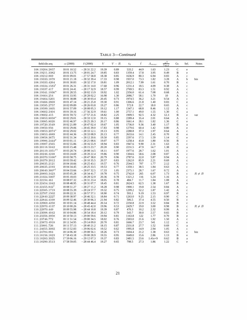
TABLE 3—Continued
field.tile.seq α (2000) δ (2000) V V − R t0 t Amaxχ2
ndofGr. Sel. Notes
108.19204.2857 18 01 10.52 −28 31 22.2 19.39 0.89 533.2 44.9 1.63 1.23 C e108.19211.3382 18 01 13.75 −28 01 24.7 19.85 0.83 1359.4 17.8 3.95 0.49 B e108.19212.869 18 01 09.01 −27 57 58.8 18.38 0.85 1636.9 80.3 6.94 0.83 A c108.19333.1878 18 01 21.18 −28 32 39.4 17.33 0.98 1937.0 73.3 1.82 3.28 A b bin108.19333.4264 18 01 30.83 −28 32 17.0 19.81 1.09 2012.1 7.99 1.61 0.70 B c108.19334.1583† 18 01 26.31 −28 31 14.0 17.68 0.96 1231.4 18.5 4.09 0.38 A c108.19337.417 18 01 24.41 −28 17 32.9 18.57 0.99 2769.5 83.3 1.51 0.92 A c108.19341.1936n 18 01 28.55 −28 02 13.9 19.92 1.02 2356.0 61.4 7.08 0.68 A c108.19464.254 18 01 33.95 −28 28 02.2 16.98 1.30 2086.7 58.1 1.70 10 A c108.19464.5201 18 01 38.88 −28 30 03.4 20.45 0.73 1974.5 36.2 3.21 0.54 A c108.19466.2869 18 01 47.14 −28 21 25.8 19.30 0.91 1306.6 21.8 1.40 0.83 C e108.19595.2757 18 02 09.89 −28 26 03.8 19.27 0.86 572.8 22.7 18.0 0.65 A c108.19599.1605 18 01 57.09 −28 08 05.3 19.12 1.17 1347.1 68.8 8.46 1.12 A c108.19602.2404 18 01 59.16 −27 56 32.9 19.61 1.00 2757.1 49.0 1.55 1.30 C a108.19602.415 18 01 59.72 −27 57 21.6 18.82 2.25 1909.5 92.5 4.32 12.3 B e var108.19853.8058o 18 02 29.01 −28 33 12.0 19.15 0.88 2289.4 35.4 2.01 0.64 A c108.19985.8020 18 02 46.97 −28 25 39.3 20.17 0.86 1661.4 28.1 1.82 1.36 C e109.19720.3549 18 02 21.89 −28 47 02.4 19.67 1.05 1736.0 9.36 3.40 1.17 B a109.19850.956 18 02 29.06 −28 45 39.0 17.83 0.98 1279.6 60.4 1.42 0.80 A e109.19853.2074o 18 02 29.02 −28 33 12.1 19.13 0.95 2288.8 37.3 1.97 0.64 A c109.19853.4889 18 02 44.36 −28 33 08.9 20.13 0.77 2633.6 14.1 2.45 0.70 B e109.19858.3675 18 02 31.34 −28 12 20.6 19.50 0.85 2297.6 17.5 1.59 1.14 C e109.19986.2444p 18 03 01.11 −28 21 08.6 19.07 0.77 1258.4 43.8 1.80 0.56 B c109.19987.2565 18 02 55.86 −28 16 55.9 18.94 0.83 1947.6 9.90 2.31 1.63 A c109.20118.5042 18 03 15.48 −28 15 23.7 20.20 0.90 2231.5 47.9 14.7 1.38 C a109.20119.1051f† 18 03 20.74 −28 08 14.5 18.11 0.97 1977.6 28.7 1.62 1.01 A c109.20246.4248 18 03 24.69 −28 20 22.4 19.86 0.90 1304.6 58.6 2.08 0.87 A c109.20370.5166q 18 03 58.75 −28 47 38.0 20.79 0.96 2787.6 22.0 5.87 0.94 A c109.20379.2012 18 03 59.42 −28 10 35.5 20.57 0.83 1262.0 85.9 2.21 0.69 A c109.20635.2121 18 04 18.66 −28 25 43.1 19.57 0.76 2544.5 707 1.77 2.12 C c109.20635.2193 18 04 34.45 −28 25 33.5 19.53 0.77 1359.1 38.5 1.84 0.63 A c109.20640.360g† 18 04 33.66 −28 07 32.5 17.33 1.05 2375.1 28.7 1.67 0.72 A c109.20893.3423 18 05 05.28 −28 34 41.7 19.78 0.75 2742.0 265 6.07 1.73 B c R 6= B
109.21024.5007 18 05 18.03 −28 28 52.9 20.36 0.78 1321.2 116 5.24 1.16 A c110.22194.461 18 08 07.32 −28 31 23.4 18.05 0.78 484.7 11.7 1.84 1.08 A c110.22454.1042 18 08 48.95 −28 31 07.7 18.45 0.81 2624.5 62.5 1.38 1.67 B e110.22455.842† 18 08 51.27 −28 27 11.2 18.28 0.98 1900.1 19.8 2.54 0.84 A c110.22585.1719 18 08 55.39 −28 24 57.7 19.32 0.75 1209.2 52.2 1.87 1.42 A c110.22707.1502 18 09 22.31 −28 57 57.1 18.90 0.74 593.1 9.19 1.53 0.97 B c110.22840.2227 18 09 38.97 −28 46 32.1 18.84 0.71 1263.0 9.25 2.15 0.90 C e110.22844.4168 18 09 32.46 −28 30 06.3 21.94 0.82 506.5 37.4 4.55 0.50 B c110.22969.4258 18 10 01.14 −28 48 44.4 20.14 0.72 2250.8 22.9 3.52 0.84 B c110.22970.4137 18 10 00.26 −28 45 42.0 19.96 0.53 2429.7 19.0 3.00 0.98 B c R 6= B110.22970.449 18 09 55.98 −28 44 10.8 19.39 0.87 470.3 10.2 2.32 0.99 A c110.23098.4042 18 10 04.86 −28 54 18.4 20.12 0.79 543.7 30.0 2.57 0.65 B c110.23356.3958 18 10 50.13 −29 00 59.6 19.94 0.81 1163.8 122 1.77 0.70 B e111.23746.772 18 11 51.54 −29 00 34.5 18.02 0.76 2303.0 21.6 1.92 1.50 A c111.23873.4918 18 11 54.95 −29 14 09.0 20.70 0.81 1666.7 23.7 541 1.12 C e111.23881.726 18 11 57.13 −28 40 21.2 18.15 0.87 2331.8 27.7 1.52 0.69 C a111.24655.3092 18 13 52.83 −29 06 02.6 19.52 0.62 1995.8 14.9 2.94 1.05 A c111.24784.884 18 14 06.30 −29 08 56.1 18.26 0.73 1604.4 21.2 1.38 0.63 C e bin113.18156.1823 17 58 43.18 −29 00 28.9 19.55 0.95 1649.0 15.6 2.86 1.13 B e113.18283.3925 17 59 06.16 −29 12 07.3 19.37 0.83 2481.5 23.6 1.41e+9 0.62 B a113.18290.3513 17 58 59.05 −28 44 46.4 19.27 0.65 798.5 27.3 1.86 1.22 C e
21

TABLE 3—Continued
field.tile.seq α (2000) δ (2000) V V − R t0 t Amaxχ2
ndofGr. Sel. Notes
113.18292.2374 17 59 00.59 −28 36 57.5 19.17 1.04 1193.5 46.1 9.11 0.49 A c113.18414.1512 17 59 14.99 −29 08 12.9 18.06 0.79 910.3 24.0 3.04 1.65 A c113.18414.4153 17 59 16.09 −29 10 35.0 19.39 0.85 636.4 11.7 3.51 0.79 A c113.18415.5194 17 59 19.59 −29 06 07.1 20.32 1.18 1692.7 25.8 2.59 0.84 C a113.18422.3531 17 59 16.72 −28 39 16.7 19.47 0.83 820.0 26.0 1.72 0.90 C e113.18550.1664 17 59 40.61 −28 47 24.5 18.44 0.95 1650.2 36.9 1.81 0.35 A c113.18550.3650 17 59 29.86 −28 43 54.8 19.32 0.72 887.9 6.84 1.75 0.70 B e113.18550.4183 17 59 39.96 −28 43 46.8 21.02 1.82 797.8 42.1 1.67 1.09 C e113.18552.581† 17 59 35.90 −28 36 24.3 17.60 1.02 603.7 27.9 1.77 1.11 B c113.18674.756 17 59 53.40 −29 09 07.8 17.42 0.94 1879.0 114 5.82e+7 3.23 A b bin113.18676.4164 18 00 01.33 −29 02 04.8 19.40 0.82 554.5 13.9 1.57 1.33 C e R 6= B
113.18680.3511 18 00 01.98 −28 45 17.8 19.36 0.80 1613.8 23.5 3.20 1.18 A c113.18681.4992 17 59 50.67 −28 42 33.1 20.21 0.96 2330.8 20.4 11.6 0.82 B c113.18804.1061† 18 00 03.38 −29 11 04.2 18.30 1.02 1166.6 6.53 1.62 0.96 B c113.18807.1433 18 00 13.15 −28 56 16.8 19.77 0.80 1574.8 26.2 1.89 0.64 B e113.18809.3408 18 00 02.91 −28 51 02.3 19.77 0.90 564.5 16.1 3.71 0.64 A c113.18810.2999r 18 00 06.81 −28 44 00.0 19.33 0.78 2334.2 14.8 2.27 0.52 B c113.18810.4076 18 00 14.08 −28 44 54.5 19.92 0.83 1756.9 34.2 3.44 10 B e113.18812.4511 18 00 03.62 −28 39 14.1 21.02 0.95 1277.6 17.3 3.04 0.88 B c113.18932.2003 18 00 37.45 −29 17 22.5 19.55 0.96 1642.8 11.1 1.59 0.74 B e113.18934.4131 18 00 28.84 −29 09 34.9 19.82 0.82 1183.0 6.31 4.61 0.39 A c113.18940.2606 18 00 37.60 −28 45 22.1 19.16 0.75 861.8 9.73 1.58 0.73 B e113.19064.1665 18 00 44.21 −29 10 32.8 18.95 1.04 949.5 28.7 1.63 0.96 A c113.19066.2168 18 00 54.05 −29 01 08.7 18.96 0.96 533.2 10.4 1.80 1.13 B e113.19192.365† 18 01 06.92 −29 18 53.8 17.80 1.17 2092.6 36.9 1.97 0.52 B c113.19196.3672 18 01 15.02 −29 01 48.4 19.77 0.89 2049.2 10.2 7.94 0.84 A c113.19325.2001 18 01 18.14 −29 05 49.4 19.07 0.90 2285.2 37.7 9.48 0.24 A c114.19583.5176 18 01 59.13 −29 12 41.4 19.58 0.84 2019.6 39.2 8.94 1.87 A c114.19587.3861 18 02 00.22 −28 57 27.4 19.67 0.90 2306.8 21.8 6.07 1.11 A c114.19589.4067 18 02 06.33 −28 50 45.3 18.66 0.83 1371.9 19.1 1.97 0.96 A c114.19589.4149 18 01 58.45 −28 50 07.5 18.65 0.79 2020.2 20.0 1.72 1.24 A c114.19712.1763 18 02 17.96 −29 18 11.3 19.15 0.92 2660.8 9.78 1.40 0.62 B e114.19712.813† 18 02 11.41 −29 19 20.8 18.13 1.09 1643.4 23.7 3.58 0.62 A c114.19846.777† 18 02 36.82 −29 01 42.1 18.00 1.02 545.4 65.0 1.55 1.86 A c114.19970.843† 18 02 54.45 −29 26 29.5 17.99 0.96 1281.9 14.7 4.47 0.65 A c114.20104.617 18 03 16.02 −29 08 20.3 19.12 0.82 2220.4 81.3 1.01e+6 0.75 C a114.20235.908 18 03 39.60 −29 05 38.6 20.12 0.89 2057.6 47.4 1.89 1.11 A c114.20360.1661 18 03 44.17 −29 26 16.9 18.76 0.90 1895.9 25.1 2.63 0.98 A c114.20370.6070q 18 03 58.80 −28 47 38.6 20.47 0.80 2788.0 28.2 6.25 1.59 A c114.20489.3552 18 04 10.63 −29 28 57.8 20.01 0.86 2653.8 6.74 1.85 1.2 B e114.20491.1613 18 04 02.25 −29 21 09.8 18.61 0.69 558.4 19.9 3.83 0.91 A c114.20494.3907 18 04 04.91 −29 11 37.9 19.98 0.66 1938.8 23.8 3.99 1.02 A c114.20496.5206 18 04 09.01 −29 03 11.3 20.06 0.84 1748.4 107 15.8 0.68 A c114.20621.2010 18 04 29.17 −29 22 22.9 18.83 0.73 2037.6 14.6 2.23 1.11 B c114.20750.2236 18 04 51.50 −29 24 42.3 19.42 0.80 1183.0 5.15 3.01 0.68 B c114.20751.4978 18 04 51.82 −29 22 40.3 20.06 0.87 1602.8 8.07 3.46 0.77 A c115.22181.2973 18 08 01.71 −29 21 01.7 19.77 0.82 2719.8 10.4 1.90 0.77 C e R 6= B115.22435.1045 18 08 46.35 −29 44 13.8 18.64 0.78 2722.0 32.6 1.60 1.30 A c115.22442.1010 18 08 38.61 −29 17 23.6 18.52 0.77 2703.3 13.2 2.59 1.30 A c115.22564.2355 18 09 00.22 −29 48 38.2 19.15 0.62 2428.8 9.68 1.64 1.29 C e R 6= B
115.22565.2060 18 09 02.87 −29 44 12.7 19.19 0.68 463.4 28.0 2.38 20 B c R 6= B115.22698.3919 18 09 18.89 −29 32 58.8 19.89 0.44 1975.5 8.90 1.94 1.85 C e115.22701.743 18 09 15.79 −29 19 49.1 18.16 0.77 1617.7 19.0 4.26 0.74 A c115.22959.667 18 10 04.14 −29 31 03.5 17.85 0.76 1573.2 91.9 1.41 0.82 B e
22

TABLE 3—Continued
field.tile.seq α (2000) δ (2000) V V − R t0 t Amaxχ2
ndofGr. Sel. Notes
116.23740.1193 18 11 40.72 −29 27 19.6 18.94 0.83 1636.0 16.2 7.96 0.31 A c116.23864.503 18 12 07.28 −29 47 54.5 17.88 0.84 1971.2 41.3 2.57 1.42 A c116.24255.4464 18 12 57.37 −29 45 11.0 20.10 0.61 2355.0 18.5 5.15 0.62 A c116.24384.2597 18 13 14.33 −29 50 33.6 19.50 0.63 2401.1 28.3 1.93 0.89 B c118.18009.35 17 58 25.53 −30 08 08.6 17.60 1.57 2808.6 55.5 2.58 3.98 A e R 6= B var118.18012.1863 17 58 14.82 −29 56 13.2 18.73 0.77 1969.3 29.8 1.64 0.66 B c118.18014.320† 17 58 25.30 −29 47 59.5 17.02 0.98 877.6 25.5 1.58 1.05 A c118.18014.4514 17 58 29.84 −29 50 02.0 20.20 1.03 2794.5 42.7 1.68 1.15 C e118.18015.1406 17 58 25.94 −29 44 47.7 18.75 1.03 878.0 9.78 1.41 0.69 B e118.18018.2379 17 58 16.01 −29 32 10.9 19.09 0.84 1245.4 84.6 2.69 0.39 A c118.18141.731† 17 58 36.77 −30 02 19.3 17.93 1.07 884.1 9.77 12.6 0.65 B cb bin118.18270.3615s 17 59 04.77 −30 07 06.0 20.46 1.13 1893.4 9.91 2.52 0.87 B c118.18271.738† 17 58 52.46 −30 02 08.0 18.30 1.20 456.4 53.7 2.23 0.69 A c118.18276.129 17 59 03.29 −29 42 59.8 17.16 0.53 530.7 14.5 4.06 0.88 A c118.18278.3065 17 58 55.62 −29 34 24.7 20.21 0.88 594.5 21.1 1.79 1.28 A c118.18402.495† 17 59 13.85 −29 55 53.4 17.65 1.11 454.1 23.8 3.60 0.96 A c118.18407.1167 17 59 16.32 −29 38 04.1 18.61 1.12 891.3 3.19 1.60 0.73 B e R 6= B118.18529.538 17 59 35.34 −30 08 47.7 19.58 1.05 1952.0 97.4 17.0 1.44 A c118.18531.1816 17 59 37.69 −30 00 52.7 19.27 0.85 1561.5 57.2 1.34 1.26 B e118.18536.3276 17 59 34.61 −29 39 48.4 19.93 0.83 1060.5 142 2.93 0.66 C c118.18660.3016 17 59 45.20 −30 05 18.6 19.88 0.96 1169.0 8.76 2.56 1.45 C e118.18662.1151t 17 59 46.51 −29 57 28.3 18.40 0.85 2622.7 15.1 3.18 0.76 A c118.18662.2180 17 59 56.33 −29 56 38.0 19.65 1.00 1944.5 26.4 1.76 0.90 A c118.18662.3919 17 59 57.17 −29 58 58.0 20.53 0.82 980.0 15.8 1.94 0.81 B e R 6= B118.18668.3942 18 00 00.81 −29 32 40.0 20.51 1.04 954.5 12.4 2.04 1.52 B e118.18669.3968 17 59 52.03 −29 31 14.4 20.71 1.04 1972.7 15.3 2.17 0.87 B e118.18797.1397† 18 00 06.94 −29 38 06.0 19.37 1.33 2013.1 126 8.35 1.07 A c118.19182.891† 18 01 09.75 −29 56 18.9 17.98 0.93 2367.0 13.6 6.28 1.2 A c118.19184.1814 18 01 02.88 −29 48 40.2 18.70 0.73 2441.7 11.7 7.46 0.82 A c118.19184.3770 18 00 58.13 −29 49 50.6 20.05 0.88 1601.1 12.2 3.75 0.89 A c118.19184.939† 18 01 10.23 −29 48 55.4 18.08 0.99 2692.8 74.4 2.14 1.13 A c118.19311.1429 18 01 20.85 −30 00 08.6 20.49 1.06 599.7 6.81 2.11 1.05 B e119.19441.2773 18 01 38.41 −30 02 02.6 19.58 0.71 1896.1 21.7 2.34 1.23 C e R 6= B119.19442.370 18 01 51.03 −29 56 50.3 18.26 0.95 2776.0 49.7 1.31 10 A a119.19444.2055 18 01 45.53 −29 49 46.9 19.24 0.79 1543.8 51.4 20.3 2.49 A ab bin119.19568.3510 18 01 54.13 −30 12 17.4 19.75 0.79 2625.6 9.77 2.01 1.26 B c119.19576.2024 18 02 04.77 −29 43 15.9 18.80 0.72 1371.0 40.0 2.27 1.29 A c R 6= B119.19576.6481 18 01 56.62 −29 39 54.7 20.29 0.72 2697.0 6.92 4.32 0.87 B e R 6= B119.19701.1513 18 02 11.79 −30 00 58.4 19.00 0.96 2700.6 26.2 1.53 2.15 B c119.19704.5147 18 02 11.09 −29 51 21.1 20.15 0.80 1294.1 15.2 2.52 0.47 B e119.19832.5483 18 02 44.85 −29 58 18.3 20.41 0.69 2366.0 36.1 2.14 0.64 B c119.19834.46 18 02 37.08 −29 47 58.9 15.21 0.90 612.0 107 1.12 1.08 C e R 6= B119.19835.4282 18 02 35.10 −29 47 18.7 19.72 0.71 1563.8 7.78 2.47 1.54 C e119.19837.1072 18 02 37.51 −29 39 35.9 18.94 1.08 1185.8 2.47 5.43 1.38 A c119.19959.4320 18 03 03.12 −30 09 56.5 19.93 0.71 488.9 56.5 2.36 1.17 C e bin119.20088.2601 18 03 10.74 −30 15 33.5 20.24 0.79 538.8 7.14 3.09 1.10 B e119.20091.1789 18 03 06.65 −30 02 37.5 19.44 0.67 2104.2 11.8 3.32 0.76 A c119.20092.3109 18 03 10.93 −29 58 12.9 19.70 0.83 2690.4 17.7 2.23 0.74 A c119.20219.2348 18 03 30.09 −30 09 55.9 19.39 0.88 2066.5 94.3 2.19 0.53 A e119.20226.2119 18 03 35.79 −29 42 01.3 19.19 0.83 553.6 106 2.63 3.81 C b bin119.20352.2589 18 03 58.67 −29 58 48.7 17.52 0.64 1987.4 24.9 1.76 1.57 A c binR 6= B
119.20354.3615 18 03 42.72 −29 49 20.1 19.67 0.75 1213.6 24.6 1.43 1.2 B e119.20356.407 18 03 54.14 −29 42 30.8 17.16 0.95 592.2 13.3 2.42 3.35 A e119.20480.2914 18 04 16.37 −30 07 23.3 19.76 0.87 1938.1 52.3 1.89 1.08 A c
23

TABLE 3—Continued
field.tile.seq α (2000) δ (2000) V V − R t0 t Amaxχ2
ndofGr. Sel. Notes
119.20610.5200 18 04 24.83 −30 05 58.9 20.41 0.71 531.9 50.1 2.59 0.79 A e119.20611.6102 18 04 20.29 −30 02 22.1 20.66 0.68 2639.6 22.3 2.11 0.92 B c119.20737.740 18 04 50.62 −30 16 34.2 18.56 1.01 2309.1 21.0 1.34 1.74 B e119.20738.3418 18 04 37.24 −30 12 11.5 20.05 0.94 1229.9 26.8 28.3 0.45 A c119.20741.4276u 18 04 48.52 −30 01 15.7 19.78 0.84 564.3 15.4 1.90 0.74 C e120.21010.1474 18 05 30.73 −29 26 15.1 17.86 0.77 1264.1 21.2 1.67 1.53 A c120.21140.3398 18 05 33.87 −29 24 52.9 20.20 0.93 1648.2 14.9 1.70 0.99 C a120.21263.1213 18 06 04.77 −29 52 38.1 18.89 0.89 1262.5 148 2.64 3.01 A cb bin120.21392.1243 18 06 07.94 −29 59 26.1 18.95 0.97 2037.0 243 1.38 0.45 B a120.21522.2448 18 06 35.36 −29 57 43.8 19.67 0.84 1173.7 10.6 5.65 1.11 B e120.21523.2457 18 06 29.67 −29 53 06.3 19.63 0.82 1632.6 13.4 1.69 1.04 C e120.21912.3560 18 07 37.03 −29 56 08.2 20.25 0.68 2474.3 71.0 5.83e+12 1.09 B a120.21917.4650 18 07 26.44 −29 39 34.2 20.94 0.67 538.2 29.7 4.47 0.65 B c120.22043.4380 18 07 50.84 −29 54 21.8 19.93 0.85 1980.5 57.9 2.41 0.92 B c bin121.21903.1151v 18 07 23.53 −30 32 55.4 19.30 0.81 470.9 31.5 5.06 0.91 A c121.21909.1805 18 07 25.28 −30 09 39.0 19.41 0.74 1954.6 21.1 1.70 0.69 A c121.21910.1940 18 07 33.59 −30 06 36.8 19.60 0.87 2031.1 7.35 1.86 1.50 A e121.22032.133† 18 07 46.89 −30 39 41.5 16.39 0.87 1287.3 19.5 1.58 2.51 A c121.22033.917 18 07 56.49 −30 34 03.3 18.84 0.81 534.4 30.7 3.30 0.84 A c121.22292.2289w 18 08 23.17 −30 36 18.6 19.59 0.72 456.5 39.0 2.71 1.35 A c121.22423.1032 18 08 49.98 −30 31 55.9 18.89 0.86 2718.8 432 3.52 2.60 A c121.22425.177 18 08 51.10 −30 24 34.7 16.59 0.87 2766.7 7.45 3.07 0.89 A a122.22816.2315 18 09 28.78 −30 22 40.7 19.93 0.94 1329.7 49.3 1.62 1.37 C e122.23205.1241 18 10 40.17 −30 26 53.7 19.24 0.70 1308.2 9.06 2.24 0.70 A c122.23855.1875 18 12 12.44 −30 26 19.2 19.32 0.58 561.5 10.1 1.65 0.67 B e123.24378.2299 18 13 10.53 −30 11 43.1 20.00 0.72 481.2 17.1 1.64 0.71 B c124.21377.353 18 06 23.60 −30 59 03.1 19.54 0.92 1677.4 34.9 1.79 1.04 A c124.21503.1711 18 06 39.24 −31 15 19.4 19.64 0.89 2376.5 18.1 1.60 1.62 B c124.22024.4124 18 07 51.91 −31 09 19.8 20.33 0.75 544.8 35.5 2.00e+3 0.89 A e124.22155.295 18 08 11.48 −31 03 48.0 18.98 0.76 1299.9 42.2 1.43 1.06 A e124.22157.151 18 08 14.74 −30 57 48.3 17.20 0.94 418.2 140 1.47e+4 1.43 A e128.21145.1300 18 05 40.59 −29 05 59.7 18.89 0.87 1635.7 37.3 2.46 0.6 B e128.21147.5157 18 05 36.49 −28 58 20.4 20.84 0.83 2653.2 14.4 4.12 0.80 B e128.21407.2080af 18 06 24.29 −28 55 46.7 19.18 0.78 2111.9 44.7 2.99 0.39 C e128.21541.1133 18 06 42.40 −28 41 15.9 18.81 0.97 1749.7 53.8 5.81 10 A c128.21666.982 18 06 57.62 −29 00 55.2 18.35 0.85 597.6 16.0 7.15 1.15 A c128.21800.522 18 07 11.15 −28 46 58.9 18.26 0.97 1315.2 2.73 4.70 0.43 A e128.21932.1362ag 18 07 20.58 −28 36 50.7 18.96 0.84 1285.4 72.8 1.71 1.48 B c128.22057.2384 18 07 38.97 −28 57 11.8 19.17 0.60 1714.3 73.1 1.69 1.30 A c130.28701.2042 18 23 11.74 −28 00 38.0 20.70 0.53 484.3 15.8 5.51 1.25 A c130.28964.2444 18 23 50.50 −27 51 39.9 20.26 0.56 483.0 40.9 3.89 0.70 A c131.29214.519x 18 24 27.07 −28 31 37.3 18.21 0.57 1633.6 56.2 1.80 1.40 A c132.30916.803 18 28 36.19 −27 42 47.7 19.14 0.60 958.5 22.1 1.70 0.86 A c132.31306.841 18 29 33.12 −27 41 35.1 19.16 0.63 2739.8 147 2.60 1.33 A c134.33390.299 18 34 25.64 −27 26 44.5 18.25 0.56 889.2 8.79 4.80 10 A c136.27650.2370y 18 21 01.78 −28 46 46.0 19.90 0.71 2044.7 115 4.91 1.24 A c137.29210.2447 18 24 37.98 −28 43 43.8 20.16 0.66 874.2 61.9 1.52 1.11 B c137.29214.59x 18 24 27.05 −28 31 36.8 18.33 0.55 1634.6 52.5 1.81 1.16 A c R 6= B137.29731.2320 18 25 46.34 −28 42 55.7 20.19 0.67 892.8 31.0 2.02 1.22 C e137.29986.2769 18 26 29.74 −29 03 39.9 20.56 0.58 1620.0 64.8 7.36 1.02 A c139.32203.2073 18 31 35.56 −28 34 04.8 20.27 0.57 2711.4 32.1 2.54 0.77 A c142.27650.6057y 18 21 01.83 −28 46 45.0 19.87 0.68 2044.4 109 4.86 0.99 A c142.27776.3952 18 21 03.28 −29 01 06.0 20.91 0.73 2351.6 66.7 4.43 0.6 B c144.32453.1528 18 32 14.17 −29 12 07.0 20.43 0.73 940.7 7.83 3.25 1.56 C e
24

TABLE 3—Continued
field.tile.seq α (2000) δ (2000) V V − R t0 t Amaxχ2
ndofGr. Sel. Notes
148.26586.2310 18 18 24.33 −30 23 37.1 19.72 0.59 2312.1 32.6 3.56 1.31 A e R 6= B148.26590.3689 18 18 33.14 −30 04 48.5 21.24 1.18 1488.9 421 114 20 C e149.27233.2244 18 19 50.87 −30 34 50.4 20.71 0.62 497.6 39.0 2.59 0.64 B e149.27237.3033 18 19 51.90 −30 16 00.0 20.87 0.72 850.4 24.3 2.78 0.91 B e150.28409.2370 18 22 45.01 −30 08 46.0 20.48 0.38 2500.6 446 1.91 1.21 C e151.31133.1607 18 28 59.51 −30 31 54.5 19.88 0.46 883.8 11.9 1.61 1.63 B e152.26320.2643 18 17 52.02 −30 45 06.1 20.17 0.46 921.7 54.7 2.11 1.04 B e152.26964.3183 18 19 16.03 −31 10 47.0 20.41 0.64 2697.3 22.1 1.75 0.85 B c153.27488.3450 18 20 36.33 −30 54 01.5 20.55 0.38 1265.4 50.8 5.89 1.42 B e R 6= B153.28787.720z 18 23 34.30 −30 57 56.0 18.03 0.63 915.0 167 2.50 0.68 A c154.28787.2812z 18 23 34.31 −30 57 55.9 18.52 0.59 915.1 169 2.53 0.90 A c154.29041.2113 18 24 06.12 −31 20 33.8 20.31 0.53 1587.3 46.9 2.01 1.08 A c154.29175.2554 18 24 36.47 −31 05 27.1 20.85 0.61 1591.1 55.1 4.15 0.74 B c155.26043.1938 18 17 22.14 −31 54 54.0 19.67 0.44 1979.4 8.52 1.58 0.81 C e156.27606.899 18 20 54.08 −31 41 12.6 19.12 0.50 1615.3 15.5 1.89 0.65 A c158.26536.1361 18 18 02.24 −25 01 37.4 19.30 0.82 1286.6 28.1 2.07 1.05 B e158.26665.3141 18 18 27.21 −25 05 56.5 19.96 0.66 2007.6 11.5 1.58 0.78 C e R 6= B
158.26802.1155 18 18 43.16 −24 37 43.7 19.83 0.84 2018.0 47.7 1.97 0.97 B c158.27052.2802 18 19 24.84 −25 18 10.2 19.78 0.67 2085.5 142 4.94e+5 0.91 A e158.27444.129† 18 20 10.24 −25 08 26.0 16.97 0.77 2376.4 41.7 2.31 1.80 A c159.25486.1627 18 15 42.82 −25 41 03.2 19.49 0.86 2010.2 68.3 1.83 0.84 C c159.25615.941 18 15 54.71 −25 43 59.5 18.73 0.77 2681.1 58.8 2.62 0.44 A c R 6= B159.25748.2254 18 16 16.98 −25 32 25.7 19.69 0.80 2364.9 39.1 2.35 0.85 B c159.25872.1610 18 16 33.13 −25 57 52.6 19.23 0.55 1284.1 15.8 1.95 0.88 B c159.26132.3182 18 17 14.80 −25 55 58.0 20.90 0.79 1277.0 26.6 5.32 1.7 B e159.26525.1401 18 18 07.98 −25 46 46.9 21.29 0.71 507.4 72.7 9.90 1.12 A c160.27701.3570 18 20 49.55 −25 20 14.0 20.05 0.66 1650.5 27.4 1.75 1.15 B e161.24182.1566 18 12 44.08 −25 57 17.6 19.97 1.07 1952.8 110 3.92 1.26 A c161.24568.876 18 13 29.30 −26 13 58.1 18.51 0.69 1219.1 21.1 2.27 1.08 A c161.24695.1323 18 14 00.99 −26 27 21.6 18.62 0.74 1668.8 57.9 1.69 0.68 A c161.24696.1161 18 13 51.87 −26 20 42.1 18.83 0.84 559.2 36.2 2.28 0.67 C e161.24827.4269 18 14 13.00 −26 16 49.6 20.58 0.83 1553.0 23.3 2.35 0.79 B c161.24956.2466 18 14 31.72 −26 20 17.3 19.77 0.92 2307.4 98.7 1.71 0.75 A c162.25212.3830 18 14 59.66 −26 36 48.1 20.18 0.77 587.4 43.8 2.12 0.70 B c162.25865.442† 18 16 30.60 −26 26 58.3 17.54 0.90 1225.3 60.9 1.58 1.32 A c162.25868.405† 18 16 45.98 −26 11 43.1 17.33 0.83 1222.8 30.8 2.77 1.39 A c162.25869.432aa 18 16 44.34 −26 09 25.7 17.52 0.71 522.0 26.6 2.26 2.08 A c bin163.27297.2111 18 19 52.42 −26 18 05.4 20.25 0.68 505.1 23.9 2.50 1.81 C e R 6= B
163.27684.1669 18 20 48.38 −26 31 06.2 19.63 0.77 1600.1 12.9 1.65 0.82 B c166.30682.3768 18 27 46.30 −25 57 08.8 21.19 0.82 497.6 35.2 3.16 0.77 B e167.23910.3170 18 11 55.15 −26 46 32.7 20.03 0.86 1607.9 65.5 1.79 1.38 B c167.24169.3673 18 12 45.02 −26 50 53.4 20.16 0.74 564.9 45.5 2.20 0.74 C e167.24173.2623 18 12 44.90 −26 34 50.3 19.62 0.73 1722.1 93.8 1.10e+3 0.97 B e167.24564.5066 18 13 32.15 −26 31 10.3 20.36 0.87 484.1 32.8 3.03 0.81 A c167.24815.4558 18 14 09.36 −27 04 57.7 20.20 0.73 1954.8 8.05 2.89 0.87 B e R 6= B
167.24815.4984 18 14 06.96 −27 05 38.0 20.59 0.90 1296.9 38.9 2.46 0.63 B e168.25079.1100 18 14 56.37 −26 51 09.9 17.89 1.65 550.8 47.8 1.52 1.35 B e168.25853.1778 18 16 30.98 −27 14 18.7 18.83 0.63 501.5 43.8 1.59 0.69 B c168.25985.4014 18 17 01.65 −27 05 45.0 20.63 0.67 1476.1 360 18.1 1.76 B e172.31579.2624 18 30 07.75 −26 48 20.5 20.37 0.69 2736.5 128 2.31 1.33 B c172.32358.313 18 31 53.24 −26 51 42.6 18.15 0.58 2700.9 42.0 1.63 0.92 A c174.29360.352 18 24 42.09 −27 25 41.6 17.59 0.66 2735.7 75.5 17.7 1.32 A c175.31446.1290 18 29 34.21 −27 03 14.2 20.96 0.82 845.1 23.4 2.17 0.76 C c176.18693.267 17 59 46.63 −27 53 51.4 17.72 1.43 2344.5 6.36 1.29e+8 2.18 A e
25

TABLE 3—Continued
field.tile.seq α (2000) δ (2000) V V − R t0 t Amaxχ2
ndofGr. Sel. Notes
176.18826.909† 18 00 15.45 −27 42 47.8 18.78 1.21 2364.7 24.3 1.77 1.17 A c176.18827.1911 18 00 11.98 −27 36 10.6 19.59 0.96 2346.3 20.3 2.27 1.06 A c176.18954.6538 18 00 20.85 −27 48 31.2 21.39 0.93 2657.1 94.7 3.74 1.06 B c176.19214.2902 18 01 01.99 −27 51 26.5 20.83 1.04 1264.6 48.1 2.91 0.71 B c176.19214.5296 18 01 11.11 −27 49 22.2 20.43 0.97 1907.7 14.7 2.44 0.98 A e176.19219.978 18 01 04.41 −27 30 41.4 18.77 1.30 1228.9 56.7 4.71 4.40 A b bin176.19343.5828 18 01 27.84 −27 52 21.0 20.13 0.72 2665.1 18.0 1.81 0.73 C a176.19602.1226 18 01 59.22 −27 56 34.4 20.20 0.90 2754.2 62.4 2.23 1.27 B c176.19735.2709 18 02 20.27 −27 45 53.4 19.59 0.91 2025.5 12.0 1.72 1.12 B c176.19997.3338 18 02 48.51 −27 38 51.8 20.70 1.05 2790.0 75.6 1.11e+4 1.23 B a177.25109.1274 18 14 54.37 −24 49 34.9 21.07 1.05 1261.0 55.5 4.89 0.58 B c177.25111.120 18 14 52.70 −24 41 07.9 17.21 1.20 1566.9 25.9 7.64 2.20 A c177.25756.2480 18 16 24.87 −25 03 26.5 20.41 1.01 2025.2 18.5 1.65 0.94 B e178.23136.5133 18 10 10.18 −26 21 03.6 20.32 0.74 1915.9 157 5.92 0.40 A e178.23273.6023 18 10 38.12 −25 53 15.3 20.59 0.95 2362.9 11.8 57.0 0.87 C a178.23398.4814 18 10 59.48 −26 13 16.5 20.51 0.94 2420.4 37.1 2.90 0.74 A c178.23531.931† 18 11 17.41 −25 59 51.4 18.72 1.11 1590.3 13.7 2.18 1.08 A c178.23660.2137 18 11 23.70 −26 04 57.0 20.58 1.02 1191.4 101 3.63 0.82 B c179.21577.1740 18 06 31.70 −26 16 01.6 19.79 0.99 2327.8 23.3 9.32 7.51 A b bin179.21578.2080 18 06 32.82 −26 15 13.6 20.80 1.41 2382.4 63.0 8.16 1.24 A c179.21584.3189 18 06 28.52 −25 49 02.1 21.08 1.26 2690.3 34.9 1.52 0.75 B a179.21844.84 18 07 08.43 −25 49 20.7 16.98 1.36 1970.2 80.6 1.68 1.86 A c179.21971.6468 18 07 28.27 −25 59 59.7 21.53 1.24 2369.2 34.8 2.37 0.80 B e179.21971.936 18 07 22.06 −25 59 44.7 19.00 1.19 2618.6 20.9 2.95 0.91 A a179.22226.151 18 07 59.13 −26 22 46.8 17.49 1.30 2581.0 70.9 1.11e+16 1.02 B a179.22486.3353 18 08 34.24 −26 21 13.6 20.08 0.91 1615.0 20.6 3.37 0.94 A c179.22616.2234 18 09 08.05 −26 20 34.3 19.77 1.06 2321.9 13.9 27.7 1.44 C e179.22619.3190 18 08 58.42 −26 08 07.6 21.06 1.33 1623.5 174 4.27 0.79 B c bin180.22240.202† 18 07 57.82 −25 24 48.1 18.98 1.44 1286.9 311 3.42 1.15 A c180.22242.2664 18 08 09.34 −25 15 56.7 20.15 1.01 2426.9 9.88 1.70 0.86 B e180.22633.2883 18 08 58.65 −25 14 22.3 20.56 1.06 2760.5 25.7 3.71 0.82 A c180.22759.707 18 09 17.80 −25 29 03.7 19.21 1.15 2832.0 71.8 2.14 1.98 A a180.22767.1452 18 09 15.50 −24 58 14.9 20.33 1.30 1957.9 22.2 7.92 1.40 A c180.23412.3949 18 10 53.70 −25 17 28.0 21.18 1.14 2358.8 19.2 2.11 0.89 B c301.45441.747 18 31 36.15 −13 31 37.4 21.56 1.37 2682.9 45.4 5.23 1.07 C c301.45445.840 18 31 38.13 −13 16 01.1 19.32 1.00 1895.4 197 1.81 0.92 B a bin301.46110.1056 18 32 43.60 −13 44 19.0 19.81 1.15 1951.2 98.5 2.10 0.87 A c301.46285.1166 18 33 09.38 −13 16 54.1 21.20 1.20 2661.8 279 3.69 0.76 C c301.46613.3271 18 33 38.09 −13 50 23.9 20.99 1.06 2079.3 112 2.68 0.99 B c301.46616.2156 18 33 36.01 −13 35 09.1 20.18 0.94 1962.7 41.3 2.55 0.98 A c302.44927.2559 18 30 41.95 −14 14 08.1 19.52 0.97 1993.3 86.2 1.41 1.29 B e302.44928.3523 18 30 49.42 −14 10 52.9 21.41 1.07 2770.3 86.7 25.4 1.12 A c bin302.45258.1038 18 31 20.04 −14 34 07.9 19.05 0.81 1605.1 146 1.99 0.94 A c304.35391.650 18 15 08.27 −22 45 05.1 20.04 0.90 1252.8 10.9 1.58 0.78 C e304.35564.26 18 15 11.46 −22 22 59.1 17.64 1.78 1705.4 25.4 2.11 1.97 A c304.35730.425 18 15 35.67 −22 32 11.2 19.43 1.41 2686.1 81.9 2.42 0.87 A c304.35899.3004 18 15 54.97 −22 27 33.5 21.17 1.12 2632.6 38.5 3.42 0.67 B e304.36403.2137 18 16 38.95 −22 28 52.8 21.12 1.05 1244.5 57.6 2.25 0.99 B c304.36904.698 18 17 24.55 −22 41 57.2 19.94 1.04 1750.6 208 2.11 0.94 B c305.35237.685 18 14 43.51 −21 48 10.6 19.65 1.11 2655.4 260 1.47 1.66 C e305.35738.35 18 15 36.08 −22 01 54.7 17.43 1.80 1285.9 36.2 4.52 2.95 A c305.36746.2411 18 17 16.16 −22 01 18.3 20.75 1.17 2375.6 40.7 69.0 0.86 A c306.35894.1371 18 15 53.15 −22 47 22.9 20.64 1.17 1192.5 184 2.51 0.76 A e306.36223.3023 18 16 32.59 −23 17 26.8 20.29 0.86 1921.5 11.4 2.27 1.35 B c
26

TABLE 3—Continued
field.tile.seq α (2000) δ (2000) V V − R t0 t Amaxχ2
ndofGr. Sel. Notes
307.35374.3058 18 15 02.51 −23 52 41.5 20.95 1.14 2740.4 50.7 2.67 0.85 B c307.35709.1490 18 15 37.63 −23 55 11.1 19.68 0.93 1557.6 15.3 2.33 0.96 B e307.36378.482 18 16 35.35 −24 09 12.5 19.61 1.22 1267.3 32.8 1.58 0.82 B c307.36884.258ab 18 17 28.63 −23 59 45.9 17.69 1.10 1315.4 30.8 2.32 0.85 A c308.38259.1981 18 19 43.15 −21 57 45.4 20.15 0.76 2388.3 8.30 1.54 2.37 C e308.38595.1020 18 20 30.03 −21 57 04.3 19.81 1.01 2769.4 58.0 14.2 1.2 A c309.38081.3420 18 19 30.55 −22 37 56.0 21.12 1.01 1712.1 68.4 5.48 0.69 B c310.37067.3803 18 17 50.51 −23 02 22.8 21.12 0.96 1605.6 10.8 2.20 1.34 C e310.37233.3924 18 18 06.37 −23 10 06.5 20.77 0.92 1230.4 11.8 4.69 0.74 B e310.37235.3685 18 18 04.38 −23 02 11.1 21.15 1.09 2056.8 70.0 2.98 0.87 A c310.37398.2274 18 18 19.82 −23 19 08.9 21.00 0.85 1283.1 118 2.20 0.68 B c310.37400.1067 18 18 19.85 −23 14 45.3 19.43 0.98 2663.3 83.7 4.74 0.69 A c310.37407.336 18 18 28.16 −22 45 50.9 18.75 1.02 2802.6 182 1.52 1.86 C c bin310.38237.1062 18 19 52.32 −23 25 35.7 18.94 0.81 1311.7 11.9 1.57 0.81 C e R 6= B
310.38242.570 18 19 40.58 −23 04 44.2 20.00 0.94 1304.2 11.3 1.55 2.71 C e R 6= B310.38407.3684 18 19 56.45 −23 18 41.4 20.64 0.80 2726.0 639 1.71 1.30 D c310.38573.911 18 20 24.90 −23 25 17.5 19.34 0.87 1222.5 127 1.95 0.85 A c311.36884.287ab 18 17 28.62 −23 59 47.0 17.55 0.93 1315.4 30.9 2.42 0.65 A c311.36890.444 18 17 39.60 −23 36 07.4 18.67 1.09 2813.1 200 4.38 1.49 A c311.37050.344 18 17 45.38 −24 09 04.0 17.93 0.80 1295.2 27.4 1.40 1.09 A e311.37223.967 18 18 10.73 −23 47 16.5 20.99 1.09 1600.6 21.8 3.76 0.56 A c311.37727.1742 18 18 59.74 −23 49 26.7 20.10 0.95 1577.7 99.5 3.05 1.25 B c bin311.37893.6302 18 19 20.38 −23 55 36.9 21.47 0.77 2705.9 71.5 11.5 0.76 A c311.38229.2494 18 19 43.81 −23 58 55.4 19.52 0.66 2689.3 5.79 1.67 1.82 C e311.38394.386 18 20 04.48 −24 08 11.1 19.65 0.76 1268.3 31.1 3.14 1.49 A c bin311.38567.3476 18 20 19.31 −23 49 41.5 20.32 0.79 2028.1 7.20 1.80 1.19 C e401.47870.1026 17 56 22.00 −28 14 32.3 18.75 1.23 2433.3 51.7 1.49 1.33 B e401.47990.2762 17 56 51.83 −28 14 47.7 20.28 1.32 1714.1 118 2.18 0.78 B c401.47991.1840† 17 57 07.51 −28 13 44.2 19.48 1.39 1953.0 44.7 1.92 0.61 A c401.47994.1182† 17 57 07.82 −28 00 27.9 19.68 1.55 2362.7 60.6 3.68 1.05 A c401.48047.3195 17 57 14.57 −28 29 23.9 20.05 1.09 2272.9 46.9 2.19 0.41 B c401.48049.670 17 57 13.63 −28 19 12.3 18.34 1.14 1587.0 25.1 1.34 1.74 C e401.48052.861† 17 57 23.81 −28 10 24.6 18.77 1.32 2291.5 72.0 2.65 0.69 B c401.48114.174 17 57 42.91 −28 01 02.6 18.72 1.96 2624.0 51.9 6.79 0.66 A c401.48167.1934† 17 57 57.40 −28 27 09.6 18.44 1.23 2179.0 125 2.53 0.89 C c401.48167.2536 17 58 00.72 −28 27 24.3 19.59 1.32 2682.2 14.1 1.40 1.07 B e401.48229.760† 17 58 13.42 −28 20 32.2 18.07 1.15 2694.5 20.1 1.82 1.18 A c binR 6= B
401.48230.2825 17 58 13.75 −28 17 16.2 20.07 1.00 1698.3 9.43 6.43 0.46 A c401.48406.2341 17 59 01.59 −28 31 28.1 20.09 1.09 2340.3 7.64 2.83 1.15 B e401.48408.649† 17 59 08.99 −28 24 54.7 17.72 1.22 2325.4 74.6 3.07 1.30 B cb bin401.48410.1407 17 58 58.85 −28 16 30.2 18.83 1.20 2022.4 6.70 1.81 1.54 B e401.48467.4621 17 59 16.98 −28 29 42.0 20.12 0.93 2339.8 45.2 2.57 1.11 A c401.48469.789† 17 59 22.27 −28 20 21.9 18.22 1.18 1554.8 5.67 5.96 0.42 B c402.47619.1009 17 55 13.59 −28 58 33.6 20.23 1.09 1605.1 31.2 3.25 2.4 B c bin402.47623.80 17 55 15.07 −28 43 23.6 18.62 2.42 2139.5 341 1.59 5.36 D c var402.47678.1353 17 55 21.18 −29 04 12.6 18.89 1.24 2470.2 21.9 1.65 0.95 B e402.47678.1666† 17 55 22.60 −29 04 12.9 19.21 1.33 2393.1 13.6 2.48 0.88 A c402.47681.2971 17 55 28.72 −28 50 43.5 19.96 1.22 1731.8 29.6 3.32 0.85 B e402.47682.912 17 55 34.50 −28 48 26.8 18.79 0.88 1550.4 243 2.77 1.27 A c402.47736.2869 17 55 45.00 −29 13 59.1 19.58 1.07 2647.2 58.0 2.45 0.54 B e402.47737.1590† 17 55 41.50 −29 09 00.6 18.49 1.05 1552.3 5.47 2.79 1.03 B c402.47742.3318† 17 55 42.88 −28 49 17.6 20.21 1.63 1377.1 50.1 8.64 1.21 A c402.47745.3587 17 55 52.82 −28 36 43.7 21.10 1.27 2763.1 28.3 2.52 0.93 C c402.47796.1893† 17 56 10.91 −29 10 44.2 19.51 1.34 1678.7 19.3 22.5 1.47 B c
27
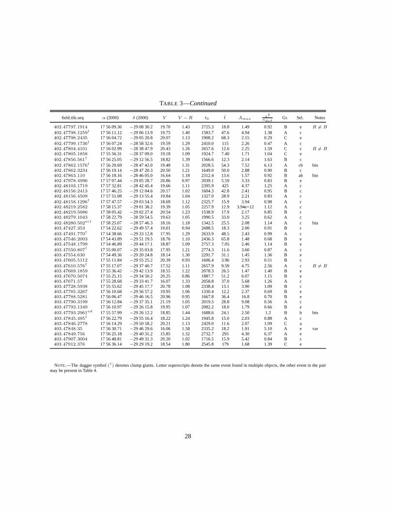
TABLE 3—Continued
field.tile.seq α (2000) δ (2000) V V − R t0 t Amaxχ2
ndofGr. Sel. Notes
402.47797.1914 17 56 09.36 −29 08 30.2 19.70 1.43 2725.3 18.8 1.49 0.92 B e R 6= B
402.47798.1259† 17 56 11.12 −29 06 13.9 19.75 1.40 1583.7 47.6 4.94 1.38 A c402.47798.2435 17 56 04.72 −29 05 20.8 20.07 1.13 1908.2 68.3 2.15 0.29 C e402.47799.1736† 17 56 07.24 −28 58 32.6 19.59 1.29 2410.0 115 2.26 0.47 A c402.47804.4101 17 56 02.99 −28 38 47.9 20.43 1.26 2657.6 12.6 2.25 1.59 C c R 6= B402.47805.1858 17 55 56.31 −28 37 09.0 19.18 1.09 1924.7 7.40 1.71 1.04 C e402.47856.561† 17 56 25.05 −29 12 56.5 18.82 1.39 1566.6 12.3 2.14 1.63 B c402.47862.1576† 17 56 20.69 −28 47 42.0 19.48 1.31 2028.5 54.3 7.52 6.13 A cb bin402.47862.3234 17 56 19.14 −28 47 20.3 20.50 1.21 1649.0 50.0 2.88 0.90 B c402.47863.110 17 56 18.16 −28 46 05.0 16.64 1.18 2312.4 13.6 1.57 0.92 B ab bin402.47978.4996 17 57 07.44 −29 05 28.7 20.86 0.97 2039.1 5.59 3.33 0.83 B e402.48103.1719 17 57 32.81 −28 42 45.4 19.66 1.11 2395.9 425 4.37 1.25 A c402.48156.2413 17 57 46.25 −29 12 04.6 20.17 1.02 1604.3 42.8 2.41 0.95 B c402.48156.4509 17 57 51.08 −29 13 55.4 19.84 1.04 1327.0 28.9 2.21 0.83 A c402.48158.1296† 17 57 47.57 −29 03 54.3 18.69 1.12 2325.7 15.9 3.94 0.98 A c402.48219.2582 17 58 15.37 −29 01 38.2 19.39 1.05 2257.9 12.9 3.94e+12 1.12 A c402.48219.5086 17 58 05.42 −29 02 27.4 20.54 1.23 1538.9 17.9 2.17 0.85 B c402.48279.1043 17 58 22.79 −28 59 54.5 19.63 1.05 1990.5 33.0 3.25 0.62 A c402.48280.502ac† 17 58 25.07 −28 57 46.3 18.16 1.18 1342.5 25.5 2.08 1.14 A c bin403.47427.353 17 54 22.62 −29 49 57.4 19.01 0.94 2688.5 18.3 2.00 0.91 B c403.47491.770† 17 54 38.66 −29 33 12.8 17.95 1.29 2633.9 48.5 2.43 0.99 A c403.47546.2003 17 54 43.89 −29 51 19.5 18.76 1.10 2436.3 65.8 1.48 0.68 B e403.47548.1799 17 54 46.89 −29 44 17.1 18.87 1.09 2757.3 7.05 2.46 1.14 B e403.47550.807† 17 55 00.07 −29 35 03.8 17.95 1.21 2774.3 11.6 3.60 0.87 A c403.47554.630 17 54 49.36 −29 20 24.8 18.14 1.30 2291.7 31.1 1.45 1.36 B e403.47605.5112 17 55 11.84 −29 55 25.2 20.39 0.93 1606.4 3.96 2.93 0.51 B c403.47610.576† 17 55 17.07 −29 37 40.7 17.52 1.11 2657.9 9.59 4.75 2.56 A c R 6= B403.47669.1859 17 55 36.42 −29 42 13.9 18.55 1.22 2078.3 26.5 1.47 1.40 B e403.47670.5074 17 55 25.15 −29 34 50.2 20.25 0.86 1887.7 51.2 6.07 1.15 B e403.47671.57 17 55 28.68 −29 33 41.7 16.07 1.33 2058.8 37.0 5.68 1.26 A c403.47728.5938 17 55 55.62 −29 45 17.7 20.78 1.08 2338.4 13.1 3.90 1.09 B c403.47785.3267 17 56 10.68 −29 56 57.2 19.95 1.06 1330.4 12.2 2.37 0.69 B e403.47788.5281 17 56 06.47 −29 46 16.5 20.96 0.95 1667.8 36.4 16.8 0.70 B e403.47790.3199 17 56 12.84 −29 37 35.1 21.19 1.05 2019.5 28.8 9.08 0.56 A c403.47793.1349 17 56 10.97 −29 26 15.8 19.95 1.07 2082.2 18.0 1.79 0.66 B e403.47793.2961ad 17 55 57.99 −29 26 12.2 18.85 1.44 1688.6 24.1 2.50 1.2 B b bin403.47845.495† 17 56 22.79 −29 55 16.4 18.22 1.24 1945.8 15.0 2.03 0.88 A c403.47846.2778 17 56 14.29 −29 50 58.2 20.21 1.13 2429.0 11.6 2.07 1.09 C a403.47848.35 17 56 30.71 −29 46 29.6 16.06 1.58 2335.2 18.2 1.91 5.10 A e var403.47849.756 17 56 25.18 −29 40 31.2 15.85 1.32 2732.7 293 4.30 6.37 A e403.47907.3004 17 56 48.81 −29 49 31.3 20.20 1.02 1716.5 15.9 5.42 0.84 B c403.47912.376 17 56 36.14 −29 29 19.2 18.54 1.80 2545.8 179 1.68 1.39 C e
NOTE.—The dagger symbol(†) denotes clump giants. Letter superscripts denote the same event found in multiple objects, the other event in the pairmay be present in Table 4.
28

TABLE 4
PARAMETERS FORNON-MICROLENSING EVENTS
field.tile.seq α (2000) δ (2000) V V − R t0 t Amaxχ2
ndofGr. Sel. Notes
101.20650.3427a 18 04 20.25 −27 24 47.3 19.61 0.77 1971.2 12.7 2.75 0.6 B e101.21042.1247c 18 05 28.07 −27 16 21.3 17.92 0.59 2806.9 19.3 1.64 0.55 B e101.21174.3112d 18 05 38.77 −27 08 28.4 19.59 0.89 1908.5 9.89 1.83 0.78 C e R 6= B
102.22851.5108e 18 09 30.47 −28 00 49.2 20.48 0.80 1307.6 15.9 2.25 0.84 C e104.19991.1951 18 03 01.33 −28 01 45.1 19.34 0.83 1739.0 54.4 2.96 1.80 C c cv104.21421.273ae 18 06 08.61 −28 00 24.7 18.61 0.70 2641.0 6.57 8.30 1.15 B e105.21291.7441 18 05 53.59 −28 03 29.8 18.59 0.79 1603.1 8.11 2.53 3.46 C e cv108.18943.3528m 18 00 21.74 −28 32 01.1 19.34 0.84 2271.8 20.0 4.68e+10 0.54 C e108.19341.2253n 18 01 28.51 −28 02 15.4 19.90 0.89 2356.0 26.1 3.95 0.69 B e109.19986.3305p 18 03 01.12 −28 21 09.5 19.33 0.70 1258.6 19.9 2.19 0.72 B e109.20370.5051q 18 03 58.70 −28 47 40.3 20.16 0.81 2787.7 10.2 7.29 0.82 B e113.18676.5195 18 00 01.25 −29 02 06.4 19.86 0.73 2255.4 12.5 2.03 2.25 C e cv113.18810.4409r 18 00 06.69 −28 44 00.3 20.04 0.82 2333.2 25.0 2.32 0.82 B e114.19842.2283 18 02 40.21 −29 19 20.1 19.67 1.11 1721.6 12.1 1.74 1.7 C a cv115.22695.3361 18 09 13.79 −29 47 36.4 19.77 0.66 2657.3 21.7 2.15 2.19 C e cvR 6= B
118.18270.4540s 17 59 04.60 −30 07 06.7 20.53 1.02 1894.2 6.11 2.04 0.96 B e118.18662.2288t 17 59 46.56 −29 57 30.1 19.65 0.99 2623.5 14.0 2.61 0.53 C e119.19707.2379 18 02 25.95 −29 39 40.4 19.84 0.80 2770.3 20.5 1.53 1.52 D c cv119.20742.2884u 18 04 48.74 −29 58 35.5 19.29 0.83 564.9 9.90 1.69 0.78 C e121.21903.3479v 18 07 23.50 −30 32 56.6 20.27 0.84 467.7 37.4 3.06 0.38 B e121.22292.3358w 18 08 23.00 −30 36 18.1 19.88 0.68 457.6 38.0 2.11 0.94 A c125.23850.4190 18 11 58.88 −30 43 54.0 20.71 0.74 2724.1 18.9 2.64 0.77 C a cv128.21407.1674af 18 06 24.32 −28 55 47.9 18.91 0.92 2106.5 27.9 2.45 0.67 B e R 6= B
128.21926.3361 18 07 33.92 −29 00 36.5 19.52 0.67 552.2 15.2 2.00 1.24 C e cvR 6= B128.21932.2196ag 18 07 20.51 −28 36 51.9 19.66 1.07 1283.8 69.1 1.45 0.79 C e145.34015.1280 18 35 55.58 −29 04 44.2 24.41 0.37 854.9 168 33.2 1.37 C c cv153.28398.2677 18 22 35.67 −30 54 35.3 22.95 −0.06 858.7 134 10.1 0.67 D c cvR 6= B162.25869.1615aa 18 16 44.38 −26 09 27.2 20.10 0.74 523.6 72.8 4.52 0.40 A c173.33002.479 18 33 17.45 −27 16 09.2 19.54 0.50 953.4 37.2 1.91 4.91 B e cvR 6= B178.23266.2918 18 10 35.18 −26 23 40.4 19.91 0.94 1323.5 6.99 7.00e+5 1.14 C e cv178.24048.3166 18 12 20.91 −26 14 03.0 20.54 0.73 2035.5 11.4 3.01 2.05 B e cvR 6= B306.36059.752 18 16 05.96 −23 02 38.9 25.20 −0.39 1265.1 536 130 5.90 D c cvR 6= B311.37730.4143 18 18 50.30 −23 36 14.9 21.89 0.76 1271.6 26.8 5.64 1.92 C e cvR 6= B
402.48280.894ac 17 58 25.01 −28 57 44.8 19.36 0.99 1343.3 22.6 3.28 0.62 A e403.47614.3183 17 55 05.97 −29 20 32.2 20.09 1.14 1323.1 14.4 1.78 2.06 C e cv403.47793.3138ad 17 55 58.04 −29 26 11.6 19.24 1.27 1689.5 19.4 3.01 0.68 B e
NOTE.—etter superscripts denote the same event found in multiple objects, events in this table are due to blending of flux froma real event and shouldbe ignored for any analysis.
29

TABLE 5
ALTERNATIVE DESIGNATIONS OF OUR EVENTS
field.tile.seq OGLE field.tile.seq OGLE ID
104.20515.498 BULSC35144974 118.19182.891 BULSC3895103104.20640.8423 BULSC35451130 118.19184.1814 sc383314104.20779.9616 BULSC35770398 118.19184.939 BULSC38120518104.20906.3973 sc366759 119.19442.370 BULSC38627315105.21287.3893 sc361245 119.19701.1513 sc11943108.19073.2291 BULSC21833776 119.19832.5483 BULSC1 460673108.19204.267 BULSC30165305 119.20092.3109 sc451286108.19333.1878 BULSC30352272 119.20219.2348 sc45810108.19464.254 BULSC30559419 178.23136.5133 BULSC16436041108.19464.5201 BULSC30553231 178.23398.4814 BULSC17270411108.19853.8058 BULSC31513194 308.38595.1020 BULSC10454300109.19853.2074 BULSC31513194 401.48406.2341 sc205229109.19853.4889 sc312369 401.48408.649 BULSC20395103109.19987.2565 sc324302 401.48467.4621 BULSC20391296109.20370.5166 sc23095 402.48158.1296 BULSC34144644109.20640.360 BULSC35451130 402.48219.2582 sc344536109.20893.3423 BULSC33164492 402.48279.1043 BULSC34639703113.18674.756 sc211395 403.47427.353 sc43503113.18810.2999 BULSC21388360 403.47491.770 BULSC4 522952113.19196.3672 sc301782 403.47546.2003 BULSC4 463924113.19325.2001 BULSC30236837 403.47550.807 BULSC4 708424114.19587.3861 BULSC3124931 403.47554.630 BULSC4 568740114.19589.4149 BULSC3148308 403.47669.1859 BULSC39323517114.20370.6070 sc23095 403.47671.57 BULSC39361372114.20494.3907 BULSC2 27414 403.47728.5938 sc393550
30

TABLE 6
CANDIDATE SAGITTARIUS EVENTS
Event ID l b V (V − R)
130.28701.2042 4.8512 −6.7517 20.70 0.53130.28964.2444 5.0507 −6.8103 20.26 0.56131.29214.519/137.29214.59 4.5149−7.2331 18.21 0.57132.30916.803 5.6640 −7.6825 19.14 0.60132.31306.841 5.7772 −7.8612 19.16 0.63134.33390.299 6.4858 −8.7196 18.25 0.56136.27650.2370/142.27650.6057 3.9432−6.6806 19.90 0.71137.29210.2447 4.3518 −7.3602 20.16 0.66137.29731.2320 4.4779 −7.5769 20.19 0.67137.29986.2769 4.2386 −7.8740 20.56 0.58139.32203.2073 5.1877 −8.6533 20.27 0.57142.27776.3952 3.7321 −6.7952 20.91 0.73144.32453.1528 4.6748 −9.0594 20.43 0.73148.26586.2310 2.2356 −6.9174 19.72 0.59148.26590.3689 2.5305 −6.8008 21.24 1.18149.27233.2244 2.2123 −7.2793 20.71 0.62149.27237.3033 2.4953 −7.1386 20.87 0.72150.28409.2370 2.8904 −7.6381 20.48 0.38151.31133.1607 3.1521 −9.0148 19.88 0.46152.26320.2643 1.8618 −6.9798 20.17 0.46152.26964.3183 1.6179 −7.4432 20.41 0.64153.27488.3450 2.0007 −7.5704 20.55 0.38153.28787.720/154.28787.2812 2.2335−8.1667 18.03 0.63154.29041.2113 1.9448 −8.4379 20.31 0.53154.29175.2554 2.2214 −8.4213 20.85 0.61155.26043.1938 0.7719 −7.4219 19.67 0.44156.27606.899 1.3232 −7.9849 19.12 0.50166.30682.3768 7.1637 −6.7227 21.19 0.82172.31579.2624 6.6359 −7.5785 20.37 0.69172.32358.313 6.7620 −7.9545 18.15 0.58173.33002.479 6.5333 −8.4153 19.54 0.50173.33142.1986 7.1540 −8.1955 20.40 0.62174.29360.352 5.5261 −6.7824 17.59 0.66175.31446.1290 6.3557 −7.5785 20.96 0.82
31

REFERENCES
Alcock, C., et al. 1993, Nature, 365, 621
Alcock, C., et al. 1996, ApJ, 463, L67
Alcock, C., et al. 1997, ApJ, 479, 119
Alcock, C., et al. 1999, PASP, 111, 1539
Alcock, C., et al. 2000a, ApJ, 541, 270
Alcock, C., et al. 2000b, ApJ, 541, 734
Alcock, C., et al. 2000c, ApJ, 542, 281
Alcock, C., et al. 2001, Nature, 414, 617
Afonso, C., et al. 2003, A&A, 404, 145
Aubourg, E. et al. 1993, Nature, 265, 623
Bellazzini, M., Ferraro, F.R., & Buonanno, R.1999, MNRAS, 307, 619
Bennett, D., et al. 2002, ApJ, 579, 639
Binney, J., Bissantz, N., & Gerhard, O. 2000,ApJ, 537, L99
Bissantz, N., Englmaier, P., Binney, J., & Ger-hard, O. 1997, MNRAS, 289, 651
Cavallo, R.M., Cook, K.H., Minniti, D., & Van-dehei, T. 2002, preprint (astro-ph/0209196)
Cseresnjes, P., & Alard, C. 2001, A&A, 369, 778
Evans, N.W. & Belokurov, V. 2002, ApJ, 567,L119
Gaudi, B.S., et al. 2002, ApJ, 566, 463
Girardi, L., Bertelli, G., Bressan, A., Chiosi, C.,Groenewegen, M. A. T., Marigo, P., Salasnich,B., Weiss, A. 2002, A&A, 391, 195
Gould, A. & Loeb, A. 1992, ApJ, 396, 104
Gould, A. 2000, ApJ, 535, 928
Griest, K. 1991a, ApJ, 366, 412
Griest, K. et al. 1991b, ApJ, 372, L79
Griest, K. & Safizadeh, N. 1998, ApJ, 500, 37
Gyuk, G. 1999, ApJ, 510, 205
Han, C, & Gould, A., 2003, ApJ, 592, 172
Hart, J., et al. 1996, PASP, 108, 220
Ibata, R.A., Gilmore, G., & Irwin, M.J. 1995,MNRAS, 277, 781
Kane, S.R., & Sahu, K.C. 2003, ApJ, 582, 743
Kiraga, M., & Paczynski, B. 1994, ApJ, 430,L101
Marshall, S.L., et al. 1994, in IAU Symp. 161,Astronomy From Wide Field Imaging, ed.H.T. MacGillivray et al., (Dordrecht: Kluwer)
Mao, S. & Paczynski, B. 1991, ApJ, 374, L37
Metcalf, R.B. 1995 ApJ, 110, 869
Monaco, L., Ferraro, F.R., Ballazzini, M., & Pan-cino, E. 2002, ApJ, 578, L47
Nair, V. & Miralda-Escude, J. 1999, ApJ, 515,206
Nemiroff, R.J. 1991, A&A, 247, 73
Paczynski, B. 1986, ApJ, 304, 1
Paczynski, B. 1991, ApJ, 371, L63
Popowski, P., et al. 2001a, ASP Conference Se-ries: ‘Microlensing 2000: A New Era ofMicrolensing Astrophysics’, eds. J.W. Men-zies & P.D. Sackett, Vol. 239, p. 244 (astro-ph/0005466)
Popowski, P., Cook, K.H., & Becker, A.C. 2003,AJ, 126, 2910
Popowski, P., et al. 2004 (companion Paper)
Rhie, S. et al. 2000, ApJ, 533, 378
Schechter, P.L., Mateo, M. & Saha A. 1993,PASP, 105, 1342
Sevenster, M.N. & Kalnajs, A.J. 2001, AJ, 122,885
Sterken, C., & Jaschek, C., 1996 “Light Curves ofVariable Stars”, Cambridge University Press,Cambridge, UK
Stubbs, C.W., et al. 1993, in Proceedings of theSPIE, Charge Coupled Devices and Solid StateOptical Sensors III, ed. M. Blouke, 1900, 192
Sumi, T., et al. 2003, ApJ, 591, 204
Udalski, A., et al. 1993, Acta Astron., 43, 69
Udalski, A., et al. 1994a, ApJ, 426, L69
Udalski, A., et al. 1994b, Acta Astron., 44, 165
Udalski, A., et al. 2000, Acta Astron., 50, 307
32

Wozniak, P.R., Udalski, A., Szymanski, M., Ku-biak, M., Pietrzynski, G., Soszynski, I., &Zebrun, K. 2001, Acta Astron., 51, 175
Zhao, H., Spergel, D.N., & Rich, R.M., 1995,ApJ, 440, L13
Zhao, H., & Mao, S. 1996, MNRAS, 283, 1197
This 2-column preprint was prepared with the AAS LATEXmacros v5.2.
33

Fig. 10.— Example lightcurves of microlensing candidates and some non-microlensing candidates, orga-nized by field.tile.sequence. Also given areAmax, t, our subjective grade of data quality (A-F), the methodby which the event was selected, and any notes concerning ourclassification of the event. All lightcurvedata and figures will be available athttp://wwwmacho.mcmaster.ca.
34
Related Documents