GACV for Support Vector Machines - pages.stat.wisc.edupages.stat.wisc.edu/~wahba/ftp1/GACVforSVM.pdf · SVM classifier GACV for Support Vector Machines For future reference we review

16 GACV for Support Vector Machines

Grace Wahba Department of Statistics University of Wisconsin 1210 West Dayton Street Madison, WI 53706, USA [email protected]

Yi Lin Department of Statistics University of Wisconsin 1210 West Dayton Street Madison, WI 53706, USA yilin@stat. wisc. edu

Hao Zhang Department of Statistics University of Wisconsin 1210 West Dayton Street Madison, WI 53706, USA [email protected]

We introduce the Generalized Approximate Cross Validation (GACV) for estimat­ing tuning parameter(s) in SVMs. The GACV has as its target the choice of param­eters which will minimize the Generalized Comparative Kullback-Leibler Distance (GCKL). The GCKL is seen to be an upper bound on the expected misclassifica­tion rate. Some modest simulation examples suggest how it might work in practice. The GACV is the sum of a term which is the observed (sample) GCKL plus a margin-like quantity.

298 GACV for Support Vector Machines

16.1 Introduction

reproducing kernel Hilbert space (RKHS)

GCKL

GACV

It is now common knowledge that the support vector machine (SVM) paradigm, which has proved highly successful in a number of classification studies, can be cast as a variational/regularization problem in a reproducing kernel Hilbert space (RKHS) , see [Kimeldorf and Wahba, 1971, Wahba, 1990, Girosi, 1998, Poggio and Girosi, 1998], the papers and references in [Scholkopf et al., 1999a], and elsewhere. In this note, which is a sequel to [Wahba, 1999b], we look at the SVM paradigm from the point of view of a regularization problem, which allows a comparison with penalized log likelihood methods, as well as the application of model selection and tuning approaches which have been used with those and other regularization-type algorithms to choose tuning parameters in nonparametric statistical models.

We first note the connection between the SVM paradigm in RKHS and the (dual) mathematical programming problem traditional in SVM classification problems. We then review the Generalized Comparative Kullback-Leibler distance (GCKL) for the usual SVM paradigm, and observe that it is trivially a simple upper bound on the expected misclassification rate. Next we revisit the GACV (Generalized Approximate Cross Validation) as a proxy for the GCKL proposed by Wahba [1999b] and the argument that it is a reasonable estimate of the GCKL. We found that it is not necessary to do the randomization of the GACV in [Wahba, 1999b] , because it can be replaced by an equally justifiable approximation which is readily computed exactly, along with the SVM solution to the dual mathematical programming problem. This estimate turns out interestingly, but not surprisingly to be simply related to what several authors have identified as the (observed) VC dimension of the estimated SVM. Some preliminary simulations are suggestive of the fact that the minimizer of the GACV is in fact a reasonable estimate of the minimizer of the GCKL, although further simulation and theoretical studies are warranted. It is hoped that this preliminary work will lead to better understanding of "tuning" issues in the optimization of SVM's and related classifiers.

16.2 The SVM Variational Problem

reproducing kernel

Let T be an index set, t E T Usually T = Ed , Euclidean d-space, but not necessar­ily. Let K(s, t), s, t E T, be a positive definite function on T 0 T, and let HK be the RKHS with reproducing kernel (RK) K. See [Wahba, 1990, 1982, Lin et al., 1998] for more on RKHS. RK's which are tensor sums and products of RK's are discussed there and elsewhere. K may contain one or more tuning parameters, to be chosen. A variety of RK's with success in practical applications have been proposed by var­ious authors, see, e.g., the Publications list at http://www . kernel-machines. org. Recently [Poggio and Girosi, 1998] interestingly observed how different scales may be accommodated using RKHS methods. We are given a training set {Yi, td, where the attribute vector t i E T , and Yi = ±1 according as an example with attribute

16.3 The Dual Problem 299

regularization problem

vector ti is in category A or B. The classical SVM paradigm is equivalent to: find f>.. of the form canst + h, where h E llK to minimize

1 n

- 2)1 - ydi)+ + Allhll~K ' n i=1

(16.1)

here fi = f (ti) , and (T)+ = T, T > 0; = 0 otherwise. Similar regularization problems have a long history, see, for example [Kimeldorf and Wahba, 1971]. Once the minimizer, call it f>.. is found , then the decision rule for a new example with attribute vector t is: A if f>..(t) > 0, B if f>..(t) < O.

We will assume for simplicity that K is strictly positive definite on T ® T, although this is not necessary. The minimizer of (16.1) is known to be in the span {K ( ., ti ), i = 1"" n} , of representers of evaluation in 1£ K . The nmc­tion K(· , ti ) is K(s , ti) considered as a function of s with ti fixed. The fa­mous "reproducing" property gives the inner product in llK of two represen­ters as < K(-, ti), K(-, tj) >1i.K= K(ti, tj) . Thus, if h(·) = 2::~=1 CiK(· , ti), then Ilhll~K = 2::~j=I CiCjK(ti, tj). Letting e = (l , ·· ·, l)',y = (Yl,"' ,Yn)' ,c = (cl , · · · ,en)' , (f(h) ,· ··f(tn))' = (h,···,fn)' , and with some abuse of notation, letting f = (h ," " fn)' and K now be the n x n matrix with ijth entry K(ti , tj) , and noting that f(t) = d + 2::~=1 CiK(t , ti) for some c, d, we have

f=Kc+ ed

and the variational problem (16.1) becomes: find (c, d) to minimize

1 n - 2)1 - ydi)+ + AC' K c. n i=1

(16.2)

(16.3)

16.3 The Dual Problem

Let Y be the n x n diagonal matrix with Yi in the iith position, and let H = 2;'>. Y KY. By going to the dual form of (16.3), it can be shown that c = 2;'>. Ya , where a is the solution to the problem

.. L 1 'H ' maXImIze = --a a + e a 2 . (16.4)

{ 0 < a < e

subject to - -e'Ya = y'a = O.

(16.5)

Assuming that there is an i for which 0 < ai < 1, it can also be shown that d = l/Yi - 2::;=1 cjK(ti, tj). This is the usual form in which the SVM is computed. In the experiments reported below, we used the MINOS [Murtagh and Saunders, 1998] optimization routine to find a, and hence c. The support vectors are those K(· , ti) for which a i =1= 0, equivalently Ci =1= O. d can be found from any of the support vectors for which 0 < a i < 1.

300

margin of the SVM classifier

GACV for Support Vector Machines

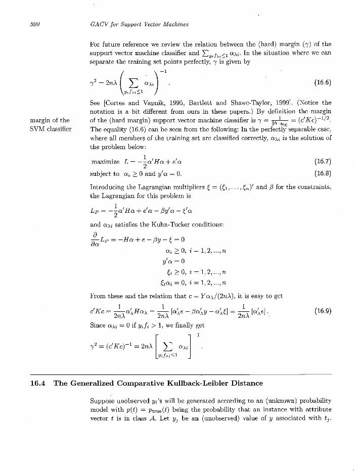
For future reference we review the relation between the (hard) margin (J) of the support vector machine classifier and L y ;JAi9 a.>,i. In the situation where we can separate the training set points perfectly, "( is given by

(16.6)

See [Cortes and Vapnik, 1995, Bartlett and Shawe-Taylor, 1999]. (Notice the notation is a bit different from ours in these papers.) By definition the margin of the (hard margin) support vector machine classifier is "( = Ilhll1iJC = (C'KC)-1/2. The equality (16.6) can be seen from the following: In the perfectly separable case, where all members of the training set are classified correctly, a.>,i is the solution of the problem below:

1 , , maximize L = - -a H a + e a

2 subject to ai 2: 0 and y' a = o.

(16.7)

(16.8)

Introducing the Lagrangian multipliers ~ = (6, ... '~n)' and f3 for the constraints, the Lagrangian for this problem is

L 1 'H ' f3' (:, p=-2"a a+ea- ya-",a

and aM satisfies the Kuhn-Tucker conditions:

[) [)a Lp = -Ha + e - f3y - ~ = 0

ai 2: 0, i = 1,2, ... ,n

y'a = 0

~i 2: 0, i = 1,2, ... ,n

~iai = 0, i = 1,2, ... ,n

From these and the relation that c = Ya.>,/(2nA), it is easy to get

, 1, 1 [' , '] 1 [' ] eKe = 2nA a.>,Ha.>, = 2nA a.>,e - f3a.>,y - a.>,~ = 2nA a.>,e .

Since a'>'i = 0 if Ydi > 1, we finally get

(16.9)

16.4 The Generalized Comparative Kullback-Leibler Distance

Suppose unobserved y/s will be generated according to an (unknown) probability model with p(t) = Ptrue(t) being the probability that an instance with attribute vector t is in class A. Let Yj be an (unobserved) value of y associated with tj.

16.5 Leaving-aut-one and the GACV 301

GCKL

penalized log likelihood

Given f>. , define the Generalized Comparative Kullback-Leibler distance (GCKL distance) with respect to 9 as

1 n

GCKL(Ptrue, !>.J == GCKL(>") = Etrue - "Lg(Yjf>.j). n j=l

(16.10)

Here f>. is considered fixed and the expectation is taken over future , unobserved Yj. If g(T) = In(1 + e-T

), (which corresponds to classical penalized log likelihood estimation if it replaces (1 - T)+ in (16.1)) GCKL(>") reduces to the usual CKL for Bernoulli data l averaged over the attribute vectors of the training set. More details may be found in [Wahba, 1999b] . Let [T]* = 1 if T > 0 and 0 otherwise. If g(T) = [-T] *, then

Etrue[-Yjf>.j]* = P[trueU[- f>.j]* + (1- P[trueU) [f.\j] *

= P[trueJj, f>.j < 0

= (1- P[trueJj), f>.j > 0,

(16.11)

(16.12)

(16.l3)

where P[trueJj = P[true] (tj) , so that the GCK L(>..) is the expected misclassification rate for f.\ on unobserved instances if they have the same distribution of tj as the training set. Similarly, if g(T) = (1- T)+, then

E true(1- Yjf>.j)+ = P[trueJj(1 - f>.j), f>.j < -1

= 1 + (1 - 2P[trueJj) f>.i> - 1 ::; f>.j ::; 1

= (1 - P[trueJj)(1 + f>.j), f>.j > 1.

(16.14)

(16.15)

(16.16)

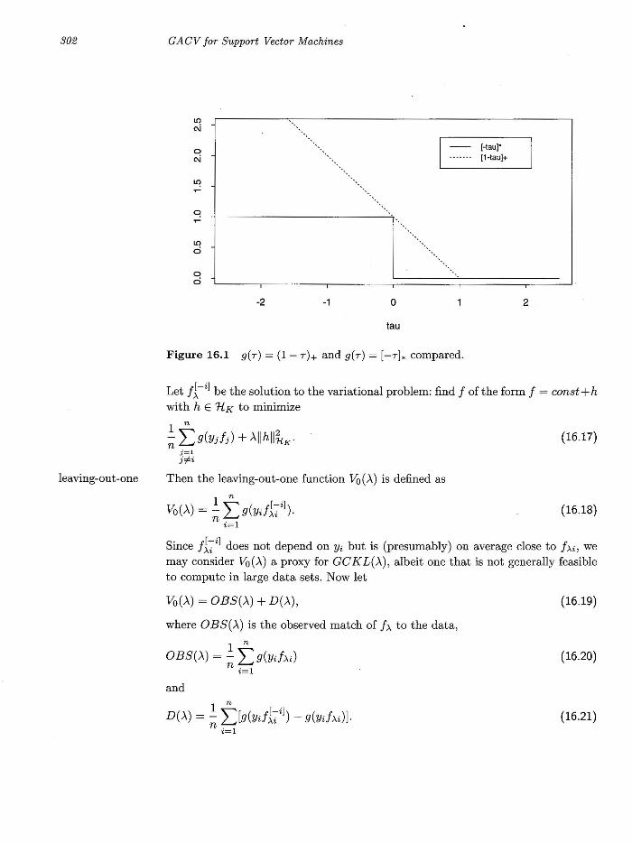
Note that [-ydi]* ::; (1 - ydi)+, so that the GCKL for (1 - ydi)+ is an upper bound for the expected misclassification rate - see Figure 16.1.

16.5 Leaving-out-one and the GACV

Recently there has been much interest in choosing>.. (or its equivalent, referred to in the literature as 2~C)' as well as other parameters inside K. See for example [Burges, 1998, Cristianini et al., 1999, Kearns et al. , 1997], surely not a complete list. Important references in the statistics literature that are related include [Efron and Tibshirani , 1997, Ye and Wong, 1997]. Lin et al. [1998] consider in detail the case g(T) = In(l+ e-T

). We now obtain the GACV estimate for>.. and other tuning parameters.

1. The usual CKL (comparative KuIlback-Leibler distance) is the KuIlback-Leibler dis­tance plus a term which depends only on P[trueJ. In this case 9 is the negative log likelihood and f>. plays the role of (an estimate of) the logit In[p/1 - pJ. See also [Friedman et al., 1998J .

302

leaving-out-one

GACV for Support Vector Machines

o N

LO o

o o

-2 -1

.[ .......................... .

o

tau

Figure 16.1 g(r) = (1 - r)+ and g(r) = [-r]. compared_

[-tau]" [1-tau]+

2

Let li- i] be the solution to the variational problem: find I of the form I = const + h with h E 1lK to minimize

1 n

:; Lg(Yj!i) + '\llhll~K-j=l

#i

Then the leaving-out-one function Vo(,\) is defined as

( ) _ 1 ~ ( [-i] Vo ,\ - - ~g yd)..i ). n i=l

(16.17)

(16.18)

Since Iti] does not depend on Yi but is (presumably) on average close to 1M , we

may consider Vo('\) a proxy for GCKL(,\), albeit one that is not generally feasible to compute in large data sets. Now let

Vo('\) = OBS('\) + D(,\),

where OBS{'\) is the observed match of J>-. to the data,

1 n

OBS('\) = - Lg(YdM) n i=l

and

(16.19)

(16.20)

(16.21 )

16.5 Leaving-out-one and the GACV 303

Using a first order Taylor series expansion gives

( ) 1 ~ 8g ( [-i l ) D A ~ --~ 8f . f>... i - f>'i . n i=l >.t

(16.22)

Next we let f..L(J) be a "prediction" of Y given f. Here we let

8 L: af/(Ydi). yE{+l,-l}

(16.23)

When g(7) = In(l+e- T) then f..L(J) = 2p-l = E{Ylp}. Since this g(7) corresponds

to the penalized log likelihood estimate, it is natural in this case to define the "prediction" of Y given f as the expected value of Y given f (equivalently, p). For g(7) = (1- 7)+ , this definition results in f..L(J) = -1 , f < -1; f..L(J) = 0, -1 ::; f ::; 1 and f..L(J) = 1 for f > 1. This might be considered a kind of all-or-nothing prediction of y, being, essentially, ±1 outside of the margin and ° inside it. Letting f..L>'i = f..L(J>d) and f..L~~il = f..L(Jt il ), we may write (ignoring, for the moment, the possibility of dividing by 0) ,

n 8 (f f[- il ) D(A) ~ _..!:. ~ ----.!L >.i - >.i ( . _ [-:il) ~ ~ £:If . [-il Yt f..L>.t

n i=l U >.t (Yi - f..L>'i ) (16 .24)

This is equation (6.36) in [Wahba, 1999b]. We now provide somewhat different arguments than in [Wahba, 1999b] to obtain a similar result , which, however is easily computed as soon as the dual variational problem is solved.

Let f>...[i, x] be the solution of the variational problem (16.1) 2 given the data {Yl,···, Yi-l, x, Yi+1,·· · , Yn}. Note that the variational problem does not require that x = ±1. Thus f>...[i,Yi](ti) == f>.i. To simplify the notation, let f>...[i,X](ti) = f>... i [i, x] = f>...dx]. In [Wahba, 1999b] it is shown, via a generalized leaving-out-one lemma, that f..L(J) as we have defined it has the property that ft il = f>... [i, f..Ltil](ti). Letting f..L~~il = x, this justifies the approximation

(16.25)

Furthermore, f..Lt il == f..L(Jt il ) = f..L(J>. i ) whenever ftil and f>... i are both in the interval (-00, -1), or [-1, 1], or (1 , (0), which can be expected to happen with few exceptions. Thus, we make the further approximation (Yi - f..Ltil) ~ (Yi - f..L>.i) , and we replace (16.24) by

1 L:n 8g 8f>...i D(A) ~ -- --(Yi - f..L>. i ).

n 8f>. · ay· i=l t t (16.26)

2. d is not always uniquely determined; this however does not appear to be a problem in practice, and we shall ignore it.

i~ .. 'I

!I

304

GACV

GACV for Support Vector Machines

Now, for g(T) = (1 - T)+

8g 8hi (Yi - J1>.i) = -2, Yd>.i < -1

= -1, Yd>.i E [-1,1]

= 0, Yd>.i > 1,

(16.27)

It is not hard to see how 8/.:: should be interpreted. Fixing A and solving the variational problem for h we obtain a = a>., C = c>. = 2~>' Ya>. and for the moment letting h be the column vector with ith component hi, we have h = Kc>. + ed = 2~>.KYa>. + ed. From this we may write

(16.28)

The resulting GACV(A), which is believed to be a reasonable proxy for GCKL(A), is, finally

1 n

GACV(A) = - 2)1 - Yd>.ih + iJ(A), n i=l

(16.29)

where

If K = Ke, where () are some parameters inside K to which the result is sensitive, then we may let GACV(A) = GACV(A, ()). Note the relationship between iJ and ~Yi!Ai9 aM and the margin I. If K(·,·) is a radial basis function then IIK(·, ti)II~K = K(O, 0). Furthermore IIK(-, ti) - K(-, tj)II~K is bounded above by 2K(0, 0). If all members of the training set are classified correctly then Ydi > ° and the sum following the 2 in (16.30) does not appear and iJ(A) = K(O, 0)jnI2.

We note that Opper and Winther (Chapter 17) have obtained a different approx­imation for hi - ftiJ.

16.6 Numerical Results

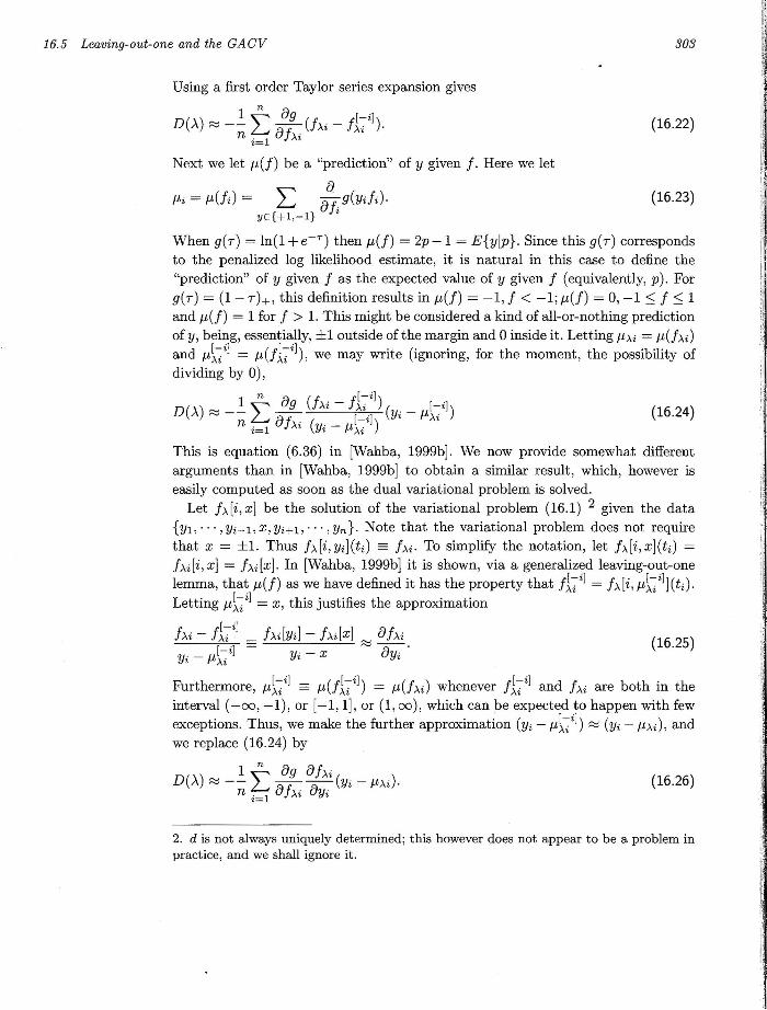
We give two rather simple examples. For the first example, attribute vectors t were generated according to a uniform distribution on T, the square depicted in Figure 16.2. The points outside the larger circle were randomly assigned +1 (" +") with probability P[trueJ = .95 and -1 (" 0") with probability .05. The points between the outer and inner circles were assigned + 1 with probability P[trueJ = .50, and the

16.6 Numerical Results 305

points inside the inner circle were assigned +1 with probability P[trueJ = .05. In this and the next example, K(s , t) = e-~lIs-tIl2 , where (7 is a tunable parameter to be

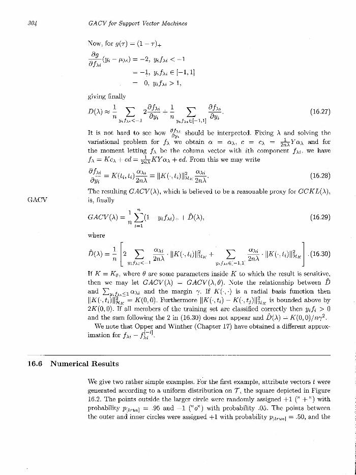
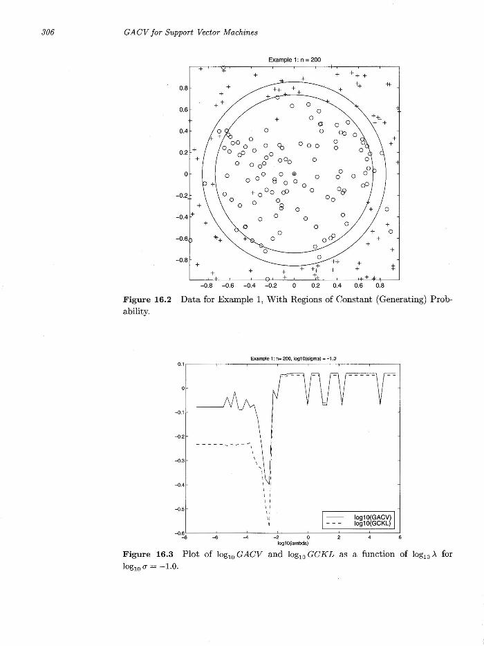
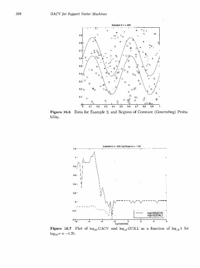
chosen. Figure 16.3 gives a plot of 10glO(GACV) of (16.29) and 10glO(GCKL) of (16.10) as a function of log 10 A, for 10glO (7 = -1. Figure 16.4 gives the corresponding plot as a function of 10glO (7 for 10glO A = -2.5 , which was the minimizer of 10glO(GACV) in Figure 16.3. Figure 16.5 shows the level curve for 1>. = 0 for 10glOA = -2.5 and 10glO(7 = -1.0, which was the minimizer of loglO(GACV) over the two plots. This can be compared to the theoretically optimal classifier, which the Neyman-Pearson Lemma says would be any curve between the inner and outer circles, where the theoretical log-odds ratio is O. For the second example, Figure 16.6 corresponds to Figure 16.2, with P[trueJ = .95, .5 and .05 respectively in the three regions, starting from the top. Figure 16.7 gives a plot of 10glO(GACV) and loglO (GC K L) as a function of 10glO A for loglO (7 = -1.25 and Figure 16.8 gives 10glO(GACV) and 10glO(GCKL) as a function of 10glO(7 for 10glOA = -2.5, which was the minimizer of Figure 16.7. Figure 16.9 gives the level curves for 1>. at 0 for 10glO A = -2.5, 10glO (7 = -1.25, which was the minimizer of 10glO(GACV) over Figures 16.7 and 16.8. This can also be compared to the theoretically optimal classifier, which would be any curve falling between the two sine waves of Figure 16.7.

It can be seen that 10glO GACV tracks 10glO GCKL very well in Figures 16.3, 16.4, 16.7 and 16.8, more precisely, the minimizer of 10glO GACV is a good estimate of the minimizer of loglO GC K L.

A number of cross-sectional curves were plotted, first in 10glO A for a trial value of 10glO (7 and then in 10glO (7 for the minimizing value of 10glO A (in the GACV curve), and so forth, to get to the plots shown. A more serious effort to obtain the global minimizers over of 10glO(GACV) over 10glO A and 10glO (7 is hard to do since both the G ACV and the GC K L curves are quite rough. The curves have been obtained by evaluating the functions at increments on a log scale of .25 and joining the points by straight line segments. However, these curves (or surfaces) are not actually continuous, since they may have a jump (or tear) whenever the active constraint set changes. This is apparently a characteristic of generalized cross validation functions for constrained optimization problems when the solution is not a continuously differentiable function of the observations, see, for example [Wahba, 1982, Figure 7] . In practice, something reasonably close to the minimizer can be expected to be adequate.

Work is continuing on examining the G ACV and the GC K L in more complex situations.

Acknowledgments

The authors thank Fangyu Gao and David Callan for important suggestions in this project. This work was partly supported by NSF under Grant DMS-9704758 and NIH under Grant ROl EY09946.

306 GA CV for Support Vector Machines

Example 1: n = 200

+ + + + + + +

0.8 + + ++ +t-++ +

+ + +

++ 0 0 0.6 0

+ 0 <!:il

0.4 0 0

0 + 0 CO 00 0 +

+ 0 0.2 0

+ g 000 0 00

0 0 0 6) 0 o 0 €I 0 0 0

0 0 0

+ 00 0 cf) 0 0& -0.2 0 0

0 0 + B 0

-0.4 + 0 0 0

0

0 0 +

0& 0

-0.6 -++ T + 0 +

+ - 0.8 0

++ + + +: :I: + + + + +

+ + + + - 0.8 -0.6 - 0.4 -0.2 0 0.2 0.4 0.6 0 .8

Figure 16.2 Data for Example 1, Wit h Regions of Constant (Generating) Prob­ability.

Example 1: n= 200. log10(sigma) = -1 .0 0.1,--- ---.------;,------.----,- --.,------,------,

o

- 0.1

-0.2

- - - - - ..... -..... - - \

-0.3

-0.4

-0.5

I I

I I

I I

I I

\I II

• log10(GACV) log10(GCKL)

-O.6 L - ---'------'. _ _ ---L. __ -"--~==:::::;:::====:::;::==:=:.J -8 -6 -4 -2 0

log10(lambda)

Figure 16.3 Plot of loglO GACV and lOglO GCKL as a function of loglO A for loglO 0" = -1.0.

j

16.6 Numerical Results

Example 1: n = 200. IoglO(lambda) = -2.5 0.2,----.---.-----r----.----,-----,r-----,

0.1

-0.1

-0.2

-0.3

-0.4

-0.5

I

" " " "

log10(OB5+D) log10(GCKL)

-0.6 L_---'. __ --':-__ --:'-__ -'--==::::i====~====~ -8 -6 -4 -2 0 2

log10(sigma)

307

Figure 16.4 Plot of loglOGACV and loglOGCKL as a function of !og IOO" for loglO>' = -2.5.

Example 1: log10(lambda) = -2.5, log10(sigma) = -1.0

0.8 + +

0.6 ++

0.4

0.2 +

+ o

-0.: \+ 00

0 + 0

-0.4 + + 0

o -0.6 "++

-0.8 +

+

-0.8 -0.6

+ + + ++ + + +

+o+~ \:l 0 0

-++-

+ o

o o

:; 0 00 00

0 0 o 0 8 0

+ 0 00 OJ 0 0

8 0 0

0 0

+ 0 0 0

0

+

-0.4 -0.2

o o

o o 0

Cb

+

o

+-Ij. + +

0 00 o o ~b +

+

e 0

0

0

o

o

o

0

0

o o

o 0 0 o

OJ

o

+ 0 o

ooo&ro 00+

+ 0 0& +

o

0.2

++ +

0.4

+ +

: :j:

+ 0.6 0.8

Figure 16.5 Level curve for 1>.. = o.

308 GACV for Support Vector Machines

Example 2: n = 200

+ + +

-+;- +

0.1 0 00 0 0 oJ 8 0 0

0 0 0 0

0 0 0

0 0.1 0.2 0.3 0.4 0.5 0.6 0.7 0.8 0.9

Figure 16.6 Data for Example 2, and Regions of Constant (Generating) Proba­bility.

0.6

0.4

0.2

-0.2

Example 2: n = 200, log1 O(sigma) = -1.25

log10(GACV) log10(GCKL)

-0.4 L_---' __ ---'-_---'!......L __ --'---'==::::;:::====::::L:====.J -8 -6 -4 -2 0 2

10910(lambda)

Figure 16.7 Plot of loglO G ACV and loglO GC K L as a function of loglO A for loglO CT = -1.25.

16.6 Numerical Results

Example 2: n = 200, log10(lambda) = -2.5 0.1r------,-------r------,-------.-------r------.------~

0.05

-0.05

-0.1

-0.15

-0.2

-0.25

-0.3

-0.35

- - - - - - - - - - - - - ..... 1

11 11 11 ]1

IOg1°IGACV) log10 GCKL)

-0.4 L----:----L..---:--~---"'---==i=====i'::===-! -8 -6 -4 - 2 0 4

log10(sigma)

309

Figure 16.8 Plot of loglOGACV and loglOGCKL as a function of loglOO' for loglO>' = -2.5.

Example 2: log10(lambda) = -2.5, log10(sigma) = -1.25

+

0.1 o o o

o 0.1 0.2 0.3

Figure 16.9 Level curve for 1>. = o. 0.4

o o

0.5

+

00 o

o o 8