G. Cowan Discovery and limits / DESY, 4-7 October 2011 / Lecture 3 1 Statistical Methods for Discovery and Limits Lecture 3: Limits for Poisson mean: Bayesian.

G. Cowan Discovery and limits / DESY, 4-7 October 2011 / Lecture 3 1

Statistical Methods for Discovery and Limits

Lecture 3: Limits for Poisson mean: Bayesian and frequentist

School on Data Combination and Limit SettingDESY, 4-7 October, 2011

Glen CowanPhysics DepartmentRoyal Holloway, University of [email protected]/~cowan

http://www.pp.rhul.ac.uk/~cowan/stat_desy.htmlhttps://indico.desy.de/conferenceDisplay.py?confId=4489

http://www.rhul.ac.uk/


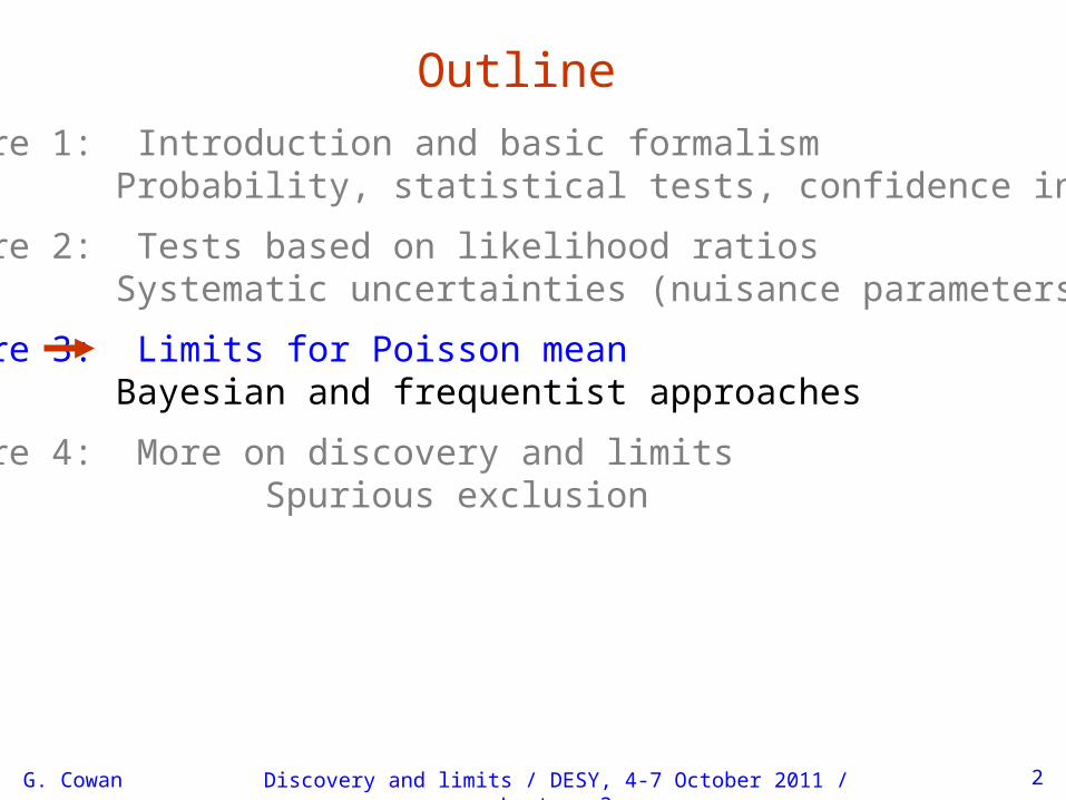
Outline

Lecture 1: Introduction and basic formalism Probability, statistical tests, confidence intervals.

Lecture 2: Tests based on likelihood ratios Systematic uncertainties (nuisance parameters)

Lecture 3: Limits for Poisson mean Bayesian and frequentist approaches

Lecture 4: More on discovery and limits Spurious exclusion

G. Cowan Discovery and limits / DESY, 4-7 October 2011 / Lecture 3 Lecture 12 page 3

Setting limits on Poisson parameter

Consider again the case of finding n = ns + nb events where

nb events from known processes (background)ns events from a new process (signal)

are Poisson r.v.s with means s, b, and thus n = ns + nb

is also Poisson with mean = s + b. Assume b is known.

Suppose we are searching for evidence of the signal process,but the number of events found is roughly equal to theexpected number of background events, e.g., b = 4.6 and we observe nobs = 5 events.

→ set upper limit on the parameter s.

The evidence for the presence of signal events is notstatistically significant,


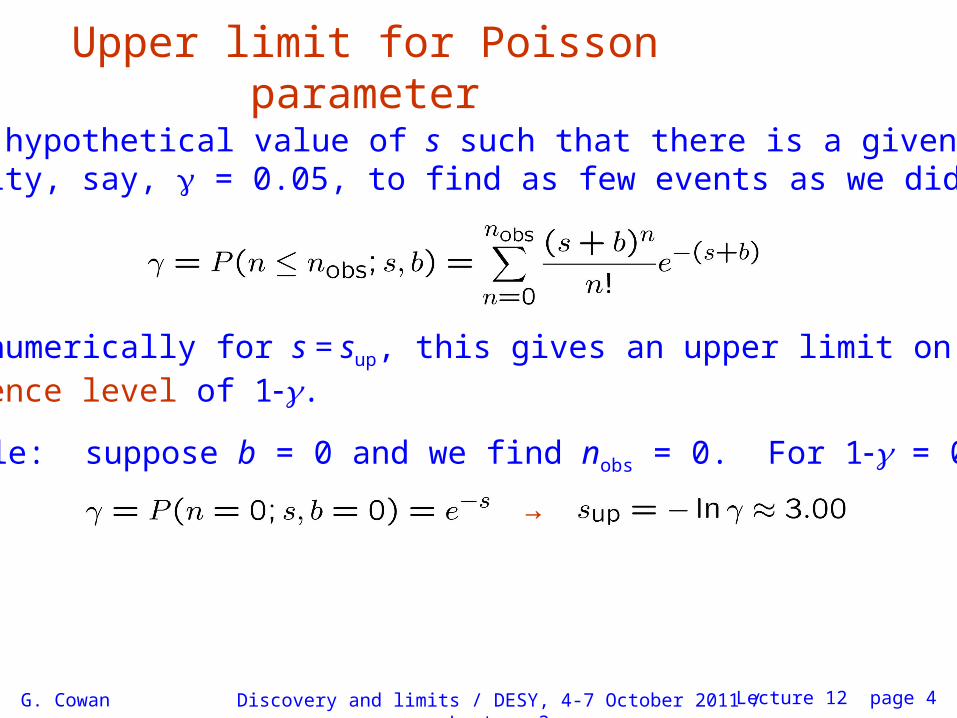
Upper limit for Poisson parameter

Find the hypothetical value of s such that there is a given smallprobability, say, = 0.05, to find as few events as we did or less:

Solve numerically for s = sup, this gives an upper limit on s at aconfidence level of 1.

Example: suppose b = 0 and we find nobs = 0. For 1 = 0.95,

→


Calculating Poisson parameter limitsTo solve for slo, sup, can exploit relation to 2 distribution:

Quantile of 2 distribution

For low fluctuation of n the formula can give negative result for sup; i.e. confidence interval is empty.


Limits near a physical boundarySuppose e.g. b = 2.5 and we observe n = 0.

If we choose CL = 0.9, we find from the formula for sup

Physicist: We already knew s ≥ 0 before we started; can’t use negative upper limit to report result of expensive experiment!

Statistician:The interval is designed to cover the true value only 90%of the time — this was clearly not one of those times.

Not uncommon dilemma when limit of parameter is close to a physical boundary.


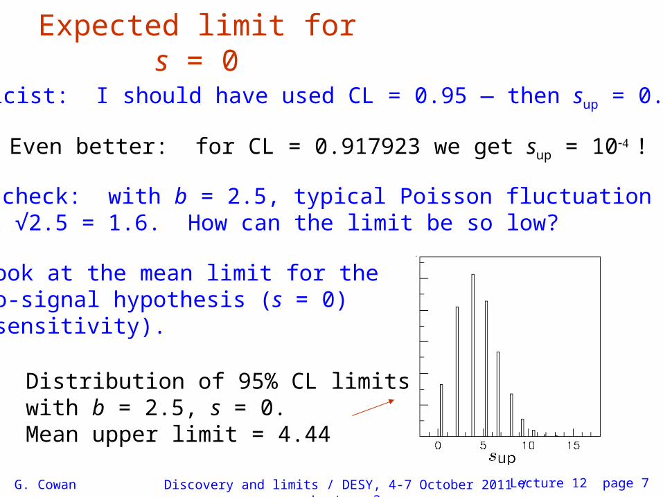
Expected limit for s = 0

Physicist: I should have used CL = 0.95 — then sup = 0.496

Even better: for CL = 0.917923 we get sup = 10!

Reality check: with b = 2.5, typical Poisson fluctuation in n isat least √2.5 = 1.6. How can the limit be so low?

Look at the mean limit for the no-signal hypothesis (s = 0)(sensitivity).

Distribution of 95% CL limitswith b = 2.5, s = 0.Mean upper limit = 4.44


The Bayesian approach to limitsIn Bayesian statistics need to start with ‘prior pdf’ (), this reflects degree of belief about before doing the experiment.

Bayes’ theorem tells how our beliefs should be updated inlight of the data x:

Integrate posterior pdf p(| x) to give interval with any desiredprobability content.

For e.g. n ~ Poisson(s+b), 95% CL upper limit on s from


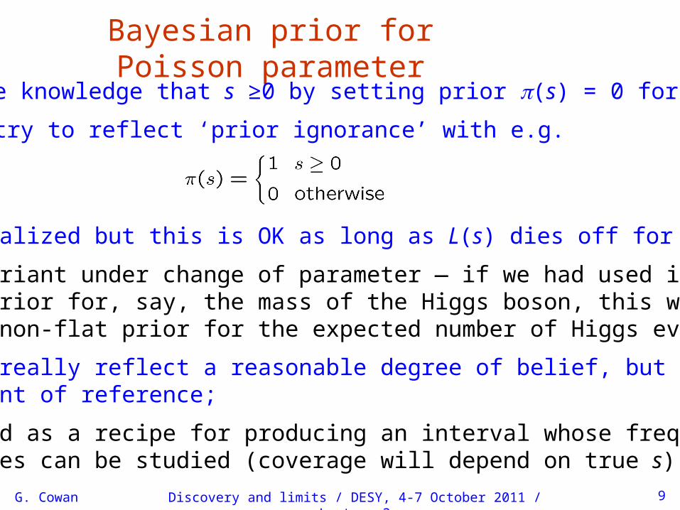
Bayesian prior for Poisson parameterInclude knowledge that s ≥0 by setting prior (s) = 0 for s<0.

Could try to reflect ‘prior ignorance’ with e.g.

Not normalized but this is OK as long as L(s) dies off for large s.

Not invariant under change of parameter — if we had used insteada flat prior for, say, the mass of the Higgs boson, this would imply a non-flat prior for the expected number of Higgs events.

Doesn’t really reflect a reasonable degree of belief, but often usedas a point of reference;

or viewed as a recipe for producing an interval whose frequentistproperties can be studied (coverage will depend on true s).


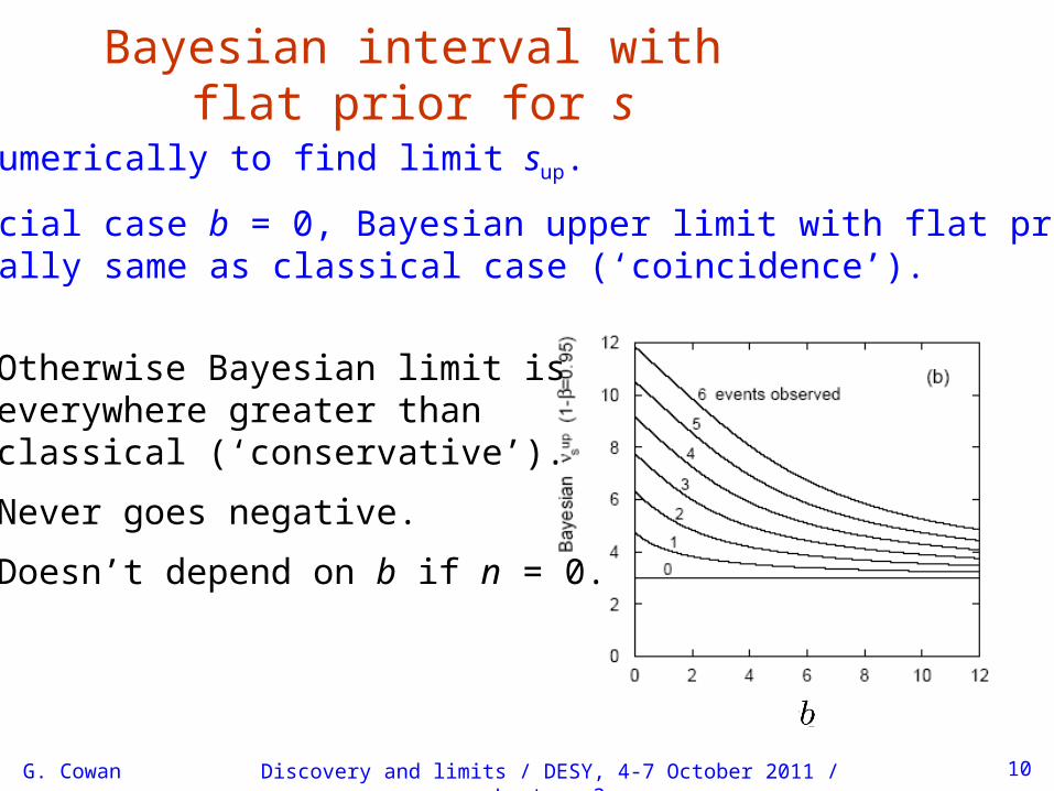
Bayesian interval with flat prior for s

Solve numerically to find limit sup.

For special case b = 0, Bayesian upper limit with flat priornumerically same as classical case (‘coincidence’).

Otherwise Bayesian limit iseverywhere greater thanclassical (‘conservative’).

Never goes negative.

Doesn’t depend on b if n = 0.


Priors from formal rules Because of difficulties in encoding a vague degree of beliefin a prior, one often attempts to derive the prior from formal rules,e.g., to satisfy certain invariance principles or to provide maximuminformation gain for a certain set of measurements.

Often called “objective priors” Form basis of Objective Bayesian Statistics

The priors do not reflect a degree of belief (but might representpossible extreme cases).

In a Subjective Bayesian analysis, using objective priors can be an important part of the sensitivity analysis.


Priors from formal rules (cont.)

In Objective Bayesian analysis, can use the intervals in afrequentist way, i.e., regard Bayes’ theorem as a recipe to producean interval with certain coverage properties. For a review see:

Formal priors have not been widely used in HEP, but there isrecent interest in this direction; see e.g.

L. Demortier, S. Jain and H. Prosper, Reference priors for highenergy physics, Phys. Rev. D 82 (2010) 034002, arxiv:1002.1111 (Feb 2010)


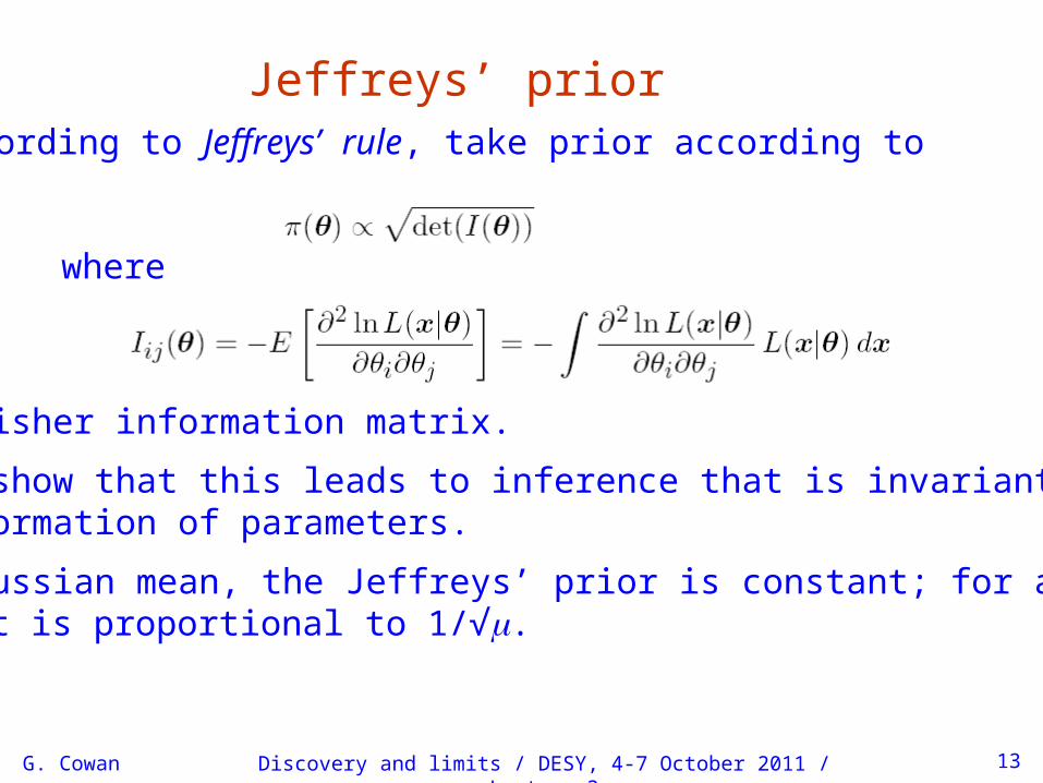
Jeffreys’ priorAccording to Jeffreys’ rule, take prior according to

where

is the Fisher information matrix.

One can show that this leads to inference that is invariant undera transformation of parameters.

For a Gaussian mean, the Jeffreys’ prior is constant; for a Poisson mean it is proportional to 1/√.


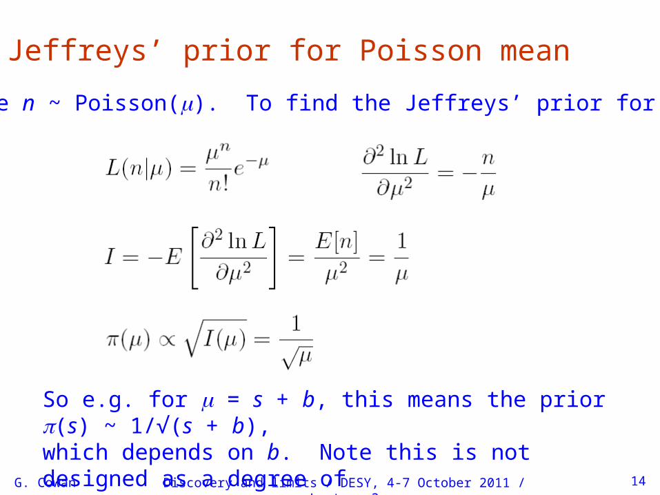
Jeffreys’ prior for Poisson mean

Suppose n ~ Poisson(). To find the Jeffreys’ prior for ,

So e.g. for = s + b, this means the prior (s) ~ 1/√(s + b), which depends on b. Note this is not designed as a degree of belief about s.


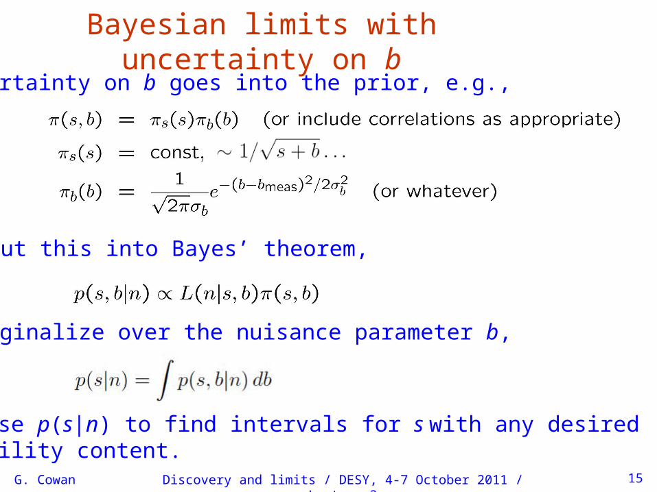
Bayesian limits with uncertainty on bUncertainty on b goes into the prior, e.g.,

Put this into Bayes’ theorem,

Marginalize over the nuisance parameter b,

Then use p(s|n) to find intervals for s with any desired probability content.



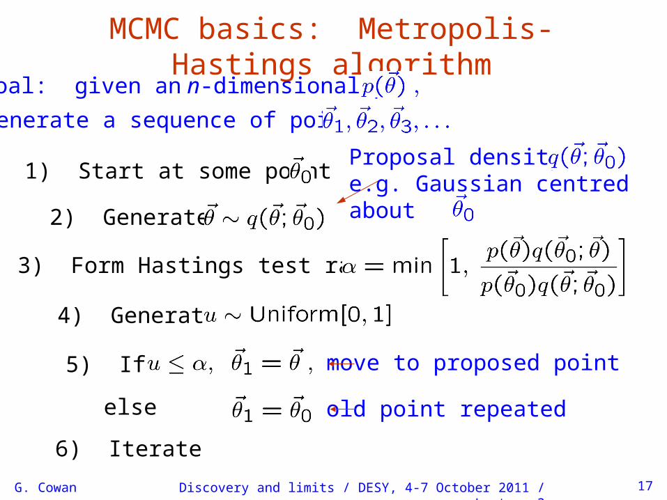
MCMC basics: Metropolis-Hastings algorithmGoal: given an n-dimensional pdf

generate a sequence of points

1) Start at some point

2) Generate

Proposal densitye.g. Gaussian centredabout

3) Form Hastings test ratio

4) Generate

5) If

else

move to proposed point

old point repeated

6) Iterate


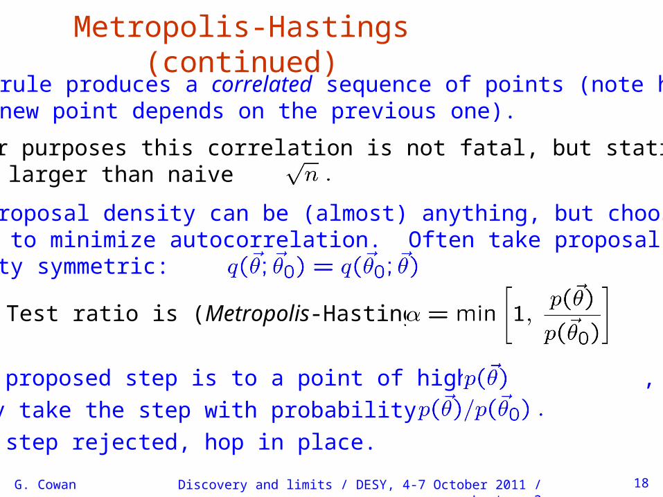
Metropolis-Hastings (continued)This rule produces a correlated sequence of points (note how each new point depends on the previous one).

For our purposes this correlation is not fatal, but statisticalerrors larger than naive

The proposal density can be (almost) anything, but chooseso as to minimize autocorrelation. Often take proposaldensity symmetric:

Test ratio is (Metropolis-Hastings):

I.e. if the proposed step is to a point of higher , take it;

if not, only take the step with probability

If proposed step rejected, hop in place.


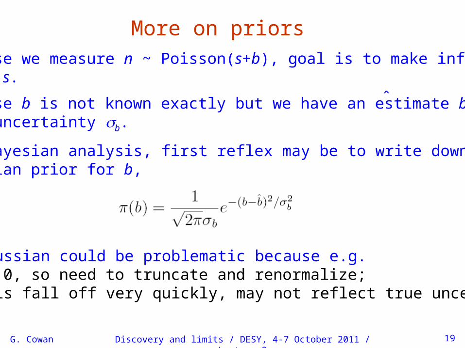
More on priorsSuppose we measure n ~ Poisson(s+b), goal is to make inferenceabout s.

Suppose b is not known exactly but we have an estimate bwith uncertainty b.

For Bayesian analysis, first reflex may be to write down a Gaussian prior for b,

But a Gaussian could be problematic because e.g.b ≥ 0, so need to truncate and renormalize;tails fall off very quickly, may not reflect true uncertainty.

ˆ


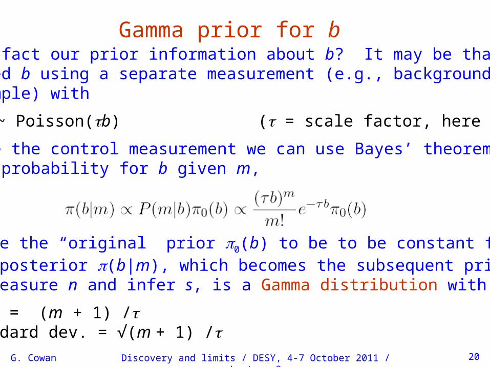
Gamma prior for bWhat is in fact our prior information about b? It may be that we estimated b using a separate measurement (e.g., background control sample) with

m ~ Poisson(b) ( = scale factor, here assume known)

Having made the control measurement we can use Bayes’ theoremto get the probability for b given m,

If we take the “original” prior 0(b) to be to be constant for b ≥ 0,then the posterior (b|m), which becomes the subsequent prior when we measure n and infer s, is a Gamma distribution with:

mean = (m + 1) /standard dev. = √(m + 1) /


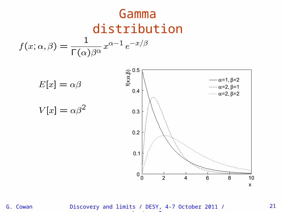
Gamma distribution


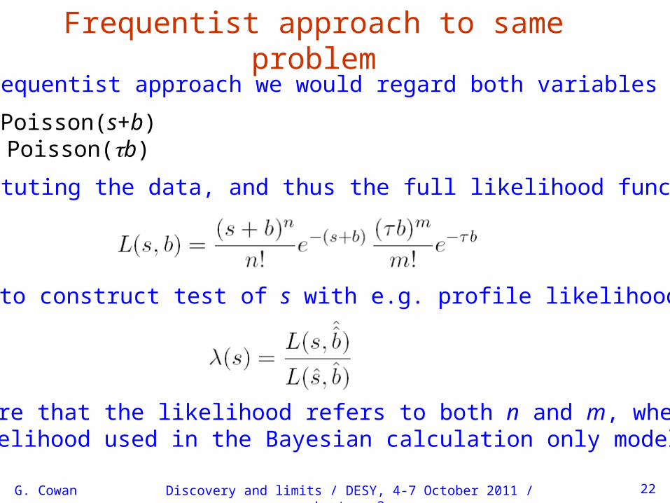
Frequentist approach to same problemIn the frequentist approach we would regard both variables

n ~ Poisson(s+b)m ~ Poisson(b)

as constituting the data, and thus the full likelihood function is

Use this to construct test of s with e.g. profile likelihood ratio

Note here that the likelihood refers to both n and m, whereasthe likelihood used in the Bayesian calculation only modeled n.


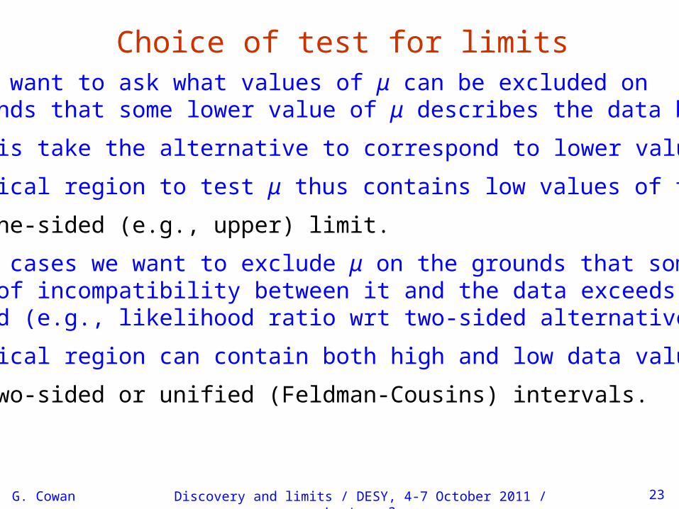
Choice of test for limitsOften we want to ask what values of μ can be excluded on the grounds that some lower value of μ describes the data better.

To do this take the alternative to correspond to lower values of μ.

The critical region to test μ thus contains low values of the data.

→ One-sided (e.g., upper) limit.

In other cases we want to exclude μ on the grounds that some othermeasure of incompatibility between it and the data exceeds somethreshold (e.g., likelihood ratio wrt two-sided alternative).

The critical region can contain both high and low data values.

→ Two-sided or unified (Feldman-Cousins) intervals.

I.e. for purposes of setting an upper limit, take critical region oftest to correspond to data outcomes better described by alower value of .

From observed q find p-value:

Large sample approximation:

95% CL upper limit on is highest value for which p-value is not less than 0.05.


A test statistic for upper limitsFor purposes of setting an upper limit on can use

where

25

Unified (Feldman-Cousins) intervals

We can use directly

G. Cowan Discovery and limits / DESY, 4-7 October 2011 / Lecture 3

as a test statistic for a hypothesized .

where

Large discrepancy between data and hypothesis can correspondeither to the estimate for being observed high or low relativeto .

This is essentially the statistic used for Feldman-Cousins intervals(here also treats nuisance parameters). G. Feldman and R.D. Cousins, Phys. Rev. D 57 (1998) 3873.

Lower edge of interval can be at = 0, depending on data.

26

Distribution of tUsing Wald approximation, f (t|′) is noncentral chi-squarefor one degree of freedom:

G. Cowan Discovery and limits / DESY, 4-7 October 2011 / Lecture 3

Special case of = ′ is chi-square for one d.o.f. (Wilks).

The p-value for an observed value of t is

and the corresponding significance is

Discovery and limits / DESY, 4-7 October 2011 / Lecture 3 27

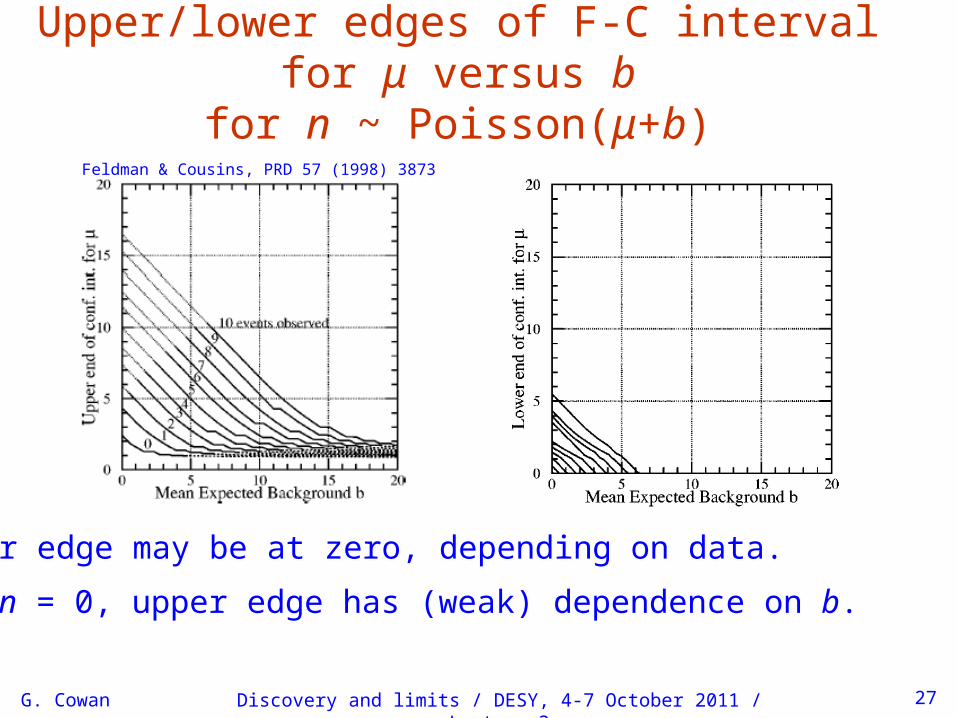
Upper/lower edges of F-C interval for μ versus bfor n ~ Poisson(μ+b)

Lower edge may be at zero, depending on data.

For n = 0, upper edge has (weak) dependence on b.

Feldman & Cousins, PRD 57 (1998) 3873

G. Cowan


Feldman-Cousins discussion

The initial motivation for Feldman-Cousins (unified) confidenceintervals was to eliminate null intervals.

The F-C limits are based on a likelihood ratio for a test of μ with respect to the alternative consisting of all other allowed valuesof μ (not just, say, lower values).

The interval’s upper edge is higher than the limit from the one-sided test, and lower values of μ may be excluded as well. A substantial downward fluctuation in the data gives a low (but nonzero) limit.

This means that when a value of μ is excluded, it is becausethere is a probability α for the data to fluctuate either high or lowin a manner corresponding to less compatibility as measured bythe likelihood ratio.


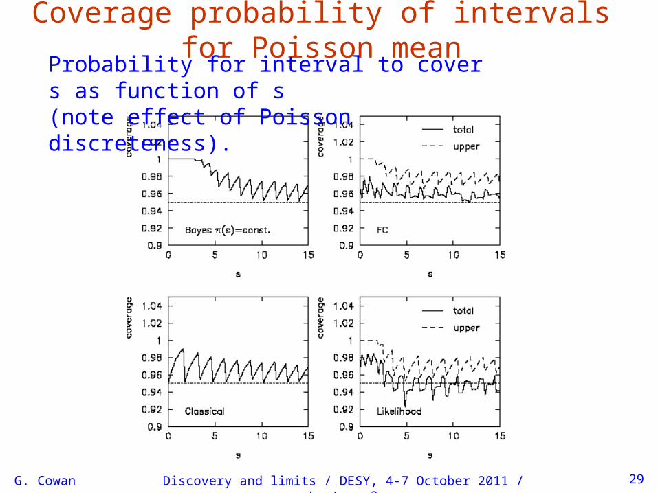
Coverage probability of intervals for Poisson meanProbability for interval to cover s as function of s(note effect of Poisson discreteness).


Summary for first three lectures

Using a frequentist statistical test we can:test the background-only model (rejection = discovery),test possible signal models (rejection leads to limits).

For large enough data sample, approximate formulae allow foreasy evaluation of discovery/exclusion significance.

The important properties of limits include:specified probability to cover true parameter.

Bayesian approach extends probability to degree of belief,and also produce intervals with good frequentist properties.

We saw in the Poisson example that with a one-sided test,all parameter values can be excluded (null interval). We will return to this point on Friday.


Extra slides

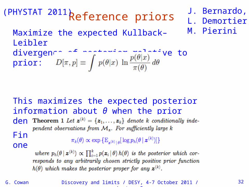
Reference priorsJ. Bernardo,L. Demortier,M. PieriniMaximize the expected Kullback–Leibler

divergence of posterior relative to prior:

This maximizes the expected posterior information about θ when the prior density is π(θ).

Finding reference priors “easy” for one parameter:

G. Cowan 32Discovery and limits / DESY, 4-7 October 2011 / Lecture 3

(PHYSTAT 2011)

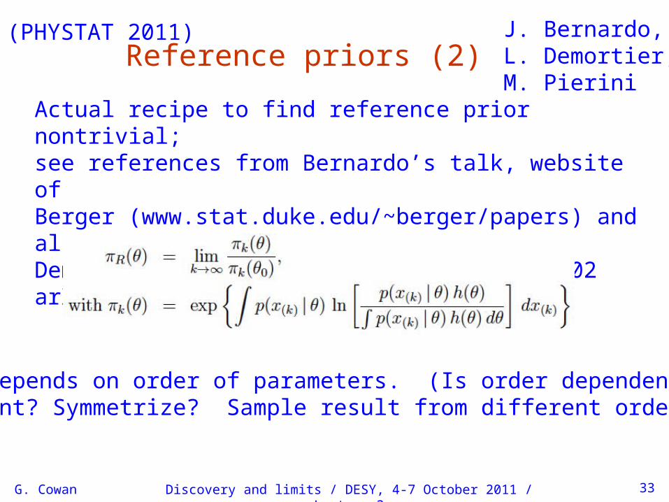
Reference priors (2)J. Bernardo,L. Demortier,M. Pierini

Actual recipe to find reference prior nontrivial;see references from Bernardo’s talk, website ofBerger (www.stat.duke.edu/~berger/papers) and also Demortier, Jain, Prosper, PRD 82:33, 34002 arXiv:1002.1111:

Prior depends on order of parameters. (Is order dependence important? Symmetrize? Sample result from different orderings?)


(PHYSTAT 2011)

L. Demortier


(PHYSTAT 2011)

35G. Cowan

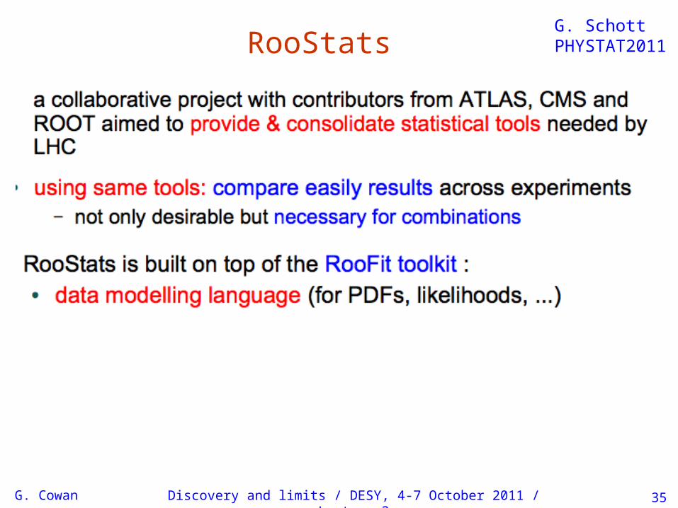
RooStatsG. SchottPHYSTAT2011

Discovery and limits / DESY, 4-7 October 2011 / Lecture 3

36G. Cowan

RooFit Workspaces

Able to construct full likelihood for combination of channels(or experiments).

Discovery and limits / DESY, 4-7 October 2011 / Lecture 3

G. SchottPHYSTAT2011

Discovery and limits / DESY, 4-7 October 2011 / Lecture 337G. Cowan

Combined ATLAS/CMS Higgs searchK. CranmerPHYSTAT2011

Given p-values p1,..., pN of H, what is combined p?

Better, given the results of N (usually independent) experiments, what inferences can one draw from their combination?

Full combination is difficult but worth the effort for e.g. Higgs search.

G. Cowan Discovery and limits / DESY, 4-7 October 2011 / Lecture 3 1 Statistical Methods for Discovery and Limits Lecture 3: Limits for Poisson mean: Bayesian.

Documents