Fuzzy Indicators and Multi-criteria Evaluation

1

Fuzzy Indicators and Multi-criteria Evaluation.

Henri Gwét Department of Computer Sciences National Polytechnic Institute P.O. Box 8390 Yaounde, Cameroon. Fax: (237) 222 4547 @mail : [email protected]

ABSTRACT. This paper provides a new way of multi-criteria evaluation. This method is based on the use of fuzzy set connectives and fuzzy measures. At the end, we make some comparisons between new and old ways. KEY-WORDS : aggregation of preferences, classification, utility, multi-criteria evaluation

1 Introduction

The problem of choosing the best way of evaluation is an important issue, especially when we use many criteria. Every criterion corresponds to a different a preference relation on the set of objects to be evaluated. Whether it is in medicine or in economics, to make multi-criteria evaluation is to find an optimal method that combines all these criteria into only one criterion, in order to obtain a global preference on the set of objects. In heath care economics for example, the classical aggregation methods, like analytical methods, do not take into consideration the conjunction or the disjunction of information. Only the average is being taken into consideration (see [1] p. 178). This is very disturbing as the criteria that enter into play are not always monetary in nature. For several authors, another way to aggregate fuzzy goals is to use fuzzy connectives (see [2]) like minimum or maximum. In a previous research work, Yager ([9]) tries to provide a formulation for the aggregation of multi-criteria based on the use of fuzzy measures.

The central focus of this work is to propose a new concept of multi-criteria evaluation based on the distance between sets and the use of fuzzy measures and fuzzy set connectives. We provide a general framework for the representation of states to be evaluated as a fuzzy set. It is in a way, another approach of imagining the notion of cost and benefit, or advantage and inconveniences in a non-cardinal frame.

2

This article is organized as follows. In section 2, we have a run down of the principal results on the operators and the fuzzy application, distances and the fuzzy measures. The section 3 and 4 constitute the core of the work. In these paragraphs, we start by stating the working hypothesis and their practical applications in each case. Then we introduce the different notions that will later on permit us to define the aggregation concepts. In section 5, we make some comparison between our new concept of evaluation and old aggregation methods.

2 Basic Concepts.

2.1 Definition.

Let E be a set. A fuzzy subset A of E is defined by using the membership function: µA : E→[0,1]. We write A=(x, µA(x))/x∈ E.

The number µA(x) indicates the degree to which the element x belong to A.

2.2 Definition.

Let A and B be two fuzzy subset of E.

We say that A and B are equal, and we write A=B, if and only if µA(x)=µB(x) for all x∈ E. If there is an element x of E such that µA(x)≠µB(x), we say that A and B are different and it is written A≠B.

A is included in B is written A⊂ B, if and only if for all x∈ E, µA(x) ≤ µB(x).

The intersection of A and B is the fuzzy subset of E denoted A∩B and defined as µA∩B(x) = µA(x) ∧ µB(x) for all x∈ E (where ∧ is the minimum).

The union of A and B is the fuzzy subset of E denoted A∪ B and defined as µA∪ B(x) = µA(x) ∨ µB(x) for all x∈ E (where ∨ is the maximum).

The complement of A in E is the fuzzy subset of E denoted A and defined as Aµ (x)=1–µA(x) for all x∈ E.

2.3 Remark.

The operations defined above verify all the classical set properties with the exception of the excluded-middle and non-contradiction laws.

The following properties are not generally verified: A∪ A ≠E and A∩ A ≠∅ .

3

2.4 Definition.

A t-norm (t-conorm respectively) is a binary operator on [0,1] denoted by ∗ (⊕ respectively) which is commutative, associative, continuous, increasing and having 1 (0 respectively) as the neutral element.

A negation is an unary operator on [0,1] defined as a =1–a for all a∈ [0,1].

A t-norm ∗ and a t-conorm ⊕ are said to be dual if and only if ba ba ⊕=∗ .

A pseudo-division (or quasi-inverse) associated to a t-norm ∗ is a binary operator denoted by | and defined as a|b=maxt∈ [0,1]/a∗ t≤b.

An associated difference to a t-norm ∗ is the binary operator denoted and defined as ab = 1–a|b.

2.5 Examples.

The principal t-norms, t-conorms, pseudo-division and difference are:

1. Zadeh : − a∗ b = a∧ b − a⊕ b = a∨ b

− a|b =

>

≤

ba if b

ba if 1

− ab =

>−

≤

ba if b1

ba if 0

2. Probabilistic : − a∗ b = ab − a⊕ b = a+b–ab

− a|b = 1∧ ab

− ab = 0∨ (1– ab )

3. Lukasiewicz : − a∗ b = 0∨ (a+b–1) − a⊕ b = 1∧ (a+b) − a|b = 1∧ (1–a+b) − ab = 0∨ (a–b)

with the convention that 0b =1 for all b∈ [0,1]

4

2.6 Properties.

Some properties of fuzzy operators are given below. See [5] for more information about pseudo-division properties.

1. a|(b∨ c) = a|b ∨ a|c

2. a|(b∧ c) = a|b ∧ a|c

3. (a∨ b)|c = a|c ∧ b|c

4. (a∧ b)|c = a|c ∨ b|c

5. a≤b ⇔ a|c ≥ b|c

6. b≤c ⇔ a|b ≤ a|c

2.7 Definition.

Let A and B be two fuzzy subsets of E.

The difference of A and B is the fuzzy subset of E denoted by A–B and defied as follow :

− µA–B(x) = µA(x)µB(x) for all x of E.

The symmetric difference of A and B is the fuzzy subset of E denoted by A∆B and defined as follow :

− A∆B = (A∪ B) – (A∩B).

2.8 Properties.

These are some properties on difference and symmetric difference:

1. (A–B)∩(B–A) = ∅

2. A⊂ B ⇒ A–B = ∅

3. A⊂ B ⇒ A–C⊂ B–C

4. A–B = A–(A∩B)

5. A–A = ∅

6. A∆B = (A–B)∪ (B–A)

7. A∆A =∅

5

2.9 Example. 1. If | is the Lukasiewicz pseudo-division then we have

− µA–B(x) = 0∨ (µA(x)–µB(x)) − µA∆B(x) = |µA(x)–µB(x)|

2. If | is the probabilistic pseudo-division then we have

− µA–B(x) = 0∨ (1– )x()x(

A

B

µµ )

− µA∆B(x) = )x()x( )x()x(

BA

BA

µ∨µµ−µ

2.10 Definition.

If we denote C(E) the set of fuzzy subsets of E, a fuzzy measure on E is a function m : C(E) → [0,1] such that :

− m(∅ )=0, m(E)=1 (limit condition) − A⊂ B ⇒ m(A)≤m(B) (monotony)

2.11 Example. 1. The height of a fuzzy set is given by

h(A) = )x(AExµ

∈∨ .

2. The uniform probability (we say cardinal measure) of a fuzzy set is given by

Card(A) =

1Ω ∑

∈µ

ExA )x( , where | Ω | is the cardinal of Ω

We verify that the cardinal and the height are fuzzy measures.

2.12 Definition.

A possibility measure is a fuzzy measure Π such that − Π(A∪ B) = Π(A)∨Π (B)

A necessity measure is a fuzzy measure N such that − N(A∩B) = N(A)∧ N(B)

A possibility distribution on E is a function π : E → [0,1] such that − 1 )x(

Ex=π

∈∨ .

6

From a possibility distribution, it is possible to construct a possibility measure and a necessity measure using the formulas that follow :

− Π(A) = )x()x( AExµ∧π

∈∨

− N(A) = )x())x(1( AExµ∨π−

∈∧

2.13 Definition.

Let A and B be two fuzzy subsets of E. Let m be a fuzzy measure on E. We define the dissimilarity measure between A and B by :

− d(A,B) = m(A∆B) = m(A∪ B) – (A∩B)

2.14 Properties.

The dissimilarity d verify the following properties: − d(A,A) = 0 − d(A,B) = d(B,A)

2.15 Example.

If we use the height measure, the dissimilarity measure d is defined by − d(A,B) = )x()x(|)x()x( 1 BABAEx

µ∧µµ∨µ−∈∨

and it is a transitive distance for the t-conorm ⊕ , i.e. − d(A,B) ≤ d(A,C)⊕ d(C,B).

If we use the cardinal measure, the dissimilarity measure d is defined by

− d(A,B) = )x()x(|)x()x( 1 E

1Ex

BABA∑∈

µ∧µµ∨µ−

and it is a transitive distance for addition, i.e. − d(A,B) ≤ d(A,C)+ d(C,B).

in the case where | is a pseudo-division associated to the Zadeh, Lukasiewicz or probabilistic t-norm,

7

E F

f -1(y)

2.16 Example.

If we choose the Lukasiewicz pseudo-division and the cardinal measure for example, we obtain

− d(A,B) = ∑∈

µ−µEx

BA )x()x( E

1

If we choose the probabilistic pseudo-division and the cardinal measure for example, we obtain

− d(A,B) = ∑∈ µ∨µ

µ−µEx BA

BA

)x()x( )x()x(

E 1

2.17 Definition.

Let E and F be two universal sets.

A fuzzy correspondence R from E to F is presented as a rectangular table E×F where at the intersection of line x and column y, we have the number µR(x,y)∈ [0,1]. This number represents the degree to which x is in relation with y.

A fuzzy function f : E → F is a relation R which associates each element x of E to the subset f(x) of F such that µf(x)(y) = µR(x,y). We say that the fuzzy function f is normalized if and only if h(f(x)) = 1 for all elements x of E. The inverse image of an element y∈ F is given by )x()y(f 1−µ =µR(x,y).

Table 1 summarized these definitions. So the row x represents the image of x by f and the column y represents the inverse image of y by f.

y

x µf(x)(y)

Table 1 : Image and Inverse Images

f(x)

f

8

Ω Ej

[0,1]

Xj

cj uj

3 Fuzzy Indicator and Global Preference.

3.1 Preliminaries.

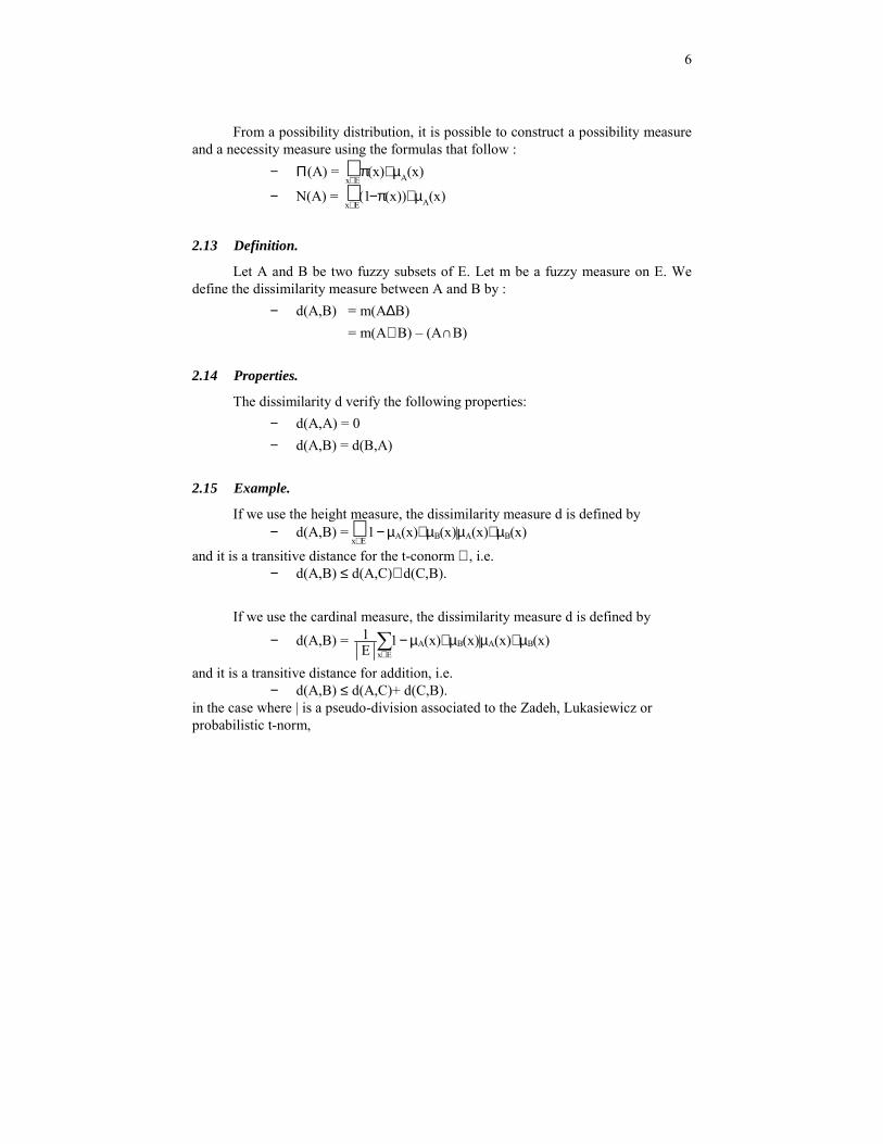
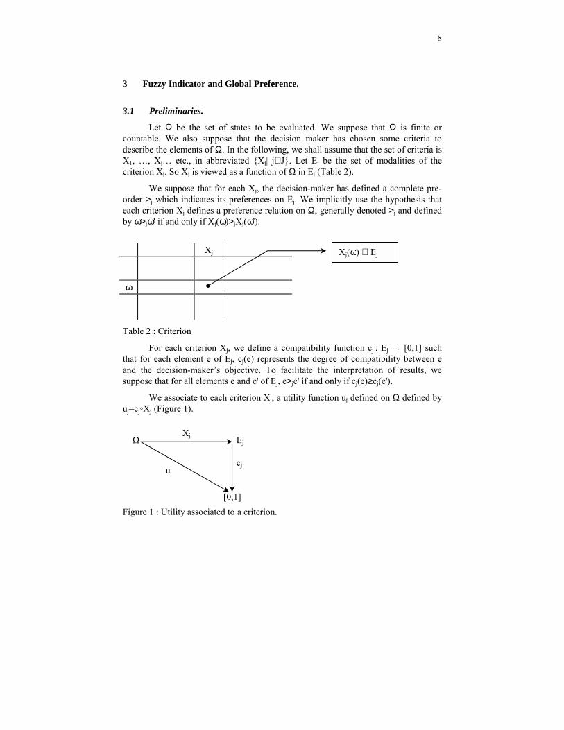
Let Ω be the set of states to be evaluated. We suppose that Ω is finite or countable. We also suppose that the decision maker has chosen some criteria to describe the elements of Ω. In the following, we shall assume that the set of criteria is X1, …, Xj… etc., in abbreviated Xj| j∈ J. Let Ej be the set of modalities of the criterion Xj. So Xj is viewed as a function of Ω in Ej (Table 2).

We suppose that for each Xj, the decision-maker has defined a complete pre-order >j which indicates its preferences on Ej. We implicitly use the hypothesis that each criterion Xj defines a preference relation on Ω, generally denoted >j and defined by ω>jω' if and only if Xj(ω)>jXj(ω').

Xj

ω

Table 2 : Criterion

For each criterion Xj, we define a compatibility function cj : Ej → [0,1] such that for each element e of Ej, cj(e) represents the degree of compatibility between e and the decision-maker’s objective. To facilitate the interpretation of results, we suppose that for all elements e and e' of Ej, e>je' if and only if cj(e)≥cj(e').

We associate to each criterion Xj, a utility function uj defined on Ω defined by uj=cjXj (Figure 1).

Figure 1 : Utility associated to a criterion.

Xj(ω) ∈ Ej

9

(X=j)

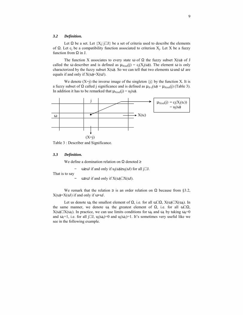
3.2 Definition.

Let Ω be a set. Let Xj| j∈ J be a set of criteria used to describe the elements of Ω. Let cj be a compatibility function associated to criterion Xj. Let X be a fuzzy function from Ω in J.

The function X associates to every state ω of Ω the fuzzy subset X(ω) of J called the ω describer and is defined as µX(ω)(j) = cj(Xj(ω)). The element ω is only characterized by the fuzzy subset X(ω). So we can tell that two elements ω and ω′ are equals if and only if X(ω)=X(ω′).

We denote (X=j) the inverse image of the singleton j by the function X. It is a fuzzy subset of Ω called j significance and is defined as µX=j(ω) = µX(ω)(j) (Table 3). In addition it has to be remarked that µX(ω)(j) = uj(ω).

j

ω

Table 3 : Describer and Significance.

3.3 Definition.

We define a domination relation on Ω denoted ≥

− ω≥ω' if and only if uj(ω)≥uj(ω') for all j∈ J. That is to say

− ω≥ω' if and only if X(ω)⊃ X(ω').

We remark that the relation ≥ is an order relation on Ω because from §3.2, X(ω)=X(ω′) if and only if ω=ω′.

Let us denote ω0 the smallest element of Ω, i.e. for all ω∈Ω , X(ω)⊃ X(ω0). In the same manner, we denote ω1 the greatest element of Ω, i.e. for all ω∈Ω , X(ω)⊂ X(ω1). In practice, we can use limits conditions for ω0 and ω1 by taking ω0=0 and ω1=1, i.e. for all j∈ J, uj(ω0)=0 and uj(ω1)=1. It’s sometimes very useful like we see in the following example.

X(ω)

µX(ω)(j) = cj(Xj(ω)) = uj(ω)

10

X2

very good good bad very bad

1 2 3 4

0 0.3 0.7 1

c2

3.4 Example.

Let us suppose we want to evaluate a set of patients ω∈Ω by mean of two criteria X1 (satisfaction) and X2 (health). The modalities are described below : Criterion X1 : satisfaction

1– great 2– average 3– small

Criterion X2 : health 1– very good 2– quite good 3– bad 4– very bad

So the modality sets are E1=great, average, small for the criterion X1 and E2=very good, quite good, bad, very bad for the criterion X2. Let us consider a reference population of six individuals having the characteristics below. We have X1(ω1)=1, …, X1(ω6)=3, X2(ω1)=1, … etc.

satisfaction health ω1 1 1 ω2 2 1 ω3 2 2 ω4 2 3 ω5 2 4 ω6 3 4

Table 4 : Description of population.

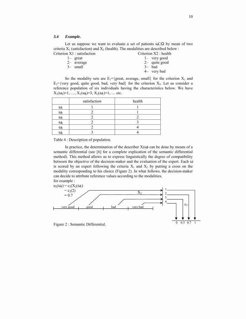
In practice, the determination of the describer X(ω) can be done by means of a semantic differential (see [6] for a complete explication of the semantic differential method). This method allows us to express linguistically the degree of compatibility between the objective of the decision-maker and the evaluation of the expert. Each ω is scored by an expert following the criteria X1 and X2 by putting a cross on the modality corresponding to his choice (Figure 2). In what follows, the decision-maker can decide to attribute reference values according to the modalities, for example : u2(ω3) = c2(X2(ω3) = c2(2) = 0.7

Figure 2 : Semantic Differential.

11

3.5 Definition.

Let ω, ω′∈Ω . Let m be a fuzzy measure.

We call the utility deviation between ω and ω′ with respect to Xj, the degree of membership of j to the fuzzy subset X(ω)∆X(ω'), i.e.

− ∆j(ω,ω') = µX(ω)∆X(ω')(j)

We call the utility of ω with respect to ω′, the measure of the difference between the describer of ω and ω′, i.e.

− U(ω,ω') = m(X(ω)–X(ω'))

We call the dissimilarity between ω and ω′, the measure of the symmetrical difference between the describers of ω and ω′, i.e.

− d(ω,ω') = m(X(ω)∆X(ω'))

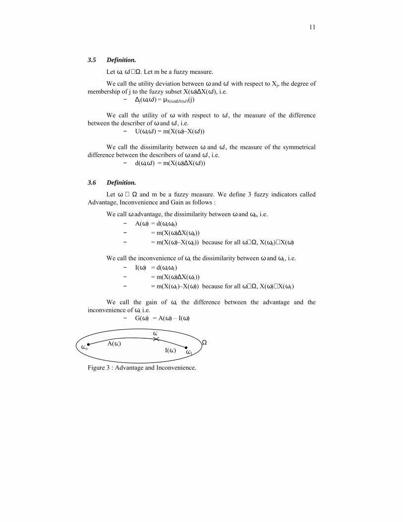
3.6 Definition.

Let ω ∈ Ω and m be a fuzzy measure. We define 3 fuzzy indicators called Advantage, Inconvenience and Gain as follows :

We call ω advantage, the dissimilarity between ω and ω0, i.e. − A(ω) = d(ω,ω0) − = m(X(ω)∆X(ω0)) − = m(X(ω)–X(ω0)) because for all ω∈Ω , X(ω0)⊂ X(ω)

We call the inconvenience of ω, the dissimilarity between ω and ω1, i.e. − I(ω) = d(ω,ω1) − = m(X(ω)∆X(ω1)) − = m(X(ω1)–X(ω)) because for all ω∈Ω , X(ω)⊂ X(ω1)

We call the gain of ω, the difference between the advantage and the inconvenience of ω, i.e.

− G(ω) = A(ω) – I(ω)

Figure 3 : Advantage and Inconvenience.

ωo ω1

ω Ω A(ω)

I(ω)

12

3.7 Remark.

The notions we define above related to a t-norm ∗ . The choice of this t-norm depends on the context in which it will be used. In practice, many t-norm are tested before choosing that which gives the best results. Suppose that we choose the Lukasiewicz’s t-norm

If we use the cardinal measure, we will have − A(ω) = ∑

∈ Jj J 1 (uj(ω)–uj(ω0))

− I(ω) = ∑∈ Jj J

1 (uj(ω1)–uj(ω))

If we use the height measure and if our preferences are normalized, i.e. for all j∈ J, uj(ω0)=0 and uj(ω1)=1, we will have

− A(ω) = Jj∈∨ uj(ω)

− I(ω) = 1–Jj∈∧ uj(ω1)

We recognize here, the maximum and the minimum aggregation connectives commonly used in the literature.

4 Aggregation Procedures and Proximity Index.

4.1 Hypothesis.

Let Ω and J be two sets. Let X be a fuzzy function from Ω to J. We suppose that Ω has a fuzzy algebra structure (Ω, ∧ , ∨ , —) compatible with the function X, i.e. such that

− X(∧ω ') = X(ω)∩X(ω') − X(ω∨ω ') = X(ω)∪ X(ω')

− X(ω) = )(X ω

We should remember that a fuzzy algebra structure is nothing else but a distributive lattice (Ω, ∧ , ∨ ) with a neutral element for ∧ and ∨ denoted ω0 and ω1 respectively, and a negation denoted — such that

− ω = ω (involution)

− 'ω∧ω = 'ω∨ω and 'ω∨ω = 'ω∧ω (De Morgan laws).

13

In referring to Table 3, we notice that ω∧ω ' is nothing else but the minimum of two rows ω and ω'. In the same manner, ω∨ω′ is defined as the maximum of the row ω and ω'.

Generally, we take ω0= ∧ ω and ω1= ∨ ω, i.e. ω0 is the minimum of all the rows and ω1 is the maximum.

In practice, we are not sure that ∧ is an internal operator, i.e. for all ω and ω', it is not certain to find an element ω'' such that µX(ω'')(j) = µX(ω)(j)∧µ X(ω')(j) for all j∈ J. The existence of ω'' can be assured by adding some virtual states to the set.

We define the complement of ω, denoted ω such that the ω row is the pseudo-complement of the row ω, i.e. X(ω) = 1–X(ω). De Morgan laws are verified given that

− X( 'ω∧ω ) = )'(X ω∧ω

= )'(X )(X ω∧ω

= )(X ω ∨ )'(X ω

In the same way,

− X( 'ω∨ω ) = )(X ω ∧ )'(X ω

4.2 Definition.

Let (Ω, ∧ , ∨ , —) be a fuzzy algebra. For all elements ω and ω′ of Ω, we define the global preference >A, >I and >G by :

− ω >A ω' ⇔ A(ω) ≥ A(ω') − ω >I ω' ⇔ I(ω) ≤ I(ω') − ω >G ω' ⇔ G(ω) ≥ G(ω')

4.3 Remark.

In practice, ω0 stands for the worst state of Ω and ω1 represents the best state of Ω. The preference >A indicates that we give preference to states far from the worst state. While the preference >I gives preference to the state nearest to the best state.

These two procedures are not equivalent because in a multidimensional frame, moving far away from the minimum does not necessarily mean that we are approaching the maximum, but all depends on the direction we take. It is clear that if the analysis is done in one dimension, then these two procedures become equivalent.

14

4.4 Properties. 1– >A, >I and >G are completes pre-orders 2– if ω>Aω' and ω>Iω', then ω>Gω' 3– if ω∼ Aω' and ω>Gω' then ω>Iω' 4– if ω∼ Iω' and ω>Gω' then ω>Aω' 5– if ω∼ Gω' and ω>Aω' then ω'>Iω 6– if ω∼ Gω' and ω>Iω' then ω'>Aω

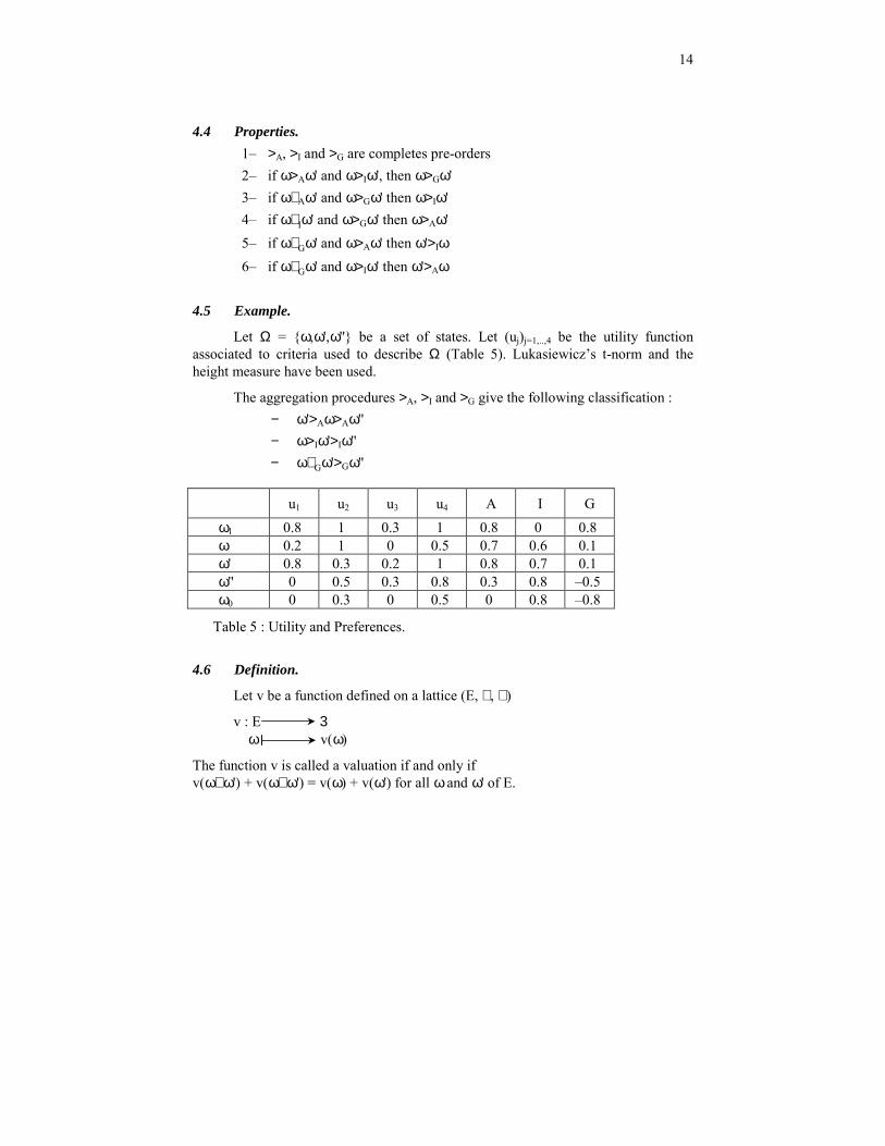
4.5 Example.

Let Ω = ω,ω',ω'' be a set of states. Let (uj)j=1,..,4 be the utility function associated to criteria used to describe Ω (Table 5). Lukasiewicz’s t-norm and the height measure have been used.

The aggregation procedures >A, >I and >G give the following classification : − ω'>Aω>Aω'' − ω>Iω'>Iω'' − ω∼ Gω'>Gω''

u1 u2 u3 u4 A I G

ω1 0.8 1 0.3 1 0.8 0 0.8 ω 0.2 1 0 0.5 0.7 0.6 0.1 ω' 0.8 0.3 0.2 1 0.8 0.7 0.1 ω'' 0 0.5 0.3 0.8 0.3 0.8 –0.5 ω0 0 0.3 0 0.5 0 0.8 –0.8

Table 5 : Utility and Preferences.

4.6 Definition.

Let v be a function defined on a lattice (E, ∧ , ∨ )

v : E 3 ω v(ω)

The function v is called a valuation if and only if v(ω∧ω ') + v(ω∨ω ') = v(ω) + v(ω') for all ω and ω' of E.

15

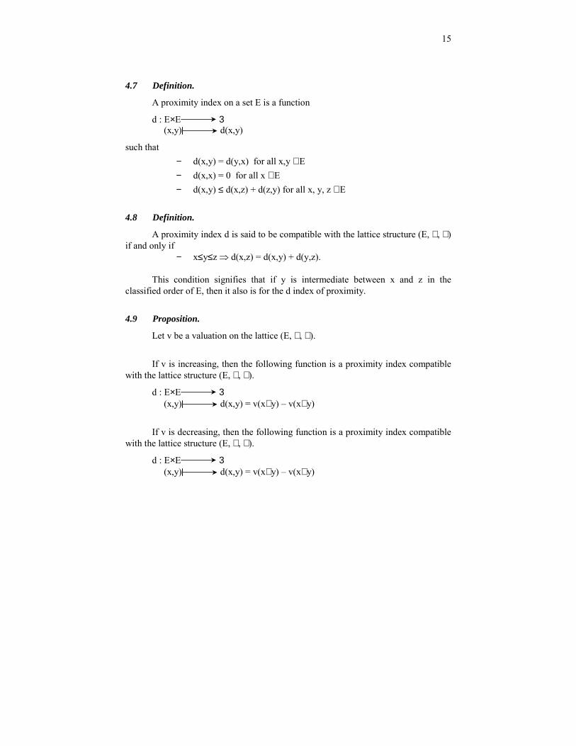
4.7 Definition.

A proximity index on a set E is a function

d : E×E 3 (x,y) d(x,y)

such that − d(x,y) = d(y,x) for all x,y ∈ E − d(x,x) = 0 for all x ∈ E − d(x,y) ≤ d(x,z) + d(z,y) for all x, y, z ∈ E

4.8 Definition.

A proximity index d is said to be compatible with the lattice structure (E, ∧ , ∨ ) if and only if

− x≤y≤z ⇒ d(x,z) = d(x,y) + d(y,z).

This condition signifies that if y is intermediate between x and z in the classified order of E, then it also is for the d index of proximity.

4.9 Proposition.

Let v be a valuation on the lattice (E, ∧ , ∨ ).

If v is increasing, then the following function is a proximity index compatible with the lattice structure (E, ∧ , ∨ ).

d : E×E 3 (x,y) d(x,y) = v(x∨ y) – v(x∧ y)

If v is decreasing, then the following function is a proximity index compatible with the lattice structure (E, ∧ , ∨ ).

d : E×E 3 (x,y) d(x,y) = v(x∧ y) – v(x∨ y)

16

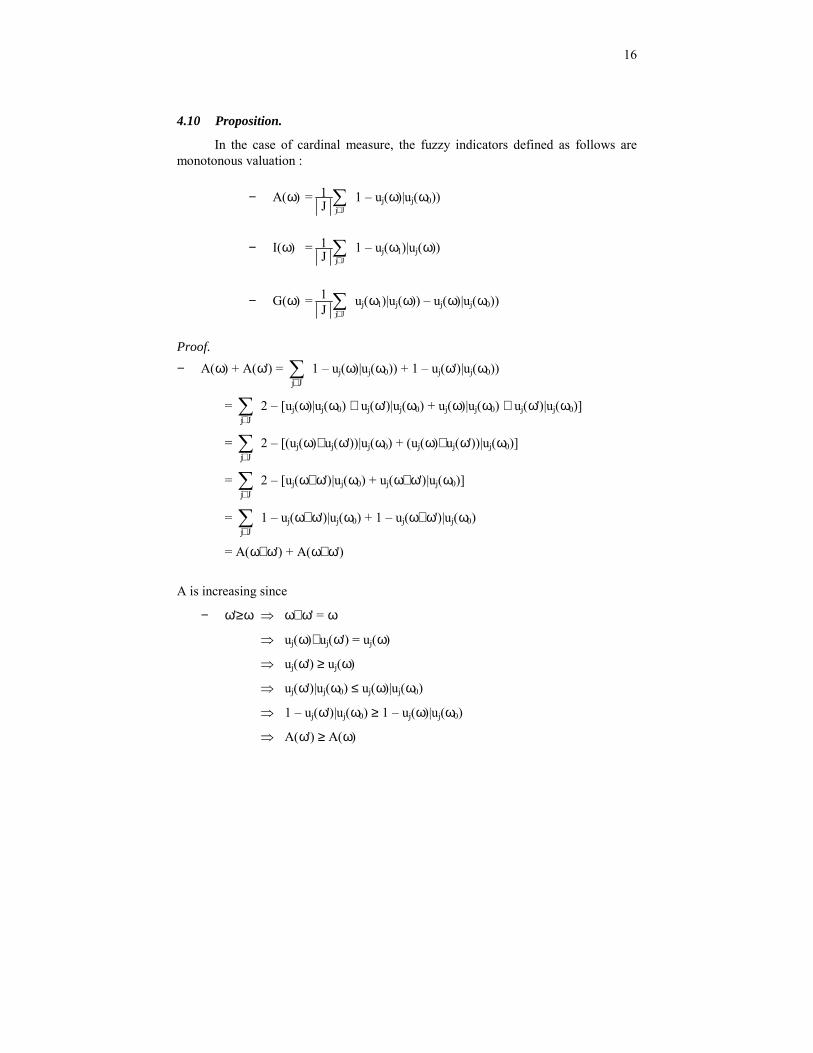
4.10 Proposition.

In the case of cardinal measure, the fuzzy indicators defined as follows are monotonous valuation :

− A(ω) = ∑∈ Jj J

1 1 – uj(ω)|uj(ω0))

− I(ω) = ∑∈ Jj J

1 1 – uj(ω1)|uj(ω))

− G(ω) = ∑∈ Jj J

1 uj(ω1)|uj(ω)) – uj(ω)|uj(ω0))

Proof. − A(ω) + A(ω') = ∑

∈ Jj1 – uj(ω)|uj(ω0)) + 1 – uj(ω')|uj(ω0))

= ∑∈ Jj

2 – [uj(ω)|uj(ω0) ∨ uj(ω')|uj(ω0) + uj(ω)|uj(ω0) ∧ uj(ω')|uj(ω0)]

= ∑∈ Jj

2 – [(uj(ω)∧ uj(ω'))|uj(ω0) + (uj(ω)∨ uj(ω'))|uj(ω0)]

= ∑∈ Jj

2 – [uj(ω∧ω ')|uj(ω0) + uj(ω∨ω ')|uj(ω0)]

= ∑∈ Jj

1 – uj(ω∧ω ')|uj(ω0) + 1 – uj(ω∨ω ')|uj(ω0)

= A(ω∧ω ') + A(ω∨ω ')

A is increasing since

− ω'≥ω ⇒ ω∧ω ' = ω

⇒ uj(ω)∧ uj(ω') = uj(ω)

⇒ uj(ω') ≥ uj(ω)

⇒ uj(ω')|uj(ω0) ≤ uj(ω)|uj(ω0)

⇒ 1 – uj(ω')|uj(ω0) ≥ 1 – uj(ω)|uj(ω0)

⇒ A(ω') ≥ A(ω)

17

In the same way, − I(ω) + I(ω') = ∑

∈ Jj1 – uj(ω1)|uj(ω)) + 1 – uj(ω1)|uj(ω'))

= ∑∈ Jj

2 – [uj(ω1)|uj(ω)∨ uj(ω1)|uj(ω')+uj(ω1)|uj(ω)∧ uj(ω1)|uj(ω')]

= ∑∈ Jj

2 – [uj(ω1)|(uj(ω')∨ uj(ω)) + (uj(ω1)|(uj(ω)∧ uj(ω'))]

= ∑∈ Jj

2 – [uj(ω1)|uj(ω∨ω ') + uj(ω1)|uj(ω∧ω ')]

= ∑∈ Jj

1 –uj(ω1)|uj(ω∨ω ') + 1 – uj(ω1)|uj(ω∧ω ')

= I(ω∨ω ') + I(ω∧ω ')

I is decreasing because

− ω'≥ω ⇒ ω∧ω ' = ω

⇒ uj(ω)∧ uj(ω') = uj(ω)

⇒ uj(ω') ≥ uj(ω)

⇒ uj(ω1)|uj(ω') ≥ uj(ω1)|uj(ω)

⇒ 1 – uj(ω1)|uj(ω') ≤ 1 – uj(ω1)|uj(ω)

⇒ I(ω') ≤ I(ω)

At last,

− G(ω) + G(ω') = A(ω)–I(ω) + A(ω')–I(ω')

= A(ω)+A(ω') – (I(ω)+I(ω'))

= A(ω∧ω ') + A(ω∨ω ') – (I(ω∨ω ') + I(ω∧ω '))

− = A(ω∧ω ') – I(ω∧ω ') + A(ω∨ω ') – I(ω∨ω ')

= G(ω∨ω ') + G(ω∧ω ')

G is increasing because − ω'≥ω ⇒ A(ω')≥ A(ω) et –I(ω')≥ –I(ω)

⇒ A(ω')–I(ω')≥ A(ω)–I(ω) ⇒ G(ω') ≥ G(ω)

18

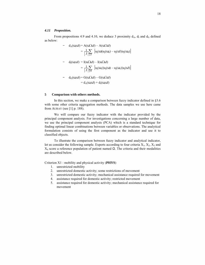
4.11 Proposition.

From propositions 4.9 and 4.10, we deduce 3 proximity dA, dI and dG defined as below:

− dA(ω,ω') = A(ω∨ω ') – A(ω∧ω ')

= ∑∈ Jj J

1 |uj(ω)|uj(ω0) – uj(ω')|uj(ω0)|

− dI(ω,ω') = I(ω∧ω ') – I(ω∨ω ')

= ∑∈ Jj J

1 |uj(ω1)|uj(ω) – uj(ω1)|uj(ω')|

− dG(ω,ω') = G(ω∨ω ') – G(ω∧ω ') = dA(ω,ω') + dI(ω,ω')

5 Comparison with others methods.

In this section, we make a comparison between fuzzy indicator defined in §3.6 with some other criteria aggregation methods. The data samples we use here came from AURAY (see [1] p. 188).

We will compare our fuzzy indicator with the indicator provided by the principal component analysis. For investigations concerning a large number of data, we use the principal component analysis (PCA) which is a standard technique for finding optimal linear combinations between variables or observations. The analytical formulation consists of using the first component as the indicator and use it to classified objects.

To illustrate the comparison between fuzzy indicator and analytical indicator, let us consider the following sample. Experts according to four criteria X1, X2, X3 and X4 score a reference population of patient named Ω. The criteria and their modalities are described below.

Criterion X1 : mobility and physical activity (PHYS) 1. unrestricted mobility 2. unrestricted domestic activity; some restrictions of movement 3. unrestricted domestic activity; mechanical assistance required for movement 4. assistance required for domestic activity; restricted movement 5. assistance required for domestic activity; mechanical assistance required for

movement

19

6. assistance required for domestic activity; no control over limbs. Criterion X2 : self-care and role activity (AUTO)

1. total autonomy 2. restricted access to professional (school, work,… ) or leisure activity 3. incapable of gaining access to professional (school, work,… ) or leisure

activity 4. difficulties of eating, washing, … without help and restricted access to

professional or leisure activities 5. difficulties of eating, washing, … without help and access to professional or

leisure activities impossible.

Criterion X3 : emotional well-being and social activity (EMOT) 1. happy, relaxed, numerous relationships 2. happy, relaxed, few relationships 3. quite often anxious and depressed, numerous relationships 4. quite often anxious and depressed, few relationships

Criterion X4 : health problem (HEAL) 1. no problems 2. slight physical anomalies 3. requires assistance with hearing 4. problems causing some chronic pain 5. some disorders of understanding or memory 6. impaired sight, even with glasses 7. visible behavioral disorders 8. deaf or dumb or blind.

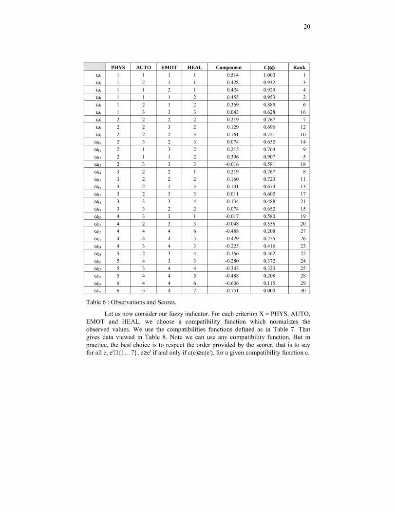
Let us consider a reference set of 30 individuals with the characteristics described in Table 1. The proportion of the first component provided by a principal components analysis (PCA) is 81.186%.

So the first component can be used as an indicator of the health of the population. Generally, this component is normalized by situating it between 0 (the worst value) and 1 (the best value). We would obtain the following values and ranking according this normalized component (named C(ω) in Table 6).

20

PHYS AUTO EMOT HEAL Component C(ωωωω) Rank ω1 1 1 1 1 0.514 1.000 1 ω2 1 2 1 1 0.428 0.932 3 ω3 1 1 2 1 0.424 0.929 4 ω4 1 1 1 2 0.455 0.953 2 ω5 1 2 1 2 0.369 0.885 6 ω6 1 3 3 3 0.043 0.628 16 ω7 2 2 2 2 0.219 0.767 7 ω8 2 2 3 2 0.129 0.696 12 ω9 2 2 2 3 0.161 0.721 10 ω10 2 3 2 3 0.074 0.652 14 ω11 2 1 3 2 0.215 0.764 9 ω12 2 1 1 2 0.396 0.907 5 ω13 2 3 3 3 -0.016 0.581 18 ω14 3 2 2 1 0.219 0.767 8 ω15 3 2 2 2 0.160 0.720 11 ω16 3 2 2 3 0.101 0.674 13 ω17 3 2 3 3 0.011 0.602 17 ω18 3 3 3 4 -0.134 0.488 21 ω19 3 3 2 2 0.074 0.652 15 ω20 4 3 3 1 -0.017 0.580 19 ω21 4 2 3 3 -0.048 0.556 20 ω22 4 4 4 6 -0.488 0.208 27 ω23 4 4 4 5 -0.429 0.255 26 ω24 4 3 4 3 -0.225 0.416 23 ω25 5 2 3 4 -0.166 0.462 22 ω26 5 4 3 3 -0.280 0.372 24 ω27 5 3 4 4 -0.343 0.323 25 ω28 5 4 4 5 -0.488 0.208 28 ω29 6 4 4 6 -0.606 0.115 29 ω30 6 5 4 7 -0.751 0.000 30

Table 6 : Observations and Scores.

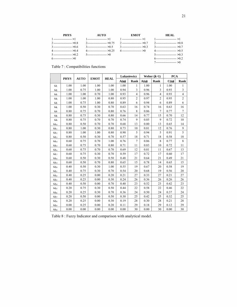
Let us now consider our fuzzy indicator. For each criterion X = PHYS, AUTO, EMOT and HEAL, we choose a compatibility function which normalizes the observed values. We use the compatibilities functions defined as in Table 7. That gives data viewed in Table 8. Note we can use any compatibility function. But in practice, the best choice is to respect the order provided by the scorer, that is to say for all e, e'∈ 1…7, e≥e' if and only if c(e)≥c(e'), for a given compatibility function c.

21

PHYS AUTO EMOT HEAL 1 ------------------ >1 2 ------------------ >0.8 3 ------------------ >0.6 4 ------------------ >0.4 5 ------------------ >0.2 6 ------------------ >0

1------------------- >1 2------------------- >0.75 3------------------- >0.5 4------------------- >0.25 5------------------- >0

1 ------------------- >1 2 ------------------- >0.7 3 ------------------- >0.3 4 ------------------- >0

1-------------------- >1 2-------------------- >0.8 3-------------------- >0.7 4-------------------- >0.5 5-------------------- >0.3 6-------------------- >0.2 7-------------------- >0

Table 7 : Compatibilities functions

Lukasiewicz Weber (λλλλ=1) PCA PHYS AUTO EMOT HEAL

A(ωωωω) Rank A(ωωωω) Rank C(ωωωω) Rank ω1 1.00 1.00 1.00 1.00 1.00 1 1.00 1 1.00 1 ω2 1.00 0.75 1.00 1.00 0.94 3 0.96 3 0.93 3 ω3 1.00 1.00 0.70 1.00 0.93 4 0.96 4 0.93 4 ω4 1.00 1.00 1.00 0.80 0.95 2 0.97 2 0.95 2 ω5 1.00 0.75 1.00 0.80 0.89 6 0.94 6 0.89 6 ω6 1.00 0.50 0.30 0.70 0.63 16 0.74 16 0.63 16 ω7 0.80 0.75 0.70 0.80 0.76 8 0.86 7 0.77 7 ω8 0.80 0.75 0.30 0.80 0.66 14 0.77 15 0.70 12 ω9 0.80 0.75 0.70 0.70 0.74 9 0.85 9 0.72 10 ω10 0.80 0.50 0.70 0.70 0.68 13 0.80 13 0.65 14 ω11 0.80 1.00 0.30 0.80 0.73 10 0.81 12 0.76 9 ω12 0.80 1.00 1.00 0.80 0.90 5 0.94 5 0.91 5 ω13 0.80 0.50 0.30 0.70 0.57 18 0.71 18 0.58 18 ω14 0.60 0.75 0.70 1.00 0.76 7 0.86 8 0.77 8 ω15 0.60 0.75 0.70 0.80 0.71 11 0.83 10 0.72 11 ω16 0.60 0.75 0.70 0.70 0.69 12 0.81 11 0.67 13 ω17 0.60 0.75 0.30 0.70 0.59 17 0.72 17 0.60 17 ω18 0.60 0.50 0.30 0.50 0.48 21 0.64 21 0.49 21 ω19 0.60 0.50 0.70 0.80 0.65 15 0.78 14 0.65 15 ω20 0.40 0.50 0.30 1.00 0.55 19 0.67 20 0.58 19 ω21 0.40 0.75 0.30 0.70 0.54 20 0.68 19 0.56 20 ω22 0.40 0.25 0.00 0.20 0.21 27 0.33 27 0.21 27 ω23 0.40 0.25 0.00 0.30 0.24 26 0.36 26 0.26 26 ω24 0.40 0.50 0.00 0.70 0.40 23 0.52 23 0.42 23 ω25 0.20 0.75 0.30 0.50 0.44 22 0.58 22 0.46 22 ω26 0.20 0.25 0.30 0.70 0.36 24 0.50 24 0.37 24 ω27 0.20 0.50 0.00 0.50 0.30 25 0.42 25 0.32 25 ω28 0.20 0.25 0.00 0.30 0.19 28 0.30 28 0.21 28 ω29 0.00 0.25 0.00 0.20 0.11 29 0.18 29 0.12 29 ω30 0.00 0.00 0.00 0.00 0.00 30 0.00 30 0.00 30

Table 8 : Fuzzy Indicator and comparison with analytical model.

22

The Table 8 shows that ω1 is the best patient and ω30 is worst. By using the cardinal measure, we have defined the fuzzy indicator as follow.

− A(ω) = ∑∈ Jj J

1 (uj(ω) uj(ω30))

where J= PHYS, AUTO, EMOT, HEAL

Since uj(ω30)=0 for all j∈ J, we obtain − A(ω) = ∑

∈ Jj41 uj(ω) 0

Now we use two connectives to illustrate our fuzzy indicator :

the Lukasiewicz’s t-norm defined by − a∗ b = 0 ∨ (a+b–1)

and the Weber’s t-norm defined by − a∗ b = 0 ∨ λ+

λ−−+1

ab1ba

According to §2.4,

if we use the Lukasiewicz’s t-norm, we obtain a∗ b = 0 ∨ (a+b–1)

⇒ a|b = maxt∈ [0,1]/a∗ t≤b = 1 ∧ (1–a+b)

⇒ ab = 1–a|b = 1 – 1 ∧ (1–a+b) = 0 ∨ (a–b)

if we use the Weber’s t-norm (with λ=1), we obtain a∗ b = 0 ∨ 2

ab1ba −−+

⇒ a|b = maxt∈ [0,1]/a∗ t≤b = 1 ∧ a1

1ab2++−

23

⇒ ab = 1–a|b = 1 – 1 ∧ a1

1ab2++−

= 0 ∨ a1ba2 +−⋅

From these connectives, we deduce two fuzzy indicators as below

− A(ω) = ∑∈ Jj4

1 uj(ω) by using the Lukasiewicz’s t-norm

− A(ω) = ∑∈ ω+

ωJj j

j

)(u1)(u

21 by using the Weber’s t-norm (with λ=1)

We compare these two fuzzy indicators with the indicator provide by the principal component analysis method (column C(ω) in Table 8). We associate a rank to each indicator so that we can easily make a comparison between these three indicators. From Table 8, we can see that for the first seven patients (ω1 to ω7), the three indicators provide the same classification.

Note that we can use any other t-norm to define the fuzzy indicator. But, be careful of this choice. For example, if we choose an Archimedean t-norm generated by f, we obtain a∗ b = f –1(f(a)+f(b)) where f : [0,1] → [0,+∞] is a decreasing so that f(0) = +∞ and f(1) = 0

⇒ a|b = maxt∈ [0,1]/a∗ t≤b = f –1(0 ∨ (f(b)–f(a)))

For normalized preferences, i.e. uj(ω0) = 0 for all j∈ J, we have uj(ω)uj(ω0) = uj(ω)0 = 1 – f –1(0 ∨ (f(0)–f(uj(ω))) = 1 – f –1(+∞) = 1 for all j∈ J

⇒ A(ω) = ∑∈ Jj J

1 uj(ω) uj(ω0)

= 1 for all ω∈Ω

In this situation, we cannot use A as an indicator.

24

6 Conclusion.

We have introduced new aggregation procedures. These aggregation procedures are based on the fuzzy utility concept. The aim of the new model is to help construct a global preference in the case where we do not have a cardinal or Neumann utility function. Most of these procedures depend on the choice of the fuzzy connectives or fuzzy measures. It is possible to try to choose the best connective by using elicitation procedures, but the precision of that approach is unwarranted (see [3] for a full discussion on this topic).

7 Bibliography. [1] AURAY J.-P., DURU G. LAMURE M., PELC A., ZIGHED A. (1990) : Guidelines for evaluation

in health care economics, GYD Institute, Lyon

[2] DUBOIS D. & PRADE H. (1985) : A review of fuzzy set aggregation connectives, Information Sciences, 36, 85-121

[3] DUBOIS D. & PRADE H. : Possibility theory: An approach to computerized processing of uncertainty. Plenum Press, New York.

[4] DUBOIS D., GODO, L. PRADE H. (1998) : Possibilistic representation of qualitative utility : an improved characterization, Proceedings 7th IPMU'98, Editions EDK, 180-187

[5] GWÉT H. (1997) : Normalized Conditional Possibility Distribution and Informational Connection between Fuzzy Variables, International Journal of Uncertainty, Fuzziness and Knowledge-Based Systems, 5, 177-198

[6] GWÉT H. (1997) : Fuzzy Questionnaire and differential analysis: An application in pediatrics. Health and System Sciences, 1, 57-84

[7] GWÉT H. (2000) : Fuzzy Utility and non-Cardinal Representation of Preferences, Health and System Sciences, 4, 117-132

[8] OKUDA T., TANAKA H. & ASAI K. (1978) : A formulation of fuzzy decision problems with fuzzy information using probability measures events, Information and Control, 38, 135–147

[9] YAGER R. R. (1993) : A general approach to criteria aggregation using fuzzy measures, Information Journal of Man-Machine Studies, 38, 187–213

[10] ZIMMERMANN H. J. & ZYSNO P. (1980): Latent connectives in human decision-making, Fuzzy Sets and Systems, 4, pp. 37–51