Fuzzy classificationof brain MRI using a priori knowledge: weighted fuzzy C-means

Fuzzy classification of brain MRI using a priori knowledge: weighted fuzzy

C-means

Olivier Salvado, Pierrick Bourgeat, Oscar Acosta Tamayo, Maria Zuluaga, Sebastien Ourselin

BioMedIA Lab, e-Health Research Centre, CSIRO ICT Centre

level 20 - 300 Adelaide St, Brisbane, QLD Australia

olivier.salvado;pierrick.bourgeat;oscar.acostatamayo;

maria.zuluaga;[email protected]

Abstract

We report in this communication a new formulation for

the cost function of the well-known fuzzy C-means classifi-

cation technique whereby we introduce weights. We derive

the equations of this new weighted fuzzy C-means algorithm

(WFCM) in the presence of additive and multiplicative bias

field. We show that the weights can be designed in the

same manner as prior probabilities commonly used in maxi-

mum a posteriori classifier (MAP) to introduce prior knowl-

edge (e.g. using atlas), and increase robustness to noise

(e.g. using Markov random field). Using prior probabilities

of three popular MAP algorithms, we compare the perfor-

mances of our proposed WFCM scheme using the simulated

MRI T1W BrainWeb datasets, as well as five T1W MR pa-

tient scans. Our results show that WFCM achieves superior

performances for low SNR conditions, whereas a Gaussian

mixture model is desirable for high noise levels. WFCM

allows rigorous comparison of fuzzy and probabilistic clas-

sifiers, and offers a framework where improvements can be

shared between those two types of classifier.

1. Introduction

Segmentation is the main task of computer assisted di-

agnostic. Organs, tissues, or diseases need to be identified

from multi-dimensional and often multi-spectral datasets

with the objective to provide physicians better and faster in-

formation. One common assumption is that each tissue has

a constant intensity across the data. Such intensity-based

methods are numerous and have been successful in many

applications. Of particular interest to us, the main brain tis-

sues can now be routinely segmented from magnetic reso-

nance imaging (MRI) by a plethora of commercial and re-

search softwares. We are developing methods to diagnose

diseases (Alzheimer’s and schizophrenia) in vivo from MRI,

and one of our goal is to segment accurately the three main

brain tissues: gray matter (GM), white matter (WM), and

cerebro-spinal fluid (CSF) in order to quantify cortex and

white matter atrophy during the evolution of the disease.

Two main categories of classification methods exist.

Parametric methods model each tissue as one, or as a sum

of probability density functions often using a mixtures of

Gaussian, whereas non-parametric techniques identify clus-

ters as a single point in the feature space by minimizing a

cost function. Both methods model each tissue intensity

as a unique or as a combination of clusters. In the former

category, the maximum likelihood estimator (MLE) is one

of the most widely used techniques for maximum a poste-

riori (MAP) classification. Parameters defining a mixture

of Gaussian functions are optimized to fit the image his-

togram, and each pixel is classified by computing its poste-

rior probability to belong to each tissue. The expectation-

maximization (EM) is a popular method that has been used

by many authors to estimate the parameters of the intensity

distributions of brain MRI [7, 12, 15, 17, 18]. Non para-

metric methods include the fuzzy C-means (FCM) which

has been also used in many studies to classify brain tis-

sues [1, 5, 8, 10, 11, 13]. In FCM, a cost function is min-

imized using zero-gradient conditions to obtain similarity

maps, equivalent to the posterior probabilities of MAP, and

cluster centers.

MRI suffers from three major artifacts: intensity inho-

mogeneity, noise, and partial volume effect. The main

source of intensity homogeneity is the receiver coils sen-

sitivity and is characterized by a low frequency multiplica-

tive bias field that can be modeled and optimized during the

classification for both the EM [17] and the FCM [1, 11].

The noise in MRI is Rician distributed and can affect sig-

nificantly the performances of classification methods. The

best solutions consist of either filtering the image prior to

classification or to embed spatial regularization inside the

classifier itself. Markov random fields (MRF) have been

used with success with the EM [15, 18] to reduce noise

978-1-4244-1631-8/07/$25.00 ©2007 IEEE

effects, whereas different neighborhood weighted schemes

have been proposed for the FCM [1, 5, 10, 11].

The last major artifact is due to the size of anatomical

features being imaged which can be smaller than the image

resolution. For example cortical thickness is about 3mmand deep sulci are often poorly resolved with the standard

1mm3 isotropic resolution. In those cases signal averaging

occurs producing blurring, at the interface of CSF and GM,

for instance.

Using normal distributions to model only pure tissues

does not take into account partial volume effect in maxi-

mum likelihood (ML) methods, and more classes modeling

mixture of tissues have been proposed [7, 16, 12]. Fuzzy

classification generates membership maps more suitable to

take into account partial volume effect from pure tissue

classes.

When the MAP and FCM results are compared, in many

cases the authors compare two different implementations

with different parameters making difficult to conclude in fa-

vor of one or the other [9, 13]. Part of the problem lies in

the fact that the objective functions of the two methods are

different and it is difficult to use identical spatial regulariza-

tion, for example. In this communication, we try to address

this issue by reformulating the FCM using a weighted least

square cost function. Doing so, allows us to use techniques

from MAP techniques such as Markov random fields and a

priori atlas in the framework of the fuzzy classification. In

the next section, we describe our method, before presenting

our experimental protocol and results. In the last sections,

we discuss some important points of our method and con-

clude.

2. Method

2.1. Weighted Fuzzy C-means

We consider in this section only one image, but the re-

sults can be extended to multi-dimensional classification

using matrix notation. In our case, we acquire only a

T1 weighted (T1W) image to obtain anatomical informa-

tion. We consider that the data Y measured by the scan-

ner are over a regular lattice Ω of N voxels: yi, with

i ∈ 1, . . ., N. We assume also that Nc tissue classes

are present in the data. We model the intensity variations

due mostly to the receiver coils by a smooth bias field bi

that modulates the class centers vc. Under those assumption

we modify the standard fuzzy C-means cost function [4] by

adding a weight wic > 0 with c ∈ [1, ..Nc] to regularize

spatially the similarity measures:

J =

Nc∑

c=1

N∑

i=1

wicupic‖yi − bivc‖2 (1)

with p tuning the fuzziness, usually set to 2. Using the

constraint on the membership u at each pixel i:

Nc∑

c=1

uic = 1 (2)

A cost function using a Lagrangian operator is mini-

mized:

F =

Nc∑

c=1

N∑

i=1

wicupic‖yi − bivc‖2 + λ(1 −

Nc∑

c=1

upic) (3)

Taking the necessary conditions that the derivative of F

be null w.r.t. the memberships u, the class centers v, and

the bias field b, yields to the equations for estimating the

corresponding values. We further assume that the weight

wic does not depend the membership uic (we discuss this

assumption later). The first derivative w.r.t. the membership

gives:

∂F

∂uic= 0 ⇔ pwicu

p−1ic dic − λ = 0 (4)

⇔ uic = (λ

pwicdic)1/(p−1) (5)

with dic = max(ǫ, ‖yi − bivc‖2) the gray level Euclid-

ian distance between the measured intensity and the class

center modulated by the bias field, and ε a small real num-

ber. Applying 5 to equation 2 for every pixel:

Nc∑

c=1

(

λ

pwicdic

)1/(p−1)

= 1 (6)

equivalent to

λ = p/

[

Nc∑

c=1

(1/wicdic)1/p−1

]p−1

(7)

Substituting 7 in 5 gives the final estimate of the mem-

bership:

uic =(1/wicdic)

1/p−1

∑Nc

c=1 (1/wicdic)1/p−1

(8)

Similarly the first derivative of F w.r.t. the class centers

being equal zero yields:

N∑

i=1

wicupicbi(yi − bivc) = 0 (9)

Solving for vc:

vc =

∑Ni=1 wicu

picbiyi

∑Ni=1 wicu

picb

2i

(10)

The same condition applied to the bias field gives:

Nc∑

c=1

wicupicvc(yi − bivc) = 0 (11)

which yields the expression for the bias field:

bi = yi

∑Nc

c=1 wicupicvc

∑Nc

c=1 wicupicv

2c

(12)

The bias field can be forced to be slowly varying by using

smooth models such as polynomial functions [15], discrete

cosine transform [2, 3], filtering [1], or adding a constraint

on its derivatives [11]. When a log transform is applied

on the intensity, the bias field becomes additive [1] and the

corresponding equations can be derived in the same manner:

uic =(1/wicdic)

1/p−1

∑Nc

c=1 (1/wicdic)1/p−1

(13)

with dic = max(ǫ, ‖ log(yi) − bi − vc‖2)

vc =

∑Ni=1 wicu

pic(log(yi) − bi)

∑Ni=1 wicu

pic

(14)

and

bi = log(yi) −∑Nc

c=1 wicupicvc

∑Nc

c=1 wicupic

(15)

As in the standard fuzzy C-means algorithm, the mem-

bership u, the class centers v, and the bias field b are iterated

successively until convergence of either the class centers vc

or the cost function.

2.2. Relationship to MAP classifier

Each tissue is modeled using a Gaussian distribution

defined with the parameters: µ and σ. A sum of multi-

ple Gaussian can be used to model non normal distributed

tissues in the same manner. Let’s denote the set of pa-

rameters defining the Nc classes as θ. The probability of

observing the intensity yi, for a voxel of pure tissue xi

(xi ∈ Γ = GM,WM,CSF), and an additive bias field

bi is:

P (yi|xi, θ) =1

σx

√2π

exp(

−(log(yi) − µx − bi)2/2σ2

x

)

(16)

Because the point spread function of a MRI scanner is

close to a boxcar and thus the voxels can be considered in-

dependent, the overall probability to observe the image Ycan be expressed as the product of the probabilities to ob-

serve each voxel individually:

P (Y |θ) =∏

Ω

P (yi|θ) (17)

MAP classification is performed by writing the Bayes

rule to express the posterior probability to find the tissue xi:

P (xi|yi, θ) = P (yi|xi, θ)P (xi)/P (yi) (18)

and the probability to observe the intensity yi is the sum

over all the classes Nc:

P (yi|θ) =∑

xi∈Γ

P (yi|xi, θ)P (xi) (19)

Estimating the missing parameters can be done using the

EM algorithm as described in detail elsewhere [15]. The

EM algorithm estimates the ML parameters θ:

θ = argmax log(P (y|θ))θ

(20)

From a guess of the parameters, the expectation step

computes the posterior probability using 18 from the cur-

rent estimate of the parameters. In a the subsequent maxi-

mization step the parameters are estimated:

µx =

∑

i∈Ω P (xi|yi, θ)(log(yi) − bi)∑

i∈Ω P (xi|yi, θ)(21)

σ2x =

∑

i∈Ω P (xi|yi, θ)(log(yi) − bi − µx)2∑

i∈Ω P (xi|yi, θ)(22)

Similarly the bias field can be estimated estimated using

[14]:

bi = log(yi) −∑

xi∈Γ P (yi|xi, θ)P (xi)µxi

∑

xi∈Γ P (yi|xi, θ)P (xi)(23)

Those two steps (expectation and maximization) and the

bias field estimation 23 are iterated until convergence of the

parameters and/or of the log-likelihood 19 [3, 2, 15]. The

prior probability P (xi) defines the probability to find the

tissue x at the location i, without knowledge of the intensity

yi. As described elsewhere [2, 15] prior probabilities can be

computed using an atlas registered to the data, and include a

term to force spatial regularization as we explain in the next

sub-section.

2.3. Choice of the weights

The equations of the EM algorithm (18, 21, and 23) are

remarkably similar to the ones from the WFCM (8, 10 , and

12). Comparing the two methods one can observe that the

posterior probability estimate 18 is analogous to the mem-

bership 8, whereby the Gaussian model plays the same role

as the inverse of the distance function 1/dic or 1/dic de-

pending on the case.

The WFCM does not include parameters to model the

spread of each cluster and equation 22 has no correspon-

dence, but the class centers and the means of the Gaussian

distribution are computed in the same manner: (equations

21 and 10).

The novelty of our proposed WFCM approach lies in the

weights. They can be used to penalize unlikely membership

of a pixel to a particular class, either by forcing spatial reg-

ularization to increase robustness to noise, or to add extra

information of the image to be segmented. In these roles,

they are similar to the prior probabilities used in the MAP

technique and can be set as the reciprocal of the prior prob-

abilities

wic =1

max(ǫ, P (xi))(24)

(with ǫ a small real number). Indeed, in this publica-

tion we chose to use existing prior probabilities formulation

published by others to compare fairly WFCM and MAP:

we used an atlas registered to the image to be segmented

as prior probability maps [2, 3, 15], and a Markov random

field technique [15] to improve robustness to noise.

3. Experimental methods

We modified the code of three publicly available, and

arguably the most widely used methods, at least for com-

parison purposes. The first one has been published by Van

Leemput et al. [15] and will be referred as EMS (expecta-

tion maximization segmentation). It is a maximum a pos-

teriori technique that uses prior probability maps registered

to the image to guide the segmentation. It incorporates a

Markov random field technique to take into account neigh-

borhood relationship for improving the performances in the

presence of noise. We re-used the publicly available Mat-

lab (Natwick, Massachusetts US) toolbox from the authors

and modified only the computation of the posterior proba-

bility to use the membership formulation described by (1).

The other two methods that we modified are two consecu-

tive versions of the widely used Statistical Parametric Maps

toolbox. We tested the version 2 (SPM2) [2] which does not

include spatial regularization but register the T1W image to

a T1W template with an affine transformation in order to

use an atlas as prior probability maps. Finally we tested

the latest version of SPM (SPM5) [3] which implements

a new algorithm where prior probability maps are non lin-

early registered during the classification loop. For this latest

method we modified the computation of the three likelihood

functions that are optimized successively to update the pa-

rameters, the bias field, and the non-linear warping.

We used the BrainWeb datasets (1mm isotropic resolu-

tion) available online from the McGill university [6]. They

are realistic simulations of MRI acquisition with different

levels of noise and intensity inhomogeneity, and a ground

truth volume is available to quantify the performances of the

classification results. Furthermore, those datasets have been

used extensively in the literature as a validation tool for seg-

mentation methods, including the ones in this manuscript.

We used the T1W volumes with 0% and 20% intensity in-

homogeneity and noise levels of 0%, 1%, 3%, 5%, 7% and

9%.

We compared the performances of six different seg-

mentation methods: EMS, EMS-WFCM, SPM2, SPM2-

WFCM, SPM5, SPM5-WFCM to segment the three main

tissues (GM, WM, and CSF). For each method we com-

puted a crisp segmentation by assigning to each pixel the

most likely tissues, and compared each resulting binary tis-

sue mask (S) to the binary tissue mask obtained from the

ground truth (G) using the Dice metric:

D =2|S ∩ G|

(|S| + |G|) (25)

We computed also the classification error with respect to

the ground truth fuzzy maps as a percentage of the total vol-

ume of each tissue as computed from the ground truth. Total

tissue volumes were computed for comparison by summing

the probability/similarity maps of each tissues over the en-

tire volume.

The number of iterations for each method was chosen

empirically sufficiently large to avoid bias due to conver-

gence speed differences: we used 100 iterations for SPM2,

10 for SPM5, and 35 for EMS. All other parameters were

set to their default values, and p was set to 2.

We segmented five patients available in our database part

of a larger schizophrenic study in collaboration with Dr An-

thony Harris from the Westmead hospital. Acquisition was

performed on a Siemens Vision plus 1.5T using a 3D MP-

RAGE sequence yielding T1W images with 1 mm isotropic

resolution (flip angle = 12o, TR = 9.7 ms, TE = 4 ms). We

ran SPM2 and compared it to our modified SPM2-WFCM

method. Probability and similarity maps were visually com-

pared for differences, and we computed the Dice metric be-

tween the two techniques as well as the percentage differ-

ence in tissue volume.

4. Results

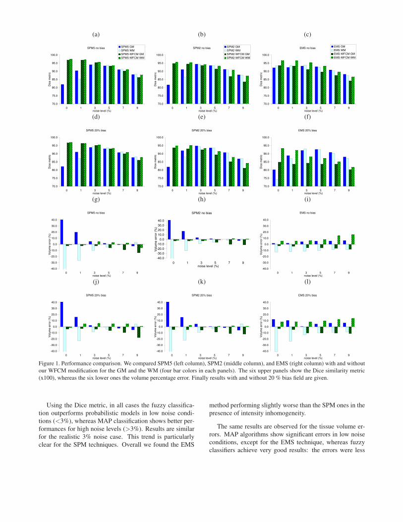
Figure 1 shows the results for all six methods in the cases

of 0% and 20 % bias field. The white and gray matter clas-

sification performances are compared locally using the Dice

metric, and total tissue volume errors are used for global ac-

curacy. Those two metrics are important since the first one

reflects how well the cortex can be segmented, while tis-

sue volume errors indicate how well partial volume effect is

modeled, in addition to being a clinically relevant measure.

(a) (b) (c)

(d) (e) (f)

(g) (h) (i)

(j) (k) (l)

Figure 1. Performance comparison. We compared SPM5 (left column), SPM2 (middle column), and EMS (right column) with and without

our WFCM modification for the GM and the WM (four bar colors in each panels). The six upper panels show the Dice similarity metric

(x100), whereas the six lower ones the volume percentage error. Finally results with and without 20 % bias field are given.

Using the Dice metric, in all cases the fuzzy classifica-

tion outperforms probabilistic models in low noise condi-

tions (<3%), whereas MAP classification shows better per-

formances for high noise levels (>3%). Results are similar

for the realistic 3% noise case. This trend is particularly

clear for the SPM techniques. Overall we found the EMS

method performing slightly worse than the SPM ones in the

presence of intensity inhomogeneity.

The same results are observed for the tissue volume er-

rors. MAP algorithms show significant errors in low noise

conditions, except for the EMS technique, whereas fuzzy

classifiers achieve very good results: the errors were less

than 5% when WFCM was used in all cases with noise

<5%. Tissue volume errors of less than 10% can be

achieved with WFCM in almost all conditions but the worst

SNR case (9% noise).

The patients that we segmented had an average noise of

4.8% (σ=0.44) as expressed as the ratio of the intensity stan-

dard deviation over the mean intensity in a manually seg-

mented region of interest of the white matter. Using the

same measure, the 5% BrainWeb dataset had 4.45% noise.

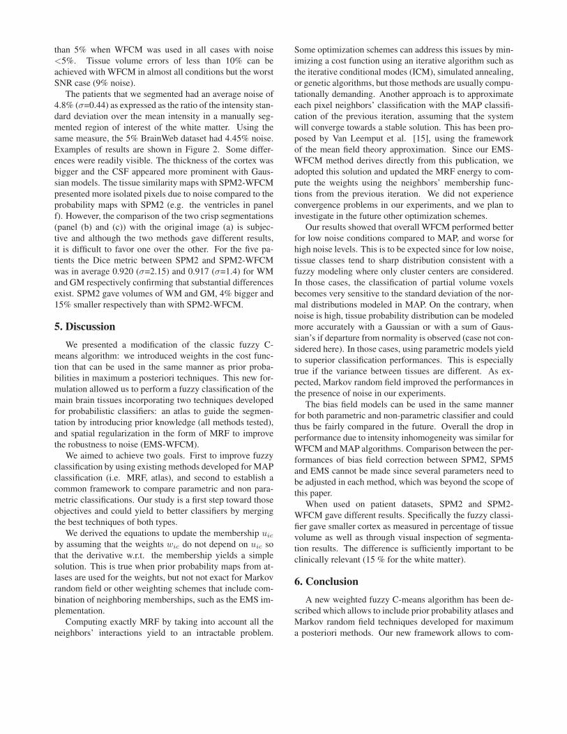
Examples of results are shown in Figure 2. Some differ-

ences were readily visible. The thickness of the cortex was

bigger and the CSF appeared more prominent with Gaus-

sian models. The tissue similarity maps with SPM2-WFCM

presented more isolated pixels due to noise compared to the

probability maps with SPM2 (e.g. the ventricles in panel

f). However, the comparison of the two crisp segmentations

(panel (b) and (c)) with the original image (a) is subjec-

tive and although the two methods gave different results,

it is difficult to favor one over the other. For the five pa-

tients the Dice metric between SPM2 and SPM2-WFCM

was in average 0.920 (σ=2.15) and 0.917 (σ=1.4) for WM

and GM respectively confirming that substantial differences

exist. SPM2 gave volumes of WM and GM, 4% bigger and

15% smaller respectively than with SPM2-WFCM.

5. Discussion

We presented a modification of the classic fuzzy C-

means algorithm: we introduced weights in the cost func-

tion that can be used in the same manner as prior proba-

bilities in maximum a posteriori techniques. This new for-

mulation allowed us to perform a fuzzy classification of the

main brain tissues incorporating two techniques developed

for probabilistic classifiers: an atlas to guide the segmen-

tation by introducing prior knowledge (all methods tested),

and spatial regularization in the form of MRF to improve

the robustness to noise (EMS-WFCM).

We aimed to achieve two goals. First to improve fuzzy

classification by using existing methods developed for MAP

classification (i.e. MRF, atlas), and second to establish a

common framework to compare parametric and non para-

metric classifications. Our study is a first step toward those

objectives and could yield to better classifiers by merging

the best techniques of both types.

We derived the equations to update the membership uic

by assuming that the weights wic do not depend on uic so

that the derivative w.r.t. the membership yields a simple

solution. This is true when prior probability maps from at-

lases are used for the weights, but not not exact for Markov

random field or other weighting schemes that include com-

bination of neighboring memberships, such as the EMS im-

plementation.

Computing exactly MRF by taking into account all the

neighbors’ interactions yield to an intractable problem.

Some optimization schemes can address this issues by min-

imizing a cost function using an iterative algorithm such as

the iterative conditional modes (ICM), simulated annealing,

or genetic algorithms, but those methods are usually compu-

tationally demanding. Another approach is to approximate

each pixel neighbors’ classification with the MAP classifi-

cation of the previous iteration, assuming that the system

will converge towards a stable solution. This has been pro-

posed by Van Leemput et al. [15], using the framework

of the mean field theory approximation. Since our EMS-

WFCM method derives directly from this publication, we

adopted this solution and updated the MRF energy to com-

pute the weights using the neighbors’ membership func-

tions from the previous iteration. We did not experience

convergence problems in our experiments, and we plan to

investigate in the future other optimization schemes.

Our results showed that overall WFCM performed better

for low noise conditions compared to MAP, and worse for

high noise levels. This is to be expected since for low noise,

tissue classes tend to sharp distribution consistent with a

fuzzy modeling where only cluster centers are considered.

In those cases, the classification of partial volume voxels

becomes very sensitive to the standard deviation of the nor-

mal distributions modeled in MAP. On the contrary, when

noise is high, tissue probability distribution can be modeled

more accurately with a Gaussian or with a sum of Gaus-

sian’s if departure from normality is observed (case not con-

sidered here). In those cases, using parametric models yield

to superior classification performances. This is especially

true if the variance between tissues are different. As ex-

pected, Markov random field improved the performances in

the presence of noise in our experiments.

The bias field models can be used in the same manner

for both parametric and non-parametric classifier and could

thus be fairly compared in the future. Overall the drop in

performance due to intensity inhomogeneity was similar for

WFCM and MAP algorithms. Comparison between the per-

formances of bias field correction between SPM2, SPM5

and EMS cannot be made since several parameters need to

be adjusted in each method, which was beyond the scope of

this paper.

When used on patient datasets, SPM2 and SPM2-

WFCM gave different results. Specifically the fuzzy classi-

fier gave smaller cortex as measured in percentage of tissue

volume as well as through visual inspection of segmenta-

tion results. The difference is sufficiently important to be

clinically relevant (15 % for the white matter).

6. Conclusion

A new weighted fuzzy C-means algorithm has been de-

scribed which allows to include prior probability atlases and

Markov random field techniques developed for maximum

a posteriori methods. Our new framework allows to com-

pare more fairly non parametric and probabilistic classifiers.

Our experiments with the BrainWeb datasets showed over-

all best performances using SPM5 with our new proposed

WFCM modification. Segmentation of patients T1W im-

ages with a signal to noise ratio of about 20, showed sub-

stantial differences between Gaussian mixture model and

WFCM. We plan in the future to investigate in more detail

those differences using a larger patient database and to test

whether more advanced spatial regularization could be ben-

eficial to WFCM.

References

[1] M. Ahmed, S. Yamany, N. Mohamed, A. Farag, and T. Mo-

riarty. A modified fuzzy C-means algorithm for bias field

estimation and segmentation of MRI data. IEEE Transac-

tions on Medical Imaging, 21(3):193–199, 2002.

[2] J. Ashburner and K. Friston. Voxel-based morphometry – the

methods. NeuroImage, 11(6):805, 2000.

[3] J. Ashburner and K. Friston. Unified segmentation. Neu-

roImage, 26:839–851, 2005.

[4] J. Bezdek, H. L.O., and C. L.P. Review of MR image

segmentation techniques using pattern-recognition. Medical

Physics, 20(4):1033, 1993.

[5] K. S. Chuang, H. L. Tzeng, S. Chen, J. Wu, and T. J. Chen.

Fuzzy c-means clustering with spatial information for image

segmentation. Computerized Medical Imaging and Graph-

ics, 30:9–15, 2006.

[6] D. Collins, A. Zijdenbos, V. Kollokian, J. Sled, N. Kabani,

C. Holmes, and A. Evans. Design and construction of a re-

alistic digital brain phantom. IEEE Transactions on Medical

Imaging, 17(3):463–468, 1998.

[7] M. Cuadra, L. Cammoun, T. Butz, O. Cuisenaire, and

J. Thiran. Comparison and validation of tissue modeliza-

tion and statistical classification methods in T1-weighted

MR brain images. IEEE Transactions on Medical Imaging,

24(12):1548–1565, 2005.

[8] Feng and Chen. Brain MR Image Segmentation Using Fuzzy

Clustering with Spatial Constraints Based on Markov Ran-

dom Field Theory, 2004.

[9] X. Li, L. Li, H. Lu, and Z. Liang. Partial volume segmen-

tation of brain magnetic resonance images based on max-

imum a posteriori probability. Medical Physics, 32:2337–

2345, 2005.

[10] A.-C. Liew and H. Yan. An adaptive spatial fuzzy clustering

algorithm for 3-D MR image segmentation. IEEE Transac-

tions on Medical Imaging, 22(9), 2003.

[11] D. L. Pham and J. L. Prince. An adaptive fuzzy C-means

algorithm for image segmentation in the presence of intensity

inhomogeneities. Pattern Recognition Letters, 20(1):57–68,

1999.

[12] P. Santago and H. Gage. Statistical models of partial volume

effect. IEEE Transactions on Image Processing, 4(11):1531–

1540, 1995.

[13] M. Siyal and L. Yu. An intelligent modified fuzzy c-means

based algorithm for bias estimation and segmentation of

brain MRI. Pattern Recognition Letters, 26:2052–2062, Oct.

2005.

[14] K. Van Leemput, F. Maes, D. Vandermeulen, and P. Suetens.

Automated model-based bias field correction of MR images

of the brain. IEEE Transactions on Medical Imaging, 18(10),

1999.

[15] K. Van Leemput, F. Maes, D. Vandermeulen, and P. Suetens.

Automated model-based tissue classification of MR images

of the brain. IEEE Transactions on Medical Imaging,

18(10):897–908, 1999.

[16] K. Van Leemput, F. Maes, D. Vandermeulen, and P. Suetens.

A unifying framework for partial volume segmentation of

brain MR images. IEEE Transactions on Medical Imaging,

22(1):105–119, 2003.

[17] I. Wells, W.M., W. Grimson, R. Kikinis, and F. Jolesz. Adap-

tive segmentation of MRI data. IEEE Transactions on Med-

ical Imaging, 15(4):429–442, 1996.

[18] L. Zhengrong, J. MacFall, and D. Harrington. Parameter

estimation and tissue segmentation from multispectral MR

images. IEEE Transactions on Medical Imaging, 13(3):441–

449, 1994.

(a) (b) (c)

(d) (e) (f)

(g) (h) (i)

Figure 2. Example on a patient MRI. Comparison of segmentation results between SPM2 and SPM2-WFCM. The original T1W image (a)

is shown as well as the resulting crisp segmentations for the two methods (b: SPM2-WFCM, c: SPM2). The middle row of panels show

the similarity maps using SPM2-WFCM of GM (d), WM (e), and CSF (f), whereas the bottom row shows the corresponding probability

maps using SPM2 of GM (g), WM (h), and CSF (i).