Fuzyy

Optimisation of a Fuzzy Logic Controller Using Genetic

Algor ithms

M.Eng Project Repor t Summer 2002

Student Name: Joseph Foran Student ID: 51161001

Optimisation of a Fuzzy Logic Controller Using Genetic

Algor ithms

M.Eng Project Repor t Summer 2002

Student Name: Joseph Foran Student ID: 51161001

Acknowledgements

I would like to thank my supervisor Ms. Jennifer Bruton for her help, guidance and support throughout the duration of the project. I would also like to thank my fiancée, family and friends for providing support and the occasional welcome distraction while I worked on this project.

Declaration I hereby declare that, except where otherwise indicated, this document is entirely my own work and has not been submitted in whole or in part to any other university. Signed: ......................................................................Date: ...............................

ii

Abstract Many non-linear, inherently unstable systems exist whose control using conventional methods is both difficult to design and unsatisfactory in implementation. Fuzzy Logic Controllers are a class of non-linear controllers that make use of human expert knowledge and an implicit imprecision to apply control to such systems. The construction of these controllers can be quick and effective in the presence of expert knowledge; conversely, in the absence of such knowledge, their design can be slow and based on trial-and-error rather than a guided approach.

Genetic Algorithms provide a way of surmounting this shortcoming. These algorithms use some of the concepts of evolutionary theory, and provide an effective way of searching a large and complex solution space to give close to optimal solutions in much faster times than random trial-and-error. They are also generally more effective at avoiding local minima than differentiation-based approaches. In this report the application of Genetic Algorithms to the design and optimisation of Fuzzy Logic Controllers is demonstrated. These controllers are characterised by a set of parameters. The inverted pendulum system, being a commonly used example of a non-linear, unstable system is used as a test system for this approach. Control was successfully achieved in various simulations using the outlined methods and the results from these simulations are presented. Details are also presented of efforts to use an online GA to continually improve the performance of a Fuzzy Logic Controller. Although these efforts were not fully successful, significant progress was made.

iii

Table of Contents

Acknowledgements.............................................................................................................. i

Declaration........................................................................................................................... i

Abstract .............................................................................................................................. ii

1 Introduction.................................................................................................................. 1 1.1 Fuzzy Logic........................................................................................................... 1 1.2 Genetic Algorithms ............................................................................................... 2 1.3 Overview of Work of Other Researchers ............................................................... 2

2 Inverted Pendulum System........................................................................................... 4 2.1 Equations of Motion.............................................................................................. 4 2.2 Linearised Equations of Motion............................................................................. 6 2.3 SIMULINK model ................................................................................................ 7 2.4 Open Loop Response............................................................................................. 8 2.5 Closed-Loop Control ............................................................................................. 9

3 Fuzzy Logic And Fuzzy Control................................................................................. 15 3.1 Fuzzy Logic......................................................................................................... 15 3.2 Fuzzy Control...................................................................................................... 17 3.3 FLC Design......................................................................................................... 20

4 Genetic Algorithms.................................................................................................... 22 4.1 Genetic Algorithm Basics.................................................................................... 22 4.2 Selection Algorithms........................................................................................... 23 4.3 Crossover Algorithms.......................................................................................... 24 4.4 Mutation Algorithms........................................................................................... 25 4.5 Elitism................................................................................................................. 26 4.6 Encoding............................................................................................................. 26 4.7 Investigating GA Parameters............................................................................... 27

5 Designing a Fuzzy Logic Controller Using Matlab..................................................... 33 5.1 Assumptions and Constraints............................................................................... 33 5.2 Spacing Parameter ............................................................................................... 34 5.3 Designing the Rule-Base ..................................................................................... 35 5.4 Matlab Implementation........................................................................................ 36

6 Using Genetic Algorithms to Design Fuzzy Logic Controllers.................................... 44 6.1 Evaluation Functions........................................................................................... 44 6.2 Parameter Encoding............................................................................................. 47 6.3 Running the GA .................................................................................................. 48 6.4 Controlling Both Pole Angle and Cart Position.................................................... 53

7 Online Genetic Algorithms......................................................................................... 55 7.1 SIMULINK S-Functions ..................................................................................... 55 7.2 Implementing a GA in SIMULINK ..................................................................... 56 7.3 Genetic-Based Machine Learning........................................................................ 61

8 Conclusion................................................................................................................. 65 8.1 Suggestions for Future Work ............................................................................... 65 8.2 Conclusions......................................................................................................... 66

iv

References ........................................................................................................................ 67

Appendix A Matlab Script and Function Files................................................................... 69 Appendix A.1 Invpenstspace.m......................................................................................... 69 Appendix A.2 gaMultimax.m............................................................................................ 69 Appendix A.3 StocRemSelec.m ........................................................................................ 71 Appendix A.4 maskXover.m............................................................................................. 72 Appendix A.5 make_fis.m................................................................................................. 72 Appendix A.6 create_mfs.m.............................................................................................. 73 Appendix A.7 create_rules.m............................................................................................ 74 Appendix A.8 run_fuzzy_pole_only.................................................................................. 76 Appendix A.9 ga_poleonly.m............................................................................................ 77 Appendix A.10 run_ga.m.................................................................................................. 78 Appendix A.11 initGa.m................................................................................................... 82 Appendix A.12 ga_sfn.m................................................................................................... 84 Appendix A.13 evalfis_sfn.m............................................................................................ 87 Appendix A.14 fuzz_class.m............................................................................................. 89 Appendix A.15 match_message.m .................................................................................... 91 Appendix A.16 apportion_credit.m ................................................................................... 91 Appendix A.17 fuzzify_online.m ...................................................................................... 92 Appendix A.18 defuzzify_online.m................................................................................... 94 Appendix A.19 centroid.m................................................................................................ 96 Appendix A.20 calcbits2.m............................................................................................... 97

v

Table of Figures Figure 2-1 Inverted Pendulum System........................................................................4

Figure 2-2 Pole in Isolation........................................................................................5

Figure 2-3 SIMULINK model of inverted pendulum system ......................................7

Figure 2-4 Model used to obtain Open Loop Response...............................................8

Figure 2-5 Open Loop Response................................................................................8

Figure 2-6 System Schematic.....................................................................................9

Figure 2-7 Rearranged Schematic...............................................................................9

Figure 2-8 State-Space Schematic ............................................................................10

Figure 2-9 State-Space Controller Impulse Response Model ....................................11

Figure 2-10 State-Space Controller Impulse Response (Impulse: 10N for 100ms) ....11

Figure 2-11 State-Space Controller Impulse Response (Impulse: 150N for 100ms) ..12

Figure 2-12 State-Space Controller Balances Pole From Initial Angle of 30°............13

Figure 2-13 State-Space Controller fails to Balance Pole From Initial Angle of 35°..13

Figure 3-1 The Fuzzy Set “Young” ..........................................................................16

Figure 3-2 “Age” Universe of Discourse..................................................................17

Figure 3-3 Membership Functions............................................................................18

Figure 3-4 Degree of Firing of Mfs ..........................................................................19

Figure 3-5 Area to be defuzzufied ............................................................................20

Figure 4-1 Single Point Crossover ............................................................................24

Figure 4-2 Multi-point Crossover .............................................................................24

Figure 4-3 Uniform Crossover..................................................................................25

Figure 4-4 Test Function with Multiple Maxima......................................................27

Figure 4-5 Run 1......................................................................................................29

Figure 4-6 Run 2......................................................................................................29

Figure 4-7 Run 10....................................................................................................30

Figure 4-8 Run 5......................................................................................................30

Figure 4-9 Run 7......................................................................................................31

Figure 4-10 Run 9....................................................................................................32

Figure 5-1 Effects of Spacing Parameters on Mfs.....................................................34

Figure 5-2 Seed Points and Grid Pts For Rule-Base Construction.............................36

Figure 6-1 Simulink Model used to evaluate FLCs...................................................46

Figure 6-2 Progress of GA that found best fitness.....................................................49

Figure 6-3 Membership functions of Optimised FLC................................................50

Figure 6-4 Surface Plot of Optimised FLC (Scaled)..................................................50

Figure 6-5 FLC and SSC Impulse Response Comparison .........................................51

Figure 6-6 Response To Large Impulse....................................................................51

vi

Figure 6-7 Bringing Pole to Upright Position ...........................................................52

Figure 6-8 Comparison of FLC and SSC from Initial Angle of 5°.............................52

Figure 6-9 Response to 1kN disturbance ..................................................................54

Figure 6-10 Response to 150N disturbance impulse .................................................54

Figure 7-1 Simulink Block Characteristics...............................................................55

Figure 7-2 Simulink Model for GA ..........................................................................60

Figure 7-3 SIMULINK Implementation of Fuzzy Classifier System.........................62

Figure 7-4 GBML Progress (Disturbance Impulse 0.1N 0.01s).................................63

Figure 7-5 GMBL Progress (Impulse Disturbance 100N, 0.01s)...............................63

Figure 7-6 Close up of Figure 7-5.............................................................................64

vii

Table of Tables Table 3-1 Simple Rule Base.....................................................................................17

Table 3-2 Typical Rule Base....................................................................................19

Table 4-1 Parameters for GA Runs...........................................................................28

Table 5-1 Derived Rule Base....................................................................................36

Table 6-1Parameters used for encoding....................................................................47

Table 6-2 Parameters for GA Runs with FLC...........................................................48

Table 6-3 Rule-Base of Optimised FLC ...................................................................50

Table of L istings Listing 4-1Code for Test Objective Function............................................................28

Listing 5-1 make_fis.m ............................................................................................38

Listing 5-2 create_mfs.m..........................................................................................40

Listing 5-3 create_rules.m........................................................................................43

Listing 6-1 Evaluation Function run_fuzy_pole_only.m...........................................46

Listing 7-1 Initialising State Information..................................................................56

Listing 7-2 Updating GA s-function.........................................................................57

Listing 7-3 S_Function GA Operation......................................................................58

Listing 7-4 S-Function Output Routine.....................................................................59

1

1 Introduction This report presents details of the work carried out to optimise a Fuzzy Logic

Controller using Genetic Algorithms. Detailed explanations of both these concepts are

presented as well as a demonstration of how they can be applied to control a non-

linear, unstable system. The inverted pendulum is both unstable and non-linear and is

used to test out the methods tried for this project.

1.1 Fuzzy Logic

Fuzzy Logic is a logic system that uses imprecision. Just as human beings would

never say that a table is 1.456 metres long, but rather that it is about one and a half

metres long, fuzzy logic categorises objects into sets which are described by linguistic

variables such as “ long” , ‘ fast” , “cool” , “heavy” , “middle-aged” and so on. Objects

can have varying degrees of membership of such fuzzy sets, ranging from a crisp

“definitely not a member” (denoted by 0) to a crisp “definitely a member” (denoted

by 1). The crucial distinction is that between these crisp extremes, objects can have

less certain degrees of membership such as “not really a member” (perhaps denoted

by a 0.1) and “pretty much a member” (0.9 possibly).

Fuzzy Logic can be applied to control, and when it is, is known as Fuzzy Control.

Fuzzy Control is made up of control rules which mimic those used by humans when

they control or operate machinery: “If you need to go a little bit faster, push the

accelerator pedal slightly” . Fuzzy Control can be an especially effective way of

controlling non-linear systems when expert human knowledge of the system is

available.

The details of how Fuzzy Logic and Fuzzy Control are applied are given in Chapter 3.

Much more detailed information is available from Passino et al. [2].

2

1.2 Genetic Algor ithms

Genetic Algorithms (GAs) are useful algorithms for optimising solutions to problems;

especially those that are analytically intractable. They are inspired, as the name

suggests, by the biological concepts of genetics and evolution.

Considering that the most accomplished controller known to man, the human brain,

and other numerous marvels found in nature, all arose through the process of

evolution through natural selection, the principles behind this highly successful

“design” procedure should be able to provide some inspiration to improve the

engineering design process. Genetic Algorithms use these principles to refine and

optimise designs whose parameters interact in a complex manner. Individuals

representing different potential solutions are preferentially selected according to their

fitness and pass on their “genes” , i.e. characteristics, to future generations. Mating

takes place between these individuals with the hope that by sharing the characteristics

of successful individuals, even fitter individuals can be created. Mutation also occurs

to inject new genes into a population. As in nature, most mutations are harmful but

the occasional beneficial one can help improve the fitness of the individuals it affects,

i.e. find better solutions.

1.3 Overview of Work of Other Researchers

A significant number of researchers in the field have applied Genetic Algorithms to

the task of optimising Fuzzy Logic Controllers (FLCs). Many different approaches to

this task have been taken. For example, Herrera et al. [11] apply GAs to optimise a

rule-base of a FLC for which the membership functions have already been created,

whereas Lee at al. [12] use a GA that determines the number of membership

functions, the number of fuzzy rules and the rule-base. In both of these cases, the

GA is implemented using real-valued encodings, whereas Belarbi et al. [13] use

binary encoding for their approach, where they implement the FLC as a neural

network and use the GA to train the weights.

Park et. al [8] implement a GA by using characteristic parameters to automate FLC

design and this method is used for this project also. Using this technique, a FLC can

3

be designed very flexibly, with the numbers and positions of membership functions

determined by the GA as well as the rule-base. Rule-bases that are well-formed, as the

term is used by Cheong et al.[9], emerge, which is another benefit.

In this report the basic principles of Fuzzy Logic and Genetic Algorithms are

explained after which the main body of work performed is presented along with the

results obtained. But before all that, the inverted pendulum system is analysed and an

effort is made to build a controller based on a linear model of this system.

4

2 Inver ted Pendulum System In this chapter the Inverted Pendulum System is examined. It is analysed with a view

to obtaining its equations of motion and then to linearise these equations in order to

find a state-space-based model of the system. This model is used to design a

controller, which is applied to a non-linear model of the system. Following this, the

inadequacies of this controller, especially in dealing with the non-linearities are

highlighted.

2.1 Equations of Motion

The inverted pendulum system is made up of a cart on top of which a pole is pivoted

as shown in Figure 2-1. The cart is constrained to move only in the horizontal x-

direction, while the pole can only rotate in the x-y plane.

M

mg

x

θ

u

l

y

Figure 2-1 Inver ted Pendulum System

The equations of motion for the system are derived using the following parameters

• M is the mass of the cart,

• m the mass of the pole,

• l the distance from the pivot to the centre of mass of the pole

• I the moment of inertia of the pole about the pivot,

• x the cart’s position

5

• θ the angle the pole makes with the vertical and

• u the horizontal control force imparted to the cart.

The position of the centre of gravity of the pole is given by

θsin�

−= xxG (1)

Taking the second derivative of this with respect to time we get

θθθθ sincos 2��

llxxG +−= (2)

The sum of the external forces on the system equals the mass multiplied by

acceleration of each component, i.e.

GxmxMu �� +=

)sincos( 2 θθθθ��

llxmxMu +−+=�

umlmlmMx =−++� θθθθ cossin)( 2 �� (3)

..

θI

θsinl

θcosl

..

mx

mg

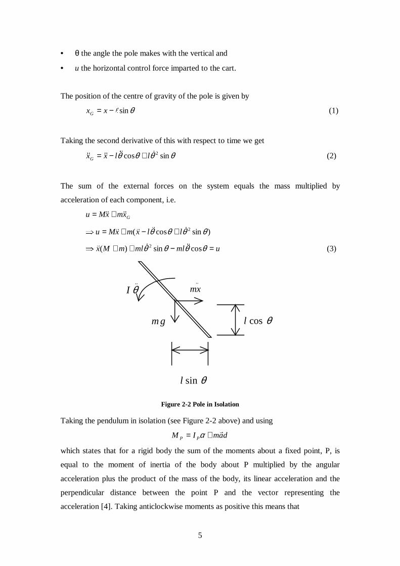
Figure 2-2 Pole in Isolation

Taking the pendulum in isolation (see Figure 2-2 above) and using

damIM PP

�+= α

which states that for a rigid body the sum of the moments about a fixed point, P, is

equal to the moment of inertia of the body about P multiplied by the angular

acceleration plus the product of the mass of the body, its linear acceleration and the

perpendicular distance between the point P and the vector representing the

acceleration [4]. Taking anticlockwise moments as positive this means that

6

θθθ cossin lxmImgl �� −= (4)

Rearranging (4) gives

I

xmlmgl��

�� θθθ cossin +=

Substituting this into (3) and rearranging gives

θθθθθ

222

222

cos)(

sinImsincos

lmImM

lglmIux

−+−+=

��

(5)

Substituting this back into (4) and rearranging gives

θθθθθθθ

222

222

cos)(

sincoscossin)(

lmImM

lmumlmglmM

−+−++=

��

(6)

For a uniform rod of mass m and length L=2l the moment of inertia about one end is

2

3

4ml [4]

Equations (5) and (6) thus become

θ

θθθθ

2

2

cos)(3

4

sin3

4sincos

3

4

mmM

lmgux

−+

−+=

�

�� (7)

and

θ

θθθθθθ2

2

cos)(3

4sincoscossin)(

mllmM

mlugmM

−+

−++=�

�� (8)

2.2 L inear ised Equations of Motion

These equations can be linearised by noting that for small θ, sinθ ≈ θ, cosθ ≈ 1 and

θ�≈ 0. The equations then become

mmM

mgux

−+

+=

)(3

43

4 θ��

(9)

and

7

mllmM

ugmM

−+

++=)(

3

4)( θθ

�� (10)

These linearised equations can be represented in state-space form as follows:

ux

x

x

x

mllmM

mmM

mllmM

gmM

mmM

mg

��

�

�

��

�

�

+��

�

�

��

�

�

��

�

�

��

�

�

=��

�

�

��

�

�

−+

−+

−+

+

−+

)(3

41

)(3

43

4

)(3

4)(

)(3

4

0

0

000

1000

000

0010

θθ

θθ �

�

��

��

(11)

This is in the usual form uBAxx +=�

used for state-space expressions.

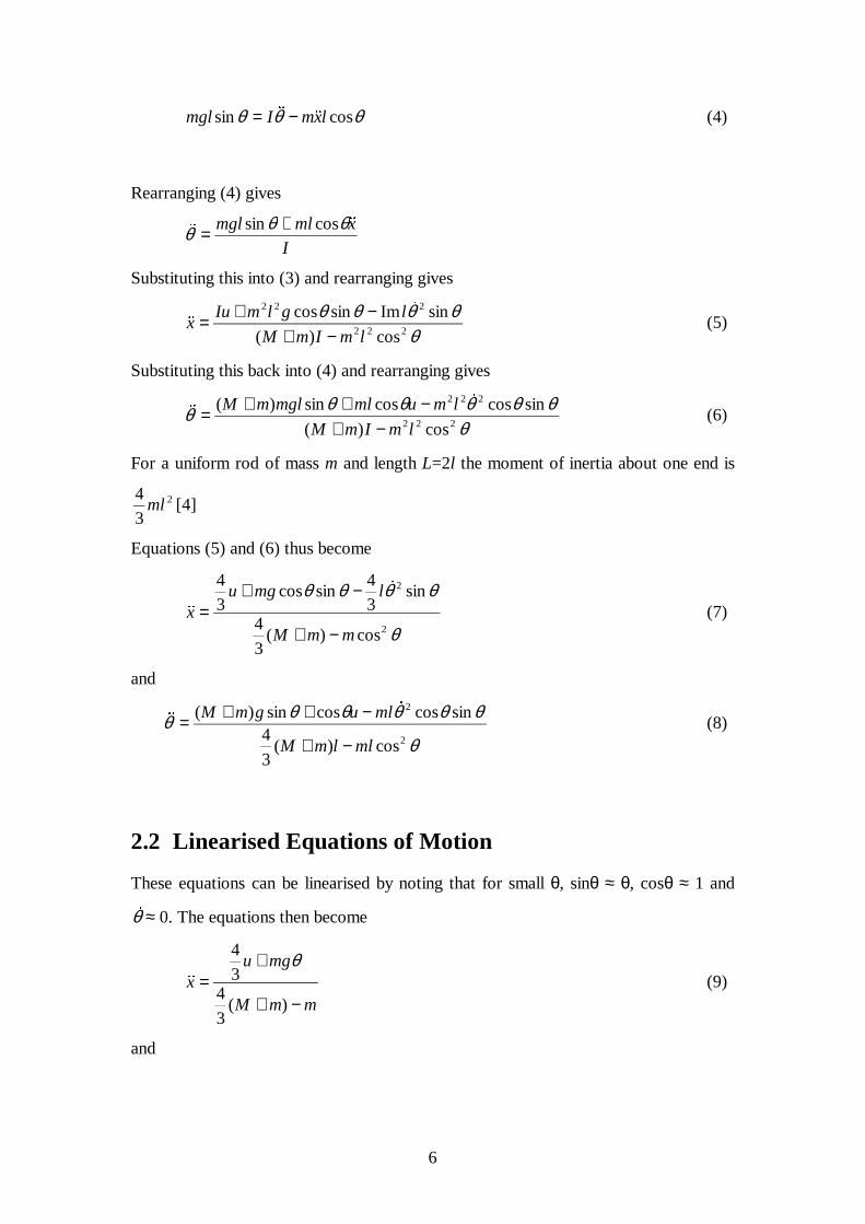
2.3 SIMULINK model

Using SIMULINK1, a model of the system, (see Figure 2-3 below) was created. In

this model, the control action is an input. In combination with the angle and angular

velocity from the previous time step, it is used to calculate the cart’s acceleration and

the pole’s angular acceleration using equations (7) and (8) respectively. Integration is

then performed to get the speeds and positions for both components. It should also be

noted that the value of the pole’s angle is limited to remain between ±90°. The pole

angle and angular velocity and the cart position and velocity are the outputs of this

model.

Figure 2-3 SIMULINK model of inver ted pendulum system

1 For the SIMULINK solver, the ode4 (Runge-Kutta) algorithm was used with a fixed time step of 0.01s and Single-Tasking. Except where otherwise noted, these parameters were used for all models mentioned in this report.

8

2.4 Open Loop Response

The open loop response of this system was obtained using the SIMULINK model

shown in Figure 2-4 below.

x

v

sX

sX

sTheta

sTheta

Theta

Step

sTime

STime

OmegaControl Action

Theta

Omega

x

v

InvertedPendulumDynamics

u*180/pi

Fcn

Clock

Figure 2-4 Model used to obtain Open Loop Response

The simulation was run for ten seconds and the parameters1 used were:

• M, the mass of the cart: 1kg

• m, the mass of the pendulum: 0.1kg

• l, the distance from the pivot to the pendulum centre of mass: 0.5m

The open loop response is plotted in Figure 2-5. The system can be seen to be

unstable, with the pole becoming horizontal very quickly. To keep the pole vertical, a

controller will be needed.

0 0.5 1 1.5 2 2.5 30

10

20

30

40

50

60

70

80

90

100Open Loop Response

Time (s)

Ang

le (

degr

ees)

Figure 2-5 Open Loop Response

1 These parameters were also used for all models detailed in this report

9

2.5 Closed-Loop Control

An attempt is now made to design a controller for the system. The state-space method

is used to do this as this allows the design of a controller of both the pendulum angle

and cart position. Much of the work in this section is based on a tutorial on the

University of Michigan website [6].

As the main objective for controlling this system is to keep the pendulum upright as

much as possible, the reference value for the angle to which the output is compared

will be zero throughout all simulations. When analysing the system’s response, it is

the response to a disturbance force applied to the cart, rather than to a change in the

reference that will be examined. This is shown schematically in Figure 2-6 below.

Plant G(s)

Σ

Σ

Controller

K C(s)

Reference r(s)=0

+

-

Disturbance Force f(s)

+

+

Output y(s)

Figure 2-6 System Schematic

The schematic can be rearranged as in Figure 2-7.

Plant G(s)

Σ

Controller

K C(s)

-

Disturbance Force f(s)

+

Output y(s)

Figure 2-7 Rear ranged Schematic

As it is a response to a disturbance force that is being analysed, the reference position

for the cart will also be zero. To control both angle and position, a state-space

controller will be designed. The schematic for this is shown in Figure 2-8.

10

Plant

Cxy

BuAxx

=+=

�

Σ

Contr oller

K

-

Reference R(s)

+

Output y(s)

Figure 2-8 State-Space Schematic

To design a controller the Linear-Quadratic Regulator (LQR) method described by

Friedland [3] is used. Using the state-space equation (11), this method finds the

optimal K based on the state feedback law

K x−=u (12)

such that the cost function

( )�

+= τdJ Ruu'Qxx' (13)

is minimised. Q is a weighting matrix specifying the relative importance of each of

the system states and similarly, R is a weighting matrix that specifies the relative

importance of the inputs. As there is only one input into the system, R is set to one in

this specific case. The function lqr provided with the Control Systems Toolbox for

Matlab is used to calculate the matrix K.

Code obtained from the University of Michigan Control Tutorials website [6] was

modified to obtain the controller gain K (See Appendix A.1). The weighting is set so

that the position and angle each had a relative importance of 5000 compared to the

control action. The modified code was run and the vector K obtained was

[ ]97.4905.205919.52711.70 −−=K (14)

11

sXNonLin

To Workspace4

sThetaNonLin

To Workspace3

sTimeNonLin

To Workspace2

Position

Mux

K

MatrixGain

Control Action

Theta

Omega

x

v


Impulse

u*180/pi

Fcn

0

Constant

Clock1

Angle

Figure 2-9 State-Space Controller Impulse Response Model

This controller was modelled in SIMULINK (Figure 2-9). The response to an impulse

disturbance of 10N applied for 100ms was obtained and the plot of this response

appears in Figure 2-10 below. As can be seen, the controller succeeds in restoring

both the angle and pendulum to zero after a settling time of approximately 2s.

0 0.5 1 1.5 2 2.5 3−2

−1

0

1

2

3Impulse Response of State−Space Controlled Inverted Pendulum System

Time(s)

Ang

le (

degr

ees)

0 0.5 1 1.5 2 2.5 3−0.03

−0.02

−0.01

0

0.01

0.02

0.03

Time (s)

Pos

ition

(m

)

Figure 2-10 State-Space Controller Impulse Response (Impulse: 10N for 100ms)

This controller is based upon a linearised model and hence is expected to work when

the assumptions taken to linearise the model are valid, i.e. when the angle, θ, is small.

12

To see how the controller works when the angle is quite large, the disturbance force

needs to be bigger. Hence, the above system was modelled again with an impulse

force of 150N again applied for 100ms. The response obtained is plotted in Figure

2-11.

0 0.1 0.2 0.3 0.4 0.5 0.6 0.7 0.8 0.9 1−100

−50

0

50

100Impulse Response Of State−Space Controlled Inverted Pendulum System

Time (s)

Ang

le (

degr

ees)

0 0.1 0.2 0.3 0.4 0.5 0.6 0.7 0.8 0.9 1−15

−10

−5

0

5x 10

9

Time (s)

Pos

ition

(m

)

Figure 2-11 State-Space Controller Impulse Response (Impulse: 150N for 100ms)

Here, the perturbation to the system is too large for the controller to handle. The non-

linearities, assumed to be negligible when the controller was designed, begin to

dominate when the angle gets too large and hence, the pole collapses and falls to 90°.

Following this, the ability of the controller to bring the pendulum to its equilibrium

position from an initial non-equilibrium position was investigated. As can be seen

from Figure 2-12, when the initial angle is 30°, the controller successfully balances

the pole. However, when the initial angle is increased to 35°, the pole collapses. This

gives an indication of the region in which the controller can operate.

13

0 0.5 1 1.5−30

−20

−10

0

10

20

30

40Balancing Pole from Initial Angle of 30 degrees

Time (s)

Ang

le (

degr

ees)

0 0.5 1 1.5−0.2

0

0.2

0.4

0.6

0.8

1

1.2

Time (s)

Pos

ition

(x)

Figure 2-12 State-Space Controller Balances Pole From Initial Angle of 30°°°°

0 0.5 1 1.5−100

−50

0

50

100Balancing Pole from Initial Angle 35 degrees

Time (s)

Ang

le (

degr

ees)

0 0.5 1 1.5−4

−3

−2

−1

0

1x 10

9

Time (s)

Pos

ition

(m

)

Figure 2-13 State-Space Controller fails to Balance Pole From Initial Angle of 35°°°°

This controller successfully controls the system as long as the pole is not allowed to

stray too much from the equilibrium position. When the pole angle gets too large it is

unable to restore it to the upright position. A controller that can successfully achieve

14

this needs to be able to handle the non-linearities. For this reason, Fuzzy Logic

Controllers are investigated to see if they can help solve the problem.

15

3 Fuzzy Logic And Fuzzy Control

Fuzzy Control is based on the principles of Fuzzy Logic developed by Zadeh [14] in

1965. It is a non-linear control method, which attempts to apply the expert knowledge

of an experienced user to the design of a controller. In this chapter, the basic

principles of fuzzy logic are presented as well as a demonstration of how these

principles are applied to the control of engineering systems.

3.1 Fuzzy Logic

Fuzzy logic is based on the theory of fuzzy sets where variables can have differing

degrees of membership of sets. This is unlike the more familiar crisp set theory where

a variable is either a full member of a set or it is not a member of that set at all. The

degree to which a variable belongs to a set can vary between 0 and 1. This can allow

for the handling of borderline cases and other hard-to-categorise situations in a more

intuitively satisfying way.

A universe of discourse is defined as the whole range of fuzzy sets to which a variable

can belong. Each set on this universe of discourse is referred to as a membership

function and is often described using a ‘ linguistic variable’ . On a universe of

discourse, a variable has a degree of membership of each membership function that

varies between 0 and 1.

Fuzzy Logic uses rules with antecedents and consequents to produce outputs from

inputs. The antecedents are the inputs that are used in the decision-making process or

the “IF” parts of the rules. The consequents are the implications of the rules or the

“THEN” parts.

3.1.1 Fuzzy Logic Example

An example of a fuzzy set is the set of humans who could be described as young.

Most people would agree that anyone aged between zero and twenty could be

described as being definitely young, whereas anyone over forty would be described as

16

not at all young. The ages between twenty and forty are more of a grey area, however.

The closer a person’s age is to twenty the more readily they could be described as

young. This fuzzy set is displayed in Figure 3-1 below. According to this fuzzy set a

person aged fifteen is definitely young, i.e. their degree of membership of the fuzzy

set Young is one. However, it is less clear-cut whether a person aged thirty could be

described as young, i.e. their degree of membership is less than one, in this example,

0.5.

0 5 10 15 20 25 30 35 40 45 500

0.25

0.5

0.75

1

The Fuzzy Set "Young"

Age

Deg

ree

of M

embe

rshi

p

Figure 3-1 The Fuzzy Set “ Young”

The Universe of Discourse of a variable is the range of values that that variable can

take. Many fuzzy sets can be defined on one Universe of Discourse and a single

variable can have membership of more than one fuzzy set. For example, in Figure 3-2

below we return to our “Age” example and examine the Universe of Discourse on

which, in addition to Young, the fuzzy sets Middle Aged and Old are added. Here we

can see that a person aged 35 has membership of two sets, Young and Middle Aged

with degrees of membership of 0.25 and 0.33 respectively.

17

0 10 20 30 40 50 60 70 80 90 1000

0.25

0.5

0.75

1

Universe of Discourse for Age

Age

Deg

ree

of M

emeb

ersh

ip

Young Middle Aged Old

Figure 3-2 “ Age” Universe of Discourse

3.2 Fuzzy Control

Fuzzy Control applies fuzzy logic to the control of processes by utilising different

categories, usually ‘error’ and ‘change in error’ , for the process state and applying

rules to decide a level of output, i.e. a suitable control action. The linguistic variables

used for both input and output variables are often of the form ‘negative large’ ,

‘positive small’ , ‘zero’ etc. A typical rule base for a two-input, single-output system

with three membership functions per variable is shown in Table 3-1

DE

E N Z P

N N N Z

Z N Z P

P Z P P

Table 3-1 Simple Rule Base

For example, using this rule base, if the error, E, was negative, N, and the change in

error, DE, was positive, P, then the output would be zero, Z. This particular rule

recognises the fact that although there is an error in the system, it is approaching zero

so no control action needs to be applied.

18

3.2.1 Defuzzification

Often input variables are members of more than one fuzzy set defined on their

universe of discourse. This means that for each combination of inputs, there will, in

general, be more than one rule fired. Also, the output needs to have a precise numeric

value. Defuzzification is the process by which the sets of the various fired rules are

combined to produce an output.

To illustrate this, take the following example. The FLC has two inputs, Error and

Change in Error and one output, Action. The universe of discourse for each of these

variables is normalised so that their values always lie between –1 and 1. (Scaling

gains are applied to each variable to give the appropriate range). There are five

membership functions for each variable spaced as in Figure 3-3. The rule-base is as

given in Table 3-2.

−1 −0.75 −0.5 −0.25 0 0.25 0.5 0.75 10

0.1

0.2

0.3

0.4

0.5

0.6

0.7

0.8

0.9

1

Membership Functions for Error, Change of Error and Action Variables

Variable Value

Deg

ree

Of M

embe

rshi

p

NB NS Z PS PB

Figure 3-3 Membership Functions

19

e

de N B N S Z PS P B

N B N B N B N S NS Z

N S N B N S N S Z PS

Z N S N S Z PS PS

P S N S Z P S PS PB

P B Z P S P S PB PB

Table 3-2 Typical Rule Base

If the input error is 0.4, this means that it is a member of two sets, Z to a degree of 0.2,

and PS, to a degree of 0.8 (see Figure 3-4). If the input change in error is –0.2, this is

a member of Z to a degree of 0.6 and of NS to a degree of 0.4. Four rules altogether

are fired in this situation and the degree to which each is fired is given by the

minimum degree of the two inputs firing it. (This is how the boolean AND operation

is performed in Fuzzy Logic). The rules fired and the degrees to which they are fired

are:

• If error is Z and change in error is Z then the control action is Z (degree 0.2)

• If error is Z and change in error is NS, then the control action is NS (degree 0.2)

• If error is PS and change of error is Z then the control action is PS (degree 0.6)

• If error is PS and change of error is NS then the control action is Z (degree 0.4)

−1 −0.75 −0.5 −0.25 0 0.25 0.5 0.75 10

0.1

0.2

0.3

0.4

0.5

0.6

0.7

0.8

0.9

1

Membership Functions for Error, Change of Error and Action Variables

Variable Value

Deg

ree

Of M

embe

rshi

p

NB NS Z PS PB

Figure 3-4 Degree of Fir ing of Mfs

20

Combining these control actions, with each output fuzzy set cut off at the level

corresponding to the degree to which they are fired, gives a shape as shown in Figure

3-5. This needs to be converted into a numerical value for the control action to be

applied. The process of conversion is known as defuzzification and there are many

methods of performing it. A very popular method is to take the centre of gravity of the

resultant shape and apply a control action corresponding to the x-axis value of this

point. In our example, the centre of gravity lies at (0.1528,0.2213) which means that

the control action has a value of 0.1528. This is then scaled by the appropriate scaling

factor to give a suitable output.

−1 −0.8 −0.6 −0.4 −0.2 0 0.2 0.4 0.6 0.8 10

0.1

0.2

0.3

0.4

0.5

0.6

0.7

Centre Of Gravity

Figure 3-5 Area to be defuzzufied

3.3 FLC Design

When designing a Fuzzy Logic Controller (FLC) expert knowledge of the process to

be controlled can be used to design the membership functions and rule base.

Unfortunately there is no general procedure for designing a FLC from first principles,

and heuristics are usually required as well as much trial and error to achieve a FLC

that meets the design objectives and constraints. In this traditional approach,

designing an FLC can be a laborious, time-consuming process [16]. These FLCs also

tend to be non-portable to other applications.

21

However, another technique exists for optimising a FLC. Genetic Algorithms (GAs)

are a class of algorithms that can be used to search large solution spaces for solutions

that are close to optimal. How they work is explained in the next chapter.

22

4 Genetic Algor ithms

Genetic Algorithms are reliable and robust methods for searching solution spaces [1],

[5]. They are inspired by the biological theory of evolution through natural selection

and much of the terminology is similar.

4.1 Genetic Algor ithm Basics

A chromosome is an encoded string of possible values for the parameters to be

optimised. These chromosomes can be made up of real-valued or binary strings. Often

one of the main challenges in designing a genetic algorithm to find a solution to a

problem is finding a suitable way to encode the parameters.

A set of potential solutions, called a population, is created. Each member of this set is

referred to as an individual and they are evaluated by decoding the parameter values

from the chromosomes and applying them to the problem to see how well they

perform the task at hand (the objective that is to be optimised). The score that an

individual achieves at performing the required task is called its fitness.

After the fitness of each individual has been calculated, a procedure known as

selection is performed. Individuals are selected to contribute towards creating the next

generation, the probability of selection being related to the individual’s fitness.

Once selection has occurred, crossover takes place between pairs of selected

individuals. The strings of two individuals are mixed. In this way, new individuals are

created that contain characteristics that come from different hereto relatively

successful individuals.

A third operation that occurs is mutation, the random changing of bits in the

chromosome. It is generally performed with a relatively low probability. Mutation

ensures that the probability of searching a given part of the solution space is never

zero.

23

There are many ways in which these different operations can be applied. Different

algorithms can be used for each and they can also be applied with varying degrees of

probability. Some of the more popular algorithms for each of these operations are now

examined and their effects on the GA’s performance is investigated.

4.2 Selection Algor ithms

A popular selection algorithm is stochastic sampling with replacement, more

commonly known as the “Roulette Wheel” algorithm, so called because this method

works in a way that is analogous to a roulette wheel. Each individual in a population

is allocated a share of a wheel, the size of the share being in proportion to the

individual’s fitness. A pointer is spun (a random number generated) and the individual

to which it points is selected. This continues until the requisite number of individuals

has been selected. An individual’s probability of selection is thus related to its fitness

ensuring that fitter individuals are more likely to leave offspring. A problem with this

approach is that the number of times an individual is actually selected has a high

variance so there is no guarantee that fitter individuals will be represented in the next

generation.

Stochastic Remainder Selection is another popular algorithm. In this method the

expectation of the number of times selected is calculated for each individual. The

integer portions of this expectation for each individual are assigned deterministically

and the fractional remainders are assigned in the same way as in roulette wheel

selection. For example, an individual whose expectation of number of times selected

was 2.4 would be certain of being selected twice and the probability of being selected

a third time would be 0.4. This approach reduces the variance associated with the

roulette wheel algorithm and ensures that all individuals with above-average fitness

will be represented in the next generation.

24

4.3 Crossover Algor ithms

Once selection is finished crossover is performed. Individuals are paired for mating

and by mixing their strings new individuals are created. The most basic crossover

algorithm is known as Single Point Crossover. A single point along the string is

chosen and the strings are swapped over at this point.

Parent 1 101 | 11100

Parent 2 110 | 10010

Child 1 101 10010

Child 2 110 11100

Figure 4-1 Single Point Crossover

Multipoint crossover algorithms extend simple crossover by selecting multiple

crossover points and alternately assigning to the first or second offspring the portions

of string between these points.

Parent 1 10 | 111 | 100

Parent 2 11 | 010 | 010

Child 1 10 010 100

Child 2 11 111 010

Figure 4-2 Multi-point Crossover

Uniform crossover is another crossover algorithm. This time a random mask of 1s and

0s of the same length as the parent strings is generated. If a bit in the mask is 1 then

the corresponding bit in the first child will come from the first parent and the second

parent will contribute that bit to the second offspring. If the mask bit is 0 the first

parent contributes to the second child and the second parent to the first child.

25

Parent 1 10111100

Parent 2 11010010

Mask 01001101

Child 1 10011110

Child 2 11110000

Figure 4-3 Uniform Crossover

Uniform crossover is the most disruptive of the crossover algorithms [15], i.e. it is the

most likely to cause neighbouring bits that contribute in a positive way to the fitness

of the individual to be split up. However at the same time, uniform crossover allows

for more extensive searching of the solution space as there are significantly more

potential offspring using this method.

4.4 Mutation Algor ithms

For binary codings, there is really only one way to mutate. For each bit generate a

random number and if it is less than the specified mutation probability, flip the bit,

i.e., if it is a 1 change it to 0 or vice versa. This mutation probability is generally kept

quite low and is constant throughout the lifetime of the GA. However, a variation on

this basic algorithm changes the mutation probability throughout the lifetime of the

algorithm, starting with a relatively high rate and steadily decreasing it as the GA

progresses. This allows the GA to search more for potential solutions at the outset and

to settle down more as it approaches convergence.

When real-valued codings are used, the mutation algorithm can be more complex.

Many different algorithms are used some of which are as follows:

• Uniform Mutation: A random value within the constraints of the variable is

chosen.

• Boundary Mutation: The variable is set to either its lower or upper bound.

• Non-Uniform Mutation: The variable is assigned a value based on a bell curve

that becomes progressively narrower as the GA progresses. This ensures that as

26

convergence is approached, the range within which a variable can be mutated

also narrows.

4.5 Elitism

With crossover and mutation taking place, there is a high risk that optimum solutions

may be lost as there is no guarantee that these operations will preserve fitness. To

combat this elitist models are often used [1]. In these models, the best individual

from a population is saved before any of the operations take place. After the new

population is formed and evaluated, it is examined to see if this best structure has

been preserved. If not, the saved copy is reinserted back into the population, usually at

the expense of the weakest member. The GA then proceeds to perform the operations

on this population.

4.6 Encoding

Genetic Algorithms can be performed using either binary or real-valued encodings.

With binary encoding, each parameter is converted into a binary string. These strings

are concatenated and the genetic operations are performed on this concatenated string.

With real-valued encoding, the parameters are kept in their real number format. Both

forms of encodings are used in practice.

The advantages of using a binary format is that it

… maximises the number of hyperplane partitions directly available in the

encoding for schema processing. [15]

In other words, binary alphabets allow for greater sampling of the solution space and

for the processing of more combinations of alleles.

However encoding using higher cardinalities can be more efficient. For example, if a

certain parameter could take on five possible values then it would need to be encoded

using three bits in a binary scheme. However, this leads to eight possible alleles, three

of which are superfluous. Using a five-letter alphabet in this case would lead to more

efficient coding.

27

4.7 Investigating GA Parameters

Other factors also have an effect on how the GA performs. These include population

size, mutation probability and crossover probability among others. To investigate

how some of these factors affected the GA an experiment was performed using a test

function with multiple maxima.

The test function is )5cos(2)7sin(58 xx −+ . This function is plotted in Figure 4-4. As

can be seen from the plot, this function has many maxima whose peak values are

different. It is hoped that the GA searching this solution space will find the peak value

in this range which occurs at x = 5.618, y = 14.958 or somewhere close to it. There

are also two local maxima whose peaks fall just short of the global peak. Those

searches that succeed in avoiding getting stuck at these local maxima are those whose

properties should be noted and emulated.

0 1 2 3 4 5 6 7 8 9 100

5

10

15Test Multiple Maxima Function: 8+5sin(7x)−2cos(5x)

x

Fun

ctio

n V

alue

Figure 4-4 Test Function with Multiple Maxima

To perform the GA, Matlab was used in conjunction with the GAOT toolbox, which

is open-source code provided by Houck et al. [7]. An objective function has to be

provided for this toolbox that evaluates the string passed in. This code is shown

below.

28

f unct i on [ x , mul t i maxval ] = mul t i max( x, Ops) %Eval uat es t he t est mul t i pl e maxi ma f unct i on %f or t he GAOT t ool box mul t i maxval = 8 + ( 5* s i n( 7* x) - 2* cos( 5* x) ) ;

Listing 4-1Code for Test Objective Function

To apply the parameters to the GA a script file was written in which the essential

parameters are set. This file is listed in Appendix A.2. Ten different runs of the GA

were performed, each for 100 generations. The parameters for these runs are given in

Table 4-1. To implement some of the algorithms in these runs new Matlab .m files

were written to supplement the GAOT toolbox. These were stocRemSelec.m, which

performs Stochastic Remainder Selection, and maskXover.m which performs uniform

crossover. The code for these files is listed in Appendices A.4 and A.5.

Run Population

Size

Selection

Algorithm

Crossover

Algorithm

Crossover

Probability

Mutation

Probability

Best

Find Gen

1 10 Roulette Uniform 0.5 0.001 14.586 16

2 200 Stoc. Rem. Single Pt. 1.0 0.1 14.958 77

3 200 Stoc. Rem. Uniform 1.0 0.01 14.958 16

4 10 Stoc. Rem. Uniform 1.0 0.01 14.632 28

5 50 Stoc. Rem. Uniform 1.0 0.01 14.958 86

6 100 Stoc. Rem. Uniform 1.0 0.01 14.958 41

7 50 Stoc. Rem. Single Pt. 1.0 0.01 14.958 20

8 50 Stoc. Rem. Uniform 0.5 0.01 14.958 13

9 50 Roulette Uniform 1.0 0.01 14.958 12

10 50 Stoc. Rem. Uniform 1.0 0.1 14.958 66

Table 4-1 Parameters for GA Runs

Of these ten runs only runs 1 (Figure 4-5) and 4 failed to come to within 1% of the

actual peak value within the first hundred generations. In both of these cases the run

converged to the final value before the thirtieth generation suggesting that both of

these runs got stuck at a local maximum. This suggests strongly that population size

has a strong bearing on the performance of a genetic algorithm.

29

0 10 20 30 40 50 60 70 80 90 1007

8

9

10

11

12

13

14

15

Generation

Fitn

ess

Progress of GA over time

Population: 10 Selection Method: RouletteXover Method: Uniform Xover Prob: 0.5 Mutation Prob: 0.001

Maximum FitnessMean Fitness

Figure 4-5 Run 1

Runs 2 (Figure 4-6) and 10 (Figure 4-7) both have high mutation rates (10%). As the

average value of the test function is 8.02 and the mean fitness of the individuals for

these runs does not go much higher than this, it can be seen that high mutation rates

render the GA as almost a random search, i.e., the purposefulness of the search is

reduced significantly.

0 10 20 30 40 50 60 70 80 90 1007

8

9

10

11

12

13

14

15

Generation

Fitn

ess


Population: 50 Selection Method: Stoc. Rem.Xover Method: Single Pt.Xover Prob: 1 Mutation Prob: 0.1


Figure 4-6 Run 2

30

0 10 20 30 40 50 60 70 80 90 1007

8

9

10

11

12

13

14

15

Generation

Fitn

ess


Population: 50 Selection Method: Stoc. Rem.Xover Method: Uniform Xover Prob: 1 Mutation Prob: 0.1


Figure 4-7 Run 10

Runs 3 to 6 differ in only their population size. Run 5 (Figure 4-8) performed well as

the mean fitness is significantly larger than that of a random search while it remains

low enough to suggest that the GA is doing a significant amount of searching of the

solution space. This is desirable as it increases the likelihood of the GA finding a

better solution (even though we know there isn’ t one in this case). If the GA

converges too quickly (prematurely), it is more likely to get stuck in a local

maximum.

0 10 20 30 40 50 60 70 80 90 1007

8

9

10

11

12

13

14

15

Generation

Fitn

ess


Population: 50 Selection Method: Stoc. Rem.Xover Method: Uniform Xover Prob: 1 Mutation Prob: 0.01


Figure 4-8 Run 5

31

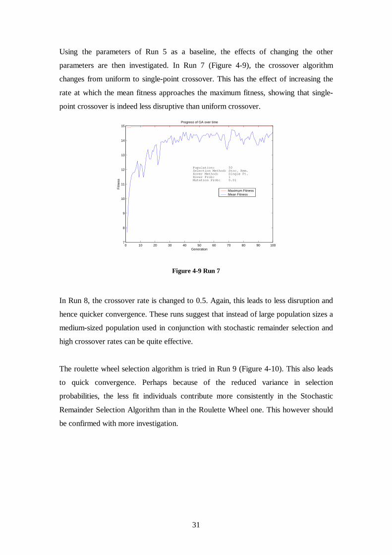
Using the parameters of Run 5 as a baseline, the effects of changing the other

parameters are then investigated. In Run 7 (Figure 4-9), the crossover algorithm

changes from uniform to single-point crossover. This has the effect of increasing the

rate at which the mean fitness approaches the maximum fitness, showing that single-

point crossover is indeed less disruptive than uniform crossover.

0 10 20 30 40 50 60 70 80 90 1007

8

9

10

11

12

13

14

15

Generation

Fitn

ess


Population: 50 Selection Method: Stoc. Rem.Xover Method: Single Pt.Xover Prob: 1 Mutation Prob: 0.01


Figure 4-9 Run 7

In Run 8, the crossover rate is changed to 0.5. Again, this leads to less disruption and

hence quicker convergence. These runs suggest that instead of large population sizes a

medium-sized population used in conjunction with stochastic remainder selection and

high crossover rates can be quite effective.

The roulette wheel selection algorithm is tried in Run 9 (Figure 4-10). This also leads

to quick convergence. Perhaps because of the reduced variance in selection

probabilities, the less fit individuals contribute more consistently in the Stochastic

Remainder Selection Algorithm than in the Roulette Wheel one. This however should

be confirmed with more investigation.

32

0 10 20 30 40 50 60 70 80 90 1007

8

9

10

11

12

13

14

15

Generation

Fitn

ess


Population: 50 Selection Method: RouletteXover Method: Uniform Xover Prob: 1 Mutation Prob: 0.01


Figure 4-10 Run 9

Having gained a good knowledge of how various parameters affect GA performance,

the GA can now be applied to the main task of optimising a FLC. Before this can be

done, a way of automating the design of the FLC in Matlab needs to be devised. This

problem is tackled in the next chapter.

33

5 Designing a Fuzzy Logic Controller Using

Matlab

In this chapter, a demonstration is given of how to automate the design of a Fuzzy

Logic Controller. The assumptions used and the constraints introduced to simplify this

process are explained. Reference is made to the Matlab code that is written to

implement this process and a summary of how this code works is provided.

5.1 Assumptions and Constraints

To apply the Fuzzy Logic Controller to the Inverted Pendulum System, certain

properties of the system are exploited so that the design of the controller can be made

easier. As the system is symmetrical, it is assumed that symmetrical membership

functions about the y-axis will provide a valid controller. A symmetrical rule-base is

also assumed.

• Other constraints are also introduced to the design of the FLC:

• All universes of discourses are normalised to lie between –1 and 1 with scaling

factors external to the FLC used to give appropriate values to the variables.

• It is assumed that the first and last membership functions have their apexes at –1

and 1 respectively. This can be justified by the fact that changing the external

scaling would have similar effect to changing these positions.

• Only triangular membership functions are to be used.

• The number of fuzzy sets is constrained to be an odd integer greater than unity. In

combination with the symmetry requirement, this means that the central

membership function for all variables will have its apex at zero.

• The base vertices of membership functions are coincident with the apex of the

adjacent membership functions. This ensures that the value of any input variable

is a member of at most two fuzzy sets, which is an intuitively sensible situation. It

also ensures that when a variable’s membership of any set is certain, i.e. unity, it

is a member of no other sets.

34

Using these constraints the design of the membership functions can be described

using two parameters:

• The number of membership functions

• The positioning of the triangle apexes

5.2 Spacing Parameter

The second parameter specifies how the centres are spaced out across the universe of

discourse. A value of one indicates even spacing, while a value larger than unity

indicates that the membership functions are closer together in the centre of the range

and more spaced out at the extremes as shown in Figure 5-1. The position of each

centre is calculated by taking the position the centre would be if the spacing were

even and by raising this to the power of the spacing parameter. For example, in the

case where there are five sets, with even spacing (p=1) the centre of one set would be

at 0.5. If p is set to two, the position of this centre moves to 0.25. If the spacing

parameter is set to 0.5 then this centre moves to 0.707 in the normalised universe of

discourse.

−1 −0.8 −0.6 −0.4 −0.2 0 0.2 0.4 0.6 0.8 10

0.5

1

−1 −0.8 −0.6 −0.4 −0.2 0 0.2 0.4 0.6 0.8 10

0.5

1

−1 −0.8 −0.6 −0.4 −0.2 0 0.2 0.4 0.6 0.8 10

0.5

1

NB NS Z PS PB

NB

NB

NS

NS

Z

Z

PS

PS

PB

PB

Spacing Parameter = 1

Spacing Parameter = 2

Spacing Parameter = 0.5

Figure 5-1 Effects of Spacing Parameters on Mfs

35

This method of designing the membership functions is inspired by the work of Park et

al. [8] and Cheong et al [9]. It does mean that there is a reduction in the number of

possible FLCs than if the design was fully flexible but the trade-off is that the design

process is made much simpler. Also it is felt that even within these constraints there is

sufficient flexibility to allow a FLC that meets the design requirements to be built.

5.3 Designing the Rule-Base

As well as specifying the membership functions, the rule-base also needs to be

designed. Again ideas presented by Park et al. [8] were used. In specifying a rule

base, characteristic spacing parameters for each variable and characteristic angles for

each input variable less one are used to construct the rules.

Certain characteristics of the rule-base are assumed in using the proposed construction

method:

• Extreme outputs more usually occur when the inputs have extreme values while

mid-range outputs generally are generated when the input values are mid-range.

• Similar combinations of input linguistic values lead to similar output values

Using these assumptions the output space is partitioned into different regions

corresponding to different output linguistic values. How the space is partitioned is

determined by the characteristic spacing parameters and the characteristic angle. The

angle determines the slope of a line1 through the origin on which seed points are

placed. The positioning of the seed points is determined by a similar spacing method

as was used to determine the centres of the membership functions.

Grid points are also placed in the output space representing each possible

combination of input linguistic values. These are spaced in the same way as before.

The rule-base is determined by calculating which seed-point is closest to each grid

point. The output linguistic value representing the seed-point is set as the consequent

of the antecedent represented by the grid point. This is illustrated in Figure 5-2,

which is a graph showing seed points (blue circles) and grid-points (red circles). 1 For two input (2-D) variables the angle of the line with the x-axis needs to be specified. For three inputs (3-D) two angles need to be specified to position the line, and so on. Therefore the number of characteristic angles needed is one less than the number of input variables. To account for the lost degree of freedom note that the line is fixed to pass through the origin.

36

Table 5-1 shows the derived rule base. The lines on the graph delineate the different

regions corresponding to different consequents. The parameters for this example are

0.9 for both input spacings, 1 for the output spacing and 45° for the angle.

NB

NS

Z

PS

PB

NB NS Z PS PB

NB

NS

Z

PS

PB

Figure 5-2 Seed Points and Gr id Pts For Rule-Base Construction

e

de NB NS Z PS PB

NB NB NB NS NS Z

NS NB NS NS Z PS

Z NS NS Z PS PS

PS NS Z PS PS PB

PB Z PS PS PB PB

Table 5-1 Der ived Rule Base

5.4 Matlab Implementation

To implement these design methodologies in Matlab, .m function files were written.

These functions make use of the Fuzzy Logic Toolbox for Matlab in creating the

fuzzy logic controller. Two function files create_mfs.m and create_rules.m

37

respectively create the membership functions and the rule-base. A third function

make_fis.m puts together the Fuzzy Inference System (FIS) by using these two

functions.

The code for make_fis.m is listed in Listing 5-1. Firstly, error checking is performed

to ensure that the parameters are valid. Once this is done, create_mfs.m is called to get

the parameters for the membership functions of each of the variables. Then a suitable

rule-base is created for each of the output variables by calling create_rules.m, which

returns a rules matrix in the format required by the Fuzzy Logic Toolbox. This

information is then put together in a suitable way to create the FIS. Only triangular

membership functions can be created using this function.

f unct i on t he_f i s = make_f i s( i np, out , n, pm, ps, t het a_s) %MAKE_FI S Cr eat e a FI S based on i nput t ed par amet er s % %t he_f i s = make_f i s( i np, out , n, pm, ps, t het a_s) %i np Number of i nput var i abl es %out Number of out put var i abl es %n Col umn vect or of l engt h i np+out cont ai ni ng t he number % of member shi p f unct i ons per var i abl e %pm Col umn vect or of l engt h i np+out i ndi cat i ng how t he % member shi p f unct i ons ar e spr ead f or each var i abl e %ps Mat r i x of s i ze i np+1 x out i ndi cat i ng how t he r ul e- % base i s % f or med %t het a_s Mat r i x of s i ze i np- 1 x out . Each col umn cont ai ns t he % seed angl es f or t he r ul e mat r i ces % %Cr eat ed By Joe For an Jul y 2002 i f ~i sposi nt ( i np) | ~i sposi nt ( out ) er r or ( ' i np and out shoul d be posi t i ve i nt eger scal ar s' ) end i f s i ze( n) ~= [ i np+out 1] er r or ( ' n shoul d be a col umn vect or whose l engt h i s equal t o t he number of i nput s and out put s' ) end i f s i ze( pm) ~= [ i np+out 1] er r or ( ' pm shoul d be a col umn vect or whose l engt h i s equal t o t he number of i nput s and out put s' ) end i f s i ze( ps) ~= [ i np+1 out ] er r or ( ' pm shoul d be a col umn vect or whose l engt h i s equal t o t he number of out put s' ) end i f s i ze( t het a_s) ~= [ i np- 1 out ] er r or ( ' t het a_s shoul d be a mat r i x of s i ze i np- 1 x out ' ) end

38

%Get t he member shi p f unct i on par amet er s mf par = zer os( i np+out , 3* max( n) ) ; f or i = 1: i np+out mf par ( i , 1: 3* n( i ) ) = cr eat e_mf s( n( i ) , pm( i ) ) ; end %Cr eat e t he r ul e mat r i x f or i = 1: out r ul e_mat = cr eat e_r ul es( i np, [ n( 1: i np) ; n( i np+i ) ] , ps( : , i ) , t het a_s( : , i ) ) ; i f i == 1 r ul es = r ul e_mat ; el se r ul es( : , i np+i +1: i np+i +2) = r ul es( : , i np+i : i np+i +1) ; r ul es( : , i np+i ) = r ul e_mat ( : , end- 2) ; end end %Cr eat e t he FI S t he_f i s = newf i s( ' f i sname' ) ; f or i = 1: i np var name = [ ' i np' i nt 2st r ( i ) ] ; r ange = [ mf par ( i , 2) mf par ( i , n( i ) * 3- 1) ] ; t he_f i s = addvar ( t he_f i s, ' i nput ' , var name, r ange) ; end f or i = i np+1: i np+out var name = [ ' out ' i nt 2st r ( i - i np) ] ; r ange = [ mf par ( i , 2) mf par ( i , n( i ) * 3- 1) ] ; t he_f i s = addvar ( t he_f i s, ' out put ' , var name, r ange) ; end %I ni t i al l y onl y t r i angul ar member shi p f unct i ons ar e t o be al l owed. f or i =1: i np f or j = 1: n( i ) mf name = i nt 2st r ( j ) ; t he_f i s = addmf ( t he_f i s, ' i nput ' , i , mf name, ' t r i mf ' , mf par ( i , ( ( j * 3) - 2) : ( j * 3) ) ) ; end end f or i = i np+1: i np+out f or j = 1: n( i ) mf name = i nt 2st r ( j ) ; t he_f i s = addmf ( t he_f i s, ' out put ' , i -i np, mf name, ' t r i mf ' , mf par ( i , ( ( j * 3) - 2) : ( j * 3) ) ) ; end end t he_f i s = addr ul e( t he_f i s, r ul es) ;

Listing 5-1 make_fis.m

The function that calculates the appropriate parameters for these membership

functions, create_mfs.m is listed in Listing 5-2. This function takes two parameters,

the number of membership functions and the spacing parameter for the centres of

these functions. Based on these parameters, the centres of each membership function

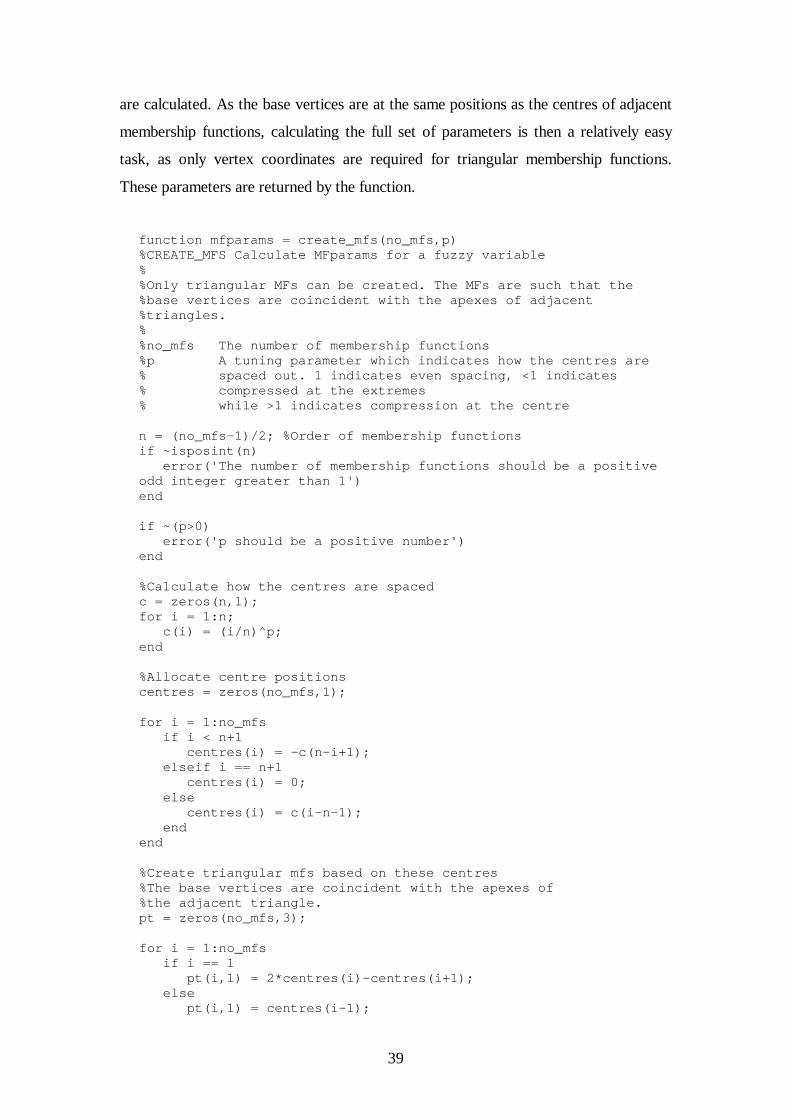
39

are calculated. As the base vertices are at the same positions as the centres of adjacent

membership functions, calculating the full set of parameters is then a relatively easy

task, as only vertex coordinates are required for triangular membership functions.

These parameters are returned by the function.

f unct i on mf par ams = cr eat e_mf s( no_mf s, p) %CREATE_MFS Cal cul at e MFpar ams f or a f uzzy var i abl e % %Onl y t r i angul ar MFs can be cr eat ed. The MFs ar e such t hat t he %base ver t i ces ar e coi nci dent wi t h t he apexes of adj acent %t r i angl es. % %no_mf s The number of member shi p f unct i ons %p A t uni ng par amet er whi ch i ndi cat es how t he cent r es ar e % spaced out . 1 i ndi cat es even spaci ng, <1 i ndi cat es % compr essed at t he ext r emes % whi l e >1 i ndi cat es compr essi on at t he cent r e n = ( no_mf s- 1) / 2; %Or der of member shi p f unct i ons i f ~i sposi nt ( n) er r or ( ' The number of member shi p f unct i ons shoul d be a posi t i ve odd i nt eger gr eat er t han 1' ) end i f ~( p>0) er r or ( ' p shoul d be a posi t i ve number ' ) end %Cal cul at e how t he cent r es ar e spaced c = zer os( n, 1) ; f or i = 1: n; c( i ) = ( i / n) ^ p; end %Al l ocat e cent r e posi t i ons cent r es = zer os( no_mf s, 1) ; f or i = 1: no_mf s i f i < n+1 cent r es( i ) = - c( n- i +1) ; el sei f i == n+1 cent r es( i ) = 0; el se cent r es( i ) = c( i - n- 1) ; end end %Cr eat e t r i angul ar mf s based on t hese cent r es %The base ver t i ces ar e coi nci dent wi t h t he apexes of %t he adj acent t r i angl e. pt = zer os( no_mf s, 3) ; f or i = 1: no_mf s i f i == 1 pt ( i , 1) = 2* cent r es( i ) - cent r es( i +1) ; el se pt ( i , 1) = cent r es( i - 1) ;

40

end i f i ==no_mf s pt ( i , 3) = 2* cent r es( i ) - cent r es( i - 1) ; el se pt ( i , 3) = cent r es( i +1) ; end pt ( i , 2) = cent r es( i ) ; end mf par ams = zer os( 1, no_mf s* 3) ; f or i = 1: no_mf s mf par ams( 3* i - 2: 3* i ) = pt ( i , : ) ; end

Listing 5-2 create_mfs.m

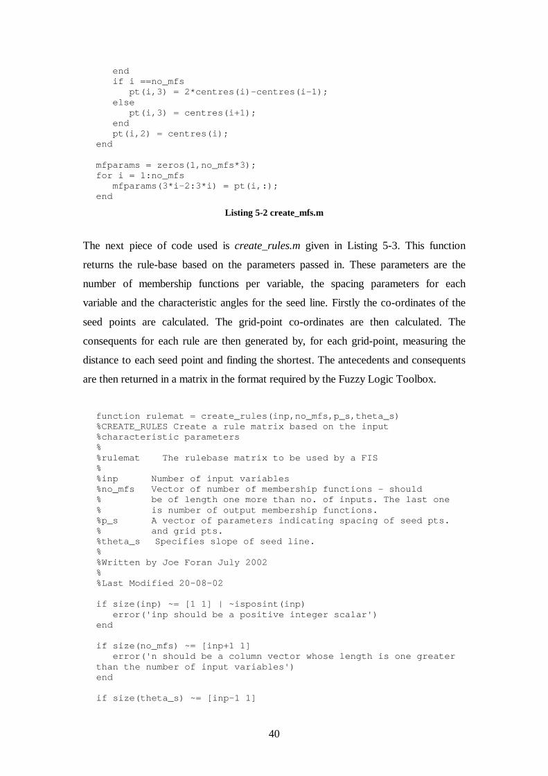
The next piece of code used is create_rules.m given in Listing 5-3. This function

returns the rule-base based on the parameters passed in. These parameters are the

number of membership functions per variable, the spacing parameters for each

variable and the characteristic angles for the seed line. Firstly the co-ordinates of the

seed points are calculated. The grid-point co-ordinates are then calculated. The

consequents for each rule are then generated by, for each grid-point, measuring the

distance to each seed point and finding the shortest. The antecedents and consequents

are then returned in a matrix in the format required by the Fuzzy Logic Toolbox.

f unct i on r ul emat = cr eat e_r ul es( i np, no_mf s, p_s, t het a_s) %CREATE_RULES Cr eat e a r ul e mat r i x based on t he i nput %char act er i st i c par amet er s % %r ul emat The r ul ebase mat r i x t o be used by a FI S % %i np Number of i nput var i abl es %no_mf s Vect or of number of member shi p f unct i ons - shoul d % be of l engt h one mor e t han no. of i nput s. The l ast one % i s number of out put member shi p f unct i ons. %p_s A vect or of par amet er s i ndi cat i ng spaci ng of seed pt s. % and gr i d pt s. %t het a_s Speci f i es sl ope of seed l i ne. % %Wr i t t en by Joe For an Jul y 2002 % %Last Modi f i ed 20- 08- 02 i f s i ze( i np) ~= [ 1 1] | ~i sposi nt ( i np) er r or ( ' i np shoul d be a posi t i ve i nt eger scal ar ' ) end i f s i ze( no_mf s) ~= [ i np+1 1] er r or ( ' n shoul d be a col umn vect or whose l engt h i s one gr eat er t han t he number of i nput var i abl es' ) end i f s i ze( t het a_s) ~= [ i np- 1 1]

41

er r or ( ' t het a_s shoul d be a col umn vect or whose l engt h i s one l ess t han t he number of i nput var i abl es' ) end i f s i ze( p_s) ~= [ i np+1 1] er r or ( ' p_s shoul d be a col umn vect or whose l engt h i s one gr eat er t han t he number of i nput var i abl es' ) end mf Or der = ( no_mf s- 1) / 2; f or i = 1: l engt h( mf Or der ) i f ~i sposi nt ( mf Or der ( i ) ) er r or ( ' The number of out put member shi p f ns. shoul d be an odd i nt eger of at l east val ue 3' ) end end out Or der = mf Or der ( end) ; % Fi nd posi t i ons of seed pt s. al ong seed hyper pl ane c = zer os( out Or der , 1) ; f or i = 1: out Or der ; c( i ) = ( i / out Or der ) ^ p_s( end) ; end n_out = no_mf s( end) ; %Get t he co- or di nat es of t he seed poi nt s %Ther e ar e n_out seed poi nt s and t hey need t o be speci f i ed %i n n- di mensi onal space, n bei ng equal t o i np co_or ds = zer os( i np, n_out ) ; %Speci f y x- posi t i on of co_or ds f or j = 1: n_out i f j < out Or der +1 co_or ds( 1, j ) = - c( out Or der - j +1) ; el se i f j == out Or der +1 co_or ds( 1, j ) = 0; el se co_or ds( 1, j ) = c( j - out Or der - 1) ; end end end %To get co- or di nat es i n ot her di mensi ons mul t i pl y by t an %of appr opr i at e angl e f or k = 2: i np co_or ds( k, : ) = co_or ds( 1, : ) * t an( t het a_s( k- 1) ) ; end %Nor mal i se t he co_or di ant es t o be bet ween - 1 and 1 nor m_f act = max( max( abs( co_or ds) ) ) ; co_or ds = co_or ds. / nor m_f act ; %Get t he gr i d poi nt co- or di nat es no_r ul es = pr od( no_mf s( 1: i np) ) ; c = zer os( i np, ( max( no_mf s( 1: i np) ) - 1) / 2) ; cent r es = zer os( i np, max( no_mf s( 1: i np) ) ) ; ant ecedent s = zer os( no_r ul es, i np) ;

42

%Space out gr i d- poi nt s i n each di mensi on f or i = 1: i np f or j = 1: no_mf s( i ) ; c( i , j ) = ( j / ( ( no_mf s( i ) - 1) / 2) ) ^ p_s( i ) ; end end f or i = 1: i np f or j = 1: no_mf s( i ) i f j < mf Or der ( i ) +1 cent r es( i , j ) = - c( i , mf Or der ( i ) - j +1) ; el sei f j == mf Or der ( i ) +1 cent r es( i , j ) = 0; el se cent r es( i , j ) = c( i , j - mf Or der ( i ) - 1) ; end end end %Cr eat e each possi bl e combi nat i on of ant ecedent s f or i = 1: no_r ul es f or j = 1: i np i f j == i np ant ecedent s( i , j ) = mod( i , no_mf s( i np) ) ; el se ant ecedent s( i , j ) = mod( cei l ( i / pr od( no_mf s( j +1: i np) ) ) , no_mf s( j ) ) ; end i f ant ecedent s( i , j ) ==0 ant ecedent s( i , j ) = no_mf s( j ) ; end end end %Di st ance f r om each seed- poi nt of al l gr i d- pt s r egi on = zer os( no_r ul es, n_out ) ; poi nt = ones( no_r ul es, i np) ; %Co- or di nat es of each gr i d- poi nt %Cal cul at e di st ance f r om each gr i d- poi nt t o each seed- poi nt f or i = 1: no_r ul es f or j = 1: i np poi nt ( i , j ) =cent r es( j , ant ecedent s( i , j ) ) ; end f or j = 1: n_out r egi on( i , j ) = sum( ( poi nt ( i , : ) - co_or ds( : , j ) ' ) . ^ 2) ; end end consequent = zer os( no_r ul es, 1) ; %To ensur e f ul l r ot at i on of r ul es adj ust t he r egi on f i ndi ng al gor i t hm accor di ng t o t he r egi me t emp = mean( t het a_s) ; %Fi nd t he aver age angl e t emp = mod( t emp, 2* pi ) ; %Map back t o bet ween 0- >360 degr ees %I f r egi me i s i n l ef t - hand hal f - pl ane i f 180* t emp/ pi >90 & t emp* 180/ pi <=270

43

t 2 = - 1; el se t 2 =1; end f l i p =1; %Fi nd t he r egi on i n whi ch each gr i d_pt l i es. f or i = 1: no_r ul es i ndex = f i nd( r egi on( i , : ) ==mi n( r egi on( i , : ) ) ) ; i f s i ze( i ndex) == [ 1 1] consequent ( i ) = i ndex; el se %i f gr i d- poi nt i s equi di st ant f r om t wo seed- poi nt s i f f l i p ==1 consequent ( i ) = i ndex( 1) ; el se consequent ( i ) = i ndex( 2) ; end f l i p = - f l i p; end i f t 2 == - 1 %Swap over consequent s i f we ar e i n l ef t - hand hal f -pl ane consequent ( i ) = n_out +1- consequent ( i ) ; end end r ul emat = [ ant ecedent s consequent ones( no_r ul es, 2) ] ;

Listing 5-3 create_rules.m

With all of this code a full FIS can be specified using only a few parameters. This is

ideal for using a Genetic Algorithm to find an optimal FLC as the GA can work on

these parameters and improve the FLC characteristics. How this is achieved is

demonstrated in the next chapter.

44

6 Using Genetic Algor ithms to Design

Fuzzy Logic Controllers In this chapter an attempt is made to apply GAs to achieve satisfactory design of a

FLC. It is shown how designs can be evaluated to determine their efficacy. Results are

presented from various different experimental runs to show the effectiveness of the

approach taken and a resultant FLC is then evaluated more thoroughly.

6.1 Evaluation Functions

To apply a Genetic Algorithm to the design of Fuzzy Logic Controllers, a means of

evaluating different designs is required. This evaluation needs to be performed

relatively quickly as a GA needs to be able to process large numbers of different

combinations of parameters.

Evaluation Functions are functions called by a GA to calculate the fitness of a set of

parameters. The parameters are passed to the evaluation function, which processes

them and returns a value corresponding to how well the parameters performed the

task at hand.

For this project the evaluation function run_fuzzy_pole_only.m was written. This is

listed in Listing 6-1. This function firstly extracts the relevant parameters from the

chromosome passed in. After performing some error checking, the parameters are

used to create a Fuzzy Inference System (FIS) and set the appropriate scaling factors.

A SIMULINK model is then called, from which a record of the error in the pole angle

throughout the duration of the simulation is returned. The square of the error is

multiplied by a time weight and the sum of this time weighted square error is inverted

to give a fitness value. If the pole angle should at any stage of the simulation saturate,

i.e. reach ±90°, then the simulation is stopped immediately so that time is not wasted

modelling controllers that fail to balance the pole. In this case the fitness is calculated

45

as the time taken before the pole collapsed multiplied by 1x109. This gives a reward to

designs that manage to keep the pole from collapsing that little bit longer.

f unct i on [ chr om, ef f ] = r un_f uzzysi m( chr om, opt i ons) %RUN_FUZZYSI M Thi s i s t he eval uat i on f unct i on f or t he f uzzy si mul at i on used by t he GA %Thi s r uns a 2 i nput one out put f unct i on % %chr om The r eal - val ued chr omosome passed i n% %ef f The cal cul at ed f i t ness val ue %Wr i t t en by: Joe For an Jul y 2002 % %Last Modi f i ed: Joe For an 07/ 08/ 2002 n = chr om( 1: 3) ' ; pm = ( chr om( 4: 6) . ^ chr om( 10: 12) ) ' ; pr = ( chr om( 7: 9) . ^ chr om( 13: 15) ) ' ; scal e = chr om( 16: 18) ' ; t het a = chr om( 19) ; i np = 2; out = 1; i f s i ze( n) ~= [ i np+out 1] er r or ( ' n shoul d be a col umn vect or whose l engt h i s equal t o t he number of i nput s and out put s' ) end i f s i ze( pm) ~= [ i np+out 1] er r or ( ' pm shoul d be a col umn vect or whose l engt h i s equal t o t he number of i nput s and out put s' ) end i f s i ze( pr ) ~= [ i np+1 out ] er r or ( ' pm shoul d be a col umn vect or whose l engt h i s equal t o t he number of out put s' ) end i f s i ze( t het a) ~= [ i np- 1 out ] er r or ( ' t het a_s shoul d be a mat r i x of s i ze i np- 1 x out ' ) end i f s i ze( scal e) ~= [ i np+out 1] er r or ( ' scal e shoul d be a col umn vect or whose l engt h equal s t he number of i nput s and out put s' ) end gl obal FUZZY_SCALI NG I NVPEND_FUZZY FUZZY_SCALI NG = scal e; I NVPEND_FUZZY = make_f i s( i np, out , n, pm, pr , t het a) ; t = 0: 0. 01: 6; st abl e = 1; eval ( ' s i m( ' ' s_i nvpen_f uzzy_di st ' ' , t ) ; ' , ' st abl e = 0; ' ) ; i f st abl e == 0 | s_Ti me( end) ~= t ( end)

46

ef f = 1e- 9* s_Ti me( end) * st abl e; el se ef f = 1/ ( ( s_Er r or . ^ 2) ' * s_Ti me) ; end

Listing 6-1 Evaluation Function run_fuzy_pole_only.m

A diagram of the SIMULINK model that is used is shown in Figure 6-1. The desired

angle of the pole is 0°, i.e. upright. The error in the angle and the change of error are

scaled by the appropriate gains (these parameters are also set by the GA) and the

result is clipped so that it lies in the range –1 to 1. These inputs are fed into the FLC

and the FLC’s output is then scaled by another gain. This force is applied to the

system, which in turn, outputs the pendulum angle, angular speed, cart position and

cart velocity.

−K−

de Gain

s_Error

To Workspace3

s_Time

To Workspace2STOP

Stop Simulation

Speed

Saturation1

Saturation

Position

Mux Control Action

Theta

Omega

x

v


Fuzzy Logic Controller

u*180/pi

Fcn1

f(u)

Fcn

−K−

Error Gain

Dist

Disturbance

Dist. Scope

du/dt

Derivative

0

Constant

Clock

Angular Speed

Angle

−K−

Action Gain

Action Figure 6-1 Simulink Model used to evaluate FLCs

A periodic disturbance is also applied to the system. This is a force of relatively large

magnitude, which ensures that the arena in which the FLC is examined is a testing

one. This disturbance is of the magnitude of 8kN and has a duration of 10ms (which is

also the step time of the simulation) and is applied every two seconds, in alternately

positive and negative directions. This disturbance perturbs the pendulum enough to

make controlling the system a sufficiently challenging task. Each FLC is tested over

three cycles, i.e. for six seconds. It is felt that this is enough time for an adequately

large range of the system’s properties to be examined.

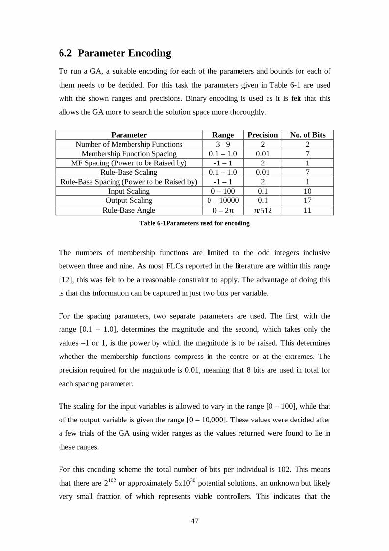
47

6.2 Parameter Encoding

To run a GA, a suitable encoding for each of the parameters and bounds for each of

them needs to be decided. For this task the parameters given in Table 6-1 are used

with the shown ranges and precisions. Binary encoding is used as it is felt that this

allows the GA more to search the solution space more thoroughly.

Parameter Range Precision No. of Bits

Number of Membership Functions 3 –9 2 2 Membership Function Spacing 0.1 – 1.0 0.01 7

MF Spacing (Power to be Raised by) -1 – 1 2 1 Rule-Base Scaling 0.1 – 1.0 0.01 7

Rule-Base Spacing (Power to be Raised by) -1 – 1 2 1 Input Scaling 0 – 100 0.1 10

Output Scaling 0 – 10000 0.1 17 Rule-Base Angle 0 – 2π π/512 11

Table 6-1Parameters used for encoding

The numbers of membership functions are limited to the odd integers inclusive

between three and nine. As most FLCs reported in the literature are within this range

[12], this was felt to be a reasonable constraint to apply. The advantage of doing this

is that this information can be captured in just two bits per variable.

For the spacing parameters, two separate parameters are used. The first, with the

range [0.1 – 1.0], determines the magnitude and the second, which takes only the

values –1 or 1, is the power by which the magnitude is to be raised. This determines

whether the membership functions compress in the centre or at the extremes. The

precision required for the magnitude is 0.01, meaning that 8 bits are used in total for

each spacing parameter.

The scaling for the input variables is allowed to vary in the range [0 – 100], while that

of the output variable is given the range [0 – 10,000]. These values were decided after

a few trials of the GA using wider ranges as the values returned were found to lie in

these ranges.

For this encoding scheme the total number of bits per individual is 102. This means

that there are 2102 or approximately 5x1030 potential solutions, an unknown but likely

very small fraction of which represents viable controllers. This indicates that the

48

solution space is large despite the constraints that are introduced. If GAs succeed in

finding close to optimal solutions in such a large space despite having no prior

knowledge this would indicate their power.

6.3 Running the GA

Run Pop. Size

Selection Routine

Crossover Routine

Crossover Probability

Mutation Probability

Best Fitness

1 150 Stoc. Rem Uniform 1.0 0.01 1.1597 2 50 Stoc. Rem Uniform 1.0 0.01 0.9105 3 100 Stoc. Rem Uniform 1.0 0.01 0.9449 4 100 Stoc. Rem Single Pt. 1.0 0.01 1.1171 5 100 Stoc. Rem Uniform 0.5 0.01 1.1851 6 50 Stoc. Rem Uniform 1.0 0.05 0.8880 7 50 Roulette Uniform 1.0 0.01 1.0925 8 50 Roulette Uniform 1.0 0.001 0.0141 9 50 Stoc. Rem Single Pt. 0.5 0.05 1.2525 10 50 Stoc. Rem Uniform 1.0 0.01 0.8937

Table 6-2 Parameters for GA Runs with FLC

The file in which the GA parameters are set and which calls the main GA routine is

ga_poleonly.m. The source code for this file is given in Appendix A.9

ga_poleonly.mThis file calls the Matlab functions run_ga.m and initGa.m, which are

modified versions of the routines provided with the GAOT toolbox. The code for

these files is listed in Appendices A.10 and A.11 respectively. The reason modified

code is used is

• to eliminate some small bugs discovered in the process of converting from binary

to real values and vice-versa (see also Appendix A.20) and

• to change the way the progress of the GA was output to the screen.

An elitist model was used for all runs of the GA also.

Ten runs of the GA were performed for a hundred generations each. The details of

these runs are listed in Table 6-2. Again the parameters that were varied were

selection routine, crossover routine, crossover probability and mutation probability.

The best controller was found during Run 9. This run was continued for a further two

hundred generations, but the best fitness did not increase much. A plot of the progress

of this GA run is shown in Figure 6-2.

49

0 50 100 150 200 250 3000

0.2

0.4

0.6

0.8

1

1.2

1.4GA Progress

Generation

Fitn

ess


Figure 6-2 Progress of GA that found best fitness

Details of the FLC found by the GA are presented in Figure 6-3, Table 6-3 and Figure

6-4. The Error variable was assigned seven membership functions, whereas both the

error derivative and control actions were assigned nine membership functions. For

both of the inputs, the membership functions are compressed towards the centre,

while they were compressed at the extremes for the output. The control surface shown

in Figure 6-4 shows that the mapping between the input and output spaces is highly

linear. An advantage of FLCs over linear controllers is that they allow the creation of

these kinds of mappings; the control surface of a two-input linear controller, no matter

how well designed, will always be a plane in three-dimensional space [2].

50

−1 −0.8 −0.6 −0.4 −0.2 0 0.2 0.4 0.6 0.8 10

0.5

1

Error Mfs

−1 −0.8 −0.6 −0.4 −0.2 0 0.2 0.4 0.6 0.8 10

0.5

1

dError Mfs

−1 −0.8 −0.6 −0.4 −0.2 0 0.2 0.4 0.6 0.8 10

0.5

1

Action Mfs

NB NM NS Z PS PM PB

NB NM NS NZ Z PZ PS PM PB

NB NM NS NZ Z PZ

PS PM PB

Figure 6-3 Membership functions of Optimised FLC

Rate of Change of Er ror

NB NM NS NZ Z PZ PS PM PB

NB NB NB NB NB NM NM NS NZ NZ NM NB NM NS NS NZ NZ NZ NZ NZ NS NS NZ NZ NZ NZ NZ NZ NZ Z Z Z Z Z Z Z Z Z Z Z

PS Z PZ PZ PZ PZ PZ PZ PZ PS PM PZ PZ PZ PZ PZ PS PS PM PB

Err

or

PB PZ PZ PS PM PM PB PB PB PB

Table 6-3 Rule-Base of Optimised FLC

−10−5

05

10

−1

−0.5

0

0.5

1−1

−0.5

0

0.5

1

x 104

Error (degrees)

Control Surface of GA−Optimised FLC

dError (degrees/sec)

Act

ion

(N)

Figure 6-4 Sur face Plot of Optimised FLC (Scaled)

51

In Figure 6-5 the impulse responses of this FLC and that of the linear controller

examined in Chapter 2 are compared. It can be seen that while the pole collapses

when controlled by the linear controller, it hardly moves when the FLC is used.

0 0.1 0.2 0.3 0.4 0.5 0.6 0.7 0.8 0.9 1−60

−40

−20

0

20

40

60

80

100

Comparison of FLC and SSC Impulse (150N, 0.1s) Response

Time (s)

Ang

le (

degr

ees)

State Space ControllerFuzzy Logic Controller

Figure 6-5 FLC and SSC Impulse Response Compar ison

The response of the controller to a larger impulse is shown in Figure 6-6. This time

the pole does move, but it is quickly brought under control and settles to the

equilibrium position in about 0.1s.

0 0.1 0.2 0.3 0.4 0.5 0.6 0.7 0.8 0.9 1−40

−20

0

20

40

60

80

100

Comparison of SSC and FLCImpulse (7500N, 0.01s) Responses

Time (s)

Ang

le (

degr

ees)


Figure 6-6 Response To Large Impulse

This FLC is also successful at bringing the pole to its equilibrium position from a

large range of initial angles as shown in Figure 6-7. Interestingly, the settling time is

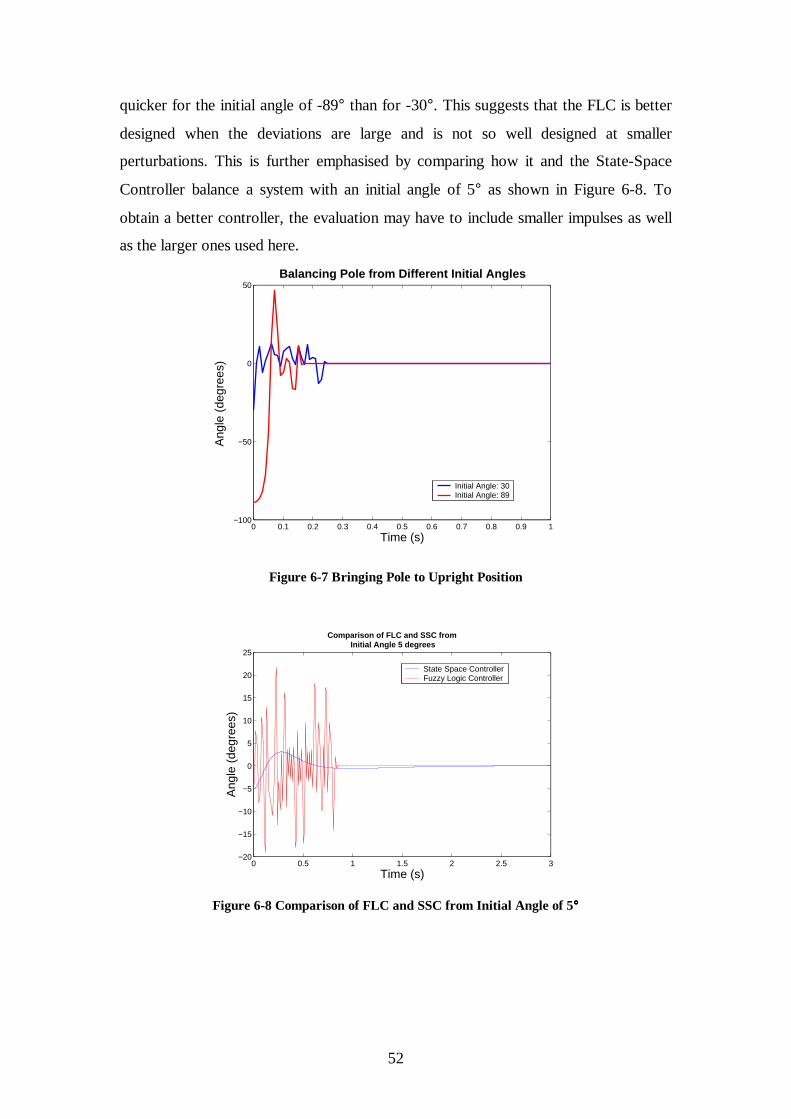
52

quicker for the initial angle of -89° than for -30°. This suggests that the FLC is better

designed when the deviations are large and is not so well designed at smaller

perturbations. This is further emphasised by comparing how it and the State-Space

Controller balance a system with an initial angle of 5° as shown in Figure 6-8. To

obtain a better controller, the evaluation may have to include smaller impulses as well

as the larger ones used here.

0 0.1 0.2 0.3 0.4 0.5 0.6 0.7 0.8 0.9 1−100

−50

0

50Balancing Pole from Different Initial Angles

Time (s)

Ang

le (

degr

ees)

Initial Angle: 30Initial Angle: 89

Figure 6-7 Br inging Pole to Upr ight Position

0 0.5 1 1.5 2 2.5 3−20

−15

−10

−5

0

5

10

15

20

25

Time (s)

Ang

le (

degr

ees)

Comparison of FLC and SSC from Initial Angle 5 degrees


Figure 6-8 Compar ison of FLC and SSC from Initial Angle of 5°°°°

53

6.4 Controlling Both Pole Angle and Car t Position

These algorithms were run with the cart being allowed to move an infinite distance in

either direction, i.e., no effort was made to control the cart’s position. As this would

be impractical if a real controller were to be built, an attempt was made to use the

Genetic Algorithm to find a Fuzzy Controller that could control both the angle and

cart position.

To this end, the Fuzzy Logic Controller used would have to have four input variables,

the error and change in error for both angle and position. It was found that the time

taken to evaluate the fitness for one individual was approximately one minute for five

seconds of simulation time (This was on a machine whose processor speed was 1.3

GHz). Thus, it took one hour to evaluate a single generation. This length of time was

considered impractical and so this approach was abandoned. The reason the time had

increased so much was as there was now four input variables, each being generally a

member of two fuzzy sets, there was 24 rules fired per time-step. The extra time

required to infer the control action slowed the simulation significantly.

A new method was then tried. This time two two-input fuzzy controllers were used,

one for the angle and one for the position. Their output actions were then added to

give the actual force applied to the system. It was found that using the 8kN

disturbance as used in the previous runs to test the controllers was too onerous a task

and no controllers of significant fitness were found. The requirement was reduced to

coping with a disturbance impulse of 1 kN and a controller that met this requirement

was discovered by the GA. The response of this controller to this 1kN impulse is

plotted in Figure 6-9. The controller in this case does keep the system close to the

desired state, though there are still oscillations about this position.

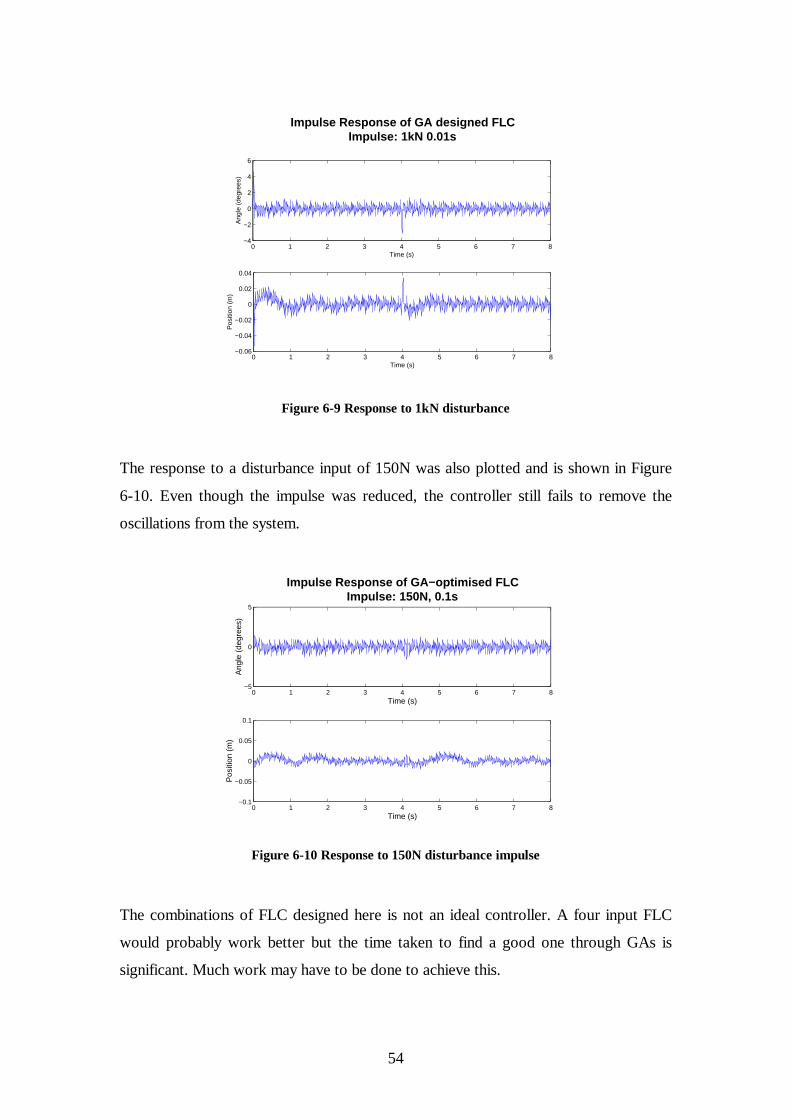
54

0 1 2 3 4 5 6 7 8−4

−2

0

2

4

6

Impulse Response of GA designed FLCImpulse: 1kN 0.01s

Time (s)

Ang

le (

degr

ees)

0 1 2 3 4 5 6 7 8−0.06

−0.04

−0.02

0

0.02

0.04

Time (s)

Pos

ition

(m

)

Figure 6-9 Response to 1kN disturbance

The response to a disturbance input of 150N was also plotted and is shown in Figure

6-10. Even though the impulse was reduced, the controller still fails to remove the

oscillations from the system.

0 1 2 3 4 5 6 7 8−5

0

5

Time (s)

Ang

le (

degr

ees)

Impulse Response of GA−optimised FLCImpulse: 150N, 0.1s

0 1 2 3 4 5 6 7 8−0.1

−0.05

0

0.05

0.1

Time (s)

Pos

ition

(m

)

Figure 6-10 Response to 150N disturbance impulse

The combinations of FLC designed here is not an ideal controller. A four input FLC

would probably work better but the time taken to find a good one through GAs is

significant. Much work may have to be done to achieve this.

55

7 Online Genetic Algor ithms Online GAs applied to controllers are Genetic Algorithms that attempt to adjust the

parameters of a controller during operation. When successfully implemented, they enable

continuous improvement in performance. However, as they are operating on a real system,

care must be taken to ensure that no action is imparted to the system that could cause

damage. For this reason, online GAs are more difficult to design and are less flexible than

offline GAs which only work on models of a system and can therefore handle inappropriate

actions [17].

7.1 SIMULINK S-Functions

To design an online GA, the first step taken was to try to apply it in SIMULINK. No pre-

existing software tools were available so the code for this needed to be written. This code

was written in the form of S-functions, which are functions that allow the creation of user-

defined blocks in SIMULINK [18].

Each block in SIMULINK has the following general characteristic. A vector of inputs is

applied to the system and these inputs interact with the system states, also in vector form, to

generate a vector of outputs.

Figure 7-1 Simulink Block Character istics

To create S-Functions, the user must write code that instructs SIMULINK on how to update

the states and how to generate outputs. Therefore, the code written must have a special form.

Each S-Function generally consists of sub-functions that initialise states, generate outputs

and update state information. The only memory that the S-Function has is contained in the

state vector so it is important that any information that needs to be carried over from time-

step to time-step is contained here. The size of the state vector is static which also introduces

another constraint on how the code can be designed.

56

7.2 Implementing a GA in SIMULINK

With all this in mind, an s-function was written to create a GA block for SIMULINK. This

code is listed in Appendix A.12 The parameters passed into this block by the user are

population size, a matrix of bounds for each variable, a vector of bits specifying how many

bits are to represent each variable and the time allocated to each individual. The input to the

block is the fitness of the set of parameters outputted in the previous time-step, while the

block output is the set of chromosome parameters to be evaluated as well as details of the

generation number and optimum fitness found so far.

In the code to initialise the model, listed below, each bit of every individual is a system state.

States are allocated for a tracker of the optimum individual found up to the present time as

well. Another three states are also used, a generation counter, an individual counter and a

store for the number of bits per individual. This is stored as a state so that it doesn’t need to

be recalculated every simulation step.

f unct i on [ sys, x0, st r , t s] = mdl I ni t i al i zeSi zes( popSi ze, bounds, bi t s, per i od) numVar = si ze( bounds, 1) ; i ni t Pop = i ni t ga( popSi ze, bi t s) ; numGenes = si ze( i ni t Pop, 2) ; gen = 1; %Gener at i on count er s i zes = si msi zes; s i zes. NumCont St at es = 0; s i zes. NumDi scSt at es = ( popSi ze+1) * numGenes+3; si zes. NumOut put s = numVar +3; si zes. NumI nput s = 1; s i zes. Di r Feedt hr ough = 0; s i zes. NumSampl eTi mes = 1; sys = si msi zes( si zes) ; i ni t Pop = r eshape( i ni t Pop' , popSi ze* numGenes, 1) ; %Make i ni t Pop a vect or x0 = zer os( si zes. NumDi scSt at es, 1) ; x0( 1: popSi ze* numGenes) = i ni t Pop; %Pl ace i ni t Pop i nt o st at e vect or x0( end- 2) = numGenes; %St or e t hi s val ue so i t doesn' t have t o be const ant l y r ecal cul at ed x0( end- 1) = gen; %Pl ace gener at i on count er i nt o st at e vect or ; x0( end) = 1; %Tr acks whi ch chr omosome i s bei ng eval uat ed st r = [ ] ; t s = [ per i od 0] ;

Listing 7-1 Initialising State Information

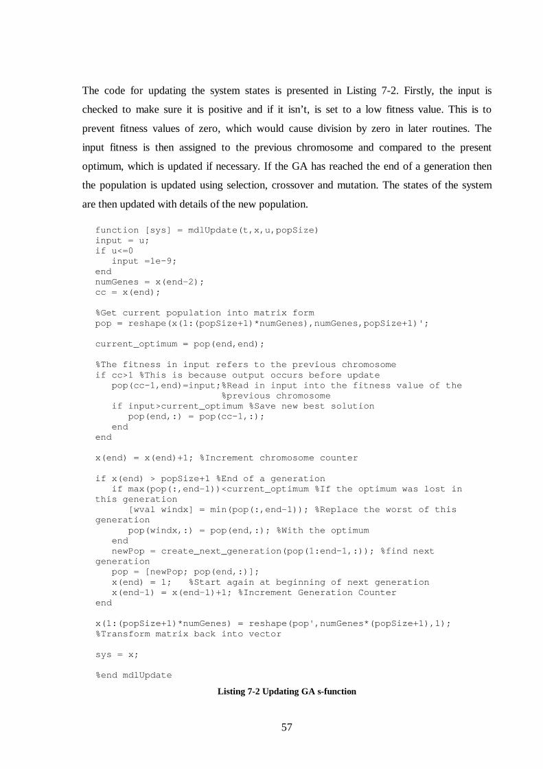
57

The code for updating the system states is presented in Listing 7-2. Firstly, the input is

checked to make sure it is positive and if it isn’ t, is set to a low fitness value. This is to

prevent fitness values of zero, which would cause division by zero in later routines. The

input fitness is then assigned to the previous chromosome and compared to the present

optimum, which is updated if necessary. If the GA has reached the end of a generation then

the population is updated using selection, crossover and mutation. The states of the system

are then updated with details of the new population.

f unct i on [ sys] = mdl Updat e( t , x, u, popSi ze) i nput = u; i f u<=0 i nput =1e- 9; end numGenes = x( end- 2) ; cc = x( end) ; %Get cur r ent popul at i on i nt o mat r i x f or m pop = r eshape( x( 1: ( popSi ze+1) * numGenes) , numGenes, popSi ze+1) ' ; cur r ent _opt i mum = pop( end, end) ; %The f i t ness i n i nput r ef er s t o t he pr evi ous chr omosome i f cc>1 %Thi s i s because out put occur s bef or e updat e pop( cc- 1, end) =i nput ; %Read i n i nput i nt o t he f i t ness val ue of t he %pr evi ous chr omosome i f i nput >cur r ent _opt i mum %Save new best sol ut i on pop( end, : ) = pop( cc- 1, : ) ; end end x( end) = x( end) +1; %I ncr ement chr omosome count er i f x( end) > popSi ze+1 %End of a gener at i on i f max( pop( : , end- 1) ) <cur r ent _opt i mum %I f t he opt i mum was l ost i n t hi s gener at i on [ wval wi ndx] = mi n( pop( : , end- 1) ) ; %Repl ace t he wor st of t hi s gener at i on pop( wi ndx, : ) = pop( end, : ) ; %Wi t h t he opt i mum end newPop = cr eat e_next _gener at i on( pop( 1: end- 1, : ) ) ; %f i nd next gener at i on pop = [ newPop; pop( end, : ) ] ; x( end) = 1; %St ar t agai n at begi nni ng of next gener at i on x( end- 1) = x( end- 1) +1; %I ncr ement Gener at i on Count er end x( 1: ( popSi ze+1) * numGenes) = r eshape( pop' , numGenes* ( popSi ze+1) , 1) ; %Tr ansf or m mat r i x back i nt o vect or sys = x; %end mdl Updat e

Listing 7-2 Updating GA s-function

58

The functions that perform the GA operations are listed below. The selection routine used

was Stochastic Remainder Selection and uniform crossover was performed with 100%

probability. A mutation rate of 10% was also specified. The code specifies these routines and

probabilities at present, but it could be easily modified to have them specified by the user

using input parameters to the block.

f unct i on newPop = cr eat e_next _gener at i on( ol dPop) [ popSi ze, nVar s] = si ze( ol dPop) ; %Sel ect usi ng st ochast i c Remai nder Sel ect i on newPop = st ocRemSel ec( ol dPop) ; %Cr ossover usi ng mask cr ossover l i st = r and( popSi ze, 1) ; %Gener at e a l i st t o deci de how cr ossover s ar e %pai r ed f or i = 1: f l oor ( popSi ze/ 2) [ t mp, i nd] = max( l i st ( : , 1) ) ; a = newPop( i nd, : ) ; l i st ( i nd) = 0; [ t mp, i nd] = max( l i st ( : , 1) ) ; b = newPop( i nd, : ) ; l i st ( i nd) = 0; [ c d] = maskXover ( a, b) ; newPop( i * 2- 1, : ) = c; newPop( i * 2, : ) = d; end %Mut at e f or i = 1: popSi ze newPop( i , : ) = bi nMut at i on( newPop( i , : ) , 0. 01) ; end %end of cr eat e_next _gener at i on

Listing 7-3 S_Function GA Operation

The last major part of the S-Function is the output routine (Listing 7-4). In this part of the

code, the binary representation of the chromosome to be evaluated is converted into a real-

valued representation. The present optimum fitness, the current generation number and the

current individual number are also outputted for the user’s information.

f unct i on sys = mdl Out put s( t , x, u, popSi ze, bounds, bi t s) numGenes = x( end- 2) ; gener at i on = x( end- 1) ; cc = x( end) ; opt i mum = x( ( popSi ze+1) * numGenes) ; pop = r eshape( x( 1: ( popSi ze+1) * numGenes) , numGenes, popSi ze+1) ' ; chr om = b2f ( pop( cc, 1: end- 1) , bounds, bi t s) ;

59

%Out put cur r ent chr omosome, best chr omosome so f ar , best f i t ness so f ar and cur r ent gener at i on number sys = [ chr om cc opt i mum gener at i on] ;

Listing 7-4 S-Function Output Routine

The reader may have noted that the s-function as presented outputs the chromosome

corresponding to the optimum at the end of each generation. The reason this is done is to

synchronise the assignment of the fitness of the last chromosome so that it occurs before the

GA operations are performed.

The GA S-function thus created is then applied to the optimisation of a FLC as shown in

Figure 7-2. The parameters outputted from the GA are input into another S-Function (listed

in Appendix A.13), which creates the FLC described by the parameters and uses this

controller to calculate a control action based on information fed back from the plant. The

square of the error is calculated and it is multiplied by a time-weight. This is fed into an

integration block which sums up the total time-weighted error. After a unit delay this is then

fed into another sub-system that calculates the inverse. This sub-system is a triggered one

and it outputs the calculated inverse sum of time-weighted error back to the GA as the

fitness. The reason for the delay is to ensure that the fitness fed into the GA is the correct

value. If this were not done the fitness input to the GA would be zero corresponding to the

beginning of a new cycle. A disturbance impulse is used to reset the integrators and to trigger

the sub-system so that everything is synchronized with the GA.

When running this model initially it was found that unless the angle and angular velocity

were reset to zero at the beginning of each cycle, then the GA wouldn’t be able to find a

good controller as it found it too hard to lift the pole from its horizontal state. However, if the

angle and angular velocity are being reset, then the behaviour of this system is more like an

offline GA as the ability to reset the system would not be present in a real-life application.

Therefore a different approach to creating an online GA is taken, and this is outlined in the

next section. The work done here is not in vain however, as a block for performing offline

GAs in SIMULINK has been created which wasn’t available beforehand.

60

x

v4

v3

v1

v theta

omega

z 1

Unit D

elay

eval_chrom

To Workspace

In1O

ut1

SubS

ystem

0

Result

Pulse

Generator

0

Optim

um D

isplay

Optim

um

Mux

Mux

u 2

Math

Function

Control A

ction

Reset

Theta

Om

egaxv

InvertedP

endulumD

ynamics

s 1

Integrator1

s 1

Integrator0

Generation

evalfis_sfn3

GA

S

−Function1ga_sfn2

GA

S

−Function

u*180/pi

Fcn

Double−C

lick to Initialize

Dot P

roduct

du/dt

Derivative

Dem

ux

0

Current Individual

1

Constant

Figure 7-2 Simulink Model for GA

61

7.3 Genetic-Based Machine Learning

In an effort to achieve a working online genetic algorithm, the use of Genetic-Based

Machine Learning (GBML) was studied. More specifically, classifier systems, common

GBML architectures, were investigated to see if they could help in the search for a

continually self-improving controller.

A major feature of classifier systems1 is that each individual classifier consists of a message

and an action. Each message is compared to a message from the environment (in the case of

controllers this could represent the state of the system) and those that match compete in an

auction to have their associated action become the output. The amount each classifier bids is

proportional to its strength, which increases when it is successful and decreases when it

competes in auctions and loses. A winner is chosen and their action is performed. If the

action has a beneficial effect then a reward is paid to the winner, who becomes stronger and

hence has a better chance of winning subsequent auctions. In this way, those classifiers

whose actions are the most suitable responses to the states that their messages represent

should become stronger and dominate the population.

To apply this idea to a fuzzy logic controller, the classifier population was initialised to be

every possible combination of antecedents and consequents for a fuzzy system. Each

classifier was given the same initial strength. As code to implement this was not immediately

available, the Pascal code presented by Goldberg [1] was converted to Matlab code and then

inserted into an S-Function. Code was also written to fuzzify the inputs and de-fuzzify the

outputs of the system. The code written for all this is listed in Appendices A.14 to A.19.

A SIMULINK model was created to implement this classifier system and is shown in Figure

7-3. A reference value of 0 degrees is used and periodic disturbances are applied as before.

The error and error derivative are input into a S-Function block fuzzifyOnline.m which

converts the real-numbered variables to fuzzy variables. The four fuzzy sets are passed to the

classifier system for an auction to determine suitable output rules. These output rules are

combined with the degrees of firing calculated by the fuzzification block to produce a control

action.

1 For a more detailed discussion of how GBML and classifier systems operate, please refer to Goldberg [1]

62

x

v

theta

omega

z 1

Unit D

elay

s_error

To W

orkspace3

s_action

To W

orkspace2

s_theta

To W

orkspace

Rew

ard

Mux

Mux

Mux

Control A

ction

Theta

Om

egaxv

InvertedP

endulumD

ynamics

defuzzifyOnline

GA

S

−F

unction3

fuzzifyOnline

GA

S

−F

unction2

fuzz_class

GA

S

−F

unction1u*u

Fcn1

u*180/pi

Fcn

Error

Double−

Click T

o Initialise

Dist

Disturbance

du/dt

Derivative

Dem

ux

0

Constant

Action

Figure 7-3 SIMULINK Implementation of Fuzzy Classifier System

63

The error in the system is compared with that of the previous time-step and used to calculate

the reward, which is passed to the classifier S-Function Block so that the appropriate

classifier can have its strength increased. The membership functions and scaling for all

variables were ones found using an offline GA. Also the disturbance impulse applied was a

very small one, being 0.1N for 0.01s every second.

When this model was run, it was found to have some beneficial effect but with lots of room

for improvement. In the early stages, the pole swung dramatically around (the limits on the

poles movement to the upper half of the plane was removed). It then settled to a steady state

value as shown in Figure 7-4. When the impulse was increased to 100N the classifier system

still failed to remove the steady state error (see Figure 7-5).

0 5 10 15 20 25 30 35 40−50

−40

−30

−20

−10

0

10

20

30

40

50Angle position in GBML System

Time (s)

Ang

le (

degr

ees)

Angle Reference Point

Figure 7-4 GBML Progress (Disturbance Impulse 0.1N 0.01s)

0 5 10 15 20 25 30 35 40−50

−40

−30

−20

−10

0

10

20

30

40

50Angle Position in GBML System

Time (s)

Ang

le (d

egre

es)

Figure 7-5 GMBL Progress (Impulse Disturbance 100N, 0.01s)

64

Examining a close-up, Figure 7-6, we see that the angle oscillates between approximately 1

and 9 degrees, showing that there is still some work to be done to improve this system. It is

felt that the system of deciding the reward passed to the classifiers is too simplistic and that a

more sophisticated algorithm may be required. Also more investigation may be needed into

the parameters used for the classifiers such as what proportion of a classifier’s strength is bid

in the auctions.

39 39.1 39.2 39.3 39.4 39.5 39.6 39.7 39.8 39.9 400

1

2

3

4

5

6

7

8

9

10Angle Position in GBML System

Time (s)

Ang

le (

degr

ees)

Figure 7-6 Close up of Figure 7-5

Unfortunately due to time constraints, it was not possible to investigate these matters further

before the project was due to be completed. However, should there be a continuation of this

work, enough may have been done to provide a foundation for further investigation and

improvements.

It must also be noted that no action was taken in developing this system to ensure that no

damage was inflicted on the plant. For an online GA to be successfully implemented, this

defect needs to be remedied.

65

8 Conclusion The main objective of this project was to find a way to optimise a Fuzzy Logic

Controller using Genetic Algorithms and this was successfully achieved. However,

the attempt to do this using online GAs was less successful. This effort was not in

vain and some insights arose from it.

8.1 Suggestions for Future Work

During this project, a broad investigation into applying Genetic Algorithms to Fuzzy

Logic Controllers was carried out. As well as successfully keeping the pole upright,

an attempt to control both pole angle and cart position was made. Though the results

from this effort were not entirely satisfactory, progress was made. Progress was also

made in the quest to apply an online GA to the system.

Suggestions for follow-up work that may come after this project are:

• Perform a more in-depth study of how the various parameters and encodings

affect GA performance in FLC optimisation. This work attempted here was too

broad to allow enough time for more investigations of this kind.

• Investigate more thoroughly if GAs can be applied to FLCs or other types of non-

linear controllers so that they may successfully control fully the inverted

pendulum system. This may then lead eventually to the building of a real-life

controller. Perhaps by limiting the range of the parameters using heuristics, GAs

with faster performance may be found.

• Search for a more sophisticated algorithm to pass reward to successful classifiers

so that a successful online GA may be built.

• Investigate how damaging control actions may be prevented from affecting the

plant when building such a system. One possibility may be to process an offline

GA in parallel using a model that is updated using System Identification

techniques and only trying actions that the offline GA suggests would be

successful.

• Investigate whether any of the assumptions made in designing FLCs such as

using only triangular membership functions or only allowing an odd number of

66

these sets have a significant impact on the performance obtainable from the

controllers.

• Attempt to optimise some of the code written here by using techniques such as

vectorisation so that these algorithms can run quicker.

8.2 Conclusions

Genetic Algorithms have been shown to be powerful search tools that can reduce the

time and effort involved in designing systems for which no systematic design

procedure exists. They can quickly find close-to-optimal solutions and if set-up well

can avoid local optima. They are certainly useful tools when trying to solve

analytically difficult problems. However, they are only as good as the model they are

presented with. In other words, if the model of the problem to be solved is not

realistic, then a good solution should not be expected.

Fuzzy Logic Controllers can provide more effective control of non-linear systems

than linear controllers, as there is more flexibility in designing the mapping from the

input to the output space. Whereas expert knowledge is usually required to design a

fuzzy controller using traditional methods, it has been shown in this report that even

without using any knowledge of the system, GAs can build an effective controller

relatively quickly. This technique may lead an increase in the use of FLCs as the

previously time-consuming design procedure can be reduced dramatically.

It has also been shown that it is possible to use Genetic-Based Machine Learning to

build an intelligent controller, intelligent in this sense meaning one that can improve

its own performance as it progresses. More work is needed in this area but it is felt

that a good foundation has been laid.

67

References

[1] Goldberg, D.E. Genetic Algorithms in Search, Optimization, and Machine Learning. Addison-Wesley, 1989.

[2] Passino, K.M., Yurkovich, S., Fuzzy Control Addison Wesley Longman, 1997 [3] Friedland, B. Control System Design 2nd Ed., McGraw Hill 1986. [4] Meriam, J.L., and Kraige, L.G., Engineering Mechanics, 3rd Ed., J. Wiley &

Sons, 1993. [5] Chipperfield, A., Fleming, P., Pohlheim, H., Fonseca, C., Genetic Algorithm

Toolbox User’s Guide Version 1.2, Dept of Automatic Control and Systems Engineering, University of Sheffield, 1995

[6] University of Michigan Control Tutorials for Matlab http://www.engin.umich.edu/group/ctm/index.html

[7] C. R. Houck, J. Joines. and M.Kay. A genetic algotithm for function optimisation: A Matlab implementation. ACM Transactions on Mathematical Software, 1996 http://www.eos.ncsu.edu/eos/service/ie/research/kay_res/GAToolBox/gaot

[8] Park, Y. J., Cho, H.S., Cha, D.H., Genetic Algorithm-Based Optimization of Fuzzy Logic Controller Using Characteristic Parameters, Proceedings of the 1995 IEEE International Conference on Evolutionary Computation, pp 831-836

[9] Cheong, F., Lai, R., Constraining the Optimization of a Fuzzy Logic Controller Using an Enhanced Genetic Algorithm, IEEE Transactions on Systems, Man and Cybernetics-Part B: Cybernetics, Vol 30, No.1, Feb 2000

[10] Pavel, O., Radomil, M. Automatic Optimal Design of Fuzzy Controllers Based on Genetic Algorithms IEE Conference Publication 446, Genetic Algorithms in Engineering Systems: Innovations and Applications, 2-4 Sept 1997.

[11] Herrera, F., Lozano, M., Verdegay, J. L., Tuning Fuzzy Logic Controllers by Genetic Algorithms International Journal of Approximate Reasoning 1995; 12:299-315

[12] Lee, M.A., Takagi, Integrating Design Stages of Fuzzy Systems Using Genetic Algortithms, Proc. 2nd IEEE Int. Conf. Fuzzy Systems, San Francisco, 1993; 612-617

[13] Belarbi K; Titel F, Genetic algorithm for the design of a class of fuzzy controllers: An alternative approach, IEEE Transactions On Fuzzy Systems 2000, Vol 8, Iss 4, pp 398-405

[14] Zadeh, L.A., Fuzzy Sets, Information and Control, 1965, Vol 8 pp338-353 [15] Whitley, A Genetic Algorithm Tutorial, Technical Report CS-93-103, Dept.

of Computer Science, Colorado State University, 1993. [16] Linkens, D.A., Nyongesa, H.O., Genetic Algorithms for Fuzzy Control. Part

1: Offline System Development and Application IEEE Proc.- Control Theory Appl., Vol. 142 No.3 May 1995 pp161-176

[17] Linkens, D.A., Nyongesa, H.O., Genetic Algorithms for Fuzzy Control. Part 1: Online System Development and Application IEEE Proc.- Control Theory Appl., Vol. 142 No.3 May 1995 pp177-185

68

[18] MathWorks Inc., The Using S-Functions, Version for Simulink 3.0, Oct. 1998

69

Appendix A Matlab Scr ipt and Function

Files

Appendix A.1 Invpenstspace.m %Thi s scr i pt f i l e cr eat es t he st at e- space mat r i ces and usi ng t he l qr f unct i on %cr eat es a cont r ol l er f or t he l i near i sed i nver t ed pendul um model . %Thi s i s a modi f i cat i on of wor k f ound at %ht t p: / / www. engi n. umi ch. edu/ gr oup/ ct m/ exampl es/ pend/ i nvSS. ht ml #l qr % %Last Modi f i ed: Joe For an 06- 08- 02 %Fi r st set t he par amet er s of t he syst em. M = 1; %Mass of car t m = 0. 1; %Mass of pendul um l = 0. 5; %Di st ance f r om pi vot t o cent r e of mass of pendul um i = ( 4/ 3) * m* l ^ 2; %Moment of I ner t i a of pendul um g = 9. 81; %Accel er at i on due t o gr avi t y p = ( M+m) * i - ( m* l ) ^ 2; %denomi nat or %Cr eat e t he st at e- space mat r i ces A = [ 0 1 0 0; 0 0 ( ( m* l ) ^ 2) * g/ p 0; 0 0 0 1; 0 0 ( M+m) * m* g* l / p 0] ; B = [ 0; i / p; 0 m* l / p] ; C = [ 1 0 0 0; 0 0 1 0] ; D = [ 0; 0] ; %Set r el at i ve wei ght s of Q mat r i x x = 5000; y = 5000; Q = [ x 0 0 0; 0 0 0 0; 0 0 y 0; 0 0 0 0] ; R = 1; %Desi gn cont r ol l er K = l qr ( A, B, Q, R) Ac = [ ( A- B* K) ] ; Bc = [ B] ; Cc = [ C] ; Dc = [ D] ; %f i nd Nbar t o el i mi nat e t he st eady st at e er r or Nbar = r scal e( A, B, Cn, 0, K) %The f unct i on r scal e was cr eat ed by t he or i gi nal aut hor s and i s avai l abl e %at ht t p: / / www. engi n. umi ch. edu/ gr oup/ ct m/ ext r as/ r scal e. ht ml

Appendix A.2 gaMultimax.m %Thi s scr i pt f i l e set s t he par amet er s, i ni t i al i ses t he popul at i on, r uns t he genet i c %al gor i t hm and col l ect s t he r esul t s f or t he t est f unct i on mul t i max echo of f

70

cl ear obj Fun = ' mul t i max' ; ngens = 100; l b = [ 0] ' ; %Lower Bound on t he Popul at i on ub = [ 10] ' ; %Upper Bound on t he Popul at i on pr ec = [ 0. 0001] ' ; bounds = [ l b ub] ; bi t s = cal cbi t s2( bounds, pr ec) ; evOpt s = [ ] ; popSi ze = 50; %Number of i ndi v i dual s i n popul at i on epsi l on = 1e- 6; % change r equi r ed t o consi der t wo sol ut i ons di f f er ent pr ob_ops = 0; % 0 i f you want t o appl y t he genet i c oper at or s pr obabi l i s t i c l y t o each sol ut i on, 1 i f % you ar e suppl y i ng a det er mi ni s t i c number of oper at or appl i cat i ons di spl ay =0; % 1 t o out put pr ogr ess 0 f or qui et . opt s = [ epsi l on pr ob_ops di spl ay] ; t er mFn = ' maxGenTer m' ; %Ter mi nat i on Funct i on t er mOps = ngens; %No of Gener at i ons t o be r un f or i n case of maxGenTer m sel ect Fn = ' s t ocRemSel ec ' ; %name of t he . m sel ect i on f unct i on ( [ ' nor mGeomSel ect ' ] ) sel ect Ops = [ 0. 08] ; %opt i ons f or sel ect Funct i on xover Fn = [ ' maskXover ' ] ; % a st r i ng cont ai ni ng bl ank seper at ed names of Xover . m f i l es % ( [ ' ar i t hXover heur i s t i cXover s i mpl eXover ' ] ) xover Ops = [ 1 0] ; % A mat r i x of opt i ons t o pass t o Xover . m f i l es wi t h t he % f i r s t col umn bei ng t he number of t hat xOver t o per f or m s i mi l i ar l y f or mut at i on mut Fn = ' bi nar yMut at i on' ; % a st r i ng cont ai ni ng bl ank seper at ed names of mut at i on. m f i l es %( [ ' boundar yMut at i on mul t i NonUni f Mut at i on nonUni f Mut at i on uni f Mut at i on' ] ) mut Ops = [ 0. 1 ngens 3] ; % A mat r i x of opt i ons t o pass t o Xover . m f i l es wi t h t he % f i r s t col umn bei ng t he number of t hat xOver t o per f or m % s i mi l i ar l y f or mut at i on %Cr eat e a r andom i ni t i al popul at i on f or t he GA i ni t Pop=i ni t Ga( popSi ze, bounds, bi t s , obj Fun, evOpt s, opt s( 1: 2) ) ; %Run t he GA [ x endPop bpop t r ace] = r un_ga( bounds, bi t s , obj Fun, evOpt s, i ni t Pop, opt s, t er mFn, t er mOps, . . . sel ect Fn, sel ect Ops, xover Fn, xover Ops, mut Fn, mut Ops) ; %Pl ot t he pr ogr ess of t he f i t ness hol d of f pl ot ( t r ace( : , 1) , t r ace( : , 2) , ' r - ' ) ; hol d on pl ot ( t r ace( : , 1) , t r ace( : , 3) , ' b- - ' ) ; x l abel ( ' Gener at i on' ) ; y l abel ( ' Fi t ness ' ) ; t i t l e( ' Pr ogr ess of GA over t i me' ) ; popSi zeText = num2st r ( popSi ze) ; pXover Text = num2st r ( xover Ops( 1) , 4+l og10( xover Ops( 1) ) ) ; pMut Text = num2st r ( mut Ops( 1) , 4+l og10( mut Ops( 1) ) ) ; i f s t r cmp( sel ect Fn, ' r oul et t e' ) sel ect FnText = ' Roul et t e' ; el sei f s t r cmp( sel ect Fn, ' s t ocRemSel ec ' ) sel ect FnText = ' St oc. Rem. ' ; el se sel ect FnText = sel ect Fn; end i f s t r cmp( xover Fn, ' maskXover ' ) xover FnText = ' Uni f or m' ; el sei f s t r cmp( xover Fn, ' s i mpl eXover ' ) xover FnText = ' Si ngl e Pt . ' ; el se xover FnText = xover Fn; end pl ot Text { 1} = [ ' Popul at i on: ' popSi zeText ] ; pl ot Text { 2} = [ ' Sel ect i on Met hod: ' sel ect FnText ] ; pl ot Text { 3} = [ ' Xover Met hod: ' xover FnText ] ; pl ot Text { 4} = [ ' Xover Pr ob: ' pXover Text ] ; pl ot Text { 5} = [ ' Mut at i on Pr ob: ' pMut Text ] ;

71

t ext ( ngens/ 2, 13, char ( pl ot Text ) , ' Font Name' , ' Fi xedWi dt h' ) ; i f 0 %Comment out next sect i on l oad GAr esul t s . mat GA( end+1) . gen = bpop( end- 1, 1) ; GA( end) . best = bpop( end, end) ; save GAr esul t s . mat GA end

Appendix A.3 StocRemSelec.m f unct i on newPop = st ocRemSel ec( ol dPop, opt i ons) %STOCREMSELEC St ochast i c Remai nder Sel ect i on a l a Gol dber g p. 123 % %Thi s al gor i t hm r et ur ns a popul at i on t he same s i ze as t he one passed i n. % %newPop The new popul at i on sel ect ed f r om t he ol d one % %ol dPop The popul at i on f r om whi ch t he new Popul at i on i s t o be sel ect ed %opt i ons Opt i ons t o be passed t o sel ect i on al gor i t hms. % Not used f or t hi s al gor i t hm popSi ze = s i ze( ol dPop, 1) ; expec = ol dPop( : , end) / mean( ol dPop( : , end) ) ; %Expect at i on of sel ect i on i nt exp = f l oor ( expec) ; %I nt eger por t i on of expect at i on f r acexp = expec - i nt exp; %Fr act i onal por t i on of expect at i on. choi ce = zer os( popSi ze, 1) ; %Hol ds r ecor d of sel ect ed i ndi v i dual s count = 1; %Recor d of whi ch posi t i on i s t o be f i l l ed. %al l ocat e I nt eger por t i ons f or j = 1: popSi ze al l oc = i nt exp( j ) ; whi l e al l oc >0 choi ce( count ) = j ; al l oc = al l oc - 1; count = count +1; end end %Al l ocat e f r act i onal por t i ons nr emai n = popSi ze - count +1; %Number of pl aces r emai ni ng whi l e nr emai n >0 r andNums = r and( popSi ze, 1) ; %Gener at e r andom number s sel ec = f r acexp > r andNums; %Compar e t o f r act . exp. of sel ect i on f or each i nd. numSel ec = sum( sel ec) ; %Number sel ect ed t hi s r ound i f numSel ec>nr emai n %I f mor e wer e sel ect ed t han pl aces ar e avai l abl e sel ec( : , 2) = cumsum( sel ec) ; %Thi s gi ves a di f f er ent t i cket t o each ent r y r andNums = r and( numSel ec, 1) ; [ t mp i nd] = sor t ( r andNums) ; %Choose t he wi nni ng t i cket s at r andom f or i = 1: nr emai n %Fi nd t he wi nner s and gi eve t hem t hei r pr i ze choi ce( count ) = f i nd( ( sel ec( : , 2) == i nd( i ) ) & ( sel ec( : , 1) == 1) ) ; f r acexp( i nd( i ) ) = 0; count = count +1; end nr emai n = 0; el se %Ot her wi se al l ocat e pl aces t o al l t hose sel ect ed nr emai n = nr emai n- numSel ec; f or i = 1: popSi ze i f sel ec( i ) == 1 choi ce( count ) = i ; count = count +1; f r acexp( i ) = 0; end end end end %Shuf f l e t he sel ect ed popul at i on [ ans, shuf ] = sor t ( r and( popSi ze, 1) ) ; newPop= ol dPop( choi ce( shuf ) , : ) ;

72

Appendix A.4 maskXover .m f unct i on [ c1, c2] = maskXover ( p1, p2, bounds, Ops) % Mask cr ossover t akes t wo par ent s P1, P2 and per f or ms % uni f or m cr ossover us i ng a r andom mask. % % f unct i on [ c1, c2] = s i mpl eXover ( p1, p2, bounds, Ops) % p1 - t he f i r s t par ent ( [ sol ut i on st r i ng f unct i on val ue] ) % p2 - t he second par ent ( [ sol ut i on st r i ng f unct i on val ue] ) % bounds - t he bounds mat r i x f or t he sol ut i on space % Ops - Opt i ons mat r i x f or s i mpl e cr ossover [ gen #Si mpXover s] . %Wr i t t en by Joe For an 19 - 07 - 2002 % numVar = s i ze( p1, 2) - 1; % Get t he number of var i abl es mask1 = r ound( r and( 1, numVar ) ) ; %Gener at e a mask mask2 = ~mask1; %Gener at e i t s compl ement c1 = zer os( 1, numVar +1) ; %Al l ocat e space f or chi l dr en c2 = zer os( 1, numVar +1) ; %Gener at e chi l dr en c1( 1: numVar ) = ( p1( 1: end- 1) . * mask1+p2( 1: end- 1) . * mask2) ; c2( 1: numVar ) = ( p1( 1: end- 1) . * mask2+p2( 1: end- 1) . * mask1) ;

Appendix A.5 make_fis.m f unct i on t he_f i s = make_f i s( i np, out , n, pm, ps, t het a_s) %MAKE_FI S Cr eat e a FI S based on i nput t ed par amet er s % %t he_f i s = make_f i s( i np, out , n, pm, ps, t het a_s) %i np Number of i nput var i abl es %out Number of out put var i abl es %n Col umn vect or of l engt h i np+out cont ai ni ng t he number % of member shi p f unct i ons per var i abl e %pm Col umn vect or of l engt h i np+out i ndi cat i ng how t he member shi p % f unct i ons ar e spr ead f or each var i abl e %ps Mat r i x of s i ze i np+1 x out i ndi cat i ng how t he r ul e- base i s f or med %t het a_s Mat r i x of s i ze i np- 1 x out . Each col umn cont ai ns t he seed angl es f or t he r ul e mat r i ces i f ~i sposi nt ( i np) | ~i sposi nt ( out ) er r or ( ' i np and out shoul d be posi t i ve i nt eger scal ar s ' ) end i f s i ze( n) ~= [ i np+out 1] er r or ( ' n shoul d be a col umn vect or whose l engt h i s equal t o t he number of i nput s and out put s ' ) end i f s i ze( pm) ~= [ i np+out 1] er r or ( ' pm shoul d be a col umn vect or whose l engt h i s equal t o t he number of i nput s and out put s ' ) end i f s i ze( ps) ~= [ i np+1 out ] er r or ( ' pm shoul d be a col umn vect or whose l engt h i s equal t o t he number of out put s ' ) end i f s i ze( t het a_s) ~= [ i np- 1 out ] er r or ( ' t het a_s shoul d be a mat r i x of s i ze i np- 1 x out ' ) end %Get t he member shi p f unct i on par amet er s mf par = zer os( i np+out , 3* max( n) ) ; f or i = 1: i np+out

73

mf par ( i , 1: 3* n( i ) ) = cr eat e_mf s( n( i ) , pm( i ) ) ; end %Cr eat e t he r ul e mat r i x f or i = 1: out r ul e_mat = cr eat e_r ul es( i np, [ n( 1: i np) ; n( i np+i ) ] , ps( : , i ) , t het a_s( : , i ) ) ; i f i == 1 r ul es = r ul e_mat ; el se r ul es( : , i np+i +1: i np+i +2) = r ul es( : , i np+i : i np+i +1) ; r ul es( : , i np+i ) = r ul e_mat ( : , end- 2) ; end end %Cr eat e t he FI S t he_f i s = newf i s( ' f i sname' ) ; f or i = 1: i np var name = [ ' i np' i nt 2st r ( i ) ] ; r ange = [ mf par ( i , 2) mf par ( i , n( i ) * 3- 1) ] ; t he_f i s = addvar ( t he_f i s , ' i nput ' , var name, r ange) ; end f or i = i np+1: i np+out var name = [ ' out ' i nt 2st r ( i - i np) ] ; r ange = [ mf par ( i , 2) mf par ( i , n( i ) * 3- 1) ] ; t he_f i s = addvar ( t he_f i s , ' out put ' , var name, r ange) ; end %I ni t i al l y onl y t r i angul ar member shi p f unct i ons ar e t o be al l owed. f or i =1: i np f or j = 1: n( i ) mf name = i nt 2st r ( j ) ; t he_f i s = addmf ( t he_f i s , ' i nput ' , i , mf name, ' t r i mf ' , mf par ( i , ( ( j * 3) - 2) : ( j * 3) ) ) ; end end f or i = i np+1: i np+out f or j = 1: n( i ) mf name = i nt 2st r ( j ) ; t he_f i s = addmf ( t he_f i s , ' out put ' , i - i np, mf name, ' t r i mf ' , mf par ( i , ( ( j * 3) - 2) : ( j * 3) ) ) ; end end t he_f i s = addr ul e( t he_f i s , r ul es) ;

Appendix A.6 create_mfs.m f unct i on mf par ams = cr eat e_mf s( no_mf s, p) %CREATE_MFS Cal cul at e MFpar ams f or a f uzzy var i abl e % %Onl y t r i angul ar MFs can be cr eat ed. The MFs ar e such t hat t he base ver t i ces %ar e coi nc i dent wi t h t he apexes of adj acent t r i angl es. % %no_mf s The number of member shi p f unct i ons %p A t uni ng par amet er whi ch i ndi cat es how t he cent r es ar e spaced out % 1 i ndi cat es even spaci ng, <1 i ndi cat es compr essed at t he ext r emes % whi l e >1 i ndi cat es compr essi on at t he cent r e n = ( no_mf s- 1) / 2; %Or der of member shi p f unct i ons i f ~i sposi nt ( n) er r or ( ' The number of member shi p f unct i ons shoul d be a posi t i ve odd i nt eger gr eat er t han 1' ) end i f ~( p>0) er r or ( ' p shoul d be a posi t i ve number ' ) end %Cal cul at e how t he cent r es ar e spaced c = zer os( n, 1) ; f or i = 1: n; c( i ) = ( i / n) ^ p; end %Al l ocat e cent r e posi t i ons cent r es = zer os( no_mf s, 1) ;

74

f or i = 1: no_mf s i f i < n+1 cent r es( i ) = - c( n- i +1) ; el sei f i == n+1 cent r es( i ) = 0; el se cent r es( i ) = c( i - n- 1) ; end end %Cr eat e t r i angul ar mf s based on t hese cent r es %The base ver t i ces ar e coi nc i dent wi t h t he apexes of %t he adj acent t r i angl e. pt = zer os( no_mf s, 3) ; f or i = 1: no_mf s i f i == 1 pt ( i , 1) = 2* cent r es( i ) - cent r es( i +1) ; el se pt ( i , 1) = cent r es( i - 1) ; end i f i ==no_mf s pt ( i , 3) = 2* cent r es( i ) - cent r es( i - 1) ; el se pt ( i , 3) = cent r es( i +1) ; end pt ( i , 2) = cent r es( i ) ; end mf par ams = zer os( 1, no_mf s* 3) ; f or i = 1: no_mf s mf par ams( 3* i - 2: 3* i ) = pt ( i , : ) ; end

Appendix A.7 create_rules.m f unct i on r ul emat = cr eat e_r ul es( i np, no_mf s, p_s, t het a_s, pl ot _on) %CREATE_RULES Cr eat e a r ul e mat r i x based on t he i nput char act er i s t i c par amet er s % %r ul emat The r ul ebase mat r i x t o be used by a FI S % %i np Number of i nput var i abl es %no_mf s Vect or of number of member shi p f unct i ons - shoul d be of l engt h one mor e t han no. of i nput s % The l ast one i s number of out put member shi p f unct i ons. %p_s A vect or of par amet er s i ndi cat i ng spaci ng of seed pt s. and gr i d pt s. %t het a_s Speci f i es s l ope of seed l i ne. % %Wr i t t en by Joe For an Jul y 2002 % %Last Modi f i ed 20- 08- 02 i f s i ze( i np) ~= [ 1 1] | ~i sposi nt ( i np) er r or ( ' i np shoul d be a posi t i ve i nt eger scal ar ' ) end i f s i ze( no_mf s) ~= [ i np+1 1] er r or ( ' n shoul d be a col umn vect or whose l engt h i s one gr eat er t han t he number of i nput var i abl es ' ) end i f s i ze( t het a_s) ~= [ i np- 1 1] er r or ( ' t het a_s shoul d be a col umn vect or whose l engt h i s one l ess t han t he number of i nput var i abl es ' ) end i f s i ze( p_s) ~= [ i np+1 1] er r or ( ' p_s shoul d be a col umn vect or whose l engt h i s one gr eat er t han t he number of i nput var i abl es ' ) end n_out = no_mf s( end) ;

75

n = ( n_out - 1) / 2; i f ~i sposi nt ( n) er r or ( ' The number of out put member shi p f ns. shoul d be an odd i nt eger of at l east val ue 3' ) end % Fi nd posi t i ons of seed pt s. al ong seed hyper pl ane c = zer os( n, 1) ; f or i = 1: n; c( i ) = ( i / n) ^ p_s( end) ; end %Get t he co- or di nat es of t he seed poi nt s %Ther e ar e n_out seed poi nt s and t hey need t o be speci f i ed %i n n- di mensi onal space, n bei ng equal t o i np co_or ds = zer os( i np, n_out ) ; %Speci f y x- posi t i on of co_or ds f or j = 1: n_out i f j < n+1 co_or ds( 1, j ) = - c( n- j +1) ; el se i f j == n+1 co_or ds( 1, j ) = 0; el se co_or ds( 1, j ) = c( j - n- 1) ; end end end %To get co- or di nat es i n ot her di mensi ons mul t i pl y by t an %of appr opr i at e angl e f or k = 2: i np co_or ds( k, : ) = co_or ds( 1, : ) * t an( t het a_s( k- 1) ) ; end %Nor mal i se t he co_or di ant es t o be bet ween - 1 and 1 nor m_f act = max( max( abs( co_or ds) ) ) ; co_or ds = co_or ds. / nor m_f act ; %Get t he gr i d poi nt co- or di nat es no_r ul es = pr od( no_mf s( 1: i np) ) ; c = zer os( i np, ( max( no_mf s( 1: i np) ) - 1) / 2) ; cent r es = zer os( i np, max( no_mf s( 1: i np) ) ) ; ant ecedent s = zer os( no_r ul es, i np) ; %Space out gr i d- poi nt s i n each di mensi on f or i = 1: i np f or j = 1: no_mf s( i ) ; c( i , j ) = ( j / ( ( no_mf s( i ) - 1) / 2) ) ^ p_s( i ) ; end end f or i = 1: i np f or j = 1: no_mf s( i ) n = ( no_mf s( i ) - 1) / 2; i f j < n+1 cent r es( i , j ) = - c( i , n- j +1) ; el sei f j == n+1 cent r es( i , j ) = 0; el se cent r es( i , j ) = c( i , j - n- 1) ; end end end %Cr eat e each possi bl e combi nat i on of ant ecedent s f or i = 1: no_r ul es f or j = 1: i np i f j == i np ant ecedent s( i , j ) = mod( i , no_mf s( i np) ) ; el se ant ecedent s( i , j ) = mod( cei l ( i / pr od( no_mf s( j +1: i np) ) ) , no_mf s( j ) ) ;

76

end i f ant ecedent s( i , j ) ==0 ant ecedent s( i , j ) = no_mf s( j ) ; end end end r egi on = zer os( no_r ul es, n_out ) ; %Di st ance f r om each seed- poi nt of al l gr i d- pt s poi nt = ones( no_r ul es, i np) ; %Co- or di nat es of each gr i d- poi nt %Cal cul at e di s t ance f r om each gr i d- poi nt t o each seed- poi nt f or i = 1: no_r ul es f or j = 1: i np poi nt ( i , j ) =cent r es( j , ant ecedent s( i , j ) ) ; end f or j = 1: n_out r egi on( i , j ) = sum( ( poi nt ( i , : ) - co_or ds( : , j ) ' ) . ^ 2) ; end end consequent = zer os( no_r ul es, 1) ; %To ensur e f ul l r ot at i on of r ul es adj ust t he r egi on f i ndi ng al gor i t hm accor di ng t o %t he r egi me t emp = mean( t het a_s) ; %Fi nd t he aver age angl e t emp = mod( t emp, 2* pi ) ; %Map back t o bet ween 0- >360 degr ees i f 180* t emp/ pi >90 & t emp* 180/ pi <=270 %I f r egi me i s i n l ef t - hand hal f - pl ane t 2 = - 1; el se t 2 =1; end f l i p =1; %Fi nd t he r egi on i n whi ch each gr i d_pt l i es. f or i = 1: no_r ul es i ndex = f i nd( r egi on( i , : ) ==mi n( r egi on( i , : ) ) ) ; i f s i ze( i ndex) == [ 1 1] consequent ( i ) = i ndex; el se %i f gr i d- poi nt i s equi di s t ant f r om t wo seed- poi nt s i f f l i p ==1 consequent ( i ) = i ndex( 1) ; el se consequent ( i ) = i ndex( 2) ; end f l i p = - f l i p; end i f t 2 == - 1 %Swap over consequent s i f we ar e i n l ef t - hand hal f - pl ane consequent ( i ) = n_out +1- consequent ( i ) ; end end r ul emat = [ ant ecedent s consequent ones( no_r ul es, 2) ] ;

Appendix A.8 run_fuzzy_pole_only f unct i on [ chr om, ef f ] = r un_f uzzysi m( chr om, opt i ons) %RUN_FUZZYSI M Thi s i s t he eval uat i on f unct i on f or t he f uzzy s i mul at i on used by t he GA % Thi s r uns a 2 i nput one out put f unct i on % %chr om The r eal - val ued chr omosome passed i n % %ef f The cal cul at ed f i t ness val ue %Wr i t t en by: Joe For an Jul y 2002 % %Last Modi f i ed: Joe For an 07/ 08/ 2002 n = chr om( 1: 3) ' ; pm = ( chr om( 4: 6) . ^ chr om( 10: 12) ) ' ; pr = ( chr om( 7: 9) . ^ chr om( 13: 15) ) ' ;

77

scal e = chr om( 16: 18) ' ; t het a = chr om( 19) ; i np = 2; out = 1; i f s i ze( n) ~= [ i np+out 1] er r or ( ' n shoul d be a col umn vect or whose l engt h i s equal t o t he number of i nput s and out put s ' ) end i f s i ze( pm) ~= [ i np+out 1] er r or ( ' pm shoul d be a col umn vect or whose l engt h i s equal t o t he number of i nput s and out put s ' ) end i f s i ze( pr ) ~= [ i np+1 out ] er r or ( ' pm shoul d be a col umn vect or whose l engt h i s equal t o t he number of out put s ' ) end i f s i ze( t het a) ~= [ i np- 1 out ] er r or ( ' t het a_s shoul d be a mat r i x of s i ze i np- 1 x out ' ) end i f s i ze( scal e) ~= [ i np+out 1] er r or ( ' scal e shoul d be a col umn vect or whose l engt h equal s t he number of i nput s and out put s ' ) end gl obal FUZZY_SCALI NG I NVPEND_FUZZY FUZZY_SCALI NG = scal e; I NVPEND_FUZZY = make_f i s( i np, out , n, pm, pr , t het a) ; t = 0: 0. 01: 3; s t abl e = 1; eval ( ' s i m( ' ' s_i nvpen_f uzzy ' ' , t ) ; ' , ' s t abl e = 0; ' ) ; i f s t abl e == 0 | s_Ti me( end) ~= t ( end) ef f = 1e- 9* s_Ti me( end) * st abl e; el se ef f = 1e4/ ( s_Er r or . ^ 2) ' * s_Ti meWei ght ; end

Appendix A.9 ga_poleonly.m %Scr i pt Fi l e t o set bounds and par amet er s f or of f l i ne GA opt i mi sat i on of %FLC f or I nver t ed Pendul um Syst em - t hi s onl y t r i es t o bal ance t he pol e %wi t hout r egar d f or t he car t posi t i on. gl obal FUZZY_SCALI NG I NVPEND_FUZZY %Gl obal var i abl es needed by SI MULI NK model l oad r unDet ai l s . mat %St r uct ur e r un has di f f er ent par amet er s f or di f f er ent r uns f or i = 1: s i ze( r un, 2) popSi ze = r un( i ) . popSi ze; sel ect Fn = r un( i ) . sRout i ne; xover Fn = r un( i ) . Xr out i ne; xOver Rat e = r un( i ) . xRat e; mut Pr ob = r un( i ) . mRat e; obj Fun = ' r un_f uzzy_pol e_onl y_2' ; ngens = 100; l b = [ 3 3 3 0. 1 0. 1 0. 1 0. 1 0. 1 0. 1 - 1 - 1 - 1 - 1 - 1 - 1 0 0 0 0] ' ; %Lower Bound on t he Popul at i on ub = [ 9 9 9 1 1 1 1 1 1 1 1 1 1 1 1 100 100 10000 2* pi ] ' ; %Upper Bound on t he Popul at i on pr ec = [ 2 2 2 0. 01 0. 01 0. 01 0. 01 0. 01 0. 01 2 2 2 2 2 2 0. 1 0. 1 0. 1 pi / 512] ' ; bounds = [ l b ub] ; bi t s = cal cbi t s2( bounds, pr ec) ; evOpt s = 1; %popSi ze = 60; %Number of i ndi v i dual s i n popul at i on epsi l on = 1e- 6; % change r equi r ed t o consi der t wo sol ut i ons di f f er ent

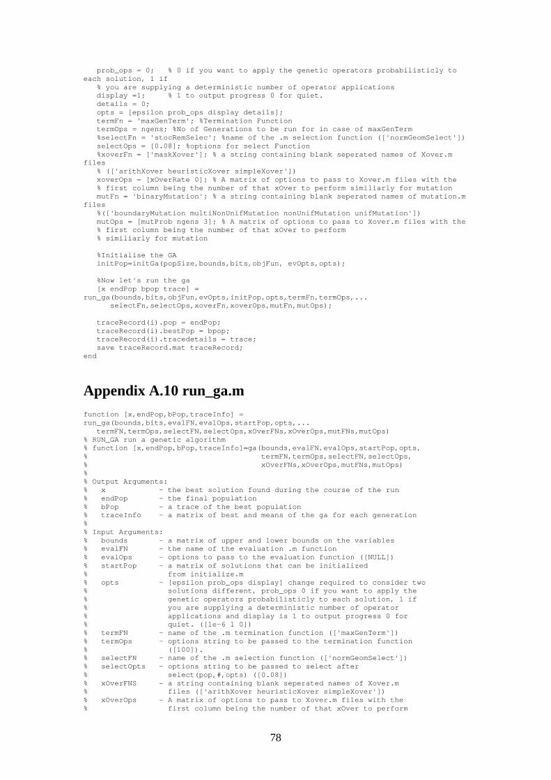
78

pr ob_ops = 0; % 0 i f you want t o appl y t he genet i c oper at or s pr obabi l i s t i c l y t o each sol ut i on, 1 i f % you ar e suppl y i ng a det er mi ni s t i c number of oper at or appl i cat i ons di spl ay =1; % 1 t o out put pr ogr ess 0 f or qui et . det ai l s = 0; opt s = [ epsi l on pr ob_ops di spl ay det ai l s ] ; t er mFn = ' maxGenTer m' ; %Ter mi nat i on Funct i on t er mOps = ngens; %No of Gener at i ons t o be r un f or i n case of maxGenTer m %sel ect Fn = ' s t ocRemSel ec ' ; %name of t he . m sel ect i on f unct i on ( [ ' nor mGeomSel ect ' ] ) sel ect Ops = [ 0. 08] ; %opt i ons f or sel ect Funct i on %xover Fn = [ ' maskXover ' ] ; % a st r i ng cont ai ni ng bl ank seper at ed names of Xover . m f i l es % ( [ ' ar i t hXover heur i s t i cXover s i mpl eXover ' ] ) xover Ops = [ xOver Rat e 0] ; % A mat r i x of opt i ons t o pass t o Xover . m f i l es wi t h t he % f i r s t col umn bei ng t he number of t hat xOver t o per f or m s i mi l i ar l y f or mut at i on mut Fn = ' bi nar yMut at i on' ; % a st r i ng cont ai ni ng bl ank seper at ed names of mut at i on. m f i l es %( [ ' boundar yMut at i on mul t i NonUni f Mut at i on nonUni f Mut at i on uni f Mut at i on' ] ) mut Ops = [ mut Pr ob ngens 3] ; % A mat r i x of opt i ons t o pass t o Xover . m f i l es wi t h t he % f i r s t col umn bei ng t he number of t hat xOver t o per f or m % s i mi l i ar l y f or mut at i on %I ni t i al i se t he GA i ni t Pop=i ni t Ga( popSi ze, bounds, bi t s , obj Fun, evOpt s, opt s) ; %Now l et ' s r un t he ga [ x endPop bpop t r ace] = r un_ga( bounds, bi t s , obj Fun, evOpt s, i ni t Pop, opt s, t er mFn, t er mOps, . . . sel ect Fn, sel ect Ops, xover Fn, xover Ops, mut Fn, mut Ops) ; t r aceRecor d( i ) . pop = endPop; t r aceRecor d( i ) . best Pop = bpop; t r aceRecor d( i ) . t r acedet ai l s = t r ace; save t r aceRecor d. mat t r aceRecor d; end

Appendix A.10 run_ga.m f unct i on [ x , endPop, bPop, t r aceI nf o] = r un_ga( bounds, bi t s , eval FN, eval Ops, st ar t Pop, opt s, . . . t er mFN, t er mOps, sel ect FN, sel ect Ops, xOver FNs, xOver Ops, mut FNs, mut Ops) % RUN_GA r un a genet i c al gor i t hm % f unct i on [ x , endPop, bPop, t r aceI nf o] =ga( bounds, eval FN, eval Ops, st ar t Pop, opt s, % t er mFN, t er mOps, sel ect FN, sel ect Ops, % xOver FNs, xOver Ops, mut FNs, mut Ops) % % Out put Ar gument s: % x - t he best sol ut i on f ound dur i ng t he cour se of t he r un % endPop - t he f i nal popul at i on % bPop - a t r ace of t he best popul at i on % t r aceI nf o - a mat r i x of best and means of t he ga f or each gener at i on % % I nput Ar gument s: % bounds - a mat r i x of upper and l ower bounds on t he var i abl es % eval FN - t he name of t he eval uat i on . m f unct i on % eval Ops - opt i ons t o pass t o t he eval uat i on f unct i on ( [ NULL] ) % s t ar t Pop - a mat r i x of sol ut i ons t hat can be i ni t i al i zed % f r om i ni t i al i ze. m % opt s - [ epsi l on pr ob_ops di spl ay] change r equi r ed t o consi der t wo % sol ut i ons di f f er ent , pr ob_ops 0 i f you want t o appl y t he % genet i c oper at or s pr obabi l i s t i c l y t o each sol ut i on, 1 i f % you ar e suppl y i ng a det er mi ni s t i c number of oper at or % appl i cat i ons and di spl ay i s 1 t o out put pr ogr ess 0 f or % qui et . ( [ 1e- 6 1 0] ) % t er mFN - name of t he . m t er mi nat i on f unct i on ( [ ' maxGenTer m' ] ) % t er mOps - opt i ons st r i ng t o be passed t o t he t er mi nat i on f unct i on % ( [ 100] ) . % sel ect FN - name of t he . m sel ect i on f unct i on ( [ ' nor mGeomSel ect ' ] ) % sel ect Opt s - opt i ons st r i ng t o be passed t o sel ect af t er % sel ect ( pop, #, opt s) ( [ 0. 08] ) % xOver FNS - a s t r i ng cont ai ni ng bl ank seper at ed names of Xover . m % f i l es ( [ ' ar i t hXover heur i s t i cXover s i mpl eXover ' ] ) % xOver Ops - A mat r i x of opt i ons t o pass t o Xover . m f i l es wi t h t he % f i r s t col umn bei ng t he number of t hat xOver t o per f or m

79

% s i mi l i ar l y f or mut at i on ( [ 2 0; 2 3; 2 0] ) % mut FNs - a s t r i ng cont ai ni ng bl ank seper at ed names of mut at i on. m % f i l es ( [ ' boundar yMut at i on mul t i NonUni f Mut at i on . . . % nonUni f Mut at i on uni f Mut at i on' ] ) % mut Ops - A mat r i x of opt i ons t o pass t o Xover . m f i l es wi t h t he % f i r s t col umn bei ng t he number of t hat xOver t o per f or m % s i mi l i ar l y f or mut at i on ( [ 4 0 0; 6 100 3; 4 100 3; 4 0 0] ) % Bi nar y and Real - Val ued Si mul at i on Evol ut i on f or Mat l ab % Copyr i ght ( C) 1996 C. R. Houck, J . A. Joi nes, M. G. Kay % % C. R. Houck, J . Joi nes, and M. Kay. A genet i c al gor i t hm f or f unct i on % opt i mi zat i on: A Mat l ab i mpl ement at i on. ACM Tr ansact i ons on Mat hmat i cal % Sof t war e, Submi t t ed 1996. % % Thi s pr ogr am i s f r ee sof t war e; you can r edi st r i but e i t and/ or modi f y % i t under t he t er ms of t he GNU Gener al Publ i c Li cense as publ i shed by % t he Fr ee Sof t war e Foundat i on; ei t her ver s i on 1, or ( at your opt i on) % any l at er ver s i on. % % Thi s pr ogr am i s di s t r i but ed i n t he hope t hat i t wi l l be usef ul , % but WI THOUT ANY WARRANTY; wi t hout even t he i mpl i ed war r ant y of % MERCHANTABI LI TY or FI TNESS FOR A PARTI CULAR PURPOSE. See t he % GNU Gener al Publ i c Li cense f or mor e det ai l s . A copy of t he GNU % Gener al Publ i c Li cense can be obt ai ned f r om t he % Fr ee Sof t war e Foundat i on, I nc. , 675 Mass Ave, Cambr i dge, MA 02139, USA. %%$Log: ga. m, v $ %Revi s i on 1. 10 1996/ 02/ 02 15: 03: 00 j j oi ne % Fi xed t he or der i ng of i mput ar gument s i n t he comment s t o mat ch % t he act ual or der i n t he ga f unct i on. % %Revi s i on 1. 9 1995/ 08/ 28 20: 01: 07 chouck % Updat ed i ni t i al i zat i on par amet er s, updat ed mut at i on par amet er s t o r ef l ect % b bei ng t he t hi r d opt i on t o t he nonuni f or m mut at i ons % %Revi s i on 1. 8 1995/ 08/ 10 12: 59: 49 j j oi ne %St ar t ed Logf i l e t o keep t r ack of r ev i s i ons % n=nar gi n; i f n<2 | n==6 | n==10 | n==12 di sp( ' I nsuf f i c i ent ar guement s ' ) end i f n<3 %Def aul t eval at i on opt s. eval Ops=[ ] ; end i f n<5 opt s = [ 1e- 6 1 0 0] ; end i f i sempt y( opt s) opt s = [ 1e- 6 1 0 0] ; end i f any( eval FN<48) %Not us i ng a . m f i l e i f opt s( 2) ==1 %Fl oat ga e1st r =[ ' x=c1; c1( xZomeLengt h) =' , eval FN ' ; ' ] ; e2st r =[ ' x=c2; c2( xZomeLengt h) =' , eval FN ' ; ' ] ; el se %Bi nar y ga e1st r =[ ' x=b2f ( endPop( j , : ) , bounds, bi t s) ; endPop( j , xZomeLengt h) =' , . . . eval FN ' ; ' ] ; end el se %Ar e usi ng a . m f i l e i f opt s( 2) ==1 %Fl oat ga e1st r =[ ' [ c1 c1( xZomeLengt h) ] =' eval FN ' ( c1, [ gen eval Ops] ) ; ' ] ; e2st r =[ ' [ c2 c2( xZomeLengt h) ] =' eval FN ' ( c2, [ gen eval Ops] ) ; ' ] ; el se %Bi nar y ga % e1st r =[ ' x=b2f ( endPop( j , : ) , bounds, bi t s) ; [ x v ] =' eval FN . . . % ' ( x , [ gen eval Ops] ) ; endPop( j , : ) =[ f 2b( x, bounds, bi t s) v ] ; ' ] ; e1st r =[ ' x=b2f ( endPop( j , : ) , bounds, bi t s) ; [ x v ] =' eval FN . . . ' ( x , [ gen eval Ops] ) ; endPop( j , end) = v; ' ] ; %Ther e seems t o be a di scr epancy i n how f 2b wor ks so avoi d us i ng i t end end

80

i f n<6 %Def aul t t er mi nat i on i nf or mat i on t er mOps=[ 100] ; t er mFN=' maxGenTer m' ; end i f n<12 %Def aul t muat at i on i nf or mat i on i f opt s( 2) ==1 %Fl oat GA mut FNs=[ ' boundar yMut at i on mul t i NonUni f Mut at i on nonUni f Mut at i on uni f Mut at i on' ] ; mut Ops=[ 4 0 0; 6 t er mOps( 1) 3; 4 t er mOps( 1) 3; 4 0 0] ; el se %Bi nar y GA mut FNs=[ ' bi nar yMut at i on' ] ; mut Ops=[ 0. 05] ; end end i f n<10 %Def aul t cr ossover i nf or mat i on i f opt s( 2) ==1 %Fl oat GA xOver FNs=[ ' ar i t hXover heur i s t i cXover s i mpl eXover ' ] ; xOver Ops=[ 2 0; 2 3; 2 0] ; el se %Bi nar y GA xOver FNs=[ ' s i mpl eXover ' ] ; xOver Ops=[ 0. 6] ; end end i f n<9 %Def aul t sel ect opt s onl y i . e. r oul l et e wheel . sel ect Ops=[ ] ; end i f n<8 %Def aul t sel ect i nf o sel ect FN=[ ' nor mGeomSel ect ' ] ; sel ect Ops=[ 0. 08] ; end i f n<6 %Def aul t t er mi nat i on i nf or mat i on t er mOps=[ 100] ; t er mFN=' maxGenTer m' ; end i f n<4 %No st ar t i ng popul at i on passed gi ven s t ar t Pop=[ ] ; end i f i sempt y( st ar t Pop) %Gener at e a popul at i on at r andom %st ar t Pop=zer os( 80, s i ze( bounds, 1) +1) ; s t ar t Pop=i ni t i al i zega( 80, bounds, eval FN, eval Ops, opt s( 1: 2) ) ; end i f opt s( 2) ==0 %bi nar y %bi t s=cal cbi t s( bounds, opt s( 1) ) ; %bi t s = cal cbi t s( bounds( : , 1: 2) , bounds( : , 3) ' ) ; end bounds = bounds( : , 1: 2) ; xOver FNs=par se( xOver FNs) ; mut FNs=par se( mut FNs) ; xZomeLengt h = s i ze( st ar t Pop, 2) ; %Lengt h of t he xzome=numVar s+f i t t ness numVar = xZomeLengt h- 1; %Number of var i abl es popSi ze = s i ze( st ar t Pop, 1) ; %Number of i ndi v i dual s i n t he pop endPop = zer os( popSi ze, xZomeLengt h) ; %A secondar y popul at i on mat r i x c1 = zer os( 1, xZomeLengt h) ; %An i ndi v i dual c2 = zer os( 1, xZomeLengt h) ; %An i ndi v i dual numXOver s = s i ze( xOver FNs, 1) ; %Number of Cr ossover oper at or s numMut s = s i ze( mut FNs, 1) ; %Number of Mut at i on oper at or s epsi l on = opt s( 1) ; %Thr eshol d f or t wo f i t t ness t o di f f er oval = max( st ar t Pop( : , xZomeLengt h) ) ; %Best val ue i n s t ar t pop bFoundI n = 1; %Number of t i mes best has changed done = 0; %Done wi t h s i mul at ed evol ut i on gen = 1; %Cur r ent Gener at i on Number col l ect Tr ace = ( nar gout >3) ; %Shoul d we col l ect i nf o ever y gen f l oat GA = opt s( 2) ==1; %Pr obabi l i s t i c appl i cat i on of ops di spl ay = opt s( 3) ; %Di spl ay summar y det ai l s = opt s( 4) ; %Di spl ay det ai l s i f col l ect Tr ace f i gur e end whi l e( ~done) %El i t i s t Model [ bval , bi ndx] = max( st ar t Pop( : , xZomeLengt h) ) ; %Best of cur r ent pop best = s t ar t Pop( bi ndx, : ) ;

81

i f col l ect Tr ace t r aceI nf o( gen, 1) =gen; %cur r ent gener at i on t r aceI nf o( gen, 2) =st ar t Pop( bi ndx, xZomeLengt h) ; %Best f i t t ness t r aceI nf o( gen, 3) =mean( st ar t Pop( : , xZomeLengt h) ) ; %Avg f i t t ness t r aceI nf o( gen, 4) =st d( st ar t Pop( : , xZomeLengt h) ) ; hol d of f pl ot ( t r aceI nf o( : , 1) , t r aceI nf o( : , 2) , ' r ' ) hol d on pl ot ( t r aceI nf o( : , 1) , t r aceI nf o( : , 3) , ' b' ) end i f ( ( abs( bval - oval ) >epsi l on) | ( gen==1) ) %I f we have a new best sol i f di spl ay %f pr i nt f ( 1, ' \ n%d %f \ n' , gen, bval ) ; %Updat e t he di spl ay f pr i nt f ( 1, ' St ar t i ng Gener at i on %d. New best i s %g\ n' , gen, bval ) ; end i f f l oat GA bPop( bFoundI n, : ) =[ gen st ar t Pop( bi ndx, : ) ] ; %Updat e bPop Mat r i x el se bPop( bFoundI n, : ) =[ gen b2f ( st ar t Pop( bi ndx, 1: numVar ) , bounds, bi t s) . . . s t ar t Pop( bi ndx, xZomeLengt h) ] ; end bFoundI n=bFoundI n+1; %Updat e number of changes oval =bval ; %Updat e t he best val end endPop = f eval ( sel ect FN, st ar t Pop, [ gen sel ect Ops] ) ; %Sel ect i f f l oat GA %Runni ng wi t h t he model wher e t he par amet er s ar e number s of ops f or i =1: numXOver s, f or j =1: xOver Ops( i , 1) , a = r ound( r and* ( popSi ze- 1) +1) ; %Pi ck a par ent b = r ound( r and* ( popSi ze- 1) +1) ; %Pi ck anot her par ent xN=debl ank( xOver FNs( i , : ) ) ; %Get t he name of cr ossover f unct i on [ c1 c2] = f eval ( xN, endPop( a, : ) , endPop( b, : ) , bounds, [ gen xOver Ops( i , : ) ] ) ; i f c1( 1: numVar ) ==endPop( a, ( 1: numVar ) ) %Make sur e we cr eat ed a new c1( xZomeLengt h) =endPop( a, xZomeLengt h) ; %sol ut i on bef or e eval uat i ng el sei f c1( 1: numVar ) ==endPop( b, ( 1: numVar ) ) c1( xZomeLengt h) =endPop( b, xZomeLengt h) ; el se %[ c1( xZomeLengt h) c1] = f eval ( eval FN, c1, [ gen eval Ops] ) ; eval ( e1st r ) ; end i f c2( 1: numVar ) ==endPop( a, ( 1: numVar ) ) c2( xZomeLengt h) =endPop( a, xZomeLengt h) ; el sei f c2( 1: numVar ) ==endPop( b, ( 1: numVar ) ) c2( xZomeLengt h) =endPop( b, xZomeLengt h) ; el se %[ c2( xZomeLengt h) c2] = f eval ( eval FN, c2, [ gen eval Ops] ) ; eval ( e2st r ) ; end endPop( a, : ) =c1; endPop( b, : ) =c2; end end f or i =1: numMut s, f or j =1: mut Ops( i , 1) , a = r ound( r and* ( popSi ze- 1) +1) ; c1 = f eval ( debl ank( mut FNs( i , : ) ) , endPop( a, : ) , bounds, [ gen mut Ops( i , : ) ] ) ; i f c1( 1: numVar ) ==endPop( a, ( 1: numVar ) ) c1( xZomeLengt h) =endPop( a, xZomeLengt h) ; el se %[ c1( xZomeLengt h) c1] = f eval ( eval FN, c1, [ gen eval Ops] ) ; eval ( e1st r ) ; end endPop( a, : ) =c1; end end el se %We ar e r unni ng a pr obabi l i s t i c model of genet i c oper at or s % f or i =1: numXOver s,

82

i = 1; xN=debl ank( xOver FNs( i , : ) ) ; %Get t he name of cr ossover f unct i on cp=f i nd( r and( popSi ze, 1) <xOver Ops( i , 1) ==1) ; i f ~i sempt y( cp) i f r em( si ze( cp, 1) , 2) cp=cp( 1: ( s i ze( cp, 1) - 1) ) ; end l i s t = r and( s i ze( cp) ) ; %Gener at e a r andom l i s t f or choosi ng whi ch i ndi v i dual s get pai r ed f or xOver f or j =1: s i ze( cp, 1) %NEED TO TEST THAT I NDI VI DUALS ARE CHOSEN RANDOMLY [ t mp, a] = max( l i s t ) ; l i s t ( a) = 0; [ t mp, b] = max( l i s t ) ; l i s t ( b) = 0; a = cp( a) ; b = cp( b) ; [ endPop( a, : ) endPop( b, : ) ] = f eval ( xN, endPop( a, : ) , endPop( b, : ) , . . . bounds, [ gen xOver Ops( i , : ) ] ) ; end end %end %f or i =1: numMut s mN=debl ank( mut FNs( i , : ) ) ; f or j =1: popSi ze endPop( j , : ) = f eval ( mN, endPop( j , : ) , bounds, [ gen mut Ops( i , : ) ] ) ; eval ( e1st r ) ; i f det ai l s f pr i nt f ( 1, ' Gen: %d\ t I nd: %d\ t Fi t ness: %g\ n' , gen, j , v) ; end end %end end gen=gen+1; done=f eval ( t er mFN, [ gen t er mOps] , bPop, endPop) ; %See i f t he ga i s done s t ar t Pop=endPop; %Swap t he popul at i ons [ bval , bi ndx] = mi n( st ar t Pop( : , xZomeLengt h) ) ; %Keep t he best sol ut i on s t ar t Pop( bi ndx, : ) = best ; %r epl ace i t wi t h t he wor st save l at est . mat s t ar t Pop t r aceI nf o bPop end endPop = st ar t Pop; [ bval , bi ndx] = max( st ar t Pop( : , xZomeLengt h) ) ; i f di spl ay f pr i nt f ( 1, ' \ n%d %f \ n' , gen, bval ) ; end x=st ar t Pop( bi ndx, : ) ; i f opt s( 2) ==0 %bi nar y x=b2f ( x, bounds, bi t s) ; bPop( bFoundI n, : ) =[ gen b2f ( st ar t Pop( bi ndx, 1: numVar ) , bounds, bi t s) . . . s t ar t Pop( bi ndx, xZomeLengt h) ] ; el se bPop( bFoundI n, : ) =[ gen st ar t Pop( bi ndx, : ) ] ; end i f col l ect Tr ace t r aceI nf o( gen, 1) =gen; %cur r ent gener at i on t r aceI nf o( gen, 2) =st ar t Pop( bi ndx, xZomeLengt h) ; %Best f i t t ness t r aceI nf o( gen, 3) =mean( st ar t Pop( : , xZomeLengt h) ) ; %Avg f i t t ness t r aceI nf o( gen, 4) =st d( st ar t Pop( : , xZomeLengt h) ) ; %St d. Devi at i on hol d of f pl ot ( t r aceI nf o( : , 1) , t r aceI nf o( : , 2) , ' r ' ) hol d on pl ot ( t r aceI nf o( : , 1) , t r aceI nf o( : , 3) , ' b' ) end

Appendix A.11 initGa.m f unct i on [ pop] = i ni t i al i ze_r un_ga( num, bounds, bi t s , eval FN, eval Ops, opt s) % f unct i on [ pop] =i ni t i al i zega( popul at i onSi ze, var i abl eBounds, eval FN, % eval Ops, opt s)

83

% i ni t i al i zega cr eat es a mat r i x of r andom number s wi t h % a number of r ows equal t o t he popul at i onSi ze and a number % col umns equal t o t he number of r ows i n bounds pl us 1 f or % t he f ( x) val ue whi ch i s f ound by appl y i ng t he eval FN. % Thi s i s used by t he ga t o cr eat e t he popul at i on i f i t % i s not suppl i ed. % % pop - t he i ni t i al , eval uat ed, r andom popul at i on % popul at oi nSi ze - t he s i ze of t he popul at i on, i . e. t he number t o cr eat e % var i abl eBounds - a mat r i x whi ch cont ai ns t he bounds of each var i abl e, i . e. % [ var 1_hi gh var 1_l ow; var 2_hi gh var 2_l ow; . . . . ] % eval FN - t he eval uat i on f n, usual l y t he name of t he . m f i l e f or % eval uat i on % eval Ops - any opt s t o be passed t o t he eval f unct i on def aul t s [ ] % opt s - opt i ons t o t he i ni t i al i ze f unct i on, i e. % [ t ype pr ec] wher e eps i s t he epsi l on val ue % and t he second opt i on i s 1 f or f l oat and 0 f or bi nar y, % pr ec i s t he pr eci s i on of t he var i abl es def aul t s [ 1e- 6 1] % Bi nar y and Real - Val ued Si mul at i on Evol ut i on f or Mat l ab GAOT V2 % Copyr i ght ( C) 1998 C. R. Houck, J . A. Joi nes, M. G. Kay % % C. R. Houck, J . Joi nes, and M. Kay. A genet i c al gor i t hm f or f unct i on % opt i mi zat i on: A Mat l ab i mpl ement at i on. ACM Tr ansact i ons on Mat hmat i cal % Sof t war e, Submi t t ed 1996. % % Thi s pr ogr am i s f r ee sof t war e; you can r edi st r i but e i t and/ or modi f y % i t under t he t er ms of t he GNU Gener al Publ i c Li cense as publ i shed by % t he Fr ee Sof t war e Foundat i on; ei t her ver s i on 1, or ( at your opt i on) % any l at er ver s i on. % % Thi s pr ogr am i s di s t r i but ed i n t he hope t hat i t wi l l be usef ul , % but WI THOUT ANY WARRANTY; wi t hout even t he i mpl i ed war r ant y of % MERCHANTABI LI TY or FI TNESS FOR A PARTI CULAR PURPOSE. See t he % GNU Gener al Publ i c Li cense f or mor e det ai l s . A copy of t he GNU % Gener al Publ i c Li cense can be obt ai ned f r om t he % Fr ee Sof t war e Foundat i on, I nc. , 675 Mass Ave, Cambr i dge, MA 02139, USA. i f nar gi n<5 opt s = [ 1e- 6 1 0 0] ; end i f i sempt y( opt s) opt s = [ 1e- 6 1 0 0] ; end i f any( eval FN<48) %Not a . m f i l e i f opt s( 2) ==1 %Fl oat GA est r =[ ' x=pop( i , 1) ; pop( i , xZomeLengt h) =' , eval FN ' ; ' ] ; el se %Bi nar y GA est r =[ ' x=b2f ( pop( i , : ) , bounds, bi t s) ; pop( i , xZomeLengt h) =' , eval FN ' ; ' ] ; end el se %A . m f i l e i f opt s( 2) ==1 %Fl oat GA est r =[ ' [ pop( i , : ) pop( i , xZomeLengt h) ] =' eval FN ' ( pop( i , : ) , [ 0 eval Ops] ) ; ' ] ; el se %Bi nar y GA % est r =[ ' x=b2f ( pop( i , : ) , bounds, bi t s) ; [ x v ] =' eval FN . . . % ' ( x , [ 0 eval Ops] ) ; pop( i , : ) =[ f 2b( x, bounds, bi t s) v ] ; ' ] ; est r =[ ' x=b2f ( pop( i , : ) , bounds, bi t s) ; [ x v ] =' eval FN . . . ' ( x , [ 0 eval Ops] ) ; pop( i , end) = v ; ' ] ; %Ther e seems t o be a di scr epancy i n how f 2b wor ks so avoi d us i ng i t end end det ai l s = opt s( 4) ; numVar s = s i ze( bounds, 1) ; %Number of var i abl es r ng = ( bounds( : , 2) - bounds( : , 1) ) ' ; %The var i abl e r anges' i f opt s( 2) ==1 %Fl oat GA xZomeLengt h = numVar s+1; %Lengt h of s t r i ng i s numVar + f i t pop = zer os( num, xZomeLengt h) ; %Al l ocat e t he new popul at i on pop( : , 1: numVar s) =( ones( num, 1) * r ng) . * ( r and( num, numVar s) ) +. . . ( ones( num, 1) * bounds( : , 1) ' ) ; el se %Bi nar y GA %bi t s=cal cbi t s( bounds( : , 1: 2) , bounds( : , 3) ' ) ; xZomeLengt h = sum( bi t s) +1; %Lengt h of s t r i ng i s numVar + f i t

84

pop = r ound( r and( num, sum( bi t s) +1) ) ; end bounds = bounds( : , 1: 2) ; f or i =1: num eval ( est r ) ; i f det ai l s f pr i nt f ( ' I ni t i al i s i ng: I ndi v i dual %d \ t Fi t ness %g\ n' , i , v) ; end end

Appendix A.12 ga_sfn.m f unct i on [ sys, x0, st r , t s ] = ga_sf n( t , x , u, f l ag, popSi ze, bounds, bi t s , per i od) %Run a genet i c al gor i t hm as an S- Funct i on %Assume a bi nar y GA wi t h r oul et et e sel ect i on, maskXover , %bi nar y mut at i on wi t h pr obabi l i t y . 01 % %Wr i t t en By Joe For an August 2002 swi t ch f l ag, %%%%%%%%%%%%%%%%%% % I ni t i al i zat i on % %%%%%%%%%%%%%%%%%% case 0, [ sys, x0, st r , t s ] = mdl I ni t i al i zeSi zes( popSi ze, bounds, bi t s , per i od) ; %%%%%%%%%% % Updat e % %%%%%%%%%% case 2, [ sys] = mdl Updat e( t , x , u, popSi ze) ; %%%%%%%%%% % Out put % %%%%%%%%%% case 3, sys = mdl Out put s( t , x , u, popSi ze, bounds, bi t s) ; %%%%%%%%%%%%% % Ter mi nat e % %%%%%%%%%%%%% case 9, mdl Ter mi nat e( t , x , u, popSi ze, bounds, bi t s) ; %save r esul t s t o di sk %%%%%%%%%%%%%%%%%%%% % Unexpect ed f l ags % %%%%%%%%%%%%%%%%%%%% ot her wi se er r or ( [ ' unhandl ed f l ag = ' , num2st r ( f l ag) ] ) ; end % %======================================================================= % mdl I ni t i al i zeSi zes % Ret ur n t he s i zes, i ni t i al condi t i ons, and sampl e t i mes f or t he S- f unct i on. %======================================================================= % f unct i on [ sys, x0, st r , t s ] = mdl I ni t i al i zeSi zes( popSi ze, bounds, bi t s , per i od) numVar = s i ze( bounds, 1) ; i ni t Pop = i ni t ga( popSi ze, bi t s) ; numGenes = s i ze( i ni t Pop, 2) ; gen = 1; %Gener at i on count er s i zes = s i msi zes; s i zes. NumCont St at es = 0; s i zes. NumDi scSt at es = ( popSi ze+1) * numGenes+3; s i zes. NumOut put s = numVar +3; s i zes. NumI nput s = 1;

85

si zes. Di r Feedt hr ough = 0; s i zes. NumSampl eTi mes = 1; sys = s i msi zes( s i zes) ; i ni t Pop = r eshape( i ni t Pop' , popSi ze* numGenes, 1) ; %Make i ni t Pop a vect or x0 = zer os( s i zes. NumDi scSt at es, 1) ; x0( 1: popSi ze* numGenes) = i ni t Pop; %Pl ace i ni t Pop i nt o s t at e vect or x0( end- 2) = numGenes; %St or e t hi s val ue so i t doesn' t have t o be const ant l y r ecal cul at ed x0( end- 1) = gen; %Pl ace gener at i on count er i nt o s t at e vect or ; x0( end) = 1; %Tr acks whi ch chr omosome i s bei ng eval uat ed s t r = [ ] ; t s = [ per i od 0] ; % end mdl I ni t i al i zeSi zes % %======================================================================= % mdl Updat e % Handl e di scr et e s t at e updat es, sampl e t i me hi t s , and maj or t i me st ep % r equi r ement s. %======================================================================= % f unct i on [ sys] = mdl Updat e( t , x , u, popSi ze) i nput = u; i f u<=0 i nput =1e- 9; end numGenes = x( end- 2) ; cc = x( end) ; %Get cur r ent popul at i on i nt o mat r i x f or m pop = r eshape( x( 1: ( popSi ze+1) * numGenes) , numGenes, popSi ze+1) ' ; cur r ent _opt i mum = pop( end, end) ; %The f i t ness i n i nput r ef er s t o t he pr evi ous chr omosome i f cc>1 %Thi s i s because out put occur s bef or e updat e pop( cc- 1, end) =i nput ; %Read i n i nput i nt o t he f i t ness val ue of t he pr evi ous chr omosome i f i nput >cur r ent _opt i mum %Save new best sol ut i on pop( end, : ) = pop( cc- 1, : ) ; end end x( end) = x( end) +1; %I ncr ement chr omosome count er i f x( end) > popSi ze+1 %End of a gener at i on i f max( pop( : , end- 1) ) <cur r ent _opt i mum %I f t he opt i mum was l ost i n t hi s gener at i on [ wval wi ndx] = mi n( pop( : , end- 1) ) ; %Repl ace t he wor st of t hi s gener at i on pop( wi ndx, : ) = pop( end, : ) ; %Wi t h t he opt i mum end newPop = cr eat e_next _gener at i on( pop( 1: end- 1, : ) ) ; %f i nd next gener at i on pop = [ newPop; pop( end, : ) ] ; x( end) = 1; %St ar t agai n at begi nni ng of next gener at i on x( end- 1) = x( end- 1) +1; %I ncr ement Gener at i on Count er end x( 1: ( popSi ze+1) * numGenes) = r eshape( pop' , numGenes* ( popSi ze+1) , 1) ; %Tr ansf or m mat r i x back i nt o vect or sys = x; %end mdl Updat e % %======================================================================= % mdl Out put s % Ret ur n Ret ur n t he out put vect or f or t he S- f unct i on %======================================================================= % f unct i on sys = mdl Out put s( t , x , u, popSi ze, bounds, bi t s) numGenes = x( end- 2) ;

86

gener at i on = x( end- 1) ; cc = x( end) ; opt i mum = x( ( popSi ze+1) * numGenes) ; pop = r eshape( x( 1: ( popSi ze+1) * numGenes) , numGenes, popSi ze+1) ' ; chr om = b2f ( pop( cc, 1: end- 1) , bounds, bi t s) ; %Out put cur r ent chr omosome, best chr omosome so f ar , best f i t ness so f ar and cur r ent gener at i on number sys = [ chr om cc opt i mum gener at i on] ; %end mdl Out put s f unct i on mdl Ter mi nat e( t , x , u, popSi ze, bounds, bi t s) numGenes = x( end- 2) ; cur r ent Chr om = x( end) ; cur r ent Gen = x( end) - 1; pop = r eshape( x( 1: ( popSi ze+1) * numGenes) , numGenes, popSi ze+1) ' ; best _chr om = pop( end, : ) ; save f i nal St at e. mat best _chr om cur r ent Chr om cur r ent Gen pop %end Mdl Ter mi nat e f unct i on [ pop] = i ni t ga( num, bi t s) % f unct i on [ pop] =i ni t i al i zega( popul at i onSi ze, var i abl eBounds, bi t s) % % i ni t i al i zega cr eat es a mat r i x of r andom number s wi t h % a number of r ows equal t o t he popul at i onSi ze % % pop - t he i ni t i al , eval uat ed, r andom popul at i on % popul at oi nSi ze - t he s i ze of t he popul at i on, i . e. t he number t o cr eat e % bi t s - a vect or wi t h t he number of bi t s r equi r ed per var i abl e pop = r ound( r and( num, sum( bi t s) +1) ) ; pop( : , end) = zer os( num, 1) ; %end i ni t ga f unct i on newPop = cr eat e_next _gener at i on( ol dPop) [ popSi ze, nVar s] = s i ze( ol dPop) ; %Sel ect us i ng st ochast i c Remai nder Sel ect i on newPop = st ocRemSel ec( ol dPop) ; %Cr ossover us i ng mask cr ossover l i s t = r and( popSi ze, 1) ; %Gener at e a l i s t t o deci de how cr ossover s ar e pai r ed f or i = 1: f l oor ( popSi ze/ 2) [ t mp, i nd] = max( l i s t ( : , 1) ) ; a = newPop( i nd, : ) ; l i s t ( i nd) = 0; [ t mp, i nd] = max( l i s t ( : , 1) ) ; b = newPop( i nd, : ) ; l i s t ( i nd) = 0; [ c d] = maskXover ( a, b) ; newPop( i * 2- 1, : ) = c ; newPop( i * 2, : ) = d; end %Mut at e f or i = 1: popSi ze newPop( i , : ) = bi nMut at i on( newPop( i , : ) , 0. 01) ; end %end of cr eat e_next _gener at i on f unct i on par ent = bi nMut at i on( par ent , mut _pr ob) % Bi nar y mut at i on changes each of t he bi t s of t he par ent % based on t he pr obabi l i t y of mut at i on

87

%Based on bi nar yMut at i on i n GAOT t ool box. Modi f i ed by Joe For an numVar = s i ze( par ent , 2) - 1; % Get t he number of var i abl es % Pi ck a var i abl e t o mut at e r andoml y f r om 1- number of var s r N=r and( 1, numVar ) <mut _pr ob; par ent =[ abs( par ent ( 1: numVar ) - r N) par ent ( numVar +1) ] ;

Appendix A.13 evalfis_sfn.m f unct i on [ sys, x0, st r , t s ] = eval f i s_sf n3( t , x , u, f l ag) %Eval uat es a t wo- i nput FI S based on par amet er s and er r or %val ues i nput i nt o t he bl ock gl obal t he_f uzzy swi t ch f l ag, %%%%%%%%%%%%%%%%%% % I ni t i al i zat i on % %%%%%%%%%%%%%%%%%% case 0, [ sys, x0, st r , t s ] =mdl I ni t i al i zeSi zes; %%%%%%%%%%%%%%% % Der i vat i ves % %%%%%%%%%%%%%%% case 1, sys=[ ] ; %%%%%%%%%% % Updat e % %%%%%%%%%% case 2, sys=mdl Updat e( t , x , u) ; %%%%%%%%%%% % Out put s % %%%%%%%%%%% case 3, sys=mdl Out put s( t , x , u) ; %%%%%%%%%%%%%%%%%%%%%%% % Get Ti meOf Next Var Hi t % %%%%%%%%%%%%%%%%%%%%%%% case 4, sys=[ ] ; %%%%%%%%%%%%% % Ter mi nat e % %%%%%%%%%%%%% case 9, sys=[ ] ; %%%%%%%%%%%%%%%%%%%% % Unexpect ed f l ags % %%%%%%%%%%%%%%%%%%%% ot her wi se er r or ( [ ' Unhandl ed f l ag = ' , num2st r ( f l ag) ] ) ; end % end sf unt mpl % %============================================================================= % mdl I ni t i al i zeSi zes % Ret ur n t he s i zes, i ni t i al condi t i ons, and sampl e t i mes f or t he S- f unct i on. %============================================================================= % f unct i on [ sys, x0, st r , t s ] =mdl I ni t i al i zeSi zes % % cal l s i msi zes f or a s i zes st r uct ur e, f i l l i t i n and conver t i t t o a % s i zes ar r ay. % % Not e t hat i n t hi s exampl e, t he val ues ar e har d coded. Thi s i s not a % r ecommended pr act i ce as t he char act er i s t i cs of t he bl ock ar e t ypi cal l y

88

% def i ned by t he S- f unct i on par amet er s. % s i zes = s i msi zes; s i zes. NumCont St at es = 0; s i zes. NumDi scSt at es = 19; s i zes. NumOut put s = 1; s i zes. NumI nput s = 21; s i zes. Di r Feedt hr ough = 1; s i zes. NumSampl eTi mes = 1; % at l east one sampl e t i me i s needed sys = s i msi zes( s i zes) ; % % i ni t i al i ze t he i ni t i al condi t i ons % x0 = zer os( s i zes. NumDi scSt at es, 1) ; % % st r i s al ways an empt y mat r i x % st r = [ ] ; % % i ni t i al i ze t he ar r ay of sampl e t i mes % t s = [ - 1 0] ; % end mdl I ni t i al i zeSi zes % %============================================================================= % mdl Updat e % Handl e di scr et e s t at e updat es, sampl e t i me hi t s , and maj or t i me st ep % r equi r ement s. %============================================================================= f unct i on sys = mdl Updat e( t , x , u) sys = u( 1: 19) ; %============================================================================= % mdl Out put s % Ret ur n t he bl ock out put s. %============================================================================= % f unct i on sys=mdl Out put s( t , x , u) gl obal t he_f uzzy i nput = u( 20: 21) ; %Check i f FLC needs t o be changed i f any( u( 1: 15) ~= x( 1: 15) ) | u( 19) ~=x( 19) n = u( 1: 3) ; pm = u( 4: 6) . ^ u( 10: 12) ; pr = u( 7: 9) . ^ u( 13: 15) ; t het a = u( 19) ; t he_f uzzy = make_f i s( 2, 1, n, pm, pr , t het a) ; end scal e = u( 16: 18) ; i nput = i nput . * scal e( 1: 2) ; %Sat ur at e t he i nput t o bet ween - 1 and 1 f or i = 1: l engt h( i nput ) i f abs( i nput ( i ) ) >1 i nput ( i ) = s i gn( i nput ( i ) ) ; end end %Cal cul at e out put sys = scal e( end) * eval f i s( i nput , t he_f uzzy) ; % end mdl Out put s

89

Appendix A.14 fuzz_class.m f unct i on [ sys, x0, st r , t s ] = f uzz_cl ass( t , x , u, f l ag, bi dOpt s, t axOpt s) %S_Funct i on t hat r uns a genet i c based f uzzy c l assi f i er gl obal RULES THE_FUZZY WI NNERS swi t ch f l ag, %%%%%%%%%%%%%%%%%% % I ni t i al i zat i on % %%%%%%%%%%%%%%%%%% case 0, [ sys, x0, st r , t s ] =mdl I ni t i al i zeSi zes; %%%%%%%%%%%%%%% % Der i vat i ves % %%%%%%%%%%%%%%% case 1, sys=[ ] ; %%%%%%%%%% % Updat e % %%%%%%%%%% case 2, sys=mdl Updat e( t , x , u) ; %%%%%%%%%%% % Out put s % %%%%%%%%%%% case 3, sys=mdl Out put s( t , x , u, bi dOpt s, t axOpt s) ; %%%%%%%%%%%%%%%%%%%%%%% % Get Ti meOf Next Var Hi t % %%%%%%%%%%%%%%%%%%%%%%% case 4, sys=[ ] ; %%%%%%%%%%%%% % Ter mi nat e % %%%%%%%%%%%%% case 9, sys=mdl Ter mi nat e( t , x , u) ; %%%%%%%%%%%%%%%%%%%% % Unexpect ed f l ags % %%%%%%%%%%%%%%%%%%%% ot her wi se er r or ( [ ' Unhandl ed f l ag = ' , num2st r ( f l ag) ] ) ; end % end sf unt mpl % %============================================================================= % mdl I ni t i al i zeSi zes % Ret ur n t he s i zes, i ni t i al condi t i ons, and sampl e t i mes f or t he S- f unct i on. %============================================================================= % f unct i on [ sys, x0, st r , t s ] =mdl I ni t i al i zeSi zes % % cal l s i msi zes f or a s i zes st r uct ur e, f i l l i t i n and conver t i t t o a % s i zes ar r ay. % % Not e t hat i n t hi s exampl e, t he val ues ar e har d coded. Thi s i s not a % r ecommended pr act i ce as t he char act er i s t i cs of t he bl ock ar e t ypi cal l y % def i ned by t he S- f unct i on par amet er s. % gl obal RULES THE_FUZZY WI NNERS numMf s = zer os( 1, 2) ;

90

f or i = 1: 2 numMf s( i ) = s i ze( THE_FUZZY. i nput ( i ) . mf , 2) ; end numOut Mf s = s i ze( THE_FUZZY. out put . mf , 2) ; RULES = combi neVect or s( [ numMf s numOut Mf s] ) ; numRul es = s i ze( RULES, 1) ; RULES( : , 4) = 3* ones( numRul es, 1) ; RULES( : , 5) = 100* ones( numRul es, 1) ; %Make I ni t i al Fi t ness of al l r ul es 100; WI NNERS = [ 1 1 1 1] ' ; %Set t he f i r s t r ul e t o be t he i ni t i al wi nner s i zes = s i msi zes; s i zes. NumCont St at es = 0; s i zes. NumDi scSt at es = numRul es* 5+5; s i zes. NumOut put s = 4; s i zes. NumI nput s = 5; s i zes. Di r Feedt hr ough = 1; s i zes. NumSampl eTi mes = 1; % at l east one sampl e t i me i s needed sys = s i msi zes( s i zes) ; % % i ni t i al i ze t he i ni t i al condi t i ons % x0 = [ r eshape( RULES, numRul es* 5, 1) ; numRul es; WI NNERS] ; % % st r i s al ways an empt y mat r i x % st r = [ ] ; % % i ni t i al i ze t he ar r ay of sampl e t i mes % t s = [ - 1 0] ; % end mdl I ni t i al i zeSi zes % %============================================================================= % mdl Updat e % Handl e di scr et e s t at e updat es, sampl e t i me hi t s , and maj or t i me st ep % r equi r ement s. %============================================================================= % f unct i on sys=mdl Updat e( t , x , u) gl obal RULES WI NNERS numRul es = x( end- 4) ; sys = [ r eshape( RULES, numRul es* 5, 1) ; numRul es; WI NNERS] ; % end mdl Updat e % %============================================================================= % mdl Out put s % Ret ur n t he bl ock out put s. %============================================================================= % f unct i on sys=mdl Out put s( t , x , u, bi dOpt s, t axOpt s) gl obal RULES WI NNERS r ewar d = u( 1) ; mf s = u( 2: end) ' ; message = [ mf s( 1) mf s( 1) mf s( 2) mf s( 2) mf s( 3) mf s( 4) mf s( 3) mf s( 4) ] ' ; message = r eshape( message, 4, 2) ; numRul es = x( end- 4) ; RULES = r eshape( x( 1: end- 5) , numRul es, 5) ; ol dWi nner = x( end- 3: end) ; newWi nner = ol dWi nner ; act i on = zer os( 4, 1) ; numOl dWi nner s = sum( f i nd( ol dWi nner >0) ) ;

91

f or i = 1: 4 i f ~al l ( message( i ) ) newWi nner ( i ) = 0; %Def aul t t o r ul e 1 i f not appl i cabl e act i on( i ) = 0; el se mat chLi st = mat chMessage( RULES, message( i ) ) ; i f ol dWi nner ( i ) == 0 [ wi nner s, RULES] = appor t i onCr edi t ( RULES, mat chLi st , [ ] , bi dOpt s, t axOpt s) ; el se [ wi nner s, RULES] = appor t i onCr edi t ( RULES, mat chLi st , ol dWi nner ( i ) , bi dOpt s, t axOpt s) ; RULES( ol dWi nner ( i ) , end) = RULES( ol dWi nner ( i ) , end) +r ewar d/ numOl dWi nner s; end i f i sempt y( wi nner s) newWi nner ( i ) = 0; act i on( i ) = 0; el se newWi nner ( i ) = wi nner s( cei l ( r and* l engt h( wi nner s) ) ) ; act i on( i ) = RULES( newWi nner ( i ) , 3) ; end end end WI NNERS = newWi nner ; sys = act i on; % end mdl Out put s % %============================================================================= % mdl Ter mi nat e % Per f or m any end of s i mul at i on t asks. %============================================================================= % f unct i on sys=mdl Ter mi nat e( t , x , u) numRul es = x( end- 4) ; RULES = r eshape( x( 1: end- 5) , numRul es, 5) ; save Fi nal Rul es. mat RULES c l ear RULES; sys = [ ] ; % end mdl Ter mi nat e

Appendix A.15 match_message.m f unct i on mat chLi st = mat chMessage( c l assi f i er s, message) %MATCHMESSAGE Ret ur ns a l i s t of whi ch c l assi f i er s mat ch t he message % %Ret ur ns a 0 i f no mat ch 1 i f a succesf ul mat ch [ numMess l enMess] = s i ze( message) ; t est Samp = r ound( c l assi f i er s( : , 1: l enMess) ) ; f or i = 1: s i ze( c l assi f i er s, 1) f or j = 1: numMess mat chLi st ( i , j ) = al l ( ( t est Samp( i , : ) == message( j , : ) ) | ( t est Samp( i , : ) == - 1) ) ; end end

Appendix A.16 appor tion_credit.m f unct i on [ wi nner , c l assi f i er s] = appor t i onCr edi t ( c l ass i f i er s, mat chLi st , ol dWi nner , bi dOpt s, t axOpt s) %APPORTI ONCREDI T appor t i ons cr edi t i n a c l ass i f i er syst em % %wi nner The wi nner of t hi s r ound

92

% %cl assi f i er s The l i s t of c l ass i f i er s %mat chLi st Li s t of t hose mat chi ng cur r ent messages %ol dWi nner The wi nner f r om pr evi ous r ounds %b1, b2 Par amet er s f or scal i ng bi d wi t h r egar d t o speci f i c i t y i f nar gi n<3 er r or ( ' I nsuf f i c i ent i nput ar gument s ' ) ; end i f nar gi n<5 | l engt h( t axOpt s) < 2 t axOpt s = [ 0 0] ; end exi s t Tax = t axOpt s( 1) ; bi dTax = t axOpt s( 2) ; i f nar gi n<4 | l engt h( bi dOpt s <3) bi dOpt s = [ 0. 1 0. 25 0. 125] ; end cBi d = bi dOpt s( 1) ; b1 = bi dOpt s( 2) ; b2 = bi dOpt s( 3) ; maxBi d = 0; i f any( mat chLi st ) act i veI nd = f i nd( mat chLi st == 1) ; bi d = cBi d* c l assi f i er s( act i veI nd, end) . * ( c l assi f i er s( act i veI nd, end- 1) * b2+b1) ; maxBi d = max( bi d) ; maxI nd = f i nd( bi d == maxBi d) ; wi nner = act i veI nd( maxI nd) ; el se wi nner = ol dWi nner ; %I f t her e i s no mat ch, t he ol d wi nner wi ns agai n end %Col l ect Taxes c l assi f i er s( : , end) = c l assi f i er s( : , end) - c l ass i f i er s( : , end) * exi s t Tax - c l ass i f i er s( : , end) . * mat chLi st * bi dTax; %Di st r i but e Payment s c l ass i f i er s( wi nner , end) = c l assi f i er s( wi nner , end) - maxBi d; negI nd = f i nd( c l assi f i er s( wi nner , end) <0) ; c l ass i f i er s( negI nd, end) =0; i f ~i sempt y( ol dWi nner ) c l ass i f i er s( ol dWi nner , end) = c l assi f i er s( ol dWi nner , end) +maxBi d* l engt h( wi nner ) / l engt h( ol dWi nner ) ; end

Appendix A.17 fuzzify_online.m f unct i on [ sys, x0, st r , t s ] = f uzz i f yOnl i ne( t , x , u, f l ag, scal e) %S_Funct i on t hat f uzz i f i es er r or f or c l ass i f i er %Onl y wor ks f or t r i angul ar MFs and assumes t hat t he set s ar e spaced such %t hat any val ue i s a member of at most t wo set s gl obal THE_FUZZY swi t ch f l ag, %%%%%%%%%%%%%%%%%% % I ni t i al i zat i on % %%%%%%%%%%%%%%%%%% case 0, [ sys, x0, st r , t s ] =mdl I ni t i al i zeSi zes; %%%%%%%%%%%%%%% % Der i vat i ves % %%%%%%%%%%%%%%% case 1, sys=[ ] ; %%%%%%%%%% % Updat e %

93

%%%%%%%%%% case 2, sys = [ ] ; %%%%%%%%%%% % Out put s % %%%%%%%%%%% case 3, sys=mdl Out put s( t , x , u, scal e) ; %%%%%%%%%%%%%%%%%%%%%%% % Get Ti meOf Next Var Hi t % %%%%%%%%%%%%%%%%%%%%%%% case 4, sys=[ ] ; %%%%%%%%%%%%% % Ter mi nat e % %%%%%%%%%%%%% case 9, sys=[ ] ; %%%%%%%%%%%%%%%%%%%% % Unexpect ed f l ags % %%%%%%%%%%%%%%%%%%%% ot her wi se er r or ( [ ' Unhandl ed f l ag = ' , num2st r ( f l ag) ] ) ; end % end sf unt mpl % %============================================================================= % mdl I ni t i al i zeSi zes % Ret ur n t he s i zes, i ni t i al condi t i ons, and sampl e t i mes f or t he S- f unct i on. %============================================================================= % f unct i on [ sys, x0, st r , t s ] =mdl I ni t i al i zeSi zes % % cal l s i msi zes f or a s i zes st r uct ur e, f i l l i t i n and conver t i t t o a % s i zes ar r ay. % % Not e t hat i n t hi s exampl e, t he val ues ar e har d coded. Thi s i s not a % r ecommended pr act i ce as t he char act er i s t i cs of t he bl ock ar e t ypi cal l y % def i ned by t he S- f unct i on par amet er s. % gl obal THE_FUZZY numEr r or Mf s = s i ze( THE_FUZZY. i nput ( 1) . mf , 2) ; numDeMf s = s i ze( THE_FUZZY. i nput ( 2) . mf , 2) ; er r or Mf Par ams = zer os( numEr r or Mf s, 3) ; deMf Par ams = zer os( numDeMf s, 3) ; f or i = 1: numEr r or Mf s er r or Mf Par ams( i , : ) = THE_FUZZY. i nput ( 1) . mf ( i ) . par ams; end f or i = 1: numDeMf s deMf Par ams( i , : ) = THE_FUZZY. i nput ( 2) . mf ( i ) . par ams; end s i zes = s i msi zes; s i zes. NumCont St at es = 0; s i zes. NumDi scSt at es = 2+3* numEr r or Mf s+3* numDeMf s; s i zes. NumOut put s = 8; s i zes. NumI nput s = 2; s i zes. Di r Feedt hr ough = 1; s i zes. NumSampl eTi mes = 1; % at l east one sampl e t i me i s needed sys = s i msi zes( s i zes) ; %

94

% i ni t i al i ze t he i ni t i al condi t i ons % x0 = [ numEr r or Mf s; numDeMf s; r eshape( er r or Mf Par ams, numEr r or Mf s* 3, 1) ; r eshape( deMf Par ams, 3* numDeMf s, 1) ] ; % % st r i s al ways an empt y mat r i x % st r = [ ] ; % % i ni t i al i ze t he ar r ay of sampl e t i mes % t s = [ - 1 0] ; % end mdl I ni t i al i zeSi zes % end mdl Updat e % %============================================================================= % mdl Out put s % Ret ur n t he bl ock out put s. %============================================================================= % f unct i on sys = mdl Out put s( t , x , u, scal e) er r or = u( 1) * scal e( 1) ; dEr r or = u( 2) * scal e( 2) ; numEr r or Mf s = x( 1) ; numDeMf s= x( 2) ; er r or Mf Par ams = r eshape( x( 3: 2+numEr r or Mf s* 3) , numEr r or Mf s, 3) ; deMf Par ams = r eshape( x( 3+numEr r or Mf s* 3: end) , numDeMf s, 3) ; [ er r or Set s, er r or Dof ] = f i ndSet s( er r or , numEr r or Mf s, er r or Mf Par ams) ; [ deSet s, deDof ] = f i ndSet s( dEr r or , numDeMf s, deMf Par ams) ; sys = [ er r or Set s; deSet s; er r or Dof ; deDof ] ; % end mdl Out put s

Appendix A.18 defuzzify_online.m

f unct i on [ sys, x0, st r , t s ] = def uzzi f yOnl i ne( t , x , u, f l ag, scal e) %S_Funct i on t hat f uzz i f i es er r or f or c l ass i f i er %Onl y wor ks f or t r i angul ar MFs and assumes t hat t he set s ar e spaced such %t hat any val ue i s a member of at most t wo set s gl obal THE_FUZZY swi t ch f l ag, %%%%%%%%%%%%%%%%%% % I ni t i al i zat i on % %%%%%%%%%%%%%%%%%% case 0, [ sys, x0, st r , t s ] =mdl I ni t i al i zeSi zes; %%%%%%%%%%%%%%% % Der i vat i ves % %%%%%%%%%%%%%%% case 1, sys=[ ] ; %%%%%%%%%% % Updat e % %%%%%%%%%% case 2, sys = [ ] ; %%%%%%%%%%% % Out put s %

95

%%%%%%%%%%% case 3, sys=mdl Out put s( t , x , u, scal e) ; %%%%%%%%%%%%%%%%%%%%%%% % Get Ti meOf Next Var Hi t % %%%%%%%%%%%%%%%%%%%%%%% case 4, sys=[ ] ; %%%%%%%%%%%%% % Ter mi nat e % %%%%%%%%%%%%% case 9, sys=[ ] ; %%%%%%%%%%%%%%%%%%%% % Unexpect ed f l ags % %%%%%%%%%%%%%%%%%%%% ot her wi se er r or ( [ ' Unhandl ed f l ag = ' , num2st r ( f l ag) ] ) ; end % end sf unt mpl % %============================================================================= % mdl I ni t i al i zeSi zes % Ret ur n t he s i zes, i ni t i al condi t i ons, and sampl e t i mes f or t he S- f unct i on. %============================================================================= % f unct i on [ sys, x0, st r , t s ] =mdl I ni t i al i zeSi zes % % cal l s i msi zes f or a s i zes st r uct ur e, f i l l i t i n and conver t i t t o a % s i zes ar r ay. % % Not e t hat i n t hi s exampl e, t he val ues ar e har d coded. Thi s i s not a % r ecommended pr act i ce as t he char act er i s t i cs of t he bl ock ar e t ypi cal l y % def i ned by t he S- f unct i on par amet er s. % gl obal THE_FUZZY numOut put Mf s = s i ze( THE_FUZZY. out put . mf , 2) ; out put Mf Par ams = zer os( numOut put Mf s, 3) ; f or i = 1: numOut put Mf s out put Mf Par ams( i , : ) = THE_FUZZY. out put . mf ( i ) . par ams; end out put Mf Par ams( 1, 1) = - 1; out put Mf Par ams( end, end) = 1; s i zes = s i msi zes; s i zes. NumCont St at es = 0; s i zes. NumDi scSt at es = 1+3* numOut put Mf s; s i zes. NumOut put s = 1; s i zes. NumI nput s = 8; s i zes. Di r Feedt hr ough = 1; s i zes. NumSampl eTi mes = 1; % at l east one sampl e t i me i s needed sys = s i msi zes( s i zes) ; % % i ni t i al i ze t he i ni t i al condi t i ons % x0 = [ numOut put Mf s; r eshape( out put Mf Par ams, numOut put Mf s* 3, 1) ] ; % % st r i s al ways an empt y mat r i x % st r = [ ] ; %

96

% i ni t i al i ze t he ar r ay of sampl e t i mes % t s = [ - 1 0] ; % end mdl I ni t i al i zeSi zes % %============================================================================= % mdl Out put s % Ret ur n t he bl ock out put s. %============================================================================= % f unct i on sys = mdl Out put s( t , x , u, scal e) numOut put Mf s = x( 1) ; out put Mf Par ams = r eshape( x( 2: end) , numOut put Mf s, 3) ; mf s = u( 1: 4) ; dof = u( 5: 8) ; mf s = mf s( f i nd( mf s>0) ) ; dof = dof ( f i nd( mf s>0) ) ; t r i angl es = out put Mf Par ams( mf s, : ) ; sys = scal e* cent r oi d( t r i angl es, dof ) ;

Appendix A.19 centroid.m f unct i on cent r oi d = cent r oi d( t r i angl es, cut of f s) %CENTROI D Ret ur ns t he cent r oi d of t he over al l gr oup of t r i angl es numTr i = s i ze( t r i angl es, 1) ; i f s i ze( t r i angl es, 2) ~=3 er r or ( ' Tr i angl es mat r i x shoul d have t hr ee col umns' ) end i f any( [ t r i angl es( : , 2) - t r i angl es( : , 1) t r i angl es( : , 3) - t r i angl es( : , 2) ] <0) er r or ( ' Par amet er s f or al l t r i angl es shoul d be i n ascendi ng or der ' ) end i f l engt h( cut of f s) ~=numTr i er r or ( ' cut of f s shoul d be a vect or of same l engt h as t her e ar e t r i angl es ' ) end t r i angl es = sor t r ows( t r i angl es) ; sumI yx = 0; sumI y = 0; pr evOver l ap = 0; f or i = 1: numTr i i f i <numTr i &( t r i angl es( i , 3) >t r i angl es( i +1, 1) ) %Over l ap bet ween t hi s and next t r i angl e next Over l ap = 1; el se next Over l ap = 0; end i f ~pr evOver l ap a = t r i angl es( i , 1) ; b = a+cut of f s( i ) * ( t r i angl es( i , 2) - a) ; [ sumI yx sumI y] = addLi neI nt s( a, b, 0, cut of f s( i ) , sumI yx, sumI y) ; end i f ~next Over l ap d = t r i angl es( i , 3) ; c = d- cut of f s( i ) * ( d- t r i angl es( i , 2) ) ; [ sumI yx sumI y] = addLi neI nt s( b, c, cut of f s( i ) , cut of f s( i ) , sumI yx, sumI y) ; [ sumI yx sumI y] = addLi neI nt s( c, d, cut of f s( i ) , 0, sumI yx, sumI y) ; el se i f cut of f s( i ) <cut of f s( i +1) c = t r i angl es( i +1, 1) +cut of f s( i ) * ( t r i angl es( i +1, 2) - t r i angl es( i +1, 1) ) ; d = t r i angl es( i +1, 1) +cut of f s( i +1) * ( t r i angl es( i +1, 2) - t r i angl es( i +1, 1) ) ; el se c = t r i angl es( i , 3) - cut of f s( i ) * ( t r i angl es( i , 3) - t r i angl es( i , 2) ) ; d = t r i angl es( i , 3) - cut of f s( i +1) * ( t r i angl es( i , 3) - t r i angl es( i , 2) ) ; end

97

[ sumI yx, sumI y] = addLi neI nt s( b, c, cut of f s( i ) , cut of f s( i ) , sumI yx, sumI y) ; [ sumI yx sumI y] = addLi neI nt s( c, d, cut of f s( i ) , cut of f s( i +1) , sumI yx, sumI y) ; b = d; %Br i ng f or war d f or next cal cul at i ons end pr evOver l ap = next Over l ap; end cent r oi d = sumI yx/ sumI y; %END cent r oi d f unct i on f unct i on [ I yx, I y ] = l i neI nt s( x1, x2, y1, y2) I yx = ( ( y2- y1) / ( x2- x1) ) * ( ( x2^ 3) / 3+( x1^ 3) / 6- ( x1* ( x2^ 2) ) / 2) +0. 5* y1* ( x2^ 2- x1^ 2) ; I y = ( x2- x1) * ( y1+0. 5* ( y2- y1) ) ; f unct i on [ s I yx, s I y ] = addLi neI nt s( x1, x2, y1, y2, sI yx, sI y) i f x1~=x2 %avoi d di v i s i on by zer o - i n t hi s case i nt egr al s ar e bot h zer o anyway so no need t o add [ i yx, i y ] = l i neI nt s( x1, x2, y1, y2) ; s I yx = sI yx+i yx; s I y = s I y+i y; end

Appendix A.20 calcbits2.m f unct i on [ bi t s , pr ec] = cal cbi t s2( bounds, des_pr ec) %cal cbi t s2 Cal cul at e t he number of bi t s r equi r ed t o r epr esent t he %desi r ed pr eci s i on bet ween bounds %Based on cal cbi t s . m i n GAOT t ool box %Thi s f i xes a smal l bug i n t he or i gi nal pr ogr am [ numVar , ans] = s i ze( bounds) ; i f ( s i ze( des_pr ec, 1) ~= numVar ) er r or ( ' des_pr ec shoul d have t he same number of r ows as bounds' ) end r ange = ( bounds( : , 2) - bounds( : , 1) ) ' ; %Or i gi nal l y was cei l and 1 wasn' t added. bi t s=f l oor ( l og2( r ange . / des_pr ec ' ) ) +1; pr ec = r ange. / ( 2. ^ bi t s- 1) ;

Fuzyy

Documents

increment chromosome counter

ensure full rotation

positive integer scalars

positive integer scalar

stochastic remainder selection

fuzzy logic toolbox

ps ps pb

fuzzy logic controllers