Future navigability of Arctic sea routes: High-resolution projections of the Arctic Ocean and Sea Ice decline Yevgeny Aksenov 1 , Ekaterina Popova 1 , Andrew Yool 1 , A.J. George Nurser 1 , Timothy Williams 2 , Laurent Bertino 2 and Jon Bergh 2 (1) National Oceanography Centre, Southampton, SO14 3ZH, UK (2) Nansen Environmental and Remote Sensing Center, Bergen, N-5006, Norway Email: [email protected] (corresponding author, Tel: +44-2380-599582) [email protected] [email protected] [email protected] [email protected] [email protected] [email protected] ___________________________________________________________________________

Welcome message from author
This document is posted to help you gain knowledge. Please leave a comment to let me know what you think about it! Share it to your friends and learn new things together.
Transcript
Future navigability of Arctic sea routes:
High-resolution projections of the Arctic Ocean and Sea Ice decline
Yevgeny Aksenov1, Ekaterina Popova1, Andrew Yool1, A.J. George Nurser1, Timothy
Williams2, Laurent Bertino2 and Jon Bergh2
(1) National Oceanography Centre, Southampton, SO14 3ZH, UK
(2) Nansen Environmental and Remote Sensing Center, Bergen, N-5006, Norway
Email: [email protected] (corresponding author, Tel: +44-2380-599582)
___________________________________________________________________________

Abstract 1
The rapid Arctic summer sea ice reduction in the last decade has lead to debates in the 2
maritime industries whether one could expect an increase in cargo transportation in the region. 3
After a dramatic drop in Arctic maritime transport in the 1990s and 2000s, the number of 4
vessels sailing along the Northern Sea Route (NSR) increased from 4 in 2010 to 71 in 2013, 5
before declining to 53 in 2014. Shipping data shows a reduction in average sailing time from 6
of ca. 20 days in 1990s to 11 days in 2012-2013, attributed to easing sea ice conditions along 7
the Siberian coast. However, the economic risk of exploiting the Arctic routes is substantial. It 8
lies in the uncertainty of the length of the navigation season, and in changes in sea ice and 9
ocean, and requires robust environmental predictions. Here a detailed high-resolution future 10
projection of ocean and sea ice forced with the RCP8.5 IPCC emission scenario is used to 11
examine navigability of the Arctic sea routes. In summer, opening of large areas of the 12
Arctic Ocean previously covered by pack ice to the wind and surface waves leads to the 13
Arctic pack ice cover evolving into the Marginal Ice Zone (MIZ). In winter, Arctic sea ice 14
extent decreases to 14.8 million km2 in the 2030s and to 8.8 million km2 by the end of the 21st 15
century. Using the projected sea ice and ocean model data and the Arctic Transport 16
Accessibility Model, the summer season sailing times along the Arctic North Pole Route 17
(NPR) in the mid 21st century are estimated to be of 13-17 days, which makes the this route as 18
fast as the NSR. The new emerging state of the Arctic Ocean features large areas of ice-free 19
ocean, fragmented and thinner sea ice, stronger winds, ocean currents and waves. It presents 20
new challenges for resources mining and transportation in the Arctic and for forecasting. 21
Keywords: Arctic Ocean, shipping, CO2 emission scenarios, climate change projections, sea 22
ice, Marginal Ice Zone, ocean waves 23
24
3
1. Introduction 1
The United Nations Framework Convention on Climate Change (UNFCC) held in 2
Copenhagen in December 2009 agreed that global greenhouse emissions, including shipping, 3
must be capped to prevent global temperature rising by more than 2°C. This places heavy 4
challenges on the industry. The estimated share of CO2 emissions from shipping in the total 5
global anthropogenic CO2 emissions was about 3.3 percent in the 2000s [1]. Taking into 6
account the projected increase in the volume of shipping, the emissions from global shipping 7
operations will rise by 20-60 percent by 2050. To achieve the target global CO2 concentration 8
level of 450 ppm by 2050, global shipping is targeted to reduce its emissions at the rate of 2.6 9
percent/yr from 2020 to 2050 [2-4]. The measures put in place by the International Maritime 10
Organisation (IMO) [5,6], including the recently adopted Energy Efficiency Design Index 11
(EEDI), do not guarantee reaching the required reduction. Additional solutions must be 12
sought, like switching to low-emission fuels, such as Liquid Natural Gas (LNG), hydrogen, 13
biofuels, or non-emissive propulsion, solar- and wind-powered [7], reducing the water drag of 14
ship’s hulls and reducing the speed of sailing for cargo vessels (slow steaming). These 15
measures will require several years to implement, and will require refitting the existing fleet 16
at a very large expense for industry [8,9]. 17
The exploitation of shipping routes in the Arctic Ocean can, in principle, reduce the 18
navigational distances between Europe and Asia by about 40 percent, saving fuel and 19
reducing CO2 emissions [10]. Schøyen and Bråthen analysed a potential reduction in sailing 20
time, fuel and CO2 emission savings for two types of bulk cargo vessels sailing along the 21
Northern Sea Route (NSR) instead of via the Suez Canal [10]. They concluded that the main 22
advantage of shipping operations using an ice-free NSR would the reduction of sailing time, 23
more then doubling of the fuel efficiency and reduction of CO2 emission (49-78 percent 24

4
emission savings), however asserting that this would not necessary be the case for liner 1
shipping, as an uncertainty in schedule reliability on the NSR is a principal obstacle and, in 2
the short term, this route would first be of an interest for bulk shipping. Overall, the saving in 3
fuel, might not necessarily translate to cost savings because of other factors, such as, higher 4
building costs for ice-classed ships, non-regularity and slower speeds, navigation difficulties, 5
greater safety risks, etc., and, probably the most important factor, fees for icebreaker services. 6
[10,11]. 7
Here it is important to distinguish between trans-Arctic navigation, i.e., transporting cargo 8
between Europe and Asia (and vice versa), which is driven by reducing navigational distances, 9
and the regional Arctic shipping of commodities to Arctic settlements and natural resources 10
from the Arctic. The present study addresses the former, whereas the latter has somewhat 11
different economic controls (such as the quantity and type of cargo, commodity prices, 12
vessels draft and accessibility of the few existing ports along the Arctic routes) and as well as 13
social motivation (some of the Arctic settlements are not accessible by roads and can be 14
supplied only by sea [12]. This regional Arctic shipping is beyond the scope of this study. The 15
next section discusses the current state of the Arctic shipping and formulates the aims of the 16
present study. 17
1.1 Current State of shipping on the Northern Sea Route 18
Sailing routes between Europe and East Asian ports through the Arctic Ocean along the 19
Northern Sea Route (NSR) are about 6000 nautical miles (1 nm=1,852 m) shorter (43 percent 20
shorter) than the routes around the Cape of Good Hope and are about 2700 nm shorter (25 21
percent shorter) than the Europe to East Asia routes via Suez Canal (Table 1 in [13]). The 22
NSR route is also shorter than the Panama Canal route by about 5380 nm (e.g., [10]. The use 23
of the shipping route across the Arctic to bring cargo from Europe to Asia and vice versa has 24
5
been explored in the 1990s in a series of international projects [14]. Based on Arctic sea ice 1
and other environmental conditions characteristic of the pre-2000s, the International Northern 2
Sea Route Program (INSROP) estimated that the Arctic shipping route along the NSR could 3
save about 10 days of sailing (a reduction of about 50 percent) for general type cargo vessels, 4
compared to the shipping route from Asia to Europe via the Suez Canal. The project 5
concluded that savings in sailing time could be achieved if low ice or ice-free conditions are 6
present along the NSR, although no comprehensive comparison between these two routes was 7
made by the INSROP at that time [15-18]. Schøyen and Bråthen estimated that the NSR 8
reduces the sailing time between Yokohama and London by 44 percent, as compared to the 9
route via the Suez Canal, if the same average speed is maintained on these two routes [10]. 10
These estimates were later put to the test by practice. For instance, in 2012 a Hong-Kong 11
registered general cargo ship “Yong Sheng” of 14,357 tones of gross register tonnage (GRT) 12
sailed between Dalian (China) and Rotterdam (Netherlands) along the NSR [19]. The ship 13
spent 7.4 days on the NSR, at an averaged speed of 14.1 knots (1 knot=1nm per hour) (NSR 14
Information Office, 2015), saving 27 percent of the sailing time by using the NSR, instead of 15
the route via the Suez Canal (35 days vs. 48 days respectively). 16
The volume of cargo shipping along the NSR reached its peak in 1987 at 6.6 million tons 17
(331 vessels, 1306 voyages), and then declined in 1990s and 2000s almost to zero [20,21] 18
Since the 2000s, the number of cargo-carrying vessels sailing along the NSR has increased to 19
71 in 2013, with shipped cargo reaching 1.4 million tons. In 2014 there was a drop in the 20
number of vessels sailing along the NSR to 53. Amongst these, 31 vessels transited across 21
NSR and 22 vessels were involved in regional supply operations [22]. Data on the volume of 22
cargo in 2014 are not yet available [22]. 23
The shipping data shows a reduction of sailing time along the NSR from 20 days in 1990s to 24
11 days on average in 2012-2013. For this calculation the sailing time data is selected only for 25
6
transit voyages between the Pacific ports and Europe from the NSR Information Office 1
database [22]. The sailing time reduction is attributed to the easier summer ice conditions (ice 2
extent and thickness) in the last decade [12,23]. 3
Although the Arctic is projected to become seasonally ice-free by the end of the 21st century 4
[24,25], the beginning and the duration of the ice-free season will be different for each of the 5
three principal shipping routes across the Arctic Ocean from Europe to the Pacific Asia: (i) 6
the route along the Siberian Coast, the NSR (between Murmanks, Russia, and the Cape 7
Dezhnev in Bering Strait); (ii) the Northwest Passage (NWP), the route through the Canadian 8
Arctic Archipelago, which for purpose of the present analysis is combined with the Arctic 9
Bridge (AB) between Canada (Churchill) and Europe; and (iii) the North Pole Route (NPR), 10
which runs from Europe via Fram Strait and across the North Pole to the Bering Strait 11
[13,26,27]. 12
Potential economic and environmental risks in exploiting the NSR lie in the uncertainty of the 13
length of the navigation season, and sudden changes in the oceanic and sea ice regimes in the 14
Arctic [13,28]. One of the risks is shipping accidents involving oil spills and contamination of 15
the Arctic environment. Changes in the Arctic will also have ecological and socio-economic 16
impacts. Adaptation to the changes requires detailed environmental predictions of the sea ice, 17
ocean, atmosphere and ecosystem. 18
Since the Rossby radius in the Arctic is less than a few kilometres [29], the ocean circulation 19
features (boundary current and eddies) may also have scales a few kilometers or less, so high-20
resolution eddy-permitting/resolving ocean models must be used to obtain realistic and 21
detailed ocean simulations. Advanced modelling capabilities are required to quantify spatial 22
and temporal variability of the sea ice in the Arctic, and assess scenarios of the future retreat 23
of Arctic sea ice. This study demonstrates the use of high-resolution ocean and sea ice models 24
7
for long-term predictions of the future state of the Arctic Ocean, focusing not only on sea ice 1
changes, but also on changes in the ocean circulation, ocean waves and wind. All these are 2
key factors for safe navigation. The aims of the study are two-fold: firstly, to examine the 3
navigability of the Arctic sea routes using a realistic high-resolution detailed future 4
projection of ocean and sea ice conditions, and, secondly, to discuss requirements for sea ice 5
and ocean forecasting models in the changing Arctic. 6
The paper is structured as follows. The model simulations and analysis methods are described 7
in Section 2. A description of the principal results of the study follows in Section 3 and a 8
more detailed discussion of the findings and directions of the future investigations in Section 9
4. Section 5 summarizes the study and discusses policy implications, followed by the 10
Glossary and Appendices. 11
2. Data and Methods 12
2.1 High-resolution model projections 13
An eddy-permitting projection of sea ice and ocean state using an Ocean General Circulation 14
Model (OGCM) is used to examine changes in ocean circulation and sea ice cover in the 15
Arctic Ocean in 2000-2099. The model (hereafter, NEMO-ROAM025) is a configuration 16
developed in the Regional Ocean Acidification Modelling project (ROAM) [30]. This is a 17
global high-resolution configuration (nominal horizontal resolution of 1/4° or ca. 28 km, 18
increasing to 9-14 km resolution in the Arctic due to the usage of tri-polar model grid and 19
model grid convergence) of the coupled sea ice-ocean European model NEMO (Nucleus for 20
European Modelling of the Ocean). The oceanic component of the model Ocean Parallelisé 21
(OPA 9.10) is described in detail in [31]. The sea ice component is the Louvain-la-Neuve sea 22
ice model (LIM2) updated with the Elastic-Viscous-Plastic (EVP) rheology (formalism 23
prescribing how sea ice cover deforms under external forces) [32,33] and a sea ice thickness 24

8
distribution in model cells (fractional areas of the cell occupied by sea ice of different 1
thicknesses). The model has been used extensively for oceanographic research, operational 2
seasonal ocean and climate forecasts [34] and climate studies [35]. It is used in operational 3
and climate research modes by a number of operational agencies and centers, such as the UK 4
Meteorological Office (UKMO, UK), Mercator-Océan (France), Metéo France (France), the 5
European Center for Medium Range Weather Forecasting (ECMWF, EU) and Environnement 6
Canada (Canada). NEMO is part of the Global Monitoring for Environment and Security 7
(GMES) and is used in the Intergovernmental Panel on Climate Change (IPCC) Assessment 8
Reports (AR) as the ocean model component of the CMCC-CM, CNRM-CM5 and IPSL-9
CM5A(B)-L(M)R climate models [24]. 10
For the present simulation global NEMO-ROAM025 is forced by output from a simulation of 11
the UKMO Hadley Center Global Environment Earth System Model (HadGEM2-ES), run 12
under IPCC Assessment Report 5 (AR5) Representative Concentration Pathways 8.5 baseline 13
(excluding climate policies in capping emissions) scenario, hereafter RCP8.5 [36]. The 14
HadGEM2-ES simulation spans 1860-2099 and included terrestrial and oceanic carbon cycles, 15
atmospheric chemistry and aerosols [37] and is one of an ensemble of runs performed for the 16
Coupled Model Intercomparison Project 5 (CMIP5) and IPCC AR5 [37,38]. The output 17
frequency of the forcing is monthly for precipitation, which includes rain, snow and runoff, 18
daily for downwelling shortwave and long-wave solar radiation and 6 hourly for the 19
atmospheric boundary layer variables: near surface air temperature, humidity and wind 20
velocities [30]. Turbulent air–sea and air–sea ice fluxes are calculated from the HadGEM2-ES 21
output atmospheric fields using standard bulk formulae for the atmospheric near surface 22
boundary layer [39]. 23
The choice to use the high-radiative forcing scenario RCP8.5 was motivated by recent 24
assessment of the current CO2 emissions [4,40,41], which placed the present-day emission 25
9
trajectory within the 5-95 percent range and above the 15-percent centile of the RCP8.5 (on 1
an estimated carbon budget of 34.8-39.3 Gt CO2 in 2014). This changes RCP8.5 scenario 2
from being an extreme climate impact scenario into a high-likelihood climate change 3
scenario, unless sustained emission mitigation from the largest emitting countries is put in 4
place [41]. 5
The model was integrated in two stages. First, a coarser resolution version of global NEMO- 6
ROAM1 (global nominal horizontal resolution of 1° or 111 km, resolution in the Arctic is of 7
36-56 km) was spun up for the period 1860-1974 to obtain a near-present climate state [42]. 8
Next, this state (ocean and sea ice) was used as the initial condition for high-resolution 9
integrations for the period 1975-2099. Sea ice concentration, thickness and drift, along with 10
ocean currents, temperature and salinity, and near surface air temperature (at a 10-m height), 11
latent and sensible heat fluxes between the atmosphere and underlying surface, and 10-m-12
height winds were output as 5-day mean fields. The output fields were then averaged, to give 13
monthly, seasonal, annual and decadal means. The NEMO-ROAM1 model has the same 14
resolution as the highest resolution of the CMIP5 models (resolution of 1-2°) and its results 15
are largely comparable with those from the CMIP5 ensemble [24,30], whereas the NEMO-16
ROAM025 has a 4-times higher resolution. Both the NEMO-ROAM configurations have 17
vertical resolution almost twice as in the CMIP5 models (75 levels in NEMO vs. 30-40 levels 18
in the CMIP5 models), with 19 levels in the upper 50 m and 25 levels in the upper 100 m. The 19
thickness of the top model layer is ~1 m and partial steps in the model bottom topography are 20
used to improve the accuracy of the model approximation of the steep continental slopes. The 21
advantage of the high-resolution NEMO-ROAM025 projections, when compared to the 22
CMIP5 ensemble, is in more realistic simulations of the ocean currents in the Arctic Ocean 23
and elsewhere because it resolves most of the ocean eddies while “permitting” small eddies, 24
and improves simulations of the Arctic Ocean Boundary Current, a principal conduit of the 25

10
warm Atlantic water in the Arctic Ocean [29,43]. The high vertical resolution and partial 1
bottom steps also improve simulations of the ocean currents on the continental shelf, which is 2
essential for modeling surface ocean dynamics and sea ice. The model has a non-linear ocean 3
free surface, improving simulations of the sea surface height and changes in sea level. For 4
detailed discussion of the model setup please see [42]. 5
The present study also uses the lower resolution projection of NEMO-ROAM1 forced with 6
the same RCP8.5 HadGEM2-ES output described above, and with the IPCC AR5 RCP2.6 7
low emission stabilisation scenario [40,41]; both simulations have run continuously for the 8
period 1860-2099 [30]. The integrations were used to examine changes in the sea ice and 9
ocean under different emission scenarios. 10
2.2 Ship safe speed and Sailing Times 11
The approach taken here is to utilize the high-resolution projection described above to provide 12
a quantitative assessment of Arctic accessibility for shipping in the 21st century. In the present 13
study the Arctic Transport Accessibility Model (ATAM) [12,44] is applied to the sea ice 14
fields from the projections with NEMO-ROAM025 to calculate safe ship speed (SS) and 15
sailing time (ST) along the Arctic routes. The method closely follows the papers of [12,44], 16
which is the first published use of ATAM. The ATAM model assumes sea ice conditions are 17
the primary factor impacting the SS and ST in the Arctic Ocean and employs a concept of Ice 18
Numerals (IN) developed by the Arctic Ice Regime Shipping System (AIRSS) [45] in 19
determining ships’ ability to navigate sea-ice-covered ocean (eqn. 1, Appendix 1). The AIRSS 20
algorithm defines IN as a sum of Ice Multipliers (IM) for different ice types weighted by their 21
partial fraction. Ice types are derived from the stage of ice development (sea ice age, Table 1, 22
Appendix 1), which, following [12,44] are defined from ice thickness [46]. IM are obtained 23
empirically according to different ship classes, taking into account ice types [45]. If IN is 24

11
positive, the ice conditions are unlikely to be hazardous, thus navigation is safe and SS can be 1
calculated and sailing times along the chosen route are obtained (eqn. 2, Appendix 1). If IN is 2
zero or negative, the ice conditions may be dangerous and sailing unsafe and SS is set to zero 3
(Table 2, Appendix 1). It should be noted, however, that the IN should be considered only as 4
guidance, and the ultimate decision whether to proceed lies with the ship’s Master [45]. 5
A major simplification in the IM calculations made in this study, as well as in previous 6
studies [12,21,27,44] is that IM depends only on ship classes, concentration of different sea 7
ice types and sea ice thickness, but does not explicitly account for ice roughness (area of 8
ridged ice) and ice decay parameters. The reason for this is that thermal ice decay is not 9
routinely available in sea ice models and has been only recently included in the Los-Alamos 10
CICE sea ice model as an extra prognostic variable [47], and ice roughness is not always 11
included in current sea-ice models. The absence of these parameters from sea-ice models is 12
partly due to the lack of robust observational remotely-sensed data that might be used to 13
validate and be assimilated into the sea-ice models, and currently these sea ice parameters are 14
still derived qualitatively from visual observations [44,48]. 15
Summer navigation (defined as from June to October, JJASO) conditions along the NPR in 16
the 21st century are assessed for the following 7 types of cargo vessels currently sailing in the 17
Arctic: Canadian Arctic Categories CAC3 (Polar Class 3, PC3) and CAC4 ice-capable vessels 18
and general cargo vessels Types A-E. Type A corresponds to moderately ice-strengthened 19
Polar Class 6 (PC6) and Type E is non-ice strengthened open water vessel (OW) 20
[12,26,45,49]. The ATAM model is used with monthly mean sea ice thicknesses and 21
concentration fields for the decades 2010-2019 (near future state of the Arctic) and 2030-2039 22
(medium-term state of the Arctic). The results along the NPR are compared with the SS and 23
ST for the three Arctic routes (NSR, NWP-AB and NPR), as assessed by [12,26]. Since in 24
NEMO-ROAM025 with RCP8.5 forcing the summer Arctic sea ice is very low after the 25

12
2050s, a different approach, detailed in the next section, is explored to examine conditions in 1
the Arctic over this period. 2
2.3 Sea Ice Fragmentation and Waves in Marginal Ice Zone 3
The definition of the Marginal Ice Zone (MIZ) varies between different publications. The 4
approach taken in this study is based on satellite products and considers sea ice covered areas 5
with concentration 0.15-0.80 as MIZ [50]. 6
Information on sea ice cover fragmentation (the two-dimensional distribution of maximum ice 7
floe sizes) is presently not routinely available from forecasts or satellite products. For the MIZ 8
in the Arctic the distribution of maximum ice floe sizes can be parameterized following [51] 9
as an exponential function of the sea ice concentration (eqns., 2–3, Appendix 2). The 10
limitation of this approach is that the parameterisation has been developed from the analysis 11
of data from Fram Strait, and so may not represent conditions in the compressed winter ice 12
pack. However, with the decline of sea ice and widening of the MIZ in the Arctic, the winter 13
ice pack will occupy less area and this parameterisation should be sufficiently accurate for the 14
present analysis. Since the NEMO-ROAM025 projection does not include ocean waves, a 15
quadratic dependency of significant wave height !! on wind speed !!"#$ is assumed for 16
simplification: !!!!!!
= !!"#$!!!"#$!
!; indices 1 and 2 refer to wind speed and wave heights at times 17
1 and 2. This allows us to obtain an estimate of the !! increase, although this does not 18
account for the wave fetch increase [52]. For the short-term forecasting the coupled wave and 19
sea-ice models can be used as is it shown in the Section 3.5 [53]. 20
21
13
3. Results 1
3.1 Verification of the Sea Ice Model 2
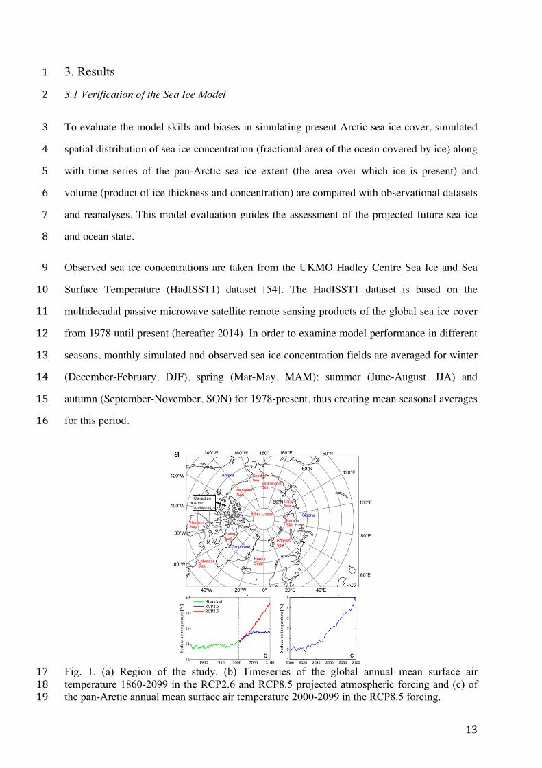
To evaluate the model skills and biases in simulating present Arctic sea ice cover, simulated 3
spatial distribution of sea ice concentration (fractional area of the ocean covered by ice) along 4
with time series of the pan-Arctic sea ice extent (the area over which ice is present) and 5
volume (product of ice thickness and concentration) are compared with observational datasets 6
and reanalyses. This model evaluation guides the assessment of the projected future sea ice 7
and ocean state. 8
Observed sea ice concentrations are taken from the UKMO Hadley Centre Sea Ice and Sea 9
Surface Temperature (HadISST1) dataset [54]. The HadISST1 dataset is based on the 10
multidecadal passive microwave satellite remote sensing products of the global sea ice cover 11
from 1978 until present (hereafter 2014). In order to examine model performance in different 12
seasons, monthly simulated and observed sea ice concentration fields are averaged for winter 13
(December-February, DJF), spring (Mar-May, MAM); summer (June-August, JJA) and 14
autumn (September-November, SON) for 1978-present, thus creating mean seasonal averages 15
for this period. 16
Fig. 1. (a) Region of the study. (b) Timeseries of the global annual mean surface air 17 temperature 1860-2099 in the RCP2.6 and RCP8.5 projected atmospheric forcing and (c) of 18 the pan-Arctic annual mean surface air temperature 2000-2099 in the RCP8.5 forcing. 19

14
The realism of the simulated variability and trends in sea ice are assessed by comparing 1
monthly timeseries of sea ice extent obtained from HadISST1 with those from the model and 2
by comparing simulated sea ice volumes with those from the Pan-Arctic Ice-Ocean Modeling 3
and Assimilation System reanalysis (PIOMAS) [55]. The sea ice extent time series is 4
computed by summing two-dimensional monthly sea ice extent fields for 1978-2013 over the 5
area north of 65°N, including the Arctic Ocean, the Arctic shelf seas and the waters of the 6
Canadian Arctic Archipelago, the Nordic Seas, the Baffin Bay, but excluding the Hudson 7
Strait and Bay, the Labrador and Bering seas (Fig. 1a). The simulated volumes are integrated 8
over the area above for 1979-2005 and compared to those from the PIOMAS. 9
The sea ice state for the current climate (1970s–2010s) simulated by NEMO-ROAM025 10
agrees with data (Fig. 2 and 3). Winter ice fractional concentration (or ice fraction) in the 11
model and data is in good agreement (Fig. 2a,c). In the model there is a moderate 12
underestimation of summer sea ice fraction north-east of Svalbard and an overestimation of 13
ice summer fraction the Chukchi and East Siberian seas (Fig. 2b, d). The simulated sea ice 14
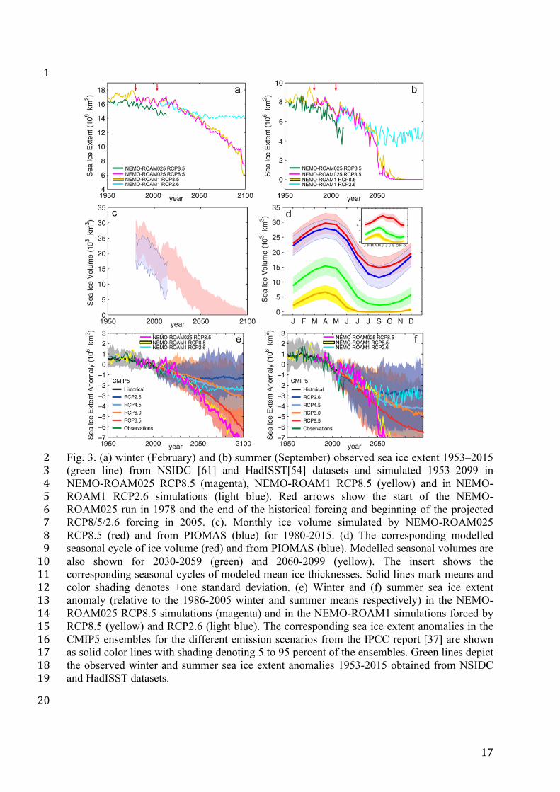
extent and volume trends are consistent with that currently observed (Fig. 3a,b,c), although 15
the model overestimates both sea ice extent by about 7 percent and 15 percent in the winter in 16
the summer respectively (Fig. 3a,b) and annual volume by about 15 percent (Fig. 3c,d). 17
3.2 Changes in Sea Ice 18
The NEMO-ROAM025 high-resolution forward projection, forced with the RCP8.5 scenario, 19
and the lower-resolution NEMO-ROAM1 forced by both RCP8.5 and RCP2.6 forcing give a 20
consistent picture of sea ice changes in the 21st century, as compared to the CMIP5 model 21
scenarios (Fig. 3e,f) [24,37]. Both NEMO-ROAM simulations and the corresponding IPCC 22
AR5 RCP8.5 models appear similarly too conservative in predicting currently observed sea 23
ice decline (sea ice reduction in the models is too low) [56-59]. Moreover, there is a little 24
difference in both, the sea ice extent and volume between the NEMO-ROAM025 and 25

15
1
Fig. 2. (a,c,e) Mean 1978-2005 winter (Dec–Feb) and (b,d,f) summer (Jun–Aug) sea ice 2 fraction (color and black contours) from the HadISST1 [54] (a, b) and from the NEMO-3 ROAM025 model (c, d). (e) Model winter (Dec–Feb) and (f) summer (Jun–Aug) 2030–2039 4 ice fraction from the NEMO-ROAM025 RCP8.5 projection (color and black contours). 5

16
NEMO-ROAM1 forced forward projections on one hand, and the respective HadGEM2-ES 1
coupled simulations on the other (cf., Fig. 3a,b,c and Fig. 3 and 4 in [60]). Since, the forced 2
and coupled models show a similar sea ice response to the warming, the conservative biases 3
in the projections are not due to the lack of ocean-ice-atmosphere feedbacks, but because of 4
deficiencies in the physical description of the underlying sea ice processes [57,59]. Until the 5
2050s NEMO ROAM projections closely follow the CMIP5 RCP8.5 ensemble mean and for 6
the 2060s-2090s are within 5-95 percent of the CMIP5 ensemble (Fig. 3e,f). 7
The RCP8.5 scenario presents a substantial increase in global and Arctic surface air 8
temperatures (SAT) (Fig. 1b,c) and in Arctic sea surface temperature (SST). Between the 9
2000s and 2090s, SST in the Arctic Ocean and Siberian seas increases by about 2°C in the 10
winter and by about 7°C in the summer, reaching averaged values of about 2-3°C and 5-8°C 11
in the winter and summer respectively (not shown). Similar to the CMIP5 RCP8.5 model 12
ensemble, the model presents conservative simulations for the current sea ice climate (Fig. 13
3e,f). The NEMO-ROAM1 sea ice simulations with RCP8.5 are similar to those with NEMO-14
ROAM025, except for the last ten years of the integrations, when ice in NEMO-ROAM025 15
declines more slowly than in NEMO-ROAM1 in the winter and more rapidly in the summer. 16
In both runs the shape of the volume seasonal cycle does not change with declining ice, 17
although there is a clear reduction in the mean and the amplitude of the cycle. The seasonal 18
cycle of mean ice thickness changes: the maximum shifts from June to May and the 19
secondary maximum in September, due to melting of first-year ice, disappears (Fig. 3d). In 20
the model projection, summer ice retreats first in the Eurasian Arctic and in the Siberian seas 21
(Fig. 2) but there are only moderate changes in winter ice extent until the 2030s, from 16.2 22
million km2 in 2000-2009 to 14.8 million km2 in 2030-2039 (area changed from 15.4 million 23
km2 to 14.1 million km2) (Fig. 3a,b). Ice retreats more rapidly from the 2030s with ice extent 24
reaching 8.8 million km2 (area of 7.7 million km2) in the Arctic by the 2090s (Fig. 3a,b). 25
17
1
Fig. 3. (a) winter (February) and (b) summer (September) observed sea ice extent 1953–2015 2 (green line) from NSIDC [61] and HadISST[54] datasets and simulated 1953–2099 in 3 NEMO-ROAM025 RCP8.5 (magenta), NEMO-ROAM1 RCP8.5 (yellow) and in NEMO-4 ROAM1 RCP2.6 simulations (light blue). Red arrows show the start of the NEMO-5 ROAM025 run in 1978 and the end of the historical forcing and beginning of the projected 6 RCP8/5/2.6 forcing in 2005. (c). Monthly ice volume simulated by NEMO-ROAM025 7 RCP8.5 (red) and from PIOMAS (blue) for 1980-2015. (d) The corresponding modelled 8 seasonal cycle of ice volume (red) and from PIOMAS (blue). Modelled seasonal volumes are 9 also shown for 2030-2059 (green) and 2060-2099 (yellow). The insert shows the 10 corresponding seasonal cycles of modeled mean ice thicknesses. Solid lines mark means and 11 color shading denotes ±one standard deviation. (e) Winter and (f) summer sea ice extent 12 anomaly (relative to the 1986-2005 winter and summer means respectively) in the NEMO-13 ROAM025 RCP8.5 simulations (magenta) and in the NEMO-ROAM1 simulations forced by 14 RCP8.5 (yellow) and RCP2.6 (light blue). The corresponding sea ice extent anomalies in the 15 CMIP5 ensembles for the different emission scenarios from the IPCC report [37] are shown 16 as solid color lines with shading denoting 5 to 95 percent of the ensembles. Green lines depict 17 the observed winter and summer sea ice extent anomalies 1953-2015 obtained from NSIDC 18 and HadISST datasets. 19
20

18
3.3 Changes in Ocean Circulation 1
The oceanic geostrophic balance (i.e., ocean pressure gradient is balanced by the Coriolis 2
force) holds in the Arctic Ocean (except for near surface fresh water-driven flows) for time 3
averaging longer than a month, which permits the ocean circulation to be analyzed using the 4
Montgomery function, mapped on pseudo-neutral surfaces [43]. 5
The method allows the use of scalar stream-function-like surfaces instead of the vector fields, 6
and simplifies analysis of the ocean circulation and attribution of driving mechanisms. The 7
present analysis is focused on the effects of wind on the upper ocean dynamics (down to 600 8
m depth). To examine the changes in the surface ocean currents two-dimensional fields of sea 9
surface height are analyzed as an approximation of the geostrophic surface circulation. 10
Like the sea ice, the surface circulation shows a large change after the 2040s. The anti-11
cyclonic circulation in the Beaufort Sea of the Canadian Basin, a characteristic of the present-12
day Arctic circulation [62,63], disappears, and a large cyclonic gyre develops in the western 13
Arctic Ocean, with a strong localized anti-cyclonic gyre in the East-Siberian Sea and in the 14
eastern Canadian Basin (Fig. 4a,b). The principal driving mechanism is reduction of the high 15
atmospheric sea level pressure (SLP) in the Beaufort Sea and decrease of the Ekman 16
convergence in the Beaufort Gyre [64]. The other feature is the “short-circuiting” of the 17
Arctic surface circulation in the Nordic Seas, resulting in the Arctic surface waters 18
recirculating back in the Arctic Ocean, instead of flowing out into the North Atlantic (Fig. 19
4a,b). The Montgomery potential shows a similar change from a weak cyclonic boundary 20
flow at intermediate (200-600m) depths in the Canadian Basin after the 2040s (Fig. 4c,d). 21
This change also results from changes in the atmospheric wind, which increase the high 22
oceanic pressure (high Montgomery potential) in the Central Arctic in the 2090s and block 23
the boundary current emerging northwards from the Barents Sea driven by the high oceanic 24
pressure that is present in the Barents Sea before the 2040s (Fig. 4c,d). 25

19
Fig. 4. Model mean sea surface heights (a) in 2040-2049 and (b) change between 2000–2009 1 and 2090–2099 from RCP8.5 NEMO projection. Mean 2040–2049 (c) and 2090–2099 (d) 2 Montgomery potential (equivalent of geostrophic streamfunctions) at the 27.8 kg/m3 density 3 surface (about 300-600 m depth) from the same projection. 4
3.4 Accessibility of Summer Shipping Routes 5
Following the method described in Section 2.2, the ships safe speed (SS) on the NPR is 6
calculated for the 7 ship classes (CAC3, CAC4, and Types A-E) for the projected averaged 7
summer sea ice conditions in 2010-2019 and 2030-2039. For each model cell Ice Multipliers 8
(IM) and Ice Numerals (IN) are computed (Tables 1 and 2). To obtain the corresponding 9
sailing time (ST) on the NPR, the shortest path in the model domain between Aberdeen (UK) 10
and Bering Strait is defined (Fig. 5). In addition, optimized routes to avoid impassible ice type 11
for each of the 7 ship classes are defined via choosing a path through the 2-D IN fields, which 12

20
steps only through the positive IN values and minimizes the distance between the port of 1
departure (Aberdeen, UK) and destination (Bering Strait). All sailing times are calculated by 2
summing up the times required to cross each of the model cells along a selected route. 3
In the 2010s, the thick and compact second year ice remains in the Central Arctic on the NPR 4
(Fig. 5a) and the route is inaccessible for the Type A-E general cargo vessels, The ice-capable 5
vessels CAC3 (PC3) and CAC4 can navigate the NPR by avoiding areas of thickest ice in the 6
Canadian Basin (Fig. 5a). The sailing time estimates are of 16-20 days for these optimised 7
routes (Table 3). To transit the high Arctic, Type A (PC6) vessels have to avoid multi-year 8
and second year pack ice and thick first-year pack ice as well. This pathway takes these 9
vessels far away from the NPR, almost along the NSR (Fig. 5a). Easier ice conditions on the 10
NSR but longer distances result in the sailing time of 20 days (Table 3). The less ice-capable 11
Type B-E are unable to safely break compact pack ice thicker than 0.7 m, therefore they 12
cannot transit the Arctic Ocean offshore and have to follow the NSR (Fig. 5a). The 13
inaccessibility of the NPR for general cargo vessels until end of the 2010s in the present 14
analysis is consistent with the results by Smith and Stephenson [26], who performed the 15
Arctic shipping accessibility analysis using the CMIP5 ensemble and concluded that the 16
direct route across the North Pole is closed for PC6 (Type A) and open water OW (Type E) 17
ship classes (Fig. 2 in [26]). 18
During the summers in the 2010s and 2020s sea ice concentration in the Central Arctic is 19
predicted to be in the range of 70-100 percent (the ocean is covered in close pack ice, very 20
close pack ice and compact pack ice [46]) and, therefore, accessibility of the NPR and 21
navigability on the route should be primarily controlled by sea ice thickness (ice types) 22
distribution along the route. To examine this, a series of optimised route scenarios with fixed 23
ice concentration and perturbations in the ice thickness fields are assessed. It should be noted 24

21
that all the calculations presented here assume unescorted sailing. If icebreakers support is 1
used, the NPR can be more accessible for the other classes of vessels. 2
In the 2030s, a large part of the NPR in summer is either ice-free or is covered in open ice (ice 3
concentration of 40-60 percent [46] (Fig. 5b) and the four ship classes, CAC3 and 4 and 4
Types A and B can safely access the route (Table 3). For the optimised routes constructed in a 5
similar way as for the 2010s, all general cargo vessels are able to navigate the NPR (Table 3). 6
With the averaged sailing times from 13 to 17 days, the navigation via the North Pole can 7
compete with coastal routes. The sailing times along the NSR were 11 days on average (range 8
of 8-19 days) for the transit shipping in 2012-13 [21,22] and the estimated projected averaged 9
sailing time is of 11 days for Type A vessels in summer 2045-2059 [12]. 10
Fig. 5. Model 2010–2019 (a) and 2030–2039 (b) sea ice concentration (percent, color) and 11 thickness (red contours) during the navigation period (Jun-Oct) from the RCP8.5 NEMO 12 projection. The Arctic shipping routes are shown schematically: the Northern Sea Route 13 (NSR) (yellow line), the North Pole Route (NPR) (green line) and the Northwest Passage 14 (NWP) and Arctic Bridge (AB) (white line). 15
The sailing times along the NPR obtained using the sea ice data from the NEMO-ROAM025 16
projection agrees well with those obtained using the ATAM with a subset of the CMIP5 17
models [12,21,27], e.g., average sailing time on the NPR in the 2040-2050s is 16 days for 18
Type A vessels vs. 15 days in the NEMO-ROAM025 analysis (Table 3). This is evident of the 19

22
validity of the current approach. The thick sea ice remains in the Canadian Basin in the 2030s 1
and affects navigation along the NWP (Fig. 5), making this route practically non-operational 2
at least until the mid-21st century [12]. 3
After the 2050s, the summer sea ice has a very low extent (less than 1 million km2) and 4
thickness (less than 0.2 m) (Fig. 3d,f) and does not affect the sailing. All types of examined 5
vessels can safely navigate the NPR. Since, a substantial areas of the ice-covered Arctic 6
Ocean are transformed to MIZ, the main factors affecting the sailing become distances along 7
the route, waves and wind. 8
3.5 Forecasting in the Marginal Ice Zone 9
Currently the summer Arctic MIZ is widening, reaching on average about 150 km in width 10
[50] (Fig. 6). The NEMO-ROAM025 projection shows a nearly two-fold increase in the MIZ 11
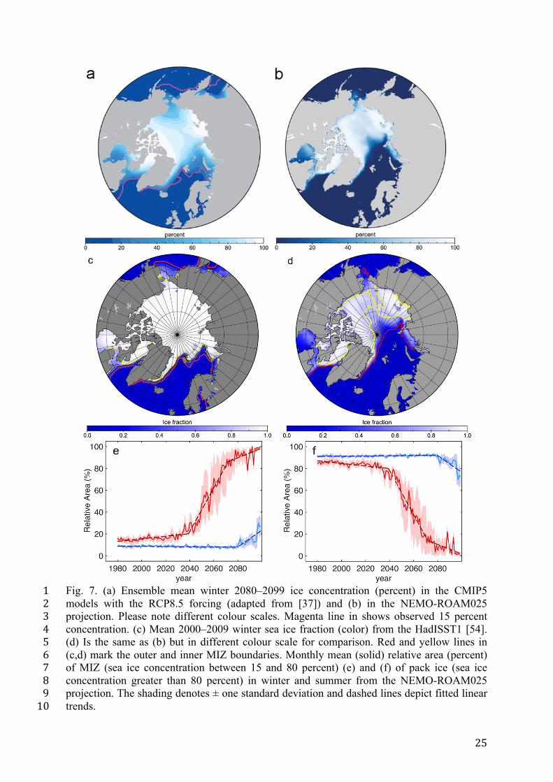
area in summer between the 1978-2005 and 2030s (Fig. 6a,b and 7e). After the 2030s the MIZ 12
relative area in the summer increases from about 20 percent to about 90 percent in the 2080s-13
90s (Fig. 7e). The simulated winter MIZ is about 10 percent in the 2000s, decreases until the 14
2080s and then increases, constituting about 30 percent of the area of the Arctic sea ice in the 15
2090s (Fig. 7c,d,e). With the summer MIZ area increasing, the pack ice (ice fraction greater 16
than 0.8) area in the summer declines in the simulations and in the 2050s has about the same 17
area as the summer MIZ (Fig. 7c,d,f). The winter pack ice does not change significantly until 18
the 2090s, when it declines to about 70-80 percent of total ice area (Fig. 7d,f). Both the 19
CMIP5 model ensembles and the NEMO-ROAM025 projection predict changes of the winter 20
ice pack concentration in the central Arctic Ocean from 90-100 percent to 70-90 percent by 21
the 2090s (Fig. 7a,b), caused by erosion of the Arctic halocline in summer, making the heat 22
from the Atlantic and Pacific inflows available to melt ice in winter. This is especially 23
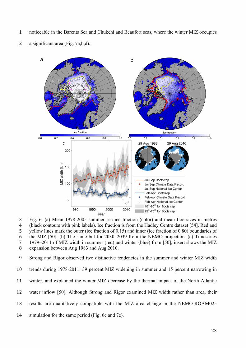
23
noticeable in the Barents Sea and Chukchi and Beaufort seas, where the winter MIZ occupies 1
a significant area (Fig. 7a,b,d). 2
Fig. 6. (a) Mean 1978-2005 summer sea ice fraction (color) and mean floe sizes in metres 3 (black contours with pink labels). Ice fraction is from the Hadley Centre dataset [54]. Red and 4 yellow lines mark the outer (ice fraction of 0.15) and inner (ice fraction of 0.80) boundaries of 5 the MIZ [50]. (b) The same but for 2030–2039 from the NEMO projection. (c) Timeseries 6 1979–2011 of MIZ width in summer (red) and winter (blue) from [50]; insert shows the MIZ 7 expansion between Aug 1983 and Aug 2010. 8
Strong and Rigor observed two distinctive tendencies in the summer and winter MIZ width 9
trends during 1978-2011: 39 percent MIZ widening in summer and 15 percent narrowing in 10
winter, and explained the winter MIZ decrease by the thermal impact of the North Atlantic 11
water inflow [50]. Although Strong and Rigor examined MIZ width rather than area, their 12
results are qualitatively compatible with the MIZ area change in the NEMO-ROAM025 13
simulation for the same period (Fig. 6c and 7e). 14

24
In this emerging state of the Arctic Ocean, when open sea ice cover conditions dominate, sea 1
ice fragmentation (floe sizes), wind and waves become the prevailing factors affecting Arctic 2
navigation (e.g., EU Project “Ships and Waves Reaching Polar Regions”, 3
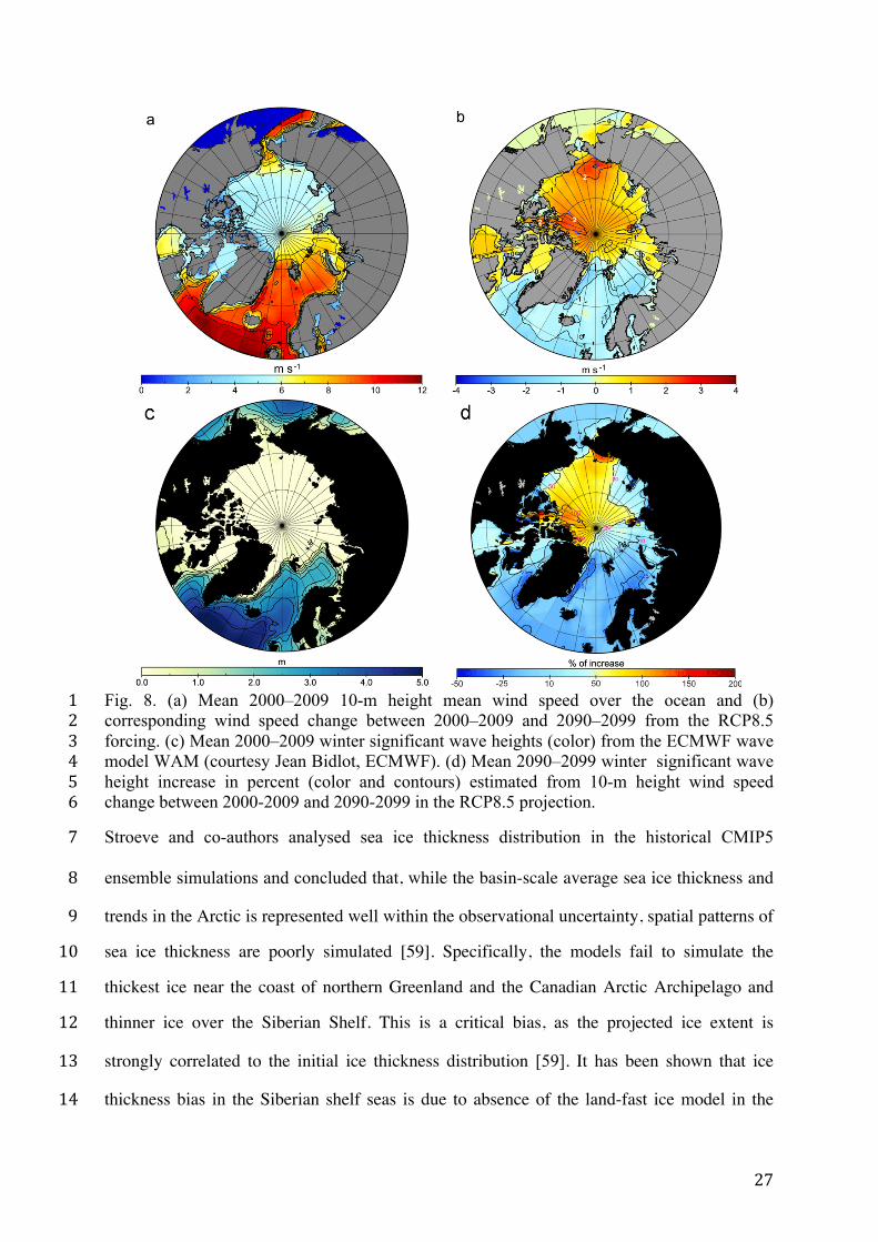
http://swarp.nersc.no/). The RCP8.5 forcing demonstrates an increase in winter (DJF) wind 4
speed in the Arctic Ocean by about 50 percent on average (Fig. 8a,b). 5
Fig. 8c,d shows that this is accompanied by an increase in significant wave heights in the 6
Arctic Ocean by about 100 percent on average. (See Section 2.5 for the calculation method). 7
The ice becomes more fragmented, with the maximum floe size in the Arctic Ocean 8
decreasing from about 100-1000m to less than 50m in the 2030s, whereas the floe size in the 9
MIZ decreases to less than 25 m (Fig. 6a,b). With Arctic sea ice shrinking and becoming 10
thinner, the influence of surface waves is stronger. Consequently, a larger part of the sea ice 11
cover acquires dynamic and thermodynamic properties resembling those in the MIZ, rather 12
than the pack ice (Fig. 6 and 7a,b). These changes require revised approaches to improve the 13
skills of operational simulations and forecasts. Specifically sea ice break-up by the ocean 14
waves and dynamics of the highly fragmented sea ice floes needs to be included in 15
operational modeling [53]. 16
The above approach is taken by the operational modeling and forecasting system TOPAZ 17
(Towards an Operational Prediction system for the North Atlantic European coastal Zones, 18
http://topaz.nersc.no/, [65]. A waves-in-ice module (WIM), which describes propagation and 19
attenuation of waves into ice-covered areas and mechanical breaking of sea ice floes is 20
implemented in the system [53,66,67]. TOPAZ runs experimental forecasts for the North 21
Atlantic and Arctic Ocean at 11-16-km resolution. The system also has a data assimilation 22
component based on the Ensemble Kalman Filter [65]. To study the impact of surface waves 23
during the August 2012 event of strongly enhanced melting in the Arctic Ocean, the WIM has 24
been used in a two week long experiment. A strong low-pressure system builds up over a few 25
25
Fig. 7. (a) Ensemble mean winter 2080–2099 ice concentration (percent) in the CMIP5 1 models with the RCP8.5 forcing (adapted from [37]) and (b) in the NEMO-ROAM025 2 projection. Please note different colour scales. Magenta line in shows observed 15 percent 3 concentration. (c) Mean 2000–2009 winter sea ice fraction (color) from the HadISST1 [54]. 4 (d) Is the same as (b) but in different colour scale for comparison. Red and yellow lines in 5 (c,d) mark the outer and inner MIZ boundaries. Monthly mean (solid) relative area (percent) 6 of MIZ (sea ice concentration between 15 and 80 percent) (e) and (f) of pack ice (sea ice 7 concentration greater than 80 percent) in winter and summer from the NEMO-ROAM025 8 projection. The shading denotes ± one standard deviation and dashed lines depict fitted linear 9 trends. 10

26
days and generates high amplitude surface waves that are able to travel into the ice-cover and 1
break up the ice into smaller floes (Fig. 9). For instance, the area of broken ice is 2
comparatively larger on the Pacific side of the Arctic where the storms have generated strong 3
waves. 4
4. Discussion 5
Several studies have suggested that an Arctic annual surface air temperature increase of ca. 2-6
3°C has been observed during the last three decades between 1971-2000 and 2001-2012, with 7
the trends about twice higher than those from the RCP8.5 scenario [68,69]. Therefore, it 8
appears possible that the current emissions in the future may lead to even higher Arctic 9
temperatures than climate model simulations with the RCP8.5 emission scenario predict. This 10
could result in faster sea ice decline in the Arctic, than present day climate scenarios suggest, 11
with summer Arctic sea ice disappearance before 2040s [70]. Moreover, with present 12
perennial sea ice reduction to about 20 percent, the Arctic Ocean has become more vulnerable 13
to a potentially rapid transition toward a seasonally ice-free Arctic state, triggered by natural 14
climate variability [71]. The implications of the rapid Arctic state change for the economies of 15
the Arctic regions are anticipated to be substantial. Along with other industries, the Arctic 16
transport system and maritime industries will have to evolve on the short time scale to adapt 17
to the change and mitigate potential consequences [12,44]. The analysis presented in this 18
study suggests that the unescorted navigation in the high Arctic in the summer is possible as 19
early as the 2030-2040s and is probable after the 2050s. The winter seasonal ice in the Arctic 20
will be more fragmented than at present, and its mean thickness will be greatly reduced to 21
about 1 m in the mid 21st century and to about 0.5m in the second half of the century (Fig. 3d). 22
The winter navigation in the high Arctic most likely will still require support from icebreakers 23
due to highly variable sea ice and ocean conditions in this season. 24
27
Fig. 8. (a) Mean 2000–2009 10-m height mean wind speed over the ocean and (b) 1 corresponding wind speed change between 2000–2009 and 2090–2099 from the RCP8.5 2 forcing. (c) Mean 2000–2009 winter significant wave heights (color) from the ECMWF wave 3 model WAM (courtesy Jean Bidlot, ECMWF). (d) Mean 2090–2099 winter significant wave 4 height increase in percent (color and contours) estimated from 10-m height wind speed 5 change between 2000-2009 and 2090-2099 in the RCP8.5 projection. 6
Stroeve and co-authors analysed sea ice thickness distribution in the historical CMIP5 7
ensemble simulations and concluded that, while the basin-scale average sea ice thickness and 8
trends in the Arctic is represented well within the observational uncertainty, spatial patterns of 9
sea ice thickness are poorly simulated [59]. Specifically, the models fail to simulate the 10
thickest ice near the coast of northern Greenland and the Canadian Arctic Archipelago and 11
thinner ice over the Siberian Shelf. This is a critical bias, as the projected ice extent is 12
strongly correlated to the initial ice thickness distribution [59]. It has been shown that ice 13
thickness bias in the Siberian shelf seas is due to absence of the land-fast ice model in the 14

28
simulations [72,73]; most of the present-day climate models do not include fast ice physics. 1
On the other hand, the MIZ dynamics is also poorly represented in the climate models [74], 2
which historically use ice rheology developed for compact thick pack ice in the central Arctic 3
[75]. The above and many other examples demonstrate importance of advanced, physically 4
based sea ice models for the accurate predictions of Arctic sea ice evolution and decline. The 5
ice thickness is a key parameter for assessing shipping routes navigability and time 6
expenditures. Despite advances in the satellite technology, sea ice thickness observations are 7
still difficult to make on the routine basis and during all seasons [59] and model reanalysis 8
and predictions are still the main source of this vital information. 9
The simulations presented in this study project a 50 percent increase in the significant wave 10
height !! (Fig. 8). Both observations and the hindcast simulations already show an increase 11
in !! in the Arctic Ocean between the 1990s and 2010s, with the average !! doubling in the 12
Chukchi and Beaufort Seas [76]. Over this period extreme wave heights have also increased 13
and their recurrence has more than doubled [76]. Thomson and Rogers present observations 14
of !! reaching over 5 metres in the Beaufort Sea in September 2012 [52]. This increase in 15
!! is attributed to the thinning of sea ice and a longer wave fetch [76]. Since most projections 16
(including the present HaDGEM2 projection) also suggest a significant (50 percent or more) 17
increase in the wind speed, a larger than 100 percent increase in !! in the Arctic Ocean in the 18
21st century is probable [77]. Higher winds and waves, combined with subzero air 19
temperature in the winter, may increase the danger of icing, which has accounted for a 20
substantial number of ship accidents and shipwrecks on the NSR [78]. This poses significant 21
challenges to navigation and offshore exploration, as well as for the ship classification and 22
insurance industries. 23
Another key result from the simulation is a significant change in the Arctic Ocean circulation, 24
at the surface as well as at depth. By the 2090s the cyclonic flow of the intermediate water in 25
the Canada Basin becomes anti-cyclonic and the boundary current in the Canadian Basin and 26

29
the Laptev Sea reverses. The changes are similar to those discussed by Karcher and co-1
workers [79]. In their paper the changes in wind and reduction of sea ice cover were 2
responsible for modification of the momentum transfer from atmosphere to the ocean, leading 3
to an increased anti-cyclonicity in the ocean circulation and reversal of currents. Our forward 4
simulation suggests a potentially complex picture of the future Arctic Ocean Change, 5
highlighting the importance of high-resolution forecasts and challenging the views that most 6
of the changes in the Arctic concern sea ice and the atmosphere. 7
Fig. 9. Examples of Arctic wave and ice forecasts with the Towards an Operational Prediction 8 system for the North Atlantic European coastal Zones (TOPAZ): (a) maximum significant 9 wave heights (color) on 6 Aug 2012 12.00 GMT and (b) the same but for maximum floe size 10 (http://topaz.nersc.no/). 11
The changes in the Arctic ocean surface and subsurface currents may potentially affect 12
planning of maritime operations in several ways. Firstly, in the absence of sea ice, surface 13
currents become one of the prime factors influencing ship safety, safe speed and sailing times. 14
Secondly, they impact the redistribution of icebergs around Greenland and in the Canadian 15
Arctic Archipelago. Due to a potential “short-circuiting” of the Arctic surface circulation in 16
the Nordic Sea (Fig. 4) some Greenland icebergs may potentially reach Arctic shipping routes. 17
Simulations with an iceberg model coupled to the NEMO OGCM [80] show iceberg spread in 18
the central Arctic Ocean. Lastly, the environmental impact of potential shipping accidents or 19

30
pollution during the navigation will depend on ocean currents. The pathways can be addressed 1
using high-resolution simulations to track pollutant spread by ocean currents and sea ice. 2
5. Conclusions and Policy Implications 3
According to the simulations, before the 2030s the principal factors for navigation and ship 4
safety are the sea ice conditions. For long term planning, as well as for operational support of 5
navigation and maritime industry, the present transport accessibility models which use static 6
information such as sea ice concentration and sea ice types (e.g. ATAM) are adequate in the 7
pack ice areas. However, the acceleration in sea ice drift that has occurred in the last decade 8
requires accounting for sea ice dynamics, i.e., ice drift and ice internal pressure due to sea ice 9
convergence and compression [81]. Marchenko analysed shipping accidents and shipwrecks 10
on the NSR occurring between the 1930s and 1990s and concluded that ice drift and 11
compression caused about a half of the shipwrecks [78,82], highlighting ice jets (a rapid sea 12
ice flow between drifting and land-fast ice, typically generated by storm surges) as the most 13
dangerous phenomenon for marine transportation in the area. 14
For more detailed short-term forecasting, a route optimization algorithm is needed to estimate 15
sailing times and accessibility projections should be extended by developing a route 16
optimization tool to estimate the fastest trans-Arctic route given the ice conditions for a 17
particular season and year [26,83] Additional improvements of the optimal route simulations 18
are envisaged since the present-day coupled atmosphere–ocean general circulation models are 19
continue incorporating more advanced representation of sea ice, ocean and atmosphere 20
physics, amongst these, ice ridging and thermal decay affect shipping the most [26]. 21
After the 2030s, when pack ice begin to decline and MIZ-type sea ice provinces emerge, new 22
approaches to forecasting should be considered. The new transport and accessibility models 23
will require more information, including forecasts of winds, currents and waves. More 24

31
detailed sea ice data will also be required, such as sea ice floe sizes and ice drift parameters. 1
Definitions of sea ice mechanical properties (used for example by oil-rig designers) may need 2
revisiting, as sea ice would be thinner, more saline and weaker [84]. 3
Presently, Arctic exploitation is the centre of discussion, weighing mitigation of consequences 4
of the Arctic changes against potential economical benefits. Therefore there is a little surprise, 5
that after a century of intensive Arctic exploration and more than a six decades of using Arctic 6
shipping routes, the economical viability of Arctic shipping is still debated [85]. The 7
challenges are great and lie in balancing economic drivers in Europe, the Americas and in the 8
far-eastern countries, such as China, Malaysia, Singapore, Taiwan [86,87], economic risk [85] 9
a need for Arctic infrastructure development, accessible modern ports, roads, etc. [88], and 10
also the impact on the Arctic communities, ecosystems, as well as political and social drivers. 11
Another caveat is that, while the shift of shipping to shorter Arctic routes may decrease fuel 12
use and lower CO2 emissions, the impact on climate warming may not be wholly negative. 13
This is because the use of Arctic routes may lead to increased concentrations of non-CO2 14
gases, aerosols and particles in the Arctic, which can change radiative forcing (e.g. deposition 15
of black carbon on sea ice and snow) and produce more complex regional warming/cooling 16
effects. Simulations of these aspects of Arctic routes suggest that there may actually be a net 17
global warming effect before net cooling takes over [89], thus suggesting that changes in the 18
Arctic maritime use could potentially affect the global economy and global natural 19
environment. 20
The changes in the Arctic natural environment are occurring faster than elsewhere in the 21
world, and are likely to continue that way for the next few decades with an increased 22
variability of the environmental parameters. They require a system-based approach, 23
combining expertise in different areas, natural and social sciences, engineering, economics, 24

32
law, policymaking and ecology, capitalizing on the synergy between disciplines. This requires 1
cross-subject international collaboration and close links between science, engineering and 2
industry. For the shipping industry it is important to initiate cooperation with the forecasting, 3
climate modeling, sea ice, oceanographic and atmospheric observational and modelling 4
communities in order to establish requirements for the environmental data and forecasts [23]. 5
This will help assessing the potential benefits and risks of Arctic maritime operations and 6
make them safe. 7
The present study gives an overview of potential changes in the Arctic relevant to the 8
operation of the sea routes and discusses approaches and challenges in modelling them. The 9
study neither advocates the usage of the Arctic routes, nor presents a complete forecast of the 10
Arctic conditions suitable for detailed shipping planning. For the former, it necessitates a 11
comprehensive socio-economic analysis of Arctic navigation, which is beyond the scope of 12
this study, whereas the latter requires further in-depth modelling studies addressing 13
uncertainties in future projections. To the best of the authors’ knowledge, this study presents 14
one of the first attempts to combine comprehensive detailed high-resolution environmental 15
information on the future state of sea ice and ocean in the Arctic for practical use by the 16
shipping industry. 17
The study is linked to several oceanographic initiatives and projects and specifically co-18
operates with the EU FP7 SWARP Project on introducing ocean wave information and ice 19
break up in the MIZ, as well as with UKMO Earth System Model (ESM) development. With 20
this study the authors have attempted to demonstrate the need for closer interactions between 21
environmental science, engineering and industry in a changing global environment and 22
envisage strong benefits from creating these links. 23
24

33
Acknowledgements 1
The authors are grateful to Dr. Andrew Coward (NOC) for the help with the global NEMO-2
ROAM model configuration and Jean Bidlot (ECMWF) for providing the study with the 3
WAM model data. The authors are also thankful to Prof Kay Riska (Total) for his 4
illuminating talk on the present-day Arctic maritime operations, presented at the Sea Ice 5
Royal Society Meeting in September 2014 and for his comments on the manuscript, to Dr 6
Scott Stephenson (University of Connecticut, CT, USA) for his enthusiasm in discussing 7
industrial and societal consequences of Arctic environmental change, and to Dr Michael Traut 8
(University of Manchester, UK) for his lecture on the impact of the commercial shipping on 9
Climate, given at the NOC in October 2014 and for the follow up conversations. The waves-10
in-ice simulation relied on the Norwegian Meteorological Institute (Met Norway) for initial 11
conditions and the Institut français de recherché pour l’exploitation de la mer (Ifremer) for 12
wave information over its duration. The manuscript was also inspired by discussions at the 13
annual Forum for Arctic Modeling and Observing Synthesis (FAMOS) meetings. The 14
authors are also grateful to the anonymous referees for the valuable comments and 15
suggestions, which helped to improve the manuscript. The authors would like to thank the 16
organisers of the Shipping in Changing Climate Conference, which took place in Liverpool in 17
June 2014 under the umbrella of International Business Festival, for providing an excellent 18
opportunity for interaction and discussions between scientists and industry. 19
Funding for the study 20
Drs. Aksenov, Bergh, Bertino, Nurser and Williams acknowledge support from European 21
Union Seventh Framework Programme SWARP (grant agreement 607476) for this research. 22
Drs. Aksenov, Nurser, Popova and Yool were also funded from the UK Natural Environment 23
Research Council (NERC) Marine Centres' Strategic Research Programme. Dr. Aksenov also 24

34
was supported from the UK NERC TEA-COSI Research Project (NE/I028947/). The authors 1
are thankful to FAMOS (funded by the National Science Foundation Office of Polar 2
Programs, awards PLR-1313614 and PLR-1203720) for travel support to attend FAMOS 3
meetings. The global simulation work in this study was performed as part of the Regional 4
Ocean Acidification Modelling project (ROAM; NERC grant number NE/H01732/1) and 5
part-funded by the European Union Seventh Framework Programme EURO-BASIN 6
(FP7/2007-2013, ENV.2010.2.2.1-1; grant agreement 264933). The study used 7
supercomputing facilities provided by the Norwegian Metacenter for Computational Science 8
(Notur). The NEMO-ROAM025 simulations were performed on the ARCHER UK National 9
Supercomputing Service (http://www.archer.ac.uk). 10
11

35
Glossary 1
AIRSS Arctic Ice Regime Shipping System AB Arctic Bridge AR Assessment Reports ATAM Arctic Transport Accessibility Model CAC Canadian Arctic Categories CICE C-ICE Los Alamos sea ice model CMIP5 Coupled Model Intercomparison Project 5 ECMWF European Center for Medium Range Weather Forecasting EEDI Energy Efficiency Design Index EU European Union EVP Elastic-Viscous-Plastic Sea Ice rheology FYI First-year ice GMES Global Monitoring for Environment and Security HadGEM2-ES Hadley Center Global Environment Earth System Model, version 2 HadISST1 Hadley Centre Sea Ice and Sea Surface Temperature IASC International Association of Classification Societies IM Ice Multiplier IMO International Maritime Organisation IN Ice Numeral INSROP International Northern Sea Route Program IPCC Intergovernmental Panel on Climate Change LIM2 Louvain-la-Neuve Sea Ice Model LNG Liquid Natural Gas MYI Multi-year ice MIZ Marginal Ice Zone NEMO Nucleus for European Modelling of the Ocean modeling framework NPR Arctic North Pole Route NSR Northern Sea Route NWP North-west Passage OGCM Ocean General Circulation Model OPA Ocean Parallelisé Model PIOMAS Pan-Arctic Ice-Ocean Modeling and Assimilation System reanalysis RCP Representative Concentration Pathways ROAM Regional Ocean Acidification Modelling SS Ship Safe Speed ST Sailing Time SWARP EU Project “Ships and Waves Reaching Polar Regions” TOPAZ Towards an Operational Prediction system for the North Atlantic European
coastal Zones UKMO UK Meteorological Office UNFCC United Nations Framework Convention on Climate Change WIM Wave in Ice Model WMO World Meteorological Organisation
2

36
Appendix 1. Calculation of safe ship speed and sailing times 1
Following the Arctic Transport Accessibility Model (ATAM) of Stephenson et al. (2011b), 2
the Ice Numerals (IN) are given by (1): 3
!" = !!"×!"!" + !!×!"! + !!"×!"!" + !!"!×!"!"! + !!"!×!"!"! +
+!!"#×!"!"# + !!"#×!"!"# + !!"×!"!" + !!"×!"!"
(1), 4
where !!",!,!",…,!" and !!!",!,!",…,!" is the sea ice concentration for different Ice Types 5
(IT) and corresponding Ice Multipliers (IM) (Table 1). Ice Types are derived from the mean 6
sea ice thickness in the model cell (Table 1), as it is a good representation of the ice stage of 7
ice development (ice age), (e.g., Maskanik et al, 2007). From the Ice Numerals, the safe ship 8
speed (SS) is defined for each grid cell on a shipping route (Table 2). The sailing time (ST) is 9
defined by adding the time required to cross all model cells along the route (2). 10
!" = !!!!!
!!!! (2). 11
Here !! and !!! are the distances across- and ship safe speed for- each model cell. !! is 12
calculated as a half of the distance between the central points of two model cells along the 13
chosen sailing track, and there are a total of N model cells along the sailing track. 14
15

37
Appendix 2. Maximum floe sizes 1
Maximum sea ice floe size can be empirically related to sea ice concentration as follows 2
(Lüpkes et al., 2012): 3
!! = !!"# 1− !∗ !!
(3). 4
Here - is the minimum flow size, ! is an exponent to fit the observational the data (here 5
! = 1), and ! and !∗ – are the actual and maximum sea ice concentration, where the latter 6
can be written as below: 7
!∗ = 1− !!"# !!"# !! ! (4). 8
9
Lmin

38
Tables 1
Table 1. Ice Multipliers (IM) for different Ice Types and Ship Classes (Arctic Ice Regime 2 Shipping System, 1998). Details are in the text 3 4
WMO
Ice Type
WMO Ice
Thickness
(m)
Ship Classes
Type E (OW)
Type D Type C Type B Type A (PC6)
CAC4 CAC3 (PC3)
MY 300-‐400* -4 -4 -4 -4 -4 -3 -1
SY 250-‐300* -4 -4 -4 -4 -3 -2 1
TFY 120-‐250* -3 -3 -3 -2 -1 1 2
MFY 70-‐120 -2 -2 -2 -1 1 2 2
FY 2 50-‐70 -1 -1 -1 1 2 2 2
FY 1 30-‐50 -1 -1 1 1 2 2 2
GW 15-‐30 -1 1 1 1 2 2 2
G 10-‐15 1 2 2 2 2 2 2
Ni <10 2 2 2 2 2 2 2
5
Table 2. Ship safe speed (SS) in nautical miles per hour (nm/h) by Ice Numeral (IN) (Table 1) 6 following AIRSS (Arctic Ice Regime Shipping System, 1998) and Stephenson et al. (2011a,b) 7 8
Ice Numeral Safe speed (nm/h)
<0 0 (Impassable/not safe)
0-8 4
9-13 5
14-15 6
16 7
17 8
18 9
19 10
20 11
9 10

39
Table 3. Predicted averaged sailing time (ST) in days for different Ship Classes (Arctic Ice 1 Regime Shipping System, 1998) along the NPR for the summers 2010-2019 and 2030-2039; 2 n/s - marks sailing is not safe; number in brackets show sailing time for the routes optimised 3 to avoid impassible ice type for different ship classes (Table 1). 4 5
Ship Class NPR ST
2010-2019
(days)
NPR ST
2030-2039
(days)
CAC3
(PC3)
n/s (16) 13
CAC4 n/s (19) 13
Type A
(PC6)
n/s (20) 15
Type B n/s (20) 16
Type C n/s (21) n/s (16)
Type D n/s (21) n/s (17)
Type E
(OW)
n/s (21) n/s (17)
Range (16- 21) 13-16(17)
6
7
40
References 1
[1] Heitmann N, Khalilian S. Accounting for carbon dioxide emissions from international 2
shipping: burden sharing under different UNFCCC allocation options and regime 3
scenarios. Mar. Policy 2011; 35(5): 682–691. 4
[2] Anderson K, Bows A. Beyond ‘dangerous’ climate change: emission scenarios for a new 5
world. Phil Trans R Soc A: Math Phys Eng Sci 2011; 369: 20-44. 6
[3] Anderson K, Bows A. Executing a Scharnow turn: reconciling shipping emissions with 7
international commitments on climate change. Carbon Manage 2012; 3(6): 615–28. 8
[4] Bows-Larkin A, Anderson K, Mander S, Traut M, Walsh C. Shipping charts a high carbon 9
course. Nature Climate Change 2015; 5: 293-95. 10
[5] Bazari Z, Longva T. Assessment of IMO mandated energy efficiency measures for 11
international shipping. Estimated CO2 emissions reduction form introduction of 12
mandatory technical and operational energy efficiency measures for ships. Project Final 13
Report, MEPC 63/INF.2, October 31, 2011. 14
[6] International Maritime Organization. Reduction of GHG emissions from ships. Third IMO 15
GHG Study 2014 - Executive Summary and Final Report. MEPC 67/INF.3, June 2014. 16
[7] Traut M, et al. Propulsive power contribution of a kite and a Flettner rotor on selected 17
shipping routes. Applied Energy 2014; 113: 362-72. 18
[8] Eide MS, Longva T, Hoffmann P, Endresen Ø, Dalsøren SB. Future cost scenarios for 19
reduction of ship CO2 emissions. Maritime Policy and Management 2011; 38(1): 11-37, 20
DOI: 10.1080/03088839.2010.533711. 21
[9] Eide MS, Endresen Ø, Skjong R, Longva T, Alvik S. Cost-effectiveness assessment of 22
CO2 reducing measures in shipping. Maritime Policy and Management 2009; 36(4): 367-23
84, DOI: 10.1080/03088830903057031. 24

41
[10] Schøyen H, Bråthen S. The Northern Sea Route versus the Suez Canal: cases from bulk 1
shipping. J Transport Geography 2011; 19(4): 977-83. 2
[11] Liu M, Kronbak J. The potential economic viability of using the Northern Sea Route 3
(NSR) as an alternative route between Asia and Europe. J Transport Geography 2010; 4
18(3): 434-44. 5
[12] Stephenson SR., Smith LC, Agnew JA. Divergent long-term trajectories of human access 6
to the Arctic. Nature Climate Change 2011; 1: 156-60, DOI: 10.10-38/NCLIMATE1120. 7
[13] Farré AB, Stephenson SR, Chen L, Czub M, Dai Y, Demchev D, Efimov Y, et al. 8
Commercial Arctic shipping through the Northeast Passage: routes, resources, 9
governance, technology, and infrastructure. Polar Geography 2014; 37(4): 298-324, DOI: 10
10.1080/1088937X.2014.965769. 11
[14] Brubaker RD, Ragner CL. A review of the International Northern Sea Route Program 12
(INSROP) - 10 years on. Polar Geography 2010; 33(1-2): 15-38, DOI: 13
10.1080/1088937X.2010.493308. 14
[15] Andersen Ø, Heggeli TJ, Wergeland T. III.10.1: Assessment of Potential Cargo from and 15
to Europe via the NSR. INSROP Working Paper 11-1995. Lysaker: INSROP Secretariat; 16
1995. 17
[16] Tamvakis M, Granberg A, Gold E. Economy and commercial viability. In: Ostreng W, 18
editor. The Natural and Societal Challenges of the Northern Sea Route: A Reference 19
Work. Dordrecht/Boston/London: Kluwer Academic Publishers; 1999. 20
[17] Ragner CL. Northern Sea Route Cargo Flows and Infrastructure – Present State and 21
Future Potential. FNI Report 13/2000. Lysaker: Fridtjof Nansen Institute; 2000. 22
[18] Ragner CL. The Northern Sea Route - Commercial Potential, Economic Significance, 23
and Infrastructure Requirements. Post-Soviet Geography and Economics 2000; 41(8): 24
541-80. Available at: <http://dx.doi.org/10.1080/10889388.2000.10641157>. 25

42
[19] Mitchell T, Milne R. Chinese cargo ship sets sail for Arctic short-cut. Financial Times, 1
August 11, 2013. Available at: <http://www.ft.com>. 2
[20] Brigham LW, Ellis B, editors. Arctic marine transport workshop (Scott Polar Research 3
Institute, University of Cambridge, 28–30 September 2004). Institute of the North, US 4
Arctic Research Commission, International Arctic Science Committee. Anchorage (AK): 5
Northern Printing; 2004. 6
[21] Stephenson SR, Brigham LW, Smith LC. Marine accessibility along Russia's Northern 7
Sea Route. Polar Geography 2014; 37(2): 111-33, doi:10.1080/1088937X.2013.845859. 8
[22] North Sea Route Information Office. 2015. Available at: <http://www.arctic-9
lio.com/nsr_transits>. 10
[23] Rogers TS, et al. Future Arctic marine access: analysis and evaluation of observations, 11
models, and projections of sea ice. The Cryosphere 2013; 7: 321-32. 12
[24] Flato G, Marotzke J, Abiodun B, Braconnot P, Chou SC, Collins W, Cox P, Driouech F, 13
Emori S, Eyring V, Forest C, Gleckler P, Guilyardi E, Jakob C, Kattsov V, Reason C, 14
Rummukainen M. Evaluation of Climate Models. In: Stocker TF, Qin D, Plattner GK, 15
Tignor M, Allen SK, Boschung J, Nauels A, Xia Y, Bex V, Midgley PM, editors. Climate 16
Change 2013: The Physical Science Basis. Contribution of Working Group I to the Fifth 17
Assessment Report of the Intergovernmental Panel on Climate Change. Cambridge (UK) 18
and New York (NY): Cambridge University Press; 2013. 19
[25] Vaughan DG, et al. Observations: Cryosphere. In: Stocker TF, Qin D, Plattner GK, 20
Tignor M, Allen SK, Boschung J, Nauels A, Xia Y, Bex V, Midgley PM, editors. Climate 21
Change 2013: The Physical Science Basis. Contribution of Working Group I to the Fifth 22
Assessment Report of the Intergovernmental Panel on Climate Change. Cambridge (UK) 23
and New York (NY): Cambridge University Press; 2013. 24
43
[26] Smith LC, Stephenson SR. New Trans-Arctic shipping routes navigable by midcentury. 1
Proceedings of the National Academy of Sciences 2013; 110(13): E1191-E1195. 2
[27] Stephenson SR, Smith LC, Brigham LW, Agnew JA. Projected 21st-century changes to 3
Arctic marine access. Climatic Change 2013; 118(3-4): 885-99. 4
[28] Riska K. Impacts on Navigation of Arctic Sea Ice Change. Proceedings of Royal Society 5
(in review) 2014. 6
[29] Nurser AJG, Bacon S. Eddy length scales and the Rossby radius in the Arctic Ocean. 7
Ocean Sci Discuss 2013; 10(5): 1807-31. 8
[30] Yool A, Popova EE, Coward AC, Bernie D, Anderson TR. Climate change and ocean 9
acidification impacts on lower trophic levels and the export of organic carbon to the deep 10
ocean. Biogeosciences 2013; 10: 5831-54. 11
[31] Madec G and NEMO team. NEMO ocean engine, version 3.4. Note du Pole de 12
modelisation de l’Institut Pierre-Simon Laplace, No 27 ISSN No 1288-1619; 2012. 13
[32] Fichefet T, Maqueda MÁM. Sensitivity of a global sea ice model to the treatment of ice 14
thermodynamics and dynamics. J Geophys Res: Oceans (1978–2012) 1997; 102(C6): 15
12609-46. 16
[33] Bouillon S, Maqueda MÁM, Legat V, Fichefet T. An elastic–viscous–plastic sea ice 17
model formulated on Arakawa B and C grids. Ocean Modelling 2009; 27(3): 174-84. 18
[34] Storkey D, Blockley EW, Furner R, Guiavarc'h C, Lea D, Martin MJ, Barciela RM, 19
Hines A, Hyder P, Siddorn JR. Forecasting the ocean state using NEMO: The new FOAM 20
system. J Operational Oceanography 2010; 3(1): 3-15. 21
[35] Dufresne J-L, Foujols M-A, Denvil S, Caubel A, Marti O, Aumont O, Balkanski Y, et 22
al. Climate change projections using the IPSL-CM5 Earth System Model: from CMIP3 to 23
CMIP5. Climate Dynamics 2013; 40(9-10): 2123-65. 24

44
[36] Rogelj J, Meinshausen M, Knutti R. Global warming under old and new scenarios using 1
IPCC climate sensitivity range estimates. Nature Climate Change 2012; 2: 248-53, 2
DOI:10.1038/NCLIMATE1385. 3
[37] Collins M, et al. Long-term Climate Change: Projections, Commitments and 4
Irreversibility. In: Stocker TF, Qin D, Plattner GK, Tignor M, Allen SK, Boschung J, 5
Nauels A, Xia Y, Bex V, Midgley PM, editors. Climate Change 2013: The Physical 6
Science Basis. Contribution of Working Group I to the Fifth Assessment Report of the 7
Intergovernmental Panel on Climate Change. Cambridge (UK) and New York (NY): 8
Cambridge University Press; 2013. 9
[38] Jones, CD, et al. The HadGEM2-ES implementation of CMIP5 centennial simulations. 10
Geosci Model Dev 2011; 4: 543–70, DOI:10.5194/gmd-4-543-2011. 11
[39] Large WG, Yeager SG. The global climatology of an interannually varying air-sea flux 12
data set. Climate Dynamics 2009; 33(2-3): 341–64, DOI:10.1007/s00382-008-0441-3. 13
[40] Friedlingstein P, et al. Persistent growth of CO2 emissions and implications for reaching 14
climate targets. Nature Geoscience 2014; 7: 709-15. 15
[41] Peters GP, et al. The challenge to keep global warming below 2C. Nature Climate 16
Change 2013; 3: 4-6. 17
[42] Popova EE, Yool A, Aksenov Y, Coward AC, Anderson TR. Regional variability of 18
acidification in the Arctic: a sea of contrasts. Biogeosciences 2014; 11: 293-308. 19
[43] Aksenov Y, Ivanov VV, Nurser AJG, Bacon S, Polyakov IV, Coward AC, Naveira‐20
Garabato AC, Beszczynska‐Moeller A. The Arctic circumpolar boundary current. J 21
Geophys Res: Oceans (1978–2012) 2011; 116(C09017). 22
[44] Stephenson SR, Smith LC, Agnew JA. Divergent long-term trajectories of human access 23
to the Arctic. Supplementary Information Nature Climate Change 2011; 1(3): 1-28, DOI: 24
10.10-38/NCLIMATE1120. 25

45
[45] Arctic Ice Regime Shipping System (AIRSS) Standards. Ottawa: Transport Canada; 1
1998. 2
[46] World Meteorological Organization. WMO sea-ice nomenclature: Terminology, codes 3
and illustrated glossary. (WMO/OMM/ BMO 259, TP 145, revision Mar 2010). Geneva: 4
World Meteorological Organization; 1970. 5
[47] Flocco D, Schroeder D, Feltham DL, Hunke EC. Impact of melt ponds on Arctic sea ice 6
simulations from 1990 to 2007. J Geophys Res: Oceans (1978–2012) 2012; 117(C9). 7
[48] Timco G, Johnston M. Arctic Ice Regime Shipping System Pictorial Guide - TP14044. 8
January 2003. Ottawa: Canadian Hydraulics Institute, Transport Canada; 2003. 9
[49] International Association of Classification Societies (IACS) Unified Requirements for 10
Polar Class Ships. Ottawa: Transport Canada; 2009. 11
[50] Strong C, Rigor IG. Arctic marginal ice zone trending wider in summer and narrower in 12
winter. Geophys Res Lett 2013; 40(18): 4864-68. 13
[51] Lüpkes C, Gryanik VM, Hartmann J, Andreas EL. A parametrization, based on sea ice 14
morphology, of the neutral atmospheric drag coefficients for weather prediction and 15
climate models. J Geophys Res: Atmospheres (1984–2012) 2012; 117(D13). 16
[52] Thomson J, Rogers WE. Swell and sea in the emerging Arctic Ocean. Geophys Res Lett 17
2014; 41(9): 3136-40. 18
[53] Williams TD, Bennetts LG, Squire VA, Dumont D, Bertino L. Wave–ice interactions in 19
the marginal ice zone. Part 1: Theoretical foundations. Ocean Model 2013; 71: 81-91. 20
[54] Rayner NA, Parker DE, Horton EB, Folland CK, Alexander LV, Rowell DP, Kent EC, 21
Kaplan A. Global analyses of sea surface temperature, sea ice, and night marine air 22
temperature since the late nineteenth century. J Geophys Res: Oceans 2003; 108(D14): 23
4407, DOI:10.1029/2002JD002670. 24

46
[55] Zhang J, Thomas DR, Rothrock DA, Lindsay RW, Yu Y, Kwok R. Assimilation of ice 1
motion observations and comparisons with submarine ice thickness data. J Geophys Res: 2
Oceans 2003; 108(C6): 3170, doi:10.1029/2001JC001041. 3
[56] Overland JE, Wang M. When will the summer Arctic be nearly sea ice free? Geophys 4
Res Lett 2013, 40: 2097–2101, DOI:10.1002/grl.50316. 5
[57] Stroeve JC, Kattsov V, Barrett A, Serreze M, Pavlova T, Holland M, Meier WN. Trends 6
in Arctic sea ice extent from CMIP5, CMIP3 and observations. Geophys Res Lett 2012; 7
39(L16502), DOI:10.1029/2012GL052676. 8
[58] Malone ED, et al. North American Climate in CMIP5 Experiments: Part III: Assessment 9
of Twenty-First-Century Projections. J Climate 2014; 27(6): 2230–70. Available at: 10
<http://dx.doi.org/10.1175/JCLI-D-13-00273.1>. 11
[59] Stroeve JC, Barrett A, Serreze M, Schweiger A. Using records from submarine, aircraft 12
and satellites to evaluate climate model simulations of Arctic sea ice thickness. The 13
Cryosphere 2014; 8: 1839-54. [52] Thomson J, Rogers WE. Swell and sea in the emerging 14
Arctic Ocean. Geophys Res Lett 2014; 41(9): 3136-40. 15
[60] Hezel PJ, Fichefet T, Massonnet F. Modeled Arctic sea ice evolution through 2300 in 16
CMIP5 extended RCPs. The Cryosphere 2014; 8(4): 1195-1204. 17
[61] Comiso JC, Nishio F. Trends in the sea ice cover using enhanced and compatible AMSR-18
E, SSM/I, and SMMR data. J Geophys Res 2008; 113(C02S07), 19
DOI:10.1029/2007JC004257. 20
[62] Giles KA, Laxon S, Ridout AL, Wingham DJ, Bacon S. Western Arctic Ocean 21
freshwater storage increased by wind driven spin-up of the Beaufort Gyre. Nature 22
Geoscience 2012; 5: 194-97, DOI: 10.1038/NGEO1379. 23
[63] Farrell SL, McAdoo DC, Laxon SW, Zwally HJ, Yi D, Ridout A, Giles K. Mean 24
dynamic topography of the Arctic Ocean. Geophys Res Lett 2012; 39(L01601). 25
47
[64] Proshutinsky A, Krishfield R, Timmermans ML, Toole J, Carmack E, McLaughlin F, 1
Williams WJ, Zimmermann S, Itoh M, Shimada K. Beaufort Gyre freshwater reservoir: 2
State and variability from observations. J Geophys Res 2009; 114(C00A10), 3
DOI:10.1029/2008JC005104. 4
[65] Sakov P, Counillon F, Bertino L, Lisæter KA, Oke PR, Korablev A. TOPAZ4: an 5
ocean-sea ice data assimilation system for the North Atlantic and Arctic. Ocean Sci 2012; 6
8: 633-56. 7
[66] Dumont D, Kohout A, Bertino L. A wave-based model for the marginal ice zone 8
including a floe breaking parameterization. J Geophys Res 2011; 116(C04001): 1–12, 9
DOI:10.1029/2010JC006682. 10
[67] Squire VA, Williams TD, Bennetts LG. Better operational forecasting for contemporary 11
Arctic via ocean wave integration. International Journal of Offshore Polar Engineering 12
2013: 23(2): 81-88. 13
[68] Jeffries MO, Overland JE, Perovich DK. The Arctic shifts to a new normal. Physics 14
Today 2013; 66(10): 35, DOI: 10.1063/PT.3.2147. 15
[69] Overland JE, Wang M, Walsh JE, Stroeve JC. Future Arctic climate changes: Adaptation 16
and mitigation time scales. Earth’s Future 2013b; 2(2): 68-74, 17
DOI:10.1002/2013EF000162. 18
[70] Koenigk T, Brodeau , Graversen RG, Karlsson J, Svensson G, Tjernström M, Willén U, 19
Wyser K. Arctic climate change in 21st century CMIP5 simulations with EC-Earth. 20
Climate dynamics 2013; 40(11-12: 2719-43. 21
[71] Stroeve JC, Markus T, Boisvert L, Miller L, Barrett A. Changes in Arctic melt season 22
and implications for sea ice loss, Geophys Res Lett 2014b; 41: 1216–25, 23
doi:10.1002/2013GL058951 24

48
[72] Johnson M, Proshutinsky A, Aksenov Y, Nguyen AT, Lindsay R, Haas C, ... & Cuevas 1
B. Evaluation of Arctic sea ice thickness simulated by Arctic Ocean Model 2
Intercomparison Project models 2012: Journal of Geophysical Research: Oceans: 3
117(C8). 4
[73] Janout M, Aksenov Y, Hölemann J, Rabe B, Schauer U, Polyakov I, Bacon S, Coward A, 5
Karcher M, Lenn YD, Kassens H, Timokhov L. Kara Sea freshwater transport through 6
Vilkitsky Strait: Variability, forcing, and further pathways from a model and observations 7
2015: Journal of Geophysical Research: Oceans: accepted. 8
[74] Zhang J., Schweiger A, Steele M, Stern H. Sea ice floe size distribution in the marginal 9
ice zone: Theory and numerical experiments 2015; J. Geophys. Res. Oceans: 120, 10
doi:10.1002/2015JC010770. 11
[75] Feltham DL. Granular flow in the marginal ice zone. Philosophical Transactions of the 12
Royal Society of London A: Mathematical, Physical and Engineering Sciences 2005; 13
363(1832): 1677-1700. 14
[76] Francis OP, Panteleev GG, Atkinson DE. Ocean wave conditions in the Chukchi Sea 15
from satellite and in situ observations. Geophys Res Lett 2011; 38(L24610). 16
[77] Khon VC, Mokhov II, Pogarskiy FA, Babanin A, Dethloff K, Rinke A, Matthes H. 17
Wave heights in the 21st century Arctic Ocean simulated with a regional climate model. 18
Geophys Res Lett 2014; 41(8): 2956–61, DOI:10.1002/2014GL05984. 19
[78] Marchenko NA. Russian Arctic Seas. Navigation conditions and accidents: Springer; 20
2012: 278 pp. 21
[79] Karcher M, Smith JN, Kauker F, Gerdes R, Smethie Jr WM. Recent changes in Arctic 22
Ocean circulation revealed by iodine-129 observations and modeling. J Geophys Res 23
2012; 117(C08007), DOI:10.1029/2011JC007513. 24
49
[80] Marsh R, Ivchenko VO, Skliris N, Alderson S, Bigg GR, Madec G, Blaker A, Aksenov 1
Y. NEMO-ICB (v1.0): interactive icebergs in the NEMO ocean model globally 2
configured at eddy-permitting resolution. Geosci Model Dev 2015; 8(5): 1547-62, 3
DOI:10.5194/gmdd-7-5661-2014. 4
[81] Somanathan S, Flynn P, Szymanski J. The Northwest Passage: A simulation. 5
Transportation Research Part A: Policy and Practice 2009; 43(2): 127-35. 6
[82] Marchenko NA. Navigation in the Russian Arctic. Sea Ice caused Difficulties and 7
Accidents. Offshore and Arctic Engineering 2013; 32nd International Conference on 8
Ocean OMAE 2013, June, France. OMAE2013-10546. 9
[83] Kotovirta V, Jalonen R, Axell L, Riska K, Berglund R. A system for route optimization 10
in ice-covered waters. Cold Regions Science and Technology 2009; 55(1): 52-62. 11
[84] Sanderson TJO. Ice mechanics and risks to offshore structures. Norwell (MA): Kluwer 12
Academic Publishers; 1988. 13
[85] Lasserre F. Case studies of shipping along Arctic routes. Analysis and profitability 14
perspectives for the container sector. Transportation Research Part A: Policy and Practice 15
2014; 66: 144-161. 16
[86] Ho J. The implications of Arctic sea ice decline on shipping. Marine Policy 2010; 34(3): 17
713-715. 18
[87] Hong N. The melting arctic and its impact on china’s maritime transport. Research in 19
transportation economics 2012; 35(1): 50-57. 20
[88] Noble B, Ketilson S, Aitken A, Poelzer G. Strategic environmental assessment 21
opportunities and risks for Arctic offshore energy planning and development. Marine 22
Policy 2013; 39: 296-302. 23
[89] Fuglestvedt JS, et al. Climate Penalty for Shifting Shipping to the Arctic. Environ Sci 24
Technol 2014; 48(22): 13273-79. 25
26
50
List of Figures 1
Fig. 1. (a) Region of the study. (b) Timeseries of the global annual mean surface air 2
temperature 1860-2099 in the RCP2.6 and RCP8.5 projected atmospheric forcing and (c) 3
of the pan-Arctic annual mean surface air temperature 2000-2099 in the RCP8.5 forcing. 4
Fig. 2. (a,c,e) Mean 1978-2005 winter (Dec–Feb) and (b,d,f) summer (Jun–Aug) sea ice 5
fraction (color and black contours) from the HadISST1 (Rayner et al., 2003) (a, b) and 6
from the NEMO-ROAM025 model (c, d). (e) Model winter (Dec–Feb) and (f) summer 7
(Jun–Aug) 2030–2039 ice fraction from the NEMO-ROAM025 RCP8.5 projection (color 8
and black contours). 9
Fig. 3. (a) winter (February) and (b) summer (September) observed sea ice extent 1953–2015 10
(green line) from NSIDC (Comiso and Nishio, 2008) and HadISST (Rayner et al, 2003) 11
datasets and simulated 1953–2099 in NEMO-ROAM025 RCP8.5 (magenta), NEMO-12
ROAM1 RCP8.5 (yellow) and in NEMO-ROAM1 RCP2.6 simulations (light blue). Red 13
arrows show the start of the NEMO-ROAM025 run in 1978 and the end of the historical 14
forcing and beginning of the projected RCP8/5/2.6 forcing in 2005. (c). Monthly ice 15
volume simulated by NEMO-ROAM025 RCP8.5 (red) and from PIOMAS (blue) for 16
1980-2015. (d) The corresponding modelled seasonal cycle of ice volume (red) and from 17
PIOMAS (blue). Modelled seasonal volumes are also shown for 2030-2059 (green) and 18
2060-2099 (yellow). The insert shows the corresponding seasonal cycles of modeled 19
mean ice thicknesses. Solid lines mark means and color shading denotes ±one standard 20
deviation. (e) Winter (February) and (f) summer (September) sea ice extent anomaly 21
(relative to the 1986-2005 winter and summer means respectively) in the NEMO-22
ROAM025 RCP8.5 simulations (magenta) and in the NEMO-ROAM1 simulations forced 23
by RCP8.5 (yellow) and RCP2.6 (light blue). The corresponding sea ice extent anomalies 24

51
in the CMIP5 ensembles for the different emission scenarios from the IPCCA report 1
(Collins et al., 2013) are shown as solid color lines with shading denoting 5 to 95 percent 2
of the ensembles. Green lines depict the observed winter and summer sea ice extent 3
anomalies 1953-2015 obtained from NSIDC and HadISST datasets. 4
Fig. 4. Model mean sea surface heights (a) in 2040-2049 and (b) change between 2000–2009 5
and 2090–2099 from RCP8.5 NEMO projection. Mean 2040–2049 (c) and 2090–2099 (d) 6
Montgomery potential (equivalent of geostrophic streamfunctions) at the 27.8 kg/m3 7
density surface (about 300-600 m depth) from the same projection. 8
Fig. 5. Model 2010–2019 (a) and 2030–2039 (b) sea ice concentration (percent, color) and 9
thickness (red contours) during the navigation period (Jun-Oct) from the RCP8.5 NEMO 10
projection. The Arctic shipping routes are shown schematically: the Northern Sea Route 11
(NSR) (yellow line), the North Pole Route (NPR) (green line) and the Northwest Passage 12
(NWP) and Arctic Bridge (AB) (white line). 13
Fig. 6. (a) Mean 1978-2005 summer (Jun–Aug) sea ice fraction (color) and mean floe sizes in 14
metres (black contours with pink labels). Ice fraction is from the Hadley Centre dataset 15
(Rayner et al, 2003). Red and yellow lines mark the outer (ice fraction of 0.15) and inner 16
(ice fraction of 0.80) boundaries of the MIZ (Strong and Rigor, 2013). (b) The same but 17
for 2030–2039 from the NEMO projection. (c) Timeseries 1979–2011 of MIZ width in 18
summer (J–S, red) and winter (F–A, blue) from Strong and Rigor (2013); insert shows the 19
MIZ expansion between Aug 1983 and Aug 2010. 20
Fig. 7. (a) Ensemble mean winter 2080–2099 ice concentration (percent) in the CMIP5 21
models with the RCP8.5 forcing (adapted from Collins et al., 2013) and (b) in the NEMO-22
ROAM025 projection. Please note different colour scales. Magenta line in shows 23
observed 15 percent concentration. (c) Mean 2000–2009 winter sea ice fraction (color) 24
52
from the HadISST1 (Rayner et al, 2003). (d) Is the same as (b) but in different colour 1
scale for comparison. Red and yellow lines in (c,d) mark the outer and inner MIZ 2
boundaries. Monthly mean (solid) relative area (percent) of MIZ (sea ice concentration 3
between 15 and 80 percent) (e) and (f) of pack ice (sea ice concentration greater than 80 4
percent) in winter and summer from the NEMO-ROAM025 projection. The shading 5
denotes ± one standard deviation and dashed lines depict fitted linear trends. 6
Fig. 8. (a) Mean 2000–2009 10-m height mean wind speed over the ocean and (b) 7
corresponding wind speed change between 2000–2009 and 2090–2099 from the RCP8.5 8
forcing. (c) Mean 2000–2009 winter (Dec–Feb) significant wave heights (color) from the 9
ECMWF wave model WAM (courtesy Jean Bidlot, ECMWF). (d) Mean 2090–2099 10
winter (Dec–Feb) significant wave height increase in percent (color and contours) 11
estimated from 10-m height wind speed change between 2000-2009 and 2090-2099 in the 12
RCP8.5 projection. 13
Fig. 9. Examples of Arctic wave and ice forecasts with the Towards an Operational Prediction 14
system for the North Atlantic European coastal Zones (TOPAZ): (a) maximum significant 15
wave heights (color) on 6 Aug 2012 12.00 GMT and (b) the same but for maximum floe 16
size (http://topaz.nersc.no/). 17
Related Documents