FURTHER INVESTIGATION OF PARAMETERS AFFECTING WATER HAMMER ... · FURTHER INVESTIGATION OF PARAMETERS AFFECTING WATER HAMMER ... is for turbulent flow. The classic water hammer ...

FURTHER INVESTIGATION OF PARAMETERS AFFECTING WATER

HAMMER WAVE ATTENUATION, SHAPE AND TIMING PART 1: MATHEMATICAL TOOLS

by Anton Bergant1, Arris Tijsseling2, John Vítkovský3, Dídia Covas4, Angus Simpson3, Martin Lambert3

1 Litostroj E.I. d.o.o, 1000 Ljubljana, Slovenia. 2 Eindhoven University of Technology, 5600 MB Eindhoven, The Netherlands.

3 The University of Adelaide, Adelaide SA 5005, Australia. 4 Instituto Superior Técnico, 1049-001 Lisboa, Portugal.

ABSTRACT This paper further investigates parameters that may affect water hammer wave attenuation, shape and timing (Bergant and Tijsseling 2001). New sources that may affect the waveform predicted by classical water hammer theory include viscoelastic behaviour of the pipe-wall material, blockage and leakage in addition to the previously discussed unsteady friction, cavitation and fluid-structure interaction. These discrepancies are based on the same basic assumptions used in the derivation of the water hammer equations for the liquid unsteady pipe flow, i.e. the flow is considered to be one-dimensional (cross-sectionally averaged velocity and pressure distributions), the pressure is higher than the liquid vapour pressure, the pipe-wall and liquid have a linear-elastic behaviour, unsteady friction losses are approximated as steady state losses, the amount of free gas in the liquid is negligible, fluid-structure coupling is weak (precursor wave pressure changes are much smaller than the water hammer pressures), the pipe is straight and of uniform shape (no blockage) and there is no lateral outflow (leakage) or inflow (pollution). Part 1 of the paper describes additional mathematical tools to those presented in the authors 2001 paper for improved modelling of unsteady friction (convolution-based model), viscoelastic behaviour of the pipe-wall material, blockage and leakage. The method of characteristics transformation of the classical water hammer equations gives the standard water hammer solution procedure. The convolution-based unsteady friction model is explicitly incorporated into the staggered grid of the method of characteristics. The viscoelastic behaviour of the pipe-wall material is described by a generalised Kelvin-Voigt model. A retarded pipe-wall strain term is added to the continuity equation. Again, the method of characteristics transformation of the expanded system of equations is used. Blockage and leakage are modelled as an end or an interior boundary condition within the characteristics grid. 1. BACKGROUND The water hammer phenomenon is usually explained by considering an ideal reservoir-pipe-valve system in which a steady flow with velocity V0 is stopped by an instantaneous valve closure (see Fig. 1). The valve closure generates a pressure wave which travels at the wave speed or celerity, a, towards the reservoir at distance, L. The amplitude, P, of the pressure wave is given by the Joukowsky formula

0P aVρ= (1) where ρ is the mass density of the fluid. The travelling pressure wave reflects at the reservoir and returns at the valve at time 2L/a. Finally, a standing wave occurs in the pipe. In fact, water hammer is nothing more than the

1

free vibration of the liquid column. The natural frequency of the vibration is a/(4L) for the open-closed system of Fig. 1.

Fig. 1 Reservoir-pipe-valve system

Basic Water Hammer The pressure waves in the ideal system of Fig. 1 are plane waves that obey the standard wave equation

2 22

2 2 0P Pat x

∂ ∂−∂ ∂

= (2)

with t = time, x = axial distance, and the wave speed given by the Korteweg formula

11 D K

eE

Kaρ ψ

=+

(3)

where K = bulk modulus of elasticity of the fluid, E = Young's modulus of elasticity of the pipe material, D = pipe diameter, e = pipe thickness and ψ = 1. The coefficient ψ accounts for the support conditions of the pipe and it may take values between 0.75 and 1. Eq (2) has exact solutions according to D’Alembert. The pressure histories at valve and midpoint in Fig. 2 are the exact solutions for water hammer in an ideal reservoir-pipe-valve system.

0 2 4 6 8 102

1

0

1

2

time (L/a)

pres

sure

(PJ

)

0 2 4 6 8 102

1

0

1

2

time (L/a)

pres

sure

(PJ

)

Fig. 2 Basic water hammer in reservoir-pipe-valve system. Left: pressure at valve. Right: pressure at midpoint.

Classic Water Hammer The pressure variations in Fig. 2 repeat forever; however, in reality, the pressure variations will die out because of friction and damping mechanisms. The classic theory of water hammer takes into account the effect of skin (fluid-wall) friction. In fact, it describes the transient free vibration of a liquid column. Pressure, P, and average velocity, V, obey the equations for conservation of mass and momentum

21 0V P

x taρ∂ ∂+∂ ∂

= (4)

1

2V VV P f

t xρ∂ ∂+ = −∂ ∂ D

(5)

where f = friction coefficient according to Darcy-Weisbach. Differentiation and combination of Eqs (4) and (5) yields the associated wave equation

2

2 22 2

2 2

VP Pa f aD xt x

ρ∂ ∂− =∂∂ ∂V∂ (6)

The quasi-steady friction term on the right side of Eqs (5) and (6) is for turbulent flow. The classic water hammer equations (4) and (5) are herein referred to as the reference model. They describe the acoustic behaviour of weakly compressible (elastic) flow in thin-walled prismatic pipes of circular cross-section. The pipe wall is assumed to behave linearly elastic and cavitation does not occur. The standard procedure to solve the reference model is provided by the method of characteristics (MOC). The MOC transforms the PDEs represented by (4) and (5) into ODEs—the compatibility equations— as d dd d

V VP Va f at t

ρ ρ± = m2D

(7)

which are valid along characteristic lines of slope dx/dt = ±a in the distance-time plane. The families of characteristic lines define staggered (diamond) or interlaced (rectangular) grids covering the x-t plane. The left side of Eq (7) is integrated exactly, the right side numerically. Using proper boundary conditions, the numerical solution is found by time-marching from a given initial condition. It is common to use the alternative variables Q = AV and H = P / (ρg) − x sin θ, where Q = discharge, H = piezometric head, A = cross-sectional pipe area, g = gravitational acceleration, and θ = pipe slope. Aims of this Paper In practice the situation is typically far from ideal. The square wave in Fig. 2 is an idealised solution that never will be measured in reality. Friction, in the classic way of Eq (5), gives damping (Leslie and Tijsseling 2000) and line pack. Sometimes this is not sufficient and more advanced models, referred to as unsteady or frequency-dependent friction, have to be applied. Many other complications may exist in practical situations. These are: air (free and dissolved) in the liquid, cavitation and column-separation (low-pressure phenomena), fluid-structure interaction (if unrestrained pipes move), visco-elastic pipe-wall behaviour (if pipes are made of plastic or if steel pipes deform plastically), and leaks and blockages at unknown locations in the system. Bergant and Tijsseling (2001) presented a paper at the previous meeting that dealt with unsteady friction, column-separation, cavitation, fluid-structure-interaction, and combinations of these. The idea was born to complete the review with the help of specialists in the field. As a result, the present paper revisits unsteady friction and adds the new subjects visco-elasticity, leakage and blockage. Unsteady friction is a dynamic two- (or even three-) dimensional effect difficult to model because of turbulence. It is a subject that deserves continuing study. The ever-increasing use of plastic pipes of ever-increasing diameters justifies the study of visco-elastic pipe-wall behaviour. Unsteady friction and visco-elasticity are also important issues in acoustic leak detection. This method, in its ideal form, determines leak locations and sizes from the leak-induced distortion of the square waves. The paper presents one-dimensional mathematical models in the framework of the MOC. Numerical models including all of the aforementioned aspects do not exist (to the authors’ knowledge), but this could be one goal of the present collaboration (initiated through the EC Surge-Net project). If not, the different models are suited for easy implementation in standard water hammer codes. Part 2 of this paper presents case studies with experimental results confirming the different models and their underlying assumptions. 2. FURTHER CONSIDERATION OF UNSTEADY FRICTION The role of friction in one-dimensional pipe flow depends on the system under analysis. For example, the majority of laboratory systems are unsteady friction dominant (i.e., unsteady friction dominates over steady friction). Unsteady friction arises from the extra losses from the two-dimensional nature of the unsteady velocity profile. If turbulence is considered unsteady friction is a three-dimensional problem; however, modelling both the two-dimensional and three-dimensional cases is complicated, computationally intensive and defining boundary conditions in more complicated systems (e.g., junctions, inline valve, etc.) becomes difficult. It is desirable to have a model that takes into account higher dimensional velocity profile behaviour, but still can be efficiently implemented in the one-dimensional analysis. The equation representing the conservation of linear-momentum in unsteady pipe flow can be expressed as follows

3

01 =+

∂∂+

∂∂+

∂∂

fhxQV

tQ

gAxH (8)

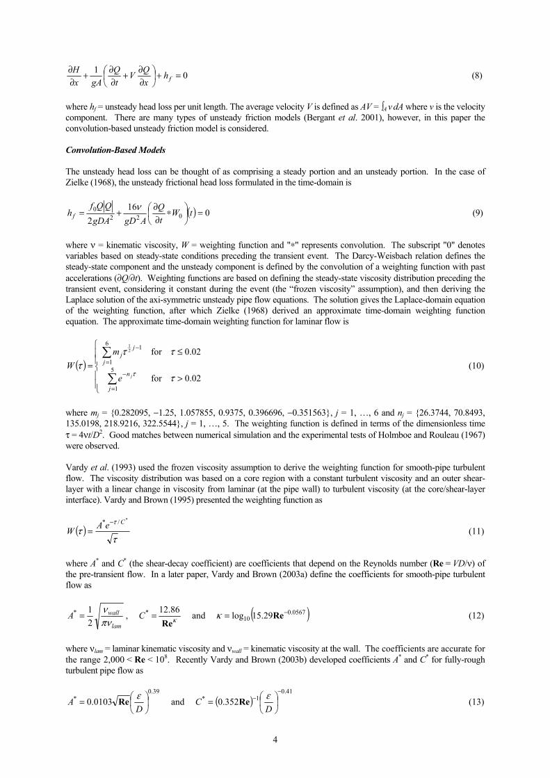
where hf = unsteady head loss per unit length. The average velocity V is defined as AV = ∫A v dA where v is the velocity component. There are many types of unsteady friction models (Bergant et al. 2001), however, in this paper the convolution-based unsteady friction model is considered. Convolution-Based Models The unsteady head loss can be thought of as comprising a steady portion and an unsteady portion. In the case of Zielke (1968), the unsteady frictional head loss formulated in the time-domain is

( ) 0162 022

0 =

∗∂∂+= tW

tQ

AgDgDAQQf

hfν (9)

where ν = kinematic viscosity, W = weighting function and "∗" represents convolution. The subscript "0" denotes variables based on steady-state conditions preceding the transient event. The Darcy-Weisbach relation defines the steady-state component and the unsteady component is defined by the convolution of a weighting function with past accelerations (∂Q/∂t). Weighting functions are based on defining the steady-state viscosity distribution preceding the transient event, considering it constant during the event (the “frozen viscosity” assumption), and then deriving the Laplace solution of the axi-symmetric unsteady pipe flow equations. The solution gives the Laplace-domain equation of the weighting function, after which Zielke (1968) derived an approximate time-domain weighting function equation. The approximate time-domain weighting function for laminar flow is

( )

>

≤=

∑

∑

=

−

=

−

02.0for

02.0for 5

1

6

1

121

τ

τττ

τ

j

n

j

jj

je

mW (10)

where mj = {0.282095, −1.25, 1.057855, 0.9375, 0.396696, −0.351563}, j = 1, …, 6 and nj = {26.3744, 70.8493, 135.0198, 218.9216, 322.5544}, j = 1, …, 5. The weighting function is defined in terms of the dimensionless time τ = 4νt/D2. Good matches between numerical simulation and the experimental tests of Holmboe and Rouleau (1967) were observed. Vardy et al. (1993) used the frozen viscosity assumption to derive the weighting function for smooth-pipe turbulent flow. The viscosity distribution was based on a core region with a constant turbulent viscosity and an outer shear-layer with a linear change in viscosity from laminar (at the pipe wall) to turbulent viscosity (at the core/shear-layer interface). Vardy and Brown (1995) presented the weighting function as

( )τ

ττ */* CeAW−

= (11)

where A* and C* (the shear-decay coefficient) are coefficients that depend on the Reynolds number (Re = VD/ν) of the pre-transient flow. In a later paper, Vardy and Brown (2003a) define the coefficients for smooth-pipe turbulent flow as

lam

wallAπνν

21* = , κRe

86.12* =C and ( )0567.010 29.15log −= Reκ (12)

where νlam = laminar kinematic viscosity and νwall = kinematic viscosity at the wall. The coefficients are accurate for the range 2,000 < Re < 108. Recently Vardy and Brown (2003b) developed coefficients A* and C* for fully-rough turbulent pipe flow as

39.0* 0103.0

=

DA εRe and ( )

41.01* 352.0

−−

=

DC εRe (13)

4

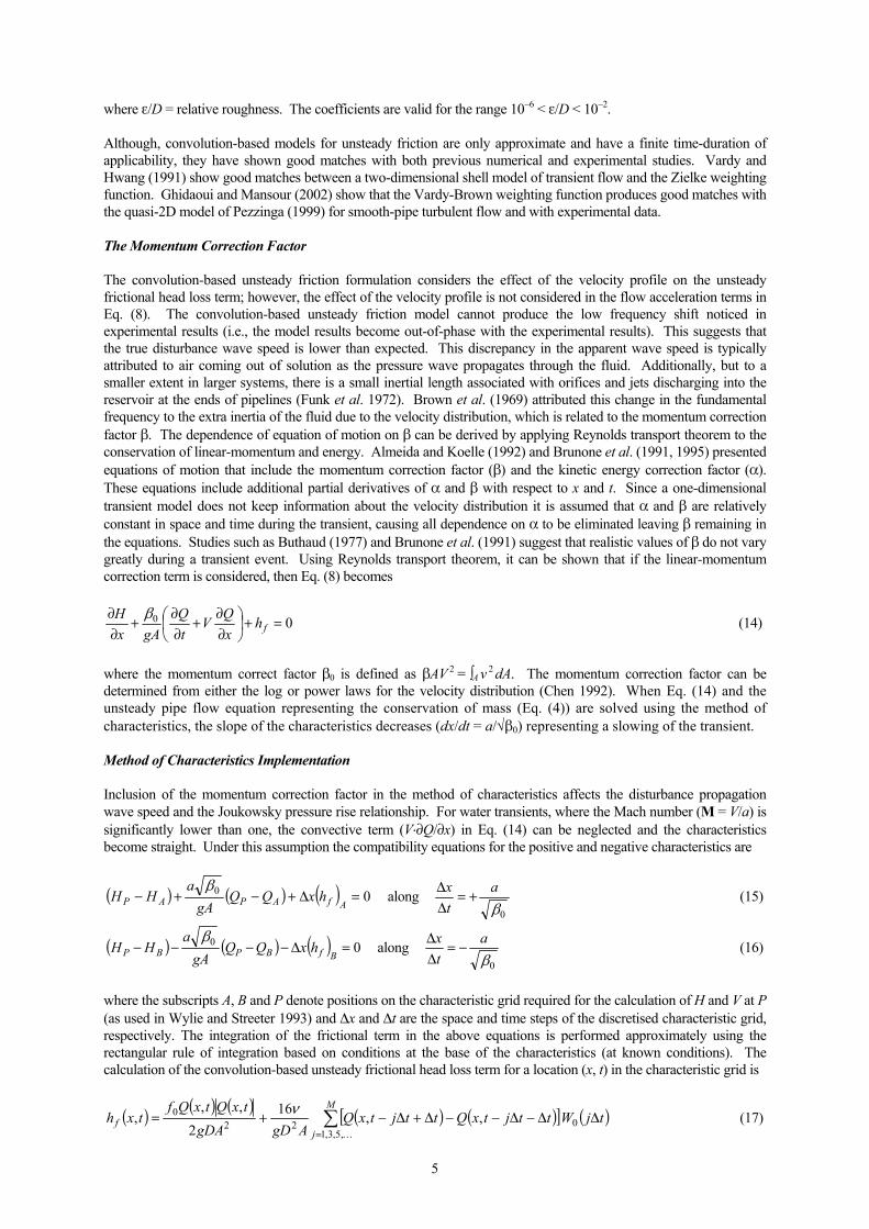
where ε/D = relative roughness. The coefficients are valid for the range 10−6 < ε/D < 10−2. Although, convolution-based models for unsteady friction are only approximate and have a finite time-duration of applicability, they have shown good matches with both previous numerical and experimental studies. Vardy and Hwang (1991) show good matches between a two-dimensional shell model of transient flow and the Zielke weighting function. Ghidaoui and Mansour (2002) show that the Vardy-Brown weighting function produces good matches with the quasi-2D model of Pezzinga (1999) for smooth-pipe turbulent flow and with experimental data. The Momentum Correction Factor The convolution-based unsteady friction formulation considers the effect of the velocity profile on the unsteady frictional head loss term; however, the effect of the velocity profile is not considered in the flow acceleration terms in Eq. (8). The convolution-based unsteady friction model cannot produce the low frequency shift noticed in experimental results (i.e., the model results become out-of-phase with the experimental results). This suggests that the true disturbance wave speed is lower than expected. This discrepancy in the apparent wave speed is typically attributed to air coming out of solution as the pressure wave propagates through the fluid. Additionally, but to a smaller extent in larger systems, there is a small inertial length associated with orifices and jets discharging into the reservoir at the ends of pipelines (Funk et al. 1972). Brown et al. (1969) attributed this change in the fundamental frequency to the extra inertia of the fluid due to the velocity distribution, which is related to the momentum correction factor β. The dependence of equation of motion on β can be derived by applying Reynolds transport theorem to the conservation of linear-momentum and energy. Almeida and Koelle (1992) and Brunone et al. (1991, 1995) presented equations of motion that include the momentum correction factor (β) and the kinetic energy correction factor (α). These equations include additional partial derivatives of α and β with respect to x and t. Since a one-dimensional transient model does not keep information about the velocity distribution it is assumed that α and β are relatively constant in space and time during the transient, causing all dependence on α to be eliminated leaving β remaining in the equations. Studies such as Buthaud (1977) and Brunone et al. (1991) suggest that realistic values of β do not vary greatly during a transient event. Using Reynolds transport theorem, it can be shown that if the linear-momentum correction term is considered, then Eq. (8) becomes

00 =+

∂∂+

∂∂+

∂∂

fhxQV

tQ

gAxH β (14)

where the momentum correct factor β0 is defined as βAV 2 = ∫A v 2 dA. The momentum correction factor can be determined from either the log or power laws for the velocity distribution (Chen 1992). When Eq. (14) and the unsteady pipe flow equation representing the conservation of mass (Eq. (4)) are solved using the method of characteristics, the slope of the characteristics decreases (dx/dt = a/√β0) representing a slowing of the transient. Method of Characteristics Implementation Inclusion of the momentum correction factor in the method of characteristics affects the disturbance propagation wave speed and the Joukowsky pressure rise relationship. For water transients, where the Mach number (M = V/a) is significantly lower than one, the convective term (V⋅∂Q/∂x) in Eq. (14) can be neglected and the characteristics become straight. Under this assumption the compatibility equations for the positive and negative characteristics are

( ) ( ) ( ) 00 =∆+−+−AfAPAP hxQQ

gAa

HHβ

along 0β

atx +=∆∆ (15)

( ) ( ) ( ) 00 =∆−−−−BfBPBP hxQQ

gAa

HHβ

along 0β

atx −=∆∆ (16)

where the subscripts A, B and P denote positions on the characteristic grid required for the calculation of H and V at P (as used in Wylie and Streeter 1993) and ∆x and ∆t are the space and time steps of the discretised characteristic grid, respectively. The integration of the frictional term in the above equations is performed approximately using the rectangular rule of integration based on conditions at the base of the characteristics (at known conditions). The calculation of the convolution-based unsteady frictional head loss term for a location (x, t) in the characteristic grid is

( ) ( ) ( ) ( ) ( )[ ] ( )∑=

∆∆−∆−−∆+∆−+=M

jf tjWttjtxQttjtxQ

AgDgDAtxQtxQf

txhK,5,3,1

0220 ,,16

2,,

, ν (17)

5

where M = t/∆t − 1. This scheme, called the full convolution scheme, was first implemented by Zielke (1968) and does not exhibit “grid separation” problems because it is applied on a single diamond grid. The full convolution scheme is computationally intensive and can be prohibitive to its use. Trikha (1975) and Kagawa et al. (1983) improved computation speed by approximating Zielke’s weighting function. Recently Ghidaoui and Mansour (2002) presented an efficient implementation for the Vardy and Brown (1995) weighting function. However their results show an amount of error due to the approximations used in their derivation. 3. GASEOUS CAVITATION This section summarises theoretical tools for gaseous cavitation as presented in the 2001 paper by Bergant and Tijsseling. Gaseous cavitation occurs in fluid flows when free gas is either distributed throughout a liquid (small void fraction) or trapped at discrete positions along the pipe and at boundaries (large void fraction). Gas may be entrained in a liquid due to gas release during low-pressure transients, cavitation or column separation. Transient gaseous cavitation is associated with dispersion and shock waves. The pressure-dependent wave speed in a gas-liquid mixture is significantly reduced. Gas release takes several seconds whereas vapour release takes only a few milliseconds. The effect of gas release during transients is important in long pipelines in which the wave reflection time is in the order of several seconds. Methods for describing the amount of gas release were developed by Zielke and Perko (1985). Transient flow of a homogeneous gas-liquid mixture with a low gas fraction and with the liquid’s mass density may be described by classical water hammer equations (4) and (5) in which the liquid wave speed a is replaced by the pressure-dependent gas-mixture wave speed am (Wylie 1984):

)(α

12

2

v

gm

hzHga

a a

−−+

= (18)

where, in addition, the ideal gas equation assumes isothermal conditions. The pressure-dependent wave speed am makes the system of equations highly non-linear. A number of numerical schemes including the method of characteristics have been used for solving the above set of equations (Wylie 1980; Chaudhry et al. 1990; Wylie and Streeter 1993). These methods are complex and could not be easily incorporated into a standard water hammer code. Alternatively, the mass of distributed free gas can be lumped at computational sections leading to a discrete gas cavity model (Wylie 1984). The discrete gas cavity model (DGCM) allows gas cavities to form at computational sections in the method of characteristics. A liquid phase with a constant wave speed a is assumed to occupy the computational reach. The discrete gas cavity is described by the water hammer compatibility equations, the continuity equation for the gas cavity volume, and the ideal gas equation (Wylie 1984) and their numerical form within the staggered grid of the method of characteristics is: - compatibility equation along the C+ characteristic line (∆x/∆t = a):

0)(2

))(( ,1,2,1,,1, =∆+−+− ∆−−∆−−∆−− ttitiuttitiuttiti QQgDA

xfQQgAaHH (19)

- compatibility equation along the C- characteristic line (∆x/∆t = -a):

0)(2

))(( ,1,2,1,,1, =∆−−−− ∆−+∆−+∆−+ ttiutittiutittiti QQgDA

xfQQgAaHH (20)

- continuity equation for the gas cavity volume:

tQQQQ tiutittiuttittigtig ∆−+−−+∀=∀ ∆−∆−∆− 2)))((ψ))()(ψ1(()()( ,,2,2,2,, (21)

- ideal gas equation: ( ) xAhzHhzH igvvititig ∆−−=−−∀ 000,,

α)()( (22)

6

The treatment of gas release by the DGCM is straightforward (Barbero and Ciaponi 1991). In addition, the DGCM model can be successfully used for simulation of vaporous cavitation by utilizing a low gas void fraction (αg ≤ 10-7) (Wylie 1984; Simpson and Bergant 1994). In this case, when the discrete cavity volume calculated by the equation (21) is negative, then the cavity volume is recalculated by equation (22). 4. VISCOELASTIC BEHAVIOUR OF PIPE WALL Plastic pipes have been increasingly used in water supply systems due to their high resistant properties (mechanical, chemical, temperature and abrasion) and cost-effective price. The viscoelastic behaviour of polymers is well-known (Ferry, 1970; Aklonis et al., 1972). This behaviour influences the pressure response during transient events by attenuating the pressure fluctuations and by increasing the dispersion of the pressure wave. Two different approaches have been developed to simulate this effect in fluid systems. The first approach assumes that the viscoelastic effect of the pipe-wall can be described by a frequency-dependent wave speed (Meiβner and Franke, 1977). The second approach is based on the mechanical principle associated with viscoelasticity in which strain can be decomposed into instantaneous-elastic strain and retarded-viscoelastic strain. The elastic strain is included in the wave speed, whereas the retarded strain is an additional term included in the mass-balance equation (Rieutford and Blanchard, 1979; Covas et al., 2002; Pezzinga, 2002). This section focuses on the mathematical modelling of hydraulic transients in polyethylene pipes by adding the retarded strain in the transient pipe flow equations and by taking into account unsteady friction losses. Linear-Viscoelastic Model Polyethylene pipes have a different rheological behaviour in comparison to metal and concrete pipes. When subject to an instantaneous stress σ, polymers do not respond according to Hooke’s law. Plastics have an instantaneous-elastic response and a retarded-viscous response. Consequently, strain can be decomposed into an elastic, εe, and a retarded component, εr: ( ) ( )tt re εεε += (23)

According to the “Boltzmann superposition principle”, for small strains, a combination of stresses that act independently in a system result in strains that can be added linearly. The total strain generated by a continuous application of stress σ(t) is (Covas, 2003):

( ) ( ) ( ) ( )0 0

'' '

't J t

t J t t t dtt

ε σ σ∂

= + −∂∫ (24)

where J0 = instantaneous creep-compliance and J(t′)= creep function at t′ time. For linear-elastic materials, the creep-compliance J0 is equal to the inverse modulus of elasticity, J0 = 1/ E0. Assuming that the pipe material is homogeneous and isotropic, it has linear viscoelastic behaviour for small strains, Poisson’s ratioν is constant so that the mechanical behaviour is only dependent on a creep-function, and circumferential-stress σ is expressed by σ=α∆PD/2e, the total circumferential strain, ε=(D-D0)/D0, is described by (Covas, 2003):

( ) ( ) ( ) ( )( ) ( ) ( )0 0

0 0 000

' ' ''

2 2 't t t D t t J tD

t P t P J P t t Pe e t t

ααε− − ∂

= − + − − − ∂∫ ''

dtt

(25)

The first term of Equation (25) corresponds to the elastic strain εe and the integral part to the retarded strain εr. The creep-compliance function J(t), which describes the viscoelastic behaviour of the pipe material, can be determined experimentally in a mechanical test or calibrated based on collected transient data (Covas, 2003). The creep-function of the pipe was represented by the mechanical model of a generalised viscoelastic solid (Fig. 3):

( ) ( )ktN

kk eJJtJ τ/

10 1 −

=−+= ∑ (26)

in which J0 = creep-compliance of the first spring, J0=1/E0; Jk = creep-compliance of the spring of k-element Kelvin-Voigt, Jk=1/Ek; Ek = modulus of elasticity of the spring of k-element; τk = retardation time of the dashpot

7

of k-element, τk = µk/Ek; µk = the viscosity of the dashpots of k-element. The parameters Jk and τk of the viscoelastic mechanical model should be adjusted to the creep experimental data.

Eo E1 E2 E3 EN

µ1 µ2 µ3 µN

Fig. 3 Generalised Kelvin-Voigt model for viscoelastic solid Taking into account the relationship between cross-sectional area, S, and total strain, ε (dA/dt=2Adε/dt), and the two components of strain, ε=εe+εr, the continuity equation yields

02 22

=∂∂+

∂∂+

∂∂

tε

ga

xQ

g Aa

tH r (27)

Whilst the third term represents the retarded effect of the pipe-wall, the elastic strain is included in the piezometric head time derivative and in the elastic wave speed, a. The elastic wave speed is calculated by Eq. (3) considering E0=1/ J0. Eq. (27) solved with Eq. (8) and the second term of Eq. (25) describe the pressure-flow fluctuations along a pressurised pipeline. Method of Characteristics Implementation The set of partial differential equations (8) and (27) is solved by the MOC (convective term is neglected) as follows

02 2=±

∂∂+± f

r ahtε

ga

dtdQ

gSa

dtdH (28)

and are valid along the characteristic lines dx/dt = ± a. The complete equations including the convective term can be found in Covas (2003). Numerical solution of Eq. (28) is

( ) ( )[ ] ( ) ( )[ ] 0 2,,,,,

2=∆±

∂∂∆+∆−∆−±∆−∆−

∆f

xxx

r htatg

tattxxQtxQgSattxxHtxH

m

mmε (29)

where the time-derivative of the retarded strain is obtained by taking the derivative of the second term of Eq. (26). Terms εr and ∂εr/∂t are evaluated by means of (26) considering the creep-function defined by the mechanical model of the viscoelastic solid as follows:

( ) ( ) ( ) ( )'

τ00

1.. 1.., , , '

2 τk

tt k

r rkkk N k N

JD 'x t x t H x t t H x ee

αε ε γ−

= =

= = − −

∑ ∑ ∫ dt (30)

( ) ( ) ( ) ( )[ ] ( )∑∑

==

−−=∂

∂=∂

∂

Nk k

rk

k

k

Nk

rkr txxHtxHJeD

ttx

ttx

..10

..1 τ,,

τ2,, εγαεε (31)

The parameters Jk and τk are usually adjusted to the creep experimental data. The pipe diameter D, wall-thickness e and pipe-wall constraints coefficient α, which are time-dependent parameters, are assumed constant and equal to steady-state values. 5. LEAKAGE AND BLOCKAGE Leaks and blockages represent common faults that pipeline systems can experience during their design lifetime. In many cases transients measured in the field show significant damping above that predicted by models including unsteady friction. In some cases this additional damping is caused by unknown pipeline faults such as leaks and blockages. Leaks and blockages are complimentary phenomena; for example a leak represents a flow loss with no head loss whereas a blockage represents a head loss with no flow loss. Both leaks and blockages are modelled using the orifice equation

8

OOdO HgACQ ∆= 2 (32) where QO = flow through the orifice, ∆HO = head loss across the orifice, Cd = discharge coefficient and AO = orifice area. For both leaks and blockages, Eq. (32) is implemented in the method of characteristics as an internal boundary condition (see Fig. 4).

Leak orBlockage

++PP HQ , −−

PP HQ ,

C+ C−P

BA

Fig. 4 Leak and blockage implementation in the MOC The classical compatibility equations (Wylie and Streeter 1993) either side of the leak or blockage are

PPP CBQH =+ ++ along atx +=∆∆ (33)

MPP CBQH =− −− along atx −=∆∆ (34) where B = characteristic impedance (= a/gA) and CP and CM represent all known variables for the positive and negative characteristics respectively. Leaks are treated as an off-line orifice. The two relationships that relate the upstream head and flow to the downstream head and flow are

( ) 02 =−−−− −+ zHHgACQQ OUTPOdPP where (35) −+ == PPP HHH where z = pipe elevation at the leak and HOUT = outside pressure at the leak. In most cases the outside pressure is the atmospheric pressure and assumed zero. Eqs. (33), (34) and (35) form a set of quadratic equations in √HP that is solved using the quadratic formula. Once HP is determined the upstream and downstream flows are calculated using the positive and negative compatibility equations respectively. Care must be taken to account for the case when the pressure inside the pipe becomes less than the outside pressure. In that case, Eq. (35) is re-written assuming that the leak works in reverse injecting fluid into the pipe. For real leaks, it is unlikely that the orifice equation will completely describe their behaviour. Real leaks come in a variety of sizes and shapes resulting in deviations from the classical orifice relationship. In many cases a power law can be used for modelling the discharge-head loss relationship; however, typically the details of the leak are unknown and the orifice relation is sufficient. Blockages are treated as an inline orifice. The relationships that relates the upstream and downstream head to the flow through the blockage are

( ) ( ) 02 2 =−− −+PPOdPP HHACgQQ where Q (35) −+ == PPP QQ

Eqs. (33), (34) and (36) form a set of quadratic equations in QP and can be solved using the quadratic formula; however, care must be taken to account for the case when the flow reverses through the orifice. Again, the orifice equation represents the simplest model of a blockage. In most cases the orifice relationship will approximate a blockage that could be of any shape and length. Additionally, for low pipe flows a blockage can cause additional delays in the transient response due to inertial lengths associated with the submerged jet created by the blockage (Prenner 1998).

7. CONCLUSIONS Transients in pipelines are modified by phenomena that can be broadly classified into four areas:

9

1. The impact of three-dimensional nature of the flow and fluid turbulence 2. Modification of fluid properties – gas entrainment 3. Non-elastic response of the containing pipe 4. Local changes in pipeline cross-section or geometry – blocks or leaks

The one dimensional assumptions that are made to aid solution fail to capture the full three dimensional nature of the resulting damped oscillatory flow that creates and then destroys the velocity profile and boundary layer. Unsteady friction is the primary manifestation of this effect. The damping of the pressure trace is significantly greater (and frequency dependent) than that given by the application of steady state friction relationships. The assumption of a uniform velocity profile (β=1) produces less dramatic effects on the transient pressure trace but it does result in a reduction in the wave speed and an observable shift in the modelled trace. Modification of the fluid property due to gas entrainment and cavity formation results in significant wave speed reduction. While relationships exist that provide an estimate of the reduced wave speed , a more satisfactory approach is to use a discrete gas cavity model that distributes the gas present in the system at the computational nodes. The non-elastic behaviour of the pipe wall is an area that is increasing in importance as plastic pipes are being employed for serviceability reasons. In this instance, pressure relief is provided as the pipe wall expands and contracts in a visco-elastic fashion. A non-linear model of this process using a series of dashpots and springs provides an effective way to model this behaviour. Local changes in the pipeline cross-section or geometry (leaks) can also lead to significant modification of the transient behaviour. This is dealt with by breaking the solution space either side of the leak or blockage using interior boundary conditions that satisfy the relevant compatibility conditions across the node. Most of the phenomena described in this paper cause additional damping of the modelled transient traces. Current models are crude but effective given the computational demands of transient modelling, however, there is potential for further investigation and refinement. ACKNOWLEDGEMENT AND DISCLAIMER The Surge-Net project (see http://www.surge-net.info) is supported by funding under the European Commission’s Fifth Framework ‘Growth’ Programme via Thematic Network “Surge-Net” contract reference: G1RT-CT-2002-05069. The authors of this paper are solely responsible for the content and it does not represent the opinion of the Community, the Community is not responsible for any use that might be made of data therein. APPENDIX I - REFERENCES Aklonis, J. J., MacKnight, W. J., and Shen, M. (1972). Introduction to Polymer Viscoelasticity , Wiley-IntersWiley-Interscience - John Wiley & Sons, Inc. Almeida, A.B., and Koelle, E. (1992). Fluid Transients in Pipe Networks. Computational Mechanics Publications, Elsevier Applied Science. Barbero, G., and Ciaponi, C. (1991). Experimental validation of a discrete free gas model for numerical simulation of hydraulic transients with cavitation. Int. Meeting on Hydraulic Transients with Column Separation, 9th Round Table, IAHR, Valencia, Spain, 17 - 33. Bergant, A., and Tijsseling, A. (2001). “Parameters affecting water hammer wave attenuation, shape and timing.” Proceedings of the 10th International Meeting of the IAHR Work Group on the Behaviour of Hydraulic Machinery under Steady Oscillatory Conditions, Trondheim, Norway, Paper C2, 12 pp. Bergant, A., Simpson, A.R., and Vítkovský, J.P. (2001). “Developments in Unsteady Pipe Flow Friction Modelling.” Journal of Hydraulic Research, IAHR, 39(3), 249-257. Brown, F.T., Margolis, D.L., and Shah, R.P. (1969). “Small-Amplitude Frequency Behavior of Fluid Lines with Turbulent Flow.” Journal of Basic Engineering, Transactions of the ASME, Series D, 91(4), December, 678-693. Brunone, B., Golia, U.M., and Greco, M. (1991). “Some Remarks on the Momentum Equations for Fast Transients.” Hydraulic Transients with Column Separation (9th and Last Round Table of the IAHR Group), IAHR, Valencia, Spain, 4-6 September, 201-209. Brunone, B., Golia, U.M., and Greco, M. (1995). “Effects of Two-Dimensionality on Pipe Transients Modeling.” Journal of Hydraulic Engineering, ASCE, 121(12), December, 906-912. Buthaud, H. (1977). “On the Momentum Correction Factor in Pulsatile Blood Flow.” Journal of Applied Mechanics, Transactions of the ASME, 44(2), June, 343-344. Chaudhry, M.H., Bhallamudi, S.M., Martin, C.S., and Nagash, M. (1990). Analysis of transient pressures in bubbly, homogeneous, gas-liquid mixtures. Journal of Fluids Engineering, ASME, 112(2), 225 - 231. Chen, C.-L. (1992). “Momentum and Energy Coefficients Based on Power-Law Velocity Profile.” Journal of Hydraulic Engineering, ASCE, 118(11), 1571-1584. Covas, D. (2003). "Inverse Transient Analysis for Leak Detection and Calibration of Water Pipe Systems - Modelling Special Dynamic Effects." PhD, Imperial College of Science, Technology and Medicine, University of London, London, UK.

10

Covas, D., Stoianov, I., Graham, N., Maksimovic, C., Ramos, H., and Butler, D. (2002). "Hydraulic Transients in Polyethylene Pipes.", Proceedings of 1st Annual Environmental & Water Resources Systems Analysis (EWRSA) Symposium, A.S.C.E. EWRI Annual Conference , Roanoke, Virginia, USA. Ferry, J. D. (1970). Viscoelastic Properties of Polymers (Second Edition), Wiley-Interscience - John Wiley & Sons. Funk, J.E., Wood, D.J., and Chao, S.P. (1972). “The Transient Response of Orifices and Very Short Lines.” Journal of Basic Engineering, Transactions of the ASME, Series D, 94(2), June, 483-491. Ghidaoui, M.S., and Mansour, S. (2002). “Efficient Treatment of Vardy-Brown Unsteady Shear in Pipe Transients.” Journal of Hydraulic Engineering, ASCE, 128(1), January, 102-112. Holmboe, E.L., and Rouleau, W.T. (1967). “The Effect of Viscous Shear on Transients in Liquid Lines.” Journal of Basic Engineering, ASME, 89(March), 174-180. Kagawa, T., Lee, I., Kitagawa, A., and Takenaka, T. (1983). “High Speed and Accurate Computing Method of Frequency-Dependent Friction in Laminar Pipe Flow for Characteristics Method.” Transactions of the Japanese Society of Mechanical Engineers, 49(447), 2638-2644. (in Japanese) Leslie, D.J., and Tijsseling, A.S., (2000). “Travelling discontinuities in waterhammer theory: attenuation due to friction.” In Proceedings of the 8th International Conference on Pressure Surges, BHR Group, The Hague, The Netherlands, April 2000, pp. 323-335; Bury St Edmunds, UK: Professional Engineering Publishing, ISBN 1-86058-250-8. Meiβner, E. and Franke, G. (1977). "Influence of Pipe Material on the Dampening of Waterhammer." Proceedings of the 17th Congress of the International Association for Hydraulic Research, Pub. IAHR, Baden-Baden, F.R. Germany. Pezzinga, G. (1999). “Quasi-2D Model for Unsteady Flow in Pipe Networks.” Journal of Hydraulic Engineering, ASCE, 125(7), 676-685. Pezzinga, G. (2002). "Unsteady Flow in Hydraulic Networks with Polymeric Additional Pipe." Journal of Hydraulic Engineering, ASCE, 128(2), 238-244. Prenner , R.K. (1998). “Design of Throttled Surge Tanks for High-Head Plants. Pressure Wave Transmission and Reflection at an In-Line Orifice in a Straight Pipe.” Hydro Vision 98, 28-31 July, Reno, Nevada, USA. Rieutford, E. and Blanchard, A. (1979). "Ecoulement Non-permanent en Conduite Viscoelastique - Coup de Bélier." Journal of Hydraulic Research, IAHR, 17(1), 217-229. Simpson, A.R., and Bergant, A. (1994). Numerical comparison of pipe-column-separation models. Journal of Hydraulic Engineering, ASCE, 120(3), 361 - 377. Trikha, A.K. (1975). “An Efficient Method for Simulating Frequency-Dependent Friction in Transient Liquid Flow.” Journal of Fluids Engineering, Transactions of the ASME, 97, 97-105. Vardy, A.E., and Brown, J.M. (1995). “Transient, Turbulent, Smooth Pipe Friction.” Journal of Hydraulic Research, IAHR, 33(4), 435-456. Vardy, A.E., and Brown, J.M.B. (2003a). “Transient Turbulent Friction in Smooth Pipe Flows.” Journal of Sound and Vibration, 259(5), January, 1011-1036. Vardy, A.E., and Brown, J.M.B. (2003b). “Transient Turbulent Friction in Fully-Rough Pipe Flows.” Journal of Sound and Vibration. [in press] Vardy, A.E., and Hwang, K.-L. (1991). “A Characteristics Model of Transient Friction in Pipes.” Journal of Hydraulic Research, IAHR, 29(5), 669-684. Vardy, A.E., Hwang, K.-L., and Brown, J.M. (1993). “A Weighting Function Model of Transient Turbulent Pipe Friction.” Journal of Hydraulic Research, IAHR, 31(4), 533-548. Wylie, E.B. (1980). Free air in liquid transient flow. Proceedings of the 3rd International Conference on Pressure Surges, BHRA, Canterbury, England, 27 - 42. Wylie, E.B. (1984). Simulation of vaporous and gaseous cavitation. Journal of Fluids Engineering, ASME, 106(3), 307 - 311. Wylie, E.B., and Streeter, V.L. (1993). Fluid Transients in Systems. Prentice-Hall Inc., Englewood Cliffs, New Jersey, USA. Zielke, W. (1968). “Frequency-Dependent Friction in Transient Pipe Flow.” Journal of Basic Engineering, Transactions of the ASME, 90(1), 109-115. Zielke, W., and Perko, H.D. (1985). Unterdruckerscheinungen und Drucksto⇓berechnung. 3R international, 24(7), 348 - 355 (in German). APPENDIX II - NOTATION The following symbols are used in this paper: A = cross-sectional pipe area; a = liquid wave speed; am = gas-mixture wave speed; B = characteristic impedance;

11

12

A*, C*, κ = Vardy-Brown weighting function coefficients; AO = cross-sectional orifice area; Cd = orifice discharge coefficient; CP, CM = known variable coefficient for the method of characteristics; D = inner pipe diameter; e = pipe-wall thickness; E, E0 = Young’s modulus of elasticity of pipe; f = Darcy-Weisbach friction factor; g = gravitational acceleration; H = head; hf = frictional head loss per unit length; hv = gauge vapour pressure head; J, J0 = creep-compliance, instantaneous or elastic creep-compliance; Jk = creep of the springs of the Kelvin-Voigt elements; L = pipe length; K = bulk modulus; M = Mach number; nj, mj = Zielke weighting function coefficients; P = pressure; Q = discharge (flow) or node downstream-end discharge; Qu = node upstream-end discharge; Re = Reynolds number; t, t’ = time; V = average velocity; W = weighting function for convolution-based unsteady friction model; x = distance; z = elevation; α = kinetic energy correction factor, pipe-wall constraint coefficient; αg = gas void fraction; β = momentum correction factor; ∆H0 = head loss across orifice; ∆t = MOC time step; ∆x = MOC space step; ε = pipe roughness height; strain; circumferential total strain; εe = instantaneous-elastic strain; εr = retarded strain; θ = pipe slope; ν = kinematic viscosity, Poisson’s ratio; ρ = mass density of fluid ; σ = stress; circumferential-stress; τ = dimensionless time; τk = retardation time of the dashpot of k-element; µk = viscosity of the dashpots of k-element; ψ = pipe constraint coefficient, weighting factor; ∀ = discrete cavity volume; Subscripts: g = gas; i = node number; O = relating to an orifice; 0 = based on steady-state or reference conditions; elastic component + = relating to the positive characteristic; − = relating to the negative characteristic; Abbreviations: DGCM = discrete gas cavity model; MOC = method of characteristics; ODE = ordinary differential equation(s); PDE = partial differential equations(s).