Graduate Theses, Dissertations, and Problem Reports 2010 Further hydrogeologic investigations in the Davis Spring drainage Further hydrogeologic investigations in the Davis Spring drainage basin, Greenbrier County, West Virginia basin, Greenbrier County, West Virginia John Kazimierz Tudek Jr. West Virginia University Follow this and additional works at: https://researchrepository.wvu.edu/etd Recommended Citation Recommended Citation Tudek, John Kazimierz Jr., "Further hydrogeologic investigations in the Davis Spring drainage basin, Greenbrier County, West Virginia" (2010). Graduate Theses, Dissertations, and Problem Reports. 2982. https://researchrepository.wvu.edu/etd/2982 This Thesis is protected by copyright and/or related rights. It has been brought to you by the The Research Repository @ WVU with permission from the rights-holder(s). You are free to use this Thesis in any way that is permitted by the copyright and related rights legislation that applies to your use. For other uses you must obtain permission from the rights-holder(s) directly, unless additional rights are indicated by a Creative Commons license in the record and/ or on the work itself. This Thesis has been accepted for inclusion in WVU Graduate Theses, Dissertations, and Problem Reports collection by an authorized administrator of The Research Repository @ WVU. For more information, please contact [email protected].

Welcome message from author
This document is posted to help you gain knowledge. Please leave a comment to let me know what you think about it! Share it to your friends and learn new things together.
Transcript
Graduate Theses, Dissertations, and Problem Reports
2010
Further hydrogeologic investigations in the Davis Spring drainage Further hydrogeologic investigations in the Davis Spring drainage
basin, Greenbrier County, West Virginia basin, Greenbrier County, West Virginia
John Kazimierz Tudek Jr. West Virginia University
Follow this and additional works at: https://researchrepository.wvu.edu/etd
Recommended Citation Recommended Citation Tudek, John Kazimierz Jr., "Further hydrogeologic investigations in the Davis Spring drainage basin, Greenbrier County, West Virginia" (2010). Graduate Theses, Dissertations, and Problem Reports. 2982. https://researchrepository.wvu.edu/etd/2982
This Thesis is protected by copyright and/or related rights. It has been brought to you by the The Research Repository @ WVU with permission from the rights-holder(s). You are free to use this Thesis in any way that is permitted by the copyright and related rights legislation that applies to your use. For other uses you must obtain permission from the rights-holder(s) directly, unless additional rights are indicated by a Creative Commons license in the record and/ or on the work itself. This Thesis has been accepted for inclusion in WVU Graduate Theses, Dissertations, and Problem Reports collection by an authorized administrator of The Research Repository @ WVU. For more information, please contact [email protected].
Further Hydrogeologic Investigations in the Davis Spring Drainage Basin, Greenbrier County, West Virginia
John Kazimierz Tudek Jr.
Thesis submitted to the Eberly College of Arts and Sciences
at West Virginia University in partial fulfillment of the requirements
for the degree of
Master of Science In
Geology
Dr. Henry Rauch, Ph.D., Chair Dr. Dorothy Vesper, Ph.D. Dr. Douglas Boyer, Ph.D.
Department of Geology and Geography Morgantown, West Virginia
2010
Keywords: karst, hydrology, Davis Spring
Copyright 2010 John K. Tudek
Abstract
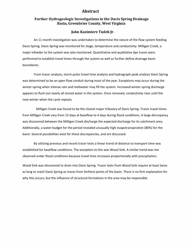
An 11 month investigation was undertaken to determine the nature of the flow system feeding
Davis Spring. Davis Spring was monitored for stage, temperature and conductivity. Milligan Creek, a
major infeeder to the system was also monitored. Quantitative and qualitative dye traces were
performed to establish travel times through the system as well as further define drainage basin
boundaries.
From tracer analysis, storm pulse travel time analysis and hydrograph peak analysis Davis Spring
was determined to be an open flow conduit during most of the year. Exceptions may occur during the
winter-spring when intense rain and meltwater may fill the system. Increased winter-spring discharge
appears to flush out nearly all stored water in the system. Once removed, conductivity rises until the
next winter when the cycle repeats.
Milligan Creek was found to be the closest major tributary of Davis Spring. Tracer travel times
from Milligan Creek vary from 15 days at baseflow to 4 days during flood conditions. A large discrepancy
was discovered between the Milligan Creek discharge the expected discharge for its catchment area.
Additionally, a water budget for the period revealed unusually high evapotranspiration (80%) for the
basin. Several possibilities exist for these discrepancies, and are discussed.
By utilizing previous and recent tracer tests a linear trend of distance to transport time was
established for baseflow conditions. The exception to this was Wood Sink. A similar trend was not
observed under flood conditions because travel time increases proportionally with precipitation.
Wood Sink was discovered to drain into Davis Spring. Tracer tests from Wood Sink require at least twice
as long to reach Davis Spring as traces from farthest points of the basin. There is no firm explanation for
why this occurs, but the influence of structural formations in the area may be responsible

iii
For mom, dad, and Jen
Who watched me play in the dirt and prayed something useful would come of it.
It did.
iv
2 Table of Contents
1 Abstract ................................................................................................................................................ ii
2 Table of Contents ................................................................................................................................. iv
2.1 List of Figures .............................................................................................................................. vii
2.2 List of Tables ................................................................................................................................ ix
3 Overview of the Davis Spring Basin ...................................................................................................... 1
3.1 Geography ..................................................................................................................................... 1
3.2 A Brief History of Exploration and Study in the Davis Spring Basin .............................................. 5
3.3 Geology of the Area ...................................................................................................................... 6
3.3.1 Geologic Setting .................................................................................................................... 7
3.3.2 Lithologic Sequence .............................................................................................................. 9
3.3.3 Structural Geology .............................................................................................................. 11
4 Thesis Objectives ................................................................................................................................. 13
4.1 Tasks necessary to accomplish objectives .................................................................................. 13
5 Methods and Procedures .................................................................................................................... 14
5.1 GIS Mapping ................................................................................................................................ 14
5.2 Water Budget .............................................................................................................................. 14
5.2.1 Background and Governing Principles ................................................................................ 14
5.3 Datalogging ................................................................................................................................. 18
5.3.1 Explanation of datalogging equipment. .............................................................................. 18
5.3.2 Location of datalogging equipment. ................................................................................... 19
5.3.3 Equipment used to measure flow ....................................................................................... 20
5.3.4 Difficulties with flow measurements at the datalogging sites ............................................ 21
5.4 Streamflow Measurement .......................................................................................................... 23
5.4.1 Procedure for streamflow measurement. .......................................................................... 23
5.4.2 Flow to discharge conversion; rating curve. ....................................................................... 23
5.4.3 Conversion of Stage to Discharge ....................................................................................... 24
5.4.4 Rating Curve Methodology ................................................................................................. 24
5.4.5 Locations for Stage Measurement ...................................................................................... 25
5.4.6 Previous rating curves ......................................................................................................... 25
v
5.5 Data Reduction and Curve Generation ....................................................................................... 26
5.6 Verification of the Rating Curve .................................................................................................. 28
5.7 Field Reconnaissance – ............................................................................................................... 30
5.8 Dye Tracing – ............................................................................................................................... 31
5.8.1 Quantitative Dye Tracing Overview. ................................................................................... 31
5.8.2 Dyes used, relative advantages and disadvantages. ........................................................... 31
5.8.3 Determination of amount of dye needed. .......................................................................... 32
5.8.4 Dye detection process; Charcoal and automatic sampling ................................................. 33
5.8.5 QTRACER2 Background ....................................................................................................... 36
5.8.6 Chemical Analysis ................................................................................................................ 37
6 Data Analysis and Results ................................................................................................................... 39
6.1 Further Definition of the Davis Spring Drainage Basin boundaries ............................................ 39
6.1.1 North, northwest and western boundaries ........................................................................ 39
6.1.2 Eastern and Northeastern Boundaries ............................................................................... 41
6.1.3 Southeastern and Southern boundary................................................................................ 44
6.2 Water Budget .............................................................................................................................. 48
6.2.1 Results and Discussion ........................................................................................................ 48
6.3 Dye Tracing and QTRACER2 ........................................................................................................ 58
6.3.1 Previous Work ..................................................................................................................... 58
6.3.2 Traces Performed for this Project ....................................................................................... 58
6.3.3 Discussion and Conclusions ................................................................................................ 60
6.4 Datalogging: Discharge, Conductivity and Temperature ............................................................ 71
6.4.1 Background ......................................................................................................................... 71
6.4.2 Milligan Creek Datalogger Results ...................................................................................... 73
6.4.3 Davis Spring Datalogger Results .......................................................................................... 80
6.4.4 Davis Spring Baseflow Separation ....................................................................................... 83
6.4.5 Storm Pulse Travel Time from Milligan Creek to Davis Spring ............................................ 91
7 Discussion and Conclusions ................................................................................................................ 95
7.1 Introduction ................................................................................................................................ 95
7.2 Open or Closed flow? .................................................................................................................. 95
7.2.1 Evidence and scenarios supporting an open flow system ................................................. 95
7.2.2 Evidence and scenarios supporting a closed flow system ................................................. 97
vi
7.2.3 Open or Closed? .................................................................................................................. 97
7.3 Speculation about the Master Conduit and its characteristics ................................................... 98
7.3.1 The Master Conduit near Davis Spring ............................................................................... 98
7.3.2 Possible locations of the junction of the Milligan Creek conduit and the Master Conduit 99
7.3.3 Milligan Creek and the Discharge Problem ....................................................................... 100
7.3.4 The Route of the Master Conduit as it Parallels Muddy Creek Mountain ........................ 104
7.3.5 An Attempt at the Paleohistory of the Davis Spring Drainage Basin ................................ 105
7.3.6 The Paleo-Weaver Knob Ridge .......................................................................................... 106
7.4 Conclusions ............................................................................................................................... 110
7.5 Further Research ....................................................................................................................... 112
7.6 Final Words ............................................................................................................................... 114
8 Acknowledgements ........................................................................................................................... 115
9 Bibliography ...................................................................................................................................... 116
10 Appendix A – Davis Spring Datalogger Data ................................................................................. 121
11 Appendix B – Milligan Creek Datalogger Data .............................................................................. 140
12 Appendix C – Chemistry Data for September 2008 ...................................................................... 153
Note
Click this link or same in the left sidebar panel to access the supplementary high-resolution map file. Both the main thesis and supplementary files needs to be downloaded for the active links to work properly.
vii
2.1 List of Figures
Figure 1: Overview of the Davis Spring basin and surrounding basins.) ................................................................. 2
Figure 2: An Overview of the reach between Davis Spring and the Greenbrier River. ............................................ 3
Figure 3: Elevation and surface streams of the Davis Spring and some surrounding basins. .................................. 4
Figure 4: Geologic Map of the Davis Spring and surrounding basins. ..................................................................... 8
Figure 5: Comparison of the stratigraphic column in Monroe County, Greenbrier County and Pocohantas County;
After White and White (1983) ....................................................................................................................... 9
Figure 6: The Davis Spring rating curve. 1993 data courtesy Boyer (2008). .......................................................... 27
Figure 7: The Milligan Creek rating curve. ............................................................................................................ 28
Figure 8: Rhodamine WT Calibration Curve.......................................................................................................... 35
Figure 9: Fluorescein Calibration Curve ................................................................................................................ 36
Figure 10: The northwestern boundary of the Davis Spring basin.. ...................................................................... 40
Figure 11: The southwestern boundary of the Davis Spring drainage basin. ........................................................ 43
Figure 12: USGS 1:24000 Map of the Rockland Indian and Davis Spring drainage basin divide. . ......................... 45
Figure 13: Increases in forested areas in the Davis Spring Basin, 1992-2001. ....................................................... 54
Figure 14: Increases in urban areas in the Davis Spring Basin, 1992-2001. ........................................................... 55
Figure 15 Locations of dye injections for tracer tests performed during this thesis. ............................................ 60
Figure 16: The geology between Wood Sink and Davis Spring. ............................................................................ 64
Figure 17: John Tudek standing in the Wood Sink Swallet. .................................................................................. 65
Figure 18: Time - distance relationship for tracer injections under low flow conditions to Davis Spring from 1967-
2009. ........................................................................................................................................................... 70
Figure 19: Time - distance relationship for tracer injections under high flow conditions to Davis Spring from 1967-
2009. ........................................................................................................................................................... 70
Figure 20: A possible configuration to the Davis Spring Sub-basins. ..................................................................... 71
Figure 21: Different proposed sub-basin extents for the Northern Milligan Creek Sub-basin. .............................. 73
Figure 22: Relative Milligan Creek and Davis Spring volumes by month............................................................... 74
Figure 23: Daily averages for discharge and conductivity at Milligan Creek. ........................................................ 76
Figure 24: Conductivity and Temperature at Milligan Creek, July 2008. ............................................................... 78
Figure 25: Conductivity and Temperature at Milligan Creek, October 2008. ........................................................ 79
Figure 26: Seven Day averages for discharge and conductivity at Davis Spring from May 2008-Mar 2009. .......... 80
Figure 27: Daily averages for discharge and conductivity at Davis Spring from May 2008-Mar 2009. .................. 82
Figure 28: A comparison of different forms of graphical baseflow separation. .................................................... 84
Figure 29: Specific conductivity at the Milligan Ck and Davis Spring dataloggers from May 2008 - March 2009. .. 86
Figure 30: A baseflow separation of the storm event of 11-25-08 to 11-27-08 using specific conductivity ........... 87
Figure 32: A Comparison among the fluxes of Na+ and Ca2+ and discharge at Davis Spring from September 9-23,
2008.. .......................................................................................................................................................... 89
Figure 31: Baseflow separation of the 09-09-2008 storm event at Davis Spring using specific conductivity to
differentiate between quick flow and baseflow. ......................................................................................... 89
Figure 33: Baseflow separation of the 12-10-08 to 12-12-08 storm event using specific conductivity. ................. 91
Figure 34: Dye trap results for August and September 2008.. ............................................................................ 100
Figure 35: Milligan Creek upstream of the Milligan Creek Datalogger. ............................................................... 102
Figure 36 Pickaway Pavement (foreground) along Milligan Creek...................................................................... 103

viii
Figure 37: 2003 3-meter USGS Digital Elevation map of (clockwise from the upper right) portions of the
Williamsburg, Lewisburg, Asbury and Cornstalk quadrangles. ................................................................... 107
Figure 38: USGS 3-Meter 2003 DEM (same as previous figure) showing individual locations within the map. ... 108

ix
2.2 List of Tables
Table 1: A comparison among different water budgets for the Davis Spring basin. ............................................. 49
Table 2: Table of Traces to Davis Spring between August 2008 and March 2009. ................................................ 59
Table 3: Parameters for Milligan Creek traces in 2008-09 derived from QTRACER2. ............................................ 62
Table 4: A compilation of all traces before 3/1/2009 in the Davis Spring basin. ................................................... 67
Table 5: Expected results for storm pulse travel time from the Milligan Creek Datalogger to the Davis Spring
Datalogger. .................................................................................................................................................. 93
Table 6: Observed results for ten storm hydrograph pulse events from the Milligan Creek Datalogger to the Davis
Spring Datalogger. ....................................................................................................................................... 94
1
3 Overview of the Davis Spring Basin
3.1 Geography
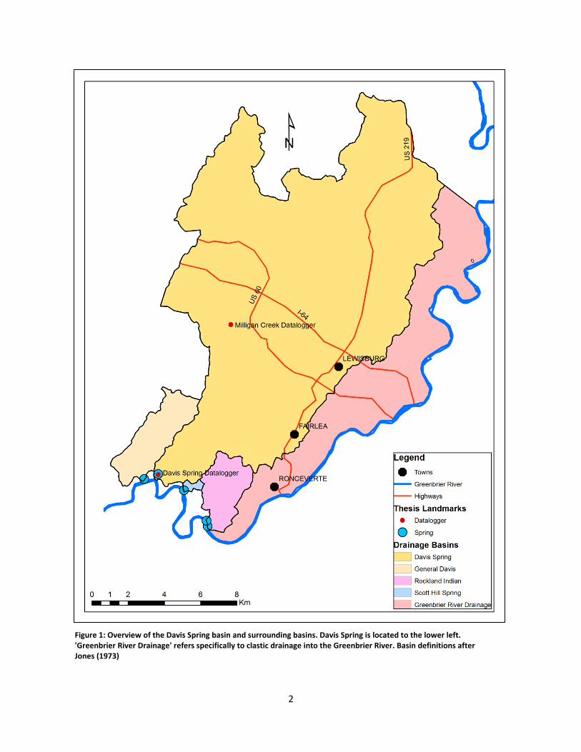
The Davis Spring drainage basin (Figure 1) is the largest karst basin in West Virginia. It is located
in southeastern West Virginia in the central part of Greenbrier County. Its total area is approximately
190 sq km (73 sq mi). It is nearly comparable in size to the 234 sq km (90.4 sq mi) Turnhole Spring basin
which drains a significant portion of the Mammoth Cave area (Quinlan and Ray, 1995). Davis Spring is a
roughly triangular shaped basin whose southern point is the resurgence. A second point is located
northeast of Lewisburg and the third is to the northwest where the valley has breached Muddy Creek
Mountain. The Davis Spring basin is bounded on the west by Muddy Creek Mountain and on the east
and south by the Greenbrier River except where it adjoins the Rockland Indian basin. It is bounded on
the north by the Culverson Creek and Spring Creek basins. The Davis Spring basin breaches Muddy Creek
Mountain in its northwestern end and enters the northern extension of the adjoining karst valley known
as Rader’s Valley. Dozens of kilometers of cave passages have been discovered and mapped under the
eastern part of the basin, while very little cave passage has been discovered in the central and western
portions (Dasher, 2000; WVACS, 2009).
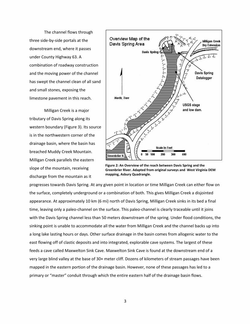
Davis Spring (Figure 2) is the only outlet for the drainage basin. At the spring water surfaces
along a large breakdown slope 10 meters (30 feet) below the base of a 30 meter (100 foot) cliff face.
Discharge comes from two separate sections at the base of the cliff. A long peninsula of breakdown
separates the two sections. Under high flow water issues from the entire length of the spring head.
Under low flow it issues from discrete points on either side of the peninsula. Water from the spring
flows along an unnamed surface channel for 350 meters (1200 feet) before emptying into the
Greenbrier River. The channel follows along a ravine until it reaches the river.
A low stone dam not more than one meter high divides the spring channel into an upper and
lower section. The upper section is characterized by deep (greater than 1 meter), slow moving pools of
water. The streambed is lined with cobble smaller than 1 m in diameter. The lower section is
characterized by shallow, swift moving water. Under storm conditions the force of the downstream
section is sufficient to knock a person over and carry him out to the Greenbrier River. Under flood
conditions the dam is completely submerged and acts as a rapid.
2
Figure 1: Overview of the Davis Spring basin and surrounding basins. Davis Spring is located to the lower left. 'Greenbrier River Drainage' refers specifically to clastic drainage into the Greenbrier River. Basin definitions after Jones (1973)
3
The channel flows through
three side-by-side portals at the
downstream end, where it passes
under County Highway 63. A
combination of roadway construction
and the moving power of the channel
has swept the channel clean of all sand
and small stones, exposing the
limestone pavement in this reach.
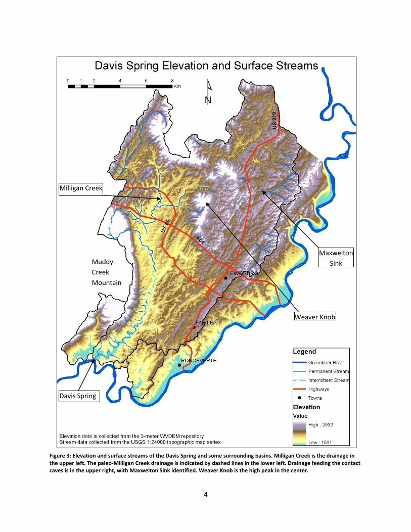
Milligan Creek is a major
tributary of Davis Spring along its
western boundary (Figure 3). Its source
is in the northwestern corner of the
drainage basin, where the basin has
breached Muddy Creek Mountain.
Milligan Creek parallels the eastern
slope of the mountain, receiving
discharge from the mountain as it
progresses towards Davis Spring. At any given point in location or time Milligan Creek can either flow on
the surface, completely underground or a combination of both. This gives Milligan Creek a disjointed
appearance. At approximately 10 km (6 mi) north of Davis Spring, Milligan Creek sinks in its bed a final
time, leaving only a paleo-channel on the surface. This paleo-channel is clearly traceable until it joins
with the Davis Spring channel less than 50 meters downstream of the spring. Under flood conditions, the
sinking point is unable to accommodate all the water from Milligan Creek and the channel backs up into
a long lake lasting hours or days. Other surface drainage in the basin comes from allogenic water to the
east flowing off of clastic deposits and into integrated, explorable cave systems. The largest of these
feeds a cave called Maxwelton Sink Cave. Maxwelton Sink Cave is found at the downstream end of a
very large blind valley at the base of 30+ meter cliff. Dozens of kilometers of stream passages have been
mapped in the eastern portion of the drainage basin. However, none of these passages has led to a
primary or “master” conduit through which the entire eastern half of the drainage basin flows.
Figure 2: An Overview of the reach between Davis Spring and the Greenbrier River. Adapted from original surveys and West Virginia DEM mapping, Asbury Quadrangle.
Davis Spring
Datalogger
USGS stage
and low dam.
4
Figure 3: Elevation and surface streams of the Davis Spring and some surrounding basins. Milligan Creek is the drainage in the upper left. The paleo-Milligan Creek drainage is indicated by dashed lines in the lower left. Drainage feeding the contact caves is in the upper right, with Maxwelton Sink identified. Weaver Knob is the high peak in the center.
Milligan Creek
Maxwelton
Sink Muddy
Creek
Mountain
Davis Spring
Weaver Knob
5
3.2 A Brief History of Exploration and Study in the Davis Spring Basin
The history of the Davis Spring basin is a combination of hydrologic investigation and cave
exploration. Cave exploration began in earnest in the 1930s to the south in the Organ Cave basin but
caves with obvious entrances like McClungs Cave were also visited (WVACS, 2009). A more thorough
investigation was organized by William Davies in the 1950s which resulted in the publication of the
“Caverns of West Virginia” (Davies, 1958). Continued exploration after the publication of “Caverns of
West Virginia” revealed the need for a long term organization to manage and organize exploration
within the drainage basin. WVACS – the West Virginia Association for Cave Studies and WVaSS - the
West Virginia Speleological Survey were created by cave explorers and speleologists to explore and
scientifically understand the area’s karst.
Several researchers have conducted work in the Davis Spring basin In association with WVACS.
William Jones , in conjunction with others, traced several routes of groundwater flow in the 1960s and
1970s, providing rough estimates for tracer travel time from different locations to Davis Spring (Jones,
1997). These investigations also established the basic shape and size of the drainage basin. In the early
1960s a USGS Staff gauge was placed a few hundred feet downstream from the spring. Jones measured
stage at the spring in 1972 and 1973 at regular intervals. Discharge measurements by Jones, et al. placed
the average flow of the spring at 3.2 m3/sec (110 cfs) (Jones, 1997). Peaks of over 28 m3/sec (1000 cfs)
were estimated based on stage – discharge relationships and occurred most frequently during the
winter – spring months. However, the actual peaks were lost as the USGS arbitrarily cropped the peak
flow at 28 m3/sec (1000 cfs) (Jones, 2009). Jones estimates that the highest flow may have approached
57 m3/sec (2000 cfs) during that year (Jones, 2009). In 1974 Art Palmer conducted a study of passage
orientation in Luddington Cave at the northeastern edge of the drainage basin (Palmer, 1974).
Throughout the 1970s mapping and exploration occurred primarily along the eastern edge of
the drainage basin. These “contact caves” formed primarily at the base of the Greenbrier Limestone and
yielded large dendritic stream patterns on several levels before ultimately sumping. Close to 80 km (50
mi) of cave were mapped by the early 1980s, and almost 40 km (25 mi) more since then, providing a
detailed description of the conduit orientation and hydrology of the eastern third of the drainage basin
(Gulden, 2010).
6
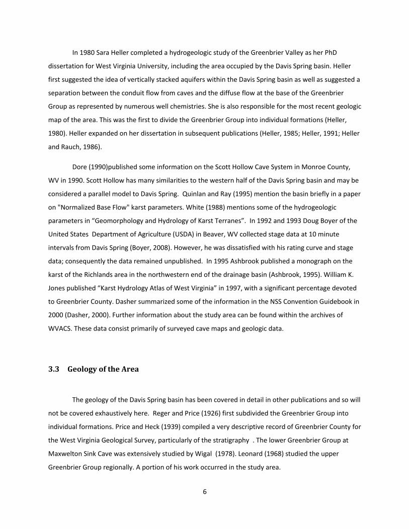
In 1980 Sara Heller completed a hydrogeologic study of the Greenbrier Valley as her PhD
dissertation for West Virginia University, including the area occupied by the Davis Spring basin. Heller
first suggested the idea of vertically stacked aquifers within the Davis Spring basin as well as suggested a
separation between the conduit flow from caves and the diffuse flow at the base of the Greenbrier
Group as represented by numerous well chemistries. She is also responsible for the most recent geologic
map of the area. This was the first to divide the Greenbrier Group into individual formations (Heller,
1980). Heller expanded on her dissertation in subsequent publications (Heller, 1985; Heller, 1991; Heller
and Rauch, 1986).
Dore (1990)published some information on the Scott Hollow Cave System in Monroe County,
WV in 1990. Scott Hollow has many similarities to the western half of the Davis Spring basin and may be
considered a parallel model to Davis Spring. Quinlan and Ray (1995) mention the basin briefly in a paper
on "Normalized Base Flow" karst parameters. White (1988) mentions some of the hydrogeologic
parameters in “Geomorphology and Hydrology of Karst Terranes”. In 1992 and 1993 Doug Boyer of the
United States Department of Agriculture (USDA) in Beaver, WV collected stage data at 10 minute
intervals from Davis Spring (Boyer, 2008). However, he was dissatisfied with his rating curve and stage
data; consequently the data remained unpublished. In 1995 Ashbrook published a monograph on the
karst of the Richlands area in the northwestern end of the drainage basin (Ashbrook, 1995). William K.
Jones published “Karst Hydrology Atlas of West Virginia” in 1997, with a significant percentage devoted
to Greenbrier County. Dasher summarized some of the information in the NSS Convention Guidebook in
2000 (Dasher, 2000). Further information about the study area can be found within the archives of
WVACS. These data consist primarily of surveyed cave maps and geologic data.
3.3 Geology of the Area
The geology of the Davis Spring basin has been covered in detail in other publications and so will
not be covered exhaustively here. Reger and Price (1926) first subdivided the Greenbrier Group into
individual formations. Price and Heck (1939) compiled a very descriptive record of Greenbrier County for
the West Virginia Geological Survey, particularly of the stratigraphy . The lower Greenbrier Group at
Maxwelton Sink Cave was extensively studied by Wigal (1978). Leonard (1968) studied the upper
Greenbrier Group regionally. A portion of his work occurred in the study area.
7
Heller (1980) devoted significant dissertation space to the geology of the study area, bringing
together all previous works. She also drafted the first geologic map to subdivide the Greenbrier Group,
though it was not widely distributed. The Heller map was the base map for further work in the area,
most notably by Ashbrook and WVACS (Balfour, 2004). This work will follow the naming style used by
Heller for the area. Formation thicknesses follow Balfour’s estimates which in turn follow Price and
Heck (Ashbrook, 1995).
3.3.1 Geologic Setting
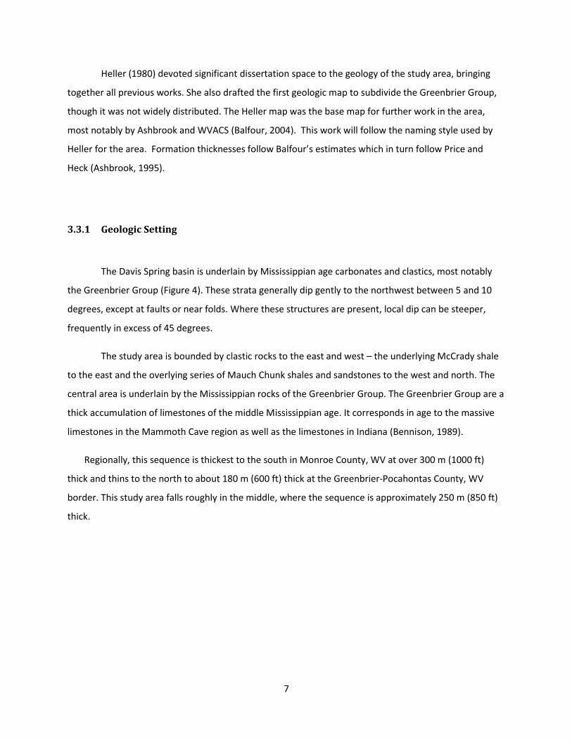
The Davis Spring basin is underlain by Mississippian age carbonates and clastics, most notably
the Greenbrier Group (Figure 4). These strata generally dip gently to the northwest between 5 and 10
degrees, except at faults or near folds. Where these structures are present, local dip can be steeper,
frequently in excess of 45 degrees.
The study area is bounded by clastic rocks to the east and west – the underlying McCrady shale
to the east and the overlying series of Mauch Chunk shales and sandstones to the west and north. The
central area is underlain by the Mississippian rocks of the Greenbrier Group. The Greenbrier Group are a
thick accumulation of limestones of the middle Mississippian age. It corresponds in age to the massive
limestones in the Mammoth Cave region as well as the limestones in Indiana (Bennison, 1989).
Regionally, this sequence is thickest to the south in Monroe County, WV at over 300 m (1000 ft)
thick and thins to the north to about 180 m (600 ft) thick at the Greenbrier-Pocahontas County, WV
border. This study area falls roughly in the middle, where the sequence is approximately 250 m (850 ft)
thick.
8
Figure 4: Geologic Map of the Davis Spring and surrounding basins, after Price and Heck (1939) and Heller (1980). Units labeled "1939" are from Price and Heck. All other data from Heller. See Figure 1 and 3 for geographic features.
9
3.3.2 Lithologic Sequence
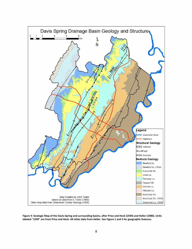
The Greenbrier Group is composed of a series of thick limestone and occasional shale units
which are overlain and underlain by sandstones and shales. The group itself can be divided into three
sections - a lower sequence of limestones, a middle sequence of limestones and shales and an upper
sequence of limestones. The lower
limestones tend to have cherty nodules or
layers while the bottom of the upper
sequence tends to have shaley beds. The
middle sequence acts as a confining layer,
hydrologically dividing the Greenbrier
Group vertically.
The Greenbrier sequence (Figure
5) is Mississippian in age, with the lower
portion in the Meramecian and the middle
and upper portions in the Chestarian. The
lower portion is contemporary with the St.
Louis / Genevieve limestones of the
Mammoth Cave region while the upper
portions match to the Girkin and Big Clifty
formations in the same area (Bennison,
1989).
The base of the Greenbrier
sequence is underlain by the MacCrady
Formation of the Price Group. The
MacCrady is composed primarily of red
shales and mudrock. Several of the master conduits within drainage basins in Greenbrier County have
cut down from the basal Greenbrier into the MacCrady, making the contact very visible underground
(Stevens, 1988).
Figure 5: Comparison of the stratigraphic column in Monroe County, Greenbrier County and Pocohantas County; After White and White (1983)
10
Above the MacCrady lies the basal formation of the Greenbrier Group – the Hillsdale Limestone. The
Hillsdale is a grey-blue massive limestone most noticeable for its extensive chert beds throughout its
thickness. Most of the long, integrated cave systems in Greenbrier and Monroe counties are formed at
or just above the Hillsdale – MacCrady contact. Conduit dimensions within the Hillsdale can be quite
large and continue for long distances. Much of the groundwater in the region is believed to travel slowly
along the base of the Hillsdale making it a very productive, albeit deep formation (Heller, 1980). Total
thickness of the Hillsdale is 10-35 meters (30-115 feet) thick (Ashbrook, 1995).
Above the Hillsdale lies the Denmar Formation, which to the south in Monroe County is split into an
upper Patton Formation and a lower Sinks Grove Formation. This distinction is difficult to determine
within the study area and so is not subdivided (Heller, 1980). The Denmar is another blue-grey
limestone, with abundant marine fossils. It is sometimes difficult to discern from the Hillsdale due to
similar weathering and coloring. Though the boundary between the Hillsdale and the Denmar is
recognizable, it is very infrequently exposed. Total thickness of the Denmar is 12-30 meters (40-100
feet) (Ashbrook, 1995).
Above the Denmar lies the Taggard Formation, which is composed of a thin red shale on top of a
thin grey shaley limestone on top of another thin red shale. The shales in the Taggard are reasonably
easy to recognize as few other strata weather red into the surrounding soil. The Taggard is the major
confining layer in the study area. Subterranean drainage is forced to the surface when it encounters the
Taggard only to disappear underground once it moves back over the next limestone. The relative
incompetence of the Taggard makes it a preferential layer for faulting. Vertical displacement along
Taggard faults can be several meters if not more. The Taggard thins noticeably to the north. Total
thickness of the Taggard is 3-26 meters (10-85 feet) (Ashbrook, 1995).
Above the Taggard lies the Pickaway Formation, a dark grey hard limestone which is relatively
fossil-free. The base of the Pickaway can be very shaley. The characteristic feature of the Pickaway is
hexagonal jointing similar in appearance to columnar basalt. In places caves of some length are formed
near the base of the Pickaway. However, layers within the Pickaway can be very poor passage formers,
leaving the Pickaway without cave systems equal in length to the Hillsdale. This is despite the Pickaway
resting on the Taggard confining layer. Total thickness of the Pickaway is 15-40 meters (50-130 feet)
(Ashbrook, 1995).
11
Above the Pickaway lies the Union Formation, a white to light grey hard limestone which can be
oolitic and fossiliferous. The change in color makes the Union and Pickaway fairly easy to distinguish.
The Union Formation is the other major cave former besides the Hillsdale Formation in the region,
though within the study area few caves of significant length have been found. Lost World Caverns
(Grapevine Cave), a commercial cave near Lewisburg, is 3 km (2 mi) in length and developed at the base
of the Union. However, the Union is the host rock for large cave systems to the north of the Davis Spring
basin. The Union commonly crops out along the base of ridges and individual hills such as Weaver Knob
and Muddy Creek Mountain. Total thickness of the Union is 45-60 meters (150-200 feet) (Ashbrook,
1995).
The Union marks the upper end of the massive limestones of the Greenbrier Group. Two
formations exist above the Union – the Greenville Shale and the Alderson Limestone. The Greenville is a
dark brown shale while the Alderson is a grey sandy limestone. Caves in the Alderson are generally short
and hydrologically separated from the rest of the Greenbrier Group by the Greenville Shale. Total
thickness of the Greenville is 0-20 meters (0-65 feet). Total thickness of the Alderson is 15-45 meters
(50-150 feet) (Ashbrook, 1995).
Above the Greenbrier Group lies the basal member of the Mauch Chunk Group, the Lilydale
Shale of the Bluefield Formation. The Bluefield Formation is composed of red and green shales grading
upwards to sandstones. Muddy Creek Mountain on the western border of the study area is capped by
the Bluefield Formation.
3.3.3 Structural Geology
The Davis Spring basin lies at the border between two geologic provinces: the Valley and Ridge
Province and the Appalachian Plateau Province. Though most of the study area consists of relatively flat
lying bedding (there is a slight dip to the northwest), several north-south trending reverse and normal
faults and localized folds cross the drainage basin. Dip can be steep to vertical in these areas. These
structures are the westernmost expression of the Valley and Ridge Province and decrease in frequency
as one moves westward. Only one of these faults is easily visible and that is in a large road cut along I-64
just west of Lewisburg (Heller, 1980). In order from east to west, these structures are called: Lewisburg
Fault, Lewisburg Syncline, Lewisburg Anticline, Rockland Syncline, Rockland Structure (Fault), Lost World

12
Syncline, Lost World Thrust Fault, Weaver Knob Anticline, Greystone Quarry Fault and the Muddy Creek
Mountian Syncline.

13
4 Thesis Objectives To explore basic hydrogeologic aspects of the Davis Spring drainage basin with emphasis on (1)
the components and configuration of the system at its downstream end and( 2) the relationship Davis
Spring has to the Milligan Creek infeeder.
4.1 Tasks necessary to accomplish objectives
1) Create a GIS-based map of the geology of the Davis Spring drainage basin from existing geological
maps.
2) Further refine the flow boundaries between the Davis Spring basin and Rockland Indian Spring basin
and distinguish the sub-basin boundaries on the basis of tracer travel times and geomorphology.
a) This includes reconnaissance for additional springs which would alter our understanding of the
current basin boundaries.
3) Define some specific drainage characteristics of the Davis Spring basin based on spring discharge,
conductivity and tracer testing data.
4) Determine the likely configuration of the conduit system feeding the spring with respect to
discharge.
5) Delineation of some of the basic aspects of the karst groundwater system within the Davis Spring
drainage basin, specifically:
a) Determine if the main conduit has closed, open or alternating flow.
b) Determine the approximate minimum dimensions of the possible conduit channel.
6) Explore the relationship between discharge and the conduit system at Davis Spring, including the
timing of the spring discharge to rain events.
7) Show the degree of influence Milligan Creek has on the overall Davis Spring system in terms of
discharge and conductivity under high and low flow.
8) Speculate on the overall geologic framework of the conduit system in the Davis Spring drainage
basin with respect to stratigraphy and structural controls.

14
5 Methods and Procedures
5.1 GIS Mapping
The most recent published map (Heller, 1980) of the Davis Spring drainage basin is poorly
distributed throughout the karst community. Original maps are impossible to acquire and interpretation
requires a topographic map be overlaid on the Heller map to illustrate the relationship between geology
and topography. Given that geologic mapping is the basis of all further work, it was necessary to convert
the paper Heller map to a digital format.
ArcGIS 9.3 was used to create the new maps. Baseline topographical maps were acquired from
the WV GIS depository at West Virginia University. Because the original map was folded and slightly
warped, it was unsuitable for direct scanning. Map data was transferred into ArcGIS manually. In some
locations the Heller map is unclear. Heller’s working maps were also obtained to resolve these confusing
points. The finished geologic polygons are included. This information was also submitted to the West
Virginia Geological and Economic Survey for inclusion in their database. Heller’s working maps have
been transferred to the West Virginia University Student Grotto Reference Library as items of historical
interest.
5.2 Water Budget
5.2.1 Background and Governing Principles
Over any long term period (several years or more), any water budget must follow the simple
formula of
Precipitation (P) = Runoff (R) + Evapotranspiration (ET) (1)
(Fetter, 2001)
15
However, over a shorter period an additional term representing the change in storage should be
added to the right side to represent any temporary increase or decrease in aquifer levels or surface
pools (water storage). The equation over the short term would become:
Precipitation (P) = Runoff (R) + Evapotranspiration (ET) ± Storage Change (ΔS) (2)
(Fetter, 2001)
Determining the change in storage becomes problematic in a karst environment as pools are
often hidden in the subsurface and may be inaccessible or unknown. Changes in aquifer levels are
unknowable unless monitoring wells are installed throughout the area. Due to cost, monitoring wells
were not installed for this study. A significant storage change does not always have to occur – there may
be long intervals where storage is relatively stable. This study will therefore make the assumption that
storage change is negligible.
Runoff can be divided further into a surface component and a ground water component:
Runoff (R) = Surface Runoff (RS) + Ground Water Runoff (RG) (3)
(White, 1988)
For non-karst drainage basins this is a perfectly acceptable division. However, in mature karst
systems most storm flow runoff flows through underground conduits. Runoff of this kind behaves much
more like surface runoff than traditional ground water runoff, even though it would technically be
classified as the latter. Therefore, a further distinction is required for ground water runoff, dividing it
into quick flow (quick movement of water through conduits as a result of precipitation events) and base
flow (slow movement of water due to the draining of stored water in the aquifer).
Ground Water Runoff (RG) = Quick Flow (QF) + Base Flow (BF) (4)
(Ford and Williams, 2007)
Lastly, there is Interbasin Transfer (IBT). IBT represents water which exits the basin through any
other route other than the monitored downstream outlet of the system. In karst systems overflow
routes can bypass downstream monitoring stations. Water may also leave a basin through
anthropogenic means; for example by being pumped out. In most places IBT is also negligible; however
it should not be assumed to be so.
16
The final equation for the Davis Spring drainage basin would then be:
Precipitation (P) = (ET) + Interbasin Transfer (IBT) + Quick Flow (QF) + Base Flow (BF) (5)
The numbers used for each variable come from the following sources:
Precipitation – These data are generated from daily precipitation events at Maxwelton Airport (Figure
38). Maxwelton Airport is located in the northeastern portion of the basin, about 8 km north of
Lewisburg.
Evapotranspiration – This is calculated as the net difference after all the other parameters in Equation 5
have been established.
Interbasin Transfer – Storage change is possible in two ways in the Davis Spring Basin and it is important
to be able to estimate the relative importance of each possibility:
(a) Change through water leaving the Davis Spring basin without passing the datalogger
at the spring. The entire Davis Spring channel was thoroughly checked during low
flow for additional outlets either at or above the water level. None were found
between the datalogger and the Greenbrier River. It is possible that there are
additional outlets in the bed of the Greenbrier River. However, outlets such as these
would be extremely difficult to detect and impossible to monitor.
(b) The idea of water leaving the Davis Spring basin through the Lewisburg sewer
system also required examination. Conversations with the Lewisburg City Planning
Department revealed that much of the eastern part of the basin receives “city
water” pumped from a treatment plant along the Greenbrier River near Ronceverte.
Waste water is then pumped back to Ronceverte, treated, and returned to the
Greenbrier River. Theoretically this should result in no net change in water in the
Davis Spring basin. Storm runoff, on the other hand is collected in city sewers which
are then funneled into several sinkholes to exit via Davis Spring. As storm water is
already accounted for in the precipitation variable, this is another net zero change
(Tubbs, 2008).
Overall, this suggests that IBT is effectively zero in the basin.

17
Quick Flow + Base Flow – Although these are separate variables, they are recorded as one by the
datalogger at Davis Spring.
In the Lewisburg area, the average amount of rainfall per annum was recorded by Jones as 979
mm while the average potential evapotranspiration (PET) was 671 mm. Jones’ data covers the period of
1951-1960, a 10 year average (Jones, 1973). In his MS Thesis, Boyer has slightly different values for a
similar area for the period between 1958-1972. Boyer recorded annual precipitation at 1073 mm,
annual PET at 606.5 mm and annual observed ET at 590 mm (see Table 1). Boyer’s data covers the
slightly longer period of 15 years. The location of Boyer’s study is slightly to the south and west of the
current study area in a similar geographical setting near Fort Spring (Boyer, 1976). Data by Boyer and
Jones overlap for three years ( 1958-1960) which is 30 percent of Jones’ data and 20 percent of Boyer’s.
Historically, evapotranspiration increases in the summer resulting in a net loss of discharge.
Evapotranspiration decreases in the winter with a corresponding rise in discharge at Davis Spring. Frozen
ground also contributes to increased storm runoff during winter months. In this region
evapotranspiration is mostly due to plant growth combined with higher temperatures.
Ground water recharge is a function of the amount of rain fallen over an area (usually expressed
as vertical thickness in inches or millimeters over time) multiplied by the area of the drainage basin
multiplied by the elapsed time. Discharge at a given station is expressed in volume of water per unit
time and must be aggregated over the total time to determine cumulative discharge. When both
calculations are complete the relative amounts will be expressed as volumes over the same time
interval. Discharge can then be subtracted from precipitation. The remainder is the calculated loss due
to evapotranspiration or in the case of short term water budgets a combination of evapotranspiration
and a change in storage.
18
5.3 Datalogging
5.3.1 Explanation of datalogging equipment.
Two Campbell 21x Micrologger dataloggers for hydrological measurements were loaned from
the United States Department of Agriculture's (USDA’s) Beckley office for use in the project. The 21x
features 19MB of available internal storage. However, this storage is volatile and so it is preferable to
write information to external drive space. Each external drive can hold 4MB. Data stored in memory are
exportable into comma-delimited .txt files. These can be easily imported into the spreadsheet program
of choice.
The 21x can be powered by alkaline D-cells or it can be connected to a car / boat battery. The
USDA prefers the latter option. This provides a longer battery life (at least 1 month). Battery life can be
monitored through the on-board display.
With the above configuration, more than 1 month of data can be stored onto the logger before
the unit runs out of memory and/or battery life. Memory units were changed on a monthly basis, if not
more frequently. Battery units were changed only when the voltage ran down on the operating unit – as
changing the battery deletes the volatile memory thus necessitating reprogramming.
The 21x has several input channels to which various sensors can be connected. For purposes of
this project the following were connected to the datalogger:
Pressure transducer - to determine stage
Conductivity sensor
Temperature sensor
Auto-sampling device (for water samples - Davis Spring only)
The 21x must be programmed before use. Programming can be done in the field through the
numeric keypad or at the lab through a personal computer. In the field the program can be stored in the
memory unit and downloaded into the volatile memory for execution. This is to provide backup in case
of volatile data loss without the need to return the unit to the lab for reprogramming.
19
In the field the dataloggers are stored within sealed Pelican Cases. Desiccant is added alongside
the units to prevent condensation and corrosion to the equipment. Sensors are cable-tied to cement
blocks which are gently lowered into the water. Cement blocks are necessary to prevent the sensors
from moving unnecessarily and to prevent damage from accidental impacts. At Milligan Creek, large
floods moved the cement blocks in the winter months. They were returned to their original location,
recalibrated and the blocks further anchored with rebar and rocks.
5.3.2 Location of datalogging equipment.
For this project dataloggers were placed at Davis Spring and at Milligan Creek. In each instance
the location for the loggers fulfilled the following requirements:
The dataloggers were sufficiently high above the channel to not flood under high flow
conditions.
The channel was sufficiently developed (i.e. deep enough) to not run dry. The logger should be
placed in the deepest accessible part of the channel.
The location was relatively easily accessible but at the same time secluded enough to discourage
theft and vandalism.
The location was representative of the overall flow dynamics of the channel. (i.e. not in a
stagnant pool off to the side).
The location was contemporary with the sampling and flow measuring point in order to be
completely compatible. This was perhaps the most important point.
At Davis Spring (Figure 2) the logger was placed near a thin peninsula which jutted out into the
main channel. The sensors were placed several feet away from the bank, about a third of the way across
the channel. The Davis Spring channel is about 15 meters wide (50 feet) and about 1 meter deep. At this
location the channel does not run dry, so any position in the base of the channel should give equivalent
results. The location was secluded in the summer months, but observable in the winter months once the
foliage disappeared. Despite being visible from the road in the winter the datalogger was not vandalized
or stolen.
20
The initial suggestion for datalogger placement at Milligan Creek was near the Hern’s Mill
bridge. However, that location was deemed too insecure because Milligan Creek is fished in the spring
and summer months. Access to Milligan Creek downstream was through the generosity of a nearby
landowner and the logger was placed about 0.5 km downstream of the bridge. Milligan Creek is a pool
and riffle type stream in this reach and the sensors were placed in a large pool. Though slightly remote
compared to Davis Spring, this arrangement worked well. However, mechanical problems plagued the
logger placed there, and when it was replaced in late summer 2008, similar problems occurred to the
replacement unit. Furthermore in December 2008, large storms washed the sensors several feet
downstream. Although the logger worked intermittently well afterwards, it continued to have problems
throughout the 2008-2009 winter. Consequently, data collected after mid-December 2008 from the
Milligan Creek site should be viewed with skepticism. While this is unfortunate, the situation would have
been catastrophic had the same problems befallen the Davis Spring datalogger.
5.3.3 Equipment used to measure flow
A Marsh-McBirney model 201D portable water current meter was used to measure flow in the
study area. The 201D measures velocity electromagnetically with a range of -.5 to +20 ft/sec and an
accuracy of +/- 2% of the reading. It is capable of displaying flow in ft/sec, m/sec or knots. It is powered
by 6 D-Cell batteries which are rated for 100 hours of continuous use. It is important to remember as
one struggles with borrowed equipment over the algae encrusted rocks in knee-deep fast moving water
that the unit is water resistant and not waterproof.
Flow is measured using the Faraday principle which states that “as a conductor moves through
and cuts lines of magnetic flux, a voltage is produced. The magnitude of the generated voltage is directly
proportional to the velocity at which the conductor moves through the magnetic field. When the flow
approaches the sensor from directly in front, then the direction of the flow, the magnetic field and the
sensed voltage are mutually perpendicular to each other, and thus, the voltage output will represent the
velocity of the flow at the electrodes” (Marsh-McBirney, 1984).
From a mechanical standpoint this means that the sensor contains an electromagnetic coil
which produces a field. Two electrodes measure the voltage produced as a conductive fluid (in this case
21
the water) passes through the field. If the field is not exactly perpendicular, the voltage will be under-
represented. The voltage is then converted to a velocity measurement in the units of the user’s choice.
The sensor is then connected to either a standard wading rod or a top-set wading rod by way of
a double-end hanger. These rods are divided into increments of a tenth of a foot. Each tenth is marked
by a single horizontal line in the rod. Each half-foot (five-tenths) are marked by a double horizontal line
and each foot is marked by a triple horizontal line. A top-set wading rod differs from the standard in that
there are two rods connected – the previously described main rod and a secondary rod attached to the
main one. This secondary rod is marked in increments 60% the distance of the first rod. The reason for
this will be explained in the "Procedure for streamflow measurement", below.
Lastly, a fiberglass or plastic tape was used to measure the width across the channel and as a
guide for setting individual stations in the channel. Data were recorded and reduced using Microsoft
Excel 2007.
5.3.4 Difficulties with flow measurements at the datalogging sites
Both Davis Spring and Milligan Creek have significant drawbacks from an idealized site. Both
sites are underlain by the Pickaway limestone, a shaley limestone with significant karst pavement
development.
At Davis Spring there are the following difficulties with measurement:
The downstream Davis Spring channel (Figure 2) is generally wide and can be deep, with depths
of over 1.5 meters possible during high flow. This posed significant problems for measuring the
upper end of the flow regime. In the past, this measurement had been conducted from the
bridge approximately a 300 meters downstream from the spring. The bridge is located less than
20 meters from the confluence of the spring channel and the Greenbrier River. Under the same
high flow conditions the Greenbrier can be expected to back-flow into the Davis Spring channel
causing the meter to under-report the flow at the bridge.
The Davis Spring channel is divided by a small man-made dam into an upper and lower reach. All
the equipment was placed in the upper reach. The dam contributes to deep pools (1-2 m) in the
upper reach. This reduces stream velocity. Early measurements showed this slowing was enough
22
to reduce very low flow velocity to zero on the flow meter. This led to underreporting in the
discharge (Soupir et al., 2009). The problem was resolved when discharge measurements were
moved downstream of the dam.
The bottom of the Davis Spring stream channel is lined with cobbles and boulders up to 0.5
meters in diameter. These can cause problems with accurate depth reporting and flow
redirection, giving errors in flow measurement.
At Milligan Creek there are the following difficulties with measurement:
The whole reach is a pool and riffle type stream with occasional short reaches of limestone
pavement. In order to have the flow measurement consistent with the stage measurement, the
flow needs to be measured very close to the datalogger.
Riffles are unusable because they combine very low stage and abundant cobbles. A shallow,
uneven surface is the result. Boulders also litter the stream and the stream flows between them.
Limestone pavement is undesirable because it tends to occur in wide swaths with shallow
stream depths (under 0.3 meter). Additional flow passes via underflow through the exposed
epikarst in the pavement. It is believed that limestone pavement underlies the entirety of
Milligan Creek as it passes through the Pickaway Limestone. This can cause under-reporting of
the true flow at Milligan Creek as the volume of water associated with the underflow passing
through the grikes remains an unknown.
Pools are by process of elimination the most acceptable option for flow measurement.
However, they have drawbacks as well. They can have cobble beds or limestone pavement, or
both. They can be semi-circular in origin, with water flowing in from several angles to the main
channel. They can host eddies, which complicate the overall flow.
There is considerable error in the high flow measurements at Hern's Mill. Milligan Creek is very
flashy at Hern's Mill, amplified by the restricted area in the bottom of the ravine. In the middle
of December 2008, floods were sufficient to move the datalogger. Typical high stage discharges
lasted only hours and were difficult to accurately predict from Morgantown, 200 miles away.
23
5.4 Streamflow Measurement
5.4.1 Procedure for streamflow measurement.
Measuring streamflow is a relatively simple, mechanical process. A tape is strung across the
channel to be measured and subdivided into about 20 even increments. Increments can be moved to
account for no flow or changes in the channel dimensions to provide a more accurate description of the
overall flow. In an ideal channel cross-section, the individual stations should be directed towards the
central flow of the channel. However, in the channels measured here it is probably more important to
weight towards the greatest flow, no matter where it might be in the channel.
The flow velocity sensor is then attached to the wading staff. At each channel the sensor is
lowered to 60% of the depth from the stream surface. With the standard staff, the depth must first be
read off the staff and then the 60% depth must be calculated from the water surface and subtracted.
The sensor is then moved to that depth. With the top-set staff the depth is read off the staff (along the
primary rod) and then the secondary staff is set to exactly the same depth. The gradations on the
secondary staff are already 60% of the primary staff and consequently no math is required (Rantz,
1982a).
5.4.2 Flow to discharge conversion; rating curve.
Measured velocities can be converted to discharge using the following formula:
qi = vi*di*wi (6)
Where qi =discharge, vi = recorded velocity, di = depth and wi = the distance between midpoints
of individual stations. This provides the discharge for an individual sub-section of the measured stream.
Discharge for the whole stream is then simply the summation of all individual sub-sections.
24
A rating curve is comprised of several discharge measurements over several different stages. A
variety of stage heights is necessary for the rating curve to be applicable over a large distance. The curve
becomes less meaningful the farther one gets from the measured maxima and minima. A rating curve
can be plotted in a spreadsheet program and the best fit line automatically generated. Note – fourth
and fifth order polynomials may be unreliable in Microsoft Excel 2007 (Rantz, 1982a).
5.4.3 Conversion of Stage to Discharge
Stage measurement, while useful, is less than ideal for describing flow. Discharge is far more
useful. Consequently, a conversion of stage to discharge is desirable. This conversion is accomplished
through use of a rating curve. A rating curve is a graphical relationship between stage (X axis) and
discharge (y-axis). This can then be interpreted as a polynomial mathematical formula which can be
applied to any stage measurement.
A rating curve is based on several flow measurements across a range of stage heights. The ideal
rating curve includes the highest stage measurement, the lowest stage measurement and a
representative sample of measurements in-between. Oftentimes, however, the ideal curve cannot be
created. Extending the rating curve above and below the end-points should only be done provisionally.
5.4.4 Rating Curve Methodology
A rating curve was created to correlate between stage and discharge. Rating curves are
common in hydrology and there is copious information about their construction. The premise behind
the rating curve is a relationship between the rise in stage and the increase in discharge. The
relationship is determined by measuring the different discharges over a wide range of stages at a single
point along the flow path. The results are then graphed and a trend line plotted for the best fit of the
data. The trend line usually follows some sort of curve. Using statistical or spreadsheet software an
equation for the curve is generated. Although it is common to see stage as the dependent variable, for
purposes of making a useful equation to convert stage to discharge, this thesis will swap the axes,
placing stage as the independent (x-axis) variable.
25
5.4.5 Locations for Stage Measurement
Stage was measured at predetermined locations in Milligan Creek and Davis Spring at fifteen
minute intervals using a Campbell datalogger and pressure transducer. The transducer is attached to a
cinder block and placed along the bottom of the deepest part of the channel. Pressure from the
transducer is converted into depth below the stream surface. When the transducer is first installed the
depth reading is checked against a stiff ruler for accuracy. Thereafter, the pressure transducer is
occasionally rechecked.
At Davis Spring, the force of flow was dispersed over a wide channel and so there was little
danger of the transducer moving. However, at Milligan Creek the narrow channel and high flows meant
it was always a concern. In December 2008, large storms moved the cinder block anchoring the
transducer several feet downstream. The cinder block was returned to its starting location and more
securely fastened to the bottom with rebar. Subsequent large storms combined with below freezing
conditions continued to disrupt the transducer enough that high flow data became unreliable in January
and February 2009.
5.4.6 Previous rating curves
At least two previous rating curves have already been created for Davis Spring. Boyer created
one in the mid 1990s (Boyer, 2008) and Jones created one in the early 1970s (Jones, 2009). The Boyer
rating curve had been considered to be less than ideal for use at the time, while the Jones rating curve
was too far in the distant past to accurately relate to current measurements. All three rating curves
could be compared to a permanent staff gauge placed at Davis Spring in the 1960s (Jones, 2009). No
known rating curves have ever been created for Milligan Creek.
26
5.5 Data Reduction and Curve Generation
A rating curve was created from 10 stage measurements and corresponding discharges as
previously described. When multiple traverses were consecutively measured, the results were averaged
then added to the tabulation. Discharge measurements taken in the mid 1990s by Boyer at Davis Spring
were also used in this rating curve (Boyer, 2008). These measurements were at the upper end of the
curve, at stages which rarely occurred during fieldwork. These measurements were included, in the
absence of more current measurements at an equivalent stage, because the concrete bridge under
where they were measured has remained unchanged.
Inclusion of these data were possible because they and the current data could be correlated to a
single staff gauge placed in the Davis Spring channel in the 1960s by the USGS. Those measurements
could be correlated to the current datalogger measurements through the following formula:
USGS staff gauge (feet) = 2008 datalogger (feet) + 6.04 (feet) (7)
This formula has an R-squared value of about 0.99 (Boyer, 2008). However, they should still be treated
with modest skepticism and as a better alternative to complete estimation of the upper portion of the
rating curve. These data were inspected both visually and through the use of a confidence interval, to
determine if there were any unusual data or outliers. However, falling outside of the confidence interval
was insufficient to invalidate data. Several data points do not fall neatly along the trend line and only
one point was removed. The data on 12-1-08 were considered to be an under-reporting of a comparable
stage. Examination of the data concluded either user error or equipment error were at fault. It is
possible that on that day the current meter was accidentally in meters/second mode rather than the
standard feet/second mode. It is more likely that low batteries combined with freezing temperatures
adversely affected the flowmeter’s performance, under-reporting the data. A total of four cross-sections
were made that day – two at the datalogger and two at the bridge. The two cross-sections at the
datalogger varied badly in precision error (more than 100%). When compared to subsequent
measurements at a similar stage, the two measurements at the bridge under-reported the data by 50%
or more. The datalogger data made previous upstream measurements suspect for awhile. It was only
with the benefit of the full dataset that the bridge measurements stood out. Only then did it become
apparent that it was the instrument that day as much as the location that presented problems. As a
result that whole day’s field work was discarded.
27
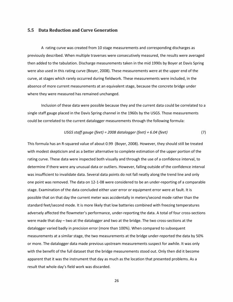
Using the remaining data, a power curve was generated for the described relationship. (Figure
6) The resulting equation was:
Q=0.4796x 4.2764 (8)
Where Q is discharge in cfs and x is stage in feet at the datalogger. This relationship had an R-
squared value of 0.840. This is far from ideal, but quite acceptable. Improvements could be made to the
R-squared value by removing more of the outliers; however that would only improve the relationship by
decreasing the number of points plotted.
The primary cause for the error lies within the comparatively short time frame for the fieldwork.
Definitive rating curves are composed over several years. Over shorter time periods there is the danger
of not having an even distribution of data points. This leaves gaps in the data and over represents other
parts of the curve.
Figure 6: The Davis Spring rating curve. 1993 data courtesy Boyer (2008).
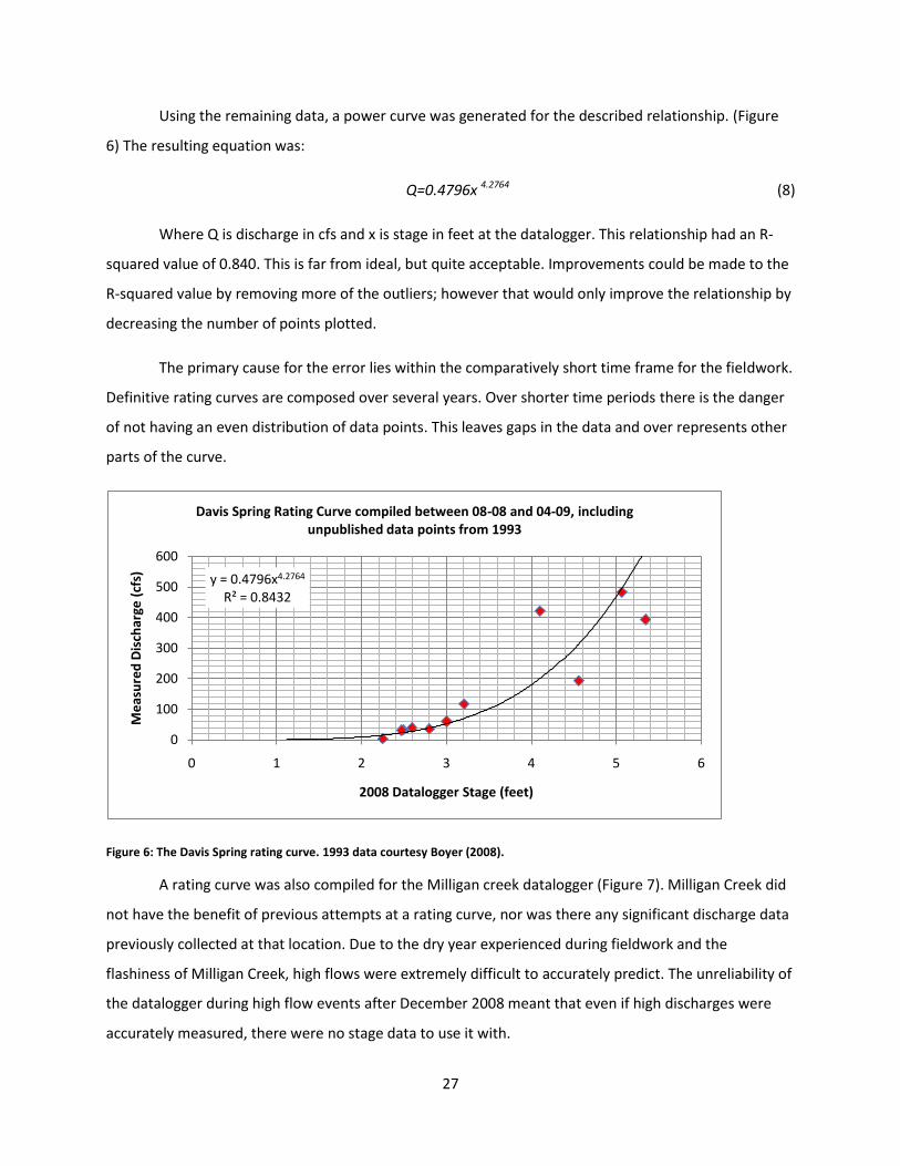
A rating curve was also compiled for the Milligan creek datalogger (Figure 7). Milligan Creek did
not have the benefit of previous attempts at a rating curve, nor was there any significant discharge data
previously collected at that location. Due to the dry year experienced during fieldwork and the
flashiness of Milligan Creek, high flows were extremely difficult to accurately predict. The unreliability of
the datalogger during high flow events after December 2008 meant that even if high discharges were
accurately measured, there were no stage data to use it with.
y = 0.4796x4.2764
R² = 0.8432
0
100
200
300
400
500
600
0 1 2 3 4 5 6
Me
asu
red
Dis
char
ge (
cfs)
2008 Datalogger Stage (feet)
Davis Spring Rating Curve compiled between 08-08 and 04-09, including unpublished data points from 1993
28
The resulting equation was:
Q=1.3838x 6.2824 (9)
Where Q is discharge in cfs and x is stage in feet. This relationship had an R-squared value of 0.9668.
This high R-squared value appears excellent but may also be a function of the clumping of data into two
distinct regions. Though the trend line extends past the data, this should be considered provisional. The
farther the trend line moves from the data the less reliable that portion of the line becomes (Rantz,
1982b).
Figure 7: The Milligan Creek rating curve.
5.6 Verification of the Rating Curve
Independent verification of the rating curve is important to ascertain how accurate the curve is.
Two lines of investigation have been followed to see how robust the curve is in extrapolating stage data.
The first method of verification is through a simple water budget. The second method of verification is
through use of the EPA’s QTRACER software to report the amount of dye recovered during tracer tests.
y = 1.3838x6.2824
R² = 0.9668
0
10
20
30
40
50
60
70
80
90
100
0.8 1 1.2 1.4 1.6 1.8 2 2.2
Me
asu
red
Dis
char
ge (
cfs)
2008 datalogger stage (feet)
Milligan Creek Rating Curve collected between 08/08 and 3/09

29
Discussion on both topics are in their respective thesis sections and will not be duplicated here.
However, this rating curve returns an ET of 80% and recovers 84% of the August 2008 Rhodamine WT
dye trace.
30
5.7 Field Reconnaissance –
Field reconnaissance was necessary to complement both dye tracing and the map conversion.
Because of the large size of the study area, it was impossible to examine every square foot of terrain
personally. Therefore, fieldwork primarily consisted of locating the following features:
Sinking streams and swallets: These are useful to be able to delineate the drainage basin
boundaries. In particular, the area along Davis Stuart Road (the boundary between the Davis Spring
drainage basin and the Rockland Indian drainage basin) was examined for large sinking streams. This
area is of particular importance in that no dye traces in this area have ever been undertaken. One
stream, in the large karst valley to the west of Davis Stuart road was particularly useful, as the stream is
perennial. This swallet is referred to as Wood Sink (Figure 16, Figure 17). Other sinking streams in the
area were discovered to be intermittent and dry throughout most of the fieldwork. They remain useful
candidates for tracer tests during wetter periods.
Springs and seeps: These were useful in determining the extent the water exits through Davis
Spring. A major question was to determine if additional large springs were discovered. Such springs
would imply that the drainage basin is fragmented into one or more additional basins. In particular, the
northern bank of the Greenbrier River between Ronceverte and Davis Spring was examined (Figure 1).
This area is very infrequently inspected for karst features due to its inaccessibility from roads as well as
its rugged terrain. The only feasible time to examine this area was under low flow in October. Higher
flows make slow navigation of the river difficult. Higher flows also make detection of small to moderate
sized springs difficult. Even under low flows several likely locations could not be definitely shown to not
have springs due to deep pools which may have resurgences at or near the stream bottom.
Additionally, the surface channel of Davis Spring was examined for additional seeps which might
be overflow routes for karst waters. Due to the low, wide stream channel downstream of the dam, there
is considerable confidence in stating there are no significant additional springs downstream of Davis
Spring.
31
5.8 Dye Tracing –
5.8.1 Quantitative Dye Tracing Overview.
Dye traces fall into two major categories – qualitative and quantitative. Qualitative traces
concern themselves primarily with linking two points hydrologically. The positives to a qualitative dye
trace are as follows: they are simple, relatively inexpensive and low maintenance. On the negative side,
they say very little beyond determining whether two points may be hydrologically connected. A
qualitative dye trace can be as simple as dumping a rough amount of tracer into a swallet, and leaving a
charcoal trap to detect it at a spring. Many of the dye traces done in the past in the Davis Spring basin
have been of this nature.
A fully quantitative trace involves more effort, but reveals more about the system. In a fully
quantitative trace, as the name implies, nearly everything is measured and monitored. During a
quantitative test, discharge and dye concentrations are monitored at specified intervals, the tracer
added must be an exactly known quantity and all likely exits must be monitored. This ensures that all
detectable tracer is accounted for. Computer programs like QTRACER2 can be used to significantly
reduce the mathematical workload after the trace has been completed. Automatic samplers and
dataloggers can be used to reduce the time spent at the site and eliminate user bias in field collecting.
A semi-quantitative test tracks one or some parameters, but not all. A popular semi-quantitative
trace would be to frequently change out the charcoal traps to better identify the moment when dye is
first detected. Recording stage at the spring at the same time (or at regular intervals) would give a
rough idea of discharge which would aid in subsequent analysis.
5.8.2 Dyes used, relative advantages and disadvantages.
Four tracers – Rhodamine WT, fluorescein, sodium bromide and optical brightener 23 were
available for use. Of the four, two – Sodium bromide and the optical brightener have concerns and so
were only used on a limited basis. Optical brightener is often confused by background noise and can be
adsorbed by organics, leading to excessive tracer values reported (Mull et al., 1988). It was not used in
32
this study at all. Sodium bromide is a salt and may be viewed with concern by the local farming industry
(Boyer, 2008). It was only used in one test, and in an insufficient quantity to be visually detectible at the
resurgence.
Rhodamine WT and Fluorescein tracer were used for tracer tests in this thesis. Rhodamine WT is
the tracer of choice for tracing where a long reach travels over the surface as Rhodamine WT does not
photodecay easily. Fluorescein does photodecay and so is useful for tracing at points where the flow is
almost exclusively underground. The parameters on Rhodamine WT are as follows: maximum excitation
= 558nm, maximum emission = 583nm, fluorescence intensity = 25%, detection limit = 0.0006 ug/L,
sorption tendency = moderate. The parameters for fluorescein are as follows: maximum excitation =
492nm, maximum emission = 513nm, fluorescence intensity = 100%, detection limit =0 .0002 ug/L,
sorption tendency = very low (Aley, 2002).
The USDA generously supplied Rhodamine WT dye in liquid form, listed as 20% Rhodamine.
They also supplied solid fluorescein dye, which required grinding before use.
5.8.3 Determination of amount of dye needed.
From a general overview, the amount of dye necessary for a tracer test is such that at the spring
detection levels fall above the minimum amount detectable by the spectrofluorometer and below visual
detection. Ideally, a good test falls closer to the former than the latter. From a quantitative view, the
amount of dye necessary is the amount needed to record a concentration curve over time. Because of
variability between basins it is always better to exceed the minimum detection limit a little. There is a
certain amount of skill and art to this educated guesswork. Two mathematical procedures were located
to help discover the minimum limits.
The first comes from Worthington and Smart (2003) as recounted in ‘Cave Geology’ (Palmer,
2007). The formula is as follows:
m = 19*(LQC)0.95 (10)
Where m = mass of dye in grams, L = distance in meters, Q = spring discharge in m3/sec and C = desired
dye concentration at the outlet. The above formula is useable for any type of dye (Palmer, 2007).
33
Aley and Fletcher (1976) use different formulas for Rhodamine WT and fluorescein. They also
employ a nomograph based on the equation for each. The Rhodamine WT equation is as follows:
Vd = f(QL/V)Cp (11)
Where Vd = volume of dye in mL and where 1 mL of dye = 1.16 g; f = coefficient equal to 0.4 divided by
the dye solution strength (0.2 for Rhodamine WT); Q = mean discharge of the stream in m3/sec; L =
length of stream reach in km; V = estimated mean velocity of stream in m/s; Cp = desired peak dye
concentration In ppb.
For fluorescein the empirical equation is as follows:
Wd = 1.478 sqrt(DQ/V) (12)
Where Wd = weight of fluorescein dye in kg; D = straight line distance in km from insurgence to
resurgence; Q = discharge at resurgence in m3/sec; V = velocity of flow in meters/hour (Aley and
Fletcher, 1976).
Several sources point out that minimum dye equations vary across the literature, sometimes by
orders of magnitude. The above equations are two of the more respected equations, so as a rule a
minimum quantity should exceed both equations.
5.8.4 Dye detection process; Charcoal and automatic sampling
Dye was recovered through the use of automatic samplers and regularly changed charcoal traps.
The USDA's automatic sampler was placed adjacent to the Davis Spring datalogger with the tube
extending into the channel adjacent to the sensors. This central location had the best chance of
detecting the tracer given at least partial mixing. Charcoal traps were placed at different points along
the spring and at the confluence with the Greenbrier River to serve as a backup should the automatic
sampler miss the dye.
Charcoal traps were constructed out of 3.5 x 6 inch pieces of fiberglass screen folded
longitudinally and stapled on the ends and side. Each trap was filled about two thirds full with activated
carbon (6-14 mesh; Fisher Scientific #05-685A) and tied off with a fishing line attached to a weight
34
(washer or nut). The automatic sampler provided by the USDA was an ISCO 3700 portable sampler. It
consists of 24 individual sampling bottles in a carousel connected to the datalogger with a tube
extending into the stream. At the predetermined interval (this was usually every 6 hours), the tube
sampled the water, filled the bottle and advanced the carousel to the next bottle.
Charcoal traps were placed and retrieved by a ‘dye clean’ person (a person uncontaminated by
dye) to avoid false positive results. Collected charcoal traps required a small amount of preparation
before anaysis. The USDA uses 20 mLs of a solution described by Smart (Smart and Brown, 1973)
comprised of 5 parts 1- Propanol, 2 parts Ammonium Hydroxide (NH4OH) and 3 parts distilled water
(H2O). Prior to immersion in the ‘smart solution’ charcoal traps were rinsed off to remove excess silt,
algae, and other materials. It was necessary for charcoal traps to sit overnight in the solution prior to
analysis in the spectrofluorophotometer (Boyer, 2008).
The USDA ISCO 3700 Sampler was used to automatically collect tracer samples. The ISCO was
integrated with the datalogger so that the datalogger chronometer could be used to alert the sampler to
collect at the appropriate interval. The ISCO has 24 1 L sample bottles in a carousel arrangement. The
ISCO can be programmed to collect at any sample interval requested. Taking into account that most of
the published data on tracer travel times to Davis Spring occur over many days to a few weeks, an initial
sample interval of 6 hours was a good compromise between a sufficient number of data points and
having to constantly retrieve sample bottles. During the late fall 2008 when there was no new dye in the
system the sampling interval was reduced to 12 hours. This was to check to see if substantial amounts of
dye could be trapped in pools and released in storms weeks later. Prior to analysis water samples were
filtered using a 0.45 μm filter.
A concern over whether dye was preferentially exiting the northeastern or northwestern side of
Davis Spring led to hand sampling the Davis Spring site during elevated levels in early March 2009.
Results from the hand sampling showed less than a 5% difference between opposite sides of the
channel. This indicates that the dye is mixing completely with all the discharge before reaching the
Davis Spring monitoring station.
Individual samples, whether stored in charcoal or water were analyzed by the USDA using a
Shimadzu RF-5301PC Scanning Spectrofluorophotometer controlled by Panorama v2.1 spectroscopy
software. A spectrofluorophotometer works by exciting the sample with a particular wavelength. The
sample reflects back the excitation at a different wavelength if the tracer is present. For example
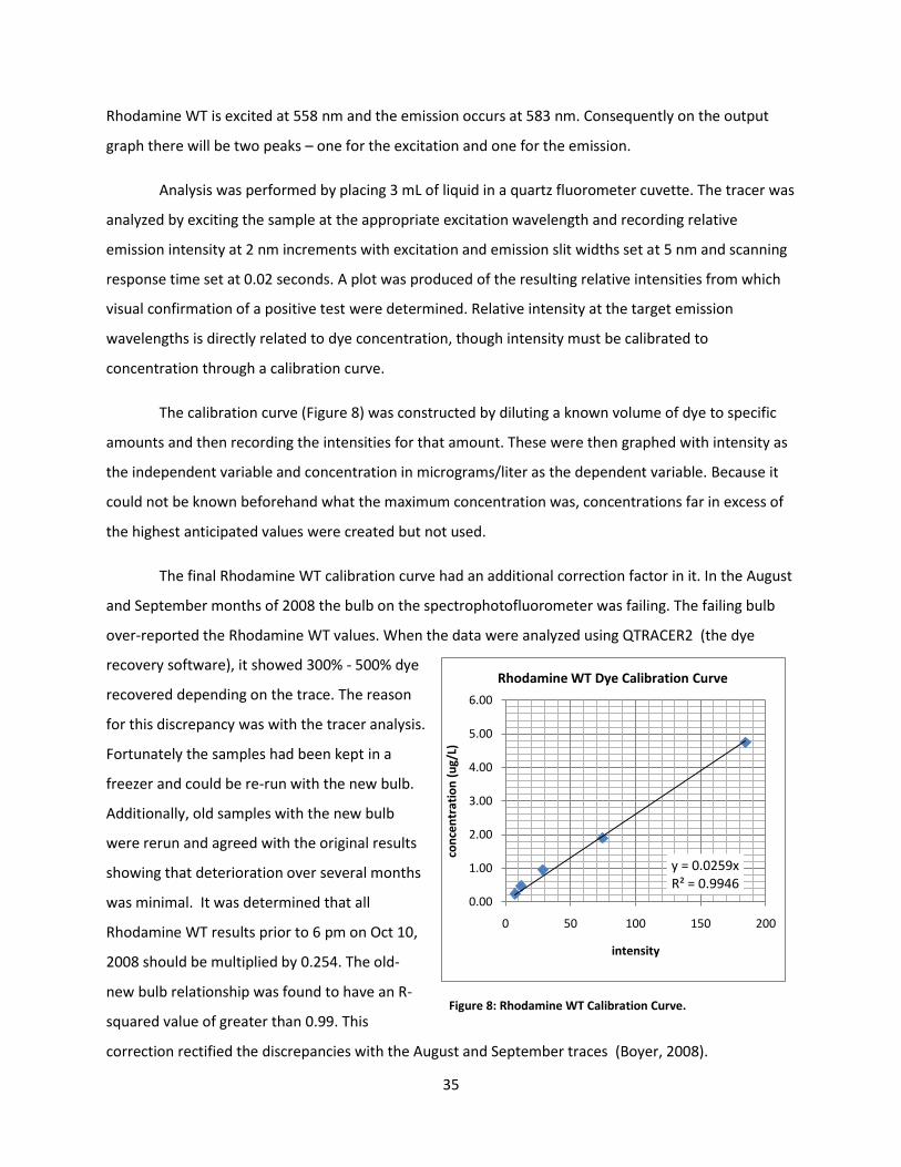
35
Rhodamine WT is excited at 558 nm and the emission occurs at 583 nm. Consequently on the output
graph there will be two peaks – one for the excitation and one for the emission.
Analysis was performed by placing 3 mL of liquid in a quartz fluorometer cuvette. The tracer was
analyzed by exciting the sample at the appropriate excitation wavelength and recording relative
emission intensity at 2 nm increments with excitation and emission slit widths set at 5 nm and scanning
response time set at 0.02 seconds. A plot was produced of the resulting relative intensities from which
visual confirmation of a positive test were determined. Relative intensity at the target emission
wavelengths is directly related to dye concentration, though intensity must be calibrated to
concentration through a calibration curve.
The calibration curve (Figure 8) was constructed by diluting a known volume of dye to specific
amounts and then recording the intensities for that amount. These were then graphed with intensity as
the independent variable and concentration in micrograms/liter as the dependent variable. Because it
could not be known beforehand what the maximum concentration was, concentrations far in excess of
the highest anticipated values were created but not used.
The final Rhodamine WT calibration curve had an additional correction factor in it. In the August
and September months of 2008 the bulb on the spectrophotofluorometer was failing. The failing bulb
over-reported the Rhodamine WT values. When the data were analyzed using QTRACER2 (the dye
recovery software), it showed 300% - 500% dye
recovered depending on the trace. The reason
for this discrepancy was with the tracer analysis.
Fortunately the samples had been kept in a
freezer and could be re-run with the new bulb.
Additionally, old samples with the new bulb
were rerun and agreed with the original results
showing that deterioration over several months
was minimal. It was determined that all
Rhodamine WT results prior to 6 pm on Oct 10,
2008 should be multiplied by 0.254. The old-
new bulb relationship was found to have an R-
squared value of greater than 0.99. This
correction rectified the discrepancies with the August and September traces (Boyer, 2008).
y = 0.0259xR² = 0.9946
0.00
1.00
2.00
3.00
4.00
5.00
6.00
0 50 100 150 200
con
cen
trat
ion
(u
g/L)
intensity
Rhodamine WT Dye Calibration Curve
Figure 8: Rhodamine WT Calibration Curve.
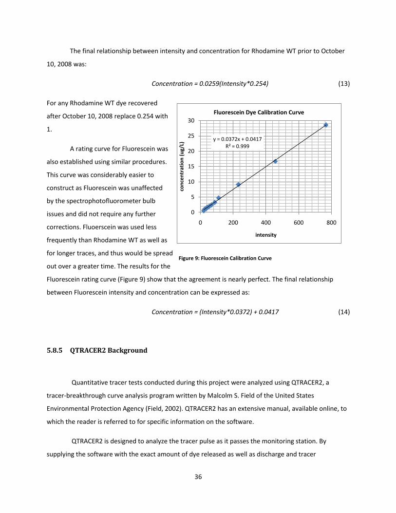
36
The final relationship between intensity and concentration for Rhodamine WT prior to October
10, 2008 was:
Concentration = 0.0259(Intensity*0.254) (13)
For any Rhodamine WT dye recovered
after October 10, 2008 replace 0.254 with
1.
A rating curve for Fluorescein was
also established using similar procedures.
This curve was considerably easier to
construct as Fluorescein was unaffected
by the spectrophotofluorometer bulb
issues and did not require any further
corrections. Fluoerscein was used less
frequently than Rhodamine WT as well as
for longer traces, and thus would be spread
out over a greater time. The results for the
Fluorescein rating curve (Figure 9) show that the agreement is nearly perfect. The final relationship
between Fluorescein intensity and concentration can be expressed as:
Concentration = (Intensity*0.0372) + 0.0417 (14)
5.8.5 QTRACER2 Background
Quantitative tracer tests conducted during this project were analyzed using QTRACER2, a
tracer-breakthrough curve analysis program written by Malcolm S. Field of the United States
Environmental Protection Agency (Field, 2002). QTRACER2 has an extensive manual, available online, to
which the reader is referred to for specific information on the software.
QTRACER2 is designed to analyze the tracer pulse as it passes the monitoring station. By
supplying the software with the exact amount of dye released as well as discharge and tracer
y = 0.0372x + 0.0417R² = 0.999
0
5
10
15
20
25
30
0 200 400 600 800
con
cen
trat
ion
(u
g/L)
intensity
Fluorescein Dye Calibration Curve
Figure 9: Fluorescein Calibration Curve
37
concentrations at regular intervals QTRACER2 is able to integrate the data using standard hydraulic
modeling and return a clear picture of the tracer pulse as it passes the monitoring station over time.
Accurate modeling of the pulse is an essential aid to understanding the hidden conduit system as it is
allows for a more detailed interpretation of the tracer travel. By repeating the same trace over different
discharges and at different times of the year a clearer picture of the overall behavior of a spring or
monitored location can be determined.
5.8.6 Chemical Analysis
Chemical analysis was performed on an as-needed basis to support the hydrologic data.
Sampling was primarily performed at Davis Spring in conjunction with storm events and dye traces. In
those cases, excess water from the automatic sampler were used for chemical analysis, providing
additional data in conjunction with tracer analysis and discharge data at the sample location. Some
chemical data in the form of temperature and conductivity were automatically collected by the
datalogging instrumentation. pH was not sampled during the study. Automatic sampling of pH was
determined to involve too much drift over time and required frequent recalibration. Samples were
sometimes collected by hand for quantitative dye analysis or chemical analysis. All samples were chilled
and stored at the USDA’s facilities in Beckley, WV, approximately a 1 hour drive from the sampling sites.
The USDA uses a Dionex 600 Ion Chromatography System with a Dionex EG40 Eluent Generator.
The chromatographer measures the common anions and cations. However, the chromatographer does
not test for bicarbonate.
The Eluent Generator uses electrolysis to convert pure water into potassium hydroxide eluent
for anion separations or methanesulfonic acid eluent for cation separations. Because the generation
takes place entirely within the system, it is unnecessary to create eluent manually.
The ion chromatograper is based on the principle that ionic species will separate differently
from an eluent based on the chemical character of the ion species. The process proceeds as follows:
First a sample solution passes through a chromatographic column. Within the column, free ions are
absorbed into the column. An eluent is then passed through the column and it separates the ions from

38
the column. The time it takes for each ion species to move through the column varies based on the
species. The resulting conductivity of the solution is a measure of the concentration of the ionic species.
Chemical analyses did not play a significant role in this thesis. pH and alkalinity were impossible
to acquire over long periods of time, significantly limiting the possible analyses. Calcium ion
concentrations were used in a chemical hydrograph separation. Collected chemical data are retained as
Appendix C for future studies.
39
6 Data Analysis and Results
The data analysis portion is subdivided into several sections, each concerned with a specific
aspect of the overall study. Formal conclusions will be presented in 7: Discussions and Conclusions.
Supplementary information will be presented in the Appendices, as will all the graphs from the whole
study period.
6.1 Further Definition of the Davis Spring Drainage Basin boundaries
Accurate definition of the Davis Spring basin boundaries is crucial to this hydrologic study. The
previous basin definition by Jones was completed in the early 1970s, without the benefit of GIS
mapping. Furthermore, Jones mentions locations where the basin boundaries may be incomplete
(Jones, 1973). This section will re-examine the Davis Spring basin boundaries to determine the extent to
which they are accurately drawn.
6.1.1 North, northwest and western boundaries
These boundaries can be grouped together as generally being underlain by clastic rocks of the
overlying Bluefield Group. In most cases, delineating drainage basin boundaries is a simple matter of
determining topographic highs. For this portion of this study the drainage basins’ path was retraced
along the topographic highs to ensure that the boundary was accurate. Starting near Rt 219 in the
north, this line follows a series of unnamed hills from east to west until it intersects Muddy Creek
Mountain. From Muddy Creek Mountain the line turns south, following the ridgeline until it intersects
the Greenbrier River just west of Davis Spring (Figure 1 and Figure 3).
Two places along that line warrant particular mention. In the northwestern area, erosion has
breached Muddy Creek Mountain, allowing water to cross a former drainage divide from the Upper
Raders’ Valley to the west into the Davis Spring Basin (Figure 10). This has been confirmed via dye
tracing in the 1990s (Jones, 1997). However, there is only one documented dye trace in that area at
Jarret's Water Cave. The basin boundaries have been slightly revised to include the remainder of this
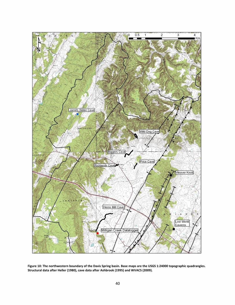
40
Figure 10: The northwestern boundary of the Davis Spring basin. Base maps are the USGS 1:24000 topographic quadrangles. Structural data after Heller (1980), cave data after Ashbrook (1995) and WVACS (2009).
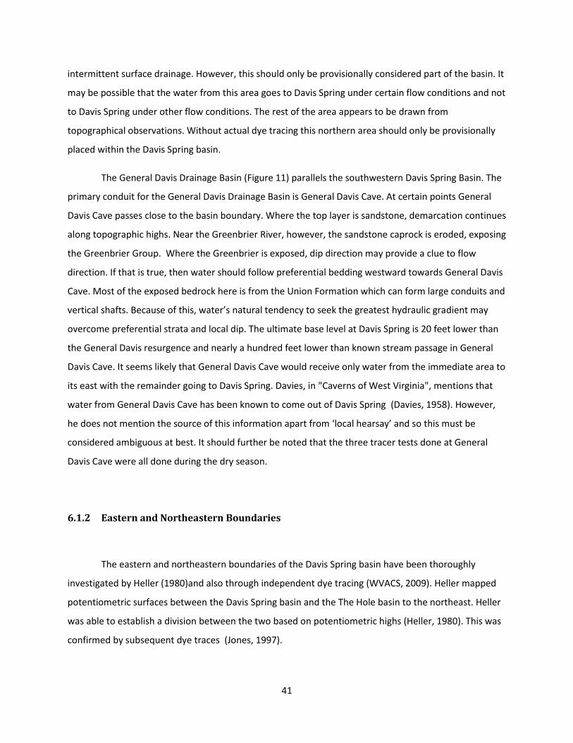
41
intermittent surface drainage. However, this should only be provisionally considered part of the basin. It
may be possible that the water from this area goes to Davis Spring under certain flow conditions and not
to Davis Spring under other flow conditions. The rest of the area appears to be drawn from
topographical observations. Without actual dye tracing this northern area should only be provisionally
placed within the Davis Spring basin.
The General Davis Drainage Basin (Figure 11) parallels the southwestern Davis Spring Basin. The
primary conduit for the General Davis Drainage Basin is General Davis Cave. At certain points General
Davis Cave passes close to the basin boundary. Where the top layer is sandstone, demarcation continues
along topographic highs. Near the Greenbrier River, however, the sandstone caprock is eroded, exposing
the Greenbrier Group. Where the Greenbrier is exposed, dip direction may provide a clue to flow
direction. If that is true, then water should follow preferential bedding westward towards General Davis
Cave. Most of the exposed bedrock here is from the Union Formation which can form large conduits and
vertical shafts. Because of this, water’s natural tendency to seek the greatest hydraulic gradient may
overcome preferential strata and local dip. The ultimate base level at Davis Spring is 20 feet lower than
the General Davis resurgence and nearly a hundred feet lower than known stream passage in General
Davis Cave. It seems likely that General Davis Cave would receive only water from the immediate area to
its east with the remainder going to Davis Spring. Davies, in "Caverns of West Virginia", mentions that
water from General Davis Cave has been known to come out of Davis Spring (Davies, 1958). However,
he does not mention the source of this information apart from ‘local hearsay’ and so this must be
considered ambiguous at best. It should further be noted that the three tracer tests done at General
Davis Cave were all done during the dry season.
6.1.2 Eastern and Northeastern Boundaries
The eastern and northeastern boundaries of the Davis Spring basin have been thoroughly
investigated by Heller (1980)and also through independent dye tracing (WVACS, 2009). Heller mapped
potentiometric surfaces between the Davis Spring basin and the The Hole basin to the northeast. Heller
was able to establish a division between the two based on potentiometric highs (Heller, 1980). This was
confirmed by subsequent dye traces (Jones, 1997).

42
Drainage boundaries to the east follow the topographic highs for the MacCrady Shale, the unit
beneath the Greenbrier Series. (Figure 4) The MacCrady forms a low ridge above the easternmost end of
the Greenbrier exposure, providing allogenic recharge for the contact caves. Basin boundaries are easily
placed along topographic highs northeast of Lewisburg. However, south of Lewisburg erosion has
removed enough of the MacCrady that the very edge of the Greenbrier exposure is east of the drainage
basin divide. This presents a scenario similar to the one at the General Davis basin boundary. Regional
dip here is also towards the west, which is towards Davis Spring. However the hydraulic gradient would
be steeper towards the east and the Greenbrier River.
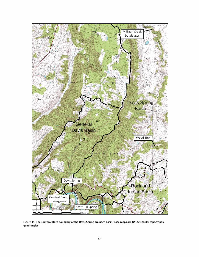
43
Figure 11: The southwestern boundary of the Davis Spring drainage basin. Base maps are USGS 1:24000 topographic quadrangles
Milligan Creek Datalogger
Davis Spring
Scott Hill Spring
General Davis Resurgence
Wood Sink
Rockland
Indian Basin
Davis Spring
Basin
General
Davis Basin
44
6.1.3 Southeastern and Southern boundary
The southern boundary to the Davis Spring drainage basin (Figure 12) follows the Greenbrier
River but is removed from the river’s edge. In this area most local recharge flows towards the river as a
collection of tiny basins instead of towards the spring. There is considerable uncertainty as to where any
of this local recharge exits. Problems with detecting these flowpaths can be grouped into two issues.
The first issue was finding suitable places to insert dye traces into the system. Because the area in
question is very long and narrow there is often insufficient breadth for sinking streams to develop,
preventing suitable places for easy tracer tests. Ponds in the area tend to be artificial in origin, with
problematic connections to the aquifer. The second issue is finding suitable places to detect dye in the
Greenbrier River. The Greenbrier River tends to be deep where it comes into contact with the bedrock
along meander bends and has a thick extent of alluvium everywhere else. Where deep, the bank often
expresses itself as anastamosing tubes or numerous enlarged joints both above and below the water.
Any of these could be the primary outlet for any dye test. Where shallow, the alluvium masks the
locations of nearly all conduits and disperses the water. Since the expectation is that these would be
poorly developed conduits where flow through them is slow, the dilution once it enters the Greenbrier
River would make any tracer indistinguishable from background levels.
One new spring was identified through visual reconnaissance along the Greenbrier River in
October, 2008. This spring has been designated as Scott Hill Spring after the property owner (Figure 11).
Observations of this spring by both the author and the landowner suggest that this spring is an overflow
spring for a very small drainage basin. The main spring likely wells up from the base of the Greenbrier or
trickles out through the alluvium. During the course of the fall through the winter 2008 Scott Hill Spring
remained dry and the landowner states that after several years of observation the only time the spring
does discharge water is immediately after sudden, strong rains. He also added that there were several
small ponds at the top of the ridge above the spring. It is his suspicion that those ponds are part of the
source for the spring’s waters (Hill, 2008).
The southeastern boundary is defined as the boundary the Davis Spring basin shares with the
Rockland Indian drainage basin (Figure 12). The Rockland Indian basin is a smaller basin with a single
cave system (Rockland Indian Cave) as the main conduit to the Greenbrier River. Shortly inside the cave
the main passage divides into an east and west branch. The east branch consists of a large stream
passage with moderate to deep pools. This passage eventually terminates at its upstream end in a
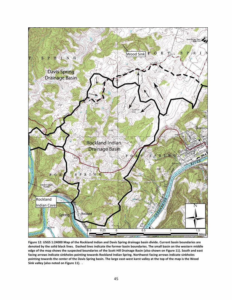
45
Figure 12: USGS 1:24000 Map of the Rockland Indian and Davis Spring drainage basin divide. Current basin boundaries are denoted by the solid black lines. Dashed lines indicate the former basin boundaries. The small basin on the western middle edge of the map shows the suspected boundaries of the Scott Hill Drainage Basin (also shown on Figure 11). South and east facing arrows indicate sinkholes pointing towards Rockland Indian Spring. Northwest facing arrows indicate sinkholes pointing towards the center of the Davis Spring basin. The large east-west karst valley at the top of the map is the Wood Sink valley (also noted on Figure 11). .
Rockland
Indian Cave
Wood Sink
46
siphon. A thousand feet upstream of the siphon the stream is encountered again in Alexander Cave #2.
Alexander Cave #2 is technically a “contact cave” whose upstream end is the contact with the MacCrady
Shale. The western passage trends towards the northwestern end of the Rockland Indian Drainage
Basin. The western passages are smaller in size, even though they are drained by the larger part of the
drainage basin. The western passages abruptly end near a fault called the “Rockland Structure”. This is
consistent with passages ending near other mapped faults in Greenbrier County (Heller, 1980).
Jones (1973, 1997) mapped the southeastern Davis Spring drainage divide based on topographic
highs due to difficulty in finding suitable places to trace flow from. This thesis author found similar
difficulties, due to the dry study period. Homes in the area are connected to the city water and sewer
system. Because no wells are drilled in the area potentiometric mapping similar to Heller's mapping in
the northeastern end of the basin is prohibitively expensive. However, some improvement in basin
boundary definition was made. One large sink (Wood Sink, Figure 12) continued to have water in it and
locals were able to relate other oral evidence from personal history. Additional mapping of cave
passages since 1973 show localized flow paths unknown to Jones.
Jones expounded on a Christopher Smart idea and suggested that for large karst drainage basins
which border each other, absolute, stationary lines dividing them do not always apply. This may be
particularly true where fracture networks and not conduit networks predominate (Jones, 1984). Where
drainage basins can be characterized by very slight hydraulic gradients and poor conduit development,
the drainage divide can vary within a zone depending on the potentiometric level at that time. The lack
of any sort of concentrated drainage discovered on or below the surface between the Davis Spring and
Rockland Indian basins in that area suggest that an integrated conduit system has not yet developed.
The only perennial stream along this drainage basin divide was traced twice to determine
whether it exits at Davis Spring, Rockland Indian Spring or even Scott Hill Spring. This stream can be
found in the bottom of the large karst valley just west of Davis Stuart Road where it intersects Coffman
Cemetery Road. Informally this location is known as ‘Wood Sink’ (Figure 12) after the landowner. The
karst valley floor is filled with alluvium - primarily clay. This creates an impermeable layer on which the
surface stream flows. Stratigraphically, the eastern end of the valley starts at the base of the Pickaway
Limestone, drops through the Taggard Shale and then intersects the Denmar. This is the nearest location
to Davis Spring where a perennial stream sinks in the lower portion of the Greenbrier Group.
47
It was initially hoped that by following the sinking stream one could eventually come to a
continuation of the downstream terminus of the 'contact caves'. Water was expected to travel quickly to
Davis Spring, taking no more than 2 weeks under low flow. As Figure 11 illustrates Wood Sink is much
closer to Davis Spring than the datalogger at Milligan Creek.
The first dye trace at Wood Sink used Fluorescein while the second used Eosin. The use of Eosin
was necessitated because the first trace returned levels of Fluorescein so low they were difficult to
distinguish from background levels and from leftovers from a previous Fluorescein trace at Maxwelton
Sink Cave. Eosin, having not been previously used in the study, was better suited for detection. The first
tracer test was conducted in early September 2008 at a time of low flow. This trace was detected at
Davis Spring after more than 2 months passed. The second trace, under higher flow, required
approximately 1 month to reach Davis Spring. The first trace travel time was more than twice the time
from Maxwelton Sink Cave under similar conditions and more than 4 times the time from a trace
released from Milligan Creek at the same time. This suggests that the water from this centrally located
point requires a very circuitous route to reach Davis Spring. These tracer tests are described in detail
later in the thesis.
When tracer testing is not possible, sinkhole orientation may suggest flow path orientation.
Sinkholes are not necessarily even-sided. Some sinks are elongated, where one sinkhole end has a
shallow gradient and the other end is nearly vertical. The most extreme example of these are ‘blind
valleys’ such as at Maxwelton Sink Cave and Organ Cave.
Figure 12 shows the change in orientation of elongated sinkholes along the Davis Spring basin –
Rockland Indian basin drainage divide. Within the study area, regional dip is to the northwest and so a
larger percentage of sinkholes may be organized parallel or perpendicular to regional dip. Examination
of the local topography shows a definite change from northwest sloping sinkholes to southwest sloping
sinkholes. Elongated sinkholes dipping towards the northwest may be considered as headed towards
Davis Spring while sinkholes dipping to the south or southeast may be considered as headed towards
Rockland Indian Cave. Therefore arrows pointing northwest on Figure 12 are assumed to point towards
the Davis Spring basin and arrows pointing southwest or southeast are assumed to point towards the
Rockland Indian basin. The solid line drainage divide is the revised basin divide based on this new
interpretation while the dashed line is the old topographic drainage divide.

48
Considering that the previous drainage divide was based solely on topographic highs (Jones,
1973), provisionally refining the drainage basin divide by drawing a line between the sinkholes pointing
south and north does not seem unreasonable. However, it may be more useful to call this stretch of the
divide “unknown” until further tracer tests can be performed.
6.2 Water Budget
A water budget was constructed for the Davis Spring drainage basin covering the following time
span: from noon on May 20th, 2008 to the end of day (midnight) April 30th, 2009. The primary reason for
the budget was to check the accuracy of the rating curve used to determine discharge at Davis Spring by
aggregating total discharge for the period against total rainfall over the area for the same period to see
if the results agree with the expected discharge and evapotranspiration (ET) as calculated from previous
studies in the basin. Secondary reasons include investigating whether rainfall totals and yearly discharge
totals have changed over time. A previous water budget for the basin was calculated in 1974 by Jones
(Jones, 2009).
6.2.1 Results and Discussion
By applying the rating curve generated during this project to the 11 1/2 months of Davis Spring
stage data a final figure of 33,153,364 m3 of discharge was aggregated. The corresponding precipitation
was 167,264,781 m3. The difference between the two represents an 80% loss of water to
evapotranspiration (see section 5.2.1). This presumes no significant change in groundwater or interbasin
transfer. This represents an 11 1/2 month period. 1 The missing half month (the first half of May) is a
period when ET is about equal to precipitation and should not significantly affect the overall water
budget (Jones, 1997).
Table 1 illustrates the differences in the previously mentioned water budgets. Unfortunately
Jones recorded either potential evapotranspiration from a hydrologic budget or observed 1 This thesis commonly refers to 10 1/2 months of data (May- March). However, the datalogger was kept in Davis
Spring until April 30, 2009. It was simpler and more accurate to just tabulate the additional month of data for this portion than to mathematically estimate the extra month of data.
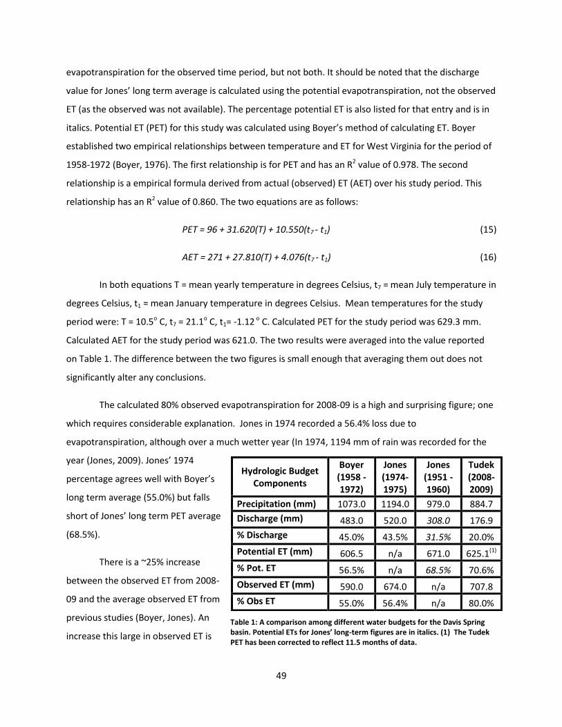
49
evapotranspiration for the observed time period, but not both. It should be noted that the discharge
value for Jones’ long term average is calculated using the potential evapotranspiration, not the observed
ET (as the observed was not available). The percentage potential ET is also listed for that entry and is in
italics. Potential ET (PET) for this study was calculated using Boyer’s method of calculating ET. Boyer
established two empirical relationships between temperature and ET for West Virginia for the period of
1958-1972 (Boyer, 1976). The first relationship is for PET and has an R2 value of 0.978. The second
relationship is a empirical formula derived from actual (observed) ET (AET) over his study period. This
relationship has an R2 value of 0.860. The two equations are as follows:
PET = 96 + 31.620(T) + 10.550(t7 - t1) (15)
AET = 271 + 27.810(T) + 4.076(t7 - t1) (16)
In both equations T = mean yearly temperature in degrees Celsius, t7 = mean July temperature in
degrees Celsius, t1 = mean January temperature in degrees Celsius. Mean temperatures for the study
period were: T = 10.5o C, t7 = 21.1o C, t1= -1.12 o C. Calculated PET for the study period was 629.3 mm.
Calculated AET for the study period was 621.0. The two results were averaged into the value reported
on Table 1. The difference between the two figures is small enough that averaging them out does not
significantly alter any conclusions.
The calculated 80% observed evapotranspiration for 2008-09 is a high and surprising figure; one
which requires considerable explanation. Jones in 1974 recorded a 56.4% loss due to
evapotranspiration, although over a much wetter year (In 1974, 1194 mm of rain was recorded for the
year (Jones, 2009). Jones’ 1974
percentage agrees well with Boyer’s
long term average (55.0%) but falls
short of Jones’ long term PET average
(68.5%).
There is a ~25% increase
between the observed ET from 2008-
09 and the average observed ET from
previous studies (Boyer, Jones). An
increase this large in observed ET is
Hydrologic Budget Components
Boyer (1958 - 1972)
Jones (1974- 1975)
Jones (1951 -1960)
Tudek (2008-2009)
Precipitation (mm) 1073.0 1194.0 979.0 884.7
Discharge (mm) 483.0 520.0 308.0 176.9
% Discharge 45.0% 43.5% 31.5% 20.0%
Potential ET (mm) 606.5 n/a 671.0 625.1(1)
% Pot. ET 56.5% n/a 68.5% 70.6%
Observed ET (mm) 590.0 674.0 n/a 707.8
% Obs ET 55.0% 56.4% n/a 80.0%
Table 1: A comparison among different water budgets for the Davis Spring basin. Potential ETs for Jones’ long-term figures are in italics. (1) The Tudek PET has been corrected to reflect 11.5 months of data.
50
difficult to explain. Several hypotheses can help account for this dramatic increase, and the actual
answer is likely a combination of reasons. A detailed study of the relative probabilities accounting for
this discrepancy is beyond the scope of this thesis. This author will aim only to illustrate that a high ET is
simply within the realm of feasibility. Presented in no particular order are some possible explanations
which could account for this discrepancy in observed evapotranspiration values.
The data are wrong – Whenever new data are uncovered there is always the possibility that
some user or equipment error has rendered the data unusable and the question must be asked
“With what certainty can one say that the data are reliable?” As previously mentioned, the
flowmeter equipment was well maintained, monitored and recalibrated when necessary. The
section on establishing the Davis Spring rating curve explains fully the steps taken to minimize
user error. To recount: individual cross-sections were measured multiple times to insure
consistency. Repeat measurements were performed by different individuals to minimize user
bias. Individual data points were examined against the overall mass of evidence to determine if
(as on 12-1-08) there was an equipment or user error which could have resulted in unusable
data. The consistency of the data is such that if there is a systematic error it is likely a product of
the equipment. Furthermore, said error has to be one which is not easily visible to routine
calibration or maintenance. The flow meter manual states the flow velocity precision error for
the meter as ±2% of the measured value. Precision error determined mathematically from
repeated measurements taken adds an additional ±2%, making the total velocity precision error
at least ±4%. Dingman suggests that ±4% is near the least amount of error possible in measuring
flow velocities (Dingman, 2002). Based on these procedures and the corresponding low level of
error there is a high level of confidence on the part of the collectors that the data are sound.
Not all the water is being accounted for – If Davis Spring is not the only discharge point for the
Davis Spring basin then some discharge has been omitted from the water budget. Missing
discharge would overestimate the ET. Sara Heller suggested (Heller, 1980; Heller, 2008) that
the Greenbrier Group may consist of several vertically stacked aquifers of varying thicknesses.
Her suggestion is that groundwater flow from the basal aquifer (Hillsdale Formation) may not
exit completely through Davis Spring. Rather, it was her suggestion that additional diffuse
51
discharge points may exist in the bed of the Greenbrier either upstream or downstream of Davis
Spring (Heller, 2008). The suggestion that additional discharge points exist in the bed of the
Greenbrier River is difficult to prove without tracer testing above visible detection limits. This is
an unattractive proposal. Instead the Greenbrier River was examined for possible outlets during
the dry period of October 2008. Even then portions of the Greenbrier were tens of feet deep,
specifically in the outer edges of bends.
The Hillsdale is exposed at the north-facing bend upstream of the Greenbrier River 4 km
upstream of Davis Spring (Figure 4 and Figure 11). This is the likeliest place for discharge to
emerge. Small and large holes dot the cliff face on the north side of the bend. Any of these could
be an outlet. Unfortunately the Greenbrier is both deep and swift-moving in this area, making
detection difficult. Any additions to the Greenbrier’s discharge would be negligible compared to
the total discharge of the river.
Similar investigations should be made along the Greenbrier downstream of the spring.
While the Greenbrier remains relatively straight and shallow along this reach, it passes through
the gap between Muddy Creek Mountain and Flat Top Mountain. Here the banks of the river are
lined with talus and sediment from the mountains. These flat areas are able to hide all but the
highest discharge springs. Diffuse springs would be hidden by the talus as well as by the volume
of water travelling through the Greenbrier River.
A further complication with the idea that all the drainage basin water is not being
recorded at the Davis Spring datalogger lays with the already high dye recovery rates. Dye traces
performed at Davis Spring have recovered between 83% and 97% of inserted dyes. High
percentages of recovered dyes are unusual and recovery of more than 100% of inserted dye is
considered impossible. Dye tracing results represent an upper boundary for Davis Spring total
discharge. In order for the Davis Spring drainage basin discharge to increase further any
additional discharge recorded must not have come into contact with the dye at any point.
Two scenarios which could fulfill this requirement suggest themselves. Scenario 1
postulates that some water from Milligan Creek is diverted to a parallel flow path which exits to
the Greenbrier River independent of Davis Spring. This is the more plausible scenario. Milligan
Creek upstream of the dye insertion point sinks and rises several times in the cavernous Union
Formation. Though no enterable conduits have been located, the possibility of a parallel flow
path should not be discounted. Questions about the relationship between the measured
discharge along Milligan Creek and the expected discharge based on catchment area support
52
this hypothesis as well. This Milligan Creek question will be further investigated in a subsequent
section. Scenario 2 postulates that water from the Hillsdale aquifer does not all exit through
Davis Spring. This is likely to be a weaker argument. All dye traces (qualitative and quantitative)
performed from several cave systems and sinking streams in the Hillsdale exit through Davis
Spring. Any water from the aquifer matrix would have to not only avoid Davis Spring but also all
the conduits leading to Davis Spring as well. This seems unlikely.
Finally, it is reasonable to assume that any significant discharge that has been omitted
by this study was also omitted from previous studies. There must then be a correction made to
all previous studies (though such a correction is not necessarily linear). The magnitude of the
correction may call into question the usefulness of previous studies .
This is normal – Jones (2009) mentioned that the previous attempt at long-term monitoring at
Davis Spring was done during years with above-average precipitation. This would create a
conflict, as the ET values for those studies were about 55%. Evapotranspiration in West Virginia
varies - in the Potomac River basin it is 66% (Hobba et al., 1977). Based on recharge data and
average precipitation data by Kozar, the rest of West Virginia appears to have 50% - 60%
evapotranspiration (Kozar and Mathes, 2001). It is unclear which long term result this refers to.
However, Boyer’s averages for 15 years closely resemble Jones’ average for his “very wet” year.
As a result, there may be no baseline for average to below average flow for long periods of time.
It is possible, though unlikely, that ~75% ET might be normal for an average year.
Land-use change – Changes in land use can often lead to changes in percentage ET. There is a
strong correlation between an increase in forest ET over pastureland ET (Zhang et al., 2001).
This is particularly true for forested areas with trees between 20 and 100 years old. Trees with
deep, wide root systems and larger masses require more water than pastureland covering the
same area. Young and intermediate age forests (i.e. in the 20 – 100 year period) also have a
large undergrowth component to the same area, increasing the water requirements even
further.
Figure 13 shows the increase in forested areas in the Davis Spring drainage basin over a
9 year period. The map was generated by comparing the 1992 NLCD data with the 2001 NLCD
data. Using the 1992 NLCD data as a base map, the result shows a 6.8% increase in forested area
across the whole basin over the 9 year span. This appears to be consistent with aerial
53
photographs taken of Lewisburg in the 1960s which show nearly the entire western half of the
basin had been clear-cut for pastureland.
Studies have indicated that the change from pastureland to forested area can double
the expected ET for a given area. According to Zhang (Zhang et al., 2001) for the average
amount of rainfall in the Davis Spring basin, forested area can be expected to increase ET by
50% – 75% over pastureland depending on annual rainfall. Consequently, a small increase in
forested area can have a disproportionate effect on the overall amount of ET (Zhang et al.,
2001).
Another land use change to consider is the increase in paved areas over time (Figure
14). Long-term studies showing ET change due to pavement increase are fewer and the overall
results are less conclusive (Toran et al., 2009). The underlying premise is that as the amount of
impermeable surface increases, the tendency is to divert surface runoff to sewers which feed
local streams or in case of karst conduits. This has the effect of bypassing the process of
recharging the aquifer. Water which would have fallen on the ground and slowly made its way
through the aquifer to the resurgence over a long period of time now exits quickly through
conduits. Having quickly exited, this water cannot be used to replenish the aquifer over the long
term. The aquifer is thus deprived of a large part of its long term recharge source (the paved
areas). From a recharge point of view, this is equivalent to decreasing rainfall. With decreased
recharge the average elevation of the water table must drop. This should show up graphically as
a period of time with normal baseflow and increased storm flow followed by a longer period of
substantially reduced baseflow and normal storm flow.
Paved areas are difficult to map, and the category of “urban areas” are often used as a
proxy (Figure 14). Urban areas occur mostly along the eastern edge of the drainage basin,
particularly along the Route 219 corridor around Lewisburg. The area between Lewisburg and
Ronceverte has seen a dramatic increase in shopping centers, businesses, and infrastructure in
the 1990s. This is reflected in Figure 14. This map also demonstrates some of the shortcomings
of raster datasets. Though most of the roads predate the 1992 NLCD map, they were mapped in
1992 according to the land use surrounding them. For the 2001 map, the roads were mapped as
urban. As a result the percent urban increase is artificially inflated.
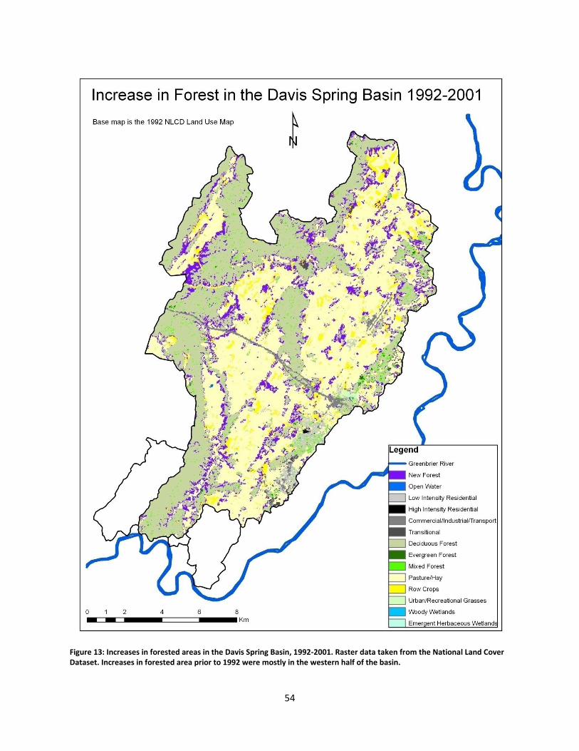
54
Figure 13: Increases in forested areas in the Davis Spring Basin, 1992-2001. Raster data taken from the National Land Cover Dataset. Increases in forested area prior to 1992 were mostly in the western half of the basin.
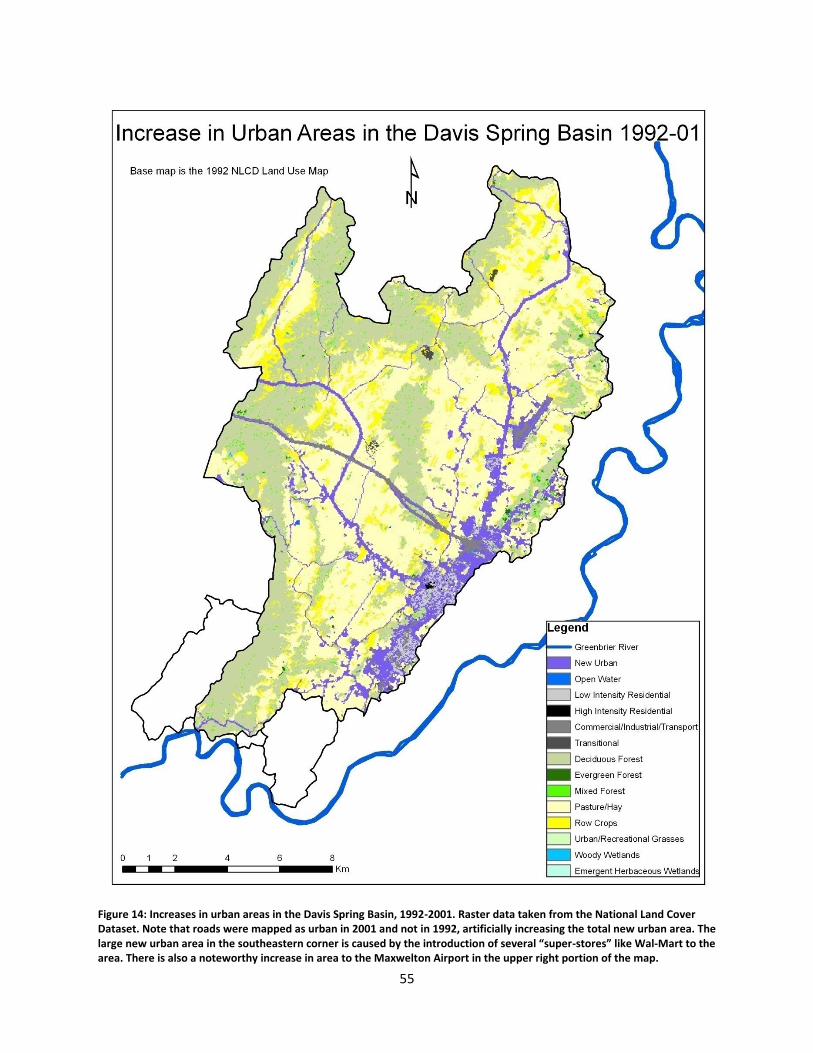
55
Figure 14: Increases in urban areas in the Davis Spring Basin, 1992-2001. Raster data taken from the National Land Cover Dataset. Note that roads were mapped as urban in 2001 and not in 1992, artificially increasing the total new urban area. The large new urban area in the southeastern corner is caused by the introduction of several “super-stores” like Wal-Mart to the area. There is also a noteworthy increase in area to the Maxwelton Airport in the upper right portion of the map.
56
Drainage Basin Size Changes – Total discharge values require an accurate assessment of the
basin size. The preceding section about basin boundaries showed areas where the basin
boundaries are incompletely defined. If the basin were smaller, the aggregated precipitation
values would be smaller. Discharge, being measured independently, would remain the same.
The percentage ET would become correspondingly smaller. However, a change in basin size
would necessitate a recalculation of previous water budgets with corresponding shrinkages in
percentage ET for those budgets.
Other problems – There are other discrepancies between the 1970s work and the current study.
Jones’ original rating curve for 1974 was plotted by hand; the current rating curve is a best fit
line using graphing software. Hand plotting was common in the 1970s but has been less
frequently used since. Spreadsheet software such as Excel is now common now and less prone
to user bias. Jones also reported that the total discharge was “capped” at 1000 ft3/sec by the
USGS leading to under-reporting of the highest flows and consequently total discharge (Jones,
2009). Since this would affect only the peaks of the largest precipitation events, it is likely that
these changes would not dramatically affect the total annual discharge values.
The above points preclude a definitive answer to the question “Is the percent
evapotranspiration for this study too high?” The study length introduces some uncertainty to the
argument. In order to eliminate variables like change in storage, most water budgets are multi-year
endeavors. However, as Table 1 clearly shows, even long term studies do not necessarily agree. Jones
and Boyer disagree in their percentage potential evapotranspiration by 12.0% (56.5% for Boyer, 68.5%
for Jones). A non-weighted average between the two would be around 62%.
To refer back to the original question – “Does this help corroborate the accuracy of the rating
curve?” – it is necessary to find out where all these water budgets agree. Table 1 shows that while the
percentages of evapotranspiration vary considerably, the ET amounts are all much closer, and they all
fall around the potential evapotranspiration figures. It appears from the data that the average ET should
fall consistently in the range of 600 -700 mm/year. Arguments can be made further narrowing that
range, but as ET is literally evaporation (from sunlight and heat) as well as transpiration (from flora),
these can be so variable over years that any more narrow figure becomes less applicable over the long
term.
57
Because the 2008-2009 data marks the upper end of the 600-700 mm/year range, it can be
concluded that the rating curve is, from the point of view of the water budget, reasonably accurate. The
rating curve would have been more accurate with the benefit of additional discharge measurements,
but at present it appears to be plausible. If the data are accepted as accurate, then reasons for the
unusually high ET during the study would include the following:
Changes in land use, particularly an increase in forested areas in the western half of the
drainage basin. Larger flora also requires more water to survive.
Fewer large storm events, particularly in the summer, as a corollary to less rain overall. Less
severe weather means that the soil is oversaturated less frequently and less water flows
through conduits to discharge at Davis Spring.
Several drier years may have reduced the capacity of the basin to maintain previous levels of
groundwater contribution to Davis Spring. Another way to suggest this would be to cite Jones’
assertion that earlier years were considerably wetter.
There remains one more issue with the Table 1 data. The difference between the observed ET
and calculated potential ET during this study is much larger than for Boyer’s long term values. There is a
83 mm difference between PET and OET in this study compared to a 16 mm difference in Boyer’s data in
the other direction. Furthermore, the observed ET in this study is higher than the potential ET, a
phenomenon which almost never happens (Fetter, 2001; Rauch, 2009). This suggests that the observed
ET is incorrect by 100 mm. Where has that water gone?
The obvious possibility is that this is the water escaping through some other, unknowable
channel in the Greenbrier, as per Heller’s hypothesis or simply as underflow. The 100 mm/yr accounts
for 10% of the total precipitation over the study period. This 10% would help account for the missing
water at the Milligan Creek datalogger – a topic which will be discussed in the Milligan Creek datalogger
section. A second possibility is that the rating curve (and consequently the discharge) is incorrect by
10%. Any upwards shifting in discharge, however, would have to account for an increase in dye
recovery, which may bring dye recovery amounts close to or slightly over 100%. A third possibility is that
the drier weather in 2008-2009 could be having a longer and more deleterious effect than supposed,
skewing Boyer’s equations, which after all are designed for long-term observations.
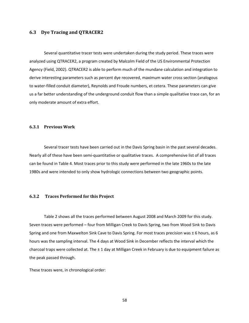
58
6.3 Dye Tracing and QTRACER2
Several quantitative tracer tests were undertaken during the study period. These traces were
analyzed using QTRACER2, a program created by Malcolm Field of the US Environmental Protection
Agency (Field, 2002). QTRACER2 is able to perform much of the mundane calculation and integration to
derive interesting parameters such as percent dye recovered, maximum water cross section (analogous
to water-filled conduit diameter), Reynolds and Froude numbers, et cetera. These parameters can give
us a far better understanding of the underground conduit flow than a simple qualitative trace can, for an
only moderate amount of extra effort.
6.3.1 Previous Work
Several tracer tests have been carried out in the Davis Spring basin in the past several decades.
Nearly all of these have been semi-quantitative or qualitative traces. A comprehensive list of all traces
can be found in Table 4. Most traces prior to this study were performed in the late 1960s to the late
1980s and were intended to only show hydrologic connections between two geographic points.
6.3.2 Traces Performed for this Project
Table 2 shows all the traces performed between August 2008 and March 2009 for this study.
Seven traces were performed – four from Milligan Creek to Davis Spring, two from Wood Sink to Davis
Spring and one from Maxwelton Sink Cave to Davis Spring. For most traces precision was ± 6 hours, as 6
hours was the sampling interval. The 4 days at Wood Sink in December reflects the interval which the
charcoal traps were collected at. The ± 1 day at Milligan Creek in February is due to equipment failure as
the peak passed through.
These traces were, in chronological order:
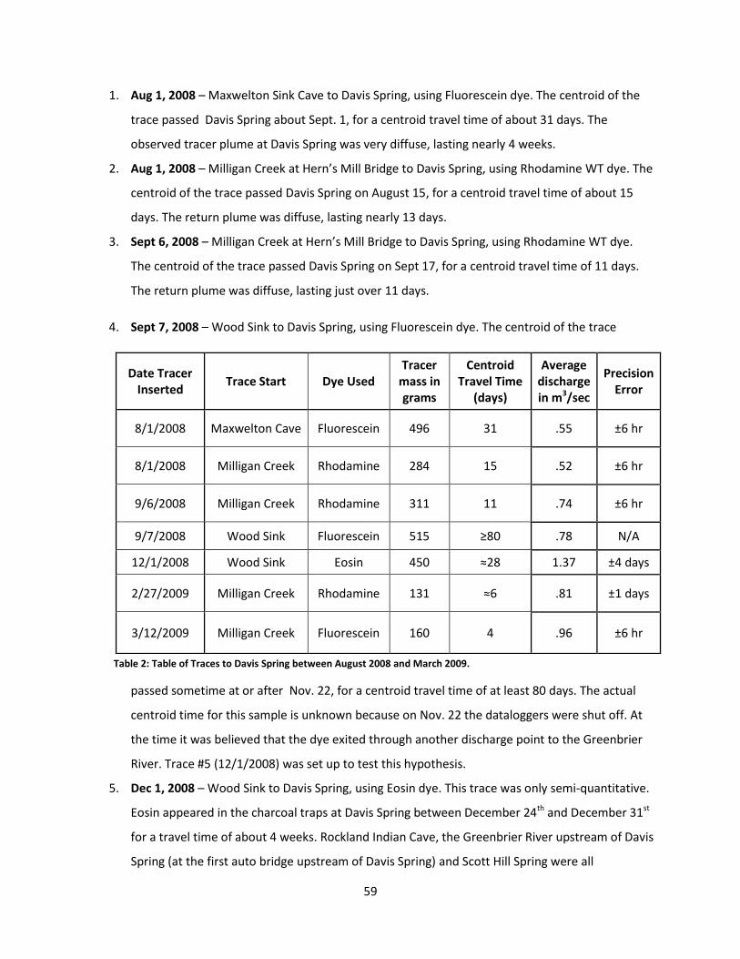
59
1. Aug 1, 2008 – Maxwelton Sink Cave to Davis Spring, using Fluorescein dye. The centroid of the
trace passed Davis Spring about Sept. 1, for a centroid travel time of about 31 days. The
observed tracer plume at Davis Spring was very diffuse, lasting nearly 4 weeks.
2. Aug 1, 2008 – Milligan Creek at Hern’s Mill Bridge to Davis Spring, using Rhodamine WT dye. The
centroid of the trace passed Davis Spring on August 15, for a centroid travel time of about 15
days. The return plume was diffuse, lasting nearly 13 days.
3. Sept 6, 2008 – Milligan Creek at Hern’s Mill Bridge to Davis Spring, using Rhodamine WT dye.
The centroid of the trace passed Davis Spring on Sept 17, for a centroid travel time of 11 days.
The return plume was diffuse, lasting just over 11 days.
4. Sept 7, 2008 – Wood Sink to Davis Spring, using Fluorescein dye. The centroid of the trace
passed sometime at or after Nov. 22, for a centroid travel time of at least 80 days. The actual
centroid time for this sample is unknown because on Nov. 22 the dataloggers were shut off. At
the time it was believed that the dye exited through another discharge point to the Greenbrier
River. Trace #5 (12/1/2008) was set up to test this hypothesis.
5. Dec 1, 2008 – Wood Sink to Davis Spring, using Eosin dye. This trace was only semi-quantitative.
Eosin appeared in the charcoal traps at Davis Spring between December 24th and December 31st
for a travel time of about 4 weeks. Rockland Indian Cave, the Greenbrier River upstream of Davis
Spring (at the first auto bridge upstream of Davis Spring) and Scott Hill Spring were all
Date Tracer Inserted
Trace Start Dye Used Tracer
mass in grams
Centroid Travel Time
(days)
Average discharge in m3/sec
Precision Error
8/1/2008 Maxwelton Cave Fluorescein 496 31 .55 ±6 hr
8/1/2008 Milligan Creek Rhodamine 284 15 .52 ±6 hr
9/6/2008 Milligan Creek Rhodamine 311 11 .74 ±6 hr
9/7/2008 Wood Sink Fluorescein 515 ≥80 .78 N/A
12/1/2008 Wood Sink Eosin 450 ≈28 1.37 ±4 days
2/27/2009 Milligan Creek Rhodamine 131 ≈6 .81 ±1 days
3/12/2009 Milligan Creek Fluorescein 160 4 .96 ±6 hr
Table 2: Table of Traces to Davis Spring between August 2008 and March 2009.
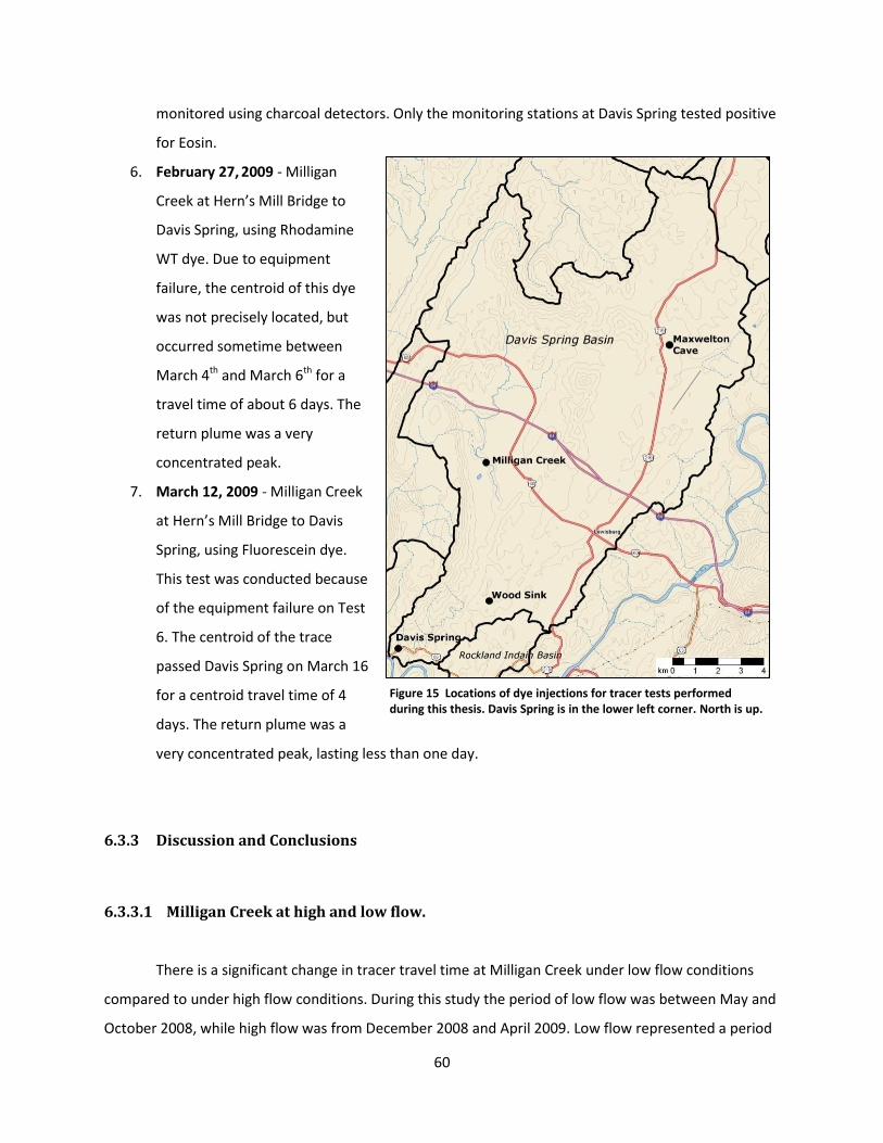
60
monitored using charcoal detectors. Only the monitoring stations at Davis Spring tested positive
for Eosin.
6. February 27, 2009 - Milligan
Creek at Hern’s Mill Bridge to
Davis Spring, using Rhodamine
WT dye. Due to equipment
failure, the centroid of this dye
was not precisely located, but
occurred sometime between
March 4th and March 6th for a
travel time of about 6 days. The
return plume was a very
concentrated peak.
7. March 12, 2009 - Milligan Creek
at Hern’s Mill Bridge to Davis
Spring, using Fluorescein dye.
This test was conducted because
of the equipment failure on Test
6. The centroid of the trace
passed Davis Spring on March 16
for a centroid travel time of 4
days. The return plume was a
very concentrated peak, lasting less than one day.
6.3.3 Discussion and Conclusions
6.3.3.1 Milligan Creek at high and low flow.
There is a significant change in tracer travel time at Milligan Creek under low flow conditions
compared to under high flow conditions. During this study the period of low flow was between May and
October 2008, while high flow was from December 2008 and April 2009. Low flow represented a period
Figure 15 Locations of dye injections for tracer tests performed during this thesis. Davis Spring is in the lower left corner. North is up.
61
when baseflow discharge predominated; that is, the primary discharge was due to dewatering of stored
water in the aquifer. High flow represented a period when recent precipitation dominated discharge.
November represented a transitional period between these two seasonal end members. The Milligan
Creek tracer tests in August 2008, September 2008 and March 2009 were analyzed using QTRACER2
with the results appearing as Table 3. QTRACER2 calculates many parameters based on hydrogeologic
equations and the assumption that the conduit is under a pipe-full condition.
Tracer velocity more than doubled during the high flow. Furthermore, two traces were
performed during each season – August and September 2008 in the low flow season; February and
March 2009 during the high flow season. This helps to demonstrate that these travel times are
representative of the system. It appears that, under high flow, there are sufficiently numerous or
sufficiently large developed conduits between Milligan Creek and Davis Spring to move substantial
quantities of water quickly.
An unfortunate shortcoming of the QTRACER2 software is in the calculation of the cross-
sectional area. This formula is an approximation at best and likely inadequate to handle the complex
inputs to a system like the Davis Spring basin (Field, 2002). The brevity of the dye plume in the March
2009 tracer test may also be a contributing factor. The September and August 2008 traces lasted three
times longer than the March trace, providing far more detail on the event.
Consequently, the examples taken at lower flow, where the individual hydrograph components
are more likely separated temporally, are possibly more accurate than the high flows associated with
spring flooding. This method can only provide a range of between 71m2 and 93 m2 (790 ft2 to 1000 ft2)
for the cross-sectional area. This suggests a square passage size of between 8.4 x 8.4 meters to 9.6 x 9.6
meters (27ft x 27ft to 32ft x 32ft). Of course this does not mean there is one, large passage being used
by Milligan Creek; the discharge could be flowing through dozens of small openings which aggregate to
the above cross-sectional area.
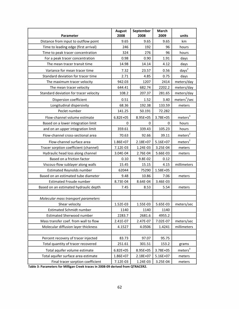
62
Parameter August 2008
September 2008
March 2009 units
Distance from input to outflow point 9.65 9.65 9.65 km
Time to leading edge (first arrival) 246 192 96 hours
Time to peak tracer concentration 324 276 96 hours
For a peak tracer concentration 0.98 0.90 1.91 days
The mean tracer transit time 14.98 14.14 4.12 days
Variance for mean tracer time 7.32 23.57 0.56 days2
Standard deviation for tracer time 2.71 4.85 0.75 days
The maximum tracer velocity 942.03 1207 2414 meters/day
The mean tracer velocity 644.41 682.74 2202.2 meters/day
Standard deviation for tracer velocity 108.2 207.37 281.65 meters/day
Dispersion coefficient 0.51 1.52 3.40 meters2/sec
Longitudinal dispersivity 68.36 192.38 133.59 meters
Peclet number 141.25 50.191 72.282
Flow-channel volume estimate 6.82E+05 8.95E+05 3.78E+05 meters3
Based on a lower integration limit 0 0 0 hours
and on an upper integration limit 359.61 339.43 105.23 hours
Flow-channel cross-sectional area 70.63 92.66 39.11 meters2
Flow-channel surface area 1.86E+07 2.18E+07 5.16E+07 meters2
Tracer sorption coefficient (channel) 7.12E-03 1.24E-03 3.25E-04 meters
Hydraulic head loss along channel 3.04E-04 2.76E-04 5.66E-03 meters
Based on a friction factor 0.10 9.8E-02 0.12
Viscous-flow sublayer along walls 15.45 15.15 4.15 millimeters
Estimated Reynolds number 62044 75290 1.58E+05
Based on an estimated tube diameter 9.48 10.86 7.06 meters
Estimated Froude number 8.73E-04 8.64E-04 3.46E-03
Based on an estimated hydraulic depth 7.45 8.53 5.54 meters
Molecular mass transport parameters
Shear velocity 1.52E-03 1.55E-03 5.65E-03 meters/sec
Estimated Schmidt number 1140 1140 1140
Estimated Sherwood number 2283.7 2681.6 4955.2
Mass transfer coef. from wall to flow 2.41E-07 2.47E-07 7.02E-07 meters/sec
Molecular diffusion layer thickness 4.1527 4.0506 1.4241 millimeters
Percent recovery of tracer injected 83.73 97.07 95.75
Total quantity of tracer recovered 251.61 301.51 153.2 grams
Total aquifer volume estimate 6.82E+05 8.95E+05 3.78E+05 meters3
Total aquifer surface area estimate 1.86E+07 2.18E+07 5.16E+07 meters
Final tracer sorption coefficient 7.12E-03 1.24E-03 3.25E-04 meters Table 3: Parameters for Milligan Creek traces in 2008-09 derived from QTRACER2.
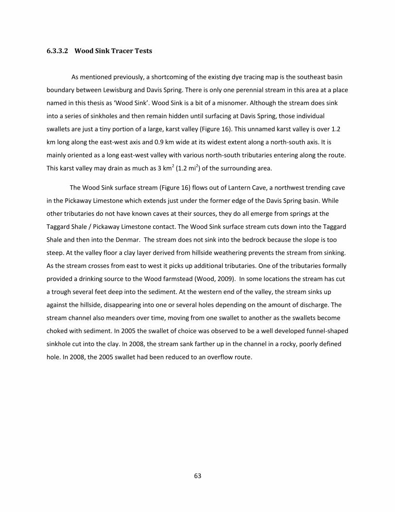
63
6.3.3.2 Wood Sink Tracer Tests
As mentioned previously, a shortcoming of the existing dye tracing map is the southeast basin
boundary between Lewisburg and Davis Spring. There is only one perennial stream in this area at a place
named in this thesis as ‘Wood Sink’. Wood Sink is a bit of a misnomer. Although the stream does sink
into a series of sinkholes and then remain hidden until surfacing at Davis Spring, those individual
swallets are just a tiny portion of a large, karst valley (Figure 16). This unnamed karst valley is over 1.2
km long along the east-west axis and 0.9 km wide at its widest extent along a north-south axis. It is
mainly oriented as a long east-west valley with various north-south tributaries entering along the route.
This karst valley may drain as much as 3 km2 (1.2 mi2) of the surrounding area.
The Wood Sink surface stream (Figure 16) flows out of Lantern Cave, a northwest trending cave
in the Pickaway Limestone which extends just under the former edge of the Davis Spring basin. While
other tributaries do not have known caves at their sources, they do all emerge from springs at the
Taggard Shale / Pickaway Limestone contact. The Wood Sink surface stream cuts down into the Taggard
Shale and then into the Denmar. The stream does not sink into the bedrock because the slope is too
steep. At the valley floor a clay layer derived from hillside weathering prevents the stream from sinking.
As the stream crosses from east to west it picks up additional tributaries. One of the tributaries formally
provided a drinking source to the Wood farmstead (Wood, 2009). In some locations the stream has cut
a trough several feet deep into the sediment. At the western end of the valley, the stream sinks up
against the hillside, disappearing into one or several holes depending on the amount of discharge. The
stream channel also meanders over time, moving from one swallet to another as the swallets become
choked with sediment. In 2005 the swallet of choice was observed to be a well developed funnel-shaped
sinkhole cut into the clay. In 2008, the stream sank farther up in the channel in a rocky, poorly defined
hole. In 2008, the 2005 swallet had been reduced to an overflow route.
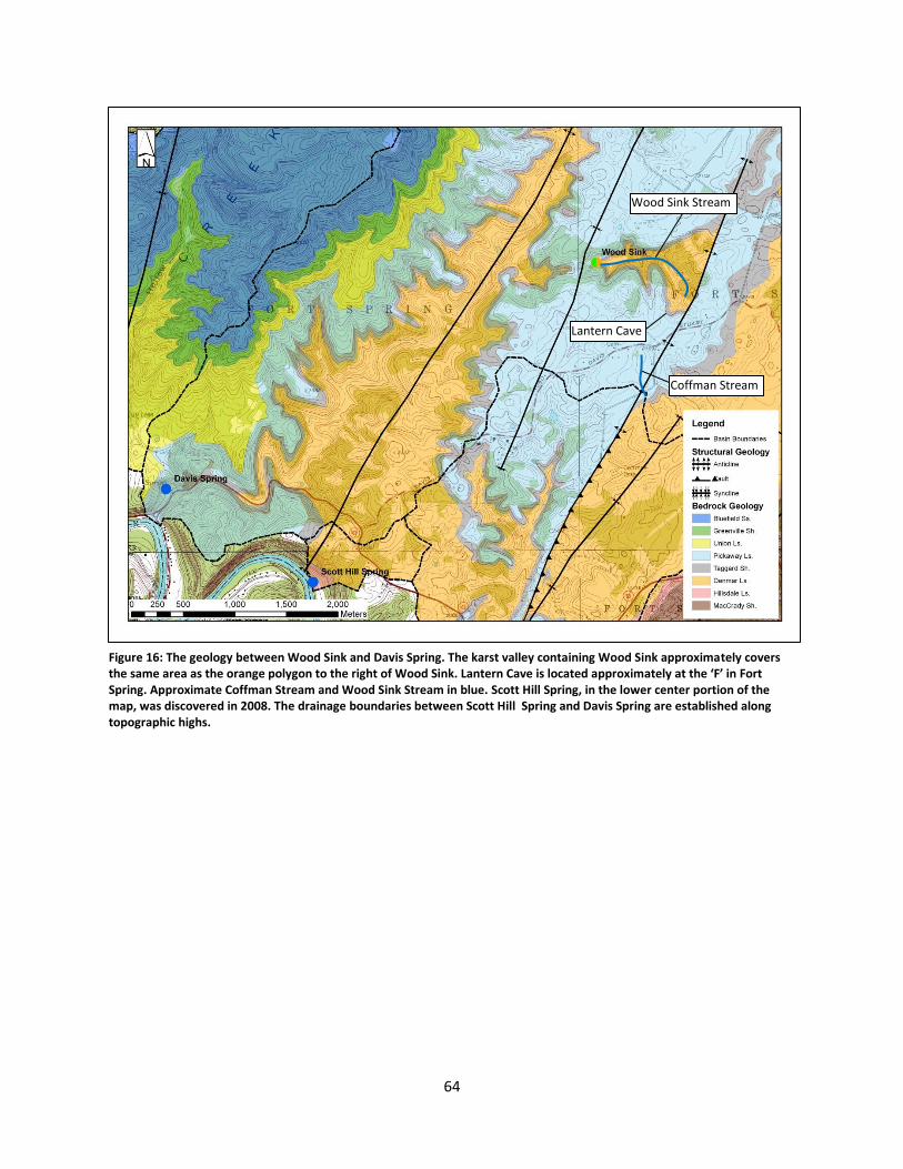
64
Figure 16: The geology between Wood Sink and Davis Spring. The karst valley containing Wood Sink approximately covers the same area as the orange polygon to the right of Wood Sink. Lantern Cave is located approximately at the ‘F’ in Fort Spring. Approximate Coffman Stream and Wood Sink Stream in blue. Scott Hill Spring, in the lower center portion of the map, was discovered in 2008. The drainage boundaries between Scott Hill Spring and Davis Spring are established along topographic highs.
Wood Sink Stream
Lantern Cave
Coffman Stream
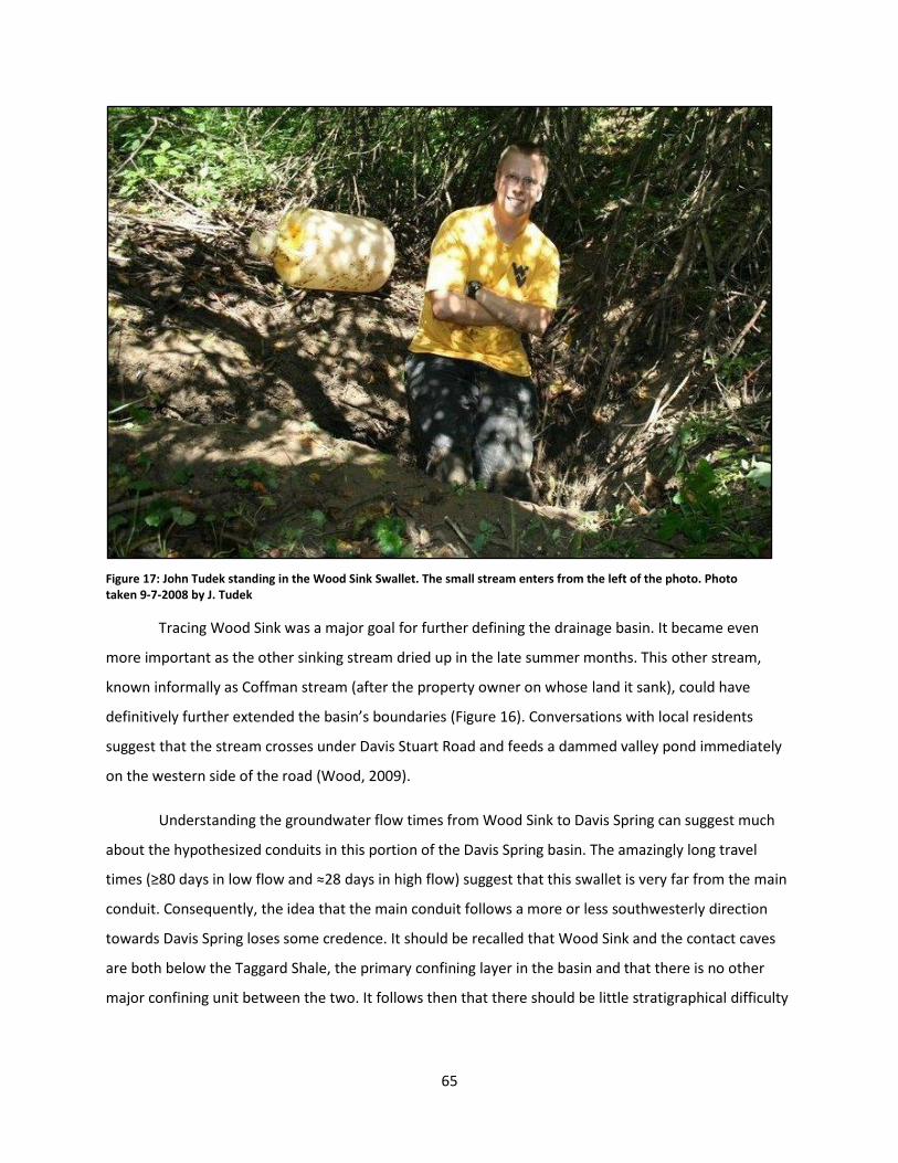
65
Tracing Wood Sink was a major goal for further defining the drainage basin. It became even
more important as the other sinking stream dried up in the late summer months. This other stream,
known informally as Coffman stream (after the property owner on whose land it sank), could have
definitively further extended the basin’s boundaries (Figure 16). Conversations with local residents
suggest that the stream crosses under Davis Stuart Road and feeds a dammed valley pond immediately
on the western side of the road (Wood, 2009).
Understanding the groundwater flow times from Wood Sink to Davis Spring can suggest much
about the hypothesized conduits in this portion of the Davis Spring basin. The amazingly long travel
times (≥80 days in low flow and ≈28 days in high flow) suggest that this swallet is very far from the main
conduit. Consequently, the idea that the main conduit follows a more or less southwesterly direction
towards Davis Spring loses some credence. It should be recalled that Wood Sink and the contact caves
are both below the Taggard Shale, the primary confining layer in the basin and that there is no other
major confining unit between the two. It follows then that there should be little stratigraphical difficulty
Figure 17: John Tudek standing in the Wood Sink Swallet. The small stream enters from the left of the photo. Photo taken 9-7-2008 by J. Tudek
66
for both sources of water to meet in the same conduit. Structural constraints on the two joining will be
discussed later.
Lastly, it should be emphasized that neither Eosin nor Fluorescein from Wood Sink traces were
ever detected in substantial quantities in any of the other springs along the Greenbrier River during the
study period. Minor amounts of Fluoresecin were detected at Rockland Indian Spring during these
traces, but these were more appropriate to background noise than tracer confirmation. Under the
extremely low flow conditions of September to November 2008 it appears that the Fluorescein injected
at Wood Sink became trapped somewhere in the flow path, likely in underground pools near the
swallet. Neither tracer was detected until the heavy rains and the decrease in evapotranspiration
associated with winter occurred, even though the stream feeding Wood Sink flowed throughout the fall.
6.3.3.3 Overall Dye Tracing picture (low and high flows)
By combining the tracer test results performed for this study with those previously performed a
clearer picture forms for some of the Davis Spring drainage basin characteristics. However, the semi-
quantitative nature of many of the previous tracer tests limit the strength of the conclusions which can
be drawn. Ideally, all of these tracer tests should be quantitatively repeated. Retesting should be a series
of tests during different flow regimes for each trace in order to reduce the uncertainty in the data.
Table 4 is a complete table of all tracer tests performed in the Davis Spring basin over the past
43 years (1967-2009, inclusive). The table is chronological, with oldest tracer tests first. Tracer tests in
bold were performed during what will be referred to as the ‘dry season’. All other tests were performed
during the 'wet season'. The wet season is commonly the winter to spring months, usually between
December and April. Wet season months are characterized by large storms, exceptionally high and sharp
hydrograph peaks, significant drops in conductivity during precipitation events and flooding of the
Greenbrier River. The dry season (usually between June and November) tends to be dominated by
baseflow, modest hydrograph peaks and little to no change in conductivity. The Luddington Cave trace
appears to be the result of a significant storm event on June 6-7 1970. This event tripled the Greenbrier
River discharge at Alderson (from 8 m3/sec to 23 m3/sec) (USGS, 1970).
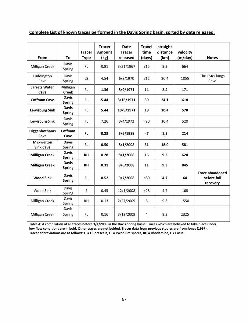
67
Complete List of known traces performed in the Davis Spring basin, sorted by date released.
Table 4: A compilation of all traces before 3/1/2009 in the Davis Spring basin. Traces which are believed to take place under low flow conditions are in bold. Other traces are not bolded. Tracer data from previous studies are from Jones (1997) . Tracer abbreviations are as follows: Fl = Fluorescein, LS = Lycodium spores, RH = Rhodamine, E = Eosin.
From To Tracer Type
Tracer Amount
(kg)
Date Tracer
released
Travel time
(days)
straight distance
(km) velocity (m/day) Notes
Milligan Creek Davis Spring
FL 0.91 3/31/1967 ≤15 9.3 664
Luddington Cave
Davis Spring
LS 4.54 6/8/1970 ≤12 20.4 1855 Thru McClungs
Cave
Jarrets Water Cave
Milligan Creek
FL 1.36 8/9/1971 14 2.4 171
Coffman Cave Davis Spring
FL 5.44 8/16/1971 39 24.1 618
Lewisburg Sink Davis Spring
FL 5.44 10/9/1971 18 10.4 578
Lewisburg Sink Davis Spring
FL 7.26 3/4/1972 <20 10.4 520
Higgenbothams Cave
Coffman Cave
FL 0.23 5/6/1989 <7 1.5 214
Maxwelton Sink Cave
Davis Spring
FL 0.50 8/1/2008 31 18.0 581
Milligan Creek Davis Spring
RH 0.28 8/1/2008 15 9.3 620
Milligan Creek Davis Spring
RH 0.31 9/6/2008 11 9.3 845
Wood Sink Davis Spring
FL 0.52 9/7/2008 ≥80 4.7 64 Trace abandoned
before full recovery
Wood Sink Davis Spring
E 0.45 12/1/2008 ≈28 4.7 168
Milligan Creek Davis Spring
RH 0.13 2/27/2009 6 9.3 1550
Milligan Creek
Davis
Spring FL 0.16 3/12/2009 4 9.3 2325
68
Figure 18 shows the relationship between the distance to Davis Spring and the time for the
tracer to reach Davis Spring under low flow conditions. Low flow conditions for the older traces (Jones,
1997) were inferred based on the time of year, and so may not be entirely accurate. (For example, there
may have been a large storm which disproportionately shortened the travel time.) From left to right the
points are: Milligan Creek (two), City of Lewisburg, Maxwelton Sink Cave, and Coffman Cave. The
Luddington Cave trace is excluded for reasons stated in the previous paragraph. If a trend line is plotted
through the origin, a linear equation can be derived for that slope. That equation would be:
y=0.6113x (17)
where x is travel time in days and y is the straight-line distance to Davis Spring in kilometers. The
corresponding R-squared value for this trend line is 0.9543. This R-squared value should provide a good
rule of thumb for tracer travel time throughout the conduit portion of the system in low flow. Based on
this trend, the averaged low flow travel rate is about 0.61 km/day. The Wood Sink tracer test is omitted
from this graph as the Wood Sink data point would plot twice as far as the right edge of the chart (x=74)
while only a sixth up from the origin (y=4.7).
However, if the Wood Sink travel time were input into the above equation the resulting Wood
Sink travel distance would be calculated as 45.2km! This is far too distant a flow path from any point in
the basin. Even if the water from Wood Sink travels first to the northern boundary of the drainage basin
and then turns back south to Davis Spring, it would only cover about 27 km in the process. Clearly
something additional besides distance must cause this water to be delayed while it is still a tributary to
the main conduit system. An examination of the numerous structural features as well as the difficult
stratigraphy (covered in a later section) suggests, but does not prove an answer.
A similar graph (Figure 19) of tracer tests for high flows does not show any trend between
tracer travel time and distance. High flow data appear to be more randomly scattered. This is consistent
with the tremendous variety in flow associated with individual storm events, particularly during months
of low evapotranspiration. This wide range in discharge is not as easily identifiable simply by time of
year and requires more in depth knowledge of the aquifer conditions surrounding these data. As an
example, Milligan Creek’s range for trace travel time during traditionally high flow months varies
between 4 and 14 days. This higher value may be misleading as 14 days is the maximum time the trace
could have taken to reach Davis Spring. However, Jones (1997) does not state how often the traps were
checked. Since the 15 day Milligan Creek trace was performed in March (the same time of year as the

69
other two high flow Milligan traces) it is possible that the 15 day trace is more in line with the 4 and 6
day trace. Additionally, the Luddington Cave trace in this figure is the trace omitted from the low-flow
figure (Figure 18).
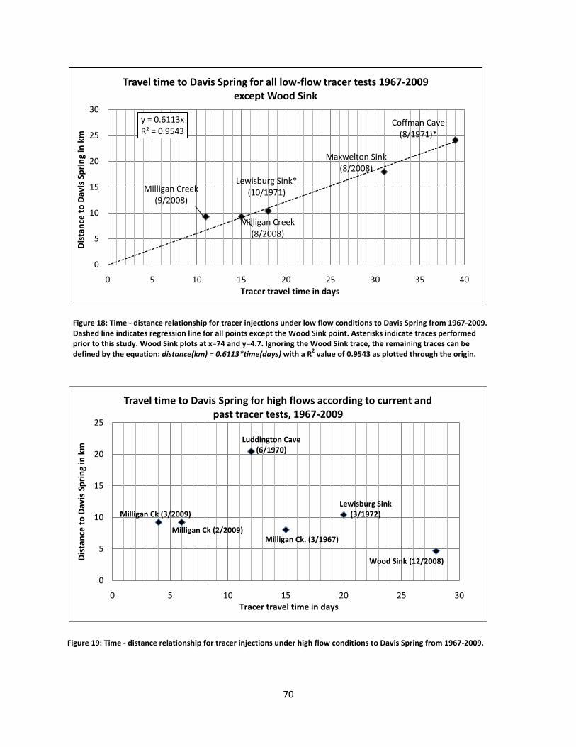
70
Coffman Cave (8/1971)*
Maxwelton Sink (8/2008)
Lewisburg Sink* (10/1971)
Milligan Creek (8/2008)
Milligan Creek (9/2008)
y = 0.6113xR² = 0.9543
0
5
10
15
20
25
30
0 5 10 15 20 25 30 35 40
Dis
tan
ce t
o D
avis
Sp
rin
g in
km
Tracer travel time in days
Travel time to Davis Spring for all low-flow tracer tests 1967-2009 except Wood Sink
Wood Sink (12/2008)
Lewisburg Sink (3/1972)
Milligan Ck. (3/1967)
Luddington Cave (6/1970)
Milligan Ck (2/2009)
Milligan Ck (3/2009)
0
5
10
15
20
25
0 5 10 15 20 25 30
Dis
tan
ce t
o D
avis
Sp
rin
g in
km
Tracer travel time in days
Travel time to Davis Spring for high flows according to current and past tracer tests, 1967-2009
Figure 18: Time - distance relationship for tracer injections under low flow conditions to Davis Spring from 1967-2009. Dashed line indicates regression line for all points except the Wood Sink point. Asterisks indicate traces performed prior to this study. Wood Sink plots at x=74 and y=4.7. Ignoring the Wood Sink trace, the remaining traces can be defined by the equation: distance(km) = 0.6113*time(days) with a R
2 value of 0.9543 as plotted through the origin.
Figure 19: Time - distance relationship for tracer injections under high flow conditions to Davis Spring from 1967-2009.
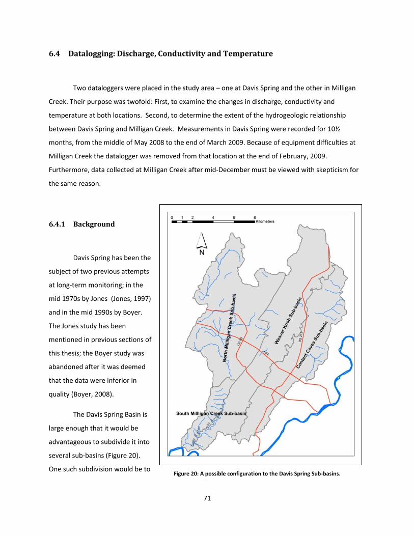
71
6.4 Datalogging: Discharge, Conductivity and Temperature
Two dataloggers were placed in the study area – one at Davis Spring and the other in Milligan
Creek. Their purpose was twofold: First, to examine the changes in discharge, conductivity and
temperature at both locations. Second, to determine the extent of the hydrogeologic relationship
between Davis Spring and Milligan Creek. Measurements in Davis Spring were recorded for 10½
months, from the middle of May 2008 to the end of March 2009. Because of equipment difficulties at
Milligan Creek the datalogger was removed from that location at the end of February, 2009.
Furthermore, data collected at Milligan Creek after mid-December must be viewed with skepticism for
the same reason.
6.4.1 Background
Davis Spring has been the
subject of two previous attempts
at long-term monitoring; in the
mid 1970s by Jones (Jones, 1997)
and in the mid 1990s by Boyer.
The Jones study has been
mentioned in previous sections of
this thesis; the Boyer study was
abandoned after it was deemed
that the data were inferior in
quality (Boyer, 2008).
The Davis Spring Basin is
large enough that it would be
advantageous to subdivide it into
several sub-basins (Figure 20).
One such subdivision would be to Figure 20: A possible configuration to the Davis Spring Sub-basins.
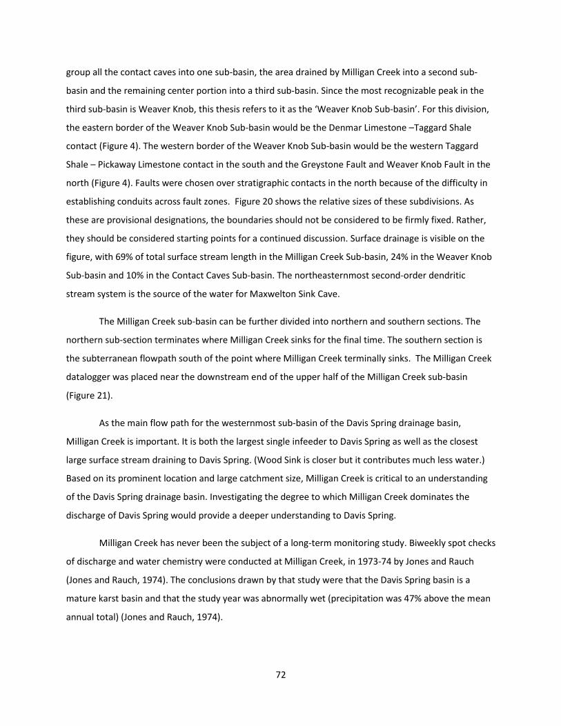
72
group all the contact caves into one sub-basin, the area drained by Milligan Creek into a second sub-
basin and the remaining center portion into a third sub-basin. Since the most recognizable peak in the
third sub-basin is Weaver Knob, this thesis refers to it as the ‘Weaver Knob Sub-basin’. For this division,
the eastern border of the Weaver Knob Sub-basin would be the Denmar Limestone –Taggard Shale
contact (Figure 4). The western border of the Weaver Knob Sub-basin would be the western Taggard
Shale – Pickaway Limestone contact in the south and the Greystone Fault and Weaver Knob Fault in the
north (Figure 4). Faults were chosen over stratigraphic contacts in the north because of the difficulty in
establishing conduits across fault zones. Figure 20 shows the relative sizes of these subdivisions. As
these are provisional designations, the boundaries should not be considered to be firmly fixed. Rather,
they should be considered starting points for a continued discussion. Surface drainage is visible on the
figure, with 69% of total surface stream length in the Milligan Creek Sub-basin, 24% in the Weaver Knob
Sub-basin and 10% in the Contact Caves Sub-basin. The northeasternmost second-order dendritic
stream system is the source of the water for Maxwelton Sink Cave.
The Milligan Creek sub-basin can be further divided into northern and southern sections. The
northern sub-section terminates where Milligan Creek sinks for the final time. The southern section is
the subterranean flowpath south of the point where Milligan Creek terminally sinks. The Milligan Creek
datalogger was placed near the downstream end of the upper half of the Milligan Creek sub-basin
(Figure 21).
As the main flow path for the westernmost sub-basin of the Davis Spring drainage basin,
Milligan Creek is important. It is both the largest single infeeder to Davis Spring as well as the closest
large surface stream draining to Davis Spring. (Wood Sink is closer but it contributes much less water.)
Based on its prominent location and large catchment size, Milligan Creek is critical to an understanding
of the Davis Spring drainage basin. Investigating the degree to which Milligan Creek dominates the
discharge of Davis Spring would provide a deeper understanding to Davis Spring.
Milligan Creek has never been the subject of a long-term monitoring study. Biweekly spot checks
of discharge and water chemistry were conducted at Milligan Creek, in 1973-74 by Jones and Rauch
(Jones and Rauch, 1974). The conclusions drawn by that study were that the Davis Spring basin is a
mature karst basin and that the study year was abnormally wet (precipitation was 47% above the mean
annual total) (Jones and Rauch, 1974).
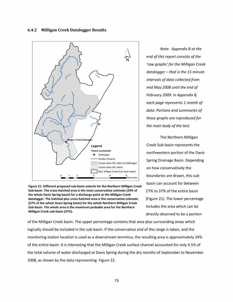
73
6.4.2 Milligan Creek Datalogger Results
Note: Appendix B at the
end of this report consists of the
‘raw graphs’ for the Milligan Creek
datalogger – that is the 15 minute
intervals of data collected from
mid May 2008 until the end of
February 2009. In Appendix B,
each page represents 1 month of
data. Portions and summaries of
those graphs are reproduced for
the main body of the test.
The Northern Milligan
Creek Sub-basin represents the
northwestern portion of the Davis
Spring Drainage Basin. Depending
on how conservatively the
boundaries are drawn, this sub-
basin can account for between
27% to 37% of the entire basin
(Figure 21). The lower percentage
includes the area which can be
directly observed to be a portion
of the Milligan Creek basin. The upper percentage contains that area plus surrounding areas which
logically should be included in the sub-basin. If the conservative end of the range is taken, and the
monitoring station location is used as a downstream terminus, the resulting area is approximately 24%
of the entire basin. It is interesting that the Milligan Creek surface channel accounted for only 4.5% of
the total volume of water discharged at Davis Spring during the dry months of September to November
2008, as shown by the data representing Figure 22.
Figure 21: Different proposed sub-basin extents for the Northern Milligan Creek Sub-basin. The cross-hatched area is the most conservative estimate (24% of the whole Davis Spring basin) for a discharge point at the Milligan Creek datalogger. The hatched plus cross-hatched area is the conservative estimate (27% of the whole Davis Spring basin) for the whole Northern Milligan Creek Sub-basin. The whole area is the maximum probable area for the Northern Milligan Creek sub-basin (37%).
74
This study author was unable to trace a storm pulse hydrograph peak from Milligan Creek to
Davis Spring. One reason for this was that the relative sizes of the two storm pulses meant the Milligan
Creek pulse was overwhelmed by the Davis Spring signal. While some storms did generate pulses soon
after the event, this author was unable to conclusively show that the pulse originated at Milligan Creek.
Tracer testing failed for another reason. It was virtually impossible to predict storm events with
sufficient precision to drive four hours to the study area and trace the pulse as it passed the Milligan
Creek datalogger. Storm pulses at Milligan creek tend to be brief and sharp, occurring hours after the
storm passed. In form, Milligan Creek pulses appear very similar to surface stream pulses. This is
unsurprising considering the frequency with which this channel surfaces.
If the northwestern Milligan Creek Basin drains 24% of the Davis Spring Basin and rainfall is
uniform across the basin then the percentage of water passing the Milligan Creek datalogger should be
24%. This expectation is inconsistent with the 10 months of data collected at the Milligan Creek
datalogger. Figure 22 shows the relationship between the recorded Davis Spring volume by month, the
recorded Milligan Creek volume by month and the calculated expected Milligan Creek volume by month.
0
1,000,000
2,000,000
3,000,000
4,000,000
5,000,000
6,000,000
7,000,000
May-08 Jun-08 Jul-08 Aug-08 Sep-08 Oct-08 Nov-08 Dec-08 Jan-09 Feb-09
Mo
nth
ly d
isch
arge
vo
lum
e in
m3
Relative Milligan Creek and Davis Spring volumes, by Month
MC vol
DS vol
Exp. MC Vol
Figure 22: Relative Milligan Creek and Davis Spring volumes by month. The expected Milligan Creek volume by month is calculated as 24% of the Davis Spring volume and displayed as a hollow vertical bar. Observed Milligan Creek volume is displayed by a grey bar, while observed Davis Spring volume is a solid black bar.
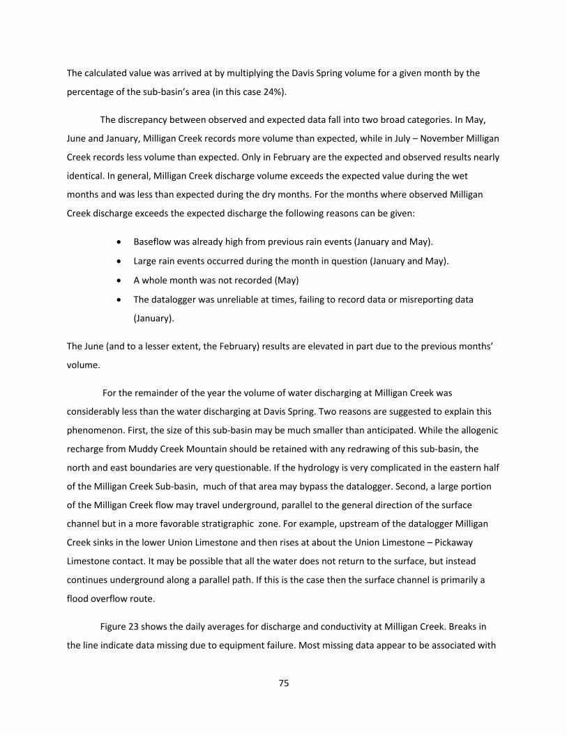
75
The calculated value was arrived at by multiplying the Davis Spring volume for a given month by the
percentage of the sub-basin’s area (in this case 24%).
The discrepancy between observed and expected data fall into two broad categories. In May,
June and January, Milligan Creek records more volume than expected, while in July – November Milligan
Creek records less volume than expected. Only in February are the expected and observed results nearly
identical. In general, Milligan Creek discharge volume exceeds the expected value during the wet
months and was less than expected during the dry months. For the months where observed Milligan
Creek discharge exceeds the expected discharge the following reasons can be given:
Baseflow was already high from previous rain events (January and May).
Large rain events occurred during the month in question (January and May).
A whole month was not recorded (May)
The datalogger was unreliable at times, failing to record data or misreporting data
(January).
The June (and to a lesser extent, the February) results are elevated in part due to the previous months’
volume.
For the remainder of the year the volume of water discharging at Milligan Creek was
considerably less than the water discharging at Davis Spring. Two reasons are suggested to explain this
phenomenon. First, the size of this sub-basin may be much smaller than anticipated. While the allogenic
recharge from Muddy Creek Mountain should be retained with any redrawing of this sub-basin, the
north and east boundaries are very questionable. If the hydrology is very complicated in the eastern half
of the Milligan Creek Sub-basin, much of that area may bypass the datalogger. Second, a large portion
of the Milligan Creek flow may travel underground, parallel to the general direction of the surface
channel but in a more favorable stratigraphic zone. For example, upstream of the datalogger Milligan
Creek sinks in the lower Union Limestone and then rises at about the Union Limestone – Pickaway
Limestone contact. It may be possible that all the water does not return to the surface, but instead
continues underground along a parallel path. If this is the case then the surface channel is primarily a
flood overflow route.
Figure 23 shows the daily averages for discharge and conductivity at Milligan Creek. Breaks in
the line indicate data missing due to equipment failure. Most missing data appear to be associated with
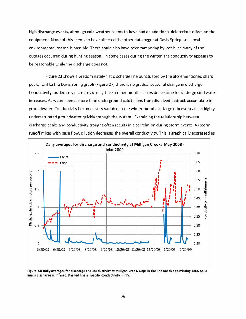
76
high discharge events, although cold weather seems to have had an additional deleterious effect on the
equipment. None of this seems to have affected the other datalogger at Davis Spring, so a local
environmental reason is possible. There could also have been tampering by locals, as many of the
outages occurred during hunting season. In some cases during the winter, the conductivity appears to
be reasonable while the discharge does not.
Figure 23 shows a predominately flat discharge line punctuated by the aforementioned sharp
peaks. Unlike the Davis Spring graph (Figure 27) there is no gradual seasonal change in discharge.
Conductivity moderately increases during the summer months as residence time for underground water
increases. As water spends more time underground calcite ions from dissolved bedrock accumulate in
groundwater. Conductivity becomes very variable in the winter months as large rain events flush highly
undersaturated groundwater quickly through the system. Examining the relationship between
discharge peaks and conductivity troughs often results in a correlation during storm events. As storm
runoff mixes with base flow, dilution decreases the overall conductivity. This is graphically expressed as
0.20
0.25
0.30
0.35
0.40
0.45
0.50
0.55
0.60
0.65
0.70
0
0.5
1
1.5
2
2.5
5/20/08 6/20/08 7/20/08 8/20/08 9/20/08 10/20/08 11/20/08 12/20/08 1/20/09 2/20/09
con
du
ctiv
ity
in m
ilisi
em
en
s
Dis
char
ge in
cu
bic
me
ters
pe
r se
con
d
Daily averages for discharge and conductivity at Milligan Creek: May 2008 -Mar 2009
MC Q
Cond
Figure 23: Daily averages for discharge and conductivity at Milligan Creek. Gaps in the line are due to missing data. Solid line is discharge in m
3/sec. Dashed line is specific conductivity in mS.
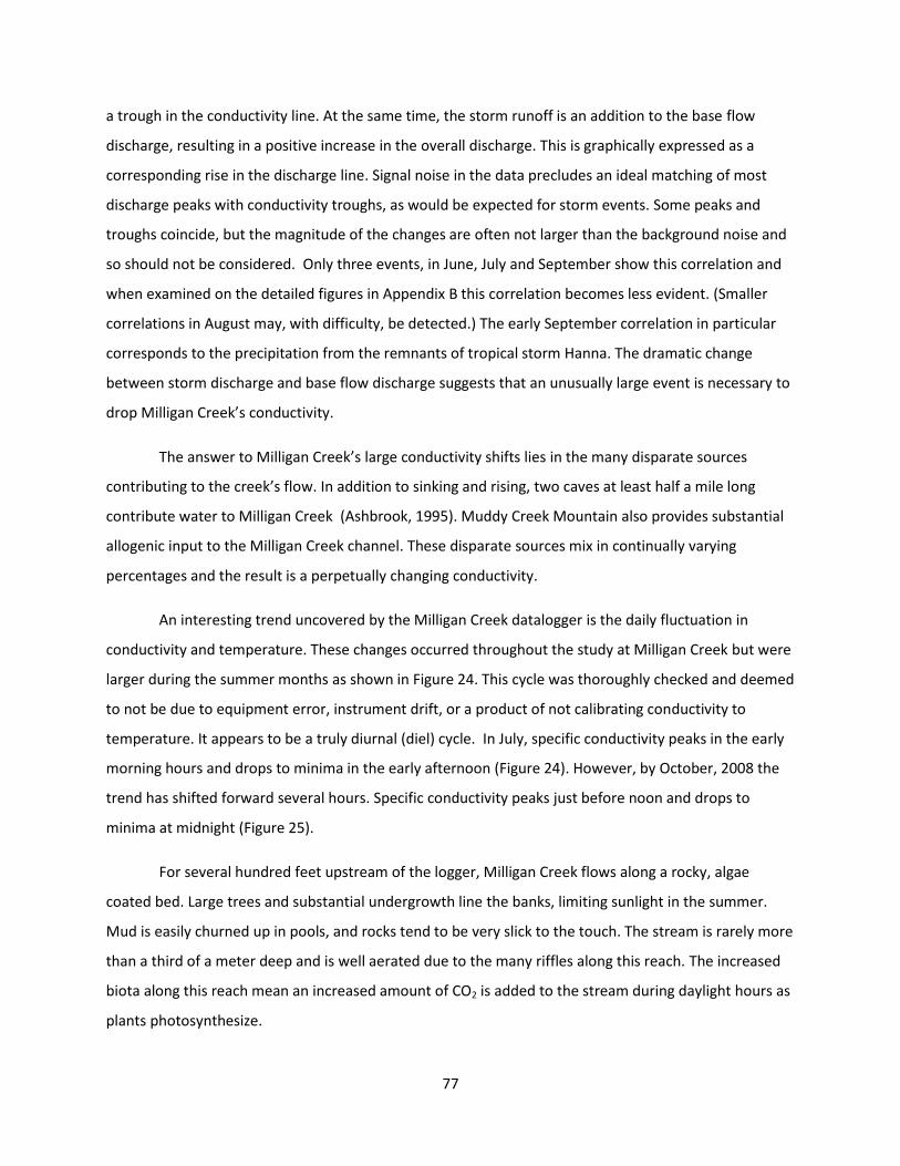
77
a trough in the conductivity line. At the same time, the storm runoff is an addition to the base flow
discharge, resulting in a positive increase in the overall discharge. This is graphically expressed as a
corresponding rise in the discharge line. Signal noise in the data precludes an ideal matching of most
discharge peaks with conductivity troughs, as would be expected for storm events. Some peaks and
troughs coincide, but the magnitude of the changes are often not larger than the background noise and
so should not be considered. Only three events, in June, July and September show this correlation and
when examined on the detailed figures in Appendix B this correlation becomes less evident. (Smaller
correlations in August may, with difficulty, be detected.) The early September correlation in particular
corresponds to the precipitation from the remnants of tropical storm Hanna. The dramatic change
between storm discharge and base flow discharge suggests that an unusually large event is necessary to
drop Milligan Creek’s conductivity.
The answer to Milligan Creek’s large conductivity shifts lies in the many disparate sources
contributing to the creek’s flow. In addition to sinking and rising, two caves at least half a mile long
contribute water to Milligan Creek (Ashbrook, 1995). Muddy Creek Mountain also provides substantial
allogenic input to the Milligan Creek channel. These disparate sources mix in continually varying
percentages and the result is a perpetually changing conductivity.
An interesting trend uncovered by the Milligan Creek datalogger is the daily fluctuation in
conductivity and temperature. These changes occurred throughout the study at Milligan Creek but were
larger during the summer months as shown in Figure 24. This cycle was thoroughly checked and deemed
to not be due to equipment error, instrument drift, or a product of not calibrating conductivity to
temperature. It appears to be a truly diurnal (diel) cycle. In July, specific conductivity peaks in the early
morning hours and drops to minima in the early afternoon (Figure 24). However, by October, 2008 the
trend has shifted forward several hours. Specific conductivity peaks just before noon and drops to
minima at midnight (Figure 25).
For several hundred feet upstream of the logger, Milligan Creek flows along a rocky, algae
coated bed. Large trees and substantial undergrowth line the banks, limiting sunlight in the summer.
Mud is easily churned up in pools, and rocks tend to be very slick to the touch. The stream is rarely more
than a third of a meter deep and is well aerated due to the many riffles along this reach. The increased
biota along this reach mean an increased amount of CO2 is added to the stream during daylight hours as
plants photosynthesize.
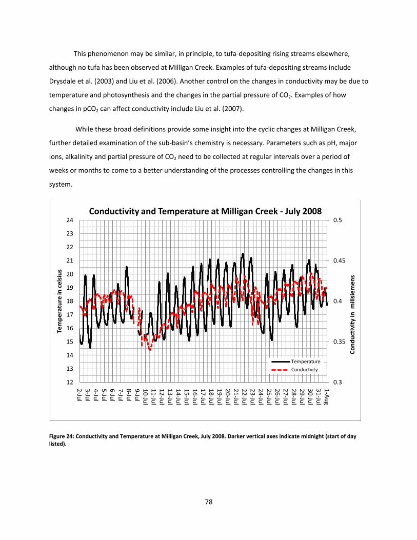
78
This phenomenon may be similar, in principle, to tufa-depositing rising streams elsewhere,
although no tufa has been observed at Milligan Creek. Examples of tufa-depositing streams include
Drysdale et al. (2003) and Liu et al. (2006). Another control on the changes in conductivity may be due to
temperature and photosynthesis and the changes in the partial pressure of CO2. Examples of how
changes in pCO2 can affect conductivity include Liu et al. (2007).
While these broad definitions provide some insight into the cyclic changes at Milligan Creek,
further detailed examination of the sub-basin’s chemistry is necessary. Parameters such as pH, major
ions, alkalinity and partial pressure of CO2 need to be collected at regular intervals over a period of
weeks or months to come to a better understanding of the processes controlling the changes in this
system.
Figure 24: Conductivity and Temperature at Milligan Creek, July 2008. Darker vertical axes indicate midnight (start of day listed).
0.3
0.35
0.4
0.45
0.5
12
13
14
15
16
17
18
19
20
21
22
23
24
2-Ju
l3
-Jul
4-Ju
l5
-Jul
6-Ju
l7
-Jul
8-Ju
l9
-Jul
10
-Jul
11
-Jul
12
-Jul
13
-Jul
14
-Jul
15
-Jul
16
-Jul
17
-Jul
18
-Jul
19
-Jul
20
-Jul
21
-Jul
22
-Jul
23
-Jul
24
-Jul
25
-Jul
26
-Jul
27
-Jul
28
-Jul
29
-Jul
30
-Jul
31
-Jul
1-A
ug
Co
nd
uct
ivit
y in
mili
sie
me
ns
Tem
pe
ratu
re in
ce
lsiu
s
Conductivity and Temperature at Milligan Creek - July 2008
Temperature
Conductvity
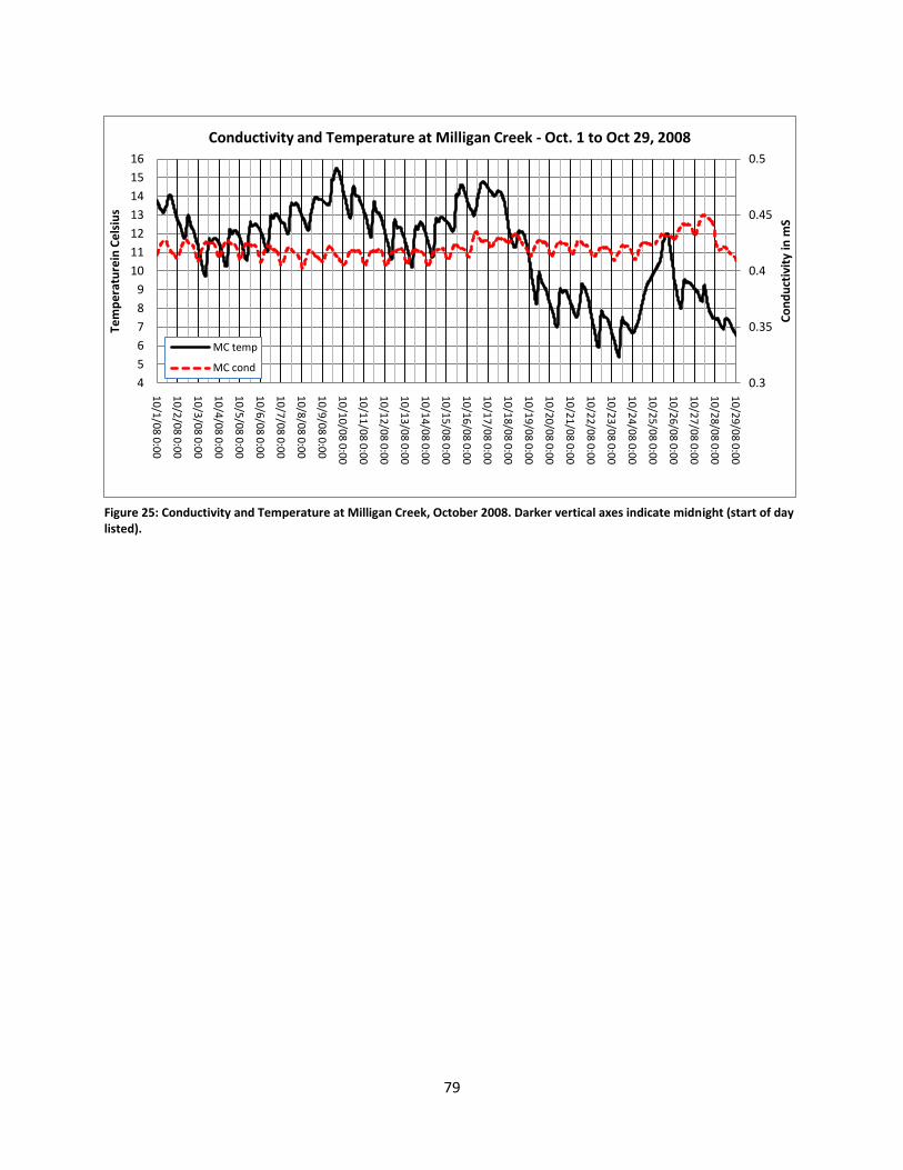
79
0.3
0.35
0.4
0.45
0.5
4
5
6
7
8
9
10
11
12
13
14
15
16
10
/1/0
8 0
:00
10
/2/0
8 0
:00
10
/3/0
8 0
:00
10
/4/0
8 0
:00
10
/5/0
8 0
:00
10
/6/0
8 0
:00
10
/7/0
8 0
:00
10
/8/0
8 0
:00
10
/9/0
8 0
:00
10
/10
/08
0:0
0
10
/11
/08
0:0
0
10
/12
/08
0:0
0
10
/13
/08
0:0
0
10
/14
/08
0:0
0
10
/15
/08
0:0
0
10
/16
/08
0:0
0
10
/17
/08
0:0
0
10
/18
/08
0:0
0
10
/19
/08
0:0
0
10
/20
/08
0:0
0
10
/21
/08
0:0
0
10
/22
/08
0:0
0
10
/23
/08
0:0
0
10
/24
/08
0:0
0
10
/25
/08
0:0
0
10
/26
/08
0:0
0
10
/27
/08
0:0
0
10
/28
/08
0:0
0
10
/29
/08
0:0
0
Co
nd
uct
ivit
y in
mS
Tem
pe
ratu
rein
Ce
lsiu
s
Conductivity and Temperature at Milligan Creek - Oct. 1 to Oct 29, 2008
MC temp
MC cond
Figure 25: Conductivity and Temperature at Milligan Creek, October 2008. Darker vertical axes indicate midnight (start of day listed).
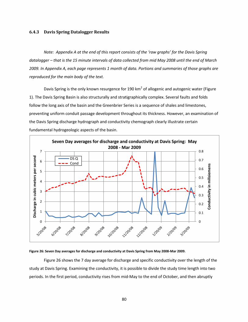
80
6.4.3 Davis Spring Datalogger Results
Note: Appendix A at the end of this report consists of the ‘raw graphs’ for the Davis Spring
datalogger – that is the 15 minute intervals of data collected from mid May 2008 until the end of March
2009. In Appendix A, each page represents 1 month of data. Portions and summaries of those graphs are
reproduced for the main body of the text.
Davis Spring is the only known resurgence for 190 km2 of allogenic and autogenic water (Figure
1). The Davis Spring Basin is also structurally and stratigraphically complex. Several faults and folds
follow the long axis of the basin and the Greenbrier Series is a sequence of shales and limestones,
preventing uniform conduit passage development throughout its thickness. However, an examination of
the Davis Spring discharge hydrograph and conductivity chemograph clearly illustrate certain
fundamental hydrogeologic aspects of the basin.
Figure 26: Seven Day averages for discharge and conductivity at Davis Spring from May 2008-Mar 2009.
Figure 26 shows the 7 day average for discharge and specific conductivity over the length of the
study at Davis Spring. Examining the conductivity, it is possible to divide the study time length into two
periods. In the first period, conductivity rises from mid-May to the end of October, and then abruptly
0
0.1
0.2
0.3
0.4
0.5
0.6
0.7
0.8
0
1
2
3
4
5
6
7
Co
nd
uct
ivit
y in
mili
sie
me
ns
Dis
char
ge in
cu
bic
me
ters
pe
r se
con
d
Seven Day averages for discharge and conductivity at Davis Spring: May 2008 - Mar 2009
DS QCond
81
drops in November. The second period begins when the conductivity stabilizes at this lower level in mid
December and remains at that level throughout the winter months through April.
These two periods have corresponding distinct patterns of discharge. During the first period
(May-October) discharge is relatively uniform and low. The second period (November-April) is
characterized by sharp spikes of discharge corresponding to large rain events during the winter months.
Background discharge levels also appear to be slightly elevated during this second period. Because
discharge is more intuitive, these two periods will be referred to as the ‘Dry Period’ and the ‘Wet
Period’, respectively. The Wet Period begins when the first major precipitation event capable of
significantly dropping the conductivity occurs. The Wet Period ends with the start of significant ET in
spring, about May 1st, when conductivity begins its climb. Unfortunately, the moment of conductivity
rise was not captured during this study. It is possible to extrapolate back to a reasonable, hypothetical,
horizontal conductivity line for the Wet Period. Such a line would intersect near the end of April 2008 or
the start of May 2008. During the 2008-2009 year the Davis Spring Basin spent about 7 months in the
‘Dry Period’ and 5 months in the ‘Wet Period’. An interesting long-term study would be to see the
changes (if any) in this wet to dry ratio over several years of varying precipitation.
The cause of the increase in specific conductivity over the dry period is the increased residence
time of the system’s stored water. Water reacts with atmospheric CO2 to form a weak carbonic acid.
This acid dissolves small amounts of calcite from the conduit walls. This dissolution continues until the
water becomes nearly saturated or saturated with calcite and the water is near equilibrium with the
rock around it. The primary way to increase the capacity of the water for calcite dissolution is to mix the
nearly saturated water with undersaturated water. An increase in dissolved calcite concentration is
reflected by a corresponding increase in conductivity.
Every precipitation event has an accompanying storm pulse. This pulse of water pushes out the
old water from the system and replaces it with new, undersaturated water. During the Dry Period the
force of the pulse is insufficient to push out all of the stored water. Some calcite-rich water remains to
mix with the new water. Over time this will result in an overall seasonal rise of specific conductivity.
The cause of the decrease in specific conductivity for Davis Spring at the start of the Wet Period
is the nearly complete flushing of the saturated, stored water from the conduit system. This could
happen with one exceptionally large storm, or a series of large storms in succession. When displayed on
a graph (Figure 26) a sharp rise in conductivity is first observed, followed by a sharper drop in
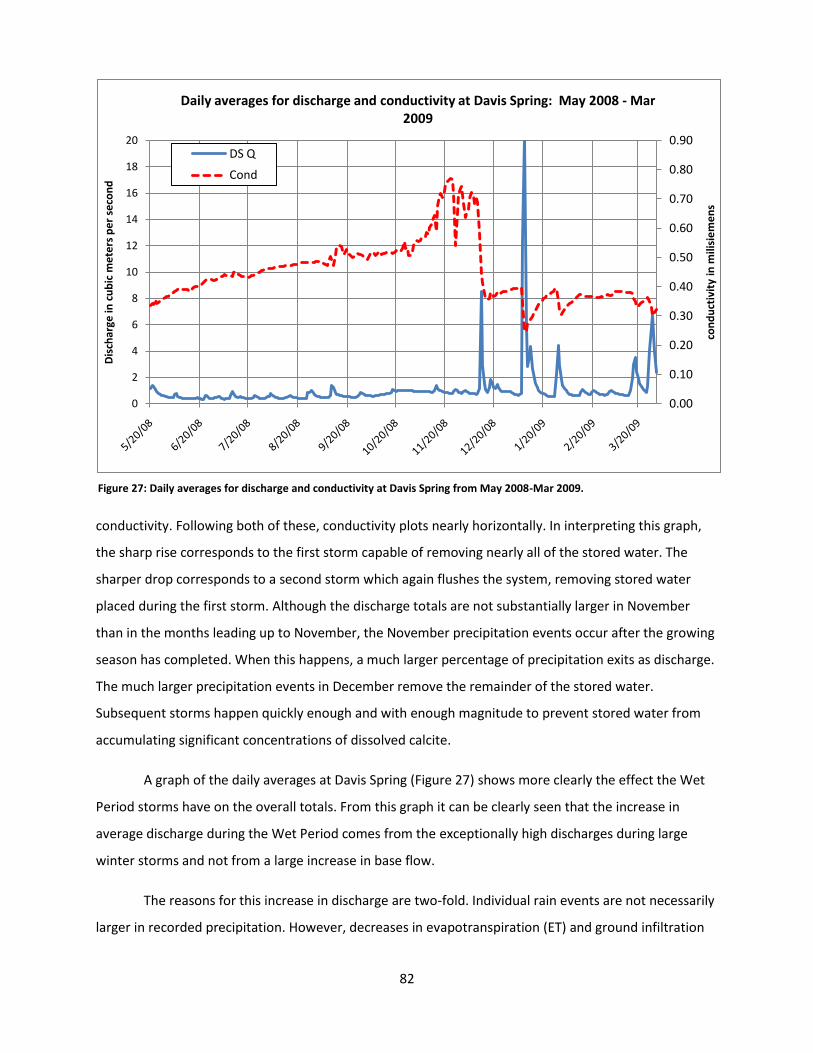
82
conductivity. Following both of these, conductivity plots nearly horizontally. In interpreting this graph,
the sharp rise corresponds to the first storm capable of removing nearly all of the stored water. The
sharper drop corresponds to a second storm which again flushes the system, removing stored water
placed during the first storm. Although the discharge totals are not substantially larger in November
than in the months leading up to November, the November precipitation events occur after the growing
season has completed. When this happens, a much larger percentage of precipitation exits as discharge.
The much larger precipitation events in December remove the remainder of the stored water.
Subsequent storms happen quickly enough and with enough magnitude to prevent stored water from
accumulating significant concentrations of dissolved calcite.
A graph of the daily averages at Davis Spring (Figure 27) shows more clearly the effect the Wet
Period storms have on the overall totals. From this graph it can be clearly seen that the increase in
average discharge during the Wet Period comes from the exceptionally high discharges during large
winter storms and not from a large increase in base flow.
The reasons for this increase in discharge are two-fold. Individual rain events are not necessarily
larger in recorded precipitation. However, decreases in evapotranspiration (ET) and ground infiltration
0.00
0.10
0.20
0.30
0.40
0.50
0.60
0.70
0.80
0.90
0
2
4
6
8
10
12
14
16
18
20
con
du
ctiv
ity
in m
ilisi
em
en
s
Dis
char
ge in
cu
bic
me
ters
pe
r se
con
dDaily averages for discharge and conductivity at Davis Spring: May 2008 - Mar
2009
DS Q
Cond
Figure 27: Daily averages for discharge and conductivity at Davis Spring from May 2008-Mar 2009.
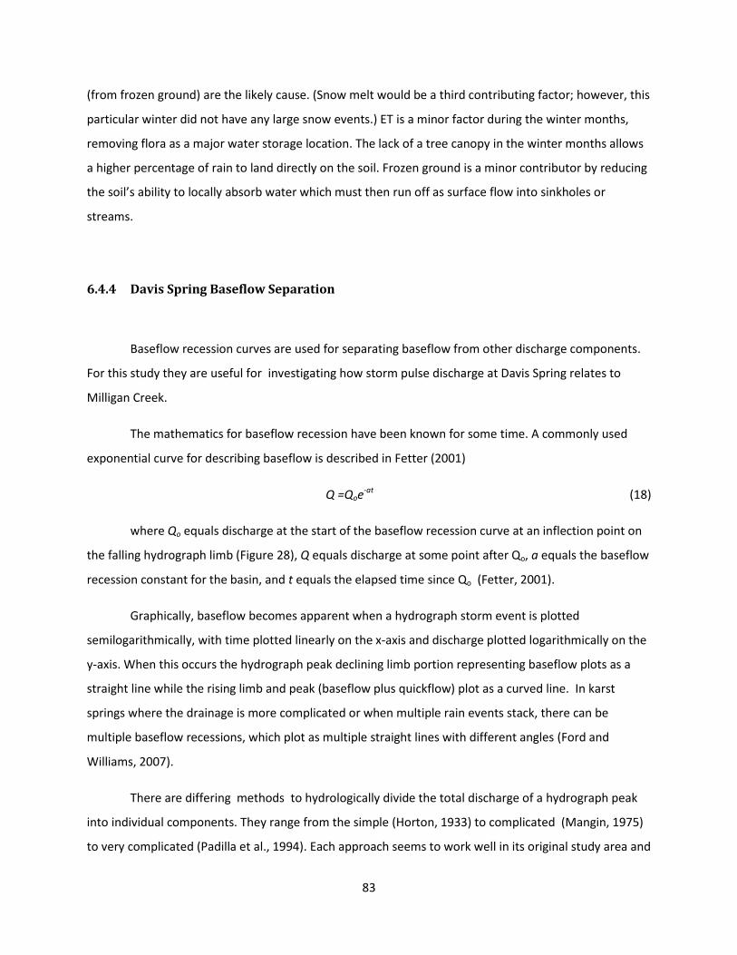
83
(from frozen ground) are the likely cause. (Snow melt would be a third contributing factor; however, this
particular winter did not have any large snow events.) ET is a minor factor during the winter months,
removing flora as a major water storage location. The lack of a tree canopy in the winter months allows
a higher percentage of rain to land directly on the soil. Frozen ground is a minor contributor by reducing
the soil’s ability to locally absorb water which must then run off as surface flow into sinkholes or
streams.
6.4.4 Davis Spring Baseflow Separation
Baseflow recession curves are used for separating baseflow from other discharge components.
For this study they are useful for investigating how storm pulse discharge at Davis Spring relates to
Milligan Creek.
The mathematics for baseflow recession have been known for some time. A commonly used
exponential curve for describing baseflow is described in Fetter (2001)
Q =Qoe-at (18)
where Qo equals discharge at the start of the baseflow recession curve at an inflection point on
the falling hydrograph limb (Figure 28), Q equals discharge at some point after Qo, a equals the baseflow
recession constant for the basin, and t equals the elapsed time since Qo (Fetter, 2001).
Graphically, baseflow becomes apparent when a hydrograph storm event is plotted
semilogarithmically, with time plotted linearly on the x-axis and discharge plotted logarithmically on the
y-axis. When this occurs the hydrograph peak declining limb portion representing baseflow plots as a
straight line while the rising limb and peak (baseflow plus quickflow) plot as a curved line. In karst
springs where the drainage is more complicated or when multiple rain events stack, there can be
multiple baseflow recessions, which plot as multiple straight lines with different angles (Ford and
Williams, 2007).
There are differing methods to hydrologically divide the total discharge of a hydrograph peak
into individual components. They range from the simple (Horton, 1933) to complicated (Mangin, 1975)
to very complicated (Padilla et al., 1994). Each approach seems to work well in its original study area and
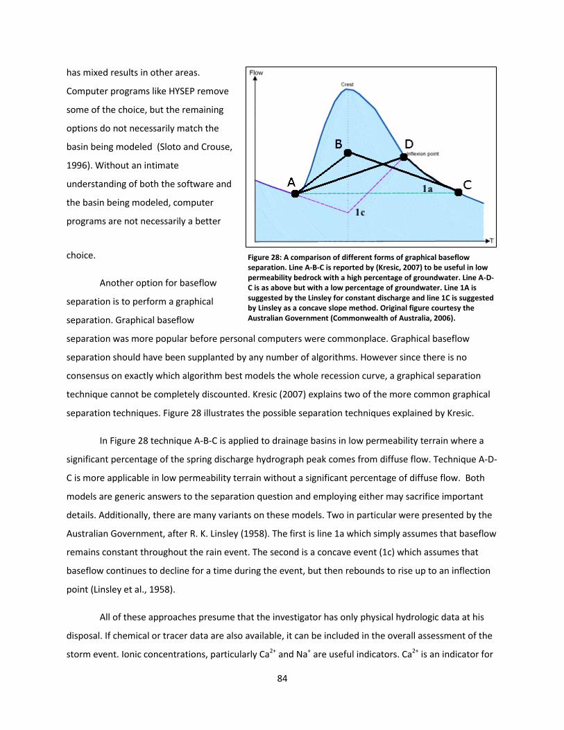
84
has mixed results in other areas.
Computer programs like HYSEP remove
some of the choice, but the remaining
options do not necessarily match the
basin being modeled (Sloto and Crouse,
1996). Without an intimate
understanding of both the software and
the basin being modeled, computer
programs are not necessarily a better
choice.
Another option for baseflow
separation is to perform a graphical
separation. Graphical baseflow
separation was more popular before personal computers were commonplace. Graphical baseflow
separation should have been supplanted by any number of algorithms. However since there is no
consensus on exactly which algorithm best models the whole recession curve, a graphical separation
technique cannot be completely discounted. Kresic (2007) explains two of the more common graphical
separation techniques. Figure 28 illustrates the possible separation techniques explained by Kresic.
In Figure 28 technique A-B-C is applied to drainage basins in low permeability terrain where a
significant percentage of the spring discharge hydrograph peak comes from diffuse flow. Technique A-D-
C is more applicable in low permeability terrain without a significant percentage of diffuse flow. Both
models are generic answers to the separation question and employing either may sacrifice important
details. Additionally, there are many variants on these models. Two in particular were presented by the
Australian Government, after R. K. Linsley (1958). The first is line 1a which simply assumes that baseflow
remains constant throughout the rain event. The second is a concave event (1c) which assumes that
baseflow continues to decline for a time during the event, but then rebounds to rise up to an inflection
point (Linsley et al., 1958).
All of these approaches presume that the investigator has only physical hydrologic data at his
disposal. If chemical or tracer data are also available, it can be included in the overall assessment of the
storm event. Ionic concentrations, particularly Ca2+ and Na+ are useful indicators. Ca2+ is an indicator for
Figure 28: A comparison of different forms of graphical baseflow separation. Line A-B-C is reported by (Kresic, 2007) to be useful in low permeability bedrock with a high percentage of groundwater. Line A-D-C is as above but with a low percentage of groundwater. Line 1A is suggested by the Linsley for constant discharge and line 1C is suggested by Linsley as a concave slope method. Original figure courtesy the Australian Government (Commonwealth of Australia, 2006).
85
dissolved calcite. Calcite concentrations are high in water which has a long underground residence time.
Na+ is an indicator of dissolved salts. Salt can be from briny water and is also used in the winter to de-ice
roads. This makes Na+ an indicator of surface runoff, particularly in the winter. In shallow unpolluted
karst systems the amount of Ca2+ should exceed the amount of Na+ in the summer. Since specific
conductivity is a useful proxy for the amount of free ions in a solution and since for nearly any given
storm event Ca2+ >> Na+, then specific conductivity can be used as a quick approximation for discharge
composed mostly of stored water.
To attempt to use specific conductivity to separate baseflow from quickflow in a given storm
event, at least two things are needed. First the specific conductivity for the quickflow (surface flow or
rain) must be known. Second, it would be helpful if there was no net change in specific conductivity
before and after a storm event. This simplifies the overall mathematics and reduces the number of
variables. If this is the case and it is assumed that the water is composed of two discrete sources
(baseflow and quickflow) then dividing the two should be:
Total Specific Conductivity = ((% BFQ)*(BF sC)) + ((%QFQ)*(QF sC)) (19)
where %BFQ equals percent baseflow discharge, BF sC equals specific conductivity of baseflow, %QFQ
equals percent quickflow discharge, QF sC equals quickflow specific conductivity. This can be easily
integrated into an Excel spreadsheet to separate quickflow from baseflow.
The specific conductivity of rain varies by location and time of year. Generally, it is less than 200
µS and often much less. For example at Babcock State Park in Fayette WV (about 70 km west of the
study area) the specific conductivity of precipitation was measured during 1997-1998. During that
interval, the minimum specific conductivity was 17 µS and the maximum specific conductivity was 26 µS
with a median of 22 µS (Sheets and Kozar, 2000). Similar specific conductivities for rain are likely
appropriate to the Davis Spring area. Given that the specific conductivity at Davis Spring ranges from
200 to 500 µS the specific conductivity of rainwater is effectively zero. Specific conductivities as low as
these suggest that for Davis Spring the percentage of rainwater representing quickflow should be equal
to the drop in the percentage of specific conductivity. While this all seems reasonable and should be the
resolution to the baseflow separation issue, it unfortunately is not. Like most baseflow separation
86
models, this model makes some assumptions. The first assumption is that precipitation traveling to the
spring does become enriched in ions along the way. This is not true. The greater the distance traveled,
the more ions dissolved and consequently the higher specific conductivity. The only portion of the
drainage basin whose specific conductivity should be nearly equal to precipitation would be in the
immediate area of the spring. This is a very small percentage of the total Davis Spring drainage basin
area, equivalent to a few percent. This amount is trivial compared to the remainder of the basin and can
be ignored. What is the conductivity of the remainder of the quickflow?
A reasonable guess at the answer can be found by looking at the specific conductivity of Milligan
Creek. As a major tributary in the basin, Milligan Creek represents a good proxy for water which has
been in the basin for hours to days but not for weeks to months. A look at the comparative differences
in the specific conductivities of the two waters shows that there is enough of a difference to be
measurable.
If a specific conductivity of 0.4 mS (Figure 29) is used as a general figure for quickflow, a
baseflow separation using Equation (19) can be performed. Using the storm event of 11-25-08 to 11-27-
08 as an example (Figure 30), the separation is clearly evident. Note that this separation appears
inverted compared to the graphical separations proposed by Kresic (2007). Whereas Kresic’s ABC
Figure 29: Specific conductivity at the Milligan Creek and Davis Spring dataloggers from May 2008 - March 2009.
0
0.1
0.2
0.3
0.4
0.5
0.6
0.7
0.8
0.9
5/20/08 6/20/08 7/20/08 8/20/08 9/20/08 10/20/08 11/20/08 12/20/08 1/20/09 2/20/09
spe
cifi
c co
nd
uct
ivit
y in
mS
A comparison in specific conductivity between Milligan Creek and Davis Spring, May 2008 - March 2009
MC Cond
DS Cond
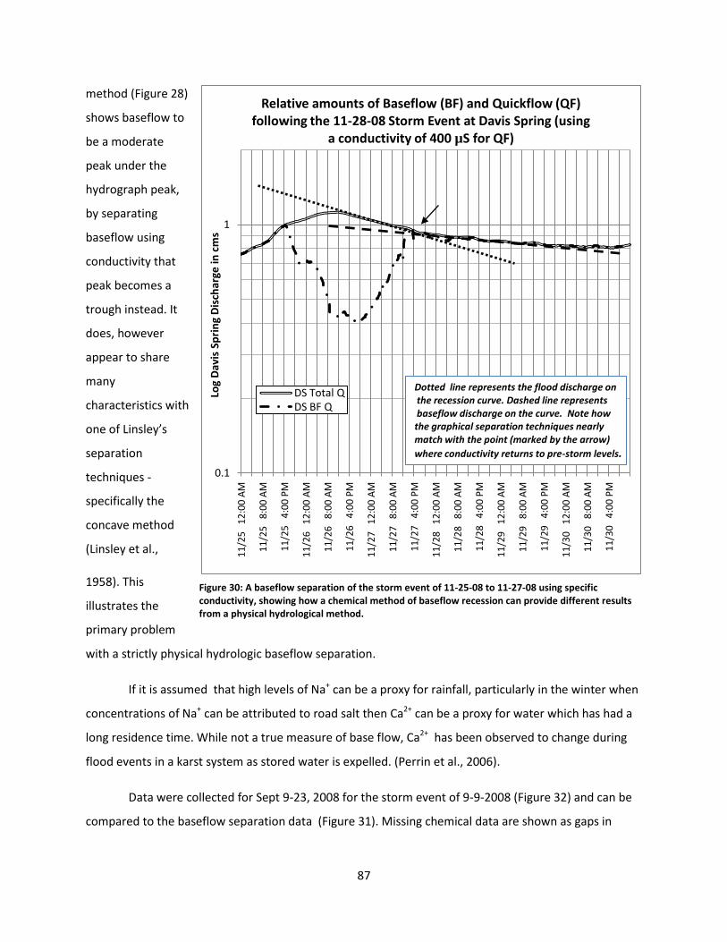
87
method (Figure 28)
shows baseflow to
be a moderate
peak under the
hydrograph peak,
by separating
baseflow using
conductivity that
peak becomes a
trough instead. It
does, however
appear to share
many
characteristics with
one of Linsley’s
separation
techniques -
specifically the
concave method
(Linsley et al.,
1958). This
illustrates the
primary problem
with a strictly physical hydrologic baseflow separation.
If it is assumed that high levels of Na+ can be a proxy for rainfall, particularly in the winter when
concentrations of Na+ can be attributed to road salt then Ca2+ can be a proxy for water which has had a
long residence time. While not a true measure of base flow, Ca2+ has been observed to change during
flood events in a karst system as stored water is expelled. (Perrin et al., 2006).
Data were collected for Sept 9-23, 2008 for the storm event of 9-9-2008 (Figure 32) and can be
compared to the baseflow separation data (Figure 31). Missing chemical data are shown as gaps in
0.1
1
11
/25
1
2:0
0 A
M
11
/25
8
:00
AM
11
/25
4
:00
PM
11
/26
1
2:0
0 A
M
11
/26
8
:00
AM
11
/26
4
:00
PM
11
/27
1
2:0
0 A
M
11
/27
8
:00
AM
11
/27
4
:00
PM
11
/28
1
2:0
0 A
M
11
/28
8
:00
AM
11
/28
4
:00
PM
11
/29
1
2:0
0 A
M
11
/29
8
:00
AM
11
/29
4
:00
PM
11
/30
1
2:0
0 A
M
11
/30
8
:00
AM
11
/30
4
:00
PM
Log
Dav
is S
pri
ng
Dis
char
ge in
cm
s
Relative amounts of Baseflow (BF) and Quickflow (QF) following the 11-28-08 Storm Event at Davis Spring (using
a conductivity of 400 µS for QF)
DS Total QDS BF Q
Dotted line represents the flood discharge onthe recession curve. Dashed line represents baseflow discharge on the curve. Note how the graphical separation techniques nearly match with the point (marked by the arrow)
where conductivity returns to pre-storm levels.
Figure 30: A baseflow separation of the storm event of 11-25-08 to 11-27-08 using specific conductivity, showing how a chemical method of baseflow recession can provide different results from a physical hydrological method.

88
Figure 32. Rather than displaying the calcium and sodium as concentrations, it is more useful to show
the changes in the amounts of both ions by displaying their flux.
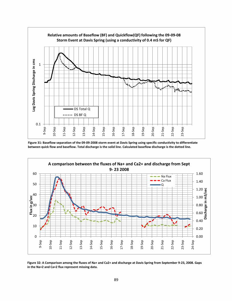
89
Figure 32: A Comparison among the fluxes of Na+ and Ca2+ and discharge at Davis Spring from September 9-23, 2008. Gaps in the Na+2 and Ca+2 flux represent missing data.
0.00
0.20
0.40
0.60
0.80
1.00
1.20
1.40
1.60
0
10
20
30
40
50
60
9-S
ep
10
-Sep
11
-Sep
12
-Sep
13
-Sep
14
-Sep
15
-Sep
16
-Sep
17
-Sep
18
-Sep
19
-Sep
20
-Sep
21
-Sep
22
-Sep
23
-Sep
24
-Sep
Dis
char
ge in
m3
/se
c
Flu
x in
g/s
ec
A comparison between the fluxes of Na+ and Ca2+ and discharge from Sept 9- 23 2008
Na Flux Ca Flux Q
0.1
1
9-S
ep
10
-Sep
11
-Sep
12
-Sep
13
-Sep
14
-Sep
15
-Sep
16
-Sep
17
-Sep
18
-Sep
19
-Sep
20
-Sep
21
-Sep
22
-Sep
23
-Sep
Log
Dav
is S
pri
ng
Dis
char
ge in
cm
sRelative amounts of Baseflow (BF) and Quickflow(QF) following the 09-09-08
Storm Event at Davis Spring (using a conductivity of 0.4 mS for QF)
DS Total Q
DS BF Q
Figure 31: Baseflow separation of the 09-09-2008 storm event at Davis Spring using specific conductivity to differentiate between quick flow and baseflow. Total discharge is the solid line. Calculated baseflow discharge is the dotted line.
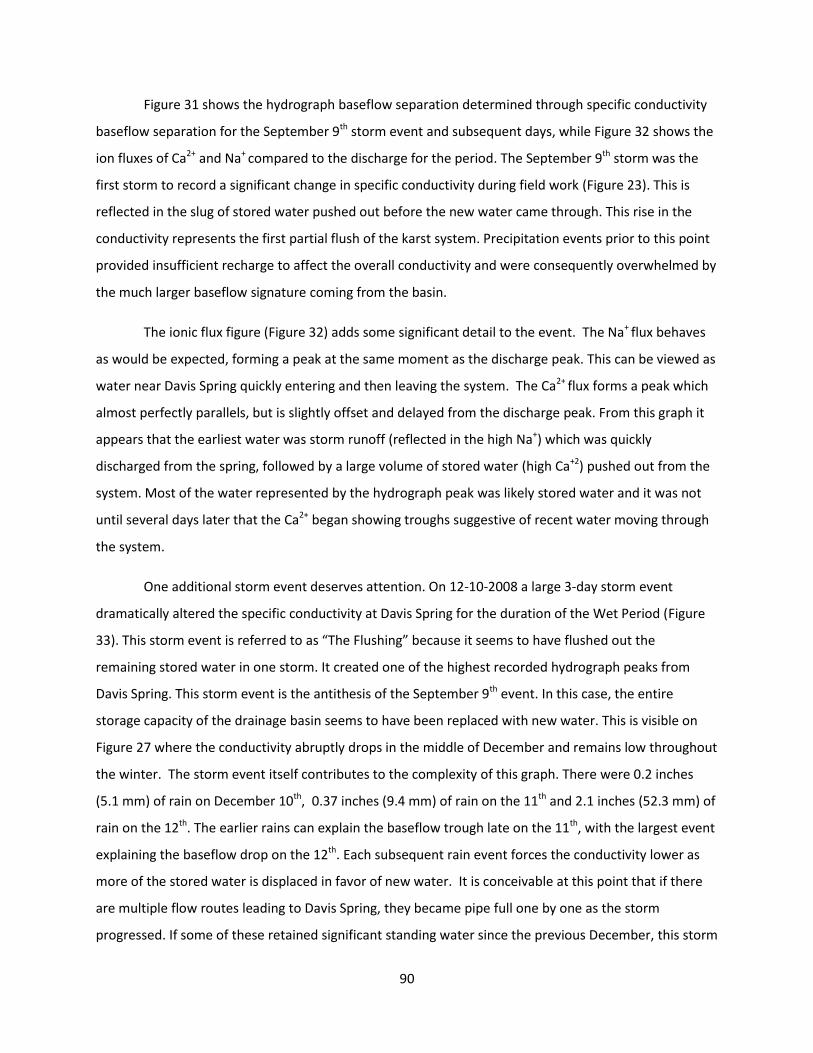
90
Figure 31 shows the hydrograph baseflow separation determined through specific conductivity
baseflow separation for the September 9th storm event and subsequent days, while Figure 32 shows the
ion fluxes of Ca2+ and Na+ compared to the discharge for the period. The September 9th storm was the
first storm to record a significant change in specific conductivity during field work (Figure 23). This is
reflected in the slug of stored water pushed out before the new water came through. This rise in the
conductivity represents the first partial flush of the karst system. Precipitation events prior to this point
provided insufficient recharge to affect the overall conductivity and were consequently overwhelmed by
the much larger baseflow signature coming from the basin.
The ionic flux figure (Figure 32) adds some significant detail to the event. The Na+ flux behaves
as would be expected, forming a peak at the same moment as the discharge peak. This can be viewed as
water near Davis Spring quickly entering and then leaving the system. The Ca2+ flux forms a peak which
almost perfectly parallels, but is slightly offset and delayed from the discharge peak. From this graph it
appears that the earliest water was storm runoff (reflected in the high Na+) which was quickly
discharged from the spring, followed by a large volume of stored water (high Ca+2) pushed out from the
system. Most of the water represented by the hydrograph peak was likely stored water and it was not
until several days later that the Ca2+ began showing troughs suggestive of recent water moving through
the system.
One additional storm event deserves attention. On 12-10-2008 a large 3-day storm event
dramatically altered the specific conductivity at Davis Spring for the duration of the Wet Period (Figure
33). This storm event is referred to as “The Flushing” because it seems to have flushed out the
remaining stored water in one storm. It created one of the highest recorded hydrograph peaks from
Davis Spring. This storm event is the antithesis of the September 9th event. In this case, the entire
storage capacity of the drainage basin seems to have been replaced with new water. This is visible on
Figure 27 where the conductivity abruptly drops in the middle of December and remains low throughout
the winter. The storm event itself contributes to the complexity of this graph. There were 0.2 inches
(5.1 mm) of rain on December 10th, 0.37 inches (9.4 mm) of rain on the 11th and 2.1 inches (52.3 mm) of
rain on the 12th. The earlier rains can explain the baseflow trough late on the 11th, with the largest event
explaining the baseflow drop on the 12th. Each subsequent rain event forces the conductivity lower as
more of the stored water is displaced in favor of new water. It is conceivable at this point that if there
are multiple flow routes leading to Davis Spring, they became pipe full one by one as the storm
progressed. If some of these retained significant standing water since the previous December, this storm
91
forced out the highly conductive water. This is represented by the conductivity rises on the 12th and 13th.
Nevertheless by the 14th, the entire system is overwhelmed and cleaned of all the stored water. While
this adequately explains the chemograph, it should be recalled that other scenarios could be
constructed which are equally plausible. Without being able to directly observe the conduits, this can
only be one possible solution.
6.4.5 Storm Pulse Travel Time from Milligan Creek to Davis Spring
Storm pulse travel time is a useful tool in basin analysis. A storm pulse is a large slug of water
moving through the conduit system. When recorded by a datalogger, it appears as a temporary rise in
stage. This stage rise can then be converted into an increased discharge measurement. All storm
hydrograph peaks are storm pulses.
In conduit-dominated systems, knowing the time elapsed from sinking point to resurgence can
be helpful in determining whether a conduit is open or closed. Open flow (pipe open to air) conduits will
Figure 33: Baseflow separation of the 12-10-08 to 12-12-08 storm event using specific conductivity. Labeled vertical lines mark the start of the labeled day.
0.01
0.1
1
10
100
10
-Dec
11
-Dec
12
-Dec
13
-Dec
14
-Dec
15
-Dec
Log
Dav
is S
pri
ng
Dis
char
ge in
cm
sRelative amounts of Baseflow (BF) and Quick Flow (QF) following the 12-10-08
Storm Event at Davis Spring (using a conductance of 0.4 mS)
DS Total Q
DS BF Q
92
behave in the manner of surface streams. Conduit water travels at equivalent (or slower) speeds to
surface water. Closed (pipe full) conduits behave differently than open flow systems. When a storm
pulse transitions from an open flow system to a closed flow system, the hydrograph pulse transforms
from a wave pulse to a pressure pulse. A pressure pulse travels along the length of a pipe full conduit at
the speed of sound and reappears as a wave pulse at the far end (Ford and Williams, 2007). This can be
demonstrated in the field by careful placement of monitoring stations. If monitoring stations are placed
at either end of the pipe full portion of the conduit, the pulse travel time between stations should take
several seconds, rather than minutes or hours.
This method was applied to the Davis Spring drainage basin using the two dataloggers installed
for the project. If, for a given event, a storm pulse is monitored at the Milligan Creek datalogger and the
same storm pulse is monitored at Davis Spring, the difference in time between the two pulses
represents the travel time of the pulse from the Milligan Creek monitoring point to the Davis Spring
monitoring point. However, there is an assumption which is required for this model to be valid.
It must be assumed that the pulse coming from Milligan Creek is the same pulse reaching Davis
Spring. Though this is a reasonable assumption, it has not been conclusively proven. If the peak is not
from Milligan Creek then it must have arrived from some other portion of the basin intact or some
unknown source within the basin. The only other known portion of the basin known to transmit a
sufficient volume of water is the eastern “contact cave” portion of the basin. Two points argue against
the contact caves being the source of the hydrograph peak. The first involves timing. Though referred to
as a single sub-basin, the contact caves are an aggregate of several small sub-basins, each with different
catchment sizes and each with different distances from Davis Spring. This would suggest that discharge
from the individual contact caves would appear as a series of small peaks, rather than aggregate into
one large peak. The second point is that several faults and folds lie between the contact caves and Davis
Spring. Each of these are an impediment to groundwater flow, delaying the arrival of the pulse. Folds
delay the arrival by forcing passage development through different strata which may be less ideal for
cave development. This results in a smaller passage diameter and a constriction. Faults have shatter
zones associated with them as well as vertical displacement. Both retard passage development and also
create constrictions.
Passage constrictions may create short reaches under pipe-full conditions, but they are far
better at reducing the overall height of the wave. The end result of alternating open flow and closed
flow segments is a slightly quicker arrival time, but also a smaller and wider hydrograph peak. This
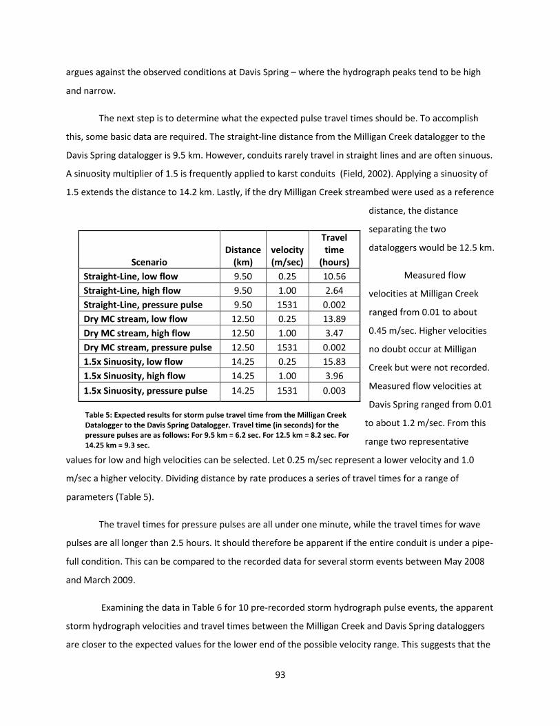
93
argues against the observed conditions at Davis Spring – where the hydrograph peaks tend to be high
and narrow.
The next step is to determine what the expected pulse travel times should be. To accomplish
this, some basic data are required. The straight-line distance from the Milligan Creek datalogger to the
Davis Spring datalogger is 9.5 km. However, conduits rarely travel in straight lines and are often sinuous.
A sinuosity multiplier of 1.5 is frequently applied to karst conduits (Field, 2002). Applying a sinuosity of
1.5 extends the distance to 14.2 km. Lastly, if the dry Milligan Creek streambed were used as a reference
distance, the distance
separating the two
dataloggers would be 12.5 km.
Measured flow
velocities at Milligan Creek
ranged from 0.01 to about
0.45 m/sec. Higher velocities
no doubt occur at Milligan
Creek but were not recorded.
Measured flow velocities at
Davis Spring ranged from 0.01
to about 1.2 m/sec. From this
range two representative
values for low and high velocities can be selected. Let 0.25 m/sec represent a lower velocity and 1.0
m/sec a higher velocity. Dividing distance by rate produces a series of travel times for a range of
parameters (Table 5).
The travel times for pressure pulses are all under one minute, while the travel times for wave
pulses are all longer than 2.5 hours. It should therefore be apparent if the entire conduit is under a pipe-
full condition. This can be compared to the recorded data for several storm events between May 2008
and March 2009.
Examining the data in Table 6 for 10 pre-recorded storm hydrograph pulse events, the apparent
storm hydrograph velocities and travel times between the Milligan Creek and Davis Spring dataloggers
are closer to the expected values for the lower end of the possible velocity range. This suggests that the
Scenario Distance
(km) velocity (m/sec)
Travel time
(hours)
Straight-Line, low flow 9.50 0.25 10.56
Straight-Line, high flow 9.50 1.00 2.64
Straight-Line, pressure pulse 9.50 1531 0.002
Dry MC stream, low flow 12.50 0.25 13.89
Dry MC stream, high flow 12.50 1.00 3.47
Dry MC stream, pressure pulse 12.50 1531 0.002
1.5x Sinuosity, low flow 14.25 0.25 15.83
1.5x Sinuosity, high flow 14.25 1.00 3.96
1.5x Sinuosity, pressure pulse 14.25 1531 0.003
Table 5: Expected results for storm pulse travel time from the Milligan Creek Datalogger to the Davis Spring Datalogger. Travel time (in seconds) for the pressure pulses are as follows: For 9.5 km = 6.2 sec. For 12.5 km = 8.2 sec. For 14.25 km = 9.3 sec.
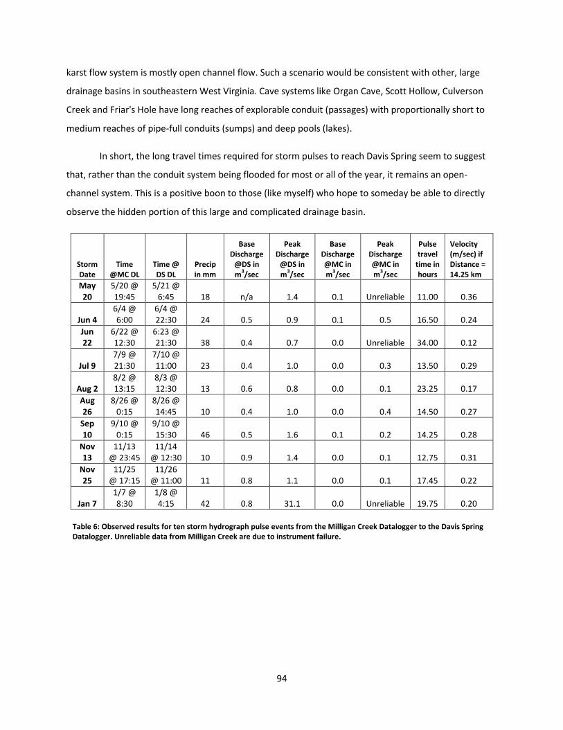
94
karst flow system is mostly open channel flow. Such a scenario would be consistent with other, large
drainage basins in southeastern West Virginia. Cave systems like Organ Cave, Scott Hollow, Culverson
Creek and Friar's Hole have long reaches of explorable conduit (passages) with proportionally short to
medium reaches of pipe-full conduits (sumps) and deep pools (lakes).
In short, the long travel times required for storm pulses to reach Davis Spring seem to suggest
that, rather than the conduit system being flooded for most or all of the year, it remains an open-
channel system. This is a positive boon to those (like myself) who hope to someday be able to directly
observe the hidden portion of this large and complicated drainage basin.
Storm Date
Time @MC DL
Time @ DS DL
Precip in mm
Base Discharge
@DS in m
3/sec
Peak Discharge
@DS in m
3/sec
Base Discharge @MC in m
3/sec
Peak Discharge @MC in m
3/sec
Pulse travel
time in hours
Velocity (m/sec) if Distance = 14.25 km
May 20
5/20 @ 19:45
5/21 @ 6:45 18 n/a 1.4 0.1 Unreliable 11.00 0.36
Jun 4 6/4 @ 6:00
6/4 @ 22:30 24 0.5 0.9 0.1 0.5 16.50 0.24
Jun 22
6/22 @ 12:30
6:23 @ 21:30 38 0.4 0.7 0.0 Unreliable 34.00 0.12
Jul 9 7/9 @ 21:30
7/10 @ 11:00 23 0.4 1.0 0.0 0.3 13.50 0.29
Aug 2 8/2 @ 13:15
8/3 @ 12:30 13 0.6 0.8 0.0 0.1 23.25 0.17
Aug 26
8/26 @ 0:15
8/26 @ 14:45 10 0.4 1.0 0.0 0.4 14.50 0.27
Sep 10
9/10 @ 0:15
9/10 @ 15:30 46 0.5 1.6 0.1 0.2 14.25 0.28
Nov 13
11/13 @ 23:45
11/14 @ 12:30 10 0.9 1.4 0.0 0.1 12.75 0.31
Nov 25
11/25 @ 17:15
11/26 @ 11:00 11 0.8 1.1 0.0 0.1 17.45 0.22
Jan 7 1/7 @ 8:30
1/8 @ 4:15 42 0.8 31.1 0.0 Unreliable 19.75 0.20
Table 6: Observed results for ten storm hydrograph pulse events from the Milligan Creek Datalogger to the Davis Spring Datalogger. Unreliable data from Milligan Creek are due to instrument failure.
95
7 Discussion and Conclusions
7.1 Introduction
The previous section concerned itself mostly with limited analysis of individual parameters
collected during fieldwork. However the two overreaching questions “Where is the master conduit
system (hereafter referred to as the “Master Conduit”) associated with Davis Spring?” and “Is this
conduit system accessible?” were only touched upon. Part IV will address those questions. Using the
data collected during this and previous studies along with established karst principles, a logical scenario
will be built up for the location of the conduit system. Much of this discussion is speculative and deals
with the “black box” scenario, for which there are many possible solutions.
7.2 Open or Closed flow?
The question of whether the "Master Conduit" for Davis Spring is an open (partly air filled
passage) or closed (water filled passage) is the first and most important question as answering that will
strongly influence the ability to determine where the conduits lie and whether they are accessible to
exploration. Conclusions supporting an open flow system will be presented first, followed by conclusions
supporting a closed flow system.
7.2.1 Evidence and scenarios supporting an open flow system
Pulse travel times from Milligan Creek to Davis Spring – As mentioned in the previous section,
storm pulse travel times (11 hours to 34 hours) from Milligan Creek to Davis Spring are in excess
of what is expected if the entire conduit is water-filled. Longer travel times imply the pulse is a
slug of water rather than increased pressure through a pipe-full system.
Large variability in discharge during storms – Variability in storm discharge is very high, which is
typical for conduit flow systems. In all cases, the Reynolds number is far in excess of the
96
necessary figure for turbulent flow. A large variation in discharge is more suggestive of a
passage capacity capable of containing large storm discharge volumes than of water under
tremendous pressure being forced out. Furthermore, the characterization of the spring itself
during high flow does not suggest water being forced out under extremely high pressures (i.e.
there are no geysers, jets of water, et cetera at Davis Spring).
Large variability in dye speeds – Tracer test travel times from Milligan Creek to Davis Spring
varied from 4 to 15 days, suggesting that under lower flow conditions cave pools retard the flow
of water. Pools can be created in wide spots of the passage (i.e. cave rooms) or upstream of
constrictions. Where pools form, water velocity slows considerably. Long pools in stream
passages typically begin as plunge pools from waterfalls and elongate as the falls cut upstream.
Waterfalls are common in Greenbrier County due to the variability in the stratigraphic sequence
(WVACS, 2009). A wide pool is preferable to a long pool for purposes of quicker tracer travel
times. For a long pool, the incoming water has to push past a greater percentage of the pool
volume. With a wide pool the water may only needs to push through the center of the pool’s
volume to reach the channel on the far side, leaving the sides of the pool stagnant. Stagnant
side pools can be repositories for high conductivity waters which are only flushed out during
large precipitation events.
Caves tend to down cut as they age – Most of the known caves in the study area are old enough
to have developed on multiple, parallel levels, where only the lowest level remains accessible to
water. The Master Conduit is likely comparable in age to the rest of these caves and so should
have developed similar features. Other caves in the upper Greenbrier Group such as: Buckeye,
Culverson Creek, Higgenbotham and Lost World Caverns show that at least some of their known
length occurs over multiple, parallel levels (Dasher and Balfour, 1994; WVACS, 2009). Upper
level passages can act as overflow channels for extremely large storm events, preventing the
cave from becoming “pipe full”. They can also be locations for stored water, to be flushed out
only rarely. Lastly, a multiple-leveled system holds the promise for human access, allowing the
researcher the possibility to directly observe the Master Conduit directly.
97
7.2.2 Evidence and scenarios supporting a closed flow system
A “diving bell” scenario – By this it is meant that the vast majority of the cave is completely
flooded with one or several short, very large, partially flooded rooms which slow down a storm
pressure pulse. While very large cave rooms are possible in Greenbrier County, they remain the
exception rather than the rule.
An upper discharge limit due to floods – There may be an as-yet unknown upper limit to
discharge at Davis Spring, or a significant flattening of the hydrograph curve consistent with pipe
full conditions. Another possibility is that this limit has already been seen, but not measured.
Some of the yearly winter storms may reach this level.
Impassable passage size due to the Pickaway limestone – The Pickaway limestone member of
the Greenbrier Group is an inferior limestone for the purposes of large, integrated passages
when compared to the cave-forming members above and below it. The known caves in the
Pickaway are comparatively short and under-developed compared to the other members in the
Greenbrier sequence. The numerous shaley layers, especially in the lower Pickaway Formation
inhibit the formation of large passages.. Water would be forced through a network of small
inaccessible passages. Alternatively, the shaley layers could contribute to roof breakdown which
would make a large, rock filled passage, inaccessible to exploration but not to the movement of
water. It is possible that the extensive breakdown seen at Davis Spring extends all the way back
along the conduit to where Milligan Creek sinks. Therefore the Pickaway limestone could have a
damming effect and facilitate pipe-full conditions.
7.2.3 Open or Closed?
While the evidence suggests that the Master Conduit is more likely to be open than
closed the reality likely lies somewhere in between. While it is possible that the route from
Milligan Creek to Davis Spring is entirely flooded, it seems more likely that long stretches of it
are open flow, at least at low flow. The volume and speed of the water moving through the
system during high flow must imply that during the dry season the master conduit can easily
take in all the baseflow. If this were not the case, there would be insufficient passage volume for
the large winter storm flows, let alone the massive ones. Yet these massive storms display a
98
similar sharp hydrograph peak for Davis Spring. If it were a closed system the hydrograph peaks
would be broader.
7.3 Speculation about the Master Conduit and its characteristics
The Master Conduit extends for some unknown distance upgradient from Davis Spring to a point
where it diverges into at least two smaller conduits – the Milligan Creek conduit and the aggregated
discharge from the contact caves. The contact caves' conduit should further diverge upgradient into
individual feeder passages. Milligan Creek is considered comparable in size to the contact cave drainage
area and so the Master Conduit could be considered to be shaped like a wish-bone with one arm
extending to the northwest and the other arm to the northeast. Where these two sections join up would
be of considerable hydrogeologic interest as well as speleological beauty.
7.3.1 The Master Conduit near Davis Spring
Directly behind Davis Spring is a large pile of limestone breakdown, likely extending into the
hillside for at least several meters. The hillside scree slope rises several meters above the spring. Large
(car sized) boulders deposited from the cliff above make the excavation of an access point to the conduit
system behind the spring difficult.
As the resurgence likely presents a flow constriction, particularly at high flow, the cave
immediately upstream from it probably has the characteristics of a network maze. Network mazes occur
when passage constrictions force flood waters into every available crevice upstream of the constriction.
The force of the water enlarges all available passages simultaneously (Palmer, 2001, 2007). This is visible
in nearby Rockland Indian Cave as well as in many other caves.
However, there may also be a main conduit whose dimensions exceed the average conduit size.
The scree slope suggests that Davis Spring is exposing more of the conduit as it cuts upstream into the
hill. A combination of surface erosion, frost and chemical weathering (dissolution) is likely pushing the
spring northward. The spring has already migrated 50 meters farther north than the intersection with
the paleo-Milligan Creek channel (Figure 2). Additionally, the curvature of the exposed spring channel
99
suggests that it is angling back into Muddy Creek Mountain rather than towards the contact caves
(although this could simply be an expression of the normal meandering of the stream). If a large central
tube is already present and a network conduit pattern is superimposed onto it in the form of alcoves,
small tubes and the like, then digging in the correct spot (presumably in the area of largest flow) might
eventually yield a passable route into the system. However, this is probably less than an ideal solution as
the force of the Master Conduit is likely sufficient to create a similar sized breakdown pile inside the
cave as can be seen on the surface.
7.3.2 Possible locations of the junction of the Milligan Creek conduit and the Master
Conduit
During the March 2009 tracer tests, water samples were collected from a cross-section of the
Davis Spring surface channel to determine if tracer was preferentially coming out the NE side or the NW
side of the spring (Figure 2). Results (not shown here) indicated that the differences in dye
concentration from either side of the channel were less than 10%, showing that by the time the tracer
reached Davis Spring it had completely mixed. This shows that the junction of the Milligan Creek conduit
and the contact caves conduit likely occurs some distance upstream of Davis Spring. With the current
information it is not possible to be more specific than that. Furthermore, repeating the test using a trace
from the contact caves would show whether the contact caves do definitively mix far upstream as well.
It should also be noted that some of the dye traps preferentially showed strong positives from
one side of the spring or the other for the contact caves and Milligan Creek. However, dye traps are
considered unreliable in being able to determine concentration accurately. Furthermore, this was most
commonly noted in low water conditions. This may in fact be a further indicator of which portions of the
spring are most active during low-flow conditions, further strengthening the idea that Davis Spring can
behave quite differently depending on flow rate.
Figure 34 shows the difference in dye recovery by way of charcoal traps during the dye tests in
August and September 2008. As can be seen, Fluorescein tracer tests from Maxwelton Sink were
preferential on either side of the spring depending on the day recovered. The drop in Fluorescein
intensity at the junction with the Greenbrier River may be due to photodecaying of tracer while in the
large pool in front of Davis Spring (average movement through the pool was much less than 1
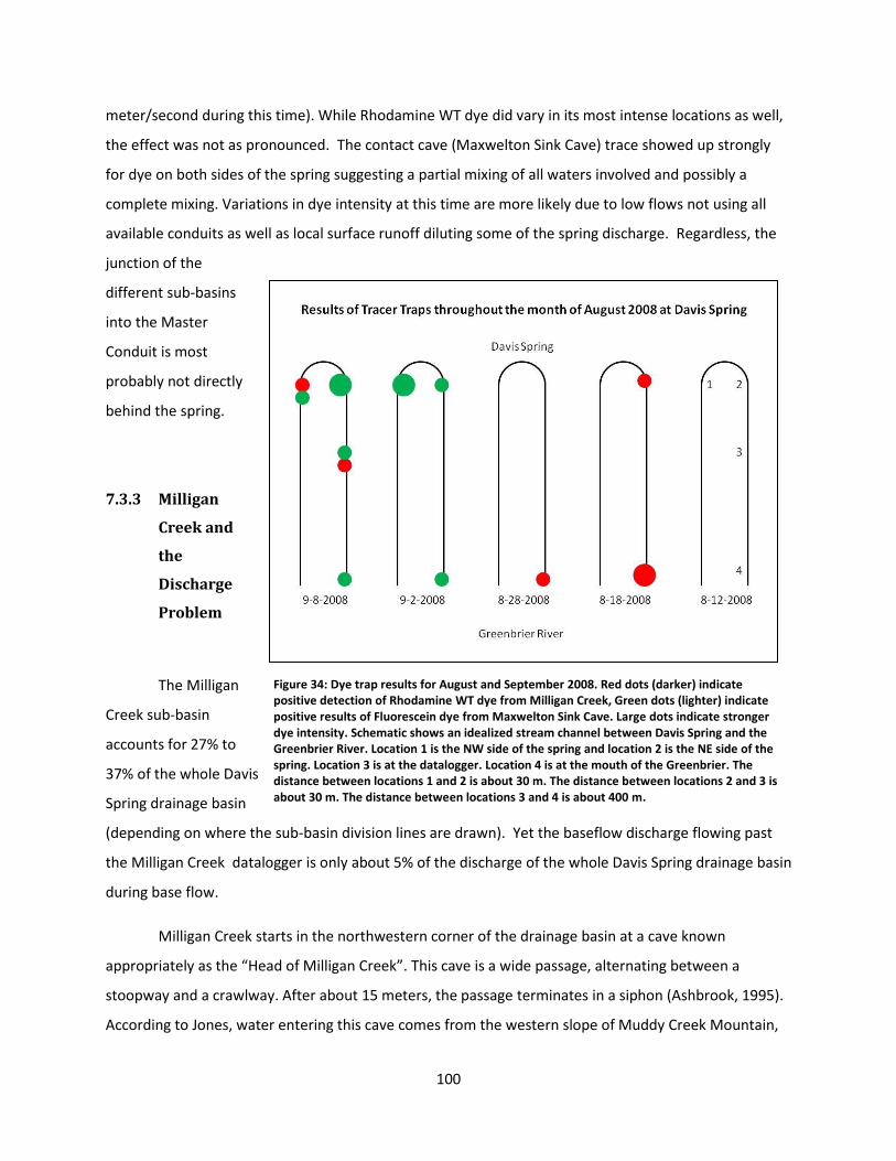
100
meter/second during this time). While Rhodamine WT dye did vary in its most intense locations as well,
the effect was not as pronounced. The contact cave (Maxwelton Sink Cave) trace showed up strongly
for dye on both sides of the spring suggesting a partial mixing of all waters involved and possibly a
complete mixing. Variations in dye intensity at this time are more likely due to low flows not using all
available conduits as well as local surface runoff diluting some of the spring discharge. Regardless, the
junction of the
different sub-basins
into the Master
Conduit is most
probably not directly
behind the spring.
7.3.3 Milligan
Creek and
the
Discharge
Problem
The Milligan
Creek sub-basin
accounts for 27% to
37% of the whole Davis
Spring drainage basin
(depending on where the sub-basin division lines are drawn). Yet the baseflow discharge flowing past
the Milligan Creek datalogger is only about 5% of the discharge of the whole Davis Spring drainage basin
during base flow.
Milligan Creek starts in the northwestern corner of the drainage basin at a cave known
appropriately as the “Head of Milligan Creek”. This cave is a wide passage, alternating between a
stoopway and a crawlway. After about 15 meters, the passage terminates in a siphon (Ashbrook, 1995).
According to Jones, water entering this cave comes from the western slope of Muddy Creek Mountain,
Figure 34: Dye trap results for August and September 2008. Red dots (darker) indicate positive detection of Rhodamine WT dye from Milligan Creek, Green dots (lighter) indicate positive results of Fluorescein dye from Maxwelton Sink Cave. Large dots indicate stronger dye intensity. Schematic shows an idealized stream channel between Davis Spring and the Greenbrier River. Location 1 is the NW side of the spring and location 2 is the NE side of the spring. Location 3 is at the datalogger. Location 4 is at the mouth of the Greenbrier. The distance between locations 1 and 2 is about 30 m. The distance between locations 2 and 3 is about 30 m. The distance between locations 3 and 4 is about 400 m.
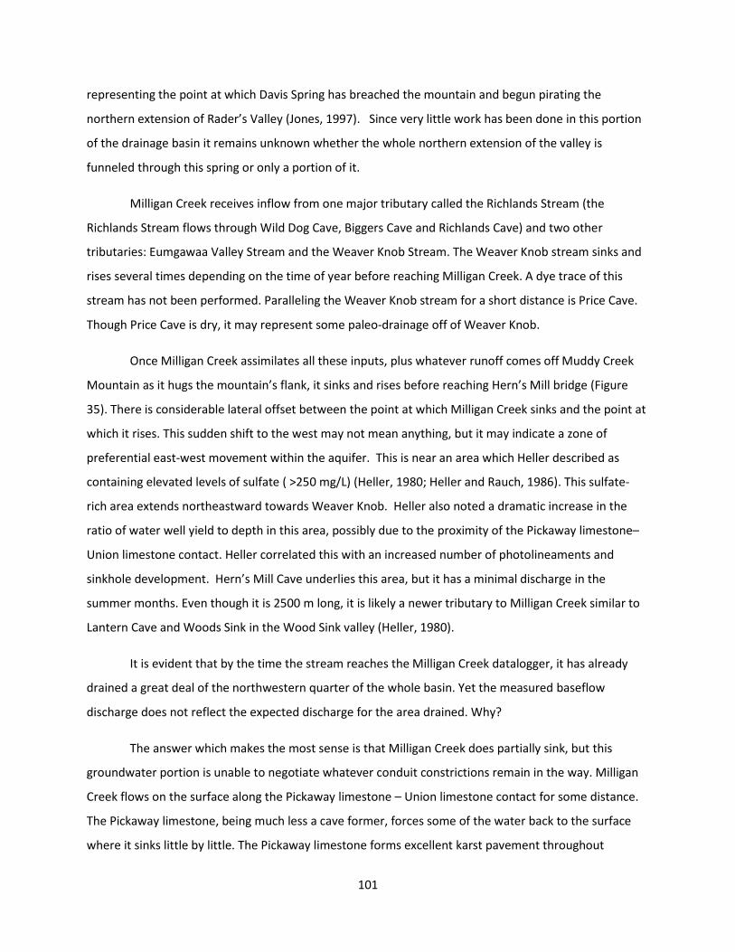
101
representing the point at which Davis Spring has breached the mountain and begun pirating the
northern extension of Rader’s Valley (Jones, 1997). Since very little work has been done in this portion
of the drainage basin it remains unknown whether the whole northern extension of the valley is
funneled through this spring or only a portion of it.
Milligan Creek receives inflow from one major tributary called the Richlands Stream (the
Richlands Stream flows through Wild Dog Cave, Biggers Cave and Richlands Cave) and two other
tributaries: Eumgawaa Valley Stream and the Weaver Knob Stream. The Weaver Knob stream sinks and
rises several times depending on the time of year before reaching Milligan Creek. A dye trace of this
stream has not been performed. Paralleling the Weaver Knob stream for a short distance is Price Cave.
Though Price Cave is dry, it may represent some paleo-drainage off of Weaver Knob.
Once Milligan Creek assimilates all these inputs, plus whatever runoff comes off Muddy Creek
Mountain as it hugs the mountain’s flank, it sinks and rises before reaching Hern’s Mill bridge (Figure
35). There is considerable lateral offset between the point at which Milligan Creek sinks and the point at
which it rises. This sudden shift to the west may not mean anything, but it may indicate a zone of
preferential east-west movement within the aquifer. This is near an area which Heller described as
containing elevated levels of sulfate ( >250 mg/L) (Heller, 1980; Heller and Rauch, 1986). This sulfate-
rich area extends northeastward towards Weaver Knob. Heller also noted a dramatic increase in the
ratio of water well yield to depth in this area, possibly due to the proximity of the Pickaway limestone–
Union limestone contact. Heller correlated this with an increased number of photolineaments and
sinkhole development. Hern’s Mill Cave underlies this area, but it has a minimal discharge in the
summer months. Even though it is 2500 m long, it is likely a newer tributary to Milligan Creek similar to
Lantern Cave and Woods Sink in the Wood Sink valley (Heller, 1980).
It is evident that by the time the stream reaches the Milligan Creek datalogger, it has already
drained a great deal of the northwestern quarter of the whole basin. Yet the measured baseflow
discharge does not reflect the expected discharge for the area drained. Why?
The answer which makes the most sense is that Milligan Creek does partially sink, but this
groundwater portion is unable to negotiate whatever conduit constrictions remain in the way. Milligan
Creek flows on the surface along the Pickaway limestone – Union limestone contact for some distance.
The Pickaway limestone, being much less a cave former, forces some of the water back to the surface
where it sinks little by little. The Pickaway limestone forms excellent karst pavement throughout
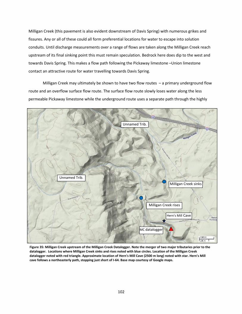
102
Milligan Creek (this pavement is also evident downstream of Davis Spring) with numerous grikes and
fissures. Any or all of these could all form preferential locations for water to escape into solution
conduits. Until discharge measurements over a range of flows are taken along the Milligan Creek reach
upstream of its final sinking point this must remain speculation. Bedrock here does dip to the west and
towards Davis Spring. This makes a flow path following the Pickaway limestone –Union limestone
contact an attractive route for water travelling towards Davis Spring.
Milligan Creek may ultimately be shown to have two flow routes – a primary underground flow
route and an overflow surface flow route. The surface flow route slowly loses water along the less
permeable Pickaway limestone while the underground route uses a separate path through the highly
Figure 35: Milligan Creek upstream of the Milligan Creek Datalogger. Note the merger of two major tributaries prior to the datalogger. Locations where Milligan Creek sinks and rises noted with blue circles. Location of the Milligan Creek datalogger noted with red triangle. Approximate location of Hern's Mill Cave (2500 m long) noted with star. Hern's Mill cave follows a northeasterly path, stopping just short of I-64. Base map courtesy of Google maps.
Hern's Mill Cave
MC datalogger
Milligan Creek sinks
Milligan Creek rises
Unnamed Trib.
#1
Unnamed Trib.
#2
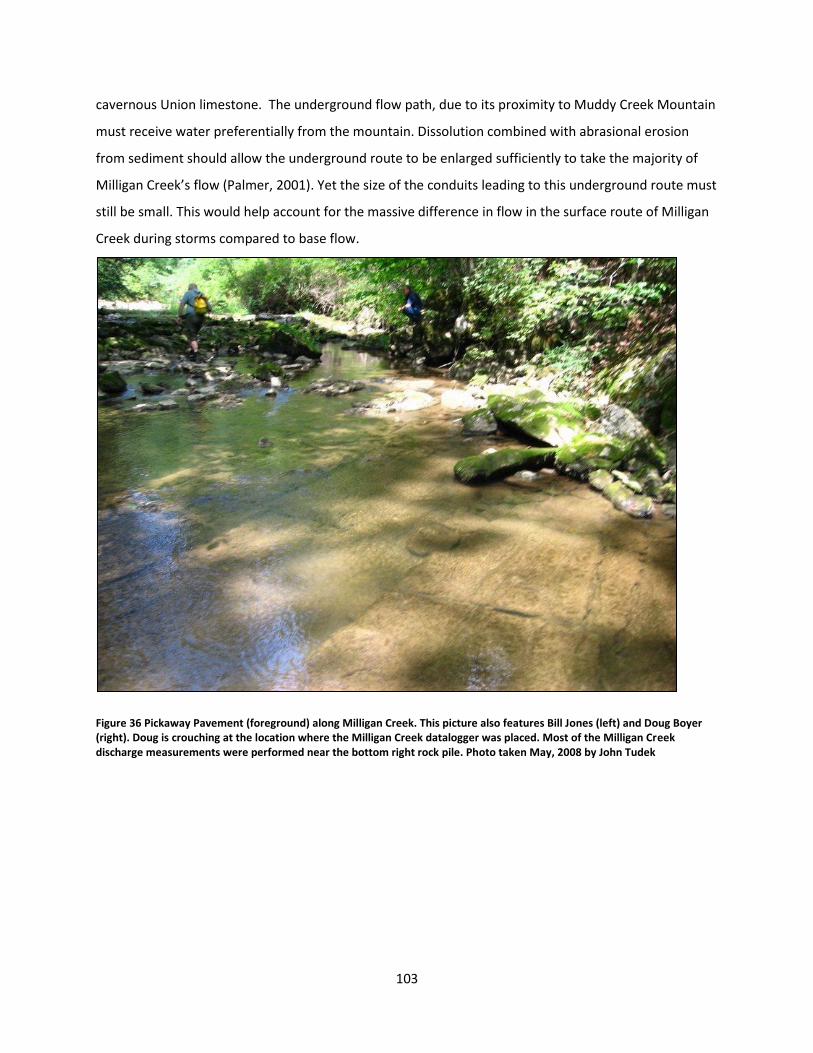
103
cavernous Union limestone. The underground flow path, due to its proximity to Muddy Creek Mountain
must receive water preferentially from the mountain. Dissolution combined with abrasional erosion
from sediment should allow the underground route to be enlarged sufficiently to take the majority of
Milligan Creek’s flow (Palmer, 2001). Yet the size of the conduits leading to this underground route must
still be small. This would help account for the massive difference in flow in the surface route of Milligan
Creek during storms compared to base flow.
Figure 36 Pickaway Pavement (foreground) along Milligan Creek. This picture also features Bill Jones (left) and Doug Boyer (right). Doug is crouching at the location where the Milligan Creek datalogger was placed. Most of the Milligan Creek discharge measurements were performed near the bottom right rock pile. Photo taken May, 2008 by John Tudek
104
7.3.4 The Route of the Master Conduit as it Parallels Muddy Creek Mountain
In this section possibilities for the Master Conduit route downstream of the Milligan Creek
datalogger will be explored. Because the conduit route has not been identified anywhere throughout
the area, logical inferences will be made based on the known data.
Several things should be kept in mind when the proposed route of this conduit is considered.
They are, as follows:
The effect of Muddy Creek Mountain – Muddy Creek Mountain must be a primary source of
allogenic recharge as well as allogenic sediment for any passage following its flanks. A quick
glance at any topographic map will illustrate that many streams flow off of Muddy Creek
Mountain, only to sink at the Union limestone –Greenville shale contact. Several vertical shafts
have already been located in these stream beds, some shafts deeper than 20 m, indicating that
these streams are able to inject considerable amounts of water into the conduit system
immediately following a precipitation event. Rader’s Valley is the valley to the west of Davis
Spring and on the opposite side of Muddy Creek Mountain. Several long caves in Rader’s Valley
follow the flank of Muddy Creek Mountain, illustrating that integrated conduit development
along the flanks of Muddy Creek Mountain is possible (Hall, 2003). These caves are formed
predominantly in the Union limestone and may be considered analogous to undiscovered caves
on the Davis Spring basin side.
Allogenic stream sediments can be as effective if not more effective than carbonate dissolution
in enlarging existing cave passages (Palmer, 2001). Palmer suggests that under severe flooding
pipe full fissures can enlarge from 0.01 cm to traversable size in under 10,000 years. This
represents a considerable advantage in the selection of preferential flow routes when compared
to autogenic sources or sources with less abrasive sediment load (Palmer, 2001). Whether
abrasive erosion exceeds dissolution along Muddy Creek Mountain is less relevant than the fact
that total enlargement rate is the combination of both dissolution and erosion. This should have
the effect of keeping conduit passage development close to the flanks of Muddy Creek
Mountain.
As mentioned before, the proposed location of the Master Conduit is likely to be located closer
to the Muddy Creek Mountian Syncline than farther from it. Based on existing cave pattern data
105
across the drainage basin, regional dip appears to have little impact on the direction of cave
development. The influence of local structure seems to be far more pronounced. In the regional
area, large and small cave systems – Rockland Indian Cave, Taylor Falls Cave and Culverson
Creek Cave - all cease traversable passage when those passages intersect major faults (Heller,
1980; WVACS, 2009). Additionally, the drainage of some large systems such as Organ Cave and
Scott Hollow Cave follow major synclinal folds (Stevens, 1988). Passage development at Scott
Hollow Cave seems to be constrained between the Sinks Grove Anticline at the upstream end
and Knobs Syncline at the downstream end (Reger and Price, 1926). Note that in both cases it is
likely that neither Scott Hollow nor the Davis Spring Master Conduit has migrated far enough
under the mountain to reach the axis of the syncline.
Northeast of the Milligan Creek datalogger it is virtually impossible to say with any certainty
where the Master Conduit may lie. There is suspicion (partially based on the unusual well yields
and geochemistry measured by Heller) that near the area where route US 60 passes under I-64
the contact caves meet with the Davis Spring master conduit. However, there is very little hard
evidence to support this.
7.3.5 An Attempt at the Paleohistory of the Davis Spring Drainage Basin
The Davis Spring drainage basin likely has a history as long and complex as the passages which
make up the system. As with all other aspects of the study area, the known is still far exceeded by the
unknown. This makes this final section perhaps the most speculative of any within this document. Much
of what will be drawn upon within this section consists of published and unpublished cave survey data,
most of which has been compiled in the last 30 years by the West Virginia Association for Cave Studies
(WVACS, 2009).
The primary question facing any investigation of the paleohistory of the Davis Spring Drainage
basin is determining why the water from the contact caves chose the obviously longer and more
complex flow route to the Greenbrier River by way of Davis Spring than through some similar outlet
closer to the contact caves. This is particularly interesting when it is realized that Rockland Indian Cave,
which straddles the Rockland Syncline (previously mapped but unnamed) would be the ideal location for
the contact caves to discharge. The plan of Rockland Indian Cave is a wishbone, with two main paths
diverging a short way inside the cave. The eastern fork has a large passage which contains a very small
stream. Deep, still pools of water mark the back half of this passage until the passage ends in a siphon.
106
The western fork parallels the Rockland Fault (Rockland Structure) until they intersect. All the water in
that half of the cave likely comes from autogenic sinkhole recharge. The stream in the eastern fork
begins in Alexander Cave #2 which in turn receives its water from allogenic runoff from the MacCrady
shale. This makes Rockland Indian Cave system a very simple, compact drainage basin. However,
anastamosing tubes, cupolas and pockets high on the walls near the downstream end suggest a time
when more water flowed through the cave system. The difference in elevation between the tubes and
the current stream level (at least 3 meters) suggests a long time has passed since these tubes were
formed.
Does this suggest that water from the contact caves once flowed through Rockland Indian Cave?
Probably not. Although Rockland Indian Cave’s main passage is large, it is probably not large enough to
take all of the water from the contact caves under high flow. What it does show is that it is possible to
develop a large conduit system east of Davis Spring. Perhaps such a system existed in strata higher in the
Greenbrier Group sequence and subsequently eroded away.
7.3.6 The Paleo-Weaver Knob Ridge
The Paleo-Weaver Knob Ridge is a new term coined for the residual upland area between the
contact caves sinkhole plain and the Milligan Creek valley. The Paleo-Weaver Knob Ridge is underlain by
the Weaver Knob Anticline and the Weaver Knob thrust fault near its western end as well as the Lost
World Syncline in its center. The Paleo-Weaver Knob Ridge shows up very well using the USGS 3-meter
2003 Digital Elevation Maps as do many of the large man-made features in the study area (Figure 37,
Figure 38).
Examination of the ridge shows that it extended at least as far south as the Wood Sink karst
valley and possibly farther south still. It is difficult to determine anything further south as local surface
runoff towards the Greenbrier River has dissected the uplands to an enormous degree. This landform
sets apart the contact caves area from the Milligan Creek drainage basin and seems to restrict passage
development to either side of the paleo-ridge. Helix Cave and Lost World Caverns (Grapevine Cave) may
be examples of relict systems along the eastern flank of the Paleo-Weaver Knob Ridge. The size of
Grapevine Cave may also suggest that at one point it may have been a major drainage route – though
with so much of the passage full of breakdown and the walls covered with speleothems it is difficult to
determine how it was initially created.
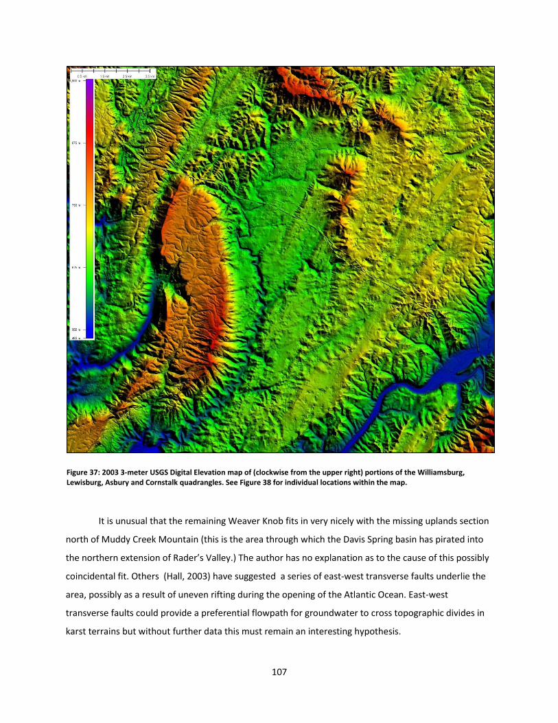
107
It is unusual that the remaining Weaver Knob fits in very nicely with the missing uplands section
north of Muddy Creek Mountain (this is the area through which the Davis Spring basin has pirated into
the northern extension of Rader’s Valley.) The author has no explanation as to the cause of this possibly
coincidental fit. Others (Hall, 2003) have suggested a series of east-west transverse faults underlie the
area, possibly as a result of uneven rifting during the opening of the Atlantic Ocean. East-west
transverse faults could provide a preferential flowpath for groundwater to cross topographic divides in
karst terrains but without further data this must remain an interesting hypothesis.
Figure 37: 2003 3-meter USGS Digital Elevation map of (clockwise from the upper right) portions of the Williamsburg, Lewisburg, Asbury and Cornstalk quadrangles. See Figure 38 for individual locations within the map.
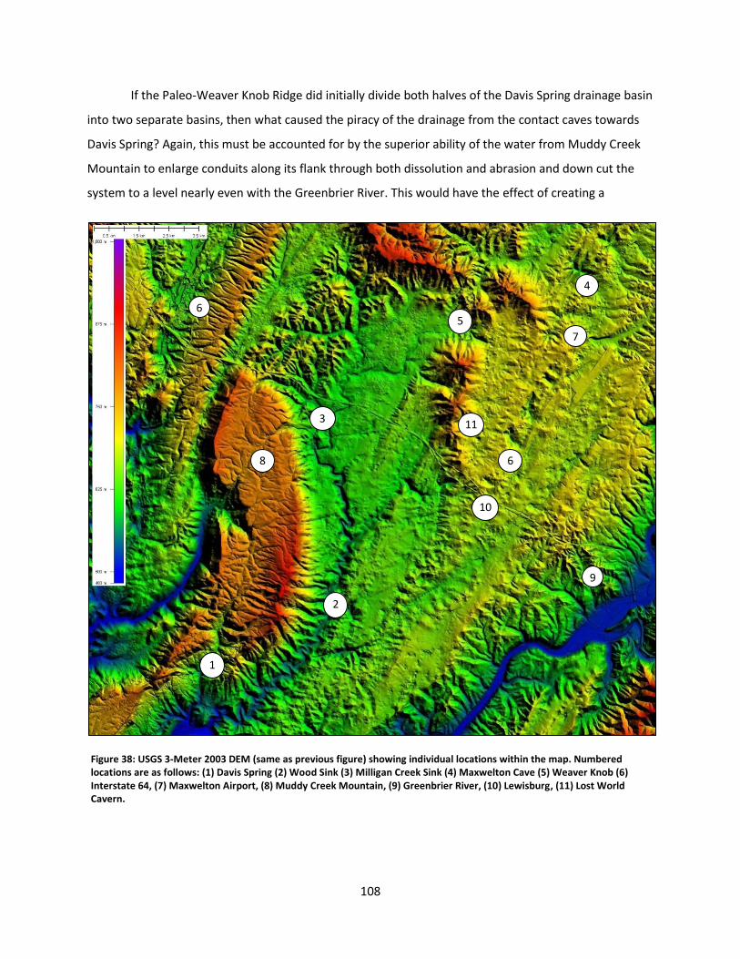
108
If the Paleo-Weaver Knob Ridge did initially divide both halves of the Davis Spring drainage basin
into two separate basins, then what caused the piracy of the drainage from the contact caves towards
Davis Spring? Again, this must be accounted for by the superior ability of the water from Muddy Creek
Mountain to enlarge conduits along its flank through both dissolution and abrasion and down cut the
system to a level nearly even with the Greenbrier River. This would have the effect of creating a
Figure 38: USGS 3-Meter 2003 DEM (same as previous figure) showing individual locations within the map. Numbered locations are as follows: (1) Davis Spring (2) Wood Sink (3) Milligan Creek Sink (4) Maxwelton Cave (5) Weaver Knob (6) Interstate 64, (7) Maxwelton Airport, (8) Muddy Creek Mountain, (9) Greenbrier River, (10) Lewisburg, (11) Lost World Cavern.
1
2
9
10
6
7
4
5
3
6
8
11

109
potentiometric trough in the water table all along the eastern flank of the mountain, and the resulting
change in hydrologic gradient would force cave development westward rather than southward. Like a
positive feedback loop, successive piracy of part of the contact cave basin would only further encourage
the remainder of the basin to migrate westward. However, additional data needs to be uncovered
before this is more than a speculative hypothesis.
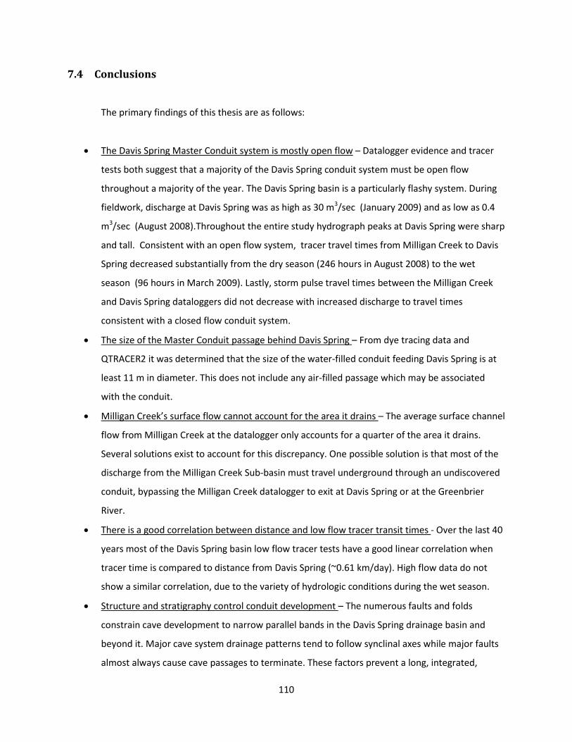
110
7.4 Conclusions
The primary findings of this thesis are as follows:
The Davis Spring Master Conduit system is mostly open flow – Datalogger evidence and tracer
tests both suggest that a majority of the Davis Spring conduit system must be open flow
throughout a majority of the year. The Davis Spring basin is a particularly flashy system. During
fieldwork, discharge at Davis Spring was as high as 30 m3/sec (January 2009) and as low as 0.4
m3/sec (August 2008).Throughout the entire study hydrograph peaks at Davis Spring were sharp
and tall. Consistent with an open flow system, tracer travel times from Milligan Creek to Davis
Spring decreased substantially from the dry season (246 hours in August 2008) to the wet
season (96 hours in March 2009). Lastly, storm pulse travel times between the Milligan Creek
and Davis Spring dataloggers did not decrease with increased discharge to travel times
consistent with a closed flow conduit system.
The size of the Master Conduit passage behind Davis Spring – From dye tracing data and
QTRACER2 it was determined that the size of the water-filled conduit feeding Davis Spring is at
least 11 m in diameter. This does not include any air-filled passage which may be associated
with the conduit.
Milligan Creek’s surface flow cannot account for the area it drains – The average surface channel
flow from Milligan Creek at the datalogger only accounts for a quarter of the area it drains.
Several solutions exist to account for this discrepancy. One possible solution is that most of the
discharge from the Milligan Creek Sub-basin must travel underground through an undiscovered
conduit, bypassing the Milligan Creek datalogger to exit at Davis Spring or at the Greenbrier
River.
There is a good correlation between distance and low flow tracer transit times - Over the last 40
years most of the Davis Spring basin low flow tracer tests have a good linear correlation when
tracer time is compared to distance from Davis Spring (~0.61 km/day). High flow data do not
show a similar correlation, due to the variety of hydrologic conditions during the wet season.
Structure and stratigraphy control conduit development – The numerous faults and folds
constrain cave development to narrow parallel bands in the Davis Spring drainage basin and
beyond it. Major cave system drainage patterns tend to follow synclinal axes while major faults
almost always cause cave passages to terminate. These factors prevent a long, integrated,
111
traversable cave system similar to Mammoth Cave from developing in the area.
Stratigraphically, although the Greenbrier Group strata are equivalent to many of the units in
the Mammoth Cave area, facies changes between the two regions have introduced considerable
differences. The most important of these is the Taggard shale-Pickaway limestone confining
layer. While the Taggard Shale is often considered to be the only confining layer, the lower
Pickaway Limestone is also a deterrent to water movement and passage development due to its
shaley nature. No long cave system in the area has managed to develop significantly both above
and below the Taggard. As a result cave development in the Greenbrier Valley is dissected both
horizontally and vertically into individual areas.

112
7.5 Further Research
This investigation into the Davis Spring basin is the second of its kind. A project like this often
raises more questions than it answers. And when that happens the hardest thing to do is to not abandon
the original project goals and go running off investigating every new thing. This project cast out a wide
net, and as such touched on many areas. Most of those areas are worth of thorough investigations in
their own right. Presented in no order now are some ideas for further research ideas.
Further investigations in Milligan Creek – Much of what was uncovered at Milligan Creek only
served as a springboard to asking further questions about that sub-basin. The most important of
these questions is “How does the discharge change as one proceeds down the length of the
creek?” Monitoring stations set up along various points of the upper end of the creek could tell
a great deal about where the water goes and its relationship to the structure and stratigraphy of
the area. As an upper corner of the drainage basin Milligan Creek is a contained, manageable
area for study.
Long term monitoring of Davis Spring – With the re-establishment of a good rating curve for
Davis Spring, an opportunity to continue long-term monitoring of the spring is available.
Monitoring over several years would prove or disprove trends suggested at or hinted at in this
study. Further discharge measurements made during long term monitoring, particularly at high
and low flows would improve on the rating curve further and answer questions as to the
maximum discharge at the spring.
Expanded monitoring of the drainage basin – Monitoring of individual cave systems and
infeeders would show the relative percentages each system does have on the overall spring.
Monitoring of flood pulses at different points would provide a useful counterpoint to tracer
testing times.
Additional Quantitative Dye Traces – Many of the dye traces performed thus far have been of
the qualitative or semi-quantitative form. They should all be redone as quantitative traces.
Additionally, all locations traced should be traced during high flow and again during low flow.
Additional locations along the basin boundaries should be utilized to further delineate some of
the remaining basin divides as well as anchor areas which until now have only been assumed to
be part of the Davis Spring drainage basin.

113
Remote Sensing – Although the depth to passage above Davis Spring is likely too deep to allow
for remote sensing, passages are likely to be shallower farther upstream. There is ample
opportunity for remote sensing techniques to be developed and used within the Davis Spring
drainage basin, both in locating existing caves and discovering new ones. Cleared, rolling
pastureland predominates in the western half of the basin making transverses easy.
Geochemistry of the Spring- While this paper and the previous paper have concentrated on the
hydrology of the Davis Spring basin, little has been done concerning the geochemistry.
Geochemical information collected during this project combined with similar information
collected by Heller suggest that the geochemistry is at least as interesting as the hydrology.
Furthermore, complete baseflow separation may only be possible with a complete chemical
inventory accompanying the hydrologic data.
3-D Cartogtahy – The advent of GIS, computerized cave survey data and powerful personal
computers finally realizes the possibility of illustrating the relationship between cave passage,
structure and stratigraphy in a 3-D environment. The ability to see and understand these
relationships intuitively cannot be underestimated in being able to explain and predict the
movement of groundwater and the continued development of cave passages.
Paleo-drainage of the Individual Cave Systems – Very little work has been done in trying to
understand the history of drainage of individual caves, particularly the contact caves.
Understanding the early development of these systems should provide clues to the overall
development of the drainage basin.
Speleothem dating and integration of data into a paleo-climatological model of the basin –
Some speleothem dating (Springer, et al) has been performed in the area to this point, but how
climatological changes over the past few million years have affected the cave development of
the area is still poorly understood and often ignored.

114
7.6 Final Words
The Greenbrier Valley remains one of the premier karst regions of planet earth. Five of the 30
longest caves in the US (with a sixth, Windy Mouth, being #32) occupy the valley. The Davis Spring basin
is the largest basin within that karst region. Two of the 50 longest caves in the United States occupy this
basin (Gulden, 2010). It is in part because this basin is so large and so diverse that it has not attracted
the attention it otherwise might. The question has not been what to include in any study of this basin,
but what not to include.
This thesis has been the second major work on the basin, after (Heller, 1980). If publications on
the basin are to come out on average every 30 years then the Davis Spring basin will remain unknown
for a very long time. Thirty years is simply too long to wait. It is hoped then that this work will spur
others on to their own investigations of the basin. Investigators to Davis Spring will find a friendly,
enthusiastic populace interested in the ground under their feet. They will find an established group of
cave explorers organized into a long-standing organization, WVACS, willing and able to assist them. To
this point WVACS has concerned itself properly with the exploration and mapping of known cave
systems. Mapping is the first real science done underground and a good map is the basis of all other
speleology. As local caretakers to this exceptional karst area, WVACS is particularly suited for both long
term monitoring of the Davis Spring basin as well as becoming the primary repository for information
gathered and published on the area. It is hoped that they will embrace these twin goals in the future by
helping make Davis Spring a first-rate location for scientific investigation while remaining a world-class
organization for exploration and discovery. (Marsh-McBirney, 1984)
115
8 Acknowledgements
This thesis could not have been possible without the contributions and support of many people.
They are (in no particular order) as follows:
At West Virginia University: Dr. Henry Rauch for agreeing to be my advisor and urging me to
pursue a graduate education in Geology. Dr. Dorothy Vesper for agreeing to serve on my committee
and providing both scientific and editorial support. Dr. Helen Lang for guidance during the revision
phase.
At the USDA in Beverly, WV: Doctor Douglas Boyer for agreeing to be on my committee and for
generously allowing me the use of USDA equipment and facilities and lastly for the guidance provided in
field methods. Derek Hall for being an excellent technician, field partner and fellow computer game
geek. Laura Cooper for being an excellent field partner as well photographer.
In Lewisburg, WV : Denny Wood and Arabelle for allowing us to dye trace, ridgewalk and talk
about the study area for hours at a time. Bob and Janet Jeffries for allowing us to place the Milligan
Creek datalogger (as well as sheltering us from the cold and rain). Mr. and Mrs. Wilchert for allowing us
the use of the Davis Spring property for the Davis Spring datalogger. Oak Hall for letting us trace from
Maxwelton Sink Cave. Jimmie Coffman for introducing us to Lantern Cave and his neighbors.
Caving Community: WVACS for granting me membership and allowing me the use of their
facilities as well as their archives. Bill Jones for somehow transforming from a scary old curmudgeon to a
happy mentor figure, all while being an inexhaustible font of knowledge. I suspect beer was involved.
Bill Balfour for patiently bringing me up to speed on the geology of the area. Kevin and Carolyn
Psarianos and Buzz Rudderow for support as well as rafting or wading down the Greenbrier. Jeff
MacDonald for many hours of listening to my cockamamie ideas in person and over the phone.
Family: Janice Kilgallon (mom) and John Tudek, Sr. (dad) for not buying me what I wanted as a
kid unless it was a book. That was sheer genius. Also for letting me find my own way through life, letting
me make mistakes, but being there to help pick up the pieces. Jen Carter (sister) for all the emotional
and Disney support and just for being there since forever. Jeff Carter (brother-in-law) for hospitality in
my home away from home. Mike Rusignuolo for being my friend since - wow... 1987? Dear lord, we've
put in some time. Sam (beagle) for being fuzzy, understanding me better than people and having 'nose'.
And Sherrye Dobrin (Peep) for being there for me every day of my life for the past eleven years. For
that, I can never express my thanks enough. We did it, Peep!
Meow!

116
9 Bibliography
Aley, T., 2002, The Ozark Underground Labratory's Groundwater Tracing Handbook: Protem, MO, Ozark
Underground Library, 35 p.
Aley, T., and Fletcher, M. W., 1976, Water Tracer's Cookbook, Missouri Speleology: Protem, MO,
Missouri Speleological Survey, 33 p.
Ashbrook, B., 1995, Caves in the Richlands Area of Greenbrier County, West Virginia, WvASS Monograph
Series: Lewisburg, WV, West Virginia Speleological Survey, 37 p.
Balfour, W., 2004, personal comm.: Lewisburg, WV.
Bennison, A. P., 1989, Geologic Highway Map of the Mid Atlantic Region: Tulsa, OK, American
Association of Petroleum Geologists.
Boyer, D., 2008, personal comm.: Beaver, WV.
Boyer, D. G., 1976, The Climatological Water Balance in a Mountainous Terrain (MS Thesis):
Morgantown, WV, West Virginia University, 98 p.
Commonwealth of Australia. 2006. Connected Water: Managing the linkages between surface water and
gorund water [Online]. Australian Government; Dept. of Agriculture Fisheries and Forestry.
Available: http://www.connectedwater.gov.au/framework/baseflow_separation.php [Accessed
June 10, 2009].
Dasher, G. R., 2000, The caves of east-central West Virginia : the guidebook of the National Speleological
Society's 2000 Convention: Barrackville, W. Va., West Virginia Speleological Survey, 296 p.
Dasher, G. R., and Balfour, W. M., 1994, The caves and karst of the Buckeye Creek basin, Greenbrier
County, West Virginia, Bulletin - West Virginia Speleological Survey West Virginia Speleological
Survey, 236 p.
Davies, W. E., 1958, Caverns of West Virginia: Morgantown, WV, West Virginia Geological and
Economical Survey, 330 p.
Dingman, S. L., 2002, Physical Hydrology: Upper Saddle River, NJ, Prentice Hall, 600 p.
Dore, M., 1990, The Discovery and Exploration of Scott Hollow Cave, West Virginia, NSS News, p. 148-
158.
Drysdale, R., Lucas, S., and Carthew, K., 2003, The Influence of Diurnal Temperatures on the
hydrochemistry of a tufa-depositing stream: Hydrological Processes, p. 3421-3441.
Fetter, C. W., 2001, Applied Hydrogeology: Upper Saddle River, NJ, Prentice-Hall, 598 p.
117
Field, M. S., 2002, The QTRACER2 Program for Tracer-Breakthrough Curve Analysis: Washington D.C.,
U.S. Evnvironmental Protection Agency, 179 p.
Ford, D., and Williams, P., 2007, Karst Hydrogeology and Geomorphology: West Sussex, UK, John Wiley
and Sons, 562 p.
Gulden, R. 2010. USA Longest Caves [Online]. Available: http://www.caverbob.com/usalong.htm
[Accessed March 1, 2010].
Hall, M., 2003, Karst Hydrology Evaluation of Rader's Valley, Greenbrier County WV: Karst Research and
Technology Center.
Heller, S. A., 1980, A Hydrogeologic Study of the Greenbrier Limestone of Central Greenbrier County,
West Virginia (PhD Dissertaion): Morgantown, WV, West Virginia University, 167 p.
-, 1985, Karst Topography of Central Greenbrier County, West Virginia: Southeastern Geology, v. 26, no.
2, p. 111-116.
-, 1991, An Attempt to Model an Appalachian Karst Aquifer Using MODFLOW, in Appalachian Karst,
Radford, VA, p. 177-186.
-, 2008, personal comm.: Charleston, SC.
Heller, S. A., and Rauch, H., 1986, Anomalous Natural Sulfate in Water Wells of the Greenbrier Group,
West Virginia: Water Resources Bulletin, v. 22, no. 4, p. 581-585.
Hill, S., 2008, personal comm.: Lewisburg, WV.
Hobba, W. A., Friel, E. A., and Chisholm, J. L., 1977, Water Resources of the Potomac River basin, West
Virginia, River Basin Bulletin
Morgantown, WV, West Virginia Geological and Economic Survey.
Horton, R. E., 1933, The role of infiltration in hydrologic cycle: Trans. Am. Geophys. Union, v. 14, p. 446-
460.
Jones, W., 1984, Analysis and Interpretation of Data from Tracer Tests in Karst Areas: NSS Bulletin, p.
375-380.
Jones, W. K., 1973, Bulletin 36: Hydrology of Limestone Karst in Greenbrier County, WV: Charleston,
West Virginia Geological and Economic Survey, 49 p.
-, 1997, Karst Hydrology Atlas of West Virginia - Special Publication No. 4: Charleston, WV, USA, Karst
Waters Institute, 111 p.
-, 2009, personal comm.: Warm Springs, VA.
118
Jones, W. K., and Rauch, H., 1974, Discharge Characteristics of Karst Drainage Basins in Greenbrier
County, West Virginia, USA, in Proceedings of the Twelfth Inernational Congress - Karst
hydrology.
Kozar, M. D., and Mathes, M. V., 2001, Aquifer-Characteristics Data for West Virginia, in Survey, U. G.,
ed.: Water Resources Investigation: Charleston, WV, U.S. Geological Survey, p. 79.
Kresic, N., 2007, Hydrogeology and Groundwater Modeling, Second Edition: Boca Raton, FL, CRC Press,
807 p.
Leonard, A. D., 1968, The petrology and stratigraphy of upper Mississippian Greenbrier limestones of
eastern West Virginia [PhD thesis]: West Virginia University., ix, 219 (some folded) p.
Linsley, R. K., Kohler, M. A., Paulhus, J. L. H., and Wallace, J. S., 1958, Hydrology for Engineers: New York,
NY, MacGraw Hill.
Liu, Z., Li, Q., Sun, H., Liao, C., Li, H., Wang, J., and Wu, K., 2006, Diurnal Variations of Hydrochemistry in
a Travertine-depositing Stream at Baishuitai, Yunnan, SW China: Aquatic Geochemistry, v. 12,
no. 2, p. 103-121.
Liu, Z., Li, Q., Sun, H., and Wang, J., 2007, Seasonal, diurnal and storm-scale hydrochemical variations of
typical epikarst springs in subtropical karst areas of SW China: Soil CO2 and dilution effects:
Journal of Hydrology, v. 337, no. 1-2, p. 207-223.
Mangin, A., 1975, Contribution a` l’e´tude hydrodynamique des aquife`res karstiques: Institut des
sciences de la Terre de l’universite´ de Dijon, Moulis.
Marsh-McBirney, 1984, Instruction Manual Model 201/201D Portable Water Flowmeter: Frederick,
Marsh McBirney, 21 p.
Mull, D. S., Liebermann, T. D., J.L. Smoot, and L.H. Woosley, J., 1988, Application Of Dye-Tracing
Techniques For Determining Solute-Transport Characteristics Of Ground Water In Karst
Terranes, in U. S. Geological Survey., W. R. D., Louisville, KY, United States (USA), ed.: Atlanta,
U.S. Environmental Protection Agency, p. 103.
Padilla, A., Pulido-Bosh, A., and Mangin, A., 1994, Relative importance of baseflow and quickflow from
hydrographs of karst springs: Ground Water, v. 32, p. 267-277.
Palmer, A. N., 1974, Geologic Influence on Cave-Passage Orientation in Luddington Cave, Greenbrier
County, West Virginia: Fourth Conference on Karst Geology and Hydrology Proceedings, p. 33-
39.
-, 2001, Dynamics of Cave Development by Allogenic Water: Acta Carsologica, v. 30, no. 2, p. 14-32.
-, 2007, Cave Geology: Dayton, OH, Cave Books, 454 p.
119
Perrin, J., Jeannin, P. Y., and Cornaton, F., 2006, The role of tributary mixing in chemical variations at a
karst spring, Milandre, Switzerland: Journal of Hydrology, v. 332, p. 16.
Price, P. H., and Heck, E. T., 1939, Greenbrier County, County reports and maps: Wheeling, W. Va., West
Virginia Geological and Economic Survey, xxiv, 846 p., 53 p. of plates p.
Quinlan, J. F., and Ray, J. A., 1995, Normalized Base-flow Discharge of Gorundwater Basins: A Useful
Parameter for Estimating Recharge Area of Springs and for Recognizing Drainage Anomalies in
Karst Terranes, in Fifth Multidisciplinary Conference on Sinkholes and the Engineering and
Enviornmental Impacts of Karst, Brookfield, p. 149-164.
Rantz, S. E., 1982a, Measurement and Computation of Streamflow: Volume 1. Measurement of Stage
and Discharge: Wahington DC, U.S. Geological Survey, 631 p.
-, 1982b, Measurement and Computation of Streamflow: Volume 2. Computation of Discharge:
Wahington DC, U.S. Geological Survey, 631 p.
Rauch, H., 2009, personal comm.: Morgantown, WV.
Reger, D. B., and Price, P. H., 1926, Mercer, Monroe and Summers Counties: Wheeling, WV, West
Virginia Geological and Economic Survey, 963 p.
Sheets, C. J., and Kozar, M. D., 2000, Ground-Water Quality in the Appalachian Plateaus, Kanawha River
Basin, West Virginia; Water-Resources Investigations Report 99-4269: U.S. Geological Survey.
Sloto, R. A., and Crouse, M. Y., 1996, HYSSEP: A Computer Program for Streamflow Hydrograph
Separation and Analysis: U.S. Geological Survey Water Resources Investigations.
Smart, P. L., and Brown, M. C., 1973, The use of activated carbon for the detection of tracer dye
Rhodamine WT: International Speleology, p. 285-292.
Soupir, M. L., Mostaghimi, S., and Mitchem, J., C. E., 2009, A Comparative Study of Stream Gauging
Techniques for Low-Flow Measurements in Two Virginia Tributaries: Journal of the American
Water Resources Assocaitaion, v. 45, no. 1, p. 110-122.
Stevens, P. J., 1988, Caves of the Organ Cave Plateau : Greenbrier County, West Virginia, West Virginia
Speleological Survey Bulletin West Virginia Speleological Survey, 200 p.
Toran, L., Gross, K., and Yang, Y., 2009, Effects of restricted recharge in an urban karst system:
Environmental Geology, v. 58, p. 8.
Tubbs, K., 2008, personal comm.: Lewisburg, WV.
USGS. 1970. National Water Information System: Web Interface [Online]. Available:
http://waterdata.usgs.gov/usa/nwis/uv?03183500 [Accessed January 1, 2010].
White, W. B., 1988, Geomorphology and Hydrology of Karst Terrains: New York, NY, Oxford Press.
120
White, W. B., and White, E. L., 1983, Patterns of Cave Development and Speleogenesis in West Virginia,
in Medville, D., Dasher, G., and Werner, E., eds., 1983 NSS Convention Guidebook: Morgantown,
WV, West Virginia Speleological Survey, p. 464.
Wigal, J. M., 1978, A Study of the Lower Greenbrier Group and Some Geologic Controls on Cavern
Development within Greenbrier County, West Virginia. M.S. Thesis: Morgantown, WV, West
Virginia University.
Wood, D., 2009, personal comm.: Lewisburg, WV.
Worthington, S. R. H., and Smart, C. C., 2003, Empirical determination of tracer mass for sink to spring
tests in karst, in 9th multidisciplinary conference on Sinkholes and the engineering and
environmental impacts of karst, Huntsville, AL, United States, Sept. 6-10, 2003.
WVACS, 2009, unpublished notes: Lewisburg, WV.
Zhang, L., Dawes, W. R., and Walker, G. R., 2001, Response of Mean Annual Evapotranspiration to
Vegetation Changes at Catchment Scale: Water Resources Research, v. 37, no. 3, p. 701-708.
121
10 Appendix A – Davis Spring Datalogger Data
Eleven and a half months of datalogger data were collected at Davis Spring, from the middle of
May 2008 to the end of April 2009. Data were collected in fifteen minute increments. The following
parameters were recorded: stage, temperature, conductivity and daily rain totals. For purposes of this
appendix, stage was converted to discharge. During dye tracing events, Davis Spring was automatically
sampled in six or twelve hour intervals for dye intensity. These data were then converted to µg/L and
reported in separate graphs at the end of Appendix A.
Given a choice between smaller graphs and commentary on the same page as the graph or
larger graphs and commentary preceding the graphs, I have chosen the latter. It is recommended that as
a first glance through the data that the reader keep these comments handy. There remains much about
the data that is either poorly understood or not understood at all.
Please note that for most months the axes are identical – however - occasionally the axes have
had to be changed to include all the data within a given month. The left axis goes from 0 -20 in all
months except January, 2009. The right axis is a little more complicated. It ranges from 300-600
between May – October 2008. In November 2008, the range changes to 500-800. In December 2008 it
expands to 300-800. Lastly, from January – April 2009 the range changes again to 200-500. Thus, for all
months except December, the range is 300 units wide and the graph is simply offset. The reader is, of
course, invited to refer to the daily averages figure for Davis Spring to see the long term trends in one
graph.
Notes for Individual Datalogging Months
May 2008 – Data collection began at about noon on the 20th of May. A rain event the night before
accounts for the recession curve at the start of data collection. Of interest are the vertical spikes in
conductivity following the storm event. Daily spikes in the temperature are from the pool where the
datalogger was warming during the day.
122
June 2008 – Again, note the vertical spikes; they seem to more frequently point downward as overall
conductivity rises. They also tend to happen in groups of four. The spikes at the end of June are the most
extreme example. No mechanism or reason is suggested for them at this time.
July 2008 – A large bulge in conductivity immediately following the rain event of 07/09, followed by
four negative spikes. The rain even also had some effect on the daily temperature spike. As conductivity
rises, noise in the conductivity seems to rise as well.
August 2008 – There was very little rain in August. August is characterized by an almost linear rise in
conductivity. The first dyes were released on 08/01.
September 2008 – The largest rain event to this point occurred on 09/10. This is the same event which
is talked about within the text. Noise in the conductivity seems to be the result of the previous storm
event. It can be suggested that as conductivity rises, storm events disrupt the smooth conductivity line
through an increase in turbidity. The second set of dye traces were performed on 09/07 and 09/08.
October 2008 – It remains unknown what caused the violent peaks in conductivity throughout the
month of October. October may be the driest month on record (worse than August). Though August
had some noise during the month, October seems to be most erratic of all.
November 2008 – The right axis changes for November by shifting upwards 200 units. The highest
conductivities throughout the study period are recorded on the morning of 11/23. Impressive drops in
conductivity within a day or two of what appear to be minor storms suggest that the system is
approaching a critical point and is beginning to discharge some of its longest-term stored water.
December 2008 – The rain event of 12/12 is only slightly higher than the rain event of 09/10. However,
the events in November preceding it seem to have pushed the system to a tipping point and caused a
nearly complete turnover in stored water. It should be noted that while the main rain occurred
sometime on 12/12, there had been rain on 12/11, 12/10, 12/7, 12/2 and 12/1. While none of these
seem to have had a profound effect on the system by themselves, they can help to account for the drop
in conductivity preceding the storm pulse. Regardless, the storm pulse’s effect on conductivity can be
observed as the sharp vertical spike on the latter part of 12/12. The other major difference between the
September rain event and the December rain event is the dormancy of plant life in the wintertime
123
coupled with the relative freezing of the topsoil, leading to a much larger percentage of all runoff
directly entering the conduit system.
January 2009 – Please note that the left axis has expanded to 30 units wide and the right axis has
contracted to 300 units wide and shifted downward to a minimum of 200 units. The largest storm pulse
of the study period occurred on the morning of 1/8 following a 1.75 inch rain event the day before. This
had the effect of dropping conductivity down to its lowest value, about 240 µS. January continues the
December trend of large rain events flushing out massive parts of the system (the previously mentioned
“flushing”). It should also be noted that the water, even during the deep winter months, remains at least
8o Celsius.
February 2009 – The left axis has reverted back to 20 units wide. February returns to a relatively dry
month, with considerable noise in the conductivity. The daily peaks in the temperature have returned
now that the December – January storms have abated.
March 2009 – Storm peaks during March are unusually wide, perhaps as winter runoff contributes to
the overall discharge, but also because storms occur in two clumps- the first sround 3/16 and the second
around 3-27. Two dye traces were performed in March, on 3/2 and on 3/12.
April 2009 – (Bonus Month) This month was collected after most of the data analysis thanks to the good
people at the USDA. Its included for completeness’ sake. What is initially apparent is the small return on
an individual rain event as the plant life reawakens and the ground finishes thawing out.
Notes on Dye Tracing Graphs
August 2008 – Fluorescein was inserted into Maxwelton Sink Cave and Rhodamine was inserted into
Milligan Creek on 8/01. The Rhodamine peak can be seen in the waning hours of 8/14. Some Fluorescein
peaks can be seen on 8/05 and 8/10, however, these cannot be attributed to the Maxwelton trace.
Dasher mentions other recent Fluorescein traces where there have been unaccounted-for spikes in the
background levels (Dasher, pers. comm., 2009) so this may not be uncommon. The Fluorescein
September 2008 – The first half of the month is dominated by a steady drop in the levels of
Fluorescein from the Maxwelton Sink trace. A second trace of Rhodamine on 9/6 at Milligan Creek as
124
well as a Fluorescein trace at Wood Sink on 9/7 were performed in September. The Rhodamine peak is
clearly visible just after midnight on 9/18. The quicker travel time was no doubt aided by the rain event
of 9/10.
October 2008 – No significant dye amounts were recovered and no additional traces were performed.
The expected Wood Sink dye was not recovered at all during October. Several minor peaks of dye were
noted and at the time were considered to be small amounts of the Wood Sink dye to be exiting. While
this is conceivable, is would only be a tiny percentage of the whole.
November 2008 – The Wood Sink trace was finally recovered beginning on 11/15. A peak at midnight
of 11/20 may be the peak of the recovery. However, this cannot be absolutely determined as the
samplers were shut down on 11/21 because it was believed the trace had been lost completely. It was
only after the last batch of samples were analyzed that the recovery was realized.
March 2009- Two traces were performed in March 2009 in Milligan Creek . The first on 3/2
(Rhodamine) and the second on 3/12 (Fluorescein). Freezing in the automatic sampler’s tubing on 3/4
prevented the first peak from being recorded and necessitating a second test. The second test
confirmed the suggestion of the first, returning Fluorescein dye in 4 days and showing that at least two
tests are essential to capture high and low flow travel times.
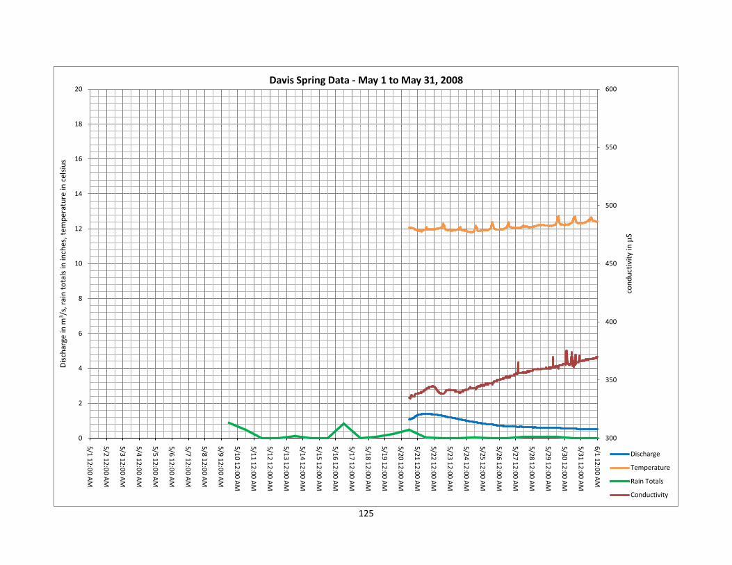
125
300
350
400
450
500
550
600
0
2
4
6
8
10
12
14
16
18
20
5/1
12
:00
AM
5/2
12
:00
AM
5/3
12
:00
AM
5/4
12
:00
AM
5/5
12
:00
AM
5/6
12
:00
AM
5/7
12
:00
AM
5/8
12
:00
AM
5/9
12
:00
AM
5/1
0 1
2:0
0 A
M
5/1
1 1
2:0
0 A
M
5/1
2 1
2:0
0 A
M
5/1
3 1
2:0
0 A
M
5/1
4 1
2:0
0 A
M
5/1
5 1
2:0
0 A
M
5/1
6 1
2:0
0 A
M
5/1
7 1
2:0
0 A
M
5/1
8 1
2:0
0 A
M
5/1
9 1
2:0
0 A
M
5/2
0 1
2:0
0 A
M
5/2
1 1
2:0
0 A
M
5/2
2 1
2:0
0 A
M
5/2
3 1
2:0
0 A
M
5/2
4 1
2:0
0 A
M
5/2
5 1
2:0
0 A
M
5/2
6 1
2:0
0 A
M
5/2
7 1
2:0
0 A
M
5/2
8 1
2:0
0 A
M
5/2
9 1
2:0
0 A
M
5/3
0 1
2:0
0 A
M
5/3
1 1
2:0
0 A
M
6/1
12
:00
AM
con
du
ctiv
ity
in µ
S
Dis
char
ge in
m3 /
s, r
ain
to
tals
in in
ches
, tem
per
atu
re in
cel
siu
s
Davis Spring Data - May 1 to May 31, 2008
Discharge
Temperature
Rain Totals
Conductivity
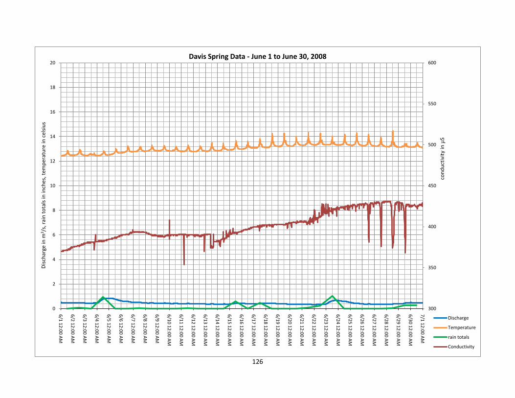
126
300
350
400
450
500
550
600
0
2
4
6
8
10
12
14
16
18
20
6/1
12
:00
AM
6/2
12
:00
AM
6/3
12
:00
AM
6/4
12
:00
AM
6/5
12
:00
AM
6/6
12
:00
AM
6/7
12
:00
AM
6/8
12
:00
AM
6/9
12
:00
AM
6/1
0 1
2:0
0 A
M
6/1
1 1
2:0
0 A
M
6/1
2 1
2:0
0 A
M
6/1
3 1
2:0
0 A
M
6/1
4 1
2:0
0 A
M
6/1
5 1
2:0
0 A
M
6/1
6 1
2:0
0 A
M
6/1
7 1
2:0
0 A
M
6/1
8 1
2:0
0 A
M
6/1
9 1
2:0
0 A
M
6/2
0 1
2:0
0 A
M
6/2
1 1
2:0
0 A
M
6/2
2 1
2:0
0 A
M
6/2
3 1
2:0
0 A
M
6/2
4 1
2:0
0 A
M
6/2
5 1
2:0
0 A
M
6/2
6 1
2:0
0 A
M
6/2
7 1
2:0
0 A
M
6/2
8 1
2:0
0 A
M
6/2
9 1
2:0
0 A
M
6/3
0 1
2:0
0 A
M
7/1
12
:00
AM
con
du
ctiv
ity
in µ
S
Dis
char
ge in
m3 /
s, r
ain
to
tals
in in
ches
, tem
per
atu
re in
cel
siu
s
Davis Spring Data - June 1 to June 30, 2008
Discharge
Temperature
rain totals
Conductivity
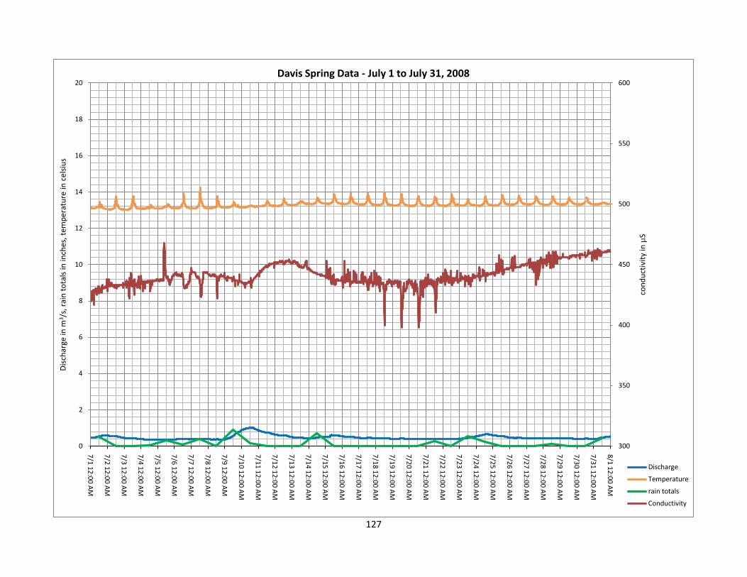
127
300
350
400
450
500
550
600
0
2
4
6
8
10
12
14
16
18
20
7/1
12
:00
AM
7/2
12
:00
AM
7/3
12
:00
AM
7/4
12
:00
AM
7/5
12
:00
AM
7/6
12
:00
AM
7/7
12
:00
AM
7/8
12
:00
AM
7/9
12
:00
AM
7/1
0 1
2:0
0 A
M
7/1
1 1
2:0
0 A
M
7/1
2 1
2:0
0 A
M
7/1
3 1
2:0
0 A
M
7/1
4 1
2:0
0 A
M
7/1
5 1
2:0
0 A
M
7/1
6 1
2:0
0 A
M
7/1
7 1
2:0
0 A
M
7/1
8 1
2:0
0 A
M
7/1
9 1
2:0
0 A
M
7/2
0 1
2:0
0 A
M
7/2
1 1
2:0
0 A
M
7/2
2 1
2:0
0 A
M
7/2
3 1
2:0
0 A
M
7/2
4 1
2:0
0 A
M
7/2
5 1
2:0
0 A
M
7/2
6 1
2:0
0 A
M
7/2
7 1
2:0
0 A
M
7/2
8 1
2:0
0 A
M
7/2
9 1
2:0
0 A
M
7/3
0 1
2:0
0 A
M
7/3
1 1
2:0
0 A
M
8/1
12
:00
AM
con
du
ctiv
ity
in µ
S
Dis
char
ge in
m3 /
s, r
ain
to
tals
in in
ches
, tem
per
atu
re in
cel
siu
s
Davis Spring Data - July 1 to July 31, 2008
Discharge
Temperature
rain totals
Conductivity
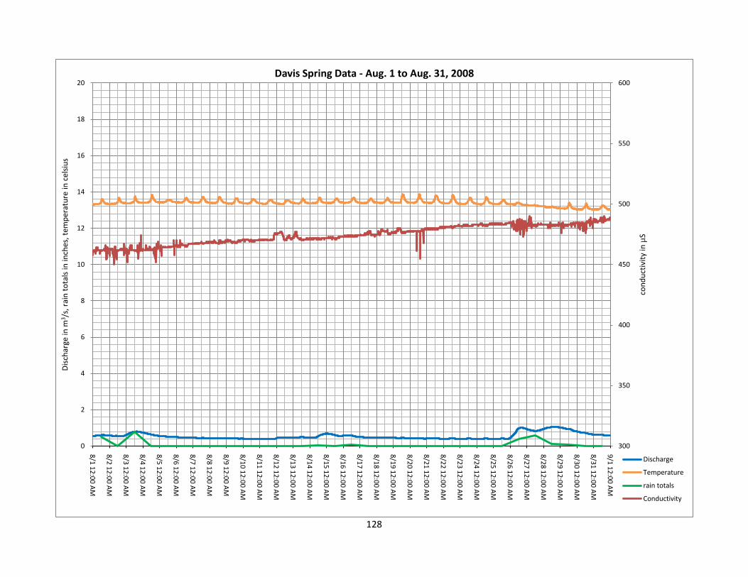
128
300
350
400
450
500
550
600
0
2
4
6
8
10
12
14
16
18
20
8/1
12
:00
AM
8/2
12
:00
AM
8/3
12
:00
AM
8/4
12
:00
AM
8/5
12
:00
AM
8/6
12
:00
AM
8/7
12
:00
AM
8/8
12
:00
AM
8/9
12
:00
AM
8/1
0 1
2:0
0 A
M
8/1
1 1
2:0
0 A
M
8/1
2 1
2:0
0 A
M
8/1
3 1
2:0
0 A
M
8/1
4 1
2:0
0 A
M
8/1
5 1
2:0
0 A
M
8/1
6 1
2:0
0 A
M
8/1
7 1
2:0
0 A
M
8/1
8 1
2:0
0 A
M
8/1
9 1
2:0
0 A
M
8/2
0 1
2:0
0 A
M
8/2
1 1
2:0
0 A
M
8/2
2 1
2:0
0 A
M
8/2
3 1
2:0
0 A
M
8/2
4 1
2:0
0 A
M
8/2
5 1
2:0
0 A
M
8/2
6 1
2:0
0 A
M
8/2
7 1
2:0
0 A
M
8/2
8 1
2:0
0 A
M
8/2
9 1
2:0
0 A
M
8/3
0 1
2:0
0 A
M
8/3
1 1
2:0
0 A
M
9/1
12
:00
AM
con
du
ctiv
ity
in µ
S
Dis
char
ge in
m3 /
s, r
ain
to
tals
in in
ches
, tem
per
atu
re in
cel
siu
sDavis Spring Data - Aug. 1 to Aug. 31, 2008
Discharge
Temperature
rain totals
Conductivity
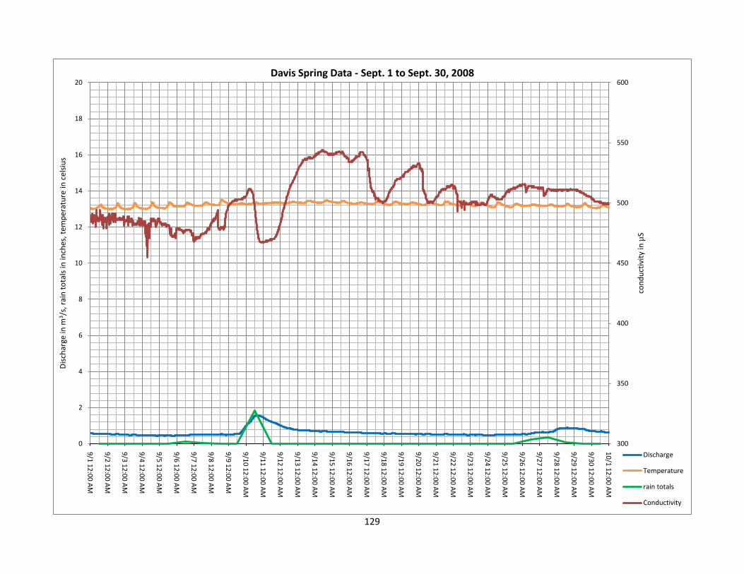
129
300
350
400
450
500
550
600
0
2
4
6
8
10
12
14
16
18
20
9/1
12
:00
AM
9/2
12
:00
AM
9/3
12
:00
AM
9/4
12
:00
AM
9/5
12
:00
AM
9/6
12
:00
AM
9/7
12
:00
AM
9/8
12
:00
AM
9/9
12
:00
AM
9/1
0 1
2:0
0 A
M
9/1
1 1
2:0
0 A
M
9/1
2 1
2:0
0 A
M
9/1
3 1
2:0
0 A
M
9/1
4 1
2:0
0 A
M
9/1
5 1
2:0
0 A
M
9/1
6 1
2:0
0 A
M
9/1
7 1
2:0
0 A
M
9/1
8 1
2:0
0 A
M
9/1
9 1
2:0
0 A
M
9/2
0 1
2:0
0 A
M
9/2
1 1
2:0
0 A
M
9/2
2 1
2:0
0 A
M
9/2
3 1
2:0
0 A
M
9/2
4 1
2:0
0 A
M
9/2
5 1
2:0
0 A
M
9/2
6 1
2:0
0 A
M
9/2
7 1
2:0
0 A
M
9/2
8 1
2:0
0 A
M
9/2
9 1
2:0
0 A
M
9/3
0 1
2:0
0 A
M
10
/1 1
2:0
0 A
M
con
du
ctiv
ity
in µ
S
Dis
char
ge in
m3 /
s, r
ain
to
tals
in in
ches
, tem
per
atu
re in
cel
siu
s
Davis Spring Data - Sept. 1 to Sept. 30, 2008
Discharge
Temperature
rain totals
Conductivity
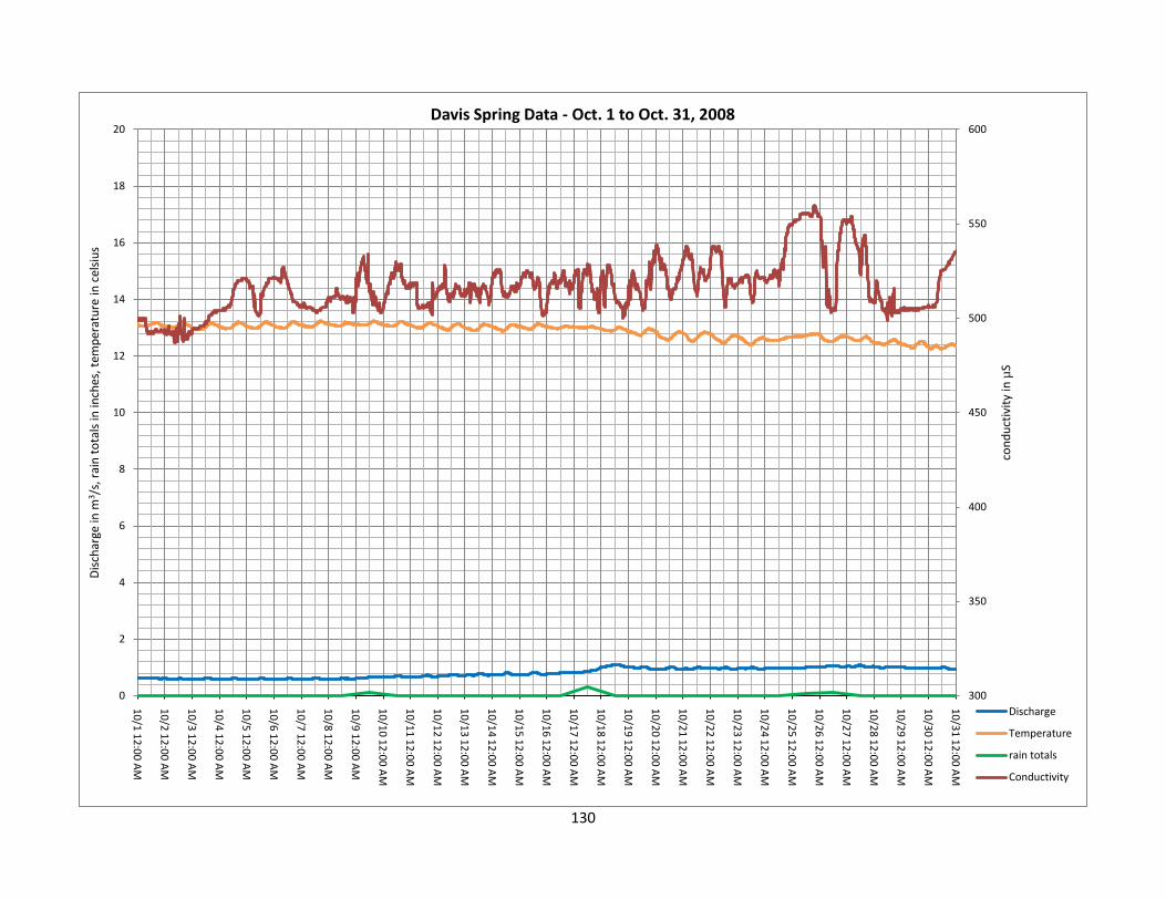
130
300
350
400
450
500
550
600
0
2
4
6
8
10
12
14
16
18
20
10
/1 1
2:0
0 A
M
10
/2 1
2:0
0 A
M
10
/3 1
2:0
0 A
M
10
/4 1
2:0
0 A
M
10
/5 1
2:0
0 A
M
10
/6 1
2:0
0 A
M
10
/7 1
2:0
0 A
M
10
/8 1
2:0
0 A
M
10
/9 1
2:0
0 A
M
10
/10
12
:00
AM
10
/11
12
:00
AM
10
/12
12
:00
AM
10
/13
12
:00
AM
10
/14
12
:00
AM
10
/15
12
:00
AM
10
/16
12
:00
AM
10
/17
12
:00
AM
10
/18
12
:00
AM
10
/19
12
:00
AM
10
/20
12
:00
AM
10
/21
12
:00
AM
10
/22
12
:00
AM
10
/23
12
:00
AM
10
/24
12
:00
AM
10
/25
12
:00
AM
10
/26
12
:00
AM
10
/27
12
:00
AM
10
/28
12
:00
AM
10
/29
12
:00
AM
10
/30
12
:00
AM
10
/31
12
:00
AM
con
du
ctiv
ity
in µ
S
Dis
char
ge in
m3 /
s, r
ain
to
tals
in in
ches
, tem
per
atu
re in
cel
siu
s
Davis Spring Data - Oct. 1 to Oct. 31, 2008
Discharge
Temperature
rain totals
Conductivity
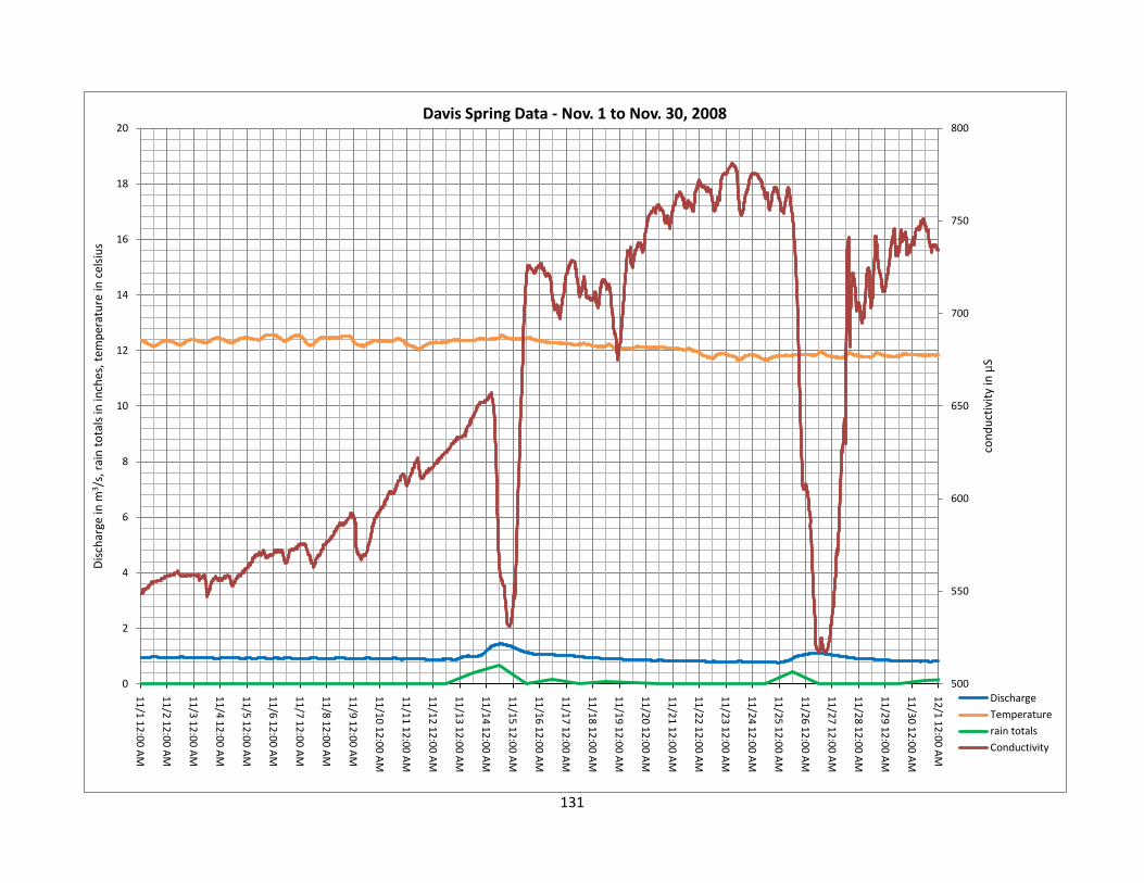
131
500
550
600
650
700
750
800
0
2
4
6
8
10
12
14
16
18
20
11
/1 1
2:0
0 A
M
11
/2 1
2:0
0 A
M
11
/3 1
2:0
0 A
M
11
/4 1
2:0
0 A
M
11
/5 1
2:0
0 A
M
11
/6 1
2:0
0 A
M
11
/7 1
2:0
0 A
M
11
/8 1
2:0
0 A
M
11
/9 1
2:0
0 A
M
11
/10
12
:00
AM
11
/11
12
:00
AM
11
/12
12
:00
AM
11
/13
12
:00
AM
11
/14
12
:00
AM
11
/15
12
:00
AM
11
/16
12
:00
AM
11
/17
12
:00
AM
11
/18
12
:00
AM
11
/19
12
:00
AM
11
/20
12
:00
AM
11
/21
12
:00
AM
11
/22
12
:00
AM
11
/23
12
:00
AM
11
/24
12
:00
AM
11
/25
12
:00
AM
11
/26
12
:00
AM
11
/27
12
:00
AM
11
/28
12
:00
AM
11
/29
12
:00
AM
11
/30
12
:00
AM
12
/1 1
2:0
0 A
M
con
du
ctiv
ity
in µ
S
Dis
char
ge in
m3 /
s, r
ain
to
tals
in in
ches
, tem
per
atu
re in
cel
siu
s
Davis Spring Data - Nov. 1 to Nov. 30, 2008
Discharge
Temperature
rain totals
Conductivity
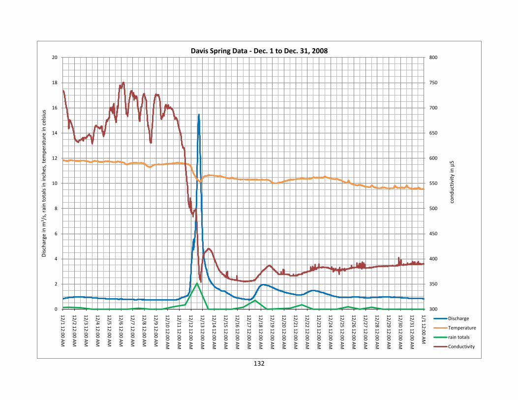
132
300
350
400
450
500
550
600
650
700
750
800
0
2
4
6
8
10
12
14
16
18
20
12
/1 1
2:0
0 A
M
12
/2 1
2:0
0 A
M
12
/3 1
2:0
0 A
M
12
/4 1
2:0
0 A
M
12
/5 1
2:0
0 A
M
12
/6 1
2:0
0 A
M
12
/7 1
2:0
0 A
M
12
/8 1
2:0
0 A
M
12
/9 1
2:0
0 A
M
12
/10
12
:00
AM
12
/11
12
:00
AM
12
/12
12
:00
AM
12
/13
12
:00
AM
12
/14
12
:00
AM
12
/15
12
:00
AM
12
/16
12
:00
AM
12
/17
12
:00
AM
12
/18
12
:00
AM
12
/19
12
:00
AM
12
/20
12
:00
AM
12
/21
12
:00
AM
12
/22
12
:00
AM
12
/23
12
:00
AM
12
/24
12
:00
AM
12
/25
12
:00
AM
12
/26
12
:00
AM
12
/27
12
:00
AM
12
/28
12
:00
AM
12
/29
12
:00
AM
12
/30
12
:00
AM
12
/31
12
:00
AM
1/1
12
:00
AM
con
du
ctiv
ity
in µ
S
Dis
char
ge in
m3 /
s, r
ain
to
tals
in in
ches
, tem
per
atu
re in
cel
siu
s
Davis Spring Data - Dec. 1 to Dec. 31, 2008
Discharge
Temperature
rain totals
Conductivity
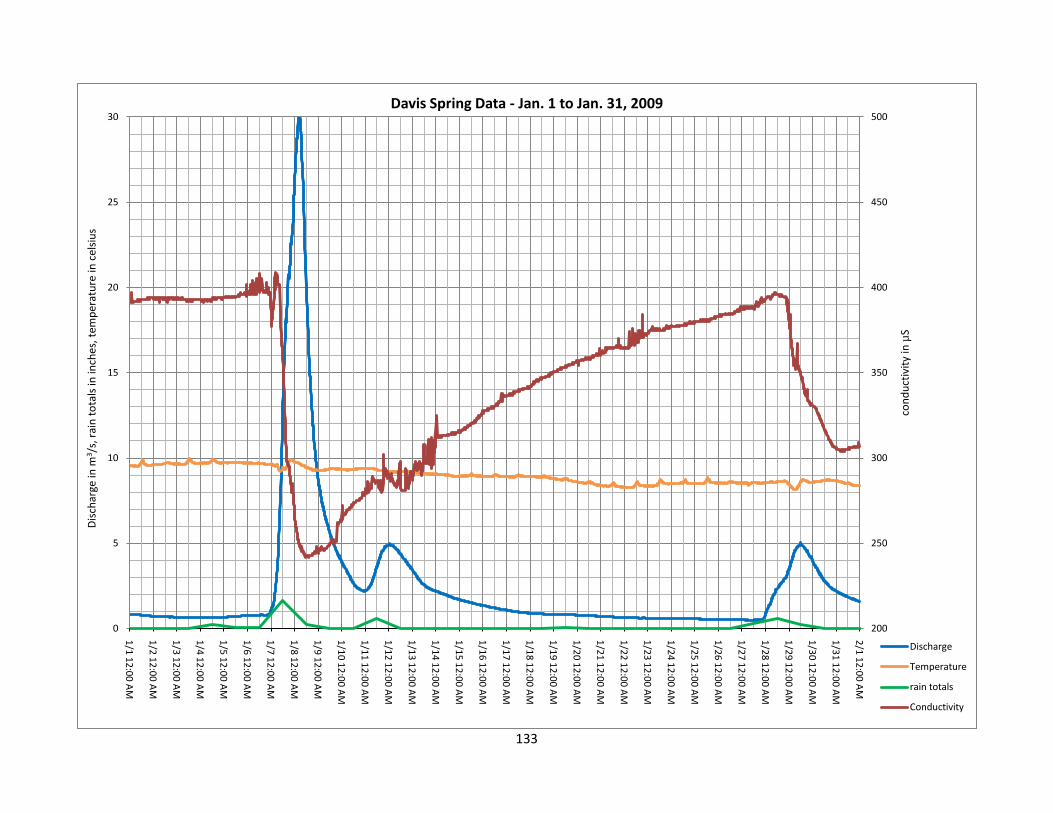
133
200
250
300
350
400
450
500
0
5
10
15
20
25
30
1/1
12
:00
AM
1/2
12
:00
AM
1/3
12
:00
AM
1/4
12
:00
AM
1/5
12
:00
AM
1/6
12
:00
AM
1/7
12
:00
AM
1/8
12
:00
AM
1/9
12
:00
AM
1/1
0 1
2:0
0 A
M
1/1
1 1
2:0
0 A
M
1/1
2 1
2:0
0 A
M
1/1
3 1
2:0
0 A
M
1/1
4 1
2:0
0 A
M
1/1
5 1
2:0
0 A
M
1/1
6 1
2:0
0 A
M
1/1
7 1
2:0
0 A
M
1/1
8 1
2:0
0 A
M
1/1
9 1
2:0
0 A
M
1/2
0 1
2:0
0 A
M
1/2
1 1
2:0
0 A
M
1/2
2 1
2:0
0 A
M
1/2
3 1
2:0
0 A
M
1/2
4 1
2:0
0 A
M
1/2
5 1
2:0
0 A
M
1/2
6 1
2:0
0 A
M
1/2
7 1
2:0
0 A
M
1/2
8 1
2:0
0 A
M
1/2
9 1
2:0
0 A
M
1/3
0 1
2:0
0 A
M
1/3
1 1
2:0
0 A
M
2/1
12
:00
AM
con
du
ctiv
ity
in µ
S
Dis
char
ge in
m3 /
s, r
ain
to
tals
in in
ches
, tem
per
atu
re in
cel
siu
sDavis Spring Data - Jan. 1 to Jan. 31, 2009
Discharge
Temperature
rain totals
Conductivity
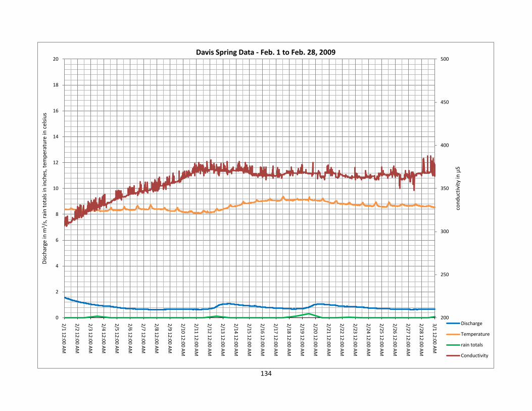
134
200
250
300
350
400
450
500
0
2
4
6
8
10
12
14
16
18
20
2/1
12
:00
AM
2/2
12
:00
AM
2/3
12
:00
AM
2/4
12
:00
AM
2/5
12
:00
AM
2/6
12
:00
AM
2/7
12
:00
AM
2/8
12
:00
AM
2/9
12
:00
AM
2/1
0 1
2:0
0 A
M
2/1
1 1
2:0
0 A
M
2/1
2 1
2:0
0 A
M
2/1
3 1
2:0
0 A
M
2/1
4 1
2:0
0 A
M
2/1
5 1
2:0
0 A
M
2/1
6 1
2:0
0 A
M
2/1
7 1
2:0
0 A
M
2/1
8 1
2:0
0 A
M
2/1
9 1
2:0
0 A
M
2/2
0 1
2:0
0 A
M
2/2
1 1
2:0
0 A
M
2/2
2 1
2:0
0 A
M
2/2
3 1
2:0
0 A
M
2/2
4 1
2:0
0 A
M
2/2
5 1
2:0
0 A
M
2/2
6 1
2:0
0 A
M
2/2
7 1
2:0
0 A
M
2/2
8 1
2:0
0 A
M
3/1
12
:00
AM
con
du
ctiv
ity
in µ
S
Dis
char
ge in
m3 /
s, r
ain
to
tals
in in
ches
, tem
per
atu
re in
cel
siu
s
Davis Spring Data - Feb. 1 to Feb. 28, 2009
Discharge
Temperature
rain totals
Conductivity
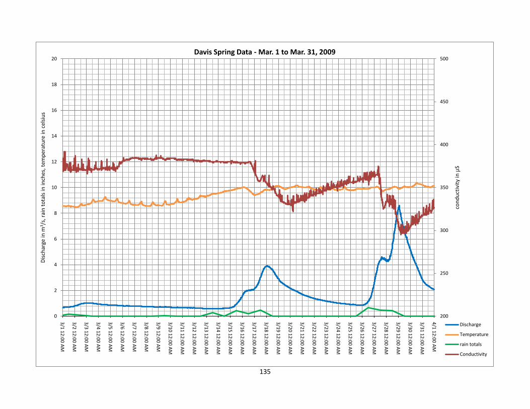
135
200
250
300
350
400
450
500
0
2
4
6
8
10
12
14
16
18
20
3/1
12
:00
AM
3/2
12
:00
AM
3/3
12
:00
AM
3/4
12
:00
AM
3/5
12
:00
AM
3/6
12
:00
AM
3/7
12
:00
AM
3/8
12
:00
AM
3/9
12
:00
AM
3/1
0 1
2:0
0 A
M
3/1
1 1
2:0
0 A
M
3/1
2 1
2:0
0 A
M
3/1
3 1
2:0
0 A
M
3/1
4 1
2:0
0 A
M
3/1
5 1
2:0
0 A
M
3/1
6 1
2:0
0 A
M
3/1
7 1
2:0
0 A
M
3/1
8 1
2:0
0 A
M
3/1
9 1
2:0
0 A
M
3/2
0 1
2:0
0 A
M
3/2
1 1
2:0
0 A
M
3/2
2 1
2:0
0 A
M
3/2
3 1
2:0
0 A
M
3/2
4 1
2:0
0 A
M
3/2
5 1
2:0
0 A
M
3/2
6 1
2:0
0 A
M
3/2
7 1
2:0
0 A
M
3/2
8 1
2:0
0 A
M
3/2
9 1
2:0
0 A
M
3/3
0 1
2:0
0 A
M
3/3
1 1
2:0
0 A
M
4/1
12
:00
AM
con
du
ctiv
ity
in µ
S
Dis
char
ge in
m3 /
s, r
ain
to
tals
in in
ches
, tem
per
atu
re in
cel
siu
s
Davis Spring Data - Mar. 1 to Mar. 31, 2009
Discharge
Temperature
rain totals
Conductivity
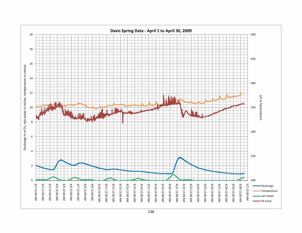
136
200
250
300
350
400
450
500
0
2
4
6
8
10
12
14
16
18
20
4/1
12
:00
AM
4/2
12
:00
AM
4/3
12
:00
AM
4/4
12
:00
AM
4/5
12
:00
AM
4/6
12
:00
AM
4/7
12
:00
AM
4/8
12
:00
AM
4/9
12
:00
AM
4/1
0 1
2:0
0 A
M
4/1
1 1
2:0
0 A
M
4/1
2 1
2:0
0 A
M
4/1
3 1
2:0
0 A
M
4/1
4 1
2:0
0 A
M
4/1
5 1
2:0
0 A
M
4/1
6 1
2:0
0 A
M
4/1
7 1
2:0
0 A
M
4/1
8 1
2:0
0 A
M
4/1
9 1
2:0
0 A
M
4/2
0 1
2:0
0 A
M
4/2
1 1
2:0
0 A
M
4/2
2 1
2:0
0 A
M
4/2
3 1
2:0
0 A
M
4/2
4 1
2:0
0 A
M
4/2
5 1
2:0
0 A
M
4/2
6 1
2:0
0 A
M
4/2
7 1
2:0
0 A
M
4/2
8 1
2:0
0 A
M
4/2
9 1
2:0
0 A
M
4/3
0 1
2:0
0 A
M
5/1
12
:00
AM
con
du
ctiv
ity
in µ
S
Dis
char
ge in
m3 /
s, r
ain
to
tals
in in
ches
, tem
per
atu
re in
cel
siu
s
Davis Spring Data - April 1 to April 30, 2009
Discharge
Temperature
rain totals
DS cond
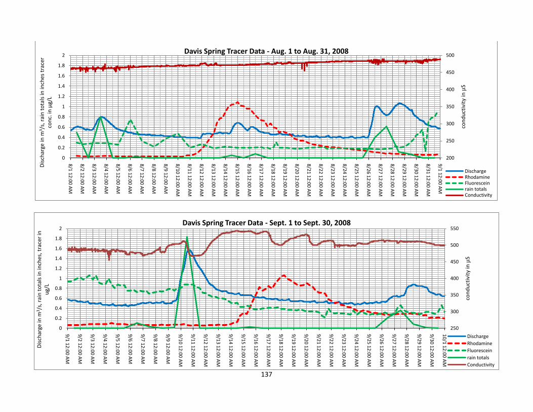
137
200
250
300
350
400
450
500
0
0.2
0.4
0.6
0.8
1
1.2
1.4
1.6
1.8
2
8/1
12
:00
AM
8/2
12
:00
AM
8/3
12
:00
AM
8/4
12
:00
AM
8/5
12
:00
AM
8/6
12
:00
AM
8/7
12
:00
AM
8/8
12
:00
AM
8/9
12
:00
AM
8/1
0 1
2:0
0 A
M
8/1
1 1
2:0
0 A
M
8/1
2 1
2:0
0 A
M
8/1
3 1
2:0
0 A
M
8/1
4 1
2:0
0 A
M
8/1
5 1
2:0
0 A
M
8/1
6 1
2:0
0 A
M
8/1
7 1
2:0
0 A
M
8/1
8 1
2:0
0 A
M
8/1
9 1
2:0
0 A
M
8/2
0 1
2:0
0 A
M
8/2
1 1
2:0
0 A
M
8/2
2 1
2:0
0 A
M
8/2
3 1
2:0
0 A
M
8/2
4 1
2:0
0 A
M
8/2
5 1
2:0
0 A
M
8/2
6 1
2:0
0 A
M
8/2
7 1
2:0
0 A
M
8/2
8 1
2:0
0 A
M
8/2
9 1
2:0
0 A
M
8/3
0 1
2:0
0 A
M
8/3
1 1
2:0
0 A
M
9/1
12
:00
AM
con
du
ctiv
ity
in µ
S
Dis
char
ge in
m3 /
s, r
ain
to
tals
in in
ches
tra
cer
con
c. in
µg/
LDavis Spring Tracer Data - Aug. 1 to Aug. 31, 2008
DischargeRhodamineFluoresceinrain totalsConductivity
250
300
350
400
450
500
550
0
0.2
0.4
0.6
0.8
1
1.2
1.4
1.6
1.8
2
9/1
12
:00
AM
9/2
12
:00
AM
9/3
12
:00
AM
9/4
12
:00
AM
9/5
12
:00
AM
9/6
12
:00
AM
9/7
12
:00
AM
9/8
12
:00
AM
9/9
12
:00
AM
9/1
0 1
2:0
0 A
M
9/1
1 1
2:0
0 A
M
9/1
2 1
2:0
0 A
M
9/1
3 1
2:0
0 A
M
9/1
4 1
2:0
0 A
M
9/1
5 1
2:0
0 A
M
9/1
6 1
2:0
0 A
M
9/1
7 1
2:0
0 A
M
9/1
8 1
2:0
0 A
M
9/1
9 1
2:0
0 A
M
9/2
0 1
2:0
0 A
M
9/2
1 1
2:0
0 A
M
9/2
2 1
2:0
0 A
M
9/2
3 1
2:0
0 A
M
9/2
4 1
2:0
0 A
M
9/2
5 1
2:0
0 A
M
9/2
6 1
2:0
0 A
M
9/2
7 1
2:0
0 A
M
9/2
8 1
2:0
0 A
M
9/2
9 1
2:0
0 A
M
9/3
0 1
2:0
0 A
M
10
/1 1
2:0
0 A
M
con
du
ctiv
ity
in µ
S
Dis
char
ge in
m3 /
s, r
ain
to
tals
in in
ches
, tra
cer
in
ug/
L
Davis Spring Tracer Data - Sept. 1 to Sept. 30, 2008
Discharge
Rhodamine
Fluorescein
rain totals
Conductivity
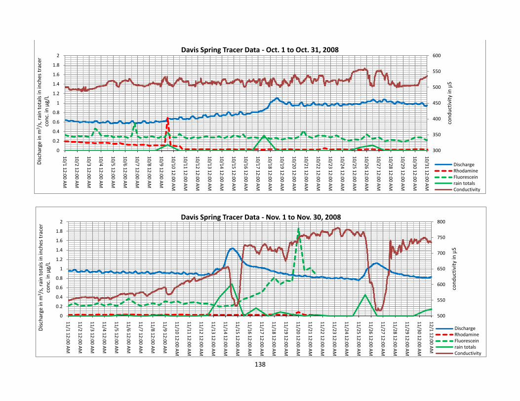
138
300
350
400
450
500
550
600
0
0.2
0.4
0.6
0.8
1
1.2
1.4
1.6
1.8
2
10
/1 1
2:0
0 A
M
10
/2 1
2:0
0 A
M
10
/3 1
2:0
0 A
M
10
/4 1
2:0
0 A
M
10
/5 1
2:0
0 A
M
10
/6 1
2:0
0 A
M
10
/7 1
2:0
0 A
M
10
/8 1
2:0
0 A
M
10
/9 1
2:0
0 A
M
10
/10
12
:00
AM
10
/11
12
:00
AM
10
/12
12
:00
AM
10
/13
12
:00
AM
10
/14
12
:00
AM
10
/15
12
:00
AM
10
/16
12
:00
AM
10
/17
12
:00
AM
10
/18
12
:00
AM
10
/19
12
:00
AM
10
/20
12
:00
AM
10
/21
12
:00
AM
10
/22
12
:00
AM
10
/23
12
:00
AM
10
/24
12
:00
AM
10
/25
12
:00
AM
10
/26
12
:00
AM
10
/27
12
:00
AM
10
/28
12
:00
AM
10
/29
12
:00
AM
10
/30
12
:00
AM
10
/31
12
:00
AM
con
du
ctiv
ity
in µ
S
Dis
char
ge in
m3 /
s, r
ain
to
tals
in in
ches
tra
cer
con
c. in
µg/
LDavis Spring Tracer Data - Oct. 1 to Oct. 31, 2008
DischargeRhodamineFluoresceinrain totalsConductivity
500
550
600
650
700
750
800
0
0.2
0.4
0.6
0.8
1
1.2
1.4
1.6
1.8
2
11
/1 1
2:0
0 A
M
11
/2 1
2:0
0 A
M
11
/3 1
2:0
0 A
M
11
/4 1
2:0
0 A
M
11
/5 1
2:0
0 A
M
11
/6 1
2:0
0 A
M
11
/7 1
2:0
0 A
M
11
/8 1
2:0
0 A
M
11
/9 1
2:0
0 A
M
11
/10
12
:00
AM
11
/11
12
:00
AM
11
/12
12
:00
AM
11
/13
12
:00
AM
11
/14
12
:00
AM
11
/15
12
:00
AM
11
/16
12
:00
AM
11
/17
12
:00
AM
11
/18
12
:00
AM
11
/19
12
:00
AM
11
/20
12
:00
AM
11
/21
12
:00
AM
11
/22
12
:00
AM
11
/23
12
:00
AM
11
/24
12
:00
AM
11
/25
12
:00
AM
11
/26
12
:00
AM
11
/27
12
:00
AM
11
/28
12
:00
AM
11
/29
12
:00
AM
11
/30
12
:00
AM
12
/1 1
2:0
0 A
M
con
du
ctiv
ity
in µ
S
Dis
char
ge in
m3 /
s, r
ain
to
tals
in in
ches
tra
cer
con
c. in
µg/
L
Davis Spring Tracer Data - Nov. 1 to Nov. 30, 2008
DischargeRhodamineFluoresceinrain totalsConductivity
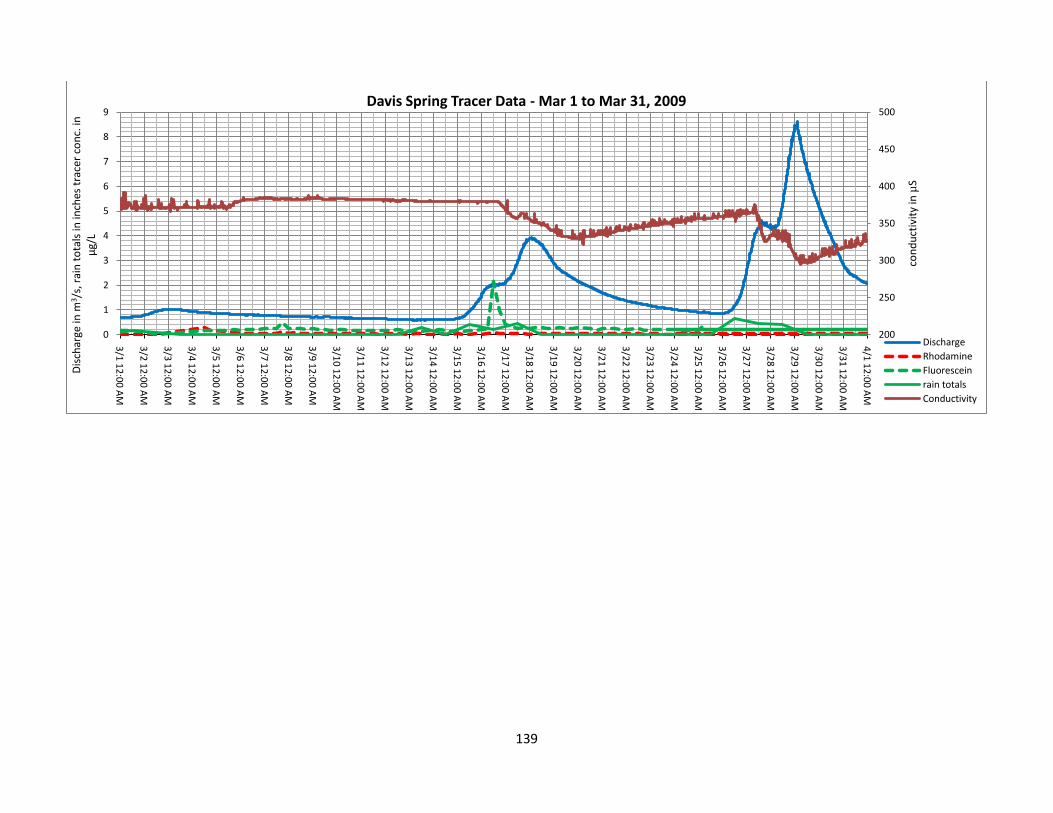
139
200
250
300
350
400
450
500
0
1
2
3
4
5
6
7
8
9
3/1
12
:00
AM
3/2
12
:00
AM
3/3
12
:00
AM
3/4
12
:00
AM
3/5
12
:00
AM
3/6
12
:00
AM
3/7
12
:00
AM
3/8
12
:00
AM
3/9
12
:00
AM
3/1
0 1
2:0
0 A
M
3/1
1 1
2:0
0 A
M
3/1
2 1
2:0
0 A
M
3/1
3 1
2:0
0 A
M
3/1
4 1
2:0
0 A
M
3/1
5 1
2:0
0 A
M
3/1
6 1
2:0
0 A
M
3/1
7 1
2:0
0 A
M
3/1
8 1
2:0
0 A
M
3/1
9 1
2:0
0 A
M
3/2
0 1
2:0
0 A
M
3/2
1 1
2:0
0 A
M
3/2
2 1
2:0
0 A
M
3/2
3 1
2:0
0 A
M
3/2
4 1
2:0
0 A
M
3/2
5 1
2:0
0 A
M
3/2
6 1
2:0
0 A
M
3/2
7 1
2:0
0 A
M
3/2
8 1
2:0
0 A
M
3/2
9 1
2:0
0 A
M
3/3
0 1
2:0
0 A
M
3/3
1 1
2:0
0 A
M
4/1
12
:00
AM
con
du
ctiv
ity
in µ
S
Dis
char
ge in
m3 /
s, r
ain
to
tals
in in
ches
tra
cer
con
c. in
µ
g/L
Davis Spring Tracer Data - Mar 1 to Mar 31, 2009
Discharge
Rhodamine
Fluorescein
rain totals
Conductivity
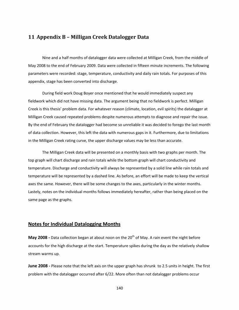
140
11 Appendix B – Milligan Creek Datalogger Data
Nine and a half months of datalogger data were collected at Milligan Creek, from the middle of
May 2008 to the end of February 2009. Data were collected in fifteen minute increments. The following
parameters were recorded: stage, temperature, conductivity and daily rain totals. For purposes of this
appendix, stage has been converted into discharge.
During field work Doug Boyer once mentioned that he would immediately suspect any
fieldwork which did not have missing data. The argument being that no fieldwork is perfect. Milligan
Creek is this thesis’ problem data. For whatever reason (climate, location, evil spirits) the datalogger at
Milligan Creek caused repeated problems despite numerous attempts to diagnose and repair the issue.
By the end of February the datalogger had become so unreliable it was decided to forego the last month
of data collection. However, this left the data with numerous gaps in it. Furthermore, due to limitations
in the Milligan Creek rating curve, the upper discharge values may be less than accurate.
The Milligan Creek data will be presented on a monthly basis with two graphs per month. The
top graph will chart discharge and rain totals while the bottom graph will chart conductivity and
temperature. Discharge and conductivity will always be represented by a solid line while rain totals and
temperature will be represented by a dashed line. As before, an effort will be made to keep the vertical
axes the same. However, there will be some changes to the axes, particularly in the winter months.
Lastely, notes on the individual months follows immediately hereafter, rather than being placed on the
same page as the graphs.
Notes for Individual Datalogging Months
May 2008 - Data collection began at about noon on the 20th of May. A rain event the night before
accounts for the high discharge at the start. Temperature spikes during the day as the relatively shallow
stream warms up.
June 2008 - Please note that the left axis on the upper graph has shrunk to 2.5 units in height. The first
problem with the datalogger occurred after 6/22. More often than not datalogger problems occur
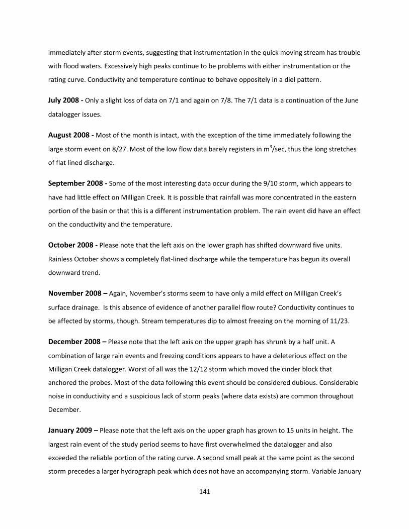
141
immediately after storm events, suggesting that instrumentation in the quick moving stream has trouble
with flood waters. Excessively high peaks continue to be problems with either instrumentation or the
rating curve. Conductivity and temperature continue to behave oppositely in a diel pattern.
July 2008 - Only a slight loss of data on 7/1 and again on 7/8. The 7/1 data is a continuation of the June
datalogger issues.
August 2008 - Most of the month is intact, with the exception of the time immediately following the
large storm event on 8/27. Most of the low flow data barely registers in m3/sec, thus the long stretches
of flat lined discharge.
September 2008 - Some of the most interesting data occur during the 9/10 storm, which appears to
have had little effect on Milligan Creek. It is possible that rainfall was more concentrated in the eastern
portion of the basin or that this is a different instrumentation problem. The rain event did have an effect
on the conductivity and the temperature.
October 2008 - Please note that the left axis on the lower graph has shifted downward five units.
Rainless October shows a completely flat-lined discharge while the temperature has begun its overall
downward trend.
November 2008 – Again, November’s storms seem to have only a mild effect on Milligan Creek’s
surface drainage. Is this absence of evidence of another parallel flow route? Conductivity continues to
be affected by storms, though. Stream temperatures dip to almost freezing on the morning of 11/23.
December 2008 – Please note that the left axis on the upper graph has shrunk by a half unit. A
combination of large rain events and freezing conditions appears to have a deleterious effect on the
Milligan Creek datalogger. Worst of all was the 12/12 storm which moved the cinder block that
anchored the probes. Most of the data following this event should be considered dubious. Considerable
noise in conductivity and a suspicious lack of storm peaks (where data exists) are common throughout
December.
January 2009 – Please note that the left axis on the upper graph has grown to 15 units in height. The
largest rain event of the study period seems to have first overwhelmed the datalogger and also
exceeded the reliable portion of the rating curve. A second small peak at the same point as the second
storm precedes a larger hydrograph peak which does not have an accompanying storm. Variable January

142
temperatures suggest the last peak may be a result of meltwater. Conductivity is especially ragged,
possibly indicative of long term flushing.
February 2008 – Please note that the left axis on the upper graph has shrunk to 3.5 units in height.
Storms and equipment failure at the end of February made further attempts at data collecting seem
non-productive. Additional peaks are accompanied by long term increases in water temperature.
Whether this represents large movement of stored water or an increase in overall warmth is unclear.
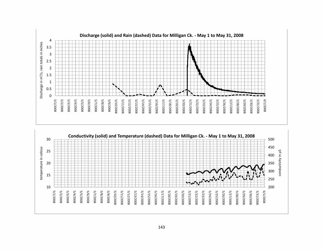
143
0
0.5
1
1.5
2
2.5
3
3.5
4
5/1
/20
08
5/2
/20
08
5/3
/20
08
5/4
/20
08
5/5
/20
08
5/6
/20
08
5/7
/20
08
5/8
/20
08
5/9
/20
08
5/1
0/2
00
8
5/1
1/2
00
8
5/1
2/2
00
8
5/1
3/2
00
8
5/1
4/2
00
8
5/1
5/2
00
8
5/1
6/2
00
8
5/1
7/2
00
8
5/1
8/2
00
8
5/1
9/2
00
8
5/2
0/2
00
8
5/2
1/2
00
8
5/2
2/2
00
8
5/2
3/2
00
8
5/2
4/2
00
8
5/2
5/2
00
8
5/2
6/2
00
8
5/2
7/2
00
8
5/2
8/2
00
8
5/2
9/2
00
8
5/3
0/2
00
8
5/3
1/2
00
8
6/1
/20
08
Dis
char
ge in
m3 /
s, r
ain
to
tals
in in
ches
Discharge (solid) and Rain (dashed) Data for Milligan Ck. - May 1 to May 31, 2008
200
250
300
350
400
450
500
10
15
20
25
30
5/1
/20
08
5/2
/20
08
5/3
/20
08
5/4
/20
08
5/5
/20
08
5/6
/20
08
5/7
/20
08
5/8
/20
08
5/9
/20
08
5/1
0/2
00
8
5/1
1/2
00
8
5/1
2/2
00
8
5/1
3/2
00
8
5/1
4/2
00
8
5/1
5/2
00
8
5/1
6/2
00
8
5/1
7/2
00
8
5/1
8/2
00
8
5/1
9/2
00
8
5/2
0/2
00
8
5/2
1/2
00
8
5/2
2/2
00
8
5/2
3/2
00
8
5/2
4/2
00
8
5/2
5/2
00
8
5/2
6/2
00
8
5/2
7/2
00
8
5/2
8/2
00
8
5/2
9/2
00
8
5/3
0/2
00
8
5/3
1/2
00
8
6/1
/20
08
con
du
ctiv
ity
in µ
S
tem
per
atu
re in
cel
siu
s
Conductivity (solid) and Temperature (dashed) Data for Milligan Ck. - May 1 to May 31, 2008
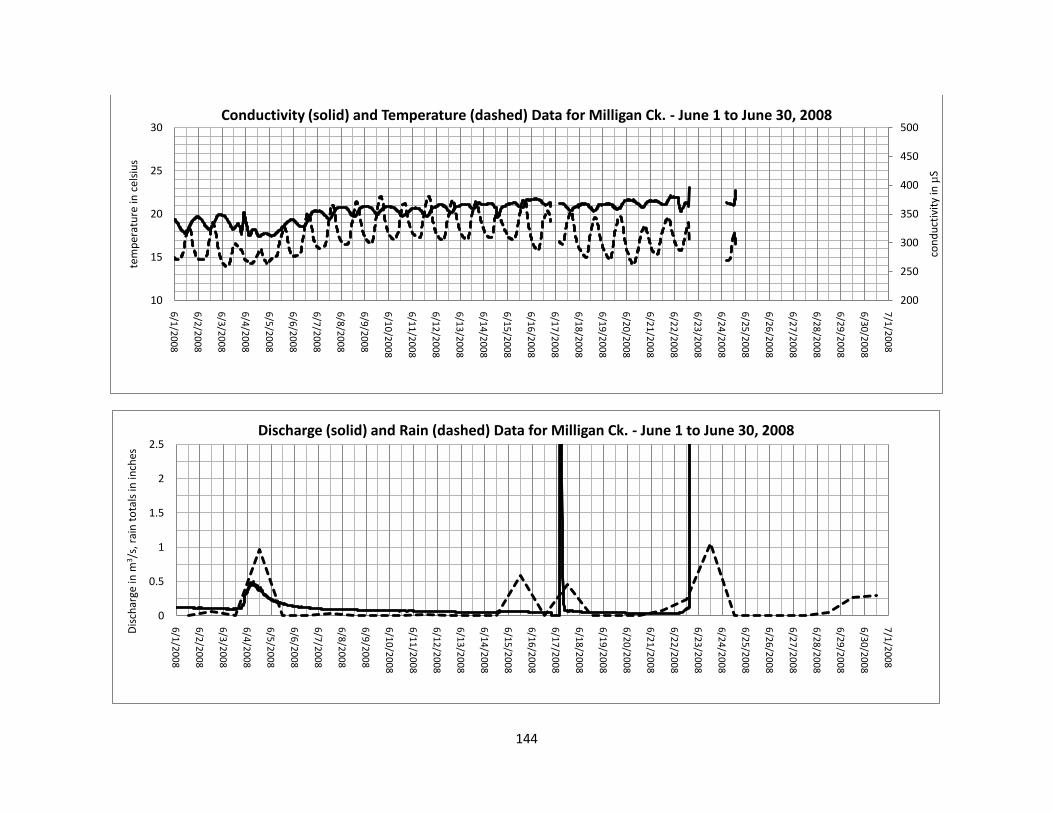
144
200
250
300
350
400
450
500
10
15
20
25
30
6/1
/20
08
6/2
/20
08
6/3
/20
08
6/4
/20
08
6/5
/20
08
6/6
/20
08
6/7
/20
08
6/8
/20
08
6/9
/20
08
6/1
0/2
00
8
6/1
1/2
00
8
6/1
2/2
00
8
6/1
3/2
00
8
6/1
4/2
00
8
6/1
5/2
00
8
6/1
6/2
00
8
6/1
7/2
00
8
6/1
8/2
00
8
6/1
9/2
00
8
6/2
0/2
00
8
6/2
1/2
00
8
6/2
2/2
00
8
6/2
3/2
00
8
6/2
4/2
00
8
6/2
5/2
00
8
6/2
6/2
00
8
6/2
7/2
00
8
6/2
8/2
00
8
6/2
9/2
00
8
6/3
0/2
00
8
7/1
/20
08
con
du
ctiv
ity
in µ
S
tem
per
atu
re in
cel
siu
s
Conductivity (solid) and Temperature (dashed) Data for Milligan Ck. - June 1 to June 30, 2008
0
0.5
1
1.5
2
2.5
6/1
/20
08
6/2
/20
08
6/3
/20
08
6/4
/20
08
6/5
/20
08
6/6
/20
08
6/7
/20
08
6/8
/20
08
6/9
/20
08
6/1
0/2
00
8
6/1
1/2
00
8
6/1
2/2
00
8
6/1
3/2
00
8
6/1
4/2
00
8
6/1
5/2
00
8
6/1
6/2
00
8
6/1
7/2
00
8
6/1
8/2
00
8
6/1
9/2
00
8
6/2
0/2
00
8
6/2
1/2
00
8
6/2
2/2
00
8
6/2
3/2
00
8
6/2
4/2
00
8
6/2
5/2
00
8
6/2
6/2
00
8
6/2
7/2
00
8
6/2
8/2
00
8
6/2
9/2
00
8
6/3
0/2
00
8
7/1
/20
08
Dis
char
ge in
m3 /
s, r
ain
to
tals
in in
ches
Discharge (solid) and Rain (dashed) Data for Milligan Ck. - June 1 to June 30, 2008
145
0
0.5
1
1.5
2
2.5
7/1
/20
08
7/2
/20
08
7/3
/20
08
7/4
/20
08
7/5
/20
08
7/6
/20
08
7/7
/20
08
7/8
/20
08
7/9
/20
08
7/1
0/2
00
8
7/1
1/2
00
8
7/1
2/2
00
8
7/1
3/2
00
8
7/1
4/2
00
8
7/1
5/2
00
8
7/1
6/2
00
8
7/1
7/2
00
8
7/1
8/2
00
8
7/1
9/2
00
8
7/2
0/2
00
8
7/2
1/2
00
8
7/2
2/2
00
8
7/2
3/2
00
8
7/2
4/2
00
8
7/2
5/2
00
8
7/2
6/2
00
8
7/2
7/2
00
8
7/2
8/2
00
8
7/2
9/2
00
8
7/3
0/2
00
8
7/3
1/2
00
8
8/1
/20
08D
isch
arge
in m
3 /s,
rai
n t
ota
ls in
inch
es
Discharge (solid) and Rain (dashed) Data for Milligan Ck. - July 1 to July 31, 2008
200
250
300
350
400
450
500
550
10
15
20
25
30
7/1
/20
08
7/2
/20
08
7/3
/20
08
7/4
/20
08
7/5
/20
08
7/6
/20
08
7/7
/20
08
7/8
/20
08
7/9
/20
08
7/1
0/2
00
8
7/1
1/2
00
8
7/1
2/2
00
8
7/1
3/2
00
8
7/1
4/2
00
8
7/1
5/2
00
8
7/1
6/2
00
8
7/1
7/2
00
8
7/1
8/2
00
8
7/1
9/2
00
8
7/2
0/2
00
8
7/2
1/2
00
8
7/2
2/2
00
8
7/2
3/2
00
8
7/2
4/2
00
8
7/2
5/2
00
8
7/2
6/2
00
8
7/2
7/2
00
8
7/2
8/2
00
8
7/2
9/2
00
8
7/3
0/2
00
8
7/3
1/2
00
8
8/1
/20
08
con
du
ctiv
ity
in µ
S
tem
per
atu
re in
cel
siu
s
Conductivity (solid) and Temperature (dashed) Data for Milligan Ck. - July 1 to July 31, 2008
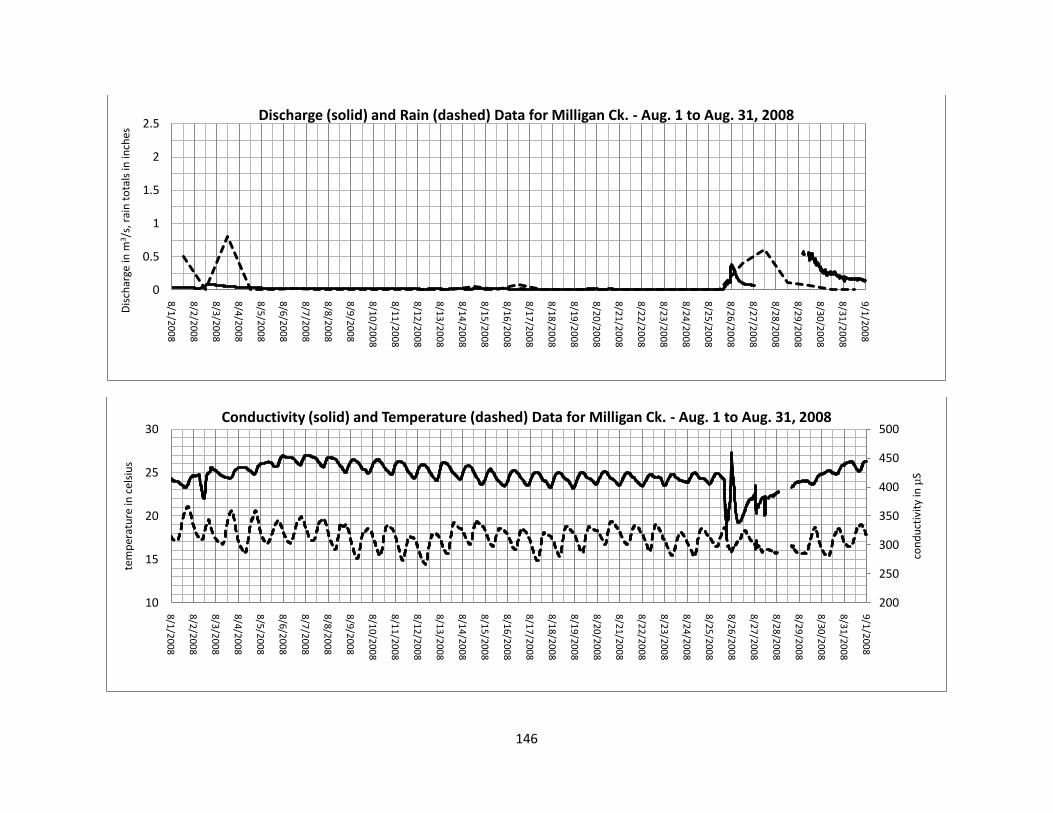
146
0
0.5
1
1.5
2
2.5
8/1
/20
08
8/2
/20
08
8/3
/20
08
8/4
/20
08
8/5
/20
08
8/6
/20
08
8/7
/20
08
8/8
/20
08
8/9
/20
08
8/1
0/2
00
8
8/1
1/2
00
8
8/1
2/2
00
8
8/1
3/2
00
8
8/1
4/2
00
8
8/1
5/2
00
8
8/1
6/2
00
8
8/1
7/2
00
8
8/1
8/2
00
8
8/1
9/2
00
8
8/2
0/2
00
8
8/2
1/2
00
8
8/2
2/2
00
8
8/2
3/2
00
8
8/2
4/2
00
8
8/2
5/2
00
8
8/2
6/2
00
8
8/2
7/2
00
8
8/2
8/2
00
8
8/2
9/2
00
8
8/3
0/2
00
8
8/3
1/2
00
8
9/1
/20
08
Dis
char
ge in
m3 /
s, r
ain
to
tals
in in
ches
Discharge (solid) and Rain (dashed) Data for Milligan Ck. - Aug. 1 to Aug. 31, 2008
200
250
300
350
400
450
500
10
15
20
25
30
8/1
/20
08
8/2
/20
08
8/3
/20
08
8/4
/20
08
8/5
/20
08
8/6
/20
08
8/7
/20
08
8/8
/20
08
8/9
/20
08
8/1
0/2
00
8
8/1
1/2
00
8
8/1
2/2
00
8
8/1
3/2
00
8
8/1
4/2
00
8
8/1
5/2
00
8
8/1
6/2
00
8
8/1
7/2
00
8
8/1
8/2
00
8
8/1
9/2
00
8
8/2
0/2
00
8
8/2
1/2
00
8
8/2
2/2
00
8
8/2
3/2
00
8
8/2
4/2
00
8
8/2
5/2
00
8
8/2
6/2
00
8
8/2
7/2
00
8
8/2
8/2
00
8
8/2
9/2
00
8
8/3
0/2
00
8
8/3
1/2
00
8
9/1
/20
08
con
du
ctiv
ity
in µ
S
tem
per
atu
re in
cel
siu
s
Conductivity (solid) and Temperature (dashed) Data for Milligan Ck. - Aug. 1 to Aug. 31, 2008
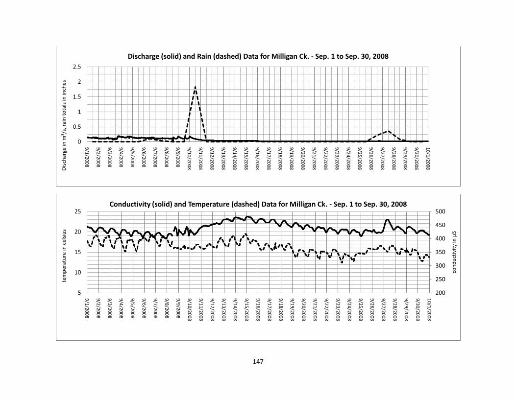
147
0
0.5
1
1.5
2
2.5
9/1
/20
08
9/2
/20
08
9/3
/20
08
9/4
/20
08
9/5
/20
08
9/6
/20
08
9/7
/20
08
9/8
/20
08
9/9
/20
08
9/1
0/2
00
8
9/1
1/2
00
8
9/1
2/2
00
8
9/1
3/2
00
8
9/1
4/2
00
8
9/1
5/2
00
8
9/1
6/2
00
8
9/1
7/2
00
8
9/1
8/2
00
8
9/1
9/2
00
8
9/2
0/2
00
8
9/2
1/2
00
8
9/2
2/2
00
8
9/2
3/2
00
8
9/2
4/2
00
8
9/2
5/2
00
8
9/2
6/2
00
8
9/2
7/2
00
8
9/2
8/2
00
8
9/2
9/2
00
8
9/3
0/2
00
8
10
/1/2
00
8
Dis
char
ge in
m3 /
s, r
ain
to
tals
in in
ches
Discharge (solid) and Rain (dashed) Data for Milligan Ck. - Sep. 1 to Sep. 30, 2008
200
250
300
350
400
450
500
5
10
15
20
25
9/1
/20
08
9/2
/20
08
9/3
/20
08
9/4
/20
08
9/5
/20
08
9/6
/20
08
9/7
/20
08
9/8
/20
08
9/9
/20
08
9/1
0/2
00
8
9/1
1/2
00
8
9/1
2/2
00
8
9/1
3/2
00
8
9/1
4/2
00
8
9/1
5/2
00
8
9/1
6/2
00
8
9/1
7/2
00
8
9/1
8/2
00
8
9/1
9/2
00
8
9/2
0/2
00
8
9/2
1/2
00
8
9/2
2/2
00
8
9/2
3/2
00
8
9/2
4/2
00
8
9/2
5/2
00
8
9/2
6/2
00
8
9/2
7/2
00
8
9/2
8/2
00
8
9/2
9/2
00
8
9/3
0/2
00
8
10
/1/2
00
8
con
du
ctiv
ity
in µ
S
tem
per
atu
re in
cel
siu
s
Conductivity (solid) and Temperature (dashed) Data for Milligan Ck. - Sep. 1 to Sep. 30, 2008
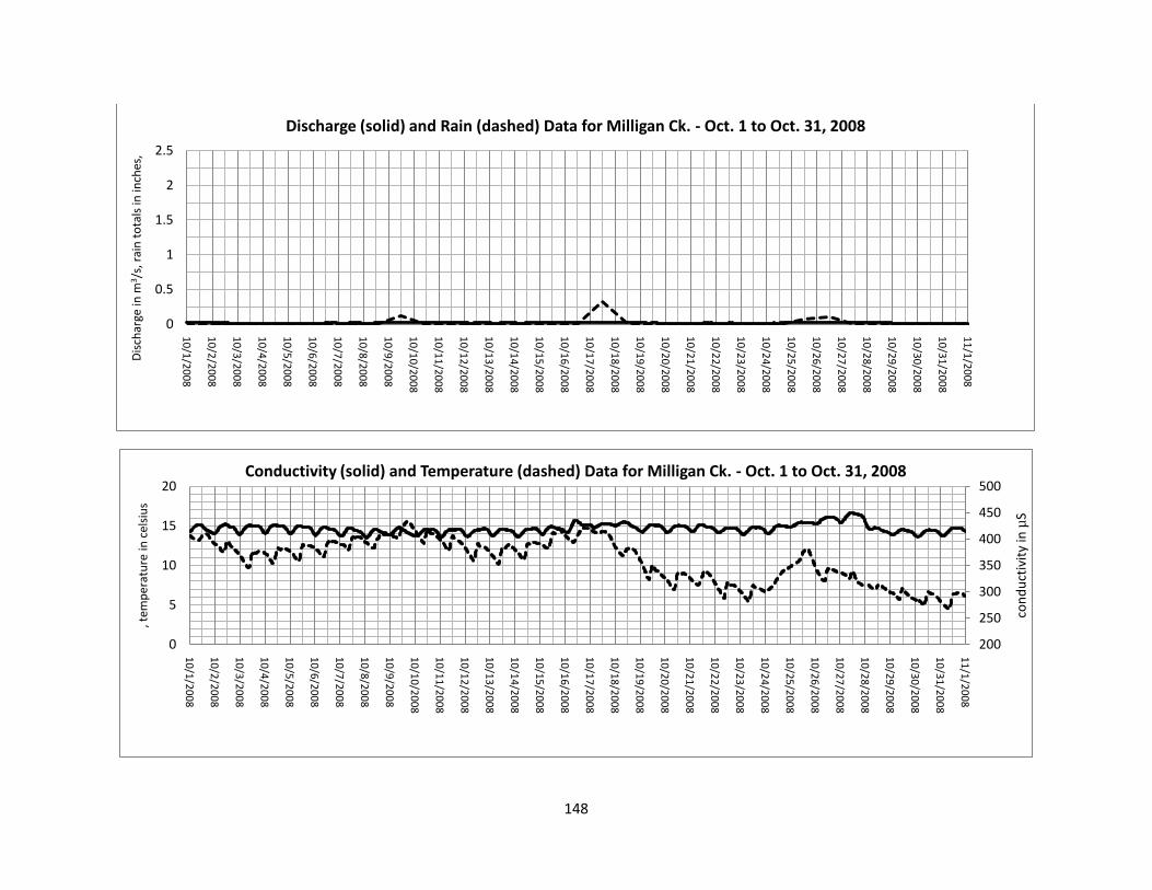
148
0
0.5
1
1.5
2
2.5
10
/1/2
00
8
10
/2/2
00
8
10
/3/2
00
8
10
/4/2
00
8
10
/5/2
00
8
10
/6/2
00
8
10
/7/2
00
8
10
/8/2
00
8
10
/9/2
00
8
10
/10
/20
08
10
/11
/20
08
10
/12
/20
08
10
/13
/20
08
10
/14
/20
08
10
/15
/20
08
10
/16
/20
08
10
/17
/20
08
10
/18
/20
08
10
/19
/20
08
10
/20
/20
08
10
/21
/20
08
10
/22
/20
08
10
/23
/20
08
10
/24
/20
08
10
/25
/20
08
10
/26
/20
08
10
/27
/20
08
10
/28
/20
08
10
/29
/20
08
10
/30
/20
08
10
/31
/20
08
11
/1/2
00
8
Dis
char
ge in
m3 /
s, r
ain
to
tals
in in
ches
, Discharge (solid) and Rain (dashed) Data for Milligan Ck. - Oct. 1 to Oct. 31, 2008
200
250
300
350
400
450
500
0
5
10
15
20
10
/1/2
00
8
10
/2/2
00
8
10
/3/2
00
8
10
/4/2
00
8
10
/5/2
00
8
10
/6/2
00
8
10
/7/2
00
8
10
/8/2
00
8
10
/9/2
00
8
10
/10
/20
08
10
/11
/20
08
10
/12
/20
08
10
/13
/20
08
10
/14
/20
08
10
/15
/20
08
10
/16
/20
08
10
/17
/20
08
10
/18
/20
08
10
/19
/20
08
10
/20
/20
08
10
/21
/20
08
10
/22
/20
08
10
/23
/20
08
10
/24
/20
08
10
/25
/20
08
10
/26
/20
08
10
/27
/20
08
10
/28
/20
08
10
/29
/20
08
10
/30
/20
08
10
/31
/20
08
11
/1/2
00
8
con
du
ctiv
ity
in µ
S
, tem
per
atu
re in
cel
siu
s
Conductivity (solid) and Temperature (dashed) Data for Milligan Ck. - Oct. 1 to Oct. 31, 2008
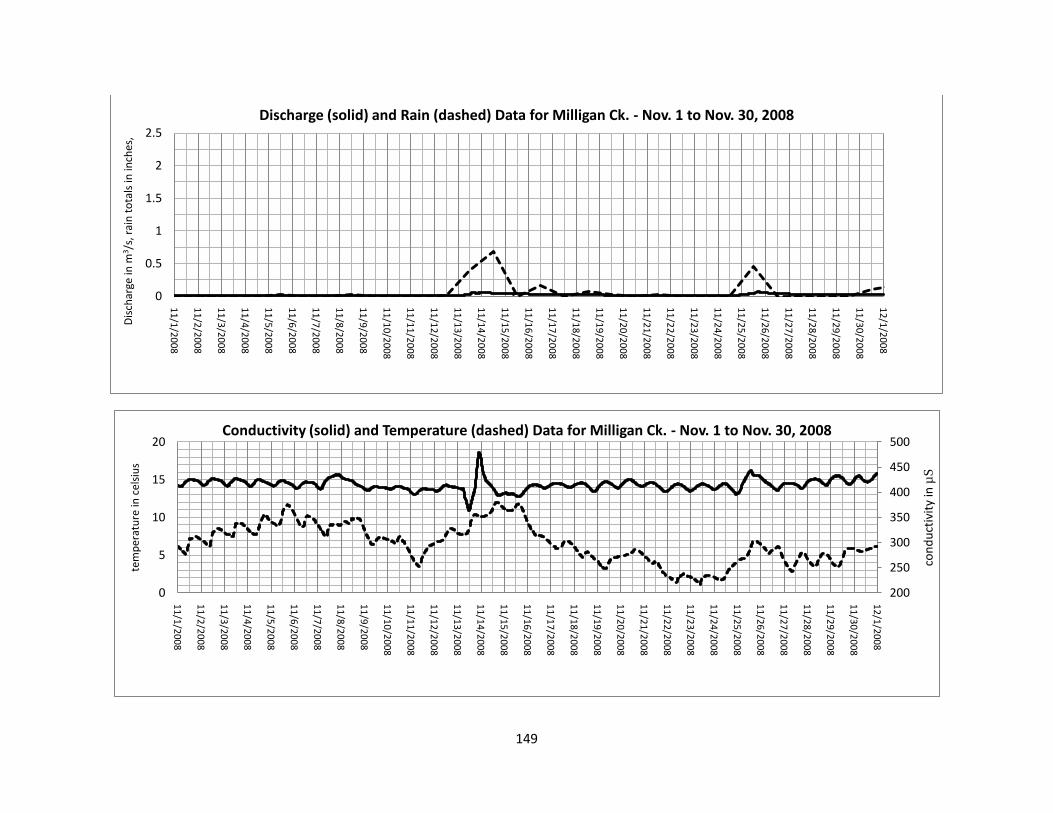
149
0
0.5
1
1.5
2
2.5
11
/1/2
00
8
11
/2/2
00
8
11
/3/2
00
8
11
/4/2
00
8
11
/5/2
00
8
11
/6/2
00
8
11
/7/2
00
8
11
/8/2
00
8
11
/9/2
00
8
11
/10
/20
08
11
/11
/20
08
11
/12
/20
08
11
/13
/20
08
11
/14
/20
08
11
/15
/20
08
11
/16
/20
08
11
/17
/20
08
11
/18
/20
08
11
/19
/20
08
11
/20
/20
08
11
/21
/20
08
11
/22
/20
08
11
/23
/20
08
11
/24
/20
08
11
/25
/20
08
11
/26
/20
08
11
/27
/20
08
11
/28
/20
08
11
/29
/20
08
11
/30
/20
08
12
/1/2
00
8
Dis
char
ge in
m3 /
s, r
ain
to
tals
in in
ches
, Discharge (solid) and Rain (dashed) Data for Milligan Ck. - Nov. 1 to Nov. 30, 2008
200
250
300
350
400
450
500
0
5
10
15
20
11
/1/2
00
8
11
/2/2
00
8
11
/3/2
00
8
11
/4/2
00
8
11
/5/2
00
8
11
/6/2
00
8
11
/7/2
00
8
11
/8/2
00
8
11
/9/2
00
8
11
/10
/20
08
11
/11
/20
08
11
/12
/20
08
11
/13
/20
08
11
/14
/20
08
11
/15
/20
08
11
/16
/20
08
11
/17
/20
08
11
/18
/20
08
11
/19
/20
08
11
/20
/20
08
11
/21
/20
08
11
/22
/20
08
11
/23
/20
08
11
/24
/20
08
11
/25
/20
08
11
/26
/20
08
11
/27
/20
08
11
/28
/20
08
11
/29
/20
08
11
/30
/20
08
12
/1/2
00
8
con
du
ctiv
ity
in µ
S
tem
per
atu
re in
cel
siu
s
Conductivity (solid) and Temperature (dashed) Data for Milligan Ck. - Nov. 1 to Nov. 30, 2008
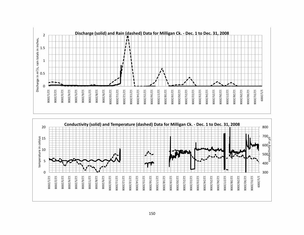
150
0
0.5
1
1.5
2
12
/1/2
00
8
12
/2/2
00
8
12
/3/2
00
8
12
/4/2
00
8
12
/5/2
00
8
12
/6/2
00
8
12
/7/2
00
8
12
/8/2
00
8
12
/9/2
00
8
12
/10
/20
08
12
/11
/20
08
12
/12
/20
08
12
/13
/20
08
12
/14
/20
08
12
/15
/20
08
12
/16
/20
08
12
/17
/20
08
12
/18
/20
08
12
/19
/20
08
12
/20
/20
08
12
/21
/20
08
12
/22
/20
08
12
/23
/20
08
12
/24
/20
08
12
/25
/20
08
12
/26
/20
08
12
/27
/20
08
12
/28
/20
08
12
/29
/20
08
12
/30
/20
08
12
/31
/20
08
1/1
/20
09
Dis
char
ge in
m3 /
s, r
ain
to
tals
in in
ches
, Discharge (solid) and Rain (dashed) Data for Milligan Ck. - Dec. 1 to Dec. 31, 2008
300
400
500
600
700
800
0
5
10
15
20
12
/1/2
00
8
12
/2/2
00
8
12
/3/2
00
8
12
/4/2
00
8
12
/5/2
00
8
12
/6/2
00
8
12
/7/2
00
8
12
/8/2
00
8
12
/9/2
00
8
12
/10
/20
08
12
/11
/20
08
12
/12
/20
08
12
/13
/20
08
12
/14
/20
08
12
/15
/20
08
12
/16
/20
08
12
/17
/20
08
12
/18
/20
08
12
/19
/20
08
12
/20
/20
08
12
/21
/20
08
12
/22
/20
08
12
/23
/20
08
12
/24
/20
08
12
/25
/20
08
12
/26
/20
08
12
/27
/20
08
12
/28
/20
08
12
/29
/20
08
12
/30
/20
08
12
/31
/20
08
1/1
/20
09
con
du
ctiv
ity
in µ
S
tem
per
atu
re in
cel
siu
s
Conductivity (solid) and Temperature (dashed) Data for Milligan Ck. - Dec. 1 to Dec. 31, 2008
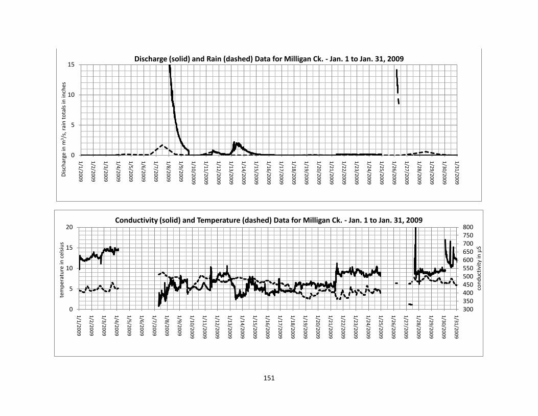
151
0
5
10
15
1/1
/20
09
1/2
/20
09
1/3
/20
09
1/4
/20
09
1/5
/20
09
1/6
/20
09
1/7
/20
09
1/8
/20
09
1/9
/20
09
1/1
0/2
00
9
1/1
1/2
00
9
1/1
2/2
00
9
1/1
3/2
00
9
1/1
4/2
00
9
1/1
5/2
00
9
1/1
6/2
00
9
1/1
7/2
00
9
1/1
8/2
00
9
1/1
9/2
00
9
1/2
0/2
00
9
1/2
1/2
00
9
1/2
2/2
00
9
1/2
3/2
00
9
1/2
4/2
00
9
1/2
5/2
00
9
1/2
6/2
00
9
1/2
7/2
00
9
1/2
8/2
00
9
1/2
9/2
00
9
1/3
0/2
00
9
1/3
1/2
00
9
Dis
char
ge in
m3 /
s, r
ain
to
tals
in in
ches
Discharge (solid) and Rain (dashed) Data for Milligan Ck. - Jan. 1 to Jan. 31, 2009
300350400450500550600650700750800
0
5
10
15
20
1/1
/20
09
1/2
/20
09
1/3
/20
09
1/4
/20
09
1/5
/20
09
1/6
/20
09
1/7
/20
09
1/8
/20
09
1/9
/20
09
1/1
0/2
00
9
1/1
1/2
00
9
1/1
2/2
00
9
1/1
3/2
00
9
1/1
4/2
00
9
1/1
5/2
00
9
1/1
6/2
00
9
1/1
7/2
00
9
1/1
8/2
00
9
1/1
9/2
00
9
1/2
0/2
00
9
1/2
1/2
00
9
1/2
2/2
00
9
1/2
3/2
00
9
1/2
4/2
00
9
1/2
5/2
00
9
1/2
6/2
00
9
1/2
7/2
00
9
1/2
8/2
00
9
1/2
9/2
00
9
1/3
0/2
00
9
1/3
1/2
00
9
con
du
ctiv
ity
in µ
S
tem
per
atu
re in
cel
siu
s
Conductivity (solid) and Temperature (dashed) Data for Milligan Ck. - Jan. 1 to Jan. 31, 2009
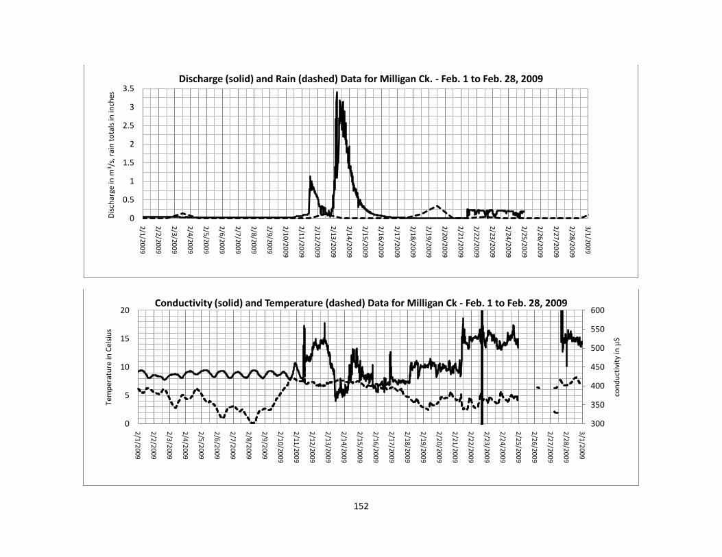
152
0
0.5
1
1.5
2
2.5
3
3.5
2/1
/20
09
2/2
/20
09
2/3
/20
09
2/4
/20
09
2/5
/20
09
2/6
/20
09
2/7
/20
09
2/8
/20
09
2/9
/20
09
2/1
0/2
00
9
2/1
1/2
00
9
2/1
2/2
00
9
2/1
3/2
00
9
2/1
4/2
00
9
2/1
5/2
00
9
2/1
6/2
00
9
2/1
7/2
00
9
2/1
8/2
00
9
2/1
9/2
00
9
2/2
0/2
00
9
2/2
1/2
00
9
2/2
2/2
00
9
2/2
3/2
00
9
2/2
4/2
00
9
2/2
5/2
00
9
2/2
6/2
00
9
2/2
7/2
00
9
2/2
8/2
00
9
3/1
/20
09
Dis
char
ge in
m3/s
, rai
n t
ota
ls in
inch
es
Discharge (solid) and Rain (dashed) Data for Milligan Ck. - Feb. 1 to Feb. 28, 2009
300
350
400
450
500
550
600
0
5
10
15
20
2/1
/20
09
2/2
/20
09
2/3
/20
09
2/4
/20
09
2/5
/20
09
2/6
/20
09
2/7
/20
09
2/8
/20
09
2/9
/20
09
2/1
0/2
00
9
2/1
1/2
00
9
2/1
2/2
00
9
2/1
3/2
00
9
2/1
4/2
00
9
2/1
5/2
00
9
2/1
6/2
00
9
2/1
7/2
00
9
2/1
8/2
00
9
2/1
9/2
00
9
2/2
0/2
00
9
2/2
1/2
00
9
2/2
2/2
00
9
2/2
3/2
00
9
2/2
4/2
00
9
2/2
5/2
00
9
2/2
6/2
00
9
2/2
7/2
00
9
2/2
8/2
00
9
3/1
/20
09
con
du
ctiv
ity
in µ
S
Tem
per
atu
re in
Cel
siu
s
Conductivity (solid) and Temperature (dashed) Data for Milligan Ck - Feb. 1 to Feb. 28, 2009
153
12 Appendix C – Chemistry Data for September 2008
Cation and anion data were collected for two weeks in September (from September 9th to
September 23rd, inclusive). The automatic sampler at Davis Spring sampled every six hours for
fluorescein and rhodamine. These samples were also processed through the USDA’s Dionex 600 Ion
Chromatography System with the Dionex EG40 Eluent Generator to ascertain the levels of major cations
and anions. Results were reported as parts per million (ppm). Bicarbonate was not reported by the Ion
Chromatographer.
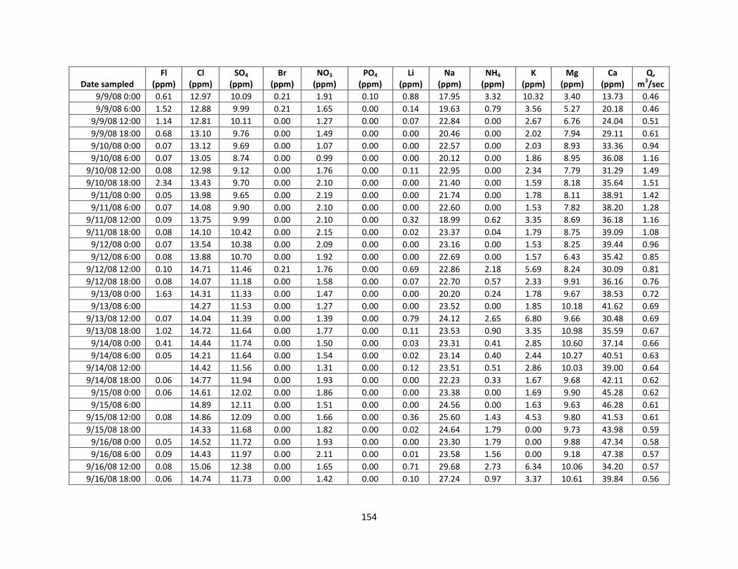
154
Date sampled Fl
(ppm) Cl
(ppm) SO4
(ppm) Br
(ppm) NO3
(ppm) PO4
(ppm) Li
(ppm) Na
(ppm) NH4
(ppm) K
(ppm) Mg
(ppm) Ca
(ppm) Q,
m3/sec
9/9/08 0:00 0.61 12.97 10.09 0.21 1.91 0.10 0.88 17.95 3.32 10.32 3.40 13.73 0.46
9/9/08 6:00 1.52 12.88 9.99 0.21 1.65 0.00 0.14 19.63 0.79 3.56 5.27 20.18 0.46
9/9/08 12:00 1.14 12.81 10.11 0.00 1.27 0.00 0.07 22.84 0.00 2.67 6.76 24.04 0.51
9/9/08 18:00 0.68 13.10 9.76 0.00 1.49 0.00 0.00 20.46 0.00 2.02 7.94 29.11 0.61
9/10/08 0:00 0.07 13.12 9.69 0.00 1.07 0.00 0.00 22.57 0.00 2.03 8.93 33.36 0.94
9/10/08 6:00 0.07 13.05 8.74 0.00 0.99 0.00 0.00 20.12 0.00 1.86 8.95 36.08 1.16
9/10/08 12:00 0.08 12.98 9.12 0.00 1.76 0.00 0.11 22.95 0.00 2.34 7.79 31.29 1.49
9/10/08 18:00 2.34 13.43 9.70 0.00 2.10 0.00 0.00 21.40 0.00 1.59 8.18 35.64 1.51
9/11/08 0:00 0.05 13.98 9.65 0.00 2.19 0.00 0.00 21.74 0.00 1.78 8.11 38.91 1.42
9/11/08 6:00 0.07 14.08 9.90 0.00 2.10 0.00 0.00 22.60 0.00 1.53 7.82 38.20 1.28
9/11/08 12:00 0.09 13.75 9.99 0.00 2.10 0.00 0.32 18.99 0.62 3.35 8.69 36.18 1.16
9/11/08 18:00 0.08 14.10 10.42 0.00 2.15 0.00 0.02 23.37 0.04 1.79 8.75 39.09 1.08
9/12/08 0:00 0.07 13.54 10.38 0.00 2.09 0.00 0.00 23.16 0.00 1.53 8.25 39.44 0.96
9/12/08 6:00 0.08 13.88 10.70 0.00 1.92 0.00 0.00 22.69 0.00 1.57 6.43 35.42 0.85
9/12/08 12:00 0.10 14.71 11.46 0.21 1.76 0.00 0.69 22.86 2.18 5.69 8.24 30.09 0.81
9/12/08 18:00 0.08 14.07 11.18 0.00 1.58 0.00 0.07 22.70 0.57 2.33 9.91 36.16 0.76
9/13/08 0:00 1.63 14.31 11.33 0.00 1.47 0.00 0.00 20.20 0.24 1.78 9.67 38.53 0.72
9/13/08 6:00 14.27 11.53 0.00 1.27 0.00 0.00 23.52 0.00 1.85 10.18 41.62 0.69
9/13/08 12:00 0.07 14.04 11.39 0.00 1.39 0.00 0.79 24.12 2.65 6.80 9.66 30.48 0.69
9/13/08 18:00 1.02 14.72 11.64 0.00 1.77 0.00 0.11 23.53 0.90 3.35 10.98 35.59 0.67
9/14/08 0:00 0.41 14.44 11.74 0.00 1.50 0.00 0.03 23.31 0.41 2.85 10.60 37.14 0.66
9/14/08 6:00 0.05 14.21 11.64 0.00 1.54 0.00 0.02 23.14 0.40 2.44 10.27 40.51 0.63
9/14/08 12:00 14.42 11.56 0.00 1.31 0.00 0.12 23.51 0.51 2.86 10.03 39.00 0.64
9/14/08 18:00 0.06 14.77 11.94 0.00 1.93 0.00 0.00 22.23 0.33 1.67 9.68 42.11 0.62
9/15/08 0:00 0.06 14.61 12.02 0.00 1.86 0.00 0.00 23.38 0.00 1.69 9.90 45.28 0.62
9/15/08 6:00 14.89 12.11 0.00 1.51 0.00 0.00 24.56 0.00 1.63 9.63 46.28 0.61
9/15/08 12:00 0.08 14.86 12.09 0.00 1.66 0.00 0.36 25.60 1.43 4.53 9.80 41.53 0.61
9/15/08 18:00 14.33 11.68 0.00 1.82 0.00 0.02 24.64 1.79 0.00 9.73 43.98 0.59
9/16/08 0:00 0.05 14.52 11.72 0.00 1.93 0.00 0.00 23.30 1.79 0.00 9.88 47.34 0.58
9/16/08 6:00 0.09 14.43 11.97 0.00 2.11 0.00 0.01 23.58 1.56 0.00 9.18 47.38 0.57
9/16/08 12:00 0.08 15.06 12.38 0.00 1.65 0.00 0.71 29.68 2.73 6.34 10.06 34.20 0.57
9/16/08 18:00 0.06 14.74 11.73 0.00 1.42 0.00 0.10 27.24 0.97 3.37 10.61 39.84 0.56

155
Date sampled Fl
(ppm) Cl
(ppm) SO4
(ppm) Br
(ppm) NO3
(ppm) PO4
(ppm) Li
(ppm) Na
(ppm) NH4
(ppm) K
(ppm) Mg
(ppm) Ca
(ppm) Q,
m3/sec
9/17/08 0:00 15.38 12.12 0.00 1.70 0.00 25.75 0.45 2.59 10.74 43.51 0.55
9/17/08 6:00 0.06 14.90 11.95 0.00 1.45 0.00 0.54
9/17/08 12:00 14.70 11.62 0.00 1.55 0.00 0.55
9/17/08 18:00 0.07 14.48 11.40 0.00 1.92 0.00 0.53
9/18/08 0:00 0.07 15.00 11.78 0.00 2.25 0.00 0.52
9/18/08 6:00 0.08 14.96 11.78 0.00 2.05 0.00 0.52
9/18/08 12:00 0.14 13.71 10.09 0.14 1.90 0.00 0.73 17.07 1.98 5.31 7.94 27.24 0.53
9/18/08 18:00 0.10 13.91 10.29 0.00 2.04 0.00 0.50
9/19/08 0:00 0.07 13.38 9.97 0.00 1.79 0.00 0.00 22.13 15.88 2.67 5.33 21.79 0.50
9/19/08 6:00 0.11 13.61 9.91 0.00 2.06 0.00 0.00 19.87 0.99 1.17 3.51 17.94 0.49
9/19/08 12:00 0.08 13.93 10.03 0.00 1.83 0.00 0.00 22.97 0.06 1.16 5.24 23.76 0.51
9/19/08 18:00 0.09 13.39 9.59 0.00 1.72 0.00 0.00 20.56 0.26 1.06 6.34 29.00 0.49
9/20/08 0:00 0.08 13.38 9.54 0.00 1.98 0.00 0.08 21.58 0.62 1.79 6.35 30.13 0.49
9/20/08 6:00 0.09 13.84 9.90 0.00 2.10 0.00 0.00 22.77 0.00 1.09 7.64 36.12 0.48
9/20/08 12:00 0.07 13.42 9.46 0.00 1.83 0.00 0.00 20.44 0.00 1.04 7.41 38.51 0.50
9/20/08 18:00 0.08 13.68 9.25 0.00 1.73 0.00 0.00 22.14 0.00 1.06 7.33 40.91 0.48
9/21/08 0:00 0.07 14.01 9.84 0.00 2.10 0.00 0.31 24.06 1.01 3.12 7.76 36.48 0.48
9/21/08 6:00 0.09 14.09 9.66 0.00 2.15 0.00 0.00 22.27 0.00 1.28 8.39 41.45 0.48
9/21/08 12:00 0.10 14.24 9.90 0.00 1.94 0.00 0.00 22.09 0.28 1.24 8.07 43.27 0.49
9/21/08 18:00 0.06 13.42 9.33 0.00 1.98 0.00 0.00 21.72 0.00 1.00 7.32 40.79 0.47
9/22/08 0:00 0.12 14.84 10.11 0.00 2.24 0.00 0.71 23.33 2.15 4.73 8.41 31.95 0.47
9/22/08 6:00 0.07 14.32 9.98 0.00 2.06 0.00 0.15 23.03 2.23 3.68 5.95 25.98 0.46
9/22/08 12:00 0.10 15.02 9.39 0.00 2.02 0.00 0.00 22.06 0.00 1.31 8.41 33.40 0.48
9/22/08 18:00 0.09 14.61 9.48 0.00 1.76 0.00 0.45
9/23/08 0:00 0.08 14.51 9.32 0.00 2.11 0.00 0.45
9/23/08 6:00 0.05 14.16 9.36 0.00 2.15 0.00 0.00 20.96 0.68 0.95 3.53 20.32 0.45
9/23/08 12:00 0.07 14.28 9.30 0.00 2.00 0.00 0.00 20.68 0.35 0.94 4.08 22.79 0.46
9/23/08 18:00 0.07 14.16 9.09 0.00 1.87 0.00 0.00 22.66 0.39 0.96 5.46 27.42 0.44

156
Vita
Name: John Kazimierz Tudek, Jr.
Parents: John Kazimierz Tudek Sr.
Janice Marie Kilgallon
Date of Birth: September 8, 1972
Place of Birth: Passaic, NJ
Schools Attended
St. John Kanty Elementary School, Clifton, NJ 1977-1986
St. Peter's Preparatory School, Jersey City, NJ 1986-1990
Jersey City State College, Jersey City, NJ 1990-1992
Montclair State College, Montclair NJ 1992
The Chubb Institute, Paramus, NJ 1994-1995
Degrees Received:
Certificate in Computer Programming May 1995
Rutgers University, Newark NJ 1998-2004
Degrees Received:
B.A., English May 2004

157
Approval of the Examining Committee
Dr. Douglas Boyer, Ph.D.
Dr. Dorothy Vesper, Ph.D.
Dr. Henry Rauch, Ph.D., Chair
Related Documents