Fundamentals of Wireless Communication The past decade has seen many advances in physical-layer wireless communi- cation theory and their implementation in wireless systems. This textbook takes a unified view of the fundamentals of wireless communication and explains the web of concepts underpinning these advances at a level accessible to an audience with a basic background in probability and digital communication. Topics covered include MIMO (multiple input multiple output) communication, space-time coding, opportunistic communication, OFDM and CDMA. The concepts are illustrated using many examples from wireless systems such as GSM, IS-95 (CDMA), IS-856 (1× EV-DO), Flash OFDM and ArrayComm SDMA systems. Particular emphasis is placed on the interplay between concepts and their implementation in systems. An abundant supply of exercises and figures reinforce the material in the text. This book is intended for use on graduate courses in electrical and computer engineering and will also be of great interest to practicing engineers. David Tse is a professor at the Department of Electrical Engineering and Computer Sciences, University of California at Berkeley. Pramod Viswanath is an assistant professor at the Department of Electrical and Computer Engineering, University of Illinois at Urbana-Champaign.

Welcome message from author
This document is posted to help you gain knowledge. Please leave a comment to let me know what you think about it! Share it to your friends and learn new things together.
Transcript
Fundamentals of Wireless Communication
The past decade has seen many advances in physical-layer wireless communi-cation theory and their implementation in wireless systems. This textbook takesa unified view of the fundamentals of wireless communication and explainsthe web of concepts underpinning these advances at a level accessible to anaudience with a basic background in probability and digital communication.Topics covered includeMIMO(multiple inputmultiple output) communication,space-time coding, opportunistic communication, OFDM and CDMA. Theconcepts are illustrated using many examples from wireless systems such asGSM, IS-95 (CDMA), IS-856 (1× EV-DO), Flash OFDM and ArrayCommSDMA systems. Particular emphasis is placed on the interplay betweenconcepts and their implementation in systems. An abundant supply of exercisesand figures reinforce the material in the text. This book is intended for use ongraduate courses in electrical and computer engineering andwill also be of greatinterest to practicing engineers.
David Tse is a professor at the Department of Electrical Engineering andComputer Sciences, University of California at Berkeley.
Pramod Viswanath is an assistant professor at the Department of Electricaland Computer Engineering, University of Illinois at Urbana-Champaign.

Fundamentals ofWireless Communication
David TseUniversity of California, Berkeley
and
Pramod ViswanathUniversity of Illinois, Urbana-Champaign

c a m b r i d g e u n i v e r s i t y p r e s s
Cambridge, New York, Melbourne, Madrid, Cape Town, Singapore, São Paulo
c a m b r i d g e u n i v e r s i t y p r e s s
The Edinburgh Building, Cambridge CB2 2RU, UK
Published in the United States of America by Cambridge University Press, New York
www.cambridge.orgInformation on this title: www.cambridge.org/9780521845274
© Cambridge University Press 2005
This book is in copyright. Subject to statutory exceptionand to the provisions of relevant collective licensing agreements,no reproduction of any part may take place withoutthe written permission of Cambridge University Press.
First published 2005
Printed in the United Kingdom at the University Press, Cambridge
A catalog record for this book is available from the British Library
ISBN-13 978-0-521-84527-4 hardbackISBN-10 0-521-84527-0 hardback
Cambridge University Press has no responsibility for the persistence or accuracy of URLs forexternal or third-party internet websites referred to in this book, and does not guarantee that anycontent on such websites is, or will remain, accurate or appropriate.

To my familyDT
To my parents and to SumaPV


Contents
Preface page xvAcknowledgements xviiiList of notation xx
1 Introduction 11.1 Book objective 11.2 Wireless systems 21.3 Book outline 5
2 The wireless channel 102.1 Physical modeling for wireless channels 10
2.1.1 Free space, fixed transmit and receive antennas 122.1.2 Free space, moving antenna 132.1.3 Reflecting wall, fixed antenna 142.1.4 Reflecting wall, moving antenna 162.1.5 Reflection from a ground plane 172.1.6 Power decay with distance and shadowing 182.1.7 Moving antenna, multiple reflectors 192.2 Input /output model of the wireless channel 20
2.2.1 The wireless channel as a linear time-varying system 202.2.2 Baseband equivalent model 222.2.3 A discrete-time baseband model 25
Discussion 2.1 Degrees of freedom 282.2.4 Additive white noise 292.3 Time and frequency coherence 30
2.3.1 Doppler spread and coherence time 302.3.2 Delay spread and coherence bandwidth 312.4 Statistical channel models 34
2.4.1 Modeling philosophy 342.4.2 Rayleigh and Rician fading 36
vii

viii Contents
2.4.3 Tap gain auto-correlation function 37Example 2.2 Clarke’s model 38Chapter 2 The main plot 40
2.5 Bibliographical notes 422.6 Exercises 42
3 Point-to-point communication: detection, diversityand channel uncertainity 49
3.1 Detection in a Rayleigh fading channel 503.1.1 Non-coherent detection 503.1.2 Coherent detection 523.1.3 From BPSK to QPSK: exploiting the degrees
of freedom 563.1.4 Diversity 593.2 Time diversity 60
3.2.1 Repetition coding 603.2.2 Beyond repetition coding 64
Summary 3.1 Time diversity code design criterion 68Example 3.1 Time diversity in GSM 69
3.3 Antenna diversity 713.3.1 Receive diversity 713.3.2 Transmit diversity: space-time codes 733.3.3 MIMO: a 2×2 example 77
Summary 3.2 2×2 MIMO schemes 823.4 Frequency diversity 83
3.4.1 Basic concept 833.4.2 Single-carrier with ISI equalization 843.4.3 Direct-sequence spread-spectrum 913.4.4 Orthogonal frequency division multiplexing 95
Summary 3.3 Communication over frequency-selective channels 1013.5 Impact of channel uncertainty 102
3.5.1 Non-coherent detection for DS spread-spectrum 1033.5.2 Channel estimation 1053.5.3 Other diversity scenarios 107
Chapter 3 The main plot 1093.6 Bibliographical notes 1103.7 Exercises 111
4 Cellular systems: multiple access and interference management 1204.1 Introduction 1204.2 Narrowband cellular systems 123
4.2.1 Narrowband allocations: GSM system 1244.2.2 Impact on network and system design 126

ix Contents
4.2.3 Impact on frequency reuse 127Summary 4.1 Narrowband systems 128
4.3 Wideband systems: CDMA 1284.3.1 CDMA uplink 1314.3.2 CDMA downlink 1454.3.3 System issues 147
Summary 4.2 CDMA 1474.4 Wideband systems: OFDM 148
4.4.1 Allocation design principles 1484.4.2 Hopping pattern 1504.4.3 Signal characteristics and receiver design 1524.4.4 Sectorization 153
Example 4.1 Flash-OFDM 153Chapter 4 The main plot 154
4.5 Bibliographical notes 1554.6 Exercises 155
5 Capacity of wireless channels 1665.1 AWGN channel capacity 167
5.1.1 Repetition coding 1675.1.2 Packing spheres 168
Discussion 5.1 Capacity-achieving AWGNchannel codes 170Summary 5.1 Reliable rate of communicationand capacity 171
5.2 Resources of the AWGN channel 1725.2.1 Continuous-time AWGN channel 1725.2.2 Power and bandwidth 173
Example 5.2 Bandwidth reuse in cellular systems 1755.3 Linear time-invariant Gaussian channels 179
5.3.1 Single input multiple output (SIMO) channel 1795.3.2 Multiple input single output (MISO) channel 1795.3.3 Frequency-selective channel 1815.4 Capacity of fading channels 186
5.4.1 Slow fading channel 1875.4.2 Receive diversity 1895.4.3 Transmit diversity 191
Summary 5.2 Transmit and recieve diversity 1955.4.4 Time and frequency diversity 195
Summary 5.3 Outage for parallel channels 1995.4.5 Fast fading channel 1995.4.6 Transmitter side information 203
Example 5.3 Rate adaptation in IS-856 2095.4.7 Frequency-selective fading channels 213

x Contents
5.4.8 Summary: a shift in point of view 213Chapter 5 The main plot 214
5.5 Bibliographical notes 2175.6 Exercises 217
6 Multiuser capacity and opportunistic communication 2286.1 Uplink AWGN channel 229
6.1.1 Capacity via successive interference cancellation 2296.1.2 Comparison with conventional CDMA 2326.1.3 Comparison with orthogonal multiple access 2326.1.4 General K-user uplink capacity 2346.2 Downlink AWGN channel 235
6.2.1 Symmetric case: two capacity-achieving schemes 2366.2.2 General case: superposition coding achieves capacity 238
Summary 6.1 Uplink and downlink AWGN capacity 240Discussion 6.1 SIC: implementation issues 241
6.3 Uplink fading channel 2436.3.1 Slow fading channel 2436.3.2 Fast fading channel 2456.3.3 Full channel side information 247
Summary 6.2 Uplink fading channel 2506.4 Downlink fading channel 250
6.4.1 Channel side information at receiver only 2506.4.2 Full channel side information 2516.5 Frequency-selective fading channels 2526.6 Multiuser diversity 253
6.6.1 Multiuser diversity gain 2536.6.2 Multiuser versus classical diversity 2566.7 Multiuser diversity: system aspects 256
6.7.1 Fair scheduling and multiuser diversity 2586.7.2 Channel prediction and feedback 2626.7.3 Opportunistic beamforming using dumb antennas 2636.7.4 Multiuser diversity in multicell systems 2706.7.5 A system view 272
Chapter 6 The main plot 2756.8 Bibliographical notes 2776.9 Exercises 278
7 MIMO I: spatial multiplexing and channel modeling 2907.1 Multiplexing capability of deterministic MIMO channels 291
7.1.1 Capacity via singular value decomposition 2917.1.2 Rank and condition number 294

xi Contents
7.2 Physical modeling of MIMO channels 2957.2.1 Line-of-sight SIMO channel 2967.2.2 Line-of-sight MISO channel 2987.2.3 Antenna arrays with only a line-of-sight path 2997.2.4 Geographically separated antennas 3007.2.5 Line-of-sight plus one reflected path 306
Summary 7.1 Multiplexing capability of MIMO channels 3097.3 Modeling of MIMO fading channels 309
7.3.1 Basic approach 3097.3.2 MIMO multipath channel 3117.3.3 Angular domain representation of signals 3117.3.4 Angular domain representation of MIMO channels 3157.3.5 Statistical modeling in the angular domain 3177.3.6 Degrees of freedom and diversity 318
Example 7.1 Degrees of freedom in clusteredresponse models 319
7.3.7 Dependency on antenna spacing 3237.3.8 I.i.d. Rayleigh fading model 327
Chapter 7 The main plot 3287.4 Bibliographical notes 3297.5 Exercises 330
8 MIMO II: capacity and multiplexing architectures 3328.1 The V-BLAST architecture 3338.2 Fast fading MIMO channel 335
8.2.1 Capacity with CSI at receiver 3368.2.2 Performance gains 3388.2.3 Full CSI 346
Summary 8.1 Performance gains in a MIMO channel 3488.3 Receiver architectures 348
8.3.1 Linear decorrelator 3498.3.2 Successive cancellation 3558.3.3 Linear MMSE receiver 3568.3.4 Information theoretic optimality 362
Discussion 8.1 Connections with CDMA multiuser detectionand ISI equalization 364
8.4 Slow fading MIMO channel 3668.5 D-BLAST: an outage-optimal architecture 368
8.5.1 Suboptimality of V-BLAST 3688.5.2 Coding across transmit antennas: D-BLAST 3718.5.3 Discussion 372
Chapter 8 The main plot 3738.6 Bibliographical notes 3748.7 Exercises 374

xii Contents
9 MIMO III: diversity–multiplexing tradeoff and universalspace-time codes 383
9.1 Diversity–multiplexing tradeoff 3849.1.1 Formulation 3849.1.2 Scalar Rayleigh channel 3869.1.3 Parallel Rayleigh channel 3909.1.4 MISO Rayleigh channel 3919.1.5 2×2 MIMO Rayleigh channel 3929.1.6 nt ×nr MIMO i.i.d. Rayleigh channel 3959.2 Universal code design for optimal diversity–multiplexing
tradeoff 3989.2.1 QAM is approximately universal for scalar channels 398
Summary 9.1 Approximate universality 4009.2.2 Universal code design for parallel channels 400
Summary 9.2 Universal codes for the parallel channel 4069.2.3 Universal code design for MISO channels 407
Summary 9.3 Universal codes for the MISO channel 4109.2.4 Universal code design for MIMO channels 411
Discussion 9.1 Universal codes in the downlink 415Chapter 9 The main plot 415
9.3 Bibliographical notes 4169.4 Exercises 417
10 MIMO IV: multiuser communication 42510.1 Uplink with multiple receive antennas 426
10.1.1 Space-division multiple access 42610.1.2 SDMA capacity region 42810.1.3 System implications 431
Summary 10.1 SDMA and orthogonal multiple access 43210.1.4 Slow fading 43310.1.5 Fast fading 43610.1.6 Multiuser diversity revisited 439
Summary 10.2 Opportunistic communication and multiplereceive antennas 442
10.2 MIMO uplink 44210.2.1 SDMA with multiple transmit antennas 44210.2.2 System implications 44410.2.3 Fast fading 44610.3 Downlink with multiple transmit antennas 448
10.3.1 Degrees of freedom in the downlink 44810.3.2 Uplink–downlink duality and transmit beamforming 44910.3.3 Precoding for interference known at transmitter 45410.3.4 Precoding for the downlink 46510.3.5 Fast fading 468

xiii Contents
10.4 MIMO downlink 47110.5 Multiple antennas in cellular networks: a system view 473
Summary 10.3 System implications of multiple antennas onmultiple access 473
10.5.1 Inter-cell interference management 47410.5.2 Uplink with multiple receive antennas 47610.5.3 MIMO uplink 47810.5.4 Downlink with multiple receive antennas 47910.5.5 Downlink with multiple transmit antennas 479
Example 10.1 SDMA in ArrayComm systems 479Chapter 10 The main plot 481
10.6 Bibliographical notes 48210.7 Exercises 483
Appendix A Detection and estimation in additive Gaussian noise 496A.1 Gaussian random variables 496
A.1.1 Scalar real Gaussian random variables 496A.1.2 Real Gaussian random vectors 497A.1.3 Complex Gaussian random vectors 500
Summary A.1 Complex Gaussian random vectors 502A.2 Detection in Gaussian noise 503
A.2.1 Scalar detection 503A.2.2 Detection in a vector space 504A.2.3 Detection in a complex vector space 507
Summary A.2 Vector detection in complex Gaussian noise 508A.3 Estimation in Gaussian noise 509
A.3.1 Scalar estimation 509A.3.2 Estimation in a vector space 510A.3.3 Estimation in a complex vector space 511
Summary A.3 Mean square estimation in a complex vector space 513A.4 Exercises 513
Appendix B Information theory from first principles 516B.1 Discrete memoryless channels 516
Example B.1 Binary symmetric channel 517Example B.2 Binary erasure channel 517
B.2 Entropy, conditional entropy and mutual information 518Example B.3 Binary entropy 518
B.3 Noisy channel coding theorem 521B.3.1 Reliable communication and conditional entropy 521B.3.2 A simple upper bound 522B.3.3 Achieving the upper bound 523
Example B.4 Binary symmetric channel 524Example B.5 Binary erasure channel 525
B.3.4 Operational interpretation 525

xiv Contents
B.4 Formal derivation of AWGN capacity 526B.4.1 Analog memoryless channels 526B.4.2 Derivation of AWGN capacity 527B.5 Sphere-packing interpretation 529
B.5.1 Upper bound 529B.5.2 Achievability 530B.6 Time-invariant parallel channel 532B.7 Capacity of the fast fading channel 533
B.7.1 Scalar fast fading channnel 533B.7.2 Fast fading MIMO channel 535B.8 Outage formulation 536B.9 Multiple access channel 538
B.9.1 Capacity region 538B.9.2 Corner points of the capacity region 539B.9.3 Fast fading uplink 540B.10 Exercises 541
References 546Index 554

Preface
Why we wrote this book
The writing of this book was prompted by two main developments in wirelesscommunication in the past decade. First is the huge surge of research activitiesin physical-layer wireless communication theory. While this has been a subjectof study since the sixties, recent developments such as opportunistic and mul-tiple input multiple output (MIMO) communication techniques have broughtcompletely new perspectives on how to communicate over wireless channels.Second is the rapid evolution of wireless systems, particularly cellular net-works, which embody communication concepts of increasing sophistication.This evolution started with second-generation digital standards, particularlythe IS-95 Code Division Multiple Access standard, continuing to more recentthird-generation systems focusing on data applications. This book aims topresent modern wireless communication concepts in a coherent and unifiedmanner and to illustrate the concepts in the broader context of the wirelesssystems on which they have been applied.
Structure of the book
This book is a web of interlocking concepts. The concepts can be structuredroughly into three levels:
1. channel characteristics and modeling;2. communication concepts and techniques;3. application of these concepts in a system context.
A wireless communication engineer should have an understanding of theconcepts at all three levels as well as the tight interplay between the levels.We emphasize this interplay in the book by interlacing the chapters acrossthese levels rather than presenting the topics sequentially from one level tothe next.
xv

xvi Preface
• Chapter 2: basic properties of multipath wireless channels and their mod-eling (level 1).
• Chapter 3: point-to-point communication techniques that increase reliabilityby exploiting time, frequency and spatial diversity (2).
• Chapter 4: cellular system design via a case study of three systems, focusingon multiple access and interference management issues (3).
• Chapter 5: point-to-point communication revisited from a more fundamentalcapacity point of view, culminating in the modern concept of opportunisticcommunication (2).
• Chapter 6: multiuser capacity and opportunistic communication, and itsapplication in a third-generation wireless data system (3).
• Chapter 7: MIMO channel modeling (1).• Chapter 8: MIMO capacity and architectures (2).• Chapter 9: diversity–multiplexing tradeoff and space-time code design (2).• Chapter 10: MIMO in multiuser channels and cellular systems (3).
How to use this book
This book is written as a textbook for a first-year graduate course in wirelesscommunication. The expected background is solid undergraduate/beginninggraduate courses in signals and systems, probability and digital communica-tion. This background is supplemented by the two appendices in the book.Appendix A summarizes some basic facts in vector detection and estimationin Gaussian noise which are used repeatedly throughout the book. Appendix Bcovers the underlying information theory behind the channel capacity resultsused in this book. Even though information theory has played a significantrole in many of the recent developments in wireless communication, in themain text we only introduce capacity results in a heuristic manner and usethem mainly to motivate communication concepts and techniques. No back-ground in information theory is assumed. The appendix is intended for thereader who wants to have a more in-depth and unified understanding of thecapacity results.At Berkeley and Urbana-Champaign, we have used earlier versions of this
book to teach one-semester (15 weeks) wireless communication courses. Wehave been able to cover most of the materials in Chapters 1 through 8 andparts of 9 and 10. Depending on the background of the students and the timeavailable, one can envision several other ways to structure a course aroundthis book. Examples:
• A senior level advanced undergraduate course in wireless communication:Chapters 2, 3, 4.
• An advanced graduate course for students with background in wirelesschannels and systems: Chapters 3, 5, 6, 7, 8, 9, 10.

xvii Preface
• A short (quarter) course focusing on MIMO and space-time coding: Chap-ters 3, 5, 7, 8, 9.
The more than 230 exercises form an integral part of the book. Working onat least some of them is essential in understanding the material. Most of themelaborate on concepts discussed in the main text. The exercises range fromrelatively straightforward derivations of results in the main text, to “back-of-envelope” calculations for actual wireless systems, to “get-your-hands-dirty” MATLAB types, and to reading exercises that point to current researchliterature. The small bibliographical notes at the end of each chapter providepointers to literature that is very closely related to the material discussed inthe book; we do not aim to exhaust the immense research literature related tothe material covered here.

Acknowledgements
We would like first to thank the students in our research groups for the selflesshelp they provided. In particular, many thanks to: Sanket Dusad, Raúl Etkinand Lenny Grokop, who between them painstakingly produced most of thefigures in the book; Aleksandar Jovicic, who drew quite a few figures andproofread some chapters; Ada Poon whose research shaped significantly thematerial in Chapter 7 and who drew several figures in that chapter as wellas in Chapter 2; Saurabha Tavildar and Lizhong Zheng whose research ledto Chapter 9; Tie Liu and Vinod Prabhakaran for their help in clarifying andimproving the presentation of Costa precoding in Chapter 10.Several researchers read drafts of the book carefully and provided us
with very useful comments on various chapters of the book: thanks to StarkDraper, Atilla Eryilmaz, Irem Koprulu, Dana Porrat and Pascal Vontobel.This book has also benefited immensely from critical comments from stu-dents who have taken our wireless communication courses at Berkeley andUrbana-Champaign. In particular, sincere thanks to Amir Salman Avestimehr,Alex Dimakis, Krishnan Eswaran, Jana van Greunen, Nils Hoven, ShridharMubaraq Mishra, Jonathan Tsao, Aaron Wagner, Hua Wang, Xinzhou Wuand Xue Yang.Earlier drafts of this book have been used in teaching courses at several
universities: Cornell, ETHZ, MIT, Northwestern and University of Coloradoat Boulder. We would like to thank the instructors for their feedback: HelmutBölcskei, Anna Scaglione, Mahesh Varanasi, Gregory Wornell and LizhongZheng. We would like to thank Ateet Kapur, Christian Peel and Ulrich Schus-ter from Helmut’s group for their very useful feedback. Thanks are also dueto Mitchell Trott for explaining to us how the ArrayComm systems work.This book contains the results of many researchers, but it owes an intellec-
tual debt to two individuals in particular. Bob Gallager’s research and teachingstyle have greatly inspired our writing of this book. He has taught us thatgood theory, by providing a unified and conceptually simple understandingof a morass of results, should shrink rather than grow the knowledge tree.This book is an attempt to implement this dictum. Our many discussions with
xviii

xix Acknowledgements
Rajiv Laroia have significantly influenced our view of the system aspects ofwireless communication. Several of his ideas have found their way into the“system view” discussions in the book.Finally we would like to thank the National Science Foundation, whose
continual support of our research led to this book.

Notation
Some specific sets Real numbers Complex numbers A subset of the users in the uplink of a cell
Scalarsm Non-negative integer representing discrete-timeL Number of diversity branches Scalar, indexing the diversity branchesK Number of usersN Block lengthNc Number of tones in an OFDM systemTc Coherence timeTd Delay spreadW Bandwidthnt Number of transmit antennasnr Number of receive antennasnmin Minimum of number of transmit and receive antennashm Scalar channel, complex valued, at time m
h∗ Complex conjugate of the complex valued scalar hxm Channel input, complex valued, at time m
ym Channel output, complex valued, at time m
2 Real Gaussian random variable with mean and variance 2
02 Circularly symmetric complex Gaussian random variable: thereal and imaginary parts are i.i.d. 02/2
N0 Power spectral density of white Gaussian noisewm Additive Gaussian noise process, i.i.d. 0N0 with time m
zm Additive colored Gaussian noise, at time m
P Average power constraint measured in joules/symbolP Average power constraint measured in wattsSNR Signal-to-noise ratioSINR Signal-to-interference-plus-noise ratio
xx

xxi List of notation
b Energy per received bitPe Error probability
CapacitiesCawgn Capacity of the additive white Gaussian noise channelC -Outage capacity of the slow fading channelCsum Sum capacity of the uplink or the downlinkCsym Symmetric capacity of the uplink or the downlinkCsym
-Outage symmetric capacity of the slow fading uplink channelpout Outage probability of a scalar fading channelpAlaout Outage probability when employing the Alamouti scheme
prepout Outage probability with the repetition scheme
pulout Outage probability of the uplink
pmimoout Outage probability of the MIMO fading channel
pul—mimoout Outage probability of the uplink with multiple antennas at the
base-station
Vectors and matricesh Vector, complex valued, channelx Vector channel inputy Vector channel output 0K Circularly symmetric Gaussian random vector with
mean zero and covariance matrix Kw Additive Gaussian noise vector 0N0Ih∗ Complex conjugate-transpose of hd Data vectord Discrete Fourier transform of dH Matrix, complex valued, channelKx Covariance matrix of the random complex vector xH∗ Complex conjugate-transpose of HHt Transpose of matrix HQ, U, V Unitary matricesIn Identity n×n matrix Diagonal matricesdiagp1 pn Diagonal matrix with the diagonal entries equal
to p1 pn
C Circulant matrixD Normalized codeword difference matrix
Operationsx Mean of the random variable x
A Probability of an event ATrK Trace of the square matrix Ksinct Defined to be the ratio of sint to t
Qa∫ a1/
√2 exp−x2/2 dx
· · Lagrangian function

C H A P T E R
1 Introduction
1.1 Book objective
Wireless communication is one of the most vibrant areas in the commu-nication field today. While it has been a topic of study since the 1960s,the past decade has seen a surge of research activities in the area. This isdue to a confluence of several factors. First, there has been an explosiveincrease in demand for tetherless connectivity, driven so far mainly by cellu-lar telephony but expected to be soon eclipsed by wireless data applications.Second, the dramatic progress in VLSI technology has enabled small-areaand low-power implementation of sophisticated signal processing algorithmsand coding techniques. Third, the success of second-generation (2G) digitalwireless standards, in particular, the IS-95 Code Division Multiple Access(CDMA) standard, provides a concrete demonstration that good ideas fromcommunication theory can have a significant impact in practice. The researchthrust in the past decade has led to a much richer set of perspectives and toolson how to communicate over wireless channels, and the picture is still verymuch evolving.There are two fundamental aspects of wireless communication that make
the problem challenging and interesting. These aspects are by and large notas significant in wireline communication. First is the phenomenon of fading:the time variation of the channel strengths due to the small-scale effect ofmultipath fading, as well as larger-scale effects such as path loss via dis-tance attenuation and shadowing by obstacles. Second, unlike in the wiredworld where each transmitter–receiver pair can often be thought of as anisolated point-to-point link, wireless users communicate over the air and thereis significant interference between them. The interference can be betweentransmitters communicating with a common receiver (e.g., uplink of a cellu-lar system), between signals from a single transmitter to multiple receivers(e.g., downlink of a cellular system), or between different transmitter–receiverpairs (e.g., interference between users in different cells). How to deal with fad-ing and with interference is central to the design of wireless communication
1

2 Introduction
systems and will be the central theme of this book. Although this book takesa physical-layer perspective, it will be seen that in fact the management offading and interference has ramifications across multiple layers.Traditionally the design of wireless systems has focused on increasing the
reliability of the air interface; in this context, fading and interference areviewed as nuisances that are to be countered. Recent focus has shifted moretowards increasing the spectral efficiency; associated with this shift is a newpoint of view that fading can be viewed as an opportunity to be exploited.The main objective of the book is to provide a unified treatment of wirelesscommunication from both these points of view. In addition to traditionaltopics such as diversity and interference averaging, a substantial portion ofthe book will be devoted to more modern topics such as opportunistic andmultiple input multiple output (MIMO) communication.An important component of this book is the system view emphasis: the
successful implementation of a theoretical concept or a technique requires anunderstanding of how it interacts with the wireless system as a whole. Unlikethe derivation of a concept or a technique, this system view is less malleableto mathematical formulations and is primarily acquired through experiencewith designing actual wireless systems. We try to help the reader developsome of this intuition by giving numerous examples of how the concepts areapplied in actual wireless systems. Five examples of wireless systems areused. The next section gives some sense of the scope of the wireless systemsconsidered in this book.
1.2 Wireless systems
Wireless communication, despite the hype of the popular press, is a fieldthat has been around for over a hundred years, starting around 1897 withMarconi’s successful demonstrations of wireless telegraphy. By 1901, radioreception across the Atlantic Ocean had been established; thus, rapid progressin technology has also been around for quite a while. In the interveninghundred years, many types of wireless systems have flourished, and oftenlater disappeared. For example, television transmission, in its early days, wasbroadcast by wireless radio transmitters, which are increasingly being replacedby cable transmission. Similarly, the point-to-point microwave circuits thatformed the backbone of the telephone network are being replaced by opticalfiber. In the first example, wireless technology became outdated when a wireddistribution network was installed; in the second, a new wired technology(optical fiber) replaced the older technology. The opposite type of example isoccurring today in telephony, where wireless (cellular) technology is partiallyreplacing the use of the wired telephone network (particularly in parts ofthe world where the wired network is not well developed). The point ofthese examples is that there are many situations in which there is a choice

3 1.2 Wireless systems
between wireless and wire technologies, and the choice often changes whennew technologies become available.In this book, we will concentrate on cellular networks, both because they are
of great current interest and also because the features of many other wirelesssystems can be easily understood as special cases or simple generalizationsof the features of cellular networks. A cellular network consists of a largenumber of wireless subscribers who have cellular telephones (users), that canbe used in cars, in buildings, on the street, or almost anywhere. There arealso a number of fixed base-stations, arranged to provide coverage of thesubscribers.The area covered by a base-station, i.e., the area from which incoming
calls reach that base-station, is called a cell. One often pictures a cell asa hexagonal region with the base-station in the middle. One then picturesa city or region as being broken up into a hexagonal lattice of cells (seeFigure 1.1a). In reality, the base-stations are placed somewhat irregularly,depending on the location of places such as building tops or hill tops thathave good communication coverage and that can be leased or bought (seeFigure 1.1b). Similarly, mobile users connected to a base-station are chosenby good communication paths rather than geographic distance.When a user makes a call, it is connected to the base-station to which it
appears to have the best path (often but not always the closest base-station).The base-stations in a given area are then connected to a mobile telephoneswitching office (MTSO, also called a mobile switching centerMSC) by high-speed wire connections or microwave links. The MTSO is connected to thepublic wired telephone network. Thus an incoming call from a mobile useris first connected to a base-station and from there to the MTSO and then tothe wired network. From there the call goes to its destination, which mightbe an ordinary wire line telephone, or might be another mobile subscriber.Thus, we see that a cellular network is not an independent network, but ratheran appendage to the wired network. The MTSO also plays a major role incoordinating which base-station will handle a call to or from a user and whento handoff a user from one base-station to another.When another user (either wired or wireless) places a call to a given user, the
reverse process takes place. First the MTSO for the called subscriber is found,
Figure 1.1 Cells andbase-stations for a cellularnetwork. (a) An oversimplifiedview in which each cell ishexagonal. (b) A more realisticcase where base-stations areirregularly placed and cellphones choose the bestbase-station. (a) (b)

4 Introduction
then the closest base-station is found, and finally the call is set up throughthe MTSO and the base-station. The wireless link from a base-station to themobile users is interchangeably called the downlink or the forward channel,and the link from the users to a base-station is called the uplink or a reversechannel. There are usually many users connected to a single base-station,and thus, for the downlink channel, the base-station must multiplex togetherthe signals to the various connected users and then broadcast one waveformfrom which each user can extract its own signal. For the uplink channel, eachuser connected to a given base-station transmits its own waveform, and thebase-station receives the sum of the waveforms from the various users plusnoise. The base-station must then separate out the signals from each user andforward these signals to the MTSO.Older cellular systems, such as the AMPS (advanced mobile phone service)
system developed in the USA in the eighties, are analog. That is, a voicewaveform is modulated on a carrier and transmitted without being trans-formed into a digital stream. Different users in the same cell are assigneddifferent modulation frequencies, and adjacent cells use different sets of fre-quencies. Cells sufficiently far away from each other can reuse the same setof frequencies with little danger of interference.Second-generation cellular systems are digital. One is the GSM (global
system for mobile communication) system, which was standardized in Europebut now used worldwide, another is the TDMA (time-division multiple access)standard developed in the USA (IS-136), and a third is CDMA (code divisionmultiple access) (IS-95). Since these cellular systems, and their standards,were originally developed for telephony, the current data rates and delaysin cellular systems are essentially determined by voice requirements. Third-generation cellular systems are designed to handle data and/or voice. Whilesome of the third-generation systems are essentially evolution of second-generation voice systems, others are designed from scratch to cater for thespecific characteristics of data. In addition to a requirement for higher rates,data applications have two features that distinguish them from voice:
• Many data applications are extremely bursty; users may remain inactivefor long periods of time but have very high demands for short periods oftime. Voice applications, in contrast, have a fixed-rate demand over longperiods of time.
• Voice has a relatively tight latency requirement of the order of 100ms.Data applications have a wide range of latency requirements; real-timeapplications, such as gaming, may have even tighter delay requirementsthan voice, while many others, such as http file transfers, have a muchlaxer requirement.
In the book we will see the impact of these features on the appropriatechoice of communication techniques.

5 1.3 Book outline
As mentioned above, there are many kinds of wireless systems other thancellular. First there are the broadcast systems such as AM radio, FM radio,TV and paging systems. All of these are similar to the downlink part ofcellular networks, although the data rates, the sizes of the areas covered byeach broadcasting node and the frequency ranges are very different. Next,there are wireless LANs (local area networks). These are designed for muchhigher data rates than cellular systems, but otherwise are similar to a singlecell of a cellular system. These are designed to connect laptops and otherportable devices in the local area network within an office building or similarenvironment. There is little mobility expected in such systems and their majorfunction is to allow portability. The major standards for wireless LANs arethe IEEE 802.11 family. There are smaller-scale standards like Bluetooth ora more recent one based on ultra-wideband (UWB) communication whosepurpose is to reduce cabling in an office and simplify transfers betweenoffice and hand-held devices. Finally, there is another type of LAN calledan ad hoc network. Here, instead of a central node (base-station) throughwhich all traffic flows, the nodes are all alike. The network organizes itselfinto links between various pairs of nodes and develops routing tables usingthese links. Here the network layer issues of routing, dissemination of controlinformation, etc. are important concerns, although problems of relaying anddistributed cooperation between nodes can be tackled from the physical-layeras well and are active areas of current research.
1.3 Book outline
The central object of interest is the wireless fading channel. Chapter 2 intro-duces the multipath fading channel model that we use for the rest of the book.Starting from a continuous-time passband channel, we derive a discrete-timecomplex baseband model more suitable for analysis and design. Key physicalparameters such as coherence time, coherence bandwidth, Doppler spreadand delay spread are explained and several statistical models for multipathfading are surveyed. There have been many statistical models proposed in theliterature; we will be far from exhaustive here. The goal is to have a smallset of example models in our repertoire to evaluate the performance of basiccommunication techniques we will study.Chapter 3 introduces many of the issues of communicating over fading
channels in the simplest point-to-point context. As a baseline, we start by look-ing at the problem of detection of uncoded transmission over a narrowbandfading channel. We find that the performance is very poor, much worsethan over the additive white Gaussian noise (AWGN) channel with the sameaverage signal-to-noise ratio (SNR). This is due to a significant probabilitythat the channel is in deep fade. Various diversity techniques to mitigatethis adverse effect of fading are then studied. Diversity techniques increase

6 Introduction
reliability by sending the same information through multiple independentlyfaded paths so that the probability of successful transmission is higher. Someof the techniques studied include:
• interleaving of coded symbols over time to obtain time diversity;• inter-symbol equalization, multipath combining in spread-spectrum systemsand coding over sub-carriers in orthogonal frequency division multiplexing(OFDM) systems to obtain frequency diversity;
• use of multiple transmit and/or receive antennas, via space-time coding, toobtain spatial diversity.
In some scenarios, there is an interesting interplay between channel uncer-tainty and the diversity gain: as the number of diversity branches increases,the performance of the system first improves due to the diversity gain butthen subsequently deteriorates as channel uncertainty makes it more difficultto combine signals from the different branches.In Chapter 4 the focus is shifted from point-to-point communication to
studying cellular systems as a whole. Multiple access and inter-cell interfer-ence management are the key issues that come to the forefront. We explainhow existing digital wireless systems deal with these issues. The conceptsof frequency reuse and cell sectorization are discussed, and we contrast nar-rowband systems such as GSM and IS-136, where users within the samecell are kept orthogonal and frequency is reused only in cells far away, andCDMA systems, such as IS-95, where the signals of users both within thesame cell and across different cells are spread across the same spectrum,i.e., frequency reuse factor of 1. Due to the full reuse, CDMA systems haveto manage intra-cell and inter-cell interference more efficiently: in additionto the diversity techniques of time-interleaving, multipath combining and softhandoff, power control and interference averaging are the key interferencemanagement mechanisms. All the five techniques strive toward the same sys-tem goal: to maintain the channel quality of each user, as measured by thesignal-to-interference-and-noise ratio (SINR), as constant as possible. Thischapter is concluded with the discussion of a wideband OFDM system, whichcombines the advantages of both the CDMA and the narrowband systems.Chapter 5 studies the capacity of wireless channels. This provides a higher
level view of the tradeoffs involved in the earlier chapters and also lays thefoundation for understanding the more modern developments in the subse-quent chapters. The performance over the (non-faded) AWGN channel, as abaseline for comparison. We introduce the concept of channel capacity asthe basic performance measure. The capacity of a channel provides the fun-damental limit of communication achievable by any scheme. For the fadingchannel, there are several capacity measures, relevant for different scenarios.Two distinct scenarios provide particular insight: (1) the slow fading channel,where the channel stays the same (random value) over the entire time-scale

7 1.3 Book outline
of communication, and (2) the fast fading channel, where the channel variessignificantly over the time-scale of communication.In the slow fading channel, the key event of interest is outage: this is
the situation when the channel is so poor that no scheme can communicatereliably at a certain target data rate. The largest rate of reliable communicationat a certain outage probability is called the outage capacity. In the fast fadingchannel, in contrast, outage can be avoided due to the ability to average overthe time variation of the channel, and one can define a positive capacity atwhich arbitrarily reliable communication is possible. Using these capacitymeasures, several resources associated with a fading channel are defined:(1) diversity; (2) number of degrees of freedom; (3) received power. Thesethree resources form a basis for assessing the nature of performance gain bythe various communication schemes studied in the rest of the book.Chapters 6 to 10 cover the more recent developments in the field. In
Chapter 6 we revisit the problem of multiple access over fading channelsfrom a more fundamental point of view. Information theory suggests thatif both the transmitters and the receiver can track the fading channel, theoptimal strategy to maximize the total system throughput is to allow onlythe user with the best channel to transmit at any time. A similar strategy isalso optimal for the downlink. Opportunistic strategies of this type yield asystem-wide multiuser diversity gain: the more users in the system, the largerthe gain, as there is more likely to be a user with a very strong channel.To implement this concept in a real system, three important considerationsare: fairness of the resource allocation across users; delay experienced by theindividual user waiting for its channel to become good; and measurementinaccuracy and delay in feeding back the channel state to the transmitters.We discuss how these issues are addressed in the context of IS-865 (alsocalled HDR or CDMA 2000 1× EV-DO), a third-generation wireless datasystem.A wireless system consists of multiple dimensions: time, frequency, space
and users. Opportunistic communication maximizes the spectral efficiency bymeasuring when and where the channel is good and only transmits in thosedegrees of freedom. In this context, channel fading is beneficial in the sensethat the fluctuation of the channel across the degrees of freedom ensures thatthere will be some degrees of freedom in which the channel is very good.This is in sharp contrast to the diversity-based approach in Chapter 3, wherechannel fluctuation is always detrimental and the design goal is to averageout the fading to make the overall channel as constant as possible. Takingthis philosophy one step further, we discuss a technique, called opportunisticbeamforming, in which channel fluctuation can be induced in situations whenthe natural fading has small dynamic range and/or is slow. From the cellularsystem point of view, this technique also increases the fluctuations of theinterference imparted on adjacent cells, and presents an opposing philosophyto the notion of interference averaging in CDMA systems.

8 Introduction
Chapters 7, 8, 9 and 10 discuss multiple input multiple output (MIMO)communication. It has been known for a while that the uplink with multiplereceive antennas at the base-station allow several users to simultaneouslycommunicate to the receiver. The multiple antennas in effect increase thenumber of degrees of freedom in the system and allow spatial separation ofthe signals from the different users. It has recently been shown that a similareffect occurs for point-to-point channels with multiple transmit and receiveantennas, i.e., even when the antennas of the multiple users are co-located.This holds provided that the scattering environment is rich enough to allowthe receive antennas to separate out the signal from the different transmitantennas, allowing the spatial multiplexing of information. This is yet anotherexample where channel fading is beneficial to communication. Chapter 7studies the properties of the multipath environment that determine the amountof spatial multiplexing possible and defines an angular domain in which suchproperties are seen most explicitly. We conclude with a class of statisticalMIMO channel models, based in the angular domain, which will be used inlater chapters to analyze the performance of communication techniques.Chapter 8 discusses the capacity and capacity-achieving transceiver archi-
tectures for MIMO channels, focusing on the fast fading scenario. It is demon-strated that the fast fading capacity increases linearly with the minimum ofthe number of transmit and receive antennas at all values of SNR. At highSNR, the linear increase is due to the increase in degrees of freedom fromspatial multiplexing. At low SNR, the linear increase is due to a power gainfrom receive beamforming. At intermediate SNR ranges, the linear increaseis due to a combination of both these gains. Next, we study the transceiverarchitectures that achieve the capacity of the fast fading channel. The focus ison the V-BLAST architecture, which multiplexes independent data streams,one onto each of the transmit antennas. A variety of receiver structures areconsidered: these include the decorrelator and the linear minimum meansquare-error (MMSE) receiver. The performance of these receivers can beenhanced by successively canceling the streams as they are decoded; thisis known as successive interference cancellation (SIC). It is shown that theMMSE–SIC receiver achieves the capacity of the fast fading MIMO channel.The V-BLAST architecture is very suboptimal for the slow fading MIMO
channel: it does not code across the transmit antennas and thus the diversitygain is limited by that obtained with the receive antenna array. A modifi-cation, called D-BLAST, where the data streams are interleaved across thetransmit antenna array, achieves the outage capacity of the slow fading MIMOchannel. The boost of the outage capacity of a MIMO channel as comparedto a single antenna channel is due to a combination of both diversity andspatial multiplexing gains. In Chapter 9, we study a fundamental tradeoffbetween the diversity and multiplexing gains that can be simultaneously har-nessed over a slow fading MIMO channel. This formulation is then used as aunified framework to assess both the diversity and multiplexing performance

9 1.3 Book outline
of several schemes that have appeared earlier in the book. This frameworkis also used to motivate the construction of new tradeoff-optimal space-timecodes. In particular, we discuss an approach to design universal space-timecodes that are tradeoff-optimal.Finally, Chapter 10 studies the use of multiple transmit and receive antennas
in multiuser and cellular systems; this is also called space-division multi-ple access (SDMA). Here, in addition to providing spatial multiplexing anddiversity, multiple antennas can also be used to mitigate interference betweendifferent users. In the uplink, interference mitigation is done at the base-station via the SIC receiver. In the downlink, interference mitigation is alsodone at the base-station and this requires precoding: we study a precodingscheme, called Costa or dirty-paper precoding, that is the natural analog ofthe SIC receiver in the uplink. This study allows us to relate the performanceof an SIC receiver in the uplink with a corresponding precoding scheme ina reciprocal downlink. The ArrayComm system is used as an example of anSDMA cellular system.

C H A P T E R
2 The wireless channel
A good understanding of the wireless channel, its key physical parametersand the modeling issues, lays the foundation for the rest of the book. This isthe goal of this chapter.A defining characteristic of the mobile wireless channel is the variations
of the channel strength over time and over frequency. The variations can beroughly divided into two types (Figure 2.1):
• Large-scale fading, due to path loss of signal as a function of distanceand shadowing by large objects such as buildings and hills. This occurs asthe mobile moves through a distance of the order of the cell size, and istypically frequency independent.
• Small-scale fading, due to the constructive and destructive interference of themultiple signal paths between the transmitter and receiver. This occurs at thespatial scaleof theorderof thecarrierwavelength, and is frequencydependent.
We will talk about both types of fading in this chapter, but with moreemphasis on the latter. Large-scale fading is more relevant to issues such ascell-site planning. Small-scale multipath fading is more relevant to the designof reliable and efficient communication systems – the focus of this book.We start with the physical modeling of the wireless channel in terms of elec-
tromagnetic waves. We then derive an input/output linear time-varying modelfor the channel, and define some important physical parameters. Finally, weintroduce a few statistical models of the channel variation over time and overfrequency.
2.1 Physical modeling for wireless channels
Wireless channels operate through electromagnetic radiation from the trans-mitter to the receiver. In principle, one could solve the electromagneticfield equations, in conjunction with the transmitted signal, to find the
10

11 2.1 Physical modeling for wireless channels
Figure 2.1 Channel qualityvaries over multipletime-scales. At a slow scale,channel varies due tolarge-scale fading effects. At afast scale, channel varies dueto multipath effects.
Time
Channel quality
electromagnetic field impinging on the receiver antenna. This would have tobe done taking into account the obstructions caused by ground, buildings,vehicles, etc. in the vicinity of this electromagnetic wave.1
Cellular communication in the USA is limited by the Federal Commu-nication Commission (FCC), and by similar authorities in other countries,to one of three frequency bands, one around 0.9GHz, one around 1.9GHz,and one around 5.8GHz. The wavelength of electromagnetic radiation atany given frequency f is given by = c/f , where c = 3× 10⁸ m/s is thespeed of light. The wavelength in these cellular bands is thus a fraction of ameter, so to calculate the electromagnetic field at a receiver, the locations ofthe receiver and the obstructions would have to be known within sub-meteraccuracies. The electromagnetic field equations are therefore too complex tosolve, especially on the fly for mobile users. Thus, we have to ask what wereally need to know about these channels, and what approximations might bereasonable.One of the important questions is where to choose to place the base-stations,
and what range of power levels are then necessary on the downlink and uplinkchannels. To some extent this question must be answered experimentally, butit certainly helps to have a sense of what types of phenomena to expect.Another major question is what types of modulation and detection techniqueslook promising. Here again, we need a sense of what types of phenomena toexpect. To address this, we will construct stochastic models of the channel,assuming that different channel behaviors appear with different probabilities,and change over time (with specific stochastic properties). We will return tothe question of why such stochastic models are appropriate, but for now wesimply want to explore the gross characteristics of these channels. Let us startby looking at several over-idealized examples.
1 By obstructions, we mean not only objects in the line-of-sight between transmitter andreceiver, but also objects in locations that cause non-negligible changes in the electro-magnetic field at the receiver; we shall see examples of such obstructions later.

12 The wireless channel
2.1.1 Free space, fixed transmit and receive antennas
First consider a fixed antenna radiating into free space. In the far field,2 theelectric field and magnetic field at any given location are perpendicular bothto each other and to the direction of propagation from the antenna. Theyare also proportional to each other, so it is sufficient to know only one ofthem ( just as in wired communication, where we view a signal as simplya voltage waveform or a current waveform). In response to a transmittedsinusoid cos 2ft, we can express the electric far field at time t as
Ef t r = s f cos 2ft− r/c
r (2.1)
Here, r represents the point u in space at which the electric field isbeing measured, where r is the distance from the transmit antenna to u andwhere represents the vertical and horizontal angles from the antennato u respectively. The constant c is the speed of light, and s f is theradiation pattern of the sending antenna at frequency f in the direction ;it also contains a scaling factor to account for antenna losses. Note that thephase of the field varies with fr/c, corresponding to the delay caused by theradiation traveling at the speed of light.We are not concerned here with actually finding the radiation pattern for
any given antenna, but only with recognizing that antennas have radiationpatterns, and that the free space far field behaves as above.It is important to observe that, as the distance r increases, the electric field
decreases as r−1 and thus the power per square meter in the free space wavedecreases as r−2. This is expected, since if we look at concentric spheres ofincreasing radius r around the antenna, the total power radiated through thesphere remains constant, but the surface area increases as r2. Thus, the powerper unit area must decrease as r−2. We will see shortly that this r−2 reductionof power with distance is often not valid when there are obstructions to freespace propagation.Next, suppose there is a fixed receive antenna at the location u= r .
The received waveform (in the absence of noise) in response to the abovetransmitted sinusoid is then
Erf tu= f cos 2ft− r/c
r (2.2)
where f is the product of the antenna patterns of transmit and receiveantennas in the given direction. Our approach to (2.2) is a bit odd since westarted with the free space field at u in the absence of an antenna. Placing a
2 The far field is the field sufficiently far away from the antenna so that (2.1) is valid. Forcellular systems, it is a safe assumption that the receiver is in the far field.

13 2.1 Physical modeling for wireless channels
receive antenna there changes the electric field in the vicinity of u, but thisis taken into account by the antenna pattern of the receive antenna.Now suppose, for the given u, that we define
Hf = fe−j2fr/c
r (2.3)
We then have Erf tu = [Hfe j2ft]. We have not mentioned it yet,
but (2.1) and (2.2) are both linear in the input. That is, the received field(waveform) at u in response to a weighted sum of transmitted waveforms issimply the weighted sum of responses to those individual waveforms. Thus,Hf is the system function for an LTI (linear time-invariant) channel, and itsinverse Fourier transform is the impulse response. The need for understandingelectromagnetism is to determine what this system function is. We will find inwhat follows that linearity is a good assumption for all the wireless channelswe consider, but that the time invariance does not hold when either theantennas or obstructions are in relative motion.
2.1.2 Free space, moving antenna
Next consider the fixed antenna and free space model above with a receiveantenna that is moving with speed v in the direction of increasing distancefrom the transmit antenna. That is, we assume that the receive antenna is ata moving location described as ut= rt with rt= r0+ vt. Using(2.1) to describe the free space electric field at the moving point ut (for themoment with no receive antenna), we have
Ef t r0+vt = s f cos 2ft− r0/c−vt/c
r0+vt (2.4)
Note that we can rewrite ft− r0/c− vt/c as f1− v/ct− fr0/c. Thus,the sinusoid at frequency f has been converted to a sinusoid of frequencyf1− v/c; there has been a Doppler shift of −fv/c due to the motion ofthe observation point.3 Intuitively, each successive crest in the transmittedsinusoid has to travel a little further before it gets observed at the movingobservation point. If the antenna is now placed at ut, and the change offield due to the antenna presence is again represented by the receive antennapattern, the received waveform, in analogy to (2.2), is
Erf t r0+vt = f cos 2f1−v/ct− r0/c
r0+vt (2.5)
3 The reader should be familiar with the Doppler shift associated with moving cars. When anambulance is rapidly moving toward us we hear a higher frequency siren. When it passes uswe hear a rapid shift toward a lower frequency.

14 The wireless channel
This channel cannot be represented as an LTI channel. If we ignore the time-varying attenuation in the denominator of (2.5), however, we can represent thechannel in terms of a system function followed by translating the frequency f
by the Doppler shift −fv/c. It is important to observe that the amount of shiftdepends on the frequency f . We will come back to discussing the importanceof this Doppler shift and of the time-varying attenuation after considering thenext example.The above analysis does not depend on whether it is the transmitter or
the receiver (or both) that are moving. So long as rt is interpreted as thedistance between the antennas (and the relative orientations of the antennasare constant), (2.4) and (2.5) are valid.
2.1.3 Reflecting wall, fixed antenna
Consider Figure 2.2 in which there is a fixed antenna transmitting the sinusoidcos2ft, a fixed receive antenna, and a single perfectly reflecting large fixedwall. We assume that in the absence of the receive antenna, the electromag-netic field at the point where the receive antenna will be placed is the sum ofthe free space field coming from the transmit antenna plus a reflected wavecoming from the wall. As before, in the presence of the receive antenna, theperturbation of the field due to the antenna is represented by the antenna pattern.An additional assumption here is that the presence of the receive antenna doesnot appreciably affect the plane wave impinging on the wall. In essence, whatwe have done here is to approximate the solution of Maxwell’s equations by amethod called ray tracing. The assumption here is that the received waveformcan be approximated by the sum of the free spacewave from the transmitter plusthe reflected free space waves from each of the reflecting obstacles.In the present situation, if we assume that the wall is very large, the reflected
wave at a given point is the same (except for a sign change4) as the free spacewave thatwould exist on the opposite side of thewall if thewall were not present(seeFigure2.3).Thismeans that the reflectedwavefromthewallhas the intensityof a free space wave at a distance equal to the distance to the wall and then
Figure 2.2 Illustration of adirect path and a reflectedpath.
Wall
Transmit antenna
Receive antenna
r
d
4 By basic electromagnetics, this sign is a consequence of the fact that the electric field isparallel to the plane of the wall for this example.

15 2.1 Physical modeling for wireless channels
Figure 2.3 Relation of reflectedwave to wave without wall.
Transmit antenna Wall
back to the receive antenna, i.e., 2d− r . Using (2.2) for both the direct and thereflected wave, and assuming the same antenna gain for both waves, we get
Erf t= cos2ft− r/c
r− cos2ft− 2d− r/c
2d− r (2.6)
The received signal is a superposition of two waves, both of frequency f .The phase difference between the two waves is
=(2f2d− r
c+
)
−(2frc
)
= 4fc
d− r+ (2.7)
When the phase difference is an integer multiple of 2, the two waves addconstructively, and the received signal is strong. When the phase differenceis an odd integer multiple of , the two waves add destructively, and thereceived signal is weak. As a function of r , this translates into a spatial patternof constructive and destructive interference of the waves. The distance froma peak to a valley is called the coherence distance:
xc =
4 (2.8)
where = c/f is the wavelength of the transmitted sinusoid. At distancesmuch smaller than xc, the received signal at a particular time does notchange appreciably.The constructive and destructive interference pattern also depends on the
frequency f : for a fixed r , if f changes by
12
(2d− r
c− r
c
)−1
(2.9)
we move from a peak to a valley. The quantity
Td =2d− r
c− r
c(2.10)
is called thedelay spreadof the channel: it is the difference between the propaga-tion delays along the two signal paths. The constructive and destructive interfer-ence pattern does not change appreciably if the frequency changes by an amountmuch smaller than 1/Td. This parameter is called the coherence bandwidth.
16 The wireless channel
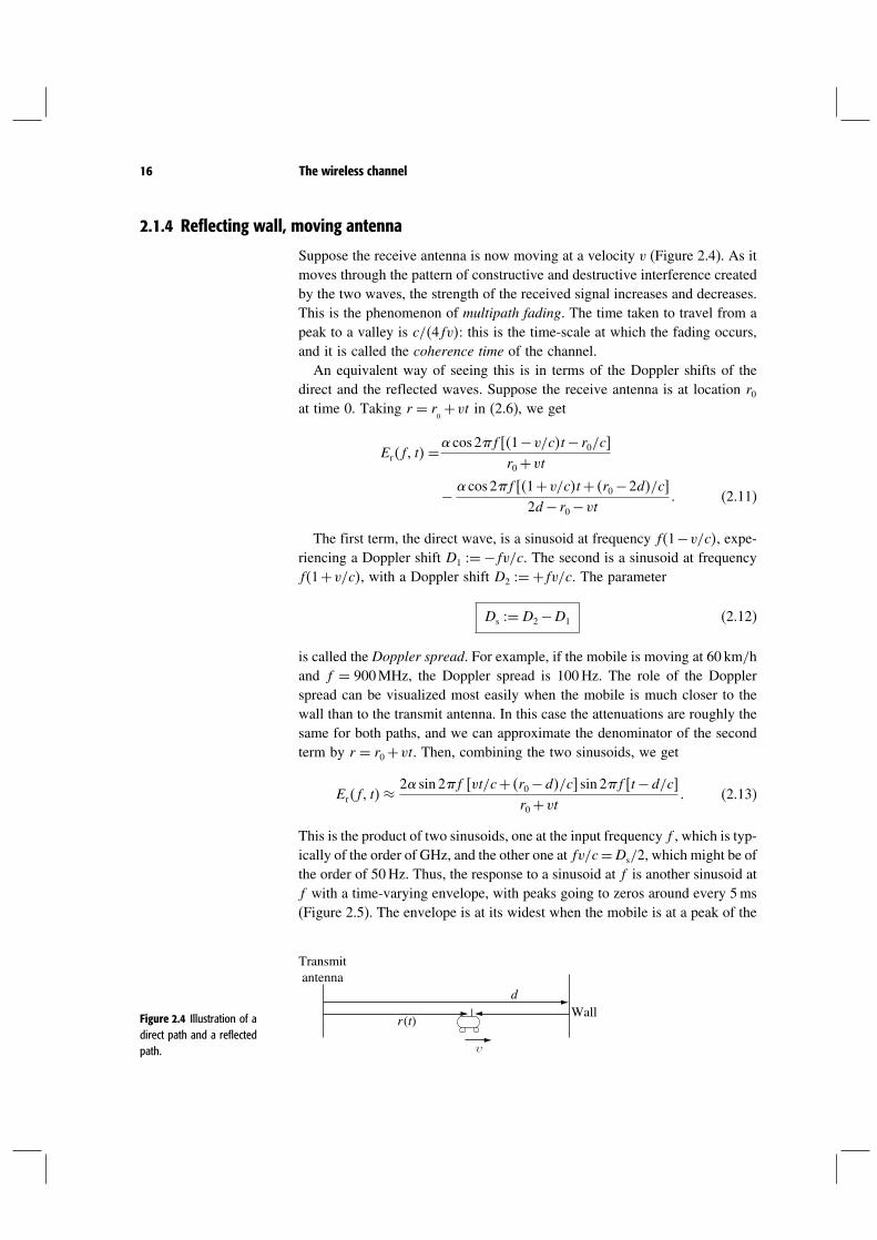
2.1.4 Reflecting wall, moving antenna
Suppose the receive antenna is now moving at a velocity v (Figure 2.4). As itmoves through the pattern of constructive and destructive interference createdby the two waves, the strength of the received signal increases and decreases.This is the phenomenon of multipath fading. The time taken to travel from apeak to a valley is c/4fv: this is the time-scale at which the fading occurs,and it is called the coherence time of the channel.An equivalent way of seeing this is in terms of the Doppler shifts of the
direct and the reflected waves. Suppose the receive antenna is at location r0at time 0. Taking r = r
0+vt in (2.6), we get
Erf t= cos2f1−v/ct− r0/c
r0+vt
− cos2f1+v/ct+ r0−2d/c2d− r0−vt
(2.11)
The first term, the direct wave, is a sinusoid at frequency f1−v/c, expe-riencing a Doppler shift D1 =−fv/c. The second is a sinusoid at frequencyf1+v/c, with a Doppler shift D2 =+fv/c. The parameter
Ds =D2−D1 (2.12)
is called the Doppler spread. For example, if the mobile is moving at 60 km/hand f = 900MHz, the Doppler spread is 100Hz. The role of the Dopplerspread can be visualized most easily when the mobile is much closer to thewall than to the transmit antenna. In this case the attenuations are roughly thesame for both paths, and we can approximate the denominator of the secondterm by r = r0+vt. Then, combining the two sinusoids, we get
Erf t≈2 sin 2f vt/c+ r0−d/c sin 2ft−d/c
r0+vt (2.13)
This is the product of two sinusoids, one at the input frequency f , which is typ-ically of the order of GHz, and the other one at fv/c=Ds/2, which might be ofthe order of 50Hz. Thus, the response to a sinusoid at f is another sinusoid atf with a time-varying envelope, with peaks going to zeros around every 5ms(Figure 2.5). The envelope is at its widest when the mobile is at a peak of the
Figure 2.4 Illustration of adirect path and a reflectedpath.
Wall
Transmit antenna
r (t)
d
υ

17 2.1 Physical modeling for wireless channels
Figure 2.5 The receivedwaveform oscillating atfrequency f with a slowlyvarying envelope at frequencyDs/2.
t
Er (t)
interference pattern and at its narrowest when the mobile is at a valley. Thus,the Doppler spread determines the rate of traversal across the interferencepattern and is inversely proportional to the coherence time of the channel.We now see why we have partially ignored the denominator terms in (2.11)
and (2.13). When the difference in the length between two paths changes bya quarter wavelength, the phase difference between the responses on the twopaths changes by /2, which causes a very significant change in the overallreceived amplitude. Since the carrier wavelength is very small relative tothe path lengths, the time over which this phase effect causes a significantchange is far smaller than the time over which the denominator terms causea significant change. The effect of the phase changes is of the order ofmilliseconds, whereas the effect of changes in the denominator is of the orderof seconds or minutes. In terms of modulation and detection, the time-scalesof interest are in the range of milliseconds and less, and the denominators areeffectively constant over these periods.The reader might notice that we are constantly making approximations in
trying to understand wireless communication, much more so than for wiredcommunication. This is partly because wired channels are typically time-invariant over a very long time-scale, while wireless channels are typicallytime-varying, and appropriate models depend very much on the time-scales ofinterest. For wireless systems, the most important issue is what approximationsto make. Thus, it is important to understand these modeling issues thoroughly.
2.1.5 Reflection from a ground plane
Consider a transmit and a receive antenna, both above a plane surface suchas a road (Figure 2.6). When the horizontal distance r between the antennasbecomes very large relative to their vertical displacements from the ground

18 The wireless channel
Figure 2.6 Illustration of adirect path and a reflectedpath off a ground plane.
Transmit antenna
Groud plane
Receive antenna
hr
hsr2
r
r1
plane (i.e., height), a very surprising thing happens. In particular, the differ-ence between the direct path length and the reflected path length goes to zeroas r−1 with increasing r (Exercise 2.5). When r is large enough, this differencebetween the path lengths becomes small relative to the wavelength c/f . Sincethe sign of the electric field is reversed on the reflected path5, these two wavesstart to cancel each other out. The electric wave at the receiver is then attenu-ated as r−2, and the received power decreases as r−4. This situation is partic-ularly important in rural areas where base-stations tend to be placed on roads.
2.1.6 Power decay with distance and shadowing
The previous example with reflection from a ground plane suggests that thereceived power can decrease with distance faster than r−2 in the presence ofdisturbances to free space. In practice, there are several obstacles betweenthe transmitter and the receiver and, further, the obstacles might also absorbsome power while scattering the rest. Thus, one expects the power decay tobe considerably faster than r−2. Indeed, empirical evidence from experimentalfield studies suggests that while power decay near the transmitter is like r−2,at large distances the power can even decay exponentially with distance.The ray tracing approach used so far provides a high degree of numerical
accuracy in determining the electric field at the receiver, but requires a precisephysical model including the location of the obstacles. But here, we are onlylooking for the order of decay of power with distance and can consider analternative approach. So we look for a model of the physical environment withthe fewest parameters but one that still provides useful global informationabout the field properties. A simple probabilistic model with two parametersof the physical environment, the density of the obstacles and the fraction ofenergy each object absorbs, is developed in Exercise 2.6. With each obstacle
5 This is clearly true if the electric field is parallel to the ground plane. It turns out that this isalso true for arbitrary orientations of the electric field, as long as the ground is not a perfectconductor and the angle of incidence is small enough. The underlying electromagnetics isanalyzed in Chapter 2 of Jakes [62].

19 2.1 Physical modeling for wireless channels
absorbing the same fraction of the energy impinging on it, the model allowsus to show that the power decays exponentially in distance at a rate that isproportional to the density of the obstacles.With a limit on the transmit power (either at the base-station or at the
mobile), the largest distance between the base-station and a mobile at whichcommunication can reliably take place is called the coverage of the cell. Forreliable communication, a minimal received power level has to be met andthus the fast decay of power with distance constrains cell coverage. On theother hand, rapid signal attenuation with distance is also helpful; it reduces theinterference between adjacent cells. As cellular systems become more popular,however, the major determinant of cell size is the number of mobiles in thecell. In engineering jargon, the cell is said to be capacity limited instead ofcoverage limited. The size of cells has been steadily decreasing, and one talksof micro cells and pico cells as a response to this effect. With capacity limitedcells, the inter-cell interference may be intolerably high. To alleviate theinter-cell interference, neighboring cells use different parts of the frequencyspectrum, and frequency is reused at cells that are far enough. Rapid signalattenuation with distance allows frequencies to be reused at closer distances.The density of obstacles between the transmit and receive antennas depends
very much on the physical environment. For example, outdoor plains havevery little by way of obstacles while indoor environments pose many obsta-cles. This randomness in the environment is captured by modeling the densityof obstacles and their absorption behavior as random numbers; the overallphenomenon is called shadowing.6 The effect of shadow fading differs frommultipath fading in an important way. The duration of a shadow fade lasts formultiple seconds or minutes, and hence occurs at a much slower time-scalecompared to multipath fading.
2.1.7 Moving antenna, multiple reflectors
Dealingwithmultiple reflectors, using the techniqueof ray tracing, is inprinciplesimply a matter of modeling the received waveform as the sum of the responsesfrom the different paths rather than just two paths. We have seen enough exam-ples, however, to understand that finding the magnitudes and phases of theseresponses is no simple task. Even for the very simple large wall example inFigure 2.2, the reflected field calculated in (2.6) is valid only at distances fromthe wall that are small relative to the dimensions of the wall. At very large dis-tances, the total power reflected from the wall is proportional to both d−2 andto the area of the cross section of the wall. The power reaching the receiver isproportional to d− rt−2. Thus, the power attenuation from transmitter toreceiver (for the large distance case) is proportional to dd− rt−2 rather
6 This is called shadowing because it is similar to the effect of clouds partly blocking sunlight.
20 The wireless channel
than to 2d− rt−2. This shows that ray tracing must be used with somecaution. Fortunately, however, linearity still holds in thesemore complex cases.Another type of reflection is known as scattering and can occur in the
atmosphere or in reflections from very rough objects. Here there are a verylarge number of individual paths, and the received waveform is better modeledas an integral over paths with infinitesimally small differences in their lengths,rather than as a sum.Knowing how to find the amplitude of the reflected field from each type
of reflector is helpful in determining the coverage of a base-station (althoughultimately experimentation is necessary). This is an important topic if ourobjective is trying to determine where to place base-stations. Studying this inmore depth, however, would take us afield and too far into electromagnetictheory. In addition, we are primarily interested in questions of modulation,detection, multiple access, and network protocols rather than location ofbase-stations. Thus, we turn our attention to understanding the nature of theaggregate received waveform, given a representation for each reflected wave.This leads to modeling the input/output behavior of a channel rather than thedetailed response on each path.
2.2 Input/output model of the wireless channel
We derive an input/output model in this section. We first show that the mul-tipath effects can be modeled as a linear time-varying system. We then obtaina baseband representation of this model. The continuous-time channel is thensampled to obtain a discrete-time model. Finally we incorporate additive noise.
2.2.1 The wireless channel as a linear time-varying system
In the previous section we focused on the response to the sinusoidal inputt= cos2ft. The receivedsignal canbewrittenas
∑i aif tt−if t,
where aif t and if t are respectively the overall attenuation and prop-agation delay at time t from the transmitter to the receiver on path i. Theoverall attenuation is simply the product of the attenuation factors due to theantenna pattern of the transmitter and the receiver, the nature of the reflector,as well as a factor that is a function of the distance from the transmittingantenna to the reflector and from the reflector to the receive antenna. We havedescribed the channel effect at a particular frequency f . If we further assumethat the aif t and the if t do not depend on the frequency f , then wecan use the principle of superposition to generalize the above input/outputrelation to an arbitrary input xt with non-zero bandwidth:
yt=∑
i
aitxt− it (2.14)

21 2.2 Input/output model of the wireless channel
In practice the attenuations and the propagation delays are usually slowlyvarying functions of frequency. These variations follow from the time-varyingpath lengths and also from frequency-dependent antenna gains. However, weare primarily interested in transmitting over bands that are narrow relativeto the carrier frequency, and over such ranges we can omit this frequencydependence. It should however be noted that although the individual attenua-tions and delays are assumed to be independent of the frequency, the overallchannel response can still vary with frequency due to the fact that differentpaths have different delays.For the example of a perfectly reflecting wall in Figure 2.4, then,
a1t=
r0+vt a2t=
2d− r0−vt
(2.15)
1t=r0+vt
c− ∠1
2f 2t=
2d− r0−vt
c− ∠2
2f (2.16)
where the first expression is for the direct path and the second for the reflectedpath. The term ∠j here is to account for possible phase changes at thetransmitter, reflector, and receiver. For the example here, there is a phasereversal at the reflector so we take 1 = 0 and 2 = .Since the channel (2.14) is linear, it can be described by the response
h t at time t to an impulse transmitted at time t− . In terms of h t,the input/output relationship is given by
yt=∫
−h txt− d (2.17)
Comparing (2.17) and (2.14), we see that the impulse response for the fadingmultipath channel is
h t=∑
i
ait− it (2.18)
This expression is really quite nice. It says that the effect of mobile users,arbitrarily moving reflectors and absorbers, and all of the complexities of solv-ing Maxwell’s equations, finally reduce to an input/output relation betweentransmit and receive antennas which is simply represented as the impulseresponse of a linear time-varying channel filter.The effect of the Doppler shift is not immediately evident in this repre-
sentation. From (2.16) for the single reflecting wall example, ′i t = vi/c
where vi is the velocity with which the ith path length is increasing. Thus,the Doppler shift on the ith path is −f ′i t.In the special case when the transmitter, receiver and the environment
are all stationary, the attenuations ait and propagation delays it do not

22 The wireless channel
depend on time t, and we have the usual linear time-invariant channel withan impulse response
h=∑
i
ai− i (2.19)
For the time-varying impulse response h t, we can define a time-varyingfrequency response
Hf t =∫
−h te−j2f d =∑
i
aite−j2fit (2.20)
In the special case when the channel is time-invariant, this reduces to theusual frequency response. One way of interpreting Hf t is to think of thesystem as a slowly varying function of t with a frequency response Hf t
at each fixed time t. Corresponding, h t can be thought of as the impulseresponse of the system at a fixed time t. This is a legitimate and usefulway of thinking about many multipath fading channels, as the time-scaleat which the channel varies is typically much longer than the delay spread(i.e., the amount of memory) of the impulse response at a fixed time. In thereflecting wall example in Section 2.1.4, the time taken for the channel tochange significantly is of the order of milliseconds while the delay spread isof the order of microseconds. Fading channels which have this characteristicare sometimes called underspread channels.
2.2.2 Baseband equivalent model
In typical wireless applications, communication occurs in a passbandfc−W/2 fc+W/2 of bandwidth W around a center frequency fc, thespectrum having been specified by regulatory authorities. However, mostof the processing, such as coding/decoding, modulation/demodulation,synchronization, etc., is actually done at the baseband. At the transmitter, thelast stage of the operation is to “up-convert” the signal to the carrier frequencyand transmit it via the antenna. Similarly, the first step at the receiver is to“down-convert” the RF (radio-frequency) signal to the baseband before furtherprocessing. Therefore from a communication system design point of view, itis most useful to have a baseband equivalent representation of the system.We first start with defining the baseband equivalent representation of signals.Consider a real signal st with Fourier transform Sf, band-limited in
fc−W/2 fc+W/2 with W< 2fc. Define its complex baseband equivalentsbt as the signal having Fourier transform:
Sbf=√
2Sf +fc f +fc > 00 f +fc ≤ 0
(2.21)

23 2.2 Input/output model of the wireless channel
Figure 2.7 Illustration of therelationship between apassband spectrum S(f ) andits baseband equivalent Sb(f ).
W2
1
Sb ( f )
S( f )
f
f
–fc –W2
fc –W2
– fcW2
+ W2
fc +
W2
–
2√
Since st is real, its Fourier transform satisfies Sf= S∗−f, which meansthat sbt contains exactly the same information as st. The factor of
√2 is
quite arbitrary but chosen to normalize the energies of sbt and st to bethe same. Note that sbt is band-limited in −W/2W/2. See Figure 2.7.To reconstruct st from sbt, we observe that
√2Sf= Sbf −fc+S∗
b−f −fc (2.22)
Taking inverse Fourier transforms, we get
st= 1√2
[sbte
j2fct + s∗bte−j2fct
]=√2 [sbte j2fct
] (2.23)
In terms of real signals, the relationship between st and sbt isshown in Figure 2.8. The passband signal st is obtained by modulatingsbt by
√2 cos2fct and sbt by −√
2 sin 2fct and summing, toget
√2 [sbtej2fct
](up-conversion). The baseband signal sbt (respec-
tively sbt) is obtained by modulating st by√2 cos2fct (respec-
tively −√2 sin 2fct) followed by ideal low-pass filtering at the baseband
−W/2W/2 (down-conversion).Let us now go back to the multipath fading channel (2.14) with impulse
response given by (2.18). Let xbt and ybt be the complex basebandequivalents of the transmitted signal xt and the received signal yt,respectively. Figure 2.9 shows the system diagram from xbt to ybt. Thisimplementation of a passband communication system is known as quadratureamplitude modulation (QAM). The signal xbt is sometimes called the

24 The wireless channel
Figure 2.8 Illustration ofupconversion from sb(t) tos(t), followed bydownconversion from s(t)back to sb(t).
X
X
X
X
[sb(t)]
[sb(t)]
[sb(t)]
[sb(t)]
–√2 sin 2π fc t –√2 sin 2π fc
t
√2 cos 2π fc t√2 cos 2π fc
t
s(t)
–W2
W2
–W2
W2
1
1
+
Figure 2.9 System diagramfrom the baseband transmittedsignal xb(t) to the basebandreceived signal yb(t). X
X
X
X
[xb(t)]
[xb(t)]
[yb(t)]
[yb(t)]
–W2
W2
–W2
W2
1
1
+x(t) y(t)
h(τ, t)
–√2 sin 2π fc t –√2 sin 2π fc
t
√2 cos 2π fc t√2 cos 2π fc
t
in-phase component I and xbt the quadrature component Q (rotatedby /2). We now calculate the baseband equivalent channel. Substitutingxt=√
2xbte j2fct and yt=√2ybte j2fct into (2.14) we get
ybte j2fct = ∑
i
aitxbt− itej2fct−it
= [∑
i
aitxbt− ite−j2fcit
e j2fct
]
(2.24)
Similarly, one can obtain (Exercise 2.13)
ybte j2fct= [∑
i
aitxbt− ite−j2fcit
e j2fct
]
(2.25)
Hence, the baseband equivalent channel is
ybt=∑
i
abi txbt− it (2.26)

25 2.2 Input/output model of the wireless channel
where
abi t = aite
−j2fcit (2.27)
The input/output relationship in (2.26) is also that of a linear time-varyingsystem, and the baseband equivalent impulse response is
hb t=∑
i
abi t− it (2.28)
This representation is easy to interpret in the time domain, where the effectof the carrier frequency can be seen explicitly. The baseband output is thesum, over each path, of the delayed replicas of the baseband input. Themagnitude of the ith such term is the magnitude of the response on the givenpath; this changes slowly, with significant changes occurring on the order ofseconds or more. The phase is changed by /2 (i.e., is changed significantly)when the delay on the path changes by 1/4fc, or equivalently, when thepath length changes by a quarter wavelength, i.e., by c/4fc. If the pathlength is changing at velocity v, the time required for such a phase changeis c/4fcv. Recalling that the Doppler shift D at frequency f is fv/c, andnoting that f ≈ fc for narrowband communication, the time required for a/2 phase change is 1/4D. For the single reflecting wall example, this isabout 5ms (assuming fc = 900MHz and v = 60km/h). The phases of bothpaths are rotating at this rate but in opposite directions.Note that the Fourier transform Hbf t of hb t for a fixed t is simply
Hf +fc t, i.e., the frequency response of the original system (at a fixed t)shifted by the carrier frequency. This provides another way of thinking aboutthe baseband equivalent channel.
2.2.3 A discrete-time baseband model
The next step in creating a useful channel model is to convert the continuous-time channel to a discrete-time channel. We take the usual approach of thesampling theorem. Assume that the input waveform is band-limited to W .The baseband equivalent is then limited to W/2 and can be represented as
xbt=∑
n
xnsincWt−n (2.29)
where xn is given by xbn/W and sinct is defined as
sinct = sintt
(2.30)
This representation follows from the sampling theorem, which says that anywaveform band-limited to W/2 can be expanded in terms of the orthogonal

26 The wireless channel
basis sincWt−nn, with coefficients given by the samples (taken uniformlyat integer multiples of 1/W ).Using (2.26), the baseband output is given by
ybt=∑
n
xn∑
i
abi tsincWt−Wit−n (2.31)
The sampled outputs at multiples of 1/W , ym = ybm/W, are thengiven by
ym=∑
n
xn∑
i
abi m/Wsincm−n− im/WW (2.32)
The sampled output ym can equivalently be thought of as the projectionof the waveform ybt onto the waveform W sincWt−m. Let = m−n.Then
ym=∑
xm−∑
i
abi m/Wsinc− im/WW (2.33)
By defining
hm =∑
i
abi m/Wsinc− im/WW (2.34)
(2.33) can be written in the simple form
ym=∑
hmxm− (2.35)
We denote hm as the th (complex) channel filter tap at time m. Its valueis a function of mainly the gains ab
i t of the paths, whose delays it areclose to /W (Figure 2.10). In the special case where the gains ab
i t and thedelays it of the paths are time-invariant, (2.34) simplifies to
h =∑
i
abi sinc− iW (2.36)
and the channel is linear time-invariant. The th tap can be interpreted asthe sample /Wth of the low-pass filtered baseband channel response hb
(cf. (2.19)) convolved with sinc(W).We can interpret the sampling operation as modulation and demodulation in
a communication system. At time n, we are modulating the complex symbolxm (in-phase plus quadrature components) by the sinc pulse before theup-conversion. At the receiver, the received signal is sampled at times m/W

27 2.2 Input/output model of the wireless channel
Figure 2.10 Due to the decayof the sinc function, the i thpath contributes mostsignificantly to the th tap ifits delay falls in the window/W − 1/2W /W +1/2W.
1W
Main contribution l = 0
Main contribution l = 0
Main contribution l = 1
Main contribution l = 2
Main contribution l = 2
i = 0
i = 1
i = 2
i = 3
i = 4
0 1 2l
at the output of the low-pass filter. Figure 2.11 shows the complete system.In practice, other transmit pulses, such as the raised cosine pulse, are oftenused in place of the sinc pulse, which has rather poor time-decay propertyand tends to be more susceptible to timing errors. This necessitates samplingat the Nyquist sampling rate, but does not alter the essential nature of themodel. Hence we will confine to Nyquist sampling.Due to the Doppler spread, the bandwidth of the output ybt is generally
slightly larger than the bandwidth W/2 of the input xbt, and thus the outputsamples ym do not fully represent the output waveform. This problem isusually ignored in practice, since the Doppler spread is small (of the orderof tens to hundreds of Hz) compared to the bandwidth W . Also, it is veryconvenient for the sampling rate of the input and output to be the same.Alternatively, it would be possible to sample the output at twice the rate ofthe input. This would recapture all the information in the received waveform.

28 The wireless channel
X X
XX[x[m]]
sinc (Wt – n)
[x[m]]sinc (Wt – n)
h(τ, t)
1
–W W
–W W
1
+
[xb(t)]
[y[m]]
[y[m]][yb(t)]
[yb(t)]
y(t)x(t)
[xb(t)]
2 2
22
–√2 sin 2π fc t –√2 sin 2π fc
t
√2 cos 2π fc t√2 cos 2π fc
t
The number of taps would be almost doubled because of the reduced sampleFigure 2.11 System diagramfrom the baseband transmittedsymbol x[m] to the basebandsampled received signal y[m].
interval, but it would typically be somewhat less than doubled since therepresentation would not spread the path delays so much.
Discussion 2.1 Degrees of freedom
The symbol xm is the mth sample of the transmitted signal; there areW samples per second. Each symbol is a complex number; we say that itrepresents one (complex) dimension or degree of freedom. The continuous-time signal xt of duration one second corresponds toW discrete symbols;thus we could say that the band-limited, continuous-time signal has W
degrees of freedom, per second.The mathematical justification for this interpretation comes from the
following important result in communication theory: the signal space ofcomplex continuous-time signals of duration T which have most of theirenergy within the frequency band −W/2W/2 has dimension approx-imately WT . (A precise statement of this result is in standard com-munication theory text/books; see Section 5.3 of [148] for example.)This result reinforces our interpretation that a continuous-time signalwith bandwidth W can be represented by W complex dimensions persecond.The received signal yt is also band-limited to approximately W (due
to the Doppler spread, the bandwidth is slightly larger than W ) and has Wcomplex dimensions per second. From the point of view of communicationover the channel, the received signal space is what matters because itdictates the number of different signals which can be reliably distinguishedat the receiver. Thus, we define the degrees of freedom of the channelto be the dimension of the received signal space, and whenever we referto the signal space, we implicitly mean the received signal space unlessstated otherwise.

29 2.2 Input/output model of the wireless channel
2.2.4 Additive white noise
As a last step, we include additive noise in our input/output model. We makethe standard assumption that wt is zero-mean additive white Gaussian noise(AWGN) with power spectral density N0/2 (i.e., Ew0wt= N0/2t.The model (2.14) is now modified to be
yt=∑
i
aitxt− it+wt (2.37)
See Figure 2.12. The discrete-time baseband-equivalent model (2.35) nowbecomes
ym=∑
hmxm−+wm (2.38)
where wm is the low-pass filtered noise at the sampling instant m/W .Just like the signal, the white noise wt is down-converted, filtered at thebaseband and ideally sampled. Thus, it can be verified (Exercise 2.11) that
wm =∫
−wtm1tdt (2.39)
wm =∫
−wtm2tdt (2.40)
where
m1t = √2W cos2fctsincWt−m
m2t = −√2W sin2fctsincWt−m (2.41)
It can further be shown that m1tm2tm forms an orthonormal set ofwaveforms, i.e., the waveforms are orthogonal to each other (Exercise 2.12).In Appendix A we review the definition and basic properties of white Gaus-sian random vectors (i.e., vectors whose components are independent andidentically distributed (i.i.d.) Gaussian random variables). A key property isthat the projections of a white Gaussian random vector onto any orthonor-mal vectors are independent and identically distributed Gaussian randomvariables. Heuristically, one can think of continuous-time Gaussian whitenoise as an infinite-dimensional white random vector and the above prop-erty carries through: the projections onto orthogonal waveforms are uncorre-lated and hence independent. Hence the discrete-time noise process wm
is white, i.e., independent over time; moreover, the real and imaginarycomponents are i.i.d. Gaussians with variances N0/2. A complex Gaussianrandom variable X whose real and imaginary components are i.i.d. satis-fies a circular symmetry property: e jX has the same distribution as X forany . We shall call such a random variable circular symmetric complex

30 The wireless channel
X
XX
X[x[m]] [y[m]]
[y[m]][x[m]]
[xb(t)] [yb(t)]
[yb(t)][xb(t)]sinc(Wt – n)
sinc(Wt – n)
w(t)
y(t)
x(t)h(τ, t) ++
W2
2
– W2
W2
2
– W2
–√2 sin 2π fc t –√2 sin 2π fc
t
√2 cos 2π fc t√2 cos 2π fc
t
Gaussian, denoted by 02, where 2 = EX2. The concept of cir-Figure 2.12 A complete systemdiagram. cular symmetry is discussed further in Section A.1.3 of Appendix A.
The assumption of AWGN essentially means that we are assuming that theprimary source of the noise is at the receiver or is radiation impinging onthe receiver that is independent of the paths over which the signal is beingreceived. This is normally a very good assumption for most communicationsituations.
2.3 Time and frequency coherence
2.3.1 Doppler spread and coherence time
An important channel parameter is the time-scale of the variation of thechannel. How fast do the taps hm vary as a function of time m? Recall that
hm = ∑
i
abi m/Wsinc− im/WW
= ∑
i
aim/We−j2fcim/Wsinc− im/WW (2.42)
Let us look at this expression term by term. From Section 2.2.2 we gather thatsignificant changes in ai occur over periods of seconds or more. Significantchanges in the phase of the ith path occur at intervals of 1/4Di, whereDi = fc
′i t is the Doppler shift for that path. When the different paths
contributing to the th tap have different Doppler shifts, the magnitude ofhm changes significantly. This is happening at the time-scale inverselyproportional to the largest difference between the Doppler shifts, the Dopplerspread Ds:
Ds =maxi j
fc ′i t− ′jt (2.43)

31 2.3 Time and frequency coherence
where the maximum is taken over all the paths that contribute significantly toa tap.7 Typical intervals for such changes are on the order of 10ms. Finally,changes in the sinc term of (2.42) due to the time variation of each it areproportional to the bandwidth, whereas those in the phase are proportionalto the carrier frequency, which is typically much larger. Essentially, it takesmuch longer for a path to move from one tap to the next than for its phaseto change significantly. Thus, the fastest changes in the filter taps occurbecause of the phase changes, and these are significant over delay changesof 1/4Ds.The coherence time Tc of a wireless channel is defined (in an order of
magnitude sense) as the interval over which hm changes significantly as afunction of m. What we have found, then, is the important relation
Tc =1
4Ds
(2.44)
This is a somewhat imprecise relation, since the largest Doppler shifts maybelong to paths that are too weak to make a difference. We could also view aphase change of /4 to be significant, and thus replace the factor of 4 aboveby 8. Many people instead replace the factor of 4 by 1. The important thingis to recognize that the major effect in determining time coherence is theDoppler spread, and that the relationship is reciprocal; the larger the Dopplerspread, the smaller the time coherence.In the wireless communication literature, channels are often categorized as
fast fading and slow fading, but there is little consensus on what these termsmean. In this book, we will call a channel fast fading if the coherence time Tc
is much shorter than the delay requirement of the application, and slow fadingif Tc is longer. The operational significance of this definition is that, in afast fading channel, one can transmit the coded symbols over multiple fadesof the channel, while in a slow fading channel, one cannot. Thus, whether achannel is fast or slow fading depends not only on the environment but alsoon the application; voice, for example, typically has a short delay requirementof less than 100ms, while some types of data applications can have a laxerdelay requirement.
2.3.2 Delay spread and coherence bandwidth
Another important general parameter of a wireless system is the multipathdelay spread, Td, defined as the difference in propagation time between the
7 The Doppler spread can in principle be different for different taps. Exercise 2.10 exploresthis possibility.

32 The wireless channel
longest and shortest path, counting only the paths with significant energy.Thus,
Td =maxi j
it− jt (2.45)
This is defined as a function of t, but we regard it as an order of magnitudequantity, like the time coherence and Doppler spread. If a cell or LAN hasa linear extent of a few kilometers or less, it is very unlikely to have pathlengths that differ by more than 300 to 600 meters. This corresponds to pathdelays of one or two microseconds. As cells become smaller due to increasedcellular usage, Td also shrinks. As was already mentioned, typical wirelesschannels are underspread, which means that the delay spread Td is muchsmaller than the coherence time Tc.The bandwidths of cellular systems range between several hundred kilohertz
and several megahertz, and thus, for the above multipath delay spread values,all the path delays in (2.34) lie within the peaks of two or three sinc functions;more often, they lie within a single peak. Adding a few extra taps to eachchannel filter because of the slow decay of the sinc function, we see thatcellular channels can be represented with at most four or five channel filtertaps. On the other hand, there is a recent interest in ultra-wideband (UWB)communication, operating from 3.1 to 10.6GHz. These channels can have upto a few hundred taps.When we study modulation and detection for cellular systems, we shall see
that the receiver must estimate the values of these channel filter taps. The tapsare estimated via transmitted and received waveforms, and thus the receivermakes no explicit use of (and usually does not have) any information aboutindividual path delays and path strengths. This is why we have not studied thedetails of propagation over multiple paths with complicated types of reflectionmechanisms. All we really need is the aggregate values of gross physicalmechanisms such as Doppler spread, coherence time, and multipath spread.The delay spread of the channel dictates its frequency coherence. Wireless
channels change both in time and frequency. The time coherence showsus how quickly the channel changes in time, and similarly, the frequencycoherence shows how quickly it changes in frequency. We first understoodabout channels changing in time, and correspondingly about the duration offades, by studying the simple example of a direct path and a single reflectedpath. That same example also showed us how channels change with frequency.We can see this in terms of the frequency response as well.Recall that the frequency response at time t is
Hf t=∑
i
aite−j2fit (2.46)
The contribution due to a particular path has a phase linear in f . For mul-tiple paths, there is a differential phase, 2fit− kt. This differential

33 2.3 Time and frequency coherence
10
0.55 0.6 0.65 0.7 0.75 0.8 0.85 0.9 0.95 1
–60
–50
–40
–30
–20
–10
0
0.65 0.66 0.67 0.68 0.69 0.7 0.71 0.72 0.73 0.74 0.75 0.76
0.45
0
–10
–20
–0.001
–0.0008
–0.0006
–0.0004
–0.0002
0
0.0002
0.0004
0.0006
0.0008
0.001
0 50 100 150 200 250 300 350 400 450 500 550
–30
–40
–50
–60
–70–0.006
–0.005
–0.004
–0.003
–0.002
–0.001
0
0.001
0.002
0.003
0.004
50 100 150 200 250 300 350 400 450 500 5500 0.5
(d)Po
wer
spe
ctru
m
(dB
)Po
wer
spe
ctur
m
(dB
)
Am
plitu
de
(lin
ear
scal
e)A
mpl
itude
(l
inea
r sc
ale)
(b)
Time (ns)
Time (ns)
(a)
(c)
40 MHz
Frequency (GHz)
Frequency (GHz)
200 MHz
phase causes selective fading in frequency. This says that Erf t changesFigure 2.13 (a) A channel over200MHz is frequency-selective,and the impulse response hasmany taps. (b) The spectralcontent of the same channel.(c) The same channel over40MHz is flatter, and has forfewer taps. (d) The spectralcontents of the same channel,limited to 40MHz bandwidth.At larger bandwidths, the samephysical paths are resolved intoa finer resolution.
significantly, not only when t changes by 1/4Ds, but also when f changesby 1/2Td. This argument extends to an arbitrary number of paths, so thecoherence bandwidth, Wc, is given by
Wc =12Td
(2.47)
This relationship, like (2.44), is intended as an order of magnitude relation,essentially pointing out that the coherence bandwidth is reciprocal to themultipath spread. When the bandwidth of the input is considerably less thanWc, the channel is usually referred to as flat fading. In this case, the delayspread Td is much less than the symbol time 1/W , and a single channelfilter tap is sufficient to represent the channel. When the bandwidth is muchlarger than Wc, the channel is said to be frequency-selective, and it has tobe represented by multiple taps. Note that flat or frequency-selective fadingis not a property of the channel alone, but of the relationship between thebandwidth W and the coherence bandwidth Td (Figure 2.13).The physical parameters and the time-scale of change of key parameters of
the discrete-time baseband channel model are summarized in Table 2.1. Thedifferent types of channels are summarized in Table 2.2.

34 The wireless channel
Table 2.1 A summary of the physical parameters of the channel and thetime-scale of change of the key parameters in its discrete-time basebandmodel.
Key channel parameters and time-scales Symbol Representative values
Carrier frequency fc 1GHzCommunication bandwidth W 1MHzDistance between transmitter and receiver d 1 kmVelocity of mobile v 64 km/hDoppler shift for a path D = fcv/c 50HzDoppler spread of paths corresponding to
a tap Ds 100HzTime-scale for change of path amplitude d/v 1 minuteTime-scale for change of path phase 1/4D 5msTime-scale for a path to move over a tap c/vW 20 sCoherence time Tc = 1/4Ds 2.5msDelay spread Td 1sCoherence bandwidth Wc = 1/2Td 500 kHz
Table 2.2 A summary of the types of wirelesschannels and their defining characteristics.
Types of channel Defining characteristic
Fast fading Tc delay requirementSlow fading Tc delay requirementFlat fading W Wc
Frequency-selective fading W Wc
Underspread Td Tc
2.4 Statistical channel models
2.4.1 Modeling philosophy
We defined Doppler spread and multipath spread in the previous section asquantities associated with a given receiver at a given location, velocity, andtime. However, we are interested in a characterization that is valid over somerange of conditions. That is, we recognize that the channel filter taps hmmust be measured, but we want a statistical characterization of how manytaps are necessary, how quickly they change and how much they vary.Such a characterization requires a probabilistic model of the channel tap
values, perhaps gathered by statistical measurements of the channel. We arefamiliar with describing additive noise by such a probabilistic model (asa Gaussian random variable). We are also familiar with evaluating errorprobability while communicating over a channel using such models. These

35 2.4 Statistical channel models
error probability evaluations, however, depend critically on the independenceand Gaussian distribution of the noise variables.It should be clear from the description of the physical mechanisms gener-
ating Doppler spread and multipath spread that probabilistic models for thechannel filter taps are going to be far less believable than the models foradditive noise. On the other hand, we need such models, even if they arequite inaccurate. Without models, systems are designed using experience andexperimentation, and creativity becomes somewhat stifled. Even with highlyover-simplified models, we can compare different system approaches and geta sense of what types of approaches are worth pursuing.To a certain extent, all analytical work is done with simplified models. For
example, white Gaussian noise (WGN) is often assumed in communicationmodels, although we know the model is valid only over sufficiently smallfrequency bands. With WGN, however, we expect the model to be quite goodwhen used properly. For wireless channel models, however, probabilisticmodels are quite poor and only provide order-of-magnitude guides to systemdesign and performance. We will see that we can define Doppler spread, multi-path spread, etc. much more cleanly with probabilistic models, but the underly-ing problem remains that these channels are very different from each other andcannot really be characterized by probabilistic models. At the same time, thereis a large literature based on probabilistic models for wireless channels, and ithas been highly useful for providing insight into wireless systems. However,it is important to understand the robustness of results based on these models.There is another question in deciding what to model. Recall the continuous-
time multipath fading channel
yt=∑
i
aitxt− it+wt (2.48)
This contains an exact specification of the delay and magnitude of each path.From this, we derived a discrete-time baseband model in terms of channelfilter taps as
ym=∑
hmxm−+wm (2.49)
where
hm=∑
i
aim/We−j2fcim/Wsinc− im/WW (2.50)
We used the sampling theorem expansion in which xm = xbm/W andym = ybm/W. Each channel tap hm contains an aggregate of paths,with the delays smoothed out by the baseband signal bandwidth.Fortunately, it is the filter taps that must be modeled for input/output
descriptions, and also fortunately, the filter taps often contain a sufficient pathaggregation so that a statistical model might have a chance of success.

36 The wireless channel
2.4.2 Rayleigh and Rician fading
The simplest probabilistic model for the channel filter taps is based onthe assumption that there are a large number of statistically independentreflected and scattered paths with random amplitudes in the delay window cor-responding to a single tap. The phase of the ith path is 2fci modulo 2. Now,fci = di/, where di is the distance travelled by the ith path and is the carrierwavelength. Since the reflectors and scatterers are far away relative to the car-rier wavelength, i.e., di , it is reasonable to assume that the phase for eachpath is uniformly distributed between 0 and 2 and that the phases of differentpaths are independent. The contribution of each path in the tap gain hm is
aim/We−j2fcim/Wsinc− im/WW (2.51)
and this can be modeled as a circular symmetric complex random variable.8
Each tap hm is the sum of a large number of such small independentcircular symmetric random variables. It follows that hm is the sum ofmany small independent real random variables, and so by the Central LimitTheorem, it can reasonably be modeled as a zero-mean Gaussian randomvariable. Similarly, because of the uniform phase, hme j is Gaussianwith the same variance for any fixed . This assures us that hm is infact circular symmetric 02
(see Section A.1.3 in Appendix A for anelaboration). It is assumed here that the variance of hm is a function of thetap , but independent of time m (there is little point in creating a probabilisticmodel that depends on time). With this assumed Gaussian probability density,we know that the magnitude hm of the th tap is a Rayleigh randomvariable with density (cf. (A.20) in Appendix A and Exercise 2.14)
x
2
exp−x2
22
x ≥ 0 (2.52)
and the squared magnitude hm2 is exponentially distributed with density
1
2
exp−x
2
x ≥ 0 (2.53)
This model, which is called Rayleigh fading, is quite reasonable for scat-tering mechanisms where there are many small reflectors, but is adoptedprimarily for its simplicity in typical cellular situations with a relatively smallnumber of reflectors. The word Rayleigh is almost universally used for this
8 See Section A.1.3 in Appendix A for a more in-depth discussion of circular symmetricrandom variables and vectors.

37 2.4 Statistical channel models
model, but the assumption is that the tap gains are circularly symmetriccomplex Gaussian random variables.There is a frequently used alternative model in which the line-of-sight path
(often called a specular path) is large and has a known magnitude, and thatthere are also a large number of independent paths. In this case, hm, atleast for one value of , can be modeled as
hm=√
+1e
j+√
1+1
(02
)(2.54)
with the first term corresponding to the specular path arriving with uniformphase and the second term corresponding to the aggregation of the largenumber of reflected and scattered paths, independent of . The parameter (so-called K-factor) is the ratio of the energy in the specular path to theenergy in the scattered paths; the larger is, the more deterministic is thechannel. The magnitude of such a random variable is said to have a Riciandistribution. Its density has quite a complicated form; it is often a better modelof fading than the Rayleigh model.
2.4.3 Tap gain auto-correlation function
Modeling each hm as a complex random variable provides part of the statis-tical description that we need, but this is not the most important part. The moreimportant issue is how these quantities vary with time. As we will see in the restof thebook, the rateof channelvariationhas significant impacton several aspectsof the communication problem. A statistical quantity that models this relation-ship is known as the tap gain auto-correlation function,Rn. It is defined as
Rn = h∗mhm+n (2.55)
For each tap , this gives the auto-correlation function of the sequence ofrandom variables modeling that tap as it evolves in time. We are tacitlyassuming that this is not a function of time m. Since the sequence of randomvariables hm for any given has both a mean and covariance functionthat does not depend on m, this sequence is wide-sense stationary. We alsoassume that, as a random variable, hm is independent of h′ m
′ for all = ′ and all mm′. This final assumption is intuitively plausible since pathsin different ranges of delay contribute to hm for different values of .9
The coefficient R0 is proportional to the energy received in the thtap. The multipath spread Td can be defined as the product of 1/W timesthe range of which contains most of the total energy
∑=0R0. This is
9 One could argue that a moving reflector would gradually travel from the range of one tap toanother, but as we have seen, this typically happens over a very large time-scale.
38 The wireless channel
somewhat preferable to our previous “definition” in that the statistical natureof Td becomes explicit and the reliance on some sort of stationarity becomesexplicit. Now, we can also define the coherence time Tc more explicitly asthe smallest value of n > 0 for which Rn is significantly different fromR0. With both of these definitions, we still have the ambiguity of what“significant” means, but we are now facing the reality that these quantitiesmust be viewed as statistics rather than as instantaneous values.The tap gain auto-correlation function is useful as a way of expressing the
statistics for how tap gains change given a particular bandwidth W , but giveslittle insight into questions related to choice of a bandwidth for communication.If we visualize increasing the bandwidth, we can see several things happening.First, the ranges of delay that are separated into different taps becomenarrower(1/W seconds), so there are fewer paths corresponding to each tap, and thus theRayleigh approximation becomes poorer. Second, the sinc functions of (2.50)becomenarrower, andR0 gives a finer grained picture of the amount of powerbeing received in the th delay window of width 1/W . In summary, as we tryto apply this model to larger W , we get more detailed information about delayand correlation at that delay, but the information becomes more questionable.
Example 2.2 Clarke’s modelThis is a popular statistical model for flat fading. The transmitter is fixed,the mobile receiver is moving at speed v, and the transmitted signal isscattered by stationary objects around the mobile. There are K paths, theith path arriving at an angle i = 2i/K, i = 0 K−1, with respectto the direction of motion. K is assumed to be large. The scattered patharriving at the mobile at the angle has a delay of t and a time-invariant gain a, and the input/output relationship is given by
yt=K−1∑
i=0
aixt− i t (2.56)
The most general version of the model allows the received power distri-bution p and the antenna gain pattern to be arbitrary functions ofthe angle , but the most common scenario assumes uniform power distri-bution and isotropic antenna gain pattern, i.e., the amplitudes a = a/
√K
for all angles . This models the situation when the scatterers are locatedin a ring around the mobile (Figure 2.14). We scale the amplitude of eachpath by
√K so that the total received energy along all paths is a2; for large
K, the received energy along each path is a small fraction of the total energy.Suppose the communication bandwidth W is much smaller than the
reciprocal of the delay spread. The complex baseband channel can berepresented by a single tap at each time:
ym= h0mxm+wm (2.57)

39 2.4 Statistical channel models
Rx
Figure 2.14 The one-ring model.
The phase of the signal arriving at time 0 from an angle is 2fc0mod 2, where fc is the carrier frequency. Making the assumption thatthis phase is uniformly distributed in 02 and independently distributedacross all angles , the tap gain process h0m is a sum of many smallindependent contributions, one from each angle. By the Central LimitTheorem, it is reasonable to model the process as Gaussian. Exercise 2.17shows further that the process is in fact stationary with an autocorrelationfunction R0n given by:
R0n= 2a2J0 nDs/W (2.58)
where J0· is the zeroth-order Bessel function of the first kind:
J0x =1
∫
0ejx cosd (2.59)
and Ds = 2fcv/c is the Doppler spread. The power spectral density Sf,defined on −1/2+1/2, is given by
Sf=
4a2W
Ds
√1−2fW/Ds
2−Ds/2W f +Ds/2W
0 else(2.60)
This can be verified by computing the inverse Fourier transform of (2.60)to be (2.58). Plots of the autocorrelation function and the spectrum for areshown in Figure 2.15. If we define the coherence time Tc to be the valueof n/W such that R0n= 005R00, then
Tc =J−10 005Ds
(2.61)
i.e., the coherence time is inversely proportional to Ds.

40 The wireless channel
2000
2.5
3
3.5
1.5
1
0.5
0
–0.5
–1
–1.5200 400 600 800 1000 1200 1400 1600 1800
2
R0 [n]
–1/2 1/2
S ( f )
–Ds / (2W ) Ds / (2W )0
Figure 2.15 Plots of the auto-correlation function and Doppler spectrum in Clarke’s model.
In Exercise 2.17, you will also verify that Sfdf has the physicalinterpretation of the received power along paths that have Doppler shiftsin the range f f + df. Thus, Sf is also called the Doppler spectrum.Note that Sf is zero beyond the maximum Doppler shift.
Chapter 2 The main plot
Large-scale fadingVariation of signal strength over distances of the order of cell sizes.Received power decreases with distance r like:
1r2
(free space)
1r4
(reflection from ground plane)
Decay can be even faster due to shadowing and scattering effects.

41 2.4 Statistical channel models
Small-scale fadingVariation of signal strength over distances of the order of the carrierwavelength, due to constructive and destructive interference of multipaths.Key parameters:
Doppler spread Ds ←→ coherence time Tc ∼ 1/Ds
Doppler spread is proportional to the velocity of the mobile and to theangular spread of the arriving paths.
delay spread Td ←→ coherence bandwidth Wc ∼ 1/Td
Delay spread is proportional to the difference between the lengths of theshortest and the longest paths.
Input/output channel models
• Continuous-time passband (2.14):
yt=∑
i
aitxt− it
• Continuous-time complex baseband (2.26):
ybt=∑
i
aite−j2fcitxbt− it
• Discrete-time complex baseband with AWGN (2.38):
ym=∑
hmxm−+wm
The th tap is the aggregation of the physical paths with delays in/W −1/2W/W +1/2W.
Statistical channel models
• hmm is modeled as circular symmetric processes independent acrossthe taps.
• If for all taps,
hm∼ 02
the model is called Rayleigh.• If for one tap,
hm=√
+1e
j+√
1+1
02
the model is called Rician with K-factor .

42 The wireless channel
• The tap gain auto-correlation function Rn = Eh∗0hn models
the dependency over time.• The delay spread is 1/W times the range of taps which contains mostof the total gain
∑=0R0. The coherence time is 1/W times the range
of n for which Rn is significantly different from R0.
2.5 Bibliographical notes
This chapter was modified from R. G. Gallager’s MIT 6.450 course notes on digitalcommunication. The focus is on small-scale multipath fading. Large-scale fadingmodels are discussed in many texts; see for example Rappaport [98]. Clarke’s modelwas introduced in [22] and elaborated further in [62]. Our derivation here of the Clarkepower spectrum follows the approach of [111].
2.6 Exercises
Exercise 2.1 (Gallager) Consider the electric field in (2.4).1. It has been derived under the assumption that the motion is in the direction of
the line-of-sight from sending antenna to receive antenna. Find the electric fieldassuming that is the angle between the line-of-sight and the direction of motionof the receiver. Assume that the range of time of interest is small enough so thatchanges in can be ignored.
2. Explain why, and under what conditions, it is a reasonable approximation to ignorethe change in over small intervals of time.
Exercise 2.2 (Gallager) Equation (2.13) was derived under the assumption thatrt≈ d. Derive an expression for the received waveform for general rt. Break thefirst term in (2.11) into two terms, one with the same numerator but the denominator2d− r0−vt and the other with the remainder. Interpret your result.
Exercise 2.3 In the two-path example in Sections 2.1.3 and 2.1.4, the wall is on theright side of the receiver so that the reflected wave and the direct wave travel in oppositedirections. Suppose now that the reflectingwall is on the left side of transmitter. Redo theanalysis. What is the nature of the multipath fading, both over time and over frequency?Explain any similarity or difference with the case considered in Sections 2.1.3 and 2.1.4.
Exercise 2.4 A mobile receiver is moving at a speed v and is receiving signals arrivingalong two reflected paths which make angles 1 and 2 with the direction of motion.The transmitted signal is a sinusoid at frequency f .1. Is the above information enough for estimating (i) the coherence time Tc; (ii) the
coherence bandwidth Wc? If so, express them in terms of the given parameters. Ifnot, specify what additional information would be needed.
2. Consider an environment in which there are reflectors and scatterers in all directionsfrom the receiver and an environment in which they are clustered within a small

43 2.6 Exercises
angular range. Using part (1), explain how the channel would differ in these twoenvironments.
Exercise 2.5 Consider the propagation model in Section 2.1.5 where there is a reflectedpath from the ground plane.1. Let r1 be the length of the direct path in Figure 2.6. Let r2 be the length of the
reflected path (summing the path length from the transmitter to the ground planeand the path length from the ground plane to the receiver). Show that r2 − r1 isasymptotically equal to b/r and find the value of the constant b. Hint: Recall thatfor x small,
√1+x ≈ 1+x/2 in the sense that
√1+x−1/x→ 1/2 as x→ 0.
2. Assume that the received waveform at the receive antenna is given by
Erf t= cos2ft−fr1/c
r1− cos2ft−fr2/c
r2 (2.62)
Approximate the denominator r2 by r1 in (2.62) and show that Er ≈ /r2 for r−1
much smaller than c/f . Find the value of .3. Explain why this asymptotic expression remains valid without first approximating
the denominator r2 in (2.62) by r1.
Exercise 2.6 Consider the following simple physical model in just a single dimension.The source is at the origin and transmits an isotropic wave of angular frequency .The physical environment is filled with uniformly randomly located obstacles. Wewill model the inter-obstacle distance as an exponential random variable, i.e., it hasthe density10
e−r r ≥ 0 (2.63)
Here 1/ is the mean distance between obstacles and captures the density of the obsta-cles. Viewing the source as a stream of photons, suppose each obstacle independently(from one photon to the other and independent of the behavior of the other obstacles)either absorbs the photon with probability or scatters it either to the left or to theright (both with equal probability 1−/2).
Now consider the path of a photon transmitted either to the left or to the right withequal probability from some fixed point on the line. The probability density functionof the distance (denoted by r) to the first obstacle (the distance can be on either sideof the starting point, so r takes values on the entire line) is equal to
qr = e−r
2 r ∈ (2.64)
So the probability density function of the distance at which the photon is absorbedupon hitting the first obstacle is equal to
f1r = qr r ∈ (2.65)
10 This random arrangement of points on a line is called a Poisson point process.

44 The wireless channel
1. Show that the probability density function of the distance from the origin at whichthe second obstacle is met is
f2r =∫
−1−qxf1r−xdx r ∈ (2.66)
2. Denote by fkr the probability density function of the distance from the originat which the photon is absorbed by exactly the kth obstacle it hits and show therecursive relation
fk+1r=∫
−1−qxfkr−xdx r ∈ (2.67)
3. Conclude from the previous step that the probability density function of the distancefrom the source at which the photon is absorbed (by some obstacle), denoted byfr, satisfies the recursive relation
fr= qr+ 1−∫
−qxfr−xdx r ∈ (2.68)
Hint: Observe that fr=∑k=1 fkr.
4. Show that
fr=√
2e−
√r (2.69)
is a solution to the recursive relation in (2.68). Hint: Observe that the convolutionbetween the probability densities q· and f· in (2.68) is more easily representedusing Fourier transforms.
5. Now consider the photons that are absorbed at a distance of more than r from thesource. This is the radiated power density at a distance r and is found by integratingfx over the range r if r > 0 and − r if r < 0. Calculate the radiatedpower density to be
e−√r
2 (2.70)
and conclude that the power decreases exponentially with distance r. Also observethat with very low absorption → 0 or very few obstacles → 0, the powerdensity converges to 0.5; this is expected since the power splits equally on eitherside of the line.
Exercise 2.7 In Exercise 2.6, we considered a single-dimensional physical model of ascattering and absorption environment and concluded that power decays exponentiallywith distance. A reading exercise is to study [42], which considers a natural extensionof this simple model to two- and three-dimensional spaces. Further, it extends theanalysis to two- and three-dimensional physical models. While the analysis is morecomplicated, we arrive at the same conclusion: the radiated power decays exponentiallywith distance.

45 2.6 Exercises
Exercise 2.8 (Gallager) Assume that a communication channel first filters the trans-mitted passband signal before adding WGN. Suppose the channel is known and thechannel filter has an impulse response ht. Suppose that a QAM scheme with symbolduration T is developed without knowledge of the channel filtering. A baseband filtert is developed satisfying the Nyquist property that t−kTk is an orthonormalset. The matched filter −t is used at the receiver before sampling and detection.
If one is aware of the channel filter ht, one may want to redesign either thebaseband filter at the transmitter or the baseband filter at the receiver so that thereis no intersymbol interference between receiver samples and so that the noise on thesamples is i.i.d.1. Which filter should one redesign?2. Give an expression for the impulse response of the redesigned filter (assume a
carrier frequency fc).3. Draw a figure of the various filters at passband to show why your solution is
correct. (We suggest you do this before answering the first two parts.)
Exercise 2.9 Consider the two-path example in Section 2.1.4 with d = 2km and thereceiver at 1.5 km from the transmitter moving at velocity 60 km/h away from thetransmitter. The carrier frequency is 900MHz.1. Plot in MATLAB the magnitudes of the taps of the discrete-time baseband channel
at a fixed time t. Give a few plots for several bandwidths W so as to exhibit bothflat and frequency-selective fading.
2. Plot the time variation of the phase and magnitude of a typical tap of the discrete-time baseband channel for a bandwidth where the channel is (approximately)flat and for a bandwidth where the channel is frequency-selective. How do thetime-variations depend on the bandwidth? Explain.
Exercise 2.10 For each tap of the discrete-time channel response, the Doppler spreadis the range of Doppler shifts of the paths contributing to that tap. Give an exampleof an environment (i.e. location of reflectors/scatterers with respect to the location ofthe transmitter and the receiver) in which the Doppler spread is the same for differenttaps and an environment in which they are different.
Exercise 2.11 Verify (2.39) and (2.40).
Exercise 2.12 In this problem we consider generating passband orthogonal waveformsfrom baseband ones.1. Show that if the waveforms t − nTn form an orthogonal set, then the
waveforms n1n2n also form an orthogonal set, provided that t is band-limited to −fc fc. Here,
n1t = t−nT cos2fct
n2t = t−nT sin 2fct
How should we normalize the energy of t to make the t orthonormal?2. For a given fc, find an example where the result in part (1) is false when the
condition that t is band-limited to −fc fc is violated.
Exercise 2.13 Verify (2.25). Does this equation contain any more information aboutthe communication system in Figure 2.9 beyond what is in (2.24)? Explain.

46 The wireless channel
Exercise 2.14 Compute the probability density function of the magnitude X of acomplex circular symmetric Gaussian random variable X with variance 2.
Exercise 2.15 In the text we have discussed the various reasons why the channel tapgains, hm, vary in time (as a function of m) and how the various dynamics operateat different time-scales. The analysis is based on the assumption that communicationtakes place on a bandwidth W around a carrier frequency fc with fc W . Thisassumption is not valid for ultra-wideband (UWB) communication systems, where thetransmission bandwidth is from 3.1GHz to 10.6GHz, as regulated by the FCC. Redothe analysis for this system. What is the main mechanism that causes the tap gains tovary at the fastest time-scale, and what is this fastest time-scale determined by?
Exercise 2.16 In Section 2.4.2, we argue that the channel gain hm at a particulartime m can be assumed to be circular symmetric. Extend the argument to show that itis also reasonable to assume that the complex random vector
h =
hm
hm+1
hm+n
is circular symmetric for any n.
Exercise 2.17 In this question, we will analyze in detail Clarke’s one-ring modeldiscussed at the end of the chapter. Recall that the scatterers are assumed to be locatedin a ring around the receiver moving at speed v. There are K paths coming in at anglesi = 2i/K with respect to the direction of motion of the mobile, i = 0 K−1The path coming at angle has a delay of t and a time-invariant gain a/
√K (not
dependent on the angle), and the input/output relationship is given by
yt= a√K
K−1∑
i=0
xt− i t (2.71)
1. Give an expression for the impulse response h t for this channel, and give anexpression for t in terms of 0. (You can assume that the distance the mobiletravelled in 0 t is small compared to the radius of the ring.)
2. Suppose communication takes place at carrier frequency fc and over a narrowbandof bandwidth W such that the delay spread of the channel Td satisfies Td 1/W .Argue that the discrete-time baseband model can be approximately represented bya single tap
ym= h0mxm+wm (2.72)
and give an approximate expression for that tap in terms of the a’s and t’s.Hint: Your answer should contain no sinc functions.
3. Argue that it is reasonable to assume that the phase of the path from an angle attime 0,
2fc0 mod 2
is uniformly distributed in 02 and that it is i.i.d. across .

47 2.6 Exercises
4. Based on the assumptions in part (3), for large K one can use the Central LimitTheorem to approximate h0m as a Gaussian process. Verify that the limitingprocess is stationary and the autocorrelation function R0n is given by (2.58).
5. Verify that the Doppler spectrum Sf is given by (2.60). Hint: It is easier to showthat the inverse Fourier transform of (2.60) is (2.58).
6. Verify that Sfdf is indeed the received power from the paths that have Dopplershifts in f f +df. Is this surprising?
Exercise 2.18 Consider a one-ring model where there are K scatterers located atangles i = 2i/K, i = 0 K−1, on a circle of radius 1 km around the receiverand the transmitter is 2 km away. (The angles are with respect to the line joining thetransmitter and the receiver.) The transmit power is P. The power attenuation along apath from the transmitter to a scatterer to the receiver is
G
K· 1s2
· 1r2 (2.73)
where G is a constant and r and s are the distance from the transmitter to the scattererand the distance from the scatterer to the receiver respectively. Communication takesplace at a carrier frequency fc = 19 GHz and the bandwidth isW Hz. You can assumethat, at any time, the phases of each arriving path in the baseband representation ofthe channel are independent and uniformly distributed between 0 and 2.1. What are the key differences and the similarities between this model and the
Clarke’s model in the text?2. Find approximate conditions on the bandwidth W for which one gets a flat fading
channel.3. Suppose the bandwidth is such that the channel is frequency selective. For large
K, find approximately the amount of power in tap of the discrete-time basebandimpulse response of the channel (i.e., compute the power-delay profile.). Make anysimplifying assumptions but state them. (You can leave your answers in terms ofintegrals if you cannot evaluate them.)
4. Compute and sketch the power-delay profile as the bandwidth becomes very large(and K is large).
5. Suppose now the receiver is moving at speed v towards the (fixed) transmitter. Whatis the Doppler spread of tap ? Argue heuristically from physical considerationswhat the Doppler spectrum (i.e., power spectral density) of tap is, for large K.
6. We have made the assumptions that the scatterers are all on a circle of radius 1kmaround the receiver and the paths arrive with independent and uniform distributedphases at the receiver. Mathematically, are the two assumptions consistent? If not,do you think it matters, in terms of the validity of your answers to the earlier partsof this question?
Exercise 2.19 Often in modeling multiple input multiple output (MIMO) fadingchannels the fading coefficients between different transmit and receive antennas areassumed to be independent random variables. This problem explores whether this isa reasonable assumption based on Clarke’s one-ring scattering model and the antennaseparation.1. (Antenna separation at the mobile) Assume a mobile with velocity v moving away
from the base-station, with uniform scattering from the ring around it.

48 The wireless channel
(a) Compute the Doppler spread Ds for a carrier frequency fc, and the correspond-ing coherence time Tc.
(b) Assuming that fading states separated by Tc are approximately uncorrelated, atwhat distance should we place a second antenna at the mobile to get an inde-pendently faded signal? Hint: How much distance does the mobile travel in Tc?
2. (Antenna separation at the base-station) Assume that the scattering ring has radiusR and that the distance between the base-station and the mobile is d. Furtherassume for the time being that the base-station is moving away from the mobilewith velocity v′. Repeat the previous part to find the minimum antenna spacing atthe base-station for uncorrelated fading. Hint: Is the scattering still uniform aroundthe base-station?
3. Typically, the scatterers are local around the mobile (near the ground) and far awayfrom the base-station (high on a tower). What is the implication of your result inpart (2) for this scenario?

C H A P T E R
3 Point-to-point communication:detection, diversity, and channeluncertainty
In this chapter we look at various basic issues that arise in communication overfading channels. We start by analyzing uncoded transmission in a narrowbandfading channel. We study both coherent and non-coherent detection. In bothcases the error probability is much higher than in a non-faded AWGN channel.The reason is that there is a significant probability that the channel is ina deep fade. This motivates us to investigate various diversity techniquesthat improve the performance. The diversity techniques operate over time,frequency or space, but the basic idea is the same. By sending signals that carrythe same information through different paths, multiple independently fadedreplicas of data symbols are obtained at the receiver end and more reliabledetection can be achieved. The simplest diversity schemes use repetitioncoding. More sophisticated schemes exploit channel diversity and, at the sametime, efficiently use the degrees of freedom in the channel. Compared torepetition coding, they provide coding gains in addition to diversity gains. Inspace diversity, we look at both transmit and receive diversity schemes. Infrequency diversity, we look at three approaches:
• single-carrier with inter-symbol interference equalization,• direct-sequence spread-spectrum,• orthogonal frequency division multiplexing.
Finally, we study the impact of channel uncertainty on the performance ofdiversity combining schemes. We will see that, in some cases, having toomany diversity paths can have an adverse effect due to channel uncertainty.To familiarize ourselves with the basic issues, the emphasis of this chapter is
on concrete techniques for communication over fading channels. In Chapter 5we take a more fundamental and systematic look and use information theoryto derive the best performance one can achieve. At that fundamental level,we will see many of the issues discussed here recur.The derivations in this chapter make repeated use of a few key results in
vector detection under Gaussian noise. We develop and summarize the basicresults in Appendix A, emphasizing the underlying geometry. The reader is
49
50 Point-to-point communication
encouraged to take a look at the appendix before proceeding with this chapterand to refer back to it often. In particular, a thorough understanding of thecanonical detection problem in Summary A.2 will be very useful.
3.1 Detection in a Rayleigh fading channel
3.1.1 Non-coherent detection
We start with a very simple detection problem in a fading channel. For sim-plicity, let us assume a flat fading model where the channel can be representedby a single discrete-time complex filter taph0m, whichwe abbreviate ashm:
ym= hmxm+wm (3.1)
wherewm∼ 0N0. We suppose Rayleigh fading, i.e., hm∼ 01,where we normalize the variance to be 1. For the time being, however, we donot specify the dependence between the fading coefficients hm at differenttimes m nor do we make any assumption on the prior knowledge the receivermight have of hm. (This latter assumption is sometimes called non-coherentcommunication.)First consider uncoded binary antipodal signaling (or binary phase-shift-
keying, BPSK) with amplitude a, i.e., xm=±a, and the symbols xm areindependent over time. This signaling scheme fails completely, even in theabsence of noise, since the phase of the received signal ym is uniformlydistributed between 0 and 2 regardless of whether xm= a or xm=−a
is transmitted. Further, the received amplitude is independent of the trans-mitted symbol. Binary antipodal signaling is binary phase modulation andit is easy to see that phase modulation in general is similarly flawed. Thus,signal structures are required in which either different signals have differentmagnitudes, or coding between symbols is used. Next we look at orthogonalsignaling, a special type of coding between symbols.Consider the following simple orthogonal modulation scheme: a form of
binary pulse-position modulation. For a pair of time samples, transmit either
xA =(x0x1
)
=(a
0
)
(3.2)
or
xB =(0a
)
(3.3)
We would like to perform detection based on
y =(y0y1
)
(3.4)

51 3.1 Detection in a Rayleigh fading channel
This is a simple hypothesis testing problem, and it is straightforward toderive the maximum likelihood (ML) rule:
y≥<
XA
XB
0 (3.5)
where y is the log-likelihood ratio
y = lnfyxAfyxB
(3.6)
It can be seen that, if xA is transmitted, y0 ∼ 0 a2 +N0 and y1 ∼ 0N0 and y0 y1 are independent. Similarly, if xB is transmitted,y0 ∼ 0N0 and y1 ∼ 0 a2 +N0. Further, y0 and y1 areindependent. Hence the log-likelihood ratio can be computed to be
y=y02−y12a2
a2+N0N0
(3.7)
The optimal rule is simply to decide xA is transmitted if y02 > y12 anddecide xB otherwise. Note that the rule does not make use of the phases ofthe received signal, since the random unknown phases of the channel gainsh0 h1 render them useless for detection. Geometrically, we can interpretthe detector as projecting the received vector y onto each of the two possibletransmit vectors xA and xB and comparing the energies of the projections(Figure 3.1). Thus, this detector is also called an energy or a square-lawdetector. It is somewhat surprising that the optimal detector does not dependon how h0 and h1 are correlated.We can analyze the error probability of this detector. By symmetry, we
can assume that xA is transmitted. Under this hypothesis, y0 and y1 are
Figure 3.1 The non-coherentdetector projects the receivedvector y onto each of the twoorthogonal transmitted vectorsxA and xB and compares thelengths of the projections.
m = 1
m = 0
y
xB
|y[1]|
|y[0]|
xA

52 Point-to-point communication
independent circular symmetric complex Gaussian random variables withvariances a2+N0 and N0 respectively. (See Section A.1.3 in the appendices fora discussion on circular symmetric Gaussian random variables and vectors.)As shown there, y02 y12 are exponentially distributed with mean a2+N0 and N0 respectively.1 The probability of error can now be computed bydirect integration:
pe = y12 > y02xA
=[
2+ a2
N0
]−1
(3.8)
We make the general definition
SNR = average received signal energy per (complex) symbol timenoise energy per (complex) symbol time
(3.9)
which we use consistently throughout the book for any modulation scheme.The noise energy per complex symbol time is N0.
2 For the orthogonal mod-ulation scheme here, the average received energy per symbol time is a2/2and so
SNR = a2
2N0
(3.10)
Substituting into (3.8), we can express the error probability of the orthogonalscheme in terms of SNR:
pe =1
21+ SNR (3.11)
This is a very discouraging result. To get an error probability pe = 10−3
one would require SNR ≈ 500 (27 dB). Stupendous amounts of power wouldbe required for more reliable communication.
3.1.2 Coherent detection
Why is the performance of the non-coherent maximum likelihood (ML)receiver on a fading channel so bad? It is instructive to compare its perfor-mance with detection in an AWGN channel without fading:
ym= xm+wm (3.12)
1 Recall that a random variable U is exponentially distributed with mean if its pdf isfU u= 1
e−u/.
2 The orthogonal modulation scheme considered here uses only real symbols and hencetransmits only on the I channel. Hence it may seem more natural to define the SNR interms of noise energy per real symbol, i.e., N0/2. However, later we will considermodulation schemes that use complex symbols and hence transmit on both the I and Qchannels. In order to be consistent throughout, we choose to define SNR this way.

53 3.1 Detection in a Rayleigh fading channel
For antipodal signaling (BPSK), xm=±a, a sufficient statistic is ym
and the error probability is
pe =Q
(a
√N0/2
)
=Q(√
2SNR) (3.13)
where SNR= a2/N0 is the received signal-to-noise ratio per symbol time, andQ· is the complementary cumulative distribution function of an N01 ran-dom variable. This function decays exponentially with x2; more specifically,
Qx < e−x2/2 x > 0 (3.14)
and
Qx >1√2x
(
1− 1x2
)
e−x2/2 x > 1 (3.15)
Thus, the detection error probability decays exponentially in SNR in theAWGN channel while it decays only inversely with the SNR in the fadingchannel. To get an error probability of 10−3, an SNR of only about 7 dBis needed in an AWGN channel (as compared to 27 dB in the non-coherentfading channel). Note that 2
√SNR is the separation between the two
constellation points as a multiple of the standard deviation of the Gaussiannoise; the above observation says that when this separation is much largerthan 1, the error probability is very small.Compared to detection in the AWGN channel, the detection problem con-
sidered in the previous section has two differences: the channel gains hm
are random, and the receiver is assumed not to know them. Suppose nowthat the channel gains are tracked at the receiver so that they are known atthe receiver (but still random). In practice, this is done either by sending aknown sequence (called a pilot or training sequence) or in a decision directedmanner, estimating the channel using symbols detected earlier. The accu-racy of the tracking depends, of course, on how fast the channel varies. Forexample, in a narrowband 30-kHz channel (such as that used in the NorthAmerican TDMA cellular standard IS-136) with a Doppler spread of 100Hz,the coherence time Tc is roughly 80 symbols and in this case the channel canbe estimated with minimal overhead expended in the pilot.3 For our currentpurpose, let us suppose that the channel estimates are perfect.Knowing the channel gains, coherent detection of BPSK can now be per-
formed on a symbol by symbol basis. We can focus on one symbol time anddrop the time index
y = hx+w (3.16)
3 The channel estimation problem for a broadband channel with many taps in the impulseresponse is more difficult; we will get to this in Section 3.5.

54 Point-to-point communication
Detection of x from y can be done in a way similar to that in the AWGNcase; the decision is now based on the sign of the real sufficient statistic
r =h/h∗y= hx+ z (3.17)
where z∼ N0N0/2. If the transmitted symbol is x=±a, then, for a givenvalue of h, the error probability of detecting x is
Q
(ah√N0/2
)
=Q(√
2h2SNR)
(3.18)
where SNR = a2/N0 is the average received signal-to-noise ratio per symboltime. (Recall that we normalized the channel gain such that h2 = 1.)We average over the random gain h to find the overall error probability. ForRayleigh fading when h∼ 01, direct integration yields
pe = [Q(√
2h2SNR)]
= 12
1−√
SNR1+ SNR
(3.19)
(See Exercise 3.1.) Figure 3.2 compares the error probabilities of coherentBPSK and non-coherent orthogonal signaling over the Rayleigh fading chan-nel, as well as BPSK over the AWGN channel. We see that while the errorprobability for BPSK over the AWGN channel decays very fast with theSNR, the error probabilities for the Rayleigh fading channel are much worse,
Figure 3.2 Performance ofcoherent BPSK vs.non-coherent orthogonalsignaling over Rayleigh fadingchannel vs. BPSK over AWGNschannel.
0 10 20 30 40
Non-coherentorthogonalCoherent BPSK
BPSK over AWGN
pe
SNR (dB)
10–8
–10–20
1
10–2
10–4
10–6
10–10
10–12
10–14
10–16

55 3.1 Detection in a Rayleigh fading channel
whether the detection is coherent or non-coherent. At high SNR, Taylor seriesexpansion yields
√SNR
1+ SNR= 1− 1
2SNR+O
(1
SNR2
)
(3.20)
Substituting into (3.19), we get the approximation
pe ≈1
4SNR (3.21)
which decays inversely proportional to the SNR, just as in the non-coherentorthogonal signaling scheme (cf. (3.11)). There is only a 3 dB difference in therequired SNRbetween the coherent and non-coherent schemes; in contrast, at anerror probability of 10−3, there is a 17 dB difference between the performanceon the AWGN channel and coherent detection on the Rayleigh fading channel.4
We see that themain reasonwhy detection in the fading channel has poor per-formance is not because of the lack of knowledge of the channel at the receiver.It is due to the fact that the channel gain is random and there is a significantprobability that the channel is in a “deep fade”. At high SNR, we can in fact bemore precise about what a “deep fade”means by inspecting (3.18). The quantityh2SNR is the instantaneous received SNR. Under typical channel conditions,i.e., h2SNR 1, the conditional error probability is very small, since the tail ofthe Q-function decays very rapidly. In this regime, the separation between theconstellation points is much larger than the standard deviation of the Gaussiannoise. On the other hand, when h2SNR is of the order of 1 or less, the separationis of the sameorder as the standarddeviationof thenoise and theerror probabilitybecomes significant. The probability of this event is
h2SNR< 1 =∫ 1/SNR
0e−xdx (3.22)
= 1SNR
+O
(1
SNR2
)
(3.23)
This probability has the same order of magnitude as the error probability itself(cf. (3.21)). Thus, we can define a “deep fade” via an order-of-magnitudeapproximation:
Deep fade event h2 < 1SNR
deep fade≈ 1SNR
4 Communication engineers often compare schemes based on the difference in the requiredSNR to attain the same error probability. This corresponds to the horizontal gap between theerror probability versus SNR curves of the two schemes.

56 Point-to-point communication
We conclude that high-SNR error events most often occur because the channelis in deep fade and not as a result of the additive noise being large. In contrast,in the AWGN channel the only possible error mechanism is for the additivenoise to be large. Thus, the error probability performance over the AWGNchannel is much better.We have used the explicit error probability expression (3.19) to help iden-
tify the typical error event at high SNR. We can in fact turn the table aroundand use it as a basis for an approximate analysis of the high-SNR performance(Exercises 3.2 and 3.3). Even though the error probability pe can be directlycomputed in this case, the approximate analysis provides much insight as tohow typical errors occur. Understanding typical error events in a communi-cation system often suggests how to improve it. Moreover, the approximateanalysis gives some hints as to how robust the conclusion is to the Rayleighfading model. In fact, the only aspect of the Rayleigh fading model that isimportant to the conclusion is the fact that h2 < is proportional to for small. This holds whenever the pdf of h2 is positive and continuous at 0.
3.1.3 From BPSK to QPSK: exploiting the degrees of freedom
In Section 3.1.2, we have considered BPSK modulation, xm = ±a. Thisuses only the real dimension (the I channel), while in practice both the I andQ channels are used simultaneously in coherent communication, increasingspectral efficiency. Indeed, an extra bit can be transmitted by instead usingQPSK (quadrature phase-shift-keying) modulation, i.e., the constellation is
a1+ j a1− j a−1+ j a−1− j (3.24)
in effect, a BPSK symbol is transmitted on each of the I and Q channelssimultaneously. Since the noise is independent across the I and Q channels,the bits can be detected separately and the bit error probability on the AWGNchannel (cf. (3.12)) is
Q
(√2a2
N0
)
(3.25)
the same as BPSK (cf. (3.13)). For BPSK, the SNR (as defined in (3.9)) isgiven by
SNR= a2
N0
(3.26)
while for QPSK,
SNR= 2a2
N0
(3.27)

57 3.1 Detection in a Rayleigh fading channel
is twice that of BPSK since both the I and Q channels are used. Equiv-alently, for a given SNR, the bit error probability of BPSK is Q
√2SNR
(cf. (3.13)) and that of QPSK is Q√SNR. The error probability of QPSK
under Rayleigh fading can be similarly obtained by replacing SNR by SNR/2in the corresponding expression (3.19) for BPSK to yield
pe =12
1−√
SNR2+ SNR
≈ 12SNR
(3.28)
at high SNR. For expositional simplicity, we will consider BPSK modulationin many of the discussions in this chapter, but the results can be directlymapped to QPSK modulation.One important point worth noting is that it is much more energy-efficient
to use both the I and Q channels rather than just one of them. For example,if we had to send the two bits carried by the QPSK symbol on the I channelalone, then we would have to transmit a 4-PAM symbol. The constellation is−3b−bb3b and the average error probability on the AWGN channel is
32Q
(√2b2
N0
)
(3.29)
To achieve approximately the same error probability as QPSK, the argumentinside the Q-function should be the same as that in (3.25) and hence b shouldbe the same as a, i.e., the same minimum separation between points in the twoconstellations (Figure 3.3). But QPSK requires a transmit energy of 2a2 persymbol, while 4-PAM requires a transmit energy of 5b2 per symbol. Hence,for the same error probability, approximately 2.5 times more transmit energyis needed: a 4 dB worse performance. Exercise 3.4 shows that this loss is evenmore significant for larger constellations. The loss is due to the fact that it ismore energy efficient to pack, for a desired minimum distance separation, a
Figure 3.3 QPSK versus4-PAM: for the same minimumseparation betweenconstellation points, the 4-PAMconstellation requires highertransmit power.
Re
b
–b
b–b
QPSKIm
Re–3b –b b 3b
4-PAMIm

58 Point-to-point communication
given number of constellation points in a higher-dimensional space than in alower-dimensional space. We have thus arrived at a general design principle(cf. Discussion 2.1):
A good communication scheme exploits all the available degrees of free-dom in the channel.
This important principle will recur throughout the book, and in fact willbe shown to be of a fundamental nature as we talk about channel capacityin Chapter 5. Here, the choice is between using just the I channel and usingboth the I and Q channels, but the same principle applies to many othersituations. As another example, the non-coherent orthogonal signaling schemediscussed in Section 3.1.1 conveys one bit of information and uses one realdimension per two symbol times (Figure 3.4). This scheme does not assumeany relationship between consecutive channel gains, but if we assume thatthey do not change much from symbol to symbol, an alternative schemeis differential BPSK, which conveys information in the relative phases ofconsecutive transmitted symbols. That is, if the BPSK information symbol isum at time m (um=±1), the transmitted symbol at time m is given by
xm= umxm−1 (3.30)
Exercise 3.5 shows that differential BPSK can be demodulated non-coherentlyat the expense of a 3-dB loss in performance compared to coherent BPSK(at high SNR). But since non-coherent orthogonal modulation also has a3-dB worse performance compared to coherent BPSK, this implies that dif-ferential BPSK and non-coherent orthogonal modulation have the same errorprobability performance. On the other hand, differential BPSK conveys one
Figure 3.4 Geometry oforthogonal modulation.Signaling is performed overone real dimension, but two(complex) symbol times areused.
Im
2 a
xA
xB
Re
√

59 3.1 Detection in a Rayleigh fading channel
bit of information and uses one real dimension per single symbol time, andtherefore has twice the spectral efficiency of orthogonal modulation. Betterperformance is achieved because differential BPSK uses more efficiently theavailable degrees of freedom.
3.1.4 Diversity
The performance of the various schemes considered so far for fading channelsis summarized in Table 3.1. Some schemes are spectrally more efficient thanothers, but from a practical point of view, they are all bad: the error proba-bilities all decay very slowly, like 1/SNR. From Section 3.1.2, it can be seenthat the root cause of this poor performance is that reliable communicationdepends on the strength of a single signal path. There is a significant proba-bility that this path will be in a deep fade. When the path is in a deep fade,any communication scheme will likely suffer from errors. A natural solutionto improve the performance is to ensure that the information symbols passthrough multiple signal paths, each of which fades independently, makingsure that reliable communication is possible as long as one of the paths isstrong. This technique is called diversity, and it can dramatically improve theperformance over fading channels.There are many ways to obtain diversity. Diversity over time can be
obtained via coding and interleaving: information is coded and the coded sym-bols are dispersed over time in different coherence periods so that differentparts of the codewords experience independent fades. Analogously, one canalso exploit diversity over frequency if the channel is frequency-selective.In a channel with multiple transmit or receive antennas spaced sufficiently,diversity can be obtained over space as well. In a cellular network, macro-diversity can be exploited by the fact that the signal from a mobile can bereceived at two base-stations. Since diversity is such an important resource,a wireless system typically uses several types of diversity.In the next few sections, we will discuss diversity techniques in time,
frequency and space. In each case, we start with a simple scheme based onrepetition coding: the same information symbol is transmitted over severalsignal paths. While repetition coding achieves the maximal diversity gain,it is usually quite wasteful of the degrees of freedom of the channel. Moresophisticated schemes can increase the data rate and achieve a coding gainalong with the diversity gain.To keep the discussion simple we begin by focusing on the coherent
scenario: the receiver has perfect knowledge of the channel gains and cancoherently combine the received signals in the diversity paths. As discussedin the previous section, this knowledge is learnt via training (pilot) symbolsand the accuracy depends on the coherence time of the channel and thereceived power of the transmitted signal. We discuss the impact of channelmeasurement error and non-coherent diversity combining in Section 3.5.

60 Point-to-point communication
Table 3.1 Performance of coherent and non-coherent schemes under Rayleighfading. The data rates are in bits/s/Hz, which is the same as bits per complexsymbol time. The performance of differential QPSK is derived in Exercise 3.5.It is also 3-dB worse than coherent QPSK.
Scheme Bit error prob. (High SNR) Data rate (bits/s/Hz)
Coherent BPSK 1/(4SNR) 1Coherent QPSK 1/(2SNR) 2Coherent 4-PAM 5/(4SNR) 2Coherent 16-QAM 5/(2SNR) 4
Non-coherent orth. mod. 1/(2SNR) 1/2Differential BPSK 1/(2SNR) 1Differential QPSK 1/SNR 2
3.2 Time diversity
Time diversity is achieved by averaging the fading of the channel over time.Typically, the channel coherence time is of the order of tens to hundreds ofsymbols, and therefore the channel is highly correlated across consecutivesymbols. To ensure that the coded symbols are transmitted through indepen-dent or nearly independent fading gains, interleaving of codewords is required(Figure 3.5). For simplicity, let us consider a flat fading channel. We transmita codeword x= x1 xL
t of length L symbols and the received signal isgiven by
y = hx+w = 1 L (3.31)
Assuming ideal interleaving so that consecutive symbols x are transmittedsufficiently far apart in time, we can assume that the h are independent.The parameter L is commonly called the number of diversity branches. Theadditive noises w1 wL are i.i.d. 0N0 random variables.
3.2.1 Repetition coding
The simplest code is a repetition code, in which x = x1 for = 1 L.In vector form, the overall channel becomes
y= hx1+w (3.32)
where y= y1 yLt, h= h1 hL
t and w = w1 wLt.

61 3.2 Time diversity
Figure 3.5 The codewords aretransmitted over consecutivesymbols (top) and interleaved(bottom). A deep fade willwipe out the entire codewordin the former case but onlyone coded symbol from eachcodeword in the latter. In thelatter case, each codeword canstill be recovered from theother three unfaded symbols.
Interleaving
x2
Codewordx3
Codewordx0
Codewordx1
Codeword
| hl |
L = 4
l
No interleaving
Consider now coherent detection of x1, i.e., the channel gains are knownto the receiver. This is the canonical vector Gaussian detection problem inSummary A.2 of Appendix A. The scalar
h∗
hy= hx1+h∗
hw (3.33)
is a sufficient statistic. Thus, we have an equivalent scalar detection problemwith noise h∗/hw∼ 0N0. The receiver structure is a matched filterand is also called a maximal ratio combiner: it weighs the received signal ineach branch in proportion to the signal strength and also aligns the phasesof the signals in the summation to maximize the output SNR. This receiverstructure is also called coherent combining.Consider BPSK modulation, with x1 = ±a. The error probability, condi-
tional on h, can be derived exactly as in (3.18):
Q(√
2h2SNR)
(3.34)
where as before SNR= a2/N0 is the average received signal-to-noise ratio per(complex) symbol time, and h2SNR is the received SNR for a given channelvector h. We average over h2 to find the overall error probability. UnderRayleigh fading with each gain h i.i.d. 01,
h2 =L∑
=1
h2 (3.35)

62 Point-to-point communication
is a sum of the squares of 2L independent real Gaussian random variables,each term h2 being the sum of the squares of the real and imaginary partsof h. It is Chi-square distributed with 2L degrees of freedom, and the densityis given by
fx= 1L−1!x
L−1e−x x ≥ 0 (3.36)
The average error probability can be explicitly computed to be (cf. Exer-cise 3.6)
pe =∫
0Q(√
2xSNR)fxdx
=(1−
2
)L L−1∑
=0
(L−1+
)(1+
2
)
(3.37)
where
=√
SNR1+ SNR
(3.38)
The error probability as a function of the SNR for different numbers of diver-sity branches L is plotted in Figure 3.6. Increasing L dramatically decreasesthe error probability.At high SNR, we can see the role of L analytically: consider the leading
term in the Taylor series expansion in 1/SNR to arrive at the approximations
1+
2≈ 1 and
1−
2≈ 1
4SNR (3.39)
Figure 3.6 Error probability asa function of SNR for differentnumbers of diversitybranches L.
–10
L = 1
L = 2
L = 3
L = 4
L = 5
–5 0 5 10 15 25 3530 4020
1
10–5
10–10
10–15
10–20
10–25
pe
SNR (dB)

63 3.2 Time diversity
Furthermore,
L−1∑
=0
(L−1+
)
=(2L−1
L
)
(3.40)
Hence,
pe ≈(2L−1
L
)1
4SNRL(3.41)
at high SNR. In particular, the error probability decreases as the Lth power ofSNR, corresponding to a slope of −L in the error probability curve (in dB/dBscale).To understand this better, we examine the probability of the deep fade
event, as in our analysis in Section 3.1.2. The typical error event at high SNRis when the overall channel gain is small. This happens with probability
h2 < 1/SNR (3.42)
Figure 3.7 plots the distribution of h2 for different values of L; clearly thetail of the distribution near zero becomes lighter for larger L. For small x, theprobability density function of h2 is approximately
fx≈ 1L−1!x
L−1 (3.43)
and so
h2 < 1/SNR≈∫ 1
SNR
0
1L−1!x
L−1dx = 1L!
1
SNRL (3.44)
Figure 3.7 The probabilitydensity function of h2 fordifferent values of L. Thelarger the L, the faster theprobability density functiondrops off around 0.
0
0.7
0.8
0.9
1.0
0 5 7.5 10
0.5
0.4
0.3
0.2
0.1
0.6
22L
2.5
χ
L = 1
L = 2
L = 3L = 4
L = 5

64 Point-to-point communication
This analysis is too crude to get the correct constant before the 1/SNRL termin (3.41), but does get the correct exponent L. Basically, an error occurs when∑L
=1 h2 is of the order of or smaller than 1/SNR, and this happens whenall the magnitudes of the gains h2 are small, of the order of 1/SNR. Sincethe probability that each h2 is less than 1/SNR is approximately 1/SNR andthe gains are independent, the probability of the overall gain being small isof the order 1/SNRL. Typically, L is called the diversity gain of the system.
3.2.2 Beyond repetition coding
The repetition code is the simplest possible code. Although it achieves adiversity gain, it does not exploit the degrees of freedom available in thechannel effectively because it simply repeats the same symbol over the L
symbol times. By using more sophisticated codes, a coding gain can also beobtained beyond the diversity gain. There are many possible codes that onecan use. We first focus on the example of a rotation code to explain some ofthe issues in code design for fading channels.Consider the case L= 2. A repetition code which repeats a BPSK symbol
u=±a twice obtains a diversity gain of 2 but would only transmit one bit ofinformation over the two symbol times. Transmitting two independent BPSKsymbols u1 u2 over the two times would use the available degrees of freedommore efficiently, but of course offers no diversity gain: an error would bemade whenever one of the two channel gains h1 h2 is in deep fade. To getboth benefits, consider instead a scheme that transmits the vector
x = R[u1
u2
]
(3.45)
over the two symbol times, where
R =[cos − sin sin cos
]
(3.46)
is a rotation matrix (for some ∈ 02). This is a code with four codewords:
xA = R[a
a
]
xB = R[−a
a
]
xC = R[−a
−a
]
xD = R[
a
−a
]
(3.47)they are shown in Figure 3.8(a).5 The received signal is given by
y = hx+w = 12 (3.48)
5 Here communication is over the (real) I channel since both x1 and x2 are real, but as inSection 3.1.3, the spectral efficiency can be doubled by using both the I and the Q channels.Since the two channels are orthogonal, one can apply the same code separately to thesymbols transmitted in the two channels to get the same performance gain.

65 3.2 Time diversity
Figure 3.8 (a) Codewords ofrotation code. (b) Codewordsof repetition code.
xC
xD
xB = (b, b)
xA = (3b, 3b)
xC = (–b, –b)
x2
x1
(–a, a)
(–a, –a) (a, –a)
(a, a)
xA
x2
xB
x1
xD = (–3b, –3b)
It is difficult to obtain an explicit expression for the exact error probability.So, we will proceed by looking at the union bound. Due to the symmetryof the code, without loss of generality we can assume xA is transmitted. Theunion bound says that
pe ≤ xA → xB+xA → xC+xA → xD (3.49)
where xA → xB is the pairwise error probability of confusing xA withxB when xA is transmitted and when these are the only two hypotheses.Conditioned on the channel gains h1 and h2, this is just the binary detectionproblem in Summary A.2 of Appendix A, with
uA =[h1xA1h2xA2
]
and uB =[h1xB1h2xB2
]
(3.50)
Hence,
xA→xBh1 h2=Q
(uA−uB2√N0/2
)
=Q
(√SNRh12d12+h22d22
2
)
(3.51)
where SNR= a2/N0 and
d = 1axA−xB=
[2 cos2 sin
]
(3.52)
is the normalized difference between the codewords, normalized such that thetransmit energy is 1 per symbol time. We use the upper bound Qx≤ e−x2/2,for x > 0, in (3.51) to get
xA → xBh1 h2≤ exp(−SNRh12d12+h22d22
4
)
(3.53)

66 Point-to-point communication
Averaging with respect to h1 and h2 under the independent Rayleigh fadingassumption, we get
xA → xB ≤ h1h2
[
exp(−SNRh12d12+h22d22
4
)]
=(
11+ SNRd12/4
)(1
1+ SNRd22/4)
(3.54)
Here we have used the fact that the moment generating function for a unitmean exponential random variable X is esX = 1/1− s for s < 1. Whileit is possible to get an exact expression for the pairwise error probability,this upper bound is more explicit; moreover, it is asymptotically tight at highSNR (Exercise 3.7).We first observe that if d1 = 0 or d2 = 0, then the diversity gain of the
code is only 1. If they are both non-zero, then at high SNR the above boundon the pairwise error probability becomes
xA → xB≤16
d1d22SNR−2 (3.55)
Call
AB = d1d22 (3.56)
the squared product distance between xA and xB, when the average energy ofthe code is normalized to be 1 per symbol time (cf. (3.52)). This determinesthe pairwise error probability between the two codewords. Similarly, wecan define ij to be the squared product distance between xi and xj , i j =ABCD. Combining (3.55) with (3.49) yields a bound on the overall errorprobability:
pe ≤ 16(
1AB
+ 1AC
+ 1AD
)
SNR−2
≤ 48minj=BCD Aj
SNR−2 (3.57)
We see that as long as ij > 0 for all i j, we get a diversity gain of 2. Theminimum squared product distance minj=BCD Aj then determines the codinggain of the scheme beyond the diversity gain. This parameter depends on ,and we can optimize over to maximize the coding gain. Here
AB = AD = 4 sin2 2 and AC = 16cos2 2 (3.58)

67 3.2 Time diversity
The angle ∗ that maximizes the minimum squared product distance makesAB equal AC , yielding ∗ = 1/2 tan−12 and minij = 16/5. The bound in(3.57) now becomes
pe ≤ 15 SNR−2 (3.59)
To get more insight into why the product distance is important, we see from(3.51) that the typical way for xA to be confused with xB is for the squaredEuclidean distance h12d12+h22d22 between the received codewords tobe of the order of 1/SNR. This event holds roughly when both h12d12and h22d22 are of the order of 1/SNR, and this happens with probabilityapproximately
(1
d12SNR)(
1d22SNR
)
= 1d12d22
SNR−2 (3.60)
Thus, it is important that both d12 and d22 are large to ensure diversityagainst fading in both components.It is interesting to see how this code compares to the repetition scheme. To
keep the bit rate the same (2 bits over 2 real-valued symbols), the repetitionscheme would be using 4-PAM modulation −3b−bb3b. The codewordsof the repetition scheme are shown in Figure 3.8(b). From (3.51), the pairwiseerror probability between two adjacent codewords (say, xA and xB) is
xA → xB= [Q(√
SNR/2 · h12d12+h22d22)]
(3.61)
But now SNR= 5b2/N0 is the average SNR per symbol time for the 4-PAMconstellation,6 and d1 = d2 = 2/
√5 are the normalized component differences
between the adjacent codewords. The minimum squared product distance forthe repetition code is therefore 16/25 and we can compare this to the minimumsquared product distance of 16/5 for the previous rotation code. Since theerror probability is proportional to SNR−2 in both cases, we conclude thatthe rotation code has an improved coding gain over the repetition code interms of a saving in transmit power by a factor of
√5 (3.5 dB) for the
same product distance. This improvement comes from increasing the overallproduct distance, and this is in turn due to spreading the codewords in thetwo-dimensional space rather than packing them on a single-dimensional lineas in the repetition code. This is the same reason that QPSK is more efficientthan BPSK (as we have discussed in Section 3.1.3).We summarize and generalize the above development to any time diversity
code.
6 As we have seen earlier, the 4-PAM constellation requires five times more energy thanBPSK for the same separation between the constellation points.

68 Point-to-point communication
Summary 3.1 Time diversity code design criterion
Ideal time-interleaved channel
y = hx+w = 1 L (3.62)
where h are i.i.d. 01 Rayleigh faded channel gains.
x1 xM are the codewords of a time diversity code with block lengthL, normalized such that
1ML
M∑
i=1
xi2 = 1 (3.63)
Union bound on overall probability of error:
pe ≤1M
∑
i =j
xi → xj (3.64)
Bound on pairwise error probability:
xi → xj≤L∏
=1
11+ SNRxi−xj2/4
(3.65)
where xi is the th component of codeword xi, and SNR = 1/N0.
Let Lij be the number of components on which the codewords xi and xjdiffer. Diversity gain of the code is
mini =j
Lij (3.66)
If Lij = L for all i = j, then the code achieves the full diversity L of thechannel, and
pe ≤4L
M
∑
i =j
1ij
SNR−L ≤ 4LM−1mini =j ij
SNR−L (3.67)
where
ij =L∏
=1
xi−xj2 (3.68)
is the squared product distance between xi and xj .

69 3.2 Time diversity
The rotation code discussed above is specifically designed to exploit timediversity in fading channels. In the AWGN channel, however, rotation ofthe constellation does not affect performance since the i.i.d. Gaussian noiseis invariant to rotations. On the other hand, codes that are designed forthe AWGN channel, such as linear block codes or convolutional codes, canbe used to extract time diversity in fading channels when combined withinterleaving. Their performance can be analyzed using the general frameworkabove. For example, the diversity gain of a binary linear block code wherethe coded symbols are ideally interleaved is simply the minimum Hammingdistance between the codewords or equivalently the minimum weight of acodeword; the diversity gain of a binary convolutional code is given bythe free distance of the code, which is the minimum weight of the codedsequence of the convolutional code. The performance analysis of these codesand various decoding techniques is further pursued in Exercise 3.11.It should also be noted that the above code design criterion is derived assum-
ing i.i.d. Rayleigh fading across the symbols. This can be generalized to thecase when the coded symbols pass through correlated fades of the channel (seeExercise 3.12). Generalization to the case when the fading is Rician is also pos-sible and is studied in Exercise 3.18. Nevertheless these code design criteriaall depend on the specific channel statistics assumed.Motivated by informationtheoretic considerations, we take a completely different approach in Chapter 9where we seek a universal criterion which works for all channel statistics. Wewill also be able to define what it means for a time-varying code to be optimal.
Example 3.1 Time diversity in GSMGlobal System for Mobile (GSM) is a digital cellular standard developedin Europe in the 1980s. GSM is a frequency division duplex (FDD) systemand uses two 25-MHz bands, one for the uplink (mobiles to base-station)and one for the downlink (base-station to mobiles). The original bands setaside for GSM are the 890–915MHz band (uplink) and the 935–960MHzband (downlink). The bands are further divided into 200-kHz sub-channelsand each sub-channel is shared by eight users in a time-division fashion(time-division multiple access (TDMA)). The data of each user are sentover time slots of length 577 microseconds (s) and the time slots of theeight users together form a frame of length 4.615ms (Figure 3.9).Voice is the main application for GSM. Voice is coded by a speech
encoder into speech frames each of length 20ms. The bits in each speechframe are encoded by a convolutional code of rate 1/2, with the twogenerator polynomials D4+D3+1 and D4+D3+D+1. The number ofcoded bits for each speech frame is 456. To achieve time diversity, thesecoded bits are interleaved across eight consecutive time slots assigned tothat specific user: the 0th, 8th, . . . , 448th bits are put into the first timeslot, the 1st, 9th, . . . , 449th bits are put into the second time slot, etc.

70 Point-to-point communication
125 sub-channels
25 MHz
200 kHz
TS0 TS2 TS3 TS5 TS6 TS7TS4TS1
8 users per sub-channel
Figure 3.9 The 25-MHz band of a GSM system is divided into 200-kHz sub-channels, which arefurther divided into time slots for eight different users.
Since one time slot occurs every 4.615ms for each user, this translatesinto a delay of roughly 40ms, a delay judged tolerable for voice. The eighttime slots are shared between two 20-ms speech frames. The interleavingstructure is summarized in Figure 3.10.The maximum possible time diversity gain is 8, but the actual gain that
can be obtained depends on how fast the channel varies, and that dependsprimarily on the mobile speed. If the mobile speed is v, then the largestpossible Doppler spread (assuming full scattering in the environment) isDs = 2fcv/c, where fc is the carrier frequency and c is the speed of light.(Recall the example in Section 2.1.4.) The coherence time is roughlyTc = 1/4Ds= c/8fcv (cf. (2.44)). For the channel to fade more or lessindependently across the different time slots for a user, the coherence timeshould be less than 5ms. For fc = 900MHz, this translates into a mobilespeed of at least 30 km/h.
User 1’s time slots
User 1’s coded bitstream
Figure 3.10 How interleaving is done in GSM.

71 3.3 Antenna diversity
For a walking speed of say 3 km/h, there may be too little time diversity.In this case, GSM can go into a frequency hopping mode, where consec-utive frames (each composed of the time slots of the eight users) can hopfrom one 200-kHz sub-channel to another. With a typical delay spread ofabout 1s, the coherence bandwidth is 500 kHz (cf. Table 2.1). The totalbandwidth equal to 25MHz is thus much larger than the typical coherencebandwidth of the channel and the consecutive frames can be expected tofade independently. This provides the same effect as having time diversity.Section 3.4 discusses other ways to exploit frequency diversity.
3.3 Antenna diversity
To exploit time diversity, interleaving and coding over several coherencetime periods is necessary. When there is a strict delay constraint and/or thecoherence time is large, this may not be possible. In this case other forms ofdiversity have to be obtained. Antenna diversity, or spatial diversity, can beobtained by placing multiple antennas at the transmitter and/or the receiver.If the antennas are placed sufficiently far apart, the channel gains betweendifferent antenna pairs fade more or less independently, and independentsignal paths are created. The required antenna separation depends on the localscattering environment as well as on the carrier frequency. For a mobile whichis near the ground with many scatterers around, the channel decorrelates overshorter spatial distances, and typical antenna separation of half to one carrierwavelength is sufficient. For base-stations on high towers, larger antennaseparation of several to tens of wavelengths may be required. (A more carefuldiscussion of these issues is found in Chapter 7.)We will look at both receive diversity, using multiple receive antennas
(single input multiple output or SIMO channels), and transmit diversity, usingmultiple transmit antennas (multiple input single output or MISO channels).Interesting coding problems arise in the latter and have led to recent excite-ment in space-time codes. Channels with multiple transmit and multiplereceive antennas (so-called multiple input multiple output or MIMO chan-nels) provide even more potential. In addition to providing diversity, MIMOchannels also provide additional degrees of freedom for communication. Wewill touch on some of the issues here using a 2× 2 example; the full studyof MIMO communication will be the subject of Chapters 7 to 10.
3.3.1 Receive diversity
In a flat fading channel with 1 transmit antenna and L receive antennas(Figure 3.11(a)), the channel model is as follows:
ym= hmxm+wm = 1 L (3.69)

72 Point-to-point communication
Figure 3.11 (a) Receivediversity; (b) transmit diversity;(c) transmit and receivediversity.
(c)(a) (b)
where the noise wm∼ 0N0 and is independent across the antennas.We would like to detect x1 based on y11 yL1. This is exactly thesame detection problem as in the use of a repetition code and interleavingover time, with L diversity branches now over space instead of over time. Ifthe antennas are spaced sufficiently far apart, we can assume that the gainsh1 are independent Rayleigh, and we get a diversity gain of L.With receive diversity, there are actually two types of gain as we increase L.
This can be seen by looking at the expression (3.34) for the error probabilityof BPSK conditional on the channel gains:
Q(√
2h2SNR) (3.70)
We can break up the total received SNR conditioned on the channel gainsinto a product of two terms:
h2SNR= LSNR · 1Lh2 (3.71)
The first term corresponds to a power gain (also called array gain): by havingmultiple receive antennas and coherent combining at the receiver, the effectivetotal received signal power increases linearly with L: doubling L yields a3-dB power gain.7 The second term reflects the diversity gain: by averagingover multiple independent signal paths, the probability that the overall gainis small is decreased. The diversity gain L is reflected in the SNR exponentin (3.41); the power gain affects the constant before the 1/SNRL. Note that ifthe channel gains h1 are fully correlated across all branches, then we onlyget a power gain but no diversity gain as we increase L. On the other hand,even when all the h are independent there is a diminishing marginal returnas L increases: due to the law of large numbers, the second term in (3.71),
1Lh2 = 1
L
L∑
=1
h12 (3.72)
7 Although mathematically the same situation holds in the time diversity repetition codingcase, the increase in received SNR there comes from increasing the total transmit energyrequired to send a single bit; it is therefore not appropriate to call that a power gain.

73 3.3 Antenna diversity
converges to 1 with increasing L (assuming each of the channel gains isnormalized to have unit variance). The power gain, on the other hand, suffersfrom no such limitation: a 3-dB gain is obtained for every doubling of thenumber of antennas.8
3.3.2 Transmit diversity: space-time codes
Now consider the case when there are L transmit antennas and 1 receiveantenna, the MISO channel (Figure 3.11(b)). This is common in the downlinkof a cellular system since it is often cheaper to have multiple antennas at thebase-station than to have multiple antennas at every handset. It is easy to geta diversity gain of L: simply transmit the same symbol over the L differentantennas during L symbol times. At any one time, only one antenna is turnedon and the rest are silent. This is simply a repetition code, and, as we haveseen in the previous section, repetition codes are quite wasteful of degrees offreedom. More generally, any time diversity code of block length L can beused on this transmit diversity system: simply use one antenna at a time andtransmit the coded symbols of the time diversity code successively over thedifferent antennas. This provides a coding gain over the repetition code. Onecan also design codes specifically for the transmit diversity system. Therehave been a lot of research activities in this area under the rubric of space-timecoding and here we discuss the simplest, and yet one of the most elegant,space-time code: the so-called Alamouti scheme. This is the transmit diversityscheme proposed in several third-generation cellular standards. The Alamoutischeme is designed for two transmit antennas; generalization to more thantwo antennas is possible, to some extent.
Alamouti schemeWith flat fading, the two transmit, single receive channel is written as
ym= h1mx1m+h2mx2m+wm (3.73)
where hi is the channel gain from transmit antenna i. The Alamouti schemetransmits two complex symbols u1 and u2 over two symbol times: at time 1,x11= u1 x21= u2; at time 2, x12=−u∗
2 x22= u∗1. If we assume that
the channel remains constant over the two symbol times and set h1 = h11=h12 h2 = h21= h22, then we can write in matrix form:
[y1 y2
]= [h1 h2
][u1 −u∗
2
u2 u∗1
]
+ [w1 w2] (3.74)
8 This will of course ultimately not hold since the received power cannot be larger than thetransmit power, but the number of antennas for our model to break down will have to behumongous.

74 Point-to-point communication
We are interested in detecting u1 u2, so we rewrite this equation as
[y1y2∗
]
=[h1 h2
h∗2 −h∗
1
][u1
u2
]
+[w1w2∗
]
(3.75)
We observe that the columns of the square matrix are orthogonal. Hence, thedetection problem for u1 u2 decomposes into two separate, orthogonal, scalarproblems. We project y onto each of the two columns to obtain the sufficientstatistics
ri = hui+wi i= 12 (3.76)
where h = h1 h2t and wi ∼ 0N0 and w1w2 are independent. Thus,
the diversity gain is 2 for the detection of each symbol. Compared to therepetition code, two symbols are now transmitted over two symbol timesinstead of one symbol, but with half the power in each symbol (assuming thatthe total transmit power is the same in both cases).The Alamouti scheme works for any constellation for the symbols u1 u2,
but suppose now they are BPSK symbols, thus conveying a total of two bitsover two symbol times. In the repetition scheme, we need to use 4-PAMsymbols to achieve the same data rate. To achieve the same minimum distanceas the BPSK symbols in the Alamouti scheme, we need five times the energyper symbol. Taking into account the factor of 2 energy saving since we areonly transmitting one symbol at a time in the repetition scheme, we see thatthe repetition scheme requires a factor of 2.5 (4 dB) more power than theAlamouti scheme. Again, the repetition scheme suffers from an inefficientutilization of the available degrees of freedom in the channel: over the twosymbol times, bits are packed into only one dimension of the received signalspace, namely along the direction h1 h2
t. In contrast, the Alamouti schemespreads the information onto two dimensions – along the orthogonal directionsh1 h
∗2
t and h2−h∗1
t.
The determinant criterion for space-time code designIn Section 3.2, we saw that a good code exploiting time diversity shouldmaximize the minimum product distance between codewords. Is there ananalogous notion for space-time codes? To answer this question, let us thinkof a space-time code as a set of complex codewords Xi, where each Xi is anL by N matrix. Here, L is the number of transmit antennas and N is the blocklength of the code. For example, in the Alamouti scheme, each codeword isof the form
[u1 −u∗
2
u2 u∗1
]
(3.77)

75 3.3 Antenna diversity
with L = 2 and N = 2. In contrast, each codeword in the repetition schemeis of the form
[u 00 u
]
(3.78)
More generally, any block length L time diversity code with codewordsxi translates into a block length L transmit diversity code with codewordmatrices Xi, where
Xi = diagxi1 xiL (3.79)
For convenience, we normalize the codewords so that the average energyper symbol time is 1, hence SNR= 1/N0. Assuming that the channel remainsconstant for N symbol times, we can write
yt = h∗X+wt (3.80)
where
y =
y1
yN
h =
h∗1
h∗L
w =
w1
wN
(3.81)
To bound the error probability, consider the pairwise error probability ofconfusing XB with XA, when XA is transmitted. Conditioned on the fadinggains h, we have the familiar vector Gaussian detection problem (see Sum-mary A.2): here we are deciding between the vectors h∗XA and h∗XB underadditive circular symmetric white Gaussian noise. A sufficient statistic isv∗y, where v = h∗XA−XB. The conditional pairwise error probabilityis
XA → XB h=Q
(h∗XA−XB
2√N0/2
)
(3.82)
Hence, the pairwise error probability averaged over the channel statistics is
XA → XB=
[
Q
(√SNR h∗XA−XBXA−XB
∗h2
)]
(3.83)
The matrix XA−XBXA−XB∗ is Hermitian9 and is thus diagonalizable by
a unitary transformation, i.e., we can write XA−XBXA−XB∗ = UU∗,
9 A complex square matrix X is Hermitian if X∗ = X.

76 Point-to-point communication
where U is unitary10 and = diag21
2L. Here are the singular
values of the codeword difference matrix XA−XB. Therefore, we can rewritethe pairwise error probability as
XA → XB=
Q
√SNR
∑L=1 h22
2
(3.84)
where h = U∗h. In the Rayleigh fading model, the fading coefficients h
are i.i.d. 01 and then h has the same distribution as h (cf. (A.22) inAppendix A). Thus we can bound the average pairwise error probability, asin (3.54),
XA → XB≤L∏
=1
1
1+ SNR2/4
(3.85)
If all the 2 are strictly positive for all the codeword differences, then the
maximal diversity gain of L is achieved. Since the number of positive eigen-values 2
equals the rank of the codeword difference matrix, this is possibleonly if N ≥ L. If indeed all the 2
are positive, then,
XA → XB ≤ 4L
SNRL∏L
=1 2
= 4L
SNRL detXA−XBXA−XB∗ (3.86)
and a diversity gain of L is achieved. The coding gain is determined by theminimum of the determinant detXA −XBXA −XB
∗ over all codewordpairs. This is sometimes called the determinant criterion.In the special case when the transmit diversity code comes from a time
diversity code, the space-time code matrices are diagonal (cf. (3.79)), and = d2, the squared magnitude of the component difference between thecorresponding time diversity codewords. The determinant criterion then coin-cides with the squared product distance criterion (3.68) we already derivedfor time diversity codes.We can compare the coding gains obtained by the Alamouti scheme with the
repetition scheme. That is, how much less power does the Alamouti schemeconsume to achieve the same error probability as the repetition scheme? Forthe Alamouti scheme with BPSK symbols ui, the minimum determinant is 4.For the repetition scheme with 4-PAM symbols, the minimum determinantis 16/25. (Verify!) This translates into the Alamouti scheme having a coding
10 A complex square matrix U is unitary if U∗U= UU∗ = I.

77 3.3 Antenna diversity
gain of roughly a factor of 6 over the repetition scheme, consistent with theanalysis above.The Alamouti transmit diversity scheme has a particularly simple receiver
structure. Essentially, a linear receiver allows us to decouple the two symbolssent over the two transmit antennas in two time slots. Effectively, both sym-bols pass through non-interfering parallel channels, both of which afford adiversity of order 2. In Exercise 3.16, we derive some properties that a codeconstruction must satisfy to mimic this behavior for more than two transmitantennas.
3.3.3 MIMO: a 2×2 example
Degrees of freedomConsider now a MIMO channel with two transmit and two receive antennas(Figure 3.11(c)). Let hij be the Rayleigh distributed channel gain from transmitantenna j to receive antenna i. Suppose both the transmit antennas and thereceive antennas are spaced sufficiently far apart that the fading gains, hij ,can be assumed to be independent. There are four independently faded signalpaths between the transmitter and the receiver, suggesting that the maximumdiversity gain that can be achieved is 4. The same repetition scheme describedin the last section can achieve this performance: transmit the same symbolover the two antennas in two consecutive symbol times (at each time, nothingis sent over the other antenna). If the transmitted symbol is x, the receivedsymbols at the two receive antennas are
yi1= hi1x+wi1 i= 12 (3.87)
at time 1, and
yi2= hi2x+wi2 i= 12 (3.88)
at time 2. By performing maximal-ratio combining of the four received sym-bols, an effective channel with gain
∑2i=1
∑2j=1 hij2 is created, yielding a
four-fold diversity gain.However, just as in the case of the 2× 1 channel, the repetition scheme
utilizes the degrees of freedom in the channel poorly; it only transmits onedata symbol per two symbol times. In this regard, the Alamouti schemeperforms better by transmitting two data symbols over two symbol times.Exercise 3.20 shows that the Alamouti scheme used over the 2× 2 channelprovides effectively two independent channels, analogous to (3.76), but withthe gain in each channel equal to
∑2i=1
∑2j=1 hij2. Thus, both the data symbols
see a diversity gain of 4, the same as that offered by the repetition scheme.But does the Alamouti scheme utilize all the available degrees of freedom
in the 2×2 channel? How many degrees of freedom does the 2×2 channelhave anyway?

78 Point-to-point communication
In Section 2.2.3 we have defined the degrees of freedom of a channel asthe dimension of the received signal space. In a channel with two transmitand a single receive antenna, this is equal to one for every symbol time. Therepetition scheme utilizes only half a degree of freedom per symbol time,while the Alamouti scheme utilizes all of it.With L receive, but a single transmit antenna, the received signal lies in an
L-dimensional vector space, but it does not span the full space. To see thisexplicitly, consider the channel model from (3.69) (suppressing the symboltime index m):
y= hx+w (3.89)
where y = y1 yLt h= h1 hL
t and w= w1 wLt. The sig-
nal of interest, hx, lies in a one-dimensional space.11 Thus, we conclude thatthe degrees of freedom of a multiple receive, single transmit antenna channelis still 1 per symbol time.But in a 2× 2 channel, there are potentially two degrees of freedom per
symbol time. To see this, we can write the channel as
y= h1x1+h2x2+w (3.90)
where xj and hj are the transmitted symbol and the vector of channel gainsfrom transmit antenna j respectively, and y = y1 y2
t and w = w1w2t are
the vectors of received signals and 0N0 noise respectively. As long ash1 and h2 are linearly independent, the signal space dimension is 2: the signalfrom transmit antenna j arrives in its own direction hj , and with two receiveantennas, the receiver can distinguish between the two signals. Compared toa 2×1 channel, there is an additional degree of freedom coming from space.Figure 3.12 summarizes the situation.
Figure 3.12 (a) In the 1× 2channel, the signal space isone-dimensional, spanned byh. (b) In the 2× 2 channel,the signal space istwo-dimensional, spanned byh1 and h2.
h
x
(a)
x2
h2x1
h1
(b)
11 This is why the scalar h∗/hy is a sufficient statistic to detect x (cf. (3.33)).

79 3.3 Antenna diversity
Spatial multiplexingNow we see that neither the repetition scheme nor the Alamouti scheme uti-lizes all the degrees of freedom in a 2× 2 channel. A very simple schemethat does is the following: transmit independent uncoded symbols over thedifferent antennas as well as over the different symbol times. This is anexample of a spatial multiplexing scheme: independent data streams are mul-tiplexed in space. (It is also called V-BLAST in the literature.) To analyzethe performance of this scheme, we extend the derivation of the pairwiseerror probability bound (3.85) from a single receive antenna to multiplereceive antennas. Exercise 3.19 shows that with nr receive antennas, the corre-sponding bound on the probability of confusing codeword XB with codewordXA is
XA → XB≤[
L∏
=1
1
1+ SNR2/4
]nr
(3.91)
where are the singular values of the codeword difference XA−XB. Thisbound holds for space-time codes of general block lengths. Our specificscheme does not code across time and is thus “space-only”. The blocklength is 1, the codewords are two-dimensional vectors x1x2 and the boundsimplifies to
x1 → x2 ≤[
11+ SNRx1−x22/4
]2
≤ 16
SNR2 x1−x24 (3.92)
The exponent of the SNR factor is the diversity gain: the spatial multi-plexing scheme achieves a diversity gain of 2. Since there is no codingacross the transmit antennas, it is clear that no transmit diversity can beexploited; thus the diversity comes entirely from the dual receive antennas.The factor x1−x24 plays a role analogous to the determinant detXA−XB
XA−XB∗ in determining the coding gain (cf. (3.86)).
Compared to the Alamouti scheme, we see that V-BLAST has a smallerdiversity gain (2 compared to 4). On the other hand, the full use of the spatialdegrees of freedom should allow a more efficient packing of bits, resulting ina better coding gain. To see this concretely, suppose we use BPSK symbolsin the spatial multiplexing scheme to deliver 2 bits/s/Hz. Assuming that theaverage transmit energy per symbol time is normalized to be 1 as before, wecan use (3.92) to explicitly calculate a bound on the worst-case pairwise errorprobability:
maxi =j
xi → xj≤ 4 · SNR−2 (3.93)
80 Point-to-point communication
On the other hand, the corresponding bound for the Alamouti scheme using4-PAM symbols to deliver the same 2 bits/s/Hz can be calculated from (3.86)to be
maxi =j
xi → xj≤ 1600 · SNR−4 (3.94)
We see that indeed the bound for the Alamouti scheme has a much poorerconstant before the factor that decays with SNR.We can draw two lessons from the V-BLAST scheme. First, we see a
new role for multiple antennas: in addition to diversity, they can also provideadditional degrees of freedom for communication. This is in a sense a morepowerful view of multiple antennas, one that will be further explored inChapter 7. Second, the scheme also reveals limitations in our performanceanalysis framework for space-time codes. In the earlier sections, our approachhas always been to seek schemes which extract the maximum diversity fromthe channel and then compare them on the basis of the coding gain, whichis a function of how efficiently the schemes utilize the available degrees offreedom. This approach falls short in comparing V-BLAST and the Alam-outi scheme for the 2× 2 channel: V-BLAST has poorer diversity than theAlamouti scheme but is more efficient in exploiting the spatial degrees of free-dom, resulting in a better coding gain. A more powerful framework combiningthe two performance measures into a unified metric is needed; this is one ofthe main subjects of Chapter 9. There we will also address the issue of whatit means by an optimal scheme and whether it is possible to find a schemewhich achieves the full diversity and the full degrees of freedom of the channel.
Low-complexity detection: the decorrelatorOne advantage of the Alamouti scheme is its low-complexity ML receiver: thedecoding decouples into two orthogonal single-symbol detection problems.MLdetection ofV-BLASTdoes not enjoy the same advantage: joint detection of thetwo symbols is required. The complexity grows exponentially with the numberof antennas. A natural question to ask is: what performance can suboptimalsingle-symbol detectors achieve? We will study MIMO receiver architecturesin depth in Chapters 7 and 9, but here we will give an example of a simpledetector, the decorrelator, and analyze its performance in the 2×2 channel.To motivate the definition of this detector, let us rewrite the channel (3.90)
in matrix form:
y=Hx+w (3.95)
where H= h1h2 is the channel matrix. The input x = x1 x2t is composed
of two independent symbols x1 x2. To decouple the detection of the twosymbols, one idea is to invert the effect of the channel:
y=H−1y= x+H−1w = x+ w (3.96)
81 3.3 Antenna diversity
and detect each of the symbols separately. This is in general suboptimalcompared to joint ML detection, since the noise samples w1 and w2 arecorrelated. How much performance do we lose?Let us focus on the detection of the symbol x1 from transmit antenna 1.
By direct computation, the variance of the noise w1 is
h222+h212h11h22−h21h122
N0 (3.97)
Hence, we can rewrite the first component of the vector equation in (3.96) as
y1 = x1+√h222+h212h11h22−h21h12
z1 (3.98)
where z1 ∼ 0N0, the scaled version of w1, is independent of x1. Equi-valently, the scaled output can be written as
y′1 = h11h22−h21h12√h222+h212y1
= ∗2h1x1+ z1 (3.99)
where
hi =[hi1
hi2
]
i =1
√hi22+hi12[
h∗i2
−h∗i1
]
i= 12 (3.100)
Geometrically, one can interpret hj as the “direction” of the signal fromtransmit antenna j and j as the direction orthogonal to hj . Equation (3.99)says that when demodulating the symbol from antenna 1, channel inversioneliminates the interference from transmit antenna 2 by projecting the receivedsignal y in the direction orthogonal to h2 (Figure 3.13). The signal part is∗
2h1x1. The scalar gain ∗2h1 is circular symmetric Gaussian, being the
projection of a two-dimensional i.i.d. circular symmetric Gaussian randomvector (h1) onto an independent unit vector (2) (cf. (A.22) in Appendix A).The scalar channel (3.99) is therefore Rayleigh faded like a 1×1 channel andhas only unit diversity. Note that if there were no interference from antenna 2,the diversity gain would have been 2: the norm h12 of the entire vector h1
has to be small for poor reception of x1. However, here, the component of h1
perpendicular to h2 being small already wreacks havoc; this is the price paidfor nulling out the interference from antenna 2. In contrast, the ML detector,by jointly detecting the two symbols, retains the diversity gain of 2.We have discussed V-BLAST in the context of a point-to-point link with
two transmit antennas. But since there is no coding across the antennas,we can equally think of the two transmit antennas as two distinct userseach with a single antenna. In the multiuser context, the receiver describedabove is sometimes called the interference nuller, zero-forcing receiver or

82 Point-to-point communication
Figure 3.13 Demodulation ofx1: the received vector y isprojected onto the direction2 orthogonal to h2. Theeffective channel for x1 is indeep fade whenever theprojection of h1 onto 2 issmall.
h2
h1
y φ2
y1
y2
the decorrelator. It nulls out the effect of the other user (interferer) whiledemodulating the symbol of one user. Using this receiver, we see that dualreceive antennas can perform one of two functions in a wireless system: theycan either provide a two-fold diversity gain in a point-to-point link when thereis no interference, or they can be used to null out the effect of an interferinguser but provide no diversity gain more than 1. But they cannot do both. Thisis however not an intrinsic limitation of the channel but rather a limitation ofthe decorrelator; by performing joint ML detection instead, the two users canin fact be simultaneously supported with a two-fold diversity gain each.
Summary 3.2 2×2 MIMO schemes
The performance of the various schemes for the 2 × 2 channel issummarized below.
Diversity gainDegrees of freedom utilizedper symbol time
Repetition 4 1/2Alamouti 4 1V-BLAST (ML) 2 2V-BLAST (nulling) 1 2
Channel itself 4 2

83 3.4 Frequency diversity
3.4 Frequency diversity
3.4.1 Basic concept
So far we have focused on narrowband flat fading channels. These channelsare modeled by a single-tap filter, as most of the multipaths arrive during onesymbol time. In wideband channels, however, the transmitted signal arrivesover multiple symbol times and the multipaths can be resolved at the receiver.The frequency response is no longer flat, i.e., the transmission bandwidth W
is greater than the coherence bandwidth Wc of the channel. This providesanother form of diversity: frequency.We begin with the discrete-time baseband model of the wireless channel
in Section 2.2. Recalling (2.35) and (2.38), the sampled output ym can bewritten as
ym=∑
hmxm−+wm (3.101)
Here hm denotes the th channel filter tap at time m. To understand theconcept of frequency diversity in the simplest setting, consider first the one-shot communication situation when one symbol x0 is sent at time 0, and nosymbols are transmitted after that. The receiver observes
y= hx0+w = 012 (3.102)
If we assume that the channel response has a finite number of taps L, then thedelayed replicas of the signal are providing L branches of diversity in detectingx0, since the tap gains h are assumed to be independent. This diversityis achieved by the ability of resolving the multipaths at the receiver due to thewideband nature of the channel, and is thus called frequency diversity.A simple communication scheme can be built on the above idea by sending an
information symbol everyL symbol times. Themaximal diversity gain ofL canbeachieved, but theproblemwith this scheme is that it is verywasteful ofdegreesof freedom: only one symbol canbe transmitted every delay spread.This schemecan actually be thought of as analogous to the repetition codes used for bothtime and spatial diversity, where one information symbol is repeated L times.In this setting, once one tries to transmit symbols more frequently, inter-symbolinterference (ISI) occurs: thedelayed replicas of previous symbols interferewiththe current symbol. The problem is then how to deal with the ISI while at thesame time exploiting the inherent frequency diversity in the channel. Broadlyspeaking, there are three common approaches:
• Single-carrier systems with equalization By using linear and non-linearprocessing at the receiver, ISI can be mitigated to some extent. OptimalML detection of the transmitted symbols can be implemented using theViterbi algorithm. However, the complexity of the Viterbi algorithm grows

84 Point-to-point communication
exponentially with the number of taps, and it is typically used only when thenumber of significant taps is small. Alternatively, linear equalizers attemptto detect the current symbol while linearly suppressing the interferencefrom the other symbols, and they have lower complexity.
• Direct-sequence spread-spectrum In this method, information symbolsare modulated by a pseudonoise sequence and transmitted over a band-width W much larger than the data rate. Because the symbol rate is verylow, ISI is small, simplifying the receiver structure significantly. Althoughthis leads to an inefficient utilization of the total degrees of freedom in thesystem from the perspective of one user, this scheme allows multiple usersto share the total degrees of freedom, with users appearing as pseudonoiseto each other.
• Multi-carrier systems Here, transmit precoding is performed to convertthe ISI channel into a set of non-interfering, orthogonal sub-carriers, eachexperiencing narrowband flat fading. Diversity can be obtained by codingacross the symbols in different sub-carriers. This method is also called Dis-crete Multi-Tone (DMT) or Orthogonal Frequency Division Multiplexing(OFDM). Frequency-hop spread-spectrum can be viewed as a special casewhere one carrier is used at a time.
For example, GSM is a single-carrier system, IS-95 CDMA andIEEE 802.11b (a wireless LAN standard) are based on direct-sequence spread-spectrum, and IEEE 802.11a is a multi-carrier system,Below we study these three approaches in turn. An important conceptual
point is that, while frequency diversity is something intrinsic in a widebandchannel, the presence of ISI is not, as it depends on the modulation techniqueused. For example, under OFDM, there is no ISI, but sub-carriers that are sep-arated by more than the coherence bandwidth fade more or less independentlyand hence frequency diversity is still present.Narrowband systems typically operate in a relatively high SNR regime.
In contrast, the energy is spread across many degrees of freedom in manywideband systems, and the impact of the channel uncertainty on the ability ofthe receiver to extract the inherent diversity in frequency-selective channelsbecomes more pronounced. This point will be discussed in Section 3.5, butin the present section, we assume that the receiver has a perfect estimate ofthe channel.
3.4.2 Single-carrier with ISI equalization
Single-carrier with ISI equalization is the classic approach to communicationover frequency-selective channels, and has been used in wireless as well aswireline applications such as voiceband modems. Much work has been donein this area but here we focus on the diversity aspects.Starting at time 1, a sequence of uncoded independent symbols
x1 x2 is transmitted over the frequency-selective channel (3.101).

85 3.4 Frequency diversity
Assuming that the channel taps do not vary over these N symbol times, thereceived symbol at time m is
ym=L−1∑
=0
hxm−+wm (3.103)
where xm = 0 for m < 1. For simplicity, we assume here that the taps h
are i.i.d. Rayleigh with equal variance 1/L, but the discussion below holdsmore generally (see Exercise 3.25).We want to detect each of the transmitted symbols from the received signal.
The process of extracting the symbols from the received signal is calledequalization. In contrast to the simple scheme in the previous section where asymbol is sent every L symbol times, here a symbol is sent every symbol timeand hence there is significant ISI. Can we still get the maximum diversitygain of L?
Frequency-selective channel viewed as a MISO channelTo analyze this problem, it is insightful to transform the frequency-selectivechannel into a flat fading MISO channel with L transmit antennas and asingle receive antenna and channel gains h0 hL−1. Consider the followingtransmission scheme on the MISO channel: at time 1, the symbol x1 istransmitted on antenna 1 and the other antennas are silent. At time 2, x1is transmitted at antenna 2, x2 is transmitted on antenna 1 and the otherantennas remain silent. At time m, xm− is transmitted on antenna +1,for = 0 L−1. See Figure 3.14. The received symbol at time m in thisMISO channel is precisely the same as that in the frequency-selective channelunder consideration.Once we transform the frequency-selective channel into a MISO channel,
we can exploit the machinery developed in Section 3.3.2. First, it is clearthat if we want to achieve full diversity on a symbol, say xN, we need toobserve the received symbols up to time N +L−1. Over these symbol times,we can write the system in matrix form (as in (3.80)):
yt = h∗X+wt (3.104)
where yt = y1 yN +L−1h∗ = h0 hL−1wt = w1
wN +L−1 and the L by N +L−1 space-time code matrix
X=
x1 x2 · · · xN · · xN +L−10 x1 x2 · · · xN · xN +L−20 0 x1 x2 · · · · ·· · · · · · · · ·0 0 · · x1 x2 · · xN
(3.105)
corresponds to the transmitted sequence x = x1 xN +L−1t.

86 Point-to-point communication
Figure 3.14 The MISOscenario equivalent to thefrequency- selective channel.
h0
h0
h1
h0
h1
h2
h0
h1
h2
x [1]
y[1]
y[2]
y[3]
y[4]
x [3]
x [3]
x [4]
x [2]
x [2]
x [2]
Increasing time
x [1]
x [3]
Error probability analysisConsider the maximum likelihood detection of the sequence x based on thereceived vector y (MLSD). With MLSD, the pairwise error probability ofconfusing xA with xB, when xA is transmitted is, as in (3.85),
xA → xB≤L∏
=1
1
1+ SNR2/4
(3.106)
where 2 are the eigenvalues of the matrix XA−XBXA−XB
∗ and SNR isthe total received SNR per received symbol (summing over all paths). This

87 3.4 Frequency diversity
error probability decays like SNR−L whenever the difference matrix XA−XB
is of rank L.By a union bound argument, the probability of detecting the particular
symbol xN incorrectly is bounded by
∑
xBxBN =xAN
xA → xB (3.107)
summing over all the transmitted vectors xB which differ with xA in the N thsymbol.12 To get full diversity, the difference matrix XA −XB must be fullrank for every such vector xB (cf. (3.86)). Suppose m∗ is the symbol timein which the vectors xA and xB first differ. Since they differ at least oncewithin the first N symbol times, m∗ ≤ N and the difference matrix is of theform
XA−XB =
0 · 0 xAm∗−xBm
∗ · · · ·0 · · 0 xAm
∗−xBm∗ · · ·
0 · · · 0 · · ·· · · · · · · ·0 · · · · 0 xAm
∗−xBm∗ ·
(3.108)
By inspection, all the rows in the difference matrix are linearly independent.Thus XA−XB is of full rank (i.e., the rank is equal to L). We can summarize:
Uncoded transmission combined with maximum likelihood sequence det-ection achieves full diversity on symbol xN using the observations up totime N +L−1, i.e., a delay of L−1 symbol times.
Compared to the scheme in which a symbol is transmitted every L symboltimes, the same diversity gain of L is achieved and yet an independent symbolcan be transmitted every symbol time. This translates into a significant “codinggain” (Exercise 3.26).In the analysis here it was convenient to transform the frequency-selective
channel into a MISO channel. However, we can turn the transformationaround: if we transmit the space-time code of the form in (3.105) on a MISOchannel, then we have converted the MISO channel into a frequency-selective
12 Strictly speaking, the MLSD only minimizes the sequence error probability, not the symbolerror probability. However, this is the standard detector implemented for ISI equalizationvia the Viterbi algorithm, to be discussed next. In any case, the symbol error probabilityperformance of the MLSD serves as an upper bound to the optimal symbol errorperformance.
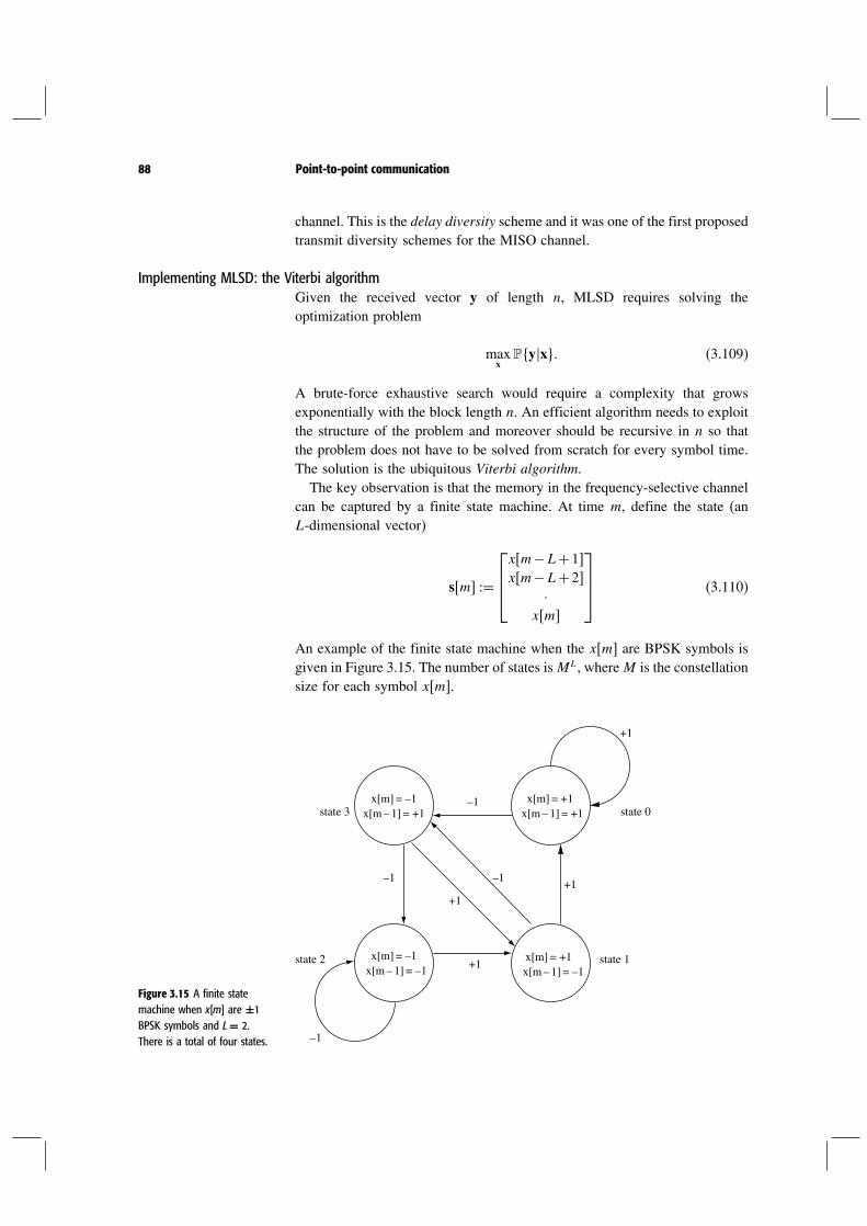
88 Point-to-point communication
channel. This is the delay diversity scheme and it was one of the first proposedtransmit diversity schemes for the MISO channel.
Implementing MLSD: the Viterbi algorithmGiven the received vector y of length n, MLSD requires solving theoptimization problem
maxx
yx (3.109)
A brute-force exhaustive search would require a complexity that growsexponentially with the block length n. An efficient algorithm needs to exploitthe structure of the problem and moreover should be recursive in n so thatthe problem does not have to be solved from scratch for every symbol time.The solution is the ubiquitous Viterbi algorithm.The key observation is that the memory in the frequency-selective channel
can be captured by a finite state machine. At time m, define the state (anL-dimensional vector)
sm =
xm−L+1xm−L+2
·xm
(3.110)
An example of the finite state machine when the xm are BPSK symbols isgiven in Figure 3.15. The number of states isML, whereM is the constellationsize for each symbol xm.
Figure 3.15 A finite statemachine when x[m] are ±1BPSK symbols and L= 2.There is a total of four states.
x[m] = –1x[m – 1] = –1
x[m] = –1x[m – 1] = +1 state 0state 3
state 2 state 1
–1
+1
+1
+1
–1
–1–1
x[m] = +1
+1
x[m – 1] = –1
x[m] = +1x[m – 1] = +1

89 3.4 Frequency diversity
The received symbol ym is given by
ym= h∗sm+wm (3.111)
with h representing the frequency-selective channel, as in (3.104). The MLSDproblem (3.109) can be rewritten as
mins1 sn
− logy1 yn s1 sn (3.112)
subject to the transition constraints on the state sequence (i.e., the second com-ponent of sm is the same as the first component of sm+1). Conditionedon the state sequence s1 sn, the received symbols are independentand the log-likelihood ratio breaks into a sum:
logy1 yn s1 sn=n∑
m=1
logym sm (3.113)
The optimization problem in (3.112) can be represented as the problem offinding the shortest path through an n-stage trellis, as shown in Figure 3.16.Each state sequence s1 sn is visualized as a path through the trellis,and given the received sequence y1 yn, the cost associated with themth transition is
cmsm =− logym sm (3.114)
Figure 3.16 The trellisrepresentation of the channel.
s[0] s[1] s[2] s[3] s[4] s[5] s[0] s[1] s[2] s[3] s[4] s[5]at time 2 at time 3
at time 4 at time 5
state 0
state 1
state 2
state 3
state 0
state 1
state 2
state 3
s[0] s[1] s[2] s[3] s[4] s[5]
m = 0 m = 1 m = 2 m = 3 m = 4 m = 5
state 0
state 1
state 2
state 3
s[0] s[1] s[2] s[3] s[4] s[5]
m = 0 m = 1 m = 2 m = 3 m = 4 m = 5
m = 0 m = 1 m = 2 m = 3 m = 4 m = 5m = 0 m = 1 m = 2 m = 3 m = 4 m = 5
state 0
state 1
state 2
state 3

90 Point-to-point communication
The solution is given recursively by the optimality principle of dynamicprogramming. Let Vms be the cost of the shortest path to a given state s atstage m. Then Vms for all states s can be computed recursively:
V1s= c1sVms=min
uVm−1u+ cms m > 1
(3.115)
(3.116)
Here the minimization is over all possible states u, i.e., we only considerthe states that the finite state machine can be in at stage m−1 and, further,can still end up at state s at stage m. The correctness of this recursion is basedon the following intuitive fact: if the shortest path to state s at stage m goesthrough the state u∗ at stage m−1, then the part of the path up to stage m−1must itself be the shortest path to state u∗. See Figure 3.17. Thus, to computethe shortest path up to stage m, it suffices to augment only the shortest pathsup to stage m−1, and these have already been computed.Once Vms is computed for all states s, the shortest path to stage m is
simply the minimum of these values over all states s. Thus, the optimizationproblem (3.112) is solved. Moreover, the solution is recursive in n.The complexity of the Viterbi algorithm is linear in the number of stages n.
Thus, the cost is constant per symbol, a vast improvement over brute-forceexhaustive search. However, its complexity is also proportional to the sizeof the state space, which is ML, where M is the constellation size of eachsymbol. Thus, while MLSD can be done for channels with a small numberof taps, it becomes impractical when L becomes large.The computational complexity of MLSD leads to an interest in seeking
suboptimal equalizers which yield comparable performance. Some candi-dates are linear equalizers (such as the zero-forcing and minimum meansquare error (MMSE) equalizers, which involve simple linear operationson the received symbols followed by simple hard decoders), and theirdecision-feedback versions (DFE), where previously detected symbols areremoved from the received signal before linear equalization is performed.We will discuss these equalizers further in Discussion 8.1, where we exploit
Figure 3.17 The dynamicprogramming principle. If thefirst m−1 segments of theshortest path to state s atstage m were not the shortestpath to state u∗ at stage m−1,then one could have found aneven shorter path to state s.
s
m – 1 m
shorter path
u∗

91 3.4 Frequency diversity
a correspondence between the MIMO channel and the frequency-selectivechannel.
3.4.3 Direct-sequence spread-spectrum
A common communication system that employs a wide bandwidth is thedirect-sequence (DS) spread-spectrum system. Its basic components are shownin Figure 3.18. Information is encoded and modulated by a pseudonoise (PN)sequence and transmitted over a bandwidth W . In contrast to the systemwe analyzed in the last section where an independent symbol is sent ateach symbol time, the data rate R bits/s in a spread-spectrum system istypically much smaller than the transmission bandwidth W Hz. The ratioW/R is sometimes called the processing gain of the system. For example,IS-95 (CDMA) is a direct-sequence spread-spectrum system. The bandwidthis 1.2288MHz and a typical data rate (voice) is 9.6 kbits/s, so the processinggain is 128. Thus, very few bits are transmitted per degree of freedom peruser. In spread-spectrum jargon, each sample period is called a chip, andanother way of describing a spread-spectrum system is that the chip rate ismuch larger than the data rate.Because the symbol rate per user is very low in a spread-spectrum system,
ISI is typically negligible and equalization is not required. Instead, as wewill discuss next, a much simpler receiver called the Rake receiver can beused to extract frequency diversity. In the cellular setting, multiple spread-spectrum users would share the large bandwidth so that the aggregate bitrate can be high even though the rate of each user is low. The large pro-cessing gain of a user serves to mitigate the interference from other users,which appears as random noise. In addition to providing frequency diversityagainst multipath fading and allowing multiple access, spread-spectrum sys-tems serve other purposes, such as anti-jamming from intentional interferers,and achieving message privacy in the presence of other listeners. We will dis-cuss the multiple access aspects of spread-spectrum systems in Chapter 4. Fornow, we focus on how DS spread-spectrum systems can achieve frequencydiversity.
The Rake receiverSuppose we transmit one of two n-chips long pseudonoise sequences xA or xB.Consider the problem of binary detection over a wideband multipath channel.In this context, a binary symbol is transmitted over n chips. The receivedsignal is given by
ym=∑
hmxm−+wm (3.117)
We assume that hm is non-zero only for = 0 L−1, i.e., the channelhas L taps. One can think of L/W as the delay spread Td. Also, we assume

92 Point-to-point communication
Channel decoder
ModulatorChannel encoder
Pseudorandom pattern
generator
Pseudorandom pattern
generator
Informationsequence
OutputdataDemodulatorChannel
that hm does not vary with m during the transmission of the sequence,Figure 3.18 Basic elements of adirect sequence spread-spectrum system.
i.e., the channel is considered time-invariant. This holds if n TcW , whereTc is the coherence time of the channel. We also assume that there is negli-gible interference between consecutive symbols, so that we can consider thebinary detection problem in isolation for each symbol. This assumption isvalid if n L, which is quite common in a spread-spectrum system with highprocessing gain. Otherwise, ISI between consecutive symbols becomes signif-icant, and an equalizer would be needed to mitigate the ISI. Note however weassume that simultaneously n TdW and n TcW , which is possible only ifTd Tc. In a typical cellular system, Td is of the order of microseconds andTc of the order of tens of milliseconds, so this assumption is quite reasonable.(Recall from Chapter 2, Table 2.2 that a channel satisfying this condition iscalled an underspread channel.)With the above assumptions, the output is just a convolution of the input
with the LTI channel plus noise
ym= h∗xm+wm m= 1 n+L (3.118)
where h is the th tap of the time-invariant channel filter response, withh = 0 for < 0 and > L− 1. Assuming the channel h is known to thereceiver, two sufficient statistics, rA and rB, can be obtained by projectingthe received vector y = y1 yn+Lt onto the n+L dimensionalvectors vA and vB, where vA = h∗xA1 h∗xAn+Lt and vB =h∗xB1 h∗xBn+Lt, i.e.,
rA = v∗Ay rB = v∗By (3.119)
The computation of rA and rB can be implemented by first matched filteringthe received signal to xA and to xB. The outputs of the matched filters arepassed through a filter matched to the channel response h and then sampledat time n+L (Figure 3.19). This is called the Rake receiver. What the Rakeactually does is taking inner products of the received signal with shiftedversions at the candidate transmitted sequences. Each output is then weightedby the channel tap gains at the appropriate delays and summed. The signalpath associated with a particular delay is sometimes called a finger of theRake receiver.

93 3.4 Frequency diversity
Figure 3.19 The Rake receiver.Here, h is the filter matched toh, i.e., h = h∗− . Each tap of hrepresents a finger of the Rake.
XA
XB
h
w[m]
XA
h
XB
h
Decision
Estimate h
+
As discussed earlier, we are continuing with the assumption that the channelgains h are known at the receiver. In practice, these gains have to be estimatedand tracked from either a pilot signal or in a decision-directed mode usingthe previously detected symbols. (The channel estimation problem will bediscussed in Section 3.5.2.) Also, due to hardware limitations, the actualnumber of fingers used in a Rake receiver may be less than the total numberof taps L in the range of the delay spread. In this case, there is also a trackingmechanism in which the Rake receiver continuously searches for the strongpaths (taps) to assign the limited number of fingers to.
Performance analysisLet us now analyze the performance of the Rake receiver. To simplify ournotation, we specialize to antipodal modulation (i.e., xA = −xB = u); theanalysis for other modulation schemes is similar. One key aspect of spread-spectrum systems is that the transmitted signal ±u has a pseudonoise char-acteristic. The defining characteristic of a pseudonoise sequence is that itsshifted versions are nearly orthogonal to each other. More precisely, if wewrite u= u1 un, and
u = 0 0 u1 un0 0t (3.120)
as the n+L dimensional version of u shifted by chips (hence there are zeros preceding u and L− zeros following u above), the pseudonoiseproperty means that for every = 0 L−1,
u∗u′ n∑
i=1
ui2 = ′ (3.121)
To simplify the analysis, we assume full orthogonality: u∗u′ = 0 if = ′.We will now show that the performance of the Rake is the same as that
in the diversity model with L branches for repetition coding described inSection 3.2. We can see this by looking at a set of sufficient statistics for the

94 Point-to-point communication
detection problem different from the ones we used earlier. First, we rewritethe channel model in vector form
y=L−1∑
=0
hx+w (3.122)
where w = w1 wn+Lt and x =±u, the version of the trans-mitted sequence (either u or −u) shifted by chips. The received signal(without the noise) therefore lies in the span of the L vectors u/u. Bythe pseudonoise assumption, all these vectors are orthogonal to each other.A set of L sufficient statistics r can be obtained by projecting y ontoeach of these vectors
r = hx+w = 0 L−1 (3.123)
where x=±u. Further, the orthogonality of u implies that w are i.i.d. 0N0. Comparing with (3.32), this is exactly the same as the L-branchdiversity model for the case of repetition code interleaved over time. Thus, wesee that the Rake receiver in this case is nothing more than a maximal ratiocombiner of the signals from the L diversity branches. The error probabilityis given by
pe =
Q
√√√2u2
L∑
=1
h2/N0
(3.124)
If we assume a Rayleigh fading model such that the tap gains h are i.i.d. 01/L, i.e., the energy is spread equally among all the L taps (normaliz-ing such that the
∑ h2= 1), then the error probability can be explicitly
computed (as in (3.37)):
pe =(1−
2
)L L−1∑
=0
(L−1+
)(1+
2
)
(3.125)
where
=√
SNR1+ SNR
(3.126)
and SNR = u2/N0L can be interpreted as the average signal-to-noise ratioper diversity branch. Noting that u2 is the average total energy receivedper bit of information, we can define b = u2. Hence, the SNR per branchis 1/L ·b/N0. Observe that the factor of 1/L accounts for the splitting ofenergy due to spreading: the larger the spread bandwidth W , the larger L is,

95 3.4 Frequency diversity
and the more diversity one gets, but there is less energy in each branch.13
As L→,∑L
=1 h2 converges to 1 with probability 1 by the law of largenumbers, and from (3.124) we see that
pe →Q(√
2b/N0
) (3.127)
i.e., the performance of the AWGN channel with the same b/N0 is asymp-totically achieved.The above analysis assumes an equal amount of energy in each tap. In a
typical multipath delay profile, there is more energy in the taps with shorterdelays. The analysis can be extended to the cases when the h have unequalvariances as well. (See Section 14.5.3 in [96]).
3.4.4 Orthogonal frequency division multiplexing
Both the single-carrier system with ISI equalization and the DS spread-spectrum system with Rake reception are based on a time-domain view of thechannel. But we know that if the channel is linear time-invariant, sinusoidsare eigenfunctions and they get transformed in a particularly simple way.ISI occurs in a single-carrier system because the transmitted signals are notsinusoids. This suggests that if the channel is underspread (i.e., the coherencetime is much larger than the delay spread) and is therefore approximatelytime-invariant for a sufficiently long time-scale, then transformation intothe frequency domain can be a fruitful approach to communication overfrequency-selective channels. This is the basic idea behind OFDM.We begin with the discrete-time baseband model
ym=∑
hmxm−+wm (3.128)
For simplicity, we first assume that for each , the th tap is not changingwith m and hence the channel is linear time-invariant. Again assuming afinite number of non-zero taps L = TdW , we can rewrite the channel modelin (3.128) as
ym=L−1∑
=0
hxm−+wm (3.129)
Sinusoids are eigenfunctions of LTI systems, but they are of infinite dura-tion. If we transmit over only a finite duration, say Nc symbols, then thesinusoids are no longer eigenfunctions. One way to restore the eigenfunction
13 This is assuming a very rich scattering environment, leading to many paths, all of equalenergy. In reality, however, there are just a few paths that are strong enough to matter.

96 Point-to-point communication
property is by adding a cyclic prefix to the symbols. For every block ofsymbols of length Nc, denoted by
d= d0 d1 dNc−1t
we create an Nc+L−1 input block as
x= dNc−L+1 dNc−L+2 dNc−1 d0 d1 dNc−1t(3.130)
i.e., we add a prefix of length L− 1 consisting of data symbols rotatedcyclically (Figure 3.20). With this input to the channel (3.129), consider theoutput
ym=L−1∑
=0
hxm−+wm m= 1 Nc+L−1
The ISI extends over the first L− 1 symbols and the receiver ignores it byconsidering only the output over the time interval m ∈ LNc+L− 1. Dueto the additional cyclic prefix, the output over this time interval (of lengthNc) is
ym=L−1∑
=0
hdm−L− modulo Nc+wm (3.131)
See Figure 3.21.Denoting the output of length Nc by
y= yL yNc+L−1t
Figure 3.20 The cyclic prefixoperation.
x [N + L – 1] = d[N –1]dN–1
d0
IDFT
d [N – 1]
d [0] Cyclic prefix
x [L] = d [0]
x [L –1] = d [N –1]
x [1] = d [N – L + 1]

97 3.4 Frequency diversity
Figure 3.21 Convolutionbetween the channel h andthe input x formed from thedata symbols d by adding acyclic prefix. The output isobtained by multiplying thecorresponding values of x andh on the circle, and outputs atdifferent times are obtained byrotating the x-values withrespect to the h-values. Thecurrent configuration yields theoutput y [L].
x [L + 1] = d [1]
x [N + L – 1] = d[N – 1]
x [1]
x [L – 1] = d [N – 1]
x [L] = d [0]
hL – 1
0
0
h1
h0
and the channel by a vector of length Nc
h= h0 h1 hL−10 0t (3.132)
(3.131) can be written as
y= h⊗d+w (3.133)
Here we denoted
w = wL wNc+L−1t (3.134)
as a vector of i.i.d. 0N0 random variables. We also used the notationof ⊗ to denote the cyclic convolution in (3.131). Recall that the discreteFourier transform (DFT) of d is defined to be
dn =1√Nc
Nc−1∑
m=0
dm exp(−j2nm
Nc
)
n= 0 N −1 (3.135)
Taking the discrete Fourier transform (DFT) of both sides of (3.133) andusing the identity
DFTh⊗dn =√NcDFThn ·DFTdn n= 0 Nc−1 (3.136)
we can rewrite (3.133) as
yn = hndn+ wn n= 0 Nc−1 (3.137)
Here we have denoted w0 wNc−1 as the Nc-point DFT of the noise vectorw1 wNc. The vector h0 hNc−1
t is defined as the DFT of theL-tap channel h, multiplied by
√Nc,
hn =L−1∑
=0
h exp(−j2n
Nc
)
(3.138)
98 Point-to-point communication
Note that the nth component hn is equal to the frequency response of thechannel (see (2.20)) at f = nW/Nc.We can redo everything in terms of matrices, a viewpoint which will prove
particularly useful in Chapter 7 when we will draw a connection between thefrequency-selective channel and the MIMO channel. The circular convolutionoperation u= h⊗d can be viewed as a linear transformation
u= Cd (3.139)
where
C =
h0 0 · 0 hL−1 hL−2 · h1
h1 h0 0 · 0 hL−1 · h2
· · · · · · · ·0 · 0 hL−1 hL−2 · h1 h0
(3.140)
is a circulant matrix, i.e., the rows are cyclic shifts of each other. On the otherhand, the DFT of d can be represented as an Nc-length vector Ud, where Uis the unitary matrix with its knth entry equal to
1√Nc
exp(−j2kn
Nc
)
kn= 0 Nc−1 (3.141)
This can be viewed as a coordinate change, expressing d in the basis definedby the rows of U. Equation (3.136) is equivalent to
Uu=Ud (3.142)
where is the diagonal matrix with diagonal entries√Nc times the DFT of
h, i.e.,
nn = hn =(√
NcUh)
n n= 0 Nc−1
Comparing (3.139) and (3.142), we come to the conclusion that
C= U−1U (3.143)
Equation (3.143) is the matrix version of the key DFT property (3.136).In geometric terms, this means that the circular convolution operation isdiagonalized in the coordinate system defined by the rows of U, and theeigenvalues of C are the DFT coefficients of the channel h. Equation (3.133)can thus be written as
y= Cd+w = U−1Ud+w (3.144)

99 3.4 Frequency diversity
d[N–1]
y0
x [N + L – 1] = d[N – 1]
Cyclic
prefix
y [N + L – 1]dN–1
IDFT DFT
Remove
prefix
yN–1
y[L]
y[N + L – 1]
y[1]
y[L – 1]
y[L]
x [L – 1] = d[N – 1]
x [L] = d[0]
x [1] = d[N – L + 1]
d0 d[0]Channel
This representation suggests a natural rotation at the input and at the outputFigure 3.22 The OFDMtransmission and receptionschemes.
to convert the channel to a set of non-interfering channels with no ISI.In particular, the actual data symbols (denoted by the length Nc vector d)in the frequency domain are rotated through the IDFT (inverse DFT) matrixU−1 to arrive at the vector d. At the receiver, the output vector of lengthNc (obtained by ignoring the first L symbols) is rotated through the DFTmatrix U to obtain the vector y. The final output vector y and the actual datavector d are related through
yn = hndn+ wn n= 0 Nc−1 (3.145)
We have denoted w = Uw as the DFT of the random vector w and we seethat since w is isotropic, w has the same distribution as w, i.e., a vector ofi.i.d. 0N0 random variables (cf. (A.26) in Appendix A).These operations are illustrated in Figure 3.22, which affords the following
interpretation. The data symbols modulate Nc tones or sub-carriers, whichoccupy the bandwidth W and are uniformly separated by W/Nc. The datasymbols on the sub-carriers are then converted (through the IDFT) to timedomain. The procedure of introducing the cyclic prefix before transmissionallows for the removal of ISI. The receiver ignores the part of the output signalcontaining the cyclic prefix (along with the ISI terms) and converts the lengthNc symbols back to the frequency domain through a DFT. The data symbolson the sub-carriers are maintained to be orthogonal as they propagate throughthe channel and hence go through narrowband parallel sub-channels. Thisinterpretation justifies the name of OFDM for this communication scheme.Finally, we remark that DFT and IDFT can be very efficiently implemented(using Fast Fourier Transform) whenever Nc is a power of 2.
OFDM block lengthThe OFDM scheme converts communication over a multipath channel intocommunication over simpler parallel narrowband sub-channels. However, thissimplicity is achieved at a cost of underutilizing two resources, resulting ina loss of performance. First, the cyclic prefix occupies an amount of timewhich cannot be used to communicate data. This loss amounts to a fraction

100 Point-to-point communication
L/Nc +L of the total time. The second loss is in the power transmitted.A fraction L/Nc+L of the average power is allocated to the cyclic prefix andcannot be used towards communicating data. Thus, to minimize the overhead(in both time and power) due to the cyclic prefix we prefer to have Nc aslarge as possible. The time-varying nature of the wireless channel, however,constrains the largest value Nc can reasonably take.We started the discussion in this section by considering a simple channel
model (3.129) that did not vary with time. If the channel is slowly time-varying (as discussed in Section 2.2.1, this is a reasonable assumption) thenthe coherence time Tc is much larger than the delay spread Td (the under-spread scenario). For underspread channels, the block length of the OFDMcommunication scheme Nc can be chosen significantly larger than the multi-path length L= TdW , but still much smaller than the coherence block lengthTcW . Under these conditions, the channel model of linear time invarianceapproximates a slowly time-varying channel over the block length Nc, whilekeeping the overhead small.The constraint on the OFDM block length can also be understood in the
frequency domain. A block length of Nc corresponds to an inter-sub-carrierspacing equal to W/Nc. In a wireless channel, the Doppler spread introducesuncertainty in the frequency of the received signal; from Table 2.1 we seethat the Doppler spread is inversely proportional to the coherence time of thechannel: Ds = 1/4Tc. For the inter-sub-carrier spacing to be much larger thanthe Doppler spread, the OFDM block length Nc should be constrained to bemuch smaller than TcW . This is the same constraint as above.Apart from an underutilization of time due to the presence of the cyclic
prefix, we also mentioned the additional power due to the cyclic prefix.OFDM schemes that put a zero signal instead of the cyclic prefix have beenproposed to reduce this loss. However, due to the abrupt transition in thesignal, such schemes introduce harmonics that are difficult to filter in theoverall signal. Further, the cyclic prefix can be used for timing and frequencyacquisition in wireless applications, and this capability would be lost if a zerosignal replaced the cyclic prefix.
Frequency diversityLet us revert to the non-overlapping narrowband channel representation ofthe ISI channel in (3.145). The correlation between the channel frequencycoefficients h0 hNc−1 depends on the coherence bandwidth of the chan-nel. From our discussion in Section 2.3, we have learned that the coherencebandwidth is inversely proportional to the multipath spread. In particular, wehave from (2.47) that
Wc =12Td
= W
2L

101 3.4 Frequency diversity
where we use our notation for L as denoting the length of the ISI. Since eachsub-carrier is W/Nc wide, we expect approximately
NcWc
W= Nc
2L
as the number of neighboring sub-carriers whose channel coefficients areheavily correlated (Exercise 3.28). One way to exploit the frequency diver-sity is to consider ideal interleaving across the sub-carriers (analogousto the time-interleaving done in Section 3.2) and consider the modelof (3.31)
y = hx+w = 1 L
The difference is that now represents the sub-carriers while it is used todenote time in (3.31). However, with the ideal frequency interleaving assump-tion we retain the same independent assumption on the channel coefficients.Thus, the discussion of Section 3.2 on schemes harnessing diversity is directlyapplicable here. In particular, an L-fold diversity gain (proportional to thenumber of ISI symbols L) can be obtained. Since the communication schemeis over sub-carriers, the form of diversity is due to the frequency-selectivechannel and is termed frequency diversity (as compared to the time diversitydiscussed in Section 3.2 which arises due to the time variations of the channel).
Summary 3.3 Communication over frequency-selectivechannels
We have studied three approaches to extract frequency diversity ina frequency-selective channel (with L taps). We summarize their keyattributes and compare their implementational complexity.
1 Single-carrier with ISI equalizationUsing maximum likelihood sequence detection (MLSD), full diversity ofL can be achieved for uncoded transmission sent at symbol rate.
MLSD can be performed by the Viterbi algorithm. The complexity is con-stant per symbol time but grows exponentially with the number of taps L.
The complexity is entirely at the receiver.
2 Direct-sequence spread-spectrumInformation is spread, via a pseudonoise sequence, across a bandwidthmuch larger than the data rate. ISI is typically negligible.
The signal received along the L nearly orthogonal diversity paths ismaximal-ratio combined using the Rake receiver. Full diversity is achieved.
102 Point-to-point communication
Compared to MLSD, complexity of the Rake receiver is much lower. ISIis avoided because of the very low spectral efficiency per user, but thespectrum is typically shared between many interfering users. Complexityis thus shifted to the problem of interference management.
3 Orthogonal frequency division multiplexingInformation is modulated on non-interfering sub-carriers in the frequencydomain.
The transformation between the time and frequency domains is done bymeans of adding/subtracting a cyclic prefix and IDFT/DFT operations.This incurs an overhead in terms of time and power.
Frequency diversity is attained by coding over independently faded sub-carriers. This coding problem is identical to that for time diversity.
Complexity is shared between the transmitter and the receiver in perform-ing the IDFT and DFT operations; the complexity of these operationsis insensitive to the number of taps, scales moderately with the numberof sub-carriers Nc and is very manageable with current implementationtechnology.
Complexity of diversity coding across sub-carriers can be traded off withthe amount of diversity desired.
3.5 Impact of channel uncertainty
In the past few sections we assumed perfect channel knowledge so thatcoherent combining can be performed at the receiver. In fast varying channels,it may not be easy to estimate accurately the phases and magnitudes of thetap gains before they change. In this case, one has to understand the impact ofestimation errors on performance. In some situations, non-coherent detection,which does not require an estimate of the channel, may be the preferred route.In Section 3.1.1, we have already come across a simple non-coherent detectorfor fading channels without diversity. In this section, we will extend this tochannels with diversity.When we compared coherent and non-coherent detection for channels with-
out diversity, the difference was seen to be relatively small (cf. Figure 3.2).An important question is what happens to that difference as the number ofdiversity paths L increases. The answer depends on the specific diversityscenario. We first focus on the situation where channel uncertainty has themost impact: DS spread-spectrum over channels with frequency diversity.Once we understand this case, it is easy to extend the insights to otherscenarios.

103 3.5 Impact of channel uncertainty
3.5.1 Non-coherent detection for DS spread-spectrum
We considered this scenario in Section 3.4.3, except now the receiver hasno knowledge of the channel gains h. As we saw in Section 3.1.1, noinformation can be communicated in the phase of the transmitted signal inconjunction with non-coherent detection (in particular, antipodal signalingcannot be used). Instead, we consider binary orthogonal modulation,14 i.e., xAand xB are orthogonal and xA = xB.
Recall that the central pseudonoise property of the transmitted sequencesin DS spread-spectrum is that the shifted versions are nearly orthogonal. Forsimplicity of analysis, we continue with the assumption that shifted versionsof the transmitted sequence are exactly orthogonal; this holds for both xA andxB here. We make the further assumption that versions of the two sequenceswith different shifts are also orthogonal to each other, i.e., xA ∗x
′B = 0
for = ′ (the so-called zero cross-correlation property). This approximatelyholds in many spread-spectrum systems. For example, in the uplink of IS-95,the transmitted sequence is obtained by multiplying the selected codeword ofan orthogonal code by a (common) pseudonoise ±1 sequence, so that the lowcross-correlation property carries over from the auto-correlation property ofthe pseudonoise sequence.Proceeding as in the analysis of coherent detection, we start with the
channel model in vector form (3.122) and observe that the projection of yonto the 2L orthogonal vectors xA /xAxB /xB yields 2L sufficientstatistics:
rA = hx1+w
A = 0 L−1
rB = hx2+w
B = 0 L−1
where wA and w
B are i.i.d. 0N0, and
(x1x2
)
=
(xA0
)
ifxAis transmitted
(0
xB
)
ifxBis transmitted
(3.146)
This is essentially a generalization of the non-coherent detection problem inSection 3.1.1 from 1 branch to L branches. Just as in the 1 branch case, a
14 Typically M-ary orthogonal modulation is used. For example, the uplink of IS-95 employsnon-coherent detection of 64-ary orthogonal modulation.

104 Point-to-point communication
square-law type detector is the optimal non-coherent detector: decide in favorof xA if
L−1∑
=0
rA 2 ≥L−1∑
=0
rB 2 (3.147)
otherwise decide in favor of xB. The performance can be analyzed as in the1 branch case: the error probability has the same form as in (3.125), but with given by
= 1/L ·b/N0
2+1/L ·b/N0
(3.148)
where b = xA2. (See Exercise 3.31.) As a basis of comparison, the perfor-mance of coherent detection of binary orthogonal modulation can be analyzedas for the antipodal case; it is again given by (3.125) but with given by(Exercise 3.33):
=√
1/L ·b/N0
2+1/L ·b/N0
(3.149)
It is interesting to compare the performance of coherent and non-coherentdetection as a function of the number of diversity branches. This is shown inFigures 3.23 and 3.24. For L = 1, the gap between the performance of bothschemes is small, but they are bad anyway, as there is a lack of diversity. Thispoint has already been made in Section 3.1. As L increases, the performanceof coherent combining improves monotonically and approaches the perfor-mance of an AWGN channel. In contrast, the performance of non-coherentdetection first improves with L but then degrades as L is increased further.
Figure 3.23 Comparison oferror probability undercoherent detection (——) andnon-coherent detection (- - -),as a function of the number oftaps L. Here b/N0 = 10 dB.
0 10 20 30 40 50 60 70 80
log 10
( pe)
–5.5
–0.5
–1
–1.5
–2
–2.5
–3
–3.5
–4
–4.5
–5
Number of taps L

105 3.5 Impact of channel uncertainty
Figure 3.24 Comparison oferror probability undercoherent detection (——) andnon-coherent detection (- - -),as a function of the number oftaps L. Here b/N0 = 15dB.
log 10
( pe)
–14
0
–2
–4
–6
–8
–10
–12
0 10 20 30 40 50 60 70 80Number of taps L
The initial improvement comes from a diversity gain. There is however alaw of diminishing return on the diversity gain. At the same time, when L
becomes too large, the SNR per branch becomes very poor and non-coherentcombining cannot effectively exploit the available diversity. This leads to anultimate degradation in performance. In fact, it can be shown that as L→the error probability approaches 1/2.
3.5.2 Channel estimation
The significant performance difference between coherent and non-coherentcombining when the number of branches is large suggests the importanceof channel knowledge in wideband systems. We assumed perfect channelknowledge when we analyzed the performance of the coherent Rake receiver,but in practice, the channel taps have to be estimated and tracked. It istherefore important to understand the impact of channel measurement errorson the performance of the coherent combiner. We now turn to the issue ofchannel estimation.In data detection, the transmitted sequence is one of several possible
sequences (representing the data symbol). In channel estimation, the trans-mitted sequence is assumed to be known at the receiver. In a pilot-basedscheme, a known sequence (called a pilot, sounding tone, or training sequence)is transmitted and this is used to estimate the channel.15 In a decision-feedback scheme, the previously detected symbols are used instead to updatethe channel estimates. If we assume that the detection is error free, thenthe development below applies to both pilot-based and decision-directedschemes.
15 The downlink of IS-95 uses a pilot, which is assigned its own pseudonoise sequence andtransmitted superimposed on the data.

106 Point-to-point communication
Focus on one symbol duration, and suppose the transmitted sequence is aknown pseudonoise sequence u. We return to the channel model in vectorform (cf. (3.122))
y=L−1∑
=0
hu+w (3.150)
We see that since the shifted versions of u are orthogonal to each otherand the taps are assumed to be independent of each other, projecting yonto u/u will yield a sufficient statistic to estimate h (seeSummary A.3)
r = u∗y= hu+w =√h+w (3.151)
where = u2. This is implemented by filtering the received signal by afilter matched to u and sampling at the appropriate chip time. This operationis the same as the first stage of the Rake receiver, and the channel estimatorcan in fact be combined with the Rake receiver if done in a decision-directedmode. (See Figure 3.19.)Typically, channel estimation is obtained by averaging K such measure-
ments over a coherence time period in which the channel is constant:
rk =√
h+wk k= 1 K (3.152)
Assuming that h ∼ 01/L, the minimum mean square estimate of h
given these measurements is (cf. (A.84) in Summary A.3)
h =√
K+LN0
K∑
k=1
rk (3.153)
The mean square error associated with this estimate is (cf. (A.85) inSummary A.3)
1L· 11+K/LN0
(3.154)
the same for all branches.The key parameter affecting the estimation error is
SNRest =K
LN0
(3.155)
When SNRest 1, the mean square estimation error is much smaller than thevariance of h (equal to 1/L) and the impact of the channel estimation erroron the performance of the coherent Rake receiver is not significant; perfect

107 3.5 Impact of channel uncertainty
channel knowledge is a reasonable assumption in this regime. On the otherhand, when SNRest 1, the mean square error is close to 1/L, the varianceof h. In this regime, we hardly have any information about the channelgains and the performance of the coherent combiner cannot be expected to bebetter than the non-coherent combiner, which we know has poor performancewhenever L is large.How should we interpret the parameter SNRest? Since the channel is constant
over the coherence time Tc, we can interpret K as the total received energyover the channel coherence time Tc. We can rewrite SNRest as
SNRest =PTc
LN0
(3.156)
where P is the received power of the signal from which channel measurementsare obtained. Hence, SNRest can be interpreted as the signal-to-noise ratioavailable to estimate the channel per coherence time per tap. Thus, channeluncertainty has a significant impact on the performance of the Rake receiverwhenever this quantity is significantly below 0 dB.If the measurements are done in a decision-feedback mode, P is the received
power of the data stream itself. If the measurements are done from a pilot,then P is the received power of the pilot. On the downlink of a CDMAsystem, one can have a pilot common to all users, and the power allocated tothe pilot can be larger than the power of the signals for the individual users.This results in a larger SNRest, and thus makes coherent combining easier.On the uplink, however, it is not possible to have a common pilot, and thechannel estimation will have to be done with a weaker pilot allotted to theindividual user. With a lower received power from the individual users, SNRestcan be considerably smaller.
3.5.3 Other diversity scenarios
There are two reasons why wideband DS spread-spectrum systems aresignificantly impacted by channel uncertainty:
• the amount of energy per resolvable path decreases inversely with increas-ing number of paths, making their gains harder to estimate when there aremany paths;
• the number of diversity paths depends both on the bandwidth and the delayspread and, given these parameters, the designer has no control over thisnumber.
What about in other diversity scenarios?In antenna diversity with L receive antennas, the received energy per
antenna is the same regardless of the number of antennas, so the channel

108 Point-to-point communication
measurement problem is the same as with a single receive antenna and doesnot become harder. The situation is similar in the time diversity scenario. Inantenna diversity with L transmit antennas, the received energy per diversitypath does decrease with the number of antennas used, but certainly we canrestrict the number L to be the number of different channels that can bereliably learnt by the receiver.How about in OFDM systems with frequency diversity? Here, the designer
has control over how many sub-carriers to spread the signal energy over.Thus, while the number of available diversity branches L may increase withthe bandwidth, the signal energy can be restricted to a fixed number of sub-carriers L′ <L over any one OFDM time block. Such communication can berestricted to concentrated time-frequency blocks and Figure 3.25 visualizesone such scheme (for L′ = 2), where the choice of the L′ sub-carriers isdifferent for different OFDM blocks and is hopped over the entire bandwidth.Since the energy in each OFDM block is concentrated within a fixed numberof sub-carriers at any one time, coherent reception is possible. On the otherhand, the maximum diversity gain of L can still be achieved by codingacross the sub-carriers within one OFDM block as well as across differentblocks.One possible drawback is that since the total power is only concentrated
within a subset of sub-carriers, the total degrees of freedom available in thesystem are not utilized. This is certainly the case in the context of point-to-point communication; in a system with other users sharing the same band-width, however, the other degrees of freedom can be utilized by the otherusers and need not go wasted. In fact, one key advantage of OFDM over DSspread-spectrum is the ability to maintain orthogonality across multiple usersin a multiple access scenario. We will return to this point in Chapter 4.
Figure 3.25 An illustration of ascheme that uses only a fixedpart of the bandwidth at everytime. Here, one small squaredenotes a single sub-carrierwithin one OFDM block. Thetime-axis indexes the differentOFDM blocks; thefrequency-axis indexes thedifferent sub-carriers. Time
Freq
uenc
y

109 3.5 Impact of channel uncertainty
Chapter 3 The main plot
BaselineWe first looked at detection on a narrowband slow fading Rayleigh channel.Under both coherent and non-coherent detection, the error probabilitybehaves like
pe ≈ SNR−1 (3.157)
at high SNR. In contrast, the error probability decreases exponentially withthe SNR in the AWGN channel. The typical error event for the fadingchannel is due to the channel being in deep fade rather than the Gaussiannoise being large.
DiversityDiversity was presented as an effective approach to improve performancedrastically by providing redundancy across independently faded branches.Three modes of diversity were considered:• time – the interleaving of coded symbols over different coherence timeperiods;
• space – the use of multiple transmit and/or receive antennas;• frequency – the use of a bandwidth greater than the coherence bandwidthof the channel.
In all cases, a simple scheme that repeats the information symbol across themultiple branches achieves full diversity. With L i.i.d. Rayleigh branchesof diversity, the error probability behaves like
pe ≈ c · SNR−L (3.158)
at high SNR.
Examples of repetition schemes:• repeating the same symbol over different coherence periods;• repeating the same symbol over different transmit antennas one at atime;
• repeating the same symbol across OFDM sub-carriers in different coher-ence bands;
• transmitting a symbol once every delay spread in a frequency-selectivechannel so that multiple delayed replicas of the symbol are receivedwithout interference.
Code design and degrees of freedomMore sophisticated schemes cannot achieve higher diversity gain but canprovide a coding gain by improving the constant c in (3.158). This is

110 Point-to-point communication
achieved by utilizing the available degrees of freedom better than in therepetition schemes.
Examples:• rotation and permutation codes for time diversity and for frequencydiversity in OFDM;
• Alamouti scheme for transmit diversity;• uncoded transmission at symbol rate in a frequency-selective channelwith ISI equalization.
Criteria to design schemes with good coding gain were derived for thedifferent scenarios by using the union bound (based on pairwise errorprobabilities) on the actual error probability:• product distance between codewords for time diversity;• determinant criterion for space-time codes.
Channel uncertaintyThe impact of channel uncertainty is significant in scenarios where thereare many diversity branches but only a small fraction of signal energy isreceived along each branch. Direct-sequence spread-spectrum is a primeexample.
The gap between coherent and non-coherent schemes is very significantin this regime. Non-coherent schemes do not work well as they cannotcombine the signals along each branch effectively.
Accurate channel estimation is crucial. Given the amount of transmitpower devoted to channel estimation, the efficacy of detection performancedepends on the key parameter SNRest, the received SNR per coherence timeper diversity branch. If SNRest 0dB, then detection performance is nearcoherent. If SNRest 0dB, then effective combining is impossible.
Impact of channel uncertainty can be ameliorated in some schemes wherethe transmit energy can be focused on smaller number of diversity branches.Effectively SNRest is increased. OFDM is an example.
3.6 Bibliographical notes
Reliable communication over fading channels has been studied since the 1960s.Improving the performance via diversity is also an old topic. Standard digital commu-nication texts contain many formulas for the performance of coherent and non-coherentdiversity combiners, which we have used liberally in this chapter (see Chapter 14 ofProakis [96], for example).
Early works recognizing the importance of the product distance criterion for improv-ing the coding gain under Rayleigh fading are Wilson and Leung [144] and Divsalar

111 3.7 Exercises
and Simon [30], in the context of trellis-coded modulation. The rotation example istaken from Boutros and Viterbo [13]. Transmit antenna diversity was studied exten-sively in the late 1990s code design criteria were derived by Tarokh et al. [115] andby Guey et al. [55]; in particular, the determinant criterion is obtained in Tarokh et al.[115]. The delay diversity scheme was introduced by Seshadri and Winters [107].The Alamouti scheme was introduced by Alamouti [3] and generalized to orthog-onal designs by Tarokh et al. [117]. The diversity analysis of the decorrelator wasperformed by Winters et al. [145], in the context of a space-division multiple accesssystem with multiple receive antennas.
The topic of equalization has been studied extensively and is covered comprehen-sively in standard textbooks on communication theory; for example, see the book byBarry et al. [4]. The Viterbi algorithm was introduced in [139]. The diversity analysisof MLSD is adopted from Grokop and Tse [54].
The OFDM approach to communicate over a wideband channel was first used in mil-itary systems in the 1950s and discussed in early papers in the 1960s by Chang [18] andSaltzberg [104].Circular convolution and the DFT are classical undergraduate materialin digital signal processing (Chapter 8, and Section 8.7.5, in particular, of [87]).
The spread-spectrum approach to harness frequency diversity has been well sum-marized by Viterbi [140]. The Rake receiver was designed by Price and Green [95].The impact of channel uncertainty on the performance has been studied by variousauthors, including Médard and Gallager [85], Telatar and Tse [120] and Subramanianand Hajek [113].
3.7 Exercises
Exercise 3.1 Verify (3.19) and the high SNR approximation (3.21). Hint: Write theexpression as a double integral and interchange the order of integration.
Exercise 3.2 In Section 3.1.2 we studied the performance of antipodal signaling undercoherent detection over a Rayleigh fading channel. In particular, we saw that the errorprobability pe decreases like 1/SNR. In this question, we study a deeper characterizationof the behavior of pe with increasing SNR.1. A precise way of saying that pe decays like 1/SNR with increasing SNR is the
following:
limSNR→
pe · SNR= c
where c is a constant. Identify the value of c for the Rayleigh fading channel.2. Now we want to test how robust the above result is with respect to the fading
distribution. Let h be the channel gain, and suppose h2 has an arbitrary continuouspdf f satisfying f0 > 0. Does this give enough information to compute the highSNR error probability like in the previous part? If so, compute it. If not, specifywhat other information you need. Hint: You may need to interchange limit andintegration in your calculations. You can assume that this can be done withoutworrying about making your argument rigorous.
3. Suppose now we have L independent branches of diversity with gains h1 hL,and h2 having an arbitrary distribution as in the previous part. Is there enough

112 Point-to-point communication
information for you to find the high SNR performance of repetition coding andcoherent combining? If so, compute it. If not, what other information do you need?
4. Using the result in the previous part or otherwise, compute the high SNR perfor-mance under Rician fading. How does the parameter affect the performance?
Exercise 3.3 This exercise shows how the high SNR slope of the probability of error(3.19) versus SNR curve can be obtained using a typical error event analysis, withoutthe need for directly carrying out the integration.
Fix > 0 and define the -typical error events and − , where
= h h2 < 1/SNR1− (3.159)
1. By conditioning on the event , show that at high SNR
limSNR→
logpe
log SNR≤−1− (3.160)
2. By conditioning on the event − , show that
limSNR→
logpe
log SNR≥−1+ (3.161)
3. Hence conclude that
limSNR→
logpe
log SNR=−1 (3.162)
This says that the asymptotic slope of the error probability versus SNR plot(in dB/dB scale) is −1.
Exercise 3.4 In Section 3.1.2, we saw that there is a 4-dB energy loss when using4-PAM on only the I channel rather than using QPSK on both the I and the Q channels,although both modulations convey two bits of information. Compute the correspondingloss when one wants to transmit k bits of information using 2k-PAM rather than2k-QAM. You can assume k to be even. How does the loss depend on k?
Exercise 3.5 Consider the use of the differential BPSK scheme proposed inSection 3.1.3 for the Rayleigh flat fading channel.1. Find a natural non-coherent scheme to detect um based on ym− 1 and ym,
assuming the channel is constant across the two symbol times. Your scheme doesnot have to be the ML detector.
2. Analyze the performance of your detector at high SNR. You may need to makesome approximations. How does the high SNR performance of your detectorcompare to that of the coherent detector?
3. Repeat your analysis for differential QPSK.
Exercise 3.6 In this exercise we further study coherent detection in Rayleigh fading.1. Verify Eq. (3.37).2. Analyze the error probability performance of coherent detection of binary orthogo-
nal signaling with L branches of diversity, under an i.i.d. Rayleigh fading assump-tion (i.e., verify Eq. (3.149)).

113 3.7 Exercises
Exercise 3.7 In this exercise, we study the performance of the rotated code inSection 3.2.2.1. Give an explicit expression for the exact pairwise error probability xA → xB in
(3.49). Hint: The techniques from Exercise 3.1 will be useful here.2. This pairwise error probability was upper bounded in (3.54). Show that the product
of SNR and the difference between the upper bound and the actual pairwise errorprobability goes to zero with increasing SNR. In other words, the upper bound in(3.54) is tight up to the leading term in 1/SNR.
Exercise 3.8 In the text, we mainly use real symbols to simplify the notation. Inpractice, complex constellations are used (i.e., symbols are sent along both the I andQ components). The simplest complex constellation is QPSK: the constellation isa1+ j a1− j a−1− j a−1+ j.1. Compute the error probability of QPSK detection for a Rayleigh fading channel
with repetition coding over L branches of diversity. How does the performancecompare to a scheme which uses only real symbols?
2. In Section 3.2.2, we developed a diversity scheme based on rotation of real symbols(thus using only the I channel). One can develop an analogous scheme for QPSKcomplex symbols, using a 2×2 complex unitary matrix instead. Find an analogouspairwise code-design criterion as in the real case.
3. Real orthonormal matrices are special cases of complex unitary matrices. Withinthe class of real orthonormal matrices, find the optimal rotation to maximize yourcriterion.
4. Find the optimal unitary matrix to maximize your criterion. (This may be difficult!)
Exercise 3.9 In Section 3.2.2, we rotate two BPSK symbols to demonstrate the possibleimprovement over repetition coding in a time diversity channel with two diversitypaths. Continuing with the same model, now consider transmitting at a higher rateusing a 2n-PAM constellation for each symbol. Consider rotating the resulting 2Dconstellation by a rotation matrix of the form in (3.46). Using the performance criterionof the minimum squared product distance, construct the optimal rotation matrix.
Exercise 3.10 In Section 3.2.2, we looked at the example of the rotation code toachieve time diversity (with the number of branches, L, equal to 2). In the text, we usereal symbols and in Exercise 3.8 we extend to complex symbols. In the latter scenario,another coding scheme is the permutation code. Shown in Figure 3.26 are two 16-QAM constellations. Each codeword in the permutation code for L = 2 is obtainedby picking a pair of points, one from each constellation, which are represented by thesame icon. The codeword is transmitted over two (complex) symbol times.1. Why do you think this is called a permutation code?2. What is the data rate of this code?3. Compute the diversity gain and the minimum product distance for this code.4. How does the performance of this code compare to the rotation code in Exercise 3.8,
part (3), in terms of the transmit power required?
Exercise 3.11 In the text, we considered the use of rotation codes to obtain timediversity. Rotation codes are designed specifically for fading channels. Alternatively,one can use standard AWGN codes like binary linear block codes. This question looksat the diversity performance of such codes.
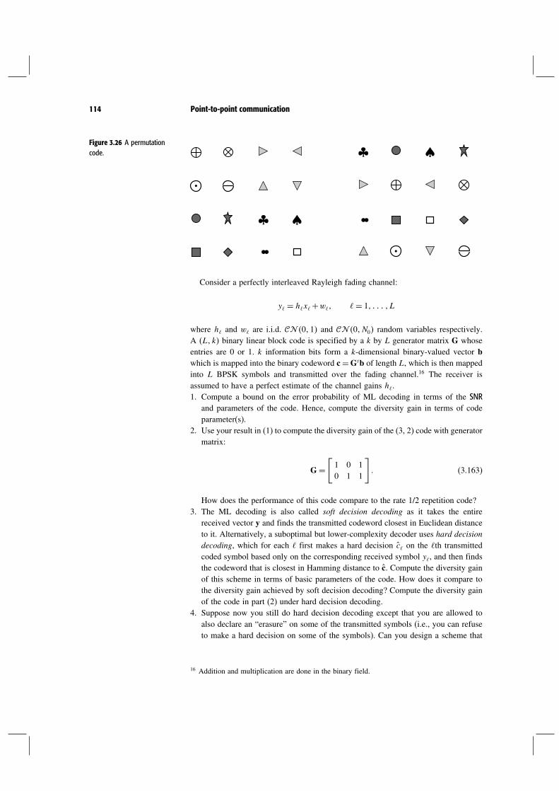
114 Point-to-point communication
Figure 3.26 A permutationcode.
♣
♣
♠
♠
Consider a perfectly interleaved Rayleigh fading channel:
y = hx+w = 1 L
where h and w are i.i.d. 01 and 0N0 random variables respectively.A Lk binary linear block code is specified by a k by L generator matrix G whoseentries are 0 or 1. k information bits form a k-dimensional binary-valued vector bwhich is mapped into the binary codeword c=Gtb of length L, which is then mappedinto L BPSK symbols and transmitted over the fading channel.16 The receiver isassumed to have a perfect estimate of the channel gains h.1. Compute a bound on the error probability of ML decoding in terms of the SNR
and parameters of the code. Hence, compute the diversity gain in terms of codeparameter(s).
2. Use your result in (1) to compute the diversity gain of the (3, 2) code with generatormatrix:
G=[1 0 10 1 1
]
(3.163)
How does the performance of this code compare to the rate 1/2 repetition code?3. The ML decoding is also called soft decision decoding as it takes the entire
received vector y and finds the transmitted codeword closest in Euclidean distanceto it. Alternatively, a suboptimal but lower-complexity decoder uses hard decisiondecoding, which for each first makes a hard decision c on the th transmittedcoded symbol based only on the corresponding received symbol y, and then findsthe codeword that is closest in Hamming distance to c. Compute the diversity gainof this scheme in terms of basic parameters of the code. How does it compare tothe diversity gain achieved by soft decision decoding? Compute the diversity gainof the code in part (2) under hard decision decoding.
4. Suppose now you still do hard decision decoding except that you are allowed toalso declare an “erasure” on some of the transmitted symbols (i.e., you can refuseto make a hard decision on some of the symbols). Can you design a scheme that
16 Addition and multiplication are done in the binary field.

115 3.7 Exercises
yields a better diversity gain than the scheme in part (3)? Can you do as well assoft decision decoding? Justify your answers. Try your scheme out on the examplein part (2). Hint: the trick is to figure out when to declare an erasure. You maywant to start thinking of the problems in terms of the example in part (2). Thetypical error event view in Exercise 3.3 may also be useful here.
Exercise 3.12 In our study of diversity models (cf. (3.31)), we have modeled theL branches to have independent fading coefficients. Here we explore the impact ofcorrelation between the L diversity branches. In the time diversity scenario, considerthe correlated model: h1 hL are jointly circular symmetric complex Gaussianwith zero mean and covariance Kh ( 0Kh in our notation).1. Redo the diversity calculations for repetition coding (Section 3.2.1) for this cor-
related channel model by calculating the rate of decay of error probability withSNR. What is the dependence of the asymptotic (in SNR) behavior of the typicalerror event on the correlation Kh? You can answer this by characterizing the rateof decay of (3.42) at high SNR (as a function of Kh).
2. We arrived at the product distance code design criterion to harvest coding gainalong with time diversity in Section 3.2.2. What is the analogous criterion forcorrelated channels? Hint: Jointly complex Gaussian random vectors are relatedto i.i.d. complex Gaussian vectors via a linear transformation that depends on thecovariance matrix.
3. For transmit diversity with independent fading across the transmit antennas,we have arrived at the generalized product distance code design criterion inSection 3.3.2. Calculate the code design criterion for the correlated fading channelhere (the channel h in (3.80) is now 0Kh).
Exercise 3.13 The optimal coherent receiver for repetition coding with L branches ofdiversity is a maximal ratio combiner. For implementation reasons, a simpler receiverone often builds is a selection combiner. It does detection based on the received signalalong the branch with the strongest gain only, and ignores the rest. For the i.i.d.Rayleigh fading model, analyze the high SNR performance of this scheme. How muchof the inherent diversity gain can this scheme get? Quantify the performance loss fromoptimal combining. Hint: You may find the techniques developed in Exercise 3.2useful for this problem.
Exercise 3.14 It is suggested that full diversity gain can be achieved over a Rayleighfaded MISO channel by simply transmitting the same symbol at each of the transmitantennas simultaneously. Is this correct?
Exercise 3.15 An L×1 MISO channel can be converted into a time diversity channelwith L diversity branches by simply transmitting over one antenna at a time.1. In this way, any code designed for a time diversity channel with L diversity branches
can be used for a MISO (multiple input single output) channel with L transmitantennas. If the code achieves k-fold diversity in the time diversity channel, howmuch diversity can it obtain in the MISO channel? What is the relationship betweenthe minimum product distance metric of the code when viewed as a time diversitycode and its minimum determinant metric when viewed as a transmit diversitycode?

116 Point-to-point communication
2. Using this transformation, the rotation code can be used as a transmit diversityscheme. Compare the performance of this code and the Alamouti scheme in a 2×1Rayleigh fading channel, using BPSK symbols. Which one is better? How aboutusing QPSK symbols?
3. Use the permutation code (cf. Figure 3.26) from Exercise 3.10 on the 2×1 Rayleighfading channel and compare (via a numerical simulation) its performance withthe Alamouti scheme using QPSK symbols (so the rate is the same in both theschemes).
Exercise 3.16 In this exercise, we derive some properties a code construction mustsatisfy to mimic the Alamouti scheme behavior for more than two transmit anten-nas. Consider communication over n time slots on the L transmit antenna channel(cf. (3.80)):
yt = h∗X+wt (3.164)
Here X is the L×n space-time code. Over n time slots, we want to communicate L
independent constellation symbols, d1 dL; the space-time code X is a determin-istic function of these symbols.1. Consider the following property for every channel realization h and space-time
codeword X
h∗Xt = Ad (3.165)
Here we have written d = d1 dLt and A = a1 aL, a matrix with
orthogonal columns. The vector d depends solely on the codeword X and thematrix A depends solely on the channel h. Show that, if the space-time codewordX satisfies the property in (3.165), the joint receiver to detect d separates intoindividual linear receivers, each separately detecting d1 dL.
2. We would like the effective channel (after the linear receiver) to provide eachsymbol dm (m= 1 L) with full diversity. Show that, if we impose the conditionthat
am = h m= 1 L (3.166)
then each data symbol dm has full diversity.3. Show that a space-time code X satisfying (3.165) (the linear receiver property) and
(3.166) (the full diversity property) must be of the form
XX∗ = d2IL (3.167)
i.e., the columns of X must be orthogonal. Such an X is called an orthogonaldesign. Indeed, we observe that the codeword X in the Alamouti scheme (cf. (3.77))is an orthogonal design with L= n= 2.
Exercise 3.17 This exercise is a sequel to Exercise 3.16. It turns out that if werequire n= L, then for L > 2 there are no orthogonal designs. (This result is provedin Theorem 5.4.2 in [117].) If we settle for n > L then orthogonal designs exist for

117 3.7 Exercises
L > 2. In particular, Theorem 5.5.2 of [117] constructs orthogonal designs for allL and n ≥ 2L. This does not preclude the existence of orthogonal designs with ratelarger than 0.5. A reading exercise is to study [117] where orthogonal designs withrate larger than 0.5 are constructed.
Exercise 3.18 The pairwise error probability analysis for the i.i.d. Rayleigh fadingchannel has led us to the product distance (for time diversity) and generalized productdistance (for transmit diversity) code design criteria. Extend this analysis for the i.i.d.Rician fading channel.1. Does the diversity order change for repetition coding over a time diversity channel
with the L branches i.i.d. Rician distributed?2. What is the new code design criterion, analogous to product distance, based on the
pairwise error probability analysis?
Exercise 3.19 In this exercise we study the performance of space-time codes (thesubject of Section 3.3.2) in the presence of multiple receive antennas.1. Derive, as an extension of (3.83), the pairwise error probability for space-time
codes with nr receive antennas.2. Assuming that the channel matrix has i.i.d. Rayleigh components, derive, as an
extension of (3.86), a simple upper bound for the pairwise error probability.3. Conclude that the code design criterion remains unchanged with multiple receive
antennas.
Exercise 3.20 We have studied the performance of the Alamouti scheme in a channelwith two transmit and one receive antenna. Suppose now we have an additional receiveantenna. Derive the ML detector for the symbols based on the received signals at bothreceive antennas. Show that the scheme effectively provides two independent scalarchannels. What is the gain of each of the channels?
Exercise 3.21 In this exercise we study some expressions for error probabilities thatarise in Section 3.3.3.1. Verify Eqs. (3.93) and (3.94). In which SNR range is (3.93) smaller than (3.94)?2. Repeat the derivation of (3.93) and (3.94) for a general target rate of R bits/s/Hz
(suppose that R is an integer). How does the SNR range in which the spatialmultiplexing scheme performs better depend on R?
Exercise 3.22 In Section 3.3.3, the performance comparison between the spatialmultiplexing scheme and the Alamouti scheme is done for PAM symbols. Extend thecomparison to QAM symbols with the target data rate R bits/s/Hz (suppose that R≥ 4is an even integer).
Exercise 3.23 In the text, we have developed code design criteria for pure timediversity and pure spatial diversity scenarios. In some wireless systems, one can getboth time and spatial diversity simultaneously, and we want to develop a code designcriterion for that. More specifically, consider a channel with L transmit antennas and1 receive antenna. The channel remains constant over blocks of k symbol times, butchanges to an independent realization every k symbols (as a result of interleaving,say). The channel is assumed to be independent across antennas. All channel gainsare Rayleigh distributed.

118 Point-to-point communication
1. What is the maximal diversity gain that can be achieved by coding over n
such blocks?2. Develop a pairwise code design criterion over this channel. Show how this criterion
reduces to the special cases we have derived for pure time and pure spatial diversity.
Exercise 3.24 A mobile having a single receive antenna sees a Rayleigh flat fadingchannel
ym= hmxm+wm
where wm ∼ 0N0 and i.i.d. and hm is a complex circular symmetricstationary Gaussian process with a given correlation function Rm which is mono-tonically decreasing with m. (Recall that Rm is defined to be h0hm∗.)1. Suppose now we want to put an extra antenna on the mobile at a separation d.
Can you determine, from the information given so far, the joint distribution of thefading gains the two antennas see at a particular symbol time? If so, compute it. Ifnot, specify any additional information you have to assume and then compute it.
2. We transmit uncoded BPSK symbols from the base-station to the mobile with dualantennas. Give an expression for the average error probability for the ML detector.
3. Give a back-of-the-envelope approximation to the high SNR error probability, mak-ing explicit the effect of the correlation of the channel gains across antennas. Whatis the diversity gain from having two antennas in the correlated case? How does theerror probability compare to the case when the fading gains are assumed to be inde-pendent across antennas? What is the effect of increasing the antenna separation d?
Exercise 3.25 Show that full diversity can still be obtained with the maximum likeli-hood sequence equalizer in Section 3.4.2 even when the channel taps h have differentvariances (but are still independent). You can use a heuristic argument based on typicalerror analysis.
Exercise 3.26 Consider the maximum likelihood sequence detection described inSection 3.4.2. We computed the achieved diversity gain but did not compute an explicitbound on the error probability on detecting each of the symbol xm. Below you canassume that BPSK modulation is used for the symbols.1. SupposeN =L. Find a boundon the error probability of theMLSD incorrectly detect-
ingx0.Hint: finding theworst-case pairwise error probability does not requiremuchcalculation, but you should be a little careful in applying the union bound.
2. Use your result to estimate the coding gain over the scheme that completely avoidsISI by sending a symbol every L symbol times. How does the coding gain dependon L?
3. Extend your analysis to general block length N ≥ L and the detection of xm form≤ N −L.
Exercise 3.27 Consider the equalization problem described in Section 3.4.2. Westudied the performance of MLSD. In this exercise, we will look at the performanceof a linear equalizer. For simplicity, suppose N = L= 2.1. Over the two symbol times (time 0 and time 1), one can think of the ISI channel as
a 2×2 MIMO channel between the input and output symbols. Identify the channelmatrix H.
2. The MIMO point of view suggests using, as an alternative to MLSD, the zero-forcing (decorrelating) receiver to detect x0 based on completely inverting the

119 3.7 Exercises
channel. How much diversity gain can this equalizer achieve? How does it compareto the performance of MLSD?
Exercise 3.28 ConsideramultipathchannelwithL i.i.d.Rayleighfaded taps.Let hn be thecomplexgain of thenth carrier in theOFDMmodulation at a particular time.Compute thejoint statistics of the gains and lend evidence to the statement that the gains of the carriersseparated by more than the coherence bandwidths are approximately independent.
Exercise 3.29 Argue that for typical wireless channels, the delay spread is much lessthan the coherence time. What are the implications of this observation on: (1) anOFDM system; (2) a direct-sequence spread-spectrum system with Rake combining?(There may be multiple implications in each case.)
Exercise 3.30 Communication takes place at passband over a bandwidth W arounda carrier frequency of fc. Suppose the baseband equivalent discrete-time model hasa finite number of taps. We use OFDM modulation. Let hni be the complex gainfor the nth carrier and the ith OFDM symbol. We typically assume there are a largenumber of reflectors so that the tap gains of the discrete-time model can be modeled asGaussian distributed, but suppose we do not make this assumption here. Only relyingon natural assumptions on fc and W , argue the following. State your assumptions onfc and W and make your argument as clear as possible.1. At a fixed symbol time i, the hni are identically distributed across the carriers.2. More generally, the processes hnin have the same statistics for different n.
Exercise 3.31 Show that the square-law combiner (given by (3.147)) is the optimalnon-coherent ML detector for a channel with i.i.d. Rayleigh faded branches, andanalyze the non-coherent error probability performance (i.e., verify (3.148)).
Exercise 3.32 Consider the problem of Rake combining under channel measurementuncertainty, discussed in Section 3.4.3. Assume a channel with L i.i.d. Rayleigh fadedbranches. Suppose the channel estimation is as given in Eqs. (3.152) and (3.153).We communicate using binary orthogonal signaling. The receive is coherent with thechannel estimates used in place of the true channel gains h. It is not easy to computeexplicitly the error probability of this detector, but through either an approximateanalysis, numerical computation or simulation, get an idea of its performance as afunction of L. In particular, give evidence supporting the intuitive statement that, whenL K/N0, the performance of this detector is very poor.
Exercise 3.33 We have studied coherent performance of antipodal signaling of theRake receiver in Section 3.4.3. Now consider binary orthogonal modulation: we eithertransmit xA or xB, which are both orthogonal and their shifts are also orthogonal witheach other. Calculate the error probability with the coherent Rake (i.e., verify (3.149)).

C H A P T E R
4 Cellular systems: multiple accessand interference management
4.1 Introduction
In Chapter 3, our focus was on point-to-point communication, i.e., the sce-nario of a single transmitter and a single receiver. In this chapter, we turn toa network of many mobile users interested in communicating with a commonwireline network infrastructure.1 This form of wireless communication is dif-ferent from radio or TV in two important respects: first, users are interested inmessages specific to them as opposed to the common message that is broad-cast in radio and TV. Second, there is two-way communication between theusers and the network. In particular, this allows feedback from the receiver tothe transmitter, which is missing in radio and TV. This form of communica-tion is also different from the all-wireless walkie-talkie communication sincean access to a wireline network infrastructure is demanded. Cellular systemsaddress such a multiuser communication scenario and form the focus of thischapter.Broadly speaking, two types of spectra are available for commercial cel-
lular systems. The first is licensed, typically nationwide and over a periodof a few years, from the spectrum regulatory agency (FCC, in the UnitedStates). The second is unlicensed spectrum made available for experimentalsystems and to aid development of new wireless technologies. While licens-ing spectrum provides immunity from any kind of interference outside ofthe system itself, bandwidth is very expensive. This skews the engineeringdesign of the wireless system to be as spectrally efficient as possible. Thereare no hard constraints on the power transmitted within the licensed spectrumbut the power is expected to decay rapidly outside. On the other hand, unli-censed spectrum is very cheap to transmit on (and correspondingly larger
1 A common example of such a network (wireline, albeit) is the public switched telephonenetwork.
120

121 4.1 Introduction
than licensed spectrum) but there is a maximum power constraint over theentire spectrum as well as interference to deal with. The emphasis thus isless on spectral efficiency. The engineering design can thus be very differentdepending on whether the spectrum is licensed or not. In this chapter, wefocus on cellular systems that are designed to work on licensed spectrum.Such cellular systems have been deployed nationwide and one of the drivingfactors for the use of licensed spectrum for such networks is the risk of hugecapital investment if one has to deal with malicious interference, as would bethe case in unlicensed bands.A cellular network consists of a number of fixed base-stations, one for each
cell. The total coverage area is divided into cells and a mobile communicateswith the base-station(s) close to it. (See Figure 1.2.) At the physical andmedium access layers, there are two main issues in cellular communication:multiple access and interference management. The first issue addresses howthe overall resource (time, frequency, and space) of the system is sharedby the users in the same cell (intra-cell) and the second issue addresses theinterference caused by simultaneous signal transmissions in different cells(inter-cell). At the network layer, an important issue is that of seamlessconnectivity to the mobile as it moves from one cell to the other (and thusswitching communication from one base-station to the other, an operationknown as handoff). In this chapter we will focus primarily on the physical-layer issues of multiple access and interference management, although wewill see that in some instances these issues are also coupled with how handoffis done.In addition to resource sharing between different users, there is also an
issue of how the resource is allocated between the uplink (the communicationfrom the mobile users to the base-station, also called the reverse link) andthe downlink (the communication from the base-station to the mobile users,also called the forward link). There are two natural strategies for separatingresources between the uplink and the downlink: time division duplex (TDD)separates the transmissions in time and frequency division duplex (FDD)achieves the separation in frequency. Most commercial cellular systems arebased on FDD. Since the powers of the transmitted and received signalstypically differ by more than 100 dB at the transmitter, the signals in eachdirection occupy bands that are separated far apart (tens of MHz), and a
Sector 3 Sector 1
Sector 2
Figure 4.1 A hexagonal cellwith three sectors.
device called a duplexer is required to filter out any interference between thetwo bands.A cellular network provides coverage of the entire area by dividing it into
cells. We can carry this idea further by dividing each cell spatially. This iscalled sectorization and involves dividing the cell into, say three, sectors.Figure 4.1 shows such a division of a hexagonal cell. One way to thinkabout sectors is to consider them as separate cells, except that the base-stationcorresponding to the sectors is at the same location. Sectorization is achievedby having a directional antenna at the base-station that focuses transmissions

122 Cellular systems
into the sector of interest, and is designed to have a null in the other sectors.The ideal end result is an effective creation of new cells without the addedburden of new base-stations and network infrastructure. Sectorization is mosteffective when the base-station is quite tall with few obstacles surroundingit. Even in this ideal situation, there is inter-sector interference. On the otherhand, if there is substantial local scattering around the base-station, as is thecase when the base-stations are low-lying (such as on the top of lamp posts),sectorization is far less effective because the scattering and reflection wouldtransfer energy to sectors other than the one intended. We will discuss theimpact of sectorization on the choice of the system design.In this chapter, we study three cellular system designs as case studies
to illustrate several different approaches to multiple access and interferencemanagement. Both the uplink and the downlink designs will be studied. In thefirst system, which can be termed a narrowband system, user transmissionswithin a cell are restricted to separate narrowband channels. Further, neigh-boring cells use different narrowband channels for user transmissions. Thisrequires that the total bandwidth be split and reduces the frequency reuse inthe network. However, the network can now be simplified and approximatedby a collection of point-to-point non-interfering links, and the physical-layerissues are essentially point-to-point ones. The IS-136 and GSM standards areprime examples of this system. Since the level of interference is kept minimal,the point-to-point links typically have high signal-to-interference-plus-noiseratios (SINRs).2
The second and third system designs propose a contrasting strategy: alltransmissions are spread to the entire bandwidth and are hence wideband.The key feature of these systems is universal frequency reuse: the samespectrum is used in every cell. However, simultaneous transmissions can nowinterfere with each other and links typically operate at low SINRs. The twosystem designs differ in how the users’ signals are spread. The code divisionmultiple access (CDMA) system is based on direct-sequence spread-spectrum.Here, users’ information bits are coded at a very low rate and modulated bypseudonoise sequences. In this system, the simultaneous transmissions, intra-cell and inter-cell, cause interference. The IS-95 standard is the main exampleto highlight the design features of this system. In the orthogonal frequencydivision multiplexing (OFDM) system, on the other hand, users’ information isspread by hopping in the time–frequency grid. Here, the transmissions withina cell can be kept orthogonal but adjacent cells share the same bandwidthand inter-cell interference still exists. This system has the advantage of thefull frequency reuse of CDMA while retaining the benefits of the narrowbandsystem where there is no intra-cell interference.
2 Since interference plays an important role in multiuser systems, SINR takes the placeof the parameter SNR we used in Chapter 3 when we only talked about point-to-pointcommunication.

123 4.2 Narrowband cellular systems
We also study the power profiles of the signals transmitted in these systems.This study will be conducted for both the downlink and the uplink to obtainan understanding of the peak and average power profile of the transmissions.We conclude by detailing the impact on power amplifier settings and overallpower consumption in the three systems.Towards implementing the multiple access design, there is an overhead
in terms of communicating certain parameters from the base-station to themobiles and vice versa. They include: authentication of the mobile by thenetwork, allocation of traffic channels, training data for channel measurement,transmit power level, and acknowledgement of correct reception of data.Some of these parameters are one-time communication for a mobile; otherscontinue in time. The amount of overhead this constitutes depends to someextent on the design of the system itself. Our discussions include this topiconly when a significant overhead is caused by a specific design choice.The table at the end of the chapter summarizes the key properties of the
three systems.
4.2 Narrowband cellular systems
In this section, we discuss a cellular system design that uses naturally theideas of reliable point-to-point wireless communication towards constructinga wireless network. The basic idea is to schedule all transmissions so that notwo simultaneous transmissions interfere with each other (for the most part).We describe an identical uplink and downlink design of multiple access andinterference management that can be termed narrowband to signify that theuser transmissions are restricted to a narrow frequency band and the maindesign goal is to minimize all interference.Our description of the narrowband system is the same for the uplink and
the downlink. The uplink and downlink transmissions are separated, eitherin time or frequency. For concreteness, let us consider the separation to bein frequency, implemented by adopting an FDD scheme which uses widelyseparated frequency bands for the two types of transmissions. A bandwidth ofW Hz is allocated for the uplink as well as for the downlink. Transmissions ofdifferent users are scheduled to be non-overlapping in time and frequency thuseliminating intra-cell interference. Depending on how the overall resource(time and bandwidth) is split among transmissions to the users, the systemperformance and design implications of the receivers are affected.We first divide the bandwidth into N narrowband chunks (also denoted as
channels). Each narrowband channel has width W/N Hz. Each cell is allottedsome n of these N channels. These n channels are not necessarily contigu-ous. The idea behind this allocation is that all transmissions within this cell(in both the uplink and the downlink) are restricted to those n channels.To prevent interference between simultaneous transmissions in neighboring

124 Cellular systems
Figure 4.2 A hexagonalarrangements of cells and apossible reuse pattern ofchannels 1 through 7 with thecondition that a channelcannot be used in oneconcentric ring of cells aroundthe cell using it. The frequencyreuse factor is 1/7.
5
5
5
4
4
4
3
3
3
3
2
2
2
1
1
1
1
5
4
7
7
7
7
7
6
6
6
6
6
6
5
5
4
32
1
1
1
cells, a channel is allocated to a cell only if it is not used by a few con-centric rings of neighboring cells. Assuming a regular hexagonal cellulararrangement, Figure 4.2 depicts cells that can use the same channel simulta-neously (such cells are denoted by the same number) if we want to avoid anyneighboring cell from using the same channel.The maximum number n of channels that a cell can be allocated depends
on the geometry of the cellular arrangement and on the interference avoid-ance pattern that dictates which cells can share the same channel. The ration/N denotes how often a channel can be reused and is termed the frequencyreuse factor. In the regular hexagonal model of Figure 4.2, for example, thefrequency reuse factor is at least 1/7. In other words, W/7 is the effectivebandwidth used by any base-station. This reduced spectral efficiency is theprice paid up front towards satisfying the design goal of reducing all interfer-ence from neighboring base-stations. The specific reuse pattern in Figure 4.2is ad hoc. A more careful analysis of the channel allocation to suit trafficconditions and the effect of reuse patterns among the cells is carried out inExercises 4.1, 4.2, and 4.3.Within a cell, different users are allocated transmissions that are non-
overlapping, in both time and channels. The nature of this allocation affectsvarious aspects of system design. To get a concrete feel for the issues involved,we treat one specific way of allocation that is used in the GSM system.
4.2.1 Narrowband allocations: GSM system
The GSM system has already been introduced in Example 3.1. Each narrow-band channel has bandwidth 200 kHz (i.e. W/N = 200kHz). Time is dividedinto slots of length T = 577s. The time slots in the different channels are thefinest divisible resources allocated to the users. Over each slot, n simultaneous

125 4.2 Narrowband cellular systems
user transmissions are scheduled within a cell, one in each of the narrowbandchannels. To minimize the co-channel interference, these n channels have tobe chosen as far apart in frequency as possible. Furthermore, each narrowbandchannel is shared among eight users in a time-division manner. Since voice isa fixed rate application with predictable traffic, each user is periodically allo-cated a slot out of every eight. Due to the nature of resource allocation (timeand frequency), transmissions suffer no interference from within the cell andfurther see minimal interference from neighboring cells. Hence the networkis stitched out of several point-to-point non-interfering wireless links withtransmissions over a narrow frequency band, justifying our term “narrowbandsystem” to denote this design paradigm.Since the allocations are static, the issues of frequency and timing synchro-
nization are the same as those faced by point-to-point wireless communication.The symmetric nature of voice traffic also enables a symmetric design ofthe uplink and the downlink. Due to the lack of interference, the operatingreceived SINRs can be fairly large (up to 30 dB), and the communicationscheme in both the uplink and the downlink is coherent. This involves learn-ing the narrowband channel through the use of training symbols (or pilots),which are time-division multiplexed with the data in each slot.
PerformanceWhat is the link reliability? Since the slot length T is fairly small, it istypically within the coherence time of the channel and there is not much timediversity. Further, the transmission is restricted to a contiguous bandwidth200 kHz that is fairly narrow. In a typical outdoor scenario the delay spread isof the order of 1s and this translates to a coherence bandwidth of 500 kHz,significantly larger than the bandwidth of the channel. Thus there is not muchfrequency diversity either. The tough message of Chapter 3 that the errorprobability decays very slowly with the SNR is looming large in this scenario.As discussed in Example 3.1 of Chapter 3, GSM solves this problem bycoding over eight consecutive time slots to extract a combination of time andfrequency diversity (the latter via slow frequency hopping of the frames, eachmade up of the eight time slots of the users sharing a narrowband channel).Moreover, voice quality not only depends on the average frame error rate butalso on how clustered the errors are. A cluster of errors leads to a far morenoticeable quality degradation than independent frame errors even though theaverage frame error rate is the same in both the scenarios. Thus, the frequencyhopping serves to break up the cluster of errors as well.
Signal characteristics and receiver designThe mobile user receives signals with energy concentrated in a contiguous,narrow bandwidth (of width (W/N ), 200 kHz in the GSM standard). Hencethe sample rate can be small and the sampling period is of the order of N/W

126 Cellular systems
(5s in the GSM standard). All the signal processing operations are driven offthis low rate, simplifying the implementation demands on the receiver design.While the sample rate is small, it might still be enough to resolve multipaths.Let us consider the signals transmitted by a mobile and by the base-station.
The average transmit power in the signal determines the performance of thecommunication scheme. On the other hand, certain devices in the RF chainthat carry the transmit signal have to be designed for the peak power of thesignal. In particular, the current bias setting of the power amplifier is directlyproportional to the peak signal power. Typically class AB power amplifiersare used due to the linearity required by the spectrally efficient modulationschemes. Further, class AB amplifiers are very power inefficient and theircost (both capital cost and operating cost) is proportional to the bias setting(the range over which linearity is to be maintained). Thus an engineeringconstraint is to design transmit signals with reduced peak power for a givenaverage power level. One way to capture this constraint is by studying thepeak to average power ratio (PAPR) of the transmit signal. This constraint isparticularly important in the mobile where power is a very scarce resource,as compared to the base-station.Let us first turn to the signal transmitted by the mobile user (in the uplink).
The signal over a slot is confined to a contiguous narrow frequency band(of width 200 kHz). In GSM, data is modulated on to this single-carrier usingconstant amplitude modulation schemes. In this context, the PAPR of thetransmitted signal is fairly small (see Exercise 4.4), and is not much of adesign issue. On the other hand, the signal transmitted from the base-station isa superposition of n such signals, one for each of the 200 kHz channels. Theaggregate signal (when viewed in the time domain) has a larger PAPR, but thebase-station is usually provided with an AC supply and power consumptionis not as much of an issue as in the uplink. Further, the PAPR of the signalat the base-station is of the same order in most system designs.
4.2.2 Impact on network and system design
The specific division of resources here in conjunction with a static allocationamong the users simplified the design complexities of multiple access andinterference management in the network. There is however no free lunch.Two main types of price have to be paid in this design choice. The first isthe physical-layer price of the inefficient use of the total bandwidth (mea-sured through the frequency reuse factor). The second is the complexity ofnetwork planning. The orthogonal design entails a frequency division that hasto be done up front in a global manner. This includes a careful study of thetopology of the base-stations and shadowing conditions to arrive at accept-able interference from a base-station reusing one of the N channels. WhileFigure 4.2 demonstrated a rather simple setting with a suggestively simpledesign of reuse pattern, this study is quite involved in a real world system.

127 4.2 Narrowband cellular systems
Further, the introduction of base-stations is done in an incremental way inreal systems. Initially, enough base-stations to provide coverage are installedand new ones are added when the existing ones are overloaded. Any newbase-station introduced in an area will require reconfiguring the assignmentof channels to the base-stations in the neighborhood.The nature of orthogonal allocations allows a high SINR link to most
users, regardless of their location in the cell. Thus, the design is geared toallow the system to operate at about the same SINR levels for mobiles thatare close to the base-stations as well as those that are at the edge of thecell. How does sectorization affect this design? Though sectored antennasare designed to isolate the transmissions of neighboring sectors, in practice,inter-sector interference is seen by the mobile users, particularly those at theedge of the sector. One implication of reusing the channels among the sectorsof the same cell is that the dynamic range of SINR is reduced due to theintra-sector interference. This means that neighboring sectors cannot reusethe same channels while at the same time following the design principlesof this system. To conclude, the gains of sectorization come not so muchfrom frequency reuse as from an antenna gain and the improved capacity ofthe cell.
4.2.3 Impact on frequency reuse
How robust is this design towards allowing neighboring base-stations to reusethe same set of channels? To answer this question, let us focus on a specificscenario. We consider the uplink of a base-station one of whose neighboringbase-stations uses the same set of channels. To study the performance of theuplink with this added interference, let us assume that there are enough usersso that all channels are in use. Over one slot, a user transmission interferesdirectly with another transmission in the neighboring cell that uses the samechannel. A simple model for the SINR at the base-station over a slot for oneparticular user uplink transmission is the following:
SINR= Ph2N0+ I
The numerator is the received power at the base-station due to the usertransmission of interest with P denoting the average received power and h2the fading channel gain (with unit mean). The denominator consists of thebackground noise N0 and an extra term due to the interference from theuser in the neighboring cell. I denotes the interference and is modeled as arandom variable with a mean typically smaller than P (say equal to 02P).The interference from the neighboring cell is random due to two reasons.One of them is small-scale fading and the other is the physical location ofthe user in the other cell that is reusing the same channel. The mean of Irepresents the average interference caused, averaged over all locations from

128 Cellular systems
which it could originate and the channel variations. But due to the fact thatthe interfering user can be at a wide range of locations, the variance of I isquite high.We see that the SINR is a random parameter leading to an undesirably poor
performance. There is an appreciably high probability of unreliable trans-mission of even a small and fixed data rate in the frame. In Chapter 3, wefocused on techniques that impart channel diversity to the system; for exam-ple, antenna diversity techniques make the channel less variable, improvingperformance. However, there is an important distinction in the variabilityof the SINR here that cannot be improved by the diversity techniques ofChapter 3. The randomness in the interference I due to the interferer’s loca-tion is inherent in this system and remains. Due to this, we can conclude thatnarrowband systems are unsuitable for universal frequency reuse. To reducethe randomness in the SINR, we would really like the interference to beaveraged over several simultaneous lower-powered transmissions from theneighboring cell instead of coming from one user only. This is one of theimportant underlying themes in the design of the next two systems that haveuniversal frequency reuse.
Summary 4.1 Narrowband systems
Orthogonal narrowband channels are assigned to users within a cell.
Users in adjacent cells cannot be assigned the same channel due to thelack of interference averaging across users. This reduces the frequencyreuse factor and leads to inefficient use of the total bandwidth.
The network is decomposed into a set of high SINR point-to-point links,simplifying the physical-layer design.
Frequency planning is complex, particularly when new cells have to beadded.
4.3 Wideband systems: CDMA
In narrowband systems, users are assigned disjoint time-frequency slots withinthe cell, and users in adjacent cells are assigned different frequency bands.The network is decomposed into a set of point-to-point non-interfering links.In a code division multiple access (CDMA) system design, the multipleaccess and interference management strategies are different. Using the direct-sequence spread-spectrum technique briefly mentioned in Section 3.4.3, eachuser spreads its signal over the entire bandwidth, such that when demodulatingany particular user’s data, other users’ signals appear as pseudo white noise.

129 4.3 Wideband systems: CDMA
Thus, not only all users in the same cell share all the time-frequency degreesof freedom, so do the users in different cells. Universal frequency reuse is akey property of CDMA systems.Roughly, the design philosophy of CDMA systems can be broken down
into two design goals:
• First, the interference seen by any user is made as similar to white Gaussiannoise as possible, and the power of that interference is kept to a minimumlevel and as consistent as possible. This is achieved by:• Making the received signal of every user as random looking as possible,via modulating the coded bits onto a long pseudonoise sequence.
• Tight power control among users within the same cell to ensure that thereceived power of each user is no more than the minimum level neededfor demodulation. This is so that the interference from users closer tothe base-station will not overwhelm users further away (the so-callednear–far problem).
• Averaging the interference of many geographically distributed users innearby cells. This averaging not only makes the aggregate interferencelook Gaussian, but more importantly reduces the randomness of the inter-ference level due to varying locations of the interferers, thus increasinglink reliability. This is the key reason why universal frequency reuse ispossible in a wideband system but impossible in a narrowband system.
• Assuming the first design goal is met, each user sees a point-to-pointwideband fading channel with additive Gaussian noise. Diversity techniquesintroduced in Chapter 3, such as coding, time-interleaving, Rake combiningand antenna diversity, can be employed to improve the reliability of thesepoint-to-point links.
Thus, CDMA is different from narrowband system design in the sense thatall users share all degrees of freedom and therefore interfere with each other:the system is interference-limited rather than degree-of-freedom-limited. Onthe other hand, it is similar in the sense that the design philosophy is stillto decompose the network problem into a set of independent point-to-pointlinks, only now each link sees both interference as well as the backgroundthermal noise. We do not question this design philosophy here, but we willsee that there are alternative approaches in later chapters. In this section, weconfine ourselves to discussing the various components of a CDMA system inthe quest to meet the two design goals. We use the IS-95 standard to discussconcretely the translation of the design goals into a real system.Compared to the narrowband systems described in the previous section,
CDMA has several potential benefits:
• Universal frequency reuse means that users in all cells get the full band-width or degrees of freedom of the system. In narrowband systems, thenumber of degrees of freedom per user is reduced by both the number ofusers sharing the resources within a cell as well as by the frequency-reuse
130 Cellular systems
factor. This increase in degrees of freedom per user of a CDMA systemhowever comes at the expense of a lower signal-to-interference-plus-noiseratio (SINR) per degree of freedom of the individual links.
• Because the performance of a user depends only on the aggregate inter-ference level, the CDMA approach automatically takes advantage of thesource variability of users; if a user stops transmitting data, the total inter-ference level automatically goes down and benefits all the other users.Assuming that users’ activities are independent of each other, this providesa statistical multiplexing effect to enable the system to accommodate moreusers than would be possible if every user were transmitting continuously.Unlike narrowband systems, no explicit re-assignment of time or frequencyslots is required.
• In a narrowband system, new users cannot be admitted into a networkonce the time–frequency slots run out. This imposes a hard capacity limiton the system. In contrast, increasing the number of users in a CDMAsystem increases the total level of interference. This allows a more gracefuldegradation on the performance of a system and provides a soft capacitylimit on the system.
• Since all cells share a common spectrum, a user on the edge of a cell canreceive or transmit signals to two or more base-stations to improve recep-tion. This is called soft handoff, and is yet another diversity technique, butat the network level (sometimes called macrodiversity). It is an importantmechanism to increase the capacity of CDMA systems.
In addition to these network benefits, there is a further link-level advantageover narrowband systems: every user in a CDMA experiences a widebandfading channel and can therefore exploit the inherent frequency diversity inthe system. This is particularly important in a slow fading environment wherethere is a lack of time diversity. It significantly reduces the fade margin ofthe system (the increased SINR required to achieve the same error probabilityas in an AWGN channel).On the cons side, it should be noted that the performance of CDMA sys-
tems depends crucially on accurate power control, as the channel attenuationof nearby and cell edge users can differ by many tens of dBs. This requiresfrequent feedback of power control information and incurs a significant over-head per active user. In contrast, tight power control is not necessary innarrowband systems, and power control is exercised mainly for reducing bat-tery consumption rather than managing interference. Also, it is important ina CDMA system that there be sufficient averaging of out-of-cell interference.While this assumption is rather reasonable in the uplink because the interfer-ence comes from many weak users, it is more questionable in the downlink,where the interference comes from a few strong adjacent base-stations.3
3 In fact, the downlink of IS-95 is the capacity limiting link.

131 4.3 Wideband systems: CDMA
A comprehensive capacity comparison between CDMA and narrowbandsystems depends on the specific coding schemes and power control strategies,the channel propagation models, the traffic characteristics and arrival patternsof the users, etc. and is beyond the scope of this book. Moreover, many ofthe advantages of CDMA outlined above are qualitative and can probably beachieved in the narrowband system, albeit with a more complex engineeringdesign. We focus here on a qualitative discussion on the key features of aCDMA system, backed up by some simple analysis to gain some insights intothese features. In Chapter 5, we look at a simplified cellular setting and applysome basic information theory to analyze the tradeoff between the increasein degrees of freedom and the increase in the level of interference due touniversal frequency reuse.In a CDMA system, users interact through the interference they cause each
other. We discuss ways to manage that interference and analyze its effect onperformance. For concreteness, we first focus on the uplink and then moveon to the downlink. Even though there are many similarities in their design,there are several differences worth pointing out.
4.3.1 CDMA uplink
The general schematic of the uplink of a CDMA system with K users in thesystem is shown in Figure 4.3. A fraction of the K users are in the cell and therest are outside the cell. The data of the kth user are encoded into two BPSKsequences4 aI
km and aQk m, which we assume to have equal amplitude
for all m. Each sequence is modulated by a pseudonoise sequence, so that thetransmitted complex sequence is
xkm= aIkmsIkm+ jaQ
k msQk m m= 12 (4.1)
where sIkm and sQk m are pseudonoise sequences taking values ±1.Recall that m is called a chip time. Typically, the chip rate is much larger thanthe data rate.5 Consequently, information bits are heavily coded and the codedsequences aI
km and aQk M have a lot of redundancy. The transmitted
sequence of user k goes through a discrete-time baseband equivalent multipathchannel hk and is superimposed at the receiver:
ym=K∑
k=1
(∑
hk mxkm−
)
+wm (4.2)
The fading channels hk are assumed to be independent across users, inaddition to the assumption of independence across taps made in Section 3.4.3.
4 Since CDMA systems operate at very low SINR per degree of freedom, a binary modulationalphabet is always used.
5 In IS-95, the chip rate is 1.2288MHz and the data rate is 9.6 kbits/s or less.

132 Cellular systems
Figure 4.3 Schematic of theCDMA uplink.
+
h (1)
h(K )
a1[m]I
Is1[m]
a1[m]Q
s1[m]Q
IaK[m]
IsK[m]QaK[m]
QsK[m]
w[m]+
Σ
×
×
×
×
The receiver for user k multiplies the I and Q components of the outputsequence ym by the pseudonoise sequences sIkm and sQk m respec-tively to extract the coded streams of user k, which are then fed into ademodulator to recover the information bits. Note that in practice, the users’signals arrive asynchronously at the transmitter but we are making the ide-alistic assumption that users are chip-synchronous, so that the discrete-timemodel in Chapter 2 can be extended to the multiuser scenario here. Also, weare making the assumption that the receiver is already synchronized with eachof the transmitters. In practice, there is a timing acquisition process by whichsuch synchronization is achieved and maintained. Basically, it is a hypothesistesting problem, in which each hypothesis corresponds to a possible relativedelay between the transmitter and the receiver. The challenge here is thatbecause timing has to be accurate to the level of a chip, there are manyhypotheses to consider and efficient search procedures are needed. Some ofthese procedures are detailed in Chapter 3 of [140].
Generation of pseudonoise sequencesThe pseudonoise sequences are typically generated by maximum length shiftregisters. For a shift register of memory length r , the value of the sequenceat time m is a linear function (in the binary field of 01) of the values attime m− 1m− 2 m− r (its state). Thus, these binary 0−1 sequencesare periodic, and the maximum period length is p = 2r − 1, the number ofnon-zero states of the register.6 This occurs when, starting from any non-zero state, the shift register goes through all possible 2r −1 distinct non-zerostates before returning to that state. Maximum length shift register (MLSR)sequences have this maximum periodic length, and they exist even for r very
6 Starting from the zero state, the register will remain at the zero state, so the zero state cannotbe part of such a period.

133 4.3 Wideband systems: CDMA
large. For CDMA applications, typically, r is somewhere between 20 and50, thus the period is very long. Note that the generation of the sequence isa deterministic process, and the only randomness is in the initial state. Anequivalent way to say this is that realizations of MLSR sequences are randomshifts of each other.The desired pseudonoise sequence sm can be obtained from an MLSR
sequence simply by mapping each value from 0 to +1 and from 1 to −1. Thispseudonoise sequence has the following characteristics which make it looklike a typical realization of a Bernoulli coin-flipped sequence ([52, 140]):
•1p
p∑
m=1
sm=− 1p (4.3)
i.e., the fraction of 0’s and 1’s is almost half-and-half over the period p.• For all = 0:
1p
p∑
m=1
smsm+=− 1p (4.4)
i.e., the shifted versions of the pseudonoise sequence are nearly orthogonalto each other.
For memory r = 2, the period is 3 and the MLSR sequence is 110110110 …The states 11, 10, 01 appear in succession within each period. 00 does notappear, and this is the reason why the sum in (4.3) is not zero. However, thisimbalance is very small when the period p is large.If we randomize the shift of the pseudonoise sequence (i.e., uniformly
chosen initial state of the shift register), then it becomes a random process.The above properties suggest that the resulting process is approximately likean i.i.d. Bernoulli sequence over a long time-scale (since p is very large).We will make this assumption below in our analysis of the statistics of theinterference.
Statistics of the interferenceIn a CDMA system, the signal of one user is typically demodulated treatingother users’ signals as interference. The link level performance then dependson the statistics of the interference. Focusing on the demodulation of user 1,the aggregate interference it sees is
Im =∑
k>1
(∑
hk mxkm−
)
(4.5)
Im has zero mean. Since the fading processes are circular symmetric,the process Im is circular symmetric as well. The second-order statistics

134 Cellular systems
are then characterized by ImIm+ ∗ for = 01 They can becomputed as
Im2=∑
k>1
ck ImIm+∗= 0 for = 0 (4.6)
where
ck = xkm2∑
hk m2 (4.7)
is the total average energy received per chip from the kth user due to themultipath. In the above variance calculation, we make use of the fact thatxkmxkm+∗= 0 (for = 0), due to the random nature of the spreadingsequences. Note that in computing these statistics, we are averaging over boththe data and the fading gains of the other users.When there are many users in the network, and none of them contributes to a
significant part of the interference, the Central Limit Theorem can be invokedto justify a Gaussian approximation of the interference process. From thesecond-order statistics, we see that this process is white. Hence, a reasonableapproximation from the point of view of designing the point-to-point link foruser 1 is to consider it as a multipath fading channel with white Gaussiannoise of power
∑k>1
ck+N0.
7
We have made the assumption that none of the users contributes a largepart of the interference. This is a reasonable assumption due to two importantmechanisms in a CDMA system:
• Power control The transmit powers of the users within the cell are con-trolled to solve the near–far problem, and this makes sure that there is nosignificant intra-cell interferer.
• Soft handoff Each base-station that receives a mobile’s signal will attemptto decode its data and send them to the MSC (mobile switching center)together with some measure of the quality of the reception. The MSC willselect the one with the highest quality of reception. Typically the user’spower will be controlled by the base-station which has the best reception.This reduces the chance that some significant out-of-cell interferer is notpower controlled.
We will discuss these two mechanisms in more detail later on.
Point-to-point link designWe have already discussed to some extent the design issues of the point-to-point link in a DS spread-spectrum system in Section 3.4.3. In the context
7 This approach is by no means optimal, however. We will see in Chapter 6 that betterperformance can be achieved by recognizing that the interference consists of the data of theother users that can in fact be decoded.

135 4.3 Wideband systems: CDMA
of the CDMA system, the only difference here is that we are now facing theaggregation of both interference and noise.The link level performance of user 1 depends on the SINR:
SINRc =c1∑
k>1 ck+N0
(4.8)
Note that this is the SINR per chip. The first observation is that typicallythe SINR per chip is very small. For example, if we consider a system withK perfectly power controlled users in the cell, even ignoring the out-of-cellinterference and background noise, SINRc is 1/K−1. In a cell with 31 users,this is −15dB. In IS-95, a typical level of out-of-cell interference is 0.6 of theinterference from within the cell. (The background noise, on the other hand, isoften negligible in CDMA systems, which are primarily interference-limited.)This reduces the SINRc further to −17dB.How can we demodulate the transmitted signal at such low SINR? To see
this in the simplest setting, let us consider an unfaded channel for user 1 andconsider the simple example of BPSK modulation with coherent detectiondiscussed in Section 3.4.3, where each information bit is modulated ontoa pseudonoise sequence of length G chips. In the system discussed herewhich uses a long pseudonoise sequence sm (cf. Figure 4.3), this cor-responds to repeating every BPSK symbol G times, aI
1Gi+m = aI1Gi
m = 1 G− 1.8 The detection of the 0th information symbol is accom-plished by projecting the in-phase component of the received signal onto thesequence u= sI10 s
I11 s
I1G−1t, and the error probability is
pe =Q
(√2u2c
1∑k>1
ck+N0
)
=Q
(√2Gc
1∑k>1
ck+N0
)
=Q
(√2b∑
k>1 ck+N0
)
(4.9)
where b =Gc1 is the received energy per bit for user 1. Thus, we see that
while the SINR per chip is low, the SINR per bit is increased by a factor ofG, due to the averaging of the noise in the G chips over which we repeat theinformation bits. In terms of system parameters, G =W/R, where W Hz isthe bandwidth and R bits/s is the data rate. Recall that this parameter is calledthe processing gain of the system, and we see its role here as increasing theeffective SINR against a large amount of interference that the user faces. Aswe scale up the size of a CDMA system by increasing the bandwidth W
and the number of users in the system proportionally, but keeping the datarate of each user R fixed, we see that the total interference
∑k>1
ck and the
8 As mentioned, a pseudonoise sequence typically has a period ranging from 220 to 250 chips,much larger than the processing gain G. In contrast, short pseudonoise sequences are used inthe IS-95 downlink to uniquely identify the individual sector or cell.

136 Cellular systems
Forward Link Data
9.6 kbpsRepetition
×4
4.8 kbps2.4 kbps1.2 kbps
BlockInterleaver
PN CodeGenerator
for I channel
PN CodeGenerator
for Q channel
28.8ksym / s
64-aryOrthogonalModulator
1.2288 Mchips/s
BasebandShaping
Filter
–90˚Carrier
Generator
BasebandShaping
Filter
1.2288 Mchips/s
1.2288 Mchips/s
OutputCDMASignal
Rate = 1/3, K = 9Convolutional
Encoder
processing gain G increase proportionally as well. This means that CDMA isFigure 4.4 The IS-95 uplink.
an inherently scalable multiple access scheme.9
IS-95 link designThe above scheme is based on repetition coding. By using more sophisti-cated low-rate codes, even better performance can be achieved. Moreover,in practice the actual channel is a multipath fading channel, and so tech-niques such as time-interleaving and the Rake receiver are important toobtain time and frequency diversity respectively. IS-95, for example, uses acombination of convolutional coding, interleaving and non-coherent demod-ulation of M-ary orthogonal symbols via a Rake receiver. (See Figure 4.4.)Compressed voice at rate 9.6 kbits/s is encoded using a rate 1/3, constraintlength 9, convolutional code. The coded bits are time-interleaved at the levelof 6-bit blocks, and each of these blocks is mapped into one of 26 = 64orthogonal Hadamard sequences,10 each of length 64. Finally, each symbolof the Hadamard sequence is repeated four times to form the coded sequenceaIm. The processing gain is seen to be 3 ·64/6 ·4= 128, with a resultingchip rate of 128 ·96= 12288Mchips/s.Each of the 6-bit blocks is demodulated non-coherently using a Rake
receiver. In the binary orthogonal modulation example in Section 3.5.1, foreach orthogonal sequence the non-coherent detector computes the correlation
9 But note that as the bandwidth gets wider and wider, channel uncertainty may eventuallybecome the bottleneck, as we have seen in Section 3.5.
10 The Hadamard sequences of length M = 2J are the orthogonal columns of the M byM matrix HM , defined recursively as H1 = 1 and for M ≥ 2:
HM =[HM/2 HM/2
HM/2 −HM/2
]

137 4.3 Wideband systems: CDMA
along each diversity branch (finger) and then forms the sum of the squares.It then decides in favor of the sequence with the largest sum (the square-law detector). (Recall the discussion around (3.147).) Here, each 6-bit blockshould be thought of as a coded symbol of an outer convolutional code, andwe are not interested in hard decision of the block. Instead, we would like tocalculate the branch metric for each of the possible values of the 6-bit block,for use by a Viterbi decoder for the outer convolutional code. It happensthat the sum of the squares above can be used as a metric, so that the Rakereceiver structure can be used for this purpose as well. It should be notedthat it is important that the time-interleaving be done at the level of the 6-bitblocks so that the channel remains constant within the chips associated witheach such block. Otherwise non-coherent demodulation cannot be performed.The IS-95 uplink design employs non-coherent demodulation. Another
design option is to estimate the channel using a pilot signal and performcoherent demodulation. This option is adopted for CDMA 2000.
Power controlThe link-level performance of a user is a function of its SINR. To achievereliable communication, the SINR, or equivalently the ratio of the energyper bit to the interference and noise per chip (commonly called b/I0 in theCDMA literature), should be above a certain threshold. This threshold dependson the specific code used, as well as the multipath channel statistics. Forexample, a typical b/I0 threshold in the IS-95 system is 6 to 7 dB. In a mobilecommunication system, the attenuation of both the user of interest and theinterferers varies as the users move, due to varying path loss and shadowingeffects. To maintain a target SINR, transmit power control is needed.The power control problem can be formulated in the network setting as
follows. There are K users in total in the system and a number of cells(base-stations). Suppose user k is assigned to base-station ck. Let Pk be thetransmit power of user k, and gkm be the attenuation of user k’s signal to base-station m.The received energy per chip for user k at base-station m is simply given by
Pkgkm/W . Using the expression (4.8), we see that if each user’s target b/I0is , then the transmit powers of the users should be controlled such that
GPkgkck∑n=k Pngnck +N0W
≥ k= 1 K (4.10)
where G = W/R is the processing gain of the system. Moreover, due toconstraints on the dynamic range of the transmitting mobiles, there is a limitof the transmit powers as well:
Pk ≤ P k= 1 K (4.11)

138 Cellular systems
These inequalities define the set of all feasible power vectors P =P1 PK
t, and this set is a function of the attenuation of the users.If this set is empty, then the SINR requirements of the users cannot besimultaneously met. The system is said to be in outage. On the other hand,whenever this set of feasible powers is non-empty, one is interested infinding a solution which requires as little power as possible to conserveenergy. In fact, it can be shown (Exercise 4.8) that whenever the feasibleset is non-empty (this characterization is carried out carefully in Exercise4.5), there exists a component-wise minimal solution P∗ in the feasible set,i.e., P∗
k ≤ Pk for every user k in any other feasible power vector P. This factfollows from a basic monotonicity property of the power control problem:when a user lowers its transmit power, it creates less interference and benefitsall other users in the system. At the optimal solution P∗, every user is atthe minimal possible power so that their SINR requirements are met withequality and no more. Note that at the optimal point all the users in the samecell have the same received power at the base-station. It can also be shownthat a simple distributed power control algorithm will converge to the optimalsolution: at each step, each user updates its transmit power so that its ownSINR requirement is just met with the current level of the interference. Evenif the updates are done asynchronously among the users, convergence is stillguaranteed. These results give theoretical justification to the robustness andstability of the power control algorithms implemented in practice. (Exercise4.12 studies the robustness of the power update algorithm to inaccuracies incontrolling the received powers of all the mobiles to be exactly equal.)
Power control in IS-95The actual power control in IS-95 has an open-loop and a closed-loop com-ponent. The open-loop sets the transmit power of the mobile user at roughlythe right level by inference from the measurements of the downlink channelstrength via a pilot signal. (In IS-95, there is a common pilot transmitted inthe downlink to all the mobiles.) However, since IS-95 is implemented inthe FDD mode, the uplink and downlink channel typically differ in carrierfrequency of tens of MHz and are not identical. Thus, open-loop control istypically accurate only up to a few dB. Closed-loop control is needed to adjustthe power more precisely.The closed-loop power control operates at 800Hz and involves 1 bit feed-
back from the base-station to the mobile, based on measured SINR values;the command is to increase (decrease) power by 1 dB if the measured SINRis below (above) a threshold. Since there is no pilot in the uplink in IS-95,the SINR is estimated in a decision-directed mode, based on the output ofthe Rake receiver. In addition to measurement errors, the accuracy of powercontrol is also limited by the 1-bit quantization. Since the SINR threshold
for reliable communication depends on the multipath channel statistics and istherefore not known perfectly in advance, there is also an outer loop which

139 4.3 Wideband systems: CDMA
Channel
±1dB
Transmittedpower
Measurederror probability
> or < target rate
MeasuredSINR < or > β
MeasuredSINR
Inner loop
Closed loop
Out
er lo
op
Open loop
Updateβ
Receivedsignal
Framedecoder
Estimateuplink power
required
Initial downlinkpower
measurement
adjusts the SINR threshold as a function of frame error rates (Figure 4.5).Figure 4.5 Inner and outerloops of power control. An important point, however, is that even though feedback occurs at a high
rate (800Hz), because of the limited resolution of 1 bit per feedback, powercontrol does not track the fast multipath fading of the users when they are atvehicular speeds. It only tracks the slower shadow fading and varying pathloss. The multipath fading is dealt with primarily by the diversity techniquesdiscussed earlier.
Soft handoffHandoff from one cell to the other is an important mechanism in cellularsystems. Traditionally, handoffs are hard: users are either assigned to onecell or the other but not both. In CDMA systems, since all the cells sharethe same spectrum, soft handoffs are possible: multiple base-stations cansimultaneously decode the mobile’s data, with the switching center choosing
Figure 4.6 Soft handoff.
Switchingcenter
Base-station 1 Base-station 2
Mobile
Power control bits± 1 dB ± 1 dB

140 Cellular systems
the best reception among them (Figure 4.6). Soft handoffs provide anotherlevel of diversity to the users.The soft handoff process is mobile-initiated and works like this. While a
user is tracking the downlink pilot of the cell it is currently in, it can besearching for pilots of adjacent cells (these pilots are known pseudonoisesequences shifted by known offsets). In general, this involves timing acqui-sition of the adjacent cell as well. However, we have observed that timingacquisition is a computationally very expensive step. Thus, a practical alter-native is for the base-station clocks to be synchronized so that the mobileonly has to acquire timing once. Once a pilot is detected and found to havesufficient signal strength relative to the first pilot, the mobile will signal theevent to its original base-station. The original base-station will in turn notifythe switching center, which enables the second cell’s base-station to bothsend and receive the same traffic to and from the mobile. In the uplink, eachbase-station demodulates and decodes the frame or packet independently, andit is up to the switching center to arbitrate. Normally, the better cell’s decisionwill be used.If we view the base-stations as multiple receive antennas, soft handoff
is providing a form of receive diversity. We know from Section 3.3.1 thatthe optimal processing of signals from the multiple antennas is maximal-ratio combining; this is however difficult to do in the handoff scenario asthe antennas are geographically apart. Instead, what soft handoff achievesis selection combining (cf. Exercise 3.13). In IS-95, there is another formof handoff, called softer handoff, which takes place between sectors of thesame cell. In this case, since the signal from the mobile is received at thesectored antennas which are co-located at the same base-station, maximal-ratio combining can be performed.How does power control work in conjunction with soft handoff? Soft
handoff essentially allows users to choose among several cell sites. In thepower control formulation discussed in the previous section, each user isassumed to be assigned to a particular cell, but cell site selection can beeasily incorporated in the framework. Suppose user k has an active set Sk ofcells among which it is performing soft handoff. Then the transmit powersPk and the cell site assignments ck ∈ Sk should be chosen such that theSINR requirements (4.10) are simultaneously met. Again, if there is a feasiblesolution, it can be shown that there is a component-wise minimal solution forthe transmit powers (Exercise 4.5). Moreover, there is an analogous distributedasynchronous algorithm that will converge to the optimal solution: at eachstep, each user is assigned the cell site that will minimize the transmit powerrequired to meet its SINR requirement, given the current interference levelsat the base-stations. Its transmit power is set accordingly (Exercise 4.8). Put itanother way, the transmit power is set in such a way that the SINR requirementis just met at the cell with the best reception. This is implemented in the IS-95system as follows: all the base-stations in the soft handoff set will feedback
141 4.3 Wideband systems: CDMA
power control bits to the mobile; the mobile will always decrease its transmitpower by 1 dB if at least one of the soft handoff cell sites instructs it to do so.In other words, the minimum transmit power is always used. The advantagesof soft handoff are studied in more detail in Exercise 4.10.
Interference averaging and system capacityPower control and soft handoff minimize the transmit powers required tomeet SINR requirements, if there is a feasible solution for the powers at all.If not, then the system is in outage. The system capacity is the maximumnumber of users that can be accommodated in the system for a desired outageprobability and a link level b/I0 requirement.
The system can be in outage due to various random events. For example,users can be in certain configurations that create a lot of interference onneighboring cells. Also, voice or data users have periods of activity, and toomany users can be active in the system at a given point in time. Anothersource of randomness is due to imperfect power control. While it is impossibleto have a zero probability of outage, one wants to maintain that probabilitysmall, below a target threshold. Fortunately, the link level performance of auser in the uplink depends on the aggregate interference at the base-stationdue to many users, and the effect of these sources of randomness tends toaverage out according to the law of large numbers. This means that one doesnot have to be too conservative in admitting users into the network and stillguarantee a small probability of outage. This translates into a larger systemcapacity. More specifically,
• Out-of-cell interference averagingUsers tend to be in random independentlocations in the network, and the fluctuations of the aggregate interferencecreated in the adjacent cell are reduced when there are many users in thesystem.
• Users’ burstiness averaging Independent users are unlikely to be activeall the time, thus allowing the system to admit more users than if it isassumed that every user sends at peak rate all the time.
• Imperfect power control averaging Imperfect power control is due totracking inaccuracy and errors in the feedback loop.11 However, these errorstend to occur independently across the different users in the system andaverage out.
These phenomena can be generally termed interference averaging, animportant property of CDMA systems. Note that the concept of interferenceaveraging is reminiscent of the idea of diversity we discussed in Chapter 3:while diversity techniques make a point-to-point link more reliable by aver-aging over the channel fading, interference averaging makes the link more
11 Since power control bits have to be fed back with a very tight delay constraint, they areusually uncoded which implies quite a high error rate.

142 Cellular systems
reliable by averaging over the effects of different interferers. Thus, interfer-ence averaging can also be termed interference diversity.To give a concrete sense of the benefit of interference averaging on system
capacity, let us consider the specific example of averaging of users’ burstiness.For simplicity, consider a single-cell situation with K users power controlledto a common base-station and no out-of-cell interference. Specializing (4.10)to this case, it can be seen that the b/I0 requirement of all users issatisfied if
GQk∑n=k Qn+N0W
≥ k= 1 K (4.12)
where Qk = Pkgk is the received power of user k at the base-station.Equivalently:
GQk ≥
(∑
n=k
Qn+N0W
)
k= 1 K (4.13)
Summing up all the inequalities, we get the following necessary condition forthe Qk:
G− K−1K∑
k=1
Qk ≥ KN0W (4.14)
Thus a necessary condition for the existence of feasible powers isG− K−1 > 0, or equivalently,
K<G
+1 (4.15)
On the other hand, if this condition is satisfied, the powers
Qk =N0W
G− K−1 k= 1 K (4.16)
will meet the b/I0 requirements of all the users. Hence, condition (4.15) isa necessary and sufficient condition for the existence of feasible powers tosupport a given b/I0 requirement.Equation (4.15) yields the interference-limited system capacity of the single
cell. It says that, because of the interference between users, there is a limiton the number of users admissible in the cell. If we substitute G=W/R into(4.15), we get
KR
W<
1 + 1
G (4.17)
The quantity KR/W is the overall spectral efficiency of the system(in bits/s/Hz). Since the processing gain G of a CDMA system is typically

143 4.3 Wideband systems: CDMA
large, (4.17) says that the maximal spectral efficiency is approximately 1/ .In IS-95, a typical b/N0 requirement is 6 dB, which translates into amaximum spectral efficiency of 0.25 bits/s/Hz.Let us now illustrate the effect of user burstiness on the system capacity
and the spectral efficiency in the single cell setting. We have assumed that allK users are active all the time, but suppose now that each user is active andhas data to send only with probability p, and users’ activities are independentof each other. Voice users, for example, are typically talking 3/8 of the time,and if the voice coder can detect silence, there is no need to send data duringthe quiet periods. If we let k be the indicator random variable for user k’sactivity, i.e., k = 1 when user k is transmitting, and k = 0 otherwise, thenusing (4.15), the b/I0 requirements of the users can be met if and only if
K∑
k=1
k <G
+1 (4.18)
Whenever this constraint is not satisfied, the system is in outage. If the systemwants to guarantee that no outage can occur, then the maximum number ofusers admissible in the network is G/ +1, the same as the case when usersare active all the time. However, more users can be accommodated if a smalloutage probability pout can be tolerated: this number K∗pout is the largest Ksuch that
Pr
[K∑
k=1
k >G
+1
]
≤ pout (4.19)
The random variable∑K
k=1 k is binomially distributed. It has mean Kp andstandard deviation
√Kp1−p, where p1−p is the variance of k. When
pout = 0, K∗pout is G/ +1. If pout > 0, then K∗pout can be chosen larger.It is straightforward to calculate K∗pout numerically for a given pout. Itis also interesting to see what happens to the spectral efficiency when thebandwidth of the system W scales with the rate R of each user fixed. In thisregime, there are many users in the system and it is reasonable to apply aGaussian approximation to
∑Kk=1 k. Hence,
Pr
[K∑
k=1
k >G
+1
]
≈Q
[G/ +1−Kp√Kp1−p
]
(4.20)
The overall spectral efficiency of the system is given by
= KpR
W (4.21)

144 Cellular systems
since the mean rate of each user is pR bits/s. Using the approximation (4.20)in (4.19), we can solve for the constraint on the spectral efficiency :
≤ 1
[
1+Q−1pout
√1−p
pK− 1
Kp
]−1
(4.22)
This bound on the spectral efficiency is plotted in Figure 4.7 as a functionof the number of users. As seen in Eq. (4.17), the number 1/ is the maximumspectral efficiency if each user is non-bursty and transmitting at a constantrate equal to the mean rate pR of the bursty user. However, the actual spectralefficiency in the system with burstiness is different from that, by a factor of
(
1+Q−1pout
√1−p
pK− 1
Kp
)−1
This loss in spectral efficiency is due to a need to admit fewer users to caterfor the burstiness of the traffic. This “safety margin” is larger when the outageprobability requirement pout is more stringent. More importantly, for a givenoutage probability, the spectral efficiency approaches 1/ as the bandwidthW(and hence the number of users K) scales. When there are many users inthe system, interference averaging occurs: the fluctuation of the aggregateinterference is smaller relative to the mean interference level. Since the linklevel performance of the system depends on the aggregate interference, lessexcess resource needs to be set aside to accommodate the fluctuations. Thisis a manifestation of the familiar principle of statistical multiplexing.In the above example, we have only considered a single cell, where each
active user is assumed to be perfectly power controlled and the only sourceof interference fluctuation is due to the random number of active users. In amulticell setting, the level of interference from outside of the cell depends onthe locations of the interfering users and this contributes to another source
Figure 4.7 Plot of the spectralefficiency as a function of thenumber of users in a systemwith burstiness (the right handside of (4.22)). Here, p= 3/8,pout = 001 and = 6 dB.
0
0.2
0.25
20 40 60 80 100 120 140 160 180 200
0.1
0.05
0.15
Number of users (K )
Spec
tral
eff
icie
ncy
( ρ)

145 4.3 Wideband systems: CDMA
of fluctuation of the aggregate interference level. Further randomness arisesdue to imperfect power control. The same principle of interference averagingapplies to these settings as well, allowing CDMA systems to benefit from anincrease in the system size. These settings are analyzed in Exercises (4.11)and (4.12).To conclude our discussion, we note that we have made an implicit assump-
tion of separation of time-scales in our analysis of the effect of interferencein CDMA systems. At a faster time-scale, we average over the pseudoran-dom characteristics of the signal and the fast multipath fading to compute thestatistics of the interference, which determine the bit error rates of the point-to-point demodulators. At a slower time-scale, we consider the burstiness ofuser traffic and the large-scale motion of the users to determine the outageprobability, i.e., the probability that the target bit error rate performance ofusers cannot be met. Since these error events occur at completely differenttime-scales and have very different ramifications from a system-level per-spective, this way of measuring the performance of the system makes moresense than computing an overall average performance.
4.3.2 CDMA downlink
The design of the one-to-many downlink uses the same basic principles ofpseudorandom spreading, diversity techniques, power control and soft handoffwe already discussed for the uplink. However, there are several importantdifferences:
• The near–far problem does not exist for the downlink, since all the signalstransmitted from a base-station go through the same channel to reach anygiven user. Thus, power control is less crucial in the downlink than in theuplink. Rather, the problem becomes that of allocating different powersto different users as a function of primarily the amount of out-of-cellinterference they see. However, the theoretical formulation of this powerallocation problem has the same structure as the uplink power controlproblem. (See Exercise 4.13.)
• Since signals for the different users in the cell are all transmitted at the base-station, it is possible to make the users orthogonal to each other, somethingthat is more difficult to do in the uplink, as it requires chip-level syn-chronization between distributed users. This reduces but does not removeintra-cell interference, since the transmitted signal goes through multipathchannels and signals with different delays from different users still interferewith each other. Still, if there is a strong line-of sight component, this tech-nique can significantly reduce the intra-cell interference, since then mostof the energy is in the first tap of the channel.
• On the other hand, inter-cell interference is more poorly behaved in thedownlink than in the uplink. In the uplink, there are many distributed

146 Cellular systems
9.6 kbps
Downlinkdata
4.8 kbps2.4 kbps1.2 kbps Symbol
cover
Blockinterleaver
1.2288Msym/s
PN code generator
for I channel
PN codegenerator
for Q channel
Basebandshaping
filter
Basebandshaping
filter
Hadamard(Walsh)sequence
–90°
Carriergenerator
1.2288 Mchips/s
1.2288 Mchips /s
19.2 ksym /sRate = 0.5, K = 9Convolutional
encoder
OutputCDMAsignal
users transmitting with small power, and significant interference averagingFigure 4.8 The IS-95 downlink.
occurs. In the downlink, in contrast, there are only a few neighboring base-stations but each transmits at high power. There is much less interferenceaveraging and the downlink capacity takes a significant hit compared tothe uplink.
• In the uplink, soft handoff is accomplished by multiple base-stations lis-tening to the transmitted signal from the mobile. No extra system resourceneeds to be allocated for this task. In the downlink, however, multiple base-stations have to simultaneously transmit to a mobile in soft handoff. Sinceeach cell has a fixed number of orthogonal codes for the users, this meansthat a user in soft handoff is consuming double or more system resources.(See Exercise 4.13 for a precise formulation of the downlink soft handoffproblem.)
• It is common to use a strong pilot and perform coherent demodulation inthe downlink, since the common pilot can be shared by all the users. Withthe knowledge of the channels from each base-station, a user in soft handoffcan also coherently combine the signals from the different base-stations.Synchronization tasks are also made easier in the presence of a strong pilot.
As an example, the IS-95 downlink is shown in Figure 4.8. Note thedifferent roles of the Hadamard sequences in the uplink and in the downlink.In the uplink, the Hadamard sequences serve as an orthogonal modulation foreach individual user so that non-coherent demodulation can be performed.In the downlink, in contrast, each user in the cell is assigned a differentHadamard sequence to keep them orthogonal (at the transmitter).

147 4.3 Wideband systems: CDMA
4.3.3 System issues
Signal characteristicsConsider the baseband uplink signal of a user given in (4.1). Due to the abrupttransitions (from +1 to −1 and vice versa) of the pseudonoise sequences sn,the bandwidth occupied by this signal is very large. On the other hand, thesignal has to occupy an allotted bandwidth. As an example, we see that the IS-95 system uses a bandwidth of 1.2288MHz and a steep fall off after 1.67MHz.To fit this allotted bandwidth, the signal in (4.1) is passed through a pulseshaping filter and then modulated on to the carrier. Thus though the signal in(4.1) has a perfect PAPR (equal to 1), the resulting transmit signal has a largerPAPR. The overall signal transmitted from the base-station is the superpositionof all the user signals and this aggregate signal has PAPR performance similarto that of the narrowband system described in the previous section.
SectorizationIn the narrowband system we saw that all users can maintain high SINRdue to the nature of the allocations. In fact, this was the benefit gained bypaying the price of poor (re)use of the spectrum. In the CDMA system,however, due to the intra and inter-cell interferences, the values of SINRpossible are very small. Now consider sectorization with universal frequencyreuse among the sectors. Ideally (with full isolation among the sectors), thisallows us to increase the system capacity by a factor equal to the number ofsectors. However, in practice each sector now has to contend with inter-sectorinterference as well. Since intra-sector and inter-cell interference dominatethe noise faced by the user signals, the additional interference caused due tosectorization does not cause a further degradation in SINR. Thus sectors of thesame cell reuse the frequency without much of an impact on the performance.
Network issuesWe have observed that timing acquisition (at a chip level accuracy) by amobile is a computationally intensive step. Thus we would like to have thisstep repeated as infrequently as possible. On the other hand, to achieve softhandoff this acquisition has to be done (synchronously) for all base-stationswith which the mobile communicates. To facilitate this step and the eventualhandoff, implementations of the IS-95 system use high precision clocks (about1 ppm (parts per million)) and further, synchronize the clocks at the base-stations through a proprietary wireline network that connects the base-stations.This networking cost is the price paid in the design to ease the handoff process.
Summary 4.2 CDMA
Universal frequency reuse: all users, both within a cell and across differentcells, transmit and receive on the entire bandwidth.

148 Cellular systems
The signal of each user is modulated onto a pseudonoise sequence so thatit appears as white noise to others.
Interference management is crucial for allowing universal frequency reuse:• Intra-cell interference is managed via power control. Accurate closed-loop power control is particularly important for combating the near–farproblem in the uplink.
• Inter-cell interference is managed via averaging of the effects of multipleinterferers. It is more effective in the uplink than in the downlink.
Interference averaging also allows statistical multiplexing of bursty users,thus increasing system capacity.
Diversity of the point-to-point links is achieved by a combination oflow-rate coding, time-interleaving and Rake combining.
Soft handoff provides a further level of macrodiversity, allowing users tocommunicate with multiple base-stations simultaneously.
4.4 Wideband systems: OFDM
The narrowband system design of making transmissions interference-freesimplified several aspects of network design. One such aspect was that theperformance of a user is insensitive to the received powers of other users. Incontrast to the CDMA approach, the requirement for accurate power controlis much less stringent in systems where user transmissions in the same cell arekept orthogonal. This is particularly important in systems designed to accom-modate many users each with very low average data rate: the fixed overheadneeded to perform tight power control for each user may be too expensive forsuch systems. On the other hand there is a penalty of poor spectral reuse innarrowband systems compared to the CDMA system. Basically, narrowbandsystems are ill suited for universal frequency reuse since they do not averageinterference. In this section, we describe a system that combines the desirablefeatures of both these systems: maintaining orthogonality of transmissionswithin the cell and having universal frequency reuse across cells. Again, thelatter feature is made possible through interference averaging.
4.4.1 Allocation design principles
The first step in the design is to decide on the user signals that ensureorthogonality after passing through the wireless channel. Recall from thediscussion of the downlink signaling in the CDMA system that though thetransmit signals of the users are orthogonal, they interfere with each other atthe receiver after passing through the multipath channel. Thus any orthogonal

149 4.4 Wideband systems: OFDM
set of signals will not suffice. If we model the wireless channel as a linear timeinvariant multipath channel, then the only eigenfunctions are the sinusoids.Thus sinusoid inputs remain orthogonal at the receiver no matter what themultipath channel is. However, due to the channel variations in time, wewant to restrict the notion of orthogonality to no more than a coherence timeinterval. In this context, sinusoids are no longer orthogonal, but the sub-carriers of the OFDM scheme of Section 3.4.4 with the cyclic prefix for themultipath channel provide a set of orthogonal signals over an OFDM blocklength.We describe an allocation of sets of OFDM sub-carriers as the user signals;
this description is identical for both the downlink and the uplink. As inSection 3.4.4, the bandwidth W is divided into Nc sub-carriers. The numberof sub-carriers Nc is chosen to be as large as possible. As we discussedearlier, Nc is limited by the coherence time, i.e., the OFDM symbol periodNc/W < Tc. In each cell, we would like to distribute these Nc sub-carriers tothe users in it (with say n sub-carriers per user). The n sub-carriers should bespread out in frequency to take advantage of frequency diversity. There is nointerference among user transmissions within a cell by this allocation.With universal frequency reuse, there is however inter-cell interference. To
be specific, let us focus on the uplink. Two users in neighboring cells sharingthe same sub-carrier in any OFDM symbol time interfere with each otherdirectly. If the two users are close to each other, the interference can be verysevere and we would like to minimize such overlaps. However, due to fullspectral reuse, there is such an overlap at every OFDM symbol time in a fullyloaded system. Thus, the best one can do is to ensure that the interference doesnot come solely from one user (or a small set of users) and the interferenceseen over a coded sequence of OFDM symbols (forming a frame) can beattributed to most of the user transmissions in the neighboring cell. Then theoverall interference seen over a frame is a function of the average receivedpower of all the users in the neighboring cells. This is yet another exampleof the interference diversity concept we already saw in Section 4.3.How are the designs of the previous two systems geared towards harvesting
interference diversity? The CDMA design fully exploits interferer diversityby interference averaging. This is achieved by every user spreading its signalsover the entire spectrum. On the other hand, the orthogonal allocation ofchannels in the GSM system is poorly suited from the point of view ofinterferer diversity. As we saw in Section 4.2, users in neighboring cells thatare close to each other and transmitting on the same channel over the sameslot cause severe interference to each other. This leads to a very degradedperformance and the reason for it is clear: interference seen by a user comessolely from one interferer and there is no scope to see an average interferencefrom all the users over a slot. If there were no hopping and coding acrossthe sub-carriers, the OFDM system would behave exactly like a narrowbandsystem and suffer the same fate.

150 Cellular systems
Turning to the downlink we see that now all the transmissions in a cell occurfrom the same place: at the base-station. However, the power in different sub-carriers transmitted from the base-station can be vastly different. For example,the pilots (training symbols) are typically at a much higher power than thesignal to a user very close to the base-station. Thus even in the downlink, wewould like to hop the sub-carriers allocated to a user every OFDM symboltime so that over a frame the interference seen by a mobile is a function ofthe average transmit power of the neighboring base-stations.
4.4.2 Hopping pattern
We have arrived at two design rules for the sub-carrier allocations to the users.Allocate the n sub-carriers for the user as spread out as possible and further,hop the n sub-carriers every OFDM symbol time. We would like the hoppatterns to be as “apart” as possible for neighboring base-stations. We nowdelve into the design of periodic hopping patterns that meet these broad designrules that repeat, say, every Nc OFDM symbol intervals. As we will see, thechoice of the period to be equal to Nc along with the assumption that Nc beprime (which we nowmake) simplifies the construction of the hopping pattern.The periodic hopping pattern of the Nc sub-carriers can be represented
by a square matrix (of dimension Nc) with entries from the set of virtualchannels, namely 01 Nc−1. Each virtual channel hops over differentsub-carriers at different OFDM symbol times. Each row of the hopping matrixcorresponds to a sub-carrier and each column represents an OFDM symboltime, and the entries represent the virtual channels that use that sub-carrierin different OFDM symbol times. In particular, the i j entry of the matrixcorresponds to the virtual channel number the ith sub-carrier is taken on by, atOFDM symbol time j. We require that every virtual channel hop over all thesub-carriers in each period for maximal frequency diversity. Further, in anyOFDM symbol time the virtual channels occupy different sub-carriers. Thesetwo requirements correspond to the constraint that each row and column ofthe hopping matrix contains every virtual channel number (0 Nc − 1),exactly once. Such a matrix is called a Latin square. Figure 4.9 shows hoppingpatterns of the 5 virtual channels over the 5 OFDM symbol times (i.e., Nc = 5).The horizontal axis corresponds to OFDM symbol times and the vertical axisdenotes the 5 physical sub-carriers (as in Figure 3.25), and the sub-carriers thevirtual channels adopt are denoted by darkened squares. The correspondinghopping pattern matrix is
0 1 2 3 42 3 4 0 14 0 1 2 31 2 3 4 03 4 0 1 2

151 4.4 Wideband systems: OFDM
Figure 4.9 Virtual channelhopping patterns for Nc = 5.
Virtual Channel 4
Virtual Channel 0 Virtual Channel 1 Virtual Channel 2
Virtual Channel 3
For example, we see that the virtual channel 0 is assigned the OFDM symboltime and sub-carrier pairs (0, 0), (1, 2), (2, 4), (3, 1), (4, 3). Now users couldbe allocated n virtual channels, accommodating Nc/n users.
Each base-station has its own hopping matrix (Latin square) that determinesthe physical structure of the virtual channels. Our design rule to maximizeinterferer diversity requires us to have minimal overlap between virtual chan-nels of neighboring base-stations. In particular, we would like to have exactlyone time/sub-carrier collision for every pair of virtual channels of two base-stations that employ these hopping patterns. Two Latin squares that have thisproperty are said to be orthogonal.When Nc is prime, there is a simple construction for a family of Nc − 1
mutually orthogonal Latin squares. For a= 1 Nc−1 we define anNc×Nc
matrix Ra with i jth entry
Raij = ai+ j modulo Nc (4.23)
Here we index rows and columns from 0 through Nc− 1. In Exercise 4.14,you are asked to verify that Ra is a Latin square and further that for everya = b the Latin squares Ra and Rb are orthogonal. Observe that Figure 4.9depicts a Latin square hopping pattern of this type with a= 2 and Nc = 5.With these Latin squares as the hopping patterns, we can assess the
performance of data transmission over a single virtual channel. First, dueto the hopping over the entire band, the frequency diversity in the chan-nel is harnessed. Second, the interference seen due to inter-cell transmis-sions comes from different virtual channels (and repeats after Nc symboltimes). Coding over several OFDM symbols allows the full interferer diver-sity to be harnessed: coding ensures that no one single strong interferencefrom a virtual channel can cause degradation in performance. If sufficient

152 Cellular systems
interleaving is permitted, then the time diversity in the system can also beobtained.To implement these design goals in a cellular system successfully, the users
within the cell must be synchronized to their corresponding base-station. Thisway, the simultaneous uplink transmissions are still orthogonal at the base-station. Further, the transmissions of neighboring base-stations also have tobe synchronized. This way the design of the hopping patterns to average theinterference is fully utilized. Observe that the synchronization needs to bedone only at the level of OFDM symbols, which is much coarser than at thelevel of chips.
4.4.3 Signal characteristics and receiver design
Let us consider the signal transmission corresponding to a particular user(either in the uplink or the downlink). The signal consists of n virtual chan-nels, which over a slot constitute a set of n OFDM sub-carriers that arehopped over OFDM symbol times. Thus, though the signal information con-tent can be “narrow” (for small ratios n/Nc), the signal bandwidth itselfis wide. Further, since the bandwidth range occupied varies from symbolto symbol, each (mobile) receiver has to be wideband. That is, the sam-pling rate is proportional to 1/W . Thus this signal constitutes a (frequencyhopped) spread-spectrum signal just as the CDMA signal is: the ratio ofdata rate to bandwidth occupied by the signal is small. However, unlike theCDMA signal, which spreads the energy over the entire bandwidth, herethe energy of the signal is only in certain sub-carriers (n of a total Nc).As discussed in Chapter 3, fewer channel parameters have to be measuredand channel estimation with this signal is superior to that with the CDMAsignal.The major advantages of the third system design are the frequency and
interferer diversity features. There are a few engineering drawbacks to thischoice. The first is that the mobile sampling rate is quite high (same asthat of the CDMA system design but much higher than that of the firstsystem). All signal processing operations (such as the FFT and IFFT) aredriven off this basic rate and this dictates the processing power required atthe mobile receiver. The second drawback is with respect to the transmitsignal on the uplink. In Exercise 4.15, we calculate the PAPR of a canoni-cal transmit signal in this design and observe that it is significantly high, ascompared to the signal in the GSM and CDMA systems. As we discussedin the first system earlier, this higher PAPR translates into a larger bias inthe power amplifier settings and a correspondingly lower average efficiency.Several engineering solutions have been proposed to this essentially engineer-ing problem (as opposed to the more central communication problem whichdeals with the uncertainties in the channel) and we review some of these inExercise 4.16.

153 4.4 Wideband systems: OFDM
4.4.4 Sectorization
What range of SINRs is possible for the users in this system? We observedthat while the first (narrowband) system provided high SINRs to all themobiles, almost no user was in a high SINR scenario in the CDMA systemdue to the intra-cell interference. The range of SINRs possible in this systemis midway between these two extremes. First, we observe that the only sourceof interference is inter-cell. So, users close to the base-station will be ableto have high SINRs since they are impacted less from inter-cell interference.On the other hand, users at the edge of the cell are interference limited andcannot support high SINRs. If there is a feedback of the received SINRs thenusers closer by the base-station can take advantage of the higher SINR bytransmitting and receiving at higher data rates.What is the impact of sectorization? If we universally reuse the frequency
among the sectors, then there is inter-sector interference. We can now observean important difference between inter-sector and inter-cell interference. Whileinter-cell interference affects mostly the users at the edge of the cell, inter-sector interference affects users regardless of whether they are at the edgeof the cell or close to the base-station (the impact is pronounced on those atthe edge of the sectors). This interference now reduces the dynamic range ofSINRs this system is capable of providing.
Example 4.1 Flash-OFDMA technology that partially implements the design features of the widebandOFDM system is Flash-OFDM, developed by Flarion Technologies [38].Over 1.25MHz, there are 113 sub-carriers, i.e., Nc = 113. The 113 virtualchannels are created from these sub-carriers using the Latin square hoppingpatterns (in the downlink the hops are done every OFDM symbol butonce in every 7 OFDM symbols in the uplink). The sampling rate (orequivalently, chip rate) is 1.25MHz and a cyclic prefix of 16 samples (orchips) covers for a delay spread of approximately 11s. This means thatthe OFDM symbol is 128 samples, or approximately 100s long.There are four traffic channels of different granularity: there are five in
the uplink (comprising 7, 14, 14, 14 and 28 virtual channels) and four in thedownlink (comprising 48, 24, 12, 12 virtual channels). Users are scheduledon different traffic channels depending on their traffic requirements andchannel conditions (we study the desired properties of the schedulingalgorithm in greater detail in Chapter 6). The scheduling algorithm operatesonce every slot: a slot is about 1.4ms long, i.e., it consists of 14 OFDMsymbols. So, if a user is scheduled (say, in the downlink) the traffic channelconsisting of 48 virtual channels, it can transmit 672 OFDM symbolsover the slot when it is scheduled. An appropriate rate LDPC (low-densityparity check) code combined with a simple modulation scheme (such as

154 Cellular systems
QPSK or 16-QAM) is used to convert the raw information bits into the672 OFDM symbols.The different levels of granularity of the traffic channels are ideally
suited to carry bursty traffic. Indeed, Flash-OFDM is designed to act ina data network where it harnesses the statistical multiplexing gains of theuser’s bursty data traffic by its packet-switching operation.The mobiles are in three different states in the network. When they are
inactive, they go to a “sleep” mode monitoring the base-station signal everyonce in a while: this mode saves power by turning off most of the mobiledevice functionalities. On the other hand,when themobile is actively receiv-ing and/or sending data it is in the “ON” mode: this mode requires the net-work to assign resources to the mobile to perform periodic power controlupdates and timing and frequency synchronization. Apart from these twostates, there is an in-between “HOLD” mode: here mobiles that have beenrecently active are placed without power control updates but still maintain-ing timing and frequency synchronization with the base-station. Since theintra-cell users are orthogonal and the accuracy of power control can becoarse, users in a HOLD state can be quickly moved to an ON state whenthere is a need to send or receive data. Flash-OFDM has the ability to holdapproximately 30, 130 and 1000mobiles in theON,HOLDand sleepmodes.Formanydata applications, it is important tobeable tokeepa largenumber
of users in the HOLD state, since each user may send traffic only once ina while and in short bursts (requests for http transfers, acknowledgements,etc.) but when they do want to send, they require short latency and quickaccess to the wireless resource. It is difficult to support this HOLD statein a CDMA system. Since accurate power control is crucial because of thenear–far problem, a user who is not currently power-controlled is requiredto slowly ramp up its power before it can send traffic. This incurs a verysignificant delay.12 On the other hand, it is very expensive to power controla large number of users who only transmit infrequently. In an orthogonalsystem like OFDM, this overhead can be largely avoided. The issue does notarise in a voice systemsince each user sends constantly and the power controloverhead is only a small percentage of the payload (about 10% in IS-95).
Chapter 4 The main plot
The focus of this chapter is on multiple access, interference managementand the system issues in the design of cellular networks. To highlight the
12 Readers from the San Francisco Bay area may be familiar with the notorious “Fast Track” lanesfor the Bay Bridge. Once a car gets on one of these lanes, it can cross the toll plaza very quickly.But the problem is that most of the delay is in getting to them through the traffic jam!

155 4.6 Exercises
issues, we looked at three different system designs. Their key characteris-tics are compared and contrasted in the table below.
Narrowbandsystem
WidebandCDMA Wideband OFDM
Signal Narrowband Wideband WidebandIntra-cell BW
allocation Orthogonal Pseudorandom OrthogonalIntra-cell
interference None Significant NoneInter-cell BW
allocation Partial reuse Universal reuse Universal reuseInter-cell uplink
interference Bursty Averaged AveragedAccuracy of
power control Low High LowOperating SINR High Low Range: low to highPAPR of uplink
signal Low Medium HighExample system GSM IS-95 Flash-OFDM
4.5 Bibliographical notes
The two important aspects that have to be addressed by a wireless system designer arehow resource is allocated within a cell among the users and how interference (bothintra- and inter-cell) is handled. Three topical wireless technologies have been usedas case studies to bring forth the tradeoffs the designer has to make. The standardsIS-136 [60] and GSM [99] have been the substrate on which the discussion of thenarrowband system design is built. The wideband CDMA design is based on the widelyimplemented second-generational technology IS-95 [61]. A succinct description ofthe the technical underpinnings of the IS-95 design has been done by Viterbi [140]with emphasis on a system view, and our discussion here has been influenced by it.The frequency hopping OFDM system based on Latin squares was first suggested byWyner [150] and Pottie and Calderbank [94]. This basic physical-layer construct hasbeen built into a technology (Flash-OFDM [38]).
4.6 Exercises
Exercise 4.1 In Figure 4.2 we set a specific reuse pattern. A channel used in a cellprecludes its use in all the neighboring cells. With this allocation policy the reusefactor is at least 1/7. This is a rather ad hoc allocation of channels to the cells and thereuse ratio can be improved; for example, the four-color theorem [102] asserts that aplanar graph can be colored with four colors with no two vertices joined by an edge

156 Cellular systems
sharing the same channel. Further, we may have to allocate more channels to cellswhich are crowded. In this question, we consider modeling this problem.
Let us represent the cells by a finite set (of vertices) V = v1 vC; one vertexfor each cell, so there are C cells. We want to be able to say that only a certaincollection of vertices can share the same channel. We do this by defining an allowableset S ⊆ V such that all the vertices in S can share the same channel. We are onlyinterested in maximal allowable sets: these are allowable sets with no strict supersetalso an allowable set. Suppose the maximal allowable sets are M in number, denotedas S1 SM . Each of these maximal allowable sets can be thought of as a hyper-edge (the traditional definition of edge means a pair of vertices) and the collection ofV and the hyper-edges forms a hyper-graph. You can learn more about hyper-graphsfrom [7].1. Consider the hexagonal cellular system in Figure 4.10. Suppose we do not allow
any two neighboring cells to share the same channel and further not allow the samechannel to be allocated to cells 1, 3 and 5. Similarly, cells 2, 4 and 6 cannot sharethe same channel. For this example, what are C and M? Enumerate the maximalallowable sets S1 SM .
2. The hyper-edges can also be represented as an adjacency matrix of size C×M:the i jth entry is
aij =1 if vi ∈ Sj
0 if vi ∈ Sj(4.24)
For the example in Figure 4.10, explicitly construct the adjacency matrix.
Exercise 4.2 [84] In Exercise 4.1, we considered a graphical model of the cellularsystem and constraints on channel allocation. In this exercise, we consider modelingthe dynamic traffic and channel allocation algorithms.
Suppose there are N channels to be allocated. Further, the allocation has to satisfythe reuse conditions: in the graphical model this means that each channel is mappedto one of the maximal allowable sets. The traffic comprises calls originating andterminating in the cells. Consider the following statistical model. The average numberof overall calls in all the cells is B. This number accounts for new call arrivals and
7
1
2
3
4
5
6
Figure 4.10 A narrowbandsystem with seven cells.Adjacent cells cannot share thesame channel and cells1 3 5 and 2 4 6 cannotshare the same channel either.
calls leaving the cell due to termination. The traffic intensity is the number of callarrivals per available channel, r = B/N (in Erlangs per channel). A fraction pi ofthese calls occur in cell i (so that
∑Ci=1 pi = 1). So, the long-term average number of
calls per channel to be handled in cell i is pir . We need a channel to service a call,so to meet this traffic we need on an average at least pir channels allocated to celli. We fix the traffic profile p1 pC over the time-scale for which the number ofcalls averaging is done. If a cell has used up all its allocated channels, then a new callcannot be serviced and is dropped.
A dynamic channel allocation algorithm allocates the N channels to the C cells tomeet the instantaneous traffic requirements and further satisfies the reuse pattern. Letus focus on the average performance of a dynamic channel allocation algorithm: thisis the sum of the average traffic per channel supported by each cell, denoted by Tr.1. Show that
Tr≤ maxj=1 M
C∑
i=1
aij (4.25)

157 4.6 Exercises
Hint: The quantity on the right hand side is the cardinality of the largest maximalallowable set.
2. Show that
Tr≤C∑
i=1
pir = r (4.26)
i.e., the total arrival rate is also an upper bound.3. Let us combine the two simple upper bounds in (4.25) and (4.26). For every fixed
list of of C numbers yi ∈ 01 i= 1 C, show that
Tr≤C∑
i=1
yipir+ maxj=1 M
C∑
i=1
1−yiaij (4.27)
Exercise 4.3 This exercise is a sequel to Exercises 4.1 and 4.2. Consider the cellularsystem example in Figure 4.10, with the arrival rates pi = 1/8 for i= 1 6 (all thecells at the edge) and p7 = 1/4 (the center cell).1. Derive a good upper bound on Tr, the traffic carried per channel for any
dynamic channel allocation algorithm for this system. In particular, use the upperbound derived in (4.27), but optimized over all choices of y1 yC . Hint: Theupper bound on Tr in (4.27) is linear in the variables y1 yC . So, you canuse software such as MATLAB (with the function linprog) to arrive at youranswer.
2. In general, a channel allocation policy is dynamic: i.e., the number of channelsallocated to a cell varies with time as a function of the traffic. Since we areinterested in the average behavior of a policy over a large amount of time, it ispossible that static channel allocation policies also do well. (Static policies allocatechannels to the cells in the beginning and do not alter this allocation to suit thevarying traffic levels.) Consider the following static allocation policy defined bythe probability vector x = x1 xM, i.e.,
∑Mj=1 xj = 1. Each maximal allowable
set Sj is allocated Nxj channels, in the sense that each cell in Sj is allocatedthese Nxj channels. Observe that cell i is allocated
M∑
j=1
Nxjaij
channels. Denote Txr as the carried traffic by using this static channel allocationalgorithm.If the incoming traffic is smooth enough that the carried traffic in each cell is theminimum of arrival traffic in that cell and the number of channels allocated tothat cell,
limN→ Txr=
C∑
i=1
min
(
rpiM∑
j=1
xjaij
)
∀r > 0 (4.28)
What are good static allocation policies? For the cellular system model inFigure 4.10, try out simple static channel allocation algorithms that you can think

158 Cellular systems
of. You can evaluate the performance of your algorithm numerically by simulatinga smooth traffic arrival process (common models are uniform arrivals and inde-pendent and exponential inter-arrival times). How does your answer compare tothe upper bound derived in part (1)?In [84], the authors show that there exists a static allocation policy that can actuallyachieve (for large N , because the integer truncation effects have to be smoothedout) the upper bound in part (1) for every graphical model and traffic arrival rate.
Exercise 4.4 In this exercise we study the PAPR of the uplink transmit signal innarrowband systems. The uplink transmit signal is confined to a small bandwidth(200 kHz in the GSM standard). Consider the folowing simple model of the transmitsignal using the idealized pulse shaping filter:
st=[ ∑
n=0
xn sinct−nT expj2fct
]
t ≥ 0 (4.29)
Here T is approximately the inverse of the bandwidth (5 s in the GSM standard) andxn is the sequence of (complex) data symbols. The carrier frequency is denotedby fc; for simplicity let us assume that fcT is an integer.1. The raw information bits are coded and modulated resulting in the data symbols
xn. Modeling the data symbols as i.i.d. uniformly distributed on the complex unitcircle, calculate the average power in the transmit signal st, averaged over thedata symbols. Let us denote the average power by Pav.
2. The statistical behavior of the transmit signal st is periodic with period T . Thuswe can focus on the peak power within the time interval 0 T, denoted as
PPd= max0≤t≤T
st2 (4.30)
The peak power is a random variable since the data symbols are random. Obtain anestimate for the average peak power. How does your estimate depend on T? Whatdoes this imply about the PAPR (ratio of PP to Pav) of the narrowband signal st?
Exercise 4.5 [56] In this problem we study the uplink power control problem in theCDMA system in some detail. Consider the uplink of a CDMA system with a total ofK mobiles trying to communicate with L base-stations. Each mobile k communicateswith just one among a subset Sk of the L base-stations; this base-station assignmentis denoted by ck (i.e., we do not model diversity combining via soft handoff in thisproblem). Observe that by restricting Sk to have just one element, we are ruling outsoft handoff as well. As in Section 4.3.1, we denote the transmit power of mobile k byPk and the channel attenuation from mobile k to base-station m by gkm. For successfulcommunication we require the b/I0 to be at least a target level , i.e., successfuluplink communication of the mobiles entails the constraints (cf. (4.10)):
b
I0= GPkgkck∑
n=k Pngnck +N0W≥ k k= 12 K (4.31)

159 4.6 Exercises
Here we have let the target level be potentially different for each mobile and denotedG=W/R as the processing gain of the CDMA system. Writing the transmit powersas the vector p= p1 pK
t, show that (4.31) can be written as
IK −Fp≥ b (4.32)
where F is the K×K matrix with strictly positive off-diagonal entries
fij =
0 if i= jgjci i
giciif i = j
(4.33)
and
b = N0W
( 1
g1c1
K
gKcK
)t
(4.34)
It can be shown (see Exercise 4.6) that there exist positive powers to make b/I0 meetthe target levels, exactly when all the eigenvalues of F have absolute value strictlyless than 1. In this case, there is in fact a component-wise minimal vector of powersthat allows successful communication and is simply given by
p∗ = IK −F−1b (4.35)
Exercise 4.6 Consider the set of linear inequalities in (4.32) that correspond to theb/I0 requirements in the uplink of a CDMA system. In this exercise we investigatethe mathematical constraints on the physical parameters of the CDMA system (i.e.,the channel gains and desired target levels) which allow reliable communication.
We begin by observing that F is a non-negative matrix (i.e., it has non-negativeentries). A non-negative matrix F is said to be irreducible if there exists a positiveinteger m such that Fm has all entries strictly positive.1. Show that F in (4.33) is irreducible. (The number of mobiles K is at least two.)2. Non-negative matrices also show up as the probability transition matrices of finite
state Markov chains. An important property of irreducible non-negative matrices isthe Perron–Frobenius theorem: There exists a strictly positive eigenvalue (calledthe Perron–Frobenius eigenvalue) which is strictly bigger than the absolute valueof any of the other eigenvalues. Further, there is a unique right eigenvector corre-sponding to the Perron–Frobenius eigenvalue, and this has strictly positive entries.Recall this result from a book on non-negative matrices such as [106].
3. Consider the vector form of the b/I0 constraints of the mobiles in (4.32) with Fa non-negative irreducible matrix and b having strictly positive entries. Show thatthe following statements are equivalent.(a) There exists p satisfying (4.32) and having strictly positive entries.(b) The Perron–Frobenius eigenvalue of F is strictly smaller than 1.(c) IK −F−1 exists and has strictly positive entries.
The upshot is that the existence or non-existence of a power vector that permitssuccessful uplink communication from all the mobiles to their corresponding base-stations (with the assignment k → ck) can be characterized in terms of the Perron–Frobenius eigenvalue of an irreducible non-negative matrix F.

160 Cellular systems
Exercise 4.7 In this problem, a sequel to Exercise 4.5, we allow the assignment ofmobiles to base-stations to be in our control. Let t = 1 K denote the vectorof the desired target thresholds on the b/I0 of the mobiles. Given an assignment ofmobiles to base-stations k → ck (with ck ∈ Sk), we say that the pair c t is feasibleif there is a power vector that permits successful communication from all the mobilesto their corresponding base-stations (i.e., user k’s b/I0 meets the target level k).1. Show that if c t1 is feasible and t2 is another vector of desired target levels
such that 1k ≥
2k for each mobile 1≤ k≤ K, then c t2 is also feasible.
2. Suppose c1 t and c2 t are feasible. Let p1∗ and p2∗ denote the correspond-ing minimal vectors of powers allowing successful communication, and define
p3k =min
(p1∗k p
2∗k
)
Define the new assignment
c3k =
c1k if p1∗
k ≤ p2∗k
c2k if p1∗
k > p2∗k
Define the new target levels
3k =
gkc
3kp3∗k
N0W +∑n=k gnc3np3∗n
k= 1 K
and the vector t3 = 31
3K . Show that c3 t3 is feasible and further
that 3k ≥ k for all mobiles 1≤ k≤ K (i.e., t3 ≥ t component-wise).
3. Using the results of the previous two parts, show that if uplink communicationis feasible, then there is a unique component-wise minimum vector of powersthat allows for successful uplink communication of all the mobiles, by appropriateassignment of mobiles to base-stations allowing successful communication. Furthershow that for any other assignment of mobiles to base-stations allowing successfulcommunication the corresponding minimal power vector is component-wise at leastas large as this power vector.
Exercise 4.8 [56, 151] In this problem, a sequel to Exercise 4.7, we will see anadaptive algorithm that updates the transmit powers of the mobiles in the uplink and theassignment of base-stations to the mobiles. The key property of this adaptive algorithmis that it converges to the component-wise minimal power among all assignmentsof base-stations to the mobiles (if there exists some assignment that is feasible, asdiscussed in Exercise 4.7(3)).
Users begin with an arbitrary power vector p1 and base-station assignment c1 atthe starting time 1. At time m, let the transmit powers of the mobiles be denoted by(the vector) pm and the base-station assignment function be denoted by cm. Let usfirst calculate the interference seen by mobile n at each of the base-stations l ∈ Sn;here Sn is the set of base-stations that can be assigned to mobile n.
Imnl =∑
k =n
gklpmk +N0W (4.36)

161 4.6 Exercises
Now, we choose greedily to assign mobile n to that base-station which requires theleast transmit power on the part of mobile n to meet its target level n. That is,
pm+1n = min
l∈Sn nI
mnl
Ggnl (4.37)
cm+1n = argmin
l∈Sn nI
mnl
gnl (4.38)
Consider this greedy update to each mobile being done synchronously: i.e., the updatesof transmit power and base-station assignment for every mobile at time m+1 is madebased on the transmit powers of all other the mobiles at time m. Let us denote thisgreedy update algorithm by the map I pm → pm+1.1. Show the following properties of I . Vector inequalities are defined to be
component-wise inequalities.(a) Ip > 0 for every p≥ 0.(b) Ip≥ Ip, whenever p≥ p.(c) Ip≤ Ip whenever > 1.
2. Using the previous part, or otherwise, show that if I has a fixed point (denotedby p∗) then it is unique.
3. Using the previous two parts, show that if I has a fixed point then pm → p∗
component-wise as m → where pm = I pm−1 and p1 and c1 are anarbitrary initial allocation of transmit powers and assignments of base-stations.
4. If I has a fixed point, then show that the uplink communication problem must befeasible and further, the fixed point p∗ must be the same as the component-wiseminimal power vector derived in Exercise 4.7(3).
Exercise 4.9 Consider the following asynchronous version of the update algorithmin Exercise 4.8. Each mobile’s update (of power and base-station assignment) occursasynchronously based on some previous knowledge of all the other users’ transmitpowers. Say the update of mobile n at time m is based on mobile k’s transmit powerat time nkm. Clearly, nkm ≤m and we require that each user eventually has anupdate of the other users’ powers, i.e., for every time m0 there exists time m1 ≥ m0
such that nkm ≥ m0 for every time m ≥ m1. We further require that each user’spower and base-station assignment is allocated infinitely often. Then, starting fromany initial condition of powers of the users, show that the asynchronous power updatealgorithm converges to the optimal power vector p∗ (assuming the problem is feasible,so that p∗ exists in the first place).
Exercise 4.10 Consider the uplink of a CDMA system. Suppose there is only a singlecell with just two users communicating to the base-station in the cell.1. Express mathematically the set of all feasible power vectors to support given b/I0
requirements (assumed to be both equal to ).2. Sketch examples of sets of feasible power vectors. Give one example where the
feasible set is non-empty and give one example where the feasible set is empty.For the case where the feasible set is non-empty, identify the component-wiseminimum power vector.
3. For the example in part (2) where the feasible set is non-empty, start from anarbitrary initial point and run the power control algorithm described in Section 4.3.1(and studied in detail in Exercise 4.8). Exhibit the trajectory of power updates and

162 Cellular systems
how it converges to the component-wise minimum solution. (You can either dothis by hand or use MATLAB.)
4. Now suppose there are two cells with two base-stations and each of the two userscan be connected to either one of them, i.e. the users are in soft handoff. Extendparts (1) and (2) to this scenario.
5. Extend the iterative power control algorithm in part (3) to the soft handoff scenarioand redo part (3).
6. For a general number of users, do you think that it is always true that, in theoptimal solution, each user is always connected to the base-station to which it hasthe strongest channel gain? Explain.
Exercise 4.11 (Out-of-cell interference averaging) Consider a cellular system with twoadjacent single-dimensional cells along a highway, each of length d. The base-stationsare at the midpoint of their respective cell. Suppose there are K users in each cell,and the location of each user is uniformly and independently located in its cell. Usersin cell i are power controlled to the base-station in cell i, and create interference atthe base-station in the adjacent cell. The power attenuation is proportional to r−
where r is the distance. The system bandwidth is W Hz and the b/I0 requirementof each user is . You can assume that the background noise is small compared tothe interference and that users are maintained orthogonal within a cell with the out-of-cell interference from each of the interferers spread across the entire bandwidth.(This is an approximate model for the OFDM system in the text.)1. Outage occurs when the users are located such that the out-of-cell interference is
too large. For a given outage probability pout, give an approximate expression forthe spectral efficiency of the system as a function of K, and .
2. What is the limiting spectral efficiency as K and W grow? How does this dependon ?
3. Plot the spectral efficiency as a function of K for = 2 and = 7dB. Is the spectralefficiency an increasing or decreasing function of K? What is the limiting value?
4. We have assumed orthogonal users within a cell. But in a CDMA system, there isintra-cell interference aswell.Assuming that all userswithin a cell are perfectly powercontrolled at their base-station, repeat the analysis in the first three parts of the ques-tion.Fromyourplots,whatqualitativedifferencesbetween theCDMAandorthogonalsystems can you observe? Intuitively explain your observations. Hint: Considerfirst what happens when the number of users increases fromK = 1 toK = 2.
Exercise 4.12 Consider the uplink of a single-cell CDMA system with N users activeall the time. In the text we have assumed the received powers are controlled such thatthey are exactly equal to the target level needed to deliver the desired SINR requirementfor each user. In practice, the received powers are controlled imperfectly due to variousfactors such as tracking errors and errors in the feedback links. Suppose that whenthe target received power level is P, the actual received power of user i is iP, wherei are i.i.d. random variables whose statistics do not depend on P. Experimental dataand theoretical analysis suggest that a good model for i is a log normal distribution,i.e., logi follows a Gaussian distribution with mean and variance 2.1. Assuming there is no power constraint on the users, give an approximate expression
for the achievable spectral efficiency (bits/s/Hz) to support N users for a givenoutage probability pout and b/I0 requirement for each user.
163 4.6 Exercises
2. Plot this expression as a function of N for reasonable values of the parametersand compare this to the perfect power control case. Do you see any interferenceaveraging effect?
3. How does this scenario differ from the users’ activity averaging example consideredin the text?
Exercise 4.13 In the downlink of a CDMA system, each users’ signal is spread ontoa pseudonoise sequence.13 Uncoded BPSK modulation is used, with a processing gainof G. Soft handoff is performed by sending the same symbol to the mobile from mul-tiple base-stations, the symbol being spread onto independently chosen pseudonoisesequences. The mobile receiver has knowledge of all the sequences used to spread thedata intended for it as well as the channel gains and can detect the transmitted symbolin the optimal way. We ignore fading and assume an AWGN channel between themobile and each of the base-stations.1. Give an expression for the detection error probability for a mobile in soft handoff
between two base-stations. You may need to make several simplifying assumptionshere. Feel free to make them but state them explicitly.
2. Now consider a whole network where each mobile is already assigned to a setof base-stations among which it is in soft handoff. Formulate the power controlproblem to meet the error probability requirement for each mobile in the downlink.
Exercise 4.14 In this problem we consider the design of hopping patterns of neigh-boring cells in the OFDM system. Based on the design principles in Section 4.4.2, wewant the hopping patterns to be Latin squares and further require these Latin squaresto be orthogonal. Another way to express the orthogonality of a pair of Latin squaresis the following. For the two Latin squares, the N 2
c ordered pairs n1 n2, where n1
and n2 are the entries (sub-carrier index) from the same position in the respective Latinsquares, exhaust the N 2
c possibilities, i.e., every ordered pair occurs exactly once.1. Show that the Nc−1 Latin squares constructed in Section 4.4.2 (denoted by Ra in
(4.23)) are mutually orthogonal.2. Show that there cannot be more than Nc − 1 mutually orthogonal Latin squares.
You can learn more about Latin squares from a book on combinatorial theory suchas [16].
Exercise 4.15 In this exercise we derive some insight into the PAPR of the uplinktransmit signal in the OFDM system. The uplink signal is restricted to n of the Nc sub-carriers and the specific choice of n depends on the allocation and further hops fromone OFDM symbol to the other. So, for concreteness, we assume that n divides Nc
and assume that sub-carriers are uniformly separated. Let us take the carrier frequencyto be fc and the inter-sub-carrier spacing to be 1/T Hz. This means that the passbandtransmit signal over one OFDM symbol (of length T ) is
st=[
1√Nc
n−1∑
i=0
di exp(
j2(
fc+iNc
nT
)
t
)]
t ∈ 0 T
13 Note that this is different from the downlink of IS-95, where each user is assigned anorthogonal sequence.

164 Cellular systems
Here we have denoted d0 dn−1 to be the data (constellation) symbols chosenaccording to the (coded) data bits. We also denote the product fcT by , which istypically a very large number. For example, with carrier frequency fc = 2GHz andbandwidth W = 1MHz with Nc = 512 tones, the length of the OFDM symbol isapproximately T = Nc/W . Then is of the order of 106.1. What is the (average) power of st as a function of the data symbols di
i = 0 n− 1? In the uplink, the constellation is usually small in size (dueto low SINR values and transmit power constraints). A typical example is equalenergy constellation such as (Q)PSK. For this problem, we assume that the datasymbols are uniform over the circle in the complex plane with unit radius. Withthis assumption, compute the average of the power of st, averaged over the datasymbols. We denote this average by Pav.
2. We define the peak power of the signal st as a function of the data symbols asthe square of the largest absolute value st can take in the time interval 0 T. Wedenote this by PPd, the peak power as a function of the data symbols d. Observethat the peak power can be written in our notation as
PPd= max0≤t≤1
(
[
1√Nc
n−1∑
i=0
di exp(
j2(
+ iNc
n
)
t
)])2
The peak to average power ratio (PAPR) is the ratio of PPd to Pav.We would like to understand how PPd behaves with the data symbols d. Since is a large number, st is wildly fluctuating with time and is rather hard to analyzein a clean way. To get some insight, let us take a look at the values of st at thesample times: t = l/W l= 0 Nc−1:
sl/W=dl exp j2l
where d0 dNc−1 is the Nc point IDFT (see Figure 3.20) of the vectorwith ith component equal to
dl when i= lNc/n for integer l
0 otherwise
The worst amplitude of sl/W is equal to the amplitude of dl, so let us focus ond0 dNc−1. With the assumption that the data symbols d0 dn−1 areuniformly distributed on the circle in the complex plane of radius 1/
√Nc, what
can you say about the marginal distributions of d0 dNc−1? In particular,what happens to these marginal distributions as nNc → with n/Nc equal toa non-zero constant? The random variable d02/Pav can be viewed as a lowerbound to the PAPR.
3. Thus, even though the constellation symbols were all of equal energy, the PAPRof the resultant time domain signal is quite large. In practice, we can toleratesome codewords having large PAPRs as long as the majority of the codewords(say a fraction equal to 1−) have well-behaved PAPRs. Using the distribution

165 4.6 Exercises
d02/Pav for large nNc as a lower bound substitute for the PAPR, calculate defined as
d02Pav
<
= 1−
Calculate for = 005. When the power amplifier bias is set to the averagepower times , then on the average 95% of the codewords do not get clipped. Thislarge value of is one of the main implementational obstacles to using OFDMin the uplink.
Exercise 4.16 Several techniques have been proposed to reduce the PAPR in OFDMtransmissions. In this exercise, we take a look at a few of these.1. A standard approach to reduce the large PAPR of OFDM signals is to restrict
signals transmitted to those that have guaranteed small PAPRs. One approach isbased on Golay’s complementary sequences [48, 49, 50]. These sequences possessan extremely low PAPR of 2 but their rate rapidly approaches zero with the numberof sub-carriers (in the binary case, there are roughly n logn Golay sequences oflength n). A reading exercise is to go through [14] and [93] which first suggestedthe applicability of Golay sequences in multitone communication.
2. However, in many communication systems codes are designed to have maximalrate. For example, LDPC and Turbo codes operate very close to the Shannonlimits on many channels (including the AWGN channel). Thus it is useful to havestrategies that improve the PAPR behavior of existing code sets. In this context,[64] proposes the following interesting idea: Introduce fixed phase rotations, say0 n−1, to each of the data symbols d0 dn−1. The choice of thesefixed rotations is made such that the overall PAPR behavior of the signal set(corresponding to the code set) is improved. Focusing on the worst case PAPR(the largest signal power at any time for any signal among the code set), [116]introduces a geometric viewpoint and a computationally efficient algorithm to findthe good choice of phase rotations. This reading exercise takes you through [64]and [116] and introduces these developments.
3. The worst case PAPR may be too conservative in predicting the bias setting. Asan alternative, one can allow large peaks to occur but they should do so withsmall probability. When a large peak does occur, the signal will not be faithfullyreproduced by the power amplifier thereby introducing noise into the signal. Sincecommunication systems are designed to tolerate a certain amount of noise, one canattempt to control the probability that peak values are exceeded and then amelioratethe effects of the additional noise through the error control codes. A probabilisticapproach to reduce PAPR of existing codesets is proposed in [70]. The idea is toremove the worst (say half) of the codewords based on the PAPR performance.This reduces the code rate by a negligible amount but the probability () that acertain threshold is exceeded by the transmit signal can be reduced a lot (as smallas 2). Since the peak threshold requirement of the amplifiers is typically chosenso as to set this probability to a sufficiently small level, such a scheme will permitthe threshold to be set lower. A reading exercise takes you through the unpublishedmanuscript [70] where a scheme that is specialized to OFDM systems is detailed.

C H A P T E R
5 Capacity of wireless channels
In the previous two chapters, we studied specific techniques for communi-cation over wireless channels. In particular, Chapter 3 is centered on thepoint-to-point communication scenario and there the focus is on diversity asa way to mitigate the adverse effect of fading. Chapter 4 looks at cellularwireless networks as a whole and introduces several multiple access andinterference management techniques.The present chapter takes a more fundamental look at the problem of
communication over wireless fading channels. We ask: what is the optimalperformance achievable on a given channel and what are the techniques toachieve such optimal performance? We focus on the point-to-point scenario inthis chapter and defer the multiuser case until Chapter 6. The material coveredin this chapter lays down the theoretical basis of the modern development inwireless communication to be covered in the rest of the book.The framework for studying performance limits in communication is infor-
mation theory. The basic measure of performance is the capacity of a chan-nel: the maximum rate of communication for which arbitrarily small errorprobability can be achieved. Section 5.1 starts with the important exam-ple of the AWGN (additive white Gaussian noise) channel and introducesthe notion of capacity through a heuristic argument. The AWGN chan-nel is then used as a building block to study the capacity of wirelessfading channels. Unlike the AWGN channel, there is no single definitionof capacity for fading channels that is applicable in all scenarios. Sev-eral notions of capacity are developed, and together they form a system-atic study of performance limits of fading channels. The various capacitymeasures allow us to see clearly the different types of resources availablein fading channels: power, diversity and degrees of freedom. We will seehow the diversity techniques studied in Chapter 3 fit into this big pic-ture. More importantly, the capacity results suggest an alternative technique,opportunistic communication, which will be explored further in the laterchapters.
166

167 5.1 AWGN channel capacity
5.1 AWGN channel capacity
Information theory was invented by Claude Shannon in 1948 to characterizethe limits of reliable communication. Before Shannon, it was widely believedthat the only way to achieve reliable communication over a noisy channel,i.e., to make the error probability as small as desired, was to reduce the datarate (by, say, repetition coding). Shannon showed the surprising result thatthis belief is incorrect: by more intelligent coding of the information, onecan in fact communicate at a strictly positive rate but at the same time withas small an error probability as desired. However, there is a maximal rate,called the capacity of the channel, for which this can be done: if one attemptsto communicate at rates above the channel capacity, then it is impossible todrive the error probability to zero.In this section, the focus is on the familiar (real) AWGN channel:
ym= xm+wm (5.1)
where xm and ym are real input and output at timem respectively and wm
is 02 noise, independent over time. The importance of this channel istwo-fold:
• It is a building block of all of the wireless channels studied in this book.• It serves as a motivating example of what capacity means operationally andgives some sense as to why arbitrarily reliable communication is possibleat a strictly positive data rate.
5.1.1 Repetition coding
Using uncoded BPSK symbols xm = ±√P, the error probability is
Q(√
P/2). To reduce the error probability, one can repeat the same
symbol N times to transmit the one bit of information. This is arepetition code of block length N , with codewords xA = √
P1 1t
and xB = √P−1 −1t. The codewords meet a power constraint of
P joules/symbol. If xA is transmitted, the received vector is
y= xA+w (5.2)
where w = w1 wNt. Error occurs when y is closer to xB than toxA, and the error probability is given by
Q
(xA−xB2
)
=Q
(√NP
2
)
(5.3)
which decays exponentially with the block length N . The good news is thatcommunication can now be done with arbitrary reliability by choosing a large

168 Capacity of wireless channels
enough N . The bad news is that the data rate is only 1/N bits per symboltime and with increasing N the data rate goes to zero.The reliably communicated data rate with repetition coding can be
marginally improved by using multilevel PAM (generalizing the two-levelBPSK scheme from earlier). By repeating anM-level PAM symbol, the levelsequally spaced between ±√
P, the rate is logM/N bits per symbol time1 andthe error probability for the inner levels is equal to
Q
( √NP
M−1
)
(5.4)
As long as the number of levels M grows at a rate less than√N , reliable
communication is guaranteed at large block lengths. But the data rate isbounded by log
√N/N and this still goes to zero as the block length
increases. Is that the price one must pay to achieve reliable communication?
5.1.2 Packing spheres
Geometrically, repetition coding puts all the codewords (the M levels) in justone dimension (Figure 5.1 provides an illustration; here, all the codewordsare on the same line). On the other hand, the signal space has a large numberof dimensions N . We have already seen in Chapter 3 that this is a veryinefficient way of packing codewords. To communicate more efficiently, thecodewords should be spread in all the N dimensions.We can get an estimate on the maximum number of codewords that can
be packed in for the given power constraint P, by appealing to the clas-sic sphere-packing picture (Figure 5.2). By the law of large numbers, theN -dimensional received vector y= x+w will, with high probability, lie within
Figure 5.1 Repetition codingpacks points inefficiently in thehigh-dimensional signal space.
√N(P + σ 2)
1 In this chapter, all logarithms are taken to be to the base 2 unless specified otherwise.

169 5.1 AWGN channel capacity
Figure 5.2 The number ofnoise spheres that can bepacked into the y-sphereyields the maximum numberof codewords that can bereliably distinguished. Nσ
2 √NP
√N(P + σ 2)
a y-sphere of radius√NP+2; so without loss of generality we need only
focus on what happens inside this y-sphere. On the other hand
1N
N∑
m=1
w2m→ 2 (5.5)
as N →, by the law of large numbers again. So, for N large, the receivedvector y lies, with high probability, near the surface of a noise sphere of radius√N around the transmitted codeword (this is sometimes called the sphere
hardening effect). Reliable communication occurs as long as the noise spheresaround the codewords do not overlap. The maximum number of codewordsthat can be packed with non-overlapping noise spheres is the ratio of thevolume of the y-sphere to the volume of a noise sphere:2
(√NP+2
)N
(√N2
)N (5.6)
This implies that the maximum number of bits per symbol that can be reliablycommunicated is
1N
log
(√NP+2
)N
(√N2
)N
= 1
2log
(
1+ P
2
)
(5.7)
This is indeed the capacity of the AWGN channel. (The argument might soundvery heuristic. Appendix B.5 takes a more careful look.)The sphere-packing argument only yields the maximum number of code-
words that can be packed while ensuring reliable communication. How to con-struct codes to achieve the promised rate is another story. In fact, in Shannon’sargument, he never explicitly constructed codes. What he showed is that if
2 The volume of an N -dimensional sphere of radius r is proportional to rN and an exactexpression is evaluated in Exercise B.10.

170 Capacity of wireless channels
one picks the codewords randomly and independently, with the componentsof each codeword i.i.d. 0P, then with very high probability the randomlychosen code will do the job at any rate R < C. This is the so-called i.i.d.Gaussian code. A sketch of this random coding argument can be found inAppendix B.5.From an engineering standpoint, the essential problem is to identify easily
encodable and decodable codes that have performance close to the capacity.The study of this problem is a separate field in itself and Discussion 5.1briefly chronicles the success story: codes that operate very close to capacityhave been found and can be implemented in a relatively straightforward wayusing current technology. In the rest of the book, these codes are referred toas “capacity-achieving AWGN codes”.
Discussion 5.1 Capacity-achieving AWGN channel codes
Consider a code for communication over the real AWGN channel in (5.1).The ML decoder chooses the nearest codeword to the received vector asthe most likely transmitted codeword. The closer two codewords are toeach other, the higher the probability of confusing one for the other: thisyields a geometric design criterion for the set of codewords, i.e., placethe codewords as far apart from each other as possible. While such a setof maximally spaced codewords are likely to perform very well, this initself does not constitute an engineering solution to the problem of codeconstruction: what is required is an arrangement that is “easy” to describeand “simple” to decode. In other words, the computational complexity ofencoding and decoding should be practical.Many of the early solutions centered around the theme of ensuring
efficient ML decoding. The search of codes that have this property leads toa rich class of codes with nice algebraic properties, but their performanceis quite far from capacity. A significant breakthrough occurred when thestringent ML decoding was relaxed to an approximate one. An iterativedecoding algorithm with near ML performance has led to turbo and lowdensity parity check codes.A large ensemble of linear parity check codes can be considered in con-
junctionwith the iterativedecodingalgorithm.Codeswithgoodperformancecan be found offline and they have been verified to perform very close tocapacity.Togeta feel for theirperformance,weconsider somesampleperfor-mance numbers. The capacity of the AWGN channel at 0 dB SNR is 0.5 bitsper symbol. The error probability of a carefully designedLDPCcode in theseoperating conditions (rate 0.5 bits per symbol, and the signal-to-noise ratio isequal to 0.1 dB)with a block length of 8000 bits is approximately 10−4.Witha larger block length, much smaller error probabilities have been achieved.These modern developments are well surveyed in [100].

171 5.1 AWGN channel capacity
The capacity of the AWGN channel is probably the most well-knownresult of information theory, but it is in fact only a special case of Shannon’sgeneral theory applied to a specific channel. This general theory is outlinedin Appendix B. All the capacity results used in the book can be derived fromthis general framework. To focus more on the implications of the results inthe main text, the derivation of these results is relegated to Appendix B. Inthe main text, the capacities of the channels looked at are justified by either
Figure 5.3 The threecommunication schemes whenviewed in N-dimensional space:(a) uncoded signaling: errorprobability is poor since largenoise in any dimension isenough to confuse the receiver;(b) repetition code: codewordsare now separated in alldimensions, but there are onlya few codewords packed in asingle dimension; (c)capacity-achieving code:codewords are separated in alldimensions and there are manyof them spread out in thespace.
Summary 5.1 Reliable rate of communication and capacity
• Reliable communication at rate R bits/symbol means that one can designcodes at that rate with arbitrarily small error probability.
• To get reliable communication, one must code over a long block; thisis to exploit the law of large numbers to average out the randomness ofthe noise.
• Repetition coding over a long block can achieve reliable communication,but the corresponding data rate goes to zero with increasing block length.
• Repetition coding does not pack the codewords in the available degreesof freedom in an efficient manner. One can pack a number of codewordsthat is exponential in the block length and still communicate reliably.This means the data rate can be strictly positive even as reliability isincreased arbitrarily by increasing the block length.
• The maximum data rate at which reliable communication is possible iscalled the capacity C of the channel.
• The capacity of the (real) AWGN channel with power constraint P andnoise variance 2 is:
Cawgn =12log
(
1+ P
2
)
(5.8)
and the engineering problem of constructing codes close to this perfor-mance has been successfully addressed.Figure 5.3 summarizes the three communication schemes discussed.
(a) (b) (c)

172 Capacity of wireless channels
transforming the channels back to the AWGN channel, or by using the typeof heuristic sphere-packing arguments we have just seen.
5.2 Resources of the AWGN channel
The AWGN capacity formula (5.8) can be used to identify the roles of thekey resources of power and bandwidth.
5.2.1 Continuous-time AWGN channel
Consider a continuous-time AWGN channel with bandwidth W Hz, powerconstraint P watts, and additive white Gaussian noise with power spectraldensity N0/2. Following the passband–baseband conversion and sampling atrate 1/W (as described in Chapter 2), this can be represented by a discrete-time complex baseband channel:
ym= xm+wm (5.9)
where wm is 0N0 and is i.i.d. over time. Note that since the noise isindependent in the I and Q components, each use of the complex channel canbe thought of as two independent uses of a real AWGN channel. The noisevariance and the power constraint per real symbol are N0/2 and P/2W
respectively. Hence, the capacity of the channel is
12log
(
1+ P
N0W
)
bits per real dimension (5.10)
or
log(
1+ P
N0W
)
bits per complex dimension (5.11)
This is the capacity in bits per complex dimension or degree of freedom.Since there areW complex samples per second, the capacity of the continuous-time AWGN channel is
CawgnPW =W log(
1+ P
N0W
)
bits/s (5.12)
Note that SNR = P/N0W is the SNR per (complex) degree of freedom.Hence, AWGN capacity can be rewritten as
Cawgn = log1+ SNRbits/s/Hz (5.13)
This formula measures the maximum achievable spectral efficiency throughthe AWGN channel as a function of the SNR.

173 5.2 Resources of the AWGN channel
5.2.2 Power and bandwidth
Let us ponder the significance of the capacity formula (5.12) to a communica-tion engineer. One way of using this formula is as a benchmark for evaluatingthe performance of channel codes. For a system engineer, however, the mainsignificance of this formula is that it provides a high-level way of thinkingabout how the performance of a communication system depends on the basicresources available in the channel, without going into the details of specificmodulation and coding schemes used. It will also help identify the bottleneckthat limits performance.The basic resources of the AWGN channel are the received power P and
the bandwidth W . Let us first see how the capacity depends on the receivedpower. To this end, a key observation is that the function
fSNR = log1+ SNR (5.14)
is concave, i.e., f ′′x≤ 0 for all x≥ 0 (Figure 5.4). This means that increasingthe power P suffers from a law of diminishing marginal returns: the higherthe SNR, the smaller the effect on capacity. In particular, let us look at thelow and the high SNR regimes. Observe that
log21+x ≈ x log2 e whenx ≈ 0 (5.15)
log21+x ≈ log2 x whenx 1 (5.16)
Thus, when the SNR is low, the capacity increases linearly with the receivedpower P: every 3 dB increase in (or, doubling) the power doubles the capacity.When the SNR is high, the capacity increases logarithmically with P: every3 dB increase in the power yields only one additional bit per dimension.This phenomenon should not come as a surprise. We have already seen in
Figure 5.4 Spectral efficiencylog1+ SNR of the AWGNchannel.
0
3
4
5
6
7
0 20 40 60 80 100
1
2
SNR
log (1 + SNR)

174 Capacity of wireless channels
Chapter 3 that packing many bits per dimension is very power-inefficient.The capacity result says that this phenomenon not only holds for specificschemes but is in fact fundamental to all communication schemes. In fact,for a fixed error probability, the data rate of uncoded QAM also increaseslogarithmically with the SNR (Exercise 5.7).The dependency of the capacity on the bandwidth W is somewhat more
complicated. From the formula, the capacity depends on the bandwidth in twoways. First, it increases the degrees of freedom available for communication.This can be seen in the linear dependency on W for a fixed SNR= P/N0W.On the other hand, for a given received power P, the SNR per dimensiondecreases with the bandwidth as the energy is spread more thinly across thedegrees of freedom. In fact, it can be directly calculated that the capacity isan increasing, concave function of the bandwidth W (Figure 5.5). When thebandwidth is small, the SNR per degree of freedom is high, and then thecapacity is insensitive to small changes in SNR. Increasing W yields a rapidincrease in capacity because the increase in degrees of freedom more thancompensates for the decrease in SNR. The system is in the bandwidth-limitedregime. When the bandwidth is large such that the SNR per degree of freedomis small,
W log(
1+ P
N0W
)
≈W
(P
N0W
)
log2 e=P
N0
log2 e (5.17)
In this regime, the capacity is proportional to the total received power acrossthe entire band. It is insensitive to the bandwidth, and increasing the bandwidthhas a small impact on capacity. On the other hand, the capacity is now linearin the received power and increasing power has a significant effect. This isthe power-limited regime.
Figure 5.5 Capacity as afunction of the bandwidth W .Here P/N0 = 106.
305
Bandwidth W (MHz)
Capacity
Limit for W → ∞
Power limited region
0.2
1
Bandwidth limited region
(Mbps)C(W )
0.4
252015100
1.6
1.4
1.2
0.8
0.6
0
PN0
log2 e
175 5.2 Resources of the AWGN channel
As W increases, the capacity increases monotonically (why must it?) andreaches the asymptotic limit
C = P
N0
log2 e bits/s (5.18)
This is the infinite bandwidth limit, i.e., the capacity of the AWGN channelwith only a power constraint but no limitation on bandwidth. It is seen thateven if there is no bandwidth constraint, the capacity is finite.In some communication applications, the main objective is to minimize
the required energy per bit b rather than to maximize the spectral effi-ciency. At a given power level P, the minimum required energy per bitb is P/CawgnPW . To minimize this, we should be operating in the mostpower-efficient regime, i.e., P → 0. Hence, the minimum b/N0 is given by
(b
N0
)
min
= limP→0
P
CawgnPW N0
= 1log2 e
=−159dB (5.19)
To achieve this, the SNR per degree of freedom goes to zero. The priceto pay for the energy efficiency is delay: if the bandwidth W is fixed, thecommunication rate (in bits/s) goes to zero. This essentially mimics theinfinite bandwidth regime by spreading the total energy over a long timeinterval, instead of spreading the total power over a large bandwidth.It was already mentioned that the success story of designing capacity-
achieving AWGN codes is a relatively recent one. In the infinite bandwidthregime, however, it has long been known that orthogonal codes3 achieve thecapacity (or, equivalently, achieve the minimum b/N0 of −159dB). This isexplored in Exercises 5.8 and 5.9.
Example 5.2 Bandwidth reuse in cellular systemsThe capacity formula for the AWGN channel can be used to conducta simple comparison of the two orthogonal cellular systems discussedin Chapter 4: the narrowband system with frequency reuse versus thewideband system with universal reuse. In both systems, users within a cellare orthogonal and do not interfere with each other. The main parameterof interest is the reuse ratio ≤ 1. If W denotes the bandwidth per userwithin a cell, then each user transmission occurs over a bandwidth of W .The parameter = 1 yields the full reuse of the wideband OFDM systemand < 1 yields the narrowband system.
3 One example of orthogonal coding is the Hadamard sequences used in the IS-95 system(Section 4.3.1). Pulse position modulation (PPM), where the position of the on–off pulse(with large duty cycle) conveys the information, is another example.

176 Capacity of wireless channels
Here we consider the uplink of this cellular system; the study of thedownlink in orthogonal systems is similar. A user at a distance r is heardat the base-station with an attenuation of a factor r− in power; in freespace the decay rate is equal to 2 and the decay rate is 4 in the modelof a single reflected path off the ground plane, cf. Section 2.1.5.The uplink user transmissions in a neighboring cell that reuses the same
frequency band are averaged and this constitutes the interference (thisaveraging is an important feature of the wideband OFDM system; in thenarrowband system in Chapter 4, there is no interference averaging but thateffect is ignored here). Let us denote by f the amount of total out-of-cellinterference at a base-station as a fraction of the received signal power ofa user at the edge of the cell. Since the amount of interference dependson the number of neighboring cells that reuse the same frequency band,the fraction f depends on the reuse ratio and also on the topology of thecellular system.For example, in a one-dimensional linear array of base-stations
(Figure 5.6), a reuse ratio of corresponds to one in every 1/ cells usingthe same frequency band. Thus the fraction f decays roughly as . Onthe other hand, in a two-dimensional hexagonal array of base-stations, areuse ratio of corresponds to the nearest reusing base-station roughly adistance of
√1/ away: this means that the fraction f decays roughly as
/2. The exact fraction f takes into account geographical features of thecellular system (such as shadowing) and the geographic averaging of theinterfering uplink transmissions; it is usually arrived at using numericalsimulations (Table 6.2 in [140] has one such enumeration for a full reusesystem). In a simple model where the interference is considered to comefrom the center of the cell reusing the same frequency band, f can betaken to be 2/2 for the linear cellular system and 6/4/2 for thehexagonal planar cellular system (see Exercises 5.2 and 5.3).The received SINR at the base-station for a cell edge user is
SINR= SNR+fSNR
(5.20)
where the SNR for the cell edge user is
SNR = P
N0Wd (5.21)
d
Figure 5.6 A linear cellular system with base-stations along a line (representing a highway).

177 5.2 Resources of the AWGN channel
with d the distance of the user to the base-station and P the uplinktransmit power. The operating value of the parameter SNR is decided by thecoverage of a cell: a user at the edge of a cell has to have a minimum SNRto be able to communicate reliably (at aleast a fixed minimum rate) withthe nearest base-station. Each base-station comes with a capital installationcost and recurring operation costs and to minimize the number of base-stations, the cell size d is usually made as large as possible; depending onthe uplink transmit power capability, coverage decides the cell size d.Using the AWGN capacity formula (cf. (5.14)), the rate of reliable
communication for a user at the edge of the cell, as a function of the reuseratio , is
R = W log21+ SINR= W log2
(
1+ SNR+fSNR
)
bits/s (5.22)
The rate depends on the reuse ratio through the available degrees offreedom and the amount of out-of-cell interference. A large increasesthe available bandwidth per cell but also increases the amount of out-of-cell interference. The formula (5.22) allows us to study the optimal reusefactor. At low SNR, the system is not degree of freedom limited and theinterference is small relative to the noise; thus the rate is insensitive to thereuse factor and this can be verified directly from (5.22). On the other hand,at large SNR the interference grows as well and the SINR peaks at 1/f.(A general rule of thumb in practice is to set SNR such that the interferenceis of the same order as the background noise; this will guarantee that theoperating SINR is close to the largest value.) The largest rate is
W log2
(
1+ 1f
)
(5.23)
This rate goes to zero for small values of ; thus sparse reuse is notfavored. It can be verified that universal reuse yields the largest rate in(5.23) for the hexagonal cellular system (Exercise 5.3). For the linearcellular model, the corresponding optimal reuse is = 1/2, i.e., reusingthe frequency every other cell (Exercise 5.5). The reduction in interferencedue to less reuse is more dramatic in the linear cellular system whencompared to the hexagonal cellular system. This difference is highlightedin the optimal reuse ratios for the two systems at high SNR: universalreuse is preferred for the hexagonal cellular system while a reuse ratio of1/2 is preferred for the linear cellular system.This comparison also holds for a range of SNR between the small and
the large values: Figures 5.7 and 5.8 plot the rates in (5.22) for differentreuse ratios for the linear and hexagonal cellular systems respectively.Here the power decay rate is fixed to 3 and the rates are plotted as afunction of the SNR for a user at the edge of the cell, cf. (5.21). In the
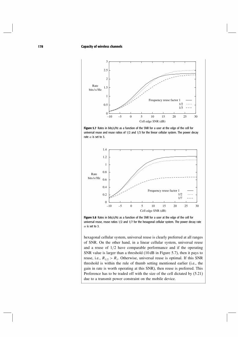
178 Capacity of wireless channels
10 15 20 25 30
Rate bits / s / Hz
Cell edge SNR (dB)
1/2Frequency reuse factor 1
1/30.5
50–5–10
3
2.5
2
1.5
1
0
Figure 5.7 Rates in bits/s/Hz as a function of the SNR for a user at the edge of the cell foruniversal reuse and reuse ratios of 1/2 and 1/3 for the linear cellular system. The power decayrate is set to 3.
10 15 20 25 30
1/7
Cell edge SNR (dB)
Frequency reuse factor 11/20.2
50–5–10
1.4
1.2
1
0.8
0.6
0.4
0
Rate bits /s / Hz
Figure 5.8 Rates in bits/s/Hz as a function of the SNR for a user at the edge of the cell foruniversal reuse, reuse ratios 1/2 and 1/7 for the hexagonal cellular system. The power decay rate is set to 3.
hexagonal cellular system, universal reuse is clearly preferred at all rangesof SNR. On the other hand, in a linear cellular system, universal reuseand a reuse of 1/2 have comparable performance and if the operatingSNR value is larger than a threshold (10 dB in Figure 5.7), then it pays toreuse, i.e., R1/2 > R1. Otherwise, universal reuse is optimal. If this SNRthreshold is within the rule of thumb setting mentioned earlier (i.e., thegain in rate is worth operating at this SNR), then reuse is preferred. ThisPreference has to be traded off with the size of the cell dictated by (5.21)due to a transmit power constraint on the mobile device.

179 5.3 Linear time-invariant Gaussian channels
5.3 Linear time-invariant Gaussian channels
We give three examples of channels which are closely related to the simpleAWGN channel and whose capacities can be easily computed. Moreover,optimal codes for these channels can be constructed directly from an optimalcode for the basic AWGN channel. These channels are time-invariant, knownto both the transmitter and the receiver, and they form a bridge to the fadingchannels which will be studied in the next section.
5.3.1 Single input multiple output (SIMO) channel
Consider a SIMO channel with one transmit antenna and L receive antennas:
ym= hxm+wm = 1 L (5.24)
where h is the fixed complex channel gain from the transmit antenna tothe th receive antenna, and wm is 0N0 is additive Gaussian noiseindependent across antennas. A sufficient statistic for detecting xm fromym = y1m yLmt is
ym = h∗ym= h2xm+h∗wm (5.25)
where h = h1 hLt and wm = w1m wLmt. This is an
AWGN channel with received SNR Ph2/N0 if P is the average energy pertransmit symbol. The capacity of this channel is therefore
C = log(
1+ Ph2N0
)
bits/s/Hz (5.26)
Multiple receive antennas increase the effective SNR and provide a powergain. For example, for L= 2 and h1 = h2 = 1, dual receive antennas providea 3 dB power gain over a single antenna system. The linear combining (5.25)maximizes the output SNR and is sometimes called receive beamforming.
5.3.2 Multiple input single output (MISO) channel
Consider a MISO channel with L transmit antennas and a single receiveantenna:
ym= h∗xm+wm (5.27)
where h = h1 hLt and h is the (fixed) channel gain from transmit
antenna to the receive antenna. There is a total power constraint of P acrossthe transmit antennas.

180 Capacity of wireless channels
In the SIMO channel above, the sufficient statistic is the projection of theL-dimensional received signal onto h: the projections in orthogonal directionscontain noise that is not helpful to the detection of the transmit signal. A naturalreciprocal transmission strategy for the MISO channel would send informationonly in the direction of the channel vector h; information sent in any orthogonaldirection will be nulled out by the channel anyway. Therefore, by setting
xm= hh xm (5.28)
the MISO channel is reduced to the scalar AWGN channel:
ym= hxm+wm (5.29)
with a power constraint P on the scalar input. The capacity of this scalarchannel is
log(
1+ Ph2N0
)
bits/s/Hz (5.30)
Can one do better than this scheme? Any reliable code for the MISO channelcanbeusedasa reliable code for the scalarAWGNchannelym= xm+wm:if Xi are the transmittedL×N (space-time) codematrices for theMISO chan-nel, then the received 1×N vectors h∗Xi form a code for the scalar AWGNchannel. Hence, the rate achievable by a reliable code for the MISO channelmust be at most the capacity of a scalar AWGN channel with the same receivedSNR. Exercise 5.11 shows that the received SNR Ph2/N0 of the transmissionstrategy above is in fact the largest possible SNR given the transmit power con-straint of P. Any other scheme has a lower received SNR and hence its reliablerate must be less than (5.30), the rate achieved by the proposed transmissionstrategy. We conclude that the capacity of the MISO channel is indeed
C = log(
1+ Ph2N0
)
bits/s/Hz (5.31)
Intuitively, the transmission strategy maximizes the received SNR by hav-ing the received signals from the various transmit antennas add up in-phase(coherently) and by allocating more power to the transmit antenna with thebetter gain. This strategy, “aligning the transmit signal in the direction ofthe transmit antenna array pattern”, is called transmit beamforming. Throughbeamforming, the MISO channel is converted into a scalar AWGN channeland thus any code which is optimal for the AWGN channel can be used directly.In both the SIMO and the MISO examples the benefit from having multiple
antennas is a power gain. To get a gain in degrees of freedom, one has to useboth multiple transmit and multiple receive antennas (MIMO). We will studythis in depth in Chapter 7.

181 5.3 Linear time-invariant Gaussian channels
5.3.3 Frequency-selective channel
Transformation to a parallel channelConsider a time-invariant L-tap frequency-selective AWGN channel:
ym=L−1∑
=0
hxm−+wm (5.32)
with an average power constraint P on each input symbol. In Section 3.4.4, wesaw that the frequency-selective channel can be converted into Nc independentsub-carriers by adding a cyclic prefix of length L− 1 to a data vector oflength Nc, cf. (3.137). Suppose this operation is repeated over blocks of datasymbols (of length Nc each, along with the corresponding cyclic prefix oflength L−1); see Figure 5.9. Then communication over the ith OFDM blockcan be written as
yni= hndni+ wni n= 01 Nc−1 (5.33)
Here,
di = d0i dNc−1it (5.34)
wi = w0i wNc−1it (5.35)
yi = y0i yNc−1it (5.36)
are the DFTs of the input, the noise and the output of the ith OFDM blockrespectively. h is the DFT of the channel scaled by
√Nc (cf. (3.138)). Since the
overhead in the cyclic prefix relative to the block lengthNc can bemade arbitrar-ily small by choosing Nc large, the capacity of the original frequency-selectivechannel is the same as the capacity of this transformed channel asNc →.
The transformedchannel (5.33) canbeviewedas a collectionof sub-channels,one for each sub-carrier n. Each of the sub-channels is an AWGN channel. The
Figure 5.9 A coded OFDMsystem. Information bits arecoded and then sent over thefrequency-selective channel viaOFDM modulation. Eachchannel use corresponds to anOFDM block. Coding can bedone across different OFDMblocks as well as over differentsub-carriers.
Encoder
OFDM modulator
Channel (use 2)
OFDM modulator
Channel (use 3)
Channel (use 1)
Information bits
OFDM modulator

182 Capacity of wireless channels
transformed noise wi is distributed as 0N0I, so the noise is 0N0
in each of the sub-channels and, moreover, the noise is independent acrosssub-channels. The power constraint on the input symbols in time translatesto one on the data symbols on the sub-channels (Parseval theorem for DFTs):
[di2]≤ NcP (5.37)
In information theory jargon, a channel which consists of a set of non-interfering sub-channels, each of which is corrupted by independent noise, iscalled a parallel channel. Thus, the transformed channel here is a parallelAWGN channel, with a total power constraint across the sub-channels. A nat-ural strategy for reliable communication over a parallel AWGN channel isillustrated in Figure 5.10. We allocate power to each sub-channel, Pn to thenth sub-channel, such that the total power constraint is met. Then, a separatecapacity-achieving AWGN code is used to communicate over each of the sub-channels. The maximum rate of reliable communication using this scheme is
Nc−1∑
n=0
log
(
1+ Pnhn2N0
)
bits/OFDM symbol (5.38)
Further, the power allocation can be chosen appropriately, so as to maximizethe rate in (5.38). The “optimal power allocation”, thus, is the solution to theoptimization problem:
CNc= max
P0 PNc−1
Nc−1∑
n=0
log
(
1+ Pnhn2N0
)
(5.39)
Figure 5.10 Codingindependently over each of thesub-carriers. This architecture,with appropriate power andrate allocations, achieves thecapacity of thefrequency-selective channel.
OFDM modulator
OFDM modulator
OFDM modulator
Channel (use 1)
Channel (use 2)
Channel (use 3)
Information bits
Information bits
Encoder for subcarrier 1
Encoder for subcarrier 2
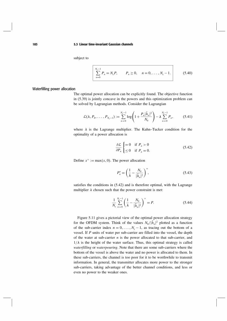
183 5.3 Linear time-invariant Gaussian channels
subject to
Nc−1∑
n=0
Pn = NcP Pn ≥ 0 n= 0 Nc−1 (5.40)
Waterfilling power allocationThe optimal power allocation can be explicitly found. The objective functionin (5.39) is jointly concave in the powers and this optimization problem canbe solved by Lagrangian methods. Consider the Lagrangian
P0 PNc−1 =Nc−1∑
n=0
log
(
1+ Pnhn2N0
)
−Nc−1∑
n=0
Pn (5.41)
where is the Lagrange multiplier. The Kuhn–Tucker condition for theoptimality of a power allocation is
Pn
= 0 if Pn > 0
≤ 0 if Pn = 0(5.42)
Define x+ =maxx0. The power allocation
P∗n =
(1− N0
hn2)+
(5.43)
satisfies the conditions in (5.42) and is therefore optimal, with the Lagrangemultiplier chosen such that the power constraint is met:
1Nc
Nc−1∑
n=0
(1− N0
hn2)+
= P (5.44)
Figure 5.11 gives a pictorial view of the optimal power allocation strategyfor the OFDM system. Think of the values N0/hn2 plotted as a functionof the sub-carrier index n = 0 Nc − 1, as tracing out the bottom of avessel. If P units of water per sub-carrier are filled into the vessel, the depthof the water at sub-carrier n is the power allocated to that sub-carrier, and1/ is the height of the water surface. Thus, this optimal strategy is calledwaterfilling or waterpouring. Note that there are some sub-carriers where thebottom of the vessel is above the water and no power is allocated to them. Inthese sub-carriers, the channel is too poor for it to be worthwhile to transmitinformation. In general, the transmitter allocates more power to the strongersub-carriers, taking advantage of the better channel conditions, and less oreven no power to the weaker ones.

184 Capacity of wireless channels
Figure 5.11 Waterfilling powerallocation over the Nc sub-carriers.
P1 = 0
N0
|H( f )|2
Subcarrier n
P2
P3
*
*
*
1λ
Observe that
hn =L−1∑
=0
h exp(
− j2nNc
)
(5.45)
is the discrete-time Fourier transform Hf evaluated at f = nW/Nc, where(cf. (2.20))
Hf =L−1∑
=0
h exp(
− j2fW
)
f ∈ 0W (5.46)
As the number of sub-carriers Nc grows, the frequency width W/Nc of thesub-carriers goes to zero and they represent a finer and finer sampling of thecontinuous spectrum. So, the optimal power allocation converges to
P∗f =(1− N0
Hf 2)+
(5.47)
where the constant satisfies (cf. (5.44))
∫ W
0P∗f df = P (5.48)
The power allocation can be interpreted as waterfilling over frequency (seeFigure 5.12). With Nc sub-carriers, the largest reliable communication rate

185 5.3 Linear time-invariant Gaussian channels
Figure 5.12 Waterfilling powerallocation over the frequencyspectrum of the two-tapchannel (high-pass filter):h0= 1 and h1= 05.
P ( f )
Frequency ( f )
0.4W0.2W0– 0.2W– 0.4W
4
0
3.5
3
2.5
2
1.5
1
0.5
N0
|H( f )|2
*
1λ
with independent coding is CNcbits per OFDM symbol or CNc
/Nc bits/s/Hz(CNc
given in (5.39)). So as Nc →, the WCNc/Nc converges to
C =∫ W
0log
(
1+ P∗f Hf 2N0
)
df bits/s (5.49)
Does coding across sub-carriers help?So far we have considered a very simple scheme: coding independently overeach of the sub-carriers. By coding jointly across the sub-carriers, presumablybetter performance can be achieved. Indeed, over a finite block length, codingjointly over the sub-carriers yields a smaller error probability than can beachieved by coding separately over the sub-carriers at the same rate. However,somewhat surprisingly, the capacity of the parallel channel is equal to thelargest reliable rate of communication with independent coding within eachsub-carrier. In other words, if the block length is very large then coding jointlyover the sub-carriers cannot increase the rate of reliable communication anymore than what can be achieved simply by allocating power and rate overthe sub-carriers but not coding across the sub-carriers. So indeed (5.49) is thecapacity of the time-invariant frequency-selective channel.To get some insight into why coding across the sub-carriers with large
block length does not improve capacity, we turn to a geometric view. Considera code, with block length NcN symbols, coding over all Nc of the sub-carrierswith N symbols from each sub-carrier. In high dimensions, i.e., N 1, theNcN -dimensional received vector after passing through the parallel channel(5.33) lives in an ellipsoid, with different axes stretched and shrunk by thedifferent channel gains hn. The volume of the ellipsoid is proportional to
Nc−1∏
n=0
(hn2Pn+N0
)N
(5.50)

186 Capacity of wireless channels
see Exercise 5.12. The volume of the noise sphere is, as in Section 5.1.2,proportional to N
NcN0 . The maximum number of distinguishable codewords
that can be packed in the ellipsoid is therefore
Nc−1∏
n=0
(
1+ Pnhn2N0
)N
(5.51)
The maximum reliable rate of communication is
1N
logNc−1∏
n=0
(
1+ Pnhn2N0
)N
=Nc−1∑
n=0
log
(
1+ Pnhn2N0
)
bits/OFDM symbol
(5.52)This is precisely the rate (5.38) achieved by separate coding and this suggeststhat coding across sub-carriers can do no better. While this sphere-packingargument is heuristic, Appendix B.6 gives a rigorous derivation from infor-mation theoretic first principles.Even though coding across sub-carriers cannot improve the reliable rate of
communication, it can still improve the error probability for a given data rate.Thus, coding across sub-carriers can still be useful in practice, particularlywhen the block length for each sub-carrier is small, in which case the codingeffectively increases the overall block length.In this section we have used parallel channels to model a frequency-
selective channel, but parallel channels will be seen to be very useful inmodeling many other wireless communication scenarios as well.
5.4 Capacity of fading channels
The basic capacity results developed in the last few sections are now appliedto analyze the limits to communication over wireless fading channels.Consider the complex baseband representation of a flat fading channel:
ym= hmxm+wm (5.53)
where hm is the fading process and wm is i.i.d. 0N0 noise.As before, the symbol rate is W Hz, there is a power constraint of P
joules/symbol, and hm2 = 1 is assumed for normalization. HenceSNR = P/N0 is the average received SNR.In Section 3.1.2, we analyzed the performance of uncoded transmission for
this channel. What is the ultimate performance limit when information canbe coded over a sequence of symbols? To answer this question, we makethe simplifying assumption that the receiver can perfectly track the fadingprocess, i.e., coherent reception. As we discussed in Chapter 2, the coherencetime of typical wireless channels is of the order of hundreds of symbols and

187 5.4 Capacity of fading channels
so the channel varies slowly relative to the symbol rate and can be estimatedby say a pilot signal. For now, the transmitter is not assumed to have anyknowledge of the channel realization other than the statistical characterization.The situation when the transmitter has access to the channel realizations willbe studied in Section 5.4.6.
5.4.1 Slow fading channel
Let us first look at the situation when the channel gain is random but remainsconstant for all time, i.e., hm = h for all m. This models the slow fad-ing situation where the delay requirement is short compared to the channelcoherence time (cf. Table 2.2). This is also called the quasi-static scenario.Conditional on a realization of the channel h, this is an AWGN channel
with received signal-to-noise ratio h2SNR. The maximum rate of reliablecommunication supported by this channel is log1+h2SNR bits/s/Hz. Thisquantity is a function of the random channel gain h and is therefore random(Figure 5.13). Now suppose the transmitter encodes data at a rate R bits/s/Hz.If the channel realization h is such that log1+h2SNR < R, then whateverthe code used by the transmitter, the decoding error probability cannot bemade arbitrarily small. The system is said to be in outage, and the outageprobability is
poutR = log1+h2SNR < R (5.54)
Thus, the best the transmitter can do is to encode the data assuming thatthe channel gain is strong enough to support the desired rate R. Reliablecommunication can be achieved whenever that happens, and outage occursotherwise.A more suggestive interpretation is to think of the channel as allowing
log1+h2SNR bits/s/Hz of information through when the fading gain is h.
Figure 5.13 Density oflog1+h2SNR, for Rayleighfading and SNR= 0 dB. Forany target rate R, there is anon-zero outage probability.
0
0.15
0.2
0.25
0.3
0.35
0.4
0.45
0 1 2 3 4 5
0.05
0.1
R
Area = pout (R)

188 Capacity of wireless channels
Reliable decoding is possible as long as this amount of information exceedsthe target rate.For Rayleigh fading (i.e., h is 01), the outage probability is
poutR= 1− exp(−2R−1
SNR
)
(5.55)
At high SNR,
poutR≈2R−1SNR
(5.56)
and the outage probability decays as 1/SNR. Recall that when we discusseduncoded transmission in Section 3.1.2, the detection error probability alsodecays like 1/SNR. Thus, we see that coding cannot significantly improve theerror probability in a slow fading scenario. The reason is that while codingcan average out the Gaussian white noise, it cannot average out the channelfade, which affects all the coded symbols. Thus, deep fade, which is thetypical error event in the uncoded case, is also the typical error event in thecoded case.There is a conceptual difference between the AWGN channel and the slow
fading channel. In the former, one can send data at a positive rate (in fact, anyrate less than C) while making the error probability as small as desired. Thiscannot be done for the slow fading channel as long as the probability thatthe channel is in deep fade is non-zero. Thus, the capacity of the slow fadingchannel in the strict sense is zero. An alternative performance measure is the-outage capacity C. This is the largest rate of transmission R such that theoutage probability poutR is less than . Solving poutR= in (5.54) yields
C = log1+F−11− SNRbits/s/Hz (5.57)
where F is the complementary cumulative distribution function of h2, i.e.,Fx = h2 > x.In Section 3.1.2, we looked at uncoded transmission and there it was natural
to focus only on the high SNR regime; at low SNR, the error probability ofuncoded transmission is very poor. On the other hand, for coded systems,it makes sense to consider both the high and the low SNR regimes. Forexample, the CDMA system in Chapter 4 operates at very low SINR anduses very low-rate orthogonal coding. A natural question is: in which regimedoes fading have a more significant impact on outage performance? One cananswer this question in two ways. Eqn (5.57) says that, to achieve the samerate as the AWGN channel, an extra 10 log1/F−11− dB of power isneeded. This is true regardless of the operating SNR of the environment. Thusthe fade margin is the same at all SNRs. If we look at the outage capacityat a given SNR, however, the impact of fading depends very much on theoperating regime. To get a sense, Figure 5.14 plots the -outage capacity as

189 5.4 Capacity of fading channels
Figure 5.14 -outage capacityas a fraction of AWGN capacityunder Rayleigh fading, for= 01 and = 001.
0
1
–10 –5 0 5 10 15 20 25 30
0.6
0.4
0.2
0.8
= 0.1
= 0.01
CCawgn
SNR (dB)35 40
∋ ∋
∋
a function of SNR for the Rayleigh fading channel. To assess the impact offading, the -outage capacity is plotted as a fraction of the AWGN capacityat the same SNR. It is clear that the impact is much more significant in thelow SNR regime. Indeed, at high SNR,
C ≈ log SNR+ logF−11− (5.58)
≈ Cawgn− log(
1F−11−
)
(5.59)
a constant difference irrespective of the SNR. Thus, the relative loss getssmaller at high SNR. At low SNR, on the other hand,
C ≈ F−11− SNR log2 e (5.60)
≈ F−11− Cawgn (5.61)
For reasonably small outage probabilities, the outage capacity is only asmall fraction of the AWGN capacity at low SNR. For Rayleigh fading,F−11− ≈ for small and the impact of fading is very significant. Atan outage probability of 001, the outage capacity is only 1% of the AWGNcapacity! Diversity has a significant effect at high SNR (as already seen inChapter 3), but can be more important at low SNR. Intuitively, the impactof the randomness of the channel is in the received SNR, and the reliablerate supported by the AWGN channel is much more sensitive to the receivedSNR at low SNR than at high SNR. Exercise 5.10 elaborates on this point.
5.4.2 Receive diversity
Let us increase the diversity of the channel by having L receive antennasinstead of one. For given channel gains h = h1 hL
t, the capacity was

190 Capacity of wireless channels
calculated in Section 5.3.1 to be log1+h2SNR. Outage occurs wheneverthis is below the target rate R:
prxoutR = log1+h2SNR < R (5.62)
This can be rewritten as
poutR=
h2 < 2R−1SNR
(5.63)
Under independent Rayleigh fading, h2 is a sum of the squares of 2Lindependent Gaussian random variables and is distributed as Chi-square with2L degrees of freedom. Its density is
fx= 1L−1!x
L−1e−x x ≥ 0 (5.64)
Approximating e−x by 1 for x small, we have (cf. (3.44)),
h2 < ≈ 1L!
L (5.65)
for small. Hence at high SNR the outage probability is given by
poutR≈2R−1L
L!SNRL (5.66)
Comparing with (5.55), we see a diversity gain of L: the outage probabilitynow decays like 1/SNRL. This parallels the performance of uncoded trans-mission discussed in Section 3.3.1: thus, coding cannot increase the diversitygain.The impact of receive diversity on the -outage capacity is plotted in
Figure 5.15. The -outage capacity is given by (5.57) with F now the cumu-lative distribution function of h2. Receive antennas yield a diversity gainand an L-fold power gain. To emphasize the impact of the diversity gain, letus normalize the outage capacity C by Cawgn = log1+LSNR. The dramaticsalutary effect of diversity on outage capacity can now be seen. At low SNRand small , (5.61) and (5.65) yield
C ≈ F−11− SNR log2 e (5.67)
≈ L! 1L
1L SNR log2 e bits/s/Hz (5.68)
and the loss with respect to the AWGN capacity is by a factor of 1/L ratherthan by when there is no diversity. At = 001 and L = 2, the outagecapacity is increased to 14% of the AWGN capacity (as opposed to 1% forL= 1).

191 5.4 Capacity of fading channels
Figure 5.15 -outage capacitywith L-fold receive diversity, asa fraction of the AWGNcapacity log1+ LSNR for= 001 and different L.
00 5 10 15 20 25 30 35 40–10
1
0.8
0.6
0.4
0.2
–5
CCawgn
L = 2
L = 4
L = 5
L = 3
L = 1
SNR (dB)
∋
5.4.3 Transmit diversity
Now suppose there are L transmit antennas but only one receive antenna, witha total power constraint of P. From Section 5.3.2, the capacity of the channelconditioned on the channel gains h = h1 hL
t is log1+ h2SNR.Following the approach taken in the SISO and the SIMO cases, one is temptedto say that the outage probability for a fixed rate R is
pfull−csiout R= log1+h2SNR < R (5.69)
which would have been exactly the same as the corresponding SIMO systemwith 1 transmit and L receive antennas. However, this outage performanceis achievable only if the transmitter knows the phases and magnitudes of thegains h so that it can perform transmit beamforming, i.e., allocate more powerto the stronger antennas and arrange the signals from the different antennas toalign in phase at the receiver. When the transmitter does not know the channelgains h, it has to use a fixed transmission strategy that does not depend on h.(This subtlety does not arise in either the SISO or the SIMO case because thetransmitter need not know the channel realization to achieve the capacity forthose channels.) How much performance loss does not knowing the channelentail?
Alamouti scheme revisitedFor concreteness, let us focus on L = 2 (dual transmit antennas). In thissituation, we can use the Alamouti scheme, which extracts transmit diversitywithout transmitter channel knowledge (introduced in Section 3.3.2). Recallfrom (3.76) that, under this scheme, both the transmitted symbols u1 u2 over ablock of 2 symbol times see an equivalent scalar fading channel with gain h

192 Capacity of wireless channels
h2
w2
h1 w1
w2
h2
MISO channel
MISO channel
repetition
Alamouti
post-processing
y1 = (|h1|2 + |h2|2)u1 + w1
y1 = (|h1|2 + |h2|2)u1 + w1
y2 = (|h1|2 + |h2|2)u2 + w2
h2
h1
h2h2
**
*
post-processing
u1
*
*
*
–*u1
u2
(b)
(a)
2 equivalent scalar channels
equivalent scalar channel
h1 w1
h1
–h1
and additive noise 0N0 (Figure 5.16(b)). The energy in the symbolsFigure 5.16 A space-timecoding scheme combined withthe MISO channel can beviewed as an equivalent scalarchannel: (a) repetition coding;(b) the Alamouti scheme. Theoutage probability of thescheme is the outageprobability of the equivalentchannel.
u1 and u2 is P/2. Conditioned on h1 h2, the capacity of the equivalent scalarchannel is
log(
1+h2 SNR2
)
bits/s/Hz (5.70)
Thus, if we now consider successive blocks and use an AWGN capacity-achieving code of rate R over each of the streams u1m and u2m
separately, then the outage probability of each stream is
pAlaout R=
log(
1+h2 SNR2
)
< R
(5.71)
Compared to (5.69) when the transmitter knows the channel, the Alamoutischeme performs strictly worse: the loss is 3 dB in the received SNR. Thiscan be explained in terms of the efficiency with which energy is transferredto the receiver. In the Alamouti scheme, the symbols sent at the two transmitantennas in each time are independent since they come from two separatelycoded streams. Each of them has power P/2. Hence, the total SNR at thereceive antenna at any given time is
(h12+h22) SNR
2 (5.72)
In contrast, when the transmitter knows the channel, the symbols trans-mitted at the two antennas are completely correlated in such a way that thesignals add up in phase at the receive antenna and the SNR is now
(h12+h22)SNR

193 5.4 Capacity of fading channels
a 3-dB power gain over the independent case.4 Intuitively, there is a powerloss because, without channel knowledge, the transmitter is sending signalsthat have energy in all directions instead of focusing the energy in a specificdirection. In fact, the Alamouti scheme radiates energy in a perfectly isotropicmanner: the signal transmitted from the two antennas has the same energywhen projected in any direction (Exercise 5.14).A scheme radiates energy isotropicallywhenever the signals transmitted from
the antennas are uncorrelated and have equal power (Exercise 5.14). Althoughthe Alamouti scheme does not perform as well as transmit beamforming, itis optimal in one important sense: it has the best outage probability amongall schemes that radiate energy isotropically. Indeed, any such scheme musthave a received SNR equal to (5.72) and hence its outage performance must beno better than that of a scalar slow fading AWGN channel with that receivedSNR. But this is precisely the performance achieved by the Alamouti scheme.Can one do even better by radiating energy in a non-isotropic manner (but
in a way that does not depend on the random channel gains)? In other words,can one improve the outage probability by correlating the signals from thetransmit antennas and/or allocating unequal powers on the antennas? Theanswer depends of course on the distribution of the gains h1 h2. If h1 h2
are i.i.d. Rayleigh, Exercise 5.15 shows, using symmetry considerations, thatcorrelation never improves the outage performance, but it is not necessarilyoptimal to use all the transmit antennas. Exercise 5.16 shows that uniformpower allocation across antennas is always optimal, but the number of anten-nas used depends on the operating SNR. For reasonable values of target outageprobabilities, it is optimal to use all the antennas. This implies that in mostcases of interest, the Alamouti scheme has the optimal outage performancefor the i.i.d. Rayleigh fading channel.What about for L> 2 transmit antennas? An information theoretic argument
in Appendix B.8 shows (in a more general framework) that
poutR=
log(
1+h2 SNRL
)
< R
(5.73)
is achievable. This is the natural generalization of (5.71) and corresponds againto isotropic transmission of energy from the antennas. Again, Exercises 5.15and 5.16 show that this strategy is optimal for the i.i.d. Rayleigh fadingchannel and for most target outage probabilities of interest. However, thereis no natural generalization of the Alamouti scheme for a larger numberof transmit antennas (cf. Exercise 3.17). We will return to the problem ofoutage-optimal code design for L > 2 in Chapter 9.
4 The addition of two in-phase signals of equal power yields a sum signal that has double theamplitude and four times the power of each of the signals. In contrast, the addition of twoindependent signals of equal power only doubles the power.
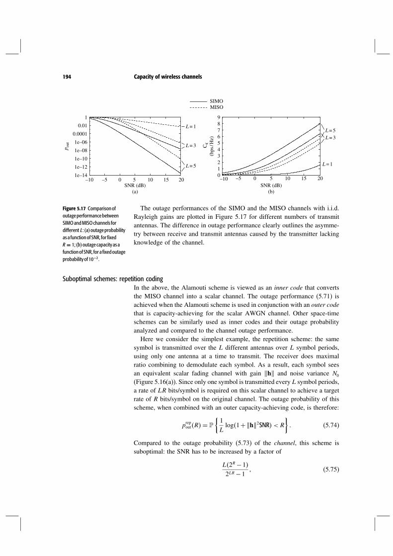
194 Capacity of wireless channels
1e–10
1510
1e–08
1e–06
0.0001
0.01
1
–10 –5 0 5 10 15 20 5
76543210
0–5–10
98
1e–14
1e–12
C
(bps
/ Hz)
(a)SNR (dB)
p out
L = 5
L = 3
L = 1
MISOSIMO
SNR (dB)(b)
20
L = 5L = 3
L = 1
∋
The outage performances of the SIMO and the MISO channels with i.i.d.Figure 5.17 ComparisonofoutageperformancebetweenSIMOandMISOchannels fordifferent L: (a)outageprobabilityasa functionofSNR, for fixedR = 1; (b)outagecapacityasafunctionofSNR, fora fixedoutageprobabilityof10−2.
Rayleigh gains are plotted in Figure 5.17 for different numbers of transmitantennas. The difference in outage performance clearly outlines the asymme-try between receive and transmit antennas caused by the transmitter lackingknowledge of the channel.
Suboptimal schemes: repetition codingIn the above, the Alamouti scheme is viewed as an inner code that convertsthe MISO channel into a scalar channel. The outage performance (5.71) isachieved when the Alamouti scheme is used in conjunction with an outer codethat is capacity-achieving for the scalar AWGN channel. Other space-timeschemes can be similarly used as inner codes and their outage probabilityanalyzed and compared to the channel outage performance.Here we consider the simplest example, the repetition scheme: the same
symbol is transmitted over the L different antennas over L symbol periods,using only one antenna at a time to transmit. The receiver does maximalratio combining to demodulate each symbol. As a result, each symbol seesan equivalent scalar fading channel with gain h and noise variance N0
(Figure 5.16(a)). Since only one symbol is transmitted every L symbol periods,a rate of LR bits/symbol is required on this scalar channel to achieve a targetrate of R bits/symbol on the original channel. The outage probability of thisscheme, when combined with an outer capacity-achieving code, is therefore:
prepoutR=
1Llog1+h2SNR < R
(5.74)
Compared to the outage probability (5.73) of the channel, this scheme issuboptimal: the SNR has to be increased by a factor of
L2R−12LR−1
(5.75)

195 5.4 Capacity of fading channels
to achieve the same outage probability for the same target rate R. Equivalently,the reciprocal of this ratio can be interpreted as the maximum achievablecoding gain over the simple repetition scheme. For a fixed R, the performanceloss increases with L: the repetition scheme becomes increasingly inefficientin using the degrees of freedom of the channel. For a fixed L, the perfor-mance loss increases with the target rate R. On the other hand, for R small,2R−1≈ R ln 2 and 2RL−1≈ RL ln 2, so
L2R−12LR−1
≈ LR ln 2LR ln 2
= 1 (5.76)
and there is hardly any loss in performance. Thus, while the repetition schemeis very suboptimal in the high SNR regime where the target rate can be high,it is nearly optimal in the low SNR regime. This is not surprising: the systemis degree-of-freedom limited in the high SNR regime and the inefficiency ofthe repetition scheme is felt more there.
Summary 5.2 Transmit and receive diversity
With receive diversity, the outage probability is
prxoutR = log1+h2SNR < R (5.77)
With transmit diversity and isotropic transmission, the outage probability is
ptxoutR =
log(
1+h2 SNRL
)
< R
(5.78)
a loss of a factor of L in the received SNR because the transmitter hasno knowledge of the channel direction and is unable to beamform in thespecific channel direction.
With two transmit antennas, capacity-achieving AWGN codes in conjunc-tion with the Alamouti scheme achieve the outage probability.
5.4.4 Time and frequency diversity
Outage performance of parallel channelsAnother way to increase channel diversity is to exploit the time-variationof the channel: in addition to coding over symbols within one coherenceperiod, one can code over symbols from L such periods. Note that this isa generalization of the schemes considered in Section 3.2, which take onesymbol from each coherence period. When coding can be performed over

196 Capacity of wireless channels
many symbols from each period, as well as between symbols from differentperiods, what is the performance limit?One can model this situation using the idea of parallel channels intro-
duced in Section 5.3.3: each of the sub-channels, = 1 L, representsa coherence period of duration Tc symbols:
ym= hxm+wm m= 1 Tc (5.79)
Here h is the (non-varying) channel gain during the th coherence period.It is assumed that the coherence time Tc is large such that one can codeover many symbols in each of the sub-channels. An average transmit powerconstraint of P on the original channel translates into a total power constraintof LP on the parallel channel.For a given realization of the channel, we have already seen in Section 5.3.3
that the optimal power allocation across the sub-channels is waterfilling.However, since the transmitter does not know what the channel gains are, areasonable strategy is to allocate equal power P to each of the sub-channels.In Section 5.3.3, it was mentioned that the maximum rate of reliable commu-nication given the fading gains h is
L∑
=1
log1+h2SNRbits/s/Hz (5.80)
where SNR= P/N0. Hence, if the target rate is R bits/s/Hz per sub-channel,then outage occurs when
L∑
=1
log1+h2SNR < LR (5.81)
Can one design a code to communicate reliably whenever
L∑
=1
log1+h2SNR > LR? (5.82)
If so, an L-fold diversity is achieved for i.i.d. Rayleigh fading: outage occursonly if each of the terms in the sum
∑L=1 log1+h2SNR is small.
The term log1+ h2SNR is the capacity of an AWGN channel withreceived SNR equal to h2SNR. Hence, a seemingly straightforward strategy,already used in Section 5.3.3, would be to use a capacity-achieving AWGNcode with rate
log1+h2SNRfor the th coherence period, yielding an average rate of
1L
L∑
=1
log1+h2SNRbits/s/Hz
197 5.4 Capacity of fading channels
and meeting the target rate whenever condition (5.82) holds. The caveat isthat this strategy requires the transmitter to know in advance the channel stateduring each of the coherence periods so that it can adapt the rate it allocates toeach period. This knowledge is not available. However, it turns out that suchtransmitter adaptation is unnecessary: information theory guarantees thatone can design a single code that communicates reliably at rate R wheneverthe condition (5.82) is met. Hence, the outage probability of the time diversitychannel is precisely
poutR=
1L
L∑
=1
log1+h2SNR < R
(5.83)
Even though this outage performance can be achieved with or withouttransmitter knowledge of the channel, the coding strategy is vastly different.With transmitter knowledge of the channel, dynamic rate allocation and sep-arate coding for each sub-channel suffices. Without transmitter knowledge,separate coding would mean using a fixed-rate code for each sub-channel andpoor diversity results: errors occur whenever one of the sub-channels is bad.Indeed, coding across the different coherence periods is now necessary: if thechannel is in deep fade during one of the coherence periods, the informationbits can still be protected if the channel is strong in other periods.
A geometric viewFigure 5.18 gives a geometric view of our discussion so far. Consider a codewith rate R, coding over all the sub-channels and over one coherence time-interval; the block length is LTc symbols. The codewords lie in an LTc-dimensional sphere. The received LTc-dimensional signal lives in an ellipsoid,with (L groups of) different axes stretched and shrunk by the different sub-channel gains (cf. Section 5.3.3). The ellipsoid is a function of the sub-channelgains, and hence random. The no-outage condition (5.82) has a geometricinterpretation: it says that the volume of the ellipsoid is large enough tocontain 2LTcR noise spheres, one for each codeword. (This was already seenin the sphere-packing argument in Section 5.3.3.) An outage-optimal code isone that communicates reliably whenever the random ellipsoid is at least thislarge. The subtlety here is that the same code must work for all such ellipsoids.Since the shrinking can occur in any of the L groups of dimensions, a robustcode needs to have the property that the codewords are simultaneously well-separated in each of the sub-channels (Figure 5.18(a)). A set of independentcodes, one for each sub-channel, is not robust: errors will be made when evenonly one of the sub-channels fades (Figure 5.18(b)).We have already seen, in the simple context of Section 3.2, codes for
the parallel channel which are designed to be well-separated in all the sub-channels. For example, the repetition code and the rotation code in Figure 3.8have the property that the codewords are separated in bot the sub-channels

198 Capacity of wireless channels
Channel fade
Channel fade
(a)
Reliable communication Noise spheres overlap
(b)
(here Tc = 1 symbol and L= 2 sub-channels). More generally, the code design
Figure 5.18 Effect of the fadinggains on codes for the parallelchannel. Here there are L= 2sub-channels and each axisrepresents Tc dimensions withina sub-channel. (a) Codingacross the sub-channels. Thecode works as long as thevolume of the ellipsoid is bigenough. This requires goodcodeword separation in boththe sub-channels. (b) Separate,non-adaptive code for eachsub-channel. Shrinking of oneof the axes is enough to causeconfusion between thecodewords.
criterion of maximizing the product distance for all pairs of codewords natu-rally favors codes that satisfy this property. Coding over long blocks affordsa larger coding gain; information theory guarantees the existence of codeswith large enough coding gain to achieve the outage probability in (5.83).To achieve the outage probability, one wants to design a code that commu-
nicates reliably over every parallel channel that is not in outage (i.e., parallelchannels that satisfy (5.82)). In information theory jargon, a code that com-municates reliably for a class of channels is said to be universal for that class.In this language, we are looking for universal codes for parallel channels thatare not in outage. In the slow fading scalar channel without diversity (L= 1),this problem is the same as the code design problem for a specific channel.This is because all scalar channels are ordered by their received SNR; hence acode that works for the channel that is just strong enough to support the targetrate will automatically work for all better channels. For parallel channels,each channel is described by a vector of channel gains and there is no naturalordering of channels; the universal code design problem is now non-trivial.In Chapter 9, a universal code design criterion will be developed to constructuniversal codes that come close to achieving the outage probability.
ExtensionsIn the above development, a uniform power allocation across the sub-channelsis assumed. Instead, if we choose to allocate power P to sub-channel , thenthe outage probability (5.83) generalizes to
poutR=
L∑
=1
log1+h2SNR < LR
(5.84)
where SNR = P/N0. Exercise 5.17 shows that for the i.i.d. Rayleigh fadingmodel, a non-uniform power allocation that does not depend on the channelgains cannot improve the outage performance.

199 5.4 Capacity of fading channels
The parallel channel is used to model time diversity, but it can modelfrequency diversity as well. By using the usual OFDM transformation, a slowfrequency-selective fading channel can be converted into a set of parallel sub-channels, one for each sub-carrier. This allows us to characterize the outagecapacity of such channels as well (Exercise 5.22).We summarize the key idea in this section using more suggestive
language.
Summary 5.3 Outage for parallel channels
Outage probability for a parallel channel with L sub-channels and the thchannel having random gain h:
poutR=
1L
L∑
=1
log1+h2SNR < R
(5.85)
where R is in bits/s/Hz per sub-channel.
The th sub-channel allows log1+h2SNR bits of information per sym-bol through. Reliable decoding can be achieved as long as the total amountof information allowed through exceeds the target rate.
5.4.5 Fast fading channel
In the slow fading scenario, the channel remains constant over the transmissionduration of the codeword. If the codeword length spans several coherenceperiods, then time diversity is achieved and the outage probability improves.When the codeword length spans many coherence periods, we are in theso-called fast fading regime. How does one characterize the performance limitof such a fast fading channel?
Capacity derivationLet us first consider a very simple model of a fast fading channel:
ym= hmxm+wm (5.86)
where hm= h remains constant over the th coherence period of Tc sym-bols and is i.i.d. across different coherence periods. This is the so-calledblock fading model; see Figure 5.19(a). Suppose coding is done over L suchcoherence periods. If Tc 1, we can effectively model this as L parallelsub-channels that fade independently. The outage probability from (5.83) is
poutR=
1L
L∑
=1
log1+h2SNR < R
(5.87)

200 Capacity of wireless channels
Figure 5.19 (a) Typicaltrajectory of the channelstrength as a function ofsymbol time under a blockfading model. (b) Typicaltrajectory of the channelstrength after interleaving. Onecan equally think of theseplots as rates of flow ofinformation allowed throughthe channel over time.
m
l = 0
h[m]
l = 1 l = 2 l = 3
m
h[m]
(a) (b)
For finite L, the quantity
1L
L∑
=1
log1+h2SNR
is random and there is a non-zero probability that it will drop below anytarget rate R. Thus, there is no meaningful notion of capacity in the sense ofmaximum rate of arbitrarily reliable communication and we have to resort tothe notion of outage. However, as L→, the law of large numbers says that
1L
L∑
=1
log1+h2SNR→ log1+h2SNR (5.88)
Now we can average over many independent fades of the channel by codingover a large number of coherence time intervals and a reliable rate of com-munication of log1+h2SNR can indeed be achieved. In this situation,it is now meaningful to assign a positive capacity to the fast fading channel:
C = log1+h2SNRbits/s/Hz (5.89)
Impact of interleavingIn the above, we considered codes with block lengths LTc symbols, whereL is the number of coherence periods and Tc is the number of symbols ineach coherence block. To approach the capacity of the fast fading channel,L has to be large. Since Tc is typically also a large number, the overall blocklength may become prohibitively large for implementation. In practice, shortercodes are used but they are interleaved so that the symbols of each codewordare spaced far apart in time and lie in different coherence periods. (Suchinterleaving is used for example in the IS-95 CDMA system, as illustrated inFigure 4.4.) Does interleaving impart a performance loss in terms of capacity?Going back to the channel model (5.86), ideal interleaving can be modeled
by assuming the hm are now i.i.d., i.e., successive interleaved symbols gothrough independent fades. (See Figure 5.19(b).) In Appendix B.7.1, it is

201 5.4 Capacity of fading channels
shown that for a large block length N and a given realization of the fadinggains h1 hN, the maximum achievable rate through this interleavedchannel is
1N
N∑
m=1
log1+hm2SNRbits/s/Hz (5.90)
By the law of large numbers,
1N
N∑
m=1
log1+hm2SNR→ log1+h2SNR (5.91)
as N → , for almost all realizations of the random channel gains. Thus,even with interleaving, the capacity (5.89) of the fast fading channel can beachieved. The important benefit of interleaving is that this capacity can nowbe achieved with a much shorter block length.A closer examination of the above argument reveals why the capacity under
interleaving (with hm i.i.d.) and the capacity of the original block fadingmodel (with hm block-wise constant) are the same: the convergence in(5.91) holds for both fading processes, allowing the same long-term averagerate through the channel. If one thinks of log1+hm2SNR as the rate ofinformation flow allowed through the channel at time m, the only differenceis that in the block fading model, the rate of information flow is constant overeach coherence period, while in the interleaved model, the rate varies fromsymbol to symbol. See Figure 5.19 again.This observation suggests that the capacity result (5.89) holds for a much
broader class of fading processes. Only the convergence in (5.91) is needed.This says that the time average should converge to the same limit for almost allrealizations of the fading process, a concept called ergodicity, and it holds inmany models. For example, it holds for the Gaussian fading model mentionedin Section 2.4. What matters from the point of view of capacity is only thelong-term time average rate of flow allowed, and not on how fast that ratefluctuates over time.
DiscussionIn the earlier parts of the chapter, we focused exclusively on deriving thecapacities of time-invariant channels, particularly the AWGN channel. Wehave just shown that time-varying fading channels also have a well-definedcapacity. However, the operational significance of capacity in the two casesis quite different. In the AWGN channel, information flows at a constantrate of log1+ SNR through the channel, and reliable communication cantake place as long as the coding block length is large enough to average outthe white Gaussian noise. The resulting coding/decoding delay is typicallymuch smaller than the delay requirement of applications and this is not abig concern. In the fading channel, on the other hand, information flows
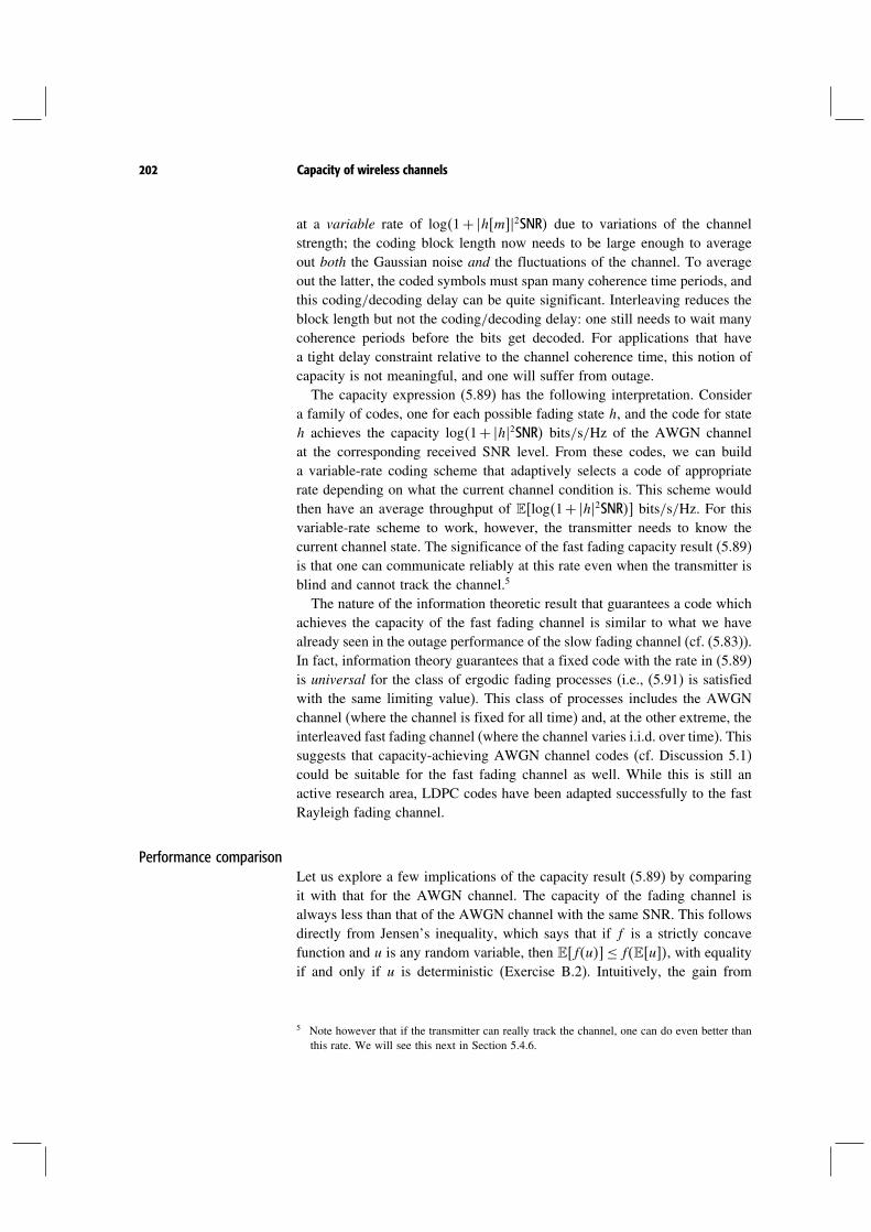
202 Capacity of wireless channels
at a variable rate of log1+ hm2SNR due to variations of the channelstrength; the coding block length now needs to be large enough to averageout both the Gaussian noise and the fluctuations of the channel. To averageout the latter, the coded symbols must span many coherence time periods, andthis coding/decoding delay can be quite significant. Interleaving reduces theblock length but not the coding/decoding delay: one still needs to wait manycoherence periods before the bits get decoded. For applications that havea tight delay constraint relative to the channel coherence time, this notion ofcapacity is not meaningful, and one will suffer from outage.The capacity expression (5.89) has the following interpretation. Consider
a family of codes, one for each possible fading state h, and the code for stateh achieves the capacity log1+ h2SNR bits/s/Hz of the AWGN channelat the corresponding received SNR level. From these codes, we can builda variable-rate coding scheme that adaptively selects a code of appropriaterate depending on what the current channel condition is. This scheme wouldthen have an average throughput of log1+h2SNR bits/s/Hz. For thisvariable-rate scheme to work, however, the transmitter needs to know thecurrent channel state. The significance of the fast fading capacity result (5.89)is that one can communicate reliably at this rate even when the transmitter isblind and cannot track the channel.5
The nature of the information theoretic result that guarantees a code whichachieves the capacity of the fast fading channel is similar to what we havealready seen in the outage performance of the slow fading channel (cf. (5.83)).In fact, information theory guarantees that a fixed code with the rate in (5.89)is universal for the class of ergodic fading processes (i.e., (5.91) is satisfiedwith the same limiting value). This class of processes includes the AWGNchannel (where the channel is fixed for all time) and, at the other extreme, theinterleaved fast fading channel (where the channel varies i.i.d. over time). Thissuggests that capacity-achieving AWGN channel codes (cf. Discussion 5.1)could be suitable for the fast fading channel as well. While this is still anactive research area, LDPC codes have been adapted successfully to the fastRayleigh fading channel.
Performance comparisonLet us explore a few implications of the capacity result (5.89) by comparingit with that for the AWGN channel. The capacity of the fading channel isalways less than that of the AWGN channel with the same SNR. This followsdirectly from Jensen’s inequality, which says that if f is a strictly concavefunction and u is any random variable, then fu≤ fu, with equalityif and only if u is deterministic (Exercise B.2). Intuitively, the gain from
5 Note however that if the transmitter can really track the channel, one can do even better thanthis rate. We will see this next in Section 5.4.6.
203 5.4 Capacity of fading channels
the times when the channel strength is above the average cannot compensatefor the loss from the times when the channel strength is below the average.This again follows from the law of diminishing marginal return on capacityfrom increasing the received power.At low SNR, the capacity of the fading channel is
C = log1+h2SNR≈ h2SNR log2 e= SNR log2 e≈ Cawgn (5.92)
where Cawgn is the capacity of the AWGN channel and is measured in bitsper symbol. Hence at low SNR the “Jensen’s loss” becomes negligible; thisis because the capacity is approximately linear in the received SNR in thisregime. At high SNR,
C ≈ logh2SNR= log SNR+log h2≈ Cawgn+log h2 (5.93)
i.e., a constant difference with the AWGN capacity at high SNR. This differ-ence is −083 bits/s/Hz for the Rayleigh fading channel. Equivalently, 2.5 dBmore power is needed in the fading case to achieve the same capacity as inthe AWGN case. Figure 5.20 compares the capacity of the Rayleigh fadingchannel with the AWGN capacity as a function of the SNR. The differenceis not that large for the entire plotted range of SNR.
5.4.6 Transmitter side information
So far we have assumed that only the receiver can track the channel. But letus now consider the case when the transmitter can track the channel as well.There are several ways in which such channel information can be obtainedat the transmitter. In a TDD (time-division duplex) system, the transmitter
Figure 5.20 Plot of AWGNcapacity, fading channelcapacity with receiver trackingthe channel only (CSIR) andcapacity with both transmitterand the receiver tracking thechannel (full CSI). (Adiscussion of the latter is inSection 5.4.6.)
–5 0 5 10 15SNR (dB)
20
AWGN
CSIRFull CSI
C (
bits
/s / H
z)
0–10–15–20
7
6
5
4
3
2
1

204 Capacity of wireless channels
can exploit channel reciprocity and make channel measurements based onthe signal received along the opposite link. In an FDD (frequency-divisionduplex) system, there is no reciprocity and the transmitter will have to relyon feedback information from the receiver. For example, power control in theCDMA system implicitly conveys some channel state information throughthe feedback in the uplink.
Slow fading: channel inversionWhen we discussed the slow fading channel in Section 5.4.1, it was seen thatwith no channel knowledge at the transmitter, outage occurs whenever thechannel cannot support the target data rate R. With transmitter knowledge,one option is now to control the transmit power such that the rate R can bedelivered no matter what the fading state is. This is the channel inversionstrategy: the received SNR is kept constant irrespective of the channel gain.(This strategy is reminiscent of the power control used in CDMA systems,discussed in Section 4.3.) With exact channel inversion, there is zero outageprobability. The price to pay is that huge power has to be consumed to invertthe channel when it is very bad. Moreover, many systems are also peak-powerconstrained and cannot invert the channel beyond a certain point. Systemslike IS-95 use a combination of channel inversion and diversity to achieve atarget rate with reasonable power consumption (Exercise 5.24).
Fast fading: waterfillingIn the slow fading scenario, we are interested in achieving a target data ratewithin a coherence time period of the channel. In the fast fading case, oneis now concerned with the rate averaged over many coherence time periods.With transmitter channel knowledge, what is the capacity of the fast fadingchannel? Let us again consider the simple block fading model (cf. (5.86)):
ym= hmxm+wm (5.94)
where hm= h remains constant over the th coherence period of TcTc1symbols and is i.i.d. across different coherence periods. The channel over Lsuch coherence periods can be modeled as a parallel channel with L sub-channels that fade independently. For a given realization of the channel gainsh1 hL, the capacity (in bits/symbol) of this parallel channel is (cf. (5.39),(5.40) in Section 5.3.3)
maxP1 PL
1L
L∑
=1
log(
1+ Ph2N0
)
(5.95)
subject to
1L
L∑
=1
P = P (5.96)

205 5.4 Capacity of fading channels
where P is the average power constraint. It was seen (cf. (5.43)) that theoptimal power allocation is waterfilling:
P∗ =
(1− N0
h2)+
(5.97)
where satisfies
1L
L∑
=1
(1− N0
h2)+
= P (5.98)
In the context of the frequency-selective channel, waterfilling is done overthe OFDM sub-carriers; here, waterfilling is done over time. In both cases,the basic problem is that of power allocation over a parallel channel.The optimal power P allocated to the th coherence period depends on
the channel gain in that coherence period and , which in turn depends onall the other channel gains through the constraint (5.98). So it seems thatimplementing this scheme would require knowledge of the future channelstates. Fortunately, as L→, this non-causality requirement goes away. Bythe law of large numbers, (5.98) converges to
[(1− N0
h2)+]
= P (5.99)
for almost all realizations of the fading process hm. Here, the expectationis taken with respect to the stationary distribution of the channel state. Theparameter now converges to a constant, depending only on the channelstatistics but not on the specific realization of the fading process. Hence, theoptimal power at any time depends only on the channel gain h at that time:
P∗h=(1− N0
h2)+
(5.100)
The capacity of the fast fading channel with transmitter channel knowledge is
C =
[
log(
1+ P∗hh2N0
)]
bits/s/Hz (5.101)
Equations (5.101), (5.100) and (5.99) together allow us to compute thecapacity.We have derived the capacity assuming the block fading model. The gen-
eralization to any ergodic fading process can be done exactly as in the casewith no transmitter channel knowledge.

206 Capacity of wireless channels
DiscussionFigure 5.21 gives a pictorial view of the waterfilling power allocation strategy.In general, the transmitter allocates more power when the channel is good,taking advantage of the better channel condition, and less or even no powerwhen the channel is poor. This is precisely the opposite of the channelinversion strategy. Note that only the magnitude of the channel gain is neededto implement the waterfilling scheme. In particular, phase information is notrequired (in contrast to transmit beamforming, for example).The derivation of the waterfilling capacity suggests a natural variable-rate
coding scheme (see Figure 5.22). This scheme consists of a set of codes ofdifferent rates, one for each channel state h. When the channel is in state h,the code for that state is used. This can be done since both the transmitter andthe receiver can track the channel. A transmit power of P∗h is used when
Figure 5.21 Pictorialrepresentation of thewaterfilling strategy.
N0
h[m]2
P[m]
1λ
Time m
P[m] = 0
Figure 5.22 Comparison of thefixed-rate and variable-rateschemes. In the fixed-ratescheme, there is only onecode spanning manycoherence periods. In thevariable-rate scheme, differentcodes (distinguished bydifferent shades) are useddepending on the channelquality at that time. Forexample, the code in white is alow-rate code used only whenthe channel is weak.
Fixed-rate scheme
Variable-rate scheme
1 5 10
h[m
] 2
Time m

207 5.4 Capacity of fading channels
the channel gain is h. The rate of that code is therefore log1+P∗hh2/N0
bits/s/Hz. No coding across channel states is necessary. This is in contrastto the case without transmitter channel knowledge, where a single fixed-rate code with the coded symbols spanning across different coherence timeperiods is needed (Figure 5.22). Thus, knowledge of the channel state at thetransmitter not only allows dynamic power allocation but simplifies the codedesign problem as one can now use codes designed for the AWGN channel.
Waterfilling performanceFigure 5.20 compares the waterfilling capacity and the capacity with channelknowledge only at the receiver, under Rayleigh fading. Figure 5.23 focuseson the low SNR regime. In the literature the former is also called the capacitywith full channel side information (CSI) and the latter is called the capacitywith channel side information at the receiver (CSIR). Several observationscan be made:
• At low SNR, the capacity with full CSI is significantly larger than theCSIR capacity.
• At high SNR, the difference between the two goes to zero.• Over a wide range of SNR, the gain of waterfilling over the CSIR capacityis very small.
The first two observations are in fact generic to a wide class of fadingmodels, and can be explained by the fact that the benefit of dynamic powerallocation is a received power gain: by spending more power when thechannel is good, the received power gets boosted up. At high SNR, however,the capacity is insensitive to the received power per degree of freedom andvarying the amount of transmit power as a function of the channel state yieldsa minimal gain (Figure 5.24(a)). At low SNR, the capacity is quite sensitiveto the received power (linear, in fact) and so the boost in received power fromoptimal transmit power allocation provides significant gain. Thus, dynamic
Figure 5.23 Plot of capacitieswith and without CSI at thetransmitter, as a fraction of theAWGN capacity.
–10 –5 0 5 100.5
–15–20
3
2.5
2
1.5
1
CCawgn
SNR (dB)
CSIRFull CSI

208 Capacity of wireless channels
(a)
(b)
Optimal allocationNear optimal allocation
Time m
Time m
P[m]
Time m
Time m
P[m]
N0
h[m]2
N0
h[m]2
N0
h[m]2
N0
h[m]2
1λ
1λ
1λ
1λ
power allocation is more important in the power-limited (low SNR) regimeFigure 5.24 (a) High SNR:allocating equal powers at alltimes is almost optimal. (b)Low SNR: allocating all thepower when the channel isstrongest is almost optimal.
than in the bandwidth-limited (high SNR) regime.Let us look more carefully at the low SNR regime. Consider first the
case when the channel gain h2 has a peak value Gmax. At low SNR, thewaterfilling strategy transmits information only when the channel is verygood, near Gmax: when there is very little water, the water ends up at thebottom of the vessel (Figure 5.24(b)). Hence at low SNR
C ≈ h2 ≈Gmax
log
(
1+Gmax ·SNR
h2 ≈Gmax
)
≈ Gmax · SNR log2 e bits/s/Hz (5.102)
Recall that at low SNR the CSIR capacity is SNR log2 e bits/s/Hz. Hence,transmitter CSI increases the capacity by Gmax times, or a 10 log10Gmax dBgain. Moreover, since the AWGN capacity is the same as the CSIR capacityat low SNR, this leads to the interesting conclusion that with full CSI, thecapacity of the fading channel can be much larger than when there is nofading. This is in contrast to the CSIR case where the fading channel capacityis always less than the capacity of the AWGN channel with the same averageSNR. The gain is coming from the fact that in a fading channel, channelfluctuations create peaks and deep nulls, but when the energy per degreeof freedom is small, the sender opportunistically transmits only when the

209 5.4 Capacity of fading channels
channel is near its peak. In a non-fading AWGN channel, the channel staysconstant at the average level and there are no peaks to take advantage of.For models like Rayleigh fading, the channel gain is actually unbounded.
Hence, theoretically, the gain of the fading channel waterfilling capacity overthe AWGN channel capacity is also unbounded. (See Figure 5.23.) However,to get very large relative gains, one has to operate at very low SNR. In thisregime, it may be difficult for the receiver to track and feed back the channelstate to the transmitter to implement the waterfilling strategy.Overall, the performance gain from full CSI is not that large compared to
CSIR, unless the SNR is very low. On the other hand, full CSI potentiallysimplifies the code design problem, as no coding across channel states isnecessary. In contrast, one has to interleave and code across many channelstates with CSIR.
Waterfilling versus channel inversionThe capacity of the fading channel with full CSI (by using the waterfill-ing power allocation) should be interpreted as a long-term average rate offlow of information, averaged over the fluctuations of the channel. Whilethe waterfilling strategy increases the long-term throughput of the systemby transmitting when the channel is good, an important issue is the delayentailed. In this regard, it is interesting to contrast the waterfilling power allo-cation strategy with the channel inversion strategy. Compared to waterfilling,channel inversion is much less power-efficient, as a huge amount of power isconsumed to invert the channel when it is bad. On the other hand, the rate offlow of information is now the same in all fading states, and so the associ-ated delay is independent of the time-scale of channel variations. Thus, onecan view the channel inversion strategy as a delay-limited power allocationstrategy. Given an average power constraint, the maximum achievable rate bythis strategy can be thought of as a delay-limited capacity. For applicationswith very tight delay constraints, this delay-limited capacity may be a moreappropriate measure of performance than the waterfilling capacity.Without diversity, the delay-limited capacity is typically very small. With
increased diversity, the probability of encountering a bad channel is reducedand the average power consumption required to support a target delay-limitedrate is reduced. Put another way, a larger delay-limited capacity is achievedfor a given average power constraint (Exercise 5.24).
Example 5.3 Rate adaptation in IS-856
IS-856 downlinkIS-856, also called CDMA 2000 1× EV-DO (Enhanced Version Data Opti-mized) is a cellular data standard operating on the 1.25-MHz bandwidth.
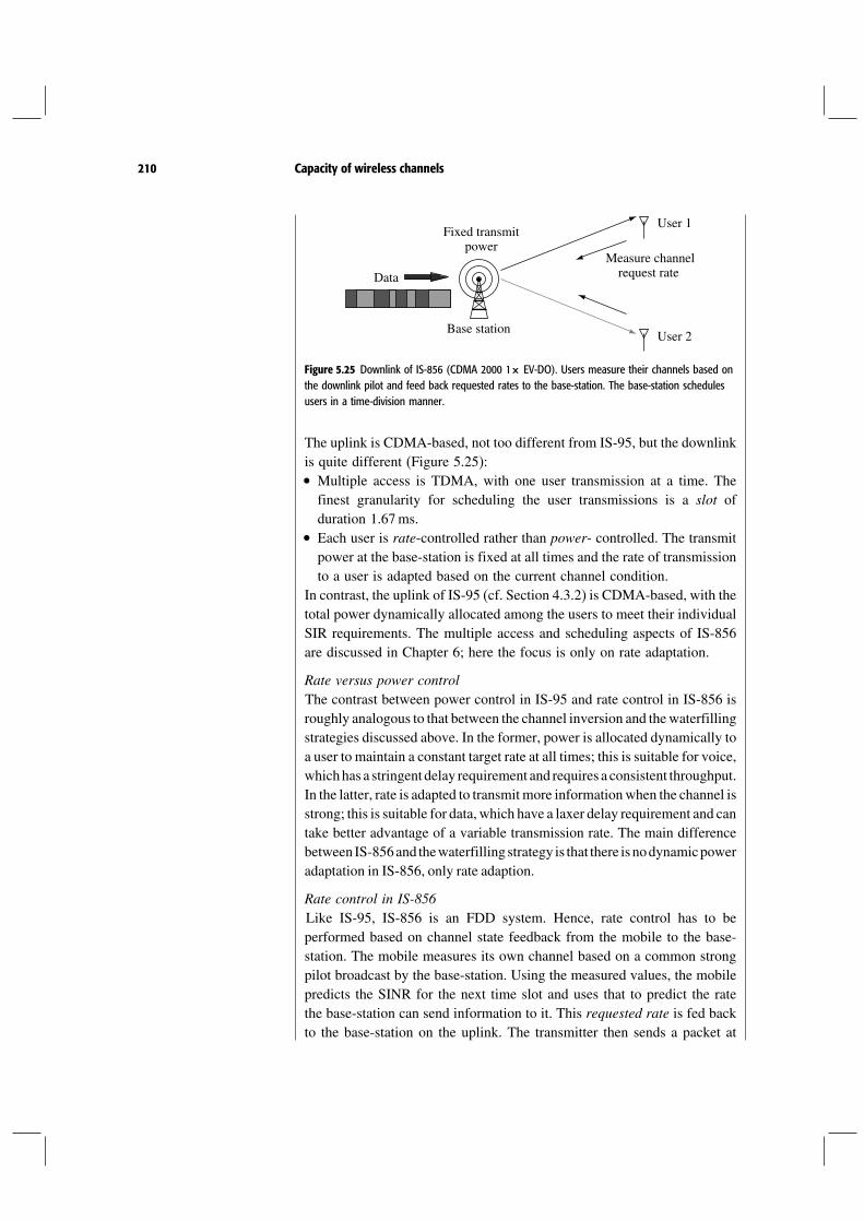
210 Capacity of wireless channels
Fixed transmitpower
User 2
User 1
Base station
Data
Measure channelrequest rate
Figure 5.25 Downlink of IS-856 (CDMA 2000 1× EV-DO). Users measure their channels based onthe downlink pilot and feed back requested rates to the base-station. The base-station schedulesusers in a time-division manner.
The uplink is CDMA-based, not too different from IS-95, but the downlinkis quite different (Figure 5.25):• Multiple access is TDMA, with one user transmission at a time. Thefinest granularity for scheduling the user transmissions is a slot ofduration 1.67ms.
• Each user is rate-controlled rather than power- controlled. The transmitpower at the base-station is fixed at all times and the rate of transmissionto a user is adapted based on the current channel condition.
In contrast, the uplink of IS-95 (cf. Section 4.3.2) is CDMA-based, with thetotal power dynamically allocated among the users to meet their individualSIR requirements. The multiple access and scheduling aspects of IS-856are discussed in Chapter 6; here the focus is only on rate adaptation.
Rate versus power controlThe contrast between power control in IS-95 and rate control in IS-856 isroughly analogous to that between the channel inversion and thewaterfillingstrategies discussed above. In the former, power is allocated dynamically toa user to maintain a constant target rate at all times; this is suitable for voice,whichhas a stringent delay requirement and requires a consistent throughput.In the latter, rate is adapted to transmitmore informationwhen the channel isstrong; this is suitable for data, which have a laxer delay requirement and cantake better advantage of a variable transmission rate. The main differencebetween IS-856and thewaterfilling strategy is that there isnodynamicpoweradaptation in IS-856, only rate adaption.
Rate control in IS-856Like IS-95, IS-856 is an FDD system. Hence, rate control has to beperformed based on channel state feedback from the mobile to the base-station. The mobile measures its own channel based on a common strongpilot broadcast by the base-station. Using the measured values, the mobilepredicts the SINR for the next time slot and uses that to predict the ratethe base-station can send information to it. This requested rate is fed backto the base-station on the uplink. The transmitter then sends a packet at

211 5.4 Capacity of fading channels
the requested rate to the mobile starting at the next time slot (if the mobileis scheduled). The table below describes the possible requested rates, theSINR thresholds for those rates, the modulation used and the number oftime slots the transmission takes.
Requested rate(kbits/s)
SINR threshold(dB) Modulation
Number ofslots
38.4 −115 QPSK 1676.8 −92 QPSK 8153.6 −65 QPSK 4307.2 −35 QPSK 2 or 4614.4 −05 QPSK 1 or 2921.6 22 8-PSK 21228.8 39 QPSK or 16-QAM 1 or 21843.2 80 8-PSK 12457.6 103 16-QAM 1
To simplify the implementation of the encoder, the codes at the differentrates are all derived from a basic 1/5-rate turbo code. The low-rate codesare obtained by repeating the turbo-coded symbols over a number of timeslots; as demonstrated in Exercise 5.25, such repetition loses little spectralefficiency in the low SNR regime. The higher-rate codes are obtained byusing higher-order constellations in the modulation.Rate control is made possible by the presence of the strong pilot to
measure the channel and the rate request feedback from the mobile tothe base-station. The pilot is shared between all users in the cell andis also used for many other functions such as coherent reception andsynchronization. The rate request feedback is solely for the purpose of ratecontrol. Although each request is only 4 bits long (to specify the variousrate levels), this is sent by every active user at every slot and moreoverconsiderable power and coding is needed to make sure the information getsfed back accurately and with little delay. Typically, sending this feedbackconsumes about 10% of the uplink capacity.
Impact of prediction uncertaintyProper rate adaptation relies on the accurate tracking and prediction of thechannel at the transmitter. This is possible only if the coherence time ofthe channel is much longer than the lag between the time the channel ismeasured at the mobile and the time when the packet is actually transmittedat the base-station. This lag is at least two slots (2×167ms) due to thedelay in getting the requested rate fed back to the base-station, but canbe considerably more at the low rates since the packet is transmitted overmultiple slots and the predicted channel has to be valid during this time.

212 Capacity of wireless channels
At a walking speed of 3 km/h and a carrier frequency fc = 19GHz,the coherence time is of the order of 25ms, so the channel can be quiteaccurately predicted. At a driving speed of 30 km/h, the coherence time isonly 2.5ms and accurate tracking of the channel is already very difficult.(Exercise 5.26 explicitly connects the prediction error to the physicalparameters of the channel.) At an even faster speed of 120 km/h, thecoherence time is less than 1ms and tracking of the channel is impossible;there is now no transmitter CSI. On the other hand, the multiple slot lowrate packets essentially go through a fast fading channel with significanttime diversity over the duration of the packet. Recall that the fast fadingcapacity is given by (5.89):
C = [log
(1+h2SNR)]≈ h2SNR log2 e bits/s/Hz (5.103)
in the low SNR regime, where h follows the stationary distribution ofthe fading. Thus, to determine an appropriate transmission rate across thisfast fading channel, it suffices for the mobile to predict the average SINRover the transmission time of the packet, and this average is quite easyto predict. Thus, the difficult regime is actually in between the very slowand very fast fading scenarios, where there is significant uncertainty in thechannel prediction and yet not very much time diversity over the packettransmission time. This channel uncertainty has to be taken into accountby being more conservative in predicting the SINR and in requesting arate. This is similar to the outage scenario considered in Section 5.4.1,except that the randomness of the channel is conditional on the predictedvalue. The requested rate should be set to meet a target outage probability(Exercise 5.27).The various situations are summarized in Figure 5.26. Note the different
roles of coding in the three scenarios. In the first scenario, when the pre-dicted SINR is accurate, the main role of coding is to combat the additiveGaussian noise; in the other two scenarios, coding combats the residualrandomness in the channel by exploiting the available time diversity.
lag
pred
ictio
n
t
SINR
(a) (b)
pred
ictio
n
tlag
SINR
(c)
tlag
SINR
conservativeprediction
Figure 5.26 (a) Coherence time is long compared to the prediction time lag; predicted SINR isaccurate. Near perfect CSI at transmitter. (b) Coherence time is comparable to the prediction timelag, predicted SINR has to be conservative to meet an outage criterion. (c) Coherence time is shortcompared to the prediction time lag; prediction of average SINR suffices. No CSI at the transmitter.

213 5.4 Capacity of fading channels
To reduce the loss in performance due to the conservativeness ofthe channel prediction, IS-856 employs an incremental ARQ (or hybrid-ARQ) mechanism for the repetition-coded multiple slot packets. Instead ofwaiting until the end of the transmission of all slots before decoding, themobile will attempt to decode the information incrementally as it receivesthe repeated copies over the time slots. When it succeeds in decoding,it will send an acknowledgement back to the base-station so that it canstop the transmission of the remaining slots. This way, a rate higher thanthe requested rate can be achieved if the actual SINR is higher than thepredicted SINR.
5.4.7 Frequency-selective fading channels
So far, we have considered flat fading channels (cf. (5.53)). In Section 5.3.3,the capacity of the time-invariant frequency-selective channel (5.32) was alsoanalyzed. It is simple to extend the understanding to underspread time-varyingfrequency-selective fading channels: these are channels with the coherencetime much larger than the delay spread. We model the channel as a time-invariant L-tap channel as in (5.32) over each coherence time interval andview it as Nc parallel sub-channels (in frequency). For underspread chan-nels, Nc can be chosen large so that the cyclic prefix loss is negligible.This model is a generalization of the flat fading channel in (5.53): herethere are Nc (frequency) sub-channels over each coherence time intervaland multiple (time) sub-channels over the different coherence time inter-vals. Overall it is still a parallel channel. We can extend the capacity resultsfrom Sections 5.4.5 and 5.4.6 to the frequency-selective fading channel. Inparticular, the fast fading capacity with full CSI (cf. Section 5.4.6) can begeneralized here to a combination of waterfilling over time and frequency:the coherence time intervals provide sub-channels in time and each coher-ence time interval provides sub-channels in frequency. This is carried out inExercise 5.30.
5.4.8 Summary: a shift in point of view
Let us summarize our investigation on the performance limits of fadingchannels. In the slow fading scenario without transmitter channel knowledge,the amount of information that is allowed through the channel is random, andno positive rate of communication can be reliably supported (in the senseof arbitrarily small error probability). The outage probability is the mainperformance measure, and it behaves like 1/SNR at high SNR. This is dueto a lack of diversity and, equivalently, the outage capacity is very small.With L branches of diversity, either over space, time or frequency, the outage

214 Capacity of wireless channels
probability is improved and decays like 1/SNRL. The fast fading scenariocan be viewed as the limit of infinite time diversity and has a capacity oflog1+ h2SNR bits/s/Hz. This however incurs a coding delay muchlonger than the coherence time of the channel. Finally, when the transmitterand the receiver can both track the channel, a further performance gain can beobtained by dynamically allocating power and opportunistically transmittingwhen the channel is good.The slow fading scenario emphasizes the detrimental effect of fading: a
slow fading channel is very unreliable. This unreliability is mitigated by pro-viding more diversity in the channel. This is the traditional way of viewing thefading phenomenon and was the central theme of Chapter 3. In a narrowbandchannel with a single antenna, the only source of diversity is through time.The capacity of the fast fading channel (5.89) can be viewed as the perfor-mance limit of any such time diversity scheme. Still, the capacity is less thanthe AWGN channel capacity as long as there is no channel knowledge at thetransmitter. With channel knowledge at the transmitter, the picture changes.Particularly at low SNR, the capacity of the fading channel with full CSIcan be larger than that of the AWGN channel. Fading can be exploited bytransmitting near the peak of the channel fluctuations. Channel fading is nowturned from a foe to a friend.This new theme on fading will be developed further in the multiuser context
in Chapter 6, where we will see that opportunistic communication will havea significant impact at all SNRs, and not only at low SNR.
Chapter 5 The main plot
Channel capacityThe maximum rate at which information can be communicated across anoisy channel with arbitrary reliability.
Linear time-invariant Gaussian channelsCapacity of the AWGN channel with SNR per degree of freedom is
Cawgn = log1+ SNRbits/s/Hz (5.104)
Capacity of the continuous-time AWGN channel with bandwidth W , aver-age received power P and white noise power spectral density N0 is
Cawgn =W log(
1+ P
N0W
)
bits/s (5.105)
Bandwidth-limited regime: SNR = P/N0W is high and capacity is loga-rithmic in the SNR.

215 5.4 Capacity of fading channels
Power-limited regime: SNR is low and capacity is linear in the SNR.
Capacities of the SIMO and the MISO channels with time-invariant channelgains h1 hL are the same:
C = log1+ SNRh2bits/s/Hz (5.106)
Capacity of frequency-selective channel with response Hf and powerconstraint P per degree of freedom:
C =∫ W
0log
(
1+ P∗f Hf 2N0
)
df bits/s (5.107)
where P∗f is waterfilling:
P∗f =(1− N0
Hf 2)+
(5.108)
and satisfies:
∫ W
0
(1− N0
Hf 2)+
df = P (5.109)
Slow fading channels with receiver CSI onlySetting: coherence time is much longer than constraint on coding delay.
Performance measures:
Outage probability poutR at a target rate R.
Outage capacity C at a target outage probability .
Basic flat fading channel:
ym= hxm+wm (5.110)
Outage probability is
poutR= log
(1+h2SNR)< R
(5.111)
where SNR is the average signal-to-noise ratio at each receive antenna.

216 Capacity of wireless channels
Outage probability with receive diversity is
poutR = log
(1+h2SNR)< R
(5.112)
This provides power and diversity gains.
Outage probability with L-fold transmit diversity is
poutR =
log(
1+h2 SNRL
)
< R
(5.113)
This provides diversity gain only.
Outage probability with L-fold time diversity is
poutR=
1L
L∑
=1
log(1+h2SNR
)< R
(5.114)
This provides diversity gain only.
Fast fading channelsSetting: coherence time is much shorter than coding delay.
Performance measure: capacity.
Basic model:
ym= hmxm+wm (5.115)
hm is an ergodic fading process.
Receiver CSI only:
C = [log
(1+h2SNR)] (5.116)
Full CSI:
C =
[
log(
1+ P∗hh2N0
)]
bits/s/Hz (5.117)
where P∗h waterfills over the fading states:
P∗h=(1− N0
h2)+
(5.118)
and satisfies:
[(1− N0
h2)+]
= P (5.119)
Power gain over the receiver CSI only case. Significant at low SNR.

217 5.6 Exercises
5.5 Bibliographical notes
Information theory and the formulation of the notions of reliable communicationand channel capacity were introduced in a path-breaking paper by Shannon [109].The underlying philosophy of using simple models to understand the essence of anengineering problem has pervaded the development of the communication field eversince. In that paper, as a consequence of his general theory, Shannon also derived thecapacity of the AWGN channel. He returned to a more in-depth geometric treatmentof this channel in a subsequent paper [110]. Sphere-packing arguments were usedextensively in the text by Wozencraft and Jacobs [148].
The linear cellular model was introduced by Shamai and Wyner [108]. One of theearly studies of wireless channels using information theoretic techniques is due toOzarow. et al. [88], where they introduced the concept of outage capacity. Telatar [119]extended the formulation to multiple antennas. The capacity of fading channels withfull CSI was analyzed by Goldsmith and Varaiya [51]. They observed the optimalityof the waterfilling power allocation with full CSI and the corollary that full CSI overCSI at the receiver alone is beneficial only at low SNRs. A comprehensive survey ofinformation theoretic results on fading channels was carried out by Biglieri, Proakisand Shamai [9].
The design issues in IS-856 have been elaborately discussed in Benderet al. [6] and by Wu and Esteves [149].
5.6 Exercises
Exercise 5.1 What is the maximum reliable rate of communication over the (complex)AWGN channel when only the I channel is used? How does that compare to the capac-ity of the complex channel at low and high SNR, with the same average power con-straint? Relate your conclusion to the analogous comparison between uncoded schemesin Section 3.1.2 and Exercise 3.4, focusing particularly on the high SNR regime.
Exercise 5.2 Consider a linear cellular model with equi-spaced base-stations at distance2d apart. With a reuse ratio of , base-stations at distances of integer multiples of2d/ reuse the same frequency band. Assuming that the interference emanates fromthe center of the cell, calculate the fraction f defined as the ratio of the interference tothe received power from a user at the edge of the cell. You can assume that all uplinktransmissions are at the same transmit power P and that the dominant interferencecomes from the nearest cells reusing the same frequency.
Exercise 5.3 Consider a regular hexagonal cellular model (cf. Figure 4.2) with afrequency reuse ratio of .1. Identify “appropriate” reuse patterns for different values of , with the design
goal of minimizing inter-cell interference. You can use the assumptions made inExercise 5.2 on how the interference originates.
2. For the reuse patterns identified, show that f = 6√/2 is a good approximation
to the fraction of the received power of a user at the edge of the cell that theinterference represents. Hint: You can explicitly construct reuse patterns for =11/31/41/71/9 with exactly these fractions.
218 Capacity of wireless channels
3. What reuse ratio yields the largest symmetric uplink rate at high SNR (an expressionfor the symmetric rate is in (5.23))?
Exercise 5.4 In Exercise 5.3 we computed the interference as a fraction of the signalpower of interest assuming that the interference emanated from the center of the cellusing the same frequency. Re-evaluate f using the assumption that the interferenceemanates uniformly in the cells using the same frequency. (You might need to donumerical computations varying the power decay rate .)
Exercise 5.5 Consider the expression in (5.23) for the rate in the uplink at very highSNR values.1. Plot the rate as a function of the reuse parameter .2. Show that = 1/2, i.e., reusing the frequency every other cell, yields the largest rate.
Exercise 5.6 In this exercise, we study time sharing, as a means to communicate overthe AWGN channel by using different codes over different intervals of time.1. Consider a communication strategy over the AWGN channel where for a fraction
of time a capacity-achieving code at power level P1 is used, and for the rest ofthe time a capacity-achieving code at power level P2 is used, meeting the overallaverage power constraint P. Show that this strategy is strictly suboptimal, i.e., it isnot capacity-achieving for the power constraint P.
2. Consider an additive noise channel:
ym= xm+wm (5.120)
The noise is still i.i.d. over time but not necessarily Gaussian. Let CP be thecapacity of this channel under an average power constraint of P. Show that CPmust be a concave function of P. Hint: Hardly any calculation is needed. Theinsight from part (1) will be useful.
Exercise 5.7 In this exercise we use the formula for the capacity of the AWGNchannel to see the contrast with the performance of certain communication schemesstudied in Chapter 3. At high SNR, the capacity of the AWGN channel scales likelog2 SNR bits/s/Hz. Is this consistent with how the rate of an uncoded QAM systemscales with the SNR?
Exercise 5.8 For the AWGN channel with general SNR, there is no known explicitlyconstructed capacity-achieving code. However, it is known that orthogonal codescan achieve the minimum b/N0 in the power-limited regime. This exercise showsthat orthogonal codes can get arbitrary reliability with a finite b/N0. Exercise 5.9demonstrates how the Shannon limit can actually be achieved. We focus on thediscrete-time complex AWGN channel with noise variance N0 per dimension.1. An orthogonal code consists of M orthogonal codewords, each with the same
energy s. What is the energy per bit b for this code? What is the block lengthrequired? What is the data rate?
2. Does the ML error probability of the code depend on the specific choice of theorthogonal set? Explain.
3. Give an expression for the pairwise error probability, and provide a good upperbound for it.
4. Using the union bound, derive a bound on the overall ML error probability.

219 5.6 Exercises
5. To achieve reliable communication, we let the number of codewords M grow andadjust the energy s per codeword such that the b/N0 remains fixed. What is theminimum b/N0 such that your bound in part (4) vanishes with M increasing?How far are you from the Shannon limit of −159 dB?
6. What happens to the data rate? Reinterpret the code as consuming more and morebandwidth but at a fixed data rate (in bits/s).
7. How do you contrast the orthogonal code with a repetition code of longer and longerblock length (as in Section 5.1.1)? In what sense is the orthogonal code better?
Exercise 5.9 (Orthogonal codes achieve b/N0 = −159dB.) The minimum b/N0
derived in Exercise 5.8 does notmeet the Shannon limit, not because the orthogonal codeis not good but because the union bound is not tight enough when b/N0 is close to theShannon limit. This exercise explores how the union bound can be tightened in this range.1. Let ui be the real part of the inner product of the received signal vector with the
ith orthogonal codeword. Express the ML detection rule in terms of the ui.2. Suppose codeword 1 is transmitted. Conditional on u1 large, the ML detector can get
confusedwith very fewother codewords, and the union bound on the conditional errorprobability is quite tight. On the other hand, when u1 is small, theML detector can getconfused with many other codewords and the union bound is lousy and can be muchlarger than 1. In the latter regime, one might as well bound the conditional error by1. Compute then a bound on the ML error probability in terms of , a threshold thatdetermineswhetheru1 is “large” or “small”. Simplify your bound asmuch as possible.
3. By an appropriate choice of , find a good bound on the ML error probability interms of b/N0 so that you can demonstrate that orthogonal codes can approachthe Shannon limit of −159dB. Hint: a good choice of is when the union boundon the conditional error is approximately 1. Why?
4. In what range of b/N0 does your bound in the previous part coincide with theunion bound used in Exercise 5.8?
5. From your analysis, what insights about the typical error events in the variousranges of b/N0 can you derive?
Exercise 5.10 The outage performance of the slow fading channel depends on therandomness of log1+ h2SNR. One way to quantify the randomness of a randomvariable is by the ratio of the standard deviation to the mean. Show that this parametergoes to zero at high SNR. What about low SNR? Does this make sense to you in lightof your understanding of the various regimes associated with the AWGN channel?
Exercise 5.11 Show that the transmit beamforming strategy in Section 5.3.2 maximizesthe received SNR for a given total transmit power constraint. (Part of the questioninvolves making precise what this means!)
Exercise 5.12 Consider coding over N OFDM blocks in the parallel channel in(5.33), i.e., i = 1 N , with power Pn over the nth sub-channel. Suppose thatyn = yn1 ynN
t, with dn and wn defined similarly. Consider the entirereceived vector with 2NNc real dimensions:
y = diag h1IN hNcIN d+ w (5.121)
where d =[dt1 d
tNc
]tand w = wt
1 wtNct.

220 Capacity of wireless channels
1. Fix > 0 and consider the ellipsoid E defined as
a a∗(diag
P1h12IN PNc
hNc2IN
+N0INNc
)−1a ≤ NNc+
(5.122)
Show for every that
y ∈ E→ 1 as N → (5.123)
Thus we can conclude that the received vector lives in the ellipsoid E0 for largeN with high probability.
2. Show that the volume of the ellipsoid E0 is equal to
(Nc∏
n=1
(hn2Pn+N0
)N)
(5.124)
times the volume of a 2NNc-dimensional real sphere with radius√NNc. This
justifies the expression in (5.50).3. Show that
w2 ≤ N0NNc+ → 1 as N → (5.125)
Thus w lives, with high probability, in a 2NNc-dimensional real sphere of radius√N0NNc. Compare the volume of this sphere to the volume of the ellipsoid in
(5.124) to justify the expression in (5.51).
Exercise 5.13 Consider a system with 1 transmit antenna and L receive antennas.Independent 0N0 noise corrupts the signal at each of the receive antennas. Thetransmit signal has a power constraint of P.1. Suppose the gain between the transmit antenna and each of the receive antennas is
constant, equal to 1. What is the capacity of the channel? What is the performancegain compared to a single receive antenna system? What is the nature of theperformance gain?
2. Suppose now the signal to each of the receive antennas is subject to independentRayleigh fading. Compute the capacity of the (fast) fading channel with channelinformation only at the receiver. What is the nature of the performance gaincompared to a single receive antenna system? What happens when L→?
3. Give an expression for the capacity of the fading channel in part (2) with CSI atboth the transmitter and the receiver. At low SNR, do you think the benefit ofhaving CSI at the transmitter is more or less significant when there are multiplereceive antennas (as compared to having a single receive antenna)? How aboutwhen the operating SNR is high?
4. Now consider the slow fading scenario when the channel is random but constant.Compute the outage probability and quantify the performance gain of havingmultiple receive antennas.

221 5.6 Exercises
Exercise 5.14 Consider a MISO slow fading channel.1. Verify that the Alamouti scheme radiates energy in an isotropic manner.2. Show that a transmit diversity scheme radiates energy in an isotropic manner if
and only if the signals transmitted from the antennas have the same power and areuncorrelated.
Exercise 5.15 Consider the MISO channel with L transmit antennas and channel gainvector h = h1 hL
t. The noise variance is N0 per symbol and the total powerconstraint across the transmit antennas is P.1. First, think of the channel gains as fixed. Suppose someone uses a transmission
strategy for which the input symbols at any time have zero mean and a covariancematrix Kx. Argue that the maximum achievable reliable rate of communicationunder this strategy is no larger than
log(
1+ htKxhN0
)
bits/symbol (5.126)
2. Now suppose we are in a slow fading scenario and h is random and i.i.d. Rayleigh.The outage probability of the scheme in part (1) is given by
poutR=
log(
1+ htKxhN0
)
< R
(5.127)
Show that correlation never improves the outage probability: i.e., given a totalpower constraint P, one can do no worse by choosing Kx to be diagonal. Hint:Observe that the covariance matrix Kx admits a decomposition of the formU diag P1 PLU
∗.
Exercise 5.16 Exercise 5.15 shows that for the i.i.d. Rayleigh slow fading MISOchannel, one can always choose the input to be uncorrelated, in which case the outageprobability is
log(
1+∑L
=1 Ph2N0
)
< R
(5.128)
where P is the power allocated to antenna . Suppose the operating SNR is highrelative to the target rate and satisfies
log(
1+ P
N0
)
≥ R (5.129)
with P equal to the total transmit power constraint.1. Show that the outage probability (5.128) is a symmetric function of P1 PL.2. Show that the partial double derivative of the outage probability (5.128) with
respect to Pj is non-positive as long as∑L
=1 P = P, for each j = 1 L.These two conditions imply that the isotropic strategy, i.e., P1 = · · · = PL = P/L
minimizes the outage probability (5.128) subject to the constraint P1+· · ·+PL =P.This result is adapted from Theorem 1 of [11], where the justification for the laststep is provided.
3. For different values of L, calculate the range of outage probabilities for which theisotropic strategy is optimal, under condition (5.129).

222 Capacity of wireless channels
Exercise 5.17 Consider the expression for the outage probability of the parallel fadingchannel in (5.84). In this exercise we consider the Rayleigh model, i.e., the channelentries h1 hL to be i.i.d. 01, and show that uniform power allocation,i.e., P1 = · · · = PL = P/L achieves the minimum in (5.84). Consider the outageprobability:
L∑
=1
log(
1+ Ph2N0
)
< LR
(5.130)
1. Show that (5.130) is a symmetric function of P1 PL.2. Show that (5.130) is a convex function of P, for each = 1 L.6
With the sum power constraint∑L
=1 P =P, these two conditions imply that the outageprobability in (5.130) is minimized when P1 = · · · = PL = P/L. This observationfollows from a result in the theory of majorization, a partial order on vectors. Inparticular, Theorem 3.A.4 in [80] provides the required justification.
Exercise 5.18 Compute a high-SNR approximation of the outage probability for theparallel channel with L i.i.d. Rayleigh faded branches.
Exercise 5.19 In this exercise we study the slow fading parallel channel.1. Give an expression for the outage probability of the repetition scheme when used
on the parallel channel with L branches.2. Using the result in Exercise 5.18, compute the extra SNR required for the repetition
scheme to achieve the same outage probability as capacity, at high SNR. How doesthis depend on L, the target rate R and the SNR?
3. Redo the previous part at low SNR.
Exercise 5.20 In this exercise we study the outage capacity of the parallel channel infurther detail.1. Find an approximation for the -outage capacity of the parallel channel with L
branches of time diversity in the low SNR regime.2. Simplify your approximation for the case of i.i.d. Rayleigh faded branches and
small outage probability .3. IS-95 operates over a bandwidth of 1.25MHz. The delay spread is 1s, the
coherence time is 50ms, the delay constraint (on voice) is 100ms. The SINR eachuser sees is −17dB per chip. Estimate the 1%-outage capacity for each user. Howfar is that from the capacity of an unfaded AWGN channel with the same SNR?Hint: You can model the channel as a parallel channel with i.i.d. Rayleigh fadedsub-channels.
Exercise 5.21 In Chapter 3, we have seen that one way to communicate over theMISO channel is to convert it into a parallel channel by sending symbols over thedifferent transmit antennas one at a time.1. Consider first the case when the channel is fixed (known to both the transmitter
and the receiver). Evaluate the capacity loss of using this strategy at high and lowSNR. In which regime is this transmission scheme a good idea?
6 Observe that this condition is weaker than saying that (5.130) is jointly convex in thearguments P1 PL.

223 5.6 Exercises
2. Now consider the slow fading MISO channel. Evaluate the loss in performance ofusing this scheme in terms of (i) the outage probability poutR at high SNR; (ii)the -outage capacity C at low SNR.
Exercise 5.22 Consider the frequency-selective channel with CSI only at the receiverwith L i.i.d. Rayleigh faded paths.1. Compute the capacity of the fast fading channel. Give approximate expressions at
the high and low SNR regimes.2. Provide an expression for the outage probability of the slow fading channel. Give
approximate expressions at the high and low SNR regimes.3. In Section 3.4, we introduced a suboptimal scheme which transmits one symbol
every L symbol times and uses maximal ratio combining at the receiver to detecteach symbol. Find the outage and fast fading performance achievable by thisscheme if the transmitted symbols are ideally coded and the outputs from themaximal-ratio are soft combined. Calculate the loss in performance (with respectto the optimal outage and fast fading performance) in using this scheme for a GSMsystem with two paths operating at average SNR of 15 dB. In what regime do wenot lose much performance by using this scheme?
Exercise 5.23 In this exercise, we revisit the CDMA system of Section 4.3 in the lightof our understanding of capacity of wireless channels.1. In our analysis in Chapter 4 of the performance of CDMA systems, it was common
for us to assume a b/N0 requirement for each user. This requirement dependson the data rate R of each user, the bandwidth W Hz, and also the code used.Assuming an AWGN channel and the use of capacity-achieving codes, computethe b/N0 requirement as a function of the data rate and bandwidth. What is thisnumber for an IS-95 system with R= 96 kbits/s and W = 125MHz? At the lowSNR, power-limited regime, what happens to this b/N0 requirement?
2. In IS-95, the code used is not optimal: each coded symbol is repeated four timesin the last stage of the spreading. With only this constraint on the code, findthe maximum achievable rate of reliable communication over an AWGN channel.Hint: Exercise 5.13(1) may be useful here.
3. Compare the performance of the code used in IS-95 with the capacity of the AWGNchannel. Is the performance loss greater in the low SNR or high SNR regime?Explain intuitively.
4. With the repetition constraint of the code as in part (2), quantify the resultingincrease in b/N0 requirement compared to that in part (1). Is this penalty seriousfor an IS-95 system with R= 96 kbits/s and W = 125MHz?
Exercise 5.24 In this exercise we study the price of channel inversion.1. Consider a narrowband Rayleigh flat fading SISO channel. Show that the aver-
age power (averaged over the channel fading) needed to implement the channelinversion scheme is infinite for any positive target rate.
2. Suppose now there are L > 1 receive antennas. Show that the average power forchannel inversion is now finite.
3. Compute numerically and plot the average power as a function of the target ratefor different L to get a sense of the amount of gain from having multiple receiveantennas. Qualitatively describe the nature of the performance gain.

224 Capacity of wireless channels
Exercise 5.25 This exercise applies basic capacity results to analyze the IS-856 system.You should use the parameters of IS-865 given in the text.1. The table in the IS-865 example in the text gives the SINR thresholds for using
the various rates. What would the thresholds have been if capacity-achieving codeswere used? Are the codes used in IS-856 close to optimal? (You can assume thatthe interference plus noise is Gaussian and that the channel is time-invariant overthe time-scale of the coding.)
2. At low rates, the coding is performed by a turbo code followed by a repetition codeto reduce the complexity. How much is the sub- optimality of the IS-865 codesdue to the repetition structure? In particular, at the lowest rate of 38.4 kbits/s,coded symbols are repeated 16 times. With only this constraint on the code, findthe minimum SINR needed for reliable communication. Comparing this to thecorresponding threshold calculated in part (1), can you conclude whether one losesa lot from the repetition?
Exercise 5.26 In this problem we study the nature of the error in the channel estimatefed back to the transmitter (to adapt the transmission rate, as in the IS-856 system).Consider the following time-varying channel model (called the Gauss–Markov model):
hm+1=√1−hm+√
wm+1 m≥ 0 (5.131)
with wm a sequence of i.i.d. 01 random variables independent of h0 ∼ 01. The coherence time of the channel is controlled by the parameter .1. Calculate the auto-correlation function of the channel process in (5.131).2. Defining the coherence time as the largest time for which the auto-correlation
is larger than 0.5 (cf. Section 2.4.3), derive an expression for in terms of thecoherence time and the sample rate. What are some typical values of for theIS-856 system at different vehicular speeds?
3. The channel is estimated at the receiver using training symbols. The estimationerror (evaluated in Section 3.5.2) is small at high SNR and we will ignore itby assuming that h0 is estimated exactly. Due to the delay, the fed back h0reaches the transmitter at time n. Evaluate the predictor hn of hn from h0that minimizes the mean squared error.
4. Show that the minimum mean squared error predictor can be expressed as
hn= hn+hen (5.132)
with the error hen independent of hn and distributed as 02e . Find an
expression for the variance of the prediction error 2e in terms of the delay n and
the channel variation parameter . What are some typical values of 2e for the
IS-856 system with a 2-slot delay in the feedback link?
Exercise 5.27 Consider the slow fading channel (cf. Section 5.4.1)
ym= hxm+wm (5.133)

225 5.6 Exercises
with h∼ 01. If there is a feedback link to the transmitter, then an estimate ofthe channel quality can be relayed back to the transmitter (as in the IS-856 system).Let us suppose that the transmitter is aware of h, which is modeled as
h= h+he (5.134)
where the error in the estimate he is independent of the estimate h and is 02e
(see Exercise 5.26 and (5.132) in particular). The rate of communication R is chosenas a function of the channel estimate h. If the estimate is perfect, i.e., 2
e = 0, thenthe slow fading channel is simply an AWGN channel and R can be chosen to be lessthan the capacity and an arbitrarily small error probability is achieved. On the otherhand, if the estimate is very noisy, i.e., 2
e 1, then we have the original slow fadingchannel studied in Section 5.4.1.1. Argue that the outage probability, conditioned on the estimate of the channel h, is
log1+h2SNR < Rhh
(5.135)
2. Let us fix the outage probability in (5.135) to be less than for every realization ofthe channel estimate h. Then the rate can be adapted as a function of the channelestimate h. To get a feel for the amount of loss in the rate due to the imperfectchannel estimate, carry out the following numerical experiment. Fix = 001 andevaluate numerically (using a software such as MATLAB) the average differencebetween the rate with perfect channel feedback and the rate R with imperfectchannel feedback for different values of the variance of the channel estimate error2e (the average is carried out over the joint distribution of the channel and its
estimate).What is the average difference for the IS-856 system at different vehicular speeds?You can use the results from the calculation in Exercise 5.26(3) that connect thevehicular speeds to 2
e in the IS-856 system.3. The numerical example gave a feel for the amount of loss in transmission rate due
to the channel uncertainty. In this part, we study approximations to the optimaltransmission rate as a function of the channel estimate.(a) If h is small, argue that the optimal rate adaptation is of the form
Rh≈ log(1+a1h2+b1
) (5.136)
by finding appropriate constants a1 b1 as functions of and 2e .
(b) When h is large, argue that the optimal rate adaptation is of the form
Rh≈ log(1+a2h+b2
) (5.137)
and find appropriate constants a2 b2.
Exercise 5.28 In the text we have analyzed the performance of fading channelsunder the assumption of receiver CSI. The CSI is obtained in practice by transmittingtraining symbols. In this exercise, we will study how the loss in degrees of freedomfrom sending training symbols compares with the actual capacity of the non-coherentfading channel. We will conduct this study in the context of a block fading model: the
226 Capacity of wireless channels
channel remains constant over a block of time equal to the coherence time and jumpsto independent realizations over different coherent time intervals. Formally,
ym+nTc= hnxm+nTc+wm+nTc m= 1 Tc n≥ 1 (5.138)
where Tc is the coherence time of the channel (measured in terms of the number ofsamples). The channel variations across the blocks hn are i.i.d. Rayleigh.1. For the IS-856 system, what are typical values of Tc at different vehicular speeds?2. Consider the following pilot (or training symbol) based scheme that converts the
non-coherent communication into a coherent one by providing receiver CSI. Thefirst symbol of the block is a known symbol and information is sent in the remainingsymbols (Tc − 1 of them). At high SNR, the pilot symbol allows the receiver toestimate the channel (hn, over the nth block) with a high degree of accuracy.Argue that the reliable rate of communication using this scheme at high SNR isapproximately
Tc−1Tc
CSNRbits/s/Hz (5.139)
where CSNR is the capacity of the channel in (5.138) with receiver CSI. In whatmathematical sense can you make this approximation precise?
3. A reading exercise is to study [83] where the authors show that the capacity of theoriginal non-coherent block fading channel in (5.138) is comparable (in the samesense as the approximation in the previous part) to the rate achieved with the pilotbased scheme (cf. (5.139)). Thus there is little loss in performance with pilot basedreliable communication over fading channels at high SNR.
Exercise 5.29 Consider the block fading model (cf. (5.138)) with a very short coherenttime Tc. In such a scenario, the pilot based scheme does not perform very well ascompared to the capacity of the channel with receiver CSI (cf. (5.139)). A readingexercise is to study the literature on the capacity of the non-coherent i.i.d. Rayleighfading channel (i.e., the block fading model in (5.138) with Tc = 1) [68, 114, 1]. Themain result is that the capacity is approximately
log log SNR (5.140)
at high SNR, i.e., communication at high SNR is very inefficient. An intuitive wayto think about this result is to observe that a logarithmic transform converts themultiplicative noise (channel fading) into an additive Gaussian one. This allows us touse techniques from the AWGN channel, but now the effective SNR is only log SNR.
Exercise 5.30 In this problem we will derive the capacity of the underspread frequency-selective fading channel modeled as follows. The channel is time invariant over eachcoherence time interval (with length Tc). Over the ith coherence time interval thechannel has Ln taps with coefficients7
h0i hLi−1i (5.141)
7 We have slightly abused our notation here: in the text hm was used to denote the th tapat symbol time m, but here hi is the th tap at the ith coherence interval.

227 5.6 Exercises
The underspread assumption Tc Li means that the edge effect of having the nextcoherent interval overlap with the last Li−1 symbols of the current coherent intervalis insignificant. One can then jointly code over coherent time intervals with the same(or nearly the same) channel tap values to achieve the corresponding largest reliablecommunication rate afforded by that frequency-selective channel. To simplify notationwe use this operational reasoning to make the following assumption: over the finitetime interval Tc, the reliable rate of communication can be well approximated as equalto the capacity of the corresponding time-invariant frequency-selective channel.1. Suppose a power Pi is allocated to the ith coherence time interval. Use the
discussion in Section 5.4.7 to show that the largest rate of reliable communicationover the ith coherence time interval is
maxP0i PTc−1i
1Tc
Tc−1∑
n=0
log
(
1+ Pnihni2N0
)
(5.142)
subject to the power constraint
Tc−1∑
n=0
Pni≤ TcPi (5.143)
It is optimal to choose Pni to waterfill N0/hni2 where h0i hTc−1i isthe Tc-point DFT of the channel h0i hLi−1i scaled by
√Tc.
2. Now consider M coherence time intervals over which the powers P1 PM
are to be allocated subject to the constraint
M∑
i=1
Pi≤MP
Determine the optimal power allocation Pni n= 0 Tc−1 and i= 1 Mas a function of the frequency-selective channels in each of the coherence timeintervals.
3. What happens to the optimal power allocation as M , the number of coherencetime intervals, grows large? State precisely any assumption you make about theergodicity of the frequency-selective channel sequence.

C H A P T E R
6 Multiuser capacity andopportunistic communication
In Chapter 4, we studied several specific multiple access techniques(TDMA/FDMA, CDMA, OFDM) designed to share the channel among sev-eral users. A natural question is: what are the “optimal” multiple accessschemes? To address this question, one must now step back and take a fun-damental look at the multiuser channels themselves. Information theory canbe generalized from the point-to-point scenario, considered in Chapter 5,to the multiuser ones, providing limits to multiuser communications andsuggesting optimal multiple access strategies. New techniques and conceptssuch as successive cancellation, superposition coding and multiuser diversityemerge.The first part of the chapter focuses on the uplink (many-to-one) and
downlink (one-to-many) AWGN channel without fading. For the uplink, anoptimal multiple access strategy is for all users to spread their signal acrossthe entire bandwidth, much like in the CDMA system in Chapter 4. However,rather than decoding every user treating the interference from other usersas noise, a successive interference cancellation (SIC) receiver is needed toachieve capacity. That is, after one user is decoded, its signal is strippedaway from the aggregate received signal before the next user is decoded.A similar strategy is optimal for the downlink, with signals for the userssuperimposed on top of each other and SIC done at the mobiles: each userdecodes the information intended for all of the weaker users and strips themoff before decoding its own. It is shown that in situations where users havevery disparate channels to the base-station, CDMA together with successivecancellation can offer significant gains over the conventional multiple accesstechniques discussed in Chapter 4.In the second part of the chapter, we shift our focus to multiuser fading
channels. One of the main insights learnt in Chapter 5 is that, for fast fadingchannels, the ability to track the channel at the transmitter can increase point-to-point capacity by opportunistic communication: transmitting at high rateswhen the channel is good, and at low rates or not at all when the channelis poor. We extend this insight to the multiuser setting, both for the uplink
228

229 6.1 Uplink AWGN channel
and for the downlink. The performance gain of opportunistic communicationcomes from exploiting the fluctuations of the fading channel. Compared tothe point-to-point setting, the multiuser settings offer more opportunities toexploit. In addition to the choice of when to transmit, there is now an additionalchoice of which user(s) to transmit from (in the uplink) or to transmit to (inthe downlink) and the amount of power to allocate between the users. Thisadditional choice provides a further performance gain not found in the point-to-point scenario. It allows the system to benefit from a multiuser diversityeffect: at any time in a large network, with high probability there is a userwhose channel is near its peak. By allowing such a user to transmit at thattime, the overall multiuser capacity can be achieved.In the last part of the chapter, we will study the system issues arising from
the implementation of opportunistic communication in a cellular system. Weuse as a case study IS-856, the third-generation standard for wireless dataalready introduced in Chapter 5. We show how multiple antennas can be usedto further boost the performance gain that can be extracted from opportunisticcommunication, a technique known as opportunistic beamforming. We dis-till the insights into a new design principle for wireless systems based onopportunistic communication and multiuser diversity.
6.1 Uplink AWGN channel
6.1.1 Capacity via successive interference cancellation
The baseband discrete-time model for the uplink AWGN channel with twousers (Figure 6.1) is
ym= x1m+x2m+wm (6.1)
where wm ∼ 0N0 is i.i.d. complex Gaussian noise. User k has anaverage power constraint of Pk joules/symbol (with k= 12).
Figure 6.1 Two-user uplink.
In the point-to-point case, the capacity of a channel provides the per-formance limit: reliable communication can be attained at any rate R < C;reliable communication is impossible at rates R > C. In the multiuser case,we should extend this concept to a capacity region : this is the set of allpairs R1R2 such that simultaneously user 1 and 2 can reliably commu-nicate at rate R1 and R2, respectively. Since the two users share the samebandwidth, there is naturally a tradeoff between the reliable communicationrates of the users: if one wants to communicate at a higher rate, the otheruser may need to lower its rate. For example, in orthogonal multiple accessschemes, such as OFDM, this tradeoff can be achieved by varying the numberof sub-carriers allocated to each user. The capacity region characterizesthe optimal tradeoff achievable by any multiple access scheme. From this

230 Multiuser capacity and opportunistic communication
capacity region, one can derive other scalar performance measures of interest.For example:
• The symmetric capacity:
Csym = maxRR∈
R (6.2)
is the maximum common rate at which both the users can simultaneouslyreliably communicate.
• The sum capacity:
Csum = maxR1R2∈
R1+R2 (6.3)
is the maximum total throughput that can be achieved.
Just like the capacity of the AWGN channel, there is a very simple char-acterization of the capacity region of the uplink AWGN channel: this isthe set of all rates R1R2 satisfying the three constraints (Appendix B.9provides a formal justification):
R1 < log(1+ P1
N0
)
R2 < log(1+ P2
N0
)
R1+R2 < log(1+ P1+P2
N0
)
(6.4)
(6.5)
(6.6)
The capacity region is the pentagon shown in Figure 6.2. All the three con-straints are natural. The first two say that the rate of the individual user cannotexceed the capacity of the point-to-point link with the other user absent from
Figure 6.2 Capacity region ofthe two-user uplink AWGNchannel.
R1
R2
C
B
A
log 1 + P2
N0
log 1 + P1
N0
log 1 + P2
P1 + N0
log 1 + P1
P2 + N0

231 6.1 Uplink AWGN channel
the system (these are called single-user bounds). The third says that the totalthroughput cannot exceed the capacity of a point-to-point AWGN channelwith the sum of the received powers of the two users. This is indeed a validconstraint since the signals the two users send are independent and hencethe power of the aggregate received signal is the sum of the powers of theindividual received signals.1 Note that without the third constraint, the capac-ity region would have been a rectangle, and each user could simultaneouslytransmit at the point-to-point capacity as if the other user did not exist. Thisis clearly too good to be true and indeed the third constraint says this is notpossible: there must be a tradeoff between the performance of the two users.Nevertheless, something surprising does happen: user 1 can achieve its
single-user bound while at the same time user 2 can get a non-zero rate; infact as high as its rate at point A, i.e.,
R∗2 = log
(
1+ P1+P2
N0
)
− log(
1+ P1
N0
)
= log(
1+ P2
P1+N0
)
(6.7)
How can this be achieved? Each user encodes its data using a capacity-achieving AWGN channel code. The receiver decodes the information of boththe users in two stages. In the first stage, it decodes the data of user 2, treatingthe signal from user 1 as Gaussian interference. The maximum rate user 2can achieve is precisely given by (6.7). Once the receiver decodes the dataof user 2, it can reconstruct user 2’s signal and subtract it from the aggregatereceived signal. The receiver can then decode the data of user 1. Since there isnow only the background Gaussian noise left in the system, the maximum rateuser 1 can transmit at is its single-user bound log1+P1/N0. This receiveris called a successive interference cancellation (SIC) receiver or simply asuccessive cancellation decoder. If one reverses the order of cancellation, thenone can achieve point B, the other corner point. All the other rate points onthe segment AB can be obtained by time-sharing between the multiple accessstrategies in point A and point B. (We see in Exercise 6.7 another techniquecalled rate-splitting that also achieves these intermediate points.)The segment AB contains all the “optimal” operating points of the channel,
in the sense that any other point in the capacity region is component-wisedominated by some point on AB. Thus one can always increase both users’rates by moving to a point on AB, and there is no reason not to.2 No suchdomination exists among the points on AB, and the preferred operating pointdepends on the system objective. If the goal of the system is to maximizethe sum rate, then any point on AB is equally fine. On the other hand, someoperating points are not fair, especially if the received power of one user is
1 This is the same argument we used for deriving the capacity of the MISO channel inSection 5.3.2.
2 In economics terms, the points on AB are called Pareto optimal.

232 Multiuser capacity and opportunistic communication
much larger than the other. In this case, consider operating at the corner pointin which the strong user is decoded first: now the weak user gets the bestpossible rate.3 In the case when the weak user is the one further away fromthe base-station, it is shown in Exercise 6.10 that this decoding order has theproperty of minimizing the total transmit power to meet given target ratesfor the two users. Not only does this lead to savings in the battery powerof the users, it also translates to an increase in the system capacity of aninterference-limited cellular system (Exercise 6.11).
6.1.2 Comparison with conventional CDMA
There is a certain similarity between the multiple access technique thatachieves points A and B, and the CDMA technique discussed in Chapter 4.The only difference is that in the CDMA system described there, every useris decoded treating the other users as interference. This is sometimes called aconventional or a single-user CDMA receiver. In contrast, the SIC receiveris a multiuser receiver: one of the users, say user 1, is decoded treating user 2as interference, but user 2 is decoded with the benefit of the signal of user 1already removed. Thus, we can immediately conclude that the performanceof the conventional CDMA receiver is suboptimal; in Figure 6.2, it achievesthe point C which is strictly in the interior of the capacity region.The benefit of SIC over the conventional CDMA receiver is particularly
significant when the received power of one user is much larger than that ofthe other: by decoding and subtracting the signal of the strong user first, theweaker user can get a much higher data rate than when it has to contend withthe interference of the strong user (Figure 6.3). In the context of a cellularsystem, this means that rather than having to keep the received powers of allusers equal by transmit power control, users closer to the base-station can beallowed to take advantage of the stronger channel and transmit at a higherrate while not degrading the performance of the users in the edge of the cell.With a conventional receiver, this is not possible due to the near–far problem.With the SIC, we are turning the near–far problem into a near–far advantage.This advantage is less apparent in providing voice service where the requireddata rate of a user is constant over time, but it can be important for providingdata services where users can take advantage of the higher data rates whenthey are closer to the base-station.
6.1.3 Comparison with orthogonal multiple access
How about orthogonal multiple access techniques? Can they be informationtheoretically optimal? Consider an orthogonal scheme that allocates a fraction
3 This operating point is said to be max–min fair.
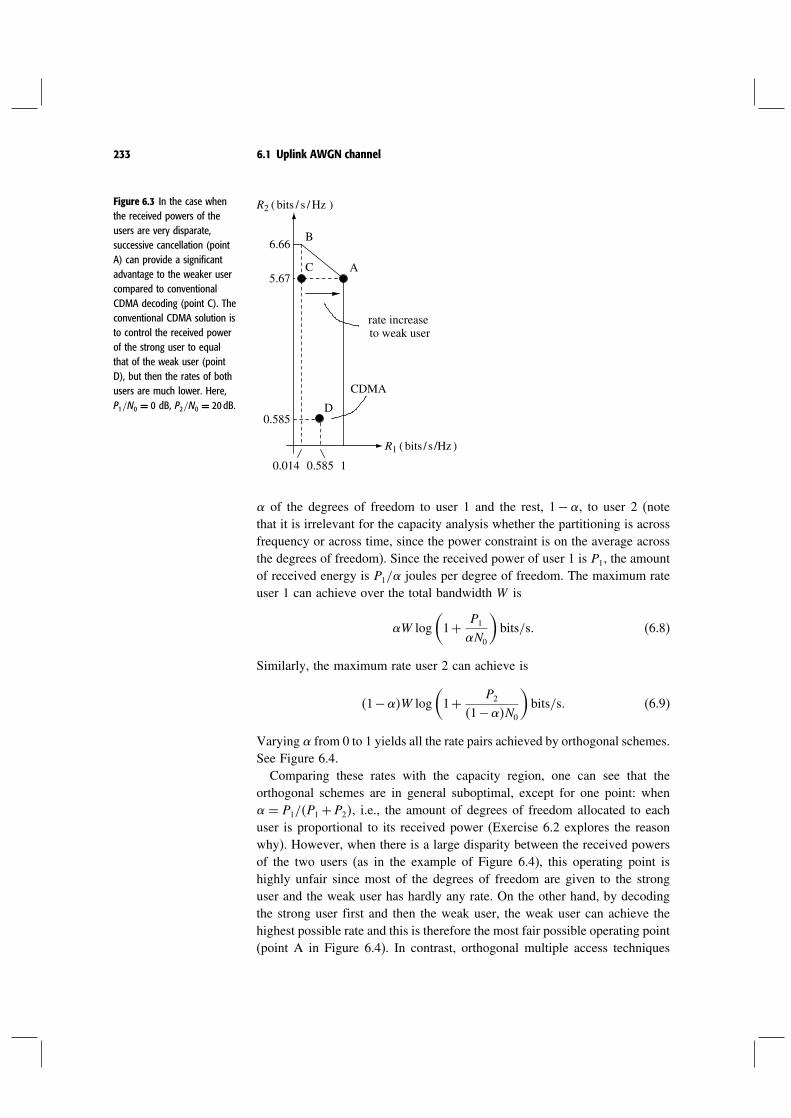
233 6.1 Uplink AWGN channel
Figure 6.3 In the case whenthe received powers of theusers are very disparate,successive cancellation (pointA) can provide a significantadvantage to the weaker usercompared to conventionalCDMA decoding (point C). Theconventional CDMA solution isto control the received powerof the strong user to equalthat of the weak user (pointD), but then the rates of bothusers are much lower. Here,P1/N0 = 0 dB, P2/N0 = 20 dB.
CDMA
R2 ( bits / s / Hz )
R1 ( bits / s /Hz )
1
5.67
6.66
C
B
0.585
0.5850.014
D
rate increase to weak user
A
of the degrees of freedom to user 1 and the rest, 1−, to user 2 (notethat it is irrelevant for the capacity analysis whether the partitioning is acrossfrequency or across time, since the power constraint is on the average acrossthe degrees of freedom). Since the received power of user 1 is P1, the amountof received energy is P1/ joules per degree of freedom. The maximum rateuser 1 can achieve over the total bandwidth W is
W log(
1+ P1
N0
)
bits/s (6.8)
Similarly, the maximum rate user 2 can achieve is
1−W log(
1+ P2
1−N0
)
bits/s (6.9)
Varying from 0 to 1 yields all the rate pairs achieved by orthogonal schemes.See Figure 6.4.Comparing these rates with the capacity region, one can see that the
orthogonal schemes are in general suboptimal, except for one point: when = P1/P1 +P2, i.e., the amount of degrees of freedom allocated to eachuser is proportional to its received power (Exercise 6.2 explores the reasonwhy). However, when there is a large disparity between the received powersof the two users (as in the example of Figure 6.4), this operating point ishighly unfair since most of the degrees of freedom are given to the stronguser and the weak user has hardly any rate. On the other hand, by decodingthe strong user first and then the weak user, the weak user can achieve thehighest possible rate and this is therefore the most fair possible operating point(point A in Figure 6.4). In contrast, orthogonal multiple access techniques

234 Multiuser capacity and opportunistic communication
Figure 6.4 Performance oforthogonal multiple accesscompared to capacity. TheSNRs of the two users are:P1/N0 = 0 dB andP2/N0 = 20 dB. Orthogonalmultiple access achieves thesum capacity at exactly onepoint, but at that point theweak user 1 has hardly anyrate and it is therefore a highlyunfair operating point. Point Agives the highest possible rateto user 1 and is most fair.
0.014
R2 ( bits / s / Hz )
R1 ( bits / s / Hz )
1
5.67
6.66
AC
B Sum capacityachieved here
0.065
can approach this performance for the weak user only by nearly sacrificingall the rate of the strong user. Here again, as in the comparison with CDMA,SIC’s advantage is in exploiting the proximity of a user to the base-station togive it high rate while protecting the far-away user.
6.1.4 General K -user uplink capacity
Wehave so far focused on the two-user case for simplicity, but the results extendreadily to an arbitrary number of users. TheK-user capacity region is describedby 2K −1 constraints, one for each possible non-empty subset of users:
∑
k∈Rk < log
(
1+∑
k∈ Pk
N0
)
for all ⊂ 1 K (6.10)
The right hand side corresponds to the maximum sum rate that can be achievedby a single transmitter with the total power of the users in and with noother users in the system. The sum capacity is
Csum = log(
1+∑K
k=1 Pk
N0
)
bits/s/Hz (6.11)
It can be shown that there are exactlyK! corner points, each one correspondingto a successive cancellation order among the users (Exercise 6.9).The equal received power case (P1 = = PK = P) is particularly simple.
The sum capacity is
Csum = log(
1+ KP
N0
)
(6.12)

235 6.2 Downlink AWGN channel
The symmetric capacity is
Csym = 1K
· log(
1+ KP
N0
)
(6.13)
This is the maximum rate for each user that can be obtained if every useroperates at the same rate. Moreover, this rate can be obtained via orthogonalmultiplexing: each user is allocated a fraction 1/K of the total degrees of free-dom.4 In particular, we can immediately conclude that under equal receivedpowers, the OFDM scheme considered in Chapter 4 has a better performancethan the CDMA scheme (which uses conventional receivers.)Observe that the sum capacity (6.12) is unbounded as the number of users
grows. In contrast, if the conventional CDMA receiver (decoding every usertreating all other users as noise) is used, each user will face an interferencefrom K−1 users of total power K−1P, and thus the sum rate is only
K · log(
1+ P
K−1P+N0
)
bits/s/Hz (6.14)
which approaches
K · P
K−1P+N0
log2 e≈ log2 e= 1442bits/s/Hz (6.15)
as K → . Thus, the total spectral efficiency is bounded in this case: thegrowing interference is eventually the limiting factor. Such a rate is said tobe interference-limited.The above comparison pertains effectively to a single-cell scenario, since
the only external effect modeled is white Gaussian noise. In a cellular network,the out-of-cell interference must be considered, and as long as the out-of-cellsignals cannot be decoded, the system would still be interference-limited, nomatter what the receiver is.
6.2 Downlink AWGN channel
The downlink communication features a single transmitter (the base-station)sending separate information to multiple users (Figure 6.5). The basebanddownlink AWGN channel with two users is
ykm= hkxm+wkm k= 12 (6.16)
where wkm∼ 0N0 is i.i.d. complex Gaussian noise and ykm is thereceived signal at user k at time m, for both the users k = 12. Here hk is
4 This fact is specific to the AWGN channel and does not hold in general. See Section 6.3.

236 Multiuser capacity and opportunistic communication
the fixed (complex) channel gain corresponding to user k. We assume that hk
Figure 6.5 Two-user downlink.
is known to both the transmitter and the user k (for k = 12). The transmitsignal xm has an average power constraint of P joules/symbol. Observethe difference from the uplink of this overall constraint: there the powerrestrictions are separate for the signals of each user. The users separatelydecode their data using the signals they receive.As in the uplink, we can ask for the capacity region , the region of the rates
R1R2, at which the two users can simultaneously reliably communicate.We have the single-user bounds, as in (6.4) and (6.5),
Rk < log(
1+ Phk2N0
)
k= 12 (6.17)
This upper bound on Rk can be attained by using all the power and degreesof freedom to communicate to user k (with the other user getting zero rate).Thus, we have the two extreme points (with rate of one user being zero) inFigure 6.6. Further, we can share the degrees of freedom (time and bandwidth)between the users in an orthogonal manner to obtain any rate pair on theline joining these two extreme points. Can we achieve a rate pair outside thistriangle by a more sophisticated communication strategy?
6.2.1 Symmetric case: two capacity-achieving schemes
To get more insight, let us first consider the symmetric case where h1 = h2.In this symmetric situation, the SNR of both the users is the same. This meansthat if user 1 can successfully decode its data, then user 2 should also be
Figure 6.6 The capacity regionof the downlink with two usershaving symmetric AWGNchannels, i.e., h1 = h2.
R2
R1
log 1+ h2P2N0
log 1+h2P1
N0

237 6.2 Downlink AWGN channel
able to decode successfully the data of user 1 (and vice versa). Thus the suminformation rate must also be bounded by the single-user capacity:
R1+R2 < log(
1+ Ph12N0
)
(6.18)
Comparing this with the single-user bounds in (6.17) and recalling the sym-metry assumption h1 = h2, we have shown the triangle in Figure 6.6 to bethe capacity region of the symmetric downlink AWGN channel.Let us continue our thought process within the realm of the symmetry
assumption. The rate pairs in the capacity region can be achieved by strategiesused on point-to-point AWGN channels and sharing the degrees of freedom(time and bandwidth) between the two users. However, the symmetry betweenthe two channels (cf. (6.16)) suggests a natural, and alternative, approach.The main idea is that if user 1 can successfully decode its data from y1, thenuser 2, which has the same SNR, should also be able to decode the data ofuser 1 from y2. Then user 2 can subtract the codeword of user 1 from itsreceived signal y2 to better decode its own data, i.e., it can perform successiveinterference cancellation. Consider the following strategy that superposes thesignals of the two users, much like in a spread-spectrum CDMA system. Thetransmit signal is the sum of two signals,
xm= x1m+x2m (6.19)
where xkm is the signal intended foruserk.The transmitter encodes the infor-mation for each user using an i.i.d.Gaussian code spread on the entire bandwidth(and powers P1P2, respectively, with P1+P2 = P). User 1 treats the signal foruser 2 as noise and can hence be communicated to reliably at a rate of
R1 = log(
1+ P1h12P2h12+N0
)
= log(
1+ P1+P2h12N0
)
− log(
1+ P2h12N0
)
(6.20)
User 2 performs successive interference cancellation: it first decodes the dataof user 1 by treating x2 as noise, subtracts the exactly determined (with highprobability) user 1 signal from y2 and extracts its data. Thus user 2 can supportreliably a rate
R2 = log(
1+ P2h22N0
)
(6.21)
This superposition strategy is schematically represented in Figures 6.7 and6.8. Using the power constraint P1+P2 = P we see directly from (6.20) and(6.21) that the rate pairs in the capacity region (Figure 6.6) can be achievedby this strategy as well. We have hence seen two coding schemes for the

238 Multiuser capacity and opportunistic communication
Figure 6.7 Superpositionencoding example. The QPSKconstellation of user 2 issuperimposed on that ofuser 1.
x2
x1
x2
x1
x
Figure 6.8 Superpositiondecoding example. Thetransmitted constellation pointof user 1 is decoded first,followed by decoding of theconstellation point of user 2.
x2
yy
^
x1^
symmetric downlink AWGN channel that are both optimal: single-user codesfollowed by orthogonalization of the degrees of freedom among the users,and the superposition coding scheme.
6.2.2 General case: superposition coding achieves capacity
Let us now return to the general downlink AWGN channel without thesymmetry assumption and take h1 < h2. Now user 2 has a better channelthan user 1 and hence can decode any data that user 1 can successfully decode.Thus, we can use the superposition coding scheme: First the transmit signalis the (linear) superposition of the signals of the two users. Then, user 1 treatsthe signal of user 2 as noise and decodes its data from y1. Finally, user 2,which has the better channel, performs SIC: it decodes the data of user 1 (andhence the transmit signal corresponding to user 1’s data) and then proceeds tosubtract the transmit signal of user 1 from y2 and decode its data. As before,with each possible power split of P = P1+P2, the following rate pair can beachieved:
R1 = log(
1+ P1h12P2h12+N0
)
bits/s/Hz
R2 = log(
1+ P2h22N0
)
bits/s/Hz (6.22)

239 6.2 Downlink AWGN channel
On the other hand, orthogonal schemes achieve, for each power splitP = P1+P2 and degree-of-freedom split ∈ 01, as in the uplink (cf. (6.8)and (6.9)),
R1 = log(
1+ P1h12N0
)
bits/s/Hz
R2 = 1− log(
1+ P2h221−N0
)
bits/s/Hz (6.23)
Here, represents the fraction of the bandwidth devoted to user 1. Figure 6.9plots the boundaries of the rate regions achievable with superposition codingand optimal orthogonal schemes for the asymmetric downlink AWGN channel(with SNR1 = 0dB and SNR2 = 20dB). We observe that the performance ofthe superposition coding scheme is better than that of the orthogonal scheme.One can show that the superposition decoding scheme is strictly better than
the orthogonalization schemes (except for the two corner points where onlyone user is being communicated to). That is, for any rate pair achieved byorthogonalization schemes there is a power split for which the successivedecoding scheme achieves rate pairs that are strictly larger (see Exercise 6.25).This gap in performance is more pronounced when the asymmetry betweenthe two users deepens. In particular, superposition coding can provide a veryreasonable rate to the strong user, while achieving close to the single-userbound for the weak user. In Figure 6.9, for example, while maintaining therate of the weaker user R1 at 09 bits/s/Hz, superposition coding can providea rate of around R2 = 3 bits/s/Hz to the strong user while an orthogonalscheme can provide a rate of only around 1 bits/s/Hz. Intuitively, the stronguser, being at high SNR, is degree-of-freedom limited and superpositioncoding allows it to use the full degrees of freedom of the channel while beingallocated only a small amount of transmit power, thus causing small amount
Figure 6.9 The boundary ofrate pairs (in bits/s/Hz)achievable by superpositioncoding (solid line) andorthogonal schemes (dashedline) for the two-userasymmetric downlink AWGNchannel with the user SNRsequal to 0 and 20dB(i.e., Ph12/N0 = 1 andPh22/N0 = 100). In theorthogonal schemes, both thepower split P = P1+ P2 andsplit in degrees of freedom
are jointly optimized tocompute the boundary.
0 0.1 0.2 0.3 0.4 0.5 0.6 0.7 0.8 0.9 10
1
2
3
4
5
6
7
Rate of user 1
Rat
e of
use
r 2

240 Multiuser capacity and opportunistic communication
of interference to the weak user. In contrast, an orthogonal scheme has toallocate a significant fraction of the degrees of freedom to the weak user toachieve near single-user performance, and this causes a large degradation inthe performance of the strong user.So far we have considered a specific signaling scheme: linear superposition
of the signals of the two users to form the transmit signal (cf. (6.19)). With thisspecific encoding method, the SIC decoding procedure is optimal. However,one can show that this scheme in fact achieves the capacity and the boundaryof the capacity region of the downlink AWGN channel is given by (6.22)(Exercise 6.26).While we have restricted ourselves to two users in the presentation, these
results have natural extensions to the general K-user downlink channel. Inthe symmetric case hk = h for all k, the capacity region is given by thesingle constraint
K∑
k=1
Rk < log(
1+ Ph2N0
)
(6.24)
In general with the ordering h1 ≤ h2 ≤ · · · ≤ hK, the boundary of thecapacity region of the downlink AWGN channel is given by the parameterizedrate tuple
Rk = log
(
1+ Pkhk2N0+
(∑Kj=k+1 Pj
) hk2)
k= 1 K (6.25)
where P =∑Kk=1 Pk is the power split among the users. Each rate tuple on the
boundary, as in (6.25), is achieved by superposition coding.Since we have a full characterization of the tradeoff between the rates at
which users can be reliably communicated to, we can easily derive specificscalar performance measures. In particular, we focused on sum capacity in theuplink analysis; to achieve the sum capacity we required all the users to trans-mit simultaneously (using the SIC receiver to decode the data). In contrast,we see from (6.25) that the sum capacity of the downlink is achieved bytransmitting to a single user, the user with the highest SNR.
Summary 6.1 Uplink and downlink AWGN capacity
Uplink:
ym=K∑
k=1
xkm+wm (6.26)
with user k having power constraint Pk.

241 6.2 Downlink AWGN channel
Achievable rates satisfy:
∑
k∈Rk ≤ log
(
1+∑
k∈ Pk
N0
)
for all ⊂ 1 K (6.27)
The K! corner points are achieved by SIC, one corner point for eachcancellation order. They all achieve the same optimal sum rate.
A natural ordering would be to decode starting from the strongest userfirst and move towards the weakest user.
Downlink:
ykm= hkxm+wkm k= 1 K (6.28)
with h1 ≤ h2 ≤ ≤ hK.The boundary of the capacity region is given by the rate tuples:
Rk = log
(
1+ Pkhk2N0+
∑Kj=k+1 Pjhk2
)
k= 1 K (6.29)
for all possible splits P =∑k Pk of the total power at the base-station.
The optimal points are achieved by superposition coding at the transmitterand SIC at each of the receivers.
The cancellation order at every receiver is always to decode the weakerusers before decoding its own data.
Discussion 6.1 SIC: implementation issues
We have seen that successive interference cancellation plays an importantrole in achieving the capacities of both the uplink and the downlinkchannels. In contrast to the receivers for the multiple access systems inChapter 4, SIC is a multiuser receiver. Here we discuss several potentialpractical issues in using SIC in a wireless system.• Complexity scaling with the number of users In the uplink, the base-station has to decode the signals of every user in the cell, whether it usesthe conventional single-user receiver or the SIC. In the downlink, on theother hand, the use of SIC at the mobile means that it now has to decodeinformation intended for some of the other users, something it would notbe doing in a conventional system. Then the complexity at each mobilescales with the number of users in the cell; this is not very acceptable.However, we have seen that superposition coding in conjunction with

242 Multiuser capacity and opportunistic communication
SIC has the largest performance gain when the users have very disparatechannels from the base-station. Due to the spatial geometry, typicallythere are only a few users close to the base-station while most ofthe users are near the edge of the cell. This suggests a practical wayof limiting complexity: break the users in the cell into groups, witheach group containing a small number of users with disparate channels.Within each group, superposition coding/SIC is performed, and acrossthe groups, transmissions are kept orthogonal. This should capture asignificant part of the performance gain.
• Error propagation Capacity analysis assumes error-free decoding butof course, with actual codes, errors are made. Once an error occurs fora user, all the users later in the SIC decoding order will very likely bedecoded incorrectly. Exercise 6.12 shows that if pi
e is the probabilityof decoding the ith user incorrectly, assuming that all the previous usersare decoded correctly, then the actual error probability for the kth userunder SIC is at most
k∑
i=1
pie (6.30)
So, if all the users are coded with the same target error probabilityassuming no propagation, the effect of error propagation degrades theerror probability by a factor of at most the number of usersK. IfK is rea-sonably small, this effect can easily be compensated by using a slightlystronger code (by, say, increasing the block length by a small amount).
• Imperfect channel estimates To remove the effect of a user fromthe aggregate received signal, its contribution must be reconstructedfrom the decoded information. In a wireless multipath channel, thiscontribution depends also on the impulse response of the channel.Imperfect estimate of the channel will lead to residual cancellationerrors. One concern is that, if the received powers of the users arevery disparate (as in the example in Figure 6.3 where they differ by20 dB), then the residual error from cancelling the stronger user canstill swamp the weaker user’s signal. On the other hand, it is also easierto get an accurate channel estimate when the user is strong. It turns outthat these two effects compensate each other and the effect of residualerrors does not grow with the power disparity (Exercise 6.13).
• Analog-to-digital quantization error When the received powers ofthe users are very disparate, the analog-to-digital (A/D) converter needsto have a very large dynamic range, and at the same time, enoughresolution to quantize accurately the contribution from the weak signal.For example, if the power disparity is 20 dB, even 1-bit accuracy forthe weak signal would require an 8-bit A/D converter. This may wellpose an implementation constraint on how much gain SIC can offer.

243 6.3 Uplink fading channel
6.3 Uplink fading channel
Let us now include fading. Consider the complex baseband representation ofthe uplink flat fading channel with K users:
ym=K∑
k=1
hkmxkm+wm (6.31)
where hkmm is the fading process of user k. We assume that the fadingprocesses of different users are independent of each other andhkm2= 1.Here, we focus on the symmetric case when each user is subject to thesame average power constraint, P, and the fading processes are identicallydistributed. In this situation, the sum and the symmetric capacities are thekey performance measures. We will see later in Section 6.7 how the insightsobtained from this idealistic symmetric case can be applied to more realisticasymmetric situations. To understand the effect of the channel fluctuations, wemake the simplifying assumption that the base-station (receiver) can perfectlytrack the fading processes of all the users.
6.3.1 Slow fading channel
Let us start with the slow fading situation where the time-scale of commu-nication is short relative to the coherence time interval for all the users, i.e.,hkm = hk for all m. Suppose the users are transmitting at the same rate R
bits/s/Hz. Conditioned on each realization of the channels h1 hK , wehave the standard uplink AWGN channel with received SNR of user k equalto hk2P/N0. If the symmetric capacity of this uplink AWGN channel is lessthan R, then the base-station can never recover all of the users’ informationaccurately; this results in outage. From the expression for the capacity regionof the general K-user uplink AWGN channel (cf. (6.10)), the probability ofthe outage event can be written as
pulout =
log
(
1+ SNR∑
k∈hk2
)
< R for some ⊂ 1 K
(6.32)
Here denotes the cardinality of the set and SNR = P/N0. The corre-sponding -outage symmetric capacity, Csym
, is then the largest rate R suchthat the outage probability in (6.32) is smaller than or equal to .In Section 5.4.1, we have analyzed the behavior of the outage capacity,
CSNR, of the point-to-point slow fading channel. Since this corresponds tothe performance of just a single user, it is equal to Csym
with K = 1. Withmore than one user, Csym
is only smaller: now each user has to deal not only
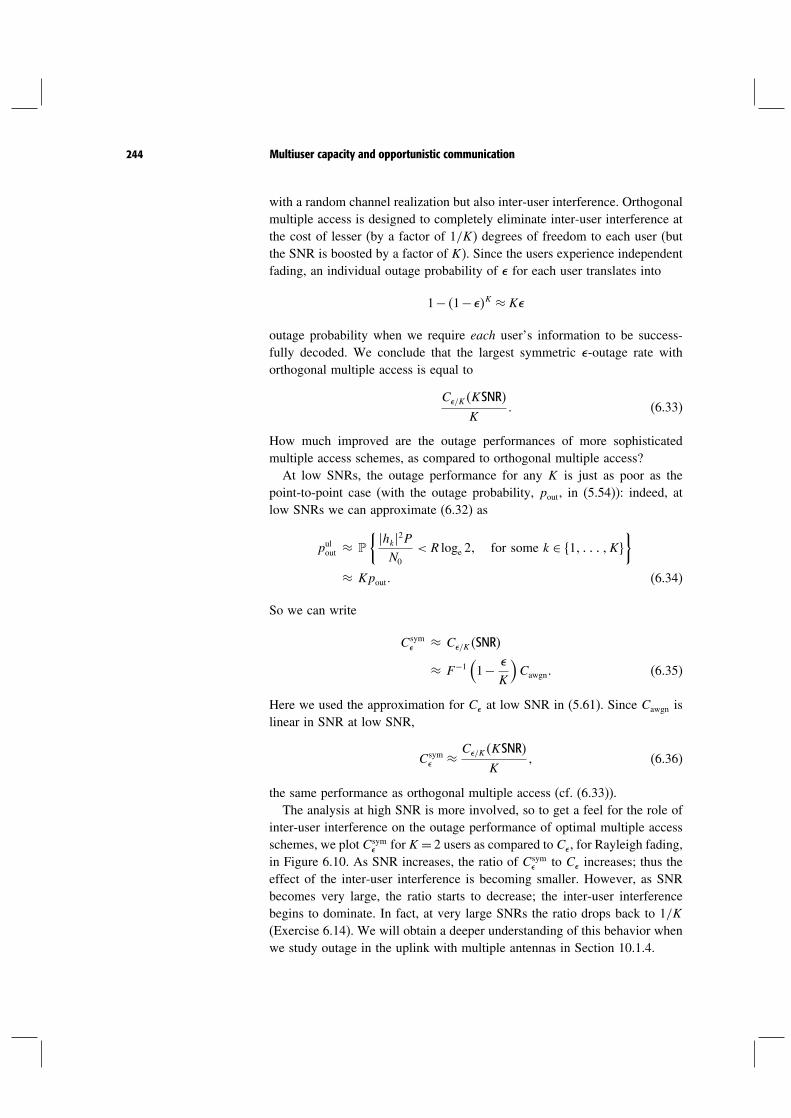
244 Multiuser capacity and opportunistic communication
with a random channel realization but also inter-user interference. Orthogonalmultiple access is designed to completely eliminate inter-user interference atthe cost of lesser (by a factor of 1/K) degrees of freedom to each user (butthe SNR is boosted by a factor of K). Since the users experience independentfading, an individual outage probability of for each user translates into
1− 1− K ≈ K
outage probability when we require each user’s information to be success-fully decoded. We conclude that the largest symmetric -outage rate withorthogonal multiple access is equal to
C/KKSNRK
(6.33)
How much improved are the outage performances of more sophisticatedmultiple access schemes, as compared to orthogonal multiple access?At low SNRs, the outage performance for any K is just as poor as the
point-to-point case (with the outage probability, pout, in (5.54)): indeed, atlow SNRs we can approximate (6.32) as
pulout ≈
hk2PN0
< R loge 2 for some k ∈ 1 K
≈ Kpout (6.34)
So we can write
Csym ≈ C/KSNR
≈ F−1(1−
K
)Cawgn (6.35)
Here we used the approximation for C at low SNR in (5.61). Since Cawgn islinear in SNR at low SNR,
Csym ≈ C/KKSNR
K (6.36)
the same performance as orthogonal multiple access (cf. (6.33)).The analysis at high SNR is more involved, so to get a feel for the role of
inter-user interference on the outage performance of optimal multiple accessschemes, we plot Csym
for K= 2 users as compared to C, for Rayleigh fading,in Figure 6.10. As SNR increases, the ratio of Csym
to C increases; thus theeffect of the inter-user interference is becoming smaller. However, as SNRbecomes very large, the ratio starts to decrease; the inter-user interferencebegins to dominate. In fact, at very large SNRs the ratio drops back to 1/K(Exercise 6.14). We will obtain a deeper understanding of this behavior whenwe study outage in the uplink with multiple antennas in Section 10.1.4.

245 6.3 Uplink fading channel
Figure 6.10 Plot of thesymmetric -outage capacity ofthe two-user Rayleigh slowfading uplink as compared toC , the correspondingperformance of apoint-to-point Rayleigh slowfading channel.
5 10 15 20 25 30 35 40
SNR (dB)
0.50–5–10
0.8
0.75
0.7
0.65
0.6
0.55
C
sym
C
∋
∋
6.3.2 Fast fading channel
Let us now turn to the fast fading scenario, where each hkmm is modelledas a time-varying ergodic process. With the ability to code over multiplecoherence time intervals, we can have a meaningful definition of the capacityregion of the uplink fading channel. With only receiver CSI, the transmitterscannot track the channel and there is no dynamic power allocation. Analogousto the discussion in the point-to-point case (cf. Section 5.4.5 and, in particular,(5.89)), the sum capacity of the uplink fast fading channel can be expressedas:
Csum =
[
log(
1+∑K
k=1 hk2PN0
)]
(6.37)
Here hk is the random variable denoting the fading of user k at a particulartime and the time averages are taken to converge to the same limit for allrealizations of the fading process (i.e., the fading processes are ergodic).A formal derivation of the capacity region of the fast fading uplink (withpotentially multiple antenna elements) is carried out in Appendix B.9.3.How does this compare to the sum capacity of the uplink channel without
fading (cf. (6.12))? Jensen’s inequality implies that
[
log(
1+∑K
k=1 hk2PN0
)]
≤ log(
1+ ∑K
k=1 hk2PN0
)
= log(
1+ KP
N0
)

246 Multiuser capacity and opportunistic communication
Hence, without channel state information at the transmitter, fading alwayshurts, just as in the point-to-point case. However, when the number of usersbecomes large, 1/K ·∑K
k=1 hk2 → 1 with probability 1, and the penalty dueto fading vanishes.To understand why the effect of fading goes away as the number of users
grows, let us focus on a specific decoding strategy to achieve the sum capacity.With each user spreading their information on the entire bandwidth simul-taneously, the successive interference cancellation (SIC) receiver, which isoptimal for the uplink AWGN channel, is also optimal for the uplink fadingchannel. Consider the kth stage of the cancellation procedure, where user k isbeing decoded and users k+1 K are not canceled. The effective channelthat user k sees is
ym= hkmxkm+K∑
i=k+1
himxim+wm (6.38)
The rate that user k gets is
Rk =
[
log
(
1+ hk2P∑K
i=k+1 hi2P+N0
)]
(6.39)
Since there are many users sharing the spectrum, the SINR for user k is low.Thus, the capacity penalty due to the fading of user k is small (cf. (5.92)).Moreover, there is also averaging among the interferers. Thus, the effect ofthe fading of the interferers also vanishes. More precisely,
Rk ≈
[hk2P
∑Ki=k+1 hi2P+N0
]
log2 e
≈
[ hk2PK−kP+N0
]
log2 e
= P
K−kP+N0
log2 e
which is the rate that user k would have got in the (unfaded) AWGN channel.The first approximation comes from the linearity of log1+ SNR for smallSNR, and the second approximation comes from the law of large numbers.In the AWGN case, the sum capacity can be achieved by an orthogonal
multiple access scheme which gives a fraction, 1/K, of the total degrees offreedom to each user. How about the fading case? The sum rate achieved bythis orthogonal scheme is
K∑
k=1
1K
[
log(
1+ Khk2PN0
)]
=
[
log(
1+ Khk2PN0
)]
(6.40)

247 6.3 Uplink fading channel
which is strictly less than the sum capacity of the uplink fading channel (6.37)for K ≥ 2. In particular, the penalty due to fading persists even when there isa large number of users.
6.3.3 Full channel side information
We now come to a case of central interest in this chapter, the fast fadingchannel with tracking of the channels of all the users at the receiver and allthe transmitters.5 As opposed to the case with only receiver CSI, we can nowdynamically allocate powers to the users as a function of the channel states.Analogous to the point-to-point case, we can without loss of generality focuson the simple block fading model
ym=K∑
k=1
hkmxkm+wm (6.41)
where hkm = hk remains constant over the th coherence period ofTcTc 1 symbols and is i.i.d. across different coherence periods. Thechannel over L such coherence periods can be modeled as a parallel uplinkchannel with L sub-channels which fade independently. Each sub-channel isan uplink AWGN channel. For a given realization of the channel gains hk ,k= 1 K = 1 L, the sum capacity (in bits/symbol) of this parallelchannel is, as for the point-to-point case (cf. (5.95)),
maxPk k=1 K =1 L
1L
L∑
=1
log
(
1+∑K
k=1 Pk hk 2N0
)
(6.42)
subject to the powers being non-negative and the average power constrainton each user:
1L
L∑
=1
Pk = P k= 1 K (6.43)
The solution to this optimization problem as L→ yields the appropriatepower allocation policy to be followed by the users.As discussed in the point-to-point communication context with full CSI
(cf. Section 5.4.6), we can use a variable rate coding scheme: in the thsub-channel, the transmit powers dictated by the solution to the optimizationproblem above (6.42) are used by the users and a code designed for thisfading state is used. For this code, each codeword sees a time-invariant uplink
5 As we will see, the transmitters will not need to explicitly keep track of the channelvariations of all the users. Only an appropriate function of the channels of all the usersneeds to be tracked, which the receiver can compute and feed back to the users.

248 Multiuser capacity and opportunistic communication
AWGN channel. Thus, we can use the encoding and decoding procedures forthe code designed for the uplink AWGN channel. In particular, to achieve themaximum sum rate, we can use orthogonal multiple access: this means that thecodes designed for the point-to-point AWGN channel can be used. Contrastthis with the case when only the receiver has CSI, where we have shownthat orthogonal multiple access is strictly suboptimal for fading channels.Note that this argument on the optimality of orthogonal multiple access holdsregardless of whether the users have symmetric fading statistics.In the case of the symmetric uplink considered here, the optimal power
allocation takes on a particularly simple structure. To derive it, let us considerthe optimization problem (6.42), but with the individual power constraints in(6.43) relaxed and replaced by a total power constraint:
1L
L∑
=1
K∑
k=1
Pk = KP (6.44)
The sum rate in the th sub-channel is
log
(
1+∑K
k=1 Pk hk 2N0
)
(6.45)
and for a given total power∑K
k=1 Pk allocated to the th sub-channel, thisquantity is maximized by giving all that power to the user with the strongestchannel gain. Thus, the solution of the optimization problem (6.42) subjectto the constraint (6.44) is that at each time, allow only the user with the bestchannel to transmit. Since there is just one user transmitting at any time,we have reduced to a point-to-point problem and can directly infer from ourdiscussion in Section 5.4.6 that the best user allocates its power according tothe waterfilling policy. More precisely, the optimal power allocation policy is
Pk =
(1− N0
maxi hi 2)+
if hk =maxi hi 0 else
(6.46)
where is chosen to meet the sum power constraint (6.44). Taking the numberof coherence periods L → and appealing to the ergodicity of the fadingprocess, we get the optimal capacity-achieving power allocation strategy,which allocates powers to the users as a function of the joint channel stateh = h1 hK:
P∗k h=
(1− N0
maxi hi2)+
if hk2 =maxi hi20 else
(6.47)

249 6.3 Uplink fading channel
with chosen to satisfy the power constraint
K∑
k=1
P∗k h= KP (6.48)
(Rigorously speaking, this formula is valid only when there is exactly oneuser with the strongest channel. See Exercise 6.16 for the generalization tothe case when multiple users can have the same fading state.) The resultingsum capacity is
Csum =
[
log(
1+ Pk∗hhk∗ 2N0
)]
(6.49)
where k∗h is the index of the user with the strongest channel at joint channelstate h.We have derived this result assuming a total power constraint on all the
users, but by symmetry, the power consumption of all the users is the sameunder the optimal solution (recall that we are assuming independent andidentical fading processes across the users here). Therefore the individualpower constraints in (6.43) are automatically satisfied and we have solved theoriginal problem as well.This result is the multiuser generalization of the idea of opportunistic
communication developed in Chapter 5: resource is allocated at the times andto the user whose channel is good.When one attempts to generalize the optimal power allocation solution from
the point-to-point setting to the multiuser setting, it may be tempting to thinkof “users” as a new dimension, in addition to the time dimension, over whichdynamic power allocation can be performed. This may lead us to guess that theoptimal solution is waterfilling over the joint time/user space. This, as we havealready seen, is not the correct solution. The flaw in this reasoning is that havingmultiple users does not provide additional degrees of freedom in the system: theusers are just sharing the time/frequency degrees of freedom already existing inthechannel.Thus, theoptimalpowerallocationproblemshould reallybe thoughtof as how to partition the total resource (power) across the time/frequencydegrees of freedom and how to share the resource across the users in each ofthose degrees of freedom. The above solution says that from the point of view ofmaximizing the sumcapacity, the optimal sharing is just to allocate all the powerto the user with the strongest channel on that degree of freedom.We have focused on the sum capacity in the symmetric case where users
have identical channel statistics and power constraints. It turns out that in theasymmetric case, the optimal strategy to achieve sum capacity is still to haveone user transmitting at a time, but the criterion of choosing which user isdifferent. This problem is analyzed in Exercise 6.15. However, in the asym-metric case, maximizing the sum rate may not be the appropriate objective,

250 Multiuser capacity and opportunistic communication
since the user with the statistically better channel may get a much higher rateat the expense of the other users. In this case, one may be interested in oper-ating at points in the multiuser capacity region of the uplink fading channelother than the point maximizing the sum rate. This problem is analyzed inExercise 6.18. It turns out that, as in the time-invariant uplink, orthogonalmultiple access is not optimal. Instead, users transmit simultaneously and arejointly decoded (using SIC, for example), even though the rates and powersare still dynamically allocated as a function of the channel states.
Summary 6.2 Uplink fading channel
Slow Rayleigh fading At low SNR, the symmetric outage capacity isequal to the outage capacity of the point-to-point channel, but scaled downby the number of users. At high SNR, the symmetric outage capacity formoderate number of users is approximately equal to the outage capacity ofthe point-to-point channel. Orthogonal multiple access is close to optimalat low SNR.
Fast fading, receiver CSIWith a large number of users, each user gets thesame performance as in an uplink AWGN channel with the same averageSNR. Orthogonal multiple access is strictly suboptimal.
Fast fading, full CSI Orthogonal multiple access can still achieve the sumcapacity. In a symmetric uplink, the policy of allowing only the best userto transmit at each time achieves the sum capacity.
6.4 Downlink fading channel
We now turn to the downlink fading channel with K users:
ykm= hkmxm+wkm k= 1 K (6.50)
where hkmm is the channel fading process of user k. We retain the averagepower constraint of P on the transmit signal and wkm ∼ 0N0 to bei.i.d. in time m (for each user k= 1 K).As in the uplink, we consider the symmetric case: hkmm are identically
distributed processes for k = 1 K. Further, let us also make the sameassumption we did in the uplink analysis: the processes hkmm are ergodic(i.e., the time average of every realization equals the statistical average).
6.4.1 Channel side information at receiver only
Let us first consider the case when the receivers can track the channel but thetransmitter does not have access to the channel realizations (but has access

251 6.4 Downlink fading channel
to a statistical characterization of the channel processes of the users). Toget a feel for good strategies to communicate on this fading channel andto understand the capacity region, we can argue as in the downlink AWGNchannel. We have the single-user bounds, in terms of the point-to-point fadingchannel capacity in (5.89):
Rk <
[
log(
1+ h2PN0
)]
k= 1 K (6.51)
where h is a random variable distributed as the stationary distribution ofthe ergodic channel processes. In the symmetric downlink AWGN channel,we argued that the users have the same channel quality and hence coulddecode each other’s data. Here, the fading statistics are symmetric and by theassumption of ergodicity, we can extend the argument of the AWGN case tosay that, if user k can decode its data reliably, then all the other users canalso successfully decode user k’s data. Analogous to (6.18) in the AWGNdownlink analysis, we obtain
K∑
k=1
Rk <
[
log(
1+ h2PN0
)]
(6.52)
An alternative way to see that the right hand side in (6.52) is the best sumrate one can achieve is outlined in Exercise 6.27. The bound (6.52) is clearlyachievable by transmitting to one user only or by time-sharing between anynumber of users. Thus in the symmetric fading channel, we obtain the sameconclusion as in the symmetric AWGN downlink: the rate pairs in the capacityregion can be achieved by both orthogonalization schemes and superpositioncoding.How about the downlink fading channel with asymmetric fading statistics
of the users? While we can use the orthogonalization scheme in this asym-metric model as well, the applicability of superposition decoding is not soclear. Superposition coding was successfully applied in the downlink AWGNchannel because there is an ordering of the channel strength of the users fromweak to strong. In the asymmetric fading case, users in general have differentfading distributions and there is no longer a complete ordering of the users.In this case, we say that the downlink channel is non-degraded and little isknown about good strategies for communication. Another interesting situationwhen the downlink channel is non-degraded arises when the transmitter hasan array of multiple antennas; this is studied in Chapter 10.
6.4.2 Full channel side information
We saw in the uplink that the communication scenario becomes more inter-esting when the transmitters can track the channel as well. In this case, thetransmitters can vary their powers as a function of the channel. Let us now

252 Multiuser capacity and opportunistic communication
turn to the analogous situation in the downlink where the single transmittertracks all the channels of the users it is communicating to (the users continueto track their individual channels). As in the uplink, we can allocate powersto the users as a function of the channel fade level. To see the effect, let uscontinue focusing on sum capacity. We have seen that without fading, thesum capacity is achieved by transmitting only to the best user. Now as thechannels vary, we can pick the best user at each time and further allocate itan appropriate power, subject to a constraint on the average power. Underthis strategy, the downlink channel reduces to a point-to-point channel withthe channel gain distributed as
maxk=1 K
hk2
The optimal power allocation is the, by now familiar, waterfilling solution:
P∗h=(1− N0
maxk=1 K hk2)+
(6.53)
where h= h1 hKt is the joint fading state and > 0 is chosen such that
the average power constraint is met. The optimal strategy is exactly the sameas in the sum capacity of the uplink. The sum capacity of the downlink is:
[
log(
1+ P∗hmaxk=1 K h2k
N0
)]
(6.54)
6.5 Frequency-selective fading channels
The extension of the flat fading analysis in the uplink and the downlink tounderspread frequency-selective fading channels is conceptually straightfor-ward. As we saw in Section 5.4.7 in the point-to-point setting, we can think ofthe underspread channel as a set of parallel sub-carriers over each coherencetime interval and varying independently from one coherence time intervalto the other. We can see this constructively by imposing a cyclic prefix toall the transmit signals; the cyclic prefix should be of length that is largerthan the largest multipath delay spread that we are likely to encounter amongthe different users. Since this overhead is fixed, the loss is amortized whencommunicating over a long block length.We can apply exactly the same OFDM transformation to the multiuser
channels. Thus on the nth sub-carrier, we can write the uplink channel as
yni=K∑
k=1
hkn i dk
n i+ wni (6.55)

253 6.6 Multiuser diversity
where dki, hki and yi, respectively, represent the DFTs of the trans-mitted sequence of user k, of the channel and of the received sequence atOFDM symbol time i.The flat fading uplink channel can be viewed as a set of parallel multiuser
sub-channels, one for each coherence time interval. With full CSI, the optimalstrategy to maximize the sum rate in the symmetric case is to allow onlythe user with the best channel to transmit at each coherence time interval.The frequency-selective fading uplink channel can also be viewed as a set ofparallel multiuser sub-channels, one for each sub-carrier and each coherencetime interval. Thus, the optimal strategy is to allow the best user to transmit oneach of these sub-channels. The power allocated to the best user is waterfillingover time and frequency. As opposed to the flat fading case, multiple userscan now transmit at the same time, but over different sub-carriers. Exactlythe same comments apply to the downlink.
6.6 Multiuser diversity
6.6.1 Multiuser diversity gain
Let us consider the sum capacity of the uplink and downlink flat fadingchannels (see (6.49) and (6.54), respectively). Each can be interpreted as thewaterfilling capacity of a point-to-point link with a power constraint equalto the total transmit power (in the uplink this is equal to KP and in thedownlink it is equal to P), and a fading process whose magnitude varies asmaxk hkm. Compared to a system with a single transmitting user, themultiuser gain comes from two effects:
1. the increase in total transmit power in the case of the uplink;2. the effective channel gain at time m that is improved from h1m2 to
max1≤k≤K hkm2.
The first effect already appeared in the uplink AWGN channel and also inthe fading channel with channel side information only at the receiver. Thesecond effect is entirely due to the ability to dynamically schedule resourcesamong the users as a function of the channel state.The sum capacity of the uplink Rayleigh fading channel with full CSI is
plotted in Figure 6.11 for different numbers of users. The performance curvesare plotted as a function of the total SNR = KP/N0 so as to focus on thesecond effect. The sum capacity of the channel with only CSI at the receiver isalso plotted for different numbers of users. The capacity of the point-to-pointAWGN channel with received power KP (which is also the sum capacity ofa K-user uplink AWGN channel) is shown as a baseline. Figure 6.12 focuseson the low SNR regime.

254 Multiuser capacity and opportunistic communication
Figure 6.11 Sum capacity ofthe uplink Rayleigh fadingchannel plotted as a functionof SNR= KP/N0.
2
4
6
5–5–10–15–20 10 15 20
8
AWGNCSIRFull CSI
Csum(bits /s / Hz)
SNR (dB)
K = 16
K = 2
K = 4
K = 1
AWGN
Figure 6.12 Sum capacity ofthe uplink Rayleigh fadingchannel plotted as a functionof SNR= KP/N0 in the lowSNR regime. Everything isplotted as a fraction of theAWGN channel capacity.
1
5–5–15–20–25–30 10
2
3
4
5
6
7
CSIRFull CSI
SNR (dB)
Csum
CAWGNK = 16
K = 4
K = 2
K = 1
–10
Several observations can be made from the plots:
• The sum capacity without transmitter CSI increases with the number of theusers, but not significantly. This is due to the multiuser averaging effectexplained in the last section. This sum capacity is always bounded by thecapacity of the AWGN channel.
• The sum capacity with full CSI increases significantly with the number ofusers. In fact, with even two users, this sum capacity already exceeds that

255 6.6 Multiuser diversity
of the AWGN channel. At 0 dB, the capacity with K = 16 users is about afactor of 2.5 of the capacity with K = 1. The corresponding power gain isabout 7 dB. Compared to the AWGN channel, the capacity gain for K = 16is about a factor of 2.2 and an SNR gain of 5.5 dB.
• For K= 1, the capacity benefit of transmitter CSI only becomes apparent atquite low SNR levels; at high SNR there is no gain. For K> 1 the benefitis apparent throughout the entire SNR range, although the relative gain isstill more significant at low SNR. This is because the gain is still primarilya power gain.
The increase in the full CSI sum capacity comes from a multiuser diversityeffect: when there are many users that fade independently, at any one timethere is a high probability that one of the users will have a strong channel.By allowing only that user to transmit, the shared channel resource is used inthe most efficient manner and the total system throughput is maximized. Thelarger the number of users, the stronger tends to be the strongest channel, andthe more the multiuser diversity gain.The amount of multiuser diversity gain depends crucially on the tail of
the fading distribution hk2: the heavier the tail, the more likely there is auser with a very strong channel, and the larger the multiuser diversity gain.This is shown in Figure 6.13, where the sum capacity is plotted as a functionof the number of users for both Rayleigh and Rician fading with -factorequal to 5, with the total SNR, equal to KP/N0, fixed at 0 dB. Recall from
Figure 6.13 Multiuser diversitygain for Rayleigh and Ricianfading channels = 5;KP/N0 = 0 dB.
0 5 10 15 20 25 30 350.8
1
1.2
1.4
1.6
1.8
2
2.2
2.4
2.6
Number of users
Sum
cap
acity
at S
NR
= 0
dB
(bi
ts /s
/ Hz)
AWGNRayleigh fadingRician fading

256 Multiuser capacity and opportunistic communication
Section 2.4 that, Rician fading models the situation when there is a strongspecular line-of-sight path plus many small reflected paths. The parameter is defined as the ratio of the energy in the specular line-of-sight path to theenergy in the diffused components. Because of the line-of-sight component,the Rician fading distribution is less “random” and has a lighter tail than theRayleigh distribution with the same average channel gain. As a consequence,it can be seen that the multiuser diversity gain is significantly smaller in theRician case compared to the Rayleigh case (Exercise 6.21).
6.6.2 Multiuser versus classical diversity
We have called the above explained phenomenon multiuser diversity. Likethe diversity techniques discussed in Chapter 3, multiuser diversity also arisesfrom the existence of independently faded signal paths, in this case from themultiple users in the network. However, there are several important differ-ences. First, the main objective of the diversity techniques in Chapter 3 is toimprove the reliability of communication in slow fading channels; in contrast,the role of multiuser diversity is to increase the total throughput over fastfading channels. Under the sum-capacity-achieving strategy, a user has noguarantee of a high rate in any particular slow fading state; only by averagingover the variations of the channel is a high long-term average throughputattained. Second, while the diversity techniques are designed to counteract theadverse effect of fading, multiuser diversity improves system performance byexploiting channel fading: channel fluctuations due to fading ensure that withhigh probability there is a user with a channel strength much larger than themean level; by allocating all the system resources to that user, the benefit ofthis strong channel is fully capitalized. Third, while the diversity techniquesin Chapter 3 pertain to a point-to-point link, the benefit of multiuser diver-sity is system-wide, across the users in the network. This aspect of multiuserdiversity has ramifications on the implementation of multiuser diversity in acellular system. We will discuss this next.
6.7 Multiuser diversity: system aspects
The cellular system requirements to extract the multiuser diversity bene-fits are:
• the base-station has access to channel quality measurements: in the down-link, we need each receiver to track its own channel SNR, through say acommon downlink pilot, and feed back the instantaneous channel qualityto the base-station (assuming an FDD system); and in the uplink, we needtransmissions from the users so that their channel qualities can be tracked;

257 6.7 Multiuser diversity: system aspects
• the ability of the base-station to schedule transmissions among the usersas well as to adapt the data rate as a function of the instantaneous channelquality.
These features are already present in the designs of many third-generationsystems. Nevertheless, in practice there are several considerations to takeinto account before realizing such gains. In this section, we study three mainhurdles towards a system implementation of the multiuser diversity idea andsome prominent ways of addressing these issues.
1. Fairness and delay To implement the idea of multiuser diversity in a realsystem, one is immediately confronted with two issues: fairness and delay.In the ideal situation when users’ fading statistics are the same, the strategyof communicating with the user having the best channel maximizes notonly the total throughput of the system but also that of individual users.In reality, the statistics are not symmetric; there are users who are closerto the base-station with a better average SNR; there are users who arestationary and some that are moving; there are users who are in a richscattering environment and some with no scatterers around them. More-over, the strategy is only concerned with maximizing long-term averagethroughputs; in practice there are latency requirements, in which case theaverage throughput over the delay time-scale is the performance metric ofinterest. The challenge is to address these issues while at the same timeexploiting the multiuser diversity gain inherent in a system with users hav-ing independent, fluctuating channel conditions. As a case study, we willlook at one particular scheduler that harnesses multiuser diversity whileaddressing the real-world fairness and delay issues.
2. Channel measurement and feedback One of the key system requirementsto harness multiuser diversity is to have scheduling decisions by the base-station be made as a function of the channel states of the users. In theuplink, the base-station has access to the user transmissions (over tricklechannels which are used to convey control information) and has an estimateof the user channels. In the downlink, the users have access to their channelstates but need to feedback these values to the base-station. Both the errorin channel state measurement and the delay in feeding it back constitute asignificant bottleneck in extracting the multiuser diversity gains.
3. Slow and limited fluctuations We have observed that the multiuser diver-sity gains depend on the distribution of channel fluctuations. In particular,larger and faster variations in a channel are preferred over slow ones.However, there may be a line-of-sight path and little scattering in theenvironment, and hence the dynamic range of channel fluctuations maybe small. Further, the channel may fade very slowly compared to thedelay constraints of the application so that transmissions cannot wait untilthe channel reaches its peak. Effectively, the dynamic range of channelfluctuations is small within the time-scale of interest. Both are important

258 Multiuser capacity and opportunistic communication
sources of hindrance to implementing multiuser diversity in a real system.We will see a simple and practical scheme using an antenna array at thebase-station that creates fast and large channel fluctuations even when thechannel is originally slow fading with a small range of fluctuation.
6.7.1 Fair scheduling and multiuser diversity
As a case study, we describe a simple scheduling algorithm, called the pro-portional fair scheduler, designed to meet the challenges of delay and fairnessconstraints while harnessing multiuser diversity. This is the baseline schedulerfor the downlink of IS-856, the third-generation data standard, introduced inChapter 5. Recall that the downlink of IS-856 is TDMA-based, with usersscheduled on time slots of length 1.67ms based on the requested rates from theusers (Figure 5.25). We have already discussed the rate adaptation mechanismin Chapter 5; here we will study the scheduling aspect.
Proportional fair scheduling: hitting the peaksThe scheduler decides which user to transmit information to at each timeslot, based on the requested rates the base-station has previously receivedfrom the mobiles. The simplest scheduler transmits data to each user in around-robin fashion, regardless of the channel conditions of the users. Thescheduling algorithm used in IS-856 schedules in a channel-dependentmannerto exploit multiuser diversity. It works as follows. It keeps track of theaverage throughput Tkm of each user in an exponentially weighted windowof length tc. In time slot m, the base-station receives the “requested rates”Rkm, k= 1 K, from all the users and the scheduling algorithm simplytransmits to the user k∗ with the largest
Rkm
Tkm
among all active users in the system. The average throughputs Tkm areupdated using an exponentially weighted low-pass filter:
Tkm+1=1−1/tcTkm+ 1/tcRkm k= k∗
1−1/tcTkm k = k∗(6.56)
One can get an intuitive feel of how this algorithm works by inspectingFigures 6.14 and 6.15. We plot the sample paths of the requested data ratesof two users as a function of time slots (each time slot is 1.67ms in IS-856).In Figure 6.14, the two users have identical fading statistics. If the schedulingtime-scale tc is much larger than the coherence time of the channels, then bysymmetry the throughput of each user Tkm converges to the same quantity.The scheduling algorithm reduces to always picking the user with the highest
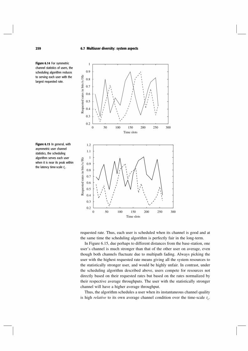
259 6.7 Multiuser diversity: system aspects
Figure 6.14 For symmetricchannel statistics of users, thescheduling algorithm reducesto serving each user with thelargest requested rate.
0 50 100 150 200 250 3000.2
0.3
0.4
0.5
0.6
0.7
0.8
0.9
1
Time slots
Req
uest
ed r
ates
in b
its /s
/ H
z
Figure 6.15 In general, withasymmetric user channelstatistics, the schedulingalgorithm serves each userwhen it is near its peak withinthe latency time-scale tc .
0 50 100 150 200 250 3000.2
0.3
0.4
0.5
0.6
0.7
0.8
0.9
1
1.1
1.2
Time slots
Req
uest
ed r
ates
in b
its / s
/ Hz
requested rate. Thus, each user is scheduled when its channel is good and atthe same time the scheduling algorithm is perfectly fair in the long-term.In Figure 6.15, due perhaps to different distances from the base-station, one
user’s channel is much stronger than that of the other user on average, eventhough both channels fluctuate due to multipath fading. Always picking theuser with the highest requested rate means giving all the system resources tothe statistically stronger user, and would be highly unfair. In contrast, underthe scheduling algorithm described above, users compete for resources notdirectly based on their requested rates but based on the rates normalized bytheir respective average throughputs. The user with the statistically strongerchannel will have a higher average throughput.Thus, the algorithm schedules a user when its instantaneous channel quality
is high relative to its own average channel condition over the time-scale tc.

260 Multiuser capacity and opportunistic communication
In short, data are transmitted to a user when its channel is near its own peaks.Multiuser diversity benefit can still be extracted because channels of differentusers fluctuate independently so that if there is a sufficient number of usersin the system, most likely there will be a user near its peak at any one time.The parameter tc is tied to the latency time-scale of the application. Peaks
are defined with respect to this time-scale. If the latency time-scale is large,then the throughput is averaged over a longer time-scale and the schedulercan afford to wait longer before scheduling a user when its channel hits areally high peak.The main theoretical property of this algorithm is the following: With a
very large tc (approaching ), the algorithm maximizes
K∑
k=1
logTk (6.57)
among all schedulers (see Exercise 6.28). Here, Tk is the long-term averagethroughput of user k.
Multiuser diversity and superposition codingProportional fair scheduling is an approach to deal with fairness among asym-metric users within the orthogonal multiple access constraint (TDMA in thecase of IS-856). But we understand from Section 6.2.2 that for the AWGNchannel, superposition coding in conjunction with SIC can yield significantlybetter performance than orthogonal multiple access in such asymmetric envi-ronments. One would expect similar gains in fading channels, and it is there-fore natural to combine the benefits of superposition coding with multiuserdiversity scheduling.One approach is to divide the users in a cell into, say, two classes depending
on whether they are near the base-station or near the cell edge, so that usersin each class have statistically comparable channel strengths. Users whosecurrent channel is instantaneously strongest in their own class are scheduledfor simultaneous transmission via superposition coding (Figure 6.16). Theuser near the base-station can decode its own signal after stripping off thesignal destined for the far-away user. By transmitting to the strongest userin each class, multiuser diversity benefits are captured. On the other hand,the nearby user has a very strong channel and the full degrees of freedomavailable (as opposed to only a fraction under orthogonal multiple access),and thus only needs to be allocated a small fraction of the power to enjoyvery good rates. Allocating a small fraction of power to the nearby userhas a salutary effect: the presence of this user will minimally affect theperformance of the cell edge user. Hence, fairness can be maintained by asuitable allocation of power. The efficiency of this approach over proportionalfair TDMA scheduling is quantified in Exercise 6.20. Exercise 6.19 showsthat this strategy is in fact optimal in achieving any point on the boundary of
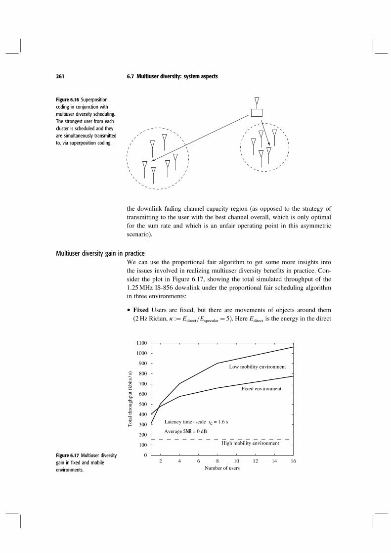
261 6.7 Multiuser diversity: system aspects
Figure 6.16 Superpositioncoding in conjunction withmultiuser diversity scheduling.The strongest user from eachcluster is scheduled and theyare simultaneously transmittedto, via superposition coding.
the downlink fading channel capacity region (as opposed to the strategy oftransmitting to the user with the best channel overall, which is only optimalfor the sum rate and which is an unfair operating point in this asymmetricscenario).
Multiuser diversity gain in practiceWe can use the proportional fair algorithm to get some more insights intothe issues involved in realizing multiuser diversity benefits in practice. Con-sider the plot in Figure 6.17, showing the total simulated throughput of the125MHz IS-856 downlink under the proportional fair scheduling algorithmin three environments:
• Fixed Users are fixed, but there are movements of objects around them(2Hz Rician, =Edirect/Especular = 5). Here Edirect is the energy in the direct
Figure 6.17 Multiuser diversitygain in fixed and mobileenvironments.
2 4 6 8 10 12 14 160
100
200
300
400
500
600
700
800
900
1000
1100
Low mobility environment
Fixed environment
Number of users
Tot
al th
roug
hput
(kb
its /
s)
High mobility environment
Latency time - scale tc = 1.6 s
Average SNR = 0 dB

262 Multiuser capacity and opportunistic communication
path that is not varying, while Especular refers to the energy in the specularor time-varying component that is assumed to be Rayleigh distributed.The Doppler spectrum of this component follows Clarke’s model with aDoppler spread of 2Hz.
• Low mobility Users move at walking speeds (3 km/hr, Rayleigh).• High mobility Users move at 30 km/hr, Rayleigh.
The average channel gain h2 is kept the same in all the three scenariosfor fairness of comparison. The total throughput increases with the numberof users in both the fixed and low mobility environments, but the increaseis more dramatic in the low mobility case. While the channel varies in bothcases, the dynamic range and the rate of the variations is larger in the mobileenvironment than in the fixed one (Figure 6.18). This means that over thelatency time-scale (tc = 167 s in these examples) the peaks of the channelfluctuations are likely to be higher in the mobile environment, and the peaksare what determines the performance of the scheduling algorithm. Thus, theinherent multiuser diversity is more limited in the fixed environment.Should one then expect an even higher throughput gain in the high mobility
environment? In fact quite the opposite is true. The total throughput hardlyincreases with the number of users! It turns out that at this speed the receiverhas trouble tracking and predicting the channel variations, so that the predictedchannel is a low-pass smoothed version of the actual fading process. Thus,even though the actual channel fluctuates, opportunistic communication isimpossible without knowing when the channel is actually good.In the next section, we will discuss how the tracking of the channel can be
improved in high mobility environments. In Section 6.7.3, we will discuss ascheme that boosts the inherent multiuser diversity in fixed environments.
6.7.2 Channel prediction and feedback
The prediction error is due to two effects: the error in measuring the channelfrom the pilot and the delay in feeding back the information to the base-station.
Figure 6.18 The channelvaries much faster and haslarger dynamic range in themobile environment.
Mobile environment
Channelstrength
Dynamicrange
Dynamicrange
Time Time
Fixed environment
Channelstrength

263 6.7 Multiuser diversity: system aspects
In the downlink, the pilot is shared between many users and is strong; so, themeasurement error is quite small and the prediction error is mainly due to thefeedback delay. In IS-856, this delay is about two time slots, i.e., 333ms. Ata vehicular speed of 30km/h and carrier frequency of 19GHz, the coherencetime is approximately 25ms; the channel coherence time is comparable tothe delay and this makes prediction difficult.One remedy to reduce the feedback delay is to shrink the size of the
scheduling time slot. However, this increases the requested rate feedbackfrequency in the uplink and thus increases the system overhead. There areways to reduce this feedback though. In the current system, every user feedsback the requested rates, but in fact only users whose channels are neartheir peaks have any chance of getting scheduled. Thus, an alternative is foreach user to feed back the requested rate only when its current requestedrate to average throughput ratio, Rkm/Tkm, exceeds a threshold . Thisthreshold, , can be chosen to trade off the average aggregate amount offeedback the users send with the probability that none of the users sends anyfeedback in a given time slot (thus wasting the slot) (Exercise 6.22).In IS-856, multiuser diversity scheduling is implemented in the downlink,
but the same concept can be applied to the uplink. However, the issues ofprediction error and feedback are different. In the uplink, the base-stationwould be measuring the channels of the users, and so a separate pilot wouldbe needed for each user. The downlink has a single pilot and this amortizationamong the users is used to have a strong pilot. However, in the uplink,the fraction of power devoted to the pilot is typically small. Thus, it is expectedthat the measurement error will play a larger role in the uplink. Moreover,the pilot will have to be sent continuously even if the user is not currentlyscheduled, thus causing some interference to other users. On the other hand,the base-station only needs to broadcast which user is scheduled at that timeslot, so the amount of feedback is much smaller than in the downlink (unlessthe selective feedback scheme is implemented).The above discussion pertains to an FDD system. You are asked to discuss
the analogous issues for a TDD system in Exercise 6.23.
6.7.3 Opportunistic beamforming using dumb antennas
The amount of multiuser diversity depends on the rate and dynamic rangeof channel fluctuations. In environments where the channel fluctuations aresmall, a natural idea comes to mind: why not amplify the multiuser diversitygain by inducing faster and larger fluctuations? Focusing on the downlink,we describe a technique that does this using multiple transmit antennas at thebase-station as illustrated in Figure 6.19.Consider a system with nt transmit antennas at the base-station. Let hlkm
be the complex channel gain from antenna l to user k in time m. In time m,the same symbol xm is transmitted from all of the antennas except that it is

264 Multiuser capacity and opportunistic communication
Figure 6.19 Same signal istransmitted over the twoantennas with time-varyingphase and powers.
User kx(t)
h1k(t)
h2k(t)
√α (t)
√1– α(t) e jθ(t)
multiplied by a complex number√lm ejlm at antenna l, for l= 1 nt ,
such that∑nt
l=1lm = 1, preserving the total transmit power. The receivedsignal at user k (see the basic downlink fading channel model in (6.50) forcomparison) is given by
ykm=(
nt∑
l=1
√lm ejlmhlkm
)
xm+wkm (6.58)
In vector form, the scheme transmits qmxm at time m, where
qm =
√1m ej1m
√nt
m ejnt m
(6.59)
is a unit vector and
ykm= hkm∗qmxm+wkm (6.60)
where hkm∗ = h1km hntkm is the channel vector from the trans-
mit antenna array to user k.The overall channel gain seen by user k is now
hkm∗qm=nt∑
l=1
√lm ejlmhlkm (6.61)
The lm denote the fractions of power allocated to each of the transmitantennas, and the lm denote the phase shifts applied at each antenna to the

265 6.7 Multiuser diversity: system aspects
Figure 6.20 Pictorialrepresentation of the slowfading channels of two usersbefore (left) and after (right)applying opportunisticbeamforming.
Transmission times
t
Channelstrength
t
User 1
User 2
Afteropportunisticbeamforming
Channelstrength
Channelstrength
t
t
Beforeopportunisticbeamforming
Channelstrength
signal. By varying these quantities over time (lm from 0 to 1 and lm
from 0 to 2) , the antennas transmit signals in a time-varying direction, andfluctuations in the overall channel can be induced even if the physical channelgains hlkm have very little fluctuation (Figure 6.20).As in the single transmit antenna system, each user k feeds back the overall
received SNR of its own channel, hkm∗qm2/N0, to the base-station (orequivalently the data rate that the channel can currently support) and thebase-station schedules transmissions to users accordingly. There is no needto measure the individual channel gains hlkm (phase or magnitude); in fact,the existence of multiple transmit antennas is completely transparent to theusers. Thus, only a single pilot signal is needed for channel measurement(as opposed to a pilot to measure each antenna gain). The pilot symbols arerepeated at each transmit antenna, exactly like the data symbols.The rate of variation of lm and lm in time (or, equivalently, of
the transmit direction qm) is a design parameter of the system. We wouldlike it to be as fast as possible to provide full channel fluctuations within thelatency time-scale of interest. On the other hand, there is a practical limitationto how fast this can be. The variation should be slow enough and shouldhappen at a time-scale that allows the channel to be reliably estimated by theusers and the SNR fed back. Further, the variation should be slow enough

266 Multiuser capacity and opportunistic communication
to ensure that the channel seen by a user does not change abruptly and thusmaintains stability of the channel tracking loop.
Slow fading: opportunistic beamformingTo get some insight into the performance of this scheme, consider the case ofslow fading where the channel gain vector of each user k remains constant,i.e., hkm= hk, for all m. (In practice, this means for all m over the latencytime-scale of interest.) The received SNR for this user would have remainedconstant if only one antenna were used. If all users in the system experiencesuch slow fading, no multiuser diversity gain can be exploited. Under theproposed scheme, on the other hand, the overall channel gain hkm∗qm foreach user k varies in time and provides opportunity for exploiting multiuserdiversity.Let us focus on a particular user k. Now if qm varies across all directions,
the amplitude squared of the channel h∗kqm2 seen by user k varies from 0
to hk2. The peak value occurs when the transmission is aligned along thedirection of the channel of user k, i.e., qm = hk/ hk (recall Example 5.2in Section 5.3). The power and phase values are then in the beamformingconfiguration:
l = hlk 2hk2
l= 1 nt
l = −arghlk l= 1 nt
To be able to beamform to a particular user, the base-station needs toknow individual channel amplitude and phase responses from all the antennas,which requires much more information to feedback than just the overall SNR.However, if there are many users in the system, the proportional fair algorithmwill schedule transmission to a user only when its overall channel SNR is nearits peak. Thus, it is plausible that in a slow fading environment, the techniquecan approach the performance of coherent beamforming but with only overallSNR feedback (Figure 6.21). In this context, the technique can be interpretedas opportunistic beamforming: by varying the phases and powers allocated tothe transmit antennas, a beam is randomly swept and at any time transmissionis scheduled to the user currently closest to the beam. With many users, thereis likely to be a user very close to the beam at any time. This intuition hasbeen formally justified (see Exercise 6.29).
Fast fading: increasing channel fluctuationsWe see that opportunistic beamforming can significantly improve perfor-mance in slow fading environments by adding fast time-scale fluctuations onthe overall channel quality. The rate of channel fluctuation is artificially spedup. Can opportunistic beamforming help if the underlying channel variationsare already fast (fast compared to the latency time-scale)?
267 6.7 Multiuser diversity: system aspects
Figure 6.21 Plot of spectralefficiency under opportunisticbeamforming as a function ofthe total number of users inthe system. The scenario is forslow Rayleigh faded channelsfor the users and the channelsare fixed in time. The spectralefficiency plotted is theperformance averaged overthe Rayleigh distribution. Asthe number of users grows,the performance approachesthe performance of truebeamforming.
0 5 10 15 20 25 30 350.8
0.9
1
1.1
1.2
1.3
1.4
1.5
Number of users
Ave
rage
thro
ughp
ut in
bits
/ s / H
zOpp. BF
Coherent BF
The long-term throughput under fast fading depends only on the stationarydistribution of the channel gains. The impact of opportunistic beamformingin the fast fading scenario then depends on how the stationary distributions ofthe overall channel gains can be modified by power and phase randomization.Intuitively, better multiuser diversity gain can be exploited if the dynamicrange of the distribution of hk can be increased, so that the maximum SNRscan be larger. We consider two examples of common fading models.
• Independent Rayleigh fading In this model, appropriate for an environ-ment where there is full scattering and the transmit antennas are spacedsufficiently, the channel gains h1km hntk
m are i.i.d. randomvariables. In this case, the channel vector hkm is isotropically distributed,and hkm∗qm is circularly symmetric Gaussian for any choice of qm;moreover the overall gains are independent across the users. Hence, thestationary statistics of the channel are identical to the original situationwith one transmit antenna. Thus, in an independent fast Rayleigh fadingenvironment, the opportunistic beamforming technique does not provideany performance gain.
• Independent Rician fading In contrast to the Rayleigh fading case, oppor-tunistic beamforming has a significant impact in a Rician environment,particularly when the -factor is large. In this case, the scheme can sig-nificantly increase the dynamic range of the fluctuations. This is becausethe fluctuations in the underlying Rician fading process come from thediffused component, while with randomization of phase and powers, thefluctuations are from the coherent addition and cancellation of the directpath components in the signals from the different transmit antennas, inaddition to the fluctuation of the diffused components. If the direct path

268 Multiuser capacity and opportunistic communication
Figure 6.22 Total throughputas a function of the number ofusers under Rician fast fading,with and without opportunisticbeamforming. The powerallocations l m areuniformly distributed in 0 1and the phases l m uniformin 0 2.
0 5 10 15 20 25 30 350.8
1
1.2
1.4
1.6
1.8
2
2.2
2.4
2.6
Number of users
Ave
rage
thro
ughp
ut in
bits
/s / H
z
1 antenna, Rician
2 antenna, Rician, Opp. BF
Rayleigh
is much stronger than the diffused part (large values), then much largerfluctuations can be created with this technique.This intuition is substantiated in Figure 6.22, which plots the total
throughput with the proportional fair algorithm (large tc, of the order of 100time slots) for Rician fading with = 10. We see that there is a considerableimprovement in performance going from the single transmit antenna caseto dual transmit antennas with opportunistic beamforming. For comparison,we also plot the analogous curves for pure Rayleigh fading; as expected,there is no improvement in performance in this case. Figure 6.23 comparesthe stationary distributions of the overall channel gain hkm∗qm in thesingle-antenna and dual-antenna cases; one can see the increase in dynamicrange due to opportunistic beamforming.
Antennas: dumb, smart and smarterIn this section so far, our discussion has focused on the use of multipletransmit antennas to induce larger and faster channel fluctuations for multiuserdiversity benefits. It is insightful to compare this with the two other point-to-point transmit antenna techniques we have already discussed earlier in thebook:
• Space-time codes like the Alamouti scheme (Section 3.3.2). They areprimarily used to increase the diversity in slow fading point-to-point links.
• Transmit beamforming (Section 5.3.2). In addition to providing diversity,a power gain is also obtained through the coherent addition of signals atthe users.

269 6.7 Multiuser diversity: system aspects
Figure 6.23 Comparison of thedistribution of the overallchannel gain with and withoutopportunistic beamformingusing two transmit antennas,Rician fading. The Rayleighdistribution is also shown.
0 0.5 1 1.5 2 2.5 30
0.2
0.4
0.6
0.8
1.0
1.2
1.4
1.6
1.8
2.0
Rayleigh
2 antenna, Rician
1 antenna, Rician
Channel amplitude
Den
sity
The three techniques have different system requirements. Coherent space-time codes like the Alamouti scheme require the users to track all the indi-vidual channel gains (amplitude and phase) from the transmit antennas. Thisrequires separate pilot symbols on each of the transmit antennas. Transmitbeamforming has an even stronger requirement that the channel should beknown at the transmitter. In an FDD system, this means feedback of theindividual channel gains (amplitude and phase). In contrast to these two tech-niques, the opportunistic beamforming scheme requires no knowledge of theindividual channel gains, neither at the users nor at the transmitter. In fact,the users are completely ignorant of the fact that there are multiple transmitantennas and the receiver is identical to that in the single transmit antennacase. Thus, they can be termed dumb antennas. Opportunistic beamformingdoes rely on multiuser diversity scheduling, which requires the feedback ofthe overall SNR of each user. However, this only needs a single pilot tomeasure the overall channel.What is the performance of these techniques when used in the downlink?
In a slow fading environment, we have already remarked that opportunisticbeamforming approaches the performance of transmit beamforming whenthere are many users in the system. On the other hand, space-time codes donot perform as well as transmit beamforming since they do not capture thearray power gain. This means, for example, using the Alamouti scheme ondual transmit antennas in the downlink is 3 dB worse than using opportunisticbeamforming combined with multiuser diversity scheduling when there aremany users in the system. Thus, dumb antennas together with smart schedulingcan surpass the performance of smart space-time codes and approach that ofthe even smarter transmit beamforming.

270 Multiuser capacity and opportunistic communication
Table 6.1 A comparison between three methods of using transmit antennas.
Dumb antennas(Opp. beamform)
Smart antennas(Space-time codes)
Smarter antennas(Transmitbeamform)
Channel knowledge Overall SNR Entire CSI at Rx Entire CSI at Rx, Tx
Slow fadingperformance gain
Diversity andpower gains Diversity gain only
Diversity and powergains
Fast fadingperformance gain No impact Multiuser diversity ↓
Multiuser diversity ↓power ↑
How about in a fast Rayleigh fading environment? In this case, we haveobserved that dumb antennas have no effect on the overall channel as the fullmultiuser diversity gain has already been realized. Space-time codes, on theother hand, increase the diversity of the point-to-point links and consequentlydecrease the channel fluctuations and hence the multiuser diversity gain.(Exercise 6.31 makes this more precise.) Thus, the use of space-time codesas a point-to-point technology in a multiuser downlink with rate control andscheduling can actually be harmful, in the sense that even the naturally presentmultiuser diversity is removed. The performance impact of using transmitbeamforming is not so clear: on the one hand it reduces the channel fluctuationand hence the multiuser diversity gain, but on the other hand it provides anarray power gain. However, in an FDD system the fast fading channel maymake it very difficult to feed back so much information to enable coherentbeamforming.The comparison between the three schemes is summarized in Table 6.1.
All three techniques use the multiple antennas to transmit to only one userat a time. With full channel knowledge at the transmitter, an even smarterscheme can transmit to multiple users simultaneously, exploiting the multipledegrees of freedom existing inherently in the multiple antenna channel. Wewill discuss this in Chapter 10.
6.7.4 Multiuser diversity in multicell systems
So far we have considered a single-cell scenario, where the noise is assumedto be white Gaussian. For wideband cellular systems with full frequency reuse(such as the CDMA and OFDM based systems in Chapter 4), it is importantto consider the effect of inter-cell interference on the performance of thesystem, particularly in interference-limited scenarios. In a cellular system, thiseffect is captured by measuring the channel quality of a user by the SINR,signal-to-interference-plus-noise ratio. In a fading environment, the energiesin both the received signal and the received interference fluctuate over time.Since the multiuser diversity scheduling algorithm allocates resources based

271 6.7 Multiuser diversity: system aspects
on the channel SINR (which depends on both the channel amplitude and theamplitude of the interference), it automatically exploits both the fluctuationsin the energy of the received signal and those of the interference: the algorithmtries to schedule resource to a user whose instantaneous channel is good andthe interference is weak. Thus, multiuser diversity naturally takes advantageof the time-varying interference to increase the spatial reuse of the network.From this point of view, amplitude and phase randomization at the base-
station transmit antennas plays an additional role: it increases not only theamount of fluctuations of the received signal to the intended users withinthe cells, it also increases the fluctuations of the interference that the base-station causes in adjacent cells. Hence, opportunistic beamforming has a dualbenefit in an interference-limited cellular system. In fact, opportunistic beam-forming performs opportunistic nulling simultaneously: while randomizationof amplitude and phase in the transmitted signals from the antennas allowsnear coherent beamforming to some user within the cell, it will create nearnulls at some other user in an adjacent cell. This in effect allows interferenceavoidance for that user if it is currently being scheduled.Let us focus on the downlink and slow flat fading scenario to get
some insight into the performance gain from opportunistic beamforming andnulling. Under amplitude and phase randomization at all base-stations, thereceived signal of a typical user that is interfered by J adjacent base-stationsis given by
ym= h∗qmxm+J∑
j=1
g∗jqjmujm+ zm (6.62)
Here, xmhqm are respectively the signal, channel vector and ran-dom transmit direction from the base-station of interest; ujmgjqjm arerespectively the interfering signal, channel vector and random transmit direc-tion from the jth base-station. All base-stations have the same transmit power,P, and nt transmit antennas and are performing amplitude and phase random-ization independently.By averaging over the signal xm and the interference ujm, the (time-
varying) SINR of the user k can be computed to be
SINRkm= Ph∗qm2P∑J
j=1 g∗jqjm2+N0
(6.63)
As the random transmit directions qmqjm vary, the overall SINRchanges over time. This is due to the variations of the overall gain from thebase-station of interest as well as those from the interfering base-stations. TheSINR is high when qm is closely aligned to the channel vector h, and/orfor many j, qjm is nearly orthogonal to gj , i.e., the user is near a nullof the interference pattern from the jth base-station. In a system with manyother users, the proportional fair scheduler will serve this user while its SINR

272 Multiuser capacity and opportunistic communication
is at its peak P h 2/N0, i.e., when the received signal is the strongest andthe interference is completely nulled out. Thus, the opportunistic nulling andbeamforming technique has the potential of shifting a user from a low SINR,interference-limited regime to a high SINR, noise-limited regime. An analysisof the tail of the distribution of SINR is conducted in Exercise 6.30.
6.7.5 A system view
A new design principle for wireless systems can now be seen through the lensof multiuser diversity. In the three systems in Chapter 4, many of the designtechniques centered on making the individual point-to-point links as close toAWGN channels as possible, with a reliable channel quality that is constantover time. This is accomplished by channel averaging, and includes the useof diversity techniques such as multipath combining, time-interleaving andantenna diversity that attempt to keep the channel fading constant in time, aswell as interference management techniques such as interference averagingby means of spreading.However, if one shifts from the view of the wireless system as a set of
point-to-point links to the view of a system with multiple users sharing thesame resources (spectrum and time), then quite a different design objectivesuggests itself. Indeed, the results in this chapter suggest that one shouldinstead try to exploit the channel fluctuations. This is done through an appro-priate scheduling algorithm that “rides the peaks”, i.e., each user is scheduledwhen it has a very strong channel, while taking into account real world trafficconstraints such as delay and fairness. The technique of dumb antennas goesone step further by creating variations when there are none. This is accom-plished by varying the strengths of both the signal and the interference thata user receives through opportunistic beamforming and nulling.The viability of the opportunistic communication scheme depends on traffic
that has some tolerance to scheduling delays. On the other hand, there aresome forms of traffic that are not so flexible. The functioning of the wirelesssystems is supported by the overhead control channels, which are “circuit-switched” and hence have very tight latency requirements, unlike data, whichhave the flexibility to allow dynamic scheduling. From the perspective ofthese signals, it is preferable that the channel remain unfaded; a requirementthat is contradictory to our scheduler-oriented observation that we wouldprefer the channel to have fast and large variations.This issue suggests the following design perspective: separate very-low
latency signals (such as control signals) from flexible latency data. One wayto achieve this separation is to split the bandwidth into two parts. One partis made as flat as possible (by using the principles we saw in Chapter 4such as spreading over this part of the bandwidth) and is used to transmitflows with very low latency requirements. The performance metric here is tomake the channel as reliable as possible (equivalently keeping the probability
273 6.7 Multiuser diversity: system aspects
of outage low) for some fixed data rate. The second part uses opportunisticbeamforming to induce large and fast channel fluctuations and a scheduler toharness the multiuser diversity gains. The performance metric on this part isto maximize the multiuser diversity gain.The gains of the opportunistic beamforming and nulling depend on the
probability that the received signal is near beamformed and all the interfer-ence is near null. In the interference-limited regime and when P/N0 1,the performance depends mainly on the probability of the latter event (seeExercise 6.30). In the downlink, this probability is large since there are onlyone or two base-stations contributing most of the interference. The uplinkposes a contrasting picture: there is interference from many mobiles allowinginterference averaging. Now the probability that the total interference is nearnull is much smaller. Interference averaging, which is one of the principledesign features of the wideband full reuse systems (such as the ones we sawin Chapter 4 based on CDMA and OFDM), is actually unfavorable for theopportunistic scheme described here, since it reduces the likelihood of thenulling of the interference and hence the likelihood of the peaks of the SINR.In a typical cell, there will be a distribution of users, some closer to
the base-station and some closer to the cell boundaries. Users close to thebase-station are at high SINR and are noise-limited; the contribution of theinter-cell interference is relatively small. These users benefit mainly fromopportunistic beamforming. Users close to the cell boundaries, on the otherhand, are at low SINR and are interference-limited; the average interferencepower can be much larger than the background noise. These users benefit bothfrom opportunistic beamforming and from opportunistic nulling of inter-cellinterference. Thus, the cell edge users benefit more in this system than usersin the interior. This is rather desirable from a system fairness point-of-view,as the cell edge users tend to have poorer service. This feature is particularlyimportant for a system without soft handoff (which is difficult to implementin a packet data scheduling system). To maximize the opportunistic nullingbenefits, the transmit power at the base-station should be set as large aspossible, subject to regulatory and hardware constraints. (See Exercise 6.30(5)where this is explored in more detail.)We have seen the multiuser diversity as primarily a form of power gain. The
opportunistic beamforming technique of using an array of multiple transmitantennas has approximately an nt-fold improvement in received SNR to a userin a slow fading environment, as compared to the single-antenna case. Withan array of nr receive antennas at each mobile (and say a single transmitantenna at the base-station), the received SNR of any user gets an nr-foldimprovement as compared to a single receive antenna; this gain is realized byreceiver beamforming. This operation is easy to accomplish since the mobilehas full channel information at each of the antenna elements. Hence the gainsof opportunistic beamforming are about the same order as that of installing areceive antenna array at each of the mobiles.
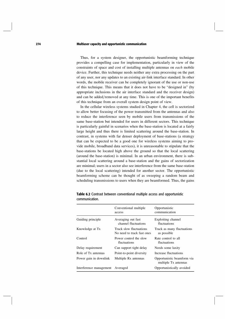
274 Multiuser capacity and opportunistic communication
Thus, for a system designer, the opportunistic beamforming techniqueprovides a compelling case for implementation, particularly in view of theconstraints of space and cost of installing multiple antennas on each mobiledevice. Further, this technique needs neither any extra processing on the partof any user, nor any updates to an existing air-link interface standard. In otherwords, the mobile receiver can be completely ignorant of the use or non-useof this technique. This means that it does not have to be “designed in” (byappropriate inclusions in the air interface standard and the receiver design)and can be added/removed at any time. This is one of the important benefitsof this technique from an overall system design point of view.In the cellular wireless systems studied in Chapter 4, the cell is sectorized
to allow better focusing of the power transmitted from the antennas and alsoto reduce the interference seen by mobile users from transmissions of thesame base-station but intended for users in different sectors. This techniqueis particularly gainful in scenarios when the base-station is located at a fairlylarge height and thus there is limited scattering around the base-station. Incontrast, in systems with far denser deployment of base-stations (a strategythat can be expected to be a good one for wireless systems aiming to pro-vide mobile, broadband data services), it is unreasonable to stipulate that thebase-stations be located high above the ground so that the local scattering(around the base-station) is minimal. In an urban environment, there is sub-stantial local scattering around a base-station and the gains of sectorizationare minimal; users in a sector also see interference from the same base-station(due to the local scattering) intended for another sector. The opportunisticbeamforming scheme can be thought of as sweeping a random beam andscheduling transmissions to users when they are beamformed. Thus, the gains
Table 6.2 Contrast between conventional multiple access and opportunisticcommunication.
Conventional multipleaccess
Opportunisticcommunication
Guiding principle Averaging out fastchannel fluctuations
Exploiting channelfluctuations
Knowledge at Tx Track slow fluctuationsNo need to track fast ones
Track as many fluctuationsas possible
Control Power control the slowfluctuations
Rate control to allfluctuations
Delay requirement Can support tight delay Needs some laxity
Role of Tx antennas Point-to-point diversity Increase fluctuations
Power gain in downlink Multiple Rx antennas Opportunistic beamform viamultiple Tx antennas
Interference management Averaged Opportunistically avoided

275 6.7 Multiuser diversity: system aspects
of sectorization are automatically realized. We conclude that the opportunistic
beamforming technique is particularly suited to harness sectorization gains
even in low-height base-stations with plenty of local scattering. In a cel-
lular system, the opportunistic beamforming scheme also obtains the gains
of nulling, a gain traditionally obtained by coordinated transmissions from
neighboring base-stations in a full frequency reuse system or by appropriately
designing the frequency reuse pattern.
The discussion is summarized in Table 6.2.
Chapter 6 The main plot
This chapter looked at the capacities of uplink and downlink channels.Two important sets of concepts emerged:• successive interference cancellation (SIC) and superposition coding;• multiuser opportunistic communication and multiuser diversity.
SIC and superposition codingUplink
Capacity is achieved by allowing users to simultaneously transmit on thefull bandwidth and the use of SIC to decode the users.
SIC has a significant performance gain over conventional multiple accesstechniques in near–far situations. It takes advantage of the strong channelof the nearby user to give it high rate while providing the weak user withthe best possible performance.
Downlink
Capacity is achieved by superimposing users’ signals and the use of SICat the receivers. The strong user decodes the weak user’s signal first andthen decodes its own.
Superposition coding/SIC has a significant gain over orthogonal tech-niques. Only a small amount of power has to be allocated to the stronguser to give it a high rate, while delivering near-optimal performance tothe weak user.
Opportunistic communicationSymmetric uplink fading channel:
ym=K∑
k=1
hkmxkm+wm (6.64)

276 Multiuser capacity and opportunistic communication
Sum capacity with CSI at receiver only:
Csum =
[
log(
1+∑K
k=1 hk2PN0
)]
(6.65)
Very close to AWGN capacity for large number of users. Orthogonalmultiple access is strictly suboptimal.
Sum capacity with full CSI:
Csum =
[
log(
1+ Pk∗hhk∗ 2N0
)]
(6.66)
where k∗ is the user with the strongest channel at joint channel state h.This is achieved by transmitting only to the user with the best channel anda waterfilling power allocation Pk∗h over the fading state.Symmetric downlink fading channel:
ykm= hkmxm+wkm k= 1 K (6.67)
Sum capacity with CSI at receiver only:
Csum =
[
log(
1+ hk2PN0
)]
(6.68)
Can be achieved by orthogonal multiple access.Sum capacity with full CSI: same as uplink.
Multiuser diversityMultiuser diversity gain: under full CSI, capacity increases with the numberof users: in a large system with high probability there is always a userwith a very strong channel.System issues in implementing multiuser diversity:• Fairness Fair access to the channel when some users are statisticallystronger than others.
• Delay Cannot wait too long for a good channel.• Channel tracking Channel has to be measured and fed back fast enough.• Small and slow channel fluctuationsMultiuser diversity gain is limitedwhen channel varies too slowly and/or has a small dynamic range.
The solutions discussed were:• Proportional fair scheduler transmits to a user when its channel is nearits peak within the delay constraint. Every user has access to the channelfor roughly the same amount of time.
• Channel feedback delay can be reduced by having shorter time slots andfeeding back more often. Aggregate feedback can be reduced by eachuser selectively feeding channel state back only when its channel is nearits peak.

277 6.8 Bibliographical notes
• Channel fluctuations can be sped up and their dynamic range increasedby the use of multiple transmit antennas to perform opportunistic beam-forming. The scheme sweeps a random beam and schedules transmis-sions to users when they are beamformed.
In a cellular system, multiuser diversity scheduling performs interferenceavoidance as well: a user is scheduled transmission when its channel isstrong and the out-of-cell interference is weak.
Multiple transmit antennas can perform opportunistic beamforming as wellas nulling.
6.8 Bibliographical notes
Classical treatment of the general multiple access channel was initiated by Ahlswede[2] and Liao [73] who characterized the capacity region. The capacity region of theGaussian multiple access channel is derived as a special case. A good survey ofthe literature on MACs was done by Gallager [45]. Hui [59] first observed that thesum capacity of the uplink channel with single-user decoding is bounded by 1.442bits/s/Hz.
The general broadcast channel was introduced by Cover [25] and a completecharacterization of its capacity is one of the famous open problems in informationtheory. Degraded broadcast channels, where the users can be “ordered” based on theirchannel quality, are fully understood with superposition coding being the optimalstrategy; a textbook reference is Chapter 14.6 in Cover and Thomas [26]. The bestinner and outer bounds are by Marton [81] and a good survey of the literatureappears in [24].
The capacity region of the uplink fading channel with receiver CSI was derivedby Gallager [44], where he also showed that orthogonal multiple access schemesare strictly suboptimal in fading channels. Knopp and Humblet [65] studied the sumcapacity of the uplink fading channel with full CSI. They noted that transmitting toonly one user is the optimal strategy. An analogous result was obtained earlier byCheng and Verdú [20] in the context of the time-invariant uplink frequency-selectivechannels. Both these channels are instances of the parallel Gaussian multiple accesschannel, so the two results are mathematically equivalent. The latter authors alsoderived the capacity region in the two-user case. The solution for arbitrary number ofusers was obtained by Tse and Hanly [122], exploiting a basic polymatroid propertyof the region.
The study of downlink fading channels with full CSI was carried out by Tse [124]and Li and Goldsmith [74]. The key aspect of the study was to observe that the fadingdownlink is really a parallel degraded broadcast channel, the capacity of which hasbeen fully understood (El Gamal [33]). There is an intriguing similarity between thedownlink resource allocation solution and the uplink one. This connection is studiedfurther in Chapter 10.
Multiuser diversity is a key distinguishing feature of the uplink and the downlinkfading channel study as compared to our understanding of the point-to-point fading

278 Multiuser capacity and opportunistic communication
channel. The term multiuser diversity was coined by Knopp and Humblet [66]. Themultiuser diversity concept was integrated into the downlink design of IS-856 (CDMA2000 EV-DO) via the proportional fair scheduler by Tse [19]. In realistic scenarios,performance gains of 50% to 100% have been reported (Wu and Esteves [149]).
If the channels are slowly varying, then the multiuser diversity gains are lim-ited. The opportunistic beamforming idea mitigates this defect by creating variationswhile maintaining the same average channel quality; this was proposed by Viswanathet al. [137], who also studied its impact on system design.
Several works have studied the design of schedulers that harness the multiuserdiversity gain. A theoretical analysis of the proportional fair scheduler has appearedin several places including a work by Borst and Whiting [12].
6.9 Exercises
Exercise 6.1 The sum constraint in (6.6) applies because the two users send inde-pendent information and cannot cooperate in the encoding. If they could cooperate,what is the maximum sum rate they could achieve, still assuming individual powerconstraints P1 and P2 on the two users? In the case P1 = P2, quantify the cooperationgain at low and at high SNR. In which regime is the gain more significant?
Exercise 6.2 Consider the basic uplink AWGN channel in (6.1) with power constraintsPk on user k (for k= 12). In Section 6.1.3, we stated that orthogonal multiple accessis optimal when the degrees of freedom are split in direct proportion to the powers ofthe users. Verify this. Show also that any other split of degrees of freedom is strictlysuboptimal, i.e., the corresponding rate pair lies strictly inside the capacity regiongiven by the pentagon in Figure 6.2. Hint: Think of the sum rate as the performanceof a point-to-point channel and apply the insight from Exercise 5.6.
Exercise 6.3 Calculate the symmetric capacity, (6.2), for the two-user uplink channel.Identify scenarios where there are definitely superior operating points.
Exercise 6.4 Consider the uplink of a single IS-95 cell where all the users are controlledto have the same received power P at the base-station.1. In the IS-95 system, decoding is done by a conventional CDMA receiver which
treats the interference of the other users as Gaussian noise. What is the maximumnumber of voice users that can be accommodated, assuming capacity-achievingpoint-to-point codes? You can assume a total bandwidth of 1.25MHz and a datarate per user of 9.6 kbits/s. You can also assume that the background noise isnegligible compared to the intra-cell interference.
2. Now suppose one of the users is a data user and it happens to be close to thebase-station. By not controlling its power, its received power can be 20 dB abovethe rest. Propose a receiver that can give this user a higher rate while still delivering9.6 kbits/s to the other (voice) users. What rate can it get?
Exercise 6.5 Consider the uplink of an IS-95 system.1. A single cell is modeled as a disk of radius 1 km. If a mobile at the edge of the
cell transmits at its maximum power limit, its received SNR at the base-stationis 15 dB when no one else is transmitting. Estimate (via numerical simulations)

279 6.9 Exercises
the average sum capacity of the uplink with 16 users that are independently anduniformly located in the disk. Compare this to the corresponding average totalthroughput in a system with conventional CDMA decoding and each user perfectlypower controlled at the base-station. What is the potential percentage gain inspectral efficiency by using the more sophisticated receiver? You can assume thatall mobiles have the same transmit power constraint and the path loss (power)attenuation is proportional to r−4.
2. Part (1) ignores out-of-cell interference. With out-of-cell interference taken intoconsideration, the received SINR of the cell edge user is only−10dB. Redo part (1).Is the potential gain from using a more sophisticated receiver still as impressive?
Exercise 6.6 Consider the downlink of the IS-856 system.1. Suppose there are two users on the cell edge. Users are scheduled on a TDMA
basis, with equal time for each user. The received SINR of each user is 0 dB when itis transmitted to. Find the rate that each user gets. The total bandwidth is 1.25MHzand you can assume an AWGN channel and the use of capacity-achieving codes.
2. Now suppose there is an extra user which is near the base-station with a 20 dB SINRadvantage over the other two users. Consider two ways to accommodate this user:• Give a fraction of the time slots to this user and divide the rest equally among
the two cell edge users.• Give a fraction of the power to this user and superimpose its signal on top
of the signals of both users. The two cell edge users are still scheduled on aTDMA basis with equal time, and the strong user uses a SIC decoder to extractits signal after decoding the other users’ signals at each time slot.
Since the two cell edge users have weak reception, it is important to maintain thebest possible quality of service to them. So suppose the constraint is that we wanteach of them to have 95% of the rates they were getting before this strong userjoined. Compare the performance that the strong user gets in the two schemes above.
Exercise 6.7 The capacity region of the two-user AWGN uplink channel is shownin Figure 6.2. The two corner points A and B can be achieved using successivecancellation. Points inside the line segment AB can be achieved by time sharing. Inthis exercise we will see another way to achieve every point R1R2 on the linesegment AB using successive cancellation. By definition we must have
Rk < log(
1+ Pk
N0
)
k= 12 (6.69)
R1+R2 = log(
1+ P1+P2
N0
)
(6.70)
Define > 0 by
R2 = log(
1+ P2
+N0
)
(6.71)
Now consider the situation when user 1 splits itself into two users, say users 1a and 1b,with power constraints P1− and respectively. We decode the users with successivecancellation in the order user 1a, 2, 1b, i.e., user 1a is decoded first, user 2 is decodednext (with user 1a cancelled) and finally user 1b is decoded (seeing no interferencefrom users 1a and 2).

280 Multiuser capacity and opportunistic communication
1. Calculate the rates of reliable communication r1a r2 r1b for the users 1a, 2 and1b using the successive cancellation just outlined.
2. Show that r2 = R2 and r1a + r1b = R1. This means that the point R1R2 on theline segment AB can be achieved by successive cancellation of three users formedby one of the users “splitting” itself into two virtual users.
Exercise 6.8 In Exercise 6.7, we studied rate splitting multiple access for two users.A reading exercise is to study [101], where this result was introduced and generalizedto the K-user uplink: K− 1 users can split themselves into two users each (withappropriate power splits) so that any rate vector on the boundary of the capacity regionthat meets the sum power constraint can be achieved via successive cancellation (withappropriate ordering of the 2K−1 users).
Exercise 6.9 Consider the K-user AWGN uplink channel with user power constraintsP1 PK . The capacity region is the set of rate vectors that lie in the intersectionof the constraints (cf. (6.10)):
∑
k∈Rk < log
(
1+∑
k∈ Pk
N0
)
(6.72)
for every subset of the K users.1. Fix an ordering of the users 1 K (here represents a permutation of set
1 K). Show that the rate vector(R
1 R
K
):
Rk
= log
(
1+ Pk∑Ki=k+1 Pi
+N0
)
k= 1 K (6.73)
is in the capacity region. This rate vector can be interpreted using the successivecancellation viewpoint: the users are successively decoded in the order 1 K
with cancellation after each decoding step. So, user k has no interference fromthe previously decoded users 1 k−1, but experiences interference from theusers following it (namely k+1 K). In Figure 6.2, the point A correspondsto the permutation 1 = 22 = 1 and the point B corresponds to the identitypermutation 1 = 12 = 2.
2. Consider maximizing the linear objective function∑K
k=1 akRk with non-negativea1 aK over the rate vectors in the capacity region. (ak can be interpreted asthe revenue per unit rate for user k.) Show that the maximum occurs at the ratevector of the form in (6.73) with the permutation defined by the property:
a1≤ a2
≤ · · · ≤ aK (6.74)
This means that optimizing linear objective functions on the capacity region can bedone in a greedy way: we order the users based on their priority (ak for user k). Thisordering is denoted by the permutation in (6.74). Next, the receiver decodes viasuccessive cancellation using this order: the user with the least priority is decodedfirst (seeing full interference from all the other users) and the user with the highestpriority decoded last (seeing no interference from the other users). Hint: Showthat if the ordering is not according to (6.74), then one can always improve theobjective function by changing the decoding order.

281 6.9 Exercises
3. Since the capacity region is the intersection of hyperplanes, it is a convex polyhe-dron. An equivalent representation of a convex polyhedron is through enumeratingits vertices: points which cannot be expressed as a strict convex combination of anysubset of other points in the polyhedron. Show that
(R
1 R
K
)is a vertex
of the capacity region. Hint: Consider the following fact: a linear object functionis maximized on a convex polyhedron at one of the vertices. Further, every vertexmust be optimal for some linear objective function.
4. Show that vertices of the form (6.73) (one for each permutation, so there are K! ofthem) are the only interesting vertices of the capacity region. (This means that anyother vertex of the capacity region is component-wise dominated by one of theseK! vertices.)
Exercise 6.10 Consider the K-user uplink AWGN channel. In the text, we focuson the capacity region P: the set of achievable rates for given power constraintvector P = P1 PK
t. A “dual” characterization is the power region R: setof all feasible received power vectors that can support a given target rate vectorR = R1 RK
t.1. Write down the constraints describing R. Sketch the region for K = 2.2. What are the vertices of R?3. Find a decoding strategy and a power allocation that minimizes
∑Kk=1 bkPk while
meeting the given target rates. Here, the constants bk are positive and should beinterpreted as “power prices”. Hint: Exercise 6.9 may be useful.
4. Suppose users are at different distances from the base-station so that the transmitpower of user k is attenuated by a factor of i. Find a decoding strategy and apower allocation that minimizes the total transmit power of the users while meetingthe target rates R.
5. In IS-95, the code used by each user is not necessarily capacity-achieving butcommunication is considered reliable as long as a b/I0 requirement of 7 dB is met.Suppose these codes are used in conjunction with SIC. Find the optimal decodingorder to minimize the total transmit power in the uplink.
Exercise 6.11 (Impact of using SIC on interference-limited capacity) Consider the two-cell system in Exercise 4.11. The interference-limited spectral efficiency in the many-user regime was calculated for both CDMA and OFDM. Now suppose SIC is usedinstead of the conventional receiver in the CDMA system. In the context of SIC, theinterference I0 in the target b/I0 requirement refers to the interference from the uncan-celled users. Below you can always assume that interference cancellation is perfect.1. Focus on a single cell first and assume a background noise power of N0. Is the
system interference-limited under the SIC receiver? Was it interference-limitedunder the conventional CDMA receiver?
2. Suppose there are K users with user k at a distance rk from the base-station. Givean expression for the total transmit power saving (in dB) in using SIC with theoptimal decoding order as compared to the conventional CDMA receiver (with anb/I0 requirement of ).
3. Give an expression for the power saving in the asymptotic regime with a largenumber of users and large bandwidth. The users are randomly located in the singlecell as specified in Exercise 4.11. What is this value when = 7dB and the powerdecay is r−2 (i.e., = 2)?
282 Multiuser capacity and opportunistic communication
4. Now consider the two-cell system. Explain why in this case the system isinterference-limited even when using SIC.
5. Nevertheless, SIC increases the interference-limited capacity because of the reduc-tion in transmit power, which translates into a reduction of out-of-cell interference.Give an expression for the asymptotic interference-limited spectral efficiency underSIC in terms of and . You can ignore the background noise and assumethat users closer to the base-station are always decoded before the users furtheraway.
6. For = 7dB and = 2, compare the performance with the conventional CDMAsystem and the OFDM system.
7. Is the cancellation order in part 5 optimal? If not, find the optimal order and givean expression for the resulting asymptotic spectral efficiency. Hint: You might findExercise 6.10 useful.
Exercise 6.12 Verify the bound (6.30) on the actual error probability of the kth userin the SIC, accounting for error propagation.
Exercise 6.13 Consider the two-user uplink fading channel,
ym= h1mx1m+h2mx2m+wm (6.75)
Here the user channels h1m h2m are statistically independent. Suppose thath1m and h2m are 01 and user k has power Pk k = 12, with P1 P2.The background noise wm is i.i.d. 0N0. An SIC receiver decodes user 1 first,removes its contribution from ym and then decodes user 2. We would like to assessthe effect of channel estimation error of h1 on the performance of user 2.1. Assuming that the channel coherence time is Tc seconds and user 1 spends 20% of
its power on sending a training signal, what is the mean square estimation error ofh1? You can assume the same setup as in Section 3.5.2. You can ignore the effectof user 2 in this estimation stage, since P1 P2.
2. The SIC receiver decodes the transmitted signal from user 1 and subtracts itscontribution from ym. Assuming that the information is decoded correctly, theresidual error is due to the channel estimation error of h1. Quantify the degradationin SINR of user 2 due to this channel estimation error. Plot this degradation as afunction of P1/N0 for Tc = 10ms. Does the degradation worsen if the power P1 ofuser 1 increases? Explain.
3. In part (2), user 2 still faced some interference due to the presence of user 1despite decoding the information meant for user 1 accurately. This is due to theerror in the channel estimate of user 1. In the calculation in part (2), we used theexpression for the error of user 1’s channel estimate as derived from the trainingsymbol. However, conditioned on the event that the first user’s information hasbeen correctly decoded, the channel estimate of user 1 can be improved. Modelthis situation appropriately and arrive at an approximation of the error in user 1’schannel estimate. Now redo part (2). Does your answer change qualitatively?
Exercise 6.14 Consider the probability of the outage event (pulout , cf. (6.32)) in a
symmetric slow Rayleigh fading uplink with the K users operating at the symmetricrate R bits/s/Hz.

283 6.9 Exercises
1. Suppose pulout is fixed to be . Argue that at very high SNR (with SNR defined to
be P/N0), the dominating event is the one on the sum rate:
KR> log(
1+∑K
k=1 Phk2N0
)
2. Show that the -outage symmetric capacity, Csym , can be approximated at very
high SNR as
Csym ≈ 1
Klog2
(
1+ P1K
N0
)
3. Argue that at very high SNR, the ratio of Csym to C (the -outage capacity with
just a single user in the uplink) is approximately 1/K.
Exercise 6.15 In Section 6.3.3, we have discussed the optimal multiple access strategyfor achieving the sum capacity of the uplink fading channel when users have identicalchannel statistics and power constraints.1. Solve the problem for the general case when the channel statistics and the power
constraints of the users are arbitrary. Hint: Construct a Lagrangian for the convexoptimization problem (6.42) with a separate Lagrange multiplier for each of theindividual power constraints (6.43).
2. Do you think the sum capacity is a reasonable performance measure in the asym-metric case?
Exercise 6.16 In Section 6.3.3, we have derived the optimal power allocation with fullCSI in the symmetric uplink with the assumption that there is always a unique userwith the strongest channel at any one time. This assumption holds with probability 1when the fading distributions are continuous. Moreover, under this assumption, thesolution is unique. This is in contrast to the uplink AWGN channel where there isa continuum of solutions that achieves the optimal sum rate, of which only one isorthogonal. We will see in this exercise that transmitting to only one user at a timeis not necessarily the unique optimal solution even for fading channels, if the fadingdistribution is discrete (to model measurement realities, such as the feedback of afinite number of rate levels).
Consider the full CSI two-user uplink with identical, independent, stationary andergodic flat fading processes for the two users. The stationary distribution of the flatfading for both of the users takes one of just two values: channel amplitude is eitherat 0 or at 1 (with equal probability). Both of the users are individually average powerconstrained (by P). Calculate explicitly all the optimal joint power allocation anddecoding policies to maximize the sum rate. Is the optimal solution unique? Hint:Clearly there is no benefit by allocating power to a user whose channel is fully faded(the zero amplitude state).
Exercise 6.17 In this exercise we further study the nature of the optimal power andrate control strategy that achieves the sum capacity of the symmetric uplink fadingchannel.

284 Multiuser capacity and opportunistic communication
1. Show that the optimal power/rate allocation policy for achieving the sum capacityof the symmetric uplink fading channel can be obtained by solving for each fadingstate the optimization problem:
maxrp
K∑
k=1
rk−K∑
k=1
pk (6.76)
subject to the constraint that
r ∈ ph (6.77)
where ph is the uplink AWGN channel capacity region with received powerpkhk2. Here is chosen to meet the average power constraint of P for each user.
2. What happens when the channels are not symmetric but we are still interested inthe sum rate?
Exercise 6.18 [122] In the text, we focused on computing the power/rate allocationpolicy that maximizes the sum rate. More generally, we can look for the policy thatmaximizes a weighted sum of rates
∑k kRk. Since the uplink fading channel capacity
region is convex, solving this for all non-negative i will enable us to characterizethe entire capacity region (as opposed to just the sum capacity point).
In analogy with Exercise 6.17, it can be shown that the optimal power/rate allocationpolicy can be computed by solving for each fading state h the optimization problem:
maxrp
K∑
k=1
krk−K∑
k=1
kpk (6.78)
subject to the constraint that
r ∈ ph (6.79)
where the k are chosen to meet the average power constraints Pk of the users (averagedover the fading distribution). If we define qk = pkhk2 as the received power, thenwe can rewrite the optimization problem as
maxrq
K∑
k=1
krk−K∑
k=1
k
hk2pk (6.80)
subject to the constraint that
r ∈ q (6.81)
where q is the uplink AWGN channel capacity region. You are asked to solve thisoptimization problem in several steps below.1. Verify that the capacity of a point-to-point AWGN channel can be written in the
integral form:
Cawgn = log(
1+ P
N0
)
=∫ P
0
1N0+ z
dz (6.82)

285 6.9 Exercises
Give an interpretation in terms of splitting the single user into many infinitesimallysmall virtual users, each with power dz (cf. Exercise 6.7). What is the interpretationof the quantity 1/N0+ zdz?
2. Consider first K = 1 in the uplink fading channel above, i.e., the point-to-pointscenario. Define the utility function:
u1z=1
N0+ z− 1
h12 (6.83)
where N0 is the background noise power. Express the optimal solution in terms ofthe graph of u1z against z. Interpret the solution as a greedy solution and also givean interpretation of u1z. Hint: Make good use of the rate-splitting interpretationin part 1.
3. Now, for K> 1, define the utility function of user k to be
ukz=k
N0+ z− k
hk2 (6.84)
Guess what the optimal solution should be in terms of the graphs of ukz againstz for k= 1 K.
4. Show that each pair of the utility functions intersects at most once for non-negative z.
5. Using the previous parts, verify your conjecture in part (3).6. Can the optimal solution be achieved by successive cancellation?7. Verify that your solution reduces to the known solution for the sum capacity
problem (i.e., when 1 = · · · = K).8. What does your solution look like when there are two groups of users such that
within each group, users have the same k and k (but not necessarily the same hk).9. Using your solution to the optimization problem (6.78), compute numerically the
boundary of the capacity region of the two-user Rayleigh uplink fading channelwith average received SNR of 0 dB for each of the two users.
Exercise 6.19 [124] Consider the downlink fading channel.1. Formulate and solve the downlink version of Exercise 6.18.2. The total transmit power varies as a function of time in the optimal solution. But
now suppose we fix the total transmit power to be P at all times (as in the IS-856system). Re-derive the optimal solution.
Exercise 6.20 Within a cell in the IS-856 system there are eight users on the edge andone user near the base-station. Every user experiences independent Rayleigh fading,but the average SNR of the user near the base-station is times that of the users onthe edge. Suppose the average SNR of a cell edge user is 0 dB when all the power ofthe base-station is allocated to it. A fixed transmit power of P is used at all times.1. Simulate the proportional fair scheduling algorithm for tc large and compute the
performance of each user for a range of from 1 to 100. You can assume the useof capacity-achieving codes.
2. Fix . Show how you would compute the optimal achievable rate among allstrategies for the user near the base-station, given a (equal) rate for all the userson the edge. Hint: Use the results in Exercise 6.19.

286 Multiuser capacity and opportunistic communication
3. Plot the potential gain in rate for the strong user over what it gets under theproportional fair algorithm, for the same rate for the weak users.
Exercise 6.21 In Section 6.6, we have seen that the multiuser diversity gain comesabout because the effective channel gain becomes the maximum of the channel gainsof the K users:
h2 = maxk=1 K
hk2
1. Let h1 hK be i.i.d. (0,1) random variables. Show that
h2=K∑
k=1
1k (6.85)
Hint: You might find it easier to prove the following stronger result (usinginduction):
h2 has the same distribution asK∑
k=1
hk2k
(6.86)
2. Using the previous part, or directly, show that
h2logeK
→ 1 as K → (6.87)
thus the mean of the effective channel grows logarithmically with the number ofusers.
3. Now suppose h1 hK are i.i.d. √/
√1+1/1+ (i.e., Rician ran-
dom variables with the ratio of specular path power to diffuse path power equalto ). Show that
h2logeK
→ 11+
as K → (6.88)
i.e., the mean of the effective channel is now reduced by a factor 1+ comparedto the Rayleigh fading case. Can you see this result intuitively as well? Hint: Youmight find the following limit theorem (p. 261 of [28]) useful for this exercise. Leth1 hK be i.i.d. real random variables with a common cdf F· and pdf f·satisfying Fh is less than 1 and is twice differentiable for all h, and is such that
limh→
ddh
[1−Fh
fh
]
= 0 (6.89)
Then
max1≤k≤K
Kf lK hk− lK
converges in distribution to a limiting random variable with cdf
exp−e−x
In the above, lK is given by FlK= 1−1/K. This result states that the maximumof K such i.i.d. random variables grows like lK .

287 6.9 Exercises
Exercise 6.22 (Selective feedback) The downlink of IS-856 has K users each experi-encing i.i.d. Rayleigh fading with average SNR of 0 dB. Each user selectively feedsback the requested rate only if its channel is greater than a threshold . Suppose is chosen such that the probability that no one sends a requested rate is . Findthe expected number of users that sends in a requested rate. Plot this number forK = 248163264 and for = 01 and = 001. Is selective feedback effective?
Exercise 6.23 The discussions in Section 6.7.2 about channel measurement, predictionand feedback are based on an FDD system. Discuss the analogous issues for a TDDsystem, both in the uplink and in the downlink.
Exercise 6.24 Consider the two-user downlink AWGN channel (cf. (6.16)):
ykm= hkxm+ zkm k= 12 (6.90)
Here zkm are i.i.d. 0N0 Gaussian processes marginally k= 12. Let us takeh1> h2 for this problem.1. Argue that the capacity region of this downlink channel does not depend on the
correlation between the additive Gaussian noise processes z1m and z2m. Hint:Since the two users cannot cooperate, it should be intuitive that the error probabilityfor user k depends only on the marginal distribution of zkm (for both k= 12).
2. Now consider the following specific correlation between the two additive noisesof the users. The pair z1m z2m is i.i.d. with time m with the distribution 0Kz. To preserve the marginals, the diagonal entries of the covariancematrix Kz have to be both equal to N0. The only parameter that is free to be chosenis the off-diagonal element (denoted by N0 with ≤ 1):
Kz =[N0 N0
N0 N0
]
Let us now allow the two users to cooperate, in essence creating a point-to-pointAWGN channel with a single transmit but two receive antennas. Calculate thecapacity C of this channel as a function of and show that if the rate pairR1R2 is within the capacity region of the downlink AWGN channel, then
R1+R2 ≤ C (6.91)
3. We can now choose the correlation to minimize the upper bound in (6.91). Findthe minimizing (denoted by min) and show that the corresponding (minimal)Cmin is equal to log1+h12P/N0.
4. The result of the calculation in the previous part is rather surprising: the ratelog1+h12P/N0 can be achieved by simply user 1 alone. This means that witha specific correlation min, cooperation among the users is not gainful. Showthis formally by proving that for every time m with the correlation given by min,the sequence of random variables xm y1m y2m form a Markov chain (i.e.,conditioned on y1m, the random variables xm and y2m are independent).This technique is useful in characterizing the capacity region of more involveddownlinks, such as when there are multiple antennas at the base station.
Exercise 6.25 Consider the rate vectors in the downlink AWGN channel (cf. (6.16))with superposition coding and orthogonal signaling as given in (6.22) and (6.23),

288 Multiuser capacity and opportunistic communication
respectively. Show that superposition coding is strictly better than the orthogonalschemes, i.e., for every non-zero rate pair achieved by an orthogonal scheme, there isa superposition coding scheme which allows each user to strictly increase its rate.
Exercise 6.26 A reading exercise is to study [8], where the sufficiency of superpositionencoding and decoding for the downlink AWGN channel is shown.
Exercise 6.27 Consider the two-user symmetric downlink fading channel with receiverCSI alone (cf. (6.50)). We have seen that the capacity region of the downlinkchannel does not depend on the correlation between the additive noise processesz1m and z2m (cf. Exercise 6.24(1)). Consider the following specific correlation:z1m z2m are 0Km and independent in time m. To preserve the marginalvariance, the diagonal entries of the covariance matrix Km must be N0 each. Let usdenote the off-diagonal term by mN0 (with m ≤ 1). Suppose now we let thetwo users cooperate.1. Show that by a careful choice of m (as a function of h1m and h2m), cooperation
is not gainful: that is, for any reliable rates R1R2 in the downlink fading channel,
R1+R2 ≤
[
log(
1+ h2PN0
)]
(6.92)
the same as can be achieved by a single user alone (cf. (6.51)). Here distributionof h is the symmetric stationary distribution of the fading processes hkm
(for k= 12). Hint: You will find Exercise 6.24(3) useful.2. Conclude that the capacity region of the symmetric downlink fading channel is
that given by (6.92).
Exercise 6.28 Show that the proportional fair algorithm with an infinite time-scalewindow maximizes (among all scheduling algorithms) the sum of the logarithms ofthe throughputs of the users. This justifies (6.57). This result has been derived in theliterature at several places, including [12].
Exercise 6.29 Consider the opportunistic beamforming scheme in conjunction with aproportional fair scheduler operating in a slow fading environment. A reading exerciseis to study Theorem 1 of [137], which shows that the rate available to each user isapproximately equal to the instantaneous rate when it is being transmit beamformed,scaled down by the number of users.
Exercise 6.30 In a cellular system, the multiuser diversity gain in the downlink isexpressed through the maximum SINR (cf. (6.63))
SINRmax = maxk=1 K
SINRk =Phk2
N0+P∑J
j=1 gkj 2 (6.93)
where we have denoted P by the average received power at a user. Let us denotethe ratio P/N0 by SNR. Let us suppose that h1 hK are i.i.d. 01 randomvariables, and gkj k = 1 K j = 1 J are i.i.d. 002 random variablesindependent of h. (A factor of 0.2 is used to model the average scenario of the mobileuser being closer to the base-station it is communicating with as opposed to all theother base-stations it is hearing interference from, cf. Section 4.2.3.)

289 6.9 Exercises
1. Show using the limit theorem in Exercise 6.21 that
SINRmax
xK→ 1 as K → (6.94)
where xK satisfies the non-linear equation:
(1+ xK
5
)J = K exp(− xKSNR
) (6.95)
2. Plot xK for K= 1 16 for different values of SNR (ranging from 0 dB to 20 dB).Can you intuitively justify the observation from the plot that xK increases withincreasing SNR values? Hint: The probability that hk2 is less than or equal to asmall positive number is approximately equal to itself, while the probability thathk2 is larger than a large number 1/ is exp−1/. Thus the likely way SINRbecomes large is by the denominator being small as opposed to the numeratorbecoming large.
3. Show using part (1), or directly, that at small values of SNR the mean of theeffective SINR grows like logK. You can also see this directly from (6.93): atsmall values of SNR, the effective SINR is simply the maximum of K Rayleighdistributed random variables and from Exercise 6.21(2) we know that the meanvalue grows like logK.
4. At very high values of SNR, we can approximate exp−xK/SNR in (6.95) by 1.With this approximation, show, using part (1), that the scaling xK is approximatelylike K1/J . This is a faster growth rate than the one at low SNR.
5. In a cellular system, typically the value of P is chosen such that the backgroundnoise N0 and the interference term are of the same order. This makes sense for asystem where there is no scheduling of users: since the system is interference plusnoise limited, there is no point in making one of them (interference or backgroundnoise) much smaller than the other. In our notation here, this means that SNR isapproximately 0 dB. From the calculations of this exercise what design setting ofP can you infer for a system using the multiuser diversity harnessing scheduler?Thus, conventional transmit power settings will have to be revisited in this newsystem point of view.
Exercise 6.31 (Interaction between space-time codes and multiuser diversity schedul-ing) A design is proposed for the downlink IS-856 using dual transmit antennas at thebase-station. It employs the Alamouti scheme when transmitting to a single user andamong the users schedules the user with the best effective instantaneous SNR underthe Alamouti scheme. We would like to compare the performance gain, if any, ofusing this scheme as opposed to using just a single transmit antenna and schedulingto the user with the best instantaneous SNR. Assume independent Rayleigh fadingacross the transmit antennas.1. Plot the distribution of the instantaneous effective SNR under the Alamouti scheme,
and compare that to the distribution of the SNR for a single antenna.2. Suppose there is only a single user (i.e., K = 1). From your plot in part (1), do you
think the dual transmit antennas provide any gain? Justify your answer. Hint: UseJensen’s inequality.
3. How about when K > 1? Plot the achievable throughput under both schemes ataverage SNR = 0dB and for different values of K.
4. Is the proposed way of using dual transmit antennas smart?

C H A P T E R
7 MIMO I: spatial multiplexingand channel modeling
In this book, we have seen several different uses of multiple antennas inwireless communication. In Chapter 3, multiple antennas were used to providediversity gain and increase the reliability of wireless links. Both receiveand transmit diversity were considered. Moreover, receive antennas can alsoprovide a power gain. In Chapter 5, we saw that with channel knowledge atthe transmitter, multiple transmit antennas can also provide a power gain viatransmit beamforming. In Chapter 6, multiple transmit antennas were usedto induce channel variations, which can then be exploited by opportunisticcommunication techniques. The scheme can be interpreted as opportunisticbeamforming and provides a power gain as well.
In this and the next few chapters, we will study a new way to use multipleantennas. We will see that under suitable channel fading conditions, havingboth multiple transmit and multiple receive antennas (i.e., a MIMO channel)provides an additional spatial dimension for communication and yields adegree-of- freedom gain. These additional degrees of freedom can be exploitedby spatially multiplexing several data streams onto the MIMO channel, andlead to an increase in the capacity: the capacity of such a MIMO channelwith n transmit and receive antennas is proportional to n.Historically, it has been known for a while that a multiple access system
with multiple antennas at the base-station allows several users to simultane-ously communicate with the base-station. The multiple antennas allow spatialseparation of the signals from the different users. It was observed in the mid1990s that a similar effect can occur for a point-to-point channel with multipletransmit and receive antennas, i.e., even when the transmit antennas are notgeographically far apart. This holds provided that the scattering environmentis rich enough to allow the receive antennas to separate out the signals fromthe different transmit antennas. We have already seen how channel fadingcan be exploited by opportunistic communication techniques. Here, we seeyet another example where channel fading is beneficial to communication.It is insightful to compare and contrast the nature of the performance
gains offered by opportunistic communication and by MIMO techniques.
290

291 7.1 Multiplexing capability of deterministic MIMO channels
Opportunistic communication techniques primarily provide a power gain.This power gain is very significant in the low SNR regime where systems arepower-limited but less so in the high SNR regime where they are bandwidth-limited. As we will see, MIMO techniques can provide both a power gainand a degree-of-freedom gain. Thus, MIMO techniques become the primarytool to increase capacity significantly in the high SNR regime.MIMO communication is a rich subject, and its study will span the remain-
ing chapters of the book. The focus of the present chapter is to investigatethe properties of the physical environment which enable spatial multiplexingand show how these properties can be succinctly captured in a statisticalMIMO channel model. We proceed as follows. Through a capacity analysis,we first identify key parameters that determine the multiplexing capability ofa deterministic MIMO channel. We then go through a sequence of physicalMIMO channels to assess their spatial multiplexing capabilities. Building onthe insights from these examples, we argue that it is most natural to model theMIMO channel in the angular domain and discuss a statistical model basedon that approach. Our approach here parallels that in Chapter 2, where westarted with a few idealized examples of multipath wireless channels to gaininsights into the underlying physical phenomena, and proceeded to statisticalfading models, which are more appropriate for the design and performanceanalysis of communication schemes. We will in fact see a lot of parallelismin the specific channel modeling technique as well.Our focus throughout is on flat fading MIMO channels. The extensions to
frequency-selective MIMO channels are straightforward and are developed inthe exercises.
7.1 Multiplexing capability of deterministic MIMO channels
A narrowband time-invariant wireless channel with nt transmit and nr receiveantennas is described by an nr by nt deterministic matrix H. What are the keyproperties of H that determine how much spatial multiplexing it can support?We answer this question by looking at the capacity of the channel.
7.1.1 Capacity via singular value decomposition
The time-invariant channel is described by
y=Hx+w (7.1)
where x ∈ nt , y ∈ nr and w ∼ 0N0Inr denote the transmitted sig-nal, received signal and white Gaussian noise respectively at a symbol time(the time index is dropped for simplicity). The channel matrix H ∈ nr×nt

292 MIMO I: spatial multiplexing and channel modeling
is deterministic and assumed to be constant at all times and known to boththe transmitter and the receiver. Here, hij is the channel gain from transmitantenna j to receive antenna i. There is a total power constraint, P, on thesignals from the transmit antennas.This is a vector Gaussian channel. The capacity can be computed by
decomposing the vector channel into a set of parallel, independent scalarGaussian sub-channels. From basic linear algebra, every linear transformationcan be represented as a composition of three operations: a rotation operation, ascaling operation, and another rotation operation. In the notation of matrices,the matrix H has a singular value decomposition (SVD):
H= UV∗ (7.2)
where U ∈ nr×nr and V ∈ nt×nt are (rotation) unitary matrices1 and ∈nr×nt is a rectangular matrix whose diagonal elements are non-negative realnumbers and whose off-diagonal elements are zero.2 The diagonal elements1 ≥ 2 ≥ · · · ≥ nmin
are the ordered singular values of the matrix H, wherenmin =minnt nr. Since
HH∗ = UtU∗ (7.3)
the squared singular values 2i are the eigenvalues of the matrix HH∗ and
also of H∗H. Note that there are nmin singular values. We can rewrite theSVD as
H=nmin∑
i=1
iuiv∗i (7.4)
i.e., the sum of rank-one matrices iuiv∗i . It can be seen that the rank of H is
precisely the number of non-zero singular values.If we define
x = V∗x (7.5)
y = U∗y (7.6)
w = U∗w (7.7)
then we can rewrite the channel (7.1) as
y=x+ w (7.8)
1 Recall that a unitary matrix U satisfies U∗U= UU∗ = I.2 We will call this matrix diagonal even though it may not be square.

293 7.1 Multiplexing capability of deterministic MIMO channels
Figure 7.1 Converting theMIMO channel into a parallelchannel through the SVD.
xV V* U U* yy
Pre-processing Post-processing
Channel
λ1
λnminwnmin
w1
+
+
x∼ ∼
∼
~...
×
×
where w ∼ 0N0Inr has the same distribution as w (cf. (A.22) inAppendix A), and x2 = x2. Thus, the energy is preserved and we havean equivalent representation as a parallel Gaussian channel:
yi = ixi+ wi i= 12 nmin (7.9)
The equivalence is summarized in Figure 7.1.The SVD decomposition can be interpreted as two coordinate transforma-
tions: it says that if the input is expressed in terms of a coordinate systemdefined by the columns of V and the output is expressed in terms of a coordi-nate system defined by the columns of U, then the input/output relationshipis very simple. Equation (7.8) is a representation of the original channel (7.1)with the input and output expressed in terms of these new coordinates.We have already seen examples of Gaussian parallel channels in Chapter 5,
when we talked about capacities of time-invariant frequency-selective chan-nels and about time-varying fading channels with full CSI. The time-invariantMIMO channel is yet another example. Here, the spatial dimension plays thesame role as the time and frequency dimensions in those other problems. Thecapacity is by now familiar:
C =nmin∑
i=1
log(
1+ P∗i
2i
N0
)
bits/s/Hz (7.10)
where P∗1 P
∗nmin
are the waterfilling power allocations:
P∗i =
(
− N0
2i
)+ (7.11)
with chosen to satisfy the total power constraint∑
i P∗i = P. Each i
corresponds to an eigenmode of the channel (also called an eigenchannel).Each non-zero eigenchannel can support a data stream; thus, the MIMOchannel can support the spatial multiplexing of multiple streams. Figure 7.2pictorially depicts the SVD-based architecture for reliable communication.

294 MIMO I: spatial multiplexing and channel modeling
+
AWGNcoder
AWGNcoder
x1[m]~ y1 [m]~
xnmin[m]~ ynmin[m]~
.
.
.
.
.
.
.
.
.
n min information
streams
0
0
w[m]
U*HV
Decoder
Decoder
There is a clear analogy between this architecture and the OFDM systemFigure 7.2 The SVD architecturefor MIMO communication. introduced in Chapter 3. In both cases, a transformation is applied to convert a
matrix channel into a set of parallel independent sub-channels. In the OFDMsetting, the matrix channel is given by the circulant matrix C in (3.139),defined by the ISI channel together with the cyclic prefix added onto theinput symbols. In fact, the decomposition C=Q−1Q in (3.143) is the SVDdecomposition of a circulant matrix C, with U = Q−1 and V∗ = Q. Theimportant difference between the ISI channel and the MIMO channel is that,for the former, the U and V matrices (DFTs) do not depend on the specificrealization of the ISI channel, while for the latter, they do depend on thespecific realization of the MIMO channel.
7.1.2 Rank and condition number
What are the key parameters that determine performance? It is simpler tofocus separately on the high and the low SNR regimes. At high SNR, thewater level is deep and the policy of allocating equal amounts of power onthe non-zero eigenmodes is asymptotically optimal (cf. Figure 5.24(a)):
C ≈k∑
i=1
log(
1+ P2i
kN0
)
≈ k log SNR+k∑
i=1
log(2i
k
)
bits/s/Hz (7.12)
where k is the number of non-zero 2i , i.e., the rank of H, and SNR = P/N0.
The parameter k is the number of spatial degrees of freedom per second perhertz. It represents the dimension of the transmitted signal as modified bythe MIMO channel, i.e., the dimension of the image of H. This is equal tothe rank of the matrix H and with full rank, we see that a MIMO channelprovides nmin spatial degrees of freedom.
295 7.2 Physical modeling of MIMO channels
The rank is a first-order but crude measure of the capacity of the channel.To get a more refined picture, one needs to look at the non-zero singularvalues themselves. By Jensen’s inequality,
1k
k∑
i=1
log(
1+ P
kN0
2i
)
≤ log
(
1+ P
kN0
(1k
k∑
i=1
2i
))
(7.13)
Now,
k∑
i=1
2i = TrHH∗=∑
ij
hij2 (7.14)
which can be interpreted as the total power gain of the matrix channel ifone spreads the energy equally between all the transmit antennas. Then, theabove result says that among the channels with the same total power gain,the one that has the highest capacity is the one with all the singular valuesequal. More generally, the less spread out the singular values, the larger thecapacity in the high SNR regime. In numerical analysis, maxi i/mini i isdefined to be the condition number of the matrix H. The matrix is said to bewell-conditioned if the condition number is close to 1. From the above result,an important conclusion is:
Well-conditioned channel matrices facilitate communication in the highSNR regime.
At low SNR, the optimal policy is to allocate power only to the strongesteigenmode (the bottom of the vessel to waterfill, cf. Figure 5.24(b)). Theresulting capacity is
C ≈ P
N0
(max
i2i
)log2 e bits/s/Hz (7.15)
The MIMO channel provides a power gain of maxi 2i . In this regime, the
rank or condition number of the channel matrix is less relevant. What mattersis how much energy gets transferred from the transmitter to the receiver.
7.2 Physical modeling of MIMO channels
In this section, we would like to gain some insight on how the spatial multi-plexing capability of MIMO channels depends on the physical environment.We do so by looking at a sequence of idealized examples and analyzing the

296 MIMO I: spatial multiplexing and channel modeling
rank and conditioning of their channel matrices. These deterministic exampleswill also suggest a natural approach to statistical modeling of MIMO chan-nels, which we discuss in Section 7.3. To be concrete, we restrict ourselvesto uniform linear antenna arrays, where the antennas are evenly spaced on astraight line. The details of the analysis depend on the specific array structurebut the concepts we want to convey do not.
7.2.1 Line-of-sight SIMO channel
The simplest SIMO channel has a single line-of-sight (Figure 7.3(a)). Here,there is only free space without any reflectors or scatterers, and only adirect signal path between each antenna pair. The antenna separation is rc,where c is the carrier wavelength and r is the normalized receive antennaseparation, normalized to the unit of the carrier wavelength. The dimensionof the antenna array is much smaller than the distance between the transmitterand the receiver.The continuous-time impulse response hi between the transmit antenna
and the ith receive antenna is given by
hi = a −di/c i= 1 nr (7.16)
Figure 7.3 (a) Line-of-sightchannel with single transmitantenna and multiple receiveantennas. The signals from thetransmit antenna arrive almostin parallel at the receivingantennas. (b) Line-of-sightchannel with multiple transmitantennas and single receiveantenna.
.
.
.
.
.
.
Rx antenna i
∆rλc
φd
(i −1)∆rλccosφ
(a)
.
.
.
.
.
.
∆tλc
φ
(i −1)∆tλccosφ
Tx antenna i
d
(b)

297 7.2 Physical modeling of MIMO channels
where di is the distance between the transmit antenna and ith receive antenna,c is the speed of light and a is the attenuation of the path, which we assumeto be the same for all antenna pairs. Assuming di/c 1/W , where W isthe transmission bandwidth, the baseband channel gain is given by (2.34)and (2.27):
hi = a exp(
− j2fcdi
c
)
= a exp(
− j2di
c
)
(7.17)
where fc is the carrier frequency. The SIMO channel can be written as
y= hx+w (7.18)
where x is the transmitted symbol, w ∼ 0N0I is the noise and y is thereceived vector. The vector of channel gains h= h1 hnr
t is sometimescalled the signal direction or the spatial signature induced on the receiveantenna array by the transmitted signal.Since the distance between the transmitter and the receiver is much larger
than the size of the receive antenna array, the paths from the transmit antennato each of the receive antennas are, to a first-order, parallel and
di ≈ d+ i−1rc cos i= 1 nr (7.19)
where d is the distance from the transmit antenna to the first receiveantenna and is the angle of incidence of the line-of-sight onto the receiveantenna array. (You are asked to verify this in Exercise 7.1.) The quantityi−1rc cos is the displacement of receive antenna i from receive antenna1 in the direction of the line-of-sight. The quantity
= cos
is often called the directional cosine with respect to the receive antenna array.The spatial signature h= h1 hnr
t is therefore given by
h= a exp(
− j2dc
)
1exp−j2r
exp−j22r
exp−j2nr −1r
(7.20)
298 MIMO I: spatial multiplexing and channel modeling
i.e., the signals received at consecutive antennas differ in phase by 2r
due to the relative delay. For notational convenience, we define
er = 1√nr
1exp−j2r
exp−j22r
exp−j2nr −1r
(7.21)
as the unit spatial signature in the directional cosine .The optimal receiver simply projects the noisy received signal onto the
signal direction, i.e., maximal ratio combining or receive beamforming(cf. Section 5.3.1). It adjusts for the different delays so that the receivedsignals at the antennas can be combined constructively, yielding an nr-foldpower gain. The resulting capacity is
C = log(
1+ Ph2N0
)
= log(
1+ Pa2nr
N0
)
bits/s/Hz (7.22)
The SIMO channel thus provides a power gain but no degree-of-freedomgain.In the context of a line-of-sight channel, the receive antenna array is some-
times called a phased-array antenna.
7.2.2 Line-of-sight MISO channel
The MISO channel with multiple transmit antennas and a single receiveantenna is reciprocal to the SIMO channel (Figure 7.3(b)). If the transmitantennas are separated by tc and there is a single line-of-sight with angleof departure of (directional cosine = cos), the MISO channel isgiven by
y = h∗x+w (7.23)
where
h= a exp(j2dc
)
1exp−j2t
exp−j22t
exp−j2nr −1t
(7.24)

299 7.2 Physical modeling of MIMO channels
The optimal transmission (transmit beamforming) is performed along thedirection et of h, where
et = 1√nt
1exp−j2t
exp−j22t
exp−j2nt −1t
(7.25)
is the unit spatial signature in the transmit direction of (cf. Section 5.3.2).The phase of the signal from each of the transmit antennas is adjusted so thatthey add constructively at the receiver, yielding an nt-fold power gain. Thecapacity is the same as (7.22). Again there is no degree-of-freedom gain.
7.2.3 Antenna arrays with only a line-of-sight path
Let us now consider a MIMO channel with only direct line-of-sight pathsbetween the antennas. Both the transmit and the receive antennas are in lineararrays. Suppose the normalized transmit antenna separation is t and thenormalized receive antenna separation is r . The channel gain between thekth transmit antenna and the ith receive antenna is
hik = a exp−j2dik/c (7.26)
where dik is the distance between the antennas, and a is the attenuation alongthe line-of-sight path (assumed to be the same for all antenna pairs). Assumingagain that the antenna array sizes are much smaller than the distance betweenthe transmitter and the receiver, to a first-order:
dik = d+ i−1rc cosr − k−1tc cost (7.27)
where d is the distance between transmit antenna 1 and receive antenna 1, andtr are the angles of incidence of the line-of-sight path on the transmit andreceive antenna arrays, respectively. Define t = cost and r = cosr .Substituting (7.27) into (7.26), we get
hik = a exp(
− j2dc
)
·exp j2k−1tt ·exp−j2i−1rr (7.28)
and we can write the channel matrix as
H= a√ntnr exp
(
− j2dc
)
errett∗ (7.29)

300 MIMO I: spatial multiplexing and channel modeling
where er· and et· are defined in (7.21) and (7.25), respectively. Thus, His a rank-one matrix with a unique non-zero singular value 1 = a
√ntnr . The
capacity of this channel follows from (7.10):
C = log(
1+ Pa2ntnr
N0
)
bits/s/Hz (7.30)
Note that although there are multiple transmit and multiple receive antennas,the transmitted signals are all projected onto a single-dimensional space (theonly non-zero eigenmode) and thus only one spatial degree of freedom isavailable. The receive spatial signatures at the receive antenna array from allthe transmit antennas (i.e., the columns of H) are along the same direction,err. Thus, the number of available spatial degrees of freedom does notincrease even though there are multiple transmit and multiple receive antennas.The factor ntnr is the power gain of the MIMO channel. If nt = 1, the power
gain is equal to the number of receive antennas and is obtained by maximalratio combining at the receiver (receive beamforming). If nr = 1, the powergain is equal to the number of transmit antennas and is obtained by transmitbeamforming. For general numbers of transmit and receive antennas, one getsbenefits from both transmit and receive beamforming: the transmitted signalsare constructively added in-phase at each receive antenna, and the signal ateach receive antenna is further constructively combined with each other.In summary: in a line-of-sight only environment, a MIMO channel provides
a power gain but no degree-of-freedom gain.
7.2.4 Geographically separated antennas
Geographically separated transmit antennasHow do we get a degree-of-freedom gain? Consider the thought experimentwhere the transmit antennas can now be placed very far apart, with a separationof the order of the distance between the transmitter and the receiver. Forconcreteness, suppose there are two transmit antennas (Figure 7.4). Each
Figure 7.4 Two geographicallyseparated transmit antennaseach with line-of-sight to areceive antenna array.
.
.
.Rx antenna array
φr1φr2Tx antenna 1
Tx antenna 2

301 7.2 Physical modeling of MIMO channels
transmit antenna has only a line-of-sight path to the receive antenna array,with attenuations a1 and a2 and angles of incidence r1 and r2, respectively.Assume that the delay spread of the signals from the transmit antennas ismuch smaller than 1/W so that we can continue with the single-tap model.The spatial signature that transmit antenna k impinges on the receive antennaarray is
hk = ak
√nr exp
(−j2d1k
c
)
errk k= 12 (7.31)
where d1k is the distance between transmit antenna k and receive antenna 1,rk = cosrk and er· is defined in (7.21).It can be directly verified that the spatial signature er is a periodic
function of with period 1/r , and within one period it never repeats itself(Exercise 7.2). Thus, the channel matrix H= h1h2 has distinct and linearlyindependent columns as long as the separation in the directional cosines
r =r2−r1 = 0 mod1r
(7.32)
In this case, it has two non-zero singular values 21 and 2
2, yielding twodegrees of freedom. Intuitively, the transmitted signal can now be receivedfrom two different directions that can be resolved by the receive antennaarray. Contrast this with the example in Section 7.2.3, where the antennas areplaced close together and the spatial signatures of the transmit antennas areall aligned with each other.Note that sincer1r2, being directional cosines, lie in −11 and cannot
differ by more than 2, the condition (7.32) reduces to the simpler conditionr1 =r2 whenever the antenna spacing r ≤ 1/2.
Resolvability in the angular domainThe channel matrix H is full rank whenever the separation in the directionalcosines r = 0 mod 1/r . However, it can still be very ill-conditioned. Wenow give an order-of-magnitude estimate on how large the angular separationhas to be so that H is well-conditioned and the two degrees of freedom canbe effectively used to yield a high capacity.The conditioning of H is determined by how aligned the spatial signatures
of the two transmit antennas are: the less aligned the spatial signatures are, thebetter the conditioning of H. The angle between the two spatial signaturessatisfies
cos = err1∗err2 (7.33)
Note that err1∗err2 depends only on the difference r = r2 −r1.
Define then
frr2−r1 = err1∗err2 (7.34)

302 MIMO I: spatial multiplexing and channel modeling
By direct computation (Exercise 7.3),
frr=1nr
exp jrrnr −1sinLrr
sinLrr/nr (7.35)
where Lr = nrr is the normalized length of the receive antenna array. Hence,
cos =∣∣∣∣
sinLrr
nr sinLrr/nr
∣∣∣∣ (7.36)
The conditioning of the matrix H depends directly on this parameter. Forsimplicity, consider the case when the gains a1 = a2 = a. The squared singularvalues of H are
21 = a2nr1+ cos 2
2 = a2nr1− cos (7.37)
and the condition number of the matrix is
1
2
=√1+ cos1− cos (7.38)
The matrix is ill-conditioned whenever cos ≈ 1, and is well-conditionedotherwise. In Figure 7.5, this quantity cos = frr is plotted as a functionof r for a fixed array size and different values of nr . The function fr· hasthe following properties:
• frr is periodic with period nr/Lr = 1/r;• frr peaks at r = 0; f0= 1;• frr= 0 at r = k/Lr k= 1 nr −1.
The periodicity of fr· follows from the periodicity of the spatial signatureer·. It has a main lobe of width 2/Lr centered around integer multiples of1/r . All the other lobes have significantly lower peaks. This means that thesignatures are close to being aligned and the channel matrix is ill conditionedwhenever
r −m
r
1Lr
(7.39)
for some integer m. Now, since r ranges from −2 to 2, this conditionreduces to
r 1Lr
(7.40)
whenever the antenna separation r ≤ 1/2.

303 7.2 Physical modeling of MIMO channels
Figure 7.5 The function |f(r)|plotted as a function of r forfixed Lr = 8 and differentvalues of the number ofreceive antennas nr .
0
0.70.80.9
1
– 2 – 1.5 – 1
0.50.40.30.20.1
0.6
nr = 16
Ωr
sinc functionnr = 8
Ωr
nr = 4
– 0.5 0 0.5 1 1.5 20
0.1 0.2 0.3 0.4 0.5 0.6 0.7 0.8 0.9
1
– 2 – 1.5 – 1 – 0.5 0 0.5 1 1.5 2
0 0.1 0.2 0.3 0.4 0.5 0.6 0.7 0.8 0.9
1
– 2 – 1.5 – 1 – 0.5 0 0.5 1 1.5 20
0.1 0.2 0.3 0.4 0.5 0.6 0.7 0.8 0.9
1
– 2 – 1.5 – 1 – 0.5 0 0.5 1 1.5 2
Ωr
Ωr
|f(Ωr)| |f(Ωr)|
|f(Ωr)||f(Ωr)|
Increasing the number of antennas for a fixed antenna length Lr does notsubstantially change the qualitative picture above. In fact, as nr → andr → 0,
frr→ ejLrr sincLrr (7.41)
and the dependency of fr· on nr vanishes. Equation (7.41) can be directlyderived from (7.35), using the definition sincx= sinx/x (cf. (2.30)).The parameter 1/Lr can be thought of as a measure of resolvability in the
angular domain: ifr 1/Lr , then the signals from the two transmit antennascannot be resolved by the receive antenna array and there is effectively onlyone degree of freedom. Packing more and more antenna elements in a givenamount of space does not increase the angular resolvability of the receiveantenna array; it is intrinsically limited by the length of the array.A common pictorial representation of the angular resolvability of an antenna
array is the (receive) beamforming pattern. If the signal arrives from a singledirection 0, then the optimal receiver projects the received signal onto thevector ercos0; recall that this is called the (receive) beamforming vector.A signal from any other direction is attenuated by a factor of
ercos0∗ercos = frcos− cos0 (7.42)
The beamforming pattern associated with the vector ercos is the polarplot
frcos− cos0 (7.43)

304 MIMO I: spatial multiplexing and channel modeling
Figure 7.6 Receivebeamforming patterns aimedat 90 , with antenna arraylength Lr = 2 and differentnumbers of receive antennasnr . Note that the beamformingpattern is always symmetricalabout the 0 − 180 axis, solobes always appear in pairs.For nr = 4 6 32, the antennaseparation r ≤ 1/2, andthere is a single main lobearound 90 (together with itsmirror image). For nr = 2,r = 1> 1/2 and there is anadditional pair of main lobes.
0.2
0.4
0.6
0.8
1
30
210
60
240
90
270
120
300
150
330
180 0
Lr = 2, nr = 2
0.2
0.4
0.6
0.8
1
30
210
60
240
90
270
120
300
150
330
180 0
0.2 0.4
0.6
0.8
1
30
210
60
240
90
270
120
300
150
330
180 0
0.2 0.4
0.6
0.8
1
30
210
60
240
90
270
120
300
150
330
180 0
Lr = 2, nr = 4
Lr = 2, nr = 6 Lr = 2, nr = 32
(Figures 7.6 and 7.7). Two important points to note about the beamformingpattern:
• It has main lobes around 0 and also around any angle for which
cos= cos0 mod1r
(7.44)
this follows from the periodicity of fr·. If the antenna separation r isless than 1/2, then there is only one main lobe at , together with its mirrorimage at −. If the separation is greater than 1/2, there can be severalmore pairs of main lobes (Figure 7.6).
• The main lobe has a directional cosine width of 2/Lr; this is also calledthe beam width. The larger the array length Lr , the narrower the beamand the higher the angular resolution: the array filters out the signal fromall directions except for a narrow range around the direction of interest(Figure 7.7). Signals that arrive along paths with angular seperation largerthan 1/Lr can be discriminated by focusing different beams at them.
There is a clear analogy between the roles of the antenna array size Lr andthe bandwidth W in a wireless channel. The parameter 1/W measures the

305 7.2 Physical modeling of MIMO channels
Figure 7.7 Beamformingpatterns for different antennaarray lengths. (Left) Lr = 4 and(right) Lr = 8. Antennaseparation is fixed at half thecarrier wavelength. The largerthe length of the array, thenarrower the beam.
0.5
1
30
210
60
240
90
270
120
300
150
330
180 0
0.5
1
30
210
60
240
90
270
120
300
150
330
180 0
Lr = 4, nr = 8 Lr = 8, nr = 16
resolvability of signals in the time domain: multipaths arriving at time sepa-ration much less than 1/W cannot be resolved by the receiver. The parameter1/Lr measures the resolvability of signals in the angular domain: signalsthat arrive within an angle much less than 1/Lr cannot be resolved by thereceiver. Just as over-sampling cannot increase the time-domain resolvabilitybeyond 1/W , adding more antenna elements cannot increase the angular-domain resolvability beyond 1/Lr . This analogy will be exploited in thestatistical modeling of MIMO fading channels and explained more preciselyin Section 7.3.
Geographically separated receive antennasWe have increased the number of degrees of freedom by placing the transmitantennas far apart and keeping the receive antennas close together, but we canachieve the same goal by placing the receive antennas far apart and keepingthe transmit antennas close together (see Figure 7.8). The channel matrix isgiven by
H=[h∗1
h∗2
]
(7.45)
Figure 7.8 Two geographicallyseparated receive antennaseach with line-of-sight from atransmit antenna array.
.
.
.Tx antennaarray
φt1
φt2
Rx antenna 2
Rx antenna 1

306 MIMO I: spatial multiplexing and channel modeling
where
hi = ai exp(j2di1
c
)
etti (7.46)
and ti is the directional cosine of departure of the path from the transmitantenna array to receive antenna i and di1 is the distance between transmitantenna 1 and receive antenna i. As long as
t =t2−t1 = 0 mod1t
(7.47)
the two rows ofH are linearly independent and the channel has rank 2, yielding2 degrees of freedom. The output of the channel spans a two-dimensionalspace as we vary the transmitted signal at the transmit antenna array. In orderto make H well-conditioned, the angular separation t of the two receiveantennas should be of the order of or larger than 1/Lt , where Lt = ntt is thelength of the transmit antenna array, normalized to the carrier wavelength.Analogous to the receive beamforming pattern, one can also define a trans-
mit beamforming pattern. This measures the amount of energy dissipated inother directions when the transmitter attempts to focus its signal along a direc-tion 0. The beam width is 2/Lt ; the longer the antenna array, the sharperthe transmitter can focus the energy along a desired direction and the betterit can spatially multiplex information to the multiple receive antennas.
7.2.5 Line-of-sight plus one reflected path
Can we get a similar effect to that of the example in Section 7.2.4, withoutputting either the transmit antennas or the receive antennas far apart? Consideragain the transmit and receive antenna arrays in that example, but now supposein addition to a line-of-sight path there is another path reflected off a wall(see Figure 7.9(a)). Call the direct path, path 1 and the reflected path, path 2.Path i has an attenuation of ai, makes an angle of ti (ti = costi) withthe transmit antenna array and an angle of riri = cosri) with the receiveantenna array. The channel H is given by the principle of superposition:
H= ab1err1ett1
∗ +ab2err2ert2
∗ (7.48)
where for i= 12,
abi = ai
√ntnr exp
(
− j2di
c
)
(7.49)
and di is the distance between transmit antenna 1 and receive antenna 1along path i. We see that as long as
t1 =t2 mod1t
(7.50)

307 7.2 Physical modeling of MIMO channels
Figure 7.9 (a) A MIMOchannel with a direct path anda reflected path. (b) Channel isviewed as a concatenation oftwo channels H′ and H′′ withintermediate (virtual) relaysA and B.
Tx antennaarray
Tx antennaarray Rx antenna
array
Rx antenna 1
Tx antenna 1
.
.
.
(b)
(a)
A
B
~~
~~~~
Rx antennaarray
path 2
path 1
.
.
.
H′ H″
A
B
φr2
φt2
φt1
φr1
and
r1 =r2 mod1r
(7.51)
the matrix H is of rank 2. In order to make H well-conditioned, the angularseparation t of the two paths at the transmit array should be of the sameorder or larger than 1/Lt and the angular separation r at the receive arrayshould be of the same order as or larger than 1/Lr , where
t = cost2− cost1 Lt = ntt (7.52)
and
r = cosr2− cosr1 Lr = nrr (7.53)
To see clearly what the role of the multipath is, it is helpful to rewrite Has H=H′′H′, where
H′′ = [ab1err1 a
b2err2
] H′ =
[e∗t t1
e∗t t2
]
(7.54)
H′ is a 2 by nt matrix while H′′ is an nr by 2 matrix. One can interpret H′ asthe matrix for the channel from the transmit antenna array to two imaginaryreceivers at point A and point B, as marked in Figure 7.9. Point A is the pointof incidence of the reflected path on the wall; point B is along the line-of-sightpath. Since points A and B are geographically widely separated, the matrixH′ has rank 2; its conditioning depends on the parameter Ltt . Similarly,

308 MIMO I: spatial multiplexing and channel modeling
one can interpret the second matrix H′′ as the matrix channel from twoimaginary transmitters at A and B to the receive antenna array. This matrixhas rank 2 as well; its conditioning depends on the parameter Lrr . If bothmatrices are well-conditioned, then the overall channel matrix H is also well-conditioned.The MIMO channel with two multipaths is essentially a concatenation of the
nt by 2 channel in Figure 7.8 and the 2 by nr channel in Figure 7.4. Althoughboth the transmit antennas and the receive antennas are close together, mul-tipaths in effect provide virtual “relays”, which are geographically far apart.The channel from the transmit array to the relays as well as the channel fromthe relays to the receive array both have two degrees of freedom, and sodoes the overall channel. Spatial multiplexing is now possible. In this con-text, multipath fading can be viewed as providing an advantage that can beexploited.It is important to note in this example that significant angular separation
of the two paths at both the transmit and the receive antenna arrays is crucialfor the well-conditionedness of H. This may not hold in some environments.For example, if the reflector is local around the receiver and is much closerto the receiver than to the transmitter, then the angular separation t at thetransmitter is small. Similarly, if the reflector is local around the transmitterand is much closer to the transmitter than to the receiver, then the angularseparation r at the receiver is small. In either case H would not be verywell-conditioned (Figure 7.10). In a cellular system this suggests that if thebase-station is high on top of a tower with most of the scatterers and reflectorslocally around the mobile, then the size of the antenna array at the base-station
Figure 7.10 (a) The reflectorsand scatterers are in a ringlocally around the receiver;their angular separation at thetransmitter is small. (b) Thereflectors and scatterers are ina ring locally around thetransmitter; their angularseparation at the receiver issmall.
~~
~~
~~
~~
Tx antenna array
Tx antenna array
Rx antennaarray
Rx antennaarray
Very smallangular separation
Large angularseparation
(a)
(b)

309 7.3 Modeling of MIMO fading channels
will have to be many wavelengths to be able to exploit this spatial multiplexingeffect.
Summary 7.1 Multiplexing capability of MIMO channels
SIMO and MISO channels provide a power gain but no degree-of-freedomgain.
Line-of-sight MIMO channels with co-located transmit antennas andco-located receive antennas also provide no degree-of-freedom gain.
MIMO channels with far-apart transmit antennas having angular separationgreater than 1/Lr at the receive antenna array provide an effective degree-of-freedom gain. So do MIMO channels with far-apart receive antennashaving angular separation greater than 1/Lt at the transmit antenna array.
Multipath MIMO channels with co-located transmit antennas andco-located receive antennas but with scatterers/reflectors far away alsoprovide a degree-of-freedom gain.
7.3 Modeling of MIMO fading channels
The examples in the previous section are deterministic channels. Building onthe insights obtained, we migrate towards statistical MIMO models whichcapture the key properties that enable spatial multiplexing.
7.3.1 Basic approach
In the previous section, we assessed the capacity of physical MIMO channelsby first looking at the rank of the physical channel matrix H and then itscondition number. In the example in Section 7.2.4, for instance, the rankof H is 2 but the condition number depends on how the angle between thetwo spatial signatures compares to the spatial resolution of the antenna array.The two-step analysis process is conceptually somewhat awkward. It suggeststhat physical models of the MIMO channel in terms of individual multipathsmay not be at the right level of abstraction from the point of view of thedesign and analysis of communication systems. Rather, one may want toabstract the physical model into a higher-level model in terms of spatiallyresolvable paths.We have in fact followed a similar strategy in the statistical modeling
of frequency-selective fading channels in Chapter 2. There, the modeling isdirectly on the gains of the taps of the discrete-time sampled channel ratherthan on the gains of the individual physical paths. Each tap can be thought

310 MIMO I: spatial multiplexing and channel modeling
of as a (time-)resolvable path, consisting of an aggregation of individualphysical paths. The bandwidth of the system dictates how finely or coarselythe physical paths are grouped into resolvable paths. From the point of viewof communication, it is the behavior of the resolvable paths that matters,not that of the individual paths. Modeling the taps directly rather than theindividual paths has the additional advantage that the aggregation makesstatistical modeling more reliable.Using the analogy between the finite time-resolution of a band-limited
system and the finite angular-resolution of an array-size-limited system, wecan follow the approach of Section 2.2.3 in modeling MIMO channels. Thetransmit and receive antenna array lengths Lt and Lr dictate the degree ofresolvability in the angular domain: paths whose transmit directional cosinesdiffer by less than 1/Lt and receive directional cosines by less than 1/Lr
are not resolvable by the arrays. This suggests that we should “sample” theangular domain at fixed angular spacings of 1/Lt at the transmitter and atfixed angular spacings of 1/Lr at the receiver, and represent the channel interms of these new input and output coordinates. The k lth channel gain inthese angular coordinates is then roughly the aggregation of all paths whosetransmit directional cosine is within an angular window of width 1/Lt aroundl/Lt and whose receive directional cosine is within an angular window ofwidth 1/Lr around k/Lr . See Figure 7.11 for an illustration of the lineartransmit and receive antenna array with the corresponding angular windows.In the following subsections, we will develop this approach explicitly foruniform linear arrays.
Figure 7.11 A representationof the MIMO channel in theangular domain. Due to thelimited resolvability of theantenna arrays, the physicalpaths are partitioned intoresolvable bins of angularwidths 1/Lr by 1/Lt . Herethere are four receiveantennas (Lr = 2) and sixtransmit antennas (Lr = 3).
4
45
5
0
0
0
0
2
2
2
2
3
1
1
1
1
3
3
3
+1
+1 –1
–1
path B
1 / Lr
1 / Lt
path A
path B
path A
Resolvable binsΩt
Ωr

311 7.3 Modeling of MIMO fading channels
7.3.2 MIMO multipath channel
Consider the narrowband MIMO channel:
y=Hx+w (7.55)
The nt transmit and nr receive antennas are placed in uniform linear arraysof normalized lengths Lt and Lr , respectively. The normalized separationbetween the transmit antennas is t = Lt/nt and the normalized separationbetween the receive antennas is r = Lr/nr . The normalization is by thewavelength c of the passband transmitted signal. To simplify notation, we arenow thinking of the channel H as fixed and it is easy to add the time-variationlater on.Suppose there is an arbitrary number of physical paths between the trans-
mitter and the receiver; the ith path has an attenuation of ai, makes an angleof ti (ti = costi) with the transmit antenna array and an angle of ri
(ri = cosri) with the receive antenna array. The channel matrix H isgiven by
H=∑
i
abi errietti
∗ (7.56)
where, as in Section 7.2,
abi = ai
√ntnr exp
(
− j2di
c
)
er = 1√nr
1exp−j2r
exp−j2nr −1r
(7.57)
et = 1√nt
1exp−j2t
exp−j2nt −1t
(7.58)
Also, di is the distance between transmit antenna 1 and receive antenna 1along path i. The vectors et and er are, respectively, the transmittedand received unit spatial signatures along the direction .
7.3.3 Angular domain representation of signals
The first step is to define precisely the angular domain representation of thetransmitted and received signals. The signal arriving at a directional cosine
312 MIMO I: spatial multiplexing and channel modeling
onto the receive antenna array is along the unit spatial signature er, givenby (7.57). Recall (cf. (7.35))
fr = er0∗er= 1
nr
exp jrnr −1sinLr
sinLr/nr (7.59)
analyzed in Section 7.2.4. In particular, we have
fr
(k
Lr
)
= 0 andfr
(−k
Lr
)
= fr
(nr −k
Lr
)
k= 1 nr −1 (7.60)
(Figure 7.5). Hence, the nr fixed vectors:
r =
er0 er
(1Lr
)
er
(nr −1Lr
)
(7.61)
form an orthonormal basis for the received signal space nr . This basisprovides the representation of the received signals in the angular domain.Why is this representation useful? Recall that associated with each vec-
tor er is its beamforming pattern (see Figures 7.6 and 7.7 for exam-ples). It has one or more pairs of main lobes of width 2/Lr and smallside lobes. The different basis vectors erk/Lr have different main lobes.This implies that the received signal along any physical direction will havealmost all of its energy along one particular erk/Lr vector and very littlealong all the others. Thus, this orthonormal basis provides a very simple(but approximate) decomposition of the total received signal into the multi-paths received along the different physical directions, up to a resolutionof 1/Lr .We can similarly define the angular domain representation of the transmit-
ted signal. The signal transmitted at a direction is along the unit vectoret, defined in (7.58). The nt fixed vectors:
t =
et0 et
(1Lt
)
et
(nt −1Lt
)
(7.62)
form an orthonormal basis for the transmitted signal space nt . This basisprovides the representation of the transmitted signals in the angular domain.The transmitted signal along any physical direction will have almost all itsenergy along one particular etk/Lt vector and very little along all the oth-ers. Thus, this orthonormal basis provides a very simple (again, approximate)

313 7.3 Modeling of MIMO fading channels
Figure 7.12 Receivebeamforming patterns of theangular basis vectors.Independent of the antennaspacing, the beamformingpatterns all have the samebeam widths for the mainlobe, but the number of mainlobes depends on the spacing.(a) Critically spaced case; (b)Sparsely spaced case. (c)Densely spaced case.
0.5 0.5 0.5
0.50.5
0.5 0.5 0.5 0.5
0.5 0.50.50.5
1
30
210
60
240
90
270
120
300
150
330
180 0
0.5
1
30
210
60
240
90
270
120
300
150
330
180 0
1
30
210
60
240
90
270
120
300
150
330
180 0
1
30
210
60
240
90
270
120
300
150
330
180 0
1
30
210
60
240
90
270
120
300
150
330
180 0
1
30
210
60
240
90
270
120
300
150
330
180 0
1
30
210
60
240
90
270
120
300
150
330
180 0
1
30
210
60
240
90
270
120
300
150
330
180 0
1
30
210
60
240
90
270
120
300
150
330
180 0
1
30
210
60
240
90
270
120
300
150
330
180 0
1
30
210
60
240
90
270
120
300
150
330
180 0
1
30
210
60
240
90
270
120
300
150
330
180 0
1
30
210
60
240
90
270
120
300
150
330
180 0
1
30
210
60
240
90
270
120
300
150
330
180 0
(a) L r = 2, n r = 4
(b) L r = 2, n r = 2
(c) L r = 2, n r = 8
decomposition of the overall transmitted signal into the components transmit-ted along the different physical directions, up to a resolution of 1/Lt .
Examples of angular basesExamples of angular bases, represented by their beamforming patterns, areshown in Figure 7.12. Three cases are distinguished:
• Antennas are critically spaced at half the wavelength (r = 1/2). In thiscase, each basis vector erk/Lr has a single pair of main lobes around theangles ± arccosk/Lr.
• Antennas are sparsely spaced (r > 1/2). In this case, some of the basisvectors have more than one pair of main lobes.
• Antennas are densely spaced (r < 1/2). In this case, some of the basisvectors have no main lobes.

314 MIMO I: spatial multiplexing and channel modeling
These statements can be understood from the fact that the function frr
is periodic with period 1/r . The beamforming pattern of the vector erk/Lr
is the polar plot
(
∣∣∣∣fr
(
cos− k
Lr
)∣∣∣∣
)
(7.63)
and the main lobes are at all angles for which
cos= k
Lr
mod1r
(7.64)
In the critically spaced case, 1/r = 2 and k/Lr is between 0 and 2; there isa unique solution for cos in (7.64). In the sparsely spaced case, 1/r < 2and for some values of k there are multiple solutions: cos = k/Lr +m/r
for integers m. In the densely spaced case, 1/r > 2, and for k satisfyingLr < k < nr −Lr , there is no solution to (7.64). These angular basis vectorsdo not correspond to any physical directions.Only in the critically spaced antennas is there a one-to-one correspondence
between the angular windows and the angular basis vectors. This case is thesimplest and we will assume critically spaced antennas in the subsequentdiscussions. The other cases are discussed further in Section 7.3.7.
Angular domain transformation as DFTActually the transformation between the spatial and angular domains is afamiliar one! Let Ut be the nt ×nt unitary matrix the columns of which arethe basis vectors in t . If x and xa are the nt-dimensional vector of trans-mitted signals from the antenna array and its angular domain representationrespectively, then they are related by
x = Utxa xa = U∗
t x (7.65)
Now the k lth entry of Ut is
1√nt
exp(−j2kl
nt
)
k l= 0 nr −1 (7.66)
Hence, the angular domain representation xa is nothing but the inverse dis-crete Fourier transform of x (cf. (3.142)). One should however note thatthe specific transformation for the angular domain representation is in facta DFT because of the use of uniform linear arrays. On the other hand, therepresentation of signals in the angular domain is a more general concept andcan be applied to other antenna array structures. Exercise 7.8 gives anotherexample.

315 7.3 Modeling of MIMO fading channels
7.3.4 Angular domain representation of MIMO channels
We now represent the MIMO fading channel (7.55) in the angular domain.Ut and Ur are respectively the nt×nt and nr×nr unitary matrices the columnsof which are the vectors in t and r respectively (IDFT matrices). Thetransformations
xa = U∗t x (7.67)
ya = U∗r y (7.68)
are the changes of coordinates of the transmitted and received signals intothe angular domain. (Superscript “a” denotes angular domain quantities.)Substituting this into (7.55), we have an equivalent representation of thechannel in the angular domain:
ya = U∗rHUtx
a+U∗rw
= Haxa+wa (7.69)
where
Ha = U∗rHUt (7.70)
is the channel matrix expressed in angular coordinates and
wa = U∗rw ∼ 0N0Inr (7.71)
Now, recalling the representation of the channel matrix H in (7.56),
hakl = erk/Lr
∗Hetl/Lt
= ∑
i
abi erk/Lr
∗erri · etti∗etl/Lt (7.72)
Recall from Section 7.3.3 that the beamforming pattern of the basis vectorerk/Lr has a main lobe around k/Lr . The term erk/Lr
∗erri is significantfor the ith path if
∣∣∣∣ri−
k
Lr
∣∣∣∣<
1Lr
(7.73)
Define then k as the set of all paths whose receive directional cosine iswithin a window of width 1/Lr around k/Lr (Figure 7.13). The bin k can beinterpreted as the set of all physical paths that have most of their energy alongthe receive angular basis vector erk/Lr. Similarly, define l as the set ofall paths whose transmit directional cosine is within a window of width 1/Lt

316 MIMO I: spatial multiplexing and channel modeling
Figure 7.13 The bin k is theset of all paths that arriveroughly in the direction of themain lobes of thebeamforming pattern oferk/L. Here Lr = 2 andnr = 4.
1
30
210
600.8
0.6
0.4
0.2
240
90
270
120
300
150
330
180 0
k = 0k = 1k = 2k = 3
around l/Lt . The bin l can be interpreted as the set of all physical paths thathave most of their energy along the transmit angular basis vector etl/Lt.The entry ha
kl is then mainly a function of the gains abi of the physical paths
that fall in l ∩k, and can be interpreted as the channel gain from the lthtransmit angular bin to the kth receive angular bin.The paths in l ∩k are unresolvable in the angular domain. Due to
the finite antenna aperture sizes (Lt and Lr), multiple unresolvable physicalpaths can be appropriately aggregated into one resolvable path with gain ha
kl.Note that
l∩k l= 01 nt −1 k= 01 nr −1
forms a partition of the set of all physical paths. Hence, different physical paths(approximately) contribute to different entries in the angular representationHa of the channel matrix.The discussion in this section substantiates the intuitive picture in
Figure 7.11. Note the similarity between (7.72) and (2.34); the latter quanti-fies how the underlying continuous-time channel is smoothed by the limitedbandwidth of the system, while the former quantifies how the underlyingcontinuous-space channel is smoothed by the limited antenna aperture. In thelatter, the smoothing function is the sinc function, while in the former, thesmoothing functions are fr and ft .To simplify notations, we focus on a fixed channel as above. But time-
variation can be easily incorporated: at time m, the ith time-varying pathhas attenuation aim, length dim, transmit angle ti
m and receive angleri
m. At time m, the resulting channel and its angular representation aretime-varying: Hm and Ham, respectively.

317 7.3 Modeling of MIMO fading channels
7.3.5 Statistical modeling in the angular domain
The basis for the statistical modeling of MIMO fading channels is the approxi-mation that the physical paths are partitioned into angularly resolvable bins andaggregated to form resolvable pathswhose gains are ha
klm. Assuming that thegains ab
i m of the physical paths are independent, we can model the resolvablepathgainsha
klm as independent.Moreover, the angles rimm and timmtypically evolve at a much slower time-scale than the gains ab
i mm; there-fore, within the time-scale of interest it is reasonable to assume that paths donot move from one angular bin to another, and the processes ha
klmm can bemodeled as independent acrossk and l (seeTable 2.1 inSection 2.3 for the analo-gous situation for frequency-selective channels). In an angular bin k l, wherethere are many physical paths, one can invoke the Central Limit Theorem andapproximate the aggregate gain ha
klm as a complex circular symmetric Gaus-sian process. On the other hand, in an angular bin k l that contains no paths,the entries ha
klm can be approximated as 0. For a channel with limited angularspread at the receiver and/or the transmitter,many entries ofHammaybe zero.Some examples are shown in Figures 7.14 and 7.15.
Figure 7.14 Some examples ofHa . (a) Small angular spread atthe transmitter, such as thechannel in Figure 7.10(a). (b)Small angular spread at thereceiver, such as the channel inFigure 7.10(b). (c) Smallangular spreads at both thetransmitter and the receiver. (d)Full angular spreads at both thetransmitter and the receiver.
510
1520
2530 5
1015
2025
305
1015202530
k – Receiver bins
(a) 60° spread at transmitter, 360° spread at receiver
(c) 60° spread at transmitter, 60° spread at receiver
l – Transmitter bins
510
1520
2530 5
1015
2025
30
5
10
15
20
25
k – Receiver bins
(b) 360° spread at transmitter, 60° spread at receiver
(d) 360° spread at transmitter, 360° spread at receiver
l – Transmitter bins
510
1520
2530
510
1520
2530
1020304050
k – Receiver binsl – Transmitter bins
510
1520
2530 5
1015
2025
30
5
10
15
k – Receiver binsl – Transmitter bins
|hkl
|a
|hkl
|a
|hkl
|a
|hkl
|a

318 MIMO I: spatial multiplexing and channel modeling
7.3.6 Degrees of freedom and diversity
Degrees of freedomGiven the statistical model, one can quantify the spatial multiplexing capa-bility of a MIMO channel. With probability 1, the rank of the random matrixHa is given by
rankHa=minnumber of non-zero rows, number of non-zero columns
(7.74)
(Exercise 7.6). This yields the number of degrees of freedom available in theMIMO channel.The number of non-zero rows and columns depends in turn on two separate
factors:
• The amount of scattering and reflection in the multipath environment. The
Figure 7.15 Some examples ofHa . (a) Two clusters ofscatterers, with all paths goingthrough a single bounce.(b) Paths scattered via multiplebounces.
more scatterers and reflectors there are, the larger the number of non-zeroentries in the random matrix Ha, and the larger the number of degrees offreedom.
• The lengths Lt and Lr of the transmit and receive antenna arrays. With smallantenna array lengths, many distinct multipaths may all be lumped into asingle resolvable path. Increasing the array apertures allows the resolution
510
1520
2530
510
1520
2530
5
10
15
20
510
1520
2530
510
1520
2530
5
15
10
120°
–175°
–20°
40°Tx Rx
10°
5°
15°
10°
70°
–175°
–120°
–60°
Tx
Rx10°
5°
15°
10°
(a) (b)
|hkl
|a
|hkl
|a
l – Transmitter bins K – Receiver bins l – Transmitter bins K – Receiver bins

319 7.3 Modeling of MIMO fading channels
of more paths, resulting in more non-zero entries of Ha and an increasednumber of degrees of freedom.
The number of degrees of freedom is explicitly calculated in terms of themultipath environment and the array lengths in a clustered response modelin Example 7.1.
Example 7.1 Degrees of freedom in clustered response models
Clarke’s modelLet us start with Clarke’s model, which was considered in Example 2.2.In this model, the signal arrives at the receiver along a continuum setof paths, uniformly from all directions. With a receive antenna array oflength Lr , the number of receive angular bins is 2Lr and all of thesebins are non-empty. Hence all of the 2Lr rows of H
a are non-zero. If thescatterers and reflectors are closer to the receiver than to the transmitter(Figures 7.10(a) and 7.14(a)), then at the transmitter the angular spread t
(measured in terms of directional cosines) is less than the full span of 2.The number of non-empty rows in Ha is therefore Ltt, such paths areresolved into bins of angular width 1/Lt . Hence, the number of degreesof freedom in the MIMO channel is
minLtt2Lr (7.75)
If the scatterers and reflectors are located at all directions from the trans-mitter as well, then t = 2 and the number of degrees of freedom in theMIMO channel is
min2Lt2Lr (7.76)
the maximum possible given the antenna array lengths. Since the antennaseparation is assumed to be half the carrier wavelength, this formula canalso be expressed as
minnt nr
the rank of the channel matrix H
General clustered response modelIn a more general model, scatterers and reflectors are not located at alldirections from the transmitter or the receiver but are grouped into severalclusters (Figure 7.16). Each cluster bounces off a continuum of paths.Table 7.1 summarizes several sets of indoor channel measurements thatsupport such a clustered responsemodel. In an indoor environment, cluster-ing can be the result of reflections from walls and ceilings, scattering fromfurniture, diffraction from doorway openings and transmission through softpartitions. It is a reasonable model when the size of the channel objects iscomparable to the distances from the transmitter and from the receiver.

320 MIMO I: spatial multiplexing and channel modeling
Table 7.1 Examples of some indoor channel measurements. The Intelmeasurements span a very wide bandwidth and the number of clusters andangular spread measured are frequency dependent. This set of data is furtherelaborated in Figure 7.18.
Frequency (GHz) No. of clusters Total angular spread ()
USC UWB [27] 0–3 2–5 37Intel UWB [91] 2–8 1–4 11–17Spencer [112] 6.75–7.25 3–5 25.5COST 259 [58] 24 3–5 18.5
Cluster of scatterers
Receivearray
Transmitarray
φ t φ rΘ t,1
Θ t,2
Θ r,1
Θ r,2
Figure 7.16 The clustered response model for the multipath environment. Each cluster bouncesoff a continuum of paths.
In such a model, the directional cosines r along which paths arriveare partitioned into several disjoint intervals: r = ∪krk. Similarly, onthe transmit side, t = ∪ktk. The number of degrees of freedom in thechannel is
min
∑
k
Lttk∑
k
Lrtk
(7.77)
For Lt and Lr large, the number of degrees of freedom is approximately
minLtttotalLrrtotal (7.78)
where
ttotal =∑
k
tk and rtotal =∑
k
rk (7.79)
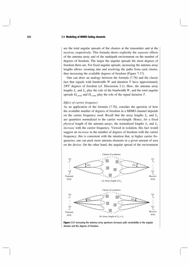
321 7.3 Modeling of MIMO fading channels
are the total angular spreads of the clusters at the transmitter and at thereceiver, respectively. This formula shows explicitly the separate effectsof the antenna array and of the multipath environment on the number ofdegrees of freedom. The larger the angular spreads the more degrees offreedom there are. For fixed angular spreads, increasing the antenna arraylengths allows zooming into and resolving the paths from each cluster,thus increasing the available degrees of freedom (Figure 7.17).One can draw an analogy between the formula (7.78) and the classic
fact that signals with bandwidth W and duration T have approximately2WT degrees of freedom (cf. Discussion 2.1). Here, the antenna arraylengths Lt and Lr play the role of the bandwidth W , and the total angularspreads ttotal and rtotal play the role of the signal duration T .
Effect of carrier frequencyAs an application of the formula (7.78), consider the question of howthe available number of degrees of freedom in a MIMO channel dependson the carrier frequency used. Recall that the array lengths Lt and Lr
are quantities normalized to the carrier wavelength. Hence, for a fixedphysical length of the antenna arrays, the normalized lengths Lt and Lr
increase with the carrier frequency. Viewed in isolation, this fact wouldsuggest an increase in the number of degrees of freedom with the carrierfrequency; this is consistent with the intuition that, at higher carrier fre-quencies, one can pack more antenna elements in a given amount of areaon the device. On the other hand, the angular spread of the environment
Cluster of scatterers
(a) Array length of L1
(b) Array length of L2 > L1
Cluster of scatterers
Receivearray
Receivearray
1/L1 1/L1
1/L21/L2
Transmitarray
Transmitarray
Figure 7.17 Increasing the antenna array apertures increases path resolvability in the angulardomain and the degrees of freedom.

322 MIMO I: spatial multiplexing and channel modeling
typically decreases with the carrier frequency. The reasons aretwo-fold:• signals at higher frequency attenuate more after passing through orbouncing off channel objects, thus reducing the number of effectiveclusters;
• at higher frequency the wavelength is small relative to the feature sizeof typical channel objects, so scattering appears to be more specular innature and results in smaller angular spread.
These factors combine to reduce ttotal and rtotal as the carrier frequencyincreases. Thus the impact of carrier frequency on the overall degrees offreedom is not necessarily monotonic. A set of indoor measurements isshown in Figure 7.18. The number of degrees of freedom increases andthen decreases with the carrier frequency, and there is in fact an optimalfrequency at which the number of degrees of freedom is maximized. Thisexample shows the importance of taking into account both the physicalenvironment as well as the antenna arrays in determining the availabledegrees of freedom in a MIMO channel.
2 3 4 5 6 70
0.05
0.1
0.15
0.2
0.25
0.3
0.35
0.4
0.45
2 3 4 5 6 70
1
2
3
4
5
6
7
Frequency (GHz) Frequency (GHz)
(b)(a)
Ω total in townhouse
Ω to
tal
Ω to
tal /
λ c (m
−1)
1/λ
(m-1
)
1/λ c
Ω total in officeOfficeTownhouse
0
5
10
15
20
25
8 8
Figure 7.18 (a) The total angular spread total of the scattering environment (assumed equal atthe transmitter side and at the receiver side) decreases with the carrier frequency; the normalizedarray length increases proportional to 1/c . (b) The number of degrees of freedom of the MIMOchannel, proportional to total/c , first increases and then decreases with the carrier frequency.The data are taken from [91].
DiversityIn this chapter, we have focused on the phenomenon of spatial multiplexingand the key parameter is the number of degrees of freedom. In a slow fadingenvironment, another important parameter is the amount of diversity in thechannel. This is the number of independent channel gains that have to be ina deep fade for the entire channel to be in deep fade. In the angular domainMIMO model, the amount of diversity is simply the number of non-zero

323 7.3 Modeling of MIMO fading channels
Figure 7.19 Angular domainrepresentation of three MIMOchannels. They all have fourdegrees of freedom but theyhave diversity 4, 8 and 16respectively. They modelchannels with increasingamounts of bounces in thepaths (cf. Figure 7.15).
(a)
nt
n r n r n r
nt nt
(b) (c)
entries in Ha. Some examples are shown in Figure 7.19. Note that channelsthat have the same degrees of freedom can have very different amounts ofdiversity. The number of degrees of freedom depends primarily on the angularspreads of the scatters/reflectors at the transmitter and at the receiver, whilethe amount of diversity depends also on the degree of connectivity betweenthe transmit and receive angles. In a channel with multiple-bounced paths,signals sent along one transmit angle can arrive at several receive angles(see Figure 7.15). Such a channel would have more diversity than one withsingle-bounced paths with signal sent along one transmit angle received at aunique angle, even though the angular spreads may be the same.
7.3.7 Dependency on antenna spacing
So far we have been primarily focusing on the case of critically spacedantennas (i.e., antenna separations t and r are half the carrier wavelength).What is the impact of changing the antenna separation on the channel statisticsand the key channel parameters such as the number of degrees of freedom?To answer this question, we fix the antenna array lengths Lt and Lr and vary
the antenna separation, or equivalently the number of antenna elements. Letus just focus on the receiver side; the transmitter side is analogous. Given theantenna array length Lr , the beamforming patterns associated with the basisvectors erk/Lrk all have beam widths of 2/Lr (Figure 7.12). This dictatesthe maximum possible resolution of the antenna array: paths that arrive withinan angular window of width 1/Lr cannot be resolved no matter how manyantenna elements there are. There are 2Lr such angular windows, partitioningall the receive directions (Figure 7.20). Whether or not this maximum reso-lution can actually be achieved depends on the number of antenna elements.Recall that the bins k can be interpreted as the set of all physical
paths which have most of their energy along the basis vector etk/Lr. Thebins dictate the resolvability of the antenna array. In the critically spaced caser = 1/2), the beamforming patterns of all the basis vectors have a singlemain lobe (together with its mirror image). There is a one-to-one correspon-dence between the angular windows and the resolvable bins k, and pathsarriving in different windows can be resolved by the array (Figure 7.21). In

324 MIMO I: spatial multiplexing and channel modeling
Figure 7.20 An antenna arrayof length Lr partitions thereceive directions into 2Lrangular windows. Here, Lr = 3and there are six angularwindows. Note that because ofsymmetry across the 0 −180
axis, each angular windowcomes as a mirror image pair,and each pair is only countedas one angular window.
3
245 1
15
4 2
3
0
0
Figure 7.21 Antennas arecritically spaced at half thewavelength. Each resolvablebin corresponds to exactly oneangular window. Here, thereare six angular windows andsix bins.
L r = 3, n r = 6
24
0 1 2 3 4 5k
5 1
15
4 2
3
0
0
3
Bins
the sparsely spaced case (r > 1/2), the beamforming patterns of some of thebasis vectors have multiple main lobes. Thus, paths arriving in the differentangular windows corresponding to these lobes are all lumped into one binand cannot be resolved by the array (Figure 7.22). In the densely spaced case(r < 1/2), the beamforming patterns of 2Lr of the basis vectors have a singlemain lobe; they can be used to resolve among the 2Lr angular windows. Thebeamforming patterns of the remaining nr −2Lr basis vectors have no mainlobe and do not correspond to any angular window. There is little receivedenergy along these basis vectors and they do not participate significantly inthe communication process. See Figure 7.23.The key conclusion from the above analysis is that, given the antenna
array lengths Lr and Lt , the maximum achievable angular resolution canbe achieved by placing antenna elements half a wavelength apart. Placingantennas more sparsely reduces the resolution of the antenna array and can

325 7.3 Modeling of MIMO fading channels
(b)
Bins
0
0
1
0
1 1
0
1
0
11
0
k10
L r = 3, n r = 2
(a)
Bins
0
0
2
3
14
2
3
2
14
3
k10 2 3 4
L r = 3, n r = 5
reduce the number of degrees of freedom and the diversity of the channel.Figure 7.22 (a) Antennas aresparsely spaced. Some of thebins contain paths frommultiple angular windows.(b) The antennas are verysparsely spaced. All binscontain several angularwindows of paths.
Placing the antennas more densely adds spurious basis vectors which do notcorrespond to any physical directions, and does not add resolvability. In termsof the angular channel matrix Ha, this has the effect of adding zero rows andcolumns; in terms of the spatial channel matrixH, this has the effect of makingthe entries more correlated. In fact, the angular domain representation makesit apparent that one can reduce the densely spaced system to an equivalent2Lt ×2Lr critically spaced system by just focusing on the basis vectors thatdo correspond to physical directions (Figure 7.24).Increasing the antenna separation within a given array length Lr does not
increase the number of degrees of freedom in the channel. What about increas-ing the antenna separation while keeping the number of antenna elements nr
the same? This question makes sense if the system is hardware-limited ratherthan limited by the amount of space to put the antenna array in. Increasingthe antenna separation this way reduces the beam width of the nr angularbasis beamforming patterns but also increases the number of main lobes ineach (Figure 7.25). If the scattering environment is rich enough such that thereceived signal arrives from all directions, the number of non-zero rows ofthe channel matrix Ha is already nr , the largest possible, and increasing thespacing does not increase the number of degrees of freedom in the channel.On the other hand, if the scattering is clustered to within certain directions,increasing the separation makes it possible for the scattered signal to be

326 MIMO I: spatial multiplexing and channel modeling
Figure 7.23 Antennas aredensely spaced. Some binscontain no physical paths.
0
0
7
8
9 1
2
3
2
198
k0 1 98765432
Empty bins
L r = 3, n r = 10
Figure 7.24 A typical Ha
when the antennas aredensely spaced.
1020
3040
50 510
1520
2530
3540
4550
1
2
3
4
5
L = 16, n = 50
|hkl
|a
l – Transmitter bins K–Receiver bins
received in more bins, thus increasing the number of degrees of freedom(Figure 7.25). In terms of the spatial channel matrix H, this has the effect ofmaking the entries look more random and independent. At a base-station ona high tower with few local scatterers, the angular spread of the multipaths issmall and therefore one has to put the antennas many wavelengths apart todecorrelate the channel gains.
Sampling interpretationOne can give a sampling interpretation to the above results. First, think ofthe discrete antenna array as a sampling of an underlying continuous array−Lr/2Lr/2. On this array, the received signal xs is a function of the

327 7.3 Modeling of MIMO fading channels
Figure 7.25 An example of aclustered response channel inwhich increasing theseparation between a fixednumber of antennas increasesthe number of degrees offreedom from 2 to 3.
Cluster of scatterers
(a) Antenna separation of ∆1 = 1/2
(b) Antenna separation of ∆2 > ∆1
Cluster of scatterers
Receivearray
Receivearray
Transmitarray
Transmitarray
1 / (nt∆1) 1 / (nr∆1)
1 / (nt∆2) 1 / (nr∆2)
continuous spatial location s ∈ −Lr/2Lr/2. Just like in the discrete case(cf. Section 7.3.3), the spatial-domain signal xs and its angular representa-tion xa form a Fourier transform pair. However, since only ∈ −11corresponds to directional cosines of actual physical directions, the angularrepresentation xa of the received signal is zero outside −11. Hence, thespatial-domain signal xs is “bandlimited” to −WW, with “bandwidth”W = 1. By the sampling theorem, the signal xs can be uniquely specifiedby samples spaced at distance 1/2W = 1/2 apart, the Nyquist samplingrate. This is precise when Lr → and approximate when Lr is finite. Hence,placing the antenna elements at the critical separation is sufficient to describethe received signal; a continuum of antenna elements is not needed. Antennaspacing greater than 1/2 is not adequate: this is under-sampling and the lossof resolution mentioned above is analogous to the aliasing effect when onesamples a bandlimited signal at below the Nyquist rate.
7.3.8 I.i.d. Rayleigh fading model
A very common MIMO fading model is the i.i.d. Rayleigh fading model:the entries of the channel gain matrix Hm are independent, identically

328 MIMO I: spatial multiplexing and channel modeling
distributed and circular symmetric complex Gaussian. Since the matrix Hm
and its angular domain representation Ham are related by
Ham = U∗rHmUt (7.80)
andUr andUt are fixedunitarymatrices, thismeans thatHa shouldhave the samei.i.d. Gaussian distribution asH. Thus, using the modeling approach describedhere, we can see clearly the physical basis of the i.i.d Rayleigh fading model, interms of both the multipath environment and the antenna arrays. There shouldbe a significant number of multipaths in each of the resolvable angular bins,and the energy should be equally spread out across these bins. This is the so-called richly scattered environment. If there are very few or no paths in someof the angular directions, then the entries inHwill be correlated. Moreover, theantennas shouldbeeither criticallyor sparsely spaced. If theantennasaredenselyspaced, then some entries ofHa are approximately zero and the entries inH itselfare highly correlated. However, by a simple transformation, the channel can bereduced toanequivalentchannelwith fewerantennaswhicharecriticallyspaced.Compared to the critically spaced case, having sparser spacing makes it
easier for the channel matrix to satisfy the i.i.d. Rayleigh assumption. This isbecause each bin now spans more distinct angular windows and thus containsmore paths, from multiple transmit and receive directions. This substantiatesthe intuition that putting the antennas further apart makes the entries of Hless dependent. On the other, if the physical environment already providesscattering in all directions, then having critical spacing of the antennas isenough to satisfy the i.i.d. Rayleigh assumption.Due to the analytical tractability, we will use the i.i.d. Rayleigh fading
model quite often to evaluate performance of MIMO communication schemes,but it is important to keep in mind the assumptions on both the physicalenvironment and the antenna arrays for the model to be valid.
Chapter 7 The main plot
The angular domain provides a natural representation of the MIMO chan-nel, highlighting the interaction between the antenna arrays and the physicalenvironment.
The angular resolution of a linear antenna array is dictated by its length: anarray of length L provides a resolution of 1/L. Critical spacing of antennaelements at half the carrier wavelength captures the full angular resolutionof 1/L. Sparser spacing reduces the angular resolution due to aliasing.Denser spacing does not increase the resolution beyond 1/L.
Transmit and receive antenna arrays of length Lt and Lr partition theangular domain into 2Lt ×2Lr bins of unresolvable multipaths. Paths thatfall within the same bin are aggregated to form one entry of the angularchannel matrix Ha.

329 7.4 Bibliographical notes
A statistical model of Ha is obtained by assuming independent Gaussiandistributed entries, of possibly different variances. Angular bins that con-tain no paths correspond to zero entries.
The number of degrees of freedom in the MIMO channel is the minimumof the number of non-zero rows and the number of non-zero columns ofHa. The amount of diversity is the number of non-zero entries.
In a clustered-response model, the number of degrees of freedom is approx-imately:
minLtttotalLrrtotal (7.81)
The multiplexing capability of a MIMO channel increases with the angu-lar spreads ttotalrtotal of the scatterers/reflectors as well as withthe antenna array lengths. “This number of degrees of freedom can beachieved when the antennas are critically spaced at half the wavelength orcloser.” With a maximum angular spread of 2, the number of degrees offreedom is
min2Lt2Lr
and this equals
minnt nr
when the antennas are critically spaced.
The i.i.d. Rayleigh fading model is reasonable in a richly scattering envi-ronment where the angular bins are fully populated with paths and there isroughly equal amount of energy in each bin. The antenna elements shouldbe critically or sparsely spaced.
7.4 Bibliographical notes
The angular domain approach to MIMO channel modeling is based on works bySayeed [105] and Poon et al. [90, 92]. [105] considered an array of discrete antenna ele-ments, while [90, 92] considered a continuum of antenna elements to emphasize thatspatial multiplexability is limited not by the number of antenna elements but by thesize of the antenna array. We considered only linear arrays in this chapter, but [90] alsotreated other antenna array configurations such as circular rings and spherical surfaces.Thedegree-of-freedomformula (7.78) is derived in [90] for the clustered responsemodel.
Other related approaches to MIMO channel modeling are by Raleigh and Cioffi[97], by Gesbert et al. [47] and by Shiu et al. [111]. The latter work used a Clarke-likemodel but with two rings of scatterers, one around the transmitter and one around thereceiver, to derive the MIMO channel statistics.
330 MIMO I: spatial multiplexing and channel modeling
7.5 Exercises
Exercise 7.11. For the SIMO channel with uniform linear array in Section 7.2.1, give an exact
expression for the distance between the transmit antenna and the ith receive antenna.Make precise in what sense is (7.19) an approximation.
2. Repeat the analysis for the approximation (7.27) in the MIMO case.
Exercise 7.2 Verify that the unit vector err, defined in (7.21), is periodic withperiod r and within one period never repeats itself.
Exercise 7.3 Verify (7.35).
Exercise 7.4 In an earlier work on MIMO communication [97], it is stated that thenumber of degrees of freedom in a MIMO channel with nt transmit, nr receive antennasand K multipaths is given by
minnt nrK (7.82)
and this is the key parameter that determines the multiplexing capability of the channel.What are the problems with this statement?
Exercise 7.5 In this question we study the role of antenna spacing in the angularrepresentation of the MIMO channel.1. Consider the critically spaced antenna array in Figure 7.21; there are six bins, each
one corresponding to a specific physical angular window. All of these angularwindows have the same width as measured in solid angle. Compute the angularwindow width in radians for each of the bins l, with l= 0 5. Argue that thewidth in radians increases as we move from the line perpendicular to the antennaarray to one that is parallel to it.
2. Now consider the sparsely spaced antenna arrays in Figure 7.22. Justify the depictedmapping from the angular windows to the bins l and evaluate the angular windowwidth in radians for each of the bins l (for l = 01 nt − 1). (The angularwindow width of a bin l is the sum of the widths of all the angular windows thatcorrespond to the bin l.)
3. Justify the depiction of the mapping from angular windows to the bins l in thedensely spaced antenna array of Figure 7.23. Also evaluate the angular width ofeach bin in radians.
Exercise 7.6 The non-zero entries of the angular matrix Ha are distributed as inde-pendent complex Gaussian random variables. Show that with probability 1, the rankof the matrix is given by the formula (7.74).
Exercise 7.7 In Chapter 2, we introduced Clarke’s flat fading model, where both thetransmitter and the receiver have a single antenna. Suppose now that the receiver hasnr antennas, each spaced by half a wavelength. The transmitter still has one antenna(a SIMO channel). At time m
ym= hmxm+wm (7.83)
where ymhm are the nr-dimensional received vector and receive spatial signature(induced by the channel), respectively.

331 7.5 Exercises
1. Consider first the case when the receiver is stationary. Compute approximately thejoint statistics of the coefficients of h in the angular domain.
2. Now suppose the receiver is moving at a speed v. Compute the Doppler spread andthe Doppler spectrum of each of the angular domain coefficients of the channel.
3. What happens to the Doppler spread as nr → ? What can you say about thedifficulty of estimating and tracking the process hm as n grows? Easier, harder,or the same? Explain.
Exercise 7.8 [90] Consider a circular array of radius R normalized by the carrierwavelength with n elements uniformly spaced.1. Compute the spatial signature in the direction .2. Find the angle, f12, between the two spatial signatures in the direction 1
and 2.3. Does f12 only depend on the difference 1−2? If not, explain why.4. Plot f10 for R= 2 and different values of n, from n equal to R/2, R,
2R, to 4R. Observe the plot and describe your deductions.5. Deduce the angular resolution.6. Linear arrays of length L have a resolution of 1/L along the cos-domain, that
is, they have non-uniform resolution along the -domain. Can you design a lineararray with uniform resolution along the -domain?
Exercise 7.9 (Spatial sampling) Consider a MIMO system with Lt = Lr = 2 in achannel with M = 10 multipaths. The ith multipath makes an angle of i with thetransmit array and an angle of i with the receive array where = /M .1. Assuming there are nt transmit and nr receive antennas, compute the channel
matrix.2. Compute the channel eigenvalues for nt = nr varying from 4 to 8.3. Describe the distribution of the eigenvalues and contrast it with the binning inter-
pretation in Section 7.3.4.
Exercise 7.10 In this exercise, we study the angular domain representation offrequency-selective MIMO channels.1. Starting with the representation of the frequency-selective MIMO channel in time
(cf. (8.112)) describe how you would arrive at the angular domain equivalent(cf. (7.69)):
yam=L−1∑
=0
Hamxam−+wam (7.84)
2. Consider the equivalent (except for the overhead in using the cyclic prefix) parallelMIMO channel as in (8.113).
(a) Discuss the role played by the density of the scatterers and the delay spread inthe physical environment in arriving at an appropriate statistical model for Hn atthe different OFDM tones n.
(b) Argue that the (marginal) distribution of the MIMO channel Hn is the same foreach of the tones n= 0 N −1.
Exercise 7.11 A MIMO channel has a single cluster with the directional cosine rangesas t =r = 01. Compute the number of degrees of freedom of an n×n channelas a function of the antenna separation t = r = .

C H A P T E R
8 MIMO II: capacity and multiplexingarchitectures
In this chapter, we will look at the capacity of MIMO fading channels anddiscuss transceiver architectures that extract the promised multiplexing gainsfrom the channel. We particularly focus on the scenario when the transmitterdoes not know the channel realization. In the fast fading MIMO channel, weshow the following:
• At high SNR, the capacity of the i.i.d. Rayleigh fast fading channel scaleslike nmin log SNR bits/s/Hz, where nmin is the minimum of the numberof transmit antennas nt and the number of receive antennas nr . This isa degree-of-freedom gain.
• At low SNR, the capacity is approximately nrSNR log2 e bits/s/Hz. This isa receive beamforming power gain.
• At all SNR, the capacity scales linearly with nmin. This is due to a combi-nation of a power gain and a degree-of-freedom gain.
Furthermore, there is a transmit beamforming gain together with an oppor-tunistic communication gain if the transmitter can track the channel as well.Over a deterministic time-invariant MIMO channel, the capacity-achieving
transceiver architecture is simple (cf. Section 7.1.1): independent data streamsare multiplexed in an appropriate coordinate system (cf. Figure 7.2). Thereceiver transforms the received vector into another appropriate coordinatesystem to separately decode the different data streams. Without knowledgeof the channel at the transmitter the choice of the coordinate system in whichthe independent data streams are multiplexed has to be fixed a priori. Inconjunction with joint decoding, we will see that this transmitter architectureachieves the capacity of the fast fading channel. This architecture is alsocalled V-BLAST1 in the literature.
1 Vertical Bell Labs Space-Time Architecture. There are several versions of V-BLAST withdifferent receiver structures but they all share the same transmitting architecture ofmultiplexing independent streams, and we take this as its defining feature.
332

333 8.1 The V-BLAST architecture
In Section 8.3, we discuss receiver architectures that are simpler than jointML decoding of the independent streams. While there are several receiverarchitectures that can support the full degrees of freedom of the channel, a par-ticular architecture, the MMSE-SIC, which uses a combination of minimummean square estimation (MMSE) and successive interference cancellation(SIC), achieves capacity.The performance of the slow fading MIMO channel is characterized through
the outage probability and the corresponding outage capacity. At low SNR,the outage capacity can be achieved, to a first order, by using one transmitantenna at a time, achieving a full diversity gain of nt nr and a power gainof nr . The outage capacity at high SNR, on the other hand, benefits from adegree-of-freedom gain as well; this is more difficult to characterize succinctlyand its analysis is relegated until Chapter 9.Although it achieves the capacity of the fast fading channel, the V-BLAST
architecture is strictly suboptimal for the slow fading channel. In fact, it doesnot even achieve the full diversity gain promised by the MIMO channel.To see this, consider transmitting independent data streams directly over thetransmit antennas. In this case, the diversity of each data stream is limitedto just the receive diversity. To extract the full diversity from the channel,one needs to code across the transmit antennas. A modified architecture,D-BLAST2, which combines transmit antenna coding with MMSE-SIC, notonly extracts the full diversity from the channel but its performance alsocomes close to the outage capacity.
8.1 The V-BLAST architecture
We start with the time-invariant channel (cf. (7.1))
ym=Hxm+wm m= 12 (8.1)
When the channel matrix H is known to the transmitter, we have seen inSection 7.1.1 that the optimal strategy is to transmit independent streams in thedirections of the eigenvectors of H∗H, i.e., in the coordinate system definedby the matrix V, where H=UV∗ is the singular value decomposition of H.This coordinate system is channel-dependent. With an eye towards dealingwith the case of fading channels where the channel matrix is unknown tothe transmitter, we generalize this to the architecture in Figure 8.1, wherethe independent data streams, nt of them, are multiplexed in some arbitrary
2 Diagonal Bell Labs Space-Time Architecture

334 MIMO II: capacity and multiplexing architectures
Figure 8.1 The V-BLASTarchitecture for communicatingover the MIMO channel.
+
Pnt
P1
Qx[m]
H[m]
w[m]
y[m]Joint
ML
decoder
AWGN coderrate R1
AWGN coderrate Rnt
····
········
coordinate system given by a unitary matrix Q, not necessarily dependent onthe channel matrix H. This is the V-BLAST architecture. The data streamsare decoded jointly. The kth data stream is allocated a power Pk (such thatthe sum of the powers, P1+· · ·+Pnt
, is equal to P, the total transmit powerconstraint) and is encoded using a capacity-achieving Gaussian code with rateRk. The total rate is R=∑nt
k=1Rk.As special cases:
• If Q=V and the powers are given by the waterfilling allocations, then wehave the capacity-achieving architecture in Figure 7.2.
• If Q= Inr , then independent data streams are sent on the different transmitantennas.
Using a sphere-packing argument analogous to the ones used in Chapter 5,we will argue an upper bound on the highest reliable rate of communication:
R < logdet(
Inr +1N0
HKxH∗)
bits/s/Hz (8.2)
Here Kx is the covariance matrix of the transmitted signal x and is a functionof the multiplexing coordinate system and the power allocations:
Kx =Q diagP1 PntQ∗ (8.3)
Considering communication over a block of time symbols of length N , thereceived vector, of length nrN , lies with high probability in an ellipsoid ofvolume proportional to
detN0Inr +HKxH∗N (8.4)
This formula is a direct generalization of the corresponding volume for-mula (5.50) for the parallel channel, and is justified in Exercise 8.2. Sincewe have to allow for non-overlapping noise spheres (of radius
√N0 and,
hence, volume proportional to NnrN0 ) around each codeword to ensure reliable

335 8.2 Fast fading MIMO channel
communication, the maximum number of codewords that can be packed isthe ratio
detN0Inr +HKxH∗N
NnrN0
(8.5)
We can now conclude the upper bound on the rate of reliable communicationin (8.2).Is this upper bound actually achievable by the V-BLAST architecture?
Observe that independent data streams are multiplexed in V-BLAST; perhapscoding across the streams is required to achieve the upper bound (8.2)? To getsome insight on this question, consider the special case of a MISO channel(nr = 1) and set Q= Int in the architecture, i.e., independent streams on eachof the transmit antennas. This is precisely an uplink channel, as considered inSection 6.1, drawing an analogy between the transmit antennas and the users.We know from the development there that the sum capacity of this uplinkchannel is
log(
1+∑nt
k=1 hk2Pk
N0
)
(8.6)
This is precisely the upper bound (8.2) in this special case. Thus, theV-BLAST architecture, with independent data streams, is sufficient to achievethe upper bound (8.2). In the general case, an analogy can be drawn betweenthe V-BLAST architecture and an uplink channel with nr receive antennasand channel matrix HQ; just as in the single receive antenna case, the upperbound (8.2) is the sum capacity of this uplink channel and therefore achievableusing the V-BLAST architecture. This uplink channel is considered in greaterdetail in Chapter 10 and its information theoretic analysis is in Appendix B.9.
8.2 Fast fading MIMO channel
The fast fading MIMO channel is
ym=Hmxm+wm m= 12 (8.7)
where Hm is a random fading process. To properly define a notion ofcapacity (achieved by averaging of the channel fading over time), we makethe technical assumption (as in the earlier chapters) that Hm is a stationaryand ergodic process. As a normalization, let us suppose that hij2= 1. Asin our earlier study, we consider coherent communication: the receiver tracksthe channel fading process exactly. We first start with the situation when thetransmitter has only a statistical characterization of the fading channel. Finally,we look at the case when the transmitter also perfectly tracks the fading

336 MIMO II: capacity and multiplexing architectures
channel (full CSI); this situation is very similar to that of the time-invariantMIMO channel.
8.2.1 Capacity with CSI at receiver
Consider using the V-BLAST architecture (Figure 8.1) with a channel-independent multiplexing coordinate system Q and power allocationsP1 Pnt
. The covariance matrix of the transmit signal is Kx and is notdependent on the channel realization. The rate achieved in a given channelstate H is
logdet(
Inr +1N0
HKxH∗)
(8.8)
As usual, by coding over many coherence time intervals of the channel, along-term rate of reliable communication equal to
H
[
logdet(
Inr +1N0
HKxH∗)]
(8.9)
is achieved. We can now choose the covariance Kx as a function of thechannel statistics to achieve a reliable communication rate of
C = maxKxTrKx≤P
[
logdet(
Inr +1N0
HKxH∗)]
(8.10)
Here the trace constraint corresponds to the total transmit power constraint.This is indeed the capacity of the fast fading MIMO channel (a formaljustification is in Appendix B.7.2). We emphasize that the input covarianceis chosen to match the channel statistics rather than the channel realization,since the latter is not known at the transmitter.The optimal Kx in (8.10) obviously depends on the stationary distribution
of the channel process Hm. For example, if there are only a few dominantpaths (no more than one in each of the angular bins) that are not time-varying, then we can view H as being deterministic. In this case, we knowfrom Section 7.1.1 that the optimal coordinate system to multiplex the datastreams is in the eigen-directions of H∗H and, further, to allocate powers ina waterfilling manner across the eigenmodes of H.Let us now consider the other extreme: there are many paths (of approxi-
mately equal energy) in each of the angular bins. Some insight can be obtainedby looking at the angular representation (cf. (7.80)): Ha = U∗
rHUt . The keyadvantage of this viewpoint is in statistical modeling: the entries of Ha aregenerated by different physical paths and can be modeled as being statisticallyindependent (cf. Section 7.3.5). Here we are interested in the case when theentries of Ha have zero mean (no single dominant path in any of the angular

337 8.2 Fast fading MIMO channel
windows). Due to independence, it seems reasonable to separately send infor-mation in each of the transmit angular windows, with powers correspondingto the strength of the paths in the angular windows. That is, the multiplex-ing is done in the coordinate system given by Ut (so Q = Ut in (8.3)). Thecovariance matrix now has the form
Kx = UtU∗t (8.11)
where is a diagonal matrix with non-negative entries, representing thepowers transmitted in the angular windows, so that the sum of the entries isequal to P. This is shown formally in Exercise 8.3, where we see that thisobservation holds even if the entries of Ha are only uncorrelated.If there is additional symmetry among the transmit antennas, such as when
the elements of Ha are i.i.d. 01 (the i.i.d. Rayleigh fading model),then one can further show that equal powers are allocated to each transmitangular window (see Exercises 8.4 and 8.6) and thus, in this case, the optimalcovariance matrix is simply
Kx =(P
nt
)
Int (8.12)
More generally, the optimal powers (i.e., the diagonal entries of ) are chosento be the solution to the maximization problem (substituting the angularrepresentation H= UrH
aU∗t and (8.11) in (8.10)):
C = maxTr≤P
[
logdet(
Inr +1N0
UrHaHa∗U∗
r
)]
(8.13)
= maxTr≤P
[
logdet(
Inr +1N0
HaHa∗)]
(8.14)
With equal powers (i.e., the optimal is equal to P/ntInt, the resultingcapacity is
C =
[
logdet(
Inr +SNRnt
HH∗)]
(8.15)
where SNR = P/N0 is the common SNR at each receive antenna.If 1 ≥ 2 ≥ · · · ≥ nmin
are the (random) ordered singular values of H, thenwe can rewrite (8.15) as
C =
[nmin∑
i=1
log(
1+ SNRnt
2i
)]
=nmin∑
i=1
[
log(
1+ SNRnt
2i
)]
(8.16)

338 MIMO II: capacity and multiplexing architectures
Comparing this expression to the waterfilling capacity in (7.10), we see thecontrast between the situation when the transmitter knows the channel andwhen it does not. When the transmitter knows the channel, it can allocatedifferent amounts of power in the different eigenmodes depending on theirstrengths. When the transmitter does not know the channel but the channelis sufficiently random, the optimal covariance matrix is identity, resulting inequal amounts of power across the eigenmodes.
8.2.2 Performance gains
The capacity, (8.16), of the MIMO fading channel is a function of the distri-bution of the singular values, i, of the random channel matrix H. By Jensen’sinequality, we know that
nmin∑
i=1
log(
1+ SNRnt
2i
)
≤ nmin log
(
1+ SNRnt
[1
nmin
nmin∑
i=1
2i
])
(8.17)
with equality if and only if the singular values are all equal. Hence, one wouldexpect a high capacity if the channel matrix H is sufficiently random andstatistically well conditioned, with the overall channel gain well distributedacross the singular values. In particular, one would expect such a channel toattain the full degrees of freedom at high SNR.We plot the capacity for the i.i.d. Rayleigh fading model in Figure 8.2
for different numbers of antennas. Indeed, we see that for such a randomchannel the capacity of a MIMO system can be very large. At moderate tohigh SNR, the capacity of an n by n channel is about n times the capacity ofa 1 by 1 system. The asymptotic slope of capacity versus SNR in dB scale isproportional to n, which means that the SNR like n log SNR.
High SNR regimeThe performance gain can be seen most clearly in the high SNR regime. Athigh SNR, the capacity for the i.i.d. Rayleigh channel is given by
C ≈ nmin logSNRnt
+nmin∑
i=1
log2i (8.18)
and
log2i >− (8.19)
for all i. Hence, the full nmin degrees of freedom is attained. In fact, furtheranalysis reveals that
nmin∑
i=1
log2i =
maxntnr∑
i=nt−nr +1
log 22i (8.20)

339 8.2 Fast fading MIMO channel
Figure 8.2 Capacity of an i.i.d.Rayleigh fading channel.Upper: 4 by 4 channel. Lower:8 by 8 channel.
nt = nr = 1
nt = nr = 4nt = 1 nr = 4
nt = nr = 1
nt = nr = 8nt = 1 nr = 8
C (bits /s / Hz)
C (bits /s / Hz)
35
30
25
20
15
10
5
–10 10 20 30
70
60
50
40
30
20
10
SNR (dB)
–10 10 20 30SNR (dB)
where 22i is a -square distributed random variable with 2i degrees of
freedom.Note that the number of degrees of freedom is limited by the minimum
of the number of transmit and the number of receive antennas, hence, to geta large capacity, we need multiple transmit and multiple receive antennas.To emphasize this fact, we also plot the capacity of a 1 by nr channel inFigure 8.2. This capacity is given by
C =
[
log
(
1+ SNRnr∑
i=1
hi2)]
bits/s/Hz (8.21)
We see that the capacity of such a channel is significantly less than that of annr by nr system in the high SNR range, and this is due to the fact that thereis only one degree of freedom in a 1 by nr channel. The gain in going froma 1 by 1 system to a 1 by nr system is a power gain, resulting in a parallel

340 MIMO II: capacity and multiplexing architectures
shift of the capacity versus SNR curves. At high SNR, a power gain is muchless impressive than a degree-of-freedom gain.
Low SNR regimeHerewe use the approximation log21+x≈ x log2 e for x small in (8.15) to get
C =nmin∑
i=1
[
log(
1+ SNRnt
2i
)]
≈nmin∑
i=1
SNRnt
[2i
]log2 e
= SNRnt
TrHH∗ log2 e
= SNRnt
[∑
ij
hij2]
log2 e
= nrSNR log2 e bits/s/Hz
Thus, at low SNR, an nt by nr system yields a power gain of nr over a singleantenna system. This is due to the fact that the multiple receive antennas cancoherently combine their received signals to get a power boost. Note thatincreasing the number of transmit antennas does not increase the power gainsince, unlike the case when the channel is known at the transmitter, transmitbeamforming cannot be done to constructively add signals from the differentantennas. Thus, at low SNR and without channel knowledge at the transmitter,multiple transmit antennas are not very useful: the performance of an nt bynr channel is comparable with that of a 1 by nr channel. This is illustratedin Figure 8.3, which compares the capacity of an n by n channel with thatof a 1 by n channel, as a fraction of the capacity of a 1 by 1 channel. Wesee that at an SNR of about −20 dB, the capacities of a 1 by 4 channel anda 4 by 4 channel are very similar.Recall from Chapter 4 that the operating SINR of cellular systems with
universal frequency reuse is typically very low. For example, an IS-95 CDMAsystem may have an SINR per chip of −15 to −17dB. The above observationthen suggests that just simply overlaying point-to-point MIMO technology onsuch systems to boost up per link capacity will not provide much additionalbenefit than just adding antennas at one end. On the other hand, the storyis different if the multiple antennas are used to perform multiple access andinterference management. This issue will be revisited in Chapter 10.Another difference between the high and the low SNR regimes is that while
channel randomness is crucial in yielding a large capacity gain in the highSNR regime, it plays little role in the low SNR regime. The low SNR resultabove does not depend on whether the channel gains, hij, are independentor correlated.

341 8.2 Fast fading MIMO channel
Figure 8.3 Low SNR capacities.Upper: a 1 by 4 and a 4 by 4channel. Lower: a 1 by 8 an 8by 8 channel. Capacity is afraction of the 1 by 1 channelin each case.
CC1,1
(bits / s / Hz)
CC1,1
(bits / s / Hz)
4
3.5
2.5
3
10–10–20–30
nt = 1 nr = 4nt = nr = 4
8
7
6
5
4
3
SNR (dB)
SNR (dB)
10–10–20–30
nt = 1 nr = 8nt = nr = 8
Large antenna array regimeWe saw that in the high SNR regime, the capacity increases linearly with theminimum of the number of transmit and the number of receive antennas. Thisis a degree-of-freedom gain. In the low SNR regime, the capacity increaseslinearly with the number of receive antennas. This is a power gain. Will thecombined effect of the two types of gain yield a linear growth in capacity atany SNR, as we scale up both nt and nr? Indeed, this turns out to be true. Letus focus on the square channel nt = nr = n to demonstrate this.With i.i.d. Rayleigh fading, the capacity of this channel is (cf. (8.15))
CnnSNR=
[n∑
i=1
log(
1+ SNR2i
n
)]
(8.22)
where we emphasize the dependence on n and SNR in the notation. The i/√n
are the singular values of the random matrixH/√n. By a random matrix result

342 MIMO II: capacity and multiplexing architectures
due to Marcenko and Pastur [78], the empirical distribution of the singularvalues of H/
√n converges to a deterministic limiting distribution for almost
all realizations of H. Figure 8.4 demonstrates the convergence. The limitingdistribution is the so-called quarter circle law.3 The corresponding limitingdensity of the squared singular values is given by
f ∗x=
1
√1x− 1
4 0 ≤ x ≤ 4
0 else(8.23)
Hence, we can conclude that, for increasing n,
1n
n∑
i=1
log(
1+ SNR2i
n
)
→∫ 4
0log1+ SNRxf ∗xdx (8.24)
If we denote
c∗SNR =∫ 4
0log1+ SNRxf ∗xdx (8.25)
Figure 8.4 Convergence of theempirical singular valuedistribution of H/
√n. For
each n, a single randomrealization of H/
√n is
generated and the empiricaldistribution (histogram) of thesingular values is plotted. Wesee that as n grows, thehistogram converges to thequarter circle law.
0 0.5 1 1.5 20
1
2
3
4n = 32
0 0.5 1 1.5 20
2
4
6
8
10n = 64
0 0.5 1 1.5 20
5
10
15
20n = 128
0 0.5 1 1.5 20
0.1
0.2
0.3
0.4
0.5
0.6
0.7Quarter circle law
3 Note that although the singular values are unbounded, in the limit they lie in the interval02 with probability 1.

343 8.2 Fast fading MIMO channel
we can solve the integral for the density in (8.23) to arrive at (see Exer-cise 8.17)
c∗SNR= 2 log(
1+ SNR− 14FSNR
)
− log e4SNR
FSNR (8.26)
where
FSNR =(√
4SNR+1−1)2
(8.27)
The significance of c∗SNR is that
limn→
CnnSNRn
= c∗SNR (8.28)
So capacity grows linearly in n at any SNR and the constant c∗SNR is therate of the growth.We compare the large-n approximation
CnnSNR≈ nc∗SNR (8.29)
with the actual value of the capacity for n = 24 in Figure 8.5. We see theapproximation is very good, even for such small values of n. In Exercise 8.7,we see statistical models other than i.i.d. Rayleigh, which also have a linearincrease in capacity with an increase in n.
Linear scaling: a more in-depth lookTo better understand why the capacity scales linearly with the number ofantennas, it is useful to contrast the MIMO scenario here with three otherscenarios:
Figure 8.5 Comparisonbetween the large-napproximation and the actualcapacity for n= 2 4.
–5 0 10 15 20SNR (dB)
25 30
Approximate capacity c∗
–10
9
8
7
6
5
4
3
2
1
0
Rat
e(b
its /s
/ Hz)
5
Exact capacity 14 C44
Exact capacity 12 C22

344 MIMO II: capacity and multiplexing architectures
• MISO channel with a large transmit antenna array Specializing (8.15)to the n by 1 MISO channel yields the capacity
Cn1 =
[
log
(
1+ SNRn
n∑
i=1
hi2)]
bits/s/Hz (8.30)
As n→, by the law of large numbers,
Cn1 → log1+ SNR= Cawgn (8.31)
For n = 1, the 1 by 1 fading channel (with only receiver CSI) has lowercapacity than the AWGN channel; this is due to the “Jensen’s loss”(Section 5.4.5). But recall from Figure 5.20 that this loss is not large forthe entire range of SNR. Increasing the number of transmit antennas hasthe effect of reducing the fluctuation of the instantaneous SNR
1n
n∑
i=1
hi2 · SNR (8.32)
and hence reducing the Jensen’s loss, but the loss was not big to startwith, hence the gain is minimal. Since the total transmit power is fixed,the multiple transmit antennas provide neither a power gain nor a gain inspatial degrees of freedom. (In a slow fading channel, the multiple transmitantennas provide a diversity gain, but this is not relevant in the fast fadingscenario considered here.)
• SIMO channel with a large receive antenna array A 1 by n SIMOchannel has capacity
C1n =
[
log
(
1+ SNRn∑
i=1
hi2)]
(8.33)
For large n
C1n ≈ lognSNR= logn+ log SNR (8.34)
i.e., the receive antennas provide a power gain (which increases linearlywith the number of receive antennas) and the capacity increases logarith-mically with the number of receive antennas. This is quite in contrast tothe MISO case: the difference is due to the fact that now there is a lin-ear increase in total received power due to a larger receive antenna array.However, the increase in capacity is only logarithmic in n; the increasein total received power is all accumulated in the single degree of freedomof the channel. There is power gain but no gain in the spatial degrees offreedom.The capacities, as a function of n, are plotted for the SIMO, MISO and
MIMO channels in Figure 8.6.

345 8.2 Fast fading MIMO channel
Figure 8.6 Capacities of the nby 1 MISO channel, 1 by nSIMO channel and the n by nMIMO channel as a function ofn, for SNR= 0 dB
Number of antennas (n)14 16
MISO channelSIMO channelMIMO channel
20
14
12
12
10
10
8
8
6
4
64
2
0
Rat
e (b
its /s
/ Hz)
• AWGN channel with infinite bandwidth Given a power constraint ofP and AWGN noise spectral density N0/2, the infinite bandwidth limit is(cf. 5.18)
C = limW→
W log(
1+ P
N0W
)
= P
N0
bits/s (8.35)
Here, although the number of degrees of freedom increases, the capacityremains bounded. This is because the total received power is fixed andhence the SNR per degree of freedom vanishes. There is a gain in thedegrees of freedom, but since there is no power gain the received powerhas to be spread across the many degrees of freedom.
In contrast to all of these scenarios, the capacity of an n by n MIMOchannel increases linearly with n, because simultaneously:
• there is a linear increase in the total received power, and• there is a linear increase in the degrees of freedom, due to the substantialrandomness and consequent well-conditionedness of the channel matrix H.
Note that the well-conditionedness of the matrix depends on maintaining theuncorrelated nature of the channel gains, hij, while increasing the numberof antennas. This can be achieved in a rich scattering environment by keepingthe antenna spacing fixed at half the wavelength and increasing the aperture,L, of the antenna array. On the other hand, if we just pack more and moreantenna elements in a fixed aperture, L, then the channel gains will becomemore and more correlated. In fact, we know from Section 7.3.7 that in theangular domain a MIMO channel with densely spaced antennas and apertureL can be reduced to an equivalent 2L by 2L channel with antennas spacedat half the wavelength. Thus, the number of degrees of freedom is ultimately

346 MIMO II: capacity and multiplexing architectures
limited by the antenna array aperture rather than the number of antennaelements.
8.2.3 Full CSI
We have considered the scenario when only the receiver can track the channel.This is the most interesting case in practice. In a TDD system or in an FDDsystem where the fading is very slow, it may be possible to track the channelmatrix at the transmitter. We shall now discuss how channel capacity canbe achieved in this scenario. Although channel knowledge at the transmitterdoes not help in extracting an additional degree-of-freedom gain, extra powergain is possible.
CapacityThe derivation of the channel capacity in the full CSI scenario is only a slighttwist on the time-invariant case discussed in Section 7.1.1. At each time m,we decompose the channel matrix as Hm = UmmVm∗, so that theMIMO channel can be represented as a parallel channel
yim= imxim+ wim i= 1 nmin (8.36)
where 1m ≥ 2m ≥ ≥ nminm are the ordered singular values of
Hm and
xm = V∗mxm
ym = U∗mym
wm = U∗mwm
We have encountered the fast fading parallel channel in our study of thesingle antenna fast fading channel (cf. Section 5.4.6). We allocate powers tothe sub-channels based on their strength according to the waterfilling policy
P∗=(
− N0
2
)+ (8.37)
with chosen so that the total transmit power constraint is satisfied:
nmin∑
i=1
[(
− N0
2i
)+]
= P (8.38)
Note that this is waterfilling over time and space (the eigenmodes). Thecapacity is given by
C =nmin∑
i=1
[
log(
1+ P∗i2i
N0
)]
(8.39)

347 8.2 Fast fading MIMO channel
Transceiver architectureThe transceiver architecture that achieves the capacity follows naturally fromthe SVD-based architecture depicted in Figure 7.2. Information bits are splitinto nmin parallel streams, each coded separately, and then augmented by nt −nmin streams of zeros. The symbols across the streams at time m form the vec-tor xm. This vector is pre-multiplied by the matrix Vm before being sentthrough the channel, where Hm = UmmV∗m is the singular valuedecomposition of the channel matrix at time m. The output is post-multipliedby the matrix U∗m to extract the independent streams, which are then sepa-rately decoded. The power allocated to each stream is time-dependent and isgiven by the waterfilling formula (8.37), and the rates are dynamically allo-cated accordingly. If anAWGNcapacity-achieving code is used for each stream,then the entire system will be capacity-achieving for the MIMO channel.
Performance analysisLet us focus on the i.i.d. Rayleigh fading model. Since with probability 1,the random matrix HH∗ has full rank (Exercise 8.12), and is, in fact, well-conditioned (Exercise 8.14), it can be shown that at high SNR, the waterfillingstrategy allocates an equal amount of power P/nmin to all the spatial modes,as well as an equal amount of power over time. Thus,
C ≈nmin∑
i=1
[
log(
1+ SNRnmin
2i
)]
(8.40)
where SNR = P/N0. If we compare this to the capacity (8.16) with onlyreceiver CSI, we see that the number of degrees of freedom is the same nmin
but there is a power gain of a factor of nt/nmin when the transmitter can trackthe channel. Thus, whenever there are more transmit antennas then receiveantennas, there is a power boost of nt/nr from having transmitter CSI. Thereason is simple. Without channel knowledge at the transmitter, the transmitenergy is spread out equally across all directions in nt . With transmitter CSI,the energy can now be focused on only the nr non-zero eigenmodes, whichform a subspace of dimension nr inside nt . For example, with nr = 1, thecapacity with only receiver CSI is
[
log
(
1+ SNR/nt
nt∑
i=1
hi2)]
while the high SNR capacity when there is full CSI is
[
log
(
1+ SNRnt∑
i=1
hi2)]

348 MIMO II: capacity and multiplexing architectures
Thus a power gain of a factor of nt is achieved by transmit beamforming.With dual transmit antennas, this is a gain of 3 dB.At low SNR, there is a further gain from transmitter CSI due to dynamic
allocation of power across the eigenmodes: at any given time, more poweris given to stronger eigenmodes. This gain is of the same nature as the onefrom opportunistic communication discussed in Chapter 6.What happens in the large antenna array regime?Applying the randommatrix
result of Marcenko and Pastur from Section 8.2.2, we conclude that the randomsingular valuesim/
√n of the channelmatrixHm/
√n converge to the same
deterministic limiting distribution f ∗ across all timesm. This means that in thewaterfilling strategy, there is no dynamic power allocation over time, only overspace. This is sometimes known as a channel hardening effect.
Summary 8.1 Performance gains in a MIMO channel
The capacity of an nt ×nr i.i.d. Rayleigh fading MIMO channel H withreceiver CSI is
CnnSNR=
[
logdet(
Inr +SNRnt
HH∗)]
(8.41)
At high SNR, the capacity is approximately equal (up to an additiveconstant) to nmin log SNR bits/s/Hz.
At low SNR, the capacity is approximately equal to nr SNR log2 e bits/s/Hz,so only a receive beamforming gain is realized.
With nt = nr = n, the capacity can be approximated by nc∗SNR wherec∗SNR is the constant in (8.26).
Conclusion: In an n×n MIMO channel, the capacity increases linearlywith n over the entire SNR range.
With channel knowledge at the transmitter, an additional nt/nr-fold trans-mit beamforming gain can be realized with an additional power gain fromtemporal–spatial waterfilling at low SNR.
8.3 Receiver architectures
The transceiver architecture of Figure 8.1 achieves the capacity of the fastfading MIMO channel with receiver CSI. The capacity is achieved by jointML decoding of the data streams at the receiver, but the complexity growsexponentially with the number of data streams. Simpler decoding rulesthat provide soft information to feed to the decoders of the individual datastreams is an active area of research; some of the approaches are reviewed

349 8.3 Receiver architectures
in Exercise 8.15. In this section, we consider receiver architectures that uselinear operations to convert the problem of joint decoding of the data streamsinto one of individual decoding of the data streams. These architecturesextract the spatial degree of freedom gains characterized in the previoussection. In conjunction with successive cancellation of data streams, we canachieve the capacity of the fast fading MIMO channel. To be able to focus onthe receiver design, we start with transmitting the independent data streamsdirectly over the antenna array (i.e., Q= Int in Figure 8.1).
8.3.1 Linear decorrelator
Geometric derivationIs it surprising that the full degrees of freedom of H can be attained evenwhen the transmitter does not track the channel matrix? When the transmitterdoes know the channel, the SVD architecture enables the transmitter to sendparallel data streams through the channel so that they arrive orthogonallyat the receiver without interference between the streams. This is achievedby pre-rotating the data so that the parallel streams can be sent along theeigenmodes of the channel. When the transmitter does not know the channel,this is not possible. Indeed, after passing through the MIMO channel of (7.1),the independent data streams sent on the transmit antennas all arrive cross-coupled at the receiver. It is not clear a priori that the receiver can separatethe data streams efficiently enough so that the resulting performance has fulldegrees of freedom. But in fact we have already seen such a receiver: thechannel inversion receiver in the 2× 2 example discussed in Section 3.3.3.We develop the structure of this receiver in full generality here.To simplify notations, let us first focus on the time-invariant case, where the
channel matrix is fixed. We can write the received vector at symbol timem as
ym=nt∑
i=1
hixim+wm (8.42)
where h1 hntare the columns of H and the data streams transmitted on
the antennas, xim on the ith antenna, are all independent. Focusing on thekth data stream, we can rewrite (8.42):
ym= hkxkm+∑i =k
hixim+w (8.43)
Compared to the SIMO point-to-point channel from Section 7.2.1, we seethat the kth data stream faces an extra source of interference, that fromthe other data streams. One idea that can be used to remove this inter-stream interference is to project the received signal y onto the subspaceorthogonal to the one spanned by the vectors h1 hk−1hk+1 hnt

350 MIMO II: capacity and multiplexing architectures
(denoted henceforth by Vk). Suppose that the dimension of Vk is dk. Projectionis a linear operation and we can represent it by a dk by nr matrix Qk, therows of which form an orthonormal basis of Vk; they are all orthogonalto h1 hk−1hk+1 hnt
. The vector Qkv should be interpreted as theprojection of the vector v onto Vk, but expressed in terms of the coordinatesdefined by the basis of Vk formed by the rows of Qk. A pictorial depiction ofthis projection operation is in Figure 8.7.Now, the inter-stream interference “nulling” is successful (that is, the result-
ing projection of hk is a non-zero vector) if the kth data stream “spatialsignature” hk is not a linear combination of the spatial signatures of the otherdata streams. In other words, if there are more data streams than the dimen-sion of the received signal (i.e., nt > nr), then the nulling operation will notbe successful, even for a full rank H. Hence, we should choose the numberof data streams to be no more than nr . Physically, this corresponds to usingonly a subset of the transmit antennas and for notational convenience we willcount only the transmit antennas that are used, by just making the assumptionnt ≤ nr in the decorrelator discussion henceforth.After the projection operation,
ym =Qkym=Qkhkxkm+ wm
where wm =Qkwm is the noise, still white, after the projection. Optionaldemodulation of the kth stream can now be performed by match filtering tothe vector Qkhk. The output of this matched filter (or maximal ratio combiner)has SNR
PkQkhk2N0
(8.44)
where Pk is the power allocated to stream k.
Figure 8.7 A schematicrepresentation of theprojection operation: y isprojected onto the subspaceorthogonal to h1 todemodulate stream 2.
h1
h2
y

351 8.3 Receiver architectures
The combination of the projection operation followed by the matched filteris called the decorrelator (also known as interference nulling or zero-forcingreceiver). Since projection and matched filtering are both linear operations,the decorrelator is a linear filter. The filter ck is given by
c∗k = Qkhk∗Qk (8.45)
or
ck = Q∗kQkhk (8.46)
which is the projection of hk onto the subspace Vk, expressed in terms ofthe original coordinates. Since the matched filter maximizes the output SNR,the decorrelator can also be interpreted as the linear filter that maximizes theoutput SNR subject to the constraint that the filter nulls out the interferencefrom all other streams. Intuitively, we are projecting the received signal inthe direction within Vk that is closest to hk.Only the kth stream has been in focus so far. We can now decorrelate each
of the streams separately, as illustrated in Figure 8.8. We have described thedecorrelator geometrically; however, there is a simple explicit formula forthe entire bank of decorrelators: the decorrelator for the kth stream is the kthcolumn of the pseudoinverse H† of the matrix H, defined by
H† = H∗H−1H∗ (8.47)
Figure 8.8 A bank ofdecorrelators, each estimatingthe parallel data streams.
Decorrelator for stream nt
Decorrelator for stream 2
Decorrelator for stream 1
y[m]

352 MIMO II: capacity and multiplexing architectures
The validity of this formula is verified in Exercise 8.11. In the special casewhen H is square and invertible, H† =H−1 and the decorrelator is preciselythe channel inversion receiver we already discussed in Section 3.3.3.
Performance for a deterministic HThe channel from the kth stream to the output of the corresponding decor-relator is a Gaussian channel with SNR given by (8.44). A Gaussian codeachieves the maximum data rate, given by
Ck = log(
1+ PkQkhk2N0
)
(8.48)
To get a better feel for this performance, let us compare it with the idealsituation of no inter-stream interference in (8.43). As we observed above, ifthere were no inter-stream interference in (8.43), the situation is exactly theSIMO channel of Section 7.2.1; the filter would be matched to hk and theachieved SNR would be
Pkhk2N0
(8.49)
Since the inter-stream interference only hampers the recovery of the kthstream, the performance of the decorrelator (in terms of the SNR in (8.44))must in general be less than that achieved by a matched filter with no inter-stream interference. We can also see this explicitly: the projection operationcannot increase the length of a vector and hence Qkhk ≤ hk. We canfurther say that the projection operation always reduces the length of hk
unless hk is already orthogonal to the spatial signatures of the other datastreams.Let us return to the bank of decorrelators in Figure 8.8. The total rate
of communication supported here with efficient coding in each of the datastreams is the sum of the individual rates in (8.48) and is given by
nt∑
k=1
Ck
Performance in fading channelsSo far our analysis has focused on a deterministic channel H. As usual, inthe time-varying fast fading scenario, coding should be done over time acrossthe different fades, usually in combination with interleaving. The maximumachievable rate can be computed by simply averaging over the stationarydistribution of the channel process Hmm, yielding
Rdecorr =nt∑
k=1
Ck (8.50)

353 8.3 Receiver architectures
where
Ck =
[
log(
1+ PkQkhk2N0
)]
(8.51)
The achievable rate in (8.50) is in general less than or equal to the capacityof the MIMO fading channel with CSI at the receiver (cf. (8.10)) sincetransmission using independent data streams and receiving using the bankof decorrelators is only one of several possible communication strategies.To get some further insight, let us look at a specific statistical model, thatof i.i.d. Rayleigh fading. Motivated by the fact that the optimal covariancematrix is of the form of scaled identity (cf. (8.12)), let us choose equal powersfor each of the data streams (i.e., Pk = P/nt). Continuing from (8.50), thedecorrelator bank performance specialized to i.i.d. Rayleigh fading is (recallthat for successful decorrelation nmin = nt)
Rdecorr =
[nmin∑
k=1
log(
1+ SNRnt
Qkhk2)]
(8.52)
Sincehk ∼ 0 Inr, we know thathk2 ∼ 22nr, where 2
2i is a -squared ran-domvariablewith2idegreesof freedom(cf. (3.36)).HereQkhk ∼ 0 IdimVk
(since QkQ∗k = IdimVk
). It can be shown that the channel H is full rank withprobability 1 (see Exercise 8.12), and this means that dimVk = nr −nt +1 (seeExercise 8.13). Thus Qkhk2 ∼ 2
2nr−nt+1 This provides us with an explicitexample for our earlier observation that the projection operation reduces thelength. In the special case of a square system, dimVk = 1, and Qkhk is a scalardistributed as circular symmetricGaussian;wehave already seen this in the2×2example of Section 3.3.3.Rdecorr is plotted in Figure 8.9 for different numbers of antennas. We see
that the asymptotic slope of the rate obtained by the decorrelator bank as a
Figure 8.9 Rate achieved(in bits/s/Hz) by thedecorrelator bank.
–10
nt = 8, nr = 12
20 25 30
SNR (dB)
Rde
corr
(b
its /s
/ Hz)
nt = 4, nr = 6
00
50
45
40
35
30
25
20
15
15
10
10
5
–5 5

354 MIMO II: capacity and multiplexing architectures
function of SNR in dB is proportional to nmin; the same slope in the capacityof the MIMO channel. More specifically, we can approximate the rate in(8.52) at high SNR as
Rdecorr ≈ nmin logSNRnt
+
[nt∑
k=1
log(Qkhk2
)]
(8.53)
= nmin log(SNRnt
)
+nt[log 2
2nr−nt+1
] (8.54)
Comparing (8.53) and (8.54) with the corresponding high SNR expansion ofthe capacity of this MIMO channel (cf. (8.18) and (8.20)), we can make thefollowing observations:
• The first-order term (in the high SNR expansion) is the same for boththe rate achieved by the decorrelator bank and the capacity of the MIMOchannel. Thus, the decorrelator bank is able to fully harness the spatialdegrees of freedom of the MIMO channel.
• The next term in the high SNR expansion (constant term) shows the per-formance degradation, in rate, of using the decorrelator bank as comparedto the capacity of the channel. Figure 8.10 highlights this difference in thespecial case of nt = nr = n.
The above analysis is for the high SNR regime. At any fixed SNR, it is alsostraightforward to show that, just like the capacity, the total rate achievableby the bank of decorrelators scales linearly with the number of antennas (seeExercise 8.21).
Figure 8.10 Plot of rateachievable with thedecorrelator bank for thent = nr = 8 i.i.d. Rayleighfading channel. The capacity ofthe channel is also plotted forcomparison.
DecorrelatorCapacity
70
60
50
40
30
20
10
–10 –5 0 5 10 15 20 25 300
bits
/ s / H
z
SNR (dB)

355 8.3 Receiver architectures
8.3.2 Successive cancellation
We have just considered a bank of separate filters to estimate the data streams.However, the result of one of the filters could be used to aid the operation ofthe others. Indeed, we can use the successive cancellation strategy described inthe uplink capacity analysis (in Section 6.1): once a data stream is successfullyrecovered, we can subtract it off from the received vector and reduce theburden on the receivers of the remaining data streams. With this motivation,consider the following modification to the bank of separate receiver structuresin Figure 8.8. We use the first decorrelator to decode the data stream x1m
and then subtract off this decoded stream from the received vector. If the firststream is successfully decoded, then the second decorrelator has to deal onlywith streams x3 xnt as interference, since x1 has been correctly subtractedoff. Thus, the second decorrelator projects onto the subspace orthogonal to thatspanned by h3 hnt
. This process is continued until the final decorrelatordoes not have to deal with any interference from the other data streams(assuming successful subtraction in each preceding stage). This decorrelator–SIC (decorrelator with successive interference cancellation) architecture isillustrated in Figure 8.11.One problem with this receiver structure is error propagation: an error in
decoding the kth data stream means that the subtracted signal is incorrectand this error propagates to all the streams further down, k+ 1 nt .A careful analysis of the performance of this scheme is complicated, butcan be made easier if we take the data streams to be well coded and theblock length to be very large, so that streams are successfully cancelledwith very high probability. With this assumption the kth data stream seesonly down-stream interference, i.e., from the streams k+ 1 nt . Thus,
Figure 8.11 Decorrelator–SIC:A bank of decorrelators withsuccessive cancellation ofstreams.
Decode stream nt
Decode stream 3
Decode stream 2
Decode stream 1
Decorrelator 2
Decorrelator 3
Decorrelator nt
Decorrelator 1
Stream nt
Stream 1
Subtract stream
1, 2, ..., nt –1
y[m]Stream 3Subtract
stream1, 2
Subtract stream1
Stream 2

356 MIMO II: capacity and multiplexing architectures
the corresponding projection operation (denoted by Qk) is onto a higherdimensional subspace (one orthogonal to that spanned by hk+1 hnt
, asopposed to being orthogonal to the span of h1 hk−1hk+1 hnt
). Asin the calculation of the previous section, the SNR of the kth data stream is(cf. (8.44))
PkQkhk2N0
(8.55)
While we clearly expect this to be an improvement over the simple bankof decorrelators, let us again turn to the i.i.d. Rayleigh fading model to seethis concretely. Analogous to the high SNR expansion of (8.52) in (8.53) forthe simple decorrelator bank, with SIC and equal power allocation to eachstream, we have
Rdec−sic ≈ nmin logSNRnt
+
[nt∑
k=1
logQkhk2]
(8.56)
Similar to our analysis of the basic decorrelator bank, we can argue thatQkhk2 ∼ 2
2nr−nt+k with probability 1 (cf. Exercise 8.13), thus arriving at
[logQkhk2
]= log 2
2nr−nt+k (8.57)
Comparing this rate at high SNR with both the simple decorrelator bank andthe capacity of the channel (cf. (8.53) and (8.18)), we observe the following
• The first-order term in the high SNR expansion is the same as that in therate of the decorrelator bank and in the capacity: successive cancellationdoes not provide additional degrees of freedom.
• Moving to the next (constant) term, we see the performance boost inusing the decorrelator–SIC over the simple decorrelator bank: the improvedconstant term is now equal to that in the capacity expansion. This boost inperformance can be viewed as a power gain: by decoding and subtractinginstead of linear nulling, the effective SNR at each stage is improved.
8.3.3 Linear MMSE receiver
Limitation of the decorrelatorWe have seen the performance of the basic decorrelator bank and thedecorrelator–SIC. At high SNR, for i.i.d. Rayleigh fading, the basic decorre-lator bank achieves the full degrees of freedom in the channel. With SIC eventhe constant term in the high SNR capacity expansion is achieved. What aboutlow SNR? The performance of the decorrelator bank (both with and withoutthe modification of successive cancellation) as compared to the capacity ofthe MIMO channel is plotted in Figure 8.12.

357 8.3 Receiver architectures
Figure 8.12 Performance ofthe decorrelator bank, withand without successivecancellation at low SNR. Herent = nr = 8.
SNR (dB)
20 30
Without successive cancellation
With successive cancellation
0.1
0.8
0.7
0.6
0.5
0.4
0.3
0.2
Rdecorr
C88
–30 –20 –10 0 10
The main observation is that while the decorrelator bank performs well athigh SNR, it is really far away from the capacity at low SNR. What is goingon here?To get more insight, let us plot the performance of a bank of matched
filters, the kth filter being matched to the spatial signature hk of transmitantenna k. From Figure 8.13 we see that the performance of the bank ofmatched filters is far superior to the decorrelator bank at low SNR (althoughfar inferior at high SNR).
Derivation of the MMSE receiverThe decorrelator was motivated by the fact that it completely nulls out inter-stream interference; in fact it maximizes the output SNR among all linear
Figure 8.13 Performance (ratioof the rate to the capacity) ofthe matched filter bank ascompared to that of thedecorrelator bank. At low SNR,the matched filter is superior.The opposite is true for thedecorrelator. The channel isi.i.d. Rayleigh with nt = nr = 8.
DecorrelatorMatched fillter
SNR (dB)
20 30
0.1
0.8
0.9
0.7
0.6
0.5
0.4
0.3
0.2
–30 –20 –10 0 10
1
0

358 MIMO II: capacity and multiplexing architectures
receivers that completely null out the interference. On the other hand, matchedfiltering (maximal ratio combining) is the optimal strategy for SIMO channelswithout any inter-stream interference. We called this receive beamformingin Example 1 in Section 7.2.1. Thus, we see a tradeoff between completelyeliminating inter-stream interference (without any regard to how much energyof the stream of interest is lost in this process) and preserving as much energycontent of the stream of interest as possible (at the cost of possibly facing highinter-stream interference). The decorrelator and the matched filter operate attwo extreme ends of this tradeoff. At high SNR, the inter-stream interference isdominant over the additive Gaussian noise and the decorrelator performs well.On the other hand, at low SNR the inter-stream interference is not as much ofan issue and receive beamforming (matched filter) is the superior strategy. Infact, the bank of matched filters achieves capacity at low SNR (Exercise 8.20).We can ask for a linear receiver that optimally trades off fighting inter-
stream interference and the background Gaussian noise, i.e., the receiver thatmaximizes the output signal-to-interference-plus-noise ratio (SINR) for anyvalue of SNR. Such a receiver looks like the decorrelator when the inter-stream interference is large (i.e., when SNR is large) and like the matchedfilter when the interference is small (i.e., when SNR is small) (Figure 8.14).This can be thought of as the natural generalization of receive beamformingto the case when there is interference as well as noise.To formulate this tradeoff precisely, let us first look at the following generic
vector channel:
y= hx+ z (8.58)
where z is complex circular symmetric colored noise with an invertible covari-ance matrixKz, h is a deterministic vector and x is the unknown scalar symbol
Figure 8.14 The optimal filtergoes from being thedecorrelator at high SNR tobeing the matched filter at lowSNR.
Interference subspace
DecorrelatorOptimal filter
Signal direction(matched filter)

359 8.3 Receiver architectures
to be estimated. z and x are assumed to be uncorrelated. We would like tochoose a filter with maximum output SNR. If the noise is white, we knowthat it is optimal to project y onto the direction along h. This observationsuggests a natural strategy for the colored noise situation: first whiten thenoise, and then follow the strategy used with white additive noise. That is,we first pass y through the invertible4 linear transformation K
− 12
z such thatthe noise z =K
− 12
z z becomes white:
K− 1
2z y=K
− 12
z hx+ z (8.59)
Next, we project the output in the direction of K− 1
2z h to get an effective scalar
channel
K− 1
2z h∗K− 1
2z y= h∗K−1
z y= h∗K−1z hx+h∗K−1
z z (8.60)
Thus the linear receiver in (8.60), represented by the vector
vmmse =K−1z h (8.61)
maximizes the SNR. It can also be shown that this receiver, with an appro-priate scaling, minimizes the mean square error in estimating x (see Exer-cise 8.18), and hence it is also called the linear MMSE (minimum meansquared error) receiver. The corresponding SINR achieved is
2xh
∗K−1z h (8.62)
We can now upgrade the receiver structure in Section 8.3.1 by replacingthe decorrelator for each stream by the linear MMSE receiver. Again, let usfirst consider the case where the channel H is fixed. The effective channelfor the kth stream is
ym= hkxkm+ zkm (8.63)
where zk represents the noise plus interference faced by data stream k:
zkm =∑i =k
hixim+wm (8.64)
4 Kz is an invertible covariance matrix and so it can be written as UU∗ for rotation matrix U
and diagonal matrix with positive diagonal elements. Now K12z is defined as U
12 U∗, with
12 defined as a diagonal matrix with diagonal elements equal to the square root of the
diagonal elements of .

360 MIMO II: capacity and multiplexing architectures
With power Pi associated with the data stream i, we can explicitly calculatethe covariance of zk
Kzk= N0Inr +
nt∑
i =k
Pihih∗i (8.65)
and also note that the covariance is invertible. Substituting this expression forthe covariance matrix into (8.61) and (8.62), we see that the linear receiverin the kth stage is given by
(
N0Inr +nt∑
i =k
Pihih∗i
)−1
hk (8.66)
and the corresponding output SINR is
Pkh∗k
(
N0Inr +nt∑
i =k
Pihih∗i
)−1
hk (8.67)
PerformanceWe motivated the design of the linear MMSE receiver as something inbetween the decorrelator and receiver beamforming. Let us now see thisexplicitly. At very low SNR (i.e., P1 Pnt
are very small compared to N0)we see that
Kzk≈ N0Inr (8.68)
and the linear MMSE receiver in (8.66) reduces to the matched filter. On the
other hand, at high SNR, the K− 1
2zk operation reduces to the projection of y
onto the subspace orthogonal to that spanned by h1 hk−1hk+1 hnt
and the linear MMSE receiver reduces to the decorrelator.Assuming the use of capacity-achieving codes for each stream, the maxi-
mum data rate that stream k can reliably carry is
Ck = log(1+Pkh
∗kK
−1zkhk
) (8.69)
As usual, the analysis directly carries over to the time-varying fadingscenario, with data rate of the kth stream being
Ck = log1+Pkh∗kK
−1zkhk (8.70)
where the average is over the stationary distribution of H.The performance of a bank of MMSE filters with equal power allocation
over an i.i.d. Rayleigh fading channel is plotted in Figure 8.15. We see thatthe MMSE receiver performs strictly better than both the decorrelator and thematched filter over the entire range of SNRs.

361 8.3 Receiver architectures
Figure 8.15 Performance (theratio of rate to the capacity) ofa basic bank of MMSEreceivers as compared to thematched filter bank and to thedecorrelator bank. MMSEperforms better than both,over the entire range of SNR.The channel is i.i.d. Rayleighwith nt = nr = 8.
Decorrelator
20100–10–20–30 30SNR (dB)
MMSEMatched filter
0
1
0.9
0.8
0.7
0.6
0.5
0.4
0.3
0.2
0.1
RC88
MMSE–SICAnalogous to what we did in Section 8.3.2 for the decorrelator, we can nowupgrade the basic bank of linear MMSE receivers by allowing successivecancellation of streams as well, as depicted in Figure 8.16. What is theperformance improvement in using the MMSE–SIC receiver? Figure 8.17plots the performance as compared to the capacity of the channel (with nt =nr = 8) for i.i.d. Rayleigh fading. We observe a startling fact: the bank of linearMMSE receivers with successive cancellation and equal power allocationachieves the capacity of the i.i.d. Rayleigh fading channel.
Figure 8.16 MMSE–SIC: abank of linear MMSE receivers,each estimating one of theparallel data streams, withstreams successively cancelledfrom the received vector ateach stage.
Subtract stream
1, 2, ... , nt –1
Stream 2
Decode stream nt
Stream nt
Subtract stream 1
Stream 1Decode stream 1
Decode stream 2
Decode stream 3
Subtract stream 1, 2
MMSE receiver 1
MMSE receiver nt
MMSE receiver 3
MMSE receiver 2
y[m]Stream 3

362 MIMO II: capacity and multiplexing architectures
Figure 8.17 The MMSE–SICreceiver achieves the capacityof the MIMO channel whenfading is i.i.d. Rayleigh.
–30 100–10–20 20
Decorrelator
30SNR (dB)
MMSE–SICMMSEMatched filter
0
1.1
1
0.9
0.8
0.7
0.6
0.5
0.4
0.3
0.2
0.1
RC88
In fact, the MMSE–SIC receiver is optimal in a much stronger sense: itachieves the best possible sum rate (8.2) of the transceiver architecture inSection 8.1 for any given H. That is, if the MMSE–SIC receiver is used fordemodulating the streams and the SINR and rate for stream k are SINRk andlog1+ SINRk respectively, then the rates sum up to
nt∑
k=1
log1+ SINRk= logdetInr +HKxH∗ (8.71)
which is the best possible sum rate. While this result can be verified directlyby matrix manipulations (Exercise 8.22), the following section gives a deeperexplanation in terms of the underlying information theory (the backgroundof which is covered in Appendix B). Understanding at this level will be veryuseful as we adapt the MMSE–SIC architecture to the analysis of the uplinkwith multiple antennas in Chapter 10.
8.3.4 Information theoretic optimality∗
MMSE is information losslessAs a key step to understanding why the MMSE–SIC receiver is optimal, letus go back to the generic vector channel with additive colored noise (8.58):
y= hx+ z (8.72)
∗ This section can be skipped on a first reading. It requires knowledge of material in Appendix Band is not essential for understanding the rest of the book, except for the analysis of theMIMO uplink in Chapter 10.

363 8.3 Receiver architectures
but now with the further assumption that x and z are Gaussian. In this case, itcan be seen that the linear MMSE filter (vmmse =K−1
z h, cf. (8.61)) not onlymaximizes the SNR, but also provides a sufficient statistic to detect x, i.e., itis information lossless. Thus,
Ixy= Ixv∗mmsey (8.73)
The justification for this step is carried out in Exercise 8.19.
A time-invariant channelConsider again the MIMO channel with a time-invariant channel matrix H:
ym=Hxm+wm
We choose the input x to be 0diagP1 Pnt. We can rewrite the
mutual information between the input and the output as
Ixy = Ix1 x2 xnt y
= Ix1y+ Ix2yx1+· · ·+ Ixnt yx1 xnt−1 (8.74)
where the last equality is a consequence of the chain rule of mutual infor-mation (see (B.18) in Appendix B). Let us look at the kth term in the chainrule expansion: Ixkyx1 xk−1. Conditional on x1 xk−1, we cansubtract their effect from the output and obtain
y′ = y−k−1∑
i=1
hixi = hkxk+∑
i>k
hixi+w
Thus,
Ixkyx1 xk−1= Ixky′= Ixkv
∗mmsey
′ (8.75)
where vmmse is the MMSE filter for estimating xk from y′ and the last equalityfollows directly from the fact that the MMSE receiver is information-lossless.Hence, the rate achieved in kth stage of the MMSE–SIC receiver is preciselyIxkyx1 xk−1, and the total rate achieved by this receiver is preciselythe overall mutual information between the input x and the output y of theMIMO channel.We now see why the MMSE filter is special: its scalar output preserves
the information in the received vector about xk. This property does not holdfor other filters such as the decorrelator or the matched filter.In the special case of a MISO channel with a scalar output
ym=nt∑
k=1
hkxkm+wm (8.76)

364 MIMO II: capacity and multiplexing architectures
the MMSE receiver at the kth stage is reduced to simple scalar multiplicationfollowed by decoding; thus it is equivalent to decoding xk while treatingsignals from antennas k+ 1 k+ 2 nt as Gaussian interference. If weinterpret (8.76) as an uplink channel with nt users, the MMSE–SIC receiverthus reduces to the SIC receiver introduced in Section 6.1. Here we see anotherexplanation why the SIC receiver is optimal in the sense of achieving thesum rate Ix1 x2 xK y of the K-user uplink channel: it “implements”the chain rule of mutual information.
Fading channelNow consider communicating using the transceiver architecture in Figure 8.1but with the MMSE–SIC receiver on a time-varying fading MIMO channelwith receiver CSI. If Q= Int , the MMSE–SIC receiver allows reliable com-munication at a sum of the rates of the data streams equal to the mutualinformation of the channel under inputs of the form
0diagP1 Pnt (8.77)
In the case of i.i.d. Rayleigh fading, the optimal input is precisely 0 Int,and so the MMSE–SIC receiver achieves the capacity as well.More generally, we have seen that if a MIMO channel, viewed in the
angular domain, can be modeled by a matrix H having zero mean, uncor-related entries, then the optimal input distribution is always of the form in(8.77) (cf. Section 8.2.1 and Exercise 8.3). Independent data streams decodedusing the MMSE–SIC receiver still achieve the capacity of such MIMOchannels, but the data streams are now transmitted over the transmit angularwindows (instead of directly on the antennas themselves). This means thatthe transceiver architecture of Figure 8.1 with Q = Ut and the MMSE-SICreceiver, achieves the capacity of the fast fading MIMO channel.
Discussion 8.1 Connections with CDMA multiuser detection and ISIequalization
Consider the situation where independent data streams are sent outfrom each antenna (cf. (8.42)). Here the received vector is a combi-nation of the streams arriving in different receive spatial signatures,with stream k having a receive spatial signature of hk. If we makethe analogy between space and bandwidth, then (8.42) serves as amodel for the uplink of a CDMA system: the streams are replaced bythe users (since the users cannot cooperate, the independence betweenthem is justified naturally) and hk now represents the received signa-ture sequence of user k. The number of receive antennas is replaced by

365 8.3 Receiver architectures
the number of chips in the CDMA signal. The base-station has accessto the received signal and decodes the information simultaneously com-municated by the different users. The base-station could use a bank oflinear filters with or without successive cancellation. The study of thereceiver design at the base-station, its complexities and performance, iscalled multiuser detection. The progress of multiuser detection is wellchronicled in [131].Another connection can be drawn to point-to-point communication over
frequency-selective channels. In our study of the OFDM approach tocommunicating over frequency-selective channels in Section 3.4.4, weexpressed the effect of the ISI in a matrix form (see (3.139)). This rep-resentation suggests the following interpretation: communicating over ablock length of Nc on the L-tap time-invariant frequency-selective chan-nel (see (3.129)) is equivalent to communicating over an Nc×Nc MIMOchannel. The equivalent MIMO channel H is related to the taps of thefrequency-selective channel, with the th tap denoted by h (for ≥ L,the tap h = 0), is
Hij =hi−j for i ≥ j
0 otherwise(8.78)
Due to the nature of the frequency-selective channel, previously trans-mitted symbols act as interference to the current symbol. The study ofappropriate techniques to recover the transmit symbols in a frequency-selective channel is part of classical communication theory under therubric of equalization. In our analogy, the transmitted symbols at differenttimes in the frequency-selective channel correspond to the ones sent overthe transmit antennas. Thus, there is a natural analogy between equaliza-tion for frequency-selective channels and transceiver design for MIMOchannels (Table 8.1).
Table 8.1 Analogies between ISI equalization and MIMO communicationtechniques. We have covered all of these except the last one, which will bediscussed in Chapter 10.
ISI equalization MIMO communication
OFDM SVDLinear zero-forcing equalizer Decorrelator/interference nullerLinear MMSE equalizer Linear MMSE receiverDecision feedback equalizer (DFE) Successive interference cancellation (SIC)ISI precoding Costa precoding

366 MIMO II: capacity and multiplexing architectures
8.4 Slow fading MIMO channel
We now turn our attention to the slow fading MIMO channel,
ym=Hxm+wm (8.79)
where H is fixed over time but random. The receiver is aware of the channelrealization but the transmitter only has access to its statistical characterization.As usual, there is a total transmit power constraint P. Suppose we wantto communicate at a target rate R bits/s/Hz. If the transmitter were awareof the channel realization, then we could use the transceiver architecture inFigure 8.1 with an appropriate allocation of rates to the data streams to achievereliable communication as long as
logdet(
Inr +1N0
HKxH∗)
> R (8.80)
where the total transmit power constraint implies a condition on the covariancematrix: TrKx ≤ P. However, remarkably, information theory guaranteesthe existence of a channel-state independent coding scheme that achievesreliable communication whenever the condition in (8.80) is met. Such acode is universal, in the sense that it achieves reliable communication onevery MIMO channel satisfying (8.80). This is similar to the universalityof the code achieving the outage performance on the slow fading parallelchannel (cf. Section 5.4.4). When the MIMO channel does not satisfy thecondition in (8.80), then we are in outage. We can choose the transmit strategy(parameterized by the covariance) to minimize the probability of the outageevent:
pmimoout R= min
KxTrKx≤P
logdet(
Inr +1N0
HKxH∗)
< R
(8.81)
Section 8.5 describes a transceiver architecture which achieves this outageperformance.The solution to this optimization problem depends, of course, on the statis-
tics of channel H. For example, if H is deterministic, the optimal solution isto perform a singular value decomposition of H and waterfill over the eigen-modes. When H is random, then one cannot tailor the covariance matrix toone particular channel realization but should instead seek a covariance matrixthat works well statistically over the ensemble of the channel realizations.It is instructive to compare the outage optimization problem (8.81) with
that of computing the fast fading capacity with receiver CSI (cf. (8.10)). Ifwe think of
fKxH = logdet(
Inr +1N0
HKxH∗)
(8.82)

367 8.4 Slow fading MIMO channel
as the rate of information flow over the channel H when using a codingstrategy parameterized by the covariance matrix Kx, then the fast fadingcapacity is
C = maxKxTrKx≤P
HfKxH (8.83)
while the outage probability is
poutR= minKxTrKx≤P
fKxH < R (8.84)
In the fast fading scenario, one codes over the fades through time and therelevant performance metric is the long-term average rate of information flowthat is permissible through the channel. In the slow fading scenario, one isonly provided with a single realization of the channel and the objective is tominimize the probability that the rate of information flow falls below the targetrate. Thus, the former is concerned with maximizing the expected value of therandom variable fKxH and the latter with minimizing the tail probabilitythat the same random variable is less than the target rate. While maximizingthe expected value typically helps to reduce this tail probability, in generalthere is no one-to-one correspondence between these two quantities: the tailprobability depends on higher-order moments such as the variance.We can consider the i.i.d. Rayleigh fading model to get more insight into
the nature of the optimizing covariance matrix. The optimal covariance matrixover the fast fading i.i.d. Rayleigh MIMO channel is K∗
x = P/nt · Int . Thiscovariance matrix transmits isotropically (in all directions), and thus onewould expect that it is also good in terms of reducing the variance of theinformation rate fKxH and, indirectly, the tail probability. Indeed, we haveseen (cf. Section 5.4.3 and Exercise 5.16) that this is the optimal covariancein terms of outage performance for the MISO channel, i.e., nr = 1, at highSNR. In general, [119] conjectures that this is the optimal covariance matrixfor the i.i.d. Rayleigh slow fading MIMO channel at high SNR. Hence, theresulting outage probability
piidoutR=
logdet(
Inr +SNRnt
HH∗)
< R
(8.85)
is often taken as a good upper bound to the actual outage probability at highSNR.More generally, the conjecture is that it is optimal to restrict to a subset
of the antennas and then transmit isotropically among the antennas used.The number of antennas used depends on the SNR level: the lower the SNRlevel relative to the target rate, the smaller the number of antennas used. Inparticular, at very low SNR relative to the target rate, it is optimal to use justone transmit antenna. We have already seen the validity of this conjecture

368 MIMO II: capacity and multiplexing architectures
in the context of a single receive antenna (cf. Section 5.4.3) and we areconsidering a natural extension to the MIMO situation. However, at typicaloutage probability levels, the SNR is high relative to the target rate and it isexpected that using all the antennas is a good strategy.
High SNRWhat outage performance can we expect at high SNR? First, we see that theMIMO channel provides increased diversity. We know that with nr = 1 (theMISO channel) and i.i.d. Rayleigh fading, we get a diversity gain equal to nt .On the other hand, we also know that with nt = 1 (the SIMO channel) andi.i.d. Rayleigh fading, the diversity gain is equal to nr . In the i.i.d. Rayleighfading MIMO channel, we can achieve a diversity gain of nt ·nr , which is thenumber of independent random variables in the channel. A simple repetitionscheme of using one transmit antenna at a time to send the same symbol xsuccessively on the different nt antennas over nt consecutive symbol periods,yields an equivalent scalar channel
y =nr∑
i=1
nt∑
j=1
hij2x+w (8.86)
whose outage probability decays like 1/SNRntnr . Exercise 8.23 shows theunsurprising fact that the outage probability of the i.i.d. Rayleigh fadingMIMO channel decays no faster than this.Thus, a MIMO channel yields a diversity gain of exactly nt ·nr . The cor-
responding -outage capacity of the MIMO channel benefits from both thediversity gain and the spatial degrees of freedom. We will explore the highSNR characterization of the combined effect of these two gains in Chapter 9.
8.5 D-BLAST: an outage-optimal architecture
We have mentioned that information theory guarantees the existence of cod-ing schemes (parameterized by the covariance matrix) that ensure reliablecommunication at rate R on every MIMO channel that satisfies the condition(8.80). In this section, we will derive a transceiver architecture that achievesthe outage performance. We begin with considering the performance of theV-BLAST architecture in Figure 8.1 on the slow fading MIMO channel.
8.5.1 Suboptimality of V-BLAST
Consider the V-BLAST architecture in Figure 8.1 with the MMSE–SICreceiver structure (cf. Figure 8.16) that we have shown to achieve the

369 8.5 D-BLAST: an outage-optimal architecture
capacity of the fast fading MIMO channel. This architecture has two mainfeatures:
• Independently coded data streams are multiplexed in an appropriate coordi-nate system Q and transmitted over the antenna array. Stream k is allocatedan appropriate power Pk and an appropriate rate Rk.
• A bank of linear MMSE receivers, in conjunction with successive cancel-lation, is used to demodulate the streams (the MMSE–SIC receiver).
The MMSE–SIC receiver demodulates the stream from transmit antenna 1using an MMSE filter, decodes the data, subtracts its contribution from thestream, and proceeds to stream 2, and so on. Each stream is thought of as alayer.Can this same architecture achieve the optimal outage performance in the
slow fading channel? In general, the answer is no. To see this concretely,consider the i.i.d. Rayleigh fading model. Here the data streams are transmittedover separate antennas and it is easy to see that each stream has a diversityof at most nr: if the channel gains from the kth transmit antenna to all thenr receive antennas are in deep fade, then the data in the kth stream willbe lost. On the other hand, the MIMO channel itself provides a diversitygain of nt ·nr . Thus, V-BLAST does not exploit the full diversity availablein the channel and therefore cannot be outage-optimal. The basic problem isthat there is no coding across the streams so that if the channel gains fromone transmit antenna are bad, the corresponding stream will be decoded inerror.We have said that, under the i.i.d. Rayleigh fading model, the diversity of
each stream in V-BLAST is at most nr . The diversity would be exactly nr ifit were the only stream being transmitted; with simultaneous transmission ofstreams, the diversity could be even lower depending on the receiver. Thiscan be seen most clearly if we replace the bank of linear MMSE receiversin V-BLAST with a bank of decorrelators and consider the case nt ≤ nr . Inthis case, the distribution of the output SNR at each stage can be explicitlycomputed; this was actually done in Section 8.3.2:
SINRk ∼Pk
N0
· 22nr−nt−k (8.87)
The diversity of the kth stream is therefore nr − nt −k. Since nt −k is thenumber of uncancelled interfering streams at the kth stage, one can interpretthis as saying that the loss of diversity due to interference is precisely thenumber of interferers needed to be nulled out. The first stream has the worstdiversity of nr−nt+1; this is also the bottleneck of the whole system becausethe correct decoding of subsequent streams depends on the correct decodingand cancellation of this stream. In the case of a square system, the first streamhas a diversity of only 1, i.e., no diversity gain. We have already seen thisresult in the special case of the 2×2 example in Section 3.3.3. Though this

370 MIMO II: capacity and multiplexing architectures
analysis is for the decorrelator, it turns out that the MMSE receiver yieldsexactly the same diversity gain (see Exercise 8.24). Using joint ML detectionof the streams, on the other hand, a diversity of nr can be recovered (as inthe 2×2 example in Section 3.3.3). However, this is still far away from thefull diversity gain ntnr of the channel.There are proposed improvements to the basic V-BLAST architecture. For
instance, adapting the cancellation order as a function of the channel, andallocating different rates to different streams depending on their position in thecancellation order. However, none of these variations can provide a diversitylarger than nr , as long as we are sending independently coded streams on thetransmit antennas.
A more careful lookHere is a more precise understanding of why V-BLAST is suboptimal, whichwill suggest how V-BLAST can be improved. For a given H, (8.71) yieldsthe following decomposition:
logdetInr +HKxH∗=
nt∑
k=1
log1+ SINRk (8.88)
SINRk is the output signal-to-interference-plus-noise ratio of the MMSEdemodulator at the kth stage of the cancellation. The output SINRs are randomsince they are a function of the channel matrix H. Suppose we have a targetrate of R and we split this into rates R1 Rnt
allocated to the individualstreams. Suppose that the transmit strategy (parameterized by the covariancematrix Kx = Q diagP1 Pnt
Q∗, cf. (8.3)) is chosen to be the one thatyields the outage probability in (8.81). Now we note that the channel is inoutage if
logdetInr +HKxH∗ < R (8.89)
or equivalently,
nt∑
k=1
log1+ SINRk <nt∑
k=1
Rk (8.90)
However, V-BLAST is in outage as long as the random SINR in any streamcannot support the rate allocated to that stream, i.e.,
log1+ SINRk < Rk (8.91)
for any k. Clearly, this can occur even when the channel is not in outage.Hence, V-BLAST cannot be universal and is not outage-optimal. This problem

371 8.5 D-BLAST: an outage-optimal architecture
did not appear in the fast fading channel because there we code over thetemporal channel variations and thus kth stream gets a deterministic rate of
log1+ SINRk bits/s/Hz (8.92)
8.5.2 Coding across transmit antennas: D-BLAST
Significant improvement of V-BLAST has to come from coding across thetransmit antennas. How do we improve the architecture to allow that? To seemore clearly how to proceed, one can draw an analogy between V-BLASTand the parallel fading channel. In V-BLAST, the kth stream effectively seesa channel with a (random) signal-to-noise ratio SINRk; this can therefore beviewed as a parallel channel with nt sub-channels. In V-BLAST, there isno coding across these sub-channels: outage therefore occurs whenever oneof these sub-channels is in a deep fade and cannot support the rate of thestream using that sub-channel. On the other hand, by coding across the sub-
Antenna 2:
Antenna 1:
Receive
Antenna 2:
Antenna 1:
Receive
Suppress
Antenna 2:
Antenna 1:
Antenna 2:
Antenna 1:
Receive
Cancel
(a)
(b)
(c)
(d)
Figure 8.18 How D-BLASTworks. (a) A soft estimate ofblock A of the first codeword(layer) obtained withoutinterference. (b) A soft MMSEestimate of block B is obtainedby suppressing the interferencefrom antenna 2. (c) The softestimates are combined todecode the first codeword(layer). (d) The first codewordis cancelled and the processrestarts with the secondcodeword (layer).
channels, we can average over the randomness of the individual sub-channelsand get better outage performance. From our discussion on parallel channelsin Section 5.4.4, we know reliable communication is possible whenever
nt∑
k=1
log1+ SINRk > R (8.93)
From the decomposition (8.88), we see that this is exactly the no-outagecondition of the original MIMO channel as well. Therefore, it seems thatuniversal codes for the parallel channel can be transformed directly intouniversal codes for the original MIMO channel.However, there is a problem here. To obtain the second sub-channel (with
SINR2), we are assuming that the first stream is already decoded and itsreceived signal is cancelled off. However, to code across the sub-channels,the two streams should be jointly decoded. There seems to be a chicken-and-egg problem: without decoding the first stream, one cannot cancel its signaland get the second stream in the first place. The key idea to solve this problemis to stagger multiple codewords so that each codeword spans multiple trans-mit antennas but the symbols sent simultaneously by the different transmitantennas belong to different codewords.Let us go through a simple example with two transmit antennas
(Figure 8.18). The ith codeword xi is made up of two blocks, xiA and xiB , eachof length N . In the first N symbol times, the first antenna sends nothing. Thesecond antenna sends x1A , blockA of the first codeword. The receiver performsmaximal ratio combining of the signals at the receive antennas to estimate x1A ;this yields an equivalent sub-channel with signal-to-noise ratio SINR2, since theother antenna is sending nothing.In the second N symbol times, the first antenna sends x1B (block B of the
first codeword), while the second antenna sends x2A (block A of the second

372 MIMO II: capacity and multiplexing architectures
codeword). The receiver does a linear MMSE estimation of x1B , treating x2A
as interference to be suppressed. This produces an equivalent sub-channel ofsignal-to-noise ratio SINR1. Thus, the first codeword as a whole now sees theparallel channel described above (Exercise 8.25), and, assuming the use of auniversal parallel channel code, can be decoded provided that
log1+ SINR1+ log1+ SINR2 > R (8.94)
Once codeword 1 is decoded, x1B can be subtracted off the received signalin the second N symbol times. This leaves x2A alone in the received signal,and the process can be repeated. Exercise 8.26 generalizes this architectureto arbitrary number of transmit antennas.In V-BLAST, each coded stream, or layer, extends horizontally in the space-
time grid and is placed vertically above another. In the improved architectureabove, each layer is striped diagonally across the space-time grid (Figure 8.18).This architecture is naturally called Diagonal BLAST, or D-BLAST for short.The D-BLAST scheme suffers from a rate loss because in the initialization
phase some of the antennas have to be kept silent. For example, in thetwo transmit antenna architecture illustrated in Figure 8.18 (with N = 1 and5 layers), two symbols are set to zero among the total of 10; this reduces therate by a factor of 4/5 (Exercise 8.27 generalizes this calculation). So for afinite number of layers, D-BLAST does not achieve the outage performanceof the MIMO channel. As the number of layers grows, the rate loss getsamortized and the MIMO outage performance is approached. In practice,D-BLAST suffers from error propagation: if one layer is decoded incorrectly,all subsequent layers are affected. This puts a practical limit on the numberof layers which can be transmitted consecutively before re-initialization. Inthis case, the rate loss due to initialization and termination is not negligible.
8.5.3 Discussion
D-BLAST should really be viewed as a transceiver architecture rather than aspace-time code: through signal processing and interleaving of the codewordsacross the antennas, it converts the MIMO channel into a parallel channel.As such, it allows the leveraging of any good parallel-channel code for theMIMO channel. In particular, a universal code for the parallel channel, whenused in conjunction with D-BLAST, is a universal space-time code for theMIMO channel.It is interesting to compare D-BLAST with the Alamouti scheme discussed
in Chapters 3 and 5. The Alamouti scheme can also be considered as atransceiver architecture: it converts the 2× 1 MISO slow fading channelinto a SISO slow fading channel. Any universal code for the SISO channelwhen used in conjunction with the Alamouti scheme yields a universal codefor the MISO channel. Compared to D-BLAST, the signal processing is

373 8.5 D-BLAST: an outage-optimal architecture
much simpler, and there are no rate loss or error propagation issues. On theother hand, D-BLAST works for an arbitrary number of transmit and receiveantennas. As we have seen, the Alamouti scheme does not generalize toarbitrary numbers of transmit antennas (cf. Exercise 3.16). Further, we willsee in Chapter 9 that the Alamouti scheme is strictly suboptimal in MIMOchannels with multiple transmit and receive antennas. This is because, unlikeD-BLAST, the Alamouti scheme does not exploit all the available degrees offreedom in the channel.
Chapter 8 The main plot
Capacity of fast fading MIMO channelsIn a rich scattering environment with receiver CSI, the capacity is approx-imately• minnt nr log SNR at high SNR: a gain in spatial degrees of freedom;• nrSNR log2 e at low SNR: a receive beamforming gain.With nt = nr = n, the capacity is approximately nc∗SNR for all SNR.Here c∗SNR is a constant.
Transceiver architectures
• With full CSI convert the MIMO channel into nmin parallel channels byan appropriate change in the basis of the transmit and receive signals.This transceiver structure is motivated by the singular value decomposi-tion of any linear transformation: a composition of a rotation, a scalingoperation, followed by another rotation.
• With receiver CSI send independent data streams over each of thetransmit antennas. The ML receiver decodes the streams jointly andachieves capacity. This is called the V-BLAST architecture.
Reciever structures• Simple receiver structure Decode the data streams separately. Three
main structures:– matched filter: use the receive antenna array to beamform to thereceive spatial signature of the stream. Performance close to capacityat low SNR.
– decorrelator: project the received signal onto the subspace orthogonalto the receive spatial signatures of all the other streams.• to be able to do the projection operation, need nr ≥ nt .• For nr ≥ nt , the decorrelator bank captures all the spatial degrees offreedom at high SNR.
– MMSE: linear receiver that optimally trades off capturing the energyof the data stream of interest and nulling the inter-stream interference.Close to optimal performance at both low and high SNR.

374 MIMO II: capacity and multiplexing architectures
• Successive cancellation Decode the data streams sequentially, using theresults of the decoding operation to cancel the effect of the decoded datastreams on the received signal.
Bank of linear MMSE receivers with successive cancellation achieves thecapacity of the fast fading MIMO channel at all SNR.
Outage performance of slow fading MIMO channelsThe i.i.d. Rayleigh slow fading MIMO channel provides a diversity gainequal to the product of nt and nr . Since the V-BLAST architecture does notcode across the transmit antennas, it can achieve a diversity gain of at mostnr . Staggered interleaving of the streams of V-BLAST among the transmitantennas achieves the full outage performance of the MIMO channel. Thisis the D-BLAST architecture.
8.6 Bibliographical notes
The interest in MIMO communications was sparked by the capacity analysis ofFoschini [40], Foschini and Gans [41] and Telatar [119]. Foschini and Gans focusedon analyzing the outage capacity of the slow fading MIMO channel, while Telatarstudied the capacity of fixed MIMO channels under optimal waterfilling, ergodiccapacity of fast fading channels under receiver CSI, as well as outage capacity of slowfading channels. The D-BLAST architecture was introduced by Foschini [40], whilethe V-BLAST architecture was considered by Wolniansky et al. [147] in the contextof point-to-point MIMO communication.
The study of the linear receivers, decorrelator and MMSE, was initiated in thecontext of multiuser detection of CDMA signals. The research in multiuser detectionis very well exposited and summarized in a book by Verdú [131], who was the pioneerin this field. In particular, decorrelators were introduced by Lupas and Verdú [77] andthe MMSE receiver by Madhow and Honig [79]. The optimality of the MMSE receiverin conjunction with successive cancellation was shown by Varanasi and Guess [129].
The literature on random matrices as applied in communication theory is summa-rized by Tulino and Verdú [127]. The key result on the asymptotic distribution ofthe singular values of large random matrices used in this chapter is by Marcenko andPastur [78].
8.7 Exercises
Exercise 8.1 (reciprocity) Show that the capacity of a time-invariant MIMO channelwith nt transmit, nr receive antennas and channel matrix H is the same as that ofthe channel with nr transmit, nt receive antennas, matrix H∗, and same total powerconstraint.

375 8.7 Exercises
Exercise 8.2 Consider coding over a block of length N on the data streams in thetransceiver architecture in Figure 8.1 to communicate over the time-invariant MIMOchannel in (8.1).1. Fix > 0 and consider the ellipsoid E defined as
a a∗HKxH∗ ⊗ IN +N0InrN
−1a ≤ Nnr + (8.95)
Here we have denoted the tensor product (or Kronecker product) between matricesby the symbol ⊗. In particular, HKxH
∗⊗IN is a nrN ×nrN block diagonal matrix:
HKxH∗ ⊗ IN =
HKxH∗ 0HKxH
∗
0 HKxH
Show that, for every , the received vector yN (of length nrN ) lies with highprobability in the ellipsoid E, i.e.,
yN ∈ E→ 1 as N → (8.96)
2. Show that the volume of the ellipsoid E0 is equal to
detN0Inr +HKxH∗N (8.97)
times the volume of a 2nrN -dimensional real sphere with radius√nrN . This
justifies the expression in (8.4).3. Show that the noise vector wN of length nrN satisfies
wN2 ≤ N0Nnr + → 1 as N → (8.98)
Thus wN lives, with high probability, in a 2nrN -dimensional real sphere of radius√N0nrN . Compare the volume of this sphere to the volume of the ellipsoid in
(8.97) to justify the expression in (8.5).
Exercise 8.3 [130, 126] Consider the angular representation Ha of the MIMOchannel H. We statistically model the entries of Ha as zero mean and jointly uncor-related.1. Starting with the expression in (8.10) for the capacity of the MIMO channel with
receiver CSI and substituting H = UrHaU∗
t , show that
C = maxKxTrKx≤P
[
logdet(
Inr +1N0
HaU∗t KxUtH
a∗)]
(8.99)
2. Show that we can restrict the input covariance in (8.99), without changing themaximal value, to be of the following special structure:
Kx = UtU∗t (8.100)

376 MIMO II: capacity and multiplexing architectures
where is a diagonal matrix with non-negative entries that sum to P. Hint: Wecan always consider a covariance matrix of the form
Kx = UtKxU∗t (8.101)
with K also a covariance matrix satisfying the total power constraint. To show thatK can be restricted to be diagonal, consider the following decomposition:
Kx =+Koff (8.102)
where is a diagonal matrix and Koff has zero diagonal elements (and thuscontains all the off-diagonal elements of K). Validate the following sequence ofinequalities:
[
logdet(
Inr +1N0
HaKoffHa∗)]
≤ log[
det(
Inr +1N0
HaKoffHa∗)]
(8.103)
= logdet(
[
Inr +1N0
HaKoffHa∗])
(8.104)
= 0 (8.105)
You can use Jensen’s inequality (cf. Exercise B.2) to get (8.103). In (8.104), wehave denoted X to be the matrix with i jth entry equal to Xij . Now use theproperty that the elements of Ha are uncorrelated in arriving at (8.104) and (8.105).Finally, using the decomposition in (8.102), conclude (8.100), i.e., it suffices toconsider covariance matrices Kx in (8.101) to be diagonal.
Exercise 8.4 [119] Consider i.i.d. Rayleigh fading, i.e., the entries of H are i.i.d. 01, and the capacity of the fast fading channel with only receiver CSI(cf. (8.10)).1. For i.i.d. Rayleigh fading, show that the distribution of H and that of HU are
identical for every unitary matrix U. This is a generalization of the rotationalinvariance of an i.i.d. complex Gaussian vector (cf. (A.22) in Appendix A).
2. Show directly for i.i.d. Rayleigh fading that the input covariance Kx in (8.10) canbe restricted to be diagonal (without resorting to Exercise 8.3(2)).
3. Show further that among the diagonal matrices, the optimal input covariance isP/ntInt . Hint: Show that the map
p1 pK →
[
logdet(
Inr +1N0
Hdiagp1 pntH∗
)]
(8.106)
is jointly concave. Further show that the map is symmetric, i.e., reordering theargument p1 pnt
does not change the value. Observe that a jointly concave,symmetric function is maximized, subject to a sum constraint, exactly when all thefunction arguments are the same and conclude the desired result.
Exercise 8.5 Consider the uplink of the cellular systems studied in Chapter 4: thenarrowband system (GSM), the wideband CDMA system (IS-95), and the widebandOFDM system (Flash-OFDM).

377 8.7 Exercises
1. Suppose that the base-station is equipped with an array of multiple receive antennas.Discuss the impact of the receive antenna array on the performance of the threesystems discussed in Chapter 4. Which system benefits the most?
2. Now consider the MIMO uplink, i.e., the mobiles are also equipped with multiple(transmit) antennas. Discuss the impact on the performance of the three cellularsystems. Which system benefits the most?
Exercise 8.6 In Exercise 8.3 we have seen that the optimal input covariance is of theform Kx = UtU∗
t with a diagonal matrix. In this exercise, we study the situationsunder which is P/ntInt , making the optimal input covariance also equal to P/ntInt .(We have already seen one instance when this is true in Exercise 8.4: the i.i.d. Rayleighfading scenario.) Intuitively, this should be true whenever there is complete symmetryamong the transmit angular windows. This heuristic idea is made precise below.1. The symmetry condition formally corresponds to the following assumption on the
columns (there are nt of them, one for each of the transmit angular windows) ofthe angular representation Ha = UtHU∗
r : the nt column vectors are independentand, further, the vectors are identically distributed. We do not specify the jointdistribution of the entries within any of the columns other than requiring thatthey have zero mean. With this symmetry condition, show that the optimal inputcovariance is P/ntInt .
2. Using the previous part, or directly, strengthen the result of Exercise 8.4 by showingthat the optimal input covariance is P/ntInt whenever
H = h1 hnt (8.107)
where h1 hntare i.i.d. 0Kh for some covariance matrix Kh.
Exercise 8.7 In Section 8.2.2, we showed that with receiver CSI the capacity of thei.i.d. Rayleigh fading n×n MIMO channel grows linearly with n at all SNR. In thisreading exercise, we consider other statistical channel models which also lead to alinear increase of the capacity with n.1. The capacity of the MIMO channel with i.i.d. entries (not necessarily Rayleigh),
grows linearly with n. This result is derived in [21].2. In [21], the authors also consider a correlated channel model: the entries of the
MIMOchannel are jointly complexGaussian (with invertible covariancematrix). Theauthors show that the capacity still increases linearly with the number of antennas.
3. In [75], the authors show a linear increase in capacity for a MIMO channel withthe number of i.i.d. entries growing quadratically in n (i.e., the number of i.i.d.entries is proportional to n2, with the rest of the entries equal to zero).
Exercise 8.8 Consider the block fading MIMO channel (an extension of the singleantenna model in Exercise 5.28):
ym+nTc=Hnxm+nTc+wm+nTc m= 1 Tc n≥ 1 (8.108)
where Tc is the coherence time of the channel (measured in terms of the number ofsamples). The channel variations across the blocks Hn are i.i.d. Rayleigh. A pilotbased communication scheme transmits known symbols for k time samples at thebeginning of each coherence time interval: each known symbol is sent over a different

378 MIMO II: capacity and multiplexing architectures
transmit antenna, with the other transmit antennas silent. At high SNR, the k pilotsymbols allow the receiver to partially estimate the channel: over the nth block, k ofthe nt columns of Hn are estimated with a high degree of accuracy. This allows usto reliably communicate on the k×nr MIMO channel with receiver CSI.1. Argue that the rate of reliable communication using this scheme at high SNR is
approximately at least(Tc−k
Tc
)
minknr log SNR bits/s/Hz (8.109)
Hint: An information theory fact says that replacing the effect of channel uncer-tainty as Gaussian noise (with the same covariance) can only make the reliablecommunication rate smaller.
2. Show that the optimal training time (and the corresponding number of transmitantennas to use) is
k∗ =min(
nt nrTc
2
)
(8.110)
Substituting this in (8.109) we see that the number of spatial degrees of freedomusing the pilot scheme is equal to
(Tc−k∗
Tc
)
k∗ (8.111)
3. A reading exercise is to study [155], which shows that the capacity of the non-coherent block fading channel at high SNR also has the same number of spatialdegrees freedom as in (8.111).
Exercise 8.9 Consider the time-invariant frequency-selective MIMO channel:
ym=L−1∑
=0
Hxm−+wm (8.112)
Construct an appropriate OFDM transmission and reception scheme to transform theoriginal channel to the following parallel MIMO channel:
yn = Hnxn+ wn n= 0 Nc−1 (8.113)
Here Nc is the number of OFDM tones. Identify Hn, n = 0 Nc − 1 in terms ofH = 0 L−1.
Exercise 8.10 Consider a fixed physical environment and a corresponding flat fad-ing MIMO channel. Now suppose we double the transmit power constraint and thebandwidth. Argue that the capacity of the MIMO channel with receiver CSI exactlydoubles. This scaling is consistent with that in the single antenna AWGN channel.
Exercise 8.11 Consider (8.42) where independent data streams xim are transmittedon the transmit antennas (i= 1 nt):
ym=nt∑
i=1
hixim+wm (8.114)
Assume nt ≤ nr .

379 8.7 Exercises
1. We would like to study the operation of the decorrelator in some detail here. Sowe make the assumption that hi is not a linear combination of the other vectorsh1 hi−1hi+1 hnt
for every i= 1 nt . DenotingH= h1 · · ·hnt, show
that this assumption is equivalent to the fact that H∗H is invertible.2. Consider the following operation on the received vector in (8.114):
xm = H∗H−1H∗ym (8.115)
= xm+ H∗H−1H∗wm (8.116)
Thus xim= xim+ wim where wm = H∗H−1H∗wm is colored Gaussiannoise. This means that the ith data stream sees no interference from any of the otherstreams in the received signal xim. Show that xim must be the output of thedecorrelator (up to a scaling constant) for the ith data stream and hence concludethe validity of (8.47). This property, and many more, about the decorrelator can belearnt from Chapter 5 of [99]. The special case of nt = nr = 2 can be verified byexplicit calculations.
Exercise 8.12 Suppose H (with nt < nr) has i.i.d. 01 entries and denoteh1 hnt
as the columns of H. Show that the probability that the columns arelinearly dependent is zero. Hence, conclude that the probability that the rank of H isstrictly smaller than nt is zero.
Exercise 8.13 Suppose H (with nt < nr) has i.i.d. 01 entries and denote thecolumns ofH as h1 hnt
. Use the result of Exercise 8.12 to show that the dimensionof the subspace spanned by the vectors h1 hk−1hk+1 hnt
is nt − 1 withprobability 1. Hence conclude that the dimension of the subspace Vk, orthogonal tothis one, has dimension nr −nt +1 with probability 1.
Exercise 8.14 Consider the Rayleigh fading n× n MIMO channel H with i.i.d. 01 entries. In the text we have discussed a random matrix result about theconvergence of the empirical distribution of the singular values of H/
√n. It turns out
that the condition number of H/√n converges to a deterministic limiting distribution.
This means that the random matrix H is well-conditioned. The corresponding limitingdensity is given by
fx = 4x3
e−2/x2 (8.117)
A reading exercise is to study the derivation of this result proved in Theorem 7.2 of [32].
Exercise 8.15 Consider communicating over the time-invariant nt×nr MIMO channel:
ym=Hxm+wm (8.118)
The information bits are encoded using, say, a capacity-achieving Gaussian code suchas an LDPC code. The encoded bits are then modulated into the transmit signal xm;typically the components of the transmit vector belong to a regular constellation such asQAM. The receiver, typically, operates in two stages. The first stage is demodulation:at each time, soft information (a posteriori probabilities of the bits that modulated the

380 MIMO II: capacity and multiplexing architectures
transmit vector) about the transmitted QAM symbol is evaluated. In the second stage,the soft information about the bits is fed to a channel decoder.
In this reading exercise, we study the first stage of the receiver. At time m, thedemodulation problem is to find the QAM points composing the vector xm suchthat ym−Hxm2 is the smallest possible. This problem is one of classical “leastsquares”, but with the domain restricted to a finite set of points. When the modulationis QAM, the domain is a finite subset of the integer lattice. Integer least squares isknown to be a computationally hard problem and several heuristic solutions, with lesscomplexity, have been proposed. One among them is the sphere decoding algorithm.A reading exercise is to use [133] to understand the algorithm and an analysis of theaverage (over the fading channel) complexity of decoding.
Exercise 8.16 In Section 8.2.2 we showed two facts for the i.i.d. Rayleigh fadingchannel: (i) for fixed n and at low SNR, the capacity of a 1 by n channel approachesthat of an n by n channel; (ii) for fixed SNR but large n, the capacity of a 1 by n
channel grows only logarithmically with n while that of an n by n channel growslinearly with n. Resolve the apparent paradox.
Exercise 8.17 Verify (8.26). This result is derived in [132].
Exercise 8.18 Consider the channel (8.58):
y= hx+ z (8.119)
where z is 0Kz, h is a (complex) deterministic vector and x is the zero meanunknown (complex) random variable to be estimated. The noise z and the data symbolx are assumed to be uncorrelated.1. Consider the following estimate of x from y using the vector c (normalized so that
c = 1):
x = a c∗y= a c∗hx+a c∗z (8.120)
Show that the constant a that minimizes the mean square error (x− x2) isequal to
x2c∗h2x2c∗h2+ c∗Kzc
h∗ch∗c (8.121)
2. Calculate the minimal mean square error (denoted by MMSE) of the linear estimatein (8.120) (by using the value of a in (8.121)). Show that
x2MMSE
= 1+SNR = 1+ x2c∗h2c∗Kzc
(8.122)
3. Since we have shown that c = K−1z h maximizes the SNR (cf. (8.61)) among all
linear estimators, conclude that this linear estimate (along with an appropriatechoice of the scaling a, as in (8.121)), minimizes the mean square error in thelinear estimation of x from (8.119).

381 8.7 Exercises
Exercise 8.19 Consider detection on the generic vector channel with additive coloredGaussian noise (cf. (8.72)).1. Show that the output of the linear MMSE receiver,
v∗mmsey (8.123)
is a sufficient statistic to detect x from y. This is a generalization of the scalarsufficient statistic extracted from the vector detection problem in Appendix A (cf.(A.55)).
2. From the previous part, we know that the random variables y and x are independentconditioned on v∗mmsey. Use this to verify (8.73).
Exercise 8.20 We have seen in Figure 8.13 that, at low SNR, the bank of linearmatched filter achieves capacity of the 8 by 8 i.i.d. Rayleigh fading channel, in thesense that the ratio of the total achievable rate to the capacity approaches 1. Showthat this is true for general nt and nr .
Exercise 8.21 Consider the n by n i.i.d. flat Rayleigh fading channel. Show thatthe total achievable rate of the following receiver architectures scales linearly withn: (a) bank of linear decorrelators; (b) bank of matched filters; (c) bank of linearMMSE receivers. You can assume that independent information streams are codedand sent out of each of the transmit antennas and the power allocation across antennasis uniform. Hint: The calculation involving the linear MMSE receivers is tricky. Youhave to show that the linear MMSE receiver performance, asymptotically for largen, depends on the covariance matrix of the interference faced by each stream onlythrough its empirical eigenvalue distribution, and then apply the large-n random matrixresult used in Section 8.2.2. To show the first step, compute the mean and variance ofthe output SINR, conditional on the spatial signatures of the interfering streams. Thiscalculation is done in [132, 123]
Exercise 8.22 Verify (8.71) by direct matrix manipulations.Hint: You might find useful the following matrix inversion lemma (for invertible A),
A+xx∗−1 = A−1− A−1xx∗A−1
1+x∗A−1x (8.124)
Exercise 8.23 Consider the outage probability of an i.i.d. Rayleigh MIMO channel(cf. (8.81)). Show that its decay rate in SNR (equal to P/N0) is no faster than nt ·nr byjustifying each of the following steps.
poutR ≥ logdetInr + SNRHH∗ < R (8.125)
≥ SNR TrHH∗ < R (8.126)
≥ SNR h112 < Rntnr (8.127)
=(1− e−
RSNR
)ntnr(8.128)
≈ Rntnr
SNRntnr (8.129)

382 MIMO II: capacity and multiplexing architectures
Exercise 8.24 Calculate the maximum diversity gains for each of the streams in theV-BLAST architecture using the MMSE–SIC receiver.Hint: At high SNR, interferenceseen by each stream is very high and the SINR of the linear MMSE receiver is veryclose to that of the decorrelator in this regime.
Exercise 8.25 Consider communicating over a 2× 2 MIMO channel using theD-BLAST architecture with N = 1 and equal power allocation P1 = P2 = P for boththe layers. In this exercise, we will derive some properties of the parallel channel(with L= 2 diversity branches) created by the MMSE–SIC operation. We denote theMIMO channel by H= h1h2 and the projections
h12 =h∗1h2
h22h2 h1⊥2 = h1−h12 (8.130)
Let us denote the induced parallel channel as
y = g x+w = 12 (8.131)
1. Show that
g12 = h1⊥22+h122
SNRh22+1 g22 = h22 (8.132)
where SNR= P/N0.2. What is the marginal distribution of g12 at high SNR? Are g12 and g22 positively
correlated or negatively correlated?3. What is the maximum diversity gain offered by this parallel channel?4. Now suppose g12 and g22 in the parallel channel in (8.131) are independent,
while still having the same marginal distribution as before. What is the maximumdiversity gain offered by this parallel channel?
Exercise 8.26 Generalize the staggered stream structure (discussed in the context ofa 2× nr MIMO channel in Section 8.5) of the D-BLAST architecture to a MIMOchannel with nt > 2 transmit antennas.
Exercise 8.27 Consider a block length N D-BLAST architecture on a MIMO channelwith nt transmit antennas. Determine the rate loss due to the initialization phase as afunction of N and nt .

C H A P T E R
9 MIMO III: diversity–multiplexingtradeoff and universal space-timecodes
In the previous chapter, we analyzed the performance benefits of MIMOcommunication and discussed architectures that are designed to reap thosebenefits. The focus was on the fast fading scenario. The story on slow fadingMIMO channels is more complex. While the communication capability ofa fast fading channel can be described by a single number, its capacity, thatof a slow fading channel has to be described by the outage probability curvepout· as a function of the target rate. This curve is in essence a tradeoffbetween the data rate and error probability. Moreover, in addition to thepower and degree-of-freedom gains in the fast fading scenario, multipleantennas provide a diversity gain in the slow fading scenario as well. A clearcharacterization of the performance benefits of multiple antennas in slowfading channels and the design of good space-time coding schemes that reapthose benefits are the subjects of this chapter.The outage probability curve pout· is the natural benchmark for evaluating
the performance of space-time codes. However, it is difficult to characterizeanalytically the outage probability curves for MIMO channels. We developan approximation that captures the dual benefits of MIMO communicationin the high SNR regime: increased data rate (via an increase in the spatialdegrees of freedom or, equivalently, the multiplexing gain) and increasedreliability (via an increase in the diversity gain). The dual benefits are capturedas a fundamental tradeoff between these two types of gains.1 We use theoptimal diversity–multiplexing tradeoff as a benchmark to compare the variousspace-time schemes discussed previously in the book. The tradeoff curve alsosuggests how optimal space-time coding schemes should look. A powerfulidea for the design of tradeoff-optimal schemes is universality, which wediscuss in the second part of the chapter.We have studied an approach to space-time code design in Chapter 3. Codes
designed using that approach have small error probabilities, averaged over
1 The careful reader will note that we saw an inkling of the tension between these two types ofgains in our study of the 2×2 MIMO Rayleigh fading channel in Chapter 3.
383

384 MIMO III: diversity–multiplexing tradeoff and universal space-time codes
the distribution of the fading channel gains. The drawback of the approachis that the performance of the designed codes may be sensitive to the sup-posed fading distribution. This is problematic, since, as we mentioned inChapter 2, accurate statistical modeling of wireless channels is difficult.The outage formulation, however, suggests a different approach. The oper-ational interpretation of the outage performance is based on the existenceof universal codes: codes that simultaneously achieve reliable communica-tion over every MIMO channel that is not in outage. Such codes are robustfrom an engineering point of view: they achieve the best possible outageperformance for every fading distribution. This result motivates a universalcode design criterion: instead of using the pairwise error probability aver-aged over the fading distribution of the channel, we consider the worst-casepairwise error probability over all channels that are not in outage. Somewhatsurprisingly, the universal code-design criterion is closely related to the prod-uct distance, which is obtained by averaging over the Rayleigh distribution.Thus, the product distance criterion, while seemingly tailored for the Rayleighdistribution, is actually more fundamental. Using universal code designideas, we construct codes that achieve the optimal diversity–multiplexingtradeoff.Throughout this chapter, the receiver is assumed to have perfect knowledge
of the channel matrix while the transmitter has none.
9.1 Diversity–multiplexing tradeoff
In this section, we use the outage formulation to characterize the performancecapability of slow fading MIMO channels in terms of a tradeoff betweendiversity and multiplexing gains. This tradeoff is then used as a unifiedframework to compare the various space-time coding schemes described inthis book.
9.1.1 Formulation
When we analyzed the performance of communication schemes in the slowfading scenario in Chapters 3 and 5, the emphasis was on the diversitygain. In this light, a key measure of the performance capability of a slowfading channel is the maximum diversity gain that can be extracted from it.For example, a slow i.i.d. Rayleigh faded MIMO channel with nt transmitand nr receive antennas has a maximum diversity gain of nt ·nr: i.e., for afixed target rate R, the outage probability poutR decays like 1/SNRntnr athigh SNR.On the other hand, we know from Chapter 7 that the key performance
benefit of a fast fading MIMO channel is the spatial multiplexing capabil-ity it provides through the additional degrees of freedom. For example, the

385 9.1 Diversity–multiplexing tradeoff
capacity of an i.i.d. Rayleigh fading channel scales like nmin log SNR, wherenmin =minnt nr is the number of spatial degrees of freedom in the chan-nel. This fast fading (ergodic) capacity is achieved by averaging over thevariation of the channel over time. In the slow fading scenario, no such aver-aging is possible and one cannot communicate at this rate reliably. Instead,the information rate allowed through the channel is a random variable fluc-tuating around the fast fading capacity. Nevertheless, one would still expectto be able to benefit from the increased degrees of freedom even in theslow fading scenario. Yet the maximum diversity gain provides no suchindication; for example, both an nt × nr channel and an ntnr × 1 channelhave the same maximum diversity gain and yet one would expect the for-mer to allow better spatial multiplexing than the latter. One needs somethingmore than the maximum diversity gain to capture the spatial multiplexingbenefit.Observe that to achieve the maximum diversity gain, one needs to com-
municate at a fixed rate R, which becomes vanishingly small compared tothe fast fading capacity at high SNR (which grows like nmin log SNR). Thus,one is actually sacrificing all the spatial multiplexing benefit of the MIMOchannel to maximize the reliability. To reclaim some of that benefit, onewould instead want to communicate at a rate R= r log SNR, which is a fractionof the fast fading capacity. Thus, it makes sense to formulate the followingdiversity–multiplexing tradeoff for a slow fading channel.
A diversity gain d∗r is achieved at multiplexing gain r if
R= r log SNR (9.1)
and
poutR≈ SNR−d∗r (9.2)
or more precisely,
limSNR→
logpoutr log SNRlog SNR
=−d∗r (9.3)
The curve d∗· is the diversity–multiplexing tradeoff of the slow fadingchannel.
The above tradeoff characterizes the slow fading performance limit of thechannel. Similarly, we can formulate a diversity–multiplexing tradeoff forany space-time coding scheme, with outage probabilities replaced by errorprobabilities.

386 MIMO III: diversity–multiplexing tradeoff and universal space-time codes
A space-time coding scheme is a family of codes, indexed by the signal-to-noise ratio SNR. It attains a multiplexing gain r and a diversity gain d
if the data rate scales as
R= r log SNR (9.4)
and the error probability scales as
pe ≈ SNR−d (9.5)
i.e.,
limSNR→
logpe
log SNR=−d (9.6)
The diversity–multiplexing tradeoff formulation may seem abstract at firstsight. We will now go through a few examples to develop a more concretefeel. The tradeoff performance of specific coding schemes will be analyzedand we will see how they perform compared to each other and to the opti-mal diversity–multiplexing tradeoff of the channel. For concreteness, we usethe i.i.d. Rayleigh fading model. In Section 9.2, we will describe a generalapproach to tradeoff-optimal space-time code based on universal coding ideas.
9.1.2 Scalar Rayleigh channel
PAM and QAMConsider the scalar slow fading Rayleigh channel,
ym= hxm+wm (9.7)
with the additive noise i.i.d. 01 and the power constraint equal to SNR.Suppose h is 01 and consider uncoded communication using PAMwith a data rate of R bits/s/Hz. We have done the error probability analysisin Section 3.1.2 for R= 1; for general R, the analysis is similar. The averageerror probability is governed by the minimum distance between the PAMpoints. The constellation ranges from approximately −√
SNR to +√SNR, and
since there are 2R constellation points, the minimum distance is approximately
Dmin ≈√SNR2R
(9.8)

387 9.1 Diversity–multiplexing tradeoff
and the error probability at high SNR is approximately (cf. (3.28)),
pe ≈12
(
1−√
D2min
4+D2min
)
≈ 1
D2min
≈ 22R
SNR (9.9)
By setting the data rate R= r log SNR, we get
pe ≈1
SNR1−2r (9.10)
yielding a diversity–multiplexing tradeoff of
dpamr= 1−2r r ∈[
012
]
(9.11)
Note that in the approximate analysis of the error probability above, wefocus on the scaling of the error probability with the SNR and the data ratebut are somewhat careless with constant multipliers: they do not matter as faras the diversity–multiplexing tradeoff is concerned.We can repeat the analysis for QAM with data rate R. There are now 2R/2
constellation points in each of the real and imaginary dimensions, and hencethe minimum distance is approximately
Dmin ≈√SNR2R/2
(9.12)
and the error probability at high SNR is approximately
pe ≈2R
SNR (9.13)
yielding a diversity–multiplexing tradeoff of
dqamr= 1− r r ∈ 01 (9.14)
The tradeoff curves are plotted in Figure 9.1.Let us relate the two endpoints of a tradeoff curve to notions that we already
know. The value dmax = d0 can be interpreted as the SNR exponent thatdescribes how fast the error probability can be decreased with the SNR fora fixed data rate; this is the classical diversity gain of a scheme. It is 1 forboth PAM and QAM. The decrease in error probability is due to an increasein Dmin. This is illustrated in Figure 9.2.In a dual way, the value rmax for which drmax= 0 describes how fast the
data rate can be increased with the SNR for a fixed error probability. Thisnumber can be interpreted as the number of (complex) degrees of freedomthat are exploited by the scheme. It is 1 for QAM but only 1/2 for PAM.

388 MIMO III: diversity–multiplexing tradeoff and universal space-time codes
Figure 9.1 Tradeoff curves forthe single antenna slow fadingRayleigh channel.
Spatial multiplexing gain r = R / log SNR
Div
ersi
ty G
ain
d * (
r)
(1/2, 0)Fixed reliability
(1, 0)
Fixed rate(0, 1)
PAM
QAM
Figure 9.2 Increasing the SNRby 6dB decreases the errorprobability by 1/4 for bothPAM and QAM due to adoubling of the minimumdistance.
pe
pe
↓
↓
14
QAM
PAM
SNR 4 SNR
14
√≈ √≈
This is consistent with our observation in Section 3.1.3 that PAM uses onlyhalf the degrees of freedom of QAM. The increase in data rate is due to thepacking of more constellation points for a given Dmin. This is illustrated inFigure 9.3.The two endpoints represent two extreme ways of using the increase in the
resource (SNR): increasing the reliability for a fixed data rate, or increasingthe data rate for a fixed reliability. More generally, we can simultaneouslyincrease the data rate (positive multiplexing gain r) and increase the reliability(positive diversity gain d > 0) but there is a tradeoff between how much ofeach type of gain we can get. The diversity–multiplexing curve describesthis tradeoff. Note that the classical diversity gain only describes the rateof decay of the error probability for a fixed data rate, but does not provideany information on how well a scheme exploits the available degrees offreedom. For example, PAM and QAM have the same classical diversity

389 9.1 Diversity–multiplexing tradeoff
Figure 9.3 Increasing the SNRby 6dB increases the data ratefor QAM by 2 bits/s/Hz butonly increases the data rate ofPAM by 1 bit/s/Hz.
4 SNR
+2 bitsQAM
+1 bitPAM
SNR √≈√≈
gain, even though clearly QAM is more efficient in exploiting the availabledegrees of freedom. The tradeoff curve, by treating error probability and datarate in a symmetrical manner, provides a more complete picture. We seethat in terms of their tradeoff curves, QAM is indeed superior to PAM (seeFigure 9.1).
Optimal tradeoffSo far, we have considered the tradeoff between diversity and multiplexingin the context of two specific schemes: uncoded PAM and QAM. What is thefundamental diversity–multiplexing tradeoff of the scalar channel itself? Forthe slow fading Rayleigh channel, the outage probability at a target data rateR= r log SNR is
pout = log1+h2SNR < r log SNR
=
h2 < SNRr −1SNR
≈ 1
SNR1−r (9.15)
at high SNR. In the last step, we used the fact that for Rayleigh fading,h2 < ≈ for small . Thus
d∗r= 1− r r ∈ 01 (9.16)
Hence, the uncoded QAM scheme trades off diversity and multiplexing gainsoptimally.The tradeoff between diversity and multiplexing gains can be viewed as
a coarser way of capturing the fundamental tradeoff between error proba-bility and data rate over a fading channel at high SNR. Even very simple,

390 MIMO III: diversity–multiplexing tradeoff and universal space-time codes
low-complexity schemes can trade off optimally in this coarser context (theuncoded QAM achieved the tradeoff for the Rayleigh slow fading channel).To achieve the exact tradeoff between outage probability and data rate, weneed to code over long block lengths, at the expense of higher complexity.
9.1.3 Parallel Rayleigh channel
Consider the slow fading parallel channel with i.i.d. Rayleigh fading on eachsub-channel:
ym= hxm+wm = 1 L (9.17)
Here, the w are i.i.d. 01 additive noise and the transmit power persub-channel is constrained by SNR. We have seen that L Rayleigh faded sub-channels provide a (classical) diversity gain equal to L (cf. Section 3.2 andSection 5.4.4): this is an L-fold improvement over the basic single antennaslow fading channel. In the parlance we introduced in the previous section, thissays that d∗0=L. How about the diversity gain at any positive multiplexingrate?Suppose the target data rate is R = r log SNR bits/s/Hz per sub-channel.
The optimal diversity d∗r can be calculated from the rate of decay of theoutage probability with increasing SNR. For the i.i.d. Rayleigh fading parallelchannel, the outage probability at rate per sub-channel R = r log SNR is (cf.(5.83))
pout =
L∑
=1
log1+h2SNR < Lr log SNR
(9.18)
Outage typically occurs when each of the sub-channels cannot support therate R (Exercise 9.1): so we can write
pout ≈ log1+h12SNR < r log SNRL ≈ 1
SNRL1−r (9.19)
So, the optimal diversity–multiplexing tradeoff for the parallel channel withL diversity branches is
d∗r= L1− r r ∈ 01 (9.20)
an L-fold gain over the scalar single antenna performance (cf. (9.16)) at everymultiplexing gain r; this performance is illustrated in Figure 9.4.One particular scheme is to transmit the same QAM symbol over the L
sub-channels; the repetition converts the parallel channel into a scalar channelwith squared amplitude
∑ h2, but with the rate reduced by a factor of 1/L.

391 9.1 Diversity–multiplexing tradeoff
Figure 9.4 The diversity–multiplexing tradeoff of thei.i.d. Rayleigh fading parallelchannel with L sub-channelstogether with that of therepetition scheme.
Ld(r)
RepetitionOptimal
1L
01 r
0
The diversity–multiplexing tradeoff achieved by this scheme can be computedto be
drepr= L1−Lr r ∈[
01L
]
(9.21)
(Exercise 9.2). The classical diversity gain drep0 is L, the full diversity ofthe parallel channel, but the number of degrees of freedom per sub-channelis only 1/L, due to the repetition.
9.1.4 MISO Rayleigh channel
Consider the nt transmit and single receive antenna MISO channel with i.i.d.Rayleigh coefficients:
ym= h∗xm+wm (9.22)
As usual, the additive noise wm is i.i.d. 01 and there is an overalltransmit power constraint of SNR. We have seen that the Rayleigh fadingMISO channel with nt transmit antennas provides the (classical) diversitygain of nt (cf. Section 3.3.2 and Section 5.4.3). By how much is the diversitygain increased at a positive multiplexing rate of r?We can answer this question by looking at the outage probability at target
data rate R= r log SNR bits/s/Hz:
pout =
log(
1+h2 SNRnt
)
< r log SNR
(9.23)
Now h2 is a 2 random variable with 2nt degrees of freedom and we haveseen that h2 < ≈ nt (cf. (3.44)). Thus, pout decays as SNR
−nt1−r with

392 MIMO III: diversity–multiplexing tradeoff and universal space-time codes
increasing SNR and the optimal diversity–multiplexing tradeoff for the i.i.d.Rayleigh fading MISO channel is
d∗r= nt1− r r ∈ 01 (9.24)
Thus the MISO channel provides an nt-fold increase in diversity at allmultiplexing gains.In the case of nt = 2, we know that the Alamouti scheme converts the
MISO channel into a scalar channel with the same outage behavior as theoriginal MISO channel. Hence, if we use QAM symbols in conjunction withthe Alamouti scheme, we achieve the diversity–multiplexing tradeoff of theMISO channel. In contrast, the repetition scheme that transmits the sameQAM symbol from each of the two transmit antennas one at a time achievesa diversity–multiplexing tradeoff curve of
drepr= 21−2r r ∈[
012
]
(9.25)
The tradeoff curves of these schemes as well as that of the 2× 1 MISOchannel are shown in Figure 9.5.
9.1.5 2×2 MIMO Rayleigh channel
Four schemes revisitedIn Section 3.3.3, we analyzed the (classical) diversity gains and degreesof freedom utilized by four schemes for the 2× 2 i.i.d. Rayleigh fading
Figure 9.5 The diversity–multiplexing tradeoff of the2× 1 i.i.d. Rayleigh fadingMISO channel along with thoseof two schemes. Spatial multiplexing gain r = R / log SNR
Div
ersi
ty g
ain
d * (
r)
(1/2,0)
(0,2)
(1, 0)
Optimal tradeoff
Alamouti
Repetition

393 9.1 Diversity–multiplexing tradeoff
Table 9.1 A summary of the performance of the four schemes for the 2× 2channel.
Classicaldiversity gain
Degrees offreedom utilized
D–M tradeoff
Repetition 4 1/2 4−8r r ∈ 01/2Alamouti 4 1 4−4r r ∈ 01V-BLAST (ML) 2 2 2− r r ∈ 02V-BLAST (nulling) 1 2 1− r/2 r ∈ 02
Channel itself 4 2 4−3r r ∈ 012− r r ∈ 12
Figure 9.6 Thediversity–multiplexing tradeoffof the 2× 2 i.i.d. Rayleighfading MIMO channel alongwith those of four schemes.
Spatial multiplexing gain r = R / log SNR
Div
ersi
ty g
ain
d * (
r)
(1/2, 0) (1, 0)
(0, 4)
(1, 1)
(2, 0)
Optimal tradeoff
Alamouti
(0, 1)
Repetition
V–BLAST(nulling)
V–BLAST(ML)
(0, 2)
MIMO channel (with the results summarized in Summary 3.2). The diversity–multiplexing tradeoffs of these schemes when used in conjunction withuncoded QAM can be computed as well; they are summarized in Table 9.1and plotted in Figure 9.6. The classical diversity gains and degrees of freedomutilized correspond to the endpoints of these curves.The repetition, Alamouti and V-BLAST with nulling schemes all convert
the MIMO channel into scalar channels for which the diversity–multiplexingtradeoffs can be computed in a straightforward manner (Exercises 9.3,9.4 and 9.5). The diversity–multiplexing tradeoff of V-BLAST with MLdecoding can be analyzed starting from the pairwise error probability betweentwo codewords xA and xB (with average transmit energy normalized to 1):
xA → xBH≤ 16
SNR2xA−xB4 (9.26)

394 MIMO III: diversity–multiplexing tradeoff and universal space-time codes
(cf. 3.92). Each codeword is a pair of QAM symbols transmitted on the twoantennas, and hence the distance between the two closest codewords is thatbetween two adjacent constellation points in one of the QAM constellation,i.e., xA and xB differ only in one of the two QAM symbols. With a total datarate of R bits/s/Hz, each QAM symbol carries R/2 bits, and hence each ofthe I and Q channels carries R/4 bits. The distance between two adjacentconstellation points is of the order of 1/2R/4. Thus, the worst-case pairwiseerror probability is of the order
16 ·2RSNR2
= 16 · SNR−2−r (9.27)
where the data rate R= r log SNR. This is the worst-case pairwise error prob-ability, but Exercise 9.6 shows that the overall error probability is also ofthe same order. Hence, the diversity–multiplexing tradeoff of V-BLAST withML decoding is
dr= 2− r r ∈ 02 (9.28)
As already remarked in Section 3.3.3, the (classical) diversity gain and thedegrees of freedom utilized are not always sufficient to say which scheme isbest. For example, the Alamouti scheme has a higher (classical) diversity gainthan V-BLAST but utilizes fewer degrees of freedom. The tradeoff curves,in contrast, provide a clear basis for the comparison. We see that whichscheme is better depends on the target diversity gain (error probability) of theoperating point: for smaller target diversity gains, V-BLAST is better thanthe Alamouti scheme, while the situation reverses for higher target diversitygains.
Optimal tradeoffDo any of the four schemes actually achieve the optimal tradeoff of the 2×2channel? The tradeoff curve of the 2×2 i.i.d. Rayleigh fading MIMO channelturns out to be piecewise linear joining the points (0, 4), (1, 1) and (2, 0)(also shown in Figure 9.6). Thus, all of the schemes are tradeoff-suboptimal,except for V-BLAST with ML, which is optimal but only for r > 1.
The endpoints of the optimal tradeoff curve are (0, 4) and (2, 0), con-sistent with the fact that the 2× 2 MIMO channel has a maximum diver-sity gain of 4 and 2 degrees of freedom. More interestingly, unlike allthe tradeoff curves we have computed before, this curve is not a line butpiecewise linear, consisting of two linear segments. V-BLAST with MLdecoding sends two symbols per symbol time with (classical) diversity of2 for each symbol, and achieves the gentle part, 2− r, of this curve. Butwhat about the steep part, 4−3r? Intuitively, there should be a scheme thatsends 4 symbols over 3 symbol times (with a rate of 4/3 symbols/s/Hz)

395 9.1 Diversity–multiplexing tradeoff
and achieves the full diversity gain of 4. We will see such a scheme inSection 9.2.4.
9.1.6 nt×nr MIMO i.i.d. Rayleigh channel
Optimal tradeoffConsider the nt × nr MIMO channel with i.i.d. Rayleigh faded gains. Theoptimal diversity gain at a data rate r log SNR bits/s/Hz is the rate at whichthe outage probability (cf. (8.81)) decays with SNR:
pmimoout r log SNR= min
KxTrKx≤SNRlogdetInr +HKxH
∗ < r log SNR (9.29)
While the optimal covariance matrix Kx depends on the SNR and the datarate, we argued in Section 8.4 that the choice of Kx = SNR/ntInt is oftenused as a good approximation to the actual outage probability. In the coarserscaling of the tradeoff curve formulation, that argument can be made precise:the decay rate of the outage probability in (9.29) is the same as when thecovariance matrix is the scaled identity. (See Exercise 9.8.) Thus, for thepurpose of identifying the optimal diversity gain at a multiplexing rate r itsuffices to consider the expression in (8.85):
piidoutr log SNR=
logdet(
Inr +SNRnt
HH∗)
< r log SNR
(9.30)
By analyzing this expression, the diversity–multiplexing tradeoff of the nt×nr
i.i.d. Rayleigh fading channel can be computed. It is the piecewise linearcurve joining the points
k nt −knr −k k= 0 nmin (9.31)
as shown in Figure 9.7.The tradeoff curve summarizes succinctly the performance capability of
the slow fading MIMO channel. At one extreme where r → 0, the maximaldiversity gain nt ·nr is achieved, at the expense of very low multiplexing gain.At the other extreme where r → nmin, the full degrees of freedom are attained.However, the system is now operating very close to the fast fading capacityand there is little protection against the randomness of the slow fading channel;the diversity gain is approaching 0. The tradeoff curve bridges between the twoextremes and provides a more complete picture of the slow fading performancecapability than the two extreme points. For example, adding one transmit andone receive antenna to the system increases the degrees of freedom minnt nr
by 1; this corresponds to increasing the maximum possible multiplexing gainby 1. The tradeoff curve gives a more refined picture of the system benefit: forany diversity requirement d, the supported multiplexing gain is increased by 1.

396 MIMO III: diversity–multiplexing tradeoff and universal space-time codes
Figure 9.7Diversity–multiplexing tradeoff,d∗(r) for the i.i.d. Rayleighfading channel.
Spatial multiplexing gain r = R / log SNR
Div
ersi
ty g
ain
d * (
r)
(minnt, nr, 0)
(0, nt nr)
(r, (nt – r)(nr – r))
(2, (nt – 2)(nr – 2))
(1, (nt – 1)(nr – 1))
Figure 9.8 Adding onetransmit and one receiveantenna increases spatialmultiplexing gain by 1 at eachdiversity level.
Spatial multiplexing gain r =R / log SNR
Div
ersi
ty g
ain
d * (
r)
d
This is because the entire tradeoff curve is shifted by 1 to the right; seeFigure 9.8.The optimal tradeoff curve is based on the outage probability, so in principle
arbitrarily large block lengths are required to achieve the optimal tradeoffcurve. However, it has been shown that, in fact, space-time codes of blocklength l= nt+nr−1 achieve the curve. In Section 9.2.4, we will see a schemethat achieves the tradeoff curve but requires arbitrarily large block lengths.

397 9.1 Diversity–multiplexing tradeoff
Geometric interpretationTo provide more intuition let us consider the geometric picture behind theoptimal tradeoff for integer values of r . The outage probability is given by
poutr log SNR =
logdet(
Inr +SNRnt
HH∗)
< r log SNR
=
nmin∑
i=1
log(
1+ SNRnt
2i
)
< r log SNR
(9.32)
where i are the (random) singular values of the matrix H. There are nminε
Bad H Good H
Figure 9.9 Geometric picturefor the 1× 1 channel. Outageoccurs when h is close to 0.
possible modes for communication but the effectiveness of mode i dependson how large the received signal strength SNR2
i /nt is for that mode; we canthink of a mode as fully effective if SNR2
i /nt is of order SNR and not effectiveat all when SNR2
i /nt is of order 1 or smaller.At low multiplexing gains (r → 0), outage occurs when none of the modes
are effective at all; i.e., all the squared singular values are small, of the order
Good H
ε Bad H
h2
h1
Figure 9.10 Geometric picturefor the 1× 2 channel. Outageoccurs when h12+h22 isclose to 0.
of 1/SNR. Geometrically, this event happens when the channel matrix H isclose to the zero matrix; see Figure 9.9 and 9.10. Since
∑i
2i =
∑ij hij2, this
event occurs only when all of the ntnr squared magnitude channel gains, hij2,are small, each on the order of 1/SNR. As the channel gains are independentand hij2 < 1/SNR ≈ 1/SNR, the probability of this event is on the orderof 1/SNRntnr .Now consider the case when r is a positive integer. The situation is more
complicated. For the outage event in (9.32) to occur, there are now manypossible combinations of values that the singular values, i, can take on, withmodes taking on different shades of effectiveness. However, at high SNR, itcan be shown that the typical way for outage to occur is when precisely r ofthe modes are fully effective and the rest completely ineffective. This meansthe largest r singular values of H are of order 1, while the rest are of theorder 1/SNR or smaller; geometrically, H is close to a rank r matrix. What isthe probability of this event?In the case of r = 0, the outage event is when the channel matrix H is close
to a rank 0 matrix. The channel matrix lies in the ntnr-dimensional space
Good Hfull rank
Typical bad H
Rank(H) ≤ rε
Figure 9.11 Geometric picturefor the nt×nr channel atmultiplexing gain r r integer.Outage occurs when thechannel matrix H is close to arank r matrix.
nr×nt , so for this to occur, there is a collapse in all ntnr dimensions. Thisleads to an outage probability of 1/SNRntnr . At general multiplexing gain r
(r positive integer), outage occurs when H is close to r , the space of all rankr matrices. This requires a collapse in the component of H “orthogonal” tor . Thus, one would expect the probability of this event to be approximately1/SNRd, where d is the number of such dimensions.2 See Figure 9.11. It is
2 r is not a linear space. So, strictly speaking, we cannot talk about the concept of orthogonaldimensions. However, r is a manifold, which means that the neighborhood of every pointlooks like a Euclidean space of the same dimension. So the notion of orthogonal dimensions(called the “co-dimension” of r ) still makes sense.

398 MIMO III: diversity–multiplexing tradeoff and universal space-time codes
easy to compute d. A nr×nt matrix H of rank r is described by rnt+nr−rr
parameters: rnt parameters to specify r linearly independent row vectors of Hand nr−rr parameters to specify the remaining nr−r rows in terms of linearcombinations of the first r row vectors. Hence r is ntr+nr−rr-dimensionaland the number of dimensions orthogonal to r in ntnr is simply
ntnr − ntr+ nr − rr= nt − rnr − r
This is precisely the SNR exponent of the outage probability in (9.32).
9.2 Universal code design for optimal diversity–multiplexing tradeoff
The operational interpretation of the outage formulation is based on theexistence of universal codes that can achieve arbitrarily small error wheneverthe channel is not in outage. To achieve such performance, arbitrarily longblock lengths and powerful codes are required. In the high SNR regime, wehave seen in Chapter 3 that the typical error event is the event that the channelis in a deep fade, where the deep-fade event depends on the channel as wellas the scheme. This leads to a natural high SNR relaxation of the universalityconcept:
A scheme is approximately universal if it is in deep fade only when thechannel itself is in outage.
Being approximately universal is sufficient for a scheme to achieve thediversity–multiplexing tradeoff of the channel. Moreover, one can explic-itly construct approximately universal schemes of short block lengths. Wedescribe this approach towards optimal diversity–multiplexing tradeoff codedesign in this section. We start with the scalar channel and progresstowards more complex models, culminating in the general nt × nr MIMOchannel.
9.2.1 QAM is approximately universal for scalar channels
In Section 9.1.2 we have seen that uncoded QAM achieves the optimaldiversity–multiplexing tradeoff of the scalar Rayleigh fading channel. Onecan obtain a deeper understanding of why this is so via a typical error eventanalysis. Conditional on the channel gain h, the probability of error of uncodedQAM at data rate R is approximately
Q
(√SNR2
h2d2min
)
(9.33)

399 9.2 Universal code design for optimal diversity–multiplexing tradeoff
where dmin is the minimum distance between two normalized constellationpoints, given by
dmin ≈1
2R/2 (9.34)
When√SNRhdmin 1, i.e. the separation of the constellation points
at the receiver is much larger than the standard deviation of the additiveGaussian noise, errors occur very rarely due to the very rapid drop off ofthe Gaussian tail probability. Thus, as an order-of-magnitude approximation,errors typically occur due to:
Deep-fade event h2 < 2R
SNR (9.35)
This deep-fade event is analogous to that of BPSK in Section 3.1.2. On theother hand, the channel outage condition is given by
log(1+h2SNR)< R (9.36)
or equivalently
h2 < 2R−1SNR
(9.37)
At high SNR and high rate, the channel outage condition (9.37) and the deep-fade event of QAM (9.35) coincide. Thus, typically errors occur for QAMonly when the channel is in outage. Since the optimal diversity–multiplexingtradeoff is determined by the outage probability of the channel, this explainswhy QAM achieves the optimal tradeoff. (A rigorous proof of the tradeoffoptimality of QAM based solely on this typical error event view is carried outin Exercise 9.9, which is the generalization of Exercise 3.3 where we usedthe typical error event to analyze classical diversity gain.)In Section 9.1.2, the diversity–multiplexing tradeoff of QAM is computed
by averaging the error probability over the Rayleigh fading. It happens to beequal to the optimal tradeoff. The present explanation based on relating thedeep-fade event of QAM and the outage condition is more insightful. For onething, this explanation is in terms of conditions on the channel gain h and hasnothing to do with the distribution of h. This means that QAM achieves theoptimal diversity–multiplexing tradeoff not only under Rayleigh fading but infact under any channel statistics. This is the true meaning of universality. Forexample, for a channel with the near-zero behavior of h2 < ≈ k, theoptimal diversity–multiplexing tradeoff curve follows directly from (9.15):d∗r = k1− r. Uncoded QAM on this channel can achieve this tradeoffas well.

400 MIMO III: diversity–multiplexing tradeoff and universal space-time codes
Note that the approximate universality of QAM depends only on a conditionon its normalized minimum distance:
d2min >
12R
(9.38)
Any other constellation with this property is also approximately universal(Exercise 9.9).
Summary 9.1 Approximate universality
A scheme is approximately universal if it is in deep fade only when thechannel itself is in outage.
Being approximately universal is sufficient for a scheme to achieve thediversity–multiplexing tradeoff of the channel.
9.2.2 Universal code design for parallel channels
In Section 3.2.2 we derived design criteria for codes that have a good cod-ing gain while extracting the maximum diversity from the parallel channel.The criterion was derived based on averaging the error probability over thestatistics of the fading channel. For example, the i.i.d. Rayleigh fading paral-lel channel yielded the product distance criterion (cf. Summary 3.1). In thissection, we consider instead a universal design criterion based on consideringthe performance of the code over the worst-case channel that is not in outage.Somewhat surprisingly, this universal code design criterion reduces to theproduct distance criterion at high SNR. Using this universal design criterion,we can characterize codes that are approximately universal using the idea oftypical error event used in the last section.
Universal code design criterionWe begin with the parallel channel with L diversity branches, focusing onjust one time symbol (and dropping the time index):
y = hx+w (9.39)
for = 1 L. Here, as before, the w are i.i.d. 01 noise. Supposethe rate of communication is R bits/s/Hz per sub-channel. Each codewordis a vector of length L. The th component of any codeword is transmittedover the th sub-channel in (9.39). Here, a codeword consists of one symbolfor each of the L sub-channels; more generally, we can consider coding overmultiple symbols for each of the sub-channels as well as coding across the

401 9.2 Universal code design for optimal diversity–multiplexing tradeoff
different sub-channels. The derivation of a code design criterion for the moregeneral case is done in Exercise 9.10.The channels that are not in outage are those whose gains satisfy
L∑
=1
log1+h2SNR≥ LR (9.40)
As before, SNR is the transmit power constraint per sub-channel.For a fixed pair of codewords xAxB, the probability that xB is more
likely than xA when xA is transmitted, conditional on the channel gains h, is(cf. (3.51))
xA → xBh=Q
√√√SNR
2
L∑
=1
h2d2
(9.41)
where d is the th component of the normalized codeword difference(cf. (3.52)):
d =1√SNR
xA−xB (9.42)
The worst-case pairwise error probability over the channels that are not inoutage is the Q
√· function evaluated at the solution to the optimizationproblem
minh1 hL
SNR2
L∑
=1
h2d2 (9.43)
subject to the constraint (9.40). If we define Q = SNR · h2d2, then theoptimization problem can be rewritten as
minQ1≥0 QL≥0
12
L∑
=1
Q (9.44)
subject to the constraint
L∑
=1
log(
1+ Q
d2)
≥ LR (9.45)
This is analogous to the problem of minimizing the total power required tosupport a target rate R bits/s/Hz per sub-channel over a parallel Gaussianchannel; the solution is just standard waterfilling, and the worst-case channel is
h2 =1
SNR·(
1d2
−1)+
= 1 L (9.46)

402 MIMO III: diversity–multiplexing tradeoff and universal space-time codes
Here is the Lagrange multiplier chosen such that the channel in (9.46)satisfies (9.40) with equality. The worst-case pairwise error probability is
Q
√√√1
2
L∑
=1
(1−d2
)+
(9.47)
where satisfies
L∑
=1
[
log(
1d2
)]+= LR (9.48)
ExamplesWe look at some simple coding schemes to better understand the universaldesign criterion, the argument of the Q
(√·/2) function in (9.47):
L∑
=1
(1−d2
)+ (9.49)
where satisfies the constraint in (9.48).
1. No coding Here symbols from L independent constellations (say, QAM),with 2R points each, are transmitted separately on each of the sub-channels.This has very poor performance since all but one of the d2 can besimultaneously zero. Thus the design criterion in (9.49) evaluates to zero.
2. Repetition coding Suppose the symbol is drawn from a QAM constellation(with 2RL points) but the same symbol is repeated over each of the sub-channels. For the 2-parallel channel with R= 2 bits/s/Hz per sub-channel,the repetition code is illustrated in Figure 9.12. The smallest value of d2is 4/9. Due to the repetition, for any pair of codewords, the differences in thesub-channels are equal. With the choice of the worst pairwise differences,the universal criterion in (9.49) evaluates to 8/3 (see Exercise 9.12).
3. Permutation coding Consider the 2-parallel channel where the symbol oneach of the sub-channels is drawn from a separate QAM constellation. This
Figure 9.12 A repetition codefor the 2-parallel channel withrate R = 2 bits/s/Hz persub-channel.
••
♣ ♠ ♣ ♠
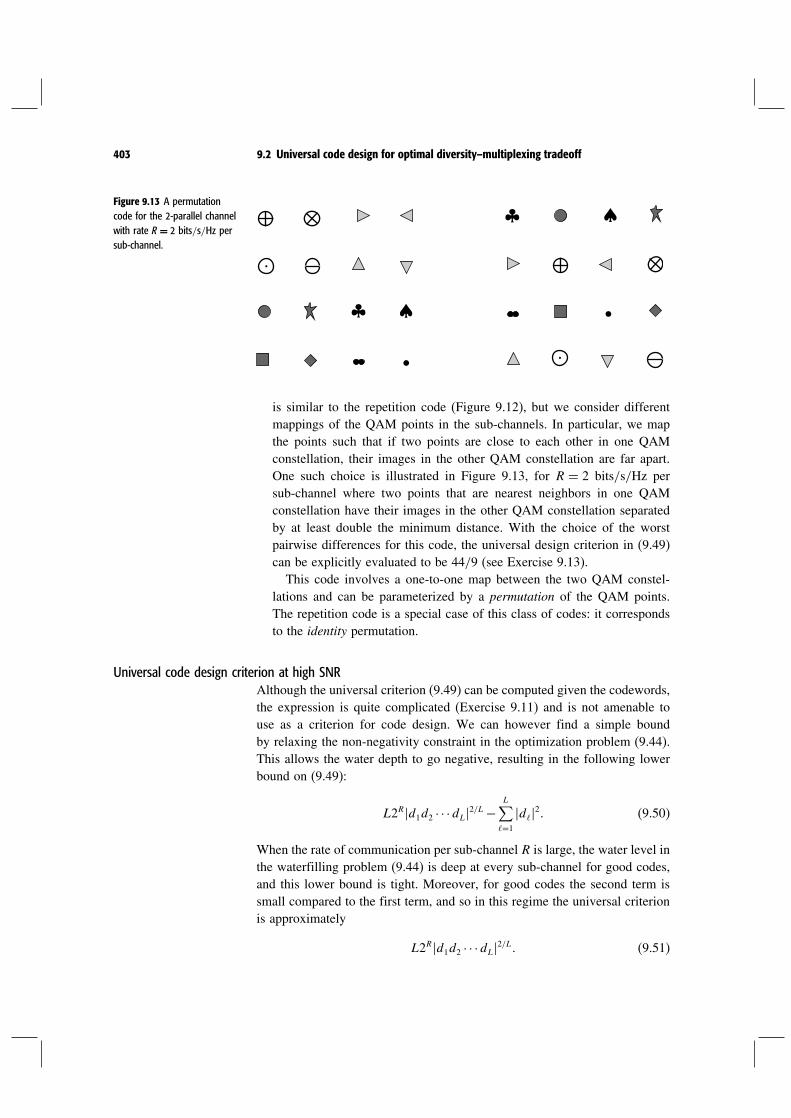
403 9.2 Universal code design for optimal diversity–multiplexing tradeoff
Figure 9.13 A permutationcode for the 2-parallel channelwith rate R = 2 bits/s/Hz persub-channel.
•
•
♣ ♠
♣ ♠
is similar to the repetition code (Figure 9.12), but we consider differentmappings of the QAM points in the sub-channels. In particular, we mapthe points such that if two points are close to each other in one QAMconstellation, their images in the other QAM constellation are far apart.One such choice is illustrated in Figure 9.13, for R = 2 bits/s/Hz persub-channel where two points that are nearest neighbors in one QAMconstellation have their images in the other QAM constellation separatedby at least double the minimum distance. With the choice of the worstpairwise differences for this code, the universal design criterion in (9.49)can be explicitly evaluated to be 44/9 (see Exercise 9.13).This code involves a one-to-one map between the two QAM constel-
lations and can be parameterized by a permutation of the QAM points.The repetition code is a special case of this class of codes: it correspondsto the identity permutation.
Universal code design criterion at high SNRAlthough the universal criterion (9.49) can be computed given the codewords,the expression is quite complicated (Exercise 9.11) and is not amenable touse as a criterion for code design. We can however find a simple boundby relaxing the non-negativity constraint in the optimization problem (9.44).This allows the water depth to go negative, resulting in the following lowerbound on (9.49):
L2Rd1d2 · · ·dL2/L−L∑
=1
d2 (9.50)
When the rate of communication per sub-channel R is large, the water level inthe waterfilling problem (9.44) is deep at every sub-channel for good codes,and this lower bound is tight. Moreover, for good codes the second term issmall compared to the first term, and so in this regime the universal criterionis approximately
L2Rd1d2 · · ·dL2/L (9.51)

404 MIMO III: diversity–multiplexing tradeoff and universal space-time codes
Thus, the universal code design problem is to choose the codewords maxi-mizing the pairwise product distance; in this regime, the criterion coincideswith that of the i.i.d. Rayleigh parallel fading channel (cf. Section 3.2.2).
Property of an approximately universal codeWe can use the universal code design criterion developed above to characterizethe property of a code that makes it approximately universal over the parallelchannel at high SNR. Following the approach in Section 9.2.1, we first definea pairwise typical error event: this is when the argument of the Q
√·/2 in(9.41) is less than 1:
SNR ·L∑
=1
h2d2 < 1 (9.52)
For a code to be approximately universal, we want this event to occur onlywhen the channel is in outage; equivalently, this event should not occurwhenever the channel is not in outage. This translates to saying that theworst-case code design criterion derived above should be greater than 1. Athigh SNR, using (9.51), the condition becomes
d1d2 · · ·dL2/L >1
L2R (9.53)
Moreover, this condition should hold for any pair of codewords. It is verifiedin Exercise 9.14 that this is sufficient to guarantee that a coding schemeachieves the optimal diversity–multiplexing tradeoff of the parallel channel.We saw the permutation code in Figure 9.13 as an example of a code with
good universal design criterion value. This class of codes contains approxi-mately universal codes. To see this, we first need to generalize the essentialstructure in the permutation code example in Figure 9.13 to higher rates andto more than two sub-channels. We consider codes of just a single blocklength to carry out the following generalization.We fix the constellation from which the codeword is chosen in each sub-
channel to be a QAM. Each of these QAM constellations contains the entireinformation to be transmitted: so, the total number of points in the QAMconstellation is 2LR if R is the data rate per sub-channel. The overall code isspecified by the maps between the QAM points for each of the sub-channels.Since the maps are one-to-one, they can be represented by permutations ofthe QAM points. In particular, the code is specified by L− 1 permutations2 L: for each message, say m, we identify one of the QAM points,say q, in the QAM constellation for the first sub-channel. Then, to conveythe message m, the transmit codeword is
q2q Lq

405 9.2 Universal code design for optimal diversity–multiplexing tradeoff
•
• •
♣ ♠
♣ ♠
♣
♠
⊗
⊗
⊗
⊕ ⊕
⊕
i.e., the QAM point transmitted over the th sub-channel is q with 1Figure 9.14 A permutationcode for a parallel channel withthree sub-channels. The entireinformation (4 bits) iscontained in each of the QAMconstellations.
defined to be the identity permutation. An example of a permutation code witha rate of 4/3 bits/s/Hz per sub-channel for L= 3 (so the QAM constellationhas 24 points) is illustrated in Figure 9.14.
Given the physical constraints (the operating SNR, the data rate, and thenumber of sub-channels), the engineer can now choose appropriate permuta-tions to maximize the universal code design criterion. Thus permutation codesprovide a framework within which specific codes can be designed based onthe requirements. This framework is quite rich: Exercise 9.15 shows thateven randomly chosen permutations are approximately universal with highprobability.
Bit-reversal scheme: an operational interpretation of the outage conditionWe can use the concept of approximately universal codes to give an oper-ational interpretation of the outage condition for the parallel channel. To beable to focus on the essential issues, we restrict our attention to just twosub-channels, so L= 2. If we communicate at a total rate 2R bits/s/Hz overthe parallel channel, the no-outage condition is
log1+h12SNR+ log1+h22SNR > 2R (9.54)
One way of interpreting this condition is as though the first sub-channelprovides log1+ h12SNR bits of information and the second sub-channelprovides log1+h22SNR bits of information, and as long as the total num-ber of bits provided exceeds the target rate, then reliable communication ispossible. In the high SNR regime, we exhibit below a permutation code thatmakes the outage condition concrete.Suppose we independently code over the I and Q channels of the two
sub-channels. So we can focus on only one of them, say, the I channel. Wewish to communicate R bits over two uses of the I-channel. Analogous to thetypical event analysis for the scalar channel, we can exactly recover all the Rinformation bits from the first I sub-channel alone if
h12 >22R
SNR (9.55)

406 MIMO III: diversity–multiplexing tradeoff and universal space-time codes
or
h12SNR> 22R (9.56)
However, we do not need to use just the first I sub-channel to recoverall the information bits: the second I sub-channel also contains the sameinformation and can be used in the recovery process. Indeed, if we create xI1by treating the ordered R bits as the binary representation of the points xI1,then one would intuitively expect that if
h12SNR> 22R1 (9.57)
then one should be able to recover at least R1 of the most significant bits ofinformation. Now, if we create xI2 by treating the reversal of the R bits as itsbinary representation, then one should be able to recover at least R2 of themost significant bits, if
h22SNR> 22R2 (9.58)
But due to the reversal, the most significant bits in the representation in thesecond I sub-channel are the least significant bits in the representation in thefirst I sub-channel. Hence, as long as R1+R2 ≥ R, then we can recover all Rbits. This translates to the condition
logh12SNR+ logh22SNR > 2R (9.59)
which is precisely the no-outage condition (9.54) at high SNR.The bit-reversal scheme described here with some slight modifications can
be shown to be approximately universal (Exercise 9.16). A simple variant ofthis scheme is also approximately universal (Exercise 9.17).
Summary 9.2 Universal codes for the parallel channel
A universal code design criterion between two codewords can be computedby finding the channel not in outage that yields the worst-case pairwiseerror probability.
At high SNR and high rate, the universal code design criterion becomesproportional to the product distance:
d1 dL2/L (9.60)
where L is the number of sub-channels and d is the difference betweenthe th components of the codewords.

407 9.2 Universal code design for optimal diversity–multiplexing tradeoff
A code is approximately universal for the parallel channel if its productdistance is large enough: for a code at a data rate of R bits/s/Hz persub-channel, we require
d1d2 · · ·dL2 >1
L2RL (9.61)
Simple bit-reversal schemes are approximately universal for the 2-parallelchannel. Random permutation codes are approximately universal for theL-parallel channel with high probability.
9.2.3 Universal code design for MISO channels
The outage event for the nt ×1 MISO channel (9.22) is
log(
1+h2 SNRnt
)
< R (9.62)
In the case when nt = 2, the Alamouti scheme converts the MISO channelto a scalar channel with gain h and SNR reduced by a factor of 2. Hence,the outage behavior is exactly the same as in the original MISO channel,and the Alamouti scheme provides a universal conversion of the 2×1 MISOchannel to a scalar channel. Any approximately universal scheme for thescalar channel, such as QAM, when used in conjunction with the Alamoutischeme is also approximately optimal for the MISO channel and achieves itsdiversity–multiplexing tradeoff.In the general case when the number of transmit antennas is greater than
two, there is no equivalence of the Alamouti scheme. Here we explore twoapproaches to constructing universal schemes for the general MISO channel.
MISO channel viewed as a parallel channelUsing one transmit antenna at a time converts the MISO channel into a parallelchannel. We have used this conversion in conjunction with repetition codingto argue the classical diversity gain of the MISO channel (cf. Section 3.3.2).Replacing the repetition code with an appropriate parallel channel code (suchas the bit-reversal scheme from Section 9.2.2), we will see that convertingthe MISO channel into a parallel channel is actually tradeoff-optimal for thei.i.d. Rayleigh fading channel.Suppose we want to communicate at rate R = r log SNR bits/s/Hz on the
MISO channel. Using one transmit antenna at a time yields a parallel chan-nel with nt diversity branches and the data rate of communication is R
bits/s/Hz per sub-channel. The optimal diversity gain for the i.i.d. Rayleighparallel fading channel is nt1− r (cf. (9.20)); thus, using one antenna at a

408 MIMO III: diversity–multiplexing tradeoff and universal space-time codes
Figure 9.15 The errorprobability of uncoded QAMwith the Alamouti scheme andthat of a permutation codeover one antenna at a time forthe Rayleigh fading MISOchannel with two transmitantennas: the permutationcode is about 1.5dB worsethan the Alamouti schemeover the plotted errorprobability range.
510–4
10–2
SNR (dB)
10–3
10–1
PeAlamouti code
1510 302520
Permutation code
time in conjunction with a tradeoff-optimal parallel channel code achieves thelargest diversity gain over the i.i.d. Rayleigh fading MISO channel (cf. (9.24)).To understand how much loss the conversion of the MISO channel into
a parallel channel entails with respect to the optimal outage performance,we plot the error probabilities of two schemes with the same rate (R = 2bits/s/Hz): uncoded QAM over the Alamouti scheme and the permutationcode in Figure 9.13. This performance is plotted in Figure 9.15 where we seethat the conversion of the MISO channel into a parallel channel entails a lossof about 1.5 dB in SNR for the same error probability performance.
Universality of conversion to parallel channelWe have seen that the conversion of the MISO channel into a parallel channelis tradeoff-optimal for the i.i.d. Rayleigh fading channel. Is this conversionuniversal? In other words, will a tradeoff-optimal scheme for the parallel chan-nel also be tradeoff-optimal for the MISO channel, under any channel statis-tics? In general, the answer is no. To see this, consider the following MISOchannel model: suppose the channels from all but the first transmit antennaare very poor. To make this example concrete, suppose h = 0 = 2 nt .The tradeoff curve depends on the outage probability (which depends onlyon the statistics of the first channel)
pout = log
(1+ SNRh12
)< R
(9.63)
Using one transmit antenna at a time is a waste of degrees of freedom: sincethe channels from all but the first antenna are zero, there is no point intransmitting any signal on them. This loss in degrees of freedom is explicitin the outage probability of the parallel channel formed by transmitting fromone antenna at a time:
pparallelout =
log
(1+ SNRh12
)< ntR
(9.64)

409 9.2 Universal code design for optimal diversity–multiplexing tradeoff
Comparing (9.64) with (9.63), we see clearly that the conversion to the parallelchannel is not tradeoff-optimal for this channel model.Essentially, using one antenna at a time equates temporal degrees of free-
dom with spatial ones. All temporal degrees of freedom are the same, butthe spatial ones need not be the same: in the extreme example above, thespatial channels from all but the first transmit antenna are zero. Thus, it seemsreasonable that when all the spatial channels are symmetric then the parallelchannel conversion of the MIMO channel is justified. This sentiment is jus-tified in Exercise 9.18, which shows that the parallel channel conversion isapproximately universal over a restricted class of MISO channels: those withi.i.d. spatial channel coefficients.
Universal code design criterionInstead of converting to a parallel channel, one can design universal schemesdirectly for the MISO channel. What is an appropriate code design criterion?In the context of the i.i.d. Rayleigh fading channel, we derived the determinantcriterion for the codeword difference matrices in Section 3.3.2. What is thecorresponding criterion for universal MISO schemes? We can answer thisquestion by considering the worst-case pairwise error probability over allMISO channels that are not in outage.The pairwise error probability (of confusing the transmit codeword matrix
XA with XB) conditioned on a specific MISO channel realization is (cf. (3.82))
XA → XBh=Q
(h∗XA−XB√2
)
(9.65)
In Section 3.3.2 we averaged this quantity over the statistics of the MISOchannel (cf. (3.83)). Here we consider the worst-case over all channels not inoutage:
maxhh2> nt 2R−1
SNR
Q
(h∗XA−XB√2
)
(9.66)
From a basic result in linear algebra, the worst-case pairwise error probabilityin (9.66) can be explicitly written as (Exercise 9.19)
Q
(√1221nt2R−1
)
(9.67)
where 1 is the smallest singular value of the normalized codeword differencematrix
1√SNR
XA−XB (9.68)

410 MIMO III: diversity–multiplexing tradeoff and universal space-time codes
Essentially, the worst-case channel aligns itself in the direction of theweakest singular value of the codeword difference matrix. So, the universalcode design criterion for the MISO channel is to ensure that no singular valueis too small; equivalently
maximize the minimum singular value of the codeword difference matrices.
969
There is an intuitive explanation for this design criterion: a universal codehas to protect itself against the worst channel that is not in outage. The condi-tion of no-outage only puts a constraint on the norm of the channel vector hbut not on its direction. So, the worst channel aligns itself to the “weakestdirection” of the codeword difference matrix to create the most havoc. Thecorresponding worst-case pairwise error probability will be governed by thesmallest singular value of the codeword difference matrix. On the other hand,the i.i.d. Rayleigh channel does not prefer any specific direction: thus thedesign criterion tailored to its statistics requires that the average direction bewell protected and this translates to the determinant criterion. While the twocriteria are different, codes with large determinant tend to also have a largevalue for the smallest singular value; the two criteria (based on worst-caseand average-case) are related in this aspect.We can use the universal code design criterion to derive a property that
makes a code universally achieve the tradeoff curve (as we did for the parallelchannel in the previous section). We want the typical error event to occuronly when the channel is in outage. This corresponds to the argument ofQ√·/2 in the worst-case error probability (9.67) to be greater than 1, i.e.,
21 >
1nt2R−1
≈ 1nt2R
(9.70)
for every pair of codewords. We can explicitly verify that the Alam-outi scheme with independent uncoded QAMs on the two data streamssatisfies the approximate universality property in (9.70). This is done inExercise 9.20.
Summary 9.3 Universal codes for the MISO channel
The MISO channel can be converted into a parallel channel by using onetransmit antenna at a time. This conversion is approximately universal forthe class of MISO channels with i.i.d. fading coefficients.
The universal code design criterion is to maximize the minimum singularvalue of the codeword difference matrices.

411 9.2 Universal code design for optimal diversity–multiplexing tradeoff
9.2.4 Universal code design for MIMO channels
We finally arrive at the multiple transmit and multiple receive antenna slowfading channel:
ym=Hxm+wm (9.71)
The outage event of this channel is
logdetInr +HKxH∗ < R (9.72)
where Kx is the optimizing covariance in (9.29).
Universality of D-BLASTIn Section 8.5, we have seen that the D-BLAST architecture with the MMSE–SIC receiver converts the MIMO channel into a parallel channel with nt
sub-channels. Suppose we pick the transmit strategy Kx in the D-BLASTarchitecture (the covariance matrix represents the combination of the powerallocated to the streams and coordinate system under which they are mixedbefore transmitting, cf. (8.3)) to be the one in (9.72). The important property ofthis conversion is the conservation expressed in (8.88): denoting the effectiveSNR of the kth sub-channel of the parallel channel by SINRk,
logdet(Inr +HKxH
∗)=nt∑
k=1
log1+ SINRk (9.73)
However, SINR1 SINRnt , across the sub-channels are correlated. On theother hand, we saw codes (with just block length 1) that universally achievethe tradeoff curve for any parallel channel (in Section 9.2.2). This meansthat, using approximately universal parallel channel codes for each of theinterleaved streams, the D-BLAST architecture with the MMSE–SIC receiverat a rate of R= r log SNR bits/s/Hz per stream has a diversity gain determinedby the decay rate of
nt∑
k=1
log1+ SINRk < R
(9.74)
with increasing SNR. With n interleaved streams, each having block length 1(i.e.,N = 1 in the notation of Section 8.5.2), the initialization loss in D-BLASTreduces a data rate of R bits/s/Hz per stream into a data rate of nR/n+nt−1bits/s/Hz on the MIMO channel (Exercise 8.27). Suppose we use the D-BLAST architecture in conjunction with a block length 1 universal parallelchannel code for each of n interleaved streams. If this code operates at amultiplexing gain of r on the MIMO channel, the diversity gain obtained

412 MIMO III: diversity–multiplexing tradeoff and universal space-time codes
is, substituting for the rate in (9.74) and comparing with (9.73), the decayrate of
logdet(Inr +HKxH
∗)<rn+nt −1
nlog SNR
(9.75)
Now comparing this with the actual decay behavior of the outage probability(cf. (9.29)), we see that the D-BLAST/MMSE–SIC architecture with n inter-leaved streams used to operate at a multiplexing gain of r over the MIMOchannel has a diversity gain equal to the decay rate of
pmimoout
(rn+nt −1
nlog SNR
)
(9.76)
Thus, with a large number, n, of interleaved streams, the D-BLAST/MMSE–SIC architecture achieves universally the tradeoff curve of the MIMO channel.With a finite number of streams, it is strictly tradeoff-suboptimal. In fact, thetradeoff performance can be improved by replacing the MMSE–SIC receiverby joint ML decoding of all the streams. To see this concretely, let usconsider the 2× 2 MIMO Rayleigh fading channel (so nt = nr = 2) withjust two interleaved streams (so n = 2). The transmit signal lasts 3 timesymbols:
[0 x
1B x
2B
x1A x
2A 0
]
(9.77)
With the MMSE–SIC receiver, the diversity gain obtained at the multiplexingrate of r is the optimal diversity gain at the multiplexing rate of 3r/2. Thisscaled version of the optimal tradeoff curve is depicted in Figure 9.16. On theother hand, with the ML receiver the performance is significantly improved,also depicted in Figure 9.16. This achieves the optimal diversity performancefor multiplexing rates between 0 and 1, and in fact is the scheme that sends4 symbols over 3 symbol times that we were seeking in Section 9.1.5! The per-formance analysis of the D-BLAST architecture with the joint ML receiveris rather intricate and is carried out in Exercise 9.21. Basically, MMSE–SICis suboptimal because it favors stream 1 over stream 2 while ML treats themequally. This asymmetry is only a small edge effect when there are manyinterleaved streams but does impact performance when there are only a smallnumber of streams.
Universal code design criterionWe have seen that the D-BLAST architecture is a universal one, but how do werecognizewhen another space-time code also has good outage performance uni-versally? To answer this question, we can derive a code design criterion basedon the worst-case MIMO channel that is not in outage. Consider space-timecode matrices with block length nt . The worst-case channel aligns itself in the“weakest directions” afforded by a codeword pair difference matrix. With just

413 9.2 Universal code design for optimal diversity–multiplexing tradeoff
Figure 9.16 Tradeoffperformance for the D-BLASTarchitecture with the MLreceiver and with theMMSE–SIC receiver.
r
1
d(r) 4
ML receiverMMSE-SIC receiver
00
23
43
one receive antenna, the MISO channel is simply a row vector and it alignsitself in the direction of the smallest singular value of the codeword differ-ence matrix (cf. Section 9.2.3). Here, there are nmin directions for the MIMOchannel and the corresponding design criterion is an extension of that for theMISO channel: the universal code design criterion at high SNR is to maximize
12 · · ·nmin (9.78)
where 1 nminare the smallest nmin singular values of the normalized
codeword difference matrices (cf. (9.68)). The derivation is carried out inExercise 9.22. With nt ≤ nr , this is just the determinant criterion, derived inChapter 3 by averaging the code performance over the i.i.d. Rayleigh statistics.The exact code design criterion at an intermediate value of SNR is sim-
ilar to the expression for the universal code design for the parallel channel(cf. (9.49)).
Property of an approximately universal codeUsing exactly the same arguments as in Section 9.2.2, we can use the uni-versal code design criterion developed above to characterize the property ofa code that makes it approximately universal over the MIMO channel (seeExercise 9.23):
12 · · ·nmin2/nmin >
1nmin2R/nmin
(9.79)
As in the parallel channel (cf. Exercise 9.14), this condition is only anorder-of-magnitude one. A relaxed condition
12 · · ·nmin2/nmin > c · 1
nmin2R/nmin for some constant c > 0 (9.80)

414 MIMO III: diversity–multiplexing tradeoff and universal space-time codes
can also be used for approximate universality: it is sufficient to guarantee thatthe code achieves the optimal diversity–multiplexing tradeoff. We can makea couple of interesting observations immediately from this result.
• If a code satisfies the condition for approximate universality in (9.80) foran nt×nr MIMO channel with nr ≥ nt , i.e., the number of receive antennasis equal to or larger than the number of transmit antennas, then it is alsoapproximately universal for an nt × l MIMO channel with l≥ nr .
• The singular values of the normalized codeword matrices are upper boundedby 2
√nt (Exercise 9.24). Thus, a code that satisfies (9.80) for an nt ×nr
MIMO channel also satisfies the criterion in (9.80) for an nt × l MIMOchannel with l ≤ nr . Thus is it also approximately universal for the nt × l
MIMO channel with l≤ nr .
We can conclude the following from the above two observations:
A code that satisfies (9.80) for an nt×nt MIMO channel is approximatelyuniversal for an nt ×nr MIMO channel for every value of the number ofreceive antennas nr .
Exercise 9.25 shows a rotation code that satisfies (9.80) for the 2× 2 MIMOchannel; so this code is approximately universal for every 2×nr MIMOchannel.
We have already observed that the D-BLAST architecture with approx-imately universal parallel channel codes for the interleaved streams isapproximately universal for the MIMO channel. Alternatively, we can see itsapproximate universality by explicitly verifying that it satisfies the conditionin (9.80) with nt = nr . Here, we will see this for the 2×2 channel with twointerleaved streams in the D-BLAST transmit codeword matrix (cf. (9.77)).The normalized codeword difference matrix can be written as
D=[
0 d1B d
2B
d1A d
2A 0
]
(9.81)
where(dB d
A
)is thenormalizedpairwisedifferencecodeword for anapprox-
imately universal parallel channel code and satisfies the condition in (9.53):
dB d
A > 1
4 ·2R = 12 (9.82)
Here R is the rate in bits/s/Hz in each of the streams. The product of the twosingular values of D is
21
22 = detDD∗
= d1B d
1A 2+d2
B d2A 2+d2
B d1A 2
>1
4 ·2R (9.83)

415 9.2 Universal code design for optimal diversity–multiplexing tradeoff
where the last inequality follows from (9.82). A rate of R bits/s/Hz oneach of the streams corresponds to a rate of 2R/3 bits/s/Hz on the MIMOchannel. Thus, comparing (9.83) with (9.79), we have verified the approximateuniversality of D-BLAST at a reduced rate due to the initialization loss. Inother words, the diversity gain obtained by the D-BLAST architecture in(9.77) at a multiplexing rate of r over the MIMO channel is d∗3r/2.
Discussion 9.1 Universal codes in the downlink
Consider the downlink of a cellular system where the base-stations areequipped with multiple transmit antennas. Suppose we want to broadcastthe same information to all the users in the cell in the downlink. We wouldlike our transmission scheme to not depend on the number of receiveantennas at the users: each user could have a different number of receiveantennas, depending on the model, age, and type of the mobile device.Universal MIMO codes provide an attractive solution to this problem.
Suppose we broadcast the common information at rate R using a space-time code that satisfies (9.79) for an nt ×nt MIMO channel. Since thiscode is approximately universal for every nt × nr MIMO channel, thediversity seen by each user is simultaneously the best possible at rate R.To summarize: the diversity gain obtained by each user is the best possiblewith respect to both• the number of receive antennas it has, and• the statistics of the fading channel the user is currently experiencing.
Chapter 9 The main plot
For a slow fading channel at high SNR, the tradeoff between data rateand error probability is captured by the tradeoff between multiplexing anddiversity gains. The optimal diversity gain d∗r is the rate at which outageprobability decays with increasing SNR when the data rate is increasing asr log SNR. The classical diversity gain is the diversity gain at a fixed rate,i.e., the multiplexing gain r = 0.
The optimal diversity gain d∗r is determined by the outage probabilityof the channel at a data rate of r log SNR bits/s/Hz. The operational inter-pretation is via the existence of a universal code that achieves reliablecommunication simultaneously over all channels that are not in outage.
The universal code viewpoint provides a new code design criterion. Insteadof averaging over the channel statistics, we consider the performance of acode over the worst-case channel that is not in outage.

416 MIMO III: diversity–multiplexing tradeoff and universal space-time codes
• For the parallel channel, the universal criterion is to maximize the productof the codeword differences. Somewhat surprisingly, this is the same asthe criterion arrived at by averaging over the Rayleigh channel statistics.
• For the MISO channel, the universal criterion is to maximize the smallestsingular value of the codeword difference matrices.
• For the nt×nr MIMO channel, the universal criterion is to maximize theproduct of the nmin smallest singular values of the codeword differencematrices. With nr ≥ nt , this criterion is the same as that arrived at byaveraging over the i.i.d. Rayleigh statistics.
The MIMO channel can be transformed into a parallel channel viaD-BLAST. This transformation is universal: universal parallel channelcodes for each of the interleaved streams in D-BLAST serve as a uni-versal code for the MIMO channel. The rate loss due to initialization inD-BLAST can be reduced by increasing the number of interleaved streams.For the MISO channel, however, the D-BLAST transformation with onlyone stream, i.e., using the transmit antennas one at a time, is approximatelyuniversal within the class of channels that have i.i.d. fading coefficients.
9.3 Bibliographical notes
The design of space-time codes has been a fertile area of research. There are books thatprovide a comprehensive viewof the subject: for example, see the books byLarsson, Sto-ica and Ganesan [72], and Paulraj et al. [89]. Several works have recognized the tradeoffbetween diversity andmultiplexing gains. The formulation of the coarser scaling of errorprobability and data rate and the corresponding characterization of their fundamentaltradeoff for the i.i.d. Rayleigh fading channel is the work of Zheng and Tse [156].
The notion of universal communication, i.e., communicating reliably over a class ofchannel, was first formulated in the context of discrete memoryless channels by Black-well et al. [10], Dobrushin [31] and Wolfowitz [146]. They showed the existence ofuniversal codes. The results were later extended to Gaussian channels by Root andVaraiya [103]. Motivated by these information theoretic results, Wesel and his coau-thors have studied the problem of universal code design in a sequence of works, start-ing with his Ph.D. thesis [142]. The worst-case code design metric for the parallelchannel and a heuristic derivation of the product distance criterion were obtained in[143]. This was extended to MIMO channels in [67]. The general concept of approxi-mate universality in the high SNR regime was formulated by Tavildar and Viswanath[118]; earlier, in the special case of the 2× 2 MIMO channel, Yao and Wornell [152]used the determinant condition (9.80) to show the tradeoff-optimality of their rotation-based codes. The conditions derived for approximate universality, (cf. (9.38), (9.53),(9.70) and (9.80)) are also necessary; this is derived in Tavildar and Viswanath [118].
The design of tradeoff-optimal space-time codes is an active area of research, andseveral approaches have been presented recently. They include: rotation-based codesfor the 2×2 channel, by Yao and Wornell [152] and Dayal and Varanasi [29]; latticespace-time (LAST) codes, by El Gamal et al. [34]; permutation codes for the parallel

417 9.4 Exercises
channel derived from D-BLAST, by Tavildar and Viswanath [118]; Golden code, byBelfiore et al. [5] for the 2× 2 channel; codes based on cyclic divisional algebras,by Elia et al. [35]. The tradeoff-optimality of most of these codes is demonstrated byverifying the approximate universality conditions.
9.4 Exercises
Exercise 9.1 Consider the L-parallel channel with i.i.d. Rayleigh coefficients. Showthat the optimal diversity gain at a multiplexing rate of r per sub-channel is L−Lr.
Exercise 9.2 Consider therepetitionschemewhere thesamecodeword is transmittedoverthe L i.i.d. Rayleigh sub-channels of a parallel channel. Show that the largest diversitygain this scheme can achieve at a multiplexing rate of r per sub-channel is L1−Lr.
Exercise 9.3 Consider the repetition scheme of transmitting the same codeword overthe nt transmit antennas, one at a time, of an i.i.d. Rayleigh fading nt×nr MIMO chan-nel. Show that the maximum diversity gain this scheme can achieve, at a multiplexingrate of r, is ntnr1−ntr.
Exercise 9.4 Consider using the Alamouti scheme over a 2×nr i.i.d. Rayleigh fadingMIMO channel. The transmit codeword matrix spans two symbol times m= 12 (cf.Section 3.3.2):
[u1 − u∗
2
u2 u∗1
]
(9.84)
1. With this input to the MIMO channel in (9.71), show that we can write the outputover the two time symbols as (cf. (3.75))
[y1
y2∗t
]
=[
h1 h2
h∗2
t −h∗1
t
][u1
u2
]
+[
w1w2∗t
]
(9.85)
Here we have denoted the two columns of H by h1 and h2.2. Observing that the two columns of the effective channel matrix in (9.85) are
orthogonal, show that we can extract simple sufficient statistics for the data symbolsu1 u2 (cf. (3.76)):
ri = Hui+wi i= 12 (9.86)
Here H2 denotes h12 +h22 and the additive noises w1 and w2 are i.i.d. 01.
3. Conclude that the maximum diversity gain seen by either stream (u1 or u2) at amultiplexing rate of r per stream is 2nr1− r.
Exercise 9.5 Consider the V-BLAST architecture with a bank of decorrelators for thent × nr i.i.d. Rayleigh fading MIMO channel with nr ≥ nt . Show that the effectivechannel seen by each stream is a scalar fading channel with distribution 2
2nr−nt+1.Conclude that the diversity gain with a multiplexing gain of r is nr−nt+1 1−r/nt.

418 MIMO III: diversity–multiplexing tradeoff and universal space-time codes
Exercise 9.6 Verify the claim in (9.28) by showing that the sum of the pairwise errorprobabilities in (9.26), with xAxB each a pair of QAM symbols (the union bound onthe error probability) has a decay rate of 2− r with increasing SNR.
Exercise 9.7 The result in Exercise 9.6 can be generalized. Show that the diversitygain of transmitting uncoded QAMs (each at a rate of R= r/n log SNR bits/s/Hz) onthe n transmit antennas of an i.i.d. Rayleigh fading MIMO channel with n receiveantennas is n− r.
Exercise 9.8 Consider the expression for pmimoout in (9.29) and for piid
out in (9.30). Supposethat the entries of the MIMO channel H have some joint distribution and are notnecessarily i.i.d. Rayleigh.1. Show that
piidoutr log SNR≥ pmimo
out r log SNR≥ logdetInr + SNR HH∗ < r log SNR(9.87)
2. Show that the lower bound above decays at the same polynomial rate as piidout with
increasing SNR.3. Conclude that the polynomial decay rates of both pmimo
out and piidout with increasing
SNR are the same.
Exercise 9.9 Consider a scalar slow fading channel
ym= hxm+wm (9.88)
with an optimal diversity–multiplexing tradeoff d∗·, i.e.,
limSNR→
logpoutr log SNRlog SNR
=−d∗r (9.89)
Let > 0 and consider the following event on the channel gain h:
= h log1+h2SNR1− < R (9.90)
1. Show, by conditioning on the event or otherwise, that the probability of errorpeSNR of QAM with rate R= r log SNR bits/symbol satisfies
limSNR→
logpeSNRlog SNR
≤−d∗r1− (9.91)
Hint: you should show that conditional on the not happening, the probabilityof error decays very fast and is negligible compared to the probability of errorconditional on happening.
2. Hence, conclude that QAM achieves the diversity–multiplexing tradeoff of anyscalar channel.
3. More generally, show that any constellation that satisfies the condition (9.38)achieves the diversity–multiplexing tradeoff curve of the channel.
4. Even more generally, show that any constellation that satisfies the condition
d2min > c · 1
2Rfor any constant c > 0 (9.92)

419 9.4 Exercises
achieves the diversity–multiplexing tradeoff curve of the channel. This shows thatthe condition (9.38) is really only an order-of-magnitude condition. A slightlyweaker version of this condition is also necessary for a code to be approximatelyuniversal; see [118].
Exercise 9.10 Consider coding over a block length N for communication over theparallel channel in (9.17). Derive the universal code design criterion, generalizing thederivation in Section 9.2.2 over a block length of 1.
Exercise 9.11 In this exercise we will try to explicitly calculate the universal codedesign criterion for the parallel fading channel; for given differences between a pairof normalized codewords, the criterion is to maximize the expression in (9.49).1. Suppose the codeword differences on all the sub-channels have the same magnitude,
i.e., d1 = · · · = dL. Show that in this case the worst case channel is the same overall the sub-channels and the universal criterion in (9.49) simplifies considerably to
L2R−1d12 (9.93)
2. Suppose the codeword differences are ordered: d1 ≤ · · · ≤ dL.(a) Argue that if the worst case channel h on the th sub-channel is non-zero,
then it is also non-zero on all the sub-channels 1 −1.(b) Consider the largest k such that
dk2k ≤ 2RLd1 · · ·dk2 ≤ dk+12k (9.94)
with dL+1 defined as +. Argue that the worst-case channel is zero on all thesub-channelsk+1 L.Observe thatk=Lwhenall thecodeworddifferenceshave the same magnitude; this is in agreement with the result in part (1).
3. Use the results of the previous part (and the notation of k from (9.94)) to derivean explicit expression for in (9.49):
kd1 · · ·dk2 = 2−RL (9.95)
Conclude that the universal code design criterion is to maximize
(
k2RLd1d2 · · ·dk21/k−k∑
=1
d2)
(9.96)
Exercise 9.12 Consider the repetition code illustrated in Figure 9.12. This code is forthe 2-parallel channel with R= 2bits/s/Hz per sub-channel. We would like to evaluatethe value of the universal design criterion, minimized over all pairs of codewords.Show that this value is equal to 8/3. Hint: The smallest value is yielded by choosingthe pair of codewords as nearest neighbors in the QAM constellation. Since this is arepetition code, the codeword differences are the same for both the channels; now use(9.93) to evaluate the universal design criterion.
Exercise 9.13 Consider the permutation code illustrated in Figure 9.13 (withR= 2bits/s/Hz per sub-channel). Show that the smallest value of the universal designcriterion, minimized over all choices of codeword pairs, is equal to 44/9.

420 MIMO III: diversity–multiplexing tradeoff and universal space-time codes
Exercise 9.14 In this exercise we will explore the implications of the condition forapproximate universality in (9.53).1. Show that if a parallel channel scheme satisfies the condition (9.53), then it achieves
the diversity–multiplexing tradeoff of the parallel channel.Hint:DoExercise 9.9 first.2. Show that the diversity–multiplexing tradeoff can still be achieved even when the
scheme satisfies a more relaxed condition:
d1d2 · · ·dL2/L > c · 1L2R
for some constant c > 0 (9.97)
Exercise 9.15 Consider the class of permutatation codes for the L-parallel channeldescribed in Section 9.2.2. The codeword is described as q2q Lqwhere qbelongs to a normalized QAM (so that each of the I and Q channels are peak constrainedby ±1) with 2LR points; so, the rate of the code is R bits/s/Hz per sub-channel. In thisexercise we will see that this class contains approximately universal codes.1. Consider random permutations with the uniform measure; since there are 2LR!
of them, each of the permutations occurs with probability 1/2LR!. Show that theaverage inverse product of the pairwise codeword differences, averaged over boththe codeword pairs and the random permutations, is upper bounded as follows:
2 L
[1
2LR2LR−1
× ∑
q1 =q2
1q1−q222q1−2q22 · · · Lq1−Lq22
]
≤ LLRL
(9.98)
2. Conclude from the previous part that there exist permutations 2 L such that
12LR
∑
q1
(∑
q2 =q1
1q1−q222q1−2q22 · · · Lq1−Lq22
)
≤ LLRL2LR (9.99)
3. Now suppose we fix q1 and consider the sum of the inverse product of all thepossible pairwise codeword differences:
fq1 =∑
q2 =q1
1q1−q222q1−2q22 · · · Lq1−Lq22
(9.100)
Since fq1≥ 0, argue from (9.99) that at least half the QAM points q1 must havethe property that
fq1≤ 2LLRL2LR (9.101)
Further, conclude that for such q1 (they make up at least half of the total QAMpoints) we must have for every q2 = q1 that
q1−q222q1−2q22 · · · Lq1−Lq22 ≥1
2LLRL2LR (9.102)

421 9.4 Exercises
4. Finally, conclude that there exists a permutation code that is approximately uni-versal for the parallel channel by arguing the following:• Expurgating no more than half the number of QAM points only reduces the
total rate LR by no more than 1 bit/s/Hz and thus does not affect the multiplex-ing gain.
• The product distance condition on the permutation codeword differences in(9.102) does not quite satisfy the condition for approximate universality in (9.97).Relax the condition in (9.97) to
d1d2 · · ·dL2/L > c · 1R2R
for some constant c > 0 (9.103)
and show that this is sufficient for a code to achieve the optimal diversity–multiplexing tradeoff curve.
Exercise 9.16 Consider the bit-reversal scheme for the parallel channel described inSection 9.2.2. Strictly speaking, the condition in (9.57) is not true for every integerbetween 0 and 2R−1. However, the set of integers for which this is not true is small(i.e., expurgating them will not change the multiplexing rate of the scheme). Thus thebit-reversal scheme with an appropriate expurgation of codewords is approximatelyuniversal for the 2-parallel channel. A reading exercise is to study [118] where theexpurgated bit-reversal scheme is described in detail.
Exercise 9.17 Consider the bit-reversal scheme described in Section 9.2.2 but withevery alternate bit flipped after the reversal. Then for every pair of normalized code-word differences, it can be shown that
d1d22 >1
64 ·22R (9.104)
where the data rate is R bits/s/Hz per sub-channel. Argue now that the bit-reversalscheme with alternate bit flipping is approximately universal for the 2-parallel channel.A reading exercise is to study the proof of (9.104) in [118]. Hint: Compare (9.104)with (9.53) and use the result derived in Exercise 9.14.
Exercise 9.18 Consider a MISO channel with the fading channels from the nt transmitantennas, h1 hnt
, i.i.d.1. Show that
log
(
1+ SNRnt
nt∑
=1
h2)
< r log SNR
(9.105)
and
nt∑
=1
log1+ SNRh2 < ntr log SNR
(9.106)
have the same decay rate with increasing SNR.2. Interpret (9.105) and (9.106) with the outage probabilities of the MISO channel
and that of a parallel channel obtained through an appropriate transformation ofthe MISO channel, respectively. Argue that the conversion of the MISO channelinto a parallel channel discussed in Section 9.2.3 is approximately universal forthe class of i.i.d. fading coefficients.

422 MIMO III: diversity–multiplexing tradeoff and universal space-time codes
Exercise 9.19 Consider an nt ×nt matrix D. Show that
minhh=1
h∗DD∗h= 21 (9.107)
where 1 is the smallest singular value of D.
Exercise 9.20 Consider the Alamouti transmit codeword (cf. (9.84)) with u1 u2 inde-pendent uncoded QAMs with 2R points in each.1. For every codeword difference matrix
[d1 − d∗
2
d2 d∗1
]
(9.108)
show that the two singular values are the same and equal to√d12+d22.
2. With the codeword difference matrix normalized as in (9.68) and each of the QAMsymbols u1 u2 constrained in power of SNR/2 (i.e., both the I and Q channels arepeak constrained by ±√SNR/2), show that if the codeword difference d is notzero, then it is
d2 ≥22R
= 12
3. Conclude from the previous steps that the square of the smallest singular valueof the codeword difference matrix is lower bounded by 2/2R. Since the conditionfor approximate universality in (9.70) is an order-of-magnitude one (the constantfactor next to the 2R term does not matter, see Exercises 9.9 and 9.14), we haveexplicitly shown that the Alamouti scheme with uncoded QAMs on the two streamsis approximately universal for the two transmit antenna MISO channel.
Exercise 9.21 Consider the D-BLAST architecture in (9.77) with just two interleavedstreams for the 2× 2 i.i.d. Rayleigh fading MIMO channel. The two streams areindependently coded at rate R = r log SNR bits/s/Hz each and composed of the pairof codewords
(xA x
B
)for = 12. The two streams are coded using an approx-
imately universal parallel channel code (say, the bit-reversal scheme described inSection 9.2.2).
A union bound averaged over the Rayleigh MIMO channel can be used to showthat the diversity gain obtained by each stream with joint ML decoding is 4− 2r.A reading exercise is to study the proof of this result in [118].
Exercise 9.22 [67] Consider transmitting codeword matrices of length at least nt onthe nt ×nr MIMO slow fading channel at rate R bits/s/Hz (cf. (9.71)).1. Show that the pairwise error probability between two codeword matrices XA and
XB, conditioned on a specific realization of the MIMO channel H, is
Q
(√SNR2
HD2)
(9.109)
where D is the normalized codeword difference matrix (cf. (9.68)).

423 9.4 Exercises
2. Writing the SVDs H = U1V∗1 and D = U2V∗
2, show that the pairwise errorprobability in (9.109) can be written as
Q
(√SNR2
V∗1U22
)
(9.110)
3. Suppose the singular values are increasingly ordered in and decreasingly orderedin . For fixed U2, show that the channel eigendirections V∗
1 that minimizethe pairwise error probability in (9.110) are
V1 = U2 (9.111)
4. Observe that the channel outage condition depends only on the singular values of H (cf. Exercise 9.8). Use the previous parts to conclude that the calculationof the worst-case pairwise error probability for the MIMO channel reduces to theoptimization problem
min1 nmin
SNR2
L∑
=1
22 (9.112)
subject to the constraint
nmin∑
=1
log(
1+ SNRnt
2)
≥ R (9.113)
Here we have written
= diag1 nmin and = diag1 nt
5. Observe that the optimization problem in (9.112) and the constraint (9.113) arevery similar to the corresponding ones in the parallel channel (cf. (9.43) and (9.40),respectively). Thus the universal code design criterion for the MIMO channel isthe same as that of a parallel channel (cf. (9.47)) with the following parameters:• there are nmin sub-channels,• the rate per sub-channel is R/nmin bits/s/Hz,• the parallel channel coefficients are 1 nmin
, the singular values of theMIMO channel, and
• the codeword differences are the smallest singular values, 1 nmin, of the
codeword difference matrix.
Exercise 9.23 Using the analogy between the worst-case pairwise error probability of aMIMO channel and that of an appropriately defined parallel channel (cf. Exercise 9.22),justify the condition for approximate universality for the MIMO channel in (9.79).
Exercise 9.24 Consider transmitting codeword matrices of length l≥ nt on the nt×nr
MIMO slow fading channel. The total power constraint is SNR, so for any transmitcodeword matrix X, we have X2 ≤ lSNR. For a pair of codeword matrices XA andXB, let the normalized codeword difference matrix be D (normalized as in (9.68)).

424 MIMO III: diversity–multiplexing tradeoff and universal space-time codes
1. Show that D satisfies
D2 ≤ 2SNR
XA2+XB2≤ 4l (9.114)
2. Writing the singular values of D as 1 nt, show that
nt∑
=1
2 ≤ 4l (9.115)
Thus, each of the singular values is upper bounded by 2√l, a constant that does
not increase with SNR.
Exercise 9.25 [152] Consider the following transmission scheme (spanning two sym-bols) for the two transmit antenna MIMO channel. The entries of the transmit codewordmatrix X = xij are defined as
[x11x22
]
= R1
[u1
u2
]
and
[x21x12
]
= R2
[u3
u4
]
(9.116)
Here u1 u2 u3 u4 are independent QAMs of size 2R/2 each (so the data rate of thisscheme is R bits/s/Hz). The rotation matrix R is (cf. (3.46))
R =[cos − sin sin cos
]
(9.117)
With the choice of the angles 1 2 equal to 1/2 tan−1 2 and 1/2 tan−11/2 radiansrespectively, Theorem 2 of [152] shows that the determinant of every normalizedcodeword difference matrix D satisfies
detD2 ≥ 110 ·2R (9.118)
Conclude that the code described in (9.116), with the appropriate choice of the angles1 2 above, is approximately universal for every MIMO channel with two transmitantennas.

C H A P T E R
10 MIMO IV: multiuser communication
In Chapters 8 and 9, we have studied the role of multiple transmit and receiveantennas in the context of point-to-point channels. In this chapter, we shiftthe focus to multiuser channels and study the role of multiple antennas inboth the uplink (many-to-one) and the downlink (one-to-many). In addition toallowing spatial multiplexing and providing diversity to each user, multipleantennas allow the base-station to simultaneously transmit or receive datafrom multiple users. Again, this is a consequence of the increase in degreesof freedom from having multiple antennas.We have considered several MIMO transceiver architectures for the point-
to-point channel in Chapter 8. In some of these, such as linear receivers withor without successive cancellation, the complexity is mainly at the receiver.Independent data streams are sent at the different transmit antennas, andno cooperation across transmit antennas is needed. Equating the transmitantennas with users, these receiver structures can be directly used in the uplinkwhere the users have a single transmit antenna each but the base-station hasmultiple receive antennas; this is a common configuration in cellular wirelesssystems.It is less apparent how to come up with good strategies for the downlink,
where the receive antennas are at the different users; thus the receiver struc-ture has to be separate, one for each user. However, as will see, there is aninteresting duality between the uplink and the downlink, and by exploiting thisduality, one can map each receive architecture for the uplink to a correspond-ing transmit architecture for the downlink. In particular, there is an interestingprecoding strategy, which is the “transmit dual” to the receiver-based succes-sive cancellation strategy. We will spend some time discussing this.The chapter is structured as follows. In Section 10.1, we first focus on
the uplink with a single transmit antenna for each user and multiple receiveantennas at the base-station. We then, in Section 10.2, extend our study to theMIMO uplink where there are multiple transmit antennas for each user. InSections 10.3 and 10.4, we turn our attention to the use of multiple antennasin the downlink. We study precoding strategies that achieve the capacity of
425

426 MIMO IV: multiuser communication
the downlink. We conclude in Section 10.5 with a discussion of the systemimplications of using MIMO in cellular networks; this will link up the newinsights obtained here with those in Chapters 4 and 6.
10.1 Uplink with multiple receive antennas
We begin with the narrowband time-invariant uplink with each user havinga single transmit antenna and the base-station equipped with an array ofantennas (Figure 10.1). The channels from the users to the base-station aretime-invariant. The baseband model is
ym=K∑
k=1
hkxkm+wm (10.1)
with ym being the received vector (of dimension nr , the number of receiveantennas) at time m, and hk the spatial signature of user k impinged on thereceive antenna array at the base-station. User k’s scalar transmit symbol attime m is denoted by xkm and wm is i.i.d. 0N0Inr noise.
10.1.1 Space-division multiple access
In the literature, the use of multiple receive antennas in the uplink is oftencalled space-division multiple access (SDMA): we can discriminate amongstthe users by exploiting the fact that different users impinge different spatialsignatures on the receive antenna array.An easy observation we can make is that this uplink is very similar to
the MIMO point-to-point channel in Chapter 5 except that the signals sent
Figure 10.1 The uplink withsingle transmit antenna at eachuser and multiple receiveantennas at the base-station.
out on the transmit antennas cannot be coordinated. We studied preciselysuch a signaling scheme using separate data streams on each of the transmitantennas in Section 8.3. We can form an analogy between users and transmitantennas (so nt , the number of transmit antennas in the MIMO point-to-pointchannel in Section 8.3, is equal to the number of users K). Further, theequivalent MIMO point-to-point channel H is h1 hK, constructed fromthe SIMO channels of the users.Thus, the transceiver architecture in Figure 8.1 in conjunction with the
receiver structures in Section 8.3 can be used as an SDMA strategy. Forexample, each of the user’s signal can be demodulated using a linear decorre-lator or an MMSE receiver. The MMSE receiver is the optimal compromisebetween maximizing the signal strength from the user of interest and sup-pressing the interference from the other users. To get better performance, onecan also augment the linear receiver structure with successive cancellationto yield the MMSE–SIC receiver (Figure 10.2). With successive cancella-tion, there is also a further choice of cancellation ordering. By choosing a

427 10.1 Uplink with multiple receive antennas
MMSE Receiver 2
MMSE Receiver 1
y[m]
User 2Decode User 2
Subtract User 1
User 1Decode User 1
different order, users are prioritized differently in the sharing of the commonFigure 10.2 The MMSE–SICreceiver: user 1’s data is firstdecoded and then thecorresponding transmit signalis subtracted off before the nextstage. This receiver structure,by changing the ordering ofcancellation, achieves the twocorner points in the capacityregion.
resource of the uplink channel, in the sense that users canceled later are treatedbetter.Provided that the overall channel matrix H is well-conditioned, all of
these SDMA schemes can fully exploit the total number of degrees of free-dom minKnr of the uplink channel (although, as we have seen, differentschemes have different power gains). This translates to being able to simul-taneously support multiple users, each with a data rate that is not limitedby interference. Since the users are geographically separated, their trans-mit signals arrive in different directions at the receive array even whenthere is limited scattering in the environment, and the assumption of a well-conditionedH is usually valid. (Recall Example 7.4 in Section 7.2.4.) Contrastthis to the point-to-point case when the transmit antennas are co-located, anda rich scattering environment is needed to provide a well-conditioned channelmatrix H.Given the power levels of the users, the achieved SINR of each user can
be computed for the different SDMA schemes using the formulas derived inSection 8.3 (Exercise 10.1). Within the class of linear receiver architecture,we can also formulate a power control problem: given target SINR require-ments for the users, how does one optimally choose the powers and linearfilters to meet the requirements? This is similar to the uplink CDMA powercontrol problem described in Section 4.3.1, except that there is a furtherflexibility in the choice of the receive filters as well as the transmit powers.The first observation is that for any choice of transmit powers, one alwayswants to use the MMSE filter for each user, since that choice maximizes theSINR for every user. Second, the power control problem shares the basicmonotonicity property of the CDMA problem: when a user lowers its transmitpower, it creates less interference and benefits all other users in the system.As a consequence, there is a component-wise optimal solution for the pow-ers, where every user is using the minimum possible power to support theSINR requirements. (See Exercise 10.2.) A simple distributed power controlalgorithm will converge to the optimal solution: at each step, each user firstupdates its MMSE filter as a function of the current power levels of the otherusers, and then updates its own transmit power so that its SINR requirementis just met. (See Exercise 10.3.)

428 MIMO IV: multiuser communication
10.1.2 SDMA capacity region
In Section 8.3.4, we have seen that the MMSE–SIC receiver achieves thebest total rate among all the receiver structures. The performance limit of theuplink channel is characterized by the notion of a capacity region, introducedin Chapter 6. How does the performance achieved by MMSE–SIC compareto this limit?With a single receive antenna at the base-station, the capacity region of
the two-user uplink channel was presented in Chapter 6; it is the pentagon inFigure 6.2:
R1 < log(
1+ P1
N0
)
R2 < log(
1+ P2
N0
)
R1+R2 < log(
1+ P1+P2
N0
)
where P1 and P2 are the average power constraints on users 1 and 2 respec-tively. The individual rate constraints correspond to the maximum rate thateach user can get if it has the entire channel to itself; the sum rate constraintis the total rate of a point-to-point channel with the two users acting as twotransmit antennas of a single user, but sending independent signals.The SDMA capacity region, for the multiple receive antenna case, is the
natural extension (Appendix B.9 provides a formal justification):
R1 < log(
1+ h12P1
N0
)
(10.2)
R2 < log(
1+ h22P2
N0
)
(10.3)
R1+R2 < logdet(
Inr +1N0
HKxH∗)
(10.4)
where Kx = diagP1P2. The capacity region is plotted in Figure 10.3.The capacities of the point-to-point SIMO channels from each user to the
base-station serve as the maximum rate each user can reliably communicateat if it has the entire channel to itself. These yield the constraints (10.2)and (10.3). The point-to-point capacity for user kk = 12 is achieved byreceive beamforming (projecting the received vector y in the direction of hk),converting the effective channel into a SISO one, and then decoding the dataof the user.Inequality (10.4) is a constraint on the sum of the rates that the users can
communicate at. The right hand side is the total rate achieved in a point-to-point channel with the two users acting as two transmit antennas of one userwith independent inputs at the antennas (cf. (8.2)).

429 10.1 Uplink with multiple receive antennas
Figure 10.3 Capacity region ofthe two-user SDMA uplink.
A
B
C
R1
R2
R1 + R2 = log det
log 1+|| h2||2P2
N0
Inr+
HKxH*
N0
log 1+|| h1||2P1
N0
Since MMSE–SIC receivers (in Figure 10.2) are optimal with respect toachieving the total rate of the point-to-point channel with the two users actingas two transmit antennas of one user, it follows that the rates for the twousers that this architecture can achieve in the uplink meets inequality (10.4)with equality. Moreover, if we cancel user 1 first, user 2 only has to contendwith the background Gaussian noise and its performance meets the single-user bound (10.2). Hence, we achieve the corner point A in Figure 10.3.By reversing the cancellation order, we achieve the corner point B. Thus,MMSE–SIC receivers are information theoretically optimal for SDMA in thesense of achieving rate pairs corresponding to the two corner points A and B.Explicitly, the rate point A is given by the rate tuple R1R2:
R2 = log(
1+ P2h22N0
)
R1 = log1+P1h∗1N0Inr +P2h2h
∗2
−1h1 (10.5)
where P1h∗1N0Inr +P2h
∗2h
∗2
−1h1 is the output SIR of the MMSE receiver foruser 1 treating user 2’s signal as colored Gaussian interference (cf. (8.62)).For the single receive antenna (scalar) uplink channel, we have already seen
in Section 6.1 that the corner points are also achievable by the SIC receiver,where at each stage a user is decoded treating all the uncanceled users as Gaus-sian noise. In the vector case with multiple receive antennas, the uncanceledusers are also treated as Gaussian noise, but now this is a colored vector Gaus-sian noise. The MMSE filter is the optimal demodulator for a user in the faceof such colored noise (cf. Section 8.3.3). Thus, we see that successive cancella-tion with MMSE filtering at each stage is the natural generalization of the SICreceiver we developed for the single antenna channel. Indeed, as explained in
430 MIMO IV: multiuser communication
Section 8.3.4, the SIC receiver is really just a special case of the MMSE–SICreceiver when there is only one receive antenna, and they are optimal for thesame reason: they “implement” the chain rule of mutual information.A comparison between the capacity regions of the uplink with and without
multiple receive antennas (Figure 6.2 and Figure 10.3, respectively) highlightsthe importance of having multiple receive antennas in allowing SDMA. Letus focus on the high SNR scenario when N0 is very small as compared withP1 and P2. With a single receive antenna at the base-station, we see fromFigure 6.2 that there is a total of only one spatial degree of freedom, sharedbetween the users. In contrast, with multiple receive antennas we see fromFigure 10.3 that while the individual rates of the users have no more than onespatial degree of freedom, the sum rate has two spatial degrees of freedom.This means that both users can simultaneously enjoy one spatial degree offreedom, a scenario made possible by SDMA and not possible with a singlereceive antenna. The intuition behind this is clear when we look back at ourdiscussion of the decorrelator (cf. Section 8.3.1). The received signal spacehas more dimensions than that spanned by the transmit signals of the users.Thus in decoding user 1’s signal we can project the received signal in adirection orthogonal to the transmit signal of user 2, completely eliminatingthe inter-user interference (the analogy between streams and users carriesforth here as well). This allows two effective parallel channels at high SNR.Improving the simple decorrelator by using the MMSE–SIC receiver allowsus to exactly achieve the information theoretic limit.In the light of this observation, we can take a closer look at the two corner
points in the boundary of the capacity region (points A and B in Figure 10.3).If we are operating at point A we see that both users 1 and 2 have one spatialdegree of freedom each. The point C, which corresponds to the symmetriccapacity of the uplink (cf. (6.2)), also allows both users to have unit spatialdegree of freedom. (In general, the symmetric capacity point C need not lie onthe line segment joining points A and B; however it will be the center of thisline segment when the channels are symmetric, i.e., h1 = h2.) While thepoint C cannot be achieved directly using the receiver structure in Figure 10.2,we can achieve that rate pair by time-sharing between the operating pointsA and B (these two latter points can be achieved by the MMSE–SIC receiver).Our discussion has been restricted to the two-user uplink. The extension to
K users is completely natural. The capacity region is now a K-dimensionalpolyhedron: the set of rates R1 RK such that
∑
k∈SRk < logdet
(
Inr +1N0
∑
k∈Pkhkh
∗k
)
for each ⊂ 1 K (10.6)
There are K! corner points on the boundary of the capacity region and eachcorner point is specified by an ordering of the K users and the correspond-ing rates are achieved by an MMSE–SIC receiver with that ordering ofcancelling users.

431 10.1 Uplink with multiple receive antennas
10.1.3 System implications
What are the practical ways of exploiting multiple receive antennas in theuplink, and how does their performance compare to capacity? Let us firstconsider the narrowband system from Chapter 4 where the allocation ofresources among the users is orthogonal. In Section 6.1 we studied orthogonalmultiple access for the uplink with a single receive antenna at the base-station.Analogous to (6.8) and (6.9), the rates achieved by two users, when thebase-station has multiple receive antennas and a fraction of the degrees offreedom is allocated to user 1, are
(
log(
1+ P1h12N0
)
1− log(
1+ P2h221−N0
))
(10.7)
It is instructive to compare this pair of rates with the one obtained withorthogonal multiple access in the single receive antenna setting (cf. (6.8)and (6.9)). The difference is that the received SNR of user k is boosted bya factor hk2; this is the receive beamforming power gain. There is howeverno gain in the degrees of freedom: the total is still one. The power gainallows the users to reduce their transmit power for the same received SNRlevel. However, due to orthogonal resource allocation and sparse reuse ofthe bandwidth, narrowband systems already operate at high SNR and in thissituation a power gain is not much of a system benefit. A degree-of-freedomgain would have made a larger impact.At high SNR, we have already seen that the two-user SDMA sum capacity
has two spatial degrees of freedom as opposed to the single one with only onereceive antenna at the base-station. Thus, orthogonal multiple access makesvery poor use of the available spatial degrees of freedom when there aremultiple receive antennas. Indeed, this can be seen clearly from a comparisonof the orthogonal multiple access rates with the capacity region. With a singlereceive antenna, we have found that we can get to exactly one point onthe boundary of the uplink capacity region (see Figure 6.4); the gap is nottoo large unless there is a significant power disparity. With multiple receiveantennas, Figure 10.4 shows that the orthogonal multiple access rates arestrictly suboptimal at all points1 and the gap is also larger.
Intuitively, to exploit the available degrees of freedom both users mustaccess the channel simultaneously and their signals should be separable atthe base-station (in the sense that h1 and h2, the receive spatial signatures ofthe users at the base-station, are linearly independent). To get this benefit,more complex signal processing is required at the receiver to extract thesignal of each user from the aggregate. The complexity of SDMA growswith the number of users K when there are more users in the system. On the
1 Except for the degenerate case when h1 and h2 are multiples of each other; see Exercise 10.4.

432 MIMO IV: multiuser communication
Figure 10.4 The two-useruplink with multiple receiveantennas at the base-station:performance of orthogonalmultiple access is strictlyinferior to the capacity.
A
B
R2
R1log 1+|| h1||2P1
N0
log 1 +|| h2||2P2
N0
other hand, the available degrees of freedom are limited by the number ofreceive antennas, nr , and so there is no further degree-of-freedom gain beyondhaving nr users performing SDMA simultaneously. This suggests a nearlyoptimal multiple access strategy where the users are divided into groups of nr
users with SDMA within each group and orthogonal multiple access betweenthe groups. Exercise 10.5 studies the performance of this scheme in greaterdetail.On the other hand, at low SNR, the channel is power-limited rather than
degrees-of-freedom-limited and SDMA provides little performance gain overorthogonal multiple access. This can be observed by an analysis as in the char-acterization of the capacity of MIMO channels at low SNR, cf. Section 8.2.2,and is elaborated in Exercise 10.6.In general, multiple receive antennas can be used to provide beamforming
gain for the users. While this power gain is not of much benefit to thenarrowband systems, both the wideband CDMA and wideband OFDM uplinkoperate at low SNR and the power gain is more beneficial.
Summary 10.1 SDMA and orthogonal multiple access
The MMSE–SIC receiver is optimal for achieving SDMA capacity.
SDMA with nr receive antennas and K users provides minnrK spatialdegrees of freedom.

433 10.1 Uplink with multiple receive antennas
Orthogonal multiple access with nr receive antennas provides only onespatial degree of freedom but nr-fold power gain.
Orthogonal multiple access provides comparable performance to SDMAat low SNR but is far inferior at high SNR.
10.1.4 Slow fading
We introduce fading first in the scenario when the delay constraint is smallrelative to the coherence time of all the users: the slow fading scenario. Theuplink fading channel can be written as an extension of (10.1), as
ym=K∑
k=1
hkmxkm+wm (10.8)
In the slow fading model, for every user k, hkm= hk for all time m. As inthe uplink with a single antenna (cf. Section 6.3.1), we will analyze only thesymmetric uplink: the users have the same transmit power constraint, P, andfurther, the channels of the users are statistically independent and identical.In this situation, symmetric capacity is a natural performance measure andwe suppose the users are transmitting at the same rate R bits/s/Hz.Conditioned on a realization of the received spatial signatures h1 hK ,
we have the time-invariant uplink studied in Section 10.1.2. When the sym-metric capacity of this channel is less than R, an outage results. The probabilityof the outage event is, from (10.6),
pul−mimoout =
logdet
(
Inr + SNR∑
k∈hkh
∗k
)
< R
for some ⊂ 1 K
(10.9)
Here we have written SNR = P/N0. The corresponding largest rate R such thatpul−mimoout is less than or equal to is the -outage symmetric capacity Csym
. Witha single user in the system, Csym
is simply the -outage capacity, CSNR,of the point-to-point channel with receive diversity studied in Section 5.4.2.More generally, with K > 1, Csym
is upper bounded by this quantity: withmore users, inter-user interference is another source of error.Orthogonal multiple access completely eliminates inter-user interference
and the corresponding largest symmetric outage rate is, as in (6.33),
C/KKSNRK
(10.10)
We can see, just as in the situation when the base-station has a single receiveantenna (cf. Section 6.3.1), that orthogonal multiple access at low SNR is

434 MIMO IV: multiuser communication
close to optimal. At low SNR, we can approximate pul−mimoout (with nr = 1,
a similar approximation is in (6.34)):
pul−mimoout ≈ Kprx
out (10.11)
where prxout is the outage probability of the point-to-point channel with receive
diversity (cf. (5.62)). Thus Csym is approximately C/KSNR. On the other
hand, the rate in (10.10) is also approximately equal to C/KSNR at low SNR.At high SNR, we have seen that orthogonal multiple access is suboptimal,
both in the context of outage performance with a single receive antenna and thecapacity region of SDMA. A better baseline performance can be obtained byconsidering the outage performance of the bank of decorrelators: this receiverstructure performed well in terms of the capacity of the point-to-point MIMOchannel, cf. Figure 8.9. With the decorrelator bank, the inter-user interferenceis completely nulled out (assuming nr ≥ K). Further, with i.i.d. Rayleighfading, each user sees an effective point-to-point channel with nr −K+ 1receive diversity branches (cf. Section 8.3.1). Thus, the largest symmetricoutage rate is exactly the -outage capacity of the point-to-point channel withnr−K+1 receive diversity branches, leading to the following interpretation:
Using the bank of decorrelators, increasing the number of receive antennas,nr , by 1 allows us to either admit one extra user with the same outageperformance for each user, or increase the effective number of diversitybranches seen by each user by 1.
How does the outage performance improve if we replace the bank of decor-relators with the joint ML receiver? The direct analysis of Csym
at high SNRis quite involved, so we resort to the use of the coarser diversity–multiplexingtradeoff introduced in Chapter 9 to answer this question. For the bank ofdecorrelators, the diversity gain seen by each user is nr −K+11− r wherer is the multiplexing gain of each user (cf. Exercise 9.5). This providesa lower bound to the diversity–multiplexing performance of the joint MLreceiver. On the other hand, the outage performance of the uplink cannot bebetter than the situation when there is no inter-user interference, i.e., eachuser sees a point-to-point channel with receiver diversity of nr branches. Thisis the single-user upper bound. The corresponding single-user tradeoff curveis nr1− r. These upper and lower bounds to the outage performance areplotted in Figure 10.5.The tradeoff curve with the joint ML receiver in the uplink can be evaluated:
with more receive antennas than the number of users (i.e., nr ≥ K), thetradeoff curve is the same as the upper bound derived with each user seeingno inter-user interference. In other words, the tradeoff curve is nr1− r andsingle-user performance is achieved even though there are other users in

435 10.1 Uplink with multiple receive antennas
Figure 10.5 The diversity–multiplexing tradeoff curves forthe uplink with a bank ofdecorrelators (equal tonr −K+ 11− r, a lowerbound to the outageperformance with the joint MLreceiver) and that when thereis no inter-user interference(equal to nr1− r, thesingle-user upper bound to theoutage performance of theuplink). The latter is actuallyachievable.
1 r
d(r)
nr
nr – K + 1
the system. This allows the following interpretation of the performance of thejoint ML receiver, in contrast to the decorrelator bank:
Using the joint ML receiver, increasing the number of receive antennas,nr , by 1 allows us to both admit one extra user and simultaneously increasethe effective number of diversity branches seen by each user by 1.
With nr < K, the optimal uplink tradeoff curve is more involved. We canobserve that the total spatial degrees of freedom in the uplink is now limitedby nr and thus the largest multiplexing rate per user can be no more thannr/K. On the other hand, with no inter-user interference, each user can havea multiplexing gain up to 1; thus, this upper bound can never be attainedfor large enough multiplexing rates. It turns out that for slightly smallermultiplexing rates r ≤ nr/K+1 per user, the diversity gain obtained is stillequal to the single-user bound of nr1− r. For r larger than this threshold(but still smaller than nr/K), the diversity gain is that of a K× nr MIMOchannel at a total multiplexing rate of Kr; this is as if the K users pooledtheir total rate together. The overall optimal uplink tradeoff curve is plottedin Figure 10.6: it has two line segments joining the points
0 nr
(nr
K+1nrK−nr +1
K+1
)
and(nr
K0)
Exercise 10.7 provides the justification to the calculation of this tradeoffcurve.In Section 6.3.1, we plotted the ratio of Csym
for a single receive antennauplink to CSNR, the outage capacity of a point-to-point channel with nointer-user interference. For a fixed outage probability , increasing the SNR

436 MIMO IV: multiuser communication
Figure 10.6 The diversity–multiplexing tradeoff curve forthe uplink with the joint MLreceiver for nr < K . Themultiplexing rate r is measuredper user. Up to a multiplexinggain of nr/K+ 1, single-usertradeoff performance ofnr1− r is achieved. Themaximum number of degreesof freedom per user is nr/K ,limited by the number ofreceive antennas.
1
d(r)
nr
nr
K+1nrK
r•
corresponds to decreasing the required diversity gain. Substituting nr = 1 andK = 2, in Figure 10.6, we see that as long as the required diversity gainis larger than 2/3, the corresponding multiplexing gain is as if there is nointer-user interference. This explains the behavior in Figure 6.10, where theratio of Csym
to CSNR increases initially with SNR. With a further increasein SNR, the corresponding desired diversity gain drops below 2/3 and nowthere is a penalty in the achievable multiplexing rate due to the inter-userinterference. This penalty corresponds to the drop of the ratio in Figure 6.10as SNR increases further.
10.1.5 Fast fading
Here we focus on the case when communication is over several coherenceintervals of the user channels; this way most channel fade levels are experi-enced. This is the fast fading assumption studied for the single antenna uplinkin Section 6.3 and the point-to-point MIMO channel in Section 8.2. As usual,to simplify the analysis we assume that the base-station can perfectly trackthe channels of all the users.
Receiver CSILet us first consider the case when the users have only a statistical model ofthe channel (taken to be stationary and ergodic, as in the earlier chapters). Inour notation, this is the case of receiver CSI. For notational simplicity, let usconsider only two users in the uplink (i.e., K = 2). Each user’s rate cannot belarger than when it is the only user transmitting (an extension of (5.91) withmultiple receive antennas):
Rk ≤
[
log(
1+ hk2Pk
N0
)]
k= 12 (10.12)

437 10.1 Uplink with multiple receive antennas
A
B
E
R2
R1
log 1+|| h2||2P2
N0
E log 1+|| h1||2P1
N0
R1 +
R2 = E log det Inr
+HKxH*
N0
We also have the sum constraint (an extension of (6.37) with multiple receiveFigure 10.7 Capacity region ofthe two-user SIMO uplink withreceiver CSI.
antennas, cf.(8.10)):
R1+R2 ≤
[
logdet(
Inr +1N0
HKxH∗)]
(10.13)
Here we have written H = h1h2 and Kx = diagP1P2. The capacityregion is a pentagon (see Figure 10.7). The two corner points are achievedby the receiver architecture of linear MMSE filters followed by succes-sive cancellation of the decoded user. Appendix B.9.3 provides a formaljustification.Let us focus on the sum capacity in (10.13). This is exactly the capacity
of a point-to-point MIMO channel with receiver CSI where the covariancematrix is chosen to be diagonal. The performance gain in the sum capacityover the single receive antenna case (cf. (6.37)) is of the same nature as thatof a point-to-point MIMO channel over a point-to-point channel with onlya single receive antenna. With a sufficiently random and well-conditionedchannel matrix H, the performance gain is significant (cf. our discussion inSection 8.2.2). Since there is a strong likelihood of the users being geograph-ically far apart, the channel matrix is likely to be well-conditioned (recallour discussion in Example 7.4 in Section 7.2.4). In particular, the importantobservation we can make is that each of the users has one spatial degree offreedom, while with a single receive antenna, the sum capacity itself has onespatial degree of freedom.

438 MIMO IV: multiuser communication
Full CSIWe now move to the other scenario, full CSI both at the base-station and ateach of the users.2 We have studied the full CSI case in the uplink for singletransmit and receive antennas in Section 6.3 and here we will see the roleplayed by an array of receive antennas.Now the users can vary their transmit power as a function of the channel
realizations; still subject to an average power constraint. If we denote thetransmit power of user k at time m by Pkh1mh2m, i.e., it is a functionof the channel states h1mh2m at time m, then the rate pairs R1R2 atwhich the users can jointly reliably communicate to the base-station satisfy(analogous to (10.12) and (10.13)):
Rk ≤
[
log(
1+ hk2Pkh1h2
N0
)]
k= 12 (10.14)
R1+R2 ≤
[
logdet(
Inr +1N0
HKxH∗)]
(10.15)
Here we have writtenKx = diagP1h1h2P2h1h2. By varying the powerallocations, the users can communicate at rate pairs in the union of thepentagons of the form defined in (10.14) and (10.15). By time sharing betweentwo different power allocation policies, the users can also achieve every ratepair in the convex hull3 of the union of these pentagons; this is the capacityregion of the uplink with full CSI. The power allocations are still subject tothe average constraint, denoted by P (taken to be the same for each user fornotational convenience):
Pkh1h2≤ P k= 12 (10.16)
In the point-to-point channel, we have seen that the power variations arewaterfilling over the channel states (cf. Section 5.4.6). To get some insightinto how the power variations are done in the uplink with multiple receiveantennas, let us focus on the sum capacity
Csum = maxPkh1h2 k=12
[
logdet(
Inr +1N0
HKxH∗)]
(10.17)
where the power allocations are subject to the average constraint in (10.16). Inthe uplink with a single receive antenna at the base-station (cf. Section 6.3.3),we have seen that the power allocation that maximizes sum capacity allowsonly the best user to transmit (a power that is waterfilling over the best user’s
2 In an FDD system, the base-station need not feedback all the channel states of all the users toevery user. Instead, only the amount of power to be transmitted needs be relayed to the users.
3 The convex hull of a set is the collection of all points that can be represented as convexcombinations of elements of the set.

439 10.1 Uplink with multiple receive antennas
channel state, cf. (6.47)). Here each user is received as a vector (hk for user k)at the base-station and there is no natural ordering of the users to bring thisargument forth here. Still, the optimal allocation of powers can be found usingthe Lagrangian techniques, but the solution is somewhat complicated and isstudied in Exercise 10.9.
10.1.6 Multiuser diversity revisited
One of the key insights from the study of the performance of the uplinkwith full CSI in Chapter 6 was the discovery of multiuser diversity. How domultiple receive antennas affect multiuser diversity? With a single receiveantenna and i.i.d. user channel statistics, we have seen (see Section 6.6)that the sum capacity in the uplink can be interpreted as the capacity of thefollowing point-to-point channel with full CSI:
• The power constraint is the sum of the power constraints of the users (equalto KP with equal power constraints for the users Pi = P).
• The channel quality is hk∗ 2 =maxk=1 K hk2, that corresponding to thestrongest user k∗.
The corresponding sum capacity is (see (6.49))
Csum =
[
log(
1+ P∗hk∗hk∗ 2N0
)]
(10.18)
where P∗ is the waterfilling power allocation (see (5.100) and (6.47)). Withmultiple receive antennas, the optimal power allocation does not allow a sim-ple characterization. To get some insight, let us first consider (the suboptimalstrategy of) transmitting from only one user at a time.
One user at a time policyIn this case, the multiple antennas at the base-station translate into receivebeamforming gain for the users. Now we can order the users based on thebeamforming power gain due to the multiple receive antennas at the base-station. Thus, as an analogy to the strongest user in the single antenna situation,here we can choose that user which has the largest receive beamforming gain:the user with the largest hk2. Assuming i.i.d. user channel statistics, thesum rate with this policy is
[
log(
1+ P∗k∗hk∗hk∗2
N0
)]
(10.19)
Comparing (10.19) with (10.18), we see that the only difference is that thescalar channel gain hk2 is replaced by the receive beamforming gain hk2.The multiuser diversity gain depends on the probability that the maxi-
mum of the users’ channel qualities becomes large (the tail probability). For

440 MIMO IV: multiuser communication
example, we have seen (cf. Section 6.7) that the multiuser diversity gain withRayleigh fading is larger than that in Rician fading (with the same averagechannel quality). With i.i.d. channels to the receive antenna array (with unitaverage channel quality), we have by the law of large numbers
hk2nr
→ 1 nr → (10.20)
So, the receive beamforming gain can be approximated as hk2 ≈ nr forlarge enough nr . This means that the tail of the receive beamforming gaindecays rapidly for large nr .As an illustration, the density of hk2 for i.i.d. Rayleigh fading (i.e., it is
a 22nr
random variable) scaled by nr is plotted in Figure 10.8. We see that thelarger the nr value is, the more concentrated the density of the scaled randomvariable 2
2nris around its mean. This illustration is similar in nature to that
in Figure 6.23 in Section 6.7 where we have seen the plot of the densities ofthe channel quality with Rayleigh and Rician fading. Thus, while the array ofreceive antennas provides a beamforming gain, the multiuser diversity gain isrestricted. This effect is illustrated in Figure 10.9 where we see that the sumcapacity does not increase much with the number of users, when comparedto the corresponding AWGN channel.
Optimal power allocation policyWe have discussed the impact of multiple receive antennas on multiuser diver-sity under the suboptimal strategy of allowing only one user (the best user)to transmit at any time. Let us now consider how the sum capacity benefitsfrom multiuser diversity; i.e., we have to study the power allocation policythat is optimal for the sum of user rates. In our previous discussions, we havefound a simple form for this power allocation policy: for a point-to-point single
Figure 10.8 Plot of the densityof a 2
2nrrandom variable
divided by nr for nr = 1 5.The larger the nr , the moreconcentrated the normalizedrandom variable is around itsmean of one.
Den
sity
Channel quality
nr = 5
nr = 1
0.25 0.5 0.75 1.0 1.25 1.5 1.75 2.00
0.1
1.0
0.9
0.8
0.7
0.6
0.5
0.4
0.3
0.2
0

441 10.1 Uplink with multiple receive antennas
Figure 10.9 Sum capacities ofthe uplink Rayleigh fadingchannel with nr the number ofreceive antennas, for nr = 1 5.Here SNR= 1 (0dB) and theRayleigh fading channel ish∼ 0 Inr . Also plottedfor comparison is thecorresponding performance forthe uplink AWGN channel withnr = 5 and SNR= 5 (7dB).
15 20 25 30 35
AWGN, nr = 5Su
m c
apac
ity
Number of users
nr = 5
nr = 1
1
1050
3.5
3
2.5
2
1.5
0.5
antenna channel, the allocation is waterfilling. For the single antenna uplink,the policy is to allow only the best user to transmit and, further, the powerallocated to the best user is waterfilling over its channel quality. In the uplinkwith multiple receive antennas, there is no such simple expression in gen-eral. However, with both nr and K large and comparable, the following sim-ple policy is very close to the optimal one. (See Exercise 10.10.) Every usertransmits and the power allocated is waterfilling over its own channel state, i.e.,
PkH=(1− I0
hk2)+
k= 1 K (10.21)
As usual the water level, , is chosen such that the average power constraintis met.It is instructive to compare the waterfilling allocation in (10.21) with the
one in the uplink with a single receive antenna (see (6.47)). The importantdifference is that when there is only one user transmitting, waterfilling isdone over the channel quality with respect to the background noise (of powerdensity N0). However, here all the users are simultaneously transmitting,using a similar waterfilling power allocation policy. Hence the waterfilling in(10.21) is done over the channel quality (the receive beamforming gain) withrespect to the background interference plus noise: this is denoted by the termI0 in (10.21). In particular, at high SNR the waterfilling policy in (10.21)simplifies to the constant power allocation at all times (under the conditionthat there are more receive antennas than the number of users).Now the impact on multiuser diversity is clear: it is reduced to the basic
opportunistic communication gain by waterfilling in a point-to-point channel.This gain depends solely on how the individual channel qualities of the usersfluctuate with time and thus the multiuser nature of the gain is lost. As wehave seen earlier (cf. Section 6.6), the gain of opportunistic communication in apoint-to-point context is much more limited than that in the multiuser context.

442 MIMO IV: multiuser communication
Summary 10.2 Opportunistic communication and multiplereceive antennas
Orthogonal multiple access: scheduled user gets a power gain but reducedmultiuser diversity gain.
SDMA: multiple users simultaneously transmit.• Optimal power allocation approximated by waterfilling with respect toan intra-cell interference level.
• Multiuser nature of the opportunistic gain is lost.
10.2 MIMO uplink
Now we move to consider the role of multiple transmit antennas (at the
Figure 10.10 The MIMO uplinkwith multiple transmit antennasat each user and multiplereceive antennas at thebase-station.
mobiles) along with the multiple receive antennas at the base-station(Figure 10.10). Let us denote the number of transmit antennas at user k byntk k= 1 K. We begin with the time-invariant channel; the correspond-ing model is an extension of (10.1):
ym=K∑
k=1
Hkxkm+wm (10.22)
where Hk is a fixed nr by ntk matrix.
10.2.1 SDMA with multiple transmit antennas
There is a natural extension of our SDMA discussion in Section 10.1.2 tomultiple transmit antennas. As before, we start with K = 2 users.
• Transmitter architecture Each user splits its data and encodes theminto independent streams of information with user k employing nk =minntk nr streams (just as in the point-to-point MIMO channel). PowersPk1Pk2 Pknk
are allocated to the nk data streams, passed througha rotation Uk and sent over the transmit antenna array at user k. This isanalogous to the transmitter structure we have seen in the point-to-pointMIMO channel in Chapter 5. In the time-invariant point-to-point MIMOchannel, the rotation matrix U was chosen to correspond to the right rota-tion in the singular value decomposition of the channel and the powersallocated to the data streams correspond to the waterfilling allocations overthe squared singular values of the channel matrix (cf. Figure 7.2). Thetransmitter architecture is illustrated in Figure 10.11.
• Receiver architecture The base-station uses the MMSE–SIC receiver todecode the data streams of the users. This is an extension of the receiver

443 10.2 MIMO uplink
y
U20
H2
x11
x21
x2n2
x2nt2 = 0
x22
x12
U10
x1n1
x1nt1 = 0
H1
w
architecture in Chapter 8 (cf. Figure 8.16). This architecture is illustratedFigure 10.11 The transmitterarchitecture for the two-userMIMO uplink. Each user splitsits data into independent datastreams, allocates powers tothe data streams and transmitsa rotated version over thetransmit antenna array.
in Figure 10.12.
The rates R1R2 achieved by this transceiver architecture must satisfy theconstraints, analogous to (10.2), (10.3) and (10.4):
Rk ≤ logdet(
Inr +1N0
HkKxkH∗k
)
k= 12 (10.23)
R1+R2 ≤ logdet
(
Inr +1N0
2∑
k=1
HkKxkH∗k
)
(10.24)
Here we have written Kxk = UkkU∗k and k to be a diagonal matrix with
the ntk diagonal entries equal to the power allocated to the data streamsPk1 Pknk
(if nk < ntk then the remaining diagonal entries are equal tozero, see Figure 10.11). The rate region defined by the constraints in (10.23)and (10.24) is a pentagon; this is similar to the one in Figure 10.3 andillustrated in Figure 10.13. The receiver architecture in Figure 10.2, where thedata streams of user 1 are decoded first, canceled, and then the data streamsof user 2 are decoded, achieves the corner point A in Figure 10.13.

444 MIMO IV: multiuser communication
SubtractStream 1, User 1
Stream 2, User 2
Stream 1, User 2
Stream 2, User 1MMSE ReceiverStream 2, User 1
MMSE ReceiverStream 2, User 2
MMSE ReceiverStream 1, User 2
MMSE ReceiverStream 1, User 1
y[m]
SubtractStream 1, User 1Stream 2, User 1Stream 1, User 2
DecodeStream 2User 2
DecodeStream 1User 2
DecodeStream 2
User1
DecodeStream 1User 1
SubtractStream 1, User 1Stream 2, User 1
Stream 1, User 1
With a single transmit antenna at each user, the transmitter architectureFigure 10.12 Receiverarchitecture for the two-userMIMO uplink. In this figure,each user has two transmitantennas and splits their datainto two data streams each. Thebase-station decodes the datastreams of the users using thelinear MMSE filter, successivelycanceling them as they aredecoded.
simplifies considerably: there is only one data stream and the entire poweris allocated to it. With multiple transmit antennas, we have a choice ofpower splits among the data streams and also the choice of the rotation Ubefore sending the data streams out of the transmit antennas. In general,different choices of power splits and rotations lead to different pentagons (seeFigure 10.14), and the capacity region is the convex hull of the union of allthese pentagons; thus the capacity region in general is not a pentagon. Thisis because, unlike the single transmit antenna case, there are no covariancematrices Kx1Kx2 that simultaneously maximize the right hand side of all thethree constraints in (10.23) and (10.24). Depending on how one wants to tradeoff the performance of the two users, one would use different input strategies.This is formulated as a convex programming problem in Exercise 10.12.Throughout this section, our discussion has been restricted to the two-user
uplink. The extension to K users is completely natural. The capacity regionis now K dimensional and for fixed transmission filters Kxk modulating thestreams of user k (here k = 1 K) there are K! corner points on theboundary region of the achievable rate region; each corner point is specifiedby an ordering of the K users and the corresponding rate tuple is achieved bythe linear MMSE filter bank followed by successive cancellation of users (andstreams within a user’s data). The transceiver structure is a K user extensionof the pictorial depiction for two users in Figures 10.11 and 10.12.
10.2.2 System implications
Simple engineering insights can be drawn from the capacity results. Consideran uplink channel with K mobiles, each with a single transmit antenna. There

445 10.2 MIMO uplink
log det(Inr +H2Kx2H2
*
)N0
log det(Inr +H1Kx1H1
*
)N0
R2
R1
log det (Inr +H1Kx1H1 + H2Kx2H2
*
)N0R1 + R2 =
*B
A
are nr receive antennas at the base-station. Suppose the system designer wantsFigure 10.13 The rate region ofthe two-user MIMO uplink withtransmitter strategies (powerallocations to the data streamsand the choice of rotationbefore sending over thetransmit antenna array) givenby the covariance matrices Kx1
and Kx2.
to add one more transmit antenna at each mobile. How does this translate toincreasing the number of spatial degrees of freedom?If we look at each user in isolation and think of the uplink channel as a set
of isolated SIMO point-to-point links from each user to the base-station, thenadding one extra antenna at the mobile increases by one the available spatialdegrees of freedom in each such link. However, this is misleading. Due tothe sum rate constraint, the total number of spatial degrees of freedom islimited by the minimum of K and nr . Hence, if K is larger than nr , then thenumber of spatial degrees of freedom is already limited by the number ofreceive antennas at the base-station, and increasing the number of transmitantennas at the mobiles will not increase the total number of spatial degreesof freedom further. This example points out the importance of looking at
Figure 10.14 The achievablerate region for the two-userMIMO MAC with two specificchoices of transmit filtercovariances: Kxk for user k,for k = 1 2.
R1
R2
A2
B1
A1B2

446 MIMO IV: multiuser communication
the uplink channel as a whole rather than as a set of isolated point-to-pointlinks.On the other hand, multiple transmit antennas at each of the users signifi-
cantly benefit the performance of orthogonal multiple access (which, however,is suboptimal to start with when nr > 1). With a single transmit antenna, thetotal number of spatial degrees of freedom with orthogonal multiple access isjust one. Increasing the number of transmit antennas at the users boosts thenumber of spatial degrees of freedom; user k has minntk nr spatial degreesof freedom when it is transmitting.
10.2.3 Fast fading
Our channel model is an extension of (10.22):
ym=K∑
k=1
Hkmxkm+wm (10.25)
The channel variations Hkmm are independent across users k and stationaryand ergodic in time m.
Receiver CSIIn the receiver CSI model, the users only have access to the statistical charac-terization of the channels while the base-station tracks all the users’ channelrealizations. The users can still follow the SDMA transmitter architecture inFigure 10.11: splitting the data into independent data streams, splitting thetotal power across the streams and then sending the rotated version of thedata streams over the transmit antenna array. However, the power allocationsand the choice of rotation can only depend on the channel statistics and noton the explicit realization of the channels at any time m.In our discussion of the point-to-point MIMO channel with receiver CSI
in Section 8.2.1, we have seen some additional structure to the transmitsignal. With linear antenna arrays and sufficiently rich scattering so thatthe channel elements can be modelled as zero mean uncorrelated entries,the capacity achieving transmit signal sends independent data streams overthe different angular windows; i.e., the covariance matrix is of the form(cf. (8.11)):
Kx = UtU∗t (10.26)
where is a diagonal matrix with non-negative entries (representing thepower transmitted in each of the transmit angular windows). The rotationmatrix Ut represents the transformation of the signal sent over the angularwindows to the actual signal sent out of the linear antenna array (cf. (7.68)).

447 10.2 MIMO uplink
A similar result holds in the uplink MIMO channel as well. When each ofthe users’ MIMO channels (viewed in the angular domain) have zero mean,uncorrelated entries then it suffices to consider covariance matrices of theform in (10.26); i.e., user k has the transmit covariance matrix:
Kxk = UtkkU∗tk (10.27)
where the diagonal entries of k represent the powers allocated to the datastreams, one in each of the angular windows (so their sum is equal to Pk,the power constraint for user k). (See Exercise 10.13.) With this choice oftransmit strategy, the pair of rates R1R2 at which users can jointly reliablycommunicate is constrained, as in (10.12) and (10.13), by
Rk ≤
[
logdet(
Inr +1N0
HkKxkH∗k
)]
k= 12 (10.28)
R1+R2 ≤
[
logdet
(
Inr +1N0
2∑
k=1
HkKxkH∗k
)]
(10.29)
This constraint forms a pentagon and the corner points are achieved by thearchitecture of the linear MMSE filter combined with successive cancellationof data streams (cf. Figure 10.12).The capacity region is the convex hull of the union of these pentagons, one
for each power allocation to the data streams of the users (i.e., the diagonalentries of 12). In the point-to-point MIMO channel, with some additionalsymmetry (such as in the i.i.d. Rayleigh fading model), we have seen thatthe capacity achieving power allocation is equal powers to the data streams(cf. (8.12)). An analogous result holds in the MIMO uplink as well. Withi.i.d. Rayleigh fading for all the users, the equal power allocation to the datastreams, i.e.,
Kxk =Pk
ntk
Intk (10.30)
achieves the entire capacity region; thus in this case the capacity region issimply a pentagon. (See Exercise 10.14.)The analysis of the capacity region with full CSI is very similar to our
previous analysis (cf. Section 10.1.5). Due to the increase in number ofparameters to feedback (so that the users can change their transmit strategiesas a function of the time-varying channels), this scenario is also somewhatless relevant in engineering practice, at least for FDD systems.

448 MIMO IV: multiuser communication
10.3 Downlink with multiple transmit antennas
We now turn to the downlink channel, from the base-station to the multiple
Figure 10.15 The downlinkwith multiple transmit antennasat the base-station and singlereceive antenna at each user.
users. This time the base-station has an array of transmit antennas but eachuser has a single receive antenna (Figure 10.15). It is often a practicallyinteresting situation since it is easier to put multiple antennas at the base-station than at the mobile users. As in the uplink case we first consider thetime-invariant scenario where the channel is fixed. The baseband model of thenarrowband downlink with the base-station having nt antennas and K userswith each user having a single receive antenna is
ykm= h∗kxm+wkm k= 1 K (10.31)
where ykm is the received vector for user k at time m, h∗k is an nt dimen-
sional row vector representing the channel from the base-station to user k.Geometrically, user k observes the projection of the transmit signal in thespatial direction hk in additive Gaussian noise. The noise wkm∼ 0N0
and is i.i.d. in time m. An important assumption we are implicitly makinghere is that the channel’s hk are known to the base-station as well as to theusers.
10.3.1 Degrees of freedom in the downlink
If the users could cooperate, then the resulting MIMO point-to- point channelwould have minntK spatial degrees of freedom, assuming that the rank ofthe matrix H= h1 hK is full. Can we attain this full spatial degrees offreedom even when users cannot cooperate?Let us look at a special case. Suppose h1 hK are orthogonal (which is
only possible if K ≤ nt). In this case, we can transmit independent streams ofdata to each user, such that the stream for the kth user xkm is along thetransmit spatial signature hk, i.e.,
xm=K∑
k=1
xkmhk (10.32)
The overall channel decomposes into a set of parallel channels; user k receives
ykm= hk2xkm+wkm (10.33)
Hence, one can transmit K parallel non-interfering streams of data to theusers, and attain the full number of spatial degrees of freedom in the channel.What happens in general, when the channels of the users are not orthogonal?
Observe that to obtain non-interfering channels for the users in the exampleabove, the key property of the transmit signature hk is that hk is orthogonal

449 10.3 Downlink with multiple transmit antennas
to the spatial direction’s hi of all the other users. For general channels (butstill assuming linear independence among h1 hK; thus K ≤ nt), we canpreserve the same property by replacing the signature hk by a vector uk thatlies in the subspace Vk orthogonal to all the other hi; the resulting channelfor user k is
ykm= h∗kukxkm+wkm (10.34)
Thus, in the general case too, we can get K spatial degrees of freedom.We can further choose uk ∈ Vk to maximize the SNR of the channel above;geometrically, this is given by the projection of hk onto the subspace Vk. Thistransmit filter is precisely the decorrelating receive filter used in the uplinkand also in the point-to-point setting. (See Section 8.3.1 for the geometricderivation of the decorrelator.)The above discussion is for the case when K ≤ nt . When K ≥ nt , one can
apply the same scheme but transmitting only to nt users at a time, achievingnt spatial degrees of freedom. Thus, in all cases, we can achieve a total spatialdegrees of freedom of minntK, the same as that of the point-to-point linkwhen all the receivers can cooperate.An important point to observe is that this performance is achieved assuming
knowledge of the channels hk at the base-station. We required the same chan-nel side information at the base-station when we studied SDMA and showedthat it achieves the same spatial degrees of freedom as when the users coop-erate. In a TDD system, the base-station can exploit channel reciprocity andmeasure the uplink channel to infer the downlink channel. In an FDD system,the uplink and downlink channels are in general quite different, and feedbackwould be required: quite an onerous task especially when the users are highlymobile and the number of transmit antennas is large. Thus the requirement ofchannel state information at the base-station is quite asymmetric in the uplinkand the downlink: it is more onerous in the downlink.
10.3.2 Uplink–downlink duality and transmit beamforming
In the uplink, we understand that the decorrelating receiver is the optimallinear filter at high SNR when the interference from other streams dominatesover the additive noise. For general SNR, one should use the linear MMSEreceiver to balance optimally between interference and noise suppression.This was also called receive beamforming. In the previous section, we found adownlink transmission strategy that is the analog of the decorrelating receivestrategy. It is natural to look for a downlink transmission strategy analogousto the linear MMSE receiver. In other words, what is “optimal” transmitbeamforming?For a given set of powers, the uplink performance of the kth user is
a function of only the receive filter uk. Thus, it is simple to formulate what

450 MIMO IV: multiuser communication
we mean by an “optimal” linear receiver: the one that maximizes the outputSINR. The solution is the MMSE receiver. In the downlink, however, theSINR of each user is a function of all of the transmit signatures u1 uK
of the users. Thus, the problem is seemingly more complex. However, thereis in fact a downlink transmission strategy that is a natural “dual” to theMMSE receive strategy and is optimal in a certain sense. This is in fact aconsequence of a more general duality between the uplink and the downlink,which we now explain.
Uplink–downlink dualitySuppose transmit signatures u1 uK are used for the K users. The trans-mitted signal at the antenna array is
xm=K∑
k=1
xkmuk (10.35)
where xkm is the data stream of user k. Substituting into (10.31) andfocusing on user k, we get
ykm= h∗kukxkm+∑
j =k
h∗kujxjm+wkm (10.36)
The SINR for user k is given by
SINRk =Pk u∗
khk 2N0+
∑j =k Pj u∗
jhk 2 (10.37)
where Pk is the power allocated to user k.Denote a = a1 aK
t where
ak =SINRk
1+ SINRk h∗kuk 2
and we can rewrite (10.37) in matrix notation as
IK −diaga1 aKAp= N0a (10.38)
Here we denoted p to be the vector of transmitted powers P1 PK. Wealso denoted the K×K matrix A to have component k j equal to u∗
jhk 2.We now consider an uplink channel that is naturally “dual” to the given
downlink channel. Rewrite the downlink channel (10.31) in matrix form:
ydlm=H∗xdlm+wdlm (10.39)
where ydlm = y1m yKmt is the vector of the received signals atthe K users and H = h1h2 hK is an nt by K matrix. We added the

451 10.3 Downlink with multiple transmit antennas
User Kydl, K
x dl
uK
H*
User 1ydl,1
wdl
u1~x1
~xK
User K
User 1
xK
x1
yul
wul
uK
u1
H
xul,1
xul, K
subscript “dl” to emphasize that this is the downlink. The dual uplink channelhas K users (each with a single transmit antenna) and nt receive antennas:
yulm=Hxulm+wulm (10.40)
where xulm is the vector of transmitted signals from the K users, yulm is thevector of received signals at the nt receive antennas, and wulm∼ N0N0.To demodulate the kth user in this uplink channel, we use the receive filter uk,which is the transmit filter for user k in the downlink. The two dual systemsare shown in Figure 10.16.In this uplink, the SINR for user k is given by
Figure 10.16 The originaldownlink with linear transmitstrategy and its uplink dual withlinear reception strategy.
SINRulk = Qk u∗khk 2
N0+∑
j =k Qj u∗khj 2
(10.41)
where Qk is the transmit power of user k. Denoting b = b1 bKt where
bk =SINRulk
1+ SINRulk u∗khk 2
we can rewrite (10.41) in matrix notation as
IK −diagb1 bKAtq= N0b (10.42)
Here, q is the vector of transmit powers of the users and A is the same as in(10.38).

452 MIMO IV: multiuser communication
What is the relationship between the performance of the downlink transmis-sion strategy and its dual uplink reception strategy? We claim that to achievethe same SINR for the users in both the links, the total transmit power is thesame in the two systems. To see this, we first solve (10.38) and (10.42) forthe transmit powers and we get
p = N0IK −diaga1 aKA−1a = N0Da−A−11 (10.43)
q = N0IK −diagb1 bKAt−1b= N0Db−At−11 (10.44)
where Da = diag1/a1 1/aK, Db = diag1/b1 1/bK and 1 is thevector of all 1’s. To achieve the same SINR in the downlink and its dualuplink, a = b, and we conclude
K∑
k=1
Pk = N01tDa−A−11= N01
t[Da−A−1
]t1
= N01tDa−At−11=
K∑
k=1
Qk (10.45)
It should be emphasized that the individual powers Pk and Qk to achievethe same SINR are not the same in the downlink and the uplink dual; onlythe total power is the same.
Transmit beamforming and optimal power allocationAs observed earlier, the SINR of each user in the downlink depends in generalon all the transmit signatures of the users. Hence, it is not meaningful topose the problem of choosing the transmit signatures to maximize each ofthe SINR separately. A more sensible formulation is to minimize the totaltransmit power needed to meet a given set of SINR requirements. The optimaltransmit signatures balance between focusing energy in the direction of theuser of interest and minimizing the interference to other users. This transmitstrategy can be thought of as performing transmit beamforming. Implicit inthis problem formulation is also a problem of allocating powers to each ofthe users.Armed with the uplink–downlink duality established above, the transmit
beamforming problem can be solved by looking at the uplink dual. Sincefor any choice of transmit signatures, the same SINR can be met in theuplink dual using the transmit signatures as receive filters and the sametotal transmit power, the downlink problem is solved if we can find receivefilters that minimize the total transmit power in the uplink dual. But thisproblem was already solved in Section 10.1.1. The receive filters are alwayschosen to be the MMSE filters given the transmit powers of the users; thetransmit powers are iteratively updated so that the SINR requirement ofeach user is just met. (In fact, this algorithm not only minimizes the total

453 10.3 Downlink with multiple transmit antennas
transmit power, it minimizes the transmit powers of every user simultane-ously.) The MMSE filters at the optimal solution for the uplink dual cannow be used as the optimal transmit signatures in the downlink, and thecorresponding optimal power allocation p for the downlink can be obtainedvia (10.43).It should be noted that the MMSE filters are the ones associated with the
minimum powers used in the uplink dual, not the ones associated with theoptimal transmit powers p in the downlink. At high SNR, each MMSE filterapproaches a decorrelator, and since the decorrelator, unlike the MMSE filter,does not depend on the powers of the other interfering users, the same filteris used in the uplink and in the downlink. This is what we have alreadyobserved in Section 10.3.1.
Beyond linear strategiesIn our discussion of receiver architectures for point-to-point communicationin Section 8.3 and the uplink in Section 10.1.1, we boosted the performanceof linear receivers by adding successive cancellation. Is there somethinganalogous in the downlink as well?In the case of the downlink with single transmit antenna at the base-station,
we have already seen such a strategy in Section 6.2: superposition codingand decoding. If multiple users’ signals are superimposed, the user with thestrongest channel can decode the signals of the weaker users, strip them offand then decode its own. This is a natural analog to successive cancellationin the uplink. In the multiple transmit antenna case, however, there is nonatural ordering of the users. In particular, if a linear superposition of signalsis transmitted at the base-station:
xm=K∑
k=1
xkmuk
then each user’s signal will be projected differently onto different users, andthere is no guarantee that there is a single user who would have sufficientSINR to decode everyone else’s data.In both the uplink and the point-to-point MIMO channel, successive can-
cellation was possible because there was a single entity (the base-station) thathad access to the entire vector of received signals. In the downlink we do nothave that luxury since the users cannot cooperate. This was overcome in thespecial case of single transmit antenna because, from a decodability point ofview, it is as though a given user has access to the received signals of all theusers with weaker channels. In the general multiple transmit antenna case,this property does not hold and a “cancellation” scheme has to be necessarilyat the base-station, which does indeed have access to the data of all theusers. But how does one cancel a signal of a user even before it has beentransmitted? We turn to this topic next.

454 MIMO IV: multiuser communication
10.3.3 Precoding for interference known at transmitter
Let us consider the precoding problem in a simple point-to-point context:
ym= xm+ sm+wm (10.46)
where xm ymwm are the real transmitted symbol, received symboland 02 noise at time m respectively. The noise is i.i.d. in time. Theinterference sequence sm is known in its entirety at the transmitter butnot at the receiver. The transmitted signal xm is subject to a powerconstraint. For simplicity, we have assumed all the signals to be real-valuedfor now. When applied to the downlink problem, sm is the signal intendedfor another user, hence known at the transmitter (the base-station) but notnecessary at the receiver of the user of interest. This problem also appearsin many other scenarios. For example, in data hiding applications, sm isthe “host” signal in which one wants to hide digital information; typicallythe encoder has access to the host signal but not the decoder. The powerconstraint on xm in this case reflects a constraint on how much the hostsignal can be distorted, and the problem here is to embed as much informationas possible given this constraint.4
How can the transmitter precode the information onto the sequence xm
taking advantage of its knowledge of the interference? How much powerpenalty must be paid when compared to the case when the interference is alsoknown at the receiver, or equivalently, when the interference does not exist?To get some intuition about the problem, let us first look at symbol-by-symbolprecoding schemes.
Symbol-by-symbol precoding: Tomlinson–HarashimaFor concreteness, suppose we would like to modulate informationusing uncoded 2M-PAM: the constellation points are a1+ 2i/2 i =−M M−1, with a separation of a. We consider only symbol-by-symbolprecoding in this subsection, and so to simplify notations below, we dropthe index m. Suppose we want to send a symbol u in this constellation. Thesimplest way to compensate for the interference s is to transmit x = u− s
instead of u, so that the received signal is y = u+w.5 However, the price topay is an increase in the required energy by s2. This power penalty growsunbounded with s2. This is depicted in Figure 10.17.The problem with the naive pre-cancellation scheme is that the PAM symbol
may be arbitrarily far away from the interference. Consider the following
4 A good application of data hiding is embedding digital information in analog televisionbroadcast.
5 This strategy will not work for the downlink channel at all because s contains the messageof the other user and cancellation of s at the transmitter means that the other user will getnothing.
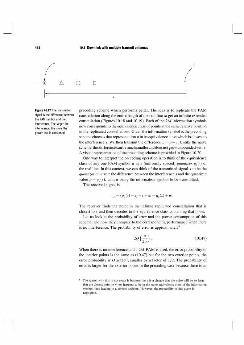
455 10.3 Downlink with multiple transmit antennas
u s
x
precoding scheme which performs better. The idea is to replicate the PAMFigure 10.17 The transmittedsignal is the difference betweenthe PAM symbol and theinterference. The larger theinterference, the more thepower that is consumed.
constellation along the entire length of the real line to get an infinite extendedconstellation (Figures 10.18 and 10.19). Each of the 2M information symbolsnow corresponds to the equivalence class of points at the same relative positionin the replicated constellations. Given the information symbol u, the precodingscheme chooses that representation p in its equivalence class which is closest tothe interference s. We then transmit the difference x = p− s. Unlike the naivescheme, thisdifferencecanbemuchsmalleranddoesnotgrowunboundedwiths.A visual representation of the precoding scheme is provided in Figure 10.20.One way to interpret the precoding operation is to think of the equivalence
class of any one PAM symbol u as a (uniformly spaced) quantizer qu· ofthe real line. In this context, we can think of the transmitted signal x to be thequantization error: the difference between the interference s and the quantizedvalue p= qus, with u being the information symbol to be transmitted.The received signal is
y = qus− s+ s+w = qus+w
The receiver finds the point in the infinite replicated constellation that isclosest to s and then decodes to the equivalence class containing that point.Let us look at the probability of error and the power consumption of this
scheme, and how they compare to the corresponding performance when thereis no interference. The probability of error is approximately6
2Q( a
2
) (10.47)
When there is no interference and a 2M-PAM is used, the error probability ofthe interior points is the same as (10.47) but for the two exterior points, theerror probability is Qa/2, smaller by a factor of 1/2. The probability oferror is larger for the exterior points in the precoding case because there is an
6 The reason why this is not exact is because there is a chance that the noise will be so largethat the closest point to y just happens to be in the same equivalence class of the informationsymbol, thus leading to a correct decision. However, the probability of this event isnegligible.

456 MIMO IV: multiuser communication
Figure 10.18 A four-pointPAM constellation.
–3a2
– a2
a2
3a2
– 5a2
– 7a2
– 9a2
– 11a2
3a2
– a2
– 3a2
11a2
9a2
7a2
5a2
a2
additional possibility of confusion across replicas. However, the difference isFigure 10.19 The four-pointPAM constellation is replicatedalong the entire real line. Pointsmarked by the same signcorrespond to the sameinformation symbol (one of thefour points in the originalconstellation).
negligible when error probabilities are small.7
What about the power consumption of the precoding scheme? The distancebetween adjacent points in each equivalence class is 2Ma; thus, unlike in thenaive interference pre-cancellation scheme, the quantization error does notgrow unbounded with s:
x ≤Ma
If we assume that s is totally random so that this quantization error is uniformbetween zero and this value, then the average transmit power is
x2= a2M2
3 (10.48)
In comparison, the average transmit power of the original 2M-PAM constel-lation is a2M2/3−a2/12. Hence, the precoding scheme requires a factor of
Figure 10.20 Depiction of theprecoding operation for M = 2and PAM information symbolu =−3a/2. The crosses formthe equivalence class for thissymbol. The difference betweens and the closest cross p istransmitted.
4M2
4M2−1
more transmit power. Thus, there is still a gap from AWGN detection per-formance. However, this power penalty is negligible when the constellationsize M is large.Our description is motivated from a similar precoding scheme for the
point-to-point frequency-selective (ISI) channel, devised independently by
transmitted signal x
s
– 11a2
– 9a2
– 7a2
– 5a2
– 3a2
– a2
a2
3a2
5a2
7a2
9a2
11a2
p
7 This factor of 2 can easily be compensated for by making the symbol separation slightlylarger.

457 10.3 Downlink with multiple transmit antennas
Tomlinson [121] and Harashima and Miyakawa [57]. In this context, theinterference is inter-symbol interference:
sm=∑
≥0
hxm−
where h is the impulse response of the channel. Since the previous transmittedsymbols are known to the transmitter, the interference is known if the transmit-ter has knowledge of the channel. In Discussion 8.1 we have alluded to con-nections between MIMO and frequency-selective channels and precoding isyet another import from one knowledge base to the other. Indeed, Tomlinson–Harashima precoding was devised as an alternative to receiver-based decision-feedback equalization for the frequency-selective channel, the analog to theSIC receiver in MIMO and uplink channels. The precoding approach has theadvantage of avoiding the error propagation problem of decision-feedbackequalizers, since in the latter the cancellation is based on detected symbols,while the precoding is based on known symbols at the transmitter.
Dirty-paper precoding: achieving AWGN capacityThe precoding scheme in the last section is only for a single-dimensional con-stellation (such as PAM), while spectrally efficient communication requirescoding over multiple dimensions. Moreover, in the low SNR regime, uncodedtransmission yields very poor error probability performance and coding isnecessary. There has been much work in devising block precoding schemesand it is still a very active research area. A detailed discussion of specificschemes is beyond the scope of this book. Here, we will build on the insightsfrom symbol-by-symbol precoding to give a plausibility argument that appro-priate precoding can in fact completely obliviate the impact of the interferenceand achieve the capacity of the AWGN channel. Thus, the power penalty weobserved in the symbol-by-symbol precoding scheme can actually be avoidedwith high-dimensional coding. In the literature, the precoding technique pre-sented here is also called Costa precoding or dirty-paper precoding.8
A first attemptConsider communication over a block of length N symbols:
y= x+ s+w (10.49)
In the symbol-by-symbol precoding scheme earlier, we started with a basicPAM constellation and replicated it to cover uniformly the entire (one-dimensional) range the interference s spans. For block coding, we would like
8 This latter name comes from the title of Costa’s paper: “Writing on dirty-paper” [23]. Thewriter of the message knows where the dirt is and can adapt his writing to help the readerdecipher the message without knowing where the dirt is.

458 MIMO IV: multiuser communication
to mimic this strategy by starting with a basic AWGN constellation and repli-
Figure 10.21 A replicatedconstellation in high dimension.The information specifies anequivalence class of pointscorresponding to replicas of acodeword (here with the samemarking).
cating it to cover the N -dimensional space uniformly. Using a sphere-packingargument, we give an estimate of the maximum rate of reliable communicationusing this type of scheme.Consider a domain of volume V in N . The exact size of the domain is
not important, as long as we ensure that the domain is large enough for thereceived signal y to lie inside. This is the domain on which we replicate thebasic codebook. We generate a codebook with M codewords, and replicateeach of the codewords K times and place the extended constellation e ofMK points on the domain sphere (Figure 10.21). Each codeword then cor-responds to an equivalence class of points in N . Equivalently, the giveninformation bits u define a quantizer qu·. The natural generalization of thesymbol-by-symbol precoding procedure simply quantizes the known inter-ference s using this quantizer to a point p = qus in e and transmits thequantization error
x1 = p− s (10.50)
Based on the received signal y, the decoder finds the point in the extendedconstellation that is closest to y and decodes to the information bits corre-sponding to its equivalence class.
PerformanceTo estimate the maximum rate of reliable communication for a given averagepower constraint P using this scheme, we make two observations:
• Sphere-packing To avoid confusing x1 with any of the other KM − 1points in the extended constellation e that belong to other equivalenceclasses, the noise spheres of radius
√N2 around each of these points
should be disjoint. This means that
KM<V
VolBN √N2
(10.51)
the ratio of the volume of the domain sphere to that of the noise sphere.• Sphere-covering To maintain the average transmit power constraint of P,the quantization error should be no more than
√NP for any interference
vector s. Thus, the spheres of radius√NP around the K replicas of a
codeword should be able to cover the whole domain such that any point iswithin a distance of
√NP from a replica. To ensure that,
K>V
VolBN √NP
(10.52)
This in effect imposes a constraint on the minimal density of the replication.

459 10.3 Downlink with multiple transmit antennas
Putting the two constraints (10.51) and (10.52) together, we get
M<VolBN
√NP
VolBN √N2
=(√
NP)N
(√N2
)N (10.53)
which implies that the maximum rate of reliable communication is, at most,
R = logMN
= 12log
P
2 (10.54)
This yields an upper bound on the rate of reliable communication. More-over, it can be shown that if the MK constellation points are independentlyand uniformly distributed on the domain, then with high probability, commu-nication is reliable if condition (10.51) holds and the average power constraintis satisfied if condition (10.52) holds. Thus, the rate (10.54) is also achievable.The proof of this is along the lines of the argument in Appendix B.5.2, wherethe achievability of the AWGN capacity is shown.Observe that the rate (10.54) is close to the AWGN capacity 1/2 log1+
P/2 at high SNR. However, the scheme is strictly suboptimal at finiteSNR. In fact, it achieves zero rate if the SNR is below 0 dB. How can theperformance of this scheme be improved?
Performance enhancement via MMSE estimationThe performance of the above scheme is limited by the two constraints (10.51)and (10.52). To meet the average power constraint, the density of replicationcannot be reduced beyond (10.52). On the other hand, constraint (10.51) is adirect consequence of the nearest neighbor decoding rule, and this rule is in factsuboptimal for the problem at hand. To see why, consider the case when theinterference vector s is 0 and the noise variance 2 is significantly larger thanP. In this case, the transmitted vector x1 is roughly at a distance
√NP from the
origin while the received vector y is at a distance√NP+2, much further
away. Blindly decoding to the point in e nearest to ymakes no use of the priorinformation that the transmitted vector x1 is of (relatively short) length
√NP
(Figure 10.22). Without using this prior information, the transmitted vector isthought of by the receiver as anywhere in a large uncertainty sphere of radius√N2 around y and the extended constellation points have to be spaced that far
apart to avoid confusion. By making use of the prior information, the size of theuncertainty sphere can be reduced. In particular, we can consider a linear estim-ate y of x1. By the law of large numbers, the squared error in the estimate is
y−x12 = w+ −1x12 ≈ N[22+ 1−2P
](10.55)
and by choosing
= P
P+2 (10.56)

460 MIMO IV: multiuser communication
Figure 10.22 MMSE decodingyields a much smalleruncertainty sphere than doesnearest neighbor decoding.
MMSE then nearest neighbor decoding
αy
Nearest neighbor decoding
y
x1
Uncertainty sphere
radius = NPσ 2
P + σ 2
radius = √NP
Uncertainty sphere
√
this error is minimized, equalling
NP2
P+2 (10.57)
In fact y is nothing but the linear MMSE estimate xmmse of x1 from y andNP2/P +2 is the MMSE estimation error. If we now use a decoderthat decodes to the constellation point nearest to y (as opposed to y), thenan error occurs only if there is another constellation point closer than thisdistance to y. Thus, the uncertainty sphere is now of radius
√NP2
P+2 (10.58)
We can now redo the analysis in the above subsection, but with the radius√N2 of the noise sphere replaced by this radius of the MMSE uncertainty
sphere. The maximum achievable rate is now
12log
(
1+ P
2
)
(10.59)
thus achieving the AWGN capacity.

461 10.3 Downlink with multiple transmit antennas
In the above, we have simplified the problem by assuming s= 0, to focus
α s
p
x1
Figure 10.23 The precodingprocess with the factor.
on how the decoder has to be modified. For a general interference vector s,
y= x1+ s+w= x1+w+s= xmmse+s (10.60)
i.e., the linear MMSE estimate of x1 but shifted by s. Since the receiverdoes not know s, this shift has to be pre-compensated for at the transmit-ter. In the earlier scheme, we were using the nearest neighbor rule and wecompensated for the effect of s by pre-subtracting s from the constellationpoint p representing the information, i.e., we sent the error in quantizing s.But now we are using the MMSE rule and hence we should compensate bypre-subtracting s instead. Specifically, given the data u, we find within theequivalence class representing u the point p that is closest to s, and transmitx1 = p−s (Figure 10.23). Then,
p = x1+s
y = xmmse+s= p
and
p−y= x1− xmmse (10.61)
The receiver finds the constellation point nearest to y and decodes the infor-mation (Figure 10.24). An error occurs only if there is another constellationpoint closer to y than p, i.e., if it lies in the MMSE uncertainty sphere. Thisis exactly the same situation as in the case of zero interference.
Figure 10.24 The decodingprocess with the factor.
y
w
x1
sp = α y
α s
α (x1 + w) = xmmse^

462 MIMO IV: multiuser communication
Transmitter knowledge of interference is enoughSomething quite remarkable has been accomplished: even though the interfer-ence is known only at the transmitter and not at the receiver, the performancethat can be achieved is as though there were no interference at all. Thecomparison between the cases with and without interference is depicted inFigure 10.25.For the plain AWGN channel without interference, the codewords lie in
a sphere of radius√NP (x-sphere). When a codeword x1 is transmitted, the
received vector y lies in the y-sphere, outside the x-sphere. The MMSE rulescales down y to y, and the uncertainty sphere of radius
√NP2/P+2
around y lies inside the x-sphere. The maximum reliable rate of communi-cation is given by the number of uncertainty spheres that can be packed intothe x-sphere:
1N
logVolBN
√NP
VolBN √NP2/P+2
= 12log
(
1+ P
2
)
(10.62)
the capacity of the AWGN channel. In fact, this is how achievability of theAWGN capacity is shown in Appendix B.5.2.
Figure 10.25 Pictorialrepresentation of the caseswith and without interference.
x1
x1
origin
Uncertainty sphere
AWGNwithout interference
AWGNwith interference
Uncertainty sphere
α y
p
origin
α y
α s
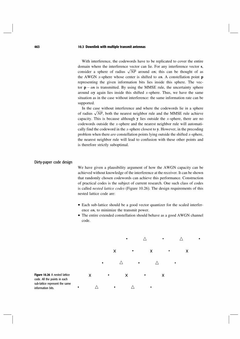
463 10.3 Downlink with multiple transmit antennas
With interference, the codewords have to be replicated to cover the entiredomain where the interference vector can lie. For any interference vector s,consider a sphere of radius
√NP around s; this can be thought of as
the AWGN x-sphere whose center is shifted to s. A constellation point prepresenting the given information bits lies inside this sphere. The vec-tor p−s is transmitted. By using the MMSE rule, the uncertainty spherearound y again lies inside this shifted x-sphere. Thus, we have the samesituation as in the case without interference: the same information rate can besupported.In the case without interference and where the codewords lie in a sphere
of radius√NP, both the nearest neighbor rule and the MMSE rule achieve
capacity. This is because although y lies outside the x-sphere, there are nocodewords outside the x-sphere and the nearest neighbor rule will automati-cally find the codeword in the x-sphere closest to y. However, in the precodingproblem when there are constellation points lying outside the shifted x-sphere,the nearest neighbor rule will lead to confusion with these other points andis therefore strictly suboptimal.
Dirty-paper code designWe have given a plausibility argument of how the AWGN capacity can beachieved without knowledge of the interference at the receiver. It can be shownthat randomly chosen codewords can achieve this performance. Constructionof practical codes is the subject of current research. One such class of codesis called nested lattice codes (Figure 10.26). The design requirements of thisnested lattice code are:
• Each sub-lattice should be a good vector quantizer for the scaled interfer-ence s, to minimize the transmit power.
• The entire extended constellation should behave as a good AWGN channelcode.
Figure 10.26 A nested latticecode. All the points in eachsub-lattice represent the sameinformation bits.

464 MIMO IV: multiuser communication
The discussion of such codes is beyond the scope of this book. The designproblem, however, simplifies in the low SNR regime. We discuss this below.
Low SNR: opportunistic orthogonal codingIn the infinite bandwidth channel, the SNR per degree of freedom is zeroand we can use this as a concrete channel to study the nature of precoding atlow SNR. Consider the infinite bandwidth real AWGN channel with additiveinterference st modelled as real white Gaussian (with power spectral densityNs/2) and known non-causally to the transmitter. The interference is indepen-dent of both the background real white Gaussian noise and the real transmitsignal, which is power constrained, but not bandwidth constrained. Sincethe interference is known non-causally only to the transmitter, the minimumb/N0 for reliable communication on this channel can be no smaller than thatin the plain AWGN channel without interference; thus a lower bound on theminimum b/N0 is −159 dB.We have already seen for the AWGN channel (cf. Section 5.2.2 and
Exercises 5.8 and 5.9) that orthogonal codes achieve the capacity in theinfinite bandwidth regime. Equivalently, orthogonal codes achieve theminimum b/N0 of −159 dB over the AWGN channel. Hence, we start withan orthogonal set of codewords representing M messages. Each of the code-words is replicated K times so that the overall constellation with MK vectorsforms an orthogonal set. Each of the M messages corresponds to a set of Korthogonal signals. To convey a specific message, the encoder transmits thatsignal, among the set of K orthogonal signals corresponding to the messageselected, that is closest to the interference st, i.e., the one that has the largestcorrelation with the st. This signal is the constellation point to which st isquantized. Note that, in the general scheme, the signal qus−s is trans-mitted, but since → 0 in the low SNR regime, we are transmitting qusitself.An equivalent way of seeing this scheme is as opportunistic pulse position
modulation: classical PPM involves a pulse that conveys information basedon the position when it is not zero. Here, every K of the pulse positionscorresponds to one message and the encoder opportunistically chooses theposition of the pulse among the K possible pulse positions (once the desiredmessage to be conveyed is picked) where the interference is the largest.The decoder first picks the most likely position of the transmit pulse (among
the MK possible choices) using the standard largest amplitude detector. Next,it picks the message corresponding to the set in which the most likely pulseoccurs. Choosing K large allows the encoder to harness the opportunisticgains afforded by the knowledge of the additive interference. On the otherhand, decoding gets harder as K increases since the number of possible pulsepositions, MK, grows with K. An appropriate choice of K as a functionof the number of messages, M , and the noise and interference powers, N0
and Ns respectively, trades off the opportunistic gains on the one hand with

465 10.3 Downlink with multiple transmit antennas
the increased difficulty in decoding on the other. This tradeoff is evaluatedin Exercise 10.16 where we see that the correct choice of K allows theopportunistic orthogonal codes to achieve the infinite bandwidth capacity ofthe AWGN channel without interference. Equivalently, the minimum b/N0 isthe same as that in the plain AWGN channel and is achieved by opportunisticorthogonal coding.
10.3.4 Precoding for the downlink
We now apply the precoding technique to the downlink channel. We first startwith the single transmit antenna case and then discuss the multiple antennacase.
Single transmit antennaConsider the two-user downlink channel with a single transmit antenna:
ykm= hkxm+wkm k= 12 (10.63)
where wkm ∼ 0N0. Without loss of generality, let us assume thatuser 1 has the stronger channel: h12 ≥ h22. Write xm = x1m+ x2m,where xkm is the signal intended for user kk= 12. Let Pk be the powerallocated to user k. We use a standard i.i.d. Gaussian codebook to encodeinformation for user 2 in x2m. Treating x2m as interference that isknown at the transmitter, we can apply Costa precoding for user 1 to achievea rate of
R1 = log(
1+ h12P1
N0
)
(10.64)
the capacity of an AWGN channel for user 1 with x2m completely absent.What about user 2? It can be shown that x1m can be made to appear likeindependent Gaussian noise to user 2. (See Exercise 10.17.) Hence, user 2gets a reliable data rate of
R2 = log(
1+ h22P2
h22P1+N0
)
(10.65)
Since we have assumed that user 1 has the stronger channel, these same ratescan in fact be achieved by superposition coding and decoding (cf. Section 6.2):we superimpose independent i.i.d. Gaussian codebook for user 1 and 2, withuser 2 decoding the signal x2m treating x1m as Gaussian noise, anduser 1 decoding the information for user 2, canceling it off, and then decodingthe information intended for it. Thus, precoding is another approach to achieverates on the boundary of the capacity region in the single antenna downlinkchannel.

466 MIMO IV: multiuser communication
Superposition coding is a receiver-centric scheme: the base-station simplyadds the codewords of the users while the stronger user has to do the decodingjob of both the users. In contrast, precoding puts a substantial computationalburden on the base-station with receivers being regular nearest neighbordecoders (though the user whose signal is being precoded needs to decodethe extended constellation, which has more points than the rate would entail).In this sense we can think of precoding as a transmitter-centric scheme.However, there is something curious about this calculation. The precoding
strategy described above encodes information for user 1 treating user 2’ssignal as known interference. But certainly we can reverse the role of user 1and user 2, and encode information for user 2, treating user 1’s signal asinterference. This strategy achieves rates
R′1 = log
(
1+ h12P1
h12P2+N0
)
R′2 = log
(
1+ h22P2
N0
)
(10.66)
But these rates cannot be achieved by superposition coding/decoding underthe power allocations P1P2: the weak user cannot remove the signal intendedfor the strong user. Is this rate tuple then outside the capacity region? It turnsout that there is no contradiction and this rate pair is strictly contained insidethe capacity region (Exercise 10.19).In this discussion, we have restricted ourselves to just two users, but the
extension to K users is obvious. See Exercise 10.19.
Multiple transmit antennasWe now return to the scenario of real interest, multiple transmit antennas(10.31):
ykm= h∗kxm+wkm k= 12 K (10.67)
The precoding technique can be applied to upgrade the performance of the lin-ear beamforming technique described in Section 10.3.2. Recall from (10.35),the transmitted signal is
xm=K∑
k=1
xkmuk (10.68)
where xkm is the signal for user k and uk is its transmit beamformingvector. The received signal of user k is given by
ykm = h∗kukxkm+∑
j =k
h∗kujxjm+wkm (10.69)
= h∗kukxkm+∑
j<k
h∗kujxjm
+∑j>k
h∗kujxjm+wkm (10.70)

467 10.3 Downlink with multiple transmit antennas
Applying Costa precoding for user k, treating the interference∑
j<kh∗kujxjm from users 1 k− 1 as known and
∑j>kh
∗kujxjm
from users k+1 K as Gaussian noise, the rate that user k gets is
Rk = log1+ SINRk (10.71)
where SINRk is the effective signal-to-interference-plus-noise ratio after pre-coding:
SINRk =Pk u∗
khk 2N0+
∑j>k Pj u∗
jhk 2 (10.72)
Here Pj is the power allocated to user j. Observe that unlike the single trans-mit antenna case, this performance may not be achievable by superpositioncoding/decoding.For linear beamforming strategies, an interesting uplink–downlink duality
is identified in Section 10.3.2. We can use the downlink transmit signatures(denoted by u1 uK) to be the same as the receive filters in the dual uplinkchannel (10.40) and the same SINR for the users can be achieved in both theuplink and the downlink with appropriate user power allocations such that thesum of these power allocations is the same for both the uplink and the downlink.Wenowextend this observation to aduality between transmit beamformingwithprecoding in the downlink and receive beamforming with SIC in the uplink.Specifically, suppose we use Costa precoding in the downlink and SIC in
the uplink, and the transmit signatures of the users in the downlink are thesame as the receive filters of the users in the uplink. Then it turns out thatthe same set SINR of the users can be achieved by appropriate user powerallocations in the uplink and the downlink and, further, the sum of thesepower allocations is the same. This duality holds provided that the order ofSIC in the uplink is the reverse of the Costa precoding order in the downlink.For example, in the Costa precoding above we employed the order 1 K;i.e., we precoded the user k signal so as to cancel the interference from thesignals of users 1 k−1. For this duality to hold, we need to reverse thisorder in the SIC in the uplink; i.e., the users are successively canceled in theorder K 1 (with user k seeing no interference from the canceled usersignals KK−1 k+1).The derivation of this duality follows the same lines as for linear strategies
and is done in Exercise 10.20. Note that in this SIC ordering, user 1 sees theleast uncanceled interference and user K sees the most. This is exactly theopposite to that under the Costa precoding strategy. Thus, we see that in thisduality the ordering of the users is reversed. Identifying this duality facilitatesthe computation of good transmit filters in the downlink. For example, weknow that in the uplink the optimal filters for a given set of powers are MMSEfilters; the same filters can be used in the downlink transmission.

468 MIMO IV: multiuser communication
In Section 10.1.2, we saw that receive beamforming in conjunction withSIC achieves the capacity region of the uplink channel with multiple receiveantennas. It has been shown that transmit beamforming in conjunction withCosta precoding achieves the capacity of the downlink channel with multipletransmit antennas.
10.3.5 Fast fading
The time-varying downlink channel is an extension of (10.31):
ykm= h∗kmxm+wkm k= 1 K (10.73)
Full CSIWith full CSI, both the base-station and the users track the channel fluctuationsand, in this case, the extension of the linear beamforming strategies combinedwith Costa precoding to the fading channel is natural. Now we can vary thepower and transmit signature allocations of the users, and the Costa precodingorder as a function of the channel variations. Linear beamforming combinedwith Costa precoding achieves the capacity of the fast fading downlink channelwith full CSI, just as in the time-invariant downlink channel.It is interesting to compare this sum capacity achieving strategy with that
when the base-station has just one transmit antenna (see Section 6.4.2). Inthis basic downlink channel, we identified the structure of the sum capac-ity achieving strategy: transmit only to the best user (using a power thatis waterfilling over the best user’s channel quality, see (6.54)). The linearbeamforming strategy proposed here involves in general transmitting to allthe users simultaneously and is quite different from the one user at a timepolicy. This difference is analogous to what we have seen in the uplink withsingle and multiple receive antennas at the base-station.Due to the duality, we have a connection between the strategies for the
downlink channel and its dual uplink channel. Thus, the impact of multipletransmit antennas at the base-station on multiuser diversity follows the dis-cussion in the uplink context (see Section 10.1.6): focusing on the one user ata time policy, the multiple transmit antennas provide a beamforming powergain; this gain is the same as in the point-to-point context and the multiusernature of the gain is lost. With the sum capacity achieving strategy, the mul-tiple transmit antennas provide multiple spatial degrees of freedom allowingthe users to be transmitted to simultaneously, but the opportunistic gains areof the same form as in the point-to-point case; the multiuser nature of thegain is diminished.
Receiver CSISo far we have made the full CSI assumption. In practice, it is often veryhard for the base-station to have access to the user channel fluctuations and

469 10.3 Downlink with multiple transmit antennas
the receiver CSI model is more natural. The major difference here is thatnow the transmit signatures of the users cannot be allocated as a functionof the channel variations. Furthermore, the base-station is not aware of theinterference caused by the other users’ signals for any specific user k (sincethe channel to the kth user is unknown) and Costa precoding is ruled out.Exercise 10.21 discusses how to use the multiple antennas at the base-
station without access to the channel fluctuations. One of the important con-clusions is that time sharing among the users achieves the capacity region inthe symmetric downlink channel with receiver CSI alone. This implies thatthe total spatial degrees of freedom in the downlink are restricted to one,the same as the degrees of freedom of the channel from the base-station toany individual user. On the other hand, with full CSI at the base-station wehave seen (Section 10.3.1) that the spatial degrees of freedom are equal tominntK. Thus lack of CSI at the base-station causes a drastic reduction inthe degrees of freedom of the channel.
Partial CSI at the base-station: opportunistic beamforming with multiple beamsIn many practical systems, there is some form of partial CSI fed back to thebase-station from the users. For example, in the IS-856 standard discussed inChapter 6 each user feeds back the overall SINR of the link to the base-stationit is communicating with. Thus, while the base-station does not have exactknowledge of the channel (phase and amplitude) from the transmit antennaarray to the users, it does have partial information: the overall quality of thechannel (such as hkm2 for user k at time m).In Section 6.7.3 we studied opportunistic beamforming that induces time
fluctuations in the channel to increase the multiuser diversity. The multipletransmit antennas were used to induce time fluctuations and the partial CSI
user 2
user 1
Figure 10.27 Opportunisticbeamforming with twoorthogonal beams. The user“closest” to a beam isscheduled on that beam,resulting in two parallel datastreams to two users.
was used to schedule the users at appropriate time slots. However, the gainfrom multiuser diversity is a power gain (boost in the SINR of the userbeing scheduled) and with just a single user scheduled at any time slot,only one of the spatial degrees of freedom is being used. This basic schemecan be modified, however, allowing multiple users to be scheduled and thusincreasing the utilized spatial degrees of freedom.The conceptual idea is to have multiple beams, each orthogonal to one
another, at the same time (Figure 10.27). Separate pilot symbols are intro-duced on each of the beams and the users feedback the SINR of each beam.Transmissions are scheduled to as many users as there are beams at each timeslot. If there are enough users in the system, the user who is beamformed withrespect to a specific beam (and orthogonal to the other beams) is scheduled onthe specific beam. Let us consider K ≥ nt (if K<nt then we use only K of thetransmit antennas), and at each time m, let Qm = q1m qnt
m bean nt ×nt unitary matrix, with the columns q1m qnt
m orthonormal.The vector qim represents the ith beam at time m.

470 MIMO IV: multiuser communication
The vector signal sent out from the antenna array at time m is
nt∑
i=1
ximqim (10.74)
Here x1 xnt are the nt independent data streams (in the case of coherentdownlink reception, these signals include pilot symbols as well). The unitarymatrix Qm is varied such that the individual components do not changeabruptly in time. Focusing on the kth user, the signal it receives at time m is(substituting (10.74) in (10.73))
ykm=nt∑
i=1
ximh∗kmqim+wkm (10.75)
For simplicity, let us consider the scenario when the channel coefficientsare not varying over the time-scale of communication (slow fading), i.e.,hkm= hk. When the ith beam takes on the value
qim= hk
hk (10.76)
then user k is in beamforming configuration with respect to the ith beam;moreover, it is simultaneously orthogonal to the other beams. The receivedsignal at user k is
ykm= hkxim+wkm (10.77)
If there are enough users in the system, for every beam i some user will benearly in beamforming configuration with respect to it (and simultaneouslynearly orthogonal to the other beams). Thus nt data streams are transmittedsimultaneously in orthogonal spatial directions and the full spatial degreesof freedom are utilized. The limited feedback from the users allows oppor-tunistic scheduling of the user transmissions in the appropriate beams at theappropriate time slots. To achieve close to the beamforming performance andcorresponding nulling to all the other beams requires a user population thatis larger than in the scenario of Section 6.7.3. In general, depending on thenumber of the users in the system, the number of spatially orthogonal beamscan be designed.There are extra system requirements to support multiple beams (as com-
pared to just the single time-varying beam introduced in Section 6.7.3). First,multiple pilot symbols have to be inserted (one for each beam) to enable coher-ent downlink reception; thus the fraction of pilot symbol power increases.Second, the receivers now track nt separate beams and feedback SINR of eachon each of the beams. On a practical note, the receivers could feedback onlythe best SINR and the identification of the beam that yields this SINR; this

471 10.4 MIMO downlink
restriction probably will not degrade the performance by much. Thus, withalmost the same amount of feedback as the single beam scheme, the modifiedopportunistic beamforming scheme utilizes all the spatial degrees of freedom.
10.4 MIMO downlink
Figure 10.28 The downlinkwith multiple transmit antennasat the base-station and multiplereceive antennas at each user.
We have seen so far how downlink is affected by the availability of multipletransmit antennas at the base-station. In this section, we study the downlinkwith multiple receive antennas (at the users) (see Figure 10.28). To focus onthe role of multiple receive antennas, we begin with a single transmit antennaat the base-station.The downlink channel with a single transmit and multiple receive antennas
at each user can be written as
ykm= hkxm+wkm k= 12 (10.78)
wherewkm∼ 0N0Inr and i.i.d. in timem. The receive spatial signatureat user k is denoted by hk. Let us focus on the time-invariant model first andfix this vector. If there is only one user, then we know from Section 7.2.1 thatthe user should do receive beamforming: project the received signal in thedirection of the vector channel. Let us try this technique here, with both usersmatched filtering their received signals w.r.t. their channels. This is illustratedin Figure 10.29 and can be shown to be the optimal strategy for both the users(Exercise 10.22). With the matched filter front-end at each user, we have aneffective AWGN downlink with a single antenna:
ykm = h∗kykm
hk= hkxm+wkm k= 12 (10.79)
Here wkm is 0N0 and i.i.d. in time m and the downlink channel in(10.79) is very similar to the basic single antenna downlink channel modelof (6.16) in Section 6.2. The only difference is that user k’s channel qualityhk2 is replaced by hk2.Thus, to study the downlink with multiple receive antennas, we can
now carry over all our discussions from Section 6.2 for the single antennascenario. In particular, we can order the two users based on their receivedSNR (suppose h1 ≤ h2) and do superposition coding: the transmit signalis the linear superposition of the signals to the two users. User 1 treats thesignal of user 2 as noise and decodes its data from y1. User 2, which hasthe better SNR, decodes the data of user 1, subtracts the transmit signalof user 1 from y2 and then decodes its data. With a total power constraintof P and splitting this among the two users P = P1 +P2 we can write the

472 MIMO IV: multiuser communication
Figure 10.29 Each user with afront-end matched filterconverting the SIMO downlinkinto a SISO downlink.
Base station
Receivebeamforming
ykykhk
hk
Userk
*
rate tuple that is achieved with the receiver architecture in Figure 10.29 andsuperposition coding (cf. (6.22)),
R1 = log(
1+ P1h12P2h12+N0
)
R2 = log(
1+ P2h22N0
)
(10.80)
Thus we have combined the techniques of Sections 7.2.1 and 6.2, namelyreceive beamforming and superposition coding into a communication strategyfor the single transmit and multiple receive antenna downlink.The matched filter operation by the users in Figure 10.29 only requires
tracking of their channels by the users, i.e., CSI is required at the receivers.Thus, even with fast fading, the architecture in Figure 10.29 allows us to trans-form the downlink with multiple receive antennas to the basic single antennadownlink channel as long as the users have their channel state information.In particular, analyzing receiver CSI and full CSI for the downlink in (10.78)simplifies to the basic single antenna downlink discussion (in Section 6.4).In particular, we can ask what impact multiple receive antennas have on
multiuser diversity, an important outcome of our discussion in Section 6.4. Theonly difference here is the distribution of the channel quality: hk2 replacinghk2. This was also the same difference in the uplink when we studied the roleof multiple receive antennas in multiuser diversity gain (in Section 10.1.6).We can carry over our main observation: the multiple receive antennas providea beamforming gain but the tail of hk2 decays more rapidly (Figure 10.8)and the multiuser diversity gain is restricted (Figure 10.9). To summarize,the traditional receive beamforming power gain is balanced by the loss of thebenefit of the multiuser diversity gain (which is also a power gain) due to the“hardening” of the effective fading distribution: hk2 ≈ nr (cf. (10.20)).With multiple transmit antennas at the base-station and multiple receive
antennas at each of the users, we can extend our set of linear strategies fromthe discussion in Section 10.3.2: now the base-station splits the informationfor user k into independent data streams, modulates them on different spatialsignatures and then transmits them. With full CSI, we can vary these spatialsignatures and powers allocated to the users (and the further allocation amongthe data streams within a user) as a function of the channel fluctuations. Wecan also embellish the linear strategies with Costa precoding, successively

473 10.5 Multiple antennas in cellular networks
precanceling the data streams. The performance of this scheme (linear beam-forming strategies with and without Costa precoding) can be related to thecorresponding performance of a dual MIMO uplink channel (much as in thediscussion of Section 10.3.2 with multiple antennas at the base-station alone).This scheme achieves the capacity of the MIMO downlink channel.
10.5 Multiple antennas in cellular networks: a system view
We have discussed the system design implications of multiple antennas inboth the uplink and the downlink. These discussions have been in the contextof multiple access within a single cell and are spread throughout the chapter(Sections 10.1.3, 10.1.6, 10.2.2, 10.3.5 and 10.4). In this section we take stockof these implications and consider the role of multiple antennas in cellularnetworks with multiple cells. Particular emphasis is on two points:
• the use of multiple antennas in suppressing inter-cell interference;• how the use of multiple antennas within cells impacts the optimal amountof frequency reuse in the network.
Summary 10.3 System implications of multiple antennas onmultiple access
Three ways of using multiple receive antennas in the uplink:• Orthogonal multiple access Each user gets a power gain, but no changein degrees of freedom.
• Opportunistic communication, one user at a time Power gain but themultiuser diversity gain is reduced.
• Space division multiple access is capacity achieving: users simultane-ously transmit and are jointly decoded at the base-station.
Comparison between orthogonal multiple access and SDMA• Low SNR: performance of orthogonal multiple access comparable tothat of SDMA.
• High SNR: SDMA allows up to nr users to simultaneously transmit witha single degree of freedom each. Performance is significantly better thanthat with orthogonal multiple access.
• An intermediate access scheme with moderate complexity performs com-parably to SDMA at all SNR levels: blocks of approximately nr usersin SDMA mode and orthogonal access for different blocks.
MIMO uplink• Orthogonal multiple access: each user has multiple degrees of freedom.• SDMA: the overall degrees of freedom are still restricted by the numberof receive antennas.

474 MIMO IV: multiuser communication
Downlink with multiple receive antennasEach user gets receive beamforming gain but reduced multiuser diversitygain.Downlink with multiple transmit antennas• No CSI at the base-station: single spatial degree of freedom.• Full CSI: the uplink–downlink duality principle makes this situationanalogous to the uplink with multiple receive antennas and now thereare up to nt spatial degrees of freedom.
• Partial CSI at the base-station: the same spatial degrees of freedom as thefull CSI scenario can be achieved by a modification of the opportunisticbeamforming scheme: multiple spatially orthogonal beams are sent outand multiple users are simultaneously scheduled on these beams.
10.5.1 Inter-cell interference management
Consider the multiple receive antenna uplink with users operating in SDMAmode. We have seen that successive cancellation is an optimal way to handleinterference among the users within the same cell. However, this techniqueis not suitable to handle interference from neighboring cells: the out-of-celltransmissions are meant to be decoded by their nearest base-stations and thereceived signal quality is usually too poor to allow decoding at base-stationsfurther away. On the other hand, linear receivers such as the MMSE do notdecode the information from the interference and can be used to suppressout-of-cell interference.The following model captures the essence of out-of-cell interference: the
received signal at the antenna array (y) comprises the signal (x) of the user ofinterest (with the signals of other users in the same cell successfully canceled)and the out-of-cell interference (z):
y= hx+ z (10.81)
Here h is the received spatial signature of the user of interest. One modelfor the random interference z is as 0Kz, i.e., it is colored Gaussiannoise with covariance matrix Kz. For example, if the interference originatesfrom just one out-of-cell transmission (with transmit power, say, q) and thebase-station has an estimate of the received spatial signature of the interferingtransmission (say, g), then the covariance matrix is
qgg∗ +N0I (10.82)
taking into account the structure of the interference and the backgroundadditive Gaussian noise.

475 10.5 Multiple antennas in cellular networks
Once such a model has been adopted, the multiple receive antennas can beused to suppress interference: we can use the linear MMSE receiver developedin Section 8.3.3 to get the soft estimate (cf. (8.61)):
x = v∗mmsey= h∗K−1z y (10.83)
The expression for the corresponding SINR is in (8.62). This is the best SINRpossible with a linear estimate. When the interfering noise is white, the oper-ation is simply traditional receive beamforming. On the other hand, when theinterference is very large and not white then the operation reduces to a decor-relator: this corresponds to nulling out the interference. The effect of channelestimation error on interference suppression is explored in Exercise 10.23.In the uplink, the model for the interference depends on the type of multi-
ple access. In many instances, a natural model for the interference is that itis white. For example, if the out-of-cell interference comes from many geo-graphically spread out users (this situation occurs when there are many usersin SDMA mode), then the overall interference is averaged over the multipleusers’ spatial locations and white noise is a natural model. In this case, thereceive antenna array does not explicitly suppress out-of-cell interference. Tobe able to exploit the interference suppression capability of the antennas, twothings must happen:
• The number of simultaneously transmitting users in each cell should besmall. For example,in a hybrid SDMA/TDMA strategy, the total numberof users in each cell may be large but the number of users simultaneouslyin SDMA mode is small (equal to or less than the number of receiveantennas).
• The out-of-cell interference has to be trackable. In the SDMA/TDMAsystem, even though the interference at any time comes from a smallnumber of users, the interference depends on the geographic location ofthe interfering user(s), which changes with the time slot. So either eachslot has to be long enough to allow enough time to estimate the color ofthe interference based only on the pilot signal received in that time slot, orthe users are scheduled in a periodic manner and the interference can betracked across different time slots.
An example of such a system is described in Example 10.1.On the other hand, interference suppression in the downlink using multiple
receive antennas at the mobiles is different. Here the interference comes froma few base-stations of the neighboring cells that reuse the same frequency, i.e.,from fixed specific geographic locations. Now, an estimate of the covarianceof the interference can be formed and the linear MMSE can be used to managethe inter-cell interference.We now turn to the role of multiple antennas in deciding the optimal
amount of frequency reuse in the cellular network. We consider the effect

476 MIMO IV: multiuser communication
on both the uplink and the downlink and the role of multiple receive andmultiple transmit antennas separately.
10.5.2 Uplink with multiple receive antennas
We begin with a discussion of the impact of multiple antennas at the base-station on the two orthogonal cellular systems studied in Chapter 4 and thenmove to SDMA.
Orthogonal multiple accessThe array of multiple antennas is used to boost the received signal strengthfrom the user within the cell via receive beamforming. One immediate benefitis that each user can lower its transmit power by a factor equal to thebeamforming gain (proportional to nr) to maintain the same signal qualityat the base-station. This reduction in transmit power also helps to reduceinter-cell interference, so the effective SINR with the power reduction is infact more than the SINR achieved in the original setting.In Example 5.2 we considered a linear array of base-stations and analyzed
the tradeoff between reuse and data rates per user for a given cell size andtransmit power setting. With an array of antennas at each base-station, theSNR of every user improves by a factor equal to the receive beamforminggain. Much of the insight derived in Example 5.2 on how much to reuse canbe naturally extended to the case here with the operating SNR boosted by thereceive beamforming gain.
SDMAIf we do not impose the constraint that uplink communication be orthogonalamong the users in the cell, we can use the SDMA strategy where manyusers simultaneously transmit and are jointly decoded at the base-station. Wehave seen that this scheme significantly betters orthogonal multiple access athigh SNR due to the increased spatial degrees of freedom. At low SNR, bothorthogonal multiple access and SDMA benefit comparably, with the usersgetting a receive beamforming gain. Thus, for SDMA to provide significantperformance improvement over orthogonal multiple access, we need the oper-ating SNR to be large; in the context of a cellular system, this means lessfrequency reuse.Whether the loss in spectral efficiency due to less frequency reuse is fully
compensated for by the increase in spatial degrees of freedom depends on thespecific physical situation. The frequency reuse ratio represents the loss inspectral efficiency. The corresponding reduction in interference is representedby the fraction f: this is the fraction of the received power from a user atthe edge of the cell that the interference constitutes. For example, in a linearcellular system f decays roughly as , but for a hexagonal cellular systemthe decay is much slower: f decays roughly as /2 (cf. Example 5.2).

477 10.5 Multiple antennas in cellular networks
Suppose all the K users are at the edge of the cell (a worst case scenario)and communicating via SDMA to the base-station with receiver CSI. W isthe total bandwidth allotted to the cellular system scaled down by the numberof simultaneous SDMA users sharing it within a cell (as with orthogonalmultiple access, cf. Example 5.2). With SDMA used in each cell, K userssimultaneously transmit over the entire bandwidth KW .The SINR of the user at the edge of the cell is, as in (5.20),
SINR= SNRK+fSNR
with SNR = P
N0Wd (10.84)
The SNR at the edge of the cell is SNR, a function of the transmit power P,the cell size d, and the power decay rate (cf. (5.21)). The notation for thefraction f is carried over from Example 5.2. The largest symmetric rate eachuser gets is, the MIMO extension of (5.22),
R = WlogdetInr + SINR HH∗bits/s (10.85)
Here the columns of H represent the receive spatial signatures of the users atthe base-station and the log det expression is the sum of the rates at whichusers can simultaneously communicate reliably.We can now address the engineering question of how much to reuse using
the simple formula for the rate in (10.85). At low SNR the situation isanalogous to the single receive antenna scenario studied in Example 5.2: therate is insensitive to the reuse factor and this can be verified directly from(10.85). On the other hand, at large SNR the interference grows as well andthe SINR peaks at 1/f. The largest rate then is, as in (5.23),
W
[
logdet(
Inr +1f
HH∗)]
bits/s (10.86)
and goes to zero for small values of : thus as in Example 5.2, less reusedoes not lead to a favorable situation.How do multiple receive antennas affect the optimal reuse ratio? Setting
K = nr (a rule of thumb arrived at in Exercise 10.5), we can use the approx-imation in (8.29) to simplify the expression for the rate in (10.86):
R ≈ Wnrc∗(1f
)
(10.87)
The first observation we can make is that since the rate grows linearly in nr ,the optimal reuse ratio does not depend on the number of receive antennas.The optimal reuse ratio thus depends only on how the inter-cell interferencef decays with the reuse parameter , as in the single antenna situation studiedin Example 5.2.

478 MIMO IV: multiuser communication
Figure 10.30 The symmetricrate for every user (in bps/Hz)with K = 5 users in SDMAmodel in an uplink with nr = 5receive antennas plotted as afunction of the power decayrate for the linear cellularsystem. The rates are plottedfor reuse ratios 1, 1/2 and 1/3.
4.5 5 5.5 6Power decay level
Frequency reuse factor 11/ 21/ 3
20
43.532.52
40
35
30
25
15
10
Symmetricrate inuplink
The rates at high SNR with reuse ratios 1, 1/2 and 1/4 are plotted inFigure 10.30 for nr = K = 5 in the linear cellular system. We observe theoptimality of universal reuse at all power decay rates: the gain in SINR fromless reuse is not worth the loss in spectral reuse. Comparing with the singlereceive antenna example, the receive antennas provide a performance boost(the rate increases linearly with nr). We also observe that universal reuse isnow preferred. The hexagonal cellular system provides even less improvementin SINR and thus universal reuse is optimal; this is unchanged from the singlereceive antenna example.
10.5.3 MIMO uplink
An implementation of SDMA corresponds to altering the nature of mediumaccess. For example, there is no simple way of incorporating SDMA in anyof the three cellular systems introduced in Chapter 4 without altering thefundamental way resource allocation is done among users. On the other hand,the use of multiple antennas at the base-station to do receive beamformingfor each user of interest is a scheme based at the level of a point-to-pointcommunication link and can be implemented regardless of the nature of themedium access. In some contexts where the medium access scheme cannot bealtered, a scheme based on improving the quality of individual point-to-pointlinks is preferred. However, an array of multiple antennas at the base-stationused to receive beamform provides only a power gain and not an increase indegrees of freedom. If each user has multiple transmit antennas as well, thenan increase in the degrees of freedom of each individual point-to-point linkcan be obtained.In an orthogonal system, the point-to-point MIMO link provides each user
with multiple degrees of freedom and added diversity. With receiver CSI,each user can use its transmit antenna array to harness the spatial degrees of
479 10.5 Multiple antennas in cellular networks
freedom when it is scheduled. The discussion of the role of frequency reuseearlier now carries over to this case. The nature of the tradeoff is similar: thereis a loss in spectral degrees of freedom (due to less reuse) but an increasein the spatial degrees of freedom (due to the availability of multiple transmitantennas at the users).
10.5.4 Downlink with multiple receive antennas
In the downlink the interference comes from a few specific locations at fixedtransmit powers: the neighboring base-stations that reuse the same frequency.Thus, the interference pattern can be empirically measured at each user andthe array of receive antennas used to do linear MMSE (as discussed inSection 10.5.1) and boost the received SINR. For orthogonal systems, theimpact on frequency reuse analysis is similar to that in the uplink with theSINR from the MMSE receiver replacing the earlier simpler expression (asin (5.20), for the uplink example).If the base-station has multiple transmit antennas as well, the interference
could be harder to suppress: in the presence of substantial scattering, each ofthe base-station transmit antennas could have a distinct receive spatial signa-ture at the mobile, and in this case an appropriate model for the interferenceis white noise. On the other hand, if the scattering is only local (at the base-station and at the mobile) then all the base-station antennas have the samereceive spatial signature (cf. Section 7.2.3) and interference suppression viathe MMSE receiver is still possible.
10.5.5 Downlink with multiple transmit antennas
With full CSI (i.e., both at the base-station and at the users), the uplink–downlink duality principle (see Section 10.3.2) allows a comparison to thereciprocal uplink with the multiple receive antennas and receiver CSI. Inparticular, there is a one-to-one relationship between linear schemes (withand without successive cancellation) for the uplink and that for the downlink.Thus, many of our inferences in the uplink with multiple receive antennashold in the downlink as well. However, full CSI may not be so practicalin an FDD system: having CSI at the base-station in the downlink requiressubstantial CSI feedback via the uplink.
Example 10.1 SDMA in ArrayComm systemsArrayComm Inc. is one of the early companies implementing SDMAtechnology. Their products include an SDMA overlay on Japan’s PHScellular system, a fixed wireless local loop system, and a mobile cellularsystem (iBurst).

480 MIMO IV: multiuser communication
An ArrayComm SDMA system exemplifies many of the design featuresthat multiple antennas at the base-station allow. It is TDMA based andis much like the narrowband system we studied in Chapter 4. The maindifference is that within each narrowband channel in each time slot, asmall number of users are in SDMA mode (as opposed to just a singleuser in the basic narrowband system of Section 4.2). The array of antennasat the base-station is also used to suppress out-of-cell interference, thusallowing denser frequency reuse than a basic narrowband system. Toenable successful SDMA operation and interference suppression in boththe uplink and the downlink, the ArrayComm system has several keydesign features.
• The time slots for TDMA are synchronized across different cells. Fur-ther, the time slots are long enough to allow accurate estimation of theinterference using the training sequence. The estimate of the color ofthe interference is then in the same time slot to suppress out-of-cellinterference. Channel state information is not kept across slots.
• The small number of SDMA users within each narrowband channel aredemodulated using appropriate linear filters: for each user, this operationsuppresses both the out-of-cell interference and the in-cell interferencefrom the other users in SDMA mode sharing the same narrowbandchannel.
• The uplink and the downlink operate in TDD mode with the down-link transmission immediately following the uplink transmission andto the same set of users. The uplink transmission provides the base-station CSI that is used in the immediately following downlink trans-mission to perform SDMA and to suppress out-of-cell interference viatransmit beamforming and nulling. TDD operation avoids the expen-sive channel state feedback required for downlink SDMA in FDDsystems.
To get a feel for the performance improvement with SDMA over thebasic narrowband system, we can consider a specific implementation ofthe ArrayComm system. There are up to twelve antennas per sector at thebase-station with up to four users in SDMA mode over each narrowbandchannel. This is an improvement of roughly a factor of four over thebasic narrowband system, which schedules only a single user over eachnarrowband channel. Since there are about three antennas per user, sub-stantial out-of-cell interference suppression is possible. This allows us toincrease the frequency reuse ratio; this is a further benefit over the basicnarrowband system. For example, the SDMA overlay on the PHS systemincreases the frequency reuse ratio of 1/8 to 1.In the Flash OFDM example in Chapter 4, we have mentioned that one
advantage of orthogonal multiple access systems over CDMA systems isthat users can get access to the system without the need to slowly ramp up

481 10.5 Multiple antennas in cellular networks
the power. The interference suppression capability of adaptive antennasprovides another way to allow users who are not power controlled to getaccess to the system quickly without swamping the existing active users.Even in a near–far situation of 40–50 dB, SDMA still works successfully;this means that potentially many users can be kept in the hold state whenthere are no active transmissions.These improvements come at an increased cost to certain system design
features. For example, while downlink transmissions meant for specificusers enjoy a power gain via transmit beamforming, the pilot signal isintended for all users and has to be isotropic, thus requiring a propor-tionally larger amount of power. This reduces the traditional amortizationbenefit of the downlink pilot. Another aspect is the forced symmetrybetween the uplink and the downlink transmissions. To successfully usethe uplink measurements (of the channels of the users in SDMA modeand the color of the out-of-cell interference) in the following downlinktransmission, the transmission power levels in the uplink and the down-link have to be comparable (see Exercise 10.24). This puts a strongconstraint on the system designer since the mobiles operate on batter-ies and are typically much more power constrained than the base-station,which is powered by an AC supply. Further, the pairing of the uplink ordownlink transmissions is ideal when the flow of traffic is symmetric inboth directions; this is usually true in the case of voice traffic. On theother hand, data traffic can be asymmetric and leads to wasted uplink(downlink) transmissions if only downlink (uplink) transmissions aredesired.
Chapter 10 The main plot
Uplink with multiple receive antennasSpace division multiple access (SDMA) is capacity-achieving: all userssimultaneously transmit and are jointly decoded by the base-station.• Total spatial degrees of freedom limited by number of users and numberof receive antennas.
• Rule of thumb is to have a group of nr users in SDMA mode anddifferent groups in orthogonal access mode.
• Each of the nr user transmissions in a group obtains the full receivediversity gain equal to nr .
Uplink with multiple transmit and receive antennasThe overall spatial degrees of freedom are still restricted by the number ofreceive antennas, but the diversity gain is enhanced.

482 MIMO IV: multiuser communication
Downlink with multiple transmit antennasUplink–downlink duality identifies a correspondence between the down-link and the reciprocal uplink.
Precoding is the analogous operation to successive cancelation in theuplink. A precoding scheme that perfectly cancels the intra-cell interferencecaused to a user was described.
Precoding operation requires full CSI; hard to justify in an FDD system.With only partial CSI at the base-station, an opportunistic beamformingscheme with multiple orthogonal beams utilizes the full spatial degrees offreedom.
Downlink with multiple receive antennasEach user’s link is enhanced by receive beamforming: both a powergain and a diversity gain equal to the number of receive antennas areobtained.
10.6 Bibliographical notes
The precoding technique for communicating on a channel where the transmitter isaware of the channel was first studied in the context of the ISI channel by Tomlinson[121] and Harashima and Miyakawa [57]. More sophisticated precoders for the ISIchannel (designed for use in telephone modems) were developed by Eyuboglu andForney [36] and Laroia et al. [71]. A survey on precoding and shaping for ISI channelsis contained in an article by Forney and Ungerböck [39].
Information theoretic study of a state-dependent channel where the transmitter hasnon-causal knowledge of the state was studied, and the capacity characterized, byGelfand and Pinsker [46]. The calculation of the capacity for the important specialcase of additive Gaussian noise and an additive Gaussian state was done by Costa[23], who concluded the surprising result that the capacity is the same as that of thechannel where the state is known to the receiver also. Practical construction of thebinning schemes (involving two steps: a vector quantization step and a channel codingstep) is still an ongoing effort and the current progress is surveyed by Zamir et al.[154]. The performance of the opportunistic orthogonal signaling scheme, which usesorthogonal signals as both channel codes and vector quantizers, was analyzed by Liuand Viswanath [76].
The Costa precoding scheme was used in the multiple antenna downlink channelby Caire and Shamai [17]. The optimality of these schemes for the sum rate wasshown in [17, 135, 138, 153]. Weingarten, et al. [141] proved that the Costa precodingscheme achieves the entire capacity region of the multiple antenna downlink.
The reciprocity between the uplink and the downlink was observed in differentcontexts: linear beamforming (Visotsky and Madhow [134], Farrokhi et al. [37]),capacity of the point-to-point MIMO channel (Telatar [119]), and achievable rates of

483 10.7 Exercises
the single antenna Gaussian MAC and BC (Jindal et al. [63]). The presentation hereis based on a unified understanding of these results (Viswanath and Tse [138]).
10.7 Exercises
Exercise 10.1 Consider the time-invariant uplink with multiple receive antennas (10.1).Suppose user k transmits data at power Pk k = 1 K. We would like to employa bank of linear MMSE receivers at the base-station to decode the data of the users:
xkm= c∗kym (10.88)
is the estimate of the data symbol xkm.1. Find an explicit expression for the linear MMSE filter ck (for user k). Hint:
Recall the analogy between the uplink here with independent data streams beingtransmitted on a point-to-point MIMO channel and see (8.66) in Section 8.3.3.
2. Explicitly calculate the SINR of user k using the linear MMSE filter. Hint: See(8.67).
Exercise 10.2 Consider the bank of linear MMSE receivers at the base-station decodingthe user signals in the uplink (as in Exercise 10.1). We would like to tune thetransmit powers of the users P1 PK such that the SINR of each user (calculated inExercise 10.1(2)) is at least equal to a target level . Show that, if it is possible to finda set of power levels that meet this requirement, then there exists a component-wiseminimum power setting that meets the SINR target level. This result is on similarlines to the one in Exercise 4.5 and is proved in [128].
Exercise 10.3 In this problem, a sequel to Exercise 10.2, we will see an adaptivealgorithm that updates the transmit powers and linear MMSE receivers for each user ina greedy fashion. This algorithm is closely related to the one we studied in Exercise 4.8and is adapted from [128].
Users begin (at time 1) with an arbitrary power setting p11 p
1K . The bank of
linear MMSE receivers (c11 c1K ) at the base-station is tuned to these transmitpowers. At time m+ 1, each user updates its transmit power and its MMSE filteras a function of the power levels of the other users at time m so that its SINR isexactly equal to . Show that if there exists a set of powers such that the SINRrequirement can be met, then this synchronous update algorithm will converge to thecomponent-wise minimal power setting identified in Exercise 10.2.
In this exercise, the update of the user powers (and corresponding MMSE filters)is synchronous among the users. An asynchronous algorithm, analogous to the one inExercise 4.9, works as well.
Exercise 10.4 Consider the two-user uplink with multiple receive antennas (10.1):
ym=2∑
k=1
hkxkm+wm (10.89)
Suppose user k has an average power constraint Pk k= 12

484 MIMO IV: multiuser communication
1. Consider orthogonal multiple access: with the fraction of the degrees of freedomallocated to user 1 (and 1− the fraction to user 2), the reliable communicationrates of the two users are given in Eq. (10.7). Calculate the fraction that yields thelargest sum rate achievable by orthogonal multiple access and the correspondingsum rate. Hint: Recall the result for the uplink with a single receive antenna inSection 6.1.3 that the largest sum rate with orthogonal multiple access is equal tothe sum capacity of the uplink, cf. Figure 6.4.
2. Consider the difference between the sum capacity of the uplink with multiplereceive antennas (see (10.4)) with the largest sum rate of this uplink with orthogonalmultiple access.(a) Show that this difference is zero exactly when h1 = ch2 for some (complex)
constant c.(b) Suppose h1 and h2 are not scalar complex multiples of each other. Show
that at high SNR (N0 goes to zero) the difference between the two sum ratesbecomes arbitrarily large. With P1 = P2 = P, calculate the rate of growth ofthis difference with SNR (P/N0). We conclude that at high SNR (large valuesof P1P2 as compared to N0) orthogonal multiple access is very suboptimal interms of the sum of the rates of the users .
Exercise 10.5 Consider the K-user uplink and focus on the sum and symmetriccapacities. The base-station has an array of nr receive antennas. With receiver CSIand fast fading, we have the following expression: the symmetric capacity is
Csym = 1Klog2 detInr + SNRHH∗bits/s/Hz (10.90)
and the sum capacity Csum is KCsym. Here the columns of H represent the receivespatial signatures of the users and are modeled as i.i.d. 01. Each user has anidentical transmit power constraint P, and the common SNR is equal to P/N0.1. Show that the sum capacity increases monotonically with the number of users.2. Show that the symmetric capacity, on the other hand, goes to zero as the number
of users K grows large, for every fixed SNR value and nr . Hint: You can useJensen’s inequality to get a bound.
3. Show that the sum capacity increases linearly in K at low SNR. Thus the symmetriccapacity is independent of K at low SNR values.
4. Argue that at high SNR the sum capacity only grows logarithmically in K as K
increases beyond nr .5. Plot Csum and Csym as a function of K for sample SNR values (from 0 dB to 30 dB)
and sample nr values (3 through 6). Can you conclude some general trends fromyour plots? In particular, focus on the following issues.(a) How does the value of K at which the sum capacity starts to grow slowly
depend on nr?(b) How does the value of K beyond which the symmetric capacity starts to decay
rapidly depend on nr?(c) How does the answer to the previous two questions change with the operating
SNR value?
You should be able to arrive at the following rule of thumb: K = nr is a goodoperating point at most SNR values in the sense that increasing K beyond it does

485 10.7 Exercises
not increase the sum capacity by much, and in fact reduces the symmetric capacityby quite a bit.
Exercise 10.6 Consider the K-user uplink with nr multiple antennas at the base-station as in Exercise 10.5. The expression for the symmetric capacity is in (10.90).Argue that the symmetric capacity at low SNR is comparable to the symmetric ratewith orthogonal multiple access. Hint: Recall the discussion on the low SNR MIMOperformance gain in Section 8.2.2.
Exercise 10.7 In a slow fading uplink, the multiple receive antennas can be used toimprove the reliability of reception (diversity gain), improve the rate of communicationat a fixed reliability level (multiplexing gain), and also spatially separate the signals ofthe users (multiple access gain). A reading exercise is to study [86] and [125] whichderive the fundamental tradeoff between these gains.
Exercise 10.8 In this exercise, we further study the comparison between orthogo-nal multiple access and SDMA with multiple receive antennas at the base-station.While orthogonal multiple access is simple to implement, SDMA is the capacityachieving scheme and outperforms orthogonal multiple access in certain scenarios(cf. Exercise 10.4) but requires complex joint decoding of the users at the base-station.
Consider the following access mechanism, which is a cross between purely orthog-onal multiple access (where all the users’ signals are orthogonal) and purely SDMA(where all the K users share the bandwidth and time simultaneously). Divide the K
users into groups of approximately nr users each. We provide orthogonal resourceallocation (time, frequency or a combination) to each of the groups but within eachgroup the users (approximately nr of them) operate in an SDMA mode.
We would like to compare this intermediate scheme with orthogonal multiple accessand SDMA. Let us use the largest symmetric rate achievable with each scheme asthe performance criterion. The uplink model (same as the one in Exercise 10.5) isthe following: receiver CSI with i.i.d. Rayleigh fast fading. Each user has the sameaverage transmit power constraint P, and SNR denotes the ratio of P to the backgroundcomplex Gaussian noise power N0.1. Write an expression for the symmetric rate with the intermediate access scheme
(the expression for the symmetric rate with SDMA is in (10.90)).2. Show that the intermediate access scheme has performance comparable to both
orthogonal multiple access and SDMA at low SNR, in the sense that the ratio ofthe performances goes to 1 as SNR→ 0.
3. Show that the intermediate access scheme has performance comparable to SDMAat high SNR, in the sense that the ratio of the performances goes to 1 as SNR→.
4. Fix the number of users K (to, say, 30) and the number of receive antennas nr (to,say, 5). Plot the symmetric rate with SDMA, orthogonal multiple access and theintermediate access scheme as a function of SNR (0 dB to 30 dB). How does theintermediate access scheme compare with SDMA and orthogonal multiple accessfor the intermediate SNR values?
Exercise 10.9 Consider the K-user uplink with multiple receive antennas (10.1):
ym=K∑
k=1
hkxkm+wm (10.91)
486 MIMO IV: multiuser communication
Consider the sum capacity with full CSI (10.17):
Csum = maxPkHk=1 K
[
logdet
(
Inr +K∑
k=1
PkHhkh∗k
)]
(10.92)
where we have assumed the noise variance N0 = 1 and have written H= h1 hK.User k has an average power constraint P; due to the ergodicity in the channel fluctu-ations, the average power is equal to the ensemble average of the power transmitted ateach fading state (PkH when the channel state is H). So the average power constraintcan be written as
PkH≤ P (10.93)
We would like to understand what power allocations maximize the sum capacity in(10.92).1. Consider the map from a set of powers to the corresponding sum rate in the uplink:
P1 PK → logdet
(
Inr +K∑
k=1
Pkhkh∗k
)
(10.94)
Show that this map is jointly concave in the set of powers.Hint: You will find usefulthe following generalization (to higher dimensions) of the elementary observationthat the map x → logx is concave for positive real x:
A → logdetA (10.95)
is concave in the set of positive definite matrices A.2. Due to the concavity property, we can characterize the optimal power allocation
policy using the Lagrangian:
P1H PKH =
[
logdet
(
Inr +K∑
k=1
PkHhkh∗k
)]
−K∑
k=1
kPkH (10.96)
The optimal power allocation policy P∗k H satisfies the Kuhn–Tucker equations:
L
PkH
= 0 if P∗
k H > 0
≤ 0 if P∗k H= 0
(10.97)
Calculate the partial derivative explicitly to arrive at:
h∗k
(
Inr +K∑
j=1
P∗j Hhjh
∗j
)−1
hk
= k if P∗
k H > 0
≤ k if P∗k H= 0
(10.98)
Here 1 K are constants such that the average power constraint in (10.93) ismet. With i.i.d. channel fading statistics (i.e., h1 hK are i.i.d. random vectors),these constants can be taken to be equal.

487 10.7 Exercises
3. The optimal power allocation P∗k H k = 1 K satisfying (10.98) is also the
solution to the following optimization problem:
maxP1 PK≥0
logdet
(
Inr +K∑
k=1
Pkhkh∗k
)
−K∑
k=1
kPk (10.99)
In general, no closed form solution to this problem is known. However, effi-cient algorithms yielding numerical solutions have been designed; see [15]. Solvenumerically an instance of the optimization problem in (10.99) with nr = 2K = 3,
h1 =[10
]
h2 =[01
]
h3 =[11
]
(10.100)
and 1 = 2 = 3 = 01. You might find the software package [82] useful.4. To get a feel for the optimization problem in (10.99) let us consider a few illustrative
examples.(a) Consider the uplink with a single receive antenna, i.e., nr = 1. Further suppose
that each of the hk2/k k = 1 K are distinct. Show that an optimalsolution to the problem in (10.99) is to allocate positive power to at most oneuser:
P∗k =
(1k
− 1hk2
)+if hk2
k=maxj=1 K
hj 2j
0 else(10.101)
This calculation is a reprise of that in Section 6.3.3.(b) Now suppose there are three users in the uplink with two receive antennas,
i.e., K = 3 and nr = 2. Suppose k = k= 123 and
h1 =[11
]
h2 =[
1exp j2/3
]
h3 =[
1exp j4/3
]
(10.102)
Show that the optimal solution to (10.99) is
P∗k =
29
(3−1
)+ k= 123 (10.103)
Thus for nr > 1 the optimal solution in general allocates positive power tomore than one user. Hint: First show that for any set of powers P1P2P3
with their sum constrained (to say P), it is always optimal to choose them allequal (to P/3).
Exercise 10.10 In this exercise, we look for an approximation to the optimal powerallocation policy derived in Exercise 10.9. To simplify our calculations, we take i.i.d.fading statistics of the users so that1 K can all be taken equal (and denoted by).1. Show that
h∗k
(
Inr +K∑
j=1
Pjhjh∗j
)−1
hk =h∗k
(Inr +
∑j =k Pjhjh
∗j
)−1hk
1+h∗k
(Inr +
∑j =k Pjhjh
∗j
)−1hkPk
(10.104)
Hint: You will find the matrix inversion lemma (8.124) useful.

488 MIMO IV: multiuser communication
2. Starting from (10.98), use (10.104) to show that the optimal power allocation policycan be rewritten as
P∗k H=
(1− 1
h∗kInr +
∑j =k P
∗j Hhjh
∗j
−1hk
)+ (10.105)
3. The quantity
SINRk = h∗k
(
Inr +∑
j =k
P∗j Hhjh
∗j
)−1
hkP∗k H (10.106)
can be interpreted as the SINR at the output of an MMSE filter used to demodulateuser k’s data (cf. (8.67)). If we define
I0 =P∗k Hhk2SINRk
(10.107)
then I0 can be interpreted as the interference plus noise seen by user k. Substitut-ing (10.107) in (10.105) we see that the optimal power allocation policy can bewritten as
PkH=(1− I0
hk2)+
(10.108)
While this power allocation appears to be the same as that of waterfilling, we haveto be careful since I0 itself is a function of the power allocations of the other users(which themselves depend on the power allocated to user k, cf. (10.105)). However,in a large system with K and nr large enough (but the ratio of K and nr being fixed)I0 converges to a constant in probability (with i.i.d. zero mean entries of H, theconstant it converges to depends only on the variance of the entries of H, the ratiobetween K and nr and the background noise density N0). This convergence resultis essentially an application of a general convergence result that is of the samenature as the singular values of a large random matrix (discussed in Section 8.2.2).This justifies (10.21) and the details of this result can be found in [136].
Exercise 10.11 Consider the two-user MIMO uplink (see Section 10.2.1) with inputcovariances Kx1Kx2.1. Consider the corner point A in Figure 10.13, which depicts the achievable rate
region using this input strategy. Show (as an extension of (10.5)) that at the pointA the rates of the two users are
R2 = logdetInr +1N0
H2Kx2H∗2 (10.109)
R1 = logdetInr +H1Kx1N0Inr +H2Kx2H∗2
−1H∗1 (10.110)
2. Analogously, calculate the rate pair represented by the point B.
Exercise 10.12 Consider the capacity region of the two-user MIMO uplink (the convexhull of the union of the pentagon in Figure 10.13 for all possible input strategiesparameterized by Kx1 and Kx2). Let us fix positive weights a1 ≤ a2 and considermaximizing a1R1+a2R2 over all rate pairs R1R2 in the capacity region.

489 10.7 Exercises
1. Fix an input strategy Kxk k = 12 and consider the value of a1R1 + a2R2 atthe two corner points A and B of the corresponding pentagon (evaluated in Exer-cise 10.12). Show that the value of the linear functional is always no less at thevertex A than at the vertex B. You can use the expression for the rate pairs atthe two corner points A and B derived in Exercise 10.11. This result is analogousto the polymatroid property derived in Exercise 6.9 for the capacity region of thesingle antenna uplink.
2. Now we would like to optimize a1R1 + a2R2 over all possible input strategies.Since the linear functional will always be optimized at one of the two vertices Aor B in one of the pentagons, we only need to evaluate a1R1+a2R2 at the cornerpoint A (cf. (10.110) and (10.109)) and then maximize over the different inputstrategies:
maxKxkTrKxk≤Pkk=12
a1 logdetInr +H1Kx1N0Inr +H2Kx2H∗2
−1H∗1
+a2 logdetInr +1N
H2Kx2H∗2 (10.111)
Show that the function being maximized above is jointly concave in the inputKx1Kx2. Hint: Show that a1R1 + a2R2 evaluated at the point A can also bewritten as
a1 logdetInr +1N
H1Kx1H∗1 +
1N0
H2Kx2H∗2+ a2−a1 logdetInr +
1N
H2Kx2H∗2
(10.112)
Now use the concavity property in (10.95) to arrive at the desired result.3. In general there is no closed-form solution to the optimization problem in (10.111).
However, the concavity property of the function being maximized has been used todesign efficient algorithms that arrive at numerical solutions to this problem, [15].
Exercise 10.13 Consider the two-user fast fading MIMO uplink (see (10.25)). In theangular domain representation (see (7.70))
Hakm= U∗
rHkmUt k= 12 (10.113)
suppose that the stationary distribution of Hakm has entries that are zero mean and
uncorrelated (and further independent across the two users). Now consider maximizingthe linear functional a1R1 +a2R2 (with a1 ≤ a2) over all rate pairs R1R2 in thecapacity region.1. As in Exercise 10.12, show that the maximal value of the linear functional is
attained at the vertex A in Figure 10.7 for some input covariances. Thus concludethat, analogous to (10.112), the maximal value of the linear functional over thecapacity region can be written as
maxKxkTrKxk≤Pkk=12
a1logdetInr +1N
H1Kx1H∗1 +
1N
H2Kx2H∗2
+a2−a1logdetInr +1N
H2Kx2H∗2 (10.114)

490 MIMO IV: multiuser communication
2. Analogous to Exercise 8.3 show that the input covariances of the form in (10.27)achieve the maximum above in (10.114).
Exercise 10.14 Consider the two-user fast fading MIMO uplink under i.i.d. Rayleighfading. Show that the input covariance in (10.30) achieves the maximal value ofevery linear functional a1R1+a2R2 over the capacity region. Thus the capacity regionin this case is simply a pentagon. Hint: Show that the input covariance in (10.30)simultaneously maximizes each of the constraints (10.28) and (10.29).
Exercise 10.15 Consider the (primal) point-to-point MIMO channel
ym=Hxm+wm (10.115)
and its reciprocal
yrecm=H∗xrecm+wrecm (10.116)
The MIMO channel H has nt transmit antennas and nr receive antennas (so thereciprocal channel H∗ is nt times nr). Here wm is i.i.d. 0N0Inr and wrecm
is i.i.d. 0N0Int . Consider sending nmin independent data streams on both thesechannels. The data streams are transmitted on the channels after passing through lineartransmit filters (represented by unit norm vectors): v1 vnmin
for the primal channeland u1 unmin
for the reciprocal channel. The data streams are then recovered fromthe received signal after passing through linear receive filters: u1 unmin
for theprimal channel and v1 vnmin
for the reciprocal channel. This process is illustratedin Figure 10.31.1. Suppose powers Q1 Qnmin
are allocated to the data streams on the primalchannel and powers P1 Pnmin
are allocated to the data streams on the reciprocalchannel. Show that the SINR for data stream k on the primal channel is
SINRk =Qku
∗kHvk
N0+∑
j =k Qju∗kHvj
(10.117)
Figure 10.31 The data streamstransmitted and received vialinear filters on the primal(top) and reciprocal (bottom)channels.
v1
v1
unmin
unmin
vnmin
vnmin
H
H*
x
xrec yrec
wrec
y
w
u1
u1
···
···
···
···

491 10.7 Exercises
and that on the reciprocal channel is
SINRreck = Pkv∗kH
∗uk
N0+∑
j =k Pjv∗kH∗uj
(10.118)
2. Suppose we fix the linear transmit and receive filters and want to allocate powersto meet a target SINR for each data stream (in both the primal and reciprocalchannels). Find an expression analogous to (10.43) for the component-wise minimalset of power allocations.
3. Show that to meet the same SINR requirement for a given data stream on both theprimal and reciprocal channels, the sum of the minimal set of powers is the samein both the primal and reciprocal channels. This is a generalization of (10.45).
4. We can use this general result to see earlier results in a unified way.(a) With the filters vk = 0 010 0t (with the single 1 in the kth
position), show that we capture the uplink–downlink duality result in (10.45).(b) Suppose H = UV∗ is the singular value decomposition. With the filters uk
equal to the first nmin rows of U and the filters vk equal to the first nmin columnsof V, show that this transceiver architecture achieves the capacity of the point-to-point MIMO primal and reciprocal channels with the same overall transmitpower constraint, cf. Figure 7.2. Thus conclude that this result captures thereciprocity property discussed in Exercise 8.1.
Exercise 10.16 [76] Consider the opportunistic orthogonal signaling scheme describedin Section 10.3.3. Each of the M messages corresponds to K (real) orthogonal signals.The encoder transmits the signal that has the largest correlation (among the K possiblechoices corresponding to the message to be conveyed) with the interference (realwhite Gaussian process with power spectral density Ns/2). The decoder decides themost likely transmit signal (among the MK possible choices) and then decides on themessage corresponding to the most likely transmit signal. Fix the number of messages,M , and the number of signals for each message, K. Suppose that message 1 is to beconveyed.1. Derive a good upper bound on the error probability of opportunistic orthogonal
signaling. Here you can use the technique developed in the upper bound on the errorprobability of regular orthogonal signaling in Exercise 5.9. What is the appropriatechoice of the threshold, , as a function of MK and the power spectral densitiesNs/2N0/2?
2. By an appropriate choice of K as a function of MNsN0 show that the upperbound you have derived converges to zero as M goes to infinity as long as b/N0
is larger than −159dB.3. Can you explain why opportunistic orthogonal signaling achieves the capacity of
the infinite bandwidth AWGN channel with no interference by interpreting thecorrect choice of K?
4. We have worked with the assumption that the interference st is white Gaussian.Suppose st is still white but not Gaussian. Can you think of a simple way tomodify the opportunistic orthogonal signaling scheme presented in the text so thatwe still achieve the same minimal b/N0 of −159dB?
Exercise 10.17 Consider a real random variable x1 that is restricted to the range [0,1]and x2 is another random variable that is jointly distributed with x1. Suppose u is a

492 MIMO IV: multiuser communication
uniform random variable on [0,1] and is jointly independent of x1 and x2. Considerthe new random variable
x1 =x1+u if x1+u≤ 1
x1+u−1 if x1+u > 1(10.119)
The random variable x1 can be thought of as the right cyclic addition of x1 and u.1. Show that x1 is uniformly distributed on [0,1].2. Show that x1 and x1 x2 are independent.Now suppose x1 is the Costa-precoded signal containing the message to user 1 in atwo-user single antenna downlink based on x2, the signal of user 2 (cf. Section 10.3.4).If the realization of the random variable u is known to user 1 also, then x1 and x1contain the same information (since the operation in (10.119) is invertible). Thus wecould transmit x1 in place of x1 without any change in the performance of user 1. Butthe important change is that the transmit signal x1 is now independent of x2.
The common random variable u, shared between the base-station and user 1, iscalled the dither. Here we have focused on a single time symbol and made x1 uniform.With a large block length, this basic argument can be extended to make the transmitvector x1 appear Gaussian and independent of x2; this dithering idea is used to justify(10.65).
Exercise 10.18 Consider the two-user single antenna downlink (cf. (10.63)) withh1> h2. Consider the rate tuple R′
1R′2 achieved via Costa precoding in (10.66).
In this exercise we show that this rate pair is strictly inside the capacity region of thedownlink. Suppose we allocate powers Q1Q2 to the two users and do superpositionencoding and decoding (cf. Figures 6.7 and 6.8) and aim to achieve the same rates asthe pair in (10.66).1. Calculate Q1Q2 such that
R′1 = log
(
1+ h12Q1
N0
)
R′2 = log
(
1+ h22Q2
N0+h22Q1
)
(10.120)
where R′1 and R′
2 are the rate pair in (10.66).2. Using the fact that user 1 has a stronger channel than user 2 (i.e., h1> h2) show
that the total power used in the superposition strategy to achieve the same rate pair(i.e., Q1+Q2 from the previous part) is strictly smaller than P1+P2, the transmitpower in the Costa precoding strategy.
3. Observe that an increase in transmit power strictly increases the capacity region ofthe downlink. Hence conclude that the rate pair in (10.66) achieved by the Costaprecoding strategy is strictly within the capacity region of the downlink.
Exercise 10.19 Consider the K-user downlink channel with a single antenna (anextension of the two-user channel in (10.63)):
ykm= hkxm+wkm k= 1 K (10.121)

493 10.7 Exercises
Show that the following rates are achievable using Costa precoding, extending theargument in Section 10.3.4:
Rk = log
(
1+ hk2Pk∑K
j=k+1 hj 2Pj +N0
)
k= 1 K (10.122)
Here P1 PK are some non-negative numbers that sum to P, the transmit powerconstraint at the base-station. You should not need to assume any specific orderingof the channels qualities h1 h2 hK in arriving at your result. On the otherhand, if we have
h1 ≤ h2 ≤ · · · ≤ hK (10.123)
then the superposition coding approach, discussed in Section 6.2, achieves the ratesin (10.122).
Exercise 10.20 Consider the reciprocal uplink channel in (10.40) with the receivefilters u1 uK as in Figure 10.16. This time we embellish the receiver with suc-cessive cancellation, canceling users in the order K through 1 (i.e., user k does not seeany interference from users KK−1 k+1). With powers Q1 QK allocatedto the users, show that the SINR for user k can be written as
SINRulk = Qk u∗khk 2
N0+∑
j<k Qj u∗khj 2
(10.124)
To meet the same SINR requirement as in the downlink with Costa precoding in thereverse order (the expression for the corresponding SINR is in (10.72)) show that thesum of the minimal powers required is the same for the uplink and the downlink.This is an extension of the conservation of sum-of-powers property seen withoutcancellation in (10.45).
Exercise 10.21 Consider the fast fading multiple transmit antenna downlink (cf.(10.73)) where the channels from antenna i to user k are modeled as i.i.d. 01random variables (for each antenna i = 1 nt and for each user k = 1 K).Each user has a single receive antenna. Further suppose that the channel fluctuationsare i.i.d. over time as well. Each user has access to the realization of its channelfluctuations, while the base-station only has knowledge of the statistics of the channelfluctuations (the receiver CSI model). There is an overall power constraint P on thetransmit power.1. With just one user in the downlink, we have a MIMO channel with receiver only
CSI. Show that the capacity of this channel is equal to
[
log(
1+ SNRh2nt
)]
(10.125)
where h∼ 0 Int and SNR= P/N0. Hint: Recall (8.15) and Exercise 8.4.2. Since the statistics of the user channels are identical, argue that if user k can decode
its data reliably, then all the other users can also successfully decode user k’s data(as we did in Section 6.4.1 for the single antenna downlink). Conclude that the

494 MIMO IV: multiuser communication
sum of the rates at which the users are being simultaneously reliably transmittedto is bounded as
K∑
k=1
Rk ≤
[
log(
1+ SNRh2nt
)]
(10.126)
analogous to (6.52).
Exercise 10.22 Consider the downlink with multiple receive antennas (cf. (10.78)).Show that the random variables xm and ykm are independent conditioned on ykm.Hence conclude that
Ixyk= Ix yk k= 12 (10.127)
Thus there is no loss in information by having a matched filter front end at each ofthe users converting the SIMO downlink into a single antenna channel to each user.
Exercise 10.23 Consider the two-user uplink fading channel with multiple antennasat the base-station:
ym= h1mx1m+h2mx2m+wm (10.128)
Here the user channels h1m h2m are statistically independent. Suppose thath1m and h2m are 0N0Inr . We operate the uplink in SDMA mode with theusers having the same power P. The background noise wm is i.i.d. 0N0Inr .An SIC receiver decodes user 1 first, removes its contribution from ym and thendecodes user 2. We would like to assess the effect of channel estimation error of h2
on the performance of user 1.1. Suppose the users send training symbols using orthogonal multiple access and
they spend 20% of their power on sending the training signal, repeated every Tc
seconds, which is the channel coherence time of the users. What is the mean squareestimation error of h1 and h2?
2. The first step of the SIC receiver is to decode user 1’s information suppressing theuser 2’s signal. Using the linear MMSE filter to suppress the interference, numer-ically evaluate the average output SINR of the filter due to the channel estimationerror, as compared to that with perfect channel estimation (cf. (8.62)). Plot thedegradation (ratio of the SINR with imperfect and perfect channel estimates) as afunction of the SNR, P/N0, with Tc = 10ms.
3. Argue using the previous calculation that better channel estimates are required tofully harness the gains of interference suppression. This means that the pilots inthe uplink with SDMA have to be stronger than in the uplink with a single receiveantenna.
Exercise 10.24 In this exercise, we explore the effect of channel measurement erroron the reciprocity relationship between the uplink and the downlink. To isolate thesituation of interest, consider just a single user in the uplink and the downlink (thisis the natural model whenever the multiple access is orthogonal) with only the base-station having an array of antennas. The uplink channel is (cf. (10.40))
yulm= hxulm+wulm (10.129)

495 10.7 Exercises
with a power constraint of Pul on the uplink transmit symbol xul. The downlink channelis (cf. (10.39))
ydlm= h∗xdlm+wdlm (10.130)
with a power constraint of Pdl on the downlink transmit vector xdl.1. Suppose a training symbol is sent with the full power Pul over one symbol time in
the uplink to estimate the channel h at the base-station. What is the mean squareerror in the best estimate h of the channel h?
2. Now suppose the channel estimate h from the previous part is used to beamformin the downlink, i.e., the transmit signal is
xdl =h
hxdl
with the power in the data symbol xdl equal to Pdl. What is the average received SNRin the downlink? The degradation in SNR is measured by the ratio of the averagereceived SNR with imperfect and perfect channel estimates. For a fixed uplinkSNR, Pul/N0, plot the average degradation for different values of the downlinkSNR, Pdl/N0.
3. Argue using your calculations that using the reciprocal channel estimate in thedownlink is most beneficial when the uplink power Pul is larger than or of thesame order as the downlink power Pdl. Further, there is a huge degradation inperformance when Pdl is much larger than Pul.

Appendix A Detection and estimation in additiveGaussian noise
A.1 Gaussian random variables
A.1.1 Scalar real Gaussian random variables
A standard Gaussian random variable w takes values over the real line andhas the probability density function
fw= 1√2
exp(
−w2
2
)
w ∈ (A.1)
The mean of w is zero and the variance is 1. A (general) Gaussian randomvariable x is of the form
x = w+ (A.2)
The mean of x is and the variance is equal to 2. The random variable x isa one-to-one function of w and thus the probability density function followsfrom (A.1) as
fx= 1√22
exp(
− x−2
22
)
x ∈ (A.3)
Since the random variable is completely characterized by its mean and vari-ance, we denote x by 2. In particular, the standard Gaussian randomvariable is denoted by 01. The tail of the Gaussian random variable w
Qa = w > a (A.4)
is plotted in Figure A.1. The plot and the computations Q1 = 0159 andQ3= 000015 give a sense of how rapidly the tail decays. The tail decaysexponentially fast as evident by the following upper and lower bounds:
1√2a
(
1− 1a2
)
e−a2/2 <Qa < e−a2/2 a > 1 (A.5)
496
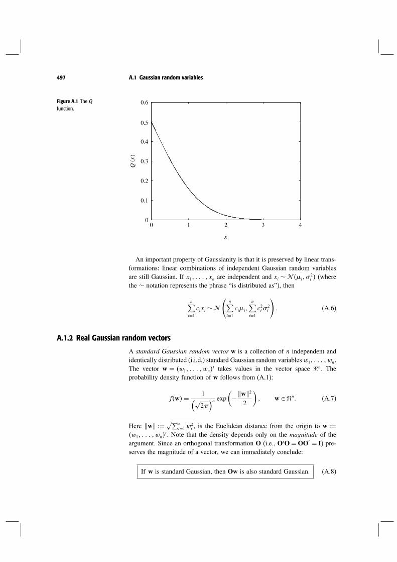
497 A.1 Gaussian random variables
Figure A.1 The Qfunction.
0 1 2 3 40
0.1
0.2
0.3
0.4
0.5
0.6
x
Q (
x )
An important property of Gaussianity is that it is preserved by linear trans-formations: linear combinations of independent Gaussian random variablesare still Gaussian. If x1 xn are independent and xi ∼ i
2i (where
the ∼ notation represents the phrase “is distributed as”), then
n∑
i=1
cixi ∼
(n∑
i=1
ciin∑
i=1
c2i 2i
)
(A.6)
A.1.2 Real Gaussian random vectors
A standard Gaussian random vector w is a collection of n independent andidentically distributed (i.i.d.) standard Gaussian random variables w1 wn.The vector w = w1 wn
t takes values in the vector space n. Theprobability density function of w follows from (A.1):
fw= 1(√
2)n exp
(
−w22
)
w ∈ n (A.7)
Here w = √∑ni=1w
2i , is the Euclidean distance from the origin to w =
w1 wnt. Note that the density depends only on the magnitude of the
argument. Since an orthogonal transformation O (i.e., OtO=OOt = I) pre-serves the magnitude of a vector, we can immediately conclude:
If w is standard Gaussian, then Ow is also standard Gaussian. (A.8)

498 Appendix A Detection and estimation in additive Gaussian noise
What this result says is that w has the same distribution in any orthonor-
f (a) = f (a′ )a2
a
a′a1
Figure A.2 The isobars, i.e.,level sets for the density fw ofthe standard Gaussian randomvector, are circles for n= 2.
mal basis. Geometrically, the distribution of w is invariant to rotations andreflections and hence w does not prefer any specific direction. Figure A.2illustrates this isotropic behavior of the density of the standard Gaussian ran-dom vector w. Another conclusion from (A.8) comes from observing that therows of matrix O are orthonormal: the projections of the standard Gaussianrandom vector in orthogonal directions are independent.How is the squared magnitude w2 distributed? The squared magnitude
is equal to the sum of the square of n i.i.d. zero-mean Gaussian randomvariables. In the literature this sum is called a -squared random variable withn degrees of freedom and denoted by 2
n . With n= 2, the squared magnitudehas density
fa= 12exp
(−a
2
) a≥ 0 (A.9)
and is said to be exponentially distributed. The density of the 2n random
variable for general n is derived in Exercise A.1.Gaussian random vectors are defined as linear transformations of a standard
Gaussian random vector plus a constant vector, a natural generalization of thescalar case (cf. (A.2)):
x = Aw+ (A.10)
Here A is a matrix representing a linear transformation from n to n and is a fixed vector in n. Several implications follow:
1. A standard Gaussian random vector is also Gaussian (with A = I and= 0).
2. For any c, a vector in n, the random variable
ctx ∼ ct ctAAtc (A.11)
this follows directly from (A.6). Thus any linear combination of the ele-ments of a Gaussian random vector is a Gaussian random variable.1 Moregenerally, any linear transformation of a Gaussian random vector is alsoGaussian.
3. If A is invertible, then the probability density function of x follows directlyfrom (A.7) and (A.10):
fx= 1
√2
n√detAAt
exp(
−12x−tAAt−1x−
)
x ∈n
(A.12)
1 This property can be used to define a Gaussian random vector; it is equivalent to ourdefinition in (A.10).

499 A.1 Gaussian random variables
Figure A.3 The isobars of ageneral Gaussian randomvector are ellipses. Theycorresponds to level setsx A−1x−2 = c forconstants c.
f (a) = f (a′)
µ
a2
a1
aa′
The isobars of this density are ellipses; the circles of the standard Gaussianvectors being rotated and scaled by A (Figure A.3). The matrix AAt
replaces 2 in the scalar Gaussian random variable (cf. (A.3)) and is equalto the covariance matrix of x:
K = x−x−t= AAt (A.13)
For invertible A, the Gaussian random vector is completely characterizedby its mean vector and its covariance matrix K = AAt, which is asymmetric and non-negative definite matrix. We make a few inferencesfrom this observation:(a) Even though the Gaussian random vector is defined via the matrix A,
only the covariance matrix K=AAt is used to characterize the densityof x. Is this surprising? Consider two matrices A and AO used to definetwo Gaussian random vectors as in (A.10). When O is orthogonal, thecovariance matrices of both these random vectors are the same, equalto AAt; so the two random vectors must be distributed identically. Wecan see this directly using our earlier observation (see (A.8)) that Owhas the same distribution as w and thus AOw has the same distributionas Aw.
(b) A Gaussian random vector is composed of independent Gaussianrandom variables exactly when the covariance matrix K is diagonal,i.e., the component random variables are uncorrelated. Such a randomvector is also called a white Gaussian random vector.
(c) When the covariance matrix K is equal to identity, i.e., the componentrandom variables are uncorrelated and have the same unit variance,then the Gaussian random vector reduces to the standard Gaussianrandom vector.
4. Now suppose that A is not invertible. Then Aw maps the standard Gaus-sian random vector w into a subspace of dimension less than n, and thedensity of Aw is equal to zero outside that subspace and impulsive inside.This means that some components of Aw can be expressed as linear

500 Appendix A Detection and estimation in additive Gaussian noise
combinations of the others. To avoid messy notation, we can focus onlyon those components of Aw that are linearly independent and representthem as a lower dimensional vector x, and represent the other componentsof Aw as (deterministic) linear combinations of the components of x. Bythis strategem, we can always take the covariance K to be invertible.
In general, a Gaussian random vector is completely characterized by itsmean and by the covariance matrix K; we denote the random vector by K.
A.1.3 Complex Gaussian random vectors
So far we have considered real random vectors. In this book, we are primarilyinterested in complex random vectors; these are of the form x = xR + jxIwhere xRxI are real random vectors. Complex Gaussian random vectors areones in which xRxI
t is a real Gaussian random vector. The distribution iscompletely specified by the mean and covariance matrix of the real vectorxRxI
t. Exercise A.3 shows that the same information is contained in themean , the covariance matrix K, and the pseudo-covariance matrix J of thecomplex vector x, where
= x (A.14)
K = x−x−∗ (A.15)
J = x−x−t (A.16)
Here, A∗ is the transpose of the matrix A with each element replaced by itscomplex conjugate, and At is just the transpose of A. Note that in general thecovariance matrix K of the complex random vector x by itself is not enoughto specify the full second-order statistics of x. Indeed, since K is Hermitian,i.e., K = K∗, the diagonal elements are real and the elements in the lower andupper triangles are complex conjugates of each other. Hence it is specifiedby n2 real parameters, where n is the (complex) dimension of x. On the otherhand, the full second-order statistics of x are specified by the n2n+1 realparameters in the symmetric 2n×2n covariance matrix of xRxI
t.For reasons explained in Chapter 2, in wireless communication we are
almost exclusively interested in complex random vectors that have the circularsymmetry property:
x is circular symmetric if e jx has the same distribution of x for any
(A.17)
For a circular symmetric complex random vector x,
x= e jx= e jx (A.18)

501 A.1 Gaussian random variables
for any ; hence the mean = 0. Moreover
xxt= e jxe jxt= e j2xxt (A.19)
for any ; hence the pseudo-covariance matrix J is also zero. Thus, thecovariance matrix K fully specifies the first- and second-order statistics ofa circular symmetric random vector. And if the complex random vector isalso Gaussian, K in fact specifies its entire statistics. A circular symmetricGaussian random vector with covariance matrix K is denoted as (0,K).Some special cases:
1. A complex Gaussian random variable w = wR + jwI with i.i.d. zero-meanGaussian real and imaginary components is circular symmetric. The circu-lar symmetry of w is in fact a restatement of the rotational invariance of thereal Gaussian random vector wRwI
t already observed (cf. (A.8)). In fact,a circular symmetric Gaussian random variable must have i.i.d. zero-meanreal and imaginary components (Exercise A.5). The statistics are fullyspecified by the variance 2 =w2, and the complex random variableis denoted as 02. (Note that, in contrast, the statistics of a generalcomplex Gaussian random variable are specified by five real parameters:the means and the variances of the real and imaginary components andtheir correlation.) The phase of w is uniform over the range 02 andindependent of the magnitude w, which has a density given by
fr= r
2exp
−r2
22
r ≥ 0 (A.20)
and is known as a Rayleigh random variable. The square of the magnitude,i.e., w2
1 +w22, is 2
2 , i.e., exponentially distributed, cf. (A.9). A randomvariable distributed as 01 is said to be standard, with the real andimaginary parts each having variance 1/2.
2. A collection of n i.i.d. 01 random variables forms a standard circularsymmetric Gaussian random vector w and is denoted by 0 I. Thedensity function of w can be explicitly written as, following from (A.7),
fw= 1n
exp−w2 w ∈ n (A.21)
As in the case of a real Gaussian random vector 0 I (cf. (A.8)), wehave the property that
Uw has the same distribution as w (A.22)
for any complex orthogonal matrix U (such a matrix is called a unitarymatrix and is characterized by the property U∗U= I). The property (A.22)is the complex extension of the isotropic property of the real standard Gaus-sian random vector (cf. (A.8)). Note the distinction between the circular

502 Appendix A Detection and estimation in additive Gaussian noise
symmetry (A.17) and the isotropic (A.22) properties: the latter is in generalmuch stronger than the former except that they coincide when w is scalar.
The square of the magnitude of w, as in the real case, is a 22n random
variable.3. If w is 0 I and A is a complex matrix, then x = Aw is also circular
symmetric Gaussian, with covariance matrix K = AA∗, i.e., 0K.Conversely, any circular symmetric Gaussian random vector with covari-ance matrixK can be written as a linearly transformed version of a standardcircular symmetric random vector. If A is invertible, the density functionof x can be explicitly calculated via (A.21), as in (A.12),
fx= 1n detK
exp(−x∗K−1x
) x ∈ n (A.23)
When A is not invertible, the earlier discussion for real random vectorsapplies here as well: we focus only on the linearly independent componentsof x, and treat the other components as deterministic linear combinationsof these. This allows us to work with a compact notation.
Summary A.1 Complex Gaussian random vectors
• An n-dimensional complex Gaussian random vector x has real and imag-inary components which form a 2n-dimensional real Gaussian randomvector.
• x is circular symmetric if for any ,
e jx ∼ x (A.24)
• A circular symmetric Gaussian x has zero mean and its statistics arefully specified by the covariance matrix K = xx∗. It is denoted by 0K.
• The scalar complex random variable w ∼ 01 has i.i.d. real andimaginary components each distributed as 01/2. The phase of w isuniformly distributed in 02 and independent of its magnitude w,which is Rayleigh distributed:
fr= r exp(
− r2
2
)
r ≥ 0 (A.25)
w2 is exponentially distributed.• If the random vector w∼ 0 I, then its real and imaginary compo-
nents are all i.i.d., and w is isotropic, i.e., for any unitary matrix U,
Uw ∼ w (A.26)

503 A.2 Detection in Gaussian noise
Equivalently, the projections of w onto orthogonal directions are i.i.d. 01. The squared magnitude w2 is distributed as 2
2n withmean n.
• If x ∼ 0K and K is invertible, then the density of x is
fx= 1n detK
exp−x∗K−1x x ∈ n (A.27)
A.2 Detection in Gaussian noise
A.2.1 Scalar detection
Consider the real additive Gaussian noise channel:
y = u+w (A.28)
where the transmit symbol u is equally likely to be uA or uB and w ∼ 0N0/2 is real Gaussian noise. The detection problem involves making adecision on whether uA or uB was transmitted based on the observation y. Theoptimal detector, with the least probability of making an erroneous decision,chooses the symbol that is most likely to have been transmitted given thereceived signal y, i.e., uA is chosen if
u= uAy≥ u= uBy (A.29)
Since the two symbols uA, uB are equally likely to have been transmitted,Bayes’ rule lets us simplify this to the maximum likelihood (ML) receiver,which chooses the transmit symbol that makes the observation y most likely.Conditioned on u = ui, the received signal y ∼ uiN0/2 i = AB, andthe decision rule is to choose uA if
1√N0
exp(
− y−uA2
N0
)
≥ 1√N0
exp(
− y−uB2
N0
)
(A.30)
and uB otherwise. The ML rule in (A.30) further simplifies: choose uA when
y−uA< y−uB (A.31)
The rule is illustrated in Figure A.4 and can be interpreted as corresponding tochoosing the nearest neighboring transmit symbol. The probability of makingan error, the same whether the symbol uA or uB was transmitted, is equal to
y <uA+uB
2u= uA
=
w >uA−uB
2
=Q
(uA−uB2√N0/2
)
(A.32)

504 Appendix A Detection and estimation in additive Gaussian noise
Figure A.4 The ML rule is tochoose the symbol that isclosest to the received symbol.
y
If y < (uA +
uB)
/
2
choose uA
If y > (uA + uB) / 2choose uB
uA2
uB(uA+uB)
y | x = uB y | x = uA
Thus, the error probability only depends on the distance between the twotransmit symbols uAuB.
A.2.2 Detection in a vector space
Now consider detecting the transmit vector u equally likely to be uA or uB
(both elements of n). The received vector is
y= u+w (A.33)
and w ∼ 0 N0/2I. Analogous to (A.30), the ML decision rule is tochoose uA if
1N0
n/2exp
(
−y−uA2N0
)
≥ 1N0
n/2exp
(
−y−uB2N0
)
(A.34)
which simplifies to, analogous to (A.31),
y−uA< y−uB (A.35)
the same nearest neighbor rule. By the isotropic property of the Gaussiannoise, we expect the error probability to be the same for both the transmitsymbols uAuB. Suppose uA is transmitted, so y = uA +w. Then an erroroccurs when the event in (A.35) does not occur, i.e., w> w+uA−uB.So, the error probability is equal to
w2 > w+uA−uB2=
uA−uBtw <−uA−uB2
2
(A.36)

505 A.2 Detection in Gaussian noise
Geometrically, this says that the decision regions are the two sides ofthe hyperplane perpendicular to the vector uB − uA, and an error occurswhen the received vector lies on the side of the hyperplane opposite to thetransmit vector (Figure A.5). We know from (A.11) that uA − uB
tw ∼ 0uA−uB2N0/2. Thus the error probability in (A.36) can be written incompact notation as
Q
(uA−uB2√N0/2
)
(A.37)
The quantity uA−uB/2 is the distance from each of the vectors uAuB tothe decision boundary. Comparing the error probability in (A.37) with thatin the scalar case (cf. (A.32)), we see that the the error probability dependsonly on the Euclidean distance between uA and uB and not on the specificorientations and magnitudes of uA and uB.
An alternative viewTo see how we could have reduced the vector detection problem to the scalarone, consider a small change in the way we think of the transmit vectoru ∈ uAuB. We can write the transmit vector u as
u= xuA−uB+12uA+uB (A.38)
where the information is in the scalar x, which is equally likely to be ±1/2.Substituting (A.38) in (A.33), we can subtract the constant vector uA+uB/2from the received signal y to arrive at
y− 12uA+uB= xuA−uB+w (A.39)
Figure A.5 The decision regionfor the nearest neighbor rule ispartitioned by the hyperplaneperpendicular to uB −uA andhalfway between uA and uB .
if y ∈UAchoose uA
if y ∈UBchoose uB
uA
uB
UA
UB
y2
y1

506 Appendix A Detection and estimation in additive Gaussian noise
We observe that the transmit symbol (a scalar x) is only in a specific direction:
v = uA−uB/uA−uB (A.40)
The components of the received vector y in the directions orthogonal to vcontain purely noise, and, due to the isotropic property of w, the noise inthese directions is also independent of the noise in the signal direction. Thismeans that the components of the received vector in these directions areirrrelevant for detection. Therefore projecting the received vector along thesignal direction v provides all the necessary information for detection:
y = vt(
y− 12uA+uB
)
(A.41)
We have thus reduced the vector detection problem to the scalar one.Figure A.6 summarizes the situation.More formally, we are viewing the received vector in a different orthonor-
mal basis: the first direction is that given by v, and the other directions areorthogonal to each other and to the first one. In other words, we form anorthogonal matrix O whose first row is v, and the other rows are orthogonalto each other and to the first one and have unit norm. Then
O(
y− 12uA+uB
)
=
xuA−uB0
0
+Ow (A.42)
Since Ow ∼ 0 N0/2I (cf. (A.8)), this means that all but the first com-ponent of the vector Oy− 1
2 uA + uB are independent of the transmitsymbol x and the noise in the first component. Thus it suffices to make adecision on the transmit symbol x, using only the first component, which isprecisely (A.41).
Figure A.6 Projecting thereceived vector y onto thesignal direction v reduces thevector detection problem tothe scalar one.
y
y
uA
uB
UA
UB
y2
y1

507 A.2 Detection in Gaussian noise
This important observation can be summarized:
1. In technical jargon, the scalar y in (A.41) is called a sufficient statistic ofthe received vector y to detect the transmit symbol u.
2. The sufficient statistic y is a projection of the received signal in the signaldirection v: in the literature on communication theory, this operation iscalled a matched filter; the linear filter at the receiver is “matched” to thedirection of the transmit signal.
3. This argument explains why the error probability depends on uA and uB
only through the distance between them: the noise is isotropic and theentire detection problem is rotationally invariant.
We now arrive at a scalar detection problem:
y = xuA−uB+w (A.43)
where w, the first component of Ow is 0N0/2 and independent of thetransmit symbol u. The effective distance between the two constellation pointsis uA−uB. The error probability is, from (A.32),
Q
(uA−uB2√N0/2
)
(A.44)
the same as that arrived at in (A.37), via a direct calculation.The above argument for binary detection generalizes naturally to the case
when the transmit vector can be one of M vectors u1 uM . The projec-tion of y onto the subspace spanned by u1 uM is a sufficient statisticfor the detection problem. In the special case when the vectors u1 uM
are collinear, i.e., ui = hxi for some vector h (for example, when we aretransmitting from a PAM constellation), then a projection onto the directionh provides a sufficient statistic.
A.2.3 Detection in a complex vector space
Consider detecting the transmit symbol u, equally likely to be one of twocomplex vectors uAuB in additive standard complex Gaussian noise. Thereceived complex vector is
y= u+w (A.45)
where w ∼ 0N0I. We can proceed as in the real case. Write
u= xuA−uB+12uA+uB (A.46)

508 Appendix A Detection and estimation in additive Gaussian noise
The signal is in the direction
v = uA−uB/uA−uB (A.47)
Projection of the received vector y onto v provides a (complex) scalar suffi-cient statistic:
y = v∗(
y− 12uA+uB
)
= xuA−uB+w (A.48)
where w∼ 0N0. Note that since x is real (±1/2), we can further extracta sufficient statistic by looking only at the real component of y:
y= xuA−uB+w (A.49)
where w∼ N0N0/2. The error probability is exactly as in (A.44):
Q
(uA−uB2√N0/2
)
(A.50)
Note that although uA and uB are complex vectors, the transmit vectors
xuA−uB+12uA+uB x =±1 (A.51)
lie in a subspace of one real dimension and hence we can extract a realsufficient statistic. If there are more than two possible transmit vectors andthey are of the form hxi, where xi is complex valued, h∗y is still a sufficientstatistic but h∗y is sufficient only if x is real (for example, when we aretransmitting a PAM constellation).The main results of our discussion are summarized below.
Summary A.2 Vector detection in complex Gaussian noise
Binary signalsThe transmit vector u is either uA or uB and we wish to detect u fromreceived vector
y= u+w (A.52)
where w∼ 0N0I. The ML detector picks the transmit vector closestto y and the error probability is
Q
(uA−uB2√N0/2
)
(A.53)

509 A.3 Estimation in Gaussian noise
Collinear signalsThe transmit symbol x is equally likely to take one of a finite set of valuesin (the constellation points) and the received vector is
y= hx+w (A.54)
where h is a fixed vector.
Projecting y onto the unit vector v = h/h yields a scalar sufficientstatistic:
v∗y= hx+w (A.55)
Here w ∼ 0N0.
If further the constellation is real-valued, then
v∗y= hx+w (A.56)
is sufficient. Here w∼ 0N0/2.
With antipodal signalling, x =±a, the ML error probability is simply
Q
(ah√N0/2
)
(A.57)
Via a translation, the binary signal detection problem in the first part ofthe summary can be reduced to this antipodal signalling scenario.
A.3 Estimation in Gaussian noise
A.3.1 Scalar estimation
Consider a zero-mean real signal x embedded in independent additive realGaussian noise (w ∼ 0N0/2):
y = x+w (A.58)
Suppose we wish to come up with an estimate x of x and we use the meansquared error (MSE) to evaluate the performance:
MSE = x− x2 (A.59)

510 Appendix A Detection and estimation in additive Gaussian noise
where the averaging is over the randomness of both the signal x and thenoise w. This problem is quite different from the detection problem studiedin Section A.2. The estimate that yields the smallest mean squared error isthe classical conditional mean:
x = xy (A.60)
which has the important orthogonality property: the error is independent ofthe observation. In particular, this implies that
x−xy= 0 (A.61)
The orthogonality principle is a classical result and all standard textbooksdealing with probability theory and random variables treat this material.In general, the conditional mean xy is some complicated non-linear
function of y. To simplify the analysis, one studies the restricted class of linearestimates that minimize the MSE. This restriction is without loss of generalityin the important case when x is a Gaussian random variable because, in thiscase, the conditional mean operator is actually linear.Since x is zero mean, linear estimates are of the form x= cy for some real
number c. What is the best coefficient c? This can be derived directly or viausing the orthogonality principle (cf. (A.61)):
c = x2
x2+N0/2 (A.62)
Intuitively, we are weighting the received signal y by the transmitted sig-nal energy as a fraction of the received signal energy. The correspondingminimum mean squared error (MMSE) is
MMSE = x2N0/2x2+N0/2
(A.63)
A.3.2 Estimation in a vector space
Now consider estimating x in a vector space:
y= hx+w (A.64)
Here x and w∼ 0 N0/2I are independent and h is a fixed vector in n.We have seen that the projection of y in the direction of h,
y = htyh2 = x+w (A.65)
is a sufficient statistic: the projections of y in directions orthogonal to hare independent of both the signal x and w, the noise in the direction

511 A.3 Estimation in Gaussian noise
of h. Thus we can convert this problem to a scalar one: estimate x fromy, with w ∼ 0N0/2h2. Now this problem is identical to the scalarestimation problem in (A.58) with the energy of the noise w suppressed by afactor of h2. The best linear estimate of x is thus, as in (A.62),
x2h2x2h2+N0/2
y (A.66)
We can combine the sufficient statistic calculation in (A.65) and the scalarlinear estimate in (A.66) to arrive at the best linear estimate x = cty of x
from y:
c = x2
x2h2+N0/2h (A.67)
The corresponding minimum mean squared error is
MMSE = x2N0/2x2h2+N0/2
(A.68)
An alternative performance measure to evaluate linear estimators is thesignal-to-noise ratio (SNR) defined as the ratio of the signal energy in theestimate to the noise energy:
SNR = cth2x2c2N0/2
(A.69)
That the matched filter (c = h) yields the maximal SNR at the output of anylinear filter is a classical result in communication theory (and is studied inall standard textbooks on the topic). It follows directly from the Cauchy–Schwartz inequality:
cth2 ≤ c2 h2 (A.70)
with equality exactly when c= h. The fact that the matched filter maximizesthe SNR and when appropriately scaled yields the MMSE is not coincidental;this is studied in greater detail in Exercise A.8.
A.3.3 Estimation in a complex vector space
The extension of our discussion to the complex field is natural. Let usfirst consider scalar complex estimation, an extension of the basic real setupin (A.58):
y = x+w (A.71)

512 Appendix A Detection and estimation in additive Gaussian noise
where w ∼ 0N0 is independent of the complex zero-mean transmittedsignal x. We are interested in a linear estimate x = c∗y, for some complexconstant c. The performance metric is
MSE = x− x2 (A.72)
The best linear estimate x = c∗y can be directly calculated to be, as anextension of (A.62),
c = x2x2+N0
(A.73)
The corresponding minimum MSE is
MMSE = x2N0
x2+N0
(A.74)
The orthogonality principle (cf. (A.61)) for the complex case is extended to:
x−xy∗= 0 (A.75)
The linear estimate in (A.73) is easily seen to satisfy (A.75).Now let us consider estimating the scalar complex zero mean x in a complex
vector space:
y= hx+w (A.76)
with w ∼ 0N0I independent of x and h a fixed vector in n. Theprojection of y in the direction of h is a sufficient statistic and we can reducethe vector estimation problem to a scalar one: estimate x from
y = h∗yh2 = x+w (A.77)
where w ∼ 0N0/h2.Thus the best linear estimator is, as an extension of (A.67),
c = x2x2h2+N0
h (A.78)
The corresponding minimum MSE is, as an extension of (A.68),
MMSE = x2N0
x2h2+N0
(A.79)

513 A.4 Exercises
Summary A.3 Mean square estimation in a complexvector space
The linear estimate with the smallest mean squared error of x from
y = x+w (A.80)
with w ∼ 0N0, is
x = x2x2+N0
y (A.81)
To estimate x from
y= hx+w (A.82)
where w ∼ 0N0I,
h∗y (A.83)
is a sufficient statistic, reducing the vector estimation problem to thescalar one.
The best linear estimator is
x = x2x2h2+N0
h∗y (A.84)
The corresponding minimum mean squared error (MMSE) is:
MMSE = x2N0
x2h2+N0
(A.85)
In the special case when x∼ 2, this estimator yields the minimummean squared error among all estimators, linear or non-linear.
A.4 Exercises
Exercise A.1 Consider the n-dimensional standard Gaussian random vectorw ∼ 0 In and its squared magnitude w2.1. With n= 1, show that the density of w2 is
f1a=1√2a
exp(−a
2
) a≥ 0 (A.86)

514 Appendix A Detection and estimation in additive Gaussian noise
2. For any n, show that the density of w2 (denoted by fn·) satisfies the recursiverelation:
fn+2a=a
nfna a≥ 0 (A.87)
3. Using the formulas for the densities for n= 1 and 2 ((A.86) and (A.9), respectively)and the recurisve relation in (A.87) determine the density of w2 for n≥ 3.
Exercise A.2 Let wt be white Gaussian noise with power spectral density N0/2.Let s1 sM be a set of finite orthonormal waveforms (i.e., orthogonal and unitenergy), and define zi =
∫ −wtsitdt. Find the joint distribution of z. Hint: Recall
the isotropic property of the normalized Gaussian random vector (see (A.8)).
Exercise A.3 Consider a complex random vector x.1. Verify that the second-order statistics of x (i.e., the covariance matrix of the real
representation xxt) can be completely specified by the covariance andpseudo-covariance matrices of x, defined in (A.15) and (A.16) respectively.
2. In the case where x is circular symmetric, express the covariance matrixxxt in terms of the covariance matrix of the complex vector x only.
Exercise A.4 Consider a complex Gaussian random vector x.1. Show that a necessary and sufficient condition for x to be circular symmetric is
that the mean and the pseudo-covariance matrix J are zero.2. Now suppose the relationship between the covariance matrix of xxt and
the covariance matrix of x in part (2) of Exercise A.3 holds. Can we conclude thatx is circular symmetric?
Exercise A.5 Show that a circular symmetric complex Gaussian random variable musthave i.i.d. real and imaginary components.
Exercise A.6 Let x be an n-dimensional i.i.d. complex Gaussian random vector, withthe real and imaginary parts distributed as 0Kx where Kx is a 2×2 covariancematrix. Suppose U is a unitary matrix (i.e., U∗U = I). Identify the conditions on Kx
under which Ux has the same distribution as x.
Exercise A.7 Let z be an n-dimensional i.i.d. complex Gaussian random vector, withthe real and imaginary parts distributed as 0Kx where Kx is a 2×2 covariancematrix. We wish to detect a scalar x, equally likely to be ±1 from
y= hx+ z (A.88)
where x and z are independent and h is a fixed vector in n. Identify the conditionson Kx under which the scalar h∗y is a sufficient statistic to detect x from y.
Exercise A.8 Consider estimating the real zero-mean scalar x from:
y= hx+w (A.89)
where w ∼ 0N0/2I is uncorrelated with x and h is a fixed vector in n.

515 A.4 Exercises
1. Consider the scaled linear estimate cty (with the normalization c = 1):
x = acty= acth x+actz (A.90)
Show that the constant a that minimizes the mean square error (x− x2) isequal to
x2cth2x2cth2+N0/2
(A.91)
2. Calculate the minimal mean square error (denoted by MMSE) of the linear estimatein (A.90) (by using the value of a in (A.91). Show that
x2
MMSE= 1+SNR = 1+ x2cth2
N0/2 (A.92)
For every fixed linear estimator c, this shows the relationship between the correspond-ing SNR and MMSE (of an appropriately scaled estimate). In particular, this relationholds when we optimize over all c leading to the best linear estimator.
Appendix B Information theory from firstprinciples
This appendix discusses the information theory behind the capacity expres-sions used in the book. Section 8.3.4 is the only part of the book that supposesan understanding of the material in this appendix. More in-depth and broaderexpositions of information theory can be found in standard texts such as [26]and [43].
B.1 Discrete memoryless channels
Although the transmitted and received signals are continuous-valued in mostof the channels we considered in this book, the heart of the communicationproblem is discrete in nature: the transmitter sends one out of a finite num-ber of codewords and the receiver would like to figure out which codewordis transmitted. Thus, to focus on the essence of the problem, we first con-sider channels with discrete input and output, so-called discrete memorylesschannels (DMCs).Both the input xm and the output ym of a DMC lie in finite sets
and respectively. (These sets are called the input and output alphabetsof the channel respectively.) The statistics of the channel are described byconditional probabilities pjii∈j∈ . These are also called transition prob-abilities. Given an input sequence x = x1 xN, the probability ofobserving an output sequence y= y1 yN is given by1
pyx=N∏
m=1
pymxm (B.1)
The interpretation is that the channel noise corrupts the input symbolsindependently (hence the term memoryless).
1 This formula is only valid when there is no feedback from the receiver to the transmitter,i.e., the input is not a function of past outputs. This we assume throughout.
516

517 B.1 Discrete memoryless channels
Example B.1 Binary symmetric channelThe binary symmetric channel has binary input and binary output = = 01. The transition probabilities are p01= p10= p00=p11 = 1− . A 0 and a 1 are both flipped with probability . SeeFigure B.1(a).
Example B.2 Binary erasure channelThe binary erasure channel has binary input and ternary output =01 = 01 e. The transition probabilities are p00 = p11 =1− pe0 = pe1 = . Here, symbols cannot be flipped but can beerased. See Figure B.1(b).
An abstraction of the communication system is shown in Figure B.2. Thesender has one out of several equally likely messages it wants to transmitto the receiver. To convey the information, it uses a codebook of blocklength N and size , where = x1 x and xi are the codewords. Totransmit the ith message, the codeword xi is sent across the noisy channel.Based on the received vector y, the decoder generates an estimate i of thecorrect message. The error probability is pe = i = i. We will assume thatthe maximum likelihood (ML) decoder is used, since it minimizes the errorprobability for a given code. Since we are transmitting one of messages,the number of bits conveyed is log . Since the block length of the codeis N , the rate of the code is R = 1
Nlog bits per unit time. The data rate
R and the ML error probability pe are the two key performance measures ofa code.
R= 1Nlog
pe = i = i
(B.2)
(B.3)
Figure B.1 Examples ofdiscrete memoryless channels:(a) binary symmetric channel;(b) binary erasure channel. (a)
0
1
0
1
0
1
0
11 –
1 –
e
1 –
1 –
(b)
∋ ∋
∋
∋
∋
∋
∋
∋

518 Appendix B Information theory from first principles
iDecoderChannelp(y | x)
xi = (xi [1], . . . , xi
[N]) y = ( y[1], . . . , y[N])
Encoder
Messagei 0 , 1, . . . , |C | – 1∋
Information is said to be communicated reliably at rate R if for everyFigure B.2 Abstraction of acommunication system à laShannon.
> 0, one can find a code of rate R and block length N such that the errorprobability pe < . The capacity C of the channel is the maximum rate forwhich reliable communication is possible.Note that the key feature of this definition is that one is allowed to code
over arbitrarily large block length N . Since there is noise in the channel, it isclear that the error probability cannot be made arbitrarily small if the blocklength is fixed a priori. (Recall the AWGN example in Section 5.1.) Onlywhen the code is over long block length is there hope that one can rely onsome kind of law of large numbers to average out the random effect of thenoise. Still, it is not clear a priori whether a non-zero reliable information ratecan be achieved in general.Shannon showed not only that C> 0 for most channels of interest but also
gave a simple way to compute C as a function of pyx. To explain thiswe have to first define a few statistical measures.
B.2 Entropy, conditional entropy and mutual information
Let x be a discrete random variable taking on values in and with aprobability mass function px. Define the entropy of x to be2
Hx =∑
i∈pxi log1/pxi (B.4)
This can be interpreted as a measure of the amount of uncertainty associatedwith the random variable x. The entropy Hx is always non-negative andequal to zero if and only if x is deterministic. If x can take on K values, thenit can be shown that the entropy is maximized when x is uniformly distributedon these K values, in which case Hx= logK (see Exercise B.1).
Example B.3 Binary entropyThe entropy of a binary-valued random variable x which takes on thevalues with probabilities p and 1−p is
Hp =−p logp− 1−p log1−p (B.5)
2 In this book, all logarithms are taken to the base 2 unless specified otherwise.

519 B.2 Entropy, conditional entropy and mutual information
0
0.3
0.4
0.5
0.6
0.7
0.8
0.9
1
0 0.1 0.2 0.3 0.4 0.5 0.6 0.7 0.8 0.9 1
0.1
0.2
p
H(p)
Figure B.3 The binary entropy function.
The function H· is called the binary entropy function, and is plotted inFigure B.3. It attains its maximum value of 1 at p= 1/2, and is zero whenp = 0 or p = 1. Note that we never mentioned the actual values x takeson; the amount of uncertainty depends only on the probabilities.
Let us now consider two random variables x and y. The joint entropy of xand y is defined to be
Hx y = ∑
i∈j∈pxyi j log1/pxyi j (B.6)
The entropy of x conditional on y = j is naturally defined to be
Hxy = j =∑
i∈pxyij log1/pxyij (B.7)
This can be interpreted as the amount of uncertainty left in x after observingthat y = j. The conditional entropy of x given y is the expectation of thisquantity, averaged over all possible values of y:
Hxy =∑
j∈pyjHxy = j= ∑
i∈j∈pxyi j log1/pxyij (B.8)

520 Appendix B Information theory from first principles
The quantity Hxy can be interpreted as the average amount of uncertaintyleft in x after observing y. Note that
Hx y=Hx+Hyx=Hy+Hxy (B.9)
This has a natural interpretation: the total uncertainty in x and y is the sumof the uncertainty in x plus the uncertainty in y conditional on x. This iscalled the chain rule for entropies. In particular, if x and y are independent,Hxy = Hx and hence Hx y = Hx+Hy. One would expect thatconditioning reduces uncertainty, and in fact it can be shown that
Hxy≤Hx (B.10)
with equality if and only if x and y are independent. (See Exercise B.2.) Hence,
Hx y=Hx+Hyx≤Hx+Hy (B.11)
with equality if and only if x and y are independent.The quantity Hx−Hxy is of special significance to the communication
problem at hand. SinceHx is the amount of uncertainty in x before observingy, this quantity can be interpreted as the reduction in uncertainty of x fromthe observation of y, i.e., the amount of information in y about x. Similarly,Hy−Hyx can be interpreted as the reduction in uncertainty of y fromthe observation of x. Note that
Hy−Hyx=Hy+Hx−Hx y=Hx−Hxy (B.12)
So if one defines
Ix y =Hy−Hyx=Hx−Hxy (B.13)
then this quantity is symmetric in the random variables x and y. Ix y iscalled the mutual information between x and y. A consequence of (B.10) isthat the mutual information Ix y is a non-negative quantity, and equal tozero if and only if x and y are independent.We have defined the mutual information between scalar random vari-
ables, but the definition extends naturally to random vectors. For example,Ix1 x2 y should be interpreted as the mutual information between the ran-dom vector x1 x2 and y, i.e., Ix1 x2 y=Hx1 x2−Hx1 x2y. One canalso define a notion of conditional mutual information:
Ix yz =Hxz−Hxy z (B.14)
Note that since
Hxz=∑
k
pzkHxz= k (B.15)

521 B.3 Noisy channel coding theorem
and
Hxy z=∑
k
pzkHxy z= k (B.16)
it follows that
Ix yz=∑
k
pzkIx yz= k (B.17)
Given three random variables x1 x2 and y, observe that
Ix1 x2 y = Hx1 x2−Hx1 x2y= Hx1+Hx2x1− Hx1y+Hx2x1 y= Ix1 y+ Ix2 yx1
This is the chain rule for mutual information:
Ix1 x2 y= Ix1 y+ Ix2 yx1 (B.18)
In words: the information that x1 and x2 jointly provide about y is equal to thesum of the information x1 provides about y plus the additional information x2provides about y after observing x1. This fact is very useful in Chapters 7 to 10.
B.3 Noisy channel coding theorem
Let us now go back to the communication problem shown in Figure B.2.We convey one of equally likely messages by mapping it to its N -lengthcodeword in the code = x1 x . The input to the channel is thenan N -dimensional random vector x, uniformly distributed on the codewordsof . The output of the channel is another N -dimensional vector y.
B.3.1 Reliable communication and conditional entropy
To decode the transmitted message correctly with high probability, it is clearthat the conditional entropy Hxy has to be close to zero3. Otherwise, thereis too much uncertainty in the input, given the output, to figure out what theright message is. Now,
Hxy=Hx− Ix y (B.19)
3 This statement can be made precise in the regime of large block lengths using Faro’sinequality.

522 Appendix B Information theory from first principles
i.e., the uncertainty in x subtracting the reduction in uncertainty in x byobserving y. The entropy Hx is equal to log = NR, where R is the datarate. For reliable communication, Hxy≈ 0, which implies
R≈ 1NIx y (B.20)
Intuitively: for reliable communication, the rate of flow of mutual informationacross the channel should match the rate at which information is generated.Now, the mutual information depends on the distribution of the random inputx, and this distribution is in turn a function of the code . By optimizing overall codes, we get an upper bound on the reliable rate of communication:
max
1NIx y (B.21)
B.3.2 A simple upper bound
The optimization problem (B.21) is a high-dimensional combinatorial oneand is difficult to solve. Observe that since the input vector x is uniformlydistributed on the codewords of , the optimization in (B.21) is over only asubset of possible input distributions. We can derive a further upper boundby relaxing the feasible set and allowing the optimization to be over all inputdistributions:
C =maxpx
1NIx y (B.22)
Now,
Ix y = Hy−Hyx (B.23)
≤N∑
m=1
Hym−Hyx (B.24)
=N∑
m=1
Hym−N∑
m=1
Hymxm (B.25)
=N∑
m=1
Ixm ym (B.26)
The inequality in (B.24) follows from (B.11) and the equality in (B.25) comesfrom the memoryless property of the channel. Equality in (B.24) is attainedif the output symbols are independent over time, and one way to achieve thisis to make the inputs independent over time. Hence,
C = 1N
N∑
m=1
maxpxm
Ixm ym=maxpx1
Ix1 y1 (B.27)

523 B.3 Noisy channel coding theorem
Thus, the optimizing problem over input distributions on the N -lengthblock reduces to an optimization problem over input distributions on singlesymbols.
B.3.3 Achieving the upper bound
To achieve this upper bound C, one has to find a code whose mutual infor-mation Ix y/N per symbol is close to C and such that (B.20) is satisfied.A priori it is unclear if such a code exists at all. The cornerstone result ofinformation theory, due to Shannon, is that indeed such codes exist if theblock length N is chosen sufficiently large.
Theorem B.1 (Noisy channel coding theorem [109]) Consider a discretememoryless channel with input symbol x and output symbol y. The capacityof the channel is
C =maxpx
Ix y (B.28)
Shannon’s proof of the existence of optimal codes is through a random-ization argument. Given any symbol input distribution px, we can randomlygenerate a code with rate R by choosing each symbol in each codewordindependently according to px. The main result is that with the rate as in(B.20), the code with large block length N satisfies, with high probability,
1NIx y≈ Ix y (B.29)
In other words, reliable communication is possible at the rate of Ix y.In particular, by choosing codewords according to the distribution p∗
x thatmaximizes Ix y, the maximum reliable rate is achieved. The smaller thedesired error probability, the larger the block length N has to be for the lawof large numbers to average out the effect of the random noise in the channelas well as the effect of the random choice of the code. We will not go intothe details of the derivation of the noisy channel coding theorem in this book,although the sphere-packing argument for the AWGN channel in Section B.5suggests that this result is plausible. More details can be found in standardinformation theory texts such as [26].The maximization in (B.28) is over all distributions of the input random
variable x. Note that the input distribution together with the channel transitionprobabilities specifies a joint distribution on x and y. This determines the

524 Appendix B Information theory from first principles
0.3
0.7
0.8
0.9
1
0 0.1 0.2 0.3 0.4 0.5 0.6 0.7 0.8 0.9 1
0.5
0.4
0.3
0.4
0.5
0.6
0.7
0.8
0.9
1
0 0.1 0.2 0.3 0.4 0.5 0.6 0.7 0.8 0.9 1
0.2
0.1
0 0
0.1
0.2
0.6
C( )C( )
(b)(a)
∋
∋ ∋
∋
value of Ix y. The maximization is over all possible input distribution Itcan be shown that the mutual information Ix y is a concave function of theinput probabilities and hence the input maximization is a convex optimizationproblem, which can be solved very efficiently. Sometimes one can evenappeal to symmetry to obtain the optimal distribution in closed form.
Figure B.4 The capacity of(a) the binary symmetricchannel and (b) the binaryerasure channel.
Example B.4 Binary symmetric channelThe capacity of the binary symmetric channel with crossover probabil-ity is
C =maxpx
Hy−Hyx
=maxpx
Hy−H
= 1−Hbits per channel use (B.30)
whereH is the binary entropy function (B.5). The maximum is achievedby choosing x to be uniform so that the output y is also uniform. Thecapacity is plotted in Figure B.4. It is 1 when = 0 or 1, and 0 when= 1/2.Note that since a fraction of the symbols are flipped in the long run,
one may think that the capacity of the channel is 1− bits per channeluse, the fraction of symbols that get through unflipped. However, this istoo naive since the receiver does not know which symbols are flippedand which are correct. Indeed, when = 1/2, the input and output areindependent and there is no way we can get any information across thechannel. The expression (B.30) gives the correct answer.

525 B.3 Noisy channel coding theorem
Example B.5 Binary erasure channelThe optimal input distribution for the binary symmetric channel is uniformbecause of the symmetry in the channel. Similar symmetry exists in thebinary erasure channel and the optimal input distribution is uniform too.The capacity of the channel with erasure probability can be calculatedto be
C = 1− bits per channel use (B.31)
In the binary symmetric channel, the receiver does not know whichsymbols are flipped. In the erasure channel, on the other hand, the receiverknows exactly which symbols are erased. If the transmitter also knowsthat information, then it can send bits only when the channel is not erasedand a long-term throughput of 1− bits per channel use is achieved. Whatthe capacity result says is that no such feedback information is necessary;(forward) coding is sufficient to get this rate reliably.
B.3.4 Operational interpretation
There is a common misconception that needs to be pointed out. In solvingthe input distribution optimization problem (B.22) for the capacity C, it wasremarked that, at the optimal solution, the outputs ym should be independent,and one way to achieve this is for the inputs xm to be independent. Does thatimply no coding is needed to achieve capacity? For example, in the binarysymmetric channel, the optimal input yields i.i.d. equally likely symbols; doesit mean then that we can send equally likely information bits raw across thechannel and still achieve capacity?Of course not: to get very small error probability one needs to code over
many symbols. The fallacy of the above argument is that reliable commu-nication cannot be achieved at exactly the rate C and when the outputs areexactly independent. Indeed, when the outputs and inputs are i.i.d.,
Hxy=N∑
m=1
Hxmym= NHxmym (B.32)
and there is a lot of uncertainty in the input given the output: the communica-tion is hardly reliable. But once one shoots for a rate strictly less than C, nomatter how close, the coding theorem guarantees that reliable communicationis possible. The mutual information Ix y/N per symbol is close to C, theoutputs ym are almost independent, but now the conditional entropy Hxyis reduced abruptly to (close to) zero since reliable decoding is possible. Butto achieve this performance, coding is crucial; indeed the entropy per inputsymbol is close to Ix y/N , less than Hxm under uncoded transmission.

526 Appendix B Information theory from first principles
For the binary symmetric channel, the entropy per coded symbol is 1−H,rather than 1 for uncoded symbols.The bottom line is that while the value of the input optimization problem
(B.22) has operational meaning as the maximum rate of reliable communica-tion, it is incorrect to interpret the i.i.d. input distribution which attains thatvalue as the statistics of the input symbols which achieve reliable communi-cation. Coding is always needed to achieve capacity. What is true, however,is that if we randomly pick the codewords according to the i.i.d. input distri-bution, the resulting code is very likely to be good. But this is totally differentfrom sending uncoded symbols.
B.4 Formal derivation of AWGN capacity
We can now apply the methodology developed in the previous sections toformally derive the capacity of the AWGN channel.
B.4.1 Analog memoryless channels
So far we have focused on channels with discrete-valued input and outputsymbols. To derive the capacity of the AWGN channel, we need to extendthe framework to analog channels with continuous-valued input and output.There is no conceptual difficulty in this extension. In particular, Theorem B.1can be generalized to such analog channels.4 The definitions of entropy andconditional entropy, however, have to be modified appropriately.For a continuous random variable x with pdf fx, define the differential
entropy of x as
hx =∫
−fxu log1/fxudu (B.33)
Similarly, the conditional differential entropy of x given y is defined as
hxy =∫
−fxyu v log1/fxyuvdudv (B.34)
The mutual information is again defined as
Ix y = hx−hxy (B.35)
4 Although the underlying channel is analog, the communication process is still digital. Thismeans that discrete symbols will still be used in the encoding. By formulating thecommunication problem directly in terms of the underlying analog channel, this meanswe are not constraining ourselves to using a particular symbol constellation (for example,2-PAM or QPSK) a priori.

527 B.4 Formal derivation of AWGN capacity
Observe that the chain rules for entropy and for mutual information extendreadily to the continuous-valued case. The capacity of the continuous-valuedchannel can be shown to be
C =maxfx
Ix y (B.36)
This result can be proved by discretizing the continuous-valued input andoutput of the channel, approximating it by discrete memoryless channels withincreasing alphabet sizes, and taking limits appropriately.For many channels, it is common to have a cost constraint on the transmitted
codewords. Given a cost function c → defined on the input symbols,a cost constraint on the codewords can be defined: we require that everycodeword xn in the codebook must satisfy
1N
N∑
m=1
cxnm≤ A (B.37)
One can then ask: what is the maximum rate of reliable communicationsubject to this constraint on the codewords? The answer turns out to be
C = maxfxEcx≤A
Ix y (B.38)
B.4.2 Derivation of AWGN capacity
We can now apply this result to derive the capacity of the power-constrained(real) AWGN channel:
y = x+w (B.39)
The cost function is cx= x2. The differential entropy of a 2 randomvariable w can be calculated to be
hw= 12log2e2 (B.40)
Not surprisingly, hw does not depend on the mean of W : differentialentropies are invariant to translations of the pdf. Thus, conditional on theinput x of the Gaussian channel, the differential entropy hyx of the output yis just 1/2 log2e2. The mutual information for the Gaussian channelis, therefore,
Ix y= hy−hyx= hy− 12log2e2 (B.41)
The computation of the capacity
C = maxfxEx
2≤PIx y (B.42)

528 Appendix B Information theory from first principles
is now reduced to finding the input distribution on x to maximize hy sub-ject to a second moment constraint on x. To solve this problem, we use akey fact about Gaussian random variables: they are differential entropy max-imizers. More precisely, given a constraint Eu2 ≤ A on a random variableu, the distribution u is 0A maximizes the differential entropy hu.(See Exercise B.6 for a proof of this fact.) Applying this to our problem,we see that the second moment constraint of P on x translates into a sec-ond moment constraint of P+2 on y. Thus, hy is maximized when y is 0P+2, which is achieved by choosing x to be 0P. Thus, thecapacity of the Gaussian channel is
C = 12log2eP+2− 1
2log2e2= 1
2log
(
1+ P
2
)
(B.43)
agreeing with the result obtained via the heuristic sphere-packing deriva-tion in Section 5.1. A capacity-achieving code can be obtained by choosingeach component of each codeword i.i.d. 0P. Each codeword is thereforeisotropically distributed, and, by the law of large numbers, with high probabil-ity lies near the surface of the sphere of radius
√NP. Since in high dimensions
most of the volume of a sphere is near its surface, this is effectively the sameas picking each codeword uniformly from the sphere.Now consider a complex baseband AWGN channel:
y = x+w (B.44)
where w is 0N0. There is an average power constraint of P per (com-plex) symbol. One way to derive the capacity of this channel is to think ofeach use of the complex channel as two uses of a real AWGN channel, withSNR= P/2/N0/2= P/N0. Hence, the capacity of the channel is
12log
(
1+ P
N0
)
bits per real dimension (B.45)
or
log(
1+ P
N0
)
bits per complex dimension (B.46)
Alternatively we may just as well work directly with the complex channeland the associated complex random variables. This will be useful when wedeal with other more complicated wireless channel models later on. To thisend, one can think of the differential entropy of a complex random variable xas that of a real random vector xx. Hence, if w is 0N0,hw= hw+hw= logeN0. The mutual information Ix y ofthe complex AWGN channel y = x+w is then
Ix y= hy− logeN0 (B.47)
529 B.5 Sphere-packing interpretation
With a power constraint Ex2 ≤ P on the complex input x, y is con-strained to satisfy Ey2 ≤ P+N0. Here, we use an important fact: amongall complex random variables, the circular symmetric Gaussian random vari-able maximizes the differential entropy for a given second moment con-straint. (See Exercise B.7.) Hence, the capacity of the complex Gaussianchannel is
C = logeP+N0− logeN0= log(
1+ P
N0
)
(B.48)
which is the same as Eq. (5.11).
B.5 Sphere-packing interpretation
In this section we consider a more precise version of the heuristic sphere-packing argument in Section 5.1 for the capacity of the real AWGN channel.Furthermore, we outline how the capacity as predicted by the sphere-packingargument can be achieved. The material here is particularly useful when wediscuss precoding in Chapter 10.
B.5.1 Upper bound
Consider transmissions over a block of N symbols, where N is large. Supposewe use a code consisting of equally likely codewords x1 x .By the law of large numbers, the N -dimensional received vector y = x+wwill with high probability lie approximately5 within a y-sphere of radius√NP+2, so without loss of generality we need only to focus on what
happens inside this y-sphere. Let i be the part of the maximum-likelihooddecision region for xi within the y-sphere. The sum of the volumes of the i
is equal to Vy, the volume of the y-sphere. Given this total volume, it can beshown, using the spherical symmetry of the Gaussian noise distribution, thatthe error probability is lower bounded by the (hypothetical) case when thei are all perfect spheres of equal volume Vy/ . But by the law of largenumbers, the received vector y lies near the surface of a noise sphere of radius√N2 around the transmitted codeword. Thus, for reliable communication,
Vy/ should be no smaller than the volume Vw of this noise sphere, otherwiseeven in the ideal case when the decision regions are all spheres of equalvolume, the error probability will still be very large. Hence, the number of
5 To make this and other statements in this section completely rigorous, appropriate and
have to be added.
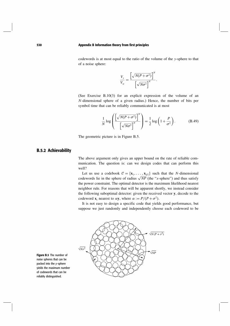
530 Appendix B Information theory from first principles
codewords is at most equal to the ratio of the volume of the y-sphere to thatof a noise sphere:
Vy
Vw
=[√
NP+2]N
[√N2
]N
(See Exercise B.10(3) for an explicit expression of the volume of anN -dimensional sphere of a given radius.) Hence, the number of bits persymbol time that can be reliably communicated is at most
1N
log
[√NP+2
]N
[√N2
]N
= 1
2log
(
1+ P
2
)
(B.49)
The geometric picture is in Figure B.5.
B.5.2 Achievability
The above argument only gives an upper bound on the rate of reliable com-munication. The question is: can we design codes that can perform thiswell?Let us use a codebook = x1 x such that the N -dimensional
codewords lie in the sphere of radius√NP (the “x-sphere”) and thus satisfy
the power constraint. The optimal detector is the maximum likelihood nearestneighbor rule. For reasons that will be apparent shortly, we instead considerthe following suboptimal detector: given the received vector y, decode to thecodeword xi nearest to y, where = P/P+2.It is not easy to design a specific code that yields good performance, but
suppose we just randomly and independently choose each codeword to be
Figure B.5 The number ofnoise spheres that can bepacked into the y-sphereyields the maximum numberof codewords that can bereliably distinguished.
√N (P + σ 2)
√Nσ 2
√NP

531 B.5 Sphere-packing interpretation
uniformly distributed in the sphere6. In high dimensions, most of the volumeof the sphere lies near its surface, so in fact the codewords will with highprobability lie near the surface of the x-sphere.What is the performance of this random code? Suppose the transmitted
codeword is x1. By the law of large numbers again,
y−x12 = w+ −1x12≈ 2N2+ −12NP
= NP2
P+2
i.e., the transmitted codeword lies inside an uncertainty sphere of radius√NP2/P+2 around the vector y. Thus, as long as all the other code-
words lie outside this uncertainty sphere, then the receiver will be able todecode correctly (Figure B.6). The probability that the random codewordxi (i = 1) lies inside the uncertainty sphere is equal to the ratio of the volumeof the uncertainty sphere to that of the x-sphere:
p=(√
NP2/P+2)N
√NPN
=(
2
P+2
)N2
(B.50)
By the union bound, the probability that any of the codewords (x2 x )lie inside the uncertainty sphere is bounded by − 1p. Thus, as long asthe number of codewords is much smaller than 1/p, then the probability oferror is small (in particular, we can take the number of codewords to be
Figure B.6 The ratio of thevolume of the uncertaintysphere to that of the x-sphereyields the probability that agiven random codeword liesinside the uncertainty sphere.The inverse of this probabilityyields a lower bound on thenumber of codewords that canbe reliably distinguished.
√NP
x1 α y
√NPσ 2
P + σ 2
6 Randomly and independently choosing each codeword to have i.i.d. 0P componentswould work too but the argument is more complex.

532 Appendix B Information theory from first principles
1/pN ). In terms of the data rate R bits per symbol time, this means that aslong as
R= log N
= log1/pN
− logNN
<12log
(
1+ P
2
)
then reliable communication is possible.Both the upper bound and the achievability arguments are based on calcu-
lating the ratio of volumes of spheres. The ratio is the same in both cases, butthe spheres involved are different. The sphere-packing picture in Figure B.5corresponds to the following decomposition of the capacity expression:
12log
(
1+ P
2
)
= Ix y= hy−hyx (B.51)
with the volume of the y-sphere proportional to 2Nhy and the volume of thenoise sphere proportional to 2Nhyx. The picture in Figure B.6, on the otherhand, corresponds to the decomposition:
12log
(
1+ P
2
)
= Ix y= hx−hxy (B.52)
with the volume of the x-sphere proportional to 2Nhx. Conditional on y, x isNy2
mmse, where =P/P+2 is the coefficient of the MMSE estimatorof x given y, and
2mmse =
P2
P+2
is the MMSE estimation error. The radius of the uncertainty sphere consideredabove is
√N2
mmse and its volume is proportional to 2Nhxy. In fact theproposed receiver, which finds the nearest codeword to y, is motivatedprecisely by this decomposition. In this picture, then, the AWGN capacityformula is being interpreted in terms of the number of MMSE error spheresthat can be packed inside the x-sphere.
B.6 Time-invariant parallel channel
Consider the parallel channel (cf. (5.33):
yni= hndni+ wni n= 01 Nc−1 (B.53)
subject to an average power per sub-carrier constraint of P (cf. (5.37)):
Edi2≤ NcP (B.54)

533 B.7 Capacity of the fast fading channel
The capacity in bits per symbol is
CNc= max
d2≤NcPId y (B.55)
Now
Id y = hy−hyd (B.56)
≤Nc−1∑
n=0
(hyn−hyndn
)(B.57)
≤Nc−1∑
n=0
log
(
1+ Pnhn2N0
)
(B.58)
The inequality in (B.57) is from (B.11) and Pn denotes the variance ofdn in (B.58). Equality in (B.57) is achieved when dn n = 0 Nc − 1,are independent. Equality is achieved in (B.58) when dn is 0Pnn =0 Nc−1. Thus, computing the capacity in (B.55) is reduced to a powerallocation problem (by identifying the variance of dn with the power allocatedto the nth sub-carrier):
CNc= max
P0 PNc−1
Nc−1∑
n=0
log
(
1+ Pnhn2N0
)
(B.59)
subject to
1Nc
Nc−1∑
n=0
Pn = P Pn ≥ 0 n= 0 Nc−1 (B.60)
The solution to this optimization problem is waterfilling and is described inSection 5.3.3.
B.7 Capacity of the fast fading channel
B.7.1 Scalar fast fading channnel
Ideal interleavingThe fast fading channel with ideal interleaving is modeled as follows:
ym= hmxm+wm (B.61)
where the channel coefficients hm are i.i.d. in time and independent of thei.i.d. 0N0 additive noise wm. We are interested in the situation whenthe receiver tracks the fading channel, but the transmitter only has access tothe statistical characterization; the receiver CSI scenario. The capacity of the

534 Appendix B Information theory from first principles
power-constrained fast fading channel with receiver CSI can be written as,by viewing the receiver CSI as part of the output of the channel,
C = maxpxx2≤P
Ix yh (B.62)
Since the fading channel h is independent of the input, Ix h= 0. Thus, bythe chain rule of mutual information (see (B.18)),
Ix yh= Ix h+ Ix yh= Ix yh (B.63)
Conditioned on the fading coefficient h, the channel is simply an AWGNone, with SNR equal to Ph2/N0, where we have denoted the transmit powerconstraint by P. The optimal input distribution for a power constrained AWGNchannel is , regardless of the operating SNR. Thus, the maximizing inputdistribution in (B.62) is 0P. With this input distribution,
Ix yh= h= log(
1+ Ph2N0
)
and thus the capacity of the fast fading channel with receiver CSI is
C = h
[
log(
1+ Ph2N0
)]
(B.64)
where the average is over the stationary distribution of the fading channel.
Stationary ergodic fadingThe above derivation hinges on the i.i.d. assumption on the fading processhm. Yet in fact (B.64) holds as long as hm is stationary and ergodic.The alternative derivation below is more insightful and valid for this moregeneral setting.We first fix a realization of the fading process hm. Recall from (B.20)
that the rate of reliable communication is given by the average rate of flowof mutual information:
1NIx y= 1
N
N∑
m=1
log1+hm2SNR (B.65)
For large N , due to the ergodicity of the fading process,
1N
N∑
m=1
log1+hm2SNR→ log1+h2SNR (B.66)
for almost all realizations of the fading process hm. This yields the sameexpression of capacity as in (B.64).

535 B.7 Capacity of the fast fading channel
B.7.2 Fast fading MIMO channel
We have only considered the scalar fast fading channel so far; the extensionof the ideas to the MIMO case is very natural. The fast fading MIMO channelwith ideal interleaving is (cf. (8.7))
ym=Hmxm+wm m= 12 (B.67)
where the channel H is i.i.d. in time and independent of the i.i.d. additivenoise, which is 0N0Inr. There is an average total power constraint of Pon the transmit signal. The capacity of the fast fading channel with receiverCSI is, as in (B.62),
C = maxpx x2≤P
Ix yH (B.68)
The observation in (B.63) holds here as well, so the capacity calculation isbased on the conditional mutual information Ix yH. If we fix the MIMOchannel at a specific realization, we have
Ix yH= H = hy−hyx= hy−hw (B.69)
= hy−nr logeN0 (B.70)
To proceed, we use the following fact about Gaussian random vectors: theyare entropy maximizers. Specifically, among all n-dimensional complex ran-dom vectors with a given covariance matrix K, the one that maximizes thedifferential entropy is complex circular-symmetric jointly Gaussian 0K
(Exercise B.8). This is the vector extension of the result that Gaussian ran-dom variables are entropy maximizers for a fixed variance constraint. Thecorresponding maximum value is given by
logdeteK (B.71)
If the covariance of x is Kx and the channel is H= H, then the covarianceof y is
N0Inr +HKxH∗ (B.72)
Calculating the corresponding maximal entropy of y (cf. (B.71)) and substi-tuting in (B.70), we see that
Ix yH= H ≤ logenr detN0Inr +HKxH∗−nr logeN0
= logdet(
Inr +1N0
HKxH∗)
(B.73)

536 Appendix B Information theory from first principles
with equality if x is 0Kx. This means that even if the transmitter doesnot know the channel, there is no loss of optimality in choosing the input tobe .Finally, the capacity of the fast fading MIMO channel is found by averaging
(B.73) with respect to the stationary distribution of H and choosing theappropriate covariance matrix subject to the power constraint:
C = maxKxTrKx≤P
H
[
logdet(
Inr +1N0
HKxH∗)]
(B.74)
Just as in the scalar case, this result can be generalized to any stationaryand ergodic fading process Hm.
B.8 Outage formulation
Consider the slow fading MIMO channel (cf. (8.79))
ym=Hxm+wm (B.75)
Here the MIMO channel, represented by H (an nr ×nt matrix with complexentries), is random but not varying with time. The additive noise is i.i.d. 0N0 and independent of H.If there is a positive probability, however small, that the entries of H are
small, then the capacity of the channel is zero. In particular, the capacity ofthe i.i.d. Rayleigh slow fading MIMO channel is zero. So we focus on char-acterizing the -outage capacity: the largest rate of reliable communicationsuch that the error probability is no more than . We are aided in this studyby viewing the slow fading channel in (B.75) as a compound channel.The basic compound channel consists of a collection of DMCs pyx,
∈ with the same input alphabet and the same output alphabet andparameterized by . Operationally, the communication between the transmit-ter and the receiver is carried out over one specific channel based on the(arbitrary) choice of the parameter from the set . The transmitter does notknow the value of but the receiver does. The capacity is the largest rate atwhich a single coding strategy can achieve reliable communication regard-less of which is chosen. The corresponding capacity achieving strategy issaid to be universal over the class of channels parameterized by ∈ . Animportant result in information theory is the characterization of the capacityof the compound channel:
C =maxpx
inf∈
Ix y (B.76)
Here, the mutual information Ix y signifies that the conditional dis-tribution of the output symbol y given the input symbol x is given by the

537 B.8 Outage formulation
channel pyx. The characterization of the capacity in (B.76) offers a naturalinterpretation: there exists a coding strategy, parameterized by the input distri-bution px, that achieves reliable communication at a rate that is the minimummutual information among all the allowed channels. We have considered onlydiscrete input and output alphabets, but the generalization to continuous inputand output alphabets and, further, to cost constraints on the input followsmuch the same line as our discussion in Section B.4.1. The tutorial article[69] provides a more comprehensive introduction to compound channels.We can view the slow fading channel in (B.75) as a compound channel
parameterized by H. In this case, we can simplify the parameterization ofcoding strategies by the input distribution px: for any fixed H and channelinput distribution px with covariance matrix Kx, the corresponding mutualinformation
Ix y≤ logdet(
Inr +1N0
HKxH∗)
(B.77)
Equality holds when px is 0Kx (see Exercise B.8). Thus we can repa-rameterize a coding strategy by its corresponding covariance matrix (the inputdistribution is chosen to be with zero mean and the corresponding covari-ance). For every fixed covariance matrix Kx that satisfies the power constrainton the input, we can reword the compound channel result in (B.76) as follows.Over the slow fading MIMO channel in (B.75), there exists a universal codingstrategy at a rate R bits/s/Hz that achieves reliable communication over allchannels H which satisfy the property
logdet(
Inr +1N0
HKxH∗)
> R (B.78)
Furthermore, no reliable communication using the coding strategy parameter-ized by Kx is possible over channels that are in outage: that is, they do notsatisfy the condition in (B.78). We can now choose the covariance matrix,subject to the input power constraints, such that we minimize the probabilityof outage. With a total power constraint of P on the transmit signal, the outageprobability when communicating at rate R bits/s/Hz is
pmimoout = min
KxTrKx≤P
logdet(
Inr +1N0
HKxH∗)
< R
(B.79)
The -outage capacity is now the largest rate R such that pmimoout ≤ .
By restricting the number of receive antennas nr to be 1, this discussionalso characterizes the outage probability of the MISO fading channel. Further,restricting the MIMO channel H to be diagonal we have also characterizedthe outage probability of the parallel fading channel.

538 Appendix B Information theory from first principles
B.9 Multiple access channel
B.9.1 Capacity region
The uplink channel (with potentially multiple antenna elements) is a specialcase of the multiple access channel. Information theory gives a formulafor computing the capacity region of the multiple access channel in termsof mutual information, from which the corresponding region for the uplinkchannel can be derived as a special case.The capacity of a memoryless point-to-point channel with input x and
output y is given by
C =maxpx
Ix y
where the maximization is over the input distributions subject to the averagecost constraint. There is an analogous theorem for multiple access channels.Consider a two-user channel, with inputs xk from user k, k= 12 and output y.For given input distributions px1
and px2and independent across the two
users, define the pentagon px1 px2
as the set of all rate pairs satisfying:
R1 < Ix1 yx2 (B.80)
R2 < Ix2 yx1 (B.81)
R1+R2 < Ix1 x2 y (B.82)
The capacity region of the multiple access channel is the convex hull of theunion of these pentagons over all possible independent input distributionssubject to the appropriate individual average cost constraints, i.e.,
= convex hull of∪px1 px2px1
px2 (B.83)
The convex hull operation means that we not only include points in∪px1
px2 in , but also all their convex combinations. This is natural since
the convex combinations can be achieved by time-sharing.The capacity region of the uplink channel with single antenna elements
can be arrived at by specializing this result to the scalar Gaussian multipleaccess channel. With average power constraints on the two users, we observethat Gaussian inputs for user 1 and 2 simultaneously maximize Ix1 yx2,Ix2 yx1 and Ix1 x2 y. Hence, the pentagon from this input distributionis a superset of all other pentagons, and the capacity region itself is thispentagon. The same observation holds for the time-invariant uplink channelwith single transmit antennas at each user and multiple receive antennas atthe base-station. The expressions for the capacity regions of the uplink witha single receive antenna are provided in (6.4), (6.5) and (6.6). The capacityregion of the uplink with multiple receive antennas is expressed in (10.6).

539 B.9 Multiple access channel
Figure B.7 The achievable rateregions (pentagons)corresponding to two differentinput distributions may notfully overlap with respect toone another.
R2
R1
B2
B1
A2
A1
In the uplink with single transmit antennas, there was a unique set of inputdistributions that simultaneously maximized the different constraints ((B.80),(B.81) and (B.82)). In general, no single pentagon may dominate over theother pentagons, and in that case the overall capacity region may not be apentagon (see Figure B.7). An example of this situation is provided by theuplink with multiple transmit antennas at the users. In this situation, zero meancircularly symmetric complex Gaussian random vectors still simultaneouslymaximize all the constraints, but with different covariance matrices. Thuswe can restrict the user input distributions to be zero mean , but leavethe covariance matrices of the users as parameters to be chosen. Considerthe two-user uplink with multiple transmit and receive antennas. Fixing thekth user input distribution to be 0Kk for k = 12, the correspondingpentagon is expressed in (10.23) and (10.24). In general, there is no singlechoice of covariance matrices that simultaneously maximize the constraints:the capacity region is the convex hull of the union of the pentagons createdby all the possible covariance matrices (subject to the power constraints onthe users).
B.9.2 Corner points of the capacity region
Consider the pentagon px1 px2
parameterized by fixed independent inputdistributions on the two users and illustrated in Figure B.8. The two cornerpoints A and B have an important significance: if we have coding schemesthat achieve reliable communication to the users at the rates advertised bythese two points, then the rates at every other point in the pentagon can beachieved by appropriate time-sharing between the two strategies that achievedthe points A and B. Below, we try to get some insight into the nature of thetwo corner points and properties of the receiver design that achieves them.

540 Appendix B Information theory from first principles
Figure B.8 The set of rates atwhich two users can jointlyreliably communicate is apentagon, parameterized bythe independent users’ inputdistributions.
R1
R2
B
A
I (x2; y|x1)
I (x1; y)
Consider the corner point B. At this point, user 1 gets the rate Ix1 y.Using the chain rule for mutual information we can write
Ix1 x2 y= Ix1 y+ Ix2 yx1
Since the sum rate constraint is tight at the corner point B, user 2 achievesits highest rate Ix2 yx1. This rate pair can be achieved by a successiveinterference cancellation (SIC) receiver: decode user 1 first, treating the signalfrom user 2 as part of the noise. Next, decode user 2 conditioned on the alreadydecoded information from user 1. In the uplink with a single antenna, thesecond stage of the successive cancellation receiver is very explicit: given thedecoded information from user 1, the receiver simply subtracts the decodedtransmit signal of user 1 from the received signal. With multiple receiveantennas, the successive cancellation is done in conjunction with the MMSEreceiver. The MMSE receiver is information lossless (this aspect is exploredin Section 8.3.4) and we can conclude the following intuitive statement: theMMSE–SIC receiver is optimal because it “implements” the chain rule formutual information.
B.9.3 Fast fading uplink
Consider the canonical two-user fast fading MIMO uplink channel:
ym=H1mx1m+H2mx2m+wm (B.84)
where the MIMO channels H1 and H2 are independent and i.i.d. over time. Asargued in Section B.7.1, interleaving allows us to convert stationary channelswith memory to this canonical form. We are interested in the receiver CSIsituation: the receiver tracks both the users’ channels perfectly. For fixed

541 B.10 Exercises
independent input distributions px1and px2
, the achievable rate region consistsof tuples R1R2 constrained by
R1 < Ix1 yH1H2x2 (B.85)
R2 < Ix2 yH1H2x1 (B.86)
R1+R2 < Ix1x2 yH1H2 (B.87)
Here we have modeled receiver CSI as the MIMO channels being part of theoutput of the multiple access channel. Since the channels are independent ofthe user inputs, we can use the chain rule of mutual information, as in (B.63),to rewrite the constraints on the rate tuples as
R1 < Ix1 yH1H2x2 (B.88)
R2 < Ix2 yH1H2x1 (B.89)
R1+R2 < Ix1x2 yH1H2 (B.90)
Fixing the realization of the MIMO channels of the users, we see again (as inthe time-invariant MIMO uplink) that the input distributions can be restrictedto be zero mean but leave their covariance matrices as parameters tobe chosen later. The corresponding rate region is a pentagon expressed by(10.23) and (10.24). The conditional mutual information is now the averageover the stationary distributions of the MIMO channels: an expression for thispentagon is provided in (10.28) and (10.29).
B.10 Exercises
Exercise B.1 Suppose x is a discrete random variable taking on K values, each withprobability p1 pK . Show that
maxp1 pK
Hx= logK
and further that this is achieved only when pi = 1/K i= 1 K, i.e., x is uniformlydistributed.
Exercise B.2 In this exercise, we will study when conditioning does not reduceentropy.1. A concave function f is defined in the text by the condition f ′′x≤ 0 for x in the
domain. Give an alternative geometric definition that does not use calculus.2. Jensen’s inequality for a random variable x states that for any concave function f
fx≤ fx (B.91)

542 Appendix B Information theory from first principles
Prove this statement. Hint: You might find it useful to draw a picture and visualizethe proof geometrically. The geometric definition of a concave function mightcome in handy here.
3. Show that Hxy≤Hx with equality if and only if x and y are independent. Givean example in which Hxy = k > Hx. Why is there no contradiction betweenthese two statements?
Exercise B.3 Under what condition on x1 x2 y does it hold that
Ix1 x2 y= Ix1 y+ Ix2 y? (B.92)
Exercise B.4 Consider a continuous real random variable x with density fx· non-zeroon the entire real line. Suppose the second moment of x is fixed to be P. Show thatamong all random variables with the constraints as those on x, the Gaussian randomvariable has the maximum differential entropy. Hint: The differential entropy is aconcave function of the density function and fixing the second moment correspondsto a linear constraint on the density function. So, you can use the classical Lagrangiantechniques to solve this problem.
Exercise B.5 Suppose x is now a non-negative random variable with density non-zerofor all non-negative real numbers. Further suppose that the mean of x is fixed. Showthat among all random variables of this form, the exponential random variable has themaximum differential entropy.
Exercise B.6 In this exercise, we generalize the results in Exercises B.4 and B.5.Consider a continuous real random variable x with density fx· on a support set S(i.e., fxu= 0 u ∈ S). In this problem we will study the structure of the randomvariable x with maximal differential entropy that satisfies the following momentconditions:
∫
Sriufxudu= Ai i= 1 m (B.93)
Show that x with density
fxu= exp
(
0−1+m∑
i=1
iriu
)
u ∈ S (B.94)
has the maximal differential entropy subject to the moment conditions (B.93). Here01 m are chosen such that the moment conditions (B.93) are met and thatfx· is a density function (i.e., it integrates to unity).
Exercise B.7 In this problem, we will consider the differential entropy of a vector ofcontinuous random variables with moment conditions.1. Consider the class of continuous real random vectors x with the covariance condi-
tion: xxt=K. Show that the jointly Gaussian random vector with covariance Khas the maximal differential entropy among this set of covariance constrainedrandom variables.
2. Now consider a complex random variable x. Show that among the class of contin-uous complex random variables x with the second moment condition x2≤ P,

543 B.10 Exercises
the circularly symmetric Gaussian complex random variable has the maximal dif-ferential entropy. Hint: View x as a length 2 vector of real random variables anduse the previous part of this question.
Exercise B.8 Consider a zero mean complex random vector x with fixed covariancexx∗=K. Show the following upper bound on the differential entropy:
hx≤ logdeteK (B.95)
with equality when x is 0K. Hint: This is a generalization of Exercise B.7(2).
Exercise B.9 Show that the structure of the input distribution in (5.28) optimizes themutual information in the MISO channel. Hint: Write the second moment of y as afunction of the covariance of x and see which covariance of x maximizes the secondmoment of y. Now use Exercise B.8 to reach the desired conclusion.
Exercise B.10 Consider the real random vector x with i.i.d. 0P components. Inthis exercise, we consider properties of the scaled vector x = 1/
√Nx. (The material
here is drawn from the discussion in Chapter 5.5 in [148].)1. Show that x2/N = P, so the scaling ensured that the mean length of x2
is P, independent of N .2. Calculate the variance of x2 and show that x2 converges to P in probability.
Thus, the scaled vector is concentrated around its mean.3. Consider the event that x lies in the shell between two concentric spheres of radius
− and . (See Figure B.9.) Calculate the volume of this shell to be
BN
(N − −N
) whereBN =
N/2/ N2 ! N even
2NN−1/2N −1/2!/N ! N odd(B.96)
4. Show that we can approximate the volume of the shell by
NBNN−1 for/ 1 (B.97)
Figure B.9 The shell betweentwo concentric spheres ofradius − and .
~x
ρ − δ
δ

544 Appendix B Information theory from first principles
Figure B.10 Behavior of−≤ x< as afunction of .
(ρ e−ρ 2 / 2P)
N
ρ e−ρ 2 / 2P
√P ρ
5. Let us approximate the density of x inside this shell to be
fxa≈(
N
2P
)N/2
exp(
−N2
2P
)
r− < a ≤ (B.98)
Combining (B.98) and (B.97), show that for /= a constant 1,
−≤ x< ≈[
exp(
− 2
2P
)]N (B.99)
6. Show that the right hand side of (B.99) has a single maximum at 2 = P (seeFigure B.10).
7. Conclude that as N becomes large, the consequence is that only values of x2 inthe vicinity of P have significant probability. This phenomenon is called spherehardening.
Exercise B.11 Calculate the mutual information achieved by the isotropic input dis-tribution x is 0P/L · IL in the MISO channel (cf. (5.27)) with given channelgains h1 hL.
Exercise B.12 In this exercise, we will study the capacity of the L-tap frequency-selective channel directly (without recourse to the cyclic prefix idea). Consider alength Nc vector input x on to the channel in (5.32) and denote the vector output (oflength Nc+L−1) by y. The input and output are linearly related as
y=Gx+w (B.100)
where G is a matrix whose entries depend on the channel coefficients h0 hL−1
as follows: Gi j= hi−j for i ≥ j and zero everywhere else. The channel in (B.100)is a vector version of the basic AWGN channel and we consider the rate of reliablecommunication Ix y/Nc.

545 B.10 Exercises
1. Show that the optimal input distribution is x is 0Kx, for some covariancematrix Kx meeting the power constraint. (Hint: You will find Exercise B.8 useful.)
2. Show that it suffices to consider only those covariances Kx that have the same setof eigenvectors as G∗G. (Hint: Use Exercise B.8 to explicitly write the reliablerate of communiation in the vector AWGN channel of (B.100).)
3. Show that
G∗Gij = ri−j (B.101)
where
rn =L−l−1∑
=0
h∗h+n n≥ 0 (B.102)
rn = r∗−n n≤ 0 (B.103)
Such a matrix G∗G is said to be Toeplitz.4. An important result about the Hermitian Toeplitz matrix GG∗ is that the empirical
distribution of its eigenvalues converges (weakly) to the discrete-time Fouriertransform of the sequence rl. How is the discrete-time Fourier transform of thesequence rl related to the discrete-time Fourier transform Hf of the sequenceh0 hL−1?
5. Use the result of the previous part and the nature of the optimal K∗x (discussed in
part (2)) to show that the rate of reliable communication is equal to
∫ W
0log
(
1+ P∗fHf2N0
)
df (B.104)
Here the waterfilling power allocation P∗f is as defined in (5.47). This answeris, of course, the same as that derived in the text (cf. (5.49)). The cyclic prefixconverted the frequency-selective channel into a parallel channel, reliable commu-nication over which is easier to understand. With a direct approach we had to useanalytical results about Toeplitz forms; more can be learnt about these techniquesfrom [53].

References
[1] I. C. Abou-Faycal, M.D. Trott and S. Shamai, “The capacity of discrete-timememoryless Rayleigh-fading channels”, IEEE Transactions on Information The-ory, 47(4), 2001, 1290–1301.
[2] R. Ahlswede, “Multi-way communication channels”, IEEE International Sym-posium on Information Theory, Tsahkadsor USSR, 1971, pp. 103–135.
[3] S.M.Alamouti, “A simple transmitter diversity scheme for wireless com-munication”, IEEE Journal on Selected Areas in Communication, 16, 1998,1451–1458.
[4] J. Barry, E. Lee and D.G.Messerschmitt, Digital Communication, ThirdEdition, Kluwer, 2003.
[5] J.-C. Belfiore, G. Rekaya and E.Viterbo, “The Golden Code: a 2× 2 fullratespace-time code with non-vanishing determinants”, Proceedings of the IEEEInternational Symposium on Information Theory, Chicago June 2004 p. 308.
[6] P. Bender, P. Black, M.Grob, R. Padovani, N. T. Sindhushayana andA. J. Viterbi, “CDMA/HDR: A bandwidth-efficient high-speed wireless dataservice for nomadic users”, IEEE Communications Magazine, July 2000.
[7] C. Berge, Hypergraphs, Amsterdam, North-Holland, 1989.[8] P. P. Bergmans, “A simple converse for broadcast channels with additive white
Gaussian noise”, IEEE Transactions on Information Theory, 20, 1974, 279–280.[9] E. Biglieri, J. Proakis and S. Shamai, “Fading channels: information theoretic
and communications aspects”, IEEE Transactions on Information Theory, 44(6),1998, 2619–2692.
[10] D. Blackwell, L. Breiman and A. J. Thomasian, “The capacity of a class ofchannels”, Annals of Mathematical Statistics, 30, 1959, 1229–1241.
[11] H. Boche and E. Jorswieck, “Outage probability of multiple antenna systems:optimal transmission and impact of correlation”, International Zurich Seminaron Communications, February 2004.
[12] S. C. Borst and P. A.Whiting, “Dynamic rate control algorithms for HDRthroughput optimization”, IEEE Proceedings of Infocom, 2, 2001, 976–985.
[13] J. Boutros and E.Viterbo, “Signal space diversity: A power and bandwidth-efficient diversity technique for the Rayleigh fading channel”, IEEE Transac-tions on Information Theory, 44, 1998, 1453–1467.
[14] S. Boyd, “Multitone signals with low crest factor”, IEEE Transactions on Cir-cuits and Systems, 33, 1986, 1018–1022.
[15] S. Boyd and L.Vandenberge, Convex Optimization, Cambridge UniversityPress, 2004.
546

547 References
[16] R. Brualdi, Introductory Combinatorics, New York, North Holland, SecondEdition, 1992.
[17] G. Caire and S. Shamai, “On the achievable throughput in multiple antennaGaussian broadcast channel”, IEEE Transactions on Information Theory, 49(7),2003, 1691–1706.
[18] R.W.Chang, “Synthesis of band-limited orthogonal signals for multichanneldata transmission”, Bell System Technical Journal, 45, 1966, 1775–1796.
[19] E. F. Chaponniere, P. Black, J.M.Holtzman and D. Tse, Transmitter directed,multiple receiver system using path diversity to equitably maximize throughput,U.S. Patent No. 6449490, September 10, 2002.
[20] R. S. Cheng and S. Verdú, “Gaussian multiaccess channels with ISI: Capacityregion and multiuser water-filling”, IEEE Transactions on Information Theory,39, 1993, 773–785.
[21] C. Chuah, D. Tse, J. Kahn and R.Valenzuela, “Capacity scaling in MIMO wire-less systems under correlated fading”, IEEE Transactions on Information The-ory, 48(3), 2002, 637–650.
[22] R.H. Clarke, “A statistical theory of mobile-radio reception”, Bell System Tech-nical Journal, 47, 1968, 957–1000.
[23] M.H.M.Costa, “Writing on dirty-paper”, IEEE Transactions on InformationTheory, 29, 1983, 439–441.
[24] T. Cover, “Comments on broadcast channels”, IEEE Transactions on Informa-tion Theory, 44(6), 1998, 2524–2530.
[25] T. Cover, “Broadcast channels”, IEEE Transactions on Information Theory,18(1), 1972, 2–14.
[26] T. Cover and J. Thomas, Elements of Information Theory, John Wiley and Sons,1991.
[27] R. Jean-Merc Cramer, An Evaluation of Ultra-Wideband Propagation Channels,Ph.D. Thesis, University of Southern California, December 2000.
[28] H.A.David, Order Statistics, Wiley, First Edition, 1970.[29] P. Dayal and M.Varanasi, “An optimal two transmit antenna space-time code
and its stacked extensions”, Proceedings of Asilomar Conference on Signals,Systems and Computers, CA, November 2003.
[30] D.Divsalar and M.K. Simon, “The Design of trellis-coded MPSK for fadingchannels: Performance criteria”, IEEE Transactions on Communications, 36(9),1988, 1004–1012.
[31] R. L. Dobrushin, “Optimum information transmission through a channel withunknown parameters”, Radio Engineering and Electronics, 4(12), 1959, 1–8.
[32] A. Edelman, Eigenvalues and Condition Numbers of Random Matrices, Ph.D.Dissertation, MIT, 1989.
[33] A. El Gamal, “Capacity of the product and sum of two unmatched broadcastchannels”, Problemi Peredachi Informatsii, 16(1), 1974, 3–23.
[34] H. El Gamal, G. Caire and M.O.Damen, “Lattice coding and decoding achievesthe optimal diversity–multiplexing tradeoff of MIMO channels”, IEEE Trans-actions on Information Theory, 50, 2004, 968–985.
[35] P. Elia, K. R. Kumar, S. A. Pawar, P. V.Kumar and Hsiao-feng Lu, “Explicitconstruction of space-time block codes achieving the diversity–multiplexinggain tradeoff”, ISIT, Adelaide 2005.
[36] M.V. Eyuboglu and G.D. Forney, Jr., “Trellis precoding: Combined coding,precoding and shaping for intersymbol interference channels”, IEEE Transac-tions on Information Theory, 38, 1992, 301–314.
[37] F. R. Farrokhi, K. J. R. Liu and L. Tassiulas, “Transmit beamforming and powercontrol in wireless networks with fading channels”, IEEE Journal on SelectedAreas in Communications, 16(8), 1998, 1437–1450.

548 References
[38] Flash-OFDM, OFDM Based All-IP Wireless Technology, IEEE C802.20-03/16, www.flarion.com.
[39] G.D. Forney and G.Ungerböck, “Modulation and coding for linear Gaussianchannels”, IEEE Transactions on Information Theory, 44(6), 1998, 2384–2415.
[40] G. J. Foschini, “Layered space-time architecture for wireless communicationin a fading environment when using multi-element antennas”, Bell Labs Tech-nical Journal, 1(2), 1996, 41–59.
[41] G. J. Foschini and M. J. Gans, “On limits of wireless communication in a fadingenvironment when using multiple antennas”, Wireless Personal Communica-tions, 6(3), 1998, 311–335.
[42] M. Franceschetti, J. Bruck and M.Cook, “A random walk model of wavepropagation”, IEEE Transactions on Antenna Propagation, 52(5), 2004,1304–1317.
[43] R.G.Gallager, Information Theory and Reliable Communication, John Wileyand Sons, 1968.
[44] R.G.Gallager, “An inequality on the capacity region of multiple access multi-path channels”, in Communications and Cryptography: Two Sides of OneTapestry, 1994, Boston, Kluwer, pp. 129–139
[45] R.G.Gallager, “A perspective on multiaccess channels”, IEEE Transactionson Information Theory, 31, 1985, 124–142.
[46] S. Gelfand and M. Pinsker, “Coding for channel with random parameters”,Problems of Control and Information Theory, 9, 1980, 19–31.
[47] D.Gesbert, H. Blcskei, D. A.Gore and A. J. Paulraj, “Outdoor MIMO wire-less channels: Models and performance prediction”, IEEE Transactions onCommunications, 50, 2002, 1926–1934.
[48] M. J. E. Golay, “Multislit spectrometry”, Journal of the Optical Society ofAmerica, 39, 1949, 437–444.
[49] M. J. E. Golay, “Static multislit spectrometry and its application to thepanoramic display of infrared spectra”, Journal of the Optical Society ofAmerica, 41, 1951, 468–472.
[50] M. J. E. Golay, “Complementary sequences”, IEEE Transactions on Informa-tion Theory, 7, 1961, 82–87.
[51] A.Goldsmith and P. Varaiya, “Capacity of fading channel with channelside information”, IEEE Transactions on Information Theory, 43, 1995,1986–1992.
[52] S.W.Golomb, Shift Register Sequences, Revised Edition, Aegean Park Press,1982.
[53] U.Grenander and G. Szego, Toeplitz Forms and Their Applications, SecondEdition, New York, Chelsea, 1984.
[54] L. Grokop and D. Tse, “Diversity–multiplexing tradeoff of the ISI channel”,Proceedings of the International Symposium on Information Theory, Chicago,2004.
[55] Jiann-Ching Guey, M. P. Fitz, M. R. Bell and Wen-Yi Kuo, “Signal design fortransmitter diversity wireless communication systems over Rayleigh fadingchannels”, IEEE Transactions on Communications, 47, 1999, 527–537.
[56] S. V.Hanly, “An algorithm for combined cell-site selection and power controlto maximize cellular spread-spectrum capacity”, IEEE Journal on SelectedAreas in Communications, 13(7), 1995, 1332–1340.
[57] H.Harashima and H.Miyakawa, “Matched-transmission technique for chan-nels with intersymbol interference”, IEEE Transactions on Communications,20, 1972, 774–780.

549 References
[58] R.Heddergott and P. Truffer, Statistical Characteristics of Indoor Radio Prop-agation in NLOS Scenarios, Technical Report: COST 259 TD(00) 024, January2000.
[59] J. Y. N.Hui, “Throughput analysis of the code division multiple accessing of thespread-spectrum channel”, IEEE Journal on Selected Areas in Communications,2, 1984, 482–486.
[60] IS-136 Standard (TIA/EIA), Telecommunications Industry Association.[61] IS-95 Standard (TIA/EIA), Telecommunications Industry Association.[62] W.C. Jakes, Microwave Mobile Communications, Wiley, 1974.[63] N. Jindal, S. Vishwanath and A.Goldsmith, “On the duality between multiple
access and broadcast channels”, Annual Allerton Conference, 2001.[64] A. E. Jones, T. A.Wilkinson, “Combined coding error control and increased
robustness to system non-linearities in OFDM”, IEEE Vehicular TechnologyConference, April 1996, pp. 904–908.
[65] R.Knopp, and P. Humblet, “Information capacity and power control in singlecell multiuser communications”, IEEE International Communications Confer-ence, Seattle, June 1995.
[66] R.Knopp and P. Humblet, “Multiuser diversity”, unpublished manuscript.[67] C.Kose and R.D.Wesel, “Universal space-time trellis codes,” IEEE Transac-
tions on Information Theory, 40(10), 2003, 2717–2727.[68] A. Lapidoth and S.Moser, “Capacity bounds via duality with applications to
multiple-antenna systems on flat fading channels”, IEEE Transactions on Infor-mation Theory, 49(10), 2003, 2426–2467.
[69] A. Lapidoth and P. Narayan, “Reliable communication under channel uncer-tainty”, IEEE Transactions on Information Theory, 44(6), 1998, 2148–2177.
[70] R. Laroia, T. Richardson and R.Urbanke, “Reduced peak power require-ments in ofdm and related systems”, unpublished manuscript, available athttp://lthcwww.epfl.ch/papers/LRU.ps.
[71] R. Laroia, S. Tretter and N. Farvardin, “A simple and effective precoding schemefor noise whitening on ISI channels”, IEEE Transactions on Communication,41, 1993, 1460–1463.
[72] E. G. Larsson, P. Stoica and G.Ganesan, Space-Time Block Coding for WirelessCommunication, Cambridge University Press, 2003.
[73] H. Liao, “A coding theorem for multiple access communications”, InternationalSymposium on Information Theory, Asilomar, CA, 1972.
[74] L. Li and A.Goldsmith, “Capacity and optimal resource allocation for fadingbroadcast channels: Part I: Ergodic capacity”, IEEE Transactions on Informa-tion Theory, 47(3), 2001, 1082–1102.
[75] K. Liu, R. Vasanthan and A.M. Sayeed, “Capacity scaling and spectral effi-ciency in wideband correlated MIMO channels”, IEEE Transactions on Infor-mation Theory, 49(10), 2003, 2504–2526.
[76] T. Liu and P. Viswanath, “Opportunistic orthogonal writing on dirty-paper”,submitted to IEEE Transactions on Information Theory, 2005.
[77] R. Lupas and S. Verdú, “Linear multiuser detectors for synchronous code-division multiple-access channels”, IEEE Transactions on Information Theory,35(1), 1989, 123–136.
[78] V.A.Marcenko and L.A. Pastur, “Distribution of eigenvalues for some sets ofrandom matrices”, Math USSR Sbornik, 1, 1967, 457–483.
[79] U.Madhow and M. L.Honig, “MMSE interference suppression for direct-sequence spread-spectrum CDMA”, IEEE Transactions on Communications,42(12), 1994, 3178–3188.
[80] A.W.Marshall and I. Olkin, Inequalities: Theory of Majorization and Its Appli-cations, Academic Press, 1979.

550 References
[81] K. Marton, “A coding theorem for the discrete memoryless broadcast channel”,IEEE Transactions on Information Theory, 25, 1979, 306–311.
[82] MAXDET: A Software for Determinant Maximization Problems, available athttp://www.stanford.edu/∼boyd/MAXDET.html.
[83] T.Marzetta and B.Hochwald, “Capacity of a mobile multiple-antenna commu-nication link in rayleigh flat fading”, IEEE Transactions on Information Theory,45(1), 1999, 139–157.
[84] R. J.McEliece and K.N. Sivarajan, “Performance limits for channelized cellulartelephone systems”, IEEE Transactions on Information Theory, 40(1), 1994,21–34.
[85] M.Médard and R.G.Gallager, “Bandwidth scaling for fading multipath chan-nels”, IEEE Transactions on Information Theory, 48(4), 2002, 840–852.
[86] N. Prasad and M.K.Varanasi, “Outage analysis and optimization formultiaccess/V-BLAST architecture over MIMO Rayleigh fading channels”,Forty-First Annual Allerton Conference on Communication, Control, and Com-puting, Monticello, IL, October 2003.
[87] A.Oppenheim and R. Schafer, Discrete-Time Signal Processing, EnglewoodCliffs, NJ, Prentice-Hall, 1989.
[88] L. Ozarow, S. Shamai and A.D.Wyner, “Information-theoretic considerationsfor cellular mobile radio”, IEEE Transactions on Vehicular Technology, 43(2),1994, 359–378.
[89] A. Paulraj, D. Gore and R.Nabar, Introduction to Space-Time Wireless Com-munication, Cambridge University Press, 2003.
[90] A. Poon, R. Brodersen and D. Tse, “Degrees of freedom in multiple-antennachannels: a signal space approach”, IEEE Transactions on Information Theory,51, 2005, 523–536.
[91] A. Poon and M.Ho, “Indoor multiple-antenna channel characterization from 2to 8 GHz”, Proceedings of the IEEE International Conference on Communica-tions, May 2003, pp. 3519–23.
[92] A. Poon, D. Tse and R. Brodersen, “Impact of scattering on the capacity, diver-sity, and propagation range of multiple-antenna channels”, submitted to IEEETransactions on Information Theory.
[93] B.M. Popovic, “Synthesis of power efficient multitone signals with flat ampli-tude spectrum”, IEEE Transactions on Communication, 39, 1991, 1031–1033.
[94] G. Pottie and R. Calderbank, “Channel coding strategies for cellular mobileradio”, IEEE Transactions on Vehicular Technology, 44(3), 1995, 763–769.
[95] R. Price and P. Green, “A communication technique for multipath channels”,Proceedings of the IRE, 46, 1958, 555–570.
[96] J. Proakis, Digital Communications, Fourth Edition, McGraw Hill, 2000.[97] G.G. Raleigh and J.M. Cioffi, “Spatio-temporal coding for wireless communi-
cation”, IEEE Transactions on Communications, 46, 1998, 357–366.[98] T. S. Rappaport, Wireless Communication: Principle and Practice, Second Edi-
tion, Prentice Hall, 2002.[99] S. Redl, M.Weber M.W.Oliphant, GSM and Personal Communications Hand-
book, Artech House, 1998.[100] T. J. Richardson and R.Urbanke, Modern Coding Theory, to be published.[101] B. Rimoldi and R.Urbanke, “A rate-splitting approach to the Gaussian multiple-
access channel”, IEEE Transactions on Information Theory, 42(2), 1996,364–375.
[102] N. Robertson, D. P. Sanders, P. D. Seymour and R. Thomas, “The four colourtheorem”, Journal of Combinatorial Theory, Series B. 70, 1997, 2–44.
[103] W. L. Root and P. P. Varaiya, “Capacity of classes of Gaussian channels”, SIAMJournal of Applied Mathematics, 16(6), 1968, 1350–1393.

551 References
[104] B. R. Saltzberg, “Performance of an efficient parallel data transmission system”,IEEE Transactions on Communications, 15, 1967, 805–811.
[105] A.M. Sayeed, “Deconstructing multi-antenna fading channels”, IEEE Transac-tions on Signal Processing, 50, 2002, 2563–2579.
[106] E. Seneta, Non-negative Matrices, New York, Springer, 1981.[107] N. Seshadri and J. H.Winters, “Two signaling schemes for improving the error
performance of frequency-division duplex (FDD) transmission systems usingtransmitter antenna diversity”, International Journal on Wireless InformationNetworks, 1(1), 1994, 49–60.
[108] S. Shamai and A.D.Wyner, “Information theoretic considerations for symmet-ric, cellular, multiple-access fading channels: Part I”, IEEE Transactions onInformation Theory, 43(6), 1997, 1877–1894.
[109] C. E. Shannon, “A mathematical theory of communication”, Bell System Tech-nical Journal, 27, 1948, 379–423 and 623–656.
[110] C. E. Shannon, “Communication in the presence of noise”, Proceedings of theIRE, 37, 1949, 10–21.
[111] D. S. Shiu, G. J. Foschini, M. J. Gans and J.M.Kahn, “Fading correlation and itseffect on the capacity of multielement antenna systems”, IEEE Transactions onCommunications, 48, 2000, 502–513.
[112] Q.H. Spencer et al., “Modeling the statistical time and angle of arrival charac-teristics of an indoor multipath channel”, IEEE Journal on Selected Areas inCommunication, 18, 2000, 347–360.
[113] V.G. Subramanian and B. E. Hajek, “Broadband fading channels: signal bursti-ness and capacity”, IEEE Transactions on Information Theory, 48(4), 2002,809–827.
[114] G. Taricco and M. Elia, “Capacity of fading channels with no side information”,Electronics Letters, 33, 1997, 1368–1370.
[115] V. Tarokh, N. Seshadri and A. R. Calderbank, “Space-time codes for high datarate wireless communication: performance, criterion and code construction”,IEEE Transactions on Information Theory, 44(2), 1998, 744–765.
[116] V. Tarokh and H. Jafarkhani, “On the computation and reduction of the peak-to-average power ratio in multicarrier communications”, IEEE Transactions onCommunication, 48(1), 2000, 37–44.
[117] V. Tarokh, H. Jafarkhani and A. R. Calderbank, “Space-time block codes fromorthogonal designs”, IEEE Transactions on Information Theory, 48(5), 1999,1456–1467.
[118] S. R. Tavildar and P. Viswanath, “Approximately universal codes over slowfading channels”, submitted to IEEE Transactions on Information Theory, 2005.
[119] E. Telatar, “Capacity of the multiple antenna Gaussian channel”, EuropeanTransactions on Telecommunications, 10(6), 1999, 585–595.
[120] E. Telatar and D. Tse, “Capacity and mutual information of wideband multi-path fading channels”, IEEE Transactions on Information Theory, 46(4), 2000,1384–1400.
[121] M. Tomlinson, “New automatic equaliser employing modulo arithmetic”, IEEElectronics Letters, 7(5/6), 1971, 138–139.
[122] D. Tse and S. Hanly, “Multi-access fading channels: Part I: Polymatroidal struc-ture, optimal resource allocation and throughput capacities”, IEEE Transactionson Information Theory, 44(7), 1998, 2796–2815.
[123] D. Tse and S. Hanly, “Linear Multiuser Receivers: Effective Interference, Effec-tive Bandwidth and User Capacity”, IEEE Transactions on Information Theory,45(2), 1999, 641–657.

552 References
[124] D. Tse, “Optimal power allocation over parallel Gaussian broadcast channels”,IEEE International Symposium on Information Theory, Ulm Germany, June1997, p. 27.
[125] D. Tse, P. Viswanath and L. Zheng, “Diversity–multiplexing tradeoff in multi-ple access channels”, IEEE Transactions on Information Theory, 50(9), 2004,1859–1874.
[126] A.M. Tulino, A. Lozano and S. Verdú, “Capacity-achieving input covariancefor correlated multi-antenna channels”, Forty-first Annual Allerton Conferenceon Communication, Control and Computing, Monticello IL, October 2003.
[127] A.M. Tulino and S. Verdú, “Random matrices and wireless communication”,Foundations and Trends in Communications and Information Theory, 1(1),2004.
[128] S. Ulukus and R.D.Yates, “Adaptive power control and MMSE interferencesuppression”, ACM Wireless Networks, 4(6), 1998, 489–496.
[129] M.K.Varanasi and T.Guess, “Optimum decision feedback multiuser equal-ization and successive decoding achieves the total capacity of the Gaussianmultiple-access channel”, Proceedings of the Asilomar Conference on Signals,Systems and Computers, 1997.
[130] V.V.Veeravalli, Y. Liang and A.M. Sayeed, “Correlated MIMO Rayleigh fad-ing channels: capacity, optimal signaling, and scaling laws”, IEEE Transactionson Information Theory, 2005, in press.
[131] S. Verdú, Multiuser Detection, Cambridge University Press, 1998.[132] S. Verdú and S. Shamai, “Spectral efficiency of CDMAwith random spreading”,
IEEE Transactions on Information Theory, 45(2), 1999, 622–640.[133] H.Vikalo and B.Hassibi, Sphere Decoding Algorithms for Communications,
Cambridge University Press, 2004.[134] E. Visotsky and U.Madhow, “Optimal beamforming using tranmit antenna
arrays”, Proceedings of Vehicular Technology Conference, 1999.[135] S. Vishwanath, N. Jindal and A.Goldsmith, “On the capacity of multiple input
multiple output broadcast channels”, IEEE Transactions on Information Theory,49(10), 2003, 2658–2668.
[136] P. Viswanath, D. Tse and V.Anantharam, “Asymptotically optimal waterfillingin vector multiple access channels”, IEEE Transactions on Information Theory,47(1), 2001, 241–267.
[137] P. Viswanath, D. Tse and R. Laroia, “Opportunistic beamforming using dumbantennas”, IEEE Transactions on Information Theory, 48(6), 2002, 1277–1294.
[138] P. Viswanath and D. Tse, “Sum capacity of the multiple antenna broadcast chan-nel and uplink-downlink duality”, IEEE Transactions on Information Theory,49(8), 2003, 1912–1921.
[139] A. J. Viterbi, “Error bounds for convolution codes and an asymptotically optimaldecoding algorithm”, IEEE Transactions on Information Theory, 13, 1967,260–269.
[140] A. J. Viterbi, CDMA: Principles of Spread-Spectrum Communication, Addison-Wesley Wireless Communication, 1995.
[141] H.Weingarten, Y. Steinberg and S. Shamai, “The capacity region of theGaussian MIMO broadcast channel”, submitted to IEEE Transactions on Infor-mation Theory, 2005.
[142] R.D.Wesel, “Trellis Code Design for Correlated Fading and Achievable Ratesfor Tomlinson–Harashima Precoding”, PhD Dissertation, Stanford University,August 1996.
[143] R.D.Wesel, and J. Cioffi, “Fundamentals of Coding for Broadcast OFDM”,in Twenty-Ninth Asilomar Conference on Signals, Systems, and Computers,October 30, 1995.

553 References
[144] S. G.Wilson and Y. S. Leung, “Trellis-coded modulation on Rayleigh fadedchannels”, International Conference on Communications, Seattle, June 1987.
[145] J. H.Winters, J. Salz and R.D.Gitlin, “The impact of antenna diversity on thecapacity of wireless communication systems”, IEEE Transactions on Commu-nication, 42(2–4), Part 3, 1994, 1740–1751.
[146] J.Wolfowitz, “Simultaneous channels”, Archive for Rational Mechanics andAnalysis, 4, 1960, 471–386.
[147] P.W.Wolniansky, G. J. Foschini, G. D.Golden and R.A.Valenzuela,“V-BLAST: an architecture for realizing very high data rates over therich-scattering wireless channel”, Proceedings of the URSI InternationalSymposium on Signals, Systems, and Electronics Conference, New York, 1998,pp. 295–300.
[148] J.M.Wozencraft and I.M. Jacobs, Principles of Communication Engineering,John Wiley and Sons, 1965, Reprinted by Waveland Press.
[149] Q.Wu and E. Esteves, “The cdma2000 high rate packet data system”, inAdvances in 3G Enhanced Technologies for Wireless Communication, EditorsJ.Wang and T.-S. Ng, Chapter 4, Artech House, 2002.
[150] A.D.Wyner,Multi-tone Multiple Access for Cellular Systems, AT&T Bell LabsTechnical Memorandum, BL011217-920812- 12TM, 1992.
[151] R.Yates, “A framework for uplink power control in cellular radio systems”,IEEE Journal on Selected Areas in Communication, 13(7), 1995, 1341–1347.
[152] H.Yao and G.Wornell, “Achieving the full MIMO diversity–multiplexing fron-tier with rotation-based space-time codes”, Annual Allerton Conference onCommunication, Control and Computing, Monticello IL, October 2003.
[153] W.Yu and J. Cioffi, “Sum capacity of Gaussian vector broadcast channels”,IEEE Transactions on Information Theory, 50(9), 2004, 1875–1892.
[154] R. Zamir, S. Shamai and U. Erez, “Nested linear/lattice codes for structuredmultiterminal binning”, IEEE Transactions on Information Theory, 48, 2002,1250–1276.
[155] L. Zheng and D. Tse, “Communicating on the Grassmann manifold: a geometricapproach to the non-coherent multiple antenna channel”, IEEE Transactions onInformation Theory, 48(2), 2002, 359–383.
[156] L. Zheng and D. Tse, “Diversity and multiplexing: a fundamental tradeoff inmultiple antenna channels”, IEEE Transactions on Information Theory, 48(2),2002, 359–383.

Index
ad hoc network 5additive white Gaussian noise (AWGN) 29,
30, 166, 241channel capacity 167
capacity-achieving AWGN channelcodes 170, 171
packing spheres 168–72, 168, 169channel resources 172
bandwidth reuse in cellular systems175–8, 178
continuous-time AWGN channel 172power and bandwidth 173–5
downlink channel 235–6, 236general case of superposition coding
achieves capacity 238–40, 239symmetric case of two
capacity-achieving schemes 236–8formal derivation of capacity 526, 527–9infinite bandwidth 345–6uplink channel 240–1
capacity via successive interferencecancellation (SIC) 229–32,229, 230
compared with conventional CDMA232, 233
compared with orthogonal multipleaccess 232–4, 234
general K-user uplink capacity 234–5advanced mobile phone service (AMPS) 4aggregate interference 141aggregate interference level 130
CDMA uplink 133Alamouti scheme for transmit diversity
73–4, 191–4, 192analog memoryless channels 526–7angular domain representation of signals
311–13, 313angular bases 313–14
angular domain transformation asDFT 314
degrees of freedom 318–22, 318diversity 322–3, 323MIMO channels 315–16, 316statistical modeling 317, 317
antenna diversity 71multiple input multiple output (MIMO)
channels 77–82, 78receive diversity 71–3, 72transmit and receive diversity 72transmit diversity 72, 73
Alamouti scheme 73–4determinant criterion for space-time
code design 74–7antennasarrays with only a line-of-sight path
299–300directional 121, 122dumb antennas for opportunistic
beamforming 263–6, 264, 265dumb, smart and smarter 268–70,
269, 270fast fading 266–8slow fading 266
geographically separated antennasreceive antennas 305–6, 305resolvability in angular domain 301–5,
303, 304, 305transmit antennas 300–1, 300
multiple antennas in cellular networks473–4
downlink with multiple receiveantennas 479, 482
downlink with multiple transmitantennas 479, 482
inter-cell interference management474–6
554

555 Index
MIMO uplink 478–9uplink with multiple receive antennas
476–8, 481uniform linear antenna arrays 296
approximate universality 398, 400code properties 404–5, 405
array gain 72ArrayComm systems 479–81asymmetric fading downlink channels 251
bandwidth reuse in cellular systems175–8, 178
bandwidth-limited systems 174, 174baseband equivalent model for wireless
channels 22–5, 23, 24discrete-time model 25–8, 27, 28, 29
beam width 304beamforming configuration 266beamforming patterns 303, 304, 305Bernoulli coin-flipped sequence 133binary antipodal signaling 50binary entropy 518–19binary entropy function 519, 519binary erasure channels 517, 517
capacity 524–5, 524binary phase-shift-keying (BPSK) 50, 60
coherent detection 53, 54degrees of freedom 56–9differential BPSK 58, 60signal-to-noise ratio (SNR) 56
binary symmetric channels 517, 517capacity 524, 524
block fading 199, 200Bluetooth 5burstiness averaging 141, 143
capacity-achieving AWGN channelcodes 170
capacity of wireless channels 166, 214see also multiuser capacityAWGN channel capacity 167
capacity-achieving AWGN channelcodes 170, 171
packing spheres 168–72, 168, 169repetition coding 167–8
AWGN channel resources 172bandwidth reuse in cellular systems
175–8, 178continuous-time AWGN channel 172power and bandwidth 173–5
fading channels 186–7, 213–14fast fading 199–203, 216frequency-selective fading channels 213rate adaptation in IS-856 209–13, 210receive diversity 189–90slow fading 187–9, 187, 215–16time and frequency diversity 195–9
transmit diversity 191–5transmitter side information 203–13
fading downlink channel 250channel side information at receiver
only 250–1full channel side information 251–2
fading uplink channel 243, 250fast fading 245–7full channel side information 247–50slow fading 243–4, 245
linear time-invariant Gaussian channels179, 214–15
frequency-selective channels 181–6,181, 184, 185
MIMO channels 332–3, 345, 373CSI at receiver 336–8performance gainss 338–46
multiple input single output (MISO)channels 179–80
reliable rate of communication 171single input multiple output (SIMO)
channels 179capacity regions 428, 429, 537–9, 539
corner points 539–40, 540carrier frequency 34cellular networks 3, 3, 120–3
bandwidth reuse 175–8, 178capacity of cells 19coverage of cells 19frequency reuse 127–8historical development
first generation systems 3–4second generation systems 4third generation systems 4
interference between adjacent cells 19interference management 121multiple access 121multiple antennas 473–4
downlink with multiple receiveantennas 479, 482
downlink with multiple transmitantennas 479
inter-cell interference management474–6
MIMO uplink 478–9uplink with multiple receive antennas
476–8, 481narrowband allocations in GSM 124–5
performance 125signal characteristics and receiver
design 125–6narrowband systems 123–4, 124, 128network and system design 126–7US frequency bands 11wideband systems 128–31
CDMA downlink 145–6, 146CDMA uplink 131–45, 132

556 Index
cellular networks (Cont.)OFDM 148–52sectorization 153system issues 147
chain rule for entropies 520chain rule for mutual information 521channel inversion 204
compared with waterfilling 209channel modeling 290–1, 328–9
angular domain representation of signals311–13, 313
angular bases 313–14angular domain transformation
as DFT 314degrees of freedom 318–22, 318diversity 322–3, 323MIMO channels 315–16, 316statistical modeling 317, 317
MIMO channels 295–6antenna arrays with only a line-of-sight
path 299–300geographically separated antennas
300–6, 300, 305line-of-sight MISO channels 298–9line-of-sight plus one reflected path
306–9, 307, 308line-of-sight SIMO channels 296–8, 296
MIMO fading channels 309basic approach 309–10, 310dependency on antenna spacing 323–7,
324, 325, 326, 327i.i.d. Rayleigh fading model 327–8multipath channels 311
physical modelingfree space, fixed transmit and receive
antennas 12–13free space, moving antenna 13–14moving antenna, multiple reflectors
19–20power decay with distance and
shadowing 18–19reflecting ground plate 17–18, 18reflecting wall, fixed antenna 14–15,
14, 15reflecting wall, moving antenna 15–17,
16, 17channel side information (CSI) 207, 207channel side information at the receiver
(CSIR) 207, 207MIMO channels 336–8, 346
capacity 346performance analysis 347–8transceiver architecture 347
multiuser communications with MIMOsystems
uplink with multiple receive antennas436–7, 437
uplink with multiple transmit andreceive antennas 445–7, 446
channel uncertainty 102, 110channel estimation 105–7non-coherent detection for DS
spread-spectrum 103–5, 104, 105other diversity scenarios 107–8, 108
channel-dependent scheduling 258, 259channel-state independent coding
scheme 366chip rate 91chip-synchronous users 132circulant matrices 98circular symmetric complex Gaussian
random variables 29–30circular symmetry 29, 500Clarke’s model
clustered response models 319flat fading 38–40, 40
clustered response modelsClarke’s model 319effect of carrier frequency 321–2, 321
total angular spread 322general model 319–21
indoor channel measurements 320multipath environment 320
code division multiple access (CDMA) 4,122, 128–31, 147–8
compared with AWGN uplink channel232, 233
downlink 145–6, 146interference averaging and system
capacity 141–5multiuser detection and ISI equalization
364–5, 365system issues 147uplink 131–2, 132
generation of pseudonoise sequences132–3
interference statistics 133–4IS-95 link design 136–7, 136point-to-point link design 134–6power control 134, 137–8power control in IP-95 138–9, 139soft handoff 134, 139–41, 139
coding 59coding gains 49, 59, 66, 67, 109–10coherence bandwidth 15, 33, 34coherence distance 15coherence time 16, 31, 34coherent combining 61coherent detection in Rayleigh fading
channels 52–6, 54communication bandwidth 34complex baseband equivalent 22conditional entropy 519–20
reliable communication 521–2

557 Index
constructive wave interference 15continuous-time AWGN channel 172convex hull 438Costa precoding see dirty paper precodingcovariance matrix 499, 500cyclic convolution 97cyclic prefix operator 96, 96
convolution 97
data communications 4D-BLAST multiplexing 368
coding across transmit antennas 371–2,371
suboptimality 368–70universality 411–12
decision-feedback equalizers (DFE) 90decorrelator 80–1, 82deep fade 55degree-of-freedom limited systems 129degrees of freedom 28, 110
angular domain representation of signals318–22, 318
clustered response models 319–22BPSK and QPSK 56–9multiple input multiple output (MIMO)
channels 77–8, 78downlink with multiple transmit
antennas 448–9delay diversity 88delay spread 15, 31–2, 34delay-limited capacity 209delay-limited power allocation 209destructive wave interference 15detection 49, 503
Rayleigh fading channelsBPSK and QPSK 56–9coherent detection 52–6, 54diversity 59–60geometry of orthogonal
modulation 57non-coherent detection 50–2, 51, 54summary of schemes 60
differential entropy 526directional cosine 297, 304direct-sequence (DS) spread-spectrum
systems 91, 92, 101–2non-coherent detection 103–5, 104, 105Rake receiver 91–3, 93
performance analysis 93–5dirty paper (Costa) precoding 457
code design 463–4, 463multiple transmit antennas 466–8single transmit antennas 465–6
discrete Fourier transform (DFT) 97angular domain transformation 314Parseval theorem 182
discrete memoryless channels 516–18,517, 518
Discrete Multi-Tone (DMT) systems 84discrete-time baseband equivalent model for
wireless channels 25–8, 27, 28, 29diversity 49, 109
see also antenna diversity; frequencydiversity; time diversity
angular domain representation of signals322–3, 323
Rayleigh fading channels 59–60diversity branches 60
error probability 62diversity gains 49, 72diversity–multiplexing tradeoffs in MIMO
channels 383–42×2 MIMO Rayleigh channel
four schemes 392–4, 392, 393, 393optimal tradeoff 394–5
formulation 384–6MISO Rayleigh channel 391–2n×n MIMO i.i.d. Rayleigh channel
geometric interpretation 397–8, 397optimal tradeoff 395–6, 396
parallel Rayleigh channel 390–1, 391scalar Rayleigh channel
optimal tradeoff 389–90PAM and QAM 386–9, 388, 389
Doppler shift 21, 34moving antennas 13, 14, 16
Doppler spectrum 40, 40Doppler spread 16–17, 27, 30–1, 34downconversion 22, 24downlink 4, 121duplexer 121dynamic programming 90, 90
eigenmode of a channel (eigenchannel) 293energy detectors 51entropy 518
chain rule 520differential entropy 526
epsilon ()-outage capacity 188, 189, 191ergodicity 201
stationary ergodic fading 534error propagation 355
fade margin 130fading 1
large-scale fading 10, 11small-scale fading 10
fast fading channels 31, 34capacity 199, 201–2, 216
derivation 199–200, 200MIMO channels 534–6performance comparison 202–3scalar channels 533–4transmitter side information 204–6, 206

558 Index
fast fading channels (Cont.)downlink with multiple transmit
antennas 468full CSI 468receiver CSI 468–9receiver CSI and partial CSI at
base-station 469–71multiuser capacity
AWGN uplink 245–7full channel side information 247–50
multiuser communications with MIMOsystems 436–9
full CSI 438–9receiver CSI 436–7, 437
uplink with multiple transmit and receiveantennas 445
receiver CSI 445–7, 446flash-OFDM 153–4flat fading channels 33, 34
Clarke’s model 38–40, 40foward channel 4, 121frequency coherence 32frequency diversity 100–1
basic concept 83–4direct-sequence (DS) spread-spectrum 91,
92, 101–2performance analysis 93–5Rake receiver 91–3, 93
error probability analysis 86–8extensions 198–9geometric view 197–8, 198implementing MLSD 88–91, 88orthogonal frequency division
multiplexing (OFDM) systems 95–9,102, 108, 108
block length 99–100outage performance of parallel channels
195–7single-carrier with ISI equalization
84–5, 101frequency-selective channel viewed as
MISO channel 85, 85frequency division duplex (FDD) systems
69, 121frequency hopping 71frequency reuse 122, 127–8frequency-selective channels
fading channels 33, 34capacity 213multiuser capacity 252–3
linear time-invariant Gaussian channelscoding across sub-carriers 185–6transformation to parallel channel
181–3, 181waterfilling power allocation 183–5,
184, 185
Gaussian noise, detection incomplex vector space detection 507–9scalar detection 503–4, 504vector space detection 504–7, 505, 506
Gaussian noise, estimation incomplex vector space estimation
511–13scalar estimation 509–10vector space estimation 510–11
Gaussian random variablescomplex Gaussian random
vectors 500–3real Gaussian random vectors 497–500,
498, 499scalar real Gaussian random variables
496–7, 497Global System for Mobile (GSM)
communication systems 4narrowband allocations 124–5performance 125signal characteristics and receiver
design 125–6time diversity 69–71, 70
Hadamard sequences 146handoff 121
see also soft handoffHermitian matrices 75hopping patterns 150–2, 151
i.i.d. Gaussian code 170ideal interweaving 533–4imperfect power control averaging 141impulse response
baseband equivalent 25fading multipath channel 21
information theory 166, 167, 516capacity of fast fading channels
MIMO channels 534–6scalar channels 533–4
discrete memoryless channels 516–18,517, 518
entropy, conditional entropy and mutualinformation 518–21
formal derivation of AWGN capacity 526,527–9
analog memoryless channels 526–7multiple access channels
capacity region 537–9, 539capacity region corner points
539–40, 540fast fading uplink 540–1
noisy channel coding theorem 521achieving upper bound 523–5operational interpretation 525–6reliable communication and conditional
entropy 521–2outage formulation 536–7

559 Index
receiver optimalityfading channels 364MMSE is information lossless 362–3time-invariant channel 363–4
sphere-packing interpretation 529achievability 530–2, 531converse 529–30, 530
time-invariant parallel channel 532–3inner codes 194inter-cell interference 145–6interference 1interference averaging 141interference avoidance 271interference diversity 141interference nuller 81, 350interference-limited rate 235interference-limited systems 129
capacity 142interleaving 59, 60, 61inter-symbol interference (ISI) 83
equalization and CDMA multiuserdetection 364–5, 365
IS-856downlink 209–10, 210prediction uncertainty 211–13rate control 210–11rate versus power control 210
IS-95 linkCDMA downlink 146, 146CDMA uplink 136–7, 136
power control 138–9, 139
Jensen inequality 202–3, 245, 295, 338
Kuhn–Tucker condition 183
large-scale fading 10, 11, 40Latin squares 150
orthogonal 151linear decorrelator 434
geometric derivation 349–52, 350, 351performance for deterministic H
matrix 352performance in fading channels 352–4,
353, 354linear equalizers 90linear time-invariant (LTI) channel 13linear time-varying system model for
wireless channels 20–2local area networks (LANs)
ad hoc network 5wireless systems 5
log-likelihood ratio 51low-complexity detection 80–1, 82
macrodiversity 59, 130matched filter 61
maximal ratio combining 61, 140maximum length shift register (MLSR)
132–3maximum likelihood (ML) rule 51, 503, 504maximum likelihood sequence detection
(MLSD) 86Viterbi algorithm 88–91, 88
memoryless channels 526–7minimum Hamming distance 69minimum mean square error (MMSE)
equalizers 90, 333information theoretic optimality
fading channels 364MMSE is information lossless 362–3time-invariant channel 363–4
linear MMSE receiverdecorrelator limitations 356–7, 357derivation 357–60, 358MMSE–SIC 361–2, 361, 362performance 360, 361
performance enhancement by MMSEdecoding 459–61, 460
mobile switching center (MSC) see mobiletelephone switching office (MTSO)
mobile telephone switching office(MTSO) 3–4
multipath fading 11, 16multiple input multiple output (MIMO)
channels 290–1, 328–9see also multiuser communications with
MIMO systemsantenna diversity
degrees of freedom 77–8, 78low-complexity detection 80–1, 82spacial multiplexing 79–80summary of 2×2 schemes 82
capacity 332–3, 345, 373CSI at receiver 336–8performance gainss 338–46
D-BLAST archicture 368coding across transmit antennas
371–2, 371suboptimality 368–70
diversity-multiplexing tradeoffs 383, 3842×2 MIMO Rayleigh channel 392–5formulation 384–6MIMO Rayleigh channel 392, 393, 393MISO Rayleigh channel 391–2n×n MIMO i.i.d. Rayleigh channel
395–8, 396, 397parallel Rayleigh channel 390–1, 391scalar Rayleigh channel 386–90,
388, 389full CSI 346
capacity 346performance analysis 347–8transceiver architecture 347

560 Index
multiple input multiple output (MIMO)channels (Cont.)
modeling fading channels 309angular domain transformation
315–16, 316basic approach 309–10, 310dependency on antenna spacing 323–7,
324, 325, 326, 327i.i.d. Rayleigh fading model 327–8multipath channels 311
multiplexing architectures 332–3, 373fast fading channels 335–6V-BLAST 333–5
multiplexing capability 291, 309capacity via singular value
decomposition 291–4, 293rank and condition number 294–5
physical modeling 295–6antenna arrays with only a line-of-sight
path 299–300geographically separated antennas
300–6, 300, 303, 304, 305line-of-sight MISO channels 298–9line-of-sight plus one reflected path
306–9, 307, 308line-of-sight SIMO channels
296–8, 296receiver architectures 348–9
information theoretic optimality 362–4linear decorrelator 349–54, 350, 351,
353, 354linear MMSE receiver 356–62, 357,
358, 361, 362successive cancellation 355–6, 355
slow fading channels 366–8high SNR 368
universal space-time codes 383, 398, 411,415–16
design criterion 412–13properties of approximately universal
codes 413–15QAM is approximately universal for
scalar channels 398–400universality of D-BLAST 411–12
multiple input single output (MISO)channels 73
frequency-selective channels 85, 85large transmit antenna arrays 344, 345linear time-invariant Gaussian channels
179–80modeling 298–9Rayleigh fading 391–2universal code design 407, 410
conversion to parallel channels408–9
design criterion 409–10viewed as parallel channels 407–8,
multiplexingD-BLAST architecture 368
coding across transmit antennas371–2, 371
suboptimality 368–70MIMO architectures 332–3, 373
fast fading channels 335–6V-BLAST 333–5
receiver architectures 348–9information theoretic optimality 362–4linear decorrelator 349–54, 350, 351,
353, 354linear MMSE receiver 356–62, 357,
358, 361, 362successive cancellation 355–6, 355
slow fading MIMO channels 366–8high SNR 368
multiuser capacity 228–9see also capacity of wireless channelsAWGN downlink 235–6, 236, 241
general case of superposition codingachieves capacity 238–40, 239
symmetric case of twocapacity-achieving schemes 236–8
AWGN fading downlink 250channel side information at receiver
only 250–1full channel side information 251–2
AWGN fading uplink 243, 250fast fading 245–7slow fading 243–4, 245
AWGN uplink 240–1capacity via successive interference
cancellation (SIC) 229–32,229, 230
compared with conventional CDMA232, 233
compared with orthogonal multipleaccess 232–4, 234
general K-user uplink capacity 234–5frequency-selective fading channels 252–3
multiuser communications with MIMOsystems 425–6
downlink with multiple receive andtransmit antennas 471–3, 471,472, 481
downlink with multiple transmit antennas448, 448
degrees of freedom 448–9fast fading 468–71precoding for downlink 465–8precoding for interference known at
transmitter 454–65, 455, 456, 457uplink-downlink duality and transmit
beamforming 449–53multiple antennas in cellular networks
uplink 478–9

561 Index
uplink with multiple receive antennas426, 426
fast fading 436–9multiuser diversity 439–42slow fading 433–6, 435, 436space-division multiple access (SDMA)
426–7space-division multiple access (SDMA)
capacity region 428–30, 429system implications 431–2, 432
uplink with multiple transmit and receiveantennas 442
fast fading 445–7SDMA 442–4, 443, 444system implications 444–5, 445
multiuser diversity 228, 229, 276–7channel prediction and feedback 262–3fair scheduling 258
multiuser diversity gain in practice261–2, 261, 262
proportional fair scheduling258–60, 259
superposition coding 260–1, 261multicell systems 270–2multiuser communications with MIMO
systems 439one user at a time policy 439–40optimal power allocation policy
440–2, 441multiuser diversity gain 253–6, 254multiuser versus classical diversity 256system aspects 256–8system view 272–5
mutual information 520–1chain rule 521
narrowband systems 122, 123–4, 124, 128allocation in GSM system 124–5
performance 125signal characteristics and receiver
design 125–6nearest neighbor rule 504, 505near-far problem 129, 232nested lattice codes 463, 463noise spheres 169, 529, 530non-coherent detection
direct-sequence (DS) spread-spectrum103–5, 104, 105
Rayleigh fading channels 50–2, 51, 54
one-ring model 39opportunistic beamforming 229, 275–6,
469, 469dumb antennas 263–6, 264, 265
dumb, smart and smarter 268–70,269, 270
fast fading 266–8slow fading 266
opportunistic communications 166,228–9, 442
opportunistic nulling 271opportunistic orthogonal coding 464–5optimality principle of dynamic
programming 90, 90orthogonal codes 175orthogonal frequency division multiplexing
(OFDM) systems 84, 95–9, 102, 108,108, 122, 148
allocations design principles 148–50block length 99–100flash-OFDM 153–4hopping pattern 150–2signal characteristics and receiver
design 152transmission and reception schemes 99
orthogonal Latin squares 151orthogonal multiple access
compared with AWGN uplink channelcapacity 232–4, 234
uplink with multiple receive antennas476, 481
orthogonality principle 510orthonormal set of waveforms 29outage 138, 187, 190
formulation 536–7parallel channels 199Rayleigh fading 188time and frequency diversity 195–7
outer codes 194out-of-cell interference averaging 141
pairwise error probability 75parallel channels
linear time-invariant Gaussian channels181–3, 181
outage 199time and frequency diversity 195–7time-invariant parallel channel 532–3universal space-time codes 400–6, 402,
403, 405, 406–7waterfilling power allocation 204–5, 206,
207–9Parseval theorem for DFTs 182passband spectrum 23peak to average power ratio (PAPR) 126peak transmit power 126performance gains in MIMO fading channels
338, 348high SNR regime 338–40large antenna array regime 341–3,
342, 343low SNR regime 340, 341
periodic hopping patterns 150, 151phased-array antenna 298power decay 18–19

562 Index
power gain 72, 179power-limited systems 174, 174processing gain 91, 135pseudo-covariance matrix 500, 501pseudonoise (PN) 91
Q function 496, 497quadrature amplitude modulation (QAM)
23–4approximately universal for scalar
channels 398–400quadrature phase-shift-keying (QPSK) 60
degrees of freedom 56–9differential QPSK 60
quarter circle law 342, 342quasi-static scenario 187
radio broadcast systems (AM, FM, etc.) 5Rake receiver 91–3, 93
performance analysis 93–5rate-splitting 231ray tracing 14Rayleigh fading 36–7
2×2 MIMO Rayleigh channelfour schemes 392–4, 392, 393, 393optimal tradeoff 394–5
channel detectioncoherent detection 52–6, 54non-coherent detection 50–2, 51, 54
dumb antennas for opportunisticbeamforming 267, 268
MIMO capacity 338–9, 339, 392–4MISO channels 391–2multiuser diversity gain 253–4, 253n×n MIMO i.i.d. Rayleigh channel
geometric interpretation 397–8, 397optimal tradeoff 395–6, 396
outage probability 188parallel channels 390–1, 391scalar channels
optimal tradeoff 389–90PAM and QAM 386–9, 388, 389
Rayleigh random variables 501receive beamforming 179, 273, 358, 449receive diversity 189–90, 195receiver architectures 348–9
information theoretic optimalityfading channels 364MMSE is information lossless 362–3time-invariant channel 363–4
linear decorrelatorgeometric derivation 349–52,
350, 351performance for deterministic H matrix
352performance in fading channels 352–4,
353, 354
linear MMSE receiverdecorrelator limitations 356–7, 357derivation 357–60, 358MMSE–SIC 361–2, 361, 362, 427,
429–30performance 360, 361
successive cancellation 355–6, 355reliability of air interface 2repetition coding 49, 59, 60–4, 65
AWGN channel capacity 167–8packing spheres 168, 169
transmit diversity 194–5reverse channel 4, 121richly scattered environment 328Rician fading 37
dumb antennas for opportunisticbeamforming 267–8, 268
multiuser diversity gain 253–4, 253rotation coding 64–6, 65
scattering reflections 20scheduler 258, 259sectorization 121–2, 122selection combining 140separation of time-scales 145shadowing 19signal-to-interference plus noise ratio
(SINR) 122CDMA uplink 135
signal-to-noise ratio (SNR)binary phase-shift-keying (BPSK) 56quadrature phase-shift-keying (QPSK) 56Rayleigh fading channels 109
coherent detection 53, 54, 55non-coherent detection 52
sinc(t) function 25single input multiple output
(SIMO) channelslarge receive antenna arrays 344, 345linear time-invariant Gaussian
channels 179modeling 296–8, 296
singular value decomposition (SVD)291–4, 293
slow fading channels 31, 34capacity 187–9, 187, 215–16
transmitter side information 204dumb antennas for opportunistic
beamforming 266multiplexing architecture for MIMO
366–8high SNR 368
multiuser capacityAWGN uplink 243–4, 245
multiuser communications with MIMOsystems 433–6, 435, 436
small-scale fading 10, 41soft capacity limit 130
563 Index
soft handoff 130see also handoffCDMA downlink 146CDMA uplink 139–41, 139
softer handoff 140space-division multiple access (SDMA)
426–7ArrayComm systems 479–81capacity region 428–30, 429orthogonal multiple access 432–3uplink with multiple receive antennas
476–8, 481uplink with multiple transmit antennas
442–4, 443, 444space-time codes 73
determinant criterion 74–7spatial multiplexing 79–80, 290–1, 308
see also V-BLAST multiplexingspatial signature 297spectral efficiency 2, 143–4, 144, 172, 173specular path 37sphere covering 458sphere hardening effect 169sphere packing 168–72, 168, 169, 458, 529
upper bound 529–30, 530squared product distance 66square-law detectors 51stationary ergodic fading 534statistical multiplexing 130, 144successive cancellation 228successive interference cancellation (SIC)
228, 275, 333AWGN uplink channel 229–32, 229, 230implementation issues 241–2MMSE–SIC receivers 361–2, 361, 362,
427, 429–30receiver architectures 355–6, 355
sum capacity 230superposition coding 228, 275
general case 238–40, 239multiuser diversity 260–1, 261symmetric case 237–8, 238
symbol-by-symbol precoding 454–7, 455,456, 457, 461
decoding 462performance 458–9transmitter knowledge of interference
461–3, 462symmetric capacity 230, 235system capacity 141system view 2
tap gain auto-correlation function 37–8time diversity 60, 61
code design criterion 68extensions 198–9geometric view 197–8, 198
Global System for Mobile (GSM) systems69–71, 70
other coding systems 64–7, 65outage performance of parallel channels
195–7repetition coding 60–4, 65
time division duplex (TDD) 121time-division multiple access (TDMA) 4
Global System for Mobile (GSM)systems 69
transition probabilities 516transmit beamforming 180, 340, 452–3transmit diversity 191, 195
Alamouti scheme 191–4, 192repetition coding 194–5
transmit power control 137transmitter-centric scheme 466trellis representation 89, 89
ultra-wideband (UWB) 5, 32uncertainty sphere 531, 531underspread channels 22, 34uniform linear antenna arrays 296universal frequency reuse 129–30universal space-time codes 383–4, 398, 400,
406–7bit-reversal scheme 405–6design criterion 400–2, 402, 403high SNR 403–4MIMO channels 411, 415–16
design criterion 412–13downlink 415properties of approximately universal
codes 413–15universality of D-BLAST 411–12
MISO channels 407, 410conversion to parallel channels 408–9design criterion 409–10viewed as parallel channels 407–8, 408
properties of approximately universalcodes 404–5, 405
QAM is approximately universal forscalar channels 398–400
universal frequency reuse 122upconversion 22, 24uplink 4, 121uplink-downlink duality 450–2, 451
V-BLAST multiplexing 332, 333see also spatial multiplexingMIMO architecture 333–5
virtual channels 150, 151Viterbi algorithm 83–4, 88–91, 88voice communications 4
waterfilling power allocation 183–5, 184,185, 204–6, 206, 207–9
compared with channel inversion 209

564 Index
well-conditioned matrices 295white Gaussian noise (WGN) 29–30, 35wideband systems 122, 128–31
CDMA downlink 145–6, 146CDMA uplink 131–45, 132
system issues 147OFDM 148–52sectorization 153
wireless channels 10input/output modeling 20, 41
additive white noise 29–30baseband equivalent model 22–5, 23, 24discrete-time baseband equivalent
model 25–8, 27, 28, 29linear time-varying system model 20–2
physical modeling 10–11channel quality variation 11free space, fixed transmit and receive
antennas 12–13free space, moving antenna 13–14moving antenna, multiple reflectors
19–20power decay with distance and
shadowing 18–19
reflecting ground plate 17–18, 18reflecting wall, fixed antenna 14–15,
14, 15reflecting wall, moving antenna 15–17,
16, 17statistical modeling 41–2
Clarke’s model for flat fading channels38–40, 40
modeling philosophy 34–5Rayleigh and Rician fading 36–7tap gain auto-correlation function 37–8
summary of defining characteristics 34summary of physical parameters 34time and frequency coherence
delay spread and coherence bandwidth31–3
Doppler spread and coherence time30–1
wireless LANs (local area networks) 5wireless systems, historical perspective 2–5
zero cross-correlation property 103zero-forcing equalizers 90zero-forcing receiver 81, 350–1
Related Documents