Welcome message from author
This document is posted to help you gain knowledge. Please leave a comment to let me know what you think about it! Share it to your friends and learn new things together.
Transcript


Developments in Petroleum Science, 8
fundamentals ofreservoir engineering
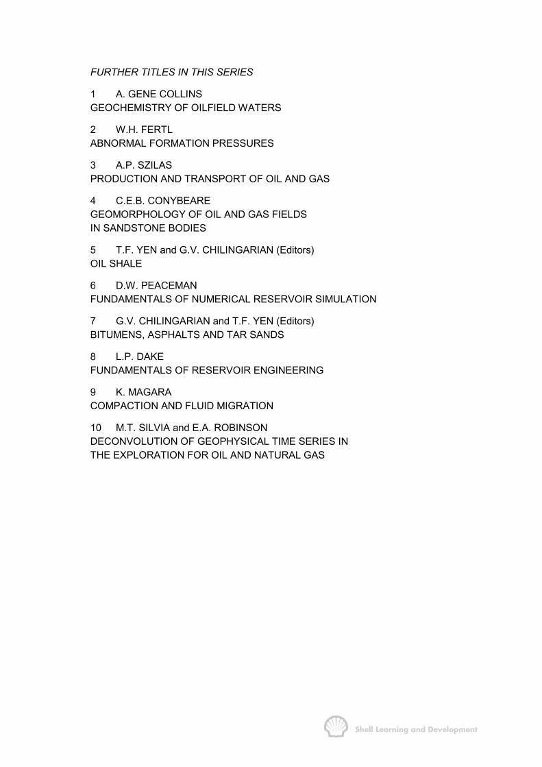
FURTHER TITLES IN THIS SERIES
1 A. GENE COLLINSGEOCHEMISTRY OF OILFIELD WATERS
2 W.H. FERTLABNORMAL FORMATION PRESSURES
3 A.P. SZILASPRODUCTION AND TRANSPORT OF OIL AND GAS
4 C.E.B. CONYBEAREGEOMORPHOLOGY OF OIL AND GAS FIELDSIN SANDSTONE BODIES
5 T.F. YEN and G.V. CHILINGARIAN (Editors)OIL SHALE
6 D.W. PEACEMANFUNDAMENTALS OF NUMERICAL RESERVOIR SIMULATION
7 G.V. CHILINGARIAN and T.F. YEN (Editors)BITUMENS, ASPHALTS AND TAR SANDS
8 L.P. DAKEFUNDAMENTALS OF RESERVOIR ENGINEERING
9 K. MAGARACOMPACTION AND FLUID MIGRATION
10 M.T. SILVIA and E.A. ROBINSONDECONVOLUTION OF GEOPHYSICAL TIME SERIES INTHE EXPLORATION FOR OIL AND NATURAL GAS

Developments in Petroleum Science, 8
fundamentals ofreservoirengineeringLP. DAKE
Senior Lecturer in Reservoir Engineering,Shell Internationale Petroleum Maatschappij B. V.,The Hague, The Netherlands
ELSEVIER, Amsterdam London New York Tokyo
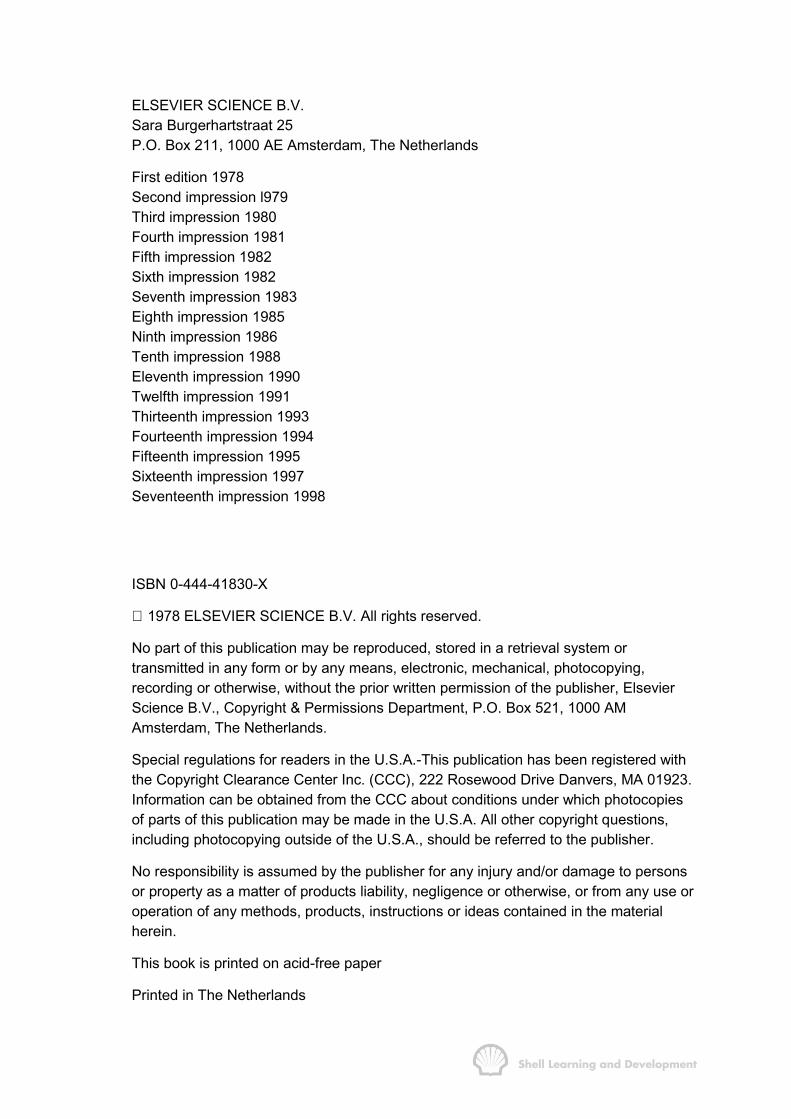
ELSEVIER SCIENCE B.V.Sara Burgerhartstraat 25P.O. Box 211, 1000 AE Amsterdam, The Netherlands
First edition 1978Second impression l979Third impression 1980Fourth impression 1981Fifth impression 1982Sixth impression 1982Seventh impression 1983Eighth impression 1985Ninth impression 1986Tenth impression 1988Eleventh impression 1990Twelfth impression 1991Thirteenth impression 1993Fourteenth impression 1994Fifteenth impression 1995Sixteenth impression 1997Seventeenth impression 1998
ISBN 0-444-41830-X
1978 ELSEVIER SCIENCE B.V. All rights reserved.
No part of this publication may be reproduced, stored in a retrieval system ortransmitted in any form or by any means, electronic, mechanical, photocopying,recording or otherwise, without the prior written permission of the publisher, ElsevierScience B.V., Copyright & Permissions Department, P.O. Box 521, 1000 AMAmsterdam, The Netherlands.
Special regulations for readers in the U.S.A.-This publication has been registered withthe Copyright Clearance Center Inc. (CCC), 222 Rosewood Drive Danvers, MA 01923.Information can be obtained from the CCC about conditions under which photocopiesof parts of this publication may be made in the U.S.A. All other copyright questions,including photocopying outside of the U.S.A., should be referred to the publisher.
No responsibility is assumed by the publisher for any injury and/or damage to personsor property as a matter of products liability, negligence or otherwise, or from any use oroperation of any methods, products, instructions or ideas contained in the materialherein.
This book is printed on acid-free paper
Printed in The Netherlands

To Grace
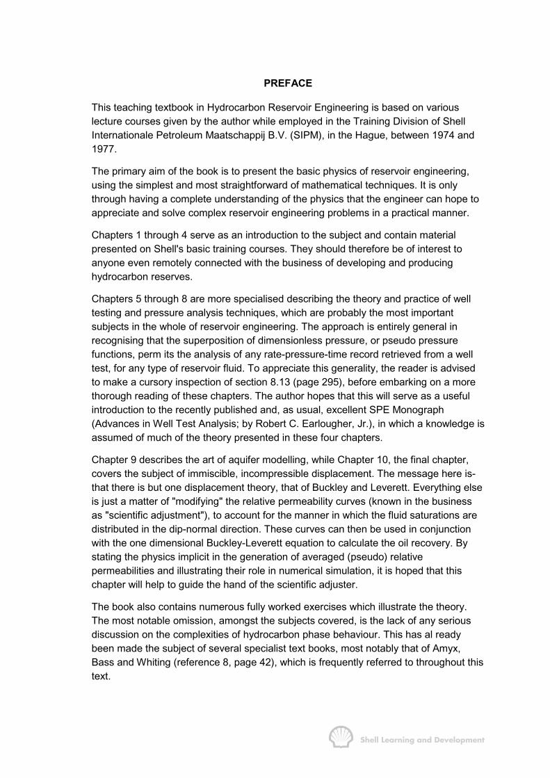
PREFACE
This teaching textbook in Hydrocarbon Reservoir Engineering is based on variouslecture courses given by the author while employed in the Training Division of ShellInternationale Petroleum Maatschappij B.V. (SIPM), in the Hague, between 1974 and1977.
The primary aim of the book is to present the basic physics of reservoir engineering,using the simplest and most straightforward of mathematical techniques. It is onlythrough having a complete understanding of the physics that the engineer can hope toappreciate and solve complex reservoir engineering problems in a practical manner.
Chapters 1 through 4 serve as an introduction to the subject and contain materialpresented on Shell's basic training courses. They should therefore be of interest toanyone even remotely connected with the business of developing and producinghydrocarbon reserves.
Chapters 5 through 8 are more specialised describing the theory and practice of welltesting and pressure analysis techniques, which are probably the most importantsubjects in the whole of reservoir engineering. The approach is entirely general inrecognising that the superposition of dimensionless pressure, or pseudo pressurefunctions, perm its the analysis of any rate-pressure-time record retrieved from a welltest, for any type of reservoir fluid. To appreciate this generality, the reader is advisedto make a cursory inspection of section 8.13 (page 295), before embarking on a morethorough reading of these chapters. The author hopes that this will serve as a usefulintroduction to the recently published and, as usual, excellent SPE Monograph(Advances in Well Test Analysis; by Robert C. Earlougher, Jr.), in which a knowledge isassumed of much of the theory presented in these four chapters.
Chapter 9 describes the art of aquifer modelling, while Chapter 10, the final chapter,covers the subject of immiscible, incompressible displacement. The message here is-that there is but one displacement theory, that of Buckley and Leverett. Everything elseis just a matter of "modifying" the relative permeability curves (known in the businessas "scientific adjustment"), to account for the manner in which the fluid saturations aredistributed in the dip-normal direction. These curves can then be used in conjunctionwith the one dimensional Buckley-Leverett equation to calculate the oil recovery. Bystating the physics implicit in the generation of averaged (pseudo) relativepermeabilities and illustrating their role in numerical simulation, it is hoped that thischapter will help to guide the hand of the scientific adjuster.
The book also contains numerous fully worked exercises which illustrate the theory.The most notable omission, amongst the subjects covered, is the lack of any seriousdiscussion on the complexities of hydrocarbon phase behaviour. This has al readybeen made the subject of several specialist text books, most notably that of Amyx,Bass and Whiting (reference 8, page 42), which is frequently referred to throughout thistext.

PREFACE / ACKNOWLEDGEMENTS VIII
A difficult decision to make, at the time of writing, is which set of units to employ.Although the logical decision has been made that the industry should adopt the SI(Système Internationale) units, no agreement has yet been reached concerning theextent to which "allowable" units, expressed in terms of the basic units, will betolerated. To avoid possible error the author has therefore elected to develop theimportant theoretical arguments in Darcy units, while equations required for applicationin the field are stated in Field units. Both these systems are defined in table 4.1, inChapter 4, which appropriately is devoted to the description of Darcy's law. Thischapter also contains a section, (4.4), which describes how to convert equationsexpressed in one set of units to the equivalent form in any other set of units. Thechoice of Darcy units is based largely on tradition. Equations expressed in these unitshave the same form as in absolute units except in their gravity terms. Field units havebeen used in practical equations to enable the reader to relate to the existing AIMEliterature.

PREFACE / ACKNOWLEDGEMENTS IX
ACKNOWLEDGEMENTS
The author wishes to express his thanks to SIPM for so readily granting permission topublish this work and, in particular, to H. L. Douwes Dekker, P.C. Kok and C. F.M.Heck for their sustained personal interest throughout the writing and publication, whichhas been a source of great encouragement.
Of those who have offered technical advice, I should like to acknowledge theassistance of G.J. Harmsen; L.A. Schipper; D. Leijnse; J. van der Burgh; L. Schenk; H.van Engen and H. Brummelkamp, all sometime members of Shell's reservoirengineering staff in the Hague. My thanks for technical assistance are also due to thefollowing members of KSEPL (Koninklijke Shell Exploratie en Productie Laboratorium)in Rijswijk, Holland: J. Offeringa; H.L. van Domseiaar; J.M. Dumore; J. van Lookerenand A.S. Williamson. Further, I am grateful to all former lecturers in reservoirengineering in Shell Training, and also to my successor A.J. de la Mar for his manyhelpful suggestions. Sincere thanks also to S.H. Christiansen (P.D. Oman) for hisdedicated attitude while correcting the text over a period of several months, andsimilarly to J.M. Willetts (Shell Expro, Aberdeen) and B.J.W. Woods (NAM, Assen) fortheir efforts.
For the preparation of the text I am indebted to G.J.W. Fransz for his co-ordinatingwork, and particulariy to Vera A. Kuipers-Betke for her enthusiastic hard work whilecomposing the final copy. For the drafting of the diagrams and the layout I am gratefulto J.C. Janse; C.L. Slootweg; J.H. Bor and S.O. Fraser-Mackenzie.
Finally, my thanks are due to all those who suffered my lectures between 1974 and1977 for their numerous suggestions which have helped to shape this textbook.
L.P. Dake,Shell Training,
The Hague,October 1977.

CONTENTS
PREFACE VII
ACKNOWLEDGEMENTS IX
CONTENTS X
LIST OF FIGURES XVII
LIST OF TABLES XXVII
LIST OF EQUATIONS XXX
NOMENCLATURE LIX
CHAPTER 1 SOME BASIC CONCEPTS IN RESERVOIR ENGINEERING 1
1.1 INTRODUCTION 1
1.2 CALCULATION OF HYDROCARBON VOLUMES 1
1.3 FLUID PRESSURE REGIMES 3
1.4 OIL RECOVERY: RECOVERY FACTOR 9
1.5 VOLUMETRIC GAS RESERVOIR ENGINEERING 12
1.6 APPLICATION OF THE REAL GAS EQUATION OF STATE 20
1.7 GAS MATERIAL BALANCE: RECOVERY FACTOR 25
1.8 HYDROCARBON PHASE BEHAVIOUR 37
REFERENCES 41
CHAPTER 2 PVT ANALYSIS FOR OIL 43
2.1 INTRODUCTION 43
2.2 DEFINITION OF THE BASIC PVT PARAMETERS 43
2.3 COLLECTION OF FLUID SAMPLES 51
2.4 DETERMINATION OF THE BASIC PVT PARAMETERS IN THELABORATORY AND CONVERSION FOR FIELD OPERATINGCONDITIONS 55
2.5 ALTERNATIVE MANNER OF EXPRESSING PVT LABORATORYANALYSIS RESULTS 65
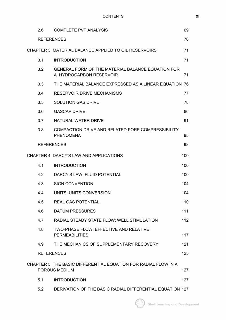
CONTENTS XI
2.6 COMPLETE PVT ANALYSIS 69
REFERENCES 70
CHAPTER 3 MATERIAL BALANCE APPLIED TO OIL RESERVOIRS 71
3.1 INTRODUCTION 71
3.2 GENERAL FORM OF THE MATERIAL BALANCE EQUATION FORA HYDROCARBON RESERVOIR 71
3.3 THE MATERIAL BALANCE EXPRESSED AS A LINEAR EQUATION 76
3.4 RESERVOIR DRIVE MECHANISMS 77
3.5 SOLUTION GAS DRIVE 78
3.6 GASCAP DRIVE 86
3.7 NATURAL WATER DRIVE 91
3.8 COMPACTION DRIVE AND RELATED PORE COMPRESSIBILITYPHENOMENA 95
REFERENCES 98
CHAPTER 4 DARCY'S LAW AND APPLICATIONS 100
4.1 INTRODUCTION 100
4.2 DARCY'S LAW; FLUID POTENTIAL 100
4.3 SIGN CONVENTION 104
4.4 UNITS: UNITS CONVERSION 104
4.5 REAL GAS POTENTIAL 110
4.6 DATUM PRESSURES 111
4.7 RADIAL STEADY STATE FLOW; WELL STIMULATION 112
4.8 TWO-PHASE FLOW: EFFECTIVE AND RELATIVEPERMEABILITIES 117
4.9 THE MECHANICS OF SUPPLEMENTARY RECOVERY 121
REFERENCES 125
CHAPTER 5 THE BASIC DIFFERENTIAL EQUATION FOR RADIAL FLOW IN APOROUS MEDIUM 127
5.1 INTRODUCTION 127
5.2 DERIVATION OF THE BASIC RADIAL DIFFERENTIAL EQUATION 127

CONTENTS XII
5.3 CONDITIONS OF SOLUTION 129
5.4 THE LINEARIZATION OF EQUATION 5.1 FOR FLUIDS OF SMALLAND CONSTANT COMPRESSIBILITY 133
REFERENCES 135
CHAPTER 6 WELL INFLOW EQUATIONS FOR STABILIZED FLOWCONDITIONS 136
6.1 INTRODUCTION 136
6.2 SEMI-STEADY STATE SOLUTION 136
6.3 STEADY STATE SOLUTION 139
6.4 EXAMPLE OF THE APPLICATION OF THE STABILIZED INFLOWEQUATIONS 140
6.5 GENERALIZED FORM OF INFLOW EQUATION UNDER SEMI-STEADY STATE CONDITIONS 144
REFERENCES 146
CHAPTER 7 THE CONSTANT TERMINAL RATE SOLUTION OF THE RADIALDIFFUSIVITY EQUATION AND ITS APPLICATION TO OILWELL TESTING 148
7.1 INTRODUCTION 148
7.2 THE CONSTANT TERMINAL RATE SOLUTION 148
7.3 THE CONSTANT TERMINAL RATE SOLUTION FOR TRANSIENTAND SEMI-STEADY STATE FLOW CONDITIONS 149
7.4 DIMENSIONLESS VARIABLES 161
7.5 SUPERPOSITION THEOREM: GENERAL THEORY OF WELLTESTING 168
7.6 THE MATTHEWS, BRONS, HAZEBROEK PRESSURE BUILDUPTHEORY 173
7.7 PRESSURE BUILDUP ANALYSIS TECHNIQUES 189
7.8 MULTI-RATE DRAWDOWN TESTING 209
7.9 THE EFFECTS OF PARTIAL WELL COMPLETION 219
7.10 SOME PRACTICAL ASPECTS OF WELL SURVEYING 221
7.11 AFTERFLOW ANALYSIS 224
REFERENCES 236

CONTENTS XIII
CHAPTER 8 REAL GAS FLOW: GAS WELL TESTING 239
8.1 INTRODUCTION 239
8.2 LINEARIZATION AND SOLUTION OF THE BASIC DIFFERENTIALEQUATION FOR THE RADIAL FLOW OF A REAL GAS 239
8.3 THE RUSSELL, GOODRICH, et. al. SOLUTION TECHNIQUE 240
8.4 THE AL-HUSSAINY, RAMEY, CRAWFORD SOLUTIONTECHNIQUE 243
8.5 COMPARISON OF THE PRESSURE SQUARED AND PSEUDOPRESSURE SOLUTION TECHNIQUES 251
8.6 NON-DARCY FLOW 252
8.7 DETERMINATION OF THE NON-DARCY COEFFICIENT F 255
8.8 THE CONSTANT TERMINAL RATE SOLUTION FOR THE FLOWOF A REAL GAS 257
8.9 GENERAL THEORY OF GAS WELL TESTING 260
8.10 MULTI-RATE TESTING OF GAS WELLS 262
8.11 PRESSURE BUILDUP TESTING OF GAS WELLS 278
8.12 PRESSURE BUILDUP ANALYSIS IN SOLUTION GAS DRIVERESERVOIRS 289
8.13 SUMMARY OF PRESSURE ANALYSIS TECHNIQUES 291
REFERENCES 295
CHAPTER 9 NATURAL WATER INFLUX 297
9.1 INTRODUCTION 297
9.2 THE UNSTEADY STATE WATER INFLUX THEORY OF HURSTAND VAN EVERDINGEN 298
9.3 APPLICATION OF THE HURST, VAN EVERDINGEN WATERINFLUX THEORY IN HISTORY MATCHING 308
9.4 THE APPROXIMATE WATER INFLUX THEORY OF FETKOVITCHFOR FINITE AQUIFERS 319
9.5 PREDICTING THE AMOUNT OF WATER INFLUX 328
9.6 APPLICATION OF INFLUX CALCULATION TECHNIQUES TOSTEAM SOAKING 333
REFERENCES 335
CONTENTS XIV
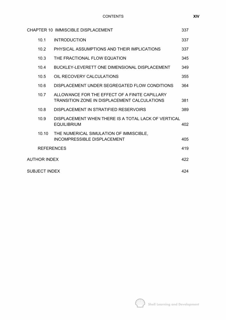
CHAPTER 10 IMMISCIBLE DISPLACEMENT 337
10.1 INTRODUCTION 337
10.2 PHYSICAL ASSUMPTIONS AND THEIR IMPLICATIONS 337
10.3 THE FRACTIONAL FLOW EQUATION 345
10.4 BUCKLEY-LEVERETT ONE DIMENSIONAL DISPLACEMENT 349
10.5 OIL RECOVERY CALCULATIONS 355
10.6 DISPLACEMENT UNDER SEGREGATED FLOW CONDITIONS 364
10.7 ALLOWANCE FOR THE EFFECT OF A FINITE CAPILLARYTRANSITION ZONE IN DISPLACEMENT CALCULATIONS 381
10.8 DISPLACEMENT IN STRATIFIED RESERVOIRS 389
10.9 DISPLACEMENT WHEN THERE IS A TOTAL LACK OF VERTICALEQUILIBRIUM 402
10.10 THE NUMERICAL SIMULATION OF IMMISCIBLE,INCOMPRESSIBLE DISPLACEMENT 405
REFERENCES 419
AUTHOR INDEX 422
SUBJECT INDEX 424
CONTENTS XV
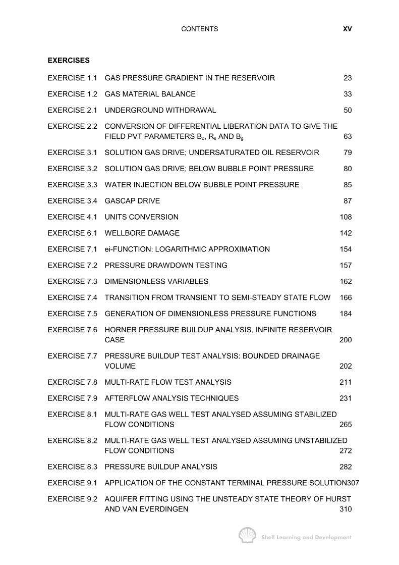
EXERCISES
EXERCISE 1.1 GAS PRESSURE GRADIENT IN THE RESERVOIR 23
EXERCISE 1.2 GAS MATERIAL BALANCE 33
EXERCISE 2.1 UNDERGROUND WITHDRAWAL 50
EXERCISE 2.2 CONVERSION OF DIFFERENTIAL LIBERATION DATA TO GIVE THEFIELD PVT PARAMETERS Bo, Rs AND Bg 63
EXERCISE 3.1 SOLUTION GAS DRIVE; UNDERSATURATED OIL RESERVOIR 79
EXERCISE 3.2 SOLUTION GAS DRIVE; BELOW BUBBLE POINT PRESSURE 80
EXERCISE 3.3 WATER INJECTION BELOW BUBBLE POINT PRESSURE 85
EXERCISE 3.4 GASCAP DRIVE 87
EXERCISE 4.1 UNITS CONVERSION 108
EXERCISE 6.1 WELLBORE DAMAGE 142
EXERCISE 7.1 ei-FUNCTION: LOGARITHMIC APPROXIMATION 154
EXERCISE 7.2 PRESSURE DRAWDOWN TESTING 157
EXERCISE 7.3 DIMENSIONLESS VARIABLES 162
EXERCISE 7.4 TRANSITION FROM TRANSIENT TO SEMI-STEADY STATE FLOW 166
EXERCISE 7.5 GENERATION OF DIMENSIONLESS PRESSURE FUNCTIONS 184
EXERCISE 7.6 HORNER PRESSURE BUILDUP ANALYSIS, INFINITE RESERVOIRCASE 200
EXERCISE 7.7 PRESSURE BUILDUP TEST ANALYSIS: BOUNDED DRAINAGEVOLUME 202
EXERCISE 7.8 MULTI-RATE FLOW TEST ANALYSIS 211
EXERCISE 7.9 AFTERFLOW ANALYSIS TECHNIQUES 231
EXERCISE 8.1 MULTI-RATE GAS WELL TEST ANALYSED ASSUMING STABILIZEDFLOW CONDITIONS 265
EXERCISE 8.2 MULTI-RATE GAS WELL TEST ANALYSED ASSUMING UNSTABILIZEDFLOW CONDITIONS 272
EXERCISE 8.3 PRESSURE BUILDUP ANALYSIS 282
EXERCISE 9.1 APPLICATION OF THE CONSTANT TERMINAL PRESSURE SOLUTION307
EXERCISE 9.2 AQUIFER FITTING USING THE UNSTEADY STATE THEORY OF HURSTAND VAN EVERDINGEN 310

CONTENTS XVI
EXERCISE 9.3 WATER INFLUX CALCULATIONS USING THE METHOD OFFETKOVITCH 324
EXERCISE 10.1 FRACTIONAL FLOW 358
EXERCISE 10.2 OIL RECOVERY PREDICTION FOR A WATERFLOOD 361
EXERCISE 10.3 DISPLACEMENT UNDER SEGREGATED FLOW CONDITIONS 375
EXERCISE 10.4 GENERATION OF AVERAGED RELATIVE PERMEABILITY CURVESFOR A LAYERED RESERVOIR (SEGREGATED FLOW) 397
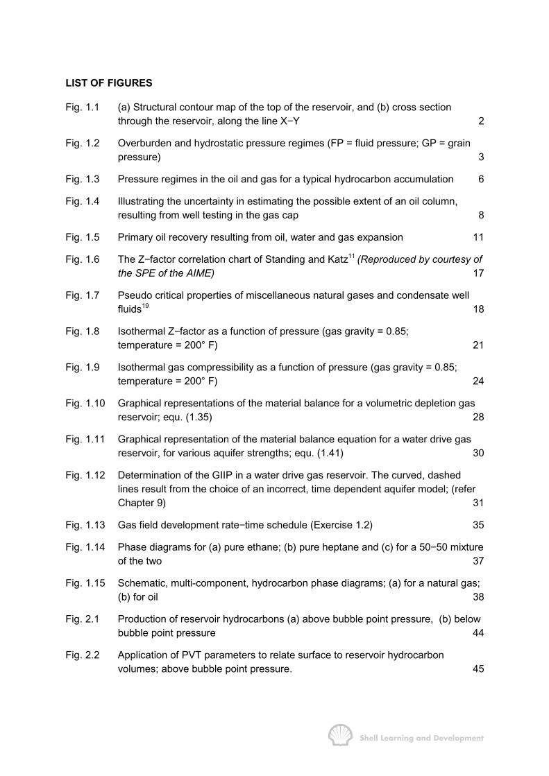
LIST OF FIGURES
Fig. 1.1 (a) Structural contour map of the top of the reservoir, and (b) cross sectionthrough the reservoir, along the line X−Y 2
Fig. 1.2 Overburden and hydrostatic pressure regimes (FP = fluid pressure; GP = grainpressure) 3
Fig. 1.3 Pressure regimes in the oil and gas for a typical hydrocarbon accumulation 6
Fig. 1.4 Illustrating the uncertainty in estimating the possible extent of an oil column,resulting from well testing in the gas cap 8
Fig. 1.5 Primary oil recovery resulting from oil, water and gas expansion 11
Fig. 1.6 The Z−factor correlation chart of Standing and Katz11 (Reproduced by courtesy ofthe SPE of the AIME) 17
Fig. 1.7 Pseudo critical properties of miscellaneous natural gases and condensate wellfluids19 18
Fig. 1.8 Isothermal Z−factor as a function of pressure (gas gravity = 0.85;temperature = 200° F) 21
Fig. 1.9 Isothermal gas compressibility as a function of pressure (gas gravity = 0.85;temperature = 200° F) 24
Fig. 1.10 Graphical representations of the material balance for a volumetric depletion gasreservoir; equ. (1.35) 28
Fig. 1.11 Graphical representation of the material balance equation for a water drive gasreservoir, for various aquifer strengths; equ. (1.41) 30
Fig. 1.12 Determination of the GIIP in a water drive gas reservoir. The curved, dashedlines result from the choice of an incorrect, time dependent aquifer model; (referChapter 9) 31
Fig. 1.13 Gas field development rate−time schedule (Exercise 1.2) 35
Fig. 1.14 Phase diagrams for (a) pure ethane; (b) pure heptane and (c) for a 50−50 mixtureof the two 37
Fig. 1.15 Schematic, multi-component, hydrocarbon phase diagrams; (a) for a natural gas;(b) for oil 38
Fig. 2.1 Production of reservoir hydrocarbons (a) above bubble point pressure, (b) belowbubble point pressure 44
Fig. 2.2 Application of PVT parameters to relate surface to reservoir hydrocarbonvolumes; above bubble point pressure. 45
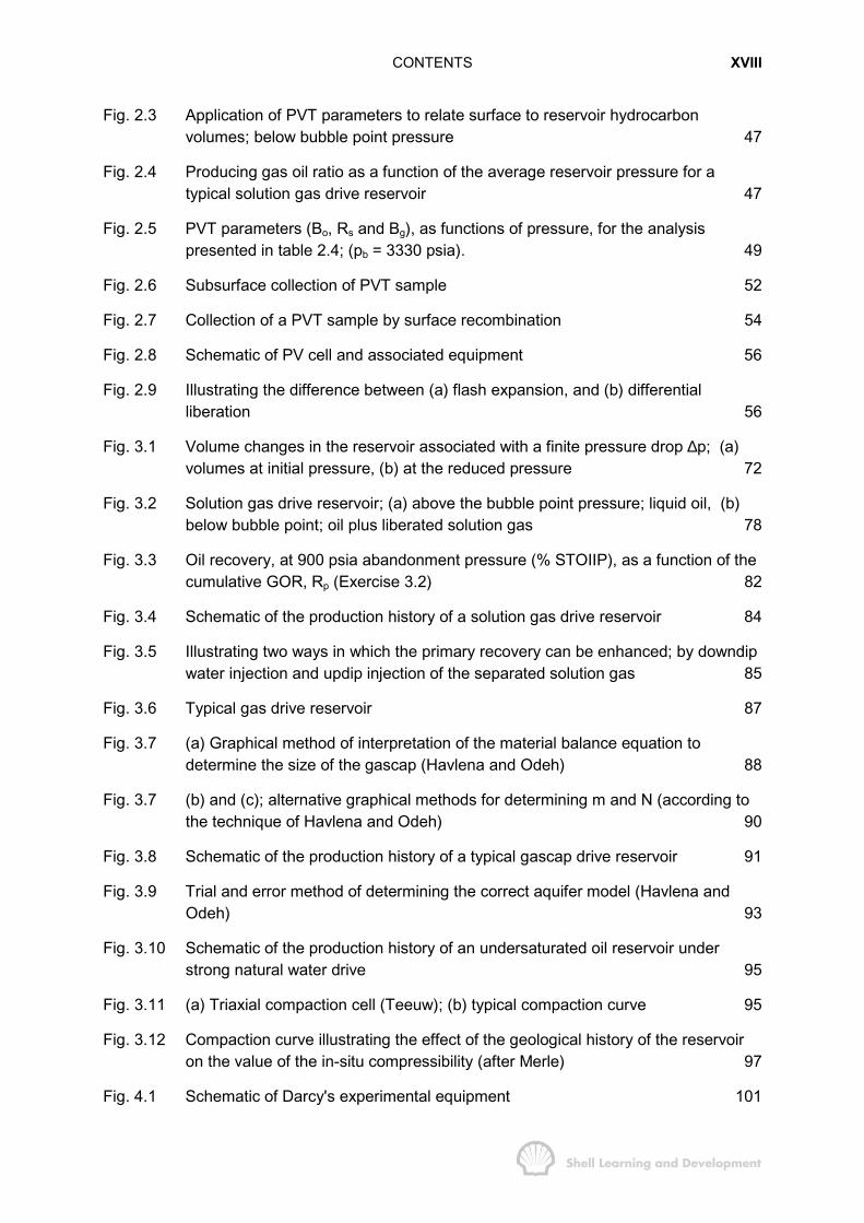
CONTENTS XVIII
Fig. 2.3 Application of PVT parameters to relate surface to reservoir hydrocarbonvolumes; below bubble point pressure 47
Fig. 2.4 Producing gas oil ratio as a function of the average reservoir pressure for atypical solution gas drive reservoir 47
Fig. 2.5 PVT parameters (Bo, Rs and Bg), as functions of pressure, for the analysispresented in table 2.4; (pb = 3330 psia). 49
Fig. 2.6 Subsurface collection of PVT sample 52
Fig. 2.7 Collection of a PVT sample by surface recombination 54
Fig. 2.8 Schematic of PV cell and associated equipment 56
Fig. 2.9 Illustrating the difference between (a) flash expansion, and (b) differentialliberation 56
Fig. 3.1 Volume changes in the reservoir associated with a finite pressure drop ∆p; (a)volumes at initial pressure, (b) at the reduced pressure 72
Fig. 3.2 Solution gas drive reservoir; (a) above the bubble point pressure; liquid oil, (b)below bubble point; oil plus liberated solution gas 78
Fig. 3.3 Oil recovery, at 900 psia abandonment pressure (% STOIIP), as a function of thecumulative GOR, Rp (Exercise 3.2) 82
Fig. 3.4 Schematic of the production history of a solution gas drive reservoir 84
Fig. 3.5 Illustrating two ways in which the primary recovery can be enhanced; by downdipwater injection and updip injection of the separated solution gas 85
Fig. 3.6 Typical gas drive reservoir 87
Fig. 3.7 (a) Graphical method of interpretation of the material balance equation todetermine the size of the gascap (Havlena and Odeh) 88
Fig. 3.7 (b) and (c); alternative graphical methods for determining m and N (according tothe technique of Havlena and Odeh) 90
Fig. 3.8 Schematic of the production history of a typical gascap drive reservoir 91
Fig. 3.9 Trial and error method of determining the correct aquifer model (Havlena andOdeh) 93
Fig. 3.10 Schematic of the production history of an undersaturated oil reservoir understrong natural water drive 95
Fig. 3.11 (a) Triaxial compaction cell (Teeuw); (b) typical compaction curve 95
Fig. 3.12 Compaction curve illustrating the effect of the geological history of the reservoiron the value of the in-situ compressibility (after Merle) 97
Fig. 4.1 Schematic of Darcy's experimental equipment 101
CONTENTS XIX
Fig. 4.2 Orientation of Darcy's apparatus with respect to the Earth's gravitational field 102
Fig. 4.3 Referring reservoir pressures to a datum level in the reservoir, as datumpressures (absolute units) 112
Fig. 4.4 The radial flow of oil into a well under steady state flow conditions 113
Fig. 4.5 Radial pressure profile for a damaged well 114
Fig. 4.6 (a) Typical oil and water viscosities as functions of temperature, and (b) pressureprofile within the drainage radius of a steam soaked well 116
Fig. 4.7 Oil production rate as a function of time during a multi-cycle steam soak 116
Fig. 4.8 (a) Effective and (b) corresponding relative permeabilities, as functions of thewater saturation. The curves are appropriate for the description of thesimultaneous flow of oil and water through a porous medium 118
Fig. 4.9 Alternative manner of normalising the effective permeabilities to give relativepermeability curves 119
Fig. 4.10 Water saturation distribution as a function of distance between injection andproduction wells for (a) ideal or piston-like displacement and (b) non-idealdisplacement 121
Fig. 4.11 Illustrating two methods of mobilising the residual oil remaining after aconventional waterflood 124
Fig. 5.1 Radial flow of a single phase fluid in the vicinity of a producing well. 128
Fig. 5.2 Radial flow under semi-steady state conditions 130
Fig. 5.3 Reservoir depletion under semi-steady state conditions. 132
Fig. 5.4 Radial flow under steady state conditions 132
Fig. 6.1 Pressure distribution and geometry appropriate for the solution of the radialdiffusivity equation under semi-state conditions 136
Fig. 6.2 Pressure profile during the steam soak production phase 140
Fig. 6.3 Pressure profiles and geometry (Exercise 6.1) 142
Fig. 6.4 Dietz shape factors for various geometries3 (Reproduced by courtesy of the SPEof the AIME). 146
Fig. 7.1 Constant terminal rate solution; (a) constant production rate (b) resulting declinein the bottom hole flowing pressure 148
Fig. 7.2 The exponential integral function ei(x) 153
Fig. 7.3 Graph of the ei-function for 0.001 ≤ × ≤ 5.0 154
CONTENTS XX
Fig. 7.4 Single rate drawdown test; (a) wellbore flowing pressure decline during the earlytransient flow period, (b) during the subsequent semi-steady state decline(Exercise 7.2) 159
Fig. 7.5 Dimensionless pressure as a function of dimensionless flowing time for a wellsituated at the centre of a square (Exercise 7.4) 168
Fig. 7.6 Production history of a well showing both rate and bottom hole flowing pressureas functions of time 169
Fig. 7.7 Pressure buildup test; (a) rate, (b) wellbore pressure response 171
Fig. 7.8 Multi-rate flow test analysis 172
Fig. 7.9 Horner pressure buildup plot for a well draining a bounded reservoir, or part of areservoir surrounded by a no-flow boundary 175
Fig. 7.10 Part of the infinite network of image wells required to simulate the no-flowcondition across the boundary of a 2 : 1 rectangular part of a reservoir in whichthe real well is centrally located 176
Fig. 7.11 MBH plots for a well at the centre of a regular shaped drainage area7
(Reproduced by courtesy of the SPE of the AIME) 178
Fig. 7.12 MBH plots for a well situated within; a) a square, and b) a 2:1 rectangle7
(Reproduced by courtesy of the SPE of the AIME) 179
Fig. 7.13 MBH plots for a well situated within; a) a 4:1 rectangle, b) various rectangulargeometries7 (Reproduced by courtesy of the SPE of the AIME) 180
Fig. 7.14 MBH plots for a well in a square and in rectangular 2:1 geometries7 181
Fig. 7.15 MBH plots for a well in a 2:1 rectangle and in an equilateral triangle7
(Reproduced by courtesy of the SPE of the AIME). 181
Fig. 7.16 Geometrical configurations with Dietz shape factors in the range, 4.5-5.5 184
Fig. 7.17 Plots of ∆pwf (calculated minus observed) wellbore flowing pressure as a functionof the flowing time, for various geometrical configurations (Exercise 7.5) 186
Fig. 7.18 Typical Horner pressure buildup plot 190
Fig. 7.19 Illustrating the dependence of the shape of the buildup on the value of the totalproduction time prior to the survey 192
Fig. 7.20 Analysis of a single set of buildup data using three different values of the flowingtime to draw the Horner plot. A - actual flowing time; B - effective flowing time; C -time required to reach semi-steady state conditions 194
Fig. 7.21 The Dietz method applied to determine both the average pressure p and thedynamic grid block pressure dp 197

CONTENTS XXI
Fig. 7.22 Numerical simulation model showing the physical no-flow boundary drained bywell A and the superimposed square grid blocks used in the simulation 198
Fig. 7.23 Horner buildup plot, infinite reservoir case 201
Fig. 7.24 Position of the well with respect to its no-flow boundary; exercise 7.7 203
Fig. 7.25 Pressure buildup analysis to determine the average pressure within the no-flowboundary, and the dynamic grid block pressure (Exercise 7.7) 204
Fig. 7.26 Influence of the shape of the drainage area and degree of well asymmetry on theHorner buildup plot (Exercise 7.7) 205
Fig. 7.27 Multi-rate oilwell test (a) increasing rate sequence (b) wellbore pressureresponse 210
Fig. 7.28 Illustrating the dependence of multi-rate analysis on the shape of the drainagearea and the degree of well asymmetry. (Exercise 7.8) 214
Fig. 7.30 Multi-rate test analysis in a partially depleted reservoir 219
Fig. 7.31 Examples of partial well completion showing; (a) well only partially penetratingthe formation; (b) well producing from only the central portion of the formation; (c)well with 5 intervals open to production (After Brons and Marting19) 220
Fig. 7.32 Pseudo skin factor Sb as a function of b and h/rw (After Brons and Marting19)(Reproduced by courtesy of the SPE of the AIME) 220
Fig. 7.33 (a) Amerada pressure gauge; (b) Amerada chart for a typical pressure buildupsurvey in a producing well 222
Fig. 7.34 Lowering the Amerada into the hole against the flowing well stream 223
Fig. 7.35 Correction of measured pressures to datum; (a) well position in the reservoir, (b)well completion design 223
Fig. 7.36 Extreme fluid distributions in the well; (a) with water entry and no rise in thetubing head pressure, (b) without water entry and with a rise in the THP 224
Fig. 7.37 Pressure buildup plot dominated by afterflow 225
Fig. 7.38 Russell plot for analysing the effects of afterflow 226
Fig. 7.39 (a) Pressure buildup plot on transparent paper for overlay on (b) McKinley typecurves, derived by computer solution of the complex afterflow problem 227
Fig. 7.40 McKinley type curves for 1 min <∆t < 1000 min. (After McKinley21) (Reproducedby courtesy of the SPE of the AIME) 228
Fig. 7.41 Buildup plot superimposed on a particular McKinley type curve for T/F = 5000 230
Fig. 7.42 Deviation of observed buildup from a McKinley type curve, indicating thepresence of skin 230

CONTENTS XXII
Fig. 7.43 Russell afterflow analysis Exercise 7.9) 234
Fig. 7.44 Match between McKinley type curves and superimposed observed buildup(Exercise 7.9). o − match for small ∆t (T/F = 2500) • − match for large ∆t (T/F =5000) 235
Fig. 8.1 Radial numerical simulation model for real gas inflow 241
Fig. 8.2 Iterative calculation of pwf using the p2 formulation of the radial, semi-steadystate inflow equation, (8.5) 244
Fig. 8.3 Real gas pseudo pressure, as a function of the actual pressure, as derived intable 8.1; (Gas gravity, 0.85; Temperature 200°F) 248
Fig. 8.4 2p/µZ as a function of pressure 248
Fig. 8.5 Calculation of pwf using the radial semi-steady state inflow equation expressed interms of real gas pseudo pressures, (equ. 8.15) 250
Fig. 8.6 p/µZ as a linear function of pressure 251
Fig. 8.7 Typical plot of p/µZ as a function of pressure 252
Fig. 8.8 Laboratory determined relationship between β and the absolute permeability Arelationship is usually derived of the form 256
Fig. 8.9 Gas well test analysis assuming semi-steady state conditions during each flowperiod. Data; table 8.3 267
Fig. 8.10 Gas well test analysis assuming semi-steady state conditions and applying equ.(8.47). Data; table 8.4 268
Fig. 8.11 MBH chart for the indicated 4:1 rectangular geometry for tDA < .01 (AfterEarlougher, et.al15) 273
Fig. 8.12 Essis-Thomas analysis of a multi-rate gas well test under assumed transient flowconditions. Data; table 8.6 274
Fig. 8.13 The effect of the length of the individual flow periods on the analysis of a multi-rate gas well test; (a) 4×1 hr periods, (b) 4×2 hrs, (c) 4×4 hrs 277
Fig. 8.14 (a) Rate-time schedule, and (b) corresponding wellbore pressure responseduring a pressure buildup test in a gas well 279
Fig. 8.15 Complete analysis of a pressure buildup test in a gas well: (a) buildup analysis(table 8.12); (b) and (c) transient flow analyses of the first and second flowperiods, respectively (table 8.10) 284
Fig. 8.16 MBH plot for a well at the centre of a square, showing the deviation of mD(MBH)
from pD(MBH) for large values of the dimensionless flowing time tDA 287
Fig. 8.17 Iterative determination of p in a gas well test analysis (Kazemi10) 288

CONTENTS XXIII
Fig. 8.18 Schematic of a general analysis program applicable to pressure buildup tests forany fluid system 294
Fig. 9.1 Radial aquifer geometry 300
Fig. 9.2 Linear aquifer geometry 300
Fig. 9.3 Dimensioniess water influx, constant terminal pressure case, radial flow. (AfterHurst and van Everdingen, ref. 1) 302
Fig. 9.4 Dimensionless water influx, constant terminal pressure case, radial flow (AfterHurst and van Everdingen, ref. 1) 303
Fig. 9.5 Dimensionless water influx, constant terminal pressure case, radial flow (AfterHurst and van Everdingen, ref. 1) 304
Fig. 9.6 Dimensionless water influx, constant terminal pressure case, radial and linearflow (After Hurst and van Everdingen, ref.1) 305
Fig. 9.7 Dimensionless water influx, constant terminal pressure case, radial and linearflow (After Hurst and van Everdingen, ref.1) 306
Fig. 9.8 Water influx from a segment of a radial aquifer 307
Fig. 9.9 Matching a continuous pressure decline at the reservoir-aquifer boundary by aseries of discrete pressure steps 309
Fig. 9.10 Aquifer-reservoir geometry, exercise 9.2 311
Fig. 9.11 Reservoir production and pressure history; exercise 9.2 311
Fig. 9.12 Rs and Bg as functions of pressure; exercise 9.2 312
Fig. 9.13 Bo as a function of pressure; exercise 9.2 312
Fig. 9.14 Reservoir pressure decline approximated by a series of discrete pressure steps;exercise 9.2 313
Fig. 9.15 Aquifer fitting using the interpretation technique of Havlena and Odeh 319
Fig. 9.16 Comparison between Hurst and van Everdingen and Fetkovitch for reD = 5 327
Fig. 9.17 Comparison between Hurst and van Everdingen and Fetkovitch for reD = 10 327
Fig. 9.18 Predicting the pressure decline in a water drive gas reservoir 329
Fig. 9.19 Prediction of gas reservoir pressures resulting from fluid withdrawal and waterinflux (Hurst and van Everdingen) 330
Fig. 9.20 Prediction of gas reservoir pressures resulting from fluid withdrawal and waterinflux (Fetkovitch) 332
Fig. 9.21 Conditions prior to production in a steam soak cycle 333
CONTENTS XXIV
Fig. 10.1 Hysteresis in contact angle in a water wet reservoir, (a) wetting phase increasing(imbibition); (b) wetting phase decreasing (drainage) 338
Fig. 10.2 Water entrapment between two spherical sand grains in a water wet reservoir 339
Fig. 10.3 Drainage and imbibition capillary pressure functions 339
Fig. 10.4 Capillary tube experiment for an oil-water system 340
Fig. 10.5 Determination of water saturation as a function of reservoir thickness above themaximum water saturation plane, Sw = 1−Sor, of an advancing waterflood 341
Fig. 10.6 Linear prototype reservoir model, (a) plan view; (b) cross section 344
Fig. 10.7 Approximation to the diffuse flow condition for H>> h 346
Fig. 10.8 (a) Capillary pressure function and; (b) water saturation distribution as a functionof distance in the displacement path 348
Fig. 10.9 Typical fractional flow curve as a function of water saturation, equ. (10.12) 349
Fig. 10.10 Mass flow rate of water through a linear volume element A dxφ 350
Fig. 10.11 (a) Saturation derivative of a typical fractional flow curve and (b) resulting watersaturation distribution in the displacement path 352
Fig. 10.12 Water saturation distribution as a function of distance, prior to breakthrough inthe producing well 353
Fig. 10.13 Tangent to the fractional flow curve from Sw = Swc 354
Fig. 10.14 Water saturation distributions at breakthrough and subsequently in a linearwaterflood 355
Fig. 10.15 Application of the Welge graphical technique to determine the oil recovery afterwater breakthrough 357
Fig. 10.16 Fractional flow plots for different oil-water viscosity ratios (table 10.2) 360
Fig. 10.17 Dimensionless oil recovery (PV) as a function of dimensionless water injected(PV), and time (exercise 10.2) 364
Fig. 10.18 Displacement of oil by water under segregated flow conditions 365
Fig. 10.19 Illustrating the difference between stable and unstable displacement, undersegregated flow conditions, in a dipping reservoir; (a) stable: G > M−1; M > 1;β < θ. (b) stable: G > M−1; M < 1; β > θ. (c) unstable: G < M−1. 366
Fig. 10.20 Segregated displacement of oil by water 369
Fig. 10.21 Linear, averaged relative permeability functions for describing segregated flow ina homogeneous reservoir 370
Fig. 10.22 Typical fractional flow curve for oil displacement under segregated conditions 371
CONTENTS XXV
Fig. 10.23 Referring oil and water phase pressures at the interface to the centre line in thereservoir. (Unstable segregated displacement in a horizontal, homogeneousreservoir) 372
Fig. 10.24 Comparison of the oil recoveries obtained in exercises 10.2 and 10.3 forassumed diffuse and segregated flow, respectively 376
Fig. 10.25 The stable, segregated displacement of oil by water at 90% of the critical rate(exercise 10.3) 378
Fig. 10.26 Segregated downdip displacement of oil by gas at constant pressure; (a)unstable, (b) stable 380
Fig. 10.27 (a) Imbibition capillary pressure curve, and (b) laboratory measured relativepermeabilities (rock curves,- table 10.1) 382
Fig. 10.28 (a) Water saturation, and (b) relative permeability distributions, with respect tothickness when the saturation at the base of the reservoir is Sw = 1 − Sor (Pc =0)383
Fig. 10.29 Water saturation and relative permeability distributions, as functions of thickness,as the maximum saturation, Sw = 1 − Sor, is allowed to rise in 10 foot incrementsin the reservoir 385
Fig. 10.30 Averaged relative permeability curves for a homogeneous reservoir, for diffuseand segregated flow; together with the intermediate case when the capillarytransition zone is comparable to the reservoir thickness 387
Fig. 10.31 Capillary and pseudo capillary pressure curves. 387
Fig. 10.32 Comparison of oil recoveries for different assumed water saturation distributionsduring displacement. 387
Fig. 10.33 Variation in the pseudo capillary pressure between +2 and -2 psi as themaximum water saturation Sw = 1−Sor rises from the base to the top of thereservoir 388
Fig. 10.34 Example of a stratified, linear reservoir for which pressure communicationbetween the layers is assumed 390
Fig. 10.35 (a)-(c) Rock relative permeabilities, and (d) laboratory measured capillarypressures for the three layered reservoir shown in fig. 10.34 391
Fig. 10.36 (a) Water saturation, and (b) relative permeability distributions, with respect tothickness, when the saturation at the base of the layered reservoir (fig. 10.34) isSw = 1−Sor (Pc° = 2 psi) 392
Fig. 10.37 (a)-(h) Water saturation and relative permeability distributions,as functions ofthickness,for various selected values of cP° (three layered reservoir, fig 10.34) 394
Fig. 10.38 Averaged relative permeability functions for the three layered reservoir,fig. 10.34: (a) high permeability layer at top, (b) at base of the reservoir 396

CONTENTS XXVI
Fig. 10.39 (a) Pseudo capillary pressure, and (b) fractional flow curves for the three layeredreservoir, fig. 10.34). (——high permeability at top; − − −at base of the reservoir).396
Fig. 10.40 Individual layer properties; exercise 10.4 397
Fig. 10.41 Averaged relative permeability curves; exercise 10.4 399
Fig. 10.42 (a) Pseudo capillary pressures, and (b) fractional flow curves, exercise 10.4 (——High permeability layer at top; − − −at base of reservoir) 400
Fig. 10.43 Methods of generating averaged relative permeabilities, as functions of thethickness averaged water saturation, dependent on the homogeneity of thereservoir and the magnitude of capillary transition zone (H). The chart is onlyapplicable when the vertical equilibrium condition pertains or when there is a totallack of vertical equilibrium 404
Fig. 10.44 Numerical simulation model for linear displacement in a homogeneous reservoir406
Fig. 10.45 Spatial linkage of the finite difference formulation of the left hand side ofequ (10.83). 408
Fig. 10.46 Example of water saturation instability (oscillation) resulting from the applicationof the IMPES solution technique (− − − correct, and incorrect saturations) 411
Fig. 10.47 Determination of the average, absolute permeability between grid blocks ofunequal size 415
Fig. 10.48 Overshoot in relative permeability during piston-like displacement 416
Fig. 10.49 Alternative linear cross sectional models required to confirm the existence ofvertical equilibrium 418
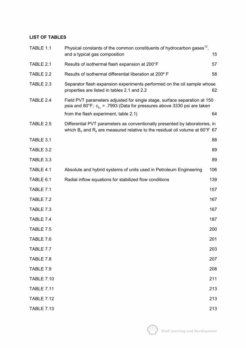
LIST OF TABLES
TABLE 1.1 Physical constants of the common constituents of hydrocarbon gases12,and a typical gas composition 15
TABLE 2.1 Results of isothermal flash expansion at 200°F 57
TABLE 2.2 Results of isothermal differential liberation at 200º F 58
TABLE 2.3 Separator flash expansion experiments performed on the oil sample whoseproperties are listed in tables 2.1 and 2.2 62
TABLE 2.4 Field PVT parameters adjusted for single stage, surface separation at 150psia and 80°F;
fbc = .7993 (Data for pressures above 3330 psi are taken
from the flash experiment, table 2.1) 64
TABLE 2.5 Differential PVT parameters as conventionally presented by laboratories, inwhich Bo and Rs are measured relative to the residual oil volume at 60°F 67
TABLE 3.1 88
TABLE 3.2 89
TABLE 3.3 89
TABLE 4.1 Absolute and hybrid systems of units used in Petroleum Engineering 106
TABLE 6.1 Radial inflow equations for stabilized flow conditions 139
TABLE 7.1 157
TABLE 7.2 167
TABLE 7.3 167
TABLE 7.4 187
TABLE 7.5 200
TABLE 7.6 201
TABLE 7.7 203
TABLE 7.8 207
TABLE 7.9 208
TABLE 7.10 211
TABLE 7.11 213
TABLE 7.12 213
TABLE 7.13 213

CONTENTS XXVIII
TABLE 7.14 214
TABLE 7.15 218
TABLE 7.16 219
TABLE 7.17 232
TABLE 7.18 233
TABLE 8.1 Generation of the real gas pseudo pressure, as a function of the actualpressure; (Gas gravity, 0.85, temperature 200°F) 245
TABLE 8.2 265
TABLE 8.3 266
TABLE 8.4 269
TABLE 8.5 272
TABLE 8.6 274
TABLE 8.7 276
TABLE 8.8 276
TABLE 8.9 276
TABLE 8.10 282
TABLE 8.11 282
TABLE 8.12 283
TABLE 8.13 285
TABLE 8.14 292
TABLE 9.1 308
TABLE 9.2 314
TABLE 9.3 314
TABLE 9.4 316
TABLE 9.5 316
TABLE 9.6 317
TABLE 9.7 318
TABLE 9.8 322
TABLE 9.9 326

CONTENTS XXIX
TABLE 9.10 328
TABLE 10.1 358
TABLE 10.2 359
TABLE 10.3 359
TABLE 10.3(a) Values of the shock front and end point relative permeabilities calculatedusing the data of exercise 10.1 361
TABLE 10.4 363
TABLE 10.5 363
TABLE 10.6 376
TABLE 10.7 377
TABLE 10.8 379
TABLE 10.9 Water saturation and point relative permeability distributions as functions ofthe reservoir thickness; fig.10.28(a) and (b). 384
TABLE 10.10 Thickness averaged saturations, relative permeabilities and pseudocapillary pressures corresponding to figs. 10.28 and 10.29 386
TABLE 10.11 Phase pressure difference, water saturation and relative permeabilitydistributions for cP° = 2 psi; fig. 10.36 392
TABLE 10.12 Pseudo capillary pressure and averaged relative permeabilitiescorresponding to figs. 10.36 and 10.37 395
TABLE 10.13 398
TABLE 10.14 399

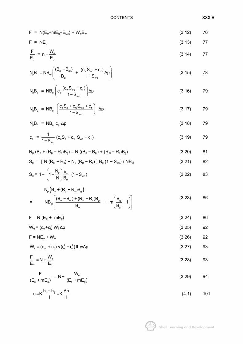
LIST OF EQUATIONS
( ) ( )wcOIP V 1 S res.vol.φ= − (1.1) 1
( )wc oiSTOIIP n v 1 S /Bφ= = − (1.2) 2
OP FP GP= + (1.3) 3
( ) ( )d FP d GP= − (1.4) 3
wwater
dpp D 14.7 (psia)dD
� � × +� �� �
(1.5) 4
wwater
dpp D 14.7 C (psia)dD
� �= × + +� �� �
(1.6) 4
wp 0.45 D 15 (psia)= + (1.7) 5
( )op 0.35D 565 psia= + (1.8) 6
( )op 0.08D 1969 psia= + (1.9) 6
wc oiUltimate Recovery (UR) (V (1 S ) /B ) RFφ= − × (1.10) 9
T
1 VcV p
∂=∂
— (1.11) 10
dV cV p= ∆ (1.12) 10
pV nRT= (1.13) 12
( )2a(p ) V b RTV
+ − = (1.14) 12
pV ZnRT= (1.15) 13
pc i cii
p n p=� (1.16) 14
pc i cii
T nT=� (1.17) 14
prpc
ppp
= (1.18) 14
prpc
TTT
= (1.19) 14
2
pr1.2(1 t)0.06125p t e
Zy
− −= (1.20) 19
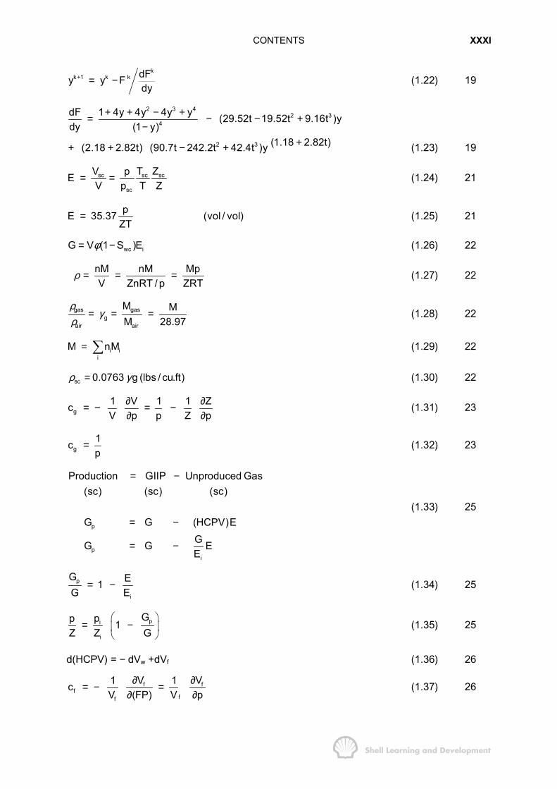
CONTENTS XXXI
kk 1 k k dFy y F
dy+ = − (1.22) 19
2 3 42 3
4dF 1 4y 4y 4y y (29.52t 19.52t 9.16t )ydy (1 y)
+ + − += − − +−
2 3 (1.18 2.82t)(2.18 2.82t) (90.7t 242.2t 42.4t )y ++ + − + (1.23) 19
sc sc sc
sc
V T ZpEV p T Z
= = (1.24) 21
pE 35.37 (vol / vol)ZT
= (1.25) 21
wc iG V (1 S )Eφ= − (1.26) 22
nM nM MpV ZnRT / p ZRT
ρ = = = (1.27) 22
gas gasg
air air
M MM 28.97
ργ
ρ= = = (1.28) 22
i ii
M nM= � (1.29) 22
sc 0.0763 g (lbs / cu.ft)ρ γ= (1.30) 22
g1 V 1 1 ZcV p p Z p
∂ ∂= − = −∂ ∂
(1.31) 23
g1cp
= (1.32) 23
p
pi
Production GIIP Unproduced Gas(sc) (sc) (sc)
G G (HCPV)EGG G EE
= −
= −
= −
(1.33) 25
p
i
G E1G E
= − (1.34) 25
pi
i
Gpp 1Z Z G
� �= −� �
� �(1.35) 25
d(HCPV) = − dVw +dVf (1.36) 26
f ff
ff
V V1 1cV (FP) V p
∂ ∂= − =∂ ∂
(1.37) 26
CONTENTS XXXII
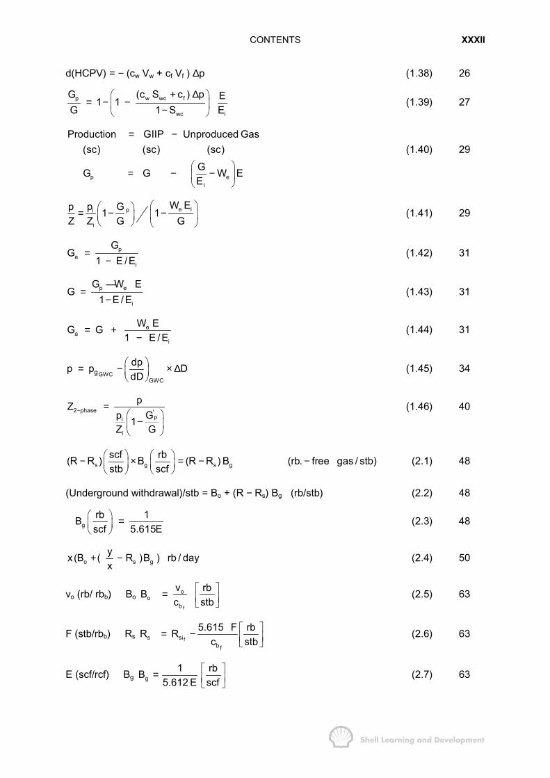
d(HCPV) = − (cw Vw + cf Vf ) ∆p (1.38) 26
w wc fp
wc i
(c S c ) pG E1 1G 1 S E
+ ∆� �= − −� �−� �
(1.39) 27
p ei
Production GIIP Unproduced Gas(sc) (sc) (sc)
GG G W EE
= −
� �= − −� �
� �
(1.40) 29
e ipi
i
W Epp G1 1Z Z G G
� �� �= − −� �� �� � � �
(1.41) 29
pa
i
GG
1 E /E=
−(1.42) 31
p e
i
G W EG
1 E /E=
−—
(1.43) 31
ea
i
W EG G1 E /E
= +−
(1.44) 31
GWCGWC
gdpp p DdD
� �= − × ∆� �� �
(1.45) 34
2 phase 'pi
i
pZp G1Z G
− =� �
−� �� �
(1.46) 40
s g s gscf rb(R R ) B (R R ) B (rb. free gas / stb)stb scf
� � � �− × = − −� � � �� � � �
(2.1) 48
(Underground withdrawal)/stb = Bo + (R − Rs) Bg (rb/stb) (2.2) 48
grb 1Bscf 5.615E
� � =� �� �
(2.3) 48
o s gyx (B ( R )B ) rb / dayx
+ − (2.4) 50
vo (rb/ rbb) Bo f
oo
b
v rbBc stb
� �= � �� �
(2.5) 63
F (stb/rbb) Rs fs sib f
5.615 F rbR Rc stb
� �= − � �� �
(2.6) 63
E (scf/rcf) Bg g1 rbB
5.612 E scf� �= � �� �
(2.7) 63
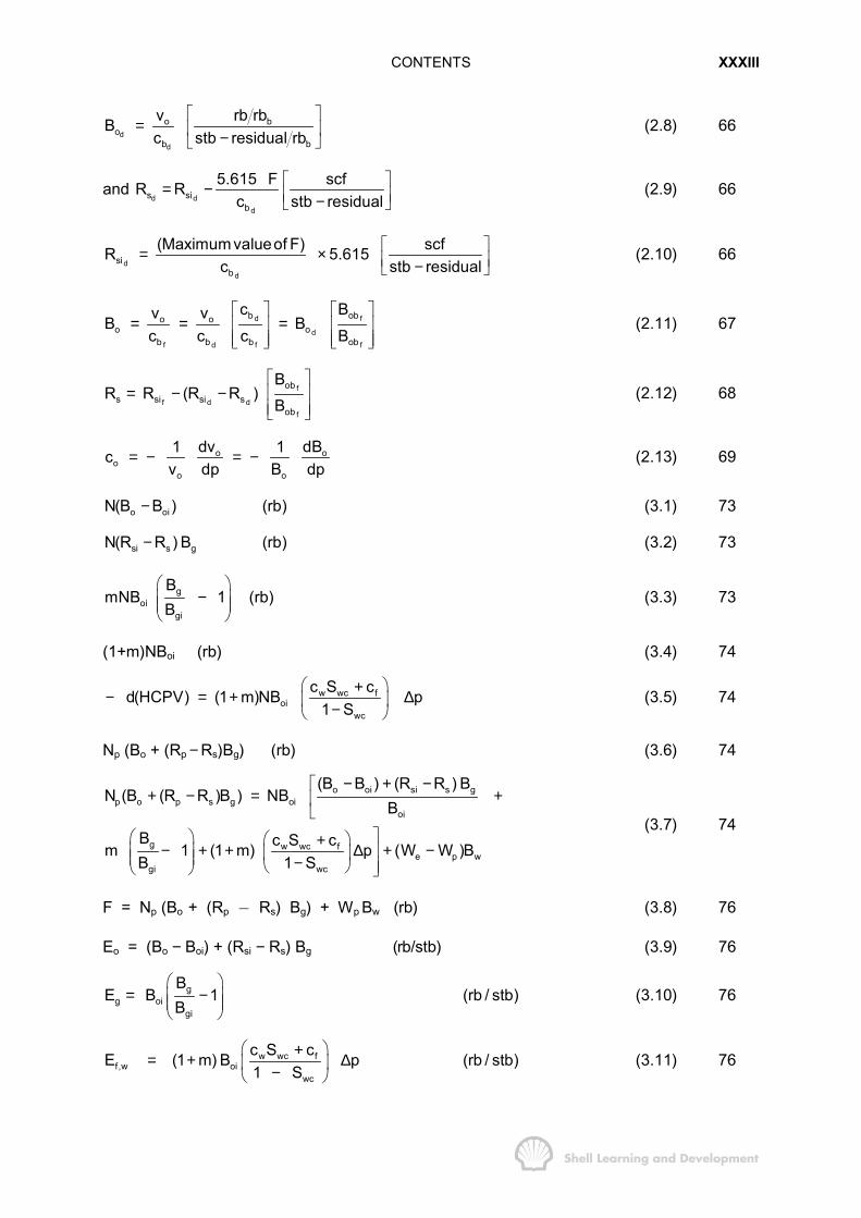
CONTENTS XXXIII
dd
o bo
b b
v rb rbBc stb residual rb
� �= � �−� �
(2.8) 66
and d d
d
s sib
5.615 F scfR Rc stb residual
� �= − � �−� �(2.9) 66
dd
sib
(Maximumvalueof F) scfR 5.615c stb residual
� �= × � �−� �(2.10) 66
d f
df d f f
b obo oo o
b b b ob
c Bv vB Bc c c B
� � � �= = =� � � �
� � � �� � � �(2.11) 67
f
f d df
obs si si s
ob
BR R (R R )
B
� �= − − � �
� �� �
(2.12) 68
o oo
o o
dv dB1 1cv dp B dp
= − = − (2.13) 69
o oiN(B B ) (rb)− (3.1) 73
si s gN(R R ) B (rb)− (3.2) 73
goi
gi
BmNB 1 (rb)
B� �
−� �� �� �
(3.3) 73
(1+m)NBoi (rb) (3.4) 74
w wc foi
wc
c S cd(HCPV) (1 m)NB p1 S
� �+− = + ∆� �−� �(3.5) 74
Np (Bo + (Rp − Rs)Bg) (rb) (3.6) 74
o oi si s gp o p s g oi
oi
g w wc fe p w
gi wc
(B B ) (R R ) BN (B (R R )B ) NB
B
B c S cm 1 (1 m) p (W W )BB 1 S
− + −�+ − = +�
�
�� � � �+− + + ∆ + −�� � � − � � � �
(3.7) 74
F = Np (Bo + (Rp � Rs) Bg) + Wp Bw (rb) (3.8) 76
Eo = (Bo − Boi) + (Rsi − Rs) Bg (rb/stb) (3.9) 76
gg oi
gi
BE B 1 (rb / stb)
B� �
= −� �� �� �
(3.10) 76
w wc ff,w oi
wc
c S cE (1 m) B p (rb / stb)1 S
� �+= + ∆� �−� �(3.11) 76
CONTENTS XXXIV
F = N(Eo+mEg+Ef,w) + WeBw (3.12) 76
F = NEo (3.13) 77
e
o o
WF nE E
= + (3.14) 77
o oi w wc fp o oi
oi wc
(B B ) (c S c )N B NB pB 1 S
� �− += + ∆� �� �−� �
(3.15) 78
w wc fp o oi o
wc
(c S c )N B NB c p1 S
� �+= ∆� �−� �(3.16) 79
o o w wc fp o oi
wc
c S c S cN B NB p1 S
� �+ += ∆� �−� �(3.17) 79
p o oi eN B NB c p= ∆ (3.18) 79
e o o w wc fwc
1c (c S c S c )1 S
= + +−
(3.19) 79
Np (Bo + (Rp − Rs)Bg) = N ((Bo − Boi) + (Rsi − Rs)Bg) (3.20) 81
Sg = [ N (Rsi − Rs) − Np (Rp − Rs) ] Bg (1 − Swc) / NBoi (3.21) 82
Sg = p owc
oi
N B1 1 (1 S )N B
� �− − −� �
� �(3.22) 83
( )p o p s g
o oi si s g goi
oi gi
N B (R R )B
(B B ) (R R )B BNB m 1
B B
+ −
� �� �− + −= + −� �� �� �� � � �
(3.23) 86
F = N (Eo + mEg) (3.24) 86
We = (cw+cf) Wi ∆p (3.25) 92
F = NEo + We (3.26) 922 2
e w f e oW (c c ) (r r ) fh pπ φ= + − ∆ (3.27) 93
e
o o
WF NE E
= + (3.28) 93
e
o g o g
WF N(E mE ) (E mE )
= ++ +
(3.29) 94
1 2h h hu K KI I− ∆= = (4.1) 101

CONTENTS XXXV
phg ( gz)ρ
= + (4.2) 102
dhu Kdl
= (4.3) 102
K d p K d(hg)u gzg dl g dlρ
� �= + =� �
� �(4.4) 102
p
1 atm
dp gzρ−
Φ = +� (4.5) 103
b
p
bp
dp g(z z )ρ
Φ = + −� (4.6) 103
p gzρ
Φ = + (4.7) 103
k dudl
ρµ
Φ= (4.8) 103
k dudl
ρµ
Φ= − (4.9) 104
k dudr
ρµ
Φ= (4.10) 104
k dpudlµ
= − (4.11) 105
k d k dp dzu gdl dl dl
ρ ρµ µ
Φ � �= = − +� �� �
� (4.12) 107
6k dp g dzu
dl dl1.0133 10ρ
µ� �
= − +� �×� �(4.13) 107
2k(D) A(cm ) dpq(cc / sec) (atm / cm)(cp) dlµ
= − (4.14) 107
2k(mD) A(ft ) dpq(std / d) (constan t) (psi / ft)(cp) dlµ
= − (4.15) 107
and since
22
2D cm atmk mD A ft
mD ft psistb r.cc / sec rb / d dp psiqcmd rb / d stb / d (cp) dl ftft
D 1 cm atm 1; 30.48 and ; equ.(4.16)mD 1000 ft psi 14.7
µ
� � � �� �× � � � �� �� �� � � � � � � �= − ×� � � � � �� � � �� �� �
� �� � � �= = =� �� � � �� � � � � �
(4.16) 108

CONTENTS XXXVI
3
o
kA dpq 1.127 10 (stb / d)dlµ
−= − × (4.17) 108
3
o
kA dpq 1.127 10 0.4335 sinB dl
γ θµ
− � �= − × +� �� �
(4.18) 110
b
p
p
RT Zdp gzM p
Φ = +� (4.19) 111
RT Z dpd dp gdz gdzM p ρ
Φ = + = + (4.20) 111
d 1 dp dzgdl dl dlρΦ = + (4.21) 111
kA d kA dqdl dl
ρ ψµ µ
Φ= − = − (4.22) 111
kA dpqdrµ
= (4.23) 113
wfw
q rp p ln2 kh r
µπ
− = (4.24) 113
ee wf
w
rqp p ln2 kh r
µπ
− = (4.25) 113
skinqp S
2 khµ
π∆ = (4.26) 114
ee wf
w
rqp p ln S2 kh r
µπ
� �− = +� �
� �(4.27) 114
o ee wf
w
q B rp p 141.2 In Skh rµ � �
− = +� �� �
(4.28) 114
e wf3
eo
w
q oil rate (stb / d)PIp p pressure drawdown (psi)
7.08 10 khrB ln Sr
µ
−
= =−
×=� �
+� �� �
(4.29) 115
o w w wro w rw w
k (S ) k (S )k (S ) and k (S )k k
= = (4.30) 118
rw rw w ork k (at S 1 S )′ = = − (4.31) 119
o w w wro w rw w
o w wc o w wc
k (S ) k (S )K (S ) and K (S )k (S S ) k (S S )
= == =
(4.32) 120

CONTENTS XXXVII
ko (Sw) = kkro (Sw) or ko (Sw) = ko (Sw = Swc) Kro (Sw) (4.33) 120
ro ro
rw rw
k Kk K
= (4.34) 120
rkkλµ
= (4.35) 121
rd d
ro o
k /Mobility of the displacing fluidMMobility of the displaced fluid k /
µµ
′= =
′(4.36) 122
1 k p pr cr r r t
ρ φ ρµ
� �∂ ∂ ∂=� �∂ ∂ ∂� �(5.1) 127
(q ) 2 rhr tρ ρπ φ∂ ∂=
∂ ∂(5.2) 128
1 k pr r r t
ρ ρρ φµ
� �∂ ∂ ∂=� �∂ ∂ ∂� �(5.3) 128
m1c
m pρρ ρρ ρ
� �∂ � � ∂� �= − =∂ ∂
(5.4) 129
pct t
ρρ ∂ ∂=∂ ∂
(5.5) 129
ep 0 at r rr
∂ = =∂
(5.6) 130
pt
∂ ≈∂
constant, for all r and t. (5.7) 130
dp dVcV qdt dt
= − = − (5.8) 131
or dp qdt cV
= − (5.9) 131
2e
dp qdt c r hπ φ
= − (5.10) 131
i ii
resi
i
p Vp
V=�
�(5.11) 131
qi ∝ Vi (5.12) 132
i ii
resi
i
p qp
q=�
�(5.13) 132
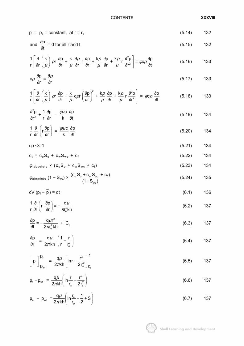
CONTENTS XXXVIII
p = pe = constant, at r = re (5.14) 132
pandt
∂∂
= 0 for all r and t (5.15) 132
2
21 k p k p k p k p pr r r cr r r r r r tr
ρ ρ ρρ φ ρµ µ µ µ
� �� �∂ ∂ ∂ ∂ ∂ ∂ ∂+ + + =� �� �∂ ∂ ∂ ∂ ∂ ∂∂ � �(5.16) 133
pcr r
ρρ ∂ ∂=∂ ∂
(5.17) 133
2 2
21 k p k p k p k p pr c r r cr r r r r tr
ρ ρρ ρ φ ρµ µ µ µ
� �� �∂ ∂ ∂ ∂ ∂ ∂� �+ + + =� �� � � �∂ ∂ ∂ ∂ ∂∂ � �� �(5.18) 133
2
2p 1 p c p
r r k trφµ∂ ∂ ∂+ =
∂ ∂∂(5 19) 134
1 p c prr r r k t
φ µ� �∂ ∂ ∂=� �∂ ∂ ∂� �(5.20) 134
cp << 1 (5.21) 134
ct = coSo + cwSw c + cf (5.22) 134
φ ab s o l u t e × (coSo + cwSw c + cf) (5.23) 134
φ a bs o l u t e (1 − Swc) × o o w wc f
wc
(c S c S c )(1 S )+ +
−(5.24) 135
cV (pi − p ) = qt (6.1) 136
2e
1 p qrr r r r kh
µπ
∂ ∂� � = −� �∂ ∂� �(6.2) 137
2
12e
p q r Ct 2 r kh
µπ
∂ = − +∂
(6.3) 137
2e
p q 1 rr 2 kh r r
µπ
� �∂ = −� �∂ � �(6.4) 137
2r
2ewf w
rp q rp lnr2 kh 2 rp r
µπ
� �� � = −� �� �� � � �(6.5) 137
2
r wf 2w e
q r rp p ln2 kh r 2r
µπ
� �− = −� �
� �(6.6) 137
ee wf
w
rq 1p p ln S2 kh r 2
µπ
� �− = − +� �
� �(6.7) 137
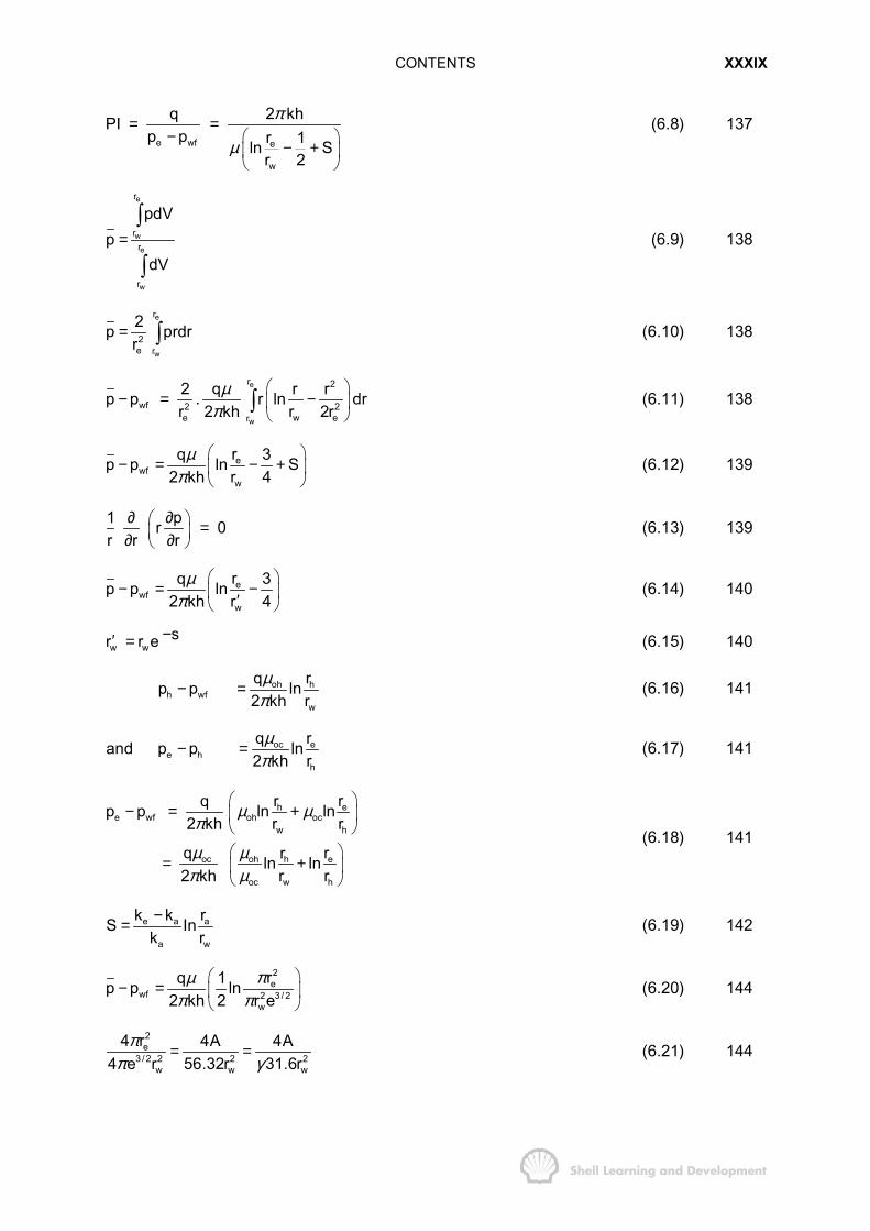
CONTENTS XXXIX
e wf e
w
q 2 khPIp p r 1ln S
r 2
π
µ= =
− � �− +� �
� �
(6.8) 137
e
w
e
w
r
rr
r
pdVp
dV=�
�
(6.9) 138
e
w
r
2e r
2p prdrr
= � (6.10) 138
e
w
r 2
wf 2 2we er
2 q r rp p . r ln dr2 kh rr 2r
µπ
� �− = −� �
� �� (6.11) 138
ewf
w
rq 3p p ln S2 kh r 4
µπ
� �− = − +� �
� �(6.12) 139
1 pr 0r r r
∂ ∂� � =� �∂ ∂� �(6.13) 139
ewf
w
rq 3p p ln2 kh r 4
µπ
� �− = −� �′� �
(6.14) 140
w wr r e′ = −s (6.15) 140
oh hh wf
w
q rp p ln2 kh r
µπ
− = (6.16) 141
oc ee h
h
q rand p p ln2 kh r
µπ
− = (6.17) 141
ehe wf oh oc
w h
oc oh eh
oc w h
rrqp p ln ln2 kh r r
q rrln ln2 kh r r
µ µπ
µ µπ µ
� �− = +� �
� �
� �= +� �
� �
(6.18) 141
e a a
a w
k k rS Ink r−= (6.19) 142
2e
wf 2 3 / 2w
rq 1p p ln2 kh 2 r e
πµπ π
� �− = � �
� �(6.20) 144
2e
3 /2 2 2 2w w w
4 r 4A 4A4 e r 56.32r 31.6r
ππ γ
= = (6.21) 144

CONTENTS XL
wf 2A w
q 1 4Ap p ln S2 kh 2 C r
µπ γ
� �− = +� �
� �(6.22) 144
i
i
r 0
a) p p at t 0, for all r
b) p p at r , for all t
p qc) lim r , for t 0r 2 kh
µπ→
= =
= = ∞
∂ = >∂
(7.1) 150
s c rt 2k t
φ µ∂ =∂
(7.2) 150
2
2s c rr 4k t
φ µ∂ =∂
(7.3) 150
( )
dpp s spdss 1dp ds
p s
′′ ′+ = −
+′= −
′
(7.4) 151
s
2ep Cs
−
′ = (7.5) 151
2
s
r,t icrx 4k t
q ep p ds4 kh sφ µ
µπ
−∞
=
= − � (7.6) 152
2
s s
x crx4k t
e eds dss s
φ µ
− −∞ ∞
=
=� � (7.7) 152
ei(x) ln x 0.5772≈ − − (7.8) 152
( )ei(x) ln x for x 0.01γ≈ − < (7.9) 153
wf i 2w
q 4ktp p ln 2S4 kh cr
µπ γ φ µ
� �= − +� �
� �(7.10) 153
2
r,t iq crp p ei
4 kh 4k tµ φ µ
π� �
= − � �� �
(7.11) 154
( )icAh p p qtφ − = (7.12) 156
wf i 2A w
q 4A ktp p ½ ln 2 S2 kh cAC r
µ ππ φ µγ
� �= − + +� �
� �(7.13) 156
CONTENTS XLI
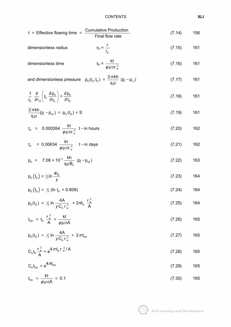
Cumulative Production t Effective flowing time Final flow rate
= = (7.14) 156
dimensionless radius rD = w
rr
(7.15) 161
dimensionless time tD = 2w
ktcrφ µ
(7.16) 161
and dimensionless pressure D D D i r,t2 khp (r , t ) (p p )
qπ
µ= − (7.17) 161
D DD
D D DD
p p1 rr r r t
� �∂ ∂∂ =� �∂ ∂ ∂� �(7.18) 161
i wf D D2 kh (p p ) p (t ) S
qπ
µ− = + (7.19) 161
D 2w
ktt 0.000264 t in hourscrφ µ
= − (7.20) 162
D 2w
ktt 0.00634 t in dayscrφ µ
= − (7.21) 162
3D i wf
o
khp 7.08 10 (p p )q Bµ
−= × − (7.22) 163
( ) D12D D
4tp t lnγ
= (7.23) 164
( ) 12D D Dp t (ln t 0.809)= + (7.24) 164
2w1
2D D D2A w
r4Ap (t ) ln 2 tAC r
πγ
= + (7.25) 164
2w
DA Dr ktt tA cAφ µ
= = (7.26) 165
12D D DA2
A w
4Ap (t ) ln 2 tC r
πγ
= + (7.27) 165
2 2w D w
A Dr 4 t r / AC t eA
π≈ (7.28) 165
DAA DA
4 tC t e π≈ (7.29) 165
DAktt 0.1
cAφ µ= ≈ (7.30) 165

CONTENTS XLII
( ) ( )j 1n
n
i wf j D D D nnj 1
2 kh p p q p t t q Sπµ −
=
− = ∆ − +� (7.31) 170
i ws D D D D D2 kh (p p ) p (t t ) p ( t )
qπ
µ− = + ∆ − ∆ (7.32) 171
( ) ( )n
n j 1
ni wf jD D D
j 1n n
p -p q2 kh p t t Sq q
πµ −
=
∆= − +� (7.33) 172
( ) ( )( ) ( )( )
n D2 t 21 n eDD
D D eD2 2 2 2n 1eD n 1 n eD 1 n
e J r2t 3p t lnr 24r J r J
α αα α α
−
=
∞= + − +
−� (7.34) 173
( )D D1 12 2i ws D D D
4 t t2 kh t t(p p ) ln p (t t ) lnq tπ
µ γ+ ∆+ ∆− = + + ∆ −
∆(7.35) 174
D1 12 2i ws D D
4t2 kh t t(p p ) ln p (t ) lnq tπ
µ γ+ ∆− = + −∆
(7.36) 174
( ) ( ) Di ws(LIN) D D
4t2 kh t tp p ½ ln p t ½lnq tπ
µ γ+ ∆− = + −∆
(7.37) 174
( )i DA2 kh 2 khqtp p 2 t
q q cA hπ π π
µ µ φ− = = (7.38) 175
( ) D12i D D
4t2 kh *p p p (t ) lnqπ
µ γ− = − (7.39) 176
( ) ( )DDA D D
4t4 kh *p p 4 t ln 2p tqπ π
µ γ− = + − (7.40) 176
( ) ( )2jD1 1
2 2i wf D Dj 2
ca4t2 kh p p p t ln eiq 4kt
φ µπµ γ =
∞− = = + � (7.41) 177
( ) ( )D1 12 2D D DA D(MBH) DA
4tp t 2 t ln p tπγ
= + − (7.42) 182
( ) ( )D(MBH) DA DA4 kh *p t p p 4 t
qπ π
µ= − = (7.43) 182
( ) ( ) ( )2w
D(MBH) DA A D A DAr4 kh *p t p p ln C t ln C t
q Aπ
µ= − = = (7.44) 182
( ) ( )DA
D(MBH) DA At4 kh *p t 1 p p ln C
1qπ
µ= = − =
=(7.45) 183
( ) ( )1 1 12 2 2D DA DA DA D(MBH) DA2
w
4Ap t 2 t ln t ln p tr
πγ
= + + − (7.46) 183
wf DA DA D(MBH) DA0.0189(3500 p ) 2 t ½ In t 8.632 ½ p (t ) 4.5π− = + + − + (7.46) 185
CONTENTS XLIII
wf D(MBH) DA0.0189 (3500 p ) ½ p (t )α− = − (7.47) 185
( ) ( )-3 Di ws(LIN) D D
o
4tkh t t7.08 10 p p 1.151 log p t ½ lnq B tµ γ
+ ∆× − = + −∆
(7.48) 189
DAktt 0.000264 (t-hours)cAφµ
= (7.49) 189
oq Bm 162.6 psi/log.cycle khµ= (7.50) 190
-3i wf D D
o
kh7.08 10 (p p ) p (t ) Sq Bµ
× − = + (7.51) 190
( )ws(LIN) 1 -hr wf2w
p p kS 1.151 log 3.23m crφ µ
� �−� �= − +� �� �
(7.52) 191
( ) ( )ro wabsk k k S= × (7.53) 191
ows i
q B t tp p 162.2 logkh tµ + ∆= −
∆(7.54) 192
( ) ( ) ( )n j
nj-3
i ws D D D 1 D Dj 1n o n
qkh7.08 10 p p p t t p tq B qµ −
=
∆× − = + ∆ − ∆� (7.55) 193
( )
( ) nn j
-3 ni ws(LIN)
n o
nDj
D D D 1j 1 n
t tkh7.08 10 p p 1.151 logq B t
4tqp t t ½ ln
q
µ
γ−=
+ ∆× − =∆
∆+ + ∆ −�
(7.56) 193
nn
tt* *p p m logt
− = (7.57) 194
D(MBH) DA A DAn o
kh *p (t )0.01416 (p - p) 2.303 log (C t )q Bµ
= (7.58) 195
( ) ( )n oA DA A DA
q B*p p 162.6 log C t m log C tkhµ− = = (7.59) 195
nn ntt A DA*p p m log(C t )− = (7.60) 195
( ) ( )nnn
ttt* *p p p p m logt
− − − = (7.61) 195
( )s
s
*p pt tlogt m
−+ ∆ =∆
(7.62) 198
( )sA DA
s
t tlog log C tt
+ ∆ =∆
(7.63) 198
CONTENTS XLIV
( )dDA
d
t tlog log 19.1 tt
+ ∆ =∆
(7.64) 199
( )
( )(
ws(LIN) 1 -hr wf2w
6
p p kS 1.151 log 3.23m cr
4752 4506 501.151 log 3.2324.5 .2 1 20 10 .09
φµ
−
� �−� �= − +� �� �
�−= − + ��× × × × �
(7.52) 202
( )ws(LIN)t t0.0144 4800 p 1.151 log 25.63
t+ ∆− = +∆
(7.65) 206
( ) ( )ws(LIN) DA A DAt t0.0144 4800 p 1.151 log 2 t ½ ln C t
tt t1.151 log
t
π
α
+ ∆− = + −∆+ ∆= +∆
(7.66) 207
( ) ( ) ( )i ws D D D D D0.0144 p p p t t p t− = + ∆ − ∆ (7.67) 207
( ) ( )ws DAD MBHt t0.0288 p p t ln
t+ ∆∆ = ∆ −∆
(7.68) 208
( ) ( )n
n j 1
ni wf j3D D D
j 1o n n
p p qkh7.08 10 p t t SB q qµ −
−
=
− ∆× = − +� (7.69) 209
( ) ( ) ( ) ( ) ( )( ) ( )
3
3 3 1
3 2
i wf 1 2 13D D D D D
o 3 3
3 2D D D
3
p p q 0 q qkh7.08 10 p t p t tB q q q3
q qp t t S
q
µ−
− − −× = + −
++ − +
(7.70) 210
( ) ( )n
n j 1
ni wf jD D D
j 1n n
p p qversus p t t
q q −=
− ∆−� (7.71) 210
( ) ( )nni wf j3
n j 1 2j 1o n n w
p p qkh k7.08 10 1.151 log t t log 3.23 0.87SB q q crµ φµ
−−
=
− ∆� �× = − + − +� �
� �� (7.72) 211
( ) 12D D D(MDH) DAp t p (t )α′ ′= − (7.73) 212
( ) ( )
( ) ( )
n N n j 1
n j 1
N3
i wf j D D D D Nj 1on
j D D D n Nj N 1
kh7.08 10 p p q p t t t q SB
q p t t q q S
δµ
δ δ
−
−
−
=
= +
× − = ∆ + − +
+ ∆ − + −
�
�
(7.74) 217
( ) ( )N n j 1 N j 1
N N
j D D D D j D D Dj 1 j 1
q p t t t q p t tδ− −
= =
∆ − − ≈ ∆ −� � (7.75) 217

CONTENTS XLV
( ) ( )N n
n j 1
nwf wf jD D D
j N 1n N n N
p p qversus p t t
q q q qδ δ
−= +
− ∆−
− −� (7.76) 217
p versus log t11C t
∆ ∆−
∆
(7.77) 225
o162.6q Bkhm
µ= (7.78) 226
wf (1 hr ) wf2w
p p kS 1.151 log 3.231 1/ C t crm
φ µ−
� �� �−
= − +� �− ∆� �� �� �
(7.79) 226
pF T pTq F q
∆ ∆× = (7.80) 229
( ) ewf
w
s.cc / sec r.cc / secQ Mscf / dratm 3Mscf / d s.cc / secp p psi ln S
D cmpsi r 42 k mD h ftmD ft
µπ
� � � �� � � � � �� � � � � �− = − + � � � � � �� � � �
� � � �� � � �
(8.1) 241
�
ewf
w
r711 Q ZT 3p p ln Sr 4khp
µ � �− = − +� �
� �(8.2) 242
� wfp pp2
+= (8.3) 242
wf wfp p p pand Z Z2 2
µ µ� � � �+ += =� � � �� � � �
(8.4) 242
2 2 ewf
w
r1422 Q ZT 3p p ln Skh r 4
µ � �− = − +� �
� �(8.5) 242
( )2 2i wf 2
wi
711 Q ZT 4 .000264ktp p ln 2Skh c r
µγ φ µ
� �− = +� �� �
� �(8.6) 242
( )b
p
p
pdpm p 2Zµ
= � (8.7) 243
Then ( )m p 2p pr rµ
∂ ∂=∂ Ζ ∂
(8.8) 248
and similarly ( )m p 2p pt tµ
∂ ∂=∂ Ζ ∂
(8.9) 248
CONTENTS XLVI
( ) ( )m p m p1 k r cr r 2p r 2p t
ρ µ µφ ρµ
� �∂ ∂∂ Ζ Ζ=� �� �∂ ∂ ∂� �(8.10) 248
( ) ( )m p m p1 crr r r k t
φµ� �∂ ∂∂ =� �� �∂ ∂ ∂� �(8.11) 248
( )2e
m p 2p p 2p qt t r h cµ µ π φ
∂ ∂= ⋅ = − ⋅∂ Ζ ∂ Ζ
(8.12) 249
( )2e res
m p1 2 pqrr r r r khπ
� �∂∂ � �= −� � � �� �∂ ∂ Ζ� �� �(8.13) 249
( ) sc sc2
sce
m p 2p q1 Trr r r Tr khπ
� �∂∂ = − ⋅� �� �∂ ∂� �(8.14) 249
( ) ( ) ewf
w
r1422 QT 3m p m p ln Skh r 4
� �− = − +� �
� �(8.15) 250
( ) ( ) ( )i wf 2wi
711 QT 4 .000264ktm p m p ln 2Skh c rγ φ µ
� �− = +� �� �
� �(8.16) 250
or ( ) ( )wf wfp p p p
2 µ
+ −
Ζ equivalent to
wf
p
p
pdpµΖ� (8.17) 251
dp udr k
µ= (8.18) 252
2dp u udr k
µ βρ= + (8.19) 253
( )e
w
2r
nDr
2p qm p dr2 rh
βρµ π
� �∆ = � �Ζ � �
� (8.20) 254
( )e
w
2rg
2 2nDr
Tpqm p constant drr hγ
µβ� �∆ = × � �ΖΤ� �
� (8.21) 254
( )e
w
r2g sc2 2nD
r
q drm p constanth r
β γµ
Τ∆ = × � (8.22) 254
( )2
g sc2nD
w e
q 1 1m p constantr rh
β γΤ � �∆ = × −� �
� �(8.23) 254
( )2
g12 22nD
w p w
Qm p 3.161 10 FQ
h rβ γµ
− Τ∆ = × = (8.24) 254

CONTENTS XLVII
( ) ( ) 2ewf
w
r1422 TQ 3m p m p ln S FQkh r 4
� �− = − + +� �
� �(8.25) 255
e
w
r1422 TQ 3ln S DQkh r 4
� �= − + +� �
� �(8.26) 255
FkhD1422T
= (8.27) 255
cons tan tkαβ = (8.28) 256
( )rg
cons tan tkk
αβ = (8.29) 256
( ) ( ) Di wf
4t711QTm p m p ln 2Skh γ
� �′− = +� �� �
(8.30) 257
( ) ( )( ) ( )i wf D Dkh m p m p m t S
1422QT′− = + (8.31) 257
( ) D12D D
4tm t lnγ
= (8.32) 258
( ) 12D D DA2
A w
4Am t ln 2 tC r
πγ
= + (8.33) 258
D DD
D D D D
m m1 rr r r t
� �∂ ∂∂ =� �∂ ∂ ∂� �(8.34) 258
( ) ( ) ( )D1 12 2D D DA DAD MBH
4tm t 2 t ln m tπγ
= + − (8.35) 258
( )DA
kt hrst 0.000264
cAφ µ= (8.36) 258
( ) ( ) ( ) ( )DAD MBHkh *m t m p m p
711QT� �= −� �� �
(8.37) 259
( ) ( )( ) ( ) 1D 2wf D 2A w
kh 4Am p m p m t S ln S1422QT C rγ
′ ′− = + = + (8.38) 259
( ) ( )( ) ( )n n j 1
n
i wf j D D D n nj 1
kh m p m p Q m t t Q S1422T −
=
′− = ∆ − +� (8.39) 260
CONTENTS XLVIII
( ) ( ) ( ) ( )n j 1D1 1
2 2D D D D D DA DAD MBH
j j j 1
n n
4tm t t m t 2 t ln m t
Q Q Qand
S S DQ
πγ−
−
′′ ′ ′− = = + −
∆ = −
′ = +
(8.40) 260
( ) ( )( ) ( )n n j 1
n2
i wf n j D D D nj 1
kh m p m p FQ Q m t t Q S1422T −
=
− − = ∆ − +� (8.41) 260
( )n2 2i wfQ C p p= − (8.42) 262
( ) ( ) 212i wf 2
A w
1422QT 4Am p m p ln S FQkh C rγ
� �− = + +� �
� �(8.43) 263
( ) ( ) 2i wfm p m p BQ FQ− = + (8.44) 263
( ) ( )ni wfn
n
m p m pversus Q
Q−
(8.45) 263
( )n
2 ni wf n j 1
2j 2j 1n n A wi
m(p ) m(p ) FQ Q2.359T 1422T 4At ln SQ c Ah Q kh C rφ µ γ=
− − � �= ∆ + +� �
� �� (8.46) 264
n
2 ni wf n j
jj 1n n
m(p ) m(p ) FQ Qversus t
Q Q=
− −∆� (8.47) 264
m(p) = (0.3457p — 414.76) × 106 psia2/cp (8.48) 265
( ) ( ) ( ) ( )n
2ni wf n j
n j 1 2j 1n n wi
m p m p FQ Q km log t t m log 3.23 .87SQ Q c rφ µ−
=
− − � �∆= − + − +� �� �
� �� (8.49) 273
( )nn j 1
2 ni wf n j
D D Dj 1n n
m(p ) m(p ) FQ Q1422T 1422Tm t t SQ kh Q kh−
=
− − ∆= − +� (8.50) 275
12D D D(MBH) DAm (t ) m (t )α′ ′= − (8.51) 275
1i ws D D D D D1
kh (m(p ) m(p )) m (t t ) m ( t )1422Q T
− = + ∆ − ∆ (8.52) 279
11
D1 12i ws(LIN) D D
1
4tt tkh (m(p ) m(p )) 1.151 log m (t ) ln1422Q T t γ
+ ∆− = + −∆
(8.53) 279
11637Q Tmkh
= (8.54) 280
ws(LIN)1 hr wf1 1 2
i w
(m(p ) m(p )) kS S DQ 1.151 log 3.23m ( c) rφ µ− −� �′ = + = − +� �
� �(8.55) 280
CONTENTS XLIX
1i wf 12
i w
1637Q T km(p ) m(p ) log t log 3.23 0.87Skh ( c) rφ µ
� �′− = + − +� �� �
(8.56) 280
i wf 1 hr1 1 2
i w
(m(p ) m(p ) ) kS S DQ 1.151 log 3.23m ( c) rφ µ
−� �−′ = + = − +� �� �
(8.57) 280
1 max maxi wf 1 D D D D D D D
2 D D 2 2
kh (m(p ) m(p )) Q (m (t t t ) m ( t t ))1422T
Q m (t ) Q S
′ ′− = + ∆ + − ∆ +
′ ′+ +(8.58) 281
i wf i ws 2 D D 2 2kh kh(m(p ) m(p )) (m(p ) m(p )) Q m (t ) Q S
1422T 1422T′ ′ ′− = − + + (8.59) 281
ws 1 hr wf 1 hr2 2 2
i w
(m(p ) m(p ) kS S DQ 1.151 log 3.23m ( c) rφ µ
− −′� �−′ = + = − +� �� �
(8.60) 281
SSSpSSS DA SSS
( c) At (t )
0.000264k
φ µ= (8.61) 286
b
pro o
o op
k (S )m (p) dpBµ
′ = � (8.62) 289
or rg o os
g ro g
k BR Rk Bµ
µ= + (8.63) 289
D1 12 2D D DA D(MBH) DA
4tm (t ) 2 t ln m (t )πγ
′ ′= + − (8.64) 290
g go s ot g w wc f
o g
S BS R Bc B c S cB p p B p
∂� ∂ ∂ �= − − + +� �∂ ∂ ∂� �(8.65) 290
1 cr r r k t
β φµ β∂ ∂ ∂� � =� �∂ ∂ ∂� �(8.66) 291
D DD
D D D D
1 rr r r t
β β� �∂ ∂∂ =� �∂ ∂ ∂� �(8.67) 292
D Df(p) (t ) Sqα β� �
= +� �� �
(8.68) 292
n j 1
n
n j D D D nj 1
f(p) q (t t ) q Sα β−
=
= ∆ − +� (8.69) 292
n j 1D1 1
2 2o D D D D DA D(MBH) DA4t(t t ) (t ) 2 t ln (t )β β π βγ−
′′ ′ ′− = = + − (8.70) 292
n j 1D1
2D D D D D4t(t t ) (t ) lnβ βγ−
′′− = = (8.71) 293
CONTENTS L
Do
rrr
= (9.1) 298
D 20
kttcrφµ
= (9.2) 298
( )D Dqq t
2 kh pµ
π=
∆(9.3) 299
( )2e 0 D DW 2 hcr pW tπφ= ∆ (9.4) 299
e D DW U p W (t )= ∆ (9.5) 299
2oU 2 f hcrπ φ= (9.6) 299
Dt = constant20
ktcrφµ
× (9.7) 300
U = 1.119 fφh 2ocr (bbl/psi) (9.8) 300
tD = constant ×2
ktcLφµ
(9.9) 301
U = .1781 wLhφc (bbl/psi) (9.10) 301
( ) ( )212D eDRadial W max r 1= − (9.11) 301
( )DLinear W max 1= (9.12) 301
ekctW 2hw p (ccs)φπµ
= ×∆ (9.13) 301
3e
kctW 3.26 10 hw x p (bbls)φπµ
−= × ∆ (9.14) 302
i 11
1 22
j 1 jj
p pp2
p pp2
p pp
2−
+=
+=
+=
�
�
�
(9.15) 309

CONTENTS LI
i 1 i 110 i i
i 1 1 2 i 21 21
2 3 1 31 22 32
j 1 j j j 1 j 1 j 1j j 1j
(p p ) p pp p p p2 2
(p p ) (p p ) p pp p p2 2 2
(p p ) p p(p p )p p p2 2 2
(p p ) (p p ) p pp p p
2 2 2
−
− + − ++
+ −∆ = − = =
+ + −∆ = − = − =
+ −+∆ = − = − =
+ + −∆ = − = − =
�
�
�
(9.16) 310
( )j
n 1
e j D D Dj 0
W T U p W (T T )−
=
= ∆ −� (9.17) 310
eaw
dWq J(p p)dt
= = − (9.18) 320
We=c Wi (pi - p a) (9.19) 320
e ea i i
eii i
W Wp p 1 p 1WcWp
� � � �= − = −� � � �� �
� �� �(9.20) 320
e ei a
i
dpdW Wdt p dt
= − (9.21) 320
( ) i eia i
Jp t / Wp p p p e−− = − (9.22) 320
e i eii
dW Jp t / WJ(p p)edt
−= − (9.23) 321
ei i eie i
i
W Jp t / WW (p p)(1 e )p
−= − − (9.24) 321
( )1ei i 1 ei
1e ii
W Jp t / WW p p (1 e )p
− ∆∆ = − − (9.25) 321
( )12ei i 2 ei
a 2ei
W Jp t / WW p p (1 e )p
− ∆∆ = − − (9.26) 321
i1
i
ea i
e
Wp p 1
W� �∆
= −� �� �� �
(9.27) 321
( )n 1nei i n ei
a nei
W Jp t / WW p p (1 e )p −
− ∆∆ = − − (9.28) 321
CONTENTS LII
j
n 1
n 1
ej 1
a iei
Wp p 1
W−
−
=
� �∆� �� �= −� �� �� �
�(9.29) 322
khw3Lµ
(9.30) 322
khwLµ
(9.31) 322
ew i
dWq J(p p)dt
= = − (9.32) 323
t
e i0
W J (p p)dt= −� (9.33) 323
3
e
o
3
7.08 10 fkhJr 3lnr 4
7.08 10 .3889 200 100 116.5b / d / psi.55(In5 .75)
µ
−
−
×=� �
−� �� �
× × × ×= =−
(9.30) 325
( ) ( )n j n 1
n 2
e j D D D n 1 D D Dj 0
W U p W T t U p W T t−
−
−=
= ∆ − + ∆ −� (9.34) 329
( ) ( ) ( )n j n 1
n 2
e j D D D n 2 n D D Dj 0
UW U p W T t p p W T t2 −
−
−=
= ∆ − + − −� (9.35) 329
n np e ii
in
G W Epp 1 1Z Z G G
� � � �� � = − −� � � �� �� � � � � �
(9.36) 329
( )n j
n 21
e j D D Dj 0
W U p W T t−
=
= ∆ −� (9.37) 330
( )n wf,non
hoh
w
2 k h p pq rln
r
π
µ
−= (9.38) 334
( )12n n 1 np p p−= + (9.39) 334
( )12wf,n wf,n 1 wf,np p p−= + (9.40) 334
( )p,n p,n 1 n 1 n wf,n 1 wf,nN N p p p p2α
− − −= + + − − (9.41) 334
( ) ( )j n 1
n 2
p,n j D D D n 1 D D Dj 0
N U p W T t U p W T t−
−
−=
= ∆ − + ∆ −� (9.42) 334
CONTENTS LIII
( ) ( )j
n 2
p,n j D D D n 2 nj 0
N U p W T t p p2β−
−=
= ∆ − + −� (9.43) 335
( ) ( ) ( )j
n 2
n j D D D p,n 1 n 2 wf,n 1 wf,n n 1j 0
1p 2U p W T t 2N p p p pβ αα β
−
= − − − −=
� �∆ − − + + + −� �+ � �
� (9.44) 335
c o w1 2
1 1P p pr r
σ� �
= − = +� �� �
(10.1) 338
o w cp p P gHρ− = = ∆ (10.2) 341
o w c2 cosp p P gh
rσ ρΘ− = = = ∆ (10.3) 341
c w o wP (S ) = p p = g cosρ γ θ− ∆ (10.4) 342
c w 6g y cosP (S ) (atm)
1.0133 10ρ θ∆=
×(10.5) 342
( )c wP S 0.4335 y cos (psi)γ θ= ∆ (10.6) 342
t o w iq q q q= + = (10.7) 344
o t o crww 6
rw ro ro
q P g sinq Akk kk kk x 1.0133 10
µ µµ ρ θ� � ∂ ∆� �= − + = + −� � � �∂ ×� �� �(10.8) 347
ro c6
t ow
row
rw o
kk A P g sin1q x 1.0133 10f k1
k
ρ θµ
µµ
∂ ∆� �+ −� �∂ ×� �=+ ⋅
(10.9) 347
3 ro c
t ow
row
rw o
kk A P1 1.127 10 .4335 sinq xf k1
k
γ θµ
µµ
− ∂� �+ × − ∆� �∂� �=+ ⋅
(10.10) 347
c c w
w
P dP Sx dS x
∂ ∂= ⋅∂ ∂
(10.11) 348
wrow
rw o
1f k1kµ
µ
=+ ⋅
(10.12) 349
w w w w w wx dxxq q A dx ( S )
tρ ρ φ ρ
+
∂− =∂
(10.13) 349
w w w w(q ) A ( S )x t
ρ φ ρ∂ ∂= −∂ ∂
(10.14) 350
CONTENTS LIV
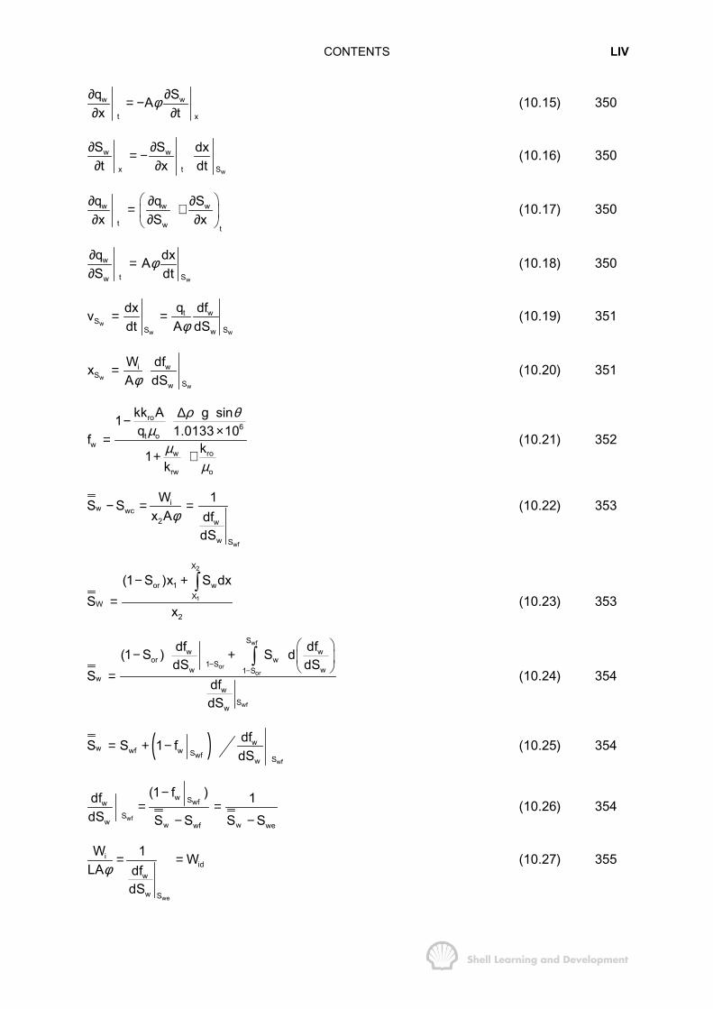
w w
t x
q SAx t
φ∂ ∂= −∂ ∂
(10.15) 350
w
w w
x t S
S S dxt x dt
∂ ∂= −∂ ∂
(10.16) 350
t
w w w
t w
q q Sx S x
� �∂ ∂ ∂= ⋅� �∂ ∂ ∂� �(10.17) 350
w
w
t Sw
q dxAS dt
φ∂ =∂
(10.18) 350
ww w
t wS
S Sw
q dfdxvdt A dSφ
= = (10.19) 351
ww
i wS
Sw
W dfxA dSφ
= (10.20) 351
ro6
t ow
row
rw o
kk A g sin1q 1.0133 10f k1
k
ρ θµ
µµ
∆−×=
+ ⋅(10.21) 352
wf
iw wc
2 w
w S
W 1S Sx A df
dSφ
− = = (10.22) 353
2
1
X
or 1 wX
W2
(1 S )x S dxS
x
− +=
�(10.23) 353
wf
oror
wf
Sw w
or w1 Sw w1 S
ww
Sw
df df(1 S ) S ddS dS
S dfdS
−−
� �− + � �
� �=�
(10.24) 354
( )wf
Swf
ww wf w
Sw
dfS S 1 fdS
= + − (10.25) 354
wf
Swf
w w
ww
Sw wf we
(1 f )df 1dS S S S S
−= =
− −(10.26) 354
we
iid
w
w S
W 1 WLA df
dSφ
= = (10.27) 355
CONTENTS LV
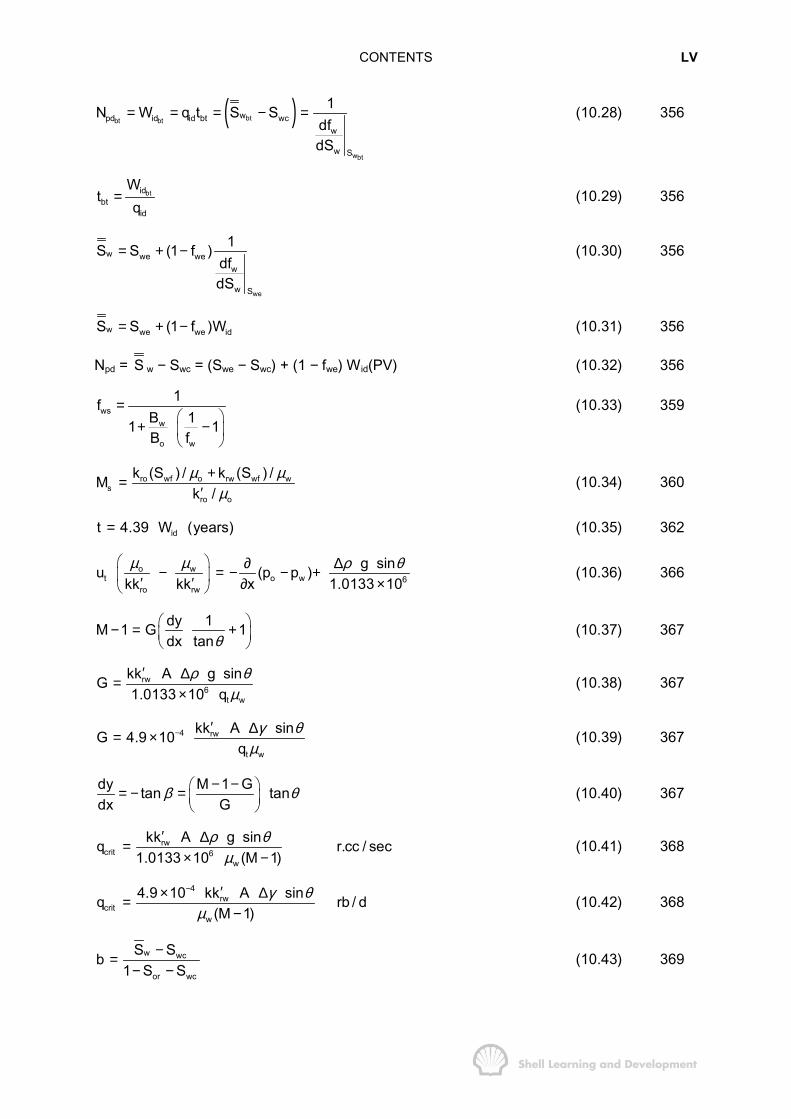
( )btbt bt
wbt
wpd id id bt wcw
w S
1N W q t S SdfdS
= = = − = (10.28) 356
btidbt
id
Wt
q= (10.29) 356
we
w we wew
w S
1S S (1 f )dfdS
= + − (10.30) 356
w we we idS S (1 f )W= + − (10.31) 356
Npd = S w − Swc = (Swe − Swc) + (1 − fwe) Wid(PV) (10.32) 356
wsw
o w
1fB 11 1B f
=� �
+ −� �� �
(10.33) 359
ro wf o rw wf ws
ro o
k (S ) / k (S ) /Mk /µ µ
µ+=
′(10.34) 360
idt 4.39 W (years)= (10.35) 362
o wt o w 6
ro rw
g sinu (p p )kk kk x 1.0133 10µ µ ρ θ� � ∂ ∆− = − − +� �′ ′ ∂ ×� �
(10.36) 366
dy 1M 1 G 1dx tanθ
� �− = +� �� �
(10.37) 367
rw6
t w
kk A g sinG1.0133 10 q
ρ θµ
′ ∆=×
(10.38) 367
4 rw
t w
kk A sinG 4.9 10q
γ θµ
− ′ ∆= × (10.39) 367
dy M 1 Gtan tandx G
β θ− −� �= − = � �� �
(10.40) 367
rwcrit 6
w
kk A g sinq r.cc / sec1.0133 10 (M 1)
ρ θµ
′ ∆=× −
(10.41) 368
4rw
critw
4.9 10 kk A sinq rb / d(M 1)
γ θµ
− ′× ∆=−
(10.42) 368
w wc
or wc
S Sb1 S S
−=
− −(10.43) 369
CONTENTS LVI
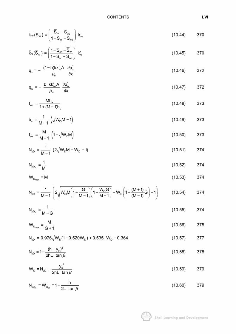
wcrw rw
or wc
ww
S Sk (S ) k1 S S
� �− ′= � �� �− −� �(10.44) 370
orro ro
or wc
ww
1 S Sk (S ) k1 S S
� �− − ′= � �� �− −� �(10.45) 370
ro oo
o
(1 b)kk A pqxµ
°′− ∂= −∂
(10.46) 372
rw ww
w
b kk A pqxµ
°′ ∂= −∂
(10.47) 372
ewe
e
Mbf1 (M 1)b
=+ −
(10.48) 373
( )e iD1b W M 1
M 1= −
−(10.49) 373
( )we iDMf 1 W M
M 1= −
−(10.50) 373
pD iD iD1N (2 W M W 1)
M 1= − −
−(10.51) 374
btpD1NM
= (10.52) 374
maxiDW M= (10.53) 374
iDpD iD iD
W G1 G (M 1)N 2 W M 1 1 W 1 G 1M 1 M 1 M 1 (M 1)
� �� �+� �� �= − − − − −� �� �� � � �� �− − − −� � � � � �� �(10.54) 374
btpD1N
M G=
−(10.55) 374
maxiDMW
G 1=
+(10.56) 375
pD iD iD iDN 0.976 W (1 0.520W ) 0.535 W 0.364= − + − (10.57) 377
2e
pD(h y )N 1
2hL tan β−= − (10.58) 378
2e
iD pDyW N
2hL tan β= + (10.59) 379
bt btpD iDhN W 1
2L tan β= = − (10.60) 379

CONTENTS LVII
rg crit6
tg t
kk A g sin qG (M 1)q1.0133 10 q
ρ θµ
′ ∆= = −
×(10.61) 380
dPc = .4335 (1.04−.81) dz = 0.1 dz (10.62) 382h
w0
w
S (z)dzS
h=�
(10.63) 382
h
rw w0
rw w
k (S (z))dzk (S )
h=�
(10.64) 383
h
ro w0
ro o
k (S (z))dzk (S )
h=�
(10.65) 383
o w c c 6
g hp p P P z (atm)21.0133 10
ρ° ° ° ∆ � �− = = + −� �× � �(10.66) 388
o w c chp p P P 0.4335 z (psi)2
γ° ° ° � �− = = + ∆ −� �� �
(10.67) 388
orc 1 S6
g hP z21.0133 10
ρ°−
∆ � �= −� �× � �(10.68) 388
orc 1 ShP 0.4335 z2
γ°−
� �= ∆ −� �� �
(10.69) 388
( )orc 1 SP 0.1 20 z°−= − (10.70) 388
1 2 3w w w1 1 2 2 3 3w 3
i ij 1
h S h S h SSh
φ φ φ
φ=
+ +=
�
(10.71) 393
j j
n
n N
j j or j j wcj 1 j n 1
w N
j jj 1
h (1 S ) h SS
h
φ φ
φ
= = +
=
− +=� �
�
(10.72) 396
n n n
n N
rw w j j rw j jj 1 j 1
k (S ) h k k h k= =
′= � � (10.73) 396
n n n
N N
ro w j j ro j jj n 1 j 1
k (S ) h k k h k= + =
′= � � (10.74) 397
jt wj
j j w j
q fvwh Sφ
� �∆= � �∆� �(10.75) 401
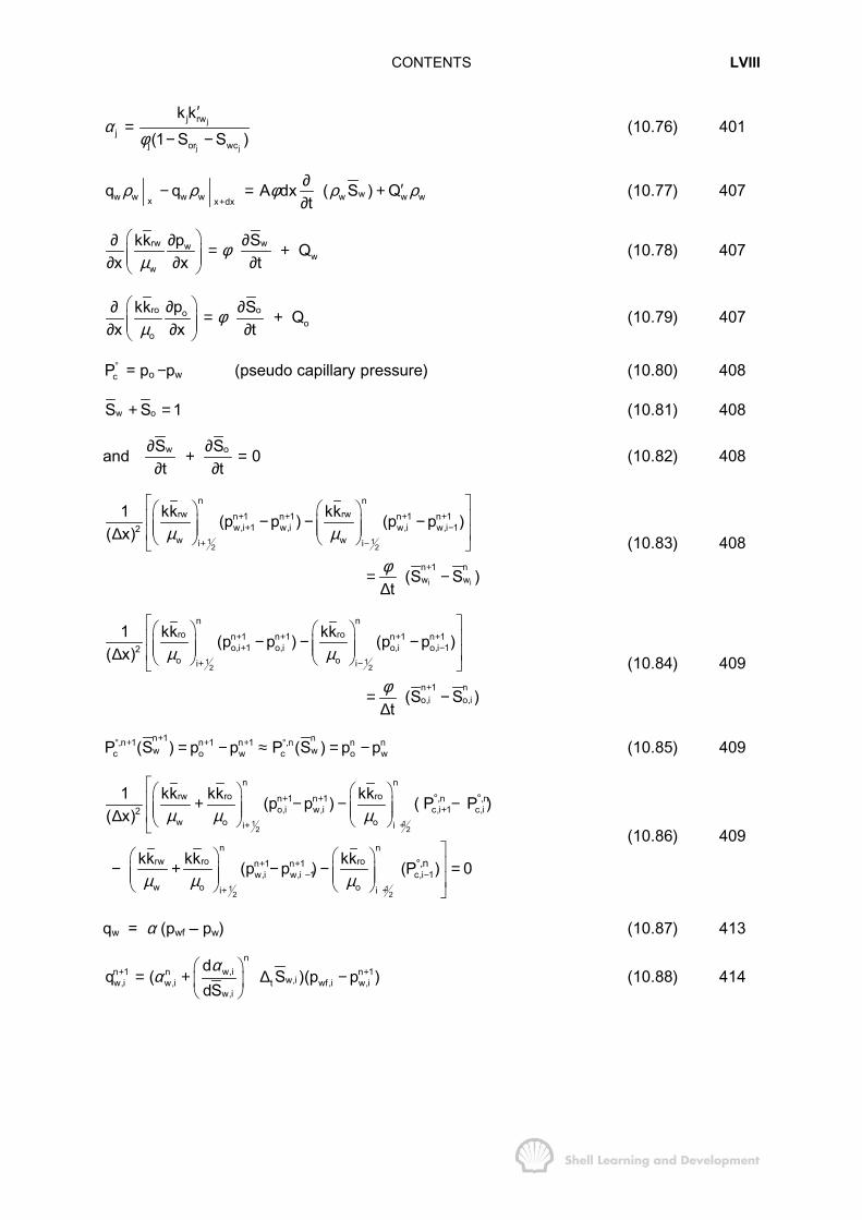
CONTENTS LVIII
j
j j
j rwj
j or wc
k k(1 S S )
αφ
′=
− −(10.76) 401
x x dxww w w w w w wq q A dx ( S ) Q
tρ ρ φ ρ ρ
+
∂ ′− = +∂
(10.77) 407
rw www
w
pkk S Qx x t
φµ
� �∂∂ ∂= +� �� �∂ ∂ ∂� �(10.78) 407
ro ooo
o
pkk S Qx x t
φµ
� �∂∂ ∂= +� �� �∂ ∂ ∂� �(10.79) 407
cP° = po −pw (pseudo capillary pressure) (10.80) 408
w oS S 1+ = (10.81) 408
and w oS S 0t t
∂ ∂+ =∂ ∂
(10.82) 408
1 12 2
i i
n nrw rwn 1 n 1 n 1 n 1
w,i 1 w,i w,i w,i 12w wi i
n 1 nw w
1 kk kk(p p ) (p p )( x)
(S S )t
µ µ
φ
+ + + ++ −
+ −
+
� �� � � �� �− − −� � � �� � � �� �∆ � �
= −∆
(10.83) 408
1 12 2
n nro ron 1 n 1 n 1 n 1
o,i 1 o,i o,i o,i 12o oi i
n 1 no,i o,i
1 kk kk(p p ) (p p )( x)
(S S )t
µ µ
φ
+ + + ++ −
+ −
+
� �� � � �� �− − −� � � �� � � �� �∆ � �
= −∆
(10.84) 409
n 1 n,n 1 n 1 n 1 ,n n nw wc o w c o wP (S ) p p P (S ) p p+° + + + °= − ≈ = − (10.85) 409
1 12 2
1 12 2
n nrw ro ron 1 n 1 ,n ,n
o,i w,i c,i 1 c,i2w o oi i
n nrw ro ron 1 n 1
w,i w,i 1 c,i 1w o oi i
,n
1 kk kk kk(p p ) ( P P )( x)
kk kk kk(p p ) (P ) 0
µ µ µ
µ µ µ
+ ++
+ +
+ +− −
+ +
° °
°
�� � � �� + − − −� � � �� � � ��∆ � � � �
� � � ��− + − − =� � � �� � � � �� � � � �
(10.86) 409
qw = α (pwf – pw) (10.87) 413n
w,in 1 n n 1w,iw,i w,i t wf,i w,i
w,i
dq ( S )(p p )
dSα
α+ +� �= + ∆ −� �
� �(10.88) 414

NOMENCLATUREENGLISH
A areaB Darcy coefficient in stabilized gas well
inflow equations (ch. 8)Bg gas formation volume factorBo oil formation volume factorBw water formation volume factorc isothermal compressibilityce effective compressibility (applied to pore
volume)cf pore compressibilityct total compressibility (applied to pore
volume)
c total aquifer compressibility (cw+cf)C arbitrary constant of integrationC coefficient in gas well back-pressure
equation (ch. 8)C pressure buildup correction factor (Russell
afterflow analysis ch. 7)CA Dietz shape factorD non-Darcy flow constant appearing in rate
dependent skin (ch. 8)D vertical depthe exponentialei exponential integral functionE gas expansion factorEf,w term in the material balance equation
accounting for the expansion of theconnate water and reduction in porevolume
Eg term in the material balance equationaccounting for the expansion of thegascap gas
Eo term in the material balance equationaccounting for the expansion of the oiland its originally dissolved gas
f fractionf fractional flow of any fluid in the reservoirf function; e.g. f(p) - function of the
pressureF cumulative relative gas volume in PVT
differential liberation experiment (ch. 2)F non-Darcy coefficient in gas flow equation
(ch. 8)F production term in the material balance
equation (chs. 3,9)F wellbore parameter in McKinley afterflow
analysis (ch. 7)g acceleration due to gravityg function; e.g.- g(p) function of pressureG gas initially in place – GIIPG gravity number (ch. 10)
G wellbore liquid gradient (McKinley after-flowanalysis, ch. 7)
Ga apparent gas in place in a water drive gasreservoir (ch. 1)
Gp cumulative gas productionh formation thicknesshp thickness of the perforated intervalH total height of the capillary transition zoneJ Bessel function (ch. 7)J Productivity indexk absolute permeability (chs. 4,9,10)k effective permeability (chs. 5,6,7,8)kr relative permeability obtained by normal-
izing the effective permeability curves bydividing by the absolute permeability
rk thickness averaged relative permeabilityk′r end point relative permeabilityk iteration counterKr relative permeability obtained by
normalizing the effective permeabilitycurves by dividing by the end pointpermeability to oil (ch. 4)
I lengthL lengthm ratio of the initial hydrocarbon pore volume
of the gascap to that of the oil (materialbalance equation)
m slope of the early, linear section of pressureanalysis plot of pressure (pseudo pressure)vs. f(time), for pressure buildup, fall-off ormulti-rate flow test
m(p) real gas pseudo pressurem′(p) pseudo pressure for two phases (gas-oil)
flowM end point mobility ratioM molecular weightMs shock front mobility ration reciprocal of the slope of the gas well back
pressure equation (ch. 8)n total number of molesN stock tank oil initially in place (STOIIP)Np cumulative oil productionNpd dimensionless cumulative oil production (in
pore volumes)NpD dimensionless cumulative oil production (in
moveable oil volumes)p pressurepa average pressure in aquifer (ch. 9)pb bubble point pressurepc critical pressurepd dynamic grid block pressurepD dimensionless pressurepe pressure at the external boundarypi initial pressure
NOMENCLATURE LX
ppc pseudo critical pressureppr pseudo reduced pressurepsc pressure at standard conditionspwf bottom hole flowing pressurepwf(1hr) bottom hole flowing pressure rec-orded
one hour after the start of flowpws bottom hole static pressurepws(LIN) (hypothetical) static pressure on the
extrapolation of the early linear trend ofthe Horner buildup plot
p average pressure
p* specific value of pws(LIN) at infiniteclosed-in time
∆p pressure drop
N.B. the same subscripts/superscripts, usedto distinguish between the abovepressures, are also used in conjunctionwith pseudo pressures, hence: m(pi);m(pwf); m(pws(LIN)); etc.
Pc capillary pressure
cP° pseudo capillary pressure
q production rateqi injection rateQ gas production rater radial distancere external boundary radiusrD dimensionless radius= r/rw (chs. 7,8)
= r/ro (ch. 9)reD dimensionless radius= re/rw (chs. 7,8)
= re/ro (ch. 9)rh radius of the heated zone around a
steam soaked wellro reservoir radiusrw wellbore radiusr′w effective wellbore radius taking account
of the mechanical skin (r′w = rwe-s)R producing (or instantaneous) gas oil
ratioR universal gas constantRp cumulative gas oil ratioRs solution (or dissolved) gas oil ratioS mechanical skin factorS saturation (always expressed as a
fraction of the pore volume)Sg gas saturationSgr residual gas saturation to waterSo oil saturation
Sor residual oil saturation to waterSw water saturationSwc connate (or irreducible) water saturationSwf water saturation at the flood front
wS thickness average water saturation
wS volume averaged water saturation behind anadvancing flood front
t reciprocal pseudo reduced temperature(Tpc/T)
t timetD dimensionless time
tDA dimensionless time (=tD 2wr /A)
∆t closed-in time during a pressure buildup∆ts closed-in time during a build-up at which
pws(LIN) = p∆td closed in time during a buildup at which
pws(LIN) = pdT absolute temperatureT transmissibility (McKinley afterflow analysis,
ch. 7)Tc critical temperatureTpc pseudo critical temperatureTpr pseudo reduced temperatureu Darcy velocity (q/A)U aquifer constantv velocityvg relative gas volume, differential liberation
experimentV volumeV net bulk volume of reservoirVf pore volume (PV)Vg cumulative relative gas volume (sc),
differential liberation PVT experimentw widthWD dimensionless cumulative water influx (ch. 9)We cumulative water influxWei initial amount of encroachable water in an
aquifer; Wei= c Wipi (ch. 9)Wi initial volume of aquifer water (ch. 9)Wi cumulative water injected (ch. 10)Wid dimensionless cumulative water injected
(pore volumes)WiD dimensionless cumulative water injected
(moveable oil volumes)Wp cumulative water producedy reduced density, (Hall-Yarborough
equations, ch. 1)Z Z-factor

NOMENCLATURE LXI
GREEK
β turbulent coefficient for non-Darcy flow(ch. 8)
β angle between the oil -water contact andthe direction of flow, -stable segregateddisplacement (ch. 10)
γ specific gravity (liquids,-relative to water=1 at standard conditions; gas,-relative toair=1 at standard conditions)
γ exponent of Euler's constant (=1.782)∆ difference (taken as a positive difference
e.g. ∆p = pi-p)λ mobilityθ dip angle of the reservoirΘ contact angleµ viscosityρ densityσ surface tensionφ porosityΦ fluid potential per unit massψ fluid potential per unit volume (datum
pressure)
SUBSCRIPTS
b bubble pointbt breakthroughc capillaryc criticald differential (PVT analysis)d dimensionless (expressed in pore
volumes)
d displacing phaseD dimensionless (pressure, time, radius)D dimensionless (expressed in movable oil
volumes)DA dimensionless (time)e effectivee at the production end of a reservoir block
(e.g. Swe)f flash separation (PVT)f flood frontf pore (e.g. cf − pore compressibility)g gash heated zonei cumulative injectioni initial conditionsn number of flow periodN " " " "n (superscript) time step numbero oilp cumulative productionr reducedr relativer residuals steams solution gassc standard conditionst totalw waterwf wellbore flowingws wellbore static
CHAPTER 1
SOME BASIC CONCEPTS IN RESERVOIR ENGINEERING
1.1 INTRODUCTION
In the process of illustrating the primary functions of a reservoir engineer, namely, theestimation of hydrocarbons in place, the calculation of a recovery factor and theattachment of a time scale to the recovery; this chapter introduces many of thefundamental concepts in reservoir engineering.
The description of the calculation of oil in place concentrates largely on thedetermination of fluid pressure regimes and the problem of locating fluid contacts in thereservoir. Primary recovery is described in general terms by considering thesignificance of the isothermal compressibilities of the reservoir fluids; while thedetermination of the recovery factor and attachment of a time scale are illustrated bydescribing volumetric gas reservoir engineering. The chapter finishes with a briefquantitative account of the phase behaviour of multi-component hydrocarbon systems.
1.2 CALCULATION OF HYDROCARBON VOLUMES
Consider a reservoir which is initially filled with liquid oil. The oil volume in the reservoir(oil in place) is
( ) ( )wcOIP V 1 S res.vol.φ= − (1.1)
where V = the net bulk volume of the reservoir rock
φ = the porosity, or volume fraction of the rock which is porous
and Swc = the connate or irreducible water saturation and is expressed as afraction of the pore volume.
The product Vφ is called the pore volume (PV) and is the total volume in the reservoirwhich can be occupied by fluids. Similarly, the product Vφ (1−Swc) is called thehydrocarbon pore volume (HCPV) and is the total reservoir volume which can be filledwith hydrocarbons either oil, gas or both.
The existence of the connate water saturation, which is normally 10−25% (PV), is anexample of a natural phenomenon which is fundamental to the flow of fluids in porousmedia. That is, that when one fluid displaces another in a porous medium, thedisplaced fluid saturation can never be reduced to zero. This applies provided that thefluids are immiscible (do not mix) which implies that there is a finite surface tension atthe interface between them.
Thus oil, which is generated in deep source rock, on migrating into a water filledreservoir trap displaces some, but not all, of the water, resulting in the presence of aconnate water saturation. Since the water is immobile its only influence in reservoir

SOME BASIC CONCEPTS IN RESERVOIR ENGINEERING 2
engineering calculations is to reduce the reservoir volume which can be occupied byhydrocarbons.
The oil volume calculated using equ. (1.1) is expressed as a reservoir volume. Since alloils, at the high prevailing pressures and temperatures in reservoirs, contain differentamounts of dissolved gas per unit volume, it is more meaningful to express oil volumesat stock tank (surface) conditions, at which the oil and gas will have separated. Thusthe stock tank oil initially in place is
( )wc oiSTOIIP n v 1 S /Bφ= = − (1.2)
where Boi is the oil formation volume factor, under initial conditions, and has the unitsreservoir volume/stock tank volume, usually, reservoir barrels/stock tank barrel (rb/stb).Thus a volume of Boi rb of oil will produce one stb of oil at the surface together with thevolume of gas which was originally dissolved in the oil in the reservoir. Thedetermination of the oil formation volume factor and its general application in reservoirengineering will be described in detail in Chapter 2.
In equ. (1.2), the parameters φ and Swc are normally determined by petrophysicalanalysis and the manner of their evaluation will not be described in this text1. The netbulk volume, V, is obtained from geological and fluid pressure analysis.
The geologist provides contour maps of the top and base of the reservoir, as shown infig. 1.1. Such maps have contour lines drawn for every 50 feet, or so, of elevation
5000
5150
5250
5050
(a)X
XY YWell
WATER OWC
OWC
OIL
(b)
Fig. 1.1 (a) Structural contour map of the top of the reservoir, and (b) cross sectionthrough the reservoir, along the line X−−−−Y
and the problem is to determine the level at which the oil water contact (OWC) is to belocated. Measurement of the enclosed reservoir rock volume above this level will thengive the net bulk volume V. For the situation depicted in fig. 1.1 (b) it would not bepossible to determine this contact by inspection of logs run in the well since only the oilzone has been penetrated. Such a technique could be applied, however, if the OWCwere somewhat higher in the reservoir.
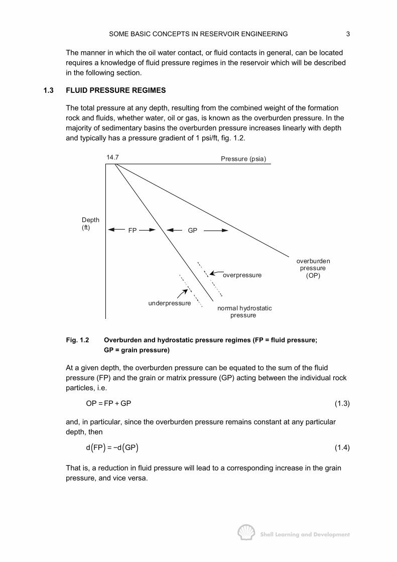
SOME BASIC CONCEPTS IN RESERVOIR ENGINEERING 3
The manner in which the oil water contact, or fluid contacts in general, can be locatedrequires a knowledge of fluid pressure regimes in the reservoir which will be describedin the following section.
1.3 FLUID PRESSURE REGIMES
The total pressure at any depth, resulting from the combined weight of the formationrock and fluids, whether water, oil or gas, is known as the overburden pressure. In themajority of sedimentary basins the overburden pressure increases linearly with depthand typically has a pressure gradient of 1 psi/ft, fig. 1.2.
Pressure (psia)
overburdenpressure
(OP)overpressure
14.7
FP GP
normal hydrostaticpressure
underpressure
Depth(ft)
Fig. 1.2 Overburden and hydrostatic pressure regimes (FP = fluid pressure;GP = grain pressure)
At a given depth, the overburden pressure can be equated to the sum of the fluidpressure (FP) and the grain or matrix pressure (GP) acting between the individual rockparticles, i.e.
OP FP GP= + (1.3)
and, in particular, since the overburden pressure remains constant at any particulardepth, then
( ) ( )d FP d GP= − (1.4)
That is, a reduction in fluid pressure will lead to a corresponding increase in the grainpressure, and vice versa.

SOME BASIC CONCEPTS IN RESERVOIR ENGINEERING 4
Fluid pressure regimes in hydrocarbon columns are dictated by the prevailing waterpressure in the vicinity of the reservoir. In a perfectly normal case the water pressure atany depth can be calculated as
wwater
dpp D 14.7 (psia)dD
� � × +� �� �
(1.5)
in which dp/dD, the water pressure gradient, is dependent on the chemical composition(salinity), and for pure water has the value of 0.4335 psi/ft.
Addition of the surface pressure of one atmosphere (14.7 psia) results in theexpression of the pressure in absolute rather than gauge units (psig), which aremeasured relative to atmospheric pressure. In many instances in reservoir engineeringthe main concern is with pressure differences, which are the same whether absolute orgauge pressures are employed, and are denoted simply as psi.
Equation (1.5) assumes that there is both continuity of water pressure to the surfaceand that the salinity does not vary with depth. The former assumption is valid, in themajority of cases, even though the water bearing sands are usually interspersed withimpermeable shales, since any break in the areal continuity of such apparent seals willlead to the establishment of hydrostatic pressure continuity to the surface. The latterassumption, however, is rather naive since the salinity can vary markedly with depth.Nevertheless, for the moment, a constant hydrostatic pressure gradient will beassumed, for illustrative purposes. As will be shown presently, what really matters tothe engineer is the definition of the hydrostatic pressure regime in the vicinity of thehydrocarbon bearing sands.
In contrast to this normal situation, abnormal hydrostatic pressure are encounteredwhich can be defined by the equation
wwater
dpp D 14.7 C(psia)dD
� �= × + +� �� �
(1.6)
where C is a constant which is positive if the water is overpressured and negative ifunderpressured.
For the water in any sand to be abnormally pressured, the sand must be effectivelysealed off from the surrounding strata so that hydrostatic pressure continuity to thesurface cannot be established. Bradley2 has listed various conditions which can causeabnormal fluid pressures in enclosed water bearing sands, which include:
− temperature change; an increase in temperature of one degree-Fahrenheit cancause an increase in pressure of 125 psi in a sealed fresh water system.
− geological changes such as the uplifting of the reservoir, or the equivalent,surface erosion, both of which result in the water pressure in the reservoir sandbeing too high for its depth of burial; the opposite effect occurs in a downthrownreservoir in which abnormally low fluid pressure can occur.

SOME BASIC CONCEPTS IN RESERVOIR ENGINEERING 5
− osmosis between waters having different salinity, the sealing shale acting as thesemi-permeable membrane in this ionic exchange; if the water within the seal ismore saline than the surrounding water the osmosis will cause an abnormallyhigh pressure and vice versa.
Some of these causes of abnormal pressuring are interactive, for instance, if areservoir block is uplifted the resulting overpressure is partially alleviated by a decreasein reservoir temperature.
The geological textbook of Chapman3 provides a comprehensive description of themechanics of overpressuring. Reservoir engineers, however, tend to be morepragmatic about the subject of abnormal pressures than geologists, the main questionsbeing; are the water bearing sands abnormally pressured and if so, what effect doesthis have on the extent of any hydrocarbon accumulations?
So far only hydrostatic pressures have been considered. Hydrocarbon pressureregimes are different in that the densities of oil and gas are less than that of water andconsequently, the pressure gradients are smaller, typical figures being
water
dp 0.45 psi / ftdD
� � =� �� �
oil
dp 0.35 psi / ftdD
� � =� �� �
gas
dp 0.08 psi / ftdD
� � =� �� �
Thus for the reservoir containing both oil and a free gascap, shown in fig. 1.3; using theabove gradients would give the pressure distribution shown on the left hand side of thediagram.
At the oil-water contact, at 5500 ft, the pressure in the oil and water must be equalotherwise a static interface would not exist. The pressure in the water can bedetermined using equ. (1.5), rounded off to the nearest psi, as
wp 0.45 D 15 (psia)= + (1.7)
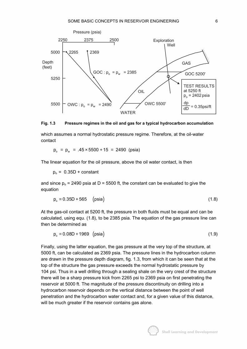
SOME BASIC CONCEPTS IN RESERVOIR ENGINEERING 6
2500 Exploration Well
OIL
GAS
GOC 5200'
WATER
OWC 5500'
TEST RESULTSat 5250 ftpo = 2402 psia
= 0.35psi/ftdpdD
2250
Depth(feet)
22655000 2369
5250
5500
2375
Pressure (psia)
OWC : po = pw = 2490
GOC : po = pw = 2385
Fig. 1.3 Pressure regimes in the oil and gas for a typical hydrocarbon accumulation
which assumes a normal hydrostatic pressure regime. Therefore, at the oil-watercontact
o wp p .45 5500 15 2490 (psia)= = × + =
The linear equation for the oil pressure, above the oil water contact, is then
po = 0.35D + constant
and since po = 2490 psia at D = 5500 ft, the constant can be evaluated to give theequation
( )op 0.35D 565 psia= + (1.8)
At the gas-oil contact at 5200 ft, the pressure in both fluids must be equal and can becalculated, using equ. (1.8), to be 2385 psia. The equation of the gas pressure line canthen be determined as
( )op 0.08D 1969 psia= + (1.9)
Finally, using the latter equation, the gas pressure at the very top of the structure, at5000 ft, can be calculated as 2369 psia. The pressure lines in the hydrocarbon columnare drawn in the pressure depth diagram, fig. 1.3, from which it can be seen that at thetop of the structure the gas pressure exceeds the normal hydrostatic pressure by104 psi. Thus in a well drilling through a sealing shale on the very crest of the structurethere will be a sharp pressure kick from 2265 psi to 2369 psia on first penetrating thereservoir at 5000 ft. The magnitude of the pressure discontinuity on drilling into ahydrocarbon reservoir depends on the vertical distance between the point of wellpenetration and the hydrocarbon water contact and, for a given value of this distance,will be much greater if the reservoir contains gas alone.
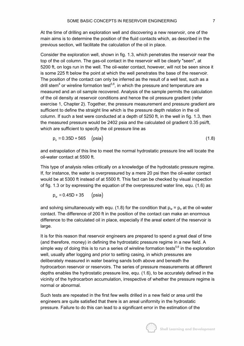
SOME BASIC CONCEPTS IN RESERVOIR ENGINEERING 7
At the time of drilling an exploration well and discovering a new reservoir, one of themain aims is to determine the position of the fluid contacts which, as described in theprevious section, will facilitate the calculation of the oil in place.
Consider the exploration well, shown in fig. 1.3, which penetrates the reservoir near thetop of the oil column. The gas-oil contact in the reservoir will be clearly "seen", at5200 ft, on logs run in the well. The oil-water contact, however, will not be seen since itis some 225 ft below the point at which the well penetrates the base of the reservoir.The position of the contact can only be inferred as the result of a well test, such as adrill stem4 or wireline formation test5,6, in which the pressure and temperature aremeasured and an oil sample recovered. Analysis of the sample permits the calculationof the oil density at reservoir conditions and hence the oil pressure gradient (referexercise 1, Chapter 2). Together, the pressure measurement and pressure gradient aresufficient to define the straight line which is the pressure depth relation in the oilcolumn. If such a test were conducted at a depth of 5250 ft, in the well in fig. 1.3, thenthe measured pressure would be 2402 psia and the calculated oil gradient 0.35 psi/ft,which are sufficient to specify the oil pressure line as
( )op 0.35D 565 psia= + (1.8)
and extrapolation of this line to meet the normal hydrostatic pressure line will locate theoil-water contact at 5500 ft.
This type of analysis relies critically on a knowledge of the hydrostatic pressure regime.If, for instance, the water is overpressured by a mere 20 psi then the oil-water contactwould be at 5300 ft instead of at 5500 ft. This fact can be checked by visual inspectionof fig. 1.3 or by expressing the equation of the overpressured water line, equ. (1.6) as
( )wp 0.45D 35 psia= +
and solving simultaneously with equ. (1.8) for the condition that pw = po at the oil-watercontact. The difference of 200 ft in the position of the contact can make an enormousdifference to the calculated oil in place, especially if the areal extent of the reservoir islarge.
It is for this reason that reservoir engineers are prepared to spend a great deal of time(and therefore, money) in defining the hydrostatic pressure regime in a new field. Asimple way of doing this is to run a series of wireline formation tests5,6 in the explorationwell, usually after logging and prior to setting casing, in which pressures aredeliberately measured in water bearing sands both above and beneath thehydrocarbon reservoir or reservoirs. The series of pressure measurements at differentdepths enables the hydrostatic pressure line, equ. (1.6), to be accurately defined in thevicinity of the hydrocarbon accumulation, irrespective of whether the pressure regime isnormal or abnormal.
Such tests are repeated in the first few wells drilled in a new field or area until theengineers are quite satisfied that there is an areal uniformity in the hydrostaticpressure. Failure to do this can lead to a significant error in the estimation of the
SOME BASIC CONCEPTS IN RESERVOIR ENGINEERING 8
hydrocarbons in place which in turn can result in the formulation of woefully inaccuratefield development plans.
Pressure (psia)
2250 2375 2500
5000
5500
Depth(feet)
GDT5150’
DPGWC5281’
OIL COLUMNFig 1.3
TEST RESULTSat 5100 ftpg = 2377 psiadpdD
g= .08 psi / ft
GAS
DPOWC5640’
Exploration well
Fig. 1.4 Illustrating the uncertainty in estimating the possible extent of an oil column,resulting from well testing in the gas cap
Figure 1.4 illustrates another type of uncertainty associated with the determination offluid contacts from pressure measurements. The reservoir is the same as depicted infig. 1.3 but in this case the exploration well has only penetrated the gascap. A well testis conducted at a depth of 5100 ft from which it is determined that the gas pressure is2377 psia and, from the analysis of a collected sample (refer exercise 1.1), that the gasgradient in the reservoir is 0.08 psi/ft. From these data the equation of the gas pressureline can be defined as
( )op 0.08D 1969 psia= + (1.9)
Having seen no oil in the well the engineer may suspect that he has penetrated a gasreservoir alone, and extrapolate equ. (1.9) to meet the normal hydrostatic pressure line
( )wp 0.45D 15 psia= + (1.7)
at a depth of 5281 ft, at which pw = pg. This level is marked in fig. 1.4 as the deepestpossible gas water contact (DPGWC), assuming there is no oil.
Alternatively, since the deepest point at which gas has been observed in the well is5150 ft (GDT − gas down to), there is no physical reason why an oil column should notextend from immediately beneath this point. The oil pressure at the top of such acolumn would be equal to the gas pressure, which can be calculated using equ. (1.9)as 2381 psia. Hence the equation of the oil pressure line, assuming the oil gradientused previously of 0.35 psi/ft, would be
( )op 0.35D 579 psia= +

SOME BASIC CONCEPTS IN RESERVOIR ENGINEERING 9
and solving this simultaneously with equ. (1.7), for the condition that po = pw, gives theoil-water contact at a depth of 5640 ft. This is marked on fig. 1.4 as the deepestpossible oil-water contact (DPOWC) and corresponds to the maximum possible oilcolumn. Therefore, in spite of the fact that the well has been carefully tested, thereremains high degree of uncertainty as to the extent of any oil column. It could indeedbe zero (DPGWC − 5281 ft) or, in the most optimistic case, could extend for 490 ft(DPOWC − 5640 ft), or, alternatively, assume any value in between these limits. Alsoshown in fig. 1.4 is the actual oil column from fig. 1.3.
Therefore, the question is always posed, on penetrating a reservoir containing onlygas; is there a significant oil column, or oil rim, down-dip which could be developed?The only sure way to find out is to drill another well further down-dip on the structure or,if mechanically feasible, plug back and deviate from the original hole. When planningthe drilling of an exploration well it is therefore, not always expedient to aim the well atthe highest point on the structure. Doing so will tend to maximise the chance of findinghydrocarbons but will oppose one of the primary aims in drilling exploration wells,which is to gain as much information about the reservoirs and their contents aspossible.
Having determined the fluid contacts in the reservoir, using the methods described inthis section, the engineer is then in a position to calculate the net bulk volume Vrequired to calculate the hydrocarbons in place. In fig. 1.1 (a), for instance, this can bedone by planimetering the contours above the OWC7,8.
Finally, with regard to the application of equ. (1.2), the correct figure for the STOIIP willonly be obtained if all the parameters in the equation are truly representative of theiraverage values throughout the reservoir. Since it is impossible to obtain such figures itis more common to represent each parameter in the STOIIP equation by a probabilitydistribution rather than a determinate value. For instance, there may be severaldifferent geological interpretations of the structure giving a spread in values of the netbulk volume V, which could be expressed as a probability distribution of the value ofthis parameter.
The STOIIP equation is then evaluated using some statistical calculation procedure,commensurate with the quality of the input data, and the results expressed in terms ofa probability distribution of the STOIIP. The advantage of this method is that while amean value of the STOIIP can be extracted from the final distribution, the results canalso be formulated in terms of the uncertainty attached to this figure, expressed, forinstance, as a standard deviation about the mean9,10. If the uncertainty is very large itmay be necessary to drill an additional well, or wells, to narrow the range beforeproceeding to develop the field.
1.4 OIL RECOVERY: RECOVERY FACTOR
Equation (1.2), for the STOIIP, can be converted into an equation for calculating theultimate oil recovery simply by multiplying by the recovery factor (RF), which is anumber between zero and unity representing the fraction of recoverable oil, thus
wc oiUltimate Recovery (UR) (V (1 S ) /B ) RFφ= − × (1.10)
SOME BASIC CONCEPTS IN RESERVOIR ENGINEERING 10
And, while it is easy to say, "simply by multiplying by the recovery factor", it is muchless easy to determine what the recovery factor should be for any given reservoir and,indeed, it is the determination of this figure which is the most important single task ofthe reservoir engineer.
For a start, one can clearly distinguish between two types of recovery factor. There isone which is governed by current economic circumstances and, ever increasingly, byenvironmental and ecological considerations, while the second can be classed as apurely technical recovery factor depending on the physics of the reservoir-fluid system.Regrettably, the former, although possibly the more interesting, is not a subject for thisbook.
The two main categories of hydrocarbon recovery are called primary andsupplementary. Primary recovery is the volume of hydrocarbons which can beproduced by virtue of utilising the natural energy available in the reservoir and itsadjacent aquifer. In contrast, supplementary recovery is the oil obtained by addingenergy to the reservoir-fluid system. The most common type of supplementaryrecovery is water flooding in which water is injected into the reservoir and displaces oiltowards the producing wells, thus increasing the natural energy of the system. Themechanics of supplementary recovery will be described later, in Chapter 4, sec. 9 andin Chapter 10; for the moment only primary recovery will be considered.
The entire mechanics of primary recovery relies on the expansion of fluids in thereservoir and can best be appreciated by considering the definition of isothermalcompressibility.
T
1 VcV p
∂=∂
— (1.11)
The isothermal compressibility is commonly applied in the majority of reservoirengineering calculations because it is considered a reasonable approximation that asfluids are produced, and so remove heat from the reservoir by convection, the cap andbase rock, which are assumed to act as heat sources of infinite extent, immediatelyreplace this heat by conduction so that the reservoir temperature remains constant.Therefore, compressibility, when referred to in this text, should always be interpretedas the isothermal compressibility.
The negative sign convention is required in equ. (1.11) because compressibility isdefined as a positive number, whereas the differential, ∂V/∂p, is negative, since fluidsexpand when their confining pressure is decreased. When using the compressibilitydefinition in isolation, to describe reservoir depletion, it is more illustrative to express itin the form
dV cV p= ∆ (1.12)
where dV is an expansion and ∆p a pressure drop, both of which are positive. This isthe very basic equation underlying all forms of primary recovery mechanism. In thereservoir, if ∆p is taken as the pressure drop from initial to some lower pressure,

SOME BASIC CONCEPTS IN RESERVOIR ENGINEERING 11
pi − p, then dV will be the corresponding fluid expansion, which manifests itself asproduction.
The skill in engineering a high primary recovery factor, utilising the natural reservoirenergy, is to ensure that the dV, which is the production, is the most commerciallyvaluable fluid in the reservoir, namely, the oil. The way in which this can be done isshown schematically in fig. 1.5.
aquifer gascapoil
Vw dVW
dV = oil productiontot
= dV + dV + dVo w g
dVg Vg
Vo
Fig. 1.5 Primary oil recovery resulting from oil, water and gas expansion
The diagram illustrates the fairly obvious fact that to produce an oil reservoir, wellsshould be drilled into the oil zone. If the reservoir is in contact with a gascap andaquifer, the oil production due to a uniform pressure drop, ∆p, in the entire system, willhave components due to the separate expansion of the oil gas and water, thus
dVTOT = Oil Production = dVo + dVw + dVg
in which the balance is expressed in fluid volumes at reservoir conditions. Applyingequ. (1.12), this may be expressed as
dVTOT = co Vo ∆p + cw Vw ∆p + cg Vg ∆p
Considering the following figures as typical for the compressibilities of the threecomponents at a pressure of 2000 psia:
co = 15 × 10−6/psi
cw = 3 × 10⁻⁶/psi
cg = 500 × 10−6/psi 1 ; refer sec.1.5p
� �≈� �
� �
it is evident that the contribution to dVTOT supplied by the oil and water expansion willonly be significant if both Vo and Vw, the initial volumes of oil and water, are large. Incontrast, because of its very high compressibility, even a relatively small volume ofgascap gas will contribute significantly to the oil production.
SOME BASIC CONCEPTS IN RESERVOIR ENGINEERING 12
Therefore, while it is obvious that one would not produce an aquifer, but rather, let thewater expand and displace the oil; so too, the gas in the gascap, although havingcommercial value, is frequently kept in the reservoir and allowed to play its verysignificant role in contributing to the primary recovery through its expansion. Themechanics of primary oil recovery will be considered in greater detail in Chapter 3.
1.5 VOLUMETRIC GAS RESERVOIR ENGINEERING
Volumetric gas reservoir engineering is introduced at this early stage in the bookbecause of the relative simplicity of the subject. lt will therefore be used to illustratehow a recovery factor can be determined and a time scale attached to the recovery.
The reason for the simplicity is because gas is one of the few substances whose state,as defined by pressure, volume and temperature (PVT), can be described by a simplerelation involving all three parameters. One other such substance is saturated steam,but for oil containing dissolved gas, for instance, no such relation exists and, as shownin Chapter 2, PVT parameters must be empirically derived which serve the purpose ofdefining the state of the mixture.
The equation of state for an ideal gas, that is, one in which the inter-molecularattractions and the volume occupied by the molecules are both negligible, is
pV nRT= (1.13)
in which, for the conventional field units used in the industry
p = pressure (psia); V = volume (cu.ft)
T = absolute temperature − degrees Rankine (°R=460+°F)
n = the number of lb. moles, where one lb. mole is the molecular weight of thegas expressed in pounds.
and R = the universal gas constant which, for the above units, has the value10.732 psia.cu.ft/lb. mole.°R.
This equation results from the combined efforts of Boyle, Charles, Avogadro and GayLussac, and is only applicable at pressures close to atmospheric, for which it wasexperimentally derived, and at which gases do behave as ideal.
Numerous attempts have been made in the past to account for the deviations of a realgas, from the ideal gas equation of state, under extreme conditions. One of the morecelebrated of these is the equation of van der Waals which, for one Ib.mole of a gas,can be expressed as
( )2a(p ) V b RTV
+ − = (1.14)
In using this equation it is argued that the pressure p, measured at the wall of a vesselcontaining a real gas, is lower than it would be if the gas were ideal. This is becausethe momentum of a gas molecule about to strike the wall is reduced by inter-molecularattractions; and hence the pressure, which is proportional to the rate of change of
SOME BASIC CONCEPTS IN RESERVOIR ENGINEERING 13
momentum, is reduced. To correct for this the term a/V2 must be added to the observedpressure, where a is a constant depending on the nature of the gas. Similarly thevolume V, measured assuming the molecules occupy negligible space, must bereduced for a real gas by the factor b which again is dependent on the nature of thegas.
The principal drawback in attempting to use equ. (1.14) to describe the behaviour ofreal gases encountered in reservoirs is that the maximum pressure for which theequation is applicable is still far below the normal range of reservoir pressures.
More recent and more successful equations of state have been derived, - the Beattie-Bridgeman and Benedict-Webb-Rubin equations, for instance (which have beenconveniently summarised in Chapter 3 of reference 18); but the equation mostcommonly used in practice by the industry is
pV ZnRT= (1.15)
in which the units are the same as listed for equ. (1.13) and Z, which is dimensionless,is called the Z−factor. By expressing the equation as
P V = nRTZ
� �� �� �
the Z−factor can be interpreted as a term by which the pressure must be corrected toaccount for the departure from the ideal gas equation.
The Z−factor is a function of both pressure and absolute temperature but, for reservoirengineering purposes, the main interest lies in the determination of Z, as a function ofpressure, at constant reservoir temperature. The Z(p) relationship obtained is thenappropriate for the description of isothermal reservoir depletion. Three ways ofdetermining this relationship are described below.
a) Experimental determination
A quantity of n moles of gas are charged to a cylindrical container, the volume of whichcan be altered by the movement of a piston. The container is maintained at thereservoir temperature, T, throughout the experiment. If Vo is the gas volume atatmospheric pressure, then applying the real gas law, equ. (1.15),
14.7 Vo = nRT
since Z=1 at atmospheric pressure. At any higher pressure p, for which thecorresponding volume of the gas is V, then
pV = ZnRT
and dividing these equations gives

SOME BASIC CONCEPTS IN RESERVOIR ENGINEERING 14
o
pVZ14.7V
=
By varying p and measuring V, the isothermal Z(p) function can be readily obtained.This is the most satisfactory method of determining the function but in the majority ofcases the time and expense involved are not warranted since reliable methods of directcalculation are available, as described below.
b) The Z-factor correlation of Standing and Katz
This correlation requires a knowledge of the composition of the gas or, at least, the gasgravity. Naturally occurring hydrocarbons are composed primarily of members of theparaffin series (CnH2n+2) with an admixture of non-hydrocarbon impurities such ascarbon dioxide, nitrogen and hydrogen sulphide. Natural gas differs from oil in that itpredominantly consists of the lighter members of the paraffin series, methane andethane, which usually comprise in excess of 90% of the volume. A typical gascomposition is listed in table 1.1.
In order to use the Standing-Katz correlation11 it is first necessary, from a knowledge ofthe gas composition, to determine the pseudo critical pressure and temperature of themixture as
pc i cii
p n p=� (1.16)
and
pc i cii
T nT=� (1.17)
where the summation is over all the components present in the gas. The parameters pci
and Tci are the critical pressure and temperature of the ith component, listed in table 1.1,while the ni are the volume fractions or, for a gas, the mole fractions of eachcomponent (Avogrado's law). The next step is to calculate the so-called pseudoreduced pressure and temperature
prpc
ppp
= (1.18)
and
prpc
TTT
= (1.19)
where p and T are the pressure and temperature at which it is required to determine Z.In the majority of reservoir engineering problems, which are isothermal, Tpr is constantand ppr variable.
With these two parameters the Standing-Katz correlation chart, fig. 1.6, which consistsof a set of isotherms giving Z as a function of the pseudo reduced pressure, can beused to determine the Z−factor.
SOME BASIC CONCEPTS IN RESERVOIR ENGINEERING 15
For instance, for the gas composition listed in table 1.1, and at a pressure of 2000 psiaand temperature of 180° F, the reader can verify that
ppc = 663.3 and Tpc = 374.1
giving
pr pr2000 640p 3.02 and T 1.71663.3 374.1
= = = =
from which, using fig.1.6, the Z−factor can be obtained as 0.865.
Component MolecularWeight
CriticalPressure
(psia)
ConstantsTemp.(oR)
Typical Composition(volume or mole
fraction, ni)
CH4 Methane 16.04 668 343 .8470
C2 H6 Ethane 30.07 708 550 .0586
C3 H8 Propane 44.10 616 666 .0220
i−C4 H10 Isobutane 58.12 529 735 .0035
n−C4 H10 Normal butane 58.12 551 765 .0058
i−C5 H12 Isopentane 72.15 490 829 .0027
n−C5 H12 Normal pentane 72.15 489 845 .0025
n−C6 H14 Normal hexane 86.18 437 913 .0028
n−C7 H14 Normal heptane 100.20 397 972 .0028
n-C8 H18 Normal octane 114.23 361 1024 .0015
n−C9 H20 Normal nonane 128.26 332 1070 .0018
n−C10 H22 Normal decane 142.29 304 1112 .0015
CO2 Carbon dioxide 44.01 1071 548 .0130
H2S Hydrogen sulphide 34.08 1306 672 .0000
N2 Nitrogen 28.01 493 227 .0345
TABLE 1.1
Physical constants of the common constituents of hydrocarbongases12, and a typical gas composition
Conventionally, the composition of natural gases is listed in terms of the individualcomponents as far as hexane, with the heptane and heavier components beinggrouped together as 7C+ (heptanes-plus). In the laboratory analysis the molecularweight and specific gravity of this group are measured, which permits the determinationof the pseudo critical pressure and temperature of the 7C+ from standard
SOME BASIC CONCEPTS IN RESERVOIR ENGINEERING 16
correlations8,13. This in turn facilitates the calculation of the Z−factor using the methoddescribed above.
In calculating the Z−factor it has been assumed that the non-hydrocarbon components,carbon dioxide, hydrogen sulphide and nitrogen, can be included in the summations,equs. (1.16) and (1.17), to obtain the pseudo critical pressure and temperature.
This approach is only valid if the volume fractions of the non-hydrocarbon componentsare small, say, less than 5% vol. For larger amounts, corrections to the abovecalculation procedures are to be found in the text book of Amyx, Bass and Whiting8. If,however, the volume fractions of the non-hydrocarbons are very large (the carbondioxide content of the Kapuni field, New Zealand, for instance, is 45% vol.) then it isbetter to determine the Z−factor experimentally as described in a), above.
SOME BASIC CONCEPTS IN RESERVOIR ENGINEERING 17
3.02.8
2.62.4
2.22.01.91.8
1.7
1.6
1.5
1.4
1.3
1.2
1.1
1.1
1.45
1.35
1.25
1.3
1.2
1.05
1.1
1.0
0.9
0.8
0.7
0.6
Z -fa
ctor
Pseudo reduced pressure
0.5
Pseudo reduced temperature
0.4
0.3
0.2
0.1
00 1 2 3 4 5 6 7 8
1.15
1.05
Fig. 1.6 The Z−−−−factor correlation chart of Standing and Katz11 (Reproduced by courtesyof the SPE of the AIME)
If the gas composition is not available, the Standing-Katz correlation can still be usedprovided the gas gravity, based on the scale air = 1, at atmospheric pressure and at60°F, is known (refer sec. 1.6). In this case fig. 1.7, is used to obtain the pseudo criticalpressure and temperature; then equs. (1.18) and (1.19) can be applied to calculate thepseudo reduced parameters required to obtain the Z−factor from fig. 1.6.

SOME BASIC CONCEPTS IN RESERVOIR ENGINEERING 18
MISCELLANEOUS GASES
CONDENSATE WELL FLUID
PSEU
DO
CR
ITIC
AL P
RES
SUR
E, p
sia
PSEU
DO
CR
ITIC
AL T
EMPE
RAT
UR
E, d
egre
es R
anki
ne
GAS GRAVITY (Air = 1)
700
650
600
550
500
450
400
350
3000.5 0.6 0.7 0.8 0.9 1.0 1.1 1.2
Fig. 1.7 Pseudo critical properties of miscellaneous natural gases and condensatewell fluids19
c) Direct calculation of Z-factors
The Standing-Katz correlation is very reliable and has been used with confidence bythe industry for the past thirty-five years. With the advent of computers, however, therearose the need to find some convenient technique for calculating Z−factors, for use ingas reservoir engineering programs, rather than feeding in the entire correlation chartfrom which Z−factors could be retrieved by table look-up. Takacs14 has compared eightdifferent methods for calculating Z−factors which have been developed over the years.These fall into two main categories: those which attempt to analytically curve-fit theStanding-Katz isotherms and those which compute Z−factors using an equation ofstate. Of the latter, the method of Hall-Yarborough15 is worthy of mention because it is
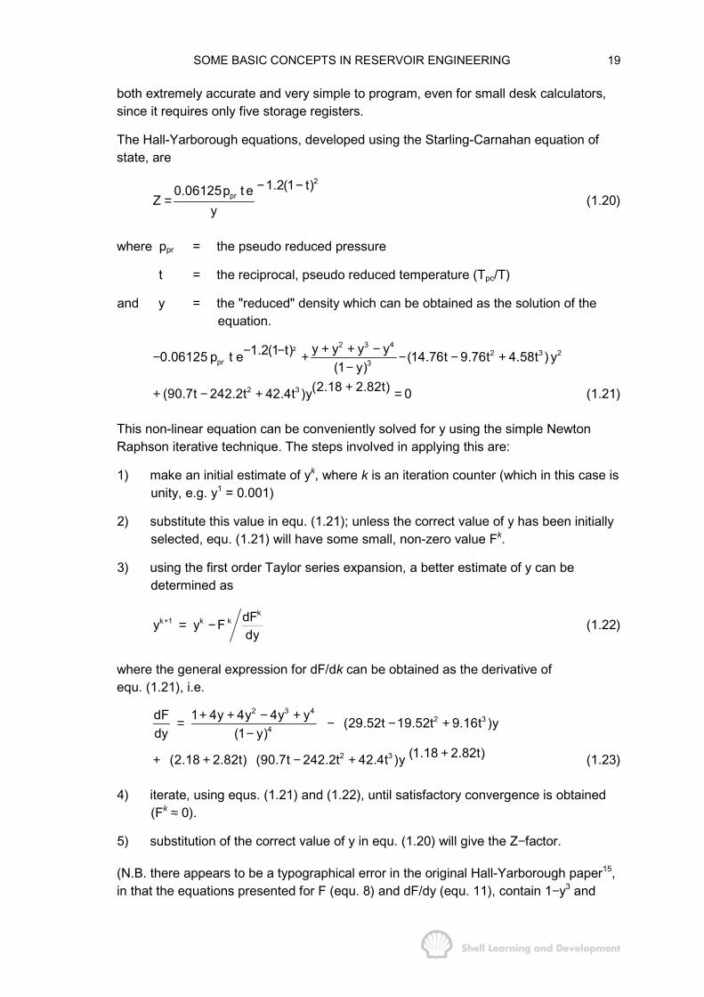
SOME BASIC CONCEPTS IN RESERVOIR ENGINEERING 19
both extremely accurate and very simple to program, even for small desk calculators,since it requires only five storage registers.
The Hall-Yarborough equations, developed using the Starling-Carnahan equation ofstate, are
2
pr1.2(1 t)0.06125p t e
Zy
− −= (1.20)
where ppr = the pseudo reduced pressure
t = the reciprocal, pseudo reduced temperature (Tpc/T)
and y = the "reduced" density which can be obtained as the solution of theequation.
2 2 3 42 3 2
pr 3y y y y1.2(1 t)0.06125 p t e (14.76t 9.76t 4.58t ) y
(1 y)+ + −− −− + − − +
−2 3 (2.18 2.82t)(90.7t 242.2t 42.4t )y 0++ − + = (1.21)
This non-linear equation can be conveniently solved for y using the simple NewtonRaphson iterative technique. The steps involved in applying this are:
1) make an initial estimate of yk, where k is an iteration counter (which in this case isunity, e.g. y1 = 0.001)
2) substitute this value in equ. (1.21); unless the correct value of y has been initiallyselected, equ. (1.21) will have some small, non-zero value Fk.
3) using the first order Taylor series expansion, a better estimate of y can bedetermined as
kk 1 k k dFy y F
dy+ = − (1.22)
where the general expression for dF/dk can be obtained as the derivative ofequ. (1.21), i.e.
2 3 42 3
4dF 1 4y 4y 4y y (29.52t 19.52t 9.16t )ydy (1 y)
+ + − += − − +−
2 3 (1.18 2.82t)(2.18 2.82t) (90.7t 242.2t 42.4t )y ++ + − + (1.23)
4) iterate, using equs. (1.21) and (1.22), until satisfactory convergence is obtained(Fk ≈ 0).
5) substitution of the correct value of y in equ. (1.20) will give the Z−factor.
(N.B. there appears to be a typographical error in the original Hall-Yarborough paper15,in that the equations presented for F (equ. 8) and dF/dy (equ. 11), contain 1−y3 and

SOME BASIC CONCEPTS IN RESERVOIR ENGINEERING 20
1−y4 in the denominators of the second and first terms, respectively, instead of (1−y)3
and (1−y)4 as in equs. (1.21) and (1.23) of this text.)
Takacs14 has determined that the average difference between the Standing-Katzcorrelation chart and the analytical Hall-Yarborough method is − 0.158% and theaverage absolute difference 0.518%. Figure 1.8 shows an isothermal Z−factor versuspressure relationship, obtained using the Hall-Yarborough method, for a gas withgravity 0.85 and at a reservoir temperature of 200°F. The plot coincides, within pencilthickness, with the similar relation obtained by the application of the method describedin b), above.
The plot shows that there is a significant deviation from the ideal gas behaviour whichis particularly noticeable in the intermediate pressure range at about 2500 psia. At thispressure, use of the ideal gas equation, (1.13), would produce an error of almost 25%in calculated gas volumes.
1.6 APPLICATION OF THE REAL GAS EQUATION OF STATE
The determination of the Z−factor as a function of pressure and temperature facilitatesthe use of the simple equation
pV ZnRT= (1.15)
to fully define the state of a real gas. This equation is a PVT relationship and inreservoir engineering, in general, the main use of such functions is to relate surface toreservoir volumes of hydrocarbons. For a real gas, in particular, this relation isexpressed by the gas expansion factor E, where

SOME BASIC CONCEPTS IN RESERVOIR ENGINEERING 21
Pressure (psia)
Z - Factor
00.75
0.85
0.95
1000 2000 3000 4000 5000
Fig. 1.8 Isothermal Z−−−−factor as a function of pressure (gas gravity = 0.85;temperature = 200° F)
scV volume of n moles of gas at standard conditionsEV volume of n moles of gas at reservoir conditions
= =
and applying equ. (1.15) at both standard and reservoir conditions this becomes
sc sc sc
sc
V T ZpEV p T Z
= = (1.24)
For the field units defined in connection with equ. (1.13), and for standard conditions ofpsc = 14.7 psia, Tsc = (460+60) = 520°R and Zsc = 1, equ. (1.24) can be reduced to
pE 35.37 (vol / vol)ZT
= (1.25)
At a pressure of 2000 psia and reservoir temperature of 180°F the gas whosecomposition is detailed in table 1.1 has a Z−factor of 0.865, as already determined insec. 1.5(b). Therefore, the corresponding gas expansion factor is
35.37 2000E 127.8 (vol / vol)0.865 640
×= =×
In particular, the gas initially in place (GIIP) in a reservoir can be calculated using anequation which is similar to equ. (1.2) for oil, that is

SOME BASIC CONCEPTS IN RESERVOIR ENGINEERING 22
wc iG V (1 S )Eφ= − (1.26)
in which Ei is evaluated at the initial pressure.
Other important parameters which can be conveniently expressed using the equationof state are, the real gas density, gravity and isothermal compressibility.
Since the mass of n moles of gas is nM, where M is the molecular weight, then thedensity is
nM nM MpV ZnRT / p ZRT
ρ = = = (1.27)
Comparing the density of a gas, at any pressure and temperature, to the density of airat the same conditions gives
gas gas
air air
(M / Z)(M/ Z)
ρρ
=
and, in particular, at standard conditions
gas gasg
air air
M MM 28.97
ργ
ρ= = = (1.28)
where γg is the gas gravity relative to air at standard conditions and is conventionallyexpressed as, for instance, γg = 0.8 (air = 1).
Therefore, if the gas gravity is known, M can be calculated using equ. (1.28) andsubstituted in equ. (1.27) to give the density at any pressure and temperature.Alternatively, if the gas composition is known M can be calculated as
i ii
M nM= � (1.29)
and again substituted in equ. (1.27). The molecular weights of the individual gascomponents, Mi, are listed in table 1.1. It is also useful to remember the density of air atstandard conditions (in whichever set of units the reader employs). For the stated unitsthis figure is
(ρair) sc = 0.0763 ib/cu.ft
which permits the gas density at standard conditions to be evaluated as
sc 0.0763 g (lbs / cu.ft)ρ γ= (1.30)
The final application of the equation of state is to derive an expression for theisothermal compressibility of a real gas. Solving equ. (1.15) for V gives
ZnRTVp
=

SOME BASIC CONCEPTS IN RESERVOIR ENGINEERING 23
the derivative of which, with respect to pressure, is
V ZnRT 1 1 Zp p p Z p
� �∂ ∂= − −� �∂ ∂� �
and substituting these two expressions in the isothermal compressibility definition,equ. (1.11), gives
g1 V 1 1 ZcV p p Z p
∂ ∂= − = −∂ ∂
(1.31)
In fig. 1.9, a plot of the gas compressibility defined by equ. (1.31) is compared to theapproximate expression.
g1cp
= (1.32)
for the 0.85 gravity gas whose isothermal Z−factor is plotted in fig. 1.8 at 200°F. As canbe seen, the approximation, equ. (1.32), is valid in the intermediate pressure rangebetween 2000−2750 psia where ∂Z/∂p is small but is less acceptable at very high orlow pressures.
EXERCISE 1.1 GAS PRESSURE GRADIENT IN THE RESERVOIR
1) Calculate the density of the gas, at standard conditions, whose composition islisted in table 1.1.
2) what is the gas pressure gradient in the reservoir at 2000 psia and 180° F(Z = 0.865).
EXERCISE 1.1 SOLUTION
1) The molecular weight of the gas can be calculated as
i ii
M nM 19.91= =�
and therefore, using equ. (1.28) the gravity is
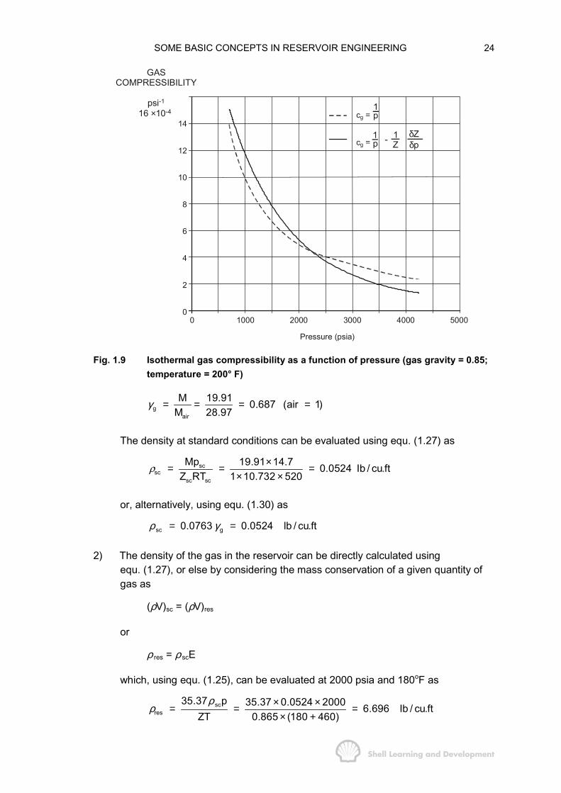
SOME BASIC CONCEPTS IN RESERVOIR ENGINEERING 24
Pressure (psia)
GASCOMPRESSIBILITY
psi-1 16 ×10-4
00
2
4
6
8
10
12
14
1000 2000 3000 4000 5000
cg =1p
1p
1Z- δZ
δp cg =
Fig. 1.9 Isothermal gas compressibility as a function of pressure (gas gravity = 0.85;temperature = 200° F)
gair
M 19.91 0.687 (air 1)M 28.97
γ = = = =
The density at standard conditions can be evaluated using equ. (1.27) as
scsc
sc sc
Mp 19.91 14.7 0.0524 Ib / cu.ftZ RT 1 10.732 520
×= = =× ×
�
or, alternatively, using equ. (1.30) as
sc g0.0763 0.0524 lb / cu.ftρ γ= =
2) The density of the gas in the reservoir can be directly calculated usingequ. (1.27), or else by considering the mass conservation of a given quantity ofgas as
(ρV)sc = (ρV)res
or
ρ res = ρ scE
which, using equ. (1.25), can be evaluated at 2000 psia and 180oF as
scres
35.37 p 35.37 0.0524 2000 6.696 Ib / cu.ftZT 0.865 (180 460)
ρρ × ×= = =
× +
SOME BASIC CONCEPTS IN RESERVOIR ENGINEERING 25
To convert this number to a pressure gradient in psi/ft requires the followingmanipulation.
2
2 2gas
dp Ib 1 ft 6.6966.696 0.0465 psi / ft.dD ft 144ft inch
� �� � = × × = =� �� �� � � �
1.7 GAS MATERIAL BALANCE: RECOVERY FACTOR
The material balance equation, for any hydrocarbon system, is simply a volumebalance which equates the total production to the difference between the initial volumeof hydrocarbons in the reservoir and the current volume. In gas reservoir engineeringthe equation is very simple and will now be considered for the separate cases in whichthere is no water influx into the reservoir and also when there is a significant degree ofinflux.
a) Volumetric depletion reservoirs
The term volumetric depletion, or simply depletion, applied to the performance of areservoir means that as the pressure declines, due to production, there is aninsignificant amount of water influx into the reservoir from the adjoining aquifer. This, inturn, implies that the aquifer must be small (refer sec. 1.4). Thus the reservoir volumeoccupied by hydrocarbons (HCPV) will not decrease during depletion. An expressionfor the hydrocarbon pore volume can be obtained from equ. (1.26) as
HCPV = Vφ (1−Swc) = G/Ei
where G is the initial gas in place expressed at standard conditions. The materialbalance, also expressed at standard conditions, for a given volume of production Gp,and consequent drop in the average reservoir pressure ∆p = pi−p is then,
p
pi
Production GIIP Unproduced Gas(sc) (sc) (sc)
G G (HCPV)EGG G EE
= −
= −
= −
(1.33)
which can be expressed as
p
i
G E1G E
= − (1.34)
or, using equ. (1.25), as
pi
i
Gpp 1Z Z G
� �= −� �
� �(1.35)
SOME BASIC CONCEPTS IN RESERVOIR ENGINEERING 26
The ratio Gp/G is the fractional gas recovery at any stage during depletion and, if thegas expansion factor E, in equ. (1.34), is evaluated at the proposed abandonmentpressure then the corresponding value of Gp/G is the gas recovery factor.
Before describing how the material balance equation is used in practice, it is worthwhilereconsidering the balance expressed by equ. (1.33) more thoroughly. Implicit in theequation is the assumption that because the water influx is negligible then thehydrocarbon pore volume remains constant during depletion. This, however, neglectstwo physical phenomena which are related to the pressure decline. Firstly, the connatewater in the reservoir will expand and secondly, as the gas (fluid) pressure declines,the grain pressure increases in accordance with equ. (1.4).
As a result of the latter, the rock particles will pack closer together and there will be areduction in the pore volume. These two effects can be combined to give the totalchange in the hydrocarbon pore volume as
d(HCPV) = − dVw +dVf (1.36)
where Vw and Vf represent the initial connate water volume and pore volume (PV),respectively. The negative sign is necessary since an expansion of the connate waterleads to a reduction in the HCPV. These volume changes can be expressed, usingequ. (1.11), in terms of the water and pore compressibilities, where the latter is definedas
ff
f
V1cV (GP)
∂= −∂
(1.4)
where GP is the grain pressure which is related to the fluid pressure by
d(FP) = − d(GP)
therefore
f ff
ff
V V1 1cV (FP) V p
∂ ∂= − =∂ ∂
(1.37)
where p is the fluid pressure. Equation (1.36) can now be expressed as
d(HCPV) = cw Vw dp + cf Vf dp
or, as a reduction in hydrocarbon pore volume as
d(HCPV) = − (cw Vw + cf Vf ) ∆p (1.38)
where ∆p = pi − p, the drop in fluid (gas) pressure. Finally, expressing the pore andconnate water volumes as
fwc i wc
HCPV GV PV(1 S ) E (1 S )
= = =− −
and

SOME BASIC CONCEPTS IN RESERVOIR ENGINEERING 27
wcw wc
i wc
GSV PV SE (1 S )
= × =−
the reduction in hydrocarbon pore volume, equ. (1.38), can be included in equ. (1.33),to give
w wc fp
wc i
(c S c ) pG E1 1G 1 S E
+ ∆� �= − −� �−� �
(1.39)
as the modified material balance. Inserting the typical values of cw = 3 × 10⁻⁶/psi,cf = 10 × 10−6/psi and Swc = 0.2 in this equation, and considering a large pressure dropof ∆p = 1000 psi; the term in parenthesis becomes
6 3(3 .2 10)1 10 10 1 0.0130.8
−× +− × × = −
That is, the inclusion of the term accounting for the reduction in the hydrocarbon porevolume, due to the connate water expansion and pore volume reduction, only alters thematerial balance by 1.3% and is therefore frequently neglected. The reason for itsomission is because the water and pore compressibilities are usually, although notalways, insignificant in comparison to the gas compressibility, the latter being defined insec. 1.6 as approximately the reciprocal of the pressure. As described in Chapter 3,sec. 8, however, pore compressibility can sometimes be very large in shallowunconsolidated reservoirs and values in excess of 100 × 10−6/ psi have beenmeasured, for instance, in the Bolivar Coast fields in Venezuela. In such reservoirs itwould be inadmissible to omit the pore compressibility from the gas material balance.In a reservoir which contains only liquid oil, with no free gas, allowance for the connatewater and pore compressibility effects must be included in the material balance sincethese compressibilities have the same order of magnitude as the liquid oil itself (referChapter 3, sec. 5).
In the majority of cases the material balance for a depletion type gas reservoir canadequately be described using equ. (1.35). This equation indicates that there is a linearrelationship between p/Z and the fractional recovery Gp/G, or the cumulative productionGp, as shown in fig. 1.10(a) and (b), respectively. These diagrams illustrate one of thebasic techniques in reservoir engineering which is, to try to reduce any equation, nomatter how complex, to the equation of a straight line; for the simple reason that linearfunctions can be readily extrapolated, whereas non-linear functions, in general, cannot.Thus a plot of p versus Gp/G or Gp, would have less utility than the representationsshown in fig. 1.10, since both would be non-linear.
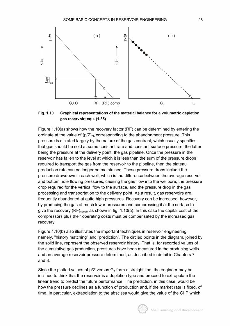
SOME BASIC CONCEPTS IN RESERVOIR ENGINEERING 28
pi
Zi
G / Gp RF Gp G
( a )
(RF) comp
pZ
Zpi
i
( b )
pZ
pZ ab
Fig. 1.10 Graphical representations of the material balance for a volumetric depletiongas reservoir; equ. (1.35)
Figure 1.10(a) shows how the recovery factor (RF) can be determined by entering theordinate at the value of (p/Z)ab corresponding to the abandonment pressure. Thispressure is dictated largely by the nature of the gas contract, which usually specifiesthat gas should be sold at some constant rate and constant surface pressure, the latterbeing the pressure at the delivery point, the gas pipeline. Once the pressure in thereservoir has fallen to the level at which it is less than the sum of the pressure dropsrequired to transport the gas from the reservoir to the pipeline, then the plateauproduction rate can no longer be maintained. These pressure drops include thepressure drawdown in each well, which is the difference between the average reservoirand bottom hole flowing pressures, causing the gas flow into the wellbore; the pressuredrop required for the vertical flow to the surface, and the pressure drop in the gasprocessing and transportation to the delivery point. As a result, gas reservoirs arefrequently abandoned at quite high pressures. Recovery can be increased, however,by producing the gas at much lower pressures and compressing it at the surface togive the recovery (RF)comp, as shown in fig. 1.10(a). In this case the capital cost of thecompressors plus their operating costs must be compensated by the increased gasrecovery.
Figure 1.10(b) also illustrates the important techniques in reservoir engineering,namely, "history matching" and "prediction". The circled points in the diagram, joined bythe solid line, represent the observed reservoir history. That is, for recorded values ofthe cumulative gas production, pressures have been measured in the producing wellsand an average reservoir pressure determined, as described in detail in Chapters 7and 8.
Since the plotted values of p/Z versus Gp form a straight line, the engineer may beinclined to think that the reservoir is a depletion type and proceed to extrapolate thelinear trend to predict the future performance. The prediction, in this case, would behow the pressure declines as a function of production and, if the market rate is fixed, oftime. In particular, extrapolation to the abscissa would give the value of the GIIP which

SOME BASIC CONCEPTS IN RESERVOIR ENGINEERING 29
can be checked against the volumetric estimate obtained as described in secs. 1.2 and1.3. This technique of matching the observed production pressure history by building asuitable mathematical model, albeit in this case a very simple one, equ. (1.35), andusing the model to predict future performance is one which is fundamental to thesubject of Reservoir Engineering.
b) Water drive reservoirs
If the reduction in reservoir pressure leads to an expansion of the adjacent aquiferwater, and consequent influx into the reservoir, the material balance equation mustthen be modified as
p ei
Production GIIP Unproduced Gas(sc) (sc) (sc)
GG G W EE
= −
� �= − −� �
� �
(1.40)
where, in this case, the hydrocarbon pore volume at the lower pressure is reduced bythe amount We, which is the cumulative amount of water influx resulting from thepressure drop. The equation assumes that there is no difference between surface andreservoir volumes of water and again neglects the effects of connate water expansionand pore volume reduction.
If some of the water influx has been produced it can be accounted for by subtractingthis volume, Wp, from the influx, We, on the right hand side of the equation. With someslight algebraic manipulation equ. (1.40) can be expressed as
e ipi
i
W Epp G1 1Z Z G G
� �� �= − −� �� �� � � �
(1.41)
where We Ei /G represents the fraction of the initial hydrocarbon pore volume floodedby water and is, therefore, always less than unity. When compared to the depletionmaterial balance, equ. (1.35), it can be seen that the effect of the water influx is tomaintain the reservoir pressure at a higher level for a given cumulative gas production.In addition, equ. (1.41) is non-linear, unlike equ. (1.35), which complicates both historymatching and prediction. Typical plots of this equation, for different aquifer strengths,are shown in fig. 1.11.
During the history matching phase, a separate part of the mathematical model must bedesigned to calculate the cumulative water influx corresponding to a given totalpressure drop in the reservoir; this part of the history match being described as "aquiferfitting". For an aquifer whose dimensions are of the same order of magnitude as thereservoir itself the following simple model can be used

SOME BASIC CONCEPTS IN RESERVOIR ENGINEERING 30
depletion lineC
B
A
pZ
GpG
pZ ab
Fig. 1.11 Graphical representation of the material balance equation for a water drivegas reservoir, for various aquifer strengths; equ. (1.41)
eW cW p= ∆
where c = the total aquifer compressibility (cw + cf)
W = the total volume of water, and depends primarily on the geometry ofthe aquifer
and p∆ = the pressure drop at the original reservoir-aquifer boundary.
This model assumes that, because the aquifer is relatively small, a pressure drop in thereservoir is instantaneously transmitted throughout the entire reservoir-aquifer system.The material balance in such a case would be as shown by plot A in fig. 1.11, which isnot significantly different from the depletion line.
To provide the pressure response shown by lines B and C, the aquifer volume must beconsiderably larger than that of the reservoir and it is then inadmissible to assumeinstantaneous transmission of pressure throughout the system. There will now be atime lag between a pressure perturbation in the reservoir and the full aquifer response.To build an aquifer model, including this time dependence, is quite complex and thesubject will be deferred until Chapter 9 where the use of such a model for both historymatching and prediction will be described in detail.
One of the unfortunate aspects in the delay in aquifer response is that, initially, all thematerial balance plots in fig. 1.11 appear to be linear and, if there is insufficientproduction and pressure history to show the deviation from linearity, one may betempted to extrapolate the early trends, assuming a depletion type reservoir, whichwould result in the determination of too large a value of the GIIP. In such a case, alarge difference between this and the volumetric estimate of the GIIP can be diagnosticin deciding whether there is an aquifer or not. It also follows that attempting to build a
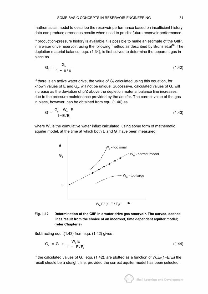
SOME BASIC CONCEPTS IN RESERVOIR ENGINEERING 31
mathematical model to describe the reservoir performance based on insufficient historydata can produce erroneous results when used to predict future reservoir performance.
If production-pressure history is available it is possible to make an estimate of the GIIP,in a water drive reservoir, using the following method as described by Bruns et.al16. Thedepletion material balance, equ. (1.34), is first solved to determine the apparent gas inplace as
pa
i
GG
1 E /E=
−(1.42)
If there is an active water drive, the value of Ga calculated using this equation, forknown values of E and Gp, will not be unique. Successive, calculated values of Ga willincrease as the deviation of p/Z above the depletion material balance line increases,due to the pressure maintenance provided by the aquifer. The correct value of the gasin place, however, can be obtained from equ. (1.40) as
p e
i
G W EG
1 E /E=
−—
(1.43)
where We is the cumulative water influx calculated, using some form of mathematicaquifer model, at the time at which both E and Gp have been measured.
Ga
We - too small
We - correct model
We - too large
G
We E/ (1−E / Ei)
Fig. 1.12 Determination of the GIIP in a water drive gas reservoir. The curved, dashedlines result from the choice of an incorrect, time dependent aquifer model;(refer Chapter 9)
Subtracting equ. (1.43) from equ. (1.42) gives
ea
i
W EG G1 E /E
= +−
(1.44)
If the calculated values of Ga, equ. (1.42), are plotted as a function of WeE/(1−E/Ei) theresult should be a straight line, provided the correct aquifer model has been selected,

SOME BASIC CONCEPTS IN RESERVOIR ENGINEERING 32
as shown in fig. 1.12, and the proper value of G can be determined by linearextrapolation to the ordinate. Selecting the correct aquifer model (aquifer fitting) is atrial and error business which continues until a straight line is obtained.
One other interesting feature shown in fig. 1.11 is that the maximum possible gasrecovery, shown by the circled points, depends on the degree of pressure maintenanceafforded by the aquifer, being smaller for the more responsive aquifers. The reason forthis has already been mentioned in sec. 1.2; that in the immiscible displacement of onefluid by another not all of the displaced fluid can be removed from each pore space.Thus as the water advances through the reservoir a residual gas saturation is trappedbehind the front. This gas saturation, Sgr, is rather high being of the order of 30−50% ofthe pore volume7,17, and is largely independent of the pressure at which the gas istrapped. This being the case, then applying the equation of state, equ. (1.15), to thegas trapped per cu.ft of pore volume behind the flood front, gives
grp S nRTZ
=
and, since Sgr is independent of pressure, then for isothermal depletion
pnZ
∝
which indicates that a greater quantity of gas is trapped at high pressure than at low.
The ultimate gas recovery depends both on the nature of the aquifer and theabandonment pressure. For the value of (p/Z)ab shown in fig. 1.11, the aquifer givingthe pressure response corresponding to line B is the most favourable. While choice ofthe abandonment pressure is under the control of the engineer, the choice of theaquifer, unfortunately, is not. It is, therefore, extremely important to accurately measureboth pressures and gas production to enable a reliable aquifer model to be built which,in turn, can be used for performance predictions.
One of the more adventurous aspects of gas reservoir engineering is that gas salescontracts, specifying the market rate and pipeline pressure, are usually agreedbetween operator and purchaser very early in the life of the field, when the amount ofhistory data is minimal. The operator is then forced to make important decisions onhow long he will be able to meet the market demand, based on the rather scant data.Sensitivity studies are usually conducted at this stage, using the simple materialbalance equations presented in this chapter, and varying the principal parameters, i.e.
− the GIIP
− the aquifer model, based on the possible geometrical configurations of the aquifer
− abandonment pressure; whether to apply surface compression or not
− the number of producing wells and their mechanical design.

SOME BASIC CONCEPTS IN RESERVOIR ENGINEERING 33
(the latter point has not been discussed so far, since it requires the development of wellinflow equations, which will be described in Chapter 8). The results of such a study cangive initial guidance on the best way to develop the gas reserve.
EXERCISE 1.2 GAS MATERIAL BALANCE
The following data are available for a newly discovered gas reservoir:
GWC = 9700 ft
Centroid depth = 9537 ft
Net bulk volume (V) = 1.776 × 10¹⁰ cu.ft
φ = 0.19
Swc = 0 20
γg = 0.85
Although a gas sample was collected during a brief production test the reservoirpressure was not recorded because of tool failure. It is known, however, that the waterpressure regime in the locality is
pw = 0.441D + 31 psia
and that the temperature gradient is 1.258°F/100 ft, with ambient surface temperature80° F.
1) Calculate the volume of the GIIP.
2) It is intended to enter a gas sales contract in which the following points havebeen stipulated by the purchaser.
a) during the first two years, a production rate build-up from zero−100 MMscf/d (million) must be achieved while developing the field
b) the plateau rate must be continued for 15 years at a sales point deliverypressure which corresponds to a minimum reservoir pressure of 1200 psia.Can this latter requirement be fulfilled? (Assume that the aquifer is small sothat the depletion material balance equation can be used).
3) Once the market requirement can no longer be satisfied the field rate will declineexponentially by 20% per annum until it is reduced to 20 MMscf/d. (This gas willeither be used as fuel in the company's operations or compressed to supply partof any current market requirement).
What will be the total recovery factor for the reservoir and what is the length of theentire project life?
EXERCISE 1.2 SOLUTION
a) In order to determine the GIIP it is first necessary to calculate the initial gaspressure at the centroid depth of the reservoir. That is, the depth at which there is
SOME BASIC CONCEPTS IN RESERVOIR ENGINEERING 34
as much gas above as there is beneath, the pressures for use in the materialbalance equation will always be evaluated at this depth.
To do this the water pressure at the gas−water contact must first be calculated as
pw = 0.441 × 9700 + 31 = 4309 psia = GWCgp
and the temperature as
o9700T (1.258 ) 80 460 662 R100
= × + + =
for this 0.85 gravity gas the isothermal Z−factor plot at 200°F (660°R), fig. 1.8,can be used to determine the Z−factor at the GWC, with negligible error. Thus
ZGWC = 0.888
and EGWC = 35.37 p 35.37 4309 259.3ZT 0.888 662
×= =×
The pressure gradient in the gas, at the GWC, can now be calculated, asdescribed in exercise 1.1, as
scEdp 0.0763 0.85 259.3 0.117 psi / ftdD 144 144
ρ × ×= = =
The gas pressure at the centroid is therefore
GWCGWC
gdpp p DdD
� �= − × ∆� �� �
(1.45)
p = 4309 − 0.117 × (9700 − 9537) = 4290 psia
and the absolute temperature at the centroid is
o9537T (1.258 ) 80 460 660 R100
= × + + =
One could improve on this estimate by re−evaluating the gas gradient at thecentroid, for p = 4290 psia and T = 660°R, and averaging this value with theoriginal value at the GWC to obtain a more reliable gas gradient to use in'equ. (1.45). Gas gradients are generally so small, however, that this correction isseldom necessary. The reader can verify that, in the present case, the correctionwould only alter the centroid pressure by less than half of one psi.
For the centroid pressure and temperature of 4290 psia and 660°R, the GIIP canbe estimated as
GIIP = G = Vφ (1−Swc) Ei (1.26)
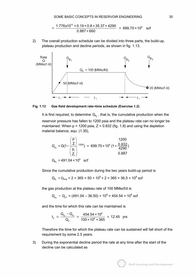
SOME BASIC CONCEPTS IN RESERVOIR ENGINEERING 35
1091.776x10 0.19 0.8 35.37 4290 699.70 10 scf
0.887 660× × × ×= = ×
×
2) The overall production schedule can be divided into three parts, the build-up,plateau production and decline periods, as shown in fig. 1.13.
t 1 t 2
Qo = 100 (MMscf/d)
50 (MMscf /d)
RateQ
(MMscf /d)
t 3
20 (MMscf /d)
Gp1Gp2
Gp3
Fig. 1.13 Gas field development rate−−−−time schedule (Exercise 1.2)
It is first required, to determine 2PG , that is, the cumulative production when the
reservoir pressure has fallen to 1200 psia and the plateau rate can no longer bemaintained. When p = 1200 psia, Z = 0.832 (fig. 1.8) and using the depletionmaterial balance, equ. (1.35),
2
2
9p
i
i
9P
1200
p 1200Z 0.832G G(1 ) 699.70 10 (1 )4290p
0.887Z
G 491.04 10 scf
� �� �� �= − = × =� �� �� �
= ×
Since the cumulative production during the two years build-up period is
1PG = Qavg × 2 × 365 = 50 × 106 × 2 × 365 = 36.5 × 10⁹ scf
the gas production at the plateau rate of 100 MMscf/d is
2pG − p1G = (491.04 – 36.50) × 109 = 454.54 × 10⁹ scf
and the time for which this rate can be maintained is
2 19
p p2 6
o
G G 454.54 10t 12.45 yrsQ 100 10 365− ×= = =
× ×
Therefore the time for which the plateau rate can be sustained will fall short of therequirement by some 2.5 years.
3) During the exponential decline period the rate at any time after the start of thedecline can be calculated as
SOME BASIC CONCEPTS IN RESERVOIR ENGINEERING 36
oQ Q e= −bt
where Qo is the rate at t = 0, i.e. 100 MMscf/d, and b is the exponential declinefactor of 0.2 p.a. Therefore, the time required for the rate to fall to 20 MMscf/d willbe
oQ1 1 100t ln ln 8.05 yrsb Q 0.2 20
= = =
If gp is the cumulative gas production at time t, measured from the start of thedecline, then
t t
p oo o
btg Qdt Q e dt−= =� �
i.e.
op
Q btg (1 e )b
−= −
and when t = 8.05 yrs.6
9(8.05)p
100 10 365 0.2 8.05g (1 e ) 146.02 10 scf0.2
× × − ×= − = ×
Therefore, the total cumulative recovery at abandonment will be
3 2 (8.05)9 9
p p pG G g (491.04 146.02) 10 637.06 10 scf= + = + × = ×
and the recovery factor
39
9pG 637.06 10RF 0.91 or 91% GIIP
G 699.70 10×= = =×
which will be recovered after a total period of
t1 + t2 + t3 = 2 + 12.45 + 8.05 = 22.5 years.
This simple exercise covers the spectrum of reservoir engineering activity,namely, estimating the hydrocarbons in place, calculating a recovery factor andattaching a time scale to the recovery. The latter is imposed by the overall marketrate required of the field, i.e.
cumulative productiontimefield rate
=
Later in the book, in Chapters 4, 6 and 8, the method of calculating individual wellrates is described, which means that the time scale can be fixed by the moreusual type of expression.
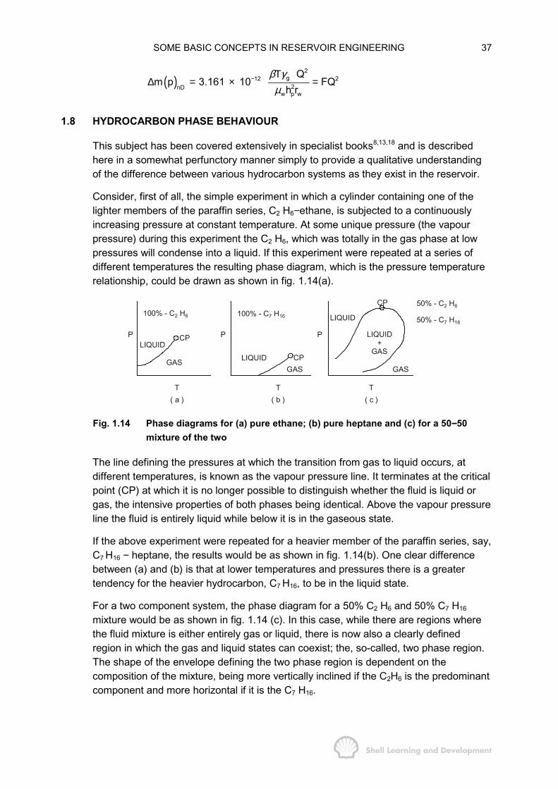
SOME BASIC CONCEPTS IN RESERVOIR ENGINEERING 37
( )2
g12 22nD
w p w
Qm p 3.161 10 FQ
h rβ γµ
− Τ∆ = × =
1.8 HYDROCARBON PHASE BEHAVIOUR
This subject has been covered extensively in specialist books8,13,18 and is describedhere in a somewhat perfunctory manner simply to provide a qualitative understandingof the difference between various hydrocarbon systems as they exist in the reservoir.
Consider, first of all, the simple experiment in which a cylinder containing one of thelighter members of the paraffin series, C2 H6−ethane, is subjected to a continuouslyincreasing pressure at constant temperature. At some unique pressure (the vapourpressure) during this experiment the C2 H6, which was totally in the gas phase at lowpressures will condense into a liquid. If this experiment were repeated at a series ofdifferent temperatures the resulting phase diagram, which is the pressure temperaturerelationship, could be drawn as shown in fig. 1.14(a).
100% - C2 H6 100% - C7 H16
50% - C2 H6
50% - C7 H16
P P PLIQUID
LIQUID
LIQUID+
GAS
LIQUID
CP
CPGASGAS GAS
T( a )
T( b )
T( c )
CP
Fig. 1.14 Phase diagrams for (a) pure ethane; (b) pure heptane and (c) for a 50−−−−50mixture of the two
The line defining the pressures at which the transition from gas to liquid occurs, atdifferent temperatures, is known as the vapour pressure line. It terminates at the criticalpoint (CP) at which it is no longer possible to distinguish whether the fluid is liquid orgas, the intensive properties of both phases being identical. Above the vapour pressureline the fluid is entirely liquid while below it is in the gaseous state.
If the above experiment were repeated for a heavier member of the paraffin series, say,C7 H16 − heptane, the results would be as shown in fig. 1.14(b). One clear differencebetween (a) and (b) is that at lower temperatures and pressures there is a greatertendency for the heavier hydrocarbon, C7 H16, to be in the liquid state.
For a two component system, the phase diagram for a 50% C2 H6 and 50% C7 H16
mixture would be as shown in fig. 1.14 (c). In this case, while there are regions wherethe fluid mixture is either entirely gas or liquid, there is now also a clearly definedregion in which the gas and liquid states can coexist; the, so-called, two phase region.The shape of the envelope defining the two phase region is dependent on thecomposition of the mixture, being more vertically inclined if the C2H6 is the predominantcomponent and more horizontal if it is the C7 H16.
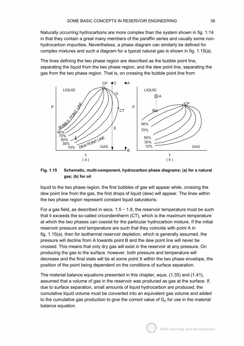
SOME BASIC CONCEPTS IN RESERVOIR ENGINEERING 38
Naturally occurring hydrocarbons are more complex than the system shown in fig. 1.14in that they contain a great many members of the paraffin series and usually some non-hydrocarbon impurities. Nevertheless, a phase diagram can similarly be defined forcomplex mixtures and such a diagram for a typical natural gas is shown in fig. 1.15(a).
The lines defining the two phase region are described as the bubble point line,separating the liquid from the two phase region, and the dew point line, separating thegas from the two phase region. That is, on crossing the bubble point line from
BUBBLE PO
INT
LINE P
x90%
90%
70%70%
50% 50%30% 30%
10% 10%
CP
B
A
CT
C
LIQUIDD
E
A
BT
( a )
P
LIQUID
T( b )
GAS GASDEW POINT LINE
CP
Fig. 1.15 Schematic, multi-component, hydrocarbon phase diagrams; (a) for a naturalgas; (b) for oil
liquid to the two phase region, the first bubbles of gas will appear while, crossing thedew point line from the gas, the first drops of liquid (dew) will appear. The lines withinthe two phase region represent constant liquid saturations.
For a gas field, as described in secs. 1.5 − 1.8, the reservoir temperature must be suchthat it exceeds the so-called cricondentherm (CT), which is the maximum temperatureat which the two phases can coexist for the particular hydrocarbon mixture. If the initialreservoir pressure and temperature are such that they coincide with point A infig. 1.15(a), then for isothermal reservoir depletion, which is generally assumed, thepressure will decline from A towards point B and the dew point line will never becrossed. This means that only dry gas will exist in the reservoir at any pressure. Onproducing the gas to the surface, however, both pressure and temperature willdecrease and the final state will be at some point X within the two phase envelope, theposition of the point being dependent on the conditions of surface separation.
The material balance equations presented in this chapter, equs. (1.35) and (1.41),assumed that a volume of gas in the reservoir was produced as gas at the surface. If,due to surface separation, small amounts of liquid hydrocarbon are produced, thecumulative liquid volume must be converted into an equivalent gas volume and addedto the cumulative gas production to give the correct value of Gp for use in the materialbalance equation.
SOME BASIC CONCEPTS IN RESERVOIR ENGINEERING 39
Thus if n pound moles of liquid have been produced, of molecular weight M, then thetotal mass of liquid is
nM = γoρ w × (liquid volume)
where γo is the oil gravity (water = 1), and ρw is the density of water (62.43 Ib/cu.ft).Since liquid hydrocarbon volumes are generally measured in stock tank barrels(1 bbl = 5.615 cu.ft), then the number of pound moles of liquid hydrocarbon produced inNp stb is
o pNn 350.5
Mγ
=
Expressing this number of moles of hydrocarbon as an equivalent gas volume atstandard conditions, gives
o pscsc
sc
o p5sc
NnRT 10.732 520V 350.5p M 14.7
Nor V 1.33 10
M
γ
γ
×= = ×
= ×
The correction in adding the equivalent gas volume to the cumulative gas production isgenerally rather small, of the order of one percent or less, and is sometimes neglected.
If the initial reservoir pressure and temperature are such that the gas is at point C,fig. 1.15(a), then during isothermal depletion liquid will start to condense in thereservoir when the pressure has fallen below the dew point at D.
The maximum liquid saturation deposited in the reservoir, when the pressure isbetween points D and E in the two phase region, is generally rather small andfrequently is below the critical saturation which must be exceeded before the liquidbecomes mobile. This phenomenon is analogous to the residual saturations, discussedpreviously, at which flow ceases. Therefore, the liquid hydrocarbons deposited in thereservoir, which are referred to as retrograde liquid condensate, are not recovered and,since the heavier components tend to condense first, this represents a loss of the mostvaluable part of the hydrocarbon mixture. It may be imagined that continued pressuredepletion below the dew point at E would lead to re-vapourisation of the liquidcondensate. This does not occur, however, because once the pressure falls belowpoint D the overall molecular weight of the hydrocarbons remaining in the reservoirincreases, since some of the heavier paraffins are left behind in the reservoir asretrograde condensate. Therefore, the composite phase envelope for the reservoirfluids tends to move downwards and to the right thus inhibiting re-vapourisation.
It is sometimes economically viable to produce a gas condensate field by the processof dry gas re-cycling. That is, from the start of production at point C, fig. 1.15(a),separating the liquid condensate from the dry gas at the surface and re-injecting thelatter into the reservoir in such a way that the dry gas displaces the wet gas towardsthe producing wells. Since only a relatively small amount of fluid is removed from thereservoir during this process, the pressure drop is small and, for a successful project,

SOME BASIC CONCEPTS IN RESERVOIR ENGINEERING 40
the aim should be to operate at above dew point pressure until dry gas breakthroughoccurs in the producing wells. After this, the injection is terminated, and the remainingdry gas produced.
The dry gas material balance equations can also be applied to gas condensatereservoirs if the single phase Z−factor is replaced by the, so-called, two phase Z−factor.This must be experimentally determined in the laboratory by performing a constantvolume depletion experiment.
A volume of gas, G scf, is charged to a PVT cell at an initial pressure pi, which is abovethe dew point, and at reservoir temperature. The pressure is reduced in stages as gasis withdrawn from the cell, and measured as pG′ scf, without altering either the cell
volume or the temperature. This simulates the production of the reservoir undervolumetric depletion conditions and therefore, applying the depletion type materialbalance equation, (1.35), and solving explicitly for Z gives
2 phase 'pi
i
pZp G1Z G
− =� �
−� �� �
(1.46)
Until the pressure has dropped to the dew point, the Z−factor measured in thisexperiment is identical with the Z−factor obtained using the technique described insec. 1.5(a). Below the dew point, however, the two techniques will produce differentresults.
The latter experiment, for determining the single phase Z−factor, implicitly assumesthat a volume of reservoir fluids, below dew point pressure, is produced in its entirety tothe surface. In the constant volume depletion experiment, however, allowance is madefor the fact that some of the fluid remains behind in the reservoir as liquid condensate,this volume being also recorded as a function of pressure during the experiment. As aresult, if a gas condensate sample is analysed using both experimental techniques, thetwo phase Z−factor determined during the constant volume depletion will be lower thanthe single phase Z−factor. This is because the retrograde liquid condensate is notincluded in the cumulative gas production pG′ in equ. (1.46), which is therefore lower
than it would be assuming that all fluids are produced to the surface, as in the singlephase experiment.
Figure 1.15(b) shows a typical phase diagram for oil. As already noted, because oilcontains a higher proportion of the heavier members of the paraffin series, the twophase envelope is more horizontally inclined than for gas.
If the initial temperature and pressure are such that the reservoir oil is at point A in thediagram, there will only be one phase in the reservoir namely, liquid oil containingdissolved gas. Reducing the pressure isothermally will eventually bring the oil to thebubble point, B. Thereafter, further reduction in pressure will produce a two phasesystem in the reservoir; the liquid oil, containing an amount of dissolved gas which iscommensurate with the pressure, and a volume of liberated gas. Unfortunately, whenliquid oil and gas are subjected to the same pressure differential in the reservoir, the

SOME BASIC CONCEPTS IN RESERVOIR ENGINEERING 41
gas, being more mobile, will travel with a much greater velocity than the oil. This leadsto a certain degree of chaos in the reservoir and greatly complicates the description offluid flow.
From this point of view, it is preferable to produce the reservoir close to (or above)bubble point pressure, which greatly simplifies the mathematical description. Not onlythat, but as will be shown in Chapter 3, operating in such a manner enhances the oilrecovery. The manner in which the reservoir pressure can be maintained at or abovebubble point is conventionally by water injection, a detailed description of which ispresented in Chapter 10.
REFERENCES
1) Lynch, E.J.,1964. Formation Evaluation. Harper and Row, New York.
2) Bradley, J.S., 1975. Abnormal Formation Pressure. The American Ass. of Pet.Geologists Bulletin, Vol. 59, No. 6, June: 957−973.
3) Chapman, R.E., 1973. Petroleum Geology, a Concise Study. Elsevier ScientificPublishing Co., Amsterdam: 67−76.
4) Earlougher, R.C., Jr., 1977. Advances in Well Test Analysis. SPE Monograph:Chapter 8.
5) Lebourg, M., Field, R.Q. and Doh, C.A., 1957. A Method of Formation Testing onLogging Cable. Trans. AIME, 210: 260−267.
6) Schultz, A.L., Bell, W.T. and Urbanosky, H.J., 1974. Advancements inUncased−Hole Wireline−Formation−Tester Techniques. SPE paper 5053,prepared for the Annual Fall Meeting of the SPE of AIME; Houston, Texas.October.
7) Craft, B.C. and Hawkins, M.F., Jr., 1959. Applied Petroleum ReservoirEngineering. Prentice−Hall, Inc. New Jersey.
8) Amyx, J.W., Bass, D.M. and Whiting, R. L., 1960. Petroleum ReservoirEngineering − Physical Properties. McGraw-Hill.
9) Walstrom, J.E., Mueller, T.D. and McFarlane, R.C., 1967. Evaluating Uncertaintyin Engineering Calculations. J.Pet. Tech., July: 1595−1603.
10) Northern, I.G., 1967. Risk Probability and Decision-Making in Oil and GasDevelopment Operations. Paper presented at Petroleum Soc. of CIM. TechnicalMeeting, Banff, Canada. May.
11) Standing, M.B. and Katz, D.L., 1942. Density of Natural Gases. Trans. AIME,146: 140−149.
12) Gas Processors Suppliers Association, 1972 (Revised 1974). Engineering DataBook. GPSA, Tulsa: 16−2.

SOME BASIC CONCEPTS IN RESERVOIR ENGINEERING 42
13) Katz, D.L., et. al., 1959. Handbook of Natural Gas Engineering. McGraw-Hill, Inc.,New York.
14) Takacs, G., 1976. Comparisons made for Computer Z−Factor Calculations. TheOil and Gas Journal, Dec. 20th: 64−66.
15) Hall, K.R. and Yarborough, L., 1974. How to Solve Equation of State forZ−Factors. The Oil and Gas Journal, Feb. 18th: 86−88.
16) Bruns, J.R., Fetkovitch, M.J. and Meitzen, V.C., 1965. The Effect of Water Influxon p/Z−Cumulative Gas Production Curves. J.Pet.Tech., March: 287−291.
17) Agarwal, R.G., Al-Hussainy, R. and Ramey, H.J., Jr., 1965. The Importance ofWater Influx in Gas Reservoirs. J.Pet.Tech., November: 1336−1342. Trans.AIME.
18) McCain, W.D. Jr., 1973. The Properties of Petroleum Fluids. PetroleumPublishing Co., Tulsa.
19) Brown, G.G., Katz, D.L., Oberfell, G.B. and Alden, R.C., 1948. Natural Gasolineand Volatile Hydrocarbons. NGAA, Tulsa.

CHAPTER 2
PVT ANALYSIS FOR OIL
2.1 INTRODUCTION
In Chapter 1, the importance of PVT analysis was stressed for relating observedvolumes of gas production at the surface to the corresponding underground withdrawal.For gas this relationship could be obtained merely by determining the single or twophase Z−factor, and using it in the equation of state. The basic PVT analysis requiredto relate surface production to underground withdrawal for an oil reservoir isnecessarily more complex due to the presence, below the bubble point pressure, ofboth a liquid oil and free gas phase in the reservoir.
This chapter concentrates on defining the three main parameters required to relatesurface to reservoir volumes, for an oil reservoir, and then proceeds to describe howthese parameters can be determined in the laboratory by controlled experimentsperformed on samples of the crude oil.
The subject is approached from a mechanistic point of view in merely recognising thatPVT parameters can be determined as functions of pressure by routine laboratoryanalysis. No attempt is made to describe the complex thermodynamic processesimplicit in the determination of these parameters. For a more exhaustive treatment ofthe entire subject the reader is referred to the text of Amyx, Bass and Whiting1 .
Finally, a great deal of attention is paid to the conversion of PVT data, as presented bythe laboratory, to the form required in the field. The former being an absolute set ofmeasurements while the latter depend upon the manner of surface separation of thegas and oil.
2.2 DEFINITION OF THE BASIC PVT PARAMETERS
The Pressure−Volume−Temperature relation for a real gas can be uniquely defined bythe simple equation of state
pV = ZnRT (1.15)
in which the Z−factor, which accounts for the departure from ideal gas behaviour, canbe determined as described in Chapter 1, sec. 5. Using this equation, it is a relativelysimple matter to determine the relationship between surface volumes of gas andvolumes in the reservoir as
sc
sc
Tp 1 pE 35.37 (scf / rcf )p T Z ZT
= × × = (1.25)
Unfortunately, no such simple equation of state exists which will describe the PVTproperties of oil. Instead, several, so-called, PVT parameters must be measured bylaboratory analysis of crude oil samples. The parameters can then be used to express
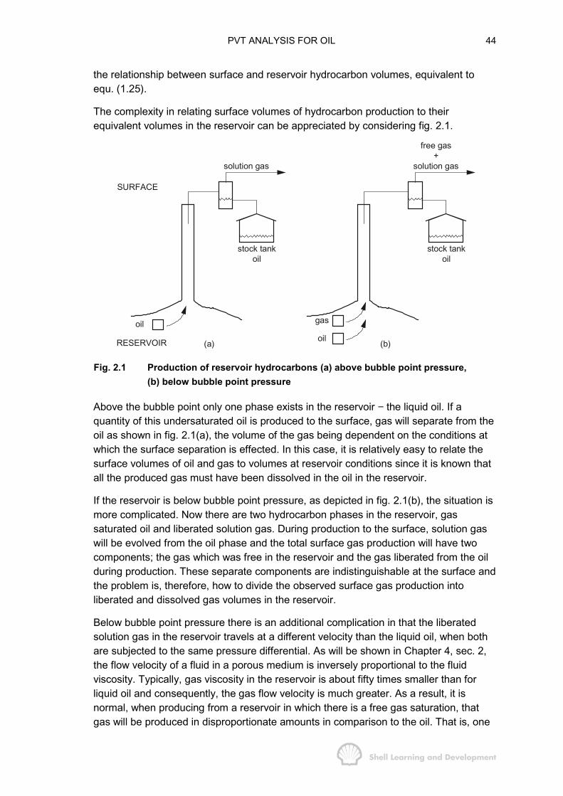
PVT ANALYSIS FOR OIL 44
the relationship between surface and reservoir hydrocarbon volumes, equivalent toequ. (1.25).
The complexity in relating surface volumes of hydrocarbon production to theirequivalent volumes in the reservoir can be appreciated by considering fig. 2.1.
oil
stock tankoil
(a)
solution gas
gas
oil
stock tankoil
(b)
free gas+
solution gas
SURFACE
RESERVOIR
Fig. 2.1 Production of reservoir hydrocarbons (a) above bubble point pressure,(b) below bubble point pressure
Above the bubble point only one phase exists in the reservoir − the liquid oil. If aquantity of this undersaturated oil is produced to the surface, gas will separate from theoil as shown in fig. 2.1(a), the volume of the gas being dependent on the conditions atwhich the surface separation is effected. In this case, it is relatively easy to relate thesurface volumes of oil and gas to volumes at reservoir conditions since it is known thatall the produced gas must have been dissolved in the oil in the reservoir.
If the reservoir is below bubble point pressure, as depicted in fig. 2.1(b), the situation ismore complicated. Now there are two hydrocarbon phases in the reservoir, gassaturated oil and liberated solution gas. During production to the surface, solution gaswill be evolved from the oil phase and the total surface gas production will have twocomponents; the gas which was free in the reservoir and the gas liberated from the oilduring production. These separate components are indistinguishable at the surface andthe problem is, therefore, how to divide the observed surface gas production intoliberated and dissolved gas volumes in the reservoir.
Below bubble point pressure there is an additional complication in that the liberatedsolution gas in the reservoir travels at a different velocity than the liquid oil, when bothare subjected to the same pressure differential. As will be shown in Chapter 4, sec. 2,the flow velocity of a fluid in a porous medium is inversely proportional to the fluidviscosity. Typically, gas viscosity in the reservoir is about fifty times smaller than forliquid oil and consequently, the gas flow velocity is much greater. As a result, it isnormal, when producing from a reservoir in which there is a free gas saturation, thatgas will be produced in disproportionate amounts in comparison to the oil. That is, one
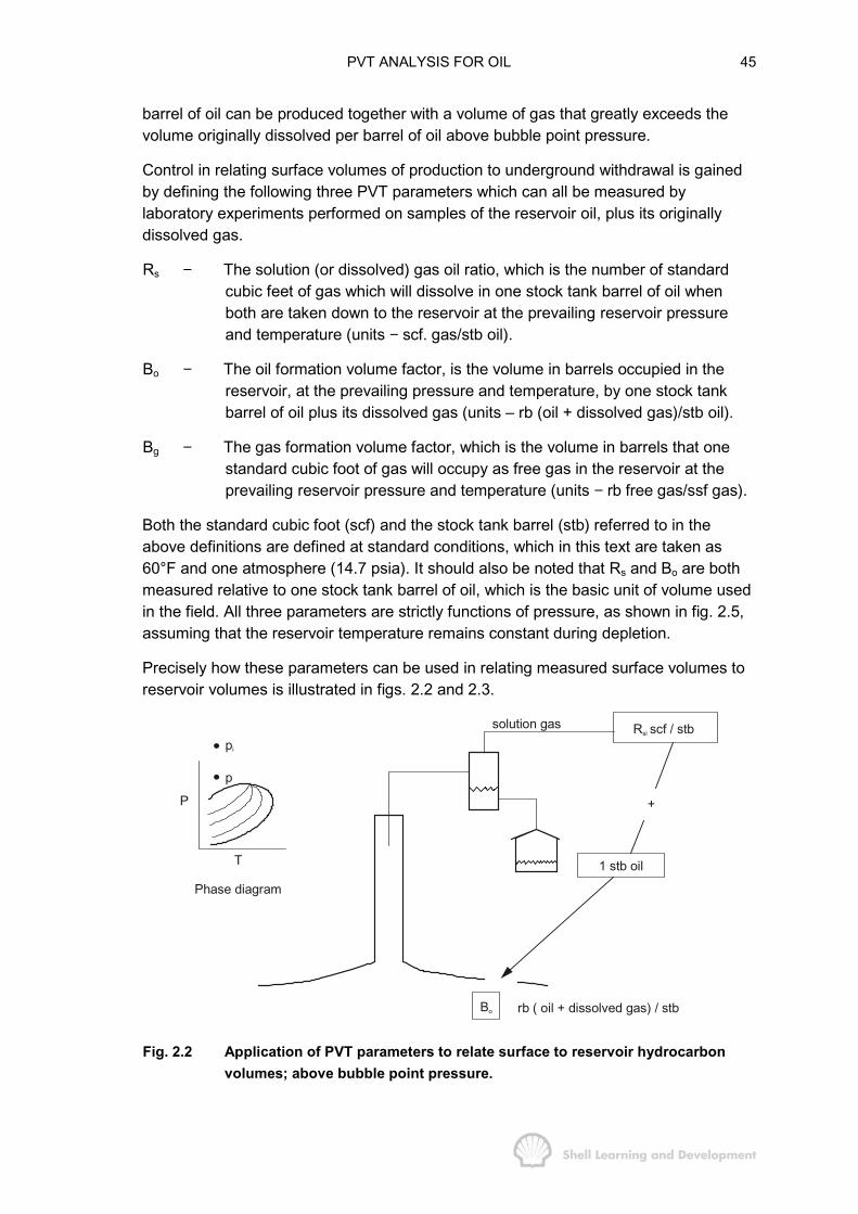
PVT ANALYSIS FOR OIL 45
barrel of oil can be produced together with a volume of gas that greatly exceeds thevolume originally dissolved per barrel of oil above bubble point pressure.
Control in relating surface volumes of production to underground withdrawal is gainedby defining the following three PVT parameters which can all be measured bylaboratory experiments performed on samples of the reservoir oil, plus its originallydissolved gas.
Rs − The solution (or dissolved) gas oil ratio, which is the number of standardcubic feet of gas which will dissolve in one stock tank barrel of oil whenboth are taken down to the reservoir at the prevailing reservoir pressureand temperature (units − scf. gas/stb oil).
Bo − The oil formation volume factor, is the volume in barrels occupied in thereservoir, at the prevailing pressure and temperature, by one stock tankbarrel of oil plus its dissolved gas (units – rb (oil + dissolved gas)/stb oil).
Bg − The gas formation volume factor, which is the volume in barrels that onestandard cubic foot of gas will occupy as free gas in the reservoir at theprevailing reservoir pressure and temperature (units − rb free gas/ssf gas).
Both the standard cubic foot (scf) and the stock tank barrel (stb) referred to in theabove definitions are defined at standard conditions, which in this text are taken as60°F and one atmosphere (14.7 psia). It should also be noted that Rs and Bo are bothmeasured relative to one stock tank barrel of oil, which is the basic unit of volume usedin the field. All three parameters are strictly functions of pressure, as shown in fig. 2.5,assuming that the reservoir temperature remains constant during depletion.
Precisely how these parameters can be used in relating measured surface volumes toreservoir volumes is illustrated in figs. 2.2 and 2.3.
pi
p
T
Phase diagram
P
Bo rb ( oil + dissolved gas) / stb
1 stb oil
+
R scf / stbsisolution gas
Fig. 2.2 Application of PVT parameters to relate surface to reservoir hydrocarbonvolumes; above bubble point pressure.
PVT ANALYSIS FOR OIL 46
Fig. 2.2 depicts the situation when the reservoir pressure has fallen from its initial valuepi to some lower value p, which is still above the bubble point. As shown in the P−Tdiagram (inset) the only fluid in the reservoir is undersaturated liquid oil. When this oil isproduced to the surface each stock tank barrel will yield, upon gas oil separation, Rsi
standard cubic feet of gas. Since the oil is undersaturated with gas, which implies that itcould dissolve more if the latter were available, then the initial value of the solution gasoil ratio must remain constant at Rsi (scf/stb) until the pressure drops to the bubblepoint, when the oil becomes saturated, as shown in fig. 2.5(b).
Figure 2.2 also shows, in accordance with the definitions of Bo and Rs, that if Rsi scf ofgas are taken down to the reservoir with one stb of oil, then the gas will totally dissolvein the oil at the reservoir pressure and temperature to give a volume of Bo rb of oil plusdissolved gas. Figure 2.5(a) shows that Bo increases slightly as the pressure is reducedfrom initial to the bubble point pressure. This effect is simply due to liquid expansionand, since the compressibility of the undersaturated oil in the reservoir is low, theexpansion is relatively small.
Typical values of Bo and Rs above the bubble point are indicated in fig. 2.5, these arethe plotted results of the laboratory analysis presented in table 2.4. The initial value ofthe oil formation volume factor Boi is 1.2417 which increases to 1.2511 at the bubblepoint. Thus initially, 1.2417 reservoir barrels of oil plus its dissolved gas will produceone stb of oil. This is a rather favourable ratio indicating an oil of moderate volatilityand, as would be expected in this case, the initial solution gas oil ratio is also relativelylow at 510 scf/stb. Under less favourable circumstances, for more volatile oils, Boi canhave much higher values. For instance, in the Statfjord field in the North Sea, Boi is2.7 rb/stb while the value of Rsi is approximately 3000 scf/stb. Obviously the mostfavourable value of Boi is as close to unity as possible indicating that the oil containshardly any dissolved gas and reservoir volumes are approximately equal to surfacevolumes. The small oil fields of Beykan and Kayaköy in the east of Turkey provide goodexamples of this latter condition having values of Boi and Rsi of 1.05 and 20 scf/stbrespectively.
Below the bubble point the situation is more complicated as shown in fig. 2.3.

PVT ANALYSIS FOR OIL 47
pi
p
T
p
rb ( oil + dissolved gas) / stb
1 stb oil
Bo
(R - R ) Bs g rb (free gas) / stb
R = R +s (R - R ) scf / stbs
Fig. 2.3 Application of PVT parameters to relate surface to reservoir hydrocarbonvolumes; below bubble point pressure
In this case each stock tank barrel of oil is produced in conjunction with R scf of gas,where R (scf/stb) is called the instantaneous or producing gas oil ratio and is measureddaily. As already noted, some of this gas is dissolved in the oil in the reservoir and isreleased during production through the separator, while the remainder consists of gaswhich is already free in the reservoir. Furthermore, the value of R can greatly exceedRsi, the original solution gas oil ratio, since, due to the high velocity of gas flow incomparison to oil, it is quite normal to produce a disproportionate amount of gas. Thisresults from an effective stealing of liberated gas from all over the reservoir and itsproduction through the relatively isolated offtake points, the wells. A typical plot of R asa function of reservoir pressure is shown as fig. 2.4.
Rscf / stb
R = Rsi
510 scf / stb
pb Reservoir pressure
4000 scf / sfb
Fig. 2.4 Producing gas oil ratio as a function of the average reservoir pressurefor a typical solution gas drive reservoir
PVT ANALYSIS FOR OIL 48
The producing gas oil ratio can be split into two components as shown in fig. 2.3, i.e.
R = Rs +(R−Rs)
The first of these, Rs scf/stb, when taken down to the reservoir with the one stb of oil,will dissolve in the oil at the prevailing reservoir pressure to give Bo rb of oil plusdissolved gas. The remainder, (R − Rs) scf/stb, when taken down to the reservoir willoccupy a volume
s g s gscf rb(R R ) B (R R ) B (rb. free gas / stb)stb scf
� � � �− × = − −� � � �� � � �
(2.1)
and therefore, the total underground withdrawal of hydrocarbons associated with theproduction of one stb of oil is
(Underground withdrawal)/stb = Bo + (R − Rs) Bg (rb/stb) (2.2)
The above relationship shows why the gas formation volume factor has the ratherunfortunate units of rb/scf. It is simply to convert gas oil ratios, measured in scf/stb,directly to rb/stb to be compatible with the units of Bo. While Bg is used almostexclusively in oil reservoir engineering its equivalent in gas reservoir engineering is E,the gas expansion factor, which was introduced in the previous chapter and has theunits scf/rcf. The relation between Bg and E is therefore,
grb 1Bscf 5.615E
� � =� �� �
(2.3)
thus Bg has always very small values; for a typical value of E of, say, 150 scf/rcf thevalue of Bg would be .00119 rb/scf.

PVT ANALYSIS FOR OIL 49
B(rb / stb)
o
1.3
1.2
1.1
1.01000 2000 3000 4000
PRESSURE (psia)
p = 3330 psiab
a
b
c
600
400
200
R(scf / stb)
s
1000 2000 3000 4000
1000 2000 3000 4000
B(rb / scf)
g
.010
.008
.006
.004
.002
E(scf / rcf)
- 200
- 100
- 0
PRESSURE (psia)
PRESSURE (psia)
Fig. 2.5 PVT parameters (Bo, Rs and Bg), as functions of pressure, for the analysispresented in table 2.4; (pb = 3330 psia).
PVT ANALYSIS FOR OIL 50
The shapes of the Bo and Rs curves below the bubble point, shown in fig. 2.5(a) and(b), are easily explained. As the pressure declines below pb, more and more gas isliberated from the saturated oil and thus Rs, which represents the amount of gasdissolved in a stb at the current reservoir pressure, continually decreases. Similarly,since each reservoir volume of oil contains a smaller amount of dissolved gas as thepressure declines, one stb of oil will be obtained from progressively smaller volumes ofreservoir oil and Bo steadily declines with the pressure.
EXERCISE 2.1 UNDERGROUND WITHDRAWAL
The oil and gas rates, measured at a particular time during the producing life of areservoir are, x stb oil/day and y scf gas/day.
1) What is the corresponding underground withdrawal rate in reservoir barrels/day.
2) If the average reservoir pressure at the time the above measurements are madeis 2400 psia, calculate the daily underground withdrawal corresponding to an oilproduction of 2500 stb/day and a gas rate of 2.125 MMscf/day. Use the PVTrelationships shown in figs. 2.5(a) − (c), which are also listed in table 2.4.
3) If the density of the oil at standard conditions is 52.8 lb/cu.ft and the gas gravity is0.67 (air = 1) calculate the oil pressure gradient in the reservoir at 2400 psia.
EXERCISE 2.1 SOLUTION
1) The instantaneous or producing gas oil ratio is R = y/x scf/stb. If, at the time thesurface rates are measured, the average reservoir pressure is known, then Bo, Rs
and Bg can be determined from the PVT relationships at that particular pressure.
The daily volume of oil plus dissolved gas produced from the reservoir is then
xBo rb, and the liberated gas volume removed daily is syx( R )x
− Bg rb. Thus the
total underground withdrawal is
o s gyx (B ( R )B ) rb / dayx
+ − (2.4)
2) At a reservoir pressure of 2400 psia, the PVT parameters obtained from table 2.4are:
Bo = 1.1822 rb/stb; Rs = 352 scf/stb and Bg = .0012 rb/ scf
Therefore, evaluating equ. (2.4) for x = 2500 stb/d and y = 2.125 MMscf/d gives atotal underground withdrawal rate of
2500 (1.1822 + (850 − 352) × .0012) = 4450 rb/d
3) The liquid oil gradient in the reservoir can be calculated by applying massconservation, as demonstrated in exercise 1.1 for the calculation of the gasgradient. In the present case the mass balance is
PVT ANALYSIS FOR OIL 51
Mass of 1 stb of oil Mass of Bo rb of oil+ = +
Rs scf dissolved gasat standard conditions
dissolved gas in thereservoir
or
sc sc
r
o s g
o o
lb lb1(stb) 5.615 R (scf)cu.ft cu.ft
lbB (rb) 5.615cu.ft
ρ ρ
ρ
� � � �� � � �× × + ×� � � �� � � � � � � �
� �= × ×� �
in which the subscripts sc and r refer to standard conditions and reservoirconditions, respectively.
The gas density at standard conditions is
ρsc = γg × 0.0763 (refer equ. (1.30))
= 0.0511 lb/cu ft
Therefore,
sc sc
r
o s go
o
( 5.615) (R )B 5.615
(52.8 5.615) (352 0.0511) 47.37 lb / cu ft1.1822 5.615
ρ ρρ
× + ×=
×× + ×= =
×
and the liquid oil gradient is 47.37/144 = 0.329 psi/ft.
2.3 COLLECTION OF FLUID SAMPLES
Samples of the reservoir fluid are usually collected at an early stage in the reservoir'sproducing life and dispatched to a laboratory for the full PVT analysis. There arebasically two ways of collecting such samples, either by direct subsurface sampling orby surface recombination of the oil and gas phases. Whichever technique is used thesame basic problem exists, and that is, to ensure that the proportion of gas to oil in thecomposite sample is the same as that existing in the reservoir. Thus, sampling areservoir under initial conditions, each stock tank barrel of oil in the sample should becombined with Rsi standard cubic feet of gas.
a) Subsurface sampling
This is the more direct method of sampling and is illustrated schematically in fig. 2.6.

PVT ANALYSIS FOR OIL 52
sample chamber
pwf
pipb
pressure
r
Fig. 2.6 Subsurface collection of PVT sample
A special sampling bomb is run in the hole, on wireline, to the reservoir depth and thesample collected from the subsurface well stream at the prevailing bottom holepressure. Either electrically or mechanically operated valves can be closed to trap avolume of the borehole fluids in the sampling chamber. This method will obviously yielda representative combined fluid sample providing that the oil is undersaturated with gasto such a degree that the bottom hole flowing pressure pwf at which the sample iscollected, is above the bubble point pressure. In this case a single phase fluid, oil plusits dissolved gas, is flowing in the wellbore and therefore, a sample of the fluid is boundto have the oil and gas combined in the correct proportion. Many reservoirs, however,are initially at bubble point pressure and under these circumstances, irrespective ofhow low the producing rate is maintained during sampling, the bottom hole flowingpressure pwf will be less than the bubble point pressure pb as depicted in fig. 2.6. In thiscase, there will be saturated oil and a free gas phase flowing in the immediate vicinityof the wellbore, and in the wellbore itself, and consequently, there is no guarantee thatthe oil and gas will be collected in the correct volume proportion in the chamber.
In sampling a gas saturated reservoir, two situations can arise depending on the time atwhich the sample is collected. If the sample is taken very early in the producing life it ispossible that the fluid flowing into the wellbore is deficient in gas. This is because theinitially liberated gas must build up a certain minimum gas saturation in the reservoirpores before it will start flowing under an imposed pressure differential. This, so−called,critical saturation is a phenomenon common to any fluid deposited in the reservoir, notjust gas. The effect on the producing gas oil ratio, immediately below bubble pointpressure, is shown in fig. 2.4 as the small dip in the value of R for a short period afterthe pressure has dropped below bubble point. As a result of this mechanism there willbe a period during which the liberated gas remains in the reservoir and the gas oil ratiomeasured from a subsurface sample will be too low. Conversely, once the liberated gassaturation exceeds the critical value, then as shown in fig. 2.4 and discussedpreviously, the producing well will effectively steal gas from more remote parts of thereservoir and the sample is likely to have a disproportionately high gas oil ratio.

PVT ANALYSIS FOR OIL 53
The problems associated with sampling an initially saturated oil reservoir, or anundersaturated reservoir in which the bottom hole flowing pressure has been allowed tofall below bubble point pressure, can be largely overcome by correct well conditioningprior to sampling. If the well has already been flowing, it should be produced at a lowstabilized rate for several hours to increase the bottom hole flowing pressure andthereby re-dissolve some, if not all, of the free gas saturation in the vicinity of the well.Following this the well is closed in for a reasonable period of time during which the oilflowing into the wellbore, under an ever increasing average pressure, will hopefully re-dissolve any of the remaining free gas. If the reservoir was initially at bubble pointpressure, or suspected of being so, the subsurface sample should then be collectedwith the well still closed in. If the reservoir is known to be initially undersaturated thesample can be collected with the well flowing at a very low rate so that the bottom holeflowing pressure is still above the bubble point. With proper well conditioning arepresentative combined sample can usually be obtained.
One of the main drawbacks in the method is that only a small sample of the wellborefluids is obtained, the typical sampler having a volume of only a few litres. Therefore,one of the only ways of checking whether the gas oil ratio is correct is to take severaldownhole samples and compare their saturation pressures at ambient temperature onthe well site. This can be done using a mercury injection pump and accurate pressuregauge connected to the sampler. The chamber normally contains both oil and a freegas phase, due to the reduction in temperature between wellbore and surface. Injectingmercury increases the pressure within the chamber until at a saturation pressurecorresponding to the ambient surface temperature all the gas will dissolve. Thissaturation pressure can be quite easily detected since there is a distinct change incompressibility between the two phase and single phase fluids. If it is experimentallydetermined, on the well site, that successive samples have markedly differentsaturation pressures, then either the tool has been malfunctioning or the well has notbeen conditioned properly.
In addition, it is necessary to determine the static reservoir pressure and temperatureby well testing, prior to collecting the samples. Further details on bottom hole samplingtechniques are given in references 2 and 3 listed at the end of this chapter.
b) Surface recombination sampling
In collecting fluid samples at the surface, separate volumes of oil and gas are taken atseparator conditions and recombined to give a composite fluid sample. The surfaceequipment is shown schematically in fig. 2.7.
PVT ANALYSIS FOR OIL 54
gas meter
gassample
oilsample
p
T
st
st
stock tank oil
p
T
sep
sep
well
separator
Fig. 2.7 Collection of a PVT sample by surface recombination
The well is produced at a steady rate for a period of several hours and the gas oil ratiois measured in scf of separator gas per stock tank barrel of oil. If this ratio is steadyduring the period of measurement then one can feel confident that recombining the oiland gas in the same ratio will yield a representative composite sample of the reservoirfluid. In fact, a slight adjustment must be made to determine the actual ratio in whichthe samples should be recombined. This is because, as shown in fig. 2.7, the oilsample is collected at separator pressure and temperature whereas the gas oil ratio ismeasured relative to the stock tank barrel, thus the required recombination ratio is
REQUIRED MEASURED SHRINKAGE
sepscf scf stbR R S
sep.bbl stb sep.bbl� � � �� �= � � � �� �
� �� � � �
Dimensionally, the measured gas oil ratio must be multiplied by the shrinkage factorfrom separator to stock tank conditions. This factor is usually determined in thelaboratory as the first stage of a PVT analysis of a surface recombination sample byplacing a small volume of the oil sample in a cell at the appropriate separatorconditions and discharging it (flash expansion) to a second cell maintained at the fieldstock tank conditions. During this process some gas will be liberated from the separatorsample, due to the reduction in pressure and temperature, and the diminished stocktank oil volume is measured, thus allowing the direct calculation of S. In order to beable to perform such an experiment it is important that the engineer should accuratelymeasure the pressure and temperature prevailing at both separator and stock tankduring sampling and provide the laboratory with these data.
One of the attractive features of surface recombination sampling is that statistically itgives a reliable value of the producing gas oil ratio measured over a period of hours;furthermore, it enables the collection of large fluid samples. Of course, just as forsubsurface sampling, the surface recombination method will only provide the correct
PVT ANALYSIS FOR OIL 55
gas oil ratio if the pressure in the vicinity of the well is at or above bubble pointpressure. If not, the surface gas oil ratio will be too low or too high, depending uponwhether the free gas saturation in the reservoir is below or above the critical saturationat which gas will start to flow. In this respect it should be emphasized that PVT samplesshould be taken as early as possible in the producing life of the field to facilitate thecollection of samples in which the oil and gas are combined in the correct ratio.
2.4 DETERMINATION OF THE BASIC PVT PARAMETERS IN THE LABORATORY ANDCONVERSION FOR FIELD OPERATING CONDITIONS
Quite apart from the determination of the three primary PVT parameters Bo, Rs and Bg,the full laboratory analysis usually consists of the measurement or calculation of fluiddensities, viscosities, composition, etc. These additional measurements will be brieflydiscussed in section 2.6. For the moment, the essential experiments required todetermine the three basic parameters will be detailed, together with the way in whichthe results of a PVT analysis must be modified to match the field operating conditions.
The analysis consists of three parts:
− flash expansion of the fluid sample to determine the bubble point pressure;
− differential expansion of the fluid sample to determine the basic parameters Bo,Rs and Bg;
− flash expansion of fluid samples through various separator combinations toenable the modification of laboratory derived PVT data to match field separatorconditions.
The apparatus used to perform the above experiments is the PV cell, as shown infig. 2.8. After recombining the oil and gas in the correct proportions, the fluid is chargedto the PV cell which is maintained at constant temperature, the measured reservoirtemperature, throughout the experiments. The cell pressure is controlled by a positivedisplacement mercury pump and recorded on an accurate pressure gauge. Theplunger movement is calibrated in terms of volume of mercury injected or withdrawnfrom the PV cell so that volume changes in the cell can be measured directly.
The flash and differential expansion experiments are presented schematically infigs. 2.9(a) and 2.9(b). In the flash experiment the pressure in the PV cell is initiallyraised to a value far in excess of the bubble point. The pressure is subsequentlyreduced in stages, and on each occasion the total volume vt of the cell contents isrecorded. As soon as the bubble point pressure is reached, gas is liberated from the oiland the overall compressibility of the system increases significantly. Thereafter, smallchanges in pressure will result in large changes in the total fluid volume contained inthe PV cell. In this manner, the flash expansion experiment can be used to "feel" thebubble point. Since the cell used is usually opaque the separate volumes of oil andgas, below bubble point pressure, cannot be measured in the experiment andtherefore, only total fluid volumes are recorded. In the laboratory analysis the basic unitof volume, against which all others are compared, is the volume of saturated oil at the
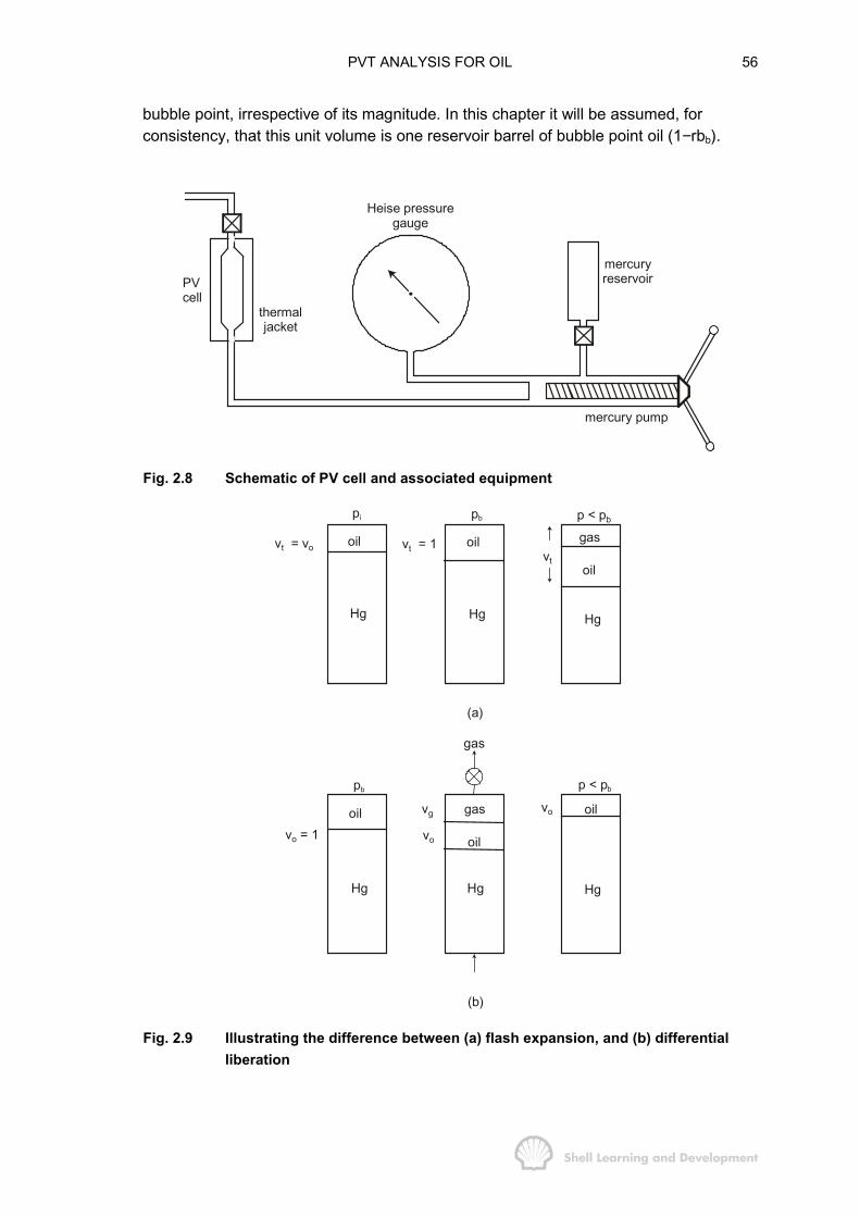
PVT ANALYSIS FOR OIL 56
bubble point, irrespective of its magnitude. In this chapter it will be assumed, forconsistency, that this unit volume is one reservoir barrel of bubble point oil (1−rbb).
PVcell
thermaljacket
Heise pressuregauge
mercuryreservoir
mercury pump
Fig. 2.8 Schematic of PV cell and associated equipment
pi
oilvt = vo
Hg
pb
oilvt = 1
Hg
p < pb
oilvt
Hg
gas
(a)
pb
oil
Hg
oil
Hg
gas
vo
vg
p < pb
vo
Hg
oil
(b)
gas
vo = 1
Fig. 2.9 Illustrating the difference between (a) flash expansion, and (b) differentialliberation
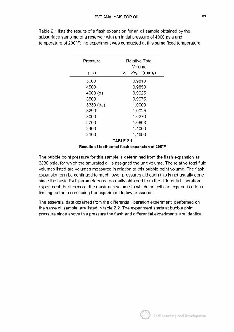
PVT ANALYSIS FOR OIL 57
Table 2.1 lists the results of a flash expansion for an oil sample obtained by thesubsurface sampling of a reservoir with an initial pressure of 4000 psia andtemperature of 200°F; the experiment was conducted at this same fixed temperature.
Pressure
psia
Relative TotalVolume
vt = v/vb = (rb/rbb)
5000 0.98104500 0.98504000 (pi) 0.99253500 0.99753330 (pb ) 1.00003290 1.00253000 1.02702700 1.06032400 1.10602100 1.1680
TABLE 2.1Results of isothermal flash expansion at 200°F
The bubble point pressure for this sample is determined from the flash expansion as3330 psia, for which the saturated oil is assigned the unit volume. The relative total fluidvolumes listed are volumes measured in relation to this bubble point volume. The flashexpansion can be continued to much lower pressures although this is not usually donesince the basic PVT parameters are normally obtained from the differential liberationexperiment. Furthermore, the maximum volume to which the cell can expand is often alimiting factor in continuing the experiment to low pressures.
The essential data obtained from the differential liberation experiment, performed onthe same oil sample, are listed in table 2.2. The experiment starts at bubble pointpressure since above this pressure the flash and differential experiments are identical.

PVT ANALYSIS FOR OIL 58
Pressure
psia
Relative GasVol. (at p and T)
vg
RelativeGas Vol. (sc)
Vg
CumulativeRelative
Gas Vol. (sc)F
Gas expansionFactor
E
Z−factor
Z
Relative OilVol. (at p and T)
vo
3330 (pb ) 1.0000
3000 .0460 8.5211 8.5211 185.24 .868 .9769
2700 .0417 6.9731 15.4942 167.22 .865 .9609
2400 .0466 6.9457 22.4399 149.05 .863 .9449
2100 .0535 6.9457 29.3856 129.83 .867 .9298
1800 .0597 6.5859 35.9715 110.32 .874 .9152
1500 .0687 6.2333 42.2048 90.73 .886 .9022
1200 .0923 6.5895 48.7943 71.39 .901 .8884
900 .1220 6.4114 55.2057 52.55 .918 .8744
600 .1818 6.2369 61.4426 34.31 .937 .8603
300 .3728 6.2297 67.6723 16.71 .962 .8459
14.7 (200°F) 74.9557 .8296
14.7 ( 60°F) 74.9557 .7794
All volumes are measured relative to the unit volume of oil at the bubble point pressure of 3330 psi
TABLE 2.2Results of isothermal differential liberation at 200º F
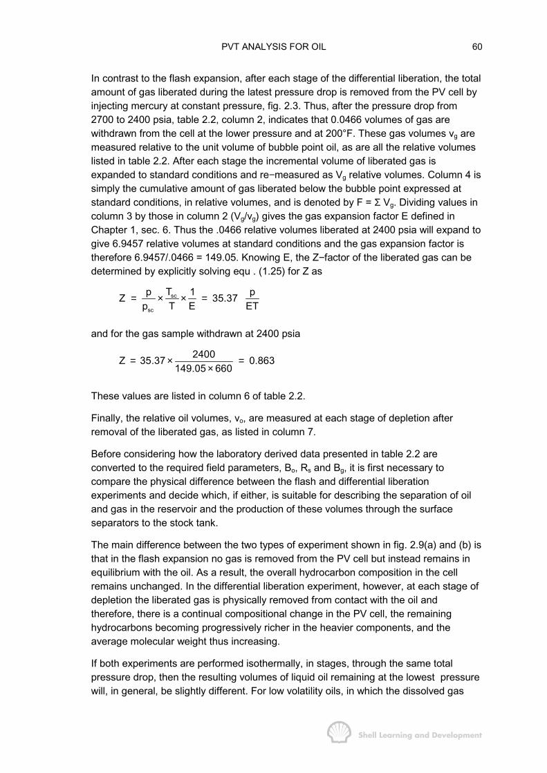
PVT ANALYSIS FOR OIL 60
In contrast to the flash expansion, after each stage of the differential liberation, the totalamount of gas liberated during the latest pressure drop is removed from the PV cell byinjecting mercury at constant pressure, fig. 2.3. Thus, after the pressure drop from2700 to 2400 psia, table 2.2, column 2, indicates that 0.0466 volumes of gas arewithdrawn from the cell at the lower pressure and at 200°F. These gas volumes vg aremeasured relative to the unit volume of bubble point oil, as are all the relative volumeslisted in table 2.2. After each stage the incremental volume of liberated gas isexpanded to standard conditions and re−measured as Vg relative volumes. Column 4 issimply the cumulative amount of gas liberated below the bubble point expressed atstandard conditions, in relative volumes, and is denoted by F = Σ Vg. Dividing values incolumn 3 by those in column 2 (Vg/vg) gives the gas expansion factor E defined inChapter 1, sec. 6. Thus the .0466 relative volumes liberated at 2400 psia will expand togive 6.9457 relative volumes at standard conditions and the gas expansion factor istherefore 6.9457/.0466 = 149.05. Knowing E, the Z−factor of the liberated gas can bedetermined by explicitly solving equ . (1.25) for Z as
sc
sc
Tp 1 pZ 35.37p T E ET
= × × =
and for the gas sample withdrawn at 2400 psia
2400Z 35.37 0.863149.05 660
= × =×
These values are listed in column 6 of table 2.2.
Finally, the relative oil volumes, vo, are measured at each stage of depletion afterremoval of the liberated gas, as listed in column 7.
Before considering how the laboratory derived data presented in table 2.2 areconverted to the required field parameters, Bo, Rs and Bg, it is first necessary tocompare the physical difference between the flash and differential liberationexperiments and decide which, if either, is suitable for describing the separation of oiland gas in the reservoir and the production of these volumes through the surfaceseparators to the stock tank.
The main difference between the two types of experiment shown in fig. 2.9(a) and (b) isthat in the flash expansion no gas is removed from the PV cell but instead remains inequilibrium with the oil. As a result, the overall hydrocarbon composition in the cellremains unchanged. In the differential liberation experiment, however, at each stage ofdepletion the liberated gas is physically removed from contact with the oil andtherefore, there is a continual compositional change in the PV cell, the remaininghydrocarbons becoming progressively richer in the heavier components, and theaverage molecular weight thus increasing.
If both experiments are performed isothermally, in stages, through the same totalpressure drop, then the resulting volumes of liquid oil remaining at the lowest pressurewill, in general, be slightly different. For low volatility oils, in which the dissolved gas
PVT ANALYSIS FOR OIL 61
consists mainly of methane and ethane, the resulting oil volumes from eitherexperiment are practically the same. For higher volatility oils, containing a relativelyhigh proportion of the intermediate hydrocarbons such as butane and pentane, thevolumes can be significantly different. Generally, in this latter case, more gas escapesfrom solution in the flash expansion than in the differential liberation, resulting in asmaller final oil volume after the flash process. This may be explained by the fact thatin the flash expansion the intermediate hydrocarbon molecules find it somewhat easierto escape into the large gas volume in contact with the oil than in the case of thedifferential liberation, in which the volume of liberated gas in equilibrium with the oil, atany stage in the depletion, is significantly smaller.
The above description is a considerable simplification of the complex processesinvolved in the separation of oil and gas; also, it is not always true that the flashseparation yields smaller oil volumes. What must be appreciated, however, is that theflash and differential processes will yield different oil volumes and this difference canbe physically measured by experiment. The problem is, of course, which type ofexperiment will provide the most realistic values of Bo, Rs and Bg, required for relatingmeasured surface volumes to volumes withdrawn from the reservoir at the currentreservoir pressure and fixed temperature.
The answer is that a combination of both flash and differential liberation is required foran adequate description of the overall volume changes. It is considered that thedifferential liberation experiment provides the better description of how the oil and gasseparate in the reservoir since, because of their different flow velocities, they will notremain together in equilibrium once gas is liberated from the oil, thus corresponding tothe process shown in fig. 2.9(b). The one exception to this is during the brief periodafter the bubble point has been reached, when the liberated gas is fairly uniformlydistributed throughout the reservoir and remains immobile until the critical gassaturation is exceeded.
The nature of the volume change occurring between the reservoir and stock tank ismore difficult to categorise but generally, the overall effect is usually likened to a non-isothermal flash expansion. One aspect in this expansion during production is worthconsidering in more detail and that is, what occurs during the passage of the reservoirfluids through the surface separator or separators.
Within any single separator the liberation of gas from the oil may be considered as aflash expansion in which, for a time, the gas stays in equilibrium with the oil. If two ormore separators are used then the gas is physically removed from the oil leaving thefirst separator and the oil is again flashed in the second separator. This physicalisolation of the fluids after each stage of separation corresponds to differentialliberation. In fact, the overall effect of multi-stage separation corresponds to theprocess shown in fig. 2.9(b), which is differential liberation, only in this case it is notconducted at constant temperature. It is for this reason that multi-stage separation iscommonly used in the field because, as already mentioned, differential liberation willnormally yield a larger final volume of equilibrium oil than the corresponding flashexpansion.
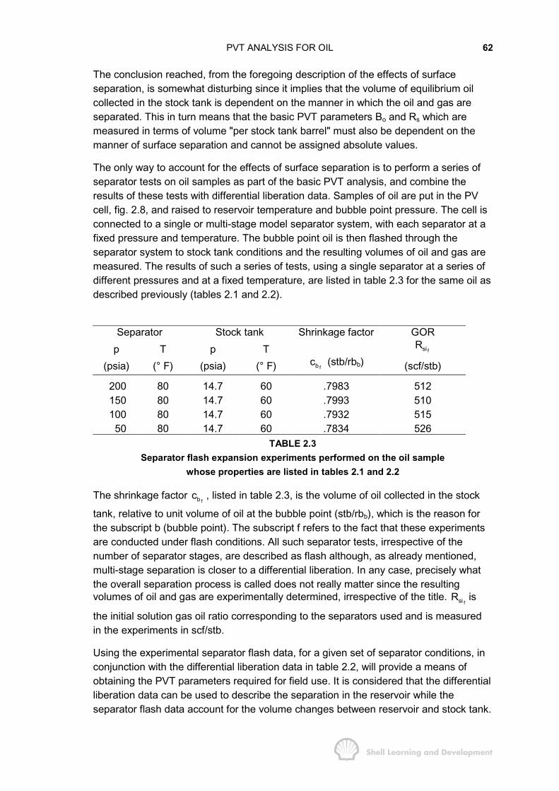
PVT ANALYSIS FOR OIL 62
The conclusion reached, from the foregoing description of the effects of surfaceseparation, is somewhat disturbing since it implies that the volume of equilibrium oilcollected in the stock tank is dependent on the manner in which the oil and gas areseparated. This in turn means that the basic PVT parameters Bo and Rs which aremeasured in terms of volume "per stock tank barrel" must also be dependent on themanner of surface separation and cannot be assigned absolute values.
The only way to account for the effects of surface separation is to perform a series ofseparator tests on oil samples as part of the basic PVT analysis, and combine theresults of these tests with differential liberation data. Samples of oil are put in the PVcell, fig. 2.8, and raised to reservoir temperature and bubble point pressure. The cell isconnected to a single or multi-stage model separator system, with each separator at afixed pressure and temperature. The bubble point oil is then flashed through theseparator system to stock tank conditions and the resulting volumes of oil and gas aremeasured. The results of such a series of tests, using a single separator at a series ofdifferent pressures and at a fixed temperature, are listed in table 2.3 for the same oil asdescribed previously (tables 2.1 and 2.2).
Separator Stock tank Shrinkage factor GORp T p T fsiR
(psia) (° F) (psia) (° F) fbc (stb/rbb) (scf/stb)
200 80 14.7 60 .7983 512150 80 14.7 60 .7993 510100 80 14.7 60 .7932 51550 80 14.7 60 .7834 526
TABLE 2.3Separator flash expansion experiments performed on the oil sample
whose properties are listed in tables 2.1 and 2.2
The shrinkage factor fbc , listed in table 2.3, is the volume of oil collected in the stock
tank, relative to unit volume of oil at the bubble point (stb/rbb), which is the reason forthe subscript b (bubble point). The subscript f refers to the fact that these experimentsare conducted under flash conditions. All such separator tests, irrespective of thenumber of separator stages, are described as flash although, as already mentioned,multi-stage separation is closer to a differential liberation. In any case, precisely whatthe overall separation process is called does not really matter since the resultingvolumes of oil and gas are experimentally determined, irrespective of the title.
fsiR is
the initial solution gas oil ratio corresponding to the separators used and is measuredin the experiments in scf/stb.
Using the experimental separator flash data, for a given set of separator conditions, inconjunction with the differential liberation data in table 2.2, will provide a means ofobtaining the PVT parameters required for field use. It is considered that the differentialliberation data can be used to describe the separation in the reservoir while theseparator flash data account for the volume changes between reservoir and stock tank.
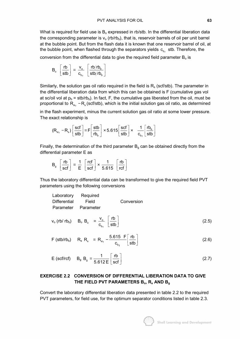
PVT ANALYSIS FOR OIL 63
What is required for field use is Bo expressed in rb/stb. In the differential liberation datathe corresponding parameter is vo (rb/rbb), that is, reservoir barrels of oil per unit barrelat the bubble point. But from the flash data it is known that one reservoir barrel of oil, atthe bubble point, when flashed through the separators yields
fbc stb. Therefore, the
conversion from the differential data to give the required field parameter Bo is
f
o bo
b b
v rb rbrbBstb c stb rb
� �� � = � �� �� � � �
Similarly, the solution gas oil ratio required in the field is Rs (scf/stb). The parameter inthe differential liberation data from which this can be obtained is F (cumulative gas volat sc/oil vol at pb = stb/rbb). In fact, F, the cumulative gas liberated from the oil, must beproportional to
fsi sR R− (scf/stb), which is the initial solution gas oil ratio, as determined
in the flash experiment, minus the current solution gas oil ratio at some lower pressure.The exact relationship is
ff
bsi s
b b
rbscf stb scf 1(R R ) F 5.615stb rb stb c stb
� � � �� � � �− = × ×� � � �� � � �� � � � � �� �
Finally, the determination of the third parameter Bg can be obtained directly from thedifferential parameter E as
grb 1 rcf 1 rbBscf E scf 5.615 rcf� � � � � �= � � � � � �� � � � � �
Thus the laboratory differential data can be transformed to give the required field PVTparameters using the following conversions
LaboratoryDifferentialParameter
RequiredField
ParameterConversion
vo (rb/ rbb) Bo f
oo
b
v rbBc stb
� �= � �� �
(2.5)
F (stb/rbb) Rs fs sib f
5.615 F rbR Rc stb
� �= − � �� �
(2.6)
E (scf/rcf) Bg g1 rbB
5.612 E scf� �= � �� �
(2.7)
EXERCISE 2.2 CONVERSION OF DIFFERENTIAL LIBERATION DATA TO GIVETHE FIELD PVT PARAMETERS Bo, Rs AND Bg
Convert the laboratory differential liberation data presented in table 2.2 to the requiredPVT parameters, for field use, for the optimum separator conditions listed in table 2.3.

PVT ANALYSIS FOR OIL 64
EXERCISE 2.2 SOLUTION
The optimum separator pressure in table 2.3 is 150 psia since this gives the largestvalue of the flash shrinkage factor
fbc as 0.7993 (stb/rbb) and correspondingly, the
lowest flash solution gas oil ratio fsiR of 510 scf/stb. Using these two figures the
laboratory differential data in table 2.2 can be converted to give the field parameters Bo,Rs and Bg using equs. (2.5) − (2.7), as follows
Pressure
(psia)f
oo
b
vBc
=
(rb/stb)
ff
s sib
5.615 FR Rc= −
(scf/stb)
g1B
5.615 E=
(rb/scf)
4000 (pi) 1.2417 foi(B ) 510
fsi(R )
3500 1.2480 510
3330 (pb) 1.2511 f
f
obb
1(B )c
= 510 .00087
3000 1.2222 450 .00096
2700 1.2022 401 .00107
2400 1.1822 352 .00119
2100 1.1633 304 .00137
1800 1.1450 257 .00161
1500 1.1287 214 .00196
1200 1.1115 167 .00249
900 1.0940 122 .00339
600 1.0763 78 .00519
300 1.0583 35 .01066TABLE 2.4
Field PVT parameters adjusted for single stage, surface separationat 150 psia and 80°F;
fbc = .7993 (Data for pressures above 3330 psi
are taken from the flash experiment, table 2.1)
The data in table 2.4 are plotted in fig. 2.5(a) − (c).
In summary of this section, it can be stated that the laboratory differential liberationexperiment, which is regarded as best simulating phase separation in the reservoir,provides an absolute set of PVT data in which all volumes are expressed relative to theunit oil volume at the bubble point, the latter being a unique volume. The PVTparameters conventionally used in the field, however, are dependent on the nature ofthe surface separation. The basic differential data can be modified in accordance withthe surface separators employed using equs. (2.5) − (2.7) in which
fbc and fbR are
determined by flashing unit volume of reservoir oil through the separator system. Themodified PVT parameters thus obtained approximate the process of differential
PVT ANALYSIS FOR OIL 65
liberation in the reservoir and flash expansion to stock tank conditions. Therefore if,during the producing life of the reservoir, the separator conditions are changed, thenthe fixed differential liberation data will have to be converted to give new tables of Boand Rs using values of
fbc and fsiR appropriate for the altered separator conditions.
This combination of differential liberation in the reservoir and flash expansion to thesurface is generally regarded as a reasonable approximation to Dodson's PVT analysistechnique4. In this form of experiment a differential liberation is performed but aftereach pressure stage the volume of the oil remaining in the PV cell is flashed to stocktank conditions through a chosen separator combination. The ratio of stock tank oilvolume to original oil volume in the PV cell prior to flashing gives a direct measure ofBo, while the gas evolved in the flash can be used directly to obtain Rs. The process isrepeated taking a new oil sample for each pressure step, since the remaining oil in thePV cell is always flashed to surface conditions. This type of analysis, while moreaccurately representing the complex reservoir-production phase separation, is moretime consuming and therefore more costly, furthermore, it requires the availability oflarge samples of the reservoir fluid. For low and moderately volatile crudes, the mannerof deriving the PVT parameters described in this section usually provides a very goodapproximation to the results obtained from the Dodson analysis. For more volatilecrudes, however, the more elaborate experimental technique may be justified.
2.5 ALTERNATIVE MANNER OF EXPRESSING PVT LABORATORY ANALYSISRESULTS
The results of the differential liberation experiment, as listed in table 2.2, provide anabsolute set of data which can be modified, according to the surface separators used,to give the values of the PVT parameters required for field use. In table 2.2 all volumesare measured relative to the unit oil volume at the bubble point. There is, however, amore common way of representing the results of the differential liberation in whichvolumes are measured relative to the volume of residual oil at stock tank conditions.This volume is obtained as the final step in the differential liberation experiment byflashing the volume of oil measured at atmospheric pressure and reservoirtemperature, to atmospheric pressure and 60°F. This final step is shown in table 2.2 inwhich 0.8296 relative oil volumes at 14.7 psia and 200°F yield 0.7794 relative oilvolumes at 14.7 psia and 60°F. This value of 0.7794 is the shrinkage factor for a unitvolume of bubble point oil during differential liberation to stock tank conditions and isdenoted by
dbc . The value of dbc ,is not dependent on any separator conditions and
therefore, relating all volumes in the differential liberation to this value of dbc , which is
normally referred to as the "residual oil volume", will provide an alternative means ofexpressing the differential liberation results.
It should be noted, however, that the magnitude of dbc is dependent on the number of
pressure steps taken in the differential experiment. Therefore, the differential liberationresults, in which all volumes are measured relative to
dbc do not provide an absolute
set of data such as that obtained by relating all volumes to the unit volume of oil at thebubble point.
PVT ANALYSIS FOR OIL 66
In the presentation of differential data, in which volumes are measured relative to dbc ,
the values of vo and F in table 2.2 are replace by doB and
dsR where
doB = Differential oil formation volume factor
(rb/stb-residual oil)
anddsR = Differential solution gas oil ratio
(scf/stb-residual oil)
Alternatively, by replacing fbc in equs. (2.5) and (2.6) by
dbc , these parameters can be
expressed as
dd
o bo
b b
v rb rbBc stb residual rb
� �= � �−� �
(2.8)
and d d
d
s sib
5.615 F scfR Rc stb residual
� �= − � �−� �(2.9)
where dsiR is the initial dissolved gas relative to the residual barrel of oil at 60°F, and is
proportional to the total gas liberated in the differential experiment, thus
dd
sib
(Maximum valueof F) scfR 5.615c stb residual
� �= × � �−� �(2.10)
and for the differential data presented in table 2.2
dsi74.9557 5.615R 540 scf stb residual oil
.7794×= = −
The majority of commercial laboratories serving the industry would normally presentthe essential data in the differential liberation experiment (table 2.2) as shown intable 2.5.
There is a danger in presenting the results of the differential liberation experiment inthis way since a great many engineers are tempted to use the
doB and dsR values
directly in reservoir calculations, without making the necessary corrections to allow forthe surface separator conditions. In many cases, the error in directly using the data intable 2.5 is negligible, however, for moderate and high volatility oils the error can bequite significant and therefore, the reader should always make the necessarycorrection to the data in table 2.5 to allow for the field separator conditions, as a matterof course.
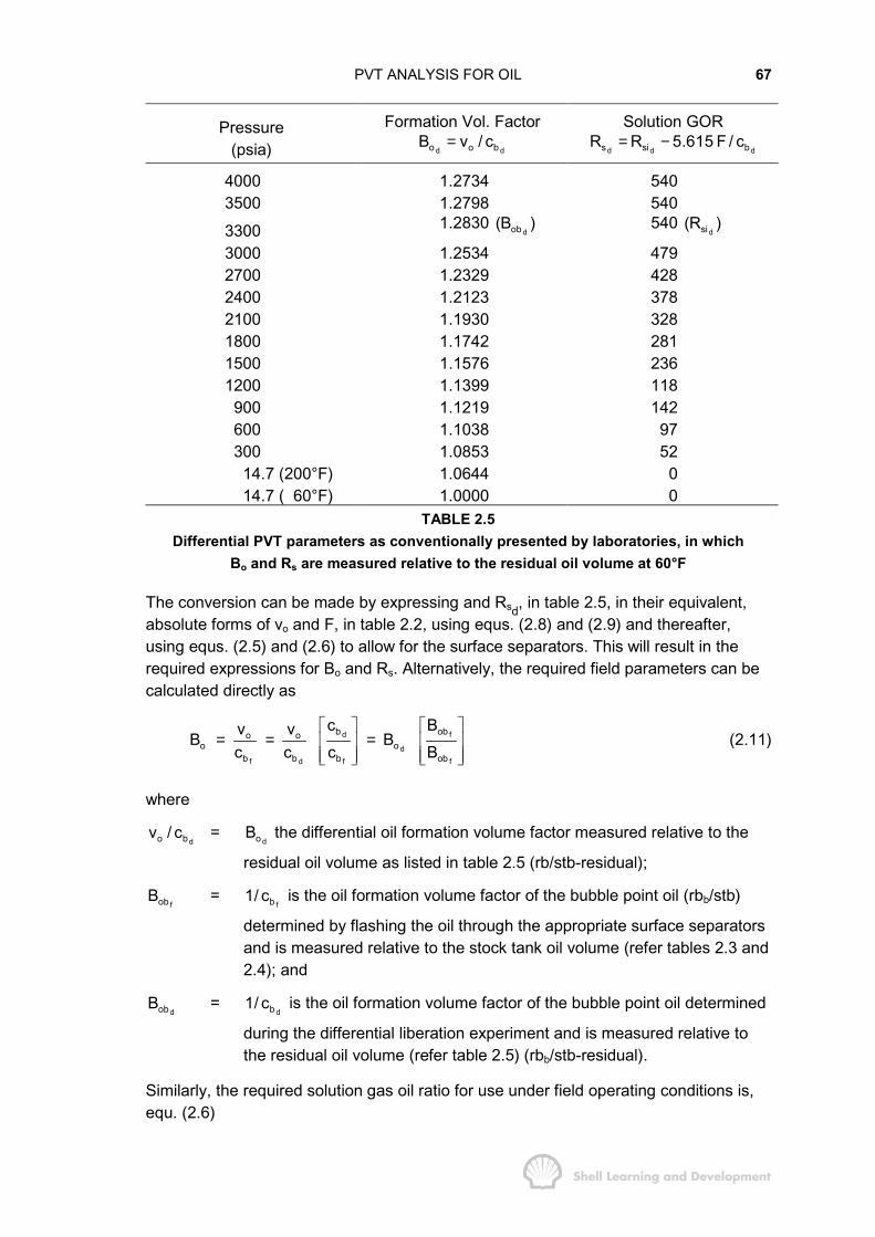
PVT ANALYSIS FOR OIL 67
Pressure(psia)
Formation Vol. Factord do o bB v / c=
Solution GORd d ds si bR R 5.615 F / c= −
4000 1.2734 5403500 1.2798 540
3300 1.2830 dob(B ) 540
dsi(R )
3000 1.2534 4792700 1.2329 4282400 1.2123 3782100 1.1930 3281800 1.1742 2811500 1.1576 2361200 1.1399 118900 1.1219 142600 1.1038 97300 1.0853 5214.7 (200°F) 1.0644 014.7 ( 60°F) 1.0000 0
TABLE 2.5Differential PVT parameters as conventionally presented by laboratories, in which
Bo and Rs are measured relative to the residual oil volume at 60°F
The conversion can be made by expressing and Rsd, in table 2.5, in their equivalent,absolute forms of vo and F, in table 2.2, using equs. (2.8) and (2.9) and thereafter,using equs. (2.5) and (2.6) to allow for the surface separators. This will result in therequired expressions for Bo and Rs. Alternatively, the required field parameters can becalculated directly as
d f
df d f f
b obo oo o
b b b ob
c Bv vB Bc c c B
� � � �= = =� � � �
� � � �� � � �(2.11)
where
do bv / c = doB the differential oil formation volume factor measured relative to the
residual oil volume as listed in table 2.5 (rb/stb-residual);
fobB =fb1/ c is the oil formation volume factor of the bubble point oil (rbb/stb)
determined by flashing the oil through the appropriate surface separatorsand is measured relative to the stock tank oil volume (refer tables 2.3 and2.4); and
dobB =db1/ c is the oil formation volume factor of the bubble point oil determined
during the differential liberation experiment and is measured relative tothe residual oil volume (refer table 2.5) (rbb/stb-residual).
Similarly, the required solution gas oil ratio for use under field operating conditions is,equ. (2.6)

PVT ANALYSIS FOR OIL 68
d
f ff d f
bs si si
b b b
c5.615 F 5.615 FR R Rc c c=
� �− = − � �
� �� �
which, using equ. (2.9), can be expressed as
f
f d df
obs si si s
ob
BR R (R R )
B
� �= − − � �
� �� �
(2.12)
where
fsiR = solution gas oil ratio of the bubble point oil, determined by flashing the oil
through the appropriate surface separators, and is measured relative to the oil volumeat 60°F and 14.7 psia (refer tables 2.3 and 2.4) (scf/stb).
dsiR = solution gas oil ratio of the bubble point oil determined during the
differential experiment and measured relative to the residual oil volume at60°F and 14.7 psia (refer table 2.5 and equ. (2.10)) (scf/stb-residual).
The differential data, as presented in table 2.5, can be directly converted to therequired form, table 2.4, using the above relations. For instance, using the followingdata from table 2.5, at a pressure of 2400 psi
doB = 1.2123 (rb /barrel of residual oil at 60°F and 14.7 psia)
dsR = 378 (scf/ —" — )
dobB = 1.2830 (rb / — " — )
dsiR = 540 (scf/ —" — )
while from the separator flash tests (table 2.3), for the optimum separator conditions of150 psia and 80°F
f fob bB (1/ c ) 1.2511(rb / stb)= =
fsiR 510 (scf / stb)=
Therefore, using equ. (2.11)
o1.2511B 1.2123 1.1822 rb stb1.2830
= × =
and equ. (2.12)
s1.2511R 510 (540 378) 352 scf / stb1.2830
= − − × =

PVT ANALYSIS FOR OIL 69
2.6 COMPLETE PVT ANALYSIS
The complete PVT analysis for oil, provided by most laboratories, usually consists ofthe following experiments and calculations.
a) Compositional analysis of the separator oil and gas, for samples collected at thesurface, together with physical recombination, refer sec. 2.3(b), or; compositionalanalysis of the reservoir fluid collected in a subsurface sample.
Such analyses usually give the mole fractions of each component up to thehexanes. The hexanes and heavier components are grouped together, and theaverage molecular weight and density of the latter are determined.
b) Flash expansion, as described in sec. 2.4 (table 2.1), conducted at reservoirtemperature. This experiment determines
− the bubble point pressure
− the compressibility of the undersaturated oil as
o oo
o o
dv dB1 1cv dp B dp
= − = − (2.13)
− the total volume vt of the oil and gas at each stage of depletion.
c) Differential liberation experiment as described in sec. 2.4 to determine
− E, Z, F and vo (as listed in table 2.2), with F and vo measured relative to theunit volume of bubble point oil.
Alternatively, by measuring dbc during the last stage of the differential liberation,
the above data can be presented as
− E, Z, dsiR −
dsR (or just dsR ) and
doB (as listed in table 2.5), with dsR and
doB measured relative to residual oil volume. In addition, the gas gravity is
measured at each stage of depletion.
d) Measurement of the oil viscosity at reservoir temperature (generally using therolling ball viscometer1,3), over the entire range of pressure steps from abovebubble point to atmospheric pressure. Gas viscosities are normally calculated atreservoir temperature, from a knowledge of the gas gravity, using standardcorrelations5.
e) Separator tests to determine the shrinkage, fbc , and solution gas oil ratio,
fsiR , of
unit volume of bubble point oil (1 barrel) when flashed through various separatorcombinations (refer table 2.3). Instead of actually performing these tests, in manycases the results are obtained using the phase equilibrium calculationtechnique1.
f) Composition and gravity of the separator gas in the above separator tests.
PVT ANALYSIS FOR OIL 70
REFERENCES
1) Amyx, J.W., Bass, D.M. and Whiting, R.L., 1960. Petroleum ReservoirEngineering; Physical Properties. McGraw-Hill Book Company: 359−425.
2) Reudelhuber, F.O., 1957. Sampling Procedures for Oil Reservoir Fluids. J.Pet.Tech., December.
3) Anonymous, 1966. API Recommended Practice for Sampling PetroleumReservoir Fluids. Official publication of the American Petroleum Institute,January (API RP 44).
4) Dodson, C.R., Goodwill, D. and Mayer, E.H., 1953. Application of Laboratory PVTData to Reservoir Engineering Problems. Trans. AIME, 198: 287−298.
5) Carr, N.L., Kobayashi, R. and Burrows, D.B., 1954. Viscosity of HydrocarbonGases under Pressure. Trans. AlME, 201: 264−272.
CHAPTER 3
MATERIAL BALANCE APPLIED TO OIL RESERVOIRS
3.1 INTRODUCTION
The Schilthuis material balance equation has long been regarded as one of the basictools of reservoir engineers for interpreting and predicting reservoir performance.
In this chapter, the zero dimensional material balance is derived and subsequentlyapplied, using mainly the interpretative technique of Havlena and Odeh, to gain anunderstanding of reservoir drive mechanisms under primary recovery conditions.Finally, some of the uncertainties attached to estimation of in-situ pore compressibility,a basic component in the material balance equation, are qualitatively discussed.
Although the classical material balance techniques, once applied, have now largelybeen superseded by numerical simulators, which are essentially multi-dimensional,multi-phase, dynamic material balance programs, the classical approach is well worthstudying since it provides a valuable insight into the behaviour of hydrocarbonreservoirs.
3.2 GENERAL FORM OF THE MATERIAL BALANCE EQUATION FOR AHYDROCARBON RESERVOIR
The general form of the material balance equation was first presented by Schilthuis1 in1941. The equation is derived as a volume balance which equates the cumulativeobserved production, expressed as an underground withdrawal, to the expansion of thefluids in the reservoir resulting from a finite pressure drop. The situation is depicted infig. 3.1 in which (a) represents the fluid volume at the initial pressure pi in a reservoirwhich has a finite gascap. The total fluid volume in this diagram is the hydrocarbonpore volume of the reservoir (HCPV). Fig. 3.1 (b) illustrates the effect of reducing thepressure by an amount ∆p and allowing the fluid volumes to expand, in an artificialsense, in the reservoir. The original HCPV is still drawn in this diagram as the solidline. Volume A is the increase due to the expansion of the oil plus originally dissolvedgas, while volume increase B is due to the expansion of the initial gascap gas. Thethird volume increment C is the decrease in HCPV due to the combined effects of theexpansion of the connate water and reduction in reservoir pore volume as alreadydiscussed in Chapter 1, sec. 7.
If the total observed surface production of oil and gas is expressed in terms of anunderground withdrawal, evaluated at the lower pressure p, (which means effectively,
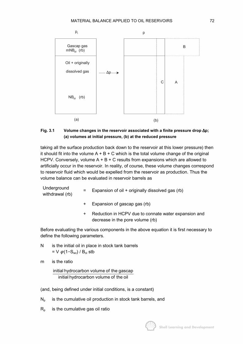
MATERIAL BALANCE APPLIED TO OIL RESERVOIRS 72
pi
Gascap gasmNBoi (rb)
Oil + originally
dissolved gas
NBoi (rb)
∆p
p
B
AC
(b)(a)
Fig. 3.1 Volume changes in the reservoir associated with a finite pressure drop ∆∆∆∆p;(a) volumes at initial pressure, (b) at the reduced pressure
taking all the surface production back down to the reservoir at this lower pressure) thenit should fit into the volume A + B + C which is the total volume change of the originalHCPV. Conversely, volume A + B + C results from expansions which are allowed toartificially occur in the reservoir. In reality, of course, these volume changes correspondto reservoir fluid which would be expelled from the reservoir as production. Thus thevolume balance can be evaluated in reservoir barrels as
Undergroundwithdrawal (rb)
= Expansion of oil + originally dissolved gas (rb)
+ Expansion of gascap gas (rb)
+ Reduction in HCPV due to connate water expansion anddecrease in the pore volume (rb)
Before evaluating the various components in the above equation it is first necessary todefine the following parameters.
N is the initial oil in place in stock tank barrels= V φ (1−Swc) / Boi stb
m is the ratio
initial hydrocarbon volume of the gascapinitial hydrocarbon volume of the oil
(and, being defined under initial conditions, is a constant)
Np is the cumulative oil production in stock tank barrels, and
Rp is the cumulative gas oil ratio
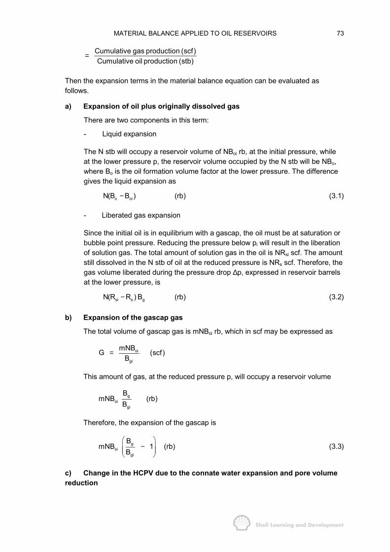
MATERIAL BALANCE APPLIED TO OIL RESERVOIRS 73
Cumulative gas production (scf)Cumulative oil production (stb)
=
Then the expansion terms in the material balance equation can be evaluated asfollows.
a) Expansion of oil plus originally dissolved gas
There are two components in this term:
- Liquid expansion
The N stb will occupy a reservoir volume of NBoi rb, at the initial pressure, whileat the lower pressure p, the reservoir volume occupied by the N stb will be NBo,where Bo is the oil formation volume factor at the lower pressure. The differencegives the liquid expansion as
o oiN(B B ) (rb)− (3.1)
- Liberated gas expansion
Since the initial oil is in equilibrium with a gascap, the oil must be at saturation orbubble point pressure. Reducing the pressure below pi will result in the liberationof solution gas. The total amount of solution gas in the oil is NRsi scf. The amountstill dissolved in the N stb of oil at the reduced pressure is NRs scf. Therefore, thegas volume liberated during the pressure drop ∆p, expressed in reservoir barrelsat the lower pressure, is
si s gN(R R ) B (rb)− (3.2)
b) Expansion of the gascap gas
The total volume of gascap gas is mNBoi rb, which in scf may be expressed as
oi
gi
mNBG (scf )B
=
This amount of gas, at the reduced pressure p, will occupy a reservoir volume
goi
gi
BmNB (rb)
B
Therefore, the expansion of the gascap is
goi
gi
BmNB 1 (rb)
B� �
−� �� �� �
(3.3)
c) Change in the HCPV due to the connate water expansion and pore volumereduction
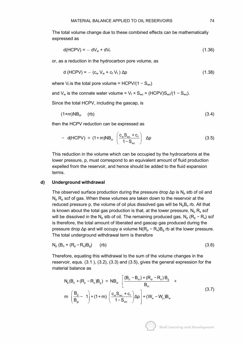
MATERIAL BALANCE APPLIED TO OIL RESERVOIRS 74
The total volume change due to these combined effects can be mathematicallyexpressed as
d(HCPV) = � dVw + dVf (1.36)
or, as a reduction in the hydrocarbon pore volume, as
d (HCPV) = � (cw Vw + cf Vf ) ∆p (1.38)
where Vf is the total pore volume = HCPV/(1 − Swc)
and Vw is the connate water volume = Vf × Swc = (HCPV)Swc/(1 − Swc).
Since the total HCPV, including the gascap, is
(1+m)NBoi (rb) (3.4)
then the HCPV reduction can be expressed as
w wc foi
wc
c S cd(HCPV) (1 m)NB p1 S
� �+− = + ∆� �−� �(3.5)
This reduction in the volume which can be occupied by the hydrocarbons at thelower pressure, p, must correspond to an equivalent amount of fluid productionexpelled from the reservoir, and hence should be added to the fluid expansionterms.
d) Underground withdrawal
The observed surface production during the pressure drop ∆p is Np stb of oil andNp Rp scf of gas. When these volumes are taken down to the reservoir at thereduced pressure p, the volume of oil plus dissolved gas will be NpBo rb. All thatis known about the total gas production is that, at the lower pressure, Np Rs scfwill be dissolved in the Np stb of oil. The remaining produced gas, Np (Rp − Rs) scfis therefore, the total amount of liberated and gascap gas produced during thepressure drop ∆p and will occupy a volume N(Rp − Rs)Bg rb at the lower pressure.The total underground withdrawal term is therefore
Np (Bo + (Rp − Rs)Bg) (rb) (3.6)
Therefore, equating this withdrawal to the sum of the volume changes in thereservoir, equs. (3.1 ), (3.2), (3.3) and (3.5), gives the general expression for thematerial balance as
o oi si s gp o p s g oi
oi
g w wc fe p w
gi wc
(B B ) (R R ) BN (B (R R )B ) NB
B
B c S cm 1 (1 m) p (W W )BB 1 S
− + −�+ − = +�
�
�� � � �+− + + ∆ + −�� � � − � � � �
(3.7)

MATERIAL BALANCE APPLIED TO OIL RESERVOIRS 75
in which the final term (We − Wp)Bw is the net water influx into the reservoir. Thishas been intuitively added to the right hand side of the balance since any suchinflux must expel an equivalent amount of production from the reservoir thusincreasing the left hand side of the equation by the same amount. In this influxterm
We = Cumulative water influx from the aquifer into the reservoir, stb.
Wp = Cumulative amount of aquifer water produced, stb.
and Bw = Water formation volume factor rb/stb.
Bw is generally close to unity since the solubility of gas in water is rather smalland this condition will be assumed throughout this text. For more detailedcalculations, correlation charts for Bw are presented in references 2 and 3.
The following features should be noted in connection with the expanded materialbalance equation
− it is zero dimensional, meaning that it is evaluated at a point in the reservoir
− it generally exhibits a lack of time dependence although, as will bediscussed in sec. 3.7 and also in Chapter 9, the water influx has a timedependence
− although the pressure only appears explicitly in the water and porecompressibility term as, ∆p = pi − p, it is implicit in all the other terms sincethe PVT parameters Bo, Rs and Bg are themselves functions of pressure.The water influx is also pressure dependent.
− the equation is always evaluated, in the way it was derived, by comparingthe current volumes at pressure p to the original volumes at pi. It is notevaluated in a step-wise or differential fashion.
Although the equation appears a little intimidating, at first sight, it should bethought of as nothing more than a sophisticated version of the compressibilitydefinition
dV = c × V × ∆p
Production = Expansion of reservoir fluids.
and, under certain circumstances, can in fact be reduced to this simple form.
In using the material balance equation, one of the main difficulties lies in thedetermination of the representative average reservoir pressure at which thepressure dependent parameters in the equation should be evaluated. Thisfollows from the zero dimensional nature of the equation which implies that thereshould be some point in the reservoir at which a volume averaged pressure canbe uniquely determined. In applying the more simple gas material balance, equ.(1.35), such a point could be defined with reasonable accuracy as the centroidpoint, at which pressures could be evaluated throughout the producing life of the
MATERIAL BALANCE APPLIED TO OIL RESERVOIRS 76
reservoir. In the case of an oil reservoir, however, the situation is generally morecomplex since below the bubble point two phases, oil and gas, will co-exist and,due to the gravity difference between the phases, will tend to segregate. As aresult, the point at which the average pressure should be determined will varywith time. Precisely how the volume averaged reservoir pressure can bedetermined from the analysis of pressure tests in wells will be detailed inChapter 7.
3.3 THE MATERIAL BALANCE EXPRESSED AS A LINEAR EQUATION
Since the advent of sophisticated numerical reservoir simulation techniques, theSchilthuis material balance equation has been regarded by many engineers as being ofhistorical interest only; a technique used back in the nineteen forties and fifties whenpeople still used slide-rules. It is therefore interesting to note that as late as 1963-4,Havlena and Odeh presented two of the most interesting papers ever published on thesubject of applying the material balance equation and interpreting the results. Theirpapers,4,5 described the technique of interpreting the material balance as the equationof a straight line, the first paper describing the technique and the second illustrating theapplication to reservoir case histories.
To express equ. (3.7) in the way presented by Havlena and Odeh requires thedefinition of the following terms
F = Np (Bo + (Rp � Rs) Bg) + Wp Bw (rb) (3.8)
which is the underground withdrawal;
Eo = (Bo − Boi) + (Rsi − Rs) Bg (rb/stb) (3.9)
which is the term describing the expansion of the oil and its originally dissolved gas;
gg oi
gi
BE B 1 (rb / stb)
B� �
= −� �� �� �
(3.10)
describing the expansion of the gascap gas, and
w wc ff,w oi
wc
c S cE (1 m) B p (rb / stb)1 S
� �+= + ∆� �−� �(3.11)
for the expansion of the connate water and reduction in the pore volume. Using theseterms the material balance equation can be written as
F = N(Eo+mEg+Ef,w) + WeBw (3.12)
Havlena and Odeh have shown that in many cases equ. (3.12) can be interpreted as alinear function. For instance, in the case of a reservoir which has no initial gascap,negligible water influx and for which the connate water and rock compressibility termmay be neglected; the equation can be reduced to
MATERIAL BALANCE APPLIED TO OIL RESERVOIRS 77
F = NEo (3.13)
in which the observed production, evaluated as an underground withdrawal, should plotas a linear function of the expansion of the oil plus its originally dissolved gas, the latterbeing calculated from a knowledge of the PVT parameters at the current reservoirpressure. This interpretation technique is useful, in that, if a simple linear relationshipsuch as equ. (3.13) is expected for a reservoir and yet the actual plot turns out to benon-linear, then this deviation can itself be diagnostic in determining the actual drivemechanisms in the reservoir. For instance, equ. (3.13) may turn out to be non-linearbecause there is an unsuspected water influx into the reservoir helping to maintain thepressure. In this case equ. (3.12) can still be expressed in a linear form as
e
o o
WF nE E
= + (3.14)
in which F/Eo should now plot as a linear function of We / E o.
Once a straight line has been achieved, based on matching observed production andpressure data, then the engineer has, in effect, built a suitable mathematical model todescribe the performance of the reservoir. As previously described, in Chapter 1,sec. 7, this phase is commonly referred to as a history match. Once this has beensatisfactorily achieved, the next step is to use the same mathematical model to predicthow the reservoir will perform in the future, possibly for a variety of productionschemes. This prediction phase is facilitated by the mathematical ease in using thesimple linear expressions for the material balance equation, as presented by Havlenaand Odeh. The technique will be illustrated in greater detail in the following sections.
3.4 RESERVOIR DRIVE MECHANISMS
If none of the terms in the material balance equation can be neglected, then thereservoir can be described as having a combination drive in which all possible sourcesof energy contribute a significant part in producing the reservoir fluids and determiningthe primary recovery factor. In many cases, however, reservoirs can be singled out ashaving predominantly one main type of drive mechanism in comparison to which allother mechanisms have a negligible effect. In the following sections, such reservoirswill be described in order to isolate and study the contribution of the individualcomponents in the material balance in influencing the recovery factor and determiningthe production policy of the field. The mechanisms which will be studied are:
- solution gas drive
- gascap drive
- natural water drive
- compaction drive
And these individual reservoir drive mechanisms will be investigated in terms of:
- reducing the material balance to a compact form, in many cases using thetechnique of Havlena and Odeh, in order to quantify reservoir performance
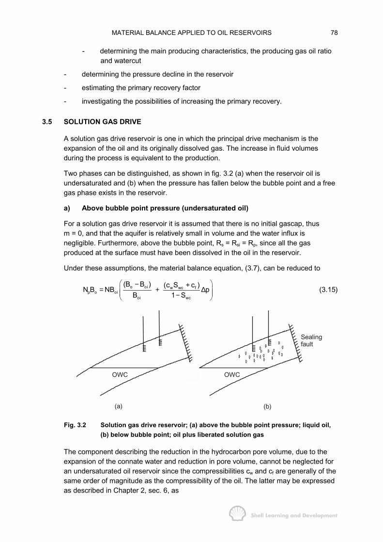
MATERIAL BALANCE APPLIED TO OIL RESERVOIRS 78
- determining the main producing characteristics, the producing gas oil ratioand watercut
- determining the pressure decline in the reservoir
- estimating the primary recovery factor
- investigating the possibilities of increasing the primary recovery.
3.5 SOLUTION GAS DRIVE
A solution gas drive reservoir is one in which the principal drive mechanism is theexpansion of the oil and its originally dissolved gas. The increase in fluid volumesduring the process is equivalent to the production.
Two phases can be distinguished, as shown in fig. 3.2 (a) when the reservoir oil isundersaturated and (b) when the pressure has fallen below the bubble point and a freegas phase exists in the reservoir.
a) Above bubble point pressure (undersaturated oil)
For a solution gas drive reservoir it is assumed that there is no initial gascap, thusm = 0, and that the aquifer is relatively small in volume and the water influx isnegligible. Furthermore, above the bubble point, Rs = Rsi = Rp, since all the gasproduced at the surface must have been dissolved in the oil in the reservoir.
Under these assumptions, the material balance equation, (3.7), can be reduced to
o oi w wc fp o oi
oi wc
(B B ) (c S c )N B NB pB 1 S
� �− += + ∆� �� �−� �
(3.15)
OWC
(a)
OWC
(b)
Sealingfault
Fig. 3.2 Solution gas drive reservoir; (a) above the bubble point pressure; liquid oil,(b) below bubble point; oil plus liberated solution gas
The component describing the reduction in the hydrocarbon pore volume, due to theexpansion of the connate water and reduction in pore volume, cannot be neglected foran undersaturated oil reservoir since the compressibilities cw and cf are generally of thesame order of magnitude as the compressibility of the oil. The latter may be expressedas described in Chapter 2, sec. 6, as
MATERIAL BALANCE APPLIED TO OIL RESERVOIRS 79
( )o oio
oi
B Bc
B p−
=∆
and substituting this in equ. (3.15) gives
w wc fp o oi o
wc
(c S c )N B NB c p1 S
� �+= ∆� �−� �(3.16)
Since there are only two fluids in the reservoir, oil and connate water, then the sum ofthe fluid saturations must be 100% of the pore volume, or
So + Swc = 1
and substituting the latter in equ. (3.16) gives the reduced form of material balance as
o o w wc fp o oi
wc
c S c S cN B NB p1 S
� �+ += ∆� �−� �(3.17)
or
p o oi eN B NB c p= ∆ (3.18)
in which
e o o w wc fwc
1c (c S c S c )1 S
= + +−
(3.19)
is the effective, saturation-weighted compressibility of the reservoir system. Since thesaturations are conventionally expressed as fractions of the pore volume, dividing by1 − Swc expresses them as fractions of the hydrocarbon pore volume.
Thus the compressibility, as defined in equ. (3.19),must be used in conjunction with thehydrocarbon pore volume. Equation (3.18) illustrates how the material balance can bereduced to nothing more than the basic definition of compressibility, equ. (1.12), inwhich NpBo = dV, the reservoir production expressed as an underground withdrawal,and NBoi = V the initial hydrocarbon pore volume.
EXERCISE 3.1 SOLUTION GAS DRIVE; UNDERSATURATED OIL RESERVOIR
Determine the fractional oil recovery, during depletion down to bubble point pressure,for the reservoir whose PVT parameters are listed in table 2.4 and for which
cw = 3.0 × 10⁻⁶ / psi Swc = .20
cf = 8.6 × 10⁻⁶ / psi
EXERCISE 3.1 SOLUTION
The data required from table 2.4 are
pi = 4000 psi Boi = 1.2417 rb/stb

MATERIAL BALANCE APPLIED TO OIL RESERVOIRS 80
pb = 3330 psi Bob = 1.2511 rb/stb
Therefore, the average compressibility of the undersaturated oil between initial andbubble point pressure is
6ob oio
oi
B B 1.2511 1.2417c 11.3 10 /psiB p 1.2417(4000 3330)
−− −= = = ×∆ −
The recovery at bubble point pressure can be calculated using equ. (3.18) as
b
p oie
obp
N B c pN B
= ∆
where
( ) 6e
6
1c 11.3 0.8 3 0.2 8.6 10 / psi.8
22.8 10
−
−
= × + × + ×
= ×
and therefore,
Recovery 61.2417 22.8 10 (4000 3330)1.2511
−= × × × −
or 1.52% of the original oil in place. Considering that the 670 psi pressure droprepresents about 17% of the initial, absolute pressure, the oil recovery is extremelylow. This is because the effective compressibility is small providing the reservoircontains just liquid oil and water. The situation will, however, be quite different once thepressure has fallen below bubble point.
b) Below bubble point pressure (saturated oil)
Below the bubble point pressure gas will be liberated from the saturated oil and a freegas saturation will develop in the reservoir. To a first order of approximation the gascompressibility is cg ≈ 1/p, as described in Chapter 1, sec. 6. Therefore, using the dataof exercise 3.1, the minimum value of the free gas phase compressibility will occur atthe bubble point pressure and will be equal to 1/pb = 1/3330 = 300 × 10-6/psi. This istwo orders of magnitude greater than the water compressibility and 35 times greaterthan the pore compressibility and, as a result, the latter two are usually neglected in thematerial balance equation. The manner in which the reservoir will now behave isillustrated by the following exercise.
EXERCISE 3.2 SOLUTION GAS DRIVE; BELOW BUBBLE POINT PRESSURE
The reservoir described in exercise 3.1 will be produced down to an abandonmentpressure of 900 psia.
1) Determine an expression for the recovery at abandonment as a function of thecumulative gas oil ratio Rp.
MATERIAL BALANCE APPLIED TO OIL RESERVOIRS 81
What do you conclude from the nature of this relationship?
2) Derive an expression for the free gas saturation in the reservoir at abandonmentpressure.
All PVT data may be taken from table 2.4.
EXERCISE 3.2 SOLUTION
1) For a solution gas drive reservoir, below the bubble point, the following areassumed
- m = 0; no initial gascap
- negligible water influx
- the term NBoi w wc f
wc
c S c1 S
� �+� �−� �
∆p is negligible once a significant free gas
saturation develops in the reservoir.
Under these conditions the material balance equation can be simplified as
Np (Bo + (Rp − Rs)Bg) = N ((Bo − Boi) + (Rsi − Rs)Bg) (3.20)
undergroundwithdrawal
= expansion of the oil plusoriginally dissolved gas
and the recovery factor at abandonment pressure of 900 psia is
o oi si s gp900
o p s g900 psi 900 psi
(B B ) (R R ) BN(RF)N B (R R ) B
− + −= =
+ −
in which all the PVT parameters Bo, Rs and Bg are evaluated at the abandonmentpressure. Using the data in table 2.4, the recovery factor can be expressed as
p
p900
N (1.0940 1.2417) (510 122) .00339N 1.0940 (R 122) .00339
− + −=+ −
which can further be reduced to
p
p900
N 344N R 201
=+
This clearly demonstrates that there is an inverse relationship between the oil recoveryand the cumulative gas oil ratio Rp, as illustrated in fig. 3.3.
The conclusion to be drawn from the relationship is that, to obtain a high primaryrecovery, as much gas as possible should be kept in the reservoir, which requires thatthe cumulative gas oil ratio should be maintained as low as possible. By keeping the

MATERIAL BALANCE APPLIED TO OIL RESERVOIRS 82
gas in the reservoir the total reservoir system compressibility in the simple materialbalance
dV = cV ∆p
will be greatly increased by the presence of the gas and the dV, which is theproduction, will be large for a given pressure drop.
50
40
30
20
10
00 1000 2000 3000 4000
R (scf / stb)p
Np
N 900%
Fig. 3.3 Oil recovery, at 900 psia abandonment pressure (% STOIIP), as a function ofthe cumulative GOR, Rp (Exercise 3.2)
2) The free gas saturation in the reservoir may be deduced in two ways, the most obviousbeing to consider the overall gas balance
liberated total gas gasstillgasin the amount producedat dissolvedreservoir of gas thesurface in theoil
� � � � � � � �� � � � � � � �= − −� � � � � � � �� � � � � � � �� � � � � � � �
which in terms of the basic PVT parameters can be evaluated at any reservoir pressureas
liberated gas (rb) = (NRsi – NpRp − (N − Np) Rs) Bg
and expressing this as a saturation, which is conventionally required as a fraction ofthe pore volume, then
Sg = [ N (Rsi − Rs) − Np (Rp − Rs) ] Bg (1 − Swc) / NBoi (3.21)
where NBoi / (1 − Swc) = HCPV / (1 − Swc) = the pore volume.
MATERIAL BALANCE APPLIED TO OIL RESERVOIRS 83
A simpler and more direct method is to consider that
liberated gas initial total current oilin the volume of oil volume in
reservoir in the reservoir the reservoir
� � � � � �� � � � � �= −� � � � � �� � � � � �� � � � � �
i.e. liberated gas = NBoi − (N − Np) Bo (rb)
and therefore
Sg = (NBoi − (N − Np) Bo) (1 − Swc) / NBoi
or
Sg = p owc
oi
N B1 1 (1 S )N B
� �− − −� �
� �(3.22)
which at abandonment pressure becomes
Sg = pN1 1 0.88 0.8N
� �− − ×� �� �
again showing that if the gas is kept in the reservoir so that Sg has a high value thenNp/N will be large, and vice versa.
Naturally equs. (3.21) and (3.22) are equatable through the material balanceequ. (3.20).
Although the lesson of the last exercise is quite clear, the practical means of keepingthe gas in the ground in a solution gas drive reservoir is not obvious. Once the free gassaturation in the reservoir exceeds the critical saturation for flow, then as noted alreadyin Chapter 2, sec. 2, the gas will start to be produced in disproportionate quantitiescompared to the oil and, in the majority of cases, there is little that can be done to avertthis situation during the primary production phase. Under very favourable conditionsthe oil and gas will separate with the latter moving structurally updip in the reservoir.This process of gravity segregation relies upon a high degree of structural relief and afavourable permeability to flow in the updip direction. Under more normalcircumstances, the gas is prevented from moving towards the top of the structure byinhomogeneities in the reservoir and capillary trapping forces. Reducing a well's offtakerate or closing it in temporarily to allow gas-oil separation to occur may, under thesecircumstances, do little to reduce the producing gas oil ratio.
A typical producing history of a solution gas drive reservoir under primary producingconditions is shown in fig. 3.4.
As can be seen, the instantaneous or producing gas oil ratio R will greatly exceed Rsi
for pressures below bubble point and the same is true for the value of Rp. The pressurewill initially decline rather sharply above bubble point because of the lowcompressibility of the reservoir system but this decline will be partially arrested once
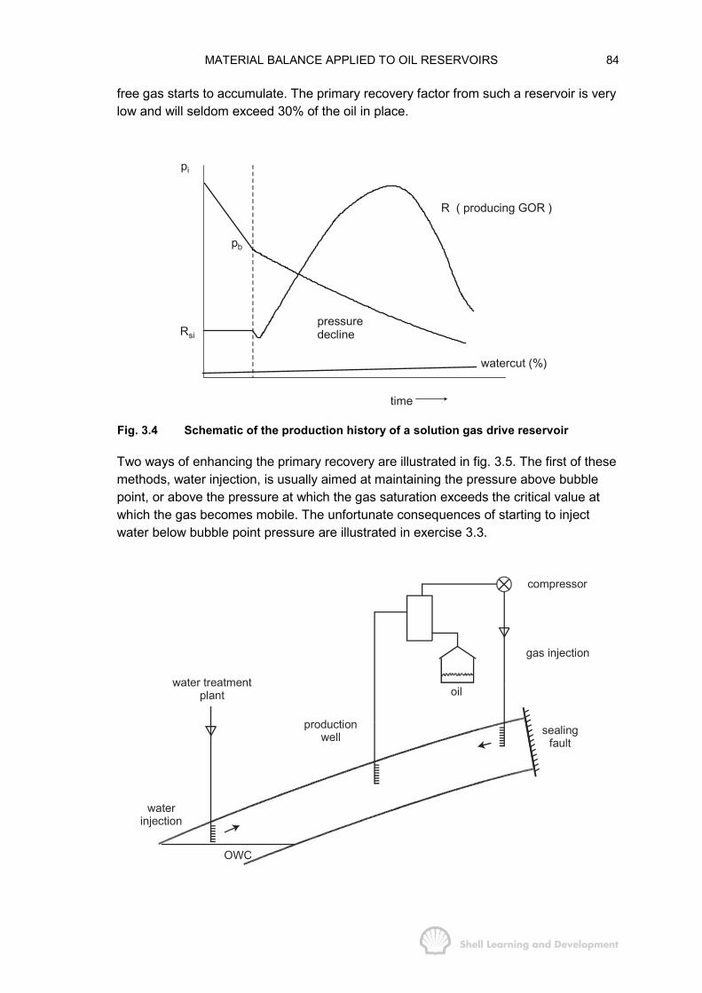
MATERIAL BALANCE APPLIED TO OIL RESERVOIRS 84
free gas starts to accumulate. The primary recovery factor from such a reservoir is verylow and will seldom exceed 30% of the oil in place.
pi
Rsi
pb
pressuredecline
R ( producing GOR )
time
watercut (%)
Fig. 3.4 Schematic of the production history of a solution gas drive reservoir
Two ways of enhancing the primary recovery are illustrated in fig. 3.5. The first of thesemethods, water injection, is usually aimed at maintaining the pressure above bubblepoint, or above the pressure at which the gas saturation exceeds the critical value atwhich the gas becomes mobile. The unfortunate consequences of starting to injectwater below bubble point pressure are illustrated in exercise 3.3.
water treatmentplant
waterinjection
OWC
productionwell
oil
compressor
gas injection
sealingfault
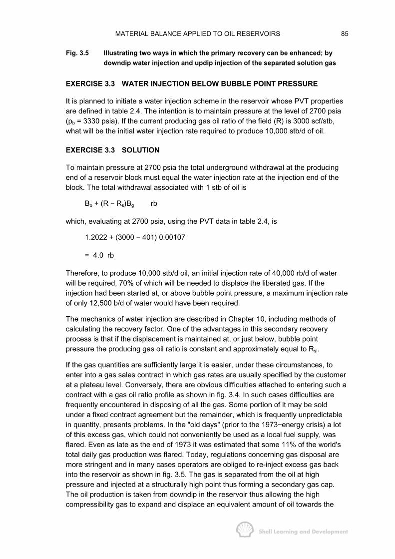
MATERIAL BALANCE APPLIED TO OIL RESERVOIRS 85
Fig. 3.5 Illustrating two ways in which the primary recovery can be enhanced; bydowndip water injection and updip injection of the separated solution gas
EXERCISE 3.3 WATER INJECTION BELOW BUBBLE POINT PRESSURE
It is planned to initiate a water injection scheme in the reservoir whose PVT propertiesare defined in table 2.4. The intention is to maintain pressure at the level of 2700 psia(pb = 3330 psia). If the current producing gas oil ratio of the field (R) is 3000 scf/stb,what will be the initial water injection rate required to produce 10,000 stb/d of oil.
EXERCISE 3.3 SOLUTION
To maintain pressure at 2700 psia the total underground withdrawal at the producingend of a reservoir block must equal the water injection rate at the injection end of theblock. The total withdrawal associated with 1 stb of oil is
Bo + (R − Rs)Bg rb
which, evaluating at 2700 psia, using the PVT data in table 2.4, is
1.2022 + (3000 − 401) 0.00107
= 4.0 rb
Therefore, to produce 10,000 stb/d oil, an initial injection rate of 40,000 rb/d of waterwill be required, 70% of which will be needed to displace the liberated gas. If theinjection had been started at, or above bubble point pressure, a maximum injection rateof only 12,500 b/d of water would have been required.
The mechanics of water injection are described in Chapter 10, including methods ofcalculating the recovery factor. One of the advantages in this secondary recoveryprocess is that if the displacement is maintained at, or just below, bubble pointpressure the producing gas oil ratio is constant and approximately equal to Rsi.
If the gas quantities are sufficiently large it is easier, under these circumstances, toenter into a gas sales contract in which gas rates are usually specified by the customerat a plateau level. Conversely, there are obvious difficulties attached to entering such acontract with a gas oil ratio profile as shown in fig. 3.4. In such cases difficulties arefrequently encountered in disposing of all the gas. Some portion of it may be soldunder a fixed contract agreement but the remainder, which is frequently unpredictablein quantity, presents problems. In the "old days" (prior to the 1973−energy crisis) a lotof this excess gas, which could not conveniently be used as a local fuel supply, wasflared. Even as late as the end of 1973 it was estimated that some 11% of the world'stotal daily gas production was flared. Today, regulations concerning gas disposal aremore stringent and in many cases operators are obliged to re-inject excess gas backinto the reservoir as shown in fig. 3.5. The gas is separated from the oil at highpressure and injected at a structurally high point thus forming a secondary gas cap.The oil production is taken from downdip in the reservoir thus allowing the highcompressibility gas to expand and displace an equivalent amount of oil towards the
MATERIAL BALANCE APPLIED TO OIL RESERVOIRS 86
producing wells. This demonstrates a method of keeping as much gas in the reservoiras possible where it can serve its most useful purpose, as suggested in exercise 3.2.
The economic success of both water and solution gas injection depends upon theadditional recovery obtained as a result of the projects. The present day value of theadditional oil recovery must be greater than the cost of the injection wells, surfacetreatment facilities (mainly for water) and compressor costs (mainly for gas). In manycases, for small reservoirs, injection of water or gas is not economically viable and thesolution gas drive process must be allowed to run its full course resulting in low oilrecovery factors.
3.6 GASCAP DRIVE
A typical gascap drive reservoir is shown in fig. 3.6. Under initial conditions the oil atthe gas oil contact must be at saturation or bubble point pressure. The oil furtherdowndip becomes progressively less saturated at the higher pressure andtemperature. Generally this effect is relatively small and reservoirs can be describedusing uniform PVT properties, as will be assumed in this text. There are exceptions,however, one of the most remarkable being the Brent field in the North Sea6 in which atthe gas oil contact the oil has a saturation pressure of 5750 psi and a solution gas oilratio of 2000 scf/stb, while at the oil water contact, some 500 feet deeper, thesaturation pressure and solution gas oil ratio are 4000 psi and 1200 scf/stb,respectively. Such extremes are rarely encountered and in the case of the Brent fieldthe anomaly is attributed to gravity segregation of the lighter hydrocarbon components.
For a reservoir in which gascap drive is the predominant mechanism it is still assumedthat the natural water influx is negligible (We = 0) and, in the presence of so much highcompressibility gas, that the effect of water and pore compressibilities is alsonegligible. Under these circumstances, the material balance equation, (3.7), can bewritten as
( )p o p s g
o oi si s g goi
oi gi
N B (R R )B
(B B ) (R R )B BNB m 1
B B
+ −
� �� �− + −= + −� �� �� �� � � �
(3.23)
in which the right hand side contains the term describing the expansion of the oil plusoriginally dissolved gas, since the solution gas drive mechanism is still active in the oilcolumn, together with the term for the expansion of the gascap gas. Equation (3.23) israther cumbersome and does not provide any kind of clear picture of the principlesinvolved in the gascap drive mechanism. A better understanding of the situation can begained by using the technique of Havlena and Odeh, described in sec. 3.3, for whichthe material balance, equ. (3.12), can be reduced to the form
F = N (Eo + mEg) (3.24)

MATERIAL BALANCE APPLIED TO OIL RESERVOIRS 87
production wells
OWC
GOCOIL ( NBoi - rb)
explorationwell
GAS ( mNBoi - rb)
Fig. 3.6 Typical gas drive reservoir
The way in which this equation can be used depends on the unknown quantities. For agascap reservoir the least certain parameter in equ. (3.24) is very often m, the ratio ofthe initial hydrocarbon pore volume of the gascap to that of the oil column. Forinstance, in the reservoir depicted in fig. 3.6, the exploration well penetrated thegascap establishing the level of the gas oil contact. Thereafter, no further wellspenetrated the gascap since it is not the intention to produce this gas but rather to let itexpand and displace oil towards the producing wells, which are spaced in rows furtherdowndip. As. a result there is uncertainty about the position of the sealing fault andhence in the value of m. The value of N, however, is fairly well defined from informationobtained from the producing wells. Under these circumstances the best way to interpretequ. (3.24) is to plot F as a function of (Eo + mEg) for an assumed value of m. If thecorrect value has been chosen then the resulting plot should be a straight line passingthrough the origin with slope N, as shown in fig. 3.7. If the value of m selected is toosmall or too large, the plot will deviate above or below the line, respectively.
In making this plot F can readily be calculated, at various times, as a function of theproduction terms Np and Rp, and the PVT parameters for the current pressure, thelatter being also required to determine Eo and Eg. Alternatively, if N is unknown and mknown with a greater degree of certainty, then N can be obtained as the slope of thestraight line.
One advantage of this particular interpretation is that the straight line must passthrough the origin which therefore acts as a control point.
EXERCISE 3.4 GASCAP DRIVE
The gascap reservoir shown in fig. 3.6 is estimated, from volumetric calculations, tohave had an initial oil volume N of 115 × 106 stb. The cumulative oil production
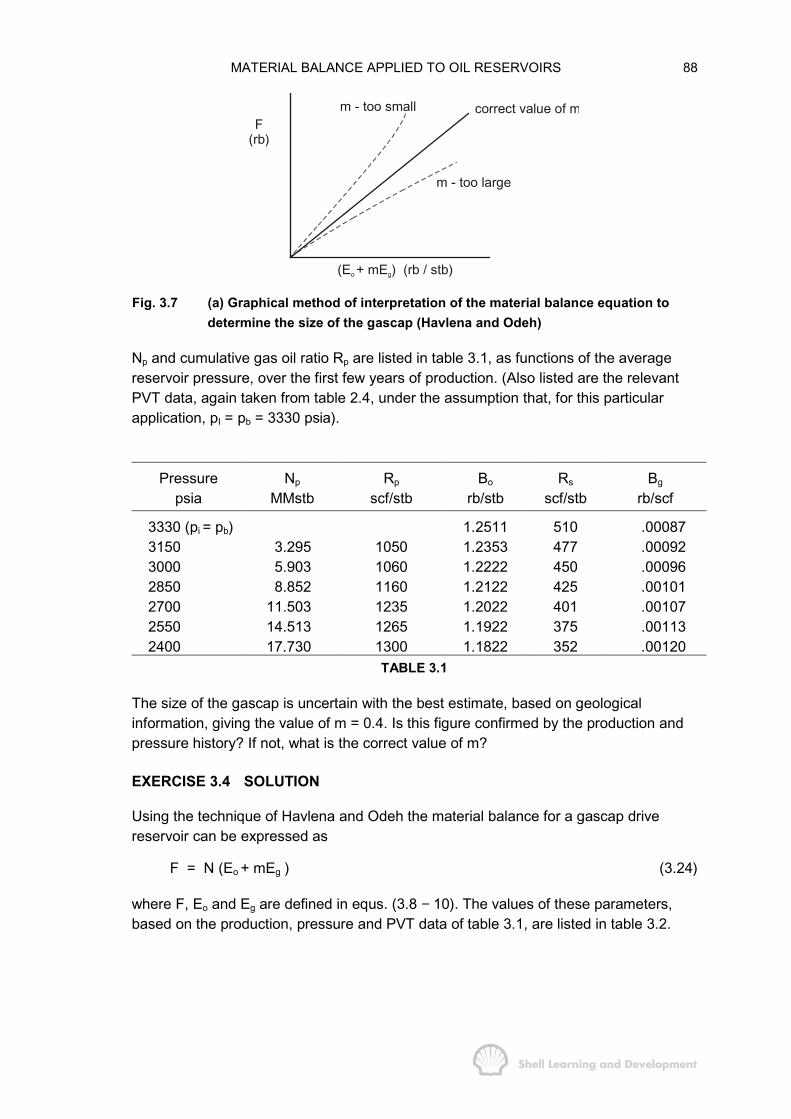
MATERIAL BALANCE APPLIED TO OIL RESERVOIRS 88
F(rb)
m - too small correct value of m
m - too large
(E + mE ) (rb / stb) o g
Fig. 3.7 (a) Graphical method of interpretation of the material balance equation todetermine the size of the gascap (Havlena and Odeh)
Np and cumulative gas oil ratio Rp are listed in table 3.1, as functions of the averagereservoir pressure, over the first few years of production. (Also listed are the relevantPVT data, again taken from table 2.4, under the assumption that, for this particularapplication, pI = pb = 3330 psia).
Pressurepsia
Np
MMstbRp
scf/stbBo
rb/stbRs
scf/stbBg
rb/scf
3330 (pi = pb) 1.2511 510 .000873150 3.295 1050 1.2353 477 .000923000 5.903 1060 1.2222 450 .000962850 8.852 1160 1.2122 425 .001012700 11.503 1235 1.2022 401 .001072550 14.513 1265 1.1922 375 .001132400 17.730 1300 1.1822 352 .00120
TABLE 3.1
The size of the gascap is uncertain with the best estimate, based on geologicalinformation, giving the value of m = 0.4. Is this figure confirmed by the production andpressure history? If not, what is the correct value of m?
EXERCISE 3.4 SOLUTION
Using the technique of Havlena and Odeh the material balance for a gascap drivereservoir can be expressed as
F = N (Eo + mEg ) (3.24)
where F, Eo and Eg are defined in equs. (3.8 − 10). The values of these parameters,based on the production, pressure and PVT data of table 3.1, are listed in table 3.2.
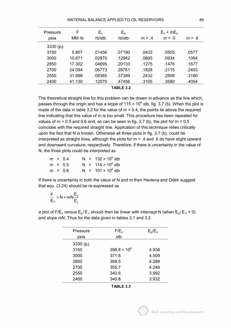
MATERIAL BALANCE APPLIED TO OIL RESERVOIRS 89
Pressurepsia
FMM rb
Eo
rb/stbEg
rb/stb m = .4Eo + mEg
m = .5 m = .6
3330 (pi)3150 5.807 .01456 .07190 .0433 .0505 .05773000 10.671 .02870 .12942 .0805 .0934 .10642850 17.302 .04695 .20133 .1275 .1476 .16772700 24.094 .06773 .28761 .1828 .2115 .24032550 31.898 .09365 .37389 .2432 .2806 .31802400 41.130 .12070 .47456 .3105 .3580 .4054
TABLE 3.2
The theoretical straight line for this problem can be drawn in advance as the line which,passes through the origin and has a slope of 115 × 106 stb, fig. 3.7 (b). When the plot ismade of the data in table 3.2 for the value of m = 0.4, the points lie above the requiredline indicating that this value of m is too small. This procedure has been repeated forvalues of m = 0.5 and 0.6 and, as can be seen in fig. 3.7 (b), the plot for m = 0.5coincides with the required straight line. Application of this technique relies criticallyupon the fact that N is known. Otherwise all three plots in fig. 3.7 (b), could beinterpreted as straight lines, although the plots for m = .4 and .6 do have slight upwardand downward curvature, respectively. Therefore, if there is uncertainty in the value ofN, the three plots could be interpreted as
m = 0.4 N = 132 × 106 stbm = 0.5 N = 114 × 106 stbm = 0.6 N = 101 × 106 stb
If there is uncertainty in both the value of N and m then Havlena and Odeh suggestthat equ. (3.24) should be re-expressed as
g
o o
EF N mNE E
= +
a plot of F/Eo versus Eg / E o should then be linear with intercept N (when Eg / E o = 0)and slope mN. Thus for the data given in tables 3.1 and 3.2
Pressurepsia
F/Eo
stbEg/Eo
3330 (pi)3150 398.8 × 10⁶ 4.9383000 371.8 4.5092850 368.5 4.2882700 355.7 4.2462550 340.6 3.9922400 340.8 3.932
TABLE 3.3

MATERIAL BALANCE APPLIED TO OIL RESERVOIRS 90
The plot of F/Eo versus Eg /E o is shown in fig. 3.7 (c), drawn over a limited range ofeach variable. The least squares fit for the six data points is the solid line which can beexpressed by the equation
g 6
o o
EF (108.9 58.8 ) 10 stbE E
= + ×
and therefore according to this interpretation
N = 108.9 × 10⁶ stb, and m = 0.54
F(MMrb)
40
30
2020
10
00 .1 .2 .3 .4
correct straight linefor N = 115 MMstb.
x m = .4o m = .5
m = .6�
(b)
(Eo + mEg) (rb / stb)
(c)
4.0 4.5 5.0
FEo
(MMstb)
400
350
300
Eg
Eo
F Eg Eo Eo
= (108.9 + 58.8 × 10⁶
Fig. 3.7 (b) and (c); alternative graphical methods for determining m and N(according to the technique of Havlena and Odeh)
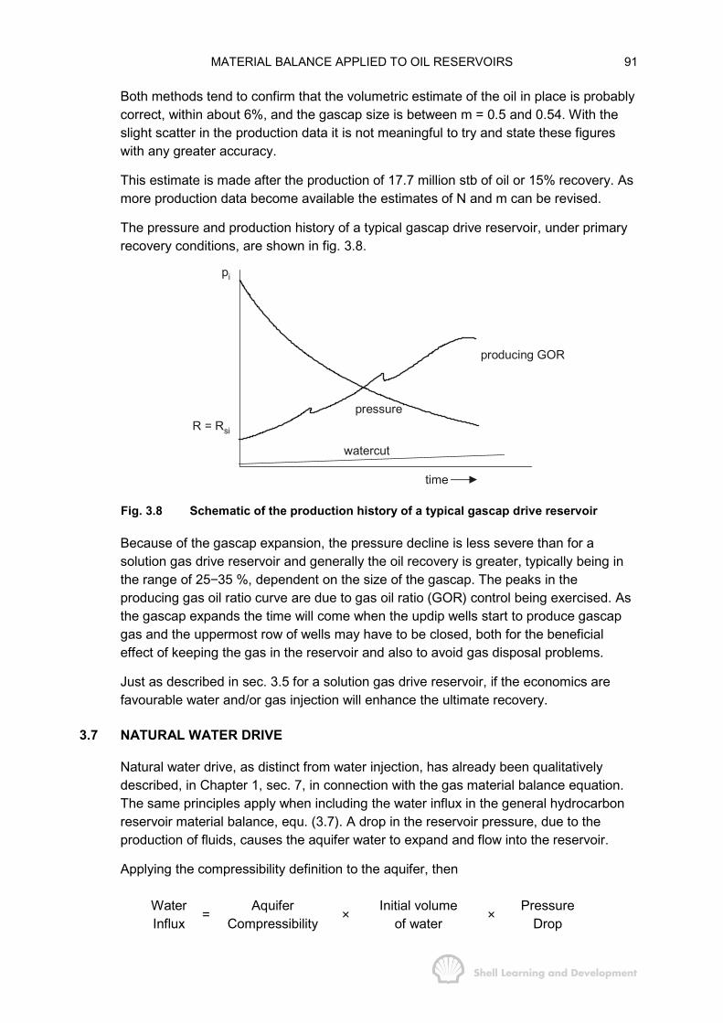
MATERIAL BALANCE APPLIED TO OIL RESERVOIRS 91
Both methods tend to confirm that the volumetric estimate of the oil in place is probablycorrect, within about 6%, and the gascap size is between m = 0.5 and 0.54. With theslight scatter in the production data it is not meaningful to try and state these figureswith any greater accuracy.
This estimate is made after the production of 17.7 million stb of oil or 15% recovery. Asmore production data become available the estimates of N and m can be revised.
The pressure and production history of a typical gascap drive reservoir, under primaryrecovery conditions, are shown in fig. 3.8.
pressure
watercut
time
pi
R = Rsi
producing GOR
Fig. 3.8 Schematic of the production history of a typical gascap drive reservoir
Because of the gascap expansion, the pressure decline is less severe than for asolution gas drive reservoir and generally the oil recovery is greater, typically being inthe range of 25−35 %, dependent on the size of the gascap. The peaks in theproducing gas oil ratio curve are due to gas oil ratio (GOR) control being exercised. Asthe gascap expands the time will come when the updip wells start to produce gascapgas and the uppermost row of wells may have to be closed, both for the beneficialeffect of keeping the gas in the reservoir and also to avoid gas disposal problems.
Just as described in sec. 3.5 for a solution gas drive reservoir, if the economics arefavourable water and/or gas injection will enhance the ultimate recovery.
3.7 NATURAL WATER DRIVE
Natural water drive, as distinct from water injection, has already been qualitativelydescribed, in Chapter 1, sec. 7, in connection with the gas material balance equation.The same principles apply when including the water influx in the general hydrocarbonreservoir material balance, equ. (3.7). A drop in the reservoir pressure, due to theproduction of fluids, causes the aquifer water to expand and flow into the reservoir.
Applying the compressibility definition to the aquifer, then
WaterInflux
= AquiferCompressibility
×Initial volume
of water×
PressureDrop
MATERIAL BALANCE APPLIED TO OIL RESERVOIRS 92
or
We = (cw+cf) Wi ∆p (3.25)
in which the total aquifer compressibility is the direct sum of the water and porecompressibilities since the pore space is entirely saturated with water. The sum of cw
and cf is usually very small, say 10-5/psi, therefore, unless the volume of water Wi isvery large the influx into the reservoir will be relatively small and its influence as a drivemechanism will be negligible. If the aquifer is large, however, equ. (3.25) will beinadequate to describe the water influx. This is because the equation implies that thepressure drop ∆p, which is in fact the pressure drop at the reservoir boundary, isinstantaneously transmitted throughout the aquifer. This will be a reasonableassumption only if the dimensions of the aquifer are of the same order of magnitude asthe reservoir itself. For a very large aquifer there will be a time lag between thepressure change in the reservoir and the full response of the aquifer. In this respectnatural water drive is time dependent. If the reservoir fluids are produced too quickly,the aquifer will never have a chance to "catch up" and therefore the water influx, andhence the degree of pressure maintenance, will be smaller than if the reservoir wereproduced at a lower rate. To account for this time dependence in water influxcalculations requires a knowledge of fluid flow equations and the subject will thereforebe deferred until Chapter 9, in which a full description of the phenomenon is provided.For the moment, the simple equation (3.25) will be used to illustrate the influence ofwater influx in the material balance.
Using the technique of Havlena and Odeh (assuming that Bw = 1), the full materialbalance can be expressed as
F = N (Eo + mEg + Ef,w) + We (3.12)
in which the term Ef,w, equ. (3.11), can frequently be neglected when dealing with awater influx. This is not only for the usual reason that the water and porecompressibilities are small but also because a water influx helps to maintain thereservoir pressure and therefore, the ∆p appearing in the Ef,w term is reduced.
This is a point which should be checked at the start of any material balance calculation(refer exercise 9.2). If, in addition, the reservoir has no initial gascap then equ. (3.12)can be reduced to
F = NEo + We (3.26)
In attempting to use this equation to match the production and pressure history of areservoir, the greatest uncertainty is always the determination of the water influx We. Infact, in order to calculate the influx the engineer is confronted with what is inherentlythe greatest uncertainty in the whole subject of reservoir engineering. The reason isthat the calculation of We requires a mathematical model which itself relies on theknowledge of aquifer properties. These, however, are seldom measured since wellsare not deliberately drilled into the aquifer to obtain such information. For instance,suppose the influx could be described using the simple model presented as equ.(3.25). Then, if the aquifer shape is radial, the water influx can be calculated as
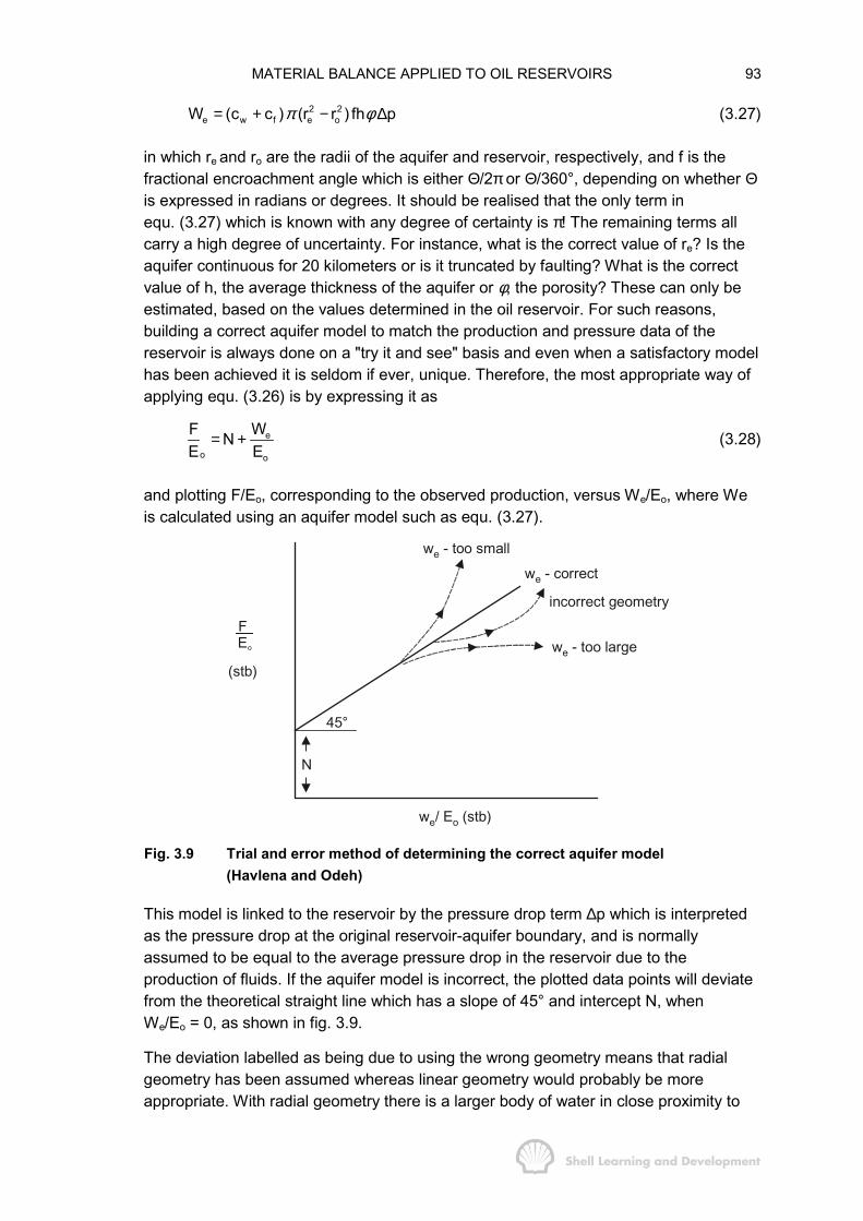
MATERIAL BALANCE APPLIED TO OIL RESERVOIRS 93
2 2e w f e oW (c c ) (r r ) fh pπ φ= + − ∆ (3.27)
in which re and ro are the radii of the aquifer and reservoir, respectively, and f is thefractional encroachment angle which is either Θ/2π or Θ/360°, depending on whether Θis expressed in radians or degrees. It should be realised that the only term inequ. (3.27) which is known with any degree of certainty is π! The remaining terms allcarry a high degree of uncertainty. For instance, what is the correct value of re? Is theaquifer continuous for 20 kilometers or is it truncated by faulting? What is the correctvalue of h, the average thickness of the aquifer or φ, the porosity? These can only beestimated, based on the values determined in the oil reservoir. For such reasons,building a correct aquifer model to match the production and pressure data of thereservoir is always done on a "try it and see" basis and even when a satisfactory modelhas been achieved it is seldom if ever, unique. Therefore, the most appropriate way ofapplying equ. (3.26) is by expressing it as
e
o o
WF NE E
= + (3.28)
and plotting F/Eo, corresponding to the observed production, versus We/Eo, where Weis calculated using an aquifer model such as equ. (3.27).
we/ Eo (stb)
we - too small
we - correct
we - too large
incorrect geometry
F E
(stb)
o
45°
N
Fig. 3.9 Trial and error method of determining the correct aquifer model(Havlena and Odeh)
This model is linked to the reservoir by the pressure drop term ∆p which is interpretedas the pressure drop at the original reservoir-aquifer boundary, and is normallyassumed to be equal to the average pressure drop in the reservoir due to theproduction of fluids. If the aquifer model is incorrect, the plotted data points will deviatefrom the theoretical straight line which has a slope of 45° and intercept N, whenWe/Eo = 0, as shown in fig. 3.9.
The deviation labelled as being due to using the wrong geometry means that radialgeometry has been assumed whereas linear geometry would probably be moreappropriate. With radial geometry there is a larger body of water in close proximity to

MATERIAL BALANCE APPLIED TO OIL RESERVOIRS 94
the reservoir, for the same aquifer volume, than for a linear aquifer and, as a result,response of the radial aquifer is greater causing deviation below the theoretical straightline. Exercise 9.2 provides an example of this technique in which the aquifer modelused for calculating We caters for time dependence.
Once a satisfactory aquifer model has been obtained by history matching, the samemodel can hopefully be used in predicting reservoir performance for any scheduledofftake policy. As already mentioned, however, there are so many uncertaintiesinvolved that the aquifer model is hardly ever unique and its validity should becontinually checked as fresh production and pressure data become available.
If the reservoir has a gascap then equ. (3.12) has the form
F = N (Eo + mEg) + We
which can alternatively be expressed as
e
o g o g
WF N(E mE ) (E mE )
= ++ +
(3.29)
in which it is assumed that both m and N are known.
By plotting F/(Eo + mEg) versus We / (Eo + mEg) the interpretation is similar to thatshown in fig 3.9.
Equation (3.29) demonstrates how the technique of Havlena and Odeh can be appliedto a combination drive reservoir in which there are three active mechanisms, solutiongas drive, gascap drive and water drive.
The pressure and production history of an undersaturated reservoir under active waterdrive are shown in fig. 3.10. The pressure decline is relatively small due to theexpansion of the aquifer water and from the producing gas oil ratio plot, it is evidentthat the pressure is being maintained above the saturation pressure. Recovery fromwater drive reservoirs can be very high, in excess of 50%, but just as in the case of theflooded out gas reservoir described in Chapter 1, sec. 7, residual oil will now betrapped behind the advancing water which can only be recovered by resorting to moreadvanced recovery methods, as described in Chapter 4, sec. 9.
pressure
watercut
time
pi
RsiGOR (R ≈ Rsi)

MATERIAL BALANCE APPLIED TO OIL RESERVOIRS 95
Fig. 3.10 Schematic of the production history of an undersaturated oil reservoir understrong natural water drive
3.8 COMPACTION DRIVE AND RELATED PORE COMPRESSIBILITY PHENOMENA
The withdrawal of liquid or gas from a reservoir results in a reduction in the fluidpressure and consequently an increase in the effective or grain pressure, the latterbeing defined in Chapter 1, sec. 3, as the difference between the overburden and fluidpressures. This increased pressure between the grains will cause the reservoir tocompact and this in turn can lead to subsidence at the surface.
Various studies7,8,9,10 have shown that compaction depends only upon the differencebetween the vertically applied stress (overburden) and the internal stress (fluidpressure) and therefore, compaction can conveniently be measured in the laboratoryby increasing the vertical stress on a rock sample while keeping the fluid pressure inthe pores constant.
If Vb is the bulk volume of a rock sample of thickness h, then the uniaxial compaction
∆Vb/Vb = ∆h/h
can best be determined in the laboratory using the triaxial compaction cell described byTeeuw11, which is shown in fig. 3.11 (a).
The core sample, which is completely saturated with water, is contained in a cell whichhas permeable cap and base plates and a cylindrical, flexible sleeve surrounding it.Vertical stress is applied by means of a piston while the fluid pressure in the pores ismaintained at one atmosphere. The pressure in the fluid surrounding the flexible sleevecan be increased independently so as to maintain the condition of
verticalstress
lateralstress sample
permeabledisc
elasticsleeve
A
B
grain pressure
h∆h
(b)(a)
Fig. 3.11 (a) Triaxial compaction cell (Teeuw); (b) typical compaction curve

MATERIAL BALANCE APPLIED TO OIL RESERVOIRS 96
zero lateral strain on the sample. This pressure is continually adjusted so that anychange in vertical thickness of the sample ∆h is uniformly related to the measuredwater expelled from the porous rock.
If such an experiment were performed on an uncompacted sample of sand and thecompaction ∆h/h plotted as a function of the applied vertical stress which, consideringthe fluid pressure is maintained at one atmosphere, is equivalent to the grain pressure,then the result would be as shown in fig. 3.11 (b). The slope of this curve, at any point,is
b fh / p c c
hφ∆ ∆ = ≈ refer equ. (1.37)
The characteristic shape of this compaction curve is intuitively what one would expect.At low grain pressures the compressibility of the uncompacted sample is very highsince it is relatively easy to effect a closer packing of the grains at this stage. As thegrain pressure increases, however, it becomes progressively more difficult to compactthe sample further and the compressibility decreases. What is clear from such anexperiment is that the bulk or pore compressibility of a reservoir is not constant but willcontinually change as fluids are withdrawn and the grain pressure increases.
Under normal hydrostatic conditions, since both the overburden and water pressuresincrease linearly with depth, then so too does the grain pressure which is the differencebetween the two. Thus a reservoir whose initial condition corresponds to point A willnormally be buried at shallow depth, while a reservoir corresponding to point B will beburied deeper.
Compaction drive is the expulsion of reservoir fluids due to the dynamic reduction ofthe pore volume and will only be significant as a drive mechanism if the porecompressibility cf is large. It therefore follows that such a drive mechanism will normallyonly provide a significant increase in the primary hydrocarbon recovery in shallowreservoirs. In parts of the Bachaquero field, Venezuela, as reported by Merle, et al12,the compaction drive mechanism accounts for more than 50% of total oil recovery. Thislarge reservoir dips between 1000−4000 ft. and has uniaxial compressibilities in excessof 100 × 10-6/psi.
If the mechanics of reservoir compaction were as simple as described above, it wouldappear possible to derive a relationship between uniaxial compressibility and depth, forvarious types of typical reservoir rock, in an attempt to apply such a correlationuniversally. Unfortunately, the process of compaction is frequently irreversible which inturn implies that in-situ compressibility cannot be estimated in such a simple manner.
If the reservoir rock consists of well cemented grains in a rigid rock frame then thecompaction, over a limited pressure range, will be approximately elastic and reversible.In loose unconsolidated sands, however, compaction is both inelastic and irreversiblesince upon each reloading cycle on such a sample, in a repeated loading experiment ina triaxial cell, it is possible for the individual grains to be packed in a differentconfiguration than on the previous cycle and, in addition, some of the grains can sufferpermanent mechanical deformation due to crushing. The effect of this inelastic
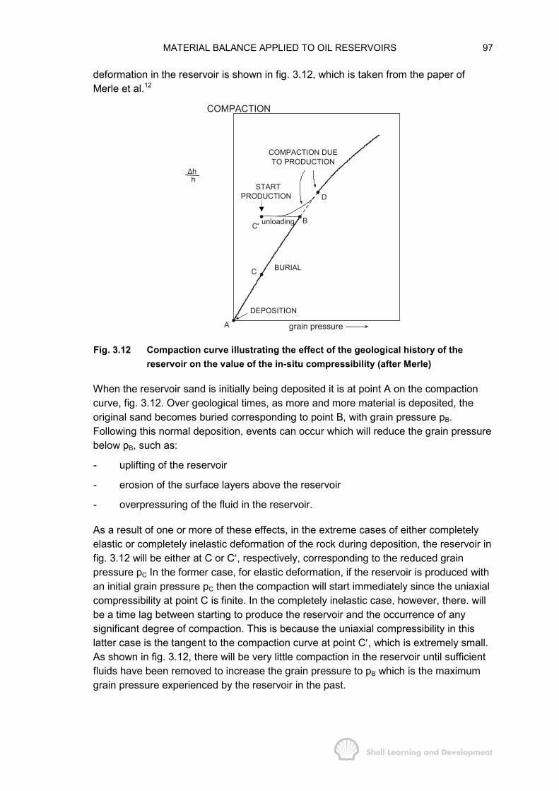
MATERIAL BALANCE APPLIED TO OIL RESERVOIRS 97
deformation in the reservoir is shown in fig. 3.12, which is taken from the paper ofMerle et al.12
COMPACTION
∆hh
unloading
COMPACTION DUETO PRODUCTION
STARTPRODUCTION
BURIAL
DEPOSITION
grain pressure
C
C′′′′
D
B
A
Fig. 3.12 Compaction curve illustrating the effect of the geological history of thereservoir on the value of the in-situ compressibility (after Merle)
When the reservoir sand is initially being deposited it is at point A on the compactioncurve, fig. 3.12. Over geological times, as more and more material is deposited, theoriginal sand becomes buried corresponding to point B, with grain pressure pB.Following this normal deposition, events can occur which will reduce the grain pressurebelow pB, such as:
- uplifting of the reservoir
- erosion of the surface layers above the reservoir
- overpressuring of the fluid in the reservoir.
As a result of one or more of these effects, in the extreme cases of either completelyelastic or completely inelastic deformation of the rock during deposition, the reservoir infig. 3.12 will be either at C or C′, respectively, corresponding to the reduced grainpressure pC In the former case, for elastic deformation, if the reservoir is produced withan initial grain pressure pC then the compaction will start immediately since the uniaxialcompressibility at point C is finite. In the completely inelastic case, however, there. willbe a time lag between starting to produce the reservoir and the occurrence of anysignificant degree of compaction. This is because the uniaxial compressibility in thislatter case is the tangent to the compaction curve at point C′, which is extremely small.As shown in fig. 3.12, there will be very little compaction in the reservoir until sufficientfluids have been removed to increase the grain pressure to pB which is the maximumgrain pressure experienced by the reservoir in the past.

MATERIAL BALANCE APPLIED TO OIL RESERVOIRS 98
Compaction, and its associated effect of surface subsidence, will be much morepronounced for shallow, unconsolidated reservoirs than for the deeper, morecompetent sands. It is therefore necessary to experimentally determine thecompressibility of shallow reservoir sands in order to estimate to what degreecompaction will enhance the hydrocarbon recovery, and also, to enable the predictionof the resulting surface subsidence, which can cause serious problems if the surfacelocation of the field is adjacent to the sea or a lake13.
Unfortunately, the deformation of unconsolidated sands is usually inelastic and this inturn leads to complications in relating laboratory measured compressibilities to the in-situ values in the reservoir. The nature of the problem can be appreciated by referringagain to fig. 3.12. Suppose that both the grain and fluid pressures in a reservoir arenormal so that under initial conditions the reservoir is at point B on the compactioncurve. The process of cutting a core and raising it to the surface will cause unloading,which for a rock which deforms inelastically, will place the core at point C′, which liesoff the normal compaction curve. During the re-loading the horizontal path B−C′ is notreversed, instead there is a mechanical hysteresis effect which means that the truecompaction curve is not re-joined until point D, where pD > pB. As a result, thelaboratory measured compressibility, determined as the slope of the line C′−D atpressure pB, will be somewhat lower than the in-situ value, which is the slope of thenormal curve at pB. Thus, initial values of the in-situ compressibility are difficult todetermine and usually require estimation by back extrapolation of laboratory valuesobtained for grain pressures in excess of pD.
The above description of the various complications in estimating in-situ, uniaxialcompressibility has been applied for the extreme case of a perfectly inelastic reservoirrock. Generally rock samples are neither perfectly elastic or inelastic but somewhere inbetween. Nevertheless, the same qualitative arguments apply and it is therefore notalways meaningful to merely estimate in-situ compressibilities by reference topublished charts for typical sandstones and limestones.
REFERENCES
1) Schilthuis, R.J., 1936. Active Oil and Reservoir Energy. Trans.,AIME, 118: 33-52.
2) Amyx, J.W., Bass, D.M., and Whiting, R.L., 1960. Petroleum ReservoirEngineering - Physical Properties. McGraw-Hill: 448-472.
3) McCain, W.D., 1973. The Properties of Petroleum Fluids. Petroleum PublishingCompany, Tulsa: 268-305.
4) Havlena, D. and Odeh, A.S., 1963. The Material Balance as an Equation of aStraight Line. J.Pet.Tech. August: 896-900. Trans., AIME, 228.
5) Havlena, D. and Odeh, A.S., 1964. The Material Balance as an Equation of aStraight Line. Part II - Field Cases. J.Pet.Tech. July: 815-822. Trans., AIME.,231.

MATERIAL BALANCE APPLIED TO OIL RESERVOIRS 99
6) Kingston, P.E. and Niko, H., 1975. Development Planning of the Brent Field.J.Pet. Tech. October: 1190-1198.
7) Geertsma, J., 1966. Problems of Rock Mechanics in Petroleum ProductionEngineering. Proc.,1st Cong. of the Intl. Soc. of Rock Mech., Lisbon. l, 585.
8) Geertsma, J., 1957. The Effect of Fluid Pressure Decline on Volumetric Changesof Porous Rocks. Trans., AIME, 210: 331-340.
9) van der Knaap, W., 1959. Non-linear Behaviour of Elastic Porous Media. Trans.,AIME, 216: 179-187.
10) Biot, M.A., 1941. General Theory of Three Dimensional Consolidation. J.Appl.Phys., Vol.12: 155.
11) Teeuw, D., 1971. Prediction of Formation Compaction from LaboratoryCompressibility Data. Soc. of Pet. Eng. J., September: 263-271.
12) Merle, H.A., Kentie, C.J.P., van Opstal, G.H.C. and Schneider, G.M.G., 1976.The Bachaquero Study - A Composite Analysis of the Behaviour of a CompactionDrive/ Solution Gas Drive Reservoir. J.Pet.Tech. September: 1107-1115.
13) Geertsma, J., 1973. Land Subsidence Above Compacting Reservoirs.J.Pet.Techn. June: 734-744.
CHAPTER 4
DARCY'S LAW AND APPLICATIONS
4.1 INTRODUCTION
Darcy's empirical flow law was the first extension of the principles of classical fluiddynamics to the flow of fluids through porous media. This chapter contains a simpledescription of the law based on experimental evidence. For a more detailed theoreticaltreatment of the subject, the reader is referred to the classical paper by King Hubbert1
in which it is shown that Darcy's law can be derived from the Navier-Stokes equation ofmotion of a viscous fluid.
The significance of Darcy's law is that it introduces flow rates into reservoir engineeringand, since the total surface oil production rate from a reservoir is
pres
dNq
dt=
it implicitly introduces a time scale in oil recovery calculations. The practical applicationof this aspect of Darcy's law is demonstrated in the latter parts of the chapter in which abrief description is given of the fundamental mechanics of well stimulation andenhanced oil recovery.
4.2 DARCY'S LAW; FLUID POTENTIAL
Every branch of science and engineering has its own particular heroes, one only has tothink, for example, of the hallowed names of Newton and Einstein in physics or Darwinin the natural sciences. In reservoir engineering, our equivalent is the nineteenthcentury French engineer Henry Darcy who, although he didn't realise it, has earnedhimself a special place in history as the first experimental reservoir engineer. In 1856Darcy published a detailed account of his work2 in improving the waterworks in Dijonand, in particular, on the design of a filter large enough to process the town's dailywater requirements. Although fluid dynamics was a fairly advanced subject in thosedays, there were no published accounts of the phenomenon of fluid flow through aporous medium and so, being a practical man, Darcy designed a filter, shownschematically in fig. 4.1, in an attempt to investigate the matter.
The equipment consisted of an iron cylinder containing an unconsolidated sand pack,about one metre in length, which was held between two permeable gauze screens.Manometers were connected into the cylinder immediately above and below the sandpack. By flowing water through the pack Darcy established that, for any flow rate, thevelocity of flow was directly proportional to the difference in manometric heights, therelationship being
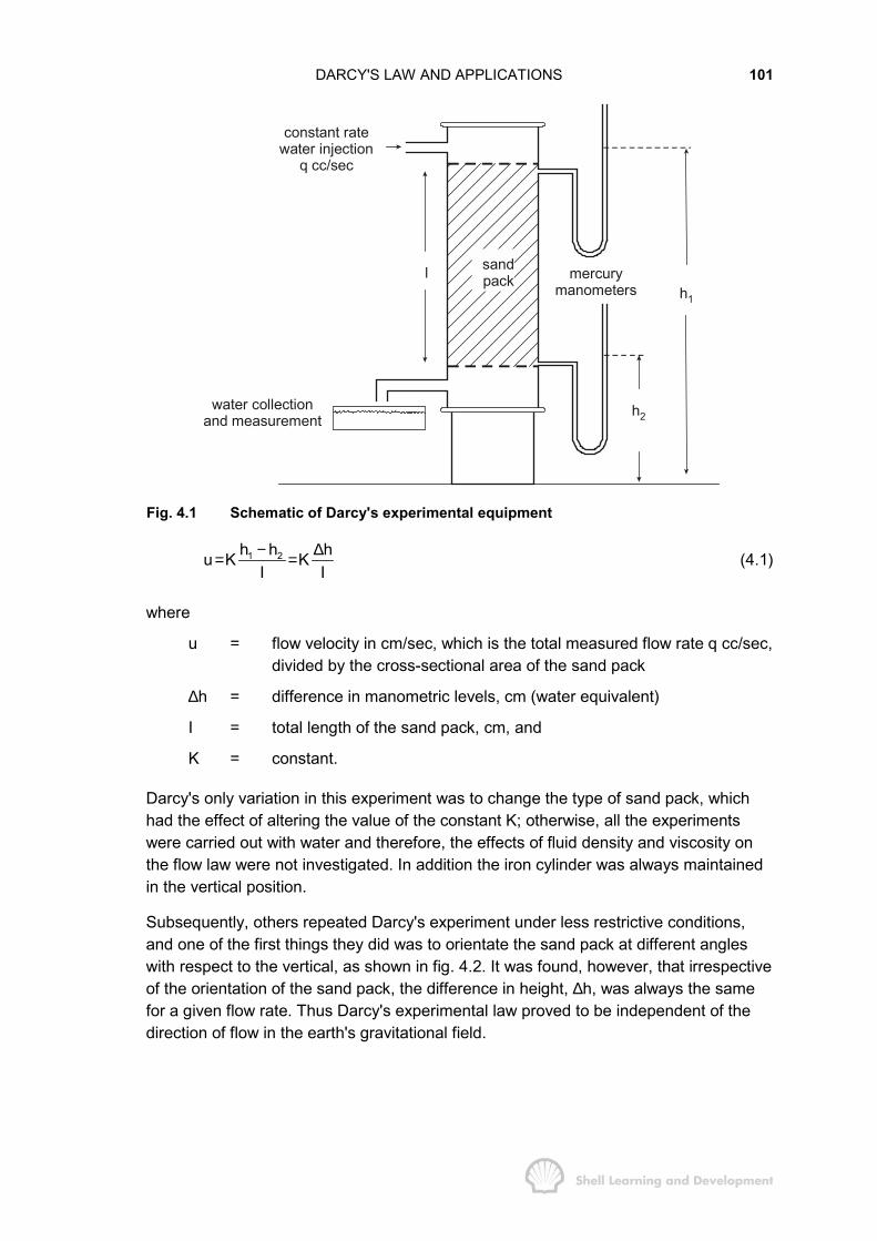
DARCY'S LAW AND APPLICATIONS 101
constant ratewater injection
q cc/sec
sand pack
water collectionand measurement
mercurymanometers h1
l
h2
Fig. 4.1 Schematic of Darcy's experimental equipment
1 2h h hu K KI I− ∆= = (4.1)
where
u = flow velocity in cm/sec, which is the total measured flow rate q cc/sec,divided by the cross-sectional area of the sand pack
∆h = difference in manometric levels, cm (water equivalent)
I = total length of the sand pack, cm, and
K = constant.
Darcy's only variation in this experiment was to change the type of sand pack, whichhad the effect of altering the value of the constant K; otherwise, all the experimentswere carried out with water and therefore, the effects of fluid density and viscosity onthe flow law were not investigated. In addition the iron cylinder was always maintainedin the vertical position.
Subsequently, others repeated Darcy's experiment under less restrictive conditions,and one of the first things they did was to orientate the sand pack at different angleswith respect to the vertical, as shown in fig. 4.2. It was found, however, that irrespectiveof the orientation of the sand pack, the difference in height, ∆h, was always the samefor a given flow rate. Thus Darcy's experimental law proved to be independent of thedirection of flow in the earth's gravitational field.
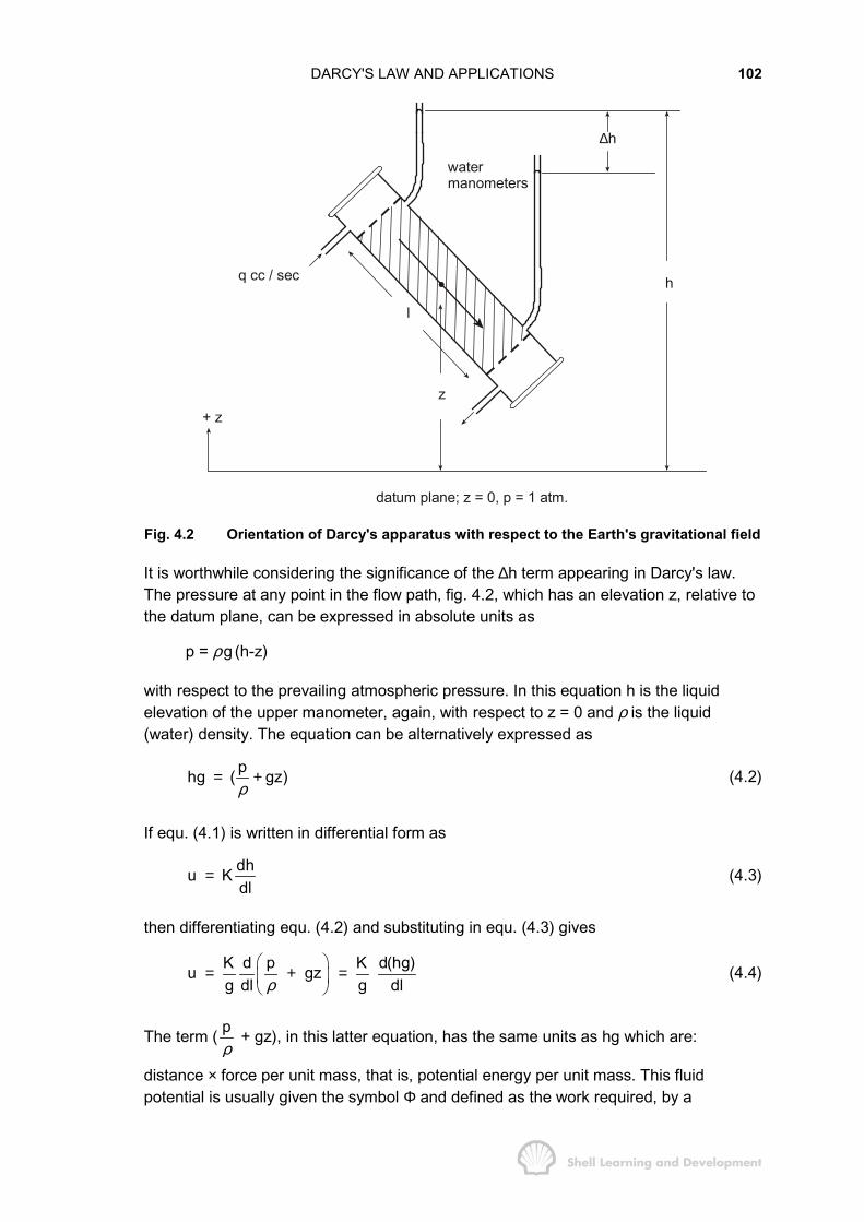
DARCY'S LAW AND APPLICATIONS 102
watermanometers
q cc / sec
+ zz
l
h
∆h
datum plane; z = 0, p = 1 atm.
Fig. 4.2 Orientation of Darcy's apparatus with respect to the Earth's gravitational field
It is worthwhile considering the significance of the ∆h term appearing in Darcy's law.The pressure at any point in the flow path, fig. 4.2, which has an elevation z, relative tothe datum plane, can be expressed in absolute units as
p = ρg (h-z)
with respect to the prevailing atmospheric pressure. In this equation h is the liquidelevation of the upper manometer, again, with respect to z = 0 and ρ is the liquid(water) density. The equation can be alternatively expressed as
phg ( gz)ρ
= + (4.2)
If equ. (4.1) is written in differential form as
dhu Kdl
= (4.3)
then differentiating equ. (4.2) and substituting in equ. (4.3) gives
K d p K d(hg)u gzg dl g dlρ
� �= + =� �
� �(4.4)
The term ( pρ
+ gz), in this latter equation, has the same units as hg which are:
distance × force per unit mass, that is, potential energy per unit mass. This fluidpotential is usually given the symbol Φ and defined as the work required, by a
DARCY'S LAW AND APPLICATIONS 103
frictionless process, to transport a unit mass of fluid from a state of atmosphericpressure and zero elevation to the point in question, thus
p
1 atm
dp gzρ−
Φ = +� (4.5)
Although defined in this way, fluid potentials are not always measured with respect toatmospheric pressure and zero elevation, but rather, with respect to any arbitrary basepressure and elevation (pb, zb ) which modifies equ. (4.5) to
b
p
bp
dp g(z z )ρ
Φ = + −� (4.6)
The reason for this is that fluid flow between two points A and B is governed by thedifference in potential between the points, not the absolute potentials, i.e.
A B A
b b B
p p p
A B A b B b A Bp p p
dp dp dpg(z z ) g(z z ) g(z z )ρ ρ ρ
Φ − Φ = + − − + − = + −� � �
It is therefore conventional, in reservoir engineering to select an arbitrary, convenientdatum plane, relative to the reservoir, and express all potentials with respect to thisplane. Furthermore, if it is assumed that the reservoir fluid is incompressible (ρindependent of pressure) then equ. (4.5) can be expressed as
p gzρ
Φ = + (4.7)
which is precisely the term appearing in equ. (4.4). It can therefore be seen that the hterm in Darcy's equation is directly proportional to the difference in fluid potentialbetween the ends of the sand pack.
The constant K/g is only applicable for the flow of water, which was the liquid usedexclusively in Darcy's experiments. Experiments performed with a variety of differentliquids revealed that the law can be generalised as
k dudl
ρµ
Φ= (4.8)
in which the dependence of flow velocity on fluid density ρ and viscosity µ is fairlyobvious. The new constant k has therefore been isolated as being solely dependent onthe nature of the sand and is described as the permeability. It is, in fact, the absolutepermeability of the sand, provided the latter is completely saturated with a fluid and,because of the manner of derivation, will have the same value irrespective of thenature of the fluid.
This latter statement is largely true, under normal reservoir pressures and flowconditions, the exception being for certain circumstances encountered in real gas flow.At very low pressures there is a slippage between the gas molecules and the walls of

DARCY'S LAW AND APPLICATIONS 104
each pore leading to an apparent increased permeability. This phenomenon, which iscalled the Klinkenberg effect3, seldom enters reservoir engineering calculations but isimportant in laboratory experiments in which, for convenience, rock permeabilities aredetermined by measuring air flow rates through core plugs at pressures close toatmospheric. This necessitates a correction to determine the absolute permeability4.
Due to its very low viscosity, the flow velocity of a real gas in a reservoir is muchgreater than for oil or water. In a limited region around the wellbore, where the pressuredrawdown is high, the gas velocity can become so large that Darcy's law does not fullydescribe the flow.5 This phenomenon, and the manner of its quantification in flowequations for gas, will be fully described in Chapter 8, sec. 6.
4.3 SIGN CONVENTION
Darcy's empirical law was described in the previous section without regard to signconvention, it being assumed that all terms in equ. (4.8) were positive. This is adequateif the law is being used independently to calculate flow rates; however, if equ. (4.8) isused in conjunction with other mathematical equations then, just as described inconnection with the definition of thermodynamic compressibility in Chapter 1, sec. 4,attention must be given to the matter of sign convention.
Linear flow
If distance is measured positive in the direction of flow, then the potential gradient dΦ/dlmust be negative in the same direction since fluids move from high to low potential.Therefore, Darcy's law is
k dudl
ρµ
Φ= − (4.9)
Radial flow
If production from the reservoir into the well is taken as positive, which is theconvention adopted in this book, then, since the radius is measured as being positive inthe direction opposite to the flow, dΦ/dr is positive and Darcy's law may be stated as
k dudr
ρµ
Φ= (4.10)
4.4 UNITS: UNITS CONVERSION
In any absolute set of units Darcy's equation for linear flow is
k dudl
ρµ
Φ= (4.9)
in which the various parameters have the following dimensions
u = L/T; ρ = M/L3; µ = M/LT; I = L and Φ (potential energy/unit mass) = L2/T2. Therefore,the following dimensional analysis performed on equ. (4.9):
DARCY'S LAW AND APPLICATIONS 105
[ ] [ ] [ ]3 2 2M/L L / TL k
T M/LT L
� � � �� � � �=
reveals that
[k] = [L2]
Thus the unit of permeability should be the cm2 in cgs units, or the metre2 in Sl units.
Both these units are impracticably large for the majority of reservoir rock, as will bedemonstrated in exercise 4.1, and therefore, a set of units was devised in which thepermeability would have a more convenient numerical size. These are the so-called"Darcy units" (refer table 4.1) in which the unit of permeability is the Darcy. The latterwas defined from the statement of Darcy's law for horizontal, linear flow of anincompressible fluid
k dpudlµ
= − (4.11)
such that k = 1 Darcy when u = 1 cm/sec; µ = 1 cp; and dp/dl = 1 atmosphere/cm.
Inspection of table 4.1 reveals that the units are a hybrid system based on the cgsunits. The only difference being that pressure is expressed in atmospheres, viscosity incp (centipoise) and, as a consequence, the permeability in Darcies. It was intended, indefining this system of units, that not only would the unit of permeability have areasonable numerical value but also, equations expressed in these units would havethe same form as equations in absolute units. That is, there would be no awkwardconstants involved in the equations other than multiples of π which reflect the geometryof the system. Unfortunately, this latter expectation is not always fulfilled because theDarcy, defined through the use of equ. (4.11), is based on an incomplete statement ofDarcy's law. Certainly, equ. (4.11) has the same form whether expressed in absolute orDarcy units but considering the general statement of the flow law, equ. (4.9), applied toan incompressible fluid (ρ ≈ constant), then
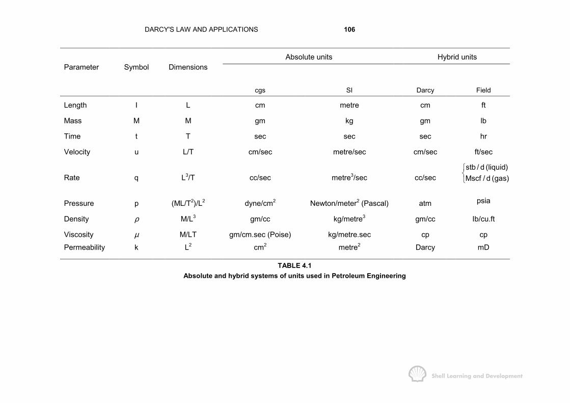
DARCY'S LAW AND APPLICATIONS 106
Absolute units Hybrid unitsParameter Symbol Dimensions
cgs SI Darcy Field
Length I L cm metre cm ft
Mass M M gm kg gm lb
Time t T sec sec sec hr
Velocity u L/T cm/sec metre/sec cm/sec ft/sec
Rate q L3/T cc/sec metre3/sec cc/sec
Pressure p (ML/T2)/L2 dyne/cm2 Newton/meter2 (Pascal) atm
stb / d (liquid)Mscf / d (gas)���
psia
Density ρ M/L3 gm/cc kg/metre3 gm/cc Ib/cu.ft
Viscosity µ M/LT gm/cm.sec (Poise) kg/metre.sec cp cp
Permeability k L2 cm2 metre2 Darcy mD
TABLE 4.1Absolute and hybrid systems of units used in Petroleum Engineering
DARCY'S LAW AND APPLICATIONS 107
k d k dp dzu gdl dl dl
ρ ρµ µ
Φ � �= = − +� �� �
� (4.12)
in absolute units, while
6k dp g dzu
dl dl1.0133 10ρ
µ� �
= − +� �×� �(4.13)
in Darcy units. The constant 1.0133 × 10⁶ is the number of dyne/cm2 in oneatmosphere and is required because both ρ and g have the same units in both the cgsand Darcy systems, and yet, the second term within the parenthesis of equ. (4.13)must have the same units as the first, namely, atm/cm.
In spite of this obvious drawback, reservoir engineers tend to work theoretically usingequations expressed in Darcy units. This practice will generally be adhered to in thistext and, in the remaining chapters, the majority of the theoretical arguments will bedeveloped with equations expressed in these units.
When dealing with the more practical aspects of reservoir engineering, such as welltest analysis described in Chapters 7 and 8, it is conventional to switch to what arecalled practical, or field units. The word practical is applied to such systems because allthe units employed are of a convenient magnitude. There are no rules governing fieldunits which therefore vary between countries and companies. The set of such unitspresented in table 4.1 is, however, probably the most widely accepted in the industry atthe time of writing this book.
Because of the wide variation in unit systems employed by the industry, it is veryimportant that reservoir engineers should be adept at converting equations expressedin Darcy units to the equivalent form in field units, or for that matter, any other set ofunits. There is a systematic approach in making such conversions which, if rigorouslyapplied, will exclude the possibility of error. Consider, as an example, the conversion ofequ. (4.11) from Darcy to field units. Since
q = u(cm/sec) × A(cm2)
the equation can be expressed in more practical form, in Darcy units, as2k(D) A(cm ) dpq(cc / sec) (atm / cm)
(cp) dlµ= − (4.14)
which, when converted to field units will have the form2k(mD) A(ft ) dpq(std / d) (constan t) (psi / ft)
(cp) dlµ= − (4.15)
in which the same symbols are used in both equations.
Making the conversion amounts to evaluating the constant in equ. (4.15) and this canbe achieved simply by remembering that equations must balance. Thus, if q in
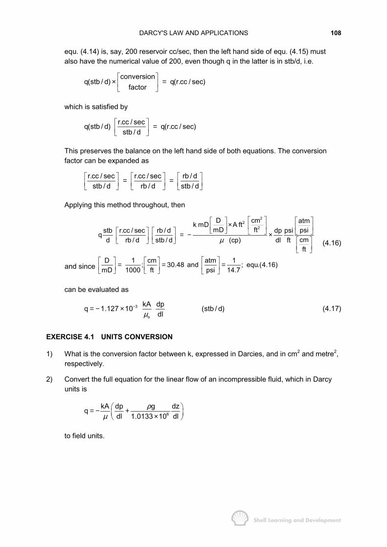
DARCY'S LAW AND APPLICATIONS 108
equ. (4.14) is, say, 200 reservoir cc/sec, then the left hand side of equ. (4.15) mustalso have the numerical value of 200, even though q in the latter is in stb/d, i.e.
conversionq(stb / d) q(r.cc / sec)
factor� �
× =� �� �
which is satisfied by
r.cc / secq(stb / d) q(r.cc / sec)stb / d
� � =� �� �
This preserves the balance on the left hand side of both equations. The conversionfactor can be expanded as
r.cc / sec r.cc / sec rb / dstb / d rb / d stb / d
� � � � � �= =� � � � � �� � � � � �
Applying this method throughout, then
and since
22
2D cm atmk mD A ft
mD ft psistb r.cc / sec rb / d dp psiqcmd rb / d stb / d (cp) dl ftft
D 1 cm atm 1; 30.48 and ; equ.(4.16)mD 1000 ft psi 14.7
µ
� � � �� �× � � � �� �� �� � � � � � � �= − ×� � � � � �� � � �� �� �
� �� � � �= = =� �� � � �� � � � � �
(4.16)
can be evaluated as
3
o
kA dpq 1.127 10 (stb / d)dlµ
−= − × (4.17)
EXERCISE 4.1 UNITS CONVERSION
1) What is the conversion factor between k, expressed in Darcies, and in cm2 and metre2,respectively.
2) Convert the full equation for the linear flow of an incompressible fluid, which in Darcyunits is
6kA dp g dzq
dl dl1.0133 10ρ
µ� �= − +� �×� �
to field units.
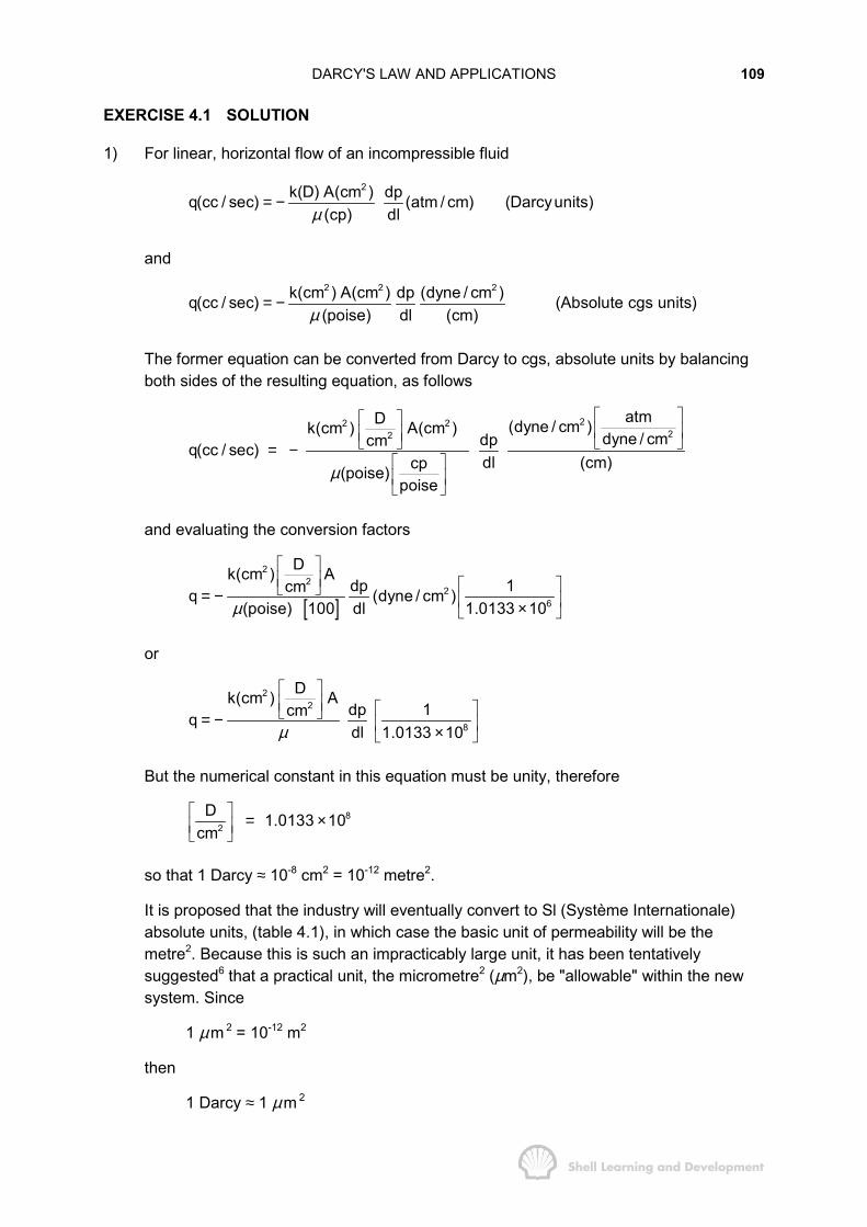
DARCY'S LAW AND APPLICATIONS 109
EXERCISE 4.1 SOLUTION
1) For linear, horizontal flow of an incompressible fluid
2k(D) A(cm ) dpq(cc / sec) (atm / cm) (Darcyunits)(cp) dlµ
= −
and2 2 2k(cm ) A(cm ) dp (dyne / cm )q(cc / sec) (Absolute cgs units)(poise) dl (cm)µ
= −
The former equation can be converted from Darcy to cgs, absolute units by balancingboth sides of the resulting equation, as follows
22 222
atmD (dyne / cm )k(cm ) A(cm ) dyne / cmdpcmq(cc / sec)dl (cm)cp(poise)
poiseµ
� �� �� �� �
� � � �= −� �� �� �
and evaluating the conversion factors
[ ]
22
26
Dk(cm ) Adp 1cmq (dyne / cm )
(poise) 100 dl 1.0133 10µ
� �� � � �� �= − � �×� �
or
22
8
Dk(cm ) Adp 1cmqdl 1.0133 10µ
� �� � � �� �= − � �×� �
But the numerical constant in this equation must be unity, therefore
82
D 1.0133 10cm� � = � �� �
so that 1 Darcy ≈ 10-8 cm2 = 10-12 metre2.
It is proposed that the industry will eventually convert to Sl (Système Internationale)absolute units, (table 4.1), in which case the basic unit of permeability will be themetre2. Because this is such an impracticably large unit, it has been tentativelysuggested6 that a practical unit, the micrometre2 (µm2), be "allowable" within the newsystem. Since
1 µm 2 = 10-12 m2
then
1 Darcy ≈ 1 µm 2
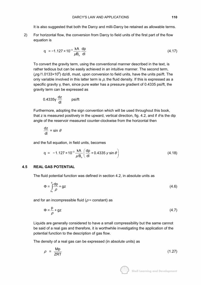
DARCY'S LAW AND APPLICATIONS 110
It is also suggested that both the Darcy and milli-Darcy be retained as allowable terms.
2) For horizontal flow, the conversion from Darcy to field units of the first part of the flowequation is
3
o
kA dpq 1.127 10B dlµ
−= − × (4.17)
To convert the gravity term, using the conventional manner described in the text, israther tedious but can be easily achieved in an intuitive manner. The second term,(ρg /1.0133×106) dz/dl, must, upon conversion to field units, have the units psi/ft. Theonly variable involved in this latter term is ρ, the fluid density. If this is expressed as aspecific gravity γ, then, since pure water has a pressure gradient of 0.4335 psi/ft, thegravity term can be expressed as
0.4335γ dzdl
psi/ft
Furthermore, adopting the sign convention which will be used throughout this book,that z is measured positively in the upward, vertical direction, fig. 4.2, and if θ is the dipangle of the reservoir measured counter-clockwise from the horizontal then
dzdl
= sin θ
and the full equation, in field units, becomes
3
o
kA dpq 1.127 10 0.4335 sinB dl
γ θµ
− � �= − × +� �� �
(4.18)
4.5 REAL GAS POTENTIAL
The fluid potential function was defined in section 4.2, in absolute units as
b
p
p
dp gzρ
Φ = +� (4.6)
and for an incompressible fluid (ρ ≈ constant) as
p gzρ
Φ = + (4.7)
Liquids are generally considered to have a small compressibility but the same cannotbe said of a real gas and therefore, it is worthwhile investigating the application of thepotential function to the description of gas flow.
The density of a real gas can be expressed (in absolute units) as
MpZRT
ρ = (1.27)
DARCY'S LAW AND APPLICATIONS 111
and substituting this in equ. (4.6) gives the real gas potential as
b
p
p
RT Zdp gzM p
Φ = +� (4.19)
But, since
RT Z dpd dp gdz gdzM p ρ
Φ = + = + (4.20)
then the gradient of the gas potential in the flow direction is simply
d 1 dp dzgdl dl dlρΦ = + (4.21)
and Darcy's equation for linear flow is again
k d k dp dzu gdl dl dl
ρ ρµ µ
Φ � �= − = − +� �� �
(4.12)
The above merely illustrates that real gas flow can be described using precisely thesame form of equations as for an incompressible liquid.
4.6 DATUM PRESSURES
An alternative way of expressing the potential of any fluid is
ψ = ρΦ = p + ρg z
where ψ is the psi-potential and has the units-potential per unit volume. Using thisfunction, Darcy's law becomes
kA d kA dqdl dl
ρ ψµ µ
Φ= − = − (4.22)
The ψ potential is also frequently referred to as the "datum pressure", since thefunction represents the pressure at any point in the reservoir referred to the datumplane, as illustrated in fig. 4.3.
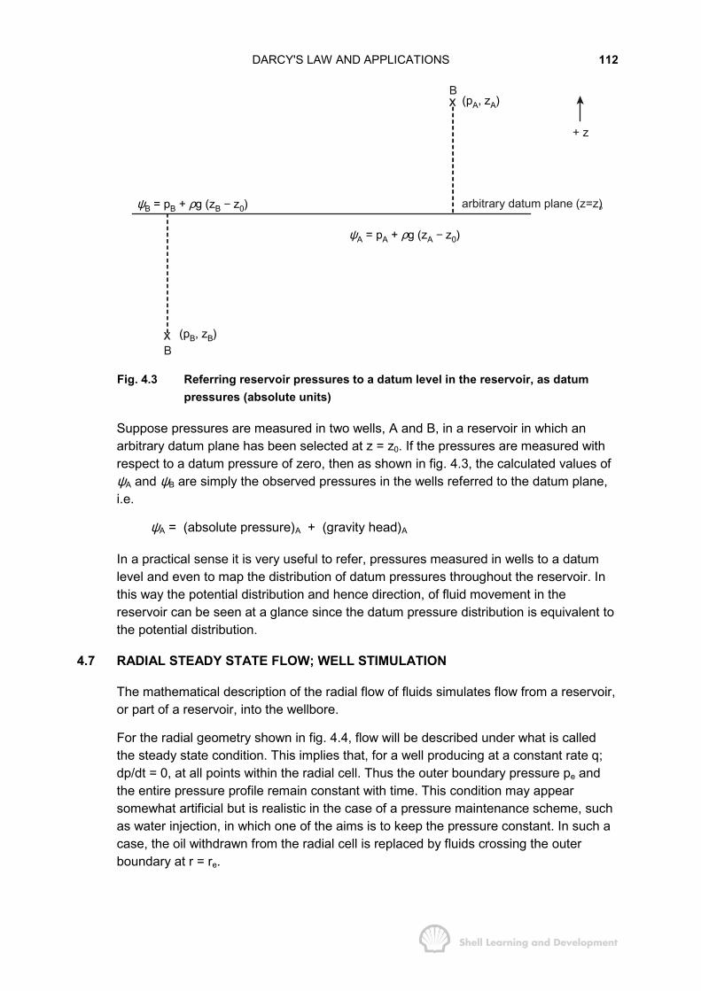
DARCY'S LAW AND APPLICATIONS 112
+ z
arbitrary datum plane (z=z)o
ψA = pA + ρg (zA − z0)
ψB = pB + ρg (zB − z0)
B(pB, zB)
B(pA, zA)
Fig. 4.3 Referring reservoir pressures to a datum level in the reservoir, as datumpressures (absolute units)
Suppose pressures are measured in two wells, A and B, in a reservoir in which anarbitrary datum plane has been selected at z = z0. If the pressures are measured withrespect to a datum pressure of zero, then as shown in fig. 4.3, the calculated values ofψA and ψB are simply the observed pressures in the wells referred to the datum plane,i.e.
ψA = (absolute pressure)A + (gravity head)A
In a practical sense it is very useful to refer, pressures measured in wells to a datumlevel and even to map the distribution of datum pressures throughout the reservoir. Inthis way the potential distribution and hence direction, of fluid movement in thereservoir can be seen at a glance since the datum pressure distribution is equivalent tothe potential distribution.
4.7 RADIAL STEADY STATE FLOW; WELL STIMULATION
The mathematical description of the radial flow of fluids simulates flow from a reservoir,or part of a reservoir, into the wellbore.
For the radial geometry shown in fig. 4.4, flow will be described under what is calledthe steady state condition. This implies that, for a well producing at a constant rate q;dp/dt = 0, at all points within the radial cell. Thus the outer boundary pressure pe andthe entire pressure profile remain constant with time. This condition may appearsomewhat artificial but is realistic in the case of a pressure maintenance scheme, suchas water injection, in which one of the aims is to keep the pressure constant. In such acase, the oil withdrawn from the radial cell is replaced by fluids crossing the outerboundary at r = re.
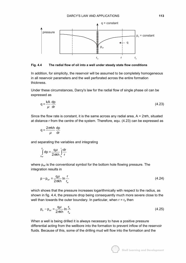
DARCY'S LAW AND APPLICATIONS 113
pressure
q = constant
rw rer
pwf
q
p = constante
Fig. 4.4 The radial flow of oil into a well under steady state flow conditions
In addition, for simplicity, the reservoir will be assumed to be completely homogeneousin all reservoir parameters and the well perforated across the entire formationthickness.
Under these circumstances, Darcy's law for the radial flow of single phase oil can beexpressed as
kA dpqdrµ
= (4.23)
Since the flow rate is constant, it is the same across any radial area, A = 2πrh, situatedat distance r from the centre of the system. Therefore, equ. (4.23) can be expressed as
2 rkh dpqdr
πµ
=
and separating the variables and integrating
wf w
p r
p r
q drdp2 kh r
µπ
=� �
where pwf is the conventional symbol for the bottom hole flowing pressure. Theintegration results in
wfw
q rp p ln2 kh r
µπ
− = (4.24)
which shows that the pressure increases logarithmically with respect to the radius, asshown in fig. 4.4, the pressure drop being consequently much more severe close to thewell than towards the outer boundary. In particular, when r = re then
ee wf
w
rqp p ln2 kh r
µπ
− = (4.25)
When a well is being drilled it is always necessary to have a positive pressuredifferential acting from the wellbore into the formation to prevent inflow of the reservoirfluids. Because of this, some of the drilling mud will flow into the formation and the

DARCY'S LAW AND APPLICATIONS 114
particles suspended in the mud can partially plug the pore spaces, reducing thepermeability, and creating a damaged zone in the vicinity of the wellbore.
The situation is shown in fig. 4.5, in which ra represents the radius of this zone. If
pressure
rw rera
pe
q
r
pskin∆
Fig. 4.5 Radial pressure profile for a damaged well
the well were undamaged, the pressure profile for r < ra would be as shown by thedashed line, whereas due to the reduction in permeability in the damaged zone,equ. (4.25) implies that the pressure drop will be larger than normal, or that pwf will bereduced. This additional pressure drop close to the well has been defined by vanEverdingen7 as
skinqp S
2 khµ
π∆ = (4.26)
in which the ∆pskin is attributed to a skin of reduced permeability around the well and Sis the mechanical skin factor, which is just a dimensionless number. This definition canbe included in equ. (4.25) to give the total steady state inflow equation as
ee wf
w
rqp p ln S2 kh r
µπ
� �− = +� �
� �(4.27)
in which it can be seen that if S is positive then pe - pwf the pressure drawdown,contains the additional pressure drop due to the perturbing effect of the skin.
Since equ. (4.27) is frequently employed by production engineers, it is useful toexpress it in field units rather than the Darcy units in which it was derived. The readershould check that this will give
o ee wf
w
q B rp p 141.2 In Skh rµ � �
− = +� �� �
(4.28)
in which the geometrical factor 2π has been absorbed in the constant. This equation isfrequently expressed as
DARCY'S LAW AND APPLICATIONS 115
e wf3
eo
w
q oil rate (stb / d)PIp p pressure drawdown (psi)
7.08 10 khrB ln Sr
µ
−
= =−
×=� �
+� �� �
(4.29)
where the PI, or Productivity Index of a well, expressed in stb/d/psi, is a direct measureof the well performance.
One of the aims of production engineering is to make the PI of each well as large as ispractically possible, consistent with the economics of doing so. This is termed wellstimulation. The ways in which a well can be stimulated can be deduced by consideringhow to vary the individual parameters in equ. (4.29) so as to increase the PI. Thevarious methods are summarised below.
a) Removal of Skin (S)
Before making any capital expenditure to remove a positive mechanical skin, it is firstnecessary to check that the formation has in fact been damaged during drilling. Thiscan best be done by performing a pressure buildup test, which is normally carried outas routine, immediately after completing the well. The manner in which S can becalculated in the analysis of such a test is detailed in Chapter 7. sec. 7.
If it is determined that S is positive, the formation damage can be reduced by acidtreatment. The type of acid used depends on the nature of the reservoir rock and thetype of plugging materials which must be removed. If the formation is limestone,treatment with hydrochloric acid will invariably remove the skin because of the solubilityof the rock itself. In sandstone reservoirs, in which the rock matrix is not soluble,special, so-called, mud acids are used. As a result of a successful acid job, the skinfactor can be reduced to zero or may even become negative.
b) Increasing the effective permeability (k)
As noted al ready, due to the logarithmic increase of pressure with radius, the mainpart of the pressure drawdown occurs close to the well. Therefore, if the effectivepermeability in this region of high drawdown can be increased, the productivity can beconsiderably enhanced. This can be achieved by hydraulic fracturing, in which highfluid pressures maintained in the wellbore will induce vertical fractures in the formation.Once the fractures have been initiated, they can be propagated deep into the formationby increasing the wellbore pressure and injecting a suitable fracturing fluid, carryinggranular propping agents. In carbonate reservoirs the same effect can be achieved byfracture-acidising.
c) Viscosity reduction (µ)
If the oil viscosity is very high, the flow rate in the reservoir will be correspondingly low,and the time scale attached to the recovery will be greatly extended. The viscosity canbe siginificantly reduced by raising the temperature of the oil, a typical viscosity-temperature relation being shown in fig. 4.6(a). The thermal stimulation process

DARCY'S LAW AND APPLICATIONS 116
applied to effect this viscosity reduction is steam soaking. Steam is injected into thereservoir and, in the simple model shown in fig. 4.6(b), extends to a radius rh, themagnitude of which is primarily a function of the amount of steam injected, usuallyseveral thousand tons, over a period of several days. During injection heat is lost in thewellbore and to the cap and base rock, but since steam is used, these losses arereflected as a reduction in latent heat and therefore take place without a significantchange of temperature.
150
0
hot zone
rw rh re
p
(b)
(a)
150 T (°F) 400
2 cp
µ (cp)
µ w
µ o
Fig. 4.6 (a) Typical oil and water viscosities as functions of temperature, and(b) pressure profile within the drainage radius of a steam soaked well
Following injection, the well is opened on production and the cold oil crossing into theheated annular region has its viscosity greatly reduced and consequently the PI isincreased. A typical steam soak production rate, in comparison to the unstimulatedrate, is shown in fig. 4.7. There is an initial surge in production followed by a steadydecline as the temperature in the hot zone is reduced, due to the continual loss of heatto the cap and base rock, as a function of time, and the removal of heat with theproduced fluids. When the production rate declines towards the unstimulated rate, thecycle is repeated.
steam soakproduction
unstimulated production
time (yrs)
oilrate
(stb/d)
1 2 3
100
10
Fig. 4.7 Oil production rate as a function of time during a multi-cycle steam soak

DARCY'S LAW AND APPLICATIONS 117
The flow equations during the initial and later part of a steam soak cycle will bedescribed in Chapter 9, sec. 6 and Chapter 6, sec. 4, respectively, since they serve asan interesting example of the flexibility of radial flow equations.
d) Reduction of the oil formation volume factor (Bo)
As already described in Chapter 2, sec. 4; Bo (rb/stb) can be minimised by choosingthe correct surface separator, or combination of separators.
e) Reduction in the ratio re / rw
Since re / rw appears as a logarithmic term, it has little influence on the PI and alterationof the ratio by, for instance, underreaming the wellbore to increase rw, is seldomconsidered as a means of well stimulation.
f) Increasing the well penetration (h)
It was assumed in deriving equ. (4.29) that the well was completed across the totalformation thickness and thus the flow was entirely radial. If the well is not fullypenetrating, there is a distortion of the radial flow pattern close to the well giving rise toan additional pressure drawdown. This is generally accounted for by using the fullformation thickness in equ. (4.29) and including the effect of partial penetration as anadditional skin factor. The method of calculating this additional skin is described inChapter 7, sec. 9. Increasing the well penetration, if possible, will obviously increasethe Pl but in many cases wells are deliberately completed over a restricted part of thereservoir to avoid excessive gas or water production from individual sands, or toprevent coning.
The methods for stimulating the production of a well, described in this section, do notnecessarily increase the ultimate oil recovery from the reservoir, but rather, reduce thetime in which the recovery is obtained. As such, they are generally regarded asacceleration projects which speed up the production, thus having a favourable effect onthe discounted cash flow.
There are exceptions. For instance, if a well has stopped producing, then anystimulation which results in oil production can be regarded as increasing the recovery.These methods, however, should be distinguished from the enhanced recoverytechniques, described in sec. 4.9, in which the reservoir is energised to increase therecovery. In stimulation there is frequently no net energy increase in the reservoir. Insteam soaking, for instance, heat energy is supplied to the reservoir and issubsequently lost during the production cycle; as opposed to continuous steam drive,in which the aim is to keep the steam in the reservoir thus increasing the total energy ofthe system.
4.8 TWO-PHASE FLOW: EFFECTIVE AND RELATIVE PERMEABILITIES
In describing Darcy's law, it has so far been assumed that the permeability is a rockproperty which is a constant, irrespective of the nature of the fluid flowing through thepores. This is correct (with the noted exception of gas flow either at low pressures orvery high rates) provided that the rock is completely saturated with the fluid in question,
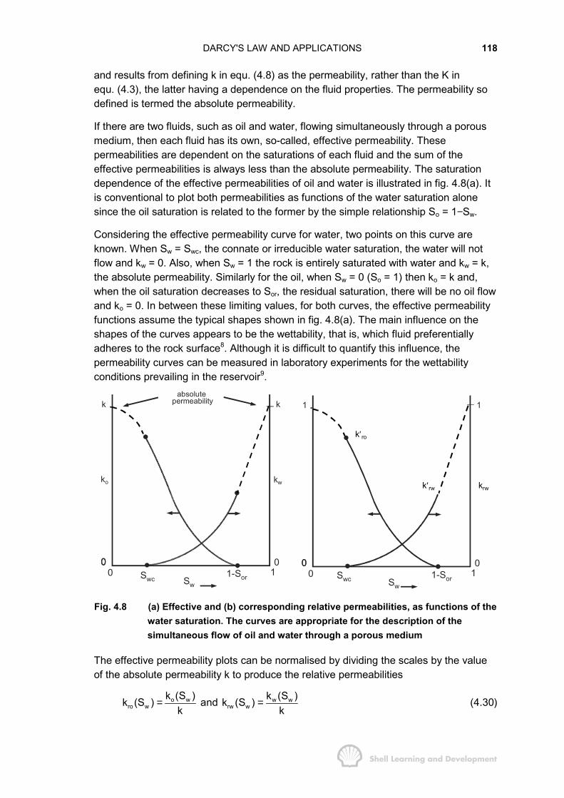
DARCY'S LAW AND APPLICATIONS 118
and results from defining k in equ. (4.8) as the permeability, rather than the K inequ. (4.3), the latter having a dependence on the fluid properties. The permeability sodefined is termed the absolute permeability.
If there are two fluids, such as oil and water, flowing simultaneously through a porousmedium, then each fluid has its own, so-called, effective permeability. Thesepermeabilities are dependent on the saturations of each fluid and the sum of theeffective permeabilities is always less than the absolute permeability. The saturationdependence of the effective permeabilities of oil and water is illustrated in fig. 4.8(a). Itis conventional to plot both permeabilities as functions of the water saturation alonesince the oil saturation is related to the former by the simple relationship So = 1−Sw.
Considering the effective permeability curve for water, two points on this curve areknown. When Sw = Swc, the connate or irreducible water saturation, the water will notflow and kw = 0. Also, when Sw = 1 the rock is entirely saturated with water and kw = k,the absolute permeability. Similarly for the oil, when Sw = 0 (So = 1) then ko = k and,when the oil saturation decreases to Sor, the residual saturation, there will be no oil flowand ko = 0. In between these limiting values, for both curves, the effective permeabilityfunctions assume the typical shapes shown in fig. 4.8(a). The main influence on theshapes of the curves appears to be the wettability, that is, which fluid preferentiallyadheres to the rock surface8. Although it is difficult to quantify this influence, thepermeability curves can be measured in laboratory experiments for the wettabilityconditions prevailing in the reservoir9.
000
01
1 1
000
01
absolute permeabilityk k
kw
1-Sor
k′ro
k′rw krw
Swc Sw
ko
1-SorSwc Sw
Fig. 4.8 (a) Effective and (b) corresponding relative permeabilities, as functions of thewater saturation. The curves are appropriate for the description of thesimultaneous flow of oil and water through a porous medium
The effective permeability plots can be normalised by dividing the scales by the valueof the absolute permeability k to produce the relative permeabilities
o w w wro w rw w
k (S ) k (S )k (S ) and k (S )k k
= = (4.30)

DARCY'S LAW AND APPLICATIONS 119
The plots of kro and krw, corresponding to the effective permeability plots of fig. 4.8(a),are drawn in fig. 4.8(b). Both sets of curves have precisely the same shape, the onlydifference being that the relative permeability scales have the range zero to unity.Relative permeabilities are used as a mathematical convenience since in a great manydisplacement calculations the ratio of effective permeabilities appears in the equations,which can be simplified as the ratio of
o w ro w ro w
w w rw w rw w
k (S ) k k (S ) k (S )k (S ) k k (S ) k (S )
×= =×
In figs. 4.8(a) and (b) the parts of the curves for water saturations below Sw = Swc andabove Sw = 1 - Sor are drawn as dashed lines because, although these sections of theplots can be determined in laboratory experiments, they will never be encountered influid displacement in the reservoir, since the practical range of water saturations is
Swc ≤ Sw ≤ 1—Sor
The maximum relative permeabilities to oil and water that can naturally occur duringdisplacement are called the end-point relative permeabilities and defined as(fig. 4.8(b)),
ro ro w wck k (at S S )′ = =
and
rw rw w ork k (at S 1 S )′ = = − (4.31)
Sometimes the effective permeability curves are normalised in a different manner thandescribed above, by dividing the scales of fig. 4.8(a) by the value of ko (Sw = Swc ) =k � rok′ , the maximum effective permeability to oil. The resulting curves are shown infig. 4.9.
S
1 1
K
000
0
ro Krw
SWC or1 SW
Fig. 4.9 Alternative manner of normalising the effective permeabilities to give relativepermeability curves
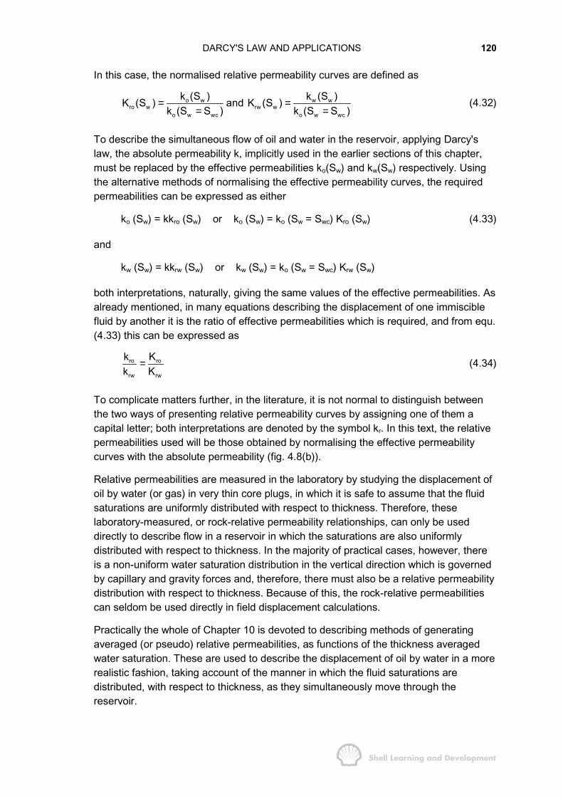
DARCY'S LAW AND APPLICATIONS 120
In this case, the normalised relative permeability curves are defined as
o w w wro w rw w
o w wc o w wc
k (S ) k (S )K (S ) and K (S )k (S S ) k (S S )
= == =
(4.32)
To describe the simultaneous flow of oil and water in the reservoir, applying Darcy'slaw, the absolute permeability k, implicitly used in the earlier sections of this chapter,must be replaced by the effective permeabilities ko(Sw) and kw(Sw) respectively. Usingthe alternative methods of normalising the effective permeability curves, the requiredpermeabilities can be expressed as either
ko (Sw) = kkro (Sw) or ko (Sw) = ko (Sw = Swc) Kro (Sw) (4.33)
and
kw (Sw) = kkrw (Sw) or kw (Sw) = ko (Sw = Swc) Krw (Sw)
both interpretations, naturally, giving the same values of the effective permeabilities. Asalready mentioned, in many equations describing the displacement of one immisciblefluid by another it is the ratio of effective permeabilities which is required, and from equ.(4.33) this can be expressed as
ro ro
rw rw
k Kk K
= (4.34)
To complicate matters further, in the literature, it is not normal to distinguish betweenthe two ways of presenting relative permeability curves by assigning one of them acapital letter; both interpretations are denoted by the symbol kr. In this text, the relativepermeabilities used will be those obtained by normalising the effective permeabilitycurves with the absolute permeability (fig. 4.8(b)).
Relative permeabilities are measured in the laboratory by studying the displacement ofoil by water (or gas) in very thin core plugs, in which it is safe to assume that the fluidsaturations are uniformly distributed with respect to thickness. Therefore, theselaboratory-measured, or rock-relative permeability relationships, can only be useddirectly to describe flow in a reservoir in which the saturations are also uniformlydistributed with respect to thickness. In the majority of practical cases, however, thereis a non-uniform water saturation distribution in the vertical direction which is governedby capillary and gravity forces and, therefore, there must also be a relative permeabilitydistribution with respect to thickness. Because of this, the rock-relative permeabilitiescan seldom be used directly in field displacement calculations.
Practically the whole of Chapter 10 is devoted to describing methods of generatingaveraged (or pseudo) relative permeabilities, as functions of the thickness averagedwater saturation. These are used to describe the displacement of oil by water in a morerealistic fashion, taking account of the manner in which the fluid saturations aredistributed, with respect to thickness, as they simultaneously move through thereservoir.
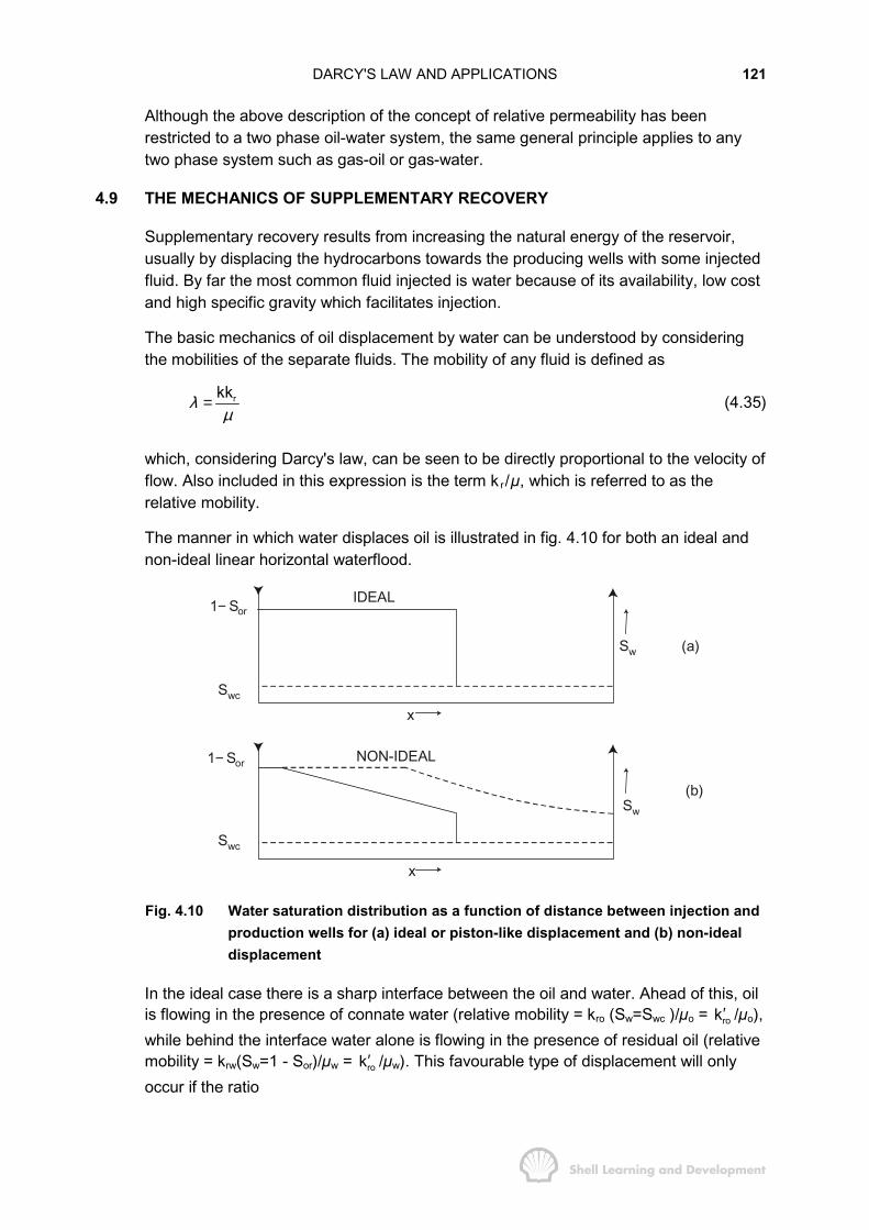
DARCY'S LAW AND APPLICATIONS 121
Although the above description of the concept of relative permeability has beenrestricted to a two phase oil-water system, the same general principle applies to anytwo phase system such as gas-oil or gas-water.
4.9 THE MECHANICS OF SUPPLEMENTARY RECOVERY
Supplementary recovery results from increasing the natural energy of the reservoir,usually by displacing the hydrocarbons towards the producing wells with some injectedfluid. By far the most common fluid injected is water because of its availability, low costand high specific gravity which facilitates injection.
The basic mechanics of oil displacement by water can be understood by consideringthe mobilities of the separate fluids. The mobility of any fluid is defined as
rkkλµ
= (4.35)
which, considering Darcy's law, can be seen to be directly proportional to the velocity offlow. Also included in this expression is the term kr/µ, which is referred to as therelative mobility.
The manner in which water displaces oil is illustrated in fig. 4.10 for both an ideal andnon-ideal linear horizontal waterflood.
IDEAL
x
x
NON-IDEAL
Sw
(a)
(b)
1− Sor
1− Sor
Swc
Swc
Sw
Fig. 4.10 Water saturation distribution as a function of distance between injection andproduction wells for (a) ideal or piston-like displacement and (b) non-idealdisplacement
In the ideal case there is a sharp interface between the oil and water. Ahead of this, oilis flowing in the presence of connate water (relative mobility = kro (Sw=Swc )/µo = rok′ /µo),while behind the interface water alone is flowing in the presence of residual oil (relativemobility = krw(Sw=1 - Sor)/µw = rok′ /µw). This favourable type of displacement will onlyoccur if the ratio
DARCY'S LAW AND APPLICATIONS 122
rw w
ro o
k / M 1k /
µµ
′= ≤
′
where M is known as the end point mobility ratio and, since both and rok′ are rwk′ the endpoint relative permeabilities, is a constant. If M ≤ 1 it means that, under an imposedpressure differential, the oil is capable of travelling with a velocity equal to, or greaterthan, that of the water. Since it is the water which is pushing the oil, there is therefore,no tendency for the oil to be by-passed which results in the sharp interface betweenthe fluids.
The displacement shown in fig. 4.10(a) is, for obvious reasons, called "piston-likedisplacement". Its most attractive feature is that the total amount of oil that can berecovered from a linear reservoir block will be obtained by the injection of the samevolume of water. This is called the movable oil volume where,
1 (MOV) = PV(1 – Sor − Swc)
The non-ideal displacement depicted in fig. 4.10(b), which unfortunately is morecommon in nature, occurs when M > 1. In this case, the water is capable of travellingfaster than the oil and, as the water pushes the oil through the reservoir, the latter willbe by-passed. Water tongues develop leading to the unfavourable water saturationprofile.
Ahead of the water front oil is again flowing in the presence of connate water. This isfollowed, in many cases, by a waterflood front, or shock front, in which there is adiscontinuity in the water saturation. There is then a gradual transition between theshock front saturation and the maximum saturation Sw = 1−Sor. The dashed line infig. 4.10(b) depicts the saturation distribution at the time when the shock front breaksthrough into the producing well (breakthrough). In contrast to the piston-likedisplacement, not all of the movable oil will have been recovered at this time. As morewater is injected, the plane of maximum water saturation (Sw = 1−Sor) will move slowlythrough the reservoir until it reaches the producing well at which time the movable oilvolume has been recovered. Unfortunately, in typical cases it may take five or sixMOV's of injected water to displace the one MOV of oil (as will be demonstrated inexercises 10.2 and 10.3 of Chapter 10). At a constant rate of water injection, the factthat much more water must be injected, in the unfavourable case, protracts the timescale attached to the oil recovery and this is economically unfavourable. In addition,pockets of by-passed oil are created which may never be recovered.
Mobility control
If the end point mobility ratio for water displacing oil is unfavourable, the injectionproject can be engineered to overcome this difficulty. The manner in which this is donecan be appreciated by considering the general expression
rd d
ro o
k /Mobility of the displacing fluidMMobility of the displaced fluid k /
µµ
′= =
′(4.36)

DARCY'S LAW AND APPLICATIONS 123
where the subscript "d" refers to the displacing fluid, which need not necessarily bewater. To improve the displacement efficiency, M should be reduced to a value of unityor less which will have the effect of converting the displacement from the type shown infig. 4.10(b), to the ideal type shown in fig. 4.10(a); this is referred to as "mobilitycontrol". The methods by which M can be reduced are.
Polymer flooding (increase, µd)
Polymers, such as polysaccharide, are dissolved in the injection water, this raises itsviscosity, thus reducing the mobility of the water. Polymer flooding will not onlyaccelerate the oil recovery but can also increase it, in comparison to a normal waterdrive, because the by-passing of oil is greatly reduced.
Thermal methods (decrease, µo/µd)
For very viscous crudes the ratio of µo / µd can be of the order of thousands (whichmeans that M has the same order of magnitude) and therefore, water drive cannot beconsidered as a feasible project (refer Chapter 10, exercise 10.1). In such cases theviscosity ratio can be drastically reduced by increasing the temperature, as shown infig. 4.6(a). This is achieved by one of the following methods:
- hot water injection- steam injection- in-situ combustion.
Although mobility control is the primary aim in applying thermal methods, there areother factors involved than merely the reduction of, µo / µd (where in this case, µd is theviscosity of the hot water or steam and differs from µw at normal reservoir temperature).In many cases distillation of the crude occurs, the lighter fractions of the oil beingvapourised and providing a miscible flood in advance of the thermal front. Expansion ofthe oil on heating will also add to the recovery. Thermal methods can therefore beconsidered as basically secondary recovery processes with some tertiary side effects,such as the crude distillation, which tends to reduce the residual oil saturation.
Tertiary flooding
Tertiary flooding aims at recovering the oil remaining in the reservoir after aconventional secondary recovery project, such as a water drive. Oil and water areimmiscible (do not mix) and as a result there is a finite surface tension at the interfacebetween the fluids. This, in turn, leads to the trapping of oil droplets within eachseparate pore which is the normal state after a waterflood.
From a strictly mechanical point of view, the methods commonly employed in tertiaryflooding can be appreciated by considering fig. 4.11, which shows an enlargement ofan oil relative permeability curve (solid line) for water-oil displacement, in the vicinity ofthe residual oil saturation point. After a water drive kro is zero when So = Sor, point A,and the oil will not flow.
Two possibilities for improving the situation are indicated which amount to altering theoil relative permeability characteristics. The first of these is to displace the oil with a
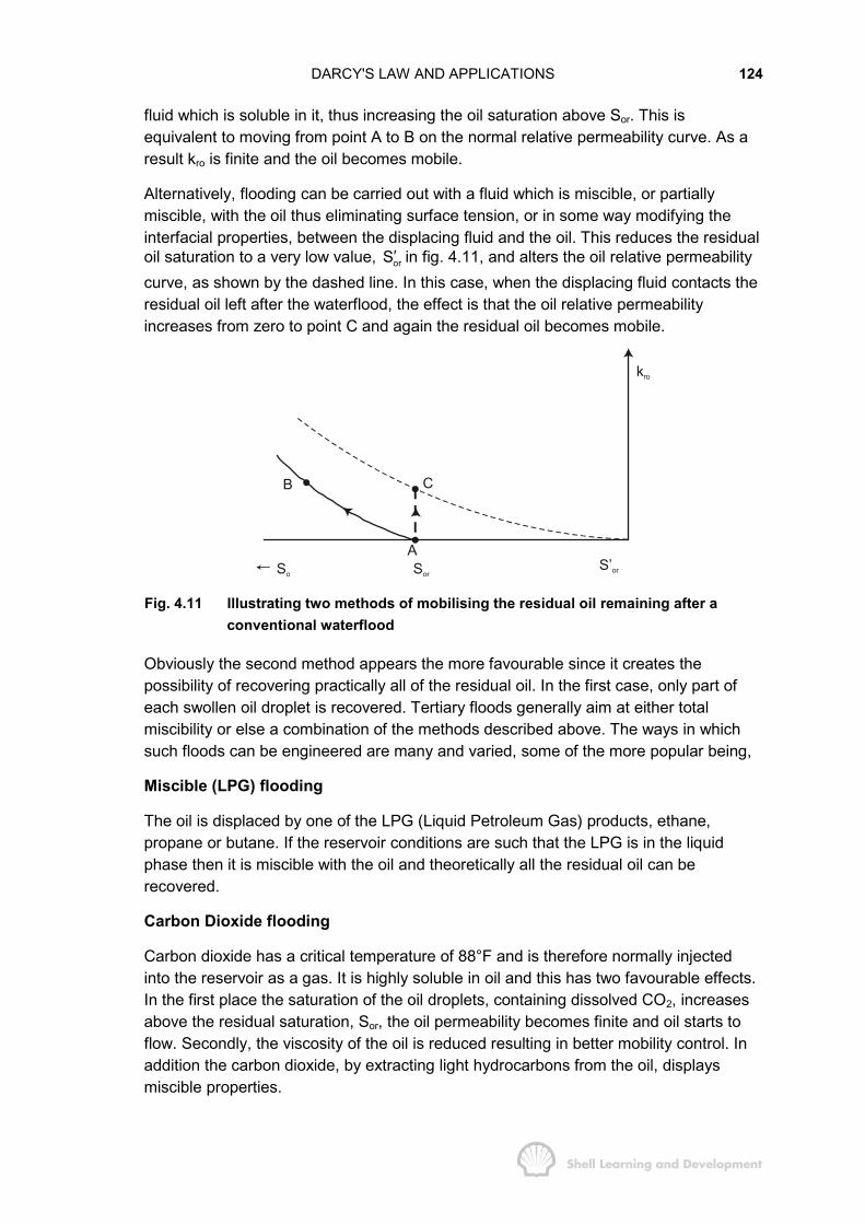
DARCY'S LAW AND APPLICATIONS 124
fluid which is soluble in it, thus increasing the oil saturation above Sor. This isequivalent to moving from point A to B on the normal relative permeability curve. As aresult kro is finite and the oil becomes mobile.
Alternatively, flooding can be carried out with a fluid which is miscible, or partiallymiscible, with the oil thus eliminating surface tension, or in some way modifying theinterfacial properties, between the displacing fluid and the oil. This reduces the residualoil saturation to a very low value, orS′ in fig. 4.11, and alters the oil relative permeabilitycurve, as shown by the dashed line. In this case, when the displacing fluid contacts theresidual oil left after the waterflood, the effect is that the oil relative permeabilityincreases from zero to point C and again the residual oil becomes mobile.
B
A
C
So SorS’or
kro
Fig. 4.11 Illustrating two methods of mobilising the residual oil remaining after aconventional waterflood
Obviously the second method appears the more favourable since it creates thepossibility of recovering practically all of the residual oil. In the first case, only part ofeach swollen oil droplet is recovered. Tertiary floods generally aim at either totalmiscibility or else a combination of the methods described above. The ways in whichsuch floods can be engineered are many and varied, some of the more popular being,
Miscible (LPG) flooding
The oil is displaced by one of the LPG (Liquid Petroleum Gas) products, ethane,propane or butane. If the reservoir conditions are such that the LPG is in the liquidphase then it is miscible with the oil and theoretically all the residual oil can berecovered.
Carbon Dioxide flooding
Carbon dioxide has a critical temperature of 88°F and is therefore normally injectedinto the reservoir as a gas. It is highly soluble in oil and this has two favourable effects.In the first place the saturation of the oil droplets, containing dissolved CO2, increasesabove the residual saturation, Sor, the oil permeability becomes finite and oil starts toflow. Secondly, the viscosity of the oil is reduced resulting in better mobility control. Inaddition the carbon dioxide, by extracting light hydrocarbons from the oil, displaysmiscible properties.
DARCY'S LAW AND APPLICATIONS 125
Surfactant flooding (Micellar Solution flooding)
Surfactants, or surface acting agents, when dissolved in minute quantities in waterhave a significant influence on the interfacial properties between the water and oilwhich it is displacing. The surfactant dissolves in the residual oil droplets thus raisingthe saturation above the residual level and, in addition, the surface tension betweenthese enlarged oil droplets and the displacing water is very significantly reduced. Boththese effects are active in reducing the residual oil saturation and, in laboratory tests,ninety percent residual oil recovery has been observed. The surfactants mostcommonly used by the industry are petroleum sulphonates.
The above description of tertiary recovery mechanisms hardly "scratches the surface"of the subject. For an excellent, simplified description the reader is referred to the set ofpapers by Herbeck, Heintz and Hastings10, which cover all aspects of the subjectincluding the vitally important economic considerations.
The above methods are described as tertiary in that they are capable of recoveringsome, if not all, of the residual oil remaining after a waterflood. This does not mean,however, that they must be preceded by a waterflood. Instead, the two can beconducted simultaneously. In all tertiary recovery schemes, continuous injection of theexpensive agents is unnecessary. The fluids are injected in batches and frequently thebatches are followed by mobility buffers. For instance, to ensure stable displacement ina surfactant flood, the chemical slug can be displaced by water thickened with apolymer, the concentration of which is gradually decreased as the flood proceeds.
REFERENCES
1) King Hubbert, M., 1956. Darcy's Law and the Field Equations of the Flow ofUnderground Fluids. Trans. AIME, 207: 222-239.
2) Darcy, H., 1856. Les Fontaines Publiques de la Ville de Dijon. Victor Dalmont,Paris.
3) Klinkenberg, L.J., 1941. The Permeability of Porous Media to Liquids and Gases.API Drill. and Prod. Prac.: 200.
4) Cole, F.W., 1961. Reservoir Engineering Manual. Gulf Publishing Co., Houston,Texas: 19-20.
5) Geertsma, J., 1974. Estimating the Coefficient of Inertial Resistance in Fluid FlowThrough Porous Media. Soc.Pet.Eng.J., October: 445-450.
6) Campbell, J.M., 1976. Report on Tentative SPE Metrication Standards. Paperpresented to the 51st Annual Fall Conference of the AIME, New Orleans,October.
7) van Everdingen, A.F., 1953. The Skin Effect and Its Impediment to Fluid Flowinto a Wellbore. Trans. AIME, 198: 171-176.
8) Craig, F.F., Jr., 1971. The Reservoir Engineering Aspects of Waterflooding. SPEMonograph:

DARCY'S LAW AND APPLICATIONS 126
9) Amyx, J.W., Bass, D.M. and Whiting, R. L., 1960. Petroleum ReservoirEngineering - Physical Properties. McGraw-Hill: 86-96.
10) Herbeck, E.F., Heintz, R.C. and Hastings, J.R., 1976. Fundamentals of TertiaryOil Recovery. Series of articles appearing in the "Petroleum Engineer",January-September.

CHAPTER 5
THE BASIC DIFFERENTIAL EQUATION FOR RADIAL FLOW IN A POROUSMEDIUM
5.1 INTRODUCTION
In this chapter the basic equation for the radial flow of a fluid in a homogeneous porousmedium is derived as
1 k p pr cr r r t
ρ φ ρµ
� �∂ ∂ ∂=� �∂ ∂ ∂� �(5.1)
This equation is non-linear since the coefficients on both sides are themselvesfunctions of the dependent variable, the pressure. In order to obtain analyticalsolutions, it is first necessary to linearize the equation by expressing it in a form inwhich the coefficients have a negligible dependence upon the pressure and can beconsidered as constants. An approximate form of linearization applicable to liquid flowis presented at the end of the chapter in which equ. (5.1) is reduced to the form of theradial diffusivity equation. Solutions of this equation and their applications for the flowof oil are presented in detail in Chapters 6 and 7. For the flow of a real gas, however, amore complex linearization by integral transformation is required which will bepresented separately in Chapter 8.
5.2 DERIVATION OF THE BASIC RADIAL DIFFERENTIAL EQUATION
The basic differential equation will be derived in radial form thus simulating the flow offluids in the vicinity of a well. Analytical solutions of the equation can then be obtainedunder various boundary and initial conditions for use in the description of well testingand well inflow, which have considerable practical application in reservoir engineering.This is considered of greater importance than deriving the basic equation in cartesiancoordinates since analytical solutions of the latter are seldom used in practice by fieldengineers. In numerical reservoir simulation, however, cartesian geometry is morecommonly used but even in this case the flow into or out of a well is controlled byequations expressed in radial form such as those presented in the next four chapters.The radial cell geometry is shown in fig. 5.1 and initially the following simplifyingassumptions will be made.
a) The reservoir is considered homogeneous in all rock properties and isotropic withrespect to permeability.
b) The producing well is completed across the entire formation thickness thusensuring fully radial flow.
c) The formation is completely saturated with a single fluid.

RADIAL DIFFERENTIAL EQUATION FOR FLUID FLOW 128
dr
rw
r
h qρ | r + drqρ | r
re
Fig. 5.1 Radial flow of a single phase fluid in the vicinity of a producing well.
Consider the flow through a volume element of thickness dr situated at a distance rfrom the centre of the radial cell. Then applying the principle of mass conservation
Mass flow rateIN
− Mass flow rateOUT
= Rate of change of mass inthe volume element
r drqρ + − rqρ = 2 rh drtρπ φ ∂
∂
where 2πrhφdr is the volume of the small element of thickness dr. The left hand side ofthis equation can be expanded as
r r(q )q dr q 2 rh dr
r tρ ρρ ρ π φ∂ ∂� �+ − =� �∂ ∂� �
which simplifies to
(q ) 2 rhr tρ ρπ φ∂ ∂=
∂ ∂(5.2)
By applying Darcy's Law for radial, horizontal flow it is possible to substitute for the flowrate q in equ. (5.2) since
2 khr pqr
πµ
∂=∂
giving
2 khr p 2 rhr r t
π ρρ π φµ
� �∂ ∂ ∂=� �∂ ∂ ∂� �
or
1 k pr r r t
ρ ρρ φµ
� �∂ ∂ ∂=� �∂ ∂ ∂� �(5.3)
The time derivative of the density appearing on the right hand side of equ. (5.3) can beexpressed in terms of a time derivative of the pressure by using the basicthermodynamic definition of isothermal compressibility
RADIAL DIFFERENTIAL EQUATION FOR FLUID FLOW 129
1 VcV p
∂= −∂
and since
mV
ρ =
then the compressibility can be alternatively expressed as
m1c
m pρρ ρρ ρ
� �∂ � � ∂� �= − =∂ ∂
(5.4)
and differentiating with respect to time gives
pct t
ρρ ∂ ∂=∂ ∂
(5.5)
Finally, substituting equ. (5.5) in equ. (5.3) reduces the latter to
1 k p pr cr r r t
ρ φ ρµ
� �∂ ∂ ∂=� �∂ ∂ ∂� �(5.1)
This is the basic, partial differential equation for the radial flow of any single phase fluidin a porous medium. The equation is referred to as non-linear because of the implicitpressure dependence of the density, compressibility and viscosity appearing in thecoefficients kρ /µ and φ cρ. Because of this, it is not possible to find simple analyticalsolutions of the equation without first linearizing it so that the coefficients somehowlose their pressure dependence. A simple form of linearization applicable to the flow ofliquids of small and constant compressibility (undersaturated oil) will be considered insec. 5.4, while a more rigorous method, using the Kirchhoff integral transformation, willbe presented in Chapter 8 for the more complex case of linearization for the flow of areal gas.
5.3 CONDITIONS OF SOLUTION
In principle, an infinite number of solutions of equ. (5.1 ) can be obtained depending onthe initial and boundary conditions imposed. The most common and useful of these iscalled the constant terminal rate solution for which the initial condition is that at somefixed time, at which the reservoir is at equilibrium pressure pi, the well is produced at aconstant rate q at the wellbore, r = rw. This type of solution will be examined in detail inChapters 7 and 8 but it is appropriate, at this stage, to describe the three mostcommon, although not exclusive, conditions for which the constant terminal ratesolution is sought. These conditions are called transient, semi-steady state and steadystate and are each applicable at different times after the start of production and fordifferent, assumed boundary conditions.
a) Transient condition

RADIAL DIFFERENTIAL EQUATION FOR FLUID FLOW 130
This condition is only applicable for a relatively short period after some pressuredisturbance has been created in the reservoir. In terms of the radial flow model thisdisturbance would be typically caused by altering the well's production rate at r = rw.In the time for which the transient condition is applicable it is assumed that thepressure response in the reservoir is not affected by the presence of the outerboundary, thus the reservoir appears infinite in extent. The condition is mainly appliedto the analysis of well tests in which the well's production rate is deliberately changedand the resulting pressure response in the wellbore is measured and analysed during abrief period of a few hours after the rate change has occurred. Then, unless thereservoir is extremely small, the boundary effects will not be felt and the reservoir is,mathematically, infinite.
This gives rise to a complex solution of equ. (5.1) in which both the pressure andpressure derivative, with respect to time, are themselves functions of both position andtime, thus
and p g(r, t)
p f(r, t)t
=∂ =∂
Transient analysis techniques and their application to oil and gas well testing will bedescribed in Chapters 7 and 8, respectively.
b) Semi-Steady State condition
q = constant
Pressure
pwf
rw r re
= constant= 0, at r = re
pe
∂ p∂ r
Fig. 5.2 Radial flow under semi-steady state conditions
This condition is applicable to a reservoir which has been producing for a sufficientperiod of time so that the effect of the outer boundary has been felt. In terms of theradial flow model, the situation is depicted in fig. 5.2. It is considered that the well issurrounded, at its outer boundary, by a solid "brick wall" which prevents the flow offluids into the radial cell. Thus at the outer boundary, in accordance with Darcy's law
ep 0 at r rr
∂ = =∂
(5.6)
Furthermore, if the well is producing at a constant flow rate then the cell pressure willdecline in such a way that
pt
∂ ≈∂
constant, for all r and t. (5.7)

RADIAL DIFFERENTIAL EQUATION FOR FLUID FLOW 131
The constant referred to in equ. (5.7) can be obtained from a simple material balanceusing the compressibility definition, thus
dp dVcV qdt dt
= − = − (5.8)
or dp qdt cV
= − (5.9)
which for the drainage of a radial cell can be expressed as
2e
dp qdt c r hπ φ
= − (5.10)
This is a condition which will be applied in Chapter 6, for oil flow, and in Chapter 8, forgas flow, to derive the well inflow equations under semi-steady state conditions, eventhough in the latter case the gas compressibility is not constant.
One important feature of this stabilized type of solution, when applied to a depletiontype reservoir, has been pointed out by Matthews, Brons and Hazebroek1 and isillustrated in fig. 5.3. This is the fact that, once the reservoir is producing under thesemi-steady state condition, each well will drain from within its own no-flow boundaryquite independently of the other wells.
For this condition dp/dt must be approximately constant throughout the entire reservoirotherwise flow would occur across the boundaries causing a re-adjustment in theirpositions until stability was eventually achieved. In this case a simple technique can beapplied to determine the volume averaged reservoir pressure
i ii
resi
i
p Vp
V=�
�(5.11)
in which
thi
thi
V the pore volume of the i drainage volume
and p the average pressure within the i drainage volume
=
=
Equation (5.9) implies that since dp/dt is constant for the reservoir then, if the variationin the compressibility is small

RADIAL DIFFERENTIAL EQUATION FOR FLUID FLOW 132
p , V4
p , V3
q3
q4
p , V1
q
p , V2
q2
3
4
2
1
1
Fig. 5.3 Reservoir depletion under semi-steady state conditions.
qi ∝ Vi (5.12)
and hence the volume average in equ. (5.11) can be replaced by a rate average, asfollows
i ii
resi
i
p qp
q=�
�(5.13)
and, whereas the Vi's are difficult to determine in practice, the qi's are measured on aroutine basis throughout the lifetime of the field thus facilitating the calculation of resp ,which is the pressure at which the reservoir material balance is evaluated. The methodby which the individual ip 's can be determined will be detailed in Chapter 7. sec. 7.
c) Steady State condition
q = constant
= 0Pressure
pe = constant
fluid index
rer
∂ p∂ t
rw
pwf
Fig. 5.4 Radial flow under steady state conditions
The steady state condition applies, after the transient period, to a well draining a cellwhich has a completely open outer boundary. It is assumed that, for a constant rate ofproduction, fluid withdrawal from the cell will be exactly balanced by fluid entry acrossthe open boundary and therefore,
p = pe = constant, at r = re (5.14)
pandt
∂∂
= 0 for all r and t (5.15)

RADIAL DIFFERENTIAL EQUATION FOR FLUID FLOW 133
This condition is appropriate when pressure is being maintained in the reservoir due toeither natural water influx or the injection of some displacing fluid (refer Chapter 10).
It should be noted that the semi-steady state and steady state conditions may never befully realised in the reservoir. For instance, semi-steady state flow equations arefrequently applied when the rate, and consequently the position of the no-flowboundary surrounding a well, are slowly varying functions of time. Nevertheless, thedefining conditions specified by equs. (5.7) and (5.15) are frequently approximated inthe field since both production and injection facilities are usually designed to operate atconstant rates and it makes little sense to unnecessarily alter these. If the productionrate of an individual well is changed, for instance, due to closure for repair orincreasing the rate to obtain a more even fluid withdrawal pattern throughout thereservoir, there will be a brief period when transient flow conditions prevail followed bystabilized flow for the new distribution of individual well rates.
5.4 THE LINEARIZATION OF EQUATION 5.1 FOR FLUIDS OF SMALL ANDCONSTANT COMPRESSIBILITY
A simple linearization of equ. (5.1) can be obtained by deletion of some of the terms,dependent upon making various assumptions concerning the nature of fluid for whichsolutions are being sought. In this section the fluid considered will be a liquid which, ina practical sense, will apply to the flow of undersaturated oil. Expanding the left handside of equ. (5.1), using the chain rule for differentiation gives
2
21 k p k p k p k p pr r r cr r r r r r tr
ρ ρ ρρ φ ρµ µ µ µ
� �� �∂ ∂ ∂ ∂ ∂ ∂ ∂+ + + =� �� �∂ ∂ ∂ ∂ ∂ ∂∂ � �(5.16)
and differentiating equ. (5.4) with respect to r gives
pcr r
ρρ ∂ ∂=∂ ∂
(5.17)
which when substituted into equ. (5.16) changes the latter to
2 2
21 k p k p k p k p pr c r r cr r r r r tr
ρ ρρ ρ φ ρµ µ µ µ
� �� �∂ ∂ ∂ ∂ ∂ ∂� �+ + + =� �� � � �∂ ∂ ∂ ∂ ∂∂ � �� �(5.18)
For liquid flow, the following assumptions are conventionally made
- the viscosity, µ is practically independent of pressure and may be regarded as aconstant
- the pressure gradient ∂p/∂r is small and therefore, terms of the order (∂p/∂r)2 canbe neglected.
These two assumptions eliminate the first two terms in the left hand side of equ. (5.18),reducing the latter to
RADIAL DIFFERENTIAL EQUATION FOR FLUID FLOW 134
2
2p 1 p c p
r r k trφµ∂ ∂ ∂+ =
∂ ∂∂(5 19)
which can be more conveniently expressed as
1 p c prr r r k t
φ µ� �∂ ∂ ∂=� �∂ ∂ ∂� �(5.20)
Making one final assumption, that the compressibility is constant, means that thecoefficient φµc/k is also constant and therefore, the basic equation has beeneffectively linearized.
For the flow of liquids the above assumptions are quite reasonable and have beenfrequently applied in the past. Dranchuk and Quon2, however, have shown that thissimple linearization by deletion must be treated with caution and can only be appliedwhen the product
cp << 1 (5.21)
This condition makes it necessary to modify the final assumption so that thecompressibility is not just constant but both small and constant. The compressibilityappearing in equ. (5.20) is the total, or saturation weighted, compressibility of the entirereservoir-liquid system
ct = coSo + cwSwc + cf (5.22)
in which the saturations are expressed as fractions of the pore volume. Using typicalfigures for the components of equ. (5.22)
co = 10 × 10−6/psi Swc = 0.2
cw = 3 × 10⁻⁶/psi p = 3000 psi
cf = 6 × 10⁻⁶/psi
then ct in equ. (5.22) has the value 14.6×10⁻⁶/psi and the product expressed byequ. (5.21) has the value 0.04, which satisfies the necessary condition for this simplelinearization to be valid. However, when dealing with reservoir systems which have ahigher total compressibility it will be necessary to linearize equ. (5.1); using some formof integral transformation as detailed by Dranchuk and Quon. Such an approach will berequired when describing the flow of a real gas since, in this case, the compressibilityof the gas alone may, to a first approximation, be expressed as the reciprocal of thepressure and the cp product, equ. (5.21), will itself be unity. The linearization ofequ. (5.1) under these circumstances will be described in Chapter 8, secs. 2 4.
Before leaving the subject of compressibility, it should be noted that the product of φand c in all the equations, in this and the following chapters, is conventionallyexpressed as
φ ab s o l u t e × (coSo + cwSwc + cf) (5.23)
RADIAL DIFFERENTIAL EQUATION FOR FLUID FLOW 135
since it was assumed in deriving equ. (5.1) that the porous medium was completelysaturated with a single fluid thus implying the use of the absolute porosity.Alternatively, allowing for the presence of a connate water saturation, the φc productcan be interpreted as
φ a bs o l u t e (1 − Swc) × o o w wc f
wc
(c S c S c )(1 S )+ +
−(5.24)
in which φa bs o lu t e (1 − Swc) is the effective, hydrocarbon porosity, and thecompressibility is equivalent to that derived in Chapter 3, equ. (3.19), which is used inconjunction with the hydrocarbon pore volume. In either event, the products expressedin equs. (5.23) and (5.24) have the same value, the reader must only be careful not tomix the individual terms appearing in the separate equations.
Equation (5.20) is the radial diffusivity equation in which the coefficient k/φµc is calledthe diffusivity constant. This is an equation which is frequently applied in physics, forinstance, the temperature distribution due to the conduction of heat in radial symmetrywould be described by the equation
1 T 1 Trr r r K t
∂ ∂ ∂� � =� �∂ ∂ ∂� �
in which T is the absolute temperature and K the thermal diffusivity constant. Becauseof the general nature of equ. (5.20) it is not surprising that many reservoir engineeringpapers, when dealing with complex solutions of the diffusivity equation, make referenceto a text book entitled "Conduction of Heat in Solids", by Carslaw and Jaeger3, whichgives the solutions of the equation for a large variety of boundary and initial conditionsand is regarded as a standard text in reservoir engineering.
REFERENCES
1) Matthews, C.S., Brons, F. and Hazebroek, P., 1954. A Method for Determinationof Average Pressure in a Bounded Reservoir. Trans. AlME. 201: 182-191.
2) Dranchuk, P.M. and Quon, D., 1967. Analysis of the Darcy Continuity Equation.Producers Monthly, October: 25-28.
3) Carslaw, H.S. and Jaeger, J.C., 1959. Conduction of Heat in Solids. Oxford at theClarendon Press, (2nd edition).
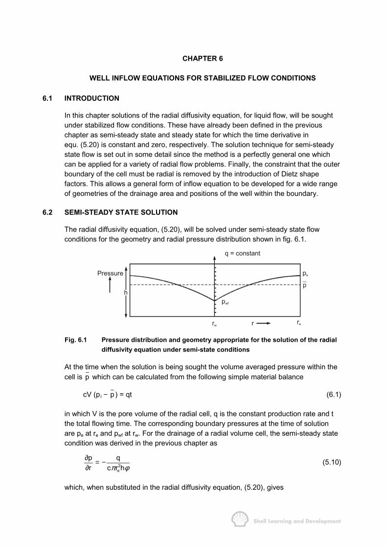
CHAPTER 6
WELL INFLOW EQUATIONS FOR STABILIZED FLOW CONDITIONS
6.1 INTRODUCTION
In this chapter solutions of the radial diffusivity equation, for liquid flow, will be soughtunder stabilized flow conditions. These have already been defined in the previouschapter as semi-steady state and steady state for which the time derivative inequ. (5.20) is constant and zero, respectively. The solution technique for semi-steadystate flow is set out in some detail since the method is a perfectly general one whichcan be applied for a variety of radial flow problems. Finally, the constraint that the outerboundary of the cell must be radial is removed by the introduction of Dietz shapefactors. This allows a general form of inflow equation to be developed for a wide rangeof geometries of the drainage area and positions of the well within the boundary.
6.2 SEMI-STEADY STATE SOLUTION
The radial diffusivity equation, (5.20), will be solved under semi-steady state flowconditions for the geometry and radial pressure distribution shown in fig. 6.1.
r re
q = constant
Pressure
rw
pe
pwf
h
Fig. 6.1 Pressure distribution and geometry appropriate for the solution of the radialdiffusivity equation under semi-state conditions
At the time when the solution is being sought the volume averaged pressure within thecell is p which can be calculated from the following simple material balance
cV (pi − p ) = qt (6.1)
in which V is the pore volume of the radial cell, q is the constant production rate and tthe total flowing time. The corresponding boundary pressures at the time of solutionare pe at re and pwf at rw. For the drainage of a radial volume cell, the semi-steady statecondition was derived in the previous chapter as
2e
p qr c r hπ φ
∂ = −∂
(5.10)
which, when substituted in the radial diffusivity equation, (5.20), gives
STABILIZED INFLOW EQUATIONS 137
2e
1 p qrr r r r kh
µπ
∂ ∂� � = −� �∂ ∂� �(6.2)
and integrating this equation2
12e
p q r Ct 2 r kh
µπ
∂ = − +∂
(6.3)
where C1 is a constant of integration. At the outer no-flow boundary ∂p/∂r is zero andhence the constant can be evaluated as C1 = qµ/2πkh which, when substituted inequ. (6.3), gives
2e
p q 1 rr 2 kh r r
µπ
� �∂ = −� �∂ � �(6.4)
Integrating once again
2r
2ewf w
rp q rp lnr2 kh 2 rp r
µπ
� �� � = −� �� �� � � �(6.5)
or
2
r wf 2w e
q r rp p ln2 kh r 2r
µπ
� �− = −� �
� �(6.6)
in which the term 2 2w er / r is considered to be negligible. Equation (6.6) is a general
expression for the pressure as a function of the radius. In the particular case whenr = re then
ee wf
w
rq 1p p ln S2 kh r 2
µπ
� �− = − +� �
� �(6.7)
This is the familiar well inflow equation under semi-steady state conditions and issimilar to that presented as equ. (4.27) for steady state flow. It can be transposed togive the Pl relationship
e wf e
w
q 2 khPIp p r 1ln S
r 2
π
µ= =
− � �− +� �
� �
(6.8)
in which the van Everdingen skin factor has been included as described in Chapter 4,sec. 7. One unfortunate aspect concerning the application of this equation is that, whileboth q and pwf can be measured directly, the outer boundary pressure cannot. It istherefore more common to express the pressure drawdown in terms of p − pwf insteadof pe − pwf, since p , the average pressure within the drainage volume, can readily bedetermined from a well test as will be shown in Chapter 7, sec. 7. To express the inflow
STABILIZED INFLOW EQUATIONS 138
equation in these terms requires the determination of the volume averaged pressurewithin the radial cell as
e
w
e
w
r
rr
r
pdVp
dV=�
�
(6.9)
and since dV = 2πrhφdr, equ. (6.9) can be expressed as
e
w
r
r2 2e w
p2 rh drp
(r r )h
π φ
π φ=
−
�
or
e
w
r
2 2e w r
2p prdr(r r )
=− �
and since 2 2 2 2 2 2e w e w e er r r (1 r / r ) r , then− = − ≈
e
w
r
2e r
2p prdrr
= � (6.10)
The pressure in the integrand of equ. (6.10) is obtained from equ. (6.6) which is ageneral expression for p as a function of r. Substituting the latter in equ. (6.10) gives
e
w
r 2
wf 2 2we er
2 q r rp p . r ln dr2 kh rr 2r
µπ
� �− = −� �
� �� (6.11)
The first term in the integrand is evaluated using the method of integration by parts, i.e.
ee e
w ww
e e
w w
rr r2 2
wwr rr
r r2 2
wr r
2 2e e e
w
r r r 1 rr ln dr ln drr 2 r r 2
r r rln2 r 4
r r rln2 r 4
� �= −� �� �� �
� � � �= −� � � �� � � �� � � �
≈ −
� �
while the integration of the latter term in equ. (6.11) givese
e
w w
rr 23 4e
2 2e er r
rr rdr82r 8r
� �= ≈� �� �
�
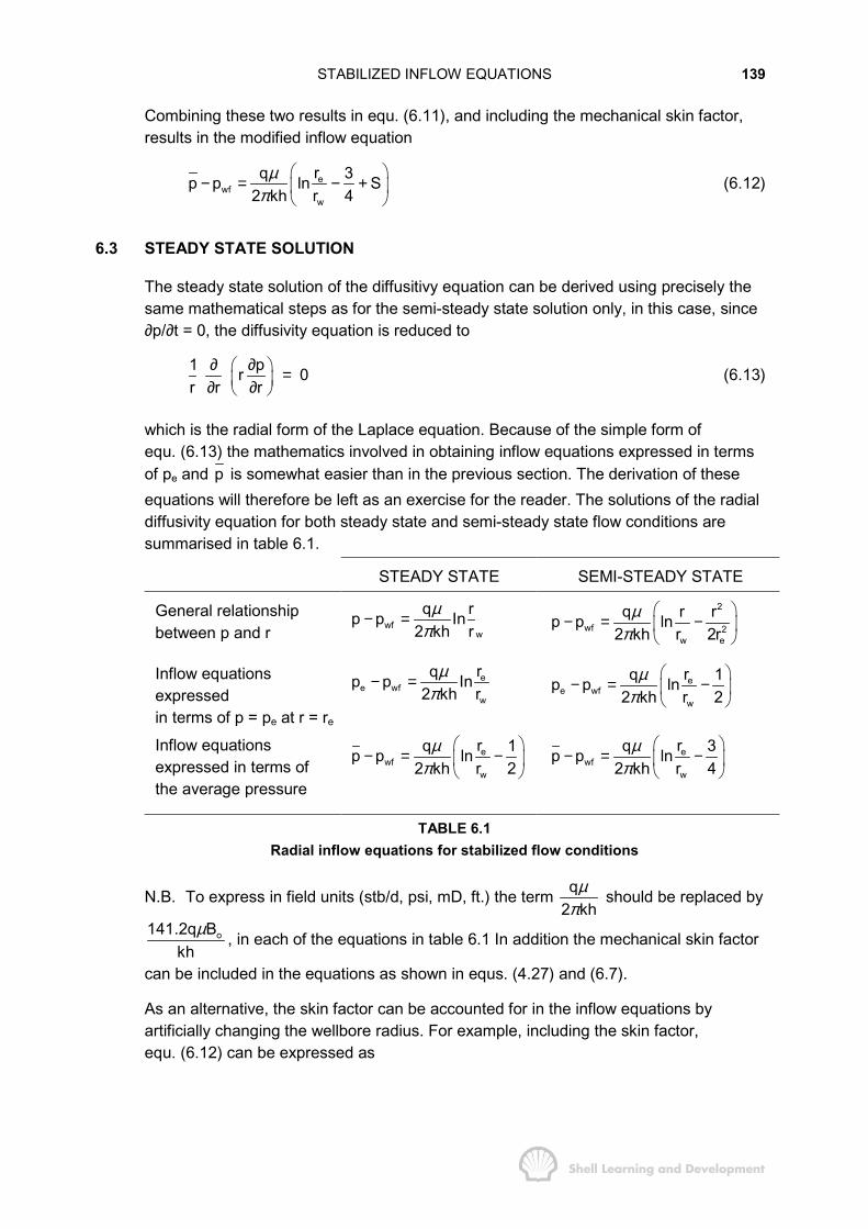
STABILIZED INFLOW EQUATIONS 139
Combining these two results in equ. (6.11), and including the mechanical skin factor,results in the modified inflow equation
ewf
w
rq 3p p ln S2 kh r 4
µπ
� �− = − +� �
� �(6.12)
6.3 STEADY STATE SOLUTION
The steady state solution of the diffusitivy equation can be derived using precisely thesame mathematical steps as for the semi-steady state solution only, in this case, since∂p/∂t = 0, the diffusivity equation is reduced to
1 pr 0r r r
∂ ∂� � =� �∂ ∂� �(6.13)
which is the radial form of the Laplace equation. Because of the simple form ofequ. (6.13) the mathematics involved in obtaining inflow equations expressed in termsof pe and p is somewhat easier than in the previous section. The derivation of theseequations will therefore be left as an exercise for the reader. The solutions of the radialdiffusivity equation for both steady state and semi-steady state flow conditions aresummarised in table 6.1.
STEADY STATE SEMI-STEADY STATE
General relationshipbetween p and r wf
w
q rp p In2 kh r
µπ
− =2
wf 2w e
q r rp p ln2 kh r 2r
µπ
� �− = −� �
� �
Inflow equationsexpressedin terms of p = pe at r = re
ee wf
w
rqp p In2 kh r
µπ
− = ee wf
w
rq 1p p ln2 kh r 2
µπ
� �− = −� �
� �
Inflow equationsexpressed in terms ofthe average pressure
ewf
w
rq 1p p ln2 kh r 2
µπ
� �− = −� �
� �
ewf
w
rq 3p p ln2 kh r 4
µπ
� �− = −� �
� �
TABLE 6.1Radial inflow equations for stabilized flow conditions
N.B. To express in field units (stb/d, psi, mD, ft.) the term q2 kh
µπ
should be replaced by
o141.2q Bkh
µ , in each of the equations in table 6.1 In addition the mechanical skin factor
can be included in the equations as shown in equs. (4.27) and (6.7).
As an alternative, the skin factor can be accounted for in the inflow equations byartificially changing the wellbore radius. For example, including the skin factor,equ. (6.12) can be expressed as
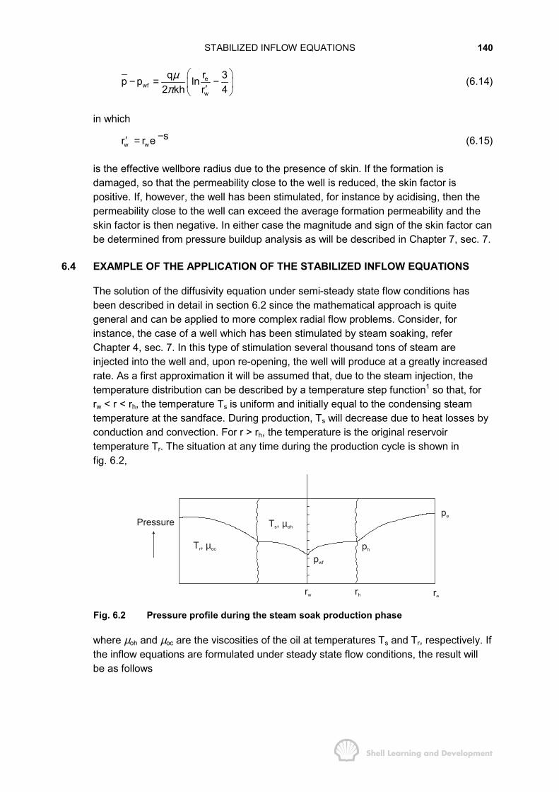
STABILIZED INFLOW EQUATIONS 140
ewf
w
rq 3p p ln2 kh r 4
µπ
� �− = −� �′� �
(6.14)
in which
w wr r e′ = −s (6.15)
is the effective wellbore radius due to the presence of skin. If the formation isdamaged, so that the permeability close to the well is reduced, the skin factor ispositive. If, however, the well has been stimulated, for instance by acidising, then thepermeability close to the well can exceed the average formation permeability and theskin factor is then negative. In either case the magnitude and sign of the skin factor canbe determined from pressure buildup analysis as will be described in Chapter 7, sec. 7.
6.4 EXAMPLE OF THE APPLICATION OF THE STABILIZED INFLOW EQUATIONS
The solution of the diffusivity equation under semi-steady state flow conditions hasbeen described in detail in section 6.2 since the mathematical approach is quitegeneral and can be applied to more complex radial flow problems. Consider, forinstance, the case of a well which has been stimulated by steam soaking, referChapter 4, sec. 7. In this type of stimulation several thousand tons of steam areinjected into the well and, upon re-opening, the well will produce at a greatly increasedrate. As a first approximation it will be assumed that, due to the steam injection, thetemperature distribution can be described by a temperature step function1 so that, forrw < r < rh, the temperature Ts is uniform and initially equal to the condensing steamtemperature at the sandface. During production, Ts will decrease due to heat losses byconduction and convection. For r > rh, the temperature is the original reservoirtemperature Tr. The situation at any time during the production cycle is shown infig. 6.2,
Pressure
T , r ocµ
T , s ohµ
pwf
rw rh re
pe
ph
Fig. 6.2 Pressure profile during the steam soak production phase
where µoh and µoc are the viscosities of the oil at temperatures Ts and Tr, respectively. Ifthe inflow equations are formulated under steady state flow conditions, the result willbe as follows
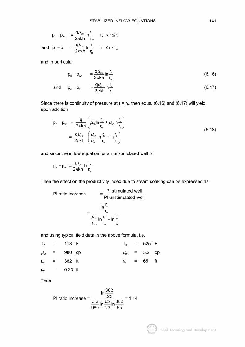
STABILIZED INFLOW EQUATIONS 141
ohr wf w h
w
ocr h h e
h
q rp p ln r r r2 kh rq rand p p ln r r r2 kh r
µπµπ
− = < ≤
− = ≤ <
and in particular
oh hh wf
w
q rp p ln2 kh r
µπ
− = (6.16)
oc ee h
h
q rand p p ln2 kh r
µπ
− = (6.17)
Since there is continuity of pressure at r = rh, then equs. (6.16) and (6.17) will yield,upon addition
ehe wf oh oc
w h
oc oh eh
oc w h
rrqp p ln ln2 kh r r
q rrln ln2 kh r r
µ µπ
µ µπ µ
� �− = +� �
� �
� �= +� �
� �
(6.18)
and since the inflow equation for an unstimulated well is
oc ee wf
w
q rp p ln2 kh r
µπ
− =
Then the effect on the productivity index due to steam soaking can be expressed as
e
w
oh eh
oc w h
PI stimulated wellPI ratio increasePI unstimulated wellrlnr
rrln lnr r
µµ
=
=+
and using typical field data in the above formula, i.e.
Tr = 113° F Ts = 525° F
µoc = 980 cp µoh = 3.2 cp
re = 382 ft rh = 65 ft
rw = 0.23 ft
Then
382In.23PI ratio increase 4.143.2 65 382In In
980 .23 65
= =

STABILIZED INFLOW EQUATIONS 142
This PI improvement is probably pessimistic since it has been assumed that steadystate conditions prevail from the start of production. In fact, transient flow is more likelyduring the initial stage which will give an early boost to production, in excess of thatcalculated from steady state considerations. The manner in which the early transientpart of the production cycle can be accounted for will be described in Chapter 9, sec. 6.
EXERCISE 6.1 WELLBORE DAMAGE
1) A homogeneous formation has an average effective permeability ke. The effectivepermeability out to a radius ra from the well has been altered (damage/stimulation) sothat its average value in this region is ka. Show that, for this situation, the skin factormay be expressed as
e a a
a w
k k rS Ink r−= (6.19)
where rw is the wellbore radius. Assume that for r< ra, the flow can be approximatelydescribed under steady state conditions and that for r >ra, semi-steady state.
2) During drilling, a well is damaged out to a radius of 4 ft from the wellbore so that thepermeability within the damaged zone is reduced to 1/100 th of the undamagedeffective permeability. After completion the well is stimulated so that the permeabilityout to a distance of 10 ft from the wellbore is increased to ten times the undamagedpermeability. What will be the PI ratio increase if the wellbore radius is 0.333 ft and thedrainage radius 660 ft?
EXERCISE 6.1 SOLUTION
Pressure
ke
rw ra
ka
pa
pwf
pe
re
Fig. 6.3 Pressure profiles and geometry (Exercise 6.1)
1) The inflow equations appropriate for the pressure distribution shown in fig. 6.3 are
r wf w aa w
2
r a a e2e a e
q rp p ln r r r2 k h r
q r rp p ln r r r2 k h r 2r
µπ
µπ
− = < ≤
� �− = − ≤ <� �
� �
In particular
STABILIZED INFLOW EQUATIONS 143
aa wf
a w
rqp p ln2 k h r
µπ
− =
and
ee a
a a
rq 1p p ln2 k h r 2
µπ
� �− = −� �
� �
At r = ra, there is continuity of pressure, therefore, adding the above equations
e e ae wf
e a a w
e e e e a
e w a w a w
r k rq 1p p ln ln2 k h r 2 k r
r r r k rq 1ln ln ln ln2 k h r 2 r r k r
µπ
µπ
� �− = − +� �
� �
� �= − + − +� �
� �
i.e.
e e ae wf
e w a w
r k rq 1p p ln 1 ln2 k h r 2 k r
µπ
� �� �− = − + −� �� �� �
� �� �
which must be equivalent to
ee wf
e w
rq 1p p ln S2 k h r 2
µπ
� �− = − +� �
� �
and therefore
e a a
a w
k k rS lnk r−=
which is an alternative expression for the skin factor presented by Craft and Hawkins2.
2) Before stimulation
14.333S (100 1)ln 254.020.333
= − =
while the skin factor after stimulation is
2(1 10) 10.333S ln 3.09
10 0.333−= = −
and since
STABILIZED INFLOW EQUATIONS 144
e
e
w
2 k hPIr 1ln Sr 2
π
µ=
� �− +� �
� �
the Pl ratio increase is
660 1ln 254.02 261.11.333 2660 1 4.00ln 3.09.333 2
65.3
− += =
− −
=
6.5 GENERALIZED FORM OF INFLOW EQUATION UNDER SEMI-STEADY STATECONDITIONS
The semi-steady state inflow equation developed in sec. 6.2 appears to be restrictive inthat it only applies for a well producing from the centre of a circular shaped drainagearea. When a reservoir is producing under semi-steady state conditions each well willassume its own fixed drainage boundary, as shown in fig. 5.3, and the shapes of thesemay be far from circular. The inflow equation will therefore require some modification toaccount for this lack of symmetry. Equation (6.12) can be expressed in a generalizedform by introducing the so-called Dietz shape factors3 denoted by CA, which arepresented for a variety of different geometrical configurations in fig. 6.4. Precisely howthese shape factors were generated, in the first place, will be explained in theappropriate place, Chapter 7, sec. 6. For the moment the reader is asked to accept thefollowing tenuous argument for the generalization of the inflow equation. Excluding themechanical skin factor, equ. (6.12) can be expressed as
2e
wf 2 3 / 2w
rq 1p p ln2 kh 2 r e
πµπ π
� �− = � �
� �(6.20)
in which the argument of the natural log can be modified as2e
3 /2 2 2 2w w w
4 r 4A 4A4 e r 56.32r 31.6r
ππ γ
= = (6.21)
in which A is the area being drained, γ is the exponential of Euler's constant and isequal to 1.781, and 31.6 is the Dietz shape factor for a well at the centre of a circle,refer fig. 6.4. Therefore, equ. (6.20) can be expressed in the general form, including theskin factor, as
wf 2A w
q 1 4Ap p ln S2 kh 2 C r
µπ γ
� �− = +� �
� �(6.22)
For a reservoir which is producing under semi-steady state conditions, then as alreadynoted, the volume drained by each well is directly proportional to the well's productionrate. Therefore, it is a fairly straightforward matter to estimate the volume being drainedby each well and, using the average thickness in the vicinity of the well, the area. If

STABILIZED INFLOW EQUATIONS 145
structural contour maps are available for the reservoir, then the areas so determinedcan be roughly matched to the reservoir geometry to obtain a reasonable estimate ofthe shape of the drainage area. Fig. 6.4 should then be consulted to determine theshape factor CA which can be seen to be dependent not only on the drainage shapebut also upon the position of the well with respect to the boundary. For irregularshapes, interpolation between the geometrical configurations presented by Dietz maybe necessary. Naturally it is never possible to obtain the exact shape of the drainagevolume but a reasonable estimate can usually be made which, when interpreted interms of a shape factor and used in equ. (6.22), can considerably improve theaccuracy of calculations made using the inflow equation.
Also listed in fig. 6.4 is the dimensionless time group tDA = kt/φµcA, in which t is thetime for which the well has been producing at a reasonably steady rate of production.Unless the calculated value of tDA exceeds the figure quoted for each geometricalconfiguration then the well is not producing under semi-steady state conditions and theDietz shape factors cannot be used.
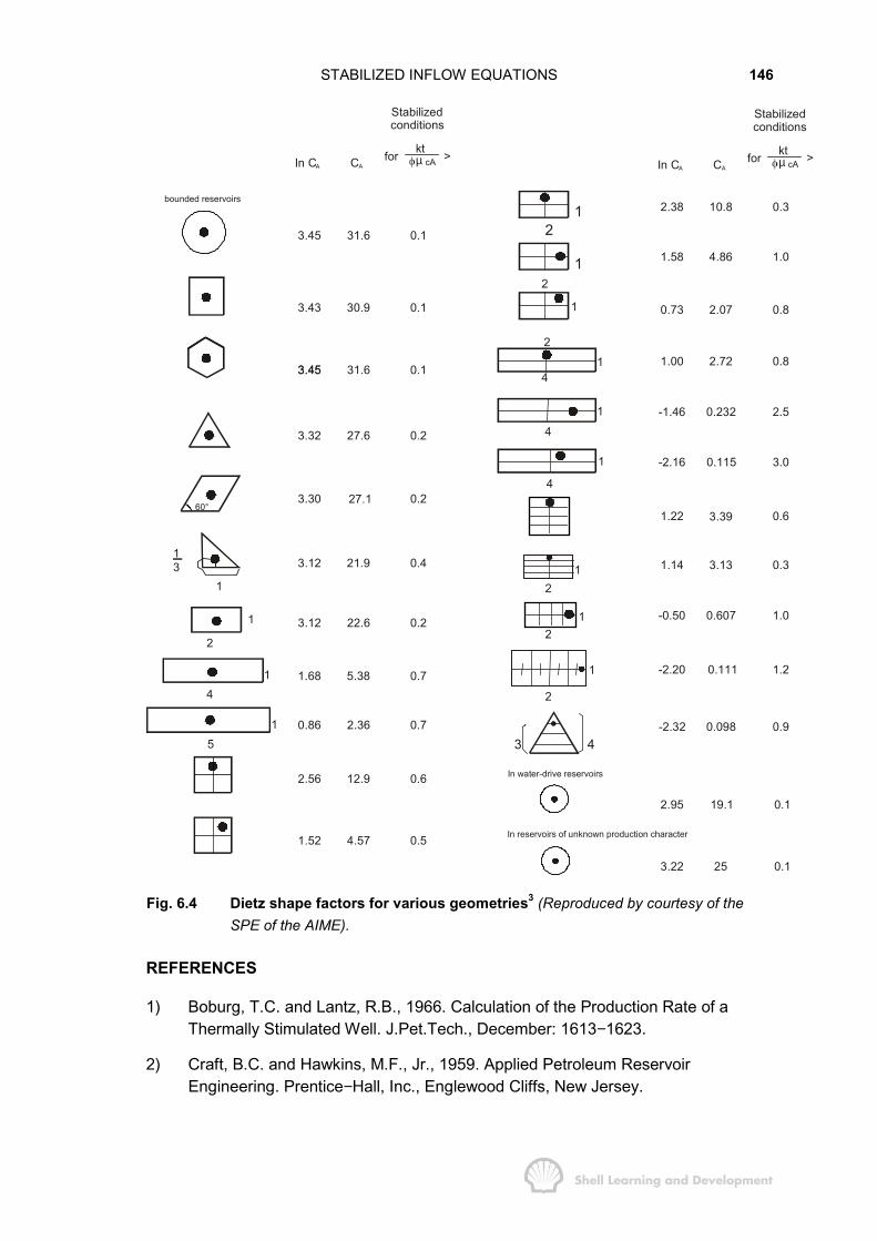
STABILIZED INFLOW EQUATIONS 146
60°
1
15
4
1
2
13
1
bounded reservoirs
3.45
3.43
3.45
In CA
3.45
3.32
3.30
3.12
3.12
1.68
0.86
2.56
1.52
31.6
30.9
31.6
CA
27.6
27.1
21.9
22.6
5.38
2.36
12.9
4.57
0.1
0.1
0.1
Stabilizedconditions
ktµ cAfor >
0.2
0.2
0.4
0.2
0.7
0.7
0.6
0.5
2.38
0.73
1.00
In CA
-1.46
-2.16
1.14
-0.50
-2.20
-2.32
2.95
3.22
1.58
1.22
10.8
2.07
2.72
CA
0.232
0.115
3.13
0.607
0.111
0.098
19.1
25
4.86
3.39
0.3
0.8
0.8
Stabilizedconditions
ktµ cAfor >
2.5
3.0
0.3
1.0
1.2
0.9
0.1
0.1
1.0
0.6
12
12
1
12
4
1
4
1
4
2
1
43
In water-drive reservoirs
2
1
In reservoirs of unknown production character
12
Fig. 6.4 Dietz shape factors for various geometries3 (Reproduced by courtesy of theSPE of the AIME).
REFERENCES
1) Boburg, T.C. and Lantz, R.B., 1966. Calculation of the Production Rate of aThermally Stimulated Well. J.Pet.Tech., December: 1613−1623.
2) Craft, B.C. and Hawkins, M.F., Jr., 1959. Applied Petroleum ReservoirEngineering. Prentice−Hall, Inc., Englewood Cliffs, New Jersey.

STABILIZED INFLOW EQUATIONS 147
3) Dietz, D.N., 1965. Determination of Average Reservoir Pressure from Build-UpSurveys. J.Pet.Tech., August: 955−959.
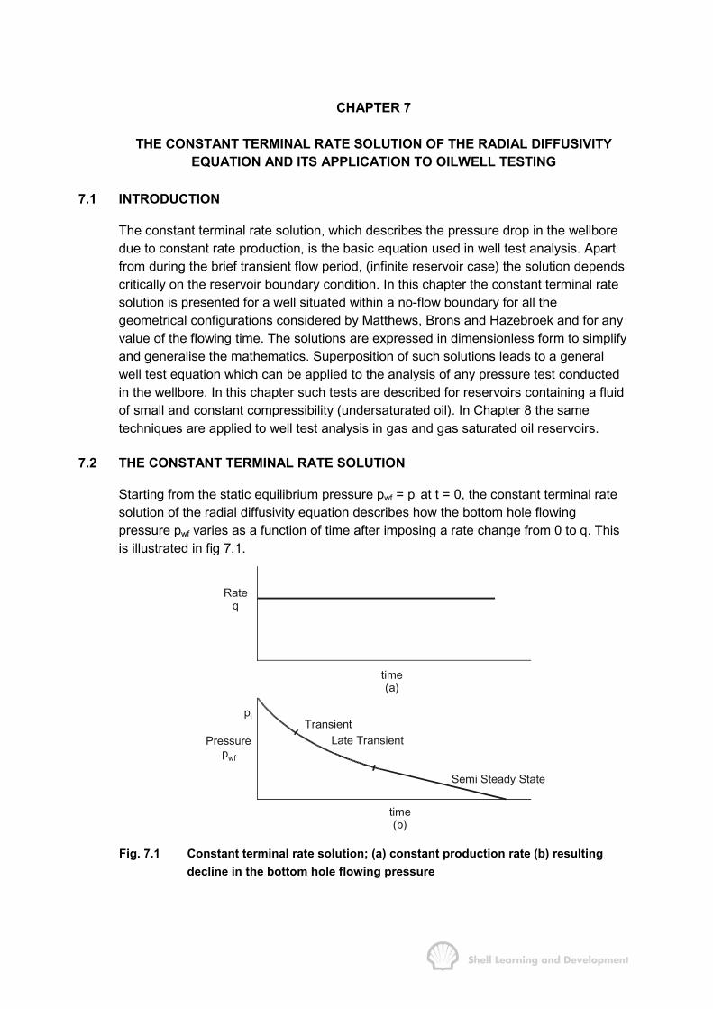
CHAPTER 7
THE CONSTANT TERMINAL RATE SOLUTION OF THE RADIAL DIFFUSIVITYEQUATION AND ITS APPLICATION TO OILWELL TESTING
7.1 INTRODUCTION
The constant terminal rate solution, which describes the pressure drop in the wellboredue to constant rate production, is the basic equation used in well test analysis. Apartfrom during the brief transient flow period, (infinite reservoir case) the solution dependscritically on the reservoir boundary condition. In this chapter the constant terminal ratesolution is presented for a well situated within a no-flow boundary for all thegeometrical configurations considered by Matthews, Brons and Hazebroek and for anyvalue of the flowing time. The solutions are expressed in dimensionless form to simplifyand generalise the mathematics. Superposition of such solutions leads to a generalwell test equation which can be applied to the analysis of any pressure test conductedin the wellbore. In this chapter such tests are described for reservoirs containing a fluidof small and constant compressibility (undersaturated oil). In Chapter 8 the sametechniques are applied to well test analysis in gas and gas saturated oil reservoirs.
7.2 THE CONSTANT TERMINAL RATE SOLUTION
Starting from the static equilibrium pressure pwf = pi at t = 0, the constant terminal ratesolution of the radial diffusivity equation describes how the bottom hole flowingpressure pwf varies as a function of time after imposing a rate change from 0 to q. Thisis illustrated in fig 7.1.
time(b)
Pressurepwf
TransientLate Transient
Semi Steady State
pi
Rateq
time(a)
Fig. 7.1 Constant terminal rate solution; (a) constant production rate (b) resultingdecline in the bottom hole flowing pressure
OILWELL TESTING 149
The constant terminal rate solution is therefore the equation of pwf versus t for constantrate production for any value of the flowing time. The pressure decline, fig. 7.1 (b), cannormally be divided into three sections depending on the value of the flowing time andthe geometry of the reservoir or part of the reservoir being drained by the well.
Initially, the pressure response can be described using a transient solution of thediffusivity equation. It is assumed during this period that the pressure response at thewellbore is not affected by the drainage boundary of the well and vice versa. This isfrequently referred to as the infinite reservoir case since, during the transient flowperiod, the reservoir appears to be infinite in extent.
The transient phase is followed by the so-called late transient period during which theinfluence of the drainage boundary begins to be felt. For a well producing from within ano-flow boundary both the shape of the area drained and position of the well withrespect to the boundary are of major importance in determining the appropriate latetransient constant terminal rate solution.
Eventually, stabilised flow conditions will prevail which means that for the no-flowboundary case the rate of change of wellbore pressure with respect to time is constant.This corresponds to the semi-steady state condition described in Chapter 5, sec 3(b).
The constant terminal rate solution, for all values of the flowing time, was firstpresented to the industry by Hurst and Van Everdingen in 1949. In their classic paperon the subject1, the authors solved the radial diffusivity equation using the Laplacetransform for both the constant terminal rate and constant terminal pressure cases. Thelatter, which is relevant to water influx calculations. will be described in Chapter 9.
The full Hurst and Van Everdingen solution, equ. 7.34, is a most intimidatingmathematical equation which contains as one of its components an infinite summationof Bessel functions. The complexity is due to the wellbore pressure response duringthe late transient period, since for transient and semi-steady state flow relatively simplesolutions can be obtained which will be described in sec. 7.3. The fact that the fullsolution is so complex is rather unfortunate since the constant terminal rate solution ofthe radial diffusivity equation can be regarded as the basic equation in wellborepressure analysis techniques. By superposition of such solutions, as will be shown insec. 7.5, the pressure response at the wellbore can be theoretically described for anysequence of different rates acting for different periods of time, and this is the generalmethod employed in the analysis of any form of oil or gas well test.
7.3 THE CONSTANT TERMINAL RATE SOLUTION FOR TRANSIENT AND SEMI-STEADY STATE FLOW CONDITIONS
During the initial transient flow period, it has been found that the constant terminal ratesolution of the radial diffusivity equation, determined using the Laplace transform, canbe approximated by the so-called line source solution which assumes that incomparison to the apparently infinite reservoir the wellbore radius is negligible and thewellbore itself can be treated as a line. This leads to a considerable simplification in the

OILWELL TESTING 150
mathematics and for this solution the boundary and initial conditions may be stated asfollows
i
i
r 0
a) p p at t 0, for all r
b) p p at r , for all t
p qc) lim r , for t 0r 2 kh
µπ→
= =
= = ∞
∂ = >∂
(7.1)
Condition (a) is merely the initial condition that, before producing, the pressureeverywhere within the drainage volume is equal to the initial equilibrium pressure pi.
Condition (b) ensures the condition of transience, namely that the pressure at theouter, infinite boundary is not affected by the pressure disturbance at the wellbore andvice versa.
Condition (c) is the line source inner boundary condition.
In addition, the assumptions made in deriving the radial diffusivity equation inChapter 5 are retained. That is, that the formation is homogeneous and isotropic, anddrained by a fully penetrating well to ensure radial flow; the fluid itself must have aconstant viscosity and a small and constant compressibility. The solution obtained will,therefore, be applicable to the flow of undersaturated oil. Having developed the simpletheory of pressure analysis based on these assumptions, many of the restrictions willbe removed by considering, for instance, the effects of partial well completion, the flowof highly compressible fluids, etc. These modifications to the basic theory will begradually introduced in this and the following chapter.
Under the above conditions the diffusivity equation
1 p c prr r r k t
φ µ� �∂ ∂ ∂=� �∂ ∂ ∂� �(5.20)
can be solved by making use of Boltzmann's transformation2 2r c rs
4 (Diffusivity constant)t 4ktφ µ= =
so that
s c rt 2k t
φ µ∂ =∂
(7.2)
and2
2s c rr 4k t
φ µ∂ =∂
(7.3)

OILWELL TESTING 151
Equation (5.20) can be expressed with respect to this new variable as
1 d dp s s c dp srr ds ds r r k ds t
φ µ� �∂ ∂ ∂=� �∂ ∂ ∂� �
and using equs. (7.2) and (7.3), this becomes221 c r d c r dp c r dp
r 2k t ds 2k t ds 2k t dsφ µ φ µ φ µ� � � �
= −� � � �� �� �
which can be simplified as
d dp dps sds ds ds
� � = −� �� �
or
dp d dp dps sds ds ds ds
� �+ = −� �� �
This is an ordinary differential equation which can be solved by letting
dp pds
′=
Then
( )
dpp s spdss 1dp ds
p s
′′ ′+ = −
+′= −
′
(7.4)
Integrating equ. (7.4) gives
1ln p ln s s C′ = − − +
or
s
2ep Cs
−
′ = (7.5)
where C1 and C2 are constants of integration and C2 can be evaluated using the linesource boundary condition
r 0
p q dp s dplim r r 2sr 2 kh ds r ds
µπ→
∂ ∂= = =∂ ∂
therefore,
OILWELL TESTING 152
s2
q C e4 kh
µπ
−=
which yields, as r (and therefore s) tends to zero
2qC
4 khµ
π=
Equation (7.5) can now be integrated between the limits t = 0 (s → ∞ ) and the currentvalue of t, for which s = x; and pi (initial pressure) and the current pressure p.
i.e.
i
p x s
p
q edp ds4 kh s
µπ
−
∞=� �
which gives
2
s
r,t icrx 4k t
q ep p ds4 kh sφ µ
µπ
−∞
=
= − � (7.6)
Equation (7.6) is the line source solution of the diffusivity equation giving the pressurepr,t as a function of position and time.
The integral
2
s s
x crx4k t
e eds dss s
φ µ
− −∞ ∞
=
=� � (7.7)
is a standard integral, called the exponential integral, and is denoted by ei(x).
Qualitatively, the nature of this integral can be understood by considering thecomponent parts, fig. 7.2.
The integral of curve (c) between x and ∞ will have the shape shown in fig. 7.2 (d).Thus ei (x) is large for small values of x, since the ei-function is the area under thegraph from the particular value of x out to infinity (i.e. the shaded area in curve (c) offig. 7.2) and, conversely, small for large values of x. The ei-function is normally plottedon a log-log scale and such a version is included as fig. 7.3. From this curve it can beseen that if x < 0.01, ei (x) can be approximated as
ei(x) ln x 0.5772≈ − − (7.8)
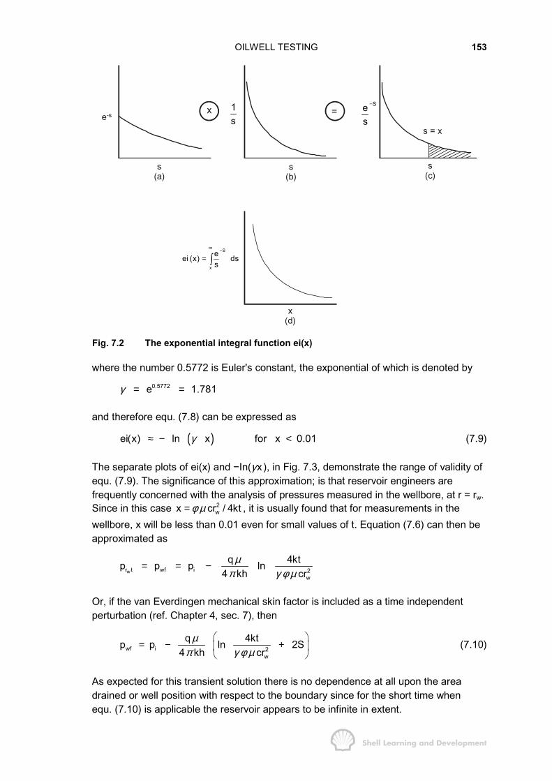
OILWELL TESTING 153
xe-s
s(a)
=
s(b)
s = x
s(c)
x(d)
1s
Ses
−
S
x
eei (x) dss
−∞
= �
Fig. 7.2 The exponential integral function ei(x)
where the number 0.5772 is Euler's constant, the exponential of which is denoted by0.5772e 1.781γ = =
and therefore equ. (7.8) can be expressed as
( )ei(x) ln x for x 0.01γ≈ − < (7.9)
The separate plots of ei(x) and −In(γx ), in Fig. 7.3, demonstrate the range of validity ofequ. (7.9). The significance of this approximation; is that reservoir engineers arefrequently concerned with the analysis of pressures measured in the wellbore, at r = rw.Since in this case 2
wx cr / 4ktφ µ= , it is usually found that for measurements in thewellbore, x will be less than 0.01 even for small values of t. Equation (7.6) can then beapproximated as
wr t wf i 2w
q 4ktp p p ln4 kh cr
µπ γ φ µ
= = −
Or, if the van Everdingen mechanical skin factor is included as a time independentperturbation (ref. Chapter 4, sec. 7), then
wf i 2w
q 4ktp p ln 2S4 kh cr
µπ γ φ µ
� �= − +� �
� �(7.10)
As expected for this transient solution there is no dependence at all upon the areadrained or well position with respect to the boundary since for the short time whenequ. (7.10) is applicable the reservoir appears to be infinite in extent.
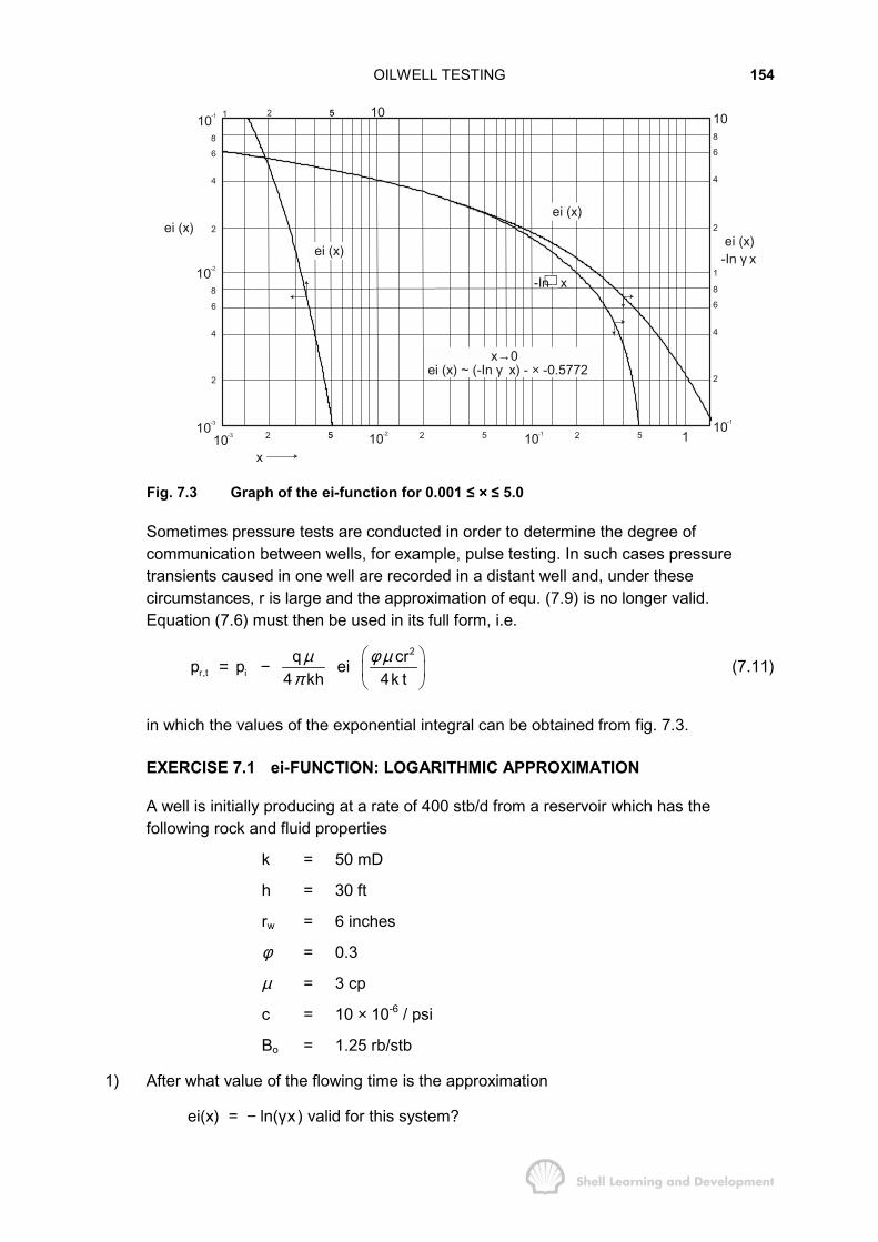
OILWELL TESTING 154
10-1
8
6
4
2
10-2
8
6
4
2
10-3
10-3 2 55 10-2 2 5 10-1 2 510-1
1
108
6
4
2
1
8
6
4
2
2 55 10
ei (x)
x→0ei (x) ~ (-In γ x) - × -0.5772
ei (x)
-In x∝
ei (x)ei (x)
-In γ x
x
1
Fig. 7.3 Graph of the ei-function for 0.001 ≤ ×××× ≤ 5.0
Sometimes pressure tests are conducted in order to determine the degree ofcommunication between wells, for example, pulse testing. In such cases pressuretransients caused in one well are recorded in a distant well and, under thesecircumstances, r is large and the approximation of equ. (7.9) is no longer valid.Equation (7.6) must then be used in its full form, i.e.
2
r,t iq crp p ei
4 kh 4k tµ φ µ
π� �
= − � �� �
(7.11)
in which the values of the exponential integral can be obtained from fig. 7.3.
EXERCISE 7.1 ei-FUNCTION: LOGARITHMIC APPROXIMATION
A well is initially producing at a rate of 400 stb/d from a reservoir which has thefollowing rock and fluid properties
k = 50 mD
h = 30 ft
rw = 6 inches
φ = 0.3
µ = 3 cp
c = 10 × 10-6 / psi
Bo = 1.25 rb/stb
1) After what value of the flowing time is the approximation
ei(x) = − ln(γx) valid for this system?
OILWELL TESTING 155
2) What will be the pressure drop at the well after flowing at the steady rate of 400 stb/dfor 3 hours, assuming transient conditions still prevail.
EXERCISE 7.1 SOLUTION
Converting the reservoir and fluid properties to Darcy units.
k = 0.05 D
h = 30 ft × 30.48 = 914.4 cm2wr = 0.25 sq.ft. = 0.25 × (30.48)2 cm2
= 232.3 cm2
c = 10 × 10-6/psi = 10 × 10-6 × 14.7/atm
= 14.7 × 10⁻⁵/atm
q = 400stb/d = 400× 1.25× 1.84 r.cc/sec = 920 r.cc/sec.
The approximation ei(x) ≈ − In(γx) applies for x < 0.01 i.e.2w
2w
5
cr 0.014k t
orcrt
0.04k.3 3 14.7 10 232.3t
.04 .05for t 15.4 seconds
φ µ
φ µ
−
<
>
× × × ×>×
>
Now in a practical sense, nobody is concerned with what happens in the well during thefirst 15 seconds, after which the pressure decline can be calculated using thelogarithmic approximation for ei(x) i.e.
2w
i wf
2w
crqp p ei4 kh 4k t
q 4k tln4 kh cr
φ µµπ
µπ γ φ µ
� �− = � �
� �
� �= � �
� �
After producing for 3 hours at a steady rate of 400 stb/d the pressure drop at thewellbore is
5
i wf920 3 4 .05 3 3600 10p p ln
4 .05 914.4 1.781 .3 3 14.7 232.3
50.8atm, or 747psi
π× × × × ×− =
× × × × × ×
=

OILWELL TESTING 156
The constant terminal rate solution of the radial diffusivity equation during the latetransient flow period is too complicated to include at this stage. A simplified method ofobtaining this solution will be described in sec. 7.6.
Once semi-steady state conditions prevail the solution can be determined by addingthe simple material balance equation for the bounded drainage volume
( )icAh p p qtφ − = (7.12)
to the semi-steady state inflow equation
wf 2A w
q 4Ap p ½ ln S2 kh C r
µπ γ
� �− = +� �
� �(6.22)
to give
wf i 2A w
q 4A ktp p ½ ln 2 S2 kh cAC r
µ ππ φ µγ
� �= − + +� �
� �(7.13)
In this equation p is the current average pressure within the drainage boundary and CA
is the Dietz shape factor introduced in Chapter 6, sec.5. The magnitude of CA dependson the shape of the area being drained and also upon the position of the well withrespect to the boundary.
Theoretically, for the constant terminal rate solution, the rate q in equs. (7.12) and(6.22) is the same. In practice, it is sometimes difficult to maintain the production rate ofa well constant over a long period of time and therefore, the current rate in equ. (6.22)may differ from the average rate which is implicitly used in material balance, equ.(7.12). In this case the rate in equ. (7.12) is set equal to the current, or final flow rate,and the flowing time is expressed as an effective flowing time, where
Cumulative Production t Effective flowing time Final flow rate
= = (7.14)
Use of the effective flowing time is therefore simply a method for equalising the ratesand preserving the material balance and is frequently used in pressure analysis, as willbe described later.
Even though no equation for describing the pressure decline during the late transientflow period has yet been developed, equs. (7.10) and (7.13), which are appropriate fortransient and semi-steady state flow, can be usefully employed by themselves in welltest analysis.
Well testing involves producing a well at a constant rate or series of rates, some ofwhich may be zero (well closed in), while simultaneously taking a continuous recordingof the changing pressure in the wellbore using some form of pressure recording device.The retrieved record of wellbore pressure as a function of time can be analysed inconjunction with the known rate sequence to determine some or all of the followingreservoir parameters:
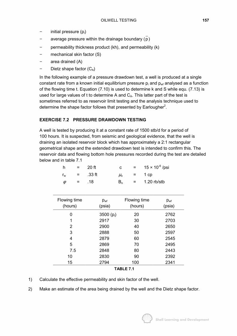
OILWELL TESTING 157
− initial pressure (pi)− average pressure within the drainage boundary (p )
− permeability thickness product (kh), and permeability (k)− mechanical skin factor (S)− area drained (A)− Dietz shape factor (CA)
In the following example of a pressure drawdown test, a well is produced at a singleconstant rate from a known initial equilibrium pressure pi and pwf analysed as a functionof the flowing time t. Equation (7.10) is used to determine k and S while equ. (7.13) isused for large values of t to determine A and CA. This latter part of the test issometimes referred to as reservoir limit testing and the analysis technique used todetermine the shape factor follows that presented by Earlougher2.
EXERCISE 7.2 PRESSURE DRAWDOWN TESTING
A well is tested by producing it at a constant rate of 1500 stb/d for a period of100 hours. It is suspected, from seismic and geological evidence, that the well isdraining an isolated reservoir block which has approximately a 2:1 rectangulargeometrical shape and the extended drawdown test is intended to confirm this. Thereservoir data and flowing bottom hole pressures recorded during the test are detailedbelow and in table 7.1
h = 20 ft c = 15 × 10-6 /psirw = .33 ft µo = 1 cpφ = .18 Bo = 1.20 rb/stb
Flowing time(hours)
pwf
(psia)Flowing time
(hours)pwf
(psia)
0 3500 (pi) 20 27621 2917 30 27032 2900 40 26503 2888 50 25974 2879 60 25455 2869 70 24957.5 2848 80 2443
10 2830 90 239215 2794 100 2341
TABLE 7.1
1) Calculate the effective permeability and skin factor of the well.
2) Make an estimate of the area being drained by the well and the Dietz shape factor.
OILWELL TESTING 158
EXERCISE 7.2 SOLUTION
1) The permeability and skin factor can be obtained by the analysis of the transient flowperiod for which
wf i 2w
q 4ktp p ln 2S4 kh cr
µπ γ φ µ
� �= − +� �
� �
or in field units
owf i 2
w
162.6q B kp p log t log 3.23 0.87Skh cr
µφ µ
� �= − + − +� �
� �
Thus for the initial period, when transient flow conditions prevail, a plot of pwf versuslog t should be linear with slope m = 162.6 q µ Bo /kh, from which kh and k can bedetermined. Furthermore, using the value of pwf(1hr) taken from the linear trend for aflowing time of one hour and solving explicitly for S gives
i wf (1hr )2w
(p p ) kS 1.151 log 3.23m crφµ
−� �= − +� �
� �
The plot of pwf versus log t for the first few recorded pressures, fig. 7.4, indicates thattransient flow conditions last for about four hours and that the values of m and pwf(1 hr)
are 61 psi/log cycle and 2917 psia, respectively.

OILWELL TESTING 159
p(psi)
wf
2900
2800
27000 .5 1.0 1.5
SLOPE m = 61 psi / log cycle
p = 2917 psiwf (1hr)
log t
0 20 40 60 80 100t HOURS
p(psi)
wf
2900
2800
2700
2600
2500
2400
2300
dpdt = 5.08 psi / hr
a
b
p = 2848 psio
Fig. 7.4 Single rate drawdown test; (a) wellbore flowing pressure decline during theearly transient flow period, (b) during the subsequent semi-steady statedecline (Exercise 7.2)

OILWELL TESTING 160
Therefore,
o162.6q B 162.6 1500 1 1.2kh 4798mD.ftm 61
µ × × ×= = =
and k = 240 mD. The skin factor can be evaluated
( ) 63500 2917 240 10S 1.151 log 3.23 4.561 .18 1 15 .109
� �− ×= − + =� �� �× × ×� �
2) The area being drained and the shape factor can be determined from the later part ofthe flow test when semi-steady state flow conditions prevail. Under thesecircumstances dp/dt ≈ constant, and as shown in the plot of pwf versus t, fig. 7.4(b), thisoccurs after a flowing time of approximately 50 hours, after which dp/dt = −5.08 psi/hr.Therefore, equ. (5.9) can be used to determine the area, since
dp q (atm / sec)dt cAhφ
= −
or, in field units
o0.2339qBdp 5.08 (psi / hr)dt cAhφ
= − = −
and hence
6
.2339 1500 1.2A 35 acres15 10 20 .18 5.08 43560−
× ×= =× × × × ×
The equation of the linear pressure decline under semi-steady state conditions is
12wf i 2
A w
q 4A ktp p ln 2 S2 kh cAC r
µ ππ φ µγ
� �= − + +� �
� �(7.13)
The linear extrapolation of this line to small values of t gives the specific value ofpo = 2848 psia when t = 0 and inserting this condition in equ. (7.13) gives
i o 2A w
q 4Ap p ln 2S4 kh C r
µπ γ
� �− = +� �
� �
or in field units
i o A2w
4Ap p m log logC 0.87Srγ
� �− = − +� �
� �
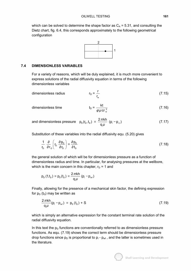
OILWELL TESTING 161
which can be solved to determine the shape factor as CA = 5.31, and consulting theDietz chart, fig. 6.4, this corresponds approximately to the following geometricalconfiguration
2
1
7.4 DIMENSIONLESS VARIABLES
For a variety of reasons, which will be duly explained, it is much more convenient toexpress solutions of the radial diffusivity equation in terms of the followingdimensionless variables
dimensionless radius rD = w
rr
(7.15)
dimensionless time tD = 2w
ktcrφ µ
(7.16)
and dimensionless pressure D D D i r,t2 khp (r , t ) (p p )
qπ
µ= − (7.17)
Substitution of these variables into the radial diffusivity equ. (5.20) gives
D DD
D D DD
p p1 rr r r t
� �∂ ∂∂ =� �∂ ∂ ∂� �(7.18)
the general solution of which will be for dimensionless pressure as a function ofdimensionless radius and time. In particular, for analysing pressures at the wellbore,which is the main concern in this chapter, rD = 1 and
D D D D i wf2 khp (1,t ) p (t ) (p p )qπ
µ= = −
Finally, allowing for the presence of a mechanical skin factor, the defining expressionfor pD (tD) may be written as
i wf D D2 kh (p p ) p (t ) S
qπ
µ− = + (7.19)
which is simply an alternative expression for the constant terminal rate solution of theradial diffusivity equation.
In this text the pD functions are conventionally referred to as dimensionless pressurefunctions. As equ. (7.19) shows the correct term should be dimensionless pressuredrop functions since pD is proportional to pi - pwf , and the latter is sometimes used inthe literature.
OILWELL TESTING 162
EXERCISE 7.3 DIMENSIONLESS VARIABLES
1) Show, using dimensional analysis, that both tD and pD are dimensionless.
2) Express tD in field units with the real time in hours and days, respectively.
3) Express pD (tD ) in field units.
EXERCISE 7.3 SOLUTION
1) In any absolute set of units the dimensions of the parameters in the expressions for tD
and pD (tD) are:
[k] = L2 [p] = (ML/T2)/L2 = M/LT2
[µ] = M/LT [c] = LT2/M
and therefore2
D 2 2 2w
kt L Ttcr (M/LT)(LT /M)Lφ µ
= =
which is dimensionless, and2 2
D i wf 32 kh (L )(L)(M/LT )p (p p )
q (L / T)(M/LT)π
µ= − =
which is also dimensionless.
2) D 2w
ktt Darcy unitscrφ µ
=
D 22 2w 2
2 2w
D seck mD thrsmD hrst field units
1 psi cmc r ftpsi atm ft
(1/1000) (3600) kt(14.7) (30.48) cr
φµ
φ µ
� � � �×� � � �� � � �=� �� �× � �� �� � � �
×=×
D 2w
ktt 0.000264 t in hourscrφ µ
= − (7.20)
similarly
D 2w
ktt 0.00634 t in dayscrφ µ
= − (7.21)
3) D i wf2 khp (p p ) Darcy units
qπ
µ= −
OILWELL TESTING 163
i wf
D
i wfo
D cm atm2 k mD h ft (p p ) psimD ft psi
p fieldunitsrb / d rcc / secqstb / dstb / d rb / d
2 (1/1000) (30.48) (1/14.7) kh (p p )B (1.84) q
π
µ
πµ
� �� � � �× × − � �� � � �� � � � � �=� � � �� � � �� � � �
× ×= −
3D i wf
o
khp 7.08 10 (p p )q Bµ
−= × − (7.22)
The reasons for using dimensionless variables in pressure analysis are as follows.
a) The variables lead to both a simplification and generality in the mathematics. The latteris probably the more important and implies that if the radial flow of any fluid can bedescribed by the differential equ. (7.18) then the solutions will be identical irrespectiveof the nature of the fluid. In this current chapter equ. (7.18) is being applied to a fluid ofsmall and constant compressibility for which the solutions are the pD (rD,tD ) functions.In Chapter 8, however, it will be shown that an equation identical in form to equ. (7.18)can be applied to the flow of a real gas. In this case the solutions are for mD (rD, tD )functions which are dimensionless real gas pseudo pressures. Nevertheless, solutionsof equ. (7.18) expressed as pD functions will have the same form as solutions in termsof the mD functions.
b) Since the variables are dimensionless then equations expressed in terms of them areinvariant in form, irrespective of the units system used. The same holds true, of course,for dimensionless plots of pD as a function of tD. The scales have the same numericalvalue whether Darcy, field or Sl units are employed. This latter point will be referred toagain in connection with the Matthews, Brons and Hazebroek plots presented insec. 7.6. Thus suppose, for instance, a value of pD (tD) = 35.71 is determined as theresult of solving an equation or reading a chart for a certain value of tD. Then if thereservoir parameters, fluid properties and rate are
pi = 3500 psi (238.1 atm) Bo = 1.2 rb/stb
k = 150 mD (.15D) µ = 3 cp
h = 20 ft (609.6 cm) q = 100 stb/d (220.8 rcc/sec)
S = 3
then equ. (7.22) (field units) can be used to determine pwf in psi as
3wf
wf
wf
)7.08 10 150 20 (3500 p 35.71 S100 3 1.2
0.059(3500 p ) 38.71
p 2844psi
−× × × − = +× ×
− =
=
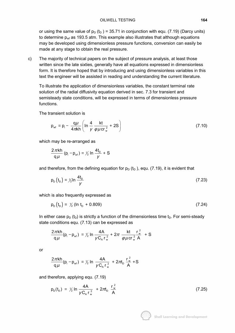
OILWELL TESTING 164
or using the same value of pD (tD ) = 35.71 in conjunction with equ. (7.19) (Darcy units)to determine pwf as 193.5 atm. This example also illustrates that although equationsmay be developed using dimensionless pressure functions, conversion can easily bemade at any stage to obtain the real pressure.
c) The majority of technical papers on the subject of pressure analysis, at least thosewritten since the late sixties, generally have all equations expressed in dimensionlessform. It is therefore hoped that by introducing and using dimensionless variables in thistext the engineer will be assisted in reading and understanding the current literature.
To illustrate the application of dimensionless variables, the constant terminal ratesolution of the radial diffusivity equation derived in sec. 7.3 for transient andsemisteady state conditions, will be expressed in terms of dimensionless pressurefunctions.
The transient solution is
wf i 2w
q 4 ktp p In 2S4 kh cr
µπ γ φ µ
� �= − +� �
� �(7.10)
which may be re-arranged as
D12i wf
4t2 kh (p p ) ln Sqπ
µ γ− = +
and therefore, from the defining equation for pD (tD ), equ. (7.19), it is evident that
( ) D12D D
4tp t lnγ
= (7.23)
which is also frequently expressed as
( ) 12D D Dp t (ln t 0.809)= + (7.24)
In either case pD (tD) is strictly a function of the dimensionless time tD. For semi-steadystate conditions equ. (7.13) can be expressed as
2w1
2i wf 2 2A w w
rkh 4A kt(p p ) ln 2 Sq AC r crπ π
µ γ φ µ2 − = + +
or2w1
2i wf D2A w
rkh 4A(p p ) ln 2 t Sq AC rπ π
µ γ2 − = + +
and therefore, applying equ. (7.19)2w1
2D D D2A w
r4Ap (t ) ln 2 tAC r
πγ
= + (7.25)
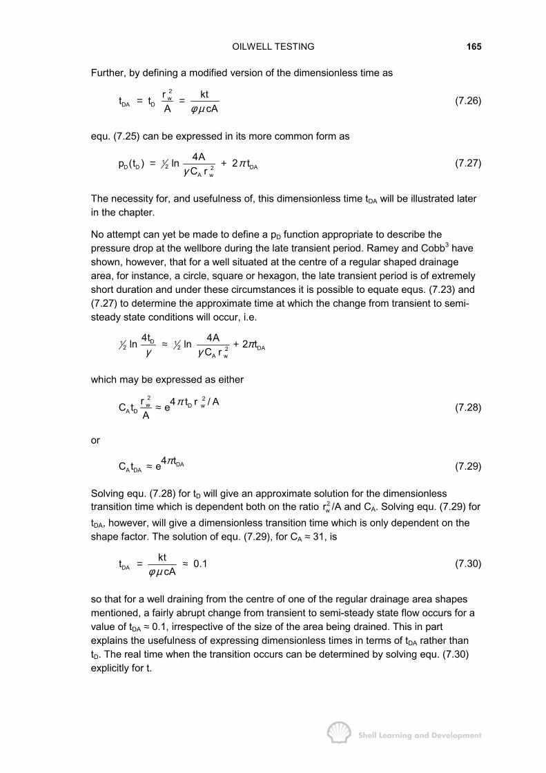
OILWELL TESTING 165
Further, by defining a modified version of the dimensionless time as2w
DA Dr ktt tA cAφ µ
= = (7.26)
equ. (7.25) can be expressed in its more common form as
12D D DA2
A w
4Ap (t ) ln 2 tC r
πγ
= + (7.27)
The necessity for, and usefulness of, this dimensionless time tDA will be illustrated laterin the chapter.
No attempt can yet be made to define a pD function appropriate to describe thepressure drop at the wellbore during the late transient period. Ramey and Cobb3 haveshown, however, that for a well situated at the centre of a regular shaped drainagearea, for instance, a circle, square or hexagon, the late transient period is of extremelyshort duration and under these circumstances it is possible to equate equs. (7.23) and(7.27) to determine the approximate time at which the change from transient to semi-steady state conditions will occur, i.e.
D1 12 2 DA2
A w
4t 4Aln ln 2 tC r
πγ γ
≈ +
which may be expressed as either2 2w D w
A Dr 4 t r / AC t eA
π≈ (7.28)
or
DAA DA
4 tC t e π≈ (7.29)
Solving equ. (7.28) for tD will give an approximate solution for the dimensionlesstransition time which is dependent both on the ratio 2
wr /A and CA. Solving equ. (7.29) fortDA, however, will give a dimensionless transition time which is only dependent on theshape factor. The solution of equ. (7.29), for CA ≈ 31, is
DAktt 0.1
cAφ µ= ≈ (7.30)
so that for a well draining from the centre of one of the regular drainage area shapesmentioned, a fairly abrupt change from transient to semi-steady state flow occurs for avalue of tDA ≈ 0.1, irrespective of the size of the area being drained. This in partexplains the usefulness of expressing dimensionless times in terms of tDA rather thantD. The real time when the transition occurs can be determined by solving equ. (7.30)explicitly for t.
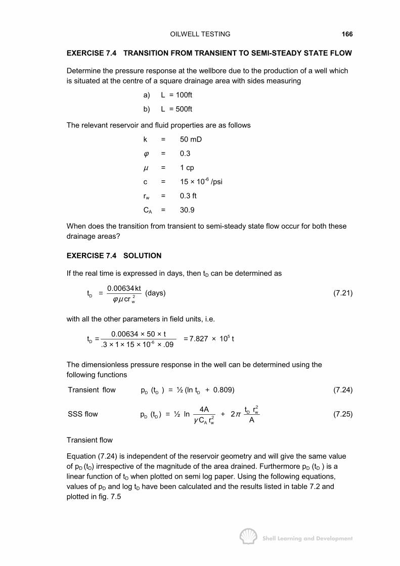
OILWELL TESTING 166
EXERCISE 7.4 TRANSITION FROM TRANSIENT TO SEMI-STEADY STATE FLOW
Determine the pressure response at the wellbore due to the production of a well whichis situated at the centre of a square drainage area with sides measuring
a) L = 100ft
b) L = 500ft
The relevant reservoir and fluid properties are as follows
k = 50 mD
φ = 0.3
µ = 1 cp
c = 15 × 10-6 /psi
rw = 0.3 ft
CA = 30.9
When does the transition from transient to semi-steady state flow occur for both thesedrainage areas?
EXERCISE 7.4 SOLUTION
If the real time is expressed in days, then tD can be determined as
D 2w
0.00634kttcrφ µ
= (days) (7.21)
with all the other parameters in field units, i.e.
5D -6
0.00634 50 tt 7.827 10 t.3 1 15 10 .09
× ×= = ×× × × ×
The dimensionless pressure response in the well can be determined using thefollowing functions
D D DTransient flow p (t ) ½ (ln t 0.809)= + (7.24)
2D w
D D 2A w
t r4ASSS flow p (t ) ½ ln 2 AC r
πγ
= + (7.25)
Transient flow
Equation (7.24) is independent of the reservoir geometry and will give the same valueof pD (tD) irrespective of the magnitude of the area drained. Furthermore pD (tD ) is alinear function of tD when plotted on semi log paper. Using the following equations,values of pD and log tD have been calculated and the results listed in table 7.2 andplotted in fig. 7.5

OILWELL TESTING 167
pD = ½ (2.303 log tD + 0.809)
= 1.151 log tD + 0.405
t (days) tD log tD pD (tD )
.05 39135 4.5926 5.69
.50 391350 5.5926 6.845.0 3913500 6.5926 8.00
TABLE 7.2
Semi-steady state flow
Evaluating equation (7.25) for cases a) and b) (refer table 7.3)
a) L = 100 ft pD (tD) = 4.4983 + 5.655 × 10⁻⁵ tD
b) L = 500 ft pD (tD) = 6.1078 + 2.2619 × 10⁻⁶ tD
Plots of pD (tD) versus log tD, fig. 7.5 show that, irrespective of the size of the squareboundary, flow will initially be under transient conditions. Eventually, however, theboundary effects will result in a transition to semi-steady state flow. The time at whichthis occurs is naturally dependent upon the dimensions of the volume drained and canbe read from the plots in fig. 7.5, as
for L = 100 ft; log tD = 4.10; tD = 12590 and t = 0.016 daysfor L = 500 ft; log tD = 5.50; tD = 316230 and t = 0.404 days
t (days) tD Dimensionless Pressure, pD
L=100 ft. L=500 ft.
.005 3914 4.72
.01 7827 4.94
.025 19568 5.60
.05 39135 6.71
.10 78270 8.92
.25 195675 15.56 6.55
.50 391350 26.63 6.991.00 782700 7.882.50 1956750 10.535.00 3913500 14.96
10.00 7827000 23.81TABLE 7.3
In themselves these figures lead to no general conclusion concerning the time at whichsemi-steady state flow commences. However, evaluating in terms of
2DA D wt t r / A= then
for L = 100 ft; tDA = 0.113and for L = 500 ft; tDA = 0.114

OILWELL TESTING 168
which indicate that semi-steady state conditions will occur for the same value of tDA
irrespective of the size of the square. It is generally true for a well situated at the centreof
- a square- a circle- a hexagon
that semi-steady state conditions will prevail after a flowing time such that tDA >0.1.
32
28
24
20
16
12
8
4
0
pD
1 2 3 4 5 6 7 log tD
SEMI STEADY STATE
L = 100 ft L = 500 ft
TRANSIENT FLOW
Fig. 7.5 Dimensionless pressure as a function of dimensionless flowing time for awell situated at the centre of a square (Exercise 7.4)
7.5 SUPERPOSITION THEOREM: GENERAL THEORY OF WELL TESTING
Mathematically the superposition theorem states that any sum of individual solutions ofa second order linear differential equation is also a solution of the equation.
In practice, this is one of the most powerful tools at the reservoir engineer's disposal forwriting down solutions to complex flow problems in the reservoir without explicitlysolving the full differential equation on each occasion. Applying the superpositiontheorem means that individual constant rate wells can be placed in any position in thereservoir at any time and an expression for the resulting pressure distribution in spaceand time derived by inspection. The principle will be illustrated with an example ofsuperposition in time at a fixed location which is particularly relevant to well testanalysis.
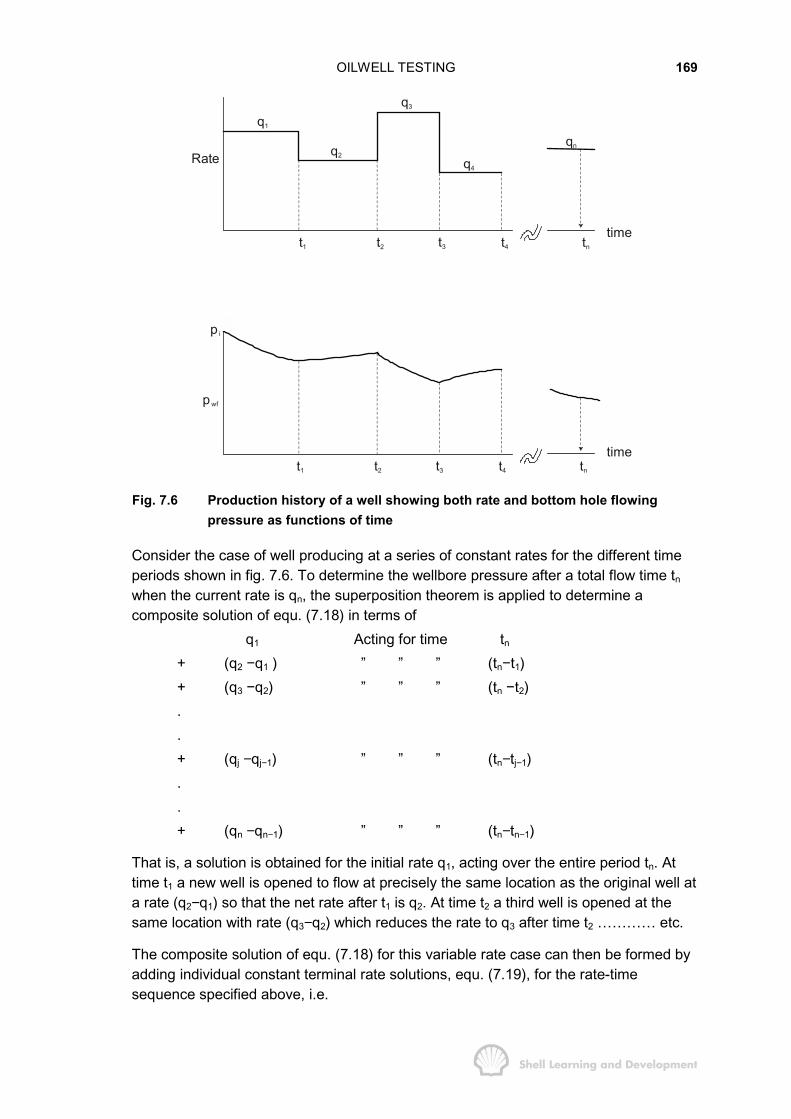
OILWELL TESTING 169
Rate
q1
q2
q3
q4
qn
t4t3t2t1 tn
time
t4t3t2t1 tn
p i
pwf
time
Fig. 7.6 Production history of a well showing both rate and bottom hole flowingpressure as functions of time
Consider the case of well producing at a series of constant rates for the different timeperiods shown in fig. 7.6. To determine the wellbore pressure after a total flow time tnwhen the current rate is qn, the superposition theorem is applied to determine acomposite solution of equ. (7.18) in terms of
q1 Acting for time tn+ (q2 −q1 ) ” ” ” (tn−t1)+ (q3 −q2) ” ” ” (tn −t2)..+ (qj −qj−1) ” ” ” (tn−tj−1)..+ (qn −qn−1) ” ” ” (tn−tn−1)
That is, a solution is obtained for the initial rate q1, acting over the entire period tn. Attime t1 a new well is opened to flow at precisely the same location as the original well ata rate (q2−q1) so that the net rate after t1 is q2. At time t2 a third well is opened at thesame location with rate (q3−q2) which reduces the rate to q3 after time t2 ………… etc.
The composite solution of equ. (7.18) for this variable rate case can then be formed byadding individual constant terminal rate solutions, equ. (7.19), for the rate-timesequence specified above, i.e.
OILWELL TESTING 170
( )n 1
n 2
n j 1
n n 1
i wf 1 D Dn n
2 1 D D D
3 2 D D D
j j 1 D D D
n n 1 D D D
2 kh p p (q 0) (p (t 0) S)
(q q ) (p (t t ) S)
(q q ) (p (t t ) S)
.
. (q q ) (p (t t ) S)
.
. (q q ) (p (t t ) S)
πµ
−
−
−
−
− = − − +
+ − − +
+ − − +
+ − − +
+ − − +
in which nwfp is the specific value of the bottom hole flowing pressure corresponding to
the total time tn which may occur at any time during the nth period of constant flow,when the rate is qn. In this summation all the skin factor terms disappear except for thelast, qn S. The summation can be expressed as
( ) ( )j 1n
n
i wf j D D D nnj 1
2 kh p p q p t t q Sπµ −
=
− = ∆ − +� (7.31)
in which j j j 1q q q −∆ = −
Equation (7.31) may be regarded as the basic equation for interpreting thepressure-time-rate data collected during any well test, and with minor modifications,described in Chapter 8, can equally well be applied to gas well test analysis. The wholephilosophy of well testing is to mechanically design the test with a series of differentflow rates, some of which may be zero (well closed in), for different periods of time sothat equ. (7.31) can be readily interpreted to yield some or all of the required reservoirparameters, pi, p , k, S, A and CA. The three most common forms of well testing are thesingle rate drawdown test, the pressure buildup test and the multi-rate drawdown test.The analysis of each of these tests using equ. (7.31) is briefly described below and inmuch greater detail in the following sections of this chapter.
a) Single rate drawdown test
In this type of test the well is flowed at a single constant rate for an extended period oftime so that
1 1 D Dnq q ; q q and t t= ∆ = =
and equ. (7.31) can be reduced to
( )i wf D D2 kh p p p (t ) S
q π
µ− = + (7.19)
which is simply the constant terminal rate solution expressed in dimensionless form.The flowing pressure pwf , which is recorded throughout the test, can be analysed as a

OILWELL TESTING 171
function of the flowing time t to yield the basic reservoir parameters k, S, A and CA. Themost common form of analysis used has already been fully described in exercise 7.2. Itis assumed that the initial equilibrium pressure pi is known and this is simply therecorded pressure prior to opening the well in the first place.
b) Pressure buildup testing
This is probably the most common of all well test techniques for which the rateschedule and corresponding pressure response are shown in fig. 7.7.
Rate
q
t ∆t time
(a)
time
(b)
Pressure
pi
pwfpws
t ∆t
Fig. 7.7 Pressure buildup test; (a) rate, (b) wellbore pressure response
Ideally the well is flowed at a constant rate q for a total time t and then closed in. Duringthe latter period the closed-in pressure pwf = pws is recorded as a function of the closedin time ∆t. Equation (7.31) can again be used but in this case with
n
n 1
1 1 D D D
2 2 D D D
q q ; q q ; t t tq 0 ; q (0 q) ; t t t
= ∆ = = + ∆
= ∆ = − − = ∆
the skin factor disappears by cancellation and the equation is reduced to
i ws D D D D D2 kh (p p ) p (t t ) p ( t )
qπ
µ− = + ∆ − ∆ (7.32)
Equation (7.32) is the basic equation for pressure buildup analysis and can beinterpreted in a variety of ways. The most common method of analysis is to plot theclosed in pressure pws as a function of log (t t)/ t+ ∆ ∆ .This is called the Horner plot4
and can be used to determine pi or p , kh, and S as will be described in detail insec. 7.7, and illustrated in exercises 7.6 and 7.7.
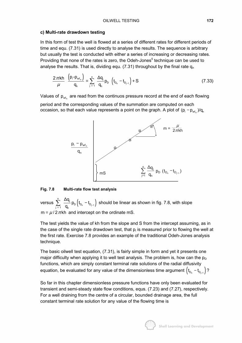
OILWELL TESTING 172
c) Multi-rate drawdown testing
In this form of test the well is flowed at a series of different rates for different periods oftime and equ. (7.31) is used directly to analyse the results. The sequence is arbitrarybut usually the test is conducted with either a series of increasing or decreasing rates.Providing that none of the rates is zero, the Odeh-Jones5 technique can be used toanalyse the results. That is, dividing equ. (7.31) throughout by the final rate qn
( ) ( )n
n j 1
ni wf jD D D
j 1n n
p -p q2 kh p t t Sq q
πµ −
=
∆= − +� (7.33)
Values of nwfp are read from the continuos pressure record at the end of each flowing
period and the corresponding values of the summation are computed on eachoccasion, so that each value represents a point on the graph. A plot of
ni wf n(p p )/q−
−ni wfp p
qn
−=
∆−� n j 1
nj
D D Dj 1 n
qp (t t )
qmS
m = µ
2π kh
Fig. 7.8 Multi-rate flow test analysis
versus ( )n j 1
nj
D D Dj 1 n
qp t t
q −=
∆−� should be linear as shown in fig. 7.8, with slope
m / 2 khµ π= and intercept on the ordinate mS.
The test yields the value of kh from the slope and S from the intercept assuming, as inthe case of the single rate drawdown test, that pi is measured prior to flowing the well atthe first rate. Exercise 7.8 provides an example of the traditional Odeh-Jones analysistechnique.
The basic oilwell test equation, (7.31), is fairly simple in form and yet it presents onemajor difficulty when applying it to well test analysis. The problem is, how can the pD
functions, which are simply constant terminal rate solutions of the radial diffusivityequation, be evaluated for any value of the dimensionless time argument ( )n j 1D Dt t
−− ?
So far in this chapter dimensionless pressure functions have only been evaluated fortransient and semi-steady state flow conditions, equs. (7.23) and (7.27), respectively.For a well draining from the centre of a circular, bounded drainage area, the fullconstant terminal rate solution for any value of the flowing time is
OILWELL TESTING 173
( ) ( )( ) ( )( )
n D2 t 21 n eDD
D D eD2 2 2 2n 1eD n 1 n eD 1 n
e J r2t 3p t lnr 24r J r J
α αα α α
−
=
∞= + − +
−� (7.34)
in which reD = re/rw and αn are the roots of
1 n eD 1 n 1 n 1 n eDJ ( r ) Y ( ) J ( ) Y ( r ) 0α α α α− =
and J1 and Y1, are Bessel functions of the first and second kind. Equation (7.34) is thefull Hurst and Van Everdingen constant terminal rate solution referred to in sec. 7.2, thedetailed derivation of which can be found in their original paper1, or in a concise form inAppendix A of the Matthews and Russell monograph6. One thing that can be observedimmediately from this equation is that it is extremely complex, to say the least, and yetthis is the expression for the case of simple radial symmetry. In fact, as already notedin sec. 7.4 and demonstrated in exercise 7.4, for a well producing from the centre of aregular shaped drainage area there is a fairly abrupt change from transient to semi-steady state flow so that equ. (7.34) need never be used in its entirity to generate pD
functions. Instead, equ. (7.23) can be used for small values of the flowing time andequ. (7.27) for large values, with the transition occurring at tDA ≈ 0.1.
Problems arise when trying to evaluate pD functions for wells producing fromasymmetrical positions with respect to irregular shaped drainage boundaries. In thiscase a similar although more complex version of equ. (7.34) could be derived whichagain would reduce to equ. (7.23) for small tD and to equ. (7.27) for large tD.
Now, however, there would be a significant late transient period during which therewould be no alternative but to use the full solution to express the pD function.
Due to the complexity of equations such as equ. (7.34) engineers have always tried toanalyse well tests using either transient or semi-steady state analysis methods and incertain cases this approach is quite valid, such analyses having already beenpresented in exercise 7.2 for a single rate drawdown test. Sometimes, however,serious errors can arise through using this simplified approach and some of these willbe described in detail in the following sections. It first remains, however, to describe anextremely simple method of generating pD functions for any value of the dimensionlesstime and for any areal geometry and well asymmetry. The method requires anunderstanding of the Matthews, Brons and Hazebroek pressure buildup analysistechnique which is described in the following section.
7.6 THE MATTHEWS, BRONS, HAZEBROEK PRESSURE BUILDUP THEORY
In this section the MBH pressure buildup analysis technique will be examined from apurely theoretical standpoint, the main aim being to illustrate a simple method ofevaluating the pD function for a variety of drainage shapes and for any value of thedimensionless flowing time.
The theoretical buildup equation was presented in the previous section as
( )i ws D D D D D2 kh (p p ) p (t t ) p t
qπ
µ− = + ∆ − ∆ (7.32)
OILWELL TESTING 174
in which tD is the dimensionless flowing time prior to closure and is therefore a constantwhile ∆tD is the dimensionless closed in time corresponding to the pressure pws, thelatter two being variables which can be determined by interpretation of the pressurechart retrieved after the survey.
For small values of ∆t, pws is a linear function of In (t+∆t)/∆t, which can be verified byadding and subtracting ½ In (tD +∆tD ) to the right hand side of equ. (7.32) andevaluating pD (∆tD) for small ∆t using equ. (7.23). Thus,
D1 12 2i ws D D D D D
4 t2 kh (p p ) p (t t ) In ln (t t )qπ
µ γ∆− = + ∆ − ± + ∆
which can alternatively be expressed as
( )D D1 12 2i ws D D D
4 t t2 kh t t(p p ) ln p (t t ) lnq tπ
µ γ+ ∆+ ∆− = + + ∆ −
∆(7.35)
in which dimensionless time has been replaced by real time in the ratio t+∆t/∆t. Again,for small values of the closed-in time ∆t
D D Dln (t t ) ln (t )+ ∆ ≈
and
D D D D Dp (t t ) p (t )+ ∆ ≈
and equ. (7.35) can be reduced to
D1 12 2i ws D D
4t2 kh t t(p p ) ln p (t ) lnq tπ
µ γ+ ∆− = + −∆
(7.36)
Since the dimensionless flowing time tD is a constant then so too are the last two termson the right-hand side of equ. (7.36) and therefore, for small values of ∆t a plot of theobserved values of pws versus In (t+∆t)/∆t should be linear with slope m q / 4 khµ π= ,from which the value of the permeability can be determined. This particularpresentation of pressure buildup data is known as a Horner plot4 and is illustrated infig. 7.9.
Equation (7.36) is the equation describing the early linear buildup and due to themanner of derivation is only valid for small values of ∆t. Nevertheless, having obtainedsuch a straight line it is perfectly valid to extrapolate the line to large values of ∆t inwhich case equ. (7.36) can be replaced by
( ) ( ) Di ws(LIN) D D
4t2 kh t tp p ½ ln p t ½lnq tπ
µ γ+ ∆− = + −∆
(7.37)
in which pws, the actual pressure in equ. (7.36), is now replaced by pws(LIN ) which issimply the pressure for any value of ∆t on the extrapolated linear trend and while thelatter may be hypothetical it is, as will be shown, mathematically very useful. Theequation can be used in two ways. Firstly, drawing a straight line through the early

OILWELL TESTING 175
linear trend of the observed points on the Horner buildup plot will automatically matchequ. (7.37) as illustrated in fig. 7.9. Extrapolation of this line is useful in thedetermination of the average reservoir pressure, Alternatively, an attempt can be madeto theoretically evaluate the pD function in the equation and then compare thetheoretical with the actual straight line with the aim of gaining additional informationabout the reservoir. The application of this method will be illustrated in exercise 7.7.
If the well could be closed in for an infinite period of time the initial linear buildup wouldtypically follow the curved solid line in fig. 7.9 and could theoretically be predicted usingequ. (7.32). The final buildup pressure p is the average pressure within the boundedvolume being drained and is consistent with the material balance for this volume, i.e.
icAh (p p) qtφ − = (7.12)
which may be expressed as
( )i DA2 kh 2 khqtp p 2 t
q q cA hπ π π
µ µ φ− = = (7.38)
t + ∆t∆t
In
4 3 2 1 0
A
B
pws equ. (7.37)
equ. (7.32)
large ∆tsmall ∆t
p*
p
Fig. 7.9 Horner pressure buildup plot for a well draining a bounded reservoir, or partof a reservoir surrounded by a no-flow boundary
The closed in pressures observed during the test are plotted between points A and B.Since it is impracticable to close in a well for a sufficient period of time so that the entirebuildup is obtained then it is not possible to determine p directly from the Horner plot ofthe observed pressures. Instead, indirect methods of calculating p are employed whichrely on the linear extrapolation of the observed pressures to large values of ∆t andtherefore implicitly require the use of equ. (7.37). In particular, the Matthews, Brons andHazebroek7 method involves the extrapolation of the early linear trend to infinite closedin time. The extrapolation to In (t+∆t) / ∆t = 0 gives the value of pws(LIN) = p* In the
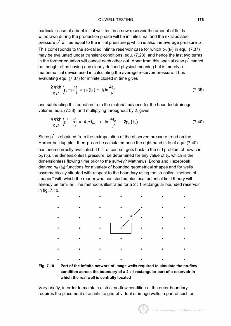
OILWELL TESTING 176
particular case of a brief initial well test in a new reservoir the amount of fluidswithdrawn during the production phase will be infinitesimal and the extrapolatedpressure p* will be equal to the initial pressure pi which is also the average pressure p .This corresponds to the so-called infinite reservoir case for which pD (tD) in equ. (7.37)may be evaluated under transient conditions, equ. (7.23), and hence the last two termsin the former equation will cancel each other out. Apart from this special case p* cannotbe thought of as having any clearly defined physical meaning but is merely amathematical device used in calculating the average reservoir pressure. Thusevaluating equ. (7.37) for infinite closed in time gives
( ) D12i D D
4t2 kh *p p p (t ) lnqπ
µ γ− = − (7.39)
and subtracting this equation from the material balance for the bounded drainagevolume, equ. (7.38), and multiplying throughout by 2, gives
( ) ( )DDA D D
4t4 kh *p p 4 t ln 2p tqπ π
µ γ− = + − (7.40)
Since p* is obtained from the extrapolation of the observed pressure trend on theHorner buildup plot, then p can be calculated once the right hand side of equ. (7.40)has been correctly evaluated. This, of course, gets back to the old problem of how canpD (tD), the dimensionless pressure, be determined for any value of tD, which is thedimensionless flowing time prior to the survey? Matthews, Brons and Hazebroekderived pD (tD) functions for a variety of bounded geometrical shapes and for wellsasymmetrically situated with respect to the boundary using the so-called "method ofimages" with which the reader who has studied electrical potential field theory willalready be familiar. The method is illustrated for a 2 : 1 rectangular bounded reservoirin fig. 7.10.
aj
Fig. 7.10 Part of the infinite network of image wells required to simulate the no-flowcondition across the boundary of a 2 : 1 rectangular part of a reservoir inwhich the real well is centrally located
Very briefly, in order to maintain a strict no-flow condition at the outer boundaryrequires the placement of an infinite grid of virtual or image wells, a part of such an
OILWELL TESTING 177
array being shown in fig. 7.10, each well producing at the same rate as the real wellwithin the boundary. The constant terminal rate solution for this complex system canthen be expressed as
( ) ( )2jD1 1
2 2i wf D Dj 2
ca4t2 kh p p p t ln eiq 4kt
φ µπµ γ =
∞− = = + � (7.41)
in which the first term on the right hand side of the equation is the component of thepressure drop due to the production of the well itself, within an infinite reservoir,equ. (7.23), and the infinite summation is the contribution to the wellbore pressure dropdue to the presence of the infinite array of image wells which simulate the no-flowboundary. The exponential integral function is the line source solution of the diffusivityequation introduced in sec. 7.2, equ. (7.11), for the constant terminal rate case and isnecessitated by the fact that the distance aj between the producing well and the jth
image well is large so that the logarithmic expression of the line source solution,equ. (7.10), is an unacceptable approximation and the full exponential integral solutionmust be used. The infinite summation in equ. (7.41) is therefore an example ofsuperposition in space of the basic constant terminal rate solution of the diffusivityequation. For further details of the mathematical technique the reader should consultthe appendices of the original MBH paper7.
Using this method to determine pD (tD), MBH were able to evaluate equ. (7.40) for awide variety of boundary conditions and presented their results as plots of
( ) DA4 kh *p p vs. t
qπ
µ−
where tDA is the dimensionless flowing time. These charts have been included in thistext as figs. 7.11-15. The individual plots are for different geometries and differentasymmetries of the producing well with respect to the no-flow boundary.
The MBH charts were originally designed to facilitate the determination of p frompressure buildup data by first determining p*, by the extrapolation of the Horner plot,and k from the slope of the straight line. If an estimate is made of the area beingdrained, tDA = kt/φµcA can be calculated for the actual flowing time t. Then, using theappropriate MBH chart the value of 4πkh (p*−p )/qµ is read off the ordinate from whichp can be calculated. The details of this important technique will be described insec. 7.7. For the moment, the MBH charts will be used in a more general manner todetermine pD (tD) functions for the range of geometries covered by the charts and forany value of the flowing time.
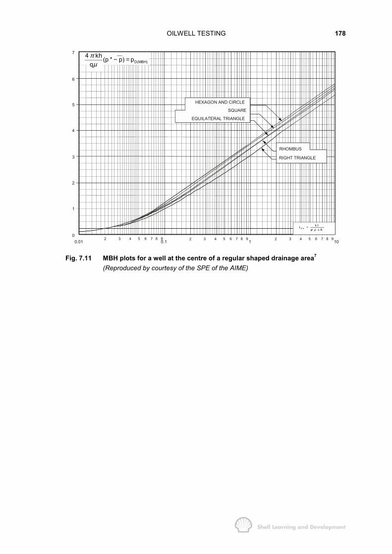
OILWELL TESTING 178
7
6
5
4
3
2
1
00.01 0.1 1 10
2 3 4 5 6 7 8 9 2 3 4 5 6 7 8 92 3 4 5 6 7 8 9
HEXAGON AND CIRCLE
SQUARE
EQUILATERAL TRIANGLE
RHOMBUS
RIGHT TRIANGLE
D(MBH)4 kh (p * p) p
qπ
µ− =
D Ak tt
c Aφ µ=
Fig. 7.11 MBH plots for a well at the centre of a regular shaped drainage area7
(Reproduced by courtesy of the SPE of the AIME)
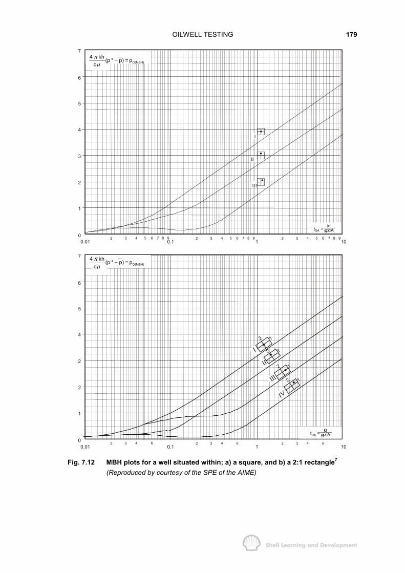
OILWELL TESTING 179
7
6
5
4
3
2
1
00.01 0.1 1 10
2 3 4 5 6 7 8 9 2 3 4 5 6 7 8 92 3 4 5 6 7 8 9
II
I
III
D(MBH)4 kh (p * p) p
qπ
µ− =
tDA = ktφµcA
7
6
5
4
2
2
1
00.01 0.1 1 10
2 3 4 6 2 3 4 62 3 4 6
2
1
2
1
2
1
2
1
I
II
III
IV
D(MBH)4 kh (p * p) p
qπ
µ− =
tDA = ktφµcA
Fig. 7.12 MBH plots for a well situated within; a) a square, and b) a 2:1 rectangle7
(Reproduced by courtesy of the SPE of the AIME)
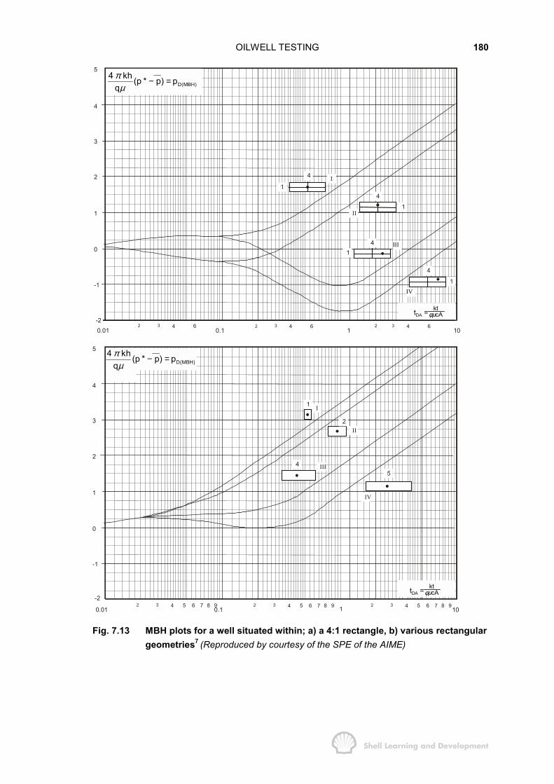
OILWELL TESTING 180
5
4
3
2
1
0
-1
0.01 0.1 1 102 3 4 6 2 3 4 62 3 4 6
-2
I
II
III
IV
4
4
4
4
1
1
1
1
D(MBH)4 kh (p * p) p
qπ
µ− =
tDA = ktφµcA
5
4
3
2
1
0
-1
0.01 0.1 1 102 3 4 5 6 7 8 9 2 3 4 5 6 7 8 92 3 4 5 6 7 8 9
I
II
III
IV
1
2
45
-2
D(MBH)4 kh (p * p) p
qπ
µ− =
tDA = ktφµcA
Fig. 7.13 MBH plots for a well situated within; a) a 4:1 rectangle, b) various rectangulargeometries7 (Reproduced by courtesy of the SPE of the AIME)

OILWELL TESTING 181
0.01 0.12 3 4 5 12 3 4 5 102 3 4 5 1002 3 4 5-1
0
1
2
3
4
5
6
I WELL 1/8 OF HEIGHT AWAY FROM SIDEII WELL 1/8 OF HEIGHT AWAY FROM SIDEIII WELL 1/8 OF HEIGHT AWAY FROM SIDE
II
III
I
2
2
D(MBH)4 kh (p * p) p
qπ
µ− =
tDA = ktφµcA
Fig. 7.14 MBH plots for a well in a square and in rectangular 2:1 geometries7
0.01 0.12 3 4 5 12 3 4 5 102 3 4 5 1002 3 4 5-3
-2
-1
0
1
2
3
4
I WELL 1/16 OF LENGTH AWAY FROM SIDEII WELL 1/4 OF ALTITUDE AWAY FROM APEX
1I
2
II
D(MBH)4 kh (p * p) p
qπ
µ− =
tDA = ktφµcA
Fig. 7.15 MBH plots for a well in a 2:1 rectangle and in an equilateral triangle7
(Reproduced by courtesy of the SPE of the AIME).

OILWELL TESTING 182
As indicated by Cobb and Dowdle8, equ. (7.40) can be solved for pD (tD) as
( ) ( )D1 12 2D D DA D(MBH) DA
4tp t 2 t ln p tπγ
= + − (7.42)
in which
( ) ( )D(MBH) DA4 kh *p t p p
qπ
µ= −
is the dimensionless MBH pressure, which is simply the ordinate of the MBH chartevaluated for the dimensionless flowing time tDA.
Equation (7.42) is extremely important since it represents the constant terminal ratesolution of the diffusivity equation which, for the case of a well draining from the centreof a bounded, circular part of a reservoir, replaces the extremely complex form ofequ. (7.34). It should be noted, however, that the mathematical complexity ofequ. (7.34) is not being avoided since it is implicitly included in the MBH charts whichwere evaluated using the method of images. Furthermore, equ. (7.42) is not restrictedto circular geometry and can be used for the range of the geometries and wellasymmetries included in the MBH charts.
For very short values of the flowing time t, when transient conditions prevail, the lefthand side of equ. (7.42) can be evaluated using equ. (7.23) and the former can bereduced to
( ) ( )D(MBH) DA DA4 kh *p t p p 4 t
qπ π
µ= − = (7.43)
Alternatively, for very long flowing times, when semi-steady state conditions prevail, theleft hand side of equ. (7.42) can be expressed as equ. (7.27) and in this caseequ. (7.42) becomes
( ) ( ) ( )2w
D(MBH) DA A D A DAr4 kh *p t p p ln C t ln C t
q Aπ
µ= − = = (7.44)
Inspection of the MBH plots of fig. 7.11, for a well situated at the centre of a regularshaped bounded area, illustrates the significance of equs. (7.43) and (7.44). For smallvalues of the dimensionless flowing time tDA the semi-log plot of pD(MBH) vs tDA is non-linear while for large tDA the plots are all linear as predicted by equ. (7.44), and haveunit slope (dpD(MBH)/d (In tDA) = 1). This latter feature is common to all the MBH charts,figs. 7.11-15. that in each case there is a value of tDA, the magnitude of which dependson the geometry and well asymmetry, for which the plots become linear indicating thestart of the semi-steady state flow condition. Furthermore, for the symmetry conditionsof fig. 7.11 there is a fairly sharp transition between transient and semi-steady stateflow at a value of tDA ≈ 0.1, which confirms the conclusion reached in sec. 7.4 andexercise 7.4. For the geometries and various degrees of well asymmetry depicted inthe remaining charts, however, there is frequently a pronounced degree of curvatureextending to quite large values of tDA before the start of semi-steady state flow. This

OILWELL TESTING 183
part of the plots represents both the pure transient flow period, equ. (7.43), and the latetransient period and it is not worthwhile trying to distinguish between the two.
Equation (7.44) is interesting since it reveals how the Dietz shape factors wereoriginally determined. Dietz, whose paper on pressure analysis9 was published someyears after that of MBH, evaluated the relationship expressed in equ. (7.44) for thespecific value of tDA = 1, thus
( ) ( )DA
D(MBH) DA At4 kh *p t 1 p p ln C
1qπ
µ= = − =
=(7.45)
Values of In CA (and hence CA ) could be determined as the ordinate of the MBH chartsfor each separate plot corresponding to the value of tDA = 1, and these are shown infig. 6.4. In some cases of extreme well asymmetry, late transient flow conditions stillprevail at tDA = 1 (e.g. fig 7.13) and in these cases the linear trend of pD(MBH) versus tDA
must be extrapolated back to the specific value tDA = 1 to determine the correct shapefactor. The usefulness of the Dietz shape factors in the formulation of equationsdescribing semi-steady state flow, for which they were derived, has already been amplyillustrated in this text.
The importance of equ. (7.42) for generating dimensionless pressure functions for avariety of boundary conditions and for any value of the flowing time cannot beoveremphasised. It is rather surprising that this equation has been lying dormant in theliterature since 1954, the date of the original MBH paper, with its full potential beinglargely unrealised. It appears in disguised form in many papers and even in the classicMatthews, Russell, SPE monograph6 (equ. 10.18, p. 109), yet it was not presented inthe simple form of equ. (7.42) of this text until it was highlighted in a brief J.P.T. Forumarticle in 1973 by Cobb and Dowdle8. The latter use a slightly modified form of theequation in which the right hand side of equ. (7.42) is expressed strictly as a function oftDA, thus
( ) ( )1 1 12 2 2D DA DA DA D(MBH) DA2
w
4Ap t 2 t ln t ln p tr
πγ
= + + − (7.46)
In application to general oilwell test analysis, any rate-time-pressure sequence can beanalysed using the following general equations
( ) ( )n n j 1
n
i wf j D D D nj 1
2 kh p p q p t t q Sπµ −
=
− = ∆ − +� (7.31)
in which ( ) ( )n j 1D D D D Dp t t p t−
′− = can be evaluated using either equ. (7.42) or (7.46), for
dimensionless time arguments Dt′ or DAt′ , respectively and as will be shown inChapter 8, with slight modification, the same combination of equations can also beapplied to gas well testing. Theoretically, at least, the use of equ. (7.42) to quantify thepD function in equ. (7.31) removes the problem of trying to decide under which flowingcondition pD should be evaluated because it is valid for all flowing times. Even if tDA
exceeds the maximum value on the abscissa of the MBH chart, the plots are all linearat this point, and therefore pD(MBH) can readily be calculated by linear extrapolation. For

OILWELL TESTING 184
very short or very long flowing times equ. (7.42) reduces to equ. (7.23) and (7.27)respectively, which can be verified by using the argument used to derive equ. (7.43)and (7.44) in reverse, i.e. by evaluating pD(MBH) in equ. (7.42) as being equal to 4πtDA
and In (CA tDA), respectively.
The relative ease with which pD functions can be generated using the MBH charts isillustrated in the following exercise which is an extension of exercise 7.2.
EXERCISE 7.5 GENERATION OF DIMENSIONLESS PRESSURE FUNCTIONS
The analysis of the single rate drawdown test, exercise 7.2, indicated that the Dietzshape factor for the 35 acre drainage area had the value CA = 5.31. The tabulatedvalues of CA presented in fig. 6.4 indicate that there are three geometricalconfigurations with shape factors in the range of 4.5 to 5.5 which are shown in fig. 7.16.
2
4
1
1
(a)
(b)
(c)
C = 4.57A
C = 4.86A
C = 5.38A
Fig. 7.16 Geometrical configurations with Dietz shape factors in the range, 4.5-5.5
The geological evidence suggests that the 2 : 1 geometry, fig. 7.16(b), is probablycorrect. Using the basic data and results of exercise 7.2, confirm the geologicalinterpretation by comparing the observed pressure decline, table 7.1, with thetheoretical decline calculated for the three geometries of fig. 7.16.
EXERCISE 7.5 SOLUTION
The constant terminal rate solution of the radial diffusivity equation, in field units, is,equ. (7.19),
( ) ( )3
i wf D Do
7.08 10 kh p p p t Sq Bµ
−× − = +
in which the pD function can be determined using equ. (7.46); and evaluating for thedata and results of exercise

OILWELL TESTING 185
7.2 (i.e. k = 240 mD, A = 35 acres, S = 4.5).
wf DA DA D(MBH) DA0.0189(3500 p ) 2 t ½ In t 8.632 ½ p (t ) 4.5π− = + + − + (7.46)
in which
DA -6
DA
.000264 kt .000264 240 t (hrs)tcA .18 1 15 10 35 43560
t 0.0154 tφ µ
× ×= =× × × × ×
=
For convenience, equ. (7.46) can be reduced to
wf D(MBH) DA0.0189 (3500 p ) ½ p (t )α− = − (7.47)
in which
DA DA2 t ½ ln t 13.132α π= + +
and has the same value for all three geometries shown in fig. 7.16. Values of pwf inequ. (7.47) can therefore be calculated by reading values of pD(MBH) (tDA) from theappropriate MBH plots contained in figs. 7.11-15. The values of ½ pD(MBH) (tDA) and pwf
for all three geometries are listed in table 7.4 for the first 50 hours of the drawdowntest. Plots of ∆pwf, which is the difference between the calculated and observed bottomhole flowing pressure, versus the flowing time, are shown in fig. 7.17. These plots tendto confirm that the geological interpretation, fig. 7.16(b), is appropriate. For the othertwo rectangular geometries the late transient flow period is not modelled correctly. Forcomparison the plot has also been made for the case of a well draining from the centreof circular bounded area, which is the simple case normally considered in the literature.As can be seen, the value of ∆pwf after 50 hours, when semi-steady state conditionsprevail, is 44 psi for this latter case.

OILWELL TESTING 186
=2
= 1
TIME (hrs)10
50
40
30
20
10
0
-20
-30
-10
20 30 40 50
= =x4
1
wfp (psi)∆
Fig. 7.17 Plots of ∆∆∆∆pwf (calculated minus observed) wellbore flowing pressure as afunction of the flowing time, for various geometrical configurations(Exercise 7.5)
To facilitate the calculation of dimensionless pressure functions, as illustrated inexercise 7.5, the MBH dimensionless plots of pD(MBH) versus tDA can be expressed indigitised form and used as a data bank in a simple computer program to evaluate pD
functions by applying equ. (7.46) (which can always be reduced to the form ofequ. (7.47)). In fact such a program could be written for the range of small deskcalculators which have sufficient memory storage capacity. Digitised MBH functionshave already been presented by Earlougher et al10 for all the rectangular geometricalconfigurations considered by Matthews, Brons and Hazebroek.

OILWELL TESTING 187
t(hrs)
Observedpwf
(psia) tDA α
2
1
4
1
½ pD(MBH) pwf ½ pD(MBH) pwf ½ pD(MBH) pwf ½ pD(MBH) pwf
1 2917 .0154 11.142* .093 2915 .093 2915 .093 2915 .093 2915
2 2900 .0308 11.585 .151 2895 .192 2897 .146 2895 .134 2897
3 2888 .0462 11.885 .167 2880 .267 2885 .171 2880 .285 2886
4 2879 .0616 12.126 .163 2867 .331 2876 .180 2868 .397 2879
5 2869 .0770 12.334 .148 2855 .357 2866 .168 2856 .474 2872
7.5 2848 .1155 12.779 .117 2830 .406 2845 .168 2833 .663 2859
10 2830 .1540 13.164 .117 2810 .429 2826 .194 2814 .809 2846
15 2794 .2310 13.851 .158 2776 .441 2790 .253 2781 1.008 2820
20 2762 .3080 14.478 .213 2745 .450 2758 .327 2751 1.152 2795
30 2703 .4620 15.649 .387 2692 .497 2697 .481 2698 1.357 2744
40 2650 .6160 16.760 .536 2642 .589 2644 .618 2646 1.501 2693
50 2597 .7700 17.839 .643 2590 .666 2591 .729 2595 1.602 2641TABLE 7.4
*) DA DA 2 t ½ ln t 13.132α π= + +
OILWELL TESTING 188
In addition, the Earlougher paper describes a relatively simple method for generatingMBH functions for rectangular geometries other than those included in figs. 7.11-15and for boundary conditions other than the no-flow condition which is assumed for theMBH plots. MBH functions for a constant outer boundary pressure and for cases inbetween pressure maintenance and volumetric depletion, corresponding to partialwater drive, can therefore be simulated. Ramey et al11 have also described thesimulation of well test analysis under water drive conditions. However, while the theoryexists to describe variable pressure conditions at the drainage boundary, the engineeris still faced with the perennial problem of trying to determine exactly what outerboundary condition he is trying to simulate.
To use the combination of equ. (7.31) and (7.42) to describe any form of oilwell testappears at first sight to offer a simplified generalization of former analysis techniques,yet, as will be shown in the remainder of this chapter and in Chapter 8, the approachintroduces certain difficulties. Providing the test is run under transient flow conditionsthen the pD function, equ. (7.42), can be described by the simplified form
DD D
4tp (t ) ½ ln γ
= (7.23)
in which there is no dependence upon the magnitude or shape of the drainageboundary nor upon the degree of asymmetry of the well with respect to the boundary.Therefore, if well tests are analysed using equ. (7.23) in conjunction with equ. (7.31),the results of the test will only yield values of the permeability, k, (which is implicit in thedefinition of tD) and the mechanical skin factor, S. As soon as the test extends for asufficient period of time so that either late transient or semi-steady state conditionsprevail then the effect of the boundary of the drainage area begins to influence theconstant terminal rate solution and the full pD function, equ. (7.42), must be used in thetest analysis. In this case the interpretation can become a great deal more complexbecause new variables, namely, the area drained, shape and well asymmetry, areintroduced which are frequently additional unknowns. Exercise 7.5 illustrated how asingle rate drawdown test can be analysed to solve for these latter three parametersusing pD functions expressed by equ. (7.42), thus gaining additional information fromthe test.
Largely due to the fact that test analysis becomes more complicated when tests arerun under conditions other than that of purely transient flow, the literature is permeatedwith transient analysis techniques. This mathematical simplification does indeedproduce convenient analysis procedures but can, in some cases, lead to severe errorsin determining even the basic parameters k and S from a well test, particularly in thecase of multi-rate flow testing as will be illustrated in sec. 7.8. Fortunately, the pressurebuildup test, if it can be applied, leads to the unambiguous determination of k and Sand therefore this method will be described in considerable detail in sec. 7.7.

OILWELL TESTING 189
7.7 PRESSURE BUILDUP ANALYSIS TECHNIQUES
The remaining sections of this chapter concentrate on the practical application of thetheory developed so far to the analysis of well tests. It is considered worthwhile at thisstage to change from Darcy to field units since, in practice, tests are invariablyanalysed using the latter and the majority of the literature on the subject employs theseunits. All equations in the remainder of this chapter will therefore be formulated usingthe field units specified in table 4.1. Since a great many of the equations are expressedin dimensionless parameters they remain invariant, or at least partially invariant inform. For instance, the most significant equation in the present subject of pressurebuildup analysis is that describing the theoretical linear buildup, which in Darcy units, is
( ) ( ) Di ws(LIN) D D
4t2 kh t tp p ½ ln p t ½ lnq tπ
µ γ+ ∆− = + −∆
(7.37)
and which, on conversion to field units becomes
( ) ( )-3 Di ws(LIN) D D
o
4tkh t t7.08 10 p p 1.151 log p t ½ lnq B tµ γ
+ ∆× − = + −∆
(7.48)
The conversion of the left hand side of this equation has already been described inexercise 7.3 and is necessary to preserve this expression as dimensionless, in fieldunits. The only change to the right hand side is that the natural log of thedimensionless time ratio has been replaced by log10, which is mainly required forplotting purposes, the remainder of the equation is invariant in form. Thus the pD
function is still
DD D DA D(MBH) DA
4tp (t ) 2 t ½ ln ½ p (t ) πγ
= + − (7.42)
which is totally invariant, although in evaluating this expression it must be rememberedthat now
D 2w
ktt 0.000264 (t-hours)crφµ
= (7.20)
and
DAktt 0.000264 (t-hours)cAφµ
= (7.49)
The pD(MBH) term is, in the majority of cases, just a number read from the MBH chartscorresponding to tDA evaluated in field units. Only when used to calculate p using theMBH method does it require interpreting as
( )D (MDH)o
khp 0.01416 p * pq Bµ
= −
The Horner plot for a typical buildup is shown as fig. 7.18.

OILWELL TESTING 190
4 3 2 1 0
observed dataequation (7.48)
pws(LIN) I − hr
p
(psi)
ws
small ∆t large ∆t
+ ∆∆
t tlogt
+ ∆∆
t tt
10000 1000 100 10 1
m
p*
Fig. 7.18 Typical Horner pressure buildup plot
The first part of the buildup is usually non-linear resulting from the combined effects ofthe skin factor and afterflow. The latter is due to the normal practice of closing in thewell at the surface rather than downhole and will be described in greater detail insec 7.11. Thereafter, a linear trend in the plotted pressures is usually observed forrelatively small values of ∆t and this can be analysed to determine the effectivepermeability and the skin factor. The former can be obtained by measuring the slope ofthe straight line, m, and from equ. (7.48) it is evident that
oq Bm 162.6 psi/log.cycle khµ= (7.50)
Providing the well is fully penetrating and the PVT properties are known, equ. (7.50)can be solved explicitly for k. The skin factor can be determined using the APIrecommended procedure which consists of subtracting equ. (7.48), the theoreticalequation of the linear buildup, from the constant terminal rate solution which describesthe pressure drawdown prior to closure and in field units is
-3i wf D D
o
kh7.08 10 (p p ) p (t ) Sq Bµ
× − = + (7.51)
where pwf is the bottom hole flowing pressure at the time of closure and t the flowingtime. The subtraction results in
( )ws(LIN)
-3 Dwf
o
4tkh t t7.08 10 p p ½ ln S 1.151 logq B tµ γ
+ ∆× − = + −∆
which may be solved for S to give

OILWELL TESTING 191
( )ws(LIN) wf
2w
p pt t 0.000264 4ktS 1.151 log logt m crγ φ µ
� �−+ ∆ ×� �= + −� �∆� �
in which m is the slope of the buildup. Finally, evaluating this latter equation for thespecific value of ∆t = 1 hour, and assuming that t >> ∆t gives
( )ws(LIN) 1 -hr wf2w
p p kS 1.151 log 3.23m crφ µ
� �−� �= − +� �� �
(7.52)
in which pWS(LIN) 1-hr is the hypothetical closed-in pressure read from the extrapolatedlinear buildup trend at ∆t = 1 hour as shown in fig. 7.18.
It should be noted in connection with the determination of the permeability from thebuildup plot that k is in fact, the average effective permeability of the formation beingtested, thus for the simultaneous flow of oil and water in a homogeneous reservoir
( ) ( )ro wabsk k k S= × (7.53)
in which ( )ro wk S is the average relative permeability representative for the flow of oil in
the entire formation and is a function of the thickness averaged water saturationprevailing at the time of the survey. It has been assumed until now that reservoirs areperfectly homogeneous. In a test conducted in an inhomogeneous, stratified reservoir,however, providing the different layers in the reservoir are in pressure communication,the measured permeability will be representative of the average for the entire layeredsystem for the current water saturation distribution. The concept of averaged (relative)permeability functions which account for both stratification and water saturationdistribution will be described in detail in Chapter 10. The permeability measured fromthe buildup, or for that matter from any well test, is therefore the most useful parameterfor assessing the well's productive capacity since it is measured under in-situ flowconditions. Problems occur in stratified reservoirs when the separate sands are not inpressure communication since the individual layers will be depleted at different rates.This leads to pressure differentials between the layers in the wellbore, resulting incrossflow.
It is also important to note that in the subtraction of equ. (7.48) from equ. (7.51) todetermine the skin factor, the pD (tD) functions in each equation disappear leading to anunambiguous determination of S. If this were not the case then one could have littleconfidence in the calculated value of S since the evaluation of pD (tD) at the time ofclosure may require a knowledge of the geometry of the drainage area and degree ofwell asymmetry with respect to the boundary. This point is made at this stage tocontrast this method of determining the skin factor with the method which will bedescribed in sec. 7.8, for multi-rate flow tests, in which the calculation of S does rely onthe correct determination of the dimensionless pressure functions throughout the test.
Figure 7.19 shows the effect of the flowing time on the Horner buildup plot. For aninitial well test in a reservoir, if the flowing period prior to the buildup is short, then pD

OILWELL TESTING 192
(tD) in equ. (7.48) can be approximated as ½ In(4 tD /γ) and the last two terms in theequation will cancel resulting in the simple buildup equation
ows i
q B t tp p 162.2 logkh tµ + ∆= −
∆(7.54)
which corresponds to the plot for t ≈ 0 in fig. 7.19.
equation (7.48)actual buildup
pws
4 3 2 1 0
p*
p*
p*
p
p
p (initial survey)
1- year
6 - monthst 0
≈≈
log t + ∆t∆t
Fig. 7.19 Illustrating the dependence of the shape of the buildup on the value of thetotal production time prior to the survey
The same result can also be obtained by evaluating both pD functions in the theoreticalbuildup equation, (7.32), for transient flow. Equation (7.54) is the original Hornerbuildup equation4, for the infinite reservoir case, in which the extrapolated buildup
pressure p* = pi, the initial reservoir pressure, when log ( )t t 0, t .t
+ ∆ = ∆ =∞∆
Furthermore, if the amount of oil withdrawn from the reservoir prior to the survey isnegligible in comparison with the oil in place then the initial pressure is approximatelyequal to the average pressure thus, ip* p p= ≈ . As the flowing time before thesurvey increases, so that the pD function in equ. (7.48) can no longer be evaluatedunder transient conditions, then the difference between the last two terms inequ. (7.48), i.e. pD (tD) − ½ In(4 tD/γ), continuously increases with the flowing time ref.exercise 7.4, fig. 7.5. Two cases are shown in fig. 7.19 for surveys conducted sixmonths and one year after the initial survey in a well producing at a constant rate.
As the flowing time increases the entire buildup is displaced downwards in fig. 7.19,resulting in ever decreasing values of p* and p . This is to be expected since for longflowing times there is a significant withdrawal of oil prior to the survey and this reducesthe average reservoir pressure. Such surveys correspond to the routine testsconducted in wells at regular intervals throughout the producing life of the reservoir.The main aim of these tests is to determine the average pressure within each drainagevolume and hence, using equ. (5.13), the average pressure in the entire reservoir foruse in the material balance equation.
OILWELL TESTING 193
Since the production history of any oilwell consists of periods during which the ratesvary considerably, including periods of closure for repair and testing, it may be felt bythe reader that to interpret any buildup test conducted after a lengthy period ofproduction would require the application of the superposition principle as presented inequ. (7.31) to obtain meaningful results.
Fortunately, this is not necessary providing that the well is producing under semi-steady state conditions at the time of the survey. The following argument will show that,in this case, the real time can be replaced by the effective flowing time, defined byequ (7.14), without altering the value of the average pressure calculated from thebuildup analysis.
Suppose a well has been producing with a variable rate history prior to closure at realtime tn for a buildup survey. If the final production rate is qn during the period (tn − tn-1),then the wellbore pressure at any time ∆t during the buildup can be determined usingthe equation
( ) ( ) ( )n j
nj-3
i ws D D D 1 D Dj 1n o n
qkh7.08 10 p p p t t p tq B qµ −
=
∆× − = + ∆ − ∆� (7.55)
which is simply a direct application of equ. (7.31) for the variable rate history, includingthe buildup. It is analogous to the theoretical buildup equation, (7.32), which wasderived for constant rate production during the entire history of the well. Therefore,repeating the steps taken in the derivation of equ. (7.37) from equ. (7.32), equ. (7.55)can be expressed as
( )
( ) nn j
-3 ni ws(LIN)
n o
nDj
D D D 1j 1 n
t tkh7.08 10 p p 1.151 logq B t
4tqp t t ½ ln
q
µ
γ−=
+ ∆× − =∆
∆+ + ∆ −�
(7.56)
which is the theoretical linear equation which matches the actual buildup for smallvalues of ∆t. Implicit in the derivation of equ. (7.56) is the condition that the final flowperiod (tn − tn- 1) >> ∆t, thus the last two terms in the equation are constants evaluatedat time tn.
Alternatively, if the effective flowing time t = Np/q is used in the analysis then a differentbuildup plot will be obtained for which the early linear trend can be matched byequ (7.48), in which the final flow rate is qn, i.e.
( ) ( )-3 Di ws(LIN) D D
o
4tkh t t7.08 10 p p 1.151 log p t ½ lnq B tµ γ
+ ∆× − = + −∆
(7.48)
The two buildup plots for real and effective flowing time are shown as lines A and B,respectively, in fig. 7.20.
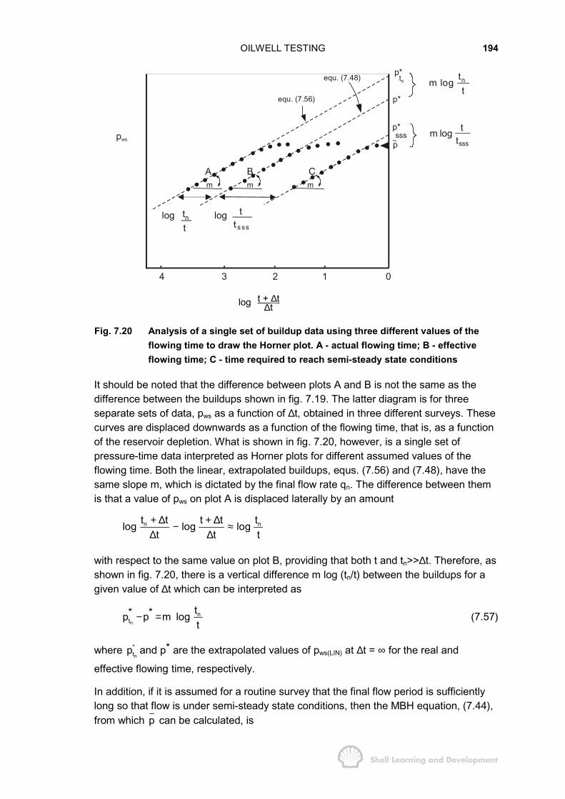
OILWELL TESTING 194
4 3 2 1 0
A B Cm m m
p*
p*
psss
equ. (7.56)
equ. (7.48)
pws
ntm logt
sss
tm logt
s ss
tt
logtnt
log
p* tn
log t + ∆t∆t
Fig. 7.20 Analysis of a single set of buildup data using three different values of theflowing time to draw the Horner plot. A - actual flowing time; B - effectiveflowing time; C - time required to reach semi-steady state conditions
It should be noted that the difference between plots A and B is not the same as thedifference between the buildups shown in fig. 7.19. The latter diagram is for threeseparate sets of data, pws as a function of ∆t, obtained in three different surveys. Thesecurves are displaced downwards as a function of the flowing time, that is, as a functionof the reservoir depletion. What is shown in fig. 7.20, however, is a single set ofpressure-time data interpreted as Horner plots for different assumed values of theflowing time. Both the linear, extrapolated buildups, equs. (7.56) and (7.48), have thesame slope m, which is dictated by the final flow rate qn. The difference between themis that a value of pws on plot A is displaced laterally by an amount
n nt t tt tlog log logt t t
+ ∆ + ∆− ≈∆ ∆
with respect to the same value on plot B, providing that both t and tn>>∆t. Therefore, asshown in fig. 7.20, there is a vertical difference m log (tn/t) between the buildups for agiven value of ∆t which can be interpreted as
nn
tt* *p p m logt
− = (7.57)
where n
*tp and p* are the extrapolated values of pws(LIN) at ∆t = ∞ for the real and
effective flowing time, respectively.
In addition, if it is assumed for a routine survey that the final flow period is sufficientlylong so that flow is under semi-steady state conditions, then the MBH equation, (7.44),from which p can be calculated, is
OILWELL TESTING 195
D(MBH) DA A DAn o
kh *p (t )0.01416 (p - p) 2.303 log (C t )q Bµ
= (7.58)
or
( ) ( )n oA DA A DA
q B*p p 162.6 log C t m log C tkhµ− = = (7.59)
Equation (7.59) is appropriate for the effective flowing time while for the real time
nn ntt A DA*p p m log(C t )− = (7.60)
Subtracting equ. (7.59) from (7.60) gives
( ) ( )nnn
ttt* *p p p p m logt
− − − = (7.61)
which, when compared with equ. (7.57), shows that ntp p− and therefore the
determination of the average pressure using the MBH method is the same whether thereal or effective flowing time is employed in the analysis.
Using an identical argument it can easily be demonstrated that the average pressuredetermined from a survey is independent of the flowing time used in the analysis. Thisis correct providing that the flowing time is equal to or greater than tsss, the timerequired for semi-steady state conditions to be established, within the drainage volume,and the final production rate is also used in the analysis. As an illustration of thisstatement, plot C in fig. 7.20 has been drawn for the limiting value of tsss. In this caseplot C is laterally displaced with respect to plot B, for the effective flowing time, so thatthe equivalent equations to equ. (7.57) and (7.61) are now
ssssss
tp* p* m logt
− =
and
( ) ( )sssssssss
t* *p p p p m logt
− − − =
which shows that the MBH analysis technique will yield the same values of p whether tor tsss is used to plot the buildup. This same conclusion has been presented in theliterature by Pinson12 and Kazemi13.
It should also be noted that the value of the skin factor determined from the analysis isalso independent of the flowing time. This is because the value of pws(LIN)1-hr required forthe calculation of S, (equ. (7.52), does not depend on the flowing time and is the samefor plots A, B and C in fig. 7.20.
It is for the above reasons that the convenient combination of final flow rate andeffective flowing time is generally used in buildup analysis. The only assumption thatcan be regarded as restrictive is that the final flow period should be of sufficient
OILWELL TESTING 196
duration so that semi-steady state flow conditions prevail at the time of closure, andeven if this condition is not exactly satisfied the error introduced will be rather small.The occasion when the use of this rate-time combination may not be acceptable is forinitial tests when the well may be produced for a relatively short period of time at anuneven rate. Odeh and Selig14 have described a method for buildup analysis underthese conditions which can improve the accuracy of the results. In the remainingdescription of pressure buildup analysis the effective flowing time will be usedexclusively and denoted by t, and the final production rate by q. An example of the useof tsss in buildup analysis for a gas well will be described in Chapter 8, sec. 11.
Having plotted the observed pressures according to the interpretation method ofHorner, the MBH method can be applied to determine p according to the followingrecipe.
1) Extrapolate the early linear buildup trend to t t 0t
+ ∆ =∆
and determine the value of p*.
From the slope of the straight line calculate k using equ. (7.50).
2) Divide the reservoir into drainage volumes so that
i i
TOT TOT
q Vq V
=
where qi is the production rate for the ith well draining a reservoir bulk volume Vi andqTOT and VTOT are the total rate and bulk volume of the reservoir respectively. Thisrelationship has been shown in Chapter 5, sec. 5.3, to be valid for wells draining areservoir under semi-steady state flow conditions, however, Matthews, Brons andHazebroek assert that the relationship can be applied with reasonable accuracyirrespective of the prevailing flow condition. This step leads to the determination of Vi
and hence Ai, the area drained by the well, can be estimated by assuming that theaverage thickness within the area is equal to that observed in the well. With the aid of ageological structural map of the reservoir, both the shape of the drainage area andposition of the well with respect to the boundary can be roughly estimated tocorrespond to one of the MBH geometrical configurations shown in figs. 7.11-15.
3) Evaluate the dimensionless time
DAktt 0.000264 (t hours)cAφµ
= − (7.49)
using values of k and A obtained from steps 1) and 2) respectively. For liquid flow theµc product is small and constant but for two phase gas-oil and for single phase gasflow this is not the case which leads to certain difficulties in interpretation which will bedescribed in Chapter 8.
4) Enter the appropriate MBH chart, fig. 7.11-15, and, for the curve corresponding closestto the estimated geometrical configuration, read the value of the ordinate, pD(MBH) (tDA),for the calculated value of the dimensionless (effective) flowing time tDA

OILWELL TESTING 197
( ) ( )D(MBH) DAo
kh *p t 0.01416 p pq Bµ
= − (7.58)
and, since p* has been determined in step 1), then p can be directly calculated. Itshould be noted that the MBH charts are equally appropriate for values of tDA andpD(MBH) evaluated in either Darcy or field units since both parameters aredimensionless.
An equivalent method of determining p is that presented by Dietz9 in which the aim is
to calculate the value of log t tt
+ ∆∆
at which to enter the Horner plot and read off the
value of p directly from the extrapolated linear buildup, as illustrated in fig. 7.21.
m
pd
pws
4 3 2 1 0
p*
p
(p* - p)
log t + ∆t∆t
log t + ∆td∆td
log t + ∆ts∆ts
Fig. 7.21 The Dietz method applied to determine both the average pressure p and the
dynamic grid block pressure dp
Let ∆ts be the closed-in time for which the hypothetical pressure on the extra polatedlinear buildup equals the average reservoir pressure. Then ws(LIN)p p= in equ. (7.48),
and the latter may be expressed as
( ) ( )3 s Di D D
o s
t t 4tkh7.08 10 p p 1.151log p t ½ lnq B tµ γ
− + ∆× − = + −∆
but the left hand side of this equation can be evaluated using equ. (7.38), the materialbalance, to give
( )s DDA D D
s
t t 4t2 t 1.151log p t ½ lnt
πγ
+ ∆= + −∆
If the pD function in this equation is expressed in general form using equ. (7.42), then
( )sD(MBH)
s o
t t kh *2.303 log p 0.01416 p pt q Bµ
+ ∆ = = −∆
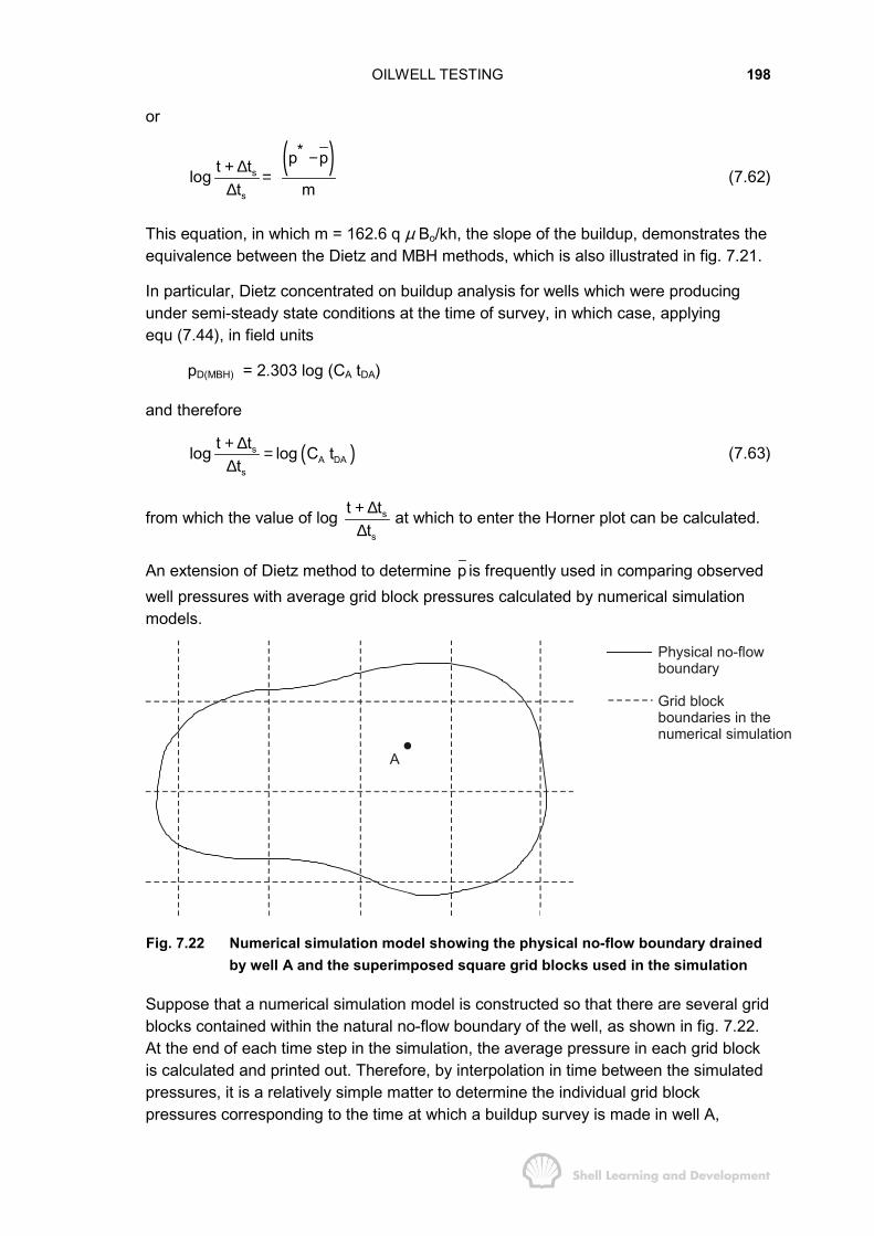
OILWELL TESTING 198
or
( )s
s
*p pt tlogt m
−+ ∆ =∆
(7.62)
This equation, in which m = 162.6 q µ Bo/kh, the slope of the buildup, demonstrates theequivalence between the Dietz and MBH methods, which is also illustrated in fig. 7.21.
In particular, Dietz concentrated on buildup analysis for wells which were producingunder semi-steady state conditions at the time of survey, in which case, applyingequ (7.44), in field units
pD(MBH) = 2.303 log (CA tDA)
and therefore
( )sA DA
s
t tlog log C tt
+ ∆ =∆
(7.63)
from which the value of log s
s
t tt
+ ∆∆
at which to enter the Horner plot can be calculated.
An extension of Dietz method to determine p is frequently used in comparing observedwell pressures with average grid block pressures calculated by numerical simulationmodels.
A
Physical no-flowboundary
Grid blockboundaries in thenumerical simulation
Fig. 7.22 Numerical simulation model showing the physical no-flow boundary drainedby well A and the superimposed square grid blocks used in the simulation
Suppose that a numerical simulation model is constructed so that there are several gridblocks contained within the natural no-flow boundary of the well, as shown in fig. 7.22.At the end of each time step in the simulation, the average pressure in each grid blockis calculated and printed out. Therefore, by interpolation in time between the simulatedpressures, it is a relatively simple matter to determine the individual grid blockpressures corresponding to the time at which a buildup survey is made in well A,
OILWELL TESTING 199
whether the latter time coincides with the end of a simulation time step or not. Thereare then two ways of comparing the observed well pressure with the simulated gridblock pressures.
The first of these is to calculate the average pressure within the no-flow boundary atthe time of survey, using the MBH or Dietz method, and compare this with the volumeaveraged pressure over all the grid blocks and partial blocks within the natural no-flowboundary. This is a rather tedious business. A simpler, approximate method has beenintroduced by van Poollen15 and further described by Earlougher16. This consists ofusing the Horner buildup plot in conjunction with the Dietz method to calculate the so-called "dynamic grid block pressure" pd which is simply the average pressure in the gridblock containing the well at the time of survey. The analysis seeks to determine at what
value of log d
d
t tt
+ ∆∆
should the Horner plot be entered so that the pressure read from
the hypothetical linear buildup has risen to be equal to the dynamic pressure, i.e.pws(LIN) = pd. Again, equ. (7.63) can be applied but in this case tDA must be evaluatedusing the grid block area rather than that of the no-flow boundary and CA takes on thefixed value of 19.1. The reasoning behind the latter choice is that the grid blockboundary is not a no-flow boundary. Instead the boundary condition corresponds moreclosely to that of steady state flow and for such Dietz has only presented one casecorresponding to a well producing from the centre of a circle for which CA = 19.1,fig 6.4. Thus the rectangular grid block shape is approximated as circular with areaequal to that of the grid block. Therefore, the Horner plot is entered for a value of
( )dDA
d
t tlog log 19.1 tt
+ ∆ =∆
(7.64)
and pd read from the linear buildup as shown in fig. 7.21. Again, use of equ. (7.64)depends on the fact that the well is flowing under stabilised conditions at the time ofsurvey. Normally, in this case t >>∆td and van Poollen, using this assumption, haspresented an expression for explicitly calculating the closed in time at whichpWS(LIN) = pd. This can readily be obtained from equ. (7.64), as
2e
dc rcAt
0.000264x19.1k 0.005042kφ µ πφ µ∆ = =
or2e
dcrt 623
kφ µ∆ =
where re is the radius of the circle with area equivalent to that of the grid block. Thisapproximate but speedy method for comparing observed with simulated pressures isvery useful in performing a history match on well pressures.
The following two exercises will illustrate the application of the pressure builduptechniques, described in this section, to an under saturated oil reservoir.

OILWELL TESTING 200
EXERCISE 7.6 HORNER PRESSURE BUILDUP ANALYSIS, INFINITERESERVOIR CASE
A discovery well is produced for a period of approximately 100 hours prior to closurefor an initial pressure buildup survey. The production data and estimated reservoir andfluid properties are listed below
q = 123 stb/d φ = 0.2
Np = 500 stb µ = 1 cph = 20 ft Boi = 1.22 rb/stbrw = 0.3 ft c = 20×10-6/psiA ≈ 300 acres = (co So +cw +Sw + fc )
and the pressures recorded during the test are listed in table 7.5.
1) What is the initial reservoir pressure?
2) If the well is completed across the entire formation thickness, calculate the effectivepermeability.
3) Calculate the value of the mechanical skin factor.
4) What is the additional pressure drop in the wellbore due to the skin?
5) If it is initially assumed that the well is draining from the centre of a circle, is it validto equate pi to p*?
Closed-in time∆t (hrs)
Wellbore pressure(psi)
Closed-in time∆t (hrs)
Wellbore pressure(psi)
0.0 4506 (pwf )0.5 4675 3.0 47630.66 4705 4.0 47661.0 4733 6.0 47701.5 4750 8.0 47732.0 4757 10.0 47752.5 4761 12.0 4777
TABLE 7.5
EXERCISE 7.6 SOLUTION
1) The effective flowing time is
p
final
N 500t 24 24 97.6 hrsq 123
= × = × =
Points on the Horner build up plot of pws versus log t tt
+ ∆∆
are listed in table 7.6.

OILWELL TESTING 201
Closed-in time∆t (hrs)
t tt
+ ∆∆
log t tt
+ ∆∆
pws (psi)
0 4506(pwf).5 196.2 2.29 4675.66 148.9 2.17 4705
1.0 98.6 1.99 47331.5 66.1 1.82 47502.0 49.8 1.70 47572.5 40.04 1.60 47613.0 33.53 1.52 47634.0 25.40 1.40 47666.0 17.27 1.24 47708.0 13.20 1.12 4773
10.0 10.76 1.03 477512.0 9.13 .96 4777
TABLE 7.6
The pressure buildup plot, on a linear scale, is shown as fig. 7.23. The last seven
points define a straight line and the extrapolation of this trend to the value of t tt
+ ∆∆
= 0
gives p* = 4800 psi and, assuming the validity of equ. (7.54) for an initial well test,pi = 4800 psi.
4800
4700 4700
4600 46002 1 0
p*=4800 psi
p (psi)ws
x p =ws (1 hr)
4752 psi
+ ∆∆
t tlogt
Fig. 7.23 Horner buildup plot, infinite reservoir case
OILWELL TESTING 202
2) The slope of the linear section of the buildup plot is m = 24.5 psi/log cycle. Therefore,since the well is fully penetrating the effective permeability of the formation is
oi162.6q B 162.6 123 1 1.22k 50 mDmh 24.5 20
µ × × ×= = =×
3) The skin factor can be evaluated using equ. (7.52) in which the hypothetical value ofpws(LIN) 1-hr = 4752 psi is obtained from the extrapolation of the linear buildup trend to∆t = 1 hour, fig. 7.23, therefore,
( )
( )(
ws(LIN) 1 -hr wf2w
6
p p kS 1.151 log 3.23m cr
4752 4506 501.151 log 3.2324.5 .2 1 20 10 .09
φµ
−
� �−� �= − +� �� �
�−= − + ��× × × × �
(7.52)
4) The additional pressure drop due to the skin, while producing, can be calculated as
qp S atm.2 kh
2m S 0.87mS psi2.303128 psi
µπ
∆ = ×
= × =
=
5) The assumption that pi = p* relies entirely on the fact that both pD functions in thetheoretical buildup equation (7.32) can be evaluated under transient flow conditions sothat the equation can be reduced to the simple form equ. (7.54) for the infinite reservoircase. As already noted for a well at the centre of a circular bounded reservoir, there isa fairly sharp change from transient to semi-steady state flow for a value of tDA ≈ 0.1.Therefore, for the effective flowing time of 97.6 hours, the minimum area for which theassumption is valid is
min
min 6
0.000264kt 1A0.1 c 43560
0.000264 50 97.6 1A 74 acres435600.1 2 1 20 10
φ µ
−
= ×
× ×= × ≈× × × ×
and since the estimated area is 300 acres the assumption that p* = pi is perfectly validas the test is conducted entirely under transient flow conditions.
EXERCISE 7.7 PRESSURE BUILDUP TEST ANALYSIS: BOUNDED DRAINAGEVOLUME
A pressure buildup test is conducted in the same well described in exercise 7.6, someseven and a half months after the start of production. At the time, the well is producing400 stb/d and the cumulative production is 74400 stb. The only change in the well datapresented in the previous exercise is that Bo has increased from 1.22 to 1.23 rb/stb.The closed-in pressures as a function of time are listed in table 7.7.
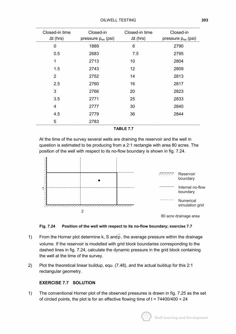
OILWELL TESTING 203
Closed-in time∆t (hrs)
Closed-inpressure pws (psi)
Closed-in time∆t (hrs)
Closed-inpressure pws (psi)
0 1889 6 2790
0.5 2683 7.5 2795
1 2713 10 2804
1.5 2743 12 2809
2 2752 14 2813
2.5 2760 16 2817
3 2766 20 2823
3.5 2771 25 2833
4 2777 30 2840
4.5 2779 36 2844
5 2783TABLE 7.7
At the time of the survey several wells are draining the reservoir and the well inquestion is estimated to be producing from a 2:1 rectangle with area 80 acres. Theposition of the well with respect to its no-flow boundary is shown in fig. 7.24.
80 acre drainage area
Reservoirboundary
Internal no-flowboundary
Numericalsimulation grid
2
1
Fig. 7.24 Position of the well with respect to its no-flow boundary; exercise 7.7
1) From the Horner plot determine k, S andp , the average pressure within the drainagevolume. If the reservoir is modelled with grid block boundaries corresponding to thedashed lines in fig. 7.24, calculate the dynamic pressure in the grid block containingthe well at the time of the survey.
2) Plot the theoretical linear buildup, equ. (7.48), and the actual buildup for this 2:1rectangular geometry.
EXERCISE 7.7 SOLUTION
1) The conventional Horner plot of the observed pressures is drawn in fig. 7.25 as the setof circled points, the plot is for an effective flowing time of t = 74400/400 × 24
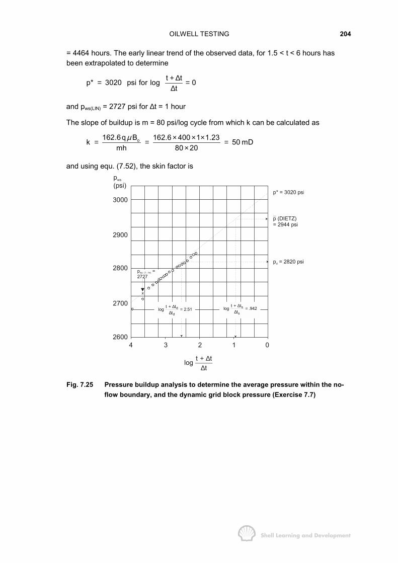
OILWELL TESTING 204
= 4464 hours. The early linear trend of the observed data, for 1.5 < t < 6 hours hasbeen extrapolated to determine
t tp* 3020 psi for log 0t
+ ∆= =∆
and pws(LIN) = 2727 psi for ∆t = 1 hour
The slope of buildup is m = 80 psi/log cycle from which k can be calculated as
o162.6q B 162.6 400 1 1.23k 50 mDmh 80 20
µ × × ×= = =×
and using equ. (7.52), the skin factor isp(
ws
psi)
3000
2900
2800
2700
26004 3 2 1 0
+ ∆ =∆
s
s
t tlog .942t
+ ∆ =∆
d
d
t tlog 2.51t
+ ∆∆
t tlogt
p = 2727
ws (1 - hr)
x
p* = 3020 psi
p (DIETZ)= 2944 psi
p = 2820 psid
Fig. 7.25 Pressure buildup analysis to determine the average pressure within the no-flow boundary, and the dynamic grid block pressure (Exercise 7.7)
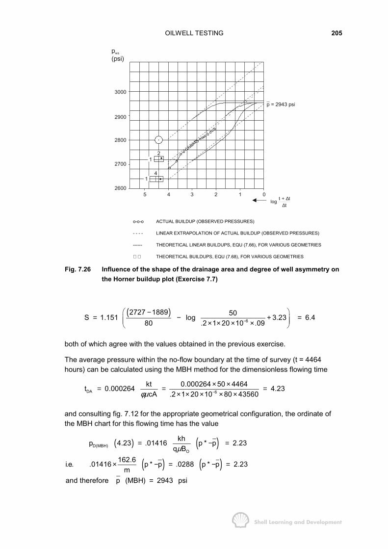
OILWELL TESTING 205
p(
ws
psi)
3000
2900
2800
2700
2600
p = 2943 psi
+ ∆∆
t tlogt
5 4 3 2 1 0
21
41
o-o-o ACTUAL BUILDUP (OBSERVED PRESSURES)
- - - - LINEAR EXTRAPOLATION OF ACTUAL BUILDUP (OBSERVED PRESSURES)
------ THEORETICAL LINEAR BUILDUPS, EQU (7.66), FOR VARIOUS GEOMETRIES
THEORETICAL BUILDUPS, EQU (7.68), FOR VARIOUS GEOMETRIES
Fig. 7.26 Influence of the shape of the drainage area and degree of well asymmetry onthe Horner buildup plot (Exercise 7.7)
( )6
2727 1889 50S 1.151 log 3.23 6.480 .2 1 20 10 .09−
� �−= − + =� �� �× × × ×� �
both of which agree with the values obtained in the previous exercise.
The average pressure within the no-flow boundary at the time of survey (t = 4464hours) can be calculated using the MBH method for the dimensionless flowing time
DA 6kt 0.000264 50 4464t 0.000264 4.23cA .2 1 20 10 80 43560φµ −
× ×= = =× × × × ×
and consulting fig. 7.12 for the appropriate geometrical configuration, the ordinate ofthe MBH chart for this flowing time has the value
( ) ( )
( ) ( )D(MBH)
O
khp 4.23 .01416 p * p 2.23q B
162.6i.e. .01416 p * p .0288 p * p 2.23m
and therefore p (MBH) 2943 psi
µ= − =
× − = − =
=

OILWELL TESTING 206
The MBH curve, fig. 7.12 (IV), shows that for tDA = 4.23 semi-steady state flowconditions prevail in the reservoir and therefore the method of Dietz can also beapplied to calculate p , i.e.
( )
( )
sA DA
s
t tlog log C tt
log 2.07 4.23 0.942
+ ∆ =∆
= × =(7.63)
and entering the buildup plot for this value of the abscissa gives the correspondingvalue of pws(LIN) = p as
p (Dietz) 2944 psi=
To determine the dynamic pressure in the grid block containing the well at the time ofsurvey, equ. (7.64) can be applied for '
DAt = tDA × 4 since the grid block area is only onequarter of the total drainage area. Thus
( )t tlog log 19.1 16.92 2.51t
+ ∆ = × =∆
and from the buildup plot, the corresponding dynamic pressure can be read as
pws(LIN) = pd = 2820 psi.
2) The theoretical equation of the straight line which matches the observed linear buildupis
( ) ( )-3 Di ws(LIN) D D
o
4tkh t t7.08 10 p p 1.151log p t ½ lnq B tµ γ
+ ∆× − = + −∆
(7.48)
and since 2D DA wt t A / r= × , this may be expressed as
( ) ( )i ws(LIN) D Dt t0.0144 p p 1.151 log p t 9.862
t+ ∆− = + −∆
Taking several points on the straight line, pD (tD) can be evaluated as
pD (tD ) = 35.49
and therefore, the correct linear equation is
( )ws(LIN)t t0.0144 4800 p 1.151 log 25.63
t+ ∆− = +∆
(7.65)
If the geometry and well position within the bounded area have been estimatedcorrectly, then it should be possible to match equ. (7.65) by theoretically calculating Dpusing equ. (7.42) or, since semi-steady state conditions prevail at the time of thesurvey, Dp can be alternatively expressed as
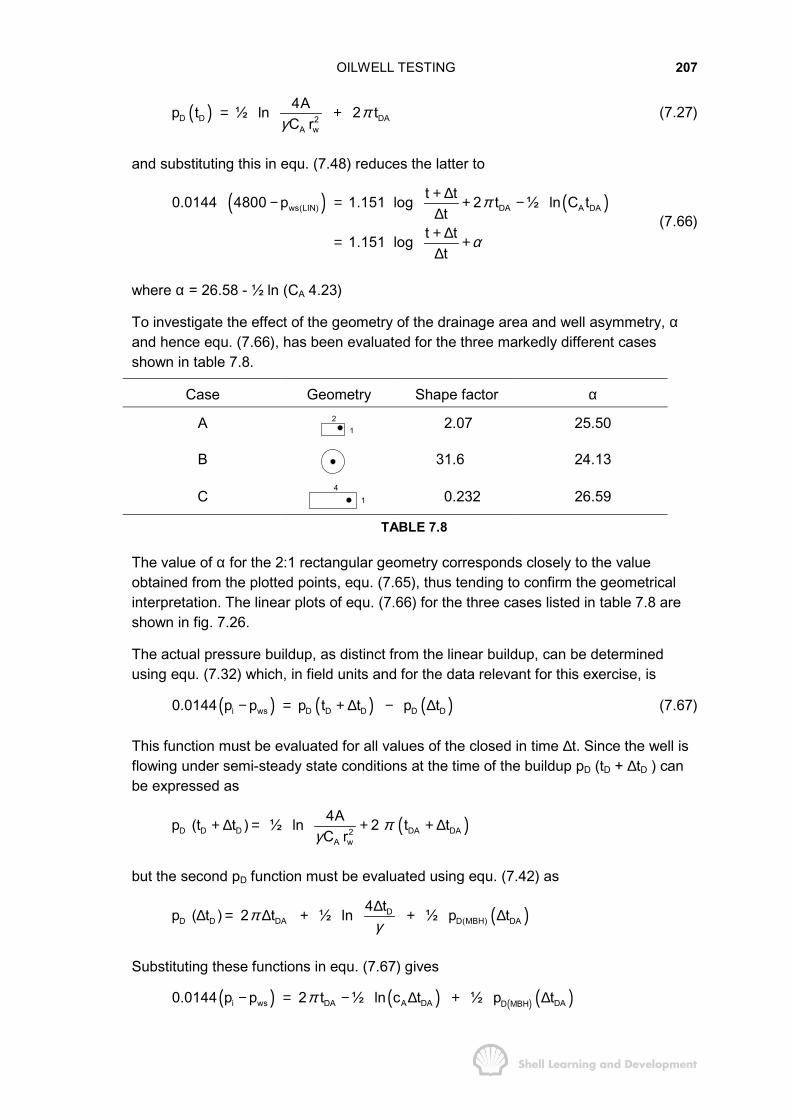
OILWELL TESTING 207
( )D D DA2A w
4Ap t ½ ln 2 tC r
πγ
= + (7.27)
and substituting this in equ. (7.48) reduces the latter to
( ) ( )ws(LIN) DA A DAt t0.0144 4800 p 1.151 log 2 t ½ ln C t
tt t1.151 log
t
π
α
+ ∆− = + −∆+ ∆= +∆
(7.66)
where α = 26.58 - ½ ln (CA 4.23)
To investigate the effect of the geometry of the drainage area and well asymmetry, αand hence equ. (7.66), has been evaluated for the three markedly different casesshown in table 7.8.
Case Geometry Shape factor α
A 21 2.07 25.50
B 31.6 24.13
C4
1 0.232 26.59
TABLE 7.8
The value of α for the 2:1 rectangular geometry corresponds closely to the valueobtained from the plotted points, equ. (7.65), thus tending to confirm the geometricalinterpretation. The linear plots of equ. (7.66) for the three cases listed in table 7.8 areshown in fig. 7.26.
The actual pressure buildup, as distinct from the linear buildup, can be determinedusing equ. (7.32) which, in field units and for the data relevant for this exercise, is
( ) ( ) ( )i ws D D D D D0.0144 p p p t t p t− = + ∆ − ∆ (7.67)
This function must be evaluated for all values of the closed in time ∆t. Since the well isflowing under semi-steady state conditions at the time of the buildup pD (tD + ∆tD ) canbe expressed as
( )D D D DA DA2A w
4Ap (t t ) ½ ln 2 t tC r
πγ
+ ∆ = + + ∆
but the second pD function must be evaluated using equ. (7.42) as
( )DD D DA D(MBH) DA
4 tp ( t ) 2 t ½ ln ½ p tπγ∆∆ = ∆ + + ∆
Substituting these functions in equ. (7.67) gives
( ) ( ) ( ) ( )i ws DA A DA DAD MBH0.0144 p p 2 t ½ ln c t ½ p tπ− = − ∆ + ∆
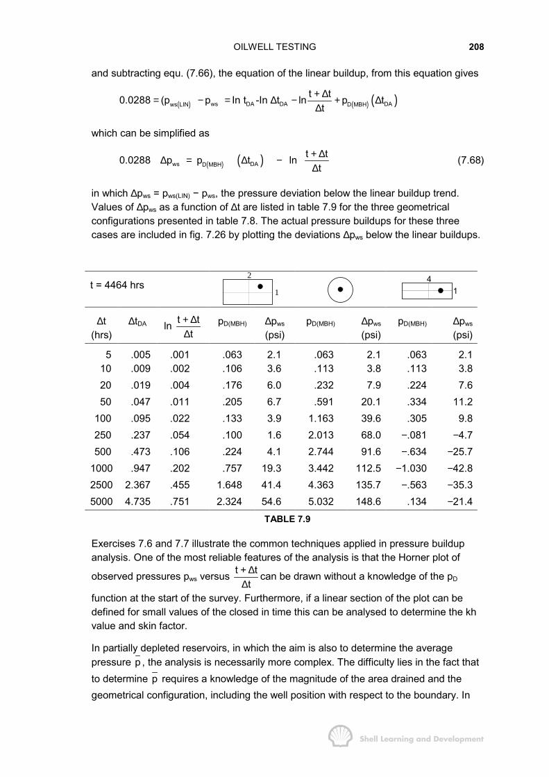
OILWELL TESTING 208
and subtracting equ. (7.66), the equation of the linear buildup, from this equation gives
( ) ( ) ( )ws DA DA DAws LIN D MBHt t0.0288 (p p In t -In t ln p t
t+ ∆= − = ∆ − + ∆∆
which can be simplified as
( ) ( )ws DAD MBHt t0.0288 p p t ln
t+ ∆∆ = ∆ −∆
(7.68)
in which ∆pws = pws(LIN) − pws, the pressure deviation below the linear buildup trend.Values of ∆pws as a function of ∆t are listed in table 7.9 for the three geometricalconfigurations presented in table 7.8. The actual pressure buildups for these threecases are included in fig. 7.26 by plotting the deviations ∆pws below the linear buildups.
t = 4464 hrs2
14
1
∆t(hrs)
∆tDA ln t tt
+ ∆∆
pD(MBH) ∆pws
(psi)pD(MBH) ∆pws
(psi)pD(MBH) ∆pws
(psi)
5 .005 .001 .063 2.1 .063 2.1 .063 2.110 .009 .002 .106 3.6 .113 3.8 .113 3.820 .019 .004 .176 6.0 .232 7.9 .224 7.650 .047 .011 .205 6.7 .591 20.1 .334 11.2
100 .095 .022 .133 3.9 1.163 39.6 .305 9.8250 .237 .054 .100 1.6 2.013 68.0 −.081 −4.7500 .473 .106 .224 4.1 2.744 91.6 −.634 −25.7
1000 .947 .202 .757 19.3 3.442 112.5 −1.030 −42.82500 2.367 .455 1.648 41.4 4.363 135.7 −.563 −35.35000 4.735 .751 2.324 54.6 5.032 148.6 .134 −21.4
TABLE 7.9
Exercises 7.6 and 7.7 illustrate the common techniques applied in pressure buildupanalysis. One of the most reliable features of the analysis is that the Horner plot of
observed pressures pws versus t tt
+ ∆∆
can be drawn without a knowledge of the pD
function at the start of the survey. Furthermore, if a linear section of the plot can bedefined for small values of the closed in time this can be analysed to determine the khvalue and skin factor.
In partially depleted reservoirs, in which the aim is also to determine the averagepressure p , the analysis is necessarily more complex. The difficulty lies in the fact thatto determine p requires a knowledge of the magnitude of the area drained and thegeometrical configuration, including the well position with respect to the boundary. In
OILWELL TESTING 209
other words, complex boundary conditions of the differential equations implicit in theanalysis are required to obtain meaningful results. As fig. 7.26 clearly demonstrates,varying the boundary conditions can have a profound influence on the shape andposition of the theoretical buildup plot. One hopeful feature in this diagram is again thefact that the observed data gives an absolute buildup plot. By the appropriate choice ofthe boundary condition it may therefore be possible to match the observed buildup asdemonstrated in exercise 7.7, in which the original geological interpretation wasconfirmed. With a reasonable geological map of the reservoir the technique can bediagnostic in building a model of the current drainage patterns.
In addition, attempting even some crude match of the observed buildup can eliminateserious error. If it were assumed, for instance, that the well in exercise 7.7 was locatedat the centre of a circle, which is the conventional boundary condition assumed in theliterature, then the reader can confirm by calculation, or merely by inspection offig. 7.26, that the estimated value of p calculated in this latter exercise would be about100 psi too low.
One other feature in fig. 7.26 is of interest and that is the rather strange shape of thetheoretical buildup plot for the assumed 4:1 rectangular geometry. In this case there isa pronounced increase of slope which is due to the proximity of the no-flow boundaries.This is just a more complex manifestation of the phenomenon of "doubling of the slope"due to the presence of a fault close to a well in an otherwise infinite reservoir, whichhas repeatedly featured in the literature4,6. References 17 and 18 of this chapter arerecommended to the reader who is further interested in the subject of matchingtheoretical with actual pressure buildups.
7.8 MULTI-RATE DRAWDOWN TESTING
Closing in a well for a pressure buildup survey is often inconvenient since it involvesloss of production and sometimes it is difficult, for a variety of reasons, to start the wellproducing again after the survey. Therefore, multi-rate drawdown testing is sometimespractised as an alternative means of measuring the basic reservoir parameters andindeed, in some places the regulatory bodies insist that such surveys be conducted inpreference to other forms of testing. This restriction is more common in the case of gaswell testing which will be described separately in Chapter 8, sec. 10.
The basic equation for analysing a multi-rate drawdown test for liquid flow has alreadybeen presented in sec. 7.5 as equ. (7.33). In field units this becomes
( ) ( )n
n j 1
ni wf j3D D D
j 1o n n
p p qkh7.08 10 p t t SB q qµ −
−
=
− ∆× = − +� (7.69)
in which nwfp is the specific value of the flowing pressure at total flowing time tn during
the nth production period at rate qn. It should also be noted that throughout this section tis the actual rather than effective flowing time.
Consider the typical multi-rate test shown in fig. 7.27 for four sequential flow periods.

OILWELL TESTING 210
Conventionally in the analysis of such a test the pressures 1 2wf wfp , p , . . . are read
from the pressure chart at the end of each separate flow period and matched to thetheoretical equation (7.69). For instance, the calculation of
3wfp at the end of the third
flow period is
( ) ( ) ( ) ( ) ( )( ) ( )
3
3 3 1
3 2
i wf 1 2 13D D D D D
o 3 3
3 2D D D
3
p p q 0 q qkh7.08 10 p t p t tB q q q3
q qp t t S
q
µ−
− − −× = + −
++ − +
(7.70)
in which, e.g. tD3 is the dimensionless flowing time evaluated for t = t3, fig. 7.27.Furthermore, it will be assumed that the test starts from some known initial equilibriumpressure pi which is a conventional although theoretically unnecessary assumption, aswill be demonstrated presently.
Rate
t1 t2 t3 t4Time
Time
pi
pwf
pwf1pwf2
pwf4pwf3
(a)
(b)
q1
q2
q3
q4
Fig. 7.27 Multi-rate oilwell test (a) increasing rate sequence (b) wellbore pressureresponse
The correct way to analyse such a test, as already described in sec. 7.5, is to plot
( ) ( )n
n j 1
ni wf jD D D
j 1n n
p p qversus p t t
q q −=
− ∆−� (7.71)
which should result in a straight line with slope m = 141.2µBo/kh and intercept on theordinate equal to mS. The main drawback to this form of analysis technique is that itpre-supposes that the engineer is able to evaluate the pD functions for all values of thedimensionless time argument during the test period, and this in turn can demand aknowledge of the drainage area, shape and degree of well asymmetry. Because of thisdifficulty, the literature on the subject deals exclusively with multi-rate testing undertransient flow conditions thus assuming the infinite reservoir case.

OILWELL TESTING 211
The original paper on the subject was presented by Odeh and Jones5 in which theanalysis technique is precisely as described above except that the Dp functions inequ. (7.69) were evaluated for transient flow as
( ) D12D D
4tp t lnγ
= (7.23)
This leads to the test analysis equation (with t in hours)
( ) ( )nni wf j3
n j 1 2j 1o n n w
p p qkh k7.08 10 1.151 log t t log 3.23 0.87SB q q crµ φµ
−−
=
− ∆� �× = − + − +� �
� ��
(7.72)
which, providing the assumption of transient flow is appropriate for the test, will give alinear plot of (pi−pwf)/qn versus Σ ∆qj/qn log(tn−tj-1), with slope m = 162.6µBo/kh andintercept m(log(k/φµc 2
wr ) −3.23 + .87S), from which k and S can be calculated.
It is frequently stated in the literature that the separate flow periods should be of shortduration so that transient flow conditions will prevail at each rate. While this condition isnecessary, it is insufficient for the valid application of transient analysis to the test.Instead, the entire test, from start to finish, should be sufficiently short so thattransience is assured throughout the whole test period. The reason for this restriction isthat the largest value of the dimensionless time argument, for which the pD functions inequ. (7.69) must be evaluated, is equal to the total duration of the test. This point isillustrated in fig. 7.27 (b), which again demonstrates the basic principle of superpositionand shows that in evaluating the flowing pressure at the very end of the test there isstill a component of the pressure response due to the first flow rate to be included inthe superposed constant terminal rate solution. The following example will illustrate themagnitude of the error that can be made by automatically assuming that a multi-rateflow test can be interpreted using transient analysis techniques.
EXERCISE 7.8 MULTI-RATE FLOW TEST ANALYSIS
An initial test in a discovery well is conducted by flowing the well at four different ratesover a period of 12 hours as detailed in table 7.10.
Flowing time(hours)
Oil rate(stb/d)
pwf
(psia)
0 0 3000(pi)3 500 28926 1000 27789 1500 2660
12 2000 2538TABLE 7.10
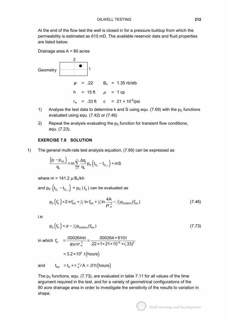
OILWELL TESTING 212
At the end of the flow test the well is closed in for a pressure buildup from which thepermeability is estimated as 610 mD. The available reservoir data and fluid propertiesare listed below.
Drainage area A = 80 acres
Geometry
2
1
φ = .22 Bo = 1.35 rb/stb
h = 15 ft µ = 1 cp
rw = .33 ft c = 21 × 10-6/psi
1) Analyse the test data to determine k and S using equ. (7.69) with the pD functionsevaluated using equ. (7.42) or (7.46)
2) Repeat the analysis evaluating the pD function for transient flow conditions,equ. (7.23).
EXERCISE 7.8 SOLUTION
1) The general multi-rate test analysis equation, (7.69) can be expressed as
( ) ( )n
n j 1
ni wf jD D D
j 1n n
p p qm p t t mS
q q −=
− ∆= − +�
where m = 141.2 µ Bo/kh
and pD ( )n j 1D Dt t−
− = pD ( 'Dt ) can be evaluated as
( ) 1 1 12 2 2D D DA DA D(MDH) DA2
w
4Ap t 2 t ln t ln p (t )r
πγ
′ ′ ′ ′= + + − (7.46)
i.e.
( ) 12D D D(MDH) DAp t p (t )α′ ′= − (7.73)
in which D 2 6 2w
.000264kt .000264 610 ttcr .22 1 21 10 (.33)φ µ −
×′ = =× × × ×
( )53.2 10 t hours= ×
and ( )2DA D wt t r / A .01t hours= × =
The pD functions, equ. (7.73), are evaluated in table 7.11 for all values of the timeargument required in the test, and for a variety of geometrical configurations of the80 acre drainage area in order to investigate the sensitivity of the results to variation inshape.
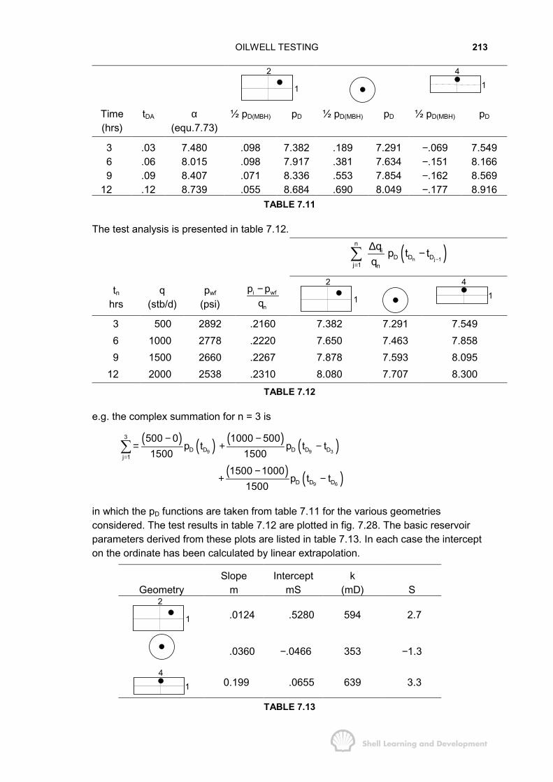
OILWELL TESTING 213
2
1
41
Time(hrs)
tDA α(equ.7.73)
½ pD(MBH) pD ½ pD(MBH) pD ½ pD(MBH) pD
3 .03 7.480 .098 7.382 .189 7.291 −.069 7.5496 .06 8.015 .098 7.917 .381 7.634 −.151 8.1669 .09 8.407 .071 8.336 .553 7.854 −.162 8.569
12 .12 8.739 .055 8.684 .690 8.049 −.177 8.916TABLE 7.11
The test analysis is presented in table 7.12.
( )n j 1
ni
D D Dj 1 n
q p t tq −
=
∆ −�
tnhrs
q(stb/d)
pwf
(psi)i wf
n
p pq−
2
1
41
3 500 2892 .2160 7.382 7.291 7.5496 1000 2778 .2220 7.650 7.463 7.8589 1500 2660 .2267 7.878 7.593 8.095
12 2000 2538 .2310 8.080 7.707 8.300TABLE 7.12
e.g. the complex summation for n = 3 is
( ) ( ) ( ) ( )( ) ( )
9 9 3
9 6
3
D D D D Dj 1
D D D
500 0 1000 500p t p t t
1500 15001500 1000
p t t1500
=
− −= + −
−+ −
�
in which the pD functions are taken from table 7.11 for the various geometriesconsidered. The test results in table 7.12 are plotted in fig. 7.28. The basic reservoirparameters derived from these plots are listed in table 7.13. In each case the intercepton the ordinate has been calculated by linear extrapolation.
GeometrySlope
mIntercept
mSk
(mD) S2
1 .0124 .5280 594 2.7
.0360 −.0466 353 −1.3
41 0.199 .0655 639 3.3
TABLE 7.13
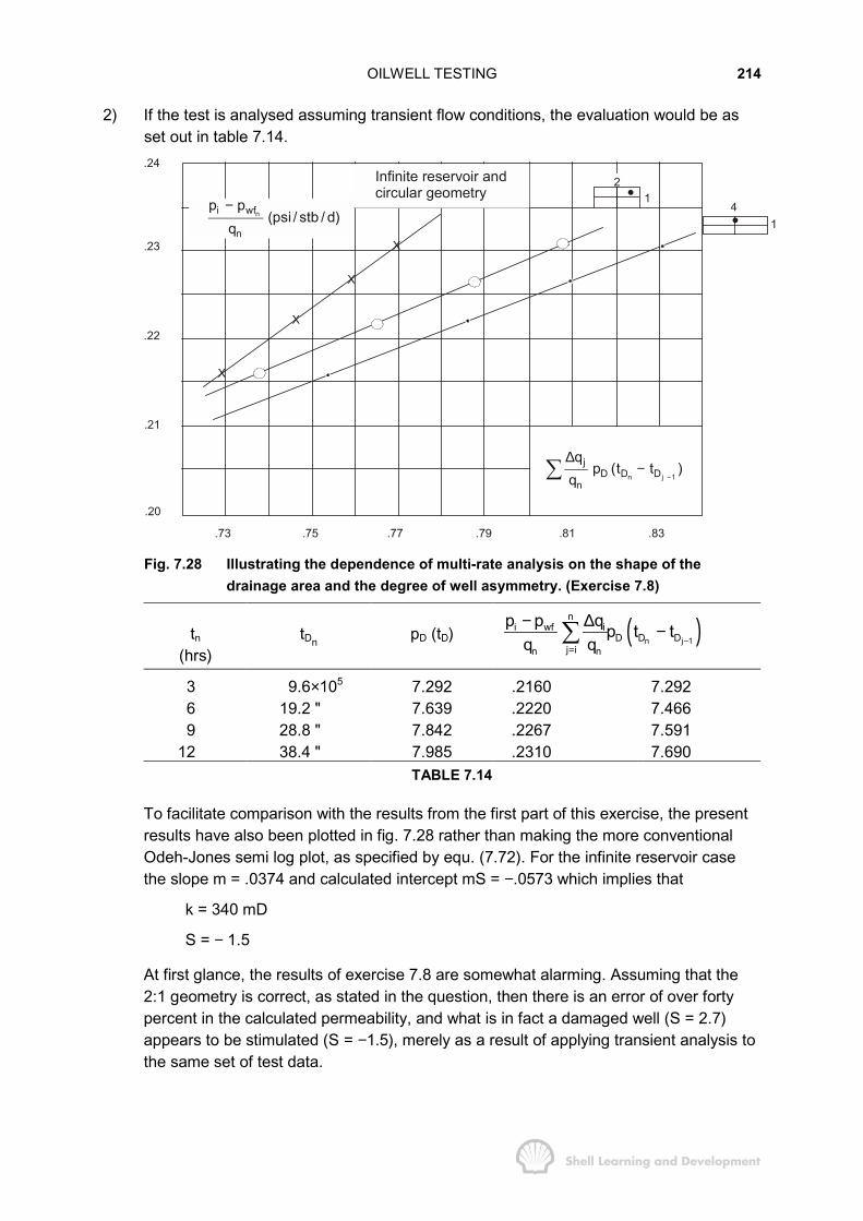
OILWELL TESTING 214
2) If the test is analysed assuming transient flow conditions, the evaluation would be asset out in table 7.14.
.83.81.79.77.75.73
.20
.21
.22
.23
.242
4 1
1
Infinite reservoir andcircular geometry
X
X
X
X
−ni wf
n
p p(psi / stb / d)
q
n j 1
jD D D
n
qp (t t )
q −
∆−�
Fig. 7.28 Illustrating the dependence of multi-rate analysis on the shape of thedrainage area and the degree of well asymmetry. (Exercise 7.8)
tn(hrs)
tDn pD (tD) ( )n j 1
ni wf i
D D Dj in n
p p q p t tq q −
=
− ∆ −�
3 9.6×10⁵ 7.292 .2160 7.2926 19.2 " 7.639 .2220 7.4669 28.8 " 7.842 .2267 7.591
12 38.4 " 7.985 .2310 7.690TABLE 7.14
To facilitate comparison with the results from the first part of this exercise, the presentresults have also been plotted in fig. 7.28 rather than making the more conventionalOdeh-Jones semi log plot, as specified by equ. (7.72). For the infinite reservoir casethe slope m = .0374 and calculated intercept mS = −.0573 which implies that
k = 340 mD
S = − 1.5
At first glance, the results of exercise 7.8 are somewhat alarming. Assuming that the2:1 geometry is correct, as stated in the question, then there is an error of over fortypercent in the calculated permeability, and what is in fact a damaged well (S = 2.7)appears to be stimulated (S = −1.5), merely as a result of applying transient analysis tothe same set of test data.
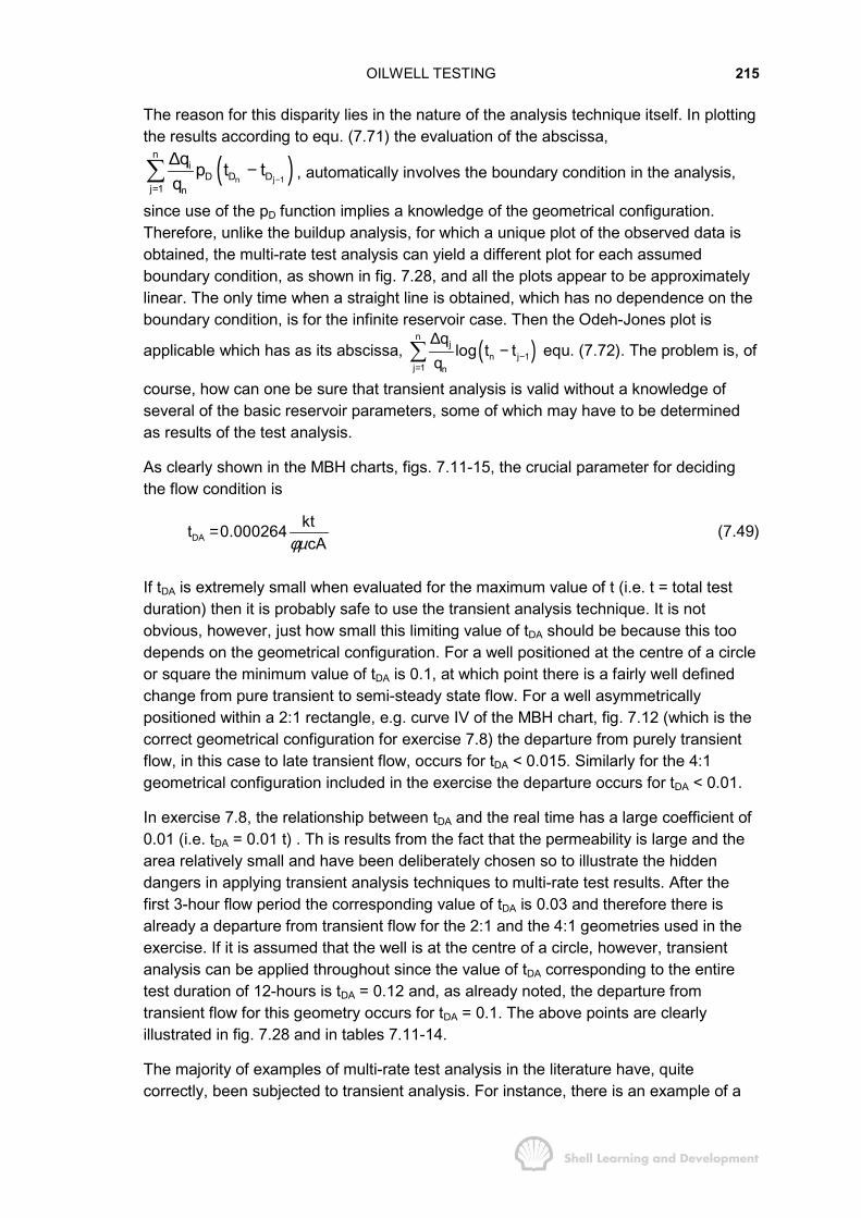
OILWELL TESTING 215
The reason for this disparity lies in the nature of the analysis technique itself. In plottingthe results according to equ. (7.71) the evaluation of the abscissa,
( )n j 1
ni
D D Dj 1 n
q p t tq −
=
∆ −� , automatically involves the boundary condition in the analysis,
since use of the pD function implies a knowledge of the geometrical configuration.Therefore, unlike the buildup analysis, for which a unique plot of the observed data isobtained, the multi-rate test analysis can yield a different plot for each assumedboundary condition, as shown in fig. 7.28, and all the plots appear to be approximatelylinear. The only time when a straight line is obtained, which has no dependence on theboundary condition, is for the infinite reservoir case. Then the Odeh-Jones plot is
applicable which has as its abscissa, ( )n
jn j 1
j 1 n
qlog t t
q −=
∆−� equ. (7.72). The problem is, of
course, how can one be sure that transient analysis is valid without a knowledge ofseveral of the basic reservoir parameters, some of which may have to be determinedas results of the test analysis.
As clearly shown in the MBH charts, figs. 7.11-15, the crucial parameter for decidingthe flow condition is
DAktt 0.000264cAφµ
= (7.49)
If tDA is extremely small when evaluated for the maximum value of t (i.e. t = total testduration) then it is probably safe to use the transient analysis technique. It is notobvious, however, just how small this limiting value of tDA should be because this toodepends on the geometrical configuration. For a well positioned at the centre of a circleor square the minimum value of tDA is 0.1, at which point there is a fairly well definedchange from pure transient to semi-steady state flow. For a well asymmetricallypositioned within a 2:1 rectangle, e.g. curve IV of the MBH chart, fig. 7.12 (which is thecorrect geometrical configuration for exercise 7.8) the departure from purely transientflow, in this case to late transient flow, occurs for tDA < 0.015. Similarly for the 4:1geometrical configuration included in the exercise the departure occurs for tDA < 0.01.
In exercise 7.8, the relationship between tDA and the real time has a large coefficient of0.01 (i.e. tDA = 0.01 t) . Th is results from the fact that the permeability is large and thearea relatively small and have been deliberately chosen so to illustrate the hiddendangers in applying transient analysis techniques to multi-rate test results. After thefirst 3-hour flow period the corresponding value of tDA is 0.03 and therefore there isalready a departure from transient flow for the 2:1 and the 4:1 geometries used in theexercise. If it is assumed that the well is at the centre of a circle, however, transientanalysis can be applied throughout since the value of tDA corresponding to the entiretest duration of 12-hours is tDA = 0.12 and, as already noted, the departure fromtransient flow for this geometry occurs for tDA = 0.1. The above points are clearlyillustrated in fig. 7.28 and in tables 7.11-14.
The majority of examples of multi-rate test analysis in the literature have, quitecorrectly, been subjected to transient analysis. For instance, there is an example of a
OILWELL TESTING 216
multi-rate test in a gas well presented in the original Odeh-Jones paper5 for a wellpositioned at the centre of a circular shaped area of radius 3000 ft (A ≈ 650 acres) andfor which the permeability is 19.2 mD. In the example tDA = 9.2×10⁻⁵, and for thegeometry considered, transient analysis can be applied for a total of 1086 hours. It is incases where reservoirs are not continuous and homogeneous over large areas butsplintered into separate reservoir blocks on account of faulting that errors can occur inassuming the infinite reservoir case is applicable in the test analysis.
One further, complication arises in connection with this type of analysis, and that is,that in order to apply the correct technique, using the general pD function, equ. (7.42),requires a knowledge of the permeability in order to calculate tD or tDA. In buildupanalysis this presents no problem since k can be readily calculated from the slope ofthe linear section of the buildup plot. In multi-rate testing, however, this can prove moredifficult. Sometimes it is possible to separately analyse the initial flow period by plottingpwf versus log t and applying the transient analysis technique described in exercise 7.2.Unfortunately, in high permeability reservoirs this is very difficult to apply in practice,since the pressure fall-off is initially very rapid. Under these circumstances it may benecessary, and indeed is always advisable, to conduct a buildup at the end of the flowtest which tends to defeat one of the main purposes of the multi-rate test, namely, toavoid well closure.
It is commonly believed that multi-rate flow tests can only be analysed if the initialequilibrium pressure within the drainage volume is known. This is an unnecessaryrestriction which has tended to limit the application of this technique to initial well testsfor which pi can be readily determined. The following analysis shows that, with minormodifications to the method presented so far, the multi-rate test can be analysed withonly a knowledge of the bottom hole pressure and surface production rate prior to thesurvey.
Suppose that a well with the variable rate history shown in fig. 7.29 is to be tested byflowing it at a series of different rates.
Prior to the test the well is produced at a constant rate qN during the Nth and final flowperiod before the multi-rate test commences at time tN. Then, for any value of the totaltime tn during the test, when the current rate is qn, the bottom hole flowing pressure
nwfp
can be calculated as
( ) ( )n n j 1
n3
i wf j D D D nj 1o
kh7.08 10 p p q p t t q SBµ −
−
=
× − = ∆ − +�
in which pi is the initial pressure at t = 0 and the summation includes all the variablerate history up to and including the test itself. This equation can be subdivided as

OILWELL TESTING 217
Rate
Time
Start of multi-rate test
t N-1 t N t n
q N
Fig. 7.29 Multi-rate test conducted after a variable rate production history
( ) ( )
( ) ( )
n N n j 1
n j 1
N3
i wf j D D D D Nj 1on
j D D D n Nj N 1
kh7.08 10 p p q p t t t q SB
q p t t q q S
δµ
δ δ
−
−
−
=
= +
× − = ∆ + − +
+ ∆ − + −
�
�
(7.74)
in which n n Nt t tδ = −
and j 1 j 1 Nt t t for j N 1δ − −= − ≥ +
Then if the condition is imposed that (tN−tN-1)>> tn(max), i.e. the last flow period before thetest commences is considerably greater than the total duration of the test itself, then
( ) ( )N n j 1 N j 1
N N
j D D D D j D D Dj 1 j 1
q p t t t q p t tδ− −
= =
∆ − − ≈ ∆ −� � (7.75)
and
( ) ( )N j 1 N
N3
j D D D N i wfj 1 o
khq p t t q S 7.08 10 p pBµ−
−
=
∆ − + ≈ × −�
where Nwfp is the flowing pressure recorded immediately before the multi-rate test
commences.
Equation (7.74) can therefore be simplified as
( ) ( ) ( )N n n j 1
N n3
wf wf j D D D n nj 1 j N 1o
kh7.08 10 p p q p t t q q SB
δ δµ −
−
= = +
× − = ∆ − + −� �
and therefore a plot of
( ) ( )N n
n j 1
nwf wf jD D D
j N 1n N n N
p p qversus p t t
q q q qδ δ
−= +
− ∆−
− −� (7.76)
should again be linear with slope m = 141.2 µBo/kh and the intercept on the ordinateequal to mS. Using this modified technique provides a useful way of applying the multi-rate flow test for routine well surveys. The only condition for its application is that theflow period before the test should be much longer than the totai test duration. This
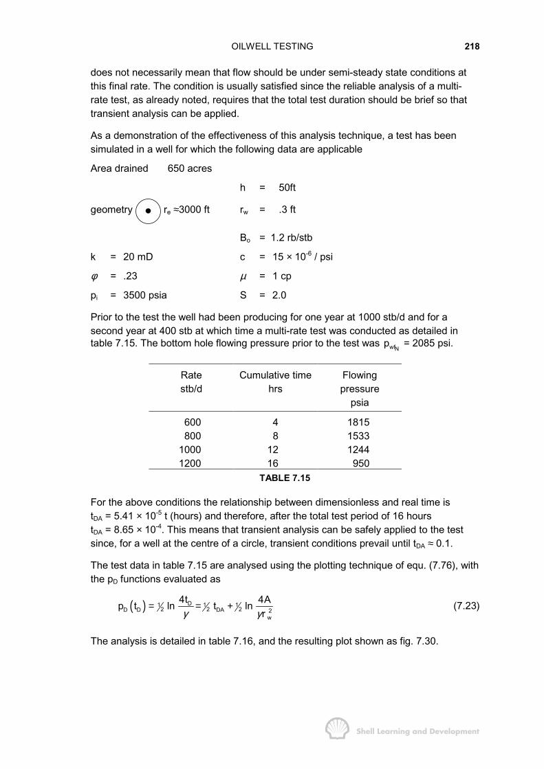
OILWELL TESTING 218
does not necessarily mean that flow should be under semi-steady state conditions atthis final rate. The condition is usually satisfied since the reliable analysis of a multi-rate test, as already noted, requires that the total test duration should be brief so thattransient analysis can be applied.
As a demonstration of the effectiveness of this analysis technique, a test has beensimulated in a well for which the following data are applicable
Area drained 650 acres
h = 50ft
geometry re ≈3000 ft rw = .3 ft
Bo = 1.2 rb/stb
k = 20 mD c = 15 × 10-6 / psi
φ = .23 µ = 1 cp
pi = 3500 psia S = 2.0
Prior to the test the well had been producing for one year at 1000 stb/d and for asecond year at 400 stb at which time a multi-rate test was conducted as detailed intable 7.15. The bottom hole flowing pressure prior to the test was
Nwfp = 2085 psi.
Ratestb/d
Cumulative timehrs
Flowingpressure
psia
600 4 1815800 8 1533
1000 12 12441200 16 950
TABLE 7.15
For the above conditions the relationship between dimensionless and real time istDA = 5.41 × 10⁻⁵ t (hours) and therefore, after the total test period of 16 hourstDA = 8.65 × 10⁻⁴. This means that transient analysis can be safely applied to the testsince, for a well at the centre of a circle, transient conditions prevail until tDA ≈ 0.1.
The test data in table 7.15 are analysed using the plotting technique of equ. (7.76), withthe pD functions evaluated as
( ) D1 1 12 2 2D D DA 2
w
4t 4Ap t ln t lnrγ γ
= = + (7.23)
The analysis is detailed in table 7.16, and the resulting plot shown as fig. 7.30.
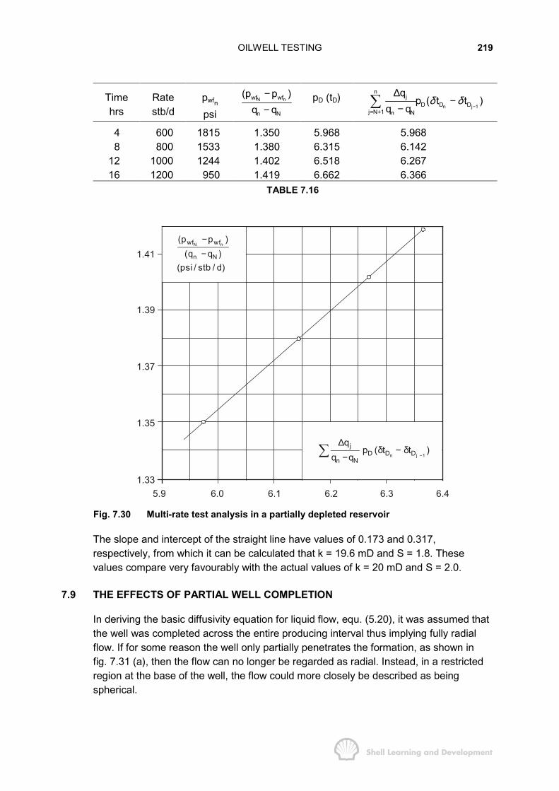
OILWELL TESTING 219
Timehrs
Ratestb/d
pwfn
psiN nwf wf
n N
(p p )q q
−−
pD (tD)n j 1
nj
D D Dj N 1 n N
qp ( t t )
q qδ δ
−= +
∆−
−�
4 600 1815 1.350 5.968 5.9688 800 1533 1.380 6.315 6.142
12 1000 1244 1.402 6.518 6.26716 1200 950 1.419 6.662 6.366
TABLE 7.16
1.41
1.39
1.37
1.35
1.335.9 6.0 6.1 6.2 6.3 6.4
n j 1
jD D D
n N
qp ( t t )
q q −
∆δ − δ
−�
N nwf wf
n N
(p p )(q q )
(psi / stb / d)
−−
Fig. 7.30 Multi-rate test analysis in a partially depleted reservoir
The slope and intercept of the straight line have values of 0.173 and 0.317,respectively, from which it can be calculated that k = 19.6 mD and S = 1.8. Thesevalues compare very favourably with the actual values of k = 20 mD and S = 2.0.
7.9 THE EFFECTS OF PARTIAL WELL COMPLETION
In deriving the basic diffusivity equation for liquid flow, equ. (5.20), it was assumed thatthe well was completed across the entire producing interval thus implying fully radialflow. If for some reason the well only partially penetrates the formation, as shown infig. 7.31 (a), then the flow can no longer be regarded as radial. Instead, in a restrictedregion at the base of the well, the flow could more closely be described as beingspherical.
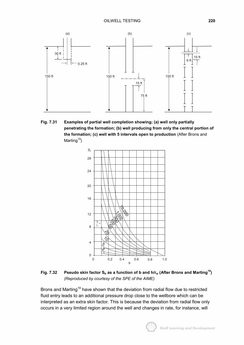
OILWELL TESTING 220
(a)
30 ft
0.25 ft
150 ft
(b)
150 ft
15 ft
75 ft
150 ft
6 ft15 ft
(c)
Fig. 7.31 Examples of partial well completion showing; (a) well only partiallypenetrating the formation; (b) well producing from only the central portion ofthe formation; (c) well with 5 intervals open to production (After Brons andMarting19)
10,0003001005020
10
1
52
0 0.2 0.4 0.6 0.8 1.0b
0
4
8
12
16
20
24
28
Sb
w
hr
=
Fig. 7.32 Pseudo skin factor Sb as a function of b and h/rw (After Brons and Marting19)(Reproduced by courtesy of the SPE of the AIME)
Brons and Marting19 have shown that the deviation from radial flow due to restrictedfluid entry leads to an additional pressure drop close to the wellbore which can beinterpreted as an extra skin factor. This is because the deviation from radial flow onlyoccurs in a very limited region around the well and changes in rate, for instance, will
OILWELL TESTING 221
lead to an instantaneous perturbation in the wellbore pressure without any associatedtransient effects. This pseudo skin can be determined as a function of two parameters,the penetration ratio b and the ratio h/rw, where
the total interval open to flowbthe total thickness of the producing zone
=
and
w
h thickness of the producing zoner wellbore radius
=
The latter definition is somewhat more complex than it appears since if the well is opento flow over several sections of the total producing interval then h represents thethickness of the symmetry element within the total zone. This point is made clear infig. 7.31 (a)-(c), which has been taken from the Brons and Marting paper and illustratesthree possible types of partial well completion. In all three cases the ratiob = 30/150 = 0.2 while the ratio of h/rw is 150/.25 = 600 for case (a), 75/.25 = 300 forcase (b) and 15/.25 = 60 for case (c). Having thus determined the values of b and h/rw
the pseudo skin Sb can be determined using the chart presented as fig. 7.32. For thethree geometric configurations shown in fig. 7.31, the pseudo skin factors areapproximately 17, 15 and 9, respectively. Once the pseudo skin has been calculated itmust be subtracted from the total skin measured in the well test to give the mechanicalskin factor.
7.10 SOME PRACTICAL ASPECTS OF WELL SURVEYING
This section deals with some of the practical aspects involved in the routine pressuretesting of wells in a producing oilfield.
a) Wireline Pressure Recording Instrument
Due to its accuracy and ruggedness the most popular wireline pressure gauge is theAmerada (RPG), a rough schematic diagram of this tool is shown in fig. 7.33(a). Thecontinuous trace of pressure versus time is made by the contact of a stylus with a chartwhich has been specially treated on one side to permit the stylus movement to bepermanently recorded. The chart is held in a cylindrical chart holder which in turn isconnected to a clock which drives the holder in the vertical direction. The stylus isconnected to a bourdon tube and is constrained to record pressures in theperpendicular direction to the movement of the chart holder. The combined movementis such that, on removing the chart from the holder after the survey, a continuous traceof pressure versus time is obtained as shown in fig. 7.33(b), for a typical pressurebuildup survey. Both the clock and pressure element can be selected to match themaximum time and pressure anticipated for the particular survey. With carefulhandling, regular calibration and accurate reading of the pressure chart with amagnifying instrument, an accuracy of about 0.2 can be achieved.
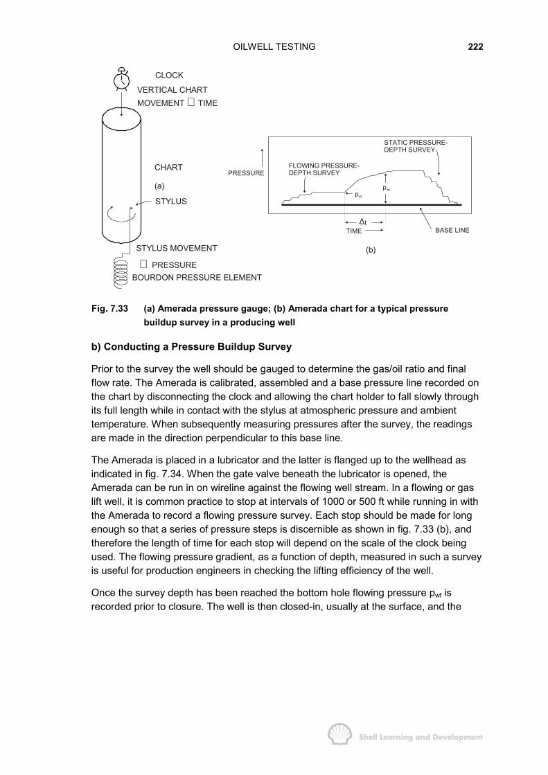
OILWELL TESTING 222
CLOCK
VERTICAL CHARTMOVEMENT ∝ TIME
CHART
(a)
STYLUS
STYLUS MOVEMENT
∝ PRESSUREBOURDON PRESSURE ELEMENT
PRESSUREFLOWING PRESSURE-DEPTH SURVEY
STATIC PRESSURE-DEPTH SURVEY
TIMEt∆
BASE LINE
pwf
pws
(b)
Fig. 7.33 (a) Amerada pressure gauge; (b) Amerada chart for a typical pressurebuildup survey in a producing well
b) Conducting a Pressure Buildup Survey
Prior to the survey the well should be gauged to determine the gas/oil ratio and finalflow rate. The Amerada is calibrated, assembled and a base pressure line recorded onthe chart by disconnecting the clock and allowing the chart holder to fall slowly throughits full length while in contact with the stylus at atmospheric pressure and ambienttemperature. When subsequently measuring pressures after the survey, the readingsare made in the direction perpendicular to this base line.
The Amerada is placed in a lubricator and the latter is flanged up to the wellhead asindicated in fig. 7.34. When the gate valve beneath the lubricator is opened, theAmerada can be run in on wireline against the flowing well stream. In a flowing or gaslift well, it is common practice to stop at intervals of 1000 or 500 ft while running in withthe Amerada to record a flowing pressure survey. Each stop should be made for longenough so that a series of pressure steps is discernible as shown in fig. 7.33 (b), andtherefore the length of time for each stop will depend on the scale of the clock beingused. The flowing pressure gradient, as a function of depth, measured in such a surveyis useful for production engineers in checking the lifting efficiency of the well.
Once the survey depth has been reached the bottom hole flowing pressure pwf isrecorded prior to closure. The well is then closed-in, usually at the surface, and the
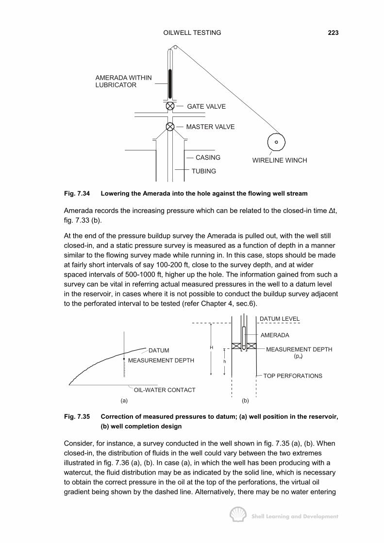
OILWELL TESTING 223
AMERADA WITHINLUBRICATOR
GATE VALVE
MASTER VALVE
CASING
TUBINGWIRELINE WINCH
Fig. 7.34 Lowering the Amerada into the hole against the flowing well stream
Amerada records the increasing pressure which can be related to the closed-in time ∆t,fig. 7.33 (b).
At the end of the pressure buildup survey the Amerada is pulled out, with the well stillclosed-in, and a static pressure survey is measured as a function of depth in a mannersimilar to the flowing survey made while running in. In this case, stops should be madeat fairly short intervals of say 100-200 ft, close to the survey depth, and at widerspaced intervals of 500-1000 ft, higher up the hole. The information gained from such asurvey can be vital in referring actual measured pressures in the well to a datum levelin the reservoir, in cases where it is not possible to conduct the buildup survey adjacentto the perforated interval to be tested (refer Chapter 4, sec.6).
DATUM
MEASUREMENT DEPTH
OIL-WATER CONTACT
DATUM LEVEL
AMERADA
MEASUREMENT DEPTH(p )m
TOP PERFORATIONS
(a) (b)
h
H
Fig. 7.35 Correction of measured pressures to datum; (a) well position in the reservoir,(b) well completion design
Consider, for instance, a survey conducted in the well shown in fig. 7.35 (a), (b). Whenclosed-in, the distribution of fluids in the well could vary between the two extremesillustrated in fig. 7.36 (a), (b). In case (a), in which the well has been producing with awatercut, the fluid distribution may be as indicated by the solid line, which is necessaryto obtain the correct pressure in the oil at the top of the perforations, the virtual oilgradient being shown by the dashed line. Alternatively, there may be no water entering
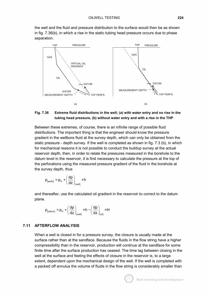
OILWELL TESTING 224
the well and the fluid and pressure distribution to the surface would then be as shownin fig. 7.36(b), in which a rise in the static tubing head pressure occurs due to phaseseparation.
THP PRESSURE
GAS
OIL
WATERMEASUREMENT DEPTH
DATUM
VIRTUAL OILGRADIENT
TOP PERFS.
(a) (b)
THP PRESSURE
GAS
OIL
DATUM
MEASUREMENT DEPTHTOP PERFS.
Fig. 7.36 Extreme fluid distributions in the well; (a) with water entry and no rise in thetubing head pressure, (b) without water entry and with a rise in the THP
Between these extremes, of course, there is an infinite range of possible fluiddistributions. The important thing is that the engineer should know the pressuregradient in the wellbore fluid at the survey depth, which can only be obtained from thestatic pressure - depth survey. If the well is completed as shown in fig. 7.3 (b), in whichfor mechanical reasons it is not possible to conduct the buildup survey at the actualreservoir depth, then, in order to relate the pressures measured in the borehole to thedatum level in the reservoir, it is first necessary to calculate the pressure at the top ofthe perforations using the measured pressure gradient of the fluid in the borehole atthe survey depth, thus
( )( )
mperfswell
dpp p hdz
� �= + � �� �
and thereafter, use the calculated oil gradient in the reservoir to correct to the datumplane.
( )( ) ( )
mdatumwell oil
dp dpp p h Hdz dz
� � � �= + × − ×� � � �� � � �
7.11 AFTERFLOW ANALYSIS
When a well is closed in for a pressure survey, the closure is usually made at thesurface rather than at the sandface. Because the fluids in the flow string have a highercompressibility than in the reservoir, production will continue at the sandface for somefinite time after the surface production has ceased. The time lag between closing in thewell at the surface and feeling the effects of closure in the reservoir is, to a largeextent, dependent upon the mechanical design of the well. If the well is completed witha packed off annulus the volume of fluids in the flow string is considerably smaller than
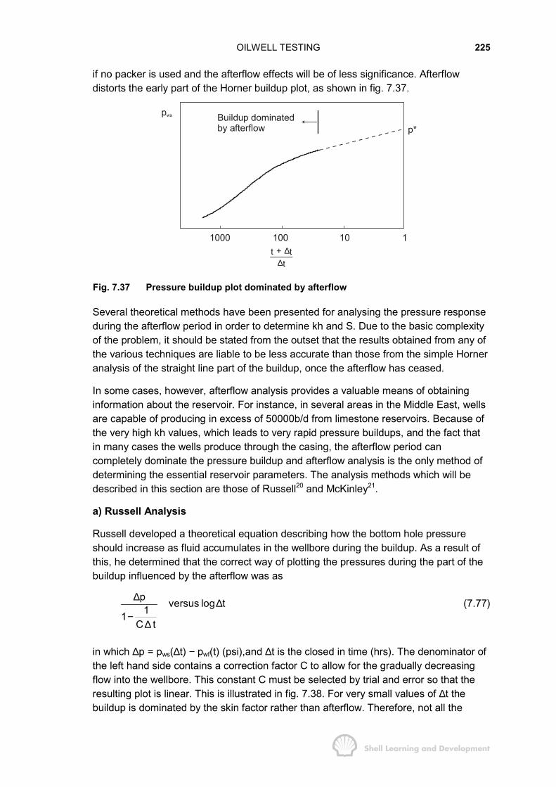
OILWELL TESTING 225
if no packer is used and the afterflow effects will be of less significance. Afterflowdistorts the early part of the Horner buildup plot, as shown in fig. 7.37.
pws Buildup dominatedby afterflow
1000 100 10 1
p*
t tt
+ ∆∆
Fig. 7.37 Pressure buildup plot dominated by afterflow
Several theoretical methods have been presented for analysing the pressure responseduring the afterflow period in order to determine kh and S. Due to the basic complexityof the problem, it should be stated from the outset that the results obtained from any ofthe various techniques are liable to be less accurate than those from the simple Horneranalysis of the straight line part of the buildup, once the afterflow has ceased.
In some cases, however, afterflow analysis provides a valuable means of obtaininginformation about the reservoir. For instance, in several areas in the Middle East, wellsare capable of producing in excess of 50000b/d from limestone reservoirs. Because ofthe very high kh values, which leads to very rapid pressure buildups, and the fact thatin many cases the wells produce through the casing, the afterflow period cancompletely dominate the pressure buildup and afterflow analysis is the only method ofdetermining the essential reservoir parameters. The analysis methods which will bedescribed in this section are those of Russell20 and McKinley21.
a) Russell Analysis
Russell developed a theoretical equation describing how the bottom hole pressureshould increase as fluid accumulates in the wellbore during the buildup. As a result ofthis, he determined that the correct way of plotting the pressures during the part of thebuildup influenced by the afterflow was as
p versus log t11C t
∆ ∆−
∆
(7.77)
in which ∆p = pws(∆t) − pwf(t) (psi),and ∆t is the closed in time (hrs). The denominator ofthe left hand side contains a correction factor C to allow for the gradually decreasingflow into the wellbore. This constant C must be selected by trial and error so that theresulting plot is linear. This is illustrated in fig. 7.38. For very small values of ∆t thebuildup is dominated by the skin factor rather than afterflow. Therefore, not all the
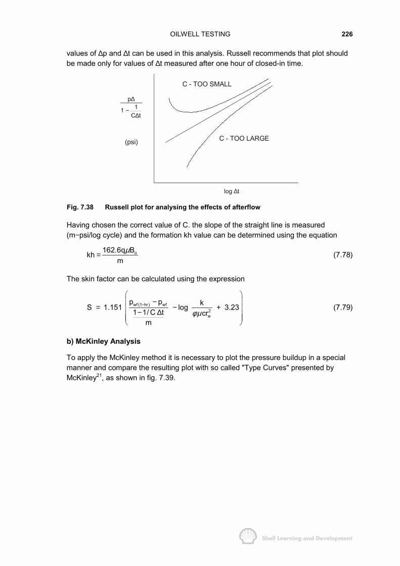
OILWELL TESTING 226
values of ∆p and ∆t can be used in this analysis. Russell recommends that plot shouldbe made only for values of ∆t measured after one hour of closed-in time.
(psi)
C - TOO SMALL
C - TOO LARGE
log ∆t
p∆
1 − 1C∆t
Fig. 7.38 Russell plot for analysing the effects of afterflow
Having chosen the correct value of C. the slope of the straight line is measured(m−psi/log cycle) and the formation kh value can be determined using the equation
o162.6q Bkhm
µ= (7.78)
The skin factor can be calculated using the expression
wf (1 hr ) wf2w
p p kS 1.151 log 3.231 1/ C t crm
φ µ−
� �� �−
= − +� �− ∆� �� �� �
(7.79)
b) McKinley Analysis
To apply the McKinley method it is necessary to plot the pressure buildup in a specialmanner and compare the resulting plot with so called "Type Curves" presented byMcKinley21, as shown in fig. 7.39.
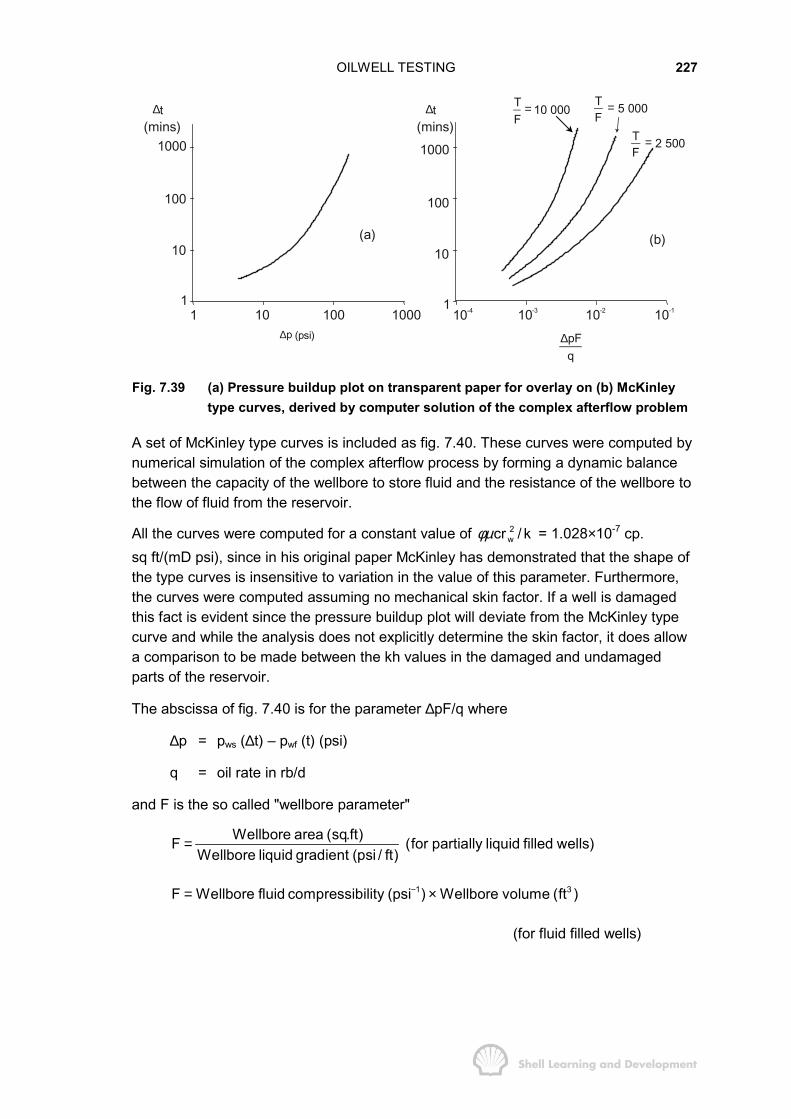
OILWELL TESTING 227
1 10 100 10001
10
100
1000
t∆(mins)
(psi)∆p
(a)
t∆(mins)
1
10
100
1000
10-4 10-3 10-2 10-1
(b)
T 10 000F
= T 5 000F
=
T 2 500F
=
q∆pF
Fig. 7.39 (a) Pressure buildup plot on transparent paper for overlay on (b) McKinleytype curves, derived by computer solution of the complex afterflow problem
A set of McKinley type curves is included as fig. 7.40. These curves were computed bynumerical simulation of the complex afterflow process by forming a dynamic balancebetween the capacity of the wellbore to store fluid and the resistance of the wellbore tothe flow of fluid from the reservoir.
All the curves were computed for a constant value of 2wcr / kφµ = 1.028×10⁻⁷ cp.
sq ft/(mD psi), since in his original paper McKinley has demonstrated that the shape ofthe type curves is insensitive to variation in the value of this parameter. Furthermore,the curves were computed assuming no mechanical skin factor. If a well is damagedthis fact is evident since the pressure buildup plot will deviate from the McKinley typecurve and while the analysis does not explicitly determine the skin factor, it does allowa comparison to be made between the kh values in the damaged and undamagedparts of the reservoir.
The abscissa of fig. 7.40 is for the parameter ∆pF/q where
∆p = pws (∆t) – pwf (t) (psi)
q = oil rate in rb/d
and F is the so called "wellbore parameter"
Wellbore area (sq.ft)F (for partially liquid filled wells)Wellbore liquid gradient (psi / ft)
=
1 3F Wellbore fluid compressibility (psi ) Wellbore volume (ft )−= ×
(for fluid filled wells)
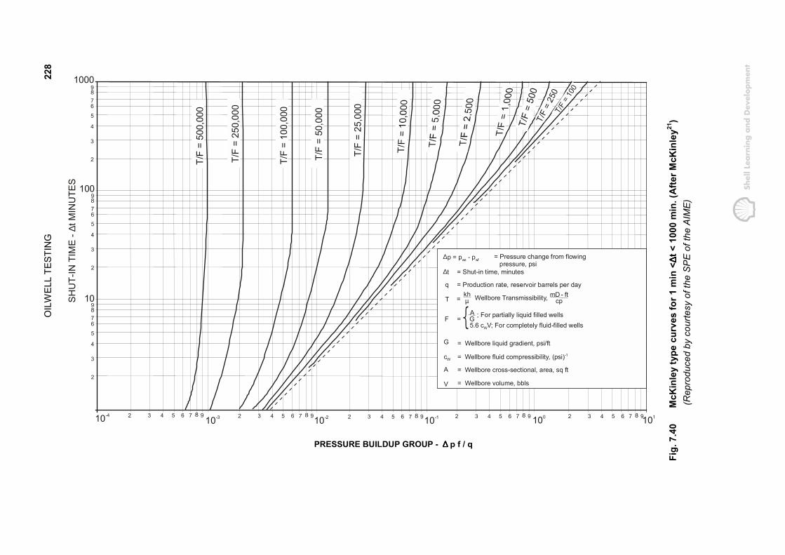
OIL
WEL
L TE
STIN
G22
8
10-410-3 10-2 10-1 100 1012 3 4 5 6 7 9 2 3 4 5 6 7 9 2 3 4 5 6 7 9 2 3 4 5 6 7 9 2 3 4 5 6 7 9
2
3
4
567
910
2
3
4
567
9100
2
3
4
5
67
91000
G
c
A
V
W
= Wellbore liquid gradient, psi/ft
= Wellbore fluid compressibility, (psi)
= Wellbore cross-sectional, area, sq ft
= Wellbore volume, bbls
-1
= Pressure change from flowing pressure, psi
= Shut-in time, minutes
= Production rate, reservoir barrels per dayq
T
F ; For partially liquid filled wells5.6 c V; For completely fluid-filled wellsW
=
∆p = p - p ws wf
∆t
khµ= Wellbore Transmissibility, mD - ft
cp
AG
SHU
T-IN
TIM
E - ∆
t MIN
UTE
S
T/F
= 50
0,00
0
T/F
= 25
0,00
0
T/F
= 10
0,00
0
T/F
= 50
,000
T/F
= 25
,000
T/F
= 50
0T/
F =
250
T/F
= 10
0
PRESSURE BUILDUP GROUP - ∆ ∆ ∆ ∆ p f / q
Fig.
7.4
0M
cKin
ley
type
cur
ves
for 1
min
<∆ ∆∆∆t
< 1
000
min
. (Af
ter M
cKin
ley21
) (R
epro
duce
d by
cou
rtesy
of t
he S
PE o
f the
AIM
E)
OILWELL TESTING 229
In practice, the value of F is seldom explicitly calculated in the McKinley analysis. It is aparameter which disappears by cancellation when calculating the wellboretransmissibility.
Each type curve is characterised by a fixed value of T/F, where T is the transmissibility= kh/µ mD.ft/cp.
The steps involved in a McKinley analysis, which is usually aimed at determiningtransmissibilities in the damaged/stimulated zone close to the wellbore, and theaverage for the formation away from the well, are as follows.
a) Make a table of values of ∆t, the closed in time (minutes), and the correspondingvalues of ∆p = pws (∆t) - pwf (t) (psi). Unlike the Russell method it is not necessaryto differentiate between the part of the buildup due to skin and that due toafterflow, all values of ∆t and ∆p can be used.
b) Overlay the McKinley chart with a sheet of transparent paper and draw verticaland horizontal axes to match those of the chart. The ordinate should have thesame log time scale as the McKinley chart but the abscissa, while using thesame log scale, should be plotted for the most suitable range of pressure values.Plot the ∆t versus ∆p data on this transparent paper.
c) The transparent paper is then moved laterally over the McKinley chart, keepingthe abscissae together, until the early part of the pressure buildup coincides withone of the type curves.
d) The value of the parameter T/F, characterising the type curve for which the matchis obtained, is noted.
e) Any one of the points on the pressure buildup, which also lies on the type curve,is now used as a match point and the corresponding value of ∆pF/q is read fromthe abscissa of the McKinley chart. Multiplying this value by the value of T/Fgives
pF T pTq F q
∆ ∆× = (7.80)
Since ∆p (psi) is known for the match point, then the transmissibility T can becalculated from this latter expression. Finally, since T = kh/µ, the values of kh andk can be determined. The procedure is illustrated in fig. 7.41.
Using the figures shown in this diagram
pF T pT0.05 5000q F q
∆ ∆× = × =
If q = 500 rb/d, then T = 5000 × 0.05 × 500800
= 156 mD.ft/cp.
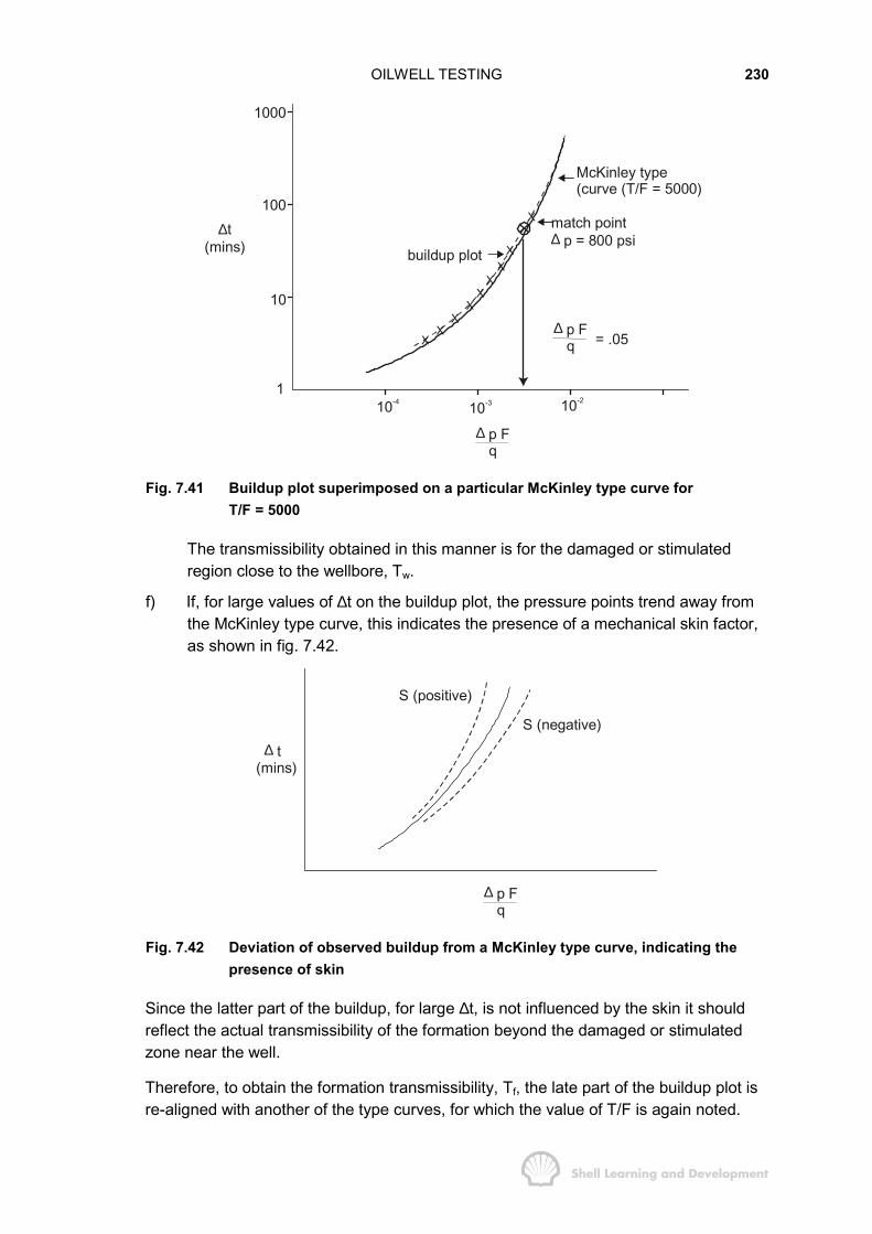
OILWELL TESTING 230
XX
XX
XX
XX
X
1000
100
10
110-4 10-3 10-2
buildup plot
match pointp = 800 psi∆
McKinley type(curve (T/F = 5000)
p Fq
∆ = .05
p Fq
∆
∆t(mins)
Fig. 7.41 Buildup plot superimposed on a particular McKinley type curve forT/F = 5000
The transmissibility obtained in this manner is for the damaged or stimulatedregion close to the wellbore, Tw.
f) If, for large values of ∆t on the buildup plot, the pressure points trend away fromthe McKinley type curve, this indicates the presence of a mechanical skin factor,as shown in fig. 7.42.
p Fq
∆
t(mins)
∆
S (positive)
S (negative)
Fig. 7.42 Deviation of observed buildup from a McKinley type curve, indicating thepresence of skin
Since the latter part of the buildup, for large ∆t, is not influenced by the skin it shouldreflect the actual transmissibility of the formation beyond the damaged or stimulatedzone near the well.
Therefore, to obtain the formation transmissibility, Tf, the late part of the buildup plot isre-aligned with another of the type curves, for which the value of T/F is again noted.
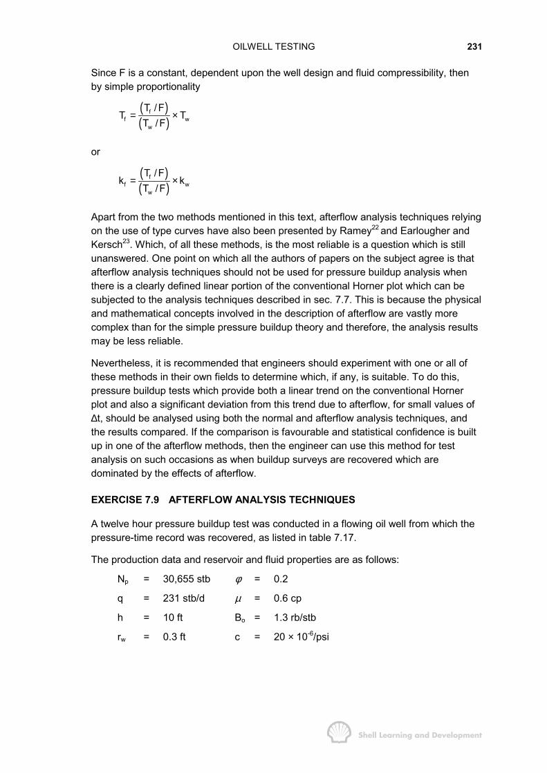
OILWELL TESTING 231
Since F is a constant, dependent upon the well design and fluid compressibility, thenby simple proportionality
( )( )
ff w
w
T /FT T
T /F= ×
or
( )( )
ff w
w
T /Fk k
T /F= ×
Apart from the two methods mentioned in this text, afterflow analysis techniques relyingon the use of type curves have also been presented by Ramey22 and Earlougher andKersch23. Which, of all these methods, is the most reliable is a question which is stillunanswered. One point on which all the authors of papers on the subject agree is thatafterflow analysis techniques should not be used for pressure buildup analysis whenthere is a clearly defined linear portion of the conventional Horner plot which can besubjected to the analysis techniques described in sec. 7.7. This is because the physicaland mathematical concepts involved in the description of afterflow are vastly morecomplex than for the simple pressure buildup theory and therefore, the analysis resultsmay be less reliable.
Nevertheless, it is recommended that engineers should experiment with one or all ofthese methods in their own fields to determine which, if any, is suitable. To do this,pressure buildup tests which provide both a linear trend on the conventional Hornerplot and also a significant deviation from this trend due to afterflow, for small values of∆t, should be analysed using both the normal and afterflow analysis techniques, andthe results compared. If the comparison is favourable and statistical confidence is builtup in one of the afterflow methods, then the engineer can use this method for testanalysis on such occasions as when buildup surveys are recovered which aredominated by the effects of afterflow.
EXERCISE 7.9 AFTERFLOW ANALYSIS TECHNIQUES
A twelve hour pressure buildup test was conducted in a flowing oil well from which thepressure-time record was recovered, as listed in table 7.17.
The production data and reservoir and fluid properties are as follows:
Np = 30,655 stb φ = 0.2
q = 231 stb/d µ = 0.6 cp
h = 10 ft Bo = 1.3 rb/stb
rw = 0.3 ft c = 20 × 10-6/psi
OILWELL TESTING 232
∆t (mins) pws (psi) ∆t (mins) pws (psi)
0 1600 (pwf)20 1920 270 287940 2160 300 290060 2350 360 293590 2525 420 2960
120 2650 480 2980150 2726 540 2998180 2779 600 3011210 2822 660 3022240 2852 720 3035
TABLE 7.17
The conventional Horner plot of pws versus log t tt
+ ∆∆
does not become linear, even for
the largest values of ∆t, and therefore the afterflow analysis techniques presented inthis section must be used to analyse this test.
1) Evaluate k and S using the Russell method.
2) Determine the permeability in the vicinity of the wellbore and of the undamagedformation using the McKinley method.
EXERCISE 7.9 SOLUTION
1) Russell Analysis
As suggested by Russell, the analysis should only be applied for pressures measuredafter ∆t = 1 hour. In table 7.18 several values of the parameter C have been selected inan attempt to linearize the plot of equ. (7.77).
OILWELL TESTING 233
p /(1 1/ C t)∆ − ∆
∆t (hrs) log ∆t ∆p (psi) C=1.7 C=2.1 C=2.5
1.5 .176 925 1522 1355 12612.0 .301 1050 1487 1378 13142.5 .398 1126 1472 1391 13403.0 .477 1179 1467 1401 13603.5 .544 1222 1469 1414 13804.0 .602 1252 1468 1421 13914.5 .653 1279 1471 1430 14045.0 .699 1300 1473 1437 14136.0 .778 1335 1480 1450 14307.0 .845 1360 1485 1459 14428.0 .903 1380 1490 1467 14539.0 .954 1398 1496 1476 1463
10.0 1.000 1411 1499 1482 147011.0 1.041 1422 1502 1486 147612.0 1.079 1435 1509 1494 1484
TABLE 7.18
As shown in fig. 7.43, the correct value of the parameter C to obtain a linear Russellplot is C = 2.1.
Since the slope of this line is 151 psi/log cycle, then the kh product can be evaluatedusing equ. (7.78) as
162.6 231 0.3 1.3kh 194 mD.ft; and k 19.4 mD151
× × ×= = =
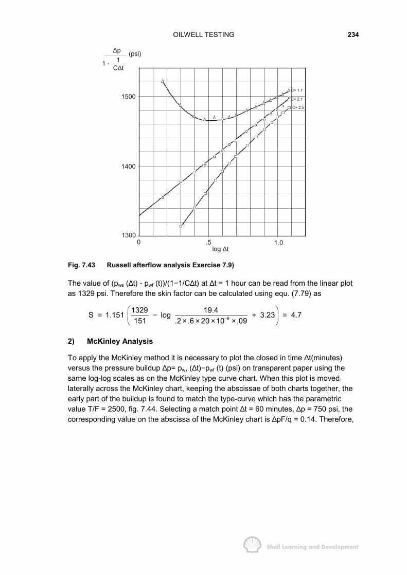
OILWELL TESTING 234
1500
1400
13000 .5 1.0
C= 1.7
C= 2.1
C= 2.5
∆p
1 - 1C t∆
(psi)
log t∆
Fig. 7.43 Russell afterflow analysis Exercise 7.9)
The value of (pws (∆t) - pwf (t))/(1−1/C∆t) at ∆t = 1 hour can be read from the linear plotas 1329 psi. Therefore the skin factor can be calculated using equ. (7.79) as
61329 19.4S 1.151 log 3.23 4.7151 .2 .6 20 10 .09−
� �= − + =� �× × × ×� �
2) McKinley Analysis
To apply the McKinley method it is necessary to plot the closed in time ∆t(minutes)versus the pressure buildup ∆p= pw, (∆t)−pwf (t) (psi) on transparent paper using thesame log-log scales as on the McKinley type curve chart. When this plot is movedlaterally across the McKinley chart, keeping the abscissae of both charts together, theearly part of the buildup is found to match the type-curve which has the parametricvalue T/F = 2500, fig. 7.44. Selecting a match point ∆t = 60 minutes, ∆p = 750 psi, thecorresponding value on the abscissa of the McKinley chart is ∆pF/q = 0.14. Therefore,
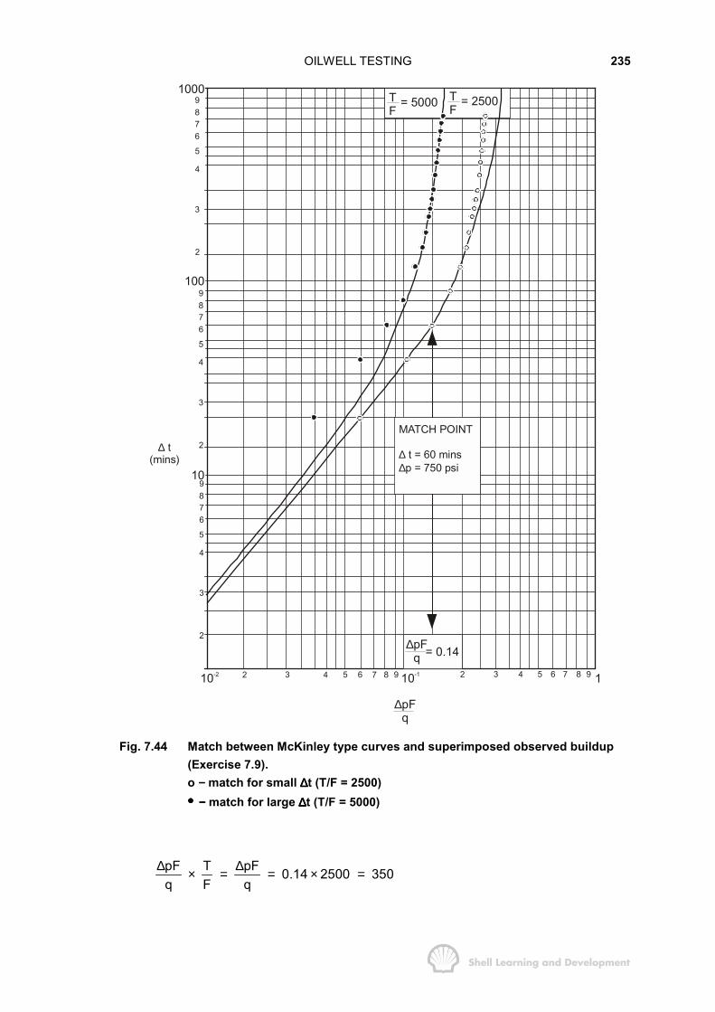
OILWELL TESTING 235
MATCH POINT
t = 60 minsp = 750 psi
∆∆
= 0.14∆pFq
10-2 10-1 1
10
100
∆pFq
1000= 5000T
F= 2500T
F
2 53 4 6 7 9 2 53 4 6 7 9
2
5
3
4
67
9
2
5
3
4
67
9
2
5
3
4
67
9
t (mins)
∆
Fig. 7.44 Match between McKinley type curves and superimposed observed buildup(Exercise 7.9).o −−−− match for small ∆∆∆∆t (T/F = 2500)•••• −−−− match for large ∆∆∆∆t (T/F = 5000)
pF T pF 0.14 2500 350q F q
∆ ∆× = = × =
OILWELL TESTING 236
and since q = 300 rb/d, then the wellbore transmissibility is
ww
k h 3500 300T 140 mD.ft / cp750µ
×= = =
and therefore
wk 8.4 mD=
For values of ∆t greater than 150 minutes the actual buildup curve breaks away fromthe parametric curve for T/F = 2500, indicating the presence of a positive skin factor.For large values of ∆t the buildup matches the McKinley curve with parametric valueT/F = 5000, fig. 7.44. Even for this latter match, however, the buildup continues to bedominated by afterflow. Therefore, a minimum value of the formation transmissibilitycan be estimated as
( )( )
ff w
w
T /FT T
T /F= ×
giving
f5000k 8.4 16.8mD2500
= × =
Thus the comparison between the Russell and McKinley techniques is quitereasonable in this case.
REFERENCES
1) van Everdingen, A.F. and Hurst, W., 1949. The Application of the LaplaceTransformation to Flow Problems in Reservoirs. Trans. AIME. 1 86: 305-324.
2) Earlougher, R.C., Jr., 1971. Estimating Drainage Shapes from Reservoir LimitTests. J. Pet. Tech., October: 1266-1268.
3) Ramey, H.J., Jr. and Cobb, W.M., 1971. A General Pressure Buildup Theory fora Well in a Closed Drainage Area. J. Pet. Tech., December: 1493-1505.Trans.AIME.
4) Horner, D.R., 1951. Pressure Build Up in Wells. Proc., Third World PetroleumCongress. E.J. Brill, Leiden. ll, 503.
5) Odeh, A.S. and Jones, L.G., 1965. Pressure Drawdown Analysis, Variable RateCase. J. Pet. Tech., August: 960-964. Trans. AIME.
6) Matthews, C.S. and Russell, D.G., 1967. Pressure Buildup and Flow Tests inWells. SPE Monograph: 130-133.
7) Matthews, C.S., Brons, F. and Hazebroek, P.,1954. A Method for theDetermination of Average Pressure in a Bounded Reservoir. Trans.AIME.201: 182-191.
OILWELL TESTING 237
8) Cobb, W.M. and Dowdle, W.L., 1973. A Simple Method for Determining WellPressures in Closed Rectangular Reservoirs, J. Pet. Tech., November:1305-1306.
9) Dietz, D.N., 1965. Determination of Average Reservoir Pressures from Build UpSurveys. J. Pet. Tech., August: 955-959. Trans. AIME.
10) Earlougher, R.C., Jr., Ramey, H.J., Jr., Miller, F.G. and Mueller, T.D., 1968.Pressure Distribution in Rectangular Reservoirs. J. Pet. Tech., February:199-208. Trans. AIME.
11) Ramey, H.J., Jr., Kumar, A. and Gulati, M.S. 1973. Gas Well Test Analysis UnderWater-Drive Conditions. American Gas Assn., Arlington, Va.
12) Pinson, A.E., Jr., 1972. Concerning the Value of Producing Time in AveragePressure Determinations from Pressure Buildup Analysis, J. Pet. Tech.,November: 1369-1370.
13) Kazemi, H., 1974. Determining Average Reservoir Pressure from PressureBuildup Tests. Soc. Pet. Eng. J., February: 55-62. Trans. AIME.
14) Odeh, A.S. and Selig, F., 1963. Pressure Buildup Analysis, Variable Rate Case.J. Pet. Tech., July: 790-794. Trans. AIME.
15) van Poollen, H.K., Breitenback, E.A. and Thurnau, D.H., 1968. Treatment ofIndividual Wells and Grids in Reservoir Modelling. Soc. Pet. Eng. J.,December: 341-346.
16) Earlougher, R.C., Jr., 1972. Comparing Single-Point Pressure Buildup Data WithReservoir Simulator Results. J. Pet. Tech., June: 711-712.
17) Cobb, W.M. and Smith, J.T., 1975. An Investigation of Pressure Buildup Tests inBounded Reservoirs. J. Pet. Tech., August: 991-996. Trans. AIME.
18) Denson, A.H., Smith, J.T. and Cobb, W.M., 1976. Determining Well DrainagePore Volume and Porosity from Pressure Buildup Tests. Soc. Pet. Eng. J.,August: 209-216.
19) Brons, F. and Marting, V.E., 1961. The Effect of Restricted Fluid Entry on WellProductivity. J. Pet. Tech., February: 172-174. Trans. AIME.
20) Russell, D.G., 1966. Extensions of Pressure Buildup Analysis Methods. J. Pet.Tech., December: 1624-1636. Trans. AIME.
21) McKinley, R.M.,1971. Wellbore Transmissibility from Afterflow-DominatedPressure Buildup Data. J. Pet. Tech. July: 863-872. Trans. AIME.
22) Ramey, H.J., Jr., 1970. Short-Time Well Test Data Interpretation in the Presenceof Skin Effect and Wellbore Storage. J. Pet. Tech., January: 97-104. Trans.AIME.

OILWELL TESTING 238
23) Earlougher, R.C., and Kersch, K.M., 1974. Analysis of Short-Time Transient TestData by Type-Curve Matching. J. Pet. Tech., July: 793-800. Trans. AIME.
CHAPTER 8
REAL GAS FLOW: GAS WELL TESTING
8.1 INTRODUCTION
The first part of this chapter describes how the basic differential equation for radial fluidflow, equ. (5.1), can be approximately linearized for real gas flow. This is achievedusing the real gas pseudo pressure function
b
p
p
pdpm(p) 2 µ
=Ζ�
and subsequently, all equations in the chapter are expressed in terms of m(p) functionsrather than real pressures. The constant terminal rate solution of the radial diffusivityequation is then presented in dimensionless form, equivalent to the pD functions forliquid flow, and the solution is applied to the analysis of gas well tests. A similarapproach is used for analysing pressure buildup tests in solution gas drive reservoirs,below bubble point pressure.
8.2 LINEARIZATION AND SOLUTION OF THE BASIC DIFFERENTIAL EQUATION FORTHE RADIAL FLOW OF A REAL GAS
By assuming mass conservation, Darcy's law and applying the definition of fluidcompressibility, the basic equation for the radial flow of a single phase fluid in a porousmedium was derived in chapter 5 as
1 k p pr cr r r t
ρ φ ρµ
� �∂ ∂ ∂=� �∂ ∂ ∂� �(5.1)
This equation was linearized for liquid flow by deletion of terms, assuming that
- µ was independent of pressure
- pr
∂∂
was small and therefore 2p
r∂� �
� �∂� � was negligible
- c was small and constant so that cp << 1
which resulted in the radial diffusivity equation
1 p c prr r r k t
φµ∂ ∂ ∂� � =� �∂ ∂ ∂� �(5.20)
Because this equation is linear for liquid flow, simple analytical methods could beapplied to describe stabilized inflow (Chapter 6) and the constant terminal rate solution(Chapter 7). The assumptions made in linearizing equ. (5.1) are inappropriate whenapplied to the flow of a real gas. In the first place, gas viscosity is highly pressuredependent. Secondly, the isothermal compressibility of a real gas is
REAL GAS FLOW: GAS WELL TESTING 240
1 1 1cp p p
∂Ζ= − ≈Ζ ∂
(1.31)
which again is highly pressure dependent and automatically violates the abovecondition that cp << 1.
These problems, although severe, are not insurmountable. Nevertheless, it was notuntil the mid sixties that reliable analytical solutions of equ. (5.1 ) were developed. Twoseparate solution methods were published almost simultaneously in 1966; these are
- the Russell, Goodrich et. al., p2 formulation1
- the Al-Hussainy, Ramey and Crawford, real gas pseudo pressure formulation2.
Both techniques will be described in this chapter although the latter, for reasonsexplained in the text, is preferred. To illustrate the difference in approach the radialsemi-steady state inflow equation, equivalent to equ. (6.12), will be derived in secs. 8.3and 8.4, using both methods. Having thus established an analogy between liquid andreal gas flow equations, the constant terminal rate solution for gas is stated byinference and its application described in detail in the remainder of the chapter.
Because of the great disparity between gas rates measured at the surface (Q) and inthe reservoir (q) it has become conventional to express gas flow equations usingsurface rates, at standard conditions, with all parameters expressed in field units. Thispractice will be adhered to in this chapter, using the following units
Q - Mscf/d µ - cp(= µg)
(at 60°F and 14.7 psia) Z - dimensionlesst - hours p - psiak - mD T - °R (460+°F)h, r - ft
In all equations µ and Z are evaluated at some defined reservoir condition. The basicderivations of the flow equations in sections 8.3 through 8.8 will still be performed inDarcy units, with conversion to field units being made upon achieving the desired formof equation.
8.3 THE RUSSELL, GOODRICH, et. al. SOLUTION TECHNIQUE
The authors approached the problem by making the initial assumption that it waspossible to linearize equ. (5.1) for real gas flow in precisely the same manner as forliquid flow, described in Chapter 5, sec. 4. Admittedly, this approach should yieldinaccurate results. However, Russell and Goodrich also designed a numerical model ofa single well draining a radial volume element which itself was subdivided into finitegrid blocks as shown in fig. 8.1.

REAL GAS FLOW: GAS WELL TESTING 241
rw r re
Fig. 8.1 Radial numerical simulation model for real gas inflow
The flow equations from block to block were solved numerically, using a finitedifference approximation, making due allowance for the variation of µ and Z asfunctions of pressure. This is equivalent to solving the non-linear second orderdifferential equation (5.1). The results may be expected to be in slight error due to theuse of finite difference calculus, but the errors were minimized by making the gridblocks smaller in the vicinity of the wellbore, where the pressure gradients are largest,thus providing a higher resolution of solution in this region. With this model it washoped that some correcting factor could be found which could be used to match theapproximate analytical results, obtained by making the same assumptions as for asingle phase liquid, with the more exact results from the numerical simulation.
As an example of the approach taken by Russell and Goodrich, consideration will begiven to adapting the semi-steady state inflow equation, developed in chapter 6, sec. 2,for the flow of oil, to an equivalent form which will be appropriate for the flow of gas.The equation of interest, expressed in Darcy units, is
ewf
w
rq 3p p ln S2 kh r 4
µπ
� �− = − +� �
� �(6.12)
which, when expressed in the field units specified in the previous section, becomes
( ) ewf
w
s.cc / sec r.cc / secQ Mscf / dratm 3Mscf / d s.cc / secp p psi ln S
D cmpsi r 42 k mD h ftmD ft
µπ
� � � �� � � � � �� � � � � �− = − + � � � � � �� � � �
� � � �� � � �
(8.1)
In this conversion the ratio
r.cc / sec reservoir cc / sec 1 1s.cc / sec s tandard cc / sec E Gas expansion factor
� �� � = = =� �� �� � � �
and in field units
�pE 35.37ZT
= (1.25)
and �p , the pressure at which E is evaluated, is as yet undefined. The full conversion ofthe rate term in equation (8.1 ) can be expressed as
REAL GAS FLOW: GAS WELL TESTING 242
Mstb / d stb / d s.cc / sec 1Q Mscf / d q r.cc / secMscf / d Mstb / d stb / d E� � � � � � =� � � � � �� � � � � �
[ ] [ ]�
1 ZTQ Mscf / d 1000 1.84 q r.cc / sec5.615 35.37p� � × × =� �� �
�
QZT9.265 Mscf / d q r.cc / secp
=
Including the remaining conversion factors in equ. (8.1 ) yields
�
ewf
w
r711 Q ZT 3p p ln Sr 4khp
µ � �− = − +� �
� �(8.2)
Russell and Goodrich, comparing equ. (8.2) with the numerical simulation, found thatfor the same reservoir and flow conditions the two were in close agreement providingthat the pressure p� , at which the gas expansion factor was evaluated, was set equal tothe average of the current, average reservoir pressure and the bottom hole flowingpressure i.e.
� wfp pp2
+= (8.3)
Furthermore, both µ and Z should also be evaluated at this same pressure so that
wf wfp p p pand Z Z2 2
µ µ� � � �+ += =� � � �� � � �
(8.4)
and substituting these values of �p , µ and Z in equ. (8.2) gives
2 2 ewf
w
r1422 Q ZT 3p p ln Skh r 4
µ � �− = − +� �
� �(8.5)
Equ. (8.5) is the familiar p2 formulation of the well inflow equation, under semi-steadystate conditions, which was tested by Russell and Goodrich and found to be applicableover a wide range of reservoir conditions and flow rates.
Similarly, the transient line source solution for the same initial and boundary conditionsdetailed in chapter 7, sec. 2, is
( )2 2i wf 2
wi
711 Q ZT 4 .000264ktp p ln 2Skh c r
µγ φ µ
� �− = +� �� �
� �(8.6)
wf wfp p p pand Z Z2 2
µ µ� � � �+ += =� � � �� � � �
(8.4)
REAL GAS FLOW: GAS WELL TESTING 243
which is the real gas equivalent of equ. (7.10) in field units. This equation was alsofound to compare favourably with the numerical simulation results, providing theviscosity-compressibility product was evaluated as (µc)i, at the initial pressure pi,(ref. sec. 8.8).
One obvious practical disadvantage in using the p2 formulation can be appreciated byconsidering a frequently occurring problem in gas inflow calculations, namely, thecalculation of pwf if both p and Q are known using, in this case, the semi-steady stateinflow equation. A schematic of the calculation procedure is shown in fig. 8.2. If it isassumed that p has been determined in the drainage volume of the well from materialbalance considerations then, for a fixed offtake rate, it will be necessary to solve theinflow equation by iteration to determine pwf since both µ and Z must be evaluated atthe pressure defined in equ. (8.4). In any iteration cycle k
wfp is calculated using valuesof µk and Zk evaluated at the pressure k 1
wf(p p ) / 2−+ , where k is the iteration counter. Fork = 1, both µ1 and Z1 can be evaluated at some convenient starting pressure, which inthis case has been selected as p . When the difference between successive values of
kwfp is less than some tolerance value (TOL) the iteration is terminated. Other
disadvantages in using the p2 formulation for inflow equations will be discussed insection 8.5.
8.4 THE AL-HUSSAINY, RAMEY, CRAWFORD SOLUTION TECHNIQUE
In their approach the authors attempted to linearize the basic flow equation, (5.1), usingthe following version of the Kirchhoff integral transformation
( )b
p
p
pdpm p 2Zµ
= � (8.7)
which was given the name, in this present context, of "the real gas pseudo pressure".
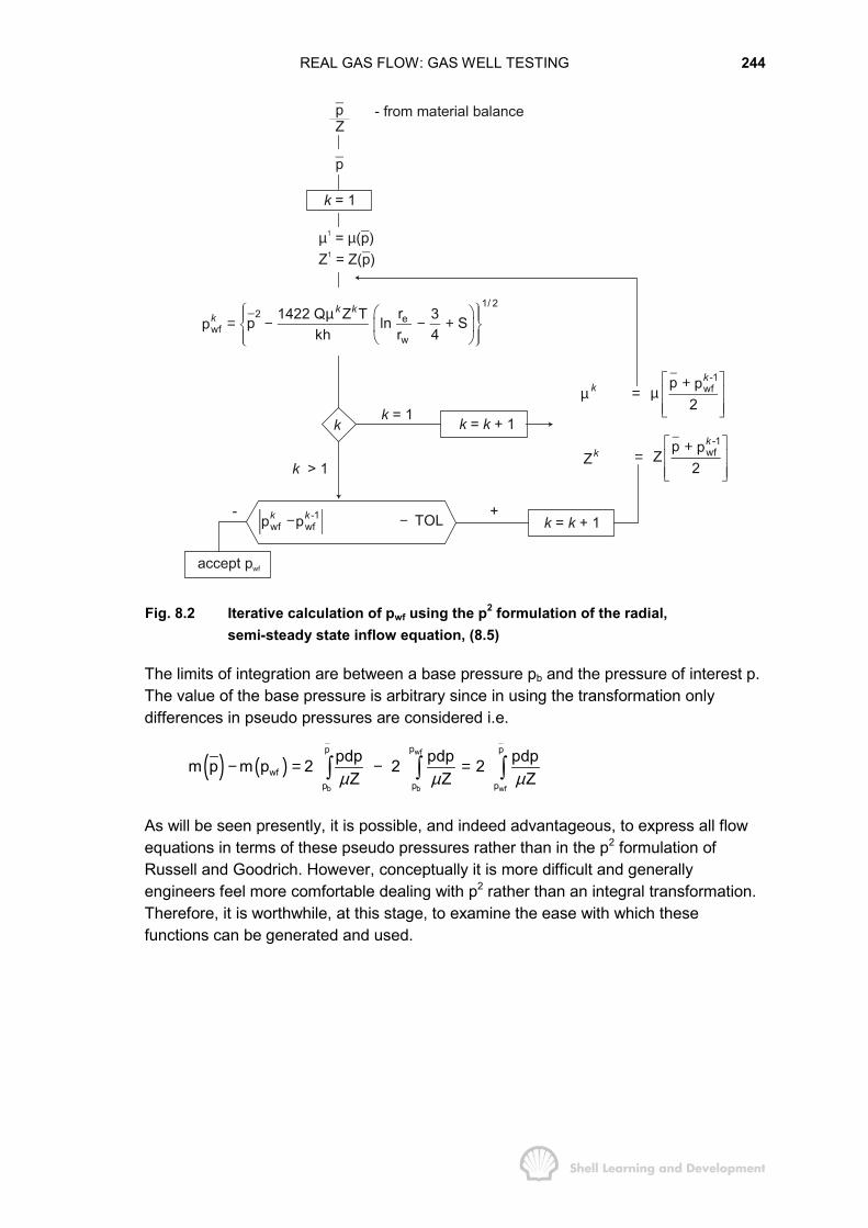
REAL GAS FLOW: GAS WELL TESTING 244
pZ
p
k = 1
µ1 = ( )Z
µ p1 = Z( )p
k = 1
1/ 22 e
wfw
r1422 Q Z T 3p ln Spkh r 4
� �� �� �= − − +� �� � � ��
µk kk
k k = 1k +
k > 1
-1wfp p
2� �+
= � �� �� �
µµk
k
-1wfp pZZ 2
� �+= � �
� �� �
kk
k = 1k + - +
accept pwf
-1wf wf TOLp p− −k k
- from material balance
Fig. 8.2 Iterative calculation of pwf using the p2 formulation of the radial,semi-steady state inflow equation, (8.5)
The limits of integration are between a base pressure pb and the pressure of interest p.The value of the base pressure is arbitrary since in using the transformation onlydifferences in pseudo pressures are considered i.e.
( ) ( )wf
b b wf
pp p
wfp p p
pdp pdp pdpm p m p 2 2 2Z Z Zµ µ µ
− = − =� � �
As will be seen presently, it is possible, and indeed advantageous, to express all flowequations in terms of these pseudo pressures rather than in the p2 formulation ofRussell and Goodrich. However, conceptually it is more difficult and generallyengineers feel more comfortable dealing with p2 rather than an integral transformation.Therefore, it is worthwhile, at this stage, to examine the ease with which thesefunctions can be generated and used.
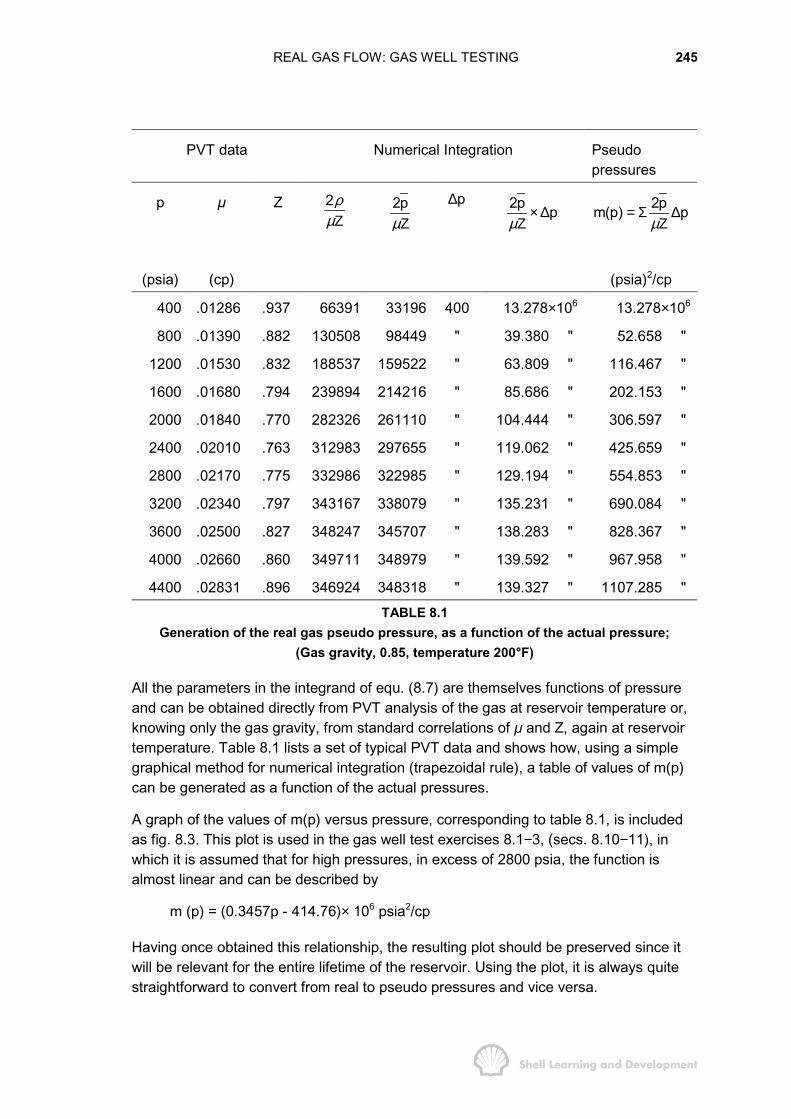
REAL GAS FLOW: GAS WELL TESTING 245
PVT data Numerical Integration Pseudopressures
p µ Z 2ρµΖ
2pµΖ
p∆ 2p pµ
× ∆Ζ
2pm(p) pµ
= Σ ∆Ζ
(psia) (cp) (psia)2/cp
400 .01286 .937 66391 33196 400 13.278×10⁶ 13.278×10⁶
800 .01390 .882 130508 98449 " 39.380 " 52.658 "
1200 .01530 .832 188537 159522 " 63.809 " 116.467 "
1600 .01680 .794 239894 214216 " 85.686 " 202.153 "
2000 .01840 .770 282326 261110 " 104.444 " 306.597 "
2400 .02010 .763 312983 297655 " 119.062 " 425.659 "
2800 .02170 .775 332986 322985 " 129.194 " 554.853 "
3200 .02340 .797 343167 338079 " 135.231 " 690.084 "
3600 .02500 .827 348247 345707 " 138.283 " 828.367 "
4000 .02660 .860 349711 348979 " 139.592 " 967.958 "
4400 .02831 .896 346924 348318 " 139.327 " 1107.285 "TABLE 8.1
Generation of the real gas pseudo pressure, as a function of the actual pressure;(Gas gravity, 0.85, temperature 200°F)
All the parameters in the integrand of equ. (8.7) are themselves functions of pressureand can be obtained directly from PVT analysis of the gas at reservoir temperature or,knowing only the gas gravity, from standard correlations of µ and Z, again at reservoirtemperature. Table 8.1 lists a set of typical PVT data and shows how, using a simplegraphical method for numerical integration (trapezoidal rule), a table of values of m(p)can be generated as a function of the actual pressures.
A graph of the values of m(p) versus pressure, corresponding to table 8.1, is includedas fig. 8.3. This plot is used in the gas well test exercises 8.1−3, (secs. 8.10−11), inwhich it is assumed that for high pressures, in excess of 2800 psia, the function isalmost linear and can be described by
m (p) = (0.3457p - 414.76)× 106 psia2/cp
Having once obtained this relationship, the resulting plot should be preserved since itwill be relevant for the entire lifetime of the reservoir. Using the plot, it is always quitestraightforward to convert from real to pseudo pressures and vice versa.

REAL GAS FLOW: GAS WELL TESTING 246
In attempting to linearize the basic radial flow equation (5.1), (using, for the moment,Darcy units), Al-Hussainy, Ramey and Crawford replaced the dependent variable p bythe real gas pseudo pressure m(p) in the following manner.
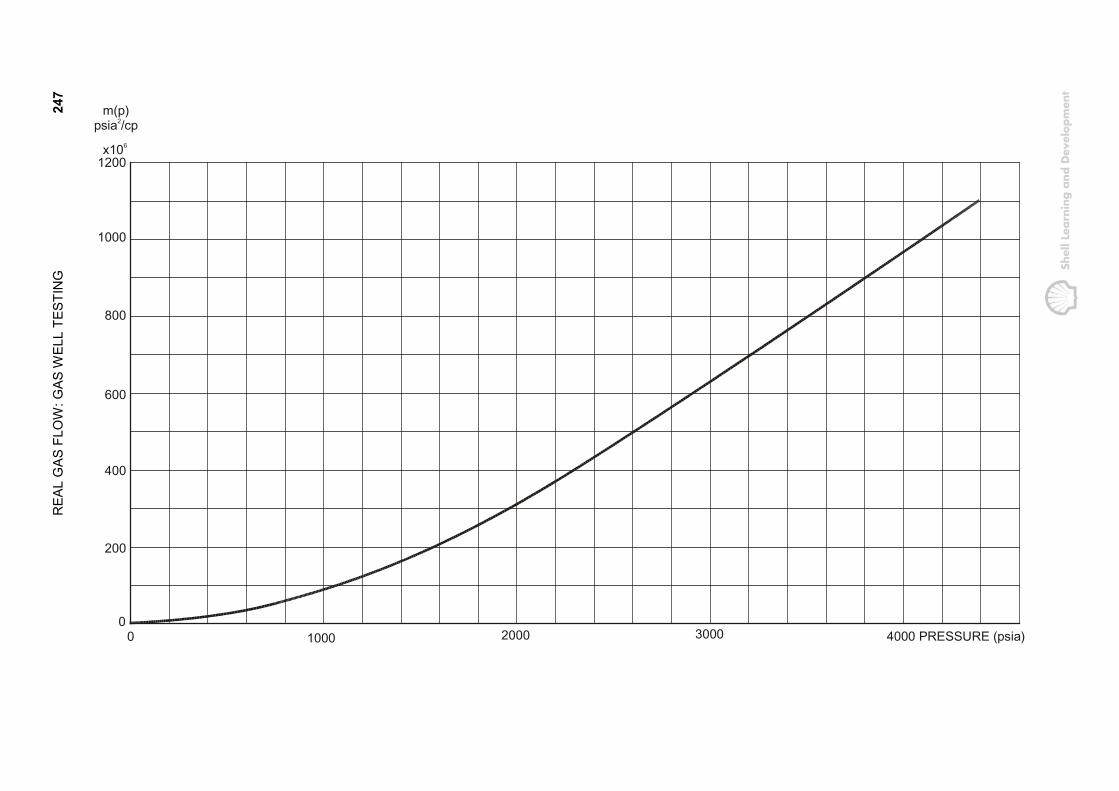
REA
L G
AS F
LOW
: GAS
WEL
L TE
STIN
G24
7
12000
800
600
400
200
1000
0x106
m(p)psia /cp2
1000 2000 3000 4000 PRESSURE (psia)

REAL GAS FLOW: GAS WELL TESTING 248
Fig. 8.3 Real gas pseudo pressure, as a function of the actual pressure, as derived intable 8.1; (Gas gravity, 0.85; Temperature 200°F)
m (p)
2pZµ
2pZµ
∆ ∆ µ(Area) = m (p) = (2p / Z) p∆
p Pressure
∆p
Fig. 8.4 2p/µZ as a function of pressure
Since ( ) ( )m p m p pr p r
∂ ∂ ∂= ⋅∂ ∂ ∂
and ( )m p 2pp µ
∂=
∂ Ζ
Then ( )m p 2p pr rµ
∂ ∂=∂ Ζ ∂
(8.8)
and similarly ( )m p 2p pt tµ
∂ ∂=∂ Ζ ∂
(8.9)
These relations are evident from fig. 8.4 and, substituting for ∂p/∂r and ∂p/∂t inequ. (5.1), using equs. (8.8) and (8.9) gives
( ) ( )m p m p1 k r cr r 2p r 2p t
ρ µ µφ ρµ
� �∂ ∂∂ Ζ Ζ=� �� �∂ ∂ ∂� �(8.10)
Finally, using the equation of state for a real gas
MpZRT
ρ =
and substituting this expression for ρ in equ. (8.10) leads, after some cancellation ofterms, to the simplified expression
( ) ( )m p m p1 crr r r k t
φµ� �∂ ∂∂ =� �� �∂ ∂ ∂� �(8.11)
Equation (8.11) has precisely the same form as the diffusivity equation, (5.20), exceptthat the dependent variable has been replaced by m(p).
REAL GAS FLOW: GAS WELL TESTING 249
Note that in reaching this stage it has not been necessary to make any restrictiveassumptions about the viscosity being independent of pressure or that the pressuregradients are small and hence squared pressure gradient terms are negligible, as wasimplicit in the approach of Russell and Goodrich.
Therefore, the problem has already been partially solved but it should be noted that theterm φµc/k in equ. (8.11) is not a constant, as it was in the case of liquid flow, since fora real gas both µ and c are highly pressure dependent. Equation (8.11) is therefore, anon-linear form of the diffusivity equation.
Continuing with the argument; in order to derive an inflow equation under semi-steadystate flow conditions, then applying the simple material balance for a well draining abounded part of the reservoir at a constant rate
p VcV qt t
∂ ∂= − = −∂ ∂
(5.8)
and for the drainage of a radial volume element
2e
p qt r h cπ φ
∂ = −∂
(5.10)
Also, using equ. (8.9)
( )2e
m p 2p p 2p qt t r h cµ µ π φ
∂ ∂= ⋅ = − ⋅∂ Ζ ∂ Ζ
(8.12)
and substituting equ. (8.12) in (8.11) gives
( )2e
m p1 c 2p qrr r r k r h c
φµµ π φ
� �∂∂ = − ⋅ ⋅� �� �∂ ∂ Ζ� �
or
( )2e res
m p1 2 pqrr r r r khπ
� �∂∂ � �= −� � � �� �∂ ∂ Ζ� �� �(8.13)
Furthermore, using the real gas equation of state,
sc scscres
pq Tp qT
� � =� �Ζ� �
equ. (8.13) can be expressed as
( ) sc sc2
sce
m p 2p q1 Trr r r Tr khπ
� �∂∂ = − ⋅� �� �∂ ∂� �(8.14)
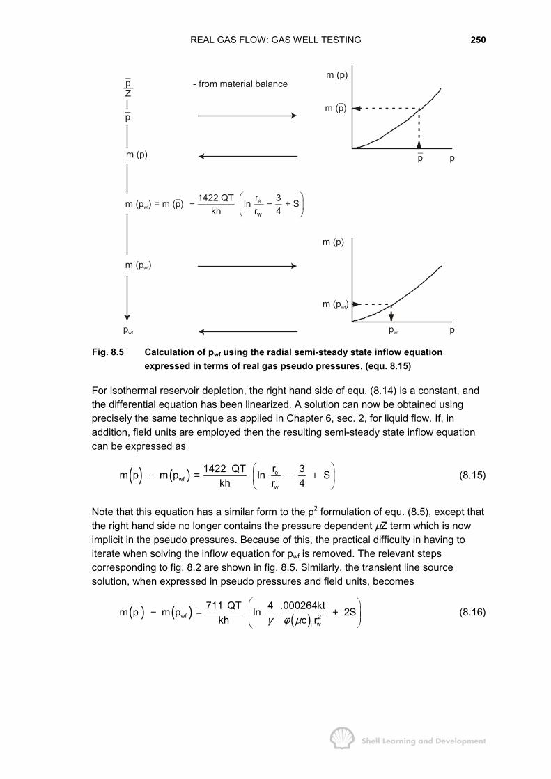
REAL GAS FLOW: GAS WELL TESTING 250
- from material balancem (p)
m ( )p
p p
m (p)
m (p )wf
pwf ppwf
m (p )wf
m (p ) = m ( )wf p
m ( )p
p
pZ
e
w
r1422 QT 3ln Skh r 4
� �− − +� �
� �
Fig. 8.5 Calculation of pwf using the radial semi-steady state inflow equationexpressed in terms of real gas pseudo pressures, (equ. 8.15)
For isothermal reservoir depletion, the right hand side of equ. (8.14) is a constant, andthe differential equation has been linearized. A solution can now be obtained usingprecisely the same technique as applied in Chapter 6, sec. 2, for liquid flow. If, inaddition, field units are employed then the resulting semi-steady state inflow equationcan be expressed as
( ) ( ) ewf
w
r1422 QT 3m p m p ln Skh r 4
� �− = − +� �
� �(8.15)
Note that this equation has a similar form to the p2 formulation of equ. (8.5), except thatthe right hand side no longer contains the pressure dependent µZ term which is nowimplicit in the pseudo pressures. Because of this, the practical difficulty in having toiterate when solving the inflow equation for pwf is removed. The relevant stepscorresponding to fig. 8.2 are shown in fig. 8.5. Similarly, the transient line sourcesolution, when expressed in pseudo pressures and field units, becomes
( ) ( ) ( )i wf 2wi
711 QT 4 .000264ktm p m p ln 2Skh c rγ φ µ
� �− = +� �� �
� �(8.16)
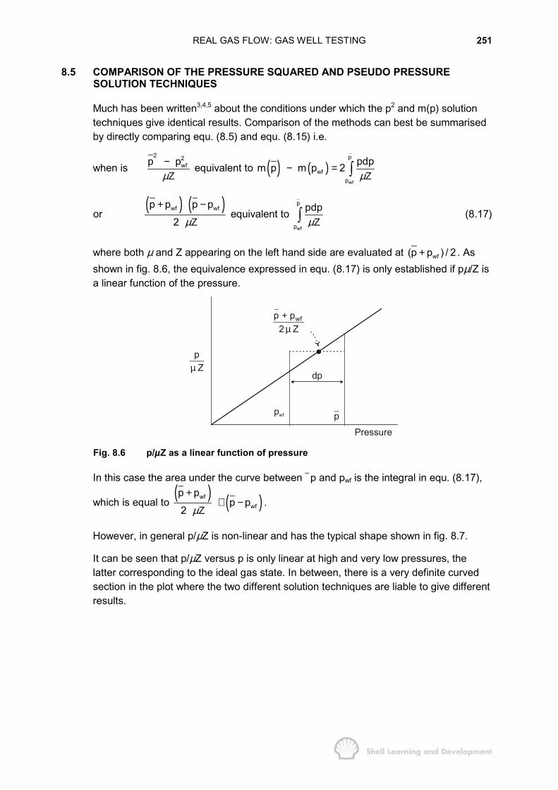
REAL GAS FLOW: GAS WELL TESTING 251
8.5 COMPARISON OF THE PRESSURE SQUARED AND PSEUDO PRESSURESOLUTION TECHNIQUES
Much has been written3,4,5 about the conditions under which the p2 and m(p) solutiontechniques give identical results. Comparison of the methods can best be summarisedby directly comparing equ. (8.5) and equ. (8.15) i.e.
when is2 2
wfp pµ−Ζ
equivalent to ( ) ( )wf
p
wfp
pdpm p m p 2µ
− =Ζ�
or ( ) ( )wf wfp p p p
2 µ
+ −
Ζ equivalent to
wf
p
p
pdpµΖ� (8.17)
where both µ and Z appearing on the left hand side are evaluated at wf(p p ) / 2+ . Asshown in fig. 8.6, the equivalence expressed in equ. (8.17) is only established if pµ/Z isa linear function of the pressure.
wfp p2 Z+µ
pZµ
pwf p
dp
Pressure
Fig. 8.6 p/µZ as a linear function of pressure
In this case the area under the curve between p and pwf is the integral in equ. (8.17),
which is equal to ( ) ( )wf
wf
p pp p
2 µ
+⋅ −
Ζ.
However, in general p/µZ is non-linear and has the typical shape shown in fig. 8.7.
It can be seen that p/µZ versus p is only linear at high and very low pressures, thelatter corresponding to the ideal gas state. In between, there is a very definite curvedsection in the plot where the two different solution techniques are liable to give differentresults.
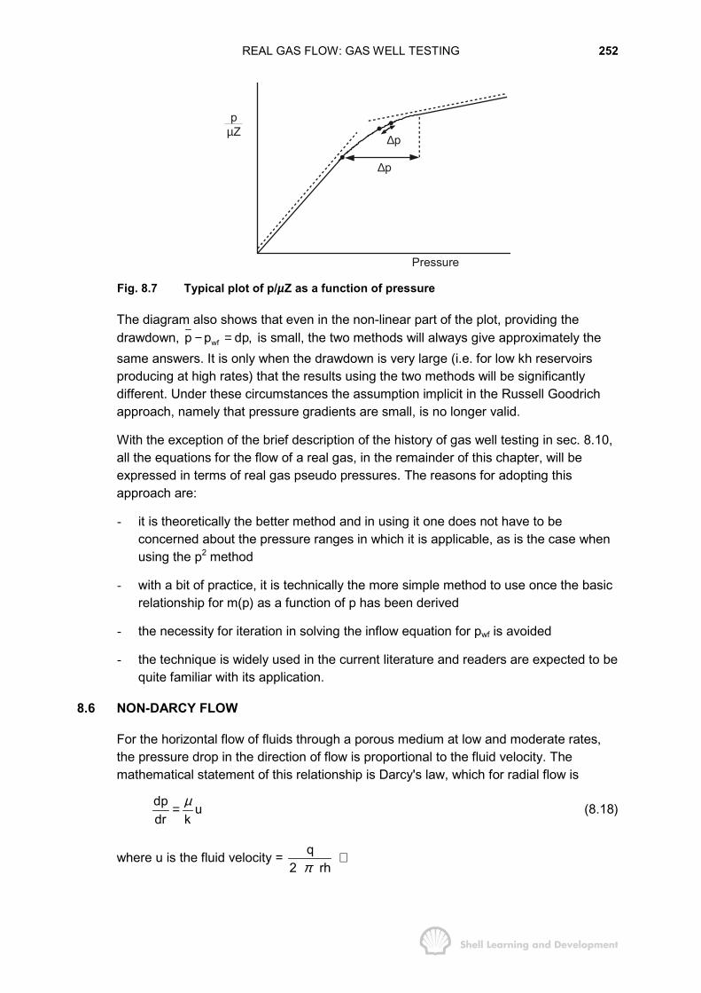
REAL GAS FLOW: GAS WELL TESTING 252
∆p
∆p
pZµ
Pressure
Fig. 8.7 Typical plot of p/µZ as a function of pressure
The diagram also shows that even in the non-linear part of the plot, providing thedrawdown, wfp p dp,− = is small, the two methods will always give approximately thesame answers. It is only when the drawdown is very large (i.e. for low kh reservoirsproducing at high rates) that the results using the two methods will be significantlydifferent. Under these circumstances the assumption implicit in the Russell Goodrichapproach, namely that pressure gradients are small, is no longer valid.
With the exception of the brief description of the history of gas well testing in sec. 8.10,all the equations for the flow of a real gas, in the remainder of this chapter, will beexpressed in terms of real gas pseudo pressures. The reasons for adopting thisapproach are:
- it is theoretically the better method and in using it one does not have to beconcerned about the pressure ranges in which it is applicable, as is the case whenusing the p2 method
- with a bit of practice, it is technically the more simple method to use once the basicrelationship for m(p) as a function of p has been derived
- the necessity for iteration in solving the inflow equation for pwf is avoided
- the technique is widely used in the current literature and readers are expected to bequite familiar with its application.
8.6 NON-DARCY FLOW
For the horizontal flow of fluids through a porous medium at low and moderate rates,the pressure drop in the direction of flow is proportional to the fluid velocity. Themathematical statement of this relationship is Darcy's law, which for radial flow is
dp udr k
µ= (8.18)
where u is the fluid velocity = q2 rhπ
⋅

REAL GAS FLOW: GAS WELL TESTING 253
At higher flow rates, in addition to the viscous force component represented by Darcy'sequation, there is also an inertial force acting due to convective accelerations of thefluid particles in passing through the pore spaces6. Under these circumstances theappropriate flow equation is that of Forchheimer (1901), which is
2dp u udr k
µ βρ= + (8.19)
In this equation the first term on the right hand side is the Darcy or viscous componentwhile the second is the non-Darcy component. In this latter term, β is the coefficient ofintertial resistance and, as the following dimensional analysis shows, has thedimension (length)-1.
[ ]2
22 2 3 2
dp ML 1 M Ludr LT L L T
β ρ� �� � � � � �= � �� � � � � �
� � � � � � � �
1Lβ −=
The non-Darcy component in equ. (8.19) is negligible at low flow velocities and isgenerally omitted from liquid flow equations. For a given pressure drawdown, however,the velocity of gas is at least an order of magnitude greater than for oil, due to the lowviscosity of the former, and the non-Darcy component is therefore always included inequations describing the flow of a real gas through a porous medium.
Because of this it should be necessary to use the Forchheimer equation, rather thanthat of Darcy, in deriving the basic radial differential equation for gas flow (referChapter 5, sec. 2). Fortunately, even for gas, the non-Darcy component in equ. (8.19)is significant only in the restricted region of high pressure drawdown, and flow velocity,close to the wellbore.
Therefore, the non-Darcy flow is conventionally included in the flow equations as anadditional skin factor, that is, as a time independent perturbation affecting the solutionsof the basic differential equation in the same manner as the van Everdingen skin(Chapter 4, sec. 7). Forchheimer's equation was originally derived for the flow of fluidsin pipes where at high velocity there is a distinct transition from laminar to turbulentflow. In fluid flow in a porous medium, however, for most practical cases in reservoirengineering, the macroscopic flow is always laminar according to the definitions ofclassical fluid dynamics. What is referred to as the non-Darcy component does notcorrespond with classical ideas of turbulent flow but, as stated earlier, is due to theaccelerations and decelerations of the fluid particles in passing through the porespaces. Nevertheless, Forchheimer's equation can be used to describe the additionalpressure drop due to this phenomenon, by integrating the second term on the righthand side of equ. (8.19), as follows.
e
w
2r
non Darcyr
qp dr2 rh
βρπ
� �∆ = � �
� ��
or expressed as a drop in the real gas pseudo pressure, using equ. (8.8)
REAL GAS FLOW: GAS WELL TESTING 254
( )e
w
2r
nDr
2p qm p dr2 rh
βρµ π
� �∆ = � �Ζ � �
� (8.20)
Also since ρ = γg × density of air at s.c. × E
gpconstant γ= × ×
ΖΤ
where γg is the gas gravity (air=1)
Then equ. (8.20) can be written as
( )e
w
2rg
2 2nDr
Tpqm p constant drr hγ
µβ� �∆ = × � �ΖΤ� �
� (8.21)
and since sc scsc
sc
p qpq constant qT
= = ×ΖΤ
then for isothermal reservoir depletion equ. (8.21) becomes
( )e
w
r2g sc2 2nD
r
q drm p constanth r
β γµ
Τ∆ = × � (8.22)
Since non-Darcy flow is usually confined to a localised region around the wellborewhere the flow velocity is greatest, the viscosity term in the integrand of equ. (8.22) isusually evaluated at the bottom hole flowing pressure pwf and hence is not a function ofposition. Integrating equ. (8.22) gives
( )2
g sc2nD
w e
q 1 1m p constantr rh
β γΤ � �∆ = × −� �
� �(8.23)
If equ. (8.23) is expressed in field units (Q - Mscf/d, β - ft-1) and assuming
w e
1 1 , thenr r
>>
( )2
g12 22nD
w p w
Qm p 3.161 10 FQ
h rβ γµ
− Τ∆ = × = (8.24)
where F is the non-Darcy flow coefficient psia2/cp/(Mscf/d)2.
Since non-Darcy flow is only significant very close to the wellbore, two assumptions arecommonly made in connection with equ. (8.24), these are
- the value of the thickness h is conventionally taken as hp, the perforated intervalof the well
- the pseudo pressure drop ∆m(p)nD = FQ2 can be considered as a perturbationwhich readjusts instantaneously after a change in the production rate.
REAL GAS FLOW: GAS WELL TESTING 255
Because of the latter assumption the FQ2 term can be included in equs. (8.15) and(8.16) in very much the same way as the mechanical skin factor, only in this case it isinterpreted as being a rate dependent skin. Thus equ. (8.15), for instance, including thenon-Darcy flow component, becomes
( ) ( ) 2ewf
w
r1422 TQ 3m p m p ln S FQkh r 4
� �− = − + +� �
� �(8.25)
e
w
r1422 TQ 3ln S DQkh r 4
� �= − + +� �
� �(8.26)
where in the latter expression, which is commonly used in the literature, DQ isinterpreted as the rate dependent skin factor and
FkhD1422T
= (8.27)
Either F or D is used in the remainder of this chapter, to allow for non-Darcy flow,depending on which is the more convenient for the application being considered.
8.7 DETERMINATION OF THE NON-DARCY COEFFICIENT F
Two methods are available for the determination of the non-Darcy flow coefficient,which are
- from the analysis of well tests
- by experimentally measuring the values of the coefficient of inertial resistance,β and using it in equ. (8.24) to calculate F.
Of these two, the well testing method will give the more reliable result just as in thecase of oil well testing in which, from the slope of the pressure buildup plot, a moremeaningful value of the kh product can be obtained than by measuring values of thepermeability on a selection of core samples and trying to average these results overthe entire formation. Furthermore, in the well test F will be measured in the presence ofany liquid saturation in the vicinity of the well. The determination of F by well testing willbe described in detail in secs. 8.10 and 8.11 and will not be discussed further at thisstage.
To determine β experimentally, the procedure is to first measure the absolutepermeability of each of the core samples and then to apply a series of increasingpressure differentials across each sample by flowing air through the core plugs at everincreasing rates. Knowing the flow rates and pressure differentials across the plugs,the coefficient of inertial resistance can be directly calculated using a linear version ofthe Forchheimer equation (8.19). The results are usually presented as shown in fig. 8.8in which β is plotted as a function of the absolute permeability over the range of coresamples tested.
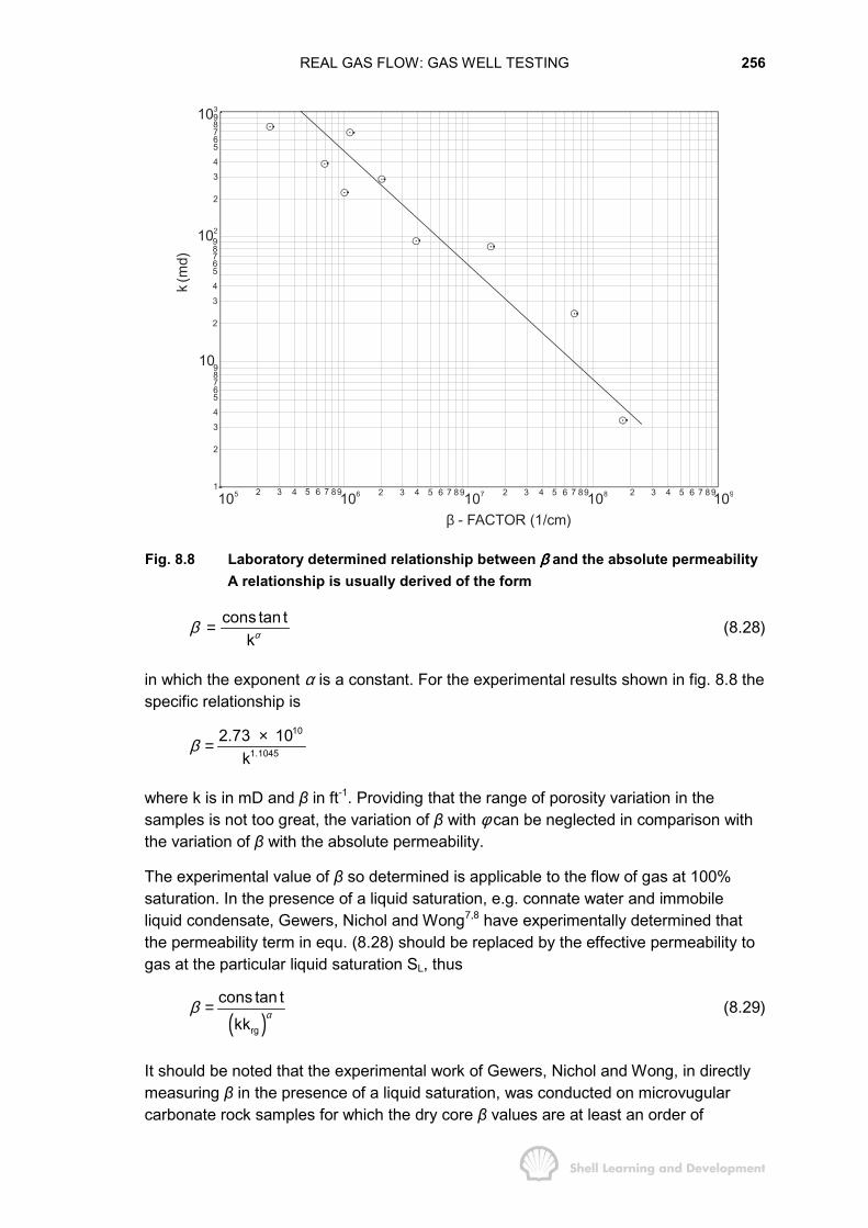
REAL GAS FLOW: GAS WELL TESTING 256
1039876543
2
1029876543
2
109876543
2
1105 106 107 108 1092 3 4 5 7 89 2 3 4 5 7 89 2 3 4 5 7 89 2 3 4 5 7 89
β - FACTOR (1/cm)
k(m
d)
Fig. 8.8 Laboratory determined relationship between ββββ and the absolute permeabilityA relationship is usually derived of the form
cons tan tkαβ = (8.28)
in which the exponent α is a constant. For the experimental results shown in fig. 8.8 thespecific relationship is
10
1.10452.73 10
kβ ×=
where k is in mD and β in ft-1. Providing that the range of porosity variation in thesamples is not too great, the variation of β with φ can be neglected in comparison withthe variation of β with the absolute permeability.
The experimental value of β so determined is applicable to the flow of gas at 100%saturation. In the presence of a liquid saturation, e.g. connate water and immobileliquid condensate, Gewers, Nichol and Wong7,8 have experimentally determined thatthe permeability term in equ. (8.28) should be replaced by the effective permeability togas at the particular liquid saturation SL, thus
( )rg
cons tan tkk
αβ = (8.29)
It should be noted that the experimental work of Gewers, Nichol and Wong, in directlymeasuring β in the presence of a liquid saturation, was conducted on microvugularcarbonate rock samples for which the dry core β values are at least an order of
REAL GAS FLOW: GAS WELL TESTING 257
magnitude greater than for typical sandstone samples. So far, the experiments havenot been repeated on sandstone but in using equ. (8.29) it is assumed that the samephysical principles will apply. Although correlation charts giving β as a function of thepermeability exist in the literature9 the reader should be aware that they are not alwaysapplicable. Irregularities in the pores can greatly modify the β versus k relationshipmaking it advisable, in many cases, to experimentally derive a relationship of the formgiven by equ. (8.28).
8.8 THE CONSTANT TERMINAL RATE SOLUTION FOR THE FLOW OF A REAL GAS
The constant terminal rate solution of the radial diffusivity equation
( ) ( )m p m p1 crr r r k t
φµ� �∂ ∂∂ =� �� �∂ ∂ ∂� �(8.11)
for the flow of a real gas, describes the change in real gas pseudo pressure at thewellbore due to production at a constant rate from time t = 0. Equation (8.11) isidentical in form with equ. (5.20) except that pseudo pressure replaces real pressure asthe dependent variable. Therefore, the constant terminal rate solution of equ. (8.11)must, by analogy, have the same form as the solution presented for liquid flow inChapter 7.
For small flowing times, the transient, constant terminal rate solution of equ. (8.11), inDarcy units, is similar to equ. (7.10), i.e.
( ) ( )i wf 2w
4 ktm p m p constan t ln 2Scrγ φ µ
� �′− = × ⋅ +� �� �
in which S' = S + DQ. The constant can be evaluated using the relationship
( ) 2pm p pµ
∆ = ∆Ζ
therefore,
( ) ( )i wf 2w
2p q 4 ktm p m p ln 2S4 kh cr
µµ π γ φ µ
� �′− = +� �Ζ � �
and converting to field units, using the fact that pq/Z = (psc qsc)T/Tsc, gives
( ) ( ) Di wf
4t711QTm p m p ln 2Skh γ
� �′− = +� �� �
(8.30)
Taking the analogy with the liquid flow equations a stage further, equ. (8.30) can beexpressed in dimensionless form as
( ) ( )( ) ( )i wf D Dkh m p m p m t S
1422QT′− = + (8.31)
REAL GAS FLOW: GAS WELL TESTING 258
in which mD (tD) is the dimensionless real gas pseudo pressure which for transient flowconditions is simply
( ) D12D D
4tm t lnγ
= (8.32)
and is identical in form to equ. (7.23).
Similarly, for long flowing times the semi-steady state constant terminal rate solution ofequ. (8.11), in Darcy units, is
( ) ( ) 12i wf 2
A w
2p q 4A ktm p m p ln 2 S2 kh cAC r
µ πµ π φ µγ
� �′− = + +� �Ζ � �
which is the equivalent of equ. (7.13). In field units this becomes
( ) ( ) 12i wf DA2
A w
1422QT 4Am p m p ln 2 t Skh C r
πγ
� �′− = + +� �� �
and therefore the mD (tD) function for semi-steady state flow is
( ) 12D D DA2
A w
4Am t ln 2 tC r
πγ
= + (8.33)
which is equivalent to equ. (7.27).
To generalise, the dimensionless real gas pseudo pressures are the constant terminalrate solutions of the equation
D DD
D D D D
m m1 rr r r t
� �∂ ∂∂ =� �∂ ∂ ∂� �(8.34)
and the solution which is valid for all values of the flowing time is
( ) ( ) ( )D1 12 2D D DA DAD MBH
4tm t 2 t ln m tπγ
= + − (8.35)
which is the same as equ. (7.42), for liquid flow.
The mD(MBH) function, the Matthews, Brons and Hazebroek dimensionless pseudopressure, can be read directly from the MBH charts, figs. 7.11-15, for the appropriatevalue of the dimensionless time argument tDA, in just the same way as the pD(MBH)
function was evaluated for use in equ. (7.42). Since field units are being used in thischapter, the abscissa and ordinate of the MBH charts should be interpreted as
( )DA
kt hrst 0.000264
cAφ µ= (8.36)
and
REAL GAS FLOW: GAS WELL TESTING 259
( ) ( ) ( ) ( )DAD MBHkh *m t m p m p
711QT� �= −� �� �
(8.37)
The right hand side of equ. (8.37) is only used to calculate ( )m p , having already
determined m(p*) from the extrapolated pseudo pressure buildup plot (ref. sec. 8.11).In the majority of cases, mD(MBH) is simply a number read from the MBH charts for theappropriate value of tDA, for use in equ. (8.35).
Because of the equivalence in form of the constant terminal rate solution for both oiland gas, when expressed in dimensionless parameters, there is no need to elaboratefurther on how this solution is used in practice since the subject has been fullydescribed in the previous chapter. The application of equ. (8.35) to gas well testing willbe demonstrated in secs. 8.10 and 11.
Although the form of the mD and pD functions is the same, it must always be kept inmind that the mD function applied to real gas flow is less accurate than the pD functionapplied to liquid flow. The reason is that the mD functions are derived as solutions ofequ. (8.11), which is non-linear. The non-linearity arises from the fact that both the realgas viscosity and compressibility in the coefficient φµc/k, in equ. (8.11),are highlypressure dependent. Fortunately, the gas viscosity is directly proportional to thepressure while the compressibility, equ. (1.31), is inversely proportional to pressure andthis tends to reduce the pressure dependence of the product.
This favourable effect is particularly pronounced in the high pressure range where theproduct is fairly constant. For instance, using the PVT data presented in table 8.1, thevalue of µc only increases from 3.54 × 10⁻⁶ cp/psi at 4400 psia to 4.96 x 10⁻⁶ cp/psi at3400 psia. In evaluating these figures, the isothermal gas compressibility has beencalculated using equ. (1.31), treating the pore and connate water compressibilities asnegligible in comparison to that of the gas. This practice is adhered to in the remainderof this chapter, thus ct ≈ cg = c.
Because of this insensitivity of the µc product to pressure change it is common, whenapplying the mD function, to use the product (µc)i evaluated at the initial equilibriumpressure, which is also the assumption made in generating pD functions for liquid flow.Thus, tD, tDA and 1/2 mD(MBH ) (tDA ) in equ. (8.35), which are dependent on the product,are all evaluated using (µc);. Al-Hussainy, Ramey and Crawford2 have demonstratedthat, using this initial value of the product, the mD functions do correlate very favourablywith the pD functions for liquid flow over a wide range of conditions. While the match isvery good for transient flow conditions, it is less reliable for very large values of theflowing time, once the boundary effects have been felt. Thus, equ. (8.32) correlateswith the pD function better than equ. (8.33). The latter must, therefore, be used withmore caution. Fortunately, the inflow equation (8.15), for semi-steady state flow, whichcan be expressed in dimensionless form as
( ) ( )( ) ( ) 1D 2wf D 2A w
kh 4Am p m p m t S ln S1422QT C rγ
′ ′− = + = + (8.38)
REAL GAS FLOW: GAS WELL TESTING 260
was found to correlate almost exactly with the equivalent function for liquid flow for allvalues of the flowing time. This is to be expected since the, µc product is not present inequ. (8.38) as a result of the use of pseudo pressures, rather than pressures, in itsformulation. The correlations between mD and pD functions were only checked for a wellproducing at the centre of a circular shaped reservoir, equs. (8.35) and (8.38) aregeneralized expressions which include the dependence of mD on geometry and wellasymmetry.
In practice, one is interested in applying the constant terminal rate solution(mD function) to the analysis of well tests and several examples of such usage areprovided in the following sections of this chapter. All the examples considered are forinitial well tests and, for this condition, the evaluation of the mD function using the (µc)i
product can be expected to be quite reliable, particularly if the test duration is notexcessively long and the pressure drawdowns imposed are not too large. Problemsarise, however, when analysing routine pressure surveys throughout the producinglifetime of the reservoir. For instance, if a pressure test is conducted in a well severalyears after the start of production, at what pressure should the µc product beevaluated? This question will be dealt with in sec. 8.11 using the method presented byKazemi10, which describes how the average reservoir pressure can be obtained from apressure analysis using a µc product which must be iteratively determined. Once theaverage reservoir pressure is known, however, the inflow equation (8.38) can be usedwith confidence to calculate the long term deliverability of wells.
8.9 GENERAL THEORY OF GAS WELL TESTING
Gas well tests can be interpreted using the following equations
( ) ( )( ) ( )n n j 1
n
i wf j D D D n nj 1
kh m p m p Q m t t Q S1422T −
=
′− = ∆ − +� (8.39)
in which
( ) ( ) ( ) ( )n j 1D1 1
2 2D D D D D DA DAD MBH
j j j 1
n n
4tm t t m t 2 t ln m t
Q Q Qand
S S DQ
πγ−
−
′′ ′ ′− = = + −
∆ = −
′ = +
(8.40)
For convenience, equ. (8.39) is frequently expressed in the form
( ) ( )( ) ( )n n j 1
n2
i wf n j D D D nj 1
kh m p m p FQ Q m t t Q S1422T −
=
− − = ∆ − +� (8.41)
in which F is the non-Darcy flow coefficient, equ. (8.27).
These equations are analogous to equs. (7.31) and (7.42) which were used for oilwelltest analysis. Equation (8.39) results from the application of the principle ofsuperposition in time, as described in Chapter 7, sec. 5. In the summation of the

REAL GAS FLOW: GAS WELL TESTING 261
individual constant terminal rate solutions it is assumed that the only skin factor termremaining which influences pwf is the value S n ′ = S + DQn. This is because the ratedependent skin factor is not, in itself, a time dependent solution of the diffusivityequation but is merely considered to have a perturbing influence on the bottom holeflowing pressure which re-adjusts instantaneously when the rate changes. Thus, eventhough the DQ terms in the summation leading to equ. (8.39) do not algebraicallycancel, as do the mechanical skin factor components, on changing the rate from Q´n-1
to Qn the value of nwfp is only influenced by DQn. The components DQn-1, DQn-2 . . .
DQn-j have no transient effects and die out immediately.
The main difference between oil and gas well testing arises from the fact that the totalskin factor in a gas well has two components, one of which is rate dependent. Becauseof this, a gas well must be tested with a minimum of two separate flow rates to be ableto differentiate between these two skins.
Thus, at rate Q1 the total skin
1 1S S DQ′ = +
can be obtained from the test analysis, while at rate Q2
2 2S S DQ′ = +
can be similarly determined. The two equations for 1S′ , and 2S′ can then be solvedsimultaneously to provide S and D (or F).
A further complication in applying equs. (8.39) and (8.40) to gas well test analysis liesin the fact that the superposition principle itself, which is implicit in the formulation ofequ. (8.39), is strictly only valid when applied to solutions of linear differentialequations. Since it is the constant terminal rate solution of the non-linear radialdiffusivity equation (8.11) that is being superposed, some fundamental mathematicalerror might therefore be expected. Al-Hussainy, Ramey and Crawford2 have shown, bycomparing superposed mD functions for gas with the superposed pD functions for liquidflow, that the error is very slight providing that the test is conducted with an increasingrather than a decreasing rate sequence.
As stated in sec. 8.8, the viscosity-compressibility product used in an initial well test is(µc)i evaluated for the initial equilibrium pressure pi. In the test analysis exercisesincluded in the following sections of the chapter, the initial pressure in each case istaken as 4290 psi and the PVT data and real gas pseudo pressures of table 8.1 arecommon to all. The value of (µc)i under these circumstances is 3.6 × 10⁻⁶ cp/psi and noallowance for its variation is made during the ensuing analyses. It is interesting to notethat, in spite of the high compressibility, the µc product for a gas reservoir (≈ µcg) isinvariably three or four times smaller than for an oil reservoir, because of the lowviscosity of the gas. This implies that, for a given drainage area, permeability andporosity, the change from transient to either late transient or stabilized flow can beexpected to occur much more rapidly in a gas than in an oil reservoir. This hasimplications which will be discussed in greater detail in secs. 8.10 and 8.11.
REAL GAS FLOW: GAS WELL TESTING 262
In conclusion, it can be stated that the use of equs. (8.39) and (8.40) to analyse gaswell tests is never quite as satisfactory as using the combination of equs. (7.31) and(7.42) for oilwell tests. Nevertheless, the former equations do provide what is usuallydescribed in the literature as "a reasonable engineering approximation" and theirapplication will now be described in detail.
8.10 MULTI-RATE TESTING OF GAS WELLS
This section will be presented in the form of a brief history of the subject of multiratetesting of gas wells in which former analysis techniques will be compared with themethod implied in the use of equ. (8.39) and (8.40).
The first and perhaps the best known equation for analysing multi-rate tests is that ofSchellhardt and Rawlins11 which was empirically established as the result of theanalysis of some 600 gas well tests during the 1930's. The equation is
( )n2 2i wfQ C p p= − (8.42)
"back pressure equation". Using the observed pressures at the end of each flow perioda plot can be made of log 2 2
i wf(p p )− versus log Q, the slope of which has the value 1/n.Having thus determined n, the value of C can be calculated using equ. (8.42).
It was originally believed that both C and n were constants that, once determined fromthe test analysis, could be used for the long term prediction of gas well deliverability.This being accomplished merely by replacing pi by the current average reservoirpressure p . Carter et al.12, have shown, however, that n is a variable with a rangebetween .5 and 1 depending on whether the value of the non-Darcy flow componentFQ2, defined by equ. (8.24), is very large (n = .5) or negligible (n = 1). Furthermore, thevalue of C can be shown to be dependent on k, A, CA and S and also on the pressuredependent functions, µ, Z and the flowing time, and can hardly be expected to remainconstant throughout the producing life of the well. These statements will not besubstantiated in this text since it is not intended to use equ. (8.42) which may beregarded, at best, as being a useful empirical approximation.
Nevertheless, in spite of all the drawbacks mentioned above, it was found that the backpressure equation could be used with tolerable accuracy in analysing tests in which itwas suspected that semi-steady state flow conditions prevailed during each separateflow period. As a result, it became, and still is, quite fashionable to test wells in such away that stabilized flow is achieved at each rate. Precisely when the change fromtransient to semi-steady state flow occurs depends on some minimum value oftDA = .000264 kt/φ (µc)iA, (a fact which is clearly illustrated by the MBH charts,figs. 7.11-15), which in turn depends upon the geometry of the drainage area and wellasymmetry. As already noted in sec. 8.8, since the µc product for gas is considerablysmaller than for a liquid, there is at least some justification in attempting to analyse gaswell tests assuming stabilized flow conditions, even for a test of relatively shortduration.
REAL GAS FLOW: GAS WELL TESTING 263
The most popular current method of analysing such a test is to use the semi-steadystate inflow equation, (8.38), which, including both skin factor components andassuming that for an initial test p = pi, becomes
( ) ( ) 212i wf 2
A w
1422QT 4Am p m p ln S FQkh C rγ
� �− = + +� �
� �(8.43)
which can be further simplified as
( ) ( ) 2i wfm p m p BQ FQ− = + (8.44)
where B is the Darcy coefficient and F the non-Darcy coefficient of the inflow equation.The purpose of testing is then to determine B and F and to use these values forpredicting the future deliverability of the well, for which pi is replaced by the currentaverage pressure p . The method of analysis is simply to plot
( ) ( )ni wfn
n
m p m pversus Q
Q−
(8.45)
in which the Qn are the surface production rates and pwf the values of the bottom holeflowing pressure recorded at the end of each separate flow period. The plot should belinear with slope F and intercept B, when Qn = 0; an example of such a plot is shown asfig. 8.9.
This method of analysis is simple and the results obtained in terms of B and F areconsidered more reliable parameters for estimating well deliverabilities than theC and n determined using equ. (8.42).
Nevertheless, the application of the stabilized well inflow equation (8.43), to analyse awell test is mathematically incorrect and the results obtained from such an analysis canonly be considered as an approximation, although, as will be demonstrated inexercise 8.1, a perfectly acceptable approximation in many cases. The fault lies inanalysing the test data using an inflow equation rather than the superposed constantterminal rate solutions, equ. (8.39). It may well be that each flow period in the test issufficiently long so that semi-steady state conditions prevail but that does not meanthat, for instance, the wellbore pressure response during the third flow period isunaffected by what happened during the first and second periods, as implied by theuse of equ. (8.43) in the analysis.
The rigorously correct technique is to use equ. (8.39) in which the mD functions,equ. (8.40), are evaluated for semi-steady state flow as
( ) 12D DA DA2
A w
4Am t ln 2 tC r
πγ
′ ′= + (8.33)
The test analysis equation is then

REAL GAS FLOW: GAS WELL TESTING 264
( )n n j 1
n1
2i wf j DA DA n n2j 1 A w
kh 4Am(p ) m(p ) Q 2 (t t ) Q ln S DQ1422T C r
πγ−
=
� �− = ∆ − + + +� �
� ��
or alternatively, by re-arranging the summation term
( )n j
n1
2i wf j DA n n2j 1 A w
kh 4Am(p ) m(p ) 2 Q t Q ln S DQ1422T C r
πγ=
� �− = ∆ + + +� �
� ��
where
j j j 1DA DA DAt t t−
∆ = −
Finally, dividing throughout by Qn, converting to real time (hours) and taking the ratedependent skin over to the left hand side of the equation gives
( )n
2 ni wf n j 1
2j 2j 1n n A wi
m(p ) m(p ) FQ Q2.359T 1422T 4At ln SQ c Ah Q kh C rφ µ γ=
− − � �= ∆ + +� �
� �� (8.46)
It can be seen immediately, from this equation, that if the first term on the right handside is ignored then it reduces to exactly the same form as the semi-steady state inflowequation, (8.43). The additional term
( )n
jj
j 1 ni
Q2.539T tc Ah Qφ µ =
∆�
can be interpreted as a material balance correction required due to the use of the initialpressure pi in the inflow equation, (8.43), rather than the current average pressurewhich, for t > 0, is somewhat lower and changes throughout the test. Therefore, thedifference between equ. (8.46) and (8.43) is generally rather small, especially in casesof interest, that is, large gas accumulations (large Ahφ). Theoretically, a plot of
n
2 ni wf n j
jj 1n n
m(p ) m(p ) FQ Qversus t
Q Q=
− −∆� (8.47)
should be linear with slope
( ) ( )i i
2.359T 2.359Tc Ah c Pore Volumeφ µ µ
=×
and intercept
12 2
A w
1422T 4AB ln Skh C rγ
� �= +� �
� �
Of course, to draw this plot requires a knowledge of the non-Darcy flow coefficient F.As a starting point the value of F determined as the slope of the plot of equ. (8.45) canbe used and the value decreased gradually until the plot of equ. (8.47) becomes linear.The slope of the latter plot will then yield the value of the pore volume and the intercept

REAL GAS FLOW: GAS WELL TESTING 265
the correct value of the Darcy flow coefficient B. At first sight this analysis techniqueappears to be rather useful but the following exercise will reveal the great sensitivity inthe plot to the chosen value of F.
EXERCISE 8.1 MULTI-RATE GAS WELL TEST ANALYSED ASSUMINGSTABILIZED FLOW CONDITIONS
A gas well is tested by producing it at four different rates over a total period of48 hours. The rate-time sequence and pressures recorded at the end of each separateflow period are listed in table 8.2.
Rate (Q)Mscf/d
Cum. Flowing time(t)hrs
pwf
psiam (pwf)
psia2/cp
10 × 103 12 4182 1030.96 × 106
20 " 24 4047 984.29 "
30 " 36 3884 927.94 "
40 " 48 3694 862.26 "TABLE 8.2
The reservoir temperature and fluid properties are the same as those listed in table 8.1and therefore, the relationship between real pressure and pseudo pressure, fig. 8.3,can be used in this exercise. For pressures in excess of 2800 psia, this relationship isalmost linear and can be matched by the equation
m(p) = (0.3457p — 414.76) × 106 psia2/cp (8.48)
from which the real gas pseudo pressures, m(pwf ), in table 8.2 have been calculated.The reservoir and well data for the exercise are as follows
pi = 4290 psi h = 40 ft
(µc)i = 3.6 × 10⁻⁶ cp/psi rw = 0.3 ft
If the correct values of the flow coefficients are
B = 3176 psia2/cp/Mscf/d and F = .04 psia2/cp/(Mscf/d)2
1. Calculate both B and F using the interpretation technique suggested by equ. (8.45).
2. If there is a possible error of 10 psi in the measurement of pi, determine the effectof this error on the analysis.
3. It is proposed to produce this reservoir block at a plateau production rate of5 MMscf/d down to some fixed minimum wellhead pressure. If the plateau rate canbe maintained until the average reservoir pressure has fallen to 1200 psi, calculatethe error in the estimate of the cumulative gas production, at this stage, due to
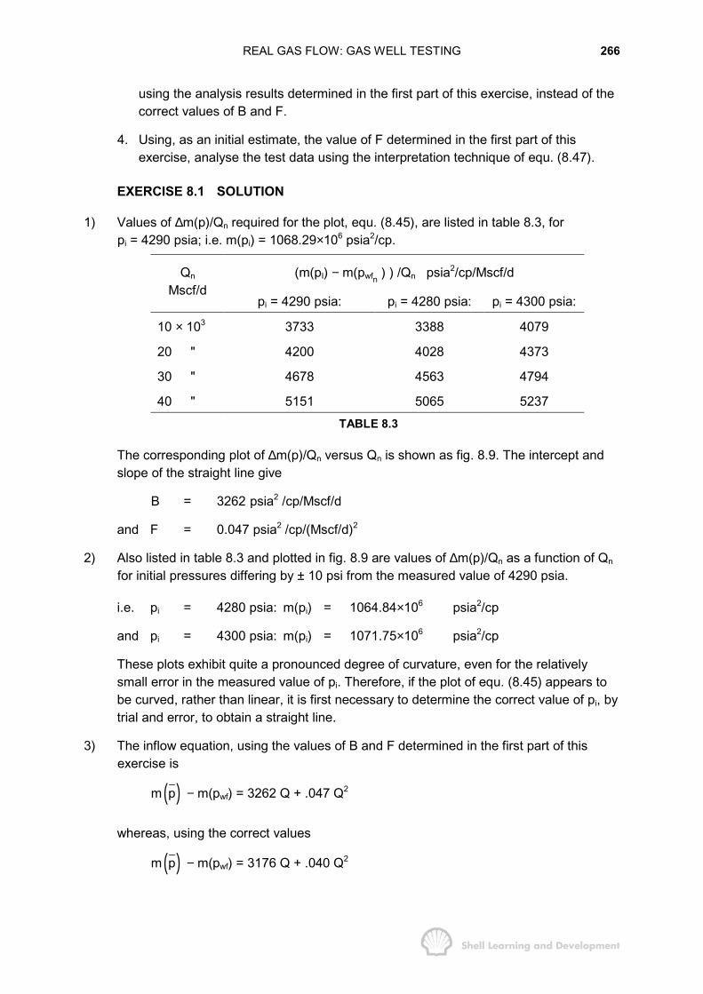
REAL GAS FLOW: GAS WELL TESTING 266
using the analysis results determined in the first part of this exercise, instead of thecorrect values of B and F.
4. Using, as an initial estimate, the value of F determined in the first part of thisexercise, analyse the test data using the interpretation technique of equ. (8.47).
EXERCISE 8.1 SOLUTION
1) Values of ∆m(p)/Qn required for the plot, equ. (8.45), are listed in table 8.3, forpi = 4290 psia; i.e. m(pi) = 1068.29×106 psia2/cp.
(m(pI) − m(pwfn ) ) /Qn psia2/cp/Mscf/dQn
Mscf/dpi = 4290 psia: pi = 4280 psia: pi = 4300 psia:
10 × 103 3733 3388 4079
20 " 4200 4028 4373
30 " 4678 4563 4794
40 " 5151 5065 5237TABLE 8.3
The corresponding plot of ∆m(p)/Qn versus Qn is shown as fig. 8.9. The intercept andslope of the straight line give
B = 3262 psia2 /cp/Mscf/d
and F = 0.047 psia2 /cp/(Mscf/d)2
2) Also listed in table 8.3 and plotted in fig. 8.9 are values of ∆m(p)/Qn as a function of Qn
for initial pressures differing by ± 10 psi from the measured value of 4290 psia.
i.e. pi = 4280 psia: m(pi) = 1064.84×106 psia2/cp
and pi = 4300 psia: m(pi) = 1071.75×106 psia2/cp
These plots exhibit quite a pronounced degree of curvature, even for the relativelysmall error in the measured value of pi. Therefore, if the plot of equ. (8.45) appears tobe curved, rather than linear, it is first necessary to determine the correct value of pi, bytrial and error, to obtain a straight line.
3) The inflow equation, using the values of B and F determined in the first part of thisexercise is
m ( )p − m(pwf) = 3262 Q + .047 Q2
whereas, using the correct values
m ( )p − m(pwf) = 3176 Q + .040 Q2
REAL GAS FLOW: GAS WELL TESTING 267
If it is assumed that these expressions will not change throughout the producinglifetime of the well then, for a given plateau rate of 5 MMscf/d, the duration of theplateau production is determined by the value of pwf. If this pressure drops below thelevel
5000
4000
30000 10 20 30 40 Q (MMscf/d)n
4300
4000
42904280
ni wfm (p ) m (p )Qn−
(psia / cp / Mscf/d)2
p (psia)i
Fig. 8.9 Gas well test analysis assuming semi-steady state conditions during eachflow period. Data; table 8.3
required to maintain the minimum allowable wellhead pressure then the rate must bereduced. Therefore, at this point the values of m(pwf ) in both the above equations mustbe equal and
( ) 2m p 86 Q .007 Q∆ = +
and for Q = 5 MMscf/d
( ) 6 2m p .605 10 psia / cp∆ = ×
Also
( ) 2pm p pµ
∆ = ∆Ζ
and using the data in table 8.1 for p = 1200 psi

REAL GAS FLOW: GAS WELL TESTING 268
6.0153 .832 .605 10p 3.21 psi2 1200
× × ×∆ = =×
Assuming a depletion type material balance, equ. (1.35), then
4p
i i
G pG ( ) 8 10 GZp / Z
−∆ = ∆ ≈ − ×
Thus the use of the flow coefficients B and F, determined using the inflow equation inthe analysis is only very slightly pessimistic and in general provides a perfectlyacceptable approximation for highly productive wells such as the one described in thisexercise.
4) For the assumed value of F = .047 psia2/cp/(Mscf/d)2, which was determined in the firstpart of this exercise, the data for the plot of equ. (8.47) are listed in table 8.4, and theplot itself shown as fig. 8.10.
(psia / cp / Mscf/d)2
2n
n
m (p) FQQ
∆ −4000
3500
300010 20
F = 0.047; A
jj
n
Qt
Q∆
∆�
F = 0.035; A = 60 ACRES
F = 0.030; A = 43 ACRES
F = 0.040; A = 100 ACRES
30
Fig. 8.10 Gas well test analysis assuming semi-steady state conditions and applyingequ. (8.47). Data; table 8.4
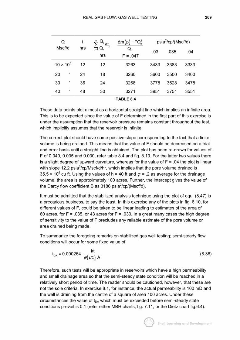
REAL GAS FLOW: GAS WELL TESTING 269
psia2/cp/(Mscf/d)QMscf/d
thrs
nj
jj 1 n
Qt
Q=
∆�
hrs
( ) 2n
n
m p FQQ
∆ −
F = .047.03 .035 .04
10 × 103 12 12 3263 3433 3383 3333
20 " 24 18 3260 3600 3500 3400
30 " 36 24 3268 3778 3628 3478
40 " 48 30 3271 3951 3751 3551TABLE 8.4
These data points plot almost as a horizontal straight line which implies an infinite area.This is to be expected since the value of F determined in the first part of this exercise isunder the assumption that the reservoir pressure remains constant throughout the test,which implicitly assumes that the reservoir is infinite.
The correct plot should have some positive slope corresponding to the fact that a finitevolume is being drained. This means that the value of F should be decreased on a trialand error basis until a straight line is obtained. The plot has been re-drawn for values ofF of 0.040, 0.035 and 0.030, refer table 8.4 and fig. 8.10. For the latter two values thereis a slight degree of upward curvature, whereas for the value of F = .04 the plot is linearwith slope 12.2 psia2/cp/Mscf/d/hr, which implies that the pore volume drained is35.5 × 106 cu ft. Using the values of h = 40 ft and φ = .2 as average for the drainagevolume, the area is approximately 100 acres. Further, the intercept gives the value ofthe Darcy flow coefficient B as 3186 psia2/cp/(Mscf/d).
It must be admitted that the stabilized analysis technique using the plot of equ. (8.47) isa precarious business, to say the least. In this exercise any of the plots in fig. 8.10, fordifferent values of F, could be taken to be linear leading to estimates of the area of60 acres, for F = .035, or 43 acres for F = .030. In a great many cases the high degreeof sensitivity to the value of F precludes any reliable estimate of the pore volume orarea drained being made.
To summarize the foregoing remarks on stabilized gas well testing; semi-steady flowconditions will occur for some fixed value of
( )DAi
ktt 0.000264c Aφ µ
= (8.36)
Therefore, such tests will be appropriate in reservoirs which have a high permeabilityand small drainage area so that the semi-steady state condition will be reached in arelatively short period of time. The reader should be cautioned, however, that these arenot the sole criteria. In exercise 8.1, for instance, the actual permeability is 100 mD andthe well is draining from the centre of a square of area 100 acres. Under thesecircumstances the value of tDA which must be exceeded before semi-steady stateconditions prevail is 0.1 (refer either MBH charts, fig. 7.11, or the Dietz chart fig.6.4).
REAL GAS FLOW: GAS WELL TESTING 270
Therefore, using equ. (8.36) and the data provided in exercise 8.1, the real time beforethe semi-steady state condition is reached is
( ) 6i
.1 c A .1 .2 3.6 10 100 43560t 11.9 hrs0.000264k 0.000264 100
φ µ −× × × × × ×= = =×
which confirms that, in this case, the separate twelve hour flow periods are justsufficient to permit the test to be analysed using semi-steady state equations. Suppose,however, the well was not situated at the centre of a square no-flow boundary butinstead, at the centre of one of the four quarters of the same square (graph III offig. 7.12(a)). In this case the value of tDA before the semi-steady state condition isreached is 0.5 and consequently, for the same reservoir properties, each flow periodwould have to be about 60 hours before semi-steady state analysis could be correctlyapplied. In this latter case, if the flow periods were each of twelve hour duration, theapplication of the stabilized analysis technique would be inappropriate since the entiretest would be run under the late transient flow condition for which the mD functionsshould be evaluated using equ. (8.40) rather than equ. (8.33). For high permeabilityreservoirs, such as that tested in exercise 8.1, the error made in using the incorrectmathematics in the analysis would not have too serious an effect on the values ofB and F determined from the test. For lower permeability reservoirs, however, use ofthe incorrect mathematics could produce a more serious error.
One other disadvantage of the stabilized analysis techniques described so far is thatwhile they provide a value of the Darcy flow coefficient
12 2
A w
1422T 4AB ln Skh C rγ
� �= +� �
� �
there is no way of determining the individual components in this expression. Inexercise 8.1 these values happen to be k = 100 mD, A = 100 acres, CA = 30.9 andS = 6.0 but, with the exception of A, which was obtained from the rather dubiousanalysis in part four of the exercise, none of these can be explicitly calculated from thetest. This can have unfortunate consequences if the value of B, derived from the test, isused in the inflow equation in an attempt to predict the long term deliverability of theaverage reservoir well. For instance, the skin factor can be expected to be high in anexploration well but this should be improved when drilling the average production wellusing a more compatible completion fluid. Indeed, if the skin factor could be reduced tozero in the well considered in exercise 8.1, the value of the flow coefficient B would bereduced from 3176 to 1768 psia2/cp/(Mscf/d). Furthermore, if the reservoir is large andrequires more than one well for drainage the value of A and CA, which are implicit in thevalue of B determined for the test well, will change during the producing lifetime of thereservoir. Therefore, the use of the coefficient B in making long term predictions of welldeliverability can be misleading. It would be preferable if some analysis techniquecould be employed which could explicitly determine k and S so that the coefficient Bcould be calculated from its component parts, and such methods will now be described.
As deeper, less permeable gas reservoirs were discovered and tested it becameevident that the stabilized analysis techniques described so far in this section were
REAL GAS FLOW: GAS WELL TESTING 271
inadequate to define the B and F factors in the well inflow equation (8.44). This isbecause if the permeability is small then the flowing time required to reach semi-steadystate conditions, which depends on tDA = 0.000264kt/φ(µc)iA, can become extremelylarge. Then, the use of a semi-steady state inflow equation to analyse the test isinadmissible because the pressure response at the wellbore is strongly timedependent. To cater for this time dependence, two methods have been presented inthe literature for analysing tests under the assumption that the wellbore pressureresponse could be matched by superposing transient constant terminal rate solutionsof the radial diffusivity equation. The first of these was the Odeh-Jones technique13
(1965), in which the test analysis equation was formulated using p-squared terms. Thiswas followed in 1971 by the method of Essis and Thomas14, in which the Odeh-Jonestest equation was modified by the use of real gas pseudo pressure to give
( ) ( )( ) ( )n n j 1
n
i wf j D D D n nj 1
kh m p m p Q m t t Q S1422T −
=
′− = ∆ − +�
which is the general form of the superposed constant terminal rate solution,equ. (8.39). Both Odeh and Jones and Essis and Thomas applied their analysistechniques strictly for transient flow conditions, for which the superposed mD functionsin equ. (8.39) can each be expressed as
( ) D12D D
4tm t lnγ
= (8.32)
rather than using the general expression, equ. (8.40), which assumes a knowledge ofthe area drained and geometry. If transient mD functions can be used then the analysisis simple and should yield values of k and S which in turn can be used to calculate avalue of the Darcy flow coefficient B, equ. (8.44), for any values of the area drained andshape factor. The analysis also directly determines F (or D), the second coefficient inthe inflow equation. The technique will be fully illustrated in exercise 8.2.
The statements made in Chapter 7, sec. 8, about the possibility of incorrectlyinterpreting multi-rate test data through making an a priori judgement concerning theprevailing flow conditions are equally, if not more, valid in gas well test analysis. This isbecause the µc product for gas is several times smaller than for oil which implies that,for the same permeability, porosity and area drained, the boundary effects will be feltmuch earlier in a gas well test. To apply transient analysis techniques it is insufficient toassume that each separate flow period should be short enough so that transientconditions prevail. Instead, the entire test duration must be so brief that the maximumvalue of the mD function in equ. (8.39), which is
( ) ( )maxD D Dm t m total dimensionless testing time′ =
can still be evaluated using the transient expression, equ. (8.32). The possible errorthat can be made by making the flow periods too long will be illustrated in the followingexercise.

REAL GAS FLOW: GAS WELL TESTING 272
EXERCISE 8.2 MULTI-RATE GAS WELL TEST ANALYSED ASSUMINGUNSTABILIZED FLOW CONDITIONS
A gas well is tested by producing at four different rates for periods of one hour, followedby a four hour pressure buildup. The rates, times and observed pressures during theflow test are listed in table 8.5.
Rate (Q)Mscf/d
Cum. Flowing Time (t)hrs
pwf
psiam (pwf)
psia2/cp
10 × 103 1 4160 1023.35 × 106
20 × " 2 3997 967.00 "
30 × " 3 3802 899.59 "
40 × " 4 3577 821.81 "TABLE 8.5
The reservoir temperature and gas properties are again the same as detailed intable 8.1 and therefore, the pressure-pseudo pressure relationship for p > 2800 psia isgiven by equ. (8.48). The reservoir and well data are listed below.
pi = 4290 psia (µc)i = 3.6 × 10⁻⁶ cp/psi
A = 200 acres φ = .15
h = 50 ftGeometry
41
rw = .3 ft
This exercise requires the evaluation of mD(MBH) (tDA) for values of tDA < 0.01, which isthe lower limit of the dimensionless time scale in each of the MBH charts, figs. 7.11-15.For tDA < 0.01, values of mD(MBH),for the 4:1 geometry, can be obtained from fig. 8.11,which has been drawn from the tabulated values of mD(MBH) versus tDA presented byEarlougher15. (N.B. There appears to be a typographical error in the latter reference inthat the data listed for the 4:1 geometries
and in table 2, p. 203, should be interchanged).
The pressure buildup is first analysed from which it is determined that the permeabilityis 50 mD. (This technique will be fully described in sec. 8.11 and illustrated inexercise 8.3).
Analyse this multi-rate test to determine values of k, S and F using
1) mD evaluated for transient conditions, equ. (8.32)
2) mD evaluated using the general expression, equ. (8.40)

REAL GAS FLOW: GAS WELL TESTING 273
EXERCISE 8.2 SOLUTION
1) The Essis-Thomas combination of equations (8.39) and (8.32) can be expressed inmore practical terms as
0.08
0.07
0.06
0.05
0.04
0.03
0.02
0.01
mD (MBH)
0
1
0.005 t DA0.010
4
Fig. 8.11 MBH chart for the indicated 4:1 rectangular geometry for tDA < .01 (AfterEarlougher, et.al15)
( ) ( ) ( ) ( )n
n2
i wf n j n j 1 n 2j 1 wi
1637T km p m p FQ Q log t t Q log 3.23 .87Skh c rφ µ−
=
� �� �− − = ∆ − + − +� �� �� �� � � �
�
or
( ) ( ) ( ) ( )n
2ni wf n j
n j 1 2j 1n n wi
m p m p FQ Q km log t t m log 3.23 .87SQ Q c rφ µ−
=
− − � �∆= − + − +� �� �
� �� (8.49)
Thus a plot of j
n
n2i wf n n n j 1
j 1 n
Q(m(p ) m(p ) FQ ) / Q versus log
Q(t t )−
=
∆− − −� should be linear with
slope m = 1637 T/kh and intercept = ( ) 2wi
km (log 3.23 .87S)c rφ µ
− + from which
values of k and S can be calculated. In this type of analysis the value of F must beobtained by trial and error until a straight line is achieved. The analysis is shown intable 8.6 and the plot as fig. 8.12.
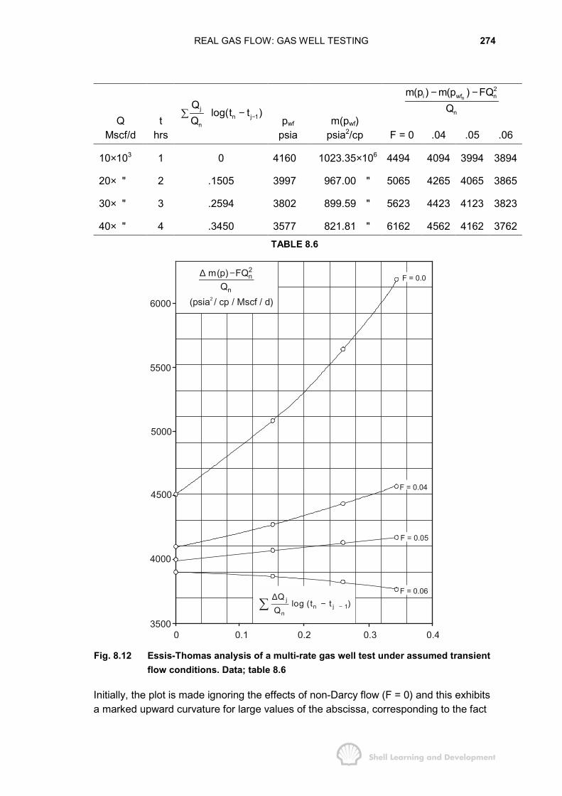
REAL GAS FLOW: GAS WELL TESTING 274
n
2i wf n
n
m(p ) m(p ) FQQ
− −
QMscf/d
thrs
jn j 1
n
Qlog(t t )
Q −−�pwf
psiam(pwf)
psia2/cp F = 0 .04 .05 .06
10×103 1 0 4160 1023.35×106 4494 4094 3994 3894
20× " 2 .1505 3997 967.00 " 5065 4265 4065 3865
30× " 3 .2594 3802 899.59 " 5623 4423 4123 3823
40× " 4 .3450 3577 821.81 " 6162 4562 4162 3762TABLE 8.6
F = 0.0
F = 0.04
F = 0.05
F = 0.06
6000
5500
5000
4500
4000
35000.10 0.2 0.3 0.4
jn j 1
n
Qlog (t t )
Q −∆
−�
2n
n
m(p) FQQ
∆ −
(psia / cp / Mscf / d)2
Fig. 8.12 Essis-Thomas analysis of a multi-rate gas well test under assumed transientflow conditions. Data; table 8.6
Initially, the plot is made ignoring the effects of non-Darcy flow (F = 0) and this exhibitsa marked upward curvature for large values of the abscissa, corresponding to the fact
REAL GAS FLOW: GAS WELL TESTING 275
that the high flow rates occur towards the end of the test. If the well had been testedwith a decreasing rate sequence, the degree of curvature would have been greater forsmaller values of the abscissa14. The calculation of the left hand side of equ. (8.49) hasbeen repeated in table 8.6 for different values of F in an attempt to linearize the plot,and from fig. 8.12 it can be seen that a value of F = .05 accomplishes this. For thisvalue, the plot has a slope of m = 491.5 and intercept 3993, from which thepermeability and skin factor can be calculated as
1637 T 1637 660k 44 mDmh 491.5 50
×= = =×
( ) 2wi
intercept kand S 1.151 log 3.23 2.7m c rφ µ
� �= − + =� �� �
� �
2) The Essis-Thomas analysis, which assumes transient flow conditions for the evaluationof mD, equ. (8.32), will now be compared with the more general case in which mD iscalculated using equ. (8.40) for the 4:1 rectangular geometry. The general well testequation (8.41) can be re-arranged as
( )nn j 1
2 ni wf n j
D D Dj 1n n
m(p ) m(p ) FQ Q1422T 1422Tm t t SQ kh Q kh−
=
− − ∆= − +� (8.50)
in which mD is evaluated as
1 1 12 2 2D D DA DA D(MBH) DA2
w
4Am (t ) 2 t ln t ln m (t )r
πγ
′ ′ ′ ′= + + − (8.40)
or
12D D D(MBH) DAm (t ) m (t )α′ ′= − (8.51)
Alternatively, adhering to the Essis-Thomas analysis expressed in terms ofdimensionless parameters
D1 1 12 2 2D D DA 2
w
4t 4Am (t ) ln ln t lnrγ γ
′ ′= = + (8.32)
A plot of the left hand side of equ. (8.50) versus n j 1
jD D D
n
Qm (t t )
Q −
∆−� should be linear
with slope m = 1422 T/kh, and intercept = 1422 TS/kh, which will yield values of k andS, respectively.
The first part of the analysis is to evaluate the mD functions, equs. (8.51) and (8.32), forall values of the dimensionless time argument
n j 1D D(t t )−
− required in the analysis.
These functions are listed in table 8.7, for k = 50 mD, the permeability value obtainedfrom the pressure buildup analysis, for which
DAi
.000264ktt .0028 t( c) Aφ µ
= =
REAL GAS FLOW: GAS WELL TESTING 276
t (hrs) tDA
αequ. (8.51) ½ mD(MBH)
equ. (8.51)mD
equ. (8.32)mD
1 .0028 6.6772 .0174 6.6598 6.6590
2 .0056 7.0413 .0266 7.0147 7.0061
3 .0084 7.2617 .0230 7.2387 7.2080
4 .0112 7.4231 .0121 7.4110 7.3527TABLE 8.7
Assuming the value of F = .05 determined from the Essis-Thomas analysis, equ. (8.50)can be evaluated for both mD functions as listed in table 8.8.
n j 1
nj
D D Dj 1 n
Qm (t t )
Q −=
∆−�Q
Mscf/dt
hrs
2n
n
m(p) FQQ
∆ −
mD (equ. (8.51) ) mD (equ. (8.32) )
10×103 1 3994 6.6598 6.6596
20 " 2 4065 6.8373 6.8329
30 " 3 4123 6.9711 6.9582
40 " 4 4162 7.0811 7.0568TABLE 8.8
The plots of the data contained in table 8.8 are shown as fig. 8.13 (a) and it can beseen that for the total test duration of four hours the difference between them is veryslight. The values of k and S calculated from the two plots are presented in table 8.9.
mD (equ. (8.51) ) mD (equ. (8.32) )
Slope, m 402.8 426.5
Intercept 1312 1153
k = 1422 T/mh 46.6 mD 44.0 mD
S = kh × intercept/1422 T 3.3 2.7TABLE 8.9
As the duration of each flow period is increased, the difference between the transientand the correct analysis becomes much more pronounced. Fig. 8.13 (b) shows thedifference for 4 × 2 hour flow periods while fig. 8.13 (c) is for a test of 4 × 4 hour flow

REAL GAS FLOW: GAS WELL TESTING 277
2n
2
( m(p) FQ ) / Qn
(psia / cp /Mscf / d)
∆ −
2n
2
( m(p) FQ ) / Qn
(psia / cp /Mscf / d)
∆ −
2n
2
( m(p) FQ ) / Qn
(psia / cp /Mscf / d)
∆ −
n j 1
jD D D
n
Qm (t t )
Q −
∆−�
n j 1
jD D D
n
Qm (t t )
Q −
∆−�
n j 1
jD D D
n
Qm (t t )
Q −
∆−�
4100
4000
39006.5 6.75 7.0 7.25
4300
4200
41007.0 7.57.25
4400
4400
4300
42008.07.5 7.75
4500
CORRECT ANALYSIS; m EVALUATED USING EQU. (8.40)TRANSIENT
D
; m (8.32)“ D “ “ “
a
b
c
Fig. 8.13 The effect of the length of the individual flow periods on the analysis of amulti-rate gas well test; (a) 4××××1 hr periods, (b) 4××××2 hrs, (c) 4××××4 hrs

REAL GAS FLOW: GAS WELL TESTING 278
periods. In each case the solid line represents the correct analysis technique, in whichmD is evaluated using equ. (8.51),while the dashed line is derived for the sameobserved pressure data but with the mD function evaluated under the assumption thattransient flow conditions prevail throughout the test. Using the correct analysistechnique always gives the same values of k and S, but the results obtained from thetransient analysis are open to severe misinterpretation. One may either treat thedashed lines in figs. 8.13 (b) and (c) as being approximately linear, which would resultin the calculated values of both k and S being too small. Alternatively, since both thedashed lines have a distinct upward curvature one may be tempted to linearize themeither by increasing the non-Darcy flow coefficient (even though the correct value ofF = .05 has been used in the analysis to produce figs. 8.13 (b) and (c) ), or by reducingthe initial pressure as demonstrated in exercise 8.1.
The majority of gas well test analyses described in the literature, for non-stabilized flowconditions, are for wells which have very low permeabilities; a few millidarcies or less.Under these circumstances, the transient analysis technique of Essis and Thomas,which is usually applied in one form or another, is probably quite justified. Theforegoing exercise illustrates what can go wrong in applying transient analysistechniques in a moderately high permeability reservoir and, of course, at the time ofplanning the test the permeability is unknown. It is therefore very difficult to estimate inadvance just how long the total test duration should be for the application of transientanalysis to be still valid.
As a safeguard, it is recommended that all sequential flow tests be followed by apressure buildup, which under normal circumstances should provide a more reliablevalue of the permeability and one which can be determined independently of theboundary condition or flow condition (refer Chapter 7, sec. 7). If the permeabilityderived from the multi-rate test, assuming the transient flow condition, is less than thatfrom the buildup it is likely that the multi-rate test analysis is incorrect and should be re-analysed, attempting to make allowance for the boundary condition and discarding theassumption of transient flow. The latter is easier said than done, however, for althoughthe value of k, obtained from the buildup, facilitates the determination of tDA, required inthe analysis, there always remains an ambiguity in the estimation of the correct shapeof the drainage area which, as shown in exercise 7.8, cannot be resolved byconventional analysis techniques.
Odeh et al.16 have also described an analysis technique for multi-rate flow tests whichare followed by a buildup. The obvious drawback to this method of testing is that itnegates one of the main aims of multi-rate testing which is to avoid well closure.
8.11 PRESSURE BUILDUP TESTING OF GAS WELLS
Just as in the case of oilwell testing, pressure buildup tests in gas wells, if analysedcorrectly using the Horner buildup plot, can provide the most reliable values of thepermeability and skin factor. The only difference is that a buildup in a gas well must beaccompanied by two separate flow periods, one before and one after the buildup, asshown in fig. 8.14. This measure is necessary in order to determine both componentsof the skin factor, S and DQ.

REAL GAS FLOW: GAS WELL TESTING 279
Rate
Q1
Q2
tt1
∆t∆tmax.
t ’
(a)
Time
(b)
tt1
∆t∆tmax.
t ’
Bottomhole
Pressure pwf
pws
Fig. 8.14 (a) Rate-time schedule, and (b) corresponding wellbore pressure responseduring a pressure buildup test in a gas well
The theoretical buildup equation for the rates and times shown in fig. 8.14 is just aspecial case of the general test equation (8.39).
1i ws D D D D D1
kh (m(p ) m(p )) m (t t ) m ( t )1422Q T
− = + ∆ − ∆ (8.52)
This is identical in form to equ. (7.32), the theoretical buildup equation for an oilwelltest. In deriving equ. (8.52) from equ. (8.39), for superposed constant terminal ratesolutions with rate changes Q1 and (0 – Q1), both the mechanical and rate dependentskin factors disappear, a fact which has been investigated by Ramey andWattenbarger4.
In analogy with the buildup theory described in Chapter 7, sec. 7, for small values of ∆t,equ. (8.52) can be expressed as a linear relationship between m(pws) and log (t1 + ∆t)/∆t. The equation of this straight line for any value of ∆t is
11
D1 12i ws(LIN) D D
1
4tt tkh (m(p ) m(p )) 1.151 log m (t ) ln1422Q T t γ
+ ∆− = + −∆
(8.53)
in which m(pws(LIN)) is the hypothetical pseudo pressure on the extrapolated linear trend,and
1D Dm (t ) and 1/2 ln 1D4t /γ , which are both evaluated for the dimensionless, effective
flowing time before the buildup, are constants. For large values of ∆t the real pseudopressure m(pws), equ. (8.52), will deviate from m(pws(LIN)) as demonstrated for the similarliquid flow equations in exercise 7.7. Therefore,. the Horner plot of
REAL GAS FLOW: GAS WELL TESTING 280
1ws
t tm(p ) versus logt
+ ∆∆
for the recorded pressure data will be linear for small ∆t and the extrapolated trend cantheoretically be matched by equ. (8.53). The attractive feature of the Horner buildup isthat the analysis to determine k and S does not involve the specific evaluation ofmD (
1Dt ) in equ. (8.53) but merely requires that the early linear buildup trend be
identified. The slope of this line is
11637Q Tmkh
= (8.54)
from which kh and k can be calculated, and the total skin factor, corresponding to rateQ1, can be determined as
ws(LIN)1 hr wf1 1 2
i w
(m(p ) m(p )) kS S DQ 1.151 log 3.23m ( c) rφ µ− −� �′ = + = − +� �
� �(8.55)
in which m(pws(LIN)1-hr) is the pseudo pressure read from the extrapolated straight line at∆t = 1 hour. The derivation of equ. (8.55) follows the same argument leading toequ. (7.52) and therefore the calculated value of 1S′ is independent of the value ofmD (
1Dt ).
The early, transient pressure response of both flow periods can be analysed todetermine values of k, 1S′ and 2S′ (= S + DQ2). The equation describing the transientpseudo pressure drop at the wellbore at any time t during the first flow period is
D12i wf 1
1
4tkh (m(p ) m(p )) ln S1422Q T γ
′− = +
which can be expressed as
1i wf 12
i w
1637Q T km(p ) m(p ) log t log 3.23 0.87Skh ( c) rφ µ
� �′− = + − +� �� �
(8.56)
Thus a plot of m(pwf) versus log t will be linear during the transient flow period withslope
11637Q Tmkh
= (8.54)
again giving the value of k, while the skin factor can be calculated by evaluatingequ. (8.56), for the specific value of m(pwf ) at t = 1 hr, as
i wf 1 hr1 1 2
i w
(m(p ) m(p ) ) kS S DQ 1.151 log 3.23m ( c) rφ µ
−� �−′ = + = − +� �� �
(8.57)
Only the values of m(pwf) which plot as a linear function of log t are used, whichensures that the application of transient analysis is valid.
REAL GAS FLOW: GAS WELL TESTING 281
The theoretical equation describing the pseudo pressure drop during the second flowperiod can be derived from the basic test equation (8.39) as
1 max maxi wf 1 D D D D D D D
2 D D 2 2
kh (m(p ) m(p )) Q (m (t t t ) m ( t t ))1422T
Q m (t ) Q S
′ ′− = + ∆ + − ∆ +
′ ′+ +(8.58)
where t′ is the time measured from the start of the second flow period at rate Q2,(fig. 8.14). This equation is analysed for transient conditions during the second flowperiod, that is, for small values of t´. In this case the expression
1 max max1 D D D D D D DQ (m (t t t ) m ( t t ))′ ′+ ∆ + − ∆ +
in equ. (8.58) can be regarded as being constant. If both t1 and ∆tmax are short so thatboth the mD functions can be evaluated under transient conditions the above statementis quite correct and, in fact, the difference between the mD functions is both small andconstant. For a very long initial flow period, corresponding to a routine well surveyrather than an initial test, the difference between the mD functions can only be regardedas constant on the grounds that t is small, which is always the case since the wellborepressure response at rate Q2 is only being analysed during the brief, initial, transientflow period. Therefore, equ. (8.58) implies that a plot of m(pwf) versus log t will belinear, for transient flow, with slope
21637Q Tmkh
=
which leads to a re-determination of k. The skin factor can be evaluated by expressingequ. (8.58) as
i wf i ws 2 D D 2 2kh kh(m(p ) m(p )) (m(p ) m(p )) Q m (t ) Q S
1422T 1422T′ ′ ′− = − + + (8.59)
in which wsp′ is the hypothetical static pressure that would be obtained had the buildupbeen continued for a time ∆tmax + t′ . The value of wsp′ will therefore increase as t´increases. Equation (8.59) can then be solved to give 2S′ as
ws 1 hr wf 1 hr2 2 2
i w
(m(p ) m(p ) kS S DQ 1.151 log 3.23m ( c) rφ µ
− −′� �−′ = + = − +� �� �
(8.60)
in which both ( )wfm p and ( )wsm p′ are evaluated for t′ = 1 hour. The latter can be
obtained by extrapolation of the final buildup trend for one hour after the buildup hasceased. However, this correction is seldom applied and usually ( )ws 1 hr
m p−
′ is set equal
to ( )wsm p , evaluated for the final closed in pressure.
The following exercise illustrates the method of buildup analysis for a well test in a newreservoir in which pi is the initial reservoir pressure.
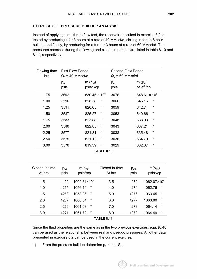
REAL GAS FLOW: GAS WELL TESTING 282
EXERCISE 8.3 PRESSURE BUILDUP ANALYSIS
Instead of applying a multi-rate flow test, the reservoir described in exercise 8.2 istested by producing it for 3 hours at a rate of 40 MMscf/d, closing in for an 8 hourbuildup and finally, by producing for a further 3 hours at a rate of 60 MMscf/d. Thepressures recorded during the flowing and closed in periods are listed in table 8.10 and8.11, respectively.
First Flow PeriodQ1 = 40 MMscf/d
Second Flow PeriodQ2 = 60 MMscf/d
Flowing timehrs
pwf
psiam (pwf)psia2 /cp
pwf
psiam (pwf)psia2 /cp
.75 3602 830.45 × 10⁶ 3076 648.61 × 10⁶
1.00 3596 828.38 " 3066 645.16 "
1.25 3591 826.65 " 3059 642.74 "
1.50 3587 825.27 " 3053 640.66 "
1.75 3583 823.88 " 3048 638.93 "
2.00 3580 822.85 " 3043 637.21 "
2.25 3577 821.81 " 3038 635.48 "
2.50 3575 821.12 " 3036 634.79 "
3.00 3570 819.39 " 3029 632.37 "TABLE 8.10
Closed in time∆t hrs
pws
psiam(pws)
psia2/cpClosed in time
∆t hrspws
psiam(pws)
psia2/cp
.5 4100 1002.61×106 3.5 4272 1062.07×106
1.0 4255 1056.19 " 4.0 4274 1062.76 "
1.5 4263 1058.96 " 5.0 4276 1063.45 "
2.0 4267 1060.34 " 6.0 4277 1063.80 "
2.5 4269 1061.03 " 7.0 4278 1064.14 "
3.0 4271 1061.72 " 8.0 4279 1064.49 "TABLE 8.11
Since the fluid properties are the same as in the two previous exercises, equ. (8.48)can be used as the relationship between real and pseudo pressures. All other datapresented in exercise 8.2 can be used in the current exercise.
1) From the pressure buildup determine pi, k and 1S′ .

REAL GAS FLOW: GAS WELL TESTING 283
2) From the flow tests determine k, 1S′ , 2S′ and hence D, or F.
EXERCISE 8.3 SOLUTION
1) Buildup Analysis
For a flowing time of 3 hours, the data necessary to draw the Horner buildup plot arelisted in table 8.12.
∆thrs
1t tlogt
+ ∆∆ m(pws)
psia2/cp∆thrs
1t tlogt
+ ∆∆ m(pws)
psia2/cp
.5 .845 1002.61×106 3.5 .269 1062.07×106
1.0 .602 1056.19 " 4.0 .243 1062.76 "
1.5 .477 1058.96 " 5.0 .204 1063.45 "
2.0 .398 1060.34 " 6.0 .176 1063.80 "
2.5 .342 1061.03 " 7.0 .155 1064.14 "
3.0 .301 1061.72 " 8.0 .138 1064.49 "
(9.0) (.125) (1064.65) "TABLE 8.12
The corresponding buildup plot is shown as fig. 8.15 (a), from which the slope hasbeen determined as
6 2 11637Q Tm 16.17 10 psia / cp / log cyclekh
= × =
which for a fully penetrating well gives3
61637 40 10 660k 53.5 mD
16.17 10 50× × ×= =
× ×
and the extrapolation to ∆t = ∞ gives
m(pi) = 1066.7 × 106 psia2/cppi = 4285 psi
The value of ( )ws 1 hrm p
−′ taken from the extrapolated linear trend is 1057 ×106 psia2/cp
and therefore, using equ. (8.55)
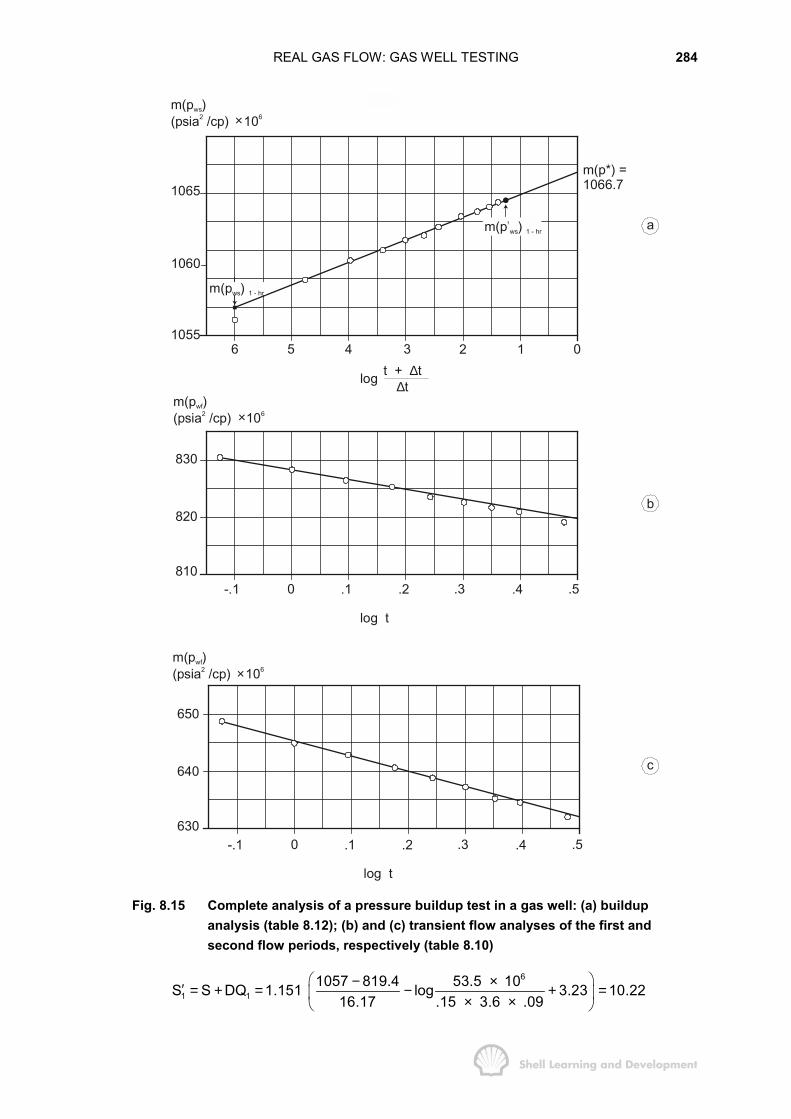
REAL GAS FLOW: GAS WELL TESTING 284
1065
1060
1055
830
820
810
650
640
630-.1 0 .1 .2 .3 .4 .5
log t
-.1 0 .1 .2 .3 .4 .5
log t
6 5 4 3 2 1 0
log t + tt∆
∆
m(p )(psia /cp) 10
ws2 6
m(p )(psia /cp) 10
wf2 6
m(p )(psia /cp) 10
wf2 6
m(p ) ws 1 - hr
m(p ) ’ws 1 - hr
m(p*) =1066.7
a
b
c
×
×
×
Fig. 8.15 Complete analysis of a pressure buildup test in a gas well: (a) buildupanalysis (table 8.12); (b) and (c) transient flow analyses of the first andsecond flow periods, respectively (table 8.10)
6
1 11057 819.4 53.5 10S S DQ 1.151 log 3.23 10.22
16.17 .15 3.6 .09� �− ×′ = + = − + =� �× ×� �

REAL GAS FLOW: GAS WELL TESTING 285
2) Flow Analysis
Plots of m(pwf) versus log t for the data listed in table 8.10, are shown as fig. 8.15 (b)and (c), from which the data presented in table 8.13 have been determined.
RateMscf/d
Slopepsia2/cp/log cycle
m(pwf)1-hr kmD
Total Skin
40×103 16.64×10⁶ 828.38×10⁶ 45 9.9
60 " 26.08 " 645.16 " 43 11.9TABLE 8.13
The values of the permeability in this table have been calculated using equ. (8.54) forrates Q1 and Q2 and the total skin factors using equs. (8.57) and (8.60) for the first andsecond flow periods respectively. In applying equ. (8.60) the value of ( )ws 1 hr
m p−
′ has
been determined from the buildup plot for ∆t = 9 hours as 1064.65 × 106 psia2/cp(fig. 8.15 (a) and table 8.12). The reader can verify that irrespective of whether
( )ws 1 hr,m p
−′ ( )wsm p for the maximum buildup time, or m(pi) is used in equ. (8.60) makes
very little difference to the calculated value of 2S′ . Finally, S and D can be calculated bysolving the equations
1S′ = 9.9 = S + 40 × 103 D
2S′ = 11.9 = S + 60 × 103 D
to give S = 5.9; D = 1.0 × 10⁻⁴/Mscf/d
and F = 1422 DTkh
= 0.043 psia2/cp/(Mscf/d)2
and from these figures the Darcy flow coefficient B can be calculated for the estimatedvalues of A and CA, equ. (8.44), for use in long term well deliverability calculations.
A similar example of a pressure buildup analysis, for a low permeability reservoir(k = 5 mD),has been presented in the literature by Al-Hussainy and Ramey3. The mainadvantage of this type of test over the multi-rate drawdown test is the same asmentioned in Chapter 7, sec. 7. It is, that the buildup analysis will provide values ofk and 1S′ which are independent of the value of m(tD ) at the time of the survey.Furthermore, since only the transient pressure response during each flow period isinterpreted, then it means that the entire test can be analysed without having to beconcerned about the size or shape of the area drained or the well position with respectto the boundary.
The pressure buildup test can also be used for the routine surveys conducted atregular intervals throughout the producing life of the field. Prior to the survey the wellmust be produced at a constant rate for a sufficient period of time so that the flow isunder semi-steady state conditions. This renders transient analysis of the first flowperiod, at rate Q1, impossible but analysis of the buildup will yield values of k and 1S′ .Following this, k and 2S′ can be determined from the transient analysis of the second
REAL GAS FLOW: GAS WELL TESTING 286
flow period at rate Q2. The main purpose of this type of test is to determine the currentaverage pressure within the drainage boundary of the well, p. Theoretically, this canbe done by using either the method of Matthews, Brons and Hazebroek, or Dietz (referChapter 7, sec. 7), but the difficulty is to determine at what pressure the µc productshould be evaluated which is required to calculate tDA for use with either of thesemethods. For the initial well tests described in exercises 8.1-3, the product (µc) i
evaluated at the initial equilibrium pressure could be used but for a survey made, say,several years after the well has started to produce this can lead to serious error. Thebasic problem is that for very long flowing times the calculation of mD using the semi-steady state equation (8.33) with the (µc)i product does not accurately correlate withthe similar pD function for liquid flow, equ. (7.27).
Kazemi10 has presented an iterative method for determining the pressure at which, µcshould be evaluated and hence the correct value of p. The method is applicable forwells producing under semi-steady state conditions at the time of the survey. In thiscase, as shown in Chapter 7, sec. 7, the value of the flowing time used to plot thebuildup is immaterial providing that t ≥ tSSS, the time required for semi-steady stateconditions to be reached for the particular geometrical configuration of the drainagearea. Strictly speaking, this statement is only valid when applied to a liquid, in whichcase the MBH plots, figs. 7.11-15, are linear functions of the dimensionless flowingtime tDA. For a real gas, however, the mD(MBH) functions deviate from the linear pD(MBH)
functions for large values of tDA, as shown in fig. 8.16. This implies that using the MBHcharts, for a large value of the (effective) flowing time, can lead to an error in thedetermination of p in the analysis of a routine buildup survey in a gas well.
Kazemi argues, and substantiates his argument with detailed numerical simulation, thatif the buildup is plotted for a flowing time tSSS,where
SSSpSSS DA SSS
( c) At (t )
0.000264k
φ µ= (8.61)
and the MBH method applied for a dimensionless flowing time (tDA)SSS, then the portionof the MBH charts for which the liquid and gas MBH functions correlate is used and thisshould result in the correct determination of p. Of course, in order to calculate tSSS,using equ. (8.61), requires a knowledge of pSSS, the average pressure at a time tSSS
prior to the buildup and the evaluation of the µc product at this pressure. A simpleiterative scheme for calculating pSSS, tSSS and hence p is shown in fig. 8.17.

REAL GAS FLOW: GAS WELL TESTING 287
m
or
D (MBH)
p D (MBH)
01 0.1 1.0 10.0
m D (MBH)
p D (MBH)
(t ) DA SSS
t =DA
.00264 ktcAφµ
Fig. 8.16 MBH plot for a well at the centre of a square, showing the deviation of mD(MBH)
from pD(MBH) for large values of the dimensionless flowing time tDA
In the first place an estimate is made of (tDA )SSS, for the particular geometricalconfiguration, fig. 6.4. Both (tDA)SSS and m(p*) - m ( )p remain constant throughout the
analysis. An estimate of µc is made, using either the initial pressure or some roughlyestimated value of pSSS, from which an initial value of tSSS is determined usingequ. (8.61). The Horner buildup is plotted using this value of tSSS instead of the effectiveflowing time. The MBH (or Dietz) method is then used to obtain an initial value of theaverage pressure at the time of the survey (refer Chapter 7, sec.7). The µc product isre-evaluated at p, and tSSS and p re-estimated. For this second, and all successivevalues of p, the material balance is applied to determine pSSS, the average pressuretSSS hours before the well closure, using dGp = Ql tSSS for the final flow rate Ql and thelatest estimate of tSSS. A cycle is entered in which µc is evaluated for the latestdetermined value of pSSS and this continues until successive values of this pressuredo not differ by more than some tolerance value (e.g. TOL = 5 psi).
Each new estimate of tSSS leads to a new buildup plot and since m(p*) – m(p ) isconstant, a new value of p is obtained on each occasion. In a worked example Kazemihas shown that applying the above method can lead to a correction of 100 psi in thevalue p compared to the normal method in which µc is evaluated as (µc)i. The methodcan also be used to correct the average pressure determined from a buildup test in asolution gas drive reservoir which is below bubble point pressure.
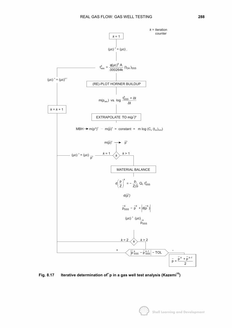
REAL GAS FLOW: GAS WELL TESTING 288
k = 1
k = iteration counter
( c) = ( c) µ kiµ
sss DA SSS( c) At (t )
.000264kφ µ=
kk
( c) = ( c)µ k k-1µ(RE)-PLOT HORNER BUILDUP
EXTRAPOLATES TO m(p*)k
SSSws
t tm(p ) vs. logt+ ∆
∆
k
MBH m(p*) m( ) = constant = m log (C (t ) )p kA DA SSS
k
m( ) p k pk
k = 1 k > 1k pk ( c) = ( c)µ k µ
MATERIAL BALANCE
k = 1k +
i1 SSS
i
ppd Q tZ Z G
� � = −� �� �
kk
d(pk)
SSSp p d(p )− +k k k
( c) ( c)µ k µSSSpk
k = 2 k > 2k
+ -SSS SSSp p TOL− −k k -1
p pp2
+=k k -1
TO m(p*)k
Fig. 8.17 Iterative determination of p in a gas well test analysis (Kazemi10)

REAL GAS FLOW: GAS WELL TESTING 289
8.12 PRESSURE BUILDUP ANALYSIS IN SOLUTION GAS DRIVE RESERVOIRS
The pressure buildup theory described in sec. 7 of the previous chapter was developedfor liquid flow and is therefore only appropriate for pressure surveys in undersaturatedoil reservoirs. For routine pressure surveys conducted throughout the producinglifetime of the field, it is more likely that the average pressure will be below bubble pointso that there will be two phases, liquid oil and free gas, in the reservoir.
To analyse pressure buildup tests under these circumstances, Raghavan17 hassuggested the use of the integral transformation
b
pro o
o op
k (S )m (p) dpBµ
′ = � (8.62)
which again is referred to as a pseudo pressure, only in this case applied to the flow ofoil, as denoted by the subscript "o". The kro(So ) is the oil relative permeability, which isa function of the oil saturation, while the other parameters, µo and Bo are functions ofpressure. This leads to a certain degree of difficulty in determining the relation betweenpressure and saturation required to evaluate equ. (8.62). Raghaven has shown thatthis relationship can be obtained from the gas-oil ratio equation which expresses theratio of the reservoir gas to oil rates at the time of closure of the well, i.e.
s g rg o
o g ro
(R R )B k(rb / gas)B (rb / oil) k
µµ
−=
or rg o os
g ro g
k BR Rk Bµ
µ= + (8.63)
In this relationship, R is the fixed value of the producing GOR at the time of closure andtherefore, since krg and kro are functions of the oil saturation and Bo, Bg and Rs arefunctions of pressure, equ. (8.63) implicitly defines the pressure-saturation relationship.The steps in evaluating the pseudo pressure integral, equ. (8.62), are then
1) Using the value of R at the time of the survey, determine the relation krg/kro as afunction of the pressure, using equ. (8.63).
2) Providing gas-oil relative permeability curves are available (kro and krg asfunctions of So, refer sec. 4.8) the relation between kro and pressure can bedetermined.
3) Using the trapezoidal rule, evaluate m (p)′ as a function of pressure, in the sameway as demonstrated in table 8.1.
It should be noted that this m (p)′ function only reflects conditions near the well at thetime of the survey and must be re-calculated for each pressure survey, as R varies.
Using the m (p)′ pseudo pressure, the constant terminal rate solution of the radialdiffusivity equation can be expressed in dimensionless form as

REAL GAS FLOW: GAS WELL TESTING 290
3i wf D D
o
kh7.08 10 (m (p ) m (p )) m (t ) Sq
− ′ ′ ′× − = +
where
D1 12 2D D DA D(MBH) DA
4tm (t ) 2 t ln m (t )πγ
′ ′= + − (8.64)
in which k is the effective permeability to oil in the presence of the connate water.Raghavan has shown, using numerical simulation, that the Dm′ (tD) functions correlatevery well with the pD (tD) functions for liquid flow but, as in the case of real gas flow, thematch is better for small values of tD, before the boundary effects are felt.
It should also be noted that the compressibility used in the evaluation of tDA is the totalcompressibility of the system. Above the bubble point this is simply
ct = coSo + cwSwc + cf (5.22)
but below bubble point there must be additional components to account for thepresence of free gas and for the transfer of solution gas from the oil18. Thus for the oil,a pressure drop ∆p will cause a reduction in the oil volume ∆Bo and an increase in theliberated gas volume Bg∆ Rs, and
o so g
o
B R1c BB p p
� ∂ ∂ �= − −� �∂ ∂� �
The total compressibility, below bubble point pressure is therefore
g go s ot g w wc f
o g
S BS R Bc B c S cB p p B p
∂� ∂ ∂ �= − − + +� �∂ ∂ ∂� �(8.65)
in which, for a significant gas saturation, the last two terms can usually be neglected.
Because of the equivalence of form of the Dm′ functions, equ. (8.64), with the pD or mD
functions, it is clear that the buildup theory must follow that detailed in Chapter 7,sec. 7, for oil, and sec. 8.11 of this chapter, for gas. A Horner plot of m´(pws) versus logt t
t+ ∆∆
is made and the early linear trend extrapolated to determine m´(p*). The slope of
the linear section is
162.6 qmkh
=
and the skin factor can be calculated using equ. (7.52), with pseudo pressuresreplacing the actual pressures in the equation. Again the MBH method can be used todetermine m (p)′ and hence the average pressure p . Furthermore, if the flowing timebefore the survey is very long, the correction method of Kazemi, described in theprevious section, can be applied to improve the estimate of p .

REAL GAS FLOW: GAS WELL TESTING 291
8.13 SUMMARY OF PRESSURE ANALYSIS TECHNIQUES
For those who have struggled through this and the previous three chapters, it isworthwhile presenting a brief summary of their contents in an effort to simplify andgeneralise the theory of well testing.
To start with, the application of the principle of mass conservation, together withDarcy's law and the definition of isothermal compressibility, lead to the non-linear,radial, second order, partial differential equation for the flow of a single phase fluid (inDarcy units) as
1 k p pr cr r r t
ρ φ ρµ
� �∂ ∂ ∂=� �∂ ∂ ∂� �(5.1)
Prior to obtaining useful solutions of this equation it must first be linearized (or partiallylinearized) and the method by which this can be achieved depends on the nature of thefluid under consideration, as follows.
Undersaturated oil
Linearization by deletion of terms, assuming that 2( p / r) 0;µ∂ ∂ ≈ ≈ constant andcp << 1.
Real gas
Partial linearization using the integral transformation
b
p
p
pdpm(p) 2µ
=Ζ� (8.7)
Gas-oil
Partial linearization using the integral transformation
b
pro o
o op
k (S )m (p) dpBµ
′ = � (8.62)
or, strictly speaking, in Darcy units, the correct form of this transformation should be
b
pro o o
op
k (S )m (p) dpρµ
′ = �
Application of any of the above methods leads to the re-formulation of equ. (5.1) as
1 cr r r k t
β φµ β∂ ∂ ∂� � =� �∂ ∂ ∂� �(8.66)
which has the form of the radial diffusivity equation and in which:
for undersaturated oil β = p

REAL GAS FLOW: GAS WELL TESTING 292
for a real gas β = m(p)
and for gas-oil (two phase) β = m (p)′
Although the term linearization has been applied to the conversion of equ. (5.1) toequ. (8.66), it should be remembered that linearization is only achieved for the case ofliquid flow (undersaturated oil) for which the coefficient k/φµc is a constant. For bothreal gas and two phase (gas-oil) systems, the µc product is pressure dependent,meaning that equ. (8.66) is still non-linear.
The basic building block in well test analysis is the constant terminal rate solution ofequ. (8.66), which predicts the pressure or pseudo pressure response at the wellbore,resulting from the production of a well at constant rate from a state of equilibriumpressure. Expressing equ. (8.66) in dimensionless form
D DD
D D D D
1 rr r r t
β β� �∂ ∂∂ =� �∂ ∂ ∂� �(8.67)
where rD = r/rW and tD = kt/φµc 2wr (= 0.000264 kt/φµc 2
wr in field units- t in hours), thegeneral constant terminal rate solution, for rD = 1, can be expressed as
D Df(p) (t ) Sqα β� �
= +� �� �
(8.68)
In this equation the various component parts are as listed in table 8.14, (in field units),again, dependent on the nature of the fluid.
To interpret the majority of practical well tests requires the superposition of constantterminal rate solutions, for different constant production rates acting for differentperiods of time, to give the value of f(p)n at time tn during the nth flow period, as
n j 1
n
n j D D D nj 1
f(p) q (t t ) q Sα β−
=
= ∆ − +� (8.69)
in whichUndersaturated
oilRealgas
Two phasegas-oil
(fieldunits)qα 3
o o o
kh7.08 10q Bµ
−× kh1422QT
3
o
kh7.08 10q
−×
f(p) pi − pwf m (pi) − m(pwf) i wfm (p ) m (p )′ ′−
βD (tD) pD(tD) mD (tD) m´D(tD)
S S S + DQ STABLE 8.14
n j 1D1 1
2 2o D D D D DA D(MBH) DA4t(t t ) (t ) 2 t ln (t )β β π βγ−
′′ ′ ′− = = + − (8.70)
REAL GAS FLOW: GAS WELL TESTING 293
where tDA = 0.000264kt /φµcA (field units), and βD(MBH)(tDA) is the ordinate of the MBHcharts, corresponding to the value of tDA, and includes allowance for the geometry ofthe drainage area and the degree of well asymmetry with respect to the boundary.
Well test analysis techniques presented in the literature invariably require thesuperposition of transient constant terminal rate solutions of equ. (8.67) which, incomparison with equ. (8.70), have the form
n j 1D1
2D D D D D4t(t t ) (t ) lnβ βγ−
′′− = = (8.71)
Superposition of such solutions, however, automatically assumes the infinite boundarycondition and is therefore only appropriate for tests of short duration, whereassuperposition of the total solution, equ. (8.70), is theoretically correct for any value ofthe flowing time and for any boundary condition.
Examples in this and the previous chapter (exercises 7.8 and 8.2), have shown that thead-hoc assumption of transient flow can be particularly dangerous in the interpretationof multi-rate flow tests. Furthermore, conventional multi-rate test analysis techniquesdo not permit the attempted matching of the drainage boundary, even using the correctβD function, equ. (8.70), in the superposed test analysis equation, (8.69), as illustratedin exercise 7.8. Multi-rate tests should only be planned when the engineer is quiteconfident that transient conditions apply for the duration of the entire test, which isdifficult to ascertain in advance of the test itself.
In this author's opinion, the safest and most useful type of test, for any fluid system, isthe pressure buildup. Definition of a linear trend, for small values of the closed in timeon a Horner buildup plot, can lead to the unambiguous determination of the effectivepermeability and the skin factor. Use of this early linear trend, in fact, imposestransience on the buildup analysis. In addition, the test can be interpreted to determinethe average pressure within the drainage boundary of the well and also to gain someimpression of the shape, area and well position within the boundary, as illustrated inexercise 7.7.
It must be admitted that the use of equ. (8.70) instead of equ. (8.71), in the basic welltest equation, (8.69), only serves to complicate well test analysis. Nevertheless, inusing the correct solution one is simply recognising the basic fact that second orderdifferential equations require the specification of both initial and boundary conditions toobtain meaningful solutions.
As illustrated in the various exercises, it is not difficult to evaluate equ. (8.70) for use intest analysis. These days when engineers have access to computers or, at least,sophisticated electronic desk calculators, the evaluation is much less tedious than inthe past.
For instance, a perfectly general program for evaluating pressure buildup tests, for anyfluid, could be structured as shown in fig. 8.18.
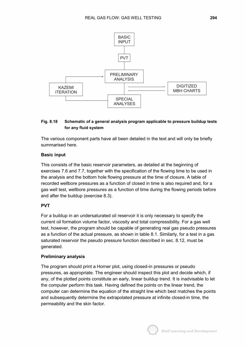
REAL GAS FLOW: GAS WELL TESTING 294
BASICINPUT
PVT
PRELIMINARYANALYSIS
KAZEMIITERATION
SPECIALANALYSES
DIGITIZEDMBH CHARTS
Fig. 8.18 Schematic of a general analysis program applicable to pressure buildup testsfor any fluid system
The various component parts have all been detailed in the text and will only be brieflysummarised here.
Basic input
This consists of the basic reservoir parameters, as detailed at the beginning ofexercises 7.6 and 7.7, together with the specification of the flowing time to be used inthe analysis and the bottom hole flowing pressure at the time of closure. A table ofrecorded wellbore pressures as a function of closed in time is also required and, for agas well test, wellbore pressures as a function of time during the flowing periods beforeand after the buildup (exercise 8.3).
PVT
For a buildup in an undersaturated oil reservoir it is only necessary to specify thecurrent oil formation volume factor, viscosity and total compressibility. For a gas welltest, however, the program should be capable of generating real gas pseudo pressuresas a function of the actual pressure, as shown in table 8.1. Similarly, for a test in a gassaturated reservoir the pseudo pressure function described in sec. 8.12, must begenerated.
Preliminary analysis
The program should print a Horner plot, using closed-in pressures or pseudopressures, as appropriate. The engineer should inspect this plot and decide which, ifany, of the plotted points constitute an early, linear buildup trend. It is inadvisable to letthe computer perform this task. Having defined the points on the linear trend, thecomputer can determine the equation of the straight line which best matches the pointsand subsequently determine the extrapolated pressure at infinite closed-in time, thepermeability and the skin factor.
REAL GAS FLOW: GAS WELL TESTING 295
For a gas well test, this part of the program should also analyse the transient pressurefall-off during the flowing periods, giving a re-determination of the permeability and twoseparate skin factors, at different flow rates, which facilitate the calculation of the ratedependent skin (exercise 8.3).
For an initial test in either an oil or gas reservoir (exercises 7.6 and 8.3, respectively)the analysis would cease at this point. In the more common instance of routinepressure surveys made throughout the producing lifetime of the well, the followingsteps are necessary which incorporate the boundary condition in the analysis.
Digitized MBH charts
This set of data is the main-spring of the special analyses part of the program. Asalready mentioned, the MBH charts (figs. 7.11-15), which are equally appropriate fordimensionless pressure or pseudo pressures, have al ready been digitized byEarlougher15, for dimensionless time in the range 0.001 ≤ tDA ≤ 10. From this data bank,values of the constant terminal rate solution βD, equ. (8.70), can be extracted for anyfluid type, geometry of the drainage area and degree of well asymmetry.
Special analyses
This part of the program should be quite flexible with the main aims being to determinethe average pressure within the drainage boundary at the time of the survey and togain some information about the magnitude and shape of the drainage area and wellposition with respect to the boundary. For instance, the program could be structured,as described in exercise 7.7, to match the equation of the observed linear buildup,obtained in the preliminary analysis, with a theoretical straight line for various assumedarea sizes and shapes. Alternatively, an attempt could be made to match the entirebuildup by evaluating both βD (tD + ∆tD) and βD (∆tD), and plotting the differencebetween the two, also as described in exercise 7.7.
Kazemi iteration
Iteration over the entire test analysis may be required for surveys conducted in gas, orin gas saturated oil reservoirs, as described in sec. 8.11. This measure is necessary torefine the estimate of the average pressure within the drainage area at the time of thesurvey.
REFERENCES
1) Russell, D.G., Goodrich, J.H., Perry, G.E. and Bruskotter, J.F., 1966. Methods ofPredicting Gas Well Performance. J.Pet.Tech., January: 99-108.Trans. AIME.
2) Al-Hussainy, R., Ramey, H.J.,Jr. and Crawford, P.B.,1966. The Flow of RealGases Through Porous Media. J.Pet.Tech., May: 624-636. Trans. AIME.
3) Al-Hussainy, R. and Ramey, H.J., Jr., 1966. Application of Real Gas Flow Theoryto Well Testing and Deliverability Forecasting. J.Pet.Tech., May: 637-642.Trans. AIME.
REAL GAS FLOW: GAS WELL TESTING 296
4) Ramey, H.J., Jr. and Wattenbarger, R.A., 1968. Gas Well Testing withTurbulence, Damage and Wellbore Storage. J.Pet.Tech., August: 877-887.Trans. AIME.
5) Aziz, K., Mathar, L., Ko, S. and Brar, G.S.,1976. Use of Pressure, Pressure-Squared or Pseudo-Pressure in the Analysis of Transient Pressure DrawdownData from Gas Wells. J.Can.Pet.Tech., April-June: 58−65.
6) Geertsma, J., 1974. Estimating the Coefficient of Inertial Resistance in Fluid FlowThrough Porous Media. Soc.Pet.Eng.J., October: 445-450.
7) Gewers, C.W.W. and Nichol, L.R., 1969. Gas Turbulence Factor in aMicrovugular Carbonate. J.Can.Pet.Tech., April.
8) Wong, S.W., 1970. Effects of Liquid Saturation on Turbulence Factors for GasLiquid Systems. J.Can.Pet.Tech., October.
9) Katz, D.L., et.al., 1959. Handbook of Natural Gas Engineering. McGraw-Hill BookCompany, Inc. 47−50.
10) Kazemi, H., 1974. Determining Average Reservoir Pressure from PressureBuildup Test. Soc.Pet.Eng.J., February: 55−62. Trans. AIME.
11) Rawlins, E.L. and Schelihardt, M.A., Back Pressure Tests on Natural GasWellsand Their Application to Production Practices. Monograph 7, USBM.
12) Carter, R.D., Millers, S.C., Jr. and Riley, H.G., 1963. Determination of StabilizedGas Well Performance from Short Flow Tests. J.Pet.Tech., June: 651−658.Trans. AIME.
13) Odeh, A.S. and Jones, L.G., 1965. Pressure Drawdown Analysis, Variable RateCase. J.Pet.Tech., August: 960−964. Trans. AIME.
14) Essis, A.E. and Thomas, G.W., 1971. The Use of Open Flow Potential Test Datain Determining Formation Capacity and Skin Factor. J.Pet.Tech., July: 879−887.Trans. AIME.
15) Earlougher, R.C., Ramey, H.J., Jr., Miller, F.G. and Mueller, T.D., 1968. PressureDistribution in Rectangular Reservoirs. J.Pet.Tech., February: 199−208.Trans. AIME.
16) Odeh, A.S., Moreland, E.E., and Schueler, S., 1975. Characterization of a GasWell from One Flow-Test Sequence. J.Pet.Tech., December: 1500−1505.Trans. AIME.
17) Raghavan, R., 1976. Well Test Analysis: Wells Producing by Solution Gas Drive.Soc.Pet.Eng.J., August: 196−208.
18) Ramey, H.J., Jr., 1964. Rapid Method for Estimating Reservoir Compressibilities.J.Pet.Tech., April: 447−454.

CHAPTER 9
NATURAL WATER INFLUX
9.1 INTRODUCTION
Natural water influx into both gas and oil reservoirs has been described previously(Chapter 1, sec. 7, and Chapter 3, sec. 7) using the simple, time independent aquifermaterial balance
We = c Wi (pi - p)
for calculating the amount of influx. In this equation
Wi = initial volume of water in the aquifer and is therefore dependent uponaquifer geometry
pi = initial aquifer/reservoir pressure
p = current reservoir pressure, which in this chapter will always be assumed tobe equal to the pressure at the original oil (or gas) water contact
c = total aquifer compressibility = cw + cf
The equation is simply a re-statement of the basic definition of compressibility and isonly applicable to very small aquifers. For large aquifers a mathematical model isrequired which includes time dependence, to cater for the fact that it takes a finite timefor the aquifer to respond fully to a pressure change in the reservoir. Two such modelswill be studied in this chapter: firstly, that of Hurst and van Everdingen1 and secondly,the more recent, approximate method of Fetkovitch2. These techniques will be appliedin the classical reservoir engineering manner of first building a model which willadequately match the reservoir's production and pressure history when included in thematerial balance equation (this is sometimes referred to as aquifer fitting) then, once asatisfactory model has been built, using it to predict the future performance of thereservoir, say, for a given offtake policy.
It should be appreciated that there are more uncertainties attached to this subject, inreservoir engineering, than to any other. This is simply because one seldom drills wellsinto an aquifer to gain the necessary information about the porosity, permeability,thickness and fluid properties. Instead, these properties have frequently to be inferredfrom what has been observed in the reservoir. Even more uncertain, however, is thegeometry and areal continuity of the aquifer itself. The reservoir engineer shouldtherefore consult both production and exploration geologists, concerning the latter,rather than relying entirely upon his own judgement. Due to these inherentuncertainties the aquifer fit obtained from history matching is seldom unique and theaquifer model may require frequent updating as more production and pressure databecome available, as illustrated in exercise 9.2.

NATURAL WATER INFLUX 298
9.2 THE UNSTEADY STATE WATER INFLUX THEORY OF HURST AND VANEVERDINGEN
The flow equations for oil into a wellbore are identical in form to the equationsdescribing flow from an aquifer into a cylindrical reservoir; only the radial scale isdifferent. In the former case, when an oil well is opened up on production at a constantrate q, the pressure response at the wellbore can first of all be described undertransient flow conditions, before the reservoir boundary effects are felt, followedpossibly by a period of late transient flow and finally by stabilized, semi-steady stateflow. Irrespective of the flow condition the general equation for calculating the pressurein the wellbore at any time was presented in Chapter 7, sec. 6, as
( ) ( ) ( )D12D D DA DAD MBH
4tp t 2 t ln p tπγ
= + − (7.42)
where
pD (tD ) = 2 khqπ
µ (pi – pwf)
which is the dimensionless pressure function describing the constant terminal ratecase. That is, it determines the pressure drop at r = rw due to a rate change from zeroto q applied at the inner boundary at time t = 0.
In the description of water influx from an aquifer into a reservoir there is greater interestin calculating the influx rate rather than the pressure drop. This leads to thedetermination of the influx as a function of a given pressure drop at the inner boundaryof the system. In this respect Hurst and van Everdingen1 solved the radial diffusivityequation for the aquifer-reservoir system by applying the Laplace transformation to theequation, expressed in terms of dimensionless variables as
D DD
D D D D
p p1 rr r t t
� �∂ ∂∂ =� �∂ ∂ ∂� �(7.18)
where in this case
Do
rrr
= (9.1)
and
D 20
kttcrφµ
= (9.2)
in which ro is the outer radius of the reservoir and all the other parameters in bothequs. (9.1) and (9.2) refer to aquifer rather than reservoir properties, which will be thecase for all the equations in this chapter unless specifically stated otherwise.
Instead of obtaining constant terminal rate solutions of equ. (7.18), Hurst and vanEverdingen derived constant terminal pressure solutions of the form
NATURAL WATER INFLUX 299
( )D Dqq t
2 kh pµ
π=
∆(9.3)
where qD (tD) is the dimensionless influx rate evaluated at rD = 1 and describes thechange in rate from zero to q due to a pressure drop ∆p applied at the outer reservoirboundary ro at time t = 0. These functions can be generated from constant terminal ratesolutions and vice-versa. It is generally more convenient to express this solution interms of cumulative water influx rather than rate of influx. Thus integrating equ. (9.3)with respect to time
Dtt
D D DDo o
dtqdt q (t ) dt2 kh p dt
µπ
=∆ � �
which gives
( )2
e 0D D
W crW t2 kh p k
µ φµπ
=∆
and therefore
( )2e 0 D DW 2 hcr pW tπφ= ∆ (9.4)
in which, since Darcy units are being employed
We = cumulative water influx (ccs) due to a pressure drop ∆p (atm)imposed at ro at t = 0
and WD (tD) = dimensionless, cumulative water influx function giving thedimensionless influx per unit pressure drop imposed at the reservoiraquifer boundary at t=0.
Equation (9.4) is frequently expressed as
e D DW U p W (t )= ∆ (9.5)
where
2oU 2 f hcrπ φ= (9.6)
which is the aquifer constant for radial geometry
and
(encroachment angle)f360
°
°=
which is to be used for aquifers which subtend angles of less than 360° at the centre ofthe reservoir-aquifer system.
The dimensionless water influx WD (tD) is frequently presented in tabular form or as aset of polynomial expressions giving WD as a function of tD for a range of ratios of the
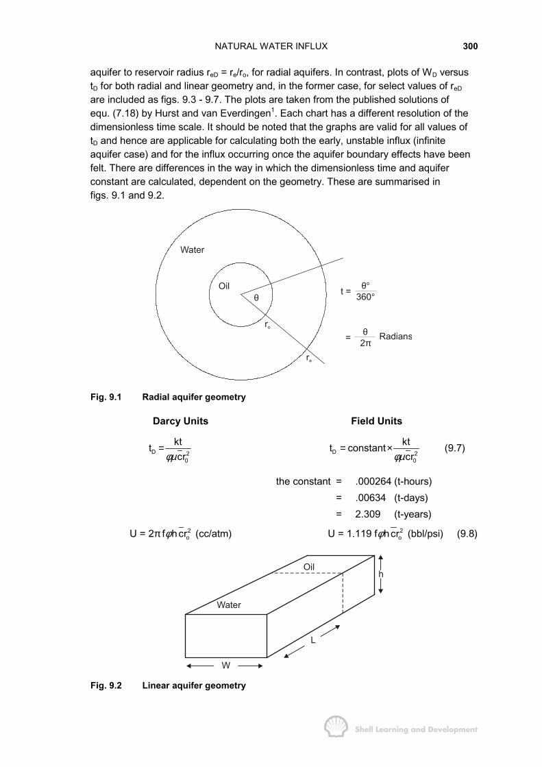
NATURAL WATER INFLUX 300
aquifer to reservoir radius reD = re/ro, for radial aquifers. In contrast, plots of WD versustD for both radial and linear geometry and, in the former case, for select values of reD
are included as figs. 9.3 - 9.7. The plots are taken from the published solutions ofequ. (7.18) by Hurst and van Everdingen1. Each chart has a different resolution of thedimensionless time scale. It should be noted that the graphs are valid for all values oftD and hence are applicable for calculating both the early, unstable influx (infiniteaquifer case) and for the influx occurring once the aquifer boundary effects have beenfelt. There are differences in the way in which the dimensionless time and aquiferconstant are calculated, dependent on the geometry. These are summarised infigs. 9.1 and 9.2.
Water
Oil
ro
re
θθ
°°
360t =
θπ2= Radians
Fig. 9.1 Radial aquifer geometry
Darcy Units Field Units
D 20
kttcrφµ
= Dt = constant20
ktcrφµ
× (9.7)
the constant = .000264 (t-hours)= .00634 (t-days)= 2.309 (t-years)
U = 2π fφh 2ocr (cc/atm) U = 1.119 fφh 2
ocr (bbl/psi) (9.8)
Water
Oilh
L
W
Fig. 9.2 Linear aquifer geometry
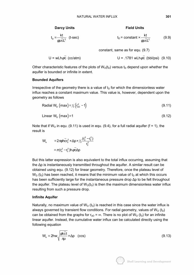
NATURAL WATER INFLUX 301
Darcy Units Field Units
D 2
kttcLφµ
= (t-sec) tD = constant ×2
ktcLφµ
(9.9)
constant, same as for equ. (9.7)
U = wLhφc (cc/atm) U = .1781 wLhφc (bbl/psi) (9.10)
Other characteristic features of the plots of WD(tD) versus tD depend upon whether theaquifer is bounded or infinite in extent.
Bounded Aquifers
Irrespective of the geometry there is a value of tD for which the dimensionless waterinflux reaches a constant maximum value. This value is, however, dependent upon thegeometry as follows
( ) ( )212D eDRadial W max r 1= − (9.11)
( )DLinear W max 1= (9.12)
Note that if WD in equ. (9.11) is used in equ. (9.4), for a full radial aquifer (f = 1), theresult is
2 22 e 01
2e 0 20
2 2e 0
(r r )W 2 hcr pr
(r r )h c p
πφ
π φ
−= ×∆ ×
= − ∆
But this latter expression is also equivalent to the total influx occurring, assuming thatthe ∆p is instantaneously transmitted throughout the aquifer. A similar result can beobtained using equ. (9.12) for linear geometry. Therefore, once the plateau level ofWD (tD) has been reached, it means that the minimum value of tD at which this occurshas been sufficiently large for the instantaneous pressure drop ∆p to be felt throughoutthe aquifer. The plateau level of WD(tD) is then the maximum dimensionless water influxresulting from such a pressure drop.
Infinite Aquifer
Naturally, no maximum value of WD (tD) is reached in this case since the water influx isalways governed by transient flow conditions. For radial geometry, values of WD (tD)can be obtained from the graphs for reD = ∞. There is no plot of WD (tD) for an infinitelinear aquifer. Instead, the cumulative water influx can be calculated directly using thefollowing equation
ekctW 2hw p (ccs)φπµ
= ×∆ (9.13)

NATURAL WATER INFLUX 302
which is expressed in Darcy units. The corresponding equation in field units, with tmeasured in hours, is
3e
kctW 3.26 10 hw x p (bbls)φπµ
−= × ∆ (9.14)
Note that dimensionless time is not used in the above equations.
r = 1.5eD
r = 2.0eD
r = 2.5eD
r = 3.0eD
r= 3
.5eDr
= 4.
0eD
r=
eD
7.06.05.04.03.02.01.000
0.5
1.0
1.5
2.0
2.5
3.0
3.5
4.0
WD
tD
Fig. 9.3 Dimensioniess water influx, constant terminal pressure case, radial flow.(After Hurst and van Everdingen, ref. 1)
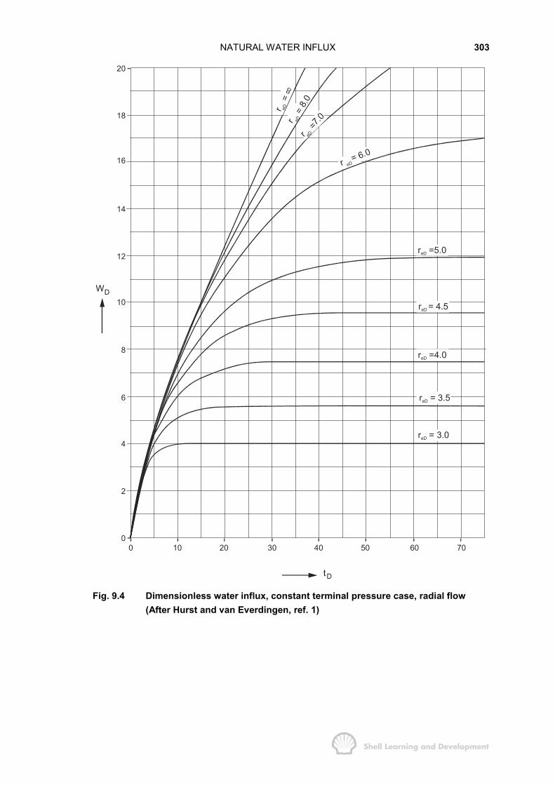
NATURAL WATER INFLUX 303
00
2
4
6
8
10
12
14
16
18
20
10 20 30 40 50 60 70
r = 3.0eD
r = 3.5eD
r =5.0D e
r = 6.0
=7.0r
=8.
0r = 4.5D e
r =4.0eD
r=
8
eD
eD
eD
r eD
WD
tD
Fig. 9.4 Dimensionless water influx, constant terminal pressure case, radial flow(After Hurst and van Everdingen, ref. 1)
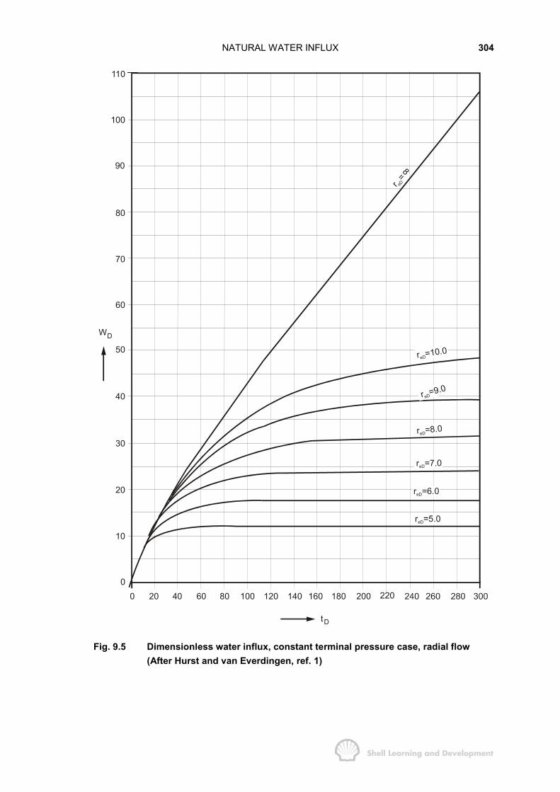
NATURAL WATER INFLUX 304
110
100
90
70
80
60
50
40
30
20
10
00 20 40 60 80 100 120 140 160 180 200
r =5.0eD
r =6.0eD
r =7.0eD
r =8.0eD
r =9.0eD
r =10.0eD
r=
eD
8
WD
tD
Fig. 9.5 Dimensionless water influx, constant terminal pressure case, radial flow(After Hurst and van Everdingen, ref. 1)
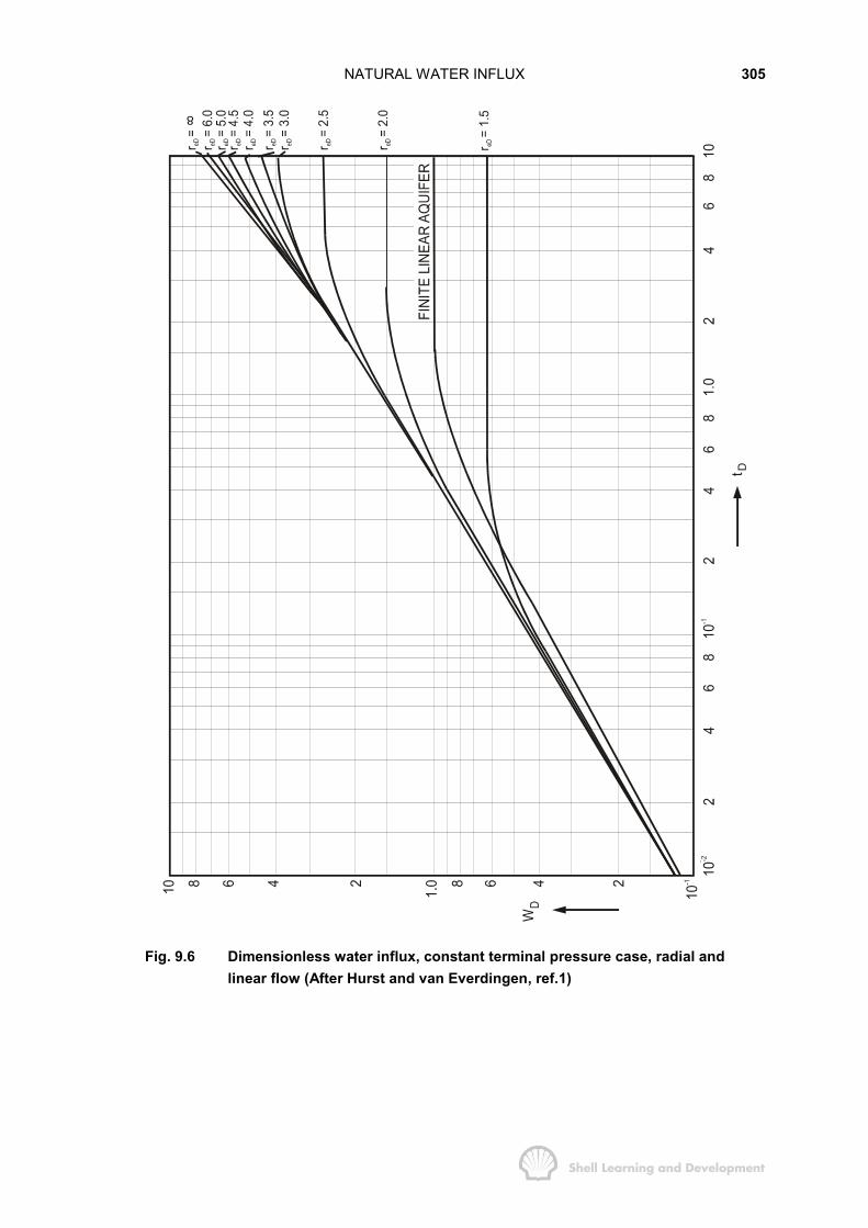
NATURAL WATER INFLUX 305
t D
Fig. 9.6 Dimensionless water influx, constant terminal pressure case, radial andlinear flow (After Hurst and van Everdingen, ref.1)

NATURAL WATER INFLUX 306
USE THIS SCALE FOR LINE reD = (CON’T) ONLY8
102 8 6 4 2 10 8 6 4 2 1 10
24
68
102
46
82
103
24
68
1041010
2
103
r=1
5.0
eD
r= eD
(cont’
d)
8
r=
eD
8
r=2
.5eDr
=3.0
eDr=3
.5eDr
=4.0
eDr=4
.5eDr
=5.0
eDr=7
.0eDr
=7.0
eDr=8
.0eDr
=9.0
eDr=1
0.0
eD r=6
.0eD
WD
t D
Fig. 9.7 Dimensionless water influx, constant terminal pressure case, radial andlinear flow (After Hurst and van Everdingen, ref.1)
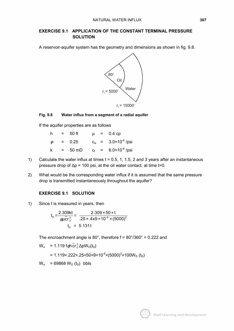
NATURAL WATER INFLUX 307
EXERCISE 9.1 APPLICATION OF THE CONSTANT TERMINAL PRESSURESOLUTION
A reservoir-aquifer system has the geometry and dimensions as shown in fig. 9.8.
r = 5000’o
r = 15000’e
Oil80O
Water
Fig. 9.8 Water influx from a segment of a radial aquifer
If the aquifer properties are as follows
h = 50 ft µ = 0.4 cp
φ = 0.25 cw = 3.0×10⁻⁶ /psi
k = 50 mD cf = 6.0×10⁻⁶ /psi
1) Calculate the water influx at times t = 0.5, 1, 1.5, 2 and 3 years after an instantaneouspressure drop of ∆p = 100 psi, at the oil water contact, at time t=0.
2) What would be the corresponding water influx if it is assumed that the same pressuredrop is transmitted instantaneously throughout the aquifer?
EXERCISE 9.1 SOLUTION
1) Since t is measured in years, then
D 6 220
D
2.309kt 2.309 50 tt.25 .4x9 10 (5000)cr
t 5.131tφµ −
× ×= =× × ×
=
The encroachment angle is 80°, therefore f = 80°/360° = 0.222 and
We = 1.119 fφh 20cr ∆pWD(tD)
= 1.119×.222×.25×50×9×10-6×(5000)2×100WD (tD)
We = 69868 WD (tD) bbls

NATURAL WATER INFLUX 308
Using figs. 9.3 and 9.4 to obtain values of WD(tD); We can be calculated as follows:
t(years)
tD WD (tD)(reD = 3.00)
We
(bbls)
.5 2.6 2.7 1886441.0 5.1 3.5 2445381.5 7.7 3.8 2654982.0 10.3 3.9 2724853.0 15.4 4.0 279472
TABLE 9.1
For dimensionless times greater than tD=15, WD(tD) = 4 and remains constant at thisvalue indicating that the maximum amount of water influx due to the 100 psi pressuredrop is 279500 bbl.
2) If the pressure drop is transmitted instantaneously throughout the aquifer, then
We = ( )2 2e ocf r -rπ hφ ∆p/5.615 bbls
= 9 × 10-6 × .222 × π (150002 − 50002) × 50 × .25 × 100/5.615
We = 279500 bbls
which again is the maximum water influx due to the 100 psi pressure drop. In using theconstant terminal pressure solution, a time scale has been attached to the water influx.
9.3 APPLICATION OF THE HURST, VAN EVERDINGEN WATER INFLUX THEORY INHISTORY MATCHING
In the previous section the cumulative water influx into a reservoir, due to aninstantaneous pressure drop applied at the outer boundary, was expressed as
( )e D DW U p W t= ∆ (9.5)
In the more practical case of history matching the observed reservoir pressure, it isnecessary to extend the theory to calculate the cumulative water influx correspondingto a continuous pressure decline at the reservoir-aquifer boundary. In order to performsuch calculations it is conventional to divide the continuous decline into a series ofdiscrete pressure steps. For the pressure drop between each step, ∆p, thecorresponding water influx can be calculated using equ. (9.5). Superposition of theseparate influxes, with respect to time, will give the cumulative water influx.
The recommended method of approximating the continuous pressure decline, by aseries of pressure steps, is that suggested by van Everdingen, Timmerman andMcMahon3, which is illustrated in fig. 9.9.
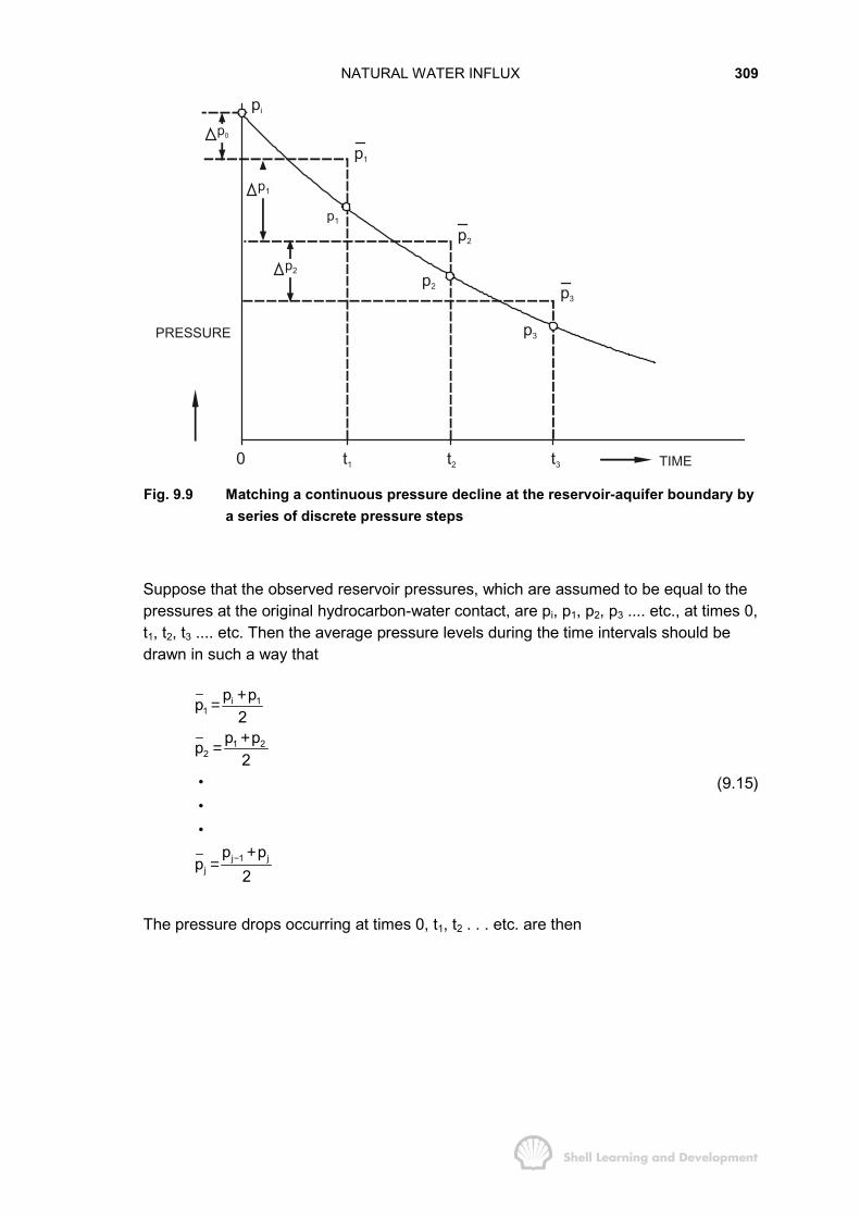
NATURAL WATER INFLUX 309
PRESSURE
TIME
p2
p1
p0
p1
p1
pi
p2
0 t1 t2 t 3
p2
p3
p3
Fig. 9.9 Matching a continuous pressure decline at the reservoir-aquifer boundary bya series of discrete pressure steps
Suppose that the observed reservoir pressures, which are assumed to be equal to thepressures at the original hydrocarbon-water contact, are pi, p1, p2, p3 .... etc., at times 0,t1, t2, t3 .... etc. Then the average pressure levels during the time intervals should bedrawn in such a way that
i 11
1 22
j 1 jj
p pp2
p pp2
p pp
2−
+=
+=
+=
�
�
�
(9.15)
The pressure drops occurring at times 0, t1, t2 . . . etc. are then

NATURAL WATER INFLUX 310
i 1 i 110 i i
i 1 1 2 i 21 21
2 3 1 31 22 32
j 1 j j j 1 j 1 j 1j j 1j
(p p ) p pp p p p2 2
(p p ) (p p ) p pp p p2 2 2
(p p ) p p(p p )p p p2 2 2
(p p ) (p p ) p pp p p
2 2 2
−
− + − ++
+ −∆ = − = =
+ + −∆ = − = − =
+ −+∆ = − = − =
+ + −∆ = − = − =
�
�
�
(9.16)
Therefore, to calculate the cumulative water influx We at some arbitrary time T, whichcorresponds to the end of the nth time step, requires the superposition of solutions oftype, equ. (9.5), to give
We (T) = U [∆poWD (TD)+∆p1 WD (TD - tD1)+ ∆p2 WD (TD - tD2)
+………….∆pjWD (TD - tD j)+…∆pn-1 WD (TD - tD n-1)]
where ∆pj is the pressure drop at time tj, given by equ. (9.16), and WD (TD - tDj) is the
dimensionless cumulative water influx, obtained from figs. 9.3 - 9.7, for the
dimensionless time TD - tDj during which the effect of the pressure drop is felt. Summing
the terms in the latter equation gives
( )j
n 1
e j D D Dj 0
W T U p W (T T )−
=
= ∆ −� (9.17)
In the special case of an infinite, linear aquifer for which, as noted in sec. 9.2, there isno WD function included in figs. 9.3 - 9.7, the cumulative water influx at time T due to astep-like pressure decline at the aquifer-reservoir boundary can be calculated usingequ. (9.13) as
( )n 1
e j jj 0
kcW T 2hw p T tφπµ
−
=
= ∆ −�
which, when expressed in field units has the same constant, 3.26×10⁻³, as equ. (9.14).The following exercise will illustrate the application of the method of superposition inhistory matching.
EXERCISE 9.2 AQUIFER FITTING USING THE UNSTEADY STATE THEORY OFHURST AND VAN EVERDINGEN
A wedge shaped reservoir is suspected of having a fairly strong natural water drive.The geometry of the reservoir-aquifer system is shown in fig. 9.10.
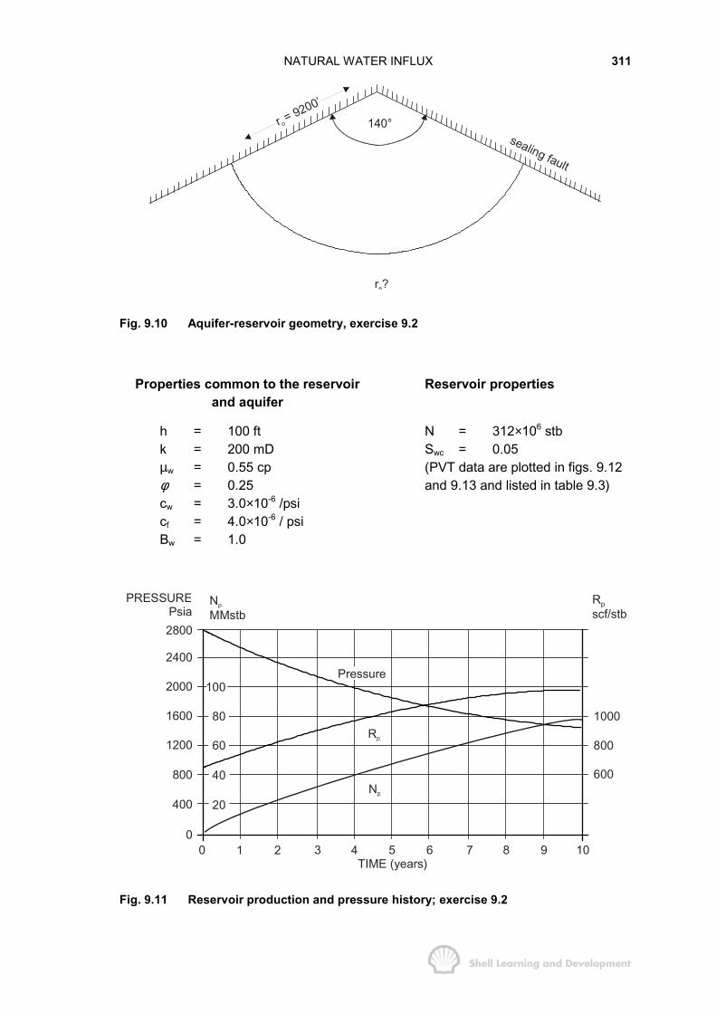
NATURAL WATER INFLUX 311
sealing fault
140°
r ?e
r = 9200’
o
Fig. 9.10 Aquifer-reservoir geometry, exercise 9.2
Properties common to the reservoirand aquifer
Reservoir properties
h = 100 ftk = 200 mDµw = 0.55 cpφ = 0.25cw = 3.0×10⁻⁶ /psicf = 4.0×10⁻⁶ / psiBw = 1.0
N = 312×106 stbSwc = 0.05(PVT data are plotted in figs. 9.12and 9.13 and listed in table 9.3)
TIME (years)0 1 2 3 4 5 6 7 8 9 10
1000
800
600
2800
2400
2000
1600
1200
800
400
0
PsiaPRESSURE Np
MMstbRpscf/stb
Pressure
Rp
Np
100
80
60
40
20
Fig. 9.11 Reservoir production and pressure history; exercise 9.2

NATURAL WATER INFLUX 312
PRESSURE (psia)0 1000 2000 3000
00
500
400
300
200
100
scf/stbRs Bg
rb/scf
0.005
0.004
0.003
0.002
0.001
Bg Rs
0.006600
Fig. 9.12 Rs and Bg as functions of pressure; exercise 9.2
PRESSURE (psia)0 1000 2000 3000
rb/stb1.4
1.3
1.2
Bo
1.1
Fig. 9.13 Bo as a function of pressure; exercise 9.2
Initially the reservoir was at bubble point pressure but apparently there was no initialgas cap (m=0). The graphs of cumulative oil production (Np), cumulative GOR (Rp) andthe average reservoir pressure (p), as functions of time, are shown in fig. 9.11, for thefirst 10 years of production. It may be assumed that the pressure decline at the oilwater contact is the same as the average pressure decline in the reservoir.
It was initially suspected, based on seismic and geological evidence that the value ofreD = re/ro was about 10. Do you consider this to be the correct value of reD based on10 years of production history, and if not, what is your estimate of the correct value ofthis ratio?
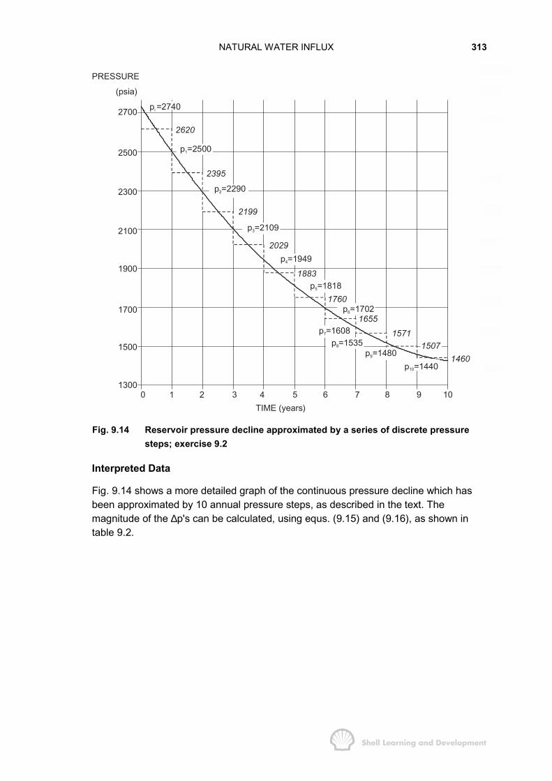
NATURAL WATER INFLUX 313
PRESSURE
(psia)
2700
2500
2300
2100
1900
1700
1500
13000 1 3 4 5 6 7 8 9 10
TIME (years)
2620
p =25001
2395
p =22902
2199
p =21093
2029p =19494
1883p =18185
1760p =17026
1655p =16087 1571
p =15358 1507p =14809 1460
p =144010
p =2740i
Fig. 9.14 Reservoir pressure decline approximated by a series of discrete pressuresteps; exercise 9.2
Interpreted Data
Fig. 9.14 shows a more detailed graph of the continuous pressure decline which hasbeen approximated by 10 annual pressure steps, as described in the text. Themagnitude of the ∆p's can be calculated, using equs. (9.15) and (9.16), as shown intable 9.2.

NATURAL WATER INFLUX 314
Time(years)
Pressure at theO.W.C.(psia)
Plateau Pressurelevels(psia)
∆p(psi)
0 2740 (pi) 1201 2500 2620 2252 2290 2395 1963 2109 2199 1704 1949 2029 1465 1818 1883 1236 1702 1760 1057 1608 1655 848 1635 1571 649 1480 1507 47
10 1440 1460TABLE 9.2
The "end of the year values" of Np, the cumulative oil production, Rp, the cumulativeGOR and PVT properties, corresponding to the pressure points given in column 2 oftable 9.2,are listed in table 9.3.
Time(years)
Np
(MM/stb)Rp
(scf/stb)Bo
(rb/stb)Rs
(scf/stb)Bg
(rb/scf)
0 650 (Rsi) 1.404(Boi) 650 (Rsi) .00093 (Bgi)1 7.88 760 1.374 592 .000982 18.42 845 1.349 545 .001073 29.15 920 1.329 507 .001174 40.69 975 1.316 471 .001285 50.14 1025 1.303 442 .001396 58.42 1065 1.294 418 .001507 65.39 1095 1.287 398 .001608 70.74 1120 1.280 383 .001709 74.54 1145 1.276 381 .00176
10 77.43 1160 1.273 364 .00182TABLE 9.3

NATURAL WATER INFLUX 315
EXERCISE 9.2 SOLUTION
The procedure in tackling this type of problem is as follows.
1) Calculate the water influx using the unsteady state influx theory of Hurst and vanEverdingen for reD = 10.
2) Apply the technique of Havlena and Odeh in interpreting the material balance as theequation of a straight line (refer Chapter 3, sec. 7). For a reservoir with no initial gascap the material balance is
( ) o oi si s g w wc fp o p s g oi e
oi wc
(B B ) (R R )B (c S c )N B R R B NB p WB 1 S
− + −� �+� �+ − = + ∆ +� �� � −
where We is the cumulative water influx (rb). If the entire pressure drop over the10 year period is considered (∆p = 1300 psi) the magnitude of the compressibility termis
6w wc f
wc
(c S c ) (3 .05 4)p 10 1300 0.0061 S .95
−+ × +∆ = × × ∼−
This is only 2% of the maximum value of the term accounting for the expansion of theoil plus its originally dissolved gas (refer table 9.6; (Eo/Boi)max = .3895/1.404 = .277) andtherefore, the pore and water compressibility effects will be neglected. The materialbalance is then reduced to
Np [Bo + (Rp - Rs)Bg] = N [(Bo - Boi) + (Rsi - Rs)Bg] + We
or F = NEo+We
and a plot of F/Eo versus We/Eo should be linear with intercept F/Eo = N when W/Eo = 0and with unit slope.
3) If such a plot is non-linear for reD = 10 , vary the value of this parameter until a straightline is obtained.
1) Calculation of We for reD = 10
Since annual time steps have been selected, the dimensionless time coefficient canmost conveniently be expressed, with t in years and all other parameters in field units,as
D 2o
6 2
2.309kttcr
2.309 200 t 5.67 t.25 .55 7 10 (9200)
φµ
−
=
× ×= =× × × ×
(9.7)
Similarly, the value of the aquifer constant, in field units, is
2oU 1.119f hcrφ= (9.8)
where f =
140°/360° = 0.3889

NATURAL WATER INFLUX 316
i.e. U = 1.119×.3889×.25×100×7×10-6×(9200)2
U = 6446 bbls/psi
Time(years)
dimensionlesstime
∆pj
(psi)WD
(reD = 10)WD
(reD = 5)
0 0 1201 5.67 225 4.95 4.882 11.34 196 8.12 7.463 17.01 170 10.90 9.104 22.68 146 13.50 10.095 28.35 123 15.90 10.836 34.02 105 18.10 11.277 36.69 84 20.20 11.528 45.36 64 22.20 11.699 51.03 47 24.00 11.81
10 56.70 25.70 11.89TABLE 9.4
The water influx can now be calculated, using values of ∆pj and WD listed in table 9.4,as shown in table 9.5.
T(years)
We = U n 1
jj 0
p−
=
∆� WD (TD - tDj) We
(MMrb)
1 6446 (120×4.95) 3.8292 6446 (120×8.12 + 225×4.95) 13.4603 6446 (120×10.90 + 225×8.12 + 196×4.95) 26.4624 6446 (120×13.50 + 225×10.90 + 196×8.12 + 170×4.95) 41.9355 6446 (120×15.90 + 225×13.50 + 196×10.90 + 170×8.12
+ 146×4.95)59.207
6 6446 (120×18.10 + 225×15.90 + 196×13.50 + 170×10.90+ 146×8.12 + 123×4.95)
77.628
7 6446 (120×20.20 + 225×18.10 + 196×15.90 + 170×13.50+ 146×10.90 + 123×8.12 + 105×4.95)
96.805
8 6446 (120×22.20 + 225×20.20 + 196×18.10 + 170×15.90+ 146×13.50 + 123×10.90 + 105×8.12 + 84×4.95)
116.284
9 6446 (120×24.00 + 225×22.20 + 196×20.20 + 170×18.10+ 146×15.90 + 123×13.50 + 105×10.90 + 84×8.12+ 64×4.95)
135.601
10 6446 (120×25.70 + 225×24.00 + 196×22.20 + 170×20.20+ 146×18.10 + 123×15.90 + 105×13.50 + 84×10.90+ 64×8.12 + 47×4.95)
154.401
TABLE 9.5

NATURAL WATER INFLUX 317
2) Material Balance Calculation
F = Np (Bo + (Rp - Rs)Bg)
Eo = ((Bo - Boi) + (Rsi - Rs)Bg)
Time(years)
F(MMrb)
Eo
(rb/stb)F/Eo
(MMstb)We/Eo
(reD = 10)We/Eo
(reD = 5)
1 12.124 .0268 452.4 142.9 140.92 30.761 .0574 535.9 234.5 223.83 52.826 .0.923 5.72.3 286.7 260.34 79.798 .1411 565.5 297.2 253.55 105.964 .1881 563.3 314.8 251.36 132.292 .2380 555.8 326.2 243.87 157.080 .2862 548.8 338.2 236.88 179.177 .3299 543.1 352.5 231.29 196.654 .3630 541.7 373.6 229.7
10 210.743 .3895 541.1 396.4 229.1TABLE 9.6
The plot of F/Eo versus We/Eo, fig. 9.15, shows that the trend deviates below thetheoretical 45° line after the first year. This indicates that the correct value of reD shouldbe somewhat smaller. The calculation has therefore been repeated with reD=5.
3) Calculation of We for reD = 5.
Values of We for reD=5 are listed in table 9.7. These have been calculated using the WD
values listed in column 5 of table 9.4.

NATURAL WATER INFLUX 318
T(years)
We = U n 1
jj 0
p−
=
∆� WD (TD - tDj) We
(MMrb)
1 6446 (120×4.88) 3.7752 6446 (120×7.46 + 225×4.88) 12.8483 6446 (120×9.10 + 225×7.46 + 196×4.88) 24.0244 6446 (120×10.09 + 225×9.10 + 196×7.46 + 170×4.88) 35.7755 6446 (120×10.83 + 225×10.09 + 196×9.10 + 170×7.46
+ 146×4.88)47.276
6 6446 (120×11.27 + 225×10.83 + 196×10.09 + 170×9.10+ 146×7.46 + 123×4.88)
58.035
7 6446 (120×11.52 + 225×11.27 + 196×10.83 + 170×10.09+ 146×9.10 + 123×7.46 + 105×4.88)
67.778
8 6446 (120×11.69 + 225×11.52 + 196×11.27 + 170×10.83+ 146×10.09 + 123×9.10 + 105×7.46 + 84×4.88)
76.259
9 6446 (120×11.81 + 225×11.69 + 196×11.52 + 170×11.27+ 146×10.83 + 123×10.09 + 105×9.10 + 84×7.46+ 64×4.88)
83.398
10 6446 (120×11.89 + 225×11.81 + 196×11.69 + 170×11.52+ 146×11.27 + 123×10.83 + 105×10.09 + 84×9.10+ 64×7.46 + 47×4.88)
89.225
TABLE 9.7
The corresponding values of We/Eo, required for the material balance calculations, arelisted in table 9.6 and plotted in fig. 9.15. As can be seen, in this case, all the points lieon the straight line of unit slope which intercepts the ordinate at Np = 312 MMstb, thusconfirming that reD = 5 is the correct value of the ratio of the aquifer/reservoir radius.
Also apparent from this plot is the fact that after the third year there occurs a reversal inthe trend of plotted points with both We/ Eo and F/Eo decreasing with time. Havlena andOdeh have pointed out4,5 that this reversal is to be expected for a finite acting aquiferbut nevertheless all points, for the correct value of reD, must lie on the linear trend. Forthe incorrect aquifer model (reD = 10), however, the calculated values of We/Eo
continually increase as F/Eo decrease, as illustrated in fig. 9.15.
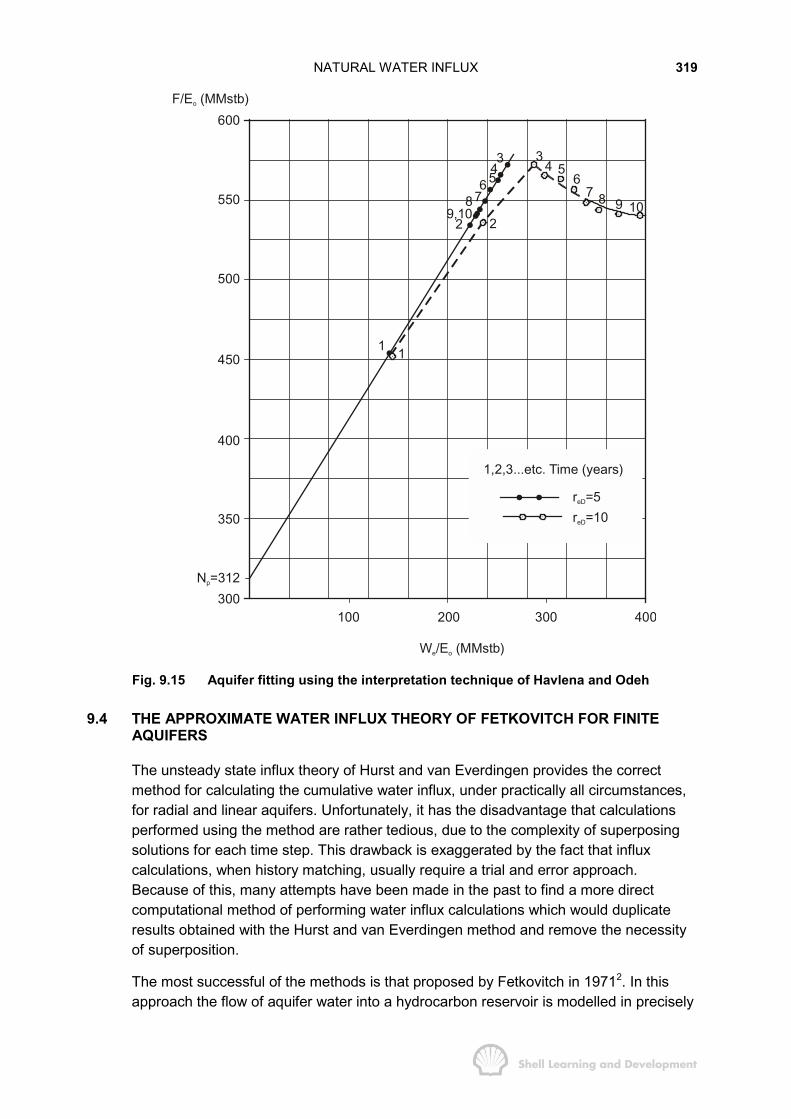
NATURAL WATER INFLUX 319
1
2
34 5
67 8 9
9,10
600
550
500
450
400
350
N =312p
300
F/E (MMstb)o
100 200 300 400
W /E (MMstb)e o
1,2,3...etc. Time (years)
r =5eD
r =10eD
108
3456
7
2
1
Fig. 9.15 Aquifer fitting using the interpretation technique of Havlena and Odeh
9.4 THE APPROXIMATE WATER INFLUX THEORY OF FETKOVITCH FOR FINITEAQUIFERS
The unsteady state influx theory of Hurst and van Everdingen provides the correctmethod for calculating the cumulative water influx, under practically all circumstances,for radial and linear aquifers. Unfortunately, it has the disadvantage that calculationsperformed using the method are rather tedious, due to the complexity of superposingsolutions for each time step. This drawback is exaggerated by the fact that influxcalculations, when history matching, usually require a trial and error approach.Because of this, many attempts have been made in the past to find a more directcomputational method of performing water influx calculations which would duplicateresults obtained with the Hurst and van Everdingen method and remove the necessityof superposition.
The most successful of the methods is that proposed by Fetkovitch in 19712. In thisapproach the flow of aquifer water into a hydrocarbon reservoir is modelled in precisely

NATURAL WATER INFLUX 320
the same way as the flow of oil from a reservoir into a well. An inflow equation of theform
eaw
dWq J(p p)dt
= = − (9.18)
is used where,
qw = water influx rate
J = aquifer productivity index
p = reservoir pressure, i.e. pressure at the oil or gas water contact.
ap = average pressure in the aquifer.
The latter is evaluated using the simple aquifer material balance
We=c Wi (pi - p a) (9.19)
in which pi is the initial pressure in the aquifer and reservoir. This balance can bealternatively expressed as
e ea i i
eii i
W Wp p 1 p 1WcWp
� � � �= − = −� � � �� �
� �� �(9.20)
where Wei = c Wipi is defined as the initial amount of encroachable water andrepresents the maximum possible expansion of the aquifer. Differentiating equ. (9.20)with respect to time gives
e ei a
i
dpdW Wdt p dt
= − (9.21)
and substituting equ. (9.21) into equ. (9.18) and separating the variables gives
a i
eia
dp Jp dtWp p
= −−
This equation will now be integrated for the initial condition that at t=0 (We = 0, ap = pi)a pressure drop ∆p = pi - p is imposed at the reservoir boundary. Furthermore, theboundary pressure p remains constant during the period of interest so that
( ) ia
ei
Jp tln p p CW
− = − +
where C is an arbitrary constant of integration which can be evaluated from the initialconditions as C = In(pi - p), and therefore
( ) i eia i
Jp t / Wp p p p e−− = − (9.22)
NATURAL WATER INFLUX 321
which on substituting in the inflow equation (9.18) gives
e i eii
dW Jp t / WJ(p p)edt
−= − (9.23)
Finally, integrating equ. (9.23) for the stated initial conditions yields the followingexpression for the cumulative water influx
ei i eie i
i
W Jp t / WW (p p)(1 e )p
−= − − (9.24)
What can be observed immediately from this expression is that as t tends to infinity,then
eie i
i
i i
WW (p p)p
cW (p p)
−=
= −
which is the maximum amount of water influx that could occur once the pressure droppi - p has been transmitted throughout the aquifer.
As it stands, equ. (9.24) is not particularly useful since it was derived for a constantinner boundary pressure. To use this solution in the practical case, in which theboundary pressure is varying continuously as a function of time, it should again benecessary to apply the superposition theorem. Fetkovitch has shown, however, that adifference form of equ. (9.24) can be used which eliminates the need for superposition.That is, for the influx during the first time step ∆t1, equ. (9.24) can be expressed as
( )1ei i 1 ei
1e ii
W Jp t / WW p p (1 e )p
− ∆∆ = − − (9.25)
where 1p is the average reservoir boundary pressure during the first time interval. Forthe second interval ∆t2
( )12ei i 2 ei
a 2ei
W Jp t / WW p p (1 e )p
− ∆∆ = − − (9.26)
where 1ap is the average aquifer pressure at the end of the first time interval and is
evaluated using equ. (9.20) as
i1
i
ea i
e
Wp p 1
W� �∆
= −� �� �� �
(9.27)
In general for the nth time period,
( )n 1nei i n ei
a nei
W Jp t / WW p p (1 e )p −
− ∆∆ = − − (9.28)
where
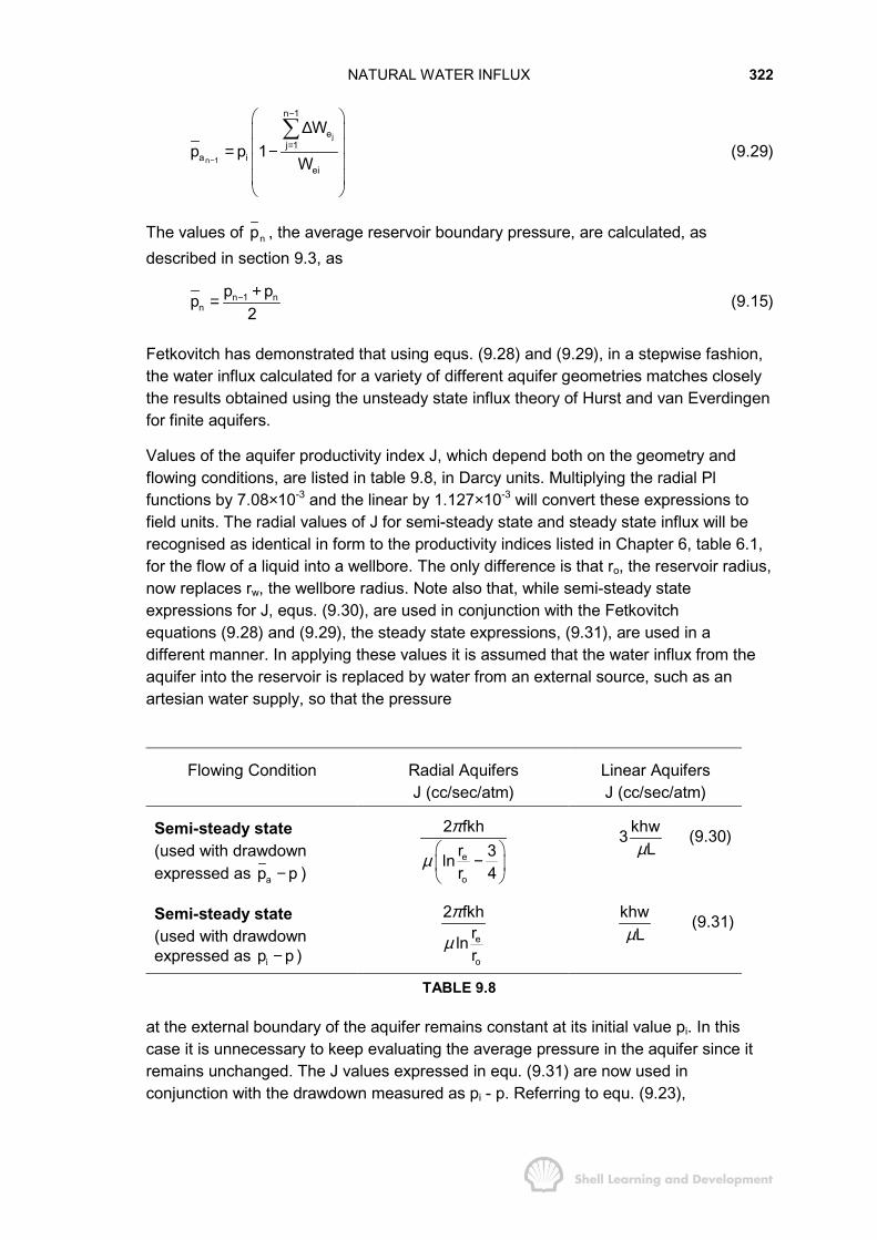
NATURAL WATER INFLUX 322
j
n 1
n 1
ej 1
a iei
Wp p 1
W−
−
=
� �∆� �� �= −� �� �� �
�(9.29)
The values of np , the average reservoir boundary pressure, are calculated, asdescribed in section 9.3, as
n 1 nn
p pp2
− += (9.15)
Fetkovitch has demonstrated that using equs. (9.28) and (9.29), in a stepwise fashion,the water influx calculated for a variety of different aquifer geometries matches closelythe results obtained using the unsteady state influx theory of Hurst and van Everdingenfor finite aquifers.
Values of the aquifer productivity index J, which depend both on the geometry andflowing conditions, are listed in table 9.8, in Darcy units. Multiplying the radial Plfunctions by 7.08×10⁻³ and the linear by 1.127×10⁻³ will convert these expressions tofield units. The radial values of J for semi-steady state and steady state influx will berecognised as identical in form to the productivity indices listed in Chapter 6, table 6.1,for the flow of a liquid into a wellbore. The only difference is that ro, the reservoir radius,now replaces rw, the wellbore radius. Note also that, while semi-steady stateexpressions for J, equs. (9.30), are used in conjunction with the Fetkovitchequations (9.28) and (9.29), the steady state expressions, (9.31), are used in adifferent manner. In applying these values it is assumed that the water influx from theaquifer into the reservoir is replaced by water from an external source, such as anartesian water supply, so that the pressure
Flowing Condition Radial AquifersJ (cc/sec/atm)
Linear AquifersJ (cc/sec/atm)
Semi-steady state(used with drawdownexpressed as ap p− )
e
o
2 fkhr 3lnr 4
π
µ� �
−� �� �
khw3Lµ
(9.30)
Semi-steady state(used with drawdownexpressed as ip p− )
e
o
2 fkhrlnr
π
µ
khwLµ
(9.31)
TABLE 9.8
at the external boundary of the aquifer remains constant at its initial value pi. In thiscase it is unnecessary to keep evaluating the average pressure in the aquifer since itremains unchanged. The J values expressed in equ. (9.31) are now used inconjunction with the drawdown measured as pi - p. Referring to equ. (9.23),
NATURAL WATER INFLUX 323
e i eiw i
dW Jp t / Wq J(p p)edt
−= = − (9.23)
the steady state case implies that Wei, the encroachable water, is infinite and therefore
ew i
dWq J(p p)dt
= = − (9.32)
which, upon integration, gives the cumulative water influx as
t
e i0
W J (p p)dt= −� (9.33)
Equs. (9.32) and (9.33), which are a special case of Fetkovitch's theory, were firstpresented in 1936 by Schilthuis6 and described as steady state influx equations.Equation (9.33) can be evaluated in stepwise fashion in which values of np , the innerboundary pressure during the nth time period, are calculated using equ. (9.15).
The reader should also be aware that the PI expressions presented in table 9.8 werederived in similar form in Chapter 6, sec. 2, under the assumption that (rw/re)2 wasapproximately zero. For small radial aquifers, the equivalent assumption that (ro/re)2 isnegligible may not always be applicable and the correct PI expression should then beobtained by solving the radial diffusivity equation, using exactly the same steps asshown in Chapter 6 but, without neglecting such terms. Considering the inherentuncertainties in aquifer fitting this approach is generally unnecessary and, in fact,Fetkovitch has demonstrated an almost perfect match between his results and those ofHurst and van Everdingen for values of reD as small as three.
For the case of a reservoir asymmetrically situated within a non-circular shaped aquiferit should, with tolerable accuracy, be possible to use the Dietz shape factors presentedin fig. 6.4, and described in Chapter 7, sec. 7, to modify the semi-steady state PIexpressions. Thus the radial PI in equ. (9.30) can be generalised as
2A o
2 fkhJ 4Aln2 C r
πµ
γ
=
which has precisely the same form as equ. (6.22).
For very large aquifers, the initial flow of water into the reservoir will be governed bytransient flow conditions. In this case, it takes a finite time for the initial pressuredisturbance at the reservoir-aquifer boundary to feel the effect of the outer boundary ofthe aquifer. Unfortunately, during this transient flow period it is no longer possible, inanalogy with wellbore equations, to derive a simple expression for the productivityindex J. This is because for inflow into a reservoir it is incorrect to use the approximateline source solution of the radial diffusivity equation, in an attempt to evaluate a PIunder transient conditions, since ro is always finite and the boundary conditions for thistype of solution, expressed in equ. (7.1), can no longer be justified. Therefore, themethod of Fetkovitch cannot be used for the description of influx from an infinite aquifer
NATURAL WATER INFLUX 324
and, when dealing with very large, finite aquifers, it is initially still necessary to applythe unsteady state influx theory of Hurst and van Everdingen for the first few timesteps. The following example will illustrate the speed and accuracy in using the methodof Fetkovitch in comparison to that of Hurst and van Everdingen. In addition, it willdemonstrate how the two methods can be combined when dealing with a large aquifer,reD = 10, in which, for the first few years, the influx occurs under transient flowconditions.
EXERCISE 9.3 WATER INFLUX CALCULATIONS USING THE METHOD OFFETKOVITCH
Recalculate the cumulative water influx as a function of time, using all the reservoir andaquifer data presented in exercise 9.2, but applying the method of Fetkovitch. Performthe calculations for both reD = 5 and 10.
EXERCISE 9.3 SOLUTION
Using the method of Fetkovitch the following two equations are required
j
n 1
n 1
ej 1
a iei
Wp p 1
W−
−
=
� �∆� �� �= −� �� �� �
�(9.29)
and
n 1nei i n ei
a nei
W Jp t / WW (p p )(1 e )p −
− ∆∆ = − − (9.28)
wheren-1ap is the average pressure in the aquifer at the end of the (n - 1)th time
interval
and np is the average reservoir-aquifer boundary pressure during the nth timeinterval.
Since in this present application a history match is being sought for available reservoirpressures, that is, values of np which are listed in column 3 of table 9.2 in the previousexercise, the manner of solving the above equations, to explicitly calculate thecumulative water influx, is as follows
- having obtained ∆Wen-1 1for the n - 1th time step
then Wen-1= j
n 1
ej 1
W−
=
∆�
- using equ. (9.29), evaluate n 1ap
−
- insert n 1ap
−in equ. (9.28) and solve for ∆Wen
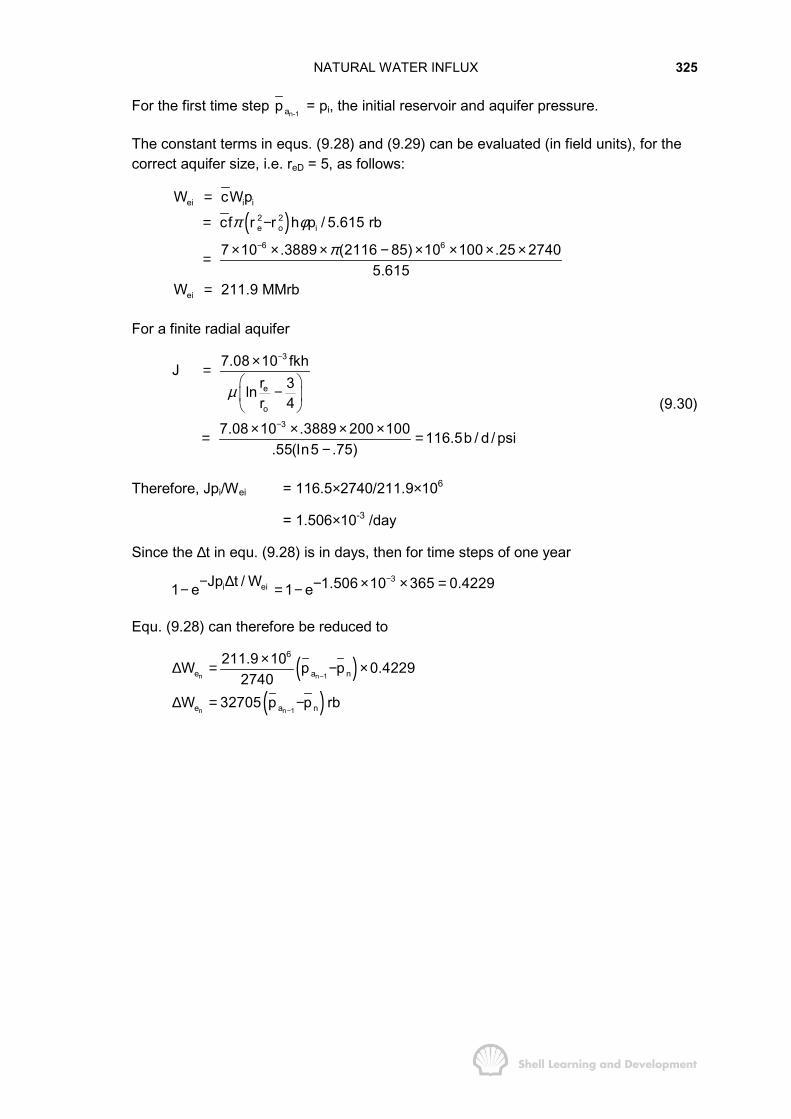
NATURAL WATER INFLUX 325
For the first time step n-1ap = pi, the initial reservoir and aquifer pressure.
The constant terms in equs. (9.28) and (9.29) can be evaluated (in field units), for thecorrect aquifer size, i.e. reD = 5, as follows:
( )ei i i
2 2e o i
6 6
ei
W cWp
cf r r h p / 5.615 rb
7 10 .3889 (2116 85) 10 100 .25 27405.615
W 211.9 MMrb
π φ
π−
=
= −
× × × − × × × ×=
=
For a finite radial aquifer
3
e
o
3
7.08 10 fkhJr 3lnr 4
7.08 10 .3889 200 100 116.5b / d / psi.55(In5 .75)
µ
−
−
×=� �
−� �� �
× × × ×= =−
(9.30)
Therefore, Jpi/Wei = 116.5×2740/211.9×106
= 1.506×10⁻³ /day
Since the ∆t in equ. (9.28) is in days, then for time steps of one year3
i eiJp t / W 1.506 10 365 0.42291 e 1 e−− ∆ − × × =− = −
Equ. (9.28) can therefore be reduced to
( )( )
n n 1
n n 1
6
e a n
e a n
211.9 10W p p 0.42292740
W 32705 p p rb
−
−
×∆ = − ×
∆ = −
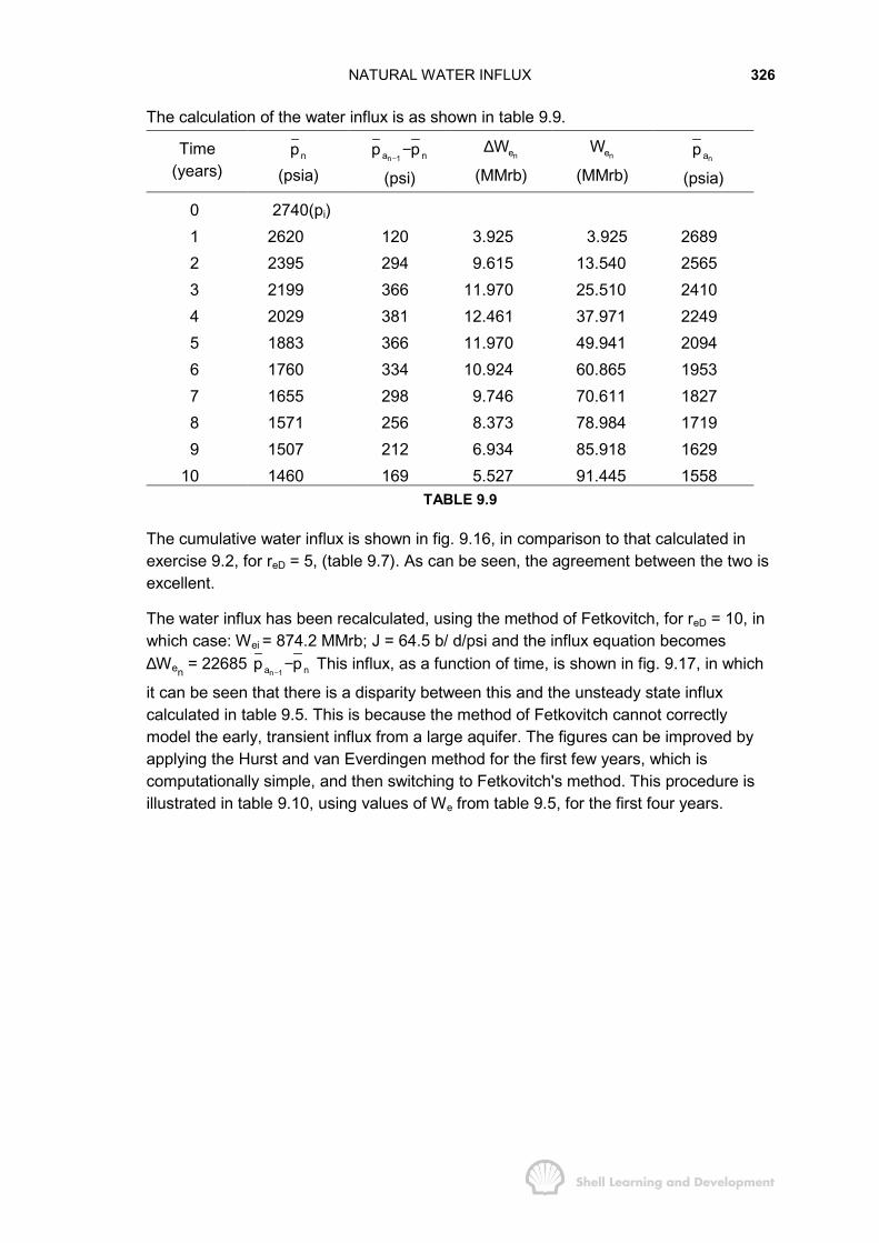
NATURAL WATER INFLUX 326
The calculation of the water influx is as shown in table 9.9.
Time(years)
np(psia)
n 1a np p−
−
(psi)neW∆
(MMrb)neW
(MMrb)nap
(psia)
0 2740(pi)1 2620 120 3.925 3.925 26892 2395 294 9.615 13.540 25653 2199 366 11.970 25.510 24104 2029 381 12.461 37.971 22495 1883 366 11.970 49.941 20946 1760 334 10.924 60.865 19537 1655 298 9.746 70.611 18278 1571 256 8.373 78.984 17199 1507 212 6.934 85.918 1629
10 1460 169 5.527 91.445 1558TABLE 9.9
The cumulative water influx is shown in fig. 9.16, in comparison to that calculated inexercise 9.2, for reD = 5, (table 9.7). As can be seen, the agreement between the two isexcellent.
The water influx has been recalculated, using the method of Fetkovitch, for reD = 10, inwhich case: Wei = 874.2 MMrb; J = 64.5 b/ d/psi and the influx equation becomes∆Wen = 22685
n 1a np p−
− This influx, as a function of time, is shown in fig. 9.17, in which
it can be seen that there is a disparity between this and the unsteady state influxcalculated in table 9.5. This is because the method of Fetkovitch cannot correctlymodel the early, transient influx from a large aquifer. The figures can be improved byapplying the Hurst and van Everdingen method for the first few years, which iscomputationally simple, and then switching to Fetkovitch's method. This procedure isillustrated in table 9.10, using values of We from table 9.5, for the first four years.
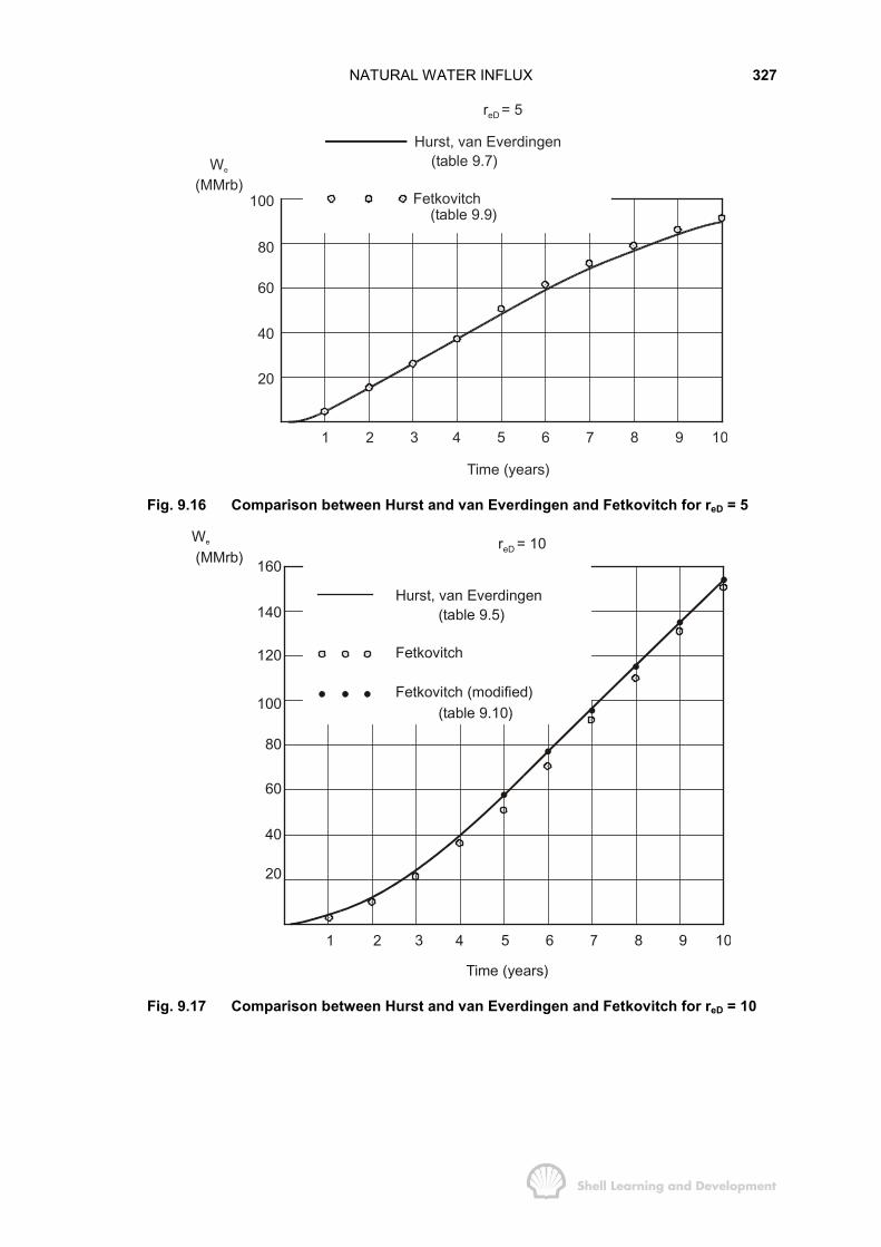
NATURAL WATER INFLUX 327
r = 5eD
We
(MMrb)100
80
60
40
20
1 2 3 4
Hurst, van Everdingen(table 9.7)
5 6 7 8 9 10
Fetkovitch(table 9.9)
Time (years)
Fig. 9.16 Comparison between Hurst and van Everdingen and Fetkovitch for reD = 5
160
120
100
80
60
40
20
1
140
2 3 4 5 6 8 109
We
(MMrb)r = 10eD
Hurst, van Everdingen(table 9.5)
Fetkovitch
Fetkovitch (modified)(table 9.10)
Time (years)
Fig. 9.17 Comparison between Hurst and van Everdingen and Fetkovitch for reD = 10
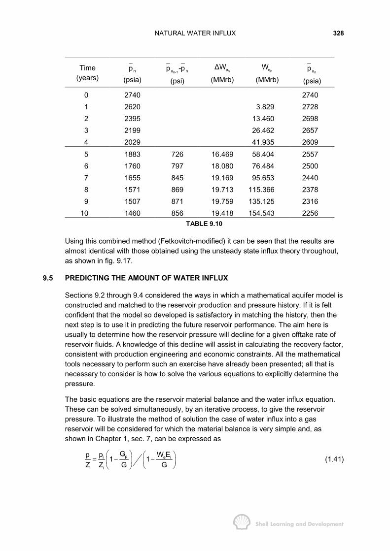
NATURAL WATER INFLUX 328
Time(years)
np(psia)
n-1a np -p
(psi)ne∆W
(MMrb)neW
(MMrb)nap
(psia)
0 2740 27401 2620 3.829 27282 2395 13.460 26983 2199 26.462 26574 2029 41.935 26095 1883 726 16.469 58.404 25576 1760 797 18.080 76.484 25007 1655 845 19.169 95.653 24408 1571 869 19.713 115.366 23789 1507 871 19.759 135.125 2316
10 1460 856 19.418 154.543 2256TABLE 9.10
Using this combined method (Fetkovitch-modified) it can be seen that the results arealmost identical with those obtained using the unsteady state influx theory throughout,as shown in fig. 9.17.
9.5 PREDICTING THE AMOUNT OF WATER INFLUX
Sections 9.2 through 9.4 considered the ways in which a mathematical aquifer model isconstructed and matched to the reservoir production and pressure history. If it is feltconfident that the model so developed is satisfactory in matching the history, then thenext step is to use it in predicting the future reservoir performance. The aim here isusually to determine how the reservoir pressure will decline for a given offtake rate ofreservoir fluids. A knowledge of this decline will assist in calculating the recovery factor,consistent with production engineering and economic constraints. All the mathematicaltools necessary to perform such an exercise have already been presented; all that isnecessary to consider is how to solve the various equations to explicitly determine thepressure.
The basic equations are the reservoir material balance and the water influx equation.These can be solved simultaneously, by an iterative process, to give the reservoirpressure. To illustrate the method of solution the case of water influx into a gasreservoir will be considered for which the material balance is very simple and, asshown in Chapter 1, sec. 7, can be expressed as
p e ii
i
G W Epp 1 1Z Z G G
� � � �= − −� � � �� �� �
(1.41)
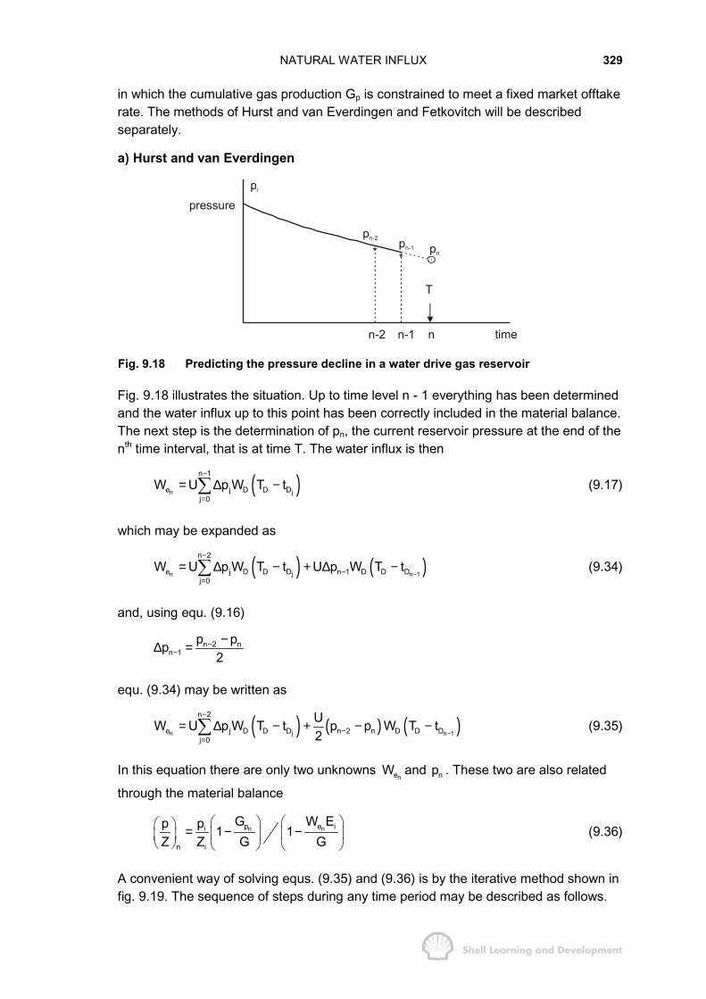
NATURAL WATER INFLUX 329
in which the cumulative gas production Gp is constrained to meet a fixed market offtakerate. The methods of Hurst and van Everdingen and Fetkovitch will be describedseparately.
a) Hurst and van Everdingen
pressure
pn-2 pn-1
n-2 n-1 n
T
time
pn
pi
**
Fig. 9.18 Predicting the pressure decline in a water drive gas reservoir
Fig. 9.18 illustrates the situation. Up to time level n - 1 everything has been determinedand the water influx up to this point has been correctly included in the material balance.The next step is the determination of pn, the current reservoir pressure at the end of thenth time interval, that is at time T. The water influx is then
( )n j
n 1
e j D D Dj 0
W U p W T t−
=
= ∆ −� (9.17)
which may be expanded as
( ) ( )n j n 1
n 2
e j D D D n 1 D D Dj 0
W U p W T t U p W T t−
−
−=
= ∆ − + ∆ −� (9.34)
and, using equ. (9.16)
n 2 nn 1
p pp2
−−
−∆ =
equ. (9.34) may be written as
( ) ( ) ( )n j n 1
n 2
e j D D D n 2 n D D Dj 0
UW U p W T t p p W T t2 −
−
−=
= ∆ − + − −� (9.35)
In this equation there are only two unknowns neW and np . These two are also related
through the material balance
n np e ii
in
G W Epp 1 1Z Z G G
� � � �� � = − −� � � �� �� � � � � �
(9.36)
A convenient way of solving equs. (9.35) and (9.36) is by the iterative method shown infig. 9.19. The sequence of steps during any time period may be described as follows.

NATURAL WATER INFLUX 330
k = 1
Time step = n
ni
n 2pi i
j D D Din j
Gp Ep 1 1 U p W (T t )Z Z G G
−
=α
� �� �� �� �= − − ∆ −� �� � � � � �� � � � � �
�k
npk
n j n 1
n 2
e j D D D n 2 n D D Dj 0
UW U p W (T t ) (p p )W (T t )2 −
−
−=
= ∆ − + − −�kk
neWk
k= 1k+
-1n np p=k k
n=n+1
n np e ii
in
G W Epp 1 1Z Z G G
� �� �� � � �= − −� �� � � � � �� � � � � �
kk
npk
k = 1
k
1n np p TOL−− −k k- +
k = iteration counterTOL = tolerance pressure
difference (psi)
0
Fig. 9.19 Prediction of gas reservoir pressures resulting from fluid withdrawal andwater influx (Hurst and van Everdingen)
Make an initial estimate of the reservoir pressure pnk = pn
1 at the end of time step n byevaluating the material balance equation with the water influx initially set equal to
( )n j
n 21
e j D D Dj 0
W U p W T t−
=
= ∆ −� (9.37)
i.e. neglecting the final term U∆pn-1 WD (TD – tDn-1) in equ. (9-35).
Note: one could also use the value of n 1eW
−, the water influx after time step n-1, in the
material balance but equ. (9.37) is usually closer to the actual influx and will lead to asmaller number of iterations.
NATURAL WATER INFLUX 331
− Insert this initial estimate of pn1, which is admittedly too small, in the water influx
equation thus calculating a new value of Wen1, which will now be too large.
− Rework the material balance with this new value of n
1eW , giving 1
np which must
now be too large.
− Iterate finding n
2 2e n(W ,p ),
n
3 3e n(W ,p ) . . . etc. until the difference between
successive values of pnk is less than some tolerance level, at which point the
procedure is repeated for the next time step.
b) Fetkovitch
The iterative solution technique can again be applied but in this case the equationsused are (9.28) and (9.29).
Aquifer material balance
n-1n 1
ea i
ei
Wp p 1
W−
� �= −� �� �
� �
Water influx
( )( )n 1n
k kei i n ei12ae n 1 n
i
W Jp t / WW p p p (1 e )p − −
− ∆∆ = − + −
n j n
n 1k k
e e ej 1
W W W−
=
= ∆ + ∆�
Reservoir material balance
n n
kkp e ii
in
G W Epp 1 1Z Z G G
� �� �� �� �= − −� �� � � �� � � � � �
A flow chart showing the sequence of steps is included as fig. 9.20. An exampleillustrating this technique is presented in Fetkovitch's paper.2

NATURAL WATER INFLUX 332
Time step = n
n 1
n 1
eia
ei
Wp p 1
W−
−
� �� �= −� �� �
k = 1
n n 1p e ii
i
G W Epp 1 1Z Z G G
−� � � �� � = − −� � � �� � � � � �� � � � � �
k
n
n n 1
ei 1e n 1 na 2
i
Jp t /Wni eiWW (p (p p )) 1 ep − −
− ∆� �∆ = − + −� �� �
k k
n n 1 ne e eW W W−
= + ∆k k pnk = pn
k-1
n=n 1 +
pnk
pnk
k k= 1 +
k = 1k
n np e ii
i
G W Epp 1 1Z Z G G
� �� �� � � �= − −� �� � � � � �� � � � � �
kk
n
-1n np p TOL− −k k
k = iteration counterTOL = tolerance pressure
difference (psi)
- +
Fig. 9.20 Prediction of gas reservoir pressures resulting from fluid withdrawal andwater influx (Fetkovitch)
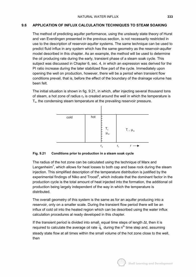
NATURAL WATER INFLUX 333
9.6 APPLICATION OF INFLUX CALCULATION TECHNIQUES TO STEAM SOAKING
The method of predicting aquifer performance, using the unsteady state theory of Hurstand van Everdingen presented in the previous section, is not necessarily restricted inuse to the description of reservoir-aquifer systems. The same technique can be used topredict fluid influx in any system which has the same geometry as the reservoir-aquifermodel described in this chapter. As an example, the method will be used to determinethe oil producing rate during the early, transient phase of a steam soak cycle. Thissubject was discussed in Chapter 6, sec. 4, in which an expression was derived for thePI ratio increase during the later stabilized flow part of the cycle. Immediately uponopening the well on production, however, there will be a period when transient flowconditions prevail, that is, before the effect of the boundary of the drainage volume hasbeen felt.
The initial situation is shown in fig. 9.21, in which, after injecting several thousand tonsof steam, a hot zone of radius rh is created around the well in which the temperature isTs, the condensing steam temperature at the prevailing reservoir pressure.
cold hot
Ts
µoh
T , r µoc
rw rh r
Fig. 9.21 Conditions prior to production in a steam soak cycle
The radius of the hot zone can be calculated using the technique of Marx andLangenheim7, which allows for heat losses to both cap and base rock during the steaminjection. This simplified description of the temperature distribution is justified by theexperimental findings of Niko and Troost8, which indicate that the dominant factor in theproduction cycle is the total amount of heat injected into the formation, the additional oilproduction being largely independent of the way in which the temperature isdistributed.
The overall geometry of this system is the same as for an aquifer producing into areservoir, only on a smaller scale. During the transient flow period there will be aninflux of cold oil into the heated region which can be described using the water influxcalculation procedures al ready developed in this chapter.
If the transient period is divided into small, equal time steps of length ∆t, then it isrequired to calculate the average oil rate nq during the nth time step and, assumingsteady state flow at all times within the small volume of the hot zone close to the well,then

NATURAL WATER INFLUX 334
( )n wf,non
hoh
w
2 k h p pq rln
r
π
µ
−= (9.38)
which is a re-formulation of the steady state inflow equation presented in table 6.1. Theoil viscosity, µoh is a function of the average temperature in the hot zone during the nth
time interval. The temperature will decline continuously during production as heat islost by conduction to the cap and base rock and by convection through the producedfluids. A simple method for predicting the temperature decline allowing for both effectshas been presented by Boburg and Lantz9. The pressure np in equ. (9.38) is theaverage pressure during the time step at rh, the outer boundary of the hot zone, and
wf,np the average wellbore pressure during the same period. If it is assumed that thepressure declines at rh and rw can be approximated by a series of discrete pressuresteps then, in accordance with equ. (9.15), np and wf,np can be expressed as
( )12n n 1 np p p−= + (9.39)
and
( )12wf,n wf,n 1 wf,np p p−= + (9.40)
where pn and pwf,n are the pressures at rh and rw respectively at the end of the nth timestep. The cumulative oil influx across the boundary rh by the end of the time step will be
np,n p,n 1N N q . t−= + ∆
in which Np,n-l is the known influx at the end of the (n - 1)th time step. Using equs. (9.39)and (9.40), the influx can be expressed as
( )p,n p,n 1 n 1 n wf,n 1 wf,nN N p p p p2α
− − −= + + − − (9.41)
where
o
hoh
w
2 k h trlnr
παµ
∆=
An expression for the cumulative oil influx can also be obtained using the unsteadystate influx theory of Hurst and van Everdingen in the manner similar to that ofequ. (9.34)
( ) ( )j n 1
n 2
p,n j D D D n 1 D D Dj 0
N U p W T t U p W T t−
−
−=
= ∆ − + ∆ −� (9.42)
in which T = n. ∆t and WD is the dimensionless influx function of Hurst and vanEverdingen, figs. 9.3-9.7. U is the aquifer constant defined in equ. (9.6), only in thiscase applied to the oil reservoir for which f = 1, and the radius ro is replaced by rh.
NATURAL WATER INFLUX 335
Values of the pressure drop ∆pj at the hot zone boundary can be evaluated usingequ. (9.16) as
( )12i j 1 j 1p p p− +∆ = − (9.16)
and in particular
( )12n 1 n 2 np p p− −∆ = −
therefore, equ. (9.42) can be written as
( ) ( )j
n 2
p,n j D D D n 2 nj 0
N U p W T t p p2β−
−=
= ∆ − + −� (9.43)
where β = U WD (TD−tDn -1)
Equations (9.41) and (9.43) can now be equated and solved explicitly for the boundarypressure pn at rh at the end of the nth time step, i.e.
( ) ( ) ( )j
n 2
n j D D D p,n 1 n 2 wf,n 1 wf,n n 1j 0
1p 2U p W T t 2N p p p pβ αα β
−
= − − − −=
� �∆ − − + + + −� �+ � �
� (9.44)
Providing that the manner in which the bottom hole flowing pressure will be allowed todecline is specified, then everything on the right hand side of equ. (9.44) is determined,thus pn can be calculated and subsequently np using equ. (9.39). Finally, substitutingthis value of np in equ.(9.38) will lead to the determination of nq . In fact, it is necessaryto iterate on this oil rate to correctly model the heat loss due to convection, since, asmentioned already, the temperature in the hot zone, which determines the oil viscosityin equ. (9.38), is reduced due to the removal of heat by the produced oil. Thisconvective heat loss is directly proportional to the production rate and therefore, the oilrate and viscosity are dependent upon one another necessitating the iterative solutiontechnique.
Bentsen and Donohue10 have reported the use of the above technique incorporated ina dynamic programming model for optimising steam soak operations.
REFERENCES
1) van Everdingen, A.F. and Hurst, W., 1949.TheApplication of the LaplaceTransformation to Flow Problems in Reservoirs. Trans. AIME. 186: 305-324.
2) Fetkovitch, M.J., 1971. A Simplified Approach to Water Influx Calculations-FiniteAquifer Systems. J.Pet.Tech., July: 814-828.
3) van Everdingen, A.F., Timmerman, E.H. and McMahon, J.J., 1953. Application ofthe Material Balance Equation to a Partial Water-Drive Reservoir. Trans. AIME.198:51.
4) Havlena, D. and Odeh, A.S., 1963. The Material Balance as an Equation of aStraight Line. J.Pet.Techn, August: 896-900. Trans. AIME.
NATURAL WATER INFLUX 336
5) Havlena, D. and Odeh, A.S.,1964. The Material Balance as an Equation of aStraight Line-Part II, Field Cases. J.Pet.Tech., July: 815-822. Trans. AIME.
6) Schilthuis, R.J., 1936. Active Oil and Reservoir Energy. Trans. AIME. 118: 37.
7) Marx, J.W. and Langenheim, R.H., 1959. Reservoir Heating by Hot FluidInjection. Trans. AIME: 118:37.
8) Niko, H. and Troost, P.J.P.M., 1971. Experimental Investigation of SteamSoaking in a Depletion-Type Reservoir. J.Pet.Tech., August: 1006-1014. Trans.AIME.
9) Boberg, T.C. and Lantz, R.B., Jr., 1966. Calculation of the Production Rate of aThermally Stimulated Well. J.Pet.Tech., December: 1613-1623.
10) Bentsen, R.G. and Donohue, D.A.T., 1969. A Dynamic Programming Model ofthe Cyclic Steam Injection Process. J.Pet.Tech., December: 1582-1596.
CHAPTER 10
IMMISCIBLE DISPLACEMENT
10.1 INTRODUCTION
This chapter describes how to calculate the oil recovery resulting from displacement byan immiscible (non-mixing) fluid which is primarily taken to be water. After consideringseveral basic assumptions, the subject is introduced in the conventional manner bydescribing fractional flow and the Buckley-Leverett equation. Since the latter is onedimensional its direct application, in calculating oil recovery, is restricted to cases inwhich the water saturation distribution is uniform with respect to thickness. In morepractical cases where there is a non-uniform saturation distribution, defined, forinstance, by the assumption of vertical equilibrium, then it is necessary to generaterelative permeabilities, which are functions of the thickness averaged water saturation,for use in conjunction with the Buckley-Leverett theory. This has the effect of reducingtwo dimensional problems to one dimension. The remainder of the chapterconcentrates on the theme of generating these averaged functions, for variousassumed flow conditions in homogeneous and layered reservoirs, and describes theirapplication in numerical reservoir simulation.
10.2 PHYSICAL ASSUMPTIONS AND THEIR IMPLICATIONS
Before undertaking to describe the mechanics of displacement, it is first necessary toconsider some of the basic physical assumptions which will later be incorporated in thesimple mathematical description of the process. The implications of each assumptionare described in detail.
a) Water is displacing oil in a water wet reservoir
When two immiscible fluids, such as oil and water, are together in contact with a rockface the situation is as depicted in fig. 10.1. The angle Θ, measured through the water,is called the contact angle. If Θ < 90° the reservoir rock is described as being waterwet, whereas if Θ > 90° it is oil wet. The wettability, as defined by the angle Θ, is ameasure of which fluid preferentially adheres to the rock.
The two dynamic situations shown in fig. 10.1 (a) and (b) are described as (a)Imbibition; in which the wetting phase saturation is Increasing and (b) Drainage; inwhich the wetting phase saturation is Decreasing. It has been determinedexperimentally that the contact angle is larger when the wetting phase is advancingover the rock face than when retreating and this difference is described as thehysteresis of the contact angle.
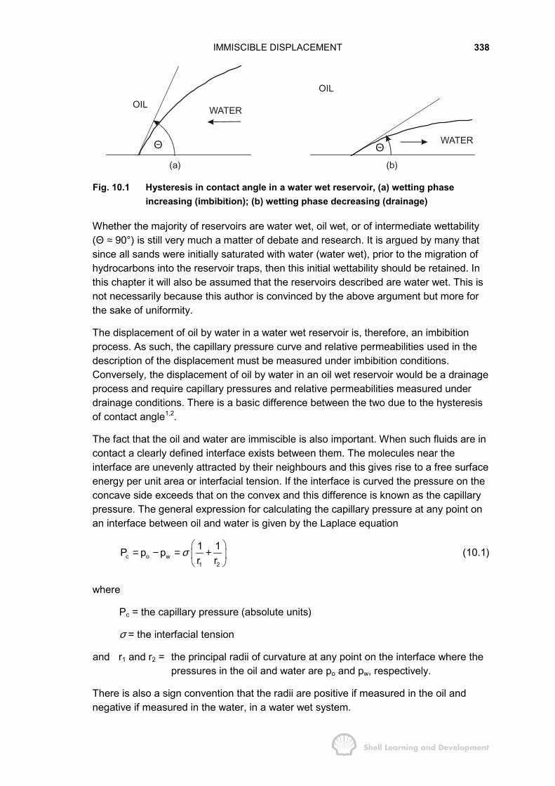
IMMISCIBLE DISPLACEMENT 338
OIL
OIL
WATER
(a)
WATER
(b)
Θ Θ
Fig. 10.1 Hysteresis in contact angle in a water wet reservoir, (a) wetting phaseincreasing (imbibition); (b) wetting phase decreasing (drainage)
Whether the majority of reservoirs are water wet, oil wet, or of intermediate wettability(Θ ≈ 90°) is still very much a matter of debate and research. It is argued by many thatsince all sands were initially saturated with water (water wet), prior to the migration ofhydrocarbons into the reservoir traps, then this initial wettability should be retained. Inthis chapter it will also be assumed that the reservoirs described are water wet. This isnot necessarily because this author is convinced by the above argument but more forthe sake of uniformity.
The displacement of oil by water in a water wet reservoir is, therefore, an imbibitionprocess. As such, the capillary pressure curve and relative permeabilities used in thedescription of the displacement must be measured under imbibition conditions.Conversely, the displacement of oil by water in an oil wet reservoir would be a drainageprocess and require capillary pressures and relative permeabilities measured underdrainage conditions. There is a basic difference between the two due to the hysteresisof contact angle1,2.
The fact that the oil and water are immiscible is also important. When such fluids are incontact a clearly defined interface exists between them. The molecules near theinterface are unevenly attracted by their neighbours and this gives rise to a free surfaceenergy per unit area or interfacial tension. If the interface is curved the pressure on theconcave side exceeds that on the convex and this difference is known as the capillarypressure. The general expression for calculating the capillary pressure at any point onan interface between oil and water is given by the Laplace equation
c o w1 2
1 1P p pr r
σ� �
= − = +� �� �
(10.1)
where
Pc = the capillary pressure (absolute units)
σ = the interfacial tension
and r1 and r2 = the principal radii of curvature at any point on the interface where thepressures in the oil and water are po and pw, respectively.
There is also a sign convention that the radii are positive if measured in the oil andnegative if measured in the water, in a water wet system.

IMMISCIBLE DISPLACEMENT 339
Consider a volume of water contained between two spherical sand grains, in a waterwet reservoir, as shown in fig. 10.2.
r1
r2
ROCK
WATER
OIL
x
Fig. 10.2 Water entrapment between two spherical sand grains in a water wet reservoir
In applying equ. (10.1) to calculate the capillary or phase pressure difference at point Xon the interface, one of the principal radii of curvature, say, r1, is positive, since it ismeasured through the oil, while the other, r2, which is measured through the water, isnegative. Since r1 < r2, however, the capillary pressure is positive. What is also evidentfrom fig. 10.2 is the fact that as the volume of water (water saturation) decreases, theradii decrease, and therefore there must be some inverse relationship between Pc
and Sw.
This relationship is called the capillary pressure curve (function) and is measuredroutinely in the laboratory. Typically, such experiments are conducted, for convenience,using air-brine or air-mercury fluid combinations and the resulting capillary pressurecurve converted for the oil-water system in the reservoir3,4. For the sake of consistency,however, a hypothetical experiment will be considered, firstly for the (non-commercial)case of oil displacing water, in a water wet core sample, and then the displacementprocess will be reversed. The results of such an experiment are shown in fig. 10.3.
Pc
B
C A
DRAINAGE
IMBIBTION
Swc1 - Sor 100%
C
S (% OF PORE VOLUME)w
Fig. 10.3 Drainage and imbibition capillary pressure functions
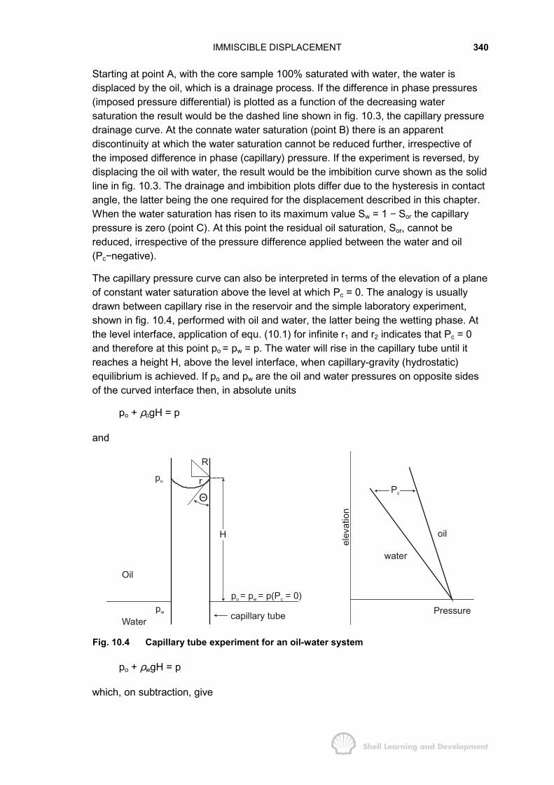
IMMISCIBLE DISPLACEMENT 340
Starting at point A, with the core sample 100% saturated with water, the water isdisplaced by the oil, which is a drainage process. If the difference in phase pressures(imposed pressure differential) is plotted as a function of the decreasing watersaturation the result would be the dashed line shown in fig. 10.3, the capillary pressuredrainage curve. At the connate water saturation (point B) there is an apparentdiscontinuity at which the water saturation cannot be reduced further, irrespective ofthe imposed difference in phase (capillary) pressure. If the experiment is reversed, bydisplacing the oil with water, the result would be the imbibition curve shown as the solidline in fig. 10.3. The drainage and imbibition plots differ due to the hysteresis in contactangle, the latter being the one required for the displacement described in this chapter.When the water saturation has risen to its maximum value Sw = 1 − Sor the capillarypressure is zero (point C). At this point the residual oil saturation, Sor, cannot bereduced, irrespective of the pressure difference applied between the water and oil(Pc−negative).
The capillary pressure curve can also be interpreted in terms of the elevation of a planeof constant water saturation above the level at which Pc = 0. The analogy is usuallydrawn between capillary rise in the reservoir and the simple laboratory experiment,shown in fig. 10.4, performed with oil and water, the latter being the wetting phase. Atthe level interface, application of equ. (10.1) for infinite r1 and r2 indicates that Pc = 0and therefore at this point po = pw = p. The water will rise in the capillary tube until itreaches a height H, above the level interface, when capillary-gravity (hydrostatic)equilibrium is achieved. If po and pw are the oil and water pressures on opposite sidesof the curved interface then, in absolute units
po + ρogH = p
and
Oil
Water
oil
water
Pressure
elev
atio
n
Pc
po
pw
r
R
H
p = po w c= p(P = 0)
capillary tube
Θ
Fig. 10.4 Capillary tube experiment for an oil-water system
po + ρwgH = p
which, on subtraction, give

IMMISCIBLE DISPLACEMENT 341
o w cp p P gHρ− = = ∆ (10.2)
where ∆ρ = ρw - ρo. Furthermore, considering in detail the geometry at the interface inthe capillary tube, fig. 10.4. If the curvature is approximately spherical with radius R,then in applying the Laplace equation, (10.1), r1 = r2 = R at all points on the interface.Also if r is the radius of the capillary tube, then r = RcosΘ and therefore
o w c2 cosp p P gh
rσ ρΘ− = = = ∆ (10.3)
This equation is frequently used to draw a comparison between simple capillary riseexperiments, as described above, and capillary rise in the reservoir, the porous tractsin the latter being likened to a collection of capillary tubes with different radii. In thiscomparison it can be seen that the capillary rise of water will be greater for small r,equ. (10.3), and will decrease as r increases. The decrease in capillary rise will beapparently a continuous function due to the continuous range of pore capillaries in thereservoir and will define, in fact, the capillary pressure-saturation relation. Thisargument is frequently applied to consider the static case of water distribution abovethe 100% water saturation level in the reservoir, under initial conditions, for which thedrainage capillary pressure curve is required. There will generally be no sharp interfacebetween the water and oil but, rather, a zone in which saturations decrease with heightabove the 100% water saturation level, at which Pc = 0, in accordance with the capillarypressure (capillary rise)-saturation relationship. The vertical distance between the pointat which Sw = 100%, Pc = 0 and Sw = Swc is called the capillary transition zone and isdenoted by H.
This chapter is more concerned with the effect of capillary pressure on thedisplacement of oil by water, for which the imbibition capillary pressure curve isrelevant (Pc = 0 at Sw = 1 − Sor). Consider the static situation during a water driveshown in fig. 10.5.
WATER
z
A
S = 1 - Sw or
y
X
θ
z = y cos θ
Pc
Swc
Swa
Sw
1 - Sor
∆ρgzOIL
Fig. 10.5 Determination of water saturation as a function of reservoir thickness abovethe maximum water saturation plane, Sw = 1−−−−Sor, of an advancing waterflood
IMMISCIBLE DISPLACEMENT 342
By static it is meant that the downdip water injection is stopped when the maximumwater saturation plane, Sw = 1 − Sor, at which Pc = 0, has just reached point X in thelinear displacement path. If the imbibition capillary pressure curve has a distinctcapillary transition zone, as shown on the right hand side of the diagram, then abovepoint X the water saturation will be distributed in accordance with the capillary pressure(capillary rise)-saturation relationship. In particular, the capillary pressure at point A, adistance y above the base of the reservoir, in the dip-normal direction (normal to theflow direction), can be calculated as
c w o wP (S ) = p p = g cosρ γ θ− ∆ (10.4)
from which the saturation at point A can be determined from the capillary pressurecurve, as shown in fig. 10.5.
Equation (10.4) is referred to, in this text, as the capillary pressure equation expressed,in this case, in absolute units. In Darcy units, which are used in this chapter to developtheoretical arguments, the general equation becomes
c w 6g y cosP (S ) (atm)
1.0133 10ρ θ∆=
×(10.5)
while in the field units defined in table 4.1, which are employed in the exercises
( )c wP S 0.4335 y cos (psi)γ θ= ∆ (10.6)
where ∆γ is the difference between the water and oil specific gravities in the reservoir.
Allowing the Sw = 1 − Sor plane to rise incrementally in fig. 10.5 will result in a differentwater saturation distribution, in the dip-normal direction, at point X in the displacementpath. This concept is applied in sec. 10.7 in which dynamic displacement is viewed asa series of static positions of the Sw = 1 − Sor plane as the flood moves through thereservoir, each position leading to a new water saturation distribution dictated by thecapillary pressure-saturation relationship.
b) Displacement generally occurs under conditions of vertical equilibrium
Coats5 has qualitatively explained the concept of vertical equilibrium by drawing ananalogy with a simple problem in heat conduction. If one were trying to mathematicallydescribe heat conduction in a thin metal plate, say, 1/8th of an inch thick and with anarea of several square feet, no allowance would be made for the heat distributionacross the thickness of the metal, in which direction thermal equilibrium would beassumed. Since reservoirs, typically, have dimensions in proportion to those describedfor the metal plate, displacement problems can be frequently tackled in a similarmanner. In this case, however, the assumption made is that of fluid potentialequilibrium across the thickness of the reservoir.
The condition for fluid potential equilibrium is simply that of hydrostatic equilibrium,discussed previously, for which the saturation distribution can be determined as afunction of capillary pressure and, therefore, height, as
IMMISCIBLE DISPLACEMENT 343
( )c w 6g y cosP S
1.0133 10ρ θ∆=
×(10.5)
that is, the fluids are distributed in accordance with capillary-gravity equilibrium. Thevertical equilibrium condition can therefore be interpreted in the following manner.When, during the displacement of oil by water, the water saturation at any point in thereservoir increases by a small amount, the new water saturation is instantaneouslyredistributed as indicated by equ. (10.5). This means that the vertical velocities of oiland water, as the two are redistributed in accordance with capillary-gravity equilibrium,appear to be infinite in comparison with the velocity of fluid movement parallel to thereservoir bedding planes resulting from the Darcy or viscous forces.
The condition of vertical equilibrium will be promoted by
- a large vertical permeability (kv)
- small reservoir thickness (h)
- large density difference between the fluids (∆ρ)
- high capillary forces (large capillary transition zone H)
- low fluid viscosities
- low injection rates.
Coats5,6 has presented two dimensionless groups, relating the above terms, themagnitudes of which can be used as "rough rules of thumb" for deciding whethervertical equilibrium conditions prevail in the reservoir. The two cases considered canbe applied when the capillary transition zone is large and also when it is negligible.These dimensionless groups are not presented in this text since, irrespective of theirmagnitude, the only way to check the validity of the vertical equilibrium is by using thenumerical simulation techniques described in sec. 10.10. In any case, when applyingsimple, analytical techniques to describe the displacement process one is obliged toassume that either vertical equilibrium is valid or else the complete opposite, that thereis a total lack of vertical equilibrium. The latter case will apply when, for instance, theinjection rate is so high that the water and oil velocities, parallel to the bedding planesare much greater than their velocity components in the dip-normal direction. Underthese circumstances the water saturation will be uniformly distributed with respect tothickness. These two extremes both represent conditions under which the saturationprofile in the dip-normal direction is definable and this facilitates the application of theanalytical techniques described in this chapter. For in-between cases the engineermust resort to numerical simulation techniques (refer sec. 10.10). It has been foundthat the vertical equilibrium condition is approximately satisfied in a great manyreservoirs. Nevertheless, it will be repeatedly stated throughout the remainder of thechapter precisely when this condition is being assumed, and when not.
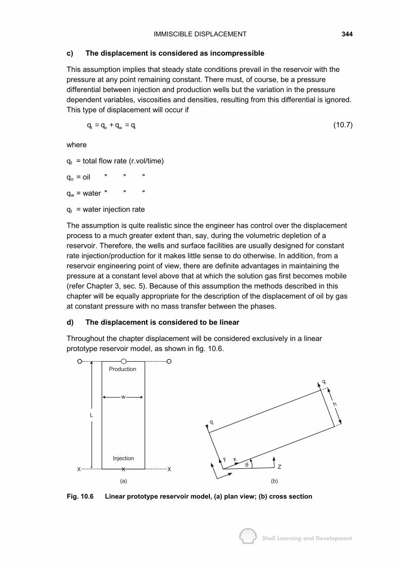
IMMISCIBLE DISPLACEMENT 344
c) The displacement is considered as incompressible
This assumption implies that steady state conditions prevail in the reservoir with thepressure at any point remaining constant. There must, of course, be a pressuredifferential between injection and production wells but the variation in the pressuredependent variables, viscosities and densities, resulting from this differential is ignored.This type of displacement will occur if
t o w iq q q q= + = (10.7)
where
qt = total flow rate (r.vol/time)
qo = oil " " "
qw = water " " "
qI = water injection rate
The assumption is quite realistic since the engineer has control over the displacementprocess to a much greater extent than, say, during the volumetric depletion of areservoir. Therefore, the wells and surface facilities are usually designed for constantrate injection/production for it makes little sense to do otherwise. In addition, from areservoir engineering point of view, there are definite advantages in maintaining thepressure at a constant level above that at which the solution gas first becomes mobile(refer Chapter 3, sec. 5). Because of this assumption the methods described in thischapter will be equally appropriate for the description of the displacement of oil by gasat constant pressure with no mass transfer between the phases.
d) The displacement is considered to be linear
Throughout the chapter displacement will be considered exclusively in a linearprototype reservoir model, as shown in fig. 10.6.
Injection
Production
w
L
(a) (b)
Zθxy
h
qi
qt
Fig. 10.6 Linear prototype reservoir model, (a) plan view; (b) cross section
IMMISCIBLE DISPLACEMENT 345
The model represents a symmetry element taken from a line drive pattern. The co-ordinates used in describing displacement in the linear cross section are shown infig. 10.6(b). Both the injection and production wells are considered to be perforatedacross the entire formation thickness, in the dip-normal direction. No account is takenof the distortion of the linear flow streamlines (lines of constant fluid potential) in thevicinity of the wells and saturations are assumed to be uniformly distributed across theentire width of the block, that is, normal to plane shown in fig. 10.6(b).
The main concern in this chapter is, therefore, to account for the fluid saturationdistributions in the dip-normal direction (y-direction) as the flood moves through thelinear reservoir block. No analytical methods are presented to account for the arealdistribution of saturations in the reservoir. Such methods do exist for regular gridspacings of injection and production wells and are described in the Craig monograph1.For irregular well spacing, however, the analytical methods are extremely complex andhave largely been superseded by numerical simulation techniques. In fact, one of themain purposes in using simulators is to determine the areal distribution of oil and water(or displacing fluid in general) resulting from a flood. This knowledge enables theengineer to place injection and production wells to gain the maximum recovery. Toprovide such results, however, it is necessary that the simulator be informed of whatcan be expected to occur in the dip-normal direction, that is, how the fluids will bedistributed in this direction. This information is generally provided as input to thesimulation.
The whole intent of this chapter is, therefore, to describe the physics governingdisplacement, as viewed through a linear cross section of the reservoir, which is of vitalconcern if the areal distributions of fluids are to be correctly modelled. The chapterdescribes, in the first place, displacement in a homogeneous linear section,secs. 10.3-7, and subsequently extends the methods developed to the description ofdisplacement in inhomogeneous (layered) reservoirs.
10.3 THE FRACTIONAL FLOW EQUATION
In this, and the following two sections, oil displacement will be assumed to take placeunder the so-called diffuse flow condition. This means that fluid saturations at any pointin the linear displacement path are uniformly distributed with respect to thickness. Thesole reason for making this assumption is that it permits the displacement to bedescribed, mathematically, in one dimension and this provides the simplest possiblemodel of the displacement process. The one dimensional description follows from thefact that since the water saturation is uniformly distributed in the dip-normal directionthen so too are the relative permeabilities to oil and water, which are themselvesfunctions of the water saturation at any point. This means that the simultaneous flow ofoil and water can be modelled using thickness averaged relative permeabilities, alongthe centre line of the reservoir, which are also equivalent to relative permeabilities atany point throughout the thickness.
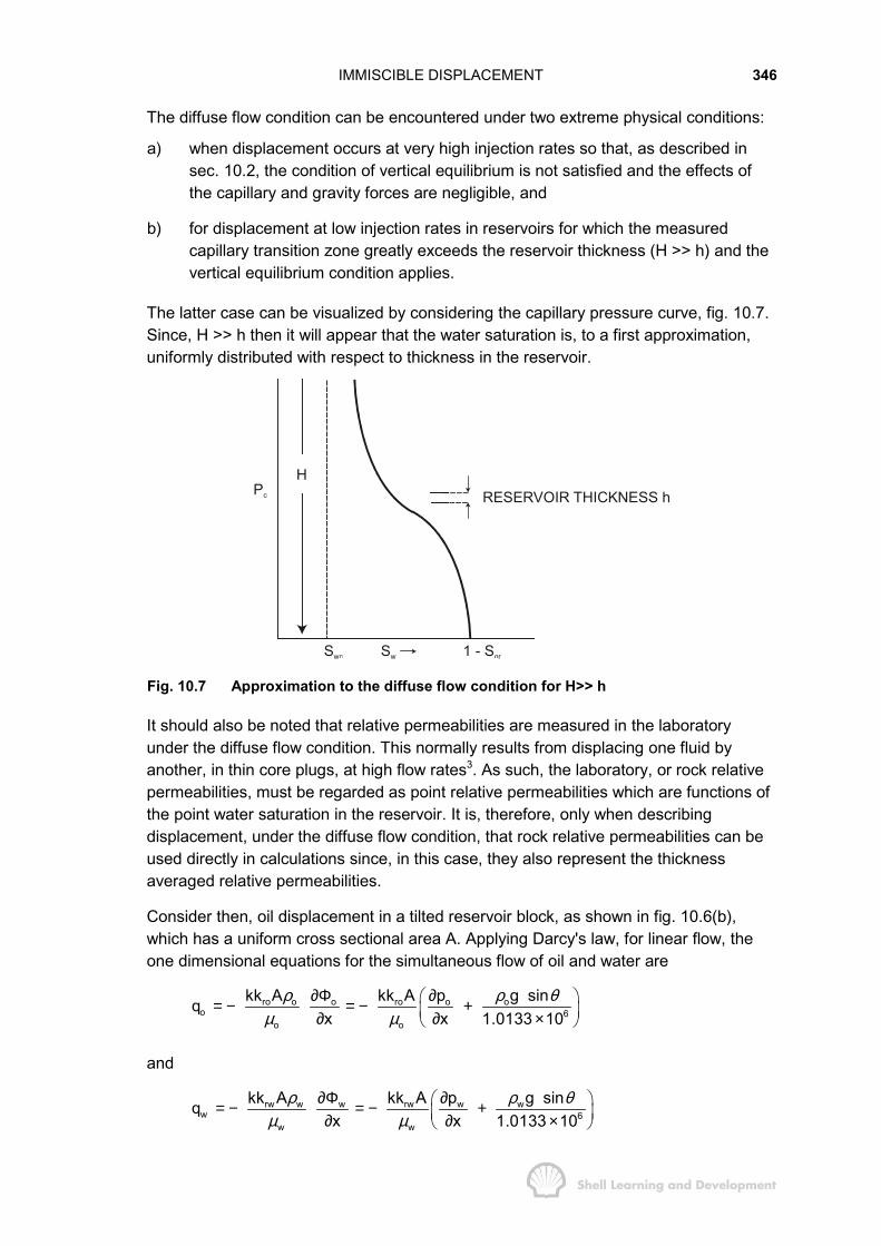
IMMISCIBLE DISPLACEMENT 346
The diffuse flow condition can be encountered under two extreme physical conditions:
a) when displacement occurs at very high injection rates so that, as described insec. 10.2, the condition of vertical equilibrium is not satisfied and the effects ofthe capillary and gravity forces are negligible, and
b) for displacement at low injection rates in reservoirs for which the measuredcapillary transition zone greatly exceeds the reservoir thickness (H >> h) and thevertical equilibrium condition applies.
The latter case can be visualized by considering the capillary pressure curve, fig. 10.7.Since, H >> h then it will appear that the water saturation is, to a first approximation,uniformly distributed with respect to thickness in the reservoir.
HPc
Swc Sw 1 - Sor
RESERVOIR THICKNESS h
Fig. 10.7 Approximation to the diffuse flow condition for H>> h
It should also be noted that relative permeabilities are measured in the laboratoryunder the diffuse flow condition. This normally results from displacing one fluid byanother, in thin core plugs, at high flow rates3. As such, the laboratory, or rock relativepermeabilities, must be regarded as point relative permeabilities which are functions ofthe point water saturation in the reservoir. It is, therefore, only when describingdisplacement, under the diffuse flow condition, that rock relative permeabilities can beused directly in calculations since, in this case, they also represent the thicknessaveraged relative permeabilities.
Consider then, oil displacement in a tilted reservoir block, as shown in fig. 10.6(b),which has a uniform cross sectional area A. Applying Darcy's law, for linear flow, theone dimensional equations for the simultaneous flow of oil and water are
ro o o ro o oo 6
o o
kk A kk A p g sinqx x 1.0133 10
ρ ρ θµ µ
∂Φ ∂� �= − = − +� �∂ ∂ ×� �
and
rw w w rw w ww 6
w w
kk A kk A p g sinqx x 1.0133 10
ρ ρ θµ µ
∂Φ ∂� �= − = − +� �∂ ∂ ×� �
IMMISCIBLE DISPLACEMENT 347
By expressing the oil rate as
qo = qt - qw
the subtraction of the above equations gives
o t o crww 6
rw ro ro
q P g sinq Akk kk kk x 1.0133 10
µ µµ ρ θ� � ∂ ∆� �= − + = + −� � � �∂ ×� �� �(10.8)
in which
c o wP p px x x
∂ ∂ ∂= −∂ ∂ ∂
the capillary pressure gradient in the direction of flow, and
∆ρ = ρw - ρo
The fractional flow of water, at any point in the reservoir, is defined as
w ww
o w t
q qfq q q
= =+
and substitution of this in equ. (10.8) gives
ro c6
t ow
row
rw o
kk A P g sin1q x 1.0133 10f k1
k
ρ θµ
µµ
∂ ∆� �+ −� �∂ ×� �=+ ⋅
(10.9)
while, by analogy with equ. (4.18), this equation can be expressed in field units as
3 ro c
t ow
row
rw o
kk A P1 1.127 10 .4335 sinq xf k1
k
γ θµ
µµ
− ∂� �+ × − ∆� �∂� �=+ ⋅
(10.10)
both of these being fractional flow equations for the displacement of oil by water, in onedimension.
It is worthwhile considering the influence of the various component parts of thisexpression. According to the convention adopted in this text θ is the angle measuredfrom the horizontal to the line indicating the direction of flow. Therefore, the gravityterm ∆ρ g sinθ /1.0133×106 will be positive for oil displacement in the updip direction(0 < θ < π), as shown in fig. 10.6(b), and negative for displacement downdip(π < θ < 2π). As a result, provided all the other terms in equ. (10.9) are the same, thefractional flow of water for displacement updip is lower than for displacement downdipsince in the former case gravity tends to suppress the flow of water.
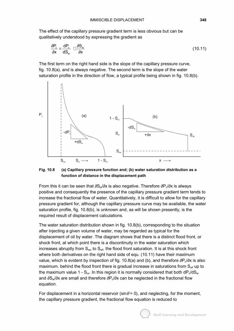
IMMISCIBLE DISPLACEMENT 348
The effect of the capillary pressure gradient term is less obvious but can bequalitatively understood by expressing the gradient as
c c w
w
P dP Sx dS x
∂ ∂= ⋅∂ ∂
(10.11)
The first term on the right hand side is the slope of the capillary pressure curve,fig. 10.8(a), and is always negative. The second term is the slope of the watersaturation profile in the direction of flow, a typical profile being shown in fig. 10.8(b).
Swc Sw 1 - Sor
Swc
Sw
1 - Sor
+dSw
-dPc
Pc (a)
-dSw
+dx Swf
(b)
x
Fig. 10.8 (a) Capillary pressure function and; (b) water saturation distribution as afunction of distance in the displacement path
From this it can be seen that ∂Sw/∂x is also negative. Therefore ∂Pc/∂x is alwayspositive and consequently the presence of the capillary pressure gradient term tends toincrease the fractional flow of water. Quantitatively, it is difficult to allow for the capillarypressure gradient for, although the capillary pressure curve may be available, the watersaturation profile, fig. 10.8(b), is unknown and, as will be shown presently, is therequired result of displacement calculations.
The water saturation distribution shown in fig. 10.8(b), corresponding to the situationafter injecting a given volume of water, may be regarded as typical for thedisplacement of oil by water. The diagram shows that there is a distinct flood front, orshock front, at which point there is a discontinuity in the water saturation whichincreases abruptly from Swc to Swf, the flood front saturation. It is at this shock frontwhere both derivatives on the right hand side of equ. (10.11) have their maximumvalue, which is evident by inspection of fig. 10.8(a) and (b), and therefore ∂Pc/∂x is alsomaximum. behind the flood front there is gradual increase in saturations from Swf up tothe maximum value 1 - Sor. In this region it is normally considered that both dPc/dSw
and ∂Sw/∂x are small and therefore ∂Pc/∂x can be neglected in the fractional flowequation.
For displacement in a horizontal reservoir (sinθ = 0), and neglecting, for the moment,the capillary pressure gradient, the fractional flow equation is reduced to
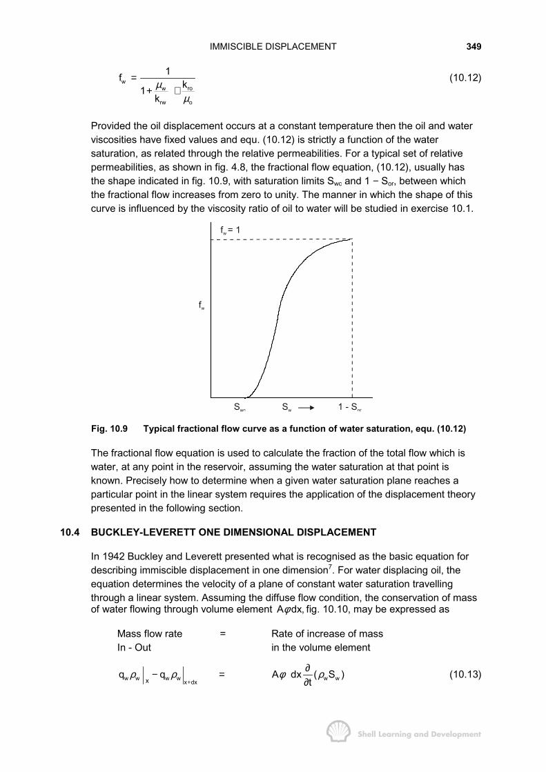
IMMISCIBLE DISPLACEMENT 349
wrow
rw o
1f k1kµ
µ
=+ ⋅
(10.12)
Provided the oil displacement occurs at a constant temperature then the oil and waterviscosities have fixed values and equ. (10.12) is strictly a function of the watersaturation, as related through the relative permeabilities. For a typical set of relativepermeabilities, as shown in fig. 4.8, the fractional flow equation, (10.12), usually hasthe shape indicated in fig. 10.9, with saturation limits Swc and 1 − Sor, between whichthe fractional flow increases from zero to unity. The manner in which the shape of thiscurve is influenced by the viscosity ratio of oil to water will be studied in exercise 10.1.
Swc Sw 1 - Sor
fw
f = 1w
Fig. 10.9 Typical fractional flow curve as a function of water saturation, equ. (10.12)
The fractional flow equation is used to calculate the fraction of the total flow which iswater, at any point in the reservoir, assuming the water saturation at that point isknown. Precisely how to determine when a given water saturation plane reaches aparticular point in the linear system requires the application of the displacement theorypresented in the following section.
10.4 BUCKLEY-LEVERETT ONE DIMENSIONAL DISPLACEMENT
In 1942 Buckley and Leverett presented what is recognised as the basic equation fordescribing immiscible displacement in one dimension7. For water displacing oil, theequation determines the velocity of a plane of constant water saturation travellingthrough a linear system. Assuming the diffuse flow condition, the conservation of massof water flowing through volume element A dx,φ fig. 10.10, may be expressed as
Mass flow rate = Rate of increase of massIn - Out in the volume element
w w w w w wx dxxq q A dx ( S )
tρ ρ φ ρ
+
∂− =∂
(10.13)

IMMISCIBLE DISPLACEMENT 350
q |wρw xq |ρw w x+dx
x
dx
Fig. 10.10 Mass flow rate of water through a linear volume element A dxφ
or
w w w w w w w wx xq q (q )dx A dx ( S )
x tρ ρ ρ φ ρ∂ ∂� �− + =� �∂ ∂� �
which can be reduced to
w w w w(q ) A ( S )x t
ρ φ ρ∂ ∂= −∂ ∂
(10.14)
and for the assumption of incompressible displacement (ρw ≈ constant)
w w
t x
q SAx t
φ∂ ∂= −∂ ∂
(10.15)
The full differential of the water saturation is
x
w ww
t
S SdS dx dtx t
∂ ∂= +∂ ∂
and since it is the intention to study the movement of a plane of constant watersaturation, that is, dSw = 0, then
w
w w
x t S
S S dxt x dt
∂ ∂= −∂ ∂
(10.16)
Furthermore,
t
w w w
t w
q q Sx S x
� �∂ ∂ ∂= ⋅� �∂ ∂ ∂� �(10.17)
and substituting equs. (10.16) and (10.17) in equ. (10.15) gives
w
w
t Sw
q dxAS dt
φ∂ =∂
(10.18)
Again, for incompressible displacement, qt is constant and, since qw = qtfw, equ. (10.18)may be expressed as
IMMISCIBLE DISPLACEMENT 351
ww w
t wS
S Sw
q dfdxvdt A dSφ
= = (10.19)
This is the equation of Buckley-Leverett which implies that, for a constant rate of waterinjection (qt = qi), the velocity of a plane of constant water saturation is directlyproportional to the derivative of the fractional flow equation evaluated for thatsaturation. If the capillary pressure gradient term is neglected in equ. (10.9) then thefractional flow is strictly a function of the water saturation, irrespective of whether thegravity term is included or not, hence the use of the total differential of fw in theBuckley-Leverett equation. Integrating for the total time since the start of injection gives
w
tw
S tw 0
df1x q dtA dSφ
= �
or
ww
i wS
Sw
W dfxA dSφ
= (10.20)
where Wi is the cumulative water injected and it is assumed, as an initial condition, thatWi = 0 when t = 0 . Therefore, at a given time after the start of injection (Wi = constant)the position of different water saturation planes can be plotted, using equ. (10.20),merely by determining the slope of the fractional flow curve for the particular value ofeach saturation.
There is a mathematical difficulty encountered in applying this technique which can beappreciated by considering the typical fractional flow curve shown in fig. 10.9 inconjunction with equ. (10.20). Since there is frequently a point of inflexion in thefractional flow curve then the plot of dfw/dSw versus Sw will have a maximum point, asshown in fig. 10.11 (a).
Using equ. (10.20) to plot the saturation distribution at a particular time will thereforeresult in the solid line shown in fig. 10.111b). This bulbous saturation profile isphysically impossible since it indicates that multiple water saturations can co-exist at agiven point in the reservoir. What actually occurs is that the intermediate values of thewater saturation, which as shown in fig. 10.11 (a) have the maximum velocity, willinitially tend to overtake the lower saturations resulting in the formation of a saturationdiscontinuity or shock front.
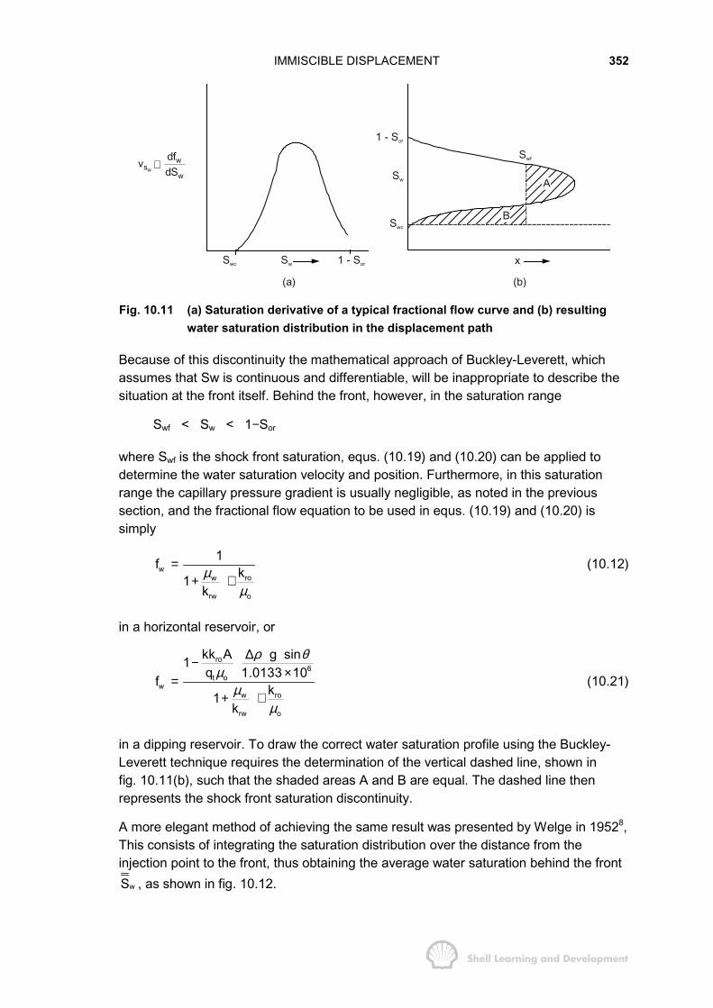
IMMISCIBLE DISPLACEMENT 352
1 - Sor
Sw
Swc
B
A
xSwc Sw 1 - Sor
ww
sw
dfvdS
(a) (b)
Swf∝
Fig. 10.11 (a) Saturation derivative of a typical fractional flow curve and (b) resultingwater saturation distribution in the displacement path
Because of this discontinuity the mathematical approach of Buckley-Leverett, whichassumes that Sw is continuous and differentiable, will be inappropriate to describe thesituation at the front itself. Behind the front, however, in the saturation range
Swf < Sw < 1−Sor
where Swf is the shock front saturation, equs. (10.19) and (10.20) can be applied todetermine the water saturation velocity and position. Furthermore, in this saturationrange the capillary pressure gradient is usually negligible, as noted in the previoussection, and the fractional flow equation to be used in equs. (10.19) and (10.20) issimply
wrow
rw o
1f k1kµ
µ
=+ ⋅
(10.12)
in a horizontal reservoir, or
ro6
t ow
row
rw o
kk A g sin1q 1.0133 10f k1
k
ρ θµ
µµ
∆−×=
+ ⋅(10.21)
in a dipping reservoir. To draw the correct water saturation profile using the Buckley-Leverett technique requires the determination of the vertical dashed line, shown infig. 10.11(b), such that the shaded areas A and B are equal. The dashed line thenrepresents the shock front saturation discontinuity.
A more elegant method of achieving the same result was presented by Welge in 19528,This consists of integrating the saturation distribution over the distance from theinjection point to the front, thus obtaining the average water saturation behind the front
wS , as shown in fig. 10.12.
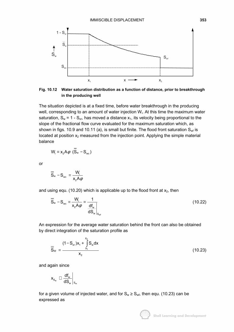
IMMISCIBLE DISPLACEMENT 353
x1 x x2
Swf
1 - Sor
Sw
Swc
Sw
Fig. 10.12 Water saturation distribution as a function of distance, prior to breakthroughin the producing well
The situation depicted is at a fixed time, before water breakthrough in the producingwell, corresponding to an amount of water injection Wi. At this time the maximum watersaturation, Sw = 1 - Sor, has moved a distance x1, its velocity being proportional to theslope of the fractional flow curve evaluated for the maximum saturation which, asshown in figs. 10.9 and 10.11 (a), is small but finite. The flood front saturation Swf islocated at position x2 measured from the injection point. Applying the simple materialbalance
wi 2 wcW x A (S S )φ= −
or
iw wc
2
WS Sx Aφ
− =
and using equ. (10.20) which is applicable up to the flood front at x2, then
wf
iw wc
2 w
w S
W 1S Sx A df
dSφ
− = = (10.22)
An expression for the average water saturation behind the front can also be obtainedby direct integration of the saturation profile as
2
1
X
or 1 wX
W2
(1 S )x S dxS
x
− +=
�(10.23)
and again since
ww
wS
Sw
dfxdS
∝
for a given volume of injected water, and for Sw ≥ Swf, then equ. (10.23) can beexpressed as
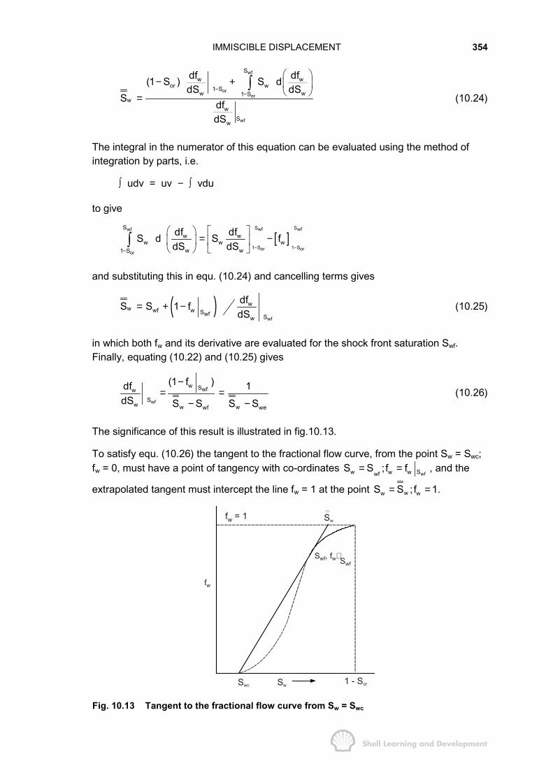
IMMISCIBLE DISPLACEMENT 354
wf
oror
wf
Sw w
or w1 Sw w1 S
ww
Sw
df df(1 S ) S ddS dS
S dfdS
−−
� �− + � �
� �=�
(10.24)
The integral in the numerator of this equation can be evaluated using the method ofintegration by parts, i.e.
∫ udv = uv − ∫ vdu
to give
[ ]S Swf wfwf
1 S 1 Sor oror
Sw w
w w ww w1 S
df dfS d S fdS dS − −−
� � � �= −� � � �
� ��
and substituting this in equ. (10.24) and cancelling terms gives
( )wf
Swf
ww wf w
Sw
dfS S 1 fdS
= + − (10.25)
in which both fw and its derivative are evaluated for the shock front saturation Swf.Finally, equating (10.22) and (10.25) gives
wf
Swf
w w
ww
Sw wf we
(1 f )df 1dS S S S S
−= =
− −(10.26)
The significance of this result is illustrated in fig.10.13.
To satisfy equ. (10.26) the tangent to the fractional flow curve, from the point Sw = Swc;fw = 0, must have a point of tangency with co-ordinates
wfwfw w w SS S ;f f= = , and the
extrapolated tangent must intercept the line fw = 1 at the point ww wS S ;f 1.= =
1 - SorSwc Sw
Swf, fw Swf
fw
fw = 1 Sw
Fig. 10.13 Tangent to the fractional flow curve from Sw = Swc
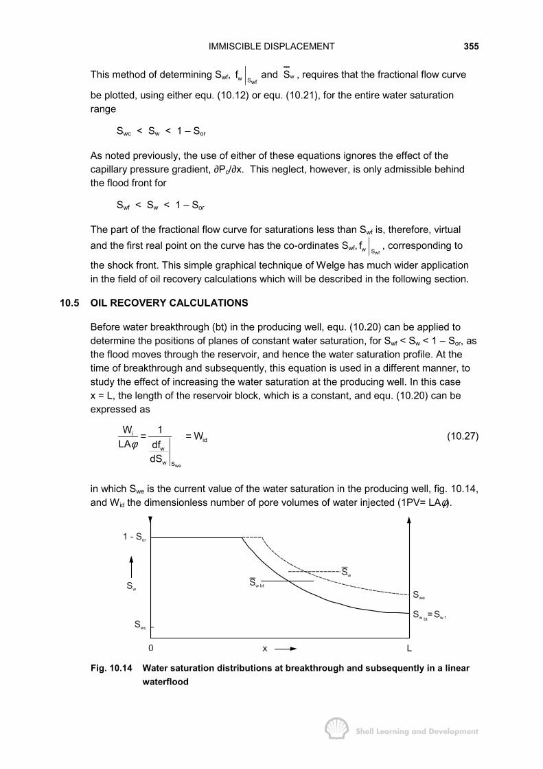
IMMISCIBLE DISPLACEMENT 355
This method of determining Swf, Swfwwf and S , requires that the fractional flow curve
be plotted, using either equ. (10.12) or equ. (10.21), for the entire water saturationrange
Swc < Sw < 1 – Sor
As noted previously, the use of either of these equations ignores the effect of thecapillary pressure gradient, ∂Pc/∂x. This neglect, however, is only admissible behindthe flood front for
Swf < Sw < 1 – Sor
The part of the fractional flow curve for saturations less than Swf is, therefore, virtualand the first real point on the curve has the co-ordinates Swf,
wfSwf , corresponding to
the shock front. This simple graphical technique of Welge has much wider applicationin the field of oil recovery calculations which will be described in the following section.
10.5 OIL RECOVERY CALCULATIONS
Before water breakthrough (bt) in the producing well, equ. (10.20) can be applied todetermine the positions of planes of constant water saturation, for Swf < Sw < 1 – Sor, asthe flood moves through the reservoir, and hence the water saturation profile. At thetime of breakthrough and subsequently, this equation is used in a different manner, tostudy the effect of increasing the water saturation at the producing well. In this casex = L, the length of the reservoir block, which is a constant, and equ. (10.20) can beexpressed as
we
iid
w
w S
W 1 WLA df
dSφ
= = (10.27)
in which Swe is the current value of the water saturation in the producing well, fig. 10.14,and Wid the dimensionless number of pore volumes of water injected (1PV= LAφ).
1 - Sor
Sw
Swc
Sw bt
Sw
Swe
0 x L
bt
Fig. 10.14 Water saturation distributions at breakthrough and subsequently in a linearwaterflood
IMMISCIBLE DISPLACEMENT 356
Before breakthrough occurs the oil recovery calculations are trivial. For incompressibledisplacement the oil recovered is simply equal to the volume of water injected, therebeing no water production during this phase. At the time of breakthrough the flood frontsaturation,
btwf wS S ,= reaches the producing well and the reservoir watercut increases
suddenly from zero to bt wfw w sf f= a phenomenon frequently observed in the field and
one which confirms the existence of a shock front. At this time equ. (10.22) can beinterpreted in terms of equ. (10.27) to give
( )btbt bt
wbt
wpd id id bt wcw
w S
1N W q t S SdfdS
= = = − = (10.28)
in which all volumes are expressed, for convenience, as dimensionless pore volumes.In particular, the dimensionless injection rate is qi/(LAφ) (PV/unit of time) whichfacilitates the calculation of the time at which breakthrough occurs as
btidbt
id
Wt
q= (10.29)
After breakthrough, L remains constant in equ. (10.27) and Swe and fwe, the watersaturation and fractional flow at the producing well, gradually increase as the floodmoves through the reservoir, as shown in fig. 10.14. During this phase the calculationof the oil recovery is somewhat more complex and requires application of the Welgeequation, (10.25), as
we
w we wew
w S
1S S (1 f )dfdS
= + − (10.30)
which, using equ. (10.27), can also be expressed as
w we we idS S (1 f )W= + − (10.31)
Finally, subtracting Swc from both sides of equ. (10.31) gives the oil recovery equation
Npd = S w − Swc = (Swe − Swc) + (1 − fwe) Wid(PV) (10.32)
The manner in which equs. (10.28) and (10.32) can be used in practice is describedbelow.
a) Draw the fractional flow curve, equ. (10.12) or (10.21), allowing for gravity effects,if necessary, but neglecting the capillary pressure gradient ∂Pc/∂x.
b) Draw the tangent to this curve from the point Sw = Swc, fw = 0. As described in theprevious section, the point of tangency has the co-ordinatesSw = Swf =
bt btwfw w w wsS , f f f= = and the extrapolation of this line to fw = 1 gives
the value of the average saturation behind the front at breakthrough btw wS S .=
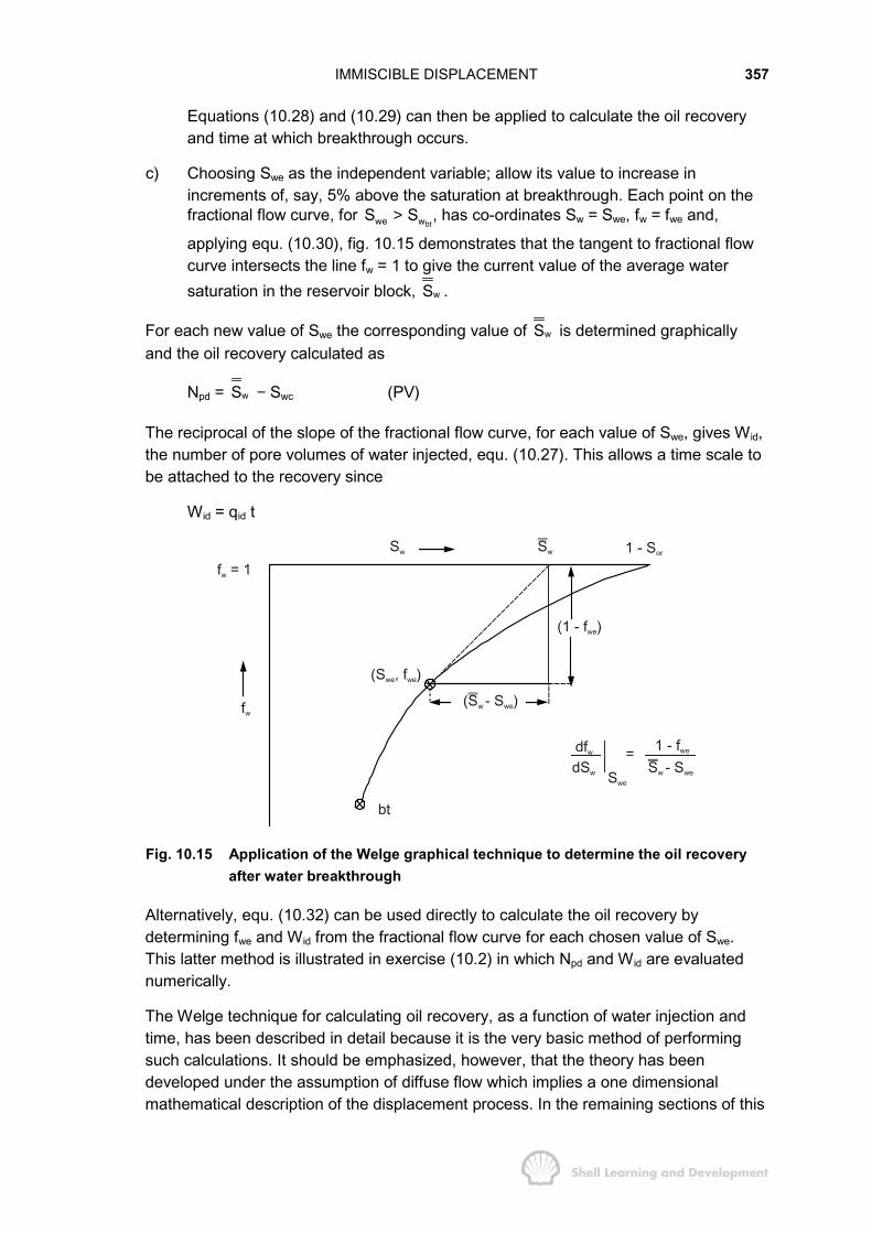
IMMISCIBLE DISPLACEMENT 357
Equations (10.28) and (10.29) can then be applied to calculate the oil recoveryand time at which breakthrough occurs.
c) Choosing Swe as the independent variable; allow its value to increase inincrements of, say, 5% above the saturation at breakthrough. Each point on thefractional flow curve, for
btwe wS S> , has co-ordinates Sw = Swe, fw = fwe and,
applying equ. (10.30), fig. 10.15 demonstrates that the tangent to fractional flowcurve intersects the line fw = 1 to give the current value of the average watersaturation in the reservoir block, wS .
For each new value of Swe the corresponding value of wS is determined graphicallyand the oil recovery calculated as
Npd = wS − Swc (PV)
The reciprocal of the slope of the fractional flow curve, for each value of Swe, gives Wid,the number of pore volumes of water injected, equ. (10.27). This allows a time scale tobe attached to the recovery since
Wid = qid t
f = 1w
Sw Sw 1 - Sor
(1 - f )we
( - S )Sw we
(S , fwe we)
bt
fw
1 - fwe
Sw we- S=dfw
dSw Swe
Fig. 10.15 Application of the Welge graphical technique to determine the oil recoveryafter water breakthrough
Alternatively, equ. (10.32) can be used directly to calculate the oil recovery bydetermining fwe and Wid from the fractional flow curve for each chosen value of Swe.This latter method is illustrated in exercise (10.2) in which Npd and Wid are evaluatednumerically.
The Welge technique for calculating oil recovery, as a function of water injection andtime, has been described in detail because it is the very basic method of performingsuch calculations. It should be emphasized, however, that the theory has beendeveloped under the assumption of diffuse flow which implies a one dimensionalmathematical description of the displacement process. In the remaining sections of this
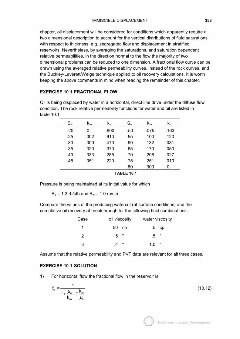
IMMISCIBLE DISPLACEMENT 358
chapter, oil displacement will be considered for conditions which apparently require atwo dimensional description to account for the vertical distributions of fluid saturationswith respect to thickness, e.g. segregated flow and displacement in stratifiedreservoirs. Nevertheless, by averaging the saturations, and saturation dependentrelative permeabilities, in the direction normal to the flow the majority of twodimensional problems can be reduced to one dimension. A fractional flow curve can bedrawn using the averaged relative permeability curves, instead of the rock curves, andthe Buckley-Leverett/Welge technique applied to oil recovery calculations. It is worthkeeping the above comments in mind when reading the remainder of this chapter.
EXERCISE 10.1 FRACTIONAL FLOW
Oil is being displaced by water in a horizontal, direct line drive under the diffuse flowcondition. The rock relative permeability functions for water and oil are listed intable 10.1.
Sw krw kro Sw krw kro
.20 0 .800 .50 .075 .163
.25 .002 .610 .55 .100 .120
.30 .009 .470 .60 .132 .081
.35 .020 .370 .65 .170 .050
.40 .033 .285 .70 .208 .027
.45 .051 .220 .75 .251 .010.80 .300 0
TABLE 10.1
Pressure is being maintained at its initial value for which
Bo = 1.3 rb/stb and Bw = 1.0 rb/stb
Compare the values of the producing watercut (at surface conditions) and thecumulative oil recovery at breakthrough for the following fluid combinations.
Case oil viscosity water viscosity
1 50 cp .5 cp
2 5 " .5 "
3 .4 " 1.0 "
Assume that the relative permeability and PVT data are relevant for all three cases.
EXERCISE 10.1 SOLUTION
1) For horizontal flow the fractional flow in the reservoir is
wrow
rw o
1f k1kµ
µ
=+ ⋅
(10.12)
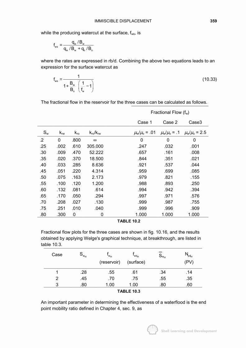
IMMISCIBLE DISPLACEMENT 359
while the producing watercut at the surface, fws, is
w wws
w w o o
q /Bfq /B q /B
=+
where the rates are expressed in rb/d. Combining the above two equations leads to anexpression for the surface watercut as
wsw
o w
1fB 11 1B f
=� �
+ −� �� �
(10.33)
The fractional flow in the reservoir for the three cases can be calculated as follows.
Fractional Flow (fw)
Case 1 Case 2 Case3
Sw krw kro kro/krw µw/µo = .01 µw/µo = .1 µw/µo = 2.5.2 0 .800 ∞ 0 0 0.25 .002 .610 305.000 .247 .032 .001.30 .009 .470 52.222 .657 .161 .008.35 .020 .370 18.500 .844 .351 .021.40 .033 .285 8.636 .921 .537 .044.45 .051 .220 4.314 .959 .699 .085.50 .075 .163 2.173 .979 .821 .155.55 .100 .120 1.200 .988 .893 .250.60 .132 .081 .614 .994 .942 .394.65 .170 .050 .294 .997 .971 .576.70 .208 .027 .130 .999 .987 .755.75 .251 .010 .040 .999 .996 .909.80 .300 0 0 1.000 1.000 1.000
TABLE 10.2
Fractional flow plots for the three cases are shown in fig. 10.16, and the resultsobtained by applying Welge's graphical technique, at breakthrough, are listed intable 10.3.
Case btwSbtwf
(reservoir)btwsf
(surface)btwS btpdN
(PV)
1 .28 .55 .61 .34 .142 .45 .70 .75 .55 .353 .80 1.00 1.00 .80 .60
TABLE 10.3
An important parameter in determining the effectiveness of a waterflood is the endpoint mobility ratio defined in Chapter 4, sec. 9, as
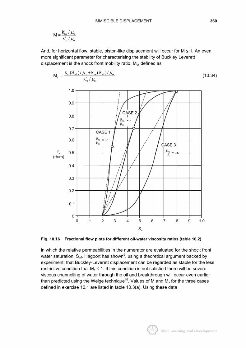
IMMISCIBLE DISPLACEMENT 360
rw w
ro o
k /Mk /
µµ
′=
′
And, for horizontal flow, stable, piston-like displacement will occur for M ≤ 1. An evenmore significant parameter for characterising the stability of Buckley Leverettdisplacement is the shock front mobility ratio, Ms, defined as
ro wf o rw wf ws
ro o
k (S ) / k (S ) /Mk /µ µ
µ+=
′(10.34)
CASE 2
CASE 3
CASE 1
1.0
0.9
1.0
0.8
0.7
0.6
0.5
0.4
0.3
0.2
0.1
00 .1 .2 .3 .4 .5 .6 .7 .8 .9 1.0
= .01wo
µµ
= .1w
o
µµ
= 2.5wo
µµ
Sw
f(rb/rb)
w
Fig. 10.16 Fractional flow plots for different oil-water viscosity ratios (table 10.2)
in which the relative permeabilities in the numerator are evaluated for the shock frontwater saturation, Swf. Hagoort has shown9, using a theoretical argument backed byexperiment, that Buckley-Leverett displacement can be regarded as stable for the lessrestrictive condition that Ms < 1. If this condition is not satisfied there will be severeviscous channelling of water through the oil and breakthrough will occur even earlierthan predicted using the Welge technique10. Values of M and Ms for the three casesdefined in exercise 10.1 are listed in table 10.3(a). Using these data
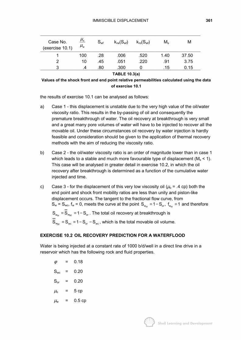
IMMISCIBLE DISPLACEMENT 361
Case No.(exercise 10.1)
o
w
µµ
Swf krw(Swf) kro(Swf) Ms M
1 100 .28 .006 .520 1.40 37.502 10 .45 .051 .220 .91 3.753 .4 .80 .300 0 .15 0.15
TABLE 10.3(a)Values of the shock front and end point relative permeabilities calculated using the data
of exercise 10.1
the results of exercise 10.1 can be analysed as follows:
a) Case 1 - this displacement is unstable due to the very high value of the oil/waterviscosity ratio. This results in the by-passing of oil and consequently thepremature breakthrough of water. The oil recovery at breakthrough is very smalland a great many pore volumes of water will have to be injected to recover all themovable oil. Under these circumstances oil recovery by water injection is hardlyfeasible and consideration should be given to the application of thermal recoverymethods with the aim of reducing the viscosity ratio.
b) Case 2 - the oil/water viscosity ratio is an order of magnitude lower than in case 1which leads to a stable and much more favourable type of displacement (Ms < 1).This case will be analysed in greater detail in exercise 10.2, in which the oilrecovery after breakthrough is determined as a function of the cumulative waterinjected and time.
c) Case 3 - for the displacement of this very low viscosity oil (µo = .4 cp) both theend point and shock front mobility ratios are less than unity and piston-likedisplacement occurs. The tangent to the fractional flow curve, fromSw = Swc, fw = 0, meets the curve at the point
bt btw or wS 1 S , f 1= − = and therefore
bt wbtw orS S 1 S= = − . The total oil recovery at breakthrough is
wbt wc or wcS S 1 S S= = − − , which is the total movable oil volume.
EXERCISE 10.2 OIL RECOVERY PREDICTION FOR A WATERFLOOD
Water is being injected at a constant rate of 1000 b/d/well in a direct line drive in areservoir which has the following rock and fluid properties.
φ = 0.18
Swc = 0.20
Sor = 0.20
µo = 5 cp
µw = 0.5 cp

IMMISCIBLE DISPLACEMENT 362
The relative permeabilities for oil and water are presented in table 10.1 and the floodpattern geometry is as follows
Dip angle = 0°
Reservoir thickness = 40 ft
Distance between injection wells = 625 ft
Distance between injectors and producers = 2000 ft
Assuming that diffuse flow conditions prevail and that the injection project startssimultaneously with oil production from the reservoir
1) determine the time when breakthrough occurs
2) determine the cumulative oil production as a function of both the cumulativewater injected and the time.
EXERCISE 10.2 SOLUTION
The relative permeabilities and viscosities of the oil and water are identical with thoseof "Case 2" in exercise 10.1. Therefore, the fractional flow curve is the same as drawnin fig. 10.16, for, which the breakthrough occurs when
bt
bt
bt bt
w
w
id pd
S 0.45f 0.70
and W N 0.35
=
=
= =
1) Calculation of the breakthrough time
For a constant rate of water injection the time is related to the dimensionless waterinflux by the general expression
id
i
W (one pore volume) (cu.ft)tq 5.615 365 (cu.ft / year)×=
× ×
idW 625 40 2000 .18t (years)1000 5.615 365× × × ×=
× ×
idt 4.39 W (years)= (10.35)
Therefore breakthrough will occur after a time
tbt = 4.39 × 0.35 = 1.54 years
2) Cumulative oil recovery
The oil recovery after breakthrough, expressed in pore volumes, can be calculatedusing the equation
Npd = (Swe – Swc) + (1 – fwe) Wid (10.32)
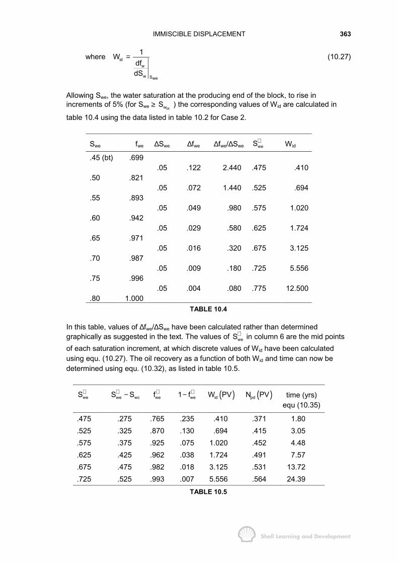
IMMISCIBLE DISPLACEMENT 363
where
we
idw
w S
1WdfdS
= (10.27)
Allowing Swe, the water saturation at the producing end of the block, to rise inincrements of 5% (for Swe ≥
btwS ) the corresponding values of Wid are calculated in
table 10.4 using the data listed in table 10.2 for Case 2.
Swe fwe ∆Swe ∆fwe ∆fwe/∆Swe weS∗ Wid
.45 (bt) .699.05 .122 2.440 .475 .410
.50 .821.05 .072 1.440 .525 .694
.55 .893.05 .049 .980 .575 1.020
.60 .942.05 .029 .580 .625 1.724
.65 .971.05 .016 .320 .675 3.125
.70 .987.05 .009 .180 .725 5.556
.75 .996.05 .004 .080 .775 12.500
.80 1.000TABLE 10.4
In this table, values of ∆fwe/∆Swe have been calculated rather than determinedgraphically as suggested in the text. The values of weS∗ in column 6 are the mid pointsof each saturation increment, at which discrete values of Wid have been calculatedusing equ. (10.27). The oil recovery as a function of both Wid and time can now bedetermined using equ. (10.32), as listed in table 10.5.
weS∗we wcS S∗ − wef ∗
we1 f∗− ( )idW PV ( )pdN PV time (yrs)equ (10.35)
.475 .275 .765 .235 .410 .371 1.80
.525 .325 .870 .130 .694 .415 3.05
.575 .375 .925 .075 1.020 .452 4.48
.625 .425 .962 .038 1.724 .491 7.57
.675 .475 .982 .018 3.125 .531 13.72
.725 .525 .993 .007 5.556 .564 24.39TABLE 10.5
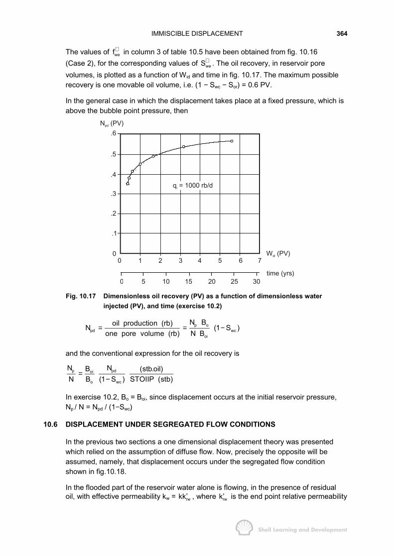
IMMISCIBLE DISPLACEMENT 364
The values of wef ∗ in column 3 of table 10.5 have been obtained from fig. 10.16(Case 2), for the corresponding values of weS∗ . The oil recovery, in reservoir porevolumes, is plotted as a function of Wid and time in fig. 10.17. The maximum possiblerecovery is one movable oil volume, i.e. (1 − Swc − Sor) = 0.6 PV.
In the general case in which the displacement takes place at a fixed pressure, which isabove the bubble point pressure, then
.6
.5
.4
.3
.2
.1
00 1 2 3 4 5 6 7
0 5 10 15 20 25 30
W (PV)id
time (yrs)
q = 1000 rb/di
N (PV)pd
Fig. 10.17 Dimensionless oil recovery (PV) as a function of dimensionless waterinjected (PV), and time (exercise 10.2)
p opd wc
oi
N Boil production (rb)N (1 S )one pore volume (rb) N B
= = −
and the conventional expression for the oil recovery is
p pdoi
o wc
N NB (stb.oil)N B (1 S ) STOIIP (stb)
=−
In exercise 10.2, Bo = Boi, since displacement occurs at the initial reservoir pressure,Np / N = Npd / (1−Swc)
10.6 DISPLACEMENT UNDER SEGREGATED FLOW CONDITIONS
In the previous two sections a one dimensional displacement theory was presentedwhich relied on the assumption of diffuse flow. Now, precisely the opposite will beassumed, namely, that displacement occurs under the segregated flow conditionshown in fig.10.18.
In the flooded part of the reservoir water alone is flowing, in the presence of residualoil, with effective permeability kw = rwkk′ , where rwk′ is the end point relative permeability
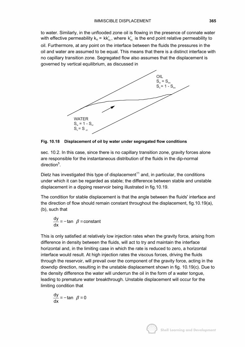
IMMISCIBLE DISPLACEMENT 365
to water. Similarly, in the unflooded zone oil is flowing in the presence of connate waterwith effective permeability ko = rokk′ , where rok′ is the end point relative permeability tooil. Furthermore, at any point on the interface between the fluids the pressures in theoil and water are assumed to be equal. This means that there is a distinct interface withno capillary transition zone. Segregated flow also assumes that the displacement isgoverned by vertical equilibrium, as discussed in
WATERS = 1 - SS = S
w or
o or
OILS = SS = 1 - S
w wc
o wc
Fig. 10.18 Displacement of oil by water under segregated flow conditions
sec. 10.2. In this case, since there is no capillary transition zone, gravity forces aloneare responsible for the instantaneous distribution of the fluids in the dip-normaldirection5.
Dietz has investigated this type of displacement11 and, in particular, the conditionsunder which it can be regarded as stable; the difference between stable and unstabledisplacement in a dipping reservoir being illustrated in fig.10.19.
The condition for stable displacement is that the angle between the fluids' interface andthe direction of flow should remain constant throughout the displacement, fig.10.19(a),(b), such that
dy tandx
β= − =constant
This is only satisfied at relatively low injection rates when the gravity force, arising fromdifference in density between the fluids, will act to try and maintain the interfacehorizontal and, in the limiting case in which the rate is reduced to zero, a horizontalinterface would result. At high injection rates the viscous forces, driving the fluidsthrough the reservoir, will prevail over the component of the gravity force, acting in thedowndip direction, resulting in the unstable displacement shown in fig. 10.19(c). Due tothe density difference the water will underrun the oil in the form of a water tongue,leading to premature water breakthrough. Unstable displacement will occur for thelimiting condition that
dy tan 0dx
β= − =
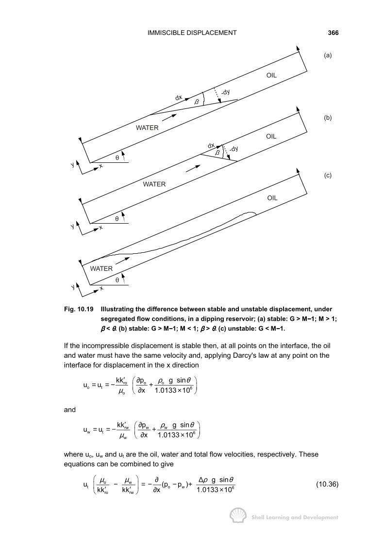
IMMISCIBLE DISPLACEMENT 366
y x
y x
y xθ
θ
θ
WATER
WATER
WATER
dx -dy
OIL
OIL
OIL
dx-dyβ
(a)
(b)
(c)
β
Fig. 10.19 Illustrating the difference between stable and unstable displacement, undersegregated flow conditions, in a dipping reservoir; (a) stable: G > M−−−−1; M > 1;ββββ < θθθθ. (b) stable: G > M−−−−1; M < 1; ββββ > θθθθ. (c) unstable: G < M−−−−1.
If the incompressible displacement is stable then, at all points on the interface, the oiland water must have the same velocity and, applying Darcy's law at any point on theinterface for displacement in the x direction
ro o oo t 6
o
kk p g sinu ux 1.0133 10
ρ θµ
′ ∂� �= = − +� �∂ ×� �
and
rw w ww t 6
w
kk p g sinu ux 1.0133 10
ρ θµ
′ ∂� �= = − +� �∂ ×� �
where uo, uw and ut are the oil, water and total flow velocities, respectively. Theseequations can be combined to give
o wt o w 6
ro rw
g sinu (p p )kk kk x 1.0133 10µ µ ρ θ� � ∂ ∆− = − − +� �′ ′ ∂ ×� �
(10.36)

IMMISCIBLE DISPLACEMENT 367
where ∆ρ = ρw − ρo. Also, applying the capillary pressure equation, (10.5),
c o w 6g cosdP d(p p ) dy
1.0133 10ρ θ∆= − =
×
and for stable displacement (dy/dx—negative)
c6
P g cos dyx dx1.0133 10
ρ θ∂ ∆= −∂ ×
which, when substituted in equ. (10.36) gives
o wt 6
ro rw
g dyu cos sinkk kk dx1.0133 10µ µ ρ θ θ
� � ∆ � �− = +� � � �′ ′ × � �� �
This equation can be alternatively expressed in terms of the total flow rate, qt, as
rorw rw6
w o w t
kk kk A g sin dy 11 1dx tan1.0133 10 q
ρ θµ µ θµ
′� �′ ′ ∆ � �− = +� � � �× � �� �
or
dy 1M 1 G 1dx tanθ
� �− = +� �� �
(10.37)
where M is the end point mobility ratio and G the dimensionless gravity number, whichin Darcy units is
rw6
t w
kk A g sinG1.0133 10 q
ρ θµ
′ ∆=×
(10.38)
and in field units can be deduced from equ. (10.10) to be
4 rw
t w
kk A sinG 4.9 10q
γ θµ
− ′ ∆= × (10.39)
Equation (10.37) can be solved to give the slope of the interface for stable flow as
dy M 1 Gtan tandx G
β θ− −� �= − = � �� �
(10.40)
In this equation M is a constant and, when displacing oil by water at a fixed rate in theupdip direction, G is a positive constant. Therefore, the inclination of the interface dy/dxassumes a fixed value. For stable displacement, as already mentioned, dy/dx must bea negative constant and this imposes the condition for stability that
G > M−1
The limiting case is when dy/dx = 0 then, as shown in fig. 10.19(c), the water willunderrun the oil in the form of a water tongue. This will occur when

IMMISCIBLE DISPLACEMENT 368
G = M−1
which, using equ. (10.38), can be solved to determine the so-called critical rate for by-passing as
rwcrit 6
w
kk A g sinq r.cc / sec1.0133 10 (M 1)
ρ θµ
′ ∆=× −
(10.41)
or in field units4
rwcrit
w
4.9 10 kk A sinq rb / d(M 1)
γ θµ
− ′× ∆=−
(10.42)
Provided the injection rate is maintained below qcrit gravity forces will stabilize thedisplacement.
The magnitude of the mobility ratio also influences the displacement. This can beappreciated from equ. (10.40), as detailed below.
M > 1This is the most common physical condition. The displacement is stable if G > M−1, inwhich case β < θ, fig. 10.19(a), and unstable if G < M−1.
M = 1This is a very favourable mobility ratio for which there is no tendency for the water toby-pass the oil (refer Chapter 4, sec. 9). For M = 1 the displacement is unconditionallystable. Furthermore, β = θ, and the interface rises horizontally in the reservoir.
M < 1This mobility ratio also leads to unconditionally stable displacement but in this case,β > θ, fig. 10.19(b).
If the displacement is stable the oil recovery, as a function of cumulative water injectedand time, can be calculated from simple geometrical considerations, as will bedemonstrated in exercise 10.3. An alternative approach is to attempt to reduce thedescription of segregated displacement to one dimension and then calculate the oilrecovery using the Buckley-Leverett displacement theory. It is worthwhile pursuing thisidea because it is quite general and can be applied whether the displacement is stableor not. Consider then the general segregated displacement in a linear, homogeneousreservoir as shown in fig.10.20.
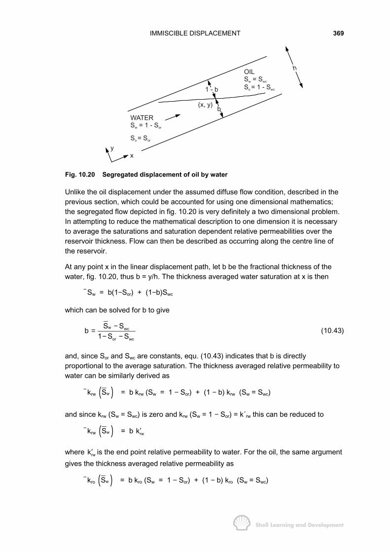
IMMISCIBLE DISPLACEMENT 369
WATERS = 1 - S
S = S
w or
o or
OILS = SS = 1 - S
w wc
o wc
xy
h
1 - b
b(x, y)
Fig. 10.20 Segregated displacement of oil by water
Unlike the oil displacement under the assumed diffuse flow condition, described in theprevious section, which could be accounted for using one dimensional mathematics;the segregated flow depicted in fig. 10.20 is very definitely a two dimensional problem.In attempting to reduce the mathematical description to one dimension it is necessaryto average the saturations and saturation dependent relative permeabilities over thereservoir thickness. Flow can then be described as occurring along the centre line ofthe reservoir.
At any point x in the linear displacement path, let b be the fractional thickness of thewater, fig. 10.20, thus b = y/h. The thickness averaged water saturation at x is then
Sw = b(1−Sor) + (1−b)Swc
which can be solved for b to give
w wc
or wc
S Sb1 S S
−=
− −(10.43)
and, since Sor and Swc are constants, equ. (10.43) indicates that b is directlyproportional to the average saturation. The thickness averaged relative permeability towater can be similarly derived as
krw ( )wS = b krw (Sw = 1 − Sor) + (1 − b) krw (Sw = Swc)
and since krw (Sw = Swc) is zero and krw (Sw = 1 − Sor) = k´rw this can be reduced to
krw ( )wS = b rwk′
where rwk′ is the end point relative permeability to water. For the oil, the same argumentgives the thickness averaged relative permeability as
kro ( )wS = b kro (Sw = 1 − Sor) + (1 − b) kro (Sw = Swc)
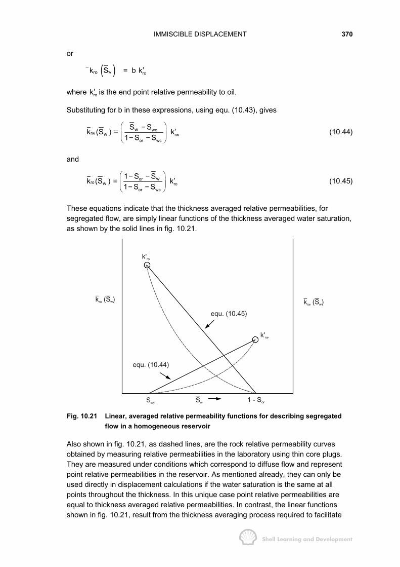
IMMISCIBLE DISPLACEMENT 370
or
kro ( )wS = b rok′
where rok′ is the end point relative permeability to oil.
Substituting for b in these expressions, using equ. (10.43), gives
wcrw rw
or wc
ww
S Sk (S ) k1 S S
� �− ′= � �� �− −� �(10.44)
and
orro ro
or wc
ww
1 S Sk (S ) k1 S S
� �− − ′= � �� �− −� �(10.45)
These equations indicate that the thickness averaged relative permeabilities, forsegregated flow, are simply linear functions of the thickness averaged water saturation,as shown by the solid lines in fig. 10.21.
k'ro
k Sro w ( )
equ. (10.45)
k Srw w ( )
equ. (10.44)
k'rw
Swc Sw 1 - Sor
Fig. 10.21 Linear, averaged relative permeability functions for describing segregatedflow in a homogeneous reservoir
Also shown in fig. 10.21, as dashed lines, are the rock relative permeability curvesobtained by measuring relative permeabilities in the laboratory using thin core plugs.They are measured under conditions which correspond to diffuse flow and representpoint relative permeabilities in the reservoir. As mentioned already, they can only beused directly in displacement calculations if the water saturation is the same at allpoints throughout the thickness. In this unique case point relative permeabilities areequal to thickness averaged relative permeabilities. In contrast, the linear functionsshown in fig. 10.21, result from the thickness averaging process required to facilitate
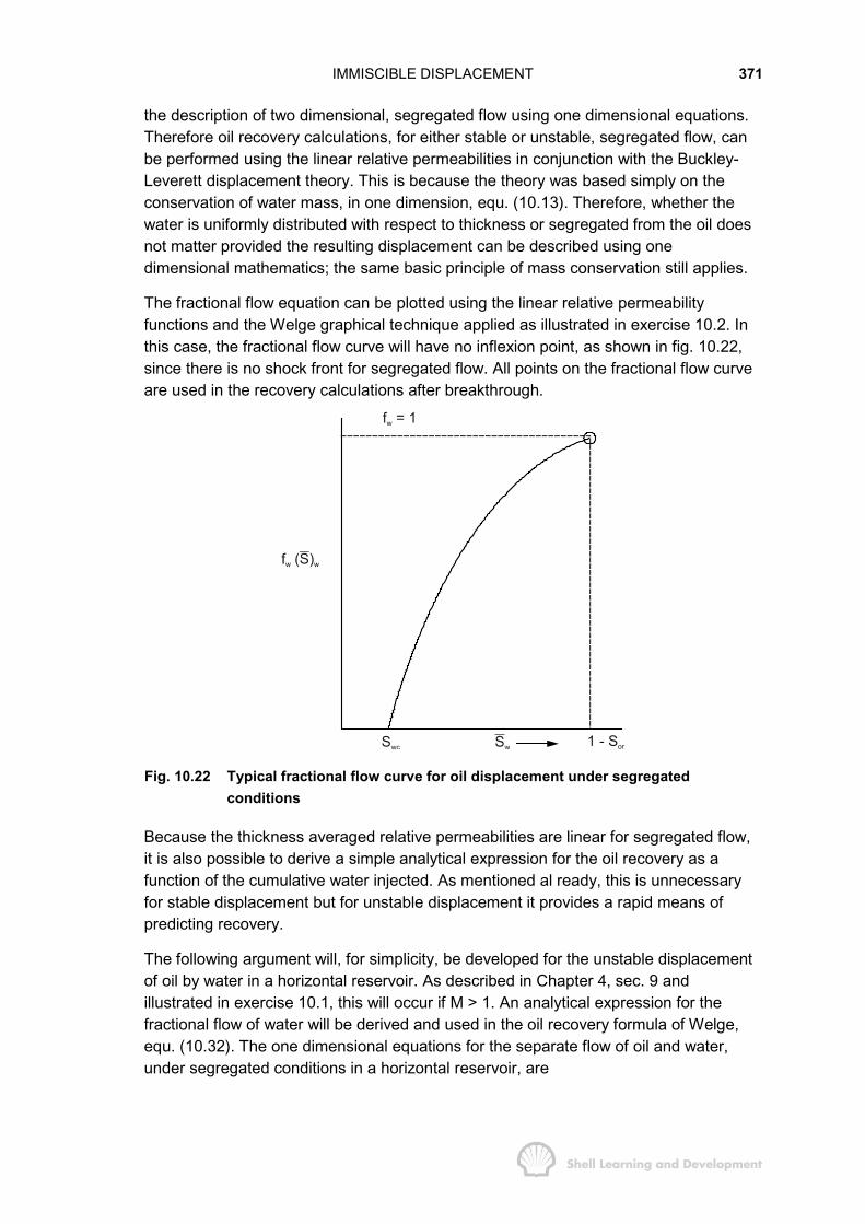
IMMISCIBLE DISPLACEMENT 371
the description of two dimensional, segregated flow using one dimensional equations.Therefore oil recovery calculations, for either stable or unstable, segregated flow, canbe performed using the linear relative permeabilities in conjunction with the Buckley-Leverett displacement theory. This is because the theory was based simply on theconservation of water mass, in one dimension, equ. (10.13). Therefore, whether thewater is uniformly distributed with respect to thickness or segregated from the oil doesnot matter provided the resulting displacement can be described using onedimensional mathematics; the same basic principle of mass conservation still applies.
The fractional flow equation can be plotted using the linear relative permeabilityfunctions and the Welge graphical technique applied as illustrated in exercise 10.2. Inthis case, the fractional flow curve will have no inflexion point, as shown in fig. 10.22,since there is no shock front for segregated flow. All points on the fractional flow curveare used in the recovery calculations after breakthrough.
f = 1w
Swc 1 - Sor
Fig. 10.22 Typical fractional flow curve for oil displacement under segregatedconditions
Because the thickness averaged relative permeabilities are linear for segregated flow,it is also possible to derive a simple analytical expression for the oil recovery as afunction of the cumulative water injected. As mentioned al ready, this is unnecessaryfor stable displacement but for unstable displacement it provides a rapid means ofpredicting recovery.
The following argument will, for simplicity, be developed for the unstable displacementof oil by water in a horizontal reservoir. As described in Chapter 4, sec. 9 andillustrated in exercise 10.1, this will occur if M > 1. An analytical expression for thefractional flow of water will be derived and used in the oil recovery formula of Welge,equ. (10.32). The one dimensional equations for the separate flow of oil and water,under segregated conditions in a horizontal reservoir, are

IMMISCIBLE DISPLACEMENT 372
ro oo
o
(1 b)kk A pqxµ
°′− ∂= −∂
(10.46)
and
rw ww
w
b kk A pqxµ
°′ ∂= −∂
(10.47)
in which A is the area of cross-section and op° and wp° are the oil and water phasepressures referred to the centre line of the reservoir, as shown in fig. 10.23.
Centre line
oil - water interface
h2
y
x
po
pw
}}
h2
( -y)
y
h
Fig. 10.23 Referring oil and water phase pressures at the interface to the centre line inthe reservoir. (Unstable segregated displacement in a horizontal,homogeneous reservoir)
From this diagram it can be seen that
oo o 6
ghp p y atm2 1.0133 10
ρ� �= − −� � ×� �
�
and
ww w 6
ghp p y atm2 1.0133 10
ρ° � �= − −� � ×� �
where y is the actual thickness of the water; i.e. y = bh. Since the pressures at theinterface, po and pw, are equal for segregated flow then the phase pressure gradient,resulting from the differentiation and subtraction of the above equations, is
o w6
p p g dyx x dx1.0133 10
ρ° °∂ ∂ ∆− = −∂ ∂ ×
For unstable, horizontal displacement the approximation is usually made that the angleof inclination of the interface, dy/dx, is small and therefore the gradient of the phasepressure difference can be neglected. In this case, using equs. (10.46) and (10.47),and following the argument used in sec. 10.3, in deriving the fractional flow equation,results in
ro rw
ro ww
o rw
ro w
kkf k1 b
b k
µµ
µµ
′⋅
′= ′− + ⋅
′

IMMISCIBLE DISPLACEMENT 373
which can be simplified as
wMbf
1 (M 1)b=
+ −
in which M is the end point mobility ratio. Until the moment of breakthrough the oilrecovery is simply equal to the cumulative water injected. After breakthrough, let be bethe fractional thickness of the water at the producing end of the reservoir block. Then,for a fully penetrating well, the fractional flow of water into the well is
ewe
e
Mbf1 (M 1)b
=+ −
(10.48)
Applying equ. (10.27) at the producing end of the block
we
weid
df1W dS
=
and using equ. (10.43) for the thickness averaged water saturation, Swe
we we e we
we wid e e or wc
df df db df1 1W db db (1 S S )dS dS
= = ⋅ = ⋅− −
and therefore
we or wc
e id iD
df (1 S S ) 1db W W
− −= =
in which WiD is the cumulative water injection expressed in movable oil volumes where
1 MOV = PV(1 − Swc − Sor)
Differentiating equ. (10.48) with respect to be gives
we2
e iD e
df 1 Mdb W (1 (M 1)b )
= =+ −
from which it can be determined that
( )e iD1b W M 1
M 1= −
−(10.49)
and substituting for be in equ. (10.48) gives
( )we iDMf 1 W M
M 1= −
−(10.50)
The oil recovery equation, (10.32), can be expressed in MOV's as
we wcpD we iD
or wc
S SN (1 f )W1 S S
−= −
− −
IMMISCIBLE DISPLACEMENT 374
or
pD e we iDN b (1 f )W= + −
and substituting in this equation for be and fwe, using equs. (10.49) and (10.50), resultsin the simple recovery formula
pD iD iD1N (2 W M W 1)
M 1= − −
−(10.51)
in which all volumes are expressed in MOV's. It should again be stressed thatequ. (10.51) is only applicable for horizontal displacement under segregated conditionsand for unstable flow (M > 1).
At the time of water breakthrough NpD = WiD and solving equ. (10.51) for this conditiongives
btpD1NM
= (10.52)
which shows that in the limiting case of M = 1, stable, piston-like displacement occursfor which
btpDN 1= . Similarly, when the total amount of oil has been recovered, NpD = 1
(MOV), and substituting this condition in equ. (10.51) gives
maxiDW M= (10.53)
Equations (10.52) and (10.53) clearly demonstrate the significance of the mobility ratioin characterising oil recovery under segregated flow conditions.
For the more general case of unstable displacement in a dipping reservoir (G<M−1),the fractional flow equation, equivalent to equ. (10.48), is
e e ewe
e
Mb b (1 b )Gf1 (M 1) b
− −=+ −
and repeating the steps leading to equ. (10.51 ) will, in this more complex case, yieldthe recovery formula
iDpD iD iD
W G1 G (M 1)N 2 W M 1 1 W 1 G 1M 1 M 1 M 1 (M 1)
� �� �+� �� �= − − − − −� �� �� � � �� �− − − −� � � � � �� �(10.54)
which if G = 0 (horizontal reservoir) reduces to the form of equ. (10.51).Equation (10.54) can readily be solved for the breakthrough condition (NpD = WiD) togive
btpD1N
M G=
−(10.55)
while for the maximum recovery (NpD = 1)
IMMISCIBLE DISPLACEMENT 375
maxiDMW
G 1=
+(10.56)
EXERCISE 10.3 DISPLACEMENT UNDER SEGREGATED FLOW CONDITIONS
1) Re-work Exercise 10.2, for the same water injection rate and using precisely thesame reservoir and fluid property data but assuming that displacement takesplace under segregated flow conditions. Compare the results with those obtainedin exercise 10.2.
2) If the same reservoir had a dip angle of 25°, what would be the critical rate forwater displacing oil updip? Compare the breakthrough times and the oil recoveryat breakthrough when injecting at 1000 rb/d and also at 90% of the critical rate.
Additional information
k = 2.0 Darcy
γw = 1.04 specific gravity in the reservoir
γo = .81 " " " "
EXERCISE 10.3 SOLUTION
1) Using the relative permeability relations given in exercise 10.1, table 10.1, and forµo = 5 cp, µw = 0.5 cp (Case 2 of exercise 10.1), the end point mobility ratio canbe evaluated as
rw w
ro o
k / .3 .8M 3.750k / .5 5
µµ
′= = =
′
Therefore, using equs. (10.52) and (10.53), breakthrough will occur when
bt btiD pD1W N .267 (MOV) .160 (PV)M
= = = =
since 1 MOV = PV(1 − Sor − Swc) = PV(1−0.2−0.2) = 0.6 PV; and the maximum oilrecovery when
WiD = M = 3.75 (MOV) = 2.25 (PV)Between breakthrough and maximum recovery, the oil recovery as a function of WiDcan be calculated using equ. (10.51), with WiD as the independent variable. The resultsare listed in table 10.6.
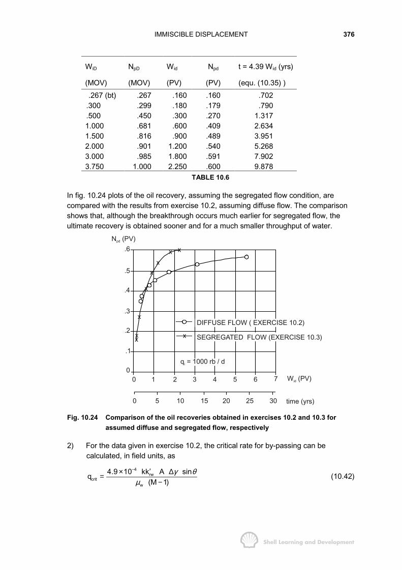
IMMISCIBLE DISPLACEMENT 376
WiD NpD Wid Npd t = 4.39 Wid (yrs)
(MOV) (MOV) (PV) (PV) (equ. (10.35) ) .267 (bt) .267 .160 .160 .702.300 .299 .180 .179 .790.500 .450 .300 .270 1.3171.000 .681 .600 .409 2.6341.500 .816 .900 .489 3.9512.000 .901 1.200 .540 5.2683.000 .985 1.800 .591 7.9023.750 1.000 2.250 .600 9.878
TABLE 10.6
In fig. 10.24 plots of the oil recovery, assuming the segregated flow condition, arecompared with the results from exercise 10.2, assuming diffuse flow. The comparisonshows that, although the breakthrough occurs much earlier for segregated flow, theultimate recovery is obtained sooner and for a much smaller throughput of water.
N (PV)pd
.6
.4
.5
.2
.3
0
.1
0 1 2 3 4 5 6 7
0 5 10 15 20 25 30
W (PV)id
time (yrs)
q = 1000 rb / di
DIFFUSE FLOW ( EXERCISE 10.2)
SEGREGATED FLOW (EXERCISE 10.3)
Fig. 10.24 Comparison of the oil recoveries obtained in exercises 10.2 and 10.3 forassumed diffuse and segregated flow, respectively
2) For the data given in exercise 10.2, the critical rate for by-passing can becalculated, in field units, as
4rw
critw
4.9 10 kk A sinq(M 1)
γ θµ
− ′× ∆=−
(10.42)
IMMISCIBLE DISPLACEMENT 377
4 o
crit4.9 10 2000 .3 625 40 (1.04 0.81) sin25q (rb / d)
.5(3.75 1)520 rb.water / d
−× × × × × × − ×=−
=
While for injection at this critical rate
G = M − 1 = 2.75
Comparison of equs. (10.39) and (10.42) indicates that
qcrit (M − 1) = qtG
and therefore, at an injection rate of qi = qt = 1000 rb/d
520G 2.75 1.4301000
= × =
Substituting this value of G and the value of M = 3.75 in equ. (10.54), for this unstabledisplacement (G < M−1), reduces the latter to
pD iD iD iDN 0.976 W (1 0.520W ) 0.535 W 0.364= − + − (10.57)
At the time of water breakthrough NpD = WiD and equ. (10.55) can be applied todetermine the breakthrough recovery as
btpD1 1N 0.431 (MOV) 0.259 (PV)
M G 3.75 1.43= = = =
− −
which, when injecting at 1000 rb/d, will occur after 4.39 btiDW = 1.137 years,
equ. (10.35). Similarly, the maximum cumulative water injection to recover the onemovable oil volume can be determined using equ. (10.56) as
maxiDM 3.75W 1.543 (MOV) 0.926 (PV)
G 1 2.43= = = =
+
Between breakthrough and total recovery equ. (10.57) can be used to calculate the oilrecovery, as listed in table 10.7.
WiD
(MOV)NpD
(MOV)Wid
(PV)Npd
(PV)t = 4.39 Wid (yrs)
(equ. (10.35))
.431 (bt) .431 .259 .259 1.137.500 .497 .300 .298 1.317.750 .697 .450 .418 1.976
1.000 .847 .600 .508 2.6341.250 .950 .750 .570 3.2931.543 1.000 .926 .600 4.064
TABLE 10.7
When compared to the water drive performance, at an injection rate of 1000 rb/d in ahorizontal reservoir (table 10.6), it can be seen that, even though the displacement is
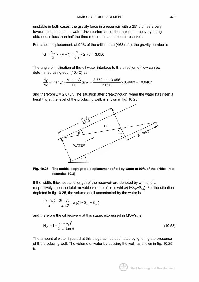
IMMISCIBLE DISPLACEMENT 378
unstable in both cases, the gravity force in a reservoir with a 25° dip has a veryfavourable effect on the water drive performance, the maximum recovery beingobtained in less than half the time required in a horizontal reservoir.
For stable displacement, at 90% of the critical rate (468 rb/d), the gravity number is
crit
t
q 1G (M 1) 2.75 3.056q 0.9
= × − = × =
The angle of inclination of the oil water interface to the direction of flow can bedetermined using equ. (10.40) as
dy M 1 G 3.750 1 3.056tan tan 0.4663 0.0467dx G 3.056
β θ− − − −= − = = × = −
and therefore β = 2.673°. The situation after breakthrough, when the water has risen aheight ye at the level of the producing well, is shown in fig. 10.25.
h - y
tan e
β
β
OIL
WATER
θ
ye y / tan e
β
h
Fig. 10.25 The stable, segregated displacement of oil by water at 90% of the critical rate(exercise 10.3)
If the width, thickness and length of the reservoir are denoted by w, h and L,respectively, then the total movable volume of oil is whLφ (1−Sor−Swc). For the situationdepicted in fig.10.25, the volume of oil uncontacted by the water is
e eor wc
(h y ) (h y ) w (1 S S )2 tan
φβ
− −× − −
and therefore the oil recovery at this stage, expressed in MOV's, is2
epD
(h y )N 12hL tan β
−= − (10.58)
The amount of water injected at this stage can be estimated by ignoring the presenceof the producing well. The volume of water by-passing the well, as shown in fig. 10.25is
IMMISCIBLE DISPLACEMENT 379
e eor wc
y y w (1 S S )2 tan
φβ
⋅ − −
and therefore the number of MOV's of water injected is2
eiD pD
yW N2hL tan β
= + (10.59)
In particular, at breakthrough, ye = 0 and
bt btpD iDhN W 1
2L tan β= = − (10.60)
For the data relevant to this exercise, the recovery at breakthrough can be calculatedusing equ. (10.60) as
btpD40N 1 0.786 MOV .472 PV
2 2000 .0467= − = =
× ×
At an injection rate of 468 rb/d the relation between water injected and time is now(refer equ. (10.35)
id id1000t 4.39 W 9.38 W (years)468
= × =
and therefore breakthrough occurs after 9.38 × .472 = 4.43 years. Thereafter the oilrecovery and cumulative water injection, as functions of time, are listed in table 10.8.These have been calculated using equs. (10.58) and (10.59) for increasing valuesof ye.
ye
ftNpD
(MOV)WiD
(MOV)Npd
(PV)Wid
(PV)t = 9.38Wid
years 0 (bt) .786 .786 .472 .472 4.427
10 .880 .893 .528 .536 5.02820 .946 1.000 .568 .600 5.62830 .987 1.107 .592 .664 6.22840 1.000 1.214 .600 .728 6.829
TABLE 10.8
When compared to the results presented in table 10.7, which were obtained at aninjection rate of 1000 rb/d, the effect of displacing the oil at a rate which is below critical(468 rb/d) is quite naturally to increase both the breakthrough time (by nearly 300% )and the total recovery time (by almost 70% ). The main advantage in displacement atthe lower rate is that the total water requirements are reduced from 1.543 to1.214 (MOV). If there are problems concerning either the availability of injection wateror disposal of produced water it may be considered expedient to inject at a rate whichis just below critical.

IMMISCIBLE DISPLACEMENT 380
The same analytical methods described in this section can be applied to the case ofgas displacing oil downdip, at constant pressure.
As shown in fig.10.26,for unstable displacement the gas will tend to override the oilcausing premature gas breakthrough in the downdip producing wells. For stabledisplacement the angle of inclination of the gas-oil interface remains constant.
GAS
OIL
y x y x
(a)
GAS
OIL
β
(b)
Fig. 10.26 Segregated downdip displacement of oil by gas at constant pressure;(a) unstable, (b) stable
Applying the method described in this section for determining the critical rate (in thiscase it is algebraically convenient to keep the same sign convention, x-positive in theupdip direction, and reverse the signs of the flow velocities) will again give thecondition for stable displacement as
G > M−1
This leads to the critical rate formula
rgcrit 6
g
kk A g sinq
1.0133 10 (M 1)ρ θ
µ′ ∆
=× −
in which, for gas displacing oil
o gρ ρ ρ∆ = −
rg crit6
tg t
kk A g sin qG (M 1)q1.0133 10 q
ρ θµ
′ ∆= = −
×(10.61)
and rg g
ro o
k /M
k /µµ
′=
′
Since µg is very small compared to µo, the mobility ratio for this displacement is largeand the requirement for unconditional stability (M ≤ 1) is never satisfied. Stability thendepends on the magnitude of G and hence on the dip angle.
An interesting extension of the methods described in this section has been presentedby van Daalen and van Domselaar12 who considered segregated displacement inreservoirs in which there is a defined (absolute) permeability distribution in the dipnormal direction. In addition, Richardson and Blackwell13 have analysed some quite

IMMISCIBLE DISPLACEMENT 381
complex displacement problems using the assumption of segregated flow, theseinclude gravity drainage and bottom water coning.
In this section a great deal of attention has been focussed on the presentation ofapproximate analytical methods for predicting oil recovery resulting from segregateddisplacement. In reading the remainder of this chapter, however, the main point tokeep in mind is that the description of segregated flow in one dimension necessitatesthe use of linear, averaged relative permeability functions, irrespective of whether thedisplacement is stable or not. It is this fact which facilitated the derivation of suchsimple recovery formulae.
10.7 ALLOWANCE FOR THE EFFECT OF A FINITE CAPILLARY TRANSITION ZONE INDISPLACEMENT CALCULATIONS
For the displacement of oil by water, exercises 10.2 and 10.3 clearly demonstrate thesensitivity of the calculated oil recovery, as a function of time, to the assumed watersaturation distribution in the dip-normal direction. So far, too extreme notions of thisdistribution have been considered; the uniform distribution (diffuse flow) and that due tofluid segregation. From the information provided in the two exercises it is not possiblefor the engineer to decide which, if either, of the assumed saturation distributions isappropriate to describe the displacement. One vital piece of data has been omitted andthat is the capillary pressure curve and, in particular, the thickness of the capillarytransition zone.
If h is the reservoir thickness and H the thickness of the capillary transition zone thenthe water saturation distribution can be approximated as uniform or segregateddepending on whether
H >> h (uniform)
H << h (segregated)
If the reservoir is very thin in comparison to the capillary transition zone the saturationin the advancing water flood will appear to be uniformly distributed with respect tothickness, fig. 10.7. On the other hand, if the transition zone is of negligible thicknesscompared to the reservoir then it will appear that the oil and water are segregated.Linear relative permeability curves can be used to describe such displacement.
The question then arises of how to describe oil displacement in a homogeneousreservoir when the capillary transition zone is of the same order of magnitude as thereservoir thickness (H ≈ h). Consider, for instance, the capillary pressure curve shownin fig. 10.27(a) in which the capillary pressure difference across the transition zone is3 psi.
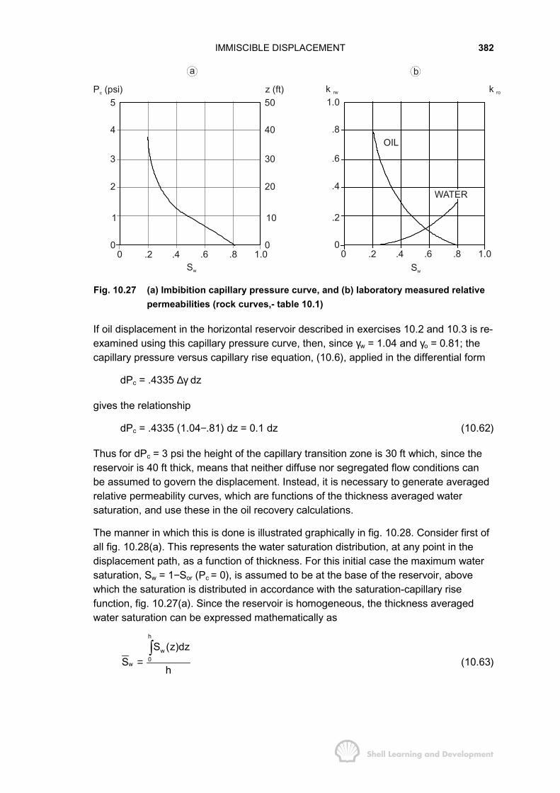
IMMISCIBLE DISPLACEMENT 382
P (psi)c
5
4
3
2
1
00 .2 .4 .6 .8 1.0
50
40
30
20
10
0
z (ft)
a
k rw
1.0
.8
.6
.4
.2
00 .2 .4 .6 .8 1.0
k ro
b
OIL
WATER
SwSw
Fig. 10.27 (a) Imbibition capillary pressure curve, and (b) laboratory measured relativepermeabilities (rock curves,- table 10.1)
If oil displacement in the horizontal reservoir described in exercises 10.2 and 10.3 is re-examined using this capillary pressure curve, then, since γw = 1.04 and γo = 0.81; thecapillary pressure versus capillary rise equation, (10.6), applied in the differential form
dPc = .4335 ∆γ dz
gives the relationship
dPc = .4335 (1.04−.81) dz = 0.1 dz (10.62)
Thus for dPc = 3 psi the height of the capillary transition zone is 30 ft which, since thereservoir is 40 ft thick, means that neither diffuse nor segregated flow conditions canbe assumed to govern the displacement. Instead, it is necessary to generate averagedrelative permeability curves, which are functions of the thickness averaged watersaturation, and use these in the oil recovery calculations.
The manner in which this is done is illustrated graphically in fig. 10.28. Consider first ofall fig. 10.28(a). This represents the water saturation distribution, at any point in thedisplacement path, as a function of thickness. For this initial case the maximum watersaturation, Sw = 1−Sor (Pc = 0), is assumed to be at the base of the reservoir, abovewhich the saturation is distributed in accordance with the saturation-capillary risefunction, fig. 10.27(a). Since the reservoir is homogeneous, the thickness averagedwater saturation can be expressed mathematically as
h
w0
w
S (z)dzS
h=�
(10.63)

IMMISCIBLE DISPLACEMENT 383
40
30
20
10
00 .2 .4 .6 .8 1.0
Sw
a Sw = .357
z(ft)
40
30
20
10
00 .2 .4 .6 .8 1.0
k r
b krw = .047; kro = .481
z(ft) kro(z)
krw (z)
Fig. 10.28 (a) Water saturation, and (b) relative permeability distributions, withrespect to thickness when the saturation at the base of the reservoir isSw = 1 −−−− Sor (Pc =0)
which can be evaluated graphically by measuring the shaded area to the left andbeneath the saturation-thickness function, fig. 10.28(a), and dividing this by the totalheight, h = 40 ft. For this initial saturation distribution Sw = 0.357.
The rock relative permeabilities presented in table 10.1, which have been used inexercises 10.2 and 10.3, are plotted as fig. 10.27(b). As already mentioned, theserepresent point relative permeabilities in the reservoir and are dependent on the watersaturation at the point in question. Therefore, since there is a defined water saturationdistribution in the reservoir, fig. 10.28(a), there must also be a relative permeabilitydistribution, with respect to thickness, for both oil and water. These distributions can bedetermined by selecting a particular height in the reservoir and reading the watersaturation at that point from fig. 10.28(a). For this saturation the corresponding pointrelative permeabilities are read from fig. 10.27 (b). These relative permeabilitydistributions are listed in table 10.9 and plotted in fig. 10.28(b).
Mathematically, the thickness averaged relative permeabilities areh
rw w0
rw w
k (S (z))dzk (S )
h=�
(10.64)
andh
ro w0
ro o
k (S (z))dzk (S )
h=�
(10.65)
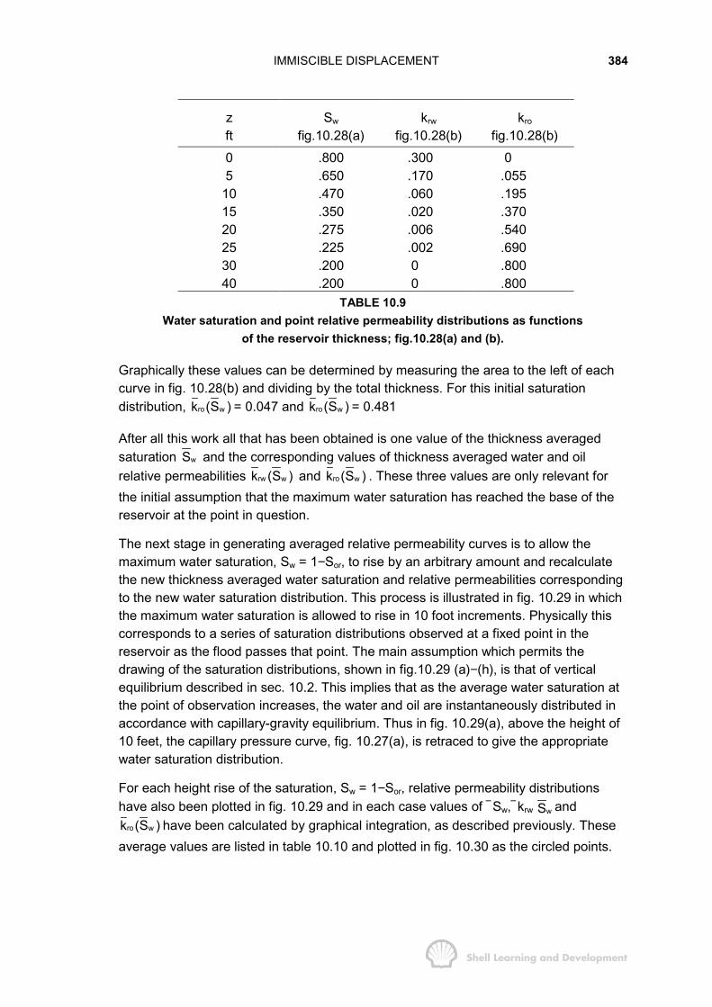
IMMISCIBLE DISPLACEMENT 384
zft
Sw
fig.10.28(a)krw
fig.10.28(b)kro
fig.10.28(b)0 .800 .300 05 .650 .170 .055
10 .470 .060 .19515 .350 .020 .37020 .275 .006 .54025 .225 .002 .69030 .200 0 .80040 .200 0 .800
TABLE 10.9Water saturation and point relative permeability distributions as functions
of the reservoir thickness; fig.10.28(a) and (b).
Graphically these values can be determined by measuring the area to the left of eachcurve in fig. 10.28(b) and dividing by the total thickness. For this initial saturationdistribution, ro wk (S ) = 0.047 and ro wk (S ) = 0.481
After all this work all that has been obtained is one value of the thickness averagedsaturation wS and the corresponding values of thickness averaged water and oilrelative permeabilities rw wk (S ) and ro wk (S ) . These three values are only relevant forthe initial assumption that the maximum water saturation has reached the base of thereservoir at the point in question.
The next stage in generating averaged relative permeability curves is to allow themaximum water saturation, Sw = 1−Sor, to rise by an arbitrary amount and recalculatethe new thickness averaged water saturation and relative permeabilities correspondingto the new water saturation distribution. This process is illustrated in fig. 10.29 in whichthe maximum water saturation is allowed to rise in 10 foot increments. Physically thiscorresponds to a series of saturation distributions observed at a fixed point in thereservoir as the flood passes that point. The main assumption which permits thedrawing of the saturation distributions, shown in fig.10.29 (a)−(h), is that of verticalequilibrium described in sec. 10.2. This implies that as the average water saturation atthe point of observation increases, the water and oil are instantaneously distributed inaccordance with capillary-gravity equilibrium. Thus in fig. 10.29(a), above the height of10 feet, the capillary pressure curve, fig. 10.27(a), is retraced to give the appropriatewater saturation distribution.
For each height rise of the saturation, Sw = 1−Sor, relative permeability distributionshave also been plotted in fig. 10.29 and in each case values of Sw, krw wS and
ro wk (S ) have been calculated by graphical integration, as described previously. Theseaverage values are listed in table 10.10 and plotted in fig. 10.30 as the circled points.
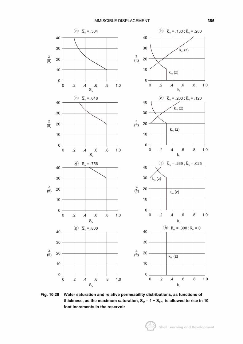
IMMISCIBLE DISPLACEMENT 385
40
30
20
10
00 .2 .4 .6 .8 1.0
40
30
20
10
00 .2 .4 .6 .8 1.0
40
30
20
10
00 .2 .4 .6 .8 1.0
40
30
20
10
00 .2 .4 .6 .8 1.0
40
30
20
10
00 .2 .4 .6 .8 1.0
40
30
20
10
00 .2 .4 .6 .8 1.0
40
30
20
10
00 .2 .4 .6 .8 1.0
40
30
20
10
00 .2 .4 .6 .8 1.0
Sw
Sw
Sw
Sw
kr
kr
kr
kr
a Sw = .504
c Sw = .648
e Sw = .756
g Sw = .800
z(ft)
z(ft)
z(ft)
z(ft)
z(ft)
z(ft)
z(ft)
z(ft)
b krw = .130 ; kro = .280
d k krw ro= .203 ; = .120
h k krw ro = .300 ; = 0
k (z)ro
k (z)rw
k (z)ro
k (z)rw
k (z)rw
f k krw ro= .269 ; = .025
k (z)rw
k (z)ro
Fig. 10.29 Water saturation and relative permeability distributions, as functions ofthickness, as the maximum saturation, Sw = 1 −−−− Sor, is allowed to rise in 10foot increments in the reservoir
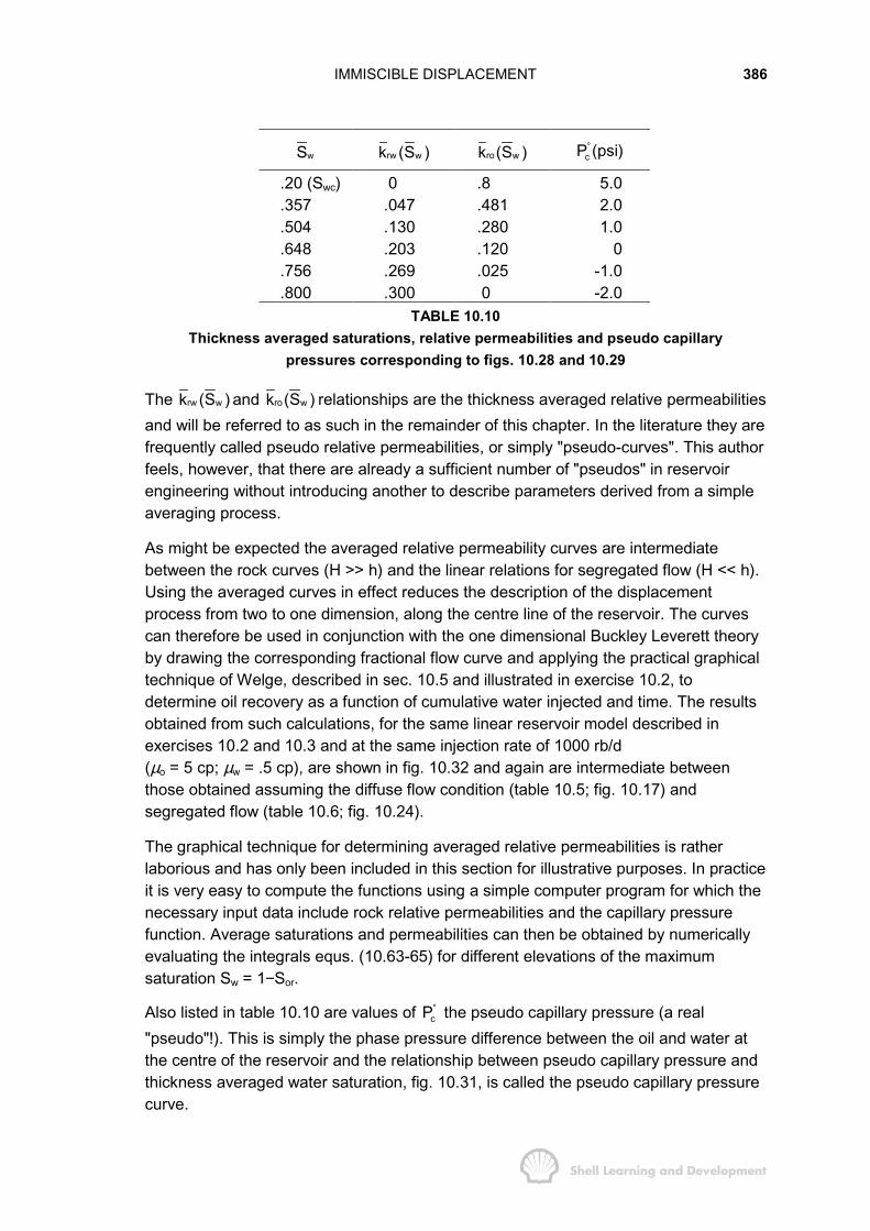
IMMISCIBLE DISPLACEMENT 386
wS rw wk (S ) ro wk (S ) cP (psi)°
.20 (Swc) 0 .8 5.0
.357 .047 .481 2.0
.504 .130 .280 1.0
.648 .203 .120 0
.756 .269 .025 -1.0
.800 .300 0 -2.0TABLE 10.10
Thickness averaged saturations, relative permeabilities and pseudo capillarypressures corresponding to figs. 10.28 and 10.29
The rw wk (S ) and ro wk (S ) relationships are the thickness averaged relative permeabilitiesand will be referred to as such in the remainder of this chapter. In the literature they arefrequently called pseudo relative permeabilities, or simply "pseudo-curves". This authorfeels, however, that there are already a sufficient number of "pseudos" in reservoirengineering without introducing another to describe parameters derived from a simpleaveraging process.
As might be expected the averaged relative permeability curves are intermediatebetween the rock curves (H >> h) and the linear relations for segregated flow (H << h).Using the averaged curves in effect reduces the description of the displacementprocess from two to one dimension, along the centre line of the reservoir. The curvescan therefore be used in conjunction with the one dimensional Buckley Leverett theoryby drawing the corresponding fractional flow curve and applying the practical graphicaltechnique of Welge, described in sec. 10.5 and illustrated in exercise 10.2, todetermine oil recovery as a function of cumulative water injected and time. The resultsobtained from such calculations, for the same linear reservoir model described inexercises 10.2 and 10.3 and at the same injection rate of 1000 rb/d(µo = 5 cp; µw = .5 cp), are shown in fig. 10.32 and again are intermediate betweenthose obtained assuming the diffuse flow condition (table 10.5; fig. 10.17) andsegregated flow (table 10.6; fig. 10.24).
The graphical technique for determining averaged relative permeabilities is ratherlaborious and has only been included in this section for illustrative purposes. In practiceit is very easy to compute the functions using a simple computer program for which thenecessary input data include rock relative permeabilities and the capillary pressurefunction. Average saturations and permeabilities can then be obtained by numericallyevaluating the integrals equs. (10.63-65) for different elevations of the maximumsaturation Sw = 1−Sor.
Also listed in table 10.10 are values of cP° the pseudo capillary pressure (a real"pseudo"!). This is simply the phase pressure difference between the oil and water atthe centre of the reservoir and the relationship between pseudo capillary pressure andthickness averaged water saturation, fig. 10.31, is called the pseudo capillary pressurecurve.
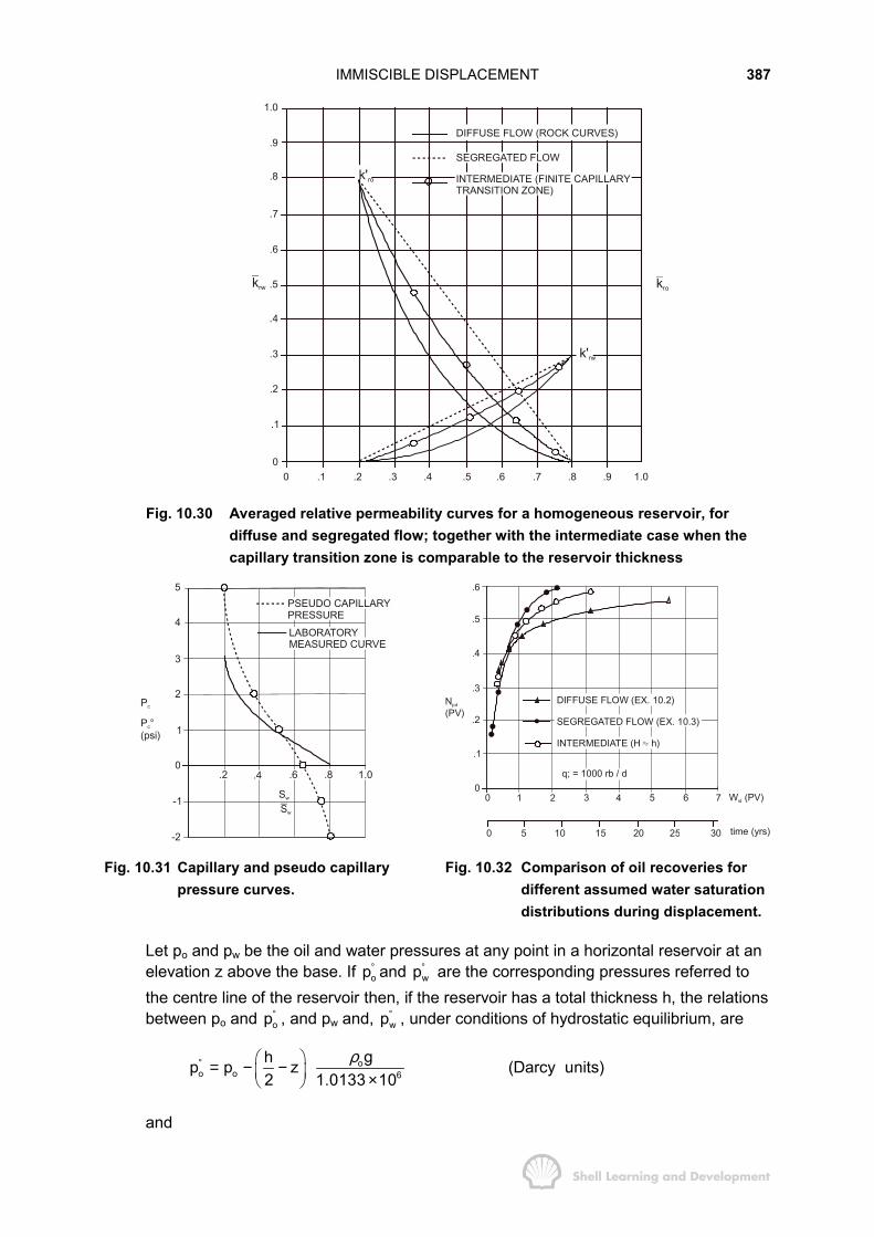
IMMISCIBLE DISPLACEMENT 387
DIFFUSE FLOW (ROCK CURVES)
SEGREGATED FLOW
INTERMEDIATE (FINITE CAPILLARYTRANSITION ZONE)
1.0
.9
.8
.7
.6
.5
.4
.3
.2
.1
00 .1 .2 .3 .4 .5 .6 .7 .8 .9 1.0
krw
k'ro
kro
k'rw
Fig. 10.30 Averaged relative permeability curves for a homogeneous reservoir, fordiffuse and segregated flow; together with the intermediate case when thecapillary transition zone is comparable to the reservoir thickness
PSEUDO CAPILLARYPRESSURE
LABORATORYMEASURED CURVE
5
4
3
2
1
0
-1
-2
.2 .4 .6 1.0.8
Sw
Sw
P
P °(psi)
c
c
0 5 10 15 20 25 30 time (yrs)
00 1 2 3 4 5 6 7
.6
.5
.4
.3
.2
.1
q; = 1000 rb / d
DIFFUSE FLOW (EX. 10.2)
SEGREGATED FLOW (EX. 10.3)
INTERMEDIATE (H h)
N(PV)
pd
W (PV)id
Fig. 10.31 Capillary and pseudo capillarypressure curves.
Fig. 10.32 Comparison of oil recoveries fordifferent assumed water saturationdistributions during displacement.
Let po and pw be the oil and water pressures at any point in a horizontal reservoir at anelevation z above the base. If op° and wp° are the corresponding pressures referred tothe centre line of the reservoir then, if the reservoir has a total thickness h, the relationsbetween po and op° , and pw and, wp° , under conditions of hydrostatic equilibrium, are
oo o 6
ghp p z (Darcy units)2 1.0133 10
ρ° � �= − −� � ×� �
and
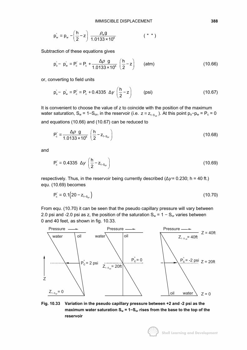
IMMISCIBLE DISPLACEMENT 388
ww w 6
ghp p z ( " " )2 1.0133 10
ρ° � �= − −� � ×� �
Subtraction of these equations gives
o w c c 6
g hp p P P z (atm)21.0133 10
ρ° ° ° ∆ � �− = = + −� �× � �(10.66)
or, converting to field units
o w c chp p P P 0.4335 z (psi)2
γ° ° ° � �− = = + ∆ −� �� �
(10.67)
It is convenient to choose the value of z to coincide with the position of the maximumwater saturation, Sw = 1−Sor, in the reservoir (i.e.
or1 Sz z −= ). At this point po−pw = Pc = 0
and equations (10.66) and (10.67) can be reduced to
orc 1 S6
g hP z21.0133 10
ρ°−
∆ � �= −� �× � �(10.68)
and
orc 1 ShP 0.4335 z2
γ°−
� �= ∆ −� �� �
(10.69)
respectively. Thus, in the reservoir being currently described (∆γ = 0.230; h = 40 ft.)equ. (10.69) becomes
( )orc 1 SP 0.1 20 z°−= − (10.70)
From equ. (10.70) it can be seen that the pseudo capillary pressure will vary between2.0 psi and -2.0 psi as z, the position of the saturation Sw = 1 − Sor varies between0 and 40 feet, as shown in fig. 10.33.
Pressure Pressure Pressure
Z
Z = 01 -S
P = 2 psi°c
P = -2 psi°cP = 0°
c
water oil water oil
wateroil
Z = 20ft1 -S
Z = 40ft
Z = 20ft
Z = 0
Z = 40ft1 -S
or
or
or
Fig. 10.33 Variation in the pseudo capillary pressure between +2 and -2 psi as themaximum water saturation Sw = 1−−−−Sor rises from the base to the top of thereservoir
IMMISCIBLE DISPLACEMENT 389
Values of cP° as a function of Sw are listed in table 10.10, and the relationship plotted infig. 10.31. In particular, the maximum value of cP° is included for Sw = Swc = .2, theconnate water saturation. In this case, the water saturation is also 0.2 at the base ofreservoir which, as shown in fig. 27(a), corresponds to a capillary pressure of at least3 psi. Therefore the phase pressure difference at the centre of the reservoir must be, atleast, cP° = 5 psi.
Using the combination of averaged relative permeabilities and pseudo capillarypressure a one dimensional fractional flow equation, representing the average flowalong the centre line of the reservoir, can be developed which is analogous toequ. (10.9). The only difference will be that the rock relative permeabilities will bereplaced by averaged permeabilities and the capillary pressure gradient term
cPx
∂∂
by cPx
°∂∂
. And, just as the capillary pressure gradient was neglected in the oil
recovery calculations described in sec. 10.5, so too, the cPx
°∂∂
term is neglected when
drawing the fractional flow curve for the present recovery calculations. The pseudocapillary pressure-saturation relationship, however, plays an important role innumerical reservoir simulation which will be described in sec. 10.10.
The methods presented in this section can also be applied in a dipping reservoir. Theaveraging is again carried out in the dip normal direction with the result that thecapillary pressures, evaluated in this section as
dPc ∝ dz
are replaced throughout by expressions of the form
dPc ∝ cosθ dy
where z is measured vertically upwards and y in the dip-normal direction from the baseof the reservoir.
10.8 DISPLACEMENT IN STRATIFIED RESERVOIRS
So far, displacement has only been considered in homogeneous, linear reservoirs. Instratified reservoirs in which there is a defined variation in reservoir parameters withthickness, in the dip-normal direction, the description of displacement is necessarilymore complex. Nevertheless, the same basic method is used, as described in theprevious section, namely, to generate thickness averaged relative permeabilities asfunctions of the thickness averaged water saturation. This will again reduce themathematical description to one dimension permitting the use of the Buckley Leveretttheory and the Welge graphical technique (sec. 10.5) for approximate calculations ofthe oil recovery.
Two cases can be distinguished, which will both be dealt with in this section. Firstly,when there is pressure communication between the individual sand layers and verticalequilibrium pertains across the entire formation thickness and, secondly, when the

IMMISCIBLE DISPLACEMENT 390
individual sands are isolated from one another by impermeable shale layers so thatthere is a total lack of pressure communication.
a) With pressure communication between the layers
Consider the case of a 40 ft. thick horizontal reservoir which can be subdivided intothree homogeneous layers each with different thickness, porosity and permeability, asshown in fig.10.34.
layer 3
layer 2
layer 1
k = 200mD;3
k = 100mD;
k = 50mD;
2
1
φ3 = 0.20;
φ
φ
2
1
= 0.17;
= 0.15;
h = 10 ft.3
h
h
2
1
= 20 ft.
= 10 ft.
h = 40 ft.
Fig. 10.34 Example of a stratified, linear reservoir for which pressure communicationbetween the layers is assumed
If the water and oil again have specific gravities of 1.04 and 0.81, respectively then thecapillary pressure is related to capillary rise by the equation
dPc = 0.1 dz (psi) (10.62)
Similarly, the pseudo capillary pressure equation for calculating the phase pressuredifference at the centre of the reservoir is still
orc 1 SP 0.1 (20 z )−° = − (10.70)
where or1 Sz − is the elevation of the maximum water saturation, Sw = 1 − Sor, in the
reservoir, at which point the phase pressure Pc is always zero. Laboratory measuredrelative permeabilities and capillary pressures for the three layers are shown infig. 10.35.
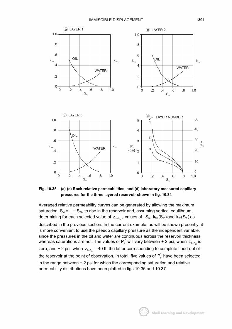
IMMISCIBLE DISPLACEMENT 391
k rw
1.0
.8
.6
.4
.2
00 .2 .4 .6 .8 1.0
k ro
a
OIL
WATER
Sw
LAYER 1
(psi)Pc
5
4
3
2
1
00 .2 .4 .6 .8 1.0
z(ft)
d
Sw
LAYER NUMBER 50
40
30
20
10
0
1
2
3k rw
1.0
.8
.6
.4
.2
00 .2 .4 .6 .8 1.0
k ro
c
OIL
WATER
Sw
LAYER 3
k rw
1.0
.8
.6
.4
.2
00 .2 .4 .6 .8 1.0
k ro
b
OIL
WATER
Sw
LAYER 2
Fig. 10.35 (a)-(c) Rock relative permeabilities, and (d) laboratory measured capillarypressures for the three layered reservoir shown in fig. 10.34
Averaged relative permeability curves can be generated by allowing the maximumsaturation, Sw = 1 − Sor, to rise in the reservoir and, assuming vertical equilibrium,determining for each selected value of
or1 Sz ,− values of Sw, rw wk (S ) and ro wk (S ) as
described in the previous section. In the current example, as will be shown presently, itis more convenient to use the pseudo capillary pressure as the independent variable,since the pressures in the oil and water are continuous across the reservoir thickness,whereas saturations are not. The values of Pc
° will vary between + 2 psi, when or1 Sz − is
zero, and − 2 psi, when or1 Sz − = 40 ft, the latter corresponding to complete flood-out of
the reservoir at the point of observation. In total, five values of cP° have been selectedin the range between ± 2 psi for which the corresponding saturation and relativepermeability distributions have been plotted in figs.10.36 and 10.37.
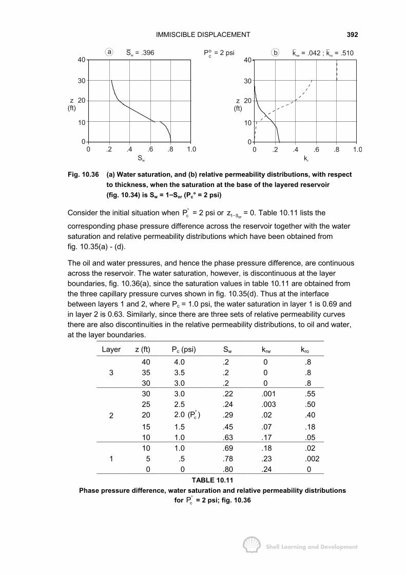
IMMISCIBLE DISPLACEMENT 392
40
30
20
10
00 .2 .4 .6 .8 1.0
z(ft)
Sw
Sw = .396a40
30
20
10
00 .2 .4 .6 .8 1.0
z(ft)
kr
krw = .042 ; kro = .510bP = 2 psioc
Fig. 10.36 (a) Water saturation, and (b) relative permeability distributions, with respectto thickness, when the saturation at the base of the layered reservoir(fig. 10.34) is Sw = 1−−−−Sor (Pc° = 2 psi)
Consider the initial situation when cP° = 2 psi or or1 Sz − = 0. Table 10.11 lists the
corresponding phase pressure difference across the reservoir together with the watersaturation and relative permeability distributions which have been obtained fromfig. 10.35(a) - (d).
The oil and water pressures, and hence the phase pressure difference, are continuousacross the reservoir. The water saturation, however, is discontinuous at the layerboundaries, fig. 10.36(a), since the saturation values in table 10.11 are obtained fromthe three capillary pressure curves shown in fig. 10.35(d). Thus at the interfacebetween layers 1 and 2, where Pc = 1.0 psi, the water saturation in layer 1 is 0.69 andin layer 2 is 0.63. Similarly, since there are three sets of relative permeability curvesthere are also discontinuities in the relative permeability distributions, to oil and water,at the layer boundaries.
Layer z (ft) Pc (psi) Sw krw kro
40 4.0 .2 0 .835 3.5 .2 0 .8330 3.0 .2 0 .830 3.0 .22 .001 .5525 2.5 .24 .003 .5020 2.0 c(P )° .29 .02 .4015 1.5 .45 .07 .18
2
10 1.0 .63 .17 .0510 1.0 .69 .18 .025 .5 .78 .23 .00210 0 .80 .24 0
TABLE 10.11Phase pressure difference, water saturation and relative permeability distributions
for cP° = 2 psi; fig. 10.36

IMMISCIBLE DISPLACEMENT 393
For the saturation distribution depicted in fig.10.36(a) the average water saturation canbe evaluated mathematically as
h h
w w0 0
S (z)S (z)dz (z)dzφ φ= � �
which, since there are three distinct, homogeneous layers, can be expressed as
1 2 3w w w1 1 2 2 3 3w 3
i ij 1
h S h S h SSh
φ φ φ
φ=
+ +=
�
(10.71)
in which, for instance,
1
1
h
w w 10
S S (z)dz h= �
The average saturations, 1 2 3w w wS ,S and S , can be evaluated either graphically ornumerically, as described in the previous section.
Similarly, rw wk (S ) can be evaluated as
h
rw w0
rw w h
0
k(z)k (S (z))dzk (S )
k(z)dz=�
�
or
1 2 31 2 3rw rw rww w w1 1 2 2 3 3rw w 3
j jj 1
h k k (S ) h k k (S ) h k k (S )k (S )h k
=
+ +=
�
where, for instance
1
1 1
h
rw w0
rw w1
k (S (z))dzk (S )
h=�
and similarly for ro wk (S ) .
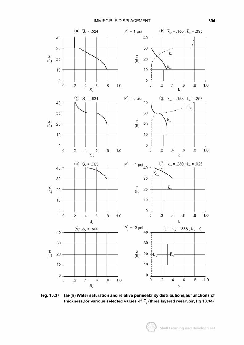
IMMISCIBLE DISPLACEMENT 394
40
30
20
10
00 .2 .4 .6 .8 1.0
40
30
20
10
00 .2 .4 .6 .8 1.0
40
30
20
10
00 .2 .4 .6 .8 1.0
40
30
20
10
00 .2 .4 .6 .8 1.0
40
30
20
10
00 .2 .4 .6 .8 1.0
40
30
20
10
00 .2 .4 .6 .8 1.0
40
30
20
10
00 .2 .4 .6 .8 1.0
40
30
20
10
00 .2 .4 .6 .8 1.0
Sw = .524
Sw = .634
Sw = .765
Sw = .800
z(ft)
z(ft)
z(ft)
z(ft)
z(ft)
z(ft)
z(ft)
z(ft)
b krw = .100 ; kro = .395
d k krw ro= .158 ; = .257
h k krw ro = .338 ; = 0
f k krw ro= .280 ; = .026
a
Sw
Sw
Sw
Sw
kr
kr
kr
kr
c
e
g P = -2 psi°c
P = -1 psi°c
P = 0 psi°c
P = 1 psi°c
kro
krw
kro
krw
kro
krw
kro krw
Fig. 10.37 (a)-(h) Water saturation and relative permeability distributions,as functions ofthickness,for various selected values of cP° (three layered reservoir, fig 10.34)
IMMISCIBLE DISPLACEMENT 395
Values of cP ,° rww wS ,k (S ) and ro wk (S ) are listed in table 10.12 and plotted infigs. 10.39(a) and 10.38(a). The latter three have been obtained by the graphicalintegration of the distributions shown in fig. 10.36(a) and (b) and fig. 10.37(a)-(h) for thefive selected values of cP°
cP° (psi) Sw krw kro
7.0 .200 0 .6782.0 .396 .042 .5101.0 .524 .100 .395 0 .634 .158 .257
-1.0 .765 .280 .026-2.0 .800 .338 0
TABLE 10.12Pseudo capillary pressure and averaged relative permeabilities
corresponding to figs. 10.36 and 10.37
In particular, when Sw = 0.2, the connate water saturation, then using the capillarypressure curve for layer 1, fig. 10.35(d), the phase pressure at the base of the reservoirmust be at least 5 psi and hence cP° = 7 psi.
The method described above is perfectly general and can be applied equally well whenthe end point saturations also vary from layer to layer. The case studied is for thegradation of permeabilities from high to low from the top to the bottom of the reservoir.If the reservoir shown in fig. 10.34 were inverted, repetition of the above exercisewould yield the averaged relative permeability and pseudo capillary pressure curvesshown in figs. 10.38(b) and 10.39(a) (dashed curve). The corresponding fractional flowcurves for the two cases are plotted in fig. 10.39(b) assuming that µo = 5 cp andµw = .5 cp, as in exercises 10.2 and 10.3. The latter curves indicate that the morefavourable displacement occurs when the high permeability layer is uppermost in thereservoir. In this case the injected water will preferentially travel through the top layerand in doing so will be pulled downwards, due to the gravity difference between thewater and oil, resulting in fairly even saturation distribution. If, however, the highpermeability layer is at the base of the reservoir, capillary forces will tend to suck upthe water but this is not as effective in creating a uniform saturation distribution.
A special, simple case of the method of averaging presented in this section occurswhen the capillary transition zone in each layer is negligible so that flow occurs undersegregated conditions, as described in sec. 10.6. Suppose there are a total of N layersin the reservoir. When the water-oil interface has risen so that it coincides with the topof the nth layer, the thickness averaged water saturation is, in analogy with equ. (10.71)
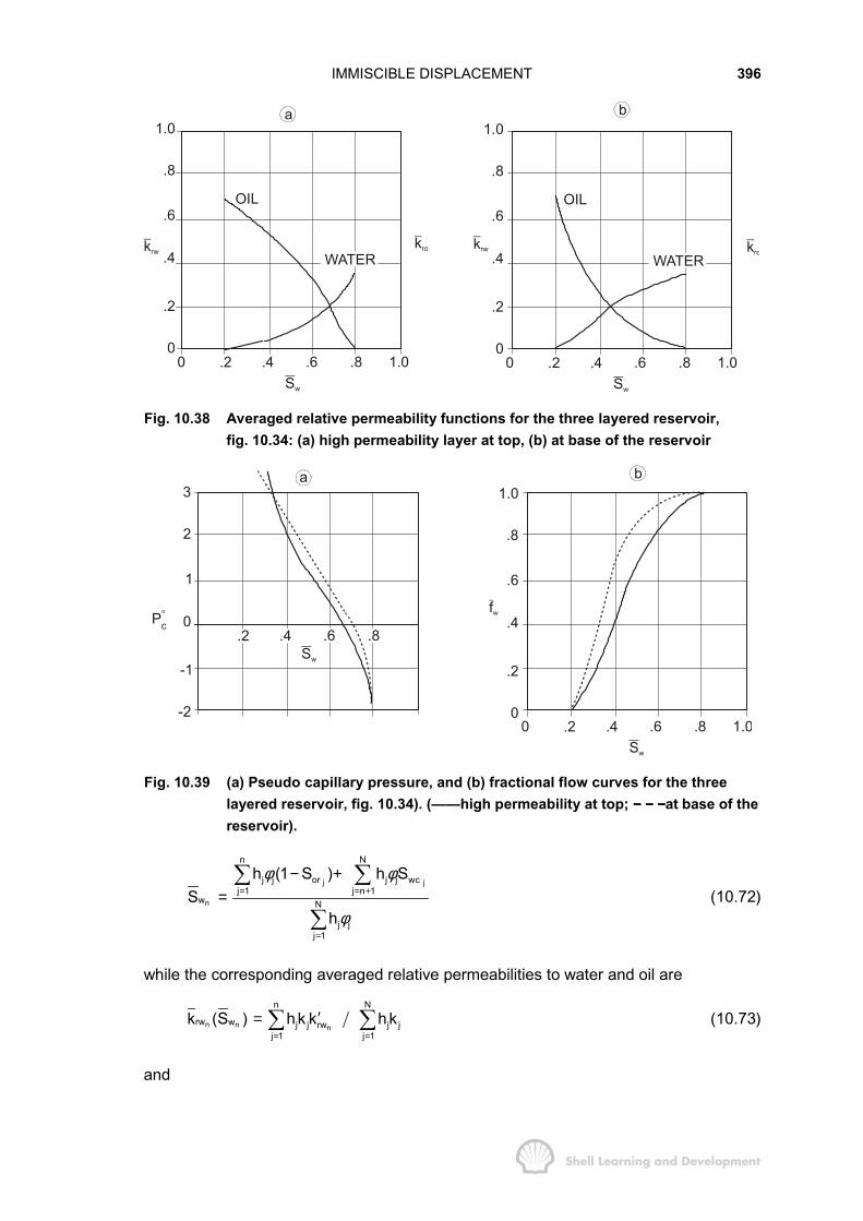
IMMISCIBLE DISPLACEMENT 396
1.0
.8
.6
.4
.2
00 .2 .4 .6 .8 1.0
b
OIL
WATER
Sw
1.0
.8
.6
.4
.2
00 .2 .4 .6 .8 1.0
OIL
WATER
Sw
krw krokrokrw
a
Fig. 10.38 Averaged relative permeability functions for the three layered reservoir,fig. 10.34: (a) high permeability layer at top, (b) at base of the reservoir
0 .2 .4 .6 .8 1.0
b
Sw
3
2
1
0
-1
-2
.2 .4 .6 .8
fw
1.0
.8
.6
.4
.2
0
a
P°c
Sw
Fig. 10.39 (a) Pseudo capillary pressure, and (b) fractional flow curves for the threelayered reservoir, fig. 10.34). (——high permeability at top; −−−− −−−− −−−−at base of thereservoir).
j j
n
n N
j j or j j wcj 1 j n 1
w N
j jj 1
h (1 S ) h SS
h
φ φ
φ
= = +
=
− +=� �
�
(10.72)
while the corresponding averaged relative permeabilities to water and oil are
n n n
n N
rw w j j rw j jj 1 j 1
k (S ) h k k h k= =
′= � � (10.73)
and
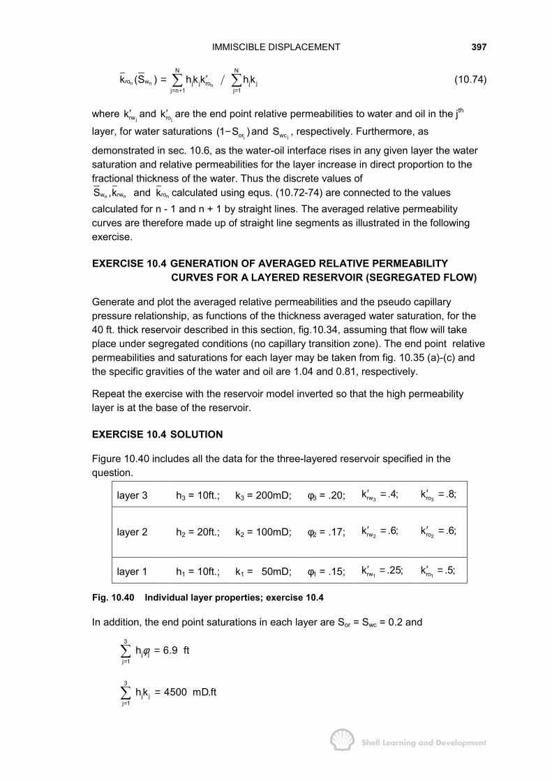
IMMISCIBLE DISPLACEMENT 397
n n n
N N
ro w j j ro j jj n 1 j 1
k (S ) h k k h k= + =
′= � � (10.74)
where jrwk′ and
jrok′ are the end point relative permeabilities to water and oil in the jth
layer, for water saturations jor(1 S )− and
jwcS , respectively. Furthermore, as
demonstrated in sec. 10.6, as the water-oil interface rises in any given layer the watersaturation and relative permeabilities for the layer increase in direct proportion to thefractional thickness of the water. Thus the discrete values of
n nn rw rowS ,k and k calculated using equs. (10.72-74) are connected to the valuescalculated for n - 1 and n + 1 by straight lines. The averaged relative permeabilitycurves are therefore made up of straight line segments as illustrated in the followingexercise.
EXERCISE 10.4 GENERATION OF AVERAGED RELATIVE PERMEABILITYCURVES FOR A LAYERED RESERVOIR (SEGREGATED FLOW)
Generate and plot the averaged relative permeabilities and the pseudo capillarypressure relationship, as functions of the thickness averaged water saturation, for the40 ft. thick reservoir described in this section, fig.10.34, assuming that flow will takeplace under segregated conditions (no capillary transition zone). The end point relativepermeabilities and saturations for each layer may be taken from fig. 10.35 (a)-(c) andthe specific gravities of the water and oil are 1.04 and 0.81, respectively.
Repeat the exercise with the reservoir model inverted so that the high permeabilitylayer is at the base of the reservoir.
EXERCISE 10.4 SOLUTION
Figure 10.40 includes all the data for the three-layered reservoir specified in thequestion.
layer 3 h3 = 10ft.; k3 = 200mD; φ3 = .20; 3rwk .4;′ =3rok .8;′ =
layer 2 h2 = 20ft.; k2 = 100mD; φ2 = .17; 2rwk .6;′ =2rok .6;′ =
layer 1 h1 = 10ft.; k1 = 50mD; φ1 = .15; 1rwk .25;′ =1rok .5;′ =
Fig. 10.40 Individual layer properties; exercise 10.4
In addition, the end point saturations in each layer are Sor = Swc = 0.2 and
3
j jj 1
h 6.9 ftφ=
=�
3
j jj 1
h k 4500 mD.ft=
=�
IMMISCIBLE DISPLACEMENT 398
When there is only connate water in each layer the initial average saturation andrelative permeabilities can be determined as (n=0)
0
3 3
w j j wc j jj 1 j 1
S h S h 0.2φ φ= =
= =� �
0 0rw wk (S ) 0=
and
0 0 j
3 3
ro w j j ro j jj 1 j 1
k (S ) h k k h k 0.678= =
′= =� �
As the water-oil interface rises in the reservoir, values of nn nrww wS , k (S ) and
n nro wk (S )can be computed using equs. (10.72-74), as n varies from 1 to 3, giving thevalues listed in table 10.13.
n nwS nrwk nrok cP°
0 .200 0 .678 2.01 .330 .028 .622 1.02 .626 .161 .356 -1.03 .800 .339 0 -2.0
TABLE 10.13
For instance, when n=2, so that the water-oil interface has risen to the top of the middlelayer,
2 1 2 3
3
w 1 1 or 2 2 or 3 3 wc j 1j 1
S (h (1 S ) h (1 S ) h S ) / hφ φ φ φ=
= − + − + �
= (10× .15×.8 + 20×.17×.8 + 10× .20×.2) /6.9 = 0.626
2 2 1 2
3
rw w 1 1 rw 2 2 rw j jj 1
k (S ) (h k k h k k ) / h k=
′ ′= + �
= (10×50×.25 + 20×100×.3) /4500 = 0.161
and
2 2 3
3
ro w 3 3 ro j jj 1
k (S ) h k k / h k=
′= �
= 10×200×.8 / 4500 = 0.356
The pseudo capillary pressures have again been calculated using the equation
orc 1 SP 0.1(20 z )−° = − (10.70)
where or1 Sz − is the elevation of the water-oil interface above the base of the reservoir.
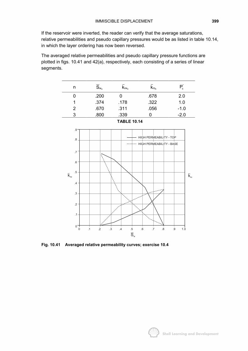
IMMISCIBLE DISPLACEMENT 399
If the reservoir were inverted, the reader can verify that the average saturations,relative permeabilities and pseudo capillary pressures would be as listed in table 10.14,in which the layer ordering has now been reversed.
The averaged relative permeabilities and pseudo capillary pressure functions areplotted in figs. 10.41 and 42(a), respectively, each consisting of a series of linearsegments.
n nwS nrwk nrok cP°
0 .200 0 .678 2.01 .374 .178 .322 1.02 .670 .311 .056 -1.03 .800 .339 0 -2.0
TABLE 10.14
.9
.8
.7
.6
.5
.4
.3
.2
.1
00 .1 .2 .3 .4 .5 .6 .7 .8 .9 1.0
krw kro
HIGH PERMEABILITY - TOP
HIGH PERMEABILITY - BASE
Sw
Fig. 10.41 Averaged relative permeability curves; exercise 10.4

IMMISCIBLE DISPLACEMENT 400
bfw
1.0
.8
.6
.4
.2
0.2 .3 .4 .5 .6 .7 .8
Sw
.3 .4 .6Sw
2.0
1.0
0
-2.0
P
(psi)
°c
a
.8.7
Fig. 10.42 (a) Pseudo capillary pressures, and (b) fractional flow curves, exercise 10.4(—— High permeability layer at top; −−−− −−−− −−−−at base of reservoir)
Inversion of the reservoir, so that the highest permeability layer is at the base, resultsin the functions represented by the dashed lines, which are simply reflections of theoriginals. Also shown in fig. 10.42(b) are the fractional flow curves for the two caseswhich again indicate that the displacement is much more favourable if the highpermeability layer is at the top of the reservoir, since vertical fluid movement isdependent on gravity alone. While the fractional flow curve for the favourable case(solid line), increases continuously with increasing water saturation, the derivative ofthe curve, which is required in oil recovery calculations, does not. Therefore to use thecurve, in conjunction with the Welge graphical technique for determining oil recovery,requires that it first be smoothed, as shown in fig. 10.42(b). This smoothing isunnecessary in the case of unfavourable displacement, with the high permeability layerat the base of the reservoir (dashed line).
b) No pressure communication between the layers
If the individual layers are isolated from one another by impermeable barriers so thatthere is a lack of pressure communication between them, there will be no flow of fluidsin the dip normal direction. Even though injection and production wells are completedacross all the layers the problem is one of dealing with a set of isolated reservoirsbetween which pressure communication can only exist in the wellbore.
Stiles has presented a simple, approximate method14 for calculating oil recovery underthese circumstances and further examples of its application have been presented byCraft and Hawkins15 and Colel6. Fundamental to the Stiles method is the assumptionthat piston-like displacement occurs in each separate layer, which is equivalent toassuming that the end point mobility ratio is unity. Furthermore, for this stabledisplacement the oil and water must have the same velocity which, applying Darcy'slaw, implies that
IMMISCIBLE DISPLACEMENT 401
ow ppMx x
∂∂ =∂ ∂
and since M = 1, the pressure gradients in the oil and water must be the same.Therefore, if a constant pressure difference ∆p is applied between injection andproduction wells, then
ow pp px x L
∂∂ ∆= =∂ ∂
in all layers, where L is the length of the reservoir block. Applying the Buckley Leveretttheory to calculate the velocity of the water in the jth layer, equ. (10.19)
jt wj
j j w j
q fvwh Sφ
� �∆= � �∆� �(10.75)
where w is the reservoir width and, at the front, for piston-like displacement,
j j
w
w or wcj
f 1S (1 S S )
� �∆ =� �∆ − −� �
Finally, since
j
j
j rw wt j
w
k k pq whxµ
′ ∂= −∂
then equ. (10.75) can be expressed as
j
j j
j rwj
j w or wc
k k pv(1 S S ) Lφ µ
′ ∆=− −
One additional imposition, inherent in the assumption that M = 1 in all layers, is that theratio of end point relative permeabilities,
j jrw rok / k′ ′ , is constant. The layer order in which
water will break through to the producing well will therefore be in the sequence ofdecreasing values of
j
j j
j rwj
j or wc
k k(1 S S )
αφ
′=
− −(10.76)
Application of the Stiles method to generate averaged relative permeability curvesrequires, as a preliminary, the re-ordering of the layer numbers in the sequence inwhich water breakthrough will occur. Thus the sand having the highest value of ∝ ,equ. (10.76), becomes layer number one; the sand having the second largest value ofa becomes layer number two, etc.
If there is a total of N layers in the reservoir then, observing the water breakthrough atthe producing well, the average saturation, nwS , after breakthrough in the nth layer, canbe calculated using an equation which is identical in form to equ. (10.72). Similarly, the

IMMISCIBLE DISPLACEMENT 402
averaged relative permeabilities, nrwk and nrok , can be calculated using equs. (10.73)and (10.74), respectively. The averaged relative permeabilities so generated are, infact, independent of the position in the linear reservoir at which the flood is observedand are not restricted to application at the wellbore. This is because, although there isa difference in water velocity between any two sands, the difference remains constantas the flood advances; this being implicit in the assumption of piston-like displacement.
When plotting the relative permeability curves, the separate points are not joined byline segments but, instead, by step functions since after breakthrough in layer n therelative permeabilities remain constant until breakthrough occurs in layer n+1 whenthere is a discrete jump to the new values of n 1rwk + and n 1rok + . If there are a largenumber of separate layers in the reservoir the step functions can be smoothed intocontinuous curves.
The main assumption in using the Stiles method, that M=1, should theoretically limit itsapplication to reservoirs in which this condition is approximately satisfied.Nevertheless, it is frequently used as a starting point even when M > 1 and theresulting relative permeability curves adjusted so that calculated oil recovery matchesthat observed in pilot floods.
10.9 DISPLACEMENT WHEN THERE IS A TOTAL LACK OF VERTICAL EQUILIBRIUM
The generation of averaged relative permeability curves, described in secs. 10.6-8,relies on the assumption that the oil displacement occurs under the vertical equilibriumcondition (refer sec. 10.2). Because of this it is possible to define both saturation andrelative permeability distributions with respect to thickness and averaging thesefacilitates the description of two dimensional displacement using simple, onedimensional equations.
A similar procedure can also be adopted for precisely the opposite flow condition, thatis, when there is an extreme lack of vertical equilibrium. This will occur when the fluidvelocity parallel to the bedding-greatly exceeds the velocity in the dipnormal direction.In extreme cases the fluid saturations will be uniformly distributed with respect tothickness, in a homogeneous reservoir, and the displacement can be described usingthe rock relative permeability curves with the one dimensional Buckley-Leverett theory.The corresponding pseudo capillary pressure relationship for such displacement issimply
cP° (Sw) = op° − wp° = 0
In a stratified reservoir, a total lack of vertical equilibrium implies that the fluids willmove through each layer in isolation from fluids in adjacent layers. Since there isnegligible fluid movement in the dip-normal direction such displacement can bedescribed in one dimension using the method of Stiles for generating averaged relativepermeabilities17.
The methods described in this chapter for reducing the description of oil displacementto one dimension are summarised in fig. 10.43. The starting point in this flow chart is
IMMISCIBLE DISPLACEMENT 403
the decision concerning the validity of the assumption of vertical equilibrium. Toattempt to describe oil displacement using ,simple analytical methods requires eitherthe assumption that vertical equilibrium predominates, or alternatively, that it does notexist at all. In both cases averaged relative permeability curves can be generated foruse with the Buckley-Leverett, one dimensional, displacement theory.
Alternatively, the averaged relative permeability functions are used as basic input forthe numerical simulation of the displacement process. The following section willdescribe the importance of using averaged relative permeabilities and pseudo capillarypressures in numerical simulation. In addition, the manner in which the assumption ofvertical equilibrium can be verified, using numerical simulation, and the manner inwhich displacement can be described under conditions intermediate between total andnon-existent vertical equilibrium, will also be described.
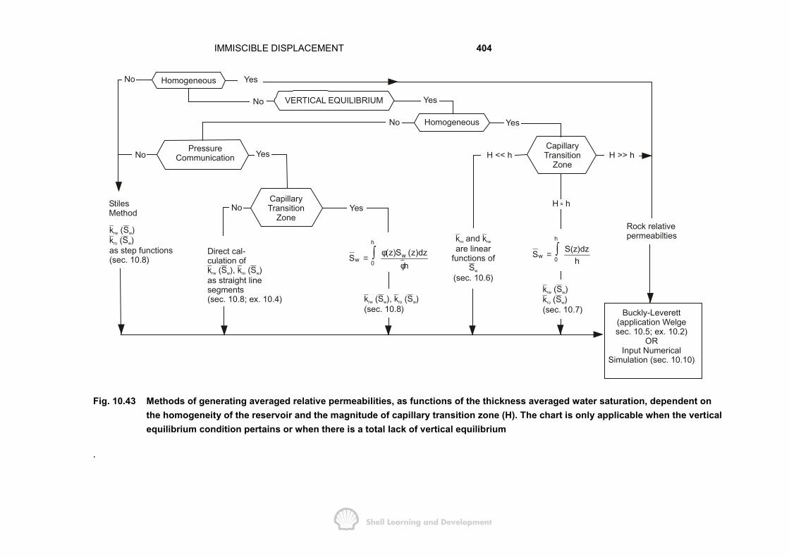
IMMISCIBLE DISPLACEMENT 404
No Homogeneous Yes
No VERTICAL EQUILIBRIUM Yes
No Homogeneous Yes
CapillaryTransition
ZoneH << h H >> hNo YesPressure
Communication
YesNoCapillaryTransition
ZoneStilesMethod
k Srw w ( )
as step functions(sec. 10.8)
k Sro w ( )Direct cal-culation of
as straight linesegments(sec. 10.8; ex. 10.4)
k S k Srw w ro w ( ), ( )
(sec. 10.8)k S k Srw w ro w ( ), ( )
k k
S
ro rw
w
and are linear
functions of
(sec. 10.6)
(sec. 10.7)
k Sk S
rw w
ro w
( ) ( )
Rock relativepermeabilties
Buckly-Leverett(application Welgesec. 10.5; ex. 10.2)
ORInput Numerical
Simulation (sec. 10.10)
H h
h
ww 0
(z)S (z)dzSh
φ=
φ�
h
w 0S(z)dzS
h= �
˜
Fig. 10.43 Methods of generating averaged relative permeabilities, as functions of the thickness averaged water saturation, dependent onthe homogeneity of the reservoir and the magnitude of capillary transition zone (H). The chart is only applicable when the verticalequilibrium condition pertains or when there is a total lack of vertical equilibrium
.

IMMISCIBLE DISPLACEMENT 405
10.10 THE NUMERICAL SIMULATION OF IMMISCIBLE, INCOMPRESSIBLEDISPLACEMENT
So far, this text has concentrated on developing simple mathematical models todescribe the physics of reservoir depletion and fluid flow. Examples of these are thezero dimensional material balance equation (Chapter 3) and the analytical solutions oflinear second order differential equations for radial flow (Chapters 5-8).
Sometimes, however, these simple models are totally inadequate to provide therequired solutions to reservoir engineering problems. In a strong natural water drivereservoir, for instance, the zero dimensional material balance can be used to predictthe volume of water influx, but it can never predict where the water will preferentiallymove in the reservoir and such knowledge may be required to determine the location ofadditional production or injection wells. Furthermore, not all reservoir problems can beformulated in terms of linear differential equations for which standard solutions can besought. Nobody, for instance, would attempt to solve simultaneously the equations forthree phase (oil — water—gas) flow in three dimensions with irregular boundaryconditions, using an analytical approach. To deal with complex reservoir problems theengineer must resort to numerical simulation methods and particularly so fordisplacement problems, in which one of the main aims is to determine the arealdistribution of fluids in the reservoir resulting from a flood.
A numerical simulator is a computer program which permits the user to divide thereservoir into discrete grid blocks which may each be characterised by having differentreservoir properties. The flow of fluids from block to block is governed by the principleof mass conservation coupled with Darcy's law. Flow into or out of a block, due topresence of an injection or production well, is also catered for. Most simulators arecapable of solving large sets of second order differential equations for thesimultaneous flow of oil, gas and water, in three dimensions. In addition the effects ofnatural water influx, fluid compressibility, mass transfer between gas and liquid phasesand the variation of such parameters as porosity and permeability, as functions ofpressure, can all be modelled. The differential equations themselves are generallyformulated using the finite difference analogue for first and second order differentialsand solved simultaneously using numerical techniques with some acceptable, smallerror attached to each solution.
It is not intended, in this text, to describe numerical simulation in any great detail.Indeed, at the time of writing, such a description would require not merely another textbook but a small encyclopaedia. Instead, since this chapter has concentrated on thegeneration of averaged relative permeabilities and pseudo capillary pressures, asfunctions of the thickness averaged water saturation; the description of simulation willbe confined to the way in which these vitally important parameters are handled by thesimulator. To accomplish this, the simple case of linear, incompressible displacementof oil by water will be considered, for which the appropriate mass conservationequations for reservoir fluids will be presented. This simplifies and concentrates thedescription since the pressure dependent terms, densities and viscosities, can safelybe regarded as being independent of pressure. Thus only the variation in time and
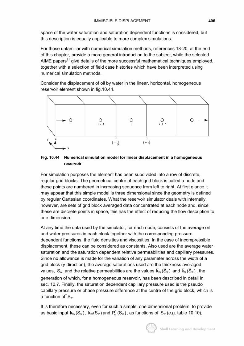
IMMISCIBLE DISPLACEMENT 406
space of the water saturation and saturation dependent functions is considered, butthis description is equally applicable to more complex simulations.
For those unfamiliar with numerical simulation methods, references 18-20, at the endof this chapter, provide a more general introduction to the subject, while the selectedAIME papers21 give details of the more successful mathematical techniques employed,together with a selection of field case histories which have been interpreted usingnumerical simulation methods.
Consider the displacement of oil by water in the linear, horizontal, homogeneousreservoir element shown in fig.10.44.
y
x
z12i − 1
2i +
Fig. 10.44 Numerical simulation model for linear displacement in a homogeneousreservoir
For simulation purposes the element has been subdivided into a row of discrete,regular grid blocks. The geometrical centre of each grid block is called a node andthese points are numbered in increasing sequence from left to right. At first glance itmay appear that this simple model is three dimensional since the geometry is definedby regular Cartesian coordinates. What the reservoir simulator deals with internally,however, are sets of grid block averaged data concentrated at each node and, sincethese are discrete points in space, this has the effect of reducing the flow description toone dimension.
At any time the data used by the simulator, for each node, consists of the average oiland water pressures in each block together with the corresponding pressuredependent functions, the fluid densities and viscosities. In the case of incompressibledisplacement, these can be considered as constants. Also used are the average watersaturation and the saturation dependent relative permeabilities and capillary pressures.Since no allowance is made for the variation of any parameter across the width of agrid block (y-direction), the average saturations used are the thickness averagedvalues, Sw, and the relative permeabilities are the values rw wk (S ) and ro wk (S ) , thegeneration of which, for a homogeneous reservoir, has been described in detail insec. 10.7. Finally, the saturation dependent capillary pressure used is the pseudocapillary pressure or phase pressure difference at the centre of the grid block, which isa function of Sw.
It is therefore necessary, even for such a simple, one dimensional problem, to provideas basic input rw wk (S ) , ro wk (S ) and cP°
w(S ) , as functions of Sw (e.g. table 10.10),

IMMISCIBLE DISPLACEMENT 407
rather than the rock relative permeability and capillary pressure functions measured onthin core plugs in the laboratory.
For this, or any other problem, the basic physical principle employed by the simulator isthat of mass conservation. Usually fluid quantities are conserved at stock tankconditions and related to reservoir fluid quantities through the pressure dependent PVTparameters. When studying the immiscible displacement of oil by water, however,there- is no loss in generality in applying mass conservation directly to both fluids in thereservoir.
Considering the one dimensional flow of water through a small volume element ofthickness dx, which may also contain a fluid source or sink (injection or productionwell), the mass conservation of water can be expressed as
x x dxww w w w w w wq q A dx ( S ) Q
tρ ρ φ ρ ρ
+
∂ ′− = +∂
(10.77)
This has the same form as equ. (10.13), which was used as the starting point of thederivation of the Buckley-Leverett equation, except that now a mass source term w wQ ρ′has been added; where wQ′ is the reservoir rate of water injection or production, forwhich it conventionally has a positive or negative sign, respectively. Reducing theequation to the form
w www w w
Q(q ) A ( S )x t dx
ρρ φ ρ′∂ ∂− = +
∂ ∂
and substituting for the reservoir flow rate qw using Darcy's equation for horizontal flow
rw ww
w
pkk Aqxµ
∂= −∂
gives
rw www
w
pkk S Qx x t
φµ
� �∂∂ ∂= +� �� �∂ ∂ ∂� �(10.78)
in which it has been assumed that, for this incompressible displacement both ρw and φare constant, and Qw = wQ / Adx′ which is the injection or production rate per unit ofreservoir bulk volume. Furthermore, in this, and in subsequent equations, the pressureshould be interpreted as the average value at the centre of the reservoir and theviscosity evaluated at this same pressure.
The analogous equation to equ. (10.78) for the mass conservation of oil is
ro ooo
o
pkk S Qx x t
φµ
� �∂∂ ∂= +� �� �∂ ∂ ∂� �(10.79)
Instead of attempting to analytically solve either equ. (10.78) or (10.79), which was theapproach employed in developing the Buckley-Leverett displacement theory, the
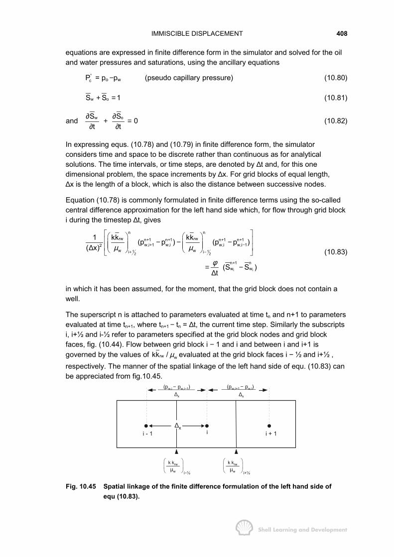
IMMISCIBLE DISPLACEMENT 408
equations are expressed in finite difference form in the simulator and solved for the oiland water pressures and saturations, using the ancillary equations
cP° = po −pw (pseudo capillary pressure) (10.80)
w oS S 1+ = (10.81)
and w oS S 0t t
∂ ∂+ =∂ ∂
(10.82)
In expressing equs. (10.78) and (10.79) in finite difference form, the simulatorconsiders time and space to be discrete rather than continuous as for analyticalsolutions. The time intervals, or time steps, are denoted by ∆t and, for this onedimensional problem, the space increments by ∆x. For grid blocks of equal length,∆x is the length of a block, which is also the distance between successive nodes.
Equation (10.78) is commonly formulated in finite difference terms using the so-calledcentral difference approximation for the left hand side which, for flow through grid blocki during the timestep ∆t, gives
1 12 2
i i
n nrw rwn 1 n 1 n 1 n 1
w,i 1 w,i w,i w,i 12w wi i
n 1 nw w
1 kk kk(p p ) (p p )( x)
(S S )t
µ µ
φ
+ + + ++ −
+ −
+
� �� � � �� �− − −� � � �� � � �� �∆ � �
= −∆
(10.83)
in which it has been assumed, for the moment, that the grid block does not contain awell.
The superscript n is attached to parameters evaluated at time tn and n+1 to parametersevaluated at time tn+1, where tn+1 − tn = ∆t, the current time step. Similarly the subscriptsi, i+½ and i-½ refer to parameters specified at the grid block nodes and grid blockfaces, fig. (10.44). Flow between grid block i − 1 and i and between i and i+1 isgoverned by the values of rw wkk / µ evaluated at the grid block faces i − ½ and i+½ ,respectively. The manner of the spatial linkage of the left hand side of equ. (10.83) canbe appreciated from fig.10.45.
∆x
(pw,i − pw,i−1)∆x
i−½
k krw
µw
� �� �� �
i - 1 i + 1
(pw,i+1 − pw,i)∆x
i+½
k krw
µw
� �� �� �
Fig. 10.45 Spatial linkage of the finite difference formulation of the left hand side ofequ (10.83).
IMMISCIBLE DISPLACEMENT 409
Similarly, equ. (10.79), for oil, can be expressed in finite difference terms as
1 12 2
n nro ron 1 n 1 n 1 n 1
o,i 1 o,i o,i o,i 12o oi i
n 1 no,i o,i
1 kk kk(p p ) (p p )( x)
(S S )t
µ µ
φ
+ + + ++ −
+ −
+
� �� � � �� �− − −� � � �� � � �� �∆ � �
= −∆
(10.84)
and adding equs. (10.83) and (10.84), using equ. (10.82) to eliminate the sum of thetime derivatives of the saturations, and equ. (10.80) expressed as
n 1 n,n 1 n 1 n 1 ,n n nw wc o w c o wP (S ) p p P (S ) p p+° + + + °= − ≈ = − (10.85)
to substitute for pon+1, gives
1 12 2
1 12 2
n nrw ro ron 1 n 1 ,n ,n
o,i w,i c,i 1 c,i2w o oi i
n nrw ro ron 1 n 1
w,i w,i 1 c,i 1w o oi i
,n
1 kk kk kk(p p ) ( P P )( x)
kk kk kk(p p ) (P ) 0
µ µ µ
µ µ µ
+ ++
+ +
+ +− −
+ +
° °
°
�� � � �� + − − −� � � �� � � ��∆ � � � �
� � � ��− + − − =� � � �� � � � �� � � � �
(10.86)
in which it is assumed, equ. (10.85), that while oil and water pressures may individuallychange during a time step, the corresponding change in the pseudo capillary pressurecan be neglected.
The finite difference expression of equ. (10.86) is not unique, but is the one which hasbeen most commonly applied in reservoir simulation. In the equation the waterpressures are all dated at the new time level n+1, at which they are unknown, whereasthe kr/µ term, which is both saturation and pressure dependent, and the pseudocapillary pressures, equ. (10.85), which are saturation dependent, are all dated at theold time level n at which their values are known. Therefore, equ. (10.86), which wasspecifically formulated for the flow of water through grid block i, contains only threeunknowns n 1 n 1 n 1
w,i 1 w,i w,i 1p , p and p+ + +− + but, when the equation is linked with the similar
equations for all the grid blocks in the one dimensional model (i = 1........n), the set ofequations can be solved simultaneously to determine the value of n 1
wp + in each block.This simultaneous solution for pressures at the new time level is referred to as beingIMPLICIT in pressure.
Having obtained the values of n 1wp + , for each grid block, the remainder of the solution at
time level n+1, and in the jth grid block, proceeds as follows:
− substitute the calculated values of n 1 n 1 n 1w,i 1 w,i w,i 1p , p and p+ + +
− + in equ. (10.83) and solve
for n 1w,iS + . (This is referred to as an EXPLICIT solution for
n 1w,iS+
, since it is the onlyunknown in the equation).
− the value of n 1w,iS+
is used to calculate n 1o,iS
+, since
n 1w,iS+
+ n 1o,iS
+ = 1, equ. (10.81)

IMMISCIBLE DISPLACEMENT 410
− the value of n 1w,iS+
is used to determine ,n 1c,iP +° n 1
w,i(S )+
since the relationship betweenpseudo capillary pressure and average water saturation is part of the input data
− the updated value of the pseudo capillary pressure is used to calculate n 1o,ip + ,
since n 1o,ip + = ,n 1
c,iP +° + n 1w,ip + , equ. (10.85).
− and finally, the values of all the pressure and saturation dependent variables(densities, viscosities, and relative permeabilities) are all updated at time leveln+1 using the newly determined pressures and saturations and the input tablesof these variables, as functions of pressure and saturation.
The procedure described above for the simulation of immiscible, incompressibledisplacement of oil by water is one that can be readily extended to three phase flow.The finite difference conservation equations for oil, gas and water, including thepossibility of mass transfer between the gas and liquid phases, are again summed toeliminate the total time change in saturation during the time step
gow SSS 0t t t
∂∂∂ + + =∂ ∂ ∂
This results in a more complex form of the water pressure equation, (10.86), in whichthe oil and gas phase pressures can be eliminated using the pseudo capillary pressurefunctions
n 1 n nc oil o w(P ) p p+° ≈ −
andn 1 n n
c gas g o(P ) p p+° ≈ −
Thereafter, water pressures are solved for implicitly, and the remainder of the solutionproceeds in very much the same way as described above.
The method, in which pressures are determined IMPLICITLY and saturations EXPLCITLY,is known as the IMPES solution technique. One of the main disadvantages in itsapplication is that in solving the water pressure equation, (10.86), at time level n+1, thesaturation dependent relative permeabilities and pseudo capillary pressures areevaluated for the known water saturation at time level n. For problems in which thewater saturation change in a grid block can be large during a time step, such as whensharp saturation fronts move through the reservoir, the evaluation o saturationdependent functions at the old time level can lead to severe instabilities in the IMPESsolution.
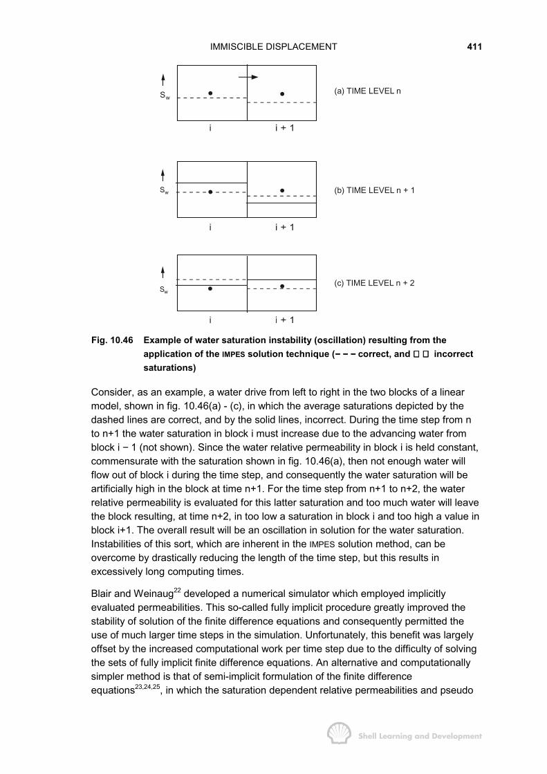
IMMISCIBLE DISPLACEMENT 411
wS
wS
wS (a) TIME LEVEL n
(c) TIME LEVEL n + 2
(b) TIME LEVEL n + 1
i
i
i
Fig. 10.46 Example of water saturation instability (oscillation) resulting from theapplication of the IMPES solution technique (−−−− −−−− −−−− correct, and incorrectsaturations)
Consider, as an example, a water drive from left to right in the two blocks of a linearmodel, shown in fig. 10.46(a) - (c), in which the average saturations depicted by thedashed lines are correct, and by the solid lines, incorrect. During the time step from nto n+1 the water saturation in block i must increase due to the advancing water fromblock i − 1 (not shown). Since the water relative permeability in block i is held constant,commensurate with the saturation shown in fig. 10.46(a), then not enough water willflow out of block i during the time step, and consequently the water saturation will beartificially high in the block at time n+1. For the time step from n+1 to n+2, the waterrelative permeability is evaluated for this latter saturation and too much water will leavethe block resulting, at time n+2, in too low a saturation in block i and too high a value inblock i+1. The overall result will be an oscillation in solution for the water saturation.Instabilities of this sort, which are inherent in the IMPES solution method, can beovercome by drastically reducing the length of the time step, but this results inexcessively long computing times.
Blair and Weinaug22 developed a numerical simulator which employed implicitlyevaluated permeabilities. This so-called fully implicit procedure greatly improved thestability of solution of the finite difference equations and consequently permitted theuse of much larger time steps in the simulation. Unfortunately, this benefit was largelyoffset by the increased computational work per time step due to the difficulty of solvingthe sets of fully implicit finite difference equations. An alternative and computationallysimpler method is that of semi-implicit formulation of the finite differenceequations23,24,25, in which the saturation dependent relative permeabilities and pseudo
IMMISCIBLE DISPLACEMENT 412
capillary pressures are evaluated at time level n+1 using the first order Taylor seriesexpansion, i.e.
nn 1 n r
wr r tw
dkk k SdS
+ � �= + ∆� �
� �
and
n,n 1 ,n c
wr c tw
dPP P SdS
+°
° ° � �= + ∆� �
� �
where ∆tS is the time change in saturation, n 1 nw wS S ,+ − and the first order derivatives are
evaluated at time level n. Peaceman has demonstrated26 that this approach producesperfectly acceptable stability in the majority of numerical simulations, whileChappelear27 has illustrated some of the practical difficulties associated with its useand how they can be overcome. On substituting such expressions for n 1 ,n 1
r ck and P ,+ +°
in the finite difference equations (10.83) and (10.84); the latter equations can bealgebraically manipulated in such a way that the saturation changes again disappearon addition since
w ot tS S 0∆ + ∆ =
The resulting water pressure equation, which is similar although more complex thanequ. (10.86), can then be solved, following which the saturations can be determined asdescribed previously for the IMPES method. The time required to solve the finitedifference equations using the semi-implicit method is longer than when using explicitsaturation dependent parameters, but this is more than compensated by the additionallength of the time step which can be tolerated using the method.
In describing the solution of equ. (10.86) the fact that a grid block could contain aninjection or production well was temporarily overlooked. In such a case there will be anadditional term, Qo + Qw, on the right hand side of the equation, which is the total oiland water rate per unit of reservoir bulk volume and is positive for injection andnegative for production. Precisely how these rates are incorporated into the solution ofequations such as equ. (10.86) depends on the way the simulator is being operated.
There is a method of running the simulator in what is described as the material balancemode. When using this, one attempts to match the observed reservoir pressure historywith the numerical simulation. In this mode the desired time steps are usually specifiedas input to the simulation and the observed injection and production rates of each fluidare assigned to each grid block, containing a well, as a function of time. In this case,since all the rates are specified they do not add any complication to the method ofsolution of equ. (10.86), described previously. As the outcome, the pressurescalculated by the simulator, for each grid block containing a well, should be comparedwith the pressures measured in the field, using the dynamic grid block pressuremethod described in Chapter 7, sec. 7. This aspect of history matching is tantamountto calibrating the simulation model and will be recognised as being nothing more than a
IMMISCIBLE DISPLACEMENT 413
sophisticated version of the history matching, using the volumetric material balanceequation, described in Chapters 1, 3 and 9.
In more normal application, however, it is necessary for the simulator to forecast theinjection or production rate of each well. Considering a single well situated at the centreof a grid block the simulator must be able to determine, for the currently evaluatedaverage fluid pressures and saturations, how much of each fluid can flow into or out ofthe grid block, through the well. Since pressure and saturation gradients do not existwithin each individual grid block, but only between blocks, the physical modelling ofwell performance presents difficulties. Pressure-gradients can be very high in theproximity of the well which should require the subdivision of the grid block into a finemesh of blocks close to the well in order to correctly account for these gradients. Suchan approach would result in very high computer costs due to the large number of gridblocks involved in the simulation.
An alternative, approximate method of modelling well performance is to design ananalytical well model to account for either injection or production from a grid block. Forinstance, the total production of water from a block, qw = Qwx (net bulk volume ofblock), could be predicted as
qw = α (pwf – pw) (10.87)
in which pwf and pw are the current bottom hole flowing pressure and average grid blockpressure for the water, respectively . The order of subtraction of these pressuresensures that water production is negative and injection Positive, in accordance with thenormal convention. The term a is the productivity index of the well and is normallyevaluated for steady state flow (Chapter 6, table 1) as
rw
ew
w
2 kk h (Darcy units)r 1ln Sr 2
παµ
=� �
− +� �� �
or
3rw
ew
w
7.08 10 kk h (field units)r 1ln Sr 2
αµ
−×=� �
− +� �� �
where re is the equivalent grid block radius
ex yrπ
∆ ∆=
for a well draining from the centre of a block. The choice of a steady state well model isusually justified by the fact that transients, within a grid block, normally die out in arelatively short time compared to the average time step used by the simulator; and thecondition at the block boundary is probably closer to steady state (open boundary —constant pressure) than semi-steady state (closed boundary — pressure depletion).

IMMISCIBLE DISPLACEMENT 414
It has been found that, even for a simulation which can be satisfactorily run using theIMPES solution technique, the well model will be unstable unless extremely small timesteps are employed. This is because of the saturation dependence of the relativepermeability term in the productivity index α. For this reason the PI is always evaluatedsemi implicitly as
nn 1 n
td SdSαα α+ � �= + ∆� �
� �
for each liquid. Thus the equation for the water rate, (10.87), at time n+1, in block i,which contains a well, is
nw,in 1 n n 1
w,iw,i w,i t wf,i w,iw,i
dq ( S )(p p )
dSα
α+ +� �= + ∆ −� �
� �(10.88)
and a similar expression can be formulated for the oil phase. Such expressions areadded to the right hand side of equs. (10.83) and (10.84), in grid blocks containingwells and addition of the equations, again with much algebraic manipulation, will leadto a modified form of the pressure equation, (10.86), in which the t S∆ terms cancel onaddition. The subsequent solution for phase saturations and pressures permits thecalculation of the rates by back substitution of these values in the well model equation,(10.88), for both oil and water.
It is intuitively obvious that since the term rkk / µ controls the flow of fluids from onegrid block to the next, it should be evaluated at the grid block faces. What is not soobvious, however, is precisely how the values of the three parameters in thisexpression are determined at the block faces since they are only defined at the gridblock nodes.
The viscosities, which are pressure dependent, are considered to be slowly varyingfunctions of position, especially in the case of incompressible displacement, and aretherefore evaluated as the average of their values at adjacent grid block nodes; thusfor regular grid block spacing
µi+½ = (µi + µi+1) / 2
The absolute permeability, which normally remains constant throughout the simulation,is. determined as the harmonic mean of its value at adjacent grid nodes. Consider thegeneral case of flow between grid blocks of unequal length, as shown in fig. 10.47.
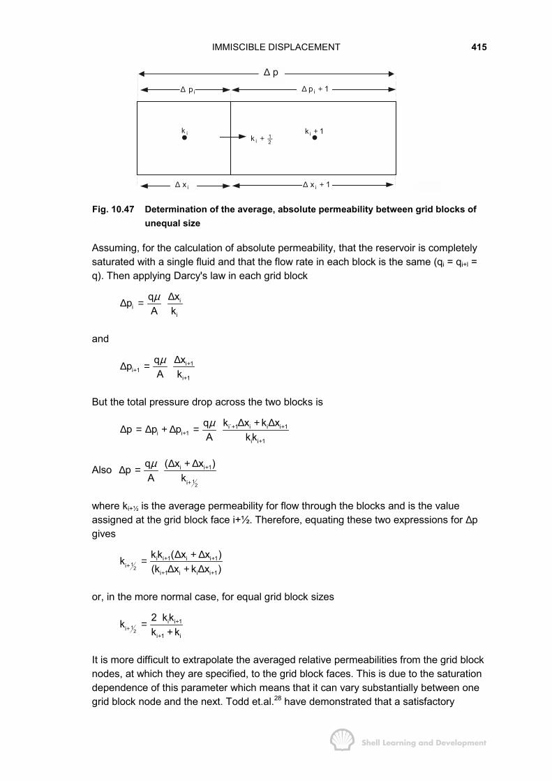
IMMISCIBLE DISPLACEMENT 415
ik ik 1+1
i 2k +
ip∆ ip 1∆ +
ix 1∆ +ix∆
p∆
Fig. 10.47 Determination of the average, absolute permeability between grid blocks ofunequal size
Assuming, for the calculation of absolute permeability, that the reservoir is completelysaturated with a single fluid and that the flow rate in each block is the same (qi = qi+l =q). Then applying Darcy's law in each grid block
ii
i
xqpA kµ ∆∆ =
and
i 1i 1
i 1
xqpA kµ +
++
∆∆ =
But the total pressure drop across the two blocks is
i 1 i i i 1i i 1
i i 1
k x k xqp p pA kkµ + +
++
∆ + ∆∆ = ∆ + ∆ =
Also 12
i i 1
i
( x x )qpA kµ +
+
∆ + ∆∆ =
where ki+½ is the average permeability for flow through the blocks and is the valueassigned at the grid block face i+½. Therefore, equating these two expressions for ∆pgives
12
i i 1 i i 1i
i 1 i i i 1
k k ( x x )k(k x k x )
+ ++
+ +
∆ + ∆=∆ + ∆
or, in the more normal case, for equal grid block sizes
12
i i 1i
i 1 i
2 k kkk k
++
+
=+
It is more difficult to extrapolate the averaged relative permeabilities from the grid blocknodes, at which they are specified, to the grid block faces. This is due to the saturationdependence of this parameter which means that it can vary substantially between onegrid block node and the next. Todd et.al.28 have demonstrated that a satisfactory
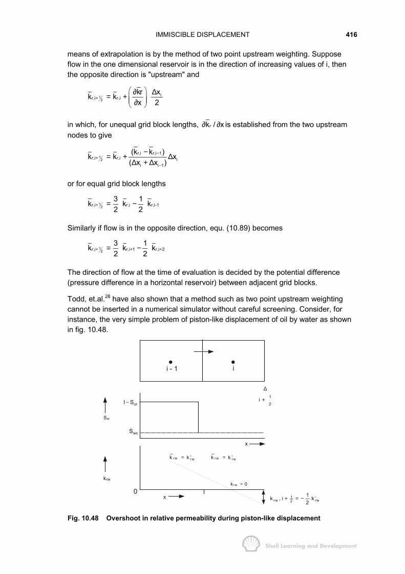
IMMISCIBLE DISPLACEMENT 416
means of extrapolation is by the method of two point upstream weighting. Supposeflow in the one dimensional reservoir is in the direction of increasing values of i, thenthe opposite direction is "upstream" and
12
ir,i r,i
xkrk kx 2
+� � ∆∂= + � �� �∂� �
in which, for unequal grid block lengths, rk / x∂ ∂ is established from the two upstreamnodes to give
12
r,i r,i 1r,i r,i i
i i 1
(k k )k k x( x x )
−+
−
−= + ∆∆ + ∆
or for equal grid block lengths
12r,i r,i r,i-1
3 1k k k2 2
+ = −
Similarly if flow is in the opposite direction, equ. (10.89) becomes
12r,i r,i 1 r,i 2
3 1k k k2 2
+ + += −
The direction of flow at the time of evaluation is decided by the potential difference(pressure difference in a horizontal reservoir) between adjacent grid blocks.
Todd, et.al.28 have also shown that a method such as two point upstream weightingcannot be inserted in a numerical simulator without careful screening. Consider, forinstance, the very simple problem of piston-like displacement of oil by water as shownin fig. 10.48.
i - 1 i
wS
wcS
orI S−
x
rwk
0x
l lrw rwrw rwk k k k= =
1
2i
∆
+
l1rw rw2
1k , i k2
+ = −
rwk 0=
Fig. 10.48 Overshoot in relative permeability during piston-like displacement
IMMISCIBLE DISPLACEMENT 417
When the sharp water front is about to enter block i the value of the relativepermeability to water at i+½ is − ½ k´rw, equ. (10.89). This negative relative permeabilityis referred to as overshoot and can obviously occur any time rw,i 1 rw,ik 3k− > . Thissituation can arise when a shock front water saturation discontinuity moves through thereservoir. Such overshoot is forbidden and is overcome by imposing the condition that
rwk 0≥ .
By considering the oil saturation and relative permeabilities corresponding to thesituation shown in fig. 10.48, the reader can verify that another condition which must beimposed is that
12
12
ro,iro,i
ro,i
kk the greater of
k+
+
≤
The above two rules controlling overshoot are generally applicable for any type ofdisplacement; that 1
2rw,ik + is not allowed to be negative and 12ro,ik + must be less than or
equal to the greater of the values at adjacent grid nodes. Although more difficult tocode than single point upstream weighting 1
2r,i r,i(k k )+ = , the two point method is moreaccurate and, using it, larger grid block sizes can be tolerated. This reduces theprogram running time and therefore, simulation costs.
Actual reservoir simulation studies are usually undertaken to determine the arealdistribution of fluids in the reservoir, resulting either from natural water influx or waterinjection . As such they require the building of a two or three dimensional model of thereservoir in which variation in the basic reservoir parameters, such as porosity,permeability etc., can be allowed for by assigning different values of these parametersto each grid block. Once a model has been constructed, which closely resembles thereservoir, it is then necessary to select relative permeabilities and a pseudo capillarypressure function which characterise the manner in which the water saturation isdistributed in the dip-normal direction, as the flood moves through the reservoir. Themanner in which this can be done is described below.
a) Generate a set of averaged relative permeabilities and the pseudo capillarypressure for a typical linear cross section through the reservoir, between theinjection and production wells, assuming vertical equilibrium.
b) Set up two simulator models of the same cross section through the reservoir.Both models should have only one grid block in the y direction but, in the dip-normal direction, one of them should be one grid block thick, fig. 10.49(a)
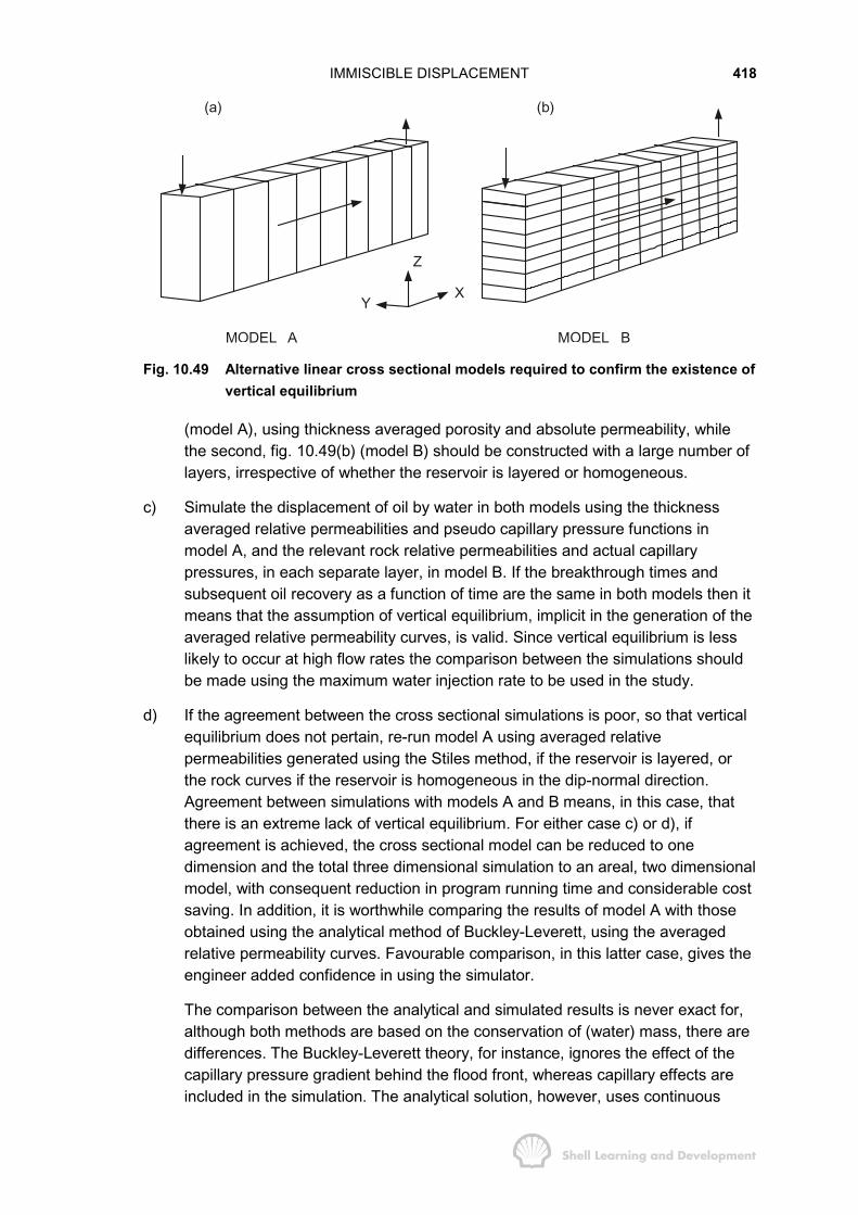
IMMISCIBLE DISPLACEMENT 418
(a) (b)
Y
Z
X
MODEL A MODEL B
Fig. 10.49 Alternative linear cross sectional models required to confirm the existence ofvertical equilibrium
(model A), using thickness averaged porosity and absolute permeability, whilethe second, fig. 10.49(b) (model B) should be constructed with a large number oflayers, irrespective of whether the reservoir is layered or homogeneous.
c) Simulate the displacement of oil by water in both models using the thicknessaveraged relative permeabilities and pseudo capillary pressure functions inmodel A, and the relevant rock relative permeabilities and actual capillarypressures, in each separate layer, in model B. If the breakthrough times andsubsequent oil recovery as a function of time are the same in both models then itmeans that the assumption of vertical equilibrium, implicit in the generation of theaveraged relative permeability curves, is valid. Since vertical equilibrium is lesslikely to occur at high flow rates the comparison between the simulations shouldbe made using the maximum water injection rate to be used in the study.
d) If the agreement between the cross sectional simulations is poor, so that verticalequilibrium does not pertain, re-run model A using averaged relativepermeabilities generated using the Stiles method, if the reservoir is layered, orthe rock curves if the reservoir is homogeneous in the dip-normal direction.Agreement between simulations with models A and B means, in this case, thatthere is an extreme lack of vertical equilibrium. For either case c) or d), ifagreement is achieved, the cross sectional model can be reduced to onedimension and the total three dimensional simulation to an areal, two dimensionalmodel, with consequent reduction in program running time and considerable costsaving. In addition, it is worthwhile comparing the results of model A with thoseobtained using the analytical method of Buckley-Leverett, using the averagedrelative permeability curves. Favourable comparison, in this latter case, gives theengineer added confidence in using the simulator.
The comparison between the analytical and simulated results is never exact for,although both methods are based on the conservation of (water) mass, there aredifferences. The Buckley-Leverett theory, for instance, ignores the effect of thecapillary pressure gradient behind the flood front, whereas capillary effects areincluded in the simulation. The analytical solution, however, uses continuous

IMMISCIBLE DISPLACEMENT 419
space and time, whereas these assume discrete values in the simulator.Because of this, shock front displacement is never accurately modelled with afinite difference simulator. Examples of the comparison between analytical andsimulated shock front displacement have been presented by Todd, et.al.28
e) If agreement is not achieved between the cross sectional simulations in either c)or d) above, then no definite assumption can be made concerning the verticalequilibrium condition. In this case model A should be re-structured with twolayers of grid blocks in the dip-normal direction, each layer having its ownaveraged porosity and permeability. Step a) should be repeated, generatingaveraged relative permeabilities and pseudo capillary pressures for each layer.Simulations with this two layer model should again be compared with the resultsfrom model B. Agreement, in this case, means that while vertical equilibrium maynot apply across the entire thickness of the reservoir, it is appropriate across halfthe reservoir. If there is still no agreement between the cross sectionalsimulations, model A should be re-structured as a three or four layered modeland the process repeated until satisfactory agreement is achieved. In this mannerit is usually possible to significantly reduce the number of layers.
The procedure outlined above should be undertaken at the commencement of anylarge numerical simulation study. It can usually be conducted very quickly and at only asmall fraction of the total study cost. If the reservoir is not areally homogeneous, sothat a cross section between injection and production wells which is representative ofthe entire reservoir cannot be selected, then several cross sections must be chosen. Itwill then be necessary to repeat step a) — the generation of averaged relativepermeabilities and pseudo capillary pressure for each cross section. If, however,vertical equilibrium has been clearly validated in one cross section, it is fairly safe toassume its validity throughout the reservoir, unless there are extremes of thickness orvertical permeability.
The relative permeability curves obtained from the above study are input to thereservoir simulation model which has, hopefully, by this stage, been reduced to twodimensions. Simulations are then conducted to try and match the available historydata. Following a successful history match, the simulator can be used to predict thefuture reservoir performance for different proposed production policies, well positionsetc.; and, as Coats18 has observed, although a reservoir can only be produced once, itsperformance can be simulated in many different ways and at comparatively low cost.
REFERENCES
1) Craig, F.F., Jr., 1971. The Reservoir Engineering Aspects of Waterflooding. SPEMonograph: Chapter 1.
2) Morrow, N.R., 1976. Capillary Pressure Correlations for Uniformly Wetted PorousMedia. J.Can.Pet.Tech., October-December: 49-69.
3) Amyx, J.W., Bass, D.M. and Whiting, R.L., 1960. Petroleum ReservoirEngineering - Physical Properties, McGraw-Hill: 176-196.
IMMISCIBLE DISPLACEMENT 420
4) Dumore, J.M., 1974 Drainage Capillary Pressure Functions and theirComputation from One Another. Soc.Pet.Eng.J., October: 440
5) Coats, K.H., Dempsey, J.R. and Henderson, J.H.,1971. The Use of VerticalEquilibrium in Two Dimensional Simulation of Three Dimensional ReservoirPerformance. Soc. Pet.Eng.J., March: 63-71. Trans. AIME.
6) Coats, K.H., Nielsen, R.L., Terhune, Mary H. and Weber, A.G., 1967. Simulationof Three Dimensional, Two Phase Flow in Oil and Gas Reservoirs.Soc.Pet.Eng.J., December: 377-388. Trans. AIME.
7) Buckley, S.E. and Leverett, M.C.,1942. Mechanism of Fluid Displacement inSands. Trans. AIME. 146: 107-116.
8) Welge, H.J., 1952. A Simplified Method for Computing Oil Recovery by Gas orWater Drive. Trans. AIME. 195: 91-98.
9) Hagoort, J., 1974. Displacement Stability of Water Drives in Water Wet ConnateWater Bearing Reservoirs. Soc.Pet.Eng.J., February: 63-74. Trans. AI ME.
10) Jacquard, P. and Seguier, P., 1962. Mouvement de Deux Fluides en Contactdans un Milieu Poreux. J. de Mechanique, Vol. 1:25.
11) Dietz, D.N., 1953. A Theoretical Approach to the Problem of Encroaching andBy-Passing Edge Water. Akad. van Wetenschappen, Amsterdam. Proc. V.56-B:83.
12) van Daalen, F. and van Domselaar, H.R., 1972. Water Drive in InhomogeneousReservoirs - Permeability Variations Perpendicular to the Layer. Soc.Pet.Eng.J.,June: 211 -219. Trans. AIME.
13) Richardson, J.G. and Blackwell, R.J., 1971. Use of Simple Mathematical Modelsfor Predicting Reservoir Behaviour. J.Pet.Tech., September: 1145-1154. Trans.AIME.
14) Stiles, W.E., 1 949. Use of Permeability Distribution in Water Flood Calculations.Trans. AIME,186:9.
15) Craft, B.C. and Hawkins, M.F., Jr., 1959. Applied Petroleum ReservoirEngineering. Prentice-Hall, Inc. New Jersey: 393-406.
16) Cole, F.W., 1961. Reservoir Engineering Manual. Gulf Publishing Company,Houston, Texas: 200-213.
17) Hearn, C.L., 1971. Simulation of Stratified Waterflooding by Pseudo RelativePermeability Curves. J.Pet.Tech., July: 805.
18) Coats, K.H., 1969. Use and Misuse of Reservoir Simulation Models. J.Pet.Tech.,November: 1391-1398. Trans. AIME.
19) Staggs, H.M. and Herbeck, E.F., 1971. Reservoir Simulation Models - AnEngineering Overview. J.Pet.Tech., December: 1428-1435. Trans. AIME.

IMMISCIBLE DISPLACEMENT 421
20) O'Dell, P.M., 1974. Numerical Reservoir Simulation: Review and State of the Art.Paper presented at 76th National AlChE Meeting, Tulsa, Oklahoma. March.
21) 1973. Numerical Simulation. SPE Reprint Series No. 11. Society of PetroleumEngineers of AIME, Dallas, Texas.
22) Blair, P.M. and Weinaug, C.F., 1969. Solution of Two Phase Flow ProblemsUsing Implicit Difference Equations. Soc.Pet.Eng.J., December: 417-424. Trans.AIME.
23) MacDonald, R.C. and Coats, K.H., 1970. Methods for Numerical Simulation ofWater and Gas Coning. Soc.Pet.Eng.J., December: 425-436. Trans. AIME.
24) Letkeman, J.P. and Ridings, R.L.,1970. A Numerical Coning Model.Soc.Pet.Eng.J., December: 418-424. Trans. AIME.
25) Nolen, J.S. and Berry, D.W., 1972. Tests of Stability and Time-Step Sensitivity ofSemi-lmplicit Reservoir Simulation Techniques. Soc.Pet.Eng.J., June: 253-266.Trans. AIME.
26) Peaceman, D.W., 1977. A Nonlinear Stability Analysis for Difference EquationsUsing Semi-lmplicit Mobility. Soc.Pet.Eng.J., February: 79-91.
27) Chappelear, J.E. and Rogers, W.L., 1974. Some Practical Considerations in theConstruction of a Semi-lmplicit Simulator. Soc.Pet.Eng.J., June: 216-220.
28) Todd, M.R., O'Dell, P.M. and Hirasaki, G.J., 1971. Methods for IncreasedAccuracy in Numerical Reservoir Simulators. Soc.Pet.Eng.J., December: 515-530. Trans. AIME.

AUTHOR INDEX
Agarwal, R.G.Alden, R.C.Al-Hussainy, R.Amyx, J.W.Aziz, K.
Bass, D.M.Bell, W.T.Bentsen, R.G.Berry, D.W.Biot, M.A.Blackwell, R.J.Blair, P.M.Boburg, T.C.Bradley, J.S.Brar, G.S.Breitenback, E.A.Brons, FBrown, G.G.Bruns, J.R.Bruskotter, J.F.Buckley, S.E.Burrows, D.B.
Campbell, J.M.Carr, N.L.Carslaw, H.S.Carter, R.D.Chapman, R.E.Chappelear, J.E.Coats, K.H.Cobb, W.M.Cole, F.W.Craft, B.C.Craig, F.F.Crawford, P.B.
Daalen, F. vanDarcy, H.Dempsey, J.R.Denson, A.H.Dietz, D.N.Dodson, C.R.Doh, C.A.
Domselaar, H.R. vanDonohue, D.A.T.Dowdle, W.L.Dranchuk, P.M.Dumoré, J.M.
Earlougher, R.C., Jr.Essis, A.E.Everdingen, A.F. van
Fetovitch, M.J.Field, R.Q.
Geertsma, J.Gewers, C.W.W.Goodrich, J.H.Goodwill, D.Gulati, M.S.
Hagoort, J.Hall, K.R.Hastings, J.R.Havlena, D.Hawkins, M.F., Jr.Hazebroek, P.Hearn, C.L.Heintz, R.C.Henderson, J.H.Herbeck, E.F.Hirasaki, G.J.Horner, D.R.Hurst, W.
Jacquard, P.Jaeger, J.C.Jones, L.G.
Katz, D.L.Kazemi, H., Jr.Kentie, C.J.P.Kersch, K.M.King Hubbert, M.,Kingston, P.E.Klinkenberg, L.J.

AUTHOR INDEX 423
Knaap, W. van derKo, S.Kobayashi, R.Kumar, A.
Langenheim, R.H.Lantz, R.B.Lebourg, M.Letkeman, J.P.Leverett, M.C.Lynch, E.J.
McCain, W.D.MacDonald, R.C.McFarlane, R.C.McKinley, R.M.McMahon, J.J.Marting, V.E.Marx, J.W.Marthar, L.Matthews, C.S.Mayer, E.H.Meitzen, V.C.Merle, H.A.Miller, F.G.Millers, S.C., Jr.Moreland, E.E.Morrow, N.R.Mueller, T.D.
Nichol, L.R.Nielsen, R.L.Niko, H.Nolen, J.S.Northern, I.G.
Oberfell, G.B.Odeh, A.S.O'Dell, P.M.Opstal, G.H.C. van
Peaceman, D.W.Perry, G.E.Pinson, A.E., Jr.
Poollen, H.K. van
Quon, D.
Raghavan, R.Ramey, H.J., Jr.Rawlins, E.L.Reudelhuber, F.O.Richardon, J.G.Ridings, R.L.Riley, H.G.Rogers, W.L.Russell, D.G.
Schellhardt, M.A.Schilthuis, R.J.Schueler, S.Schultz, A.L.Seguier, P.Selig, F.Smith, J.T.Staggs, H.M.Standing, M.B.Stiles, W.E.
Takacs, G.Teeuw, D.Terhune, Mary H.Thomas, G.W.Thurnau, D.H.Timmerman, E.L.Todd, M.R.Troost, P.J.P.M.
Urbanosky, H.J.
Walstrom, J.E.Wattenbarger, R.A.Weber, A.G.Weinaug, C.F.Welge, H.J.Whiting, R.L.Wong, S.W.
Yarbourough, L.

SUBJECT INDEX
Abnormal fluid pressure
Absolute permeabilitymeasurement of
Acceleration project
Acid treatment
Afterflow
Afterflow analysisEarlougher and KerschMcKinleyRameyRussell
Al-Hussainy, Ramey and Crawford:real gas flow
Amerada pressure gauge
Aquiferaverage pressure,bounded,compressibility, total,constant,encroachable waterencroachable anglefittinginfinite actingmodelpressure declineproductivity indexsteady state
Aquifer expansiontime dependence of
Aquifer geometry:general,linear,radial,
Average reservoir pressure,
Averaged relative permeability andsaturation (see Thickness averagedrelative permeability)
Bachaquero field (Venezuela),
Back pressure testing,
Basic differential equation, radial flow,conditions of solution,derivation of,linearization, real gas,linearization, general,linearization, liquid,
Basic well test analysis equation:general,for liquid,for real gas,
Beykan field (Turkey),
Bolivar Coast fields (Venezuela),
Boltzmann's transformation,
Boundary conditions,constant pressure,infinite,no-flow,
Breakthrough:of water in a producing well,premature,saturation,time,
Brent field (North Sea),
Brons and Marting, partial wellpenetration,
Bubble pointline,pressure,Buckley-Leverett one dimensionaldisplacement,stability of,
Buckley-Leverett equation,derivation of,mathematical difficulty with,
Buildup (see Pressure buildup)

SUBJECT INDEX 425
By-passing:critical rate to prevent,oil by gas,oil by water,
Capillary:force,-gravity equilibrium,rise, capillary tube experiment,rise, in the reservoir,tube,
Capillary pressure,equation,Laplace equation,negative value,psuedo (see Psuedo capillarypressure)
Capillary pressure curve (function):laboratory determination,oil-water, drainage,oil-water, imbibition,
Capillary pressure gradient,neglected in description of segregatedflow,neglect in fractional flow equation,
Capillary transition zone,allowance for in displacementcalculations,(homogeneous reservoir), (layeredreservoir), compared to reservoirthickness, lack of,
Carbon dioxide flooding,
Coats, K.H.,
Coefficient of inertial resistance,dependence on liquid saturation,experimental determination of units of,
Combination drive,
Compaction,cell,derive,
Compaction curve,hysteresis of,
Comparison between p2 and m(p)solution
techniques, real gas flow,
Compressibility, isothermal,application of basic definition,aquifer, totaleffective, saturation weighted,(undersaturated reservoir)fluids in the well,oil,pore,total, gas saturated reservoir,total, saturation weighted(undersaturated reservoir),water,
Compressibility program forgenerating thickness averagedrelative permeabilities,numerical simulation,well test analysis,
Condensate, retrograde,
Conduction heat transfer, tocap and base rock,reservoir from cap and base rock,
Coning,
Connate water saturation,expansion of,
Constant terminal pressure solution(radial diffusivity equation),
Constant terminal rate solution (radialdiffusivityequation):liquid,real gas,semi-steady state flow (liquid, (realgas)transient flow (liquid),(real gas)Constant volume depletionexperiment,
Contact angle,hysteresis of,
SUBJECT INDEX 426
Convection heat loss,
Correction of measured wellborepressure to adatum level,
Correction of PVT differential data toallow forsurface separation,
Cricodentherm,
Critical:point,pressure,saturation (see Saturation, critical)temperature,
Critical rate for by-passing:oil by gas,oil by water,
Damage to formation,
Darcy:Henry,the,units,
Darcy'sexperiment,flow coefficient, gas,law, linear flow,law radial flow,
Datumplane,pressure,
Depletion drive, gas reservoir,development planning:
gas field,general,
Dew point line,
Dietz:determination of average pressure ina buildup survey,segregated displacement,shape factors,
Differential liberation experiment,
Diffuse flow conditions,
Diffusivity constant,
Diffusivity equation (see Radial diffusivityequation)
Dimensionless cumulative oil production:moveable oil volumes,pore volumes,
Dimensionless cumulative water influxfunction,
maximum value of, bounded aquifer,plots of ,superposition of,
Dimensionless cumulative water injected:moveable oil volumes,pore volumes,
Dimensionless pressure functions:definition ofdifficulty in application,general expression for any value ofthe flowing time,generation of,semi-steady state,superposition of,transient,
Dimensionless pressure/pseudo pressurefunction for any fluid,
superposition of,transient,
Dimensionless pseudo pressure, gas-oil,
Dimensionless radius:aquifer/reservoir,reservoir/wellbore,
Dimensionless real gas pseudo pressurefunction,
difficulty in application,general expression for any value ofthe flowing time,generation of,semi-steady state,superposition of,transient,

SUBJECT INDEX 427
Dimensionless time, tD:aquifer,reservoir,Dimensionless time, tDA,difficulty in evaluation for a real gas,
Dimensionless time for semi-steady stateflow, (tDA)SSS,
Dimensionless variable, pressureanalysis,reasons for use,
Dip-angle of reservoir,effect on the fractional flow equation,
Displacement:immiscible (see Immiscibledisplacement) miscible,
Dissolved gas (see Gas, disolved)
Distillation of crude oil in the reservoir,
Distortion of radial flow in the vicinity of awell,
Dodson's PVT experiment,
Drainage (capillary),
Drill stem test,
Drilling mud,
Drive mechanisms (see Reservoir drivemechanisms)
Dry gas re-cycling,
Dynamic grid block pressure,
Earlougher, R.C., Jr:afterflow anlaysis,digitized MBH charts,dynamic grid block pressure,generation of MBH charts,pressure drawdown analysis,
Effective flowing time,
Effective permeability,curves, oil-water,saturation dependence,
Effective permeability, measurement of:afterflow analysisbuildup analysis, gas-oil,
" " , oil, 9" " , oil, real gas,multi-rate drawdown analysis, oilmulti-rate drawdown analysis, realgas,single rate drawdown analysis, oil," " " " , real gas,
Effective well bore raduis,
End point:
mobility ratio, gas/oil,mobility ratio, water/oil,relative permeabilities, gas-oil,relative permeabilities, water-oil,
Equations of state:ideal gas,real gas,van der Waals,
Equivalent gas volume,
Erosion of surface,
Essis-Thomas analysis,
Euler's constant,
Everdingen, A.F. van, mechanical skinfactor
(see Mechanical skin factor)
Expansion of reservoir fluids,
Exploration well,
Exponential integral,logarithmic approximation,
Fetovictch, M.J.,comparison between calculated waterinflux and that of Hurst and vanEverdingen,equations for water influxmodified method for large aquifers,
Final flow rate,
Finite difference approximation
Flash expansion of:oil sample to determine the bubblepoint pressure,separator oil sample,
SUBJECT INDEX 428
unit volume of bubble point oilthrough model separators,
Flow charts:calculation of flowing pressure in agas well,Kazemi iteration,predication of pressure decline in awater drive gas reservoir,
Flowing pressure survey,
Flowing time
Fluid:contacts in the reservoir,distributions in the well,potential equilibrium,
Fluid samples:subsurface collection,surface recombination,
Forchheimer equation,
Formation volume factor:gas (see Gas formation volumefactor)oil (see Oil " " ")water (see Water formation volumefactor)
Fractional flow,calculation of,surface conditions,
Fractional flow curvetangent to,
Fractional flow equation:dependence on water saturation,derivation of,derivation ofhorizontal, diffuse flow,horizontal, segregated, unstabledisplacement,influence of capillary pressuregradient,influence of dip angle (gravity),
Fracturing fluid,
Gascomposition,compressibility (isothermal),condensate,constant, universal,density,disposal,dissolved (solution),equation of state (see Equation ofstate)expansion factor,expansion in the reservoir,flow, (see Real gas flow)flow velocity in the reservoirformation volume factor,gravity,ideal,injection,liberated, solution,material balance (see Materialbalance, gas)pressure gradient,PVT experiment,slippage,viscosity-compressibility product,volume equivalent,Z-factor (see Z-factor)
Gascap,drive,expansion,secondary,
Gas in place:apparent, in water drive gas reservoir,initial, GIIP,
Gas-oil contact,
Gas-oil ratio:control,cumulative,equation,producing (instantaneous),solution,solution, initial, of bubble point oil(differential),

SUBJECT INDEX 429
solution, initial, of bubble point oil(flash),
Gas recovery,
Gas saturation,critical,residual, to water,
Gas-water contact,
Gas well testing:general analysis theory,buildup,multi-rate drawdown,Grain (matrix) pressure,
Gravity:force,segregation,
Gravity number:gas displacing oil,water displacing oil,
Hall-Yarborough, calculation of Z-factors,
Havlena-Odeh, interpretation of materialbalance,
gascap drive,natural water drive,solution gas drive,
History matching:reservoir performance,pressure,
Horner buildup plot:gas-oilgeneral (any fluid),oil,real gas,
Hot water injection,
Hurst and van Everdingenconstant terminal pressure solution(radial diffusivity equation),constant terminal rate solution (radialdiffusivity equation),unsteady state water influx theory,
Hydrocarbon:accumulations,
columns,migration,phase behaviour,recovery (see Recovery ofhydrocarbons)Hydrocarbon pore volume (HCPV)gascap,reduction of during depletion,
Hydrostatic:equilibrium,pressure regime (abnormal)," " (normal),
Image wells,
Imbibition,
Immisible fluids,oil by gas,oil by water,physical assumptions,water by oil,with total lack of vertical equilibrium,
Incompressible fluids,
Increasing:effective permeability,well penetration,productivity index,
Infinite:acting aquifer," reservoir,closed in time,
Inflow equations:aquifer,semi-steady state (oil), (gas),steady state (oil)," " , steam soaked well
In-situ combustion,
Interface between immiscible fluids,
Interfacial tension,
Kapuni field (New Zealand),
Kayaköy field (Turkey),
Kazemi, H., Jr.,

SUBJECT INDEX 430
Klinkenberg effect,
Kirchhoff integral transformation,
Laplace,capillary pressure equation,steady state equation,transform
Late transient flow,
Line transient flow, 153-54, 304
Late transient flow,
Line source solution (radial diffusivityequation)
liquid,real gas,
Linear prototype reservoir,
Linearization (see Basic differentialequation)
Logs, petrophysical,
McKinley afterflow analysis,transmissiblity,type curves,wellbore parameter,
Maps:datum pressure,geological contour,
Mass conservation,fluid, radial flow,oil, linear flow,water, linear displacement,
Mass transfer,Material balance:aquifer,gas reservoir, depletion," " , water drive,general hydrocarbon reservoir," , linear function,linear incompressible water injection,production from a closed radial cell,reduced equation, gascap drivereservoir," ", natural water drive reservoir,
solution gas drive reservoir,undersaturated,solution gas drive reservoir, gassaturated,
Matthews, Brons, Hazebroek (MBH):charts,determination of average pressure,buildup test,gas-oil,general,oil,real gas,dimensionless pressure,dimensionless pseudo pressure,theory, buildup testing,volume (rate) averaged reservoirpressure,
Mechanical skin factor,
Mechanical skin factor, determination ofafterflow analysis, oilbuildup testing
gas-oil,oil,real gas,
multi-rate drawdownoil,real gas,
single rate drawdownoil,
Mercury injection pump,
Method of images,
Micellar solution flooding,
Mobilituy:buffer,control,fluid,relative,
Mobility ratio:end point, gas/oil,end point, general," ", water/oil,flood front,

SUBJECT INDEX 431
reduction of,significance of,
Mobilising residual oil,
Movable oil volume,
Multi-rate testing, gas wells,back pressure testing,
Essis-Thomas analysis,Odeh-Jones analysis,non-stabilized analysis,validity of transient analysis,
Multi-rate testing, oilwells, 97ambiguity in interpretation,analysis,basic analysis equation,Odeh-Jones analysis,routine surveys, partially depletedreservoirs,validity of transient analysis,
Natural water influx (see Water influx)
Net bulk volume,
Non-Darcy flow,
Non-Darcy flow coefficient (F),
Normalization of effective permeabilitycurves,
Numerical simulation,
Numerical simulation of immiscible,incompressible displacement,comparison with analytical methods,conducting a study,evaluation of viscosity at grid blockfaces,finite difference formulation of 1-Dconservation equations,harmonic averaging of absolutepermeability,IMPES solution technique,instabilities in solution,material balance mode,one-dimensional model,purpose of,reduction of dimensions,
role of thickness averaged relativepermeabilities and pseudo capillarypressures,semi implicit rates, well model,semi implicit relative permeabilities;pseudo capillary pressure,two point upstream weighting, relativepermeabilities,well model,
Odeh-Jones analysis,
Oilcolumn,compressibility,density, reservoir," , standard conditions,displacement (see Immiscible,incompressible displacement)expansion in reservoir," on heating,formation volume factorof bubble point oil, differential,of bubble point oil, flash,differential, relative to residual oilvolume,gravity,in place,pressure gradient,saturation," , residual,undersaturated,velosity, during displacement,viscosity,volume, residual,
Oil relative permeability,altering the characteristics,
Oil viscosity reduction:carbon dioxide flooding,thermal,
Oil-water contract, 9
Oil wet,
Osmosis,
Overburden:
SUBJECT INDEX 432
pressure," , gradient,
Overpressure,
Paraffin series,
Partical penetration, of well,
Permeability:absolute,dimensions of,effective (see Effective permeability)increasing by well stimulation,reduction in vicinity of well,relative (see Relative permeability)units of,vertical,
Phase diagram,
Phase equilibrium calculations,
Piston-like displacement,
Polymer flooding,
Pore compressibility,experimental determination,
Pore volume (PV),determination of, gas well test" ", oil well test,reduction during depletion,
Porosity,
Potential:dimensions,fluid,gradient,real gas,
Practical aspects of well surveying,
Predictingpressure decline, water drive gasreservoir,reservoir performancewater influx,
Pressure:absolute,average, aquifer," , grid block,
" , reservoir," , within well's drainage boundary,bottom hole flowing,critical,drawdown,drop, across skin,dynamic grid block,extrapolated, infinite closed-in time,gauge,grain (matrix),initial, determination of,overburden,pseudo critical,pseudo reduced,squared, real gas flow,water abnormal," , normal
Pressure buildup:computer program,dominated by afterflow,Matthews, Brons, Hazebroek theory,plot, Horner (see Horner buildup plot)practical aspects,theoretical equation,theoretical linear equation,
Pressure buildup analysis:gas-oil,general,oil,real gas,
Pressure drawdown testing, multi-rate,(see Multi-rate testing)
Pressure drawdown testing, single rate:analysis of, oil," ", real gas,purpose of,
Pressure gradient:capillary (see Capillary pressuregradient)fluids in the well,gas,overburden,

SUBJECT INDEX 433
water,
Pressure maintenance, partial:gas reservoir,oil reservoir,
Pressure maintenance, total,Primary recovery (see Recovery ofhydrocarbons)
Producing gas-oil ratio (see Gas-oil ratio)
Productivity index(PI):aquifer,increase, well stimulation,numerical simulator, well model,ratio increase, skin removal," " , steam soaking,semi-steady state, liquid,
Pseudo:critical pressure," temperature,pressure, real gas (see Real gaspseudo pressure)pressure, two phase, gas-oil,reduced pressure,reduced temperature,relative permeabilities (see Thicknessaveraged relative permeabilities)skin factor,
Pseudo capillary pressure,function ,in dipping reservoir,role in numerical simulation,
Psi potential,
PV cell,
PVT:gas,oil,
PVT analysisDodson's experiment,gas,gas condensate,oil, basic analysis," , complete analysis,
PVT oil, presentation of results:corrected for surface separation,uncorrected for surface separation,
Radial diffusivity equation:constant terminal rate solution (seeConstant terminal rate)difficulty in solving, real gas,general,line source solution (see Line sourcesolution)oil,real gas,
Radial diffusivity equation, dimensionlessgeneral,liquid,real gas,
Ramey, H.J., Jr.,
Real gas pseudo pressure,generation of,reasons for using,
Recombination, fluid samples,
Recovery factor
Recovery of hydrocarbons, primary,compaction drive, gas,gascap drive,solution gas drive
Recovery of hydrocarbons, tertiary,
Reduction of displacement problems toonedimension,layered reservoirs,numerical simulation,segregated displacement,homogeneous,
Relative permeability,curves, rock,end point values, gas-oil,end point values, water-oil,gas,linear,measurement of ,oil,
SUBJECT INDEX 434
thickness averaged (see Thicknessaveraged relative permeabilities)
Relative volumes, PVTcumulative gas,gas,oil,total,
Removal of mechanical skin,
Reservoir drive mechanisms,combination,compaction,solution, gas,water,
Reservoir limit testing,
Reservoir simulation (see Numericalsimulation)
Residual:gas saturation,oil saturation,oil volume, PVT,
Retrograde liquid condensate,
Russell, afterflow analysis,
Russell-Goodrich, real gas flow,difficulty in application,
Sample collection (see Fluid samples)
Saturation:critical, gas," , gas condensate,gas (see Gas saturation)oil (see Oil saturation)water (see Water saturation)
Schilthuis, R.J.:material balance equation,steady state water influx.
Segregated displacement, oil by gas," " , oil by water (see Waterdrive)
Semi-steady state:condition,time,
Separation, gas-oil:reservoir,surface,
Shrinkage factor:bubble point oil, differential," " ", flash,oil separator-stock tank,
Sign convention:Darcy's equation,isothermal compressibility,Laplace, capillary pressure equation,source-sink terms, numerical,
Skin factor:mechanical (see Mechanical skin)pseudo,rate dependent,
Solution gas drive:above bubble point,below bubble point,
Solution gas-oil ration (see Gas-oil ratio)
Standard conditions,
Standing-Katz, Z-factor correlation,application of 14-18
Statfjörd field (North Sea),
Static pressure survey,
Steady state condition,
Steam:drive,injection,
Stiles method,
Stock tank oil, initially in place, STOIIP,probablistic determination,
Subsidence, surface,
Superposition:inspace,in time,
Summary:chart, generation of averaged relativepermeabilities,pf pressure analysis techniques,
SUBJECT INDEX 435
Surface tension,
Surfactant flooding,
Temperature:ambient, surface,distribution, steam soaked well,effect, sealed fresh water system,reservoir,seperator,
Tertiary flooding,
Thermal recovery,
Thickness averaged relativepermeabilities/water saturations,
diffuse flow,graphical determination,homogeneous reservoir, finitecapillary transition zone,homogeneous reservoir, segregatedflow,layered reservoir, lack of verticalequilibrium,layered reservoir, pressurecommunication,role in numerical simulation,summary chart,with total lack of vertical equilibrium,
Time scale for hydrocarbon recovery,
Time to reach semi-steady state
Transient flow condition,
Transient well test analysisbuildup, general," , oil," , real gas,multi-rate drawdown, general," " " , oil,multi-rate drawdown, real gassingle rate drawdown, oil" " " , real gas,
Transition from transient to semi-steadystate flow,
well at centre of regular shapeddrainage area,
Trapezoidal rule for integration,
Ultimate recovery,
Underground withdrawal,
Underreaming,
Undersaturated oil,
Units:absolute,cgs,Darcy,field,for real gas flow,Systeme Internationale (SI),
Units conversion,Darcy's ;linear equation,dimensionless variables,real gas flow,
Universal gas constant,
Uplifting, of reservoir,
Variable rate history:prior to buildup test,prior to multi-rate flow test,
Velocity ofgas, with respect to oil,maximum water saturation plane,plane of constant water saturation,
Vertical equilibrium,influences on,total lack of,
Viscosity:gas,oil,ratio, oil/displacing fluid,water,
Viscosity-compressibility product, realgas,
Viscosity-compressibility product, realgas,
Viscosity-temperature relation, oil
Viscosity-Z factor product, real gas,
SUBJECT INDEX 436
Volume:hydrocarbon (see Hydrocarbon porevolume)moveable oil,pore (see Pore volume)
Water:bearing sand,breakthrough (see Breakthrough)compressibility,expansion,formation volume factor,injection,pressure," , equation," , gradient,salinity,tongue,viscosity,
Water drive,Buckley-Leverett theory,homogeneous reservoir, diffuse flow," " , finite capillarytransition zone,homogeneous reservoir, segregatedflow,ideal (piston-like),layered reservoir, with verticalequilibrium,layered reservoir, without verticalequilibrium,mechanics of ,non-ideal,numerical simulation of,
Water drive, oil recovery equations:stable, segregated flow,unstable, segregated flow," " ", inclined,Welge,
Water influx:dimensionless cumulative influxfunction,dimensionless influx rate,
gas reservoir,oil reservoir,time dependance of,
Water influx calculations:applied to steam soaking,Fetkovitch, history matching," , prediction,Hurst-van Everdingen, historymatching,Hurst-van Everdingen, prediction,uncertainty in,
Water saturation:average, behind flood front,breakthrough,connate (see Connate watersaturation)flood front (shock front),influence, effective and relativepermeabilities,
Water saturation distribution:areal,definable,diffuse (uniform),dip normal (see Thickness averagedrelative permeability/water saturation
Water wet reservoir,
Welge'sequation,graphical technique,
Well:asymmetry,conditioning,exploration,model, numerical simulation,partial penetration,stimulation,
Well testing:collection of fluid samples,initial,practical aspects,purpose of,routine,

SUBJECT INDEX 437
Wettability,
Wireline formation test,
Z-factor:application of,as function of pressure,average value, Russell-Goodrichinflow equations,two phase,
Z-factor, determination of:correlation charts,direct calculation,experiment,

The author of "Fundamentals of Reservoir Engineering" is especially well-qualified towrite on this subject, having spent the past few years with the Training Division of ShellInternational Petroleum Company, lecturing on reservoir engineering.
In this book he gives a coherent account of the basic physics of reservoir engineering,a thorough knowledge of which is essential in the petroleum industry for the efficientrecovery of hydrocarbons. Much of the text is based on various lecture courses givenby the author and throughout the book only the simplest and most straightforwardmathematical techniques are used. The first four chapters serve as an introduction tothe subject and will interest all those connected in any way with development andproduction of hydrocarbon reserves.
The next four chapters are more specialised and describe the most important aspectsof the field, i.e. the theory and practice of oil and gas well testing and pressure analysistechniques. This is dealt with in a concise, unified and applied manner not readilyfound in other texts. Water influx and fluid displacement are described in the last twochapters with the aim of helping the reader understand the numerical simulation ofreservoir performance. Numerous modern computational techniques are describedwith the aid of flow charts and illustrated with examples.
This is an ideal text for the student as it assumes no prior knowledge of reservoirengineering, but it is also of value for the practising reservoir engineer, productiontechnologist and production engineer.
Related Documents


![Golf-Racht, T. D. Van. - Fundamentals of Fractured Reservoir Engineering[1]](https://static.cupdf.com/doc/110x72/55cf98ae550346d033990efe/golf-racht-t-d-van-fundamentals-of-fractured-reservoir-engineering1.jpg)