Fundamentals of Magnetism – 1 J. M. D. Coey School of Physics and CRANN, Trinity College Dublin Ireland. 1. Introduction; basic quantities 2. Magnetic Phenomena. 3. Units www.tcd.ie/Physics/Magnetism Comments and corrections please: [email protected]

Welcome message from author
This document is posted to help you gain knowledge. Please leave a comment to let me know what you think about it! Share it to your friends and learn new things together.
Transcript

Fundamentals of Magnetism – 1 J. M. D. Coey
School of Physics and CRANN, Trinity College Dublin
Ireland.
1. Introduction; basic quantities
2. Magnetic Phenomena.
3. Units
www.tcd.ie/Physics/MagnetismComments and corrections please: [email protected]
SUMMER SCHOOL
!

Lecture 1 covers basic concepts in magnetism; Firstly magnetic moment, magnetization and the two magnetic fields are presented. Internal and external fields are distinguished. Magnetic energy and forces are discussed. Magnetic phenomena exhibited by functional magnetic materials are briefly presented, and ferromagnetic, ferrimagnetic and antiferromagnetic order introduced. SI units are explained, and dimensions are provided for magnetic, electrical and other physical properties.
.
An e lemen ta ry know ledge o f vec to r ca l cu lus and electromagnetism is assumed.

Some useful books include:
• J. M. D. Coey; Magnetism and Magnetic Magnetic Materials. Cambridge University Press (2010) 614 pp An up to date, comprehensive general text on magnetism. Indispensable!
• S. Blundell Magnetism in Condensed Matter, Oxford 2001 A good, readable treatment of the basics.
• D. C. Jilles An Introduction to Magnetism and Magnetic Magnetic Materials, Magnetic Sensors and Magnetometers, 3rd edition CRC Press, 2014 480 ppQ & A format.
• R. C. O’Handley. Modern Magnetic Magnetic Materials, Wiley, 2000, 740 ppQ & A format.
• J. Stohr and H. C. Siegman Magnetism: From fundamentals to nanoscale dynamics Springer 2006, 820 pp. Good for spin transport and magnetization dynamics. Unconventional definition of M
• K. M. Krishnan Fundamentals and Applications of Magnetic Material, Oxford, 2017, 816 ppRecent general text.. Good for imaging, nanoparticles and medical applications.
Books
IEEE Santander 2017

1 Introduction
2 Magnetostatics
3 Magnetism of the electron
4 The many-electron atom
5 Ferromagnetism
6 Antiferromagnetism and other magnetic order
7 Micromagnetism
8 Nanoscale magnetism
9 Magnetic resonance
10 Experimental methods
11 Magnetic materials
12 Soft magnets
13 Hard magnets
14 Spin electronics and magnetic recording
15 Other topics
Appendices, conversion tables.
614 pages. Published March 2010
Available from Amazon.co.uk ~€50
www.cambridge.org/9780521816144
IEEE Santander 2017

1. Introduction; Basic quantities
IEEE Santander 2017
SUMMER SCHOOL
!

Magnets and magnetization
3 mm 10 mm 25 mm
m is the magnetic (dipole) moment of the magnet. It is proportional to volume
m = MV
magnetic moment volume magnetization
Suppose they are made of Nd2Fe14B (M ≈ 1.1 MA m-1)
What are the moments?
0.03 A m2 1.1 A m2 17.2 A m2
Magnetization is the intrinsic property of the material; Magnetic moment is a property of a particular magnet.
IEEE Santander 2017

IEEE Santander 2017
Magnitudes of M for some ferromagnets
M (MAm-1)
Nd2Fe14B 1.28 BaFe12O19 0.38
Fe 1.71 Co 1.44 Ni 0.49
Permanent magnets
Temporarymagnets
NB: These are the values for the pure phase

Magnetic moment - a vector
Each magnet creates a field around it. This acts on any material in the vicinity but strongly with another magnet. The magnets attract or repel depending on their mutual orientation
↑ ↑ Weak repulsion
↑ ↓ Weak attraction
← ← Strong attraction
← → Strong repulsion
Nd2Fe14B
tetragonal easy axis
IEEE Santander 2017

Field due to a magnetic moment m
m
Hr Hθ Hϕ
tan I = Br /Bθ = 2cotθdr/rdθ = 2cotθ
Solutions are r = c sin2θ
The Earth’s magnetic field is roughly that of a geocentric dipole
Equivalent forms
H
H1
m
m m
Note. The dipole field is scale-independent. m ~ d3; H ~ 1/r3
Hence H = f(d/r). Result: 60 years of hard disc recording !
IEEE Santander 2017
Michael Faraday
r�
ϕ
er
e�
m
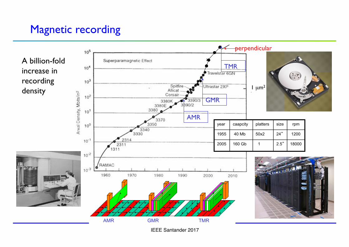
Magnetic recording
IEEE Santander 2017
1µm2
GMR
TMR
AMR
perpendicular
1 µm2
18000 2.5� 1 160 Gb 2005
1200 24� 50x2 40 Mb 1955
rpm size platters caapcity year
Porquerolles September 2012
14
Magnetic recording is the partner of semiconductor technology in the information revolution. It provides the permanent, nonvolatile storage of information for computers and the internet.
~ 10 exobit (1021bits) of data is stored
AMR GMR TMR
A billion-fold increase in recording density

How can you tell which way a magnet is magnetized?
Use the green paper!
It responds (turns dark) to the perpendicular component of H
This tells us the magnetic axis, but not the direction of vector m
We can decide the relative orientation of two magnets from the forces, but the direction of the arrow is a matter of convention.
IEEE Santander 2017
1
23-6

Permanent magnets win over electro- magnets at small sizes
Equivalence of electricity and magnetism; Units
What do the units mean?
m – A m2
M – A m-1
m = nIA
number of turns
10,000 turns
∈
∈
1 A m2
1A
10,000 A
C
m
Right-hand corkscrew
!
IEEE Santander 2017
m
Ampère,1821. A current loop or coil is equivalent to a magnet
m = IA
area of the loop
Michael Faraday
André-Marie Ampère

Magnetic field H – Oersted’s discovery
C I
H
Right-hand corkscrew
H = I/2πr
If I = 1 A, r = 1 mm H = 159 A m-1
∫ Hdℓ = I Ampère�s law
Earth�s field ≈ 40 Am-1
The relation between electric current and magnetic field was discovered by Hans-Christian Øersted, 1820.
H
r
I
δℓ
Units of H; A m-1
IEEE Santander 2017

Field due to electric currents
We need a differential form of Ampère’s Law; The Biot-Savart Law
Cj
B
Right-hand corkscrew (for the vector product)
δℓ
δBI
H
H
H
H
IEEE Santander 2017
1
1
j
r

Magnetostatics
42 Magnetostatics
B
H '
Figure 2.12
A B(H ′) hysteresis loop.
electrically polarized one. This field is the electrical displacement D, related tothe electrical polarization P (electrical dipole moment per cubic metre) by
D = ϵ0 E + P . (2.44)
The constant ϵ0, the permittivity of free space, is 1/µ0c2 = 8.854 ×
10−12 C V−1 m−1. Engineers frequently brand the quantity J = µ0 M as themagnetic polarization, where J , like B, is measured in tesla so that the relationbetween B, H and M can be writted in a superficially similar form:
B = µ0 H + J . (2.45)
This is slightly misleading because the positions of the fundamental and auxil-iary fields are reversed in the two equations. The form (2.27) H = B/µ0 − Mis preferable insofar as it emphasizes the relation of the auxiliary magneticfield to the fundamental magnetic field and the magnetization of the material.Maxwell’s equations in a material medium are expressed in terms of all fourfields:
∇ · D = ρ, (2.46)
∇ · B = 0, (2.47)
∇ × E = −∂ B/∂t, (2.48)
∇ × H = j + ∂ D/∂t. (2.49)
Here ρ is the local electric charge density and ∂ D/∂t is the displacement current.A consequence of writing the basic equations of electromagnetism in this neat
and easy-to-remember form is that the constants µ0, ϵ0 and 4π are invisible.But they inevitably crop up elsewhere, for example in the Biot–Savart law (2.5).The fields naturally form two pairs: B and E are a pair, which appear in theLorentz expression for the force on a charged particle (2.19), and H and D arethe other pair, which are related to the field sources – free current density j andfree charge density ρ, respectively.
Maxwell’s EquationsIn a medium;B � µ0H
Electromagnetism with no time-dependence
In magnetostatics, we have only magnetic material and circulating currents in conductors, all in a steady state. The fields are produced by the magnets & the currents
43 2.4 Magnetic field calculations
In magnetostatics there is no time dependence of B, D or ρ. We onlyhave magnetic material and circulating conduction currents in a steady state.Conservation of electric charge is expressed by the equation,
∇ · j = −∂ρ/∂t, (2.50)
and in a steady state ∂ρ/∂t = 0. The world of magnetostatics, which we explorefurther in Chapter 7, is therefore described by three simple equations:
∇ · j = 0 ∇ · B = 0 ∇ × H = j .
In order to solve problems in solid-state physics we need to know the responseof the solid to the fields. The response is represented by the constitutive relations
M = M(H), P = P(E), j = j (E),
portrayed by the magnetic and electric hysteresis loops and the current–voltage characteristic. The solutions are simplified in LIH media, whereM = χ H, P = ϵ0χ e E and j = σ E (Ohm’s law), χ e being the electrical sus-ceptibility and σ the electrical conductivity. In terms of the fields appearing inMaxwell’s equations, the linear constitutive relations are B = µH, D = ϵ E,
j = σ E, where µ = µ0(1 + χ) and ϵ = ϵ0(1 + χ e). Of course, the LIHapproximation is more-or-less irrelevant for ferromagnetic media, whereM = M(H) and B = B(H) are the hysteresis loops in the internal field, whichare related by (2.33).
2.4 Magnetic field calculations
In magnetostatics, the only sources of magnetic field are current-carrying con-ductors and magnetized material. The field from the currents at a point r inspace is generally calculated from the Biot–Savart law (2.5). In a few situationswith high symmetry such as the long straight conductor or the long solenoid, itis convenient to use Ampere’s law (2.17) directly.
To calculate the field arising from a piece of magnetized material we arespoilt for choice. Alternative approaches are:
(i) calculate the dipole field directly by integrating over the volume distribu-tion of magnetization M(r);
(ii) use the Amperian approach and replace the magnetization by an equivalentdistribution of current density jm;
(iii) use the Coulombian approach and replace the magnetization by an equiv-alent distribution of magnetic charge qm.
The three approaches are illustrated Fig. 2.13 for a cylinder uniformly mag-netized along its axis. They yield identical results for the field in free spaceoutside the magnetized material but not within it. The Amperian approach gives
IEEE Santander 2017
J. C. Maxwell
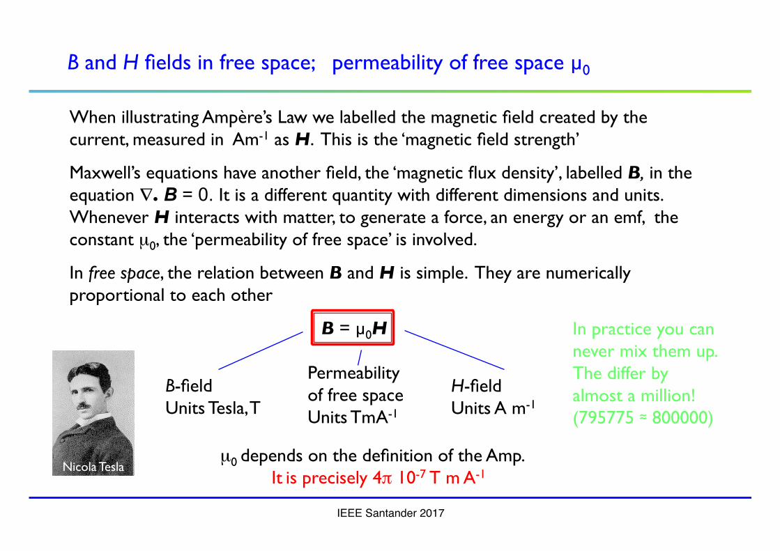
B and H fields in free space; permeability of free space µ0
When illustrating Ampère’s Law we labelled the magnetic field created by the current, measured in Am-1 as H. This is the ‘magnetic field strength’
Maxwell’s equations have another field, the ‘magnetic flux density’, labelled B, in the equation ∇. B = 0. It is a different quantity with different dimensions and units. Whenever H interacts with matter, to generate a force, an energy or an emf, the constant µ0, the ‘permeability of free space’ is involved.
In free space, the relation between B and H is simple. They are numerically proportional to each other
B = µ0H
B-fieldUnits Tesla, T
H-fieldUnits A m-1
Permeability of free spaceUnits TmA-1
Nicola Tesla µ0 depends on the definition of the Amp.
It is precisely 4π 10-7 T m A-1
In practice you can never mix them up. The differ by almost a million!(795775 � 800000)
IEEE Santander 2017

Magnetic Moment and Magnetization
The atomic magnetic moment ma is the elementary quantity in atomic-scale magnetism. (L. 2)
Define a local moment density - magnetization – M(r, t) which fluctuates wildly on an atomic, sub-nanometer scale and on a sub-nanosecond time scale.
Define a mesoscopic average magnetization
δm = MδV
The continuous medium approximation
M could be the spontaneous magnetization Ms within a ferromagnetic domain or fine particle. Most materials are not spontaneously ordered and M = 0. The atomic moments ma then fluctuate rapidly and the time average of any one of them, or the spatial average of an ensemble of atoms is zero. M is then the response of the molecular material to an external magnetic field H. At very low temperatures the spontaneous fluctuations freeze out.
Initially the response is linear; M = χH. The dimensionless constant χ is the susceptibility.
M = δm/δV
IEEE Santander 2017

Magnetization curves - Hysteresis loop
coercivity
spontaneous magnetization
remanence
major loop
virgin curveinitial susceptibility
M
H
The hysteresis loop shows the irreversible, nonlinear response of a ferromagnet to a magnetic field . It reflects the arrangement of the magnetization in ferromagnetic domains. A broad loop like this is typical of a hard or permanent magnet. The remanent state is normally metastable.
IEEE Santander 2017

Magnetization and current density
The magnetization of a solid is somehow related to a ‘magnetization current density’ Jm that produces it.
Since the magnetization is created by bound currents, ∫s Jm.dA = 0 over any surface.
Using Stokes theorem ∫ M.dℓ = ∫s(∇ × M).dA and choosing a path of integration outside
the magnetized body, we obtain ∫s M.dA = 0, so we can identify Jm
Jm = ∇ × M
We don’t know the details of the magnetization currents, but we can measure the mesoscopic average magnetization and the spontaneous magnetization of a sample.
IEEE Santander 2017

Magnetic flux density - B
Now we discuss the fundamental field in magnetism.
Magnetic poles, analogous to electric charges, do not exist. This truth is expressed in Maxwell�s equation
∇.B = 0.
This means that the lines of the B-field always form complete loops; they never start or finish on magnetic charges, the way the electric E-field lines can start and finish on +ve and -ve electric charges.
The same can be written in integral form over any closed surface S
∫SB.dA = 0 (Gauss�s law).
The flux of B across a surface is Φ = ∫B.dA. Units are Webers (Wb). The net flux across any closed surface is zero. B is known as the flux density; units are Teslas. (T = Wb m-2)
Flux quantum Φ0 = 2.07 1015 Wb (Tiny)
IEEE Santander 2017

The B-field
ex ey ez
∂/∂x ∂/∂y ∂/∂z
Bx BY BZ
Sources of B
• electric currents in conductors
• moving charges
• magnetic moments
• time-varying electric fields. (Not in magnetostatics)
In a steady state: Maxwell’s equation
(Stokes theorem;
)
Field at center of current loop
I
B = µ0I/2πr
IEEE Santander 2017

Forces between conductors; Definition of the Amp
F = q(E + v x B)
Lorentz expression. Note the Lorentz force
Gives dimensions of B and E.
If E = 0 the force on a straight wire arrying a current I in a uniform field B is F = BIℓ
The force between two parallel wires each carrying one ampere is precisely 2 10-7 N m-1. (Definition of the Amp)
The field at a distance 1 m from a wire carrying a current of 1 A is 0.2 µΤ
B = µ0I1/2πr
Force per meter = µ0I1I2/2πr
[T is equivalent to Vsm-2]
does no work on the charge
IEEE Santander 2017

1E-15 1E-12 1E-9 1E-6 1E-3 1 1000 1E6 1E9 1E12 1E15
MT
Magneta
r
Neutro
n Star
Explosiv
e Flux C
ompress
ion
Pulse M
agnet
Hybrid
Mag
net
Superco
nducting M
agnet
Perman
ent M
agnet
Human B
rain
Human H
eart
Interste
llar S
pace
Interplan
etary
Spac
e
Earth's
Field at
the S
urface
Solenoid
pT µT T
TT
The range of magnitude of B in Tesla (for H in Am-1 multiply by 800.000)
Largest continuous laboratory field 45 T (Tallahassee)
• The tesla is a rather large unit • Largest continuous laboratory field ever achieved is 45 T
IEEE Santander 2017

Typical values of B
Magnetar 1012 T Superconducting magnet 10 T
Helmholtz coils 0.01 T
Earth 50 µT
Electromagnet 1 T
Permanent magnets 0.5 T Human brain 1 fT
Electromagnet 1 T
IEEE Santander 2017

Sources of uniform magnetic fields in free space
B =µ0nI
B = µ0Mremln(r2/r1)
Long solenoid
Halbach cylinder
B = (4/5)3/2µ0NI/a
Helmholtz coils
r2
r1
IEEE Santander 2017

Why the H-field ?
Ampère’s law for the field is free space is ∇ x B = µ0( jc + jm) but jm cannot be measured !
Only the conduction current jc is accessible.
We showed that Jm = ∇ × M
Hence ∇ × (B/µ0 – M) = µ0 jc
We can retain Ampère’s law is a usable form provided we define H = B/µ0 – M
Then ∇ x H = µ0 jc
B = µ0(H + M)And
IEEE Santander 2017

The H-field plays a critical role in condensed matter.The state of a solid reflects the local value of H.Hysteresis loops are plotted as M(H)
Unlike B, H is not solenoidal. It has sources and sinks in a magnetic material wherever the magnetization is nonuniform.
∇.H = - ∇.M The sources of H (magnetic charge, qmag) are distributed
— in the bulk with charge density -∇.M— at the surface with surface charge density M.en
Coulomb approach to calculate H (in the absence of currents)
Imagine H due to a distribution of magnetic charges qm (units Am) so that
H = qmr/4πr3 [just like electrostatics]
The H-field.
IEEE Santander 2017

It is convenient to derive a field from a potential, by taking a spatial derivative. For example E = -∇ϕe(r) where ϕe(r) is the electric potential. Any constant ϕ0 can be added.
For B, we know from Maxwell�s equations that ∇.B = 0. There is a vector identity ∇. ∇× X ≡ 0. Hence, we can derive B(r) from a vector potential A(r) (units Tm),
B(r) = ∇ × A(r)
The gradient of any scalar f can be added to A (a gauge transformation) This is because of another vector identity ∇×∇.f ≡ 0.
Generally, H(r) cannot be derived from a potential. It satisfies Maxwell�s equation ∇ × H = jc + ∂D/∂t. In a static situation, when there are no conduction currents present, ∇ × H = 0, and
H(r) = - ∇ϕm(r)
In these special conditions, it is possible to derive H(r) from a magnetic scalar potential ϕm (units A). We can imagine that H is derived from a distribution of magnetic �charges�± qm.
Potentials for B and H
IEEE Santander 2017

We call the H-field due to a magnet; — stray field outside the magnet
— demagnetizing field, Hd, inside the magnet
Relation between B and H in a material
B M H
The general relation between B, H and M is
B = µ0(H + M) i.e. H = B/µ0 - M
IEEE Santander 2017

It follows from Gauss�s law
∫SB.dA = 0
that the perpendicular component of B is
continuous. It follows from from Ampère�s law
∫ H.dl = I = 0 that the parallel component of H is continuous. since there are no conduction currents on the surface. (H1- H2) x en= 0
Boundary conditions
(B1- B2).en= 0
Conditions on the potentials
Conditions on the fields
Since ∫SB.dA = ∫ A.dl (Stoke�s theorem)
(A1- A2) x en= 0
The scalar potential is continuous ϕm1 = ϕm2
IEEE Santander 2017

In LIH media, B = µ0µrH (µr = 1 + χ ) since B = µ0(H + M)
Hence B1en = B2en
H1en = µr2/µr1H2en
So field lies ~ perpendicular to the surface of soft iron but parallel to the surface of a superconductor.
Diamagnets produce weakly repulsive images.
Paramagnets produce weakly attractive images.
Boundary conditions in linear, isotropic homogeneous (LIH) media
Soft ferromagnetic mirror (attraction) Superconducting mirror (repulsion)
IEEE Santander 2017
Permeability susceptiility

Paramagnets and diamagnets; susceptibility
MH
diamagnet
paramagnet
Here |χ| << 1
χ is 10-4 - 10-6
Only a few elements and alloys are ferromagnetic. (See the magnetic periodic table). The atomic moments in a ferromagnet order spontaneosly parallel to eachother.
Most have no spontaneous magnetization, and they show only a very weak response to a magnetic field. They are paramgnetic, with a small positive susceptibility when there are disordered atomic moments; otherwise they are diamagnetic.
Disordered T > Tc
Magnetic moment/volume/field Magnetic moment/mass/field Magnetic moment/mole/field
IEEE Santander 2017

4 Be 9.01 2 + 2s0
12Mg 24.21 2 + 3s0
2 He 4.00
10Ne 20.18
24Cr 52.00 3 + 3d3
312
19K 38.21 1 + 4s0
11Na 22.99 1 + 3s0
3 Li 6.94 1 + 2s0
37Rb 85.47 1 + 5s0
55Cs 132.9 1 + 6s0
38Sr 87.62 2 + 5s0
56Ba 137.3 2 + 6s0
59Pr 140.9 3 + 4f2
1 H 1.00
5 B 10.81
9 F 19.00
17Cl 35.45
35Br 79.90
21Sc 44.96 3 + 3d0
22Ti 47.88 4 + 3d0
23V 50.94 3 + 3d2
26Fe 55.85 3 + 3d5
1043
27Co 58.93 2 + 3d7
1390
28Ni 58.69 2 + 3d8
629
29Cu 63.55 2 + 3d9
30Zn 65.39 2 + 3d10
31Ga 69.72 3 + 3d10
14Si 28.09
32Ge 72.61
33As 74.92
34Se 78.96
6 C 12.01
7 N 14.01
15P 30.97
16S 32.07
18Ar 39.95
39Y 88.91 2 + 4d0
40Zr 91.22 4 + 4d0
41Nb 92.91 5 + 4d0
42Mo 95.94 5 + 4d1
43Tc 97.9
44Ru 101.1 3 + 4d5
45Rh 102.4 3 + 4d6
46Pd 106.4 2 + 4d8
47Ag 107.9 1 + 4d10
48Cd 112.4 2 + 4d10
49In 114.8 3 + 4d10
50Sn 118.7 4 + 4d10
51Sb 121.8
52Te 127.6
53I 126.9
57La 138.9 3 + 4f0
72Hf 178.5 4 + 5d0
73Ta 180.9 5 + 5d0
74W 183.8 6 + 5d0
75Re 186.2 4 + 5d3
76Os 190.2 3 + 5d5
77Ir 192.2 4 + 5d5
78Pt 195.1 2 + 5d8
79Au 197.0 1 + 5d10
61Pm 145
70Yb 173.0 3 + 4f13
71Lu 175.0 3 + 4f14
90Th 232.0 4 + 5f0
91Pa 231.0 5 + 5f0
92U 238.0 4 + 5f2
87Fr 223
88Ra 226.0 2 + 7s0
89Ac 227.0 3 + 5f0
62Sm 150.4 3 + 4f5
105
66Dy 162.5 3 + 4f9
179 85
67Ho 164.9 3 + 4f10
132 20
68Er 167.3 3 + 4f11
85 20
58Ce 140.1 4 + 4f0
13
Ferromagnet TC > 290K
Antiferromagnet with TN > 290K
8 O 16.00 35
65Tb 158.9 3 + 4f8
229 221
64Gd 157.3 3 + 4f7
292
63Eu 152.0 2 + 4f7
90
60Nd 144.2 3 + 4f3
19
66Dy 162.5 3 + 4f9
179 85
Atomic symbol Atomic Number Typical ionic change Atomic weight
Antiferromagnetic TN(K) Ferromagnetic TC(K)
Antiferromagnet/Ferromagnet with TN/TC < 290 K Metal
Radioactive
Magnetic Periodic Table
80Hg 200.6 2 + 5d10
93Np 238.0 5 + 5f2
94Pu 244
95Am 243
96Cm 247
97Bk 247
98Cf 251
99Es 252
100Fm 257
101Md 258
102No 259
103Lr 260
36Kr 83.80
54Xe 83.80
81Tl 204.4 3 + 5d10
82Pb 207.2 4 + 5d10
83Bi 209.0
84Po 209
85At 210
86Rn 222
Nonmetal Diamagnet
Paramagnet
BOLD Magnetic atom
25Mn 55.85 2 + 3d5
96
20Ca 40.08 2 + 4s0
13Al 26.98 3 + 2p6
69Tm 168.9 3 + 4f12
56
IEEE Santander 2017

Susceptibility of the elements
IEEE Santander 2017

Antiferromagnets and ferrimagnets
M
Hantiferromagnet
For antiferromagnets χ << 1χ is 10-4 - 10-6
A few elements and many compounds are antiferromagnetic. The atomic moments order spontaneously antiparallel to eachother in two equivalent sublattices.
Ferrimagnets have two numerically inequivalent sublattices. They respond to a magnetic field like a ferromagnet.
Ordered T < Tc
IEEE Santander 2017
For ferrimagnets and ferromagnets χ 1
ferromagnet

Magnetic fields - Internal and applied fields
In ALL these materials, the H-field acting inside the material is not the one you apply. These are not the same. If they were, any applied field would instantly saturate the magnetization of a ferromagnet when χ > 1.
Consider a thin film of iron.
substrate
iron
H = H��+ Hd
Internal field Demagnetizing field External field
IEEE Santander 2017
M
Hʹ
Field applied ⊥ to film
Field applied || to film
Ms
Ms
Ms = 1.72 MAm-1

Demagnetizing field in a material - Hd
The demagnetizing field depends on the shape of the sample and the direction of magnetization.
For simple uniformly-magnetized shapes (ellipsoids of revolution) the demagnetizing field is related to the magnetization by a proportionality factor N known as the demagnetizing factor. The value of N can never exceed 1, nor can it be less than 0.
Hd = - N M
More generally, this is a tensor relation. N is then a 3 x 3 matrix, with trace 1. That is
N x + N y + N z = 1
Note that the internal field H is always less than the applied field H� since
H = H� - N M
IEEE Santander 2017

N = 0 N = 1/3 N = 1/2 N = 1
Long needle, M perpendicular to the long axis
IEEE Santander 2017
H’ Sphere
Toroid, M perpendicular to r
Thin film, M perpendicular to plane
Thin film, M parallel to plane
Long needle, M parallel to the long axis
H’
H’
H’
Demagnetizing factor N for special shapes.

Daniel Bernouilli 1743
S N
Gowind Knight 1760
Shen Kwa 1060
N < 0.1
New icon for permanent magnets! ⇒
The shape barrier
N = 0.5
T. Mishima1931
IEEE Santander 2017
Philips 1952

IEEE Santander 2017
SUMMER SCHOOL
!

M (Am-1)
H (Am-1) Hc
Ms
Mr
Hd
working point
Hd
The shape barrier ovecome !
Hd = - N M
IEEE Santander 2017

When ferromagnetic particles are no bigger than a few tens of nanometers, it does not pay to form domains. In very small particles, reversal takes place by coherent rotation of the magnetic moment m. There must be an easy direction of magnetization. If an external field H is applied at an angle ϕ to the easy direction, and the magnetization is at an angle θ to the easy direction, the energy is Etot = Ea + EZ the sum of anisotropy Zeeman terms. The first Ea = KuV sin2θ, hence there in an energy barrier KuV to reversal.
Etot = KuVsin2θ � µ0mH cos(ϕ - θ)
The energy can be minimized, and the hysteresis loop calculated numerically for a general angle ϕ. This is the Stoner-Wohlfarth model.
θ
m
Hϕ
A single domain particle where the magnetization rotates coherently.
M
H
M
H
Single-domain particles
IEEE Santander 2017

Paramagnetic and ferromagnetic responses
Susceptibility of linear, isotropic and homogeneous (LIH) materials
M = χ�H� χ���is external susceptibility (no units)
It follows that from H = H� + Hd that
1/χ = 1/χ� - N
Typical paramagnets and diamagnets: χ � χ� (10-5 to 10-3 ) Demag field is negligible.
Paramagnets close to the Curie point and ferromagnets:
χ >> χ�����χ diverges as T → TC but χ� never exceeds 1/N.
M M
H H'Ms /3 H� H
M
H’
M M
Ms/3
IEEE Santander 2017

Energy of ferromagnetic bodies
• Magnetostatic (dipole-dipole) forces are long-ranged, but weak. They determine the magnetic microstructure (domains).
• ½µ0H2 is the energy density associated with a magnetic field H
M � 1 MA m-1, µ0Hd � 1 T, hence µ0HdM � 106 J m-3
• Products B.H, B.M, µ0H2, µ0M2 are all energies per unit volume.
• Magnetic forces do no work on moving charges f = q(v x B) [Lorentz force]
• No potential energy associated with the magnetic force.
Γ = m x B ε = -m.B
In a non-uniform field, f = -∇ε f = m.∇B
Torque and energy of a magnetic moment m in a uniform field,.
Force
θB m ε = -mB cosθ. Γ = mB sinθ.
IEEE Santander 2017

Magnetostatic forces
Force density on a magnetized body at constant temperature
Fm= - ∇ G
Kelvin force
General expression, when M is dependent on H is
V =1/d d is the density
IEEE Santander 2017

Some expressions involving B
F = q(E + v × B) Force on a charged particle q
F = B lℓ Force on current-carrying wire
E = - dΦ/dt Faraday�s law of electromagnetic induction
E = -m.B Energy of a magnetic moment
F = ∇ m.B Force on a magnetic moment
Γ = m x B Torque on a magnetic moment
IEEE Santander 2017

2. Magnetic Phenomena
IEEE Santander 2017
SUMMER SCHOOL
!

Functional Magnetic Materials
IEEE Santander 2017
Magnetism is an experimental science that has spawned generations of useful technology, thanks to the range of useful phenomena associated with magnetically-ordered materials.
Property Effect Magnitude Applications
Hard (Hc < M) Creates stray field
H ≤ 2Ms Motors, actuators, flux sources
Soft (Hc ≈ 0) Amplifies flux 1 < χ < 103
Electromagnetic drives
Magnetostrictive Changes length
0 < δℓ/ℓ < 10-3
Actuators Sensors
Magnetoresistive Changes resistivity
δρ/ρ ~ 1 % or 100% in heterostructures
Spin electronics Sensors
Magnetocaloric Changes temperature
δT ~ 2 K Refrigeration
ℓ = ℓ(H)
ρ = ρ(H)
T = T (H)

IEEE Santander 2017
2015 IEEE Summer School – June 14-19, University of Minnesota
Fundamentals of Magnetism
What do magnetic field look like?
26
Flux distribution in a motor
2015 IEEE Summer School – June 14-19, University of Minnesota
Fundamentals of Magnetism
Magnets and Energy
2015 IEEE Summer School – June 14-19, University of Minnesota
Fundamentals of Magnetism
Modern Magnetic Technology – Everywhere!
• Magnetic Material Systems – Spintronics (electron + spin) – “Soft” magnets – “Hard” or permanent magnets
• Advanced Applications: – Computer technology – Electrical distribution
transformers – Sensors, Motors
• Other Applications: – Drug delivery – Cancer therapies – Biosensors
http://www.scs.illinois.edu/suslick/sonochemistry.html
http://www.medscape.com/viewarticle/712338_7
8
Nd-Fe-B spindle motor
Nd-Fe-B voice coil motor
Fe-Pt medium
Spin valve read head

IEEE Santander 2017
Magnetic materials; A 25 B€ market M
H
M
H
M
H
Hard ferrite
Nd-Fe-B
Sm-Co
Alnico
Tapes
Co-Cr-Pt
NiFe/CoFe
FeSi
FeSi(GO)
NiFe, CoFe
Amorphous
Soft Ferrite
➀ ➁
Schultz Syposium 22-ix-2014

3. Units
IEEE Santander 2017
SUMMER SCHOOL
!

A note on units:
Magnetism is an experimental science, closely linked to electricity, and it is important to be able to calculate numerical values of the physical quantities involved. There is a strong case to use SI consistently
Ø SI units relate to the practical units of electricity measured on the multimeter and the oscilloscope
Ø It is possible to check the dimensions of any expression by inspection.
Ø They are almost universally used in teaching of science and engineering
Ø Units of H, B, Φ or dΦ/dt have been introduced.
BUT
Most literature still uses cgs units. You need to understand them too.
IEEE Santander 2017

SI / cgs conversions:
SI units
B = μ0(H + M)
A m2
A m-1 (10-3 emu cc-1)
A m2 kg-1 (1 emu g-1)
A m-1 (4π/1000 � 0.0125 Oe)
Tesla (10000 G)
Weber (Tm2) (108 Mw)
V (108 Mw s-1)
- (4π cgs)
cgs units
B = H + 4πM
emu
emu cc-1 (1 k A m-1)
emu g-1 (1 A m2 kg-1)
Oersted (1000/4π � 80 A m-1)
Gauss (10-4 T)
Maxwell (G cm2) (10-8 Wb)
Mw s-1 (10 nV)
- (1/4π SI)
m
M
σ
H
B
Φ
dΦ/dt
χ
IEEE Santander 2017

592 Appendices
B.3 Dimensions
Any quantity in the SI system has dimensions which are a combination of thedimensions of the five basic quantities, m, l, t , i and θ . In any equation relatingcombinations of physical properties, each of the dimensions must balance, andthe dimensions of all the terms in a sum have to be identical.
B3.1 Dimensions
Mechanical
Quantity Symbol Unit m l t i θ
Area A m2 0 2 0 0 0Volume V m3 0 3 0 0 0Velocity v m s−1 0 1 −1 0 0Acceleration a m s−2 0 1 −2 0 0Density d kg m−3 1 −3 0 0 0Energy ε J 1 2 −2 0 0Momentum p kg m s−1 1 1 −1 0 0Angular momentum L kg m2 s−1 1 2 −1 0 0Moment of inertia I kg m2 1 2 0 0 0Force f N 1 1 −2 0 0Force density F N m−3 1 −2 −2 0 0Power P W 1 2 −3 0 0Pressure P Pa 1 −1 −2 0 0Stress σ N m−2 1 −1 −2 0 0Elastic modulus K N m−2 1 −1 −2 0 0Frequency f s−1 0 0 −1 0 0Diffusion coefficient D m2 s−1 0 2 −1 0 0Viscosity (dynamic) η N s m−2 1 −1 −1 0 0Viscosity ν m2 s−1 0 2 −1 0 0Planck’s constant ! J s 1 2 −1 0 0
Thermal
Quantity Symbol Unit m l t i θ
Enthalpy H J 1 2 −2 0 0Entropy S J K−1 1 2 −2 0 −1Specific heat C J K−1 kg−1 0 2 −2 0 −1Heat capacity c J K−1 1 2 −2 0 −1Thermal conductivity κ W m−1 K−1 1 1 −3 0 −1Sommerfeld coefficient γ J mol−1 K−1 1 2 −2 0 −1Boltzmann’s constant kB J K−1 1 2 −2 0 −1
IEEE Santander 2017

593 Appendix B Units and dimensions
Electrical
Quantity Symbol Unit m l t i θ
Current I A 0 0 0 1 0Current density j A m−2 0 −2 0 1 0Charge q C 0 0 1 1 0Potential V V 1 2 −3 −1 0Electromotive force E V 1 2 −3 −1 0Capacitance C F −1 −2 4 2 0Resistance R " 1 2 −3 −2 0Resistivity ϱ " m 1 3 −3 −2 0Conductivity σ S m−1 −1 −3 3 2 0Dipole moment p C m 0 1 1 1 0Electric polarization P C m−2 0 −2 1 1 0Electric field E V m−1 1 1 −3 −1 0Electric displacement D C m−2 0 −2 1 1 0Electric flux % C 0 0 1 1 0Permittivity ε F m−1 −1 −3 4 2 0Thermopower S V K−1 1 2 −3 −1 −1Mobility µ m2 V−1 s−1 −1 0 2 1 0
Magnetic
Quantity Symbol Unit m l t i θ
Magnetic moment m A m2 0 2 0 1 0Magnetization M A m−1 0 −1 0 1 0Specific moment σ A m2 kg−1 −1 2 0 1 0Magnetic field strength H A m−1 0 −1 0 1 0Magnetic flux ' Wb 1 2 −2 −1 0Magnetic flux density B T 1 0 −2 −1 0Inductance L H 1 2 −2 −2 0Susceptibility (M/H) χ 0 0 0 0 0Permeability (B/H) µ H m−1 1 1 −2 −2 0Magnetic polarization J T 1 0 −2 −1 0Magnetomotive force F A 0 0 0 1 0Magnetic ‘charge’ qm A m 0 1 0 1 0Energy product (BH ) J m−3 1 −1 −2 0 0Anisotropy energy K J m−3 1 −1 −2 0 0Exchange stiffness A J m−1 1 1 −2 0 0Hall coefficient RH m3 C−1 0 3 −1 −1 0Scalar potential ϕ A 0 0 0 1 0Vector potential A T m 1 1 −2 −1 0Permeance Pm T m2 A−1 1 2 −2 −2 0Reluctance Rm A T−1 m−2 −1 −2 2 2 0
IEEE Santander 2017

592 Appendices
B.3 Dimensions
Any quantity in the SI system has dimensions which are a combination of thedimensions of the five basic quantities, m, l, t , i and θ . In any equation relatingcombinations of physical properties, each of the dimensions must balance, andthe dimensions of all the terms in a sum have to be identical.
B3.1 Dimensions
Mechanical
Quantity Symbol Unit m l t i θ
Area A m2 0 2 0 0 0Volume V m3 0 3 0 0 0Velocity v m s−1 0 1 −1 0 0Acceleration a m s−2 0 1 −2 0 0Density d kg m−3 1 −3 0 0 0Energy ε J 1 2 −2 0 0Momentum p kg m s−1 1 1 −1 0 0Angular momentum L kg m2 s−1 1 2 −1 0 0Moment of inertia I kg m2 1 2 0 0 0Force f N 1 1 −2 0 0Force density F N m−3 1 −2 −2 0 0Power P W 1 2 −3 0 0Pressure P Pa 1 −1 −2 0 0Stress σ N m−2 1 −1 −2 0 0Elastic modulus K N m−2 1 −1 −2 0 0Frequency f s−1 0 0 −1 0 0Diffusion coefficient D m2 s−1 0 2 −1 0 0Viscosity (dynamic) η N s m−2 1 −1 −1 0 0Viscosity ν m2 s−1 0 2 −1 0 0Planck’s constant ! J s 1 2 −1 0 0
Thermal
Quantity Symbol Unit m l t i θ
Enthalpy H J 1 2 −2 0 0Entropy S J K−1 1 2 −2 0 −1Specific heat C J K−1 kg−1 0 2 −2 0 −1Heat capacity c J K−1 1 2 −2 0 −1Thermal conductivity κ W m−1 K−1 1 1 −3 0 −1Sommerfeld coefficient γ J mol−1 K−1 1 2 −2 0 −1Boltzmann’s constant kB J K−1 1 2 −2 0 −1
594 Appendices
B3.2 Examples
(1) Kinetic energy of a body: ε = 12mv2
[ε] = [1, 2,−2, 0, 0] [m] = [1, 0, 0, 0, 0]
[v2] = 2[0,−1,−1, 0, 0][1,−2,−2, 0, 0]
(2) Lorentz force on a moving charge; f = qv × B[f ] = [1, 1,−2, 0, 0] [q] = [0, 0, 1, 1, 0]
[v] = [0, 1,−1, 0, 0]
[B] = [1, 0,−2,−1, 0][1, 1,−2, 0, 0]
(3) Domain wall energy γ w = √AK (γ w is an energy per unit area)
[γ w] = [εA−1] [√
AK] = 1/2[AK]= [1, 2,−2, 0, 0] [
√A] = 1
2 [1, 1,−2, 0, 0]
−[ 1, 1, −2, 0, 0] [√
K] = 12
[1,−1,−2, 0, 0][1, 0,−2, 0, 0]
= [1, 0,−2, 0, 0](4) Magnetohydrodynamic force on a moving conductor F = σv × B × B
(F is a force per unit volume)[F ] = [FV −1] [σ ] = [−1,−3, 3, 2, 0]
= [1, 1,−2, 0, 0] [v] = [0, 1,−1, 0, 0]
− [0, 3, 0, 0, 0][1,−2,−2, 0, 0]
[B2] = 2[1, 0,−2,−1, 0][1,−2,−2, 0, 0]
(5) Flux density in a solid B = µ0(H + M) (note that quantities added orsubtracted in a bracket must have the same dimensions)[B] = [1, 0,−2,−1, 0] [µ0] = [1, 1,−2,−2, 0]
[M], [H ] = [0,−1, 0, 1, 0][1, 0,−2,−1, 0]
(6) Maxwell’s equation ∇ × H = j + dD/dt .[∇ × H] = [Hr−1] [j ] = [0,−2, 0, 1, 0] [dD/dt] = [Dt−1]
= [0,−1, 0, 1, 0] = [0,−2, 1, 1, 0]−[ 0, 1, 0, 0, 0] −[0, 0, 1, 0, 0]
= [0,−2, 0, 1, 0] = [0,−2, 0, 1, 0](7) Ohm’s Law V = IR
= [1, 2,−3,−1, 0] [0, 0, 0, 1, 0]+ [1, 2,−3,−2, 0]
= [1, 2,−3,−1, 0](8) Faraday’s Law E = −∂%/∂t
= [1, 2,−3,−1, 0] [1, 2, −2, −1, 0]−[0, 0, 1, 0, 0]
= [1, 2,−3,−1, 0]
- [0, 2, 0, 0, 0 ]
IEEE Santander 2017

594 Appendices
B3.2 Examples
(1) Kinetic energy of a body: ε = 12mv2
[ε] = [1, 2,−2, 0, 0] [m] = [1, 0, 0, 0, 0]
[v2] = 2[0,−1,−1, 0, 0][1,−2,−2, 0, 0]
(2) Lorentz force on a moving charge; f = qv × B[f ] = [1, 1,−2, 0, 0] [q] = [0, 0, 1, 1, 0]
[v] = [0, 1,−1, 0, 0]
[B] = [1, 0,−2,−1, 0][1, 1,−2, 0, 0]
(3) Domain wall energy γ w = √AK (γ w is an energy per unit area)
[γ w] = [εA−1] [√
AK] = 1/2[AK]= [1, 2,−2, 0, 0] [
√A] = 1
2 [1, 1,−2, 0, 0]
−[ 1, 1, −2, 0, 0] [√
K] = 12
[1,−1,−2, 0, 0][1, 0,−2, 0, 0]
= [1, 0,−2, 0, 0](4) Magnetohydrodynamic force on a moving conductor F = σv × B × B
(F is a force per unit volume)[F ] = [FV −1] [σ ] = [−1,−3, 3, 2, 0]
= [1, 1,−2, 0, 0] [v] = [0, 1,−1, 0, 0]
− [0, 3, 0, 0, 0][1,−2,−2, 0, 0]
[B2] = 2[1, 0,−2,−1, 0][1,−2,−2, 0, 0]
(5) Flux density in a solid B = µ0(H + M) (note that quantities added orsubtracted in a bracket must have the same dimensions)[B] = [1, 0,−2,−1, 0] [µ0] = [1, 1,−2,−2, 0]
[M], [H ] = [0,−1, 0, 1, 0][1, 0,−2,−1, 0]
(6) Maxwell’s equation ∇ × H = j + dD/dt .[∇ × H] = [Hr−1] [j ] = [0,−2, 0, 1, 0] [dD/dt] = [Dt−1]
= [0,−1, 0, 1, 0] = [0,−2, 1, 1, 0]−[ 0, 1, 0, 0, 0] −[0, 0, 1, 0, 0]
= [0,−2, 0, 1, 0] = [0,−2, 0, 1, 0](7) Ohm’s Law V = IR
= [1, 2,−3,−1, 0] [0, 0, 0, 1, 0]+ [1, 2,−3,−2, 0]
= [1, 2,−3,−1, 0](8) Faraday’s Law E = −∂%/∂t
= [1, 2,−3,−1, 0] [1, 2, −2, −1, 0]−[0, 0, 1, 0, 0]
= [1, 2,−3,−1, 0]
IEEE Santander 2017

IEEE Santander 2017
Table B SI–cgs conversion Locate the quantity you wish to convert in column A (its units are in the same row); to convert to a quantityin row B (its units are in the same column), multiply it by the factor in the table. Examples are given in appendix F.
Field conversions
SI SI cgs cgsA B H B H B
↓ units→ A m−1 T Oe G
SI H A m−1 1 µ0 4π × 10−3 4π × 10−3
SI B T 1/µ0 1 104 104
cgs H Oe 103/4π 10−4 1 1cgs B G 103/4π 10−4 1 1
B–H conversions are valid in free space only
Susceptibility conversions
SI SI SI cgs cgsA B SI χm χmol χ0 cgs χm χmol
↓ units→ χ m3 kg−1 m3 mol−1 J T−2 kg−1 κ emu g−1 emu mol−1
SI χ 1 1/d 10−3M/d 1/µ0d 1/4π 103/4πd 103M/4πdSI χm m3 kg−1 d 1 10−3M 1/µ0 d/4π 103/4π 103M/4π
SI χmol m3 mol−1 103d/M 103/M 1 103/µ0M 103d/4πM 106/4πM 106/4π
SI χ0 J T−2 kg−1 µ0d µ0 10−3µ0M 1 10−7d 10−4 10−4Mcgs κ 4π 4π10−3/d 4π10−6M/d 104/d 1 1/d M/dcgs χm emu g−1 4πd 4π10−3 4π10−6M 104 d 1 Mcgs χmol emu mol−1 4πd/M 4π10−3/M 4π10−6 104/M d/M 1/M 1
M is molecular weight (in g mol−1), d is density (use SI units in rows 1–4, cgs units in rows 5–7)
Magnetic moment and magnetization conversions
SI SI SI SI cgs cgs cgs cgsA B m M σ σmol m M σ σmol
↓ units→ A m2 A m−1 A m2 kg−1 A m2 mol−1 emu emu cm−3 emu g−1 emu mol−1
m µB /formula 9.274 × 10⁻²⁴ 5585d/M 5585/M 5.585 9.274 × 10⁻²¹ 5.585d/M 5585/M 5585SI m A m2 1 1/V 1/dV 10−3M/dV 103 10−3/V 1/dV M/dV
SI M A m−1 V 1 1/d 10−3M/d 103V 10−3 1/d M/dSI σ A m2 kg−1 dV d 1 10−3M 103dV 10−3d 1 MSI σmol A m2 mol−1 102dV/M 103d/M 103/M 1 106dV/M d/M 103/M 103
cgs m emu 10−3 103/V 1/dV 10−3M/dV 1 1/V 1/dV M/dV
cgs M emu cm−3 10−3V 103 1/d 10−3M/d V 1 1/d M/dcgs σ emu g−1 10−3dV 103d 1 10−3M dV d 1 Mcgs σmol emu mol−1 10−3dV/M 103d/M 1/M 10−3 dV/M d/M 1/M 1
M is molecular weight (g mol−1), d is density, V is sample volume (use SI in rows 1–5, cgc in rows 6–9 for density and volume). Note that the quantity 4 πM is frequently quoted in the cgs system,in units of gauss (G)To deduce the effective Bohr magneton number peff = meff/µB from the molar Curie constant, the relation is Cmol = 1.571 10−6 p2
eff in SI, and Cmol = 0.125 p2eff in cgs.

IEEE Santander 2017
Review — Lecture 1
You should now know:
Ø Some good booksØ How magnets behave; Magnetic moment m and magnetization M Ø How magnetism is related to electric currentØ The two fields; B and HØ Demagnetizing effects in solidsØ Energy and force of magnetic momentsØ What magnetic materials are used forØ The units used in magnetism, and understand what they meanØ How to check the dimensions of any quantity or equation.
Related Documents