Fundamentals of GIS All lecture materials by Austin Troy © 2010except where noted Lecture 4: The Vector Data Model, Spatial Joining and Geoprocessing Written.

Fundamentals of GIS

All lecture materials by Austin Troy © 2010except where noted

Lecture 4: The Vector Data Model, Spatial Joining and

Geoprocessing

Written by Austin Troy, Brian Voigt and Weiqi Zhou, University of Vermont © 2010

Fundamentals of GIS

All lecture materials by Austin Troy © 2010except where noted

1. Vector Data Model

Fundamentals of GIS

All lecture materials by Austin Troy © 2010except where noted

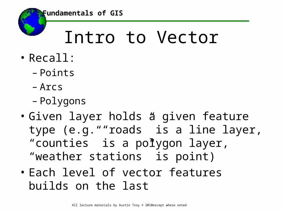
Intro to Vector• Recall:

– Points– Arcs – Polygons

• Given layer holds a given feature type (e.g. “roads” is a line layer, “counties” is a polygon layer, “weather stations” is point)

• Each level of vector features builds on the last

Fundamentals of GIS

All lecture materials by Austin Troy © 2010except where noted

Point Feature• A point layer: a collection of records with (x,y) coordinates

Image modified from ESRI Arc Info electronic help

0 1 2 3 4 5 60

1

2

3

4

5

6

2,2

6,3

5,5

3,6

1

2

3

4

ID X,Y Coordinat

es1 2,2

2 3,6

3 5,5

4 6,3

…

10 4,1

4,110

Fundamentals of GIS

All lecture materials by Austin Troy © 2010except where noted

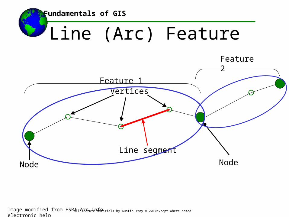
Intro to Vector• Each point has a unique location

• 2 points define a line segment

• One or several line segments define an arc

• The endpoints of an arc are “nodes

• The angle points are “vertices” (sing. Vertex)

• The feature is the arc, not the line

• Two arcs meet at the nodes

Fundamentals of GIS

All lecture materials by Austin Troy © 2010except where noted

Line (Arc) Feature

Image modified from ESRI Arc Info electronic help

Line segment

Node

Vertices

Node

Feature 1

Feature 2

Fundamentals of GIS

All lecture materials by Austin Troy © 2010except where noted

Line (Arc) Feature• Each point has a unique location

Fundamentals of GIS

All lecture materials by Austin Troy © 2010except where noted

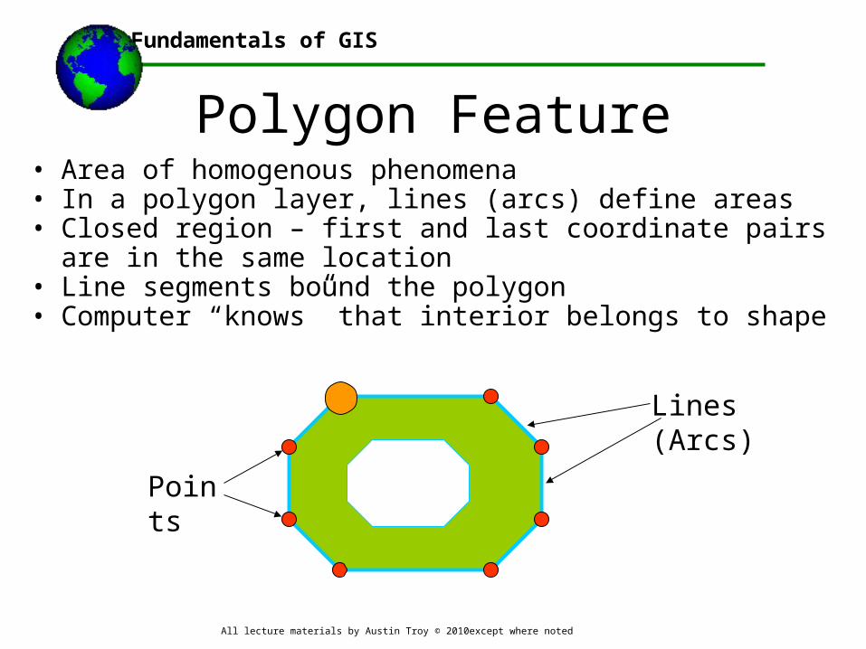
Polygon Feature• Area of homogenous phenomena • In a polygon layer, lines (arcs) define areas• Closed region – first and last coordinate pairs are in the same

location• Line segments bound the polygon• Computer “knows” that interior belongs to shape

Lines (Arcs)

Points

Fundamentals of GIS

All lecture materials by Austin Troy © 2010except where noted

Vector Representation:lines•Ring: this is a series of line segments (a string) that close upon each other

•NOT a polygon!!

Fundamentals of GIS

All lecture materials by Austin Troy © 2010except where noted

Definition1: Explicit encoding of spatial relationships between objects: the spatial location of each point, line and polygon is defined in relation to each other

Definition2: Topology is a collection of rules and relationships that enables the geodatabase to more accurately model geometric relationships found in the world.

Two major purposes:1. Allows for powerful spatial analysis 2. Quality control mechanism.

Vector: Topology

Fundamentals of GIS

All lecture materials by Austin Troy © 2010except where noted

• Arc-node and node topology : the way that line features connect to point features

• Polygon topology: the way that neighboring polygons connect and share borders

• Route topology: the way that a line feature of one type (e.g. commuter rail line) shares segments with line features of another type (e.g. Amtrack rail line)

• Regions topology: the way that polygons overlap (e.g. GIS layers with a time component) or when spatially separate polygons are part of the same feature

Types of Vector Topology

Fundamentals of GIS

All lecture materials by Austin Troy © 2010except where noted

• Ensuring data quality and “logical consistency”• Defining complex and nuanced spatial rules. • Single layer quality control:

– dangles – overshoots – polygons that don’t close – adjacent polygons that show up as not sharing a border

Quality control and topology

Fundamentals of GIS

All lecture materials by Austin Troy © 2010except where noted

Vector Topology helps deal with:

overshoots

slivers

dangles

Not sharing border

Fundamentals of GIS

All lecture materials by Austin Troy © 2010except where noted

• Mutli-Layer quality control: Defining spatial rules between layers

Quality control and topology

– Polygon rules: e.g. Must Be Covered by Feature Class of

•Define and validate topology rules in Arc Catalog and Arc Map (see http://webhelp.esri.com/arcgisdesktop/9.3/index.cfm?TopicName=Designing_a_geodatabase_topology )

– Line rules: e.g. Must not Self Intersect

– Point rules: e.g. Must be Properly Inside Polygons

Fundamentals of GIS

All lecture materials by Austin Troy © 2010except where noted

• Say we have the following layers: property lots, sidewalk, building footprints, zoning map

• We can specify topological rules, like:– Lots must be enclosed polygons– Buildings must be entirely within a lot– Sidewalks must be outside a lot polygon– Lots must fall entirely within a single zone– Lots must either share a border with another lot or with city

land, including streets and sidewalks.– In a low-density zone, no more than 20 lots can be touching

• We can’t do this yet, but will be able to shortly

Topology rules: Example

Fundamentals of GIS

All lecture materials by Austin Troy © 2010except where noted

Vector Topology TableConsists of four elements

1. Polygon topology table• Lists arcs/links comprising polygon

2. Node topology table• Lists links/arcs that meet at each node

3. Arc, or “link” topology table• Lists the nodes on which each link/arc ends and

polygons to right and left of each link/arc, based on start and finish nodes

4. Table with real world coordinates for each point

Fundamentals of GIS

All lecture materials by Austin Troy © 2010except where noted

Vector Topology Table

Graphical display of arcs, nodes, vertices and lines

Topology table for the ARCs making up the polygons

A table of the polygon topology

Fundamentals of GIS

All lecture materials by Austin Troy © 2010except where noted

Spaghetti Data Model•Non-topological data model that looks like vector•collections of line segments and points with no real connection or topology•No relative relationships encoded in this model •Each feature “unaware” of other features that it intersects, is adjacent to, contiguous with or near

Fundamentals of GIS

All lecture materials by Austin Troy © 2010except where noted

Vector Map representation and Scale

• Scale is the ratio of the map distance to the ground distance• Hence, 1:200,000 means 1 cm on the map = 200,000 cm in

the real world• The smaller the ratio, the LARGER the scale and the

smaller the area depicted• That area is known as the map extent.• Use of points and lines vs polygons depends on scale • USGS has rules about representation and scale: for

instance, on 1:24,000 topo maps, they use lines to represent streams less than 40 feet wide and double lines (areas) to represent larger watercourses.

Fundamentals of GIS

All lecture materials by Austin Troy © 2010except where noted

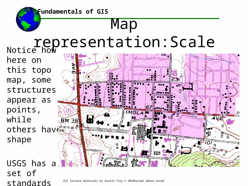
Map representation:ScaleNotice how here on this topo map, some structures appear as points, while others have shape

USGS has a set of standards for representation based on scale

Fundamentals of GIS

All lecture materials by Austin Troy © 2010except where noted

2. Multi-layer vector queries in Arc GIS

Fundamentals of GIS

All lecture materials by Austin Troy © 2010except where noted

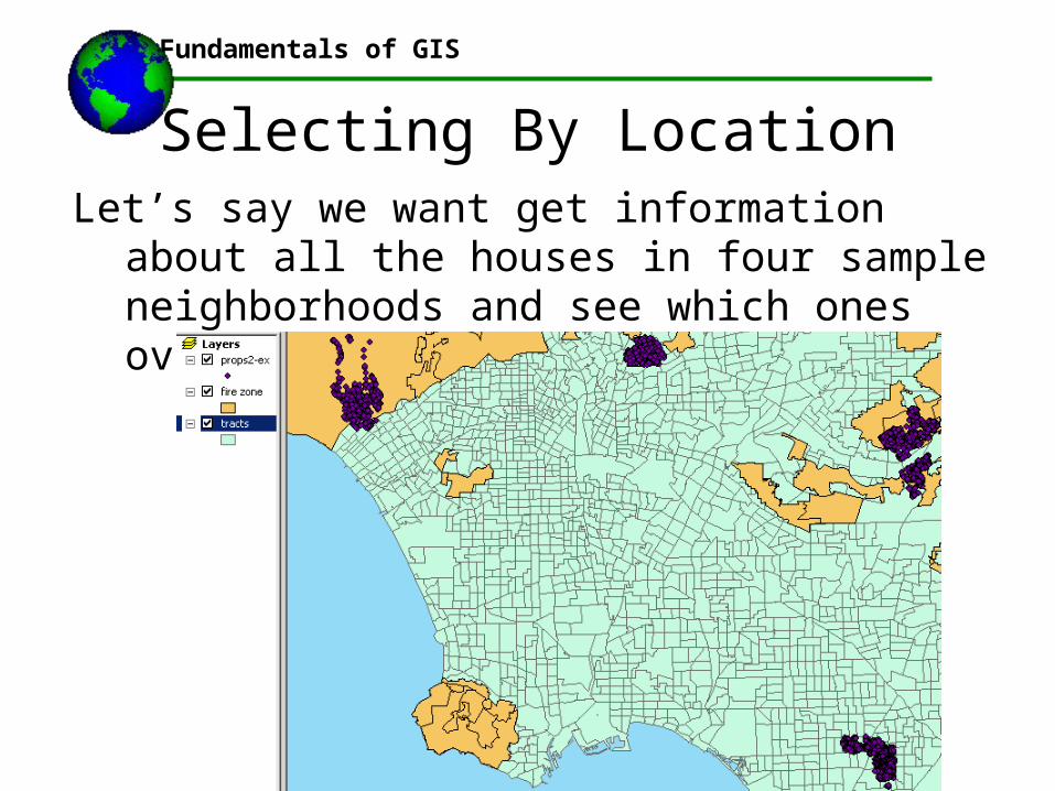
Let’s say we want get information about all the houses in four sample neighborhoods and see which ones overlay fire hazard zones

Selecting By Location

Fundamentals of GIS

All lecture materials by Austin Troy © 2010except where noted

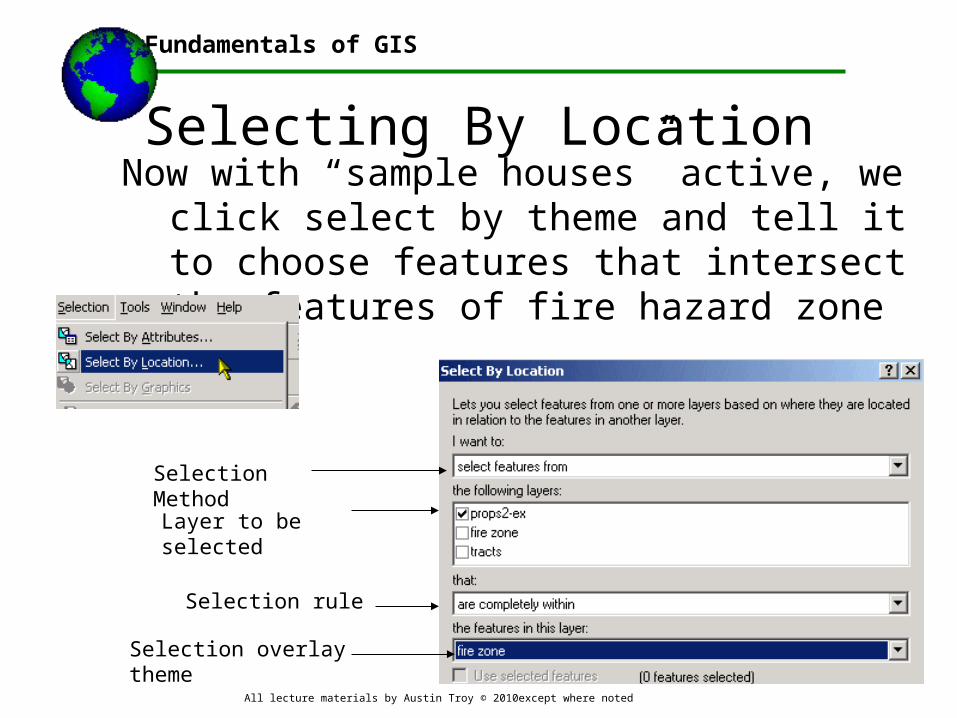
Now with “sample houses” active, we click select by theme and tell it to choose features that intersect the features of fire hazard zone

Layer to be selected

Selection Method

Selection rule

Selection overlay theme

Selecting By Location

Fundamentals of GIS

All lecture materials by Austin Troy © 2010except where noted

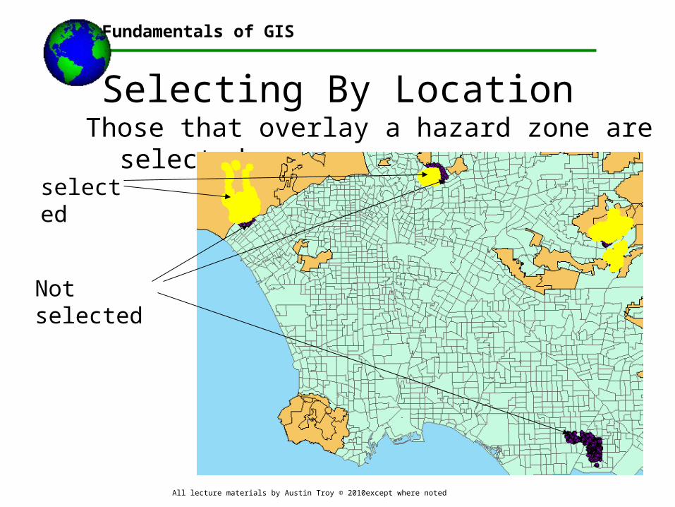
Those that overlay a hazard zone are selected

selected

Not selected

Selecting By Location

Fundamentals of GIS

All lecture materials by Austin Troy © 2010except where noted

…Zooming in to one of those neighborhoods

Selecting By Location

Fundamentals of GIS

All lecture materials by Austin Troy © 2010except where noted

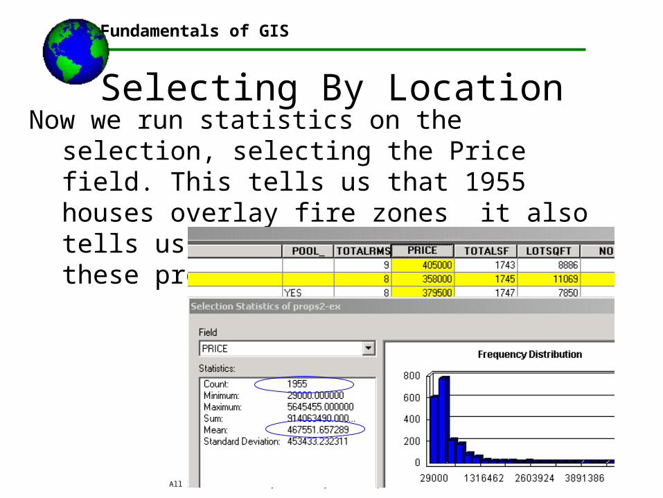
Now we run statistics on the selection, selecting the Price field. This tells us that 1955 houses overlay fire zones it also tells us that the mean price for these properties is $467,551!

Selecting By Location

Fundamentals of GIS

All lecture materials by Austin Troy © 2010except where noted

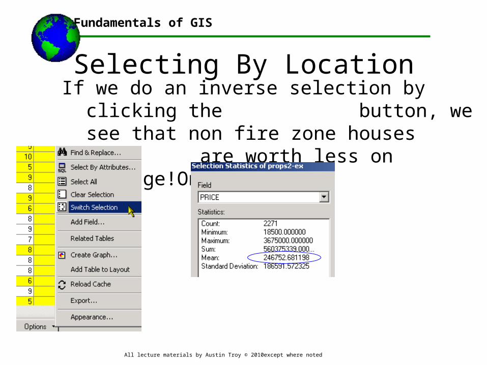
If we do an inverse selection by clicking the button, we see that non fire zone houses are worth less on average!Only $246,752

Selecting By Location

Fundamentals of GIS

All lecture materials by Austin Troy © 2010except where noted

Now, say we want to select features from layer A that are within a distance of features in layer B. In this case we’ll select houses in our sample neighborhoods that are within 1 mile of a Starbucks

Selecting By Location:Distance

Fundamentals of GIS

All lecture materials by Austin Troy © 2010except where noted

This time we use a different selection method with different parameters

Selecting By Location :Distance

Note how we can specify the distance for selection

Fundamentals of GIS

All lecture materials by Austin Troy © 2010except where noted

Results in the following selectionSelecting By Location :Distance

Fundamentals of GIS

All lecture materials by Austin Troy © 2010except where noted

Zooming into a neighborhood…Selecting By Location :Distance

Fundamentals of GIS

All lecture materials by Austin Troy © 2010except where noted

Now if we run statistics on price again…Selecting By Location :Distance

Those within a mile of a Starbucks have a mean value of $504,972

Those not within a mile of a Starbucks have a mean value of $273,866!

By the way, these are real data, I’m not making this up!!

Fundamentals of GIS

All lecture materials by Austin Troy © 2010except where noted

For that same selection we could get statistics on a different variable—here we’ll look at lot size

Selecting By Location :Distance

Those within a mile of a Starbucks have a mean size of 8776 square feet

Those not within a mile of a Starbucks have a mean lot size of 10,024 sq feet. Why might that be?

Fundamentals of GIS

All lecture materials by Austin Troy © 2010except where noted

You can also select features in a layer by distance to a linear feature in another layer. Here we’ll find houses in a neighborhood within a mile of a highway

Selecting By Location :Distance

Note that these smaller roads are in a different layer

Fundamentals of GIS

All lecture materials by Austin Troy © 2010except where noted

What if we just want to select those points that are within a distance one just one given feature within a layer?

Here we’ll find all homes within 500 meters of Valley Blvd. (let’s say there’s going to be a parade and the city needs to inform all those homeowners near that street).

First we must do a single layer query asking for Hwyname = “Valley Blvd”

Selecting By Location :Distance

Fundamentals of GIS

All lecture materials by Austin Troy © 2010except where noted

Once that feature is selected we can do a “select by location” operation

Selecting By Location :Distance

Notice that this time we check “Use selected features”

Fundamentals of GIS

All lecture materials by Austin Troy © 2010except where noted

Thus we end up only selecting those houses within 500 m of Valley Blvd, and none within 500 m of other roads

Selecting By Location :Distance

Fundamentals of GIS

All lecture materials by Austin Troy © 2010except where noted

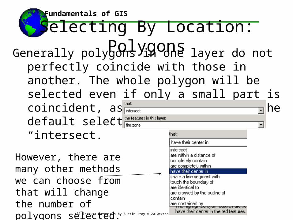
Generally polygons in one layer do not perfectly coincide with those in another. The whole polygon will be selected even if only a small part is coincident, assuming we are using the default selection overlay method, “intersect.”

Selecting By Location: Polygons

However, there are many other methods we can choose from that will change the number of polygons selected.

Fundamentals of GIS

All lecture materials by Austin Troy © 2010except where noted

Example: let’s select any census tract that intersects even slightly with a fire zone; here’s the pre-selection map

Selecting By Location: Polygons

Fundamentals of GIS

All lecture materials by Austin Troy © 2010except where noted

Using the “intersect” overlay method we get thisSelecting By Location: Polygons

Fundamentals of GIS

All lecture materials by Austin Troy © 2010except where noted

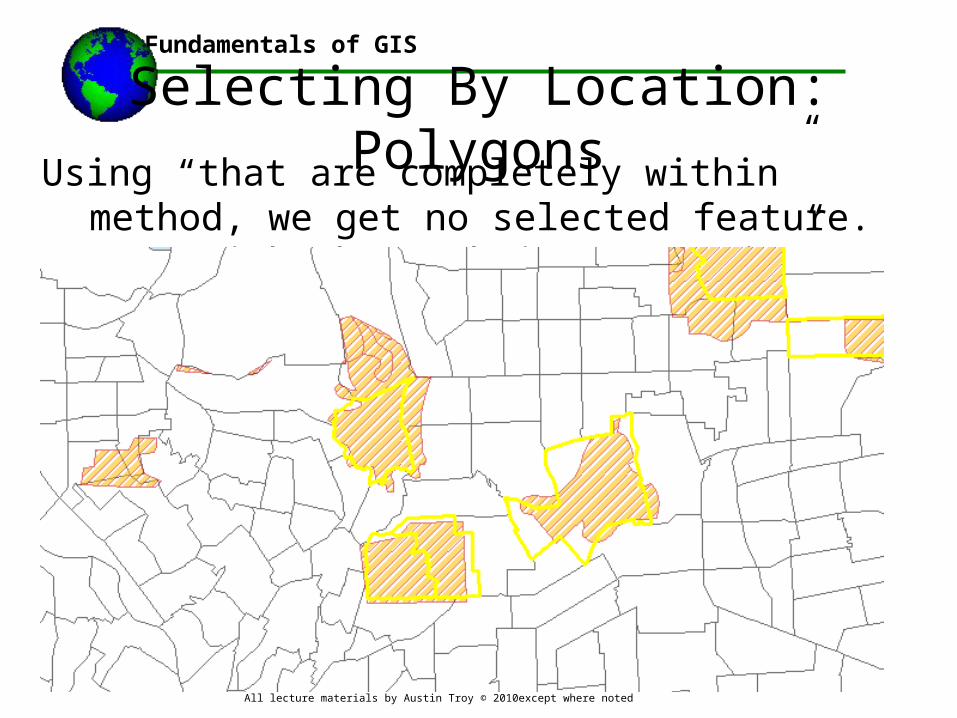
Using “that are completely within” method, we get no selected feature. But, with “have their center in” we get

Selecting By Location: Polygons

Fundamentals of GIS

All lecture materials by Austin Troy © 2010except where noted

Likewise, if we select Merced County in the counties layer, activate “highways” in the TOC, and then select by theme, we will only choose those road segments that intersect that county

Selecting By Location on Selections

Fundamentals of GIS

All lecture materials by Austin Troy © 2010except where noted

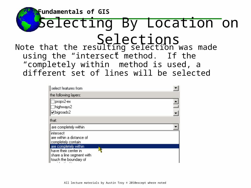
Note that the resulting selection was made using the “intersect method.” If the “completely within” method is used, a different set of lines will be selected

Selecting By Location on Selections

Fundamentals of GIS

All lecture materials by Austin Troy © 2010except where noted

Note that the resulting selection was made using the “intersect method.” If the “completely within” method is used, a different set of lines will be selected, similar to what we saw in the fire zone-census tract example given previously. Line segments that cross over into next county will not be included

Selecting By Location on Selections

Fundamentals of GIS

All lecture materials by Austin Troy © 2010except where noted

Once a selection has been done using “select by location” you can do all the same things you would do with a normal single-layer selection:– Make a new layer from the selection

– Do statistics on it

– Make a new field in that layer

– Calculate or recalculate a field for a selection

What can be done with multi-layer selections?

Fundamentals of GIS

All lecture materials by Austin Troy © 2010except where noted

3. Vector Spatial Joining —assigning attributes by location

Fundamentals of GIS

All lecture materials by Austin Troy © 2010except where noted

Spatial Join

• Assigns attribute data from features in one layer to spatially coincident features in another

• Can assign polygon data to a point that overlays• Can assign point to point and point to line

distances between two layers• Simply adds attributes to

the DBF table

Fundamentals of GIS

All lecture materials by Austin Troy © 2010except where noted

Spatial Join• We access Spatial Join by right clicking on the

“to” layer and clicking Joins and Relates>>join

• We then specify that we want to join by location and choose which layer we are joining from

Fundamentals of GIS

All lecture materials by Austin Troy © 2010except where noted

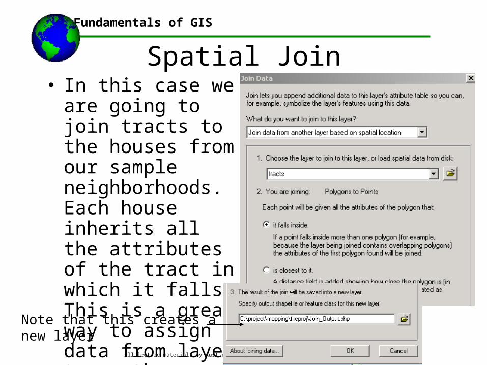
Spatial Join• In this case we are

going to join tracts to the houses from our sample neighborhoods. Each house inherits all the attributes of the tract in which it falls. This is a great way to assign data from layer to another

Note that this creates a new layer

Fundamentals of GIS

All lecture materials by Austin Troy © 2010except where noted

Spatial Join• We can now plot out houses by any of the attributes

that were in the tracts database. Here’s a plot of houses graduated by percent unemployment of the tract to which they belong

Fundamentals of GIS

All lecture materials by Austin Troy © 2010except where noted

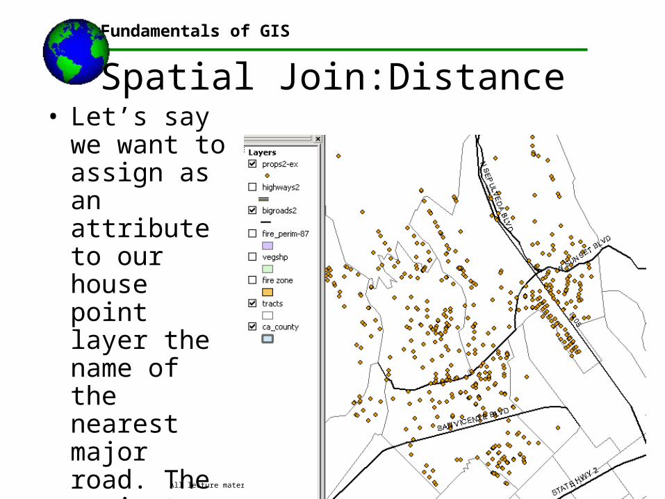
Spatial Join:Distance• We can also do spatial joins based on distance.

Whenever we join a point or line layer to another point or line layer, for each feature in the TO layer it gives us the attributes of the nearest feature in the FROM layer PLUS the distance between those features in whatever map units we specify

Fundamentals of GIS

All lecture materials by Austin Troy © 2010except where noted

Spatial Join:Distance• Let’s say we

want to assign as an attribute to our house point layer the name of the nearest major road. The easiest way to do this is with a spatial join.

Fundamentals of GIS

All lecture materials by Austin Troy © 2010except where noted

Spatial Join:Distance

Introduction to GIS

• Here I have two options: I can either choose to numerically summarize for each point the values of the lines intersecting it, or I can simply assign all attributes from the nearest line. Here we choose the latter My FROM layer

Fundamentals of GIS

All lecture materials by Austin Troy © 2010except where noted

Spatial Join:Distance• Now name of

nearest highway is an attribute for each housing point; here I’m plotting out categorically by that attribute after joining

Fundamentals of GIS

All lecture materials by Austin Troy © 2010except where noted

Spatial Join:Distance• Distance from

each point to the nearest road feature was also recorded under the attribute “Distance.” Here I’m plotting out distance to nearest major road.

Fundamentals of GIS

All lecture materials by Austin Troy © 2010except where noted

Spatial Join:Distance• We can also do

a join to get the distance from a series of points in one layer to a series of points in another: here is distance of houses to nearest Starbucks

Fundamentals of GIS

All lecture materials by Austin Troy © 2010except where noted

Spatial Join:Polygons• Spatial Join is quite intuitive when it comes to

assigning attributes to points and lines, but what about when assigning attributes to polygons? Problem: a polygon is layer A may overlay several polygons in layer B, so whose attributes to you give it?

Layer A

Layer B

Fundamentals of GIS

All lecture materials by Austin Troy © 2010except where noted

Spatial Join:Polygons• Answer: we can do spatial join and summarize (by

average, for instance) each polygon in layer A the values of all the overlapping polygons in layer B.

• Example: Say we have a census tract layer with all sorts of demographic info (population, race, etc) and we have a zip code layer with no demographic info attached to it. Our client is doing a marketing study and needs to have a map showing median age and percent Hispanic by zip code. We have both these attributes in our tract map and need to somehow “transfer” them to the zip code map

Fundamentals of GIS

All lecture materials by Austin Troy © 2010except where noted

Spatial Join:Polygons• Unfortunately, the tract boundaries and zip code

boundaries do not match up in the slightest. Note that tracts are not nested within zip codes—they cut across

Fundamentals of GIS

All lecture materials by Austin Troy © 2010except where noted

Spatial Join:Polygons• To deal with this we do a

spatial join of two polygon layers and choose the “summarize” option (the first radio button). This allows us to choose a statistic by which to summarize the value of all the constituent tract polygons for each zip code polygon. In this case we’ll choose “average” as our statistics

Fundamentals of GIS

All lecture materials by Austin Troy © 2010except where noted

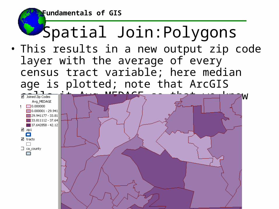
Spatial Join:Polygons• This results in a new output zip code layer with the

average of every census tract variable; here median age is plotted; note that ArcGIS calls it Avg_MEDAGE so that we know what statistic this is based on

Fundamentals of GIS

All lecture materials by Austin Troy © 2010except where noted

3. Vector Geoprocessing

Fundamentals of GIS

All lecture materials by Austin Troy © 2010except where noted

Purpose of Geoprocessing• Tools for breaking down the size of map

features: – Union, Intersect, Clip

• Tools for increasing the size of map features:– dissolve and merge (indirectly)

• Arc/Info and Arc Toolbox include various other geoprocessing overlay operations, such as Update and Dissolve Regions

• Found in Arc Toolbox

Fundamentals of GIS

All lecture materials by Austin Troy © 2010except where noted

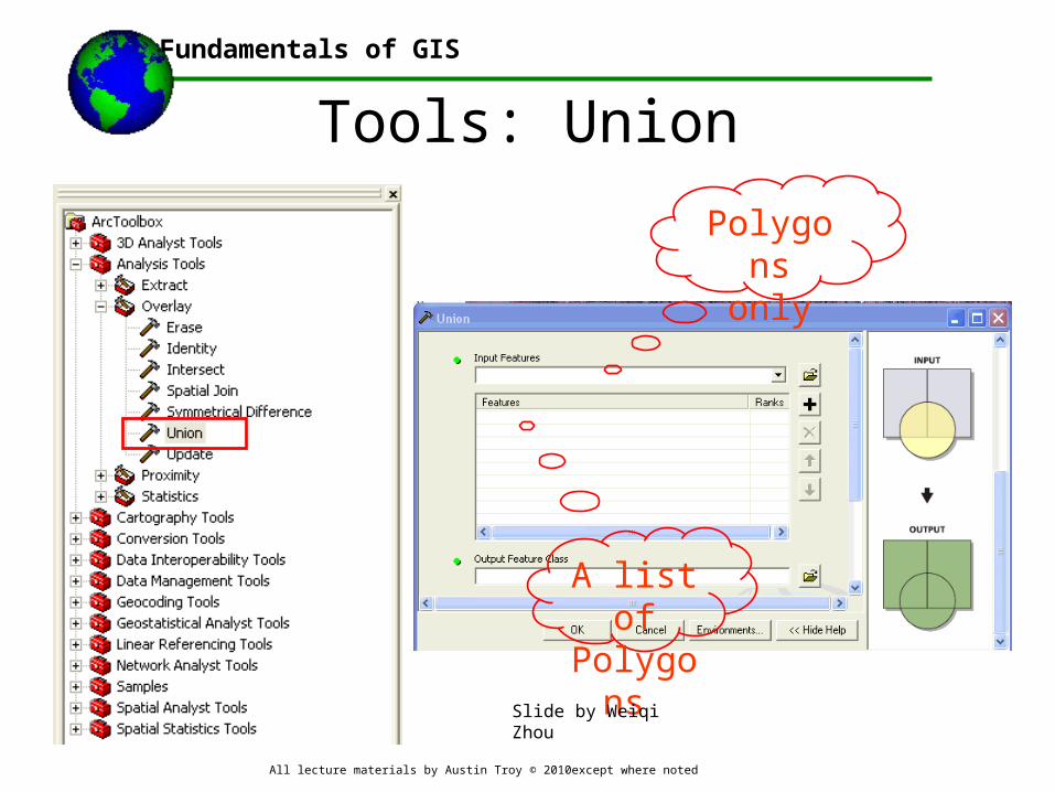
Union• Combines features of two theme• Each theme is treated the same• Goes to extent of largest theme• Keeps all line work, creates new polygons• Breaks down features into smaller minimum mapping units• Can use selected features option too• Keeps all attributes

Image source: ESRI Arc Info electronic help

Fundamentals of GIS

All lecture materials by Austin Troy © 2010except where noted

Tools: Union

Polygons only

A list of Polygon

s Slide by Weiqi Zhou

Fundamentals of GIS

All lecture materials by Austin Troy © 2010except where noted

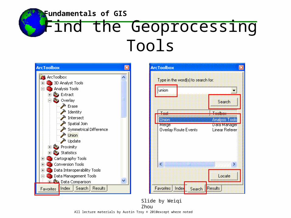
Find the Geoprocessing Tools

Slide by Weiqi Zhou

Fundamentals of GIS

All lecture materials by Austin Troy © 2010except where noted

Intersect• Yields polygons representing areas that are common

to both layers• Preserves line work within common extent • Usually creates many new, smaller polygons• Preserves all attributes from both

Fundamentals of GIS

All lecture materials by Austin Troy © 2010except where noted

Union vs. Intersection• Union is the entirety of two overlapping sets of

features and intersection is the common area only• Continuous and exhaustive vs. “island” polygons

have different ramifications for these tools

Layer 1 + Layer 2

Intersect:

Layer 1 + Layer 2

Union:

“1 AND 2”

“1 OR 2”

Fundamentals of GIS

All lecture materials by Austin Troy © 2010except where noted

Union vs. Intersection: Example• Here’s an example. Say we have deer wintering areas

in one layer and conserved lands in another.

Fundamentals of GIS

All lecture materials by Austin Troy © 2010except where noted

Union vs. Intersection: Example• Union gives us land that is EITHER conserved OR

that is a deer wintering areas

Fundamentals of GIS

All lecture materials by Austin Troy © 2010except where noted

Union vs. Intersection: Example• Intersect gives us land that is BOTH, and preserves

all polygon boundaries within that common extent

Fundamentals of GIS

All lecture materials by Austin Troy © 2010except where noted

Tools: ClipPoint, line,

polygon

Polygon

Fundamentals of GIS

All lecture materials by Austin Troy © 2010except where noted

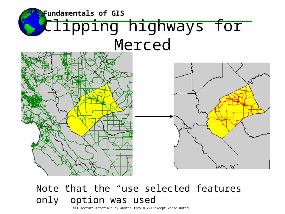
Clipping highways for Merced

Note that the “use selected features only” option was used

Fundamentals of GIS

All lecture materials by Austin Troy © 2010except where noted

Tools: Dissolve

Fundamentals of GIS

All lecture materials by Austin Troy © 2010except where noted

Dissolve: Example• Dissolve zip codes (small) into counties (large)

Fundamentals of GIS

All lecture materials by Austin Troy © 2010except where noted

Dissolve: Example• Choose the dissolve field: e.g. Dissolve based on the

County field

Fundamentals of GIS

All lecture materials by Austin Troy © 2010except where noted

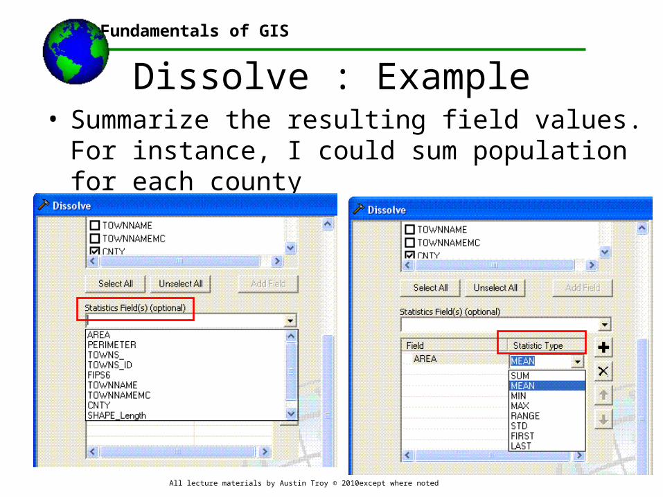
Dissolve : Example• Summarize the resulting field values. For instance, I

could sum population for each county

Fundamentals of GIS

All lecture materials by Austin Troy © 2010except where noted

Dissolve : Example

• Now we have created a county map, and for each county we have an attribute as the sum of population of the constituent zip codes

Fundamentals of GIS

All lecture materials by Austin Troy © 2010except where noted

Merge• Allows you to “join” two adjacent or non-

adjacent themes into the same layer

• Like “tiling”

• Best when attributes match

Fundamentals of GIS

All lecture materials by Austin Troy © 2010except where noted

Merge• Often when you merge you will want to follow up

by dissolving.• This is because artificial polygon boundaries were

created at the borders by the act of splitting the data up into tiles; merging brings the tiles back together and dissolving joins together polygons that were split up in the process

Fundamentals of GIS

All lecture materials by Austin Troy © 2010except where noted

Tools: BufferingBuffering is when you draw a polygon around a feature

(point, line or polygon); Here we’re buffering a stream

Fundamentals of GIS

All lecture materials by Austin Troy © 2010except where noted

Tools: Buffering

Based on

distance

Based on attribute

Fundamentals of GIS

All lecture materials by Austin Troy © 2010except where noted

Tools:Variable Width BufferingWhere width of

buffer varies with an attribute

Often we must recalculate that attribute to make the buffer width meaningful

Example from lab: a buffer based on traffic volume

Fundamentals of GIS

All lecture materials by Austin Troy © 2010except where noted

Geoprocessing vs. select by location • By building a buffer of a given distance around a

feature, we can then do overlay analysis and select features from another layer that are inside or that intersect the buffer

• With select by location, we can only do 2 layers at a time. When we combine buffering with geoprocessing, we can ask questions across unlimited numbers of layers.

• With select by location, have the problem of features with partial overlap; in geoprocessing, combine the two layers to create smallest necessary minimum mapping unit

Fundamentals of GIS

All lecture materials by Austin Troy © 2010except where noted

Combining Buffering and Geoprocessing: Example

• From Lab 4: say we made fixed buffers around deer wintering areas and water bodies, and a variable buffer

around roads, based on traffic:

(note the lab is a bit

different):

Fundamentals of GIS

All lecture materials by Austin Troy © 2010except where noted

Combining Buffering and Geoprocessing: Example

• Then we could, for instance, find areas that are near deer wintering areas and water bodies but far from traffic:

• First we would intersect the deer wintering and water body buffers, yielding areas that are near both those.

• Then we would union the result with the traffic buffer and run an attribute query to determine which areas meet the criteria

Fundamentals of GIS

All lecture materials by Austin Troy © 2010except where noted

Combining Buffering and Geoprocessing: Example

• The intersection of deer wintering buffers and water buffers would be the area in the red

Fundamentals of GIS

All lecture materials by Austin Troy © 2010except where noted

Combining Buffering and Geoprocessing: Example

• The union of that intersection with the traffic buffer:

Fundamentals of GIS

All lecture materials by Austin Troy © 2010except where noted

Combining Buffering and Geoprocessing: Example

• Now we can query for polygons that were created from the intersection (met the two good criteria) and for areas that are not within a traffic buffer

Fundamentals of GIS

All lecture materials by Austin Troy © 2010except where noted

Combining Buffering and Geoprocessing: Example

• We can then create a layer from that—Note that we have created entirely new polygon boundaries and geometry by cutting and splicing these buffers together.

Fundamentals of GIS

All lecture materials by Austin Troy © 2010except where noted

Combining Geoprocessing Tools • Involve multiple tasks performed in sequence, such as

those that clip, buffering, intersect, union, then select datasets.

–Step by step

–Create and run a script

–Build and run a model: Arc Model Builder

Fundamentals of GIS

All lecture materials by Austin Troy © 2010except where noted

Model Builder