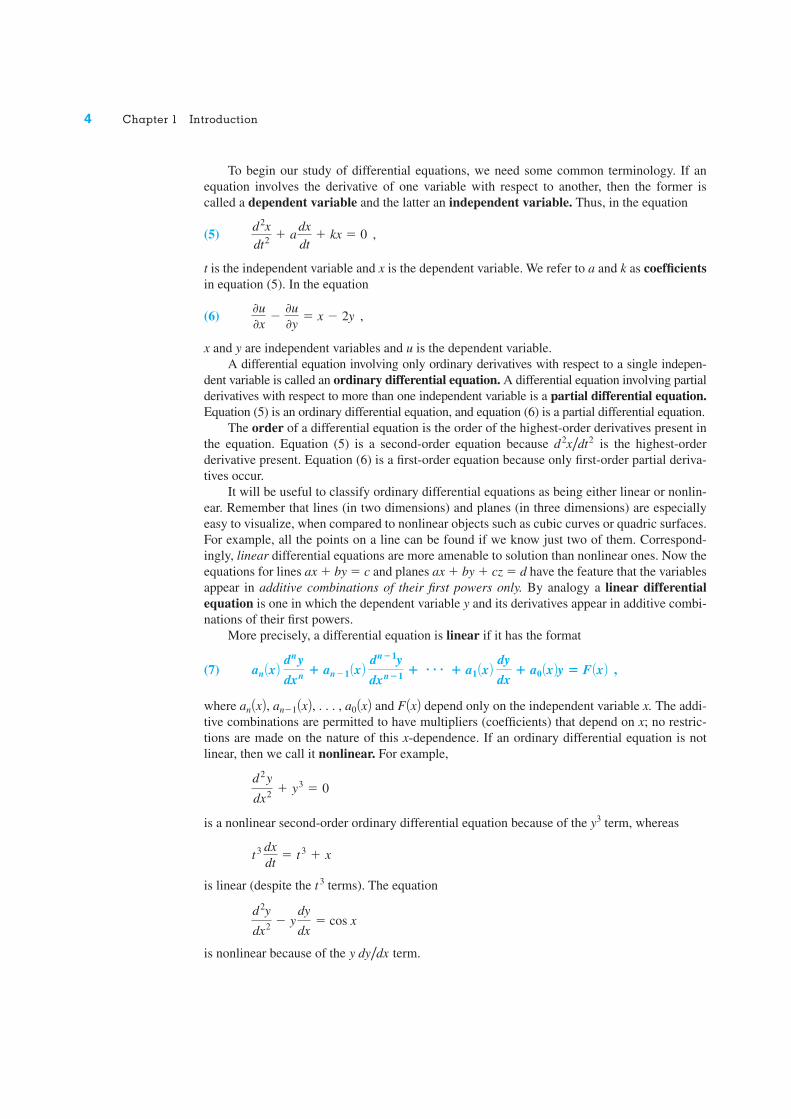
1 In the sciences and engineering, mathematical models are developed to aid in the understanding of physical phenomena. These models often yield an equation that contains some derivatives of an unknown function. Such an equation is called a differential equation. Two examples of models developed in calculus are the free fall of a body and the decay of a radioactive substance. In the case of free fall, an object is released from a certain height above the ground and falls under the force of gravity. † Newton’s second law, which states that an object’s mass times its acceleration equals the total force acting on it, can be applied to the falling object. This leads to the equation (see Figure 1.1) where m is the mass of the object, h is the height above the ground, is its acceleration, g is the (constant) gravitational acceleration, and mg is the force due to gravity. This is a differ- ential equation containing the second derivative of the unknown height h as a function of time. Fortunately, the above equation is easy to solve for h. All we have to do is divide by m and integrate twice with respect to t. That is, so and h h A t B gt 2 2 c 1 t c 2 . dh dt gt c 1 d 2 h dt 2 g , d 2 h / dt 2 m d 2 h dt 2 mg , Introduction CHAPTER 1 BACKGROUND 1.1 † We are assuming here that gravity is the only force acting on the object and that this force is constant. More general models would take into account other forces, such as air resistance. h −mg Figure 1.1 Apple in free fall

Welcome message from author
This document is posted to help you gain knowledge. Please leave a comment to let me know what you think about it! Share it to your friends and learn new things together.
Transcript

1
In the sciences and engineering, mathematical models are developed to aid in the understandingof physical phenomena. These models often yield an equation that contains some derivativesof an unknown function. Such an equation is called a differential equation. Two examples ofmodels developed in calculus are the free fall of a body and the decay of a radioactive substance.
In the case of free fall, an object is released from a certain height above the ground andfalls under the force of gravity.† Newton’s second law, which states that an object’s mass timesits acceleration equals the total force acting on it, can be applied to the falling object. Thisleads to the equation (see Figure 1.1)
where m is the mass of the object, h is the height above the ground, is its acceleration,g is the (constant) gravitational acceleration, and �mg is the force due to gravity. This is a differ-ential equation containing the second derivative of the unknown height h as a function of time.
Fortunately, the above equation is easy to solve for h. All we have to do is divide by m andintegrate twice with respect to t. That is,
so
and
h � h AtB ��gt2
2� c1t � c2 .
dhdt
� �gt � c1
d2hdt2 � �g ,
d2h/dt2
md2hdt2 � �mg ,
Introduction
CHAPTER 1
BACKGROUND1.1
†We are assuming here that gravity is the only force acting on the object and that this force is constant. More generalmodels would take into account other forces, such as air resistance.
h−mg
Figure 1.1 Apple in free fall

2 Chapter 1 Introduction
We will see that the constants of integration, c1 and c2, are determined if we know the initialheight and the initial velocity of the object. We then have a formula for the height of the objectat time t.
In the case of radioactive decay (Figure 1.2), we begin from the premise that the rate ofdecay is proportional to the amount of radioactive substance present. This leads to the equation
k � 0
where is the unknown amount of radioactive substance present at time t and k is the pro-portionality constant. To solve this differential equation, we rewrite it in the form
and integrate to obtain
Solving for A yields
A � � eln A � e�kt � Ce�kt
where C is the combination of integration constants . The value of C, as we will seelater, is determined if the initial amount of radioactive substance is given. We then have a for-mula for the amount of radioactive substance at any future time t.
Even though the above examples were easily solved by methods learned in calculus, they dogive us some insight into the study of differential equations in general. First, notice that the solu-tion of a differential equation is a function, like h or A , not merely a number. Second, inte-gration† is an important tool in solving differential equations (not surprisingly!). Third, we cannotexpect to get a unique solution to a differential equation, since there will be arbitrary “constantsof integration.” The second derivative in the free-fall equation gave rise to two constants,c1 and c2, and the first derivative in the decay equation gave rise, ultimately, to one constant, C.
Whenever a mathematical model involves the rate of change of one variable with respectto another, a differential equation is apt to appear. Unfortunately, in contrast to the examplesfor free fall and radioactive decay, the differential equation may be very complicated and diffi-cult to analyze.
d2h/dt2
AtBAtB
eC2�C1
,eC2�C1A AtB
ln A � C1 � �kt � C2 .
� 1A
dA � � �k dt
1A
dA � �k dt
A A�0B
,dAdt
� �kA ,
A
Figure 1.2 Radioactive decay
†For a review of integration techniques, see Appendix A.

Section 1.1 Background 3
Differential equations arise in a variety of subject areas, including not only the physical sci-ences but also such diverse fields as economics, medicine, psychology, and operations research.We now list a few specific examples.
1. In banking practice, if P is the number of dollars in a savings bank account thatpays a yearly interest rate of r% compounded continuously, then P satisfies the dif-ferential equation
(1)
2. A classic application of differential equations is found in the study of an electric cir-cuit consisting of a resistor, an inductor, and a capacitor driven by an electromotiveforce (see Figure 1.3). Here an application of Kirchhoff’s laws† leads to the equation
(2)
where L is the inductance, R is the resistance, C is the capacitance, E is the electro-motive force, q is the charge on the capacitor, and t is the time.
3. In psychology, one model of the learning of a task involves the equation
(3)
Here the variable y represents the learner’s skill level as a function of time t. Theconstants p and n depend on the individual learner and the nature of the task.
4. In the study of vibrating strings and the propagation of waves, we find the partialdifferential equation
(4) ††
where t represents time, x the location along the string, c the wave speed, and u thedisplacement of the string, which is a function of time and location.
02u0t2 � c2
02u0x2 � 0 ,
dy/dt
y3/2 A1 � yB3/2�
2p
1n .
AtBAtB
L
d2q
dt2 � R
dq
dt�
1
C q � E AtB ,
dPdt
�r
100 P , t in years.
AtB
†We will discuss Kirchhoff’s laws in Section 3.5.††Historical Footnote: This partial differential equation was first discovered by Jean le Rond d’Alembert (1717–1783)in 1747.
Figure 1.3 Schematic for a series RLC circuit
C
R L
emf
+
−
4 Chapter 1 Introduction
To begin our study of differential equations, we need some common terminology. If anequation involves the derivative of one variable with respect to another, then the former iscalled a dependent variable and the latter an independent variable. Thus, in the equation
(5)
t is the independent variable and x is the dependent variable. We refer to a and k as coefficientsin equation (5). In the equation
(6)
x and y are independent variables and u is the dependent variable.A differential equation involving only ordinary derivatives with respect to a single indepen-
dent variable is called an ordinary differential equation. A differential equation involving partialderivatives with respect to more than one independent variable is a partial differential equation.Equation (5) is an ordinary differential equation, and equation (6) is a partial differential equation.
The order of a differential equation is the order of the highest-order derivatives present inthe equation. Equation (5) is a second-order equation because is the highest-orderderivative present. Equation (6) is a first-order equation because only first-order partial deriva-tives occur.
It will be useful to classify ordinary differential equations as being either linear or nonlin-ear. Remember that lines (in two dimensions) and planes (in three dimensions) are especiallyeasy to visualize, when compared to nonlinear objects such as cubic curves or quadric surfaces.For example, all the points on a line can be found if we know just two of them. Correspond-ingly, linear differential equations are more amenable to solution than nonlinear ones. Now theequations for lines ax � by � c and planes ax � by � cz � d have the feature that the variablesappear in additive combinations of their first powers only. By analogy a linear differentialequation is one in which the dependent variable y and its derivatives appear in additive combi-nations of their first powers.
More precisely, a differential equation is linear if it has the format
(7)
where an , an�1 , . . . , a0 and F depend only on the independent variable x. The addi-tive combinations are permitted to have multipliers (coefficients) that depend on x; no restric-tions are made on the nature of this x-dependence. If an ordinary differential equation is notlinear, then we call it nonlinear. For example,
is a nonlinear second-order ordinary differential equation because of the y3 term, whereas
is linear (despite the t3 terms). The equation
� cos x
is nonlinear because of the term.y dy/dx
d2y
dx2 � y
dy
dx
t3 dxdt
� t3 � x
d2y
dx2 � y3 � 0
AxBAxBAxBAxBan AxB dny
dxn � an�1 AxB dn�1y
dxn�1 � p � a1 AxB dy
dx� a0 AxBy � F AxB ,
d2x/dt2
0u0x �
0u0y � x � 2y ,
d2xdt2 � a
dxdt
� kx � 0 ,

Section 1.1 Background 5
5
In Problems 1–12, a differential equation is given alongwith the field or problem area in which it arises. Classifyeach as an ordinary differential equation (ODE) or apartial differential equation (PDE), give the order, andindicate the independent and dependent variables. If theequation is an ordinary differential equation, indicatewhether the equation is linear or nonlinear.
1.
(Hermite’s equation, quantum-mechanical harmonicoscillator)
2. � 9x � 2 cos 3t
(mechanical vibrations, electrical circuits, seismology)
3.
(Laplace’s equation, potential theory, electricity, heat,aerodynamics)
4.
(competition between two species, ecology)
5. , where k is a constant
(chemical reaction rates)
6. , where C is a constant
(brachistochrone problem,† calculus of variations)
7.
(Kidder’s equation, flow of gases through a porousmedium)
11 � y d 2 y
dx2 � 2x
dy
dx� 0
y c1 � adydxb 2 d � C
dxdt
� k A4 � xB A1 � xB
dy
dx�
y A2 � 3xBx A1 � 3yB
02u0x2 �
02u0y2 � 0
5
d 2xdt2 � 4
dx
dt
d 2y
dx2 � 2x
dy
dx� 2y � 0
8. , where k and P are constants
(logistic curve, epidemiology, economics)
9.
(deflection of beams)
10.
(aerodynamics, stress analysis)
11. where k is a constant
(nuclear fission)
12.
(van der Pol’s equation, triode vacuum tube)
In Problems 13–16, write a differential equation that fitsthe physical description.
13. The rate of change of the population p of bacteria attime t is proportional to the population at time t.
14. The velocity at time t of a particle moving along astraight line is proportional to the fourth power of itsposition x.
15. The rate of change in the temperature T of coffee attime t is proportional to the difference between thetemperature M of the air at time t and the tempera-ture of the coffee at time t.
16. The rate of change of the mass A of salt at time t isproportional to the square of the mass of salt presentat time t.
17. Drag Race. Two drivers, Alison and Kevin, are par-ticipating in a drag race. Beginning from a standingstart, they each proceed with a constant acceleration.Alison covers the last of the distance in 3 sec-onds, whereas Kevin covers the last of the dis-tance in 4 seconds. Who wins and by how much time?
1/31/4
d2y
dx2 � 0.1 A1 � y2B dy
dx� 9y � 0
0N0t
�02N0r 2 �
1r 0N0r
� kN,
x
d2y
dx2 �dy
dx� xy � 0
8d4y
dx4 � x A1 � xB
dpdt
� kp AP � pB
Although the majority of equations one is likely to encounter in practice fall into the nonlin-ear category, knowing how to deal with the simpler linear equations is an important first step (justas tangent lines help our understanding of complicated curves by providing local approximations).
†Historical Footnote: In 1630 Galileo formulated the brachistochrone problem shortest, � time , that is, to determine apath down which a particle will fall from one given point to another in the shortest time. It was reproposed by John Bernoulli in 1696 and solved byhim the following year.
Bxrono�Abraxisto� �
1.1 EXERCISES
6 Chapter 1 Introduction
6
An nth-order ordinary differential equation is an equality relating the independent variable tothe nth derivative (and usually lower-order derivatives as well) of the dependent variable.Examples are
(second-order, x independent, y dependent)
(second-order, t independent, y dependent)
(fourth-order, t independent, x dependent).
Thus, a general form for an nth-order equation with x independent, y dependent, can beexpressed as
(1)
where F is a function that depends on x, y, and the derivatives of y up to order n; that is, on x,y, . . . , . We assume that the equation holds for all x in an open interval I (where a or b could be infinite). In many cases we can isolate the highest-order term and write equation (1) as
(2)
which is often preferable to (1) for theoretical and computational purposes.
dny
dxn � f ax, y, dy
dx, . . . ,
dn�1y
dxn�1b ,
dny/dxna 6 x 6 b,dny/dxn
Fax, y, dydx
, . . . , dnydxnb � 0 ,
d4xdt4 � xt
B1 � ad2y
dt2b � y � 0
x2
d2y
dx2 � x
dy
dx� y � x3
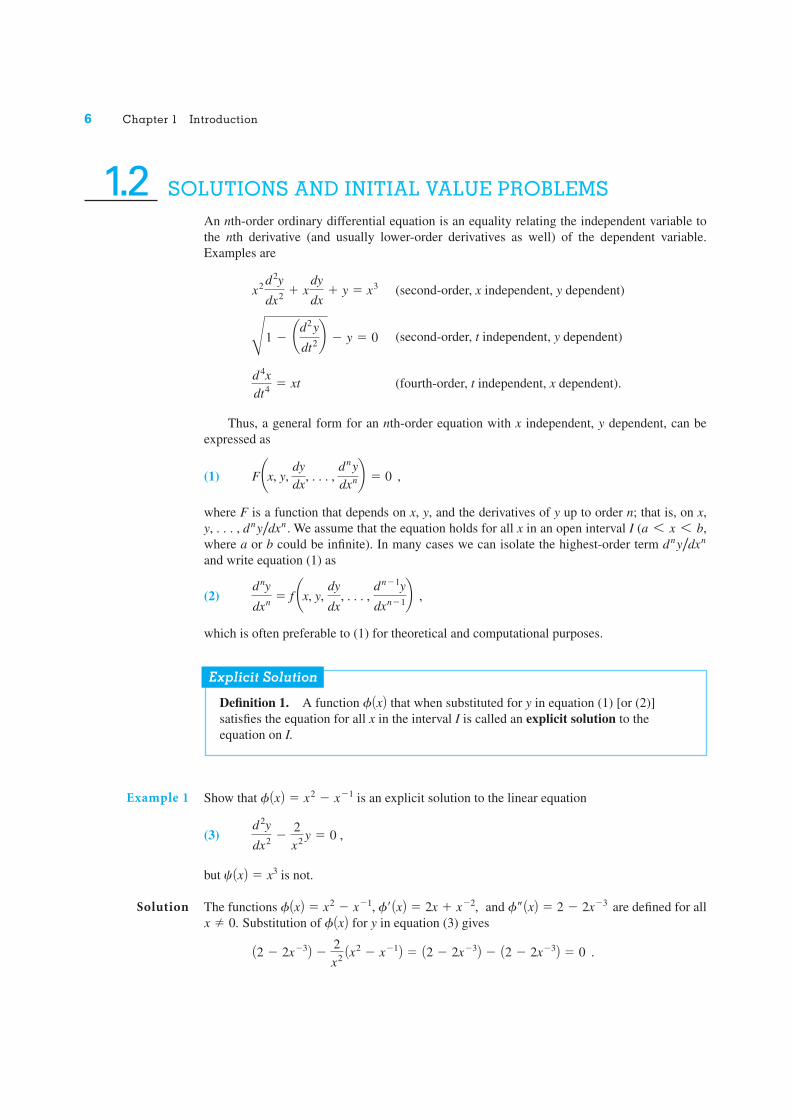
1.2 SOLUTIONS AND INITIAL VALUE PROBLEMS
Explicit Solution
Definition 1. A function that when substituted for y in equation (1) [or (2)]satisfies the equation for all x in the interval I is called an explicit solution to theequation on I.
f AxB
Show that is an explicit solution to the linear equation
(3)
but is not.
The functions and are defined for allSubstitution of for y in equation (3) gives
A2 � 2x�3B �2x2 Ax2 � x�1B � A2 � 2x�3B � A2 � 2x�3B � 0 .
f AxBx � 0.f– AxB � 2 � 2x�3f AxB � x2 � x�1, f¿ AxB � 2x � x�2,
c AxB � x3
d2y
dx2 �2x2 y � 0 ,
f AxB � x2 � x�1Example 1
Solution

Section 1.2 Solutions and Initial Value Problems 7
Since this is valid for any x 0, the function is an explicit solution to (3) onand also on .
For we have , , and substitution into (3) gives
which is valid only at the point and not on an interval. Hence is not a solution. ◆
Show that for any choice of the constants c1 and c2, the function
is an explicit solution to the linear equation
(4)
We compute and . Substitution of ,and for y, y , and y in equation (4) yields
�
Since equality holds for all x in , then is an explicit solution to(4) on the interval for any choice of the constants c1 and c2. ◆
As we will see in Chapter 2, the methods for solving differential equations do not alwaysyield an explicit solution for the equation. We may have to settle for a solution that is definedimplicitly. Consider the following example.
Show that the relation
(5)
implicitly defines a solution to the nonlinear equation
(6)
on the interval .
When we solve (5) for y, we obtain y � � . Let’s try to see if it is an
explicit solution. Since , both and are defined on .Substituting them into (6) yields
which is indeed valid for all x in . [You can check that is also anexplicit solution to (6).] ◆
c AxB � �2x3 � 8A2, q B
3x2
22x3 � 8�
3x2
2 A2x3 � 8 B ,
A2, q Bdf/dxfdf/dx � 3x2/ A22x3 � 8 Bf(x) � 2x3 � 82x3 � 8
A2, q B
dydx
�3x2
2y
y2 � x3 � 8 � 0
A�q, q Bf AxB � c1e
�x � c2e2xA�q, q B
Ac1 � c1 � 2c1Be�x � A4c2 � 2c2 � 2c2Be2x � 0 .
Ac1e�x � 4c2e
2xB � A�c1e�x � 2c2e
2xB � 2 Ac1e�x � c2e
2xB–¿f–
f, f¿f– AxB � c1e�x � 4c2e2xf¿ AxB � �c1e
�x � 2c2e2x
y– � y¿ � 2y � 0 .
f AxB � c1e�x � c2e
2x
c(x)x � 0
6x �2x2 x3 � 4x � 0 ,
c– AxB � 6xc¿ AxB � 3x2c AxB � x3A0, q BA�q, 0B
f AxB � x2 � x�1�
Example 2
Solution
Example 3
Solution
8 Chapter 1 Introduction
Show that
(7)
is an implicit solution to the nonlinear equation
(8)
First, we observe that we are unable to solve (7) directly for y in terms of x alone. However, for(7) to hold, we realize that any change in x requires a change in y, so we expect the relation (7)to define implicitly at least one function . This is difficult to show directly but can be rigor-ously verified using the implicit function theorem† of advanced calculus, which guaranteesthat such a function exists that is also differentiable (see Problem 30).
Once we know that y is a differentiable function of x, we can use the technique of implicitdifferentiation. Indeed, from (7) we obtain on differentiating with respect to x and applying theproduct and chain rules,
or
which is identical to the differential equation (8). Thus, relation (7) is an implicit solution onsome interval guaranteed by the implicit function theorem. ◆
Verify that for every constant C the relation is an implicit solution to
(9)
Graph the solution curves for C � 0, �1, �4. (We call the collection of all such solutions aone-parameter family of solutions.)
When we implicitly differentiate the equation with respect to x, we find
8x � 2y
dydx
� 0 ,
4x2 � y2 � C
y
dydx
� 4x � 0 .
4x2 � y2 � C
A1 � xexyB dydx
� 1 � yexy � 0 ,
1 �dydx
� exy ay � xdydxb � 0
ddxAx � y � exyB �
y AxBy AxB
A1 � xexyB dydx
� 1 � yexy � 0 .
x � y � exy � 0
Example 4
Solution
†See Vector Calculus, 5th ed, by J. E. Marsden and A. J. Tromba (Freeman, San Francisco, 2004).
Example 5
Implicit Solution
Definition 2. A relation is said to be an implicit solution to equation (1)on the interval I if it defines one or more explicit solutions on I.
G Ax, yB � 0
Solution

Section 1.2 Solutions and Initial Value Problems 9
x
C = 0
C = 1
C = −4
C = 4 C = 4
C = 0
C = 1
−1 1
2
−2
C = −1
y
Figure 1.4 Implicit solutions 4x2 � y2 � C
which is equivalent to (9). In Figure 1.4 we have sketched the implicit solutions for C � 0, �1,�4. The curves are hyperbolas with common asymptotes y � �2x. Notice that the implicitsolution curves (with C arbitrary) fill the entire plane and are nonintersecting for C 0. For C � 0, the implicit solution gives rise to the two explicit solutions y � 2x and y � �2x, both ofwhich pass through the origin. ◆
For brevity we hereafter use the term solution to mean either an explicit or an implicitsolution.
In the beginning of Section 1.1, we saw that the solution of the second-order free-fallequation invoked two arbitrary constants of integration c1, c2:
whereas the solution of the first-order radioactive decay equation contained a single constant C:
It is clear that integration of the simple fourth-order equation
brings in four undetermined constants:
It will be shown later in the text that in general the methods for solving nth-order differentialequations evoke n arbitrary constants. In most cases, we will be able to evaluate these constantsif we know n initial values y , y , . . . , .Ax0By An�1BAx0BAx0B
y AxB � c1x3 � c2x2 � c3x � c4 .
d4y
dx4 � 0
A AtB � Ce�kt .
h AtB ��gt2
2� c1t � c2 ,
�
10 Chapter 1 Introduction
In the case of a first-order equation, the initial conditions reduce to the single requirement
y � y0 ,
and in the case of a second-order equation, the initial conditions have the form
The terminology initial conditions comes from mechanics, where the independent variablex represents time and is customarily symbolized as t. Then if t0 is the starting time, y � y0
represents the initial location of an object and gives its initial velocity.
Show that � sin x � cos x is a solution to the initial value problem
(10)
Observe that � sin x � cos x, cos x � sin x, and � �sin x � cos x areall defined on . Substituting into the differential equation gives
which holds for all Hence, is a solution to the differential equation in (10)on . When we check the initial conditions, we find
� sin 0 � cos 0 � �1 ,
� cos 0 � sin 0 � 1 ,
which meets the requirements of (10). Therefore, is a solution to the given initial valueproblem. ◆
f AxB
dfdx
A0Bf A0B
A�q, q Bf AxBx � A�q, q B.
A�sin x � cos xB � Asin x � cos xB � 0 ,
A�q, q Bd2f/dx2df/dx �f AxB
d2y
dx2 � y � 0 ; y A0B � �1 , dy
dx A0B � 1 .
AxBf
y¿ At0BAt0B
y Ax0B � y0 , dydx
Ax0B � y1 .
Ax0B
Initial Value Problem
Definition 3. By an initial value problem for an nth-order differential equation
we mean: Find a solution to the differential equation on an interval I that satisfies at x0
the n initial conditions
···
where and y0, y1, . . . , yn – 1 are given constants.x0 � I
dn�1y
dxn�1 Ax0B � yn�1 ,
dydxAx0B � y1 ,
y Ax0B � y0 ,
Fax, y,dydx
, . . . , dnydxnb � 0 ,
Example 6
Solution

Section 1.2 Solutions and Initial Value Problems 11
11
As shown in Example 2, the function is a solution to
for any choice of the constants c1 and c2. Determine c1 and c2 so that the initial conditions
and
are satisfied.
To determine the constants c1 and c2, we first compute to get Substituting in our initial conditions gives the following system of equations:
or
Adding the last two equations yields 3c2 � �1, so c2 � . Since c1 � c2 � 2, we find c1 � . Hence, the solution to the initial value problem is ◆
We now state an existence and uniqueness theorem for first-order initial value problems.We presume the differential equation has been cast into the format
Of course, the right-hand side, , must be well defined at the starting value x0 for x and atthe stipulated initial value y0 � y for y. The hypotheses of the theorem, moreover, requirecontinuity of both f and for x in some interval a x b containing x0, and for y in someinterval c y d containing y0. Notice that the set of points in the xy-plane that satisfy a x b and c y d constitutes a rectangle. Figure 1.5 on page 12 depicts this “rectangleof continuity” with the initial point in its interior and a sketch of a portion of the solu-tion curve contained therein.
Ax0, y0B
0f/ 0yAx0B
f Ax, yB
dydx
� f Ax, yB .
f AxB � A7/3Be�x � A1/3Be2x.7/3�1/3
� c1 � c2 � 2 ,
�c1 � 2c2 � �3 .�f A0B � c1e0 � c2e
0 � 2 ,
dfdx
A0B � �c1e0 � 2c2e
0 � �3 ,
�c1e�x � 2c2e
2x.df/dx �df/dx
dydx
A0B � �3y A0B � 2
d2y
dx2 �dy
dx� 2y � 0
f AxB � c1e�x � c2e
2xExample 7
Solution
Existence and Uniqueness of Solution
Theorem 1. Consider the initial value problem
If f and are continuous functions in some rectangle
that contains the point , then the initial value problem has a unique solution in some interval x0 � d x x0 � d, where d is a positive number.f AxB
Ax0, y0BR � E Ax, yB: a 6 x 6 b, c 6 y 6 dF0f/ 0y
dydx
� f Ax, yB , y Ax0B � y0 .

12 Chapter 1 Introduction
The preceding theorem tells us two things. First, when an equation satisfies the hypothesesof Theorem 1, we are assured that a solution to the initial value problem exists. Naturally, it isdesirable to know whether the equation we are trying to solve actually has a solution before wespend too much time trying to solve it. Second, when the hypotheses are satisfied, there is aunique solution to the initial value problem. This uniqueness tells us that if we can find a solu-tion, then it is the only solution for the initial value problem. Graphically, the theorem says thatthere is only one solution curve that passes through the point . In other words, for thisfirst-order equation, two solutions cannot cross anywhere in the rectangle. Notice that the exis-tence and uniqueness of the solution holds only in some neighborhood .Unfortunately, the theorem does not tell us the span of this neighborhood (merely that it isnot zero). Problem 18 elaborates on this feature.
Problem 19 gives an example of an equation with no solution. Problem 29 displays an ini-tial value problem for which the solution is not unique. Of course, the hypotheses of Theorem 1are not met for these cases.
When initial value problems are used to model physical phenomena, many practitionerstacitly presume the conclusions of Theorem 1 to be valid. Indeed, for the initial value problemto be a reasonable model, we certainly expect it to have a solution, since physically “somethingdoes happen.” Moreover, the solution should be unique in those cases when repetition of theexperiment under identical conditions yields the same results.†
The proof of Theorem 1 involves converting the initial value problem into an integralequation and then using Picard’s method to generate a sequence of successive approximationsthat converge to the solution. The conversion to an integral equation and Picard’s method arediscussed in Group Project B at the end of this chapter. A detailed discussion and proof of thetheorem are given in Chapter 13.††
A2dBAx0 � d, x0 � dB
Ax0, y0B
y
x
d
y0
c
y = (x)
a bx0 − � x0 x0 + �
Figure 1.5 Layout for the existence–uniqueness theorem
†At least this is the case when we are considering a deterministic model, as opposed to a probabilistic model.††All references to Chapters 11–13 refer to the expanded text Fundamentals of Differential Equations and BoundaryValue Problems, 6th ed.
Section 1.2 Solutions and Initial Value Problems 13
For the initial value problem
(11)
does Theorem 1 imply the existence of a unique solution?
Dividing by 3 to conform to the statement of the theorem, we identify as and as . Both of these functions are continuous in any rectangle containing thepoint (1, 6), so the hypotheses of Theorem 1 are satisfied. It then follows from the theoremthat the initial value problem (11) has a unique solution in an interval about of the form
, where is some positive number. ◆
For the initial value problem
(12)
does Theorem 1 imply the existence of a unique solution?
Here and Unfortunately is not continuous or even definedwhen y � 0. Consequently, there is no rectangle containing in which both f and arecontinuous. Because the hypotheses of Theorem 1 do not hold, we cannot use Theorem 1 todetermine whether the initial value problem does or does not have a unique solution. It turns outthat this initial value problem has more than one solution. We refer you to Problem 29 andGroup Project G of Chapter 2 for the details. ◆
In Example 9 suppose the initial condition is changed to . Then, since f andare continuous in any rectangle that contains the point but does not intersect the x-axis—say, —it follows from Theorem 1 that this new initialvalue problem has a unique solution in some interval about x � 2.
R � E Ax, yB: 0 6 x 6 10, 0 6 y 6 5FA2, 1B
0f/ 0yy A2B � 1
0f/ 0yA2, 0B0f/ 0y0f/ 0y � 2y�1/3.f Ax, yB � 3y2/3
dydx
� 3y2/3 , y A2B � 0 ,
dA1 � d,1 � dBx � 1
�xy20f/ 0yAx2 � xy3B/3f Ax, yB
3dydx
� x2 � xy3 , y(1) � 6 ,
Example 8
Solution
Example 9
Solution
1. (a) Show that is an implicit solutionto on the interval
(b) Show that sin x = 1 is an implicit solu-tion to
on the interval .
2. (a) Show that is an explicit solution to
on the interval (b) Show that is an explicit solution to
on the interval A�q, q B.
dydx
� y2 � e2x � A1 � 2xBex � x2 � 1
f AxB � ex � xA�q, q B.
xdydx
� 2y
f AxB � x2
A0, p/2B
dy
dx�Ax cos x � sin x � 1By
3 Ax � x sin xB
xy3 � xy3A�q, 3B.dy/dx � �1/ A2yB
y2 � x � 3 � 0 (c) Show that is an explicit solu-tion to on the interval
In Problems 3–8, determine whether the given function isa solution to the given differential equation.
3. x � 2 cos t � 3 sin t , x � x � 0
4. y � sin x � ,
5. x � cos 2t ,
6.
7. y � 3 sin
8.d2y
dx2 �dy
dx� 2y � 0y � e2x � 3e�x ,
y– � 4y � 5e�x2x � e�x ,
d2u
dt2 � u du
dt� 3u � �2e2tu � 2e3t � e2t ,
dxdt
� tx � sin 2t
d2y
dx2 � y � x2 � 2x2
–
A0, q B.x2d2y/dx2 � 2yf AxB � x2 � x�1
1.2 EXERCISES
14 Chapter 1 Introduction
In Problems 9–13, determine whether the given relationis an implicit solution to the given differential equation.Assume that the relationship does define y implicitly as afunction of x and use implicit differentiation.
9. y � ln y � � 1 ,
10. � � 4 ,
11. � y � x � 1 ,
12. � sin � 1 , � 2x sec � 1
13. sin y � xy � � 2 ,
14. Show that sin x � c2 cos x is a solution to� y � 0 for any choice of the constants c1
and c2. Thus, c1 sin x � c2 cos x is a two-parameterfamily of solutions to the differential equation.
15. Verify that where c is an arbi-trary constant, is a one-parameter family of solutions to
Graph the solution curves corresponding to c � 0,�1, �2 using the same coordinate axes.
16. Verify that � � 1, where c is an arbitrarynonzero constant, is a one-parameter family ofimplicit solutions to
and graph several of the solution curves using thesame coordinate axes.
17. Show that is a solution to � 3y � �3 for any choice of the constant C.
Thus, Ce3x � 1 is a one-parameter family of solu-tions to the differential equation. Graph several of the solution curves using the same coordinateaxes.
18. Let Show that the function �is a solution to the initial value prob-
lem , , on the intervalNote that this solution becomes
unbounded as approaches Thus, the solutionexists on the interval with , but not forlarger d. This illustrates that in Theorem 1 the existence
d � c(�d, d)�c.x
�c 6 x 6 c.y(0) � 1/c2dy/dx � 2xy2
(c2 � x2)�1f AxBc 7 0.
dy/dxf AxB � Ce3x � 1
dy
dx�
xy
x2 � 1
cy2x2
dydx
�y A y � 2B
2 .
f AxB � 2/ A1 � cexB,
d2y/dx2f AxB � c1
y– �6xy¿ � Ay¿ B3sin y � 2 Ay¿ B2
3x2 � y
x3
Ax � yBdydx
Ax � yBx2
dydx
�e�xy � ye�xy � x
exy
dydx
�xy
y2x2
dydx
�2xy
y � 1x2
interval can be quite small (if c is small) or quitelarge (if c is large). Notice also that there is no cluefrom the equation itself, or from theinitial value, that the solution will “blow up” at x � �c.
19. Show that the equation hasno (real-valued) solution.
20. Determine for which values of m the functionis a solution to the given equation.
(a)
(b)
21. Determine for which values of m the functionis a solution to the given equation.
(a)
(b)
22. Verify that the function is asolution to the linear equation
for any choice of the constants c1 and c2. Determinec1 and c2 so that each of the following initial condi-tions is satisfied.
(a)(b)
In Problems 23–28, determine whether Theorem 1 impliesthat the given initial value problem has a unique solution.
23. � 7
24.
25.
26. � cos x � sin t ,
27.
28. y A2B � 1dydx
� 3x � 23 y � 1 ,
y A1B � 0y
dydx
� x ,
x ApB � 0dxdt
x A2B � �p3xdxdt
� 4t � 0 ,
y ApB � 5dydt
� ty � sin2t ,
y A0Bdydx
� y4 � x4 ,
y A1B � 1 , y¿ A1B � 0y A0B � 2 , y¿ A0B � 1
d2y
dx2 �dy
dx� 2y � 0
f AxB � c1ex � c2e
�2x
x2
d2y
dx2 � x
dy
dx� 5y � 0
3x2
d2y
dx2 � 11x
dy
dx� 3y � 0
f AxB � xm
d3y
dx3 � 3
d2y
dx2 � 2
dy
dx� 0
d2y
dx2 � 6
dy
dx� 5y � 0
f AxB � emx
Ady/dxB2 � y2 � 4 � 0
dy/dx � 2xy2

Section 1.3 Direction Fields 15
29. (a) For the initial value problem (12) of Example 9,show that aresolutions. Hence, this initial value problem hasmultiple solutions. (See also Group Project G inChapter 2.)
(b) Does the initial value problem have a unique solution in a neigh-
borhood of ?
30. Implicit Function Theorem. Let G havecontinuous first partial derivatives in the rectangle
containingthe point . If G � 0 and the partialderivative Gy 0, then there exists a differ-entiable function , defined in some intervalI � , that satisfiesfor all x � I.
G Ax, f AxBB � 0Ax0 � d, x0 � dBy � f AxB
�Ax0, y0BAx0, y0BAx0, y0B
R � E Ax, yB: a 6 x 6 b, c 6 y 6 dFAx, yB
x � 0y(0) � 10�7,
y¿ � 3y2/ 3,
f1 AxB � 0 and f2 AxB � Ax � 2B3The implicit function theorem gives conditions
under which the relationship G � 0 defines yimplicitly as a function of x. Use the implicitfunction theorem to show that the relationship x � y � � 0, given in Example 4, defines yimplicitly as a function of x near the point .
31. Consider the equation of Example 5,
(13)
(a) Does Theorem 1 imply the existence of a uniquesolution to (13) that satisfies � 0?
(b) Show that when equation (13) can’tpossibly have a solution in a neighborhood of x � x0 that satisfies � 0.
(c) Show that there are two distinct solutions to (13)satisfying � 0 (see Figure 1.4 on page 9).y A0B
y Ax0Bx0 � 0,
y Ax0B
y
dydx
� 4x � 0 .
A0, �1Bexy
Ax, yB
The existence and uniqueness theorem discussed in Section 1.2 certainly has great value, but itstops short of telling us anything about the nature of the solution to a differential equation. Forpractical reasons we may need to know the value of the solution at a certain point, or the inter-vals where the solution is increasing, or the points where the solution attains a maximum value.Certainly, knowing an explicit representation (a formula) for the solution would be a consider-able help in answering these questions. However, for many of the differential equations that weare likely to encounter in real-world applications, it will be impossible to find such a formula.Moreover, even if we are lucky enough to obtain an implicit solution, using this relationship todetermine an explicit form may be difficult. Thus, we must rely on other methods to analyze orapproximate the solution.
One technique that is useful in visualizing (graphing) the solutions to a first-order differen-tial equation is to sketch the direction field for the equation. To describe this method, we needto make a general observation. Namely, a first-order equation
specifies a slope at each point in the xy-plane where f is defined. In other words, it gives the direc-tion that a graph of a solution to the equation must have at each point. Consider, for example, theequation
(1)
The graph of a solution to (1) that passes through the point must have slope 2 � 1 � 3at that point, and a solution through has zero slope at that point.
A plot of short line segments drawn at various points in the xy-plane showing the slope ofthe solution curve there is called a direction field for the differential equation. Because the
A�1, 1BA�2BA�2, 1B
dydx
� x2 � y .
dydx
� f Ax, yB
1.3 DIRECTION FIELDS
16 Chapter 1 Introduction
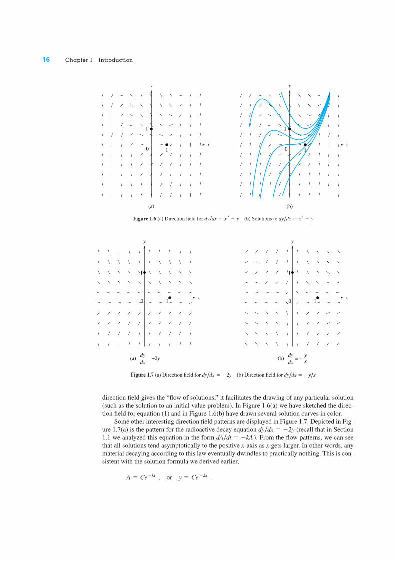
direction field gives the “flow of solutions,” it facilitates the drawing of any particular solution(such as the solution to an initial value problem). In Figure 1.6(a) we have sketched the direc-tion field for equation (1) and in Figure 1.6(b) have drawn several solution curves in color.
Some other interesting direction field patterns are displayed in Figure 1.7. Depicted in Fig-ure 1.7(a) is the pattern for the radioactive decay equation � �2y (recall that in Section1.1 we analyzed this equation in the form ). From the flow patterns, we can seethat all solutions tend asymptotically to the positive x-axis as x gets larger. In other words, anymaterial decaying according to this law eventually dwindles to practically nothing. This is con-sistent with the solution formula we derived earlier,
A � Ce�kt , or y � Ce�2x .
dA/dt � �kAdy/dx
(a) (b)
1
1
01
1
0
y
x x
y
Figure 1.6 (a) Direction field for (b) Solutions to dy/dx � x2 � ydy/dx � x2 � y
y
x
1
10
y
x
1
10
dydx
(a) = −2ydydx
(b) = − yx
Figure 1.7 (a) Direction field for (b) Direction field for dy/dx � �y/xdy/dx � �2y
Section 1.3 Direction Fields 17
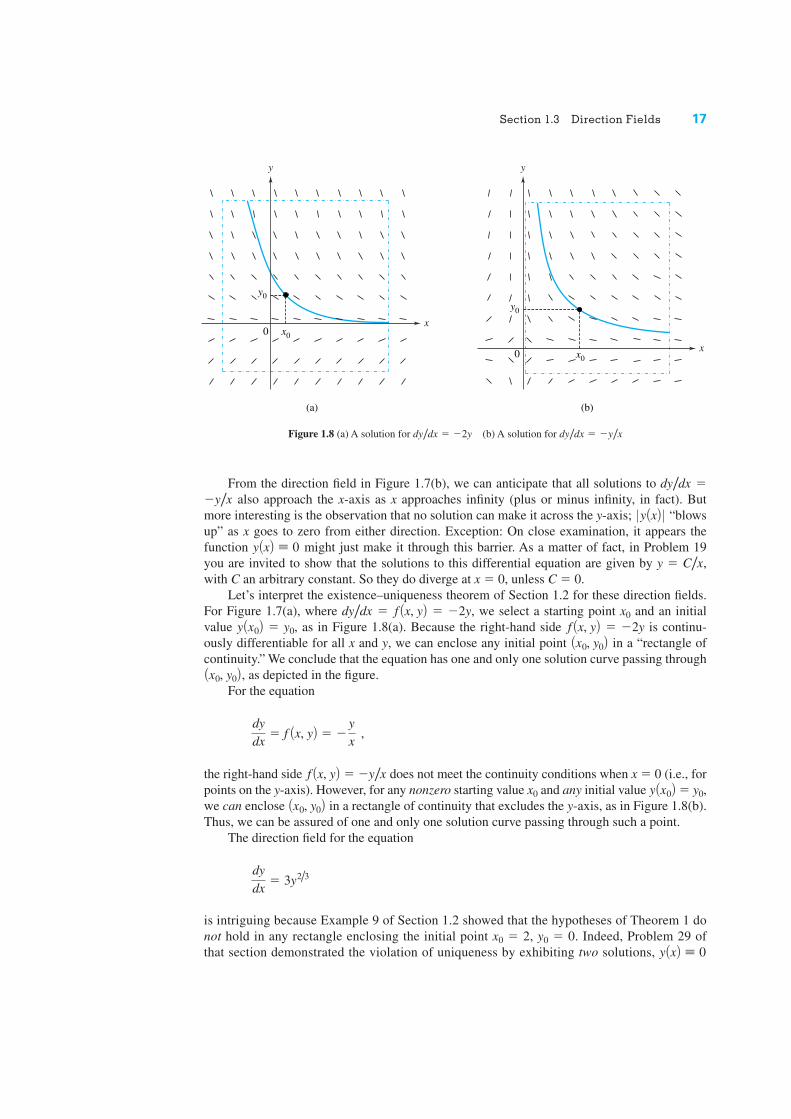
From the direction field in Figure 1.7(b), we can anticipate that all solutions to �also approach the x-axis as x approaches infinity (plus or minus infinity, in fact). But
more interesting is the observation that no solution can make it across the y-axis; “blowsup” as x goes to zero from either direction. Exception: On close examination, it appears thefunction might just make it through this barrier. As a matter of fact, in Problem 19you are invited to show that the solutions to this differential equation are given by y � ,with C an arbitrary constant. So they do diverge at x � 0, unless C � 0.
Let’s interpret the existence–uniqueness theorem of Section 1.2 for these direction fields.For Figure 1.7(a), where � � �2y, we select a starting point x0 and an initialvalue � y0, as in Figure 1.8(a). Because the right-hand side � �2y is continu-ously differentiable for all x and y, we can enclose any initial point in a “rectangle ofcontinuity.” We conclude that the equation has one and only one solution curve passing through
, as depicted in the figure.For the equation
the right-hand side � does not meet the continuity conditions when x � 0 (i.e., forpoints on the y-axis). However, for any nonzero starting value x0 and any initial value � y0,we can enclose in a rectangle of continuity that excludes the y-axis, as in Figure 1.8(b).Thus, we can be assured of one and only one solution curve passing through such a point.
The direction field for the equation
is intriguing because Example 9 of Section 1.2 showed that the hypotheses of Theorem 1 donot hold in any rectangle enclosing the initial point x0 � 2, y0 � 0. Indeed, Problem 29 ofthat section demonstrated the violation of uniqueness by exhibiting two solutions, y AxB � 0
dydx
� 3y2/3
Ax0, y0By Ax0B
�y/xf Ax, yB
dydx
� f Ax, yB � �
yx ,
Ax0, y0BAx0, y0B
f Ax, yBy Ax0Bf Ax, yBdy/dx
C/xy AxB � 0
0 y AxB 0�y/xdy/dx
(a)
0 x0
y0
(b)
0 x0
y0
y
x
y
x
Figure 1.8 (a) A solution for (b) A solution for dy/dx � �y/xdy/dx � �2y
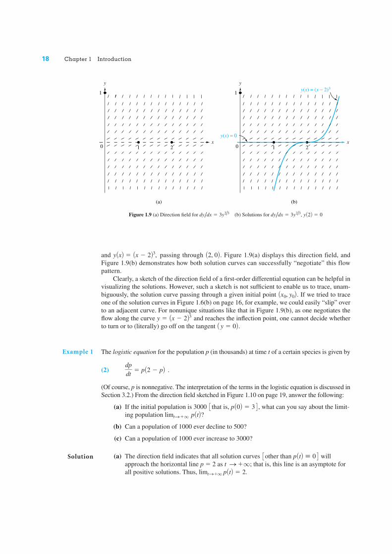
18 Chapter 1 Introduction
and passing through . Figure 1.9(a) displays this direction field, andFigure 1.9(b) demonstrates how both solution curves can successfully “negotiate” this flowpattern.
Clearly, a sketch of the direction field of a first-order differential equation can be helpful invisualizing the solutions. However, such a sketch is not sufficient to enable us to trace, unam-biguously, the solution curve passing through a given initial point . If we tried to traceone of the solution curves in Figure 1.6(b) on page 16, for example, we could easily “slip” overto an adjacent curve. For nonunique situations like that in Figure 1.9(b), as one negotiates theflow along the curve and reaches the inflection point, one cannot decide whetherto turn or to (literally) go off on the tangent .
The logistic equation for the population p (in thousands) at time t of a certain species is given by
(2)
(Of course, p is nonnegative. The interpretation of the terms in the logistic equation is discussed inSection 3.2.) From the direction field sketched in Figure 1.10 on page 19, answer the following:
(a) If the initial population is 3000 , what can you say about the limit-ing population ?
(b) Can a population of 1000 ever decline to 500?
(c) Can a population of 1000 ever increase to 3000?
(a) The direction field indicates that all solution curves willapproach the horizontal line p � 2 as that is, this line is an asymptote forall positive solutions. Thus, limtS�q p AtB � 2.
t S�q;3other than p AtB � 0 4
p AtBlimtS�q
3 that is, p A0B � 3 4
dpdt
� p A2 � pB .
A y � 0By � Ax � 2B3
Ax0, y0B
A2, 0By AxB � Ax � 2B3,
Example 1
Solution
(a)
1
1
0
(b)
12 2
1
0
y
xy(x) = 0
y(x) = (x − 2)3y
x
Figure 1.9 (a) Direction field for (b) Solutions for , y A2B � 0dy/dx � 3y2/3dy/dx � 3y2/3

Section 1.3 Direction Fields 19
(b) The direction field further shows that populations greater than 2000 will steadilydecrease, whereas those less than 2000 will increase. In particular, a population of1000 can never decline to 500.
(c) As mentioned in part (b), a population of 1000 will increase with time. But the direc-tion field indicates it can never reach 2000 or any larger value; i.e., the solution curvecannot cross the line p � 2. Indeed, the constant function is a solution toequation (2), and the uniqueness part of Theorem 1, page 11, precludes intersectionsof solution curves. ◆
Notice that the direction field in Figure 1.10 has the nice feature that the slopes do notdepend on t; that is, the slopes are the same along each horizontal line. The same is true forFigures 1.8(a) and 1.9. This is the key property of so-called autonomous equationswhere the right-hand side is a function of the dependent variable only. Group Project C, page32, investigates such equations in more detail.
Hand sketching the direction field for a differential equation is often tedious. Fortunately,several software programs have been developed to obviate this task†. When hand sketching isnecessary, however, the method of isoclines can be helpful in reducing the work.
The Method of Isoclines
An isocline for the differential equation
is a set of points in the xy-plane where all the solutions have the same slope ; thus, it is alevel curve for the function . For example, if
(3)
the isoclines are simply the curves (straight lines) x � y � c or y � �x � c. Here c is an arbi-trary constant. But c can be interpreted as the numerical value of the slope of every solu-tion curve as it crosses the isocline. (Note that c is not the slope of the isocline itself; the latteris, obviously, �1.) Figure 1.11(a) on page 20 depicts the isoclines for equation (3).
dy/dx
y¿ � f Ax, yB � x � y ,
f Ax, yBdy/dx
y¿ � f Ax, yB
y¿ � f AyB,
p AtB � 2
t43210
p (in thousands)
4
3
2
1
Figure 1.10 Direction field for logistic equation
†An applet, maintained on the web at http://alamos.math.arizona.edu/~rychlik/JOde/index.html, sketches directionfields and automates most of the differential equation algorithms discussed in this book.
20 Chapter 1 Introduction
y
x
y
x
y
x
(b)
1
1
0
(c)
1
1
0
(a)
1
c = −5
1
0
c = −4 c = −3 c = −2 c = −1
c = 0
c = 1
c = 2
c = 3
c = 4
c = 5
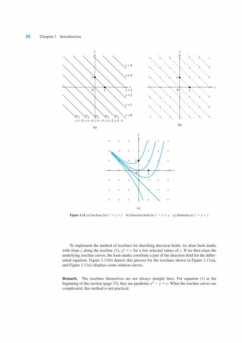
Figure 1.11 (a) Isoclines for (b) Direction field for (c) Solutions to y¿ � x � yy¿ � x � yy¿ � x � y
To implement the method of isoclines for sketching direction fields, we draw hash markswith slope c along the isocline � c for a few selected values of c. If we then erase theunderlying isocline curves, the hash marks constitute a part of the direction field for the differ-ential equation. Figure 1.11(b) depicts this process for the isoclines shown in Figure 1.11(a),and Figure 1.11(c) displays some solution curves.
Remark. The isoclines themselves are not always straight lines. For equation (1) at thebeginning of this section (page 15), they are parabolas � y � c. When the isocline curves arecomplicated, this method is not practical.
x2
f Ax, yB
Section 1.3 Direction Fields 21
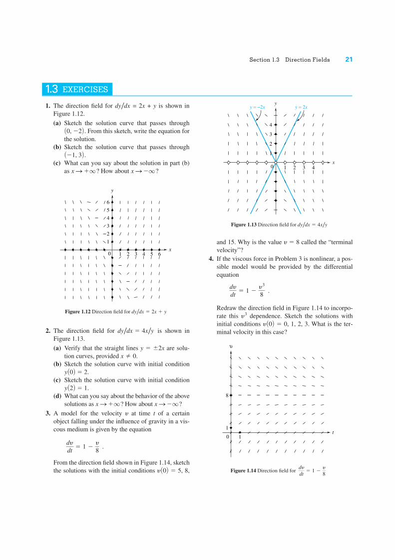
1. The direction field for = 2x + y is shown inFigure 1.12.
(a) Sketch the solution curve that passes through. From this sketch, write the equation for
the solution.(b) Sketch the solution curve that passes through
.(c) What can you say about the solution in part (b)
as ? How about ?xS�qxS�q
A�1, 3B
A0, �2B
dy/dx
and 15. Why is the value y � 8 called the “terminalvelocity”?
4. If the viscous force in Problem 3 is nonlinear, a pos-sible model would be provided by the differentialequation
Redraw the direction field in Figure 1.14 to incorpo-rate this dependence. Sketch the solutions withinitial conditions � 0, 1, 2, 3. What is the ter-minal velocity in this case?
y A0By3
dydt
� 1 �y3
8 .
1.3 EXERCISES
0
yy = −2x y = 2x
x1 32 4
1
2
3
4
Figure 1.13 Direction field for dy/dx � 4x/y
0
y
x
1
2
3
4
5
6
1 3 52 4 6
Figure 1.12 Direction field for dy/dx � 2x � y
υ
t0
1
1
8
Figure 1.14 Direction field fordydt
� 1 �y
8
2. The direction field for is shown inFigure 1.13.
(a) Verify that the straight lines y � �2x are solu-tion curves, provided
(b) Sketch the solution curve with initial condition� 2.
(c) Sketch the solution curve with initial condition� 1.
(d) What can you say about the behavior of the abovesolutions as ? How about ?
3. A model for the velocity at time t of a certainobject falling under the influence of gravity in a vis-cous medium is given by the equation
From the direction field shown in Figure 1.14, sketchthe solutions with the initial conditions � 5, 8,y A0B
dydt
� 1 �y
8 .
y
xS�qxS�q
y A2By A0B
x � 0.
dy/dx � 4x/y

22 Chapter 1 Introduction
22
5. The logistic equation for the population (in thou-sands) of a certain species is given by
(a) Sketch the direction field by using either a com-puter software package or the method of iso-clines.
(b) If the initial population is 3000 that is, �3 , what can you say about the limiting popula-tion ?
(c) If � 0.8, what is ?(d) Can a population of 2000 ever decline to 800?
6. Consider the differential equation
(a) A solution curve passes through the pointWhat is its slope at this point?
(b) Argue that every solution curve is increasing forx � 1.
(c) Show that the second derivative of every solu-tion satisfies
(d) A solution curve passes through . Provethat this curve has a relative minimum at .
7. Consider the differential equation
for the population p (in thousands) of a certainspecies at time t.
(a) Sketch the direction field by using either a com-puter software package or the method of isoclines.
(b) If the initial population is 4000 that is, �4 , what can you say about the limiting popula-tion ?
(c) If � 1.7, what is ?(d) If � 0.8, what is ?(e) Can a population of 900 ever increase to 1100?
8. The motion of a set of particles moving along thex-axis is governed by the differential equation
where denotes the position at time t of the particle.(a) If a particle is located at x � 1 when t � 2, what
is its velocity at this time?
x AtBdxdt
� t3 � x3 ,
lim tS�q p AtBp A0Blim tS�q p AtBp A0B
lim tS�q p AtB4 p A0B3
dpdt
� p A p � 1B A2 � pB
A0, 0BA0, 0B
d2y
dx2 � 1 � x cos y �1
2 sin 2y .
A1, p/2B.
dydx
� x � sin y .
lim tS�q p AtBp A0BlimtS�q p AtB
4 p A0B3
dpdt
� 3p � 2p2 .
(b) Show that the acceleration of a particle is given by
(c) If a particle is located at x � 2 when t � 2.5, canit reach the location x � 1 at any later time?
9. Let denote the solution to the initial valueproblem
(a) Show that (b) Argue that the graph of is decreasing for x
near zero and that as x increases from zero,decreases until it crosses the line y � x, whereits derivative is zero.
(c) Let x* be the abscissa of the point where thesolution curve crosses the line y � x.Consider the sign of and argue that has a relative minimum at x*.
(d) What can you say about the graph of for x � x*?
(e) Verify that y � x � 1 is a solution to �x � y and explain why the graph of alwaysstays above the line y � x � 1.
(f) Sketch the direction field for � x � y byusing the method of isoclines or a computersoftware package.
(g) Sketch the solution using the directionfield in part .
10. Use a computer software package to sketch thedirection field for the following differential equa-tions. Sketch some of the solution curves.
(a) � sin x(b) � sin y(c) � sin x sin y(d) � �(e) � �
In Problems 11–16, draw the isoclines with their directionmarkers and sketch several solution curves, including thecurve satisfying the given initial conditions.
11. � , � 4
12. � y , � 1
13. � 2x , � �1
14. � , � �1
15. � 2 � y , � 0
16. � x � 2y , � 1y A0Bdy/dx
y A0Bx2dy/dx
y A0Bx/ydy/dx
y A0Bdy/dx
y A0Bdy/dx
y A0B�x/ydy/dx
2y2x2dy/dx2y2x2dy/dx
dy/dxdy/dxdy/dx
Af By � f AxB
dy/dx
f AxBdy/dx
y � f AxBff– Ax*B
y � f AxB
f AxBf
f–AxB � 1 � f¿AxB � 1 � x � f AxB.
dydx
� x � y , y A0B � 1 .
fAxB3Hint: t3 � x3 � At � xB At2 � xt � x2B. 4
d2xdt2 � 3t2 � 3t3x2 � 3x5 .

Section 1.4 The Approximation Method of Euler 23
17. From a sketch of the direction field, what can onesay about the behavior as x approaches of asolution to the following?
18. From a sketch of the direction field, what can onesay about the behavior as x approaches of asolution to the following?
19. By rewriting the differential equation � in the form
integrate both sides to obtain the solution y �for an arbitrary constant C.
20. A bar magnet is often modeled as a magnetic dipolewith one end labeled the north pole N and the oppo-site end labeled the south pole S. The magnetic fieldfor the magnetic dipole is symmetric with respect torotation about the axis passing lengthwise throughthe center of the bar. Hence we can study the mag-netic field by restricting ourselves to a plane with thebar magnet centered on the x-axis.
For a point P that is located a distance r from theorigin, where r is much greater than the length of the
C/x
1y
dy ��1x
dx
�y/xdy/dx
dydx
� �y
�q
dydx
� 3 � y �1x
�qmagnet, the magnetic field lines satisfy the differen-tial equation
(4)
and the equipotential lines satisfy the equation
(5)
(a) Show that the two families of curves are per-pendicular where they intersect. [Hint: Con-sider the slopes of the tangent lines of the twocurves at a point of intersection.]
(b) Sketch the direction field for equation (4) for, You can use a soft-
ware package to generate the direction field oruse the method of isoclines. The direction fieldshould remind you of the experiment whereiron filings are sprinkled on a sheet of paperthat is held above a bar magnet. The iron filingscorrespond to the hash marks.
(c) Use the direction field found in part (b) to helpsketch the magnetic field lines that are solutionsto (4).
(d) Apply the statement of part (a) to the curves inpart (c) to sketch the equipotential lines that aresolutions to (5). The magnetic field lines andthe equipotential lines are examples of orthogo-nal trajectories. (See Problem 32 in Exercises2.4, pages 62–63.)†
�5 � y � 5.�5 � x � 5
dydx
�y2 � 2x2
3xy .
dydx
�3xy
2x2 � y2
†Equations (4) and (5) can be solved using the method for homogeneous equations in Section 2.6 (see Exercises 2.6,Problem 47).
Euler’s method (or the tangent-line method) is a procedure for constructing approximate solu-tions to an initial value problem for a first-order differential equation
(1)
It could be described as a “mechanical” or “computerized” implementation of the informalprocedure for hand sketching the solution curve from a picture of the direction field. Assuch, we will see that it remains subject to the failing that it may skip across solution curves.However, under fairly general conditions, iterations of the procedure do converge to truesolutions.
y¿ � f Ax, yB , y Ax0B � y0 .
1.4 THE APPROXIMATION METHOD OF EULER

24 Chapter 1 Introduction
The method is illustrated in Figure 1.15. Starting at the initial point , we follow thestraight line with slope , the tangent line, for some distance to the point . Then wereset the slope to the value and follow this line to . In this way we constructpolygonal (broken line) approximations to the solution. As we take smaller spacings betweenpoints (and thus employ more points), we may expect to converge to the true solution.
To be more precise, assume that the initial value problem (1) has a unique solution insome interval centered at x0. Let h be a fixed positive number (called the step size) and considerthe equally spaced points†
The construction of values yn that approximate the solution values proceeds as follows.At the point , the slope of the solution to (1) is given by � . Hence, thetangent line to the solution curve at the initial point is
y � y0 �
Using this tangent line to approximate we find that for the point x1 � x0 � h
Next, starting at the point , we construct the line with slope given by the direction fieldat the point — that is, with slope equal to . If we follow this line†† namely,y � y1 � in stepping from x1 to x2 � x1 � h, we arrive at the approximation
Repeating the process (as illustrated in Figure 1.15), we get
etc.f Ax4B � y4 J y3 � h f Ax3, y3B , f Ax3B � y3 J y2 � h f Ax2, y2B ,
f Ax2B � y2 J y1 � h f Ax1, y1B .Ax � x1B f Ax1, y1B 4
3f Ax1, y1BAx1, y1BAx1, y1B
f Ax1B � y1 J y0 � h f Ax0, y0B .f AxB,
Ax � x0B f Ax0, y0B .Ax0, y0B
f Ax0, y0Bdy/dxAx0, y0Bf AxnB
xn J x0 � nh , n � 0, 1, 2, . . . .
f AxB
Ax2, y2Bf Ax1, y1BAx1, y1Bf Ax0, y0B
Ax0, y0B
†The symbol means “is defined to be.”††Because y1 is an approximation to we cannot assert that this line is tangent to the solution curve y � f AxB.f Ax1B,
J
0 x0 x1 x2 x3
(x0, y 0)
(x1, y 1)(x2, y 2)
(x3, y 3)
Slopef(x0, y 0)
Slopef(x1, y 1) Slope
f(x2, y 2)
y
x
Figure 1.15 Polygonal-line approximation given by Euler’s method
Section 1.4 The Approximation Method of Euler 25
25
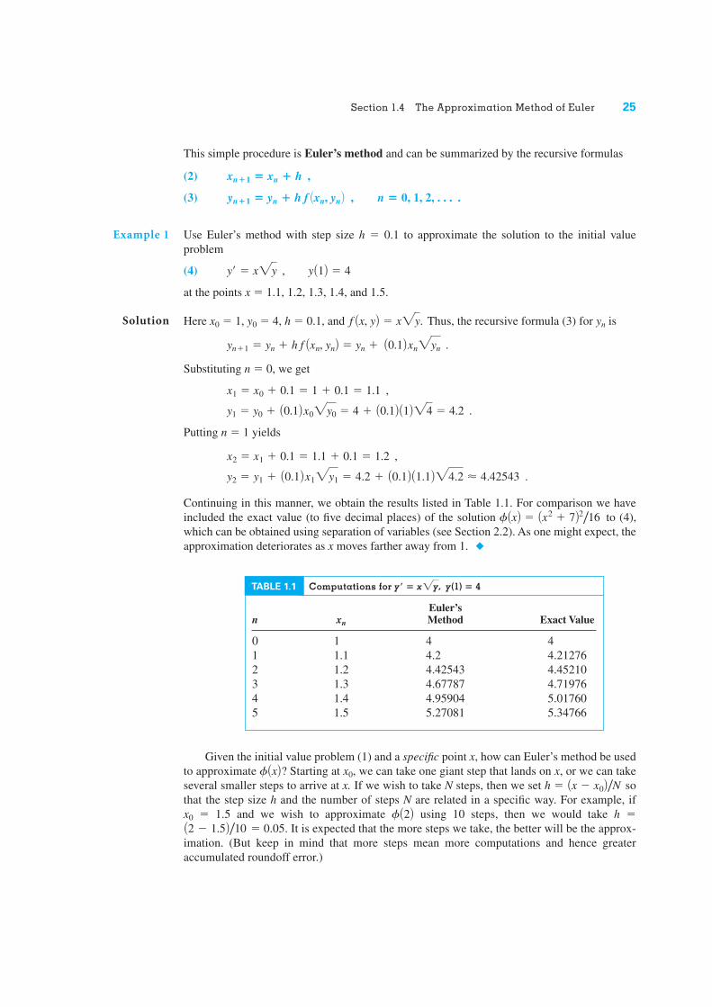
This simple procedure is Euler’s method and can be summarized by the recursive formulas
(2)
(3)
Use Euler’s method with step size h � 0.1 to approximate the solution to the initial valueproblem
(4)
at the points x � 1.1, 1.2, 1.3, 1.4, and 1.5.
Here x0 � 1, y0 � 4, h � 0.1, and Thus, the recursive formula (3) for yn is
Substituting n � 0, we get
Putting n � 1 yields
Continuing in this manner, we obtain the results listed in Table 1.1. For comparison we haveincluded the exact value (to five decimal places) of the solution to (4),which can be obtained using separation of variables (see Section 2.2). As one might expect, theapproximation deteriorates as x moves farther away from 1. ◆
f AxB � Ax2 � 7B2/16
y2 � y1 � A0.1B x12y1 � 4.2 � A0.1B A1.1B24.2 � 4.42543 .
x2 � x1 � 0.1 � 1.1 � 0.1 � 1.2 ,
y1 � y0 � A0.1B x02y0 � 4 � A0.1B A1B24 � 4.2 .
x1 � x0 � 0.1 � 1 � 0.1 � 1.1 ,
yn�1 � yn � h f Axn, ynB � yn � A0.1B xn2yn .
f Ax, yB � x2y.
y¿ � x2y , y A1B � 4
yn�1 � yn � h f Axn, ynB , n � 0, 1, 2, . . . .
xn�1 � xn � h ,
Example 1
Solution
TABLE 1.1 Computations for y , y(1) � 4
Euler’sn xn Method Exact Value
0 1 4 41 1.1 4.2 4.212762 1.2 4.42543 4.452103 1.3 4.67787 4.719764 1.4 4.95904 5.017605 1.5 5.27081 5.34766
� � x2y
Given the initial value problem (1) and a specific point x, how can Euler’s method be usedto approximate ? Starting at x0, we can take one giant step that lands on x, or we can takeseveral smaller steps to arrive at x. If we wish to take N steps, then we set h � sothat the step size h and the number of steps N are related in a specific way. For example, if x0 � 1.5 and we wish to approximate using 10 steps, then we would take h �
� 0.05. It is expected that the more steps we take, the better will be the approx-imation. (But keep in mind that more steps mean more computations and hence greateraccumulated roundoff error.)
A2 � 1.5B /10f A2B
Ax � x0B /Nf AxB

26 Chapter 1 Introduction
26
Use Euler’s method to find approximations to the solution of the initial value problem
(5)
at x � 1, taking 1, 2, 4, 8, and 16 steps.
Remark. Observe that the solution to (5) is just so Euler’s method will generatealgebraic approximations to the transcendental number e � 2.71828. . . .
Here � y, x0 � 0, and y0 � 1. The recursive formula for Euler’s method is
To obtain approximations at x � 1 with N steps, we take the step size h � . For N � 1, wehave
For In this case we get
For where
(In the above computations, we have rounded to five decimal places.) Similarly, taking N � 8and 16, we obtain even better estimates for These approximations are shown in Table 1.2.For comparison, Figure 1.16 on page 27 displays the polygonal-line approximations to usingEuler’s method with h � and h � . Notice that the smaller step sizeyields the better approximation. ◆
1/8 AN � 8B1/4 AN � 4Bex
f A1B.
f A1B � y4 � A1 � 0.25B A1.95313B � 2.44141 .
y3 � A1 � 0.25B A1.5625B � 1.95313 ,
y2 � A1 � 0.25B A1.25B � 1.5625 ,
y1 � A1 � 0.25B A1B � 1.25 ,
N � 4, f Ax4B � f A1B � y4,
f A1B � y2 � A1 � 0.5B A1.5B � 2.25 .
y1 � A1 � 0.5B A1B � 1.5 ,
N � 2, f Ax2B � f A1B � y2.
f A1B � y1 � A1 � 1B A1B � 2 .
1/N
yn�1 � yn � hyn � A1 � hByn .
f Ax, yB
f AxB � ex,
y¿ � y , y A0B � 1
Example 2
Solution
TABLE 1.2 Euler’s Method for y � = y, y(0) = 1
ApproximationN h for � e
1 1.0 2.02 0.5 2.254 0.25 2.441418 0.125 2.56578
16 0.0625 2.63793
F A1B
Section 1.4 The Approximation Method of Euler 27
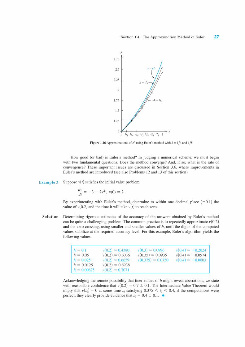
How good (or bad) is Euler’s method? In judging a numerical scheme, we must beginwith two fundamental questions. Does the method converge? And, if so, what is the rate ofconvergence? These important issues are discussed in Section 3.6, where improvements inEuler’s method are introduced (see also Problems 12 and 13 of this section).
Suppose satisfies the initial value problem
By experimenting with Euler’s method, determine to within one decimal place thevalue of and the time it will take to reach zero.
Determining rigorous estimates of the accuracy of the answers obtained by Euler’s methodcan be quite a challenging problem. The common practice is to repeatedly approximate and the zero crossing, using smaller and smaller values of h, until the digits of the computedvalues stabilize at the required accuracy level. For this example, Euler’s algorithm yields thefollowing values:
v A0.2B
v AtBv A0.2BA�0.1B
dvdt
� �3 � 2v2 , v(0) � 2 .
v AtB
Solution
Example 3
Acknowledging the remote possibility that finer values of h might reveal aberrations, we statewith reasonable confidence that . The Intermediate Value Theorem wouldimply that at some time t0 satisfying if the computations wereperfect; they clearly provide evidence that ◆t0 � 0.4 � 0.1.
0.375 6 t0 6 0.4,v At0B � 0v A0.2B � 0.7 � 0.1
v A0.2B � 0.7071h � 0.00625v A0.2B � 0.6938h � 0.0125
v A0.4B � �0.0003v A0.375B � 0.0750v A0.2B � 0.6659h � 0.025v A0.4B � �0.0574v A0.35B � 0.0935v A0.2B � 0.6036h � 0.05v A0.4B � �0.2024v A0.3B � 0.0996v A0.2B � 0.4380h � 0.1
y = e x
1.25
1
1.5
1.75
2
2.25
2.5
2.75
0 1/8 1/4 3/8 1/2 5/8 3/4 7/8 1
h = 1/8
h = 1/4
y
x
Figure 1.16 Approximations of using Euler’s method with h = and 1/81/4ex

28 Chapter 1 Introduction
In many of the problems below, it will be helpful to havea calculator or computer available.† You may also find itconvenient to write a program for solving initial valueproblems using Euler’s method. (Remember, all trigono-metric calculations are done in radians.)
In Problems 1–4, use Euler’s method to approximate thesolution to the given initial value problem at the points x � 0.1, 0.2, 0.3, 0.4, and 0.5, using steps of size 0.1 .
1.
2.
3.
4.
5. Use Euler’s method with step size h � 0.1 toapproximate the solution to the initial value problem
at the points x � 1.1, 1.2, 1.3, 1.4, and 1.5.
6. Use Euler’s method with step size h � 0.2 toapproximate the solution to the initial value problem
at the points x � 1.2, 1.4, 1.6, and 1.8.
7. Use Euler’s method to find approximations to thesolution of the initial value problem
at taking 1, 2, 4, and 8 steps.
8. Use Euler’s method to find approximations to thesolution of the initial value problem
at t � 1, taking 1, 2, 4, and 8 steps.
9. Use Euler’s method with h � 0.1 to approximate thesolution to the initial value problem
on the interval Compare these approxi-mations with the actual solution y � (verify!)by graphing the polygonal-line approximation andthe actual solution on the same coordinate system.
10. Use the strategy of Example 3 to find a value of h forEuler’s method such that is approximated towithin if y(x) satisfies the initial value problem
y¿ � x � y , y A0B � 0 .
�0.01,y A1B
�1/x1 � x � 2.
y¿ �1
x2 �y
x� y2 , y A1B � �1
dxdt
� 1 � t sin AtxB , x A0B � 0
x � p,
y¿ � 1 � sin y , y A0B � 0
y¿ �1x
A y2 � yB , y A1B � 1
y¿ � x � y2 , y A1B � 0
dy/dx � x/y , y A0B � �1
dy/dx � x � y , y A0B � 1
dy/dx � y A2 � yB , y A0B � 3
dy/dx � �x/y , y A0B � 4
Ah � 0.1B
Also find, to within the value of x0 such thatCompare your answers with those given
by the actual solution (verify!).Graph the polygonal-line approximation and theactual solution on the same coordinate system.
11. Use the strategy of Example 3 to find a value of h forEuler’s method such that is approximated towithin if satisfies the initial value problem
Also find, to within the value of t0 such thatCompare your answers with those given
by the actual solution (verify!).
12. In Example 2 we approximated the transcendentalnumber e by using Euler’s method to solve the initialvalue problem
Show that the Euler approximation yn obtained byusing the step size is given by the formula
Recall from calculus that
and hence Euler’s method converges (theoretically)to the correct value.
13. Prove that the “rate of convergence” for Euler’smethod in Problem 12 is comparable to byshowing that
[Hint: Use L’Hôpital’s rule and the Maclaurinexpansion for .]
14. Use Euler’s method with the spacings h � 0.5, 0.1,0.05, 0.01 to approximate the solution to the initialvalue problem
on the interval (The explanation for theerratic results lies in Problem 18 of Exercises 1.2.)
Heat Exchange. There are basically two mecha-nisms by which a physical body exchanges heat withits environment. The contact heat transfer across thebody’s surface is driven by the difference in the body’s
0 � x � 2.
y¿ � 2xy2 , y A0B � 1
ln A1 � tB
limnSq
e � yn
1/n�
e
2 .
1/n
limnSq
a1 �1nb n
� e ,
yn � a1 �1nb n
, n � 1, 2, . . .
1/n
y¿ � y , y A0B � 1 .
x � tan tx At0B � 1.
�0.02,
dxdt
� 1 � x2 , x A0B � 0 .
x AtB�0.01,x A1B
y � e�x � x � 1y Ax0B � 0.2.
�0.05,
1.4 EXERCISES
†An applet, maintained on the web at http://alamos.math.arizona.edu/~rychlik/JOde/index.html, automates most of the differential equation algo-rithms discussed in this book.

Technical Writing Exercises 29
29
temperature and that of the environment; this isknown as Newton’s law of cooling. However, heattransfer also occurs due to thermal radiation, whichaccording to Stefan’s law of radiation is governed bythe difference of the fourth powers of these tempera-tures. In most cases one of these modes dominates theother. Problems 15 and 16 invite you to simulate eachmode numerically for a given set of initial conditions.
15. Newton’s Law of Cooling. Newton’s law of cool-ing states that the rate of change in the temperatureT of a body is proportional to the differencebetween the temperature of the medium M and thetemperature of the body. That is,
where K is a constant. Let K � 1 (min)�1 and the tem-perature of the medium be constant, IfM AtB � 70º.
dTdt
� K 3M AtB � T AtB 4 ,AtB
AtB
the body is initially at 100º, use Euler’s method with h � 0.1 to approximate the temperature of the body after
(a) 1 minute.(b) 2 minutes.
16. Stefan’s Law of Radiation. Stefan’s law of radia-tion states that the rate of change in temperature of abody at T degrees in a medium at M degrees isproportional to . That is,
where K is a constant. Let K � and assumethat the medium temperature is constant,If � 100º, use Euler’s method with h � 0.1 toapproximate and .T A2BT A1B
T A0BM AtB � 70º.
A40B�4
dTdt
� K AM(t)4 � T(t)4B ,M4 � T 4
AtBAtB
Chapter Summary
In this chapter we introduced some basic terminology for differential equations. The order of adifferential equation is the order of the highest derivative present. The subject of this text isordinary differential equations, which involve derivatives with respect to a single independentvariable. Such equations are classified as linear or nonlinear.
An explicit solution of a differential equation is a function of the independent variable thatsatisfies the equation on some interval. An implicit solution is a relation between the dependentand independent variables that implicitly defines a function that is an explicit solution. A differ-ential equation typically has infinitely many solutions. In contrast, some theorems ensure that aunique solution exists for certain initial value problems in which one must find a solution to thedifferential equation that also satisfies given initial conditions. For an nth-order equation, theseconditions refer to the values of the solution and its first n – 1 derivatives at some point.
Even if one is not successful in finding explicit solutions to a differential equation, severaltechniques can be used to help analyze the solutions. One such method for first-order equationsviews the differential equation as specifying directions (slopes) at points onthe plane. The conglomerate of such slopes is the direction field for the equation. Knowing the“flow of solutions” is helpful in sketching the solution to an initial value problem. Further-more, carrying out this method algebraically leads to numerical approximations to the desiredsolution. This numerical process is called Euler’s method.
dy/dx � f Ax, yB
1. Select four fields (for example, astronomy, geology,biology, and economics) and for each field discuss asituation in which differential equations are used tosolve a problem. Select examples that are not coveredin Section 1.1.
2. Compare the different types of solutions discussed in this chapter—explicit, implicit, graphical, andnumerical. What are advantages and disadvantagesof each?
TECHNICAL WRITING EXERCISES

30
Group Projects for Chapter 1
Euler’s method is based on the fact that the tangent line gives a good local approximation for thefunction. But why restrict ourselves to linear approximants when higher-degree polynomialapproximants are available? For example, we can use the Taylor polynomial of degree n about x �x0, which is defined by
This polynomial is the nth partial sum of the Taylor series representation
To determine the Taylor series for the solution to the initial value problem
we need only determine the values of the derivatives of (assuming they exist) at x0; that is,, . . . . The initial condition gives the first value Using the equation
, we find To determine we differentiate the equationimplicitly with respect to x to obtain
and thereby we can compute
(a) Compute the Taylor polynomials of degree 4 for the solutions to the given initial valueproblems. Use these Taylor polynomials to approximate the solution at x � 1.
(i) (ii)
(b) Compare the use of Euler’s method with that of the Taylor series to approximate thesolution to the initial value problem
Do this by completing Table 1.3 on page 31. Give the approximations for and to the nearest thousandth. Verify that and use this formula togetherwith a calculator or tables to find the exact values of to the nearest thousandth.Finally, decide which of the first four methods in Table 1.3 will yield the closestapproximation to and give the reasons for your choice. (Remember that the com-putation of trigonometric functions must be done in the radian mode.)
(c) Compute the Taylor polynomial of degree 6 for the solution to the Airy equation
d2y
dx2 � xy
f A10Bf AxB
f AxB � cos x � e�xf A3Bf A1B
dydx
� y � cos x � sin x , y A0B � 2 .
f AxB
dydx
� y A2 � yB ; y A0B � 4 .dydx
� x � 2y ; y A0B � 1 .
f– Ax0B.y– �
0f0x �
0f0y
dydx
�0f0x �
0f0y f
y¿ � f Ax, yBf– Ax0B,f¿ Ax0B � f Ax0, y0B.y¿ � f Ax, yB
f Ax0B � y0.f Ax0B, f¿ Ax0Bf
dy/dx � f Ax, yB , y Ax0B � y0 ,
f AxBaq
k�0
y AkB Ax0Bk!
Ax � x0Bk .
Pn AxB J y Ax0B � y¿ Ax0B Ax � x0B �y– Ax0B
2! Ax � x0B2 � p �
y AnB Ax0Bn!
Ax � x0Bn .
Taylor Series MethodA

Group Projects for Chapter 1 31
with the initial conditions 1, 0. Do you see how, in general, the Taylorseries method for an nth-order differential equation will employ each of the n initialconditions mentioned in Definition 3, Section 1.2?
y¿A0B �y A0B �
TABLE 1.3
Approximation ApproximationMethod of of
Euler’s method using steps of size 0.1
Euler’s method using steps of size 0.01
Taylor polynomial of degree 2
Taylor polynomial of degree 5
Exact value of to nearest thousandthf AxB
F A3BF A1B
The initial value problem
(1)
can be rewritten as an integral equation. This is obtained by integrating both sides of (1) withrespect to x from x � x0 to x � x1:
(2)
Substituting � y0 and solving for gives
(3)
If we use t instead of x as the variable of integration, we can let x � x1 be the upper limit ofintegration. Equation (3) then becomes
(4)
Equation (4) can be used to generate successive approximations of a solution to (1). Let thefunction be an initial guess or approximation of a solution to (1). Then a new approxima-tion function is given by
where we have replaced by the approximation in the argument of f. In a similar fashion,we can use to generate a new approximation , and so on. In general, we obtain the
st approximation from the relation
(5) J y0 � �x
x0
f At, Fn AtBBdt .Fn�1 AxBAn � 1B
f2 AxBf1 AxBf0 AtBy AtB
f1 AxB J y0 � �x
x0
f At, f0 AtBBdt ,
f0 AxB
y AxB � y0 � �x
x0
f At, y AtBBdt .
y Ax1B � y0 � �x1
x0
f Ax, y AxBBdx .
y Ax1By Ax0B�
x1
x0
y¿ AxBdx � y Ax1B � y Ax0B � �x1
x0
f Ax, y AxBB dx .
y¿ AxB � f Ax, yB , y Ax0B � y0
Picard’s MethodB

32 Chapter 1 Introduction
This procedure is called Picard’s method.† Under certain assumptions on f and , thesequence is known to converge to a solution to (1). These assumptions and the proof ofconvergence are given in Chapter 13.††
Without further information about the solution to (1), it is common practice to take
(a) Use Picard’s method with to obtain the next four successive approximationsof the solution to
(6)
Show that these approximations are just the partial sums of the Maclaurin series for theactual solution .
(b) Use Picard’s method with to obtain the next three successive approximationsof the solution to the nonlinear problem
(7)
Graph these approximations for (c) In Problem 29 in Exercises 1.2, we showed that the initial value problem
(8)
does not have a unique solution. Show that Picard’s method beginning with con-verges to the solution whereas Picard’s method beginning with converges to the second solution . [Hint: For the guess ,show that has the form , where and as ]nSq.rnS 3cnS 1cn Ax � 2Brnfn AxB
f0 AxB � x � 2y AxB � Ax � 2B3f0 AxB � x � 2y AxB � 0,f0 AxB � 0
y¿ AxB � 3 3 y AxB 4 2/3 , y A2B � 0
0 � x � 1.
y¿ AxB � 3x � 3 y AxB 4 2 , y A0B � 0 .
f0 AxB � 0ex
y¿ AxB � y AxB , y A0B � 1 .
f0 AxB � 1
f0 AxB � y0.
Efn AxBFf0 AxB
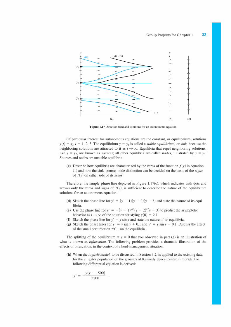
Sketching the direction field of a differential equation is particularly easy whenthe equation is autonomous—that is, the independent variable t does not appear explicitly:
(9)
In Figure 1.17(a) the graph exhibits the direction field for and and some solutions are sketched. Note the following properties of the graphs andexplain how they follow from the fact that the equation is autonomous:
(a) The slopes in the direction field are all identical along horizontal lines.(b) New solutions can be generated from old ones by time shifting [i.e., replacing with
]
From observation (a) it follows that the entire direction field can be described by a singledirection “line,” as in Figure 1.17(b).
y At � t0B.y AtB
A 7 0,y¿ � �A Ay � y1B Ay � y2B Ay � y3B2
dydt
� f A yB .
dy/dt � f At, yB
The Phase LineC
†Historical Footnote: This approximation method is a by-product of the famous Picard–Lindelöf existence theoremformulated at the end of the 19th century.††All references to Chapters 11–13 refer to the expanded text Fundamentals of Differential Equations and BoundaryValue Problems, 6th ed.
Group Projects for Chapter 1 33
Of particular interest for autonomous equations are the constant, or equilibrium, solutionsThe equilibrium is called a stable equilibrium, or sink, because the
neighboring solutions are attracted to it as Equilibria that repel neighboring solutions,like , are known as sources; all other equilibria are called nodes, illustrated by Sources and nodes are unstable equilibria.
(c) Describe how equilibria are characterized by the zeros of the function in equation(1) and how the sink–source–node distinction can be decided on the basis of the signsof on either side of its zeros.
Therefore, the simple phase line depicted in Figure 1.17(c), which indicates with dots andarrows only the zeros and signs of is sufficient to describe the nature of the equilibriumsolutions for an autonomous equation.
(d) Sketch the phase line for and state the nature of its equi-libria.
(e) Use the phase line for to predict the asymptoticbehavior as of the solution satisfying
(f) Sketch the phase line for sin y and state the nature of its equilibria.(g) Sketch the phase lines for and . Discuss the effect
of the small perturbation on the equilibria.
The splitting of the equilibrium at that you observed in part (g) is an illustration ofwhat is known as bifurcation. The following problem provides a dramatic illustration of theeffects of bifurcation, in the context of a herd-management situation.
(h) When the logistic model, to be discussed in Section 3.2, is applied to the existing datafor the alligator population on the grounds of Kennedy Space Center in Florida, thefollowing differential equation is derived:
y¿ � �y Ay � 1500B
3200 .
y � 0
�0.1y¿ � y sin y � 0.1y¿ � y sin y � 0.1
y¿ � yy A0B � 2.1.tSq
y¿ � � Ay � 1B5/3 Ay � 2B2 Ay � 3By¿ � Ay � 1B Ay � 2B Ay � 3B
f AyB,
f AyBf AyB
y � y3.y � y2
tSq.y � y1y AtB � yi, i � 1, 2, 3.
(a) (b)
y
(c)
yy(t − 5)y(t)
y1
y2
y3
t
Figure 1.17 Direction field and solutions for an autonomous equation

Here is the population and time t is measured in years. If hunters were allowed tothin the population at a rate of s alligators per year, the equation would be modified to
Draw the phase lines for s � 0, 50, 100, 125, 150, 175, and 200. Discuss the signifi-cance of the equilibria. Note the bifurcation at s � 175; should a depletion rate near 175be avoided?
y¿ � �y Ay � 1500B
3200� s .
y(t)
34 Chapter 1 Introduction
34
Related Documents