Convex Optimization Fundamentals and Applications in Statistical Signal Processing João Mota EURASIP/UDRC Summer School 2019 Heriot-Watt University 1-1

Welcome message from author
This document is posted to help you gain knowledge. Please leave a comment to let me know what you think about it! Share it to your friends and learn new things together.
Transcript
Convex OptimizationFundamentals and Applications in Statistical Signal
Processing
João Mota
EURASIP/UDRC Summer School 2019
Heriot-Watt University
1-1
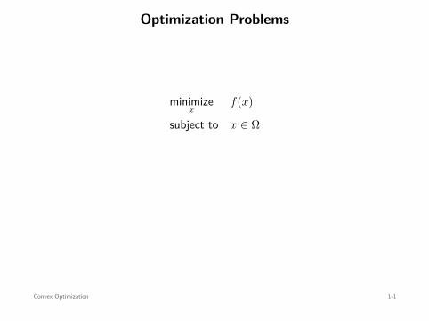
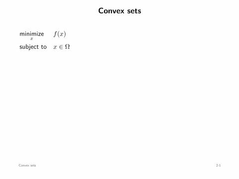
Optimization Problems
minimizex
f(x)
subject to x ∈ Ω
• x ∈ Rn: optimization variable
• f : Rn → R: cost function (or objective)
• Ω ⊂ Rn: constraint set
Convex Optimization 1-1

Optimization Problems
minimizex
f(x)
subject to x ∈ Ω
• x ∈ Rn: optimization variable
• f : Rn → R: cost function (or objective)
• Ω ⊂ Rn: constraint set
Convex Optimization 1-1
Example: Polynomial Fitting
Given
(xi, yi)m
i=1 ⊂ R2, find “best” fitting polynomial of order k < m
(xi, yi)
a0 + a1x + a2x2 + a3x3 + a4x4 + a5x5
Convex Optimization 1-2

Example: Polynomial Fitting
Given
(xi, yi)m
i=1 ⊂ R2, find “best” fitting polynomial of order k < m
(xi, yi)
a0 + a1x + a2x2 + a3x3 + a4x4 + a5x5
Convex Optimization 1-2

Example: Polynomial Fitting
Given
(xi, yi)m
i=1 ⊂ R2, find “best” fitting polynomial of order k < m
(xi, yi)
a0 + a1x + a2x2 + a3x3 + a4x4 + a5x5
Convex Optimization 1-2

Example: Polynomial Fitting
Given
(xi, yi)m
i=1 ⊂ R2, find “best” fitting polynomial of order k < m
(xi, yi)
a0 + a1x + a2x2 + a3x3 + a4x4 + a5x5
Convex Optimization 1-2

Example: Polynomial Fitting
Given
(xi, yi)m
i=1 ⊂ R2, find “best” fitting polynomial of order k < m
(xi, yi)
a0 + a1x + a2x2 + a3x3 + a4x4 + a5x5
Convex Optimization 1-2

Example: Polynomial Fitting
Polynomial of order k = 5:
y = a0 + a1x + a2x2 + a3x3 + a4x4 + a5x5
We need to find a0, a1, . . . , a5 from the data
(xi, yi)m
i=1
Criterion: minimize the sum of squared errors (least-squares)
minimizea0,...,a5
m∑
i=1
(yi − a0 − a1xi − a2x2
i − a3x3i − a4x4
i − a5x5i
)2
variable: a ∈ R5
= f(a)
Convex Optimization 1-3

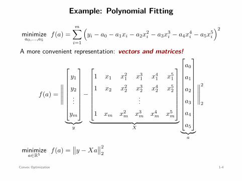
Example: Polynomial Fitting
minimizea0,...,a5
f(a) =m∑
i=1
(yi − a0 − a1xi − a2x2
i − a3x3i − a4x4
i − a5x5i
)2
A more convenient representation: vectors and matrices!
f(a) =∥∥∥∥∥
y1
y2...
ym
︸ ︷︷ ︸y
−
1 x1 x21 x3
1 x41 x5
1
1 x2 x22 x3
2 x42 x5
2...
1 xm x2m x3
m x4m x5
m
︸ ︷︷ ︸X
a0
a1
a2
a3
a4
a5
︸ ︷︷ ︸a
∥∥∥∥∥
2
2
minimizea∈R5
f(a) =∥∥y − Xa
∥∥22
∇f(a⋆) = 0 ⇐⇒ X⊤Xa⋆ = X⊤y
Convex Optimization 1-4

Example: Polynomial Fitting
minimizea0,...,a5
f(a) =m∑
i=1
(yi − a0 − a1xi − a2x2
i − a3x3i − a4x4
i − a5x5i
)2
A more convenient representation: vectors and matrices!
f(a) =∥∥∥∥∥
y1
y2...
ym
︸ ︷︷ ︸y
−
1 x1 x21 x3
1 x41 x5
1
1 x2 x22 x3
2 x42 x5
2...
1 xm x2m x3
m x4m x5
m
︸ ︷︷ ︸X
a0
a1
a2
a3
a4
a5
︸ ︷︷ ︸a
∥∥∥∥∥
2
2
minimizea∈R5
f(a) =∥∥y − Xa
∥∥22 ∇f(a⋆) = 0 ⇐⇒ X⊤Xa⋆ = X⊤y
Convex Optimization 1-4

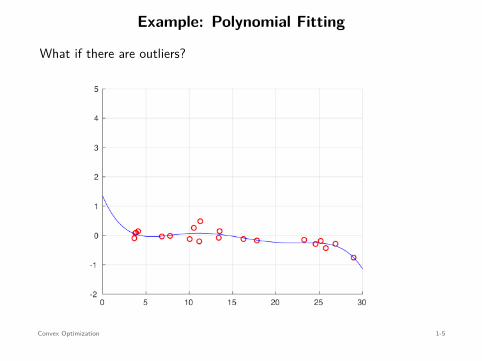
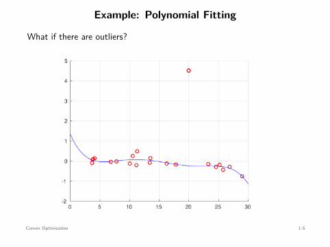
Example: Polynomial Fitting
What if there are outliers?
least-squares mina∈R5
∥∥y − Xa∥∥2
2Robust solution
⇐=
mina∈R5
∥∥y − Xa∥∥
1
no closed-form
Convex Optimization 1-5
Example: Polynomial Fitting
What if there are outliers?
least-squares mina∈R5
∥∥y − Xa∥∥2
2Robust solution
⇐=
mina∈R5
∥∥y − Xa∥∥
1
no closed-form
Convex Optimization 1-5
Example: Polynomial Fitting
What if there are outliers?
least-squares mina∈R5
∥∥y − Xa∥∥2
2Robust solution
⇐=
mina∈R5
∥∥y − Xa∥∥
1
no closed-form
Convex Optimization 1-5

Example: Polynomial Fitting
What if there are outliers?
least-squares
mina∈R5
∥∥y − Xa∥∥2
2Robust solution
⇐=
mina∈R5
∥∥y − Xa∥∥
1
no closed-form
Convex Optimization 1-5

Example: Polynomial Fitting
What if there are outliers?
least-squares mina∈R5
∥∥y − Xa∥∥2
2
Robust solution
⇐=
mina∈R5
∥∥y − Xa∥∥
1
no closed-form
Convex Optimization 1-5

Example: Polynomial Fitting
What if there are outliers?
least-squares mina∈R5
∥∥y − Xa∥∥2
2Robust solution
⇐=
mina∈R5
∥∥y − Xa∥∥
1
no closed-form
Convex Optimization 1-5

Example: Polynomial Fitting
What if there are outliers?
least-squares mina∈R5
∥∥y − Xa∥∥2
2Robust solution
⇐=
mina∈R5
∥∥y − Xa∥∥
1
no closed-form
Convex Optimization 1-5

Example: Polynomial Fitting
What if there are outliers?
least-squares mina∈R5
∥∥y − Xa∥∥2
2Robust solution
⇐=
mina∈R5
∥∥y − Xa∥∥
1
no closed-form
Convex Optimization 1-5

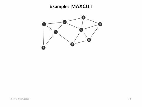
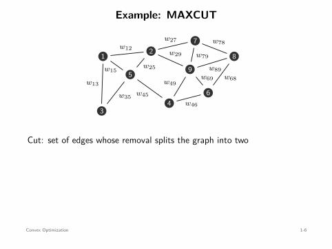
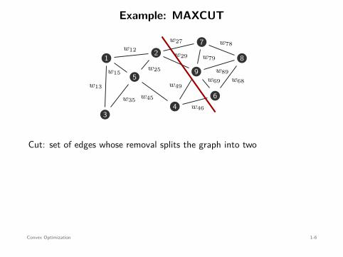
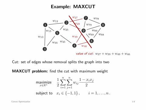
Example: MAXCUT
1 2
34
5
6
7
89
w12
w13
w15w25
w35 w45
w69 w68
w78
w79
w89
w27
w29
w49
w46
w27
w29
w49
w46
value of cut: w27 + w29 + w49 + w46
Cut: set of edges whose removal splits the graph into two
MAXCUT problem: find the cut with maximum weight
maximizex∈Rn
12
n∑
i=1
n∑
j=1wij
1 − xixj
2
subject to xi ∈ −1, 1 , i = 1, . . . , n .
Convex Optimization 1-6
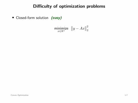
Difficulty of optimization problems
• Closed-form solution (easy)
minimizex∈Rn
∥∥y − Ax∥∥2
2
• No closed-form solution, but still solvable (easy)
minimizex∈Rn
∥∥y − Ax∥∥
1
• Combinatorial, NP-Hard, requires exhaustive search (hard)
maximizex∈Rn
12
n∑
i=1
n∑
j=1wij
1 − xixj
2
subject to xi ∈ −1, 1 , i = 1, . . . , n .
Convex Optimization 1-7

Difficulty of optimization problems
“In fact the great watershed in optimization isn’t between linearity andnonlinearity, but convexity and nonconvexity.” [Rockafellar, 93’]
x x
convex nonconvex
Convex Optimization 1-8

Difficulty of optimization problems
“In fact the great watershed in optimization isn’t between linearity andnonlinearity, but convexity and nonconvexity.” [Rockafellar, 93’]
x x
convex nonconvex
Convex Optimization 1-8

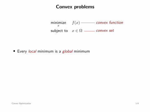
Convex problems
minimizex
f(x)
subject to x ∈ Ω
convex function
convex set
• Every local minimum is a global minimum
• Solved efficiently (polynomial-time algorithms)
• Lots of applications: machine learning, communications, economicsand finance, control systems, electronic circuit design, statistics, etc.
• Many algorithms for nonconvex optimization use convex surrogates
Convex Optimization 1-9

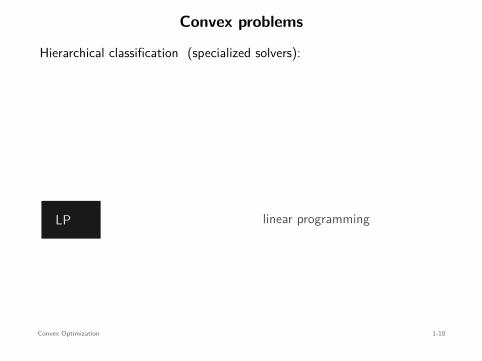
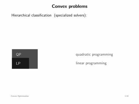
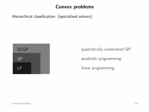
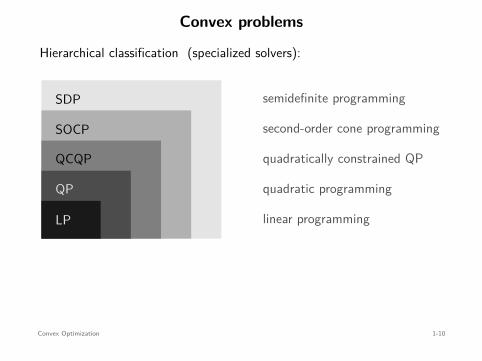
Convex problems
Hierarchical classification (specialized solvers):
LP
QP
QCQP
SOCP
SDP
linear programming
quadratic programming
quadratically constrained QP
second-order cone programming
semidefinite programming
Other classifications:differentiable vs. nondifferentiable programmingunconstrained vs. constrained programming
Convex Optimization 1-10
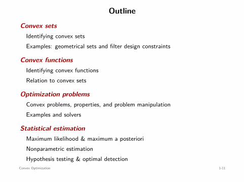
Outline
Convex setsIdentifying convex setsExamples: geometrical sets and filter design constraints
Convex functionsIdentifying convex functionsRelation to convex sets
Optimization problemsConvex problems, properties, and problem manipulationExamples and solvers
Statistical estimationMaximum likelihood & maximum a posterioriNonparametric estimationHypothesis testing & optimal detection
Convex Optimization 1-11

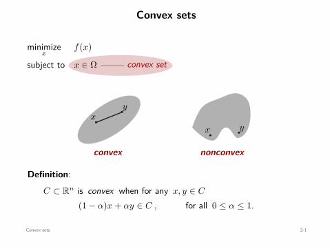
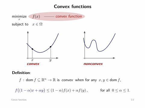
Convex sets
convex set
minimizex
f(x)
subject to x ∈ Ω
xy
convex
x y
nonconvex
Definition:C ⊂ Rn is convex when for any x, y ∈ C
(1 − α)x + αy ∈ C , for all 0 ≤ α ≤ 1.
Convex sets 2-1
Convex sets
convex set
minimizex
f(x)
subject to x ∈ Ω
xy
convex
x y
nonconvex
Definition:C ⊂ Rn is convex when for any x, y ∈ C
(1 − α)x + αy ∈ C , for all 0 ≤ α ≤ 1.
Convex sets 2-1

Convex sets
convex set
minimizex
f(x)
subject to x ∈ Ω
xy
convex
x y
nonconvex
Definition:C ⊂ Rn is convex when for any x, y ∈ C
(1 − α)x + αy ∈ C , for all 0 ≤ α ≤ 1.
Convex sets 2-1

Convex sets
convex set
minimizex
f(x)
subject to x ∈ Ω
xy
convex
x y
nonconvex
Definition:C ⊂ Rn is convex when for any x, y ∈ C
(1 − α)x + αy ∈ C , for all 0 ≤ α ≤ 1.
Convex sets 2-1

Convex sets
convex set
minimizex
f(x)
subject to x ∈ Ω
xy
convex
x y
nonconvex
Definition:C ⊂ Rn is convex when for any x, y ∈ C
(1 − α)x + αy ∈ C , for all 0 ≤ α ≤ 1.
Convex sets 2-1

Convex sets
convex set
minimizex
f(x)
subject to x ∈ Ω
xy
convex
x y
nonconvex
Definition:C ⊂ Rn is convex when for any x, y ∈ C
(1 − α)x + αy ∈ C , for all 0 ≤ α ≤ 1.
Convex sets 2-1

Convex sets
convex set
minimizex
f(x)
subject to x ∈ Ω
xy
convex
x y
nonconvex
Definition:C ⊂ Rn is convex when for any x, y ∈ C
(1 − α)x + αy ∈ C , for all 0 ≤ α ≤ 1.
Convex sets 2-1

Convex sets
convex set
minimizex
f(x)
subject to x ∈ Ω
xy
convex
x y
nonconvex
Definition:C ⊂ Rn is convex when for any x, y ∈ C
(1 − α)x + αy ∈ C , for all 0 ≤ α ≤ 1.
Convex sets 2-1
Convex sets
convex set
minimizex
f(x)
subject to x ∈ Ω
xy
convex
x y
nonconvex
Definition:C ⊂ Rn is convex when for any x, y ∈ C
(1 − α)x + αy ∈ C , for all 0 ≤ α ≤ 1.
Convex sets 2-1

Convex sets
convex set
minimizex
f(x)
subject to x ∈ Ω
xy
convex
x y
nonconvex
Definition:C ⊂ Rn is convex when for any x, y ∈ C
(1 − α)x + αy ∈ C , for all 0 ≤ α ≤ 1.
Convex sets 2-1

Examples of convex sets
x
y
Convex sets 2-2

Examples of convex sets
x
y
Convex sets 2-2

Examples of convex sets
x
y
Convex sets 2-2

Examples of convex sets
x
y
Convex sets 2-2

Examples of nonconvex sets
Rdiscrete sets
Convex sets 2-3
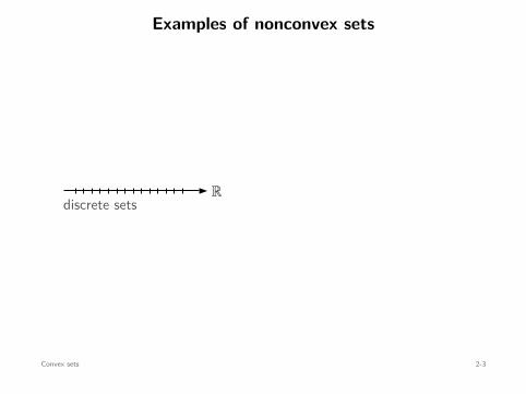
Examples of nonconvex sets
Rdiscrete sets
Convex sets 2-3

Examples of nonconvex sets
Rdiscrete sets
Convex sets 2-3

Examples of nonconvex sets
Rdiscrete sets
Convex sets 2-3

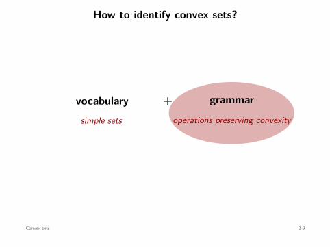
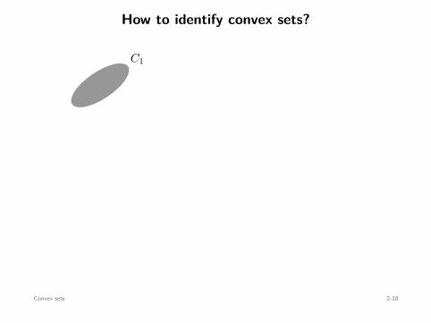
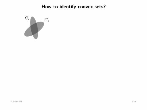
How to identify convex sets?
vocabulary + grammar
simple sets operations preserving convexity
Convex sets 2-4

How to identify convex sets?
vocabulary + grammar
simple sets operations preserving convexity
Convex sets 2-4
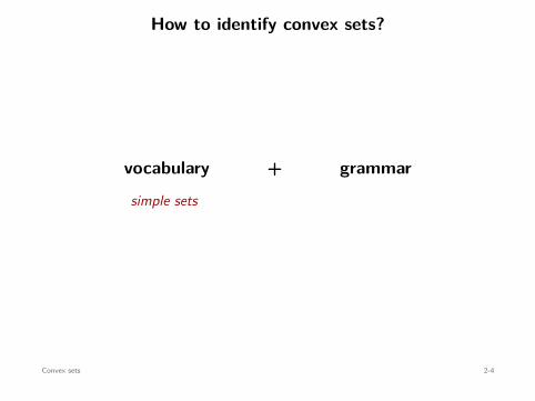
How to identify convex sets?
vocabulary + grammar
simple sets
operations preserving convexity
Convex sets 2-4

How to identify convex sets?
vocabulary + grammar
simple sets operations preserving convexity
Convex sets 2-4

Simple sets
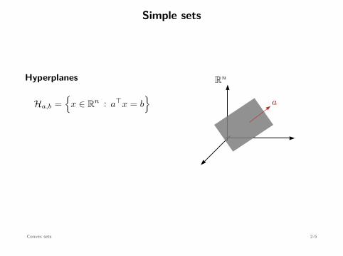
Hyperplanes
Ha,b =
x ∈ Rn : a⊤x = b
Rn
a
Convex sets 2-5

Simple sets
Hyperplanes
Ha,b =
x ∈ Rn : a⊤x = b
Rn
a
Convex sets 2-5
Simple sets
Hyperplanes
Ha,b =
x ∈ Rn : a⊤x = b
Rn
a
Convex sets 2-5

Simple sets
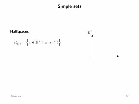
Halfspaces
H−a,b =
x ∈ Rn : a⊤x ≤ b
R2
a
Convex sets 2-6

Simple sets
Halfspaces
H−a,b =
x ∈ Rn : a⊤x ≤ b
R2
a
Convex sets 2-6
Simple sets
Halfspaces
H−a,b =
x ∈ Rn : a⊤x ≤ b
R2
a
Convex sets 2-6

Simple sets
Halfspaces
H−a,b =
x ∈ Rn : a⊤x ≤ b
R2
a
Convex sets 2-6

Simple sets
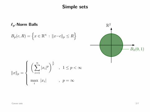
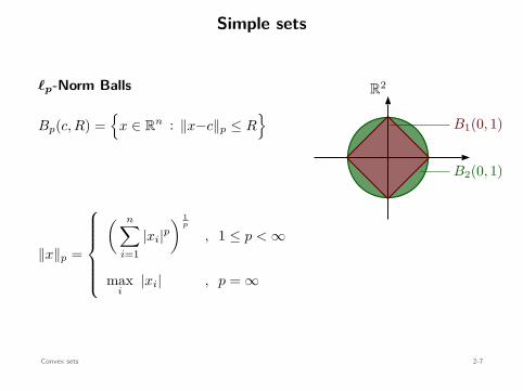
ℓp-Norm Balls
Bp(c, R) =
x ∈ Rn : ∥x−c∥p ≤ R
∥x∥p =
( n∑
i=1|xi|p
) 1p
, 1 ≤ p < ∞
maxi
|xi| , p = ∞
B∞(0, 1)B2(0, 1)
B1(0, 1)
R2
Convex sets 2-7

Simple sets
ℓp-Norm Balls
Bp(c, R) =
x ∈ Rn : ∥x−c∥p ≤ R
∥x∥p =
( n∑
i=1|xi|p
) 1p
, 1 ≤ p < ∞
maxi
|xi| , p = ∞
B∞(0, 1)B2(0, 1)
B1(0, 1)
R2
Convex sets 2-7

Simple sets
ℓp-Norm Balls
Bp(c, R) =
x ∈ Rn : ∥x−c∥p ≤ R
∥x∥p =
( n∑
i=1|xi|p
) 1p
, 1 ≤ p < ∞
maxi
|xi| , p = ∞
B∞(0, 1)B2(0, 1)
B1(0, 1)
R2
Convex sets 2-7

Simple sets
ℓp-Norm Balls
Bp(c, R) =
x ∈ Rn : ∥x−c∥p ≤ R
∥x∥p =
( n∑
i=1|xi|p
) 1p
, 1 ≤ p < ∞
maxi
|xi| , p = ∞
B∞(0, 1)B2(0, 1)
B1(0, 1)
R2
Convex sets 2-7
Simple sets
ℓp-Norm Balls
Bp(c, R) =
x ∈ Rn : ∥x−c∥p ≤ R
∥x∥p =
( n∑
i=1|xi|p
) 1p
, 1 ≤ p < ∞
maxi
|xi| , p = ∞
B∞(0, 1)
B2(0, 1)
B1(0, 1)
R2
Convex sets 2-7
Simple sets
ℓp-Norm Balls
Bp(c, R) =
x ∈ Rn : ∥x−c∥p ≤ R
∥x∥p =
( n∑
i=1|xi|p
) 1p
, 1 ≤ p < ∞
maxi
|xi| , p = ∞
B∞(0, 1)
B2(0, 1)
B1(0, 1)
R2
Convex sets 2-7

Simple sets
ℓp-Norm Balls
Bp(c, R) =
x ∈ Rn : ∥x−c∥p ≤ R
∥x∥p =
( n∑
i=1|xi|p
) 1p
, 1 ≤ p < ∞
maxi
|xi| , p = ∞
B∞(0, 1)B2(0, 1)
B1(0, 1)
R2
Convex sets 2-7
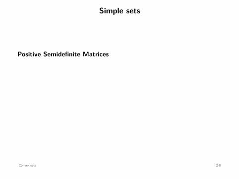
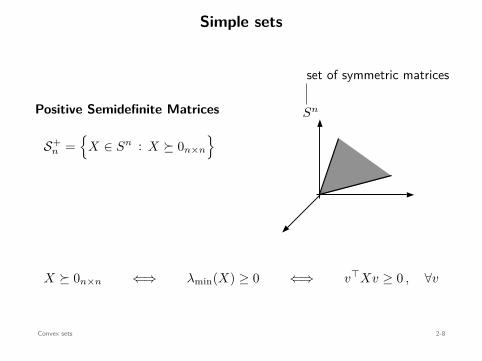
Simple sets
Positive Semidefinite Matrices
S+n =
X ∈ Sn : X ⪰ 0n×n
Sn
set of symmetric matrices
X ⪰ 0n×n ⇐⇒ λmin(X) ≥ 0 ⇐⇒ v⊤Xv ≥ 0 , ∀v
Convex sets 2-8

Simple sets
Positive Semidefinite Matrices
S+n =
X ∈ Sn : X ⪰ 0n×n
Sn
set of symmetric matrices
X ⪰ 0n×n ⇐⇒ λmin(X) ≥ 0 ⇐⇒ v⊤Xv ≥ 0 , ∀v
Convex sets 2-8

Simple sets
Positive Semidefinite Matrices
S+n =
X ∈ Sn : X ⪰ 0n×n
Sn
set of symmetric matrices
X ⪰ 0n×n ⇐⇒ λmin(X) ≥ 0 ⇐⇒ v⊤Xv ≥ 0 , ∀v
Convex sets 2-8

Simple sets
Positive Semidefinite Matrices
S+n =
X ∈ Sn : X ⪰ 0n×n
Sn
set of symmetric matrices
X ⪰ 0n×n ⇐⇒ λmin(X) ≥ 0 ⇐⇒ v⊤Xv ≥ 0 , ∀v
Convex sets 2-8

Simple sets
Positive Semidefinite Matrices
S+n =
X ∈ Sn : X ⪰ 0n×n
Sn
set of symmetric matrices
X ⪰ 0n×n ⇐⇒ λmin(X) ≥ 0 ⇐⇒ v⊤Xv ≥ 0 , ∀v
Convex sets 2-8
Simple sets
Positive Semidefinite Matrices
S+n =
X ∈ Sn : X ⪰ 0n×n
Sn
set of symmetric matrices
X ⪰ 0n×n ⇐⇒ λmin(X) ≥ 0 ⇐⇒ v⊤Xv ≥ 0 , ∀v
Convex sets 2-8

How to identify convex sets?
simple sets operations preserving convexity
vocabulary + grammar
Convex sets 2-9
How to identify convex sets?
simple sets operations preserving convexity
vocabulary + grammar
Convex sets 2-9

How to identify convex sets?
C1C2
C
Ax + b
Intersection
C1, C2, . . . , Cm : convex =⇒ C1 ∩ C2 ∩ · · · ∩ Cm : convex
Affine operations
C : convex =⇒
Ax + b : x ∈ C
: convex
C : convex ⇐=
Ax + b : x ∈ C
: convex
Convex sets 2-10
How to identify convex sets?
C1
C2
C
Ax + b
Intersection
C1, C2, . . . , Cm : convex =⇒ C1 ∩ C2 ∩ · · · ∩ Cm : convex
Affine operations
C : convex =⇒
Ax + b : x ∈ C
: convex
C : convex ⇐=
Ax + b : x ∈ C
: convex
Convex sets 2-10
How to identify convex sets?
C1C2
C
Ax + b
Intersection
C1, C2, . . . , Cm : convex =⇒ C1 ∩ C2 ∩ · · · ∩ Cm : convex
Affine operations
C : convex =⇒
Ax + b : x ∈ C
: convex
C : convex ⇐=
Ax + b : x ∈ C
: convex
Convex sets 2-10

How to identify convex sets?
C1C2
C
Ax + b
Intersection
C1, C2, . . . , Cm : convex =⇒ C1 ∩ C2 ∩ · · · ∩ Cm : convex
Affine operations
C : convex =⇒
Ax + b : x ∈ C
: convex
C : convex ⇐=
Ax + b : x ∈ C
: convex
Convex sets 2-10

How to identify convex sets?
C1C2
C
Ax + b
Intersection
C1, C2, . . . , Cm : convex
=⇒ C1 ∩ C2 ∩ · · · ∩ Cm : convex
Affine operations
C : convex =⇒
Ax + b : x ∈ C
: convex
C : convex ⇐=
Ax + b : x ∈ C
: convex
Convex sets 2-10

How to identify convex sets?
C1C2
C
Ax + b
Intersection
C1, C2, . . . , Cm : convex =⇒ C1 ∩ C2 ∩ · · · ∩ Cm : convex
Affine operations
C : convex =⇒
Ax + b : x ∈ C
: convex
C : convex ⇐=
Ax + b : x ∈ C
: convex
Convex sets 2-10

How to identify convex sets?
C1C2
C
Ax + b
Intersection
C1, C2, . . . , Cm : convex =⇒ C1 ∩ C2 ∩ · · · ∩ Cm : convex
Affine operations
C : convex =⇒
Ax + b : x ∈ C
: convex
C : convex ⇐=
Ax + b : x ∈ C
: convex
Convex sets 2-10

How to identify convex sets?
C1C2
C
Ax + b
Intersection
C1, C2, . . . , Cm : convex =⇒ C1 ∩ C2 ∩ · · · ∩ Cm : convex
Affine operations
C : convex =⇒
Ax + b : x ∈ C
: convex
C : convex ⇐=
Ax + b : x ∈ C
: convex
Convex sets 2-10

How to identify convex sets?
C1C2
C
Ax + b
Intersection
C1, C2, . . . , Cm : convex =⇒ C1 ∩ C2 ∩ · · · ∩ Cm : convex
Affine operations
C : convex =⇒
Ax + b : x ∈ C
: convex
C : convex ⇐=
Ax + b : x ∈ C
: convex
Convex sets 2-10

How to identify convex sets?
C1C2
C
Ax + b
Intersection
C1, C2, . . . , Cm : convex =⇒ C1 ∩ C2 ∩ · · · ∩ Cm : convex
Affine operations
C : convex =⇒
Ax + b : x ∈ C
: convex
C : convex ⇐=
Ax + b : x ∈ C
: convex
Convex sets 2-10

How to identify convex sets?
C1C2
C
Ax + b
Intersection
C1, C2, . . . , Cm : convex =⇒ C1 ∩ C2 ∩ · · · ∩ Cm : convex
Affine operations
C : convex =⇒
Ax + b : x ∈ C
: convex
C : convex ⇐=
Ax + b : x ∈ C
: convex
Convex sets 2-10

How to identify convex sets?
C1C2
C
Ax + b
Intersection
C1, C2, . . . , Cm : convex =⇒ C1 ∩ C2 ∩ · · · ∩ Cm : convex
Affine operations
C : convex =⇒
Ax + b : x ∈ C
: convex
C : convex ⇐=
Ax + b : x ∈ C
: convex
Convex sets 2-10

Example
Polyhedrons
P =
x ∈ Rn : a⊤i x ≤ bi , i = 1, . . . , m
=m∩
i=1H−
ai,bi
convex
convex
a1a2
a3
a4
a5
Convex sets 2-11

Example
Polyhedrons
P =
x ∈ Rn : a⊤i x ≤ bi , i = 1, . . . , m
=m∩
i=1H−
ai,bi
convex
convex
a1a2
a3
a4
a5
Convex sets 2-11

Example
Polyhedrons
P =
x ∈ Rn : a⊤i x ≤ bi , i = 1, . . . , m
=m∩
i=1H−
ai,bi
convex
convex
a1a2
a3
a4
a5
Convex sets 2-11

Example
Polyhedrons
P =
x ∈ Rn : a⊤i x ≤ bi , i = 1, . . . , m
=m∩
i=1H−
ai,bi
convex
convex
a1a2
a3
a4
a5
Convex sets 2-11

Example
Polyhedrons
P =
x ∈ Rn : a⊤i x ≤ bi , i = 1, . . . , m
=m∩
i=1H−
ai,bi
convex
convex
a1a2
a3
a4
a5
Convex sets 2-11

Example
Polyhedrons
P =
x ∈ Rn : a⊤i x ≤ bi , i = 1, . . . , m
=m∩
i=1H−
ai,bi
convex
convex
a1a2
a3
a4
a5
Convex sets 2-11

Example
Polyhedrons
P =
x ∈ Rn : a⊤i x ≤ bi , i = 1, . . . , m
=m∩
i=1H−
ai,bi
convex
convex
a1a2
a3
a4
a5
Convex sets 2-11

Example
Polyhedrons
P =
x ∈ Rn : a⊤i x ≤ bi , i = 1, . . . , m
=m∩
i=1H−
ai,bi
convex
convex
a1a2
a3
a4
a5
Convex sets 2-11

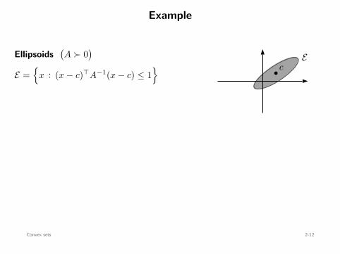
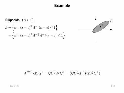
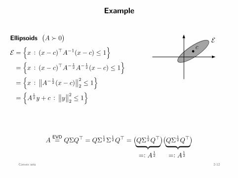
Example
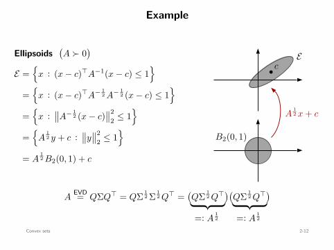
Ellipsoids
(A ≻ 0
)
E =
x : (x − c)⊤A−1(x − c) ≤ 1
=
x : (x − c)⊤A− 12 A− 1
2 (x − c) ≤ 1
=
x :∥∥A− 1
2 (x − c)∥∥2
2 ≤ 1
=
A12 y + c :
∥∥y∥∥2
2 ≤ 1
= A12 B2(0, 1) + c : convex
b cE
B2(0, 1)
A12 x + c
AEVD= QΣQ⊤ = QΣ 1
2 Σ 12 Q⊤ =
(QΣ 1
2 Q⊤)(QΣ 1
2 Q⊤)
=: A12 =: A
12
Convex sets 2-12

Example
Ellipsoids(A ≻ 0
)
E =
x : (x − c)⊤A−1(x − c) ≤ 1
=
x : (x − c)⊤A− 12 A− 1
2 (x − c) ≤ 1
=
x :∥∥A− 1
2 (x − c)∥∥2
2 ≤ 1
=
A12 y + c :
∥∥y∥∥2
2 ≤ 1
= A12 B2(0, 1) + c : convex
b cE
B2(0, 1)
A12 x + c
AEVD= QΣQ⊤ = QΣ 1
2 Σ 12 Q⊤ =
(QΣ 1
2 Q⊤)(QΣ 1
2 Q⊤)
=: A12 =: A
12
Convex sets 2-12
Example
Ellipsoids(A ≻ 0
)
E =
x : (x − c)⊤A−1(x − c) ≤ 1
=
x : (x − c)⊤A− 12 A− 1
2 (x − c) ≤ 1
=
x :∥∥A− 1
2 (x − c)∥∥2
2 ≤ 1
=
A12 y + c :
∥∥y∥∥2
2 ≤ 1
= A12 B2(0, 1) + c : convex
b cE
B2(0, 1)
A12 x + c
AEVD= QΣQ⊤ = QΣ 1
2 Σ 12 Q⊤ =
(QΣ 1
2 Q⊤)(QΣ 1
2 Q⊤)
=: A12 =: A
12
Convex sets 2-12

Example
Ellipsoids(A ≻ 0
)
E =
x : (x − c)⊤A−1(x − c) ≤ 1
=
x : (x − c)⊤A− 12 A− 1
2 (x − c) ≤ 1
=
x :∥∥A− 1
2 (x − c)∥∥2
2 ≤ 1
=
A12 y + c :
∥∥y∥∥2
2 ≤ 1
= A12 B2(0, 1) + c : convex
b cE
B2(0, 1)
A12 x + c
AEVD= QΣQ⊤ = QΣ 1
2 Σ 12 Q⊤ =
(QΣ 1
2 Q⊤)(QΣ 1
2 Q⊤)
=: A12 =: A
12
Convex sets 2-12

Example
Ellipsoids(A ≻ 0
)
E =
x : (x − c)⊤A−1(x − c) ≤ 1
=
x : (x − c)⊤A− 12 A− 1
2 (x − c) ≤ 1
=
x :∥∥A− 1
2 (x − c)∥∥2
2 ≤ 1
=
A12 y + c :
∥∥y∥∥2
2 ≤ 1
= A12 B2(0, 1) + c : convex
b cE
B2(0, 1)
A12 x + c
AEVD= QΣQ⊤
= QΣ 12 Σ 1
2 Q⊤ =(QΣ 1
2 Q⊤)(QΣ 1
2 Q⊤)
=: A12 =: A
12
Convex sets 2-12

Example
Ellipsoids(A ≻ 0
)
E =
x : (x − c)⊤A−1(x − c) ≤ 1
=
x : (x − c)⊤A− 12 A− 1
2 (x − c) ≤ 1
=
x :∥∥A− 1
2 (x − c)∥∥2
2 ≤ 1
=
A12 y + c :
∥∥y∥∥2
2 ≤ 1
= A12 B2(0, 1) + c : convex
b cE
B2(0, 1)
A12 x + c
AEVD= QΣQ⊤ = QΣ 1
2 Σ 12 Q⊤
=(QΣ 1
2 Q⊤)(QΣ 1
2 Q⊤)
=: A12 =: A
12
Convex sets 2-12
Example
Ellipsoids(A ≻ 0
)
E =
x : (x − c)⊤A−1(x − c) ≤ 1
=
x : (x − c)⊤A− 12 A− 1
2 (x − c) ≤ 1
=
x :∥∥A− 1
2 (x − c)∥∥2
2 ≤ 1
=
A12 y + c :
∥∥y∥∥2
2 ≤ 1
= A12 B2(0, 1) + c : convex
b cE
B2(0, 1)
A12 x + c
AEVD= QΣQ⊤ = QΣ 1
2 Σ 12 Q⊤ =
(QΣ 1
2 Q⊤)(QΣ 1
2 Q⊤)
=: A12 =: A
12
Convex sets 2-12

Example
Ellipsoids(A ≻ 0
)
E =
x : (x − c)⊤A−1(x − c) ≤ 1
=
x : (x − c)⊤A− 12 A− 1
2 (x − c) ≤ 1
=
x :∥∥A− 1
2 (x − c)∥∥2
2 ≤ 1
=
A12 y + c :
∥∥y∥∥2
2 ≤ 1
= A12 B2(0, 1) + c : convex
b cE
B2(0, 1)
A12 x + c
AEVD= QΣQ⊤ = QΣ 1
2 Σ 12 Q⊤ =
(QΣ 1
2 Q⊤)(QΣ 1
2 Q⊤)
=: A12 =: A
12
Convex sets 2-12

Example
Ellipsoids(A ≻ 0
)
E =
x : (x − c)⊤A−1(x − c) ≤ 1
=
x : (x − c)⊤A− 12 A− 1
2 (x − c) ≤ 1
=
x :∥∥A− 1
2 (x − c)∥∥2
2 ≤ 1
=
A12 y + c :
∥∥y∥∥2
2 ≤ 1
= A12 B2(0, 1) + c : convex
b cE
B2(0, 1)
A12 x + c
AEVD= QΣQ⊤ = QΣ 1
2 Σ 12 Q⊤ =
(QΣ 1
2 Q⊤)(QΣ 1
2 Q⊤)
=: A12 =: A
12
Convex sets 2-12
Example
Ellipsoids(A ≻ 0
)
E =
x : (x − c)⊤A−1(x − c) ≤ 1
=
x : (x − c)⊤A− 12 A− 1
2 (x − c) ≤ 1
=
x :∥∥A− 1
2 (x − c)∥∥2
2 ≤ 1
=
A12 y + c :
∥∥y∥∥2
2 ≤ 1
= A12 B2(0, 1) + c : convex
b cE
B2(0, 1)
A12 x + c
AEVD= QΣQ⊤ = QΣ 1
2 Σ 12 Q⊤ =
(QΣ 1
2 Q⊤)(QΣ 1
2 Q⊤)
=: A12 =: A
12
Convex sets 2-12

Example
Ellipsoids(A ≻ 0
)
E =
x : (x − c)⊤A−1(x − c) ≤ 1
=
x : (x − c)⊤A− 12 A− 1
2 (x − c) ≤ 1
=
x :∥∥A− 1
2 (x − c)∥∥2
2 ≤ 1
=
A12 y + c :
∥∥y∥∥2
2 ≤ 1
= A12 B2(0, 1) + c
: convex
b cE
B2(0, 1)
A12 x + c
AEVD= QΣQ⊤ = QΣ 1
2 Σ 12 Q⊤ =
(QΣ 1
2 Q⊤)(QΣ 1
2 Q⊤)
=: A12 =: A
12
Convex sets 2-12

Example
Ellipsoids(A ≻ 0
)
E =
x : (x − c)⊤A−1(x − c) ≤ 1
=
x : (x − c)⊤A− 12 A− 1
2 (x − c) ≤ 1
=
x :∥∥A− 1
2 (x − c)∥∥2
2 ≤ 1
=
A12 y + c :
∥∥y∥∥2
2 ≤ 1
= A12 B2(0, 1) + c
: convex
b cE
B2(0, 1)
A12 x + c
AEVD= QΣQ⊤ = QΣ 1
2 Σ 12 Q⊤ =
(QΣ 1
2 Q⊤)(QΣ 1
2 Q⊤)
=: A12 =: A
12
Convex sets 2-12
Example
Ellipsoids(A ≻ 0
)
E =
x : (x − c)⊤A−1(x − c) ≤ 1
=
x : (x − c)⊤A− 12 A− 1
2 (x − c) ≤ 1
=
x :∥∥A− 1
2 (x − c)∥∥2
2 ≤ 1
=
A12 y + c :
∥∥y∥∥2
2 ≤ 1
= A12 B2(0, 1) + c
: convex
b cE
B2(0, 1)
A12 x + c
AEVD= QΣQ⊤ = QΣ 1
2 Σ 12 Q⊤ =
(QΣ 1
2 Q⊤)(QΣ 1
2 Q⊤)
=: A12 =: A
12
Convex sets 2-12

Example
Ellipsoids(A ≻ 0
)
E =
x : (x − c)⊤A−1(x − c) ≤ 1
=
x : (x − c)⊤A− 12 A− 1
2 (x − c) ≤ 1
=
x :∥∥A− 1
2 (x − c)∥∥2
2 ≤ 1
=
A12 y + c :
∥∥y∥∥2
2 ≤ 1
= A12 B2(0, 1) + c : convex
b cE
B2(0, 1)
A12 x + c
AEVD= QΣQ⊤ = QΣ 1
2 Σ 12 Q⊤ =
(QΣ 1
2 Q⊤)(QΣ 1
2 Q⊤)
=: A12 =: A
12
Convex sets 2-12

Example
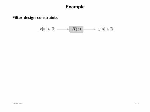
Filter design constraints
x[n] ∈ R y[n] ∈ RH(z)yref[n]
2ϵ
Goal: design H(z) such that maxn
∣∣y[n] − yref[n]∣∣ ≤ ϵ for a fixed x[n]
Assume finite impulse response (FIR):
y[n] = h0 x[n] + h1 x[n − 1] + · · · + hd x[n − d] , n = 1, . . . , N
Convex sets 2-13
Example
Filter design constraints
x[n] ∈ R y[n] ∈ RH(z)yref[n]
2ϵ
Goal: design H(z) such that maxn
∣∣y[n] − yref[n]∣∣ ≤ ϵ for a fixed x[n]
Assume finite impulse response (FIR):
y[n] = h0 x[n] + h1 x[n − 1] + · · · + hd x[n − d] , n = 1, . . . , N
Convex sets 2-13
Example
Filter design constraints
x[n] ∈ R y[n] ∈ RH(z)
yref[n]
2ϵ
Goal: design H(z) such that maxn
∣∣y[n] − yref[n]∣∣ ≤ ϵ for a fixed x[n]
Assume finite impulse response (FIR):
y[n] = h0 x[n] + h1 x[n − 1] + · · · + hd x[n − d] , n = 1, . . . , N
Convex sets 2-13

Example
Filter design constraints
x[n] ∈ R y[n] ∈ RH(z)
yref[n]
2ϵ
Goal: design H(z) such that maxn
∣∣y[n] − yref[n]∣∣ ≤ ϵ for a fixed x[n]
Assume finite impulse response (FIR):
y[n] = h0 x[n] + h1 x[n − 1] + · · · + hd x[n − d] , n = 1, . . . , N
Convex sets 2-13

Example
Filter design constraints
x[n] ∈ R y[n] ∈ RH(z)yref[n]
2ϵ
Goal: design H(z) such that maxn
∣∣y[n] − yref[n]∣∣ ≤ ϵ for a fixed x[n]
Assume finite impulse response (FIR):
y[n] = h0 x[n] + h1 x[n − 1] + · · · + hd x[n − d] , n = 1, . . . , N
Convex sets 2-13

Example
Filter design constraints
x[n] ∈ R y[n] ∈ RH(z)yref[n]
2ϵ
Goal: design H(z) such that maxn
∣∣y[n] − yref[n]∣∣ ≤ ϵ for a fixed x[n]
Assume finite impulse response (FIR):
y[n] = h0 x[n] + h1 x[n − 1] + · · · + hd x[n − d] , n = 1, . . . , N
Convex sets 2-13

Example
Filter design constraints
x[n] ∈ R y[n] ∈ RH(z)yref[n]
2ϵ
Goal: design H(z) such that maxn
∣∣y[n] − yref[n]∣∣ ≤ ϵ for a fixed x[n]
Assume finite impulse response (FIR):
y[n] = h0 x[n] + h1 x[n − 1] + · · · + hd x[n − d] , n = 1, . . . , N
Convex sets 2-13

Example
Filter design constraints
x[n] ∈ R y[n] ∈ RH(z)yref[n]
2ϵ
Goal: design H(z) such that maxn
∣∣y[n] − yref[n]∣∣ ≤ ϵ for a fixed x[n]
Assume finite impulse response (FIR):
y[n] = h0 x[n] + h1 x[n − 1] + · · · + hd x[n − d] , n = 1, . . . , N
Convex sets 2-13

Example
Filter design constraints
x[n] ∈ R y[n] ∈ RH(z)yref[n]
2ϵ
Goal: design H(z) such that maxn
∣∣y[n] − yref[n]∣∣ ≤ ϵ for a fixed x[n]
Assume finite impulse response (FIR):
y[n] = h0 x[n] + h1 x[n − 1] + · · · + hd x[n − d] , n = 1, . . . , N
Convex sets 2-13

Example
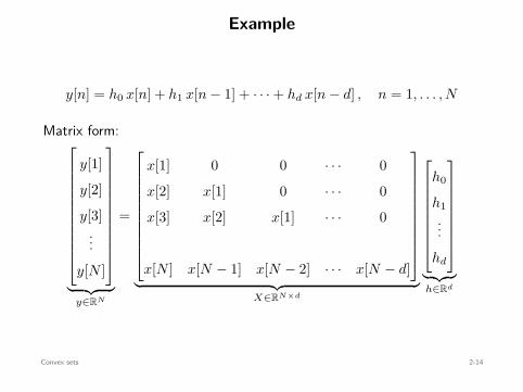
y[n] = h0 x[n] + h1 x[n − 1] + · · · + hd x[n − d] , n = 1, . . . , N
Matrix form:
y[1]
y[2]
y[3]...
y[N ]
︸ ︷︷ ︸y∈RN
=
x[1] 0 0 · · · 0
x[2] x[1] 0 · · · 0
x[3] x[2] x[1] · · · 0
x[N ] x[N − 1] x[N − 2] · · · x[N − d]
︸ ︷︷ ︸X∈RN×d
h0
h1...
hd
︸ ︷︷ ︸h∈Rd
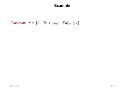
Constraint: S =
h ∈ Rd : ∥yref − Xh∥∞ ≤ ϵ
Convex sets 2-14
Example
y[n] = h0 x[n] + h1 x[n − 1] + · · · + hd x[n − d] , n = 1, . . . , N
Matrix form:
y[1]
y[2]
y[3]...
y[N ]
︸ ︷︷ ︸y∈RN
=
x[1] 0 0 · · · 0
x[2] x[1] 0 · · · 0
x[3] x[2] x[1] · · · 0
x[N ] x[N − 1] x[N − 2] · · · x[N − d]
︸ ︷︷ ︸X∈RN×d
h0
h1...
hd
︸ ︷︷ ︸h∈Rd
Constraint: S =
h ∈ Rd : ∥yref − Xh∥∞ ≤ ϵ
Convex sets 2-14
Example
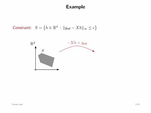
Constraint: S =
h ∈ Rd : ∥yref − Xh∥∞ ≤ ϵ
Rd
S
−Xh + yref RN
ϵ
B∞(0, ϵ)
convex⇐=convex
Convex sets 2-15

Example
Constraint: S =
h ∈ Rd : ∥yref − Xh∥∞ ≤ ϵ
Rd
S
−Xh + yref RN
ϵ
B∞(0, ϵ)
convex⇐=convex
Convex sets 2-15
Example
Constraint: S =
h ∈ Rd : ∥yref − Xh∥∞ ≤ ϵ
Rd
S
−Xh + yref
RN
ϵ
B∞(0, ϵ)
convex⇐=convex
Convex sets 2-15

Example
Constraint: S =
h ∈ Rd : ∥yref − Xh∥∞ ≤ ϵ
Rd
S
−Xh + yref RN
ϵ
B∞(0, ϵ)
convex⇐=convex
Convex sets 2-15

Example
Constraint: S =
h ∈ Rd : ∥yref − Xh∥∞ ≤ ϵ
Rd
S
−Xh + yref RN
ϵ
B∞(0, ϵ)
convex
⇐=convex
Convex sets 2-15

Example
Constraint: S =
h ∈ Rd : ∥yref − Xh∥∞ ≤ ϵ
Rd
S
−Xh + yref RN
ϵ
B∞(0, ϵ)
convex⇐=convex
Convex sets 2-15

Outline
Convex setsIdentifying convex setsExamples: geometrical sets and filter design constraints
Convex functionsIdentifying convex functionsRelation to convex sets
Optimization problemsConvex problems, properties, and problem manipulationExamples and solvers
Statistical estimationMaximum likelihood & maximum a posterioriNonparametric estimationHypothesis testing & optimal detection
Convex functions 2-1

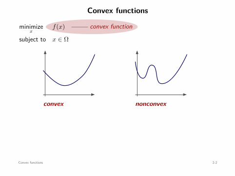
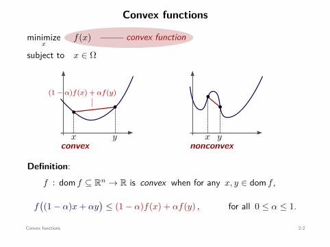
Convex functions
convex function
minimizex
f(x)
subject to x ∈ Ω
convex
bb
x y
(1 − α)f(x) + αf(y)
nonconvex
b
b
x y
Definition:f : dom f ⊆ Rn → R is convex when for any x, y ∈ dom f ,
f((1 − α)x + αy
)≤ (1 − α)f(x) + αf(y) , for all 0 ≤ α ≤ 1.
Convex functions 2-2
Convex functions
convex function
minimizex
f(x)
subject to x ∈ Ω
convex
bb
x y
(1 − α)f(x) + αf(y)
nonconvex
b
b
x y
Definition:f : dom f ⊆ Rn → R is convex when for any x, y ∈ dom f ,
f((1 − α)x + αy
)≤ (1 − α)f(x) + αf(y) , for all 0 ≤ α ≤ 1.
Convex functions 2-2

Convex functions
convex functionminimizex
f(x)
subject to x ∈ Ω
convex
bb
x y
(1 − α)f(x) + αf(y)
nonconvex
b
b
x y
Definition:f : dom f ⊆ Rn → R is convex when for any x, y ∈ dom f ,
f((1 − α)x + αy
)≤ (1 − α)f(x) + αf(y) , for all 0 ≤ α ≤ 1.
Convex functions 2-2

Convex functions
convex functionminimizex
f(x)
subject to x ∈ Ω
convex
bb
x y
(1 − α)f(x) + αf(y)
nonconvex
b
b
x y
Definition:f : dom f ⊆ Rn → R is convex when for any x, y ∈ dom f ,
f((1 − α)x + αy
)≤ (1 − α)f(x) + αf(y) , for all 0 ≤ α ≤ 1.
Convex functions 2-2
Convex functions
convex functionminimizex
f(x)
subject to x ∈ Ω
convex
bb
x y
(1 − α)f(x) + αf(y)
nonconvex
b
b
x y
Definition:f : dom f ⊆ Rn → R is convex when for any x, y ∈ dom f ,
f((1 − α)x + αy
)≤ (1 − α)f(x) + αf(y) , for all 0 ≤ α ≤ 1.
Convex functions 2-2

Convex functions
convex functionminimizex
f(x)
subject to x ∈ Ω
convex
bb
x y
(1 − α)f(x) + αf(y)
nonconvex
b
b
x y
Definition:f : dom f ⊆ Rn → R is convex when for any x, y ∈ dom f ,
f((1 − α)x + αy
)≤ (1 − α)f(x) + αf(y) , for all 0 ≤ α ≤ 1.
Convex functions 2-2

Convex functions
convex functionminimizex
f(x)
subject to x ∈ Ω
convex
bb
x y
(1 − α)f(x) + αf(y)
nonconvex
b
b
x y
Definition:f : dom f ⊆ Rn → R is convex when for any x, y ∈ dom f ,
f((1 − α)x + αy
)≤ (1 − α)f(x) + αf(y) , for all 0 ≤ α ≤ 1.
Convex functions 2-2

Convex functions
convex functionminimizex
f(x)
subject to x ∈ Ω
convex
bb
x y
(1 − α)f(x) + αf(y)
nonconvex
b
b
x y
Definition:f : dom f ⊆ Rn → R is convex when for any x, y ∈ dom f ,
f((1 − α)x + αy
)≤ (1 − α)f(x) + αf(y) , for all 0 ≤ α ≤ 1.
Convex functions 2-2
Convex functions
convex functionminimizex
f(x)
subject to x ∈ Ω
convex
bb
x y
(1 − α)f(x) + αf(y)
nonconvex
b
b
x y
Definition:f : dom f ⊆ Rn → R is convex when for any x, y ∈ dom f ,
f((1 − α)x + αy
)≤ (1 − α)f(x) + αf(y) , for all 0 ≤ α ≤ 1.
Convex functions 2-2

Convex functions
convex functionminimizex
f(x)
subject to x ∈ Ω
convex
bb
x y
(1 − α)f(x) + αf(y)
nonconvex
b
b
x y
Definition:f : dom f ⊆ Rn → R is convex when for any x, y ∈ dom f ,
f((1 − α)x + αy
)≤ (1 − α)f(x) + αf(y) , for all 0 ≤ α ≤ 1.
Convex functions 2-2

Convex functions
convex functionminimizex
f(x)
subject to x ∈ Ω
convex
bb
x y
(1 − α)f(x) + αf(y)
nonconvex
b
b
x y
Definition:f : dom f ⊆ Rn → R is convex when for any x, y ∈ dom f ,
f((1 − α)x + αy
)≤ (1 − α)f(x) + αf(y) , for all 0 ≤ α ≤ 1.
Convex functions 2-2
Convex functions
convex functionminimizex
f(x)
subject to x ∈ Ω
convex
bb
x y
(1 − α)f(x) + αf(y)
nonconvex
b
b
x y
Definition:f : dom f ⊆ Rn → R is convex when for any x, y ∈ dom f ,
f((1 − α)x + αy
)≤ (1 − α)f(x) + αf(y) , for all 0 ≤ α ≤ 1.
Convex functions 2-2

How to identify convex functions?
definitiondifferentiability conds.1D convexity
operations preserving convexity
vocabulary + grammar
Convex functions 2-3

How to identify convex functions?
definitiondifferentiability conds.1D convexity
operations preserving convexity
vocabulary + grammar
Convex functions 2-3

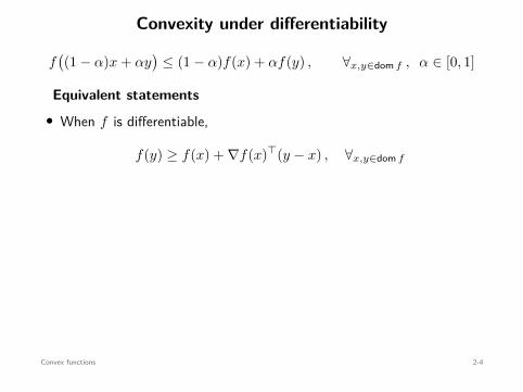
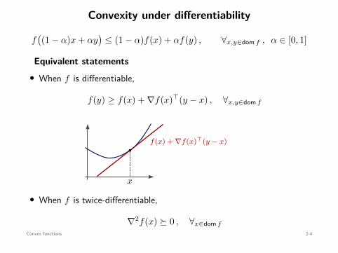
Convexity under differentiability
f((1 − α)x + αy
)≤ (1 − α)f(x) + αf(y) , ∀x,y∈dom f , α ∈ [0, 1]
Equivalent statements• When f is differentiable,
f(y) ≥ f(x) + ∇f(x)⊤(y − x) , ∀x,y∈dom f
f(x) + ∇f(x)⊤(y − x)b
x
• When f is twice-differentiable,
∇2f(x) ⪰ 0 , ∀x∈dom f
Convex functions 2-4

Convexity under differentiability
f((1 − α)x + αy
)≤ (1 − α)f(x) + αf(y) , ∀x,y∈dom f , α ∈ [0, 1]
Equivalent statements• When f is differentiable,
f(y) ≥ f(x) + ∇f(x)⊤(y − x) , ∀x,y∈dom f
f(x) + ∇f(x)⊤(y − x)b
x
• When f is twice-differentiable,
∇2f(x) ⪰ 0 , ∀x∈dom f
Convex functions 2-4

Convexity under differentiability
f((1 − α)x + αy
)≤ (1 − α)f(x) + αf(y) , ∀x,y∈dom f , α ∈ [0, 1]
Equivalent statements
• When f is differentiable,
f(y) ≥ f(x) + ∇f(x)⊤(y − x) , ∀x,y∈dom f
f(x) + ∇f(x)⊤(y − x)b
x
• When f is twice-differentiable,
∇2f(x) ⪰ 0 , ∀x∈dom f
Convex functions 2-4

Convexity under differentiability
f((1 − α)x + αy
)≤ (1 − α)f(x) + αf(y) , ∀x,y∈dom f , α ∈ [0, 1]
Equivalent statements• When f is differentiable,
f(y) ≥ f(x) + ∇f(x)⊤(y − x) , ∀x,y∈dom f
f(x) + ∇f(x)⊤(y − x)b
x
• When f is twice-differentiable,
∇2f(x) ⪰ 0 , ∀x∈dom f
Convex functions 2-4
Convexity under differentiability
f((1 − α)x + αy
)≤ (1 − α)f(x) + αf(y) , ∀x,y∈dom f , α ∈ [0, 1]
Equivalent statements• When f is differentiable,
f(y) ≥ f(x) + ∇f(x)⊤(y − x) , ∀x,y∈dom f
f(x) + ∇f(x)⊤(y − x)b
x
• When f is twice-differentiable,
∇2f(x) ⪰ 0 , ∀x∈dom f
Convex functions 2-4

Convexity under differentiability
f((1 − α)x + αy
)≤ (1 − α)f(x) + αf(y) , ∀x,y∈dom f , α ∈ [0, 1]
Equivalent statements• When f is differentiable,
f(y) ≥ f(x) + ∇f(x)⊤(y − x) , ∀x,y∈dom f
f(x) + ∇f(x)⊤(y − x)b
x
• When f is twice-differentiable,
∇2f(x) ⪰ 0 , ∀x∈dom f
Convex functions 2-4

Convexity under differentiability
f((1 − α)x + αy
)≤ (1 − α)f(x) + αf(y) , ∀x,y∈dom f , α ∈ [0, 1]
Equivalent statements• When f is differentiable,
f(y) ≥ f(x) + ∇f(x)⊤(y − x) , ∀x,y∈dom f
f(x) + ∇f(x)⊤(y − x)
b
x
• When f is twice-differentiable,
∇2f(x) ⪰ 0 , ∀x∈dom f
Convex functions 2-4

Convexity under differentiability
f((1 − α)x + αy
)≤ (1 − α)f(x) + αf(y) , ∀x,y∈dom f , α ∈ [0, 1]
Equivalent statements• When f is differentiable,
f(y) ≥ f(x) + ∇f(x)⊤(y − x) , ∀x,y∈dom f
f(x) + ∇f(x)⊤(y − x)b
x
• When f is twice-differentiable,
∇2f(x) ⪰ 0 , ∀x∈dom f
Convex functions 2-4
Convexity under differentiability
f((1 − α)x + αy
)≤ (1 − α)f(x) + αf(y) , ∀x,y∈dom f , α ∈ [0, 1]
Equivalent statements• When f is differentiable,
f(y) ≥ f(x) + ∇f(x)⊤(y − x) , ∀x,y∈dom f
f(x) + ∇f(x)⊤(y − x)b
x
• When f is twice-differentiable,
∇2f(x) ⪰ 0 , ∀x∈dom f
Convex functions 2-4

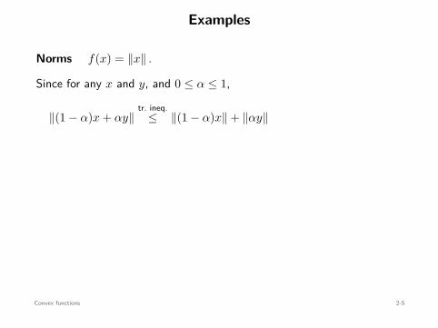
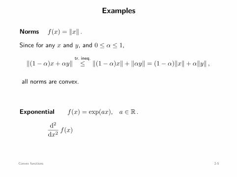
Examples
Norms f(x) = ∥x∥ .
Since for any x and y, and 0 ≤ α ≤ 1,
∥(1 − α)x + αy∥tr. ineq.
≤ ∥(1 − α)x∥ + ∥αy∥ = (1 − α)∥x∥ + α∥y∥ ,
all norms are convex.
Exponential f(x) = exp(ax), a ∈ R .
d2
dx2 f(x) = a2 exp(ax) ≥ 0 =⇒ f : convex
Convex functions 2-5
Examples
Norms f(x) = ∥x∥ .
Since for any x and y, and 0 ≤ α ≤ 1,
∥(1 − α)x + αy∥tr. ineq.
≤ ∥(1 − α)x∥ + ∥αy∥ = (1 − α)∥x∥ + α∥y∥ ,
all norms are convex.
Exponential f(x) = exp(ax), a ∈ R .
d2
dx2 f(x) = a2 exp(ax) ≥ 0 =⇒ f : convex
Convex functions 2-5

Examples
Norms f(x) = ∥x∥ .
Since for any x and y, and 0 ≤ α ≤ 1,
∥(1 − α)x + αy∥
tr. ineq.≤ ∥(1 − α)x∥ + ∥αy∥ = (1 − α)∥x∥ + α∥y∥ ,
all norms are convex.
Exponential f(x) = exp(ax), a ∈ R .
d2
dx2 f(x) = a2 exp(ax) ≥ 0 =⇒ f : convex
Convex functions 2-5
Examples
Norms f(x) = ∥x∥ .
Since for any x and y, and 0 ≤ α ≤ 1,
∥(1 − α)x + αy∥tr. ineq.
≤ ∥(1 − α)x∥ + ∥αy∥
= (1 − α)∥x∥ + α∥y∥ ,
all norms are convex.
Exponential f(x) = exp(ax), a ∈ R .
d2
dx2 f(x) = a2 exp(ax) ≥ 0 =⇒ f : convex
Convex functions 2-5

Examples
Norms f(x) = ∥x∥ .
Since for any x and y, and 0 ≤ α ≤ 1,
∥(1 − α)x + αy∥tr. ineq.
≤ ∥(1 − α)x∥ + ∥αy∥ = (1 − α)∥x∥ + α∥y∥ ,
all norms are convex.
Exponential f(x) = exp(ax), a ∈ R .
d2
dx2 f(x) = a2 exp(ax) ≥ 0 =⇒ f : convex
Convex functions 2-5

Examples
Norms f(x) = ∥x∥ .
Since for any x and y, and 0 ≤ α ≤ 1,
∥(1 − α)x + αy∥tr. ineq.
≤ ∥(1 − α)x∥ + ∥αy∥ = (1 − α)∥x∥ + α∥y∥ ,
all norms are convex.
Exponential f(x) = exp(ax), a ∈ R .
d2
dx2 f(x) = a2 exp(ax) ≥ 0 =⇒ f : convex
Convex functions 2-5

Examples
Norms f(x) = ∥x∥ .
Since for any x and y, and 0 ≤ α ≤ 1,
∥(1 − α)x + αy∥tr. ineq.
≤ ∥(1 − α)x∥ + ∥αy∥ = (1 − α)∥x∥ + α∥y∥ ,
all norms are convex.
Exponential
f(x) = exp(ax), a ∈ R .
d2
dx2 f(x) = a2 exp(ax) ≥ 0 =⇒ f : convex
Convex functions 2-5

Examples
Norms f(x) = ∥x∥ .
Since for any x and y, and 0 ≤ α ≤ 1,
∥(1 − α)x + αy∥tr. ineq.
≤ ∥(1 − α)x∥ + ∥αy∥ = (1 − α)∥x∥ + α∥y∥ ,
all norms are convex.
Exponential f(x) = exp(ax), a ∈ R .
d2
dx2 f(x) = a2 exp(ax) ≥ 0 =⇒ f : convex
Convex functions 2-5
Examples
Norms f(x) = ∥x∥ .
Since for any x and y, and 0 ≤ α ≤ 1,
∥(1 − α)x + αy∥tr. ineq.
≤ ∥(1 − α)x∥ + ∥αy∥ = (1 − α)∥x∥ + α∥y∥ ,
all norms are convex.
Exponential f(x) = exp(ax), a ∈ R .
d2
dx2 f(x)
= a2 exp(ax) ≥ 0 =⇒ f : convex
Convex functions 2-5

Examples
Norms f(x) = ∥x∥ .
Since for any x and y, and 0 ≤ α ≤ 1,
∥(1 − α)x + αy∥tr. ineq.
≤ ∥(1 − α)x∥ + ∥αy∥ = (1 − α)∥x∥ + α∥y∥ ,
all norms are convex.
Exponential f(x) = exp(ax), a ∈ R .
d2
dx2 f(x) = a2 exp(ax) ≥ 0
=⇒ f : convex
Convex functions 2-5

Examples
Norms f(x) = ∥x∥ .
Since for any x and y, and 0 ≤ α ≤ 1,
∥(1 − α)x + αy∥tr. ineq.
≤ ∥(1 − α)x∥ + ∥αy∥ = (1 − α)∥x∥ + α∥y∥ ,
all norms are convex.
Exponential f(x) = exp(ax), a ∈ R .
d2
dx2 f(x) = a2 exp(ax) ≥ 0 =⇒ f : convex
Convex functions 2-5

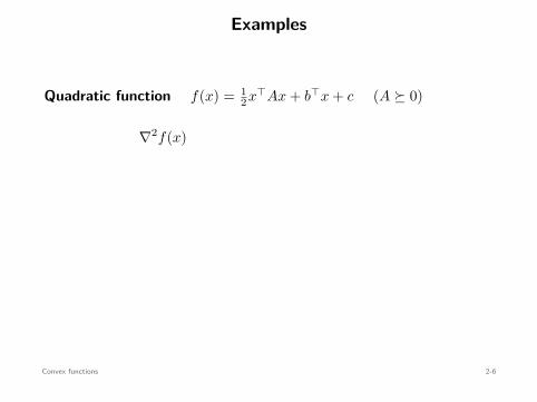
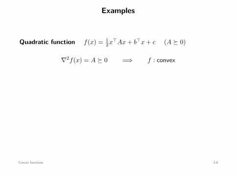
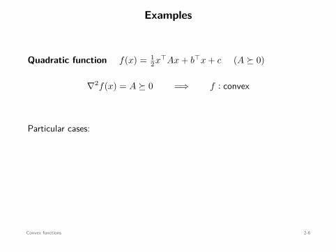
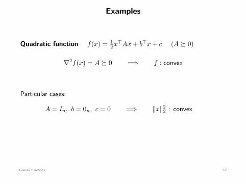
Examples
Quadratic function f(x) = 12 x⊤Ax + b⊤x + c (A ⪰ 0)
∇2f(x) = A ⪰ 0 =⇒ f : convex
Particular cases:
A = In, b = 0n, c = 0 =⇒ ∥x∥22 : convex
A = 0n×n =⇒ b⊤x + c : convex
Convex functions 2-6
Examples
Quadratic function f(x) = 12 x⊤Ax + b⊤x + c (A ⪰ 0)
∇2f(x)
= A ⪰ 0 =⇒ f : convex
Particular cases:
A = In, b = 0n, c = 0 =⇒ ∥x∥22 : convex
A = 0n×n =⇒ b⊤x + c : convex
Convex functions 2-6

Examples
Quadratic function f(x) = 12 x⊤Ax + b⊤x + c (A ⪰ 0)
∇2f(x) = A ⪰ 0
=⇒ f : convex
Particular cases:
A = In, b = 0n, c = 0 =⇒ ∥x∥22 : convex
A = 0n×n =⇒ b⊤x + c : convex
Convex functions 2-6
Examples
Quadratic function f(x) = 12 x⊤Ax + b⊤x + c (A ⪰ 0)
∇2f(x) = A ⪰ 0 =⇒ f : convex
Particular cases:
A = In, b = 0n, c = 0 =⇒ ∥x∥22 : convex
A = 0n×n =⇒ b⊤x + c : convex
Convex functions 2-6
Examples
Quadratic function f(x) = 12 x⊤Ax + b⊤x + c (A ⪰ 0)
∇2f(x) = A ⪰ 0 =⇒ f : convex
Particular cases:
A = In, b = 0n, c = 0 =⇒ ∥x∥22 : convex
A = 0n×n =⇒ b⊤x + c : convex
Convex functions 2-6

Examples
Quadratic function f(x) = 12 x⊤Ax + b⊤x + c (A ⪰ 0)
∇2f(x) = A ⪰ 0 =⇒ f : convex
Particular cases:
A = In, b = 0n, c = 0
=⇒ ∥x∥22 : convex
A = 0n×n =⇒ b⊤x + c : convex
Convex functions 2-6
Examples
Quadratic function f(x) = 12 x⊤Ax + b⊤x + c (A ⪰ 0)
∇2f(x) = A ⪰ 0 =⇒ f : convex
Particular cases:
A = In, b = 0n, c = 0 =⇒ ∥x∥22 : convex
A = 0n×n =⇒ b⊤x + c : convex
Convex functions 2-6

Examples
Quadratic function f(x) = 12 x⊤Ax + b⊤x + c (A ⪰ 0)
∇2f(x) = A ⪰ 0 =⇒ f : convex
Particular cases:
A = In, b = 0n, c = 0 =⇒ ∥x∥22 : convex
A = 0n×n
=⇒ b⊤x + c : convex
Convex functions 2-6

Examples
Quadratic function f(x) = 12 x⊤Ax + b⊤x + c (A ⪰ 0)
∇2f(x) = A ⪰ 0 =⇒ f : convex
Particular cases:
A = In, b = 0n, c = 0 =⇒ ∥x∥22 : convex
A = 0n×n =⇒ b⊤x + c : convex
Convex functions 2-6

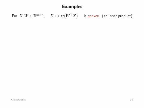
Examples
For X, W ∈ Rm×n, X 7→ tr(W ⊤X
)
is convex (an inner product)
tr(W ⊤X
)=
n∑
k=1
(W ⊤X
)kk
=n∑
k=1
m∑
i=1WikXik =
W11...
Wm1...
W1n
...Wmn
⊤
X11...
Xm1...
X1n
...Xmn
= vec(W )⊤vec(X)
Convex functions 2-7
Examples
For X, W ∈ Rm×n, X 7→ tr(W ⊤X
)is convex (an inner product)
tr(W ⊤X
)=
n∑
k=1
(W ⊤X
)kk
=n∑
k=1
m∑
i=1WikXik =
W11...
Wm1...
W1n
...Wmn
⊤
X11...
Xm1...
X1n
...Xmn
= vec(W )⊤vec(X)
Convex functions 2-7

Examples
For X, W ∈ Rm×n, X 7→ tr(W ⊤X
)is convex (an inner product)
tr(W ⊤X
)=
n∑
k=1
(W ⊤X
)kk
=n∑
k=1
m∑
i=1WikXik =
W11...
Wm1...
W1n
...Wmn
⊤
X11...
Xm1...
X1n
...Xmn
= vec(W )⊤vec(X)
Convex functions 2-7

Examples
For X, W ∈ Rm×n, X 7→ tr(W ⊤X
)is convex (an inner product)
tr(W ⊤X
)=
n∑
k=1
(W ⊤X
)kk
=n∑
k=1
m∑
i=1WikXik
=
W11...
Wm1...
W1n
...Wmn
⊤
X11...
Xm1...
X1n
...Xmn
= vec(W )⊤vec(X)
Convex functions 2-7

Examples
For X, W ∈ Rm×n, X 7→ tr(W ⊤X
)is convex (an inner product)
tr(W ⊤X
)=
n∑
k=1
(W ⊤X
)kk
=n∑
k=1
m∑
i=1WikXik =
W11...
Wm1...
W1n
...Wmn
⊤
X11...
Xm1...
X1n
...Xmn
= vec(W )⊤vec(X)
Convex functions 2-7

Examples
For X, W ∈ Rm×n, X 7→ tr(W ⊤X
)is convex (an inner product)
tr(W ⊤X
)=
n∑
k=1
(W ⊤X
)kk
=n∑
k=1
m∑
i=1WikXik =
W11...
Wm1...
W1n
...Wmn
⊤
X11...
Xm1...
X1n
...Xmn
= vec(W )⊤vec(X)Convex functions 2-7
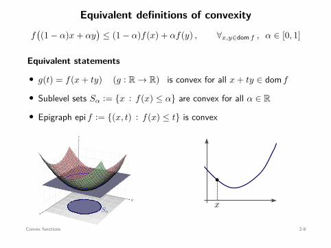
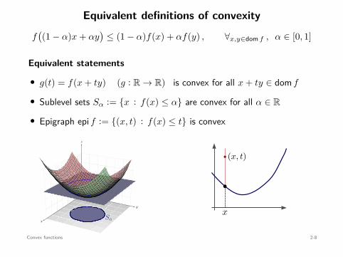
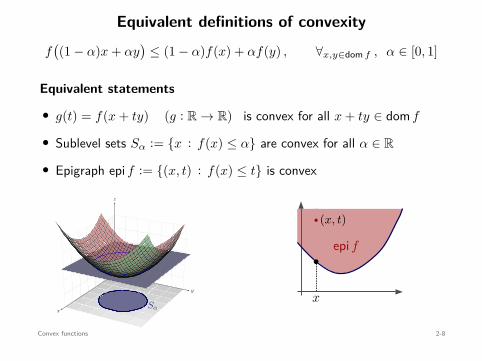
Equivalent definitions of convexity
f((1 − α)x + αy
)≤ (1 − α)f(x) + αf(y) , ∀x,y∈dom f , α ∈ [0, 1]
Equivalent statements
• g(t) = f(x + ty) (g : R → R) is convex for all x + ty ∈ dom f
• Sublevel sets Sα := x : f(x) ≤ α are convex for all α ∈ R
• Epigraph epi f := (x, t) : f(x) ≤ t is convex
x
y
z
Sα
b
x
b (x, t)
epi f
Convex functions 2-8

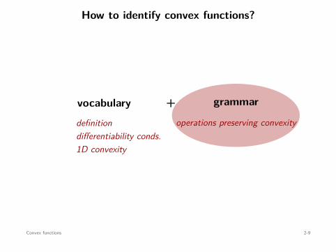
How to identify convex functions?
definitiondifferentiability conds.1D convexity
operations preserving convexity
vocabulary + grammar
Convex functions 2-9
How to identify convex functions?
definitiondifferentiability conds.1D convexity
operations preserving convexity
vocabulary + grammar
Convex functions 2-9

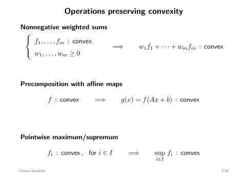
Operations preserving convexity
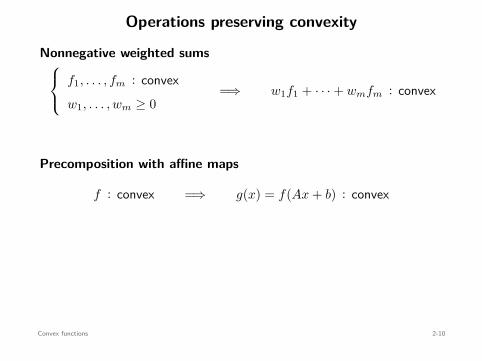
Nonnegative weighted sums
f1, . . . , fm : convexw1, . . . , wm ≥ 0
=⇒ w1f1 + · · · + wmfm : convex
Precomposition with affine maps
f : convex =⇒ g(x) = f(Ax + b) : convex
Pointwise maximum/supremum
fi : convex , for i ∈ I =⇒ supi∈I
fi : convex
Convex functions 2-10
Operations preserving convexity
Nonnegative weighted sums
f1, . . . , fm : convexw1, . . . , wm ≥ 0
=⇒ w1f1 + · · · + wmfm : convex
Precomposition with affine maps
f : convex =⇒ g(x) = f(Ax + b) : convex
Pointwise maximum/supremum
fi : convex , for i ∈ I =⇒ supi∈I
fi : convex
Convex functions 2-10
Operations preserving convexity
Nonnegative weighted sums
f1, . . . , fm : convexw1, . . . , wm ≥ 0
=⇒ w1f1 + · · · + wmfm : convex
Precomposition with affine maps
f : convex =⇒ g(x) = f(Ax + b) : convex
Pointwise maximum/supremum
fi : convex , for i ∈ I =⇒ supi∈I
fi : convex
Convex functions 2-10

Operations preserving convexity
Nonnegative weighted sums
f1, . . . , fm : convexw1, . . . , wm ≥ 0
=⇒ w1f1 + · · · + wmfm : convex
Precomposition with affine maps
f : convex =⇒ g(x) = f(Ax + b) : convex
Pointwise maximum/supremum
fi : convex , for i ∈ I =⇒ supi∈I
fi : convex
Convex functions 2-10

Operations preserving convexity
Nonnegative weighted sums
f1, . . . , fm : convexw1, . . . , wm ≥ 0
=⇒ w1f1 + · · · + wmfm : convex
Precomposition with affine maps
f : convex =⇒ g(x) = f(Ax + b) : convex
Pointwise maximum/supremum
fi : convex , for i ∈ I =⇒ supi∈I
fi : convex
Convex functions 2-10

Operations preserving convexity
Nonnegative weighted sums
f1, . . . , fm : convexw1, . . . , wm ≥ 0
=⇒ w1f1 + · · · + wmfm : convex
Precomposition with affine maps
f : convex
=⇒ g(x) = f(Ax + b) : convex
Pointwise maximum/supremum
fi : convex , for i ∈ I =⇒ supi∈I
fi : convex
Convex functions 2-10
Operations preserving convexity
Nonnegative weighted sums
f1, . . . , fm : convexw1, . . . , wm ≥ 0
=⇒ w1f1 + · · · + wmfm : convex
Precomposition with affine maps
f : convex =⇒ g(x) = f(Ax + b) : convex
Pointwise maximum/supremum
fi : convex , for i ∈ I =⇒ supi∈I
fi : convex
Convex functions 2-10

Operations preserving convexity
Nonnegative weighted sums
f1, . . . , fm : convexw1, . . . , wm ≥ 0
=⇒ w1f1 + · · · + wmfm : convex
Precomposition with affine maps
f : convex =⇒ g(x) = f(Ax + b) : convex
Pointwise maximum/supremum
fi : convex , for i ∈ I =⇒ supi∈I
fi : convex
Convex functions 2-10

Operations preserving convexity
Nonnegative weighted sums
f1, . . . , fm : convexw1, . . . , wm ≥ 0
=⇒ w1f1 + · · · + wmfm : convex
Precomposition with affine maps
f : convex =⇒ g(x) = f(Ax + b) : convex
Pointwise maximum/supremum
fi : convex , for i ∈ I
=⇒ supi∈I
fi : convex
Convex functions 2-10
Operations preserving convexity
Nonnegative weighted sums
f1, . . . , fm : convexw1, . . . , wm ≥ 0
=⇒ w1f1 + · · · + wmfm : convex
Precomposition with affine maps
f : convex =⇒ g(x) = f(Ax + b) : convex
Pointwise maximum/supremum
fi : convex , for i ∈ I =⇒ supi∈I
fi : convex
Convex functions 2-10

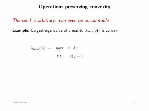
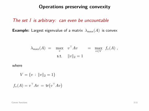
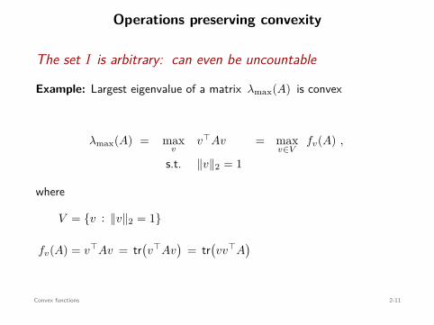
Operations preserving convexity
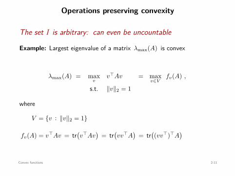
The set I is arbitrary: can even be uncountable
Example: Largest eigenvalue of a matrix λmax(A) is convex
λmax(A) = maxv
v⊤Av
s.t. ∥v∥2 = 1
= maxv∈V
fv(A) ,
where
V = v : ∥v∥2 = 1
fv(A) = v⊤Av = tr(v⊤Av
)= tr
(vv⊤A
)= tr
((vv⊤)⊤A
): convex
Convex functions 2-11

Operations preserving convexity
The set I is arbitrary: can even be uncountable
Example: Largest eigenvalue of a matrix λmax(A) is convex
λmax(A) = maxv
v⊤Av
s.t. ∥v∥2 = 1
= maxv∈V
fv(A) ,
where
V = v : ∥v∥2 = 1
fv(A) = v⊤Av = tr(v⊤Av
)= tr
(vv⊤A
)= tr
((vv⊤)⊤A
): convex
Convex functions 2-11
Operations preserving convexity
The set I is arbitrary: can even be uncountable
Example: Largest eigenvalue of a matrix λmax(A) is convex
λmax(A) = maxv
v⊤Av
s.t. ∥v∥2 = 1
= maxv∈V
fv(A) ,
where
V = v : ∥v∥2 = 1
fv(A) = v⊤Av = tr(v⊤Av
)= tr
(vv⊤A
)= tr
((vv⊤)⊤A
): convex
Convex functions 2-11

Operations preserving convexity
The set I is arbitrary: can even be uncountable
Example: Largest eigenvalue of a matrix λmax(A) is convex
λmax(A) = maxv
v⊤Av
s.t. ∥v∥2 = 1
= maxv∈V
fv(A) ,
where
V = v : ∥v∥2 = 1
fv(A) = v⊤Av = tr(v⊤Av
)= tr
(vv⊤A
)= tr
((vv⊤)⊤A
): convex
Convex functions 2-11

Operations preserving convexity
The set I is arbitrary: can even be uncountable
Example: Largest eigenvalue of a matrix λmax(A) is convex
λmax(A) = maxv
v⊤Av
s.t. ∥v∥2 = 1
= maxv∈V
fv(A) ,
where
V = v : ∥v∥2 = 1
fv(A) = v⊤Av = tr(v⊤Av
)= tr
(vv⊤A
)= tr
((vv⊤)⊤A
): convex
Convex functions 2-11

Operations preserving convexity
The set I is arbitrary: can even be uncountable
Example: Largest eigenvalue of a matrix λmax(A) is convex
λmax(A) = maxv
v⊤Av
s.t. ∥v∥2 = 1
= maxv∈V
fv(A) ,
where
V = v : ∥v∥2 = 1
fv(A) = v⊤Av
= tr(v⊤Av
)= tr
(vv⊤A
)= tr
((vv⊤)⊤A
): convex
Convex functions 2-11
Operations preserving convexity
The set I is arbitrary: can even be uncountable
Example: Largest eigenvalue of a matrix λmax(A) is convex
λmax(A) = maxv
v⊤Av
s.t. ∥v∥2 = 1
= maxv∈V
fv(A) ,
where
V = v : ∥v∥2 = 1
fv(A) = v⊤Av = tr(v⊤Av
)
= tr(vv⊤A
)= tr
((vv⊤)⊤A
): convex
Convex functions 2-11
Operations preserving convexity
The set I is arbitrary: can even be uncountable
Example: Largest eigenvalue of a matrix λmax(A) is convex
λmax(A) = maxv
v⊤Av
s.t. ∥v∥2 = 1
= maxv∈V
fv(A) ,
where
V = v : ∥v∥2 = 1
fv(A) = v⊤Av = tr(v⊤Av
)= tr
(vv⊤A
)
= tr((vv⊤)⊤A
): convex
Convex functions 2-11
Operations preserving convexity
The set I is arbitrary: can even be uncountable
Example: Largest eigenvalue of a matrix λmax(A) is convex
λmax(A) = maxv
v⊤Av
s.t. ∥v∥2 = 1
= maxv∈V
fv(A) ,
where
V = v : ∥v∥2 = 1
fv(A) = v⊤Av = tr(v⊤Av
)= tr
(vv⊤A
)= tr
((vv⊤)⊤A
)
: convex
Convex functions 2-11

Operations preserving convexity
The set I is arbitrary: can even be uncountable
Example: Largest eigenvalue of a matrix λmax(A) is convex
λmax(A) = maxv
v⊤Av
s.t. ∥v∥2 = 1
= maxv∈V
fv(A) ,
where
V = v : ∥v∥2 = 1
fv(A) = v⊤Av = tr(v⊤Av
)= tr
(vv⊤A
)= tr
((vv⊤)⊤A
): convex
Convex functions 2-11

Examples
• f(x) =∥∥y − Ax
∥∥22 = g(h(x)) : convex
h(x) = −Ax + y affine
g(z) = ∥z∥22 convex
• f(x) =∥∥y − Ax
∥∥1 = g(h(x)) : convex
h(x) = −Ax + y affine
g(z) = ∥z∥1 convex
Convex functions 2-12

Examples
• f(x) =∥∥y − Ax
∥∥22
= g(h(x)) : convex
h(x) = −Ax + y affine
g(z) = ∥z∥22 convex
• f(x) =∥∥y − Ax
∥∥1 = g(h(x)) : convex
h(x) = −Ax + y affine
g(z) = ∥z∥1 convex
Convex functions 2-12
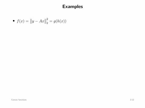
Examples
• f(x) =∥∥y − Ax
∥∥22 = g(h(x))
: convex
h(x) = −Ax + y affine
g(z) = ∥z∥22 convex
• f(x) =∥∥y − Ax
∥∥1 = g(h(x)) : convex
h(x) = −Ax + y affine
g(z) = ∥z∥1 convex
Convex functions 2-12

Examples
• f(x) =∥∥y − Ax
∥∥22 = g(h(x))
: convex
h(x) = −Ax + y
affine
g(z) = ∥z∥22 convex
• f(x) =∥∥y − Ax
∥∥1 = g(h(x)) : convex
h(x) = −Ax + y affine
g(z) = ∥z∥1 convex
Convex functions 2-12

Examples
• f(x) =∥∥y − Ax
∥∥22 = g(h(x))
: convex
h(x) = −Ax + y affine
g(z) = ∥z∥22 convex
• f(x) =∥∥y − Ax
∥∥1 = g(h(x)) : convex
h(x) = −Ax + y affine
g(z) = ∥z∥1 convex
Convex functions 2-12

Examples
• f(x) =∥∥y − Ax
∥∥22 = g(h(x))
: convex
h(x) = −Ax + y affine
g(z) = ∥z∥22
convex
• f(x) =∥∥y − Ax
∥∥1 = g(h(x)) : convex
h(x) = −Ax + y affine
g(z) = ∥z∥1 convex
Convex functions 2-12

Examples
• f(x) =∥∥y − Ax
∥∥22 = g(h(x))
: convex
h(x) = −Ax + y affine
g(z) = ∥z∥22 convex
• f(x) =∥∥y − Ax
∥∥1 = g(h(x)) : convex
h(x) = −Ax + y affine
g(z) = ∥z∥1 convex
Convex functions 2-12
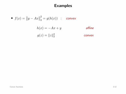
Examples
• f(x) =∥∥y − Ax
∥∥22 = g(h(x)) : convex
h(x) = −Ax + y affine
g(z) = ∥z∥22 convex
• f(x) =∥∥y − Ax
∥∥1 = g(h(x)) : convex
h(x) = −Ax + y affine
g(z) = ∥z∥1 convex
Convex functions 2-12
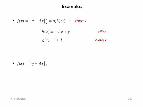
Examples
• f(x) =∥∥y − Ax
∥∥22 = g(h(x)) : convex
h(x) = −Ax + y affine
g(z) = ∥z∥22 convex
• f(x) =∥∥y − Ax
∥∥1
= g(h(x)) : convex
h(x) = −Ax + y affine
g(z) = ∥z∥1 convex
Convex functions 2-12

Examples
• f(x) =∥∥y − Ax
∥∥22 = g(h(x)) : convex
h(x) = −Ax + y affine
g(z) = ∥z∥22 convex
• f(x) =∥∥y − Ax
∥∥1 = g(h(x)) : convex
h(x) = −Ax + y affine
g(z) = ∥z∥1 convex
Convex functions 2-12
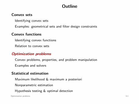
Outline
Convex setsIdentifying convex setsExamples: geometrical sets and filter design constraints
Convex functionsIdentifying convex functionsRelation to convex sets
Optimization problemsConvex problems, properties, and problem manipulationExamples and solvers
Statistical estimationMaximum likelihood & maximum a posterioriNonparametric estimationHypothesis testing & optimal detection
Optimization problems 3-1

Convex optimization problems
minimizex
f(x)
subject to gi(x) ≤ 0 , i = 1, . . . , m
hi(x) = 0 , i = 1, . . . , p
convex
convexaffine
Some notation
p⋆ = infx
f(x)
s.t. x ∈ Ω
∈ [−∞, +∞]
x⋆ ∈ argminx
f(x)
s.t. x ∈ Ω
Optimal value:
A minimizer:
unbounded
infeasible
Optimization problems 3-2

Convex optimization problems
minimizex
f(x)
subject to gi(x) ≤ 0 , i = 1, . . . , m
hi(x) = 0 , i = 1, . . . , p
convex
convexaffine
Some notation
p⋆ = infx
f(x)
s.t. x ∈ Ω
∈ [−∞, +∞]
x⋆ ∈ argminx
f(x)
s.t. x ∈ Ω
Optimal value:
A minimizer:
unbounded
infeasible
Optimization problems 3-2

Convex optimization problems
minimizex
f(x)
subject to gi(x) ≤ 0 , i = 1, . . . , m
hi(x) = 0 , i = 1, . . . , p
convex
convexaffine
Some notation
p⋆ = infx
f(x)
s.t. x ∈ Ω
∈ [−∞, +∞]
x⋆ ∈ argminx
f(x)
s.t. x ∈ Ω
Optimal value:
A minimizer:
unbounded
infeasible
Optimization problems 3-2

Convex optimization problems
minimizex
f(x)
subject to gi(x) ≤ 0 , i = 1, . . . , m
hi(x) = 0 , i = 1, . . . , p
convex
convex
affine
Some notation
p⋆ = infx
f(x)
s.t. x ∈ Ω
∈ [−∞, +∞]
x⋆ ∈ argminx
f(x)
s.t. x ∈ Ω
Optimal value:
A minimizer:
unbounded
infeasible
Optimization problems 3-2

Convex optimization problems
minimizex
f(x)
subject to gi(x) ≤ 0 , i = 1, . . . , m
hi(x) = 0 , i = 1, . . . , p
convex
convexaffine
Some notation
p⋆ = infx
f(x)
s.t. x ∈ Ω
∈ [−∞, +∞]
x⋆ ∈ argminx
f(x)
s.t. x ∈ Ω
Optimal value:
A minimizer:
unbounded
infeasible
Optimization problems 3-2
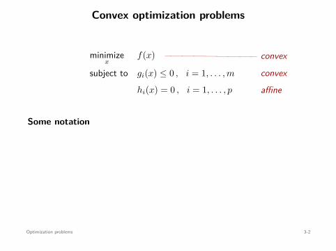
Convex optimization problems
minimizex
f(x)
subject to gi(x) ≤ 0 , i = 1, . . . , m
hi(x) = 0 , i = 1, . . . , p
convex
convexaffine
Some notation
p⋆ = infx
f(x)
s.t. x ∈ Ω
∈ [−∞, +∞]
x⋆ ∈ argminx
f(x)
s.t. x ∈ Ω
Optimal value:
A minimizer:
unbounded
infeasible
Optimization problems 3-2
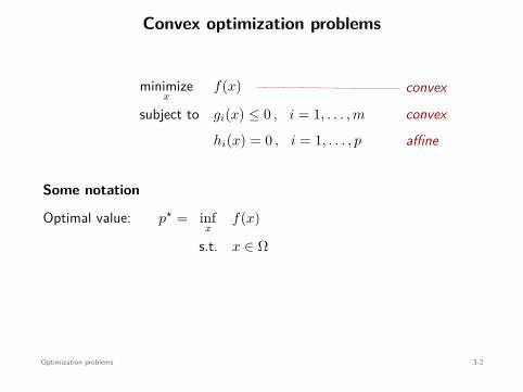
Convex optimization problems
minimizex
f(x)
subject to gi(x) ≤ 0 , i = 1, . . . , m
hi(x) = 0 , i = 1, . . . , p
convex
convexaffine
Some notation
p⋆ = infx
f(x)
s.t. x ∈ Ω
∈ [−∞, +∞]
x⋆ ∈ argminx
f(x)
s.t. x ∈ Ω
Optimal value:
A minimizer:
unbounded
infeasible
Optimization problems 3-2

Convex optimization problems
minimizex
f(x)
subject to gi(x) ≤ 0 , i = 1, . . . , m
hi(x) = 0 , i = 1, . . . , p
convex
convexaffine
Some notation
p⋆ = infx
f(x)
s.t. x ∈ Ω
∈ [−∞, +∞]
x⋆ ∈ argminx
f(x)
s.t. x ∈ Ω
Optimal value:
A minimizer:
unbounded
infeasible
Optimization problems 3-2

Convex optimization problems
minimizex
f(x)
subject to gi(x) ≤ 0 , i = 1, . . . , m
hi(x) = 0 , i = 1, . . . , p
convex
convexaffine
Some notation
p⋆ = infx
f(x)
s.t. x ∈ Ω
∈ [−∞, +∞]
x⋆ ∈ argminx
f(x)
s.t. x ∈ Ω
Optimal value:
A minimizer:
unbounded
infeasible
Optimization problems 3-2

Convex optimization problems
minimizex
f(x)
subject to gi(x) ≤ 0 , i = 1, . . . , m
hi(x) = 0 , i = 1, . . . , p
convex
convexaffine
Some notation
p⋆ = infx
f(x)
s.t. x ∈ Ω
∈ [−∞, +∞]
x⋆ ∈ argminx
f(x)
s.t. x ∈ Ω
Optimal value:
A minimizer:
unbounded
infeasible
Optimization problems 3-2
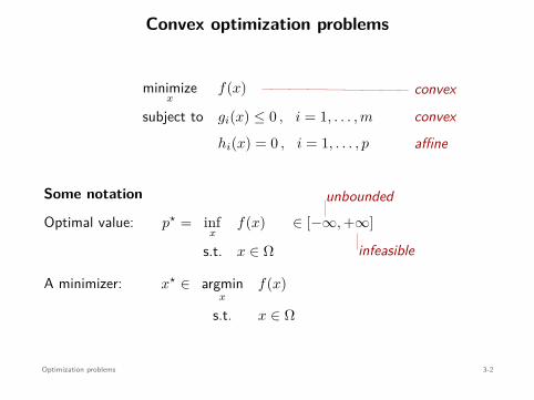
Convex optimization problems
minimizex
f(x)
subject to gi(x) ≤ 0 , i = 1, . . . , m
hi(x) = 0 , i = 1, . . . , p
convex
convexaffine
Some notation
p⋆ = infx
f(x)
s.t. x ∈ Ω
∈ [−∞, +∞]
x⋆ ∈ argminx
f(x)
s.t. x ∈ Ω
Optimal value:
A minimizer:
unbounded
infeasible
Optimization problems 3-2
Convex optimization problems
Theorem
In convex problems, a local minimizer is always a global minimizer.
Proof (for unconstrained problems w/ differentiable objective):
Recall that for any x, y ∈ dom f ,
f(y) ≥ f(x) + ∇f(x)⊤(y − x)
x⋆: local minimizer ⇒ ∇f(x⋆) = 0
Therefore, f(y) ≥ f(x⋆), for all y.
f(x) + ∇f(x)⊤(y − x)b
x
Optimization problems 3-3
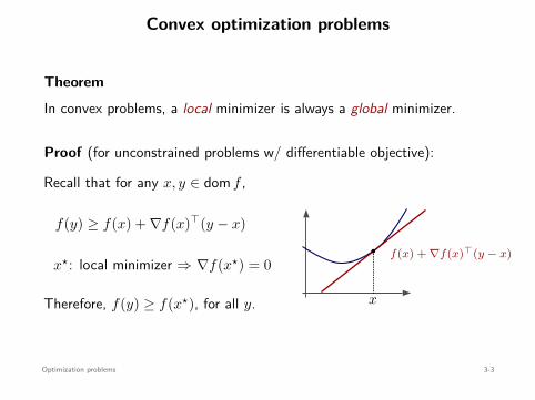

Equivalence between optimization problems
minimizex
f(x)
subject to x ∈ X
(P1)
minimizey
g(y)
subject to y ∈ Y
(P2)
(P1) and (P2) are equivalent when
• Given a solution x⋆ of (P1) we can obtain a solution y⋆ of (P2)
• Given a solution y⋆ of (P2) we can obtain a solution x⋆ of (P1)
Optimization problems 3-4

Examples
maximizex
f(x) ⇐⇒ minimizex
− f(x)
minimizex
f(x)
subject to x > 0⇐⇒ minimize
yf
(ey
)
minimizex
f(x) ⇐⇒minimize
x,tt
subject to f(x) ≤ t
Optimization problems 3-5

Examples
maximizex
f(x)
⇐⇒ minimizex
− f(x)
minimizex
f(x)
subject to x > 0⇐⇒ minimize
yf
(ey
)
minimizex
f(x) ⇐⇒minimize
x,tt
subject to f(x) ≤ t
Optimization problems 3-5

Examples
maximizex
f(x) ⇐⇒ minimizex
− f(x)
minimizex
f(x)
subject to x > 0⇐⇒ minimize
yf
(ey
)
minimizex
f(x) ⇐⇒minimize
x,tt
subject to f(x) ≤ t
Optimization problems 3-5

Examples
maximizex
f(x) ⇐⇒ minimizex
− f(x)
minimizex
f(x)
subject to x > 0
⇐⇒ minimizey
f(ey
)
minimizex
f(x) ⇐⇒minimize
x,tt
subject to f(x) ≤ t
Optimization problems 3-5

Examples
maximizex
f(x) ⇐⇒ minimizex
− f(x)
minimizex
f(x)
subject to x > 0⇐⇒ minimize
yf
(ey
)
minimizex
f(x) ⇐⇒minimize
x,tt
subject to f(x) ≤ t
Optimization problems 3-5
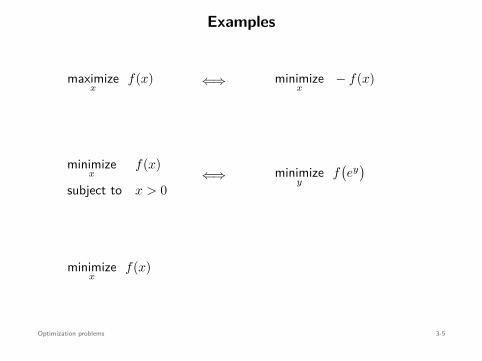
Examples
maximizex
f(x) ⇐⇒ minimizex
− f(x)
minimizex
f(x)
subject to x > 0⇐⇒ minimize
yf
(ey
)
minimizex
f(x)
⇐⇒minimize
x,tt
subject to f(x) ≤ t
Optimization problems 3-5

Examples
maximizex
f(x) ⇐⇒ minimizex
− f(x)
minimizex
f(x)
subject to x > 0⇐⇒ minimize
yf
(ey
)
minimizex
f(x) ⇐⇒minimize
x,tt
subject to f(x) ≤ t
Optimization problems 3-5

Examples
minimizex
a f(x) + b
> 0
⇐⇒ minimizex
f(x)
minimizex
f(x)
convex
⇐⇒ minimizex
g(f(x)
)
if im f ⊆ dom g
and g f : convex
Optimization problems 3-6

Examples
minimizex
a f(x) + b
> 0
⇐⇒ minimizex
f(x)
minimizex
f(x)
convex
⇐⇒ minimizex
g(f(x)
)
if im f ⊆ dom g
and g f : convex
Optimization problems 3-6

Examples
minimizex
a f(x) + b
> 0
⇐⇒ minimizex
f(x)
minimizex
f(x)
convex
⇐⇒ minimizex
g(f(x)
)
if im f ⊆ dom g
and g f : convex
Optimization problems 3-6

Examples
minimizex
a f(x) + b
> 0
⇐⇒ minimizex
f(x)
minimizex
f(x)
convex
⇐⇒ minimizex
g(f(x)
)
if im f ⊆ dom g
and g f : convex
Optimization problems 3-6

Examples
minimizex
a f(x) + b
> 0
⇐⇒ minimizex
f(x)
minimizex
f(x)
convex
⇐⇒ minimizex
g(f(x)
)
if im f ⊆ dom g
and g f : convex
Optimization problems 3-6
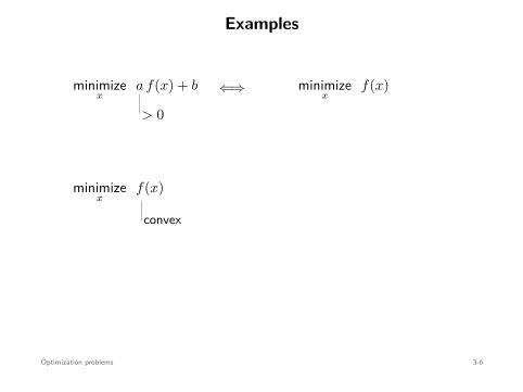
Examples
minimizex
a f(x) + b
> 0
⇐⇒ minimizex
f(x)
minimizex
f(x)
convex
⇐⇒ minimizex
g(f(x)
)
if im f ⊆ dom g
and g f : convex
Optimization problems 3-6
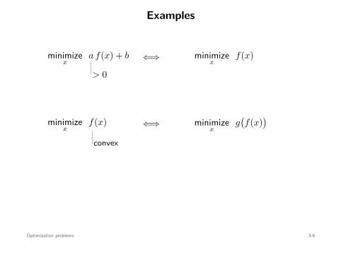
Examples
minimizex
a f(x) + b
> 0
⇐⇒ minimizex
f(x)
minimizex
f(x)
convex
⇐⇒ minimizex
g(f(x)
)
if im f ⊆ dom g
and g f : convex
Optimization problems 3-6

Examples
minimizex
a f(x) + b
> 0
⇐⇒ minimizex
f(x)
minimizex
f(x)
convex
⇐⇒ minimizex
g(f(x)
)
if im f ⊆ dom g
and g f : convex
Optimization problems 3-6

Air Traffic Control
• n airplanes land in order 1, 2, . . . , n
• ti: arrival time of airplane i
• Airplane i has to land in interval [mi, Mi]
m1 M1 m2 M2 m3 M3 m4 M4
tt1 t2 t3 t4
mini
ti+1 − ti
Goal: compute t1, . . . , tn that maximize mini ti+1 − ti
Optimization problems 3-7

Air Traffic Control
• n airplanes land in order 1, 2, . . . , n
• ti: arrival time of airplane i
• Airplane i has to land in interval [mi, Mi]
m1 M1 m2 M2 m3 M3 m4 M4
tt1 t2 t3 t4
mini
ti+1 − ti
Goal: compute t1, . . . , tn that maximize mini ti+1 − ti
Optimization problems 3-7

Air Traffic Control
• n airplanes land in order 1, 2, . . . , n
• ti: arrival time of airplane i
• Airplane i has to land in interval [mi, Mi]
m1 M1 m2 M2 m3 M3 m4 M4
t
t1 t2 t3 t4
mini
ti+1 − ti
Goal: compute t1, . . . , tn that maximize mini ti+1 − ti
Optimization problems 3-7

Air Traffic Control
• n airplanes land in order 1, 2, . . . , n
• ti: arrival time of airplane i
• Airplane i has to land in interval [mi, Mi]
m1 M1 m2 M2 m3 M3 m4 M4
t
t1 t2 t3 t4
mini
ti+1 − ti
Goal: compute t1, . . . , tn that maximize mini ti+1 − ti
Optimization problems 3-7

Air Traffic Control
• n airplanes land in order 1, 2, . . . , n
• ti: arrival time of airplane i
• Airplane i has to land in interval [mi, Mi]
m1 M1 m2 M2 m3 M3 m4 M4
tt1
t2 t3 t4
mini
ti+1 − ti
Goal: compute t1, . . . , tn that maximize mini ti+1 − ti
Optimization problems 3-7

Air Traffic Control
• n airplanes land in order 1, 2, . . . , n
• ti: arrival time of airplane i
• Airplane i has to land in interval [mi, Mi]
m1 M1 m2 M2 m3 M3 m4 M4
tt1 t2
t3 t4
mini
ti+1 − ti
Goal: compute t1, . . . , tn that maximize mini ti+1 − ti
Optimization problems 3-7

Air Traffic Control
• n airplanes land in order 1, 2, . . . , n
• ti: arrival time of airplane i
• Airplane i has to land in interval [mi, Mi]
m1 M1 m2 M2 m3 M3 m4 M4
tt1 t2 t3 t4
mini
ti+1 − ti
Goal: compute t1, . . . , tn that maximize mini ti+1 − ti
Optimization problems 3-7

Air Traffic Control
• n airplanes land in order 1, 2, . . . , n
• ti: arrival time of airplane i
• Airplane i has to land in interval [mi, Mi]
m1 M1 m2 M2 m3 M3 m4 M4
tt1 t2 t3 t4
mini
ti+1 − ti
Goal: compute t1, . . . , tn that maximize mini ti+1 − ti
Optimization problems 3-7

Air Traffic Control
• n airplanes land in order 1, 2, . . . , n
• ti: arrival time of airplane i
• Airplane i has to land in interval [mi, Mi]
m1 M1 m2 M2 m3 M3 m4 M4
tt1 t2 t3 t4
mini
ti+1 − ti
Goal: compute t1, . . . , tn that maximize mini ti+1 − ti
Optimization problems 3-7

Air Traffic Control
maximizet1,...,tn
min
t2 − t1 , t3 − t2 , . . . , tn − tn−1
subject to mi ≤ ti ≤ Mi , i = 1, . . . , n
⇐⇒ minimizet1,...,tn
− min
t2 − t1 , t3 − t2 , . . . , tn − tn−1
subject to mi ≤ ti ≤ Mi , i = 1, . . . , n
⇐⇒ minimizet1,...,tn
max
t1 − t2 , t2 − t3 , . . . , tn−1 − tn
subject to mi ≤ ti ≤ Mi , i = 1, . . . , n
Convex
Optimization problems 3-8
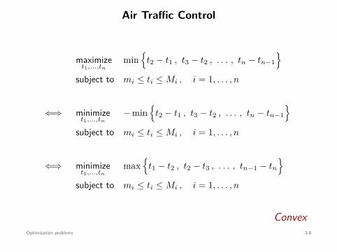
Air Traffic Control
maximizet1,...,tn
min
t2 − t1 , t3 − t2 , . . . , tn − tn−1
subject to mi ≤ ti ≤ Mi , i = 1, . . . , n
⇐⇒ minimizet1,...,tn
− min
t2 − t1 , t3 − t2 , . . . , tn − tn−1
subject to mi ≤ ti ≤ Mi , i = 1, . . . , n
⇐⇒ minimizet1,...,tn
max
t1 − t2 , t2 − t3 , . . . , tn−1 − tn
subject to mi ≤ ti ≤ Mi , i = 1, . . . , n
ConvexOptimization problems 3-8
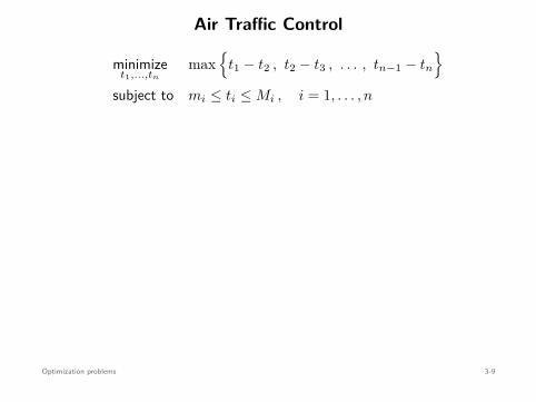
Air Traffic Control
minimizet1,...,tn
max
t1 − t2 , t2 − t3 , . . . , tn−1 − tn
subject to mi ≤ ti ≤ Mi , i = 1, . . . , n
⇐⇒ minimizet1,...,tn,s
s
subject to max
t1 − t2 , t2 − t3 , . . . , tn−1 − tn
≤ s
mi ≤ ti ≤ Mi , i = 1, . . . , n
⇐⇒ minimizet1,...,tn,s
s
subject to t1 − t2 ≤ s...
tn−1 − tn ≤ s
mi ≤ ti ≤ Mi , i = 1, . . . , n
Optimization problems 3-9
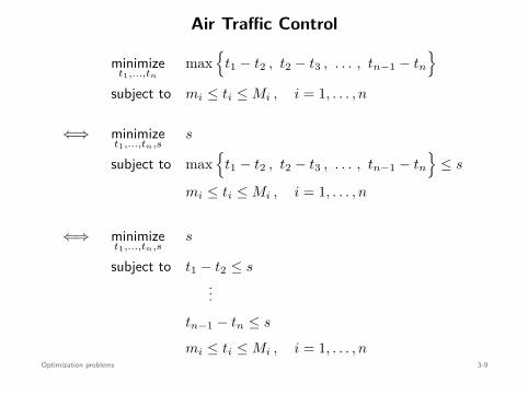
Air Traffic Control
minimizet1,...,tn
max
t1 − t2 , t2 − t3 , . . . , tn−1 − tn
subject to mi ≤ ti ≤ Mi , i = 1, . . . , n
⇐⇒ minimizet1,...,tn,s
s
subject to max
t1 − t2 , t2 − t3 , . . . , tn−1 − tn
≤ s
mi ≤ ti ≤ Mi , i = 1, . . . , n
⇐⇒ minimizet1,...,tn,s
s
subject to t1 − t2 ≤ s...
tn−1 − tn ≤ s
mi ≤ ti ≤ Mi , i = 1, . . . , nOptimization problems 3-9

Air Traffic ControlThis is a linear program (LP):
minimizex
c⊤x
subject to Ax ≤ b
with x = (t1, . . . , tn, s) ∈ Rn+1, c = (0, · · · , 0, 1), and
A =
1 −1 0 · · · 0 0 −10 1 −1 · · · 0 0 −1
. . .
0 0 0 · · · 1 −1 −1−1 0 0 · · · 0 0 0
1 0 0 · · · 0 0 0. . .
0 0 0 · · · 0 −1 00 0 0 · · · 0 1 0
b =
00...0
−m1
M1
...−mn
Mn
Optimization problems 3-10
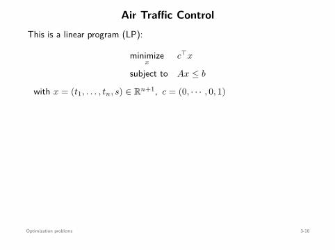
Air Traffic ControlThis is a linear program (LP):
minimizex
c⊤x
subject to Ax ≤ b
with x = (t1, . . . , tn, s) ∈ Rn+1, c = (0, · · · , 0, 1)
, and
A =
1 −1 0 · · · 0 0 −10 1 −1 · · · 0 0 −1
. . .
0 0 0 · · · 1 −1 −1−1 0 0 · · · 0 0 0
1 0 0 · · · 0 0 0. . .
0 0 0 · · · 0 −1 00 0 0 · · · 0 1 0
b =
00...0
−m1
M1
...−mn
Mn
Optimization problems 3-10
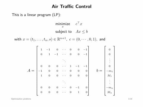
Air Traffic ControlThis is a linear program (LP):
minimizex
c⊤x
subject to Ax ≤ b
with x = (t1, . . . , tn, s) ∈ Rn+1, c = (0, · · · , 0, 1), and
A =
1 −1 0 · · · 0 0 −10 1 −1 · · · 0 0 −1
. . .
0 0 0 · · · 1 −1 −1−1 0 0 · · · 0 0 0
1 0 0 · · · 0 0 0. . .
0 0 0 · · · 0 −1 00 0 0 · · · 0 1 0
b =
00...0
−m1
M1
...−mn
Mn
Optimization problems 3-10

Air Traffic Control
Can be solved, e.g., with MATLAB’s linprog solver
But we have to explicitly construct A, b, and c . . .
CVX (cvxr.com/cvx) manipulates and solves convex problems
Optimization problems 3-11

Air Traffic Control
Can be solved, e.g., with MATLAB’s linprog solver
But we have to explicitly construct A, b, and c . . .
CVX (cvxr.com/cvx) manipulates and solves convex problems
Optimization problems 3-11

Air Traffic Control
Can be solved, e.g., with MATLAB’s linprog solver
But we have to explicitly construct A, b, and c . . .
CVX (cvxr.com/cvx) manipulates and solves convex problems
Optimization problems 3-11

Air Traffic Control
cvx_beg inv a r i a b l e s t1 t2 t3 t4 t5 ;maximize ( min ( [ t2−t1 , t3−t2 , t4−t3 , t5−t4 ] ) ) ;s u b j e c t to
1 <= t1 <= 2 ;3 <= t2 <= 4 ;5 <= t3 <= 6 ;7 <= t4 <= 8 ;9 <= t5 <= 10 ;
cvx_end
(t⋆1 , t⋆
2 , t⋆3 , t⋆
4 , t⋆5) = (1 , 3.25 , 5.5 , 7.75 , 10)
Optimization problems 3-12

Portfolio Optimization
• £T to invest in n assets• ri: return of asset i, for i = 1, . . . , n (random variables)• First two moments of the random vector r = (r1, . . . , rn) are known:
µ = E[r] Σ = E[(r − µ)(r − µ)⊤]
• An investment x = (x1, . . . , xn) has return
s(x) = r⊤x = r1x1 + · · · + rnxn
E[s(x)
]= E[r1] x1 + · · · + E[rn] xn = µ1 x1 + · · · + µn xn = µ⊤x
Var(s(x)
)= E
[(s(x) − E[s(x)]
)2]
= E[(
(r − µ)⊤x)2
]= x⊤Σ x
Optimization problems 3-13

Portfolio Optimization
• £T to invest in n assets
• ri: return of asset i, for i = 1, . . . , n (random variables)• First two moments of the random vector r = (r1, . . . , rn) are known:
µ = E[r] Σ = E[(r − µ)(r − µ)⊤]
• An investment x = (x1, . . . , xn) has return
s(x) = r⊤x = r1x1 + · · · + rnxn
E[s(x)
]= E[r1] x1 + · · · + E[rn] xn = µ1 x1 + · · · + µn xn = µ⊤x
Var(s(x)
)= E
[(s(x) − E[s(x)]
)2]
= E[(
(r − µ)⊤x)2
]= x⊤Σ x
Optimization problems 3-13

Portfolio Optimization
• £T to invest in n assets• ri: return of asset i, for i = 1, . . . , n (random variables)
• First two moments of the random vector r = (r1, . . . , rn) are known:
µ = E[r] Σ = E[(r − µ)(r − µ)⊤]
• An investment x = (x1, . . . , xn) has return
s(x) = r⊤x = r1x1 + · · · + rnxn
E[s(x)
]= E[r1] x1 + · · · + E[rn] xn = µ1 x1 + · · · + µn xn = µ⊤x
Var(s(x)
)= E
[(s(x) − E[s(x)]
)2]
= E[(
(r − µ)⊤x)2
]= x⊤Σ x
Optimization problems 3-13

Portfolio Optimization
• £T to invest in n assets• ri: return of asset i, for i = 1, . . . , n (random variables)• First two moments of the random vector r = (r1, . . . , rn) are known:
µ = E[r] Σ = E[(r − µ)(r − µ)⊤]
• An investment x = (x1, . . . , xn) has return
s(x) = r⊤x = r1x1 + · · · + rnxn
E[s(x)
]= E[r1] x1 + · · · + E[rn] xn = µ1 x1 + · · · + µn xn = µ⊤x
Var(s(x)
)= E
[(s(x) − E[s(x)]
)2]
= E[(
(r − µ)⊤x)2
]= x⊤Σ x
Optimization problems 3-13

Portfolio Optimization
• £T to invest in n assets• ri: return of asset i, for i = 1, . . . , n (random variables)• First two moments of the random vector r = (r1, . . . , rn) are known:
µ = E[r] Σ = E[(r − µ)(r − µ)⊤]
• An investment x = (x1, . . . , xn) has return
s(x) = r⊤x = r1x1 + · · · + rnxn
E[s(x)
]
= E[r1] x1 + · · · + E[rn] xn = µ1 x1 + · · · + µn xn = µ⊤x
Var(s(x)
)= E
[(s(x) − E[s(x)]
)2]
= E[(
(r − µ)⊤x)2
]= x⊤Σ x
Optimization problems 3-13

Portfolio Optimization
• £T to invest in n assets• ri: return of asset i, for i = 1, . . . , n (random variables)• First two moments of the random vector r = (r1, . . . , rn) are known:
µ = E[r] Σ = E[(r − µ)(r − µ)⊤]
• An investment x = (x1, . . . , xn) has return
s(x) = r⊤x = r1x1 + · · · + rnxn
E[s(x)
]= E[r1] x1 + · · · + E[rn] xn
= µ1 x1 + · · · + µn xn = µ⊤x
Var(s(x)
)= E
[(s(x) − E[s(x)]
)2]
= E[(
(r − µ)⊤x)2
]= x⊤Σ x
Optimization problems 3-13

Portfolio Optimization
• £T to invest in n assets• ri: return of asset i, for i = 1, . . . , n (random variables)• First two moments of the random vector r = (r1, . . . , rn) are known:
µ = E[r] Σ = E[(r − µ)(r − µ)⊤]
• An investment x = (x1, . . . , xn) has return
s(x) = r⊤x = r1x1 + · · · + rnxn
E[s(x)
]= E[r1] x1 + · · · + E[rn] xn = µ1 x1 + · · · + µn xn
= µ⊤x
Var(s(x)
)= E
[(s(x) − E[s(x)]
)2]
= E[(
(r − µ)⊤x)2
]= x⊤Σ x
Optimization problems 3-13

Portfolio Optimization
• £T to invest in n assets• ri: return of asset i, for i = 1, . . . , n (random variables)• First two moments of the random vector r = (r1, . . . , rn) are known:
µ = E[r] Σ = E[(r − µ)(r − µ)⊤]
• An investment x = (x1, . . . , xn) has return
s(x) = r⊤x = r1x1 + · · · + rnxn
E[s(x)
]= E[r1] x1 + · · · + E[rn] xn = µ1 x1 + · · · + µn xn = µ⊤x
Var(s(x)
)= E
[(s(x) − E[s(x)]
)2]
= E[(
(r − µ)⊤x)2
]= x⊤Σ x
Optimization problems 3-13
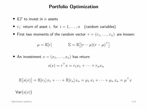
Portfolio Optimization
• £T to invest in n assets• ri: return of asset i, for i = 1, . . . , n (random variables)• First two moments of the random vector r = (r1, . . . , rn) are known:
µ = E[r] Σ = E[(r − µ)(r − µ)⊤]
• An investment x = (x1, . . . , xn) has return
s(x) = r⊤x = r1x1 + · · · + rnxn
E[s(x)
]= E[r1] x1 + · · · + E[rn] xn = µ1 x1 + · · · + µn xn = µ⊤x
Var(s(x)
)
= E[(
s(x) − E[s(x)])2
]= E
[((r − µ)⊤x
)2]
= x⊤Σ x
Optimization problems 3-13

Portfolio Optimization
• £T to invest in n assets• ri: return of asset i, for i = 1, . . . , n (random variables)• First two moments of the random vector r = (r1, . . . , rn) are known:
µ = E[r] Σ = E[(r − µ)(r − µ)⊤]
• An investment x = (x1, . . . , xn) has return
s(x) = r⊤x = r1x1 + · · · + rnxn
E[s(x)
]= E[r1] x1 + · · · + E[rn] xn = µ1 x1 + · · · + µn xn = µ⊤x
Var(s(x)
)= E
[(s(x) − E[s(x)]
)2]
= E[(
(r − µ)⊤x)2
]= x⊤Σ x
Optimization problems 3-13

Portfolio Optimization
• £T to invest in n assets• ri: return of asset i, for i = 1, . . . , n (random variables)• First two moments of the random vector r = (r1, . . . , rn) are known:
µ = E[r] Σ = E[(r − µ)(r − µ)⊤]
• An investment x = (x1, . . . , xn) has return
s(x) = r⊤x = r1x1 + · · · + rnxn
E[s(x)
]= E[r1] x1 + · · · + E[rn] xn = µ1 x1 + · · · + µn xn = µ⊤x
Var(s(x)
)= E
[(s(x) − E[s(x)]
)2]
= E[(
(r − µ)⊤x)2
]
= x⊤Σ x
Optimization problems 3-13
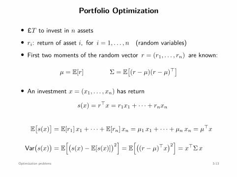
Portfolio Optimization
• £T to invest in n assets• ri: return of asset i, for i = 1, . . . , n (random variables)• First two moments of the random vector r = (r1, . . . , rn) are known:
µ = E[r] Σ = E[(r − µ)(r − µ)⊤]
• An investment x = (x1, . . . , xn) has return
s(x) = r⊤x = r1x1 + · · · + rnxn
E[s(x)
]= E[r1] x1 + · · · + E[rn] xn = µ1 x1 + · · · + µn xn = µ⊤x
Var(s(x)
)= E
[(s(x) − E[s(x)]
)2]
= E[(
(r − µ)⊤x)2
]= x⊤Σ x
Optimization problems 3-13

Portfolio Optimization
Different investment strategies
• Minimize variance while guaranteeing minimum expected return smin:
minimizex
Var(s(x)
)
subject to x ≥ 0n
1⊤n x = T
E[s(x)
]≥ smin
⇐⇒ minimizex
x⊤Σx
subject to x ≥ 0n
1⊤n x = T
µ⊤x ≥ smin
Convex Quadratic Program (QP)
Optimization problems 3-14
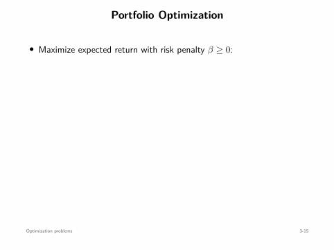
Portfolio Optimization
• Maximize expected return with risk penalty β ≥ 0:
maximizex
E[s(x)
]− β Var(s(x))
subject to x ≥ 0n
1⊤n x = T
⇐⇒ minimizex
−µ⊤x + β x⊤Σ x
subject to x ≥ 0n
1⊤n x = T
Convex QP
Optimization problems 3-15

Portfolio Optimization
• Maximize expected return with risk penalty β ≥ 0:
maximizex
E[s(x)
]− β Var(s(x))
subject to x ≥ 0n
1⊤n x = T
⇐⇒ minimizex
−µ⊤x + β x⊤Σ x
subject to x ≥ 0n
1⊤n x = T
Convex QP
Optimization problems 3-15

Portfolio Optimization
• Maximize expected return with risk penalty β ≥ 0:
maximizex
E[s(x)
]− β Var(s(x))
subject to x ≥ 0n
1⊤n x = T
⇐⇒ minimizex
−µ⊤x + β x⊤Σ x
subject to x ≥ 0n
1⊤n x = T
Convex QP
Optimization problems 3-15

Portfolio Optimization
• Maximize expected return with risk penalty β ≥ 0:
maximizex
E[s(x)
]− β Var(s(x))
subject to x ≥ 0n
1⊤n x = T
⇐⇒ minimizex
−µ⊤x + β x⊤Σ x
subject to x ≥ 0n
1⊤n x = T
Convex QP
Optimization problems 3-15

MAXCUT
1 2
34
5
6
7
89
w12
w13
w15w25
w35 w45
w69 w68
w78
w79
w89
w27
w29
w49
w46
w27
w29
w49
w46
value of cut: w27 + w29 + w49 + w46
Cut: set of edges whose removal splits the graph into two
MAXCUT problem: find the cut with maximum weight
maximizex∈Rn
12
n∑
i=1
n∑
j=1wij
1 − xixj
2
subject to xi ∈ −1, 1 , i = 1, . . . , n .
Optimization problems 3-16

p⋆ = maxx
12
n∑
i=1
n∑
j=1wij
1 − xixj
2
s.t. xi ∈ −1, 1 , i = 1, . . . , n
= − minx
14
[n∑
i=1
n∑
j=1wijxixj −
n∑
i=1
n∑
j=1wij
]
s.t. x2i = 1 , i = 1, . . . , n
= − minx
14
(x⊤Wx − 1⊤
n W1n
)
s.t. x2i = 1 , i = 1, . . . , n
W ∈ Rn×n: weighted adjacency matrix
Optimization problems 3-17

p⋆ = maxx
12
n∑
i=1
n∑
j=1wij
1 − xixj
2
s.t. xi ∈ −1, 1 , i = 1, . . . , n
= − minx
14
[n∑
i=1
n∑
j=1wijxixj −
n∑
i=1
n∑
j=1wij
]
s.t. x2i = 1 , i = 1, . . . , n
= − minx
14
(x⊤Wx − 1⊤
n W1n
)
s.t. x2i = 1 , i = 1, . . . , n
W ∈ Rn×n: weighted adjacency matrix
Optimization problems 3-17
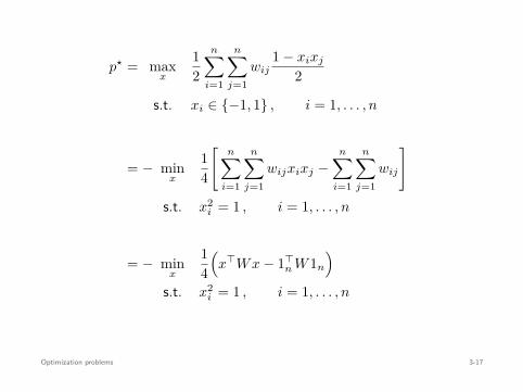
p⋆ = maxx
12
n∑
i=1
n∑
j=1wij
1 − xixj
2
s.t. xi ∈ −1, 1 , i = 1, . . . , n
= − minx
14
[n∑
i=1
n∑
j=1wijxixj −
n∑
i=1
n∑
j=1wij
]
s.t. x2i = 1 , i = 1, . . . , n
= − minx
14
(x⊤Wx − 1⊤
n W1n
)
s.t. x2i = 1 , i = 1, . . . , n
W ∈ Rn×n: weighted adjacency matrix
Optimization problems 3-17

p⋆ = maxx
12
n∑
i=1
n∑
j=1wij
1 − xixj
2
s.t. xi ∈ −1, 1 , i = 1, . . . , n
= − minx
14
[n∑
i=1
n∑
j=1wijxixj −
n∑
i=1
n∑
j=1wij
]
s.t. x2i = 1 , i = 1, . . . , n
= − minx
14
(x⊤Wx − 1⊤
n W1n
)
s.t. x2i = 1 , i = 1, . . . , n
W ∈ Rn×n: weighted adjacency matrixOptimization problems 3-17
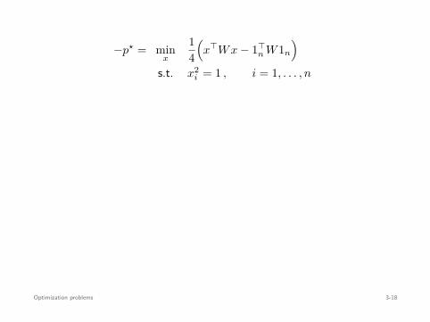
−p⋆ = minx
14
(x⊤Wx − 1⊤
n W1n
)
s.t. x2i = 1 , i = 1, . . . , n
• x⊤Wx = tr(x⊤Wx
)= tr
(Wxx⊤)
• For any X ∈ Sn and x ∈ Rn, X = xx⊤ ⇐⇒
X ⪰ 0
rank(X) = 1
−p⋆ = minX∈Sn
14
(tr
(WX
)− 1⊤
n W1n
)
s.t. Xii = 1 , i = 1, . . . , n
X ⪰ 0
rank(X) = 1 nonconvex
Optimization problems 3-18

−p⋆ = minx
14
(x⊤Wx − 1⊤
n W1n
)
s.t. x2i = 1 , i = 1, . . . , n
• x⊤Wx = tr(x⊤Wx
)= tr
(Wxx⊤)
• For any X ∈ Sn and x ∈ Rn, X = xx⊤ ⇐⇒
X ⪰ 0
rank(X) = 1
−p⋆ = minX∈Sn
14
(tr
(WX
)− 1⊤
n W1n
)
s.t. Xii = 1 , i = 1, . . . , n
X ⪰ 0
rank(X) = 1 nonconvex
Optimization problems 3-18

−p⋆ = minx
14
(x⊤Wx − 1⊤
n W1n
)
s.t. x2i = 1 , i = 1, . . . , n
• x⊤Wx = tr(x⊤Wx
)= tr
(Wxx⊤)
• For any X ∈ Sn and x ∈ Rn, X = xx⊤ ⇐⇒
X ⪰ 0
rank(X) = 1
−p⋆ = minX∈Sn
14
(tr
(WX
)− 1⊤
n W1n
)
s.t. Xii = 1 , i = 1, . . . , n
X ⪰ 0
rank(X) = 1 nonconvex
Optimization problems 3-18

−p⋆ = minx
14
(x⊤Wx − 1⊤
n W1n
)
s.t. x2i = 1 , i = 1, . . . , n
• x⊤Wx = tr(x⊤Wx
)= tr
(Wxx⊤)
• For any X ∈ Sn and x ∈ Rn, X = xx⊤ ⇐⇒
X ⪰ 0
rank(X) = 1
−p⋆ = minX∈Sn
14
(tr
(WX
)− 1⊤
n W1n
)
s.t. Xii = 1 , i = 1, . . . , n
X ⪰ 0
rank(X) = 1
nonconvex
Optimization problems 3-18
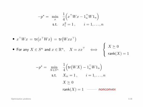
−p⋆ = minx
14
(x⊤Wx − 1⊤
n W1n
)
s.t. x2i = 1 , i = 1, . . . , n
• x⊤Wx = tr(x⊤Wx
)= tr
(Wxx⊤)
• For any X ∈ Sn and x ∈ Rn, X = xx⊤ ⇐⇒
X ⪰ 0
rank(X) = 1
−p⋆ = minX∈Sn
14
(tr
(WX
)− 1⊤
n W1n
)
s.t. Xii = 1 , i = 1, . . . , n
X ⪰ 0
rank(X) = 1 nonconvex
Optimization problems 3-18
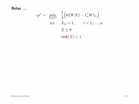
Relax . . .−p⋆ = min
X∈Sn
14
(tr
(WX
)− 1⊤
n W1n
)
s.t. Xii = 1 , i = 1, . . . , n
X ⪰ 0
rank(X) = 1
≥ minX∈Sn
14
(tr
(WX
)− 1⊤
n W1n
)
s.t. Xii = 1 , i = 1, . . . , n
X ⪰ 0
=: −d⋆
Convex Semi-Definite Program (SDP)
Optimization problems 3-19
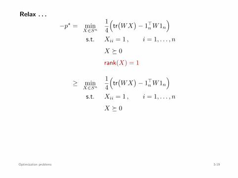
Relax . . .−p⋆ = min
X∈Sn
14
(tr
(WX
)− 1⊤
n W1n
)
s.t. Xii = 1 , i = 1, . . . , n
X ⪰ 0
rank(X) = 1
≥ minX∈Sn
14
(tr
(WX
)− 1⊤
n W1n
)
s.t. Xii = 1 , i = 1, . . . , n
X ⪰ 0
=: −d⋆
Convex Semi-Definite Program (SDP)
Optimization problems 3-19

Relax . . .−p⋆ = min
X∈Sn
14
(tr
(WX
)− 1⊤
n W1n
)
s.t. Xii = 1 , i = 1, . . . , n
X ⪰ 0
rank(X) = 1
≥ minX∈Sn
14
(tr
(WX
)− 1⊤
n W1n
)
s.t. Xii = 1 , i = 1, . . . , n
X ⪰ 0
=: −d⋆
Convex Semi-Definite Program (SDP)
Optimization problems 3-19

Relax . . .−p⋆ = min
X∈Sn
14
(tr
(WX
)− 1⊤
n W1n
)
s.t. Xii = 1 , i = 1, . . . , n
X ⪰ 0
rank(X) = 1
≥ minX∈Sn
14
(tr
(WX
)− 1⊤
n W1n
)
s.t. Xii = 1 , i = 1, . . . , n
X ⪰ 0
=: −d⋆
Convex Semi-Definite Program (SDP)
Optimization problems 3-19

Procedure: (Goemans & Williamson, 95’)
• Solve SDP, obtaining X⋆
• Factorize X⋆ = V ⊤V , where V =[v1 v2 · · · vn
]
• Draw r uniformly at random from unit-sphere
x ∈ Rn : ∥x∥2 = 1
• The following sets define a cut C on the vertices of the graph:
S =
i : r⊤vi ≥ 0
Sc =
i : r⊤vi < 0
It can be shown that
d⋆ ≥ p⋆ ≥ E[C] ≥ 0.87856 d⋆
Optimization problems 3-20
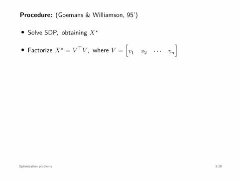
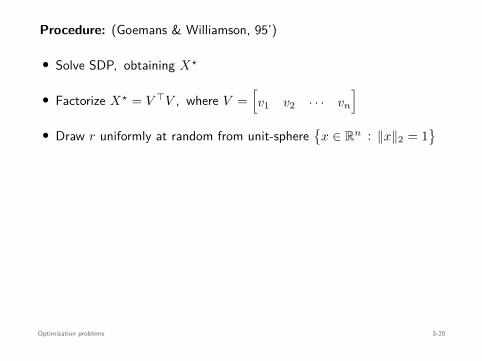
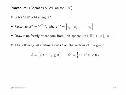

Solving Optimization Problems
CVX & other solvers are great for
• prototyping
• small-scale problems
Large-scale problems & real-time solutions require tailored solvers
Optimization problems 3-21

Solving Optimization Problems
CVX & other solvers are great for
• prototyping
• small-scale problems
Large-scale problems & real-time solutions require tailored solvers
Optimization problems 3-21
Solving Optimization Problems
CVX & other solvers are great for
• prototyping
• small-scale problems
Large-scale problems & real-time solutions require tailored solvers
Optimization problems 3-21

Solving Optimization Problems
CVX & other solvers are great for
• prototyping
• small-scale problems
Large-scale problems & real-time solutions require tailored solvers
Optimization problems 3-21

Example:
minimizex
∥x∥1
subject to Ax = b
where A ∈ Rm×n and b ∈ Rm are generated randomly.
For n = 5000 and m = 500,
• CVX: 56.16 s
• SPGL1: 0.82 s (tailored solver)
Optimization problems 3-22
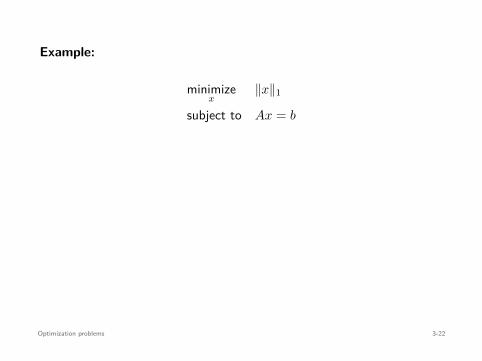
Example:
minimizex
∥x∥1
subject to Ax = b
where A ∈ Rm×n and b ∈ Rm are generated randomly.
For n = 5000 and m = 500,
• CVX: 56.16 s
• SPGL1: 0.82 s (tailored solver)
Optimization problems 3-22

Example:
minimizex
∥x∥1
subject to Ax = b
where A ∈ Rm×n and b ∈ Rm are generated randomly.
For n = 5000 and m = 500,
• CVX: 56.16 s
• SPGL1: 0.82 s (tailored solver)
Optimization problems 3-22

Example:
minimizex
∥x∥1
subject to Ax = b
where A ∈ Rm×n and b ∈ Rm are generated randomly.
For n = 5000 and m = 500,
• CVX: 56.16 s
• SPGL1: 0.82 s (tailored solver)
Optimization problems 3-22
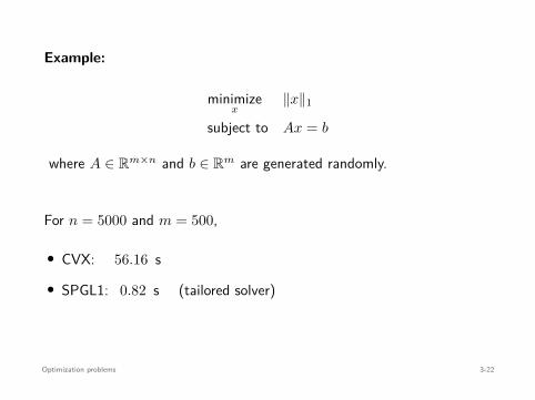
Example:
minimizex
∥x∥1
subject to Ax = b
where A ∈ Rm×n and b ∈ Rm are generated randomly.
For n = 5000 and m = 500,
• CVX: 56.16 s
• SPGL1: 0.82 s (tailored solver)
Optimization problems 3-22

Optimization Algorithms
• Unconstrained & differentiable
Gradient descent (and Nesterov’s acceleration scheme)Block coordinate descentNewton (and approximations)
• Constrained & differentiable
Projection methods (projected gradient descent, Frank-Wolfe, . . . )Interior-point algorithms (classes LP, QP, SOCP, SDP)
• Non-differentiable
Subgradient descentProximal methods (proximal gradient descent, ADMM, primal-dual)
And now, neural networks!
Optimization problems 3-23
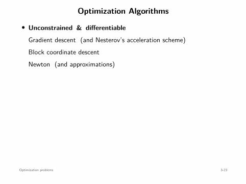

Optimization Algorithms
• Unconstrained & differentiable
Gradient descent (and Nesterov’s acceleration scheme)Block coordinate descentNewton (and approximations)
• Constrained & differentiable
Projection methods (projected gradient descent, Frank-Wolfe, . . . )Interior-point algorithms (classes LP, QP, SOCP, SDP)
• Non-differentiable
Subgradient descentProximal methods (proximal gradient descent, ADMM, primal-dual)
And now, neural networks!Optimization problems 3-23

Nesterov’s acceleration scheme
minimizex
f(x)
• f : Rn → R : differentiable
• ∇f : Lipschitz-continuous, i.e., there exists L ≥ 0 such that
∥∇f(y) − ∇f(x)∥2 ≤ L∥y − x∥2 , for all x, y ∈ dom f
• f⋆ := minx f(x) > −∞
Optimization problems 3-24

Nesterov’s acceleration scheme
minimizex
f(x)
• f : Rn → R : differentiable
• ∇f : Lipschitz-continuous, i.e., there exists L ≥ 0 such that
∥∇f(y) − ∇f(x)∥2 ≤ L∥y − x∥2 , for all x, y ∈ dom f
• f⋆ := minx f(x) > −∞
Optimization problems 3-24

Nesterov’s acceleration scheme
minimizex
f(x)
• f : Rn → R : differentiable
• ∇f : Lipschitz-continuous, i.e., there exists L ≥ 0 such that
∥∇f(y) − ∇f(x)∥2 ≤ L∥y − x∥2 , for all x, y ∈ dom f
• f⋆ := minx f(x) > −∞
Optimization problems 3-24

Nesterov’s acceleration scheme
minimizex
f(x)
• f : Rn → R : differentiable
• ∇f : Lipschitz-continuous
, i.e., there exists L ≥ 0 such that
∥∇f(y) − ∇f(x)∥2 ≤ L∥y − x∥2 , for all x, y ∈ dom f
• f⋆ := minx f(x) > −∞
Optimization problems 3-24

Nesterov’s acceleration scheme
minimizex
f(x)
• f : Rn → R : differentiable
• ∇f : Lipschitz-continuous, i.e., there exists L ≥ 0 such that
∥∇f(y) − ∇f(x)∥2 ≤ L∥y − x∥2 , for all x, y ∈ dom f
• f⋆ := minx f(x) > −∞
Optimization problems 3-24

Nesterov’s acceleration scheme
minimizex
f(x)
• f : Rn → R : differentiable
• ∇f : Lipschitz-continuous, i.e., there exists L ≥ 0 such that
∥∇f(y) − ∇f(x)∥2 ≤ L∥y − x∥2 , for all x, y ∈ dom f
• f⋆ := minx f(x) > −∞
Optimization problems 3-24

Nesterov’s acceleration scheme
Gradient descent:
starting at arbitrary x0 ∈ Rn,
xk+1 = xk − 1L
∇f(xk
)f(xk) − f⋆ ≤ L
2k
∥∥x0 − x⋆∥∥2
2
Nesterov’s method: starting at arbitrary y0 ∈ Rn,
xk+1 = yk − 1L
∇f(yk
)
yk+1 = xk − k − 1k + 2
(xk+1 − xk
) f(xk) − f⋆ ≤ 2L
(k + 1)2
∥∥x0 − x⋆∥∥2
2
Optimization problems 3-25

Nesterov’s acceleration scheme
Gradient descent: starting at arbitrary x0 ∈ Rn,
xk+1 = xk − 1L
∇f(xk
)
f(xk) − f⋆ ≤ L
2k
∥∥x0 − x⋆∥∥2
2
Nesterov’s method: starting at arbitrary y0 ∈ Rn,
xk+1 = yk − 1L
∇f(yk
)
yk+1 = xk − k − 1k + 2
(xk+1 − xk
) f(xk) − f⋆ ≤ 2L
(k + 1)2
∥∥x0 − x⋆∥∥2
2
Optimization problems 3-25

Nesterov’s acceleration scheme
Gradient descent: starting at arbitrary x0 ∈ Rn,
xk+1 = xk − 1L
∇f(xk
)f(xk) − f⋆ ≤ L
2k
∥∥x0 − x⋆∥∥2
2
Nesterov’s method: starting at arbitrary y0 ∈ Rn,
xk+1 = yk − 1L
∇f(yk
)
yk+1 = xk − k − 1k + 2
(xk+1 − xk
) f(xk) − f⋆ ≤ 2L
(k + 1)2
∥∥x0 − x⋆∥∥2
2
Optimization problems 3-25

Nesterov’s acceleration scheme
Gradient descent: starting at arbitrary x0 ∈ Rn,
xk+1 = xk − 1L
∇f(xk
)f(xk) − f⋆ ≤ L
2k
∥∥x0 − x⋆∥∥2
2
Nesterov’s method: starting at arbitrary y0 ∈ Rn,
xk+1 = yk − 1L
∇f(yk
)
yk+1 = xk − k − 1k + 2
(xk+1 − xk
) f(xk) − f⋆ ≤ 2L
(k + 1)2
∥∥x0 − x⋆∥∥2
2
Optimization problems 3-25
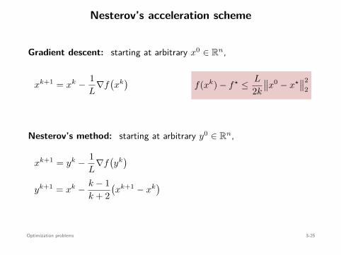
Nesterov’s acceleration scheme
Gradient descent: starting at arbitrary x0 ∈ Rn,
xk+1 = xk − 1L
∇f(xk
)f(xk) − f⋆ ≤ L
2k
∥∥x0 − x⋆∥∥2
2
Nesterov’s method: starting at arbitrary y0 ∈ Rn,
xk+1 = yk − 1L
∇f(yk
)
yk+1 = xk − k − 1k + 2
(xk+1 − xk
)
f(xk) − f⋆ ≤ 2L
(k + 1)2
∥∥x0 − x⋆∥∥2
2
Optimization problems 3-25

Nesterov’s acceleration scheme
Gradient descent: starting at arbitrary x0 ∈ Rn,
xk+1 = xk − 1L
∇f(xk
)f(xk) − f⋆ ≤ L
2k
∥∥x0 − x⋆∥∥2
2
Nesterov’s method: starting at arbitrary y0 ∈ Rn,
xk+1 = yk − 1L
∇f(yk
)
yk+1 = xk − k − 1k + 2
(xk+1 − xk
) f(xk) − f⋆ ≤ 2L
(k + 1)2
∥∥x0 − x⋆∥∥2
2
Optimization problems 3-25

Example
minimizex∈Rn
logm∑
i=1exp
(a⊤
i x + b)
randomly generated data with m = 500, n = 50
iterations k
|f(xk) − f⋆|/|f⋆|
gradient descent
Nesterov
Optimization problems 3-26

Example
minimizex∈Rn
logm∑
i=1exp
(a⊤
i x + b)
randomly generated data with m = 500, n = 50
iterations k
|f(xk) − f⋆|/|f⋆|
gradient descent
Nesterov
Optimization problems 3-26

Example
minimizex∈Rn
logm∑
i=1exp
(a⊤
i x + b)
randomly generated data with m = 500, n = 50
iterations k
|f(xk) − f⋆|/|f⋆|
gradient descent
Nesterov
Optimization problems 3-26

Example
minimizex∈Rn
logm∑
i=1exp
(a⊤
i x + b)
randomly generated data with m = 500, n = 50
iterations k
|f(xk) − f⋆|/|f⋆|
gradient descent
Nesterov
Optimization problems 3-26

Outline
Convex setsIdentifying convex setsExamples: geometrical sets and filter design constraints
Convex functionsIdentifying convex functionsRelation to convex sets
Optimization problemsConvex problems, properties, and problem manipulationExamples and solvers
Statistical estimationMaximum likelihood & maximum a posterioriNonparametric estimationHypothesis testing & optimal detection
Statistical estimation 4-1

Maximum likelihood
Y ∈ Rm: random vector with density fY
(y ; x
)
x ∈ Rn: parameter to estimate (we may know that x ∈ C ⊂ Rn)
Maximum Likelihood (ML) estimate: Given realization y of Y ,
maximizex
fY
(y ; x
)
subject to x ∈ C
⇐⇒ maximizex
log fY
(y ; x
)
subject to x ∈ C
⇐⇒ minimizex
− log fY
(y ; x
)
subject to x ∈ C
negative log-likelihood
Statistical estimation 4-2
Maximum likelihood
Y ∈ Rm: random vector with density fY
(y ; x
)
x ∈ Rn: parameter to estimate
(we may know that x ∈ C ⊂ Rn)
Maximum Likelihood (ML) estimate: Given realization y of Y ,
maximizex
fY
(y ; x
)
subject to x ∈ C
⇐⇒ maximizex
log fY
(y ; x
)
subject to x ∈ C
⇐⇒ minimizex
− log fY
(y ; x
)
subject to x ∈ C
negative log-likelihood
Statistical estimation 4-2
Maximum likelihood
Y ∈ Rm: random vector with density fY
(y ; x
)
x ∈ Rn: parameter to estimate (we may know that x ∈ C ⊂ Rn)
Maximum Likelihood (ML) estimate: Given realization y of Y ,
maximizex
fY
(y ; x
)
subject to x ∈ C
⇐⇒ maximizex
log fY
(y ; x
)
subject to x ∈ C
⇐⇒ minimizex
− log fY
(y ; x
)
subject to x ∈ C
negative log-likelihood
Statistical estimation 4-2
Maximum likelihood
Y ∈ Rm: random vector with density fY
(y ; x
)
x ∈ Rn: parameter to estimate (we may know that x ∈ C ⊂ Rn)
Maximum Likelihood (ML) estimate: Given realization y of Y ,
maximizex
fY
(y ; x
)
subject to x ∈ C
⇐⇒ maximizex
log fY
(y ; x
)
subject to x ∈ C
⇐⇒ minimizex
− log fY
(y ; x
)
subject to x ∈ C
negative log-likelihood
Statistical estimation 4-2
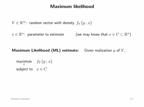
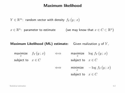

Maximum likelihood
Y ∈ Rm: random vector with density fY
(y ; x
)
x ∈ Rn: parameter to estimate (we may know that x ∈ C ⊂ Rn)
Maximum Likelihood (ML) estimate: Given realization y of Y ,
maximizex
fY
(y ; x
)
subject to x ∈ C
⇐⇒ maximizex
log fY
(y ; x
)
subject to x ∈ C
⇐⇒ minimizex
− log fY
(y ; x
)
subject to x ∈ C
negative log-likelihoodStatistical estimation 4-2

Maximum likelihoodExample: linear measurement model
• Parameter to estimate: x ∈ Rn
• Observations: Yi = a⊤i x + Vi, i = 1, . . . , m, for known ai ∈ Rn
Vi: iid copies of random variable V with density fV (v)
=⇒ Yi has density fV (yi − a⊤i x) and Yi’s are independent
=⇒ fY1···Ym(y1, . . . , ym) =m∏
i=1fYi(yi) =
m∏
i=1fV (yi − a⊤
i x)
The ai’s will denote the rows of A =
— a⊤1 —...
— a⊤m —
∈ Rm×n
Statistical estimation 4-3

Maximum likelihoodExample: linear measurement model
• Parameter to estimate: x ∈ Rn
• Observations: Yi = a⊤i x + Vi, i = 1, . . . , m, for known ai ∈ Rn
Vi: iid copies of random variable V with density fV (v)
=⇒ Yi has density fV (yi − a⊤i x)
and Yi’s are independent
=⇒ fY1···Ym(y1, . . . , ym) =m∏
i=1fYi(yi) =
m∏
i=1fV (yi − a⊤
i x)
The ai’s will denote the rows of A =
— a⊤1 —...
— a⊤m —
∈ Rm×n
Statistical estimation 4-3
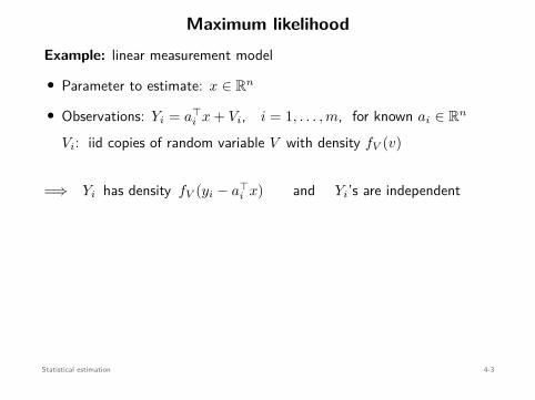
Maximum likelihoodExample: linear measurement model
• Parameter to estimate: x ∈ Rn
• Observations: Yi = a⊤i x + Vi, i = 1, . . . , m, for known ai ∈ Rn
Vi: iid copies of random variable V with density fV (v)
=⇒ Yi has density fV (yi − a⊤i x) and Yi’s are independent
=⇒ fY1···Ym(y1, . . . , ym) =m∏
i=1fYi(yi) =
m∏
i=1fV (yi − a⊤
i x)
The ai’s will denote the rows of A =
— a⊤1 —...
— a⊤m —
∈ Rm×n
Statistical estimation 4-3

Maximum likelihoodExample: linear measurement model
• Parameter to estimate: x ∈ Rn
• Observations: Yi = a⊤i x + Vi, i = 1, . . . , m, for known ai ∈ Rn
Vi: iid copies of random variable V with density fV (v)
=⇒ Yi has density fV (yi − a⊤i x) and Yi’s are independent
=⇒ fY1···Ym(y1, . . . , ym) =m∏
i=1fYi(yi) =
m∏
i=1fV (yi − a⊤
i x)
The ai’s will denote the rows of A =
— a⊤1 —...
— a⊤m —
∈ Rm×n
Statistical estimation 4-3

Maximum likelihood
xML ∈ arg minx
− logm∏
i=1fV (yi − a⊤
i x)
= arg minx
−m∑
i=1log fV (yi − a⊤
i x)
Common noise densities:
Gaussian: V ∼ N (0, σ2) fV (v) = 1√2πσ2 exp
(− v2
2σ2
)
xML ∈ arg minx
−m∑
i=1log 1√
2πσ2exp
(− (yi − a⊤
i x)2
2σ2
)
= arg minx
12σ2
m∑
i=1
(yi − a⊤
i x)2
= arg minx
12σ2
∥∥y − Ax∥∥2
2 Convex
Statistical estimation 4-4

Maximum likelihood
xML ∈ arg minx
− logm∏
i=1fV (yi − a⊤
i x) = arg minx
−m∑
i=1log fV (yi − a⊤
i x)
Common noise densities:
Gaussian:
V ∼ N (0, σ2) fV (v) = 1√2πσ2 exp
(− v2
2σ2
)
xML ∈ arg minx
−m∑
i=1log 1√
2πσ2exp
(− (yi − a⊤
i x)2
2σ2
)
= arg minx
12σ2
m∑
i=1
(yi − a⊤
i x)2
= arg minx
12σ2
∥∥y − Ax∥∥2
2 Convex
Statistical estimation 4-4

Maximum likelihood
xML ∈ arg minx
− logm∏
i=1fV (yi − a⊤
i x) = arg minx
−m∑
i=1log fV (yi − a⊤
i x)
Common noise densities:
Gaussian: V ∼ N (0, σ2)
fV (v) = 1√2πσ2 exp
(− v2
2σ2
)
xML ∈ arg minx
−m∑
i=1log 1√
2πσ2exp
(− (yi − a⊤
i x)2
2σ2
)
= arg minx
12σ2
m∑
i=1
(yi − a⊤
i x)2
= arg minx
12σ2
∥∥y − Ax∥∥2
2 Convex
Statistical estimation 4-4

Maximum likelihood
xML ∈ arg minx
− logm∏
i=1fV (yi − a⊤
i x) = arg minx
−m∑
i=1log fV (yi − a⊤
i x)
Common noise densities:
Gaussian: V ∼ N (0, σ2) fV (v) = 1√2πσ2 exp
(− v2
2σ2
)
xML ∈ arg minx
−m∑
i=1log 1√
2πσ2exp
(− (yi − a⊤
i x)2
2σ2
)
= arg minx
12σ2
m∑
i=1
(yi − a⊤
i x)2
= arg minx
12σ2
∥∥y − Ax∥∥2
2 Convex
Statistical estimation 4-4
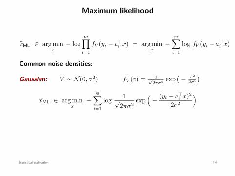
Maximum likelihood
xML ∈ arg minx
− logm∏
i=1fV (yi − a⊤
i x) = arg minx
−m∑
i=1log fV (yi − a⊤
i x)
Common noise densities:
Gaussian: V ∼ N (0, σ2) fV (v) = 1√2πσ2 exp
(− v2
2σ2
)
xML ∈ arg minx
−m∑
i=1log 1√
2πσ2exp
(− (yi − a⊤
i x)2
2σ2
)
= arg minx
12σ2
m∑
i=1
(yi − a⊤
i x)2
= arg minx
12σ2
∥∥y − Ax∥∥2
2
Convex
Statistical estimation 4-4
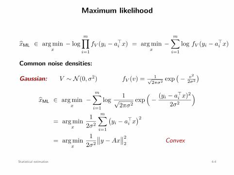
Maximum likelihood
xML ∈ arg minx
− logm∏
i=1fV (yi − a⊤
i x) = arg minx
−m∑
i=1log fV (yi − a⊤
i x)
Common noise densities:
Gaussian: V ∼ N (0, σ2) fV (v) = 1√2πσ2 exp
(− v2
2σ2
)
xML ∈ arg minx
−m∑
i=1log 1√
2πσ2exp
(− (yi − a⊤
i x)2
2σ2
)
= arg minx
12σ2
m∑
i=1
(yi − a⊤
i x)2
= arg minx
12σ2
∥∥y − Ax∥∥2
2 Convex
Statistical estimation 4-4

Maximum likelihood
xML ∈ arg minx
−m∑
i=1
log fV (yi − a⊤i x)
Laplacian:
V ∼ L(0, a) fV (v) = 1√2a
exp(
− |v|a
)(a > 0)
xML ∈ arg minx
−m∑
i=1log 1√
2aexp
(− |yi − a⊤
i x|a
)
= arg minx
1a
m∑
i=1
∣∣yi − a⊤i x
∣∣
= arg minx
1a
∥∥y − Ax∥∥
1 Convex
Statistical estimation 4-5

Maximum likelihood
xML ∈ arg minx
−m∑
i=1
log fV (yi − a⊤i x)
Laplacian: V ∼ L(0, a)
fV (v) = 1√2a
exp(
− |v|a
)(a > 0)
xML ∈ arg minx
−m∑
i=1log 1√
2aexp
(− |yi − a⊤
i x|a
)
= arg minx
1a
m∑
i=1
∣∣yi − a⊤i x
∣∣
= arg minx
1a
∥∥y − Ax∥∥
1 Convex
Statistical estimation 4-5

Maximum likelihood
xML ∈ arg minx
−m∑
i=1
log fV (yi − a⊤i x)
Laplacian: V ∼ L(0, a) fV (v) = 1√2a
exp(
− |v|a
)(a > 0)
xML ∈ arg minx
−m∑
i=1log 1√
2aexp
(− |yi − a⊤
i x|a
)
= arg minx
1a
m∑
i=1
∣∣yi − a⊤i x
∣∣
= arg minx
1a
∥∥y − Ax∥∥
1 Convex
Statistical estimation 4-5
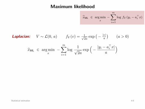
Maximum likelihood
xML ∈ arg minx
−m∑
i=1
log fV (yi − a⊤i x)
Laplacian: V ∼ L(0, a) fV (v) = 1√2a
exp(
− |v|a
)(a > 0)
xML ∈ arg minx
−m∑
i=1log 1√
2aexp
(− |yi − a⊤
i x|a
)
= arg minx
1a
m∑
i=1
∣∣yi − a⊤i x
∣∣
= arg minx
1a
∥∥y − Ax∥∥
1 Convex
Statistical estimation 4-5

Maximum likelihood
xML ∈ arg minx
−m∑
i=1
log fV (yi − a⊤i x)
Laplacian: V ∼ L(0, a) fV (v) = 1√2a
exp(
− |v|a
)(a > 0)
xML ∈ arg minx
−m∑
i=1log 1√
2aexp
(− |yi − a⊤
i x|a
)
= arg minx
1a
m∑
i=1
∣∣yi − a⊤i x
∣∣
= arg minx
1a
∥∥y − Ax∥∥
1 Convex
Statistical estimation 4-5

Maximum likelihood
xML ∈ arg minx
−m∑
i=1
log fV (yi − a⊤i x)
Laplacian: V ∼ L(0, a) fV (v) = 1√2a
exp(
− |v|a
)(a > 0)
xML ∈ arg minx
−m∑
i=1log 1√
2aexp
(− |yi − a⊤
i x|a
)
= arg minx
1a
m∑
i=1
∣∣yi − a⊤i x
∣∣
= arg minx
1a
∥∥y − Ax∥∥
1
Convex
Statistical estimation 4-5
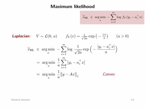
Maximum likelihood
xML ∈ arg minx
−m∑
i=1
log fV (yi − a⊤i x)
Laplacian: V ∼ L(0, a) fV (v) = 1√2a
exp(
− |v|a
)(a > 0)
xML ∈ arg minx
−m∑
i=1log 1√
2aexp
(− |yi − a⊤
i x|a
)
= arg minx
1a
m∑
i=1
∣∣yi − a⊤i x
∣∣
= arg minx
1a
∥∥y − Ax∥∥
1 Convex
Statistical estimation 4-5

Maximum likelihood
Uniform:
V ∼ U(−c, c) fV (v) = 1
2c , |v| ≤ c
0 , oth.
xML ∈ arg minx
−m∑
i=1log fV (yi − a⊤
i x)
= arg minx
− ∑mi=1 log 1
2c
s.t. |yi − a⊤i x| ≤ c , i = 1, . . . , m .
= find x
s.t. ∥y − Ax∥∞ ≤ c
feasibility problem (convex)
Statistical estimation 4-6
Maximum likelihood
Uniform: V ∼ U(−c, c)
fV (v) = 1
2c , |v| ≤ c
0 , oth.
xML ∈ arg minx
−m∑
i=1log fV (yi − a⊤
i x)
= arg minx
− ∑mi=1 log 1
2c
s.t. |yi − a⊤i x| ≤ c , i = 1, . . . , m .
= find x
s.t. ∥y − Ax∥∞ ≤ c
feasibility problem (convex)
Statistical estimation 4-6

Maximum likelihood
Uniform: V ∼ U(−c, c) fV (v) = 1
2c , |v| ≤ c
0 , oth.
xML ∈ arg minx
−m∑
i=1log fV (yi − a⊤
i x)
= arg minx
− ∑mi=1 log 1
2c
s.t. |yi − a⊤i x| ≤ c , i = 1, . . . , m .
= find x
s.t. ∥y − Ax∥∞ ≤ c
feasibility problem (convex)
Statistical estimation 4-6
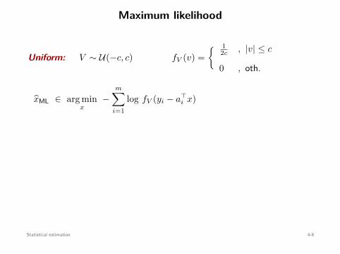
Maximum likelihood
Uniform: V ∼ U(−c, c) fV (v) = 1
2c , |v| ≤ c
0 , oth.
xML ∈ arg minx
−m∑
i=1log fV (yi − a⊤
i x)
= arg minx
− ∑mi=1 log 1
2c
s.t. |yi − a⊤i x| ≤ c , i = 1, . . . , m .
= find x
s.t. ∥y − Ax∥∞ ≤ c
feasibility problem (convex)
Statistical estimation 4-6

Maximum likelihood
Uniform: V ∼ U(−c, c) fV (v) = 1
2c , |v| ≤ c
0 , oth.
xML ∈ arg minx
−m∑
i=1log fV (yi − a⊤
i x)
= arg minx
− ∑mi=1 log 1
2c
s.t. |yi − a⊤i x| ≤ c , i = 1, . . . , m .
= find x
s.t. ∥y − Ax∥∞ ≤ c
feasibility problem (convex)
Statistical estimation 4-6

Maximum likelihood
Uniform: V ∼ U(−c, c) fV (v) = 1
2c , |v| ≤ c
0 , oth.
xML ∈ arg minx
−m∑
i=1log fV (yi − a⊤
i x)
= arg minx
− ∑mi=1 log 1
2c
s.t. |yi − a⊤i x| ≤ c , i = 1, . . . , m .
= find x
s.t. ∥y − Ax∥∞ ≤ c
feasibility problem (convex)
Statistical estimation 4-6
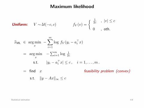
Maximum likelihood
Uniform: V ∼ U(−c, c) fV (v) = 1
2c , |v| ≤ c
0 , oth.
xML ∈ arg minx
−m∑
i=1log fV (yi − a⊤
i x)
= arg minx
− ∑mi=1 log 1
2c
s.t. |yi − a⊤i x| ≤ c , i = 1, . . . , m .
= find x
s.t. ∥y − Ax∥∞ ≤ c
feasibility problem (convex)
Statistical estimation 4-6
Example with a discrete RV
Y ∈ N: # of traffic accidents in a given period
Y ∼ Poisson(µ) P(Y = k) = e−µµk
k ! , k = 0, 1, . . .
Assumption: µ depends on vector of explanatory variables U ∈ Rn as
µ = a⊤U + b , a ∈ Rn , b ∈ R
e.g., U1 = traffic flow during the period, U2 = rainfall, . . .
Goal:
Given m independent observations(
U (i), Y (i))m
i=1, estimate a and b.
Statistical estimation 4-7

Example with a discrete RV
Y ∈ N: # of traffic accidents in a given period
Y ∼ Poisson(µ)
P(Y = k) = e−µµk
k ! , k = 0, 1, . . .
Assumption: µ depends on vector of explanatory variables U ∈ Rn as
µ = a⊤U + b , a ∈ Rn , b ∈ R
e.g., U1 = traffic flow during the period, U2 = rainfall, . . .
Goal:
Given m independent observations(
U (i), Y (i))m
i=1, estimate a and b.
Statistical estimation 4-7

Example with a discrete RV
Y ∈ N: # of traffic accidents in a given period
Y ∼ Poisson(µ) P(Y = k) = e−µµk
k ! , k = 0, 1, . . .
Assumption: µ depends on vector of explanatory variables U ∈ Rn as
µ = a⊤U + b , a ∈ Rn , b ∈ R
e.g., U1 = traffic flow during the period, U2 = rainfall, . . .
Goal:
Given m independent observations(
U (i), Y (i))m
i=1, estimate a and b.
Statistical estimation 4-7
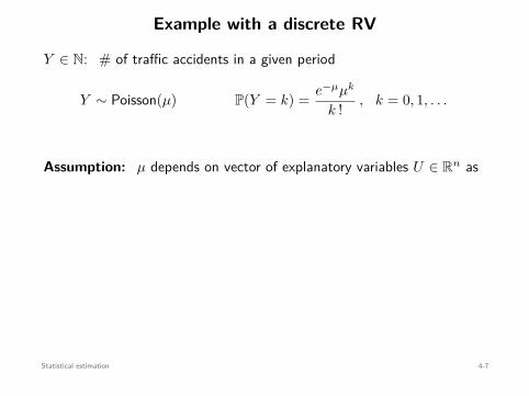
Example with a discrete RV
Y ∈ N: # of traffic accidents in a given period
Y ∼ Poisson(µ) P(Y = k) = e−µµk
k ! , k = 0, 1, . . .
Assumption: µ depends on vector of explanatory variables U ∈ Rn as
µ = a⊤U + b , a ∈ Rn , b ∈ R
e.g., U1 = traffic flow during the period, U2 = rainfall, . . .
Goal:
Given m independent observations(
U (i), Y (i))m
i=1, estimate a and b.
Statistical estimation 4-7
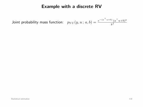
Example with a discrete RV
Joint probability mass function: pY U (y, u ; a, b) = e−(a⊤u+b) (a⊤u+b)y
y !
ML estimator:
(aML, bML
)∈ arg min
a,b−
m∑
i=1log pY U (yi, ui ; a, b)
= arg mina,b
−m∑
i=1log e−(a⊤u(i)+b) (a⊤u(i) + b)y(i)
y(i) !
= arg mina,b
m∑
i=1a⊤u(i) + b
︸ ︷︷ ︸affine
− y(i) log(a⊤u(i) + b
)
︸ ︷︷ ︸convex
Convex
Statistical estimation 4-8
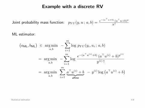
Example with a discrete RV
Joint probability mass function: pY U (y, u ; a, b) = e−(a⊤u+b) (a⊤u+b)y
y !
ML estimator:
(aML, bML
)∈ arg min
a,b−
m∑
i=1log pY U (yi, ui ; a, b)
= arg mina,b
−m∑
i=1log e−(a⊤u(i)+b) (a⊤u(i) + b)y(i)
y(i) !
= arg mina,b
m∑
i=1a⊤u(i) + b︸ ︷︷ ︸
affine
− y(i) log(a⊤u(i) + b
)︸ ︷︷ ︸
convex
Convex
Statistical estimation 4-8

Maximum a posteriori (MAP)
Y ∈ Rm: random vector w/ density fY (y)
X ∈ Rn: random vector to estimate no longer a parameterprior knowledge: fX(x)
MAP estimator:
xMAP ∈ arg maxx
fX|Y (x|y) Bayes= arg maxx
fY |X(y|x)fX(x)fY (y)
= arg maxx
fY |X(y|x)fX(x)
= arg maxx
log(fY |X(y|x)fX(x)
)
= arg minx
− log fY |X(y|x) − log fX(x)
Statistical estimation 4-9

Maximum a posteriori (MAP)
Y ∈ Rm: random vector w/ density fY (y)
X ∈ Rn: random vector to estimate
no longer a parameterprior knowledge: fX(x)
MAP estimator:
xMAP ∈ arg maxx
fX|Y (x|y) Bayes= arg maxx
fY |X(y|x)fX(x)fY (y)
= arg maxx
fY |X(y|x)fX(x)
= arg maxx
log(fY |X(y|x)fX(x)
)
= arg minx
− log fY |X(y|x) − log fX(x)
Statistical estimation 4-9

Maximum a posteriori (MAP)
Y ∈ Rm: random vector w/ density fY (y)
X ∈ Rn: random vector to estimate no longer a parameter
prior knowledge: fX(x)
MAP estimator:
xMAP ∈ arg maxx
fX|Y (x|y) Bayes= arg maxx
fY |X(y|x)fX(x)fY (y)
= arg maxx
fY |X(y|x)fX(x)
= arg maxx
log(fY |X(y|x)fX(x)
)
= arg minx
− log fY |X(y|x) − log fX(x)
Statistical estimation 4-9
Maximum a posteriori (MAP)
Y ∈ Rm: random vector w/ density fY (y)
X ∈ Rn: random vector to estimate no longer a parameterprior knowledge: fX(x)
MAP estimator:
xMAP ∈ arg maxx
fX|Y (x|y) Bayes= arg maxx
fY |X(y|x)fX(x)fY (y)
= arg maxx
fY |X(y|x)fX(x)
= arg maxx
log(fY |X(y|x)fX(x)
)
= arg minx
− log fY |X(y|x) − log fX(x)
Statistical estimation 4-9
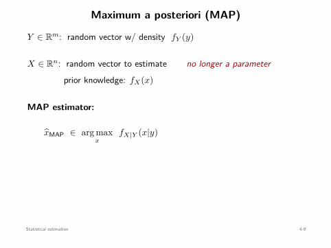
Maximum a posteriori (MAP)
Y ∈ Rm: random vector w/ density fY (y)
X ∈ Rn: random vector to estimate no longer a parameterprior knowledge: fX(x)
MAP estimator:
xMAP ∈ arg maxx
fX|Y (x|y)
Bayes= arg maxx
fY |X(y|x)fX(x)fY (y)
= arg maxx
fY |X(y|x)fX(x)
= arg maxx
log(fY |X(y|x)fX(x)
)
= arg minx
− log fY |X(y|x) − log fX(x)
Statistical estimation 4-9

Maximum a posteriori (MAP)
Y ∈ Rm: random vector w/ density fY (y)
X ∈ Rn: random vector to estimate no longer a parameterprior knowledge: fX(x)
MAP estimator:
xMAP ∈ arg maxx
fX|Y (x|y) Bayes= arg maxx
fY |X(y|x)fX(x)fY (y)
= arg maxx
fY |X(y|x)fX(x)
= arg maxx
log(fY |X(y|x)fX(x)
)
= arg minx
− log fY |X(y|x) − log fX(x)
Statistical estimation 4-9

Maximum a posteriori (MAP)
Y ∈ Rm: random vector w/ density fY (y)
X ∈ Rn: random vector to estimate no longer a parameterprior knowledge: fX(x)
MAP estimator:
xMAP ∈ arg maxx
fX|Y (x|y) Bayes= arg maxx
fY |X(y|x)fX(x)fY (y)
= arg maxx
fY |X(y|x)fX(x)
= arg maxx
log(fY |X(y|x)fX(x)
)
= arg minx
− log fY |X(y|x) − log fX(x)
Statistical estimation 4-9
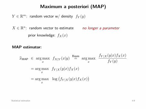
Maximum a posteriori (MAP)
Y ∈ Rm: random vector w/ density fY (y)
X ∈ Rn: random vector to estimate no longer a parameterprior knowledge: fX(x)
MAP estimator:
xMAP ∈ arg maxx
fX|Y (x|y) Bayes= arg maxx
fY |X(y|x)fX(x)fY (y)
= arg maxx
fY |X(y|x)fX(x)
= arg maxx
log(fY |X(y|x)fX(x)
)
= arg minx
− log fY |X(y|x) − log fX(x)
Statistical estimation 4-9

Maximum a posteriori (MAP)
Example: linear measurement model
• Observations: Yi = a⊤i X + Vi, i = 1, . . . , m , & Vi
iid= V ∼ U(−c, c)
fY1···Ym|X(y1, . . . , ym|x) =m∏
i=1fYi|X(yi|x) =
m∏
i=1U
(a⊤
i x − c , a⊤i x + c
)
• Random vector to estimate in Rn: X ∼ N(x, Σ
) (known x, Σ
)
fX(x) = 1(2π)n/2|Σ|1/2 exp
(− 1
2(x − x)⊤Σ−1(x − x))
xMAP ∈ arg minx
− log fY1···Ym|X(y1, . . . , ym|x) − log fX(x)
= arg minx
12 (x − x)⊤Σ−1(x − x)
s.t. ∥Ax − y∥∞ ≤ c
Convex
Statistical estimation 4-10

Maximum a posteriori (MAP)
Example: linear measurement model• Observations: Yi = a⊤
i X + Vi, i = 1, . . . , m
, & Viiid= V ∼ U(−c, c)
fY1···Ym|X(y1, . . . , ym|x) =m∏
i=1fYi|X(yi|x) =
m∏
i=1U
(a⊤
i x − c , a⊤i x + c
)
• Random vector to estimate in Rn: X ∼ N(x, Σ
) (known x, Σ
)
fX(x) = 1(2π)n/2|Σ|1/2 exp
(− 1
2(x − x)⊤Σ−1(x − x))
xMAP ∈ arg minx
− log fY1···Ym|X(y1, . . . , ym|x) − log fX(x)
= arg minx
12 (x − x)⊤Σ−1(x − x)
s.t. ∥Ax − y∥∞ ≤ c
Convex
Statistical estimation 4-10

Maximum a posteriori (MAP)
Example: linear measurement model• Observations: Yi = a⊤
i X + Vi, i = 1, . . . , m , & Viiid= V ∼ U(−c, c)
fY1···Ym|X(y1, . . . , ym|x) =m∏
i=1fYi|X(yi|x) =
m∏
i=1U
(a⊤
i x − c , a⊤i x + c
)
• Random vector to estimate in Rn: X ∼ N(x, Σ
) (known x, Σ
)
fX(x) = 1(2π)n/2|Σ|1/2 exp
(− 1
2(x − x)⊤Σ−1(x − x))
xMAP ∈ arg minx
− log fY1···Ym|X(y1, . . . , ym|x) − log fX(x)
= arg minx
12 (x − x)⊤Σ−1(x − x)
s.t. ∥Ax − y∥∞ ≤ c
Convex
Statistical estimation 4-10
Maximum a posteriori (MAP)
Example: linear measurement model• Observations: Yi = a⊤
i X + Vi, i = 1, . . . , m , & Viiid= V ∼ U(−c, c)
fY1···Ym|X(y1, . . . , ym|x)
=m∏
i=1fYi|X(yi|x) =
m∏
i=1U
(a⊤
i x − c , a⊤i x + c
)
• Random vector to estimate in Rn: X ∼ N(x, Σ
) (known x, Σ
)
fX(x) = 1(2π)n/2|Σ|1/2 exp
(− 1
2(x − x)⊤Σ−1(x − x))
xMAP ∈ arg minx
− log fY1···Ym|X(y1, . . . , ym|x) − log fX(x)
= arg minx
12 (x − x)⊤Σ−1(x − x)
s.t. ∥Ax − y∥∞ ≤ c
Convex
Statistical estimation 4-10

Maximum a posteriori (MAP)
Example: linear measurement model• Observations: Yi = a⊤
i X + Vi, i = 1, . . . , m , & Viiid= V ∼ U(−c, c)
fY1···Ym|X(y1, . . . , ym|x) =m∏
i=1fYi|X(yi|x)
=m∏
i=1U
(a⊤
i x − c , a⊤i x + c
)
• Random vector to estimate in Rn: X ∼ N(x, Σ
) (known x, Σ
)
fX(x) = 1(2π)n/2|Σ|1/2 exp
(− 1
2(x − x)⊤Σ−1(x − x))
xMAP ∈ arg minx
− log fY1···Ym|X(y1, . . . , ym|x) − log fX(x)
= arg minx
12 (x − x)⊤Σ−1(x − x)
s.t. ∥Ax − y∥∞ ≤ c
Convex
Statistical estimation 4-10

Maximum a posteriori (MAP)
Example: linear measurement model• Observations: Yi = a⊤
i X + Vi, i = 1, . . . , m , & Viiid= V ∼ U(−c, c)
fY1···Ym|X(y1, . . . , ym|x) =m∏
i=1fYi|X(yi|x) =
m∏
i=1U
(a⊤
i x − c , a⊤i x + c
)
• Random vector to estimate in Rn: X ∼ N(x, Σ
) (known x, Σ
)
fX(x) = 1(2π)n/2|Σ|1/2 exp
(− 1
2(x − x)⊤Σ−1(x − x))
xMAP ∈ arg minx
− log fY1···Ym|X(y1, . . . , ym|x) − log fX(x)
= arg minx
12 (x − x)⊤Σ−1(x − x)
s.t. ∥Ax − y∥∞ ≤ c
Convex
Statistical estimation 4-10

Maximum a posteriori (MAP)
Example: linear measurement model• Observations: Yi = a⊤
i X + Vi, i = 1, . . . , m , & Viiid= V ∼ U(−c, c)
fY1···Ym|X(y1, . . . , ym|x) =m∏
i=1fYi|X(yi|x) =
m∏
i=1U
(a⊤
i x − c , a⊤i x + c
)
• Random vector to estimate in Rn: X ∼ N(x, Σ
)
(known x, Σ
)
fX(x) = 1(2π)n/2|Σ|1/2 exp
(− 1
2(x − x)⊤Σ−1(x − x))
xMAP ∈ arg minx
− log fY1···Ym|X(y1, . . . , ym|x) − log fX(x)
= arg minx
12 (x − x)⊤Σ−1(x − x)
s.t. ∥Ax − y∥∞ ≤ c
Convex
Statistical estimation 4-10

Maximum a posteriori (MAP)
Example: linear measurement model• Observations: Yi = a⊤
i X + Vi, i = 1, . . . , m , & Viiid= V ∼ U(−c, c)
fY1···Ym|X(y1, . . . , ym|x) =m∏
i=1fYi|X(yi|x) =
m∏
i=1U
(a⊤
i x − c , a⊤i x + c
)
• Random vector to estimate in Rn: X ∼ N(x, Σ
) (known x, Σ
)
fX(x) = 1(2π)n/2|Σ|1/2 exp
(− 1
2(x − x)⊤Σ−1(x − x))
xMAP ∈ arg minx
− log fY1···Ym|X(y1, . . . , ym|x) − log fX(x)
= arg minx
12 (x − x)⊤Σ−1(x − x)
s.t. ∥Ax − y∥∞ ≤ c
Convex
Statistical estimation 4-10
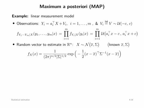
Maximum a posteriori (MAP)
Example: linear measurement model• Observations: Yi = a⊤
i X + Vi, i = 1, . . . , m , & Viiid= V ∼ U(−c, c)
fY1···Ym|X(y1, . . . , ym|x) =m∏
i=1fYi|X(yi|x) =
m∏
i=1U
(a⊤
i x − c , a⊤i x + c
)
• Random vector to estimate in Rn: X ∼ N(x, Σ
) (known x, Σ
)
fX(x) = 1(2π)n/2|Σ|1/2 exp
(− 1
2(x − x)⊤Σ−1(x − x))
xMAP ∈ arg minx
− log fY1···Ym|X(y1, . . . , ym|x) − log fX(x)
= arg minx
12 (x − x)⊤Σ−1(x − x)
s.t. ∥Ax − y∥∞ ≤ c
Convex
Statistical estimation 4-10
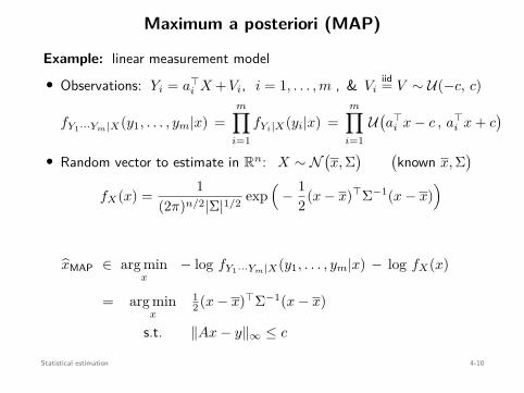
Maximum a posteriori (MAP)
Example: linear measurement model• Observations: Yi = a⊤
i X + Vi, i = 1, . . . , m , & Viiid= V ∼ U(−c, c)
fY1···Ym|X(y1, . . . , ym|x) =m∏
i=1fYi|X(yi|x) =
m∏
i=1U
(a⊤
i x − c , a⊤i x + c
)
• Random vector to estimate in Rn: X ∼ N(x, Σ
) (known x, Σ
)
fX(x) = 1(2π)n/2|Σ|1/2 exp
(− 1
2(x − x)⊤Σ−1(x − x))
xMAP ∈ arg minx
− log fY1···Ym|X(y1, . . . , ym|x) − log fX(x)
= arg minx
12 (x − x)⊤Σ−1(x − x)
s.t. ∥Ax − y∥∞ ≤ c
Convex
Statistical estimation 4-10
Maximum a posteriori (MAP)
LASSO:
• Observations: Yi = a⊤i X + Vi, i = 1, . . . , m, with
Viiid= V ∼ N (0, σ2)
• Random vector to estimate X ∈ Rn has iid Laplacian entries L(0, b)
xMAP ∈ arg minx
12
∥∥y − Ax∥∥2
2 + σ2
b∥x∥1
Known as basis pursuit denoising or LASSO (Convex)
Statistical estimation 4-11
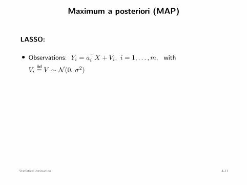
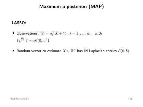

Maximum a posteriori (MAP)
LASSO:
• Observations: Yi = a⊤i X + Vi, i = 1, . . . , m, with
Viiid= V ∼ N (0, σ2)
• Random vector to estimate X ∈ Rn has iid Laplacian entries L(0, b)
xMAP ∈ arg minx
12
∥∥y − Ax∥∥2
2 + σ2
b∥x∥1
Known as basis pursuit denoising or LASSO
(Convex)
Statistical estimation 4-11

Maximum a posteriori (MAP)
LASSO:
• Observations: Yi = a⊤i X + Vi, i = 1, . . . , m, with
Viiid= V ∼ N (0, σ2)
• Random vector to estimate X ∈ Rn has iid Laplacian entries L(0, b)
xMAP ∈ arg minx
12
∥∥y − Ax∥∥2
2 + σ2
b∥x∥1
Known as basis pursuit denoising or LASSO (Convex)
Statistical estimation 4-11

Nonparametric estimation
ML and MAP allow estimating parameters of given distributions
What about estimating non-canonical distributions?
Example:
X: discrete RV taking values on 100 equidistant points in [−1, 1]
EX EX2E[3X3 − 2X]
P(X < 0)−1 0 1
We requireEX ∈ [−0.1, 0.1] EX2 ∈ [0.5, 0.6]
E[3X3 − 2X
]∈ [−0.3, −0.2]
P(X < 0
)∈ [0.3, 0.4]
Find a distribution satisfying these constraints & with maximum entropy
Statistical estimation 4-12
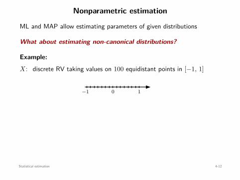
Nonparametric estimation
ML and MAP allow estimating parameters of given distributions
What about estimating non-canonical distributions?
Example:
X: discrete RV taking values on 100 equidistant points in [−1, 1]
EX EX2E[3X3 − 2X]
P(X < 0)
−1 0 1
We requireEX ∈ [−0.1, 0.1]
EX2 ∈ [0.5, 0.6]
E[3X3 − 2X
]∈ [−0.3, −0.2]
P(X < 0
)∈ [0.3, 0.4]
Find a distribution satisfying these constraints & with maximum entropy
Statistical estimation 4-12

Nonparametric estimation
ML and MAP allow estimating parameters of given distributions
What about estimating non-canonical distributions?
Example:
X: discrete RV taking values on 100 equidistant points in [−1, 1]
EX
EX2E[3X3 − 2X]
P(X < 0)
−1 0 1
We requireEX ∈ [−0.1, 0.1]
EX2 ∈ [0.5, 0.6]
E[3X3 − 2X
]∈ [−0.3, −0.2]
P(X < 0
)∈ [0.3, 0.4]
Find a distribution satisfying these constraints & with maximum entropy
Statistical estimation 4-12

Nonparametric estimation
ML and MAP allow estimating parameters of given distributions
What about estimating non-canonical distributions?
Example:
X: discrete RV taking values on 100 equidistant points in [−1, 1]
EX EX2
E[3X3 − 2X]
P(X < 0)
−1 0 1
We requireEX ∈ [−0.1, 0.1] EX2 ∈ [0.5, 0.6]
E[3X3 − 2X
]∈ [−0.3, −0.2]
P(X < 0
)∈ [0.3, 0.4]
Find a distribution satisfying these constraints & with maximum entropy
Statistical estimation 4-12

Nonparametric estimation
ML and MAP allow estimating parameters of given distributions
What about estimating non-canonical distributions?
Example:
X: discrete RV taking values on 100 equidistant points in [−1, 1]
EX EX2E[3X3 − 2X]
P(X < 0)
−1 0 1
We requireEX ∈ [−0.1, 0.1] EX2 ∈ [0.5, 0.6]
E[3X3 − 2X
]∈ [−0.3, −0.2]
P(X < 0
)∈ [0.3, 0.4]
Find a distribution satisfying these constraints & with maximum entropy
Statistical estimation 4-12

Nonparametric estimation
ML and MAP allow estimating parameters of given distributions
What about estimating non-canonical distributions?
Example:
X: discrete RV taking values on 100 equidistant points in [−1, 1]
EX EX2E[3X3 − 2X]
P(X < 0)−1 0 1
We requireEX ∈ [−0.1, 0.1] EX2 ∈ [0.5, 0.6]
E[3X3 − 2X
]∈ [−0.3, −0.2]
P(X < 0
)∈ [0.3, 0.4]
Find a distribution satisfying these constraints & with maximum entropy
Statistical estimation 4-12

Nonparametric estimation
ML and MAP allow estimating parameters of given distributions
What about estimating non-canonical distributions?
Example:
X: discrete RV taking values on 100 equidistant points in [−1, 1]
EX EX2E[3X3 − 2X]
P(X < 0)−1 0 1
We requireEX ∈ [−0.1, 0.1] EX2 ∈ [0.5, 0.6]
E[3X3 − 2X
]∈ [−0.3, −0.2]
P(X < 0
)∈ [0.3, 0.4]
Find a distribution satisfying these constraints & with maximum entropyStatistical estimation 4-12

Nonparametric estimation
α = (−1, −0.9798, . . . , 0.9798, 1) ∈ R100 values that X takesp ∈ R100 such that pi = P(X = αi)
p: pmf =⇒ belongs to the probability simplex
p ∈ ∆n :=
x ∈ Rn : x ≥ 0n , 1⊤n x = 1
Rn
∆n
EX ∈ [−0.1, 0.1] ⇐⇒ −0.1 ≤ α⊤p ≤ 0.1
EX2 ∈ [0.5, 0.6] ⇐⇒ 0.5 ≤ β⊤p ≤ 0.6 βi = α2i
E[3X3 − 2X
]∈ [−0.3, −0.2] ⇐⇒ −0.3 ≤ γ⊤p ≤ −0.2 γi = 3α2
i − 2αi
P(X < 0
)∈ [0.3, 0.4] ⇐⇒ 0.3 ≤ σ⊤p ≤ 0.4 σi = 1 if i < 50
σi = 0 if i ≥ 50All constraints are linear inequalities in p!
Statistical estimation 4-13

Nonparametric estimation
α = (−1, −0.9798, . . . , 0.9798, 1) ∈ R100 values that X takes
p ∈ R100 such that pi = P(X = αi)
p: pmf =⇒ belongs to the probability simplex
p ∈ ∆n :=
x ∈ Rn : x ≥ 0n , 1⊤n x = 1
Rn
∆n
EX ∈ [−0.1, 0.1] ⇐⇒ −0.1 ≤ α⊤p ≤ 0.1
EX2 ∈ [0.5, 0.6] ⇐⇒ 0.5 ≤ β⊤p ≤ 0.6 βi = α2i
E[3X3 − 2X
]∈ [−0.3, −0.2] ⇐⇒ −0.3 ≤ γ⊤p ≤ −0.2 γi = 3α2
i − 2αi
P(X < 0
)∈ [0.3, 0.4] ⇐⇒ 0.3 ≤ σ⊤p ≤ 0.4 σi = 1 if i < 50
σi = 0 if i ≥ 50All constraints are linear inequalities in p!
Statistical estimation 4-13

Nonparametric estimation
α = (−1, −0.9798, . . . , 0.9798, 1) ∈ R100 values that X takesp ∈ R100 such that pi = P(X = αi)
p: pmf =⇒ belongs to the probability simplex
p ∈ ∆n :=
x ∈ Rn : x ≥ 0n , 1⊤n x = 1
Rn
∆n
EX ∈ [−0.1, 0.1] ⇐⇒ −0.1 ≤ α⊤p ≤ 0.1
EX2 ∈ [0.5, 0.6] ⇐⇒ 0.5 ≤ β⊤p ≤ 0.6 βi = α2i
E[3X3 − 2X
]∈ [−0.3, −0.2] ⇐⇒ −0.3 ≤ γ⊤p ≤ −0.2 γi = 3α2
i − 2αi
P(X < 0
)∈ [0.3, 0.4] ⇐⇒ 0.3 ≤ σ⊤p ≤ 0.4 σi = 1 if i < 50
σi = 0 if i ≥ 50All constraints are linear inequalities in p!
Statistical estimation 4-13

Nonparametric estimation
α = (−1, −0.9798, . . . , 0.9798, 1) ∈ R100 values that X takesp ∈ R100 such that pi = P(X = αi)
p: pmf
=⇒ belongs to the probability simplex
p ∈ ∆n :=
x ∈ Rn : x ≥ 0n , 1⊤n x = 1
Rn
∆n
EX ∈ [−0.1, 0.1] ⇐⇒ −0.1 ≤ α⊤p ≤ 0.1
EX2 ∈ [0.5, 0.6] ⇐⇒ 0.5 ≤ β⊤p ≤ 0.6 βi = α2i
E[3X3 − 2X
]∈ [−0.3, −0.2] ⇐⇒ −0.3 ≤ γ⊤p ≤ −0.2 γi = 3α2
i − 2αi
P(X < 0
)∈ [0.3, 0.4] ⇐⇒ 0.3 ≤ σ⊤p ≤ 0.4 σi = 1 if i < 50
σi = 0 if i ≥ 50All constraints are linear inequalities in p!
Statistical estimation 4-13

Nonparametric estimation
α = (−1, −0.9798, . . . , 0.9798, 1) ∈ R100 values that X takesp ∈ R100 such that pi = P(X = αi)
p: pmf =⇒ belongs to the probability simplex
p ∈ ∆n :=
x ∈ Rn : x ≥ 0n , 1⊤n x = 1
Rn
∆n
EX ∈ [−0.1, 0.1] ⇐⇒ −0.1 ≤ α⊤p ≤ 0.1
EX2 ∈ [0.5, 0.6] ⇐⇒ 0.5 ≤ β⊤p ≤ 0.6 βi = α2i
E[3X3 − 2X
]∈ [−0.3, −0.2] ⇐⇒ −0.3 ≤ γ⊤p ≤ −0.2 γi = 3α2
i − 2αi
P(X < 0
)∈ [0.3, 0.4] ⇐⇒ 0.3 ≤ σ⊤p ≤ 0.4 σi = 1 if i < 50
σi = 0 if i ≥ 50All constraints are linear inequalities in p!
Statistical estimation 4-13

Nonparametric estimation
α = (−1, −0.9798, . . . , 0.9798, 1) ∈ R100 values that X takesp ∈ R100 such that pi = P(X = αi)
p: pmf =⇒ belongs to the probability simplex
p ∈ ∆n :=
x ∈ Rn : x ≥ 0n , 1⊤n x = 1
Rn
∆n
EX ∈ [−0.1, 0.1] ⇐⇒ −0.1 ≤ α⊤p ≤ 0.1
EX2 ∈ [0.5, 0.6] ⇐⇒ 0.5 ≤ β⊤p ≤ 0.6 βi = α2i
E[3X3 − 2X
]∈ [−0.3, −0.2] ⇐⇒ −0.3 ≤ γ⊤p ≤ −0.2 γi = 3α2
i − 2αi
P(X < 0
)∈ [0.3, 0.4] ⇐⇒ 0.3 ≤ σ⊤p ≤ 0.4 σi = 1 if i < 50
σi = 0 if i ≥ 50All constraints are linear inequalities in p!
Statistical estimation 4-13
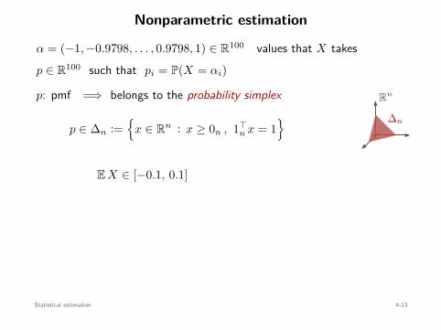
Nonparametric estimation
α = (−1, −0.9798, . . . , 0.9798, 1) ∈ R100 values that X takesp ∈ R100 such that pi = P(X = αi)
p: pmf =⇒ belongs to the probability simplex
p ∈ ∆n :=
x ∈ Rn : x ≥ 0n , 1⊤n x = 1
Rn
∆n
EX ∈ [−0.1, 0.1]
⇐⇒ −0.1 ≤ α⊤p ≤ 0.1
EX2 ∈ [0.5, 0.6] ⇐⇒ 0.5 ≤ β⊤p ≤ 0.6 βi = α2i
E[3X3 − 2X
]∈ [−0.3, −0.2] ⇐⇒ −0.3 ≤ γ⊤p ≤ −0.2 γi = 3α2
i − 2αi
P(X < 0
)∈ [0.3, 0.4] ⇐⇒ 0.3 ≤ σ⊤p ≤ 0.4 σi = 1 if i < 50
σi = 0 if i ≥ 50All constraints are linear inequalities in p!
Statistical estimation 4-13

Nonparametric estimation
α = (−1, −0.9798, . . . , 0.9798, 1) ∈ R100 values that X takesp ∈ R100 such that pi = P(X = αi)
p: pmf =⇒ belongs to the probability simplex
p ∈ ∆n :=
x ∈ Rn : x ≥ 0n , 1⊤n x = 1
Rn
∆n
EX ∈ [−0.1, 0.1] ⇐⇒ −0.1 ≤ α⊤p ≤ 0.1
EX2 ∈ [0.5, 0.6] ⇐⇒ 0.5 ≤ β⊤p ≤ 0.6 βi = α2i
E[3X3 − 2X
]∈ [−0.3, −0.2] ⇐⇒ −0.3 ≤ γ⊤p ≤ −0.2 γi = 3α2
i − 2αi
P(X < 0
)∈ [0.3, 0.4] ⇐⇒ 0.3 ≤ σ⊤p ≤ 0.4 σi = 1 if i < 50
σi = 0 if i ≥ 50All constraints are linear inequalities in p!
Statistical estimation 4-13
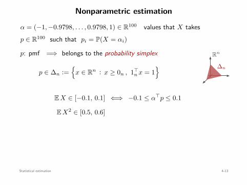
Nonparametric estimation
α = (−1, −0.9798, . . . , 0.9798, 1) ∈ R100 values that X takesp ∈ R100 such that pi = P(X = αi)
p: pmf =⇒ belongs to the probability simplex
p ∈ ∆n :=
x ∈ Rn : x ≥ 0n , 1⊤n x = 1
Rn
∆n
EX ∈ [−0.1, 0.1] ⇐⇒ −0.1 ≤ α⊤p ≤ 0.1
EX2 ∈ [0.5, 0.6]
⇐⇒ 0.5 ≤ β⊤p ≤ 0.6 βi = α2i
E[3X3 − 2X
]∈ [−0.3, −0.2] ⇐⇒ −0.3 ≤ γ⊤p ≤ −0.2 γi = 3α2
i − 2αi
P(X < 0
)∈ [0.3, 0.4] ⇐⇒ 0.3 ≤ σ⊤p ≤ 0.4 σi = 1 if i < 50
σi = 0 if i ≥ 50All constraints are linear inequalities in p!
Statistical estimation 4-13

Nonparametric estimation
α = (−1, −0.9798, . . . , 0.9798, 1) ∈ R100 values that X takesp ∈ R100 such that pi = P(X = αi)
p: pmf =⇒ belongs to the probability simplex
p ∈ ∆n :=
x ∈ Rn : x ≥ 0n , 1⊤n x = 1
Rn
∆n
EX ∈ [−0.1, 0.1] ⇐⇒ −0.1 ≤ α⊤p ≤ 0.1
EX2 ∈ [0.5, 0.6] ⇐⇒ 0.5 ≤ β⊤p ≤ 0.6 βi = α2i
E[3X3 − 2X
]∈ [−0.3, −0.2] ⇐⇒ −0.3 ≤ γ⊤p ≤ −0.2 γi = 3α2
i − 2αi
P(X < 0
)∈ [0.3, 0.4] ⇐⇒ 0.3 ≤ σ⊤p ≤ 0.4 σi = 1 if i < 50
σi = 0 if i ≥ 50All constraints are linear inequalities in p!
Statistical estimation 4-13
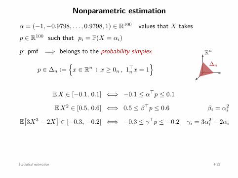
Nonparametric estimation
α = (−1, −0.9798, . . . , 0.9798, 1) ∈ R100 values that X takesp ∈ R100 such that pi = P(X = αi)
p: pmf =⇒ belongs to the probability simplex
p ∈ ∆n :=
x ∈ Rn : x ≥ 0n , 1⊤n x = 1
Rn
∆n
EX ∈ [−0.1, 0.1] ⇐⇒ −0.1 ≤ α⊤p ≤ 0.1
EX2 ∈ [0.5, 0.6] ⇐⇒ 0.5 ≤ β⊤p ≤ 0.6 βi = α2i
E[3X3 − 2X
]∈ [−0.3, −0.2] ⇐⇒ −0.3 ≤ γ⊤p ≤ −0.2 γi = 3α2
i − 2αi
P(X < 0
)∈ [0.3, 0.4]
⇐⇒ 0.3 ≤ σ⊤p ≤ 0.4 σi = 1 if i < 50
σi = 0 if i ≥ 50All constraints are linear inequalities in p!
Statistical estimation 4-13

Nonparametric estimation
α = (−1, −0.9798, . . . , 0.9798, 1) ∈ R100 values that X takesp ∈ R100 such that pi = P(X = αi)
p: pmf =⇒ belongs to the probability simplex
p ∈ ∆n :=
x ∈ Rn : x ≥ 0n , 1⊤n x = 1
Rn
∆n
EX ∈ [−0.1, 0.1] ⇐⇒ −0.1 ≤ α⊤p ≤ 0.1
EX2 ∈ [0.5, 0.6] ⇐⇒ 0.5 ≤ β⊤p ≤ 0.6 βi = α2i
E[3X3 − 2X
]∈ [−0.3, −0.2] ⇐⇒ −0.3 ≤ γ⊤p ≤ −0.2 γi = 3α2
i − 2αi
P(X < 0
)∈ [0.3, 0.4] ⇐⇒ 0.3 ≤ σ⊤p ≤ 0.4 σi = 1 if i < 50
σi = 0 if i ≥ 50
All constraints are linear inequalities in p!
Statistical estimation 4-13

Nonparametric estimation
α = (−1, −0.9798, . . . , 0.9798, 1) ∈ R100 values that X takesp ∈ R100 such that pi = P(X = αi)
p: pmf =⇒ belongs to the probability simplex
p ∈ ∆n :=
x ∈ Rn : x ≥ 0n , 1⊤n x = 1
Rn
∆n
EX ∈ [−0.1, 0.1] ⇐⇒ −0.1 ≤ α⊤p ≤ 0.1
EX2 ∈ [0.5, 0.6] ⇐⇒ 0.5 ≤ β⊤p ≤ 0.6 βi = α2i
E[3X3 − 2X
]∈ [−0.3, −0.2] ⇐⇒ −0.3 ≤ γ⊤p ≤ −0.2 γi = 3α2
i − 2αi
P(X < 0
)∈ [0.3, 0.4] ⇐⇒ 0.3 ≤ σ⊤p ≤ 0.4 σi = 1 if i < 50
σi = 0 if i ≥ 50All constraints are linear inequalities in p!
Statistical estimation 4-13

Nonparametric estimation
Maximize entropy
= minimize negative entropy:
−H(p) :=n∑
i=1pi log pi
Convex because d2
dx2 x log x = 1x > 0, for all x > 0
Optimization problem: (convex)
minimizep∈R100
∑ni=1 pi log pi
subject to −0.1 ≤ α⊤p ≤ 0.1
0.5 ≤ β⊤p ≤ 0.6
−0.3 ≤ γ⊤p ≤ −0.2
0.3 ≤ σ⊤p ≤ 0.4
Statistical estimation 4-14
Nonparametric estimation
Maximize entropy = minimize negative entropy:
−H(p) :=n∑
i=1pi log pi
Convex because d2
dx2 x log x = 1x > 0, for all x > 0
Optimization problem: (convex)
minimizep∈R100
∑ni=1 pi log pi
subject to −0.1 ≤ α⊤p ≤ 0.1
0.5 ≤ β⊤p ≤ 0.6
−0.3 ≤ γ⊤p ≤ −0.2
0.3 ≤ σ⊤p ≤ 0.4
Statistical estimation 4-14

Nonparametric estimation
n = 100 ;a lpha = l i n s p a c e ( −1 ,1 ,n ) ’ ;cvx_beg in
v a r i a b l e p (n , 1 ) ;m in im ize ( −sum( e n t r ( p ) ) ) ;s u b j e c t to
p >= 0 ;ones (1 , n )∗p == 1 ;−0.1 <= alpha ’∗ p <= 0 . 1 ;0 . 5 <= ( a lpha . ^ 2 ) ’∗ p <= 0 . 6 ;−0.3 <= (3∗ a lpha .^3 − 2∗ a lpha ) ’∗ p <= −0.2;0 . 3 <= ( a lpha < 0) ’∗ p <= 0 . 4 ;
cvx_endStatistical estimation 4-15
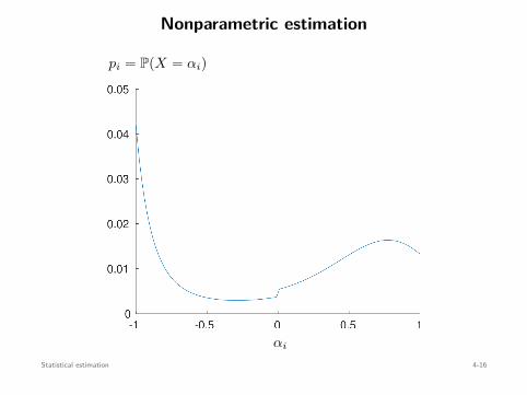
Nonparametric estimation
pi = P(X = αi)
αi
Statistical estimation 4-16

Hypothesis testing & optimal detection
X : discrete random variable w/ probability mass function (pmf) pθ
X ∈ 1, . . . , n
θ ∈ 1, . . . , mx
p1(x)
x
p2(x)
P =
P(X = 1 | θ = 1) P(X = 1 | θ = 2) · · · P(X = 1 | θ = m)
P(X = 2 | θ = 1) P(X = 2 | θ = 2) · · · P(X = 2 | θ = m)...
......
P(X = n | θ = 1) P(X = n | θ = 2) · · · P(X = n | θ = m)
∈ Rn×m
Goal: Estimate θ based on an observation of X
Statistical estimation 4-17
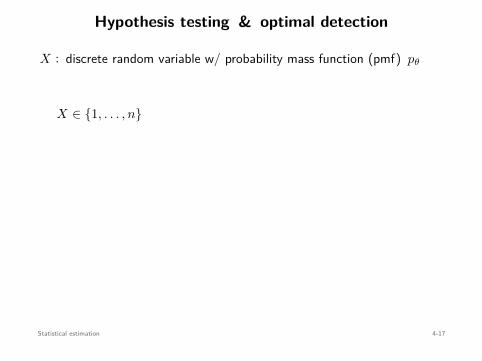
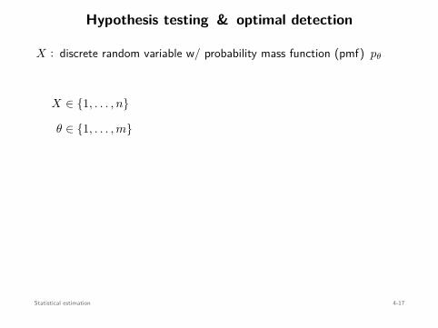
Hypothesis testing & optimal detection
X : discrete random variable w/ probability mass function (pmf) pθ
X ∈ 1, . . . , n
θ ∈ 1, . . . , m
x
p1(x)
x
p2(x)
P =
P(X = 1 | θ = 1) P(X = 1 | θ = 2) · · · P(X = 1 | θ = m)
P(X = 2 | θ = 1) P(X = 2 | θ = 2) · · · P(X = 2 | θ = m)...
......
P(X = n | θ = 1) P(X = n | θ = 2) · · · P(X = n | θ = m)
∈ Rn×m
Goal: Estimate θ based on an observation of X
Statistical estimation 4-17

Hypothesis testing & optimal detection
X : discrete random variable w/ probability mass function (pmf) pθ
X ∈ 1, . . . , n
θ ∈ 1, . . . , mx
p1(x)
x
p2(x)
P =
P(X = 1 | θ = 1) P(X = 1 | θ = 2) · · · P(X = 1 | θ = m)
P(X = 2 | θ = 1) P(X = 2 | θ = 2) · · · P(X = 2 | θ = m)...
......
P(X = n | θ = 1) P(X = n | θ = 2) · · · P(X = n | θ = m)
∈ Rn×m
Goal: Estimate θ based on an observation of X
Statistical estimation 4-17
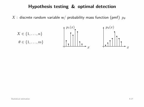
Hypothesis testing & optimal detection
X : discrete random variable w/ probability mass function (pmf) pθ
X ∈ 1, . . . , n
θ ∈ 1, . . . , mx
p1(x)
x
p2(x)
P =
P(X = 1 | θ = 1) P(X = 1 | θ = 2) · · · P(X = 1 | θ = m)
P(X = 2 | θ = 1) P(X = 2 | θ = 2) · · · P(X = 2 | θ = m)...
......
P(X = n | θ = 1) P(X = n | θ = 2) · · · P(X = n | θ = m)
∈ Rn×m
Goal: Estimate θ based on an observation of X
Statistical estimation 4-17
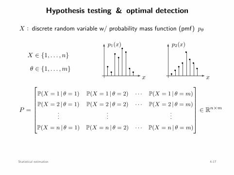
Hypothesis testing & optimal detection
X : discrete random variable w/ probability mass function (pmf) pθ
X ∈ 1, . . . , n
θ ∈ 1, . . . , mx
p1(x)
x
p2(x)
P =
P(X = 1 | θ = 1) P(X = 1 | θ = 2) · · · P(X = 1 | θ = m)
P(X = 2 | θ = 1) P(X = 2 | θ = 2) · · · P(X = 2 | θ = m)...
......
P(X = n | θ = 1) P(X = n | θ = 2) · · · P(X = n | θ = m)
∈ Rn×m
Goal: Estimate θ based on an observation of X
Statistical estimation 4-17

Detector:
Ψ : 1, . . . , n
︸ ︷︷ ︸X
−→ 1, . . . , m
︸ ︷︷ ︸θ
Example: maximum likelihood detector
θML = ΨML(x) = arg maxj
P(X = x | θ = j
)
Randomized detector: Random variable θ whose pmf depends on X
T =
P(θ = 1 | X = 1) P(θ = 1 | X = 2) · · · P(θ = 1 | X = n)
P(θ = 2 | X = 1) P(θ = 2 | X = 2) · · · P(θ = 2 | X = n)...
......
P(θ = m | X = 1) P(θ = m | X = 2) · · · P(θ = m | X = n)
∈ Rm×n
Each column ti ∈ Rm satisfies 1⊤mti = 1, ti ≥ 0
If each ti is a canonical vector (0, . . . , 1, . . . , 0), then T is deterministic
Statistical estimation 4-18

Detector: Ψ : 1, . . . , n
︸ ︷︷ ︸X
−→ 1, . . . , m
︸ ︷︷ ︸θ
Example: maximum likelihood detector
θML = ΨML(x) = arg maxj
P(X = x | θ = j
)
Randomized detector: Random variable θ whose pmf depends on X
T =
P(θ = 1 | X = 1) P(θ = 1 | X = 2) · · · P(θ = 1 | X = n)
P(θ = 2 | X = 1) P(θ = 2 | X = 2) · · · P(θ = 2 | X = n)...
......
P(θ = m | X = 1) P(θ = m | X = 2) · · · P(θ = m | X = n)
∈ Rm×n
Each column ti ∈ Rm satisfies 1⊤mti = 1, ti ≥ 0
If each ti is a canonical vector (0, . . . , 1, . . . , 0), then T is deterministic
Statistical estimation 4-18

Detector: Ψ : 1, . . . , n︸ ︷︷ ︸X
−→ 1, . . . , m︸ ︷︷ ︸θ
Example: maximum likelihood detector
θML = ΨML(x) = arg maxj
P(X = x | θ = j
)
Randomized detector: Random variable θ whose pmf depends on X
T =
P(θ = 1 | X = 1) P(θ = 1 | X = 2) · · · P(θ = 1 | X = n)
P(θ = 2 | X = 1) P(θ = 2 | X = 2) · · · P(θ = 2 | X = n)...
......
P(θ = m | X = 1) P(θ = m | X = 2) · · · P(θ = m | X = n)
∈ Rm×n
Each column ti ∈ Rm satisfies 1⊤mti = 1, ti ≥ 0
If each ti is a canonical vector (0, . . . , 1, . . . , 0), then T is deterministic
Statistical estimation 4-18
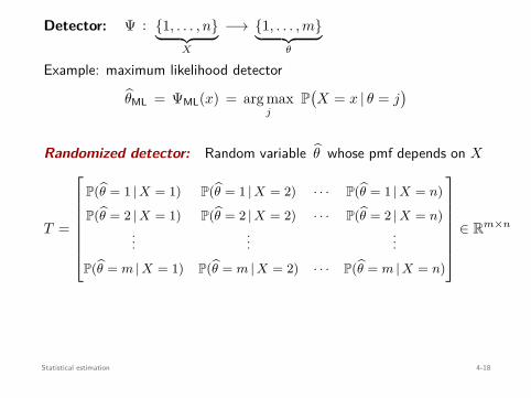
Detector: Ψ : 1, . . . , n︸ ︷︷ ︸X
−→ 1, . . . , m︸ ︷︷ ︸θ
Example: maximum likelihood detector
θML = ΨML(x) = arg maxj
P(X = x | θ = j
)
Randomized detector: Random variable θ whose pmf depends on X
T =
P(θ = 1 | X = 1) P(θ = 1 | X = 2) · · · P(θ = 1 | X = n)
P(θ = 2 | X = 1) P(θ = 2 | X = 2) · · · P(θ = 2 | X = n)...
......
P(θ = m | X = 1) P(θ = m | X = 2) · · · P(θ = m | X = n)
∈ Rm×n
Each column ti ∈ Rm satisfies 1⊤mti = 1, ti ≥ 0
If each ti is a canonical vector (0, . . . , 1, . . . , 0), then T is deterministicStatistical estimation 4-18

Detection probability matrix:
D := TP ∈ Rm×m
Dij =n∑
k=1P
(θ = i | X = k
)· P
(X = k | θ = j
)
= P(
θ = i
︸ ︷︷ ︸guess
| θ = j
︸ ︷︷ ︸true
)
Goal: Design T such that the Dij ’s, for i = j, are as small as possible
Multi-objective optimization
Statistical estimation 4-19

Detection probability matrix: D := TP ∈ Rm×m
Dij =n∑
k=1P
(θ = i | X = k
)· P
(X = k | θ = j
)
= P(
θ = i
︸ ︷︷ ︸guess
| θ = j
︸ ︷︷ ︸true
)
Goal: Design T such that the Dij ’s, for i = j, are as small as possible
Multi-objective optimization
Statistical estimation 4-19
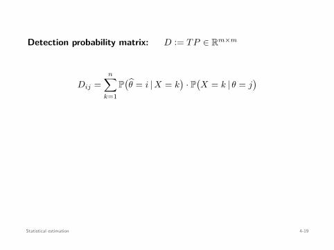
Detection probability matrix: D := TP ∈ Rm×m
Dij =n∑
k=1P
(θ = i | X = k
)· P
(X = k | θ = j
)
= P(
θ = i
︸ ︷︷ ︸guess
| θ = j
︸ ︷︷ ︸true
)
Goal: Design T such that the Dij ’s, for i = j, are as small as possible
Multi-objective optimization
Statistical estimation 4-19
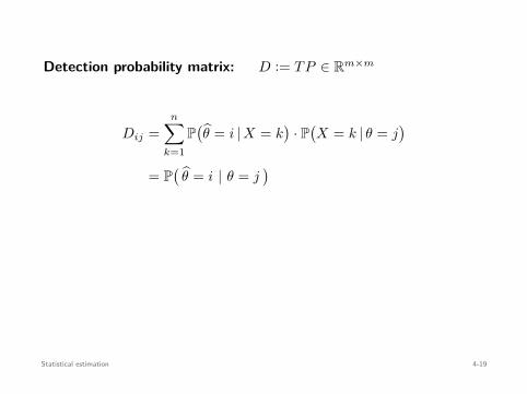
Detection probability matrix: D := TP ∈ Rm×m
Dij =n∑
k=1P
(θ = i | X = k
)· P
(X = k | θ = j
)
= P(
θ = i
︸ ︷︷ ︸guess
| θ = j
︸ ︷︷ ︸true
)
Goal: Design T such that the Dij ’s, for i = j, are as small as possible
Multi-objective optimization
Statistical estimation 4-19

Detection probability matrix: D := TP ∈ Rm×m
Dij =n∑
k=1P
(θ = i | X = k
)· P
(X = k | θ = j
)
= P(
θ = i︸ ︷︷ ︸guess
| θ = j︸ ︷︷ ︸true
)
Goal: Design T such that the Dij ’s, for i = j, are as small as possible
Multi-objective optimization
Statistical estimation 4-19

Detection probability matrix: D := TP ∈ Rm×m
Dij =n∑
k=1P
(θ = i | X = k
)· P
(X = k | θ = j
)
= P(
θ = i︸ ︷︷ ︸guess
| θ = j︸ ︷︷ ︸true
)
Goal: Design T such that the Dij ’s, for i = j, are as small as possible
Multi-objective optimization
Statistical estimation 4-19

Detection probability matrix: D := TP ∈ Rm×m
Dij =n∑
k=1P
(θ = i | X = k
)· P
(X = k | θ = j
)
= P(
θ = i︸ ︷︷ ︸guess
| θ = j︸ ︷︷ ︸true
)
Goal: Design T such that the Dij ’s, for i = j, are as small as possible
Multi-objective optimization
Statistical estimation 4-19
Minimax detector
Note that
P(θ = j | θ = j
)= 1 − P
(θ = j | θ = j
)= 1 − Djj
Minimax detector:
minimizeT ∈Rm×n
maxj=i,...,m
1 − Djj(T )
subject to T ⊤1m = 1n , T ≥ 0
⇐⇒ minimizeT ∈Rm×n
maxj=i,...,m
1 − tr(TP eje⊤
j
)
subject to T ⊤1m = 1n , T ≥ 0
Convex
Statistical estimation 4-20

Minimax detector
Note that
P(θ = j | θ = j
)
= 1 − P(θ = j | θ = j
)= 1 − Djj
Minimax detector:
minimizeT ∈Rm×n
maxj=i,...,m
1 − Djj(T )
subject to T ⊤1m = 1n , T ≥ 0
⇐⇒ minimizeT ∈Rm×n
maxj=i,...,m
1 − tr(TP eje⊤
j
)
subject to T ⊤1m = 1n , T ≥ 0
Convex
Statistical estimation 4-20

Minimax detector
Note that
P(θ = j | θ = j
)= 1 − P
(θ = j | θ = j
)
= 1 − Djj
Minimax detector:
minimizeT ∈Rm×n
maxj=i,...,m
1 − Djj(T )
subject to T ⊤1m = 1n , T ≥ 0
⇐⇒ minimizeT ∈Rm×n
maxj=i,...,m
1 − tr(TP eje⊤
j
)
subject to T ⊤1m = 1n , T ≥ 0
Convex
Statistical estimation 4-20

Minimax detector
Note that
P(θ = j | θ = j
)= 1 − P
(θ = j | θ = j
)= 1 − Djj
Minimax detector:
minimizeT ∈Rm×n
maxj=i,...,m
1 − Djj(T )
subject to T ⊤1m = 1n , T ≥ 0
⇐⇒ minimizeT ∈Rm×n
maxj=i,...,m
1 − tr(TP eje⊤
j
)
subject to T ⊤1m = 1n , T ≥ 0
Convex
Statistical estimation 4-20

Minimax detector
Note that
P(θ = j | θ = j
)= 1 − P
(θ = j | θ = j
)= 1 − Djj
Minimax detector:
minimizeT ∈Rm×n
maxj=i,...,m
1 − Djj(T )
subject to T ⊤1m = 1n , T ≥ 0
⇐⇒ minimizeT ∈Rm×n
maxj=i,...,m
1 − tr(TP eje⊤
j
)
subject to T ⊤1m = 1n , T ≥ 0
Convex
Statistical estimation 4-20

Minimax detector
Note that
P(θ = j | θ = j
)= 1 − P
(θ = j | θ = j
)= 1 − Djj
Minimax detector:
minimizeT ∈Rm×n
maxj=i,...,m
1 − Djj(T )
subject to T ⊤1m = 1n , T ≥ 0
⇐⇒ minimizeT ∈Rm×n
maxj=i,...,m
1 − tr(TP eje⊤
j
)
subject to T ⊤1m = 1n , T ≥ 0
Convex
Statistical estimation 4-20

Minimax detector
Note that
P(θ = j | θ = j
)= 1 − P
(θ = j | θ = j
)= 1 − Djj
Minimax detector:
minimizeT ∈Rm×n
maxj=i,...,m
1 − Djj(T )
subject to T ⊤1m = 1n , T ≥ 0
⇐⇒ minimizeT ∈Rm×n
maxj=i,...,m
1 − tr(TP eje⊤
j
)
subject to T ⊤1m = 1n , T ≥ 0
Convex
Statistical estimation 4-20

Minimax detector
Note that
P(θ = j | θ = j
)= 1 − P
(θ = j | θ = j
)= 1 − Djj
Minimax detector:
minimizeT ∈Rm×n
maxj=i,...,m
1 − Djj(T )
subject to T ⊤1m = 1n , T ≥ 0
⇐⇒ minimizeT ∈Rm×n
maxj=i,...,m
1 − tr(TP eje⊤
j
)
subject to T ⊤1m = 1n , T ≥ 0
Convex
Statistical estimation 4-20

Pareto-optimal detectors
Recall that we want to minimize all Dij = P(θ = i | θ = j
), for i = j
Scalarization: Fix W ∈ Rm×m w/ Wii = 0, and Wij > 0 for i = j
minimizeT
m∑
i=1
m∑
j=1WijDij(T )
subject to T ⊤1m = 1n , T ≥ 0
By varying W we can find Pareto optimal solutions
Observations:
• Constraints ⇐⇒ 1⊤mti = 1, ti ≥ 0, for i = 1, . . . , n
• Objective ⇐⇒ tr(W ⊤TP
)
= tr((WP ⊤)⊤T
)=
∑ni=1 c⊤
i ti
where ci: ith column of C := WP ⊤
Statistical estimation 4-21
Pareto-optimal detectors
Recall that we want to minimize all Dij = P(θ = i | θ = j
), for i = j
Scalarization:
Fix W ∈ Rm×m w/ Wii = 0, and Wij > 0 for i = j
minimizeT
m∑
i=1
m∑
j=1WijDij(T )
subject to T ⊤1m = 1n , T ≥ 0
By varying W we can find Pareto optimal solutions
Observations:
• Constraints ⇐⇒ 1⊤mti = 1, ti ≥ 0, for i = 1, . . . , n
• Objective ⇐⇒ tr(W ⊤TP
)
= tr((WP ⊤)⊤T
)=
∑ni=1 c⊤
i ti
where ci: ith column of C := WP ⊤
Statistical estimation 4-21

Pareto-optimal detectors
Recall that we want to minimize all Dij = P(θ = i | θ = j
), for i = j
Scalarization: Fix W ∈ Rm×m w/ Wii = 0, and Wij > 0 for i = j
minimizeT
m∑
i=1
m∑
j=1WijDij(T )
subject to T ⊤1m = 1n , T ≥ 0
By varying W we can find Pareto optimal solutions
Observations:
• Constraints ⇐⇒ 1⊤mti = 1, ti ≥ 0, for i = 1, . . . , n
• Objective ⇐⇒ tr(W ⊤TP
)
= tr((WP ⊤)⊤T
)=
∑ni=1 c⊤
i ti
where ci: ith column of C := WP ⊤
Statistical estimation 4-21

Pareto-optimal detectors
Recall that we want to minimize all Dij = P(θ = i | θ = j
), for i = j
Scalarization: Fix W ∈ Rm×m w/ Wii = 0, and Wij > 0 for i = j
minimizeT
m∑
i=1
m∑
j=1WijDij(T )
subject to T ⊤1m = 1n , T ≥ 0
By varying W we can find Pareto optimal solutions
Observations:
• Constraints ⇐⇒ 1⊤mti = 1, ti ≥ 0, for i = 1, . . . , n
• Objective ⇐⇒ tr(W ⊤TP
)= tr
((WP ⊤)⊤T
)
=∑n
i=1 c⊤i ti
where ci: ith column of C := WP ⊤
Statistical estimation 4-21

Pareto-optimal detectors
Recall that we want to minimize all Dij = P(θ = i | θ = j
), for i = j
Scalarization: Fix W ∈ Rm×m w/ Wii = 0, and Wij > 0 for i = j
minimizeT
m∑
i=1
m∑
j=1WijDij(T )
subject to T ⊤1m = 1n , T ≥ 0
By varying W we can find Pareto optimal solutions
Observations:
• Constraints ⇐⇒ 1⊤mti = 1, ti ≥ 0, for i = 1, . . . , n
• Objective ⇐⇒ tr(W ⊤TP
)= tr
((WP ⊤)⊤T
)=
∑ni=1 c⊤
i ti
where ci: ith column of C := WP ⊤
Statistical estimation 4-21

Pareto-optimal detectors
Recall that we want to minimize all Dij = P(θ = i | θ = j
), for i = j
Scalarization: Fix W ∈ Rm×m w/ Wii = 0, and Wij > 0 for i = j
minimizeT
m∑
i=1
m∑
j=1WijDij(T )
subject to T ⊤1m = 1n , T ≥ 0
By varying W we can find Pareto optimal solutions
Observations:
• Constraints ⇐⇒ 1⊤mti = 1, ti ≥ 0, for i = 1, . . . , n
• Objective ⇐⇒ tr(W ⊤TP
)= tr
((WP ⊤)⊤T
)=
∑ni=1 c⊤
i ti
where ci: ith column of C := WP ⊤
Statistical estimation 4-21
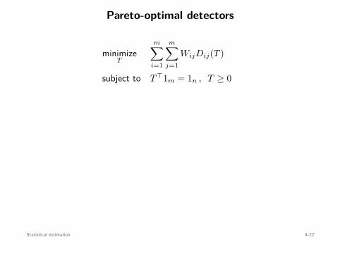
Pareto-optimal detectors
minimizeT
m∑
i=1
m∑
j=1WijDij(T )
subject to T ⊤1m = 1n , T ≥ 0
⇐⇒ minimizet1,...,tn
∑ni=1 c⊤
i ti
subject to 1⊤mti = 1 , ti ≥ 0 , i = 1, . . . , n
Decouples into n independent optimization problems: for column i,
minimizeti
c⊤i ti
subject to 1⊤mti = 1 , ti ≥ 0
t⋆i = (0, . . . , 1, . . . , 0) =⇒ T is deterministic
Rm
−cb
t⋆i
Statistical estimation 4-22
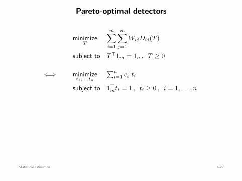
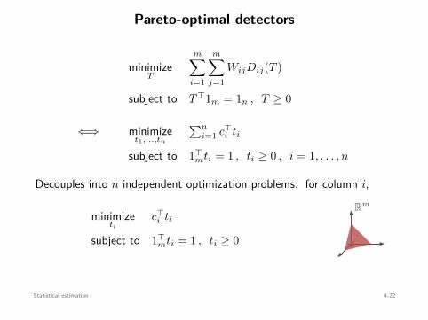
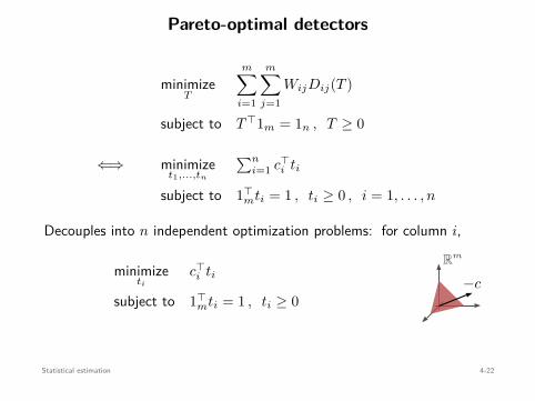
Pareto-optimal detectors
minimizeT
m∑
i=1
m∑
j=1WijDij(T )
subject to T ⊤1m = 1n , T ≥ 0
⇐⇒ minimizet1,...,tn
∑ni=1 c⊤
i ti
subject to 1⊤mti = 1 , ti ≥ 0 , i = 1, . . . , n
Decouples into n independent optimization problems: for column i,
minimizeti
c⊤i ti
subject to 1⊤mti = 1 , ti ≥ 0
t⋆i = (0, . . . , 1, . . . , 0) =⇒ T is deterministic
Rm
−c
b
t⋆i
Statistical estimation 4-22
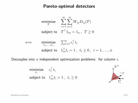
Pareto-optimal detectors
minimizeT
m∑
i=1
m∑
j=1WijDij(T )
subject to T ⊤1m = 1n , T ≥ 0
⇐⇒ minimizet1,...,tn
∑ni=1 c⊤
i ti
subject to 1⊤mti = 1 , ti ≥ 0 , i = 1, . . . , n
Decouples into n independent optimization problems: for column i,
minimizeti
c⊤i ti
subject to 1⊤mti = 1 , ti ≥ 0
t⋆i = (0, . . . , 1, . . . , 0) =⇒ T is deterministic
Rm
−cb
t⋆i
Statistical estimation 4-22

Pareto-optimal detectors
minimizeT
m∑
i=1
m∑
j=1WijDij(T )
subject to T ⊤1m = 1n , T ≥ 0
⇐⇒ minimizet1,...,tn
∑ni=1 c⊤
i ti
subject to 1⊤mti = 1 , ti ≥ 0 , i = 1, . . . , n
Decouples into n independent optimization problems: for column i,
minimizeti
c⊤i ti
subject to 1⊤mti = 1 , ti ≥ 0
t⋆i = (0, . . . , 1, . . . , 0)
=⇒ T is deterministic
Rm
−cb
t⋆i
Statistical estimation 4-22

Pareto-optimal detectors
minimizeT
m∑
i=1
m∑
j=1WijDij(T )
subject to T ⊤1m = 1n , T ≥ 0
⇐⇒ minimizet1,...,tn
∑ni=1 c⊤
i ti
subject to 1⊤mti = 1 , ti ≥ 0 , i = 1, . . . , n
Decouples into n independent optimization problems: for column i,
minimizeti
c⊤i ti
subject to 1⊤mti = 1 , ti ≥ 0
t⋆i = (0, . . . , 1, . . . , 0) =⇒ T is deterministic
Rm
−cb
t⋆i
Statistical estimation 4-22

Example: binary hypothesis testing
X is generated by either p1 (θ = 1) or p2 (θ = 2)
P =
P(X = 1 | θ = 1) P(X = 1 | θ = 2)
P(X = 2 | θ = 1) P(X = 2 | θ = 2)...
...P(X = n | θ = 1) P(X = n | θ = 2)
∈ Rn×2
T =
P(θ = 1 | X = 1) P(θ = 1 | X = 2) · · · P(θ = 1 | X = n)
P(θ = 2 | X = 1) P(θ = 2 | X = 2) · · · P(θ = 2 | X = n)
∈ R2×n
D =
P
(θ = 1 | θ = 1
)P
(θ = 1 | θ = 2
)
P(θ = 2 | θ = 1
)P
(θ = 2 | θ = 2
)
=
1 − Pfp Pfn
Pfp 1 − Pfn
Statistical estimation 4-23
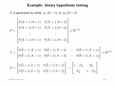

Pareto-optimal detectors:
Select W ∈ R2×2, set C = WP ⊤, and column i of TPO solves
minimizeti
c⊤i ti (ci: column i of C)
subject to 1⊤2 ti = 1 , ti ≥ 0
C =
0 W12
W21 0
P(X = 1 | θ = 1) · · · P(X = n | θ = 1)
P(X = 1 | θ = 2) · · · P(X = n | θ = 2)
=
W12 P(X = 1 | θ = 2) · · · W12 P(X = n | θ = 2)
W21 P(X = 1 | θ = 1) · · · W21 P(X = n | θ = 1)
Therefore,
c⊤i ti = t1i W12 P(X = i | θ = 2) + t2i W21 P(X = i | θ = 1)
Statistical estimation 4-24
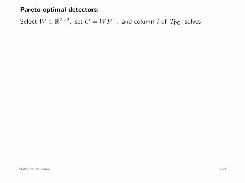

• If W12 P(X = i | θ = 2) < W21 P(X = i | θ = 1),
(t⋆1i , t⋆
2i) = (1 , 0) =⇒ θPO = 1
• If W12 P(X = i | θ = 2) ≥ W21 P(X = i | θ = 1) ,
(t⋆1i , t⋆
2i) = (0 , 1) =⇒ θPO = 2
This is the likelihood-ratio test: Decide θ = 2 if
P(X = i | θ = 2)P(X = i | θ = 1) ≥ W21
W12=: α
Neyman-Pearson lemma:
For each α > 0, the likelihood-ratio test yields a (deterministic)Pareto-optimal detector.
Statistical estimation 4-25

• If W12 P(X = i | θ = 2) < W21 P(X = i | θ = 1),
(t⋆1i , t⋆
2i) = (1 , 0)
=⇒ θPO = 1
• If W12 P(X = i | θ = 2) ≥ W21 P(X = i | θ = 1) ,
(t⋆1i , t⋆
2i) = (0 , 1) =⇒ θPO = 2
This is the likelihood-ratio test: Decide θ = 2 if
P(X = i | θ = 2)P(X = i | θ = 1) ≥ W21
W12=: α
Neyman-Pearson lemma:
For each α > 0, the likelihood-ratio test yields a (deterministic)Pareto-optimal detector.
Statistical estimation 4-25

• If W12 P(X = i | θ = 2) < W21 P(X = i | θ = 1),
(t⋆1i , t⋆
2i) = (1 , 0) =⇒ θPO = 1
• If W12 P(X = i | θ = 2) ≥ W21 P(X = i | θ = 1) ,
(t⋆1i , t⋆
2i) = (0 , 1) =⇒ θPO = 2
This is the likelihood-ratio test: Decide θ = 2 if
P(X = i | θ = 2)P(X = i | θ = 1) ≥ W21
W12=: α
Neyman-Pearson lemma:
For each α > 0, the likelihood-ratio test yields a (deterministic)Pareto-optimal detector.
Statistical estimation 4-25
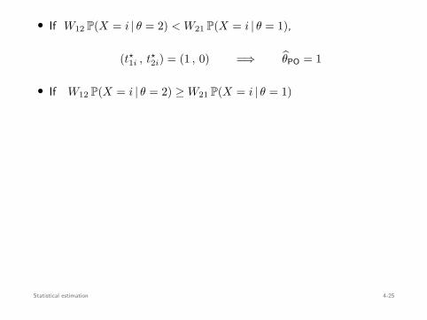
• If W12 P(X = i | θ = 2) < W21 P(X = i | θ = 1),
(t⋆1i , t⋆
2i) = (1 , 0) =⇒ θPO = 1
• If W12 P(X = i | θ = 2) ≥ W21 P(X = i | θ = 1)
,
(t⋆1i , t⋆
2i) = (0 , 1) =⇒ θPO = 2
This is the likelihood-ratio test: Decide θ = 2 if
P(X = i | θ = 2)P(X = i | θ = 1) ≥ W21
W12=: α
Neyman-Pearson lemma:
For each α > 0, the likelihood-ratio test yields a (deterministic)Pareto-optimal detector.
Statistical estimation 4-25
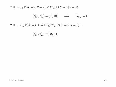
• If W12 P(X = i | θ = 2) < W21 P(X = i | θ = 1),
(t⋆1i , t⋆
2i) = (1 , 0) =⇒ θPO = 1
• If W12 P(X = i | θ = 2) ≥ W21 P(X = i | θ = 1) ,
(t⋆1i , t⋆
2i) = (0 , 1)
=⇒ θPO = 2
This is the likelihood-ratio test: Decide θ = 2 if
P(X = i | θ = 2)P(X = i | θ = 1) ≥ W21
W12=: α
Neyman-Pearson lemma:
For each α > 0, the likelihood-ratio test yields a (deterministic)Pareto-optimal detector.
Statistical estimation 4-25

• If W12 P(X = i | θ = 2) < W21 P(X = i | θ = 1),
(t⋆1i , t⋆
2i) = (1 , 0) =⇒ θPO = 1
• If W12 P(X = i | θ = 2) ≥ W21 P(X = i | θ = 1) ,
(t⋆1i , t⋆
2i) = (0 , 1) =⇒ θPO = 2
This is the likelihood-ratio test: Decide θ = 2 if
P(X = i | θ = 2)P(X = i | θ = 1) ≥ W21
W12=: α
Neyman-Pearson lemma:
For each α > 0, the likelihood-ratio test yields a (deterministic)Pareto-optimal detector.
Statistical estimation 4-25

• If W12 P(X = i | θ = 2) < W21 P(X = i | θ = 1),
(t⋆1i , t⋆
2i) = (1 , 0) =⇒ θPO = 1
• If W12 P(X = i | θ = 2) ≥ W21 P(X = i | θ = 1) ,
(t⋆1i , t⋆
2i) = (0 , 1) =⇒ θPO = 2
This is the likelihood-ratio test:
Decide θ = 2 if
P(X = i | θ = 2)P(X = i | θ = 1) ≥ W21
W12=: α
Neyman-Pearson lemma:
For each α > 0, the likelihood-ratio test yields a (deterministic)Pareto-optimal detector.
Statistical estimation 4-25
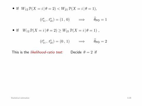
• If W12 P(X = i | θ = 2) < W21 P(X = i | θ = 1),
(t⋆1i , t⋆
2i) = (1 , 0) =⇒ θPO = 1
• If W12 P(X = i | θ = 2) ≥ W21 P(X = i | θ = 1) ,
(t⋆1i , t⋆
2i) = (0 , 1) =⇒ θPO = 2
This is the likelihood-ratio test: Decide θ = 2 if
P(X = i | θ = 2)P(X = i | θ = 1) ≥ W21
W12=: α
Neyman-Pearson lemma:
For each α > 0, the likelihood-ratio test yields a (deterministic)Pareto-optimal detector.
Statistical estimation 4-25
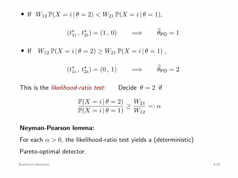
• If W12 P(X = i | θ = 2) < W21 P(X = i | θ = 1),
(t⋆1i , t⋆
2i) = (1 , 0) =⇒ θPO = 1
• If W12 P(X = i | θ = 2) ≥ W21 P(X = i | θ = 1) ,
(t⋆1i , t⋆
2i) = (0 , 1) =⇒ θPO = 2
This is the likelihood-ratio test: Decide θ = 2 if
P(X = i | θ = 2)P(X = i | θ = 1) ≥ W21
W12=: α
Neyman-Pearson lemma:
For each α > 0, the likelihood-ratio test yields a (deterministic)Pareto-optimal detector.
Statistical estimation 4-25
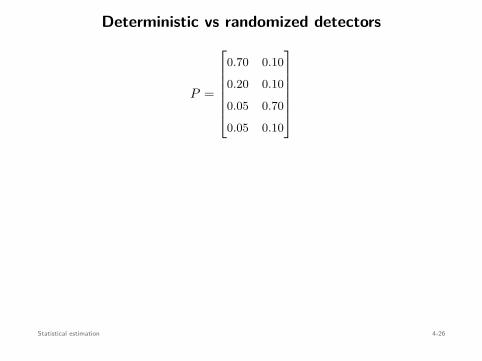
Deterministic vs randomized detectors
P =
0.70 0.10
0.20 0.10
0.05 0.70
0.05 0.10
Varying α yields 3 different Pareto-optimal detectors (excl. extremes):
T(1)PO =
1 0 0 0
0 1 1 1
T
(2)PO =
1 1 0 0
0 0 1 1
T
(3)PO =
1 1 0 1
0 0 1 0
Minimax detector (random):
TMM =
1 2/3 0 0
0 1/3 1 1
Statistical estimation 4-26
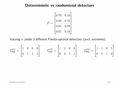

Deterministic vs randomized detectorsReceiver operating characteristic (ROC)
Minimax estimator has (Pfp, Pfn) = ( 16 , 1
6 ) and outperforms anydeterministic estimator
Statistical estimation 4-27
Deterministic vs randomized detectorsReceiver operating characteristic (ROC)
Pfp
Pfn
Minimax estimator has (Pfp, Pfn) = ( 16 , 1
6 ) and outperforms anydeterministic estimator
Statistical estimation 4-27
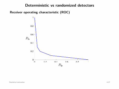
Deterministic vs randomized detectorsReceiver operating characteristic (ROC)
Pfp
Pfn
Minimax estimator has (Pfp, Pfn) = ( 16 , 1
6 ) and outperforms anydeterministic estimator
Statistical estimation 4-27

Deterministic vs randomized detectorsReceiver operating characteristic (ROC)
Pfp
Pfn
T(1)P O
T(2)P O
T(3)P O
Minimax estimator has (Pfp, Pfn) = ( 16 , 1
6 ) and outperforms anydeterministic estimator
Statistical estimation 4-27

Deterministic vs randomized detectorsReceiver operating characteristic (ROC)
Pfp
Pfn
T(1)P O
T(2)P O
T(3)P O
Pfn = Pfp
Minimax estimator has (Pfp, Pfn) = ( 16 , 1
6 ) and outperforms anydeterministic estimator
Statistical estimation 4-27
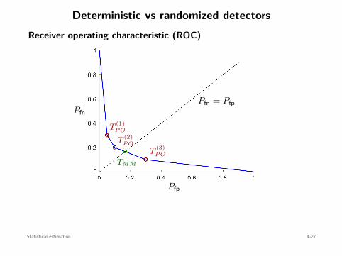
Deterministic vs randomized detectorsReceiver operating characteristic (ROC)
Pfp
Pfn
T(1)P O
T(2)P O
T(3)P O
Pfn = Pfp
TMM
Minimax estimator has (Pfp, Pfn) = ( 16 , 1
6 ) and outperforms anydeterministic estimator
Statistical estimation 4-27

Deterministic vs randomized detectorsReceiver operating characteristic (ROC)
Pfp
Pfn
T(1)P O
T(2)P O
T(3)P O
Pfn = Pfp
TMM
Minimax estimator has (Pfp, Pfn) = ( 16 , 1
6 ) and outperforms anydeterministic estimator
Statistical estimation 4-27

Conclusions
1 2
34
5
6
7
89
x x
convex nonconvex
• Optimization problems arise in many areas
• Essential to distinguish easy (convex) from hard (nonconvex) probs
• Use CVX/CVXPY/Convex for small-scale problems
• Didn’t cover optimality conditions & theory
• Didn’t cover optimization algorithms
• Statistical estimation:Find parameters of distributions (ML/MAP)Entire distributions (nonparametric)
• Multiple hypothesis testing via optimization
Statistical estimation 4-28
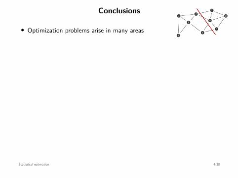
Conclusions1 2
34
5
6
7
89
x x
convex nonconvex
• Optimization problems arise in many areas
• Essential to distinguish easy (convex) from hard (nonconvex) probs
• Use CVX/CVXPY/Convex for small-scale problems
• Didn’t cover optimality conditions & theory
• Didn’t cover optimization algorithms
• Statistical estimation:Find parameters of distributions (ML/MAP)Entire distributions (nonparametric)
• Multiple hypothesis testing via optimization
Statistical estimation 4-28
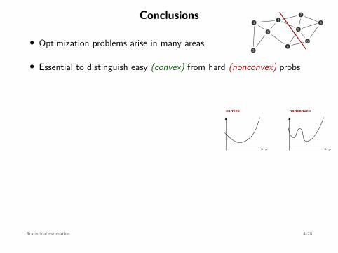
Conclusions1 2
34
5
6
7
89
x x
convex nonconvex
• Optimization problems arise in many areas
• Essential to distinguish easy (convex) from hard (nonconvex) probs
• Use CVX/CVXPY/Convex for small-scale problems
• Didn’t cover optimality conditions & theory
• Didn’t cover optimization algorithms
• Statistical estimation:Find parameters of distributions (ML/MAP)Entire distributions (nonparametric)
• Multiple hypothesis testing via optimization
Statistical estimation 4-28
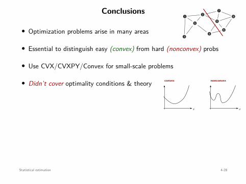
Conclusions1 2
34
5
6
7
89
x x
convex nonconvex
• Optimization problems arise in many areas
• Essential to distinguish easy (convex) from hard (nonconvex) probs
• Use CVX/CVXPY/Convex for small-scale problems
• Didn’t cover optimality conditions & theory
• Didn’t cover optimization algorithms
• Statistical estimation:Find parameters of distributions (ML/MAP)Entire distributions (nonparametric)
• Multiple hypothesis testing via optimization
Statistical estimation 4-28
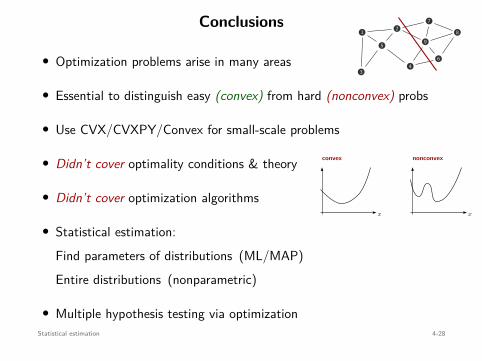
Conclusions1 2
34
5
6
7
89
x x
convex nonconvex
• Optimization problems arise in many areas
• Essential to distinguish easy (convex) from hard (nonconvex) probs
• Use CVX/CVXPY/Convex for small-scale problems
• Didn’t cover optimality conditions & theory
• Didn’t cover optimization algorithms
• Statistical estimation:Find parameters of distributions (ML/MAP)Entire distributions (nonparametric)
• Multiple hypothesis testing via optimizationStatistical estimation 4-28

References and Resources
Lectures:
• web.stanford.edu/∼boyd/cvxbook/
• users.isr.ist.utl.pt/∼jxavier/NonlinearOptimization18799-2018
• www.seas.ucla.edu/∼vandenbe/ee236cStatistical estimation 4-29
Related Documents