5 3 1 7 10 9 8 4 2 6 1 2 3 4 5 6 7 8 9 10 11 12 13 pH V [mL] pK = 15 pK = 9 pK = 11 pK = 7 pK = 5 pK = 3 pK = 1 Fundamentals of Titration

Welcome message from author
This document is posted to help you gain knowledge. Please leave a comment to let me know what you think about it! Share it to your friends and learn new things together.
Transcript
531 7 109842 6
1
2
3
4
5
6
7
8
9
10
11
12
13
pH
V [mL]
pK = 15
pK = 9
pK = 11
pK = 7
pK = 5
pK = 3
pK = 1
Fundamentals of Titration

Fundamentals of Titration
1Fundamentals of Titration
Contents
Page
1 Introduction 5
2 Base units of titrimetric analysis 6
3 The titration reaction 12
3.1 Thermodynamic fundamentals 123.1.1 The law of mass action 123.1.2 The solubility product of sparingly soluble salts 133.1.3 The ionic product of water 143.1.4 The strength of acids and bases 15
3.2 The most important titration reactions 173.2.1 Acid-base titrations in aqueous solution 173.2.2 Acid-base titrations in nonaqueous solution 193.2.3 Precipitation titrations 203.2.4 Complexometry 213.2.5 Redox titrations 22
4 Indication methods 27
4.1 Electrochemical indication 284.1.1 Galvanic cells 284.1.2 Reference electrodes 324.1.3 Metal electrodes 344.1.4 Glass electrodes 344.1.5 Ion selective electrodes 394.1.6 Measurement technique 41
4.2 Photometric indication 444.2.1 The METTLER phototrode 46
4.3 Special indication methods 474.3.1 Conductometric indication 47
Fundamentals of Titration
Fundamentals of Titration2
Page
5 Types of titration 50
5.1 The direct titration 50
5.2 The back titration 51
5.3 The inverse titration 52
5.4 The substitution titration 53
5.5 The collective titration 54
5.6 The selective titration 55
5.7 The sequential titration 55
6 Titration curves 59
6.1 Measurement signal as a function of the titrant volume: E = f(V) 59
6.2 Measurement signal as a function of time: E = f(t) 63
6.3 Titrant volume as a function of time: V = f(t) 65
7 Control of the titration 66
7.1 Titrant addition 677.1.1 Continuous titrant addition 677.1.2 Dynamic-incremental titrant addition 707.1.3 Predispensing 77
7.2 Measured value acquisition 78
7.3 Termination of the titration 82
8 The determination of the equivalence point 83
8.1 The position of the equivalence point 83
8.2 The practical recognition of the equivalence point 85
8.3 The calculation of the equivalence point of S-shaped titration curves 908.3.1 Approximation procedures 908.3.2 Interpolation procedures 938.3.3 Mathematical procedures 94
8.4 The equivalence point calculation of segmented titration curves 101
8.5 The half neutralization value 103
Fundamentals of Titration
3Fundamentals of Titration
Page
9 Direct measurement, calibration 107
9.1 pH measurement 1079.1.1 Calibration of a pH electrode 1089.1.2 Temperature compensation 111
9.2 Direct measurement with ion selective electrodes 113
9.3 Redox measurement 115
9.4 Conductivity measurement 1169.4.1 Calibration and temperature compensation 116
10 Assessment of the result 119
10.1 Fundamentals of statistics 119
10.2 Concepts relating to correctness 125
10.3 Limit of detection, limit of determination 127
10.4 Standard, standard samples, control samples 127
10.5 Consequences for practical application 128
Appendices 130
Appendix A: Tables of buffer values 131
Appendix B: Statistical tables 135
Appendix C: Tables of primary standards for the most important titrants 137
Index 141

Fundamentals of Titration
Fundamentals of Titration4
1 Introduction
Fundamentals of Titration 5
1 Introduction
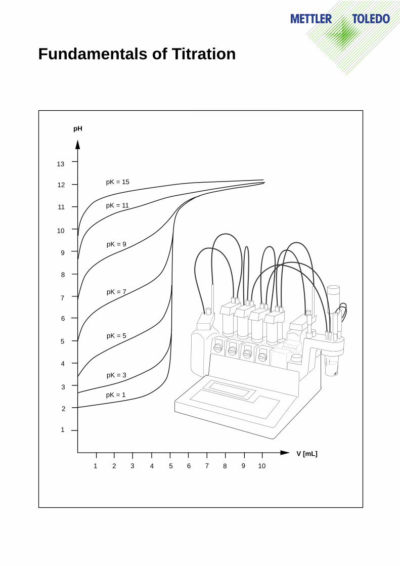
A balance, a burette and a suitable chemical reaction suffice to solve many quantitativeanalytical problems. The analytical technique employed is called titration or titrimetric analysis(titrimetry). The expression “volumetric analysis” is not recommended [1]. In a titration, part ofthe sample containing the substance to be analyzed (the analyte) is dissolved in a suitablesolvent. A second chemical compound, the titrant, is added as a solution of known concentra-tion in a controlled manner until the analyte has reacted quantitatively. From the consumptionand concentration of the titrant as well as the weight of sample used in the analysis, the contentof the analyte can be calculated.
From the above definition it follows that the following requirements must be fulfilled before atitration can be performed:
– The basic chemical reaction – the titration reaction – must be rapid, straightforward andquantitative.
– It must be possible to either prepare a titrant of exactly known content or determine thereacting strength (titer) of the solution accurately.
– The course of the titration must be observable. The method used to follow the titrationprogress is called indication.
– Determination of the equivalence point – the point at which the number of entities(equivalents) of the titrant added is the same as the number of entities of sample analytepresent – must be unambiguous.
The titration reaction, the indication, the control and evaluation of the titration as well as theassessment of the results (statistics) form the focal points of this supplement to the operatinginstructions for the titrator DL70.
[1] IUPAC Compendium of Analytical Nomenclature, Pergamon Press, 1978, page 42
2 Base units
Fundamentals of Titration6
2 Base units of titrimetric analysis
The base units and calculation parameters of titrimetric analysis are associated with the basequantity amount of substance and its base unit mole of the international system of units (SI)[1]. The concepts and definitions regarding amount of substance and the quantities derivedfrom it are defined in [2].
Mole
The SI base unit for amount of substance is the mole (symbol of unit: mol). The mole is theamount of substance of a system that contains just as many elementary entities as there areatoms in 12 g of the carbon 12C isotope. One mole of a substance contains 6.022 • 1023
elementary entities. These can be atoms, molecules, ions, groups of atoms or electrons.
Amount of substance specification
The entities referred to in specifications of the amount of substance should be entered inbrackets after the amount of substance symbol n.
Examples: n(HCl) = 2 mol
n(Ca2+) = 4 mmol
Molar mass M
The molar mass (symbol M) is a quantity related to the amount of substance. The molar massof a substance X is defined as its mass m divided by amount of substance n(X).
The usual unit in analysis is g/mol.
Examples: M(NaOH) = 39.997 g/mol
M(EDTA) = 372.24 g/mol
M(X) =m
n(X)
2 Base units
Fundamentals of Titration 7
Amount-of-substance concentration c(X)
The amount-of-substance concentration of a solution of an entity X (symbol c(X)) is the amountof substance n(x) divided by the volume V of the solution.
The usual units employed in analysis are mol/L and mmol/L.
Examples: c(HCl) = 0.1 mol/L
c(AgCl) = 0.01 mol/L
Notes: The simpler designation “concentration” for amount-of-substance concentrationis allowed.
The old designation “molarity” is no longer used.
Titer t
The titer (symbol t) of a titrimetric solution is the quotient of the actual concentration (ACTUALvalue) and the expected concentration (NOMINAL value).
Examples: c(HCl, ACTUAL) = 0.1036 mol/L
c(HCl, NOMINAL) = 0.1 mol/L
The titer t = 1.036.
Note: The name “factor” for the titer is no longer used.
c(X) =n(X)
V
t =c( X , ACTUAL )
c( X , NOMINAL )
2 Base units
Fundamentals of Titration8
Equivalent, Equivalent number z*
In the previous examples the amount of substance n, the molar mass M and the amount-of-substance concentration c refer to whole entities. In titrimetric analysis, reference to fractionsof such entities is often expedient.
The equivalent entity, abbreviated to equivalent, is the fraction 1/z* of such an entity. Thenumber of equivalents z* of each entity X is called the equivalent number.
Examples of equivalent numbers:
1. Neutralization (acid-base) equivalent: In a neutralization reaction, the entity X combineswith or releases z* protons.
a. HCl: z* = 1
H+ + Cl- + Na+ + OH- —> Na+ + Cl- + H2O
b. H2SO4: z* = 2
2H+ + SO42- + 2 Na+ + 2 OH- —> 2 Na+ + SO4
2- + 2 H2O
2. Redox equivalent: In a redox reaction, the reaction partners change their oxidationnumber.
a. KMnO4/Fe2+: KMnO4: z* = 5 Fe2+: z* = 1
VII II II IIIK+ + MnO
4- + 5Fe2+ + 8H+ —> K+ + Mn2+ + 5Fe3+ + 4H
2O
b. KMnO4/Mn2+: KMnO
4: z* = 3 Mn2+: z* = 2
VII II lV2 K+ + 2 MnO
4- + 3 Mn2+ + 4 OH- —>2 K+ + 5 MnO
2 + 2 H
2O
Note: The old name “valency” is no longer used.

2 Base units
Fundamentals of Titration 9
n(1z*
X ) = z* • n(X)
M(1z*
X ) =M(X)
z*
In titrimetric analysis the following quantities are related to equivalents:
– amount of substance
– molar mass
– concentration.
Amount of substance of equivalents
The amount of substance n of an equivalent of entity X (symbol n(1/z* X)) is equal to the productof the equivalent number z* and the amount of substance n of entity X.
The usual units are mol and mmol.
Examples: n(1/2 Ca2+) = 2 mmol
n(1/5 KMnO4) = 5 mol
Molar mass of equivalents
The molar mass M of an equivalent of entity X (symbol M(1/z* X)) is the molar mass M of theentity X divided by the equivalent number z*.
The unit is g/mol.
Examples: M(1/2 H2SO
4) = 49.04 g/mol
M(1/5 KMnO4) = 31.61 g/mol
M(1/3 KMnO4) = 52.68 g/mol
M(1/6 K2Cr
2O
7) = 49.03 g/mol
2 Base units
Fundamentals of Titration10
c(1z*
X ) =n(
1z*
X )
V=
m
M(1z*
X ) • V=
m • z*M(X) • V
c(16
K2 Cr2 O7 ) =1 • 6
294.185 • 0.05= 0.408 mol/L
Amount-of-substance concentration of equivalents (equivalent concentration)
The amount-of-substance concentration of a solution of an equivalent of entity X (symbolc(1/z* X)) is the amount of substance n(1/z*X) of an equivalent of X divided by the volume Vof the solution.
The usual units are mol/L and mmol/L.
The following relation holds:
Example: How large is the amount-of-substance concentration c(1/6 K2Cr
2O
7) of 1 g
K2Cr
2O
7 in 50 mL water?
Note: The amount-of-substance concentration replaces the concepts molarity, norma-lity, Val/L as well as the concepts “molar”, “M”, “normal”, “N”, etc. derived fromthem. These are no longer used. Unless the reaction equation is specified, the olddescriptions do not allow explicit recognition of the equivalent; for example 0.1NKMnO
4 could apply equally well to 1/3 KMnO
4 and 1/5 KMnO
4. In contrast,
specification of the amount-of-substance concentration c(1/5 KMnO4) = 0.1 mol/
L is unambiguous.
c(1z*
X ) = z* • c(X)
2 Base units
Fundamentals of Titration 11
m =c( 1/z* X ) • M(X) • V
z*
m =0.1 • 98.08 • 0.1
2= 0.4904 g
Concentration of a titrant
The concentration of a titrant should be specified as equivalent concentration.
Example: c(1/2 H2SO
4) = 0.1 mol/L
The amount-of-substance concentration needed for preparation of a titrimetric solution of theequivalent concentration c(1/z* X) is calculated with the aid of the formula
Example: Preparation of 100 mL of a titrimetric solution of sulfuric acid of concentrationc(1/2 H
2SO
4) = 0.1 mol/L.
Amount of substance required:
[1] Bureau International des Poids et Mesures, Le Système International d’Unités (SI), 5th French and EnglishEdition, BIPM, Sèvres 1985
[2] IUPAC Compendium of Analytical Nomenclature, Pergamon Press, 1978, page 175 ff. See also DIN 32625
3 Titration reaction
Fundamentals of Titration12
Xx
• Yy
• Zz
Aa
• Bb
• Cc
= K
3 The titration reaction
The basis of each titrimetric method of analysis is the chemical reaction of the analyte with thetitrant. In order to understand the demands on this titration reaction, a brief introduction intothe fundamentals of the thermodynamics of chemical reactions is called for.
3.1 Thermodynamic fundamentals
3.1.1 The law of mass action
Every reversible chemical reaction proceeds to an exactly defined equilibrium condition. It ischaracterized by the following general equation:
v1
aA + bB + cC <====> xX + yY + zZv2
In this equation a, b, c, x, y and z represent the number of moles of the substances A, B, C,X, Y and Z participating in the reaction in stoichiometric proportion. At equilibrium, the ratesof the forward and back reactions are equal (v
1 = v
2). This equilibrium is described by the so-
called law of mass action.
The constant K is known as the thermodynamic equilibrium constant.
The concentrations of entities X, Y and Z are designated here by [X], [Y] and [Z] ([X] = c(X)).This notation is usual in analytical chemistry.
Strictly speaking, the law of mass action can not be applied directly to the analyticalconcentrations of the reaction partners. Real chemical systems are distinguished by themutual interaction of all molecules present. In solution, interactions occur between themolecules of the dissolved substance and the solvent molecules. Here, it is only the quasi-freeor “effective” concentrations of the substances participating in reaction, the so-called activities,that are decisive for the chemical reaction and the law of mass action. But for a formalunderstanding and the calculations, only analytical concentrations are considered in thepresent discussion.
3 Titration reaction
Fundamentals of Titration 13
The demand that the titration reaction proceed quantitatively and to completion is fulfilled whenthe equilibrium constant K is so large that the equilibrium concentration of the analyte isinfinitely small in comparison with its concentration before titration.
The equilibrium constant K provides no direct information regarding the rate of the titrationreaction. Decisive for this is the rate of the forward reaction v
1, the reaction of the analyte with
the titrant.
The following sections treat the thermodynamic constants that appear most frequently inpotentiometry, the solubility product of sparingly soluble salts, the ionic product of water andthe acidity constant of weak acids.
3.1.2 The solubility product of sparingly soluble salts
Many salts are only slightly soluble. If solutions of the corresponding ions are mixed,precipitates are formed. The processes at the surface of a salt in contact with a saturatedsolution lead to the establishment of a heterogenous equilibrium. Ions from the salt constantlypass into solution, and ions from the solution are incorporated in the salt lattice.
AB(solid) <===> A+ + B-
For this equilibrium the following law of mass action applies:
As long as solid salt AB is present as precipitate, the concentration of AB remains constant andis thus included in the equilibrium constant. This gives rise to the solubility product K
sp:
A sparingly soluble salt is always precipitated when the solubility product of the participatingions is exceeded. The lower the solubility product, the more insoluble the salt.
The solubility product of salts having the general formula AB2 has the following form:
A+
• B-
AB= K
A+
B-
= Ksp
Ksp = A2+
B- 2
3 Titration reaction
Fundamentals of Titration14
The solubility product of many salts shows a large temperature dependence:
Examples of solubility products (type AB):
Salt Ksp
[mol2/L2]
AgCl 10-10
AgBr 5 • 10-13
AgI 10-16
PbSO4
10-8
3.1.3 The ionic product of water
When the conductivity of water is examined using very sensitive instruments, it is apparent thateven ultrapure, repeatedly distilled water has a very low conductivity. It is due to the followingreaction:
H2O + H
2O <===> H
3O+ + OH-
The forward reaction describes the proton transfer from one water molecule to another. Thisequilibrium is present not only in pure water but also in all aqueous solutions. The correspond-ing law of mass action is:
The concentrations of the H3O+ and OH--ions in solution can be changed drastically by additionof an acid or base. But the concentration of the H
2O molecules (55.5 mol/L) remains constant
in dilute solutions. The law of mass action can thus be simplified:
The equilibrium constant Kw is known as the ionic product of water. It depends on the tempe-rature and is 10-14 mol2/L2 at 23°C.
In dilute aqueous solutions the product of [H3O+] and [OH-] is thus constant. If one of the two
concentrations is known, the other can be calculated from a knowledge of Kw. In a neutralsolution the concentrations [H
3O+] and [OH-] are equal:
H3O+
• OH-
H2O2
= K
H3O+
OH-
= Kw
H3O+
= OH-
= Kw = 10-7
mol/L
3 Titration reaction
Fundamentals of Titration 15
H3O+
• A-
HA • H2O= K
H3O+
• A-
HA= Ka
pH = –log H3O+
If, for example, the H3O+ concentration is increased to 10-2 mol/L by addition of acid, the OH-
concentration decreases to 10-12 mol/L. Specification of one of these concentrations allowsunequivocal identification of the nature of an aqueous solution. This led to the introduction ofthe pH concept as
In acidic solutions([H3O+] > 10-7) the pH is less than 7, whereas in alkaline solutions it is greaterthan 7. The pH of a neutral solution is 7.
3.1.4 The strength of acids and bases
The reaction of weak acids with water is described by the following equilibrium:
HA + H2O <===> H
3O+ + A-
Acid HA reacts with the base H2O to form the conjugate base A- of HA and the conjugate acid
of H2O, namely H3O+.
The corresponding law of mass action is:
In dilute solutions ([H2O] = constant) the following formula applies:
The equilibrium constant Ka is known as the acidity constant of acid HA and characterizes
the strength of an acid. Strong acids have a large acidity constant, weak acids a very low one.The negative logarithm of Ka is frequently employed in calculations:
pKa = –logK
a
3 Titration reaction
Fundamentals of Titration16
Examples of pKa values of a few acid-base pairs (25°C):
Acid Base pKa
HClO4
ClO4
- -9
HCl Cl- -6
H2SO
4HSO
4- -3
HSO4- SO
42- 1.96
H3PO4 H2PO4- 1.96
CH3COOH CH
3COO- 4.75
H2PO
4- HPO
42- 7.21
NH4+ NH3 9.21
HPO42- PO
43- 12.32
The reaction of the base A- with water can be described in an analogous manner:
A- + H2O <===> HA + OH-
The corresponding basicity constant Kb follows from the law of mass action:
For a conjugate acid-base pair HA/A- follows:
Polyprotic acids or polyequivalent bases that donate (accept) protons in steps have a separateacidity (basicity) constant for each ionization step.
Example: H3PO4 + H2O <===> H2PO4- + H3O+ pKa = 1.96
H2PO
4- + H
2O <===> HPO
42- + H
3O+ pK
a = 7.21
HPO42- + H
2O <===> PO
43- + H
3O+ pK
a = 12.32
HA • OH-
A-
= Kb
Ka • Kb = H3O+
OH-
= Kw
3 Titration reaction
Fundamentals of Titration 17
3.2 The most important titration reactions
This section contains a summary of the titration reactions important in titration practice.
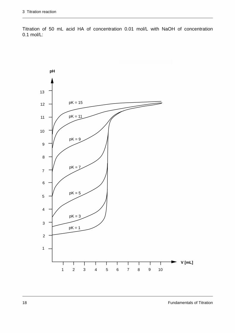
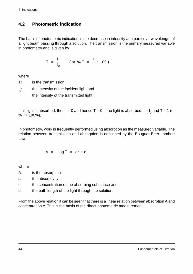
3.2.1 Acid-base titrations in aqueous solutions
In the titration of an acid HA with a strong base (e.g. NaOH) the following two chemicalequilibria occur:
HA + H2O <===> H3O+ + A-
2 H2O <===> H3O+ + OH-
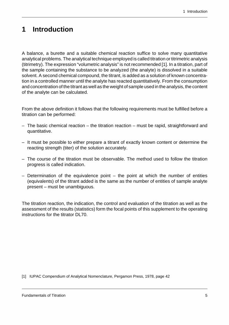
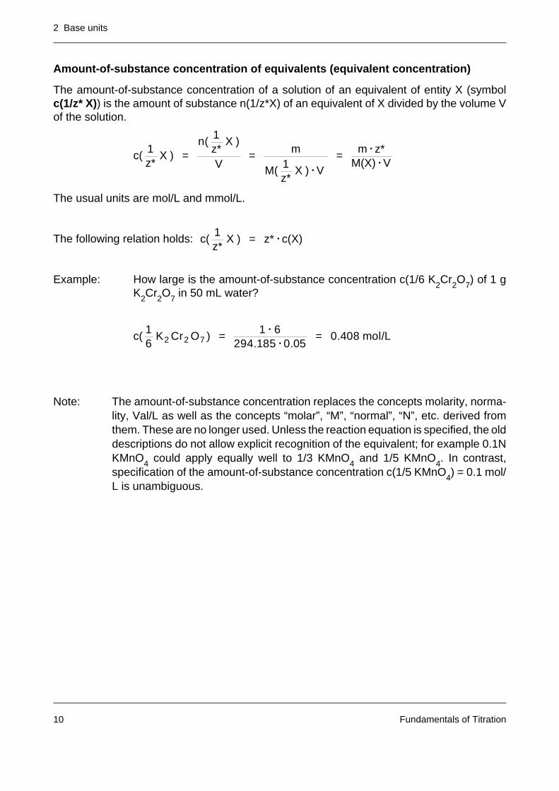
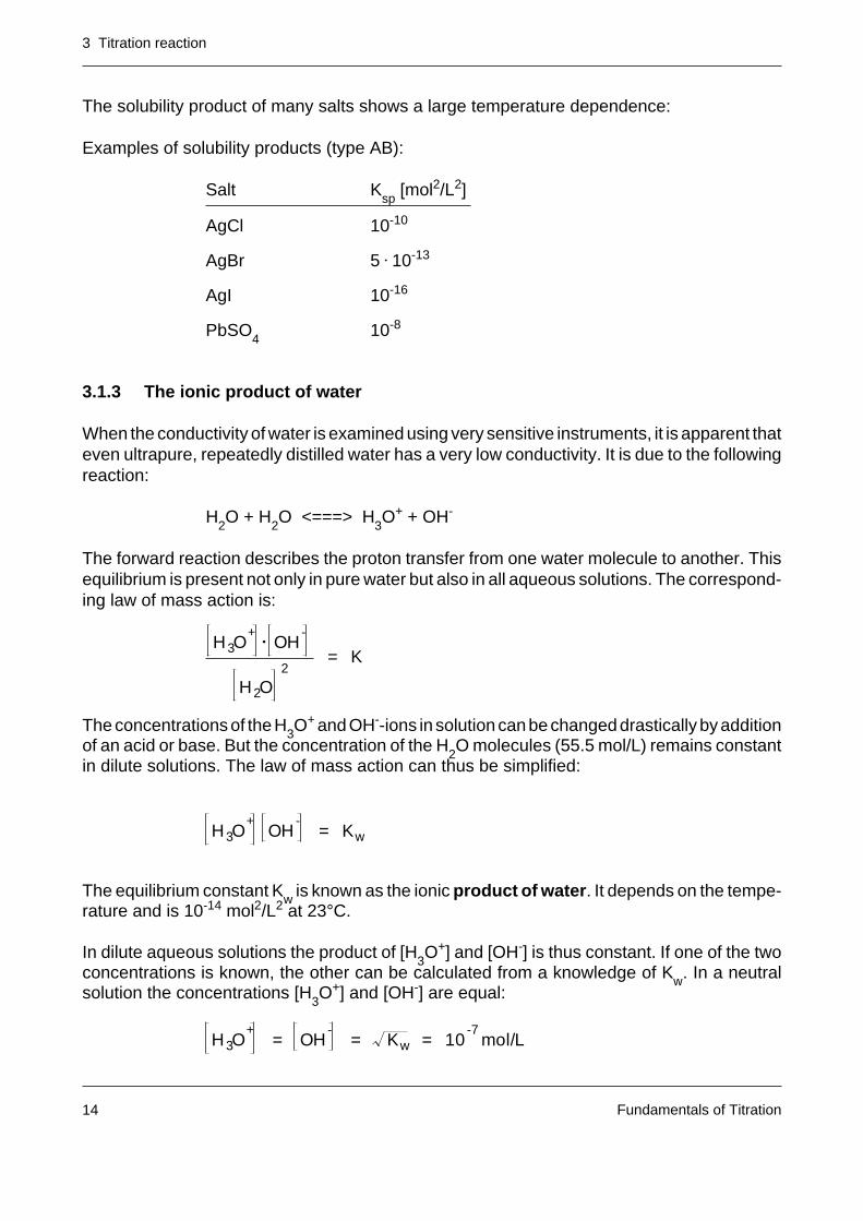
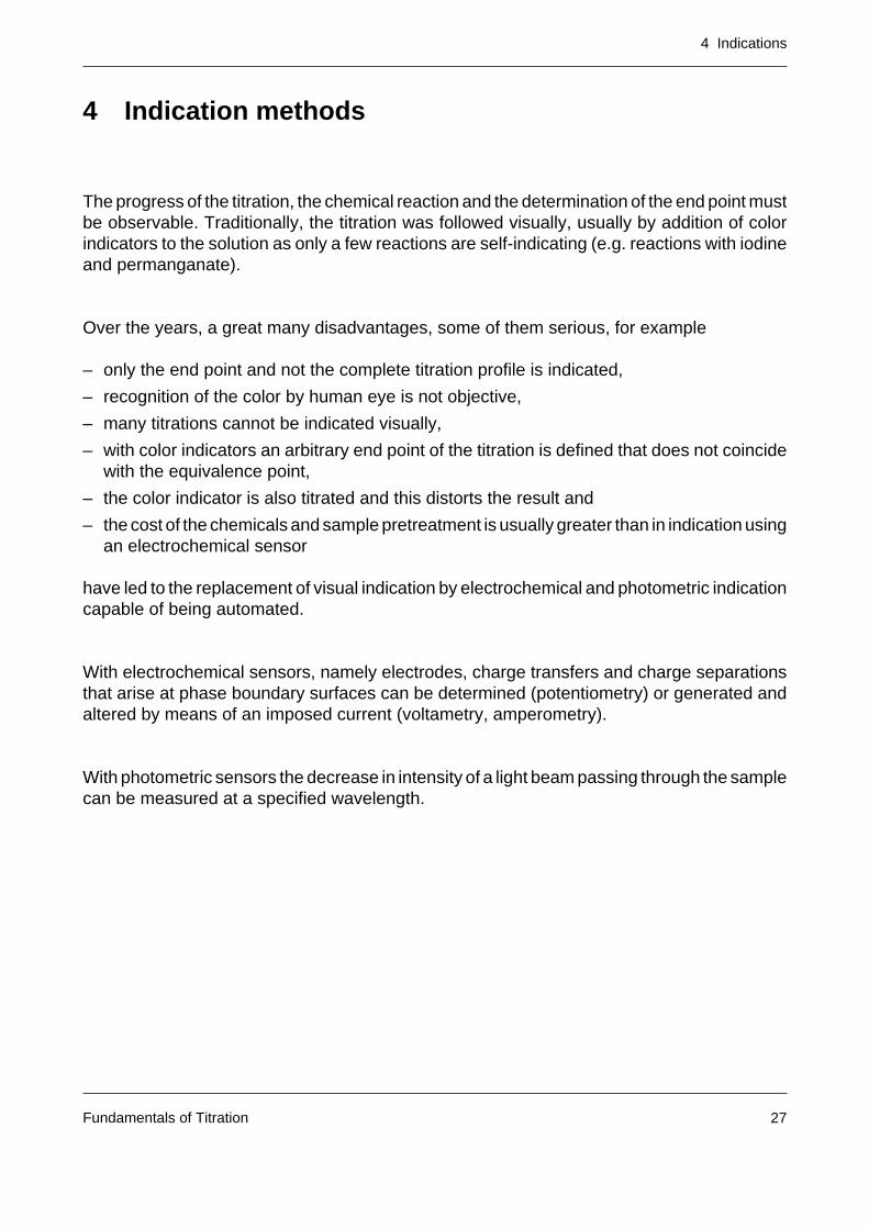
Acid-base reactions are very fast, and the chemical equilibrium is established extremelyrapidly. Acid-base reactions in aqueous solutions are thus ideal for titrations. If the solutionsused are not too dilute, the shape of the titration curves depends only on the acidity constantK
a as the following figure shows.
Notes: – Very weak acids are difficult to titrate in aqueous solution. In the figure belowit can be seen that for pKa values greater than 10, the corresponding titrationcurve no longer exhibits any jump in the region of the equivalence point.
– Bases can be titrated with a strong acid in an analogous manner. The sametitration curves result if K
a is substituted by K
b and pH by pOH (pH + pOH = pK
w= 14).
– Polyprotic acids (e.g. the first two ionization steps of phosphoric acid) andmixtures of acids can easily be titrated separately if the acidity constants differby at least two pK units.
H3O+
• A-
HA= Ka
H3O+
OH-
= Kw
3 Titration reaction
Fundamentals of Titration18
531 7 109842 6
1
2
3
4
5
6
7
8
9
10
11
12
13
pH
V [mL]
pK = 15
pK = 9
pK = 11
pK = 7
pK = 5
pK = 3
pK = 1
Titration of 50 mL acid HA of concentration 0.01 mol/L with NaOH of concentration0.1 mol/L:
3 Titration reaction
Fundamentals of Titration 19
3.2.2 Acid-base titrations in nonaqueous solution
Titrations can also be performed in nonaqueous solvents ([1], [2], [3], [4]). The use ofnonaqueous solvents is advantageous under the following conditions:
– The analyte is only sparingly soluble in water.
– The analyte or the titrant enter into an undesired reaction with water (e.g. acid chloride, acidanhydride).
– A mixture of analytes is present; this cannot be analyzed selectively in aqueous solution(pKa values too close together).
– The analyte is too weak an acid or base in water.
The main applications in nonaqueous media are acid-base titrations.
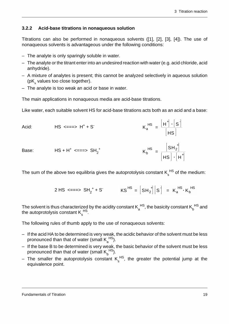
Like water, each suitable solvent HS for acid-base titrations acts both as an acid and a base:
Acid: HS <===> H+ + S-
Base: HS + H+ <===> SH2+
The sum of the above two equilibria gives the autoprotolysis constant KsHS of the medium:
2 HS <===> SH2
+ + S-
The solvent is thus characterized by the acidity constant Ka
HS, the basicity constant KbHS and
the autoprotolysis constant KsHS.
The following rules of thumb apply to the use of nonaqueous solvents:
– If the acid HA to be determined is very weak, the acidic behavior of the solvent must be lesspronounced than that of water (small Ka
HS).
– If the base B to be determined is very weak, the basic behavior of the solvent must be lesspronounced than that of water (small K
bHS).
– The smaller the autoprotolysis constant KsHS, the greater the potential jump at the
equivalence point.
KaHS
=H
+• S
-
HS
KbHS
=SH2
+
HS • H+
KSHS
= SH2+
S-
= KaHS
• KbHS
3 Titration reaction
Fundamentals of Titration20
– Many nonaqueous solvents show so-called differentiating (nonleveling) properties thatallow substances that have similar pK values in water to be determined selectively in thesame solution.
Nonaqueous media exhibit several peculiarities that should be noted:
– The coefficient of expansion of organic solvents is considerably larger than that of water.The temperature dependence of the titer can thus be very large (up to 0.2% for atemperature change of 1°C).
– Many nonaqueous solvents are more volatile than water and are sensitive to CO2. It is thus
essential to check the titer frequently.
Examples of titrants in nonaqueous solvents:
Acids: HCl in isopropanol, perchloric acid in glacial acetic acid
Bases: KOH in ethanol, sodium methoxide in chlorobenzene.
3.2.3 Precipitation titrations
Precipitation titrations are distinguished by the formation of a sparingly soluble reactionproduct (precipitate) between the titrant and the analyte. The classic example is the determi-nation of halogens with silver nitrate:
Ag+ + X- <===> AgX(solid)
In the performance of precipitation titrations, several special features should be noted:
– The titration reaction may be quite slow under certain circumstances.
– At the start of the titration, the solution may become supersaturated before a precipitate isformed.
– With solutions that are too concentrated, inclusions of sample and/or titrant may occur inthe precipitating solid, thereby falsifying the result. An effective countermeasure is rapidstirring.
Ksp = Ag+
Cl-
X- = Cl-, Br-, I-
3 Titration reaction
Fundamentals of Titration 21
3.2.4 Complexometry
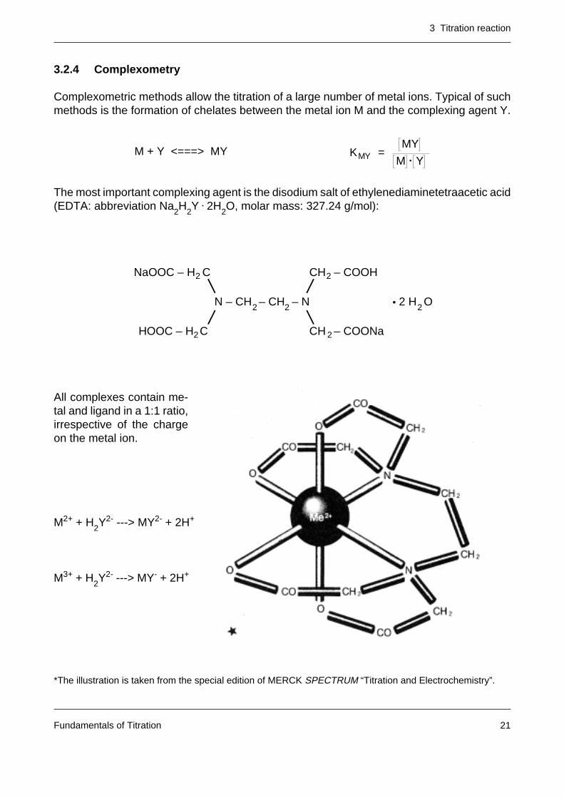
Complexometric methods allow the titration of a large number of metal ions. Typical of suchmethods is the formation of chelates between the metal ion M and the complexing agent Y.
M + Y <===> MY
The most important complexing agent is the disodium salt of ethylenediaminetetraacetic acid(EDTA: abbreviation Na
2H
2Y • 2H
2O, molar mass: 327.24 g/mol):
All complexes contain me-tal and ligand in a 1:1 ratio,irrespective of the chargeon the metal ion.
M2+ + H2Y2- ---> MY2- + 2H+
M3+ + H2Y2- ---> MY- + 2H+
*The illustration is taken from the special edition of MERCK SPECTRUM “Titration and Electrochemistry”.
NaOOC – H C CH – COOH
HOOC – H C CH – COONa
N – CH – CH – N • 2 H O 2
2
2
2
2
22 •
KMY =MY
M • Y
3 Titration reaction
Fundamentals of Titration22
If these reactions run in unbuffered solutions, the pH is lowered. If a change in pH has to beavoided, substances with sufficient buffer capacity must be added. In alkaline solutions themetal is more tightly bound in the complex than in acidic solutions.
Among the applications of the complexometric titration, the determination of water hardness(Ca, Mg) has achieved the greatest importance.
3.2.5 Redox titrations
If two reaction partners can be interconverted by the gain or loss of electrons, a redox systemis present. The process underlying this chemical reaction is called a redox reaction (= electronshift). The two partners are known as a conjugate redox couple.
Example: Fe3+ + e- <===> Fe2+
One of these entities gives up electrons. This process is called oxidation. The other entity gainsthese freed electrons. This process is known as reduction.
Substances that can oxidize other substances are called oxidizing agents. Substances thatcan reduce other substances are known as reducing agents.
But since electrons never occur in the free state in perceptible concentration, oxidation andreduction reactions can only occur together. One reaction releases exactly the same numberof electrons as the other reaction requires. There must thus always be two reaction couplesparticipating in a redox reaction.
Red1 + Ox2 ---> Ox1 + Red2
Examples: Fe + Cu2+ ---> Fe2+ + Cu
2I- + Br2 ---> I
2 + 2Br-
3 Titration reaction
Fundamentals of Titration 23
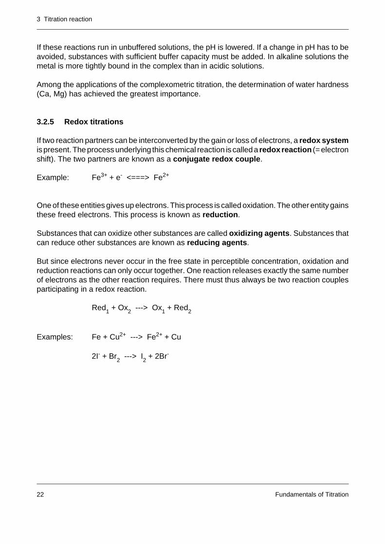
Through a comparison of a number of such reactions, the strength of oxidizing or reducingagents can easily be defined qualitatively. Similar to acids (bases), reducing and oxidizingagents can also be arranged in a series (redox series).
Reducing agent Oxidizing agent
reducing Fe Fe2+ oxidizing
action S2O
32- S
4O
62- action
(oxidizability) Cu Cu2+ (reducibility)
decreases 2I- I2
increases
Ag Ag+
2Br- Br2
2Cl- Cl2
Cr3+ Cr2O
72-
Au Au3+
Mn2+ MnO4
-
Ce3+ Ce4+
V 2F- F2
V
This redox series shows a representative selection of redox couples that includes not only themost well-known titrants but also several metals and the halogens. It can be seen immediatelyfrom this table that, for example, metallic iron in copper(II) solutions will be oxidized.
3 Titration reaction
Fundamentals of Titration24
Examples of important redox reactions for titration:
Manganometry
Manganometry is based on the powerful oxidizing effect of potassium permanganate. Theoverwhelming number of redox titrations with KMnO4 are performed in sulphuric acid solutionsaccording to the following scheme:
MnO4- + 8H+ + 5e- ---> Mn2+ + 4H
2O
Manganese with oxidation number +7 is reduced to Mn2+.
Example: Determination of peroxides
2MnO4- + 5H
2O
2 + 6H+ ---> 2Mn2+ + 5O2 + 8H
2O
Iodometry
One of the most important redox couples is iodide/iodine. The fundamental process
I2 + 2e- <===> 2I-
is completely reversible. There are thus always two possibilities:
1. Reduction of iodine: I2 + 2e- ---> 2I-
In this manner reducing agents can be determined directly with iodine solution as titrant.
Example: Determination of SO2
SO2 + I
2 + 2H
2O ---> H
2SO
4 + 2HI
2. Oxidation of iodide: 2I- ---> I2 + 2e-
The determination of oxidizing agents in iodometry is performed as a replacement titration inthe majority of cases (see section 5). An excess of iodide is added to the sample.
Example: Determination of copper 2Cu2+ + 2I- ---> 2Cu+ + I2
The liberated iodine is titrated with a suitable reducing agent. Sodium thiosulfate is used almostexclusively today.
2S2O
32- + I
2 ---> S
4O
62- + 2I-
3 Titration reaction
Fundamentals of Titration 25
Dichromate method
Chromium with oxidation number +6 is reduced by a large number of reducing agents in acidicsolution. Use is made of this property in the cleaning of glass vessels with chromosulfuric acid.The dichromate ion Cr2O7
2- is stable in acidic solution but can be reduced to the chromium(III)ion Cr3+ in the presence of hydrogen ions by gain of six electrons (three per chromium(VI))according to the equation
Cr2O72- + 14H+ + 6e- ---> 2Cr3+ + 7H2O
The hydrogen ions are consumed with formation of water.
Dichromate as a titrant has gained practical importance in the determination of the chemicaloxygen demand (COD) in wastewater analysis [5]. The COD determination is based on theoxidation of organic compounds with chromosulfuric acid using silver sulfate catalyst.
Cerimetry
Cerium(VI) sulfate is a powerful oxidizing agent. The oxidation number of cerium changes onlyby one:
Ce4+ + e- ---> Ce3+
The cerium(IV) sulfate solution (prepared in H2SO
4) has a stable titer and is insensitive to both
light and heat. In contrast to permanganate solutions it can also be used for titrations in highlyconcentrated hydrochloric acid solution. It is thus extremely versatile.
Diazotizations and nitrosations
One important oxidizing agent is sodium nitrite. It allows the determination of primary aminesthrough diazotization, and the determination of secondary amines and phenols throughnitrosation in acidic solution.
Simplified reaction schemes:
Primary amines: R – NH2 + NO
2- + 2H+ ---> [R – N = N]+ + 2H
2O
Secondary amines: R – NH – R + NO2- + H+ ---> R – N – R + H
2O
NO

3 Titration reaction
Fundamentals of Titration26
[1] W. Huber, Titrationen in nichtwässrigen Lösungsmitteln, Akademische Verlagsgesellschaft, D-6000 Frank-furt, 1964
[2] J. Kucharsky and L. Safarik, Titrations in nonaqueous solvents, Elsevier Publishing Company, Amsterdam,1965
[3] K. Stammbach, Titrationen in nichtwässrigen Lösungsmitteln, Schweizerische Laboranten-Zeitschrift, CH-4127 Birsfelden, offprint 1970
[4] I. Gyenes, Titrationen in nichtwässrigen Medien, F. Enke Verlag, Stuttgart, 1970
[5] DIN standard 38 409 – H 41-2 (1980)
4 Indications
Fundamentals of Titration 27
4 Indication methods
The progress of the titration, the chemical reaction and the determination of the end point mustbe observable. Traditionally, the titration was followed visually, usually by addition of colorindicators to the solution as only a few reactions are self-indicating (e.g. reactions with iodineand permanganate).
Over the years, a great many disadvantages, some of them serious, for example
– only the end point and not the complete titration profile is indicated,
– recognition of the color by human eye is not objective,
– many titrations cannot be indicated visually,
– with color indicators an arbitrary end point of the titration is defined that does not coincidewith the equivalence point,
– the color indicator is also titrated and this distorts the result and
– the cost of the chemicals and sample pretreatment is usually greater than in indication usingan electrochemical sensor
have led to the replacement of visual indication by electrochemical and photometric indicationcapable of being automated.
With electrochemical sensors, namely electrodes, charge transfers and charge separationsthat arise at phase boundary surfaces can be determined (potentiometry) or generated andaltered by means of an imposed current (voltametry, amperometry).
With photometric sensors the decrease in intensity of a light beam passing through the samplecan be measured at a specified wavelength.
4 Indications
Fundamentals of Titration28
4.1 Electrochemical indication
The processes that occur at an electrode in a galvanic cell form the basis of electrochemicalindication methods.
4.1.1 Galvanic cells
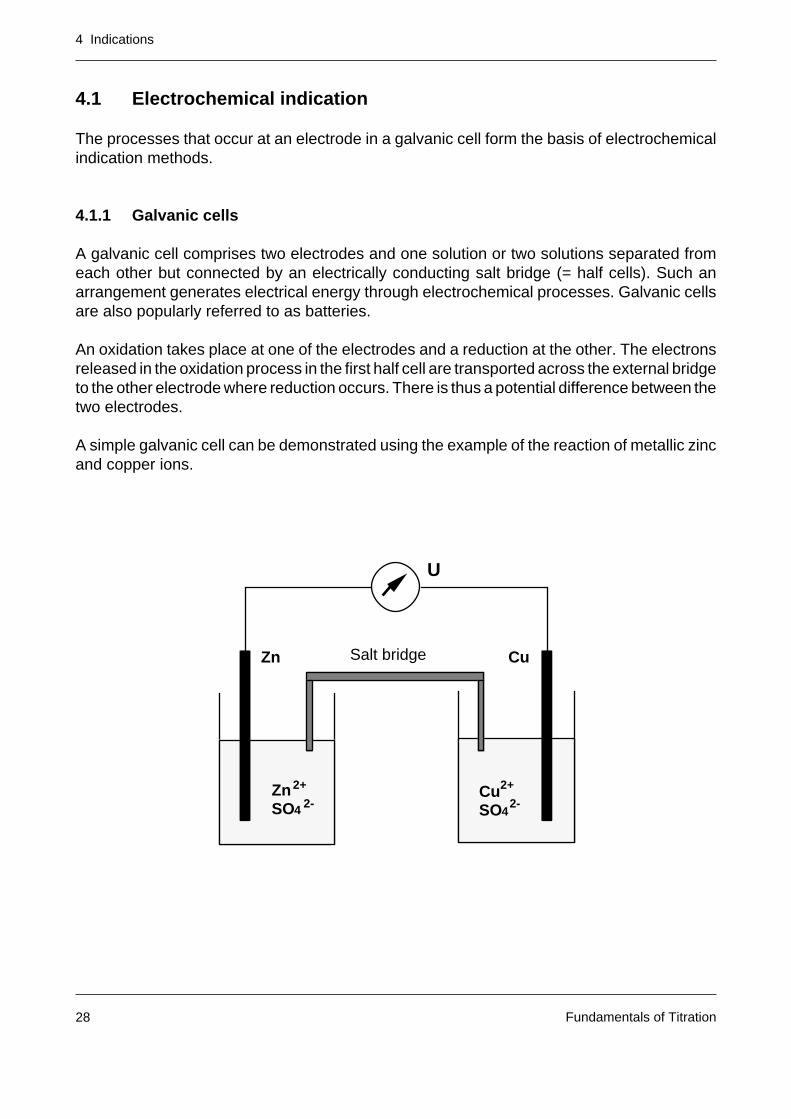
A galvanic cell comprises two electrodes and one solution or two solutions separated fromeach other but connected by an electrically conducting salt bridge (= half cells). Such anarrangement generates electrical energy through electrochemical processes. Galvanic cellsare also popularly referred to as batteries.
An oxidation takes place at one of the electrodes and a reduction at the other. The electronsreleased in the oxidation process in the first half cell are transported across the external bridgeto the other electrode where reduction occurs. There is thus a potential difference between thetwo electrodes.
A simple galvanic cell can be demonstrated using the example of the reaction of metallic zincand copper ions.
Salt bridge
U
Zn Cu
ZnSO4
CuSO4
2-2-
2+ 2+
4 Indications
Fundamentals of Titration 29
The following redox reactions take place:
Zn ---> Zn2+ + 2e- oxidation
2e- + Cu2+ ---> Cu reduction
–––––––––––––––––––––––Zn + Cu2+ ---> Zn2+ + Cu
The voltage (potential difference) measurable at the voltmeter, the slow dissolution of the zincrod and the deposition of copper on the copper rod are proof of the occurrence of theelectrochemical process.
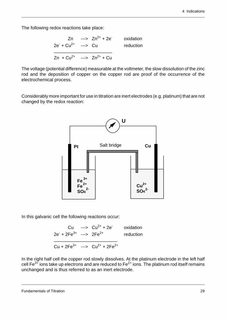
Considerably more important for use in titration are inert electrodes (e.g. platinum) that are notchanged by the redox reaction:
In this galvanic cell the following reactions occur:
Cu ---> Cu2+ + 2e- oxidation
2e- + 2Fe3+ ---> 2Fe2+ reduction
–––––––––––––––––––––––––Cu + 2Fe3+ ---> Cu2+ + 2Fe2+
In the right half cell the copper rod slowly dissolves. At the platinum electrode in the left halfcell Fe3+ ions take up electrons and are reduced to Fe2+ ions. The platinum rod itself remainsunchanged and is thus referred to as an inert electrode.
3+
Salt bridge
U
Cu
FeFeSO4
CuSO4
2-2-2+ 2+
3+
Pt
4 Indications
Fundamentals of Titration30
It is impossible to measure the potential of a single electrode directly; only the difference inpotential of two electrodes is accessible. The resulting potential of such an electrode assemblyE
tot (so-called electromotive force) is given by the difference between the potentials E
1 and E
2of the two electrodes:
The potential of a single electrode depends on the ionic concentration of the solution used tocomplete the half cell. This dependency is described by the Nernst equation:
where
E0: is the standard potential ([Ox]/[Red] = 1) of the electrode
R: the molar gas constant
T: the temperature (in K)
n: the number of electrons transferred in the electrode reaction and
F: the Faraday constant.
[Ox] and [Red] are the concentrations of the oxidized and reduced ionic species participatingin the reaction.
At 25°C the equation assumes the following form:
A change in the concentration ratio by a factor of ten causes a change in the electrode potentialby 59.16/n mV.
The half cells with zinc and copper rods mentioned in the above examples are so-calledelectrodes of the 1st kind. Each metal that is immersed in a solution of one of its salts andcan develop a reversible potential is called an electrode of the 1st kind.
Etot = E1 - E2
E = E0 +R • T • In 10
n • F• log
Ox
Red
E = E0 +59.16
n• log
Ox
RedmV
4 Indications
Fundamentals of Titration 31
E = E0 +R • T • In 10
F• log Ag
+
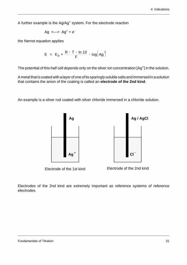
A further example is the Ag/Ag+ system. For the electrode reaction
Ag <—> Ag+ + e-
the Nernst equation applies
The potential of this half cell depends only on the silver ion concentration [Ag+] in the solution.
A metal that is coated with a layer of one of its sparingly soluble salts and immersed in a solutionthat contains the anion of the coating is called an electrode of the 2nd kind.
An example is a silver rod coated with silver chloride immersed in a chloride solution.
Electrodes of the 2nd kind are extremely important as reference systems of referenceelectrodes.
3+
Ag
Ag +
3+
Ag / AgCl
-Cl
Electrode of the 1st kind Electrode of the 2nd kind
4 Indications
Fundamentals of Titration32
A typical experimental setup in titration comprises one sensing electrode and one referenceelectrode. The task of the sensing electrode is to record all changes in the composition of thesolution. The reference electrode must be capable of supplying a stable reference potentialthat is independent of these changes.
4.1.2 Reference electrodes
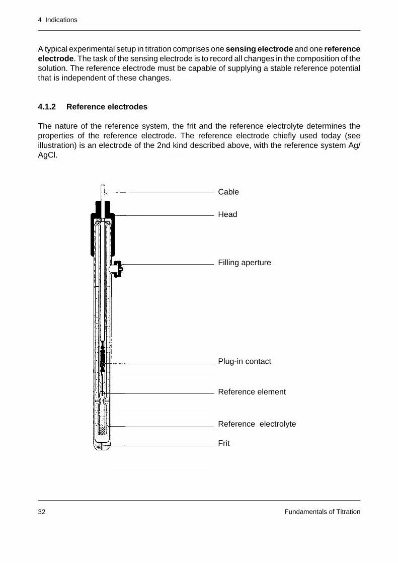
The nature of the reference system, the frit and the reference electrolyte determines theproperties of the reference electrode. The reference electrode chiefly used today (seeillustration) is an electrode of the 2nd kind described above, with the reference system Ag/AgCl.
Cable
Head
Filling aperture
Plug-in contact
Reference element
Reference electrolyte
Frit
4 Indications
Fundamentals of Titration 33
The reference system is in the form of a cartridge and contains an ample supply of silver andsilver chloride. The cartridge is connected to the reference electrolyte (e.g. KCl: c(KCl) = 3 mol/L) via an internal frit.
The external frit ensures electrical contact between the reference electrode and the analysissolution. It must fulfill the following requirements:
– chemically inert
– low outflow rate of reference electrolyte at low electrical resistance
– no ion exchanger properties.
In addition to fine-pored ceramic frits, sleeve frits made of glass or plastic are used.
The following demands are made on reference electrolytes:
– constant chloride ion activity
– low electrical resistance
– chemically inert and neutral
– no reaction with analysis solution
– same mobility of cation and anion.
A concentrated solution of KCl fulfills virtually all these conditions.
A calomel electrode (reference system Hg/Hg2Cl2) is often used as reference electrode andis constructed on similar lines to the silver chloride reference electrode.
To avoid a reaction of the reference electrolyte with constituents of the sample or titrant (e.g.Cl- with Ag+), double junction reference electrodes comprising two electrodes of the 2ndkind are often used.
In routine analysis, combined electrodes have gained wide acceptance. Here, the sensing andreference electrodes are integrated in the same shaft (glass or plastic) (see Section 4.1.4).
4 Indications
Fundamentals of Titration34
4.1.3 Metal electrodes
Metal electrodes, usually manufactured as electrodes of the 1st kind, have a wide range ofuses in titration.
Electrodes of the noble metals platinum and gold are used as redox electrodes. They areeminently suitable for the indication of redox titrations.
In addition to measurement of the silver ion concentration (silver ion activity), metal electrodesmade of silver can be used for the indication of precipitation titrations (determination ofhalogens).
An amalgamated silver electrode can be used to indicate many complexometric titrations(indicator ion: Hg2+).
4.1.4 Glass electrodes
The glass electrode is the most important and most widely used sensor in analysis.
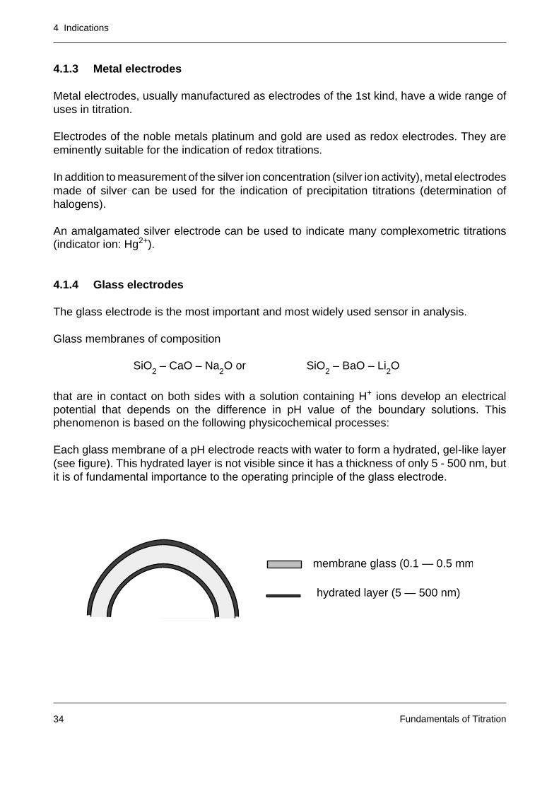
Glass membranes of composition
SiO2 – CaO – Na
2O or SiO
2 – BaO – Li
2O
that are in contact on both sides with a solution containing H+ ions develop an electricalpotential that depends on the difference in pH value of the boundary solutions. Thisphenomenon is based on the following physicochemical processes:
Each glass membrane of a pH electrode reacts with water to form a hydrated, gel-like layer(see figure). This hydrated layer is not visible since it has a thickness of only 5 - 500 nm, butit is of fundamental importance to the operating principle of the glass electrode.
membrane glass (0.1 — 0.5 mm
hydrated layer (5 — 500 nm)
4 Indications
Fundamentals of Titration 35
The basis of the glass membrane is a three dimensional network of silicon and oxygen atomswith each silicon atom being surrounded by four oxygen atoms and each oxygen atom by twosilicon atoms. The interstitial spaces in this irregular network are occupied by cations to ensureelectroneutrality of the glass membrane.
In the formation of the hydrated layer the following process occurs:
–Si–OM + H2O —> –Si–OH + MOH (M = Li, Na)
The alkali ions diffuse into the aqueous solution, leaving behind a virtually completelyprotonated Si-O skeleton. The internal glass membrane remains anhydrous.
At the phase boundary solution/hydrated layer, a thermodynamic equilibrium is established.This is possible only because the hydrogen ions in the hydrated layer are mobile. When thehydrogen ion concentration in both phases is different, hydrogen ion transport takes place.Every inflow and outflow of H+ ions into or out of the glass membrane disturbs theelectroneutrality of the hydrated layer. A potential is thus set up at the phase boundary thatopposes further transport of H+.
The number of hydrogen ions in the hydrated layer depends on the silicic acid skeleton andis constant and independent of the nature of the analysis solution. Owing to the movement ofcations through the glass membrane, the electrical potential at the hydrated layer is transferredto the inner surface of the membrane where a hydrated layer with a phase boundary potentialis also present. The total membrane potential results from the difference between the twophase boundary potentials.
4 Indications
Fundamentals of Titration36
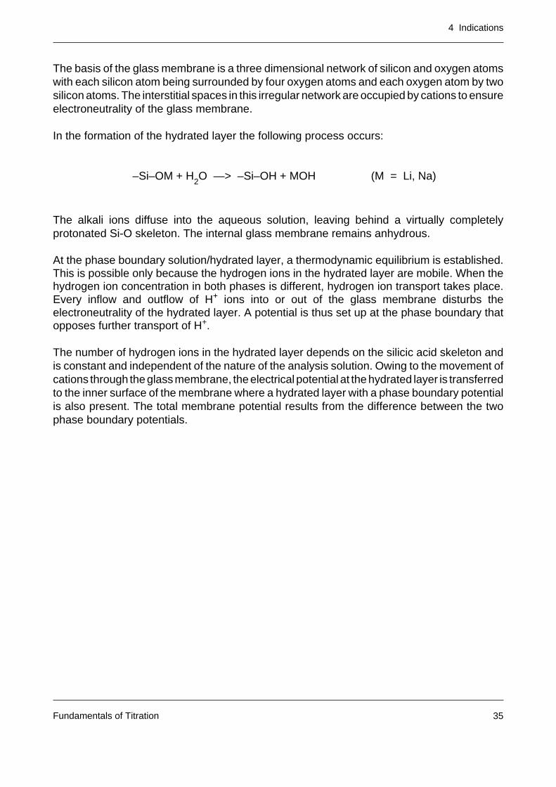
In routine work a glass electrode with integrated reference electrode (so-called combinationor combined electrode) is usually employed.
Plug-in contact of sensing electrode
Plug-in contact of reference electrode
Filling aperture
Reference electrode
Reference electrolyte (3 M KCI saturatedwith AgCI)
Ag/AgCl reference element
Ceramic frit
Sensing electrode
Internal buffer (electrolyte)
Ag/AgCl (internal) lead-off
Glass membrane
When the pH values in the two hydrated layers are identical (ideal case) and the pH value ofthe internal electrolyte (see figure) of the glass electrode remains constant, the membranepotential is given by
Emembrane = Constant +2.303 • RT
F• log H
+
4 Indications
Fundamentals of Titration 37
In practice, this equation is never satisfied exactly. Three factors contribute to the nonidealbehavior:
1. Asymmetry potential
The membrane potential should be zero when the glass membrane is in contact withidentical solutions on both sides. Generally, however, a potential of a few mV is observedowing to the different history of the two sides of the membrane. A small asymmetrypotential is unimportant since it is compensated in the calibration.
2. Alkaline error
In alkaline solutions the H+ ions of the hydrated layer are partly replaced by alkali ions,especially sodium ions. The smaller H+ concentration in the hydrated layer thus leads tolower pH values.
The difference between the theoretical and experimental pH value is called the alkalineerror. In the types of lithium-based glass used today, the pH deviations do not start untilabove pH 13. The alkaline error increases with increasing pH value, increasing alkaliconcentration and increasing temperature.
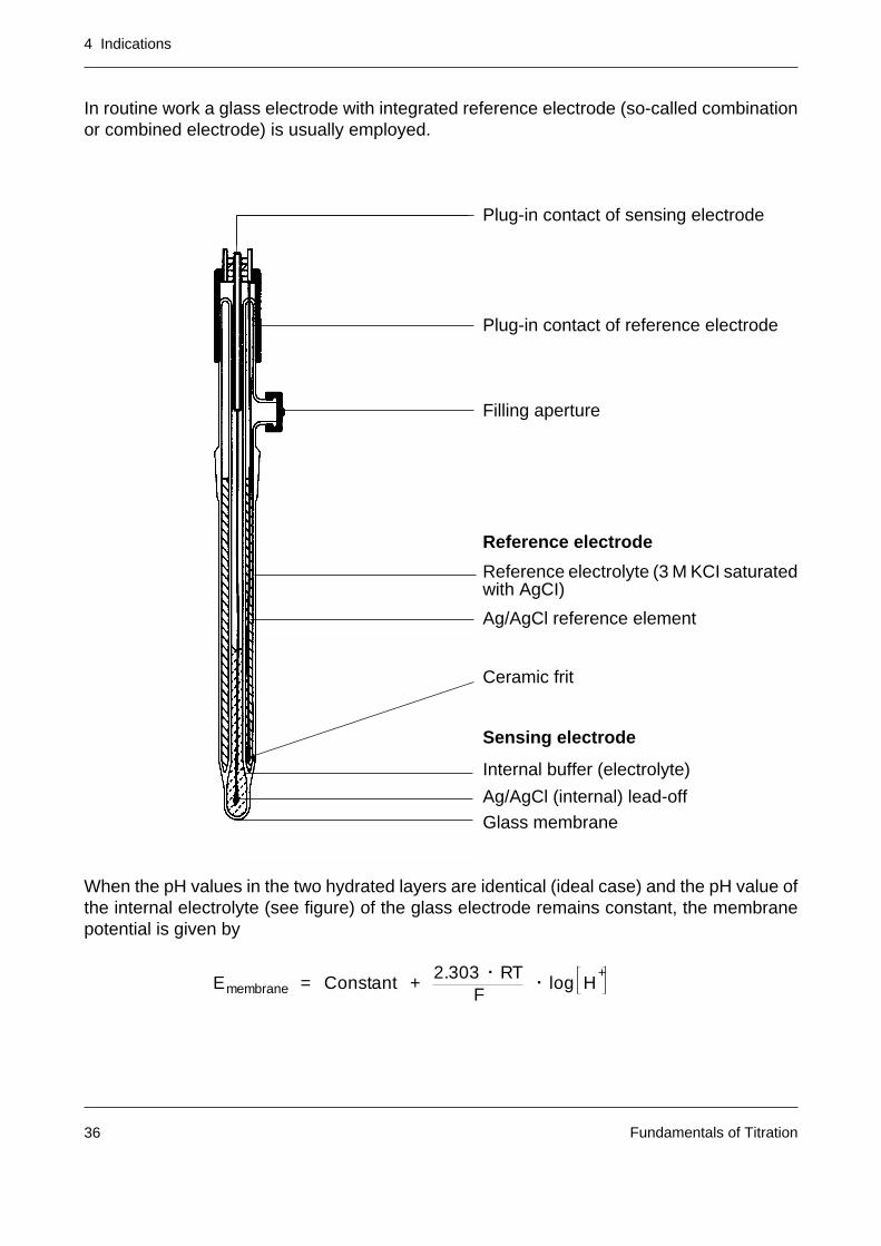
3. Acid error
In highly acidic solutions (pH < 1) the glass electrode exhibits deviations from the ideal pHfunction. Through uptake of acid molecules, the hydrogen ion activity of the hydrated layeris increased, thereby leading to positive pH shifts. The acid error is less disturbing than thealkaline error.
pH
E [mV]
Allkaline error
Acid error
7 14
0
0
200
-200

4 Indications
Fundamentals of Titration38
A further characteristic of the glass membrane is its high electrical resistance, which liesbetween 10 and 10 000 MΩ, depending on the composition of the glass, the temperature andthe size of the membrane. This high resistance thus places increased demands on themeasuring system.
The internal electrolyte ensures a constant phase boundary potential at the inner surface ofthe glass membrane and a constant potential at the internal lead-off. Usually a silver wirecoated with Ag/AgCl is used as internal lead-off, whose potential is determined by the chlorideion activity of the internal electrolyte.
4 Indications
Fundamentals of Titration 39
4.1.5 Ion selective electrodes
Ion selective electrodes are electrochemical half cells in which a potential difference arises atthe phase boundary electrode/solution that depends on the concentration (more correctlyactivity) of a certain ion in the solution.
Glass electrodes are also ion selective electrodes. The setup of an ion selective electrodeassembly is similar to that of the pH electrode and comprises an ion selective membrane anda reference electrode of constant potential.
Instead of a pH scale, an ion scale is defined, for example a pNa or a pCl scale.
Many cations and anions, neutral gases such as NH3, CO2 and SO2 and even organicsubstances such as amino acids can be measured quantitatively with ion selective electrodesdirectly. Even ions or neutral substances that are not measurable directly can be determinedindirectly if a chemical auxiliary reaction is run in which a substance that can be detected bya sensing electrode is released or bound.
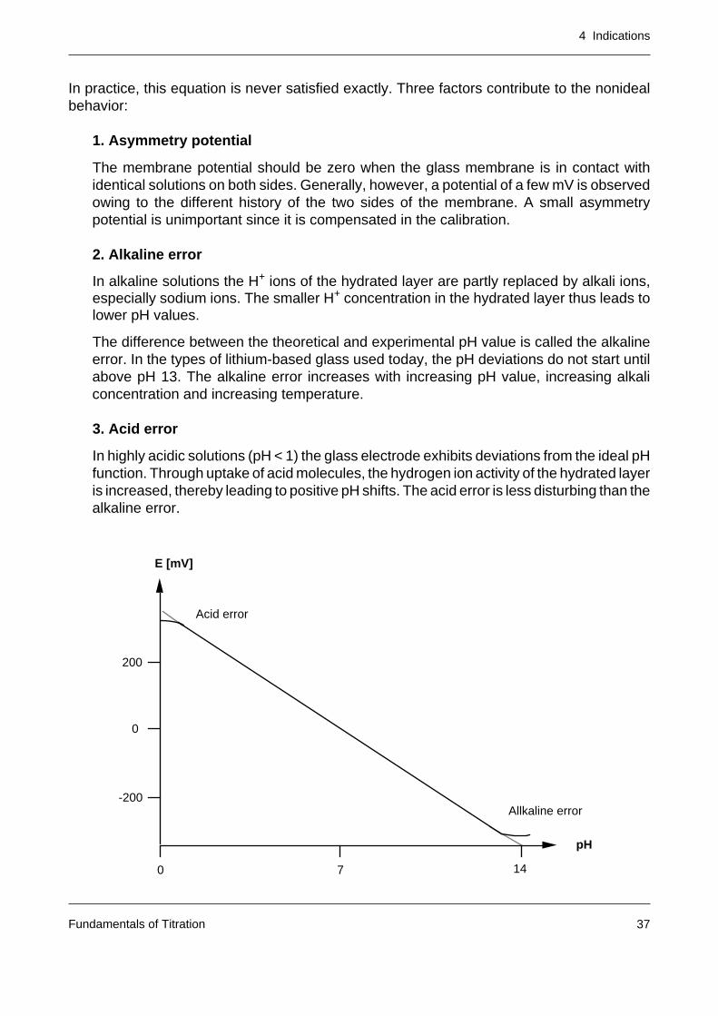
In the ideal case the electrode assembly potential of an ion selective electrode is describedby an expanded Nernst equation, the so-called Nicolsky equation:
where
E: is the electrode assembly potential
E0: the electrode assembly potential at the reference point (ai = 1, aj = 0)
S: the slope (S = 2.301 • R • T/ni • F). The sign is + for cations and – for anions.
ai: the analyte ion activity in solution
aj: the interfering ion activities in solution
Kij: the selectivity coefficients of interfering ions
ni: the charge number of analyte ion
nj: the charge numbers of interfering ions.
The selectivity coefficients of the interfering ions are a measure of the selectivity of theelectrode. They should be as small as possible so that the interfering ions in question makeno appreciable contribution to the ion selective potential change at the measuring cell. Witha value of Kij = 1 the contribution of the interfering ions to the potential change is exactly thesame as that of the analyte ion (assuming same charge numbers). A completely selectiveelectrode, i.e. one that responds only to one type of ion under all conditions does not exist.
E = E0 ± S • log a i + ∑j
K ij • ajni/nj
4 Indications
Fundamentals of Titration40
The glass electrode has a selectivity coefficient towards sodium ions of 10-12 – 10-13, in otherwords good pH electrodes are disturbed by sodium ions only at Na+ concentrations greaterthan 0.1 mol/L and pH values above 12.
The astonishing selectivity of glass electrodes is by no means attained by other ion selectiveelectrodes. Selectivity coefficients of 10-5 – 10-6 are typical.
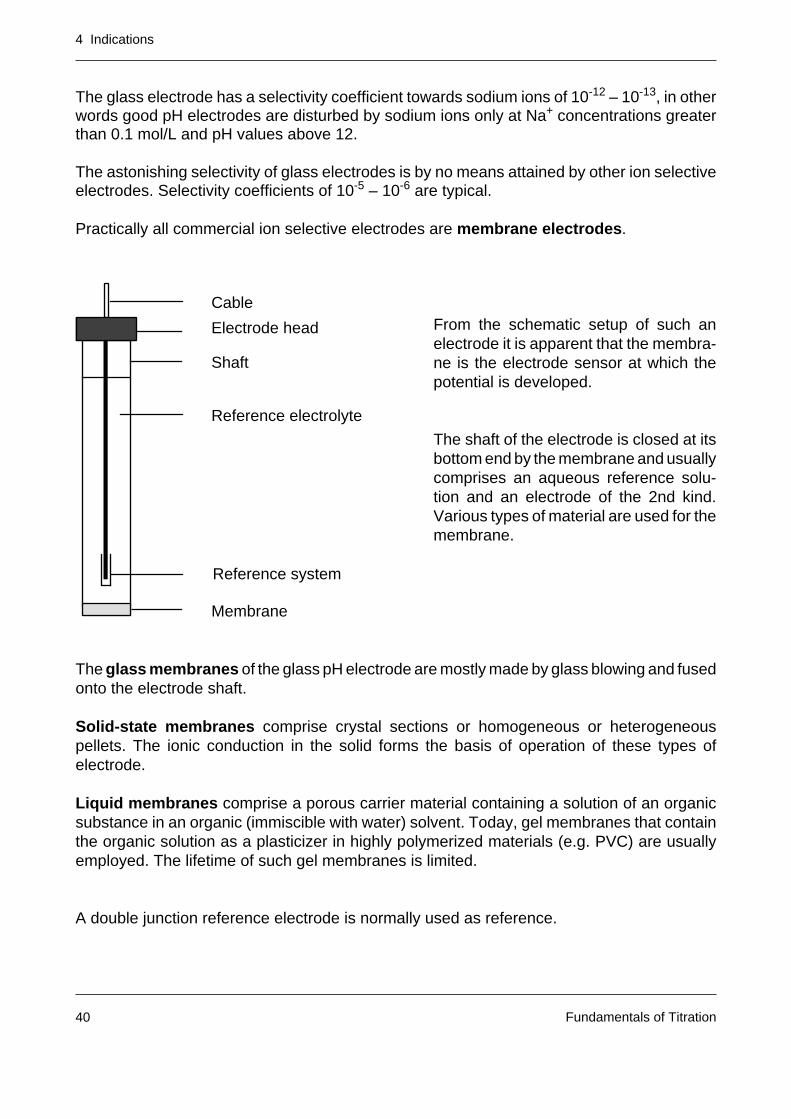
Practically all commercial ion selective electrodes are membrane electrodes.
From the schematic setup of such anelectrode it is apparent that the membra-ne is the electrode sensor at which thepotential is developed.
The shaft of the electrode is closed at itsbottom end by the membrane and usuallycomprises an aqueous reference solu-tion and an electrode of the 2nd kind.Various types of material are used for themembrane.
The glass membranes of the glass pH electrode are mostly made by glass blowing and fusedonto the electrode shaft.
Solid-state membranes comprise crystal sections or homogeneous or heterogeneouspellets. The ionic conduction in the solid forms the basis of operation of these types ofelectrode.
Liquid membranes comprise a porous carrier material containing a solution of an organicsubstance in an organic (immiscible with water) solvent. Today, gel membranes that containthe organic solution as a plasticizer in highly polymerized materials (e.g. PVC) are usuallyemployed. The lifetime of such gel membranes is limited.
A double junction reference electrode is normally used as reference.
Cable
Electrode head
Shaft
Reference electrolyte
Reference system
Membrane
4 Indications
Fundamentals of Titration 41
4.1.6 Measurement technique
All electrochemical measurements have one thing in common: they are performed using anelectrode assembly consisting of a sensing and a reference electrode.
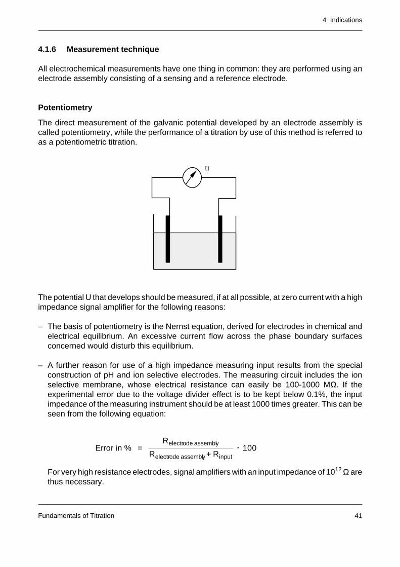
Potentiometry
The direct measurement of the galvanic potential developed by an electrode assembly iscalled potentiometry, while the performance of a titration by use of this method is referred toas a potentiometric titration.
The potential U that develops should be measured, if at all possible, at zero current with a highimpedance signal amplifier for the following reasons:
– The basis of potentiometry is the Nernst equation, derived for electrodes in chemical andelectrical equilibrium. An excessive current flow across the phase boundary surfacesconcerned would disturb this equilibrium.
– A further reason for use of a high impedance measuring input results from the specialconstruction of pH and ion selective electrodes. The measuring circuit includes the ionselective membrane, whose electrical resistance can easily be 100-1000 MΩ. If theexperimental error due to the voltage divider effect is to be kept below 0.1%, the inputimpedance of the measuring instrument should be at least 1000 times greater. This can beseen from the following equation:
For very high resistance electrodes, signal amplifiers with an input impedance of 1012 Ω arethus necessary.
Error in % =Relectrode assembly
Relectrode assembly + Rinput
• 100
U
4 Indications
Fundamentals of Titration42
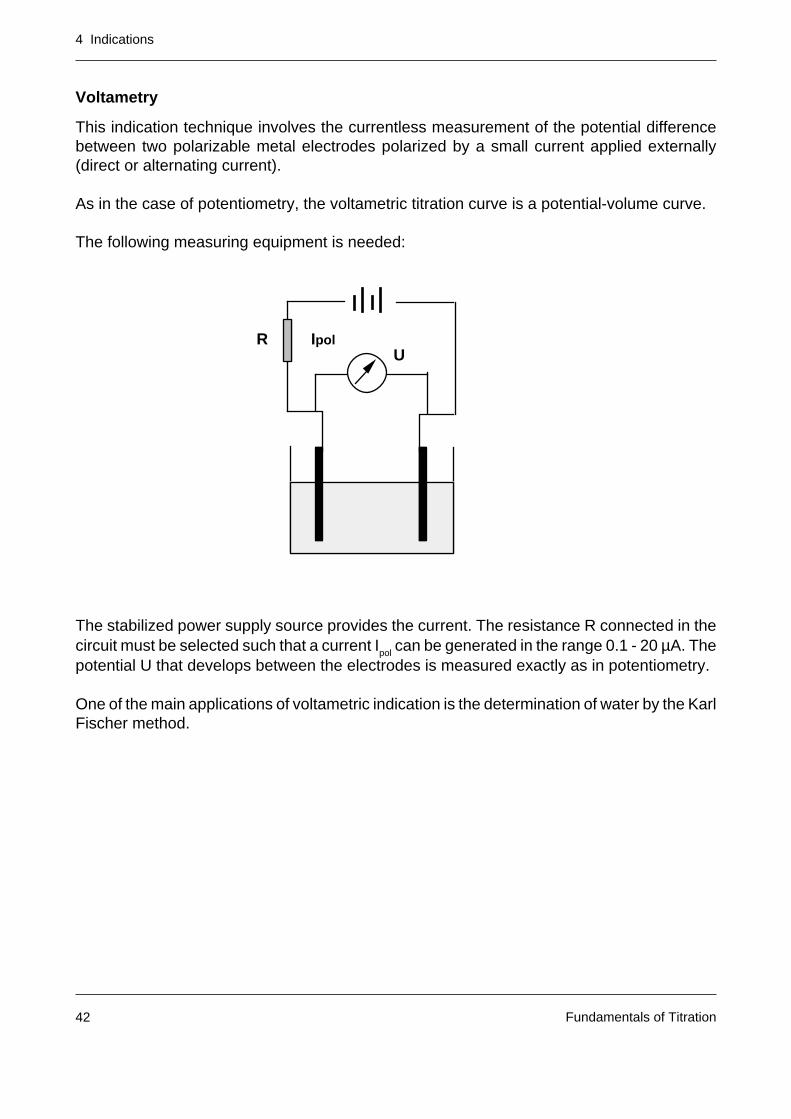
Voltametry
This indication technique involves the currentless measurement of the potential differencebetween two polarizable metal electrodes polarized by a small current applied externally(direct or alternating current).
As in the case of potentiometry, the voltametric titration curve is a potential-volume curve.
The following measuring equipment is needed:
The stabilized power supply source provides the current. The resistance R connected in thecircuit must be selected such that a current Ipol can be generated in the range 0.1 - 20 µA. Thepotential U that develops between the electrodes is measured exactly as in potentiometry.
One of the main applications of voltametric indication is the determination of water by the KarlFischer method.
UR Ipol
4 Indications
Fundamentals of Titration 43
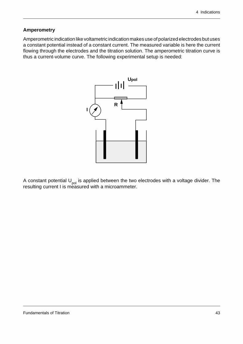
Amperometry
Amperometric indication like voltametric indication makes use of polarized electrodes but usesa constant potential instead of a constant current. The measured variable is here the currentflowing through the electrodes and the titration solution. The amperometric titration curve isthus a current-volume curve. The following experimental setup is needed:
A constant potential Upol
is applied between the two electrodes with a voltage divider. Theresulting current I is measured with a microammeter.
Upol
RI
4 Indications
Fundamentals of Titration44
4.2 Photometric indication
The basis of photometric indication is the decrease in intensity at a particular wavelength ofa light beam passing through a solution. The transmission is the primary measured variablein photometry and is given by
where
T: is the transmission
I0: the intensity of the incident light and
I: the intensity ot the transmitted light.
If all light is absorbed, then I = 0 and hence T = 0. If no light is absorbed, I = I0 and T = 1 (or
%T = 100%).
In photometry, work is frequently performed using absorption as the measured variable. Therelation between transmission and absorption is described by the Bouguer-Beer-LambertLaw:
where
A: is the absorption
ε: the absorptivity
c: the concentration ot the absorbing substance and
d: the path length of the light through the solution.
From the above relation it can be seen that there is a linear relation between absorption A andconcentration c. This is the basis of the direct photometric measurement.
A = –log T = ε • c • d
T =II0
( or % T =II0
• 100 )
4 Indications
Fundamentals of Titration 45
In comparison with electrodes, photoelectric probes have a number of advantages in titration:
– they are easier to use (no refilling of electrolyte solutions, no clogging of the frit)
– longer lifetime (they are virtually unbreakable)
– they can be used to perform all classical titrations to a color change (no change in traditionalprocedures and standards).
Photometric indication is possible for many analytical reactions:
– Acid-base titrations (aqueous and nonaqueous)
– Complexometry
– Redox titrations
– Precipitation titrations
– Turbimetric titrations
In phototitration a wavelength should be selected which gives the greatest difference intransmission before and after the equivalence point. In the visible region such wavelengths areusually in the range 500 to 700 nm.
4 Indications
Fundamentals of Titration46
4.2.1 The METTLER phototrode
The METTLER DP550 and DP660 Phototrodes are probes for photometric titration in thevisible region.
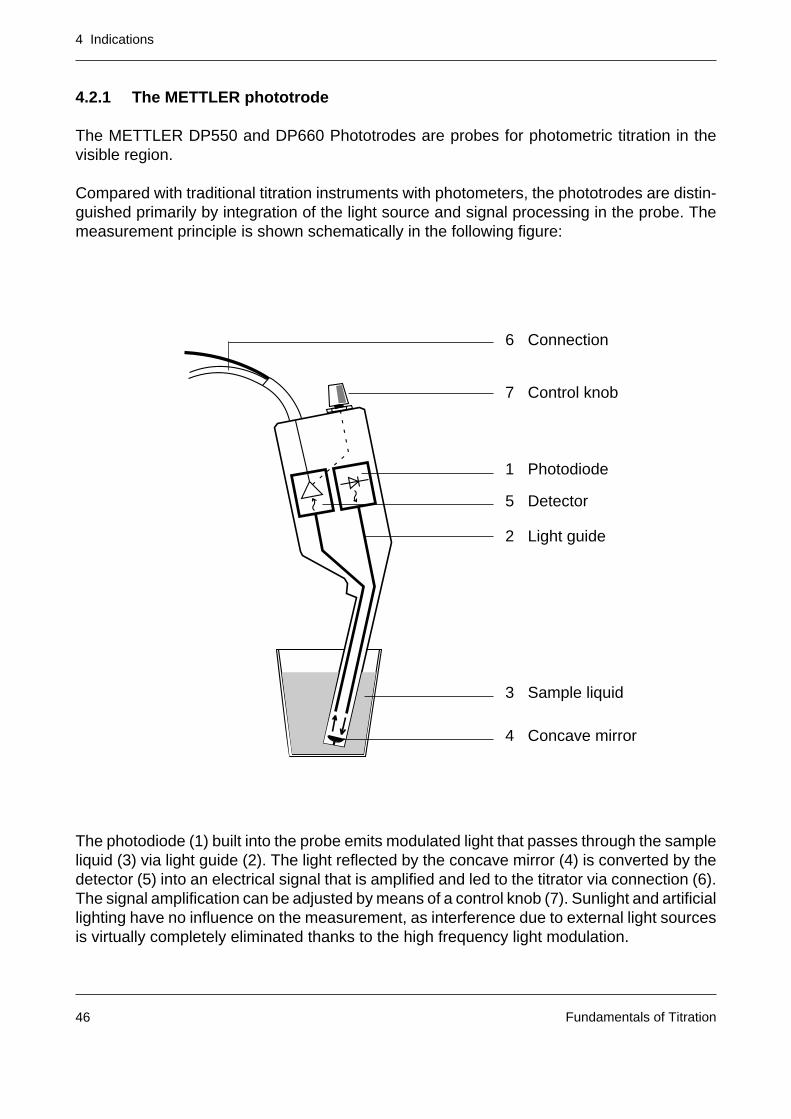
Compared with traditional titration instruments with photometers, the phototrodes are distin-guished primarily by integration of the light source and signal processing in the probe. Themeasurement principle is shown schematically in the following figure:
6 Connection
7 Control knob
1 Photodiode
5 Detector
2 Light guide
3 Sample liquid
4 Concave mirror
The photodiode (1) built into the probe emits modulated light that passes through the sampleliquid (3) via light guide (2). The light reflected by the concave mirror (4) is converted by thedetector (5) into an electrical signal that is amplified and led to the titrator via connection (6).The signal amplification can be adjusted by means of a control knob (7). Sunlight and artificiallighting have no influence on the measurement, as interference due to external light sourcesis virtually completely eliminated thanks to the high frequency light modulation.
4 Indications
Fundamentals of Titration 47
4.3 Special indication methods
4.3.1 Conductometric indication
Conductometric indication [1], [2] [3] makes use of the ability of aqueous solutions to conductan electric current. This conductivity is based on the dissociation of acids, bases and salts intoelectrically charged species (ions) in aqueous solution. In an electric field the anions migrateto the positively charged anode and the cations to the negatively charged cathode. Faraday’slaw states that per mole equivalent entity the same quantity of electricity, namely 96'485coulombs, will be transported to the electrodes.
The conductivity of a dilute electrolyte solution depends on
– the ionic concentration
– the charge number of the ions
– the mobility of the ions in the solvent in question
– the polarity of the solvent and
– the temperature (the conductivity increases by around 2.5% per degree Celsius).
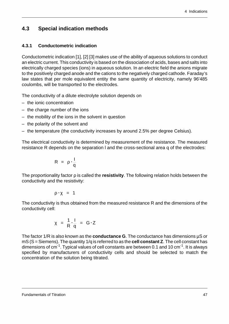
The electrical conductivity is determined by measurement of the resistance. The measuredresistance R depends on the separation l and the cross-sectional area q of the electrodes:
The proportionality factor ρ is called the resistivity. The following relation holds between theconductivity and the resistivity:
The conductivity is thus obtained from the measured resistance R and the dimensions of theconductivity cell:
The factor 1/R is also known as the conductance G. The conductance has dimensions µS ormS (S = Siemens). The quantity 1/q is referred to as the cell constant Z. The cell constant hasdimensions of cm-1. Typical values of cell constants are between 0.1 and 10 cm-1. It is alwaysspecified by manufacturers of conductivity cells and should be selected to match theconcentration of the solution being titrated.
R = ρ •Iq
ρ • χ = 1
χ =1R
•Iq
= G • Z
4 Indications
Fundamentals of Titration48
The conductivity should be specified in units of µS/cm or mS/cm, depending on its magnitude.
For the determination of the conductivity, alternating current must be used for the resistancemeasurement. If a direct current flows between the electrodes, electrolysis takes place and thecontribution of the ohmic resistance, which is the sole variable of interest, becomes so smallthat its measurement is impossible.
The practical application of conductometric indication is limited to acid-base and precipitationtitrations.
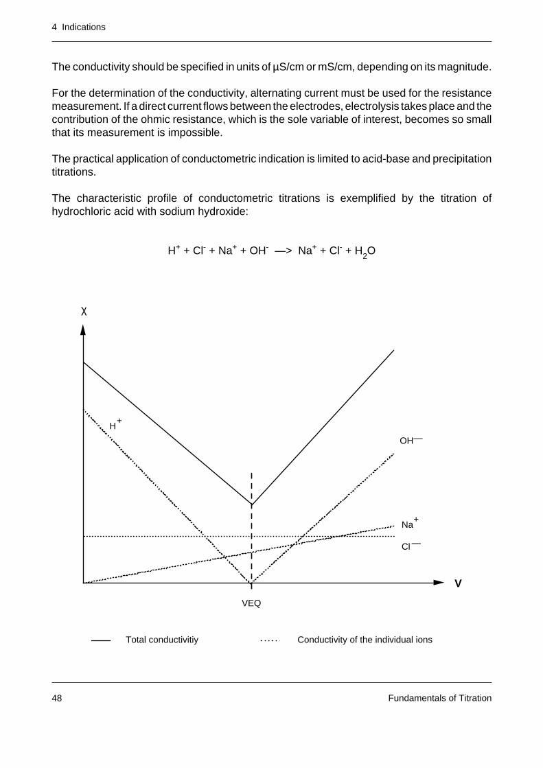
The characteristic profile of conductometric titrations is exemplified by the titration ofhydrochloric acid with sodium hydroxide:
H+ + Cl- + Na+ + OH- —> Na+ + Cl- + H2O
VEQ
χ
V
H
OH
Na
Cl
+
+
—
—
Total conductivitiy Conductivity of the individual ions
4 Indications
Fundamentals of Titration 49
The measured conductivity at every point on the titration curve is composed of the sum of theconductivity of the individual ions. The titration diagram overleaf shows the contributions of theindividual ions to the total conductivity (dilution not taken into account).
The titration curves are actually straight lines as long as each ionic species present reactsquantitatively or not at all. The typical curve character is due to the fact that one ionic speciesof the solution disappears (in our case H+) only to be replaced by a new one from the titrant(here OH-). When the equivalence point is exceeded, an increase in the conductivity is alwaysobserved in the absence of any further reaction.
[1] F. Oehme, “Angewandte Konduktometrie”, Hüthig Verlag, Heidelberg (1961)
[2] F. Oehme, “ABC der Konduktometrie”, offprint Chemische Rundschau (1979)
[3] E. Pungor, “Oscillometry and Conductometry”, Pergamon Press, Oxford (1965)
5 Types of titration
Fundamentals of Titration50
5 Types of titration
Titrations can be classified in various ways. The classification by means of indication methodand analytical reaction has been discussed in earlier sections. This section describes theclassification of titrations according to the manner in which they are performed.
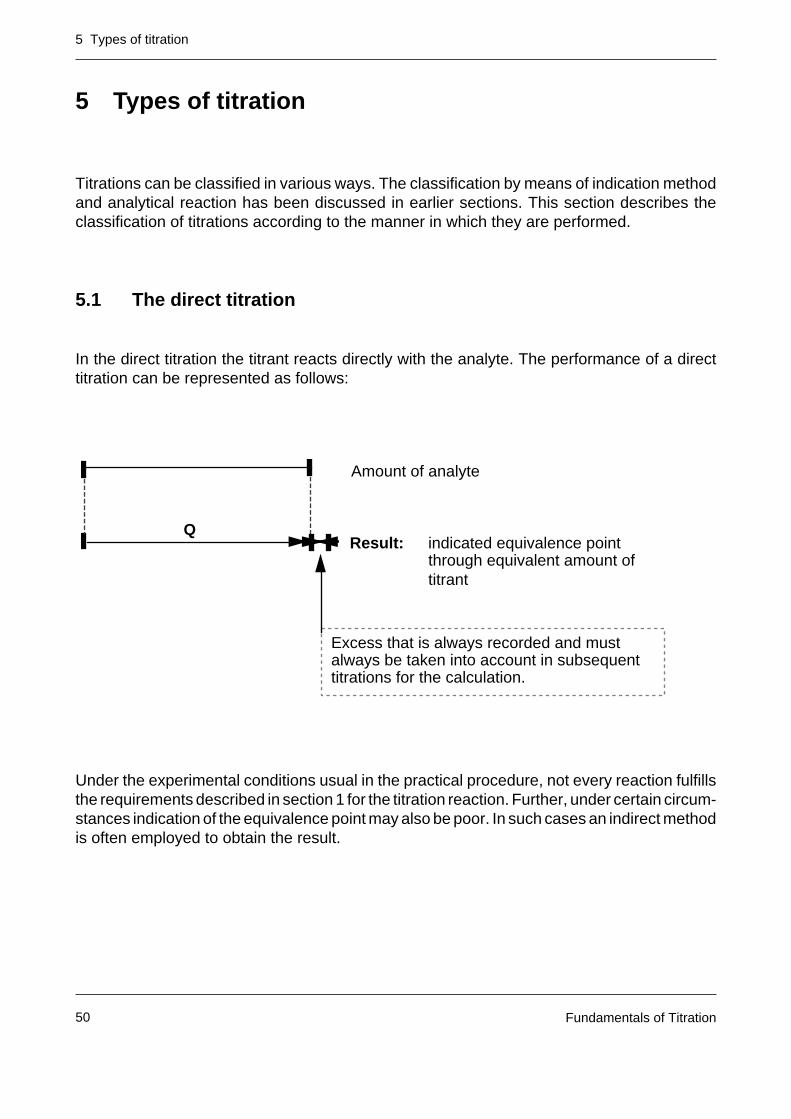
5.1 The direct titration
In the direct titration the titrant reacts directly with the analyte. The performance of a directtitration can be represented as follows:
Under the experimental conditions usual in the practical procedure, not every reaction fulfillsthe requirements described in section 1 for the titration reaction. Further, under certain circum-stances indication of the equivalence point may also be poor. In such cases an indirect methodis often employed to obtain the result.
Amount of analyte
Result:Q
indicated equivalence pointthrough equivalent amount oftitrant
Excess that is always recorded and must always be taken into account in subsequenttitrations for the calculation.
5 Types of titration
51Fundamentals of Titration
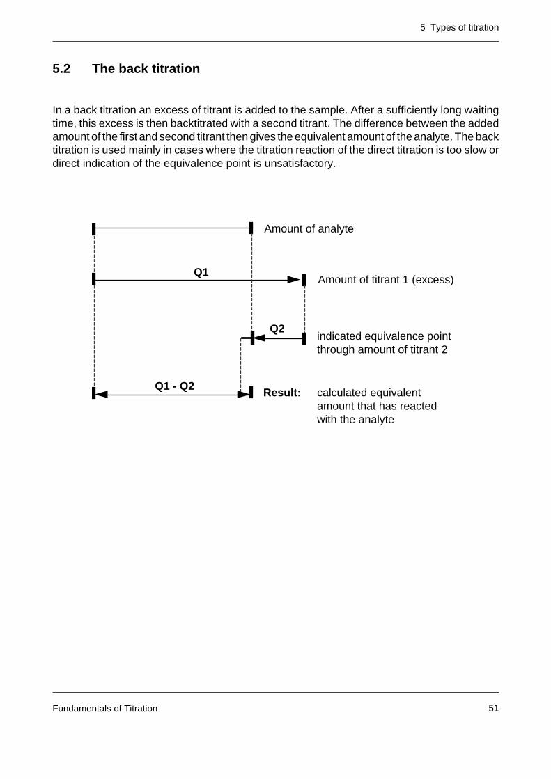
5.2 The back titration
In a back titration an excess of titrant is added to the sample. After a sufficiently long waitingtime, this excess is then backtitrated with a second titrant. The difference between the addedamount of the first and second titrant then gives the equivalent amount of the analyte. The backtitration is used mainly in cases where the titration reaction of the direct titration is too slow ordirect indication of the equivalence point is unsatisfactory.
Amount of analyte
Amount of titrant 1 (excess)
Result:
indicated equivalence pointthrough amount of titrant 2
Q1 - Q2
Q1
Q2
calculated equivalent amount that has reacted with the analyte
5 Types of titration
Fundamentals of Titration52
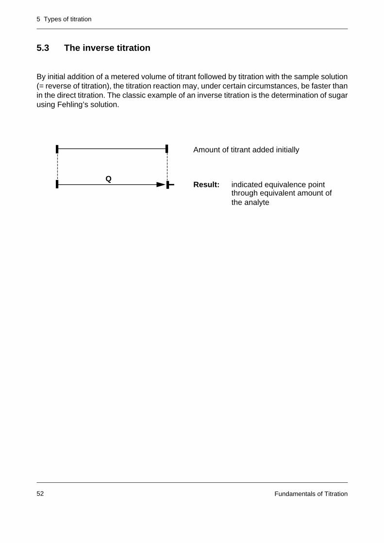
5.3 The inverse titration
By initial addition of a metered volume of titrant followed by titration with the sample solution(= reverse of titration), the titration reaction may, under certain circumstances, be faster thanin the direct titration. The classic example of an inverse titration is the determination of sugarusing Fehling’s solution.
Amount of titrant added initially
Result: Q
indicated equivalence pointthrough equivalent amount of the analyte
5 Types of titration
53Fundamentals of Titration
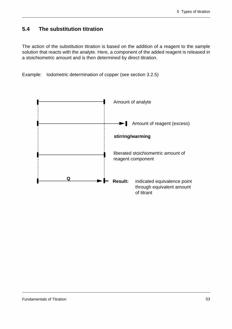
5.4 The substitution titration
The action of the substitution titration is based on the addition of a reagent to the samplesolution that reacts with the analyte. Here, a component of the added reagent is released ina stoichiometric amount and is then determined by direct titration.
Example: Iodometric determination of copper (see section 3.2.5)
Amount of analyte
Amount of reagent (excess)
stirring/warming
liberated stoichiomertric amount of reagent component
Result: indicated equivalence point through equivalent amount of titrant
Q
5 Types of titration
Fundamentals of Titration54
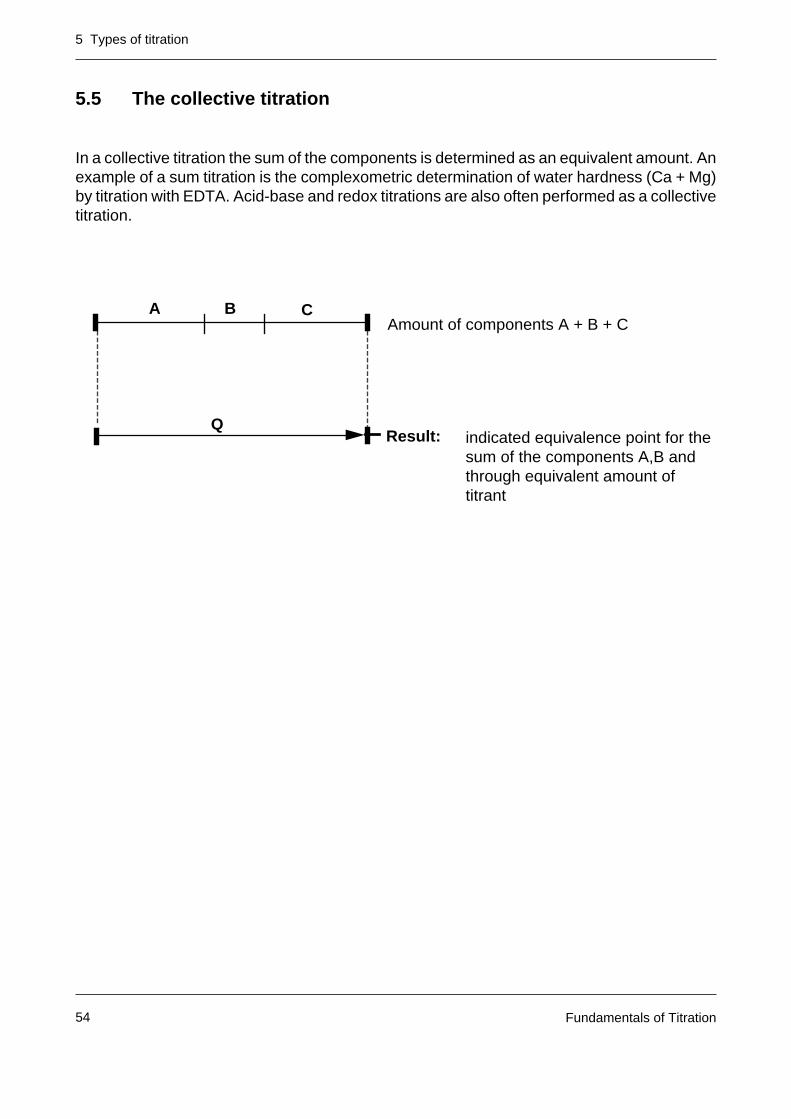
5.5 The collective titration
In a collective titration the sum of the components is determined as an equivalent amount. Anexample of a sum titration is the complexometric determination of water hardness (Ca + Mg)by titration with EDTA. Acid-base and redox titrations are also often performed as a collectivetitration.
Amount of components A + B + CA B
indicated equivalence point for thesum of the components A,B and through equivalent amount of titrant
Result:
C
Q
5 Types of titration
55Fundamentals of Titration
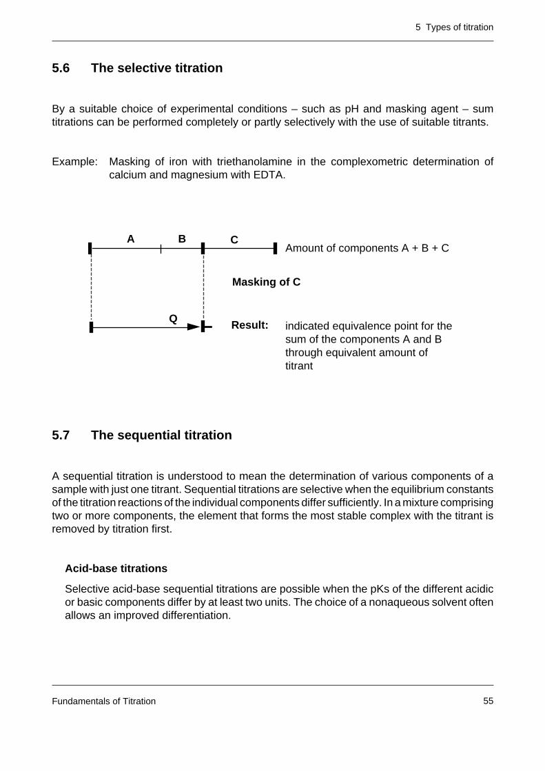
5.6 The selective titration
By a suitable choice of experimental conditions – such as pH and masking agent – sumtitrations can be performed completely or partly selectively with the use of suitable titrants.
Example: Masking of iron with triethanolamine in the complexometric determination ofcalcium and magnesium with EDTA.
5.7 The sequential titration
A sequential titration is understood to mean the determination of various components of asample with just one titrant. Sequential titrations are selective when the equilibrium constantsof the titration reactions of the individual components differ sufficiently. In a mixture comprisingtwo or more components, the element that forms the most stable complex with the titrant isremoved by titration first.
Acid-base titrations
Selective acid-base sequential titrations are possible when the pKs of the different acidicor basic components differ by at least two units. The choice of a nonaqueous solvent oftenallows an improved differentiation.
Amount of components A + B + CA B
indicated equivalence point for the sum of the components A and B through equivalent amount of titrant
Result:
C
Q
Masking of C
5 Types of titration
Fundamentals of Titration56
Complexometric titrations
In complexometric sequential titrations the following criteria must be met:
– the effective stability constants must show a difference of at least five logarithmic units
– the minimum value of the relevant stability constant (in logarithmic units) must be at leastseven.
Redox titrations
Selective redox titrations are also possible. The potential difference between the equivalen-ce points in question must be at least 300 mV.
The principle of the sequential titration is summarized in the following diagrams:
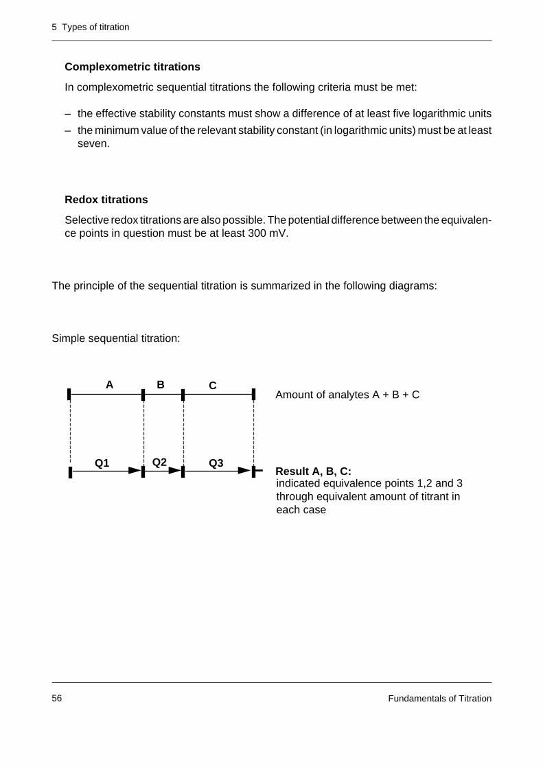
Simple sequential titration:
Amount of analytes A + B + C A B
indicated equivalence points 1,2 and 3through equivalent amount of titrant in each case
Result A, B, C:
C
Q1 Q2 Q3
5 Types of titration
57Fundamentals of Titration
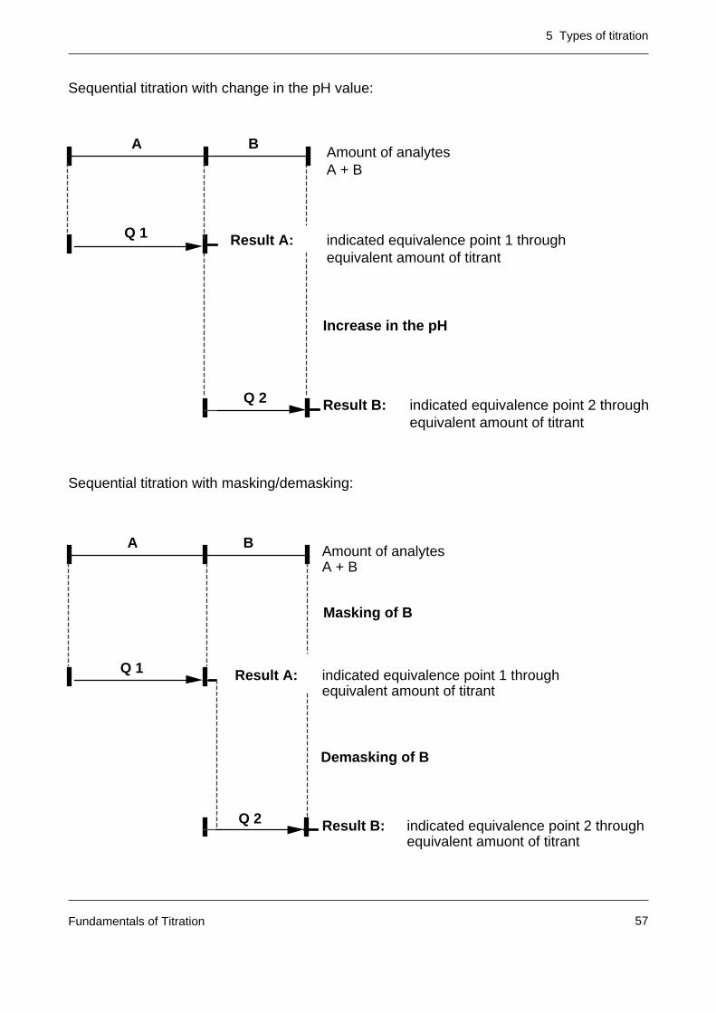
Sequential titration with change in the pH value:
Sequential titration with masking/demasking:
Amount of analytesA + B
A B
Q 1 indicated equivalence point 1 through equivalent amount of titrant
Result A:
Result B:
Increase in the pH
Q 2 indicated equivalence point 2 through equivalent amount of titrant
Amount of analytesA + B
A B
Q 1 indicated equivalence point 1 throughequivalent amount of titrant
Result A:
Result B:
Masking of B
Demasking of B
Q 2 indicated equivalence point 2 through equivalent amuont of titrant
5 Types of titration
Fundamentals of Titration58
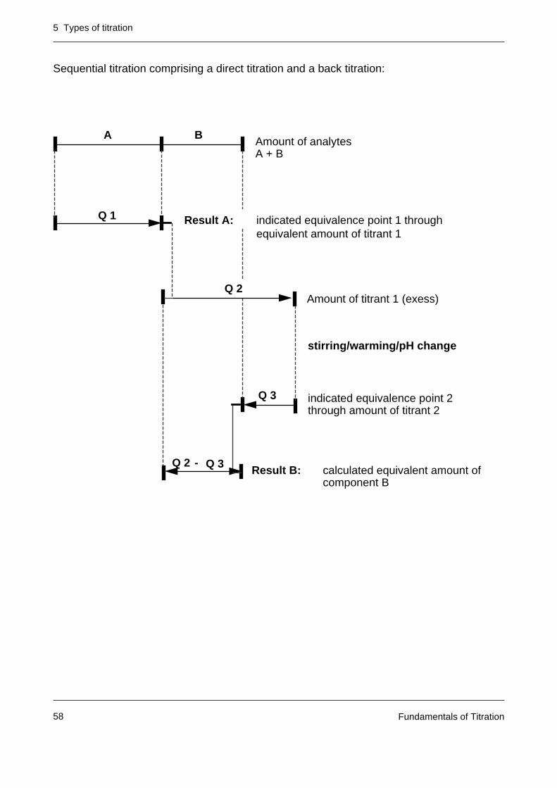
Sequential titration comprising a direct titration and a back titration:
Amount of analytesA + B
A B
Q 1
Q 2
Q 3
Q 2 Q 3-
Amount of titrant 1 (exess)
stirring/warming/pH change
indicated equivalence point 2through amount of titrant 2
indicated equivalence point 1 throughequivalent amount of titrant 1
calculated equivalent amount of component B
Result A:
Result B:
6 Titration curves
Fundamentals of Titration 59
6 Titration curves
Titration curves illustrate the qualitative progress of a titration. They allow a rapid assessmentof the titration method. A distinction is made between logarithmic and linear titration curves.
Logarithmic curves appear when the measured signal has a logarithmic dependence on theequilibrium concentration. Such curves are obtained with all indication methods that follow theNernst equation. This includes all potentiometric titrations.
If there is a linear relation between the measurement signal and the concentration, the titrationcurves are said to be linear. The most important application is photometric titration. Furtherexamples are titrations with conductometric, amperometric and thermometric indication.Linear curves can be evaluated graphically and by calculation.
6.1 Measurement signal as a function of the titrant volume: E = f(V)
This representation can be used for the graphical determination of the equivalence point (seesection 8). The various potentiometric indication methods produce in part very differenttitration curves in the range -1600 mV to +1600 mV.
The graphical and computational evaluation of titration curves is treated in section 8.
6 Titration curves
Fundamentals of Titration60
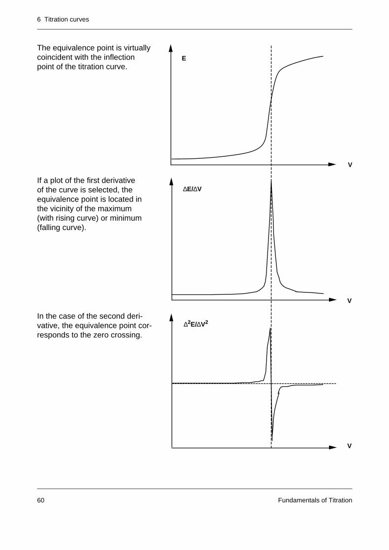
The equivalence point is virtuallycoincident with the inflectionpoint of the titration curve.
If a plot of the first derivativeof the curve is selected, theequivalence point is located inthe vicinity of the maximum(with rising curve) or minimum(falling curve).
In the case of the second deri-vative, the equivalence point cor-responds to the zero crossing.
E
V
V
V
∆E/∆V
∆2E/∆V2
6 Titration curves
Fundamentals of Titration 61
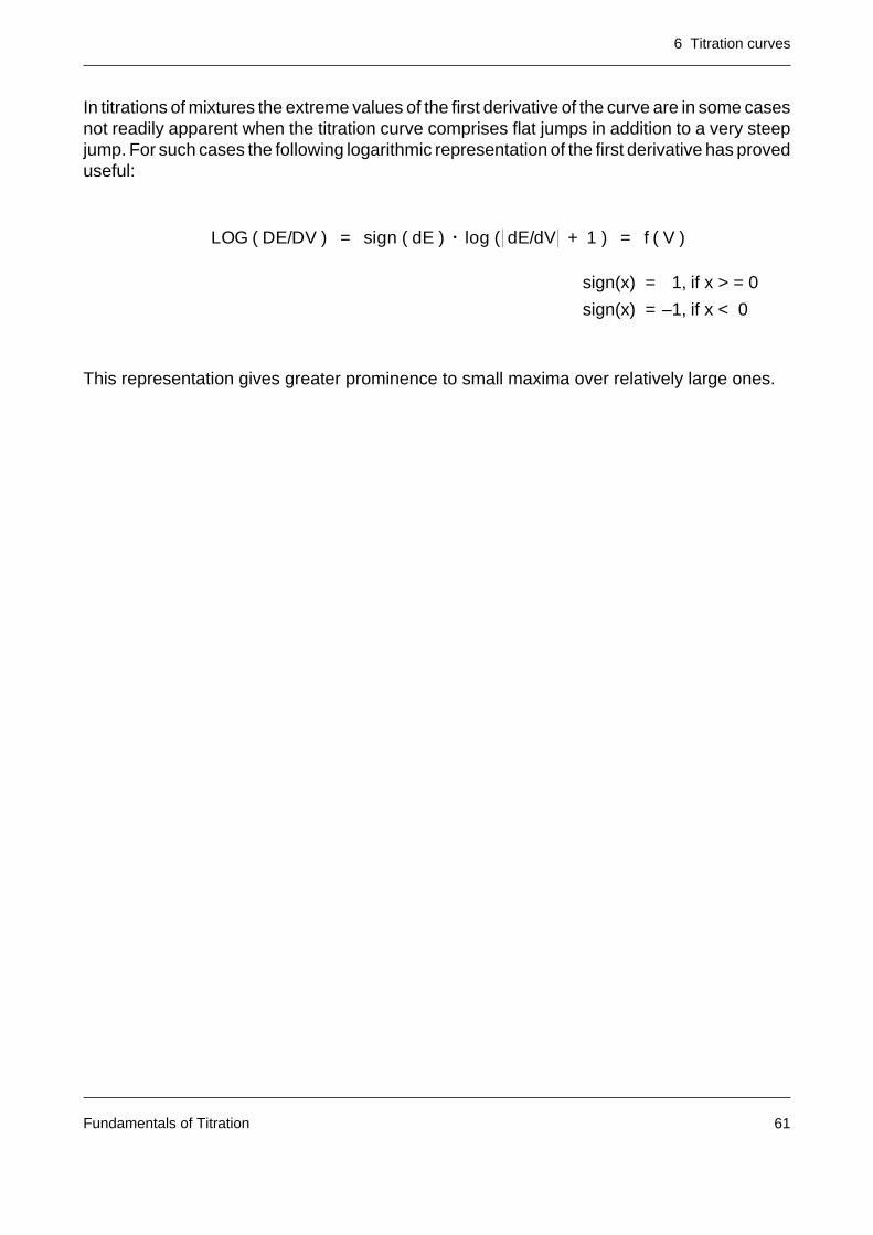
In titrations of mixtures the extreme values of the first derivative of the curve are in some casesnot readily apparent when the titration curve comprises flat jumps in addition to a very steepjump. For such cases the following logarithmic representation of the first derivative has proveduseful:
sign(x) = 1, if x > = 0
sign(x) = –1, if x < 0
This representation gives greater prominence to small maxima over relatively large ones.
LOG ( DE/DV ) = sign ( dE ) • log ( dE/dV + 1 ) = f ( V )
6 Titration curves
Fundamentals of Titration62
E
V
∆E/∆V
log ∆E/∆V
V
V
6 Titration curves
Fundamentals of Titration 63
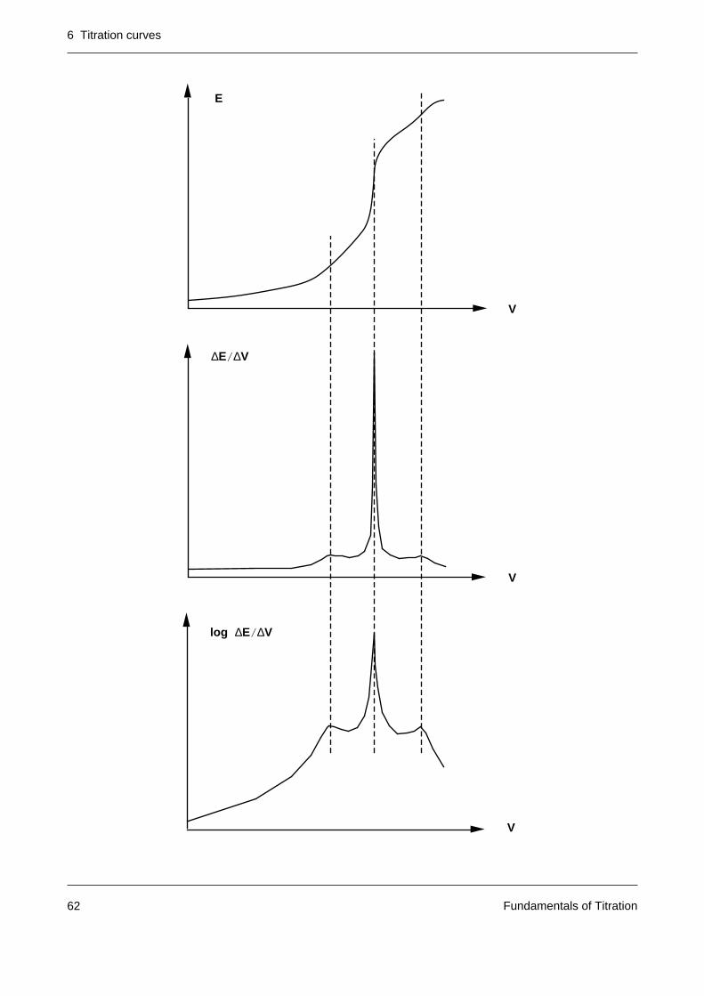
6.2 Measurement signal as a function of time: E = f(t)
Representation of the signal as a function of time (plotted on an analog recorder or a dot matrixprinter) aids the development of new methods and the optimization of the equilibrium conditionfor the measured value acquisition. The time dependance of the measurement signal allowsassessment of the response behavior of the electrode and the rate of the titration reaction.
The following figures show a few representative examples. The shape of the curve isinfluenced by the following parameters:
– response time of the electrode
– rate of the titration reaction
– stirrer speed.
This example shows the case of a slow reaction observed using an electrode with a fastresponse. The abrupt change in the signal at the start shows the immediate response of theelectrode to addition of the titrant. The stabilization of the equilibrium signal is the result of thesubsequent titration reaction.
E
t
6 Titration curves
Fundamentals of Titration64
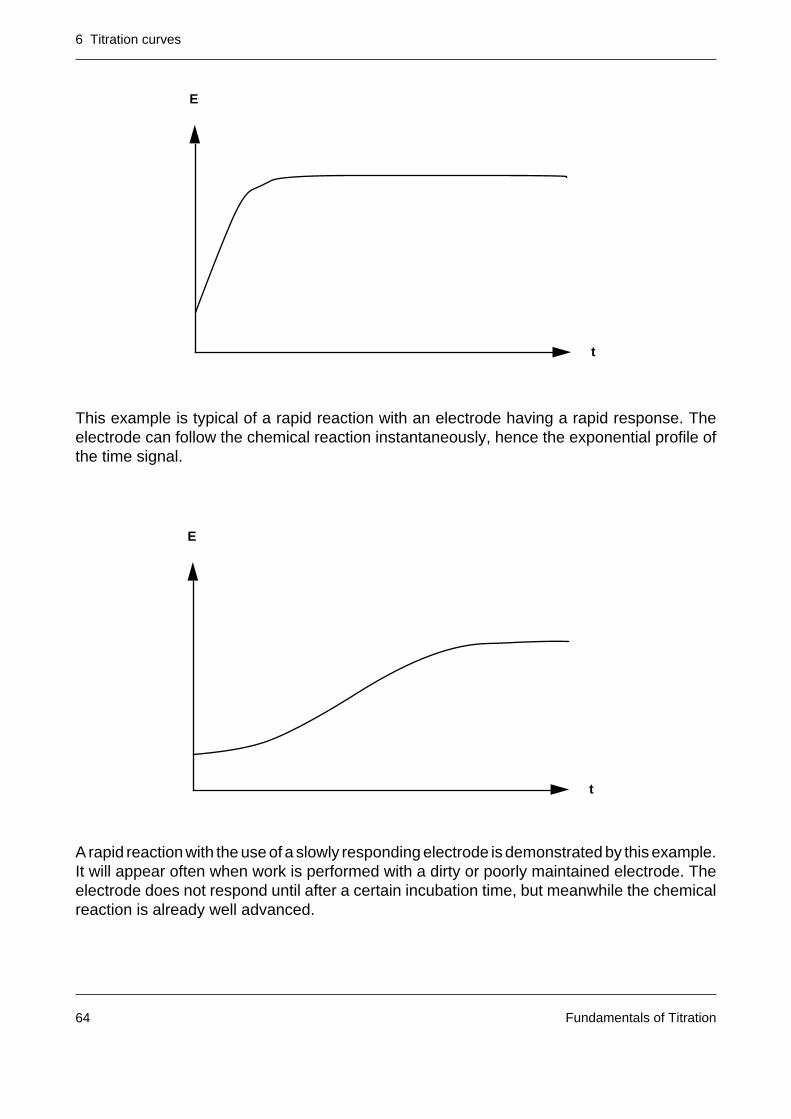
This example is typical of a rapid reaction with an electrode having a rapid response. Theelectrode can follow the chemical reaction instantaneously, hence the exponential profile ofthe time signal.
A rapid reaction with the use of a slowly responding electrode is demonstrated by this example.It will appear often when work is performed with a dirty or poorly maintained electrode. Theelectrode does not respond until after a certain incubation time, but meanwhile the chemicalreaction is already well advanced.
E
t
E
t
6 Titration curves
Fundamentals of Titration 65
The concepts of “rapid” and “slow” are naturally relative in this context. They describe the rateof the titration reaction relative to the response behavior of the electrode.
6.3 Titrant volume as a function of time: V = f(t)
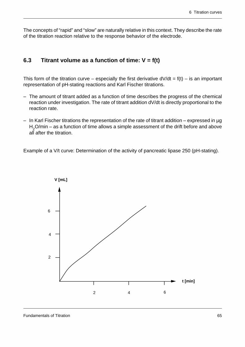
This form of the titration curve – especially the first derivative dV/dt = f(t) – is an importantrepresentation of pH-stating reactions and Karl Fischer titrations.
– The amount of titrant added as a function of time describes the progress of the chemicalreaction under investigation. The rate of titrant addition dV/dt is directly proportional to thereaction rate.
– In Karl Fischer titrations the representation of the rate of titrant addition – expressed in µgH2O/min – as a function of time allows a simple assessment of the drift before and aboveall after the titration.
Example of a V/t curve: Determination of the activity of pancreatic lipase 250 (pH-stating).
2
4
6
2 4 6
t [min]
V [mL]
7 Control
Fundamentals of Titration66
7 Control of the titration
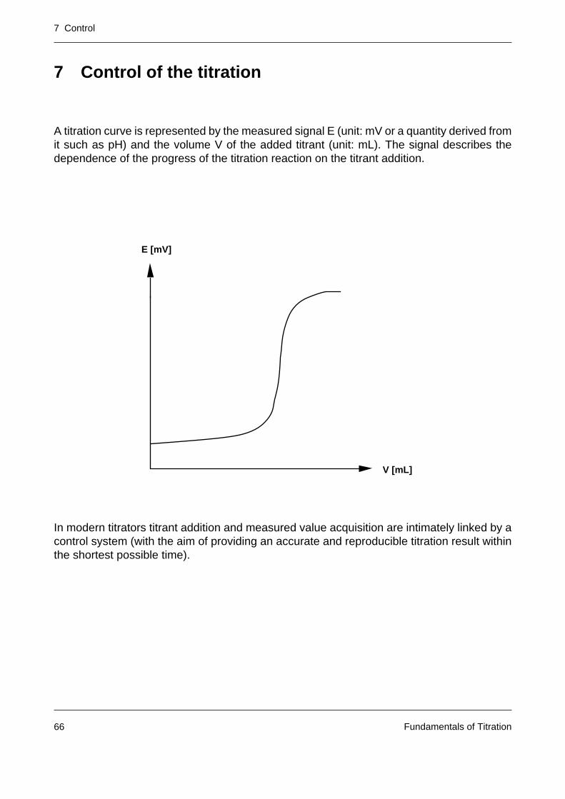
A titration curve is represented by the measured signal E (unit: mV or a quantity derived fromit such as pH) and the volume V of the added titrant (unit: mL). The signal describes thedependence of the progress of the titration reaction on the titrant addition.
In modern titrators titrant addition and measured value acquisition are intimately linked by acontrol system (with the aim of providing an accurate and reproducible titration result withinthe shortest possible time).
E [mV]
V [mL]
7 Control
Fundamentals of Titration 67
7.1 Titrant addition
The titrant can be added in two ways: continuously at a defined rate of dispensing orincremental with individual volume steps.
7.1.1 Continuous titrant addition
The continuous addition of titrant is the classic way to perform a titration with motorized pistonburette, pH meter and analog recorder. In automatic titrators the continuous titrant addition isused in the so-called recording titration and in end point titrations. In the recording titrationthe signal is plotted on an analog recorder or a dot matrix printer as a function of the addedvolume.
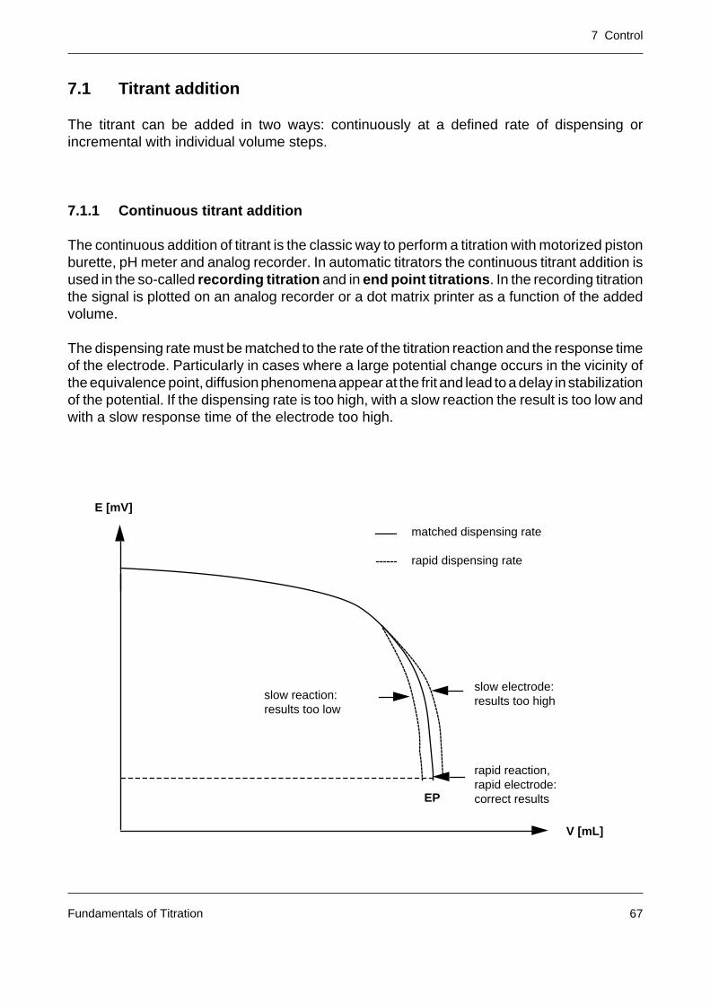
The dispensing rate must be matched to the rate of the titration reaction and the response timeof the electrode. Particularly in cases where a large potential change occurs in the vicinity ofthe equivalence point, diffusion phenomena appear at the frit and lead to a delay in stabilizationof the potential. If the dispensing rate is too high, with a slow reaction the result is too low andwith a slow response time of the electrode too high.
E [mV]
V [mL]
matched dispensing rate
rapid dispensing rate
slow electrode:results too highslow reaction:
results too low
rapid reaction,rapid electrode:correct resultsEP

7 Control
Fundamentals of Titration68
Modern titrators solve the problem with a variable dispensing rate. The titrant addition iscontrolled as a function of the measured signal change such that a distortion of the titrationcurve due to lag of the potential adjustment is avoided even in the transition interval.
The titrant is added at a high rate up to a defined control band. Within the control range therate decreases exponentially. In the vicinity of the end point single pulses are dispensed. Apulse is the smallest increment and equals 1/5000 of the burette volume of METTLER burettes.
A large control range leads to an accurate but slow titration. A narrower range results in a rapidtitration, but there is an inherent danger of overtitrating. With an S-shaped, steadily progres-sing titration curve only about the last 10% of the volume to be added should lie within thecontrol range. To avoid overtitrating, it is advisable to position the burette tip so that the stirrertransports the titrant to the electrode by the shortest route.
E [mV – pH]
V [mL]
100
-100
-200
End point
Control band = 250 mV/(4.3 pH)
8
7
6
5
4
Start of the control range
+200
+
0
9
10

7 Control
Fundamentals of Titration 69
The time from the attainment of the end point up to the definitive termination of the titration iscalled the delay. If the signal of the sample solution deviates from the original end point signalduring this time, additional increments are added until the end point is again reached. A largevalue of the delay (typical value: 10 s) should be selected with:
– large titration vessels
– inefficient stirring
– slow analytical reaction
– long response time of the sensor.
The continuous titrant addition in end point titrations is suitable only for steep titration curves.With flat curves (see figure), wrong selection of the end point (EP’ instead of EP) or a driftingelectrode leads to a false equivalence volume (VEQ’ instead of VEQ). For traditional reasons(old standards, procedures), however, even when the curves are flat, titration must sometimesbe performed to the preset end point by means of continuous titrant addition. Before suchdeterminations the appropriate electrode must always be calibrated to allow detection of theexact end point.
E
V
E
VVEQ VEQ › VEQ‘
EPEP‘
7 Control
Fundamentals of Titration70
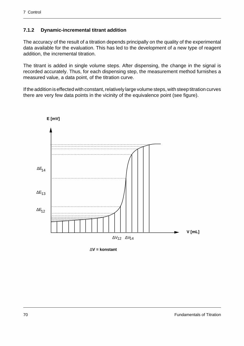
7.1.2 Dynamic-incremental titrant addition
The accuracy of the result of a titration depends principally on the quality of the experimentaldata available for the evaluation. This has led to the development of a new type of reagentaddition, the incremental titration.
The titrant is added in single volume steps. After dispensing, the change in the signal isrecorded accurately. Thus, for each dispensing step, the measurement method furnishes ameasured value, a data point, of the titration curve.
If the addition is effected with constant, relatively large volume steps, with steep titration curvesthere are very few data points in the vicinity of the equivalence point (see figure).
∆V ∆V
∆E
∆E
∆E
∆V = konstant
E [mV]
V [mL]
14
13
12
12
14
7 Control
Fundamentals of Titration 71
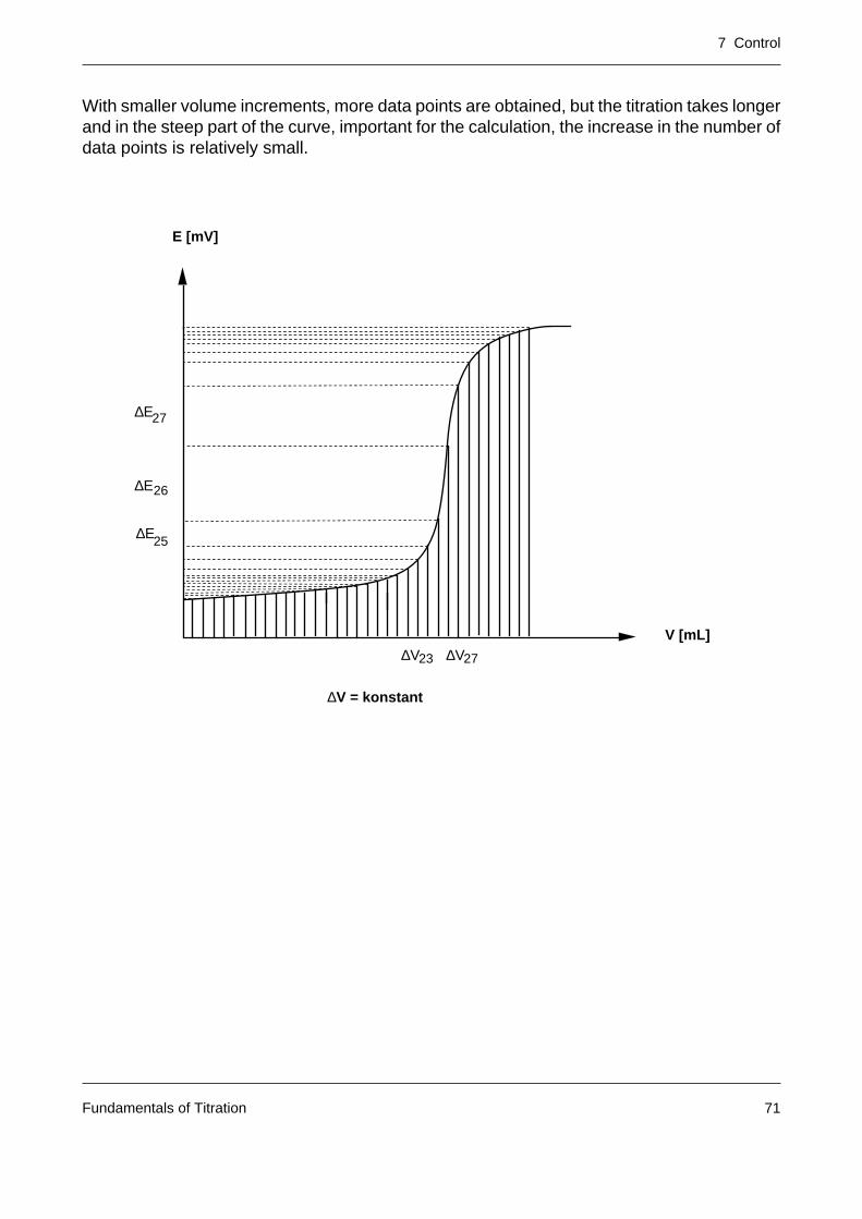
With smaller volume increments, more data points are obtained, but the titration takes longerand in the steep part of the curve, important for the calculation, the increase in the number ofdata points is relatively small.
∆V ∆V
∆E
∆E
∆E
∆V = konstant
E [mV]
V [mL]
27
26
23
25
27
7 Control
Fundamentals of Titration72
An obvious move is thus to size the titrant addition so that the signal change always remainsabout the same. This type of titrant addition is known as dynamic titrant addition and thecorresponding titration control as dynamic titration. In the flat, uninteresting part of the titrationcurve, large volume increments are dispensed and in the steep part of the curve, important forthe calculation, smaller increments.
∆E∆E
∆E ~ ∆E(set)
∆E
E [mV]
V [mL]∆V ∆V
3
4
5
3
4
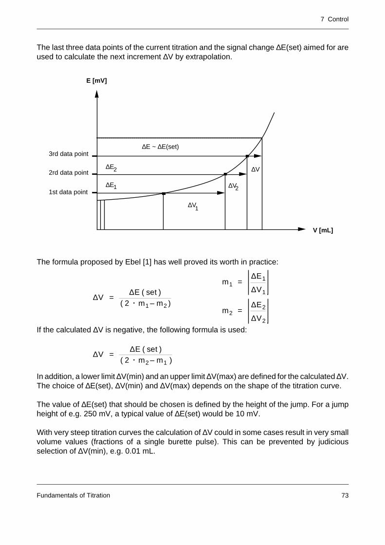
7 Control
Fundamentals of Titration 73
The last three data points of the current titration and the signal change ∆E(set) aimed for areused to calculate the next increment ∆V by extrapolation.
The formula proposed by Ebel [1] has well proved its worth in practice:
If the calculated ∆V is negative, the following formula is used:
In addition, a lower limit ∆V(min) and an upper limit ∆V(max) are defined for the calculated ∆V.The choice of ∆E(set), ∆V(min) and ∆V(max) depends on the shape of the titration curve.
The value of ∆E(set) that should be chosen is defined by the height of the jump. For a jumpheight of e.g. 250 mV, a typical value of ∆E(set) would be 10 mV.
With very steep titration curves the calculation of ∆V could in some cases result in very smallvolume values (fractions of a single burette pulse). This can be prevented by judiciousselection of ∆V(min), e.g. 0.01 mL.
m1 =∆E1
∆V1
m2 =∆E2
∆V2
∆V =∆E ( set )
( 2 • m1 – m2 )
∆V =∆E ( set )
( 2 • m2 – m1 )
E [mV]
V [mL]
∆E
∆E
∆E ~ ∆E(set)
∆V
∆V
∆V
1st data point
2rd data point
3rd data point
1
2
2
1
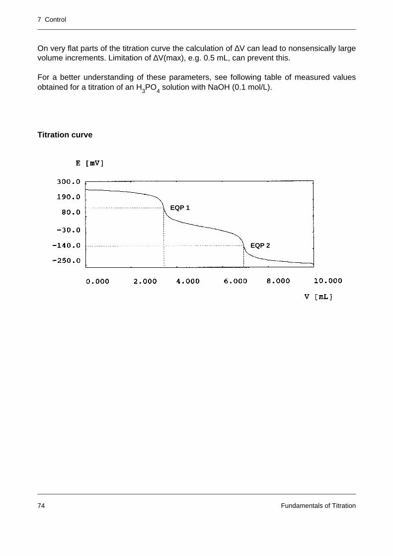
7 Control
Fundamentals of Titration74
On very flat parts of the titration curve the calculation of ∆V can lead to nonsensically largevolume increments. Limitation of ∆V(max), e.g. 0.5 mL, can prevent this.
For a better understanding of these parameters, see following table of measured valuesobtained for a titration of an H3PO4 solution with NaOH (0.1 mol/L).
Titration curve
EQP 1
EQP 2
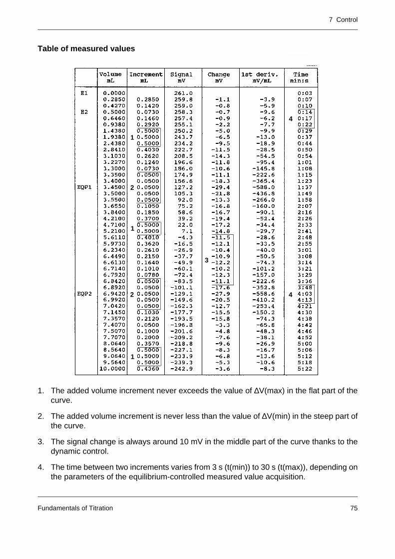
7 Control
Fundamentals of Titration 75
Table of measured values
1. The added volume increment never exceeds the value of ∆V(max) in the flat part of thecurve.
2. The added volume increment is never less than the value of ∆V(min) in the steep part ofthe curve.
3. The signal change is always around 10 mV in the middle part of the curve thanks to thedynamic control.
4. The time between two increments varies from 3 s (t(min)) to 30 s (t(max)), depending onthe parameters of the equilibrium-controlled measured value acquisition.
4
4
1
1
1
2
3
2
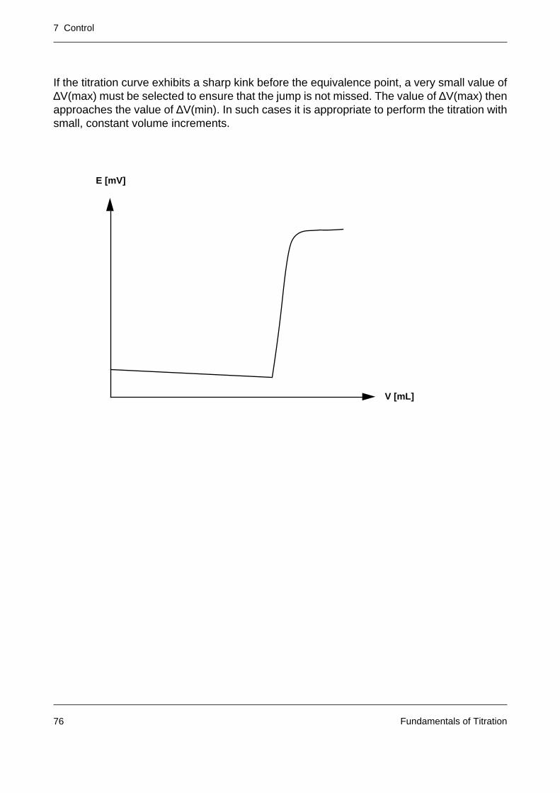
7 Control
Fundamentals of Titration76
If the titration curve exhibits a sharp kink before the equivalence point, a very small value of∆V(max) must be selected to ensure that the jump is not missed. The value of ∆V(max) thenapproaches the value of ∆V(min). In such cases it is appropriate to perform the titration withsmall, constant volume increments.
E [mV]
V [mL]
7 Control
Fundamentals of Titration 77
7.1.3 Predispensing
Predispensing can shorten the time needed for titration considerably. There is no sense toacquire accurate data points during the initial stage of the titration if such data are not neededfor the evaluation. The following predispensing modes are possible:
1. Predispensing to a fixed volume
2. Predispensing to nominal content
3. Predispensing to a certain potential value
4. Predispensing to a certain slope of the titration curve
The first two methods need no signal measurement. The two last methods take into accounta variable amount and a variable content of a sample, but necessitate control of the titrantaddition with simultaneous measurement of the signal. The titrant addition can be continuousor incremental here. Exact signal measurement is not necessary; the important factor is a rapidpredispensing.
The second method, predispensing to nominal content, also takes a variable sample quantityinto consideration, but requires no signal recording. If the expected value of the sample content(= nominal content) remains within certain limits, the volume V to be dispensed, that corres-ponds to a partial content of the sample, can be calculated taking into account the amount(weighing or initial volume) of sample:
V = (metered amount/100) • nominal content • m (or U)/(C • c • t)
where
metered amount: amount to be dispensed in % of the nominal consumption
nominal content: nominal content of the sample (any unit)
m (or U): weight (or volume) of the sample
C: calculation constant for the conversion from mmol to the unit of the nominalcontent, e.g: conversion to unit %: C = M/10 • z
c: nominal concentration of the titration
t: titer of the titrant
If a dynamic titration follows the fixed predispensing, it is advantageous to split the predispens-ing into several steps (e.g. three) with simultaneous measurement of the signal after each step.This procedure allows optimum calculation of the first increment after the predispensing.
Several predispensing modes can be used at the same time and performed one after the other.
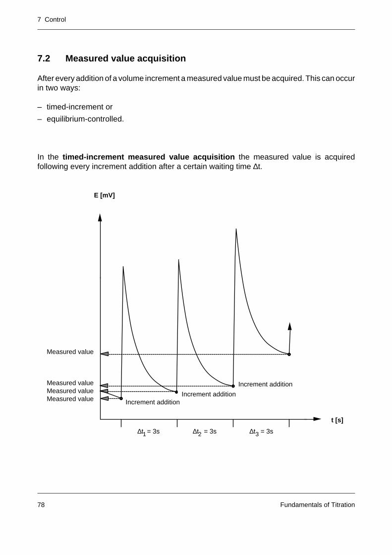
7 Control
Fundamentals of Titration78
7.2 Measured value acquisition
After every addition of a volume increment a measured value must be acquired. This can occurin two ways:
– timed-increment or
– equilibrium-controlled.
In the timed-increment measured value acquisition the measured value is acquiredfollowing every increment addition after a certain waiting time ∆t.
E [mV]
t [s]
∆t = 3s ∆t = 3s ∆t = 3s
Measured value
Measured valueMeasured valueMeasured value
Increment addition
Increment additionIncrement addition
1 2 3
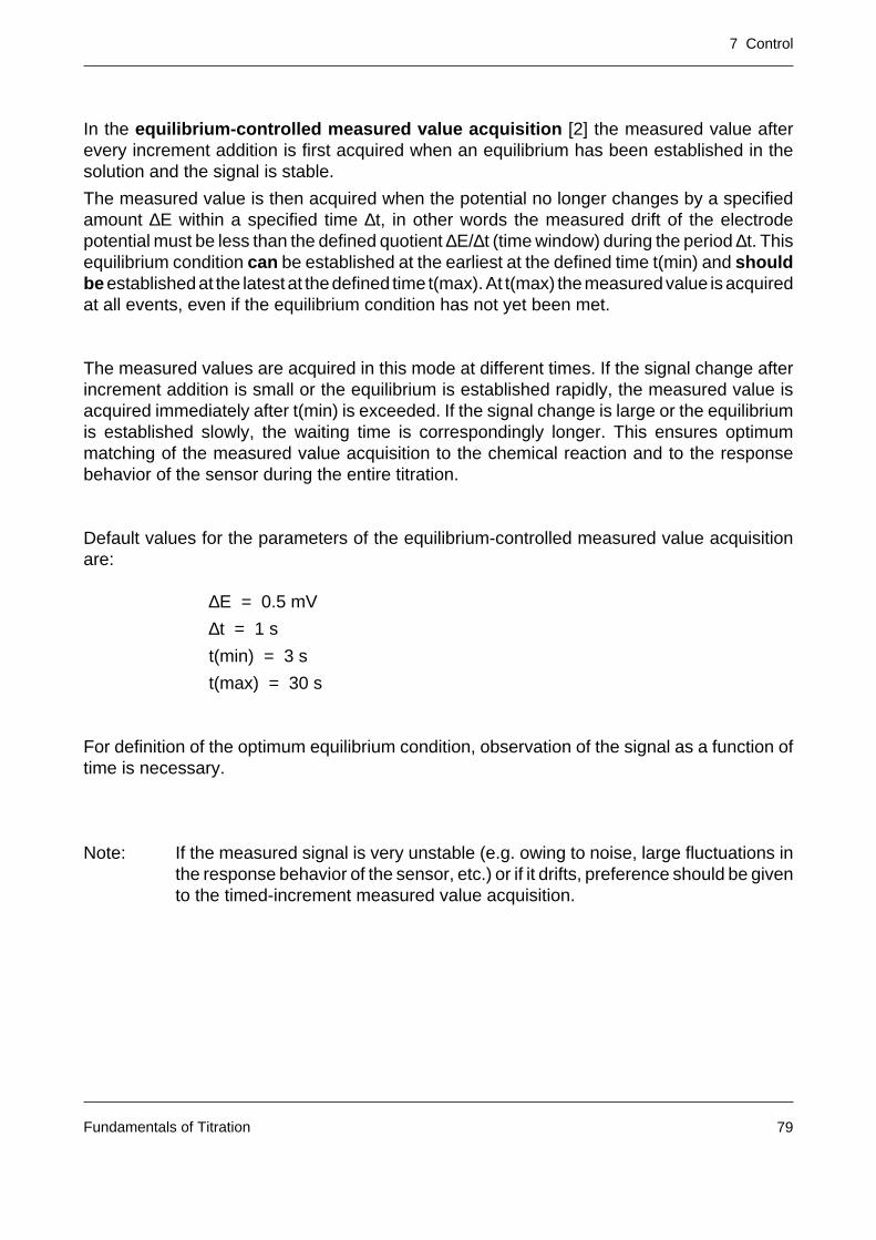
7 Control
Fundamentals of Titration 79
In the equilibrium-controlled measured value acquisition [2] the measured value afterevery increment addition is first acquired when an equilibrium has been established in thesolution and the signal is stable.
The measured value is then acquired when the potential no longer changes by a specifiedamount ∆E within a specified time ∆t, in other words the measured drift of the electrodepotential must be less than the defined quotient ∆E/∆t (time window) during the period ∆t. Thisequilibrium condition can be established at the earliest at the defined time t(min) and shouldbe established at the latest at the defined time t(max). At t(max) the measured value is acquiredat all events, even if the equilibrium condition has not yet been met.
The measured values are acquired in this mode at different times. If the signal change afterincrement addition is small or the equilibrium is established rapidly, the measured value isacquired immediately after t(min) is exceeded. If the signal change is large or the equilibriumis established slowly, the waiting time is correspondingly longer. This ensures optimummatching of the measured value acquisition to the chemical reaction and to the responsebehavior of the sensor during the entire titration.
Default values for the parameters of the equilibrium-controlled measured value acquisitionare:
∆E = 0.5 mV
∆t = 1 s
t(min) = 3 s
t(max) = 30 s
For definition of the optimum equilibrium condition, observation of the signal as a function oftime is necessary.
Note: If the measured signal is very unstable (e.g. owing to noise, large fluctuations inthe response behavior of the sensor, etc.) or if it drifts, preference should be givento the timed-increment measured value acquisition.
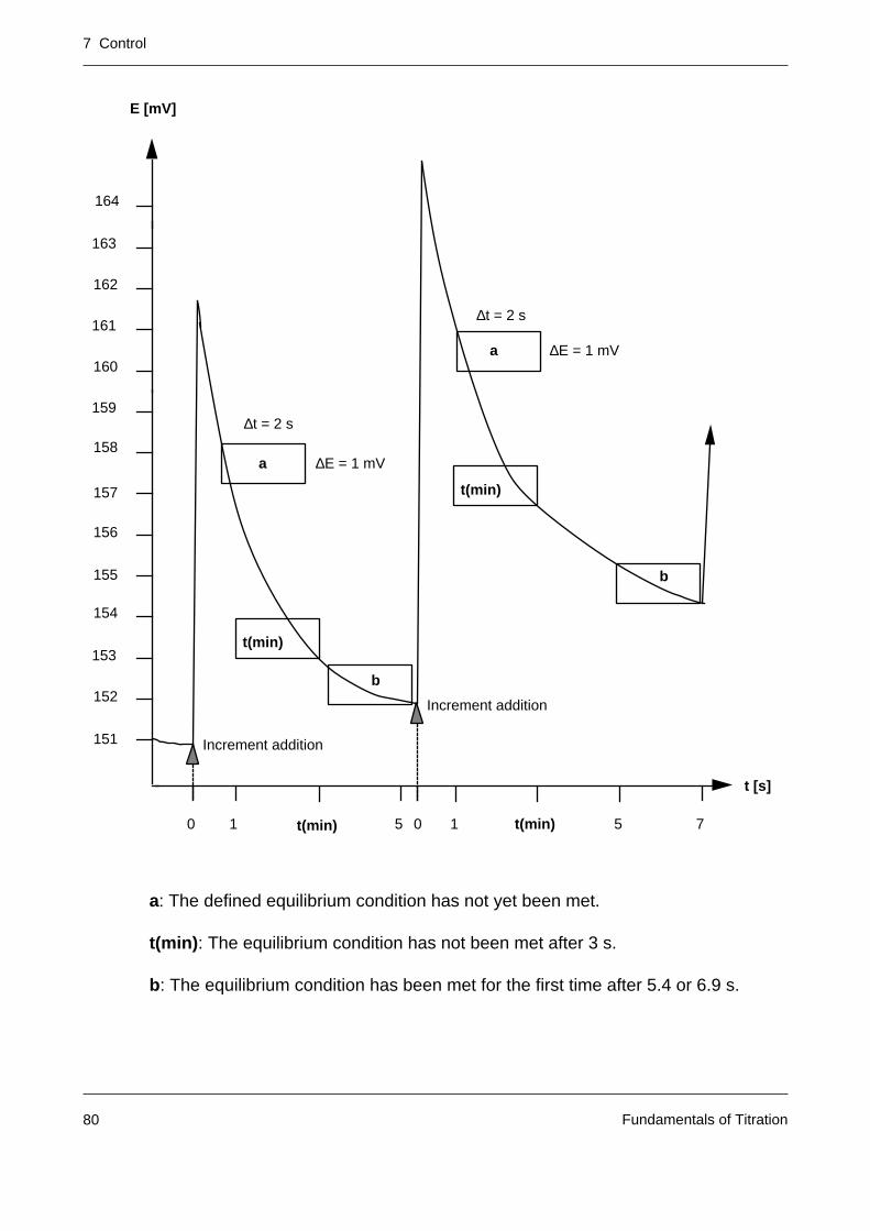
7 Control
Fundamentals of Titration80
a: The defined equilibrium condition has not yet been met.
t(min): The equilibrium condition has not been met after 3 s.
b: The equilibrium condition has been met for the first time after 5.4 or 6.9 s.
t [s]
1 5t(min)
E [mV]
0 1 t(min) 5
Increment addition
a
b
163
162
161
160
159
158
157
156
155
154
153
152
151
∆t = 2 s
∆E = 1 mV
Increment addition
a
b
∆t = 2 s
∆E = 1 mV
7
164
0
t(min)
t(min)
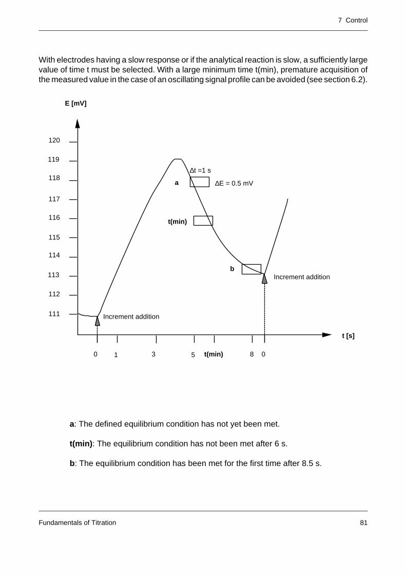
7 Control
Fundamentals of Titration 81
With electrodes having a slow response or if the analytical reaction is slow, a sufficiently largevalue of time t must be selected. With a large minimum time t(min), premature acquisition ofthe measured value in the case of an oscillating signal profile can be avoided (see section 6.2).
a: The defined equilibrium condition has not yet been met.
t(min): The equilibrium condition has not been met after 6 s.
b: The equilibrium condition has been met for the first time after 8.5 s.
t [s]
1 5
E [mV]
0 t(min) 8
120
119
118
117
116
115
114
113
112
111 Increment addition
03
a
b
t(min)
∆t =1 s
∆E = 0.5 mV
Increment addition
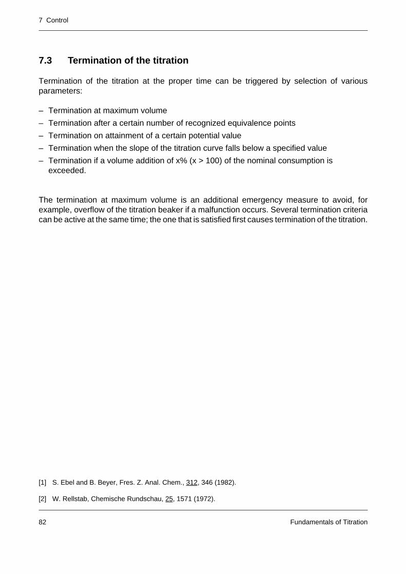
7 Control
Fundamentals of Titration82
7.3 Termination of the titration
Termination of the titration at the proper time can be triggered by selection of variousparameters:
– Termination at maximum volume
– Termination after a certain number of recognized equivalence points
– Termination on attainment of a certain potential value
– Termination when the slope of the titration curve falls below a specified value
– Termination if a volume addition of x% (x > 100) of the nominal consumption isexceeded.
The termination at maximum volume is an additional emergency measure to avoid, forexample, overflow of the titration beaker if a malfunction occurs. Several termination criteriacan be active at the same time; the one that is satisfied first causes termination of the titration.
[1] S. Ebel and B. Beyer, Fres. Z. Anal. Chem., 312, 346 (1982).
[2] W. Rellstab, Chemische Rundschau, 25, 1571 (1972).
8 Equivalence point determination
Fundamentals of Titration 83
8 The determination of the equivalence point
The end of a titration is reached when an amount of titrant equivalent to the substance beinganalyzed (the analyte) has been added. From the volume of the titrimetric solution required toreach this point – the equivalence point – and its known concentration, the amount of analytecan be calculated if the stoichiometry of the reaction is known. The correctness (precision andaccuracy, see Section 10) of the result depends to a large degree on the method chosen todetect the equivalence point. The methods for recognition and exact calculation of theequivalence point are treated in this section.
8.1 The position of the equivalence point
In the immediate vicinity of the equivalence point, those titration curves that can be evaluatedin practice exhibit a change in either the slope (so-called linear or segmented titration curves,e.g. titrations with amperometric, conductometric and photometric indication) or the directionof curvature (so-called logarithmic or S-shaped titration curves, e.g. titrations with potentiome-tric and voltametric indication). These break or inflection points are influenced by theequilibrium constants of the titration reaction, the initial concentrations, the change in volumedue to the amount of added titrant and other factors. Each form of a titration curve in theoryrequires a specific type of equivalence point determination if optimum accuracy of the analysisresult is to be achieved.
The end point of a potentiometric titration is often taken as the inflection point of the titrationcurve. The example of the titration of a strong acid with a strong base will be used here todemonstrate that determination of the inflection point provides a serviceable approximation ofthe equivalence point.
To represent the titration curve, the dependence of the H3O+ concentration or the pH value
on the amount of added titrant is needed. The following table shows the H3O+ concentration
or pH value and the extent of titration as a function of the amount of sodium hydroxideof concentration 0.1 mol/L added to a solution of 50 mL hydrochloric acid of concentration0.01 mol/L.
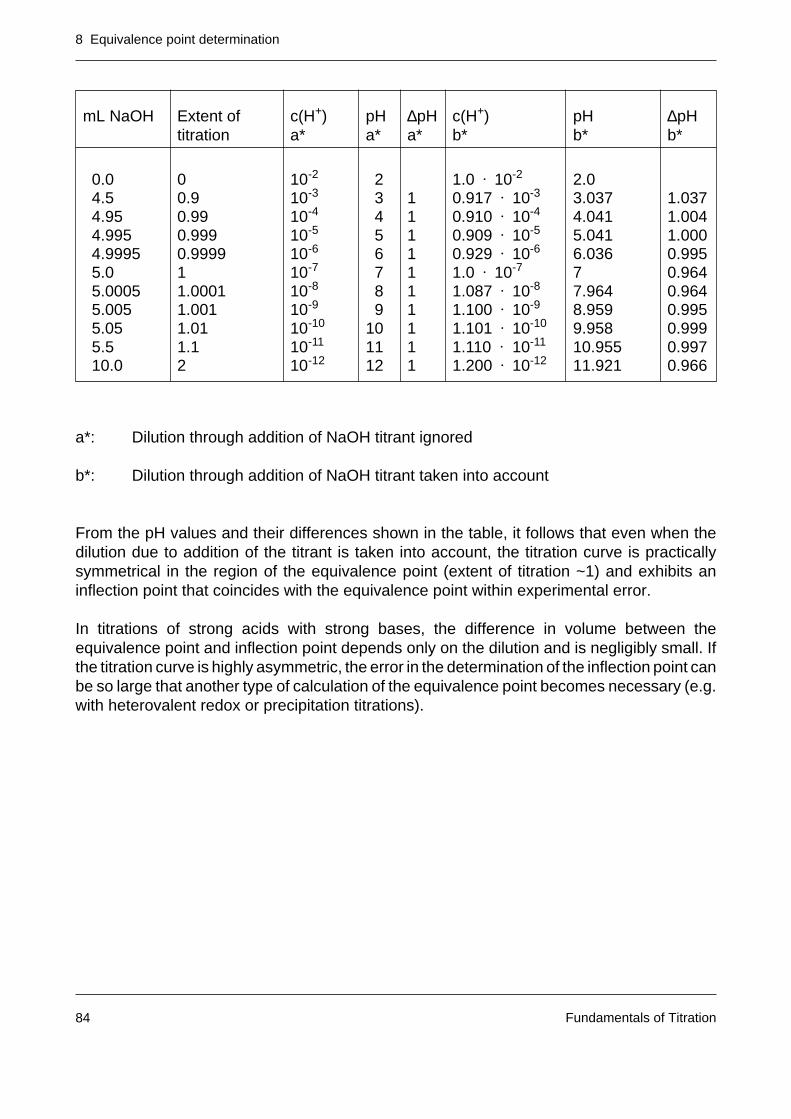
8 Equivalence point determination
Fundamentals of Titration84
mL NaOH Extent of c(H+) pH ∆pH c(H+) pH ∆pHtitration a* a* a* b* b* b*
0.0 0 10-2 2 1.0 • 10-2 2.0 4.5 0.9 10-3 3 1 0.917 • 10-3 3.037 1.037 4.95 0.99 10-4 4 1 0.910 • 10-4 4.041 1.004 4.995 0.999 10-5 5 1 0.909 • 10-5 5.041 1.000 4.9995 0.9999 10-6 6 1 0.929 • 10-6 6.036 0.995 5.0 1 10-7 7 1 1.0 • 10-7 7 0.964 5.0005 1.0001 10-8 8 1 1.087 • 10-8 7.964 0.964 5.005 1.001 10-9 9 1 1.100 • 10-9 8.959 0.995 5.05 1.01 10-10 10 1 1.101 • 10-10 9.958 0.999 5.5 1.1 10-11 11 1 1.110 • 10-11 10.955 0.997 10.0 2 10-12 12 1 1.200 • 10-12 11.921 0.966
a*: Dilution through addition of NaOH titrant ignored
b*: Dilution through addition of NaOH titrant taken into account
From the pH values and their differences shown in the table, it follows that even when thedilution due to addition of the titrant is taken into account, the titration curve is practicallysymmetrical in the region of the equivalence point (extent of titration ~1) and exhibits aninflection point that coincides with the equivalence point within experimental error.
In titrations of strong acids with strong bases, the difference in volume between theequivalence point and inflection point depends only on the dilution and is negligibly small. Ifthe titration curve is highly asymmetric, the error in the determination of the inflection point canbe so large that another type of calculation of the equivalence point becomes necessary (e.g.with heterovalent redox or precipitation titrations).
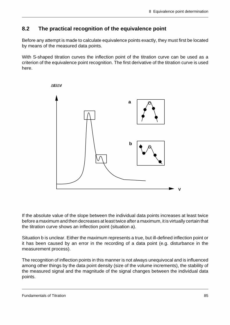
8 Equivalence point determination
Fundamentals of Titration 85
8.2 The practical recognition of the equivalence point
Before any attempt is made to calculate equivalence points exactly, they must first be locatedby means of the measured data points.
With S-shaped titration curves the inflection point of the titration curve can be used as acriterion of the equivalence point recognition. The first derivative of the titration curve is usedhere.
If the absolute value of the slope between the individual data points increases at least twicebefore a maximum and then decreases at least twice after a maximum, it is virtually certain thatthe titration curve shows an inflection point (situation a).
Situation b is unclear. Either the maximum represents a true, but ill-defined inflection point orit has been caused by an error in the recording of a data point (e.g. disturbance in themeasurement process).
The recognition of inflection points in this manner is not always unequivocal and is influencedamong other things by the data point density (size of the volume increments), the stability ofthe measured signal and the magnitude of the signal changes between the individual datapoints.
∆E/∆V
V
a
b
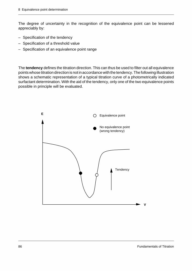
8 Equivalence point determination
Fundamentals of Titration86
The degree of uncertainty in the recognition of the equivalence point can be lessenedappreciably by:
– Specification of the tendency
– Specification of a threshold value
– Specification of an equivalence point range
The tendency defines the titration direction. This can thus be used to filter out all equivalencepoints whose titration direction is not in accordance with the tendency. The following illustrationshows a schematic representation of a typical titration curve of a photometrically indicatedsurfactant determination. With the aid of the tendency, only one of the two equivalence pointspossible in principle will be evaluated.
E
V
Equivalence point
No equivalence point(wrong tendency)
Tendency
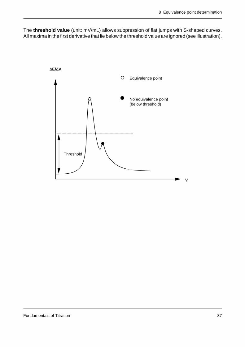
8 Equivalence point determination
Fundamentals of Titration 87
The threshold value (unit: mV/mL) allows suppression of flat jumps with S-shaped curves.All maxima in the first derivative that lie below the threshold value are ignored (see illustration).
∆E/∆V
V
Equivalence point
No equivalence point(below threshold)
Threshold
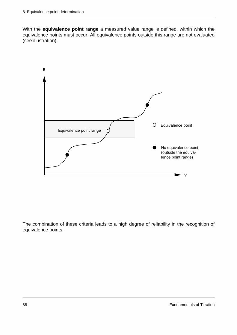
8 Equivalence point determination
Fundamentals of Titration88
With the equivalence point range a measured value range is defined, within which theequivalence points must occur. All equivalence points outside this range are not evaluated(see illustration).
The combination of these criteria leads to a high degree of reliability in the recognition ofequivalence points.
V
E
Equivalence point
No equivalence point(outside the equiva-lence point range)
quivalenzpunktbereichEquivalence point range
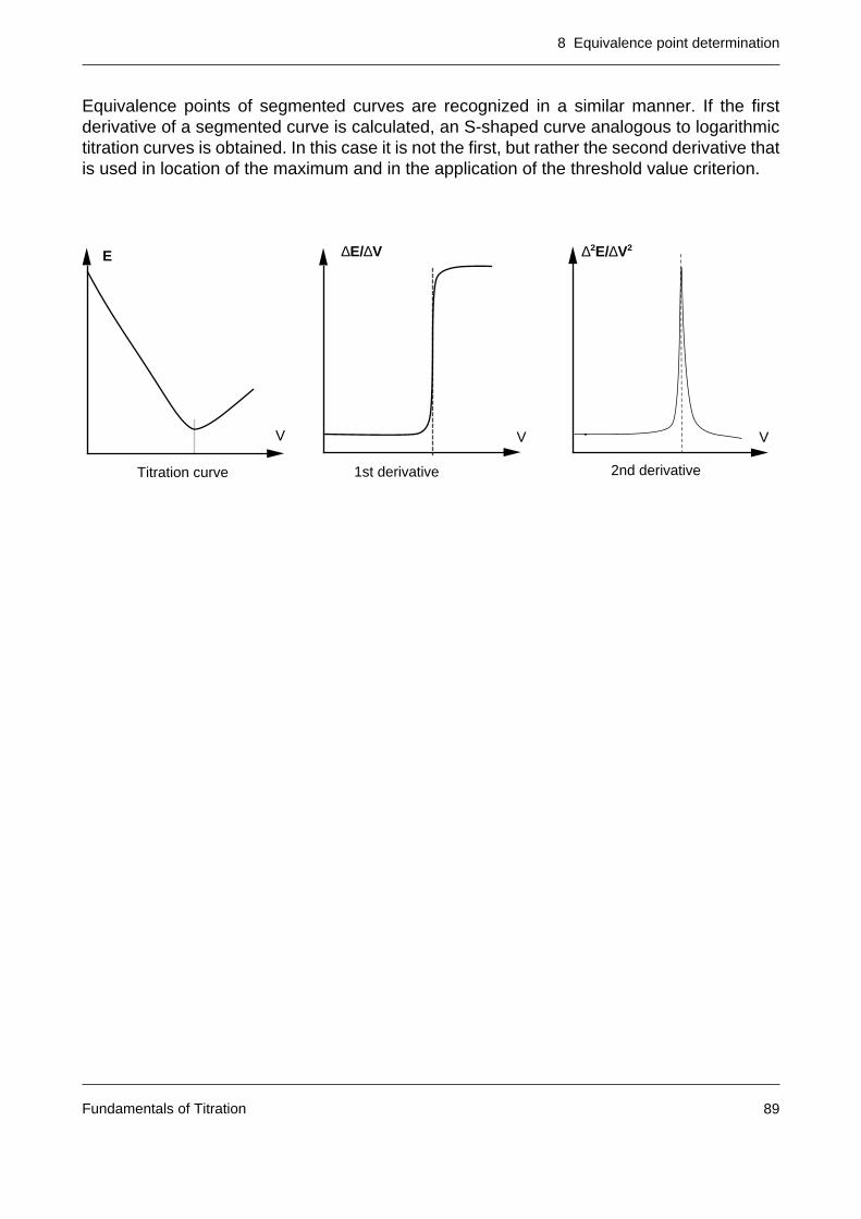
8 Equivalence point determination
Fundamentals of Titration 89
Equivalence points of segmented curves are recognized in a similar manner. If the firstderivative of a segmented curve is calculated, an S-shaped curve analogous to logarithmictitration curves is obtained. In this case it is not the first, but rather the second derivative thatis used in location of the maximum and in the application of the threshold value criterion.
E
V
Titration curve
∆E/∆V
V
1st derivative
∆2E/∆V2
V
2nd derivative
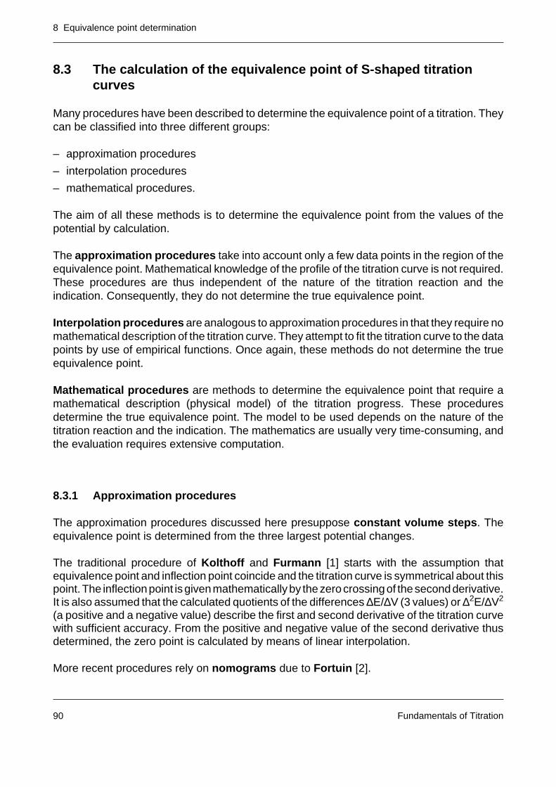
8 Equivalence point determination
Fundamentals of Titration90
8.3 The calculation of the equivalence point of S-shaped titrationcurves
Many procedures have been described to determine the equivalence point of a titration. Theycan be classified into three different groups:
– approximation procedures
– interpolation procedures
– mathematical procedures.
The aim of all these methods is to determine the equivalence point from the values of thepotential by calculation.
The approximation procedures take into account only a few data points in the region of theequivalence point. Mathematical knowledge of the profile of the titration curve is not required.These procedures are thus independent of the nature of the titration reaction and theindication. Consequently, they do not determine the true equivalence point.
Interpolation procedures are analogous to approximation procedures in that they require nomathematical description of the titration curve. They attempt to fit the titration curve to the datapoints by use of empirical functions. Once again, these methods do not determine the trueequivalence point.
Mathematical procedures are methods to determine the equivalence point that require amathematical description (physical model) of the titration progress. These proceduresdetermine the true equivalence point. The model to be used depends on the nature of thetitration reaction and the indication. The mathematics are usually very time-consuming, andthe evaluation requires extensive computation.
8.3.1 Approximation procedures
The approximation procedures discussed here presuppose constant volume steps. Theequivalence point is determined from the three largest potential changes.
The traditional procedure of Kolthoff and Furmann [1] starts with the assumption thatequivalence point and inflection point coincide and the titration curve is symmetrical about thispoint. The inflection point is given mathematically by the zero crossing of the second derivative.It is also assumed that the calculated quotients of the differences ∆E/∆V (3 values) or ∆2E/∆V2
(a positive and a negative value) describe the first and second derivative of the titration curvewith sufficient accuracy. From the positive and negative value of the second derivative thusdetermined, the zero point is calculated by means of linear interpolation.
More recent procedures rely on nomograms due to Fortuin [2].
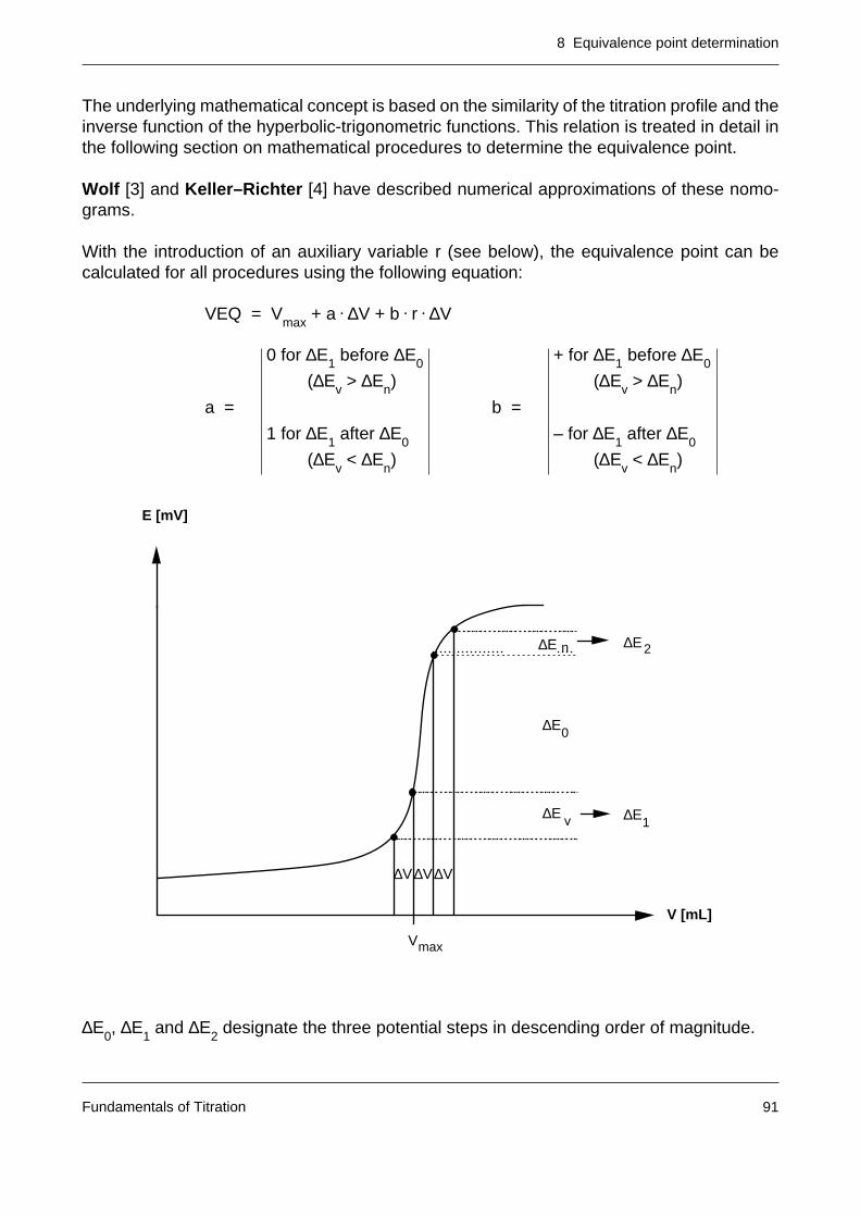
8 Equivalence point determination
Fundamentals of Titration 91
The underlying mathematical concept is based on the similarity of the titration profile and theinverse function of the hyperbolic-trigonometric functions. This relation is treated in detail inthe following section on mathematical procedures to determine the equivalence point.
Wolf [3] and Keller–Richter [4] have described numerical approximations of these nomo-grams.
With the introduction of an auxiliary variable r (see below), the equivalence point can becalculated for all procedures using the following equation:
VEQ = Vmax
+ a • ∆V + b • r • ∆V
0 for ∆E1 before ∆E0 + for ∆E1 before ∆E0
(∆Ev > ∆En) (∆Ev > ∆En)
a = b =
1 for ∆E1 after ∆E
0– for ∆E
1 after ∆E
0
(∆Ev < ∆E
n) (∆E
v < ∆E
n)
∆E0, ∆E
1 and ∆E
2 designate the three potential steps in descending order of magnitude.
∆V∆V
E [mV]
V [mL]
∆V
∆E ∆E
∆E
∆E∆E
0
v
n
1
2
Vmax
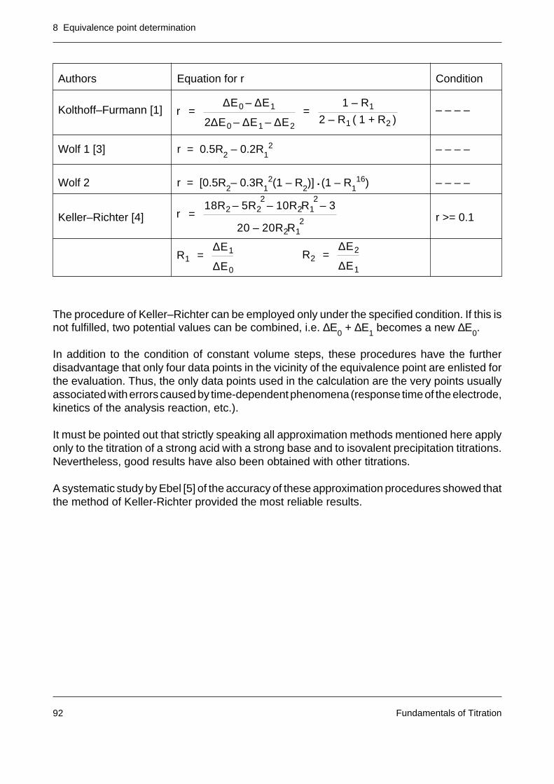
8 Equivalence point determination
Fundamentals of Titration92
r =∆E0 – ∆E1
2∆E0 – ∆E1 – ∆E2
=1 – R1
2 – R1 ( 1 + R2 )
r =18R2 – 5R2
2– 10R2R1
2– 3
20 – 20R2R12
R1 =∆E1
∆E0
R2 =∆E2
∆E1
Authors Equation for r Condition
Kolthoff–Furmann [1] – – – –
Wolf 1 [3] r = 0.5R2 – 0.2R
12 – – – –
Wolf 2 r = [0.5R2– 0.3R
12(1 – R
2)] • (1 – R
116) – – – –
Keller–Richter [4] r >= 0.1
The procedure of Keller–Richter can be employed only under the specified condition. If this isnot fulfilled, two potential values can be combined, i.e. ∆E
0 + ∆E
1 becomes a new ∆E
0.
In addition to the condition of constant volume steps, these procedures have the furtherdisadvantage that only four data points in the vicinity of the equivalence point are enlisted forthe evaluation. Thus, the only data points used in the calculation are the very points usuallyassociated with errors caused by time-dependent phenomena (response time of the electrode,kinetics of the analysis reaction, etc.).
It must be pointed out that strictly speaking all approximation methods mentioned here applyonly to the titration of a strong acid with a strong base and to isovalent precipitation titrations.Nevertheless, good results have also been obtained with other titrations.
A systematic study by Ebel [5] of the accuracy of these approximation procedures showed thatthe method of Keller-Richter provided the most reliable results.
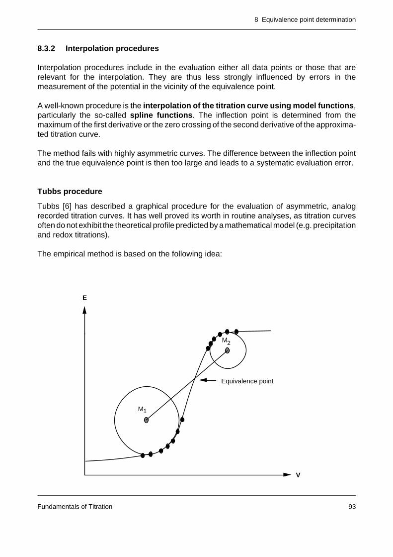
8 Equivalence point determination
Fundamentals of Titration 93
8.3.2 Interpolation procedures
Interpolation procedures include in the evaluation either all data points or those that arerelevant for the interpolation. They are thus less strongly influenced by errors in themeasurement of the potential in the vicinity of the equivalence point.
A well-known procedure is the interpolation of the titration curve using model functions,particularly the so-called spline functions. The inflection point is determined from themaximum of the first derivative or the zero crossing of the second derivative of the approxima-ted titration curve.
The method fails with highly asymmetric curves. The difference between the inflection pointand the true equivalence point is then too large and leads to a systematic evaluation error.
Tubbs procedure
Tubbs [6] has described a graphical procedure for the evaluation of asymmetric, analogrecorded titration curves. It has well proved its worth in routine analyses, as titration curvesoften do not exhibit the theoretical profile predicted by a mathematical model (e.g. precipitationand redox titrations).
The empirical method is based on the following idea:
E
V
M
M
1
2
Equivalence point
8 Equivalence point determination
Fundamentals of Titration94
A circle of curvature of minimum radius can be drawn in both branches of the titration curve.The ratio of the two radii is determined by the asymmetry of the curve. The intersection pointof the straight line drawn between the midpoints M1 and M2 of the circles with the titration curverepresents the equivalence point. Theoretical calculations show that the true equivalencepoint with asymmetric titration curves always lies between the inflection point and that branchof the titration curve with the greater curvature (the smaller circle of curvature). The result ofthe Tubbs evaluation approximates this true equivalence point very closely when the titrationcurve profile is regular and allows calculation of the circles of curvature of the two branches.
A mathematical variation of the Tubbs procedure for digitally recorded titration curve has beendescribed by Ebel [7].This involves approximation of those parts of the titration curve that lie in the region of thegreatest curvature by a hyperbola. For each approximated hyperbola the vertex is determined.This point on the hyperbola lies at the position of greatest curvature. The midpoints of theassigned smallest circles of curvature are the foci of the two hyperbolae. As in the graphicalversion, the intersection point of the straight line joining the two foci with the titration curve givesthe equivalence point.
The evaluation requires at least six measured points in the region of greatest curvature, bothbefore and after the inflection point of the titration curve (see illustration).
8.3.3 Mathematical procedures
The mathematical procedures can be divided into two groups:
– direct evaluation of the experimental data E vs V by means of iterative methods or nonlinearregression analysis
– indirect evaluation of the experimental data E vs V through mathematical linearization of thetitration curve.
8 Equivalence point determination
Fundamentals of Titration 95
Nonlinear regression analysis [8]
The aim of these procedures is to determine the parameters P1, P
2, P
3, ... etc. using a
mathematical model function
Y = f(X; P1,P2,P3,...)
with the aid of N experimental data pairs (xi, y
i) so that the sum of the squares of the errors
is minimized (method of least squares).The parameters P
1, P
2, P
3,... are determined using a time-consuming iterative procedure. One
of the most powerful nonlinear regression calculation methods is that due to Marquardt [9]. Foran efficient calculation it requires the partial derivatives ∂y/∂P
i of the model function over all
parameters. The number of data pairs used must be greater than the number of parametersto be determined by nonlinear regression.
The time required for the mathematics and computation is enormous. Optimization of functionswith more than four or five parameters exceeds the limits of possibilities of the titrators on themarket today.
Mathematical linearization of the titration curves
The idea behind this procedure is based on the mathematical transformation of a modelfunction of the titration curve
E = f(V)
such that there is a linear relationship between the new variables X and Y:
E = f(V) : E —> Y
V —> X : —> Y = A • X + B
Depending on the model, the equivalence point can then be calculated from one of thefollowing quantities:
– Slope A
– Intercept B (Y axis)
– Intercept -B/A (X axis)
This procedure was first used by Gran [10] to evaluate acid-base titrations.
S =N
∑i=1
(y i– f(x i ; P1 ,P2 , P3 ,…))2
8 Equivalence point determination
Fundamentals of Titration96
Example: Titration of a strong acid (e.g. HCl) with a strong base (e.g. NaOH)
In aqueous solution HCl and NaOH are completely dissociated throughout the titration:
HCl + H2O —> H
3O+ + Cl-
NaOH —> Na+ + OH-
The following titration reaction occurs:
2H2O —> H
3O+ + OH-
The corresponding law of mass action (ionic product of water) is given by
The charge balance is as follows:
During the titration, the mass balances of the ions that do not participate in the titration reactionare:
where
CONC: the concentration of the titrant NaOH [mol/L]
V0: the initial volume of the titration [mL]
V: the volume of titrant added [mL]
VEQ: the titrant consumption up to the equivalence point [mL]
Insertion of the mass balances in the charge balance equation and solving for [H+] ([H+] =[H3O+]) gives a quadratic equation
Na+
=CONC • V
V0 + VCI
-=
CONC • VEQV0 + V
H+ 2
– H+
•CONC • ( VEQ – V )
V0 + V– Kw = 0
H3O+
OH-
= Kw
H3O+
+ Na+
= CI-
+ OH-
8 Equivalence point determination
Fundamentals of Titration 97
With the aid of the Nernst equation
the equation of the titration curve is obtained:
This equation has five parameters: the electrode parameters E0 and S, the consumption of thetitrant VEQ up to the equivalence point , the initial volume V0 to take into account the dilutionand the ionic product of water Kw.
This equation for the titration curve profile can also be described with the aid of the inversefunction of the hyperbolic-trigonometric function:
Division of
by gives the following [2]:
This equation can also be expressed in a different manner:
E = E0 + S • pH = E0 – S • log H+
E = E0 – S • log
CONC • ( VEQ – V )V0 + V
+CONC • ( VEQ – V )
V0 + V
2
+ 4Kw
2
OH-
– H+
= NA+
– CI-
=CONC • ( V – VEQ )
V0 + V
Kw
H+
–H
+
Kw=
CONC • ( V – VEQ )Kw • ( V0 + V )
Kw
H+
–H
+
Kw= exp In
Kw
H+
– exp – InKw
H+
= 2 sinhpH – pKw / 2
log e
Kw
8 Equivalence point determination
Fundamentals of Titration98
From this, the change in pH follows
or the Nernst equation
where α = E0 + pK
w/2
and β = S • (log e).
This equation is the basic equation of the nomograms of Fortuin [2].
If only a few data points are considered in the region of the equivalence point (V ~ VEQ), thedenominator in the sinh-1 function can be combined in a single parameter g:
where
The equation for the titration curve is thus reduced to four parameters α, β, γ and VEQ.
The equation with the four unknowns can be solved exactly with four data pairs (Ei, V
i; i=1,...4).
From the four measured values, the parameter α can be eliminated through formation of threedifferences ∆Eij and the parameter β through formation of two differential quotients ∆Eij/∆Ekl.The resulting system of equations with the two unknowns γ and VEQ cannot be solved for VEQ[2]. The value of VEQ must therefore be determined iteratively using the procedure of Newton.The restriction to constant volume steps found in the procedure of Keller–Richter does not existin this method. It can thus also be used for titrations with dynamic titrant addition.
A wrong measurement point due to a disturbing influence on the measured value acquisitionhas a very great effect on the result of this procedure. It is even possible that the iteration canfail and no result is found.
E = α + β • sinh-1 CONC • ( V – VEQ )
2 Kw • ( V0 + V )
pH =pKw
2+ ( log e ) sinh
-1 CONC • ( V – VEQ )
2 Kw• ( V0 + V )
E = α + β • sinh-1 CONC • ( V – VEQ )
γ
γ = 2 Kw • (V0 + VEQ)
8 Equivalence point determination
Fundamentals of Titration 99
The effect of this error source on the evaluation is less if the procedure of nonlinear regressiondescribed above is used. Owing to the smoothing properties of the regression calculation, asingle erroneous measurement point is of less consequence than if an attempt is made to solvethe system of equations exactly.
The DL70 uses this method as a standard procedure for the evaluation of S-shaped titrationcurves. The equivalence point is determined using the Marquardt procedure [9] and the modelof the titration of a strong acid with a strong base just described.
The principle of the mathematical linearization of the titration curve can also be demonstratedusing this example.
Starting from the charge balance equation
and solving for G = VEQ - V - instead of for [H+] - gives [10]:
Representation of G as a function of V gives the desired linear relation.
Before the equivalence point (V < VEQ)
holds.
After the equivalence point (V > VEQ)
is valid.
G = VEQ – V =V0 + VCONC
H+
–Kw
H+
OH-
– H+
= Na+
– CI-
=CONC • ( V – VEQ )
V0 + V
G2 = V – VEQ =V0 + VCONC
•Kw
H+
G1 = VEQ – V =V0 + VCONC
• H+
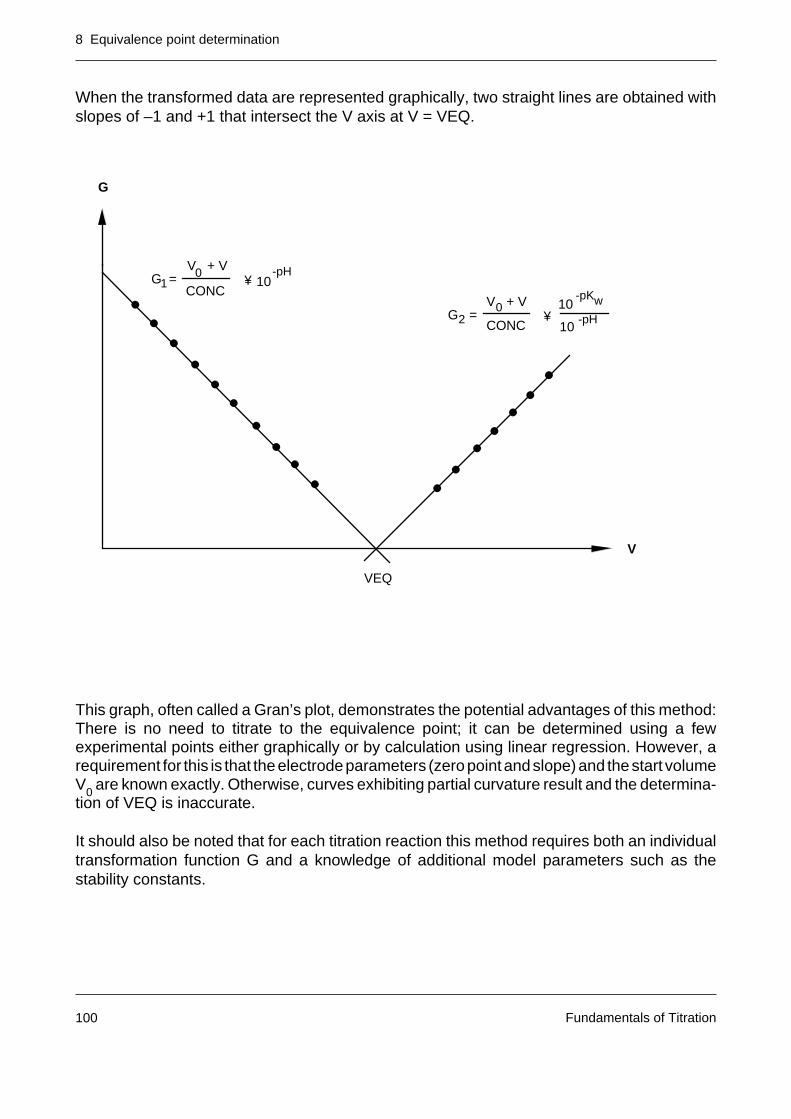
8 Equivalence point determination
Fundamentals of Titration100
When the transformed data are represented graphically, two straight lines are obtained withslopes of –1 and +1 that intersect the V axis at V = VEQ.
This graph, often called a Gran’s plot, demonstrates the potential advantages of this method:There is no need to titrate to the equivalence point; it can be determined using a fewexperimental points either graphically or by calculation using linear regression. However, arequirement for this is that the electrode parameters (zero point and slope) and the start volumeV0 are known exactly. Otherwise, curves exhibiting partial curvature result and the determina-tion of VEQ is inaccurate.
It should also be noted that for each titration reaction this method requires both an individualtransformation function G and a knowledge of additional model parameters such as thestability constants.
G
V
VEQ
G =
G =
1
2
V + V
CONC10
0
-pH
-pKw
10
10-pH
¥
V + V
CONC0
¥
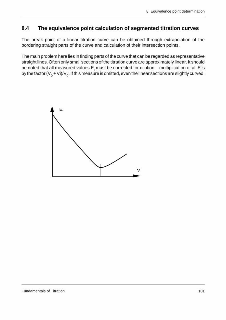
8 Equivalence point determination
Fundamentals of Titration 101
8.4 The equivalence point calculation of segmented titration curves
The break point of a linear titration curve can be obtained through extrapolation of thebordering straight parts of the curve and calculation of their intersection points.
The main problem here lies in finding parts of the curve that can be regarded as representativestraight lines. Often only small sections of the titration curve are approximately linear. It shouldbe noted that all measured values Ei must be corrected for dilution – multiplication of all Ei’sby the factor (V0 + Vi)/V0. If this measure is omitted, even the linear sections are slightly curved.
E
V
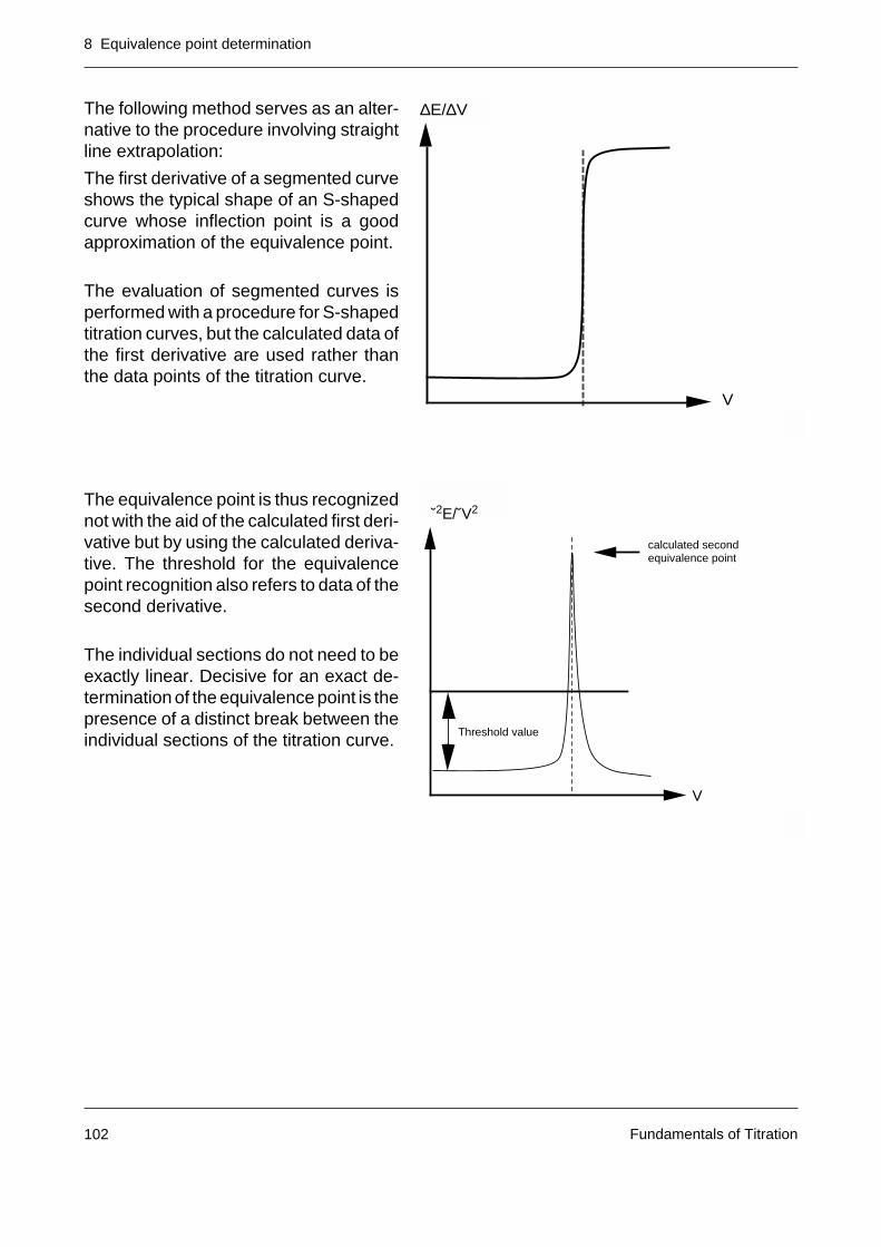
8 Equivalence point determination
Fundamentals of Titration102
The following method serves as an alter-native to the procedure involving straightline extrapolation:
The first derivative of a segmented curveshows the typical shape of an S-shapedcurve whose inflection point is a goodapproximation of the equivalence point.
The evaluation of segmented curves isperformed with a procedure for S-shapedtitration curves, but the calculated data ofthe first derivative are used rather thanthe data points of the titration curve.
The equivalence point is thus recognizednot with the aid of the calculated first deri-vative but by using the calculated deriva-tive. The threshold for the equivalencepoint recognition also refers to data of thesecond derivative.
The individual sections do not need to beexactly linear. Decisive for an exact de-termination of the equivalence point is thepresence of a distinct break between theindividual sections of the titration curve.
∆E/∆V
V
˘2E/˘V2
V
calculated second equivalence point
Threshold value
8 Equivalence point determination
Fundamentals of Titration 103
8.5 The half neutralization value
The acidity constant Ka (see Section 3.1.4) or the pKa value is a measure of the strength ofan acid in the particular solvent. The pKa value is not only an important quantity in theclassification of an acid, but also determines the properties of the substance in nature or itspossible use as a drug.
The determination of exact values of the pKa by means of titration is a demanding task. Thecorrect procedure requires not only an exact knowledge of the electrode parameters, but alsothe use of activities rather than concentrations.
From the law of mass action of the reaction of an acid HA with H2O (see Section 3.1.4)
it follows that
When the acid HA is half neutralized, i.e. V = VEQ/2, the concentration [HA] of the stillundissociated acid is approximately equal to the concentration [A-] of the base.Hence
pH = pKa
This pH value at half consumption to the equivalence point is called the half neutralizationvalue. It can easily be shown that this half neutralization value is a good estimation of the pK
avalue of weak acids.
The acidity constant Ka can be calculated at any point during the titration with a strong base
if all parameters are known [11]:
where
Ka =H
+• A
-
HA
pH = pKa + logA
-
HA
d = H+
– OH-
cT =CONC • V
V0 + VcA =
CONC • VEQV0 + V
Ka = H+
•cT + d
cA – cT – d
8 Equivalence point determination
Fundamentals of Titration104
The quantity cT is the concentration of the added titrant and c
A the concentration of acid in the
titration vessel during the titration. At the half neutralization value (V = VEQ/2)
cT = c
HNV = 0.5 • c
A
and hence
or
If the condition d << cHNV
is fulfilled, the half neutralization value pHHNV
is equal to the pKa.
pHHNV = pKa + logcHNV+ dcHNV– d
Ka = H+
•cHNV– dcHNV+ d
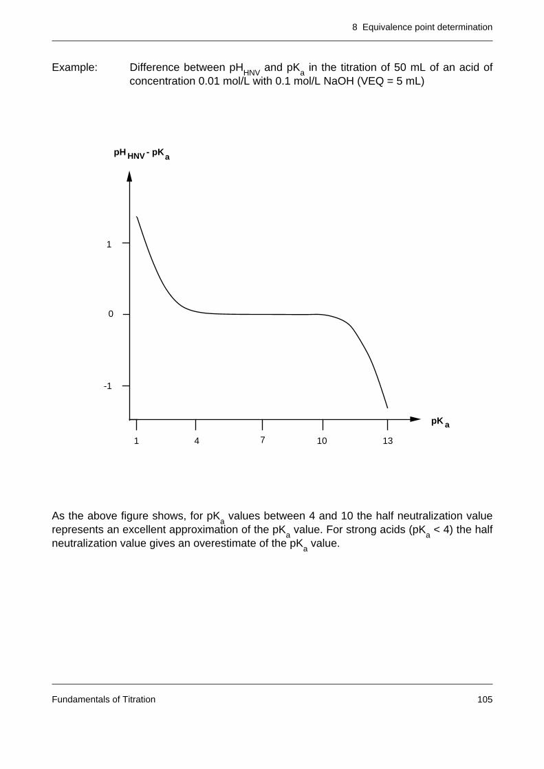
8 Equivalence point determination
Fundamentals of Titration 105
Example: Difference between pHHNV and pKa in the titration of 50 mL of an acid ofconcentration 0.01 mol/L with 0.1 mol/L NaOH (VEQ = 5 mL)
As the above figure shows, for pKa values between 4 and 10 the half neutralization value
represents an excellent approximation of the pKa value. For strong acids (pK
a < 4) the half
neutralization value gives an overestimate of the pKa value.
-1
0
1
pK
pH - pK
1 7 13
HNV a
a
4 10
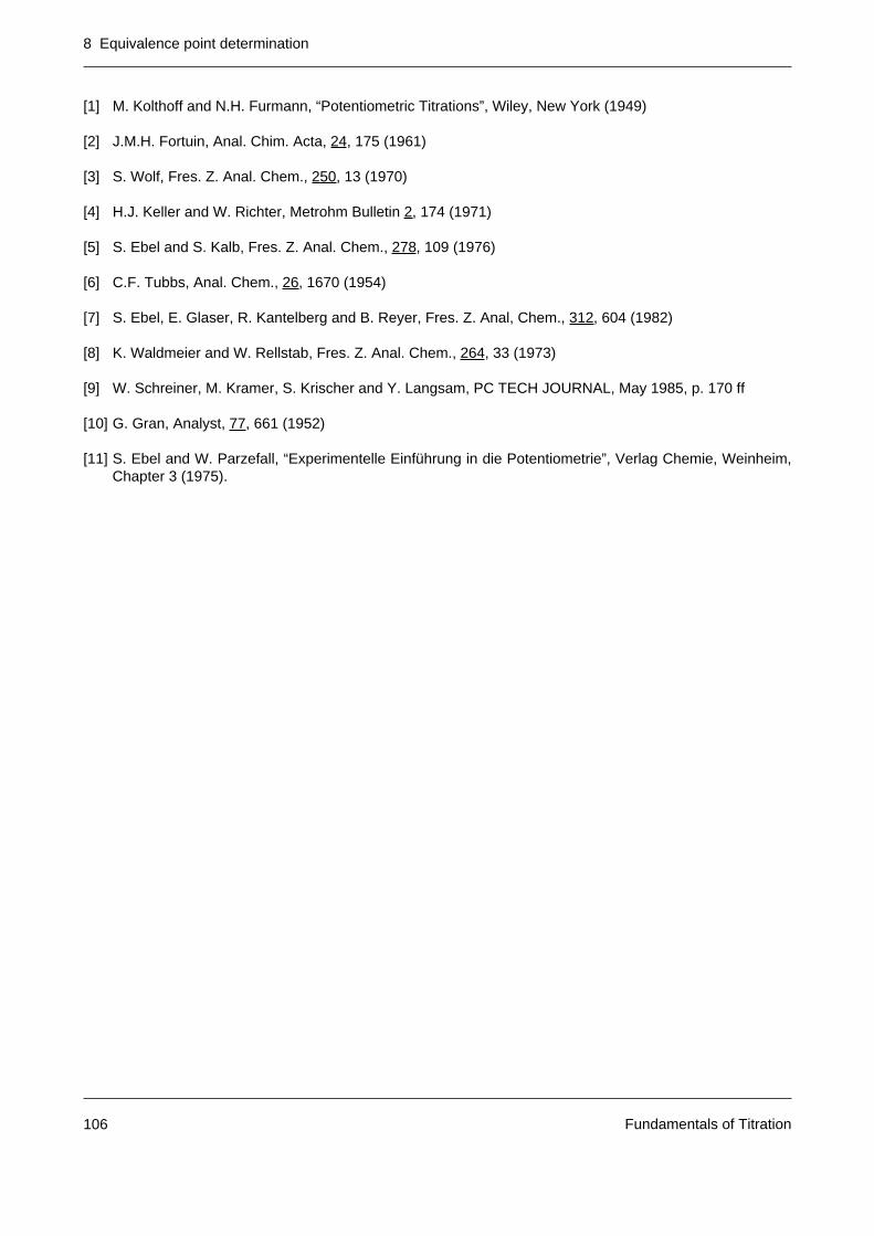
8 Equivalence point determination
Fundamentals of Titration106
[1] M. Kolthoff and N.H. Furmann, “Potentiometric Titrations”, Wiley, New York (1949)
[2] J.M.H. Fortuin, Anal. Chim. Acta, 24, 175 (1961)
[3] S. Wolf, Fres. Z. Anal. Chem., 250, 13 (1970)
[4] H.J. Keller and W. Richter, Metrohm Bulletin 2, 174 (1971)
[5] S. Ebel and S. Kalb, Fres. Z. Anal. Chem., 278, 109 (1976)
[6] C.F. Tubbs, Anal. Chem., 26, 1670 (1954)
[7] S. Ebel, E. Glaser, R. Kantelberg and B. Reyer, Fres. Z. Anal, Chem., 312, 604 (1982)
[8] K. Waldmeier and W. Rellstab, Fres. Z. Anal. Chem., 264, 33 (1973)
[9] W. Schreiner, M. Kramer, S. Krischer and Y. Langsam, PC TECH JOURNAL, May 1985, p. 170 ff
[10] G. Gran, Analyst, 77, 661 (1952)
[11] S. Ebel and W. Parzefall, “Experimentelle Einführung in die Potentiometrie”, Verlag Chemie, Weinheim,Chapter 3 (1975).
9 Direct measurement, calibration
Fundamentals of Titration 107
9 Direct measurement, calibration
Besides titration, direct measurement of the concentration with a suitable sensor is the mostfrequently used method of determination in wet chemical analysis. This is especially true in thecase of water analysis where not only measurement of the pH and the redox potential, but alsothe concentration determination with ion selective electrodes and the determination of theconductivity, turbidity and oxygen content are important.
This section discusses the pH measurement, measurement of the redox potential, directmeasurement with ion selective electrodes and measurement of the conductivity. Particularattention is paid to the special aspects of sensor calibration.
9.1 pH measurement
The pH is defined as the negative logarithm of the hydrogen ion activity (see Section 3.1.3).The range of the pH value is given by the autoprotolysis of water and lies between pH 0 andpH 14. The ionic product
Kw = a
H+ • a
OH-
and hence also the neutral point ([H+] = [OH-]) depend greatly on the temperature.
Temperature [°C] Kw [mol2/L2] Neutral point [pH]
0 0.11 • 10-14 7.47
25 1.0 • 10-14 7.00
50 5.5 • 10-14 6.63
100 54.0 • 10-14 6.13
For thermodynamic reasons it is not possible to calculate or measure the pH exactly. Variousapproximation methods and conventions have thus been suggested [1]. The standardacceptable today for the pH scale comprises different buffer solutions whose pH has beenfixed by convention. The pH values of these so-called NIST (NBS) buffer solutions have alsobeen accepted by DIN [2].
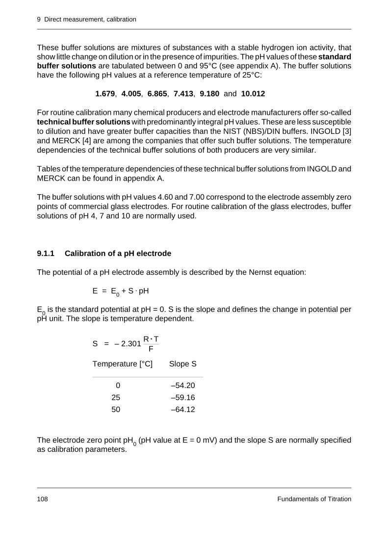
9 Direct measurement, calibration
Fundamentals of Titration108
S = – 2.301R • T
F
These buffer solutions are mixtures of substances with a stable hydrogen ion activity, thatshow little change on dilution or in the presence of impurities. The pH values of these standardbuffer solutions are tabulated between 0 and 95°C (see appendix A). The buffer solutionshave the following pH values at a reference temperature of 25°C:
1.679, 4.005, 6.865, 7.413, 9.180 and 10.012
For routine calibration many chemical producers and electrode manufacturers offer so-calledtechnical buffer solutions with predominantly integral pH values. These are less susceptibleto dilution and have greater buffer capacities than the NIST (NBS)/DIN buffers. INGOLD [3]and MERCK [4] are among the companies that offer such buffer solutions. The temperaturedependencies of the technical buffer solutions of both producers are very similar.
Tables of the temperature dependencies of these technical buffer solutions from INGOLD andMERCK can be found in appendix A.
The buffer solutions with pH values 4.60 and 7.00 correspond to the electrode assembly zeropoints of commercial glass electrodes. For routine calibration of the glass electrodes, buffersolutions of pH 4, 7 and 10 are normally used.
9.1.1 Calibration of a pH electrode
The potential of a pH electrode assembly is described by the Nernst equation:
E = E0 + S • pH
E0 is the standard potential at pH = 0. S is the slope and defines the change in potential per
pH unit. The slope is temperature dependent.
Temperature [°C] Slope S
0 –54.20
25 –59.16
50 –64.12
The electrode zero point pH0 (pH value at E = 0 mV) and the slope S are normally specified
as calibration parameters.
9 Direct measurement, calibration
Fundamentals of Titration 109
The combination glass electrodes used in routine analysis have an electrode zero point at pH7. New electrodes should have a slope greater than 97% of the theoretical slope predicted bythe Nernst equation.
Both calibration parameters vary slightly from electrode to electrode. For accurate pHmeasurements a calibration is thus necessary. The calibration can be performed as a single-or multipoint measurement.
E
pH
7 14
0
+mV
-mV
pH0
E 0
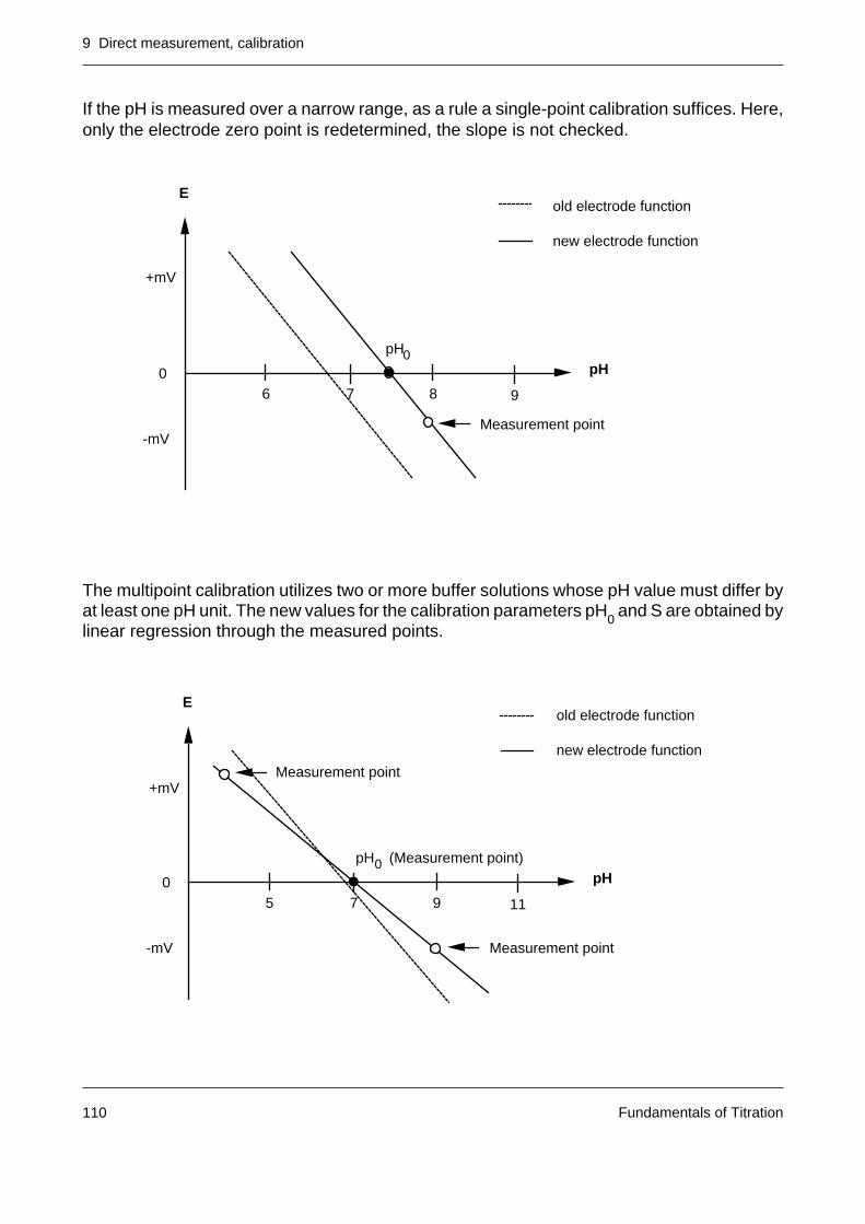
9 Direct measurement, calibration
Fundamentals of Titration110
If the pH is measured over a narrow range, as a rule a single-point calibration suffices. Here,only the electrode zero point is redetermined, the slope is not checked.
The multipoint calibration utilizes two or more buffer solutions whose pH value must differ byat least one pH unit. The new values for the calibration parameters pH
0 and S are obtained by
linear regression through the measured points.
E
pH0
+mV
-mV
pH0
6 7 8 9
Measurement point
old electrode function
new electrode function
E
pH0
+mV
-mV
pH0
5 7 9 11
Measurement point
old electrode function
new electrode function
Measurement point
(Measurement point)
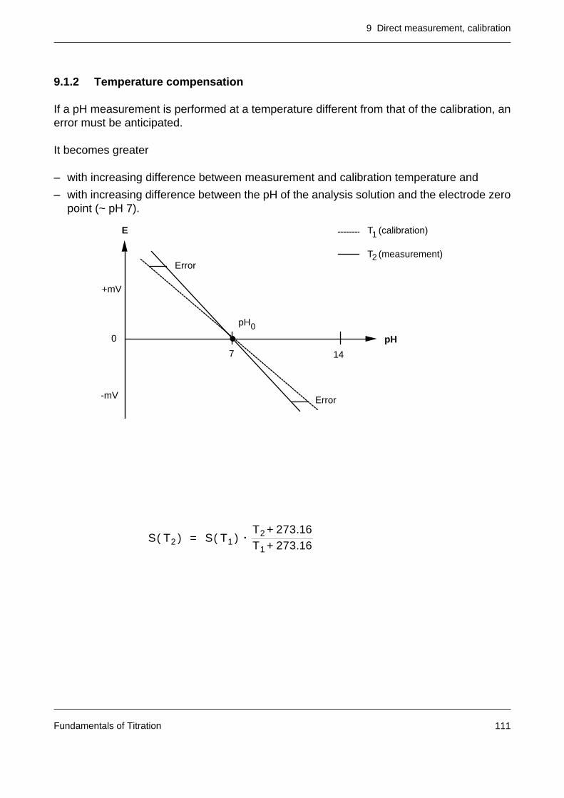
9 Direct measurement, calibration
Fundamentals of Titration 111
9.1.2 Temperature compensation
If a pH measurement is performed at a temperature different from that of the calibration, anerror must be anticipated.
It becomes greater
– with increasing difference between measurement and calibration temperature and
– with increasing difference between the pH of the analysis solution and the electrode zeropoint (~ pH 7).
S( T2 ) = S( T1 ) •T2 + 273.16T1 + 273.16
E
pH
7 14
0
+mV
-mV
pH0
Error
T (calibration)
T (measurement)2
1
Error
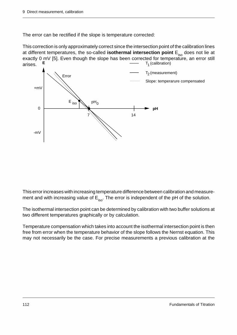
9 Direct measurement, calibration
Fundamentals of Titration112
The error can be rectified if the slope is temperature corrected:
This correction is only approximately correct since the intersection point of the calibration linesat different temperatures, the so-called isothermal intersection point Eiso does not lie atexactly 0 mV [5]. Even though the slope has been corrected for temperature, an error stillarises.
This error increases with increasing temperature difference between calibration and measure-ment and with increasing value of E
iso. The error is independent of the pH of the solution.
The isothermal intersection point can be determined by calibration with two buffer solutions attwo different temperatures graphically or by calculation.
Temperature compensation which takes into account the isothermal intersection point is thenfree from error when the temperature behavior of the slope follows the Nernst equation. Thismay not necessarily be the case. For precise measurements a previous calibration at the
E
pH
7 14
0
+mV
-mV
pH0
Error
T (calibration)
T (measurement)2
1
Slope: temperarure compensated
E iso
9 Direct measurement, calibration
Fundamentals of Titration 113
desired measurement temperature is thus always advisable.
9.2 Direct measurement with ion selective electrodes
The potential of an ion selective electrode depends on the ionic activity in the solution and likethat of the pH electrode is described by the Nernst equation:
E = E0 + S • pA
pA is the negative logarithm of the ionic concentration of entity A. The negative logarithm ofthe ionic concentration of cations is designated pM, that of anions pX.
In this notation the sign of the slope S for cations is negative and that for anions positive.
The theoretical slope of an ion selective electrode at 25°C is 59.16 mV for monovalent ions and29.58 mV for bivalent ions.
The following criteria must be heeded when working with ion selective electrodes:
Sample pretreatment
Sample pretreatment is the most important factor in direct measurement with ion selectiveelectrodes. For quantitative analyses each sample solution must be mixed with a certainamount of electrolyte solution (so-called TISAB solution). These buffer solutions can performthe following functions:
– Ensure constant ionic strength of all sample and calibration solutions. With this measure-ment technique the ion selective electrode can be used for direct measurements of theanalytical concentration of interest and not just the ionic activity.
– pH buffering: Depending on the application, the medium must be acidic, neutral or basic.
– Elimination of interfering ions through complexation, oxidation or reduction.
S = ± 2.301R • Tn • F
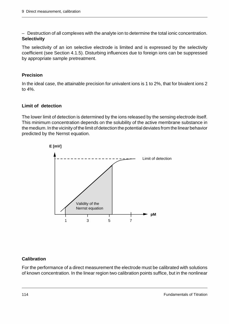
9 Direct measurement, calibration
Fundamentals of Titration114
– Destruction of all complexes with the analyte ion to determine the total ionic concentration.Selectivity
The selectivity of an ion selective electrode is limited and is expressed by the selectivitycoefficient (see Section 4.1.5). Disturbing influences due to foreign ions can be suppressedby appropriate sample pretreatment.
Precision
In the ideal case, the attainable precision for univalent ions is 1 to 2%, that for bivalent ions 2to 4%.
Limit of detection
The lower limit of detection is determined by the ions released by the sensing electrode itself.This minimum concentration depends on the solubility of the active membrane substance inthe medium. In the vicinity of the limit of detection the potential deviates from the linear behaviorpredicted by the Nernst equation.
Calibration
For the performance of a direct measurement the electrode must be calibrated with solutionsof known concentration. In the linear region two calibration points suffice, but in the nonlinear
E [mV]
pM
1 3 5
Limit of detection
7
Validity of theNernst equation
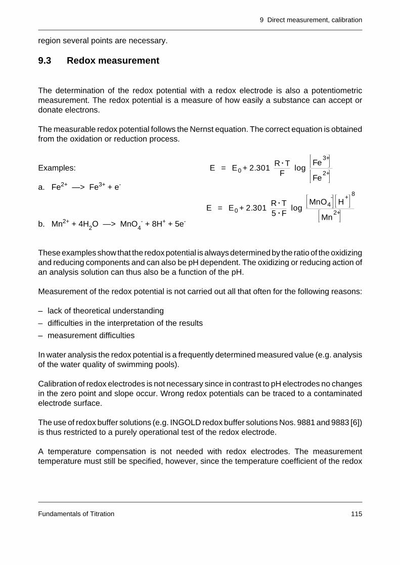
9 Direct measurement, calibration
Fundamentals of Titration 115
region several points are necessary.
9.3 Redox measurement
The determination of the redox potential with a redox electrode is also a potentiometricmeasurement. The redox potential is a measure of how easily a substance can accept ordonate electrons.
The measurable redox potential follows the Nernst equation. The correct equation is obtainedfrom the oxidation or reduction process.
Examples:
a. Fe2+ —> Fe3+ + e-
b. Mn2+ + 4H2O —> MnO4- + 8H+ + 5e-
These examples show that the redox potential is always determined by the ratio of the oxidizingand reducing components and can also be pH dependent. The oxidizing or reducing action ofan analysis solution can thus also be a function of the pH.
Measurement of the redox potential is not carried out all that often for the following reasons:
– lack of theoretical understanding
– difficulties in the interpretation of the results
– measurement difficulties
In water analysis the redox potential is a frequently determined measured value (e.g. analysisof the water quality of swimming pools).
Calibration of redox electrodes is not necessary since in contrast to pH electrodes no changesin the zero point and slope occur. Wrong redox potentials can be traced to a contaminatedelectrode surface.
The use of redox buffer solutions (e.g. INGOLD redox buffer solutions Nos. 9881 and 9883 [6])is thus restricted to a purely operational test of the redox electrode.
A temperature compensation is not needed with redox electrodes. The measurementtemperature must still be specified, however, since the temperature coefficient of the redox
E = E0 + 2.301R • T
Flog
Fe3+
Fe2+
E = E0 + 2.301R • T5 • F
logMnO4
-H
+ 8
Mn2+
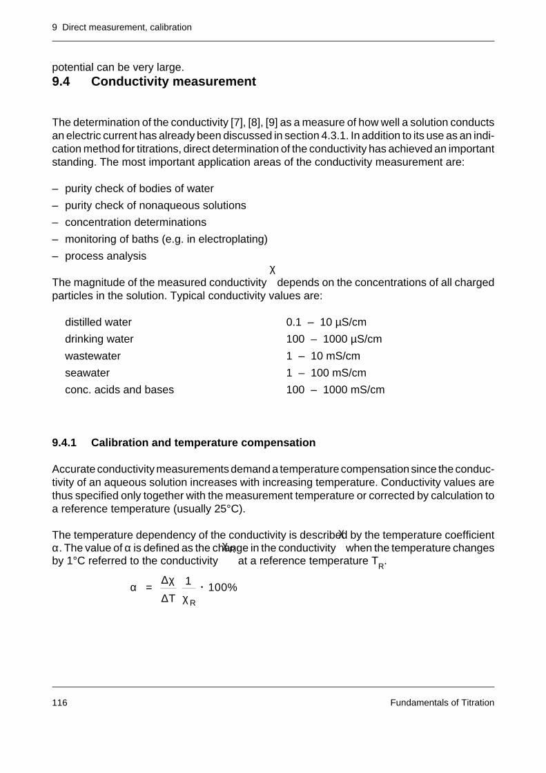
9 Direct measurement, calibration
Fundamentals of Titration116
χ
α =∆χ
∆T
1
χ R
• 100%
potential can be very large.9.4 Conductivity measurement
The determination of the conductivity [7], [8], [9] as a measure of how well a solution conductsan electric current has already been discussed in section 4.3.1. In addition to its use as an indi-cation method for titrations, direct determination of the conductivity has achieved an importantstanding. The most important application areas of the conductivity measurement are:
– purity check of bodies of water
– purity check of nonaqueous solutions
– concentration determinations
– monitoring of baths (e.g. in electroplating)
– process analysis
The magnitude of the measured conductivity depends on the concentrations of all chargedparticles in the solution. Typical conductivity values are:
distilled water 0.1 – 10 µS/cm
drinking water 100 – 1000 µS/cm
wastewater 1 – 10 mS/cm
seawater 1 – 100 mS/cm
conc. acids and bases 100 – 1000 mS/cm
9.4.1 Calibration and temperature compensation
Accurate conductivity measurements demand a temperature compensation since the conduc-tivity of an aqueous solution increases with increasing temperature. Conductivity values arethus specified only together with the measurement temperature or corrected by calculation toa reference temperature (usually 25°C).
The temperature dependency of the conductivity is described by the temperature coefficientα. The value of α is defined as the change in the conductivity when the temperature changesby 1°C referred to the conductivity at a reference temperature T
R.
χ
χ R
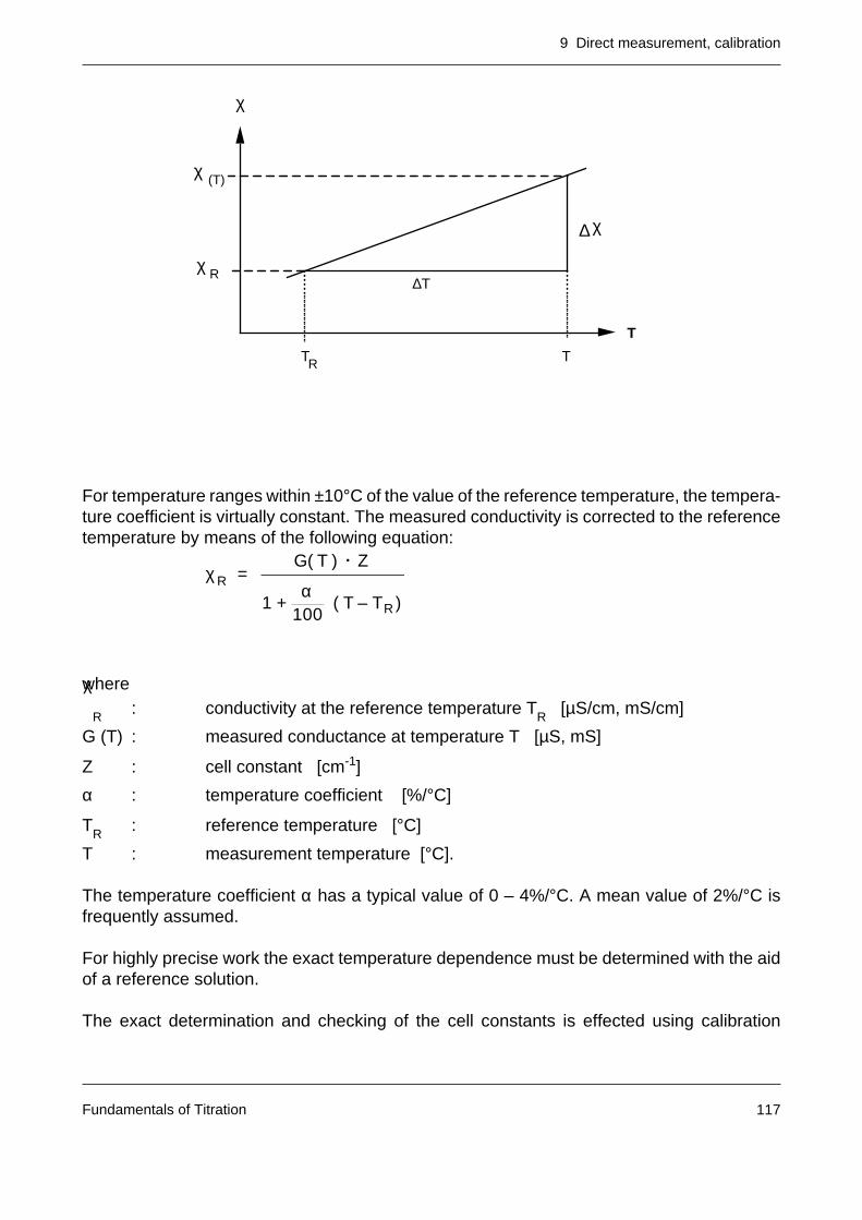
9 Direct measurement, calibration
Fundamentals of Titration 117
For temperature ranges within ±10°C of the value of the reference temperature, the tempera-ture coefficient is virtually constant. The measured conductivity is corrected to the referencetemperature by means of the following equation:
where
R: conductivity at the reference temperature T
R [µS/cm, mS/cm]
G (T) : measured conductance at temperature T [µS, mS]
Z : cell constant [cm-1]
α : temperature coefficient [%/°C]
TR
: reference temperature [°C]
T : measurement temperature [°C].
The temperature coefficient α has a typical value of 0 – 4%/°C. A mean value of 2%/°C isfrequently assumed.
For highly precise work the exact temperature dependence must be determined with the aidof a reference solution.
The exact determination and checking of the cell constants is effected using calibration
χ R =G( T ) • Z
1 +α
100( T – TR )
χ
T
TTR
∆TR
(T)
χ
χ
χ
χ∆
9 Direct measurement, calibration
Fundamentals of Titration118
solutions. The standards employed are KCl solutions of concentration 0.01, 0.1 and 1 mol/L.[1] R.G. Bates, “Determination of pH”, John Wiley (1973)
[2] DIN standard 19266
[3] INGOLD brochure TH5: Calibration of pH electrodes
[4] MERCK booklet: Laboratory products for practical applications, 1987
[5] "Practice and Theory of pH Measurement", INGOLD brochure E-pH-TH-2-CH, Section 4.7, 1989
[6] INGOLD brochure TH2: Redox measurement – Principles and problems
[7] F. Oehme, “Angewandte Konduktometrie”, Hüthig Verlag, Heidelberg (1961)
[8] F. Oehme and R. Bänninger, “ABC der Konduktometrie”, offprint, Chemische Rundschau (1979)
[9] E. Pungor, “Oscillometry and Conductometry”, Pergamon Press, Oxford (1965)
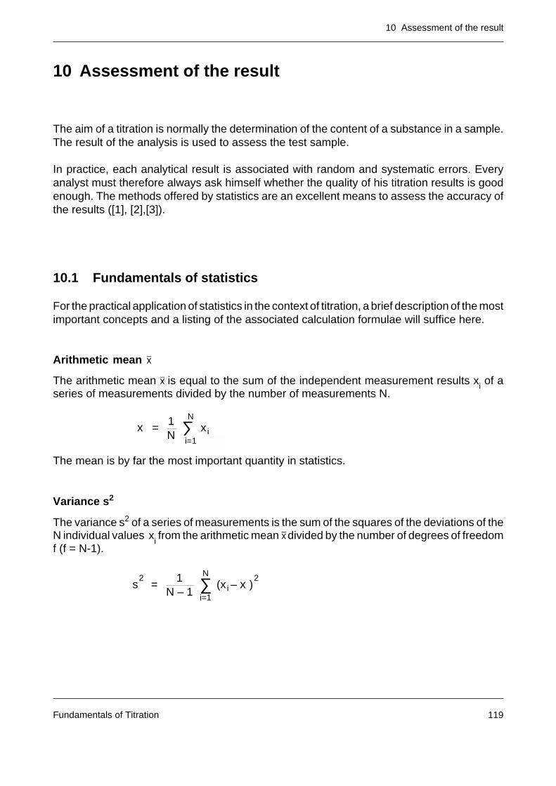
10 Assessment of the result
Fundamentals of Titration 119
10 Assessment of the result
The aim of a titration is normally the determination of the content of a substance in a sample.The result of the analysis is used to assess the test sample.
In practice, each analytical result is associated with random and systematic errors. Everyanalyst must therefore always ask himself whether the quality of his titration results is goodenough. The methods offered by statistics are an excellent means to assess the accuracy ofthe results ([1], [2],[3]).
10.1 Fundamentals of statistics
For the practical application of statistics in the context of titration, a brief description of the mostimportant concepts and a listing of the associated calculation formulae will suffice here.
Arithmetic mean x
The arithmetic mean x is equal to the sum of the independent measurement results xi of aseries of measurements divided by the number of measurements N.
The mean is by far the most important quantity in statistics.
Variance s2
The variance s2 of a series of measurements is the sum of the squares of the deviations of theN individual values x
i from the arithmetic mean x divided by the number of degrees of freedom
f (f = N-1).
x =1N
N
∑i=1
xi
s2
=1
N – 1
N
∑i=1
(xi – x )2
i=1
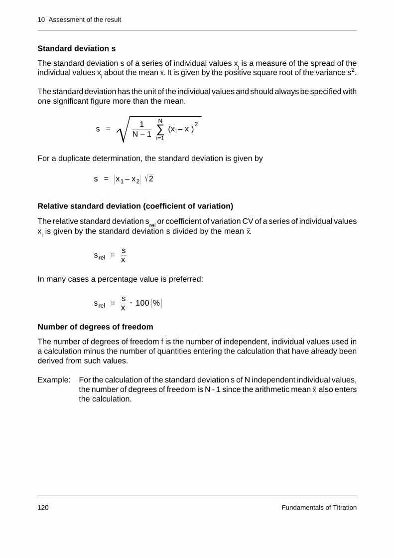
10 Assessment of the result
Fundamentals of Titration120
Standard deviation s
The standard deviation s of a series of individual values xi is a measure of the spread of theindividual values x
i about the mean x. It is given by the positive square root of the variance s2.
The standard deviation has the unit of the individual values and should always be specified withone significant figure more than the mean.
For a duplicate determination, the standard deviation is given by
Relative standard deviation (coefficient of variation)
The relative standard deviation srel
or coefficient of variation CV of a series of individual valuesx
i is given by the standard deviation s divided by the mean x.
In many cases a percentage value is preferred:
Number of degrees of freedom
The number of degrees of freedom f is the number of independent, individual values used ina calculation minus the number of quantities entering the calculation that have already beenderived from such values.
Example: For the calculation of the standard deviation s of N independent individual values,the number of degrees of freedom is N - 1 since the arithmetic mean x also entersthe calculation.
srel =sx
• 100 %
srel =sx
s = x1 – x2 2
s =1
N – 1
N
∑i=1
(xi – x )2
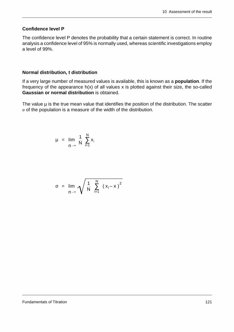
10 Assessment of the result
Fundamentals of Titration 121
µ = limn→∞
1N
N
∑i=1
xi
σ = limn→∞
1N
N
∑i=1
( xi – x )2
Confidence level P
The confidence level P denotes the probability that a certain statement is correct. In routineanalysis a confidence level of 95% is normally used, whereas scientific investigations employa level of 99%.
Normal distribution, t distribution
If a very large number of measured values is available, this is known as a population. If thefrequency of the appearance h(x) of all values x is plotted against their size, the so-calledGaussian or normal distribution is obtained.
The value µ is the true mean value that identifies the position of the distribution. The scatterσ of the population is a measure of the width of the distribution.
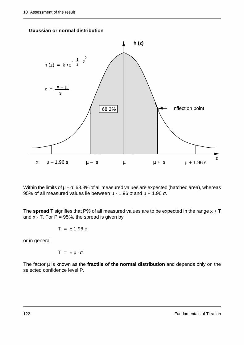
10 Assessment of the result
Fundamentals of Titration122
Within the limits of µ ± σ, 68.3% of all measured values are expected (hatched area), whereas95% of all measured values lie between µ - 1.96 σ and µ + 1.96 σ.
The spread T signifies that P% of all measured values are to be expected in the range x + Tand x - T. For P = 95%, the spread is given by
T = ± 1.96 σ
or in general
T = ± µ • σ
The factor µ is known as the fractile of the normal distribution and depends only on theselected confidence level P.
68.3%
h (z)
Inflection point
h (z) = k •
z =
e
x – µ
12
z2
zx: µ – 1.96 s µ – s µ µ + s µ + 1.96 s
Gaussian or normal distribution
s
-
10 Assessment of the result
Fundamentals of Titration 123
If a small number of measured values is present (typical in analytical practice), this is calleda random sample. If µ and σ of the population are unknown, the distribution of the randomsample values does not yet follow the normal distribution. The mean x is the best estimate ofthe true value but is still associated with a statistical uncertainty that needs to be taken intoaccount. The distribution of the random sample will thus be broader than the normaldistribution. The theoretical function of this distribution is called the t or student distribution.
The spread T of the individual measurement and the confidence interval CI of the meanvalue can thus be calculated.
T = ± s • t
The confidence interval CI (= spread of the mean) signifies that the true mean lies within therange x + CI and x - CI with P% certainty.
The factor t is the fractile of the t distribution and depends on the confidence level P and thenumber of measured values N; it can be taken from the t table (see appendix B).
Outliers, Grubbs outlier test
If a series of measurements (N > 3) includes one or more values that deviate widely from themean, the question must be asked whether these measured values are indeed correct orwhether they should be considered outliers. Outliers have the following influence on the overallresult of an analysis:
– the mean value is clearly shifted to a higher or a lower value
– the standard deviation is increased
– the distribution of the individual values about the mean is distorted and no longer follows anormal distribution.
Such outliers are uncovered by means of statistical tests, e.g. with the Grubbs test. Here, themean x and the standard deviation s of the analysis data are first calculated. From theexperimental data the value x* with the greatest deviation from the mean is sought and testedusing the following condition equation:
CI = ± s • tN
TV =x* – x
s
10 Assessment of the result
Fundamentals of Titration124
The test variable TV is compared with the value in the Grubbs table G (N, P%), which in turndepends on the number of analysis values N. A Grubbs table can be found in appendix B.
If the test variable TV is greater than G (N, P%), the experimental value under test is consideredan outlier and deleted from the series of measurements. The remaining data of the series areused to calculate new values of the mean, and the standard deviation and the outlier testrepeated for another value suspected of being an outlier.
Example: A content determination (N = 6) gave the following results:
x1 = 30.38 %
x2 = 30.23 %
x3 = 30.34 %x
4 = 29.98 %
x5 = 30.29 %
x6 = 30.31 %–––––––––––x = 30.26 %s = 0.144 %
outlier suspect: x4
G(6,90%) = 1.822 —> x4 is an outlier.
After removal of x4 the sample is free from outliers.
TV =x4 – x
s= 1.944
10 Assessment of the result
Fundamentals of Titration 125
10.2 Concepts relating to correctness
The deviation from the correct value or that value accepted as correct of an analytical resultis known as the error.
Gross errors
Gross errors arise through failure to follow analytical procedures, through faulty analyticalinstruments and through carelessness on the part of the analyst. From the statistics point ofview, gross errors are always avoidable.
Random errors
Random errors are as a rule unavoidable and are responsible for the spread in the individualmeasured values about the mean. The magnitude of the random errors – determined usingthe standard deviation s – is a measure of the precision of an analytical procedure.
Systematic errors
Systematic errors give rise to a difference between the expected value and the mean xobtained from the measurement and thus determine the accuracy of an analytical procedure.Systematic deviations have a definite cause and in principle can be rectified. A distinction ismade between proportional systematic and constant systematic deviations. It is apparent fromthe standard formula for the calculation of titration results
R = C • (VEQ • CONC – BLANK)/m
that, for example, a wrong titrant concentration will lead to a proportional systematic error anda wrong solvent blank value to a constant systematic error.
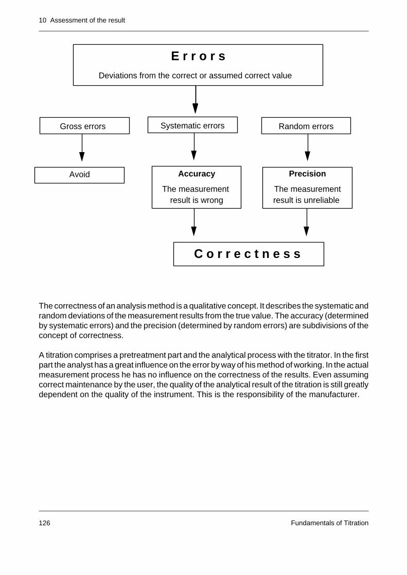
10 Assessment of the result
Fundamentals of Titration126
E r r o r sDeviations from the correct or assumed correct value
Gross errors Systematic errors Random errors
Avoid Accuracy
The measurement
Precision
The measurementresult is wrong result is unreliable
C o r r e c t n e s s
The correctness of an analysis method is a qualitative concept. It describes the systematic andrandom deviations of the measurement results from the true value. The accuracy (determinedby systematic errors) and the precision (determined by random errors) are subdivisions of theconcept of correctness.
A titration comprises a pretreatment part and the analytical process with the titrator. In the firstpart the analyst has a great influence on the error by way of his method of working. In the actualmeasurement process he has no influence on the correctness of the results. Even assumingcorrect maintenance by the user, the quality of the analytical result of the titration is still greatlydependent on the quality of the instrument. This is the responsibility of the manufacturer.
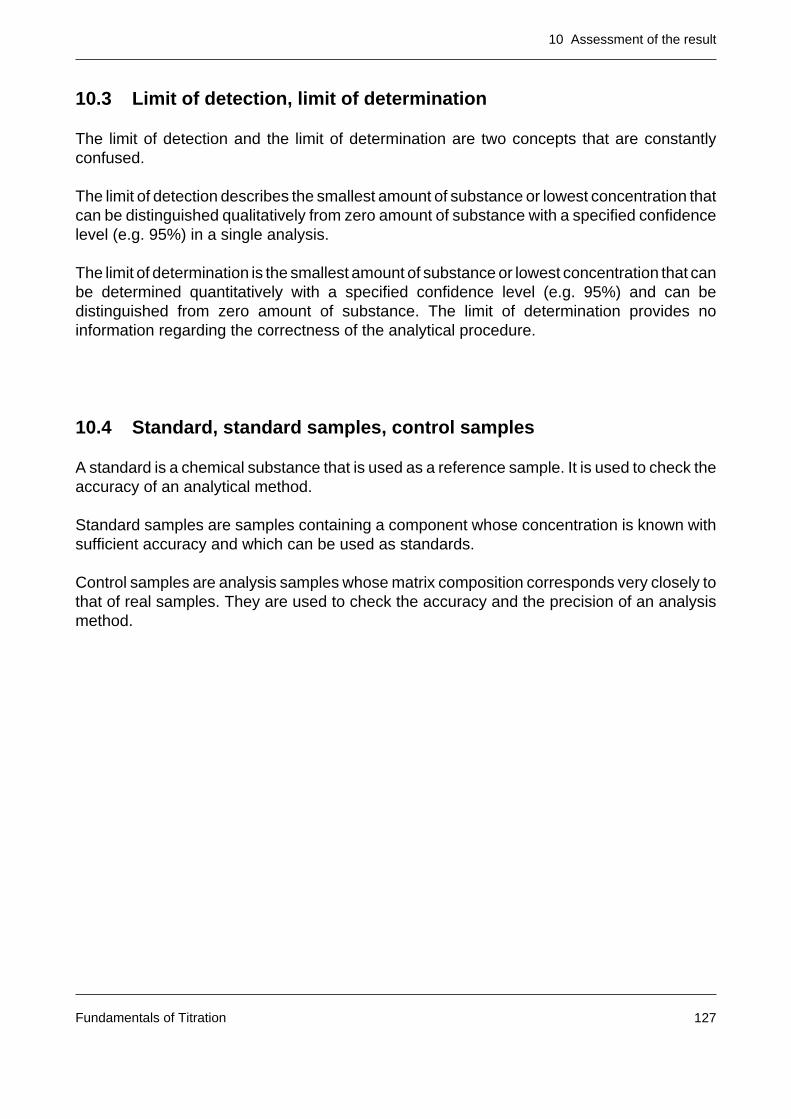
10 Assessment of the result
Fundamentals of Titration 127
10.3 Limit of detection, limit of determination
The limit of detection and the limit of determination are two concepts that are constantlyconfused.
The limit of detection describes the smallest amount of substance or lowest concentration thatcan be distinguished qualitatively from zero amount of substance with a specified confidencelevel (e.g. 95%) in a single analysis.
The limit of determination is the smallest amount of substance or lowest concentration that canbe determined quantitatively with a specified confidence level (e.g. 95%) and can bedistinguished from zero amount of substance. The limit of determination provides noinformation regarding the correctness of the analytical procedure.
10.4 Standard, standard samples, control samples
A standard is a chemical substance that is used as a reference sample. It is used to check theaccuracy of an analytical method.
Standard samples are samples containing a component whose concentration is known withsufficient accuracy and which can be used as standards.
Control samples are analysis samples whose matrix composition corresponds very closely tothat of real samples. They are used to check the accuracy and the precision of an analysismethod.
10 Assessment of the result
Fundamentals of Titration128
10.5 Consequences for practical application
To guard against systematic errors in a titration, several measures need to be implemented:
– Regular determination of the titer of the titrant used (also applies when commercialvolumetric solutions are used)
– Determination of any blank value of the solvent or the matrix
– Regular use of control samples.
For the standardization (titer determination) and control of titrimetric solutions, substances areneeded that within the limits of measurement accuracy of the titration (lower limit: 0.01%)correspond exactly to the composition given by their formula. These so-called primarystandards must have the following properties:
– Clearly defined composition and high degree of purity
– Large molar mass (avoidance of weighing errors)
– Capable of being weighed accurately without difficulties (insensitive to oxygen and/or CO2and not hygroscopic)
– Concentration of a freshly prepared titrimetric solution remains stable
– Rapidly and easily soluble in the solvents needed
– Rapid and stoichiometric titration reaction.
Determinations of the titer and blank should be performed as a multiple determination(determinations in triplicate have proved adequate).
In routine analysis (use of the same analysis procedure for many samples), the regular inser-tion of control samples of known composition (e.g. primary standards) between the individualseries has proved useful. This provides a check not only on the titer but also of the correctfunctioning of the analytical instrument. In addition to the result of the titration with the controlsample, its progress (titration time, titration curve, etc.) provides indications of any problems(contamination of the electrode, etc.).
Note: Tables of primary standards for the most important titrants can be found inappendix C.

10 Assessment of the result
Fundamentals of Titration 129
[1] J.C. Miller and J.N. Miller, “Statistics for Analytical Chemistry”, second edition, Ellis Horwood, Chichester,1988.
[2] R. Caulcutt and R. Boddy, “Statistics for Analytical Chemists”, Chapman and Hall, London, 1983.
[3] W. Funk, V. Damman, C. Vonderheid und G. Oehlmann, “Statistische Methoden der Wasseranalytik”, VCHVerlagsgesellschaft, Weinheim, 1985
Fundamentals of Titration130
Appendix A
Appendices
Appendix A: Tables showing the pH temperature dependencies of DIN/NIST (NBS),MERCK and INGOLD buffers (see section 9.1)
Appendix B: Statistical tables (see section 10.1)
Appendix C: Tables of primary standards for the most important titrants (see section 10.5)
Appendices
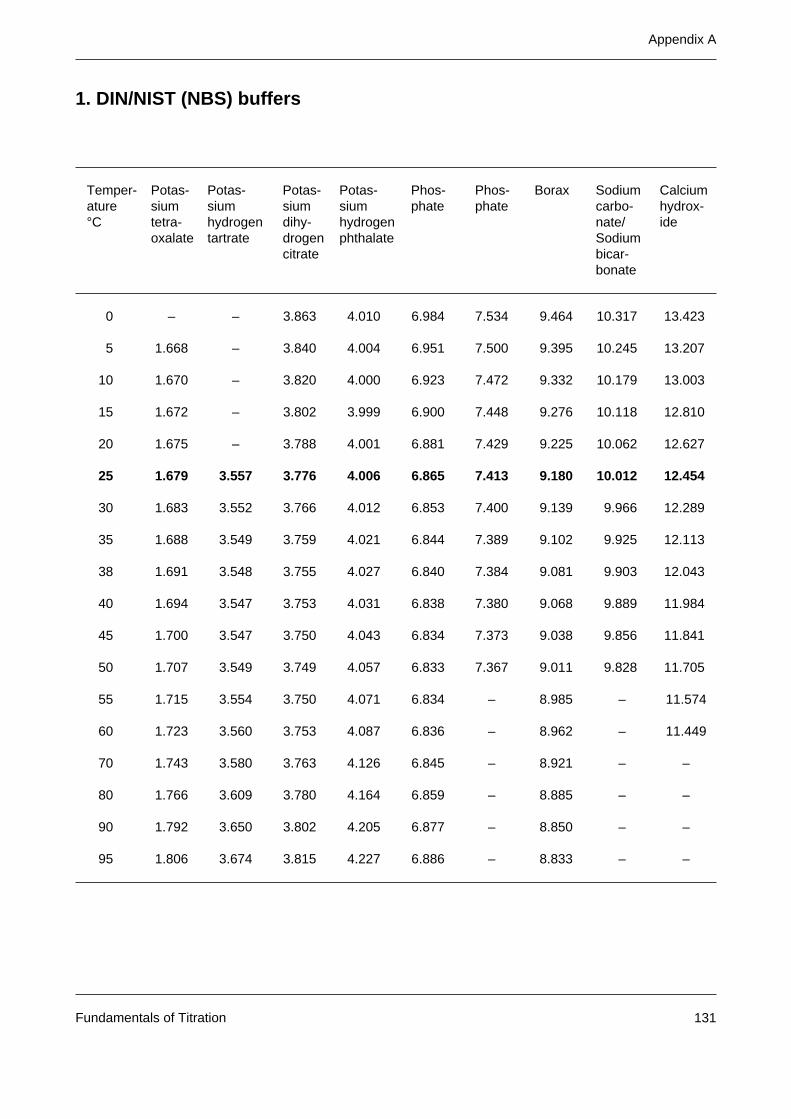
Appendix A
Fundamentals of Titration 131
1. DIN/NIST (NBS) buffers
Temper- Potas- Potas- Potas- Potas- Phos- Phos- Borax Sodium Calciumature sium sium sium sium phate phate carbo- hydrox-°C tetra- hydrogen dihy- hydrogen nate/ ide
oxalate tartrate drogen phthalate Sodiumcitrate bicar-
bonate
0 – – 3.863 4.010 6.984 7.534 9.464 10.317 13.423
5 1.668 – 3.840 4.004 6.951 7.500 9.395 10.245 13.207
10 1.670 – 3.820 4.000 6.923 7.472 9.332 10.179 13.003
15 1.672 – 3.802 3.999 6.900 7.448 9.276 10.118 12.810
20 1.675 – 3.788 4.001 6.881 7.429 9.225 10.062 12.627
25 1.679 3.557 3.776 4.006 6.865 7.413 9.180 10.012 12.454
30 1.683 3.552 3.766 4.012 6.853 7.400 9.139 9.966 12.289
35 1.688 3.549 3.759 4.021 6.844 7.389 9.102 9.925 12.113
38 1.691 3.548 3.755 4.027 6.840 7.384 9.081 9.903 12.043
40 1.694 3.547 3.753 4.031 6.838 7.380 9.068 9.889 11.984
45 1.700 3.547 3.750 4.043 6.834 7.373 9.038 9.856 11.841
50 1.707 3.549 3.749 4.057 6.833 7.367 9.011 9.828 11.705
55 1.715 3.554 3.750 4.071 6.834 – 8.985 – 11.574
60 1.723 3.560 3.753 4.087 6.836 – 8.962 – 11.449
70 1.743 3.580 3.763 4.126 6.845 – 8.921 – –
80 1.766 3.609 3.780 4.164 6.859 – 8.885 – –
90 1.792 3.650 3.802 4.205 6.877 – 8.850 – –
95 1.806 3.674 3.815 4.227 6.886 – 8.833 – –
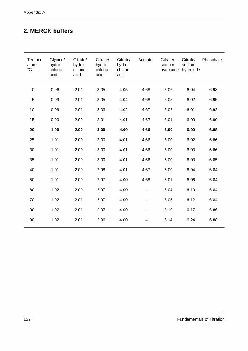
Fundamentals of Titration132
Appendix A
2. MERCK buffers
Temper- Glycine/ Citrate/ Citrate/ Citrate/ Acetate Citrate/ Citrate/ Phosphateature hydro- hydro- hydro- hydro- sodium sodium°C chloric chloric chloric chloric hydroxide hydroxide
acid acid acid acid
0 0.96 2.01 3.05 4.05 4.68 5.06 6.04 6.98
5 0.99 2.01 3.05 4.04 4.68 5.05 6.02 6.95
10 0.99 2.01 3.03 4.02 4.67 5.02 6.01 6.92
15 0.99 2.00 3.01 4.01 4.67 5.01 6.00 6.90
20 1.00 2.00 3.00 4.00 4.66 5.00 6.00 6.88
25 1.01 2.00 3.00 4.01 4.66 5.00 6.02 6.86
30 1.01 2.00 3.00 4.01 4.66 5.00 6.03 6.86
35 1.01 2.00 3.00 4.01 4.66 5.00 6.03 6.85
40 1.01 2.00 2.98 4.01 4.67 5.00 6.04 6.84
50 1.01 2.00 2.97 4.00 4.68 5.01 6.06 6.84
60 1.02 2.00 2.97 4.00 – 5.04 6.10 6.84
70 1.02 2.01 2.97 4.00 – 5.05 6.12 6.84
80 1.02 2.01 2.97 4.00 – 5.10 6.17 6.86
90 1.02 2.01 2.96 4.00 – 5.14 6.24 6.88
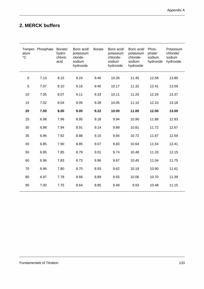
Appendix A
Fundamentals of Titration 133
2. MERCK buffers
Temper- Phosphate Borate/ Boric acid/ Borate Boric acid/ Boric acid/ Phos- Potassiumature hydro- potassium potassium potassium phate/ chloride/°C chloric cloride- chloride- chloride- sodium sodium
acid sodium sodium sodium hydroxide hydroxidehydroxide hydroxide hydroxide
0 7.13 8.15 9.24 9.46 10.26 11.45 12.58 13.80
5 7.07 8.10 9.16 9.40 10.17 11.32 12.41 13.59
10 7.05 8.07 9.11 9.33 10.11 11.20 12.26 13.37
15 7.02 8.04 9.05 9.28 10.05 11.10 12.10 13.18
20 7.00 8.00 9.00 9.22 10.00 11.00 12.00 13.00
25 6.98 7.96 8.95 9.18 9.94 10.90 11.88 12.83
30 6.98 7.94 8.91 9.14 9.89 10.81 11.72 12.67
35 6.96 7.92 8.88 9.10 9.84 10.72 11.67 12.59
40 6.85 7.90 8.85 9.07 9.83 10.64 11.54 12.41
50 6.95 7.85 8.79 9.01 9.74 10.48 11.33 12.15
60 6.96 7.83 8.73 9.96 9.67 10.45 11.04 11.75
70 6.96 7.80 8.70 8.93 9.62 10.19 10.90 11.61
80 6.97 7.78 8.66 8.89 9.55 10.06 10.70 11.39
90 7.00 7.75 8.64 8.85 9.49 9.93 10.48 11.15
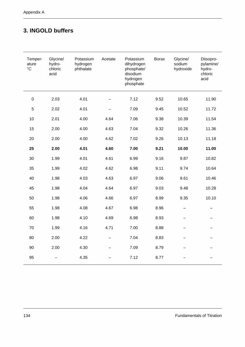
Fundamentals of Titration134
Appendix A
3. INGOLD buffers
Temper- Glycine/ Potassium Acetate Potassium Borax Glycine/ Diisopro-ature hydro- hydrogen dihydrogen sodium pylamine/°C chloric phthalate phosphate/ hydroxide hydro-
acid disodium chlorichydrogen acidphosphate
0 2.03 4.01 – 7.12 9.52 10.65 11.90
5 2.02 4.01 – 7.09 9.45 10.52 11.72
10 2.01 4.00 4.64 7.06 9.38 10.39 11.54
15 2.00 4.00 4.63 7.04 9.32 10.26 11.36
20 2.00 4.00 4.62 7.02 9.26 10.13 11.18
25 2.00 4.01 4.60 7.00 9.21 10.00 11.00
30 1.99 4.01 4.61 6.99 9.16 9.87 10.82
35 1.99 4.02 4.62 6.98 9.11 9.74 10.64
40 1.98 4.03 4.63 6.97 9.06 9.61 10.46
45 1.98 4.04 4.64 6.97 9.03 9.48 10.28
50 1.98 4.06 4.66 6.97 8.99 9.35 10.10
55 1.98 4.08 4.67 6.98 8.96 – –
60 1.98 4.10 4.69 6.98 8.93 – –
70 1.99 4.16 4.71 7.00 8.88 – –
80 2.00 4.22 – 7.04 8.83 – –
90 2.00 4.30 – 7.09 8.79 – –
95 – 4.35 – 7.12 8.77 – –
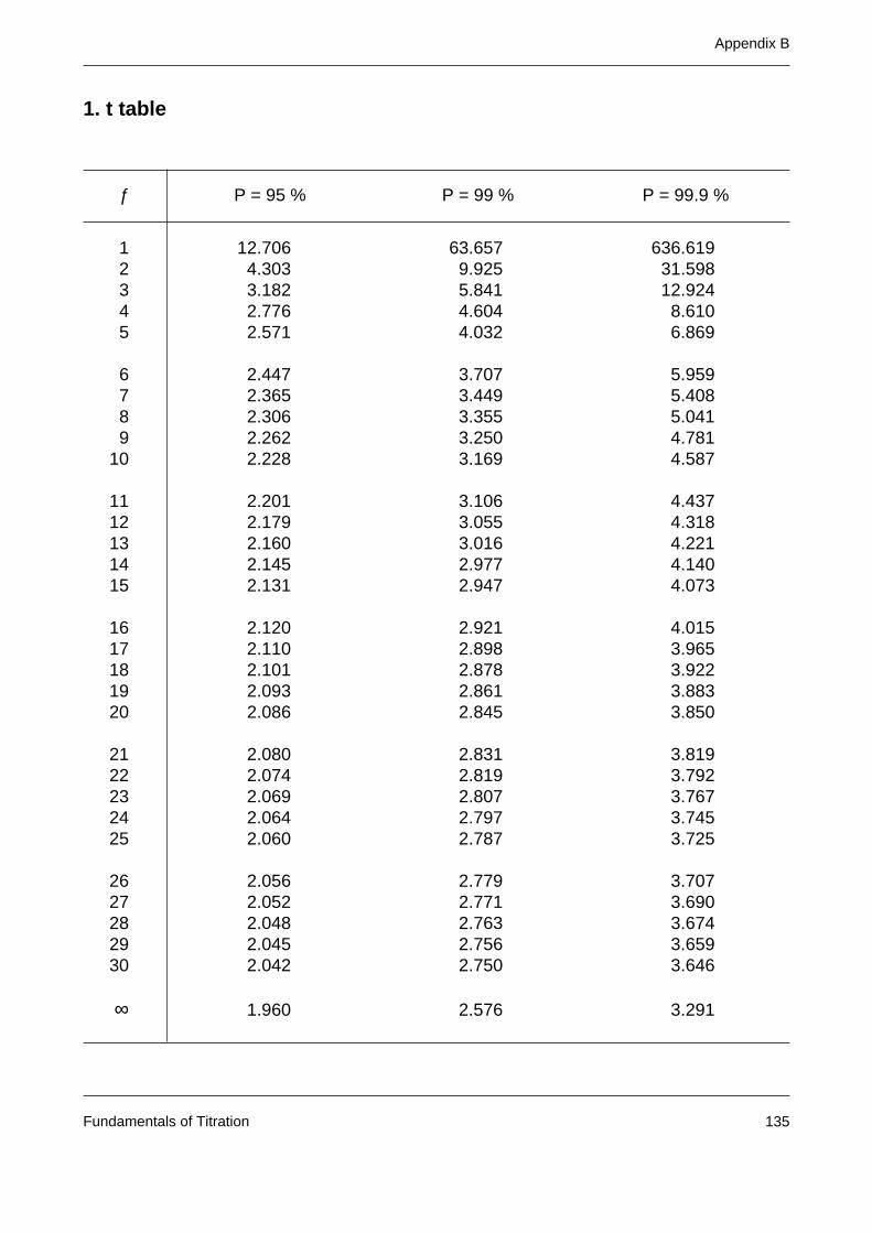
Appendix B
Fundamentals of Titration 135
1. t table
ƒ P = 95 % P = 99 % P = 99.9 %
1 12.706 63.657 636.6192 4.303 9.925 31.5983 3.182 5.841 12.9244 2.776 4.604 8.6105 2.571 4.032 6.869
6 2.447 3.707 5.9597 2.365 3.449 5.4088 2.306 3.355 5.0419 2.262 3.250 4.781
10 2.228 3.169 4.587
11 2.201 3.106 4.43712 2.179 3.055 4.31813 2.160 3.016 4.22114 2.145 2.977 4.14015 2.131 2.947 4.073
16 2.120 2.921 4.01517 2.110 2.898 3.96518 2.101 2.878 3.92219 2.093 2.861 3.88320 2.086 2.845 3.850
21 2.080 2.831 3.81922 2.074 2.819 3.79223 2.069 2.807 3.76724 2.064 2.797 3.74525 2.060 2.787 3.725
26 2.056 2.779 3.70727 2.052 2.771 3.69028 2.048 2.763 3.67429 2.045 2.756 3.65930 2.042 2.750 3.646
∞ 1.960 2.576 3.291
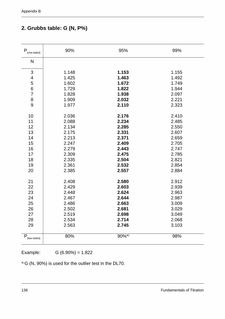
Appendix B
Fundamentals of Titration136
2. Grubbs table: G (N, P%)
P(one-tailed)
90% 95% 99%
N
3 1.148 1.153 1.1554 1.425 1.463 1.4925 1.602 1.672 1.7496 1.729 1.822 1.9447 1.828 1.938 2.0978 1.909 2.032 2.2219 1.977 2.110 2.323
10 2.036 2.176 2.41011 2.088 2.234 2.48512 2.134 2.285 2.55013 2.175 2.331 2.60714 2.213 2.371 2.65915 2.247 2.409 2.70516 2.279 2.443 2.74717 2.309 2.475 2.78518 2.335 2.504 2.82119 2.361 2.532 2.85420 2.385 2.557 2.884
21 2.408 2.580 2.91222 2.429 2.603 2.93923 2.448 2.624 2.96324 2.467 2.644 2.98725 2.486 2.663 3.00926 2.502 2.681 3.02927 2.519 2.698 3.04928 2.534 2.714 2.06829 2.563 2.745 3.103
P(two-tailed) 80% 90%*) 98%
Example: G (6.90%) = 1.822
*) G (N, 90%) is used for the outlier test in the DL70.
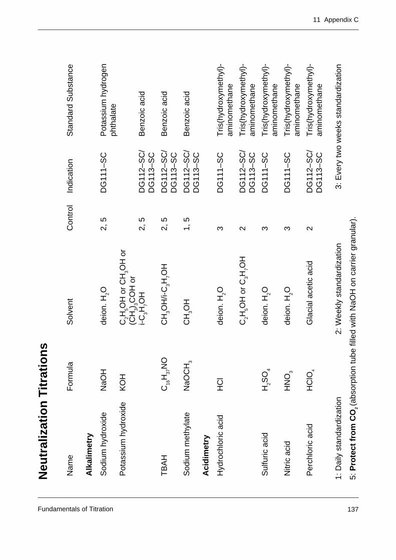
11 Appendix C
Fundamentals of Titration 137
Neu
tral
izat
ion
Tit
rati
on
s
Nam
eF
orm
ula
Sol
vent
Con
trol
Indi
catio
nS
tand
ard
Sub
stan
ce
Alk
alim
etry
Sod
ium
hyd
roxi
deN
aOH
deio
n. H
2O2,
5D
G11
1–S
CP
otas
sium
hyd
roge
nph
thal
ate
Pot
assi
um h
ydro
xide
KO
HC
2H5O
H o
r C
H3O
H o
r(C
H3)
3CO
H o
ri-C
3H7O
H2,
5D
G11
2–S
C/
Ben
zoic
aci
dD
G11
3–S
C
TB
AH
C16
H37
NO
CH
3OH
/i-C
3H7O
H2,
5D
G11
2–S
C/
Ben
zoic
aci
dD
G11
3–S
C
Sod
ium
met
hyla
teN
aOC
H3
CH
3OH
1, 5
DG
112–
SC
/B
enzo
ic a
cid
DG
113–
SC
Aci
dim
etry
Hyd
roch
loric
aci
dH
Cl
deio
n. H
2O3
DG
111–
SC
Tris
(hyd
roxy
met
hyl)-
amin
omet
hane
C2H
5OH
or
C3H
7OH
2D
G11
2–S
C/
Tris
(hyd
roxy
met
hyl)-
DG
113–
SC
amin
omet
hane
Sul
furic
aci
dH
2SO
4de
ion.
H2O
3D
G11
1–S
CT
ris(h
ydro
xym
ethy
l)-am
inom
etha
ne
Nitr
ic a
cid
HN
O3
deio
n. H
2O3
DG
111–
SC
Tris
(hyd
roxy
met
hyl)-
amin
omet
hane
Per
chlo
ric a
cid
HC
lO4
Gla
cial
ace
tic a
cid
2D
G11
2–S
C/
Tris
(hyd
roxy
met
hyl)-
DG
113–
SC
amin
omet
hane
1: D
aily
sta
ndar
diza
tion
2: W
eekl
y st
anda
rdiz
atio
n3:
Eve
ry tw
o w
eeks
sta
ndar
diza
tion
5: P
rote
ct f
rom
CO
2 (a
bsor
ptio
n tu
be fi
lled
with
NaO
H o
n ca
rrie
r gr
anul
ar).
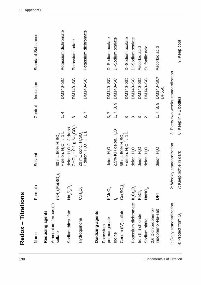
11 Appendix C
Fundamentals of Titration138
Red
ox
– Ti
trat
ion
s
Nam
eF
orm
ula
Sol
vent
Con
trol
Indi
catio
nS
tand
ard
Sub
stan
ce
Red
uci
ng
ag
ents
Am
mon
ium
ferr
ous
(ll)
sulfa
te(N
H4)
2Fe(
SO
4)2
60 m
L 50
% H
2SO
4
+ d
eion
. H2O
→ 1
L1,
4D
M14
0 –S
CP
otas
sium
dic
hrom
ate
Sod
ium
thio
sulfa
teN
a 2S2O
3de
ion.
H2O
(+
3 d
rops
CH
Cl 3
+ 0
.1 g
Na 2C
O3)
3D
M14
0–S
CP
otas
sium
ioda
te
Hyd
roqu
inon
eC
6H6O
220
mL
conc
. H2S
O4
+ d
eion
. H2O
→ 1
L2,
7D
M14
0 –S
CP
otas
sium
dic
hrom
ate
Oxi
diz
ing
ag
ents
Pot
assi
umpe
rman
gana
teK
MnO
4de
ion.
H2O
3, 7
DM
140–
SC
Di-S
odiu
m o
xala
te
Iodi
neI 2
2.5%
KI /
dei
on. H
2O1,
7, 8
, 9D
M14
0–S
CD
i-Sod
ium
oxa
late
Cer
ium
(lV
) su
lfate
Ce(
SO
4)2
58 m
L 50
% H
2SO
4
+ d
eion
. H2O
→ 1
L3
DM
140–
SC
Di-S
odiu
m o
xala
te
Pot
assi
um d
ichr
omat
eK
2Cr 2O
7de
ion.
H2O
3D
M14
0–S
CD
i-Sod
ium
oxa
late
Iron
(III
) ch
lorid
eF
eCl 3
deio
n. H
2O3
DM
140–
SC
Asc
orbi
c ac
id
Sod
ium
nitr
iteN
aNO
2de
ion.
H2O
2D
M14
0–S
CS
ulfa
nilic
aci
d
2,6
Dic
hlor
ophe
nol-
indo
phen
ol-N
a-sa
ltD
PI
deio
n. H
2O1,
7, 8
, 9D
M14
0–S
C/
Asc
orbi
c ac
idD
P55
0
1: D
aily
sta
ndar
diza
tion
2: W
eekl
y st
anda
rdiz
atio
n3:
Eve
ry tw
o w
eeks
sta
ndar
diza
tion
4: P
rote
ct fr
om O
27:
Kee
p bo
ttle
in d
ark
8: K
eep
in P
E b
ottle
s9:
Kee
p co
ol
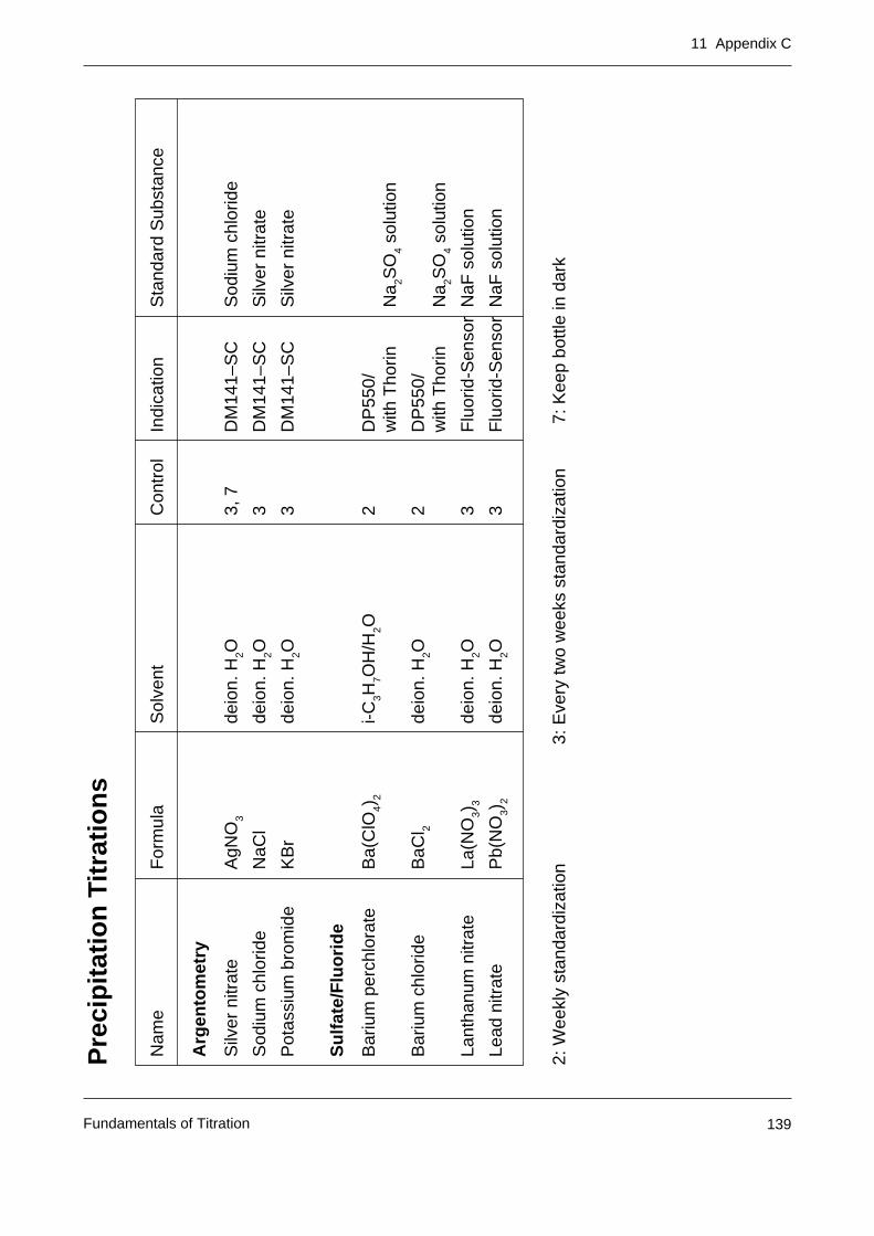
11 Appendix C
Fundamentals of Titration 139
Pre
cip
itat
ion
Tit
rati
on
s
Nam
eF
orm
ula
Sol
vent
Con
trol
Indi
catio
nS
tand
ard
Sub
stan
ce
Arg
ento
met
ry
Silv
er n
itrat
eA
gNO
3de
ion.
H2O
3, 7
DM
141–
SC
Sod
ium
chl
orid
e
Sod
ium
chl
orid
eN
aCl
deio
n. H
2O3
DM
141–
SC
Silv
er n
itrat
e
Pot
assi
um b
rom
ide
KB
rde
ion.
H2O
3D
M14
1–S
CS
ilver
nitr
ate
Su
lfat
e/F
luo
rid
e
Bar
ium
per
chlo
rate
Ba(
ClO
4)2
i-C3H
7OH
/H2O
2D
P55
0/w
ith T
horin
Na 2S
O4
solu
tion
Bar
ium
chl
orid
eB
aCl 2
deio
n. H
2O2
DP
550/
with
Tho
rinN
a 2SO
4 so
lutio
n
Lant
hanu
m n
itrat
eLa
(NO
3)3
deio
n. H
2O3
Flu
orid
-Sen
sor
NaF
sol
utio
n
Lead
nitr
ate
Pb(
NO
3)2
deio
n. H
2O3
Flu
orid
-Sen
sor
NaF
sol
utio
n
2: W
eekl
y st
anda
rdiz
atio
n3:
Eve
ry tw
o w
eeks
sta
ndar
diza
tion
7: K
eep
bottl
e in
dar
k
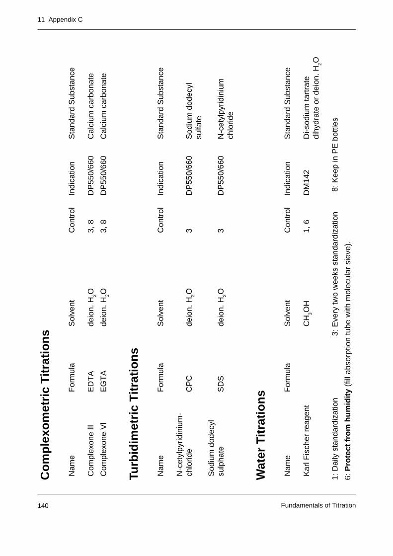
11 Appendix C
Fundamentals of Titration140
Co
mp
lexo
met
ric
Titr
atio
ns
Nam
eF
orm
ula
Sol
vent
Con
trol
Indi
catio
nS
tand
ard
Sub
stan
ce
Com
plex
one
lllE
DT
Ade
ion.
H2O
3, 8
DP
550/
660
Cal
cium
car
bona
te
Com
plex
one
Vl
EG
TA
deio
n. H
2O3,
8D
P55
0/66
0C
alci
um c
arbo
nate
Turb
idim
etri
c T
itra
tio
ns
Nam
eF
orm
ula
Sol
vent
Con
trol
Indi
catio
nS
tand
ard
Sub
stan
ce
N-c
etyl
pyrid
iniu
m-
chlo
ride
CP
Cde
ion.
H2O
3D
P55
0/66
0S
odiu
m d
odec
ylsu
lfate
Sod
ium
dod
ecyl
sulp
hate
SD
Sde
ion.
H2O
3D
P55
0/66
0N
-cet
ylpy
ridin
ium
chlo
ride
Wat
er T
itra
tio
ns
Nam
eF
orm
ula
Sol
vent
Con
trol
Indi
catio
nS
tand
ard
Sub
stan
ce
Kar
l Fis
cher
rea
gent
CH
3OH
1, 6
DM
142
Di-s
odiu
m ta
rtra
tedi
hydr
ate
or d
eion
. H2O
1: D
aily
sta
ndar
diza
tion
3: E
very
two
wee
ks s
tand
ardi
zatio
n8:
Kee
p in
PE
bot
tles
6: P
rote
ct f
rom
hu
mid
ity
(fill
abs
orpt
ion
tube
with
mol
ecul
ar s
ieve
).
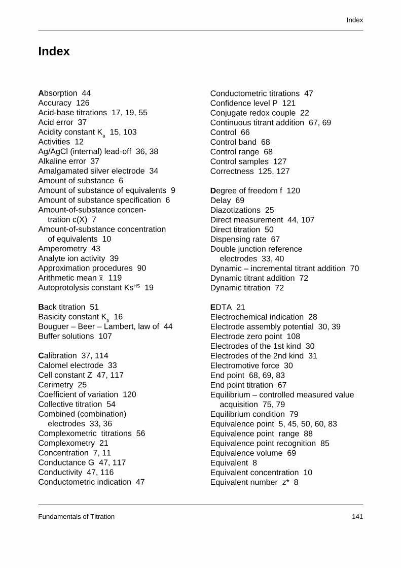
Index
Fundamentals of Titration 141
Index
Absorption 44Accuracy 126Acid-base titrations 17, 19, 55Acid error 37Acidity constant K
a 15, 103
Activities 12Ag/AgCl (internal) lead-off 36, 38Alkaline error 37Amalgamated silver electrode 34Amount of substance 6Amount of substance of equivalents 9Amount of substance specification 6Amount-of-substance concen-
tration c(X) 7Amount-of-substance concentration
of equivalents 10Amperometry 43Analyte ion activity 39Approximation procedures 90Arithmetic mean x 119Autoprotolysis constant KsHS 19
Back titration 51Basicity constant Kb 16Bouguer – Beer – Lambert, law of 44Buffer solutions 107
Calibration 37, 114Calomel electrode 33Cell constant Z 47, 117Cerimetry 25Coefficient of variation 120Collective titration 54Combined (combination)
electrodes 33, 36Complexometric titrations 56Complexometry 21Concentration 7, 11Conductance G 47, 117Conductivity 47, 116Conductometric indication 47
Conductometric titrations 47Confidence level P 121Conjugate redox couple 22Continuous titrant addition 67, 69Control 66Control band 68Control range 68Control samples 127Correctness 125, 127
Degree of freedom f 120Delay 69Diazotizations 25Direct measurement 44, 107Direct titration 50Dispensing rate 67Double junction reference
electrodes 33, 40Dynamic – incremental titrant addition 70Dynamic titrant addition 72Dynamic titration 72
EDTA 21Electrochemical indication 28Electrode assembly potential 30, 39Electrode zero point 108Electrodes of the 1st kind 30Electrodes of the 2nd kind 31Electromotive force 30End point 68, 69, 83End point titration 67Equilibrium – controlled measured value
acquisition 75, 79Equilibrium condition 79Equivalence point 5, 45, 50, 60, 83Equivalence point range 88Equivalence point recognition 85Equivalence volume 69Equivalent 8Equivalent concentration 10Equivalent number z* 8
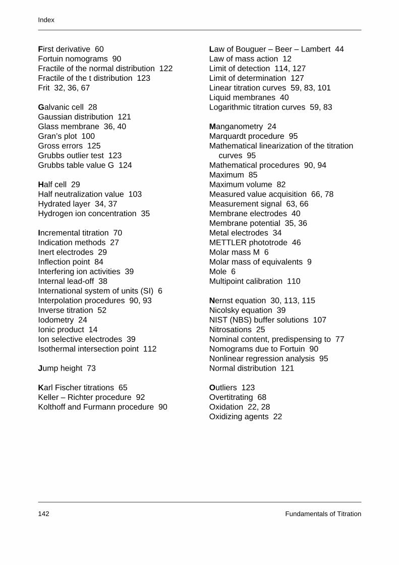
Index
Fundamentals of Titration142
First derivative 60Fortuin nomograms 90Fractile of the normal distribution 122Fractile of the t distribution 123Frit 32, 36, 67
Galvanic cell 28Gaussian distribution 121Glass membrane 36, 40Gran’s plot 100Gross errors 125Grubbs outlier test 123Grubbs table value G 124
Half cell 29Half neutralization value 103Hydrated layer 34, 37Hydrogen ion concentration 35
Incremental titration 70Indication methods 27Inert electrodes 29Inflection point 84Interfering ion activities 39Internal lead-off 38International system of units (SI) 6Interpolation procedures 90, 93Inverse titration 52Iodometry 24Ionic product 14Ion selective electrodes 39Isothermal intersection point 112
Jump height 73
Karl Fischer titrations 65Keller – Richter procedure 92Kolthoff and Furmann procedure 90
Law of Bouguer – Beer – Lambert 44Law of mass action 12Limit of detection 114, 127Limit of determination 127Linear titration curves 59, 83, 101Liquid membranes 40Logarithmic titration curves 59, 83
Manganometry 24Marquardt procedure 95Mathematical linearization of the titration
curves 95Mathematical procedures 90, 94Maximum 85Maximum volume 82Measured value acquisition 66, 78Measurement signal 63, 66Membrane electrodes 40Membrane potential 35, 36Metal electrodes 34METTLER phototrode 46Molar mass M 6Molar mass of equivalents 9Mole 6Multipoint calibration 110
Nernst equation 30, 113, 115Nicolsky equation 39NIST (NBS) buffer solutions 107Nitrosations 25Nominal content, predispensing to 77Nomograms due to Fortuin 90Nonlinear regression analysis 95Normal distribution 121
Outliers 123Overtitrating 68Oxidation 22, 28Oxidizing agents 22
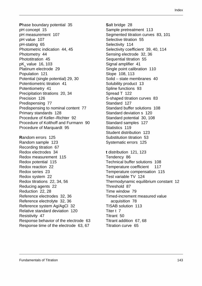
Index
Fundamentals of Titration 143
Phase boundary potential 35pH concept 15pH measurement 107pH value 107pH-stating 65Photometric indication 44, 45Photometry 44Phototitration 45pK
a value 16, 103
Platinum electrode 29Population 121Potential (single potential) 29, 30Potentiometric titration 41Potentiometry 41Precipitation titrations 20, 34Precision 126Predispensing 77Predispensing to nominal content 77Primary standards 128Procedure of Keller–Richter 92Procedure of Kolthoff and Furmann 90Procedure of Marquardt 95
Random errors 125Random sample 123Recording titration 67Redox electrodes 34Redox measurement 115Redox potential 115Redox reaction 22Redox series 23Redox system 22Redox titrations 22, 34, 56Reducing agents 22Reduction 22, 28Reference electrodes 32, 36Reference electrolyte 32, 36Reference system Ag/AgCl 32Relative standard deviation 120Resistivity 47Response behavior of the electrode 63Response time of the electrode 63, 67
Salt bridge 28Sample pretreatment 113Segmented titration curves 83, 101Selective titration 55Selectivity 114Selectivity coefficient 39, 40, 114Sensing electrode 32, 36Sequential titration 55Signal amplifier 41Single point calibration 110Slope 108, 113Solid – state membranes 40Solubility product 13Spline functions 93Spread T 122S-shaped titration curves 83Standard 127Standard buffer solutions 108Standard deviation s 120Standard potential 30, 108Standard samples 127Statistics 119Student distribution 123Substitution titration 53Systematic errors 125
t distribution 121, 123Tendency 86Technical buffer solutions 108Temperature coefficient 117Temperature compensation 115Test variable TV 124Thermodynamic equilibrium constant 12Threshold 87Time window 79Timed-increment measured value
acquisition 78TISAB solution 113Titer t 7Titrant 50Titrant addition 67, 68Titration curve 65

Index
Fundamentals of Titration144
Titration curves 59Titration reaction 12Titrimetric analysis 5, 6Titrimetric solution 7Transmission 44t table 123, 135Tubbs procedure 93Types of titration 50
Variance s2 119Visual indication 27Voltametry 42
Water determination by Karl Fischermethod 42


© Mettler-Toledo GmbH 1993, 1996, 1997, 1998 ME-704153A Printed in Switzerland 9806/9.12
*P704153*
Mettler-Toledo GmbH, Analytical, Sonnenbergstrasse 74, CH-8603 Schwerzenbach, Tel. (01) 806 77 11, Fax (01) 806 73 50, Internet:http://www.mt.com
AT Mettler-Toledo Ges.m.b.H., A-1100 Wien AU Mettler-Toledo Ltd., Port Melbourne, Victoria 3207Tel. (01) 604 19 80, Fax (01) 604 28 80 Tel. (03) 9 646 45 51, Fax (03) 9 645 39 35
BE n.v. Mettler-Toledo s.a., B-1651 Lot CH Mettler-Toledo (Schweiz) AG, CH-8606 GreifenseeTel. (02) 334 02 11, Fax (02) 378 16 65 Tel. (01) 944 45 45, Fax (01) 944 45 10
CN Mettler-Toledo (Shanghai) Ltd., Shanghai 200233 CZ Mettler-Toledo, spol, s.r.o., CZ-12000 Praha 2Tel. (21) 6485 04 35, Fax (21) 6485 33 51 Tel. (02) 25 15 55, Fax (02) 242 475 83
DE Mettler-Toledo GmbH, D-35353 Giessen DK Mettler-Toledo A/S, DK-2600 GlostrupTel. (0641) 50 70, Fax (0641) 507 128 Tel. (43) 270 800, Fax (43) 270 828
ES Mettler-Toledo S.A.E., E-08038 Barcelona FR Mettler-Toledo s.a., F-78222 ViroflayTel. (03) 223 22 22, Fax (03) 223 02 71 Tel. (01) 309 717 17, Fax (01) 309 716 16
HK Mettler-Toledo (HK) Ltd., Kowloon HR Mettler-Toledo, d.o.o., HR-10000 ZagrebTel. (02) 744 12 21, Fax (02) 744 68 78 Tel. (01)230 41 47, Fax (01) 233 63 17
HU Mettler-Toledo, KFT, H-1173 Budapest IT Mettler-Toledo S.p.A., I-20026 Novate MilaneseTel. (01) 257 98 89, Fax (01) 257 70 30 Tel. (02) 333 321, Fax (02) 356 29 73
JP Mettler-Toledo K.K., Yokohama 231 KR Mettler-Toledo (Korea) Ltd., Seoul (135-090)Tel. (45) 633 53 50, Fax (45) 664 96 50 Tel. (02) 518 20 04, Fax (02) 518 08 13
MY Mettler-Toledo (M), Sdn. Bhd. 47301 Petaling Jaya MY Mettler-Toledo (S.E.A.), 47301 Petaling JayaTel. (03) 703 27 73, Fax (03) 703 17 72 Tel. (03) 704 17 73, Fax (03) 703 17 72
MX Mettler-Toledo S.A. de C.V., México C.P. 06430 NL Mettler-Toledo B.V., NL-4000 HA TielTel. (05) 547 57 00, Fax (05) 541 22 28 Tel. (0344) 638 363, Fax (0344) 638 390
PL Mettler-Toledo, Sp. z o.o., PL-02-929 Warszawa RU Mettler-Toledo C.I.S. AG, 10 1000 MoskauTel. (22) 651 92 32, Fax (22) 651 71 72 Tel. (95) 921 92 11, Fax (95) 921 63 53
SE Mettler-Toledo AB, S-12008 Stockholm SG Mettler-Toledo (S) Pte. Ltd., Singapore 139944Tel. (08) 702 50 00, Fax (08) 642 45 62 Tel. 7 786 779, Fax 07 764 904
SK Mettler-Toledo, service, s.r.o., SK-83103 Bratislava SL Mettler-Toledo, d.o.o., SL-61111 LjubljanaTel. (07) 525 21 70, Fax (07) 525 21 73 Tel. (06) 112 35 764, Fax (06) 127 45 75
TH Mettler-Toledo (Thailand), Bangkok 10320 TW Mettler-Toledo Pac Rim AG, TaipeiTel. (02) 719 64 80, Fax (02) 719 64 79 Tel. (62) 579 59 55, Fax (62) 579 59 77
UK Mettler-Toledo Ltd., Leicester, LE4 1AW US Mettler-Toledo Inc., Worthington, OH 43085Tel. (0116) 235 70 70, Fax (0116) 236 63 99 Tel. (614) 438-4511, Fax (614) 438-4900
To protect your METTLER TOLEDO product’s future:METTLER TOLEDO Service assures the quality, measuring accuracy andpreservation of value of all METTLER TOLEDO products for years to come.Please send for full details about our attractive terms of service.Thank you.
Related Documents