Fundamental Study of Small–Signal Stability of Hybrid ...

Anand Prakasha

TU Delft

8/21/2017

Fundamental Study of Small–Signal Stability of Hybrid Power

Systems

Master of Science

1

Master of Science

2

Fundamental study of Small Signal Stability of

Hybrid Power Systems

MASTER THESIS BY

ANAND PRAKASHA

In partial fulfillment of the requirements for the degree of

Master of Science in

Electrical Sustainable Energy (ESE) track

Intelligent Electrical Power Grids (IEPG) group

Faculty of Electrical Engineering, Mathematics and Computer Science (EEMCS)

Supervisor: Asst. Prof. Dr. Ir. Jose Luis Rueda Torres

Thesis Committee Members:

Prof. Dr. Ir. Peter Palensky (Chairman IEPG)

Asst Prof. Dr. Ir. Jose Luis Rueda Torres (IEPG)

Prof. Dr. Ir. Nick van der Meijs (C&S group) (External)

To be defended on: 21st August 2017

The electronic version of this thesis can be found at: http://repository.tudelft.nl/.

Master of Science

3

Master of Science

4

ACKNOWLEDGEMENTS

After my initial years of Master’s study, I approached Prof. Dr. Jose Rueda Torres for a

thesis topic due to his profound knowledge in power systems stability. This led to my decision

to study the “stability of power systems” for my thesis. He not only offered me his supervision,

but also allowed me complete freedom to dive into the topic and narrow down to the most

interesting research questions in this field.

I appreciate his co-operation and the effort spent on reading my progress reports and

providing valuable feedback. He maintained professionalism, equality and allowed me to

express my ideas freely, sometimes even on social media for a quick small query. I want to

thank him for granting an opportunity to assist him in the Power system dynamics course,

where I developed skills to assist other students. Thank you again for providing such a

pleasant informal working environment.

I also want to thank Prof. Dr. Peter Palensky for accepting the role of core responsible

professor for my thesis work. In spite of his busy schedules and meetings, he spent enough

time in monitoring my work and providing valuable advice on various applications in the field.

Additionally, I was very lucky to meet Arcadio Perilla as my Ph.D. supervisor during my

thesis. The in-depth discussions about the purpose and research goals helped me to speed up

my work and clear up my doubts.

Being the last international students of our batch, only Vijay Purshothaman and I know

how it feels to be in a foreign country for years without taking a vacation to visit our home

countries. I want to thank Vijay for his time and the funny discussions that we had for a long

time. I also thank my parents and relatives for their support, patience and motivation

throughout. My special thanks to my education counselor John Stals for his financial and

optimistic support. My gratitude to all the numerous colleagues whose names cannot be

mentioned here for their support throughout my studies at TU Delft.

Anand Prakasha

TU Delft, 2017

Master of Science

5

Master of Science

6

Abstract

In the modern world, the load demands on the electrical grids are increasing at a very high

rate. Due to increasing power demands and deregulation of the electrical power, the power

systems are operated to their maximum capacities.

Many renewable sources are integrated to the conventional grids to meet the increasing

load demands. The HVDC technology has provided an efficient way to integrate different

renewable sources successfully to fulfil the electrical power requirements. The integration

involves incorporating different types of machines with different mechanisms and technologies.

At peak load operating conditions, the electro–mechanical modes of oscillations exist between

different parts of the system, which possess serious threat to the operations leading to

widespread blackouts. These modes depend on various factors like, loading conditions, weak

tie–lines, type of faults, topology of the system and generators. Among these, one of the key

factors that affect the system stability is the machine inertias. The stability of the system is a

key issue to be addressed when different sources are incorporated into a huge system.

In this thesis work, the effect of incorporating different inertia machines on the small signal

stability of the system is addressed. Two study cases are studied to examine the effect of

machine inertia on the system stability, case–1 is a HVAC system and case–2 is a HVAC–DC

system. Two methods are used to access the stability of the system, by linearized models and

by signal record based approach. The results from the linearized models are compared with the

result obtained from the information extracted from the measured signals.

Master of Science

7

Master of Science

8

Contents

ACKNOWLEDGEMENTS ........................................................................................................ 4

Abstract ............................................................................................................................. 6

1 Introduction .............................................................................................................. 16

1.1 Literature ............................................................................................................ 17

1.2 Research Questions .............................................................................................. 19

1.3 Research Approach .............................................................................................. 19

2 HVDC–VSC Converters Modeling.................................................................................. 22

2.1 HVDC configurations ............................................................................................ 22

2.2 VSC converters theoretical background .................................................................. 24

2.3 Equivalent circuits in dq0-frame ............................................................................ 27

2.4 VSC control methods ............................................................................................ 29

2.5 Point–to–point HVDC link operating principle .......................................................... 32

3 Modeling and System Implementation ......................................................................... 34

3.1 Generator modeling ............................................................................................. 34

3.2 Composite frame of generator............................................................................... 35

3.3 AVR initialization .................................................................................................. 36

3.4 Speed governor initialization ................................................................................. 36

3.5 System specifications ........................................................................................... 38

4 Linearized Modeling and Prony Analysis ....................................................................... 42

4.1 State–space model theory .................................................................................... 42

4.2 Eigenvectors of an Eigenvalue ............................................................................... 45

4.3 Sensitivity of an Eigenvalue .................................................................................. 47

4.4 Prony analysis ..................................................................................................... 48

4.5 Choice of signals .................................................................................................. 50

4.5.1 Pre–processing of the signals ......................................................................... 51

4.5.2 Choosing the Prony window ........................................................................... 51

5 Results ...................................................................................................................... 54

Master of Science

9

5.1 Tuning of AVR control system ............................................................................... 54

5.2 Tuning of the speed governor ............................................................................... 55

5.3 Two area system results ....................................................................................... 56

5.4 Modal analysis of three–area HVAC system ............................................................ 61

5.4.1 Characteristics of the modes HVAC system ...................................................... 63

5.5 Modal analysis of HVAC–DC system ....................................................................... 69

5.5.1 Characteristics of the modes HVAC–DC system ................................................ 71

5.6 Comparison between the modal behavior ............................................................... 75

5.7 Prony Analysis results ........................................................................................... 76

5.7.1 Step change in generator torques G1 and G2 ................................................... 77

5.7.2 Short circuit on the line .................................................................................. 79

5.7.3 Step change in the torque G5 and G6 ............................................................. 82

5.7.4 Line outage event (Area–1 and Area–2) in HVAC system .................................. 84

5.7.5 Inter–area mode (area–1 and area–2) in HVAC–DC system ............................... 88

5.7.6 Comparison between Prony analysis and DIgSILENT power factory ................... 92

6 Conclusions and Recommendations ............................................................................. 96

6.1 Conclusions ......................................................................................................... 96

6.2 Reflections .......................................................................................................... 97

6.3 Future recommendations ...................................................................................... 97

Appendix ........................................................................................................................ 104

Generators and controllers dynamic data ....................................................................... 104

Transmission line data.................................................................................................. 105

Transformer data ......................................................................................................... 107

VSC converter data ...................................................................................................... 107

Eigenvalues of three–area HVAC system ........................................................................ 108

Eigenvalues of three–area HVAC–DC system .................................................................. 110

MATLAB codes ............................................................................................................. 112

Interpolation of the time–domain signal ..................................................................... 112

Master of Science

10

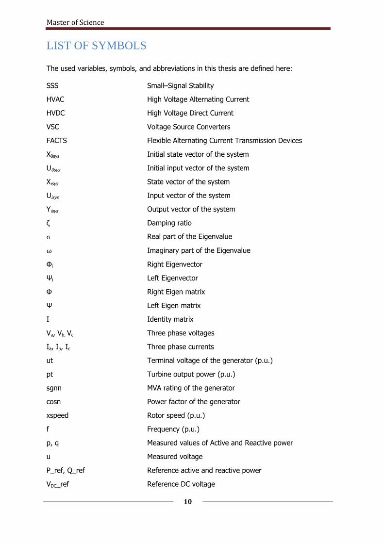
LIST OF SYMBOLS

The used variables, symbols, and abbreviations in this thesis are defined here: SSS Small–Signal Stability

HVAC High Voltage Alternating Current

HVDC High Voltage Direct Current

VSC Voltage Source Converters

FACTS Flexible Alternating Current Transmission Devices

X0sys Initial state vector of the system

U0sys Initial input vector of the system

Xisys State vector of the system

Uisys Input vector of the system

Yisys Output vector of the system

ζ Damping ratio

σ Real part of the Eigenvalue

⍵ Imaginary part of the Eigenvalue

Φi Right Eigenvector

Ψi Left Eigenvector

Φ Right Eigen matrix

Ψ Left Eigen matrix

I Identity matrix

Va, Vb, Vc Three phase voltages

Ia, Ib, Ic Three phase currents

ut Terminal voltage of the generator (p.u.)

pt Turbine output power (p.u.)

sgnn MVA rating of the generator

cosn Power factor of the generator

xspeed Rotor speed (p.u.)

f Frequency (p.u.)

p, q Measured values of Active and Reactive power

u Measured voltage

P_ref, Q_ref Reference active and reactive power

VDC_ref Reference DC voltage

Master of Science

11

id_ref, iq_ref d, and q axis reference currents

id, iq Output d and q axis currents

Pmr, Pmi Real and Imaginary part of Pulse–width modulation index

ve Field voltage of the Synchronous generator

Master of Science

12

LIST OF FIGURES

Figure 1:1–Adopted research approach flow chart ............................................................... 20

Figure 2:1– HVDC link monopole configuration .................................................................... 22

Figure 2:2– HVDC link bipole configuration .......................................................................... 23

Figure 2:3–Two stage VSC–converter ................................................................................. 23

Figure 2:4– VSC–converter station ...................................................................................... 24

Figure 2:5– Representation of a phasor in complex plane ..................................................... 26

Figure 2:6– dq0 equivalent circuit of VSC ............................................................................ 28

Figure 2:7– VSC control strategy overall block diagram [14] ................................................. 30

Figure 2:8: Inner current controller of a VSC ....................................................................... 30

Figure 2:9– Active power controller of a VSC ....................................................................... 31

Figure 2:10– DC voltage controller of a VSC ........................................................................ 31

Figure 2:11– Reactive power controller of a VSC .................................................................. 31

Figure 2:12– AC voltage controller of a VSC ........................................................................ 32

Figure 2:13– Point–to–point HVDC link operating principle block diagram .............................. 32

Figure 3:1–DIgSILENT power factory structure (inspired by DIgSILENT) [16] ......................... 34

Figure 3:2–Compsite frame of the generator and its controls ................................................ 35

Figure 3:3–Automatic voltage regulator (AVR) block definition .............................................. 36

Figure 3:4–AVR initial conditions ........................................................................................ 36

Figure 3:5–Speed governor block definition ......................................................................... 37

Figure 3:6–Speed governor initial conditions ....................................................................... 37

Figure 3:7–Two-area reference system [12] ........................................................................ 38

Figure 3:8–Implemented three-area HVAC system ............................................................... 39

Figure 3:9–Implemented three-area HVAC–DC system ......................................................... 40

Figure 3:10–Implemented point–to–point HVDC link ............................................................ 40

Figure 4:1–State space representation block diagram [12] .................................................... 44

Figure 4:2–Single input multiple output system block [17] .................................................... 49

Figure 4:3–Prony analysis input screen (DSI Toolbox) [18] ................................................... 52

Figure 4:4–Prony analysis output screen DIS toolbox [18] .................................................... 53

Figure 5:1– Eigenvalues with respect to AVR gain ................................................................ 54

Figure 5:2– Eigenvalues with respect to speed governor gain ............................................... 55

Figure 5:3–Participation factors Local mode area-1 .............................................................. 57

Figure 5:4–Mode shape area-1 ........................................................................................... 58

Figure 5:5–Participation factors Local mode area-2 .............................................................. 58

Master of Science

13

Figure 5:6–Mode shape area-2 ........................................................................................... 59

Figure 5:7–Participation factor inter-area mode ................................................................... 60

Figure 5:8–Mode shape inter-area mode ............................................................................. 60

Figure 5:9–Three–area HVAC system Eigenvalue plot w.r.t machine inertia ............................ 62

Figure 5:10–Participation factors local mode area-1 HVAC system ......................................... 63

Figure 5:11–Mode shape local area-1 HVAC system ............................................................. 64

Figure 5:12– Participation factors local mode area-2 HVAC system ........................................ 64

Figure 5:13–Mode shape local area-2 HVAC system ............................................................. 65

Figure 5:14–Participation factors local mode area-3 HVAC system ......................................... 65

Figure 5:15– Mode shape local mode area-3 HVAC system ................................................... 66

Figure 5:16– Participation factors inter-area mode area-1 and area-3 HVAC–DC system .......... 66

Figure 5:17–Mode shape inter–area mode area–1 and area–3 HVAC–DC system .................... 67

Figure 5:18–Participation factors inter–area mode area–1 and area–2 HVAC–DC system ......... 68


Figure 5:20–Three–area HVAC–DC system Eigenvalue plot w.r.t. machine inertia ................... 70

Figure 5:21– Participation factors local mode area-1 HVAC–DC system .................................. 71

Figure 5:22–Mode shape local area-1 HVAC–DC system ....................................................... 72

Figure 5:23–Participation factors local area mode–2 HVAC–DC system .................................. 72

Figure 5:24–Mode shape area–2 HVAC–DC system .............................................................. 73

Figure 5:25–Participation factors local mode area-3 HVAC–DC system ................................... 73

Figure 5:26–Mode shape local mode area–3 HVAC–DC system .............................................. 74

Figure 5:27–Participation factors inter–area mode area–1 and area–2 HVAC–DC system ......... 74


Figure 5:29–Step change in the torque for G1 and G2 at 5 seconds....................................... 77

Figure 5:30–Frequency and Phase response of signal G1 ...................................................... 78


Figure 5:32–Short–circuit on Line B at 1 second in HVAC system........................................... 80



Figure 5:35–Step increase in the torque at generator G6 at 5 seconds in HVAC system ........... 82

Figure 5:36–Frequency and Phase response of signal G5 local mode area–3 HVAC system ...... 83

Figure 5:37–Frequency and Phase response of signal G6 local mode area–3 HVAC system ...... 84

Figure 5:38–Line outage of Line-C at 5 seconds ................................................................... 85

Figure 5:39–Frequency and Phase response of signal G1 inter–area mode HVAC system ......... 86


Master of Science

14


Figure 5:42–Frequency and phase response of signal G4 inter–area mode HVAC system ......... 87

Figure 5:43–Line outage of line-C at 5 seconds HVAC–DC system ......................................... 88

Figure 5:44–Frequency and Phase response of signal G1 inter–area mode HVAC–DC system ... 89




Figure 5:48–Comparison between linear model and Prony's method ...................................... 94

LIST OF TABLES

Table 3-1: Generator specifications ..................................................................................... 38

Table 3-2: System load specifications ................................................................................. 38

Table 3-3: Generator specifications three-area system ......................................................... 41

Table 3-4: Load demand specification three–area system ..................................................... 41

Table 3-5: Time domain case studies .................................................................................. 41

Table 5-1: Electromechanical modes two-area reference system ........................................... 56

Table 5-2: Machine inertia operating points ......................................................................... 61

Table 5-3: HVAC system electr0–mechanical modes w.r.t. machine inertia ............................. 62

Table 5-4: Participation factors and right Eigenvectors ......................................................... 67

Table 5-5: Three–area HVAC–DC system operating conditions with respect to inertias ............ 69

Table 5-6: HVAC–DC system electro–mechanical modes with respect to machine inertias ........ 70

Table 5-7: Comparison between modal behavior .................................................................. 76

Table 5-8: Time domain study cases for Prony analysis ........................................................ 76

Table 5-9: Modal characteristics of local mode area–1 .......................................................... 78

Table 5-10: Modal characteristics of local mode area–2 ........................................................ 80

Table 5-11: Characteristics of the local mode area–3 ........................................................... 83

Table 5-12: Modal characteristics of inter–area mode area–1 and area–2 HVAC system .......... 85

Table 5-13: Modal characteristics of inter–area mode area–1 and area–2 HVAC–DC system .... 88

Table 5-14: Comparison between linear model and Prony analysis without controllers ............ 92

Table 5-15: Comparison between linear model and Prony analysis with controllers ................. 93

Master of Science

15

Master of Science

16

1 Introduction

Power systems have developed from their simple direct current systems to highly complex

systems to transfer the energy from the sources to users. They generally comprise of

components like high voltage cables, transmission lines, power electronics devices, Flexible

Alternating Current Transmission System (FACTS) devices, generation systems and

transformers etc. The modern systems are highly interconnected over country borders and

even continents and operated throughout the year without any breaks. Power system is the

primary means to transmit the energy generated from various sources (thermal, wind, hydro

etc.) to industrial, commercial and residential users. The various sources used for generating

electricity, have different control mechanism and can be an AC or a DC source.

The electrical power system is mainly divided into generation, transmission and distribution

systems. These systems are predominantly operated at a constant frequency and voltage

levels. The standard frequencies and voltage levels differ from place to place like for example,

in US the standard frequency is 60 Hz and in Europe and Asian countries it is 50 Hz. The

primary use of transformers is to step–up and step–down between different transmission and

sub–transmission level voltages. The introduction of the High Voltage Direct Current (HVDC)

technologies has made it possible to have an interconnection between different standards in

fundamental frequencies.

The main purpose of introducing HVDC is to control the transmitted electrical power and

to enable bulk transmission of electrical power. Different technologies are used in the

converter station to convert from AC to DC and vise– versa. One of the technologies used is

the Line Commutated Converter (LCC) technology. LCCs are reasonable, easy to build and can

handle a large amount of power, which makes it more reliable. But, there are few

disadvantages, like when the direction of the power flow changes, the polarity has to be

changed and this creates problems. The other disadvantage is that these LCCs are difficult to

operate in a meshed grid.

Due to the limitations in the LCCs, the Voltage Source Converters (VSCs) are well suited

for modern transmission network applications. The VSCs incorporate power electronic switches

like IGBTs and GTOs that are self–commutating and change the polarity by changing the

direction of the current flow. The VSCs have black start capabilities that do not require AC filters

and a higher power quality in the AC system. This technology has led to the successful

interconnection of off–shore windfarms to the rest of the grid. As a consequence, there is a high

penetration of renewable sources of energy into the electrical generation sector.

Master of Science

17

A real time power system has both AC and DC transmission systems. These systems are

known as hybrid power systems. The operation, planning and dynamic studies of hybrid

systems require in–depth analysis involving the development of detailed models of the power

networks and simulating the dynamic phenomenon like short–circuits studies, dynamic

responses of the generators and their control mechanisms in the network. The purpose is to

achieve a high degree of reliability, safety and permissible operating points from the stability

point of view.

Since the power systems are highly inter–connected with HVAC and HVDC transmission

lines and different type of sources along with their control mechanisms, the stability of the

system is a primary concern. The three major types of stability studies are rotor angle stability,

voltage stability, frequency stability. These stability studies are carried out for a small time

ranging from few milliseconds to long term (months and years). Power system stability studies

are required to achieve a high degree of reliability, stable operating points and protects the

system from faults at peak load conditions.

To obtain more accurate models and have in–depth studies, various sophisticated software

packages, such as Matlab, PSCAD, RSCAD, EMTP and DIgSILENT Power factory have been

introduced to electrical power engineers in recent times. Power Factory in particular is an

object-oriented software package used for modeling and simulation of the electrical power

network systems. This software package is highly structured and supports both graphical and

scripting interfaces with PYTHON etc. This software package can be used for RMS/RMT

simulations, load flow calculations, sensitivity analysis and modal analysis.

This thesis work mainly focuses on the small–signal stability analysis of hybrid grids. In this

thesis work, the effect of introducing a new renewable source to the existing grid is studied, with

attention to different machine inertias from a stability point of view. The in–depth analysis of

effect of machine inertia in a HVAC dominant and a hybrid grid situation is addressed.

1.1 Literature

A reliable service of electricity, demands a power system that withstands disturbances of

various types and magnitudes. Further, the system is designed and operated such that the

probable contingencies are sustained with no loss in the loads and the most adverse possible

contingencies do not result in widespread power interruptions. Research has been done in

power system stability since the 1920s. Kundur and .co in [2] [3]studied the different modes of

oscillations that exits in a weakly interconnected power system which was the root cause to

many blackouts in the recent times (North India, July–2012, Bangladesh November–2014,

South Brazil 1999, United States and Canada 1965).

Master of Science

18

Small Signal Stability (SSS) being a critical issue in meshed power systems more of

research has gone into this aspect [4]. In the modern times, due to the introduction of the

renewable energy sources like wind, solar, hydro and nuclear power, the SSS is one of the most

critical issues that needs to be addressed in grid planning and development studies. The

authors in [5] studied the different topologies of windfarms and there interconnection with

HVDC technology. Especially with the high penetration of the renewable sources there are

number of challenges to be dealt in power grids. First the generators introduce an uncertainty

into the scheduled power dispatch, which results in the generated power.

The introduction of HVDC technology has led to different directions like modelling VSC

converters, different control strategies to control the power transmission [6] [7]. A more

general approach to control the active power is given by the authors in [8]. Thus, investigating

the SSS with respect to system integration point of view in an important topic to be addressed.

Different modes of oscillations arise in huge and complex power systems and they are

classified based on the frequency ranges and the type of oscillations generated. In the

publications [9] [10] [11] the effect the dominant modes of oscillations are identified in

standard IEEE/CIGRE grid models. These power system oscillations can be stimulated due to a

disturbance in the power system operating condition or the steady state boundaries of the

various components in the system are crossed. The oscillations can be troublesome to the

power system if they are not damped. For this purpose, various controls like power system

stabilizers, speed governors are used by the authors in [13] The modern hybrid (HVAC-HVDC)

power systems have VSC based converter terminals as the dynamic devices whose interaction,

modeling and control strategies is the hot topic in the recent years [1] [14].

Most of the studies on system planning and integration of High Voltage Direct Current

(HVDC) transmission systems focusing on the fulfillment of explicit technical requirements [11]

These limits include static (e.g. thermal) and dynamic (e.g. voltage and frequency) constraints.

From the literature studies it is inferred that various studies have been done on AC dominated

systems. The stability issues have been addressed with different control strategies. There has

been research done on different technologies like LCC and VSC. But, in the modern power

sector, due to environment concerns, there is an increasing demand towards incorporating low

inertia machines (Wind turbines, small hydro turbines). The inertia being an inherent property of

the synchronous machines the frequency levels and the dynamics immediately after small

disturbances is governed by the inertial properties of the machines. This is important in weakly

meshed grids, where low inertia machines are a predominant source. In the near foreseen

future, there shall be more HVAC grids incorporated with more and more HVDC links in the

Master of Science

19

electrical power sector. It is of high importance to address the SSS issues of a hybrid network

from the system integration point of view and the effect of incorporating low inertia machines

into the existing system. This leads us to the research questions that are addressed in this

thesis work.

1.2 Research Questions

The objective of this research work is to study the impact of machine inertia on the

damping and the frequencies of the electromechanical oscillatory modes in a HVAC system and

a hybrid (HVAC–DC) power system.

1. How does the usage of different inertia machines affect the system stability?

2. How does incorporating HVDC links into an existing weak HVAC grid affect the system

stability?

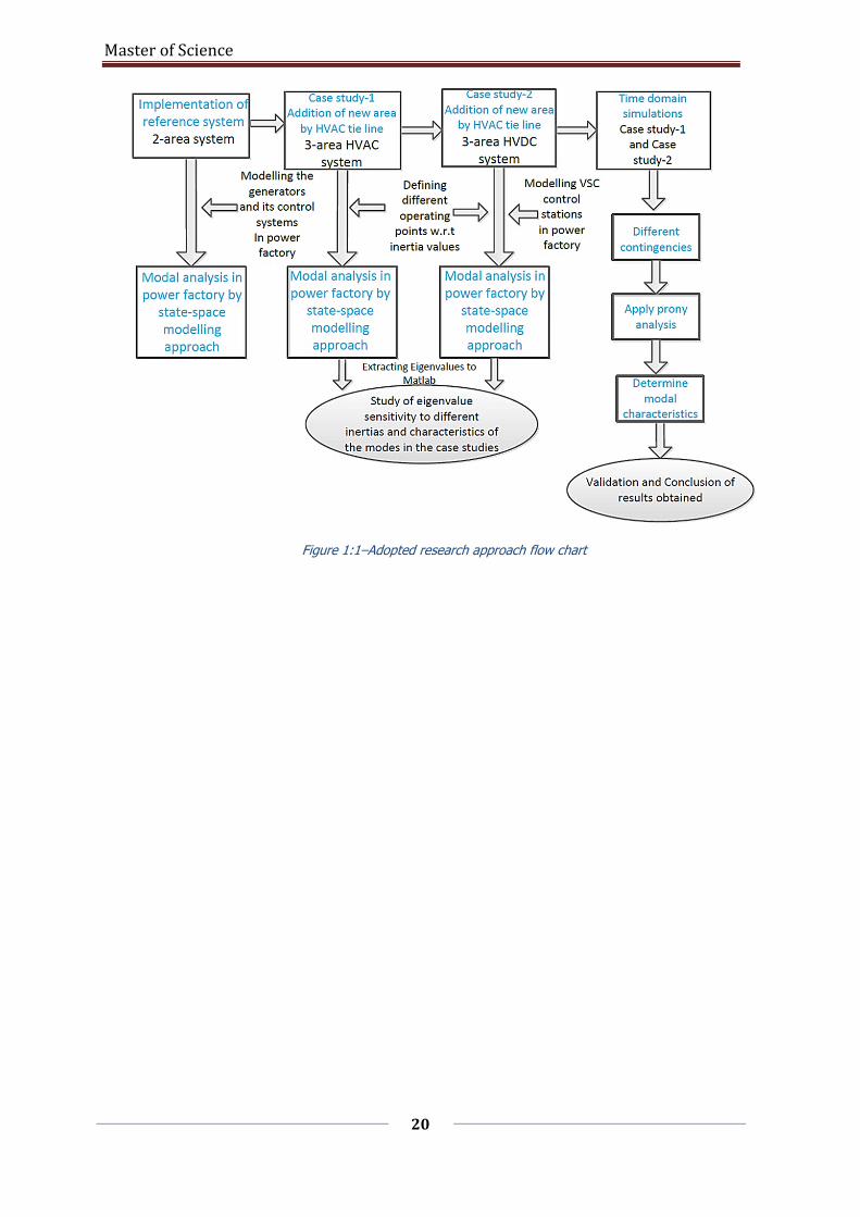
1.3 Research Approach

The overall research approach of this thesis work is presented in the Figure–1.1 below.

STEP: 1 A reference system is first developed from literature. This is a fundamental two–area

system which is weakly meshed.

STEP: 2 A new area is incorporated to the developed reference system. Two cases are defined

at this stage. In the first case, the third area is connected with an HVAC tie line. In the second

case the third area is connected with an HVDC link.

STEP: 3 The small signal stability analysis is performed by subjecting the system to small

disturbances, thereby defining different study cases through relevant time domain simulations in

DIgSILENT power factory.

STEP: 4 The SSS results obtained by power factory are validated by signal record based method

(Prony analysis).

Master of Science

20

Figure 1:1–Adopted research approach flow chart

Master of Science

21

Master of Science

22

2 HVDC–VSC Converters Modeling

The HVDC transmission technology is the most advanced technology for transmitting

electrical power over long distances. Analogous to HVAC transmission systems, this mode of

transmission uses HVDC overhead lines and undersea cables. This mode of transmission is much

more reliable and has a fast and stable control system compared to its counterpart. The major

advantage of HVDC transmission system is it allows two systems to be operated at difference

fundamental frequencies. This was first introduced on commercial bases in 1954. Until then, the

thyristors were used in the HVDC transmission systems until the modern HVDC–VSCs were

introduced to the HVDC transmission system. At present, the VSCs are the primary candidates in

HVDC transmission systems. The VSCs are FACTS devices used predominantly in HVDC

transmission. The VSC is a converter with Integrated Gate Bipolar Transistors (IGBTs) valves.

2.1 HVDC configurations

The VSCs are arranged in two configurations, namely monopole and bipole configurations.

Figure 2.1 and Figure 2.2 shows the monopole and bipolar configurations. In the monopole

link, the converters are connected with a single DC transmission line operated at positive or

negative polarity. In this configuration, the return path of the current is the ground itself. This

configuration is easy to control and has low-cost maintenance. On the other hand, the bipolar

configuration is the most common mode of HVDC transmission where two monopole

configurations is used which improves the performance of the system and is more reliable. In

this configuration, the mid–point of the system is connected to the ground and there are four

VSC stations involved. In the configuration, one of the transmission lines is maintained at

positive and negative polarity respectively. The main advantage of this configuration is the

possibility of controlling the power flow in each transmission line independently, and only one

pole can be operated when the other pole is out of service.

Figure 2:1– HVDC link monopole configuration

Master of Science

23

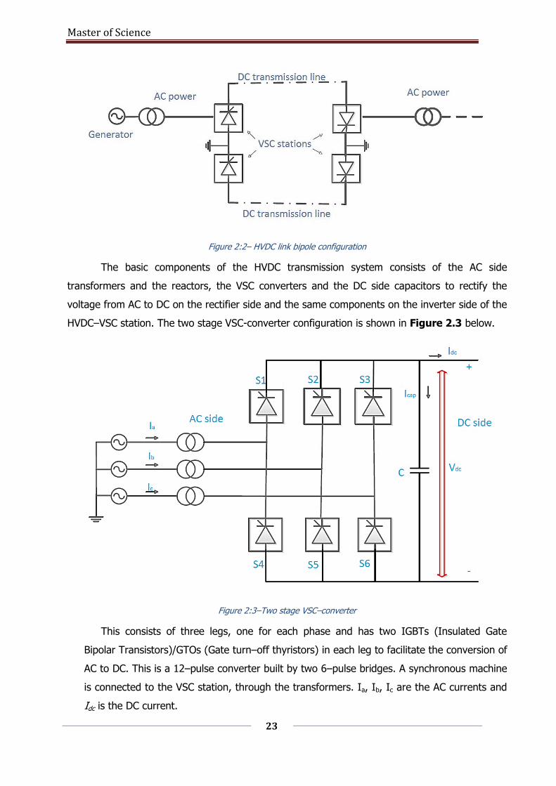
Figure 2:2– HVDC link bipole configuration

The basic components of the HVDC transmission system consists of the AC side

transformers and the reactors, the VSC converters and the DC side capacitors to rectify the

voltage from AC to DC on the rectifier side and the same components on the inverter side of the

HVDC–VSC station. The two stage VSC-converter configuration is shown in Figure 2.3 below.

Figure 2:3–Two stage VSC–converter

This consists of three legs, one for each phase and has two IGBTs (Insulated Gate

Bipolar Transistors)/GTOs (Gate turn–off thyristors) in each leg to facilitate the conversion of

AC to DC. This is a 12–pulse converter built by two 6–pulse bridges. A synchronous machine

is connected to the VSC station, through the transformers. Ia, Ib, Ic are the AC currents and

Idc is the DC current.

Master of Science

24

Switches are represented by S1, S2 S3, S4, S5 and S6. The size of the capacitor depends

on the transmission voltage levels. The purpose of the capacitor is to provide a low inductive

reactance path for the turn off current and control the active power flow in the line. The

ripple in the voltage is reduced by the capacitor.

On the AC side of the system, the VSC behaves as a constant current source and the on

the DC side it behaves as a constant voltage source. As a result, on the AC side there are AC

reactors to eliminate the harmonics coming from the AC side of the system and for energy

storage, similarly on the DC side, the capacitor is used as the energy storage device.

2.2 VSC converters theoretical background

There are various control strategies to control the active power, reactive power, voltage

on AC and DC sides of the VSC converters. The basis of the control strategy is given by space

vector theory [8] [14]. The background of the control strategies is described in this section. The

fundamental active and reactive power equations are given by the following expressions [12]:

X

sinP

UU sr

(2.1)

X

cosQ

UUU rsr

2

(2.2)

In the equations 2.1 and 2.2, 𝒫 and 𝒬 are the active and the reactive power

respectively. 𝑈𝑆 and 𝑈𝑅 are the sending and the receiving end voltages respectively. 𝑋is the total

reactance of the transmission line and 𝛿 is the total phase angle of the receiving and sending

end voltages. From the above equations, it is clear that the active power is sensitive to the

phase angle and the reactive power is sensitive to the voltage magnitudes.

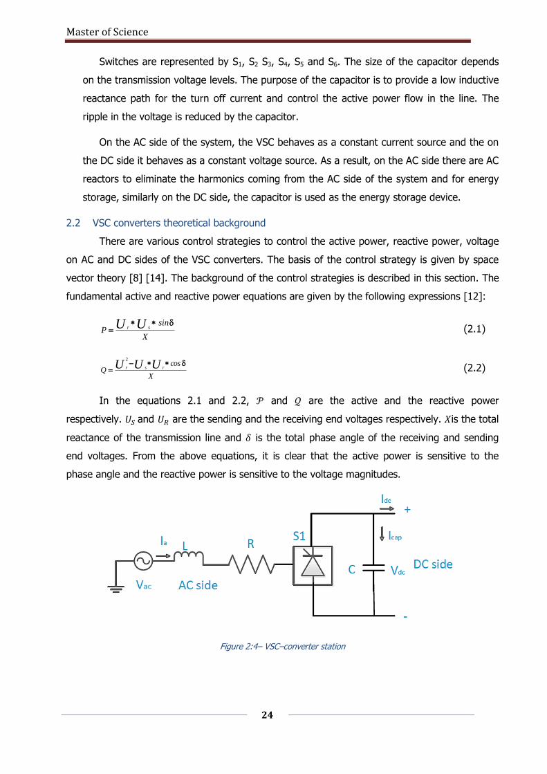
Figure 2:4– VSC–converter station

Master of Science

25

Before diving into the VSC control strategy in a d-q frame, it is very important to

understand the basic terminologies and the definitions from space vector theory. A single VSC-

converter station leg is shown in Figure 2.4. Generally, the power systems are analyzed by

symmetrical components. These transformations decouple the symmetric systems. But the

space vector theory gives a more general way of analyses of the power systems especially in the

case of VSC technology. The spatial vector transformation is given by the following equations:

eieii

evevvj

c

j

ba

j

c

j

ba

tttti

ttttv

3

2

3

4

3

4

3

2

3

2

3

2

(2.3)

In the above equation 2.3, 𝑉(𝑡)→ and

𝐼(𝑡)→ are the space vectors of voltages and currents of

the three-phase symmetrical system respectively. It has to be noted here that the space vectors

of the currents and the voltages are rotating in both space and time simultaneously [8]. The

voltagesva, vb

and vcthe currentsia

, iband ic

are sinusoidal in nature which is defined by

equation 2.4.

3

4

3

2

tsinVt

tsinVt

tsinVt

v

v

v

c

b

a

3

2

3

4

tsinIt

tsinIt

tsinIt

i

i

i

c

b

a

(2.4)

Now the space vector of the instantaneous apparent power is given by equation 2.5:

titvts (2.5)

Substituting the equation 2.3 and 2.4 in 2.5, we obtain the instantaneous apparent power as in

equation 2.6:

tsinjcosIVts 22

3 (2.6)

The apparent power obtained in the above equation 2.6, is also rotating in space and

time simultaneously. It is clear that the expression for the apparent power ts consists of the

active and the reactive power component. The active and the reactive powers are controlled

independently by the VSC in a d-q frame.

The conversion of a three–phase sinusoidal system to a d-q frame is done by the Park’s

transformation matrix which includes an intermediate 𝛼-β-0 transformation and the phase–

Master of Science

26

rotation matrix transformation which results in a d–q–0 frame of control. This is depicted in

equation 2.7 below:

vvv

VVV

c

b

a

q

d

P

0

(2.7)

Where [𝑃 (θ) ] is the Park's transformation matrix which includes Clarke's transformation

and the rotation of the phasor along the axis. The Clark’s and the rotation matrix are given by

the equation 2.8 below:

2

1

2

1

2

13

2

3

2

3

2

3

2

2

1

2

1

2

12

3

2

30

2

1

2

11

3

2sinsinsin

coscoscos

P (2.8)

Using the above transformation in equation 2.8, the three phase sinusoidal quantities

can be reproduced in terms of dq0 terms. The VSC control strategy is always implemented in

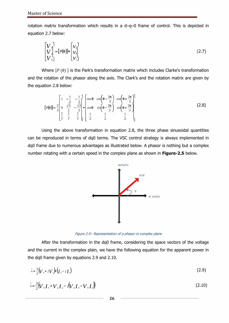
dq0 frame due to numerous advantages as illustrated below. A phasor is nothing but a complex

number rotating with a certain speed in the complex plane as shown in Figure-2.5 below.

Figure 2:5– Representation of a phasor in complex plane

After the transformation in the dq0 frame, considering the space vectors of the voltage

and the current in the complex plain, we have the following equation for the apparent power in

the dq0 frame given by equations 2.9 and 2.10.

IIVV qdqdjjs

2

3 (2.9)

IVIVIVIV qddqqqddjs

2

3 (2.10)

Master of Science

27

In the above equations 2.9 and 2.10 for the apparent power in the dq0 frame, it is

observed that the terms are no more time variant, i.e. they are DC terms, which is the most

important advantage of the Park’s transformation. The consequence of this transformation can

be realized by eliminating the term 𝑉𝑞 in equations 2.9 and 2.10. This is the done because, in

the transformation process, the voltage phasor is considered to be rotating at the same speed

as that of the d–axis. In other words, the space vector of the voltage is aligned with the d-axis

which eliminates its projection on the imaginary axis or the q-axis in the complex plane. Hence

eliminating 𝑉𝑞 in the equation of apparent power 2.10 we obtain the equation 2.11:

IjV

IV

IjVIV

qd

dd

qddd

Q

P

s

2

3

2

3

2

3

(2.11)

In the above equation 2.11 as result of Park’s transformation, we can observe that the

real and the reactive powers are decoupled. The active power is a function of current I d and the

reactive power is a function of current I q. As a consequence of dq0 transformation, a decoupling

of the active and reactive power is achieved and the quantities are DC constants which are then

fed to the VSCs in the grid. In the above equations, it should be clear that the zero sequence

component or the homo-polar component is considered to be 0.

2.3 Equivalent circuits in dq0-frame

To derive the equivalent circuits in the dq0 frame of the VSC, we apply KVL to the circuit

in Figure 2.6. If E abc,V abc

, and I abcare the three-phase grid voltages, convertor input voltages

and the grid current respectively, then we have:

RVI

E abcabc

abc

abc tL

d

d (2.12)

After the Park’s transformation we obtain the quantities in the dq0 frame. This is depicted by

the equation 2.13.

VVV

III

RR

R

III

III

EEE

q

d

q

d

c

b

a

q

d

q

d

q

d

Ldt

dL

0000000

00

00

000

001

010

(2.13)

From the above equation we obtain the decoupled equations in dq0 frame as follows:

Master of Science

28

IVII

E

IVII

E

qqd

q

q

ddq

d

d

R**L*t

L

R**L*t

L

ωd

d

ωd

d

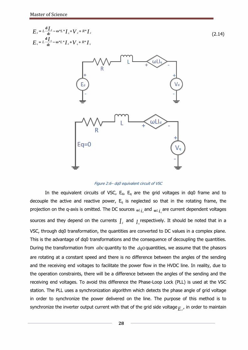
(2.14)

Figure 2:6– dq0 equivalent circuit of VSC

In the equivalent circuits of VSC, Ed, Eq are the grid voltages in dq0 frame and to

decouple the active and reactive power, Eq is neglected so that in the rotating frame, the

projection on the q-axis is omitted. The DC sources idL and iq

L are current dependent voltages

sources and they depend on the currents I d and I q

respectively. It should be noted that in a

VSC, through dq0 transformation, the quantities are converted to DC values in a complex plane.

This is the advantage of dq0 transformations and the consequence of decoupling the quantities.

During the transformation from abc quantity to the 0dq quantities, we assume that the phasors

are rotating at a constant speed and there is no difference between the angles of the sending

and the receiving end voltages to facilitate the power flow in the HVDC line. In reality, due to

the operation constraints, there will be a difference between the angles of the sending and the

receiving end voltages. To avoid this difference the Phase-Loop Lock (PLL) is used at the VSC

station. The PLL uses a synchronization algorithm which detects the phase angle of grid voltage

in order to synchronize the power delivered on the line. The purpose of this method is to

synchronize the inverter output current with that of the grid side voltagedE , in order to maintain

Master of Science

29

a unity power factor . The inputs of the PLL model are the three phase voltages V abc

measured

on the grid side and the output is the tracked phase angle . The PLL model is implemented

in synchronous dq0 reference frame by implementing Park’s transformation. The phase-locking

of the system is realized by adjusting the q-axis voltage to zero. By using the integrator of the

PI controller, the sum between the PI output and the reference frequency of the phase angle is

obtained.

2.4 VSC control methods

The main purpose of VSC is to control the active power in the HVDC line/cable and maintain

a constant voltage at the DC terminals. The VSC internal structure is shown in Figure-2.7

below. A VSC converter basically has a fast inner control loop and a slow outer control loop. The

inner control loop consists of a current controller which controls the pulse width modulation

index of the converter taking in the dq0–axis currents and the reference dq–axis currents from

the outer controllers. The outer controllers define the control modes of the converter for a

particular VSC control station [14]. A VSC station is controlled in four control modes namely:

Constant DC voltage mode

Active power control mode

Reactive power control mode

AC voltage control mode

Master of Science

30

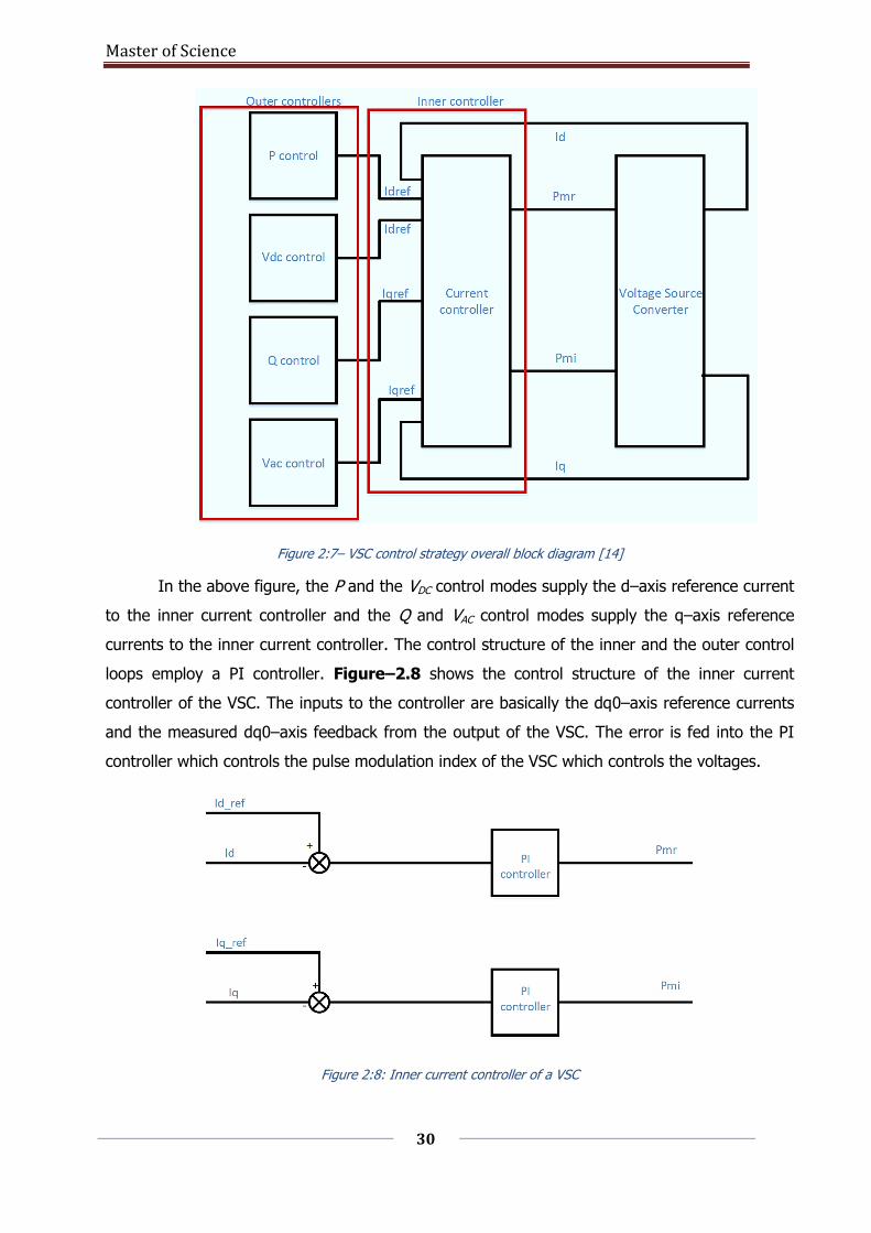
Figure 2:7– VSC control strategy overall block diagram [14]

In the above figure, the P and the VDC control modes supply the d–axis reference current

to the inner current controller and the Q and VAC control modes supply the q–axis reference

currents to the inner current controller. The control structure of the inner and the outer control

loops employ a PI controller. Figure–2.8 shows the control structure of the inner current

controller of the VSC. The inputs to the controller are basically the dq0–axis reference currents

and the measured dq0–axis feedback from the output of the VSC. The error is fed into the PI

controller which controls the pulse modulation index of the VSC which controls the voltages.

Figure 2:8: Inner current controller of a VSC

Master of Science

31

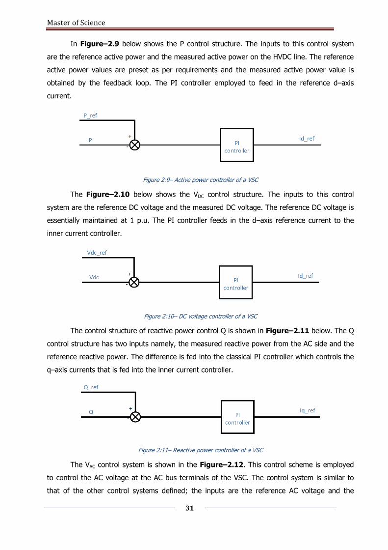
In Figure–2.9 below shows the P control structure. The inputs to this control system

are the reference active power and the measured active power on the HVDC line. The reference

active power values are preset as per requirements and the measured active power value is

obtained by the feedback loop. The PI controller employed to feed in the reference d–axis

current.

Figure 2:9– Active power controller of a VSC

The Figure–2.10 below shows the VDC control structure. The inputs to this control

system are the reference DC voltage and the measured DC voltage. The reference DC voltage is

essentially maintained at 1 p.u. The PI controller feeds in the d–axis reference current to the

inner current controller.

Figure 2:10– DC voltage controller of a VSC

The control structure of reactive power control Q is shown in Figure–2.11 below. The Q

control structure has two inputs namely, the measured reactive power from the AC side and the

reference reactive power. The difference is fed into the classical PI controller which controls the

q–axis currents that is fed into the inner current controller.

Figure 2:11– Reactive power controller of a VSC

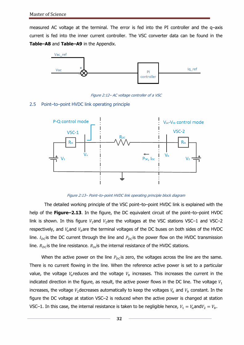
The VAC control system is shown in the Figure–2.12. This control scheme is employed

to control the AC voltage at the AC bus terminals of the VSC. The control system is similar to

that of the other control systems defined; the inputs are the reference AC voltage and the

Master of Science

32

measured AC voltage at the terminal. The error is fed into the PI controller and the q–axis

current is fed into the inner current controller. The VSC converter data can be found in the

Table–A8 and Table–A9 in the Appendix.

Figure 2:12– AC voltage controller of a VSC

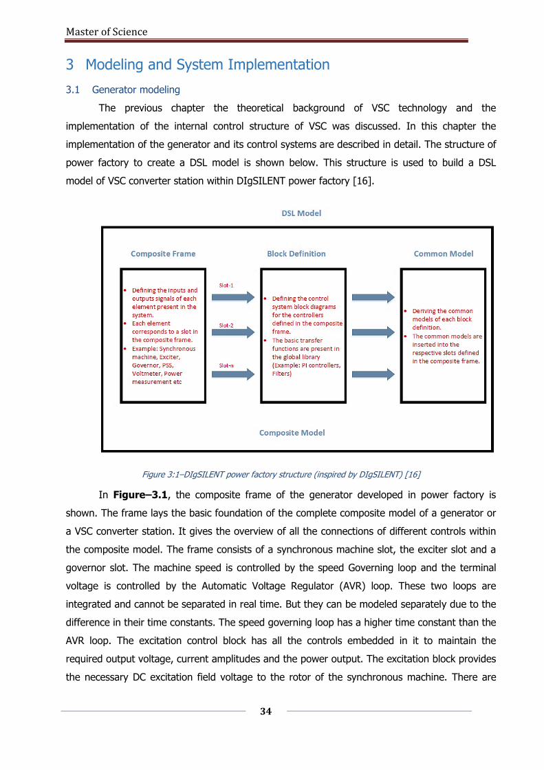
2.5 Point–to–point HVDC link operating principle

Figure 2:13– Point–to–point HVDC link operating principle block diagram

The detailed working principle of the VSC point–to–point HVDC link is explained with the

help of the Figure–2.13. In the figure, the DC equivalent circuit of the point–to–point HVDC

link is shown. In this figure 𝑉1and 𝑉2are the voltages at the VSC stations VSC–1 and VSC–2

respectively, and 𝑉𝑎and 𝑉𝑏are the terminal voltages of the DC buses on both sides of the HVDC

line. 𝐼𝐷𝐶is the DC current through the line and 𝑃𝐷𝐶 is the power flow on the HVDC transmission

line. 𝑅𝐷𝐶 is the line resistance. 𝑅𝑖𝑛is the internal resistance of the HVDC stations.

When the active power on the line 𝑃𝐷𝐶 is zero, the voltages across the line are the same.

There is no current flowing in the line. When the reference active power is set to a particular

value, the voltage 𝑉𝑎reduces and the voltage 𝑉𝑏 increases. This increases the current in the

indicated direction in the figure, as result, the active power flows in the DC line. The voltage 𝑉1

increases, the voltage 𝑉2decreases automatically to keep the voltages 𝑉𝑎 and 𝑉𝑏 constant. In the

figure the DC voltage at station VSC–2 is reduced when the active power is changed at station

VSC–1. In this case, the internal resistance is taken to be negligible hence, 𝑉1 = 𝑉𝑎and𝑉2 = 𝑉𝑏.

Master of Science

33

Master of Science

34

3 Modeling and System Implementation

3.1 Generator modeling

The previous chapter the theoretical background of VSC technology and the

implementation of the internal control structure of VSC was discussed. In this chapter the

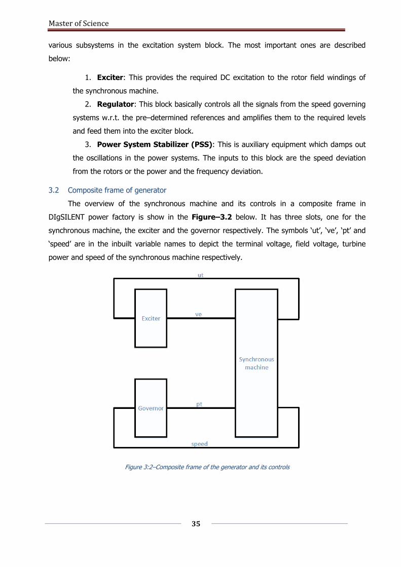
implementation of the generator and its control systems are described in detail. The structure of

power factory to create a DSL model is shown below. This structure is used to build a DSL

model of VSC converter station within DIgSILENT power factory [16].

Figure 3:1–DIgSILENT power factory structure (inspired by DIgSILENT) [16]

In Figure–3.1, the composite frame of the generator developed in power factory is

shown. The frame lays the basic foundation of the complete composite model of a generator or

a VSC converter station. It gives the overview of all the connections of different controls within

the composite model. The frame consists of a synchronous machine slot, the exciter slot and a

governor slot. The machine speed is controlled by the speed Governing loop and the terminal

voltage is controlled by the Automatic Voltage Regulator (AVR) loop. These two loops are

integrated and cannot be separated in real time. But they can be modeled separately due to the

difference in their time constants. The speed governing loop has a higher time constant than the

AVR loop. The excitation control block has all the controls embedded in it to maintain the

required output voltage, current amplitudes and the power output. The excitation block provides

the necessary DC excitation field voltage to the rotor of the synchronous machine. There are

Master of Science

35

various subsystems in the excitation system block. The most important ones are described

below:

1. Exciter: This provides the required DC excitation to the rotor field windings of

the synchronous machine.

2. Regulator: This block basically controls all the signals from the speed governing

systems w.r.t. the pre–determined references and amplifies them to the required levels

and feed them into the exciter block.

3. Power System Stabilizer (PSS): This is auxiliary equipment which damps out

the oscillations in the power systems. The inputs to this block are the speed deviation

from the rotors or the power and the frequency deviation.

3.2 Composite frame of generator

The overview of the synchronous machine and its controls in a composite frame in

DIgSILENT power factory is show in the Figure–3.2 below. It has three slots, one for the

synchronous machine, the exciter and the governor respectively. The symbols ‘ut’, ‘ve’, ‘pt’ and

‘speed’ are in the inbuilt variable names to depict the terminal voltage, field voltage, turbine

power and speed of the synchronous machine respectively.

Figure 3:2–Composite frame of the generator and its controls

Master of Science

36

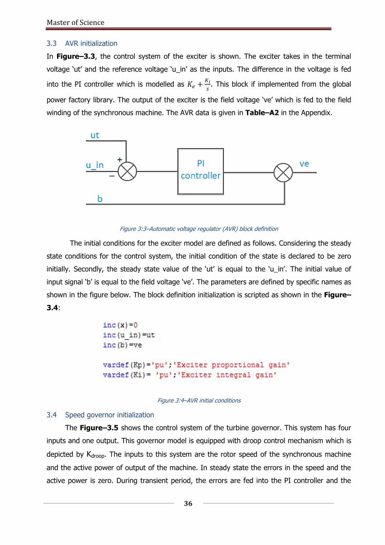
3.3 AVR initialization

In Figure–3.3, the control system of the exciter is shown. The exciter takes in the terminal

voltage ‘ut’ and the reference voltage ‘u_in’ as the inputs. The difference in the voltage is fed

into the PI controller which is modelled as 𝐾𝑒 +𝐾𝑖

𝑠. This block if implemented from the global

power factory library. The output of the exciter is the field voltage ‘ve’ which is fed to the field

winding of the synchronous machine. The AVR data is given in Table–A2 in the Appendix.

Figure 3:3–Automatic voltage regulator (AVR) block definition

The initial conditions for the exciter model are defined as follows. Considering the steady

state conditions for the control system, the initial condition of the state is declared to be zero

initially. Secondly, the steady state value of the ‘ut’ is equal to the ‘u_in’. The initial value of

input signal ‘b’ is equal to the field voltage ‘ve’. The parameters are defined by specific names as

shown in the figure below. The block definition initialization is scripted as shown in the Figure–

3.4:

Figure 3:4–AVR initial conditions

3.4 Speed governor initialization

The Figure–3.5 shows the control system of the turbine governor. This system has four

inputs and one output. This governor model is equipped with droop control mechanism which is

depicted by Kdroop. The inputs to this system are the rotor speed of the synchronous machine

and the active power of output of the machine. In steady state the errors in the speed and the

active power is zero. During transient period, the errors are fed into the PI controller and the

Master of Science

37

turbine output power is fed into the synchronous machine. The other characteristics of this

governor are that this governor operation results in both frequency stability and the rotor angle

stability. From the speed inputs, the frequency of the system is maintained within the limits and

the active power inputs results in rotor angle stability. The governor has two loops, the loop

with the speed inputs is the primary control loop and the secondary control loop is the active

power inputs. The speed governor data is given in Table–A3 and Table–A4 in the Appendix.

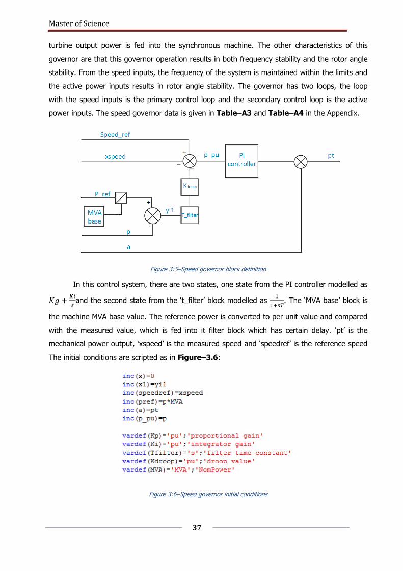
Figure 3:5–Speed governor block definition

In this control system, there are two states, one state from the PI controller modelled as

𝐾𝑔 +𝐾𝑖

𝑠and the second state from the ‘t_filter’ block modelled as

1

1+𝑠𝑇. The ‘MVA base’ block is

the machine MVA base value. The reference power is converted to per unit value and compared

with the measured value, which is fed into it filter block which has certain delay. ‘pt’ is the

mechanical power output, ‘xspeed’ is the measured speed and ‘speedref’ is the reference speed

The initial conditions are scripted as in Figure–3.6:

Figure 3:6–Speed governor initial conditions

Master of Science

38

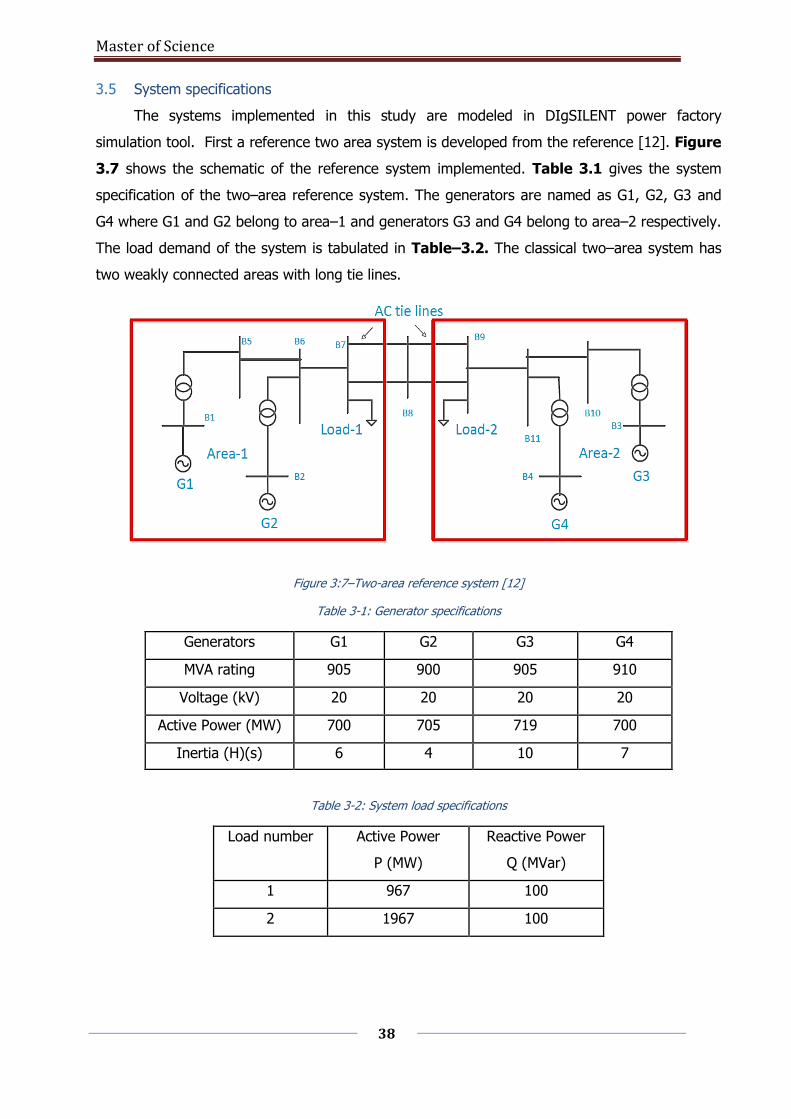
3.5 System specifications

The systems implemented in this study are modeled in DIgSILENT power factory

simulation tool. First a reference two area system is developed from the reference [12]. Figure

3.7 shows the schematic of the reference system implemented. Table 3.1 gives the system

specification of the two–area reference system. The generators are named as G1, G2, G3 and

G4 where G1 and G2 belong to area–1 and generators G3 and G4 belong to area–2 respectively.

The load demand of the system is tabulated in Table–3.2. The classical two–area system has

two weakly connected areas with long tie lines.

Figure 3:7–Two-area reference system [12]

Table 3-1: Generator specifications

Generators G1 G2 G3 G4

MVA rating 905 900 905 910

Voltage (kV) 20 20 20 20

Active Power (MW) 700 705 719 700

Inertia (H)(s) 6 4 10 7

Table 3-2: System load specifications

Load number Active Power

P (MW)

Reactive Power

Q (MVar)

1 967 100

2 1967 100

Master of Science

39

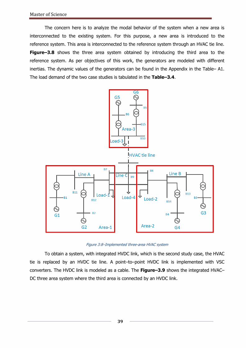
The concern here is to analyze the modal behavior of the system when a new area is

interconnected to the existing system. For this purpose, a new area is introduced to the

reference system. This area is interconnected to the reference system through an HVAC tie line.

Figure–3.8 shows the three area system obtained by introducing the third area to the

reference system. As per objectives of this work, the generators are modeled with different

inertias. The dynamic values of the generators can be found in the Appendix in the Table– A1.

The load demand of the two case studies is tabulated in the Table–3.4.

Figure 3:8–Implemented three-area HVAC system

To obtain a system, with integrated HVDC link, which is the second study case, the HVAC

tie is replaced by an HVDC tie line. A point–to–point HVDC link is implemented with VSC

converters. The HVDC link is modeled as a cable. The Figure–3.9 shows the integrated HVAC–

DC three area system where the third area is connected by an HVDC link.

Master of Science

40

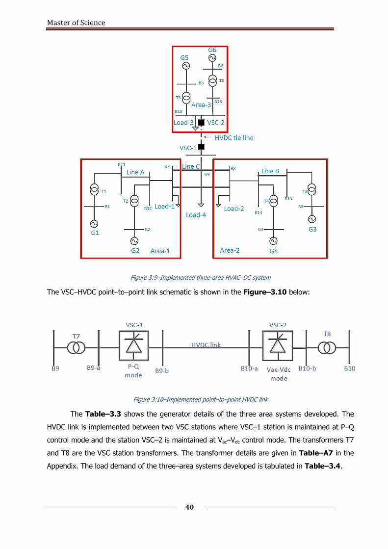
Figure 3:9–Implemented three-area HVAC–DC system

The VSC–HVDC point–to–point link schematic is shown in the Figure–3.10 below:

Figure 3:10–Implemented point–to–point HVDC link

The Table–3.3 shows the generator details of the three area systems developed. The

HVDC link is implemented between two VSC stations where VSC–1 station is maintained at P–Q

control mode and the station VSC–2 is maintained at Vac–Vdc control mode. The transformers T7

and T8 are the VSC station transformers. The transformer details are given in Table–A7 in the

Appendix. The load demand of the three–area systems developed is tabulated in Table–3.4.

Master of Science

41

Table 3-3: Generator specifications three-area system

Generators G1 G2 G3 G4 G5 G6

MVA rating 1000 900 1100 1010 890 850

Voltage (kV) 20 20 20 20 20 20

Active Power (MW) 700 700 719 500 1000 250

Table 3-4: Load demand specification three–area system

Load

number

Active Power

P (MW)

Reactive Power

Q (MVar)

1 900 150

2 950 150

3 1500 0

4 2200 150

The objective is to study the behavior of the electromechanical oscillations when

different inertia machines are incorporated into the system operating at peak loads. The

different time–domain case studies defined for the purpose of spectral analysis are summarized

in Table–3.5.

Table 3-5: Time domain case studies

Type of disturbance Element of the

system Type of Mode excited Type of system

Three–phase fault

event Line–B Local mode area–2

Three–area HVAC

system

Step change in

generator torques G1 and G2 Local mode area–1

Three–area HVAC

system

Step change in torque G5 Local mode area–3 Three–area HVAC

system

Line outage event Line–C Inter–area mode

area–1 and area–2

Three–area HVAC

system



Three–area HVAC–

DC system

Master of Science

42

4 Linearized Modeling and Prony Analysis1

4.1 State–space model theory

Power system stability is the inherent property of an electrical power system that

enables the system to stay in the state of equilibrium under normal operating conditions and

regain an acceptable state of equilibrium after being subjected to disturbance/disturbances. One

of the categories in this context is the SSS, which is defined as the ability of the power system

to maintain a synchronism when subjected to small disturbances. Eigenvalue based SSS

assessment is one of the common way to assess the SSS of the system, which is a frequency-

based approach. This assessment is done by linearizing the power system around an operating

point and analyzing the stability of the complete system by the obtained Eigenvalues.

The behavior of a power system is described as a set of ordinary nonlinear differential equations

given by the equation 4.1:

:t,:,f isysisys

uuuxxxt

xr.... . . .2,1n..... . .2,1

.

d

d (4.1)

Where, n.......,,i 321 and n is the order of the system with r inputs to the system with respect

to time t .

Let 𝑥0𝑠𝑦𝑠 and 𝑢𝑜𝑠𝑦𝑠 be the initial state vector and the input vector of the system. These

vectors correspond to an equilibrium point around which the system is linearized. The state

vector, input vector and the output vector of the system is 𝑥𝑠𝑦𝑠 ,𝑢𝑠𝑦𝑠and 𝑦𝑠𝑦𝑠respectively and are

given by the equation 4.2:

xxxxx

x

n

sys

4

3

2

1

And

uuuuu

u

n

sys

4

3

2

1

(4.2)

xxxxx

y

n

sys

4

3

2

1

And

uuuuu

u

n

sys

4

3

2

1

(4.3)

.

syssyssys

uxx,f

.0

000

(4.4)

1 This section is based on Chapter 12 from Power system stability and Control by Kundur [12]

Master of Science

43

0,000

uxy syssyssysg (4.5)

The functions f and g are the functions of the initial input state vector and the initial output

vector of the system respectively.

When the system is perturbed, the equations 4.4 and 4.5 can be written as equation 4.6.

.

.

.

syssyssyssyssyssyssys uuxxxxx ,f

000 (4.6)

The nonlinear functions are expressed in terms of Taylor’s series expansion. Neglecting the

higher order terms we get the equation 4.7:

uu

fu

u

fu

u

fu

u

f

xx

fx

x

fx

x

fx

x

fx

nsys

nsys

isys

sys

sys

isys

sys

sys

isys

sys

sys

isys

nsys

nsys

isys

sys

sys

isys

sys

sys

isys

sys

sys

isys

isys

......

.......

3

13

2

2

1

1

3

3

2

2

1

1 (4.7)

Likewise, the output equation can be defined as in equation 4.8.

uu

gu

u

gu

u

gu

u

g

xx

gx

x

gx

x

gx

x

gy

nsys

nsys

isys

sys

sys

isys

sys

sys

isys

sys

sys

isys

nsys

nsys

isys

sys

sys

isys

sys

sys

isys

sys

sys

isys

isys

......

.......

3

13

2

2

1

1

3

3

2

2

1

1 (4.8)

From the above equations, the fundamental equations of the state space representation of any

power system are given by:

U sysΧ sys

U sysΧ sys

ΔDsysΔCsysΥsysΔ

ΔΒsysΔAsysΧsysΔ

(4.9)

Where;

ΧsysΔ is defined as the state vector of size 1n

YsysΔ is defined as the output vector of size m

UsysΔ is defined as the input vector of size r

Αsys is the plant matrix which is a function of state variables 𝑥𝑠𝑦𝑠of size nn

Bsys is the input matrix which is the function of input variable 𝑢𝑠𝑦𝑠 of size rn

Csys is the output matrix which is the function of state variables 𝑦𝑠𝑦𝑠 of size nm

Master of Science

44

Dsys Is the feedforward matrix which is a function of input variables 𝑢𝑠𝑦𝑠 of the size

rm which is generally 0.

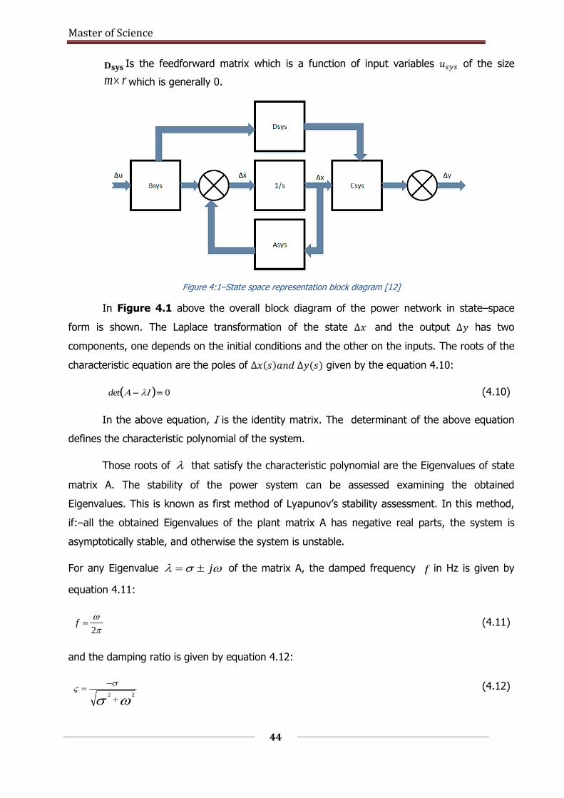
Figure 4:1–State space representation block diagram [12]

In Figure 4.1 above the overall block diagram of the power network in state–space

form is shown. The Laplace transformation of the state ∆𝑥 and the output ∆𝑦 has two

components, one depends on the initial conditions and the other on the inputs. The roots of the

characteristic equation are the poles of ∆𝑥(𝑠)𝑎𝑛𝑑 ∆𝑦(𝑠) given by the equation 4.10:

0 det (4.10)

In the above equation, I is the identity matrix. The determinant of the above equation

defines the characteristic polynomial of the system.

Those roots of that satisfy the characteristic polynomial are the Eigenvalues of state

matrix A. The stability of the power system can be assessed examining the obtained

Eigenvalues. This is known as first method of Lyapunov’s stability assessment. In this method,

if:–all the obtained Eigenvalues of the plant matrix A has negative real parts, the system is

asymptotically stable, and otherwise the system is unstable.

For any Eigenvalue j of the matrix A, the damped frequency f in Hz is given by

equation 4.11:

2f (4.11)

and the damping ratio is given by equation 4.12:

22

(4.12)

Master of Science

45

4.2 Eigenvectors of an Eigenvalue

A state matrix of the order nn has n Eigenvalues. The Eigenvalue of the state

matrix is a complex quantity. Each Eigenvalue has associated left and the right Eigenvector. The

right Eigenvector of an Eigenvalue is indicated by and the left Eigenvector of an Eigenvalue

is indicated by . The left and the right Eigenvectors of an Eigenvalue i is defined by

equation 4.13.

ψiλiAψi

iλiiA

(4.13)

The diagonal matrix has all the Eigenvalues on its diagonal.

The right Eigenvector is a row vector and the left Eigenvector is a column vector. These vectors

are of the form:

ni

3i

2i

1i

i

and ψψψψψι ιnι3ι2ι1 (4.14)

For n Eigenvalues there are n left and the right Eigenvectors. The Eigenvectors form the left

and the right Eigen matrices respectively.

ψTnψT

3ψT

2ψT

1

Tψ

n321φ

(4.15)

Using the characteristic polynomial obtained in the equation 4.10 and the equation 4.13, the

diagonal matrix is rewritten as in equation 4.16:

AΛ

Ιψ

ΛA

1

(4.16)

From the state matrix, it is observed that, each state variable is a linear combination of

all the other state variables. A mode is a cross coupling of different state variables, hence a new

state vector is defined to remove the cross coupling of state variables as given in equation

4.17:

zx Δ (4.17)

Master of Science

46

Pre–multiplying by the right Eigen matrix φ to the above equation and rewriting in terms of 𝒵

we get

zz iii

zz

A (4.18)

zz

(4.19)

From equation 4.9 we have:

xΔΑΔ

x (4.20)

In the above equation 4.19, it is very clear that the equations are decoupled unlike in the

equation 4.13. The difference is that the matrix A is not a diagonal matrix in equation 4.20

whereas the matrix Λ is a diagonal matrix with Eigenvalues on its diagonal.

The equation 4.18 can be visualized as a first order differential equation and its solution in time

t can be defined by equation 4.21:

ezzt

ii

it 0 (4.21)

Where the term 0zi is the initial condition of the differential equation. Thus the equation 4.16

can be written in a general manner using the original state vector ∆x as

eeee

e

z

e

tttt

t

i

tn

i

i

n

i

i

x......xxxtx

xtx

x

tx

0000

0

00

0

321

1

ΨniinΨ3ii3Ψ2ii2Ψi1 1i

Ψi

Δψi

zi

n

1i

i

(4.22)

From the equation 4.22, we can conclude that a state variable is expressed as a linear

combination of n dynamic modes. A mode can be defined as a function of the right and the left

Eigen matrix and the corresponding Eigenvalue with respect to time. From the above equation,

it is observed that the right and the left Eigen matrix are effectively complex numbers which can

be visualized as the magnitude of the mode corresponding to the Eigenvalue. Thus, for a given

mode, the product of the left and the right Eigenvectors gives an identity matrix indicating that

they are orthogonal to each other whereas, for a different mode, their product is zero.

Master of Science

47

4.3 Sensitivity of an Eigenvalue

The sensitivity of the Eigenvalues to the elements in the state matrix is of high importance.

From equation 4.13, we have

iii λA (4.23)

Consider an element from the state matrix A as Pkj . This is an element of the kth row and the

jth column of the state matrix A. To determine the sensitivity of the Eigenvalue, the equation

4.13 is differentiated with respect to the element Pkj , this results in the equation 4.13:

PPPP kj

i

kj

i

kji

kj

φφ

φi

i

iAA

(4.24)

Now by pre–multiplying the equation 4.24, by ψ i and substituting Ιψ , we obtain the

equation 4.25:

PP kj

i

kj

φi

Aψi

(4.25)

From the equation 4.25, it is concluded that the sensitivity of an Eigenvalue to a

parameter in the state matrix A is equal to the product of left Eigenvector and the right

Eigenvector. This brings to the definition of the participation matrix, which determines the state

variable, and hence the generator that is most involved in a mode. This matrix takes into

account both the right and the left Eigenvector of a mode, i.e. through which state variable the

mode is excited or easily observable (observability) and which state variable has the most

impact on this mode (controllability) of the mode. The participation matrix is a dimensionless

quantity and is defined as:

PPPPP n321 (4.26)

ψφ

ψφ

ψφ

ψφ

ψφ

p

p

p

p

p

p

inni

4i

i33i

i22i

i11i

ni

4i

3i

2i

1i

k

i4

(4.27)

The equation 4.25 gives a link between a state variable and the Eigenvalue. For

example, if an Eigenvalue corresponds to a local mode of an area, then the rotor speeds of the

generators in that area will have a high value and the other areas will be insignificant.

Master of Science

48

The stochastic nature of power system changes all the time due to changes in the values

of the voltages, currents and load flows between different areas. Large power systems will have

dominant electromechanical modes of oscillations under stressed conditions. These modes of

electro–mechanical oscillations can be broadly classified as in [12] [17]:

1. Inter-area modes of frequency 0.1 Hz to 0.8 Hz: When generators of two

different areas oscillate against each other. These modes are excited, when there is a

fault on the tie lines or transmission lines are taken out of service for maintenance

purposes.

2. Local area modes of frequency 0.7 Hz to 2 Hz: When generators within an area

oscillate against each other. These modes are excited when there are disturbances in

an area close to the generators. These have higher frequencies compared to that of

the inter–area modes.

3. Intra plants modes of frequency 1.5 Hz to 3 Hz: These modes are excited

when machines within the generating plant starts oscillating against each other. This

mainly depend on the MVA ratings of the machines and the reactance connecting

them.

These oscillatory modes are influenced by various elements in the power system like for

example HVDC, FACTS devices, AVRs and speed governors. The frequency of oscillation and the

damping factor of the inter-area modes depends upon various conditions of the power network.

For a strongly interconnected network, where the generators can handle a total load with

significant extra margin, the inter-area modal frequencies will be higher. While, in a weakly

connected network, with a smaller margin the inter–area modes will be lower.

4.4 Prony analysis2

Prony analysis is a mathematical tool used to analyze the recorded signals. This strategy

coupled with the classical Fourier analysis provides sufficient modal information from the

system’s signals. In this strategy, a linear combination of exponential terms are fit to signals

that are sampled equally with respect to time [17]. The problem of over–determined set of

linear equations and finding the roots of higher order polynomials by estimating the 𝜆’s of the

polynomials is solved by Prony analysis.

2 This section is based on the description given in DSI toolbox, user manual from PNNL laboratory. The

toolbox is available for download at https://github.com/ftuffner/DSIToolbox or https://www.naspi.org/node/490

https://github.com/ftuffner/DSIToolbox

Master of Science

49

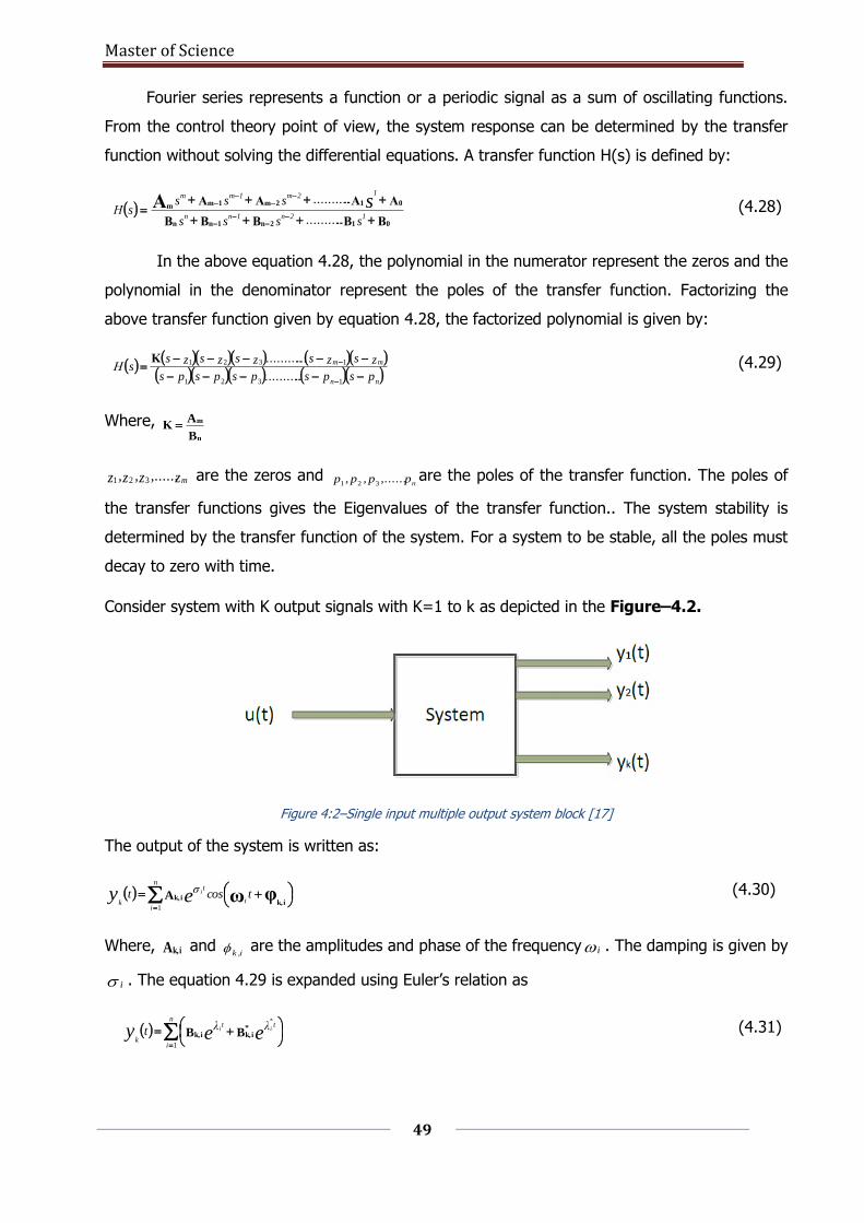
Fourier series represents a function or a periodic signal as a sum of oscillating functions.

From the control theory point of view, the system response can be determined by the transfer

function without solving the differential equations. A transfer function H(s) is defined by:

ΒΒΒΒΒ

ΑΑΑΑ

012n1nn

012m1mmΑ

s............sss

............ssssΗ

12n1nn

12m1mm

s (4.28)

In the above equation 4.28, the polynomial in the numerator represent the zeros and the

polynomial in the denominator represent the poles of the transfer function. Factorizing the

above transfer function given by equation 4.28, the factorized polynomial is given by:

psps............pspsps

zszs.............zszszss

nn

mm

1321

1321Κ (4.29)

Where, B

AΚ

n

m

z,......z,z,z m321 are the zeros and p,......p,p,pn321are the poles of the transfer function. The poles of

the transfer functions gives the Eigenvalues of the transfer function.. The system stability is

determined by the transfer function of the system. For a system to be stable, all the poles must

decay to zero with time.

Consider system with K output signals with K=1 to k as depicted in the Figure–4.2.

Figure 4:2–Single input multiple output system block [17]

The output of the system is written as:

n

ii

t

ktcosσt ey i

1

φω ik,ik,A (4.30)

Where, A ik, and i,k are the amplitudes and phase of the frequency i . The damping is given by

i . The equation 4.29 is expanded using Euler’s relation as

n

i

tt

k eey λλt*

ii

1

BB*

ik,ik, (4.31)

Master of Science

50

Where B i,k and B*

i,k are the complex conjugate of each other and iare the poles or Eigenvalues

of the system. From the equation 4.30, B i,k are the output residues of the system and is

expressed as

B ik, = eφ

k,ij

2

A ik, (4.32)

and is a complex Eigenvalue given by:

i= ii

j (4.33)

Where i is the real part and i

is the frequency of the Eigenvalue.

If the system outputs are samples over a uniform time period for a total of Νk

samples where 1321 Nk....,,k then by Prony analysis the amplitudes, phase angles, frequencies

and the damping coefficients of the signal is determined. A signal consists of few dominant

modes along with the noise.

Prony analysis uses the Linear Prediction Method (LPM), where the future values of a

discretized signal is estimated as a linear function of the previous signals. In the second step,

the coefficients of the characteristic equation is estimated using the Least Square Estimation

method. Once the coefficients are estimated, the roots of the characteristic equation is

calculated. In this step, the noises are reduced by taking a very high modal order.

First a suitable window is opened to perform Prony. Here, it is assumed that there is

maximum energy in the modes within the Prony window. This will reorder the modes according

to their energy content in the selected window according to the error criterion which reduces

the error as the modal response is closer to the actual data.

4.5 Choice of signals

To obtain reliable results, observable signals like generator speeds, output powers should

be the first choice. The part of the signals to which Prony analysis is applied depends on the

type of the disturbance. The signal should constitute to a true ringdown/periodic/stationary

signal . For example, simulating a short circuit event or applying a positive and a negative step

in the torques to the generators in an area. This will constitute a true ringdown signal as the

system is tending to a post–fault equilibrium point.

For low frequency modes like inter–area modes, removal of the load or a tie–line is a good

choice. In response to this type of disturbance, the system will move to a new post–fault

equilibrium point. In response to the disturbances, various power equipment’s like circuit

Master of Science

51

breakers, governors or capacitor banks are switched immediately after the disturbance, these

actions are considered as additional forcing functions with respect to power system oscillations.

These switching actions alter the modal characteristics, hence the Prony analysis must be

applied to that portion of the signal where no switching action occurs or after the switching has

taken place. The dominant mode should be observable in the chosen signals for the Prony

analysis. This is done by physical inspection of the signals.

4.5.1 Pre–processing of the signals

Sometimes before applying Prony analysis, to the selected signals, the signals may have

to be pre–processed to remove any kind of trending and noises. From the definitions, Prony

analysis can be applied to only periodic signals or signals that is sampled at a constant sampling

rate. The signals that is exported from power factory may not be sampled at equal time steps.

The solvers in power factory tries to sample the variables at a given time step, but in the case of

fast transient phenomenon the time step may vary in few cases. Hence to avoid difference in

the sampling time, the basic interpolation of the signal is done before applying Prony to the

signal. The interpolation involves dividing the total simulation time by the step size and

interpolating the values. This will result in loosing few data points at the end, but does not

change the signals drastically. The interpolation codes from MATLAB can be found in the

Appendix under MATLAB codes section.

4.5.2 Choosing the Prony window

Once the signals are processed by linear interpolation, they are imported to the PNNL

Prony analysis tool. This tool conducts the Prony analysis of the imported signals and outputs

the dominant modes present in the signal. Within this tool, the Prony window timings must be

entered for the tool to perform Prony analysis. This is entered manually with numerous trials,

the most suitable window is obtained. The window should be chosen in that part of the signal

where the oscillations are is close to a linear system output. The window is shown in the

Figure–4.3 below:

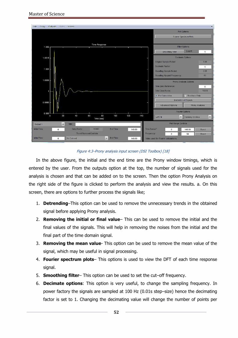
Master of Science

52

Figure 4:3–Prony analysis input screen (DSI Toolbox) [18]

In the above figure, the initial and the end time are the Prony window timings, which is

entered by the user. From the outputs option at the top, the number of signals used for the

analysis is chosen and that can be added on to the screen. Then the option Prony Analysis on

the right side of the figure is clicked to perform the analysis and view the results. a. On this

screen, there are options to further process the signals like;

1. Detrending–This option can be used to remove the unnecessary trends in the obtained

signal before applying Prony analysis.

2. Removing the initial or final value– This can be used to remove the initial and the

final values of the signals. This will help in removing the noises from the initial and the

final part of the time domain signal.

3. Removing the mean value- This option can be used to remove the mean value of the

signal, which may be useful in signal processing.

4. Fourier spectrum plots– This options is used to view the DFT of each time response

signal.

5. Smoothing filter– This option can be used to set the cut–off frequency.

6. Decimate options: This option is very useful, to change the sampling frequency. In

power factory the signals are sampled at 100 Hz (0.01s step–size) hence the decimating

factor is set to 1. Changing the decimating value will change the number of points per

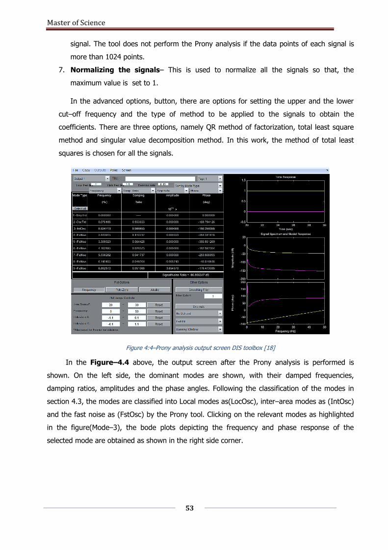
Master of Science

53

signal. The tool does not perform the Prony analysis if the data points of each signal is

more than 1024 points.

7. Normalizing the signals– This is used to normalize all the signals so that, the

maximum value is set to 1.

In the advanced options, button, there are options for setting the upper and the lower

cut–off frequency and the type of method to be applied to the signals to obtain the

coefficients. There are three options, namely QR method of factorization, total least square

method and singular value decomposition method. In this work, the method of total least

squares is chosen for all the signals.

Figure 4:4–Prony analysis output screen DIS toolbox [18]

In the Figure–4.4 above, the output screen after the Prony analysis is performed is

shown. On the left side, the dominant modes are shown, with their damped frequencies,

damping ratios, amplitudes and the phase angles. Following the classification of the modes in

section 4.3, the modes are classified into Local modes as(LocOsc), inter–area modes as (IntOsc)

and the fast noise as (FstOsc) by the Prony tool. Clicking on the relevant modes as highlighted

in the figure(Mode–3), the bode plots depicting the frequency and phase response of the

selected mode are obtained as shown in the right side corner.

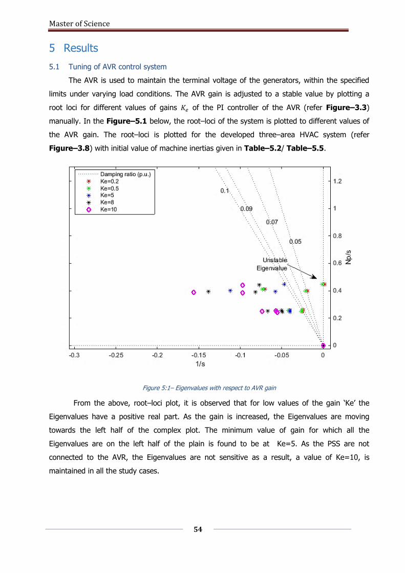
Master of Science

54

5 Results

5.1 Tuning of AVR control system

The AVR is used to maintain the terminal voltage of the generators, within the specified

limits under varying load conditions. The AVR gain is adjusted to a stable value by plotting a

root loci for different values of gains 𝐾𝑒 of the PI controller of the AVR (refer Figure–3.3)

manually. In the Figure–5.1 below, the root–loci of the system is plotted to different values of

the AVR gain. The root–loci is plotted for the developed three–area HVAC system (refer

Figure–3.8) with initial value of machine inertias given in Table–5.2/ Table–5.5.

Figure 5:1– Eigenvalues with respect to AVR gain

From the above, root–loci plot, it is observed that for low values of the gain ‘Ke’ the

Eigenvalues have a positive real part. As the gain is increased, the Eigenvalues are moving

towards the left half of the complex plot. The minimum value of gain for which all the

Eigenvalues are on the left half of the plain is found to be at Ke=5. As the PSS are not

connected to the AVR, the Eigenvalues are not sensitive as a result, a value of Ke=10, is

maintained in all the study cases.

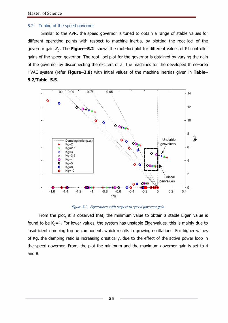
Master of Science

55

5.2 Tuning of the speed governor

Similar to the AVR, the speed governor is tuned to obtain a range of stable values for

different operating points with respect to machine inertia, by plotting the root–loci of the

governor gain 𝐾𝑔. The Figure–5.2 shows the root–loci plot for different values of PI controller

gains of the speed governor. The root–loci plot for the governor is obtained by varying the gain

of the governor by disconnecting the exciters of all the machines for the developed three–area

HVAC system (refer Figure–3.8) with initial values of the machine inertias given in Table–

5.2/Table–5.5.

Figure 5:2– Eigenvalues with respect to speed governor gain

From the plot, it is observed that, the minimum value to obtain a stable Eigen value is

found to be Kg=4. For lower values, the system has unstable Eigenvalues, this is mainly due to

insufficient damping torque component, which results in growing oscillations. For higher values

of Kg, the damping ratio is increasing drastically, due to the effect of the active power loop in

the speed governor. From, the plot the minimum and the maximum governor gain is set to 4

and 8.

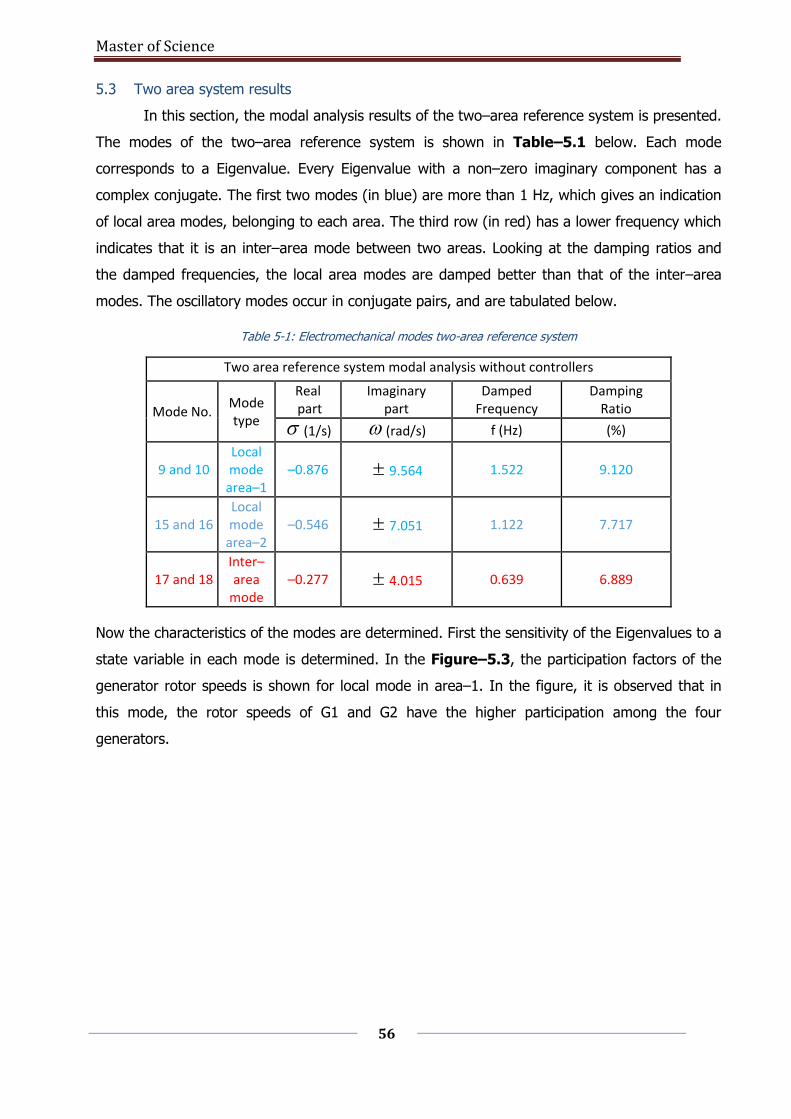
Master of Science

56

5.3 Two area system results

In this section, the modal analysis results of the two–area reference system is presented.

The modes of the two–area reference system is shown in Table–5.1 below. Each mode

corresponds to a Eigenvalue. Every Eigenvalue with a non–zero imaginary component has a

complex conjugate. The first two modes (in blue) are more than 1 Hz, which gives an indication

of local area modes, belonging to each area. The third row (in red) has a lower frequency which

indicates that it is an inter–area mode between two areas. Looking at the damping ratios and

the damped frequencies, the local area modes are damped better than that of the inter–area

modes. The oscillatory modes occur in conjugate pairs, and are tabulated below.

Table 5-1: Electromechanical modes two-area reference system

Two area reference system modal analysis without controllers

Mode No. Mode type

Real part

Imaginary part

Damped Frequency

Damping Ratio

(1/s) (rad/s) f (Hz) (%)

9 and 10 Local mode

area–1 –0.876 9.564 1.522 9.120

15 and 16 Local mode

area–2 –0.546 7.051 1.122 7.717

17 and 18 Inter–area

mode –0.277 4.015 0.639 6.889

Now the characteristics of the modes are determined. First the sensitivity of the Eigenvalues to a

state variable in each mode is determined. In the Figure–5.3, the participation factors of the

generator rotor speeds is shown for local mode in area–1. In the figure, it is observed that in

this mode, the rotor speeds of G1 and G2 have the higher participation among the four

generators.

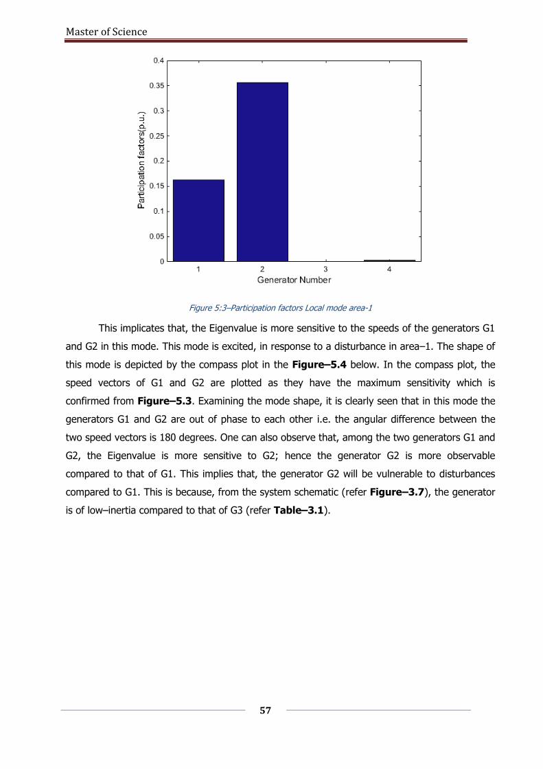
Master of Science

57

Figure 5:3–Participation factors Local mode area-1

This implicates that, the Eigenvalue is more sensitive to the speeds of the generators G1

and G2 in this mode. This mode is excited, in response to a disturbance in area–1. The shape of

this mode is depicted by the compass plot in the Figure–5.4 below. In the compass plot, the

speed vectors of G1 and G2 are plotted as they have the maximum sensitivity which is

confirmed from Figure–5.3. Examining the mode shape, it is clearly seen that in this mode the

generators G1 and G2 are out of phase to each other i.e. the angular difference between the

two speed vectors is 180 degrees. One can also observe that, among the two generators G1 and

G2, the Eigenvalue is more sensitive to G2; hence the generator G2 is more observable

compared to that of G1. This implies that, the generator G2 will be vulnerable to disturbances

compared to G1. This is because, from the system schematic (refer Figure–3.7), the generator

is of low–inertia compared to that of G3 (refer Table–3.1).

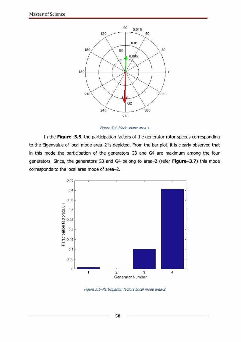
Master of Science

58

Figure 5:4–Mode shape area-1

In the Figure–5.5, the participation factors of the generator rotor speeds corresponding

to the Eigenvalue of local mode area–2 is depicted. From the bar plot, it is clearly observed that

in this mode the participation of the generators G3 and G4 are maximum among the four

generators. Since, the generators G3 and G4 belong to area–2 (refer Figure–3.7) this mode

corresponds to the local area mode of area–2.

Figure 5:5–Participation factors Local mode area-2

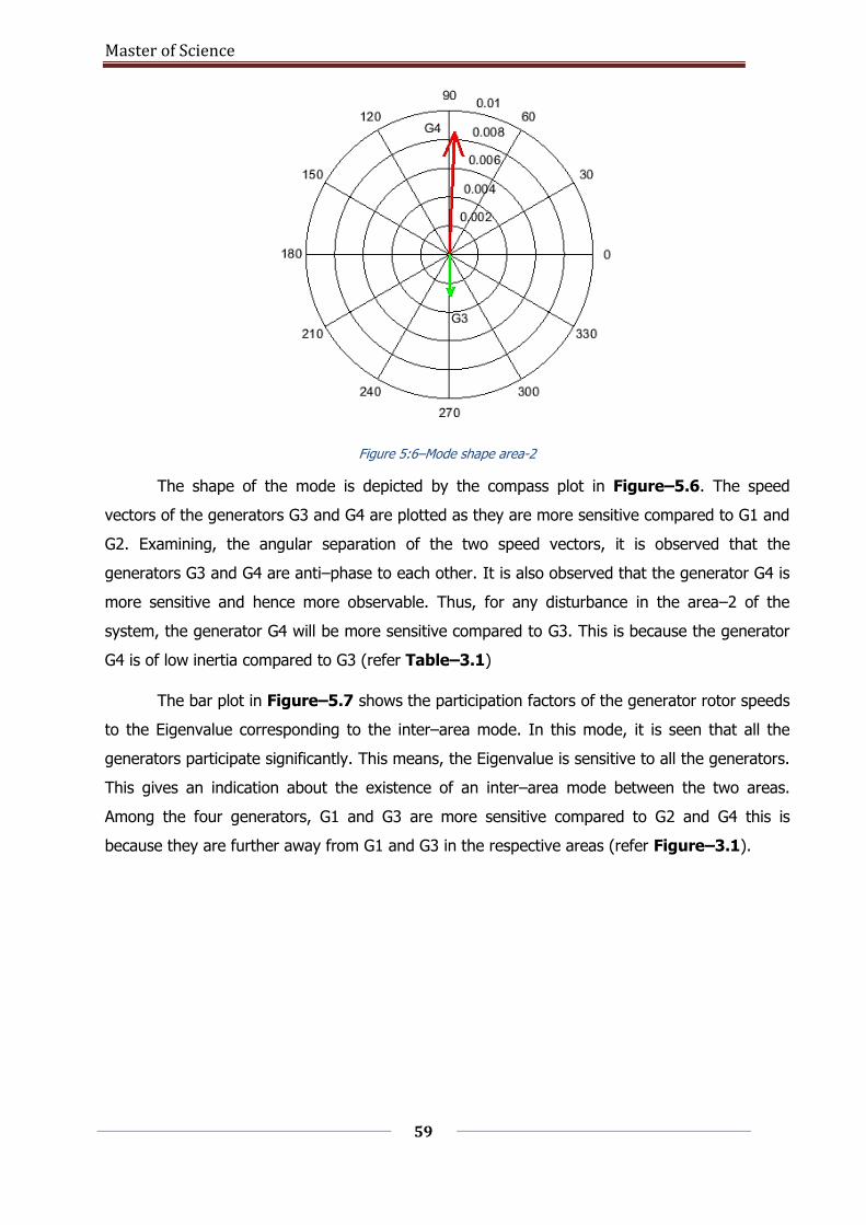
Master of Science

59

Figure 5:6–Mode shape area-2

The shape of the mode is depicted by the compass plot in Figure–5.6. The speed

vectors of the generators G3 and G4 are plotted as they are more sensitive compared to G1 and

G2. Examining, the angular separation of the two speed vectors, it is observed that the

generators G3 and G4 are anti–phase to each other. It is also observed that the generator G4 is

more sensitive and hence more observable. Thus, for any disturbance in the area–2 of the

system, the generator G4 will be more sensitive compared to G3. This is because the generator

G4 is of low inertia compared to G3 (refer Table–3.1)

The bar plot in Figure–5.7 shows the participation factors of the generator rotor speeds

to the Eigenvalue corresponding to the inter–area mode. In this mode, it is seen that all the

generators participate significantly. This means, the Eigenvalue is sensitive to all the generators.

This gives an indication about the existence of an inter–area mode between the two areas.

Among the four generators, G1 and G3 are more sensitive compared to G2 and G4 this is

because they are further away from G1 and G3 in the respective areas (refer Figure–3.1).

Master of Science

60

Figure 5:7–Participation factor inter-area mode

The mode shape is depicted by the right eigenvectors by the compass plot in Figure–

5.8. From the compass plot, it is clearly seen that the generators G1 and G2 of area–1 are in

phase with each other (angle is 0) and the generators G3 and G4 are in phase with each other

(angle is 0), but the vectors G1 and G2 together are anti–phase with the vectors G3 and G4.

This means, in this mode the generators G1 and G2 of area–1 are anti–phase to generators G3

and G4 of area–2.

Figure 5:8–Mode shape inter-area mode

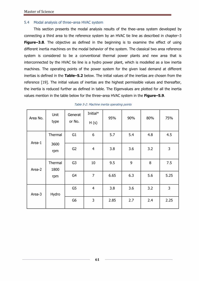
Master of Science

61

5.4 Modal analysis of three–area HVAC system

This section presents the modal analysis results of the thee–area system developed by

connecting a third area to the reference system by an HVAC tie line as described in chapter–3

Figure–3.8. The objective as defined in the beginning is to examine the effect of using

different inertia machines on the modal behavior of the system. The classical two area reference

system is considered to be a conventional thermal power plants and new area that is

interconnected by the HVAC tie line is a hydro power plant, which is modelled as a low inertia

machines. The operating points of the power system for the given load demand at different

inertias is defined in the Table–5.2 below. The initial values of the inertias are chosen from the

reference [19]. The initial values of inertias are the highest permissible values and thereafter,

the inertia is reduced further as defined in table. The Eigenvalues are plotted for all the inertia

values mention in the table below for the three–area HVAC system in the Figure–5.9.

Table 5-2: Machine inertia operating points

Area No. Unit

type

Generat

or No.

Initial*

H (s)

95% 90% 80% 75%

Area-1

Thermal

3600

rpm

G1 6 5.7 5.4 4.8 4.5

G2 4 3.8 3.6 3.2 3

Area-2

Thermal

1800

rpm

G3 10 9.5 9 8 7.5

G4 7 6.65 6.3 5.6 5.25

Area-3 Hydro

G5 4 3.8 3.6 3.2 3

G6 3 2.85 2.7 2.4 2.25

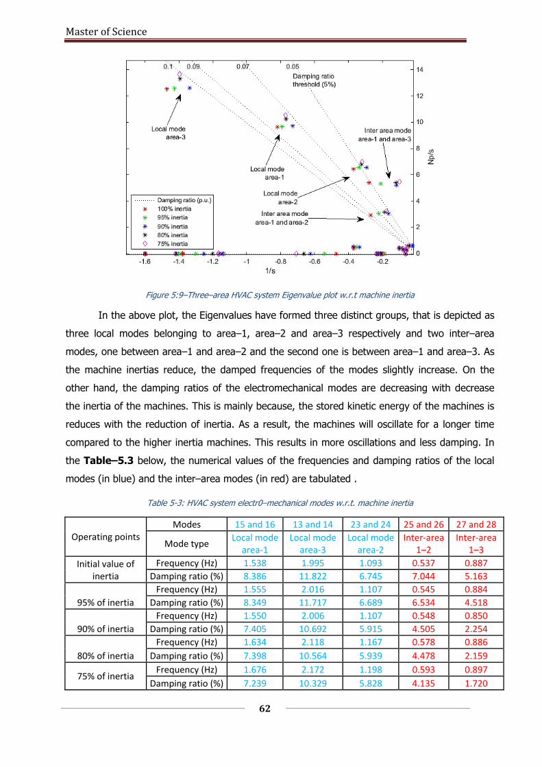
Master of Science

62

Figure 5:9–Three–area HVAC system Eigenvalue plot w.r.t machine inertia

In the above plot, the Eigenvalues have formed three distinct groups, that is depicted as

three local modes belonging to area–1, area–2 and area–3 respectively and two inter–area

modes, one between area–1 and area–2 and the second one is between area–1 and area–3. As

the machine inertias reduce, the damped frequencies of the modes slightly increase. On the

other hand, the damping ratios of the electromechanical modes are decreasing with decrease

the inertia of the machines. This is mainly because, the stored kinetic energy of the machines is

reduces with the reduction of inertia. As a result, the machines will oscillate for a longer time

compared to the higher inertia machines. This results in more oscillations and less damping. In

the Table–5.3 below, the numerical values of the frequencies and damping ratios of the local

modes (in blue) and the inter–area modes (in red) are tabulated .

Table 5-3: HVAC system electr0–mechanical modes w.r.t. machine inertia

Operating points Modes 15 and 16 13 and 14 23 and 24 25 and 26 27 and 28

Mode type Local mode

area-1 Local mode

area-3 Local mode

area-2 Inter-area

1–2 Inter-area

1–3

Initial value of inertia

Frequency (Hz) 1.538 1.995 1.093 0.537 0.887

Damping ratio (%) 8.386 11.822 6.745 7.044 5.163

95% of inertia

Frequency (Hz) 1.555 2.016 1.107 0.545 0.884

Damping ratio (%) 8.349 11.717 6.689 6.534 4.518

90% of inertia

Frequency (Hz) 1.550 2.006 1.107 0.548 0.850

Damping ratio (%) 7.405 10.692 5.915 4.505 2.254

80% of inertia

Frequency (Hz) 1.634 2.118 1.167 0.578 0.886

Damping ratio (%) 7.398 10.564 5.939 4.478 2.159

75% of inertia Frequency (Hz) 1.676 2.172 1.198 0.593 0.897

Damping ratio (%) 7.239 10.329 5.828 4.135 1.720

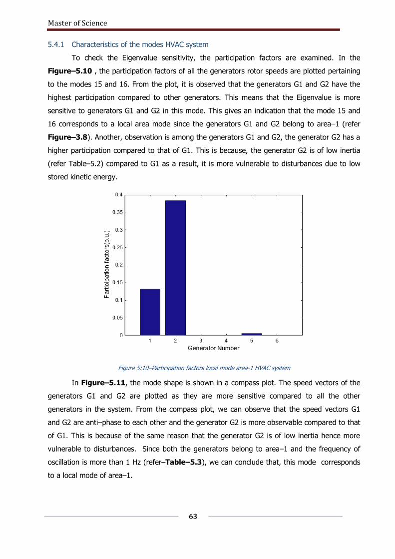
Master of Science

63

5.4.1 Characteristics of the modes HVAC system

To check the Eigenvalue sensitivity, the participation factors are examined. In the

Figure–5.10 , the participation factors of all the generators rotor speeds are plotted pertaining

to the modes 15 and 16. From the plot, it is observed that the generators G1 and G2 have the

highest participation compared to other generators. This means that the Eigenvalue is more

sensitive to generators G1 and G2 in this mode. This gives an indication that the mode 15 and

16 corresponds to a local area mode since the generators G1 and G2 belong to area–1 (refer

Figure–3.8). Another, observation is among the generators G1 and G2, the generator G2 has a

higher participation compared to that of G1. This is because, the generator G2 is of low inertia

(refer Table–5.2) compared to G1 as a result, it is more vulnerable to disturbances due to low

stored kinetic energy.

Figure 5:10–Participation factors local mode area-1 HVAC system

In Figure–5.11, the mode shape is shown in a compass plot. The speed vectors of the

generators G1 and G2 are plotted as they are more sensitive compared to all the other

generators in the system. From the compass plot, we can observe that the speed vectors G1

and G2 are anti–phase to each other and the generator G2 is more observable compared to that

of G1. This is because of the same reason that the generator G2 is of low inertia hence more

vulnerable to disturbances. Since both the generators belong to area–1 and the frequency of

oscillation is more than 1 Hz (refer–Table–5.3), we can conclude that, this mode corresponds

to a local mode of area–1.

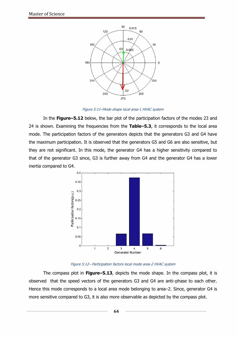
Master of Science

64

Figure 5:11–Mode shape local area-1 HVAC system

In the Figure–5.12 below, the bar plot of the participation factors of the modes 23 and

24 is shown. Examining the frequencies from the Table–5.3, it corresponds to the local area

mode. The participation factors of the generators depicts that the generators G3 and G4 have

the maximum participation. It is observed that the generators G5 and G6 are also sensitive, but

they are not significant. In this mode, the generator G4 has a higher sensitivity compared to

that of the generator G3 since, G3 is further away from G4 and the generator G4 has a lower

inertia compared to G4.

Figure 5:12– Participation factors local mode area-2 HVAC system

The compass plot in Figure–5.13, depicts the mode shape. In the compass plot, it is

observed that the speed vectors of the generators G3 and G4 are anti–phase to each other.

Hence this mode corresponds to a local area mode belonging to area–2. Since, generator G4 is

more sensitive compared to G3, it is also more observable as depicted by the compass plot.

Master of Science

65

Figure 5:13–Mode shape local area-2 HVAC system

The bar plot in Figure–5.14, depicts the sensitivity of the Eigenvalue of modes 13 and

14. From the bar plot it is clear that the generators G5 and G6 have the maximum participation

in this mode. This gives an indication that this mode is a local area mode belonging to area–3

since the generators G5 and G6 belong to area–3 (refer Figure–3.8). The generator G6 has the

higher sensitivity compared to that of G5 as the inertia of G6 is smaller than G5.

Figure 5:14–Participation factors local mode area-3 HVAC system

The mode shape is depicted by the compass plot shown in the Figure–5.15. It is

observed that the speed vectors G5 and G6 are anti–phase to each other in this mode. Since the

generator G6 has a higher participation factor, it is more observable as well.

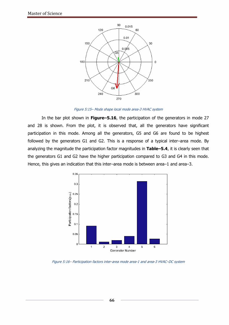
Master of Science

66

Figure 5:15– Mode shape local mode area-3 HVAC system

In the bar plot shown in Figure–5.16, the participation of the generators in mode 27

and 28 is shown. From the plot, it is observed that, all the generators have significant

participation in this mode. Among all the generators, G5 and G6 are found to be highest

followed by the generators G1 and G2. This is a response of a typical inter–area mode. By

analyzing the magnitude the participation factor magnitudes in Table–5.4, it is clearly seen that

the generators G1 and G2 have the higher participation compared to G3 and G4 in this mode.

Hence, this gives an indication that this inter–area mode is between area–1 and area–3.

Figure 5:16– Participation factors inter-area mode area-1 and area-3 HVAC–DC system

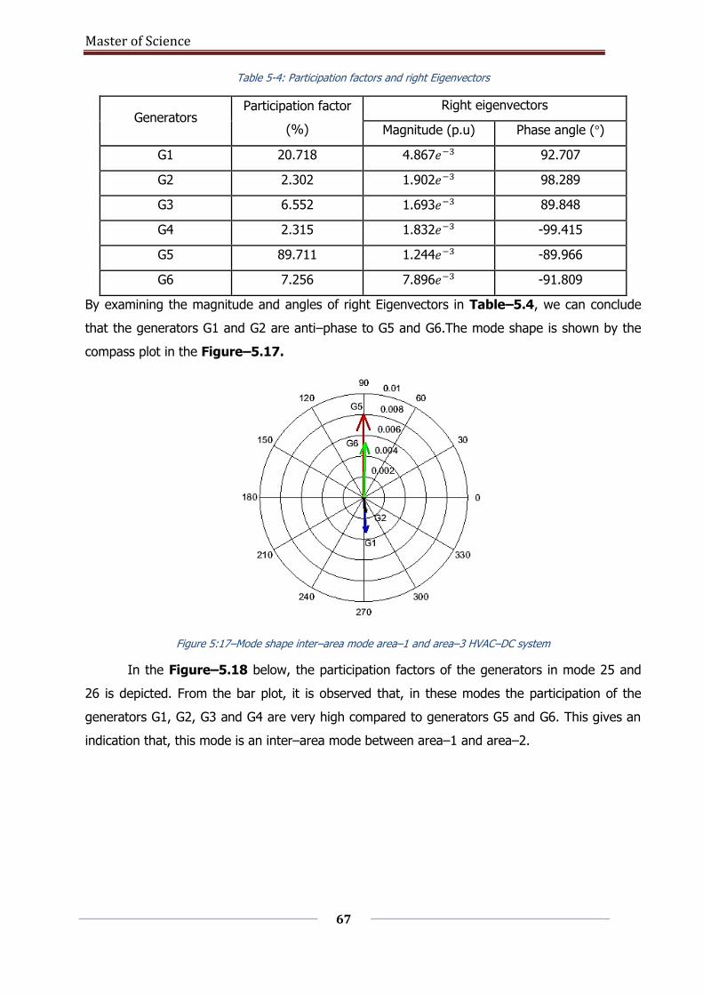
Master of Science

67

Table 5-4: Participation factors and right Eigenvectors

Generators Participation factor

(%)

Right eigenvectors

Magnitude (p.u) Phase angle (°)

G1 20.718 4.867𝑒−3 92.707

G2 2.302 1.902𝑒−3 98.289

G3 6.552 1.693𝑒−3 89.848

G4 2.315 1.832𝑒−3 -99.415

G5 89.711 1.244𝑒−3 -89.966

G6 7.256 7.896𝑒−3 -91.809

By examining the magnitude and angles of right Eigenvectors in Table–5.4, we can conclude

that the generators G1 and G2 are anti–phase to G5 and G6.The mode shape is shown by the

compass plot in the Figure–5.17.

Figure 5:17–Mode shape inter–area mode area–1 and area–3 HVAC–DC system

In the Figure–5.18 below, the participation factors of the generators in mode 25 and

26 is depicted. From the bar plot, it is observed that, in these modes the participation of the

generators G1, G2, G3 and G4 are very high compared to generators G5 and G6. This gives an

indication that, this mode is an inter–area mode between area–1 and area–2.

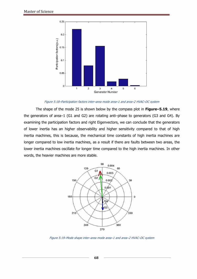
Master of Science

68

Figure 5:18–Participation factors inter–area mode area–1 and area–2 HVAC–DC system

The shape of the mode 25 is shown below by the compass plot in Figure–5.19, where

the generators of area–1 (G1 and G2) are rotating anti–phase to generators (G3 and G4). By

examining the participation factors and right Eigenvectors, we can conclude that the generators

of lower inertia has an higher observability and higher sensitivity compared to that of high

inertia machines, this is because, the mechanical time constants of high inertia machines are

longer compared to low inertia machines, as a result if there are faults between two areas, the

lower inertia machines oscillate for longer time compared to the high inertia machines. In other

words, the heavier machines are more stable.


Master of Science

69

5.5 Modal analysis of HVAC–DC system

This section presents the modal analysis results of the HVAC–DC system, which is

developed by incorporating a point–to–point HVDC link between the third area and the existing

classical two–area system. The operating points of the power system at peak loads for different

inertias are defined in the Table–5.5 below.

Table 5-5: Three–area HVAC–DC system operating conditions with respect to inertias

Area

No.

Unit

type

Generat

or No.

Initial*

H (s)

95% 90% 80% 75%

Area-1

Thermal

3600

rpm

G1 6 5.7 5.4 4.8 4.5

G2 4 3.8 3.6 3.2 3

Area-2

Thermal

1800

rpm

G3 10 9.5 9 8 7.5

G4 7 6.65 6.3 5.6 5.25

Area-3 Hydro

G5 4 3.8 3.6 3.2 3

G6 3 2.85 2.7 2.4 2.25

The modal behavior of the system is accessed to evaluating the effect of the inertias of

the machines on the Eigen values of the electro–mechanical modes. In the Figure–5.20, the

Eigenvalue plot for different values of machine inertias is shown. From the plot, it is observed

that there is an increase in the modal frequencies and decrease in the damping ratios when the

machine inertias are decreased, similar to the HVAC system. Apart from the electromechanical

modes, the states of the PLLs are also excited but they have a significantly higher damping

ratios compared to that of the electromechanical modes in the system. The reason behind the

excitation of the electro–mechanical modes are due to the frequency error that occurs during

the transmission of the active power on the AC side to the active power on the DC link. During

this transition, the PLL states are excited along with the electro–mechanical states but they are

quickly damped. Another, important observation is there were two inter–area modes in the

HVAC system first one, between area–1 and area–2 and the second one, between area–1 and

area–3 (refer Table–5.3), whereas in the HVDC system there is only one inter–area mode.

Master of Science

70

The second inter–area mode does not exist because, the point–to–point HVDC link

decouples the system completely, and as a result there will be no inter–area mode between

systems which are interconnected by only HVDC links.

Figure 5:20–Three–area HVAC–DC system Eigenvalue plot w.r.t. machine inertia

The modal frequencies and their damping ratios of the electro–mechanical modes in the

HVAC–DC system are tabulated in the Table–5.6 below. The modes labelled in blue are more

than 1 Hz and falls into the category of local modes and the modes in red are less than 1 Hz and

the modes in red are inter–area modes.

Table 5-6: HVAC–DC system electro–mechanical modes with respect to machine inertias

Operating points Modes 16 and 17 24 and 25 14 and 15 26 and 27

Mode type

Local mode area-1

Local mode area-2

Local mode area-3

Inter-area–1 and area–2

100% inertia Frequency (Hz) 1.521 1.056 1.873 0.598

Damping ratio (%) 8.283 6.528 11.348 6.713


Damping ratio (%) 7.921 6.557 10.902 6.002


Damping ratio (%) 6.982 5.785 9.805 4.349


Damping ratio (%) 6.981 5.802 9.692 4.326


Damping ratio (%) 6.826 5.688 9.453 4.052

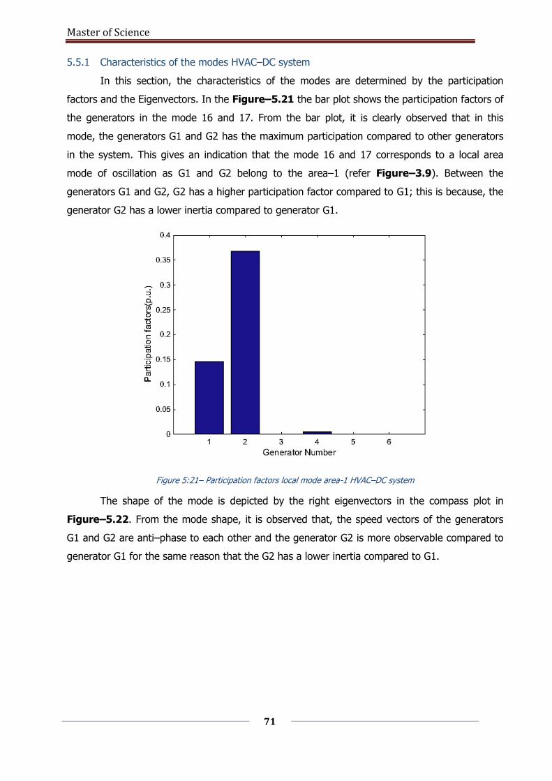
Master of Science

71

5.5.1 Characteristics of the modes HVAC–DC system

In this section, the characteristics of the modes are determined by the participation

factors and the Eigenvectors. In the Figure–5.21 the bar plot shows the participation factors of

the generators in the mode 16 and 17. From the bar plot, it is clearly observed that in this

mode, the generators G1 and G2 has the maximum participation compared to other generators

in the system. This gives an indication that the mode 16 and 17 corresponds to a local area

mode of oscillation as G1 and G2 belong to the area–1 (refer Figure–3.9). Between the

generators G1 and G2, G2 has a higher participation factor compared to G1; this is because, the

generator G2 has a lower inertia compared to generator G1.

Figure 5:21– Participation factors local mode area-1 HVAC–DC system

The shape of the mode is depicted by the right eigenvectors in the compass plot in

Figure–5.22. From the mode shape, it is observed that, the speed vectors of the generators

G1 and G2 are anti–phase to each other and the generator G2 is more observable compared to

generator G1 for the same reason that the G2 has a lower inertia compared to G1.

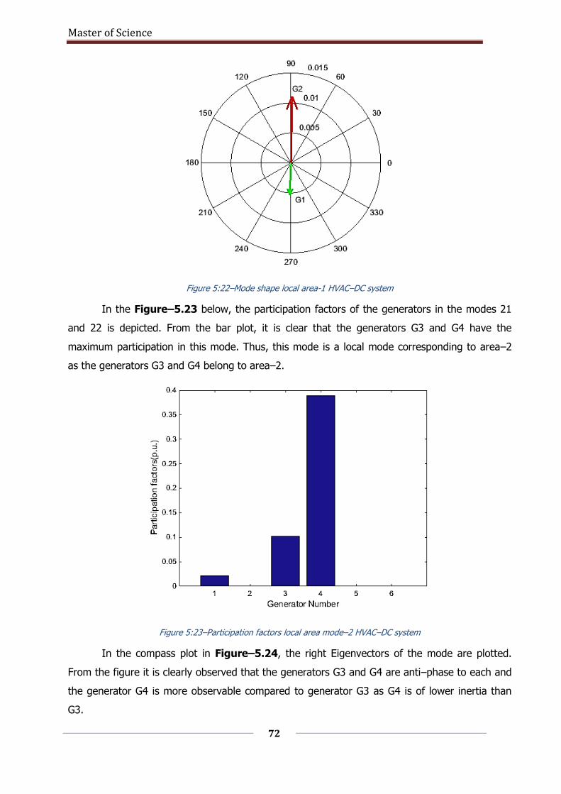
Master of Science

72

Figure 5:22–Mode shape local area-1 HVAC–DC system

In the Figure–5.23 below, the participation factors of the generators in the modes 21

and 22 is depicted. From the bar plot, it is clear that the generators G3 and G4 have the

maximum participation in this mode. Thus, this mode is a local mode corresponding to area–2

as the generators G3 and G4 belong to area–2.

Figure 5:23–Participation factors local area mode–2 HVAC–DC system

In the compass plot in Figure–5.24, the right Eigenvectors of the mode are plotted.

From the figure it is clearly observed that the generators G3 and G4 are anti–phase to each and

the generator G4 is more observable compared to generator G3 as G4 is of lower inertia than

G3.

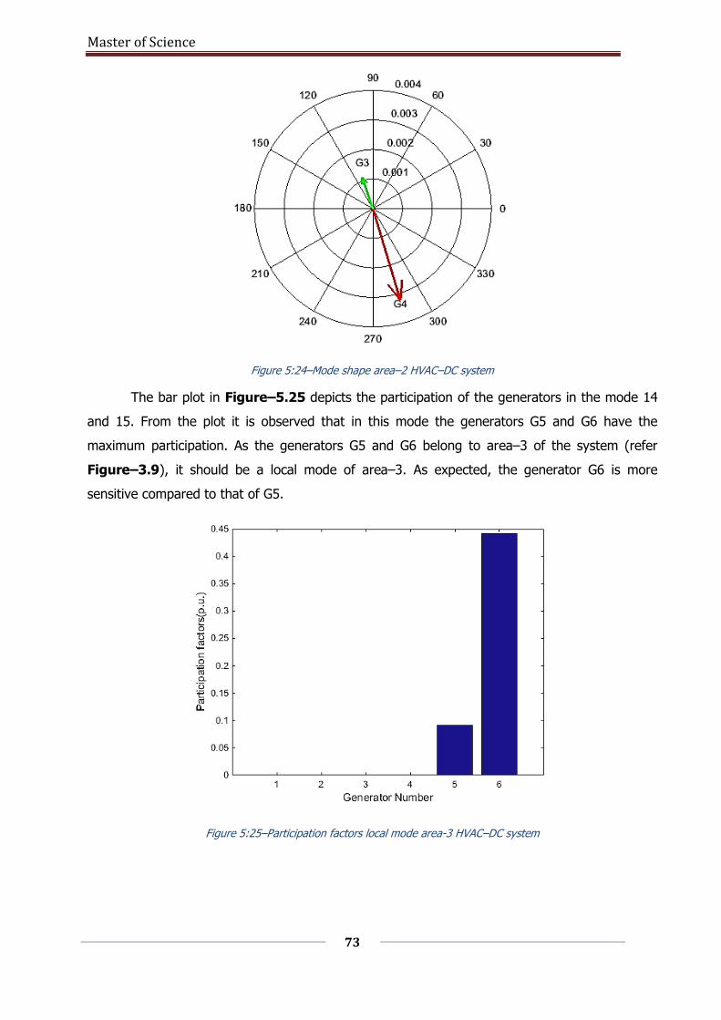
Master of Science

73

Figure 5:24–Mode shape area–2 HVAC–DC system

The bar plot in Figure–5.25 depicts the participation of the generators in the mode 14

and 15. From the plot it is observed that in this mode the generators G5 and G6 have the

maximum participation. As the generators G5 and G6 belong to area–3 of the system (refer

Figure–3.9), it should be a local mode of area–3. As expected, the generator G6 is more

sensitive compared to that of G5.

Figure 5:25–Participation factors local mode area-3 HVAC–DC system

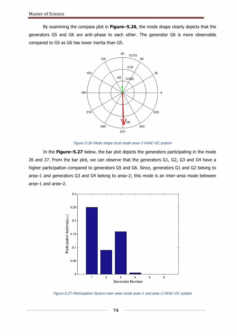
Master of Science

74

By examining the compass plot in Figure–5.26, the mode shape clearly depicts that the

generators G5 and G6 are anti–phase to each other. The generator G6 is more observable

compared to G5 as G6 has lower inertia than G5.

Figure 5:26–Mode shape local mode area–3 HVAC–DC system

In the Figure–5.27 below, the bar plot depicts the generators participating in the mode

26 and 27. From the bar plot, we can observe that the generators G1, G2, G3 and G4 have a

higher participation compared to generators G5 and G6. Since, generators G1 and G2 belong to

area–1 and generators G3 and G4 belong to area–2; this mode is an inter–area mode between

area–1 and area–2.

Figure 5:27–Participation factors inter–area mode area–1 and area–2 HVAC–DC system

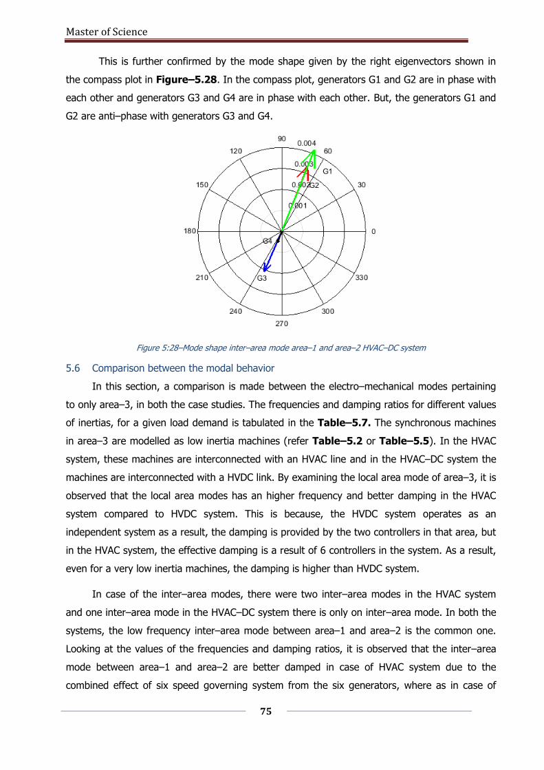
Master of Science

75

This is further confirmed by the mode shape given by the right eigenvectors shown in

the compass plot in Figure–5.28. In the compass plot, generators G1 and G2 are in phase with

each other and generators G3 and G4 are in phase with each other. But, the generators G1 and

G2 are anti–phase with generators G3 and G4.


5.6 Comparison between the modal behavior

In this section, a comparison is made between the electro–mechanical modes pertaining

to only area–3, in both the case studies. The frequencies and damping ratios for different values

of inertias, for a given load demand is tabulated in the Table–5.7. The synchronous machines

in area–3 are modelled as low inertia machines (refer Table–5.2 or Table–5.5). In the HVAC

system, these machines are interconnected with an HVAC line and in the HVAC–DC system the

machines are interconnected with a HVDC link. By examining the local area mode of area–3, it is

observed that the local area modes has an higher frequency and better damping in the HVAC

system compared to HVDC system. This is because, the HVDC system operates as an

independent system as a result, the damping is provided by the two controllers in that area, but

in the HVAC system, the effective damping is a result of 6 controllers in the system. As a result,

even for a very low inertia machines, the damping is higher than HVDC system.

In case of the inter–area modes, there were two inter–area modes in the HVAC system

and one inter–area mode in the HVAC–DC system there is only on inter–area mode. In both the

systems, the low frequency inter–area mode between area–1 and area–2 is the common one.

Looking at the values of the frequencies and damping ratios, it is observed that the inter–area

mode between area–1 and area–2 are better damped in case of HVAC system due to the

combined effect of six speed governing system from the six generators, where as in case of

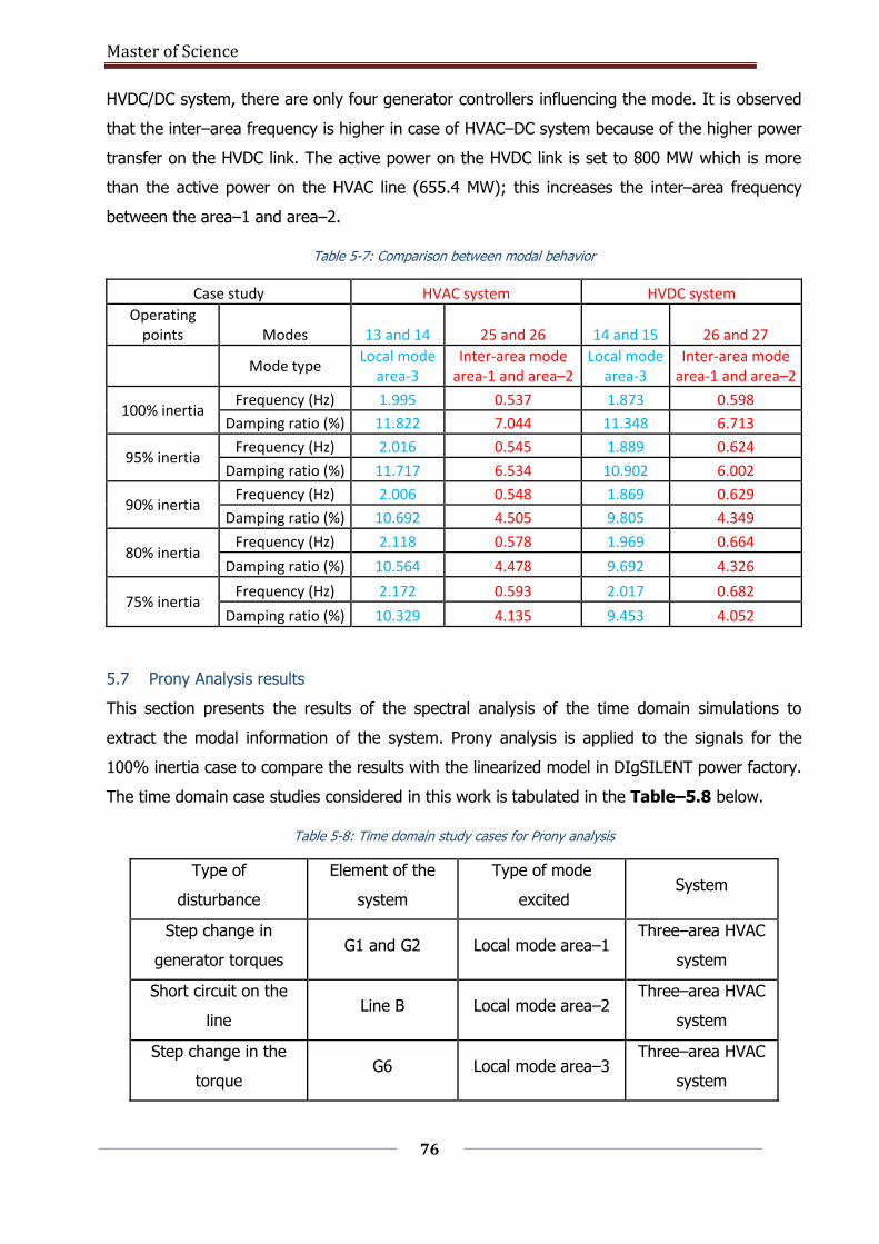
Master of Science

76

HVDC/DC system, there are only four generator controllers influencing the mode. It is observed

that the inter–area frequency is higher in case of HVAC–DC system because of the higher power

transfer on the HVDC link. The active power on the HVDC link is set to 800 MW which is more

than the active power on the HVAC line (655.4 MW); this increases the inter–area frequency

between the area–1 and area–2.

Table 5-7: Comparison between modal behavior

Case study HVAC system HVDC system

Operating points Modes 13 and 14 25 and 26 14 and 15 26 and 27

Mode type

Local mode area-3

Inter-area mode area-1 and area–2

Local mode area-3

Inter-area mode area-1 and area–2


Damping ratio (%) 11.822 7.044 11.348 6.713


Damping ratio (%) 11.717 6.534 10.902 6.002


Damping ratio (%) 10.692 4.505 9.805 4.349


Damping ratio (%) 10.564 4.478 9.692 4.326


Damping ratio (%) 10.329 4.135 9.453 4.052

5.7 Prony Analysis results

This section presents the results of the spectral analysis of the time domain simulations to

extract the modal information of the system. Prony analysis is applied to the signals for the

100% inertia case to compare the results with the linearized model in DIgSILENT power factory.

The time domain case studies considered in this work is tabulated in the Table–5.8 below.

Table 5-8: Time domain study cases for Prony analysis

Type of

disturbance

Element of the

system

Type of mode

excited System

Step change in

generator torques G1 and G2 Local mode area–1

Three–area HVAC

system

Short circuit on the

line Line B Local mode area–2

Three–area HVAC

system

Step change in the

torque G6 Local mode area–3

Three–area HVAC

system

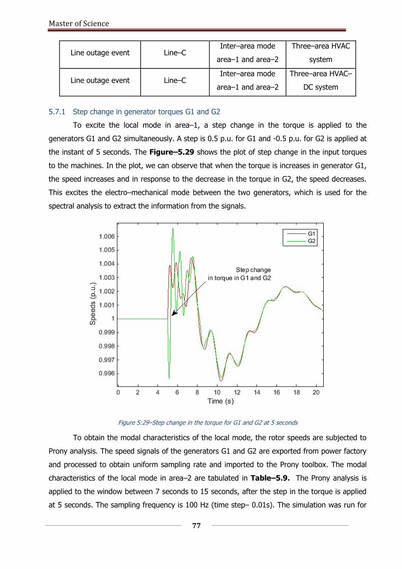
Master of Science

77



Three–area HVAC

system



Three–area HVAC–

DC system

5.7.1 Step change in generator torques G1 and G2

To excite the local mode in area–1, a step change in the torque is applied to the

generators G1 and G2 simultaneously. A step is 0.5 p.u. for G1 and -0.5 p.u. for G2 is applied at

the instant of 5 seconds. The Figure–5.29 shows the plot of step change in the input torques

to the machines. In the plot, we can observe that when the torque is increases in generator G1,

the speed increases and in response to the decrease in the torque in G2, the speed decreases.

This excites the electro–mechanical mode between the two generators, which is used for the

spectral analysis to extract the information from the signals.

Figure 5:29–Step change in the torque for G1 and G2 at 5 seconds

To obtain the modal characteristics of the local mode, the rotor speeds are subjected to

Prony analysis. The speed signals of the generators G1 and G2 are exported from power factory

and processed to obtain uniform sampling rate and imported to the Prony toolbox. The modal

characteristics of the local mode in area–2 are tabulated in Table–5.9. The Prony analysis is

applied to the window between 7 seconds to 15 seconds, after the step in the torque is applied

at 5 seconds. The sampling frequency is 100 Hz (time step– 0.01s). The simulation was run for

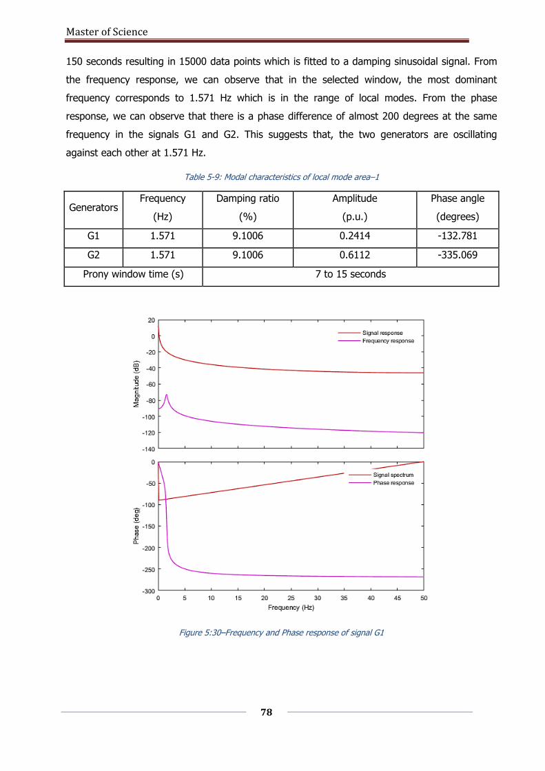
Master of Science

78

150 seconds resulting in 15000 data points which is fitted to a damping sinusoidal signal. From

the frequency response, we can observe that in the selected window, the most dominant

frequency corresponds to 1.571 Hz which is in the range of local modes. From the phase

response, we can observe that there is a phase difference of almost 200 degrees at the same

frequency in the signals G1 and G2. This suggests that, the two generators are oscillating

against each other at 1.571 Hz.

Table 5-9: Modal characteristics of local mode area–1

Generators Frequency

(Hz)

Damping ratio

(%)

Amplitude

(p.u.)

Phase angle

(degrees)

G1 1.571 9.1006 0.2414 -132.781

G2 1.571 9.1006 0.6112 -335.069

Prony window time (s) 7 to 15 seconds

Figure 5:30–Frequency and Phase response of signal G1

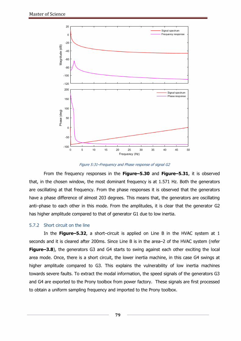
Master of Science

79


From the frequency responses in the Figure–5.30 and Figure–5.31, it is observed

that, in the chosen window, the most dominant frequency is at 1.571 Hz. Both the generators

are oscillating at that frequency. From the phase responses it is observed that the generators

have a phase difference of almost 203 degrees. This means that, the generators are oscillating

anti–phase to each other in this mode. From the amplitudes, it is clear that the generator G2

has higher amplitude compared to that of generator G1 due to low inertia.

5.7.2 Short circuit on the line

In the Figure–5.32, a short–circuit is applied on Line B in the HVAC system at 1

seconds and it is cleared after 200ms. Since Line B is in the area–2 of the HVAC system (refer

Figure–3.8), the generators G3 and G4 starts to swing against each other exciting the local

area mode. Once, there is a short circuit, the lower inertia machine, in this case G4 swings at

higher amplitude compared to G3. This explains the vulnerability of low inertia machines

towards severe faults. To extract the modal information, the speed signals of the generators G3

and G4 are exported to the Prony toolbox from power factory. These signals are first processed

to obtain a uniform sampling frequency and imported to the Prony toolbox.

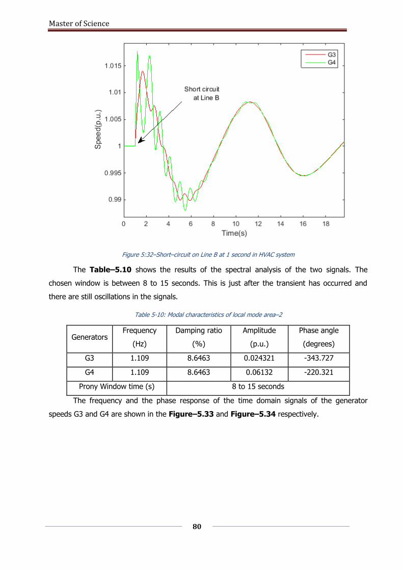
Master of Science

80

Figure 5:32–Short–circuit on Line B at 1 second in HVAC system

The Table–5.10 shows the results of the spectral analysis of the two signals. The

chosen window is between 8 to 15 seconds. This is just after the transient has occurred and

there are still oscillations in the signals.

Table 5-10: Modal characteristics of local mode area–2


(Hz)

Damping ratio

(%)

Amplitude

(p.u.)

Phase angle

(degrees)

G3 1.109 8.6463 0.024321 -343.727

G4 1.109 8.6463 0.06132 -220.321

Prony Window time (s) 8 to 15 seconds

The frequency and the phase response of the time domain signals of the generator

speeds G3 and G4 are shown in the Figure–5.33 and Figure–5.34 respectively.

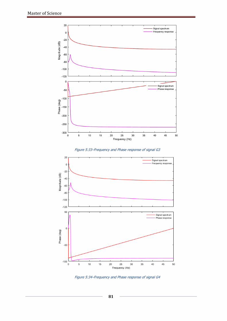
Master of Science

81



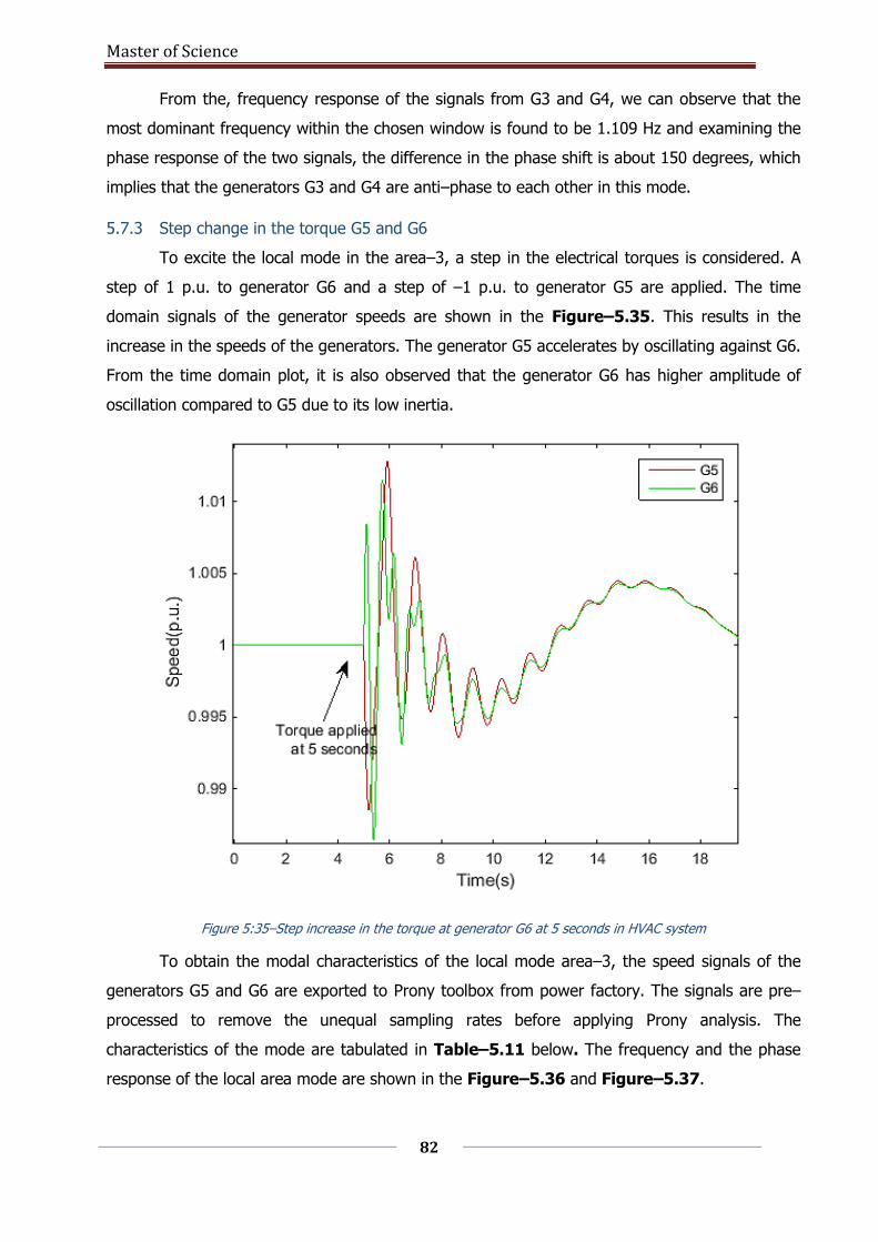
Master of Science

82

From the, frequency response of the signals from G3 and G4, we can observe that the

most dominant frequency within the chosen window is found to be 1.109 Hz and examining the

phase response of the two signals, the difference in the phase shift is about 150 degrees, which

implies that the generators G3 and G4 are anti–phase to each other in this mode.

5.7.3 Step change in the torque G5 and G6

To excite the local mode in the area–3, a step in the electrical torques is considered. A

step of 1 p.u. to generator G6 and a step of –1 p.u. to generator G5 are applied. The time

domain signals of the generator speeds are shown in the Figure–5.35. This results in the

increase in the speeds of the generators. The generator G5 accelerates by oscillating against G6.

From the time domain plot, it is also observed that the generator G6 has higher amplitude of

oscillation compared to G5 due to its low inertia.

Figure 5:35–Step increase in the torque at generator G6 at 5 seconds in HVAC system

To obtain the modal characteristics of the local mode area–3, the speed signals of the

generators G5 and G6 are exported to Prony toolbox from power factory. The signals are pre–

processed to remove the unequal sampling rates before applying Prony analysis. The

characteristics of the mode are tabulated in Table–5.11 below. The frequency and the phase

response of the local area mode are shown in the Figure–5.36 and Figure–5.37.

Master of Science

83

Table 5-11: Characteristics of the local mode area–3


(Hz)

Damping ratio

(%)

Amplitude

(p.u.)

Phase

angle

(degrees)

G5 1.763 5.389 0.01032 -204.087

G6 1.763 5.389 0.02182 -358.234

Prony window time (s) 5.5 to 8

Figure 5:36–Frequency and Phase response of signal G5 local mode area–3 HVAC system

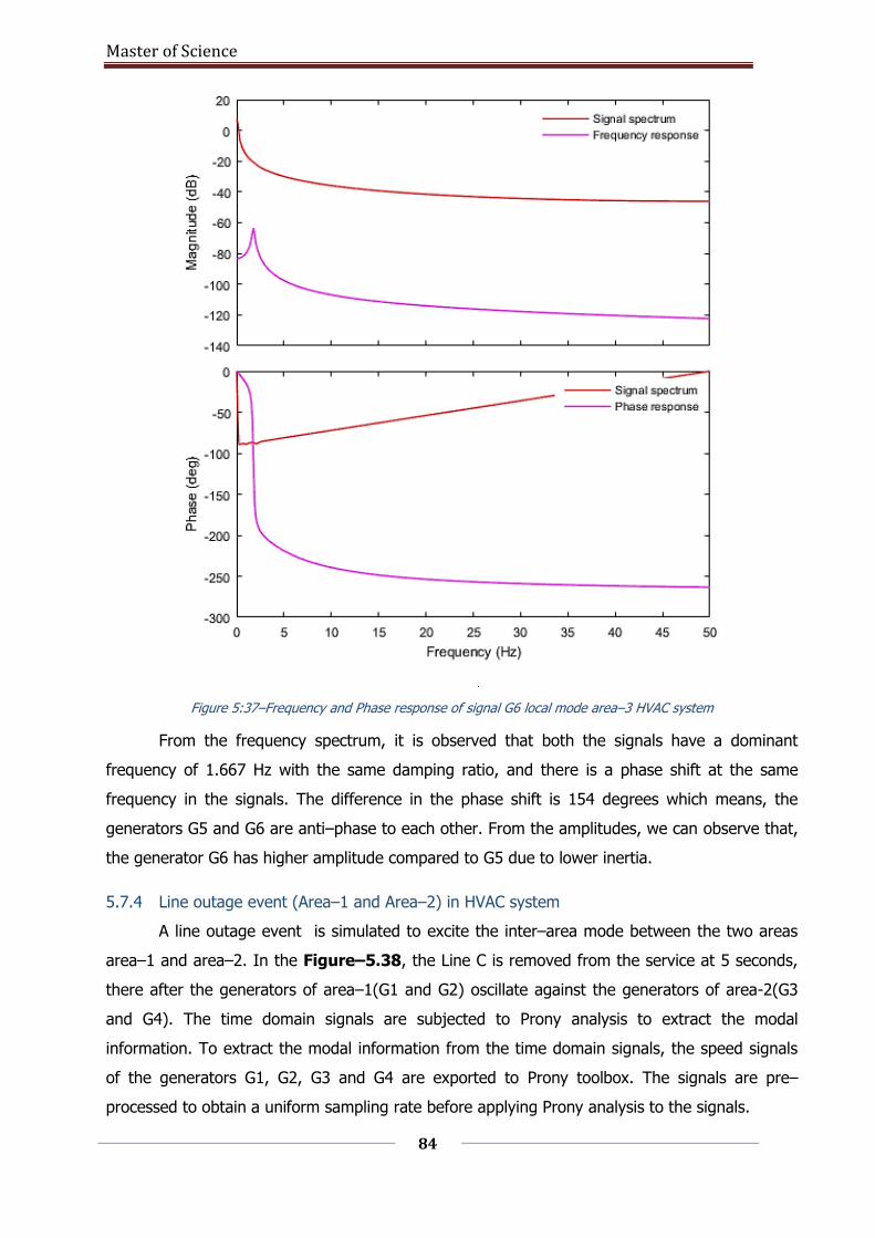
Master of Science

84

11

Figure 5:37–Frequency and Phase response of signal G6 local mode area–3 HVAC system

From the frequency spectrum, it is observed that both the signals have a dominant

frequency of 1.667 Hz with the same damping ratio, and there is a phase shift at the same

frequency in the signals. The difference in the phase shift is 154 degrees which means, the

generators G5 and G6 are anti–phase to each other. From the amplitudes, we can observe that,

the generator G6 has higher amplitude compared to G5 due to lower inertia.

5.7.4 Line outage event (Area–1 and Area–2) in HVAC system

A line outage event is simulated to excite the inter–area mode between the two areas

area–1 and area–2. In the Figure–5.38, the Line C is removed from the service at 5 seconds,

there after the generators of area–1(G1 and G2) oscillate against the generators of area-2(G3

and G4). The time domain signals are subjected to Prony analysis to extract the modal

information. To extract the modal information from the time domain signals, the speed signals

of the generators G1, G2, G3 and G4 are exported to Prony toolbox. The signals are pre–

processed to obtain a uniform sampling rate before applying Prony analysis to the signals.

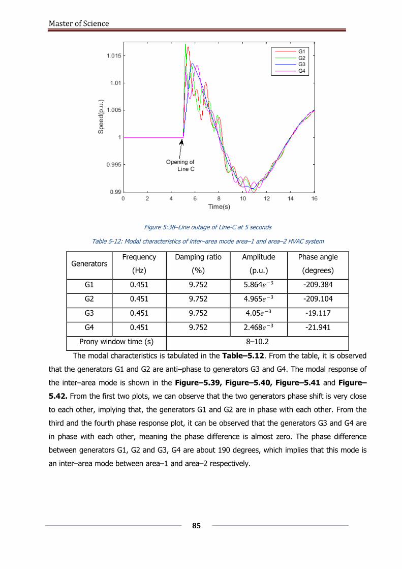
Master of Science

85

Figure 5:38–Line outage of Line-C at 5 seconds

Table 5-12: Modal characteristics of inter–area mode area–1 and area–2 HVAC system


(Hz)

Damping ratio

(%)

Amplitude

(p.u.)

Phase angle

(degrees)

G1 0.451 9.752 5.864𝑒−3 -209.384

G2 0.451 9.752 4.965𝑒−3 -209.104

G3 0.451 9.752 4.05𝑒−3 -19.117

G4 0.451 9.752 2.468𝑒−3 -21.941

Prony window time (s) 8–10.2

The modal characteristics is tabulated in the Table–5.12. From the table, it is observed

that the generators G1 and G2 are anti–phase to generators G3 and G4. The modal response of

the inter–area mode is shown in the Figure–5.39, Figure–5.40, Figure–5.41 and Figure–

5.42. From the first two plots, we can observe that the two generators phase shift is very close

to each other, implying that, the generators G1 and G2 are in phase with each other. From the

third and the fourth phase response plot, it can be observed that the generators G3 and G4 are

in phase with each other, meaning the phase difference is almost zero. The phase difference

between generators G1, G2 and G3, G4 are about 190 degrees, which implies that this mode is

an inter–area mode between area–1 and area–2 respectively.

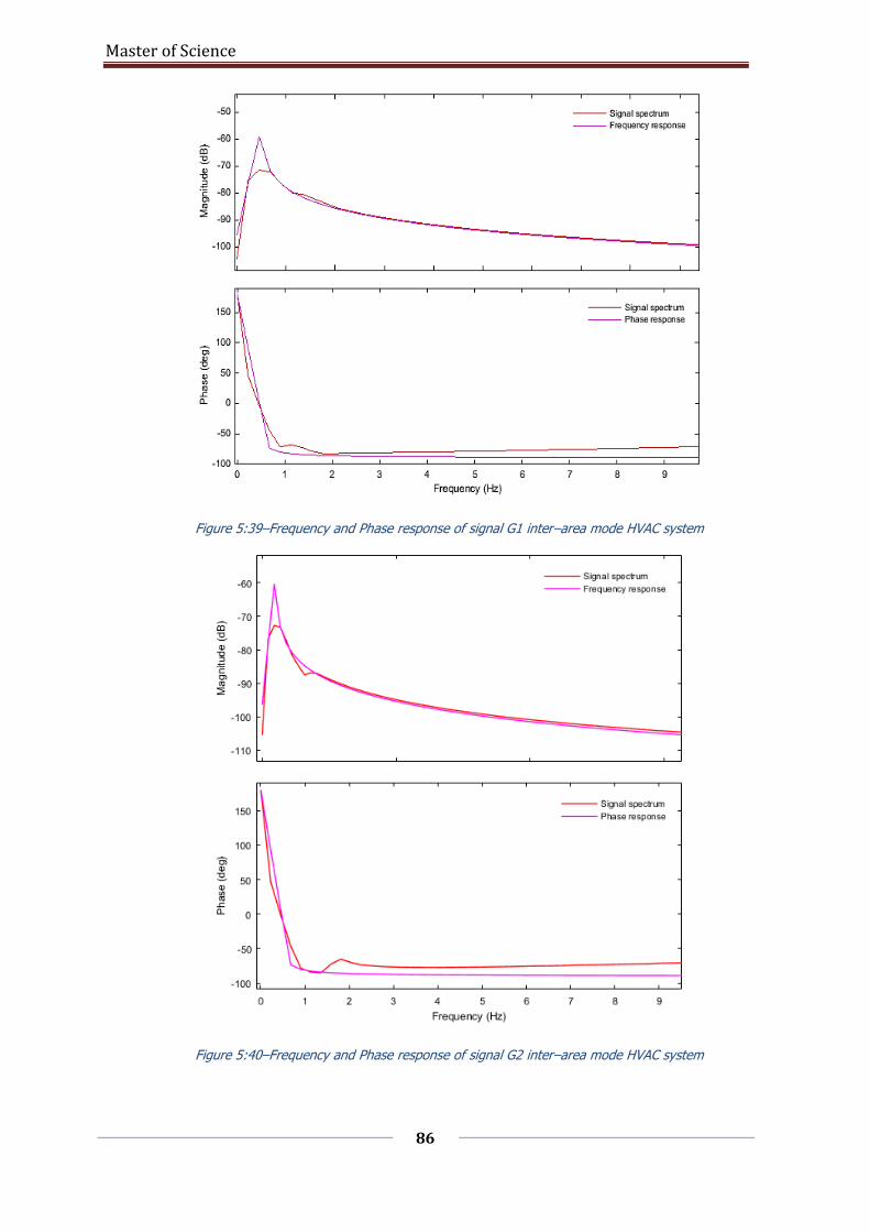
Master of Science

86

Figure 5:39–Frequency and Phase response of signal G1 inter–area mode HVAC system


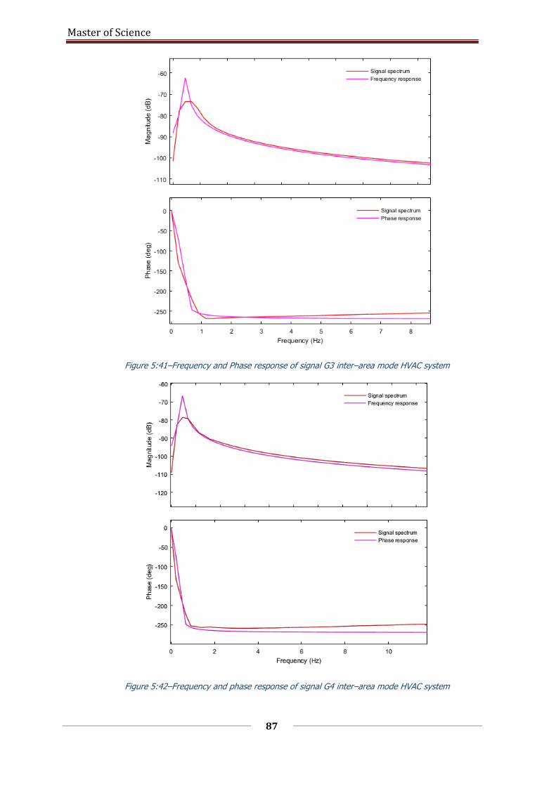
Master of Science

87


Figure 5:42–Frequency and phase response of signal G4 inter–area mode HVAC system

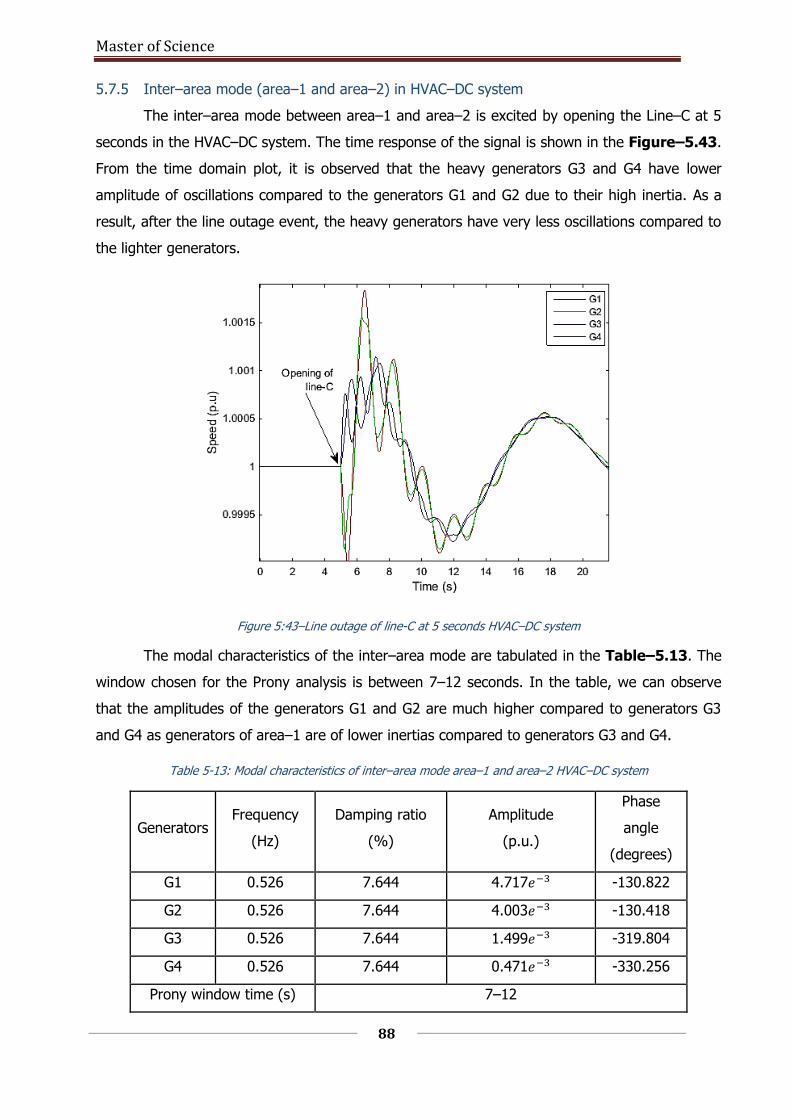
Master of Science

88

5.7.5 Inter–area mode (area–1 and area–2) in HVAC–DC system

The inter–area mode between area–1 and area–2 is excited by opening the Line–C at 5

seconds in the HVAC–DC system. The time response of the signal is shown in the Figure–5.43.

From the time domain plot, it is observed that the heavy generators G3 and G4 have lower

amplitude of oscillations compared to the generators G1 and G2 due to their high inertia. As a

result, after the line outage event, the heavy generators have very less oscillations compared to

the lighter generators.

Figure 5:43–Line outage of line-C at 5 seconds HVAC–DC system

The modal characteristics of the inter–area mode are tabulated in the Table–5.13. The

window chosen for the Prony analysis is between 7–12 seconds. In the table, we can observe

that the amplitudes of the generators G1 and G2 are much higher compared to generators G3

and G4 as generators of area–1 are of lower inertias compared to generators G3 and G4.

Table 5-13: Modal characteristics of inter–area mode area–1 and area–2 HVAC–DC system


(Hz)

Damping ratio

(%)

Amplitude

(p.u.)

Phase

angle

(degrees)

G1 0.526 7.644 4.717𝑒−3 -130.822

G2 0.526 7.644 4.003𝑒−3 -130.418

G3 0.526 7.644 1.499𝑒−3 -319.804

G4 0.526 7.644 0.471𝑒−3 -330.256

Prony window time (s) 7–12

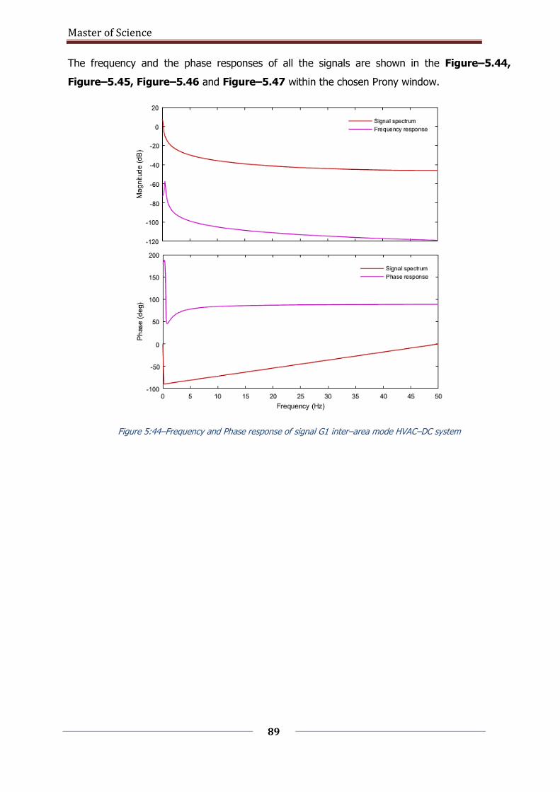
Master of Science

89

The frequency and the phase responses of all the signals are shown in the Figure–5.44,

Figure–5.45, Figure–5.46 and Figure–5.47 within the chosen Prony window.

Figure 5:44–Frequency and Phase response of signal G1 inter–area mode HVAC–DC system

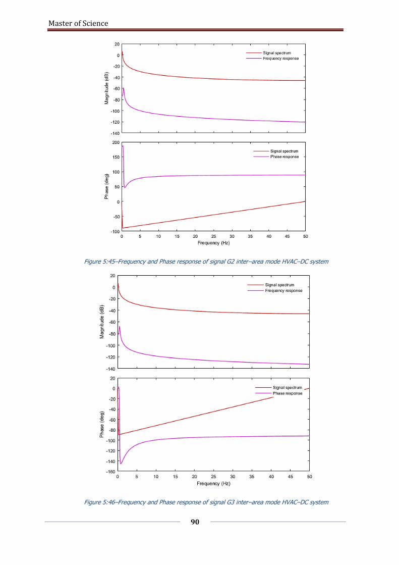
Master of Science

90



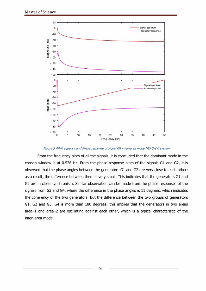
Master of Science

91


From the frequency plots of all the signals, it is concluded that the dominant mode in the

chosen window is at 0.526 Hz. From the phase response plots of the signals G1 and G2, it is

observed that the phase angles between the generators G1 and G2 are very close to each other;

as a result, the difference between them is very small. This indicates that the generators G1 and

G2 are in close synchronism. Similar observation can be made from the phase responses of the

signals from G3 and G4, where the difference in the phase angles is 11 degrees, which indicates

the coherency of the two generators. But the difference between the two groups of generators

G1, G2 and G3, G4 is more than 180 degrees; this implies that the generators in two areas

area–1 and area–2 are oscillating against each other, which is a typical characteristic of the

inter–area mode.

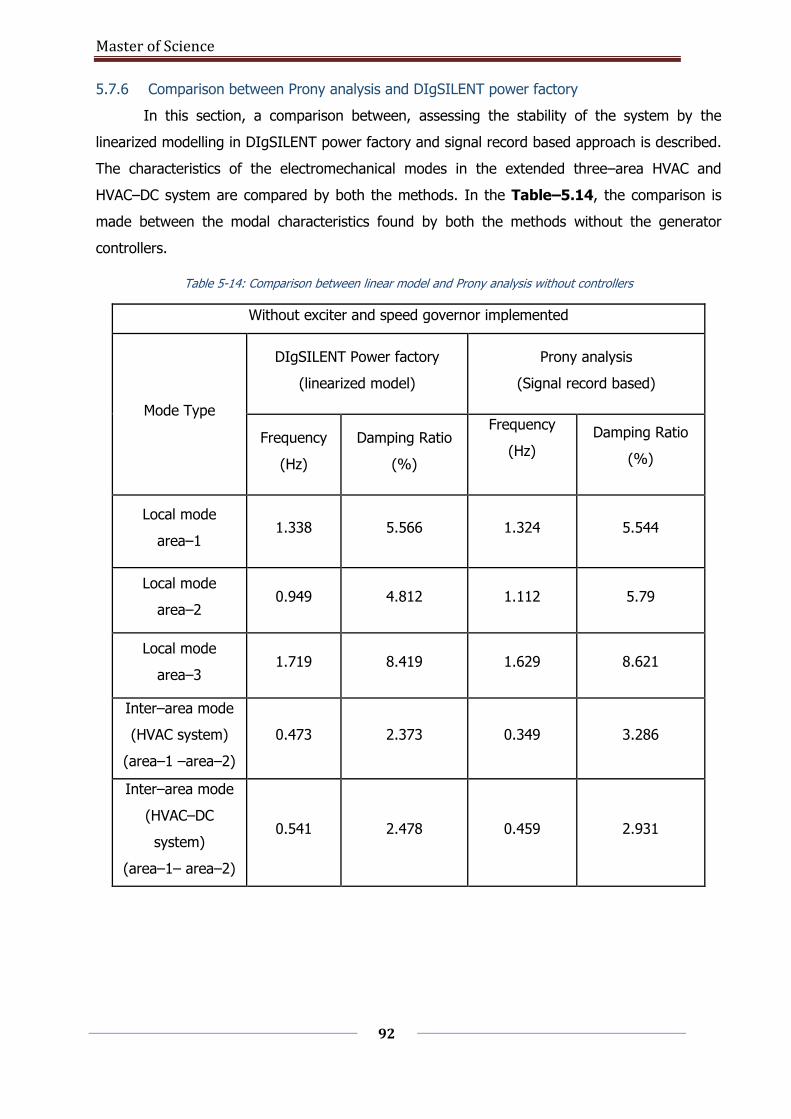
Master of Science

92

5.7.6 Comparison between Prony analysis and DIgSILENT power factory

In this section, a comparison between, assessing the stability of the system by the

linearized modelling in DIgSILENT power factory and signal record based approach is described.

The characteristics of the electromechanical modes in the extended three–area HVAC and

HVAC–DC system are compared by both the methods. In the Table–5.14, the comparison is

made between the modal characteristics found by both the methods without the generator

controllers.

Table 5-14: Comparison between linear model and Prony analysis without controllers

Without exciter and speed governor implemented

Mode Type

DIgSILENT Power factory

(linearized model)

Prony analysis

(Signal record based)

Frequency

(Hz)

Damping Ratio

(%)

Frequency

(Hz)

Damping Ratio

(%)

Local mode

area–1 1.338 5.566 1.324 5.544

Local mode

area–2 0.949 4.812 1.112 5.79

Local mode

area–3 1.719 8.419 1.629 8.621

Inter–area mode

(HVAC system)

(area–1 –area–2)

0.473 2.373 0.349 3.286

Inter–area mode

(HVAC–DC

system)

(area–1– area–2)

0.541 2.478 0.459 2.931

Master of Science

93

In Table–5.15 below, the comparison is made between the modal characteristics with

the exciter and speed governor implemented to all the generators.

Table 5-15: Comparison between linear model and Prony analysis with controllers

With Exciter and speed governor implemented

Mode Type

DIgSILENT Power factory

(linearized model)

Prony analysis

(Signal record based)

Frequency

(Hz)

Damping Ratio

(%)

Frequency

(Hz)

Damping Ratio

(%)

Local mode

area–1 1.538 8.383 1.571 9.100

Local mode

area–2 1.093 6.724 1.109 8.646

Local mode

area–3 1.995 11.806 1.763 5.389

Inter–area mode

(HVAC system)

(area–1–area–2)

0.537 7.044 0.451 9.752

Inter–area mode

(HVAC–DC

system)

(area–1–area–2)

0.598 6.713 0.526 7.644

It can be observed that the values of frequencies and damping ratios of the

electromechanical modes determined by linearized models in DIgSILENT power factory closely

matches with the signal record based approach when the controllers are not implemented. This

is mainly, because of the way the control system is implemented in the system. In the control

system definition (refer Figure–3.3 and Figure–3.5), there is an outer loop which decouples

the PI controller. As a result, during the linearization process, the effect of the controllers is not

effective. But when the signals are analyzed by Prony’s method, the effect of the controllers is

clearly evident resulting in higher values of damping ratios.

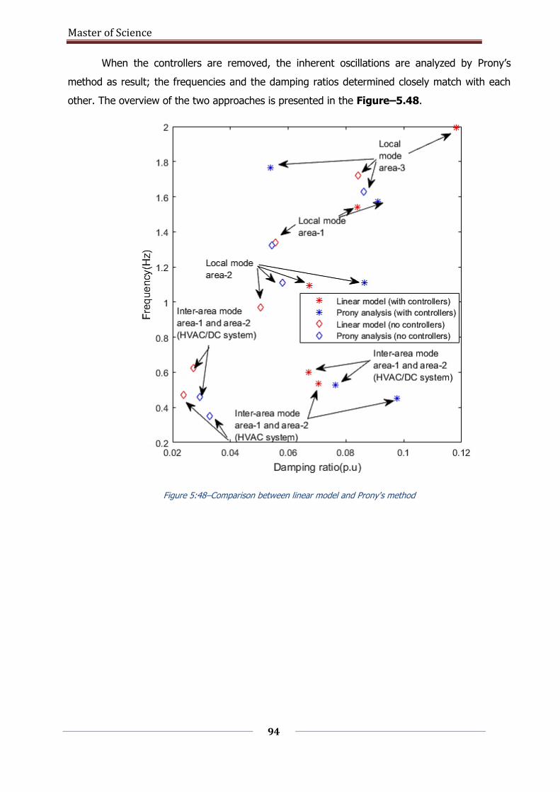
Master of Science

94

When the controllers are removed, the inherent oscillations are analyzed by Prony’s

method as result; the frequencies and the damping ratios determined closely match with each

other. The overview of the two approaches is presented in the Figure–5.48.

Figure 5:48–Comparison between linear model and Prony's method

Master of Science

95

Master of Science

96

6 Conclusions and Recommendations

In this chapter, the conclusions of this work are presented. The main objective of this thesis

work was to investigate the effect of machine inertia on the modal behavior of the system when

an HVDC link is incorporated to the existing grid. For this purpose, a classical two–area system

was implemented and thereafter, two study cases were developed. First study case was

introducing a third area with an HVAC tie line and the second study case was replacing the

HVDC tie line with a point–to point HVDC link. The modelling involved the implementation of

VSC–HVDC point–to–point link.

Different operating points were considered with respect to inertias of the synchronous

machines for a peak loaded condition to examine the sensitivity of the Eigenvalues towards

inertias. The Eigenvalue sensitivity towards the inertias of the machines was analyzed for both

the test cases developed.

Through the time–domain simulations, the modal information was extracted through

Prony analysis to validate and compare the results obtained. The Prony’s method is used in this

work is open source tool that is made available by PNNL laboratories. Hence, the modal

analysis module in DIgSILENT is validated with an independent Prony analysis tool. The error in

the determined values is because, in the Prony’s approach, a discretized time domain signal is

fitted to a curve with damped sinusoidal terms and this curve fitting is never a perfect match.

The other reason is due to manually determining the Prony window for extracting the

information about the dominant modes this would result is errors.

6.1 Conclusions

From this thesis work, the following conclusions are derived. The stability of the system is very

critical issue especially when the system is highly stressed. In such a stressed system,

monitoring the electromechanical modes is very important.

The damping of the modes depends on the dynamic elements of the system like the

speed governors and the exciters. The frequencies of the modes depend on the topology

of the network, operating conditions, loading conditions.

In both HVAC and HVAC–DC system, there are three local area modes belonging to each

area respectively. In these modes, the generators within an area swing against each

other. The low inertia machine is more sensitive hence swings with greater amplitude.

There are two inter–area modes exists when a third area is introduced with an HVAC tie–

line. One inter–area mode is between area–1 and area–2 and the other inter–area mode

is between area–1 and area-3.

Master of Science

97

In HVAC–DC system there is only one inter–area mode between area–1 and area–2 and

the second inter–area mode does not exist. This is because of the asynchronous nature

of the HVDC link.

In both the test cases, the damping of local modes is higher than that of the inter–area

modes.

Prony analysis can be very useful to determine the modal characteristics of power

systems, where the computation of the complete state matrix (A matrix) is unnecessary.

By Prony analysis an estimation of the dominant modes in the system through the

measured signals can be obtained, which is a less cumbersome process compared to

state–space modelling which involves solving complex differential equations.

6.2 Reflections

From the analysis, it is observed that, for analyzing small systems, linearized models are

very useful. The computation does not take much time due to less number of states.

For larger systems, with many states, developing the linearized models will be

cumbersome process, and during those situations the real time data from the system can be

utilized to study the system stability.

From the analysis, it can be concluded that, employing low inertia machines with an HVDC

link would be a safer option. This will make them less vulnerable to faults on the AC side of the

grid.

If the number of HVDC links is increased in a large grid, the local modes will be more

dominant ones, and it is easier to monitor them with local control mechanisms.

6.3 Future recommendations

In this thesis, two generic systems are developed from a reference system in a very well

structured simulation environment in power factory. These models are validated in both time

domain and the frequency domain.

In this thesis, a two–area reference system is extended to a three–area system by a

point–to–point HVDC link by modelling two–stage VSC converters. For large MTDC systems, with

more than one HVDC link, opting for MMC’s would be a better option to check system response

to faults and monitor the electro–mechanical modes within an area.

As the aim of the electrical power sector is to increase the penetration of the renewable

energy sources into the existing grids, the generators can be modeled as specific renewable

Master of Science

98

sources like wind turbines or hydro-power plants and the analysis for low inertia machines is to

be analyzed in detail.

A real power system is highly non–linear in nature and for the analysis purposes, it is linearized.

But, linearizing a huge system would be a difficult task, so for large systems, using advanced

technics like GMC’s (Geometric Measure of Controllability) or use of aggregated models would

give more reliable results.

Master of Science

99

Master of Science

100

Works Cited

[1] M. A. R.L. Sellick, "Comparison of HVDC Light (VSC) and HVDC Classic (LCC), Site

aspects for a MW,400kV HVDC transmission Scheme," in IET ACDC conference,

Brimingham, 2012.

[2] G. M.Klein, "A Fundamental study of inter-area oscillations in power systems," IEEE,

vol. 6, pp. 914-921, 1991.

[3] G. Rogers, Power System Oscillations, Massachusetts: Kluwer Academic Publishers,

2000.

[4] L. V. Y. Chompoobutrgool, "Identification of Power System Dominant Inter-area

oscillation paths," IEEE transactions on Power Systems, vol. 28, pp. 2798-2807,

2013.

[5] J. H. H. G. Yin.R, "Hybrid HVDC transmission topology for offshore windfarm

integration," Automation of electrical power systems, vol. 39(14), pp. 134-139, 2015.

[6] V. Mitra.P, "Dynamic Performance study of a HVDC grid using Real-Time Digital

Simulator," in RT and HIL Simulation Applications for Approaching Complexity in

Future Power and Energy Systems, Aachen, 2012.

[7] M. R. J. K. a. M. L.Shen, "The Effect of VSC HVDC Control and Operating Condition

on Dynamic Behaviour of Integrated AC/DC System," IEEE transactions on POwer

Delivery, 2015.

[8] A. B. T. P. J. A. V. M. M. I. Jose M.Aller, "Space vector applications in power

systems," IEEE, 2000.

[9] A. S. J. M. F. O. Zadeb M.K, "Small-Signal stability study of the CIGRE grid test

system with analysis of Participation factors and Parameter sensitivity of oscillatoy

modes," in 18th power systems computations conference , Wroclaw, 2014.

[10] A. S. M. F. Zadeh. M.K, "Stability analysis of interconnected AC power systems with

multi-terminal DC grids based on the CIGRE DC grid test system," in 18th Power

systems Computations Conference, Wroclaw, 2014.

Master of Science

101

[11] A. Krawita.C, "Multi-Infeed HVDC Interaction studies using Small-Signal stability

Assessment," IEEE transactions on Power Delivery, Vols. 24-2, 2009.

[12] Kundur.P, Power System Stability Dynamics and Control, New York: McGraw-Hill,

1994.

[13] V. L. Resende.F.o, "Simulataneous tuning of Power system stabilizers installed in the

VSC based MTDC networks of large offshore windfarms," in Power Systems

Computation Conference, Wroclaw, 2014.

[14] C. R. X. Ruihua.S, "VSCs based HVDC and its control strategy," in IEEE PES

Transmission and Distribution Conference and Exhibition, 2005.

[15] P. G. A. O. O.K.Giddani, "Small Signal Stability Analysis of Multi-Terminal VSC based

DC Transmission Systems," IEEE Transactions on Power System, Vols. 27-4, 2014.

[16] D. G. Germany, "User manual DIgSILENT Power factory version," [Online]. Available:

http://www.digsilent.de/.

[17] R. G. K. Klein.M, "A Fundamental study of Inter–area oscillations in power systems,"

Transactions on Power systems, vol. 3, pp. 914-921, 1991.

[18] Hauer.J.F, "Pacific Northwest National Laboratory (PNNL), US energy Department,"

PNNL, 2002. [Online]. Available: https://www.pnl.gov/.

[19] T. L. D. J. H. Theodor Borche, "Effect of rotational inertia on power system damping

and frequency transients," 2015.

[20] J. R. Torres, Power System Dynamics Lecture Slides, TU Delft EEMCS faculty, Delft,

2017.

[21] D. Zhang.P, "Emerging techniques in power system analysis," in Emerging

techniques in power system analysis, Berlin, Springer, 2010.

[22] P. J. Singh.R, "Statistical representation of distribution system loads using Gaussian

mixture model," IEEE transactions Power systems, Vols. 25-1, pp. 29-37, 2010.

[23] B. P. M. B. ,. B. Shen.L, "The effect of VSC HVDC control on AC system

electromechanical oscillations and DC system Dynamics," IEEE transactions on Pwer

Systems, 2015.

Master of Science

102

[24] R. J. Pringles R, "Optimal transmission expansion planning using mean-variance

mapping optimization," in IEEE/PES transmission and distribution, Latin America

conference and exposition, 2012.

[25] W. M. Preece.R, "The Probabilistic collocation method for power system damping and

voltage collapse studies in the presence of uncertainties," IEEE transactions Power

Systems, Vols. 28-3, pp. 2253-2262, 2013.

Master of Science

103

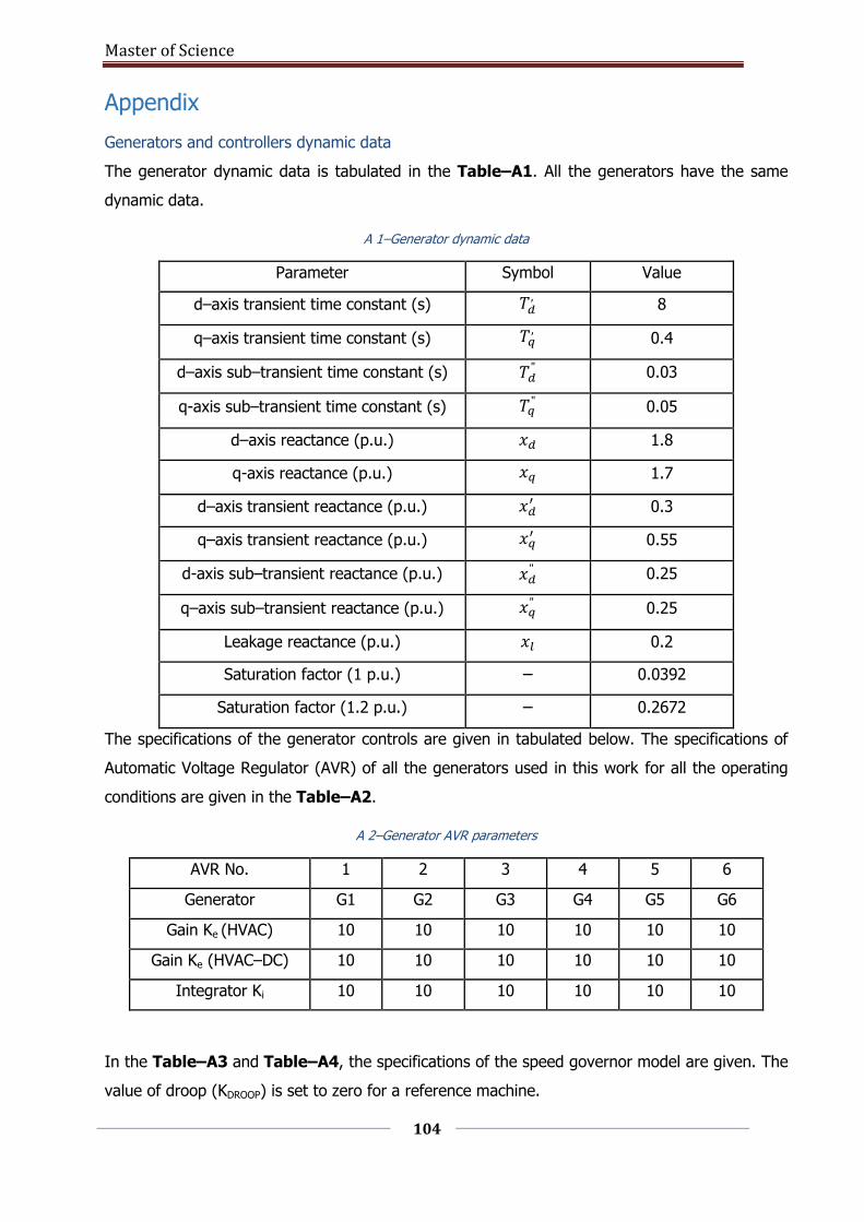
Master of Science

104

Appendix

Generators and controllers dynamic data

The generator dynamic data is tabulated in the Table–A1. All the generators have the same

dynamic data.

A 1–Generator dynamic data

Parameter Symbol Value

d–axis transient time constant (s) 𝑇𝑑, 8

q–axis transient time constant (s) 𝑇𝑞, 0.4

d–axis sub–transient time constant (s) 𝑇𝑑" 0.03

q-axis sub–transient time constant (s) 𝑇𝑞" 0.05

d–axis reactance (p.u.) 𝑥𝑑 1.8

q-axis reactance (p.u.) 𝑥𝑞 1.7

d–axis transient reactance (p.u.) 𝑥𝑑′ 0.3

q–axis transient reactance (p.u.) 𝑥𝑞′ 0.55

d-axis sub–transient reactance (p.u.) 𝑥𝑑" 0.25

q–axis sub–transient reactance (p.u.) 𝑥𝑞" 0.25

Leakage reactance (p.u.) 𝑥𝑙 0.2

Saturation factor (1 p.u.) – 0.0392

Saturation factor (1.2 p.u.) – 0.2672

The specifications of the generator controls are given in tabulated below. The specifications of

Automatic Voltage Regulator (AVR) of all the generators used in this work for all the operating

conditions are given in the Table–A2.

A 2–Generator AVR parameters

AVR No. 1 2 3 4 5 6

Generator G1 G2 G3 G4 G5 G6

Gain Ke (HVAC) 10 10 10 10 10 10

Gain Ke (HVAC–DC) 10 10 10 10 10 10

Integrator Ki 10 10 10 10 10 10

In the Table–A3 and Table–A4, the specifications of the speed governor model are given. The

value of droop (KDROOP) is set to zero for a reference machine.

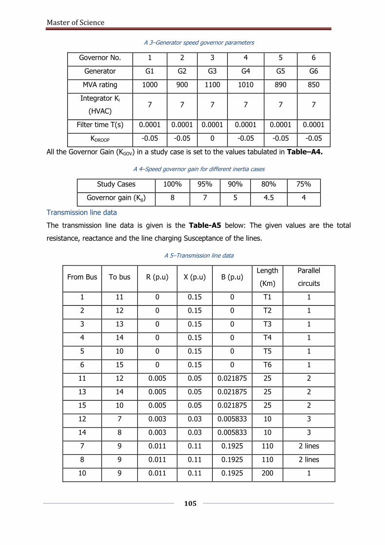
Master of Science

105

A 3–Generator speed governor parameters

Governor No. 1 2 3 4 5 6

Generator G1 G2 G3 G4 G5 G6

MVA rating 1000 900 1100 1010 890 850

Integrator Ki

(HVAC) 7 7 7 7 7 7

Filter time T(s) 0.0001 0.0001 0.0001 0.0001 0.0001 0.0001

KDROOP -0.05 -0.05 0 -0.05 -0.05 -0.05

All the Governor Gain (KGOV) in a study case is set to the values tabulated in Table–A4.

A 4–Speed governor gain for different inertia cases

Study Cases 100% 95% 90% 80% 75%

Governor gain (Kg) 8 7 5 4.5 4

Transmission line data

The transmission line data is given is the Table-A5 below: The given values are the total

resistance, reactance and the line charging Susceptance of the lines.

A 5–Transmission line data

From Bus To bus R (p.u) X (p.u) B (p.u) Length

(Km)

Parallel

circuits

1 11 0 0.15 0 T1 1

2 12 0 0.15 0 T2 1

3 13 0 0.15 0 T3 1

4 14 0 0.15 0 T4 1

5 10 0 0.15 0 T5 1

6 15 0 0.15 0 T6 1

11 12 0.005 0.05 0.021875 25 2

13 14 0.005 0.05 0.021875 25 2

15 10 0.005 0.05 0.021875 25 2

12 7 0.003 0.03 0.005833 10 3

14 8 0.003 0.03 0.005833 10 3

7 9 0.011 0.11 0.1925 110 2 lines

8 9 0.011 0.11 0.1925 110 2 lines

10 9 0.011 0.11 0.1925 200 1

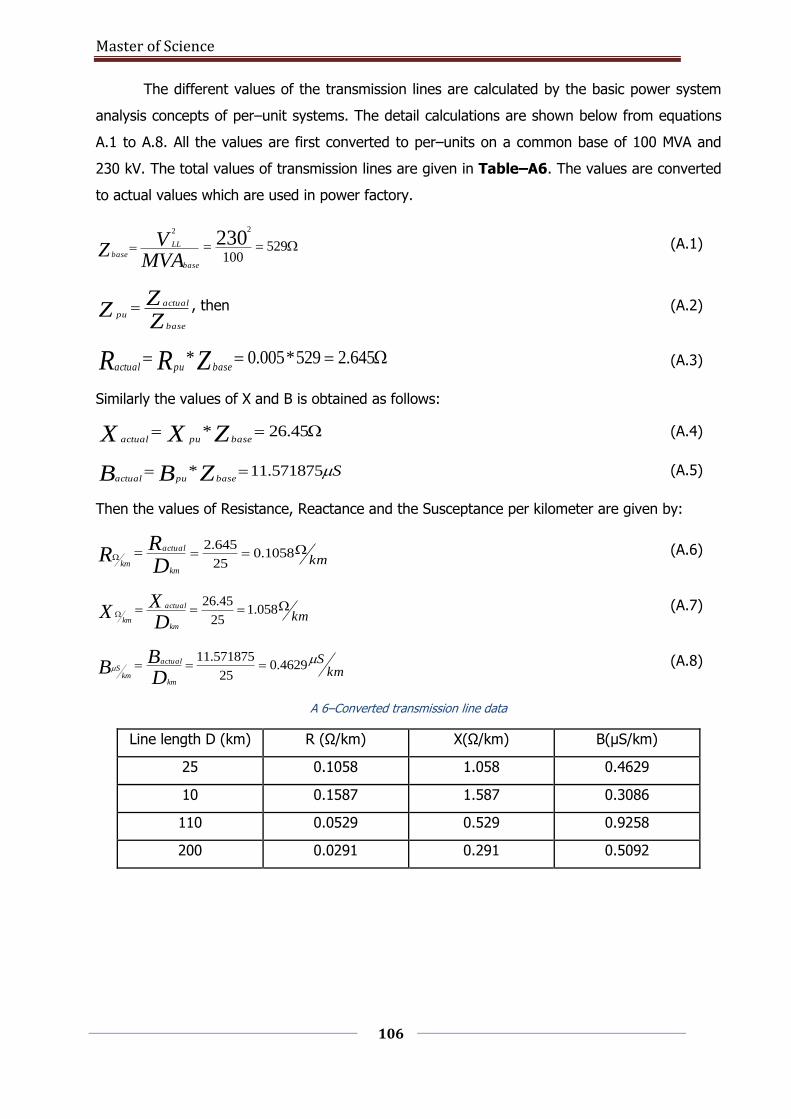
Master of Science

106

The different values of the transmission lines are calculated by the basic power system

analysis concepts of per–unit systems. The detail calculations are shown below from equations

A.1 to A.8. All the values are first converted to per–units on a common base of 100 MVA and

230 kV. The total values of transmission lines are given in Table–A6. The values are converted

to actual values which are used in power factory.

MVAV

Zbase

LL

base

2

529100

2302

(A.1)

ZZ

Zbase

actual

pu , then (A.2)

645.2529*005.0*ZRR basepuactual (A.3)

Similarly the values of X and B is obtained as follows:

45.26*ZXX basepuactual (A.4)

SZBB basepuactual571875.11* (A.5)

Then the values of Resistance, Reactance and the Susceptance per kilometer are given by:

DR

Rkm

actual

km

km 1058.0

25

645.2 (A.6)

kmDX

Xkm

actual

km

058.125

45.26 (A.7)

kmS

DB

Bkm

actual

kmS

4629.0

25

571875.11 (A.8)

A 6–Converted transmission line data

Line length D (km) R (Ω/km) X(Ω/km) B(µS/km)

25 0.1058 1.058 0.4629

10 0.1587 1.587 0.3086

110 0.0529 0.529 0.9258

200 0.0291 0.291 0.5092

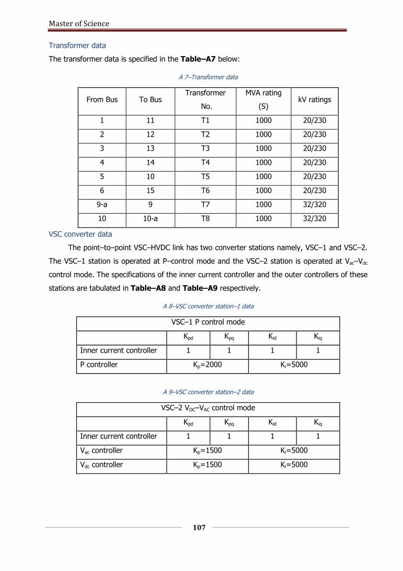
Master of Science

107

Transformer data

The transformer data is specified in the Table–A7 below:

A 7–Transformer data

From Bus To Bus Transformer

No.

MVA rating

(S) kV ratings

1 11 T1 1000 20/230

2 12 T2 1000 20/230

3 13 T3 1000 20/230

4 14 T4 1000 20/230

5 10 T5 1000 20/230

6 15 T6 1000 20/230

9-a 9 T7 1000 32/320

10 10-a T8 1000 32/320

VSC converter data

The point–to–point VSC–HVDC link has two converter stations namely, VSC–1 and VSC–2.

The VSC–1 station is operated at P–control mode and the VSC–2 station is operated at Vac–Vdc

control mode. The specifications of the inner current controller and the outer controllers of these

stations are tabulated in Table–A8 and Table–A9 respectively.

A 8–VSC converter station–1 data

VSC–1 P control mode

Kpd Kpq Kid Kiq

Inner current controller 1 1 1 1

P controller Kp=2000 Ki=5000

A 9–VSC converter station–2 data

VSC–2 VDC–VAC control mode

Kpd Kpq Kid Kiq

Inner current controller 1 1 1 1

Vac controller Kp=1500 Ki=5000

Vdc controller Kp=1500 Ki=5000

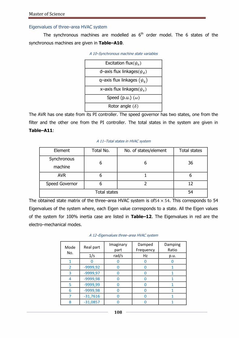
Master of Science

108

Eigenvalues of three–area HVAC system

The synchronous machines are modelled as 6th order model. The 6 states of the

synchronous machines are given in Table–A10.

A 10–Synchronous machine state variables

Excitation flux(𝜓𝑒)

d–axis flux linkages(𝜓𝑑)

q–axis flux linkages (𝜓𝑞)

x–axis flux linkages(𝜓𝑥)

Speed (p.u.) (𝜔)

Rotor angle (𝛿)

The AVR has one state from its PI controller. The speed governor has two states, one from the

filter and the other one from the PI controller. The total states in the system are given in

Table–A11:

A 11–Total states in HVAC system

Element Total No. No. of states/element Total states

Synchronous

machine 6 6 36

AVR 6 1 6

Speed Governor 6 2 12

Total states 54

The obtained state matrix of the three–area HVAC system is of54 × 54. This corresponds to 54

Eigenvalues of the system where, each Eigen value corresponds to a state. All the Eigen values

of the system for 100% inertia case are listed in Table–12. The Eigenvalues in red are the

electro–mechanical modes.

A 12–Eigenvalues three–area HVAC system

Mode No.

Real part Imaginary

part Damped

Frequency Damping

Ratio

1/s rad/s Hz p.u.

1 0 0 0 0

2 -9999,92 0 0 1

3 -9999,97 0 0 1

4 -9999,98 0 0 1

5 -9999,99 0 0 1

6 -9999,98 0 0 1

7 -31,7616 0 0 1

8 -31,0857 0 0 1

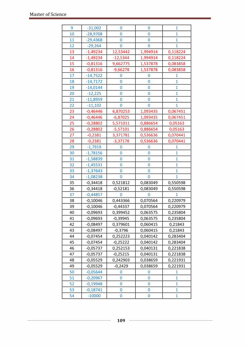
Master of Science

109

9 -31,002 0 0 1

10 -28,9708 0 0 1

11 -29,4368 0 0 1

12 -29,264 0 0 1

13 -1,49234 12,53442 1,994914 0,118224

14 -1,49234 -12,5344 1,994914 0,118224

15 -0,81316 9,662775 1,537878 0,083858

16 -0,81316 -9,66278 1,537878 0,083858

17 -14,7522 0 0 1

18 -14,7172 0 0 1

19 -14,0144 0 0 1

20 -12,225 0 0 1

21 -11,8959 0 0 1

22 -11,102 0 0 1

23 -0,46446 6,870253 1,093435 0,067451

24 -0,46446 -6,87025 1,093435 0,067451

25 -0,28802 5,571011 0,886654 0,05163

26 -0,28802 -5,57101 0,886654 0,05163

27 -0,2381 3,371781 0,536636 0,070441

28 -0,2381 -3,37178 0,536636 0,070441

29 -1,7919 0 0 1

30 -1,78156 0 0 1

31 -1,58839 0 0 1

32 -1,45531 0 0 1

33 -1,37643 0 0 1

34 -1,08238 0 0 1

35 -0,34418 0,521812 0,083049 0,550598

36 -0,34418 -0,52181 0,083049 0,550598

37 -0,44857 0 0 1

38 -0,10046 0,443366 0,070564 0,220979

39 -0,10046 -0,44337 0,070564 0,220979

40 -0,09693 0,399452 0,063575 0,235804

41 -0,09693 -0,39945 0,063575 0,235804

42 -0,08497 0,379601 0,060415 0,21843

43 -0,08497 -0,3796 0,060415 0,21843

44 -0,07454 0,252223 0,040142 0,283404

45 -0,07454 -0,25222 0,040142 0,283404

46 -0,05737 0,252153 0,040131 0,221838

47 -0,05737 -0,25215 0,040131 0,221838

48 -0,05529 0,242903 0,038659 0,221931

49 -0,05529 -0,2429 0,038659 0,221931

50 -0,05644 0 0 1

51 -0,20967 0 0 1

52 -0,19948 0 0 1

53 -0,18741 0 0 1

54 -10000 0 0 1

Master of Science

110

Eigenvalues of three–area HVAC–DC system

The obtained state matrix of the three–area HVAC–DC system is of68 × 68. This

corresponds to 68 eigenvalues of the system. The total number of states is tabulated in Table–

A13 below

A 13–Total states three–area HVAC–DC system

Element Total No. No. of states/element Total states

Synchronous

machine 6 6 36

AVR 6 1 6

Speed Governor 6 2 12

PLLs 2 2 4

VSCs 2 2 2

Inner–current

controller 2 2 4

P–control 1 1 1

Vac–control 1 1 1

Vdc–control 1 1 1

HVDC line 1 1 1

Total states 68

All the Eigen values for the 100% inertia case in HVAC–DC system is tabulated below in the

Table–A14.

A 14–Eigenvalues HVAC–DC system

Name Real part Imaginary

part Damped

Frequency Damping

Ratio

1/s rad/s Hz p.u.

1 0 0 0 0

2 -10375,3 0 0 1

3 -9999,93 0 0 1

4 -9999,98 0 0 1

5 -9999,97 0,000113 1,8E-05 1

6 -9999,97 -0,00011 1,8E-05 1

7 -9999,95 0 0 1

8 -30,7168 0 0 1

9 -30,891 0 0 1

10 -31,0049 0 0 1

11 -29,167 0 0 1

12 -28,1144 0 0 1

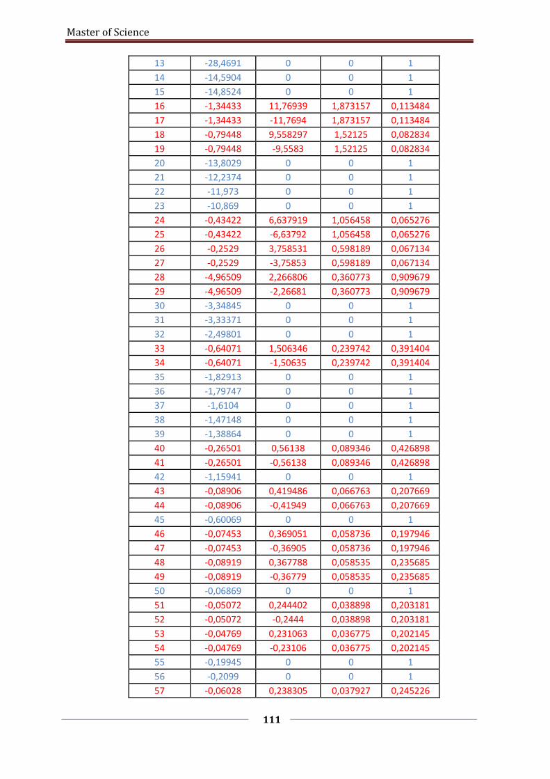
Master of Science

111

13 -28,4691 0 0 1

14 -14,5904 0 0 1

15 -14,8524 0 0 1

16 -1,34433 11,76939 1,873157 0,113484

17 -1,34433 -11,7694 1,873157 0,113484

18 -0,79448 9,558297 1,52125 0,082834

19 -0,79448 -9,5583 1,52125 0,082834

20 -13,8029 0 0 1

21 -12,2374 0 0 1

22 -11,973 0 0 1

23 -10,869 0 0 1

24 -0,43422 6,637919 1,056458 0,065276

25 -0,43422 -6,63792 1,056458 0,065276

26 -0,2529 3,758531 0,598189 0,067134

27 -0,2529 -3,75853 0,598189 0,067134

28 -4,96509 2,266806 0,360773 0,909679

29 -4,96509 -2,26681 0,360773 0,909679

30 -3,34845 0 0 1

31 -3,33371 0 0 1

32 -2,49801 0 0 1

33 -0,64071 1,506346 0,239742 0,391404

34 -0,64071 -1,50635 0,239742 0,391404

35 -1,82913 0 0 1

36 -1,79747 0 0 1

37 -1,6104 0 0 1

38 -1,47148 0 0 1

39 -1,38864 0 0 1

40 -0,26501 0,56138 0,089346 0,426898

41 -0,26501 -0,56138 0,089346 0,426898

42 -1,15941 0 0 1

43 -0,08906 0,419486 0,066763 0,207669

44 -0,08906 -0,41949 0,066763 0,207669

45 -0,60069 0 0 1

46 -0,07453 0,369051 0,058736 0,197946

47 -0,07453 -0,36905 0,058736 0,197946

48 -0,08919 0,367788 0,058535 0,235685

49 -0,08919 -0,36779 0,058535 0,235685

50 -0,06869 0 0 1

51 -0,05072 0,244402 0,038898 0,203181

52 -0,05072 -0,2444 0,038898 0,203181

53 -0,04769 0,231063 0,036775 0,202145

54 -0,04769 -0,23106 0,036775 0,202145

55 -0,19945 0 0 1

56 -0,2099 0 0 1

57 -0,06028 0,238305 0,037927 0,245226

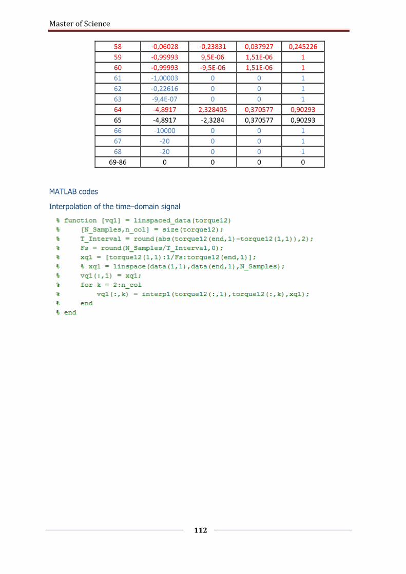
Master of Science

112

58 -0,06028 -0,23831 0,037927 0,245226

59 -0,99993 9,5E-06 1,51E-06 1

60 -0,99993 -9,5E-06 1,51E-06 1

61 -1,00003 0 0 1

62 -0,22616 0 0 1

63 -9,4E-07 0 0 1

64 -4,8917 2,328405 0,370577 0,90293

65 -4,8917 -2,3284 0,370577 0,90293

66 -10000 0 0 1

67 -20 0 0 1

68 -20 0 0 1

69-86 0 0 0 0

MATLAB codes

Interpolation of the time–domain signal

Fundamental Study of Small–Signal Stability of Hybrid ...

Documents