J. Kretinsky: Fundamental Algorithms Chapter 5: Hash Tables, Winter 2018/19 1 Fundamental Algorithms Chapter 5: Hash Tables Jan Kˇ ret´ ınsk´ y Winter 2018/19

Welcome message from author
This document is posted to help you gain knowledge. Please leave a comment to let me know what you think about it! Share it to your friends and learn new things together.
Transcript

J. Kretinsky: Fundamental Algorithms
Chapter 5: Hash Tables, Winter 2018/19 1
Fundamental AlgorithmsChapter 5: Hash Tables
Jan Kretınsky
Winter 2018/19

J. Kretinsky: Fundamental Algorithms
Chapter 5: Hash Tables, Winter 2018/19 2
Generalised Search Problem
Definition (Search Problem)
Input: a sequence or set A of n elements ∈ A, and an x ∈ A.Output: Index i ∈ {1, . . . ,n} with x = A[i], or NIL, if x 6∈ A.
• complexity depends on data structure• complexity of operations to set up data structure? (insert/delete)
Definition (Generalised Search Problem)
• Store a set of objects consisting of a key and additional data:
Object := (key : Integer , .record : Data ) ;
• search/insert/delete objects in this set

J. Kretinsky: Fundamental Algorithms
Chapter 5: Hash Tables, Winter 2018/19 3
Direct-Address Tables
Definition (table as data structure)
• similar to array: access element via index• usually contains elements only for some of the indices
Direct-Address Table:• assume: limited number of values for the keys:
U = {0,1, . . . ,m − 1}• allocate table of size m• use keys directly as index

J. Kretinsky: Fundamental Algorithms
Chapter 5: Hash Tables, Winter 2018/19 4
Direct-Address Tables (2)
Di rAdd r Inse r t (T : Table , x : Object ) {T [ x . key ] := x ;
}
DirAddrDelete (T : Table , x : Object ){T [ x . key ] := NIL ;
}
DirAddrSearch (T : Table , key : Integer ){return T [ key ] ;
}
J. Kretinsky: Fundamental Algorithms
Chapter 5: Hash Tables, Winter 2018/19 5
Direct-Address Tables (3)
Advantage:• very fast: search/delete/insert is Θ(1)
Disadvantages:• m has to be small,
or otherwise, the table has to be very large!• if only few elements are stored, lots of table elements are unused
(waste of memory)• all keys need to be distinct
(they should be, anyway)

J. Kretinsky: Fundamental Algorithms
Chapter 5: Hash Tables, Winter 2018/19 6
Hash Tables
Idea: compute index from keyWanted: function h that
• maps a given key to an index,• has a relatively small range of values, and• can be computed efficiently,
Definition (hash function, hash table)
Such a function h is called a hash function.The respective table is called a hash table.

J. Kretinsky: Fundamental Algorithms
Chapter 5: Hash Tables, Winter 2018/19 7
Hash Tables – Insert, Delete, Search
HashInsert (T : Table , x : Object ) {T [ h ( x . key ) ] := x ;
}
HashDelete (T : Table , x : Object ) {T [ h ( x . key ) ] : = NIL ;
}
HashSearch (T : Table , x : Object ) {return T [ h ( x . key ) ] ;
}

J. Kretinsky: Fundamental Algorithms
Chapter 5: Hash Tables, Winter 2018/19 8
So Far: Naive Hashing
Advantages:• still very fast: search/delete/insert is Θ(1), if h is Θ(1)
• size of the table can be chosen freely, provided there is anappropriate hash function h
Disadvantages:• values of h have to be distinct for all keys• however: impossible to find a hash function that produces
distinct values for any set of stored data
ToDo: deal with collisions:objects with different keys that share a common hash value have tobe stored in the same table element

J. Kretinsky: Fundamental Algorithms
Chapter 5: Hash Tables, Winter 2018/19 9
Resolve Collisions by Chaining
Idea:• use a table of containers• containers can hold an arbitrarily large amount of data• using (linked) lists as containers: chaining
ChainHashInsert (T : Table , x : Object ) {i n s e r t x i n t o T [ h ( x . key ) ] ;
}
ChainHashDelete (T : Table , x : Object ) {de le te x from T [ h ( x . key ) ] ;
}

J. Kretinsky: Fundamental Algorithms
Chapter 5: Hash Tables, Winter 2018/19 10
Resolve Collisions by Chaining
ChainHashSearch (T : Table , x : Object ) {return Lis tSearch ( x , T [ h ( x . key ) ] ) ;! r e s u l t : re ference to x or NIL , i f x not found ;
}
Advantages:• hash function no longer has to return distinct values• still very fast, if the lists are short
Disadvantages:• delete/search is Θ(k), if k elements are in the accessed list• worst case: all elements stored in one single list (very unlikely).

J. Kretinsky: Fundamental Algorithms
Chapter 5: Hash Tables, Winter 2018/19 11
Chaining – Average Search Complexity
Assumptions:• hash table has m slots (table of m lists)• contains n elements⇒ load factor: α = n
m
• h(k) can be computed in O(1) for all k• all values of h are equally likely to occur
Search complexity:• on average, the list corresponding to the requested key will haveα elements
• unsuccessful search: compare the requested key with all objectsin the list, i.e. O(α) operations
• successful search: requested key last in the list;⇒ also O(α) operations
Expected: Average complexity: O(α) operations

J. Kretinsky: Fundamental Algorithms
Chapter 5: Hash Tables, Winter 2018/19 12
Hash Functions
A good hash function should:• satisfy the assumption of even distribution:
each key is equally likely to be hashed to any of the slots:∑k : h(k)=j
(P(key = k)) =1m
for all j = 0, . . . ,m − 1
• be easy to compute• be “non-smooth”: keys that are close together should not
produce hash values that are close together (to avoid clustering)
Simplest choice: h = k mod m (m a prime number)• easy to compute; even distribution if keys evenly distributed• however: not “non-smooth”
J. Kretinsky: Fundamental Algorithms
Chapter 5: Hash Tables, Winter 2018/19 13
The Multiplication Method for Integer Keys
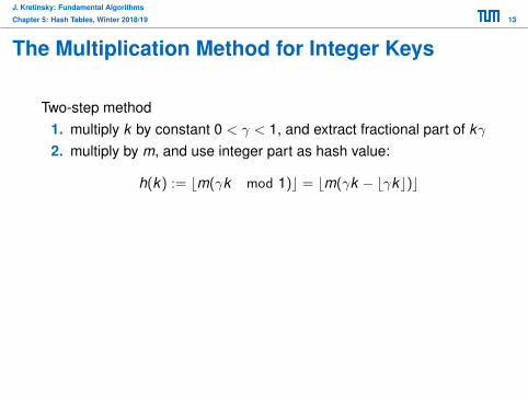
Two-step method1. multiply k by constant 0 < γ < 1, and extract fractional part of kγ2. multiply by m, and use integer part as hash value:
h(k) := bm(γk mod 1)c = bm(γk − bγkc)c
Remarks:• value of m uncritical; e.g. m = 2p
• value of γ needs to be chosen well• in practice: use fix-point arithmetics• non-integer keys: use encoding to integers
(ASCII, byte encoding, . . . )

J. Kretinsky: Fundamental Algorithms
Chapter 5: Hash Tables, Winter 2018/19 13
The Multiplication Method for Integer Keys
Two-step method1. multiply k by constant 0 < γ < 1, and extract fractional part of kγ2. multiply by m, and use integer part as hash value:
h(k) := bm(γk mod 1)c = bm(γk − bγkc)c
Remarks:• value of m uncritical; e.g. m = 2p
• value of γ needs to be chosen well• in practice: use fix-point arithmetics• non-integer keys: use encoding to integers
(ASCII, byte encoding, . . . )

J. Kretinsky: Fundamental Algorithms
Chapter 5: Hash Tables, Winter 2018/19 14
Open Addressing
Definition
• no containers: table contains objects• each slot of the hash table either contains an object or NIL• to resolve collisions, more than one position is allowed for a
specific key
Hash function: generates sequence of hash table indices:
h : U × {0, . . . ,m − 1} → {0, . . . ,m − 1}
General approach:• store object in the first empty slot specified by the probe
sequence• empty slot in the hash table guaranteed, if the probe sequence
h(k ,0),h(k ,1), . . . ,h(k ,m− 1) is a permutation of 0,1, . . . ,m− 1

J. Kretinsky: Fundamental Algorithms
Chapter 5: Hash Tables, Winter 2018/19 15
Open Addressing – Algorithms
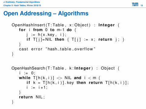
OpenHashInsert (T : Table , x : Object ) : Integer {for i from 0 to m−1 do {
j := h ( x . key , i ) ;i f T [ j ]= NIL then { T [ j ] := x ; return j ; }
}cast e r r o r ” hash tab l e over f low ”
}
OpenHashSearch (T : Table , k : Integer ) : Object {i := 0 ;while T [ h ( k , i ) ] <> NIL and i < m {
i f k = T [ h ( k , i ) ] . key then return T [ h ( k , i ) ] ;i := i +1;
}return NIL ;
}
J. Kretinsky: Fundamental Algorithms
Chapter 5: Hash Tables, Winter 2018/19 15
Open Addressing – Algorithms
OpenHashInsert (T : Table , x : Object ) : Integer {for i from 0 to m−1 do {
j := h ( x . key , i ) ;i f T [ j ]= NIL then { T [ j ] := x ; return j ; }
}cast e r r o r ” hash tab l e over f low ”
}
OpenHashSearch (T : Table , k : Integer ) : Object {i := 0 ;while T [ h ( k , i ) ] <> NIL and i < m {
i f k = T [ h ( k , i ) ] . key then return T [ h ( k , i ) ] ;i := i +1;
}return NIL ;
}

J. Kretinsky: Fundamental Algorithms
Chapter 5: Hash Tables, Winter 2018/19 16
Open Addressing – Linear Probing
Hash function: h(k , i) := (h0(k) + i) mod m• first slot to be checked is T[h0(k)]• second probe slot is T[h0(k) + 1], then T[h0(k) + 2], etc.• wrap around to T[0] after T[m − 1] has been checked
Main problem: clustering• continuous sequences of occupied slots (“clusters”) cause lots of
checks during searching and inserting• clusters tend to grow, because all objects that are hashed to a
slot inside the cluster will increase it• slight (but minor) improvement: h(k , i) := (h0(k) + ci) mod m
Main advantage: simple and fast• easy to implement• cache efficient!

J. Kretinsky: Fundamental Algorithms
Chapter 5: Hash Tables, Winter 2018/19 17
Open Addressing – Quadratic Probing
Hash function: h(k , i) := (h0(k) + c1i + c2i2) mod m• how to chose constants c1 and c2?• objects with identical h0(k) still have the same sequence of hash
values(“secondary clustering”)
Idea: double hashing h(k , i) := (h0(k) + i · h1(k)) mod m• if h0 is identical for two keys, h1 will generate different probe
sequences

J. Kretinsky: Fundamental Algorithms
Chapter 5: Hash Tables, Winter 2018/19 18
Open Addressing – Double Hashing
h(k , i) := (h0(k) + i · h1(k)) mod m
How to choose h0 and h1:
• range of h0 : U → {0, . . . ,m − 1} (cover entire table)• h1(k) must never be 0 (no probe sequence generated)• h1(k) should be prime to m for all k→ probe sequence will try all slots
• if d is the greatest common divisor of h1(k) and m, only 1d of the
hash slots will be probed
Possible choices:• m = 2M and let h1 generate odd numbers, only• m a prime number, and h1 : U → {1, . . . ,m1} with m1 < m

J. Kretinsky: Fundamental Algorithms
Chapter 5: Hash Tables, Winter 2018/19 18
Open Addressing – Double Hashing
h(k , i) := (h0(k) + i · h1(k)) mod m
How to choose h0 and h1:• range of h0 : U → {0, . . . ,m − 1} (cover entire table)• h1(k) must never be 0 (no probe sequence generated)• h1(k) should be prime to m for all k→ probe sequence will try all slots
• if d is the greatest common divisor of h1(k) and m, only 1d of the
hash slots will be probed
Possible choices:• m = 2M and let h1 generate odd numbers, only• m a prime number, and h1 : U → {1, . . . ,m1} with m1 < m

J. Kretinsky: Fundamental Algorithms
Chapter 5: Hash Tables, Winter 2018/19 19
Open Addressing – Deletion
Problem remaining: how to delete?
• search entry, remove it• does not work:
• insert 3, 7, 8 having same hash-value, then delete 7• how to find 8?
⇒ do not delete, just mark as deleted
Next problem:• searching stops if first empty entry found• after many deletions: lots of unnecessary comparisons!

J. Kretinsky: Fundamental Algorithms
Chapter 5: Hash Tables, Winter 2018/19 19
Open Addressing – Deletion
Problem remaining: how to delete?• search entry, remove it• does not work:
• insert 3, 7, 8 having same hash-value, then delete 7• how to find 8?
⇒ do not delete, just mark as deleted
Next problem:• searching stops if first empty entry found• after many deletions: lots of unnecessary comparisons!

J. Kretinsky: Fundamental Algorithms
Chapter 5: Hash Tables, Winter 2018/19 20
Open Addressing – Deletion (2)
Deletion general problem for open hashing• only “solution”: new construction of table after some deletions• hash tables therefore commonly don’t support deletion
Inserting• inserting efficient, but too many inserts⇒ not enough space⇒ if ratio α too big, new construction of table with larger size
Still. . .• searching faster than O(log n) possible
Related Documents
![Algorithms Lecture 12: Hash Tables [Sp’15] - Jeff Ericksonjeffe.cs.illinois.edu/teaching/datastructures/notes/12-hashing.pdf · Algorithms Lecture 12: Hash Tables [Sp’15] have2](https://static.cupdf.com/doc/110x72/5edb07bb09ac2c67fa68b22b/algorithms-lecture-12-hash-tables-spa15-jeff-algorithms-lecture-12-hash.jpg)
![Algorithms Lecture 5: Hash Tables [Sp’20] · Algorithms Lecture 5: Hash Tables [Sp’20] ordering,wecanstoreeachchaininabalancedbinarysearchtree.Thisreducestheexpected timeforanysearchtoO(1+log‘(x](https://static.cupdf.com/doc/110x72/5f5ae90c0a91a35f9801ad2a/algorithms-lecture-5-hash-tables-spa20-algorithms-lecture-5-hash-tables-spa20.jpg)

![Algorithms Lecture 5: Hash Tables [Sp’17]](https://static.cupdf.com/doc/110x72/6201c784b1f4342fc142ffe8/algorithms-lecture-5-hash-tables-sp17.jpg)


![Algorithms Lecture 5: Hash Tables [Sp’17] - Jeff Ericksonjeffe.cs.illinois.edu/teaching/algorithms/notes/05-hashing.pdf · Algorithms Lecture 5: Hash Tables [Sp’17] Proof: Fixanarbitraryintegera](https://static.cupdf.com/doc/110x72/5edb07bc09ac2c67fa68b22c/algorithms-lecture-5-hash-tables-spa17-jeff-algorithms-lecture-5-hash-tables.jpg)