Eingereicht von Simon Breneis Angefertigt am Institut für Analysis Beurteiler Univ.-Prof. Dr. Aicke Hin- richs Mitbetreuung O.Univ.-Prof. Dr.phil. Dr.h.c. Robert Tichy April 2020 JOHANNES KEPLER UNIVERSITÄT LINZ Altenbergerstraße 69 4040 Linz, Österreich www.jku.at DVR 0093696 Functions of bounded variation in one and multiple dimensions Masterarbeit zur Erlangung des akademischen Grades Diplom-Ingenieur im Masterstudium Mathematik in den Naturwissenschaften

Welcome message from author
This document is posted to help you gain knowledge. Please leave a comment to let me know what you think about it! Share it to your friends and learn new things together.
Transcript

Eingereicht vonSimon Breneis
Angefertigt amInstitut fürAnalysis
BeurteilerUniv.-Prof. Dr. Aicke Hin-richs
MitbetreuungO.Univ.-Prof. Dr.phil.Dr.h.c. Robert Tichy
April 2020
JOHANNES KEPLERUNIVERSITÄT LINZAltenbergerstraße 694040 Linz, Österreichwww.jku.atDVR 0093696
Functions of boundedvariation in one andmultiple dimensions
Masterarbeit
zur Erlangung des akademischen Grades
Diplom-Ingenieur
im Masterstudium
Mathematik in den Naturwissenschaften

Eidesstattliche Erklärung i
Eidesstattliche Erklärung
Ich erkläre an Eides statt, dass ich die vorliegende Masterarbeit selbstständig und ohne fremde Hilfeverfasst, andere als die angegebenen Quellen und Hilfsmittel nicht benutzt bzw. die wörtlich odersinngemäß entnommenen Stellen als solche kenntlich gemacht habe. Die vorliegende Masterarbeitist mit dem elektronisch übermittelten Textdokument identisch.
Ort, Datum Unterschrift

Abstract ii
Abstract
In this Master’s thesis, we investigate the properties of functions of bounded variation. First, weconsider univariate functions, afterwards we generalize this notion to higher dimensions. There aremany different definitions of multivariate functions of bounded variation. We study functions ofbounded variation in the senses of Vitali; Hardy and Krause; Arzelà; and Hahn. Many results forthose functions of bounded variation were previously only known in the bivariate case. We extendthem to arbitrary dimensions, and also add some new results.

Contents iii
Eidesstattliche Erklärung i
1 Introduction 1
2 Functions of one variable 4
2.1 Motivation and definition . . . . . . . . . . . . . . . . . . . . . . . . . . . . . . . . . 4
2.2 Variation functions . . . . . . . . . . . . . . . . . . . . . . . . . . . . . . . . . . . . . 7
2.3 Decomposition into monotone functions . . . . . . . . . . . . . . . . . . . . . . . . . 23
2.4 Continuity, differentiability and measurability . . . . . . . . . . . . . . . . . . . . . . 24
2.5 Signed Borel measures . . . . . . . . . . . . . . . . . . . . . . . . . . . . . . . . . . . 32
2.6 Dimension of the graph . . . . . . . . . . . . . . . . . . . . . . . . . . . . . . . . . . 35
2.7 Structure of BV . . . . . . . . . . . . . . . . . . . . . . . . . . . . . . . . . . . . . . . 40
2.8 Ideal structure of BV . . . . . . . . . . . . . . . . . . . . . . . . . . . . . . . . . . . . 44
2.9 Fourier Series . . . . . . . . . . . . . . . . . . . . . . . . . . . . . . . . . . . . . . . . 47
3 Functions of multiple variables 60
3.1 Definitions . . . . . . . . . . . . . . . . . . . . . . . . . . . . . . . . . . . . . . . . . . 60
3.2 The variation functions . . . . . . . . . . . . . . . . . . . . . . . . . . . . . . . . . . 71
3.3 Closure properties . . . . . . . . . . . . . . . . . . . . . . . . . . . . . . . . . . . . . 78
3.4 Decompositions into monotone functions . . . . . . . . . . . . . . . . . . . . . . . . . 80
3.5 Inclusions . . . . . . . . . . . . . . . . . . . . . . . . . . . . . . . . . . . . . . . . . . 83
3.6 Continuity, differentiability and measurability . . . . . . . . . . . . . . . . . . . . . . 85
3.7 Signed Borel measures . . . . . . . . . . . . . . . . . . . . . . . . . . . . . . . . . . . 96
3.8 Dimension of the graph . . . . . . . . . . . . . . . . . . . . . . . . . . . . . . . . . . 97
3.9 Product functions . . . . . . . . . . . . . . . . . . . . . . . . . . . . . . . . . . . . . . 98
3.10 Structure of the function spaces . . . . . . . . . . . . . . . . . . . . . . . . . . . . . . 108
3.11 Ideal structure of the functions spaces . . . . . . . . . . . . . . . . . . . . . . . . . . 111
4 The Koksma-Hlawka inequality 116
4.1 Harman variation . . . . . . . . . . . . . . . . . . . . . . . . . . . . . . . . . . . . . . 117
4.2 D-variation . . . . . . . . . . . . . . . . . . . . . . . . . . . . . . . . . . . . . . . . . 118
4.3 Koksma-Hlawka inequality for the Hahn-variation . . . . . . . . . . . . . . . . . . . 121
4.4 Other estimates . . . . . . . . . . . . . . . . . . . . . . . . . . . . . . . . . . . . . . . 123
Literature 125

1 Introduction 1
1 Introduction
The goal of this Master’s thesis is to study the properties of functions of bounded variation. Westudy univariate functions of bounded variation in Section 2 and multivariate functions of boundedvariation in Section 3. Finally, in Section 4, we give an application of functions of bounded variationto numerical integration.
We define the variation of a univariate function f : [a, b] → R by
Var(f ; a, b) := sup n∑
i=1
∣
∣f(xi) − f(xi−1)∣
∣ : a = x0 ≤ x1 ≤ · · · ≤ xn = b for some n ∈ N
.
If the interval [a, b] is clear from the context, we also write Var(f) := Var(f ; a, b). If the variationVar(f) is finite, we say that f is of bounded variation. Functions of bounded variation were firstintroduced by Jordan in [31] in the study of Fourier series. By now, they have many applications,for example in the study of Riemann-Stieltjes integrals.
In Section 2.1 we motivate and define functions of bounded variation in one dimension, albeit usingdifferent (non-standard) notation. The reason is that the standard notation is quite messy and hardto read in the higher-dimensional setting. Hence, to prepare the reader for Section 3, we already usenotation that can be extended more easily to multivariate functions. Furthermore, we give manyexamples and non-examples of functions of bounded variation.
In Section 2.2 we study variation functions. To every function f : [a, b] → R of bounded variation,we can associate its variation function Varf : [a, b] → R defined by
Varf (x) := Var(f ; a, x).
A function and its variation function share many regularity properties. For example, f is continuousif and only if Varf is continuous and f is Lipschitz continuous if and only if Varf is Lipschitzcontinuous, see also Theorem 2.2.5. It is also easy to see that f is α-Hölder continuous if Varf isα-Hölder continuous. The reverse direction seems to be an open problem. We answer this problemnegatively with Example 2.2.6 and prove a more general statement in Theorem 2.2.17.
In Section 2.3 we give a proof of the famous result by Jordan that a function is of bounded variationif and only if it can be written as the difference of two increasing functions, see Theorem 2.3.2.Therefore, the set of functions of bounded variation BV is the vector space induced by the monotonefunctions.
Section 2.4 deals with the regularity properties of functions of bounded variation. We show thatfunctions of bounded variation can have at most countably many discontinuities, that they aredifferentiable almost everywhere and Borel-measurable, see Theorem 2.4.2 and Theorem 2.4.6.
Section 2.5 illustrates the connection between functions of bounded variations and measures. Indeed,there is a natural correspondence between right-continuous functions of bounded variation and finitesigned Borel measures, see Theorem 2.5.5.
It is a well-known result that the graph of functions of bounded variation has Hausdorff-dimension1. In 2010, Liang proved in [38] that continuous functions of bounded variation also have Box-dimension 1, using Riemann-Liouville fractional integrals. We give a much more elementary proofof this fact in Section 2.6 and show that it is not necessary to require the function to be continuous,see Theorem 2.6.9.
Kuller proved [35] that BV is a commutative Banach algebra with respect to pointwise multiplication.We give a proof of this fact in Section 2.7 (Theorem 2.7.8), and we also show Helly’s First Theorem,which tells us that the unit ball of BV satisfies some weaker form of compactness, see Theorem
1 Introduction 2
2.7.11. Consequently, in Section 2.8 we characterize the maximal ideal space of BV in Theorem2.8.7.
Finally, in Section 2.9 we give an application of functions of bounded variation to the study of Fourierseries. In particular, we prove some famous results due to Jordan, including that the Fourier series offunctions of bounded variation converges pointwise (although not necessarily exactly to the functionitself) in Theorem 2.9.14, and that the Fourier series of a continuous function of bounded variationconverges uniformly to the function itself in Theorem 2.9.23.
The generalization of functions of bounded variation to the multidimensional setting is not imme-diately clear. Indeed, there are many different definitions. We study the variations in the sense ofVitali; Hardy and Krause; Arzela; Hahn; and Pierpont. We denote by V, HK, A, H and P thecorresponding sets of functions of bounded variation. In Section 3.1 we define those variations andgive examples of functions of bounded variation of the various kinds. Since we show in Theorem3.5.1 that the variations in the sense of Hahn and Pierpont are equivalent, thus extending a similartwo-dimensional result by Clarkson and Adams in [13], we rarely treat the Pierpont-variation in thefollowing chapters.
In Section 3.2, we again define the variation functions similarly as in the one-dimensional settings.Unfortunately, many results that hold for univariate functions do not extend to multivariate func-tions. However, in Theorem 3.2.6 we prove some previously unknown regularity correspondencessimilar to those in Theorem 2.2.5, especially for functions of bounded Arzelà-variation.
In Section 3.3, we prove that V, HK, A and H are vector spaces, and that HK, A and H areclosed under multiplication and division (given that the denominator is bounded away from 0), seeProposition 3.3.1 and Proposition 3.3.3. Most of those results were already known, although someof them had only been proved for bivariate functions.
Similarly to the one-dimensional setting, we state monotone decomposition theorems for functions inA, V and HK in Theorem 3.4.1, Theorem 3.4.2 and Theorem 3.4.3, respectively. Naturally, since thevarious definitions of bounded variation do not coincide, we use different definitions of monotonicityin those theorems. We remark that those decompositions were already known, although some ofthem again only in two dimensions.
In Section 3.5 we study the relations between the various kinds of bounded variation. We are ableto extend some (but not all) previously known results from the two-dimensional setting to arbitrarydimensions in Theorem 3.5.1.
Section 3.6 deals with the regularity properties of multivariate functions of bounded variation,where we again extend some results from the two-dimensional setting to arbitrary dimensions. Inparticular, we show that functions in HK, A and H are continuous almost everywhere (Theorem3.6.1) and thus also Lebesgue-measurable, that functions in HK and A are differentiable almosteverywhere (Theorem 3.6.13), and that functions in HK are Borel-measurable (Theorem 3.6.18).
In Section 3.7 we state the correspondence between right-continuous functions in HK and finitesigned Borel measures, which is the precise generalization of Theorem 2.5.5 to the multidimensionalsetting.
Verma and Viswanathan proved in 2020 in [49] that the graph bivariate continuous functions ofbounded Hahn-variation has Hausdorff- and Box-dimension 2. In Section 3.8, we extend this resultto arbitrary dimensions and get rid of the continuity condition.
All the higher-dimensional variations we consider are generalizations of the one-dimensional concept.In particular, for univariate functions the notions of variations are all equivalent. We show thisalready in Proposition 3.1.17. Therefore, one might hope that we can also prove that the variationscoincide for product functions, i.e. functions that are the product of one-dimensional functions.
1 Introduction 3
Adams and Clarkson already noted in [1] that such connections exist for bivariate functions, althoughtheir statements were a bit imprecise and they offered few proofs. Hence, we study those productfunctions is Section 3.9, and show in Corollary 3.9.10 that under rather weak conditions all kindsof variations are equivalent for product functions.
Blümlinger and Tichy proved in [10] that HK is a Banach algebra with respect to pointwise multi-plication. We show that A, H and P are also Banach algebras in Theorem 3.10.3, Theorem 3.10.8and Corollary 3.10.12, respectively.
Finally, in Section 3.11 we study the maximal ideal space of the Banach algebras HK and A.Blümlinger already characterized the maximal ideal space of HK in [9], and we aim to do the samefor A. However, it turns out A has far more maximal ideals than HK, which becomes especiallyclear in Proposition 3.11.12. Therefore, we were unsuccessful in obtaining a characterization.
In Section 4 we study the Koksma-Hlawka inequality. The Koksma-Hlawka inequality bounds theerror of approximating the integral of a function f : [0, 1]d → R using the quadrature rule
∫
[0,1]df(x)dx ≈ 1
n
n∑
i=1
f(xi)
for some point set Pn := x1, . . . , xn ⊂ [0, 1]d. The Koksma-Hlawka inequality states that
∣
∣
∣
∣
∫
[0,1]df(x)dx − 1
n
n∑
i=1
f(xi)∣
∣
∣
∣
≤ VarHK(f)‖D‖∞
n, (1.1)
where VarHK(f) is the Hardy-Krause variation of f and D is the discrepancy function, whichcharacterizes how well-distributed the point set Pn is. Hence, we are able to split the error ofintegration into a product of two factors, one only depending on the function and one only dependingon the point set. However, there are many simple functions (like indicator functions of rotatedboxes, see Example 3.1.9) that are not of bounded Hardy-Krause-variation. For those functions,the Koksma-Hlawka inequality is useless. Therefore, there have been many efforts to prove asimilar inequality using a less restrictive notion of variation. To this end, we also discuss morerecent concepts like the Harman variation and the D-variation. Moreover, in Theorem 4.3.1 weprove a previously unknown inequality similar to (1.1) using the Hahn-variation, which is a lot lessrestrictive than the Hardy-Krause-variation.
2 Functions of one variable 4
2 Functions of one variable
We start by studying one-dimensional functions of bounded variation. The definition of thosefunctions goes back to Jordan, see for example [30, 31], who studied functions of bounded variationin the late nineteenth century mainly in the context of Fourier series. Most results of this section arecommon knowledge. The main resources for writing this chapter were the books by Carothers ([12]),Folland ([18]), Royden ([44]), Rudin ([45]) and Yeh ([50]), as well as the book by Appell, Banaś andMerentes ([5]), which is a comprehensive introduction into functions of bounded variation. However,whenever possible, the mathematician who first proved a theorem was cited.
First, we define the variation of a function and give many examples of functions of bounded variation.Next, we study the variation function which captures the variation on subintervals and shares manyproperties with its parent function. We also solve an open problem on the Hölder continuity of thevariation function. Then, we study the monotone decomposition of functions of bounded variation,which gives us a useful tool for extending regularity properties like almost everywhere continuityand differentiability as well as Borel-measurability of monotone functions to functions of boundedvariation. Furthermore, we investigate the connection between functions of bounded variation andsigned Borel measures, as well as the Hausdorff and box dimension of the graph of functions ofbounded variation, where we improve on a previously known result. Next, we study the functionalanalytic and algebraic structure of the space of functions of bounded variation, and, finally, we givean application to Fourier series.
2.1 Motivation and definition
Let γ : [a, b] → R2 be a parametrization of a “nice” curve C = γ([a, b]). How can we define thelength of C? One possibility is to approximate C by a polygon with nodes a = t0 < t1 < · · · < tn = band determine the length of this polygon, which is
n∑
j=1
‖γ(tj) − γ(tj−1)‖2. (2.2)
Here, ‖.‖2 denotes the Euclidean norm on R2. If we include more partition points and the curveC is smooth enough, the resulting polygons should approximate C better. It is thus reasonable todefine the length of C as the limit (or better the supremum) as the partition gets finer and finer,i.e.
ℓ(C) := supn∑
j=1
‖γ(tj) − γ(tj−1)‖2,
where the supremum is taken over all partitions.
Similarly, one can interpret the graph of a function f : [a, b] → R as a curve in two dimensions. Thevariation of f then captures the vertical changes in the graph of f . To properly define this variationor vertical change of f , we introduce some notation. First, instead of partitions of an interval, weconsider ladders. There are two basic differences. First, a ladder usually does not contain the endpoint b, whereas a partition does. Second, we treat a ladder as an unordered set. Thereby we getrid of an index, making the notation more readable in higher dimensions.
Definition 2.1.1. A ladder Y on the interval [a, b] is a finite subset of a ∪ (a, b) with a ∈ Y. Inparticular, b is in Y if and only if a = b.
Let y ∈ Y. Then we define the successor y+ of y as the smallest element in Y larger than y. If thereis no such element, we define y+ as b. Similarly, we define the predecessor y− of y as the largest

2 Functions of one variable 5
element in Y smaller than y. If there is no such element, we define y− as a. Finally, we define thepredecessor b− of b as the largest element of Y.
We denote by Y = Y[a, b] = Y(a, b) = Y(I) the set of ladders on I.
The somewhat awkward inclusion of the case a = b will be useful in higher dimensions. For theresults of one-dimensional functions, however, we assume from now on that −∞ < a < b < ∞.
For a ladder Y ∈ Y, we define the variation of f on Y by
∆Yf := ∆Y(f ; I) := ∆Y(f ; a, b) :=∑
y∈Y|f(y+) − f(y)|.
Notice the similarity to (2.2). Analogously to the length of a curve, the variation on a ladderincreases as the ladder gets finer.
Proposition 2.1.2. Let f : [a, b] → R be a function and let Y1, Y2 ∈ Y be two ladders with Y1 ⊂ Y2.Then
∆Y1f ≤ ∆Y2
f.
Proof. Assume that Y2 = Y1 ∪y0, where y0 /∈ Y1. The general case can be proved by induction onthe size of Y2\Y1. Let y0− and y0+ denote the predecessor and the successor of y0 in Y2, respectively.Notice that y0+ is the successor of y0− in Y1. Then,
∆Y1
f =∑
y∈Y1
|f(y+) − f(y)|
=∑
y∈Y1\y0−|f(y+) − f(y)| + |f(y0+) − f(y0) + f(y0) − f(y0−)|
≤∑
y∈Y1\y0−|f(y+) − f(y)| + |f(y0+) − f(y0)| + |f(y0) − f(y0−)|
=∑
y∈Y2
|f(y+) − f(y)| = ∆Y2
f.
Therefore, we define the variation of a function as the supremum over all variations on ladders, asfiner ladders capture more of the oscillation of a function.
Definition 2.1.3. For a function f : I → R with I = [a, b], we define its total variation as
Var(f ; I) := Var(f ; a, b) := supY∈Y
∆Yf.
If the interval I is clear from the context, we also write Var(f) instead of Var(f ; I). We say thatf is of bounded (total) variation, if Var(f) < ∞. Finally, we denote by BV := BV[a, b] the set offunctions on [a, b] with bounded total variation.
Example 2.1.4. Indicator functions of intervals are of bounded total variation. For example, if[c, d] ⊂ (a, b), then the indicator function 1[c,d] has total variation 2.
Example 2.1.5. Monotone functions are of bounded variation. If f is monotonically increasing,then
Var(f ; a, b) = supY∈Y
∑
y∈Y|f(y+) − f(y)| = sup
Y∈Y
∑
y∈Y
(
f(y+) − f(y))
= f(b) − f(a) < ∞.
The same holds for monotonically decreasing f , except for a sign change.
2 Functions of one variable 6
Example 2.1.6. Lipschitz continuous functions are also of bounded variation. Let f be a Lipschitzcontinuous function with Lipschitz constant L. Then
Var(f ; a, b) = supY∈Y
∑
y∈Y|f(y+) − f(y)| ≤ sup
Y∈Y
∑
y∈YL|y+ − y| = L(b − a) < ∞.
Example 2.1.7. Absolutely continuous functions are of bounded variation. Recall that a functionf : [a, b] → R is called absolutely continuous, if for all ε > 0 there exists a δ > 0, such that for allfinite families of disjoint open subintervals (a1, b1), . . . , (an, bn) of [a, b] with
∑ni=1(bi − ai) ≤ δ, we
haven∑
i=1
|f(bi) − f(ai)| ≤ ε.
To prove that such functions are of bounded variation, choose ε = 1 and take δ > 0 as in thedefinition of absolute continuity. Define the ladder
Y∗ :=
y ∈ [a, b) : y = a +k
2δ for some k ∈ N0
.
Clearly, Y∗ contains
n :=⌊
2(b − a)δ
⌋
points. For a ladder Y ∈ Y we define the ladder Y ′ := Y ∪ Y∗. Then, we define the ladders
Yk := Y ′ ∩[
a +k
2δ, a +
k + 12
δ)
on[
a+ k2 δ, a+ k+1
2 δ]
for k = 0, . . . , n. We apply the absolute continuity of f to the intervals induced
by the ladder Yk on[
a + k2δ, a + k+1
2 δ]
and get
∑
y∈Y
∣
∣f(y+) − f(y)∣
∣ ≤∑
y∈Y ′
∣
∣f(y+) − f(y)∣
∣ =n∑
k=0
∑
y∈Yk
∣
∣f(y+) − f(y)∣
∣ ≤n∑
k=0
1 =⌊
2(b − a)δ
⌋
< ∞.
Thus, f is of bounded variation.
Example 2.1.8. The length of a curve C with parametrization γ : [a, b] → R2 and γ(t) =(
x(t), y(t))
can be analogously defined using ladders by
ℓ(C) := supY∈Y
∑
y∈Y
∥
∥γ(y+) − γ(y)∥
∥
2.
We call C rectifiable if ℓ(C) < ∞. Then C is rectifiable if and only if both x and y are of boundedtotal variation. This illustrates that a curve is rectifiable, if and only if the horizontal and verticalvariations of that curve are finite. The equivalence follows immediately from the observation that
max
∣
∣x(t) − x(s)∣
∣,∣
∣y(t) − y(s)∣
∣
≤∥
∥γ(t) − γ(s)∥
∥
2≤∣
∣x(t) − x(s)∣
∣+∣
∣y(t) − y(s)∣
∣.
Example 2.1.9. If f : [a, b] → R is differentiable, then one can prove that
Var(f ; a, b) ≥∫ b
a|f ′(x)| dx. (2.3)
Thus, the function f(x) = x sin(x−1) is of unbounded variation on [0, 1]. In particular, we showin Theorem 2.4.6 that functions of bounded variation are differentiable almost everywhere and alsosatisfy (2.3). Moreover, if f is absolutely continuous, we have equality in (2.3), as was shown in [5,Theorem 3.19].
Example 2.1.10. Other examples of functions of unbounded variation are the indicator function1Q on [0, 1], or paths of Brownian motion, which are of unbounded variation with probability 1.

2 Functions of one variable 7
2.2 Variation functions
The variation function of a function f : [a, b] → R captures the variation of f on all the intervals[a, x] for x ∈ [a, b]. We show that variation functions are increasing and that they share manyregularity properties with their parent functions. However, we also show that the variation functionof a Hölder continuous function need not be Hölder continuous, solving an open problem.
Definition 2.2.1. The variation function Varf : [a, b] → [0, ∞] of a function f : [a, b] → R isdefined as
Varf (x) := Var(f ; a, x).
Conversely, f is called the parent function of Varf .
First, we note that variation functions are always increasing.
Proposition 2.2.2. Let f : I → R be a function and let c ∈ I. Then
Var(f ; a, b) = Var(f ; a, c) + Var(f ; c, b).
In particular, for a ≤ x ≤ y ≤ b,
Varf (y) − Varf (x) = Var(f ; x, y) ≥ 0,
and the variation function Varf is increasing.
Proof. If c = b, this is trivial. Assume that c < b and let Y be a ladder on I. By Proposition 2.1.2we may assume that c ∈ Y. Define the ladders Y1 := y ∈ Y : y < c and Y2 := y ∈ Y : y ≥ c on[a, c] and [c, b], respectively. Then
∆Y(f ; a, b) = ∆Y1(f ; a, c) + ∆Y2(f ; c, b).
Taking the supremum over all ladders Y ∈ Y[a, b] yields
Var(f ; a, b) ≤ Var(f ; a, c) + Var(f ; c, b),
since we can assume without loss of generality that every ladder in Y[a, b] contains c.
Conversely, let Y1 and Y2 be ladders on [a, c] and [c, b], respectively. Then Y := Y1 ∪ Y2 is a ladderon [a, b] and
∆Y(f ; a, b) = ∆Y1(f ; a, c) + ∆Y2(f ; c, b).
Taking the supremum over all ladders Y1 ∈ Y[a, c] and Y2 ∈ Y[c, b] yields
Var(f ; a, b) ≥ Var(f ; a, c) + Var(f ; c, b).
This implies the desired equality.
We prove a slight generalization of the above Proposition.
Lemma 2.2.3. Let f : [a, b] → R be a function with f(a+) = f(a). Let b = z0 > z1 > z2 > . . . bea strictly decreasing sequence in [a, b] that converges to a. Then
Var(f ; a, b) =∞∑
n=0
Var(f ; zn+1, zn).

2 Functions of one variable 8
Proof. First, the series converges (potentially to infinity), since all the terms are non-negative.Applying Proposition 2.2.2, we have for k ∈ N that
Var(f ; a, b) ≥ Var(f ; zk, z0) =k−1∑
n=0
Var(f ; zn+1, zn).
Taking k to infinity yields
Var(f ; a, b) ≥∞∑
n=0
Var(f ; zn+1, zn).
On the other hand, let ε > 0 and let Y be a ladder on [a, b]. Let k ∈ N be such that a < zk < a+
and∣
∣f(a) − f(zk)∣
∣ < ε. Such a k exists, since zk → a and therefore, f(zk) → f(a). Proposition2.2.2 yields
∑
y∈Y
∣
∣f(y+) − f(y)∣
∣ =∑
y∈Y\a
∣
∣f(y+) − f(y)∣
∣+∣
∣f(a+) − f(a)∣
∣
≤ Var(f ; a+, b) +∣
∣f(a+) − f(zk)∣
∣+∣
∣f(zk) − f(a)∣
∣
≤ Var(f ; a+, b) + Var(f ; zk, a+) + ε = Var(f ; zk, b) + ε
=k−1∑
n=0
Var(f ; zn+1, zn) + ε ≤∞∑
n=0
Var(f ; zn+1, zn) + ε.
Since ε > 0 was arbitrary,
∑
y∈Y
∣
∣f(y+) − f(y)∣
∣ ≤∞∑
n=0
Var(f ; zn+1, zn).
Taking the supremum over all ladders Y ∈ Y[a, b] yields
Var(f ; a, b) ≤∞∑
n=0
Var(f ; zn+1, zn),
which proves the lemma.
The variation function and its parent function share many regularity properties. To state theseconnections, we need some definitions.
Definition 2.2.4. Let (X, d) be a metric space. Let C(X) denote the set of continuous functionson X.
A function f : X → R is called Lipschitz continuous, if there exists a constant L > 0, such that forall x1, x2 ∈ X,
d(
f(x1), f(x2)) ≤ L|x1 − x2|. (2.4)
Furthermore, we denote by
lip(f) := lip(f ; X) := supx1 6=x2
d(
f(x1), f(x2))
|x1 − x2|
the minimal Lipschitz constant L in (2.4). The set of Lipschitz continuous functions on X is denotedby Lip = Lip(X).

2 Functions of one variable 9
A function f : X → R is called α-Hölder continuous (with 0 < α < 1), if there exists a constantL > 0, such that for all x1, x2 ∈ X,
d(
f(x1), f(x2)) ≤ L|x1 − x2|α. (2.5)
Furthermore, we denote by
lipα(f) := lipα(f ; X) := supx1 6=x2
d(
f(x1), f(x2))
|x1 − x2|α
the minimal Hölder constant L in (2.5). The set of α-Hölder continuous functions on X is denotedby Lipα = Lipα(X).
Let I = [a, b] be an interval. Then a function f : I → R is called absolutely continuous if forall ε > 0 there exists a δ > 0 such that for every finite sequence of pairwise disjoint intervals(xk, yk) ⊂ I that satisfies
∑
k
(
yk − xk
)
< δ,
we have∑
k
∣
∣f(yk) − f(xk)∣
∣ < ε.
The set of all absolutely continuous functions on [a, b] is denoted by AC = AC[a, b] = AC(I).
Finally, for an interval I, C1(I) denotes the set of continuously differentiable real-valued functions.
We remind the reader that the inclusions
C1 ⊆ Lip ⊆ Lipα ⊆ Lipβ ⊆ C
hold for α ≥ β.
Before stating the connections between the variation function and its parent function, we define theleft- and right-side limit of a function f at x0 as
f(x0−) := limε↓0
f(x0 − ε) and f(x0+) := limε↓0
f(x0 + ε),
if they exist. The following theorem is a selection of statements due to Huggins [29] and Russell[46].
Theorem 2.2.5. Let f : [a, b] → R be a function and let Varf be its variation function. Then thefollowing statements hold.
1. The function f is of bounded variation if and only if the function Varf is of bounded variation.Moreover, in this case we have Var(Varf ) = Var(f).
2. If f is of bounded variation, then f is (left-/right-)continuous if and only if Varf is (left-/right-)continuous.
3. If f is of bounded variation, then f is Lipschitz continuous if and only if Varf is Lipschitzcontinuous. Moreover, in this case we have lip(Varf ) = lip(f).
4. If f is of bounded variation, then f is α-Hölder continuous if Varf is α-Hölder continuous.Moreover, in this case we have lipα(Varf ) ≥ lipα(f).
2 Functions of one variable 10
5. If f is of bounded variation, then f is absolutely continuous if and only if Varf is absolutelycontinuous.
Proof. 1. First, let f be of bounded variation. Since Varf is increasing and Varf (a) = 0, it is easyto see that
Var(Varf ) = Varf (b) − Varf (a) = Varf (b) = Var(f),
implying that Varf is of bounded variation. Conversely, let Varf be of bounded variation. ThenVar(f) = Varf (b) < ∞, as otherwise the variation of Varf would be undefined.
2. We prove that f is right-continuous if and only if Varf is right-continuous. Similarly, f is left-continuous if and only if Varf is left-continuous. Together, this shows that f is continuous if andonly if Varf is continuous.
Let f be right-continuous at x. Let ε > 0 be arbitrary and let δ > 0 be such that |f(x)−f(x+h)| <ε/2 for all 0 ≤ h < δ. Let Y0 ∈ Y[x, b] be such that
∑
y∈Y0
|f(y+) − f(y)| ≥ Var(f ; x, b) − ε/2.
Using Proposition 2.1.2, we can assume that there is a y0 ∈ Y0 with x < y0 < x + δ. Take thesmallest such y0. Hence, we have with Y1 := y ∈ Y0 : y ≥ y0 ∈ Y[y0, b] that
Var(f ; x, b) ≤∑
y∈Y0
|f(y+) − f(y)| + ε/2 ≤ |f(y0) − f(x)| +∑
y∈Y1
|f(y+) − f(y)| + ε/2
≤ ε/2 + Var(f ; y0, b) + ε/2 = Var(f ; y0, b) + ε.
Proposition 2.2.2 implies that
0 ≤ Varf (y0) − Varf (x) = Var(f ; a, y0) − Var(f ; a, x) = Var(f ; x, y0)
= Var(f ; x, b) − Var(f ; y0, b) ≤ ε
holds for all y0 ∈ (x, x + h). Thus, Varf is right-continuous at x.
On the other hand, if Varf is right-continuous at x, then it follows from Proposition 2.2.2 that
|f(x + h) − f(x)| ≤ Var(f ; x, x + h) = Var(f ; a, x + h) − Var(f ; a, x) = Varf (x + h) − Varf (x),
which implies that f is right-continuous at x.
3. If f is Lipschitz continuous and a ≤ x ≤ y ≤ b, then
| Varf (x) − Varf (y)| = Var(f ; x, y) ≤ lip(f)|x − y|
by Example 2.1.6. Conversely, if Varf is Lipschitz continuous and a ≤ x ≤ y ≤ b, then
|f(y) − f(x)| ≤ Var(f ; x, y) = Varf (y) − Varf (x) ≤ lip(Varf )|y − x|.
4. If Varf is α-Hölder continuous and a ≤ x ≤ y ≤ b, then
|f(y) − f(x)| ≤ Var(f ; x, y) = Varf (y) − Varf (x) ≤ lipα(Varf )|y − x|α.
5. Let f be absolutely continuous. Let ε > 0 and let δ > 0 be such that for all finite disjointsequences of intervals (xk, yk) ⊂ I with
∑
k
(
yk − xk
)
< δ (2.6)
2 Functions of one variable 11
we have∑
k
∣
∣f(yk) − f(xk)∣
∣ < ε.
Let (x1, y1), . . . , (xn, yn) be a disjoint sequence of intervals satisfying (2.6). On the interval [xk, yk]we can find a ladder
Yk =
yk,1, . . . , yk,mk
with yk,l < yk,l+1 for l = 1, . . . , mk − 1 such that
∑
y∈Yk
∣
∣f(y+) − f(y)∣
∣+ ε/n ≥ Var(f ; xk, yk).
Then
n∑
k=1
∣
∣Varf (yk) − Varf (xk)| =n∑
k=1
Var(f ; xk, yk) ≤n∑
k=1
(
∑
y∈Yk
∣
∣f(y+) − f(y)∣
∣+ε
n
)
≤ 2ε
by the absolute continuity of f . This shows that Varf is absolutely continuous.
Conversely, assume that Varf is absolutely continuous. Let ε > 0 and let δ > 0 be such that for allfinite disjoint sequences of intervals (xk, yk) ⊂ I with (2.6) we have
∑
k
∣
∣Varf (yk) − Varf (xk)∣
∣ < ε.
Then∑
k
∣
∣f(yk) − f(xk)| ≤∑
k
∣
∣Varf (yk) − Varf (xk)∣
∣ < ε,
implying that f is absolutely continuous.
Note the asymmetry in the fourth statement of the preceding theorem. In fact, it seems to be anopen question whether the reverse direction holds (see [5, p. 80]). Here, we show with the followingexample that the reverse does not hold.
Example 2.2.6. Let 0 < α < 1. We construct a function f that is of bounded variation andα-Hölder continuous, such that Varf is γ-Hölder continuous for no γ ∈ (0, 1).
First, consider the following general example. Let x1 > x2 > · · · > 0 be a sequence with xn → 0and let (yn) be a sequence with y2 > y4 > · · · > 0, y2n−1 = 0 for n ∈ N and yn → 0. Define thefunction f : [0, x1] → R as f(xn) = yn and interpolate linearly in between. An example of such afunction is shown in the picture below.

2 Functions of one variable 12
0 x8x7 x6 x5 x4 x3 x2 x1
y10
y8
y6
y4
y2
The blue graph is the function f on the interval [x11, x1], the red graph is the function x 7→ xα.The values y2n were chosen smaller than xα
2n in order to ensure that f is α-Hölder continuous at 0.It remains to choose the sequences (xn) and (yn) appropriately.
First, the variation function Varf is easy to determine. Using Lemma 2.2.3, we have
Varf (x2n−1) = Var(
f ; 0, x2n−1
)
= 2∞∑
k=n
y2k.
We want that Varf is γ-Hölder continuous for no γ ∈ (0, 1). In order to achieve this, we can choosethe sequence (yn) to be decreasing as slowly as possible. Since f should be of bounded variation,however, it needs to fall faster than n−1, as otherwise, the series diverges. Therefore, we set
y2n =1
2n(
log(n + 1))2 .
With this choice f is of bounded variation since
Var(f) = Varf (x1) =∞∑
n=1
1
n(
log(n + 1))2 < ∞.
Now we have to choose the sequence (xn). Its decay should be slow enough so that f is α-Höldercontinuous, but fast enough so that Varf is γ-Hölder continuous for no γ ∈ (0, 1). We set
x2n−1 = n−β
for an appropriate choice of β > 0 that remains to be determined, and
x2n =x2n−1 + x2n+1
2.

2 Functions of one variable 13
First, note that
Varf (n−β) = Varf (x2n−1) =∞∑
k=n
1
n(
log(n + 1))2 ≥
∫ ∞
n+1
1x(log x)2
dx =1
log(n + 1).
Therefore, for γ ∈ (0, 1), we have
supx∈(0,x1]
Varf (x)xγ
≥ supn∈N
Varf (n−β)n−βγ
≥ supn∈N
nβγ
log(n + 1)= ∞,
since βγ > 0. Hence, Varf is not γ-Hölder continuous regardless of our choice of β > 0.
It remains to ensure that f is α-Hölder continuous. First, f needs to be α-Hölder continuous at 0,i.e.
supx∈(0,x1]
f(x)xα
≤ supn∈N
f(x2n)xα
2n+3
≤ supn∈N
12n(log(n+1))2
(n + 2)−αβ= sup
n∈N
(n + 2)αβ
2n(log(n + 1))2≤ sup
n∈N
(3n)αβ
2n(log 2)2
≤ 3αβ
2(log 2)2supn∈N
nαβ−1 < ∞.
Therefore, we choose β such that 0 < β ≤ α−1.
Second, due to the specific structure of f , it is apparent that
supx,y∈(0,x1]
∣
∣f(x) − f(y)∣
∣
|x − y|α = supn∈N
f(x2n)(x2n−1−x2n+1
2
)α = supn∈N
2α 12n(log(n+1))2
(
n−β − (n + 1)−β)α
≤ supn∈N
2α−1
n(log 2)2
((n + 1)−β−1)α=
2α−1
(log 2)2supn∈N
(n + 1)α(β+1)
n
≤ 2α
(log 2)2supn∈N
(n + 1)α(β+1)
n + 1
≤ 2α
(log 2)2supn∈N
nα(β+1)−1.
The last supremum is finite if α(β + 1)− 1 ≤ 0, i.e. if β ≤ α−1 − 1. Hence, f is α-Hölder continuousif
0 < β ≤ min
α−1, α−1 − 1
= α−1 − 1.
Since α < 1, the choice of such a β > 0 is possible. Therefore, the function f constructed this wayis α-Hölder continuous, but Varf is γ-Hölder continuous for no γ ∈ (0, 1).
We can greatly generalize the above result. To this end, we introduce moduli of continuity.
Definition 2.2.7. A continuous, increasing function ω : [0, ∞) → [0, ∞) with ω(0) = 0 is calledmodulus of continuity.
We remark that this is not the most general definition used for moduli of continuity. Often, therequirement that ω is increasing is dropped and the continuity is replaced with continuity at zero.The reason for our more restrictive definition is to achieve simpler and clearer statements and betterconsistency with the coming definitions. Proposition 2.2.10 illustrates, however, that our definitionis in some sense the most general one.
Moduli of continuity are usually not used by themselves. Instead, they are helpful in characterizinghow continuous a given function is.
2 Functions of one variable 14
Definition 2.2.8. Let I ⊂ R be a bounded or unbounded interval and let f : I → R be a function.A modulus of continuity ω is called a modulus of continuity for f if for all x, y ∈ I, we have
∣
∣f(x) − f(y)∣
∣ ≤ ω(|x − y|).
Examples of moduli of continuity are x 7→ Lx and x 7→ Lxα for 0 < α ≤ 1. They character-ize the Lipschitz and the α-Hölder continuous functions with Lipschitz and α-Hölder constant L,respectively.
It is easy to see that given a function f and two moduli of continuity ω1 ≤ ω2, if ω1 is a modulusof continuity for f , so is ω2. In that sense, larger moduli of continuity represent weaker continuityconditions. In particular, to every continuous function we can associate its minimal modulus ofcontinuity.
Definition 2.2.9. Let I ⊂ R be a bounded or unbounded interval and let f : I → R be a continuousfunction. The minimal modulus of continuity of f is defined as
ωf (h) := sup
∣
∣f(x) − f(y)∣
∣ : x, y ∈ I, |x − y| ≤ h
.
We state the following facts about minimal moduli of continuity.
Proposition 2.2.10. Let f : [a, b] → R be a continuous function. Then ωf is a modulus ofcontinuity for f , is subadditive and satisfies ωωf
= ωf . Moreover, if ω is a modulus of continuityfor f , then ωf ≤ ω.
Proof. It is obvious from the definition that ωf (0) = 0 and that ωf is increasing. Furthermore, notethat ωf (h) is finite for all h ∈ [0, ∞). This is because f is continuous on the compact set [a, b], andhence bounded. We show that ωf is subadditive. Let s, t ≥ 0. Then
ωf (s + t) = sup
∣
∣f(x) − f(y)∣
∣ : x, y ∈ [a, b], |x − y| ≤ s + t
= sup
∣
∣f(x) − f(z) + f(z) − f(y)∣
∣ : x, y, z ∈ [a, b], |x − z| ≤ s, |z − y| ≤ t
≤ sup
∣
∣f(x) − f(z)∣
∣+∣
∣f(z) − f(y)∣
∣ : x, y, z ∈ [a, b], |x − z| ≤ s, |z − y| ≤ t
≤ sup
∣
∣f(x) − f(z)∣
∣ : x, z ∈ [a, b], |x − z| ≤ s
+ sup
∣
∣f(z) − f(y)∣
∣ : y, z ∈ [a, b], |y − z| ≤ t
= ωf (s) + ωf (t).
Next, we show that ωf is continuous at zero. Since f is continuous on the compact set [a, b], it isuniformly continuous. Hence, for all ε > 0 there exists a δ > 0 such that
∣
∣f(x) − f(y)∣
∣ ≤ ε for all|x − y| ≤ δ with x, y ∈ [a, b]. In particular, ωf (δ) ≤ ε. Since ε was arbitrary and ωf is increasing,we have ωf (0+) = ωf (0) = 0.
Now we prove that ωf is continuous everywhere. Let t, h > 0. Since ωf is subadditive and increasing,
ωf (t) ≤ ωf (t + h) ≤ ωf (t) + ωf (h).
Taking h to zero and using that ωf(0+) = 0 yields that ωf is right-continuous. The left-continuityof ωf follows similarly from
ωf (t) ≤ ωf (t − h) + ωf (h) ≤ ωf (t) + ωf (h).
2 Functions of one variable 15
Altogether, ωf is continuous.
We have shown that ωf is a modulus of continuity. Now it is trivial that ωf is also a modulus ofcontinuity for f . To show that ωωf
= ωf , let h ≥ 0. Since ωf is increasing,
ωωf(h) = sup
∣
∣ωf (x) − ωf (y)∣
∣ : x, y ≥ 0, |x − y| ≤ h
= sup
ωf (x + h) − ωf (x) : x ≥ 0
≥ ωf(0 + h) − ωf (0) = ωf (h).
On the other hand, since ωf is subadditive,
ωωf(h) = sup
ωf (x + h) − ωf (x) : x ≥ 0
≤ sup
ωf (x) + ωf (h) − ωf (x) : x ≥ 0
= ωf (h).
Finally, let ω be another modulus of continuity for f . If there exists an h ≥ 0 with ω(h) < ωf (h),then there are two points x, y ∈ [a, b] with |x − y| ≤ h and
∣
∣f(x) − f(y)∣
∣ > ω(h). Since ω is amodulus of continuity for f , and since ω is increasing,
ω(h) <∣
∣f(x) − f(y)∣
∣ ≤ ω(|x − y|) ≤ ω(h),
a contradiction.
The fourth statement of Theorem 2.2.5 can be easily generalized to moduli of continuity.
Proposition 2.2.11. Let f : [a, b] → R be a continuous function of bounded variation. Thenωf ≤ ωVarf
.
Proof. Since f is continuous and of bounded variation, also Varf is continuous by Theorem 2.2.5.Therefore, ωVarf
is well-defined. Now, for a ≤ x ≤ y ≤ b with y − x ≤ h we have with Proposition2.2.2 that
∣
∣f(y) − f(x)∣
∣ ≤ Var(f ; x, y) = Varf (y) − Varf (x) ≤ ωVarf(y − x) ≤ ωVarf
(h).
Taking the supremum over all x and y as above yields ωf (h) ≤ ωVarf(h).
Our goal is to show that the converse of Proposition 2.2.11 does not hold. In fact, given two (almostarbitrary) moduli of continuity ω, ω′, we show that there exists a function f of bounded variationwith ωf ≤ ω but ωVarf
≥ ω′.
We require a modulus of continuity to be increasing and continuous. However, we need additionalregularity properties. The following lemmas show that we can assume those regularity propertieswithout loss of generality.
Lemma 2.2.12. Let ω be a bounded modulus of continuity. Then there exists a modulus of conti-nuity ω′ ≥ ω with ω′(h) = ω′(1) for all h ≥ 1.
Proof. Clearly, the function
ω′(h) =
ω(h) +(‖ω‖∞ − ω(1)
)
h h ∈ [0, 1]
‖ω‖∞ h ∈ (1, ∞).
is a modulus of continuity, ω′ ≥ ω, and ω′(h) = ω′(1) for h ≥ 1.
Lemma 2.2.13. Let ω be a modulus of continuity with ω(h) = ω(1) for h ≥ 1. Then ωω ≥ ω, andωω(h) = ωω(1) for h ≥ 1.
2 Functions of one variable 16
Proof. First, for h ≥ 0 we have
ωω(h) = sup
∣
∣ω(x) − ω(y)∣
∣ : x, y ≥ 0, |x − y| ≤ h
≥∣
∣ω(h) − ω(0)∣
∣ = ω(h).
Second, notice that 0 = ω(0) ≤ ω(h) ≤ ω(1) for all h ≥ 0, since ω is increasing. Hence,
ωω(h) = sup
∣
∣ω(x) − ω(y)∣
∣ : x, y ≥ 0, |x − y| ≤ h
≤ ω(1) − ω(0) = ω(1).
On the other hand, for h ≥ 1,
ωω(h) = sup
∣
∣ω(x) − ω(y)∣
∣ : x, y ≥ 0, |x − y| ≤ h
≥∣
∣ω(1) − ω(0)∣
∣ = ω(1).
Hence, ωω(h) = ωω(1) = ω(1) for h ≥ 1.
Lemma 2.2.14. Let ω be a modulus of continuity that satisfies ωω = ω and ω(h) = ω(1) for h ≥ 1.Then there exists a concave modulus of continuity ω′ with ω′ ≥ ω, ωω′ = ω′ and ω′(h) = ω′(1) forh ≥ 1.
Proof. Define ω′ as the concave majorant of ω, i.e.
ω′(h) := inf
αh + β : αt + β ≥ ω(t) for all t ≥ 0
.
Clearly, ω′ ≥ ω. In particular, ω′ is non-negative and ω′(h) ≥ ω(h) = ω(1) for h ≥ 1. Also, sinceω(1) ≥ ω(t) for all t ≥ 0, ω′(h) ≤ ω(1) for all h ≥ 0. Therefore, ω′(h) = ω′(1) = ω(1) for all h ≥ 1.
We show that ω′(0) = 0. If ω(h) = 0 for all h ≥ 0, this is trivial. Otherwise, for all ε ∈ (
0, ω(1))
there exists a δ > 0 such that ω(h) < ε for h ≤ δ, since ω(0+) = ω(0) = 0. Define
α =ω(1) − ε
δ.
Then αt + ε ≥ ω(t) for all t ≥ 0. Since ε > 0 was arbitrary, ω′(0) = 0.
Next, we show that ω′ is increasing. Since ω is non-negative, we can restrict the infimum in thedefinition of ω′ to non-negative values of α (negative values of α lead to negative values of αt + βfor t sufficiently large). Let t, h, ε > 0 and let α ≥ 0, β ∈ R be such that
ω(s) ≤ αs + β for all s ≥ 0
andω′(t + h) ≥ α(t + h) + β − ε.
Then,ω′(t) ≤ αt + β ≤ α(t + h) + β ≤ ω′(t + h) + ε.
Since ε > 0 was arbitrary, we have ω′(t) ≤ ω′(t + h), and ω′ is increasing.
Now we show that ω′ is continuous. Let t ≥ 0. Since ω′ is concave,
ω′(λt + (1 − λ)x) ≥ λω′(t) + (1 − λ)ω′(x)
for λ ∈ [0, 1]. Taking x = 0 and letting λ tend to one, we have
ω′(t−) ≥ ω′(t),

2 Functions of one variable 17
at least if t 6= 0. Since ω′ is increasing, ω′(t−) = ω′(t). On the other hand,
ω′(t) = ω′(
λ(t − λ) + (1 − λ)(
t +λ2
1 − λ
)
)
≥ λω′(t − λ) + (1 − λ)ω′(
t +λ2
1 − λ
)
.
Taking λ to zero yieldsω′(t) ≥ ω′(t+).
Again since ω′ is increasing,ω′(t+) = ω′(t) = ω′(t−).
In particular, ω′ is continuous.
It remains to show that ωω′ = ω′. We show that ω′ is subadditive, the proof is then analogous tothe proof of Proposition 2.2.10. Since ω′ is concave, we have
ω′(λx) = ω′(λx + (1 − λ)0) ≥ λω′(x) + (1 − λ)ω′(0) = λω′(x)
for x ≥ 0, λ ∈ [0, 1]. Let s, t ≥ 0. Then
ω′(s + t) =s
s + tω′(s + t) +
t
s + tω′(s + t) ≤ ω′
(
s
s + t(s + t)
)
+ ω′(
t
s + t(s + t)
)
= ω′(s) + ω′(t).
We mainly exploit the following property of concave functions.
Lemma 2.2.15. Let I be a bounded or unbounded interval, and let g : I → R be a concave function.Let x, y, x + h, y + h ∈ I with x ≥ y and h ≥ 0. Then
g(x + h) − g(x) ≤ g(y + h) − g(y).
Proof. By the definition of concavity, the graph of g on the interval [y, y +h] lies “above” the secant
s(t) := g(y) + (t − y)g(y + h) − g(y)
h.
Indeed,
s(t) =y + h − t
hg(y) +
t − y
hg(y + h) ≤ g
(
y + h − t
hy +
t − y
h(y + h)
)
= g(t)
for t ∈ [y, y + h]. We show that on I\[y, y + h] the graph of g lies “below” the secant s.
Suppose that there exists a t ∈ I\[y, y + h] such that g(t) > s(t), and assume without loss ofgenerality that t > y + h. Let u ∈ (y, y + h) and let λ ∈ [0, 1] be such that
y + h = λt + (1 − λ)u.
Thens(y + h) = λs(t) + (1 − λ)s(u) < λg(t) + (1 − λ)g(u) ≤ g(y + h) = s(y + h),
a contradiction.
To prove the statement of the lemma, we distinguish two different cases. First, assume that y ≤x ≤ y + h ≤ x + h. Let s be defined as above. Since s is affine,
g(y + h) − g(y) = s(y + h) − s(y) = s(x + h) − s(x) ≥ g(x + h) − g(x).

2 Functions of one variable 18
On the other hand, assume that y ≤ y + h ≤ x ≤ x + h. Inductively applying the first case, we have
g(y + h) − g(y) ≥ g(y + 2h) − g(y + h) ≥ g(y + 3h) − g(y + 2h) ≥ . . .
For some k ∈ N, we have y + kh ≤ x ≤ y + (k + 1)h ≤ x + h. Again, we apply the first case andhave
g(y + h) − g(y) ≥ g(y + (k + 1)h) − g(y + kh) ≥ g(x + h) − g(x).
Finally, we prove that concave functions are almost Lipschitz continuous.
Lemma 2.2.16. Let g : [0, 1] → R be a concave increasing function. Then g is Lipschitz continuouson all intervals [ε, 1] with ε ∈ (0, 1).
Proof. Let ε ∈ (0, 1) and let s be the secant through the points(
0, g(0))
and(
ε, g(ε))
. We write
s(t) = αt + g(0)
for the correct value of α. In the proof of Lemma 2.2.15, we have shown that s(t) ≤ g(t) for t ∈ [0, ε]and s(t) ≥ g(t) for t ∈ [ε, 1].
Let ε ≤ x ≤ y ≤ 1 and let s′ be the secant through the points(
0, g(0))
and(
x, g(x))
. Again write
s′(t) = α′t + g(0)
for the correct value of α′. Since g is concave,
s′(ε) ≤ g(ε) = s(ε).
Therefore, 0 ≤ α′ ≤ α. Since g is increasing and concave,∣
∣g(y) − g(x)∣
∣ = g(y) − g(x) ≤ s′(y) − s′(x) = α′(y − x) ≤ α|y − x|.
Hence, g is Lipschitz continuous with Lipschitz constant α on [ε, 1].
We now prove that we cannot make any reasonable conclusion on the modulus of continuity of thevariation function if we only know the modulus of continuity of the parent function.
Theorem 2.2.17. Let ω, ω′ be two moduli of continuity such that
limh→0
ω(h)h
= ∞,
and ω′ is bounded. Then there exists a function f : [0, 1] → R of bounded variation such that ωf ≤ ωand ωVarf
≥ ω′.
Remark 2.2.18. The condition on ω is necessary, as otherwise f is Lipschitz continuous, whichagain implies that Varf is Lipschitz continuous by Theorem 2.2.5. The condition on ω′ is necessary,since f needs to be of bounded variation, and thus Varf and ωVarf
are bounded as well.
Proof. Using Lemma 2.2.12, Lemma 2.2.13 and Lemma 2.2.14, we can assume without loss ofgenerality that ω′(h) = ω′(1) for h ≥ 1, ωω′ = ω′, and ω′ is concave.
Define the function V : [0, 1] → R, V (x) = ω′(x). Then ωV = ω′. We inductively construct anon-negative function f on the intervals [x1, x0], [x2, x1], . . . with x0 = 1 and xn → 0, such that ωis a modulus of continuity for f and Varf = V .

2 Functions of one variable 19
Assume we have already constructed f on the interval [xn, 1]. If xn = 0, we have already defined fon the entire interval [0, 1]. Otherwise, we define xn+1 and construct f on the interval [xn+1, xn].First, to every point x ∈ [0, xn], we assign a point yx ∈ [x, xn] with the property that
V (yx) =V (x) + V (xn)
2.
Such a point yx exists, since V is increasing and continuous. Define the set
An+1 :=
x ∈ [0, xn] : V (x + h) − V (x) ≤ ω(h) for all h ∈ [0, yx − x]
.
Since both V and ω are continuous, the set An+1 is closed, and thus compact. It is non-empty sincexn ∈ An+1. Therefore,
xn+1 := inf An+1 ∈ An+1.
Furthermore, we defineyn+1 := yxn+1
.
Finally, we define the function f on [xn+1, xn] as
f(z) =
V (z) − V (xn+1) z ∈ [xn+1, yn+1]
V (xn) − V (z) z ∈ [yn+1, xn].
We note some simple facts about the function f . We always have f(xn) = 0 and
f(yn) =V (xn−1) − V (xn)
2.
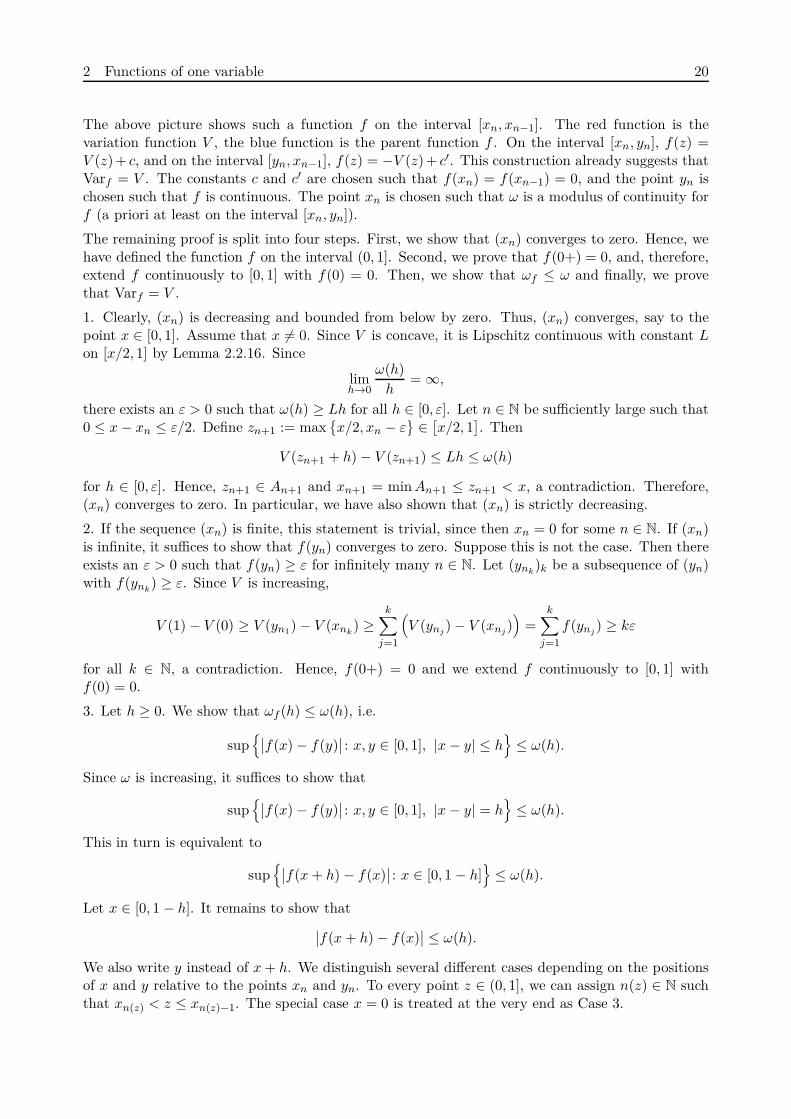
Since V is continuous, f is continuous where it is defined. Since V is increasing, f is piecewisemonotone; f is increasing on the intervals [xn, yn] and decreasing on the intervals [yn+1, xn]. SinceV is concave, f is concave on the intervals [xn, yn] and convex on the intervals [yn+1, xn].
0 xn yxn = yn xn−1
0.25
0.45
0.70
0.95
2 Functions of one variable 20
The above picture shows such a function f on the interval [xn, xn−1]. The red function is thevariation function V , the blue function is the parent function f . On the interval [xn, yn], f(z) =V (z) + c, and on the interval [yn, xn−1], f(z) = −V (z) + c′. This construction already suggests thatVarf = V . The constants c and c′ are chosen such that f(xn) = f(xn−1) = 0, and the point yn ischosen such that f is continuous. The point xn is chosen such that ω is a modulus of continuity forf (a priori at least on the interval [xn, yn]).
The remaining proof is split into four steps. First, we show that (xn) converges to zero. Hence, wehave defined the function f on the interval (0, 1]. Second, we prove that f(0+) = 0, and, therefore,extend f continuously to [0, 1] with f(0) = 0. Then, we show that ωf ≤ ω and finally, we provethat Varf = V .
1. Clearly, (xn) is decreasing and bounded from below by zero. Thus, (xn) converges, say to thepoint x ∈ [0, 1]. Assume that x 6= 0. Since V is concave, it is Lipschitz continuous with constant Lon [x/2, 1] by Lemma 2.2.16. Since
limh→0
ω(h)h
= ∞,
there exists an ε > 0 such that ω(h) ≥ Lh for all h ∈ [0, ε]. Let n ∈ N be sufficiently large such that0 ≤ x − xn ≤ ε/2. Define zn+1 := max
x/2, xn − ε ∈ [x/2, 1
]
. Then
V (zn+1 + h) − V (zn+1) ≤ Lh ≤ ω(h)
for h ∈ [0, ε]. Hence, zn+1 ∈ An+1 and xn+1 = min An+1 ≤ zn+1 < x, a contradiction. Therefore,(xn) converges to zero. In particular, we have also shown that (xn) is strictly decreasing.
2. If the sequence (xn) is finite, this statement is trivial, since then xn = 0 for some n ∈ N. If (xn)is infinite, it suffices to show that f(yn) converges to zero. Suppose this is not the case. Then thereexists an ε > 0 such that f(yn) ≥ ε for infinitely many n ∈ N. Let (ynk
)k be a subsequence of (yn)with f(ynk
) ≥ ε. Since V is increasing,
V (1) − V (0) ≥ V (yn1) − V (xnk
) ≥k∑
j=1
(
V (ynj) − V (xnj
))
=k∑
j=1
f(ynj) ≥ kε
for all k ∈ N, a contradiction. Hence, f(0+) = 0 and we extend f continuously to [0, 1] withf(0) = 0.
3. Let h ≥ 0. We show that ωf (h) ≤ ω(h), i.e.
sup
∣
∣f(x) − f(y)∣
∣ : x, y ∈ [0, 1], |x − y| ≤ h
≤ ω(h).
Since ω is increasing, it suffices to show that
sup
∣
∣f(x) − f(y)∣
∣ : x, y ∈ [0, 1], |x − y| = h
≤ ω(h).
This in turn is equivalent to
sup
∣
∣f(x + h) − f(x)∣
∣ : x ∈ [0, 1 − h]
≤ ω(h).
Let x ∈ [0, 1 − h]. It remains to show that∣
∣f(x + h) − f(x)∣
∣ ≤ ω(h).
We also write y instead of x + h. We distinguish several different cases depending on the positionsof x and y relative to the points xn and yn. To every point z ∈ (0, 1], we can assign n(z) ∈ N suchthat xn(z) < z ≤ xn(z)−1. The special case x = 0 is treated at the very end as Case 3.

2 Functions of one variable 21
Case 1. We have n := n(x) = n(y). We distinguish whether x, y are in the intervals [xn, yn] or[yn, xn−1].
Case 1.1. We have x, y ∈ [xn, yn]. Using Lemma 2.2.15,
∣
∣f(y) − f(x)∣
∣ =∣
∣
∣V (y) − V (xn) − (
V (x) − V (xn))
∣
∣
∣ =∣
∣V (y) − V (x)∣
∣
= V (y) − V (x) ≤ V (xn + h) − V (xn) ≤ ω(h).
Case 1.2. We have x, y ∈ [yn, xn−1]. Here, we need an additional distinction on the distanceh = y − x.
Case 1.2.1. Assume that h ≤ yn − xn. Using Lemma 2.2.15 and Case 1.1,
∣
∣f(y) − f(x)∣
∣ =∣
∣
∣V (xn−1) − V (y) − (
V (xn−1) − V (x))
∣
∣
∣ =∣
∣V (x) − V (y)∣
∣
= V (x + h) − V (x) ≤ V (xn + h) − V (xn) ≤ ω(h).
Case 1.2.2. Assume that h ≥ yn − xn. Using the defining property of yn,∣
∣f(y) − f(x)∣
∣ =∣
∣
∣V (xn−1) − V (y) − (
V (xn−1) − V (x))
∣
∣
∣ =∣
∣V (x) − V (y)∣
∣
= V (y) − V (x) ≤ V (xn−1) − V (yn) = V (yn) − V (xn)
≤ ω(yn − xn) ≤ ω(h).
Case 1.3. We have x ∈ [xn, yn] and y ∈ [yn, xn−1]. Using the preceding cases,
∣
∣f(y) − f(x)∣
∣ ≤ max
∣
∣f(y) − f(yn)∣
∣,∣
∣f(x) − f(yn)∣
∣
≤ max
ω(y − yn), ω(yn − x)
= ω(
max
y − yn, yn − x
)
≤ ω(h).
Case 2. We have m := n(y) < n(x) =: n. We again distinguish several different cases and reducethem all to Case 1.
Case 2.1. We have x ∈ [xn, yn].
Case 2.1.1. We have y ∈ [xm, ym].
Case 2.1.1.1. We have f(x) ≤ f(y). Then,∣
∣f(y) − f(x)∣
∣ = f(y) − f(x) ≤ f(y) = f(y) − f(xm)
=∣
∣f(y) − f(xm)∣
∣ ≤ ω(y − xm) ≤ ω(y − x) = ω(h).
Case 2.1.1.2. We have f(y) ≤ f(x). Then,∣
∣f(y) − f(x)∣
∣ = f(x) − f(y) ≤ f(x) = f(x) − f(xn−1) =∣
∣f(x) − f(xn−1)∣
∣
≤ ω(xn−1 − x) ≤ ω(y − x) = ω(h).
Case 2.1.2. We have y ∈ [ym, xm−1].
Case 2.1.2.1. We have f(x) ≤ f(y). Then,∣
∣f(y) − f(x)∣
∣ = f(y) − f(x) ≤ f(y) = f(y) − f(xm)
=∣
∣f(y) − f(xm)∣
∣ ≤ ω(y − xm) ≤ ω(y − x) ≤ ω(h).
2 Functions of one variable 22
Case 2.1.2.2. We have f(y) ≤ f(x). Then,
∣
∣f(y) − f(x)∣
∣ = f(x) − f(y) ≤ f(x) = f(x) − f(xn−1) =∣
∣f(x) − f(xn−1)∣
∣
≤ ω(xn−1 − x) ≤ ω(y − x) = ω(h).
Case 2.2. We have x ∈ [yn, xn−1].
Case 2.2.1. We have y ∈ [xm, ym].
Case 2.2.1.1. We have f(x) ≤ f(y). Then,∣
∣f(y) − f(x)∣
∣ = f(y) − f(x) ≤ f(y) = f(y) − f(xm)
=∣
∣f(y) − f(xm)∣
∣ ≤ ω(y − xm) ≤ ω(y − x) = ω(h).
Case 2.2.1.2. We have f(y) ≤ f(x). Then,
∣
∣f(y) − f(x)∣
∣ = f(x) − f(y) ≤ f(x) = f(x) − f(xn−1) =∣
∣f(x) − f(xn−1)∣
∣
≤ ω(xn−1 − x) ≤ ω(y − x) = ω(h).
Case 2.2.2. We have y ∈ [ym, xm−1].
Case 2.2.2.1. We have f(x) ≤ f(y). Then,∣
∣f(y) − f(x)∣
∣ = f(y) − f(x) ≤ f(y) = f(y) − f(xm)
=∣
∣f(y) − f(xm)∣
∣ ≤ ω(y − xm) ≤ ω(y − x) = ω(h).
Case 2.2.2.2. We have f(y) ≤ f(x). Then,
∣
∣f(y) − f(x)∣
∣ = f(x) − f(y) ≤ f(x) = f(x) − f(xn−1) =∣
∣f(x) − f(xn−1)∣
∣
≤ ω(xn−1 − x) ≤ ω(y − x) = ω(h).
Case 3. We have x = 0. Define n := n(h) = n(y). Then,
∣
∣f(y) − f(x)∣
∣ = f(h) = f(h) − f(xn) =∣
∣f(h) − f(xn)∣
∣ ≤ ω(h − xn) ≤ ω(h).
4. Using Lemma 2.2.3 and that f is continuous at zero and piecewise monotone, we have for x ∈ [0, 1]with xn ≤ x ≤ yn that
Varf (x) = Var(f ; 0, x) =∞∑
k=n
(
Var(
f ; xk+1, yk+1
)
+ Var(
f ; yk+1, xk
)
)
+ Var(
f ; xn, x)
=∞∑
k=n
(
f(yk+1) − f(xk+1) + f(yk+1) − f(xk))
+ f(x) − f(xn)
= 2∞∑
k=n
f(yk+1) + f(x) = 2∞∑
k=n
V (xk) − V (xk+1)2
+ V (x) − V (xn)
= − limk→∞
V (xk+1) + V (xn) + V (x) − V (xn) = V (x).

2 Functions of one variable 23
Similarly, for yn+1 ≤ x ≤ xn, we have
Varf (x) = Var(f ; 0, x)
=∞∑
k=n+1
(
Var(
f ; xk+1, yk+1
)
+ Var(
f ; yk+1, xk
)
)
+ Var(
f ; xn+1, yn+1
)
+ Var(
f ; yn+1, x)
=∞∑
k=n+1
(
f(yk+1) − f(xk+1) + f(yk+1) − f(xk))
+ f(yn+1) − f(xn+1) + f(yn+1) − f(x)
= 2∞∑
k=n
f(yk+1) − f(x) = 2∞∑
k=n
V (xk) − V (xk+1)2
− (
V (xn) − V (x))
= − limk→∞
V (xk+1) + V (xn) − V (xn) + V (x) = V (x).
2.3 Decomposition into monotone functions
The main result of this section is that we can decompose functions of bounded variation intothe difference of two monotone functions. We can even state such a decomposition explicitly.Throughout this section, we only consider functions defined on a fixed interval I = [a, b].
In Example 2.1.5 we have seen that monotone functions are of bounded total variation. It is easilyseen that linear combinations of functions of bounded variation are again of bounded variation.
Proposition 2.3.1. If f and g are of bounded variation and if α, β ∈ R, then
Var(αf + βg) ≤ |α| Var(f) + |β| Var(g).
In particular, the set BV(I) is a vector space.
Proof. Let f, g ∈ BV and let α, β ∈ R. Then
Var(αf + βg) = supY∈Y
∑
y∈Y|(αf + βg)(y+) − (αf + βg)(y)|
= supY∈Y
∑
y∈Y|αf(y+) − αf(y) + βg(y+) − βg(y)|
≤ supY∈Y
∑
y∈Y
(
|α||f(y+) − f(y)| + |β||g(y+) − g(y)|)
≤ |α| supY∈Y
∑
y∈Y|f(y+) − f(y)| + |β| sup
Y∈Y
∑
y∈Y|g(y+) − g(y)|
= |α| Var(f) + |β| Var(g) < ∞.
Thus, the difference of two monotone functions is again of bounded variation. The following theoremstates that the converse is also true, i.e. all functions of bounded variation can be written as thedifference of two increasing functions. This theorem is of fundamental importance, since it enablesus to extend many results for monotone functions to functions of bounded variation. It is also calledthe Jordan Decomposition Theorem and is due to Jordan, who was the first to introduce functionsof bounded variation (see for example [45]).
2 Functions of one variable 24
Theorem 2.3.2 (Jordan Decomposition Theorem). If f : [a, b] → R is of bounded variation, thenthere are increasing functions f+, f− : [a, b] → R with f+(a) = f−(a) = 0 and
f(x) − f(a) = f+(x) − f−(x) (2.7)
Varf (x) = f+(x) + f−(x).
Furthermore, this decomposition is unique and the functions satisfy
Var(f+ − f−) = Var(f+ + f−) = Var(f+) + Var(f−) = Var(f) = Var(Varf ).
If f is right-continuous, then also f+ and f− are right-continuous. Similar statements hold forleft-continuous and continuous f .
Proof. We can reformulate the equations (2.7) as
f+(x) =12
(Varf (x) + f(x) − f(a))
f−(x) =12
(Varf (x) − f(x) + f(a)).
The uniqueness is apparent from this representation and the claims about the continuity follow fromTheorem 2.2.5.
It remains to show that f+ and f− are increasing. We show that Varf (x)±f(x) is increasing. Takeε > 0 and x1, x2 ∈ [a, b] with x1 < x2 and let Y be a ladder on [a, x1] such that
∑
y∈Y|f(y+) − f(y)| ≥ Varf (x1) − ε.
Then
Varf (x2) ± f(x2) ≥∑
y∈Y|f(y+) − f(y)| + |f(x2) − f(x1)| ± f(x2)
≥ Varf (x1) − ε + |f(x2) − f(x1)| ± (f(x2) − f(x1)) ± f(x1)
≥ Varf (x1) − ε ± f(x1).
Since ε > 0 is arbitrary, we get Varf (x2) ± f(x2) ≥ Varf (x1) ± f(x1).
Finally, Var(f) = Var(f − f(a)) = Var(f+ − f−). Furthermore, by Proposition 2.2.2, Var(f) =Var(Varf ) = Var(f+ + f−). Since f+ and f− are increasing, also f+ + f− is increasing and thus
Var(f++f−) = (f++f−)(b)−(f++f−)(a) = (f+(b)−f+(a))+(f−(b)−f−(a)) = Var(f+)+Var(f−).
Remark 2.3.3. The functions f+ and f− in the above theorem are called the positive and negativevariation functions of f , respectively. Notice that the Jordan Decomposition Theorem implies thatBV is the linear hull of the monotone functions (which do not form a vector space on their own).
2.4 Continuity, differentiability and measurability
We have seen in Example 2.1.9 that there are differentiable functions that are of unbounded varia-tion. On the other hand, Example 2.1.4 shows us that there are discontinuous functions that are ofbounded variation. In light of these examples, we want to examine the connection between bounded
2 Functions of one variable 25
variation and continuity and differentiability more closely. All proofs in this chapter use the mono-tone decomposition of functions of bounded variation. So we always first prove the correspondingstatements for increasing functions, and then transfer them to functions of bounded variation.
First, recall that points of discontinuity of a function can be classified into different types. The twomost interesting types for our studies are the removable discontinuities and the discontinuities ofjump type. A function f has a removable discontinuity at x0, if f(x0−) and f(x0+) exist and arefinite, and if f(x0−) = f(x0+) 6= f(x0). Those discontinuities are called removable, since they canbe removed by redefining f at x0 as f(x0−) (or f(x0+)). A discontinuity of f at x0 is of jumptype, if f(x0+) and f(x0−) exist and are finite, but different. Other types of discontinuities are,for example, infinite discontinuities (when the function blows up) or mixed discontinuities (when atleast one of the one-sided limits does not exist).
Lemma 2.4.1. Let f : [a, b] → R be an increasing function. Then the number of discontinuities off is countable and they are all of jump type. Furthermore, f is Borel-measurable.
Proof. Let f be discontinuous at x0. Since f is increasing and bounded, the limits
f(x0−) = limε↓0
f(x0 − ε) and f(x0+) = limε↓0
f(x0 + ε)
exist and are finite. If the limits are equal, then f has a removable discontinuity at x0. It is easilyseen that this is a contradiction to the monotonicity of f . Therefore, the discontinuity is of jumptype. Again since f is increasing, we have f(x0−) < f(x0+). Since there is a different rationalnumber in all the intervals
(
f(x−), f(x+))
when x is a discontinuity of f , the set of discontinuitiesmust be countable.
The measurability follows immediately from the fact that the sets f−1((−∞, α)) are intervals.
Theorem 2.4.2. Functions of bounded variation have at most countably many discontinuities.Those discontinuities are removable or of jump type. Furthermore, functions of bounded variationare Borel-measurable.
Proof of Theorem 2.4.2. By Theorem 2.3.2 we can write functions of bounded variation as the dif-ference of two monotonically increasing functions. By Lemma 2.4.1, those functions only have acountable number of discontinuities and are Borel-measurable. Thus, also functions of boundedvariation can only have a countable number of discontinuities and are also Borel-measurable. Fur-thermore, since one-sided limits of increasing functions exist, they also exist for functions of boundedvariation, proving that the points of discontinuity are either removable or of jump type.
Next, we show that functions of bounded variation are differentiable almost everywhere. In ourproof, we follow Royden [44] closely.
Definition 2.4.3. Let A ⊂ R be a set and let J be a collection of non-degenerate intervals (i.e. weonly consider intervals with infinitely many points) covering A. Then J is called a Vitali-cover ofA if for all x ∈ A and ε > 0 there exists an interval I ∈ J such that x ∈ I and λ(I) < ε.
Lemma 2.4.4 (Vitali Covering Lemma). Let A ⊂ R be a set of finite outer measure and let J be aVitali-cover of A. Then for all ε > 0 there exists a finite collection
I1, . . . , In
of pairwise disjointintervals in J such that
λ∗(
A\n⋃
i=1
Ii
)
< ε.

2 Functions of one variable 26
Proof. We can assume without loss of generality that all the intervals in J are closed. Otherwise,we replace them by their closure and note that the set of the endpoints of I1, . . . , In has measurezero.
Let U be an open set of finite measure containing A. Since J is a Vitali-cover, we assume withoutloss of generality that U contains all the intervals in J . We construct the sequence I1, . . . , In
inductively. Choose I1 in J arbitrarily. Suppose we have already determined I1, . . . , Ik.
First, assume that there is no interval I ∈ J that is disjoint from the intervals I1, . . . , Ik. We showthat then,
A =k⋃
i=1
Ii. (2.8)
Indeed, let x ∈ A\⋃ki=1 Ii. Since
⋃ki=1 Ii is closed, there exists an δ > 0 such that
(x − δ, x + δ) ∩k⋃
i=1
Ii = ∅.
Since J is a Vitali-cover, there exists an interval I ∈ J with x ∈ I and λ(I) < δ. For this interval,we have
I ∩k⋃
i=1
Ii ⊂ (x − δ, x + δ) ∩k⋃
i=1
Ii = ∅.
This is a contradiction to our assumption that no such disjoint interval exists. Hence, (2.8) holds,which proves the lemma.
On the other hand, assume that there exists an interval I ∈ J that is disjoint from I1, . . . , Ik. Letak be the supremum over all the lengths of the intervals in J that are disjoint from I1, . . . , Ik. Sinceeach interval in J is contained in U , it is clear that ak ≤ λ(U) < ∞. Now choose Ik+1 as an intervalin J that is disjoint from I1, . . . , Ik and satisfies λ(Ik+1) ≥ ak/2.
With the above procedure we get a sequence (Ik) of pairwise disjoint intervals in J . Since
∞∑
k=1
λ(Ik) = λ
( ∞⋃
k=1
Ik
)
≤ λ(U) < ∞, (2.9)
the series converges and there exists an n ∈ N such that
∞∑
k=n+1
λ(Ik) < ε/5.
It remains to show that λ∗(R) < ε with
R = A\n⋃
k=1
Ik.
Let x ∈ R. Since⋃n
k=1 Ik is closed and J is a Vitali-cover, there exists an interval I in J smallenough such that x ∈ I and I is disjoint from I1, . . . , In. We show that I intersects some Ik fork large enough. Indeed, if I is disjoint from all Ik, then ak ≥ λ(I) for all k ∈ N. Hence, we haveλ(Ik) ≥ λ(I)/2 for all k ∈ N. This is a contradiction to (2.9). Therefore, I intersects some Ik.
Let k be the smallest integer such that I intersects Ik. Then k > n and λ(I) ≤ ak−1 ≤ 2λ(Ik).Since x ∈ I and since I intersects Ik, the distance of x to the midpoint of Ik is at most
λ(I) +12
λ(Ik) ≤ 52
λ(Ik).

2 Functions of one variable 27
Therefore, if we define Jl to be Il stretched by a factor of 5 with the same midpoint, then x ∈ Jk.Hence,
R ⊂∞⋃
k=n+1
Jk
and therefore
λ∗(R) ≤∞∑
k=n+1
λ(Jk) = 5∞∑
k=n+1
λ(Ik) < ε,
what had to be shown.
We use this lemma to prove that increasing functions are differentiable almost everywhere. To thisend, we define four different derivatives of a function f at x as follows.
D+f(x) := lim suph↓0
f(x + h) − f(x)h
D−f(x) := lim suph↓0
f(x) − f(x − h)h
D+f(x) := lim infh↓0
f(x + h) − f(x)h
D−f(x) := lim infh↓0
f(x) − f(x − h)h
Of course, f is differentiable at x if and only if D+f(x) = D−f(x) = D+f(x) = D−f(x) 6= ±∞.
Lemma 2.4.5 (Lebesgue). Let f : [a, b] → R be an increasing function. Then f is differentiablealmost everywhere, the derivative f ′ is Lebesgue-measurable, and
∫ b
af ′(x) dx ≤ f(b) − f(a).
Proof. We first show that the sets where two of the introduced derivatives differ have outer measurezero. Let A be the set on which D+f(x) > D−f(x), the other cases follow analogously. It is clearthat we can write A as the union of the sets
Ap,q :=
D+f > p > q > D−f
for p, q ∈ Q, so it suffices to show that λ∗(Ap,q) = 0.
Let ε > 0, choose p, q ∈ Q with p > q and denote s := λ∗(Ap,q). Take an open set U ⊃ Ap,q withλ(U) < s + ε. For every x ∈ Ap,q there exists an arbitrarily small interval [x − h, x] contained in Uwith
f(x) − f(x − h) < qh.
In particular, the collection of those intervals is a Vitali-cover of Ap,q. By the Vitali CoveringLemma 2.4.4, we can find a finite pairwise disjoint subcollection
I1, . . . , In
whose interiors covera subset B of Ap,q of outer measure at least s − ε. Denoting those intervals by Ik = [xk − hk, xk]and summing over all of them, we get
n∑
k=1
(
f(xk) − f(xk − hk))
< qn∑
k=1
hk < qλ(U) < q(s + ε).
2 Functions of one variable 28
For every point y ∈ B we can find an arbitrarily small interval [y, y + r] that is contained in someIk such that
f(y) − f(y − r) > pr.
The collection of those intervals is a Vitali cover of B. Applying the Vitali Covering Lemma 2.4.4,we get a finite pairwise disjoint subcollection of intervals
J1, . . . , Jm
whose union covers a subsetof B of outer measure at least s − 2ε. Again writing Jl = [yl, yl + rl] and summing over all intervalsgives
m∑
l=1
(
f(yl + rl) − f(yl))
> pm∑
l=1
rl > p(s − 2ε).
Each interval Jl is contained in some interval Ik, so if we sum over all Jl contained in Ik, we get∑
l
(
f(yl + rl) − f(yl)) ≤ f(xk) − f(xk − hk),
since f is increasing. In particular, we have
m∑
l=1
(
f(yl + rl) − f(yl)) ≤
n∑
k=1
(
f(xk) − f(xk − hk))
.
Hence,p(s − 2ε) < q(s + ε)
for all ε > 0. By taking ε to zero, we get p ≤ q, which is a contradiction.
We have shown that the function
g(x) := limh→0
f(x + h) − f(x)h
is well-defined almost everywhere, and f is differentiable whenever g is finite. Define
gn(x) := n(
f(x + 1/n) − f(x))
,
where we set f(x) = f(b) for x > b. Then gn converges to g almost everywhere. Since f isLebesgue-measurable (even Borel-measurable) by Theorem 2.4.2, g is also Lebesgue-measurable.Using Fatou’s lemma, we get
∫ b
ag(x) dx =
∫ b
alim
n→∞ gn(x) dx ≤ lim infn→∞
∫ b
agn(x) dx = lim inf
n→∞ n
∫ b
a
(
f(x + 1/n) − f(x))
dx
= lim infn→∞
(
n
∫ b+1/n
bf(x) dx − n
∫ a+1/n
af(x) dx
)
≤ lim infn→∞
(
f(b) − n
∫ a+1/n
af(a) dx
)
= f(b) − f(a).
In particular, g is integrable and thus finite almost everywhere. Hence, f is differentiable almosteverywhere.
Theorem 2.4.6. Let f : [a, b] → R be a function of bounded variation. Then f is differentiablealmost everywhere, the derivative f ′ is Lebesgue-measurable, and
∫ b
a|f ′(x)| dx ≤ Var(f). (2.10)

2 Functions of one variable 29
Proof. Let (f+, f−) be the Jordan decomposition of f . Lemma 2.4.5 implies that f+ and f− aredifferentiable almost everywhere, and their derivatives are Lebesgue-measurable. Therefore, thederivative of f , f ′ = (f+)′ − (f−)′ exists almost everywhere and is Lebesgue-measurable. Finally,
∫ b
a|f ′(x)| dx ≤
∫ b
a
∣
∣(f+)′(x)∣
∣ dx +∫ b
a
∣
∣(f−)′(x)∣
∣ dx =∫ b
a(f+)′(x) dx +
∫ b
a(f−)′(x) dx
≤ f+(b) − f+(a) + f−(b) − f−(a) = Var(f).
We have seen in Example 2.1.7 that absolutely continuous functions are of bounded variation. Itturns out that for absolutely continuous functions, we have equality in (2.10). This follows from thefundamental theorem of calculus for Lebesgue integrals. Since we use it again later, we state andprove this theorem.
First, we show some measure theoretic statements. The first lemma was proved by Egorov in [16].
Lemma 2.4.7 (Egorov). Let M ⊂ R be a measurable set with λ(M) < ∞ and let (fn) be a sequenceof measurable functions fn : M → R converging to a function f : M → R almost everywhere onM . Then for each ε > 0 there exists a measurable set Mε ⊂ M such that λ(M\Mε) < ε and (fn)converges to f uniformly on Mε.
Proof. Let ε > 0. For n, k ∈ N define
En,k :=⋃
m≥n
x ∈ M : |fm(x) − f(x)| ≥ 1k
.
Obviously, En+1,k ⊂ En,k for all n ∈ N. Furthermore, if fn(x) → f(x) for some x ∈ M , thenx /∈ En,k for n sufficiently large. Since (fn) converges to f almost everywhere, the set
⋂∞n=1 En,k is
a null-set for every k ∈ N. Since λ(M) < ∞, we can find a number nk ∈ N for every k ∈ N suchthat
λ(Enk,k) <ε
2k.
Define
A :=∞⋃
k=1
Enk,k.
Clearly, λ(A) < ε. Furthermore, if k ∈ N, then for every n > nk and for every x ∈ M\A,|fn(x) − f(x)| < 1/k, which implies that (fn) converges uniformly on M\A to f .
Lemma 2.4.8. Let M ⊂ R be a measurable set and let f : M → R be integrable. Then for eachε > 0, there exists a δ > 0 such that for all measurable sets N ⊂ M with λ(N) ≤ δ, we have
∫
N|f(x)| dx ≤ ε.
Proof. Since f is integrable, it is finite almost everywhere. Thus, the sequence
gn := 1|f |>n|f |
converges to zero almost everywhere. The functions gn are dominated by the integrable function|f |. Hence, by the dominated convergence theorem,
limn→∞
∫
|f |>n|f(x)| dx = lim
n→∞
∫
Mgn(x) dx =
∫
Mlim
n→∞ gn(x) dx = 0.
2 Functions of one variable 30
In particular, there exists an n ∈ N such that∫
|f |>n|f(x)| dx <
ε
2.
Let δ := ε/(2n). Then for all measurable sets N ⊂ M with λ(N) ≤ δ,∫
N|f(x)| dx ≤
∫
|f |>n|f(x)| dx +
∫
N\|f |>n|f(x)| dx <
ε
2+∫
N\|f |>nn dx ≤ ε
2+ λ(N)n ≤ ε.
Lemma 2.4.9. Open subsets of R can be written as a countable union of disjoint open intervals.
Proof. Let O be an open subset of R. For every x ∈ O we find an open interval in O containingx. Thus, there also exists a largest interval in O containing x (the union of all those intervals).Consider the set of those largest intervals. First, the intervals in this set are pairwise disjoint, asotherwise they would not be maximal. Second, there are at most countably many, as they arepairwise disjoint and all contain a rational number.
The proof of Lebesgue’s Theorem is taken from [5].
Theorem 2.4.10 (Lebesgue). If f : [a, b] → R is absolutely continuous, then the derivative f ′ existsalmost everywhere, is integrable, and satisfies
∫ b
af ′(x) dx = f(b) − f(a). (2.11)
Proof. Absolutely continuous functions are of bounded variation by Example 2.1.7. By Theorem2.4.6, f is differentiable almost everywhere and the derivative is integrable. Furthermore, f has theJordan decomposition (f+, f−), and the functions f+ and f− are again absolutely continuous byTheorem 2.2.5. Hence, we may assume without loss of generality that f is increasing.
Similarly to the proof of Lemma 2.4.5, we define the functions
gn(x) := n(
f(x + 1/n) − f(x))
.
We again have that∫ b
agn(x) dx = f(b) − n
∫ a+1/n
af(x) dx.
Since f is continuous, the integral on the right-hand side is a Riemann integral. By the mean valuetheorem for Riemann integrals, we have
limn→∞
∫ b
agn(x) dx = f(b) − f(a).
Thus, it remains to show that
limn→∞
∫ b
agn(x) dx =
∫ b
af ′(x) dx.
Let ε > 0. Since f is absolutely continuous, there exists a δ > 0 such that for all finite collectionsof pairwise disjoint intervals (a1, b1), . . . , (an, bn) with
n∑
k=1
(
bk − ak
)
< δ

2 Functions of one variable 31
we haven∑
k=1
∣
∣f(bk) − f(ak)∣
∣ < ε.
By Lemma 2.4.8, we can choose a 0 < δ′ < δ such that∫
N|f(x)| dx < ε
for all measurable sets N ⊂ [a, b] with λ(N) ≤ δ′.
Let D be the set of points where f is differentiable. Then [a, b]\D is a nullset. By Egorov’s theorem2.4.7, we can find a measurable set M ⊂ D such that λ(M) < δ′ and (gn) converges uniformly tof ′ on D\M . Hence, there exists an N ∈ N such that for all n ≥ N ,
∫
D\M
∣
∣gn(x) − f ′(x)∣
∣ dx < ε.
Therefore,∣
∣
∣
∣
∫ b
agn(x) dx −
∫ b
af ′(x) dx
∣
∣
∣
∣
=∣
∣
∣
∣
∫
Dgn(x) dx −
∫
Df ′(x) dx
∣
∣
∣
∣
≤∫
D
∣
∣gn(x) − f ′(x)∣
∣ dx
=∫
D\M
∣
∣gn(x) − f ′(x)∣
∣ dx +∫
M
∣
∣gn(x) − f ′(x)∣
∣ dx
< ε +∫
M|gn(x)| dx +
∫
M|f ′(x)| dx < 2ε +
∫
M|gn(x)| dx.
It remains to show that the last integral tends to zero as n goes to infinity. We want to approximateM by a finite set of disjoint intervals so that we can apply the absolute continuity of f . Sinceλ(M) ≤ δ′ < δ, there exists an open set O ⊂ (a, b) such that M ⊂ O and λ(O) < δ. By Lemma2.4.9, we can write O as a countable union of disjoint open intervals, say
O =∞⋃
i=1
(ai, bi).
If the union is finite, we can already apply the absolute continuity of f . Conversely, assume thatthe union is infinite.
For all τ ∈ [0, 1] and all m ∈ N,
m∑
i=1
∣
∣(bi + τ) − (ai + τ)∣
∣ < δ,
so thatm∑
i=1
∣
∣f(bi + τ) − f(ai + τ)∣
∣ < ε.
Since∫ bi
ai
|gn(x)| dx = n
∫ bi
ai
∣
∣f(x + 1/n) − f(x)∣
∣ dx = n
∫ bi
ai
(
f(x + 1/n) − f(x))
dx
= n
(∫ bi+1/n
bi
f(x) dx −∫ ai+1/n
ai
f(x) dx
)
= n
∫ 1/n
0
(
f(bi + x) − f(ai + x))
dx,
2 Functions of one variable 32
we have∫
M|gn(x)| dx ≤
∫
O|gn(x)| dx =
∞∑
i=1
∫ bi
ai
|gn(x)| dx = limm→∞
m∑
i=1
n
∫ 1/n
0
(
f(bi + x) − f(ai + x))
dx
= limm→∞ n
∫ 1/n
0
m∑
i=1
(
f(bi + x) − f(ai + x))
dx ≤ limm→∞ n
∫ 1/n
0ε dx = ε,
which implies (2.11).
Theorem 2.4.11. Let f : [a, b] → R be absolutely continuous. Then
∫ b
a|f ′(x)| dx = Var(f).
Proof. By Example 2.1.7, f is of bounded variation. Theorem 2.4.6 implies that
∫ b
a|f ′(x)| dx ≤ Var(f).
The converse inequality follows from Theorem 2.4.10 with
Var(f) = supY∈Y
∑
y∈Y
∣
∣f(y+) − f(y)∣
∣ = supY∈Y
∑
y∈Y
∣
∣
∣
∣
∫ y+
yf ′(x) dx
∣
∣
∣
∣
≤ supY∈Y
∑
y∈Y
∫ y+
y|f ′(x)| dx =
∫ b
a|f ′(x)| dx.
2.5 Signed Borel measures
There is a natural connection between functions of bounded variation and signed Borel measures.To study this connection, let us first define such measures. We denote by R the set [−∞, ∞].
Definition 2.5.1. Let (Ω, Σ) be a measurable space. A function ν : Σ → R is called a signedmeasure, if
1. ν(Σ) ⊂ (−∞, ∞] or ν(Σ) ⊂ [−∞, ∞),
2. ν(∅) = 0,
3. for every disjoint sequence (An) in Σ,∑∞
n=1 ν(An) exists in R and
∞∑
n=1
ν(An) = ν(
∞⋃
n=1
An
)
.
The space (Ω, Σ, ν) is called signed measure space. The measure ν is called positive if ν(Σ) ⊂ [0, ∞]and it is called finite, if ν(Σ) ⊂ R. If Ω is a topological space and Σ = B(Ω) is the Borel σ-algebra,i.e. the σ-algebra generated by the open sets, then ν is called a Borel-measure.
Definition 2.5.2. Let (Ω, Σ, ν) be a signed measure space. A set N ∈ Σ is called null set if for allN ′ ∈ Σ with N ′ ⊂ N , we have ν(N ′) = 0.
Let ν1, ν2 be two signed measures on a measure space (Ω, Σ). The two measures are called orthogonal,written ν1 ⊥ ν2, if there exist C1, C2 ∈ Σ such that C1 ∪ C2 = Ω, C1 ∩ C2 = ∅, C1 is a null set forν2 and C2 is a null set for ν1.

2 Functions of one variable 33
Similarly to functions in BV, there is also a Jordan decompositions of signed measures. A proof ofthe Jordan decomposition theorem for measures can be found in [50].
Theorem 2.5.3 (Jordan Decomposition Theorem). Let (Ω, Σ, ν) be a signed measure space. Thenthere exists a unique decomposition of ν into two positive measures ν+ and ν−, at least one of whichis finite, such that
ν = ν+ − ν− and ν+ ⊥ ν−.
For functions, we defined the Jordan decomposition in terms of the total variation. For signedmeasures, we reverse the procedure. We have found a Jordan decomposition and now define thetotal variation.
Definition 2.5.4. Let (Ω, Σ, ν) be a signed measure space and let (ν+, ν−) be the Jordan decompo-sition of ν. The positive measure |ν| := ν+ + ν− is called the variation measure of ν. The quantityVar(ν) := |ν|(Ω) = ν+(Ω) + ν−(Ω) is called the total variation of ν.
We show the following theorem.
Theorem 2.5.5. Let f : I → R be a right-continuous function of bounded variation. Then thereexists a unique finite signed Borel measure µ on I such that
f(x) = µ([a, x]), x ∈ I. (2.12)
Furthermore, we haveVar(µ) = Var(f) + |f(a)|. (2.13)
If (f+, f−) is the Jordan decomposition of f and (µ+, µ−) is the Jordan decomposition of µ, then
f+(x) = µ+((a, x]) and f−(x) = µ−((a, x]), x ∈ I. (2.14)
Similarly, let µ be a finite signed Borel-measure on I. Then there exists a unique right-continuousfunction f of bounded variation on I for which (2.12) and (2.13) hold. If we again consider thecorresponding Jordan decompositions, then (2.14) holds.
For the proof, we use the following similar correspondence between increasing functions and positiveBorel measures. A proof of this lemma can be found in [14].
Lemma 2.5.6. Let f : I → R be an increasing right-continuous function. Then there exists aunique finite positive Borel measure µ on I such that
f(x) = µ([a, x]), x ∈ I. (2.15)
Furthermore, we haveVar(µ) = Var(f) + |f(a)|. (2.16)
Similarly, let µ be a finite positive Borel measure on I. Then there exists a unique increasingright-continuous function f on I for which (2.15) and (2.16) hold.
Proof of Theorem 2.5.5. Let f : I → R be a right-continuous function of bounded variation. ByTheorem 2.3.2, we can find the Jordan decomposition (f+, f−) of f with two increasing right-continuous functions f+, f− : I → R such that f+(a) = f−(a) = 0 and
f(x) = f+(x) − f−(x) + f(a)
Varf (x) = f+(x) + f−(x).

2 Functions of one variable 34
Lemma 2.5.6 gives finite positive Borel measures ν+ and ν− on I with
f+(x) = ν+([a, x])
f−(x) = ν−([a, x]).
Denote by δx the measure that satisfies δx(A) := 1A(x) for A ∈ B(I). It is easy to see that themeasure µ := ν+ − ν− + f(a)δa is a finite signed Borel measure on I. Furthermore,
f(x) = f+(x) − f−(x) + f(a) = ν+([a, x]) − ν−([a, x]) + f(a) = µ([a, x]),
so that we have (2.12). Let (µ+, µ−) be the Jordan decomposition of µ. Then we have Borel setsC+, C− with C+ ∪ C− = [a, b], C+ ∩ C− = ∅ and µ+(C−) = µ−(C+) = 0. Define the functions
g+(x) := µ+((a, x])
g−(x) := µ−((a, x]).
We want to show that g+ = f+ and g− = f−. Since (f+, f−) is the Jordan decomposition of f ,and the Jordan decomposition is unique by Theorem 2.3.2, it is sufficient to show that (g+, g−) is aJordan decomposition of f . Obviously, g+ and g− are increasing functions with g+(a) = g−(a) = 0.Furthermore,
f(x) = f(a) + f+(x) − f−(x) = f(a) + ν+((a, x]) − ν−((a, x]) = µ([a, x]) = µ(a) + µ((a, x])
= f(a) + µ+((a, x]) − µ−((a, x]) = f(a) + g+(x) − g−(x).
It remains to show that Varf (x) = g+(x) + g−(x). Notice that
g+(x) = µ+((a, x]) = µ+(C+ ∩ (a, x]) = µ(C+ ∩ (a, x]) = ν+(C+ ∩ (a, x]) − ν−(C+ ∩ (a, x])
≤ ν+(C+ ∩ (a, x]) ≤ ν+((a, x]) = f+(x).
Similarly, g−(x) ≤ f−(x). Thus, Varf (x) = f+(x)+f−(x) ≥ g+(x)+g−(x). However, by Proposition2.3.1,
Varf (x) = Var(f ; a, x) = Var(f(a) + g+ − g−; a, x) ≤ Var(g+; a, x) + Var(g−; a, x) = g+(x) + g−(x).
Hence, Varf (x) = g+(x) + g−(x) and we can conclude that (g+, g−) = (f+, f−) is the Jordandecomposition of f . In particular, this also proves (2.14).
Finally,
Var(µ) = µ+([a, b]) + µ−([a, b]) = |f(a)| + f+(b) + f−(b) = Var(f) + |f(a)|,proving assertion (2.13).
Conversely, assume that µ is a finite signed Borel-measure on I and let (µ+, µ−) be the Jordandecomposition of µ. Define the functions
f+(x) = µ+((a, x])
f−(x) = µ−((a, x])
f(x) = f+(x) − f−(x) + µ(a).
Then f obviously satisfies (2.12). Furthermore, since µ is a Borel measure, f is right-continuous.The uniqueness of f is also clear. Since f can be written as the difference of two monotone functions,f is of bounded variation by Theorem 2.3.2. From the first implication of the theorem, which wehave already shown, it follows that (f+, f−) is the Jordan decomposition of f . Moreover,
Var(µ) = µ+([a, b]) + µ−([a, b]) = µ+((a, b]) + µ−((a, b]) + |µ(a)| = f+(b) + f−(b) + |f(a)|= Var(f) + |f(a)|,
proving the theorem.

2 Functions of one variable 35
2.6 Dimension of the graph
We study the Hausdorff and the box dimension of the graph of a function of bounded variation. Iff is a function defined on a set A, then the graph of f is defined as
graph(f) := (x, f(x)) : x ∈ A.
Throughout this chapter, we mostly follow [17].
To motivate the definition of fractal dimension, we consider the Cantor set C. The Cantor set isinductively defined as follows. Let C0 = [0, 1]. Then C1 = [0, 1/3] ∪ [2/3, 1], i.e. we remove themiddle third of C0. Next, C2 = [0, 1/9] ∪ [2/9, 1/3] ∪ [2/3, 7/9] ∪ [8/9, 1], i.e. we again remove themiddle thirds of the intervals of C1. This process of removing the middle third can be continuedinductively. We call the limit C =
⋂∞n=0 Cn the Cantor set. It is easy to see that C has Lebesgue-
measure 0, so one could argue that C is not really 1-dimensional. On the other hand, C containsuncountably many points, so one could equally well argue that C is not 0-dimensional. Thus,we introduce fractal dimensions, i.e. non-natural dimensions. Two of the most common fractaldimensions are the Hausdorff and the box dimension.
First, we define the Hausdorff dimension. For a nonempty set U ⊂ Rn, we define the diameter of Uby
diam(U) := sup‖x − y‖2 : x, y ∈ U,
where ‖.‖2 denotes the Euclidean norm. Let F ⊂ Rn. A δ-cover of F is a countable collection Uiof subsets of Rn such that diam(Ui) ≤ δ for all i ∈ N and
F ⊂∞⋃
i=1
Ui.
For s ∈ [0, ∞) and δ > 0 we define
Hsδ (F ) := inf
∞∑
i=1
diam(Ui)s : Ui is a δ-cover of F
.
Now we define the s-dimensional Hausdorff measure of F by
Hs(F ) := limδ↓0
Hsδ (F ).
In the case s = 0, we have diam(U)s = 1 for all U ⊂ Rn. Hence, it is easy to see that the 0-dimensional Hausdorff measure is exactly the counting measure, i.e. H0(F ) is the number of pointsin F .
It can be proved that the s-dimensional Hausdorff measure is an outer measure on P(Rn) and ameasure on B(Rn). Furthermore, we have the following proposition.
Proposition 2.6.1. Let q > s ≥ 0 and A ⊂ Rn. Then
Hs(A) < ∞ =⇒ Hq(A) = 0,
Hq(A) > 0 =⇒ Hs(A) = ∞.
Proof. The second statement is equivalent to the first, so we show only the first. Let δ > 0 and letUi be a δ-cover of A with
Hs(A) + 1 ≥∞∑
i=1
diam(Ui)s.
2 Functions of one variable 36
Then,
Hq(A) ≤∞∑
i=1
diam(Ui)q =∞∑
i=1
diam(Ui)s diam(Ui)q−s ≤∞∑
i=1
diam(Ui)sδq−s ≤ δq−s(Hs(A) + 1)
.
Taking δ → 0 yields Hq(A) = 0.
This proposition motivates the following definition.
Definition 2.6.2. Let F ⊂ Rn and s ≥ 0. The Hausdorff dimension of F is defined by
dimH(F ) := infs : Hs(F ) = ∞ = sups : Hs(F ) = 0.
The n-dimensional Hausdorff measure coincides up to a constant with the n-dimensional Lebesguemeasure, i.e. if F ⊂ Rn is Lebesgue measurable, then Hn(F ) = Cnλn(F ), where λn is the n-dimensional Lebesgue measure and Cn is a constant independent of F . In particular, open subsetsof Rn have Hausdorff dimension n. Furthermore, the Hausdorff dimension of the Cantor set C islog(2)/ log(3) ≈ 0.6309.
For a “nice” function, one would expect the graph of the function to have Hausdorff dimension 1,since it is a line (or curve) in R2. However, there are even continuous functions whose graph haslarger Hausdorff dimension. As an example, paths of a 1-dimensional Wiener process are continuousand have Hausdorff dimension 3/2 with probability 1. However, we have also mentioned in Example2.1.10 that paths of the Wiener process are generally not of bounded variation. Indeed, functionsof bounded variation are much more well-behaved.
Theorem 2.6.3. The graph of a function f : [a, b] → R that is of bounded total variation hasHausdorff dimension 1.
We first need the following result, which is a well-known fact about the Hausdorff dimension andLipschitz continuous functions.
Lemma 2.6.4. Let Ω ⊂ Rm and let f : Ω → Rn be Lipschitz continuous with Lipschitz constant 1,i.e. for all x, y ∈ Ω, we have
‖f(x) − f(y)‖2 ≤ ‖x − y‖2.
ThendimH(f(Ω)) ≤ dimH(Ω).
Proof. Let Ui be a δ-cover of Ω. Since
diam(
f(Ω ∩ Ui)) ≤ diam
(
Ω ∩ Ui
) ≤ diam(Ui),
f(Ω ∩ Ui)
is a δ-cover of f(Ω). Thus,
∞∑
i=1
diam(
f(Ω ∩ Ui)) ≤
∞∑
i=1
diam(Ui),
and taking the infimum over all δ-covers and letting δ → 0 gives the desired result.
We can use this lemma to prove the following statement for arbitrary functions.
Lemma 2.6.5. Let f : Ω → R be a function with Ω ⊂ Rm. Then
dimH(graph(f)) ≥ dimH(Ω).
2 Functions of one variable 37
Proof. Define the projection P : graph(f) → Ω with P ((x, f(x)) = x. This is a Lipschitz map withLipschitz constant 1. Applying Lemma 2.6.4, we get
dimH(Ω) = dimH(P (graph(f))) ≤ dimH(graph(f)).
Proof of Theorem 2.6.3. Lemma 2.6.5 already implies that dimH(graph(f)) ≥ 1, so it remains toshow that dimH(graph(f)) ≤ 1.
Let δ > 0. By Theorem 2.4.2, f only has removable discontinuities and discontinuities of jump type.Clearly, there can be at most Var(f ; a, b)/δ points at which f “jumps” by δ or more. Denote thosepoints by x1 < · · · < xk. Furthermore, set x0 = a and xk+1 = b.
Consider an interval (xi, xi+1). We know that f has no jumps on this interval with height δ or more.Thus, we can find points xi = zi,0 < zi,1 < · · · < zi,ni
= xi+1, such that δ < Var(f ; zi,j , zi,j+1) < 2δfor j = 0, . . . , ni − 2 and Var(f ; zi,ni−1, zi,ni
) < 2δ.
Consider now an interval (zi,j , zi,j+1). The horizontal variation of f on this interval is at most 2δ,while the vertical variation of f is zi,j+1 − zi,j , i.e. the part of the graph of f that lies over theinterval (zi,j , zi,j+1) is in a rectangle with side-lengths 2δ and zi,j+1 − zi,j . This rectangle can becovered by 19⌈(zi,j+1 − zi,j)/δ⌉ ≤ 19(zi,j+1 − zi,j)/δ + 19 circles of diameter δ.
Now the graph above the closed interval [zi,j , zi,j+1] can be covered by 19(zi,j+1 −zi,j)/δ+21 circles.Then, the graph above the interval [xi, xi+1] can be covered by 19(xi+1−xi)/δ+21ni circles. Finally,the graph above the interval [a, b] can be covered by
19(b − a)δ
+ 21k−1∑
i=0
ni
circles of diameter δ. Since ni ≤ Var(f ; xi, xi+1)/δ + 1, we need at most
19(b − a)δ
+21 Var(f ; a, b)
δ+ 21k ≤ 19(b − a)
δ+
21 Var(f ; a, b)δ
+ 21Var(f ; a, b)
δ
=19(b − a) + 42 Var(f ; a, b)
δ
circles of diameter δ to cover the whole graph. Thus,
H1δ (graph(f)) ≤
⌈(19(b−a)+42 Var(f ;a,b))/δ⌉∑
i=1
δ ≤ 19(b − a) + 42 Var(f ; a, b).
Therefore, dimH(graph(f)) ≤ 1.
Another definition of fractal dimension which is widely used is the box dimension. Some reasonfor its popularity is its relative ease of mathematical calculation and empirical estimation. Thereare many equivalent ways for defining the box dimension, see for example [17]. We use the mostpractical definition for functions of bounded variation. First, we need the concept of a δ-mesh.
Definition 2.6.6. For δ > 0, the δ-mesh of Rn is the collection of the cubes
[m1δ, (m1 + 1)δ] × · · · × [mnδ, (mn + 1)δ],
where the mi are integers.

2 Functions of one variable 38
Definition 2.6.7. Let F ⊂ Rn be bounded and non-empty and let δ > 0. Denote by Nδ(F ) numberof cubes of the δ-mesh of Rn that have a common point with F . Then the lower and upper boxdimension of F , respectively, are defined as
dimB(F ) := lim infδ→0
log Nδ(F )− log δ
and
dimB(F ) := lim supδ→0
log Nδ(F )− log δ
.
If dimB(F ) = dimB(F ), we define the box dimension of F as
dimB(F ) := limδ→0
log Nδ(F )− log δ
.
Hence, the box dimension of F is the order by which the number of boxes needed to cover Fincreases as the boxes get smaller. Similarly to the Hausdorff dimension, the box dimension of theCantor set is log(2)/ log(3). However, the Hausdorff dimension and the box dimension can differvastly. For example, the Hausdorff dimension of the rational numbers Q is 0 (since Q is countable),while the box dimension is 1 (since Q is dense). We have the following well-known relation betweenthe Hausdorff and the box dimension.
Proposition 2.6.8. Let F ⊂ Rn be bounded. Then, the inequalities
dimH(F ) ≤ dimB(F ) ≤ dimB(F )
hold.
Proof. The inequality dimB(F ) ≤ dimB(F ) is trivial. Let s ≥ 0 be such that Hs(F ) > ns/2 andassume that F can be covered by Nδ(F ) boxes of the δ-mesh of Rn. Each of those boxes has adiameter of
√nδ. Hence, the collection of those boxes is an
√nδ-cover of F . In particular,
Hs√nδ(F ) = inf
∞∑
i=1
diam(Ui)s : Ui is a√
nδ-cover of F
≤Nδ(F )∑
i=1
(√
nδ)s = Nδ(F )ns/2δs.
Taking the limit on the left side and the limes inferior on the right side as δ tends to zero, we get
ns/2 < Hs(F ) ≤ lim infδ→0
Nδ(F )ns/2δs.
In particular, for δ sufficiently small we have Nδ(F )δs > 1, and therefore,
log Nδ(F ) + s log δ > 0.
Hence,
s ≤ lim infδ→0
log Nδ(F )− log δ
= dimB(F ).
Furthermore, Hs(F ) > ns/2 > 0 implies that dimH(F ) ≤ s, proving the proposition.
Finally, we can state the result for the box dimension of a graph of a function of bounded variation.We note that it was proved in [38] that the box dimension of the graph of continuous functions ofbounded variation is 1. We improve on this result by getting rid of the assumption that the functionneeds to be continuous.
2 Functions of one variable 39
Theorem 2.6.9. Let f : [0, 1] → R be a function of bounded variation. Then the box dimension ofthe graph of f is 1.
First, we need a definition and two additional lemmas.
Definition 2.6.10. We define the oscillation of a function f : Ω → R on Ω as
oscΩ(f) := osc(f ; Ω) := supx,y∈Ω
|f(x) − f(y)| = supx∈Ω
f(x) − infy∈Ω
f(y).
If Ω = [a, b] is an interval, we also write osc(f ; a, b) := oscΩ(f).
Lemma 2.6.11. Let f : [0, 1] → R be a function. Suppose that 0 < δ < 1 and let m be the smallestinteger greater or equal to δ−1. Let Nδ be the number of squares of the δ-mesh that intersectgraph(f). Then
m ≤ Nδ ≤ 2m + δ−1m−1∑
i=0
osc(f ; iδ, (i + 1)δ).
Remark 2.6.12. We note that a similar lemma was proved in [17], although it required the functionto be continuous and gave a different lower bound for Nδ.
Proof. It is easily seen that the number of mesh squares of size δ in the column above the interval[iδ, (i + 1)δ] that intersect graph(f) is at most 2 + osc(f ; iδ, (i + 1)δ)/δ. Summing over all intervalsgives the upper bound. The lower bound holds, since the graph of f intersects the m mesh squares[iδ, (i + 1)δ] × [jiδ, (ji + 1)δ] with i = 0, . . . , m − 1 and ji ∈ Z such that jiδ ≤ f(iδ) ≤ (ji + 1)δ.
Lemma 2.6.13. Let f : [0, 1] → R be a function. Suppose that 0 < δ < 1 and let m be the smallestinteger greater or equal to δ−1. Then
m−1∑
i=0
osc(
f ; iδ, (i + 1)δ) ≤ Var(f).
Proof. First, note that
osc(
f ; iδ, (i+1)δ)
= supx,y∈[iδ,(i+1)δ]
∣
∣f(x)−f(y)∣
∣ ≤ supY∈Y[iδ,(i+1)δ]
∑
y∈Y
∣
∣f(y+)−f(y)∣
∣ = Var(
f ; iδ, (i+1)δ)
.
Using Proposition 2.2.2, we have
m−1∑
i=0
osc(
f ; iδ, (i + 1)δ) ≤
m−1∑
i=0
Var(
f ; iδ, (i + 1)δ)
= Var(
f ; 0, mδ)
= Var(f ; 0, 1).
Proof of Theorem 2.6.9. Let 0 < δ ≤ 1/2 and let m be the smallest integer greater or equal to δ−1.Then we have 2m ≤ 2(δ−1 + 1) ≤ 2δ−1 + 2 ≤ 3δ−1. Combining Lemma 2.6.11 and Lemma 2.6.13yields
Nδ ≤ 2m + δ−1m−1∑
i=0
osc(f ; iδ, (i + 1)δ) ≤ 3δ−1 + δ−1 Var(f).
We conclude that
dimB(graph(f)) = lim supδ→0
log Nδ
− log δ≤ lim sup
δ→0
log((Var(f) + 3)δ−1)− log δ
= 1.

2 Functions of one variable 40
Furthermore, Lemma 2.6.11 implies that
dimB(graph(f)) = lim infδ→0
log Nδ
− log δ≥ lim inf
δ→0
log m
− log δ≥ lim inf
δ→0
log δ−1
− log δ= 1.
Therefore, dimB(graph(f)) = 1.
2.7 Structure of BV
We already know that BV is a vector space. It might be tempting to try to prove that Var is anorm, thus showing that (BV, Var) is a normed space, possibly even a Banach space. However, Varis not positive definite; constant functions always have variation 0. In fact, we have the followingequivalence.
Lemma 2.7.1. A function has zero variation if and only if it is constant.
Proof. If f is constant, say f(x) = c for all x, then
Var(f) = supY∈Y
∑
y∈Y|f(y+) − f(y)| = sup
Y∈Y
∑
y∈Y|c − c| = 0.
Conversely, assume that f is not constant and let x ∈ (a, b) be such that f(x) 6= f(a). Take theladder Y0 := a, x. Then,
Var(f) = supY∈Y
∑
y∈Y|f(y+) − f(y)| ≥
∑
y∈Y0
|f(y+) − f(y)| = |f(x) − f(a)| + |f(b) − f(x)| > 0.
The case x = b follows similarly.
To get a norm, we define‖f‖BV := |f(a)| + Var(f).
Equipped with this norm, BV is a Banach space.
Theorem 2.7.2. The space BV together with the norm ‖.‖BV is a Banach space.
We split the proof into multiple steps. First, we prove that BV is a normed space.
Lemma 2.7.3. The space BV together with the norm ‖.‖BV is a normed space.
Proof. Proposition 2.3.1 immediately gives us the triangle inequality and the homogeneity of ‖.‖BV .Finally, if ‖f‖BV = 0, then Var(f) = 0 and by Lemma 2.7.1, f is constant. Since ‖f‖BV = 0 alsoimplies that f(a) = 0, f = 0. Thus, ‖.‖BV is a norm on BV.
Lemma 2.7.4. The space BV is a subspace of B, the Banach space of bounded functions equippedwith the supremum norm ‖f‖∞ := supx |f(x)|. Furthermore, for all f ∈ BV we have ‖f‖∞ ≤ ‖f‖BV .In particular, convergence in BV implies uniform convergence, i.e. convergence in B.
Proof. Let f : [a, b] → R be of bounded variation, let x ∈ [a, b] and define the ladder Y := a, x\b.Then
|f(x)| ≤ |f(a)|+ |f(b)−f(x)|+ |f(x)−f(a)| ≤ |f(a)|+∑
y∈Y|f(y+)−f(y)| ≤ |f(a)|+Var(f) = ‖f‖BV .
Taking the supremum over all x ∈ [a, b], we have ‖f‖∞ ≤ ‖f‖BV . This implies the lemma.

2 Functions of one variable 41
Lemma 2.7.5. The functional Var is lower semi-continuous; if (fn) is a sequence of functions inBV that converges pointwise to f , then Var(f) ≤ lim infn→∞ Var(fn).
Proof. Since fn → f pointwise, we have
Var(f) = supY∈Y
∑
y∈Y|f(y+) − f(y)| = sup
Y∈Y
∑
y∈Ylim
n→∞ |fn(y+) − fn(y)|
= supY∈Y
limn→∞
∑
y∈Y|fn(y+) − fn(y)| ≤ lim inf
n→∞ supY∈Y
∑
y∈Y|fn(y+) − fn(y)|
= lim infn→∞ Var(fn).
We are now able to prove that BV is complete. Instead of proving it directly for BV, we prove amore general statement that will be useful for higher-dimensional functions.
Lemma 2.7.6. Let (X, ‖.‖X ) be a Banach space and let U ⊂ X be a closed subspace. Let ‖.‖U bea norm on U and assume that for all f ∈ U we have ‖f‖X ≤ ‖f‖U . Moreover, if a sequence (fn)in U converges to a function f ∈ U with respect to ‖.‖X , assume that ‖f‖U ≤ lim infn→∞ ‖fn‖U .Then (U, ‖.‖U ) is complete.
Proof. Let (fn) be a Cauchy sequence in (U, ‖.‖U ). Since U ⊂ X and ‖fn − fm‖X ≤ ‖fn − fm‖U ,(fn) is also a Cauchy sequence in (U, ‖.‖X ). Since (X, ‖.‖X ) is complete and U is a closed subspace,(U, ‖.‖X ) is complete and (fn) converges to a function f ∈ U with respect to ‖.‖X . It remains toshow that (fn) converges to f with respect to ‖.‖U . To this end, let ε > 0 and let N be sufficientlylarge such that for all n, m ≥ N we have ‖fn − fm‖U ≤ ε. Let n ≥ N . Clearly, (fm − fn)m is asequence in U that converges to f − fn with respect to ‖.‖X . Since U is closed, f − fn ∈ U and
‖f − fn‖U ≤ lim infm→∞ ‖fm − fn‖U ≤ ε.
Since ε was arbitrary, (fn) converges to f in U .
Proof of Theorem 2.7.2. By Lemma 2.7.3, it remains to show that BV is complete. The complete-ness follows immediately from Lemma 2.7.6 with (X, ‖.‖X ) = (B, ‖.‖∞) and (U, ‖.‖U ) = (BV, ‖.‖BV),together with Lemma 2.7.4 and Lemma 2.7.5.
Next, we prove that (BV , ‖.‖BV) is a commutative Banach algebra with pointwise multiplication.Let us first define the concept of a Banach algebra.
Definition 2.7.7. A Banach space X is called a Banach algebra, if we have a (not necessarilycommutative) multiplication defined on X such that for all x, y, z ∈ X and all scalars λ we have
• x · (y + z) = x · y + x · z and (x + y) · z = x · z + y · z,
• λ(x · y) = (λx) · y = x · (λy), and
• ‖x · y‖ ≤ ‖x‖‖y‖.
The Banach algebra is called commutative if the multiplication is commutative.
The following theorem was first proved by Kuller in [36].

2 Functions of one variable 42
Theorem 2.7.8. The Banach space (BV, ‖.‖BV ) is a commutative Banach algebra with respect topointwise multiplication.
Proof. It remains to show that ‖fg‖BV ≤ ‖f‖BV‖g‖BV . Let f, g ∈ BV. By the Jordan DecompositionTheorem 2.3.2, there are increasing functions f+, f−, g+, g−, such that
f = f+ − f− + f(a)
g = g+ − g− + g(a)
‖f‖BV = f+(b) + f−(b) + |f(a)|‖g‖BV = g+(b) + g−(b) + |g(a)|.
By the triangle inequality for Var, we get
‖fg‖BV = |f(a)g(a)| + Var(fg)
≤ |f(a)g(a)| + Var(f+g+) + Var(f+g−) + Var(f+g(a)) + Var(f−g+) + Var(f−g−)
+ Var(f−g(a)) + Var(f(a)g+) + Var(f(a)g−) + Var(f(a)g(a))
= |f(a)g(a)| + f+(b)g+(b) + f+(b)g−(b) + |g(a)|f+(b) + f−(b)g+(b) + f−(b)g−(b)
+ |g(a)|f−(b) + |f(a)|g+(b) + |f(a)|g−(b)
=(
f+(b) + f−(b) + |f(a)|)(
g+(b) + g−(b) + |g(a)|)
= ‖f‖BV‖g‖BV ,
which proves the theorem.
Since BV is a Banach algebra, it is of course closed under multiplication. We show that it is alsoclosed under division, given that the denominator is bounded away from zero.
Proposition 2.7.9. Let f, g ∈ BV and let δ > 0 be such that g(x) ≥ δ for all x ∈ I. Thenf/g ∈ BV.
Proof. Since we already know that BV is closed under multiplication, it is sufficient to show that1/g ∈ BV. Given a ladder Y on I, we have
∑
y∈Y
∣
∣
∣
∣
1g(y+)
− 1g(y)
∣
∣
∣
∣
=∑
y∈Y
∣
∣
∣
∣
g(y+) − g(y)g(y)g(y+)
∣
∣
∣
∣
≤ δ−2∑
y∈Y
∣
∣g(y+) − g(y)∣
∣ ≤ δ−2 Var(g).
Taking the supremum over all ladders yields Var(1/g) ≤ δ−2 Var(g) < ∞, proving that 1/g ∈BV.
Theorem 2.7.10. The space (BV, ‖.‖BV) is not separable.
Proof. For c ∈ [a, b], we define the function fc := 1[c,b] and the ball
Bc := f ∈ BV : ‖f − fc‖BV ≤ 1.
Then, for c, d ∈ [a, b] with c 6= d, it is easy to see that
‖fc − fd‖BV = 2,
which implies that Bc ∩ Bd = ∅.
Let D ⊂ BV be dense. Then for all c ∈ [a, b], there must be a point of D in Bc. Since the ballsBc are pairwise disjoint and since their index set [a, b] is uncountable, D must also be uncountable.Thus, BV is not separable.
2 Functions of one variable 43
While BV is not separable, we get some weaker version of compactness. This is called Helly’s FirstTheorem, and was first proved by Helly in [25].
Theorem 2.7.11 (Helly’s First Theorem). Let (fn) be a uniformly bounded sequence in BV, i.e.‖fn‖BV ≤ K for all n. Then there exists a subsequence of (fn) that converges pointwise to a functionf ∈ BV with ‖f‖BV ≤ K.
For the proof of this theorem, we use Helly’s Selection Principle, which was also proved by Helly in[25].
Theorem 2.7.12 (Helly’s Selection Principle). Let X be a set, let fn : X → R be a uniformlybounded sequence of functions and let D ⊂ X be countable. Then there exists a subsequence of (fn)that converges pointwise on D.
Proof. We prove this statement with the classical diagonalization technique. Let (xk) be an enu-meration of D. Let (f1
n) be a subsequence of (fn) that converges at x1. Then, inductively, let (fkn)
be a subsequence of (fk−1n ) that converges at xk. All those subsequences exist since the sequence
(fn) is uniformly bounded. Define the sequence (gn) := (fnn ), which is a subsequence of (fn). It is
easy to see that (gn(xk))n converges for all k. This proves the theorem.
The following lemma tells us that an increasing function defined on a bounded set can be extendedto an increasing function on an encompassing interval.
Lemma 2.7.13. Let D ⊂ [a, b] and let b = sup D. If the function f : D → R is increasing, then itcan be extended to an increasing function on the whole interval [a, b].
Proof. For x ∈ [a, b], define g(x) := supf(t) : a ≤ t ≤ x, t ∈ D. Clearly, g is an increasingextension of f .
We first prove Helly’s First Theorem for increasing functions.
Lemma 2.7.14. Let (fn) be a sequence of increasing functions on the interval [a, b] with ‖fn‖∞ ≤ Kfor all n ∈ N. Then some subsequence of (fn) converges pointwise to an increasing function f with‖f‖∞ ≤ K.
Proof. Define the countable set D := ([a, b] ∩ Q) ∪ a, b. By Helly’s Selection Principle 2.7.12, weget a subsequence (fnk
) of (fn) that converges pointwise on D. Define the function
φ(x) := limk→∞
fnk(x), x ∈ D.
It is easy to see that φ is increasing. Using Lemma 2.7.13, we can extend φ to an increasing functionon [a, b]. We again call this extension φ.
Let x ∈ [a, b] be such that φ is continuous at x. We show that φ(x) = limk→∞ fnk(x). Let ε > 0
and choose rationals p, q ∈ [a, b] with p < x < q such that φ(p) − φ(q) < ε/2. For k sufficientlylarge, we have
φ(x) − ε ≤ φ(p) − ε/2 ≤ fnk(p) ≤ fnk
(x) ≤ fnk(q) ≤ φ(q) + ε/2 ≤ φ(x) + ε.
Thus, φ(x) = limk→∞ fnk(x).

2 Functions of one variable 44
Since φ is increasing, the set D′ of discontinuities of φ is at most countable by Lemma 2.4.1. Weapply Helly’s Selection Principle on (fnk
) and D′ to get a sequence (fnkj) that converges on the
entire interval [a, b]. Then, it is easy to see that the limit function
f(x) := limj→∞
fnkj(x)
is increasing.
Proof of Theorem 2.7.11. Let (fn) be a bounded sequence in BV with ‖fn‖BV ≤ K for all n. ByLemma 2.7.4, (fn) is bounded in B and in particular ‖fn‖∞ ≤ K. By the Jordan DecompositionTheorem 2.3.2, we can write each fn as the difference of the increasing functions
f+n (x) =
12
(Varfn(x) + fn(x) − fn(a)) and
f−n (x) =
12
(Varfn(x) − fn(x) + fn(a)).
Both sequences (f+n ) and (f−
n ) are uniformly bounded, since
‖f+n ‖∞ ≤ 1
2(Var(fn) + ‖fn‖∞ + |fn(a)|) =
12
(‖fn‖BV + ‖fn‖∞) ≤ ‖fn‖BV ≤ K.
The same chain of inequalities holds for (f−n ). Thus, Lemma 2.7.14 gives a subsequence (f+
nk) of
(f+n ) that converges pointwise to an increasing function f+. Analogously, Lemma 2.7.14 gives a
subsequence (f−nkj
) of (f−nk
) that converges pointwise to an increasing function f−.
Since fn = f+n − f−
n , the sequence (fnkj) converges pointwise to a function f . Finally, by Lemma
2.7.5, f is also of bounded variation and
‖f‖BV = |f(a)| + Var(f) ≤ limj→∞
|fnkj(a)| + lim inf
j→∞Var(fnkj
) = lim infj→∞
‖fnkj‖BV ≤ K.
Remark 2.7.15. Theorem 2.7.11 is called Helly’s First Theorem for a reason; there is of course alsoHelly’s Second Theorem. It deals with Riemann-Stieltjes integrals and states that given a uniformlybounded (with respect to the BV-norm) sequence of functions (αn) in BV that converges pointwiseto a function α ∈ BV, we have for all continuous functions f that
∫ b
af dαn →
∫ b
af dα.
2.8 Ideal structure of BV
We have already shown in Theorem 2.7.8 that BV is a commutative Banach algebra with respect topointwise multiplication. Furthermore, BV contains a unit element with respect to multiplication,which is the constant function x 7→ 1. The aim of this Chapter is to characterize the maximal idealsof BV.
Definition 2.8.1. Let A be a Banach algebra with unit e. An element x ∈ A is called invertible,if there exists a y ∈ A such that xy = yx = e. The inverse y is unique if it exists and we writey = x−1.
Definition 2.8.2. Let A be a Banach algebra. A subset J ⊂ A is called an ideal (of A) if J isclosed under addition and closed under multiplication by elements of A, i.e. if

2 Functions of one variable 45
• for all x, y ∈ J , also x + y ∈ J and
• for all x ∈ J and y ∈ A, also xy, yx ∈ A.
An ideal J is called proper if J 6= A.
A proper ideal J is called maximal if it is not strictly included in another proper ideal.
We prove some simple statements about ideals.
Lemma 2.8.3. Let A be a Banach algebra with unit e and let J be an ideal. If there exists aninvertible element in J , then J = A. In particular, J is proper if and only if e /∈ J .
Proof. Let x ∈ J be invertible with inverse y ∈ A. Since J is an ideal, also xy = e ∈ J . Let z ∈ Abe arbitrary. Since e ∈ J , also ze = z ∈ J , proving that J = A. The second statement followsimmediately.
Lemma 2.8.4. Let A be a Banach algebra with unit e and let Jγγ∈Γ be a chain of ideals in A,i.e. for all γ1, γ2 ∈ Γ, we have Jγ1
⊂ Jγ2or Jγ2
⊂ Jγ1. Then
J :=⋃
γ∈Γ
Jγ
is an ideal. Furthermore, if all the ideals Jγ are proper, also J is proper.
Proof. Let x, y ∈ J . Then x ∈ Jγ1and y ∈ Jγ2
for some γ1, γ2 ∈ Γ. Since the ideals Jγ forma chain, we may assume without loss of generality that x, y ∈ Jγ1
. Since Jγ1is an ideal, also
x + y ∈ Jγ1, and thus x + y ∈ J .
Next, let x ∈ J and y ∈ A. Then x ∈ Jγ for some γ ∈ Γ. Since Jγ is an ideal, also xy, yx ∈ Jγ ,and therefore xy, yx ∈ J . Hence, we have shown that J is an ideal.
Assume now that all the ideals Jγ are proper. Then e /∈ Jγ for all γ ∈ Γ, and thus also e /∈ J . ByLemma 2.8.3, J is a proper ideal.
Proposition 2.8.5. Let A be a Banach algebra and let J be a proper ideal. Then J is included ina maximal ideal.
Proof. This is an application of Zorn’s lemma. Let K be the collection of all proper ideals containingJ . Clearly, K is not empty, since J ∈ K, and K is a partially ordered set with respect to inclusion.Let C be a chain in K and define
UC :=⋃
U∈CU .
By Lemma 2.8.4, UC is again a proper ideal containing J . Hence, UC ∈ K and UC is obviously anupper bound of the chain C. We have thus proved that every chain of ideals in K has an upperbound in K. Applying Zorn’s lemma, we get that K contains a maximal element that we call V. Bythe definition of K, V is a proper ideal containing J . Furthermore, V is a maximal ideal. Indeed,if there were a proper ideal strictly containing V, then this ideal would also be in K, contradictingthe maximality of V in K.
We have the following characterization of proper ideals of BV.

2 Functions of one variable 46
Proposition 2.8.6. Let J be an ideal of BV. Then J is a proper ideal if and only if there existsa point x0 ∈ I such that for all neighbourhoods U of x0 and all functions f ∈ J ,
infx∈U
|f(x)| = 0.
Proof. First, assume that there exists a point x0 ∈ I such that for all neighbourhoods U of x0 andall functions f ∈ J ,
infx∈U
|f(x)| = 0.
Obviously, the constant function x 7→ 1 is not in J , so J is a proper ideal.
Conversely, assume that for all x ∈ I there exists a neighbourhood Ux, a function fx ∈ J and apositive number δx such that
infz∈Ux
|fx(z)| ≥ δx.
Since I is compact and the collection Uxx∈I is a cover of I, there exist finitely many pointsx1, . . . , xn ∈ I such that Ux1
, . . . , Uxn is already a cover of I. We define the function
f :=n∑
i=1
f2xi
,
and observe that f(x) ≥ mini=1,...,n δ2xi
> 0 for all x ∈ I. Furthermore, since J is an ideal, f isin J . By Proposition 2.7.9, f is invertible. Therefore, Lemma 2.8.3 shows that J is not a properideal.
We denote by M (or more precisely MA) the set of maximal ideals of a Banach algebra A, alsocalled the maximal ideal space of A. We want to fully characterize the elements in MBV .
Since a maximal ideal is a proper ideal, we already know by Proposition 2.8.6 that there must be apoint around which all functions in the ideal decay to zero, at least on some sequence convergingto that point. The easiest case is that we have the ideal
J =
f ∈ BV : f(x0) = 0
for some x0 ∈ I. It is immediately clear that J is a proper ideal. It is also easy to show that Jis maximal. Indeed, if K is a strictly larger ideal, then K contains a function f with f(x0) 6= 0.Since f ∈ BV, f is bounded by Lemma 2.7.4. Furthermore, the function g = 2‖f‖∞(1 − 1x0) isclearly in J and thus in K, implying that f + g ∈ K. However, f + g is bounded away from zeroeverywhere by |f(x0)| > 0. Therefore, K cannot be a proper ideal by Proposition 2.8.6, implyingthat J is maximal.
However, there are more maximal ideals. The characterization of proper ideals in Proposition 2.8.6only tells us that for all functions f in the ideal, there exists a sequence (xn) converging to x0 suchthat limn→∞ f(xn) = 0. A priori, the sequence can depend on the function. We show, however,that this is not really the case. By Theorem 2.4.2, the left- and right-side limits of functions ofbounded variation exist everywhere. Keeping this in mind, we show that
J =
f ∈ BV : f(x0−) = 0
is a maximal ideal. The same holds if we replace f(x0−) by f(x0+), of course.
It is clear that the set J is closed under addition. The fact that it is closed under multiplicationby elements in BV follows immediately from the fact that functions in BV are bounded by Lemma2.7.4. Therefore, J is an ideal. By Proposition 2.8.6, J is a proper ideal. It remains to show

2 Functions of one variable 47
that J is maximal. Let K be an ideal strictly containing J . Then J contains a function f withf(x0−) 6= 0. Assume without loss of generality that f(x0−) = 1. Due to the definition of theleft-side limit, there exists an ε > 0 such that f(x) > 1/2 for x ∈ (x0 − ε, x0). Furthermore, byLemma 2.7.4, f is bounded. The function g = 2‖f‖∞
(
1 − 1(x0−ε,x0)
)
is clearly in J . Therefore,f + g ∈ K. However, f + g is bounded away from zero everywhere by 1/2. Therefore, K cannot bea proper ideal by Proposition 2.8.6, implying that J is maximal.
The following theorem asserts that we have found all the maximal ideals in BV.
Theorem 2.8.7. The maximal ideal space M of BV[a, b] can be identified with the disjoint unionof the three intervals (a, b], [a, b] and [a, b) as follows.
1. Every x in the first interval (a, b] corresponds to the maximal ideal
J (x, 1) :=
f ∈ BV : f(x−) = 0
.
2. Every x in the second interval [a, b] corresponds to the maximal ideal
J (x, 2) :=
f ∈ BV : f(x) = 0
.
3. Every x in the third interval [a, b) corresponds to the maximal ideal
J (x, 3) :=
f ∈ BV : f(x+) = 0
.
Proof. It is clear that the statement of the theorem describes exactly the maximal ideals we havefound already. It remains to show that those are all the maximal ideals of BV. Let J be a maximalideal. By Proposition 2.8.6, there exists a point x0 ∈ [0, 1] such that for all neighbourhoods U of x0
and all functions f ∈ J ,infx∈U
∣
∣f(x)∣
∣ = 0.
Of course, since J is maximal, this point x0 is unique. Since the left- and right-side limits offunctions in J exist by Theorem 2.4.2, we have for all functions f ∈ J that
f(x0−) = 0 or f(x0) = 0 or f(x0+) = 0. (2.17)
Assume that J contains three functions f1, f2, f3 such that
f1(x0−) 6= 0 and f2(x0) 6= 0 and f3(x0+) 6= 0.
Then F = f21 + f2
2 + f23 ∈ J and
F (x0−) 6= 0 and F (x0) 6= 0 and F (x0+) 6= 0,
a contradiction to (2.17). Therefore, at least one of the conditions (2.17) must be satisfied byall functions in J . Then, however, J is a subset of one of the maximal ideals we have alreadyfound.
2.9 Fourier Series
The study of Fourier series started in the 1740s, when Bernoulli, D’Alembert, Lagrange and Eulerwere led by problems in mathematical physics to debate the possibility of writing a 2π-periodicfunction as a series of trigonometric functions of the form
a0
2+
∞∑
k=1
(
ak cos(kx) + bk sin(kx))
. (2.18)
2 Functions of one variable 48
In 1807, Fourier conjectured in [19] that every real-valued function can be represented as a Fourierseries with the Fourier coefficients
ak =1π
∫ π
−πf(ξ) cos(kξ) dξ and bk =
1π
∫ π
−πf(ξ) sin(kξ) dξ. (2.19)
Of course, this conjecture is false, since there are functions that are not even integrable. Dirichletwas the first to study Fourier series rigorously in 1829, where he proved in [15] that every piecewisemonotone real function on an interval has a pointwise convergent Fourier series.
As already mentioned in the beginning of this chapter, Jordan originally introduced functions ofbounded variation for the study of Fourier series. In his paper [31] he also proved that every functionof bounded variation can be decomposed into two monotone functions and hence greatly extendedDirichlet’s result to functions of bounded variation. The goal of this section is to explore thisconnection and derive convergence results for the Fourier series of functions of bounded variation.
Throughout this section, we only consider functions that are defined on the interval [−π, π]. Ourtreatment of Fourier series is mostly based on the book by Kufner and Kadlec ([34]), although wehave adapted their results using the theory of functions of bounded variation that we have alreadydeveloped. First, we define the Fourier series of a function.
Definition 2.9.1. For an integrable function f : [−π, π] → R, we define the Fourier series S(f) off by (2.18), where the coefficients ak and bk are given by (2.19).
The choice of the Fourier coefficients ak and bk is by no means arbitrary. In fact, we have thefollowing well-known theorem, which can be found in any book on Fourier series.
Theorem 2.9.2. The functions x 7→ π−1/2 sin(kx) and x 7→ π−1/2 cos(kx) for k ∈ N together withthe constant function x 7→ (2π)−1/2 are an orthonormal basis of L2[−π, π].
It is thus apparent that the representation of a function as its Fourier series is just the expansionof that function in the above mentioned orthonormal basis. Therefore, we immediately get thefollowing theorem.
Theorem 2.9.3. If f ∈ L2[−π, π], then S(f) converges to f in the L2-norm.
In particular, since functions of bounded variation are square integrable (this follows immediatelyfrom the fact that they are measurable and bounded), we know that the Fourier series of functionsof bounded variation converges in L2 to the function itself. On the other hand, we cannot expectthe Fourier series to converge uniformly; since the partial sums of the Fourier series are continuousfunctions, their uniform limit is also continuous. However, there are discontinuous functions ofbounded variation. We cannot even expect the Fourier series to converge pointwise to our originalfunction. This follows from the fact that the Fourier series cannot distinguish between the zero-function and the function 1a, where a ∈ [−π, π], both of which are functions of bounded variation.Nevertheless, we will be able to characterize the limit of the Fourier series of a function of boundedvariation completely, see Theorem 2.9.14.
Before we consider the convergence of the Fourier series of functions of bounded variation, we needsome basic facts about Fourier series. The series (2.18) is also called the real Fourier series, incontrast to the complex Fourier series. To introduce the complex Fourier series, we remind thereader of Euler’s formulas, which are
eix = cos x + i sin x, cos x =eix + e−ix
2and sin x =
eix − e−ix
2i. (2.20)
2 Functions of one variable 49
These formulas enable us to write
a0
2+
∞∑
k=1
(
ak cos(kx) + bk sin(kx))
=a0
2+
∞∑
k=1
(
akeikx + e−ikx
2+ bk
eikx − e−ikx
2i
)
(2.21)
=a0
2+
∞∑
k=1
(ak − ibk
2eikx +
ak + ibk
2e−ikx
)
=∞∑
k=−∞ckeikx,
for an appropriate choice of ck ∈ C, where the limit of the last series should be interpreted as thelimit of the partial sums
sn(x) :=n∑
k=−n
ckeikx. (2.22)
The expression∞∑
k=−∞ckeikx (2.23)
is also called the complex Fourier series of f . Using Euler’s formula (2.20), we can deduce a formulafor ck, given the formulas (2.19) for ak and bk. Indeed, for k ∈ N it is apparent from (2.21) and thedefinition (2.19) of ak and bk that
ck =ak − ibk
2=
12π
∫ π
−πf(ξ) cos(kξ) dξ − i
2π
∫ π
−πf(ξ) sin(kξ) dξ
=1
2π
∫ π
−πf(ξ)
(
cos(kξ) − i sin(kξ))
dξ =1
2π
∫ π
−πf(ξ)e−ikξ dξ.
We can prove a similar statement for non-positive k. Therefore, every square-integrable function fcan be represented by its complex Fourier series (2.23) with the coefficients
ck =1
2π
∫ π
−πf(ξ)e−ikξ dξ. (2.24)
Next, we want to deduce an alternative formula for the partial sums sn using the so-called Dirichletkernel.
Definition 2.9.4. For n ∈ N, the Dirichlet kernel Dn : R → R is defined as
Dn(t) =1
2π
sin(n + 1/2)tsin t/2
.
We extend the Dirichlet kernel continuously to the points where the denominator is zero.
Lemma 2.9.5. The partial sum sn of a function f : [−π, π] → R can be written as
sn(x) =∫ π
−πf(x + t)Dn(t) dt.
Remark 2.9.6. Notice in the preceding lemma that the function f is integrated over a set where itis not necessarily defined. From now on, we extend functions defined on [−π, π] periodically (withperiod 2π) to R. While it is not required in the preceding lemma that f(−π) = f(π), this is also notnecessary, since the integral is independent of single function values.

2 Functions of one variable 50
Proof. Using the definition (2.22) of sn together with the formula (2.24) for ck, we get
sn(x) =n∑
k=−n
(
12π
∫ π
−πf(ξ)e−ikξ dξ
)
eikx =1
2π
∫ π
−πf(ξ)
n∑
k=−n
eik(x−ξ) dξ.
The substitution t = ξ − x together with the 2π-periodicity of f and the functions t 7→ eikt yields
12π
∫ π
−πf(ξ)
n∑
k=−n
eik(x−ξ) dξ =1
2π
∫ π
−πf(x + t)
n∑
k=−n
e−ikt dt.
It remains to show thatn∑
k=−n
e−ikt =sin(
(n + 1/2)t)
sin(t/2). (2.25)
This follows from the formula for the finite geometric sum and Euler’s formula (2.20) with
n∑
k=−n
e−ikt = eint2n∑
k=0
e−ikt = eint 1 − e−i(2n+1)t
1 − e−it=
ei(n+1/2)t − e−i(n+1/2)t
eit/2 − e−it/2=
sin(
(n + 1/2)t)
sin(t/2).
We state another representation of the partial sums sn in terms of the Dirichlet kernel, which willbe useful later on.
Lemma 2.9.7. Let f : [−π, π] be an integrable function, let sn denote the partial sums of theFourier series of f and let C be a constant. Then
sn(x) − C =∫ π
0
(
f(x + t) + f(x − t) − 2C)
Dn(t) dt.
Proof. If g(x) = 1 for all x ∈ [−π, π], and tn denotes the partial sums of the Fourier series of g,then also tn(x) = 1 for all x ∈ [−π, π] and n ∈ N. Consequently, by Lemma 2.9.5,
1 = tn(x) =∫ π
−πg(x + t)Dn(t) dt =
∫ π
−πDn(t) dt.
Furthermore, since sin is an odd function, Dn is an even function. Hence,
sn(x) − C =∫ π
−πf(x + t)Dn(t) dt − C =
∫ π
−π
(
f(x + t) − C)
Dn(t) dt
=∫ π
0
(
f(x + t) + f(x − t) − 2C)
Dn(t) dt.
The Riemann-Lebesgue Lemma shows that, for any integrable function, the Fourier coefficientsak and bk (and thus ck) tend to zero as k goes to infinity. We prove a weaker version of theRiemann-Lebesgue Lemma that is sufficient for our further considerations.
Lemma 2.9.8. For f ∈ L2[a, b], we have
lim|λ|→∞
∫ b
af(x)eiλx dx = 0.

2 Functions of one variable 51
Proof. Let ε > 0. Since the trigonometric functions (correctly rescaled) also form an orthonormalbasis of L2[a, b], we find a trigonometric polynomial, i.e. a function Tm with
Tm(x) =m∑
k=−m
ckeikcx and c =2π
b − a,
such that‖f − Tm‖L2 ≤ ε√
b − a.
By Hölder’s inequality,
∫ b
a
∣
∣
∣f(x) − Tm(x)∣
∣
∣ dx =∥
∥(f − Tm) · 1∥
∥
L1 ≤ ‖f − Tm‖L2‖1‖L2 < ε.
Therefore,∣
∣
∣
∣
∫ b
af(x)eiλx dx −
∫ b
aTm(x)eiλx dx
∣
∣
∣
∣
=∣
∣
∣
∣
∫ b
a
(
f(x) − Tm(x))
eiλx dx
∣
∣
∣
∣
≤∫ b
a
∣
∣
∣f(x) − Tm(x)∣
∣
∣ dx < ε.
If we can show that∣
∣
∣
∣
∫ b
aTm(x)eiλx dx
∣
∣
∣
∣
< ε
for |λ| sufficiently large, then
∣
∣
∣
∣
∫ b
af(x)eiλx dx
∣
∣
∣
∣
≤∣
∣
∣
∣
∫ b
af(x)eiλx dx −
∫ b
aTm(x)eiλx dx
∣
∣
∣
∣
+∣
∣
∣
∣
∫ b
aTm(x)eiλx dx
∣
∣
∣
∣
< 2ε
for |λ| sufficiently large, which proves the theorem. Hence, it remains to show that
lim|λ|→∞
∫ b
aTm(x)eiλx dx = 0.
Performing the integration gives
∫ b
aTm(x)eiλx dx =
∫ b
a
( m∑
k=−m
ckeikcx)
eiλx dx =m∑
k=−m
ck
∫ b
aei(kc+λ)x dx
=m∑
k=−m
ck
i(kc + λ)
(
ei(kc+λ)b − ei(kc+λ)a)
.
Finally, a repeated application of the triangle inequality yields
∣
∣
∣
∣
∫ b
aTm(x)eiλx dx
∣
∣
∣
∣
≤m∑
k=−m
2|ck||kc + λ| ≤
m∑
k=−m
2|ck||λ| − c|k| ,
which clearly tends to zero as |λ| goes to infinity. This proves the lemma.
Remark 2.9.9. With some additional work, this theorem can also be proved under the weakerassumption that f ∈ L1[a, b], see for example [34, Theorem 3.18].
We want to study the convergence of Fourier series of functions of bounded variation. We first focuson the Fourier coefficients of increasing functions, and afterwards generalize the results to functionsof bounded variation using Jordan’s Decomposition Theorem 2.3.2.
2 Functions of one variable 52
Lemma 2.9.10. Let f : [−π, π] be an increasing function with f(−π) = 0 and let n ≥ 1. Then
|an| + |bn| ≤ 4f(π)nπ
.
Proof. Substituting nx = y in the formula for bn yields
bn =1
nπ
∫ nπ
−nπf(y/n) sin y dy =
1nπ
n−1∑
k=−n
(−1)k∫ (k+1)π
kπf(y/n)| sin y| dy.
Substituting t = y − kπ in the respective integrals and using that sin t ≥ 0 for t ∈ [0, π] yields
bn =1
nπ
∫ π
0
n−1∑
k=−n
(−1)kf(t + kπ
n
)
sin t dt.
Therefore,
|bn| ≤ 1nπ
∫ π
0
∣
∣
∣
∣
n−1∑
k=−n
(−1)kf(t + kπ
n
)
∣
∣
∣
∣
sin t dt. (2.26)
Notice that we sum over an even number of function values in the sum of inequality (2.26). If nis odd, then this sum is positive since f is increasing. In particular, we can upper bound this sumusing the inequalities
f
(
t + kπ
n
)
≤ f
(
(k + 1)πn
)
for even k and
f
(
t + kπ
n
)
≥ f
(
kπ
n
)
for odd k. Doing so, we get a telescoping sum and only f(π) − f(−π) = f(π) remains. Hence,
|bn| ≤ 1nπ
∫ π
0f(π) sin t dt ≤ 1
nπ2f(π) =
2f(π)nπ
.
We can proceed similarly for even n and for the Fourier coefficients an. Thus, we have proved thelemma.
Theorem 2.9.11. Let f be a function of bounded variation and n ≥ 1. Then
|an| + |bn| ≤ 4 Var(f)nπ
.
Proof. Letf = f+ − f− + f(−π)
be the Jordan decomposition of f (see Theorem 2.3.2). Then
an =1π
∫ π
−πf(x) cos nx dx =
1π
∫ π
−πf+(x) cos nx dx− 1
π
∫ π
−πf−(x) cos nx dx+
1π
∫ π
−πf(−π) cos nx dx.
A similar statement holds for the coefficients bn. Since n ≥ 1,
1π
∫ π
−πf(−π) cos nx dx =
1π
∫ π
−πf(−π) sin nx dx = 0.
2 Functions of one variable 53
Using that f+ and f− are increasing functions with f+(−π) = f−(−π) = 0, we apply Lemma 2.9.10to the remaining integrals and get
|an| + |bn| ≤ 4(
f+(π) + f−(π))
nπ=
4 Var(f)nπ
,
proving the theorem.
Theorem 2.9.11 tells us that the decay of the Fourier coefficients of functions of bounded variationis at least of order n−1. This decay is (almost) the best we could hope for, as a decay of ordern−(1+ε) for ε > 0 already implies that the Fourier series converges absolutely and uniformly, whichdoes not hold in general for functions of bounded variation.
Next, we want to characterize the limit of the Fourier series of functions of bounded variation. First,we need some preparatory lemmas.
Lemma 2.9.12. Let [a, b] ⊂ [−π, π] and let f : [a, b] → R be non-negative and increasing. Thenfor all p > 0,
∣
∣
∣
∣
∫ b
af(t) sin
pt
2dt
∣
∣
∣
∣
≤ 8f(b)pπ
.
Proof. We first prove this statement for natural numbers p = n. Define the function g : [−π, π] → Ras
g(t) =
f(t) t ∈ [a, b]
0 t /∈ [a, b].
Since f is increasing, g is of bounded variation. In fact,
Var(g) ≤ |f(a)| + |f(b) − f(a)| + |f(b)| = 2f(b).
Therefore, Theorem 2.9.11 implies∣
∣
∣
∣
∫ b
af(t) sin nt dt
∣
∣
∣
∣
=∣
∣
∣
∣
∫ π
−πg(t) sin nt dt
∣
∣
∣
∣
≤ 4 Var(g)nπ
≤ 8f(b)nπ
.
Now, let p > 0 and let n be a natural number larger than p. Clearly, [ap/n, bp/n] ⊂ [−π, π].Substituting x = pt/n and applying the current lemma to the natural number n, we get
∣
∣
∣
∣
∫ b
af(t) sin pt dt
∣
∣
∣
∣
=n
p
∣
∣
∣
∣
∫ bp/n
ap/nf(nx
p
)
sin nt dt
∣
∣
∣
∣
≤ n
p
8f(b)nπ
=8f(b)
pπ.
Lemma 2.9.13. Let f : (0, π] → R be a non-negative increasing function with f(0+) = 0. Then
limn→∞
∫ π
0f(t)Dn(t) dt = 0.
Proof. Let ε > 0 and let 0 < δ < π. Then∫ π
0f(t)Dn(t) dt =
∫ δ
0f(t)Dn(t) dt +
∫ π
δf(t)Dn(t) dt.
The function t 7→ f(t)(
sin(t/2))−1 is bounded on the interval [δ, π], and thus in L2[δ, π]. By Lemma
2.9.8,
limλ→∞
∫ π
δf(t)
(
sin(t/2))−1
eiλt dt = 0.
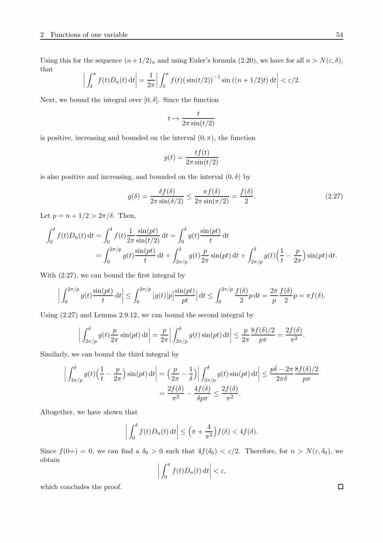
2 Functions of one variable 54
Using this for the sequence (n + 1/2)n and using Euler’s formula (2.20), we have for all n > N(ε, δ),that
∣
∣
∣
∣
∫ π
δf(t)Dn(t) dt
∣
∣
∣
∣
=1
2π
∣
∣
∣
∣
∫ π
δf(t)
(
sin(t/2))−1 sin
(
(n + 1/2)t)
dt
∣
∣
∣
∣
< ε/2.
Next, we bound the integral over [0, δ]. Since the function
t 7→ t
2π sin(t/2)
is positive, increasing and bounded on the interval (0, π), the function
g(t) =tf(t)
2π sin(t/2)
is also positive and increasing, and bounded on the interval (0, δ) by
g(δ) =δf(δ)
2π sin(δ/2)≤ πf(δ)
2π sin(π/2)=
f(δ)2
. (2.27)
Let p = n + 1/2 > 2π/δ. Then,
∫ δ
0f(t)Dn(t) dt =
∫ δ
0f(t)
12π
sin(pt)sin(t/2)
dt =∫ δ
0g(t)
sin(pt)t
dt
=∫ 2π/p
0g(t)
sin(pt)t
dt +∫ δ
2π/pg(t)
p
2πsin(pt) dt +
∫ δ
2π/pg(t)
(1t
− p
2π
)
sin(pt) dt.
With (2.27), we can bound the first integral by
∣
∣
∣
∣
∫ 2π/p
0g(t)
sin(pt)t
dt
∣
∣
∣
∣
≤∫ 2π/p
0
∣
∣g(t)∣
∣p∣
∣
∣
sin(pt)pt
∣
∣
∣dt ≤∫ 2π/p
0
f(δ)2
p dt =2π
p
f(δ)2
p = πf(δ).
Using (2.27) and Lemma 2.9.12, we can bound the second integral by
∣
∣
∣
∣
∫ δ
2π/pg(t)
p
2πsin(pt) dt
∣
∣
∣
∣
=p
2π
∣
∣
∣
∣
∫ δ
2π/pg(t) sin(pt) dt
∣
∣
∣
∣
≤ p
2π
8f(δ)/2pπ
=2f(δ)
π2.
Similarly, we can bound the third integral by∣
∣
∣
∣
∫ δ
2π/pg(t)
(1t
− p
2π
)
sin(pt) dt
∣
∣
∣
∣
=( p
2π− 1
δ
)
∣
∣
∣
∣
∫ δ
2π/pg(t) sin(pt) dt
∣
∣
∣
∣
≤ pδ − 2π
2πδ
8f(δ)/2pπ
=2f(δ)
π2− 4f(δ)
δpπ≤ 2f(δ)
π2.
Altogether, we have shown that∣
∣
∣
∣
∫ δ
0f(t)Dn(t) dt
∣
∣
∣
∣
≤(
π +4π2
)
f(δ) < 4f(δ).
Since f(0+) = 0, we can find a δ0 > 0 such that 4f(δ0) < ε/2. Therefore, for n > N(ε, δ0), weobtain
∣
∣
∣
∣
∫ π
0f(t)Dn(t) dt
∣
∣
∣
∣
< ε,
which concludes the proof.
2 Functions of one variable 55
We can finally prove the pointwise convergence of the Fourier series of functions of bounded variation.Recall that Theorem 2.4.2 implies that the one-sided limits of a function of bounded variation alwaysexist. This enables us to state the following theorem.
Theorem 2.9.14. Let f be a 2π-periodic function that is of bounded variation on the interval[−π, π]. Then the partial sums sn of the Fourier series of f converge at every point x and we have
limn→∞ sn(x) =
12
(
f(x+) − f(x−))
. (2.28)
Proof. Since f is periodic and of bounded variation on [−π, π], it is of bounded variation on everycompact interval. Hence, it is sufficient to show the theorem for x ∈ [−π, π]. Let x ∈ [−π, π] andassume for now that f is an increasing function on [x, x + π]. Lemma 2.9.7 implies
sn(x) − 12
(
f(x+) + f(x−))
=∫ π
0
(
f(x + t) − f(x − t) − f(x+) − f(x−))
Dn(t) dt
=∫ π
0
(
f(x + t) − f(x+))
Dn(t) dt +∫ π
0
(
f(x − t) − f(x−))
Dn(t) dt.
Using Lemma 2.9.13 on both integrals yields (2.28). In particular, we have proved the theorem forincreasing functions.
Now, let f be a function as in the statement of the theorem. Since f is of bounded variation in theinterval [−π, 2π], we can find two increasing functions f1, f2 on [−π, 2π] with f = f1 − f2 by theJordan Decomposition Theorem 2.3.2. For the functions f1, f2, we have already shown (2.28) on[−π, π]. Therefore, (2.28) also holds for the function f , which proves the theorem.
Theorem 2.9.14 implies that the Fourier series of a continuous function of bounded variation con-verges pointwise to the function itself. This result can be strengthened. Indeed, the Fourier seriesof a continuous function of bounded variation even converges uniformly. This statement is also dueto Jordan, who proved it using a method called “second law of the mean”. We follow a differentand perhaps simpler path that is due to Horowitz in [28].
For the proof of uniform convergence, we need the definition and some simple properties of theRiemann-Stieltjes integral. We only state them here and note their resemblance to the usual Rie-mann integral. The interested reader may find more details in many books on real analysis, forexample in [45].
Definition 2.9.15. Let f : [a, b] → R be a function and let α : [a, b] → R be an increasing function.We define the lower and upper Riemann-Stieltjes integrals by
∫ b
a
f(t) dα(t) := supY∈Y
∑
y∈Yinf
x∈[y,y+]f(x)
(
α(y+) − α(y))
and
∫ b
af(t) dα(t) := inf
Y∈Y
∑
y∈Ysup
x∈[y,y+]f(x)
(
α(y+) − α(y))
,
respectively. If the two integrals coincide, we define the Riemann-Stieltjes integral of f with respectto α as
∫ b
af(t) dα(t) :=
∫ b
a
f(t) dα(t) =∫ b
af(t) dα(t).
If α is a function of bounded variation and (α+, α−) is its Jordan decomposition, we define theRiemann-Stieltjes integral of f with respect to α as
∫ b
af(t) dα(t) :=
∫ b
af(t) dα+(t) −
∫ b
af(t) dα−(t),

2 Functions of one variable 56
if it exists.
Proposition 2.9.16. Let f : [a, b] → R be continuous and let α : [a, b] → R be of bounded variation.Then the Riemann-Stieltjes integral of f with respect to α exists. Moreover, the integral is linearboth in f and α. Furthermore, for c ∈ [a, b],
∫ b
af(t) dα(t) =
∫ c
af(t) dα(t) +
∫ b
cf(t) dα(t) and
∣
∣
∣
∣
∫ b
af(t) dα(t)
∣
∣
∣
∣
≤ ‖f‖∞ Var(α)
hold. If α is differentiable, then
∫ b
af(t) dα(t) =
∫ b
af(t)α′(t) dt.
Finally, we have a partial integration formula: If f is also of bounded variation, then
∫ b
af(t) dα(t) = f(b)α(b) − f(a)α(a) −
∫ b
aα(t) df(t).
We already know that the Fourier series of continuous functions of bounded variation convergespointwise. What we need is a theorem that enables us to deduce a posteriori that the convergencewas uniform. The theorem of our choice is the Arzelà-Ascoli Theorem.
Definition 2.9.17. A sequence of functions fn : [a, b] → R is called equicontinuous if for everyε > 0 and x ∈ [a, b], there exists a δ > 0 such that
∣
∣fn(x) − fn(y)∣
∣ < ε
for all y ∈ [a, b] with |x − y| < δ and for all n ∈ N.
Theorem 2.9.18 (Arzelà-Ascoli). Let (fn) be a sequence of real-valued functions on [a, b]. If thesequence is uniformly bounded, i.e.
supn∈N
‖fn‖∞ < ∞,
and equicontinuous, then there exists a uniformly convergent subsequence.
Proof. Let ε > 0 and for every x ∈ [a, b] choose δx > 0 such that∣
∣fn(x) − fn(y)∣
∣ < ε
for all y ∈ [a, b] with |x−y| < δ and for all n ∈ N. The balls B(x, δx) with center x and radius δx coverthe interval [a, b]. Since [a, b] is compact, we can find a finite subcover B(x1, δ1), . . . , B(xm, δm).Since the sequence (fn) is uniformly bounded,
(
fn(xi))
nis bounded for i = 1, . . . , m. Hence, there
exists a subsequence (fnk) such that
(
fnk(xi)
)
kconverges for all i = 1, . . . , m.
Let x ∈ [a, b] and let i ∈ 1, . . . , m be such that x ∈ B(xi, δi). Then,∣
∣fnk(x) − fnj
(x)∣
∣ ≤∣
∣fnk(x) − fnk
(xi)∣
∣+∣
∣fnk(xi) − fnj
(xi)∣
∣+∣
∣fnj(xi) − fnj
(x)∣
∣ ≤ 3ε
for k, j ∈ N large enough.
We have shown that for every ε > 0 there exist a subsequence (fnk) of (fn) such that
‖fnk− fnj
‖∞ < ε
holds for all k, j ∈ N.
2 Functions of one variable 57
Let (f1,n)n be a subsequence of (fn) with
‖f1,n − f1,m‖∞ < 1
for all n, m ∈ N. Inductively, let (fk,n)n be a subsequence of (fk−1,n)n with
‖fk,n − fk,m‖∞ <1k
for all n, m ∈ N. Then the sequence (fk,k)k converges uniformly.
Lemma 2.9.19. Let X be a metric space and let (xn) be a sequence in X. Then (xn) converges tox ∈ X if and only if every subsequence of (xn) has a subsequence that converges to x.
Proof. If (xn) converges to x, then every subsequence converges to x as well.
Conversely, assume that every subsequence of (xn) has a subsequence that converges to x andsuppose that (xn) does not converge to x. Then there exists an ε > 0 and a subsequence (xnk
) of(xn) such that for all k ∈ N, d(xnk
, x) > ε. By assumption, there exists a subsequence of (xnk) that
converges to x, which is a contradiction.
Corollary 2.9.20. Let (fn) be a sequence of real-valued functions on [a, b] that converges pointwiseto a function f . If the sequence (fn) is uniformly bounded and equicontinuous, the convergence isuniform.
Proof. Since (fn) is uniformly bounded and equicontinuous, so is every subsequence (fnk) of (fn).
Applying the Arzelà-Ascoli Theorem 2.9.18 to (fnk), we get a subsequence (fnkj
) that convergesuniformly to a function. Since (fnkj
) already converges pointwise to f , it thus also convergesuniformly to f . Hence, every subsequence of (fn) has a subsequence that converges uniformly to f .By Lemma 2.9.19, (fn) converges uniformly to f .
Lemma 2.9.21. Let
tn(x) :=n∑
k=1
sin kx
kand t(x) := lim
n→∞ tn(x).
Then tn and t are 2π-periodic, (tn) is uniformly bounded, and tn(x) → (π − x)/2 uniformly in everyinterval [δ, 2π − δ] with 0 < δ < π.
Proof. It is clear that tn is 2π-periodic. If the limit t exists, it is clear that it is 2π-periodic as well.Thus, we only consider x ∈ [0, 2π). Using (2.25),
tn(x) =∫ x
0
( n∑
k=1
cos(kt))
dt =∫ x
0
sin(
(n + 1/2)t) − sin(t/2)
2 sin(t/2)dt
=∫ x
0
sin(
(n + 1/2)t)
tdt +
∫ x
0
(
12 sin(t/2)
− 1t
)
sin(
(n + 1/2)t)
dt − x
2
=∫ (n+1/2)x
0
sin u
udu +
∫ x
0
(
12 sin(t/2)
− 1t
)
sin(
(n + 1/2)t)
dt − x
2.
It is easily verified that∫ h
0
sin u
udu

2 Functions of one variable 58
is non-negative for all h ≥ 0 and has its maximum at h = π. Hence,
|tn(x)| ≤∫ π
0
sin u
udu +
∫ x
0
∣
∣
∣
∣
12 sin(t/2)
− 1t
∣
∣
∣
∣
∣
∣ sin(
(n + 1/2)t)∣
∣ dt +x
2
≤∫ π
0
sin u
udu +
∫ π
0
(
12 sin(t/2)
− 1t
)
dt +π
2,
for 0 ≤ x ≤ π. Since tn is a sum of odd functions, the same bound holds for −π ≤ x ≤ 0, and byperiodicity, for all x ∈ R. A simple calculation shows that the above uniform bound on |tn(x)| isindeed finite.
Next, we calculate t(x) for 0 < x < 2π. Notice that
limn→∞
∫ (n+1/2)x
0
sin u
udu =
∫ ∞
0
sin u
udu
exists as an improper Riemann integral (but not as a Lebesgue integral) and is finite. We denotethe value of this integral by I. Also, using partial integration, we have
∫ x
0
(
12 sin(t/2)
− 1t
)
sin(
(n + 1/2)t)
dt = −(
12 sin(x/2)
− 1x
)
sin(
(n + 1/2)x)
n + 1/2
+ limt→0
(
12 sin(t/2)
− 1t
)
sin(
(n + 1/2)t)
n + 1/2
+1
n + 1/2
∫ x
0
ddt
(
12 sin(t/2)
− 1t
)
cos(
(n + 1/2)t)
dt.
Observe that the first summand tends to zero as n goes to infinity, the second summand is zero,and the third summand also tends to zero as n goes to infinity since the integrand is uniformlybounded. Hence,
t(x) = I − x
2for 0 < x < 2π.
Since t(π) = 0, we have I = π/2. Thus, t(x) = (π − x)/2.
Finally, let 0 < δ < π. We have already shown that tn converges pointwise to t on [δ, 2π−δ] and that(tn) is uniformly bounded. We want to apply Corollary 2.9.20 to get that (tn) converges uniformlyto t on [δ, 2π − δ]. It remains to show that (tn) is equicontinuous.
Let n ∈ N and let δ ≤ x < y ≤ 2π − δ. Similarly as before,
∣
∣tn(y) − tn(x)∣
∣ =
∣
∣
∣
∣
∣
∫ y
x
sin(n + 1/2)tt
dt +∫ y
x
(
12 sin t/2
− 1t
)
sin(n + 1/2)t dt − y − x
2
∣
∣
∣
∣
∣
≤∫ y
x
1δ
dt +∫ y
x
12 sin(π − δ/2)
dt +|y − x|
2= C|y − x|
for some constant C independent of x, y and n. Hence, (tn) is equicontinuous and converges uni-formly to t on [δ, 2π − δ].
Lemma 2.9.22. Let
Tn(x) :=x − π
2+ tn(x).
Then T ′n(x) = πDn(x), (Tn) is uniformly bounded on [0, 2π) and Tn(x) → 0 uniformly in every
interval [δ, 2π − δ] with 0 < δ < π.

2 Functions of one variable 59
Proof. Using (2.25) and that sin is odd and cos is even, we have
T ′n(x) =
12
+n∑
k=1
cos kx =12
+12
n∑
k=−n
eikx − 12
=sin(
(n + 1/2)x)
2 sin(x/2)= πDn(x).
The remaining statements follow immediately from Lemma 2.9.21.
Theorem 2.9.23. The Fourier series of a continuous 2π-periodic function of bounded variationconverges uniformly to the original function.
Proof. Let sn denote the n-th partial sum of the Fourier series of a continuous 2π-periodic functionf of bounded variation and let 0 < δ < π. By Lemma 2.9.5 and Lemma 2.9.7,
sn(x) − f(x) =∫ 2π
0
(
f(x + t) − f(x))
Dn(t) dt.
Let φx(t) := f(x + t) − f(x). Then φx(0) = φx(2π) = 0. Using integration by parts,
sn(x) − f(x) =∫ 2π
0φx(t)Dn(t) dt =
∫ 2π
0φx(t) dDn(t) = −
∫ 2π
0Tn(t) dφx(t)
= −∫ δ
0Tn(t) dφx(t) −
∫ 2π−δ
δTn(t) dφx(t) −
∫ 2π
2π−δTn(t) dφx(t).
Let ε > 0. Since f is continuous and of bounded variation, also φx is continuous and of boundedvariation. Hence, Var1(t) := Var(φx; 0, t) and Var2(t) := Var(φx; 2π − t, 2π) are continuous byTheorem 2.2.5. Thus, there exists a 0 < δ < π such that Var1(δ) < ε and Var2(δ) < ε. Now, let(Tn) be uniformly bounded by C, and let N ∈ N be such that for all n > N ,
supt∈[δ,2π−δ]
|Tn(t)| < ε.
Then,
∣
∣sn(x) − f(x)∣
∣ ≤ supt∈[0,δ]
|Tn(t)| Var(φx; 0, δ) + supt∈[δ,2π−δ]
|Tn(t)| Var(φx, δ, 2π − δ)
+ supt∈[2π−δ,2π]
|Tn(t)| Var(φx, 2π − δ, 2π)
≤ Cε + ε2 Var(f ; 0, 2π) + Cε.
In particular, sn converges uniformly to f .

3 Functions of multiple variables 60
3 Functions of multiple variables
3.1 Definitions
In one dimension, the definition of bounded variation was clear and straight-forward. In higherdimensions, there are many possible generalizations, each preserving different properties of theunivariate functions of bounded variation. One approach is to define ladders in higher dimensionsand then generalize the difference
∣
∣f(y+) − f(y)|. However, there are multiple ways of generalizingthis difference. Equally well, one could make the monotone decomposition the defining propertyof functions of bounded variation, i.e. define that the set of functions of bounded variation is thevector space induced by the monotone functions. However, what does it mean to be increasingin higher dimensions? Finally, one could say that the defining property of functions of boundedvariation is that they do not oscillate to much, and therefore consider oscillations of the function,similarly to Chapter 2.6 on the dimension of the graph.
We see that there are many different ways of generalizing bounded variation to higher dimensions,and all of them yield different results. We study the variations in the sense of Vitali, Hardy andKrause, Arzelà, Hahn and Pierpont, as they exhibit many useful properties.
First, we need to introduce some general notation. Vectors in Rd are written in bold font, i.e. wewrite a = (a1, . . . , ad) ∈ Rd. In particular, we use the notation 0 = (0, . . . , 0) and 1 = (1, . . . , 1).Given two vectors a and b, we write a ≤ b if ai ≤ bi for all i = 1, . . . , d. Furthermore, we write[a, b] := x : a ≤ x ≤ b. The expressions a < b, (a, b), [a, b) and (a, b] are defined similarly.
For n ∈ N we define [n] := 1, . . . , n. For u, v ⊂ [d], we write |u| for the cardinality of u and u − vfor the complement of v with respect to u. We define the unary minus of u as the complement of uin [d], i.e. −u := [d] − u. The unary minus has higher precedence than the binary minus, ∪ and ∩.
For u ⊂ [d] and x ∈ [a, b] we denote by xu the |u|-tuple of the components xi for i ∈ u. If u, v ⊂ [d]are disjoint and if x, y ∈ [a, b], then we denote by xu : yv the |u ∪ v|-tuple z ∈ [au∪v, bu∪v ] withzi = xi for i ∈ u and zj = yj for j ∈ v. We can also use this gluing symbol for more than twocomponents, as long as the subsets of [d] are mutually disjoint. Furthermore, for x ∈ [a, b] andi ∈ [d], we also write x−i instead of x−i.
For u ⊂ [d], x−u ∈ [a−u, b−u] and a function f : [a, b] → R, we can define a function g : [au, bu] → Rby g(xu) = f(xu : x−u). We write f(xu; x−u) to denote such a function with the argument on theleft of the semi-colon and the parameters on the right.
For a rectangle I = [a, b], we define the d-fold alternating sum of f over I as
∆[d](f ; I) := ∆[d](f ; a, b) :=∑
v⊂[d]
(−1)|v|f(av : b−v).
This operator ∆[d] is one of the generalizations of the difference f(y+) − f(y) in one dimension.More generally, we define for all u ⊂ [d] the operator
∆u(f ; I) := ∆u(f ; a, b) :=∑
v⊂u
(−1)|v|f(av : bu−v : a−u).
For i ∈ [d], we also write ∆i = ∆i and ∆−i = ∆−i. Finally, we define the operator ∆ by
∆(f ; I) := ∆(f ; a, b) := f(b) − f(a).
This is another generalization of the difference f(y+) − f(y).
We may also apply the operators ∆u and ∆ to a function f at a point x ∈ I. In this case, theinterpretation is ∆uf(x) := ∆u(f ; x, x + h) and ∆f(x) := ∆(f ; x, x + h), respectively, for some
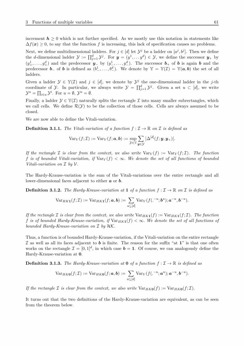
3 Functions of multiple variables 61
increment h ≥ 0 which is not further specified. As we mostly use this notation in statements like∆f(x) ≥ 0, to say that the function f is increasing, this lack of specification causes no problems.
Next, we define multidimensional ladders. For j ∈ [d] let Yj be a ladder on [aj , bj]. Then we definethe d-dimensional ladder Y :=
∏dj=1 Yj . For y = (y1, . . . yd) ∈ Y, we define the successor y+ by
(y1+, . . . , yd
+) and the predecessor y− by (y1−, . . . , yd
−). The successor b+ of b is again b and thepredecessor b− of b is defined as (b1
−, . . . , bd−). We denote by Y = Y(I) = Y(a, b) the set of all
ladders.
Given a ladder Y ∈ Y(I) and j ∈ [d], we denote by Yj the one-dimensional ladder in the j-thcoordinate of Y. In particular, we always write Y =
∏dj=1 Yj . Given a set u ⊂ [d], we write
Yu =∏
i∈u Y i. For u = ∅, Yu = ∅.
Finally, a ladder Y ∈ Y(I) naturally splits the rectangle I into many smaller subrectangles, whichwe call cells. We define R(Y) to be the collection of those cells. Cells are always assumed to beclosed.
We are now able to define the Vitali-variation.
Definition 3.1.1. The Vitali-variation of a function f : I → R on I is defined as
VarV (f ; I) := VarV (f ; a, b) := supY∈Y
∑
y∈Y
∣
∣∆[d](f ; y, y+)∣
∣.
If the rectangle I is clear from the context, we also write VarV (f) := VarV (f ; I). The functionf is of bounded Vitali-variation, if VarV (f) < ∞. We denote the set of all functions of boundedVitali-variation on I by V.
The Hardy-Krause-variation is the sum of the Vitali-variations over the entire rectangle and alllower-dimensional faces adjacent to either a or b.
Definition 3.1.2. The Hardy-Krause-variation at 1 of a function f : I → R on I is defined as
VarHK1(f ; I) := VarHK1(f ; a, b) :=∑
u([d]
VarV (f(.−u; bu); a−u, b−u).
If the rectangle I is clear from the context, we also write VarHK1(f) := VarHK1(f ; I). The functionf is of bounded Hardy-Krause-variation, if VarHK1(f) < ∞. We denote the set of all functions ofbounded Hardy-Krause-variation on I by HK.
Thus, a function is of bounded Hardy-Krause-variation, if the Vitali-variation on the entire rectangleI as well as all its faces adjacent to b is finite. The reason for the suffix “at 1” is that one oftenworks on the rectangle I = [0, 1]d, in which case b = 1. Of course, we can analogously define theHardy-Krause-variation at 0.
Definition 3.1.3. The Hardy-Krause-variation at 0 of a function f : I → R is defined as
VarHK0(f ; I) := VarHK0(f ; a, b) :=∑
u([d]
VarV (f(.−u; au); a−u, b−u).
If the rectangle I is clear from the context, we also write VarHK0(f) := VarHK0(f ; I).
It turns out that the two definitions of the Hardy-Krause-variation are equivalent, as can be seenfrom the theorem below.

3 Functions of multiple variables 62
Theorem 3.1.4. Let f : [0, 1]d → R be a function with VarHK0(f) < ∞. Then
VarHK1(f) ≤ (2d − 1) VarHK0(f).
Analogously, if VarHK1(f) < ∞, then
VarHK0(f) ≤ (2d − 1) VarHK1(f).
The proof of this theorem is non-trivial and relies on results that we discuss later in this thesis. Theinterested reader can find a proof in [2] due to Aistleitner and Dick.
Next, we define the Arzelà-variation. Unfortunately, we cannot use ladders for the definition.Instead, we need diagonals, which are special sequences. Before introducing them, we make someremarks about the notation. If (xn) is a (finite or infinite) sequence, we write z ∈ (xn) if z = xn
for some n ∈ N. Furthermore, if the sequence (xn) is finite, we denote by #(xn) the length ofthe sequence. If x = (x1, . . . , xn) is a finite sequence, we define x ∪ z := (x1, . . . , xn, z). Finally, ifx = (x1, . . . , xn) and z = (z1, . . . , zm) are finite sequences, we define x∪z := (x1, . . . , xn, z1, . . . , zm).
A one-dimensional diagonal D on a rectangle [a, b] is a non-decreasing sequence of points D =(y0, y1, . . . , yn−1) with y0 = a and yn−1 ≤ b. For an element y = yi of the diagonal, we denote byy+ := yi+1 the successor of y. If i = n − 1, then the successor is defined as b. Similarly, y− := yi−1
denotes the predecessor of y, and for i = 0, the predecessor is defined as a. The predecessor b− of bis defined as yn−1.
Given a rectangle I = [a, b] and one-dimensional diagonals Di = (yi0, yi
1, . . . , yin−1) on [ai, bi] for i ∈
[d] that are all of equal length #Di = n, we define a d-dimensional diagonal D on I as the sequenceD = (y0, y1, . . . , yn−1), where yj = (y1
j , . . . , ydj ) for j ∈ 0, . . . , n − 1. For an element y of the
diagonal, we define the successor as y+ := (y1+, . . . , yd
+) and the predecessor as y− := (y1−, . . . , yd
−).Similarly, we define b− := (b1
−, . . . , bd−). The set of diagonals on I is denoted by D = D(I) = D(a, b).
There are three basic differences between a ladder and a diagonal. First, a higher-dimensionaldiagonal always consists of equally long one-dimensional diagonals, whereas the one-dimensionalladders of a higher-dimensional ladder need not be of the same length. Second, if we interpreteda diagonal as a ladder, we would not consider all the cells of this resulting ladder, but only theones “lying on the diagonal”. This property gives diagonals their name. Finally, a one-dimensionalladder has pairwise different ladder points, while we require a one-dimensional diagonal only to benon-decreasing. This is the reason why we had to introduce sequence notation for the diagonals asopposed to set notation for ladders, because a diagonal can have the same point multiple times.
We can now define the Arzelà-variation.
Definition 3.1.5. The Arzelà-variation of a function f : I → R on I is defined as
VarA(f ; I) := VarA(f ; a, b) := supD∈D
∑
y∈D
∣
∣∆(f ; y, y+)∣
∣.
If the rectangle I is clear from the context, we also write VarA(f) := VarA(f ; I). The functionf is of bounded Arzelà-variation, if VarA(f) < ∞. We denote the set of all functions of boundedArzelà-variation on I by A.
While the three variations introduced so far are defined using difference operators, the Hahn- andthe Pierpont-variation are defined using oscillations. Both variations partition the rectangle Iinto subsets and then sum over all the oscillations of the function on those subsets. The only realdifference is the partition chosen. First, we define the Hahn-variation, for which we need equidistantladders.
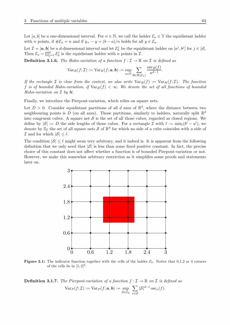
3 Functions of multiple variables 63
Let [a, b] be a one-dimensional interval. For n ∈ N, we call the ladder En ∈ Y the equidistant ladderwith n points, if #En = n and if y+ − y = (b − a)/n holds for all y ∈ En.
Let I = [a, b] be a d-dimensional interval and let Ejn be the equidistant ladder on [aj , bj ] for j ∈ [d].
Then En =∏d
j=1 Ejn is the equidistant ladder with n points in I.
Definition 3.1.6. The Hahn-variation of a function f : I → R on I is defined as
VarH(f ; I) := VarH(f ; a, b) := supn∈N
∑
R∈R(En)
oscR(f)nd−1
.
If the rectangle I is clear from the context, we also write VarH(f) := VarH(f ; I). The functionf is of bounded Hahn-variation, if VarH(f) < ∞. We denote the set of all functions of boundedHahn-variation on I by H.
Finally, we introduce the Pierpont-variation, which relies on square nets.
Let D > 0. Consider equidistant partitions of all d axes of Rd, where the distance between twoneighbouring points is D (on all axes). Those partitions, similarly to ladders, naturally split Rd
into congruent cubes. A square net S is the set of all those cubes, regarded as closed regions. Wedefine by |S| := D the side lengths of those cubes. For a rectangle I with ℓ := mini(bi − ai), wedenote by SI the set of all square nets S of Rd for which no side of a cube coincides with a side ofI and for which |S| ≤ ℓ.
The condition |S| ≤ ℓ might seem very arbitrary, and it indeed is. It is apparent from the followingdefinition that we only need that |S| is less than some fixed positive constant. In fact, the precisechoice of this constant does not affect whether a function is of bounded Pierpont-variation or not.However, we make this somewhat arbitrary restriction as it simplifies some proofs and statementslater on.
0 0.6 1.2 1.8 2.4 30
0.6
1.2
1.8
2.4
3
Figure 3.1: The indicator function together with the cells of the ladder E5. Notice that 0,1,2 or 4 cornersof the cells lie in [1, 2]2.
Definition 3.1.7. The Pierpont-variation of a function f : I → R on I is defined as
VarP (f ; I) := VarP (f ; a, b) := supS∈SI
∑
ν∈S|S|d−1 oscν(f).
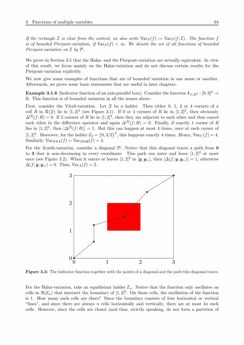
3 Functions of multiple variables 64
If the rectangle I is clear from the context, we also write VarP (f) := VarP (f ; I). The function fis of bounded Pierpont-variation, if VarP (f) < ∞. We denote the set of all functions of boundedPierpont-variation on I by P.
We prove in Section 3.5 that the Hahn- and the Pierpont-variation are actually equivalent. In viewof this result, we focus mainly on the Hahn-variation and do not discuss certain results for thePierpont-variation explicitly.
We now give some examples of functions that are of bounded variation in one sense or another.Afterwards, we prove some basic statements that are useful in later chapters.
Example 3.1.8 (Indicator function of an axis-parallel box). Consider the function 1[1,2]2 : [0, 3]2 →R. This function is of bounded variation in all the senses above.
First, consider the Vitali-variation. Let Y be a ladder. Then either 0, 1, 2 or 4 corners of acell R in R(Y) lie in [1, 2]2 (see Figure 3.1). If 0 or 4 corners of R lie in [1, 2]2, then obviously∆[2](f ; R) = 0. If 2 corners of R lie in [1, 2]2, then they are adjacent to each other and thus canceleach other in the difference operator and again ∆[2](f ; R) = 0. Finally, if exactly 1 corner of Rlies in [1, 2]2, then
∣
∣∆[2](f ; R)∣
∣ = 1. But this can happen at most 4 times, once at each corner of
[1, 2]2. Moreover, for the ladder E2 =
0, 3/22, this happens exactly 4 times. Hence, VarV (f) = 4.
Similarly, VarHK1(f) = VarHK0(f) = 4.
For the Arzelà-variation, consider a diagonal D. Notice that this diagonal traces a path from 0
to 3 that is non-decreasing in every coordinate. This path can enter and leave [1, 2]2 at mostonce (see Figure 3.2). When it enters or leaves [1, 2]2 in [y, y+], then
∣
∣∆(f ; y, y+)∣
∣ = 1, otherwise∆(f ; y, y+) = 0. Thus, VarA(f) = 2.
0 1 2 30
1
2
3
Figure 3.2: The indicator function together with the points of a diagonal and the path this diagonal traces.
For the Hahn-variation, take an equidistant ladder En. Notice that the function only oscillates oncells in R(En) that intersect the boundary of [1, 2]2. On those cells, the oscillation of the functionis 1. How many such cells are there? Since the boundary consists of four horizontal or vertical“lines”, and since there are always n cells horizontally and vertically, there are at most 4n suchcells. However, since the cells are closed (and thus, strictly speaking, do not form a partition of

3 Functions of multiple variables 65
[0, 3]2), there could be up to 8n cells intersecting the boundary of [1, 2]2. Therefore,
VarH(1[1,2]2) = supn∈N
∑
R∈R(En)
oscR(f)n
≤ 8n
n= 8,
and the function is also in H.
This example can of course be generalized to arbitrary axis-parallel boxes in all dimensions.
Example 3.1.9 (Indicator functions of a rotated box). Next, we consider indicator functions oftilted boxes. The definitions of the variations we study all heavily depend on the cartesian coordinatesystem and are not rotation invariant. Indeed, indicator functions of most rotated (not axis-parallel)boxes are not of bounded Vitali-, Hardy-Krause- and Arzelà-variation. They are, however, ofbounded Hahn-variation.
Denote by A =
(x, x) : x ∈ [0, 1]
the diagonal of [0, 1]2. We study the variations of the function1A : [0, 1]2 → R. While this is a very distorted rotated box, similar reasoning can be applied tomost rotated boxes.
First, consider the Vitali-variation and take the ladder En for some n ∈ N. From Figure 3.3, it isapparent that 2(n − 1) cells of R(En) have exactly one corner in common with A. On each of thosecells R,
∣
∣∆[2](1A; R)∣
∣ = 1. By taking n to infinity, we see that 1A is of unbounded Vitali-variation.Hence, it is also of unbounded Hardy-Krause-variation.
0 0.2 0.4 0.6 0.8 10
0.2
0.4
0.6
0.8
1
Figure 3.3: The indicator function of the diagonal A together with the cells of the ladder E5. Notice thatthere are 2 · 4 cells with exactly one corner on A, these cells are colored light blue.
For the Arzelà-variation, consider the diagonals
Dn =(
(0, 0), (1/n, 0), (1/n, 1/n), (2/n, 1/n), (2/n, 2/n), . . . , (1, 1))
.
Considering Figure 3.4 and taking n to infinity, it is clear that 1A is of unbounded Arzelà-variation.
For the Hahn-variation, let En be an equidistant ladder. The function only oscillates on cells thatintersect A. It is easy to see that there can be at most 3n such cells. Hence, VarH(1A) ≤ 3.

3 Functions of multiple variables 66
0 0.2 0.4 0.6 0.8 10
0.2
0.4
0.6
0.8
1
Figure 3.4: The indicator function of A together with the points of the diagonal D5 and the path thisdiagonal traces.
Example 3.1.10 (Monotone functions). As already discussed, there are multiple ways of definingmonotonicity in higher dimensions. We need three different definitions of monotonicity, correspond-ing to the variations in the sense of Vitali, Hardy and Krause, and Arzelà. Since those definitionsand the proofs that monotone functions are of bounded variation in the respective senses are ratherlengthy and technical, we postpone them to later sections, especially Section 3.4 on the monotonedecomposition of functions in V, HK and A.
Example 3.1.11 (Lipschitz continuous functions). Lipschitz continuous functions are always ofbounded Arzelà- and Hahn-variation, but they can be of unbounded Vitali- and Hardy-Krause-variation. For an example of a Lipschitz continuous function that is of unbounded Vitali-variation,and thus also of unbounded Hardy-Krause-variation, we refer to [7].
For the Arzelà-variation, it is easy to see that
VarA(f) = supD∈D
∑
y∈D
∣
∣f(y+) − f(y)∣
∣ ≤ L supD∈D
∑
y∈D‖y+ − y‖1 = L
d∑
i=1
|bi − ai|,
where L is the Lipschitz constant of f with respect to the ℓd1-norm on Rd.
For the Hahn-variation, let L be the Lipschitz constant of f with respect to the ℓd∞-norm on Rd.
Then,
VarH(f) = supn∈N
∑
R∈R(En)
oscR(f)nd−1
≤ supn∈N
∑
R∈R(En)
L supx,z∈R ‖x − z‖∞nd−1
.
Since En is the equidistant ladder with n points on I, we have for all R ∈ R(En) that
supx,z∈R
‖x − z‖∞ =maxi |bi − ai|
n=:
ℓ
n.

3 Functions of multiple variables 67
Since there are exactly nd cells in R(En),
supn∈N
∑
R∈R(En)
L supx,z∈R ‖x − z‖∞nd−1
≤ supn∈N
∑
R∈R(En)
Lℓ
nd= Lℓ.
So far, the Vitali-variation and the Hardy-Krause-variation behaved very similarly. At first sightthe purpose of the Hardy-Krause-variation is not clear. Why do we include the lower-dimensionalVitali-variations? In the following examples, we give two reasons.
Example 3.1.12. The Vitali-variation is blind for lower-dimensional variations. Consider thefunction f : [0, 1]2 → R defined by
f(x1, x2) =
1, if x1 ∈ Q,
0, if x1 /∈ Q.
The function f is independent of the variable x2, yet common sense indicates that it oscillates alot. However, it is not hard to verify that VarV (f) = 0. The same holds true for every functionthat is independent of one of its variables. We treat this phenomenon more thoroughly in Chapter3.9 on product functions. One very straight-forward way to avoid this problem is to just addthe lower-dimensional Vitali-variations of the function, as the Hardy-Krause-variation does. Andindeed, VarHK0(f) = VarHK1(f) = ∞, so f is of unbounded Hardy-Krause-variation.
For the second example, notice that the difference operator ∆[d] strongly resembles the differencequotient corresponding to ∂[d], the mixed partial derivative taken once in each coordinate. We evenhave the following proposition. For proofs, we refer to [20, 40].
Proposition 3.1.13. Let f : [a, b] → R be a function such that ∂[d]f(x) exists for all x ∈ [a, b].Then
∫
[a,b]∂[d]f(x) dx = ∆[d](f ; a, b).
Furthermore,
VarV (f ; a, b) ≤∫
[a,b]
∣
∣∂[d]f(x)∣
∣ dx. (3.29)
If ∂[d]f is continuous on [a, b], we have equality in (3.29).
Example 3.1.14. The Vitali-variation is blind for polynomials of low degree. For example, thefunction f : [0, 1]d → R, f(x) =
∑di=1 xi satisfies VarV (f) = 0 if d ≥ 2. This follows immediately
from the preceding proposition. Furthermore, 0 < VarHK1(f), VarHK0(f) < ∞, so the Hardy-Krause-variation does not have the same weakness.
Now that we have seen some examples of functions of bounded variation of the various types, weprove that all the introduced multi-dimensional variations actually generalize the one-dimensionaltotal variation. First, we need a technical lemma that will be used a lot throughout this thesis.
Lemma 3.1.15. Let f : Ω → R be a function. Let A, A1, . . . , An ⊂ Ω with
A ⊂n⋃
i=1
Ai.
Assume that for all i, j ∈ [n], there exists a sequence i0, i1, i2, . . . , ik ⊂ [n] with i0 = i and ik = jand the property that
Ail∩ Ail+1
6= ∅ (l = 0, . . . , k − 1). (3.30)

3 Functions of multiple variables 68
Then
oscA(f) ≤n∑
i=1
oscAi(f).
Proof. First, we consider the case oscA(f) = ∞. Then, necessarily, f is unbounded on A. Since
A1, . . . , An
is a finite collection and the union is a superset of A, f is unbounded on some Ai.Then oscAi
(f) = ∞, proving the claim.
Now, assume that oscA(f) < ∞. Let ε > 0 and let x, y ∈ A be such that f(x) − f(y) ≥ oscA(f) − ε.Let i, j ∈ [n] be such that x ∈ Ai and y ∈ Aj. Let i0, . . . , ik ⊂ [n] be a sequence such that i0 = i,ik = j and Ail
∩ Ail+16= ∅ for l = 0, . . . , k − 1. Without loss of generality, we can assume that
il 6= im for all l 6= m. We now define sequences (xl) and (yl) with xl, yl ∈ Ail. First, x0 := x. Then,
yl is chosen as an arbitrary element in Ail∩ Ail+1
. Next, we define xl+1 := yl. Finally, yk := y. Byconstruction,
k∑
l=0
(
f(xl) − f(yl))
= f(x0) − f(yk) = f(x) − f(y).
Furthermore,f(xl) − f(yl) ≤ oscAil
(f)
holds trivially, since xl, yl ∈ Ail. Altogether,
oscA(f) ≤ f(x) − f(y) + ε =k∑
l=0
(
f(xl) − f(yl))
+ ε ≤k∑
l=0
oscAil(f) + ε ≤
n∑
i=1
oscAi(f) + ε.
By taking the infimum over all ε > 0, we get the statement of the lemma.
Remark 3.1.16. We also refer to (3.30) as the path property. To see that this condition is necessary,take A1, . . . , An as a partition of A. Then f could be constant on all the Ai, while it still oscillateson the whole set A. It should be noted, however, that we do not need the path property if oscA(f) =∞. This is apparent from the proof of the lemma. In general, one need not worry too much aboutthe path property. Usually, all the sets A, A1, . . . , An are closed rectangles. Those closed rectanglesalready satisfy the path property, as their boundaries intersect.
Proposition 3.1.17. Let f : [a, b] → R be a univariate function. Then
Var(f) = VarA(f) = VarV (f) = VarHK1(f) = VarHK0(f)
andVarH(f) ≤ Var(f) ≤ 2 VarH(f).
Inequalities similar to the Hahn-variation hold for the Pierpont-variation. In particular, a functionis of bounded total variation if and only if it is of bounded variation in any and all of the sensesdefined above.
Proof. Since ∆[1](f ; x, y) = f(y)−f(x), the definitions of the Vitali-variation and the total variationare equivalent and we have Var(f) = VarV (f). Furthermore,
VarHK1(f ; a, b) =∑
u([1]
VarV
(
f(.−u; bu); a−u, b−u) = VarV (f ; a, b) = Var(f ; a, b).
A similar equality holds for VarHK0(f ; a, b).

3 Functions of multiple variables 69
The equivalence for the Hahn- and Pierpont-variations is a bit more tricky. First, consider theHahn-variation. Let n ∈ N and let ε > 0. The set R(En) contains n cells, that we label R1, . . . , Rn.Take xk, yk ∈ Rk such that
oscRk(f) ≤
∣
∣f(xk) − f(yk)∣
∣+ε
n.
ThenY =
(
En ∪ xk, yk : k ∈ [n]
)
∩ [a, b)
defines a ladder on [a, b]. Furthermore,∑
R∈R(En)
oscR(f) ≤∑
y∈Y
∣
∣f(y+) − f(y)∣
∣+ ε.
Since ε > 0 was arbitrary, we even have∑
R∈R(En)
oscR(f) ≤ Var(f).
Therefore, also VarH(f) ≤ Var(f).
On the other hand, let Y be a ladder on [a, b]. Define δ := min
y+ −y : y ∈ Y and choose n ≥ δ−1.Then every rectangle in R(En) intersects at most two rectangles of R(Y), while every rectangle inR(Y) is of course covered by rectangles in R(En). Since the path property (3.30) is fulfilled we canapply Lemma 3.1.15 to all the rectangles in R(Y) and get
∑
y∈Y
∣
∣f(y+) − f(y)∣
∣ ≤∑
R∈R(Y)
oscR(f) ≤ 2∑
R∈R(En)
oscR(f) ≤ 2 VarH(f).
Therefore, also Var(f) ≤ 2 VarH(f).
The bounds for the Pierpont-variation can be deduced analogously to the bounds for the Hahn-variation with additional constants. Alternatively, they follow immediately from the proof of The-orem 3.5.1.
Finally, we show that finer ladders and diagonals capture more of the Vitali- and Arzelà-variation,respectively.
Proposition 3.1.18. Let f : I → R be a function. Then the following statements hold.
1. If Y1, Y2 ∈ Y(I) with Y1 ⊂ Y2, then∑
y∈Y1
∣
∣∆[d](f ; y, y+)∣
∣ ≤∑
y∈Y2
∣
∣∆[d](f ; y, y+)∣
∣.
2. If D1, D2 ∈ D(I) with D1 ⊂ D2, then∑
y∈D1
∣
∣∆(f ; y, y+)∣
∣ ≤∑
y∈D2
∣
∣∆(f ; y, y+)∣
∣.
Proof. 1. Assume that Y i2\Y i
1 = ci for some i ∈ [d] and ci ∈ (ai, bi) and Yj2 = Yj
1 for all j 6= i.The general case follows by induction. Denote by ci
−, ci+ ∈ Y i
1 the predecessor and successor of ci inY i
2, respectively. We get∑
y∈Y1
∣
∣∆[d](f ; y, y+)∣
∣ =∑
y−i∈Y−i1
∑
yi∈Yi1
|∆[d](f ; y, y+)∣
∣
=∑
y−i∈Y−i1
(
∑
yi∈Yi1\ci
−
|∆[d](f ; y, y+)∣
∣+∣
∣∆[d](f ; y−i : ci−, y−i
+ : ci+)∣
∣
)
.
3 Functions of multiple variables 70
Furthermore,
∣
∣∆[d](f ; y−i : ci−, y−i
+ : ci+)∣
∣ =∣
∣
∣
∣
∑
v⊂[d]
(−1)|v|f(
(y−i : ci−)v : (y−i
+ : ci+)−v)
∣
∣
∣
∣
=∣
∣
∣
∣
∑
u⊂[d]\i(−1)|u|f
(
(y−i)u : (y−i+ )−u : ci
+)
−∑
u⊂[d]\i(−1)|u|f
(
(y−i)u : (y−i+ )−u : ci
−)
∣
∣
∣
∣
,
where we split the sum into two parts, the first of which represents the case that i /∈ v and thesecond one that i ∈ v. By the triangle inequality,∣
∣
∣
∣
∑
u⊂[d]\i(−1)|u|f
(
(y−i)u : (y−i+ )−u : ci
+) −∑
u⊂[d]\i(−1)|u|f
(
(y−i)u : (y−i+ )−u : ci
−)
∣
∣
∣
∣
≤∣
∣
∣
∣
∑
u⊂[d]\i(−1)|u|f
(
(y−i)u : (y−i+ )−u : ci
+) −∑
u⊂[d]\i(−1)|u|f
(
(y−i)u : (y−i+ )−u : ci)
∣
∣
∣
∣
+∣
∣
∣
∣
∑
u⊂[d]\i(−1)|u|f
(
(y−i)u : (y−i+ )−u : ci) −
∑
u⊂[d]\i(−1)|u|f
(
(y−i)u : (y−i+ )−u : ci
−)
∣
∣
∣
∣
=∣
∣
∣
∣
∑
v∈[d]
(−1)|v|f(
(y−i : ci)v : (y−i : ci+)−v)
∣
∣
∣
∣
+∣
∣
∣
∣
∑
v∈[d]
(−1)|v|f(
(y−i : ci−)v : (y−i : ci)−v)
∣
∣
∣
∣
=∣
∣∆[d](f ; y−i : ci, y−i+ : ci
+)∣
∣+∣
∣∆[d](f ; y−i : ci−, y−i
+ : ci)∣
∣.
Therefore, we have shown that
∑
y∈Y1
∣
∣∆[d](f ; y, y+)∣
∣ ≤∑
y−i∈Y−i1
(
∑
yi∈Yi1\ci
−
|∆[d](f ; y, y+)∣
∣+∣
∣∆[d](f ; y−i : ci, y−i+ : ci
+)∣
∣
+∣
∣∆[d](f ; y−i : ci−, y−i
+ : ci)∣
∣
)
=∑
y−i∈Y−i1
(
∑
yi∈Yi2
|∆[d](f ; y, y+)∣
∣
)
=∑
y∈Y2
|∆[d](f ; y, y+)∣
∣,
which proves the first point of the proposition.
2. Assume that D2\D1 = c. The general case again follows by induction. Denote by c− and c+ thepredecessor and successor of c in D2. Then
∑
y∈D1
∣
∣∆(f ; y, y+)∣
∣ =∑
y∈D2\c−
∣
∣∆(f ; y, y+)∣
∣+∣
∣∆(f ; c−, c+)∣
∣
≤∑
y∈D1\c−
∣
∣∆(f ; y, y+)∣
∣+∣
∣∆(f ; c−, c)∣
∣+∣
∣∆(f ; c, c+)∣
∣
=∑
y∈D2
∣
∣∆(f ; y, y+)∣
∣.
This proves the proposition.
3 Functions of multiple variables 71
3.2 The variation functions
Similarly to the one-dimensional case, we define the variation functions corresponding to the vari-ations in the sense of Vitali, Hardy and Krause, and Arzelà, and we study their properties. Wedo not consider the variation functions in the sense of Hahn or Pierpont since they lack many nat-ural properties (like monotonicity) and since functions in H and P in general have no monotonedecomposition.
Definition 3.2.1. Let f : I → R be a function and let x ∈ I. Then we define the followingvariation functions.
1. The Arzelà-variation function VarA,f of f is defined as
VarA,f (x) := VarA(f ; a, x).
2. The Vitali-variation function VarV,f of f is defined as
VarV,f (x) := VarV (f ; a, x).
3. The Hardy-Krause-variation function VarHK0,f of f is defined as
VarHK0,f(x) := VarHK0(f ; a, x).
We want to show that the variation functions are increasing. However, in the multi-dimensionalsetting there are many definitions of increasing functions. We use the following definitions.
Definition 3.2.2. A function f : I → R is called
1. coordinate-wise increasing, if
x ≤ y =⇒ ∆j(f ; x, y) ≥ 0 for j ∈ [d].
2. Vitali-increasing, ifx ≤ y =⇒ ∆[d](f ; x, y) ≥ 0.
3. completely monotone, if
x ≤ y =⇒ ∆u(f ; x, y) ≥ 0 for u ⊂ [d].
Clearly, completely monotone functions are coordinate-wise increasing and Vitali-increasing. Weshow the following characterization of coordinate-wise increasing functions.
Lemma 3.2.3. A function f : I → R is coordinate-wise increasing if and only if for all x, y ∈ Iwith x ≤ y we have f(x) ≤ f(y), i.e. if and only if ∆(f ; x, y) ≥ 0.
Proof. If for all x, y ∈ I with x ≤ y we have f(x) ≤ f(y), then f is clearly coordinate-wiseincreasing, as we can choose x and y to only differ in one coordinate.
On the other hand, if f is coordinate-wise increasing and y = x + h, then
f(y) = f(
y−i : yi) ≥ f(
y−i : xi).
By inductively applying that f is coordinate-wise increasing in all coordinates, we get f(y) ≥f(x).
3 Functions of multiple variables 72
We are now able to prove the following Proposition. We remark that Leonov proved a similarstatement for the Hardy-Krause-variation function in [37], although he used a different definitionfor the Hardy-Krause variation. In particular, Leonov’s results do not carry over to our definitionof the Hardy-Krause variation, or at least not trivially.
Proposition 3.2.4. Let f : I → R be a function and let c ∈ I.
1. If f is of bounded Arzelà-variation, then
VarA(f ; a, b) ≥ VarA(f ; a, c) + VarA(f ; c, b). (3.31)
In particular, for a ≤ x ≤ z ≤ b,
∆(
VarA,f , x, z) ≥ VarA(f ; x, z) ≥ 0, (3.32)
and VarA,f is coordinate-wise increasing.
2. If f is of bounded Vitali-variation, then
VarV (f ; a, b) =∑
v⊂[d]
VarV(
f ; av : c−v, cv : b−v). (3.33)
In particular, for a ≤ x ≤ z ≤ b and s ⊂ [d],
∆s(VarV,f , x, z)
= VarV (f ; a−s : xs, z) ≥ 0, (3.34)
and VarV,f is completely monotone.
3. If f is of bounded Hardy-Krause-variation, then VarHK0,f is completely monotone.
Proof. 1. Let D1 be a diagonal on [a, c] and let D2 be a diagonal on [c, b]. Then the sequenceD := D1 ∪ D2 defines a diagonal on [a, b]. Furthermore,
∑
y∈D1
∣
∣f(y+) − f(y)∣
∣+∑
y∈D2
∣
∣f(y+) − f(y)∣
∣ =∑
y∈D
∣
∣f(y+) − f(y)∣
∣ ≤ VarA(f ; a, b).
By taking the supremum over all D1 and D2, we get inequality (3.31). Inequality (3.31) immediatelyimplies inequality (3.32). It follows easily from Lemma 3.2.3 that the Arzelà-variation function iscoordinate-wise increasing.
2. Let Y be a ladder on [a, b]. In Proposition 3.1.18 we have shown that we increase the variationcaptured by a ladder if we add additional points. Hence, we assume without loss of generality thatc ∈ Y. Given a set v ⊂ [d], the set
Yv := Y ∩ [av : c−v, cv : b−v)
defines a ladder on[av : c−v, cv : b−v]. (3.35)
Furthermore, the rectangles in (3.35) partition [a, b] (except for the boundaries). In particular, sincec ∈ Y, every rectangle [y, y+] with y ∈ Y lies in exactly one of the rectangles (3.35). Therefore,
∑
y∈Y
∣
∣∆[d](f ; y, y+)∣
∣ =∑
v⊂[d]
∑
y∈Yv
∣
∣∆[d](f ; y, y+)∣
∣. (3.36)

3 Functions of multiple variables 73
By taking the supremum over all ladders in Y[a, b] (with c in them), we get
VarV (f ; a, b) ≤∑
v⊂[d]
VarV
(
f ; av : c−v, cv : b−v).
For the reverse inequality, let Yv be a ladder on (3.35) for v ⊂ [d]. Without loss of generality (i.e.again by refining the ladders Yv if necessary), we can assume that the coordinates of the laddersalign, i.e. that
Y =⋃
v⊂[d]
Yv
defines a ladder on [a, b]. Hence, we again have (3.36). By taking the supremum over all laddersYv for all v ⊂ [d] (and using that a refinement of them defines a ladder Y on [a, b]), we have
VarV (f ; a, b) ≥∑
v⊂[d]
VarV(
f ; av : c−v, cv : b−v).
This proves equality (3.33).
Next, we show (3.34). To this end, define the ladders Yj := aj , xj on [aj , zj ] for j ∈ s, Yj := ajfor j /∈ s and the ladder Y =
∏dj=1 Yj on [a, z]. We can rewrite (3.33) as
VarV,f (z) = VarV (f ; a, z) =∑
R∈R(Y)
VarV (f ; R),
and in particular,
VarV,f (yv : y−v+ ) = VarV (f ; a, yv : y−v
+ ) =∑
R∈R(Y)
R⊂[a,yv :y−v+
]
VarV (f ; R)
for all y ∈ Y and v ⊂ [d].
Take R ∈ R(Y). How often and with what sign does VarV (f ; R) appear in the sum
∆s(VarV,f ; x, z)
=∑
v⊂s
(−1)|v| VarV,f (xv : z−v)?
By definition, R = [y, y+] for some y ∈ Y. Due to the simple structure of the ladder Y, we canwrite y = a−s : au : xs−u for some u ⊂ s. Furthermore, y+ = z−s : xu : zs−u. Therefore, we get asummand VarV (f ; R) from every VarV,f (z−s : xv : zs−v) where
y+ = z−s : xu : zs−u ≤ z−s : xv : zs−v
. For fixed u, this happens for every v ⊂ u exactly once and with sign (−1)|v|. There are(|u|
i
)
subsets of u of size i. Hence, by the binomial theorem,
∑
v⊂u
(−1)|v| VarV (f ; R) = VarV (f ; R)|u|∑
i=0
(
|u|i
)
(−1)i = VarV (f ; R)(1 − 1)|u| = 0,
if u 6= ∅. Therefore, the summands VarV (f ; R) cancel out if u 6= ∅. Conversely, if u = ∅, thecorresponding cell is [a−s : xs, z], which appears in the sum exactly once and with a positive sign.Hence, we have shown (3.34).
3 Functions of multiple variables 74
3. Let s ⊂ [d] and let a ≤ x ≤ z ≤ b. Using the notation fw to denote f restricted to the rectangle[aw, bw] × a−w, it is easy to see that
∆s(VarHK0,f ; x, z)
=∑
v⊂s
(−1)|v| VarHK0,f(xv : z−v) =∑
v⊂s
(−1)|v| VarHK0(f ; a, xv : z−v)
=∑
v⊂s
(−1)|v| ∑
u([d]
VarV(
f(.−u; au); a−u, xv∩(−u) : z(−v)∩(−u))
=∑
u([d]
∑
v⊂s
(−1)|v| VarV(
f(.−u; au); a−u, xv∩(−u) : z(−v)∩(−u))
=∑
u([d]
∑
v⊂s
(−1)|v| VarV,f−u
(
xv∩(−u) : z(−v)∩(−u))
=∑
u([d]
∆s(VarV,f−u; x−u, z−u).
For ∅ 6= u ⊂ [d], it remains to show that
∆s(VarV,fu ; xu, zu) ≥ 0.
We distinguish two different cases. First, if s ⊂ u, then
∆s(VarV,fu ; xu, zu) = VarV(
fu; au∩(−s) : xu∩s, zu) ≥ 0
by equation (3.34). Second, if s 6⊂ u, then by Example 3.1.12,
∆s(VarV,fu ; xu, zu) = 0.
The statement of the proposition follows.
In the following lemma, Leonov again proved a similar statement for the Hardy-Krause-variation in[37].
Lemma 3.2.5. Let f : I → R be a function.
1. If f is coordinate-wise increasing, then
VarA(f) = f(b) − f(a),
and f is of bounded Arzelà-variation.
2. If f is Vitali-increasing, thenVarV (f) = ∆[d](f ; a, b)
and f is of bounded Vitali-variation.
3. If f is completely monotone, then
VarHK0(f) = f(b) − f(a)
and f is of bounded Hardy-Krause-variation.
3 Functions of multiple variables 75
Proof. 1. The statement follows immediately from∑
y∈D|f(y+) − f(y)| =
∑
y∈Df(y+) − f(y) = f(b) − f(a).
2. Let Y be a ladder on I. Then∑
y∈Y|∆[d](f ; y, y+)| =
∑
y∈Y∆[d](f ; y, y+) =
∑
y∈Y
∑
s⊂[d]
(−1)|s|f(ys : y−s+ ). (3.37)
Let x be one of the points at which f is evaluated in the sum (3.37). Then there exists a partitionof [d] into three sets u, v, w such that x = au : bw : xv with aj 6= xj 6= bj for all j ∈ v. Theny = au : bw
− : xv ∈ Y and yu∪v : yw+ = x. It follows that the point x appears in the sum (3.37)
exactly once for every subset s ⊂ v and with sign (−1)|u∪s|. This happens exactly when we pick theladder point yu∪(v\s)∪w : ys
−.
Assume that v 6= ∅. By the binomial theorem,
0 = (−1 + 1)|v| =|v|∑
i=0
(
|v|i
)
(−1)i.
Since there are(|v|
i
)
subsets of v with size i, we have
∑
s⊂v
(−1)|u∪s|f(x) = (−1)|u|f(x)∑
s⊂v
(−1)|s| = (−1)|u|f(y)|v|∑
i=0
(
|v|i
)
(−1)i = 0.
Hence, the term f(x) in the sum (3.37) cancels out.
Assume now that v = ∅. Then x = au : bw and the point x appears in the sum (3.37) exactly once.This happens when we pick y = au : bw
− and with sign (−1)|u|. We conclude that∑
y∈Y|∆[d](f ; y, y+)| =
∑
y∈Y
∑
s⊂[d]
(−1)|s|f(ys : y−s+ ) =
∑
u⊂[d]
(−1)|u|f(au : b−u) = ∆[d](f ; a, b).
3. By the definition of the Hardy-Krause-variation,
VarHK0(f) =∑
u([d]
VarV(
f(.−u; au); a−u, b−u).
Since f is completely monotone, f(.−u; au) is Vitali-increasing. Hence,∑
u([d]
VarV(
f(.−u; au); a−u, b−u) =∑
u([d]
∆−u(f(.−u; au); a−u, b−u)
=∑
u([d]
∑
v⊂−u
(−1)|v|f(
au : a(−u)∩v : b(−u)−v)
=∑
∅6=u⊂[d]
∑
v⊂u
(−1)|v|f(
a−u : au∩v : bu−v)
=∑
∅6=u⊂[d]
∑
v⊂u
(−1)|v|f(
a(−u)∪v : bu−v).
The substitution w = u − v yields∑
∅6=u⊂[d]
∑
v⊂u
(−1)|v|f(
a(−u)∪v : bu−v) =∑
∅6=u⊂[d]
∑
w⊂u
(−1)|u−w|f(
a(−u)∪(u−w) : bw)
=∑
∅6=u⊂[d]
∑
w⊂u
(−1)|u|(−1)|w|f(
a−w : bw).

3 Functions of multiple variables 76
Exchanging the order of summation, we get∑
∅6=u⊂[d]
∑
w⊂u
(−1)|u|(−1)|w|f(
a−w : bw) =∑
w⊂[d]
∑
∅6=u⊂[d]w⊂u
(−1)|u|(−1)|w|f(
a−w : bw)
=∑
w⊂[d]
(−1)|w|f(
a−w : bw)∑
∅6=u⊂[d]w⊂u
(−1)|u|.
We separate the outer sum into the cases w = ∅, w = [d], and ∅ 6= w ( [d].∑
w⊂[d]
(−1)|w|f(
a−w : bw)∑
∅6=u⊂[d]w⊂u
(−1)|u| = f(a)∑
∅6=u⊂[d]
(−1)|u| + (−1)df(b)(−1)d
+∑
∅6=w([d]
(−1)|w|f(
a−w : bw)∑
u:w⊂u⊂[d]
(−1)|u|.
By the binomial theorem, it is easy to see that f(b) − f(a) remains.
Next, we want to compare the continuity properties of the variation functions to their parentfunctions. Since the functions we consider are defined on a subset of Rd, and since all the normson Rd are equivalent, we can talk about Lipschitz and α-Hölder continuity without specifying thenorm. However, the Lipschitz and α-Hölder constants may depend on the norm. To specify thenorm, we write lipp(f) and lipp
α(f) with 1 ≤ p ≤ ∞, if we use the norm
‖x‖p :=( d∑
i=1
|xi|p)1/p
for 1 ≤ p < ∞ or‖x‖∞ := max
i∈[d]|xi|
for p = ∞. Furthermore, we say that a function is coordinate-wise (right-/left-)continuous, if it is(right-/left-)continuous in every coordinate.
Theorem 3.2.6. Let f : [a, b] → R be a function. Then the following statements hold.
1. The function f is of bounded Arzelà-variation if and only if VarA,f is of bounded Arzelà-variation. Moreover, in this case we have VarA(VarA,f ) = VarA(f).
2. If f is of bounded Arzelà-variation and VarA,f is coordinate-wise (right-/left-)continuous, thenalso f is coordinate-wise (right-/left-)continuous.
3. If f is of bounded Arzelà-variation and VarA,f is Lipschitz continuous, then also f is Lipschitzcontinuous. Moreover, in this case we have lip1(f) ≤ lip1(VarA,f ).
4. If f is of bounded Arzelà-variation and VarA,f is α-Hölder continuous, then also f is α-Höldercontinuous. Moreover, in this case we have lip1
α(f) ≤ 21−α lip1α(VarA,f ).
5. The function f is of bounded Vitali-variation if and only if VarV,f is of bounded Vitali-variationif and only if VarV,f is of bounded Hardy-Krause-variation. Moreover, in this case we haveVarV (VarV,f ) = VarV (f).
6. The function f is of bounded Hardy-Krause-variation if and only if VarHK0,f is of boundedHardy-Krause variation. Moreover, in this case we have VarHK0(VarHK0,f) = VarHK0(f).
3 Functions of multiple variables 77
Proof. 1. Let f be of bounded Arzelà-variation. Then VarA,f is coordinate-wise increasing byProposition 3.2.4, and by Lemma 3.2.5 it satisfies
VarA(
VarA,f ; a, b)
= VarA,f(b) − VarA,f (a) = VarA(f ; a, b).
Conversely, if VarA,f is of bounded Arzelà-variation, then necessarily f must be of bounded Arzelà-variation as well, as otherwise VarA,f would be infinite somewhere, and hence not of boundedArzelà-variation. Thus, we are back in the first implication and VarA(VarA,f ) = VarA(f).
2. Let f ∈ A, let VarA,f be coordinate-wise right-continuous at x and let h ≥ 0 be such that hi > 0for some i ∈ [d] and hj = 0 for j ∈ [d]\i. Then Proposition 3.2.4 implies that
|f(x + h) − f(x)| ≤ VarA(f ; x, x + h) ≤ VarA(f ; a, x + h) − VarA(f ; a, x)
= VarA,f (x + h) − VarA,f (x),
which shows that f is also coordiantewise right-continuous at x. The proof for coordinate-wiseleft-continuous functions is completely analogous. Finally, left- and right-continuity is equivalent tocontinuity, which proves the statement.
3. Let VarA,f be Lipschitz continuous and let x, z ∈ [a, b]. Define c ∈ [a, b] as the coordinate-wiseminimum of x and z, i.e. ci = minxi, zi for i ∈ [d]. Then by Proposition 3.2.4,
∣
∣f(z) − f(x)∣
∣ ≤∣
∣f(z) − f(c)∣
∣+∣
∣f(c) − f(x)∣
∣ ≤ VarA(f ; c, z) + VarA(f ; c, x)
≤ VarA(f ; a, z) − VarA(f ; a, c) + VarA(f ; a, x) − VarA(f ; a, c)
= VarA,f (z) − VarA,f (c) + VarA,f (x) − VarA,f (c)
≤ lip1(VarA,f )‖z − c‖1 + lip1(VarA,f )‖x − c‖1 = lip1(VarA,f )‖z − x‖1.
4. Assume that VarA,f is α-Hölder continuous with 0 < α < 1. Equivalently to the Lipschitzcontinuous case, we get
∣
∣f(z) − f(x)∣
∣ ≤ lip1α(VarA,f )
(‖z − c‖α1 + ‖x − c‖α
1
)
.
Since x 7→ xα is concave, Jensen’s inequality yields
∣
∣f(z) − f(x)∣
∣ ≤ 2 lip1α(VarA,f)
(‖z − c‖1 + ‖x − c‖1
2
)α
= 21−α lip1α(VarA,f )‖z − x‖α
1 ,
proving the claim.
5. If f is of bounded Vitali-variation, then VarV,f is Vitali-increasing by Proposition 3.2.4. ByLemma 3.2.5, VarV,f is of bounded Vitali-variation and
VarV (VarV,f ) = ∆[d](VarV,f ; a, b)
.
Again by Proposition 3.2.4,∆[d](VarV,f ; a, b
)
= VarV (f ; a, b).
Conversely, if VarV,f is of bounded Vitali-variation, then necessarily f must be of bounded Vitali-variation as well, as otherwise VarV,f would be infinite somewhere, and hence not of boundedVitali-variation. Thus, we are back in the first implication and VarV (VarV,f ) = VarV (f).
If f is of bounded Vitali-variation, then VarV,f is completely monotone by Proposition 3.2.4. ByLemma 3.2.5, VarV,f is of bounded Hardy-Krause-variation. Conversely, if VarV,f is of boundedHardy-Krause-variation, it is also of bounded Vitali-variation.

3 Functions of multiple variables 78
6. If f is of bounded Hardy-Krause-variation, then VarHK0,f is completely monotone by Proposition3.2.4. By Lemma 3.2.5, VarHK0,f is of bounded Hardy-Krause-variation and
VarHK0(VarHK0,f) = VarHK0,f(b) − VarHK0,f(a) = VarHK0(f).
Conversely, if VarHK0,f is of bounded Hardy-Krause-variation, then necessarily f must be ofbounded Hardy-Krause-variation as well, as otherwise VarHK0,f would be infinite somewhere, andhence not of bounded Hardy-Krause-variation. Thus, we are back in the first implication.
3.3 Closure properties
In this section, we show that the d-dimensional variations all satisfy triangle inequalities, making therespective function spaces vector spaces. We also show that HK, H, P and A are subspaces of thespace of bounded function that are closed under multiplication and division. A similar statementdoes not hold for V.
We prove that the function spaces we consider are vector spaces and that the variation functionalssatisfy the triangle inequality. We remark that Aistleitner and Dick already proved a more generaltriangle inequality for the Hardy-Krause-variation in [2].
Proposition 3.3.1. The sets A, H, V, HK and P are vector spaces. We have the triangle inequalities
VarA(αf + βg) ≤ |α| VarA(f) + |β| VarA(g)
VarV (αf + βg) ≤ |α| VarV (f) + |β| VarV (g)
VarH(αf + βg) ≤ |α| VarH(f) + |β| VarH(g)
VarHK1(αf + βg) ≤ |α| VarHK1(f) + |β| VarHK1(g)
VarHK0(αf + βg) ≤ |α| VarHK0(f) + |β| VarHK0(g)
VarP (αf + βg) ≤ |α| VarP (f) + |β| VarP (g).
Proof. We first prove the statement for A. Let f, g ∈ A and α, β ∈ R. Then
VarA(αf + βg) = supD∈D
∑
y∈D|∆(αf + βg; y, y+)| = sup
D∈D
∑
y∈D|αf(y+) + βg(y+) − αf(y) − βg(y)|
≤ supD∈D
∑
y∈D
(
|α||f(y+) − f(y)| + |β||g(y+) − g(y)|)
≤ |α| VarA(f) + |β| VarA(g).
Next, we prove the statement for V. Let f, g ∈ V and α, β ∈ R. Then
VarV (αf + βg) = supY∈Y
∑
y∈Y
∣
∣
∣
∑
v⊂[d]
(−1)|v|(αf + βg)(yv : y−v+ )
∣
∣
∣
≤ supY∈Y
∑
y∈Y
(
|α|∣
∣
∣
∑
v⊂[d]
(−1)|v|f(yv : y−v− )
∣
∣
∣ + |β|∣
∣
∣
∑
v⊂[d]
(−1)|v|g(yv : y−v− )
∣
∣
∣
)
≤ |α| supY∈Y
∑
y∈Y
∣
∣
∣
∑
v⊂[d]
(−1)|v|f(yv : y−v− )
∣
∣
∣ + |β| supY∈Y
∑
y∈Y
∣
∣
∣
∑
v⊂[d]
(−1)|v|g(yv : y−v− )
∣
∣
∣
= |α| VarV (f) + |β| VarV (g).
For the triangle inequality of H, first notice that
oscΩ(αf + βg) = supx,y∈Ω
∣
∣
∣(αf + βg)(x) − (αf + βg)(y)∣
∣
∣ ≤ |α| supx,y∈Ω
|f(x) − f(y)| + |β| supx,y∈Ω
|g(x) − g(y)|
= |α| oscΩ(f) + |β| oscΩ(g).
3 Functions of multiple variables 79
Therefore, for f, g ∈ H and α, β ∈ R, we have
VarH(αf + βg) = supn∈N
∑
ν∈R(En)
oscν(αf + βg)nd−1
≤ supn∈N
∑
ν∈R(En)
|α| oscν(f) + |β| oscν(g)nd−1
≤ |α| supn∈N
∑
ν∈R(En)
oscν(f)nd−1
+ |β| supn∈N
∑
ν∈R(En)
oscν(g)nd−1
= |α| VarH(f) + |β| VarH(g).
The triangle inequalities for HK follow immediately from their definitions and the triangle inequalityfor V.
Now, let f, g ∈ P and let α, β ∈ R. Then
VarP (αf + βg) = supS∈SI
∑
ν∈S|S|d−1 oscν(αf + βg) ≤ sup
S∈SI
∑
ν∈S|S|d−1
(
|α| oscν(f) + |β| oscν(g))
≤ |α| supS∈SI
∑
ν∈S|S|d−1 oscν(f) + |β| sup
S∈SI
∑
ν∈S|S|d−1 oscν(g)
= |α| VarP (f) + |β| VarP (g).
The following Lemma was already by proved Blümlinger and Tichy in [10] for HK.
Lemma 3.3.2. The vector spaces H, P, A and HK are subspaces of B, the space of bounded func-tions.
Proof. We prove the statement for H. If a function f : I → R is unbounded, then oscI(f) = ∞.Thus,
VarH(f) = supn∈N
∑
ν∈R(En)
oscν(f)nd−1
≥ oscI(f) = ∞,
where we lower bounded the supremum by setting n = 1. Thus, f is of unbounded Hahn-variationand not in H.
The remaining statements are not much harder to prove, but we remark that they also followimmediately from Theorem 3.5.1.
The following proposition was already proved by Adams and Clarkson in [1] for A, P and H fordimension d = 2. We extend those results to arbitrary dimensions. The closure properties forHK were already studied by Hardy in [23] and Blümlinger in [9], and we omit the proofs. Wealso remark that V is not closed under multiplication. Fréchet in [20] and Owen in [40] studied themultiplicative closure properties of V and showed that very strong conditions are required to deducethat the product of two functions in V is again in V. We study those requirements more closely inSection 3.9.
Proposition 3.3.3. The vector spaces A, P, H and HK are closed under multiplication and division(if the denominator is bounded away from 0). Furthermore,
VarA(fg) ≤ VarA(f) VarA(g) + |g(a)| VarA(f) + |f(a)| VarA(g)
VarH(fg) ≤ ‖f‖∞ VarH(g) + ‖g‖∞ VarH(f)
VarP (fg) ≤ ‖f‖∞ VarP (g) + ‖g‖∞ VarP (f).

3 Functions of multiple variables 80
For the proof of this proposition, we need the following lemma.
Lemma 3.3.4. Let f, g : Ω → R be functions and denote by ‖h‖∞ := supx∈Ω |h(x)| the supremumnorm on Ω. Then
oscΩ(fg) ≤ ‖f‖∞ oscΩ(g) + ‖g‖∞ oscΩ(f).
Proof. For all x, y ∈ Ω we have
|f(x)g(x) − f(y)g(y)| ≤ |f(x)g(x) − f(x)g(y)| + |f(x)g(y) − f(y)g(y)|≤ ‖f‖∞|g(x) − g(y)| + ‖g‖∞|f(x) − f(y)|.
By taking the supremum over x, y ∈ Ω on both sides, we have
osc(fg) ≤ ‖f‖∞ osc(g) + ‖g‖∞ osc(f).
Proof of Proposition 3.3.3. The proof for the statement of A is given after the proof of Theorem3.4.1.
For f, g ∈ H, we have with Lemma 3.3.4 that
VarH(fg) = supn∈N
∑
ν∈R(En)
oscν(fg)nd−1
≤ supn∈N
∑
ν∈R(En)
‖f‖∞ oscν(g) + ‖g‖∞ oscν(f)nd−1
≤ ‖f‖∞ supn∈N
∑
ν∈R(En)
oscν(g)nd−1
+ ‖g‖∞ supn∈N
∑
ν∈R(En)
oscn u(f)nd−1
= ‖f‖∞ VarH(g) + ‖g‖∞ VarH(f).
Since Lemma 3.3.2 implies that ‖f‖∞ and ‖g‖∞ are finite, also VarH(fg) < ∞.
To show that H is closed under division, it remains to show that f ∈ H with |f | ≥ C > 0 implies1/f ∈ H. It is easy to see that for all Ω ⊂ I,
oscΩ
(
1f
)
= supx,y∈Ω
∣
∣
∣
∣
1f(x)
− 1f(y)
∣
∣
∣
∣
= supx,y∈Ω
∣
∣
∣
∣
f(y) − f(x)f(x)f(y)
∣
∣
∣
∣
≤ supx,y∈Ω
|f(y) − f(x)|C2
=oscΩ(f)
C2.
Hence,
VarH(1/f) = supn∈N
∑
ν∈R(En)
oscν(1/f)nd−1
≤ supn∈N
∑
ν∈R(En)
oscν(f)C2nd−1
= C−2 VarH(f) < ∞.
The proof for P follows the proof for H closely. However, the statement of the proposition alsofollows immediately from Theorem 3.5.1, so we omit the proof.
3.4 Decompositions into monotone functions
In this section, we show that there exist monotone decompositions of the functions in A, V and HKsimilar to the decomposition in Theorem 2.3.2.
We first prove the existence of a monotone decomposition for functions in A. According to Adamsand Clarkson in [1], this decomposition was proved by Arzelà in [6] in 1904, at least for dimensiond = 2. Due to the age of the paper, however, the author has been unable to find it. In any case, weprove this decomposition for arbitrary dimensions.

3 Functions of multiple variables 81
Theorem 3.4.1. A function f : I → R is of bounded Arzelà-variation, if and only if it can bewritten as the difference of two coordinate-wise increasing functions f+ and f−. If f is of boundedArzelà-variation, those two functions can be chosen as
f+(x) =12
(VarA,f (x) − f(x) + f(a)) and
f−(x) =12
(VarA,f (x) + f(x) + f(a)).
We call those functions the Jordan decomposition of f . For this decomposition, we also have
VarA(f) = VarA(f+ + f−) = VarA(f+) + VarA(f−) = VarA(VarA,f ).
Proof. Let f+ and f− be coordinate-wise increasing. By Lemma 3.2.5, f+, f− ∈ A. Since A is avector space by Proposition 3.3.1, also f+ − f− ∈ A.
To prove the converse, let f ∈ A and define f+ and f− as in the theorem. We have to showthat the functions f+ and f− are coordinate-wise increasing. We show that the function g(x) :=VarA,f (x) − f(x) is coordinate-wise increasing, the condition for the functions f+ and f− followsimmediately.
Let x1, x2 ∈ I with x2 = x1 + hj . Proposition 3.2.4 implies that
g(x2) − g(x1) = VarA,f(x2) − f(x2) − (VarA,f (x1) − f(x1))
≥ VarA,f(x1) + |f(x2) − f(x1)| − f(x2) − VarA,f (x1) + f(x1)
= |f(x2) − f(x1)| − (f(x2) − f(x1)) ≥ 0.
Therefore, g is coordinate-wise increasing.
Finally, since f+ and f− are coordinate-wise increasing, also f+ + f− is coordinate-wise increasingand Lemma 3.2.5 yields
VarA(VarA,f ) = VarA(f+ + f−) = (f+ + f−)(b) − (f+ + f−)(a)
=(
f+(b) − f+(a))
+(
f−(b) − f−(a))
= VarA(f+) + VarA(f−).
The remaining equality follows from Theorem 3.2.6.
We can now prove Proposition 3.3.3 for A.
Proof of Proposition 3.3.3 for A. First, let f and g be non-negative coordinate-wise increasing func-tions. Then obviously, fg is also a non-negative coordinate-wise increasing function. Thus fg ∈ Aand VarA(fg) = f(b)g(b) − f(a)g(a) by Lemma 3.2.5.
Now, let f and g be coordinate-wise increasing functions. Then f − f(a) and g − g(a) are non-negative coordinate-wise increasing functions and by Proposition 3.3.1,
VarA(fg) = VarA
(
(f − f(a))(g − g(a)) + g(a)f + f(a)g − f(a)g(a))
≤ VarA
(
(f − f(a))(g − g(a)))
+ |g(a)| VarA(f) + |f(a)| VarA(g)
= (f(b) − f(a))(g(b) − g(a)) + |g(a)| VarA(f) + |f(a)| VarA(g)
= VarA(f) VarA(g) + |g(a)| VarA(f) + |f(a)| VarA(g).
3 Functions of multiple variables 82
Let f, g ∈ A and let (f+, f−) and (g+, g−) be their Jordan decompositions. By Theorem 3.4.1,
VarA(fg) = VarA
(
(f+ − f−)(g+ − g−))
= VarA
(
f+g+ − f+g− − f−g+ + f−g−)
≤ VarA(f+g+) + VarA(f+g−) + VarA(f−g+) + VarA(f−g−)
≤ VarA(f+) VarA(g+) + |g+(a)| VarA(f+) + |f+(a)| VarA(g+)
+ VarA(f+) VarA(g−) + |g−(a)| VarA(f+) + |f+(a)| VarA(g−)
+ VarA(f−) VarA(g+) + |g+(a)| VarA(f−) + |f−(a)| VarA(g+)
+ VarA(f−) VarA(g−) + |g−(a)| VarA(f−) + |f−(a)| VarA(g−)
=(
VarA(f+) + VarA(f−))(
VarA(g+) + VarA(g−))
+(
VarA(f+) + VarA(f−))(
|g+(a)| + |g−(a)|)
+(
|f+(a)| + |f−(a)|)(
VarA(g+) + VarA(g−))
= VarA(f) VarA(g) + |g(a)| VarA(f) + |f(a)| VarA(g).
For the closedness under division, it suffices to show that if f ∈ A such that |f | ≥ C > 0, then1/f ∈ A. This follows from
VarA(1/f) = supD∈D
∑
y∈D
∣
∣
∣
1f(y+)
− 1f(y)
∣
∣
∣ = supD∈D
∑
y∈D
∣
∣
∣
f(y) − f(y+)f(y)f(y+)
∣
∣
∣
≤ 1C2
supD∈D
∑
y∈D|f(y+) − f(y)| =
1C
VarA(f) < ∞.
We also have a monotone decomposition for functions in V. According to Adams and Clarkson in[1], this decomposition was proved in the book by Hobson in [27] in 1927, at least for dimensiond = 2. Due to the age of the book, however, the author was unable to find a version of this edition.In any case, we give a proof of this decomposition for arbitrary dimensions.
Theorem 3.4.2. A function f : I → R is of bounded Vitali-variation, if and only if it can be writtenas the difference of two Vitali-increasing functions f+ and f−. If f is of bounded Vitali-variation,those two functions can be chosen as
f+(x) =12
(VarV,f (x) − f(x) + f(a)) and
f−(x) =12
(VarV,f (x) + f(x) + f(a)).
We call those functions the Jordan decomposition of f . For this decomposition, we also have
VarV (f) = VarV (f+ + f−) = VarV (f+) + VarV (f−) = VarV (VarV,f ).
Proof. If f+, f− are Vitali-increasing functions, then by Lemma 3.2.5, f+, f− ∈ V. Using Proposi-tion 3.3.1, we also have that f+ − f− ∈ V.
To prove the other implication, assume that f is of bounded Vitali-variation and let f+ and f−
be as in the statement of the theorem. It remains to show that f+ and f− are Vitali-increasing.
3 Functions of multiple variables 83
We show that g(x) = VarV,f (x) − f(x) is Vitali-increasing, the statement for f+ and f− followsimmediately. Let x1, x2 ∈ I with x1 ≤ x2. Then
∆[d](g; x1, x2) = ∆[d](VarV,f ; x1, x2)
+ ∆[d](f ; x1, x2).
Since VarV,f is Vitali-increasing by Proposition 3.2.4, Lemma 3.2.5 implies that
∆[d](g; x1, x2) = VarV (f ; x1, x2) − ∆[d](f ; x1, x2).
Finally, notice with the trivial ladder Y = x1 that
∆[d](g; x1, x2) = VarV (f ; x1, x2) − ∆[d](f ; x1, x2) ≥ VarV (f ; x1, x2) −∑
y∈Y
∣
∣∆[d](f ; y+, y)∣
∣,
which is of course non-negative.
We also have a monotone decomposition of functions in HK. The first to state such a decompositionexplicitly was Leonov in [37]. We state a similar decomposition due to Aistleitner and Dick in [2],who also decomposed functions in HK into their positive and negative variations.
Theorem 3.4.3. A function f : [0, 1]d → R is of bounded Hardy-Krause-variation, if and only if itcan be written as the difference of two completely monotone functions f+ and f−. If f is of boundedHardy-Krause-variation, those two functions can be chosen as
f+(x) =12
(VarHK0,f(x) − f(x) + f(a)) and
f−(x) =12
(VarHK0,f(x) + f(x) + f(a)).
We call those functions the Jordan decomposition of f . For this decomposition, we also have
VarHK0(f) = VarHK0(f+ + f−) = VarHK0(f+) + VarHK0(f−) = VarHK0(VarV,f ).
A similar statement can be obtained for VarHK1 by using that for g(x) = f(1 − x), x ∈ [0, 1]d, wehave VarHK1(f) = VarHK0(g).
3.5 Inclusions
Having introduced many different kinds of variation, it is a natural question to ask about theirrelations. We prove the following theorem.
Theorem 3.5.1. The following inclusions between the different classes of functions of boundedvariation hold.
HK ⊂ V (3.38)
HK ⊂ A ⊂ P = H (3.39)
Remark 3.5.2. The inclusion (3.38) is trivial and does not require a proof. The equality of P andH was already proved by Clarkson and Adams in [13] for dimension d = 2. We show this equalityfor arbitrary dimensions. The first inclusion of (3.39) was proved by Hobson in [27], although againonly in dimension d = 2. We also extend this result to arbitrary dimensions. The second inclusion of(3.39) was proved by Hahn in [22], already for arbitrary dimensions. In dimension d = 2, Clarksonand Adams were able to prove in [13] that HK = A ∩ V = P ∩ V. We were not able to reproducethis result in arbitrary dimensions, although we have also found no counterexamples. We leave thisas an open problem.

3 Functions of multiple variables 84
Proof of Theorem 3.5.1. The inclusion in (3.38) is trivial. First, we prove that HK ⊂ A. ByTheorem 3.4.3, f ∈ HK can be written as the difference of two completely monotone functionsf+, f−. Since those functions are completely monotone, they are also coordinate-wise increasing.By Theorem 3.4.1, f is in A.
Next, we prove that P = H. Let f : I → R be of bounded Pierpont-variation. Let n ∈ N andconsider the ladder En. Denote by ℓ := mini(bi − ai) and L := maxi(bi − ai) the minimal andmaximal side length of I, respectively. Let Sn ∈ SI with |Sn| = ℓ/n and let R ∈ R(En). Thenthere are at most (L/ℓ + 2)d cubes ν ∈ Sn needed to cover R. Conversely, every cube ν ∈ Sn has anon-empty intersection with at most 2d rectangles R ∈ R(En). Furthermore, we have 1/n = |Sn|/ℓ.The sets in Sn satisfy the path property (3.30), since they are closed rectangles. Thus, we can applyLemma 3.1.15 and get
VarH(f) = supn∈N
∑
R∈R(En)
oscR(f)nd−1
≤ supn∈N
∑
ν∈Sn
2d oscν(f)|Sn|d−1ℓ−(d−1)
≤ supS∈SI
∑
ν∈S2d oscν(f)|S|d−1ℓ−(d−1) = 2dℓ−(d−1) VarP (f) < ∞.
Now, let f be of bounded Hahn-variation. Let S ∈ SI and again define ℓ := mini(bi − ai) andL := maxi(bi − ai). Choose n as the smallest integer larger than L/|S| and consider En. We mayassume without loss of generality that n ≤ 2L/|S|. Since L/n ≤ |S|, every R ∈ R(En) has a non-empty intersection with at most 2d cubes ν ∈ S. Conversely, every ν ∈ S (intersected with I) iscovered by (at most (2L/ℓ + 2)d) rectangles R ∈ R(En). Furthermore, |S| ≤ 2L/n. Again, the pathproperty (3.30) is fulfilled, since the cells in R(En) are closed. Thus, we can apply Lemma 3.1.15and get
VarP (f) = supS∈SI
∑
ν∈S|S|d−1 oscν(f) ≤ sup
S∈SI
∑
R∈R(En)
(
2L
n
)d−1
2d oscR(f)
≤ 22d−1Ld−1 supn∈N
∑
R∈R(En)
oscR(f)nd−1
= 22dLd−1 VarH(f) < ∞.
This shows that P = H.
Finally, we prove that A ⊂ H. By Theorem 3.4.1 and Proposition 3.3.1, it is sufficient to showthat coordinate-wise increasing functions are in H. Let f : I → R be a coordinate-wise increasingfunction and let n ∈ N. Clearly,
∑
R∈R(En)
oscR(f)nd−1
=∑
y∈En
osc(
f ; [y, y+])
nd−1=∑
y∈En
f(y+) − f(y)nd−1
. (3.40)
It is easy to see that all the terms f(x) where x lies in the interior of I cancel out. Only theterms f(x) where x lies on the boundary of I remain. The rectangle I has 2d different (d − 1)-dimensional faces. On each of those faces there are (n + 1)d−1 different points on which we evaluatef in (3.40). Therefore, at most 2d(n + 1)d−1 summands of the sum remain. Since f is bounded byM := max
|f(a)|, |f(b)|, we have
∑
y∈En
f(y+) − f(y)nd−1
≤ 2d(n + 1)d−1M
nd−1.
Hence,
VarH(f) = supn∈N
∑
R∈R(En)
oscR(f)nd−1
≤ supn∈N
2d(n + 1)d−1M
nd−1= 2ddM < ∞.
3 Functions of multiple variables 85
3.6 Continuity, differentiability and measurability
In the one-dimensional case, functions of bounded total variation have at most countably manydiscontinuities, are measurable and differentiable almost everywhere. Those are useful propertiesto work with. Unfortunately, similar statements often do not hold in higher dimensions.
The continuity properties of functions in V are especially weak. We refer the interested readerto [1] for some exceptionally weak statements in dimension d = 2. The authors of [1] also notedthat one cannot expect much more, as V contains functions that are everywhere discontinuous (alsoeverywhere coordinate-wise discontinuous with respect to every coordinate) and that are not evenLebesgue-measurable. The construction of such examples is straight-forward. Let f : [0, 1] → R bea one-dimensional function that is everywhere discontinuous and not Lebesgue-measurable. UsingExample 3.1.12, we see that g : [0, 1]2 → R, g(x1, x2) = f(x1) + f(x2) has the required properties.
Functions of bounded Hahn-variation exhibit better regularity properties than functions of boundedVitali-variation. The following theorem was already proved by Adams and Clarkson in [1] fordimension d = 2, we extend it to arbitrary dimensions.
Theorem 3.6.1. Functions in H are continuous almost everywhere.
Proof. Assume that the function f : I → R is discontinuous on the set A, which has positiveouter Lebesgue measure. Define Am to be the set of all x ∈ A such that oscU (f) ≥ 1/m for allneighbourhoods U of x. Clearly,
∞⋃
m=1
Am = A,
so there exists an m ∈ N such that Am has positive outer Lebesgue measure. Denote the outerLebesgue measure of Am by ε > 0.
The ladder En splits I into nd cells of equal size λ(I)/nd. Hence, Am intersects at least εnd/λ(I)of those cells. On each of those cells R, we have oscR(f) ≥ 1/m. Altogether,
VarH(f) = supn∈N
∑
R∈R(En)
oscR(f)nd−1
≥ supn∈N
εnd
λ(I)1/m
nd−1= sup
n∈N
εn
mλ(I)= ∞.
Therefore, f is of unbounded Hahn-variation.
Corollary 3.6.2. Functions in H are Lebesgue-measurable.
Proof. By Theorem 3.6.1, functions in H are continuous almost everywhere. Functions that arecontinuous almost everywhere are Lebesgue-measurable.
By Theorem 3.5.1, functions in H are also in A. Thus, functions of bounded Arzelà-variationare continuous almost everywhere. It turns out that functions in A are even differentiable almosteverywhere. This was first proved by Burkill and Haslam-Jones in [11] for dimension d = 2, wegeneralize it to arbitrary dimension. For the proof, we use Stepanov’s Theorem. It states thatfunctions that are Lipschitz continuous almost everywhere are also differentiable almost everywhere.Therefore, we first prove Stepanov’s Theorem and then show that functions of bounded Arzelà-variation are Lipschitz continuous almost everywhere.
The proof of Stepanov’s Theorem is split into multiple steps. First, we prove a theorem on extendingLipschitz continuous functions in a Lipschitz continuous way. We need the following lemma.
3 Functions of multiple variables 86
Lemma 3.6.3. Let fi : i ∈ I be a collection of Lipschitz continuous functions with Lipschitzconstant L and fi : A → R with A ⊂ Rd. Then the functions
x 7→ infi∈I
fi(x), x ∈ A and
x 7→ supi∈I
fi(x), x ∈ A
are Lipschitz continuous with Lipschitz constant L, if they are finite at one point.
Proof. We prove the lemma for the infimum, the lemma for the supremum is proved analogously.If the function is finite at some point x0 ∈ A, then it is finite everywhere, since
infi∈I
fi(x) ≥ infi∈I
fi(x0) − L|x − x0| > −∞
for all x ∈ A.
Notice thatinfi∈I
fi(x) + L|x − z| ≥ infi∈I
fi(z) ≥ infi∈I
fi(x) − L|x − z|.
Hence,∣
∣ infi∈I
fi(z) − infi∈I
fi(x)∣
∣ ≤ L|x − z|,
implying that the function is Lipschitz continuous with Lipschitz constant L.
The following extension theorem is due to Kirszbraun in [32].
Theorem 3.6.4 (Kirszbraun’s Extension Theorem). Let A ⊂ Rd and let f : A → R be a Lipschitzcontinuous function with Lipschitz constant L. Then there exists a Lipschitz continuous functionF : Rd → R with F (x) = f(x) for x ∈ A.
Proof. Because the functions fa : Rd → R given by
fa(x) := f(a) + L|x − a|, a ∈ A
are Lipschitz continuous on Rd with Lipschitz constant L, the function
F (x) := infa∈A
fa(x)
is Lipschitz continuous on Rd with Lipschitz constant L by Lemma 3.6.3. It is obvious that F (x) =f(x) for all x ∈ A.
Next, we prove a theorem due to Rademacher that tells us that Lipschitz continuous functions aredifferentiable almost everywhere. As a preparation, we need a simple technical lemma.
Lemma 3.6.5. Let f : Rd → R be a Lipschitz continuous function, let v ∈ Rd and define
Dvf(x) := limt→0
f(x + tv) − f(x)t
,
whenever this limit exists and is finite. Then the set A on which Dvf(x) is defined is measurable.
3 Functions of multiple variables 87
Proof. First, since f is Lipschitz continuous, the limit is always finite if it exists. Second, we canwrite
A =
x ∈ Rd : lim inft→0
f(x + tv) − f(x)t
= lim supt→0
f(x + tv) − f(x)t
=
x ∈ Rd : supt0>0
inf|t|<t0
f(x + tv) − f(x)t
= inft0>0
sup|t|<t0
f(x + tv) − f(x)t
=
x ∈ Rd : supt0∈Q+
inf|t|<t0
f(x + tv) − f(x)t
= inft0∈Q+
sup|t|<t0
f(x + tv) − f(x)t
=
x ∈ Rd : supt0∈Q+
inf|t|<t0
t∈Q
f(x + tv) − f(x)t
= inft0∈Q+
sup|t|<t0
t∈Q
f(x + tv) − f(x)t
=:
x ∈ Rd : f1(x) = f2(x)
,
where Q+ denotes the positive rational numbers. The second-to-last equality holds since f iscontinuous. Since f is continuous,
x 7→ f(x + tv) − f(x)t
is measurable. Since countable suprema and infima over measurable functions yield measurablefunctions, both f1 and f2 are measurable. Hence, f1 − f2 is measurable and A = (f1 − f2)−1(0)is the preimage of a measurable set under a measurable function and thus measurable.
Recall that if f and g are absolutely continuous, also fg is absolutely continuous, and (fg)′ =f ′g + fg′. Using this, we prove the partial integration formula for absolutely continuous functions.
Proposition 3.6.6. Let f, g : [a, b] → R be absolutely continuous functions. Then
∫ b
af(x)g′(x) dx = f(b)g(b) − f(a)g(a) −
∫ b
af ′(x)g(x) dx.
Proof. The statement of the proposition is equivalent to
∫ b
a(fg)′(x) dx = (fg)(b) − (fg)(a),
which immediately follows from Lebesgue’s Theorem 2.4.10.
The following theorem was first proved by Rademacher in [43].
Theorem 3.6.7 (Rademacher). Let Ω ⊂ Rd be open and let f : Ω → R be Lipschitz continuous.Then f is differentiable almost everywhere in Ω.
Proof. Due to Kirszbraun’s Extension Theorem 3.6.4, we can assume without loss of generality thatf : Rd → R is Lipschitz continuous. The proof is divided into three parts. First, we show thatthe partial derivatives of f exist almost everywhere. This enables us to define the formal gradient.Next, we show that the directional derivatives exist almost everywhere and are given in terms ofthe gradient. Finally, we show that also the total derivative exists almost everywhere.
First, let x, v ∈ Rd. Then the function
fx,v(t) := f(x + tv)

3 Functions of multiple variables 88
is a one-dimensional Lipschitz continuous function. By Example 2.1.6, this function is of boundedvariation on every compact interval and by Theorem 2.4.6, it is differentiable almost everywhere.Now, keep v ∈ Rd\0 fixed and consider the function
Dvf(x) := limt→0
f(x + tv) − f(x)t
.
Lemma 3.6.5 implies that the set where the above limit exists and is finite is measurable. Assumethat the set A of points x ∈ Rd where the limit does not exist has positive measure. Then thereexists a bounded rotated cuboid Q with one side parallel to v such that B := A ∩ Q has positivemeasure. Let E be the projection of Q to some hyperplane normal to v. Denoting by λn then-dimensional Lebesgue measure, we have
0 < λd(B) ≤ λd−1(E) supx∈E
λ1(
t ∈ R : Dvf(x + tv) is not defined
)
= λd−1(E) supx∈E
λ1(
t ∈ R : fx,v is not differentiable at t
)
= λd−1(E) · 0 = 0,
which is a contradiction. Hence, Dvf is defined almost everywhere. In particular,
∇f :=(
∂f
∂x1, . . . ,
∂f
∂xd
)
=(
De1f, . . . , Dedf)
exists almost everywhere, where ei is the i-th unit vector.
Second, let v ∈ Rd. We show thatDvf = v · ∇f (3.41)
holds almost everywhere. Let ϕ ∈ C∞0 (Rd), the space of infinitely differentiable functions with
compact support. Then,∫
RdDvf(x)ϕ(x) dx =
∫
Rdlimt→ 0
f(x + tv) − f(x)t
ϕ(x) dx.
Since f is Lipschitz continuous and ϕ is continuous and has bounded support, we can apply thedominated convergence theorem and get with a simple change of variables
∫
Rdlimt→ 0
f(x + tv) − f(x)t
ϕ(x) dx = limt→ 0
∫
Rd
f(x + tv) − f(x)t
ϕ(x) dx
= limt→0
(∫
Rd
f(x + tv)t
ϕ(x) dx −∫
Rd
f(x)t
ϕ(x) dx
)
= limt→0
(∫
Rd
f(x)t
ϕ(x − tv) dx −∫
Rd
f(x)t
ϕ(x) dx
)
= − limt→0
∫
Rdf(x)
ϕ(x) − ϕ(x − tv)t
dx.
Using the continuity of f and that ϕ′ is continuous and has bounded support, we can again applythe dominated convergence theorem to get
− limt→0
∫
Rdf(x)
ϕ(x) − ϕ(x − tv)t
dx = −∫
Rdf(x) lim
t→0
ϕ(x) − ϕ(x − tv)t
dx = −∫
Rdf(x)Dvϕ(x) dx.
Since Dvϕ = v · ∇ϕ holds, we get
−∫
Rdf(x)Dvϕ(x) dx = −
d∑
i=1
vi∫
Rdf(x)
∂ϕ
∂xi(x) dx.

3 Functions of multiple variables 89
Let i ∈ [d] and x−i ∈ Rd−1 be fixed. The support of ϕ(.i : x−i) is contained in some compactinterval, say [a, b]. Since both f(.i; x−i) and ∂ϕ
∂xi (.i; x−i) are absolutely continuous, we have withProposition 3.6.6 that
∫
Rf(x)
∂ϕ
∂xi(x) dxi =
∫ b
af(x)
∂ϕ
∂xi(x) dxi
= f(b : x−i)ϕ(b : x−i) − f(a : x−i)ϕ(a : x−i) −∫ b
a
∂f
∂xi(x)ϕ(x) dx
= −∫
R
∂f
∂xi(x)ϕ(x) dx.
Using Fubini’s theorem,
−d∑
i=1
vi∫
Rdf(x)
∂ϕ
∂xi(x) dx = −
d∑
i=1
vi∫
Rd−1
∫
Rf(x)
∂ϕ
∂xi(x) dxi dx−i
=d∑
i=1
vi∫
Rd−1
∫
R
∂f
∂xi(x)ϕ(x) dxi dx−i =
d∑
i=1
vi∫
Rd
∂f
∂xi(x)ϕ(x) dx
=∫
Rdv · ∇f(x)ϕ(x) dx.
We have thus shown that∫
RdDvf(x)ϕ(x) dx =
∫
Rdv · ∇f(x)ϕ(x) dx
holds for all ϕ ∈ C∞0 , which implies that (3.41) holds almost everywhere.
Finally, we prove that f is differentiable almost everywhere. Denote by Sd−1 the unit sphere in Rd
and let V be a countable dense set in Sd−1. We have shown so far that there exists a set A ⊂ Rd
such that λ(Rd\A) = 0 andDvf(a) = v · ∇f(a)
for all v ∈ V and a ∈ A (since V is countable).
Fix a ∈ A. For v ∈ Sd−1 and t ∈ R\0, define
D(v, t) :=f(a + tv) − f(a)
t− v · ∇f(a).
We have to show that D(v, t) → 0 as t → 0 independently of v. Let ε > 0. Since Sd−1, we can finda finite set
v1, . . . , vn ⊂ V
such that for all v ∈ Sd−1, we have |v − vi| < ε for some i ∈ [n]. Since f is Lipschitz continuous,there exists a constant C > 0 independent of v, such that
∣
∣D(v, t) − D(vi, t)∣
∣ ≤∣
∣
∣
∣
f(a + tv) − f(a + tvi)t
∣
∣
∣
∣
+∣
∣(v − vi) · ∇f(a)∣
∣ ≤ C|v − vi| < Cε.
Since D(vi, t) → 0 for t → 0, we can find a δ > 0 such that
|D(vi, t)| < ε
for all |t| < δ and all i ∈ [n]. Hence,
|D(v, t)| ≤∣
∣D(v, t) − D(vi, t)∣
∣ + |D(vi, t)| ≤ Cε + ε = (C + 1)ε
for |t| < δ with (C + 1) independent of v, which implies the differentiability of f in a. Therefore, fis differentiable in A and thus differentiable almost everywhere.
3 Functions of multiple variables 90
We are now able to prove Stepanov’s Theorem, which he proved in [47, 48], although we present anadaptation of a proof due to Malý [39].
Theorem 3.6.8 (Stepanov). Let Ω ⊂ Rn be open and let f : Ω → R be a function. Then f isdifferentiable almost everywhere in the set
L(f) :=
x ∈ Ω: lim supz→xz∈A
∣
∣f(z) − f(x)∣
∣
|z − x| < ∞
.
Proof. Let B1, B2, . . . be the countable collection of all balls in Ω with rational center and rationalradius such that f restricted to Bi is bounded. Clearly, this collection covers L(f). Define
ui(x) := inf
u(x) : u is Lipschitz continuous with Lipschitz constant i and u ≥ f on Bi
and
vi(x) := sup
v(x) : v is Lipschitz continuous with Lipschitz constant i and v ≤ f on Bi
.
By Lemma 3.6.3, the functions ui, vi : Bi → R are Lipschitz continuous with Lipschitz constanti and vi ≤ f ≤ ui on Bi. By Rademacher’s Theorem 3.6.7, ui and vi are differentiable almosteverywhere in Bi. In particular, the set
Z :=∞⋃
i=1
x ∈ Bi : ui or vi is not differentiable at x
has measure zero.
Let a ∈ L(f). Then there exists an M > 0 and a radius r > 0 such that
∣
∣f(x) − f(a)∣
∣ ≤ M |x − a|
for all x ∈ B(a, r), the ball with center a and radius r. Clearly, there exists an i > M witha ∈ Bi ⊂ B(a, r). For x ∈ Bi, we have
f(a) − i|x − a| ≤ vi(x) ≤ ui(x) ≤ f(a) + i|x − a|,
and in particular, vi(a) = f(a) = ui(a).
Since the functions ui and vi coincide on Bi ∩ L(f) with f and are differentiable on Bi\Z, f isdifferentiable on
( ∞⋃
i=1
Bi
)
\Z ⊃ L(f)\Z,
and thus almost everywhere in L(f).
We remark that Stepanov’s Theorem immediately extends to Rm-valued functions, since an Rm-valued functions is differentiable at a point if and only if all m component functions are differentiableat that point.
In order to prove that a function f ∈ A is differentiable almost everywhere, it is thus sufficient toshow that the set L(f) from Stepanov’s Theorem 3.6.8 has full measure. We start our proof withsome technical lemmas, first of all with Vitali’s Covering Lemma. Notice that this lemma sharesits name with Lemma 2.4.4, although the assertions are quite different. We denote by B(x, r) the(open) ball with center x and radius r.

3 Functions of multiple variables 91
Lemma 3.6.9 (Vitali’s Covering Lemma). Let Bj : j ∈ J be a collection of (non-degenerate) ballsin Rd that are contained in a bounded set. Then there exists a countable subcollection Bj : j ∈ J ′with J ′ ⊂ J such that the balls in this subcollection are pairwise disjoint and satisfy
⋃
j∈J
Bj ⊂⋃
j∈J ′
5Bj ,
where 5Bj denotes the ball with the same center as Bj but 5 times its radius.
Proof. Write Bj = B(xj, rj) and suppose that all the balls are contained in B(0, R). We define thesubcollection Bjn : n ∈ N inductively. Let R1 := supj∈J rj. Then 0 < R1 ≤ R. Choose j1 ∈ Jsuch that rj1
≥ R/2.
Let J1 ⊂ J be defined byJ =
j ∈ J : Bj ∩ Bj1= ∅.
Then, for j ∈ J\J1 we have Bj ∩ Bj16= ∅, and hence
Bj ⊂ B(xj1, 2rj + rj1
).
Since rj1≥ R1/2 and rj ≤ R1, we have
2rj + rj1≤ 2R1 + rj1
≤ 5rj1,
and thus,Bj ⊂ B(xj1
, 5rj1).
Next, let R2 := supj∈J1rj . Choose j2 ∈ J1 such that rj2
≥ R2/2. Define
J2 =
j ∈ J1 : Bj ∩ Bj2= ∅.
As before,Bj ⊂ B(xj2
, 5rj2)
if j ∈ J1\J2.
Continue this process inductively as long as Jn 6= ∅. The resulting set
Bj1, Bj2
, . . .
satisfies therequirements of the lemma.
We have the following corollary.
Lemma 3.6.10. Let Uj : j ∈ J be a collection of Lebesgue-measurable sets that are contained ina bounded subset of Rd. Assume that there are constants C > c > 0 such that for every j ∈ J , Uj
contains a ball with radius cλ(Uj)1/d and Uj is contained in a ball with radius Cλ(Uj)1/d. Thenthere exists a finite pairwise disjoint subcollection Uj : j ∈ J ′ with J ′ ⊂ J such that
λ
(
⋃
j∈J ′
Uj
)
≥ cd
2 · 5dCdλ∗(
⋃
j∈J
Uj
)
,
where λ∗ is the outer Lebesgue measure.
Proof. The volume of a ball Bj with radius rj is proportional to rdj . Let Bj be a ball of radius
Cλ(Uj)1/d containing Uj and let Bj be a ball of radius cλ(Uj)1/d contained in Uj. Apply Vi-tali’s covering lemma 3.6.9 to the collection Bj : j ∈ J and denote the resulting subcolletion by

3 Functions of multiple variables 92
Bj : j ∈ J ′, where J ′ is a countable subset of J . Since this subcollection is pairwise disjoint, alsothe corresponding sets Uj : j ∈ J ′ are pairwise disjoint. Therefore,
λ
(
⋃
j∈J ′
Uj
)
=∑
j∈J ′
λ(Uj) ≥∑
j∈J ′
λ(Bj) =∑
j∈J ′
cd
Cdλ(Bj) =
∑
j∈J ′
cd
5dCdλ(5Bj)
≥ cd
5dCdλ
(
⋃
j∈J ′
5Bj
)
≥ cd
5dCdλ∗(
⋃
j∈J
Uj
)
.
If J ′ is finite, the proof is finished. Assume that J ′ is infinite and write J ′ = j1, j2, . . . . Let A bea bounded Lebesgue-measurable set containing Uj : j ∈ J. Then
∞∑
n=1
λ(Ujn) =∑
j∈J ′
λ(Uj) = λ
(
⋃
j∈J ′
Uj
)
≤ λ∗(
⋃
j∈J
Uj
)
≤ λ(A) < ∞.
In particular, there exists an N ∈ N such that∞∑
n=N+1
λ(Ujn) ≤ cd
2 · 5dCdλ∗(
⋃
j∈J
Uj
)
.
For such an N , we have
λ
( N⋃
n=1
Ujn
)
= λ
( ∞⋃
n=1
Ujn
)
− λ
( ∞⋃
n=N+1
Ujn
)
= λ
(
⋃
j∈J ′
Uj
)
−∞∑
n=N+1
λ(Ujn)
≥ cd
5dCdλ∗(
⋃
j∈J
Uj
)
− cd
2 · 5dCdλ∗(
⋃
j∈J
Uj
)
=cd
2 · 5dCdλ∗(
⋃
j∈J
Uj
)
.
This proves the lemma.
We say that x z for x, z ∈ Rd, if x ≤ z and x 6= z, i.e. there exists at least one coordinate atwhich z is larger than x.
Lemma 3.6.11. Let E ⊂ Rd be such that λ∗(E) > 0. With each point z ∈ E, we associate a pointz′ z. Then there exists a constant A > 0 depending on E but not on the points z′, such that thereexists a finite number of points z1, . . . , zn ∈ E with
z1 z′1 z2 · · · zn z′
n (3.42)
andn∑
k=1
∣
∣z′k − zk
∣
∣ > A. (3.43)
Proof. We can assume that E is bounded, since unbounded sets of positive outer measure havebounded subsets of positive outer measure. Next, we can assume that
∣
∣z′ − z∣
∣ < 1 for all z ∈ E, asotherwise, we take min1, A instead of A at the end.
We construct a parallelotope Pz around each point z ∈ E as follows. The parallelotope has a uniquevertex Az that is the smallest with respect to the order . We define Pz by defining its center aswell as the vertices adjacent to Az. The center of Pz is z. Next, there are d vertices of Pz adjacentto Az. We label those vertices A1
z, . . . , Adz and we define them as
A1z := Az + 10dk(z)e,
Aiz := Az + 2k(z)ei, i ∈ 2, 3, . . . , d.

3 Functions of multiple variables 93
Here, ei is the i-th unit vector, k(z) := maxi
∣
∣(z′)i − zi∣
∣ and e :=(
1, 1, . . . , 1)
.
It is apparent that the set of all those parallelotopes covers E. By Lemma 3.6.10, we can find afinite pairwise disjoint set S =
Pz1, . . . , Pzm
of those parallelotopes that satisfies
λ
( m⋃
k=1
Pzk
)
> cλ
(
⋃
z∈E
Pz
)
≥ cλ∗(E)
for some constant c > 0 only depending on the dimension d.
Consider the set of lines ℓ in Rd with direction e. Each such line intersects a finite number ofparallelotopes in S. The intersections are always one-dimensional intervals, and those intervals arepairwise disjoint, since the parallelotopes in S are pairwise disjoint. Furthermore, the length of theinterval that is the intersection of Pz with such a line is 10dk(z), at least if it is non-empty. Toevery such line ℓ, we associate a number Bℓ that is the sum of the lengths of the intersections of ℓwith the parallelotopes in S. We claim that there is a constant B > 0 independent of the points z′,such that there always exists a line ℓ with Bℓ > B.
Indeed, since E is bounded, there exists a bounded parallelotope P (independent of all the z′)homothetic to the parallelotopes Pz such that E ⊂ P , and even Pz ⊂ P for all z ∈ E, since weassumed
∣
∣z′ − z∣
∣ and thus k(z) to be uniformly bounded from above. Let D be the area of theprojection of P to the last d − 1 coordinates and assume that for some admissible choice of thepoints z′ that
supℓ
Bℓ ≤ cλ∗(E)D
,
where the supremum is taken over all lines ℓ with direction e. Then
λ
( m⋃
k=1
Pzk
)
≤ D supℓ
Bℓ ≤ Dcλ∗(E)
D≤ cλ∗(E),
which is a contradiction. Hence, there is always a line ℓ such that
Bℓ >cλ∗(E)
D.
Take such a line ℓ and let Pz1, . . . , Pzn be the parallelotopes in S that intersect ℓ, ordered with
the usual order applied to the intersections. We show that the points z1, . . . , zn satisfy therequirements of the lemma, with a suitable choice of A > 0.
By definition, zi z′i. Furthermore,
z′i ≤ zi + k(zi)e zi+1.
The first inequality is clear. The last inequality holds, as the parallelotopes Pz are really stretchedout in the direction e. Thus, the points z1, . . . , zn satisfy (3.42).
Finally, since
Bℓ =n∑
j=1
10dk(zj),
we haven∑
j=1
∣
∣z′j − zj
∣
∣ ≥n∑
j=1
k(zj)√d
=Bℓ
10d3/2>
cλ∗(E)10Dd3/2
.
This proves the lemma.
3 Functions of multiple variables 94
Lemma 3.6.12. Let f : [a, b] → R be coordinate-wise increasing. Then
lim suph→0
∣
∣f(z + h) − f(z)∣
∣
|h|
is finite for almost all z ∈ [a, b].
Proof. The space Rd can be separated into 2d quadrants. Let E1, E2, . . . , E2d be the sets of z ∈ [a, b]where
lim suph→0
∣
∣f(z + h) − f(z)∣
∣
|h|is infinite when h comes from the corresponding quadrant. It is sufficient to show that E1, . . . , E2d
have zero Lebesgue-measure.
First, assume that the set E1 corresponding to h ≥ 0 has positive outer measure. For K > 0, wecan find a point z′ for every point z ∈ E1 with z′ z and
f(z′) − f(z) ≥ K|z′ − z|.
Applying Lemma 3.6.11, we have a sequence z1 z′1 z2 · · · z′
n with
AK ≤ Kn∑
j=1
|z′j − zj | ≤
n∑
j=1
(
f(z′j) − f(zj)
) ≤ f(z′n) − f(z1) ≤ f(b) − f(a),
since f is coordinate-wise increasing. For large enough K, this is a contradiction. Thus, E1 musthave zero outer measure.
It can be argued similarly that the set E2 corresponding to h ≤ 0 has zero outer measure.
Finally, consider the set Ek corresponding to the quadrant Q with hu ≥ 0 and h−u ≤ 0. For sucha h, denote h :=
(|h1|, |h2|, . . . , |hd|). Since f is coordinate-wise increasing,
f(z − h) ≤ f(z + h) ≤ f(z + h).
Hence,∣
∣f(z + h) − f(z)∣
∣ ≤ max
∣
∣f(z + h) − f(z)∣
∣,∣
∣f(z − h) − f(z)∣
∣
.
Therefore,
lim suph→0h∈Q
∣
∣f(z + h) − f(z)∣
∣
|h| ≤ lim suph→0h∈Q
max
∣
∣f(z + h) − f(z)∣
∣
|h|,
∣
∣f(z − h) − f(z)∣
∣
| − h|
≤ lim suph→0h∈Q
∣
∣f(z + h) − f(z)∣
∣
|h| + lim suph→0h∈Q
∣
∣f(z − h) − f(z)∣
∣
| − h|
= lim suph→0h≥0
∣
∣f(z + h) − f(z)∣
∣
|h| + lim suph→0h≤0
∣
∣f(z + h) − f(z)∣
∣
|h| .
In particular, λ∗(Ek) ≤ λ∗(E1) + λ∗(E2) = 0. This proves the lemma.
Theorem 3.6.13. Functions of bounded Arzelà-variation are differentiable almost everywhere.

3 Functions of multiple variables 95
Proof. Let g : [a, b] → R be a coordinate-wise increasing function. Lemma 3.6.12 implies that[a, b]\L(g) has zero outer measure. Then Stepanov’s Theorem 3.6.8 implies that g is differentiablealmost everywhere in L(g) ∩ (a, b), and thus also in [a, b].
Let f : [a, b] → R be a function of bounded Arzelà-variation and let (f+, f−) be its Jordandecomposition into coordinate-wise increasing functions. Since f+ and f− are differentiable almosteverywhere, also f is differentiable almost everywhere.
The left- and right-hand limits of functions of bounded total variation always exist by Theorem2.4.2. In the d-dimensional setting, we have 2d quadrants from which a sequence can converge.The limits of functions of bounded Arzelà-variation do not need to exist for all quadrants, as thefollowing example illustrates.
Example 3.6.14. Let D =
(x, 1 − x) : x ∈ [0, 1]
be the decreasing diagonal of [0, 1]2 and letA ⊂ D. Then it is easy to see that the function 1A is of bounded Arzelà-variation. However, if (xn)is a convergent sequence in D, the limit limn→∞ 1A(xn) need not exist.
Nevertheless, the limits exist if the sequence converges from strictly below or strictly above.
Definition 3.6.15. We say that a sequence (xn) in I converges from strictly below to x ∈ I, if(xn) converges to x and xn < x for all n ∈ N. Sequences that converge from strictly above aredefined similarly.
Proposition 3.6.16. Let f : I → R be of bounded Arzelà-variation. Let (xn) and (zn) be sequencesin I converging from strictly below to x ∈ I. Then
limn→∞ f(xn) = lim
n→∞ f(zn)
and in particular, both limits exist. A similar statement holds for sequences converging from strictlyabove.
Proof. We prove the statement for sequences converging from strictly below, the proof for sequencesconverging from strictly above is similar. First, let (xn) be a sequence converging from strictly belowto x. We show that the limit limn→∞ f(xn) exists.
Assume that the limit does not exist. We construct a subsequence of (xn) that we use to showthat f is not of bounded Arzelà-variation. Since f is of bounded Arzelà-variation, it is in particularbounded by Lemma 3.10.6. Hence, the sequence
(
f(xn))
has at least one limit point. Since it doesnot converge, it has at least two different limit points, which we call f1 and f2. Let (un) and (vn)be subsequences of (xn) with f(un) → f1, f(vn) → f2 and
∣
∣f(un) − f1
∣
∣ ≤ |f1 − f2|3
and∣
∣f(vn) − f2
∣
∣ ≤ |f1 − f2|3
. (3.44)
We construct a subsequence (wn) of (xn) as follows. We always take wk to be an element of (un)if k is odd and an element of (vn) if k is even. Choose w1 = u1. If we have already chosen wk and,say, k is odd, then we choose wk+1 as an element vj ∈ (vn) such that wk < vj. Such an elementexists, as the entire sequence (xn) (and thus also the subsequences (un) and (vn)) converges fromstrictly below to x. We therefore get a strictly increasing sequence (wn) that alternates betweenthe sequences (un) and (vn).
Next, we use the sequence (wn) to show that f is of unbounded Arzelà-variation. Define the diagonal
Dn :=(
a, w1, w2, . . . , wn)
.
3 Functions of multiple variables 96
This is a diagonal since the sequence (wn) is increasing. Furthermore,
∑
y∈Dn
∣
∣f(y+) − f(y)∣
∣ ≥n−1∑
i=1
∣
∣f(wi+1) − f(wi)∣
∣.
By the construction of (wn) we know that for all i ∈ N, one of wi and wi+1 is in (un) and theother one in (vn). Assume without loss of generality that wi ∈ (un) and wi+1 ∈ (vn). Then by thetriangle inequality and by (3.44),
∣
∣f(wi+1) − f(wi)∣
∣ =∣
∣f(wi+1) − f2 + f2 − f1 + f1 − f(wi)∣
∣
≥ |f2 − f1| −∣
∣f(wi+1) − f2
∣
∣−∣
∣f(wi) − f1
∣
∣ ≥ |f1 − f2|3
.
Therefore,∑
y∈Dn
∣
∣f(y+) − f(y)∣
∣ ≥n−1∑
i=1
|f1 − f2|3
=|f1 − f2|
3(n − 1).
Since f1 6= f2, we have shown that
VarA(f) ≥ supn∈N
∑
y∈Dn
∣
∣f(y+) − f(y)∣
∣ ≥ supn∈N
|f1 − f2|3
(n − 1) = ∞,
contradicting that f is of bounded Arzelà-variation. Hence, the limit limn→∞ f(xn) exists.
If (zn) is another sequence converging from strictly below to x, we already know that limn→∞ f(zn)exists. If this limit does not coincide with limn→∞ f(xn), then the sequence (s1, s2, s3, s4, . . . ) :=(x1, z1, x2, z2, . . . ) is such that
(
f(sn))
has two different limit points. However, since (sn) is asequence converging from strictly below to x, we have already shown that this is impossible. Thus,the limits coincide and we have proved the proposition.
Functions of bounded Hardy-Krause-variation exhibit greater regularity properties with respect toone-sided limits than function of bounded Arzelà-variation. The following theorem was proved byBlümlinger in [9].
Theorem 3.6.17. Let f : I → R be of bounded Hardy-Krause variation and let (xn) be a sequenceconverging to x ∈ I from one of the 2d quadrants induced by x. Then limn→∞ f(xn) exists.
We have shown in Corollary 3.6.2 that functions in H are Lebesgue-measurable. Aistleitner et al.showed in [4] that functions in HK are Borel-measurable, and Blümlinger and Tichy showed in [10]that they are Riemann-integrable.
Theorem 3.6.18. Functions in HK are Borel-measurable and Riemann-integrable.
3.7 Signed Borel measures
We have seen in Theorem 2.5.5 that there is a natural correspondence between right-continuousfunctions of bounded total variation and signed Borel-measures in one dimension. Such a connectionalso exists in higher dimensions, as was shown by Aistleitner and Dick in [2].
Theorem 3.7.1. Let f : [0, 1]d → R be a coordinate-wise right-continuous function in HK. Thenthere exists a unique signed Borel measure µ on [0, 1]d, such that
f(x) = µ([0, x]), x ∈ [0, 1]d. (3.45)

3 Functions of multiple variables 97
Furthermore, we haveVar(µ) = VarHK0(f) + |f(0)|. (3.46)
If (f+, f−) is the Jordan decomposition of f and (µ+, µ−) is the Jordan decomposition of µ, then
f+(x) = µ+([0, x]\0) and f−(x) = µ−([0, x]\0), x ∈ [0, 1]d. (3.47)
Similarly, let µ be a finite signed Borel measure on [0, 1]d. Then there exists a unique coordinate-wiseright-continuous function f ∈ HK on [0, 1]d that satisfies (3.45) and (3.46). If we again considerthe corresponding Jordan decompositions, then (3.47) holds.
3.8 Dimension of the graph
We have seen that the graph of one-dimensional functions of bounded variation has Hausdorff andbox dimension 1. For d-dimensional functions, it is natural to expect Hausdorff and box dimensiond. The appropriate variation to use for the proof of this statement is the Hahn-variation, as itis defined using the oscillations of a function, which we already considered in the one-dimensionalcase. We note that this statement was proved recently by Verma and Viswanathan in [49], however,only for bivariate continuous functions.
Theorem 3.8.1. Let f : [0, 1]d → R be of bounded Hahn-variation. Then
dimH(graph(f)) = dimB(graph(f)) = d.
Recall that the δ-mesh of Rn is the collection of the cubes[
m1δ, (m1 + 1)δ] × · · · × [
mnδ, (mn + 1)δ]
,
where the mi are integers.
Lemma 3.8.2. Let f : [0, 1]d → R be a function, let 0 < δ < 1 and let m be the smallest integergreater or equal to δ−1. Let Nδ be the number of squares of the δ-mesh that intersect graph(f).Then
Nδ ≤ 2md + δ−1∑
i∈0,...,m−1d
osc(f ; iδ, (i + 1)δ)).
Proof. Consider the square [iδ, (i + 1)δ] where i = (i1, . . . , id) ∈ 0, . . . , m − 1d. Then obviously,there are at most δ−1 osc(f ; iδ, (i + 1)δ) + 2 squares of the δ-mesh needed to cover the graph of flying above [iδ, (i + 1)δ]. By summing over all the squares of the form [iδ, (i + 1)δ], we get thestatement of the lemma.
Proof of Theorem 3.8.1. We have shown in Lemma 2.6.8 that for every set F ⊂ Rn, we have
dimH(F ) ≤ dimB(F ) ≤ dimB(F ).
Furthermore, by Lemma 2.6.5 we have dimH(graph(f)) ≥ dimH([0, 1]d) = d.
It remains to show that dimB(graph(f)) ≤ d. Let 0 < δ < 1 and let m be the smallest integergreater or equal to δ−1. Let i = (i1, . . . , id) ∈ 0, . . . , m. We have to consider osc(f ; iδ, (i + 1)δ)and relate it to VarH(f). Notice that [iδ, (i + 1)δ] lies in at most 3d cells of the ladder Em and alsothe other way around. The rectangles R(Em) fulfil the path property (3.30), since they are closed.Thus, we can apply Lemma 3.1.15 and get
∑
i
osc(f ; iδ, (i + 1)δ) ≤ 3dδ−(d+1) VarH(f).

3 Functions of multiple variables 98
Lemma 3.8.2 yields
dimB(f) = lim supδ→0
log Nδ
− log δ≤ lim sup
δ→0
log(2md + 3dδ−1δ−(d+1) VarH(f))− log δ
≤ lim supδ→0
log((3 + 3d VarH(f))δ−d)− log δ
= d,
which proves the theorem.
3.9 Product functions
We investigate how the different definitions of bounded variations behave for functions with productstructure, i.e. functions that can be written as the product of lower-dimensional functions. We notethat some of the main results of this chapter were already stated (at times in a weaker form) fordimension d = 2 by Adams and Clarkson in [1]. The statements were not proved in the paper, yetthey gave the author of this thesis a strong hint to what is possible. In particular, we show thatunder very weak conditions, functions that can be written as a product of one-dimensional functionsare in one of the spaces of functions of bounded variation if and only if they are in all the otherspaces.
Definition 3.9.1. A function f : I → R is a product function if there exists a partition of [d] intonon-empty sets u1, . . . , uk such that there exist functions fu1, . . . , fuk with
f(x) =k∏
i=1
fui(xui)
for all x ∈ I, where no function fui is identically 0. We also use the somewhat conflicting notationfui(x) = fui(xui). Furthermore, f is called a total product function if k = d. For total productfunctions f , we always write
f(x) =d∏
i=1
f i(xi).
Notice that the term product function is redundant. Every non-zero function is a product functionwith the trivial partition u1 = [d]. Thus, the following statements are only useful for k ≥ 2.Nevertheless, they are correct also for k = 1, so this case is included.
For this section, the following alternative definition of the operator ∆[d] will be useful.
Lemma 3.9.2. The one-dimensional difference operators commute, i.e. ∆i∆j = ∆j∆i for i, j ∈ [d],where the product of difference operators should be interpreted as the composition. For every setv ⊂ [d], with v = i1, . . . , ik,
∆v = ∆ik · · · ∆i1. (3.48)
More generally, if v1, . . . , vk is a partition of v, then
∆v = ∆v1 · · · ∆vk . (3.49)
Proof. The commutativity is trivial for i = j. If i 6= j, then
∆i(∆j(f))(x) = ∆j(f)(x + hi) − ∆i(f)(x) = f(x + hi + hj) − f(x + hi) − (f(x + hj) − f(x))
= f(x + hi + hj) − f(x + hj) − (f(x + hi) − f(x)) = ∆i(f)(x + hj) − ∆i(f)(x)
= ∆j(∆i(f))(x),

3 Functions of multiple variables 99
where hi and hj are positive increments in the i and j-direction, respectively.
Next, let v ⊂ [d] with v = i1, . . . , ik. We prove (3.48) by induction on k. For k = 1, the statement∆i1 = ∆i1 is clear by definition.
Suppose (3.48) has already been shown for k − 1. Let v ⊂ [d], v = i1, . . . , ik, and define w :=i1, . . . , ik−1. Furthermore, let f : I → R be a function, let x ∈ I and let h ≥ 0 be an arbitraryincrement such that x + h ∈ I. Then
∆vf(x) =∑
u⊂v
(−1)|u|f(xu : (x + h)v−u : x−v)
=∑
u⊂w
(−1)|u|f(xu : (x + h)(v−u) : x−v) −∑
u⊂w
(−1)|u|f(xu∪ik : (x + h)w−u : x−v)
=∑
u⊂w
(−1)|u|f(xu : (x + h)(w−u) : x−v : (x + h)ik)
−∑
u⊂w
(−1)|u|f(xu : (x + h)w−u : x(−v)∪ik)
= ∆w(f)(xw : x−v : (x + h)ik) − ∆w(f)(xw : x(−v)∪ik)
= ∆w(f)((x + h)ik : x−ik) − ∆w(f)(xik : x−ik)
= ∆ik(∆w(f))(xik : x−ik) = ∆ik∆wf(x)
= ∆ik∆ik−1 · · · ∆i1(f)(x).
Therefore,∆v = ∆ik · · · ∆i1,
which proves (3.48). The equality (3.49) now follows easily from (3.48) and the commutativity ofthe one-dimensional difference operators.
Lemma 3.9.3. Let f1, . . . , fn : I → R be functions. Let u ⊂ [d] and assume that there exists ak ∈ [n] such that only fk depends on xu. Then
∆u( n∏
j=1
fj
)
(x) =(
∏
j∈[n]\kfj(x)
)
∆u(fk)(x).
Proof. Let h be a non-negative increment in the coordinates of u, i.e. hu ≥ 0u and h−u = 0−u.Then fj(x + h) = fj(x) for all j ∈ [n]\k. We prove the statement by induction on the size of u.
For |u| = 1, say u = i,
∆i( n∏
j=1
fj
)
(x) =n∏
j=1
fj(x + h) −n∏
j=1
fj(x) =(
∏
j∈[n]\kfj(x)
)
fk(x + h) −(
∏
j∈[n]\kfj(x)
)
fk(x)
=(
∏
j∈[n]\kfj(x)
)
(
fk(x + h) − fk(x))
=(
∏
j∈[n]\kfj(x)
)
∆i(fk)(x).
Assume that we have already proved the statement for |u| ≤ k. Let u ⊂ [d] with |u| = k + 1 andu = v ∪ i with |v| = k. Then by Lemma 3.9.2,
∆u( n∏
j=1
fj
)
(x) = ∆i∆v( n∏
j=1
fj
)
(x) = ∆i
(
(
∏
j∈[n]\kfj(x)
)
∆v(fk)(x)
)
=(
∏
j∈[n]\kfj(x)
)
∆i∆v(fk)(x) =(
∏
j∈[n]\kfj(x)
)
∆u(fk)(x).
3 Functions of multiple variables 100
Here, we used the induction hypothesis once for v and once for i. This proves the Lemma.
Lemma 3.9.4. Let u1, . . . , uk be a partition of [d] into non-empty sets and let f =∏k
i=1 fui be acorresponding product function. Let v ⊂ [d] and define vi := ui ∩ v. Then
∆vf(x) =k∏
i=1
∆vifui(xui).
Proof. By Lemma 3.9.2 and a repeated application of Lemma 3.9.3,
∆vf(x) = ∆vk · · · ∆v1
( k∏
j=1
fuj
)
(x)
= ∆vk · · · ∆v2
(
( k∏
j=2
fuj
)
∆v1(fu1)
)
(x)
= ∆vk · · · ∆v3
(
( k∏
j=3
fuj
)( 2∏
i=1
∆vi(fui))
)
(x)
=( k∏
i=1
∆vi(fui))
(x) =k∏
i=1
∆vifui(xui).
Lemma 3.9.5. Let u1, . . . , uk be a partition of [d] into non-empty sets, let f =∏k
i=1 fui and letY =
∏di=1 Y i ∈ Y(I). Then
∑
y∈Y
∣
∣∆[d](f ; y, y+)∣
∣ =k∏
i=1
(
∑
y∈Yui
∣
∣∆ui(fui ; yui , yui+ )∣
∣
)
.
Proof. We prove this statement by induction on k. For k = 1 we have u1 = [d], Y = Yu1 andobviously
∑
y∈Y
∣
∣∆[d](f ; y, y+)∣
∣ =1∏
i=1
(
∑
y∈Yui
∣
∣∆ui(f ; y, y+)∣
∣
)
.
Assume we have already proved the lemma for k −1 and we want to prove it for k. Then by Lemma3.9.4,
∑
y∈Y
∣
∣∆[d](f ; y, y+)∣
∣ =∑
y∈Y
∣
∣
∣
∣
k∏
i=1
∆ui(fui ; yui , yui+ )∣
∣
∣
∣
=∑
y∈Y
k∏
i=1
∣
∣∆ui(fui ; yui , yui+ )∣
∣.
Using that Y = Y−uk × Yuk , we get
∑
y∈Y
k∏
i=1
∣
∣∆ui(fui ; yui , yui+ )∣
∣ =∑
y−uk ∈Y−uk
∑
yuk ∈Yuk
k∏
i=1
∣
∣∆ui(fui ; yui , yui+ )∣
∣
=
(
∑
y−uk ∈Y−uk
k−1∏
i=1
∣
∣∆ui(fui ; yui , yui+ )∣
∣
)
(
∑
yuk ∈Yuk
∣
∣∆uk(fuk ; yuk , yuk+ )∣
∣
)
.

3 Functions of multiple variables 101
Using Lemma 3.9.4 yields(
∑
y−uk ∈Y−uk
k−1∏
i=1
∣
∣∆ui(fui ; yui , yui+ )∣
∣
)
(
∑
yuk ∈Yuk
∣
∣∆uk(fuk ; yuk , yuk+ )∣
∣
)
=
(
∑
y−uk ∈Y−uk
∣
∣
∣
∣
∆−uk
( k−1∏
i=1
fui ; y−uk , y−uk+
)∣
∣
∣
∣
)
(
∑
yuk ∈Yuk
∣
∣∆uk(fuk ; yuk , yuk+ )∣
∣
)
.
Applying the induction hypothesis gives(
∑
y−uk ∈Y−uk
∣
∣
∣
∣
∆−uk
( k−1∏
i=1
fui ; y−uk , y−uk+
)∣
∣
∣
∣
)
(
∑
yuk ∈Yuk
∣
∣∆uk(fuk ; yuk , yuk+ )∣
∣
)
=
(
k−1∏
i=1
(
∑
yui ∈Yui
∣
∣∆ui(fui ; yui , yui+ )∣
∣
)
)
(
∑
yuk ∈Yuk
∣
∣∆uk(fuk ; yuk , yuk+ )∣
∣
)
=k∏
i=1
(
∑
yui ∈Yui
∣
∣∆ui(fui ; yui , yui+ )∣
∣
)
.
We have the following characterization of the Vitali-variation for product functions. To state theproposition, we define Iu :=
∏
i∈u I i for u ⊂ [d].
Proposition 3.9.6. Let u1, . . . , uk be a partition of [d] into non-empty subsets and let f =∏k
i=1 fui
be a corresponding product function. Then
VarV (f ; I) =k∏
i=1
VarV (fui ; Iui).
Proof. By Lemma 3.9.5,
VarV (f) = supY∈Y
∑
y∈Y
∣
∣∆[d](f ; y, y+)∣
∣ = supY∈Y
k∏
i=1
(
∑
yui ∈Yui
∣
∣∆ui(fui(yui , yui+ )∣
∣
)
.
Due to the product structure of multi-dimensional ladders,
supY∈Y
k∏
i=1
(
∑
yui ∈Yui
∣
∣∆ui(fui(yui , yui+ )∣
∣
)
= supYu1∈Y(Iu1)
supYu2∈Y(Iu2 )
· · · supYuk ∈Y(Iuk )
(
k∏
i=1
(
∑
yui ∈Yui
∣
∣∆ui(fui(yui , yui+ )∣
∣
)
)
.
Therefore,
VarV (f) = supYu1∈Y(Iu1)
supYu2∈Y(Iu2)
· · · supYuk∈Y(Iuk )
(
k∏
i=1
(
∑
yui ∈Yui
∣
∣∆ui(fui(yui , yui+ )∣
∣
)
)
=k∏
i=1
(
supYui∈Y(Iui )
∑
yui ∈Yui
|fui(yui+ ) − fui(yui)|
)
=k∏
i=1
VarV (fui ; Iui).

3 Functions of multiple variables 102
The above proposition might seem very promising for the Vitali-variation. However, it also illus-trates its glaring weakness: If one of the functions fui is constant, then f is already of boundedVitali-variation. The Vitali-variation is thus “blind” for lower-dimensional functions. Therefore, itis often necessary to consider the Hardy-Krause-variation. To summarize, we have the followingcorollary.
Corollary 3.9.7. Let f : I → R be a function. If f is independent of one of the d coordinates,then VarV (f) = 0.
Let u1, . . . , uk is a partition of [d] into non-empty subsets and f =∏k
i=1 fui be a correspondingproduct function. If f is of bounded non-zero Vitali-variation, then also all the functions fui areof bounded non-zero Vitali-variation. Conversely, if all the fui are of bounded (non-zero) Vitali-variation, then f is of bounded (non-zero) Vitali-variation.
Let f =∏d
i=1 f i be a total product function. If f is of bounded non-zero Vitali-variation, then allthe functions f i are of bounded non-zero total variation. Conversely, if all the f i are of bounded(non-zero) total variation, then f is of bounded (non-zero) Vitali-variation.
Proof. This follows immediately from Proposition 3.9.6 and Proposition 3.1.17.
This corollary enables us to prove the following multidimensional generalization of a theorem byAdams and Clarkson in [1] for dimension d = 2. This proposition is not necessary for our fur-ther studies, but it shows that the blindness for lower-dimensional functions is the only significantdifference between the Vitali- and the Hardy-Krause-variation.
Proposition 3.9.8. A function f : I → R is in V if and only if it can be written as
f(x) = f(x) +d∑
i=1
g−i(x−i) (3.50)
for some function f ∈ HK.
Proof. If f has a representation as in (3.50), then f ∈ V, since f ∈ HK ⊂ V and since the g−i arealso in V by Corollary 3.9.7.
Conversely, assume that f ∈ V. We work with the Hardy-Krause-variation at 1, which is defined as
VarHK1(h; I) =∑
u([d]
VarV
(
h(.−u; bu); a−u, b−u)
for a function h. We want to inductively construct a function f from f such that in every step ofthe induction, one of the lower-dimensional Vitali-variations in the above sum vanishes. To do so,we first need to order those lower-dimensional Vitali-variations.
To order those Vitali-variations, it suffices to order the sets u with ∅ 6= u ( [d]. We assign a randomtotal order on those sets u such that smaller sets come first. So, if u and v are such that |u| < |v|,then u comes before v in the order. Notice that smaller sets u correspond to higher-dimensionalfaces over which the Vitali-variation is taken.
Now that we have ordered the sets above, for the sake of a simpler notation, we assign to them theset [2d − 2] in a natural (i.e. order-preserving) way. Furthermore, we define
Vari(h) := VarV
(
h(.−u; bu); a−u, b−u)
if i and u correspond to each other.

3 Functions of multiple variables 103
Now we construct the function f by induction over the set of all u with ∅ 6= u ( [d], where theinduction is done with respect to the order we have just introduced. In every step of the induction,we modify the function f by subtracting another lower-dimensional function. We call the functionthat results after the n-th step of the induction fn.
In the beginning, we have the function f0 = f and potentially no term of the sum
2d−2∑
i=1
Vari(f0)
is finite.
Assume we have already constructed the function fn by subtracting lower-dimensional functionsfrom f such that
n∑
i=1
Vari(fn) = 0.
Then let A be the face of I over which the Vitali-variation is taken in Varn+1. Let g be the restrictionof fn to the face A. Then g is a lower-dimensional function, since A does not have dimension d.We can extend g naturally to I by leaving it independent of the remaining variables, and call thisextension again g. We define fn+1 = fn −g. Of course, Varn+1(fn+1) = 0, but we also need to checkVari(fn+1) = 0 for i ≤ n. Since Vari(fn) = 0 by the induction hypothesis, it suffices to show thatalso Vari(g) = 0. If the face B corresponding to i has a higher dimension than A, then Vari(g) = 0since g is certainly independent of at least one variable over which the Vitali-variation is taken.If B has the same dimension as A, then also Vari(g) = 0 since g is again independent of at leastone variable over which the Vitali-variation is taken; otherwise we would have A = B. Finally, Bcannot have a dimension smaller than A due to the definition of our order. We have thus finishedour induction.
The induction of course stops at n = 2d − 2, as there are no more faces left. Define f = f2d−2. Byconstruction, f ∈ HK.
We have shown in the induction that we can write
f = f −∑
i
hi
for some function f ∈ HK and for lower-dimensional functions hi. It is not hard to see that we canwrite the sum over the hi as in (3.50).
Theorem 3.9.9. Let f(x) =∏d
i=1 f i(xi) be a total product function. Then we have the followingequivalences.
f ∈ HK ⇐⇒ f ∈ A ⇐⇒ f1, . . . , fd ∈ BV
Proof. First, if f ∈ HK, then by Theorem 3.5.1, f ∈ A.
Next, assume that f ∈ A, but f i /∈ BV for some i ∈ [d]. Let Yn ∈ Y[ai, bi] be a ladder, such that∑
y∈Yn
|f i(y+) − f i(y)| ≥ n,
and write Yn = y0, y1, . . . , ykn, where yl−1 < yl for l ∈ [kn]. Let xj ∈ [aj , bj ] be such that
f j(xj) 6= 0. Define the diagonal
Dn := (a, (x1, . . . , xi−1, y0, xi+1, . . . , xd), . . . , (x1, . . . , xi−1, ykn, xi+1, . . . , xd),
(x1, . . . , xi−1, bi, xi+1, . . . , xd))
3 Functions of multiple variables 104
on I. Then
VarA(f) = supD∈D
∑
y∈D|f(y+) − f(y)| ≥
∑
y∈Dn
|f(y+) − f(y)|
= |f(x1, . . . , xi−1, y0, xi+1, . . . , xd) − f(a)| +∑
y∈Yn
∣
∣
∣
∣
∏
j∈−i
f j(xj)∣
∣
∣
∣
|f i(y+) − f i(y)|
+ |f(b) − f(x1, . . . , xi−1, bi, xi+1, . . . , xd)|≥∏
j∈−i
|f j(xj)|n.
Taking n to infinity yields an unbounded Arzelà-variation, giving a contradiction to our assumption.Thus, f ∈ A implies that all f i are of bounded total variation.
Finally, assume that all the functions f i are of bounded total variation. We have to show thatf ∈ HK. This is an immediate consequence of Proposition 3.3.1 and Proposition 3.9.6 with
VarHK1(f) =∑
u([d]
VarV (f(.−u; bu); a−u, b−u) =∑
u([d]
VarV
( d∏
i=1
f i(.−u; bu); a−u, b−u)
=∑
u([d]
(
∣
∣
∣
∣
∏
i∈u
f i(bi)∣
∣
∣
∣
VarV
(
∏
i∈−u
f i; a−u, b−u)
)
=∑
u([d]
(
∣
∣
∣
∣
∏
i∈u
f i(bi)∣
∣
∣
∣
∏
i∈−u
VarV(
f i; ai, bi))
=∑
u([d]
(
∣
∣
∣
∣
∏
i∈u
f i(bi)∣
∣
∣
∣
∏
i∈−u
Var(
f i))
< ∞
Alternatively, f ∈ HK would also follow immediately from the fact that HK is a Banach algebra.However, the above equations give us an alternative way of computing the Hardy-Krause-variation.
Corollary 3.9.10. Let f =∏d
i=1 f i be a total product function and let all the f i be non-constant.Then
f ∈ V ⇐⇒ f ∈ HK ⇐⇒ f ∈ A ⇐⇒ f1, . . . , fd ∈ BV.
Proof. By Lemma 2.7.1, the f i are non-constant if and only if their total variation is non-zero.By Corollary 3.9.7, f is of bounded non-zero Vitali-variation if and only if the f i are of boundednon-zero total variation. Thus,
f ∈ V ⇐⇒ f1, . . . , fd ∈ BV.
The remaining implications follow from Theorem 3.9.9.
The study of functions of bounded Hahn-variation proves to be more technical. We start with asimple lemma that illustrates our approach.
Lemma 3.9.11. Let ∅ 6= v ( [d] and let f(x) = f v(xv) be a function that is independent of x−v.Then
VarH(f v; Iv) = VarH(f ; I).
In particular, f ∈ H(I) if and only if f v ∈ H(Iv).

3 Functions of multiple variables 105
Proof. Let n ∈ N and let En be the equidistant ladder on I. We denote by Evn and E−v
n the equidistantladders on Iv and I−v, respectively. Since |R(E−v
n )| = n|−v| = nd−|v|,
∑
Rv∈R(Evn)
oscRv (f v)n|v|−1
=∑
R−v∈R(E−vn )
1nd−|v|
∑
Rv∈R(Evn)
oscRv (f v)n|v|−1
=∑
R−v∈R(E−vn ),Rv∈R(Ev
n)
oscRv (f v)nd−1
Since every R ∈ R(En) corresponds to exactly one pair (Rv, R−v) ∈ (R(Evn), R(E−v
n ))
and vice-versa,and since oscRv (f v) = oscR(f) for Rv ⊂ R, we have
∑
Rv∈R(Evn)
oscRv (f v)n|v|−1
=∑
R∈R(En)
oscR(f)nd−1
.
Taking the supremum over all n ∈ N, we arrive at the conclusion VarH(f v; Iv) = VarH(f ; I).
While this lemma might seem rather trivial, notice that a similar statement does not hold for theVitali-variation. We want to generalize this lemma. Realize that the preceding lemma could beinterpreted as having a product function f = f vf−v, where the function f−v was constantly 1.We weaken this assumption by only requiring f−v to be bounded away from 0 uniformly on mostrectangles.
Definition 3.9.12. Let f : I → R be a function on the d-dimensional rectangle I. Let ε > 0, n ∈ Nand define
Sn :=
R ∈ R(En) : supx∈R
|f(x)| ≥ ε
.
The function f is called strongly non-vanishing (with parameters ε and c on I), if there exists aconstant c > 0 such that for all n ∈ N, |Sn| ≥ cnd,
The condition of being strongly non-vanishing is very technical. We give a necessary and a sufficientcondition. We say that a function does not vanish almost everywhere, if there exists a set of positiveLebesgue-measure on which the function is non-zero.
Proposition 3.9.13. Functions that do not vanish almost everywhere are strongly non-vanishing.In particular, measurable functions that do not equal zero almost everywhere are strongly non-vanishing. The support of a d-dimensional function that is strongly non-vanishing has box-dimensiond.
Remark 3.9.14. It is not sufficient to ask for the support of f to have positive Lebesgue-measure.As a counterexample, let (qn) be an enumeration of the rational numbers in [0, 1] and define thefunction f : [0, 1] → R as f(qn) = 1/n and f(x) = 0 otherwise. It is easy to check that f is notstrongly non-vanishing but λ(supp(f)) = 1.
Moreover, the indicator function of the rationals is zero almost everywhere, yet it is strongly non-vanishing.
Proof. First, let f : I → R be a function that does not vanish almost everywhere and let A be aLebesgue-measurable set of positive Lebesgue-measure on which f is non-zero. For m ∈ N, define
Am :=
x ∈ A : |f(x)| > 1/m
.
Obviously,
A =∞⋃
n=1
Am.
3 Functions of multiple variables 106
Since λ(A) > 0, already λ(Am) > 0 for some m ∈ N. Take such an m and for n ∈ N, define
Tn :=
R ∈ R(En) : Am ∩ R 6= ∅
.
Clearly, Tn ⊂ Sn andAm =
⋃
R∈Tn
Am ∩ R
for all n ∈ N. The set R(En) contains nd rectangles of equal Lebesgue-measure. In fact, sincethose rectangles are pairwise disjoint (except for sets of Lebesgue-measure 0) and they cover I,λ(R) = λ(I)n−d for all R ∈ R(En). Furthermore,
λ(I)n−d|Tn| =∑
R∈Tn
λ(I)n−d =∑
R∈Tn
λ(R) ≥∑
R∈Tn
λ(Am ∩ R) = λ
(
⋃
R∈Tn
Am ∩ R
)
= λ(Am) > 0.
Therefore,
|Sn| ≥ |Tn| ≥ λ(Am)λ(I)
nd,
proving that f is strongly non-vanishing. Moreover, if f is measurable, then f does not vanishalmost everywhere if and only if it is different from zero on a set of positive measure, proving thesecond claim.
Conversely, let f be strongly non-vanishing. Then there exist constants c, ε > 0 such that |Sn| ≥ cnd.For the sake of simplicity, we assume that I = [0, 1]d, the argument for arbitrary rectangles is similar.Notice that the rectangles of the δ-mesh on [0, 1]d for δ = 1/n coincide with the rectangles in R(En).Define
A :=
x ∈ [0, 1]d : |f(x)| ≥ ε
and notice thatSn =
R ∈ R(En) : R ∩ A 6= ∅
.
Therefore, N1/n(A) = |Sn|. Now, let δ ∈ (0, 1) be arbitrary. Let m be the smallest integer greateror equal to δ−1. Every rectangle of the δ-mesh is covered by at most 3d rectangles of the 1/m-meshand vice versa. In particular, Nδ(A) ≥ 3−dN1/m(A). Then
log Nδ(A)− log δ
≥ log(3−dN1/m(A))
log m=
log(3−d|Sm|)log m
≥ log(3−dcmd)log m
=d log m − d log 3 + log c
log m= d +
log c − d log 3log m
.
Hence,
dimB(A) = lim infδ→0
log Nδ(A)− log δ
≥ lim infm→∞
(
d +log c − d log 3
log m
)
= d.
Since A ⊂ supp(f) ⊂ I,
d = dimB(A) ≤ dimB(
supp(f)) ≤ dimB
(
supp(f)) ≤ dimB(I) = d,
which implies that dimB(
supp(f))
= d.
Lemma 3.9.15. Let ∅ 6= v ( [d] and let f(x) = f v(xv)f−v(x−v) be a corresponding productfunction, where f−v is strongly non-vanishing with parameters ε, c > 0 on I−v. Then
VarH(f v; Iv) ≤ 1εc
VarH(f).
In particular, if f ∈ H(I), then f v ∈ H(Iv).
3 Functions of multiple variables 107
Proof. Similarly to the proof of Lemma 3.9.11, we have
∑
Rv∈R(Evn)
oscRv (f v)n|v|−1
=∑
Rv∈R(Evn)
R−v∈R(E−vn )
oscRv (f v)nd−1
.
Since |Sn| ≥ cn|−v|,∑
Rv∈R(Evn)
R−v∈R(E−vn )
oscRv (f v)nd−1
≤ 1c
∑
Rv∈R(Evn)
R−v∈Sn
oscRv (f v)nd−1
.
Since for all R−v ∈ Sn, supx−v∈R−v |f−v(x−v)| ≥ ε,
1c
∑
Rv∈R(Evn)
R−v∈Sn
oscRv (f v)nd−1
≤ 1εc
∑
Rv∈R(Evn)
R−v∈Sn
supx−v∈R−v
|f−v(x−v)|oscRv (f v)nd−1
Furthermore, for each R = R−v × Rv ∈ R(Evn) × Sn,
supx−v∈R−v
|f−v(x−v)| oscRv (f v) = supx−v∈R−v
|f−v(x−v)| supxv,yv∈Rv
|f v(xv) − f v(yv)|
= supx−v∈R−v
supxv,yv∈Rv
|f v(xv)f−v(x−v) − f v(yv)f−v(x−v)|
= supx−v∈R−v
supxv,yv∈Rv
|f(xv : x−v) − f(yv : x−v)|
≤ supx−v,y−v∈R−v
supxv,yv∈Rv
|f(xv : x−v) − f(yv : y−v)|
= supx,y∈R
|f(x) − f(y)| = oscR(f)
Altogether, we have shown
∑
Rv∈R(Evn)
oscRv (f v)n|v|−1
≤ 1εc
∑
Rv∈R(Evn)
R−v∈Sn
supx−v∈R−v
|f−v(x−v)|oscRv (f v)nd−1
≤ 1εc
∑
R∈R(Evn)×Sn
oscR(f)nd−1
≤ 1εc
∑
R∈R(En)
oscR(f)nd−1
.
By taking the supremum over all n ∈ N, we get VarH(f v; Iv) ≤ 1εc VarH(f).
The property of being strongly non-vanishing is closed under multiplication in the following sense.
Lemma 3.9.16. Let u1, . . . , uk be a partition of [d] into non-empty subsets and let f =∏k
i=1 fui
be a corresponding product function. If fui is strongly non-vanishing on Iui with parameters εui
and cui for all i ∈ [k], then f is strongly non-vanishing on I with parameters ε =∏k
i=1 εui andc =
∏ki=1 cui .
Proof. Define the sets
Suin :=
Rui ∈ R(Euin ) : sup
xui∈Rui
|fui(xui)| ≥ εui
and the setsSn :=
R ∈ R(En) : supx∈R
|f(x)| ≥ ε
.

3 Functions of multiple variables 108
Let the functions fui be strongly non-vanishing on Iui with parameters εui and cui . Certainly, ifRui ∈ Sui
n for i ∈ [k], then R :=∏k
i=1 Rui ∈ Sn, since R ∈ R(En) and
supx∈R
|f(x)| = supxu1 ∈Ru1
· · · supxuk ∈Ruk
k∏
i=1
∣
∣fui(xui)∣
∣ =k∏
i=1
supxui∈Rui
∣
∣fui(xui)∣
∣ ≥k∏
i=1
εui = ε.
Therefore,
|Sn| ≥∣
∣
∣
∣
k∏
i=1
Si
∣
∣
∣
∣
=k∏
i=1
|Si| ≥k∏
i=1
cuin|ui| = cnd.
We get the following statement for product functions in H.
Proposition 3.9.17. Let u1, . . . , uk be a partition of [d] into non-empty subsets and let f =∏k
i=1 fui
be a corresponding product function. Assume that the functions fui are strongly non-vanishing onIui for i ∈ [k]. Then f ∈ H(I) if and only if fui ∈ H(Iui) for all i ∈ [k].
Proof. If fui ∈ H(Iui), then by Lemma 3.9.11, fui ∈ H(I). Since H is closed under multiplicationby Proposition 3.3.3, also f ∈ H(I).
Conversely, assume that f ∈ H(I). For j ∈ [k], we can write f = fuj f−uj . Since the functions fui
are strongly non-vanishing for i ∈ [k]\j, also f−uj is strongly non-vanishing by Lemma 3.9.16,say with parameters c, ε > 0. Hence, Lemma 3.9.15 yields
VarH(fuj ; Iuj ) ≤ 1εc
VarH(f ; I) < ∞.
Thus, fuj ∈ H(Iuj ).
We get the following corollary.
Corollary 3.9.18. Let f =∏d
i=1 f i be a total product function, such that the functions f i are allnon-constant and strongly non-vanishing. Then
f ∈ H ⇐⇒ f ∈ V ⇐⇒ f ∈ HK ⇐⇒ f ∈ A ⇐⇒ f1, . . . , fd ∈ BV.
Proof. This is an immediate consequence of Corollary 3.9.10, Proposition 3.9.17, and the fact that aone-dimensional function is of bounded Hahn-variation if and only if it is of bounded total variation.
3.10 Structure of the function spaces
In this section, we prove that the spaces A, H, P and HK are commutative Banach algebras withrespect to pointwise multiplication, and we cite an analogue to Helly’s First Theorem 2.7.11 forHK.
First, we consider HK. It was proved by Blümlinger and Tichy in [10] that HK is a commutativeBanach algebra with respect to pointwise multiplication.
Theorem 3.10.1. For f ∈ HK, we define
‖f‖σ := ‖f‖∞ + σ VarHK1(f).
For σ > 0, ‖.‖σ is a norm on HK. Furthermore, for σ > 3d − 2d+1 + 1, the space HK is acommutative Banach algebra.
3 Functions of multiple variables 109
Furthermore, we also have a version of Helly’s First Theorem 2.7.11 for HK in arbitrary dimensions.This was proved by Leonov in [37].
Theorem 3.10.2. If all the elements of an infinite family of functions zγ ⊂ HK satisfy thecondition ‖zγ‖1 ≤ K for some fixed constant K, then there exists a sequence of functions of thisfamily that converges pointwise to a function in HK.
Next, we show that A is a commutative Banach algebra with respect to pointwise multiplication.
Theorem 3.10.3. The vector space A together with the norm ‖f‖A := VarA(f) + |f(a)| is acommutative Banach algebra with respect to pointwise multiplication.
We split the proof in multiple steps and note that it is similar to the one-dimensional case of thebounded total variation.
Lemma 3.10.4. A function f ∈ A satisfies VarA(f) = 0 if and only if it is constant.
Proof. If f is constant, then clearly VarA(f) = 0.
Conversely, if f is not constant, then there exists some x ∈ I such that f(a) 6= f(x). Define thediagonal D0 := (a, x). Then we have
VarA(f) = supD∈D
∑
y∈D|f(y+) − f(y)| ≥
∑
y∈D0
|f(y+) − f(y)| = |f(b) − f(x)| + |f(x) − f(a)| > 0,
proving the lemma.
Lemma 3.10.5. The vector space A together with ‖.‖A is a normed space.
Proof. We know that A is a vector space by Proposition 3.3.1. If f = 0, then obviously ‖f‖A = 0.Conversely, if ‖f‖A = 0, then necessarily f(a) = 0 and VarA(f) = 0. Since VarA(f) = 0 impliesthat f is constant by Lemma 3.10.4, we conclude that f = 0. Finally, the homogeneity and thetriangle inequality of ‖.‖A follow immediately from Proposition 3.3.1.
Lemma 3.10.6. The space A is a subspace of B, the Banach space of bounded functions equippedwith the supremum norm ‖f‖∞ := supx |f(x)|. Furthermore, for all f ∈ A we have ‖f‖∞ ≤ ‖f‖A.In particular, convergence in A implies uniform convergence, i.e. convergence in B.
Proof. Let f ∈ A and let x ∈ I. Define the diagonal D0 := (a, x). Then
|f(x)| ≤ |f(a)| + |f(b) − f(x)| + |f(x) − f(a)| = |f(a)| +∑
y∈D0
|f(y+) − f(y)|
≤ |f(a)| + VarA(f) = ‖f‖A.
By taking the supremum over all x ∈ I, we have ‖f‖∞ ≤ ‖f‖A. This implies the lemma.
Lemma 3.10.7. The functional VarA is lower semi-continuous; if (fn) is a sequence of functionsin A that converges pointwise to f , then f is in A and VarA(f) ≤ lim infn→∞ VarA(fn).
Proof. Since fn → f pointwise, we have
VarA(f) = supD∈D
∑
y∈D|f(y+) − f(y)| = sup
D∈D
∑
y∈Dlim
n→∞ |fn(y+) − fn(y)|
= supD∈D
limn→∞
∑
y∈D|fn(y+) − fn(y)| ≤ lim inf
n→∞ supD∈D
∑
y∈D|fn(y+) − fn(y)|
= lim infn→∞ VarA(fn).
3 Functions of multiple variables 110
Proof of Theorem 3.10.3. The submultiplicativity of the norm follows from Proposition 3.3.3. In-deed, if f, g ∈ A, then
‖fg‖A = VarA(fg) + |f(a)g(a)|≤ VarA(f) VarA(g) + |g(a)| VarA(f) + |f(a)| VarA(g) + |f(a)g(a)|=(
VarA(f) + |f(a)|)(
VarA(g) + |g(a)|)
= ‖f‖A‖g‖A.
Finally, the completeness of A follows from Lemma 2.7.6 together with Lemma 3.10.6 and Lemma3.10.7.
Next, we show that H is a commutative Banach algebra with respect to pointwise multiplication.
Theorem 3.10.8. The vector space H together with the norm ‖f‖H := VarH(f) + ‖f‖∞ is acommutative Banach algebra with respect to pointwise multiplication.
Lemma 3.10.9. The vector space H together with ‖.‖H is a normed space.
Proof. Lemma 3.3.2 implies that ‖f‖H < ∞ for all f ∈ H. The positive-definiteness of ‖.‖H followsfrom the positive-definiteness of ‖f‖∞ and the fact that VarH(0) = 0. The homogeneity and thetriangle inequality follow from Proposition 3.3.1 and the respective properties of the norm ‖.‖∞.
Lemma 3.10.10. Let (fn) be a sequence of bounded real-valued functions defined on Ω that con-verges uniformly to a function f . Then
oscΩ(f) ≤ lim infn→∞ oscΩ(fn).
Proof. Consider
oscΩ(f) = supx,y∈Ω
|f(x) − f(y)| ≤ supx,y∈Ω
(
|f(x) − fn(x)| + |fn(x) − fn(y)| + |fn(y) − f(y)|)
≤ ‖f − fn‖∞ + oscΩ(fn) + ‖fn − f‖∞.
In particular,oscΩ(f) ≤ lim inf
n→∞
(
2‖f − fn‖∞ + oscΩ(fn))
= lim infn→∞ oscΩ(fn).
Lemma 3.10.11. The functional VarH is lower semi-continuous in the following sense: if (fn)is a sequence of functions in H that converges uniformly to f , then f is in H and VarH(f) ≤lim infn→∞ VarH(fn).
Proof. By Lemma 3.10.10,
VarH(f) = supn∈N
∑
ν∈R(En)
oscν(f)nd−1
≤ supn∈N
∑
ν∈R(En)
lim infm→∞ oscν(fm)nd−1
≤ lim infm→∞ sup
n∈N
∑
ν∈R(En)
oscν(fm)nd−1
= lim infm→∞ VarH(fm).

3 Functions of multiple variables 111
Proof of Theorem 3.10.8. The submultiplicativity of the norm follows from Proposition 3.3.3 andthe submultiplicativity of the supremum norm with
‖fg‖H = VarH(fg) + ‖fg‖∞ ≤ ‖f‖∞ VarH(g) + ‖g‖∞ VarH(f) + ‖f‖∞‖g‖∞≤ VarH(f) VarH(g) + ‖f‖∞ VarH(g) + ‖g‖∞ VarH(f) + ‖f‖∞‖g‖∞
=(
VarH(f) + ‖f‖∞)(
VarH(g) + ‖g‖∞)
= ‖f‖H‖g‖H
The completeness of H follows from Lemma 2.7.6 together with Lemma 3.10.11 and the obviousinequality ‖f‖∞ ≤ ‖f‖H for all f ∈ H.
The fact that P is a commutative Banach algebra with respect to pointwise multiplication is aneasy corollary of Theorem 3.10.8.
Corollary 3.10.12. The vector space P together with the norm ‖f‖p := VarP (f) + ‖f‖∞ is acommutative Banach algebra with respect to pointwise multiplication.
Proof. The fact that ‖.‖p is a norm on P follows analogously to Lemma 3.10.9. Furthermore, inTheorem 3.5.1 we have shown that P = H. Moreover, it is apparent from the proof of the theoremthat there exist constants c, C > 0 such that
c VarH(f) ≤ VarP (f) ≤ C VarH(f)
for all functions f ∈ H = P. Hence, the norms ‖.‖P and ‖.‖H are equivalent and P is complete.It remains to show the submultiplicativity of the norm ‖.‖P . This follows again form Proposition3.3.3 and the submultiplicativity of ‖.‖∞ with
‖fg‖P = VarP (fg) + ‖fg‖∞ ≤ ‖f‖∞ VarP (g) + ‖g‖∞ VarP (f) + ‖f‖∞‖g‖∞≤ VarP (f) VarP (g) + ‖f‖∞ VarP (g) + ‖g‖∞ VarP (f) + ‖f‖∞‖g‖∞
=(
VarP (f) + ‖f‖∞)(
VarP (g) + ‖g‖∞)
= ‖f‖P ‖g‖P
3.11 Ideal structure of the functions spaces
We study the maximal ideal space of the Banach algebras HK and A. First, we show the followingcharacterization of proper ideals.
Lemma 3.11.1. Let J be an ideal in A, HK or H. Then J is proper if and only if there exists apoint x0 ∈ I such that for all neighbourhoods U of x0 and all functions f ∈ J we have
infx∈U
|f(x)| = 0.
Proof. We prove the lemma for A, the other cases follow analogously by replacing A with HK orH.
Let J be proper and assume that for all x ∈ I there exists a neighbourhood U(x), a functionfx ∈ J and a number δx > 0 such that
infy∈U(x)
|fx(y)| ≥ δx.

3 Functions of multiple variables 112
Since I is compact, there exists a finite set x1, . . . , xn such that Ux1, . . . , Uxn covers I. In
particular, δ := mini∈[n] δxi> 0,
f(y) :=n∑
i=1
fxi(y)2 ≥ δ2,
and f ∈ J . Since f is uniformly bounded away from 0, also 1/f ∈ A by Proposition 3.3.3. Hence,by Lemma 2.8.3, J = A and J is not proper.
The converse implication is trivial, since the constant function x 7→ 1 is in A but not in J if thereexists a point x0 ∈ I with the above properties.
First, we study the maximal ideal space of HK. The following theorem is due to Blümlinger in [9].
Theorem 3.11.2. The maximal ideal space of HK([a, b]) can be identified with the 2d +1 rectangles
[a, b], [au, bu) × (a−u, b−u]
for u ⊂ [d]. The maximal ideal corresponding to x0 ∈ [a, b] is
J (x0) :=
f ∈ HK : f(x0) = 0
,
and the maximal ideal corresponding to x0 ∈ [au, bu) × (a−u, b−u] is
Ju(x0) :=
f ∈ HK : limh→0
hu≥0,h−u≤0
f(x0 + h) = 0
.
Proof. We only give the idea of the proof, since it is rather similar to the one-dimensional case. It iseasy to see that the ideals J (x0) are maximal. The ideals Ju(x0) are maximal since the one-sidedlimits from a quadrant of functions in HK always exist by Theorem 3.6.17.
Conversely, if J is a maximal ideal, then by Lemma 3.11.1, there exists a point x0 ∈ I such thatfor every function f in J we find a sequence (xn) converging to x0 such that f(xn) converges tozero. By an argument similar to the proof of Theorem 2.8.7, one can show that J is contained inone of the intervals J (x0) or Ju(x0) for u ⊂ [d].
The characterization of the maximal ideal space of HK was a perfect generalization of the char-acterization of the maximal ideal space of BV. We cannot give a similar characterization for themaximal ideal space of A as there are much more maximal ideals. However, we aim to describeroughly what large ideals in A look like. First, it is clear that the sets
f ∈ A : f(x0) = 0
with x0 ∈ I are maximal ideals in A. We also have the following maximal ideals similar to those inTheorem 3.11.2.
Proposition 3.11.3. Let x0 ∈ I and let
J :=
f ∈ A : limn→∞ f(zn) = 0 for all sequences (zn) converging to x0 from strictly below
.
Then J is a maximal ideal of A. The same holds true if we replace “below” by “above”.

3 Functions of multiple variables 113
Proof. We only prove this statement for sequences converging from strictly below. First, we showthat J is indeed an ideal. It is clear that J is closed under linear combinations. Furthermore, iff ∈ J and g ∈ A, then g is bounded by Lemma 3.10.6, say by the constant M . Therefore, if (zn)is a sequence converging from below to x0, then
lim supn→∞
∣
∣f(zn)g(zn)∣
∣ ≤ lim supn→∞
∣
∣f(zn)∣
∣M = 0,
proving that J is an ideal.
Assume that J is not maximal and let K be a proper ideal such that J ( K. Then K contains afunction f ∈ A, such that there exists a sequence (zn) converging from strictly below to x0, suchthat
lim supn→∞
∣
∣f(zn)∣
∣ > 0.
In particular, there exists a subsequence (znk)k such that for all k ∈ N,
∣
∣f(znk)∣
∣ > ε for some ε > 0.By Proposition 3.6.16,
limn→∞ f(un)
exists for all sequences (un) converging from strictly below to x0 and the limit is larger than ε.
Let M := supx∈I |f(x)| < ∞, and consider the function
g = 2M(
1 − 1[a,x0)
)
.
It is easy to see that g is of bounded Arzelà-variation and g ∈ J ⊂ K. Furthermore, the functionf + g is uniformly bounded away from zero in a neighbourhood of x0 by ε/2. Hence, K is not anideal as in Lemma 3.11.1, contradicting that K is proper. Thus, J is maximal.
The maximal ideals in the above proposition are not the only ones.
Definition 3.11.4. Let (xn) be a sequence in I. Then we say that (xn) converges non-monotonicallyto x0, if (xn) converges to x0, xn 6= x0 for all n ∈ N and all xn are not strictly smaller or largerthan x0.
Lemma 3.11.5. Let (xn) be a sequence that converges non-monotonically to x0. Then
J(xn) :=
f ∈ A : limn→∞ f(xn) = 0
is a proper ideal.
Proof. The proof that J(xn) is an ideal is analogous to the proof in Proposition 3.11.3. The factthat it is proper follows from 3.11.1.
If we define the ideal J(xn) analogously for sequences converging from strictly below or above, noticethat those ideals are precisely the ideals in Proposition 3.11.3 by Proposition 3.6.16. However, ifthe sequence (xn) comes from another direction, the associated ideal is not necessarily maximal.We give the following counterexample.
Example 3.11.6. Consider the two-dimensional rectangle I = [0, 1]2 and the point x0 = (1/2, 1/2).Let (xn) be the sequence on the line
(x, 1 − x) : x ∈ [0, 1]
that converges from the upper left sideto x0 with distance ‖xn − x0‖∞ = 1/(2n). Then it is clear that J(xn) ⊂ J(x2n), and the inclusion isproper. Indeed, let A := x2n+1 : n ∈ N. Then 1A ∈ J(x2n)\J(xn).
Next, we aim to characterize when two ideals J(xn) and J(zn) coincide.
3 Functions of multiple variables 114
Definition 3.11.7. We say that two sequences (xn) and (zn) are equivalent, written (xn) ∼ (zn),if both converge to the same point and the sets A =
xn : n ∈ N
and B =
zn : n ∈ N
are suchthat A\B and B\A are finite.
It is immediately clear that ∼ defines an equivalence relation on the set of convergent sequences.
Lemma 3.11.8. Let (xn) and (zn) be two sequences converging non-monotonically (possibly todifferent limit points). Then J(xn) = J(zn) if and only if (xn) ∼ (zn).
Proof. First, assume that (xn) 6∼ (zn). If both sequences converge to different points, then obviouslyJ(xn) 6= J(zn). Else, if A =
xn : n ∈ N
contains infinitely many points that are not in B =
zn : n ∈N
, then we can find a subsequence (un) of (xn) with un /∈ B for all n ∈ N. Then f = 1 − 1B is inJ(zn) but not in J(xn), proving the claim.
Conversely, assume that (xn) ∼ (zn), and let x0 be their common limit point. Since xn 6= x0 6= zn
for all n ∈ N, since both A\B and B\A are finite, and since limits disregard the first finite numberof points, we may assume without loss of generality that A = B (otherwise we just throw away theterms of the sequences which are in A\B or B\A). Then again, since xn 6= x0 6= zn and since bothsequences converge, we can assume without loss of generality that the sequences (xn) and (zn) donot repeat themselves, i.e. xi 6= xj and zi 6= zj for i 6= j. Now the sequence (zn) is just a reorderof the sequence (xn), whereby their limits and the limits of
(
f(xn))
and(
f(zn))
for any functionin J(xn) or J(zn) coincide. Thus, J(xn) = J(zn), proving the lemma.
Definition 3.11.9. We say that a sequence (xn) is weaker than a sequence (zn), written (xn) (zn), if both converge to the same point and
xn : n ∈ N\zn : n ∈ N
is finite.
Clearly, (xn) (zn) and (zn) (xn) if and only if (zn) ∼ (xn). “Weaker” should be understoodas meaning “a weaker condition on the corresponding ideal”. This is illustrated in the followinglemma.
Lemma 3.11.10. Let (xn) and (zn) be two sequences converging non-monotonically (possibly todifferent limit points). Then J(xn) ⊃ J(zn) if and only if (xn) (zn).
Proof. First, assume that (xn) 6 (zn). If both sequences converge to different points, then obviouslyJ(xn) 6⊃ J(zn). Else, if A =
xn : n ∈ N
contains infinitely many points that are not in B =
zn : n ∈N
, then we can find a subsequence (un) of (xn) with un /∈ B for all n ∈ N. Then f = 1 − 1B is inJ(zn) but not in J(xn), proving the claim.
Conversely, assume that (xn) (zn), and let x0 be their common limit point. Since xn 6= x0 6= zn
for all n ∈ N, since A\B is finite, and since limits disregard the first finite number of points, wemay assume without loss of generality that A ⊂ B (otherwise we just throw away the terms ofthe sequence (xn) that are in A\B). Then again, since xn 6= x0 6= zn and since both sequencesconverge, we can assume without loss of generality that the sequences (xn) and (zn) do not repeatthemselves, i.e. xi 6= xj and zi 6= zj for i 6= j. Now the sequence (xn) is just a reorder of asubsequence of (zn), whereby we can reorder the sequence (xn) so to be a subsequence of (zn).Now it is clear that J(xn) ⊃ J(zn), proving the lemma.
Lemma 3.11.11. Let (xn) and (zn) be non-monotonically converging sequences. Then J := J(xn)∪J(zn) is contained in a proper ideal if and only if there exists a sequence weaker than both (xn) and(zn).

3 Functions of multiple variables 115
Proof. First, assume that (un) is weaker than (xn) and (zn). By Lemma 3.11.10, J(un) ⊃ J(xn) ∪J(zn) and by Lemma 3.11.5, J(un) is a proper ideal.
Conversely, assume that there is no sequence weaker than both (xn) and (zn). Let A :=
xn : n ∈ N
and B :=
zn : n ∈ N
. If A ∩ B were infinite, every enumeration of A ∩ B would be a sequenceweaker than both (xn) and (zn). Hence, A∩B is finite. Since f = 1−1A is in J(xn) and g = 1−1B
is in J(zn), an ideal containing J necessarily contains f + g. However, f + g is at least 1 except forthe finitely many points in A ∩ B. Since x0 /∈ A ∩ B, no ideal containing J is of the form as inLemma 3.11.1. Therefore, J is not contained in a proper ideal.
The following Proposition shows that there are many maximal ideals of A.
Proposition 3.11.12. Let (xn) be a non-monotonically converging sequence. Then the ideal J(xn)
is included in infinitely many different maximal ideals.
Proof. The set xn : n ∈ N is infinite. Partition this set into a countable number of infinite setsA1, A2, . . . . For each of the sets Ai, we can find a sequence (xi,n)n converging non-monotonicallywith xi,n : n ∈ N = Ai. Define Ji := J(xi,n)n
. Clearly, for all i ∈ N,
J(xn) ⊂ Ji
by Lemma 3.11.10 since (xi,n)n (xn). Since Ji is a proper ideal by Lemma 3.11.5, it is includedin a maximal ideal by Proposition 2.8.5. Since there is no sequence weaker than both (xi,n)n and(xj,n)n for i 6= j, Ji ∪Jj is not contained in a proper ideal by Lemma 3.11.11. In particular, there isno maximal ideal containing both Ji and Jj. Hence, J(xn) is contained in infinitely many differentmaximal ideals.
4 The Koksma-Hlawka inequality 116
4 The Koksma-Hlawka inequality
In numerical integration, particularly for high-dimensional functions, a popular tool is Quasi-MonteCarlo (QMC) integration. Given a function f : [0, 1]d → R, we want to approximate its integralover [0, 1]d by
1N
N∑
n=1
f(xn)
with some N -point set PN ⊂ [0, 1]d. Doing so, we make an error. Under suitable conditions onthe function f and the point set PN , we can expect the error to vanish for N → ∞. The Koksma-Hlawka inequality gives us an upper bound for the error we make in the integration for a function fthat is of bounded Hardy-Krause-variation. To state the Koksma-Hlawka inequality, we first needto define the star-discrepancy of a point set.
Definition 4.0.1. Let PN ⊂ [0, 1]d be a point set with #PN = N . The star-discrepancy of PN isdefined as
D∗N (PN ) := sup
a∈[0,1]d
∣
∣
∣
∣
1N
∑
x∈PN
1[0,a](x) − λ([0, a])∣
∣
∣
∣
.
From now on, PN will always denote an N -point set.
Theorem 4.0.2. Let f : [0, 1]d → R be of bounded Hardy-Krause-variation. Then for all PN ⊂[0, 1]d, we have
∣
∣
∣
∣
1N
∑
x∈PN
f(x) −∫
[0,1]df(x) dx
∣
∣
∣
∣
≤ VarHK1(f)D∗N (PN ).
The one-dimensional version of this equality was proved by Koksma in [33]. The multidimensionalgeneralization was proved by Hlawka in [26]. This inequality separates the error we make into onefactor only depending on the function and one factor only depending on the point set, both of whichcan be studied independently.
The best known point sets achieve the star-discrepancy
D∗N (PN ) ≤ cd(log N)d−1N−1. (4.51)
This bound does not coincide with the best known lower bound for the star-discrepancy that everypoint set needs to achieve. The best known lower bound differs from (4.51) in the exponent of thelogarithm. A more detailed explanation can be found in [8].
Recently, Aistleitner and Dick in [2] generalized the Koksma-Hlawka inequality to arbitrary Borelmeasures. To state the theorem, let us first generalize the star-discrepancy to arbitrary Borelmeasures.
Definition 4.0.3. We call a measure ν on the measurable space (Ω, Σ) normalized, if ν(Ω) = 1. Fora normalized Borel measure µ on [0, 1]d, we define the star-discrepancy of a point set PN ⊂ [0, 1]d
with respect to the measure µ by
D∗N (PN ; µ) := sup
a∈[0,1]d
∣
∣
∣
∣
1N
∑
x∈PN
1[0,a](x) − µ([0, a])∣
∣
∣
∣
.
Theorem 4.0.4 ([2]). Let f : [0, 1]d → R be in HK. Let µ be a normalized Borel measure on [0, 1]d
and let PN ⊂ [0, 1]d. Then∣
∣
∣
∣
1N
∑
x∈PN
f(x) −∫
[0,1]df(x) dµ(x)
∣
∣
∣
∣
≤ VarHK1(f)D∗N (PN ; µ).

4 The Koksma-Hlawka inequality 117
We get the following corollary, which is of particular importance for QMC.
Corollary 4.0.5 ([2]). Let f : [0, 1]d → R be measurable and let g be the density of a normalizedBorel measure µg on [0, 1]d. Assume that f/g ∈ HK and that g(x) > 0 for all x ∈ [0, 1]d. LetPN ⊂ [0, 1]d be a point set. Then
∣
∣
∣
∣
1N
∑
x∈PN
f(x)g(x)
−∫
[0,1]df(x) dx
∣
∣
∣
∣
≤ VarHK1(f/g)D∗N (PN ; µg).
Using the above corollary, the idea is that one can try to find a function g, such that the Hardy-Krause-variation of f/g is significantly smaller than the variation of f , thus greatly reducing theerror bound. This is related to the concept of importance sampling, where points are chosen withrespect to a non-uniform distribution to enhance the rate of convergence.
As for the star-discrepancy of point sets with respect to an arbitrary positive normalized Borelmeasure, we have the following result which is due to Aistleitner and Dick.
Theorem 4.0.6 ([3]). Let µ be a positive normalized Borel measure on [0, 1]d. Then for everyN ∈ N there exists a point set PN ⊂ [0, 1]d such that
D∗N (PN ; µ) ≤ 63
√d
(2 + log2 N)(3d+1)/2
N.
In the one-dimensional Koksma-Hlawka inequality, one can replace the Hardy-Krause-variation bythe total variation, since the two definitions coincide. Since many univariate functions of practicalinterest are of bounded variation, the Koksma-Hlawka inequality gives a useful upper bound onthe error of integration. However, the Koksma-Hlawka inequality is a lot more restrictive in higherdimensions, as there are many simple functions that are not of bounded Hardy-Krause variation.Therefore, there has recently been a lot of work in trying to relax the conditions imposed by theHardy-Krause-variation. Our aim is to give a short overview of the latest developments.
4.1 Harman variation
Let D be an arbitrary set of subsets of [0, 1]d with ∅, [0, 1]d ∈ D. We say that a set A ⊂ [0, 1]d is analgebraic sum of sets in D, if there exist A1, . . . , Am ∈ D such that
1A =n∑
i=1
1Ai−
m∑
i=n+1
1Ai. (4.52)
We denote the set of algebraic sums in D by A(D). For a set A ∈ A(D)\∅, [0, 1]d we define theHarman complexity hD(A) as the minimal number m such that there exist A1, . . . , Am with (4.52)and Ai ∈ D or [0, 1]d\Ai ∈ D. Furthermore, we define hD(∅) = hD([0, 1]d) = 0.
Definition 4.1.1. Let f : [0, 1]d → R be a bounded, measurable function such that f−1([α, ∞)) ∈A(D) for all α ∈ R. We write hD,f (α) := hD(f−1([α, ∞))). If the function α 7→ hD,f (α) is Riemannintegrable over [inf f, sup f ], we define the Harman variation of f with respect to D by
HD(f) :=∫ sup f
inf fhD,f (α) dα =
∫ ∞
−∞hD,f (α) dα.
Otherwise, we set HD(f) = ∞. The set of functions of bounded Harman variation is denoted byH(D).
4 The Koksma-Hlawka inequality 118
We can also generalize the discrepancy of a point set to this more general setting.
Definition 4.1.2. For a point set PN ⊂ [0, 1]d, we define the discrepancy of PN with respect to theset D by
D∗D(PN ) := sup
A∈D
∣
∣
∣
∣
1N
∑
x∈PN
1A(x) − λ(A)∣
∣
∣
∣
.
If D = K is the set of convex subsets of [0, 1]d, this is also called the isotropic discrepancy.
In this setting, Harman [24] was able to prove a Koksma-Hlawka inequality for the Harman variation.
Theorem 4.1.3. Let f ∈ H(K) and let PN be a point set in [0, 1]d. Then we have
∣
∣
∣
∣
∫
[0,1]df(x) dx − 1
N
∑
x∈PN
f(x)∣
∣
∣
∣
≤ HK(f)D∗K(PN ).
The Harman variation sometimes behaves better than the Hardy-Krause variation. For example, itis easy to see that the Harman variation of all characteristic functions 1A with A ∈ K is 1, whilethe Hardy-Krause variation is always infinite, except if A is an axis-parallel box. We now give ageneralization of this example.
Definition 4.1.4. A function f is called quasi-convex, if all the sets f−1((−∞, α]) are convex. If−f is quasi-convex, then f is called quasi-concave.
Proposition 4.1.5 ([41]). If f is convex (concave), then f is quasi-convex (quasi-concave). Fur-thermore, for quasi-convex or quasi-concave f , we have
HK(f) = sup(f) − inf(f).
However, one caveat of the set of functions of bounded Harman variation is that it is not closedunder addition and multiplication.
4.2 D-variation
First, we make the following simple observation.
Proposition 4.2.1 ([41]). If D is closed under finite intersections, then A(D) is closed under finiteunions and intersections, i.e. A(D) is a set algebra. Furthermore, if A, B ∈ A(D)\[0, 1]d, then
hD(A ∩ B) ≤ 3hD(A)hD(B).
Many interesting classes D satisfy the closure under finite intersections, for example K, the set ofconvex sets, R, the set of axis-parallel rectangles and R∗, the set of axis-parallel rectangles anchoredat the origin. An example of a class not satisfying this closure property is the set B of all balls.
Definition 4.2.2. We denote by S(D) the vector space of simple functions
h =n∑
i=1
αi1Ai,
with αi ∈ R and Ai ∈ D.

4 The Koksma-Hlawka inequality 119
For f ∈ S(D), we define
VarS,D(f) := inf m∑
i=1
|αi|hD(Ai) : f =m∑
i=1
αi1Ai, αi ∈ R, Ai ∈ D
.
This preliminary version of a variation already gives us a partial improvement on the Koksma-Hlawka inequality due to Harman (Theorem 4.1.3), as can be seen from the following proposition.
Proposition 4.2.3 ([41]). For f ∈ S(D) and PN ⊂ [0, 1]d, we have the inequality
∣
∣
∣
∣
∫
[0,1]df(x) dx − 1
N
∑
x∈PN
f(x)∣
∣
∣
∣
≤ VarS,D(f)D∗D(PN ).
Furthermore, for f ∈ S(K), we have VarS,K(f) ≤ HK(f) < ∞.
Let V∞(D) be the set of all measurable functions f : [0, 1]d → R such that there exists a sequence(fi) in S(D) that converges uniformly to f .
Definition 4.2.4. Let f be in V∞(D). Then we define the D-variation of f as
VarD(f) := inf
lim infi→∞
VarS,D(fi) : fi ⊂ S(D), limi→∞
‖f − fi‖∞ = 0
.
If f /∈ V∞(D), we set VarD(f) := ∞. The space of functions of bounded D-variation is denoted byV(D).
Among the classes of sets D that are of particular interest are the class K of convex sets and theclass R∗ of axis parallel boxes containing 0 as a vertex. We now state the most important propertiesof V(D) and V∞(D).
Proposition 4.2.5 ([41]). 1. V∞(D) and V(D) are vector spaces. In particular, VarD defines asemi-norm on V(D).
2. V∞(D) is closed with respect to the supremum norm. Moreover, if (fi) converges uniformly tof , then VarD(f) ≤ lim infi→∞ VarD(fi).
3. If D is closed under intersection, then V(D) is closed under multiplication, and
VarD(f · g) ≤ 3 VarD(f) VarD(g) + infx
|f(x)| VarD(g) + infx
|g(x)| VarD(f).
Proof. We prove the third statement. First, consider two simple functions fν ∈ S(D) with
fν =mν∑
i=1
ανi 1Aν
i+ cν1[0,1]d
andmν∑
i=1
|ανi | − VarS,D(fν) < ε
with Aνi /∈ ∅, [0, 1]d.
Note that
|cν | ≤mν∑
i=1
|ανi | + inf
x|fν(x)|.
4 The Koksma-Hlawka inequality 120
By multiplying the representations of the fν , we have that
f1f2 =m1∑
i=1
m2∑
j=1
α1i α2
j1A1i∩A2
j+ c1
m2∑
j=1
α2j1A2
j+ c2
m1∑
i=1
α1i1A1
i+ c1c21[0,1]d .
Since D is closed under intersections, we get
VarS,D(f1f2) ≤ (VarS,D(f1) + ε)(VarS,D(f2) + ε) + |c1|(VarS,D(f2) + ε) + |c2|(VarS,D(f1) + ε)
≤ (VarS,D(f1) + ε)(VarS,D(f2) + ε) +( m1∑
i=1
|α1i | + inf
x|f1(x)|
)
(VarS,D(f2) + ε)
+( m2∑
j=1
|α2j | + inf
x|f2(x)|
)
(VarS,D(f1) + ε)
≤ (VarS,D(f1) + ε)(VarS,D(f2) + ε) + (VarS,D(f1) + ε + infx
|f1(x)|)(VarS,D(f2) + ε)
+ (VarS,D(f2) + ε + infx
|f2(x)|)(VarS,D(f1) + ε).
Taking ε → 0 yields
VarS,D(f1f2) ≤ VarS,D(f1) VarS,D(f2) + (VarS,D(f1) + infx
|f1(x)|) VarS,D(f2)
+ (VarS,D(f2) + infx
|f2(x)|) VarS,D(f1)
= 3 VarS,D(f1) VarS,D(f2) + infx
|f1(x)| VarS,D(f2) + infx
|f2(x)| VarS,D(f1).
Given f, g ∈ V(D), we can find sequences (fi), (gi) of simple functions with fi → f and gi → g inthe supremum norm and VarS,D(fi) → VarD(f) and VarS,D(gi) → VarD(g). Then, the precedingdiscussion yields
VarD(fg) ≤ lim infi→∞
VarS,D(figi) ≤ 3 VarD(f) VarD(g) + infx
|f(x)| VarD(g) + infx
|g(x)| VarD(f).
The functional VarD fails to be a norm on V(D) because it is not positive definite. To resolve thisproblem, we define the quotient space V(D) as the quotient of V(D) over the space of constantfunctions. Then we get the following theorem.
Theorem 4.2.6 ([41]). The space (V(D), VarD) is a Banach space.
We also have a statement about the discontinuities of functions in V∞(K).
Theorem 4.2.7 ([41]). If f ∈ V∞(K), then the set of discontinuities of f is at most (d − 1)-dimensional.
As it turns out, the variations VarHK1 and VarR∗ coincide.
Theorem 4.2.8 ([4, 41]). We have HK = V(R∗) and for every f : [0, 1]d → R, we have
VarHK1(f) = VarR∗(f).
Furthermore, if D is closed under intersections, then V(D) is a commutative Banach algebra.
4 The Koksma-Hlawka inequality 121
Theorem 4.2.9 ([4]). Let D be closed under finite intersections. For f ∈ V(D), we define ‖f‖ :=‖f‖∞ + σ VarD(f). Then for σ ≥ 3, (V(D), ‖.‖) is a commutative Banach algebra with respect topointwise multiplication.
The bound on σ ensures that the norm is submultiplicative, as illustrated in the following lemma.
Lemma 4.2.10 ([4]). Let D be closed under finite intersections. Then for all f, g ∈ V(D) andσ ≥ 3, we have
‖fg‖ ≤ ‖f‖‖g‖.
Proof. This is a consequence of Proposition 4.2.5. We have
‖fg‖ = ‖fg‖∞ + σ VarD(fg)
≤ ‖fg‖∞ + σ infx
|f(x)| VarD(g) + σ infx
|g(x)| VarD(f) + 3σ VarD(f) VarD(g)
≤ ‖f‖∞‖g‖∞ + σ‖f‖∞ VarD(g) + σ‖g‖∞ VarD(f) + 3σ VarD(f) VarD(g)
= ‖f‖‖g‖.
We get a general Koksma-Hlawka inequality for the D-variation.
Theorem 4.2.11 ([41]). Let D be a family of measurable sets, let f ∈ V∞(D) and let PN ⊂ [0, 1]d
be an N -point set. Then
∣
∣
∣
∣
∫
[0,1]df(x) dx − 1
N
∑
x∈PN
f(x)∣
∣
∣
∣
≤ VarD(f)D∗D(PN ).
4.3 Koksma-Hlawka inequality for the Hahn-variation
Given a point set PN ⊂ [0, 1]d and an integrable function f : [0, 1]d → R, we define the error of thenumerical integration as
e(f, PN ) :=∣
∣
∣
∣
∫
[0,1]df(x) dx − 1
N
∑
x∈PN
f(x)∣
∣
∣
∣
.
We show the following Koksma-Hlawka inequality using the Hahn-variation.
Theorem 4.3.1. Let f : [0, 1]d → R be an integrable function and let PN ⊂ [0, 1]d be a point set.If N = nd and the points of PN are chosen such that in every rectangle of R(En) lies exactly onepoint, then
e(f, PN ) ≤ 1n
VarH(f).
Moreover, if the points of PN all have only irrational coordinates (we say those points are irrational),this bound is sharp, i.e. there are functions that attain this upper bound with equality. Otherwise, ifthere exists a point that has at least one rational coordinate, the upper bound is sharp up to a factorof at most 2.
4 The Koksma-Hlawka inequality 122
Proof. Assume that in every rectangle of R ∈ R(En) is exactly one point, which we call xR. Then
e(f, PN ) =∣
∣
∣
∣
∫
[0,1]df(x) dx − 1
N
∑
x∈PN
f(x)∣
∣
∣
∣
=∣
∣
∣
∣
∑
R∈R(En)
∫
Rf(x) dx − 1
N
∑
R∈R(En)
f(xR)∣
∣
∣
∣
≤∑
R∈R(En)
∣
∣
∣
∣
∫
Rf(x) dx − 1
Nf(xR)
∣
∣
∣
∣
.
Since the volumes of the rectangles R ∈ R(En) are precisely 1/N , we have∣
∣
∣
∣
∫
Rf(x) dx− 1
Nf(xR)
∣
∣
∣
∣
=∣
∣
∣
∣
∫
R
(
f(x)−f(xR))
dx
∣
∣
∣
∣
≤∫
R
∣
∣f(x)−f(xR)∣
∣dx ≤∫
RoscR(f) dx =
oscR(f)N
.
Finally, since N = nd, we have
e(f, PN ) ≤∑
R∈R(En)
oscR(f)N
=1n
∑
R∈R(En)
oscR
nd−1≤ 1
nVarH(f).
To show that the upper bound for the Hahn-variation is sharp for irrational points, take a point setPN with N = nd irrational points and consider the function 1PN
. Since every rectangle of R(En)contains exactly one point,
VarH(1PN) ≥
∑
R∈R(En)
oscR(1PN)
nd−1=
∑
R∈R(En)
1nd−1
= n,
as there are nd rectangles in R(En). We show that equality holds. Let m ≥ n. Due to theirrationality of the coordinates of the points in PN , no point is contained in two rectangles of R(Em).Therefore, at most nd rectangles in R(Em) contain a point of PN . In those rectangles R that containa point of PN , we have oscR(1PN
) = 1, in the remaining rectangles we have oscR(1PN) = 0. Hence,
∑
R∈R(Em)
oscR(1PN)
md−1=
∑
R∈R(Em)R∩PN 6=∅
1md−1
≤ nd
md−1≤ nd
nd−1= n.
On the other hand, if m ≤ n, it is clear that oscR(1PN) ≤ 1 for all R ∈ R(Em). Therefore,
∑
R∈R(Em)
oscR(1PN)
md−1≤
∑
R∈R(Em)
1md−1
= m ≤ n.
Thus, we have shown thatVarH(1PN
) = n.
Moreover,
e(1PN, PN ) =
∣
∣
∣
∣
∫
[0,1]d1PN
(x) dx − 1N
∑
x∈PN
1PN(x)∣
∣
∣
∣
= 1 =1n
n =1n
VarH(1PN).
Thus, 1PNattains the upper bound with equality.
If the point set PN has points with rational coordinates, we can still consider the same function1PN
. However, if a point in PN has k rational coordinates, it could lie in up to 2k rectangles ofR(Em) for some m (due to the closedness of those rectangles and the fact that their borders arealways on “rational” hyperplanes). So the worst that could happen is that all N points have only
4 The Koksma-Hlawka inequality 123
rational coordinates, implying that every point could lie in 2d different rectangles. Therefore, forlarge enough m, there could be up to 2dN rectangles of R(Em) containing a point of PN . Hence,for all m ≥ 2n, we have the upper bound
∑
R∈R(Em)
oscR(1PN)
md−1=
∑
R∈R(Em)R∩PN 6=∅
1md−1
≤ 2dN
md−1≤ 2n.
For m ≤ 2n, it follows equivalently to the irrational case that
∑
R∈R(Em)
oscR(1PN)
md−1≤
∑
R∈R(Em)
1md−1
≤ m ≤ 2n.
Hence,VarH(1PN
) ≤ 2n.
In fact, with some more tedious work one can show that VarH(1PN) = 2n. Regardless, we have
e(1PN, PN ) = 1 =
12n
2n ≥ 12n
VarH(1PN),
showing that the upper bound is sharp up to a constant of at most 2.
4.4 Other estimates
Another way of estimating the error of numerical integration is due to Niederreiter [35, Section 2.5],Proinov [42] and Götz [21]. To state the results, let us first generalize the star-discrepancy. Givena point set PN ⊂ [0, 1]d and a normalized measure µ on [0, 1]d, one can interpret D∗
N (PN ; µ) as thediscrepancy between the measure µ and the discrete measure induced by the point set PN . Fromthis point of view, we naturally get the following definition.
Definition 4.4.1. Let µ and ν be two normalized Borel measures on [0, 1]d. We define the star-discrepancy between those measures as
D∗(µ, ν) := supa∈[0,1]d
|µ([0, a]) − ν([0, a])|.
Next, we need a generalization of the modulus of continuity for higher-dimensional functions.
Definition 4.4.2. Let f : [0, 1]d → R be a function, and for x ∈ [0, 1]d, let ‖x‖∞ := maxi |xi|denote the maximum norm of x. We define the modulus of continuity of f with respect to themaximum norm by
ω∗f (δ) := sup|f(x) − f(y)| : x, y ∈ [0, 1]d, ‖x − y‖∞ < δ.
Definition 4.4.3. Let Ω be a topological space and let ν be a Borel-measure on Ω. Then the supportof ν is defined as the set of points of Ω for which every open neighbourhood has positive measure,i.e.
supp(ν) := x ∈ Ω : ν(U) > 0 for all open neighbourhoods U of x.
We say that a measure ν has finite support, if the set supp(ν) is finite.
We are now able to formulate the main result.
4 The Koksma-Hlawka inequality 124
Theorem 4.4.4 ([21]). Let µ and ν be normalized Borel measures on [0, 1]d and let f : [0, 1]d → Rbe a function. Then
∣
∣
∣
∣
∫
[0,1]df dµ −
∫
[0,1]df dν
∣
∣
∣
∣
≤ 7ω∗f
(
D∗(µ, ν)1/d).
If µ is the Lebesgue measure, this result can be improved slightly.
Theorem 4.4.5 ([21]). Let ν be a normalized Borel measure on [0, 1]d and let f : [0, 1]d → R be afunction. Then
∣
∣
∣
∣
∫
[0,1]df dλ −
∫
[0,1]df dν
∣
∣
∣
∣
≤ 4ω∗f
(
D∗(λ, ν)1/d).
It is known that this upper bound is almost sharp in the following sense.
Theorem 4.4.6 ([42]). Let ν be a normalized measure on [0, 1]d with finite support and let c > 0be such that for all continuous functions f : [0, 1]d → R we have
∣
∣
∣
∣
∫
[0,1]df dλ −
∫
[0,1]df dν
∣
∣
∣
∣
≤ cω∗f
(
D∗(λ, ν)1/d).
Then c ≥ 1.
Altogether, those theorems are a way of estimating the error of integration for measures with infinitesupport. The main drawbacks are that the bound is not a simple product of the variation of thefunction and the discrepancy of the point set, and that it generally does not converge to zero if thefunction f is discontinuous. And even if f is Lipschitz continuous, the rate of convergence is stillrelatively slow due to the additional exponent of 1/d.

Literature 125
References
[1] Adams, C. R. and Clarkson, J. A.: “Properties of functions f(x, y) of bounded variation”.In: Trans. Amer. Math. Soc. 36.4 (1934), pp. 711–730.
[2] Aistleitner, C. and Dick, J.: “Functions of bounded variation, signed measures, and ageneral Koksma-Hlawka inequality”. In: Acta Arith. 167.2 (2015), pp. 143–171.
[3] Aistleitner, C. and Dick, J.: “Low-discrepancy point sets for non-uniform measures”. In:Acta Arith. 163.4 (2014), pp. 345–369.
[4] Aistleitner, C. ; Pausinger, F. ; Svane, A. M., and Tichy, R. F.: “On functions ofbounded variation”. In: Math. Proc. Cambridge Philos. Soc. 162.3 (2017), pp. 405–418.
[5] Appell, J. ; Banaś, J., and Merentes, N.: Bounded variation and around. Vol. 17. DeGruyter Series in Nonlinear Analysis and Applications. De Gruyter, Berlin, 2014, pp. x+476.
[6] Arzelà, C.: “Suite funzioni di due variabili a variazione limitata”. In: Bologna Rendiconto9 (1904-05), pp. 100–107.
[7] Basu, K. and Owen, A. B.: “Transformations and Hardy-Krause variation”. In: SIAM J.Numer. Anal. 54.3 (2016), pp. 1946–1966.
[8] Bilyk, D.: “On Roth’s orthogonal function method in discrepancy theory”. In: Unif. Distrib.Theory 6.1 (2011), pp. 143–184.
[9] Blümlinger, M.: “Topological algebras of functions of bounded variation. II”. In: ManuscriptaMath. 65.3 (1989), pp. 377–384.
[10] Blümlinger, M. and Tichy, R. F.: “Topological algebras of functions of bounded variation.I”. In: Manuscripta Math. 65.2 (1989), pp. 245–255.
[11] Burkill, J. C. and Haslam-Jones, U. S.: “Notes on the Differentiability of Functions ofTwo Variables”. In: J. London Math. Soc. 7.4 (1932), pp. 297–305.
[12] Carothers, N. L.: Real analysis. Cambridge University Press, Cambridge, 2000, pp. xiv+401.
[13] Clarkson, J. A. and Adams, C. R.: “On definitions of bounded variation for functions oftwo variables”. In: Trans. Amer. Math. Soc. 35.4 (1933), pp. 824–854.
[14] Cohn, D. L.: Measure theory. Second. Birkhäuser Advanced Texts: Basler Lehrbücher.[Birkhäuser Advanced Texts: Basel Textbooks]. Birkhäuser/Springer, New York, 2013, pp. xxi+457.
[15] Dirichlet, P. L.: “Sur la convergence des séries trigonométriques que servent á représenterune fonction arbitraire entre des limites donnés”. In: J. Reine Angew. Math. 4 (1829), pp. 157–159.
[16] Egorov, D. T.: “Sur les suites des fonctions mesurables”. In: C. R. Acad. Sci. Paris 152(1911), pp. 244–246.
[17] Falconer, K.: Fractal geometry. Second. Mathematical foundations and applications. JohnWiley & Sons, Inc., Hoboken, 2003, pp. xxviii+337.
[18] Folland, G. B.: Real analysis. Second. Pure and Applied Mathematics (New York). Moderntechniques and their applications, A Wiley-Interscience Publication. John Wiley & Sons, Inc.,New York, 1999, pp. xvi+386.
[19] Fourier, J.: Théorie analytique de la chaleur. Reprint of the 1822 original. Éditions JacquesGabay, Paris, 1988, pp. xxii+644.
[20] Fréchet, M. R.: “Extension au cas des intégrales multiples d’une définition de l’intégraledue à Stieltjes”. In: (1910).
Literature 126
[21] Götz, M.: “Discrepancy and the error in integration”. In: Monatsh. Math. 136.2 (2002),pp. 99–121.
[22] Hahn, H.: Theorie der reellen Funktionen. Berlin, 1921.
[23] Hardy, G. H.: “On double Fourier series, and especially those which represent the doublezeta-function with real and incommensurable parameters”. In: (1905).
[24] Harman, G.: “Variations on the Koksma-Hlawka inequality”. In: Unif. Distrib. Theory 5.1(2010), pp. 65–78.
[25] Helly, E.: “Über lineare Funktionaloperationen”. In: Sitzungsberichte der Kaiserlichen Akademieder Wissenschaften zu Wien. Mathematisch-Naturwissenschaftlichen Klasse 121 II At (1912),pp. 265–297.
[26] Hlawka, E.: “Funktionen von beschränkter Variation in der Theorie der Gleichverteilung”.In: Ann. Mat. Pura Appl. (4) 54 (1961), pp. 325–333.
[27] Hobson, E. W.: Theory of Functions of a Real Variable. Third. Vol. 1. 1927.
[28] Horowitz, C.: “Fourier series of functions of bounded variation”. In: Amer. Math. Monthly82 (1975), pp. 391–392.
[29] Huggins, F. N.: “Some interesting properties of the variation function”. In: Amer. Math.Monthly 83.7 (1976), pp. 538–546.
[30] Jordan, C.: Cours d’Analyse. Gauthier-Villars, Paris, 1893.
[31] Jordan, C.: “Sur la série de Fourier”. In: C. R. Acad. Sci. Paris 2 (1881), pp. 228–230.
[32] Kirszbraun, M. D.: “Über die zusammenziehende und Lipschitzsche Transformationen”. In:Fund. Math. 22 (1934), pp. 77–108.
[33] Koksma, J. F.: “A general theorem from the theory of uniform distribution modulo 1”. In:Mathematica, Zutphen. B. 11 (1942), pp. 7–11.
[34] Kufner, A. and Kadlec, J.: Fourier series. Translated from the Czech. English translationedited by G. A. Toombs. Iliffe Books, London, 1971, pp. 13+358.
[35] Kuipers, L. and Niederreiter, H.: Uniform distribution of sequences. Pure and Ap-plied Mathematics. Wiley-Interscience [John Wiley & Sons], New York-London-Sydney, 1974,pp. xiv+390.
[36] Kuller, R. G.: Topics in modern analysis. Prentice-Hall, Inc., Englewood Cliffs, 1969,pp. viii+296.
[37] Leonov, A. S.: “Remarks on the total variation of functions of several variables and on amultidimensional analogue of Helly’s choice principle”. In: Mat. Zametki 63.1 (1998), pp. 69–80.
[38] Liang, Y. S.: “Box dimensions of Riemann-Liouville fractional integrals of continuous func-tions of bounded variation”. In: Nonlinear Anal. 72.11 (2010), pp. 4304–4306.
[39] Maly, J.: “A simple proof of the Stepanov theorem on differentiability almost everywhere”.In: Exposition. Math. 17.1 (1999), pp. 59–61.
[40] Owen, A. B.: “Multidimensional variation for quasi-Monte Carlo”. In: Contemporary multi-variate analysis and design of experiments. Vol. 2. Ser. Biostat. World Sci. Publ., Hackensack,NJ, 2005, pp. 49–74.
[41] Pausinger, F. and Svane, A. M.: “A Koksma-Hlawka inequality for general discrepancysystems”. In: J. Complexity 31.6 (2015), pp. 773–797.

Literature 127
[42] Proınov, P. D.: “Discrepancy and integration of continuous functions”. In: J. Approx. Theory52.2 (1988), pp. 121–131.
[43] Rademacher, H.: “Über partielle und totale Differenzierbarkeit von Funktionen mehrererVariabeln. II”. In: Math. Ann. 81.1 (1920), pp. 52–63.
[44] Royden, H. L.: Real analysis. Third. Macmillan Publishing Company, New York, 1988,pp. xx+444.
[45] Rudin, W.: Principles of mathematical analysis. Third. International Series in Pure and Ap-plied Mathematics. McGraw-Hill Book Co., New York-Auckland-Düsseldorf, 1976, pp. x+342.
[46] Russell, A. M.: “Further comments on the variation function”. In: Amer. Math. Monthly86.6 (1979), pp. 480–482.
[47] Stepanoff, W.: “Sur les conditions de l’existence de la différentielle totale”. In: Mat. Sb.32.3 (1925), pp. 511–527.
[48] Stepanoff, W.: “Über totale Differenzierbarkeit”. In: Math. Ann. 90.3-4 (1923), pp. 318–320.
[49] Verma, S. and Viswanathan, P.: “Bivariate functions of bounded variation: Fractal dimen-sion and fractional integral”. In: Indag. Math. (N.S.) 31.2 (2020), pp. 294–309.
[50] Yeh, J.: Real analysis. Third. Theory of measure and integration. World Scientific PublishingCo. Pte. Ltd., Hackensack, NJ, 2014, pp. xxiv+815.
Related Documents


![On Fourier series and functions of bounded variationrspa.royalsocietypublishing.org/content/royprsa/88/606/561.full.pdf · 1913.] Series and Functions of Bounded Variation. 563 the](https://static.cupdf.com/doc/110x72/5b0740317f8b9ad5548e0caa/on-fourier-series-and-functions-of-bounded-series-and-functions-of-bounded-variation.jpg)


