Functional feasibility analysis of variability-intensive data flow ...

HAL Id: hal-02061255https://hal.archives-ouvertes.fr/hal-02061255

Submitted on 12 Mar 2019

HAL is a multi-disciplinary open accessarchive for the deposit and dissemination of sci-entific research documents, whether they are pub-lished or not. The documents may come fromteaching and research institutions in France orabroad, or from public or private research centers.

L’archive ouverte pluridisciplinaire HAL, estdestinée au dépôt et à la diffusion de documentsscientifiques de niveau recherche, publiés ou non,émanant des établissements d’enseignement et derecherche français ou étrangers, des laboratoirespublics ou privés.

Functional feasibility analysis of variability-intensivedata flow-oriented applications over highly-configurable

platformsSami Lazreg, Philippe Collet, Sébastien Mosser

To cite this version:Sami Lazreg, Philippe Collet, Sébastien Mosser. Functional feasibility analysis of variability-intensivedata flow-oriented applications over highly-configurable platforms. ACM SIGAPP applied computingreview : a publication of the Special Interest Group on Applied Computing, Association for ComputingMachinery (ACM), 2018, 18 (3), pp.32-48. �10.1145/3284971.3284975�. �hal-02061255�

Functional Feasibility Analysis of Variability-Intensive DataFlow-Oriented Applications over Highly-Configurable

Platforms

Sami LazregVisteon Electronics and

Université Côte d’Azur, CNRS,I3S, France

[email protected]

Philippe ColletUniversité Côte d’Azur, CNRS,

I3S, [email protected]

Sébastien MosserUniversité Côte d’Azur, CNRS,

I3S, [email protected]

ABSTRACTData-flow oriented embedded systems, such as automotivesystems used to render HMI (e.g., instrument clusters, info-tainments), are increasingly built from highly variable speci-fications while targeting different constrained hardware plat-forms configurable in a fine-grained way. These variabilitiesat two different levels lead to a huge number of possible em-bedded system solutions, which functional feasibility is ex-tremely complex and tedious to predetermine. In this paper,we propose a tooled approach that capture high level spec-ifications as variable dataflows, and targeted platforms asvariable component models. Dataflows can then be mappedonto platforms to express a specification of such variability-intensive systems. The proposed solution transforms thisspecification into structural and behavioral variability mod-els and reuses automated reasoning techniques to exploreand assess the functional feasibility of all variants in a singlerun. We also report on the validation of the proposed ap-proach. A qualitative evaluation has been conducted on anindustrial case study of automotive instrument cluster, whilea quantitative one is reported on large generated datasets.

CCS Concepts•General and reference → Design; Validation;•Computer systems organization → Embedded sys-tems; •Software and its engineering → Softwareproduct lines; •Theory of computation → Verifica-tion by model checking;

KeywordsEmbedded system design engineering; variability modeling;feature model; behavioral product lines model checking.

1. INTRODUCTIONValidating embedded systems design at early stages of de-velopment is of fundamental importance in industry. Ide-ally embedded system design should be modeled from high-

Copyright is held by the authors. This work is based on an earlier work: SAC’18Proceedings of the 2018 ACM Symposium on Applied Computing, Copyright2018 ACM 978-1-4503-5191-1. http://dx.doi.org/10.1145/3167132.3167354

level specifications, and then assess against possible imple-mentations. Data-flow oriented embedded systems, such asautomotive systems used to render HMI (e.g., instrumentclusters, infotainments) are typically built from highly vari-able specifications. They are composed of a data-flow driv-ing and feeding graphical processors to provide efficient andhigh-quality graphic rendering at a lower cost, while targetedhardware platforms are composed of heterogeneous and con-strained hardware components. The variability is then two-fold, with multiple graphic data-flow variants that can meetfunctional requirements, and diverse targeted hardware plat-form, which are highly configurable in a fine-grained way.These dimensions of variability dreadfully increase the sizeof the design space of these embedded systems (i.e., the num-ber of possible embedded system implementation designs),making the feasibility assessment of these systems extremelytedious and complex.

Generally, design spaces of variable systems and protocolsare assessed through variability-aware model checking onvariable transition-based systems [1, 8]. However these ap-proaches are not capable of automatically map the vari-able data-flow specifications on configurable platform de-scriptions to apply their model-checking techniques. Con-sequently, this would imply to manually infer, model andassess embedded system design spaces from high level spec-ifications, making this activity extremely tedious, time con-suming, and error-prone.

Facing this issue, we determine three challenges to be tack-led: (i) capturing and modeling from high-level specifica-tions, structure, behavior and variability of these embed-ded systems (e.g., data-flow and platform alternatives, datasizes, memory capacities, graphic pipelines), (ii) inferringautomatically all possible embedded system design imple-mentations from specification models and, (iii) exploringand assessing the feasibility of all system implementationsw.r.t. the predefined structural, behavioral and variabilityconstraints. Current approaches [22, 15, 16] assess func-tional feasibility of constrained data-flow-oriented embed-ded systems, but do not capture nor manage variability atboth levels. Some Ad hoc techniques are trying to handle ei-ther platform variability (as reconfigurable architectures [21,20] [18]) or functional variability (as multiple scenarios [19,25] or multi-modes systems [26, 17]). On the other hand,

approaches tackling both kinds of variability [12] are focus-ing on optimal platform selections to implement multiplefunctional variants at a lower cost, but they do not man-age structural and behavioral properties (e.g. data sizes,memory capacities, graphic pipelines).

In this paper we propose an approach that extends these re-searches by supporting a complete modeling and assessmentof structural, behavioral and variability properties of thetargeted embedded systems by combining embedded systemdesign engineering [22, 15, 16] and Product line engineer-ing techniques [1, 8]. The proposed solution is model drivenand i) captures high level variable data-flow and platformspecifications following principles of separation of concern,ii) maps variable data-flow requirements into a descriptionof the targeted variable hardware platform, so to infer theembedded system design space (i.e. all system implemen-tations), iii) transforms the design space into a behavioralproduct line to reuse automated reasoning techniques (i.e.SAT solving, variability-aware model checking) to exploreand assess the functional feasibility of all system design im-plementations in a single run. The framework also allows toremove invalid designs from the design space by constrainingit.

This paper is an extended version from a paper published inthe Variability and Software Product Line Engineering trackof the SAC 2018 conference. In this extension, we detail acomplete evaluation of the proposed approach with:

• complete implementation details with end-to-end sam-ple materials,

• a qualitative evaluation on a real industrial use case inautomotive systems, i.e., an instrument cluster prod-uct line,

• a quantitative evaluation on the scalability of the ap-proach, using large generated datasets on both appli-cation and platform sides,

• a discussion on the threats to validity.

The remainder of the paper is organized as follows. Section 2introduces the context and motivations illustrated by a run-ning example. Section 3 presents the proposed framework,detailing each model and step. Section 4 details the quali-tative and quantitative validation, and discusses threats tovalidity, while Section 5 concludes the paper.

2. MOTIVATIONSRequirement gathering and validation of this research workhave been realized in the context of an industrial collabo-ration with Visteon Electronics, a world class leader in au-tomotive systems (e.g. instruments clusters, infotainment,connected vehicles). In the following we introduce one of thecompany case studies, extract a running example, determinerequirements from them and discuss related work.

2.1 Case studyThe case study is focusing on functional validation of someinstrument clusters. By applying various data-flow image

processing effects, such as blending, warping and scaling, aninstrument cluster system improves driver experience withuseful and high quality 2D/3D Human-Machine Interface(HMI). The embedded hardware platforms used to developthese systems are more and more highly configurable, butconstrained in terms of architecture and capacities. Fur-thermore, multiple graphic data-flows variants can meet theclient HMI requirements, but they also depend on the plat-form architectures and capacities. We consider this casestudy as representative of variability-intensive data-flow ori-ented systems. Different forms of variability, from high-leveldata-flows to low-level platforms lead to a huge number ofpossible system solutions, which feasibility is extremely com-plex and tedious to predetermine early in the developmentprocess.

2.2 Running ExampleWe now introduce a running example of a simplified in-strument cluster. The data-flow on Fig. 1 represents dif-ferent image flow processing that meet the HMI functionalrequirements. Images are processed by graphical tasks: im-age d2 has two different possible resolutions (e.g. 800x480,480x320) and will be processed by task C. Image d1 can beeither processed by task A or task B.

Figure 1: Functional specification

On the hardware side (cf. Fig. 2), the platform providesimage processing capabilities through non programmablepipeline processors of DCU (Display Controller Unit) orGPU (Graphic Processing Unit) type, as well as data storagefunctionalities through RAM (Random Access Memory) andROM (Read Only Memory). RAM and GPU are optional inthe actual hardware products, so a system implementationmay contain or not these components. Among variabili-ties in platforms, one can write data into and/or read datafrom RAM memory while only reading data is possible fromROM. Moreover, memory storage have limited and possiblyvariable (e.g. RAM) capacity. Contrary to a DCU, whichrenders directly processed images into display, a GPU needsto store its processing result into RAM. Graphical hard-ware processors are often designed as a multi-step pipeline,composed of several hardware implemented processing steps,and processor internal fifo memory buffers transferring datafrom one step to another. In our example, while a GPU canapply A followed by B processing on images in a single pass,a DCU can apply A, then followed by C.

Images and processing could be, respectively, stored and pro-

Figure 2: Platform specification

cessed by multiple components, while images can be storedon RAM or on ROM: task A could be processed by bothGPU and DCU, but a data-flow variant containing B taskcan only be implemented on a system containing a GPU.Finally, data mapping on memory are constrained in termsof storage capacity.

Consequently, to be valid, a system implementation has tofulfill (i) structural constraints such as not violating maxi-mum memory capacities, (ii) behavioral constraints such asusing correctly processor pipelines and memories, and (iii)variability constraints such as component dependency andexclusion. In our example, the application data-flow has 4variants while the Platform exposes 3 architecture variants.Even with this simplified case, this leads to 178 possible im-plementations, in which 58 satisfy constraints and could bedeveloped by engineers.1

2.3 Related WorkIn the context of our work, engineers must be assisted to as-sess the functional feasibility of the different potential em-bedded system solutions, with means to capture both thehigh-level functional requirements and the specifications oftargeted variable platforms. Ideally, a solution should beable to capture structural, behavioral and variability prop-erties of both functional and platform specifications at a fine-grained level, so to use these input models to automaticallyinfer all possible embedded system implementation designsand assess the resulting consistent design space.

In the product line engineering, lots of approaches [1, 8] arecapable to model variable transition-based systems such assafety-critical systems or protocols, and to validate, throughvariability-aware model-checking, temporal properties andbehavioral aspects. However, given high-level data-flows andplatform specifications, these approaches are not capable ofautomatically map data-flows on platforms in order to inferand assess the resulting design space. Assessing the different

1Finding the best solution among the remaining correct so-lutions is also an important problem, but out of the scopeof this paper.

mapping manually is not feasible in practice, as the activitywould be tedious and error-prone.

In embedded system design engineering, most of the ap-proaches capture high-level application and platform speci-fications, and map an application on hardware platforms inorder to find, by design space exploration, an optimized sys-tem implementation for a single functional specification on asingle platform [22, 15]. Consequently, they do not capturenor manage variability at the application level and hardwareplatform variability is limited to component capacities (e.g.memory and bus size, processor frequency). Some other ap-proaches try to handle some limited variability in functionalspecifications (e.g. optional task, alternative tasks, variabledata) (as multiple scenarios [19, 25] or multi-modes sys-tems [26, 17]), but they do not manage platform variability.Some others try to handle some limited variability in plat-forms (e.g. optional resource, resource dependency, memo-ries sizes) with reconfigurable architectures [21, 20] [18]. Tothe best of our knowledge, none of these approaches han-dle variability in both application and platform sides so toassess the feasibility of our class of problem.

Interestingly, the recent approach of Graf et. al. [13, 14]manages some variability in both platform and functionalspecifications. On the platform variability side, resourcecomponents can be selected or not, while optional and mu-tually exclusive task groups are managed on the functionalpart. However, the approach is handling a coarse-grain formof requirements and cannot capture some of our specifica-tions (e.g.data and memory sizes, as well as platform aspectssuch as processor pipelines or fifo buffers). Additionally,only structural validation of the system implementations issupported. Behavioral properties (e.g. data sizes, mem-ory capacities, graphic pipelines) and behavioral constraints(e.g., absence of deadlock, reachability, liveness, safety etc.),which are fundamental in our case, cannot be checked.

3. PROPOSED FRAMEWORK

3.1 OverviewThe proposed approach follows a model driven decomposi-tion, based on the well-known robust Y-Chart pattern [2,16], which separates application and platform into differentconcerns. This allows modular specification and reasoningabout the different parts of the specified embedded systems.Given high-level variable dataflow and platform inputs thatnotably captures the variability of functional and platformspecifications, the framework will i) map all implementationof each data-flow variants on each platform configuration, ii)generate a Featured Transition System (FTS) [8] from thesystem design space model, i.e. representing system imple-mentations (cf. Fig. 3). This model consists in an extendedform of automaton product line, which is then iii) checkedin one run by a variability-aware model checker.

As shown on Fig. 3, our framework consists of three mainmodels and two processes. We give here an overview whilethe following sections will detail and illustrate these ele-ments.

Variable applications: a functional expert is in charge ofcapturing the functional requirements (cf. fig. 1) of the em-

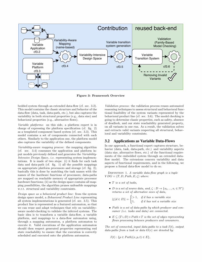
Figure 3: Framework Overview

bedded system through an extended data-flow (cf. sec. 3.2).This model contains the classic structure and behavior of thedata-flow (data, task, data-path, etc.), but also captures thevariability in both structural properties (e.g., data size) andbehavioral properties (e.g., alternative flows).

Variable platforms: on this side, a platform expert is incharge of expressing the platform specification (cf. fig. 2)as a templated component based system (cf. sec. 3.3). Thismodel contains a set of components connected with eachothers. Similarly to the application one, the platform modelalso captures the variability of the defined components.

Variability-aware mapping process: the mapping algorithm(cf. sec. 3.4) consumes the application and platform in-put models previously defined and generates the Variability-Intensive Design Space, i.e. representing system implemen-tations. It is made of two steps: (i) it finds for each taskdata and data-path (cf. fig. 1) all the possible mappingson appropriate platform processors and storage (cf. fig. 2);basically this is done by matching the task names with thenames of the hardware functions of processors; data-pathsare mapped on reachable memory of appropriate processorhardware functions; (ii) as the design space contains all map-ping possibilities, the algorithm prunes unfeasible mappingsw.r.t. structural and variability constraints.

Design space as a behavioral product line: from the systemdesign space model, a Behavioral Product Line representingall system implementations is generated (cf. sec. 3.5). Thisproduct line is represented as a featured automaton, so thatwe can reuse and adapt techniques that rely on variability-aware model-checking to validate the inferred systems. Thebasic idea is to transform a variable data-flow, a variableplatform, and mappings to a data-flow automaton using,through a mapping automaton, a platform automaton toexecute it. Valid executions of the application automatonshould then respect generated properties representing endstate reachability to ensure that the execution is correctlyscheduled and executed onto the platform automaton.

Validation process: the validation process reuses automatedreasoning techniques to assess structural and behavioral func-tional feasibility of the system variants represented by thebehavioral product line (cf. sec. 3.6). The model checking isgoing to determine classic properties, such as safety, absenceof deadlock, and our state reachability generated property,on all variants in one run. As a result, the validation solvesand extracts valid variants respecting all structural, behav-ioral and variability constraints.

3.2 Applications as Variable Data-FlowsIn our approach, a functional expert captures structure, be-havior (data, task, data-path, etc.) and variability aspects(data size, alternative flows, etc.) of the functional require-ments of the embedded system through an extended data-flow model. The extensions concern variability and dataaspects of functional requirements, and in the following, wepropose a formal data-flow model to do so.

Definition 1. A variable data-flow graph is a tupleV DG = (T,D, Path,E, ζ) where:

• T is a set of tasks,

• D is a set of source data, and, ζ : D → {s0, ..., si ∈ N∗}returns a set of alternative sizes of data,

|ζ(d ∈ D)| =

{> 1, if d has a variable size

1, if d has not a variable size

• Path is a set of data-paths by which producer and con-sumer (i.e. tasks and data) are connected.

• E ⊆ (T ∪D)×Path×T is the set of edges representingflows processing between producers and consumers.

The set of connected, input data-paths to a task I(t), outputdata-paths from a task or data O(v) are denoted by:

I(t) : {p ∈ Path|(x, p, t) ∈ E},

O(v ∈ T ∪D) : {p ∈ Path|(v, p, x) ∈ E}.

Similarly I(p), input tasks to a output data-paths, and O(p),output tasks from a input data-paths, are denoted by:

I(p) : {prod ∈ T ∪D|(prod, p, x) ∈ E},O(p) : {t ∈ T |(x, p, t) ∈ E}.

Then:

|I(p)|+ |O(p)| =

{> 2, if p has alternative flows

2, if p has not flow variability

A variable data-flow represents multiple data-flow variants.To implicitly represent all these variants in a single model,we follow the same approach as in variable workflows from[13], allowing data-paths to have multiple input and outputtasks connected.

A data-path can be connected to multiple alternative, inputtasks if |I(p)| > 1, and output tasks if |O(p)| > 1. But, If|I(p)| = 1 ∧ |O(p)| = 1, the data-path is connected to onlyone input and output task (i.e the data-path has no flowvariability).

As data can have alternative sizes, we introduce the functionζ which returns the set of alternative sizes S = ζ(d), eachdatum has at least one size and if |ζ(d)| > 1 the size of d isvariable.

If the data-flow has no flow variability, ∀p ∈ Path, |I(p)| +|O(p)| = 2, and no data variability, ∀d ∈ D, |ζ(d)| = 1, thedata-flow is not variable.

The functional specification of the running example V DGreis then represented as

(Tre = {a, b, c}, Dre = {d1, d2}, Pathre = {p1, p2, p3},

Ere = {(d1, p1, a), (a, p2, c), (d1, p1, b), (b, p2, c), (d2, p3, c)})

with,

ζ(d1) = 512, ζ(d2) = {512, 1024},

I(p1) = d1, I(p2) = {a, b}, I(p3) = d2,

O(p1) = {a, b}, O(p2) = c,O(p3) = c,

I(a) = I(b) = p1, I(c) = {p2, p3},

O(a) = O(b) = p2, O(c) = ∅, O(d1) = p1, O(d2) = p3.

3.3 Platforms as Variable Resource GraphsA variable platform specification is represented by a tem-plated component based system (multi-pass processors,streaming processor, read-only memory, read-write memory,write-only memory, first-in-first-out buffers etc) where plat-form can have optional resource components and variabilityconstraints on resources (dependency, incompatibility, etc.).To capture variability aspects of a platform specification, wepropose a formal architecture model defined as follows.

Definition 2. A variable resource graph is a tupleV RG = (Proc, S, Cs, ξ, θ, φrequires, φexcludes) where:

• Proc = (F,B,Cb ⊆ (F ×B)× (B × F )) is a processorcomposed of a set F of possible functions, B is a set of

processor internal first-in-first-out buffers and Cb theconnections between the different functions and buffersrepresenting the processor pipeline.

• S is a set of memory storage, and ξ : S → {c0, ..., ci ∈N∗} returns a set of alternative capacities of storages ∈ S,

|ξ(s)| =

{> 1, if s has a variable storage capacity

1, if s has not a variable storage capacity

• Cs ⊆ (S×Proc)∪ (Proc×S) is the set of connectionsbetween memory storage and processors,

• R ⊆ Proc ∪ S is the set of resource components (i.e.processors and memory storage),

• θ : R → B return true if a component (i.e. processoror memory storage) is optional,

• φrequires : R → R captures dependency between re-source components, similarly φexcludes : R → R cap-tures incompatibility.

The set of, input memories to a processor function I(f), out-put memories from a processor function O(f) are denoted by:

∃p = (F,B,Cb) ∈ Proc,I(f ∈ F ) : {m ∈ S ∪B|(m, p) ∈ Cs ∨ (m, f) ∈ Cb},O(f ∈ F ) : {m ∈ S ∪B|(p,m) ∈ Cs ∨ (f,m) ∈ Cb}.

As a variable platform represents multiple platform configu-rations, we also capture implicitly all these configurations byintroducing several functions, θ manages the optionality of aresource component. If θ(r) = ⊥ the resource is mandatory,otherwise the resource is optional, φrequires and φexcludesmanages constrained relations of dependency and incom-patibility between resource components. φrequires(r) = r0means that if r is implemented then r0 must be implementedtoo. r depends on r0. On the contrary φexcludes(r) = r0means that r and r0 cannot be implemented on the sameplatform variant. r and r0 are alternatives.

As memory storage can have alternative capacities, we in-troduce the function ξ which returns the set of alternativecapacities C = ξ(s), each memory storage has at least onesize and if |ξ(s)| > 1 the capacity of s is variable.

If the platform has no component variability ∀r ∈ R, θ(r) =⊥ and no variable memory storage, ∀s ∈ S, |ξ(s)| = 1, theplatform is not variable.

The platform specification of the running example V Gre isthen formalized as

(Procre = {DCU,GPU}, Sre = {RAM,ROM},

Csre = {(RAM,DCU), (ROM,DCU),(RAM,GPU), (ROM,GPU), (GPU,RAM)})

where,

DCU = (Fdcu = {adcu, cdcu}, Bdcu = r0dcu,Cbdcu = {(adcu, r0dcu), (r0dcu, cdcu)}),

GPU = (Fgpu = {agpu, bgpu}, Bgpu = r0gpu,Cbgpu{(agpu, r0gpu), (r0gpu, bgpu)}),

with,

ξ(ROM) = 4096, ξ(RAM) = {1024, 2048},

θ(GPU) = θ(RAM) = >, θ(DCU) = θ(ROM) = ⊥

φrequires(GPU) = RAM,φrequires(RAM) = ∅,

I(agpu) = {ROM,RAM}, O(agpu) = {r0gpu, RAM},

I(cdcu) = {r0dcu, ROM,RAM}, O(cdcu) = ∅.

3.4 Variability-Aware Mapping ProcessThe mapping algorithm takes as inputs the variable data-flow and configurable platform models in order to find allembedded system implementations. We propose a mappingmodel to not only capture all implementations of a singledata-flow into a single platform but to capture all data-flowvariants implementations onto all platform configurations.Our variability-aware mapping model can be seen as a prod-uct line of traditional mapping models.

Definition 3. A variability-aware data-flow-orientedmapping VM = (Tm,Dm,Em) where:

• Tm ⊆ T ×F is the set of possible mappings of tasks onprocessors ∀(t, f) ∈ Tm, t can be mapped on processorfunction f because f can implement t,

• Dm ⊆ D×S is the set of mappings of data on memorystorage,

• Em ⊆ E× (S∪B) is the set of data-paths mapping onmemory by which data are consumed/produced.

Definition 4. The Variability-Aware Mapping functionM = V DG× V RG→ VM sorts topologically the data-flowand finds appropriate mapping for each data, task and data-paths of the data-flow using resources of the resource graph.

Basically, each valid mapping should respect consistencyconstraints such as that(1) All tasks are mapped to, a least, one processor function:

∀t ∈ T,∃(t, f) ∈ Tm,(2) All data are mapped to, at least, one memory storage:

∀d ∈ D,∃(d, s) ∈ Dm,(3) All data-paths are mapped to, at least, one appropriatemapping. For data-path starting by an input datum, thestorage on which the datum is mapped has to be reachableby the processor function on which the task consuming thedatum is mapped.

∀e = (d ∈ D, p, t) ∈ E,∃(e, s ∈ S) ∈ Em,

∃(d, s) ∈ Dm,∃(t, f) ∈ Tm, s ∈ I(f),For data-path between tasks, the memory on which the out-put of the first task is mapped has to be reachable by theprocessor function on which the second task is mapped.

∀e = (t ∈ T, p, t′) ∈ E,∃(e,m) ∈ Em,

∃(t, f) ∈ Tm,∃(t′, f ′) ∈ Tm,m ∈ O(f) ∧m ∈ I(f ′)The mapping model of the running example VMre is thenformalized as

(Tmre = {(a, adcu), (a, agpu), (b, bgpu), (c, cdcu)},

Dmre = {(d1, RAM), (d1, ROM), (d2, RAM), (d2, ROM)},

Emre = {((d1, p1, a), RAM), ((d1, p1, a), ROM),((d1, p1, b), RAM), ((d1, p1, b), ROM),((a, p2, c), r0dcu), ((a, p2, c), RAM), ((b, p2, c), RAM),((d2, p3, c), RAM), ((d2, p3, c), ROM))})

Finally, The design space representing all system implemen-tations, called variability-intensive embedded system designspace is then composed of a data-flow, platform and map-ping:

V DS ⊆ (V DG× V RG× VM)

3.5 Design Space as a Behavioral Product LineAutomata and model-checking techniques have been widelyused to model and validate real-time and embedded systems[4, 5]. Interestingly, the basic approach used is to schedulean application automaton using a platform automaton [10].Unfortunately, these approaches are not design to manageany variability aspect of specifications.

Our framework relies on Featured-Transition-Systems (FTS)to represent and validate the design space. FTS has thestrength to model explicitly the variability points structural-ly, through a Feature Diagram [3] (FD), instead of modelingvariability points behaviorally, by optional transition withpossible constraints [24]. This eases the transformation tofeatured automaton and the removal of invalid implementa-tions from it. In our approach, we also use LTL propertyto ensure that all valid execution paths of all system imple-mentations reach the end state of all task of the data-flow.

Definition 5. A featured automaton is a tuple FA =(Loc, Loc0, I, Act ⊆ Aff∪φ∪Com, trans, χ, Ch, L,AP, d, λ)such that:

• Loc is a finite set of locations, Loc0 ∈ Loc, is a set ofinitial states and I ∈ Loc, is a set of final states,

• Ch is a finite set of communication channels,

• χ is a finite set of variables,

• Act is a set of, Aff which is a finite set of variable af-fectations, φ which is a finite set of guards in a booleanexpression form and Com, which is a set of communi-cations Com ⊆ {c!m, c?m, c!?m|c ∈ Ch,m ∈ χ}

• trans ⊆ Loc×Act× Loc are state transitions,

• d = (N ⊆ Nm ∪ Nopt ∪ Nxor, DE ⊆ N × N,Tcl) isa Feature Diagram (FD), N is the set of mandatory,optional and alternatives features, DE represents rela-tion between features, Tcl are constraints between fea-tures, JdKFD ⊆ P(N) is the set of valid product config-urations,

• λ : trans → B(N) is a total function that labels tran-sitions with feature expressions.

• AP is a set of atomic proposition and L : Loc → APlabels transitions with atomic propositions.

A transition sα−→ s′ is possible for the set of product config-

urations P ⊆ Jλ(sα−→ s′)K and if

∀g ∈ α ∩ φ, g is satisfied,∀(c?m) ∈ α ∩ Com, wait for data event c!m,∀(c!?m0) ∈ α∩Com, send data event c!m0 but wait for dataevent c!m1 with m0 = m1.

Definition 6. A Linear Temporal Logic property (LTL)is a temporal expression of atomic proposition that all possi-ble executions of system variants should satisfy as, JfaKFA |=ϕ whereϕ ::= a ∈ AP |ϕ ∧ ϕ| � ϕ . Symbol � means that the propertywill become true at some point in the future.

We now show how our design space is transformed to a FA.To simplify the transformation process, let us use the fol-lowing functions:

f : T ∪ Path ∪R→ N, fs : D ∪ S × N∗ → N,

fto : Path→ N, ffrom : Path→ N,

fto : Path× T → N, ffrom : T ∪D × Path→ N,

fm : T ∪Path→ N, ftm : T ×F → N, fpm : Path×S∪B →N , which transforms model elements to features.

For example, in our running example, the functions wouldbe:

f(a) = A, fs(d2, 1024) = D2Size1024

fto(p1) = p1 To, ffrom(pfrom) = p1 From,

fto(p1, a) = P1ToA, ffrom(a, p2) = P2FromA,

fm(a) = Am, fm(p1) = P1m,

ftm(a, adcu) = AOnAdcu, fpm(p1, ROM) = p1OnROM

f(RAM) = RAM, fs(RAM, 1024) = RAMSize1024, ...

Similarly,

c : T ∪D ∪ Path ∪ F ∪ S → Ch,

cm : T ∪ Path→ Ch

transforms model elements to communication channels tointeract with them at automaton level.

A first function GenFA : V DG → FA × LTL transforms avariable data-flow graph into a FA and generates the LTLproperty in the following way.

(1.1) it transforms each datum d with variable size into axor feature group (cf. fig.4(a)):

ζ(d) > 1 =⇒ ∀s ∈ ζ(d), ∃(f(d) ∈ Nxor, fs(d, s)) ∈DE

(1.2) it creates the automaton for each source datum d ∈ D(cf. fig.4(b)), after setting the datum size, calling themapping automaton (cf. fig. 6(a, b)) that will allocatethe datum on the memory.

∀s ∈ ζ(d), ∃{t0 = (s0size(in)=s−−−−−−−→ s1) , where,

|ζ(d)| > 1 =⇒ λ(t0) = fs(d, s),

s1∀p∈O(d),cm(p)!?in−−−−−−−−−−−−→ s2, s2

∀p∈O(d),c(p)!in−−−−−−−−−−→ s3} ∈ trans

(2.1) it transforms each variable data-path p in a xor featuregroup (cf. fig. 4(a)).

|O(p)| > 1 =⇒ ∀o ∈ O(p),∃(fto(p) ∈ Nxor, fto(p, o)) ∈ DE

|I(p)| > 1 =⇒ ∀i ∈ I(p),∃(ffrom(p) ∈ Nxor, ffrom(i, p)) ∈ DE

(3.1) it creates task/data-paths consistency constraints (cf.fig. 4(a)).

∀t ∈ T,∀p ∈ |I(t)|, |O(p)| > 1 =⇒∃(f(t) ⇐⇒ fto(p, t)) ∈ Tcl

∀t ∈ T,∀p ∈ |O(t)|, |I(p)| > 1,∃(f(t) ⇐⇒ ffrom(t, p)) ∈ Tcl

(3.2) it creates for each task t the automaton (cf. fig. 4(c))that will wait for data-paths allocation, then call themapping automaton (cf. fig. 6(c)) to execute the task.

∃{t0 = (s0∀p∈I(t),c(p)?in−−−−−−−−−−→ s1), where,

f(t) ∈ Nopt =⇒λ(t0) = f(t) ∧ λ((s0 −→ s4) ∈ trans) = ¬f(t),

s1∀p∈O(t),cm(p)!?out−−−−−−−−−−−−−→ s2 , s2

cm(t)!?in,out−−−−−−−−−→ s3,

s3∀p∈O(t),c(p)!out−−−−−−−−−−−→ s4 ∈ I,where, L(s4) = tend ∈ AP} ∈ trans

(3.3) it generates the LTL formula that checks that a validexecution must, at some point, satisfy atomic proposi-tion of all data-flow task terminal states.

ϕ = �(∧s∈I,L(s)6=∅L(s))

(a) Application FD

(b) Datum d1 FA

(c) Task A FA

Figure 4: Partial variable data-flow application FA

The second function GenFA : V RG → FA transforms avariable resource graph into a FA in the following way.

(1) it creates feature constraints on resource implementa-tion (cf. fig. 5(a)).

∀r ∈ R, θ(r) = > =⇒ ∃f(r) ∈ Nopt∀r ∈ R, ∀rreq ∈ φrequires(r), ∃(f(r) =⇒ f(rreq)) ∈Tcl

∀r ∈ R, ∀rexc ∈ φexcludes(r), ∃(f(r) =⇒ ¬f(rexc)) ∈Tcl

(2.1) it creates for each storage s features representing stor-age alternative sizes.

∀c ∈ ξ(s), ∃(f(s) ∈ Nxor, fs(s, c)) ∈ DE

(2.2) it creates for each storage s an automaton that rep-resents basic memory behavior (cf. fig. 5(b)), consand cap are respectively the consumed size and themaximal capacity of the storage. Through channels,one can allocate memory, and if there is not enoughmemory, an error is raised.

∀c ∈ ξ(s), ∃{t0 = (s0cons=0−−−−−→ s1), where,

f(s) ∈ Nopt =⇒λ(t0) = f(s) ∧ λ((s0 −→ s4) ∈ trans) = ¬f(s),

s1cap=c−−−−→ s2, where, λ(s1

cap=c−−−−→ s2) = f(s, c),

s2c(s)?in,cons+=size(in)−−−−−−−−−−−−−−−→ s3, s3

cons<size−−−−−−−→ s2,

s3cons≥size,error−−−−−−−−−−−→ s4} ∈ trans

(3) it creates for each processor p an automaton that mod-els basic graphic processor pipeline behavior (cf. fig.5(c)). When a processor function is executed, the in-put and output are checked to verify that the pipelineis not misused.

∀p = (F,B,Cb) ∈ Proc, ∀f ∈ F,∀(si, p) ∈ Cs, ∀(p, so) ∈ Ws, ∀(bi, f) ∈ Cb,∀(f, bo) ∈Cb,

∃{t0 = (s0c(f)?in,out−−−−−−−→ s1), where,

f(p) ∈ Nopt =⇒λ(t0) = f(p) ∧ λ((s0 −→ s4) ∈ trans) = ¬f(p),

s1loc(in)=si∧∀(bi,f)∈Rb,bi=free−−−−−−−−−−−−−−−−−−−−−→ s2,

s1loc(in)=bi∧bi=in−−−−−−−−−−−→ s2,

s2loc(out)=so∧∀(f,bo)∈Wb,bo=free−−−−−−−−−−−−−−−−−−−−−−→ s3,

s2loc(out)=bo∧bo=free−−−−−−−−−−−−−−→ s3, s3

c(f)!in,out−−−−−−−→ s0} ∈ trans

A third function GenFA : VM → FA transforms a variabi-lity-aware dataflow-oriented mapping into a FA as follows.

(1.1) it creates features representing all possible task map-pings on processor function (cf. fig. 6(a)).

∀(t, f) ∈ Tm,∃(fm(t) ∈ Nxor, ftm(t, f)) ∈ DE

(1.2) it creates for each task mapping the automaton thatexecutes the processor function according to the map-ping configuration (cf. fig. 6(c)).

∀t ∈ T,∀(t, f) ∈ Tm, ∃{t0 = (s0cm(t)?in,out−−−−−−−−→ s1),

where,fm(t) ∈ Nopt =⇒λ(t0) = fm(t) ∧ λ((s0 −→ s3) ∈ trans) = ¬fm(t)

t1 = (s1c(f)!?in,out−−−−−−−−→ s2), where, λ(t1) = ftm(t, f),

s2cm(t)!in,out−−−−−−−−→ s3},∈ trans

(2.1) Like 1.1, it creates features representing all possibledata-path mappings on memory.

∀((x, p, y), s) ∈ Em,∃(fm(p) ∈ Nxor, fpm(p, s)) ∈ DE

(2.2) Like 2.2, it creates for each data-path mapping theautomaton that allocates memory (cf. fig.6(b)).

∀p ∈ Path,∀((x, p, y), s) ∈ Em,

∃{s0cm(p)?out−−−−−−→ s1, t0 = (s1

c(s)!?out,loc(d)=s−−−−−−−−−−−→ s2)

where, λ(t0) = fpm(p, s), s2cm(p)!out−−−−−−→ s3} ∈ trans

Finally the function GenFA : V DS → FA, defined by:GenFA((vdg, vrg, vm)) :

GenFA(vdg)||GenFA(vrg)||GenFA(vm),

transforms our design space into a featured automaton.

(a) Platform FD

(b) RAM storage

(c) GPU processor

Figure 5: Partial variable platform FA

To preserve the consistency of the design space, variabilityconstraints are inferred such as:

(1.1) Task features with variable data-path features are notimplemented on all data-flow variants, then those fea-tures are made optional (cf. fig. 4(a)).

∀t ∈ T,∃pi ∈ I(t), |O(pi)| > 1 ∨ ∃po ∈ O(t), |I(po)| > 1

=⇒ f(t) ∈ Nopt

(1.2) Variable task features have their mapping variable too;if a task feature is implemented its mapping must beimplemented too, and vice-versa (cf. fig. 4(a) & 6(a)).

∀t ∈ T, f(t) ∈ Nopt =⇒fm(t) ∈ Nopt ∧ (f(t) ⇐⇒ fm(t)) ∈ Tcl

(2.1) If a task mapping feature is implemented on a proces-sor function, the implemented input and output pathmappings have to be reachable (cf. fig. 6(a)).

∀(t, f) ∈ Tm,∀pi ∈ I(t), ∀po ∈ O(t),

∃(ftm(t, f) ⇐⇒(

∨((x,pi,t),m∈I(f))∈Em

fpm(pi,m))∧

(∨

((t,po,x),m′∈O(f))∈Emfpm(po,m

′))) ∈ Tcl

(3.1) If a task mapping feature using an optional processoris implemented, the processor must be implementedtoo.

∀p = (F, x, y) ∈ Proc, f(p) ∈ Nopt, ∀(t, f ∈ F ) ∈ Tm=⇒ ∃(ftm(t, f) =⇒ f(p)) ∈ Tcl

Similarly, if a data-path mapping feature is implemented onfifo buffer of optional processor (3.2) or optional memorystorage (3.3), the resource have to be implemented.

(3.2) ∀pu = (F,B, x) ∈ Proc, ∀((y, p, z), b ∈ B) ∈ Em,f(pu) ∈ Nopt =⇒ ∃(fpm(p, b) =⇒ f(pu)) ∈ Tcl

(3.3) ∀((x, p, y), s ∈ S) ∈ Em, f(s) ∈ Nopt =⇒∃(fpm(p, s) =⇒ f(s)) ∈ Tcl

As an illustration, in our running example, the rules wouldbe:(1.2) A ⇐⇒ Am, B ⇐⇒ Bm(3.1) BOnBgpu =⇒ GPU , AOnAgpu =⇒ GPU(3.2) P2OnR0gpu =⇒ GPU(3.3) P1OnRAM =⇒ RAM , P2OnRAM =⇒ RAM

P3OnRam =⇒ RAM

3.6 Validation ProcessAs our form of behavioral product lines is based on FTS [8],model checking techniques can be directly reused. In ourimplementation (cf. next section), we reuse the ProVeLineschecker as a back-end for the validation process. The pro-cess consists in verifying all execution paths of all productsJfaKFA of the product line, in an efficient way by exploitingcommonalities between different products. Theoretically,the more the products share common behavior and the more

(a) Mapping FD

(b) data-path Mapping p1 FA

(c) Task Mapping A FA

Figure 6: Partial Variability-Aware Mapping FA

efficient should be the variability aware model checking incomparison of iterative model checking on individual sys-tems [7]. Instead of exploring all executions for each systemimplementation, the model-checker explores an execution πonce for all implementations P able to produce this specificexecution:

P = {p ∈ JdKFD|π ∈ Jfa|pKA}.

As mentioned in the previous section, some system config-urations may expose inconsistent behaviors (e.g., memoryallocation error, violation of graphical pipeline constraints).These behaviors will abort the execution and the basic prop-erties (e.g. safety, absence of deadlock, state reachability)will obviously not be satisfied. In our validation process, weare able to remove these configurations from the system byrelying again on the back-end model checker [7]. It com-putes the set of bad product configurations, which we removefrom the feature diagram of the product line by adding theappropriate cross-tree constraints.

4. VALIDATION

4.1 Implementation

4.1.1 OverviewThe framework depicted in Fig. 3 has been entirely im-plemented in Java. It consists of 3 main modules: i) meta-models of variable application and configurable platform (cf.Fig.7 and 8) ii) mapping meta-model Fig.9 and algorithm(cf. listing 3) iii) generators that transform the design space

composed by all system sub-domains (application, platform,mapping) (cf. listing 4) into formal models of behavioralproduct line (cf. listings 5 and 6) in order to remove invalidproducts (cf. listing 8) reusing automated formal reasoningtechniques (cf. listing 7).

The first module allows for specifying a variable data-floworiented application (cf. listing 1) and a configurable plat-form (cf. listing 2) via fluent APIs. As a result, the runningexample inputs are captured in less that 30 lines of code.The second module calls our mapping algorithm (cf. listing3) in order to infer, at the end, the resulting design space.The third and last module transforms the design space intoa Feature Model in TVL (cf. listing 5) and a Featured Au-tomaton in fPromela (cf. listing 6), capturing, respectivelythe structural variability and behavior of the design space.

We reuse the ProVeLines model-checker [9, 6], which con-sumes TVL and fPromela inputs to assess all system designs,in one run of variability-aware model checking. The result-ing outputs, printed as a set of invalid sub-products lines (c.flisting 7), are directly used to constraint the design space toonly obtain valid products (cf. listing 8).

4.1.2 Applications as Variable Data-FlowsListing 1 illustrates how we capture the functional require-ments (cf. fig. 1) of the embedded system through an ex-tended data-flow Java API. The data-flow meta-model (cf.Fig. 7) contains the classic structure and behavior of thedata-flow (data instanced at line 3,6, task at line 4,5,7, data-path at line 2), but also captures the variability in bothstructural properties (e.g., data size at line 6) and behavioralproperties (e.g., alternative flows by allowing data-paths tohave multiple input and output tasks connected at line 4,5).

Listing 1: Running Example Application

1 Application app = new Application("WarpWithWhat");2 Path p1 = app.addPath("P1"); Path p2 = ...; Path p3

= ...;3 DataSource d1 =

app.addDataSource("D1").addSize(512).connect("o",p1);

4 Task ta = app.addTask("ta", "A").connect(p1,"i").connect("o", p2);

5 Task tb = app.addTask("tb", "B").connect(p1,"i").connect("o", p2);

6 DataSource d2 =app.addDataSource("D2").addSizes(512,1024).connect("o", p3);

7 Task tc = app.addTask("tc", "C").connect(p2,"i0").connect(p3, "i1");

8 app.split(p1).to(ta).to(tb);9 app.join(p2).from(ta).from(tb);

4.1.3 Platforms as Variable Resource GraphsListing 2 illustrates how we express the platform specifica-tion (cf. fig. 2) of the embedded system through a resourcecomponent based Java API. The platform meta-model (cf.Fig. 8) contains templated resource components such asmulti-pass processors instanced at line 13 and streaming pro-cessor at line 6. Other elements in the template can be hard-ware functions instanced at line 7,10,14, read-only memoryat line 2, read-write RAM memory at line 3, first-in-first-

Figure 7: Application Metamodel

out buffers at line 8,14, relevant elements being connectedwith each others. In addition, a platform can have optionalresource components (line 4,13) and variability dependency(line 15) on resources.

Listing 2: Running Example Platform

1 Platform plt = new Platform("Kepler");2 Storage rom = plt.addStorage("ROM",

Type.READ_ONLY).addCapacity(4096);3 Storage ram = plt.addStorage("RAM",

Type.READ_AND_WRITE).addCapacities(1024, 2048);4 ram.setOptional();5

6 Component dcu = plt.addComponent("DCU");7 Processor a_dcu = dcu.addProcessor("a", "A");8 Memory r0_dcu = dcu.addFIFOBuffer("R0");9 a_dcu.connectToInputPort("i", ram,

rom).connectToOutputPort("o", r0_dcu);10 Processor c_dcu = dcu.addProcessor("c", "C");11 c_dcu.connectToInputPort("i0", ram, rom,

r0_dcu).connect("i1", ram, rom);12

13 Component gpu =plt.addComponent("GPU").setOptional();

14 Processor a_gpu = ...;Memory r0_gpu = ...;Processorb_gpu = ...;

15 gpu.requires(ram);

Figure 8: Platform Metamodel

4.1.4 Variability-Aware Mapping ProcessThe mapping algorithm (cf. listing 3) takes as inputs thevariable data-flow and configurable platform Java models,and generates the Variability-Aware Mapping Space(cf. Fig.9 for metamodel). It then represents all mapping of appli-cation elements onto platform resources

The process is composed of two steps : (i) it maps each datasource and output data path on storage memories (line 4-7) (ii) it maps each task on appropriate processor function(i.e., processor function can implement the task while datapath inputs can be mapped on reachable memory) and mapstask output on memory (line 8-11). Then, the algorithmprunes unfeasible mappings w.r.t. structural and variabil-ity constraints at line 12 (e.g., data-path mapping are notreachable by any task mapping or vice versa), finally addingappropriate constraints to ensure mapping space consistency(line 13).

Listing 3: Mapping Algorithm

1 Mapping mapping = new MappingAlgorithm().map(app,plt);

2 ...3 public Mapping map(Application app, Platform plt) {4 for(DataSource ds : app.getDataSources()) {5 addDataSourceMappings(ds, plt.getStorages())6 addDataPathMappings(ds);7 }8 for(Task t : app.getSortedTasks()) {9 addTaskMappings(t, getProcessors(plt, t));

10 addDataPathMappings(t);11 }12 do while(removeUselessMappingChoices());13 addMappingConstraints();14 return new Mapping(dms, tms, pms);15 }

Figure 9: Mapping Metamodel

4.1.5 Design Space as a Behavioral Product LineFrom the system design space model (cf.listing 4), whichis the consistent composition of our 3 system sub-domains(i.e., application, mapping, platform), a Behavioral ProductLine representing all system implementations is generatedinto a Feature Automaton (cf.listing 4). While the behaviorof the whole product line is encoded in fPromela (cf. listing6), a Feature Model in TVL encodes its structural variability(cf.listing 5).

Our framework relies on Featured-Transition-Systems (FTS)to formally reason on the structure and behavior of thedesign space. FTS has the strength to model explicitlythe variability points structurally, through a Feature Dia-gram [3] (FD) in TVL(cf.listing 5).

Thus, a single variability model is able to capture data sizeat line 9-12, memory capacity at line 19-22, data mapping28-31, task mapping 32-35, alternative flow 9-12,13,14 vari-

abilities, resource optionality 18,24, resource dependency 45,mapping 41 and design space consistency constraints 39,43. On the other hand, the behavior of the design space iscaptured by an executable network of featured automata infPromela where state transitions are guarded by constraintson feature values.

To execute the variable application over the configurableplatform, featured automata that capture behavior of data-flow processes, such as data node (lines 18-34) and task node(lines 36-52), call functions over platform resource featuredautomata, such as memory storage (line 2-16) and processor.

Each featured automaton may have variable properties suchas capacity for memory storage process (lines 8-11), data size(lines 21-24) and data deployment location (lines 25-30) fordata node process, or task deployment (line 42-47) for taskprocess. In addition to properties, a featured automatonmay be optional (i.e., behavior is executed if the element ispresent in the system design cf. lines 39-50).

According to the subset of design decisions to explore, vari-able properties are incrementally fixed. For example, forsystem designs where D2 with a size of 1024 is deployed onRAM with a capacity of 1024, we observe that after allo-cating D2 on RAM (line 26,6), RAM is full, and any otherdata allocation on RAM (e.g., D1 or data of P2) would leadto a memory violation (cf. listing 7 line 4).

Listing 4: Generate Running Example FormalModels from Design Space

1 DesignSpace ds = new DesignSpace(app, mapping, plt);2 ToTVL toTVL = new ToTVL().generate(ds);3 ToPML tofPML = new TofPML().generate(ds);

Listing 5: Part of Running Example Design Spacevariability in TVL

1 root DesignSpaceVariability{2 group allOf{3 ApplicationVariability group allOf{4 ...5 P1_to group oneOf{6 P1_to_TA,7 P1_to_TB8 },9 D2_size group oneOf{

10 D2_size_512,11 D2_size_102412 },13 opt TA,14 opt TB15 }16 group PlatformVariability{17 ...18 opt RAM group allOf{19 RAM_size group allOf{20 RAM_size_1024,21 RAM_size_204822 }23 },24 opt GPU25 }26 group MappingVariability{27 ...28 D2_On group oneOf{

29 D2_On_RAM,30 D2_On_ROM31 }32 opt TA_On group oneOf{33 TA_On_DCU_a,34 TA_ON_GPU_a35 },36 }37 }38 ...39 TA <=> TA_On;40 ...41 D2_On_RAM => P3_On_RAM42 ...43 D2_On_RAM => RAM;44 ...45 GPU => RAM;46 ...47 }

Listing 6: Part of Running Example Design Spacebehavior in fPromela

1 ...2 active proctype Storage_RAM(){ atomic{3 Data in;4 ...5 do6 :: RAMalloc?in ->7 cons = cons + in.size;8 if9 :: RAM_capacity_1024 -> size = 1024;

10 :: RAM_capacity_2048 -> size = 2048;11 fi;12 assert(cons <= size);13 RAMalloc!in;14 od;15 ...16 };}17 ...18 active proctype Data_D2(){ atomic{19 Data out;20 ...21 if22 :: D2_size_512 -> out.size = 512;23 :: D2_size_1024 -> out.size = 1024;24 fi;25 if26 :: D2_On_RAM -> RAMalloc!out;27 RAMalloc?eval(out);28 :: D2_On_ROM -> ROMalloc!out;29 ROMalloc?eval(out);30 fi;31 ...32 P3!out;33 ...34 };}35 ...36 active proctype Task_TA(){ atomic{37 Data in, out;38 ...39 if40 :: TA -> P1?in41 ...42 if43 :: TA_On_GPU_a -> GPU_a!in, out;44 ...45 :: TA_On_DCU_a -> DCU_a!in, out;46 ...47 fi;

48 ...49 :: else -> skip;50 fi;51 ...52 };}53 ...

4.1.6 Validation ProcessThe generated formal models (fPromela and TVL) are check-ed through ProVeLines with specific command lines (cf.list-ing 7 line 1). It returns output containing non feasible sub-sets of products (line 4) that are used to invalid variants byconstraining the design space variability space (cf. listing 8line 7). More precisely, the model checking is going to verifyproducts against inconsistent behaviors (e.g., memory allo-cation error, violation of graphical pipeline constraints) andmore classic properties, such as safety, absence of deadlockand state reachability on all variants in one run. This sin-gle execution [7] makes also possible to remove all products(cf.listing 7 at line 4) leading to an invalid execution , soto improve and speed-up the verification process (see nextSection).

Listing 7: Part of Running Exemple ProVeLinesoutput

1 .\provelines -check -exhaustive -ntrunning_example.pml

2 ...3 assertion failled : (assert(cons <= size);) at

line... for products:4 D2_size_1024 && D2_On_RAM && RAM_capacity_1024

&& D1_On_RAM && P1_On_RAM5 ...

Listing 8: Part of Valid DesignSpace Variability inTVL

1 root DesignSpaceVariability{2 group allOf{3 ...4 }5 ...6 //invalid products constraints7 !(D2_size_1024 && D2_On_RAM && RAM_capacity_1024

&& D1_On_RAM && P1_On_RAM);8 ...9 }

4.2 Evaluation

4.2.1 Industrial Use CaseIn order to validate our tooled approach on an industrialscale, we applied it to a real low-end market instrument clus-ter provided by Visteon, the automotive systems companywe collaborate with.

The functional requirements of the cluster represents a vari-able data-flow with 3 source images processed by 8 tasksconnected by 9 data-paths. Each source image has two dif-ferent resolutions (i.e HD and LD) and two tasks sub flowsequences are alternative through a xor join/split data-path,

Table 1: Industrial use case results

Variability Implementation Platform data-flow States explored Time ms / states /variants variants variants (re-explored) (ms) variants variants

NONE 78 0 0 2453 (331) 27 0.346 31.448Data size 624 0 8 15254 (2406) 201 0.322 35.976Platform 424 24 0 5673 (546) 65 0.153 13.379

Platform and data size 3392 24 8 37435 (4856) 602 0.177 11.036data-path 150 0 2 4727 (981) 74 0.493 31.513

data-path and data size 1200 0 16 29066 (6994) 587 0,489 24,222ALL >4800 24 16 72704 (14652) 2361 - -

Platform mult. mem 16408 40 0 134941 (4534) 4010 0.244 8.224Platform mult. proc 2848 80 0 19625 (3224) 337 0.118 6.890

Pltf. mult. proc & mem 516608 160 0 1341999 (175304) 289721 0.560 2.597

resulting in 16 data-flow variants. The platform specifica-tion of the cluster is then represented by a variable hardwarecomponent system with 2 memories (a Video RAM and aROM Flash) and 3 processors (two multi-pass GPU bitblit-ter and one streaming- based DCU). Each processor has apipeline processing of 4 stages and 3 fifo buffers. In termsof platform variability, the 2 bitblitters and the VRAM areoptional. Each memory has 2 different configurable sizes atmanufacturing time. The number of platform configurationsin the use case is then 24.

If each data-flow variant had one possible implementation oneach platform configuration, the number of different clustersystem implementations would be 384. In reality, some plat-form configurations do not provide the graphical functional-ities required by some data-flow variants. Furthermore, dueto multiple task implementation choices, data-flow variantshave several thousand possible implementation alternativesonto a platform configuration. Setting the platform con-figuration to the higher end (i.e. selecting VRAM and allprocessors), one can find 72 and 78 possible implementationsfor two data-flow variants that take different xor data-pathdecisions. This is due to more pipelining opportunities inthe second data-flow variant, even if there is more data-pathmapping possibilities in the first one.

Table 1 shows time measurements of the complete toolchainwhile varying the different variability dimensions over theuse case. In the first seven rows, we observe that the wholeprocess is performing well with small to medium scale ofvariabilities. Data and memory size variability verificationsare faster and require more state exploration than plat-form component and data-path variabilities. Componentand data-path variabilities are also slower to check than dataand memory size variabilities. It is likely to be due to thefact that contrary to size variability, hardware componentand data-path variability are strongly impacting the imple-mentation variability, and consequently the state space ofthe model checker.

We have also complemented this experimentation by tak-ing a single structural data-flow from the industrial use casewith a simulated larger platform, itself with multiple mem-ories and processors. Results in the last three rows of Table1 show that solving can scale to a large number of imple-mentation variants. Even if the solving time is significant,

we observe that the number of states explored to assess allthe implementation variants is significantly low. This showsthat behavioral commonalities between system variants areused to speed-up the verification process.

4.2.2 Scalability of System VariabilitiesWe now analyze the scalability of our solution against sys-tem variability by increasing the application, platform andmapping variability on simulated data. Fig. 10.a showsmeasurements of our toolchain for data size and memorycapacities variability dimensions (called element variability)while Fig. 10.b is about mapping dimensions. Each variablesystem denotes his variability dimensions in the followingformat :

flow; size; resource; capacity;mapping

Where flow represents the sum of flow variants of variabledata-paths, size the sum of alternatives data sizes, resourcethe number of optional resources, capacity the sum of alter-natives memory capacities and mapping the sum of alter-natives mapping of application element onto platform re-sources.

Fig. 10.a shows a system where data size and memory capac-ities variability dimensions have been progressively increasedso that the first and last system counts, respectively, 384and 6912 variants. We show relative time and (automaton)states metrics – in total and per variants – compared to thenormalized system presenting the lowest variability. Thus,for element variability dimensions (data size and memorycapacity), even if, obviously, the time and states numberneeded to verify the system increase according to variabilitydimensions, the verification time and states number neededby variant decrease.

For the scalability of the mapping variability dimension, wemainly increase progressively the mapping dimension over5 systems, the lowest system containing 64 variants whilethe highest has 23328. We observe that the needed timeand explored states number grow quickly. We think thisis due to the intrinsic high complexity of both binding andscheduling [22], which leads to configuration space and statespace explosion during checking. However, the verificationspeed-up by variant is still interesting for high variabilitysystem.

(a) Element Variability (b) Mapping Variability

Figure 10: Variability Analysis

(a) Mapping Complexity (b) Flow Complexity

Figure 11: Complexity Analysis

4.2.3 Scalability of System ComplexitiesWe analyze here the scalability of our solution against sys-tem complexity by growing the application and platformsize. Fig. 11.a shows an example where we increased pro-gressively the size and complexity of both application andplatform sides while keeping the mapping variability at acommon factor (i.e., %40).

The normalized system presenting the lowest complexityand variability. It contains 14 application nodes and pathsmapped on a 10 resources platform with 48 variants, whilethe most complex system has 22 nodes, 13 resources, and2880 variants. A global system complexity metric, takinginto account the system size and it’s number of variants,has been discussed with our industrial partner.

We observe that the verification time and states needed in-crease quickly according to the system complexity (applica-tion and platform sizes). Interestingly, as the needed statesand time to explore per variant in more complex while thesystem is growing, the verification time per variant is stilllower. This observation can also be made on Fig. 11.b,where we progressively increase the complexity of a systemwith flow variability.

4.3 Threats to ValidityThe validation on a single case study can be considered asthe major internal threat to validity. Nonetheless it wasincrementally built by numerous meetings with different do-main experts of the automotive systems company. We gath-ered specification and feedback from several applications andplatforms case studies, and we finally chose the presentedone as the most representative among them.

As for external threats, we identified the data sets as themain issue. While the data sets are large, they are stillsimulated. Our creation procedure has been built to mimicthe structure and behavior of both the platforms and theapplications, taking the real case studies as a basis to beexpanded by generators. Still we do not have empirical evi-dence of their correspondence.

5. CONCLUSION AND FUTURE WORKSA tremendous amount of variability can be observed in em-bedded systems, and especially in data-flow oriented ones,which are now systematically built from highly variable spec-ifications and target diverse hardware platforms configurableat a very high level of detail. To handle the early functionalassessment of all these possible configurations, we proposedin this paper a tooled approach that takes variable data-flow specifications and variable hardware platform modelsto map them together and transform them into a behavioralproduct line representing the potential design space. Thesemodels and toolchain allow to use automated reasoning tech-niques to explore and assess the functional feasibility of allrepresented variants in a single run, and invalid productscan be removed by adding constraints to the product line.

We reported on the application of the proposed approachto a real-world industrial use case of automotive instrumentcluster, giving hints on a potential good applicability. Ourexperimental validation with large simulated datasets also

shows a good scalability of the prototype implementationfor industrial-scale applications and platforms.

As future work, we first plan to facilitate the usage of theframework with domain specific languages for input models(specification and platform), and to conduct larger experi-ments with them on different and new case studies from ourindustrial partner. Interestingly, we think that some prod-uct lines optimization techniques [11, 23] could be appliedto assess more variable and complex embedded systems.

We will also extend our variability-focused framework bytaking into account quality attributes (e.g. cost, run-timeetc.). The extension would then provide optimized productselection as a complement to the functional validation pre-sented in this paper. We expect this more complete frame-work to be applicable in different contexts, being similarin the separation of application models being mapped ontocomponent-based platforms.

6. ACKNOWLEDGMENTSWe thank Visteon Electronics and the Association Nationalede la Recherche et de la Technologie for continuously sup-porting this research. We thank also Emmanuel Roncoroniand Olivier Bantiche who brought industrial expertise ininstrument cluster engineering and Maxime Cordy for hisvaluable support on the ProVeLines model-checker.

7. REFERENCES[1] P. Asirelli, M. H. ter Beek, S. Gnesi, and A. Fantechi.

Formal description of variability in product families.In Software Product Line Conference (SPLC), 201115th International, pages 130–139. IEEE, 2011.

[2] F. Balarin. Hardware-software co-design of embeddedsystems: the POLIS approach. Springer Science &Business Media, 1997.

[3] D. Batory. Feature models, grammars, andpropositional formulas. In SPLC, volume 3714, pages7–20. Springer, 2005.

[4] J. Bengtsson, K. Larsen, F. Larsson, P. Pettersson,and W. Yi. Uppaal-a tool suite for automaticverification of real-time systems. Hybrid Systems III,pages 232–243, 1996.

[5] E. M. Clarke, O. Grumberg, and D. Peled. Modelchecking. MIT press, 1999.

[6] A. Classen, M. Cordy, P. Heymans, A. Legay, andP.-Y. Schobbens. Model checking software productlines with snip. Int. Journal on Software Tools forTechnology Transfer (STTT), pages 1–24, 2012.

[7] A. Classen, P. Heymans, P.-Y. Schobbens, andA. Legay. Symbolic model checking of softwareproduct lines. In Proceedings of the 33rd InternationalConference on Software Engineering, pages 321–330.ACM, 2011.

[8] A. Classen, P. Heymans, P.-Y. Schobbens, A. Legay,and J.-F. Raskin. Model checking lots of systems:efficient verification of temporal properties in softwareproduct lines. In Proceedings of the 32nd ACM/IEEEInternational Conference on SoftwareEngineering-Volume 1, pages 335–344. ACM, 2010.

[9] M. Cordy, A. Classen, P. Heymans, P.-Y. Schobbens,and A. Legay. Provelines: a product line of verifiersfor software product lines. In Proceedings of the 17thInternational Software Product Line Conferenceco-located workshops, pages 141–146. ACM, 2013.

[10] A. E. Dalsgaard, M. C. Olesen, M. Toft, R. R. Hansen,and K. G. Larsen. Metamoc: Modular execution timeanalysis using model checking. In OASIcs-OpenAccessSeries in Informatics, volume 15. SchlossDagstuhl-Leibniz-Zentrum fuer Informatik, 2010.

[11] A. S. Dimovski, A. S. Al-Sibahi, C. Brabrand, andA. W ↪asowski. Efficient family-based model checkingvia variability abstractions. International Journal onSoftware Tools for Technology Transfer,19(5):585–603, 2017.

[12] S. Graf, M. Glaß, J. Teich, and C. Lauer.Multi-variant-based design space exploration forautomotive embedded systems. In Design, Automationand Test in Europe Conference and Exhibition(DATE), 2014, pages 1–6. IEEE, 2014.

[13] S. Graf, M. Glaß, D. Wintermann, J. Teich, andC. Lauer. Ivam: Implicit variant modeling andmanagement for automotive embedded systems. InHardware/Software Codesign and System Synthesis(CODES+ ISSS), 2013 International Conference on,pages 1–10. IEEE, 2013.

[14] S. Graf, S. Reinhart, M. Glaß, J. Teich, and D. Platte.Robust design of e/e architecture componentplatforms. In 52nd Design Automation Conference(DAC), pages 1–6. IEEE, 2015.

[15] M. Gries. Methods for evaluating and covering thedesign space during early design development.Integration, the VLSI journal, 38(2):131–183, 2004.

[16] B. Kienhuis, E. Deprettere, K. Vissers, and P. VanDer Wolf. An approach for quantitative analysis ofapplication-specific dataflow architectures. InApplication-Specific Systems, Architectures andProcessors, 1997. Proceedings., IEEE InternationalConference on, pages 338–349. IEEE, 1997.

[17] G. Palermo, C. Silvano, and V. Zaccaria. Robustoptimization of soc architectures: A multi-scenarioapproach. In Embedded Systems for Real-TimeMultimedia, 2008. ESTImedia 2008. IEEE/ACM/IFIPWorkshop on, pages 7–12. IEEE, 2008.

[18] G. Palermo, C. Silvano, and V. Zaccaria.

Variability-aware robust design space exploration ofchip multiprocessor architectures. In DesignAutomation Conference, ASP-DAC. Asia and SouthPacific, pages 323–328. IEEE, 2009.

[19] L. Schor, I. Bacivarov, D. Rai, H. Yang, S.-H. Kang,and L. Thiele. Scenario-based design flow for mappingstreaming applications onto on-chip many-coresystems. In Proceedings of the 2012 internationalconference on Compilers, architectures and synthesisfor embedded systems, pages 71–80. ACM, 2012.

[20] K. Sigdel, M. Thompson, A. D. Pimentel, C. Galuzzi,and K. Bertels. System-level runtime mappingexploration of reconfigurable architectures. In Parallel& Distributed Processing, 2009. IPDPS 2009. IEEEInternational Symposium on, pages 1–8. IEEE, 2009.

[21] V.-M. Sima and K. Bertels. Runtime decision ofhardware or software execution on a heterogeneousreconfigurable platform. In Parallel & DistributedProcessing, 2009. IPDPS 2009. IEEE InternationalSymposium on, pages 1–6. IEEE, 2009.

[22] A. K. Singh, M. Shafique, A. Kumar, and J. Henkel.Mapping on multi/many-core systems: survey ofcurrent and emerging trends. In Proceedings of the50th Annual Design Automation Conference, page 1.ACM, 2013.

[23] P. Temple, J. A. Galindo, M. Acher, and J.-M.Jezequel. Using machine learning to infer constraintsfor product lines. In Proceedings of the 20thInternational Systems and Software Product LineConference, pages 209–218. ACM, 2016.

[24] M. H. ter Beek, A. Fantechi, S. Gnesi, andF. Mazzanti. Modelling and analysing variability inproduct families: model checking of modal transitionsystems with variability constraints. Journal of Logicaland Algebraic Methods in Programming,85(2):287–315, 2016.

[25] P. Van Stralen and A. Pimentel. Scenario-based designspace exploration of mpsocs. In Computer Design(ICCD), 2010 IEEE International Conference on,pages 305–312. IEEE, 2010.

[26] S. Wildermann, F. Reimann, J. Teich, and Z. Salcic.Operational mode exploration for reconfigurablesystems with multiple applications. InField-Programmable Technology (FPT), 2011International Conference on, pages 1–8. IEEE, 2011.