Functional data analysis in shape analysis

Functional Data Analysis in Shape Analysis

Irene Epifanioa,∗, Noelia Ventura-Camposb

aDept. Matematiques, Universitat Jaume I, Campus del Riu Sec, 12071 Castello, SpainbDept. Psicologia Basica, Clınica i Psicobiologia, Universitat Jaume I, Spain

Abstract

Mid-level processes on images often return outputs in functional form. Inthis context the use of functional data analysis (FDA) in image analysis isconsidered. In particular, attention is focussed on shape analysis, where theuse of FDA in the functional approach (contour functions) shows its supe-riority over other approaches, such as the landmark based approach or theset theory approach, on two different problems (principal component anal-ysis and discriminant analysis) in a well-known database of bone outlines.Furthermore, a problem that has hardly ever been considered in the liter-ature is dealt with: multivariate functional discrimination. A discriminantfunction based on independent component analysis for indicating where thedifferences between groups are and what their level of discrimination is, isproposed. The classification results obtained with the methodology are verypromising. Finally, an analysis of hippocampal differences in Alzheimer’sdisease is carried out.

Keywords: Form analysis, Multivariate funcional data analysis, Curveclassification, Shape discrimination, Principal component analysis, outlines

1. Introduction

Functional data analysis (FDA) provides statistical procedures for func-tional observations (a whole function is a datum). The goals of functionaldata analysis are basically the same as those of any other branch of statistics.Ramsay and Silverman (2005) give an excellent overview. Ferraty and Vieu(2006) provide a complementary and very interesting view on nonparametric

∗Tel.: +34-964728390, fax: +34-964728429Email address: [email protected] (Irene Epifanio)

Preprint submitted to Computational Statistics & Data Analysis March 31, 2011

*ManuscriptClick here to view linked References

methods for functional data. The field of FDA is quite new and there is still alot of work to be done, but in recent years several applications have been de-veloped in different fields (Ramsay and Silverman, 2002). Furthermore, thesoftware that the authors used is available on the website for those books.The wide variety of disciplines where FDA is applied is also shown throughthe Special Issue on Statistics for Functional Data (Gonzalez-Manteiga andVieu, 2007) published in this journal in 2007. Some examples of these fieldsof application are: climatology, chemicals, geophysics and oceanology, eco-nomics, remote sensing, demographics (Delicado, 2011), materials science(Berrendero et al., 2011), biostatistics or genetics (Lopez-Pintado and Romo,2011; Li and Chiou, 2011). A mixture of practical and theoretical aspects isfound in Ferraty and Romain (2011).

Many mid-level processes on images return outputs in functional form,such as granulometries and other morphological curves (Soille, 2003), orspectral-energy descriptors (Gonzalez et al., 2004, pp. 468). Although FDAtechniques are specifically designed to deal with functions and are naturaltools for their analysis, FDA has hardly been used in image analysis (to thebest of our knowledge, the only article that uses FDA for analyzing 2 dimen-sional profiles is Nettel-Aguirre (2008)). The reason for this could be becauseFDA is quite new (the first book on FDA was published in 1997 (Ramsayand Silverman, 2005)), and it is not very well known in the image processingcommunity.

Shape analysis is a field where functions are frequently used to representshape (Kindratenko, 2003). According to Stoyan and Stoyan (1994), shapescan be described by three kinds of tools: firstly, set descriptors and math-ematical morphology tools; secondly, using landmarks (point description);and thirdly, employing a function describing the contours (see Kindratenko(2003) for a review of various contour functions and methods for their anal-ysis).

One of the objectives of this study is to highlight the advantages of theuse of FDA in image analysis, and particularly in shape analysis. In Section 2we analyze a well-known database of bones with these three approaches (theset theory approach, the landmark based approach and the functional ap-proach) and compare their results in two of the main problems in form statis-tics (Stoyan and Stoyan, 1994): the study of the main sources of variationamong the shapes (principal component analysis), and classification amongdifferent classes (discriminant analysis). The analysis of contour functions byFDA gives more meaningful results. The contour functions used in Section 2

2

are multivariate (two functions define the contours). Recently, independentcomponent analysis (ICA) has been successfully used for the classificationof univariate curves (Epifanio, 2008). This methodology is extended to themultivariate case in Section 3.2, where a discriminant function based on ICAis also introduced. Discriminant results obtained with this methodology arevery promising (in Section 3.2 a small comparative review is also given). Sec-tion 4 shows a FDA application in the analysis of magnetic resonance (MR)scans in order to study the hippocampal differences among the subjects ofthree groups: controls, patients with mild cognitive impairment (MCI), andpatients with early AD (Alzheimer’s disease). Finally, conclusions and someopen problems are discussed in Section 5.

2. Shapes through three approaches

In order to compare the three perspectives, we decide to use a well-knownand extensively studied database, which is publicly available: the bone shapesfrom a paleopathology study analyzed in Ramsay and Silverman (2002, Ch.4). Furthermore, this database has been analyzed previously in the literatureusing both landmarks and images, so it is perfect for our purposes. A totalof 68 outlines were studied, which correspond to 52 non-eburnated and 16eburnated femora. They considered 12 landmarks (see Shepstone et al. (1999)for details about data and identification and construction of these landmarks)1.

Apart from the landmarks, the images from which they were extractedare also available 2 (see Shepstone et al. (2000) for details about the data).As explained in the file, these images are not binary, but they can be eas-ily binarized because the background (zone without bone) is coded as zero.Although there are 121 images in that file, we only consider the images corre-sponding to the 68 cases available for the landmarks. Each image is rotatedso that the ’bottom’ of the condyles sits on the bottom of the image (as ex-plained in Shepstone et al. (2000), each femur was rotated in the horizontalplane until the articular surface was parallel with the plane of the cameralens). Furthermore, all left femora were reflected to produce ’right’ images

1available together with the code on website: http://www.stats.ox.ac.uk/∼silverma/fdacasebook/boneshapechap.html

2available on website: http://www.stats.ox.ac.uk/∼silverma/data/bones.tar.gz

3

so that the left side of any image indicates the lateral side and the right sidethe medial.

2.1. Landmark description

Each individual outline yields a vector of 24 coordinates (12 landmarksin 2 dimensions). In order to analyze the sample of 68 outlines, we follow theapproach explained in Dryden and Mardia (1998, Chapter 5). The libraryshapes (Dryden, 2007) of free software R (R Development Core Team, 2010)provides the routines for this analysis.

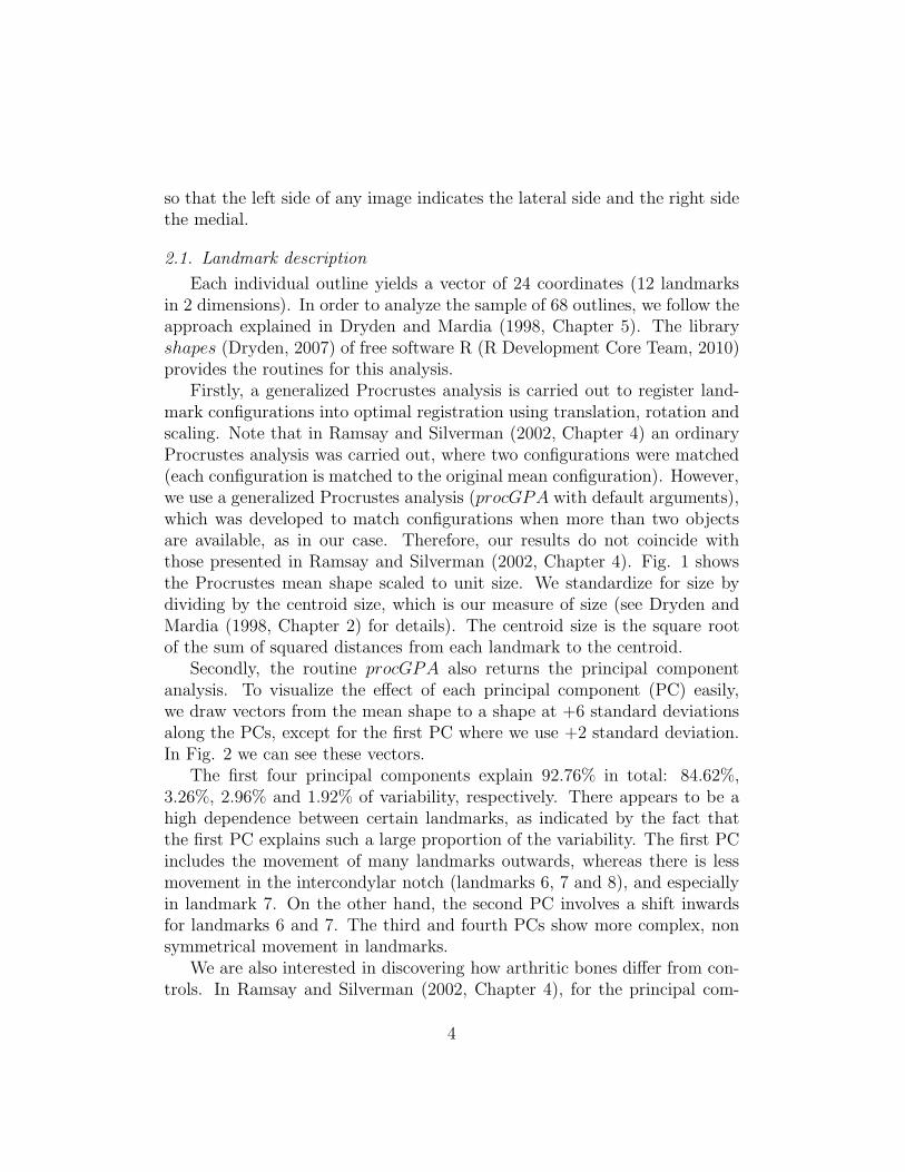
Firstly, a generalized Procrustes analysis is carried out to register land-mark configurations into optimal registration using translation, rotation andscaling. Note that in Ramsay and Silverman (2002, Chapter 4) an ordinaryProcrustes analysis was carried out, where two configurations were matched(each configuration is matched to the original mean configuration). However,we use a generalized Procrustes analysis (procGPA with default arguments),which was developed to match configurations when more than two objectsare available, as in our case. Therefore, our results do not coincide withthose presented in Ramsay and Silverman (2002, Chapter 4). Fig. 1 showsthe Procrustes mean shape scaled to unit size. We standardize for size bydividing by the centroid size, which is our measure of size (see Dryden andMardia (1998, Chapter 2) for details). The centroid size is the square rootof the sum of squared distances from each landmark to the centroid.

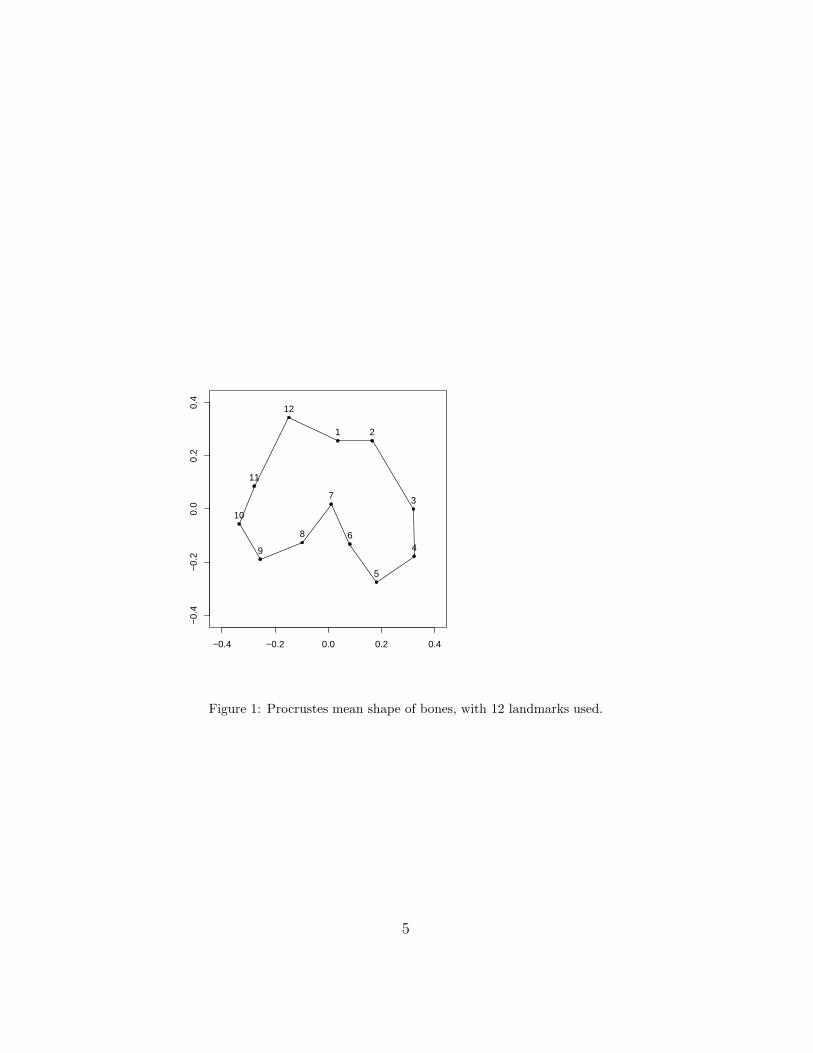
Secondly, the routine procGPA also returns the principal componentanalysis. To visualize the effect of each principal component (PC) easily,we draw vectors from the mean shape to a shape at +6 standard deviationsalong the PCs, except for the first PC where we use +2 standard deviation.In Fig. 2 we can see these vectors.

The first four principal components explain 92.76% in total: 84.62%,3.26%, 2.96% and 1.92% of variability, respectively. There appears to be ahigh dependence between certain landmarks, as indicated by the fact thatthe first PC explains such a large proportion of the variability. The first PCincludes the movement of many landmarks outwards, whereas there is lessmovement in the intercondylar notch (landmarks 6, 7 and 8), and especiallyin landmark 7. On the other hand, the second PC involves a shift inwardsfor landmarks 6 and 7. The third and fourth PCs show more complex, nonsymmetrical movement in landmarks.

We are also interested in discovering how arthritic bones differ from con-trols. In Ramsay and Silverman (2002, Chapter 4), for the principal com-

4

−0.4 −0.2 0.0 0.2 0.4

−0.

4−

0.2

0.0

0.2

0.4

1 2

3

4

5

6

7

8

9

10

11

12

Figure 1: Procrustes mean shape of bones, with 12 landmarks used.

5

−0.4 −0.2 0.0 0.2 0.4

−0.

4−

0.2

0.0

0.2

0.4

−0.4 −0.2 0.0 0.2 0.4

−0.

4−

0.2

0.0

0.2

0.4

(a) (b)

−0.4 −0.2 0.0 0.2 0.4

−0.

4−

0.2

0.0

0.2

0.4

−0.4 −0.2 0.0 0.2 0.4

−0.

4−

0.2

0.0

0.2

0.4

(c) (d)

Figure 2: The mean shape with vectors (see text for details) along the first PC (a), thesecond PC (b), the third PC (c) and the fourth PC (d).

6

ponent scores, a t-test was carried out to compare the eburnated and non-eburnated bones. As explained in Jolliffe (2002, Chapter 9), PCA can beused in discriminant analysis in order to reduce the dimensionality of theanalysis, assuming the covariance matrix is the same for all groups. How-ever, we have to be aware that there is no guarantee that the separationbetween groups will be in the direction of the high-variance PCs, the sep-aration between groups may be in the directions of the last few PCs. Onthe other hand, each PCs contribution in linear discriminant analysis canbe assessed independently thanks to their uncorrelatedness. We compute allPCs, and we consider only those for which the difference (between eburnatedand non-eburnated bones) is significant with α = 0.05, that is to say, whenthe p-value of the t-test is less than 0.05.

The difference is only significant on component 3 of 24 (p-value = 0.002).Using leave-one-out cross validation with linear discriminant analysis (ldafunction from library MASS (Venables and Ripley, 2002)) for the scores ofthis component, 16 errors are obtained: 2 false positives (non-eburnatedbones that are classified as eburnated) and 14 false negatives (eburnatedbones that fail to be so classified). If we use component 3 together withcomponent 7, which is the following component with the smallest p-value(0.052), the number of errors is the same (16 errors), with 4 false positiveand 12 false negative. Note that this is an underestimation of the true errorrate, since we are computing PCA and choosing the components with allsamples; even so, this error rate will be worse than those that we will obtainwith the other perspectives. This was predictable because more information(not just 12 points) about the shapes will be used in other perspectives.

2.2. Set description

Before the analysis of the images, position and size information will befiltered out. Remember that ’left’ images have already been reflected, andall them have already been rotated (see Shepstone et al. (2000)). We re-move location by translating each image to the origin in such a way that itscentroid coincides with the origin. Images are also standardized for size, inthe same way as we did with the landmark approach. Scale is removed bydividing through the centroid size. If Xj (j = 1, ..., k) is the set of all thepoints in each digitalized figure, each point is divided by the centroid size

(√

∑kj=1 ||Xj − X||2, where X is the average or centroid, and || · || stands for

the Euclidean norm).

7

As shapes are considered as sets, we compute the PCA as explained inHorgan (2000). Here, a variable X , which can only take value 1 or 0 de-pending on whether it belongs to the shape or not, is associated with eachposition of the image. We therefore do PCA for binary data. Note that PCAis equivalent to a Principal coordinate analysis (classical multidimensionalscaling) of the matrix of Euclidean distances between the observations (seeHorgan (2000) for details). For that reason, according to Gower (1966), PCAcan provide a plausible low-dimensional representation when all variables arebinary.

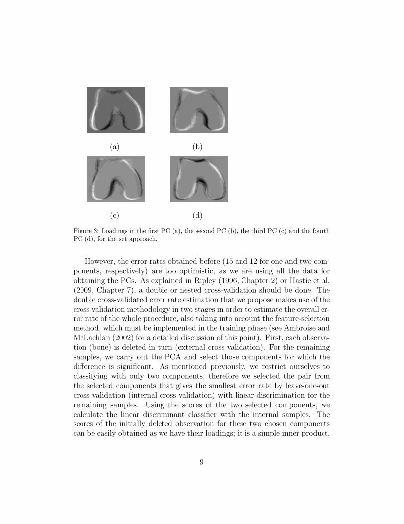
The percentages of variance accounted for the first four principal compo-nents are 13.62%, 9.47%, 8.37% and 6.22% with a cumulative total of 37.67%.44 components are necessary in order to capture 90.39% of the variability.The loadings in the first four principal components are represented as greylevels, as done in Horgan (2000), and appear in Fig. 3. Bright grey levelsindicate positive loadings, and dark negative ones. An interpretation of themis not easy. As a tentative interpretation: the first component is greatly con-centrated on the external part of the condyles, the second component on theright condyle, while the third component is concentrated on left condyle. Onthe other hand, the fourth component is associated with the joint betweencondyles and the top part of the image.

For the discriminant analysis, we follow the same strategy as in the land-mark approach. We compute all PCs with all data, and we consider onlythose for which the difference (between eburnated and non-eburnated bones)is significant. Now, five components are significant: 2, 3, 41, 43 and 59. Ifwe compute the misclassification rate by leave-one-out as before, the bestclassification with one component is obtained by the second component (15errors, 3 false positive and 12 false negative). If two components are used,the best classification is achieved by components 2 and 3, giving 12 errors(4 false positive and 8 false negative). Although in this approach (and thefollowing) more than two components could be considered jointly, we restrictourselves to classifying with only two components, for the following reasons:with only two components we try to avoid an overfitted model, and in factwe obtain a simple and parsimonious model which is able to classify withvery good results; two components (dimensions) are easier to interpret andrepresent graphically; considering only pairs is computationally faster thanconsidering all the possible subsets and finally, as only one component is sig-nificant in the landmark approach, the use of many more components in theother approaches would not be a fair comparison.

8

(a) (b)

(c) (d)

Figure 3: Loadings in the first PC (a), the second PC (b), the third PC (c) and the fourthPC (d), for the set approach.

However, the error rates obtained before (15 and 12 for one and two com-ponents, respectively) are too optimistic, as we are using all the data forobtaining the PCs. As explained in Ripley (1996, Chapter 2) or Hastie et al.(2009, Chapter 7), a double or nested cross-validation should be done. Thedouble cross-validated error rate estimation that we propose makes use of thecross validation methodology in two stages in order to estimate the overall er-ror rate of the whole procedure, also taking into account the feature-selectionmethod, which must be implemented in the training phase (see Ambroise andMcLachlan (2002) for a detailed discussion of this point). First, each observa-tion (bone) is deleted in turn (external cross-validation). For the remainingsamples, we carry out the PCA and select those components for which thedifference is significant. As mentioned previously, we restrict ourselves toclassifying with only two components, therefore we selected the pair fromthe selected components that gives the smallest error rate by leave-one-outcross-validation (internal cross-validation) with linear discrimination for theremaining samples. Using the scores of the two selected components, wecalculate the linear discriminant classifier with the internal samples. Thescores of the initially deleted observation for these two chosen componentscan be easily obtained as we have their loadings; it is a simple inner product.

9

We use the linear classifier previously built to predict the class label for theinitially deleted observation. This prediction is preserved to produce the (ex-ternal) leave-one-out estimate of the prediction error, because this processis repeated in turn for each of the observations. Of course, for each obser-vation (external iteration), different subsets of PC can be selected. As PCAis computed with different data, PCs from different external iterations arenot comparable, especially those with low variance. For example, component20 in one iteration could be quite different from component 20 obtained inanother iteration.

By the double cross-validation strategy, a total of 15 errors are obtained(3 false positive and 12 false negative).

2.3. Function description

With the standardized images (position and size filtered out) as explainedin Section 2.2, we consider the contour (outline) of the shapes. The contouris a closed planar curve that consists of the elements of the figure boundary.Although other contour functions can be used (see Kindratenko (2003) fora systematic review of various contour functions), we consider the contourparameterization by its arc length, which can be applied to any contour (notethat other contour functions have limitations). The tracing begins counter-clockwise at the easternmost outline point in the same row as the centroid,using bwtraceboundary from the image toolbox of MatLab. We normalizethese functions in such a way that the perimeter length is eliminated andthe functions are defined on [0,1]. Although they are recorded discretely,a continuous curve or function lies behind these data. In order to convertthe discrete curve observations into a true functional form, we approximate(smooth) each curve by a weighted sum (a linear combination) of fifty-oneFourier bases (note that this basis system is periodic with period 1), and de-termine the coefficients of the expansion by fitting data by least squares, asexplained in Ramsay and Silverman (2005, Chapter 4). Each curve is, there-fore, completely determined by the coefficients in this basis, and each functionis computable for any desired argument value t ∈ [0, 1]. All this work hasbeen done by means of fda library (Ramsay and Silverman, 2005). The freelibrary fda for MatLab and R, available at http://www.functionaldata.org, isespecially designed to work with functional data (Ramsay et al. (2009) is abook about this library). Finally, in order to have the same number of pointsfor all functions, we evaluate the functions in 100 equidistant points from 0

10

to 1. We therefore have two pairs of functions (representing coordinates)X(t), Y (t) for each bone, with t ∈ [0, 1].

Let us see how to apply PCA in this infinite dimensional domain. A shortanswer would be that summations change into integrations, but details aregiven in the following section.

2.3.1. PCA for functional data

In order to see how PCA works in the functional context, let us recallPCA for Multivariate Data analysis (MDA). In MDA, principal componentsare obtained by solving the eigenequation

Vξ = ρξ, (1)

where V is the sample variance-covariance matrix, V = (N−1)−1X′X, wherein turn X is the centered data matrix, N is the number of individuals ob-served, and X’ indicates the transpose of X. Furthermore, ξ is an eigenvectorof V and ρ is an eigenvalue of V.

In the functional version of PCA, vectors are not considered any more,but PCs are replaced by functions or curves. Let x1(t), . . . , xN(t) be theset of observed functions. The mean function can be defined as the aver-age of the functions point-wise across replications (x(t) = N−1

∑Ni=1 xi(t)).

Let us assume that we work with centered data (the mean function hasbeen subtracted), and define the covariance function v(s,t) analogously byv(s, t) = (N − 1)−1

∑Ni=1 xi(s)xi(t). As explained in Ramsay and Silverman

(2005, Chapter 8), the functional counterpart of equation 1 is the followingfunctional eigenequation

∫

v(s, t)ξ(t)dt = ρξ(s), (2)

where ρ is still an eigenvalue, but where ξ(s) is an eigenfunction of thevariance-covariance function, rather than an eigenvector. Now, the princi-pal component score corresponding to ξ(s) is computed by using the innerproduct for functions

si =∫

xi(s)ξ(s)ds. (3)

Note that for multivariate data, the index s is not continuous, but a discreteindex j replaces it: si =

∑

j xijξj.There are several strategies for solving the eigenanalysis problem in equa-

tion 2. In order to retain the continuity of the original functional data and

11

to reduce the amount of information, we have used the approach proposed inRamsay and Silverman (2005). Instead of using a lot of variables obtainedby discretizing the original functions, this type of analysis works with thecoefficients of the functions expressed as a linear combination of known basisfunctions (Fourier in our case, although other bases could be used, such asB-splines). Functional PCA can be carried out easily by using the libraryfda. For a complete review of computational methods for functional PCA,see Ramsay and Silverman (2005).

Regarding the problem of how many PCs can be computed, let us notethat in the functional context, “variables” now correspond to values of t,and there is no limit to these. Therefore, a maximum of N – 1 componentscan be computed. However, if the number of basis functions K defining thecurves is less than N, K would be the maximum.

2.3.2. Functional PCA with multiple functions

Our data consist of two functional data per bone. Functional PCA candeal with two (or more) functional observations per individual, two curvesx(t) and y(t). Let (x1(t), y1(t)), . . . , (xN(t), yN(t)) be the set of pairsof observed functions. Two mean functions (x(t), y(t)) and two covariancefunctions (vXX(s, t), vY Y (s, t)) can be computed for each kind of function,respectively. Furthermore, we can calculate the cross-covariance function ofthe centered data by:

vXY (s, t) = (N − 1)−1N∑

i=1

xi(s)yi(t). (4)

A typical PC is defined by a two-vector ξ=(ξX , ξY ) of weight functions(two curves). They are solutions of the eigenequation system V ξ = ρξ, whichin this case can be written as

∫

vXX(s, t)ξX(t)dt+∫

vXY (s, t)ξY (t)dt = ρξX(s)and∫

vXY (s, t)ξX(t)dt +∫

vY Y (s, t)ξY (t)dt = ρξY (s).(5)

Now, the PC score for the i -th bivariate function (xi(t), yi(t)) is computed bysi =

∫

xiξX +∫

yiξY , because the inner product between bivariate functionsis defined by the addition of the inner products of the two components. Thisamounts to stringing two functions together to form a composite function.

To solve the eigenequation system, each function xi(t) and yi(t) is replacedby a vector of values or basis coefficients, and a single synthetic function is

12

built by joining them together. When PCs have been computed, we separatethe parts belonging to each coordinate. Again, this procedure is implementedon the fda library and is explained fully in Ramsay and Silverman (2005).

The proportion of variance explained by each eigenfunction is computedas in the multivariate case, by each eigenvalue ρ divided by the sum of alleigenvalues. Moreover, for each PC, the variation accounted for each originalcurve x(t) and y(t) is given by

∫

ξX(s)ξX(s)ds and∫

ξY (s)ξY (s)ds respec-tively, because their sum is one by definition.

The first four principal components for the bones explain 80.52% of thewhole variance, made up of 55.00%, 10.59%, 9.02% and 5.91% respectively.90.21% of the variability is explained by the first seven components.

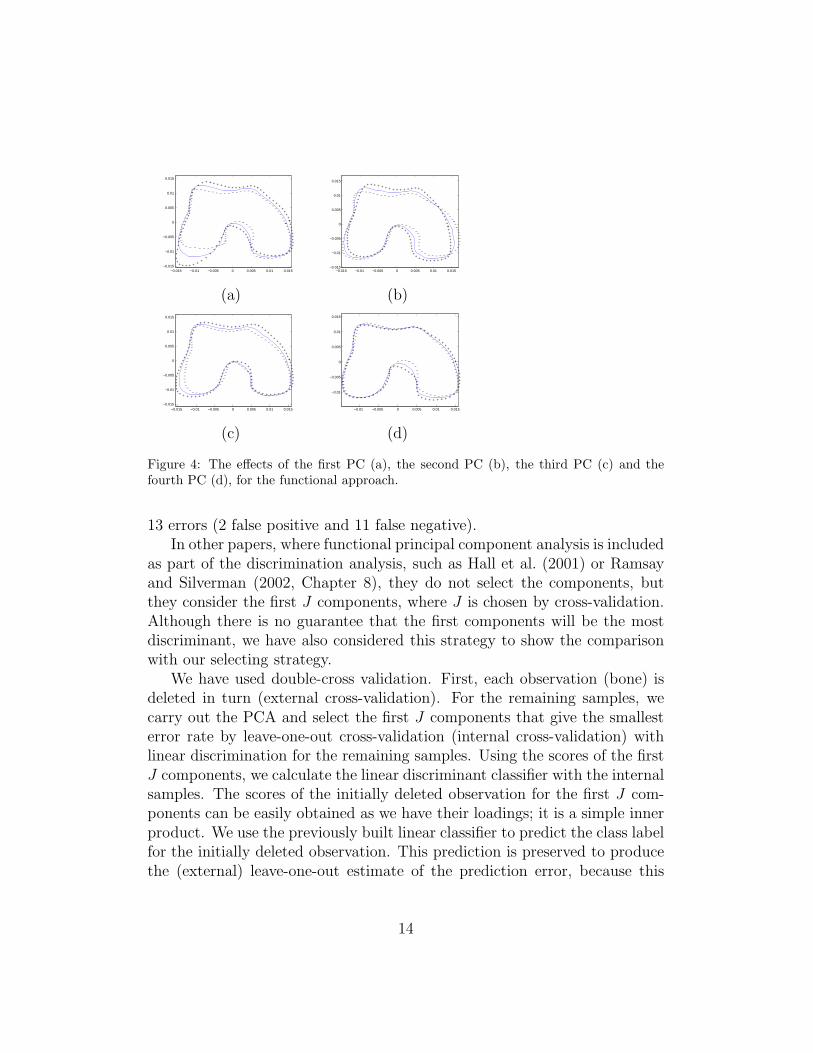
In order to display the effect of each PC, the mean function is displayedtogether with the functions obtained by adding (plotted with +) and sub-tracting (plotted with -) a suitable multiple of the principal component func-tion in question, in our case two standard deviations of each component. Inthis way, the effects of each PC are usually clarified (see Ramsay and Silver-man (2005, Chapter 8)). They are shown in Fig. 4. The first componentcorrespond to the length of the left condyle, but also to the shape of theintercondylar notch. 63.33% of the variation in this component is due to they-coordinates (function). The second component is associated with a broaderintercondylar notch (for negative scores) and the shape of the top of the im-age. In this component, 95.13% of variability comes from the x-coordinates.Component 3 is associated with the left condyle and the top right hand partof the image. The proportion of the variability in this component is 74.59%for the x-coordinates. Finally, component 4 is concentrated almost entirelyon the internal part of the right condyle. 58.12% of the variation in thiscomponent is due to the y-coordinates.

For the discriminant analysis, we follow the same strategies as in the setapproach. First, PCA with all data is calculated, but only those componentsfor which the difference is significant are considered. Now, three componentsare significant: 1, 6 and 10. If we compute the misclassification rate by leave-one-out as before, the best classification with one component is obtained bythe sixth component (16 errors, 3 false positive and 13 false negative) andthe tenth component (16 errors, 0 false positive and 16 false negative). Iftwo components are used, the best classification is achieved by components1 and 6, giving 11 errors (2 false positive and 9 false negative). However,these estimations are optimistic, and we have carried out the double crossvalidation strategy explained in Section 2.2, whose estimation has returned

13

−0.015 −0.01 −0.005 0 0.005 0.01 0.015−0.015

−0.01

−0.005

0

0.005

0.01

0.015

++

++

++

++

++

++

+++++++++++++++++

++

++++++++

++

++

+++++++++

+ + + + + ++

++

++

+++++++ + + +

++++++++

+ + + + + + + + + +++++++++++

−−

−−

−−

−−

−−

−−−−−−−−−−−−−−−−−−−−−

−−−−−

−−

−−

−−−−−−−−− − − − − − − − − − −−−

−−−−−−−

− − − − −−

−−−−−−−−

− − − − − − − −−

−−−−−−−−

−−

−0.015 −0.01 −0.005 0 0.005 0.01 0.015−0.015

−0.01

−0.005

0

0.005

0.01

0.015

++

++

++

++

++

++

++++++++++++++++++

++

+++++

++

++++++++++++

+ + + + + + + + +++++++++

+ + + ++

++++++++

+ + + + + + + + + +++++++++++

−−

−−

−−

−−

−−

−−−−−−−−−−−−−−−−−−−−−−−−−−−−

−−

−−

−−−−−−−−

− − − − − − − − −−

−−−−−−−−

− − − − − −−−−−−−−

− − − − − − − − −−

−−−−−−−

−−

−

(a) (b)

−0.015 −0.01 −0.005 0 0.005 0.01 0.015−0.015

−0.01

−0.005

0

0.005

0.01

0.015

++

++

++

++

++

+++++++++++++++++++

++

+++++

++

++

++

++

++++++

+ + + + + + + + ++

+++++++

++ + + + +

++++++++

+ + + + + + + + ++

+++++++++

+−

−−

−−

−−

−−

−−

−−−−−−−−−−−−−−−−−−−−−−−−−−−

−−

−−−−−−−−−−−

− − − − − − − −−

−−−−−−−−− − − −

−−

−−−−−−−−

− − − − − − − − −−−−−−−−−

−−

−0.01 −0.005 0 0.005 0.01 0.015

−0.01

−0.005

0

0.005

0.01

0.015

++

++

++

++

++

+++++++++++++++++++

+++++++++

++

++

++

++++++

+ + + + + + + ++

++

++++++++

+ + + ++

++++++++

+ + + + + + + ++

++++++++

++−

−−

−−

−−

−−

−−

−−−−−−−−−−−−−−−−−−−

−−−−−−

−−

−−

−−

−−−−−−−−

−− − − − − − − − −

−−−−−−

−−

− − − −−

−−−−−−−− − − − − − − − − − −

−−−−−−−−−

−

(c) (d)

Figure 4: The effects of the first PC (a), the second PC (b), the third PC (c) and thefourth PC (d), for the functional approach.

13 errors (2 false positive and 11 false negative).In other papers, where functional principal component analysis is included

as part of the discrimination analysis, such as Hall et al. (2001) or Ramsayand Silverman (2002, Chapter 8), they do not select the components, butthey consider the first J components, where J is chosen by cross-validation.Although there is no guarantee that the first components will be the mostdiscriminant, we have also considered this strategy to show the comparisonwith our selecting strategy.

We have used double-cross validation. First, each observation (bone) isdeleted in turn (external cross-validation). For the remaining samples, wecarry out the PCA and select the first J components that give the smallesterror rate by leave-one-out cross-validation (internal cross-validation) withlinear discrimination for the remaining samples. Using the scores of the firstJ components, we calculate the linear discriminant classifier with the internalsamples. The scores of the initially deleted observation for the first J com-ponents can be easily obtained as we have their loadings; it is a simple innerproduct. We use the previously built linear classifier to predict the class labelfor the initially deleted observation. This prediction is preserved to producethe (external) leave-one-out estimate of the prediction error, because this

14

process is repeated in turn for each of the observations. Of course, for eachobservation (external iteration), J can vary. By the double cross-validationstrategy with the first J components, a total of 13 errors are obtained (3false positive and 10 false negative). This is the same number of errors aswe have obtained with our selecting strategy, with only two components.However, a look at the chosen Js reveals that J very often corresponds to 15and 16, a very high number taking into account that the eburnated group isconstituted by 16 eburnated femora. Therefore, overlearning should not bediscarded when the first J components are considered in this case.

2.4. Comparison of the three approaches

Firstly, note the different distribution of the variability for the three ap-proaches. With the first four PCs with landmarks, 92.76% of the variabilityis considered. However, 84.62% of the variance is concentrated on only onecomponent, whereas the second component only accounts for 3.26% of thevariability; therefore, it is not very representative. Predictably, the landmarkapproach cannot collect fine details in variation since we only work with 12points. On the contrary, with the set approach the variability is extremelypartitioned: 44 components are needed in order to capture 90.39% of thevariability. Interpreting 44 components is not an easy issue. On the otherhand, in an intermediate position between the other two approaches, we findthe functional PCA, which gives a variability decomposition which is not soextreme: we can obtain more details on variability decomposition than withlandmarks, without being so extremely decomposed as in the set approach.

As regards the discriminant problem, obviously (as less information isconsidered), the classification results for landmarks are the worst. Similarresults are obtained for the set and functional approach (15 versus 13 errors,respectively). However, there are other procedures for carrying out func-tional data classification that will improve the results with respect to the setapproach results.

3. ICA in functional data classification

3.1. Curve discrimination

Different alternatives have been proposed for the curve discriminationproblem, although mainly for univariate functions. Two of the first meth-ods were a regularized version of LDA called penalized discriminant analysis

15

(PDA) proposed by Hastie et al. (1995), and a generalized linear regres-sion approach proposed by Marx and Eilers (1999). More recently, somenon-parametric alternatives have been proposed, such as the kernel one byFerraty and Vieu (2003), the k-NN one by Burba et al. (2009) or the locallinear one by Barrientos-Marin et al. (2010). Biau et al. (2005) also studiedk-nearest neighbor classifiers for functional data. Other recent advances infunctional data classification appear in the following papers, and all involvesome type of preprocessing (sometimes implicit) of the functional data. Rossiand Conan-Guez (2005) suggested the use of neural networks for nonlinearregression and classification of functional data; the use of neural networkswas also considered by Ferre and Villa (2006), who studied a preprocessingapproach in which functional data are described via a projection on an opti-mal basis (in the sense of the inverse regression approach), and subsequentlysubmitted to a neural network for further processing; James and Silverman(2005) studied a non linear regression model for functional descriptors; Rossiand Villa (2006) and Li and Yu (2008) used Support Vector Machines (SVM)for functional data classification. Finally, Epifanio (2008) proposed the useof several shape descriptors. One of those descriptors were coefficients of in-dependent component analysis (ICA) components. In Epifanio (2008), thosedescriptors were compared with classical and the most recent advances inunivariate functional data classification in three different problems (an artifi-cial problem, a speech recognition problem and a biomechanical application).The first two problems were considered in Ferraty and Vieu (2003), wherethey also performed a wide-ranging comparative study. In Epifanio (2008),the proposed descriptors were compared with the methodology proposed inHastie et al. (1995), in Ferraty and Vieu (2003) including the MPLSR methodin its semi-metric and PCA, in Rossi and Conan-Guez (2005), in Ferre andVilla (2006), in Rossi and Villa (2006). As Li and Yu (2008) use the sameexample (a subproblem of the speech recognition problem) as Rossi and Villa(2006), we can also compare the results in Epifanio (2008) with those of Liand Yu (2008). The descriptors proposed in Epifanio (2008) gave resultsbetter than or similar to those obtained using the previous techniques (seeEpifanio (2008) for details).

3.2. Coefficients of Independent Component Analysis Components

Coefficients of independent component analysis (ICA) components canbe computed easily, and provide better than or similar results to those fromexisting techniques (Epifanio, 2008). Furthermore, they can be extended

16

easily to the multivariate functional case, as we will explain in this section.Although Epifanio (2008) can be seen for details, a brief summary is givenhere.

Assume that we observe n linear mixtures x1(t), ..., xn(t) of n independentcomponents sj(t),

xi(t) =n∑

j=1

aijsj(t), for all i. (6)

In practice, we have discretized curves (xi = xi(tk); k = 1, ..., m), thereforewe can consider them×n data matrixX= xi(tk) to be a linear combinationof independent components, i.e. X = SA, where columns of S contain theindependent components and A is a linear mixing matrix. ICA attempts to“un-mix” the data by estimating an un-mixing matrix W where XW = S.Under this generative model, the measured “signals” in X will tend to be“more Gaussian” than the source components (in S) due to the Central LimitTheorem. Thus, in order to extract the independent components or sources,we search for an un-mixing matrix W that maximizes the nongaussianity ofthe sources.

We compute ICA for functions in the training set. The coefficients inthis base (S) can be easily obtained by least squares fitting (Ramsay andSilverman, 2005). If y = y(tk)mk=1 is a discretized function, its coefficientsare: (S′S)−1S′y. These coefficients constitute the feature vector used for theclassification step. We assume that all functions are observed at the samepoints, otherwise we can always fit a basis and estimate the functions at therequired points.

Before the application of the ICA algorithm, it is useful to reduce thedimension of the data previously by principal component analysis (PCA)(for details, see Hyvarinen et al. (2000, Section 5)), thus reducing noise andpreventing overlearning (Hyvarinen et al., 2001, Section 13.2). Thereforewe compute the PCA first, retaining a certain number of components, andthen estimate the same number of independent components as the PCAreduced dimension. The FastICA algorithm (which includes the PCA com-putation in the software available for MatLab and R: http://www.cis.hut.fi/projects/ica/fastica/), with the default parameters, is used for obtaining ICA(Hyvarinen, 1999).

When having multivariate functional data, we can concatenate observa-tions of the functions into a single long vector, as done for computing bivari-ate functional PCA (Ramsay and Silverman, 2002). Then, the coefficients in

17

ICA base can be used in a classical linear discriminant analysis.In Epifanio (2008) and Epifanio and Ventura (2008), the components were

not selected, but the first J components were considered, where J was chosenby cross-validation, such as in Hall et al. (2001) and Ramsay and Silverman(2002) with functional PCA. Here, besides extending the methodology pro-posed in Epifanio (2008) to the multivariate functional case, we also proposeto select the components in a similar way to that in Section 2 with PCA. Fur-thermore, we propose to compute a linear discriminant function α(t) basedon ICA as done in Ramsay and Silverman (2002, Chapter 8) with PCA. Thisfunction α(t) would be the functional counterpart of the linear discriminantor canonical variate (Ripley, 1996, Chapter 3), therefore,

∫ 10 α(t)xi(t)dt would

return the score or discriminant value of xi(t) on the discriminant variable.If we select two ICA functions (I,K) from the ICA base, and apply

classical linear discriminant analysis to the ICA coefficients for these twofunctions, the two coefficients (c1, c2) of the linear discriminant are obtained.From them, we can build a, a vector of the same length as the number ofthe ICA basis functions considered, constituted by zeros except for positions(I,K), with values c1 and c2, respectively.

The linear discriminant values can be expressed in terms of the ICAcoefficients and coefficients of linear discriminants l: l(S′S)−1S′X. For aspecific individual i: l(S′S)−1S′xi. At the same time, we can approximate∫

α(t)xi(t)dt by∑m

k=1 α(tk)xi(tk) if we consider the separation between pointsas one. Therefore, we estimate α(t) at points tk as l(S′S)−1S′.

3.3. Bone classification by multivariate functional data discrimination usingICA

We apply the previous methodology to the bones, following the samestrategies as for functional PCA in Section 2.3.2. Firstly, we compute ICAwith all data. As aforementioned, PCA is calculated before ICA, and only18 components remain since components associated with eigenvalues of lessthan 1e-7 are not considered, to avoid singularity of the covariance matrix (asimplemented in the FastICA algorithm). For these 18 independent compo-nents, the coefficients of 8 components present significant differences betweenthe two groups: 1, 2, 7, 10, 12, 14, 16 and 18. We compute the misclassifica-tion rate by leave-one-out, and the best classification with one component isobtained by the first (12 errors, 4 false positive and 8 false negative), whilefor two components by the first and seventh components (8 errors, 2 falsepositive and 6 false negative). In Fig. 5, the functional linear discriminant

18

−0.015 −0.010 −0.005 0.000 0.005 0.010 0.015

−0.

010

−0.

005

0.00

00.

005

0.01

0

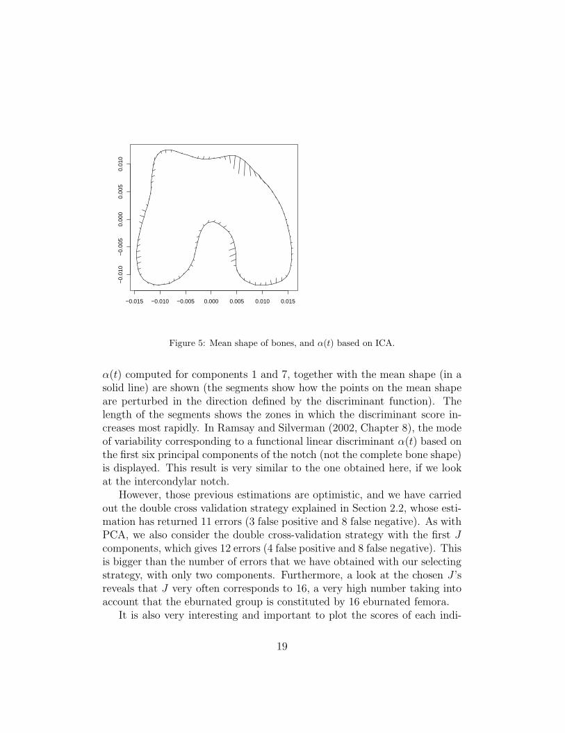
Figure 5: Mean shape of bones, and α(t) based on ICA.

α(t) computed for components 1 and 7, together with the mean shape (in asolid line) are shown (the segments show how the points on the mean shapeare perturbed in the direction defined by the discriminant function). Thelength of the segments shows the zones in which the discriminant score in-creases most rapidly. In Ramsay and Silverman (2002, Chapter 8), the modeof variability corresponding to a functional linear discriminant α(t) based onthe first six principal components of the notch (not the complete bone shape)is displayed. This result is very similar to the one obtained here, if we lookat the intercondylar notch.

However, those previous estimations are optimistic, and we have carriedout the double cross validation strategy explained in Section 2.2, whose esti-mation has returned 11 errors (3 false positive and 8 false negative). As withPCA, we also consider the double cross-validation strategy with the first Jcomponents, which gives 12 errors (4 false positive and 8 false negative). Thisis bigger than the number of errors that we have obtained with our selectingstrategy, with only two components. Furthermore, a look at the chosen J ’sreveals that J very often corresponds to 16, a very high number taking intoaccount that the eburnated group is constituted by 16 eburnated femora.

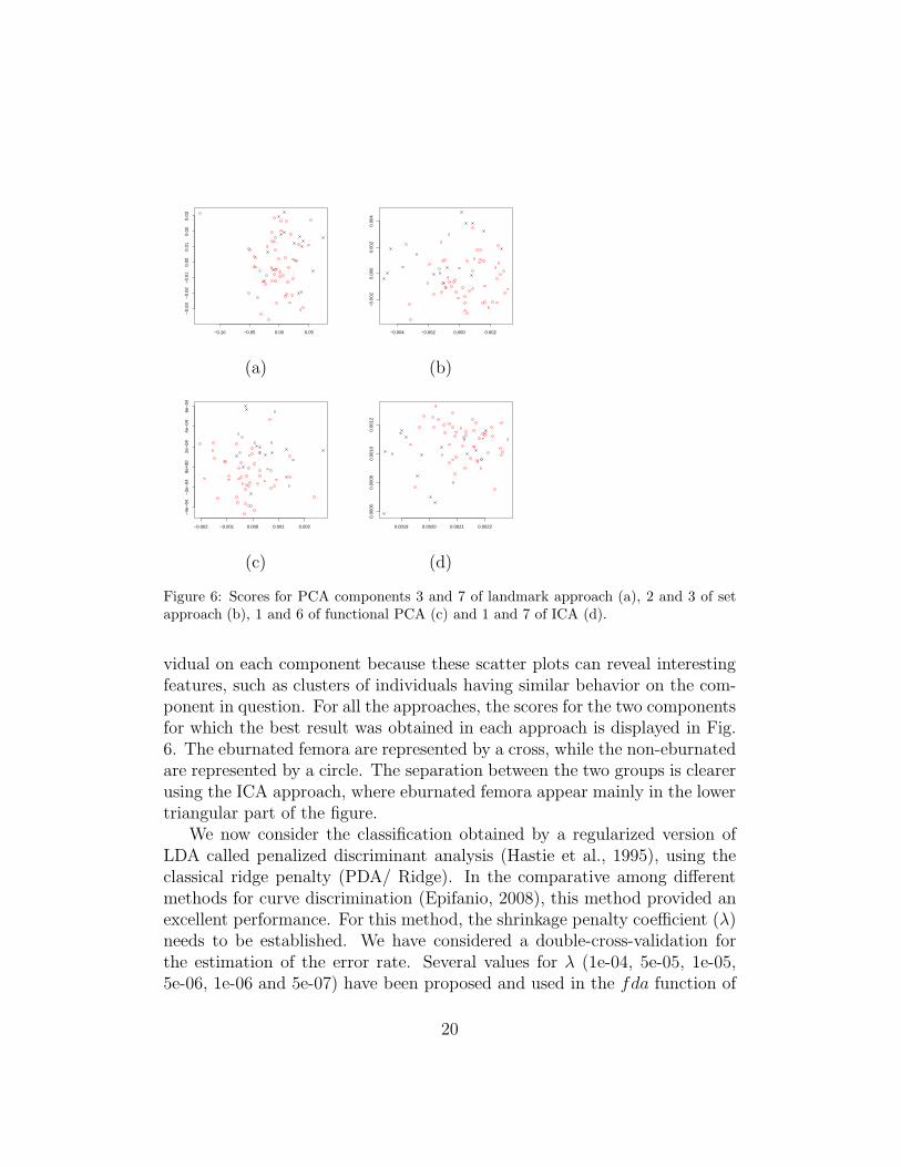
It is also very interesting and important to plot the scores of each indi-

19

−0.10 −0.05 0.00 0.05

−0.

03−

0.02

−0.

010.

000.

010.

020.

03

−0.004 −0.002 0.000 0.002

−0.

002

0.00

00.

002

0.00

4(a) (b)

−0.002 −0.001 0.000 0.001 0.002

−4e

−04

−2e

−04

0e+

002e

−04

4e−

046e

−04

0.0019 0.0020 0.0021 0.0022

0.00

060.

0008

0.00

100.

0012

(c) (d)

Figure 6: Scores for PCA components 3 and 7 of landmark approach (a), 2 and 3 of setapproach (b), 1 and 6 of functional PCA (c) and 1 and 7 of ICA (d).

vidual on each component because these scatter plots can reveal interestingfeatures, such as clusters of individuals having similar behavior on the com-ponent in question. For all the approaches, the scores for the two componentsfor which the best result was obtained in each approach is displayed in Fig.6. The eburnated femora are represented by a cross, while the non-eburnatedare represented by a circle. The separation between the two groups is clearerusing the ICA approach, where eburnated femora appear mainly in the lowertriangular part of the figure.

We now consider the classification obtained by a regularized version ofLDA called penalized discriminant analysis (Hastie et al., 1995), using theclassical ridge penalty (PDA/ Ridge). In the comparative among differentmethods for curve discrimination (Epifanio, 2008), this method provided anexcellent performance. For this method, the shrinkage penalty coefficient (λ)needs to be established. We have considered a double-cross-validation forthe estimation of the error rate. Several values for λ (1e-04, 5e-05, 1e-05,5e-06, 1e-06 and 5e-07) have been proposed and used in the fda function of

20

the R library mda (Hastie and Tibshirani, 2006). These proposed values forλ have been selected by computing the performance by leave-one-out for abigger set of values of λ, where the best result was obtained for λ = 1e-5 (theproposed values for λ are around this value): 10 errors (3 false positive and7 false negative). However, as before, this is an optimistic estimation since λis selected with the training data. For the double-cross-validation strategy,each observation is removed in turn. For each proposed λ, we perform apenalized discriminant analysis leaving-one-out of the remaining samples,and establishing which λ gives the best performance. For this λ, we predictthe class of the observation initially removed, using the remaining samples.This prediction is preserved to produce the (external) leave-one-out estimateof the prediction error, because this process is repeated in turn for each of theobservations. Of course, for each observation (external iteration), differentλs can be selected. By the double cross-validation strategy, the number oferrors is 15 (7 false positive and 8 false negative).

Analogously, we have used the nonparametric curve discrimination method(NPCD) with the semi-metric based on functional principal component anal-ysis (FPCA) and multivariate partial least-squares regression (MPLSR) in-troduced by Ferraty and Vieu (2003) (instead of λ, the tuning parameter isnow the number of components used in the semi-metric, from 1 to 7). Thebest results using leave-one-out were obtained for 1 component for the firstsemi-metric (16 errors, 0 false positive and 16 false negative), and 4 factorsfor the second semi-metric (11 errors, 6 false positive and 5 false negative).Using the double-cross-validation strategy, the number of errors is 18 (2 falsepositive and 16 false negative) for the FPCA semi-metric and 14 (6 falsepositive and 8 false negative) for the MPLSR semi-metric.

In short, in the functional approach, the best discriminant result is ob-tained by our methodology, with two ICA components (11 errors), whichis better than functional PCA (13 errors) and PDA/Ridge (15 errors) orNPCD/FPCA (18 errors) and NPCD/MPLSR (14 errors). The result withICA is better than that of the set approach (15 errors) or the landmarkapproach (16 errors in the optimistic estimate).

4. Hippocampus study in Alzheimer’s disease

The early diagnosis of Alzheimer’s disease (AD) is a very important is-sue in our society, since the administration of medicines to subjects who aresubtly impaired may render the treatments more effective. Mild cognitive

21

impairment (MCI) is considered as a diagnostic entity within the continuumof cognitive decline towards AD in old age (Grundman et al., 2004; Petersen,2004). Longitudinal studies indicate a direct relation between the hippocam-pal volume decrease in and cognitive decline (Jack et al., 1999; Mungas et al.,2001). However, volumetric measurements are simplistic characteristics andstructural changes at specific locations cannot be reflected in them. If mor-phological changes could be established, then this should enable researchersto gain an increased understanding of the condition. This is the reason whynowadays shape analysis is of an enormous importance in neuroimaging cir-cles (Styner et al., 2004).

In order to understand the way in which hippocampi differ among threedifferent groups (controls, patients with MCI, and patients with early AD),we have their magnetic resonance (MR) scans, which will be transformedinto multivariate functional data, as explained in following section. Thesemultivariate functional data will be used in a functional discriminant analysis.We will apply the methodology presented in the previous section, with somesmall modifications.

4.1. Brain MR scans processing

28 individuals were analyzed in this study: 12 controls (5 males and 7females, with mean age 70.17 and standard deviation 3.43), 6 patients withMCI (2 males and 4 females, with mean age 75.50 and standard deviation3.33), and 10 patients with early AD (1 male and 9 females, with mean age71.50 and standard deviation 4.35). All the subjects were recruited fromthe Neurology Service at La Magdalena Hospital (Castello, Spain) and theNeuropsychology Service at the Universitat Jaume I. All experimental pro-cedures complied with the guidelines of the ethical research committee atthe Universitat Jaume I. Written informed consent was obtained from everyindividual or their appropriate proxy prior to participation. Selection for theparticipant group was made after careful neurological and neuropsychologicalassessment. The neuropsychological test battery involved Digit Span, Simi-larities, Vocabulary, and Block Design of the WAIS-III; Luria’s Watches test,and Poppelreuter´s Overlapping Figure test. MR scans were carried out witha 1.5T General Electric system. A whole brain high resolution 3D-GradientEcho (FSPGR) T1-weighted anatomical reference scan was acquired (TE 4.2ms, TR 11.3 ms, FOV 24 cm; matrix = 256×256×124, 1.4 mm-thick coronalimages).

22

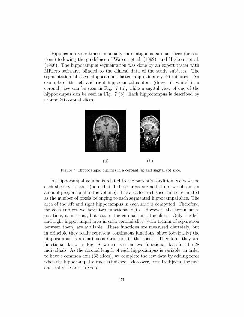
Hippocampi were traced manually on contiguous coronal slices (or sec-tions) following the guidelines of Watson et al. (1992), and Hasboun et al.(1996). The hippocampus segmentation was done by an expert tracer withMRIcro software, blinded to the clinical data of the study subjects. Thesegmentation of each hippocampus lasted approximately 40 minutes. Anexample of the left and right hippocampal contour (drawn in white) in acoronal view can be seen in Fig. 7 (a), while a sagital view of one of thehippocampus can be seen in Fig. 7 (b). Each hippocampus is described byaround 30 coronal slices.

(a) (b)

Figure 7: Hippocampal outlines in a coronal (a) and sagital (b) slice.

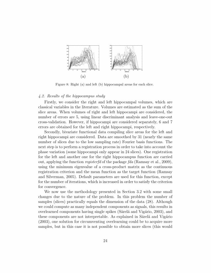
As hippocampal volume is related to the patient’s condition, we describeeach slice by its area (note that if these areas are added up, we obtain anamount proportional to the volume). The area for each slice can be estimatedas the number of pixels belonging to each segmented hippocampal slice. Thearea of the left and right hippocampus in each slice is computed. Therefore,for each subject we have two functional data. However, the argument isnot time, as is usual, but space: the coronal axis, the slices. Only the leftand right hippocampal area in each coronal slice (with 1.4mm of separationbetween them) are available. These functions are measured discretely, butin principle they really represent continuous functions, since (obviously) thehippocampus is a continuous structure in the space. Therefore, they arefunctional data. In Fig. 8, we can see the two functional data for the 28individuals. As the coronal length of each hippocampus is variable, in orderto have a common axis (33 slices), we complete the raw data by adding zeroswhen the hippocampal surface is finished. Moreover, for all subjects, the firstand last slice area are zero.

23

0 5 10 15 20 25 30 350

20

40

60

80

100

120

140

160

slices0 5 10 15 20 25 30 35

0

20

40

60

80

100

120

140

160

180

slices

(a) (b)

Figure 8: Right (a) and left (b) hippocampal areas for each slice.

4.2. Results of the hippocampus study

Firstly, we consider the right and left hippocampal volumes, which areclassical variables in the literature. Volumes are estimated as the sum of theslice areas. When volumes of right and left hippocampi are considered, thenumber of errors are 5, using linear discriminant analysis and leave-one-outcross-validation. However, if hippocampi are considered separately, 6 and 7errors are obtained for the left and right hippocampi, respectively.

Secondly, bivariate functional data compiling slice areas for the left andright hippocampi are considered. Data are smoothed by 31 (nearly the samenumber of slices due to the low sampling rate) Fourier basis functions. Thenext step is to perform a registration process in order to take into account thephase variation (some hippocampi only appear in 24 slices). One registrationfor the left and another one for the right hippocampus function are carriedout, applying the function registerfd of the package fda (Ramsay et al., 2009),using the minimum eigenvalue of a cross-product matrix as the continuousregistration criterion and the mean function as the target function (Ramsayand Silverman, 2005). Default parameters are used for this function, exceptfor the number of iterations, which is increased in order to satisfy the criterionfor convergence.

We now use the methodology presented in Section 3.2 with some smallchanges due to the nature of the problem. In this problem the number ofsamples (slices) practically equals the dimension of the data (28). Althoughwe could compute as many independent components as signals, this results inoverlearned components having single spikes (Sarela and Vigario, 2003), andthese components are not interpretable. As explained in Sarela and Vigario(2003), one solution for circumventing overlearning could be to acquire moresamples, but in this case it is not possible to obtain more slices (this would

24

increase the already long acquisition time of MR brain scans). Anothersolution is reducing dimension: the number of free parameters is n2/2, soin this problem we compute a maximum of 7 components (n <

√2 · 30),

taking into account that each hippocampus is described by around 30 slices(samples). So, the first modification is that we compute the independentcomponents varying their number from 1 to 7. For each case, we considerthe components for which the difference among the 3 groups is significant.However, in this problem the t-test cannot be used as before because we have3 groups, not 2, so we use the Kruskal-Wallis test.

As our objective is the way in which the hippocampi differ among thethree groups, we show the combination for which the best discriminant resultsare obtained, by leave-one-out. The error estimate obtained in this way willbe optimistic, but we want to investigate the shape variation among thegroups, obtaining the linear discriminant functions.

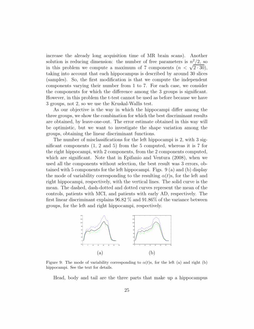
The number of misclassifications for the left hippocampi is 2, with 3 sig-nificant components (1, 2 and 5) from the 5 computed, whereas it is 7 forthe right hippocampi, with 2 components, from the 2 components computed,which are significant. Note that in Epifanio and Ventura (2008), when weused all the components without selection, the best result was 3 errors, ob-tained with 5 components for the left hippocampi. Figs. 9 (a) and (b) displaythe mode of variability corresponding to the resulting α(t)s, for the left andright hippocampi, respectively, with the vertical lines. The solid curve is themean. The dashed, dash-dotted and dotted curves represent the mean of thecontrols, patients with MCI, and patients with early AD, respectively. Thefirst linear discriminant explains 96.82 % and 91.86% of the variance betweengroups, for the left and right hippocampi, respectively.

0 5 10 15 20 25 30 35−20

0

20

40

60

80

100

120

140

0 5 10 15 20 25 30 35−20

0

20

40

60

80

100

120

140

(a) (b)

Figure 9: The mode of variability corresponding to α(t)s, for the left (a) and right (b)hippocampi. See the text for details.

Head, body and tail are the three parts that make up a hippocampus

25

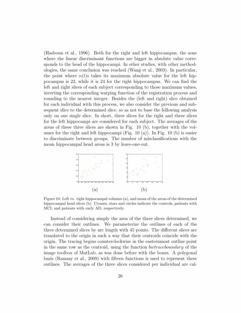
(Hasboun et al., 1996). Both for the right and left hippocampus, the zonewhere the linear discriminant functions are bigger in absolute value corre-sponds to the head of the hippocampi. In other studies, with other method-ologies, the same conclusion was reached (Wang et al., 2003). In particular,the point where α(t)s takes its maximum absolute value for the left hip-pocampus is 22, while it is 24 for the right hippocampus. We can find theleft and right slices of each subject corresponding to those maximum values,inverting the corresponding warping function of the registration process androunding to the nearest integer. Besides the (left and right) slice obtainedfor each individual with this process, we also consider the previous and sub-sequent slice to the determined slice, so as not to base the following analysisonly on one single slice. In short, three slices for the right and three slicesfor the left hippocampi are considered for each subject. The averages of theareas of these three slices are shown in Fig. 10 (b), together with the vol-umes for the right and left hippocampi (Fig. 10 (a)). In Fig. 10 (b) is easierto discriminate between groups. The number of misclassifications with themean hippocampal head areas is 3 by leave-one-out.

800 1000 1200 1400 1600 1800 2000 2200 2400 2600 2800500

1000

1500

2000

2500

3000

40 60 80 100 120 140 160 18020

40

60

80

100

120

140

(a) (b)

Figure 10: Left vs. right hippocampal volumes (a), and mean of the areas of the determinedhippocampal head slices (b). Crosses, stars and circles indicate the controls, patients withMCI, and patients with early AD, respectively.

Instead of considering simply the area of the three slices determined, wecan consider their outlines. We parameterize the outlines of each of thethree determined slices by arc length with 45 points. The different slices aretranslated to the origin in such a way that their centroids coincide with theorigin. The tracing begins counterclockwise in the easternmost outline pointin the same row as the centroid, using the function bwtraceboundary of theimage toolbox of MatLab, as was done before with the bones. A polygonalbasis (Ramsay et al., 2009) with fifteen functions is used to represent theseoutlines. The averages of the three slices considered per individual are cal-

26

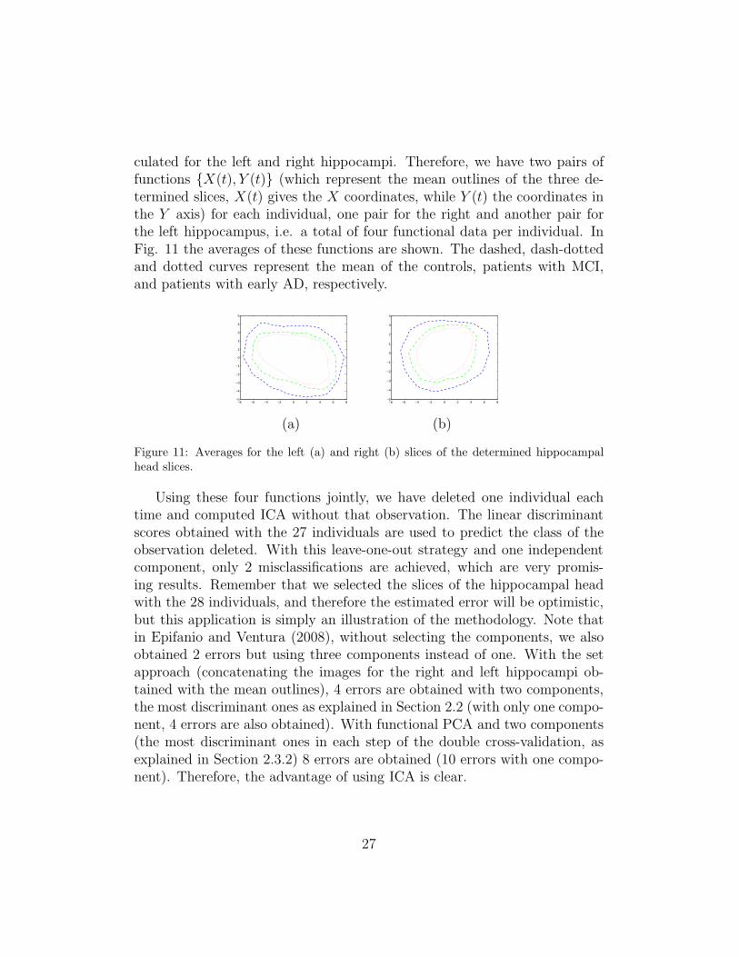
culated for the left and right hippocampi. Therefore, we have two pairs offunctions X(t), Y (t) (which represent the mean outlines of the three de-termined slices, X(t) gives the X coordinates, while Y (t) the coordinates inthe Y axis) for each individual, one pair for the right and another pair forthe left hippocampus, i.e. a total of four functional data per individual. InFig. 11 the averages of these functions are shown. The dashed, dash-dottedand dotted curves represent the mean of the controls, patients with MCI,and patients with early AD, respectively.

−8 −6 −4 −2 0 2 4 6 8−5

−4

−3

−2

−1

0

1

2

3

4

5

−8 −6 −4 −2 0 2 4 6 8−5

−4

−3

−2

−1

0

1

2

3

4

(a) (b)

Figure 11: Averages for the left (a) and right (b) slices of the determined hippocampalhead slices.

Using these four functions jointly, we have deleted one individual eachtime and computed ICA without that observation. The linear discriminantscores obtained with the 27 individuals are used to predict the class of theobservation deleted. With this leave-one-out strategy and one independentcomponent, only 2 misclassifications are achieved, which are very promis-ing results. Remember that we selected the slices of the hippocampal headwith the 28 individuals, and therefore the estimated error will be optimistic,but this application is simply an illustration of the methodology. Note thatin Epifanio and Ventura (2008), without selecting the components, we alsoobtained 2 errors but using three components instead of one. With the setapproach (concatenating the images for the right and left hippocampi ob-tained with the mean outlines), 4 errors are obtained with two components,the most discriminant ones as explained in Section 2.2 (with only one compo-nent, 4 errors are also obtained). With functional PCA and two components(the most discriminant ones in each step of the double cross-validation, asexplained in Section 2.3.2) 8 errors are obtained (10 errors with one compo-nent). Therefore, the advantage of using ICA is clear.

27

5. Conclusions and Discussion

In this study we have revealed the role that FDA can play in imageanalysis, where despite many descriptors being functions, FDA has hardlybeen applied. In particular, we have focused our attention on shape analysis,where the use of FDA in the functional approach has shown its superiorityover other approaches, such as the landmarks or the set theory approach,in two different problems (PCA and discriminant analysis) in a well-knowndatabase of bone outlines (see Section 2.4).

Furthermore, we have dealt with a problem that has hardly ever been con-sidered in the literature: the multivariate functional discrimination (most ofthe existing literature on functional classification considers univariate curvesdatasets). We have also proposed a discriminant function based on ICA, andthe classification results obtained with this methodology are very promising.

Unlike other papers in the literature where functional PCA is includedas part of the discrimination analysis, we have proposed selecting the com-ponents. This has also been proposed with ICA. Our option has been toconsider all the components and select the significant ones. However, in thehippocampus study, the number of samples practically equals the dimensionof the data, and we had to make a small modification in order to avoidoverlearned components. The problem of how many components should beestimated is an open question in ICA (Hyvarinen et al., 2001). This a pointfor future study, and maybe an order could be established such as in Cheungand Xu (1999). Another point to study is improving the smoothness of thefunctions by using a roughness penalty.

We have also applied FDA in the analysis of MR scans in order to studythe hippocampal differences among the subjects in three groups: controls,MCI, and patients with early Alzheimer’s disease. The database is quite smallfor obtaining valid medical conclusions, although the methodology could beused without modification with a larger database. This is a novel applicationof FDA in image analysis, where we use a spatial argument for the functionaldata instead of the temporal argument commonly used in FDA.

In the application, we have seen that the head was the most discrimina-tive part. This point is very interesting, since if segmentation was reducedonly to the hippocampal head, the segmentation time would be shorter.Furthermore, it is easier to implement an automatic segmentation for thehippocampal head only, which will decrease that time even more, and willeliminate variability due to the subjectivity of the manual tracer. (Remem-

28

ber that the total time for the manual segmentation of one hippocampus wasapproximately 40 minutes).

Some additional points to study are as follows: Firstly, from the statisticalpoint of view, the use of ICA in other statistical problems such as functionallogistic regression or visualization (Hyndman and Shang, 2010), or the use ofICA in the construction of a semi-metric for use with non-parametric tech-niques (Ferraty and Vieu, 2006) (PCA-type semi-metrics could be replacedby ICA-type semi-metrics by just considering the ICA expansion instead ofthe PCA-based expansion. This is a very interesting field of study, sincecompared with PCA, ICA allows better observation of the underlying struc-ture of the data. PCA is a purely second-order statistical method, whereasICA requires the use of higher-order statistics; therefore, ICA can be seenas an extension to PCA.). Secondly, from the image analysis point of view,is the application of FDA in other problems of shape analysis such as thedefinition of confidence and quantile sets (Simo et al., 2004), or its use whenthe closed contour of a figure is not always available, such as in Domingoet al. (2005), maybe using a discontinuous function. Thirdly, FDA can beexploited in other fields of image analysis besides shape analysis, such astexture analysis (Epifanio et al., 2009). Finally, in order to introduce themethodology more easily, we have restricted the analysis to two dimensionaloutlines, but FDA can be used for surfaces (multidimensional functions withtwo arguments). In fact, in the future, we are going to work in three di-mensions in the hippocampal analysis. The methodology presented can beextended for functions with two (or more) arguments.

Acknowledgements

This work has been supported by CICYT TIN2009-14392-C02-01 andMTM2009-14500-C02-02, GV/2011/004 and Bancaixa-UJI P11A2009-02. Theauthors thank V. Belloch and C. Avila for their support, and also the review-ers and editors for their comments on improving this study. A preliminaryversion was presented at the 1st International Workshop on Functional andOperatorial Statistics (IWFOS’2008) (Epifanio and Ventura, 2008).

References

Ambroise, C., McLachlan, G. J., 2002. Selection bias in gene extraction onthe basis of microarray gene-expression data. Proceedings of the NationalAcademy of Sciences 99 (10), 6562–6566.

29

Barrientos-Marin, J., Ferraty, F., Vieu, P., 2010. Locally modelled regressionand functional data. Journal of Nonparametric Statistics 22 (5), 617–632.

Berrendero, J.R., Justel, A., Svarc, M., 2011. Principal components for mul-tivariate functional data. Computational Statistics and Data Analysis,doi:10.1016/j.csda.2011.03.011.

Biau, G., Bunea, F., Wegkamp, M., 2005. Functional classification in Hilbertspaces. IEEE Transactions on Information Theory 51, 2163–2172.

Burba, F., Ferraty, F., Vieu, P., 2009. k-Nearest Neighbour method infunctional nonparametric regression. Journal of Nonparametric Statistics21 (4), 453–469.

Cheung, Y., Xu, L., 1999. MSE reconstruction criterion for independentcomponent odering in ICA time series analysis. In: Proceedings of theIEEE-EURASIP Workshop on Nonlinear Signal and Image Processing.pp. 793–797.

Delicado, P., 2011. Dimensionality reduction when data are density functions.Computational Statistics and Data Analysis 55 (1), 401-420.

Domingo, J., Nacher, B., de Ves, E., Alcantara, E., Dıaz, E., Ayala, G., Page,A., 2005. Quantifying mean shape and variability of footprints using meansets. In: Proceedings of the 7th International Symposium on MathematicalMorphology. Springer, pp. 455–464.

Dryden, I., 2007. shapes: Statistical shape analysis.URL http://www.maths.nott.ac.uk/∼ild/shapes

Dryden, I. L., Mardia, K. V., 1998. Statistical Shape Analysis. Wiley, Chich-ester.

Epifanio, I., 2008. Shape descriptors for classification of functional data.Technometrics 50 (3), 284–294.

Epifanio, I., Domingo, J., Ayala, G., 2009. Texture classification by func-tional analysis of size distributions. In: Proceedings of the 11th IASTEDInternational Conference on Signal and Image Processing. pp. 172–177.

30

Epifanio, I., Ventura, N., 2008. Multivariate Functional Data DiscriminationUsing ICA: Analysis of Hippocampal Differences in Alzheimer’s Disease.Contributions to Statistics. Springer, Ch. 25, pp. 157–163.

Ferraty, F., Romain, Y., 2011. The Oxford Handbook of functional dataanalysis. Oxford University Press.

Ferraty, F., Vieu, P., 2003. Curves discrimination: a nonparametric func-tional approach. Computational Statistics and Data Analysis 44, 161–173.

Ferraty, F., Vieu, P., 2006. Nonparametric Functional Data Analysis: Theoryand Practice. Springer.

Ferre, L., Villa, N., 2006. Multilayer perceptron with functional inputs: aninverse regression approach. Scandinavian Journal of Statistics 33 (4), 807–823.

Gonzalez, R., Woods, R., Eddins, S., 2004. Digital image processing usingMATLAB. Prentice Hall.

Gonzalez-Manteiga, W., Vieu, P., 2007. Statistics for functional data. Com-putational Statistics and Data Analysis 51 (10), 4788–4792.

Gower, J. C., 1966. Some distance properties of latent root and vector meth-ods used in multivariate analysis. Biometrika 53, 325338.

Grundman, M., Petersen, R., Ferris, S., Thomas, R., Aisen, P., Bennet, D.,Foster, N., Jack, C., Galasho, D., Dondy, R., Kaye, J., Sano, M., 2004.Mild cognitive impairment can be distinguished from Alzheimer diseaseand normal aging for clinical trials. Arch. Neurol 61, 59–66.

Hall, P., Poskitt, D., Presnell, B., 2001. A functional data-analytic approachto signal discrimination. Technometrics 43, 1–9.

Hasboun, D., Chantome, M., Zouaoui, A., Sahel, M., Deladoeuille, M.,Sourour, N., Duyme, M., Baulac, M., Marsault, C., Dormont, D., 1996.MR determination of hippocampal volume: Comparison of three methods.AJNR Am. J. Neuroradiol. 17, 1091–1098.

Hastie, T., Buja, A., Tibshirani, R., 1995. Penalized discriminant analysis.Annals of Statistics 23, 73–102.

31

Hastie, T., Tibshirani, R., 2006. mda: Mixture and flexible discriminantanalysis. R port by Leisch, F., Hornik, K. and Ripley, B. D.

Hastie, T., Tibshirani, R., Friedman, J., 2009. The Elements of StatisticalLearning. Data mining, inference and prediction, 2nd Edition. Springer-Verlag.

Horgan, G. W., 2000. Principal component analysis of random particles.Journal of Mathematical Imaging and Vision 12, 169175.

Hyndman, R. J., Shang, H. L., 2010. Rainbow plots, bagplots and boxplotsfor functional data. Journal of Computational and Graphical Statistics19 (1), 29–45.

Hyvarinen, A., 1999. Fast and robust fixed-point algorithms for indepentcomponent analysis, http://www.cis.hut.fi/ projects/ica/fastica/. IEEETransactions on Neural Networks 10 (3), 626–634.

Hyvarinen, A., Karhunen, J., Oja, E., 2000. Independent component analysis:Algorithms and applications. Neural Networks 13, 411–430.

Hyvarinen, A., Karhunen, J., Oja, E., 2001. Independent component analysis.Wiley, New York.

Jack, C. R., Petersen, R. C., Xu, Y. C., O’Brien, P. C., Smith, G. E., Ivnik,R. J., Boeve, B. F., Waring, S. C., Tangalos, E. G., Kokmen, E., 1999.Prediction of AD with MRI-based hippocampal volume in mild cognitiveimpairment. Neurology 52, 1397–1403.

James, G. M., Silverman, B., 2005. Functional adaptive model estimation.Journal of the American Statistical Association 100, 565–576.

Jolliffe, I. T., 2002. Principal Component Analysis, 2nd Edition. Springer.

Kindratenko, V. V., 2003. On using functions to describe the shape. Journalof Mathematical Imaging and Vision 18, 225–245.

Li, B., Yu, Q., 2008. Classification of functional data: A segmentation ap-proach. Computational Statistics and Data Analysis 52 (10), 4790–4800.

32

Li, P. L., Chiou, J. M., 2011. Identifying cluster number for subspace pro-jected functional data clustering. Computational Statistics and Data Anal-ysis 55 (6), 2090–2103.

Lopez-Pintado, S., Romo, J., 2011. A half-region depth for functional data.Computational Statistics and Data Analysis 55 (4), 1679–1695.

Marx, B., Eilers, P., 1999. Generalized linear regression on sampled signalsand curves: a P-spline approach. Technometrics 41, 1–13.

Mungas, D., Jagust, W. J., Reed, B. R., Kramer, J. H., Weiner, M. W.,Schuff, N., Norman, D., Mack, W. J., Willis, L., Chui, H. C., 2001.MRI predictors of cognition in subcortical ischemic vascular disease andAlzheimer’s disease. Neurology 57, 2229–2235.

Nettel-Aguirre, A., 2008. Nuclei shape analysis, a statistical approach. ImageAnalysis and Stereology 27, 1–10.

Petersen, R. C., 2004. Mild cognitive impairment as a diagnostic entity. J.Intern. Med 256, 183–194.

R Development Core Team, 2010. R: A Language and Environment for Statis-tical Computing. R Foundation for Statistical Computing, ISBN 3-900051-07-0.URL http://www.R-project.org

Ramsay, J. O., Hooker, G., Graves, S., 2009. Functional Data Analysis withR and MATLAB. Springer.

Ramsay, J. O., Silverman, B. W., 2002. Applied Functional Data Analysis.Springer.

Ramsay, J. O., Silverman, B. W., 2005. Functional Data Analysis, 2nd Edi-tion. Springer.

Ripley, B. D., 1996. Pattern recognition and neural networks. CambridgeUniversity Press.

Rossi, F., Conan-Guez, B., 2005. Functional multi-layer perceptron: a non-linear tool for functional data analysis. Neural Networks 18 (1), 45–60.

33

Rossi, F., Villa, N., 2006. Support vector machine for functional data classi-fication. Neurocomputing 69 (7–9), 730–742.

Sarela, J., Vigario, R., 2003. Overlearning in marginal distribution-basedICA: analysis and solutions. Journal of Machine Learning Research 4,1447–1469.

Shepstone, L., Rogers, J., Kirwan, J., Silverman, B., 1999. The shape ofthe distal femur: a palaeopathological comparison of eburnated and non-eburnated femora. Annals of the Rheumatic Diseases 58, 72–78.

Shepstone, L., Rogers, J., Kirwan, J., Silverman, B., 2000. Distribution ofdistal femoral osteophytes in a human skeletal population. Annals of theRheumatic Diseases 59, 513–520.

Simo, A., de Ves, E., Ayala, G., 2004. Resuming shapes with applications.Journal of Mathematical Imaging and Vision 20, 209–222.

Soille, P., 2003. Morphological Image Analysis. Principles and Applications,2nd Edition. Springer-Verlag.

Stoyan, D., Stoyan, H., 1994. Fractals, Random Shapes and Point Fields.Methods of Geometrical Statistics. Wiley.

Styner, M., Lieberman, J. A., Pantazis, D., Gerig, G., 2004. Boundary andmedial shape analysis of the hippocampus in schizophrenia. Medical ImageAnalysis Journal 8 (3), 197–203.

Venables, W. N., Ripley, B. D., 2002. Modern applied statistics with S-plus.Springer.

Wang, L., Swank, J. S., Glick, I. E., Gado, M. H., Miller, M. I., Morris,J. C., Csernanskya, J. G., 2003. Changes in hippocampal volume and shapeacross time distinguish dementia of the Alzheimer type from healthy aging.NeuroImage 20, 667–682.

Watson, C., Andermann, F., Gloor, P., Jones-Gotman, M., Peter, T., A.,E., Olivier, A., Melanson, D., G., L., 1992. Anatomic basis of amygdaloidand hippocampal volume measurement by magnetic resonance imaging.Neurology 42 (9), 1743–1750.

34