UNIVERSITÉ PARIS DESCARTES École doctorale Médicament - Toxicologie - Chimie - Imageries (EDMTCI 563) LIMMS/CNRS IIS (UMI2820) Applied Microfluidic Systems Laboratory Functional analysis of artificial DNA reaction network Par Alexandre Baccouche Thèse de doctorat de Chimie Dirigée par le Dr Yannick Rondelez Présentée et soutenue publiquement le 18/12/2015 Devant un jury composé de : Dr Zoher GUEROUI rapporteur Dr Tom DE GREEF rapporteur Pr Olivia REINAUD examinatrice Pr Dominique COLLARD examinateur Dr André ESTEVEZ-TORRES examinateur Dr Yannick RONDELEZ directeur de thèse

Welcome message from author
This document is posted to help you gain knowledge. Please leave a comment to let me know what you think about it! Share it to your friends and learn new things together.
Transcript
UNIVERSITÉ PARIS DESCARTES
École doctorale Médicament - Toxicologie - Chimie - Imageries(EDMTCI 563)
LIMMS/CNRS IIS (UMI2820) Applied Microfluidic Systems Laboratory
Functional analysis of artificial DNAreaction network
Par Alexandre Baccouche
Thèse de doctorat de Chimie
Dirigée par le Dr Yannick Rondelez
Présentée et soutenue publiquement le 18/12/2015
Devant un jury composé de :Dr Zoher GUEROUI rapporteurDr Tom DE GREEF rapporteurPr Olivia REINAUD examinatricePr Dominique COLLARD examinateurDr André ESTEVEZ-TORRES examinateurDr Yannick RONDELEZ directeur de thèse
2
Résumé : La gestion et transmission d’information au sein d’organismes vi-vants implique la production et le trafic de molécules via des voies de signalisationsutructurées en réseaux de réactions chimiques. Ces derniers varient selon leurforme, taille ainsi que la nature des molécules mises en jeu. Parmi eux, les réseauxde régulation génétiques nous ont servi de modèle pour le développement et lamise en place d’un système de programmation moléculaire in vitro.
En effet, l’expression d’un gène est majoritairement dominé par des facteursde transcription, autres protéines ou acides nucléiques, eux-mêmes exprimés pard’autres gènes. L’ensemble forme l’interactome de la cellule, carte globale desinteractions entre gènes et sous-produits, où la fonction du réseau est relié à satopologie.
L’observation des noeuds et sous-architectures dénote trois mécanismes récur-rents : premièrement, la nature des interactions est de type activation ou inhi-bition, ce qui implique que tout comportement non trivial est obtenu par unecombinaison de noeuds plutôt que le développement de nouvelles interactions.Ensuite, la longévité du réseau est assurée par la stabilité chimique de l’ADN cou-plée à la chimiosélectivié des réactions enzymatiques. Enfin, l’aspect dynamiqueest maintenu par le constant anabolisme/catabolisme des intermédiaires et doncl’utilisation de combustible/énergie.
C’est suivant ces observations que nous avons développé un ensemble de troisréactions enzymatiques élémentaires : la «PEN-DNA toolbox». L’architecture duréseau, à savoir les connections entre les noeuds est médiée par la séquence debrins d’ADN synthétiques (appelés matrice), et trois enzymes (polymérase, nick-ase, et exonucléase) assurent la catalyse des réactions chimiques. La production etdégradation des intermédiaires consomme des désoxyribonucléotides triphosphateset rejette des désoxyribonucléotides monophosphate, dissipant ainsi le potentielchimique.
Les réactions sont suivies grâce au greffage d’un fluorophore sur le brin matricielet au «nucleobase quenching» qui intervient lorsqu’une base d’un intermédiaire serapproche du fluorophore après hybdridation sur le brin matriciel. L’activationcorrespond alors à la synthèse d’un brin output en réponse à un brin input, alorsque l’inhibition survient lorsqu’un brin output s’hybride sur un brin matriciel,empêchant ainsi à l’input correspondant de s’y fixer.
Oscillations, bistabilité et mémoire sont des exemples de comportements im-plémentés en PEN-DNA toolbox, faisant appel à des architectures de plus en pluscomplexes. Pour cela, un réglage fin des concentrations en effecteurs (ADN etenzymes) est nécessaire, ce qui sous-tend l’existence de plusieurs comportementspour un même circuit, dépendant des conditions paramétriques. L’établissementd’une carte de chaque combinaison de paramètres avec le comportement globalassocié permettrait de comprendre le fonctionnement du réseau dans son ensem-
3
ble, et donnerait accès à tous les comportements disponibles. Dans le cas d’unsystème dynamique non linéaire, une telle carte est un diagramme de bifurcationdu système.
Pour explorer de manière exhaustive les possibilités d’un réseau dans un cadreexpérimental raisonable, nous avons développé une plateforme microfluidique ca-pable de générer des goutelettes d’eau dans l’huile à partir de quatres canauxaqueux différents. Ce dispositif nous donne accès, grâce à un contrôle fin des con-tributions de chaque canal aqueux, à des goutelettes monodisperses (volume del’ordre du picolitre) dont le contenu est différent pour chaque goutelette. Nousavons adapté notre dispositif aux contraintes matérielles (design microfluidique,génération de goutelettes à contenu différents et controllés, observation et stabilitéà long terme) et techniques (tracabilité des goutelettes et stabilité/compatibilitéchimique).
Jusque lors les diagrammes de bifurcation étaient calculés à partir de modèlesmathématiques décrivant l’évolution des concentrations en effecteurs en fonctiondes cinétiques enzymatiques de chaque réaction. Le modèle était affiné au regarddes données expérimentales, prises en différents points épars dans le domaine desparamètres. Ici, nous générons des millions de goutelettes et chacune contient unecombinaison de paramètres, c’est à dire un point du diagramme. Les goutelettessont localisées et leur évolution est suivie par microscopie confocale.
Nous avons appliqué cette technique sur une architecture bien connue, et avonsobtenu le premier diagramme de bifurcation bidimensionnel et expérimental d’unsystème bistable, qui montre des particularités non décrites par les modèles math-ématiques précédents. Nous avons par la suite repoussé les limites du dispositif engénerant le diagramme de bifurcation tridimensionnel (et toujours expérimental)d’un système prédateur-proie basé sur les équations de Lotka et Volterra, connudu laboratoire. Nous avons pu étudier les effets du partage de ressources sur lacroissance des proies et la prédation, facteur difficile à tester par le modèle math-ématique.
Cette technique permet donc d’explorer en routine les possibiltés de circuitsà architectures nouvelles et déceler ainsi des comportements exotiques non misen évidence par modélisation. Plus généralement, la programmation moléculaire,et plus spécifiquement les réseaux de réactions chimiques à base d’ADN sont uneapproche innovante pour modéliser les voies de signalisation cellulaire in vitro,retranscrire et étudier les interactions complexes qui sont à l’origine du Vivant.
Mots-clés : programmation moléculaire, résaeu de réactions, microfluidique,
bifurcation, microscopie confocale, bistabilité, prédateur-proie
4
Abstract: Information processing within and in between living organismsinvolves the production and exchange of molecules through signaling pathwaysorganized in chemical reactions networks. They are various by their shape, size,and by the nature of the molecules embroiled. Among them, gene regulatorynetworks were our inspiration to develop and implement a new framework forin-vitro molecular programming.
Indeed, the expression of a gene is mostly controlled by transcription factorsor regulatory proteins and/or nucleic acids that are themselves triggered by othergenes. The whole assembly draws a web of cross-interacting genes and their sub-products, in which the well controlled topology relates to a precise function.
With a closer look at the links between nodes in such architectures, we iden-tify three key points in the inner operating system. First, the interactions eitheractivate or inhibit the production of the later node, meaning that non trivial behav-iors are obtained by a combination of nodes rather than a specific new interaction.Second, the chemical stability of DNA, together with the precise reactivity of en-zymes ensures the longevity of the network. Finally, the dynamics are sustainedby the constant anabolism/catabolism of the effectors, and the subsequent use offuel/energy.
All together, these observations led us to develop an original set of 3 elementaryenzymatic reactions: the PEN-DNA toolbox. The architecture of the assembly, i.e.the connectivity between nodes relies on the sequence of synthetic DNA strands(called DNA templates), and 3 enzymes (a polymerase, a nickase and an exonucle-ase) are taking care of catalysis. The production and degradation of intermediatesconsume deoxyribonucleoside triphosphates (dNTP) and produce deoxynucleotidemonophosphates leading to the dissipation of chemical potential. Reactions aremonitored thanks to a backbone modification of a template with a fluorophoreand the nucleobase quenching effect consecutive to an input strand binding thetemplate. The activation mechanism is then the production of an output followingthe triggering of an input strand, and the inhibition comes from the production ofan output strand that binds the activator-producing sequence.
Various behaviors such as oscillation, bistability, or switchable memory havebeen implemented, requiring more and more complex topologies. For that, eachcircuit requires a fine tuning in the amount of chemical parameters, such as tem-plates and enzymes. This underlies the fact that a given network may lead to dif-ferent demeanors depending on the set of parameters. Mapping the output of eachcombination in the parameter space to find out the panel of behaviors leads to thebifurcation diagram of the system. In order to explore exhaustively the possibilitiesof one circuit with a reasonable experimental cost, we developped a microfluidictool generating picoliter-sized water-in-oil droplets with different contents. Weovercame the technical challenges in hardware (microfluidic design, droplet gen-
5
eration and long-term observation) and wetware (tracability of the droplet andemulsion compatibility/stability).
So far, bifurcation diagrams were calculated from mathematical models basedon the enzymes kinetics and the thermodynamic properties of each reaction. Themodel was then fitted with experimental data taken in distant points in the pa-rameter space. Here, millions of droplets are created, and each one encloses agiven amount of parameters, becoming one point in the diagram. The parame-ter coordinates are barcoded in the droplet, and the output fluorescence signal isrecorded by time lapse microscopy. We first applied this technique to a well-knownnetwork, and obtained the first experimental two-dimensional bifurcation diagramof the bistable system. The diagram enlightens features that were not describedby the previous mathematical model.
The next step was then to increase the potential of the device by adding onemore dimension. We successfully performed the three-dimensional mapping of aricher network : the predator-prey system based on the Lotka-Volterra equations,previously developped in the laboratory. We prospected the effects of commonresources on prey growth and predation, that would have been difficult to predictby upgrading the existing mathematical models.
Finally, using this technique, we aim at delving into the possibilities of cir-cuits displaying new architectures or mechanism leading to exotic and/or uniquebehaviours. This new mechanism will open up the way to more elaborated archi-tectures, as much as a convenient way to model non-trivial regulation pathwaysin cell. More generally, the building of self-organizing DNA chemical reaction net-works are an innovative approach to the chemical origins of biological complexity.
Keywords : molecular programming, reaction networks, microfluidics, droplets,bifurcation, confocal microscopy, bistability, predator-prey.

6
Cette thèse est dédiée à Raymond Bordier, Mohammed Heidi Baccouche etMouncef Baccouche.
Acknowledgments/Remerciements
First, I would like to express my gratitude to my supervisor, Yannick Rondelez,who gave me the opportunity to work with him, providing countless advices, sug-gesting clever ideas and thanks to whom I constantly learnt for three years. Yan-nick was always available despite his busy schedule, to guide, motivate, and correctme when necessary.
I would like to thank the members of the jury for being available to assess thiswork: Prof. Olivia Reinaud, Dr André Estévez-Torres, Prof. Collard as well asmy two referees, Dr. De Greef, Dr. Gueroui.
I thank my sempai Adrien Padirac who taught me everything about experimen-tal assembly of molecular programs and how to appreciate life in Japan, AnthonyGenot for teaching me microfluidics, microscopy, and correcting my english (maythe Rolling Stones never end), as much as Nathanaël Aubert, Kevin Montagne andGuillaume Gines for all the fruitful discussions on research, life and all the expe-rience we shared. And I wish good luck to the newcomers: Adèle Drame-Maignéand Rémi Sieskind. A special thank to Alexis Vlandas, André Estévez-Torrès andNicolas Bredeche for the fruitful discussions and good moments we spent.
I thank the Prof. Teruo Fujii and all Fujii Lab. members, who informed andguided me in this environment, with a special thank for Christophe Provin, ShoheiKaneda, Soo Hyeon Kim and Toshiro Maekawa. I would like to thank as well allmy coworkers in LIMMS and IIS for all the precious moments we spent: Denis,Filiz, Mehul, Tomoko, Pierre, Cagatay, Guillaume P, Marie, Wenjin, Nathalie,Yannick T...
I would like to thank Nagatsuka-sensei and the Gisenkai members for allowingme in the Nakameguro branch of Tamiyaryu Iaijutsu and teaching me so muchabout iaido, Japan, and peace of mind. You are my family here.
Je tiens à remercier ma famille pour sa présence et son soutien inconditionnelpendant ces trois années (mention spéciale à ma mère pour le ravitaillement enfromage), ainsi que le Pr Lotz, le Dr Selle et le service d’oncologie médicale etthérapie cellulaire de l’hôpital Tenon sans qui je n’aurai pas pu faire cette thèse.
Un merci éternel à mes mentors : Diana Over, Gregory Thiabaud, Benoit Co-lasson, Olivia Bistri, Jean-Noël Rebilly et Luc Tamisier pour m’avoir donné luneligne de conduite et des exemples à suivre.
Un merci très spécial à Axelle pour ses relectures attentives, ainsi que pouravoir pris soin de Cicéron pendant plus de trois ans.
Enfin, je voudrais remercier tous les amis qui m’ont soutenu de près comme

de loin, de jour comme de nuit : Mutsumi, Virginie, Mathilde, Tiphaine, Juan,Alexandra, Rémi, Marine P, Johnson, Richa, Patrice, Walid, Yacine, Hajar, Yous-sef...
Plus particulièrement, je me souviens très bien de ces dimanches passés avecmon père à arpenter toutes les salles du Palais de la Découverte. Du temps que tuprenais pour expliquer à un enfant trop impatient les rouages les plus subtils dela physiologie, l’importance de la clinique pour établir un diagnostic, ainsi que laconduite à tenir face à un patient en insuffisance cardiaque... Plus généralement,je me souviens de tous les efforts que tu as déployé pour me transmettre ta passionpour les Sciences. Pour tout cela, merci papa.
Contents
Contents 9
List of Figures 13
List of Tables 17
1 Introduction 191.1 Structure of nucleic acids . . . . . . . . . . . . . . . . 201.2 Tools for molecular programming . . . . . . . . . . . 231.3 Structural DNA nanotechnology . . . . . . . . . . . . 261.4 Molecular programming . . . . . . . . . . . . . . . . 29
1.4.1 RTRACS . . . . . . . . . . . . . . . . . . . . 311.4.2 Genelets . . . . . . . . . . . . . . . . . . . . . 331.4.3 PEN DNA toolbox . . . . . . . . . . . . . . . 341.4.4 Computation and modeling . . . . . . . . . . 44
2 Droplet-based parameter scanning 532.1 Introduction . . . . . . . . . . . . . . . . . . . . . . . 53
2.1.1 Compartmentalizing . . . . . . . . . . . . . . 552.1.1.1 Co-flowing . . . . . . . . . . . . . . . 602.1.1.2 Cross-flowing . . . . . . . . . . . . . 612.1.1.3 Flow-focusing . . . . . . . . . . . . . 61
2.1.2 Design . . . . . . . . . . . . . . . . . . . . . . 632.1.2.1 Design of fluidic resistances in the chip 66
2.2 Microfluidic device fabrication . . . . . . . . . . . . . 68
9
10 CONTENTS
2.2.1 Mold fabrication . . . . . . . . . . . . . . . . 692.2.2 Chip casting . . . . . . . . . . . . . . . . . . . 70
2.3 Oil & Surfactants . . . . . . . . . . . . . . . . . . . 712.4 Script generation, barcoding, and parameter space . . 75
2.4.1 Drawing a shape in parameter space . . . . . 762.4.1.1 1 dimension: the line . . . . . . . . . 762.4.1.2 2 dimensions: triangle and square . . 772.4.1.3 The cube . . . . . . . . . . . . . . . 81
2.4.2 Sorting droplets . . . . . . . . . . . . . . . . 842.4.3 Barcoding . . . . . . . . . . . . . . . . . . . . 86
2.5 Observation chamber . . . . . . . . . . . . . . . . . . 892.5.1 Confocal microscope setup . . . . . . . . . . . 95
2.6 Imaging . . . . . . . . . . . . . . . . . . . . . . . . . 952.6.1 Time-lapse . . . . . . . . . . . . . . . . . . . . 96
2.6.1.1 Fast settings . . . . . . . . . . . . . 982.6.1.2 Time constraint . . . . . . . . . . . . 982.6.1.3 Colors . . . . . . . . . . . . . . . . . 992.6.1.4 Optical defects . . . . . . . . . . . . 99
2.6.2 Endpoint method . . . . . . . . . . . . . . . . 1002.7 Conclusion . . . . . . . . . . . . . . . . . . . . . . . . 101
3 Mapping a bistable circuit 1033.1 Introduction . . . . . . . . . . . . . . . . . . . . . . 103
3.1.1 bistability: two examples in biology . . . . . . 1033.1.2 Introduction to bifurcation theory . . . . . . 1063.1.3 Two PEN-DNA-toolbox examples . . . . . . . 107
3.2 Results . . . . . . . . . . . . . . . . . . . . . . . . . 1133.2.1 Reaction assembly . . . . . . . . . . . . . . . 1133.2.2 Data analysis . . . . . . . . . . . . . . . . . . 115
3.2.2.1 Data collection . . . . . . . . . . . . 1153.2.2.2 Image processing . . . . . . . . . . . 117
3.3 Interpretation . . . . . . . . . . . . . . . . . . . . . . 1213.3.1 Simulations . . . . . . . . . . . . . . . . . . . 121
CONTENTS 11
3.3.2 Discussion . . . . . . . . . . . . . . . . . . . . 1303.4 Conclusion . . . . . . . . . . . . . . . . . . . . . . . . 132
4 Mapping the predator-prey system 1354.1 Introduction . . . . . . . . . . . . . . . . . . . . . . . 1354.2 Mapping the bifurcation diagram . . . . . . . . . . . 138
4.2.1 Experimental implementation . . . . . . . . . 1394.2.2 Barcodes and reporters . . . . . . . . . . . . 1424.2.3 Timelapse . . . . . . . . . . . . . . . . . . . . 145
4.2.3.1 Scanning time . . . . . . . . . . . . . 1454.2.3.2 Cost and storage . . . . . . . . . . . 147
4.3 Results and analysis . . . . . . . . . . . . . . . . . . 1474.3.1 Reaction assembly . . . . . . . . . . . . . . . 1474.3.2 Image processing . . . . . . . . . . . . . . . . 1494.3.3 About the diagram . . . . . . . . . . . . . . . 153
4.4 Discussion . . . . . . . . . . . . . . . . . . . . . . . . 1584.4.1 Bifurcation analysis . . . . . . . . . . . . . . . 161
5 Conclusion 169
Bibliography 175

12 CONTENTS
List of Figures
1.1 Overview of the DNA helix . . . . . . . . . . . . . . . 221.2 DNA operators for molecular programming . . . . . . 251.3 Timeline and selected breakouts in structural DNA
nanotechnology . . . . . . . . . . . . . . . . . . . . . 281.4 Implementation of a Hamiltonian path problem ac-
cording to Adleman’s strategy . . . . . . . . . . . . . 291.5 Canonical Gene Regulatory Network . . . . . . . . . 301.6 RTRACS: a RNA/DNA/enzyme molecular program-
ming machinery . . . . . . . . . . . . . . . . . . . . . 321.7 Genelet system . . . . . . . . . . . . . . . . . . . . . 341.8 PEN-DNA toolbox: overview . . . . . . . . . . . . . 361.9 General workflow of PEN-DNA toolbox-based network
implementation . . . . . . . . . . . . . . . . . . . . . 381.10 Biochemistry of PEN-DNA toolbox . . . . . . . . . . 401.11 Evaluation of several autocatalyst modules . . . . . . 431.12 Analog versus digital computation in cells . . . . . . 441.13 Mapping the dynamical behavior of a nonlinear chem-
ical system . . . . . . . . . . . . . . . . . . . . . . . . 461.14 Schematic representation of the mechanism of the DNA
predator-prey system . . . . . . . . . . . . . . . . . . 471.15 Bifurcation diagram of the 2-dimensional model ob-
tained by LSA . . . . . . . . . . . . . . . . . . . . . . 51
2.1 Theoretical and experimental bifurcation diagram ofa memory switch . . . . . . . . . . . . . . . . . . . . 55
13
14 LIST OF FIGURES
2.2 Three ways to generate droplets . . . . . . . . . . . . 572.3 Droplet size control in flow-focusing . . . . . . . . . . 622.4 Microfluidic device for diagram mapping . . . . . . . 642.5 Dust from solution/tubing trapped by the filters. . . 652.6 Preinjector and nozzle detail: microfluidic parameters 662.7 chip-prototyping methods . . . . . . . . . . . . . . . 682.8 Marangoni effect on two approaching droplets . . . . 732.9 Non-ionic fluorosurfactant adapted from Krytox . . . 732.10 Strategy for deterministic triangle mapping . . . . . . 782.11 Pressure profiles for triangle mapping . . . . . . . . . 792.12 strategy for deterministic square mapping . . . . . . 802.13 Pressure profiles for square mapping . . . . . . . . . 822.14 Pressure profiles for random-walk cube mapping . . . 832.15 Droplet indexing: rail and anchors . . . . . . . . . . . 842.16 Droplet indexing: direct readout . . . . . . . . . . . . 862.17 Molecular barcoding . . . . . . . . . . . . . . . . . . 882.18 Fluorescence spectra for the barcodes Dextran Cas-
cade Blue and Alexa 647 . . . . . . . . . . . . . . . . 892.19 Observation chamber developed by Hasatani et al. . . 912.20 Microscopy bloopers . . . . . . . . . . . . . . . . . . 942.21 Observation chamber filled with emulsion . . . . . . . 942.22 Confocal principle . . . . . . . . . . . . . . . . . . . . 97
3.1 Positive feedback loop and bistability plot of MAPKpathway . . . . . . . . . . . . . . . . . . . . . . . . . 104
3.2 Switiching probability of a cell as a function of itsinitial growth rate and initial fluorescence . . . . . . 105
3.3 Bistable circuit with two autocatalysts : reactions net-work and implementation with PEN-DNA toolbox . . 109
3.4 Alternative bistable circuit : reactions network andcorresponding implementation in PEN-DNA toolboxframework . . . . . . . . . . . . . . . . . . . . . . . . 110
3.5 Two bistable circuits and computed stability plots . . 112
LIST OF FIGURES 15
3.6 Collection of fluorescence levels for each droplet . . . 1163.7 Image processing workflow . . . . . . . . . . . . . . . 1183.8 Histogram of the distribution of raw fluorescence in
droplets for a bistable circuit started in αβ = 01 . . . 1193.9 Experimental bifurcations in the bistable circuit . . . 1203.10 1D experiment on bistable circuit . . . . . . . . . . . 1223.11 Simulated bifurcation diagrams of bistable circuit . . 1253.12 Fitting performances of 3 kinetic models . . . . . . . 129
4.1 Predator-prey system. Principle and PEN-DNA tool-box implementation . . . . . . . . . . . . . . . . . . . 136
4.2 Reaction network of the predator-prey system . . . . 1374.3 Principle of the PP mapping . . . . . . . . . . . . . . 1394.4 Timetraces 9bp long PP system vs temperature. . . 1414.5 Two nicking enzyme restriction site for two strategies 1424.6 Four fluorophores used to map the diagram . . . . . . 1424.7 Gradient of grass template in predator-prey . . . . . 1444.8 Scanning area limitation . . . . . . . . . . . . . . . . 1464.9 Droplet array for the predator-prey system with Bst2.0
WarmStart polymerase . . . . . . . . . . . . . . . . . 1484.10 Number of droplets detected in each frame and max
of jump lengths for each trajectory . . . . . . . . . . 1504.11 Trajectories after tracking and reconstruction . . . . 1524.12 Scanning result of the 3D experiment . . . . . . . . . 1544.13 Droplet array for the predator-prey system . . . . . . 1554.14 Zoom in droplet array for the predator-prey system . 1564.15 245 timetraces from the droplet array . . . . . . . . . 1574.16 Timetraces and bifurcation diagram of the predator-
prey oscillator . . . . . . . . . . . . . . . . . . . . . . 1594.17 Best oscillators . . . . . . . . . . . . . . . . . . . . . 1604.18 Bifurcation analysis of the model defined by equations 1624.19 3-dimensional bifurcation diagrams of the 2 variables
model along pol, tem, and exo . . . . . . . . . . . . . 164

16 LIST OF FIGURES
4.20 Detail on bifurcation diagram: plotting a line . . . . 1654.21 Stochastic bursting in the 2 variables model for oscil-
lators close to the extinction area . . . . . . . . . . . 166
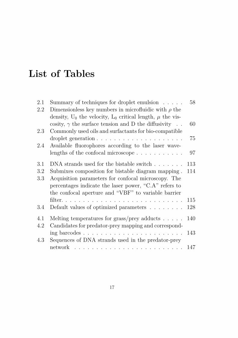
List of Tables
2.1 Summary of techniques for droplet emulsion . . . . . 582.2 Dimensionless key numbers in microfluidic with ρ the
density, U0 the velocity, L0 critical length, µ the vis-cosity, γ the surface tension and D the diffusivity . . 60
2.3 Commonly used oils and surfactants for bio-compatibledroplet generation . . . . . . . . . . . . . . . . . . . . 75
2.4 Available fluorophores according to the laser wave-lengths of the confocal microscope . . . . . . . . . . . 97
3.1 DNA strands used for the bistable switch . . . . . . . 1133.2 Submixes composition for bistable diagram mapping . 1143.3 Acquisition parameters for confocal microscopy. The
percentages indicate the laser power, “C.A” refers tothe confocal aperture and “VBF” to variable barrierfilter. . . . . . . . . . . . . . . . . . . . . . . . . . . . 115
3.4 Default values of optimized parameters . . . . . . . . 128
4.1 Melting temperatures for grass/prey adducts . . . . . 1404.2 Candidates for predator-prey mapping and correspond-
ing barcodes . . . . . . . . . . . . . . . . . . . . . . . 1434.3 Sequences of DNA strands used in the predator-prey
network . . . . . . . . . . . . . . . . . . . . . . . . . 147
17

18 LIST OF TABLES
Chapter 1
Introduction
Since its discovery in 1868 by Meischer [1], nucleic acid polymers,deoxyribonucleic acid (DNA) and ribonucleic acid (RNA) are amongthe most fascinating biomolecules. DNA carries out multiple tasksregarding the storage, process and expression of genetic information.First described as phosphorous-rich and lacking sulfur compounds,and contained within the nuclei of cells, it took 85 years before theelucidation of its structure by Franklin, Crick and Watson [2].
The robustness of Watson-Crick base-pairing, coupled with ad-vances in the solid-state synthesis of nucleic acids, has powered manyrevolutions in molecular biology: cloning [3], sequencing [4], poly-merase chain reaction [5], RNA interference [6] and recently CRISPR[7], a powerful tool for genome editing which is widely seen as a trig-ger of future biochemical, medical and possibly societal revolutions.
But in the past 3 decades, molecular engineers have also cometo realize that DNA could be used on its own to build and pro-gram at the nanoscale. So DNA computing was born and electrifiedthe scientific community. The community of DNA computing hassince grown considerably, extending beyond computing and morph-ing into the larger endeavor of “molecular programming” with twolofty goals: how can we program molecules to compute and controlmatters? What does it tell us about computation in the biologi-cal world? Actually, nature and molecular programmers face similar
19
20 CHAPTER 1. INTRODUCTION
conceptual constraints: they both need to make molecular circuitsthat use as little molecules as possible, while being robust and ver-satile and of course compliant with the law of physics. The gist ofmolecular programming is thus an unusual mixture of (obviously)chemistry and computer science, but also biology, physics, mathe-matics and information processing.
In this thesis I will introduce a new device for experimental map-ping of bifurcation diagrams of chemical reaction networks assembledwith the PEN DNA toolbox and show two examples of explorationin multi-dimensional parameter space. In chapter two, I will first in-troduce the basics of compartmentalization and microfluidics beforedescribing the microfluidic device developed for high throughput gen-eration of water-in-oil droplets with different contents, its design andmicro-fabrication, the technical challenges underlying the choice ofreagents, the strategy built to sort the droplets and their observationovertime. In Chapter 3 this process is applied to a bistable circuit toobtain its bifurcation diagram as a function of two parameters. Thesingularities of this map will be discussed. In Chapter 4 the sameprocess is upgraded and assigned to a predator-prey system, leadingto a three dimensional map. The complex behaviors displayed willbe analyzed according to the reactivity of the species involved in thecontext of small compartments.
1.1 Structure of nucleic acids
DNA consists of a sequence of monomeric units -nucleotides- show-ing a 2-deoxyribose coupled with a phosphate group on the carbon5 and a nucleobase on the carbon 1. The monomers are coupledby the hydroxyl in carbon 3 (C3) and the phosphate in carbon 5(C5) of another nucleotide, forming the primary structure: a DNAstrand with a succession of nucleotides (defined as the sequence ofthe strand). The secondary structure is a right handed double helicalshape, obtained when two complementary strands meet in solution
1.1. STRUCTURE OF NUCLEIC ACIDS 21
and passively bind (hybridize) to form rather rigid double helixes(Fig.1.1, a).
Several helical structures are found, starting from the B-DNA,the in vivo classical form. The A-DNA is quite similar to B-DNA,but shorter, and is found in dehydrated conditions. Z-DNA is a left-handed helix whose occurrence is function of the sequence. We willfocus here on the most common architecture, that is the B-DNA(Fig.1.1, b). This canonical structure shows two grooves: a 2.2 nmwide groove a 1.2 nm wide minor groove and a 2 nm wide groove,giving easier access to the bases for interacting agents.
In DNA, the supramolecular recognition and pairing between twocomplementary strands follows the celebrated Watson-Crick base-pairing rules: an adenine nucleotide faces a thymine and share twohydrogen bonds (H-bonds), while a cytosine residue faces a guanineone with 3 H-bonds (Fig.1.1, a). This, added to the covalent linkagebetween two nucleotides from the same strand give a direction tothe strands: from the free hydroxyl on C3 of the first nucleotide (3’end) to the phosphate group on C5 of the last one (5’ end). Twostrands are named antiparallel when their sequences are complemen-tary and parallel, but go on opposite direction (Fig.1.1, c). Thepitch of the helix contains 10.5 bases (3.32 nm) for a diameter of2 nm. The non-covalent bonding allows the duplex to de-hybridizeunder heat or chemical denaturing agents. The stability of the du-plex is ensured by the sum of H-bonds (10-20 kJ.mol-1 per H-bond)and the stacking occurring between the bases inside the helix (~10kJ.mol-1 per stacking), but other factors influence the stability, suchas the temperature and the amount of salts inside the medium. Asa negatively-charged molecule, the DNA structure is sensitive to theionic force of the medium, and in particular to the presence of Na+
and Mg2+.RNA shares the same backbone structure as DNA, except that
the sugar keeps its hydroxyl residue in C2, and the thymine is re-placed by an uracil motif. Because of the added constraints induced
22 CHAPTER 1. INTRODUCTION
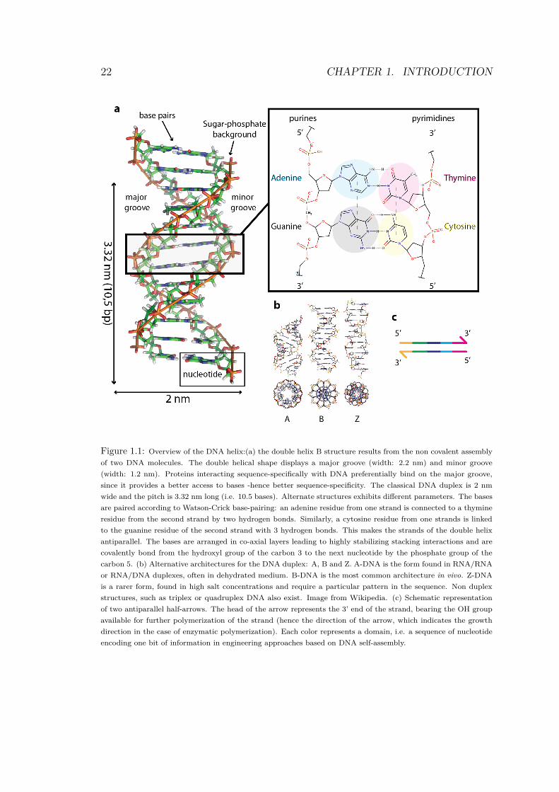
Figure 1.1: Overview of the DNA helix:(a) the double helix B structure results from the non covalent assembly
of two DNA molecules. The double helical shape displays a major groove (width: 2.2 nm) and minor groove
(width: 1.2 nm). Proteins interacting sequence-specifically with DNA preferentially bind on the major groove,
since it provides a better access to bases -hence better sequence-specificity. The classical DNA duplex is 2 nm
wide and the pitch is 3.32 nm long (i.e. 10.5 bases). Alternate structures exhibits different parameters. The bases
are paired according to Watson-Crick base-pairing: an adenine residue from one strand is connected to a thymine
residue from the second strand by two hydrogen bonds. Similarly, a cytosine residue from one strands is linked
to the guanine residue of the second strand with 3 hydrogen bonds. This makes the strands of the double helix
antiparallel. The bases are arranged in co-axial layers leading to highly stabilizing stacking interactions and are
covalently bond from the hydroxyl group of the carbon 3 to the next nucleotide by the phosphate group of the
carbon 5. (b) Alternative architectures for the DNA duplex: A, B and Z. A-DNA is the form found in RNA/RNA
or RNA/DNA duplexes, often in dehydrated medium. B-DNA is the most common architecture in vivo. Z-DNA
is a rarer form, found in high salt concentrations and require a particular pattern in the sequence. Non duplex
structures, such as triplex or quadruplex DNA also exist. Image from Wikipedia. (c) Schematic representation
of two antiparallel half-arrows. The head of the arrow represents the 3’ end of the strand, bearing the OH group
available for further polymerization of the strand (hence the direction of the arrow, which indicates the growth
direction in the case of enzymatic polymerization). Each color represents a domain, i.e. a sequence of nucleotide
encoding one bit of information in engineering approaches based on DNA self-assembly.
1.2. TOOLS FOR MOLECULAR PROGRAMMING 23
by the hydroxyl group, the structure of the base paired polymer ismostly A-DNA-like, with an exaggerated, deep major groove andwide minor groove. The structures found in RNA are various andcomplex, but the most interesting point is the number of tertiarystructures (stabilized with metal ions such as Mg2+), which are di-rectly involved in the numerous functions of RNA in cell: informationprocessing (translation, protein synthesis), regulation (microRNAs,riboswitches and riboregulators), RNA processing itself, viral mech-anism (reverse transcription, double stranded RNA), catalysis (ri-bozymes, ribosome). This ubiquity has led to the RNA hypothesishor origin of life [8].
1.2 Tools for molecular programming
The specificity of nucleic acids comes from their possibilities in termsof structure and reactivity. Indeed, the first remarkable point isthe controlled self-assembly, or hybridization: two complementaryDNA strands will spontaneously assemble when they meet, followingWatson-Crick base-pairing rules (Fig.1.2, a). The stability of theduplex is expressed as a sum of all interactions of the base pairs andstacking. The melting temperature (Tmelt) of a given duplex (orsometime by extension for a single sequence, assuming it is pairedwith its perfect complementary strand) is defined as the temperaturerequired for half of the population to be single stranded. The Tmelttherefore depends also on the concentration of the strand in solutionsand the salinity of the buffer (which must be specified for the Tmeltvalue to make sense).
Currently, our understanding of the base-pairing self-assembly isquite limited, even for a «simple» hybridization. The most usedmodel to describe the transition from single stranded DNA (ssDNA)to double stranded DNA (dsDNA) is a coarse-grained nearest neigh-bor model (n-n) proposed by SantaLucia et al. [9]. Finer model suchas force field include much more degrees of freedom, and are thus
24 CHAPTER 1. INTRODUCTION
impractical for computational purposes. The model by SantaLuciareproduces the experimental melting temperatures for duplexes upto 16 base pairs (bp) with only 2.3 oK deviation. In the n-n model,stability is defined in terms of two successive base pair doublets.The effect of base-pairing, stacking and solvatation will be consid-ered for each doublet and the stability is then calculated for eachsequence. An useful approach relies on the two-state melting the-ory (which assume the absence of significant intermediates betweenfully dissociated state and fully bound state during the hybridization-dehybridization reaction):
[AB][A] + [B]
= exp(≠β(∆HAB ≠ T∆SAB))
where ∆HAB and ∆SAB are the duplex melting transition en-thalpy and entropy, coming from the sum of all n-n interactions andbase-pairing, while β is the nucleation parameter containing the con-centration dependence plus the external factors involved in duplexformation. Once all nearest neighbor parameters are tabulated, thissimple approach can predict the approximate Tmelt of arbitrary du-plex, but the two-states model is not fine-grained enough to thor-oughly study the dynamics of DNA systems, neither can it predictthe effects due to the topology/geometry.
An application of DNA pairing programmability is the modula-tion of the kinetics of strand exchange of a duplex with a ssDNAinvasion strand, using an overhang adjacent to the helical domainof the duplex. This toehold architecture (Fig.1.2, 2a) was proposedfor the first time by Yurke et al. [10] in a paper describing a «DNAtweezer». The tweezer is a molecular motor acting like a scissor usingDNA strands as fuel. The core of the tweezer on its open state ismade of three strands A, B and C. B and C partially hybridize on A,occupying 18 bases each, 24 dangling bases are left on B (5’ end) andC (3’ end) (Fig.1.3, green, a). The F strands closes the tweezer byhybridizing the dangling edges of B and C (Fig.1.3, green, b), Thus,
1.2. TOOLS FOR MOLECULAR PROGRAMMING 25
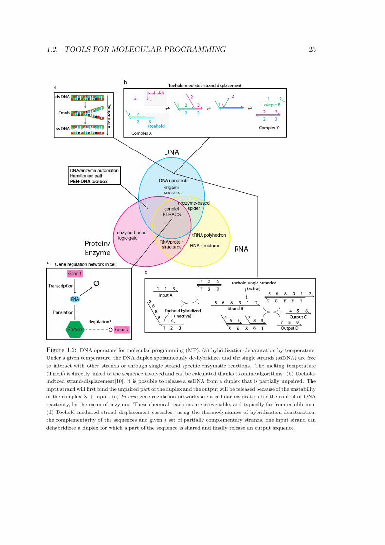
Figure 1.2: DNA operators for molecular programming (MP). (a) hybridization-denaturation by temperature.
Under a given temperature, the DNA duplex spontaneously de-hybridizes and the single strands (ssDNA) are free
to interact with other strands or through single strand specific enzymatic reactions. The melting temperature
(Tmelt) is directly linked to the sequence involved and can be calculated thanks to online algorithms. (b) Toehold-
induced strand-displacement[10]: it is possible to release a ssDNA from a duplex that is partially unpaired. The
input strand will first bind the unpaired part of the duplex and the output will be released because of the unstability
of the complex X + input. (c) In vivo gene regulation networks are a cellular inspiration for the control of DNA
reactivity, by the mean of enzymes. These chemical reactions are irreversible, and typically far from-equilibrium.
(d) Toehold mediated strand displacement cascades: using the thermodynamics of hybridization-denaturation,
the complementarity of the sequences and given a set of partially complementary strands, one input strand can
dehybridizee a duplex for which a part of the sequence is shared and finally release an output sequence.
26 CHAPTER 1. INTRODUCTION
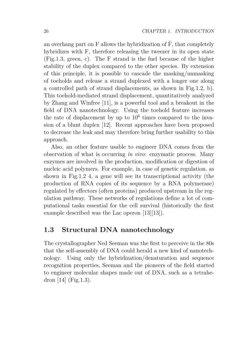
an overhang part on F allows the hybridization of F, that completelyhybridizes with F, therefore releasing the tweezer in its open state(Fig.1.3, green, c). The F strand is the fuel because of the higherstability of the duplex compared to the other species. By extensionof this principle, it is possible to cascade the masking/unmaskingof toeholds and release a strand duplexed with a longer one alonga controlled path of strand displacements, as shown in Fig.1.2, b).This toehold-mediated strand displacement, quantitatively analyzedby Zhang and Winfree [11], is a powerful tool and a breakout in thefield of DNA nanotechnology. Using the toehold feature increasesthe rate of displacement by up to 106 times compared to the inva-sion of a blunt duplex [12]. Recent approaches have been proposedto decrease the leak and may therefore bring further usability to thisapproach.
Also, an other feature usable to engineer DNA comes from theobservation of what is occurring in vivo: enzymatic process. Manyenzymes are involved in the production, modification or digestion ofnucleic acid polymers. For example, in case of genetic regulation, asshown in Fig.1.2 4, a gene will see its transcriptional activity (theproduction of RNA copies of its sequence by a RNA polymerase)regulated by effectors (often proteins) produced upstream in the reg-ulation pathway. These networks of regulations define a lot of com-putational tasks essential for the cell survival (historically the firstexample described was the Lac operon [13][13]).
1.3 Structural DNA nanotechnology
The crystallographer Ned Seeman was the first to perceive in the 80sthat the self-assembly of DNA could herald a new kind of nanotech-nology. Using only the hybridization/denaturation and sequencerecognition properties, Seeman and the pioneers of the field startedto engineer molecular shapes made out of DNA, such as a tetrahe-dron [14] (Fig.1.3).
1.3. STRUCTURAL DNA NANOTECHNOLOGY 27
Seeman hypothesized that DNA strands with the right sequencesought to self-assemble into a 3D grid, forming a rigid framework thathe expected to use to firmly latch proteins. In other words, he onlyneeded to make a 3D DNA crystal to bypass protein crystals. It tookNed Seeman and colleagues many years to demonstrate the first 2DDNA crystal [15] from the initial publication of the tetrahedron de-sign and ten more years to achieve his dream of a 3D DNA crystal(structural studies of proteins are still undergoing). But meanwhile,the idea of using synthetic DNA for non-biological purposes had blos-somed into a burgeoning field that discovered how to fold a plethoraof nanostructures: smileys and maps [16], twisted jars and meshedspheres [17], Moebius strips [18], the qwerty keyboard and its emoti-cons... Much of this revolution was fueled by the invention of DNAorigamis by Paul Rothemund [16] (Fig.1.3): a technique to fold along DNA scaffold into a prescribed thanks to the assistance of aswarm of helping strands called staples. This expansion reached thefield of robotics and lead to the development of tweezers [10] or DNAwalkers, such as the DNA spider [19] (Fig.1.3)
28 CHAPTER 1. INTRODUCTION
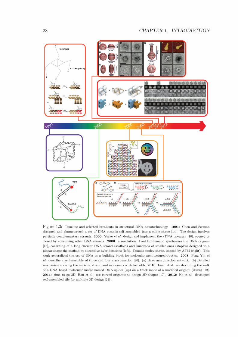
Figure 1.3: Timeline and selected breakouts in structural DNA nanotechnology. 1991: Chen and Seeman
designed and characterized a set of DNA strands self assembled into a cubic shape [14]. The design involves
partially complementary strands. 2000: Yurke et al. design and implement the «DNA tweezer» [10], opened or
closed by consuming other DNA strands. 2006: a revolution. Paul Rothemund synthesizes the DNA origami
[16], consisting of a long circular DNA strand (scaffold) and hundreds of smaller ones (staples) designed to a
planar shape the scaffold by successive hybridizations (left). Famous smiley shape, imaged by AFM (right). This
work generalized the use of DNA as a building block for molecular architecture/robotics. 2008: Peng Yin et
al. describe a self-assembly of three and four arms junction [20]. (a) three arm junction network. (b) Detailed
mechanism showing the initiator strand and monomers with toeholds. 2010: Lund et al. are describing the walk
of a DNA based molecular motor named DNA spider (up) on a track made of a modified origami (down) [19].
2011: time to go 3D: Han et al. use curved origamis to design 3D shapes [17]. 2012: Ke et al. developed
self-assembled tile for multiple 3D design [21] .
1.4. MOLECULAR PROGRAMMING 29
1.4 Molecular programming
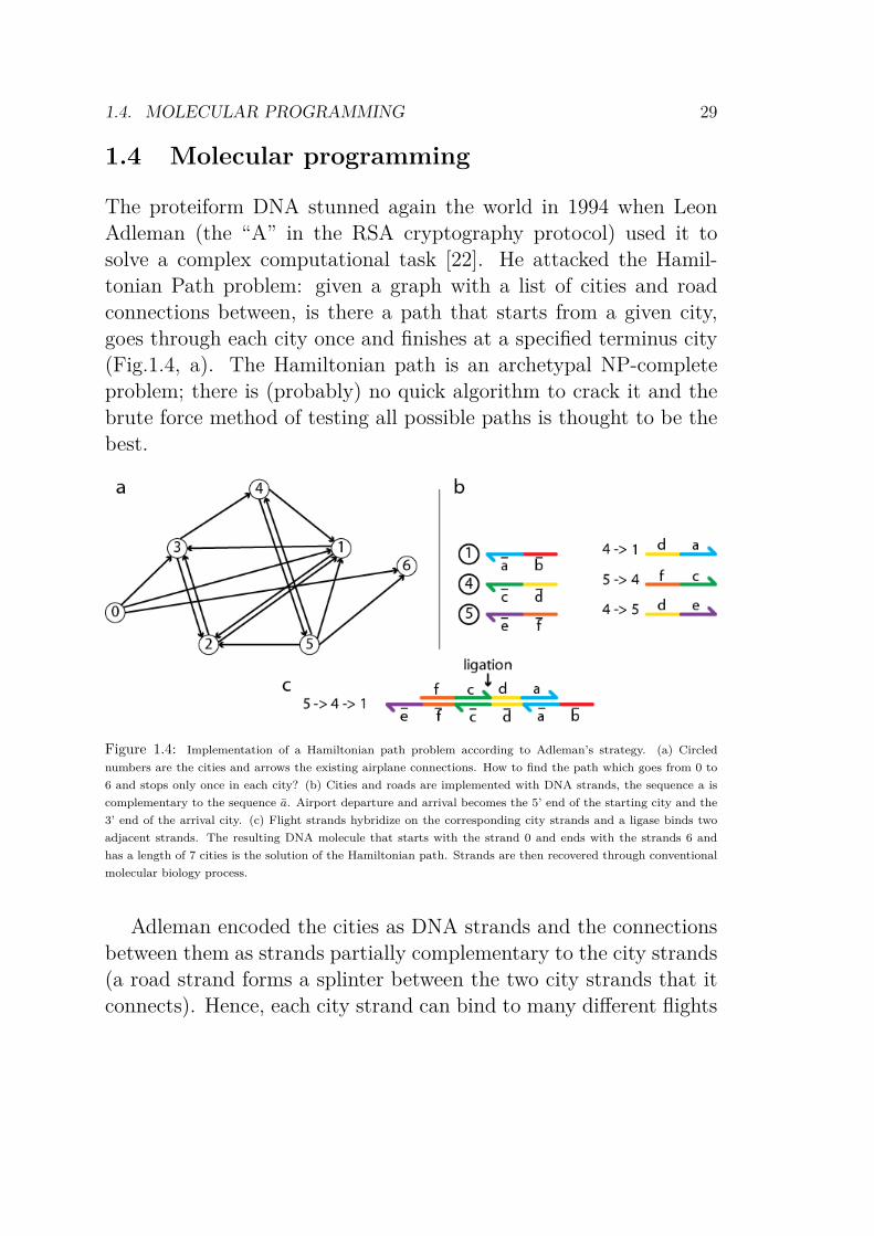
The proteiform DNA stunned again the world in 1994 when LeonAdleman (the “A” in the RSA cryptography protocol) used it tosolve a complex computational task [22]. He attacked the Hamil-tonian Path problem: given a graph with a list of cities and roadconnections between, is there a path that starts from a given city,goes through each city once and finishes at a specified terminus city(Fig.1.4, a). The Hamiltonian path is an archetypal NP-completeproblem; there is (probably) no quick algorithm to crack it and thebrute force method of testing all possible paths is thought to be thebest.
Figure 1.4: Implementation of a Hamiltonian path problem according to Adleman’s strategy. (a) Circled
numbers are the cities and arrows the existing airplane connections. How to find the path which goes from 0 to
6 and stops only once in each city? (b) Cities and roads are implemented with DNA strands, the sequence a is
complementary to the sequence a. Airport departure and arrival becomes the 5’ end of the starting city and the
3’ end of the arrival city. (c) Flight strands hybridize on the corresponding city strands and a ligase binds two
adjacent strands. The resulting DNA molecule that starts with the strand 0 and ends with the strands 6 and
has a length of 7 cities is the solution of the Hamiltonian path. Strands are then recovered through conventional
molecular biology process.
Adleman encoded the cities as DNA strands and the connectionsbetween them as strands partially complementary to the city strands(a road strand forms a splinter between the two city strands that itconnects). Hence, each city strand can bind to many different flights
30 CHAPTER 1. INTRODUCTION
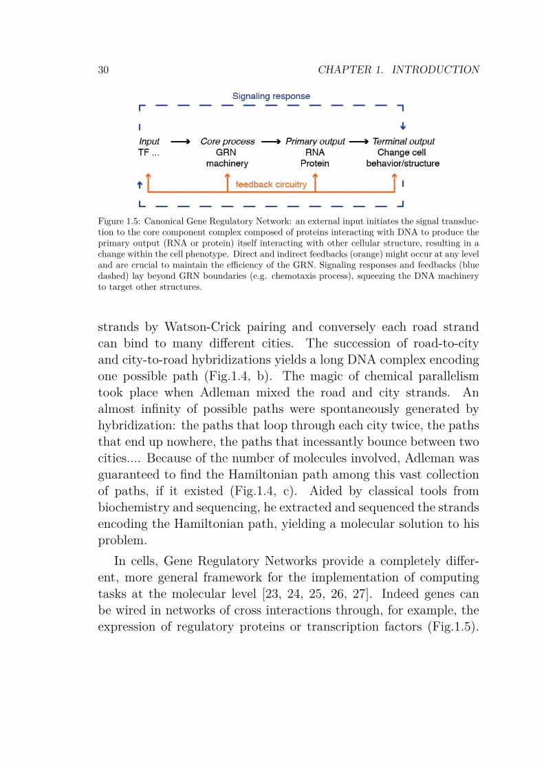
Figure 1.5: Canonical Gene Regulatory Network: an external input initiates the signal transduc-tion to the core component complex composed of proteins interacting with DNA to produce theprimary output (RNA or protein) itself interacting with other cellular structure, resulting in achange within the cell phenotype. Direct and indirect feedbacks (orange) might occur at any leveland are crucial to maintain the efficiency of the GRN. Signaling responses and feedbacks (bluedashed) lay beyond GRN boundaries (e.g. chemotaxis process), squeezing the DNA machineryto target other structures.
strands by Watson-Crick pairing and conversely each road strandcan bind to many different cities. The succession of road-to-cityand city-to-road hybridizations yields a long DNA complex encodingone possible path (Fig.1.4, b). The magic of chemical parallelismtook place when Adleman mixed the road and city strands. Analmost infinity of possible paths were spontaneously generated byhybridization: the paths that loop through each city twice, the pathsthat end up nowhere, the paths that incessantly bounce between twocities.... Because of the number of molecules involved, Adleman wasguaranteed to find the Hamiltonian path among this vast collectionof paths, if it existed (Fig.1.4, c). Aided by classical tools frombiochemistry and sequencing, he extracted and sequenced the strandsencoding the Hamiltonian path, yielding a molecular solution to hisproblem.
In cells, Gene Regulatory Networks provide a completely differ-ent, more general framework for the implementation of computingtasks at the molecular level [23, 24, 25, 26, 27]. Indeed genes canbe wired in networks of cross interactions through, for example, theexpression of regulatory proteins or transcription factors (Fig.1.5).
1.4. MOLECULAR PROGRAMMING 31
Only very recently have similar general chemical reaction network-ing frameworks been described ex vivo [26, 27]. Similar to whathas been done for neural networks, whose fundamental features havebeen abstracted into the computational framework of Artificial Neu-ral Network circuits (ANN), these approaches focus on the most im-portant dynamic properties of biological GRN to define functionalin vitro models. Therefore it has become possible to construct invitro reaction networks with well-controlled topologies [25], targetinga precise dynamic function and reproducing biological architectures.Extracting the essential dynamic features of GRN from the viewpointof dynamical systems, one is left with a set of collective moleculartransformations that can be linked in such a way that the productof one either activates or inhibits the production of another [26, 28].A second important feature is that the network linking these reac-tions is hardcoded in the sequence of stable DNA strands (genes andpromoters). The long-term stability of these DNA species stands insharp contrast with the dynamic behavior of their products (RNAand proteins) that are constantly produced and degraded/diluted.Therefore, the maintenance of a constant flux of energy through thesystem, together with a precisely controlled reactivity landscape arealso essential features of GRN. While genetic regulation in cells usesa bewilderingly complex molecular machinery, these three essentialcharacteristics have served as inspiration in a small number of in vitrosimplified schemes able to implement artificial regulatory networks:RTRACS, the genelets approach and the PEN DNA toolbox.
1.4.1 RTRACS
One example of molecular program involving DNA, RNA and en-zymes, inspired by retroviral replication was proposed by the group ofProf Suyama at the University of Tokyo. The Reverse-transcription-and-TRanscription-based Autonomous Computing System (RTRACS)processes a RNA input into a RNA output thanks to DNA-and-
32 CHAPTER 1. INTRODUCTION
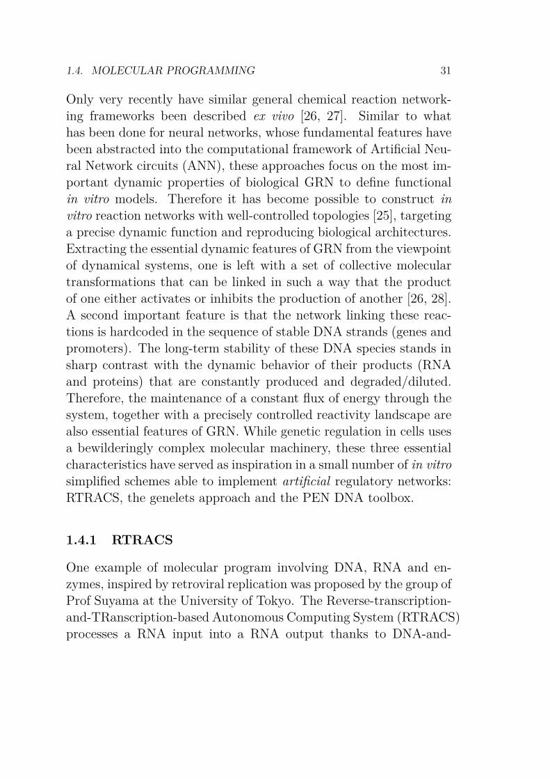
enzymes machinery (Fig.1.6, a). The hardware is composed of a re-verse transcriptase to transform the input into the equivalent DNAsequence, a DNA polymerase for DNA strand processing and a com-bination of RNA polymerase and DNA-RNA converter to generatethe output. The system keeps its dynamics thanks to the RNase.
Figure 1.6: RTRACS: a RNA/DNA/enzyme molecular programming machinery. (a) Global framework: a RNA
input is processed after reverse transcription in DNA and the molecular computation ends with the expression
of a RNA output by the T7 RNA polymerase (T7 RNA Pol). (b) Implementation of an AND gate: wavy lines
stand for RNA strands and straight ones show DNA strands. Two RNA inputs lead to the intermediate species
1 (Intm 1), fulfilling the condition imposed by the AND gate (i.e. both inputs are required to express the DNA
sequence O3). Intm1 then partially hybridizes on the DNA converter to Intm2, on which the T 7 sequence is single
stranded, generating a substrate for the DNA Polymerase (DNA Pol). Intm1 and the O4O5 sequences are hiding
the rest of the converter from DNA Pol. The goal is the production of Intm3, the trigger of output. Indeed the T7
sequence is the promoter of T7 RNA Pol, which recognizes the Intm3 pattern and synthesizes the RNA output.
The first experimental implementation was an AND gate [29](Fig.1.6, b). The AND gate needs both inputs to deliver the output.
1.4. MOLECULAR PROGRAMMING 33
The strategy lays in the condition of generation of the Intm3, theprecursor of the output. The sequence O3 is the key to the outputproduction: given the sequence of the DNA converter, knowing thatthe pattern for the T7 RNA Pol has to have its promoter doublestranded (adduct T7 T7), only the sequence O3 allows the polymer-ization along the converter to get the T7 strand. Moreover, becausethe primer DNA is O1, input 1 and 2 are required to produce theDNA strand containing O3 at its 3’ end. Later, a NAND gate wasexperimentally implemented [30] and a more general logic gate wasdeveloped as a way to implement other logic functions [31]. It shouldbe possible to implement oscillators [32], or more complex systemsmimicking cell computation. As a step toward artificial cells, someof these systems were embedded in liposomes [27].
1.4.2 Genelets
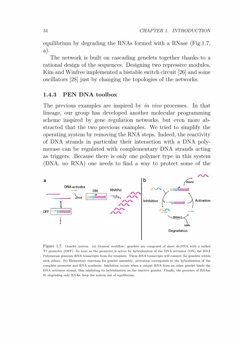
Closer to the real cell information management, but still avoidingprotein translation, the genelet MP is mimicking the in vivo regula-tion of genes as a the substrate of computation. Such an approach,developed by Kim and al [26], is not a complete mimic of what ishappening in cell, but more an analogy. Here also, the outputs areRNA strands, generated from a DNA-engraved program thanks to aRNA polymerase. A RNase degrades the inputs and outputs over-time, sustaining the system out of equilibrium. The computationstops after exhaustion of the NTP fuel.
A genelet is defined as a duplex of DNA containing two domains:the output sequence and nicked promoter. The genelet can be off oron if the promoter sequence is, respectively, partially or fully doublestranded (Fig.1.7, a). The activation of a genelet by the hybridizationof the DNA activator on the OFF genelet starts the production ofthe output with the RNA polymerase. The inhibition mechanismoccurs when the promoter sequence binds to a complementary RNAdesigned for that purpose. As for RTRACS, the system is kept out of
34 CHAPTER 1. INTRODUCTION
equilibrium by degrading the RNAs formed with a RNase (Fig.1.7,a).
The network is built on cascading genelets together thanks to arational design of the sequences. Designing two repressive modules,Kim and Winfree implemented a bistable switch circuit [26] and someoscillators [28] just by changing the topologies of the networks.
1.4.3 PEN DNA toolbox
The previous examples are inspired by in vivo processes. In thatlineage, our group has developed another molecular programmingscheme inspired by gene regulation networks, but even more ab-stracted that the two previous examples. We tried to simplify theoperating system by removing the RNA steps. Indeed, the reactivityof DNA strands in particular their interaction with a DNA poly-merase can be regulated with complementary DNA strands actingas triggers. Because there is only one polymer type in this system(DNA, no RNA) one needs to find a way to protect some of the
Figure 1.7: Genelet system. (a) General workflow: genelets are composed of short ds-DNA with a nicked
T7 promoter (OFF). As soon as the promoter is active by hybridization of the DNA activator (ON) the RNA
Polymerase generate RNA transcripts from the template. These RNA transcripts will connect the genelets within
each others. (b) Elementary reactions for genelet assembly: activation corresponds to the hybridization of the
complete promoter and RNA synthesis. Inhibition occurs when a output RNA from an other genelet binds the
DNA activator strand, thus inhibiting its hybridization on the inactive genelet. Finally, the presence of RNAse
H -degrading only RNAs- keep the system out of equilibrium.
1.4. MOLECULAR PROGRAMMING 35
species, while letting others be dynamically degraded. As with theother programs, it is possible to cascade the reactions by a thoroughdesign of the sequences involved.
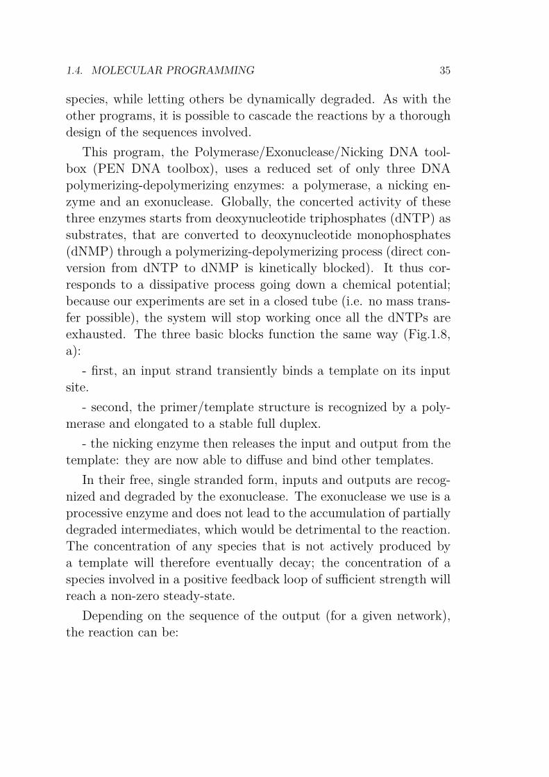
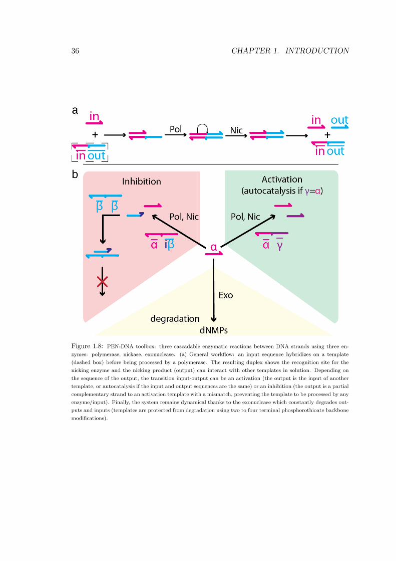
This program, the Polymerase/Exonuclease/Nicking DNA tool-box (PEN DNA toolbox), uses a reduced set of only three DNApolymerizing-depolymerizing enzymes: a polymerase, a nicking en-zyme and an exonuclease. Globally, the concerted activity of thesethree enzymes starts from deoxynucleotide triphosphates (dNTP) assubstrates, that are converted to deoxynucleotide monophosphates(dNMP) through a polymerizing-depolymerizing process (direct con-version from dNTP to dNMP is kinetically blocked). It thus cor-responds to a dissipative process going down a chemical potential;because our experiments are set in a closed tube (i.e. no mass trans-fer possible), the system will stop working once all the dNTPs areexhausted. The three basic blocks function the same way (Fig.1.8,a):
- first, an input strand transiently binds a template on its inputsite.
- second, the primer/template structure is recognized by a poly-merase and elongated to a stable full duplex.
- the nicking enzyme then releases the input and output from thetemplate: they are now able to diffuse and bind other templates.
In their free, single stranded form, inputs and outputs are recog-nized and degraded by the exonuclease. The exonuclease we use is aprocessive enzyme and does not lead to the accumulation of partiallydegraded intermediates, which would be detrimental to the reaction.The concentration of any species that is not actively produced bya template will therefore eventually decay; the concentration of aspecies involved in a positive feedback loop of sufficient strength willreach a non-zero steady-state.
Depending on the sequence of the output (for a given network),the reaction can be:
36 CHAPTER 1. INTRODUCTION
Figure 1.8: PEN-DNA toolbox: three cascadable enzymatic reactions between DNA strands using three en-
zymes: polymerase, nickase, exonuclease. (a) General workflow: an input sequence hybridizes on a template
(dashed box) before being processed by a polymerase. The resulting duplex shows the recognition site for the
nicking enzyme and the nicking product (output) can interact with other templates in solution. Depending on
the sequence of the output, the transition input-output can be an activation (the output is the input of another
template, or autocatalysis if the input and output sequences are the same) or an inhibition (the output is a partial
complementary strand to an activation template with a mismatch, preventing the template to be processed by any
enzyme/input). Finally, the system remains dynamical thanks to the exonuclease which constantly degrades out-
puts and inputs (templates are protected from degradation using two to four terminal phosphorothioate backbone
modifications).
1.4. MOLECULAR PROGRAMMING 37
• an activation (if the output of this node is the input of an otherone, Fig.1.8, b)
• an autocatalysis (in the special case where input and outputhave the same sequence)
• or can correspond to the generation of an inhibitor when theoutput released is partially complementary to a target templatebut have some mismatches at the 3’ end, hence do not triggerpolymerization (Fig.1.10, a).
These inhibitor molecules are also dynamic because they are pro-duced (by the action of the polymerase and nicking enzyme on othertemplates) and subject to degradation (by the exonuclease, whenthey are in single-strand, free-floating form). The modular construc-tion of the system allows the designer to “wire” the templates to-gether so that they control each other’s activity by exchanging smallactivators or inhibitors. This modularity is central to the building ofcomplex systems; it allows the cascading of elementary modules intoprecise network topologies. The cascadability is greatly facilitated bythe fact that the DNA strands being exchanged are small (typically10 to 20 bases long) and do not form complicated secondary struc-tures. This range of length theoretically limits the number of speciesthat can be mixed together before unwanted interactions start tooccur (see below). Although for medium scale, biologically relevantnetworks, choosing DNA sequences while avoiding unwanted inter-actions is entirely feasible. With a correct selection of the sequences,the product of any reaction can be used as the activator of any othermodule. For that, it is enough to design (and order to a DNA-synthesizing company) the corresponding templates with the ad hocsequences and modifications. In a similar way, it is always possible todefine an inhibiting module targeting any activation template. Thismodularity opens the road to the rational molecular encoding of avariety of dynamic behaviors.
38 CHAPTER 1. INTRODUCTION
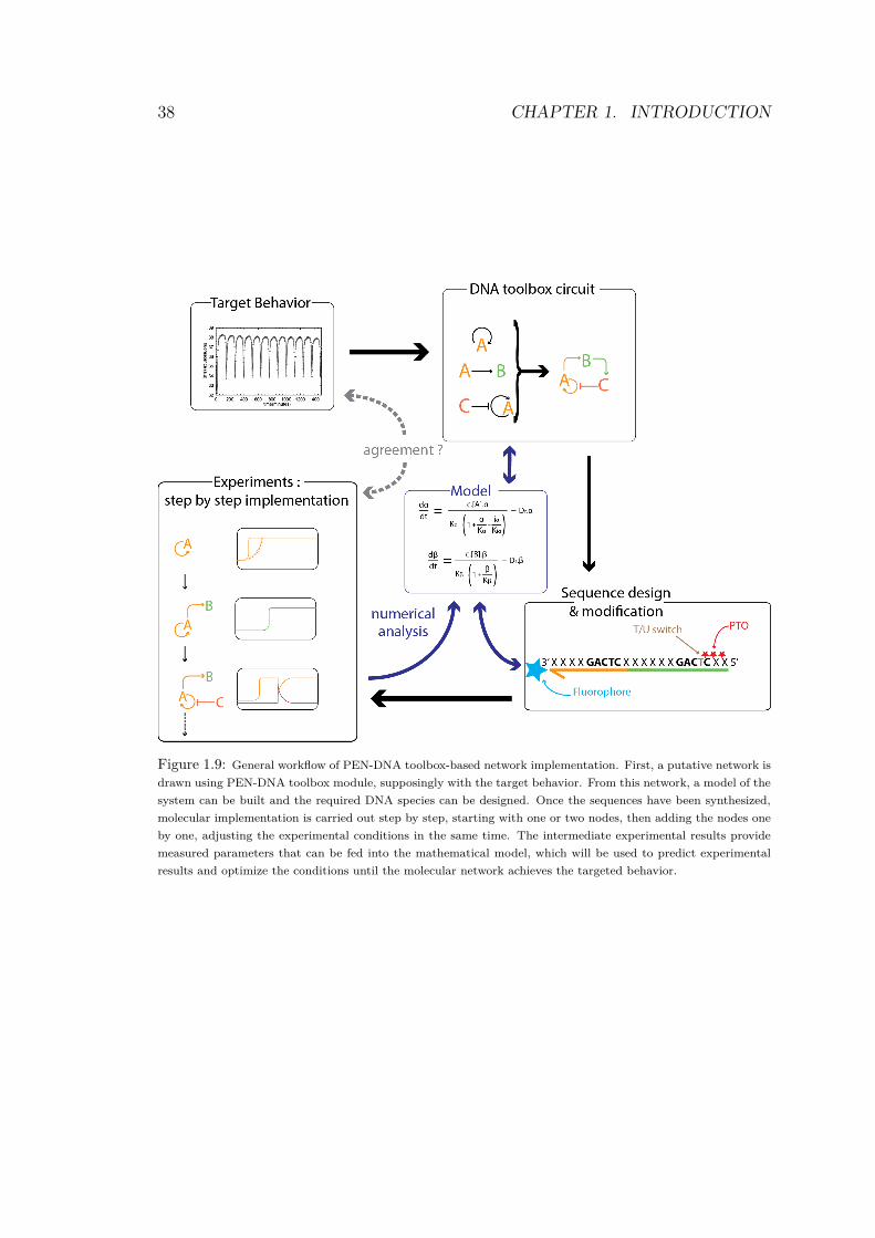
Figure 1.9: General workflow of PEN-DNA toolbox-based network implementation. First, a putative network is
drawn using PEN-DNA toolbox module, supposingly with the target behavior. From this network, a model of the
system can be built and the required DNA species can be designed. Once the sequences have been synthesized,
molecular implementation is carried out step by step, starting with one or two nodes, then adding the nodes one
by one, adjusting the experimental conditions in the same time. The intermediate experimental results provide
measured parameters that can be fed into the mathematical model, which will be used to predict experimental
results and optimize the conditions until the molecular network achieves the targeted behavior.
1.4. MOLECULAR PROGRAMMING 39
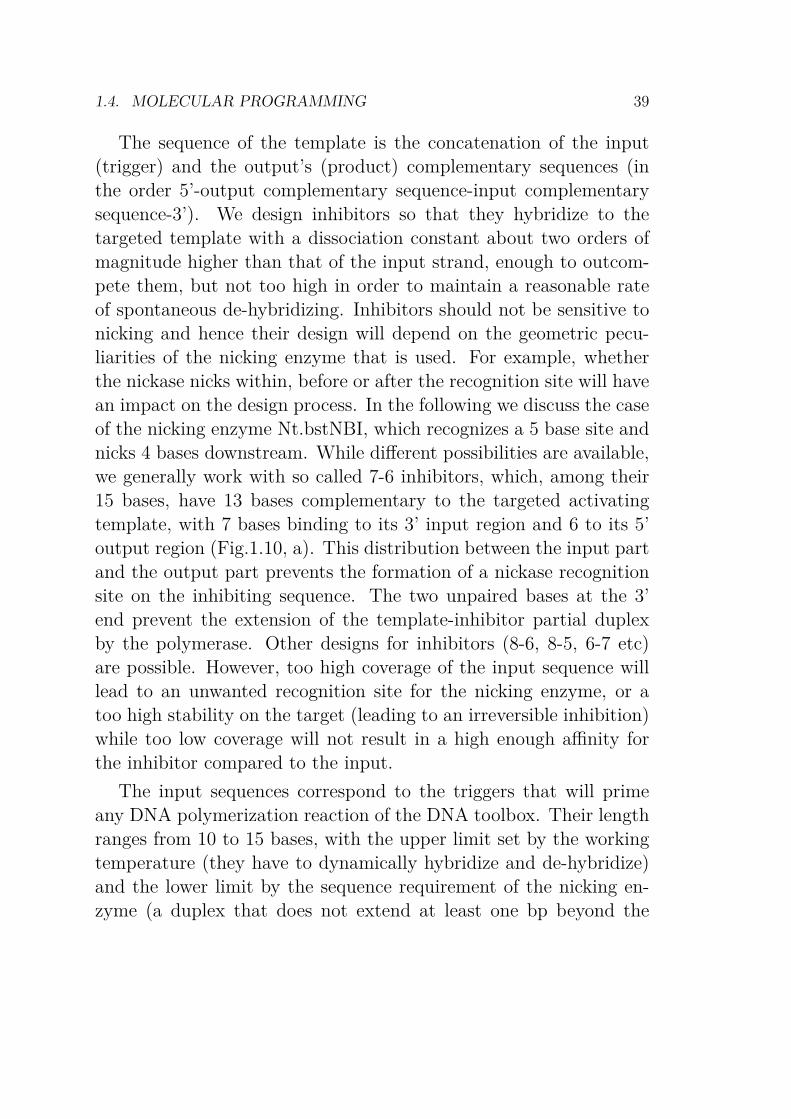
The sequence of the template is the concatenation of the input(trigger) and the output’s (product) complementary sequences (inthe order 5’-output complementary sequence-input complementarysequence-3’). We design inhibitors so that they hybridize to thetargeted template with a dissociation constant about two orders ofmagnitude higher than that of the input strand, enough to outcom-pete them, but not too high in order to maintain a reasonable rateof spontaneous de-hybridizing. Inhibitors should not be sensitive tonicking and hence their design will depend on the geometric pecu-liarities of the nicking enzyme that is used. For example, whetherthe nickase nicks within, before or after the recognition site will havean impact on the design process. In the following we discuss the caseof the nicking enzyme Nt.bstNBI, which recognizes a 5 base site andnicks 4 bases downstream. While different possibilities are available,we generally work with so called 7-6 inhibitors, which, among their15 bases, have 13 bases complementary to the targeted activatingtemplate, with 7 bases binding to its 3’ input region and 6 to its 5’output region (Fig.1.10, a). This distribution between the input partand the output part prevents the formation of a nickase recognitionsite on the inhibiting sequence. The two unpaired bases at the 3’end prevent the extension of the template-inhibitor partial duplexby the polymerase. Other designs for inhibitors (8-6, 8-5, 6-7 etc)are possible. However, too high coverage of the input sequence willlead to an unwanted recognition site for the nicking enzyme, or atoo high stability on the target (leading to an irreversible inhibition)while too low coverage will not result in a high enough affinity forthe inhibitor compared to the input.
The input sequences correspond to the triggers that will primeany DNA polymerization reaction of the DNA toolbox. Their lengthranges from 10 to 15 bases, with the upper limit set by the workingtemperature (they have to dynamically hybridize and de-hybridize)and the lower limit by the sequence requirement of the nicking en-zyme (a duplex that does not extend at least one bp beyond the
40 CHAPTER 1. INTRODUCTION
s
Figure 1.10: Typical set of DNA strands necessary for a network when using Nt.BstNBI as the nicking enzyme
and their biochemistry within the DNA toolbox. (a) The Nt.BstNBI recognition site is shown in violet. The
template illustrated here is an autocatalyst triggered by α, and producing itself. Regarding the 7-6 inhibitor, two
mismatches are introduced at the 3’ end (red). The nomenclature comes from its position on the template: 7
bases binding to the input position and 6 bases to the output position.
1.4. MOLECULAR PROGRAMMING 41
recognition site is poorly processed by the nicking enzyme Nt.BstNBI,which cuts 4 bases downstream of its 5 base cognate sequence; henceinputs should have at least 10 bases). We typically use templatesthat are 11 bases long, in which 5 bases -corresponding to the recog-nition site- are fixed. Considering two DNA species to be distinct ifat least two of their bases are different, we can design more than 1000(45) different sequences from which a number should be discarded,using the following filters:
• the sequence (or the dual repeat) should not contain a parasiticnicking enzyme recognition site,
• the melting temperature of the sequence should be neither toohigh nor too low and typically close to the experimental tem-perature (i.e. should not be composed of too many C/G norA/T),
• the sequence should not allow stable secondary structures toform (this could lead, among other uncontrolled behaviors, toself-triggering in the case of a self-fold with a matched 3’ end) orunwanted interactions between two input species (primer dimer-ization). Several softwares can be used to predict the formationof secondary structures, such as the NUPACK software suite[33].
In fact, adjusting the melting temperature of the various DNA speciesinvolved in the network is one way to tune the circuit parameters ata local level (together with changing the templates’ concentrations).Therefore, those adjustments can be very important for the properfunction of the network. However, it has been reported that theperformance of a given primer in terms of amplification is not sim-ply related to its thermodynamic stability (Fig.1.11). The sequencedependence of exponential DNA amplification [34] is still not wellunderstood, but has been the subject of a recent study [31], in which
42 CHAPTER 1. INTRODUCTION
the authors characterized the performance of about 400 autocat-alytic templates. They notably observed that GA or AG dimer-richsequences were poorly performing. The rules proposed by Qian etal. have to be considered for future design of autocatalytic templates[?].
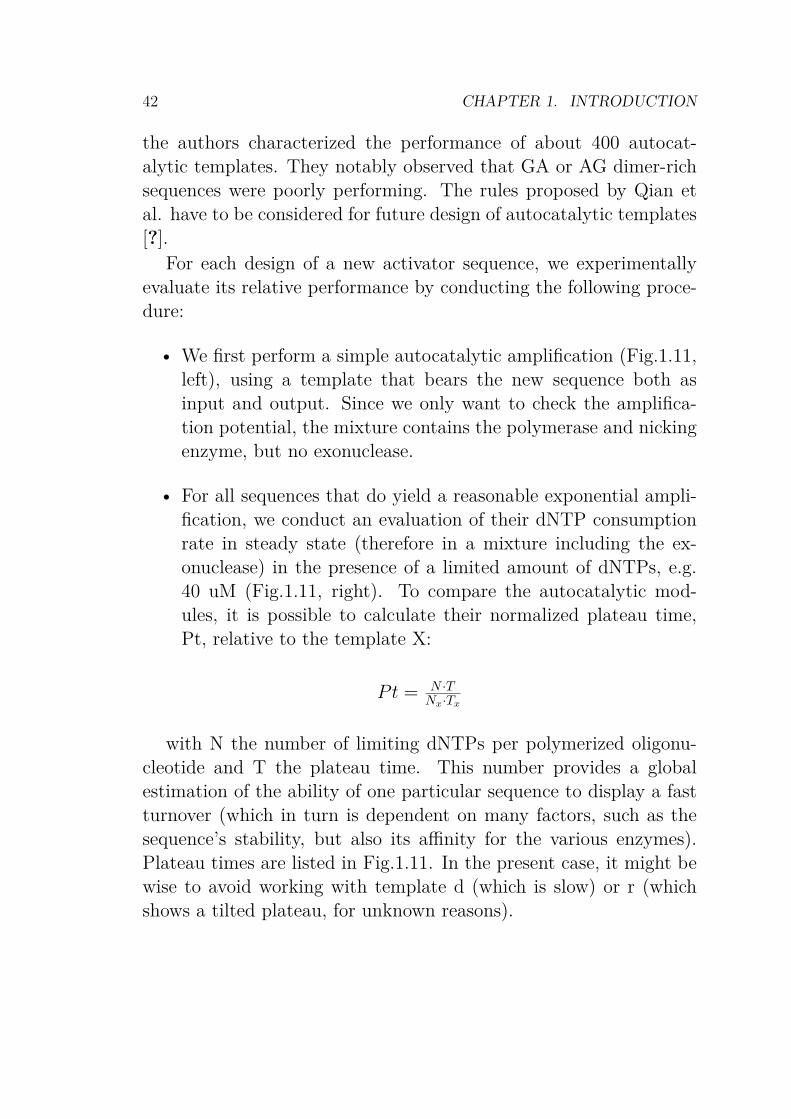
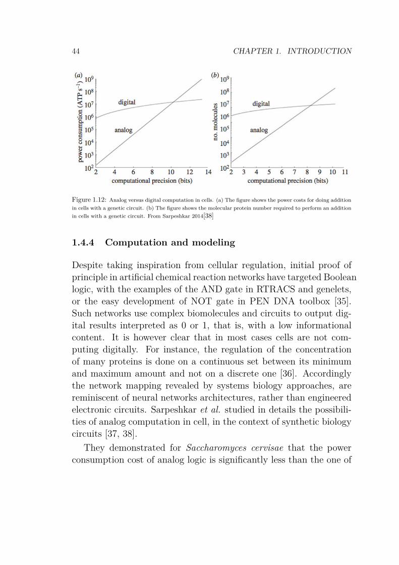
For each design of a new activator sequence, we experimentallyevaluate its relative performance by conducting the following proce-dure:
• We first perform a simple autocatalytic amplification (Fig.1.11,left), using a template that bears the new sequence both asinput and output. Since we only want to check the amplifica-tion potential, the mixture contains the polymerase and nickingenzyme, but no exonuclease.
• For all sequences that do yield a reasonable exponential ampli-fication, we conduct an evaluation of their dNTP consumptionrate in steady state (therefore in a mixture including the ex-onuclease) in the presence of a limited amount of dNTPs, e.g.40 uM (Fig.1.11, right). To compare the autocatalytic mod-ules, it is possible to calculate their normalized plateau time,Pt, relative to the template X:
Pt = N ·TNx·Tx
with N the number of limiting dNTPs per polymerized oligonu-cleotide and T the plateau time. This number provides a globalestimation of the ability of one particular sequence to display a fastturnover (which in turn is dependent on many factors, such as thesequence’s stability, but also its affinity for the various enzymes).Plateau times are listed in Fig.1.11. In the present case, it might bewise to avoid working with template d (which is slow) or r (whichshows a tilted plateau, for unknown reasons).
1.4. MOLECULAR PROGRAMMING 43
Template Sequence (5Õ æ 3Õ) Product TmNormalized
Plateau Timed CACAGACUCACCACAGACTCAC 38.3°C 2.66e CACTGACUCTGCACTGACTCTG 38.4°C 0.86n CTGTGACUCTGCTGTGACTCTG 38.4°C 1.21r CTCAGACUCAGCTCAGACTCAG 37.3°C 0.87w CTCTGACUCTGCTCTGACTCTG 37.3°C 0.73x CTTGGACUCTGCTTGGACTCTG 38.3°C 1
Figure 1.11: Comparing the performance of various autocatalytic templates by measuring the turnover of
dNTPs. The left panel shows the signal amplification phase using autocatalytic templates d, e, n, r, w and x.
The right panel shows typical plateaus in the fluorescence signal indicating that the production and destruction
of DNA species by the module has reached a dynamic equilibrium, which ends when the dNTPs are exhausted
and the signal drops back to its initial value. The duration of the plateau gives an estimation of the of the ability
of the sequence do dissipate energy by fast enzymatic turnovers. The table lists the sequences of the templates
(modifications are not shown), the Tm of their products and the normalized plateau time.
44 CHAPTER 1. INTRODUCTION
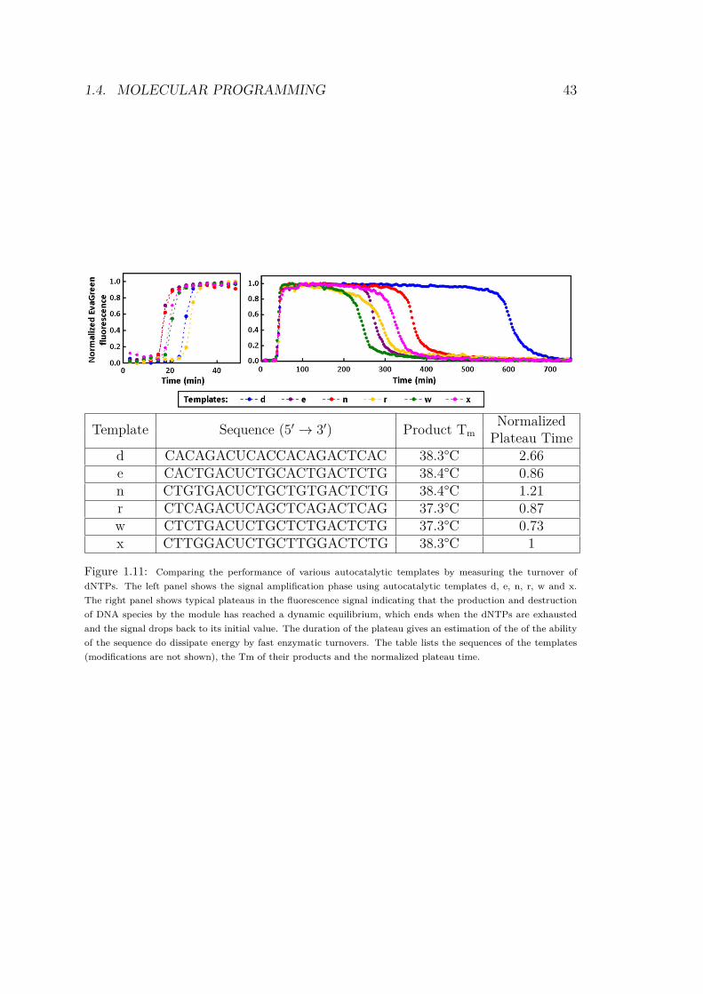
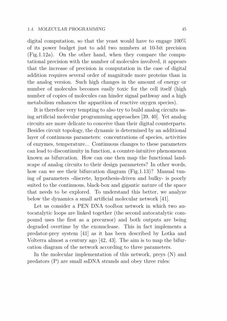
Figure 1.12: Analog versus digital computation in cells. (a) The figure shows the power costs for doing addition
in cells with a genetic circuit. (b) The figure shows the molecular protein number required to perform an addition
in cells with a genetic circuit. From Sarpeshkar 2014[38]
1.4.4 Computation and modeling
Despite taking inspiration from cellular regulation, initial proof ofprinciple in artificial chemical reaction networks have targeted Booleanlogic, with the examples of the AND gate in RTRACS and genelets,or the easy development of NOT gate in PEN DNA toolbox [35].Such networks use complex biomolecules and circuits to output dig-ital results interpreted as 0 or 1, that is, with a low informationalcontent. It is however clear that in most cases cells are not com-puting digitally. For instance, the regulation of the concentrationof many proteins is done on a continuous set between its minimumand maximum amount and not on a discrete one [36]. Accordinglythe network mapping revealed by systems biology approaches, arereminiscent of neural networks architectures, rather than engineeredelectronic circuits. Sarpeshkar et al. studied in details the possibili-ties of analog computation in cell, in the context of synthetic biologycircuits [37, 38].
They demonstrated for Saccharomyces cervisae that the powerconsumption cost of analog logic is significantly less than the one of
1.4. MOLECULAR PROGRAMMING 45
digital computation, so that the yeast would have to engage 100%of its power budget just to add two numbers at 10-bit precision(Fig.1.12a). On the other hand, when they compare the compu-tational precision with the number of molecules involved, it appearsthat the increase of precision in computation in the case of digitaladdition requires several order of magnitude more proteins than inthe analog version. Such high changes in the amount of energy ornumber of molecules becomes easily toxic for the cell itself (highnumber of copies of molecules can hinder signal pathway and a highmetabolism enhances the apparition of reactive oxygen species).
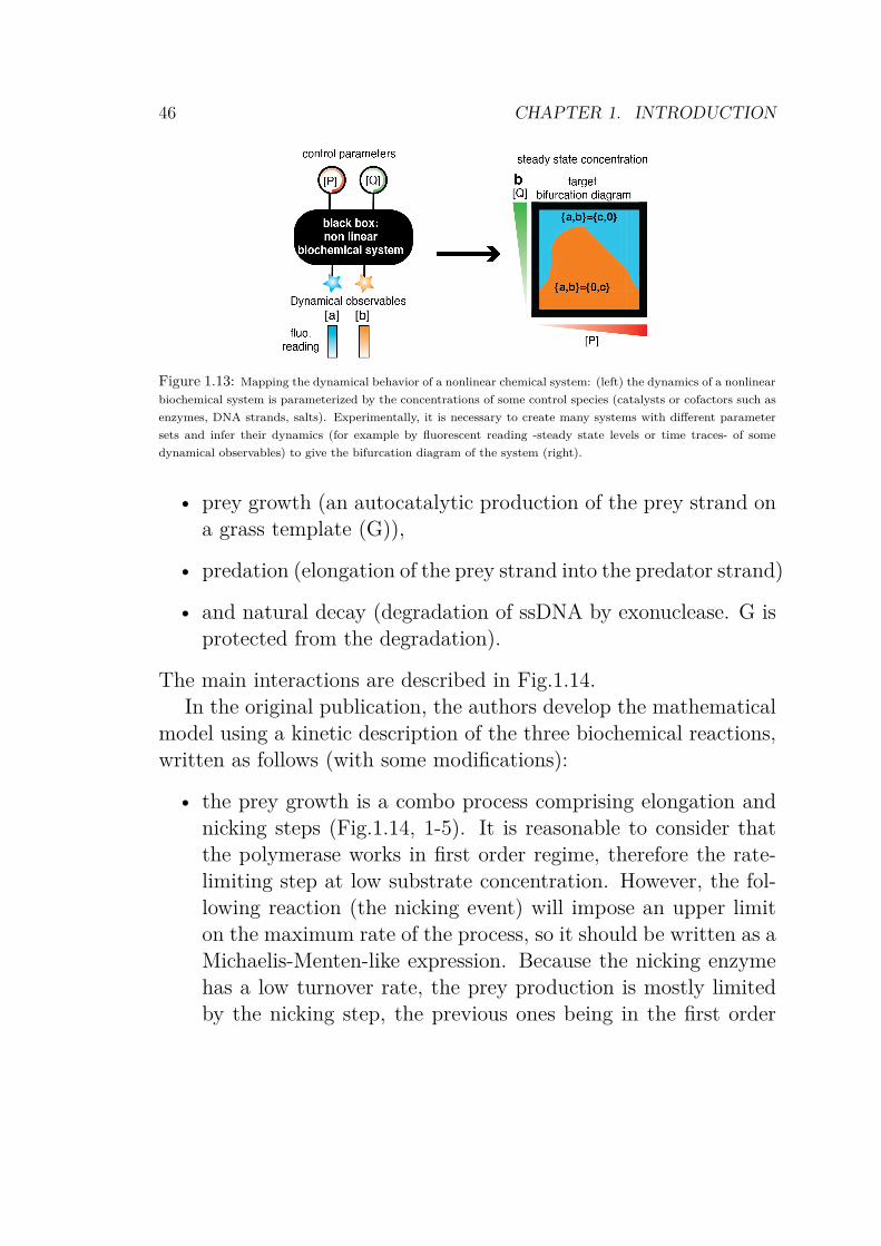
It is therefore very tempting to also try to build analog circuits us-ing artificial molecular programming approaches [39, 40]. Yet analogcircuits are more delicate to conceive than their digital counterparts.Besides circuit topology, the dynamic is determined by an additionallayer of continuous parameters: concentrations of species, activitiesof enzymes, temperature... Continuous changes to these parameterscan lead to discontinuity in function, a counter-intuitive phenomenonknown as bifurcation. How can one then map the functional land-scape of analog circuits to their design parameters? In other words,how can we see their bifurcation diagram (Fig.1.13)? Manual tun-ing of parameters -discrete, hypothesis-driven and bulky- is poorlysuited to the continuous, black-box and gigantic nature of the spacethat needs to be explored. To understand this better, we analyzebelow the dynamics a small artificial molecular network [41].
Let us consider a PEN DNA toolbox network in which two au-tocatalytic loops are linked together (the second autocatalytic com-pound uses the first as a precursor) and both outputs are beingdegraded overtime by the exonuclease. This in fact implements apredator-prey system [41] as it has been described by Lotka andVolterra almost a century ago [42, 43]. The aim is to map the bifur-cation diagram of the network according to three parameters.
In the molecular implementation of this network, preys (N) andpredators (P) are small ssDNA strands and obey three rules:
46 CHAPTER 1. INTRODUCTION
Figure 1.13: Mapping the dynamical behavior of a nonlinear chemical system: (left) the dynamics of a nonlinear
biochemical system is parameterized by the concentrations of some control species (catalysts or cofactors such as
enzymes, DNA strands, salts). Experimentally, it is necessary to create many systems with different parameter
sets and infer their dynamics (for example by fluorescent reading -steady state levels or time traces- of some
dynamical observables) to give the bifurcation diagram of the system (right).
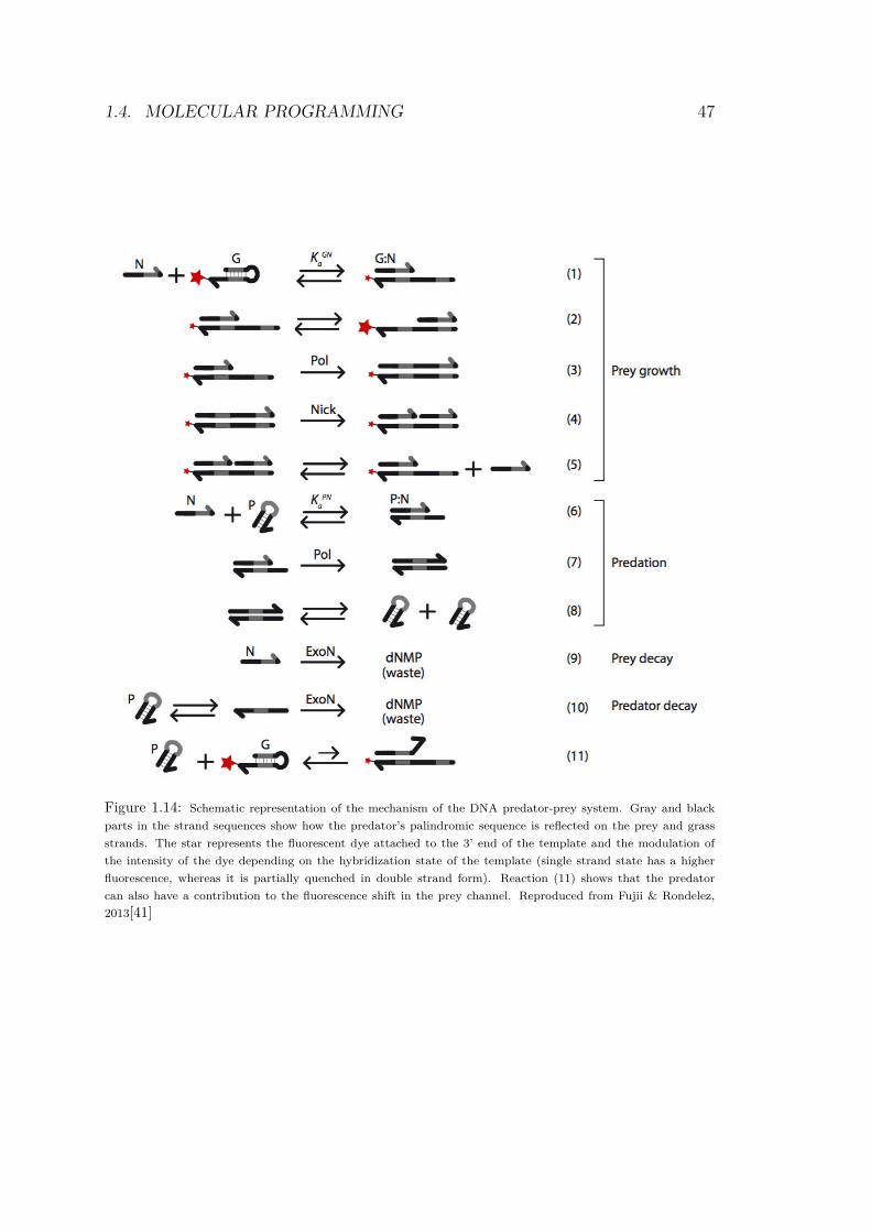
• prey growth (an autocatalytic production of the prey strand ona grass template (G)),
• predation (elongation of the prey strand into the predator strand)
• and natural decay (degradation of ssDNA by exonuclease. G isprotected from the degradation).
The main interactions are described in Fig.1.14.
In the original publication, the authors develop the mathematicalmodel using a kinetic description of the three biochemical reactions,written as follows (with some modifications):
• the prey growth is a combo process comprising elongation andnicking steps (Fig.1.14, 1-5). It is reasonable to consider thatthe polymerase works in first order regime, therefore the rate-limiting step at low substrate concentration. However, the fol-lowing reaction (the nicking event) will impose an upper limiton the maximum rate of the process, so it should be written as aMichaelis-Menten-like expression. Because the nicking enzymehas a low turnover rate, the prey production is mostly limitedby the nicking step, the previous ones being in the first order
1.4. MOLECULAR PROGRAMMING 47
Figure 1.14: Schematic representation of the mechanism of the DNA predator-prey system. Gray and black
parts in the strand sequences show how the predator’s palindromic sequence is reflected on the prey and grass
strands. The star represents the fluorescent dye attached to the 3’ end of the template and the modulation of
the intensity of the dye depending on the hybridization state of the template (single strand state has a higher
fluorescence, whereas it is partially quenched in double strand form). Reaction (11) shows that the predator
can also have a contribution to the fluorescence shift in the prey channel. Reproduced from Fujii & Rondelez,
2013[41]
48 CHAPTER 1. INTRODUCTION
regime. The expression of prey growth becomes:
ϕNæN = k · pol · G : N
K + pol.G : N
where G:N is the concentration of prey-template duplex. Then,considering the fast equilibrium in dehybridization, we can ex-press G:N as the product of the free template and preys (G andN), and since the binding constant of such complexes are smalland N and G are mostly free, the resulting equation gives:
ϕNæN = k1 · pol · G.N1+b·pol.G.N , with k1 = KGN
akK and b = KGN
a
K
• the predation is a simple elongation (Fig.1.14, 6-8) of the duplexN:P, whose binding constant is low enough for the duplex to bemostly dissociated at working temperature. Assuming that theextension of the duplex is a first-order and rate-limiting step forthe predation. We write: ϕNæP = kÕ.pol.P : N . Thus, applyingthe same assumptions on binding constants of the duplexes, wehave:
ϕNæP = k2 · pol · P · N
• finally, the degradation is solely due to the action of the proces-sive exonuclease on both prey and predator strands (Fig.1.14,8). This one-step enzymatic reaction can be described usingMichaelis-Menten kinetics:
dX
dt= rec · kcat,x
X
Km,X + X= Vm
X
Km,N + X
Since the same enzyme processes both strands, their is compe-tition between preys and predator for the enzymatic activity.Considering also that predators have a lower Km et Vmax, theequations become:
ϕNæ◆ = rec · kNN
1+ PKm,P
, with kN = kcat,N
Km,N
1.4. MOLECULAR PROGRAMMING 49
ϕPæ◆ = rec · kPP
1+ PKm,P
, with kP = kcat,P
Km,P
We can now write the complete equations as two coupled ordinarydifferential equations (ODE) by summing the contributions of preygrowth, predation and degradations:
dndτ = pol·tem·n
1+β·pol·tem·n ≠ pol · p · n ≠ λ · exo n1+p
dpdτ = pol · p · n ≠ exo p
1+p
with the dimensionless parameters τ = ttc
= t · k2 · pol · Km,P ,
p = PKm,P
, n = NKm,N
, λ = kn
kP, g = G
G0= k1·G
k2·Km,Pand β =
b·k2·K2m,P
k1and
pol, tem and exo the dimensionless concentrations of three enzymes.
Because of the non-linearities in prey growth and decay, the ana-lytical treatment is not immediate in this case, but if we consider thesaturation on all enzymes (i.e. β · pol · tem < 1), the ODE describingthe prey derivative can be re-written as:
n = pol · tem · n(1 ≠ β · pol · tem · n) ≠ pol · p · n ≠ λ · δ n1+p
To assess the number of solutions (i.e behaviors) of this systemand their stabilities, we focus on the equilibrium points, meaning thepoints where both derivative are equal to zero (i.e. the position inphase space where there is no temporal evolution) and the eigenvaluesof the Jacobian, the linearization of the system near these equilibriumpoints. According to the sign of the real part of the eigenvalues, thecorresponding point is declared stable or unstable. In this particularsystem, setting n and p to 0 reveals four points. Looking at theeigenvalues of the community matrix around these points, we foundthat three of them have a stability domain:
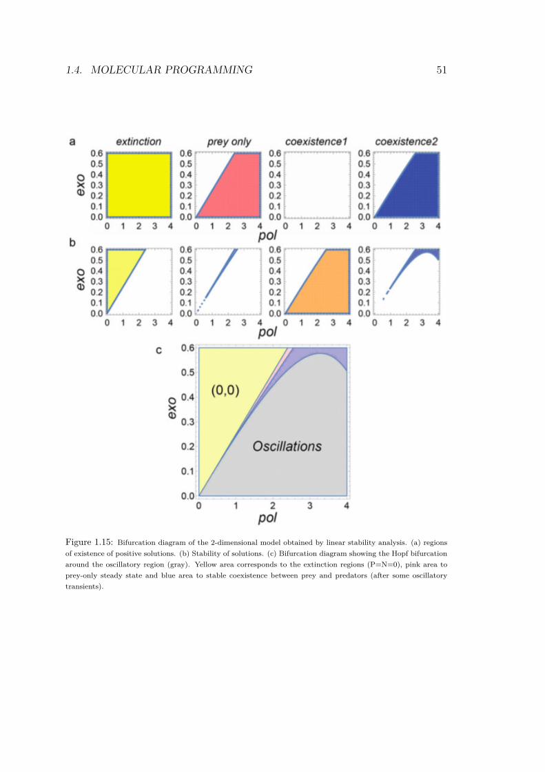
• the first point (0, 0) corresponds to the extinction of both species,stable for λ · exo > tem · pol
50 CHAPTER 1. INTRODUCTION
• the second point ( tem·pol≠exo·λβ·pol2.tem2 , 0) shows the case of the extinction
of predators and the stable production of preys. This point isstable for λ·exo < tem·pol and λ·exo > tem·pol(exo·tem·pol≠1)
• the third one (1+tem≠
√
∆pol
2(pol2·tem2) , ≠1 + tem ≠Ô
∆
2·pol), where both prey andpredator coexist is never stable over its domain of existence,with
∆ =Ò
(pol ≠ pol · tem)2 ≠ 4pol(≠pol · tem + exo · tem2β + exo · λ)
• the fourth, (1+tem≠
√
∆pol
2(pol2·tem2) , ≠1+tem+Ô
∆
2·pol) corresponds also to a co-existence of both preys and predators species. This solution hasan unstable region (corresponding to the oscillatory area) anda stable region (corresponding to damping oscillations), bothdefined by analytical expressions.
Using those results, it is possible to compute the theoretical bifur-cation diagram. The four solution’s domains are calculated and thestable parts are superimposed to reveal the diagram, as shown inFig.4.18.
The linear stability analysis gives a compact description of theexperimental dynamics of the mathematical system. Moreover, wewill see in Chapter 4 that the diagram in Fig.4.18 is quite close tothe one obtained experimentally. We distinguish 3 main domains(Fig.4.18, c):
• at low productivity (low pol and high exo), we find the extinc-tion region: no species can survive
• at high productivity (high pol and low exo) we define the stablecoexistence. Oscillations occurs at intermediate pol.
• finally, an Hopf bifurcation delineates the region of stable limitcycles.
1.4. MOLECULAR PROGRAMMING 51
Figure 1.15: Bifurcation diagram of the 2-dimensional model obtained by linear stability analysis. (a) regions
of existence of positive solutions. (b) Stability of solutions. (c) Bifurcation diagram showing the Hopf bifurcation
around the oscillatory region (gray). Yellow area corresponds to the extinction regions (P=N=0), pink area to
prey-only steady state and blue area to stable coexistence between prey and predators (after some oscillatory
transients).
52 CHAPTER 1. INTRODUCTION
However, we must not forget that the mathematical analysis uses ahighly idealized description of the actual chemistry running in thetube. For example, it considers only two dynamic species, the preyand the predator, whereas at least 6 are involved (predator, prey,grass template, polymerase, exonuclease and nicking enzyme) andmuch more if we would consider the individual steps of the enzymes(for example, each intermediate during the polymerization of suc-cessive dNTP on a template), are actually present. Therefore theproblem is double: on the one hand, can we trust linear stabilityanalysis to provide us with an actual description of the system’sfunctional capabilities? It would be possible to refine the model butwe would have then to resort to numerical predictions and an in-creasing number of parameters.
On the other hand, the challenge in realizing an experimental di-agram, hence free oneself from assumptions, is to set the mesh of thediagram as fine as possible, without consuming too much chemicals,or using too much time. It is quite easy to control the reaction vol-umes and amounts of reagents while working with volumes around10 µL but a simple 10x10 grid would use 1 mL of reaction mediumand would still be rather crude in term of spatial resolution. Here,the use of microfluidic to generate picoliter sized micro-reactors withunique combination of parameters reduces the cost since we can havemore than 10000 points for less than 100 µL engaged. Moreover thiscan be done in only a couple of hours.
Chapter 2
Droplet-based parameterscanning
2.1 Introduction
Several advances occurred recently in artificial DNA reaction net-works, a blossoming branch of molecular programming which focuseson programming artificial DNA circuits. Such systems can achievecomplex tasks, as signal processing, diagnosis or computation, whiledisplaying various behaviors such as boolean logic, multistability oroscillations [22, 26, 44, 39, 45, 25].
Despite their apparent disparity in term of size, molecular sub-strate or function, it appears that networks share some recurrent pat-terns, a topology that encodes crucial information-processing tasks[46, 47]. Alon and his group studied thoroughly the importanceand recurrence of meaningful, sub-network topologies. Consideringa triad of connected effectors, they targeted all possibilities for thistriad and screened networks from very different fields: sensory tran-scription networks for gene expression in E.Coli, yeast, signal trans-duction pathways in different organisms, links between webpages onthe world wide web... Considering each superfamily of networks,some architectures take precedence over the species considered [46].
These networks process an initial set of reagents (inputs) througha cascade of chemical reactions to yield a product (the output), whose
53
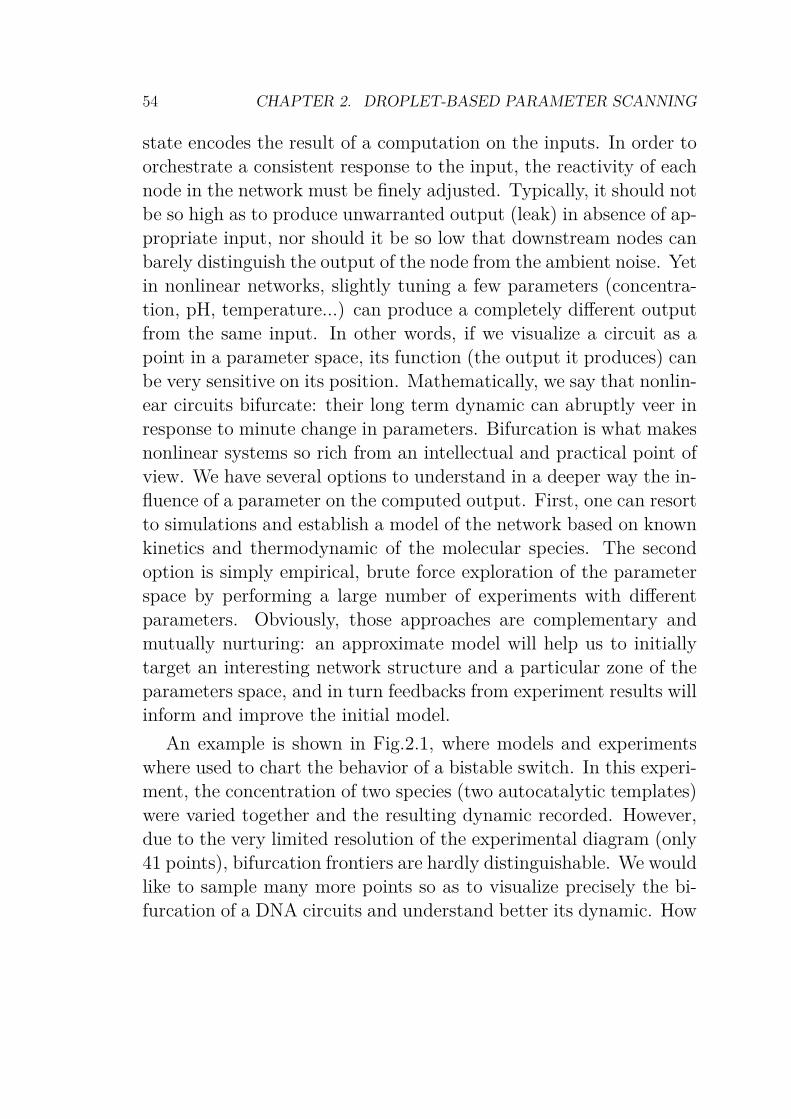
54 CHAPTER 2. DROPLET-BASED PARAMETER SCANNING
state encodes the result of a computation on the inputs. In order toorchestrate a consistent response to the input, the reactivity of eachnode in the network must be finely adjusted. Typically, it should notbe so high as to produce unwarranted output (leak) in absence of ap-propriate input, nor should it be so low that downstream nodes canbarely distinguish the output of the node from the ambient noise. Yetin nonlinear networks, slightly tuning a few parameters (concentra-tion, pH, temperature...) can produce a completely different outputfrom the same input. In other words, if we visualize a circuit as apoint in a parameter space, its function (the output it produces) canbe very sensitive on its position. Mathematically, we say that nonlin-ear circuits bifurcate: their long term dynamic can abruptly veer inresponse to minute change in parameters. Bifurcation is what makesnonlinear systems so rich from an intellectual and practical point ofview. We have several options to understand in a deeper way the in-fluence of a parameter on the computed output. First, one can resortto simulations and establish a model of the network based on knownkinetics and thermodynamic of the molecular species. The secondoption is simply empirical, brute force exploration of the parameterspace by performing a large number of experiments with differentparameters. Obviously, those approaches are complementary andmutually nurturing: an approximate model will help us to initiallytarget an interesting network structure and a particular zone of theparameters space, and in turn feedbacks from experiment results willinform and improve the initial model.
An example is shown in Fig.2.1, where models and experimentswhere used to chart the behavior of a bistable switch. In this experi-ment, the concentration of two species (two autocatalytic templates)were varied together and the resulting dynamic recorded. However,due to the very limited resolution of the experimental diagram (only41 points), bifurcation frontiers are hardly distinguishable. We wouldlike to sample many more points so as to visualize precisely the bi-furcation of a DNA circuits and understand better its dynamic. How
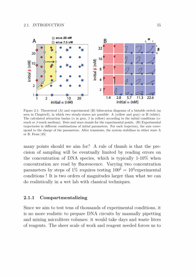
2.1. INTRODUCTION 55
Figure 2.1: Theoretical (A) and experimental (B) bifurcation diagrams of a bistable switch (asseen in Chapter3), in which two steady-states are possible: A (yellow and gray) or B (white).The calculated attraction basins (α in grey, β in yellow) according to the initial conditions (α-reach or β-reach medium). Dots and stars stands for the experimental points. (B) Experimentaltrajectories in different combinations of initial parameters. For each trajectory, the axis corre-spond to the charge of the parameters. After transients, the system stabilizes in either state Aor B. From [45]
many points should we aim for? A rule of thumb is that the pre-cision of sampling will be eventually limited by reading errors onthe concentration of DNA species, which is typically 1-10% whenconcentration are read by fluorescence. Varying two concentrationparameters by steps of 1% requires testing 1002 = 104experimentalconditions ! It is two orders of magnitudes larger than what we cando realistically in a wet lab with classical techniques.
2.1.1 Compartmentalizing
Since we aim to test tens of thousands of experimental conditions, itis no more realistic to prepare DNA circuits by manually pipettingand mixing microliters volumes: it would take days and waste litersof reagents. The sheer scale of work and reagent needed forces us to
56 CHAPTER 2. DROPLET-BASED PARAMETER SCANNING
think about newer ways to reduce volumes and automatize prepara-tion. Micro reactors -a concept that rose in the mid 80’s- combinethe ability to simultaneously generate a large number of vessels withdifferent experimental conditions from a limited amount of reagents.One of the initial incentive was the possibility of synthesizing com-pounds using a minimal amount of reagents while drastically increas-ing the safety of dangerous or explosive reactions [48].
An immediate consequence of shrinking the dimensions of reactorsfrom millimeter to micrometer is that the surface-to-volume ratioexplodes accordingly. Indeed, when the open surface of 200µL ofmixture contained in a classical PCR tube is around 140 mm2, a50µm wide water-in-oil droplet shows an accessible surface of 0.031mm2 for a volume of 500 pL (i.e. a 4.105 times smaller volume). Thismay lead to problems if the reaction carried inside the compartmentis sensitive to the presence of interfaces. Another, possibly morebeneficial, consequence is that the heat exchange being a functionof the surface of the compartment, the temperature of the dropletvary smoothly with the global temperature of the continuous phase,making the control of the temperature easier.
The appealing features of micro reactors (decreased consumptionsof reagents, faster temperature control and higher throughput) stim-ulated the development of convenient methods to generate microre-actors [49, 50, 51, 52][49, 50, 51, 52, 53]. Emulsions provide a sim-ple and economic route to compartmentalization into microreactors:when two immiscible fluids (say oil and water) are properly mixedtogether, physical instabilities force one of the fluid to partition intodroplets (the dispersed phase) suspended in the other fluid (the con-tinuous phase).
The generation and management of emulsion can be done throughmicrofluidics, which is essentially a field dedicated to miniaturizedplumbing and fluidic manipulation. This comes from fine control ofeach hydrodynamic flows, thus controlling the formation (deforma-tion and break up) of each individual droplet, structures the gener-
2.1. INTRODUCTION 57
ation of monodisperse emulsion quite easy.As powerful as they can be, these methods still have some issues.
For instance, a high heat transfer value also enhance the surfacechemistry and surface effect on the walls of the reactor, meaning thatsome local parasitic reactions might prevent the chemicals within toproperly react (i.e. as they were designed to). Another drawback isthe control of size and dispersion of the emulsion: a top-down ap-proach ( for instance vortexing a biphasic solution of continuous anddispersed phase) leads to high polydispersity in compartment size.Even if the generation of an emulsion by microfluidic devices providesa good control over size and uniformity of the droplet compared toother emulsification processes (vortexing, or membrane-based tech-niques), setting the parameters for such generation can be delicate,depending on the considered device.
Microfluidic droplets is a now mature field, and used for a widerange of applications, such as study of heat transfer [54], screeningof the conditions for crystal growth [53], single molecule enzymol-ogy [55], rare mutation detection by PCR [56], chemical oscillatingreactions [57].
Figure 2.2: Three ways to generate droplets: co flowing(a), cross flowing(b) and flow focusing(c)streams. From [58]
Generation of droplets can be divided in two types of methods:active and passive, summarized in Table2.1. In active methods, aphysical process (beyond the mere flowing of a fluid inside microchan-nels) is employed to induce instabilities. Active methods comprisetechniques such as spraying, atomization, membrane emulsificationor inkjet printing. The simplest and oldest active method is vortex-
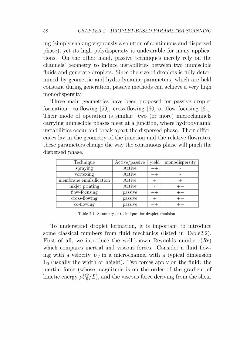
58 CHAPTER 2. DROPLET-BASED PARAMETER SCANNING
ing (simply shaking vigorously a solution of continuous and dispersedphase), yet its high polydispersity is undesirable for many applica-tions. On the other hand, passive techniques merely rely on thechannels’ geometry to induce instabilities between two immisciblefluids and generate droplets. Since the size of droplets is fully deter-mined by geometric and hydrodynamic parameters, which are heldconstant during generation, passive methods can achieve a very highmonodispersity.
Three main geometries have been proposed for passive dropletformation: co-flowing [59], cross-flowing [60] or flow focusing [61].Their mode of operation is similar: two (or more) microchannelscarrying unmiscible phases meet at a junction, where hydrodynamicinstabilities occur and break apart the dispersed phase. Their differ-ences lay in the geometry of the junction and the relative flowrates,these parameters change the way the continuous phase will pinch thedispersed phase.
Technique Active/passive yield monodispersityspraying Active ++ -vortexing Active ++ -
membrane emulsification Active + +inkjet printing Active - ++flow-focusing passive ++ ++cross-flowing passive + ++
co-flowing passive ++ ++
Table 2.1: Summary of techniques for droplet emulsion
To understand droplet formation, it is important to introducesome classical numbers from fluid mechanics (listed in Table2.2).First of all, we introduce the well-known Reynolds number (Re)which compares inertial and viscous forces. Consider a fluid flow-ing with a velocity U0 in a microchannel with a typical dimensionL0 (usually the width or height). Two forces apply on the fluid: theinertial force (whose magnitude is on the order of the gradient ofkinetic energy ρU 2
0 /L), and the viscous force deriving from the shear
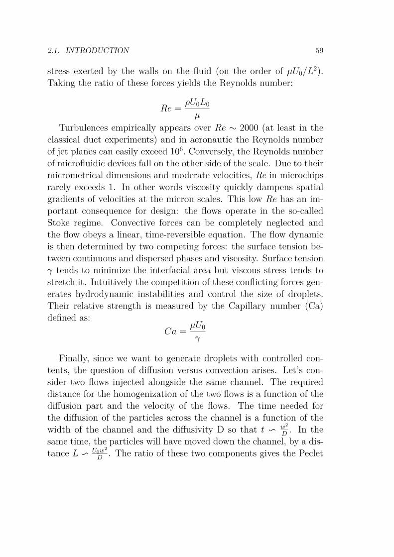
2.1. INTRODUCTION 59
stress exerted by the walls on the fluid (on the order of µU0/L2).Taking the ratio of these forces yields the Reynolds number:
Re =ρU0L0
µ
Turbulences empirically appears over Re ≥ 2000 (at least in theclassical duct experiments) and in aeronautic the Reynolds numberof jet planes can easily exceed 106. Conversely, the Reynolds numberof microfluidic devices fall on the other side of the scale. Due to theirmicrometrical dimensions and moderate velocities, Re in microchipsrarely exceeds 1. In other words viscosity quickly dampens spatialgradients of velocities at the micron scales. This low Re has an im-portant consequence for design: the flows operate in the so-calledStoke regime. Convective forces can be completely neglected andthe flow obeys a linear, time-reversible equation. The flow dynamicis then determined by two competing forces: the surface tension be-tween continuous and dispersed phases and viscosity. Surface tensionγ tends to minimize the interfacial area but viscous stress tends tostretch it. Intuitively the competition of these conflicting forces gen-erates hydrodynamic instabilities and control the size of droplets.Their relative strength is measured by the Capillary number (Ca)defined as:
Ca =µU0
γ
Finally, since we want to generate droplets with controlled con-tents, the question of diffusion versus convection arises. Let’s con-sider two flows injected alongside the same channel. The requireddistance for the homogenization of the two flows is a function of thediffusion part and the velocity of the flows. The time needed forthe diffusion of the particles across the channel is a function of thewidth of the channel and the diffusivity D so that t v w2
D . In thesame time, the particles will have moved down the channel, by a dis-tance L v U0w2
D . The ratio of these two components gives the Peclet
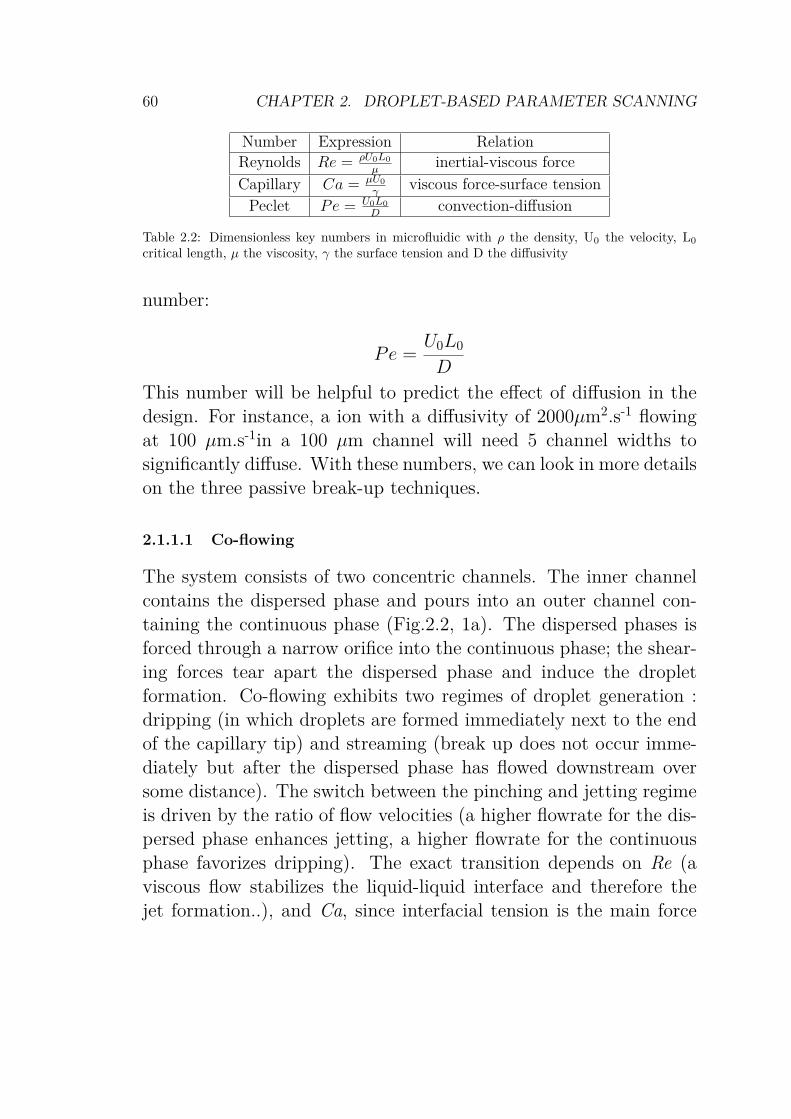
60 CHAPTER 2. DROPLET-BASED PARAMETER SCANNING
Number Expression Relation
Reynolds Re = ρU0L0
µinertial-viscous force
Capillary Ca = µU0
γviscous force-surface tension
Peclet Pe = U0L0
Dconvection-diffusion
Table 2.2: Dimensionless key numbers in microfluidic with ρ the density, U0 the velocity, L0
critical length, µ the viscosity, γ the surface tension and D the diffusivity
number:
Pe =U0L0
D
This number will be helpful to predict the effect of diffusion in thedesign. For instance, a ion with a diffusivity of 2000µm2.s-1 flowingat 100 µm.s-1in a 100 µm channel will need 5 channel widths tosignificantly diffuse. With these numbers, we can look in more detailson the three passive break-up techniques.
2.1.1.1 Co-flowing
The system consists of two concentric channels. The inner channelcontains the dispersed phase and pours into an outer channel con-taining the continuous phase (Fig.2.2, 1a). The dispersed phases isforced through a narrow orifice into the continuous phase; the shear-ing forces tear apart the dispersed phase and induce the dropletformation. Co-flowing exhibits two regimes of droplet generation :dripping (in which droplets are formed immediately next to the endof the capillary tip) and streaming (break up does not occur imme-diately but after the dispersed phase has flowed downstream oversome distance). The switch between the pinching and jetting regimeis driven by the ratio of flow velocities (a higher flowrate for the dis-persed phase enhances jetting, a higher flowrate for the continuousphase favorizes dripping). The exact transition depends on Re (aviscous flow stabilizes the liquid-liquid interface and therefore thejet formation..), and Ca, since interfacial tension is the main force
2.1. INTRODUCTION 61
applied on the droplet at the end of the tip. Co-flowing leads tohighly monodisperse droplets, whose size is controlled by the diam-eter of the inner capillary. Although co-flowing was used for one ofthe first demonstration of microfluidic droplet generation, it is notin wide use now. One of the reason is that it is relatively delicateto fabricate two coaxial channels, microfluidic methods being moreadapted at «extruding» 2D shapes that are projected by lithography.
2.1.1.2 Cross-flowing
Cross-flowing is one of the most common method to produce droplets,laying on a T-shaped device where the dispersed phase is crossed bythe continuous phase (Fig.2.2, b). Here ratio between the pressures inthe dispersed phase channel (Qd) and the pressure in the continuousphase channel (Qc), as well as the width of the channels (wd wc) arekey parameters which determine the rate and size of droplets. A lowor high Qd
Qcmeans the invasion of one channel by the other, so that
Qd
Qcv 1. The resulting shear forces elongate the dispersed channel
and break up when Ca v 1. Generating droplets using T-junctionsis easy and the monodispersity is good. The formation of droplet ispossible over a wide range of flowrates, and the frequency is regular.
2.1.1.3 Flow-focusing
Flow focusing is by far the most common geometry to generatedroplets. The dispersed phase flows in a central channel and meetsthe continuous phase at a symmetric junction (Fig.2.2, c) The twophases are then evacuated through a small constriction located down-stream: the nozzle. The flow of the continuous phase Qc is higherthan the flow of the dispersed phase Qd, creating viscous stresseson the dispersed phase inside the nozzle which breaks down the dis-persed phase into droplets. This technique was pioneered by Annaet al. [61]. The targeted droplet size is not much more dependenton the ratio of Qc
Qdthan the nozzle’s size wor (Fig2.3). This flexibility
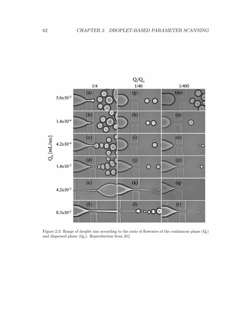
62 CHAPTER 2. DROPLET-BASED PARAMETER SCANNING
Figure 2.3: Range of droplet size according to the ratio of flowrates of the continuous phase (Qi)and dispersed phase (Qo). Reproduction from [61]
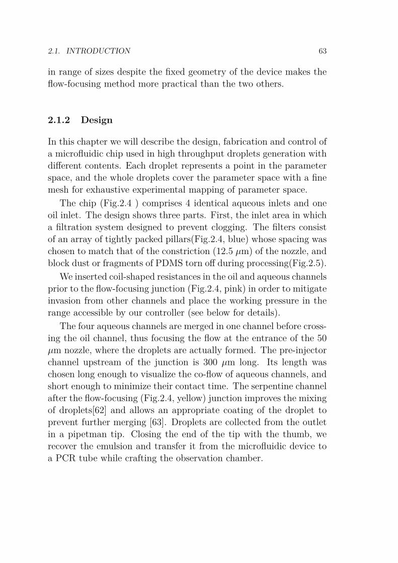
2.1. INTRODUCTION 63
in range of sizes despite the fixed geometry of the device makes theflow-focusing method more practical than the two others.
2.1.2 Design
In this chapter we will describe the design, fabrication and control ofa microfluidic chip used in high throughput droplets generation withdifferent contents. Each droplet represents a point in the parameterspace, and the whole droplets cover the parameter space with a finemesh for exhaustive experimental mapping of parameter space.
The chip (Fig.2.4 ) comprises 4 identical aqueous inlets and oneoil inlet. The design shows three parts. First, the inlet area in whicha filtration system designed to prevent clogging. The filters consistof an array of tightly packed pillars(Fig.2.4, blue) whose spacing waschosen to match that of the constriction (12.5 µm) of the nozzle, andblock dust or fragments of PDMS torn off during processing(Fig.2.5).
We inserted coil-shaped resistances in the oil and aqueous channelsprior to the flow-focusing junction (Fig.2.4, pink) in order to mitigateinvasion from other channels and place the working pressure in therange accessible by our controller (see below for details).
The four aqueous channels are merged in one channel before cross-ing the oil channel, thus focusing the flow at the entrance of the 50µm nozzle, where the droplets are actually formed. The pre-injectorchannel upstream of the junction is 300 µm long. Its length waschosen long enough to visualize the co-flow of aqueous channels, andshort enough to minimize their contact time. The serpentine channelafter the flow-focusing (Fig.2.4, yellow) junction improves the mixingof droplets[62] and allows an appropriate coating of the droplet toprevent further merging [63]. Droplets are collected from the outletin a pipetman tip. Closing the end of the tip with the thumb, werecover the emulsion and transfer it from the microfluidic device toa PCR tube while crafting the observation chamber.
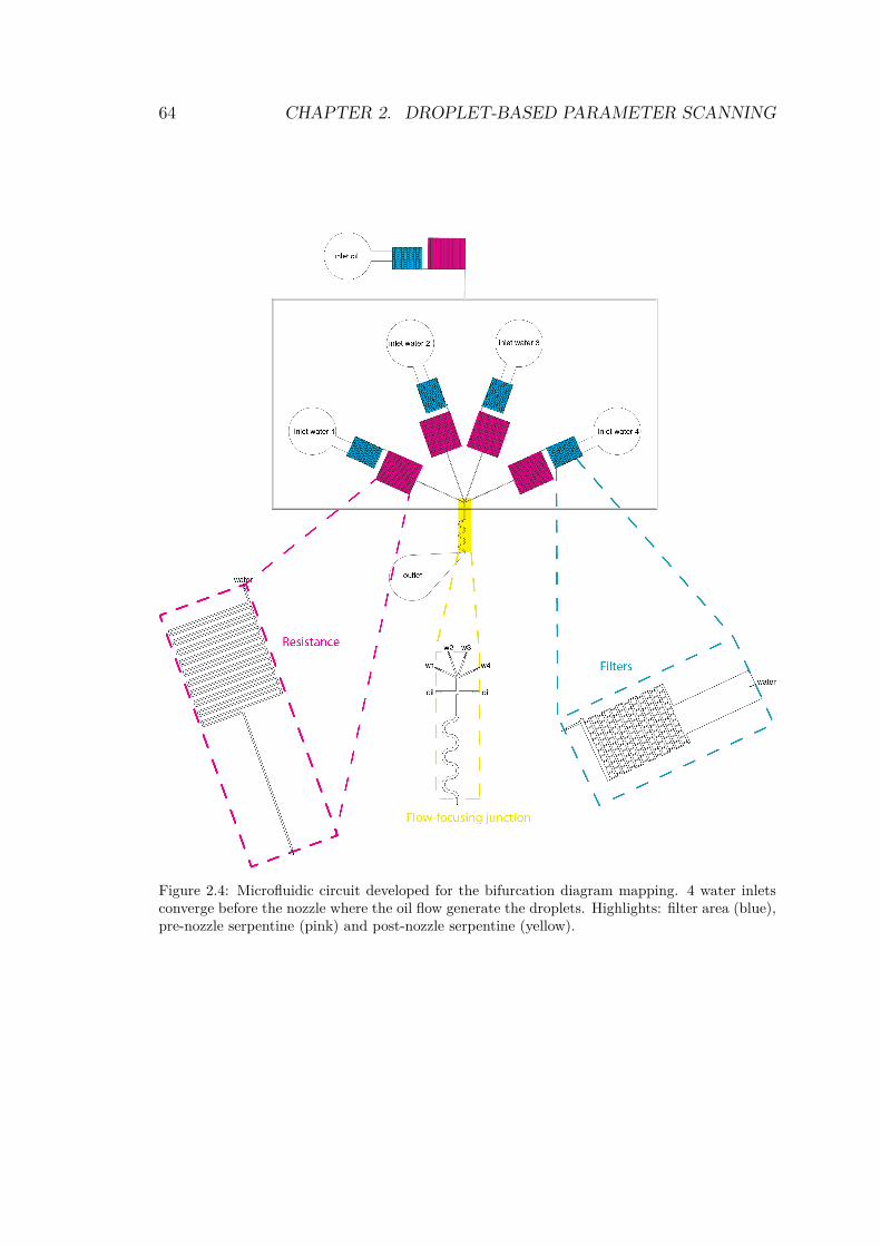
64 CHAPTER 2. DROPLET-BASED PARAMETER SCANNING
Figure 2.4: Microfluidic circuit developed for the bifurcation diagram mapping. 4 water inletsconverge before the nozzle where the oil flow generate the droplets. Highlights: filter area (blue),pre-nozzle serpentine (pink) and post-nozzle serpentine (yellow).
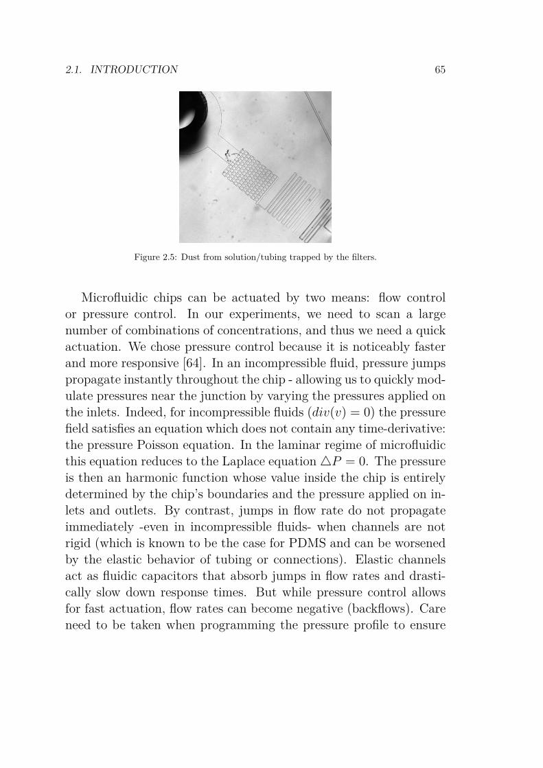
2.1. INTRODUCTION 65
Figure 2.5: Dust from solution/tubing trapped by the filters.
Microfluidic chips can be actuated by two means: flow controlor pressure control. In our experiments, we need to scan a largenumber of combinations of concentrations, and thus we need a quickactuation. We chose pressure control because it is noticeably fasterand more responsive [64]. In an incompressible fluid, pressure jumpspropagate instantly throughout the chip - allowing us to quickly mod-ulate pressures near the junction by varying the pressures applied onthe inlets. Indeed, for incompressible fluids (div(v) = 0) the pressurefield satisfies an equation which does not contain any time-derivative:the pressure Poisson equation. In the laminar regime of microfluidicthis equation reduces to the Laplace equation —P = 0. The pressureis then an harmonic function whose value inside the chip is entirelydetermined by the chip’s boundaries and the pressure applied on in-lets and outlets. By contrast, jumps in flow rate do not propagateimmediately -even in incompressible fluids- when channels are notrigid (which is known to be the case for PDMS and can be worsenedby the elastic behavior of tubing or connections). Elastic channelsact as fluidic capacitors that absorb jumps in flow rates and drasti-cally slow down response times. But while pressure control allowsfor fast actuation, flow rates can become negative (backflows). Careneed to be taken when programming the pressure profile to ensure
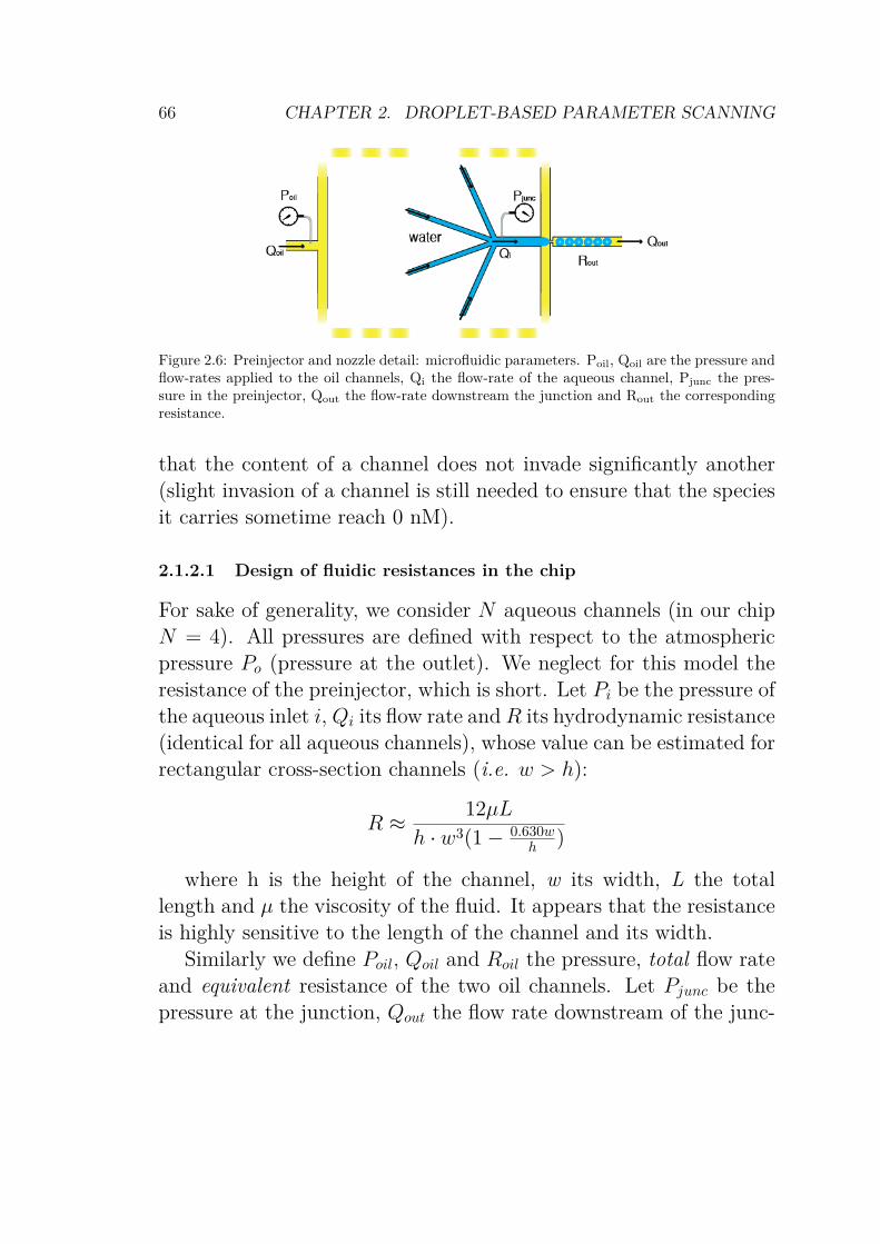
66 CHAPTER 2. DROPLET-BASED PARAMETER SCANNING
Figure 2.6: Preinjector and nozzle detail: microfluidic parameters. Poil, Qoil are the pressure andflow-rates applied to the oil channels, Qi the flow-rate of the aqueous channel, Pjunc the pres-sure in the preinjector, Qout the flow-rate downstream the junction and Rout the correspondingresistance.
that the content of a channel does not invade significantly another(slight invasion of a channel is still needed to ensure that the speciesit carries sometime reach 0 nM).
2.1.2.1 Design of fluidic resistances in the chip
For sake of generality, we consider N aqueous channels (in our chipN = 4). All pressures are defined with respect to the atmosphericpressure Po (pressure at the outlet). We neglect for this model theresistance of the preinjector, which is short. Let Pi be the pressure ofthe aqueous inlet i, Qi its flow rate and R its hydrodynamic resistance(identical for all aqueous channels), whose value can be estimated forrectangular cross-section channels (i.e. w > h):
R ¥ 12µL
h · w3(1 ≠ 0.630wh )
where h is the height of the channel, w its width, L the totallength and µ the viscosity of the fluid. It appears that the resistanceis highly sensitive to the length of the channel and its width.
Similarly we define Poil, Qoil and Roil the pressure, total flow rateand equivalent resistance of the two oil channels. Let Pjunc be thepressure at the junction, Qout the flow rate downstream of the junc-
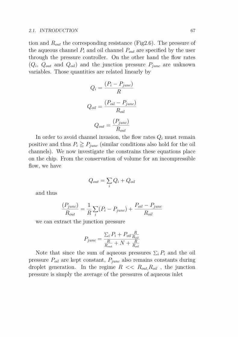
2.1. INTRODUCTION 67
tion and Rout the corresponding resistance (Fig2.6). The pressure ofthe aqueous channel Pi and oil channel Pout are specified by the userthrough the pressure controller. On the other hand the flow rates(Qi, Qout and Qoil) and the junction pressure Pjunc are unknownvariables. Those quantities are related linearly by
Qi =(Pi ≠ Pjunc)
R
Qoil =(Poil ≠ Pjunc)
Roil
Qout =(Pjunc)
Rout
In order to avoid channel invasion, the flow rates Qi must remainpositive and thus Pi = Pjunc (similar conditions also hold for the oilchannels). We now investigate the constrains these equations placeon the chip. From the conservation of volume for an incompressibleflow, we have
Qout =ÿ
i
Qi + Qoil
and thus
(Pjunc)
Rout=
1
R
ÿ
i
(Pi ≠ Pjunc) +Poil ≠ Pjunc
Roil
we can extract the junction pressure
Pjunc =
q
i Pi + PoilR
Roil
RRout
+ N + RRoil
Note that since the sum of aqueous pressuresq
i Pi and the oilpressure Poil are kept constant, Pjunc also remains constants duringdroplet generation. In the regime R << Rout,Roil , the junctionpressure is simply the average of the pressures of aqueous inlet
68 CHAPTER 2. DROPLET-BASED PARAMETER SCANNING
Figure 2.7: Four chip-prototyping methods, from [65].
Pjunc=1
N
ÿ
i
Pi
Since it is impossible for all the aqueous pressures to exceed theirmean, at least one of the aqueous channel must be invaded. To avoidthis, we dimensionalized the resistances of the oil channels Roil andthe aqueous channels R to be noticeably larger than the resistance ofthe chip after the junction Rout (we have Roil ƒ R and R ƒ 80Rout).
2.2 Microfluidic device fabrication
Thanks to progress in microfabrication, there are now many op-tions available to pattern a microfluidic design into a material chip.The nature of the fluids, the features of the design, the size of thedroplets, the cost and amount of emulsion will dictate the choice ofone material over another. The main specification that is sought isa cheap, rapid generation of the emulsion from a limited amount ofreagents. Historically, the first microfluidic devices were fabricatedby lithographing and etching channels into a glass substrate. Themethod is laborious as the fabrications steps must be repeated in a
2.2. MICROFLUIDIC DEVICE FABRICATION 69
clean room each time a new batch of chip is need. This difficultyin fabricating chips held back the initial development of microflu-idic. The situation changed in the late 90s with the introduction ofreplica molding by Georges Whitesides and colleagues [66]. Theyshowed that polydimethylsiloxane (PDMS) -a polymer with elas-tomeric properties- could replicate the shape of a master mold uponcuring, with a resolution of dozens of nanometers. The properties ofPDMS, such as gas permeability and control of the hydrophobicity,have made it a golden standard for (molecular) biology microfluidics.The polymer has allowed hundreds of labs in the world to cheaplyand effortlessly fabricate microfluidics chips.
Fig.2.7 shows an overview of the main techniques mentioned above.In the case of glass micromachining, the main drawbacks are thecomplexity of the process and its cost, but these devices resist highpressures. Laser-based ablation or drilling on plastic polymers arefar cheaper methods, but their channels are not well defined andrugged. Soft-lithography techniques are more common, because oftheir simplicity. This technique has been developed and tuned formicrofluidics by Whiteside’s group [67, 66] and are interesting interms of cost, throughput and accuracy in the design.
2.2.1 Mold fabrication
This step patterns a silicon wafer using a negative photoresist withthe mask. The patterned wafer becomes a negative mold of thefluidic circuit. A clean, dustless, silicon wafer is covered with negativephotoresist uniformly spread on the wafer by spincoating. The choiceof the photoresist, its amount and the spincoating procedure arelead by the aimed thickness of the microfluidic channels. Since therheology of the photoresist is depending on the temperature of theroom, one may follow the instructions given by the furnisher. In ourcase, we target a thickness of 55 µm (+/- 10 µm), so we used thenegative photoresist SU-8 2075 (MicroChem) on a 4 inches silicon
70 CHAPTER 2. DROPLET-BASED PARAMETER SCANNING
wafer. The spincoater is set on 2000 rpm for 25 s.
The spincoat process is followed by a pre-baking step on a TripletTH-900 Hot Plate: 1 min at 65 °C, then 6 min at 95 °C and aslow return to room temperature. The resulting assembly is thenready for UV-exposure. The mask is tightly laid on the hardenedphotoresist, and exposed for 20 seconds (6000 W, 150 mJ) undera Super High Pressure UV lamp (Ushio USH-250LT, USA). Hereagain, heating time, temperature and exposure time are driven bythe final thickness and lamp power.
The next step is the post-exposure baking, in which the photo-activated compounds diffuse to surface and trigger the polymeriza-tion of the photo-resist. Time and temperature define the final thick-ness, and according to the literature the settings should be 1 min at65 °C and 6 min at 95 °C for 55 µm.
The photoresist then soaks 5 min in a solution of SU-8 developer(MicroChem). Parts that were not exposed to UV remain polymer-ized and the UV-patterned surface is revealed. A second bath ofdeveloper and a rinse with isopropanol complete the revelation ofthe mold. During this step, the mold should remain immersed insolution to avoid the clogging of clots on the surface. Finally, we ap-ply a Teflon coating on the mold to protect it from attrition/aging,and it makes the PDMS peeling easier. A mold can be used ~ 100times before significant erosion occur. Actually breaking, rather thanoveruse, is the main reason a mold needs to be replaced.
2.2.2 Chip casting
Chips come from polymerization of PDMS on the mold. First across linking agent is added to the PDMS (SILPOT 184 W/C, DowCorning Toray, Japan) with a typical ratio of 10% (w/w), mixedthoroughly for 30 s at 2000 rpm (Thinky ARE 310) and poured in aPetri dish with the mold. Typically, we use 72 g of PDMS base and8 g of cross linking agent for one batch, the final thickness of the chip
2.3. OIL & SURFACTANTS 71
is ~ 8 mm. Thicker chips will facilitate the tubing process. After 20minutes under reduced pressure to degas the mixture, the PDMS iscured at 75 °C for one hour and a half. Once hardened, the PDMScake is peeled off and immediately put on a plastic sheet (peeled facein contact with the plastic) to prevent any clogging of the channel bydust in the air. Inlets and outlets are opened thanks to a clean hole-puncher with a diameter slightly smaller than the external diameterof the tube. The punching should be neat in order to avoid any tearof the PDMS, because it would lead to fluidic clogging/problems laterin the process. Just before bonding, both PDMS surface and a glassslide are cleaned with an O2plasma by reactive ion etching process(RIE-10NR, Samco International): 50 SCCM, 20 Pa, 75 W for 5 s.This allows a covalent bound between the resulting silanols of thePDMS surface on the glass slide [66]. This step is critical because itis the most probable chance to catch dust particle on the PDMS orglass, leading to an unusable chip.
Finally, a baking step (190 °C, 5 h) is used to make the wholechannel surface (glass and PDMS) hydrophobic and improve bonding[68].
2.3 Oil & Surfactants
The size of droplets can be easily adjusted in a microfluidic deviceto fall within a range useful for single cell biology, biochemistry andmolecular programming (1-100 µm). But in addition to size, dropletsmust meet other important specifications for biological applications:they must be stable against coalescence over a long time, biocom-patible, and reagents should no leak between them. Here the choiceof oil and surfactant will prove crucial to meet these requirements.
Two physical effects (Ostwald ripening and coalescence) conspireto destabilize and coalesce droplets arrays. Coalescence occurs afterdrainage of continuous layer between two droplets. Ostwal ripening isa passive, thermodynamic effect. Consider a polydisperse emulsion,
72 CHAPTER 2. DROPLET-BASED PARAMETER SCANNING
in which larger droplets are more stable than smaller ones thanksto their lower surface tension. Because of this imbalance, smallerdroplets tend to transfer material to larger ones to reduce their sur-face tension, further increasing the size of the larger droplets. Theaverage radius R of droplets will evolve in function of the tempera-ture (T), surface tension (γ), solubility (cŒ) of the transiting particle,its molar volume (ν) and its diffusion coefficient (D). Here Rg is theideal gas constant [69]:
R3 ≠ R30 =
8γcŒν2D
9RgTt
SURFace ACTive AgeNTs (named hereafter surfactants) are de-signed to prevent both coalescence and Ostwald ripening. They con-sist of amphiphilic molecules, that is molecules that carry both hy-drophobic and hydrophilic moeities. Because of this, they preferen-tially sit at interface of droplets, which reduces the global surfacetension between the phases. The surfactant effect is quantified bythe amount of surfactant molecules on the droplet’s surface (Γ, sur-face concentration), the surface tension and its bulk concentration(c) [70]:
Γ = ≠ c
RgT
dγ
dc
Surfactants prevent coalescence thanks to the Marangoni stress pro-duced when two droplets approach. As two droplets get close, theresulting flows expel surfactants, which increases surface tension. Inturn, the surface tension gradient drives the convection of surfactantsto replenish the depleted area, thus slowing drainage and stabilizingdroplets (Fig.2.8).
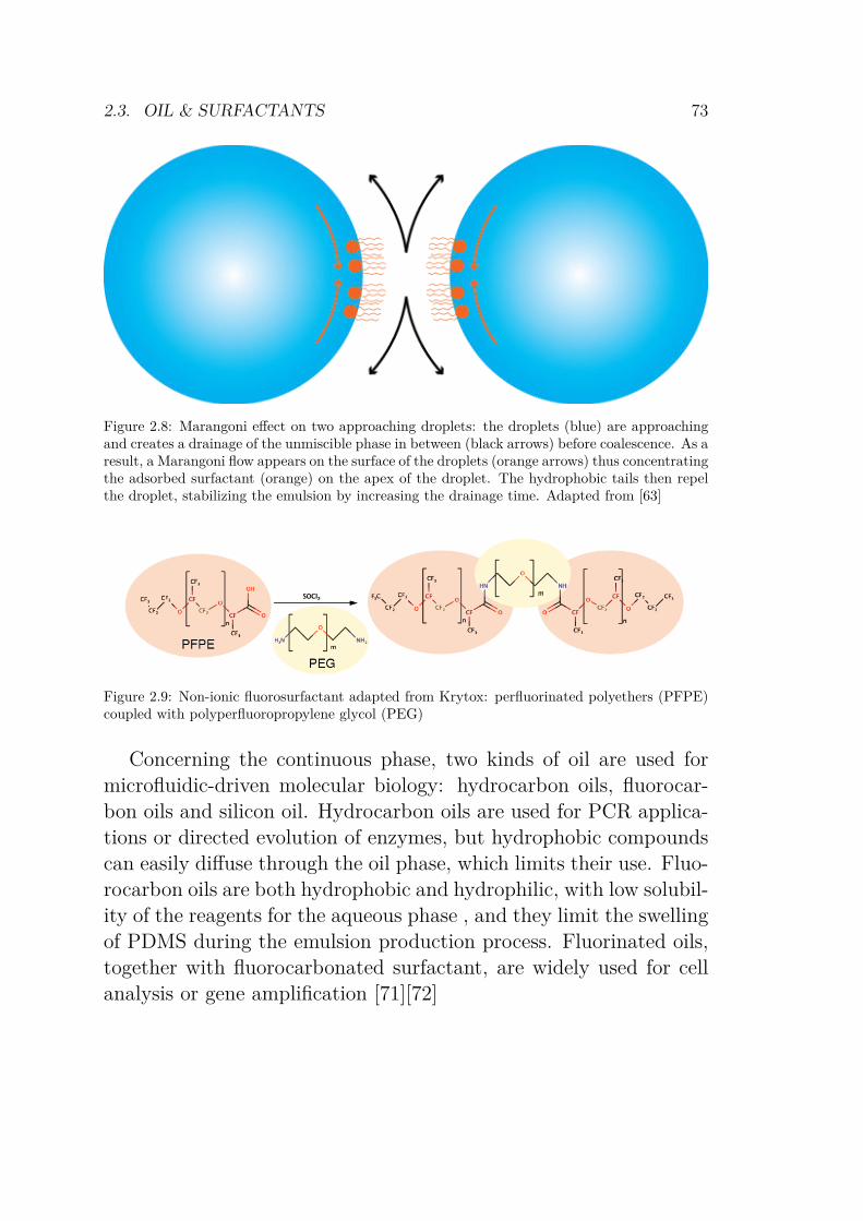
2.3. OIL & SURFACTANTS 73
Figure 2.8: Marangoni effect on two approaching droplets: the droplets (blue) are approachingand creates a drainage of the unmiscible phase in between (black arrows) before coalescence. As aresult, a Marangoni flow appears on the surface of the droplets (orange arrows) thus concentratingthe adsorbed surfactant (orange) on the apex of the droplet. The hydrophobic tails then repelthe droplet, stabilizing the emulsion by increasing the drainage time. Adapted from [63]
Figure 2.9: Non-ionic fluorosurfactant adapted from Krytox: perfluorinated polyethers (PFPE)coupled with polyperfluoropropylene glycol (PEG)
Concerning the continuous phase, two kinds of oil are used formicrofluidic-driven molecular biology: hydrocarbon oils, fluorocar-bon oils and silicon oil. Hydrocarbon oils are used for PCR applica-tions or directed evolution of enzymes, but hydrophobic compoundscan easily diffuse through the oil phase, which limits their use. Fluo-rocarbon oils are both hydrophobic and hydrophilic, with low solubil-ity of the reagents for the aqueous phase , and they limit the swellingof PDMS during the emulsion production process. Fluorinated oils,together with fluorocarbonated surfactant, are widely used for cellanalysis or gene amplification [71][72]
74 CHAPTER 2. DROPLET-BASED PARAMETER SCANNING
The nature of the oil has a strong effect on the generation andhandling of the droplets. For instance, viscous oils, such as mineraloils, requires a high oil-to-water pressure ratios during generations.The material of the microfluidic device is another important criteria:in case of PDMS-based devices, silicon oil are unusable because oftheir solubility in PDMS (which is why we did not consider such oils).In this case, hydrocarbon oils provide an alternative (although careshould be taken about possible diffusion of reagents in it, as men-tioned above) [73]. Temperature also affects the physicochemicalproperties of oils and surfactants, which may destabilize the emul-sion. Therefore, a careful choice of oil, surfactant, aqueous reagentsand chip material should be made upon designing the experiment inorder to provide an appropriate control over the size of droplets, theleakage of reagents and the stability of the emulsion.
Another practical difference between oils is their densities. Inthe case of hydrocarbon or fluorocarbon oil, the emulsion lays ontop of the oil phase. In the case of mineral oil, the emulsion isheavier and sit below the oil phase. Since we want to process theemulsion off chip, the use of fluorinated oil is more comfortable tocollect the “cream”. An additional point is that the lower viscosityof hydrocarbon oils leads to a smaller Ca, so the pinch off occurs asmaller oil/water pressures ratio and provides a finer tuning over thedroplet size. Commonly used oils, and available surfactants are listedin Table 2.3. We chose the fluorinated oil HFE7500 (3M Novec) asthe continuous phase for all experiments.
Fluorosurfactants suitable for use with fluorinated oil have beendeveloped by several academics groups [56, 63, 74]... Commerciallyavailable fluorosurfactants are sold as Krytox by DuPont. Theirstructure consists of a fluorocarbon tail like perfluorinated polyethers(soluble in the oil phase) and ionic headgroups (soluble in the aque-ous phase) such as poly(perfluoropropylene glycol)-carboxylates. Un-fortunately, ionic headgroups interact with charged biomolecules likeDNA or RNA or proteins.
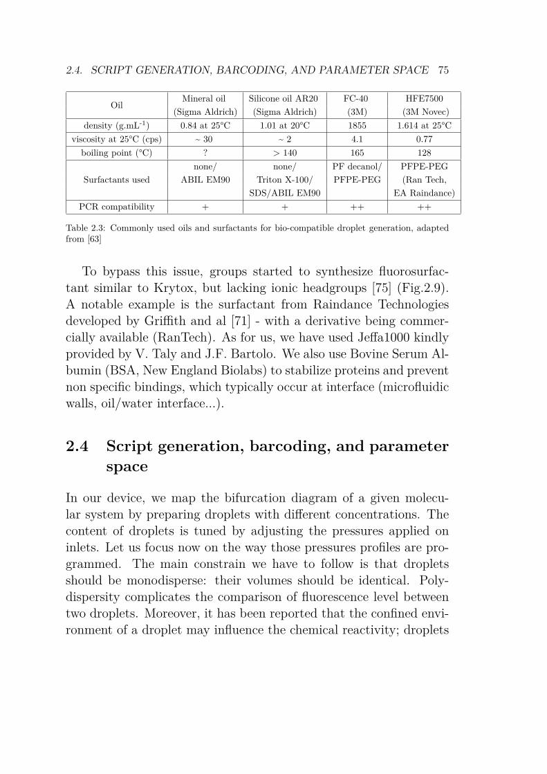
2.4. SCRIPT GENERATION, BARCODING, AND PARAMETER SPACE 75
OilMineral oil Silicone oil AR20 FC-40 HFE7500
(Sigma Aldrich) (Sigma Aldrich) (3M) (3M Novec)
density (g.mL-1) 0.84 at 25°C 1.01 at 20°C 1855 1.614 at 25°C
viscosity at 25°C (cps) ~ 30 ~ 2 4.1 0.77
boiling point (°C) ? > 140 165 128
Surfactants used
none/ none/ PF decanol/ PFPE-PEG
ABIL EM90 Triton X-100/ PFPE-PEG (Ran Tech,
SDS/ABIL EM90 EA Raindance)
PCR compatibility + + ++ ++
Table 2.3: Commonly used oils and surfactants for bio-compatible droplet generation, adaptedfrom [63]
To bypass this issue, groups started to synthesize fluorosurfac-tant similar to Krytox, but lacking ionic headgroups [75] (Fig.2.9).A notable example is the surfactant from Raindance Technologiesdeveloped by Griffith and al [71] - with a derivative being commer-cially available (RanTech). As for us, we have used Jeffa1000 kindlyprovided by V. Taly and J.F. Bartolo. We also use Bovine Serum Al-bumin (BSA, New England Biolabs) to stabilize proteins and preventnon specific bindings, which typically occur at interface (microfluidicwalls, oil/water interface...).
2.4 Script generation, barcoding, and parameterspace
In our device, we map the bifurcation diagram of a given molecu-lar system by preparing droplets with different concentrations. Thecontent of droplets is tuned by adjusting the pressures applied oninlets. Let us focus now on the way those pressures profiles are pro-grammed. The main constrain we have to follow is that dropletsshould be monodisperse: their volumes should be identical. Poly-dispersity complicates the comparison of fluorescence level betweentwo droplets. Moreover, it has been reported that the confined envi-ronment of a droplet may influence the chemical reactivity; droplets
76 CHAPTER 2. DROPLET-BASED PARAMETER SCANNING
with different size may therefore exhibit different chemical dynamic[76]. To enforce monodispersity during droplet generation, we ensurethat the total pressure applied on the aqueous channels is constant.Since the aqueous channels are identical (modulo fabrication error),this guarantees that the total aqueous flow rate is constant. To thatend, we use an additional channel (the compensation channel con-taining the master mix) which tracks and compensates variation inflow rates in the other aqueous channels (the working channel).
2.4.1 Drawing a shape in parameter space
2.4.1.1 1 dimension: the line
The simplest case is when one parameter only is explored: one onlyneeds to change one concentration. The droplets explore a 1D line inthe parameter space. For the microfluidic generation, we need twochannels: one channel containing the master mix and the parameterat maximal desired concentration, and another channel containingthe master mix only.
The first step of the protocol for droplet generation is to em-pirically find the maximum (Pmax) and minimum pressures (Pmin),corresponding to the pressure for which one channel invades or isinvaded by the other one. The script starts from an equal pressurein channel 1 and 2, and consists of a loop in which the pressure inchannel is gradually decreased 1 and increased in channel 2 graduallyuntil the Pmin in channel 1 is reached. Then the pressure in channel1 is increased as much as the pressure in channel 2 is decreased untilthe invasion of channel 2. The pressure increment is Pmax≠Pmin
nbiterwhere
nbiter is the number of iterations during one scanning. The highernbiteris, the higher the resolution of the line is, but the drawback isthe time spent running the script. We usually use 20 iterations toensure a good coverage over the pressure range.
2.4. SCRIPT GENERATION, BARCODING, AND PARAMETER SPACE 77
2.4.1.2 2 dimensions: triangle and square
Adding a variable to the system means that we now have to screenthe parameter space accross a surface and not a line. Therefore anadditional channel is required for the second parameter. We nowhave three channels : channel (Ch1) containing the parameter 1,channel 2 (Ch2) containing the parameter 2 and Channel 3 for thecompensation (Ch3).
The first geometry we could achieve was the triangle shape. Forthis polygon, each vertex of the simplex corresponds to one channelinvading the two others. As a starting point, we chose the one vertexcorresponding to the Ch1 reaching its Pmax. On that point, (Fig.2.11,a) Ch2 and 3 are invaded and the pressure in Ch1 is decrementedby 1.5(Pmax≠Pmin)
nbiter(while Ch3 is incremented by the same amount, in
order to keep the sum PCh1 + PCh2 + PCh3 constant (Fig.2.11, b);then, PCh2 increases by the same increment (Fig.2.11, c) before thedecrease of PCh1(Fig.2.11, d). Finally, the decrease of PCh2 brings itto its original value (Fig.2.11, e). This pattern is iterated nbiter timesuntil the PCh2 reaches the Pmax value. Here we name Ch2 the fastvariable and Ch1 the slow variable because the pressure range for Ch2was higher than the range for Ch1. The fast and slow variables arethen exchanged, i.e. we start from the vertex in which PCh2 = Pmax
and perform the same routine. The whole scan is completed ~10times in order to obtain at least 30 µL of emulsion.Pressures andscript are summarized in Fig.2.11.
The main advantage of this geometry is the simplicity of imple-mentation, and the time spent in running the script. Indeed, findingthe boundary pressures and perform one complete scanning will re-quire less than 10 min, which means that the embedded chemicalswill have less time to react before the encapsulation. The drawbackcomes from the fact the triangle shape itself: if two parameters aresupposed to interfere with the global behavior of the network, thetriangular shape give access to half of the possible combinations of
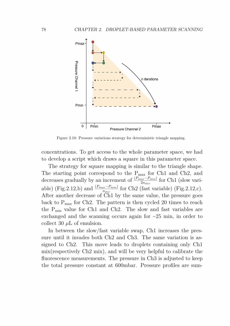
78 CHAPTER 2. DROPLET-BASED PARAMETER SCANNING
Figure 2.10: Pressure variations strategy for deterministic triangle mapping.
concentrations. To get access to the whole parameter space, we hadto develop a script which draws a square in this parameter space.
The strategy for square mapping is similar to the triangle shape.The starting point correspond to the Pmax for Ch1 and Ch2, anddecreases gradually by an increment of (Pmax≠Pmin)
2niterfor Ch1 (slow vari-
able) (Fig.2.12,b) and (Pmax≠Pmin)niter
for Ch2 (fast variable) (Fig.2.12,c).After another decrease of Ch1 by the same value, the pressure goesback to Pmax for Ch2. The pattern is then cycled 20 times to reachthe Pmin value for Ch1 and Ch2. The slow and fast variables areexchanged and the scanning occurs again for ~25 min, in order tocollect 30 µL of emulsion.
In between the slow/fast variable swap, Ch1 increases the pres-sure until it invades both Ch2 and Ch3. The same variation is as-signed to Ch2. This move leads to droplets containing only Ch1mix(respectively Ch2 mix), and will be very helpful to calibrate thefluorescence measurements. The pressure in Ch3 is adjusted to keepthe total pressure constant at 600mbar. Pressure profiles are sum-
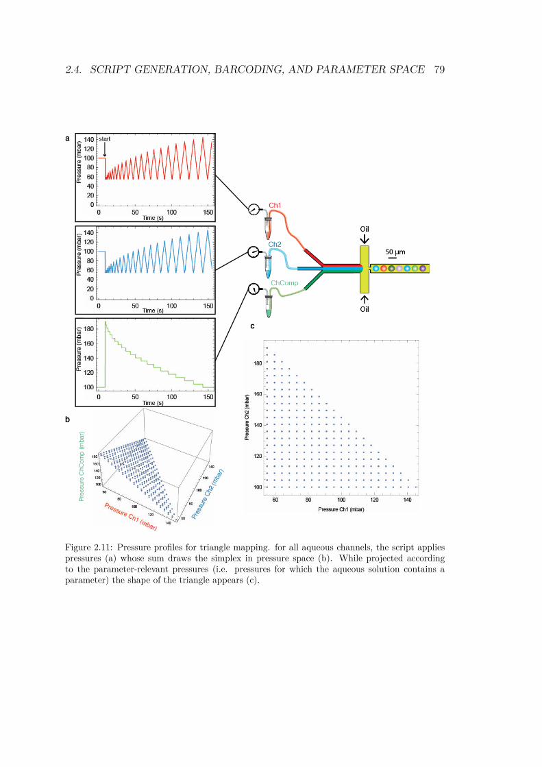
2.4. SCRIPT GENERATION, BARCODING, AND PARAMETER SPACE 79
Figure 2.11: Pressure profiles for triangle mapping. for all aqueous channels, the script appliespressures (a) whose sum draws the simplex in pressure space (b). While projected accordingto the parameter-relevant pressures (i.e. pressures for which the aqueous solution contains aparameter) the shape of the triangle appears (c).
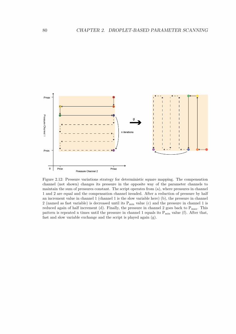
80 CHAPTER 2. DROPLET-BASED PARAMETER SCANNING
Figure 2.12: Pressure variations strategy for deterministic square mapping. The compensationchannel (not shown) changes its pressure in the opposite way of the parameter channels tomaintain the sum of pressures constant. The script operates from (a), where pressures in channel1 and 2 are equal and the compensation channel invaded. After a reduction of pressure by halfan increment value in channel 1 (channel 1 is the slow variable here) (b), the pressure in channel2 (named as fast variable) is decreased until its Pmin value (c) and the pressure in channel 1 isreduced again of half increment (d). Finally, the pressure in channel 2 goes back to Pmax. Thispattern is repeated n times until the pressure in channel 1 equals its Pmin value (f). After that,fast and slow variable exchange and the script is played again (g).
2.4. SCRIPT GENERATION, BARCODING, AND PARAMETER SPACE 81
marized in Fig.2.13.
2.4.1.3 The cube
Adding a third parameter to the exploration of the bifurcation re-quires a fourth aqueous channel and means that the resulting dia-gram will be in three dimensions. Our first approach was a gen-eralization of the square script. The volume is sliced in n-squares(typically 20), and we gradually decrease the pressure in the chan-nel corresponding to the third parameter to switch from one sliceto the next one. In order to thoroughly scan the whole cube, the 3channels containing the parameters are in turn slow variable of thesquare, fast variable of the square, and sliced third dimension. Thisdeterministic method is quite difficult to implement in terms of code,and one of the main drawback is the time required to scan the entirecube. In fact, since we repeat the previous script on 20 slices along 3dimensions, one full scan lasts 40 minutes. During this time, chemi-cal reaction could occur inside the reservoirs and corrupt the wholeexperiment. To reduce the scanning time, we put aside the deter-ministic approach for a Monte-Carlo sampling within the parameterspace. We generate a random walk inside the [0, 1]3 cube thanks toMathematica software, that is rescaled in the scripting software into[Pmin, Pmax]3 with the Pmin and Pmax values. The script is a sum ofthousands of 3D increments (—1, —2, —3), where each —i is drawnindependently from a Pareto distribution. Pareto distributions areset to ensure that the pressures sometimes move abruptly to newregions of the cube, offering a better coverage of the volume. Theboundary conditions maintain the random walk inside the cube. Theoil pressure is set to 700mbar. The pressure profiles and resultingvolume in pressure space are shown in Fig.2.14.
Thanks to this new method for volume sampling by random-walk,the scanning time is lowered to 20 minutes (setting 3000 points withinthe cube, plus three calibration processes as described for the square
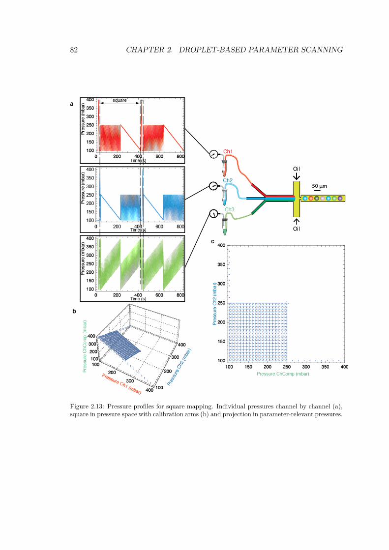
82 CHAPTER 2. DROPLET-BASED PARAMETER SCANNING
Figure 2.13: Pressure profiles for square mapping. Individual pressures channel by channel (a),square in pressure space with calibration arms (b) and projection in parameter-relevant pressures.
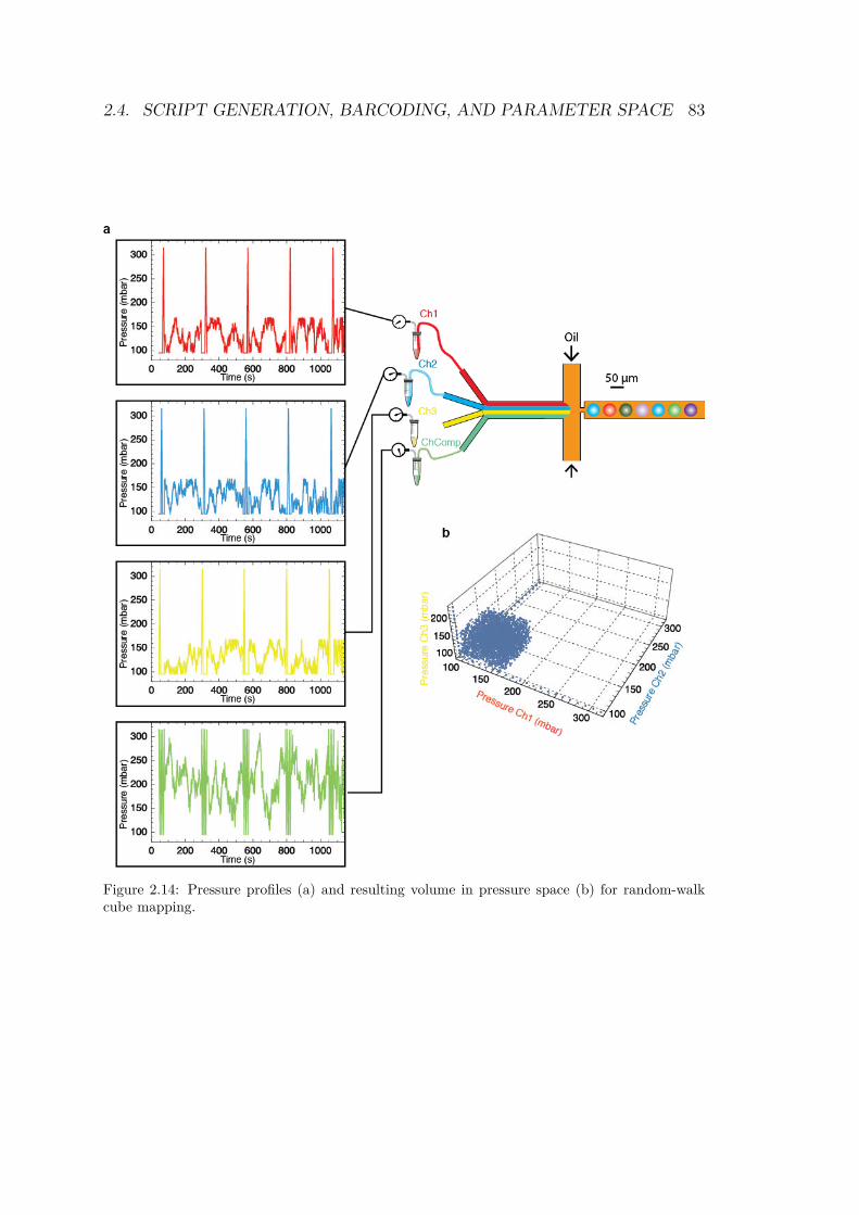
2.4. SCRIPT GENERATION, BARCODING, AND PARAMETER SPACE 83
Figure 2.14: Pressure profiles (a) and resulting volume in pressure space (b) for random-walkcube mapping.
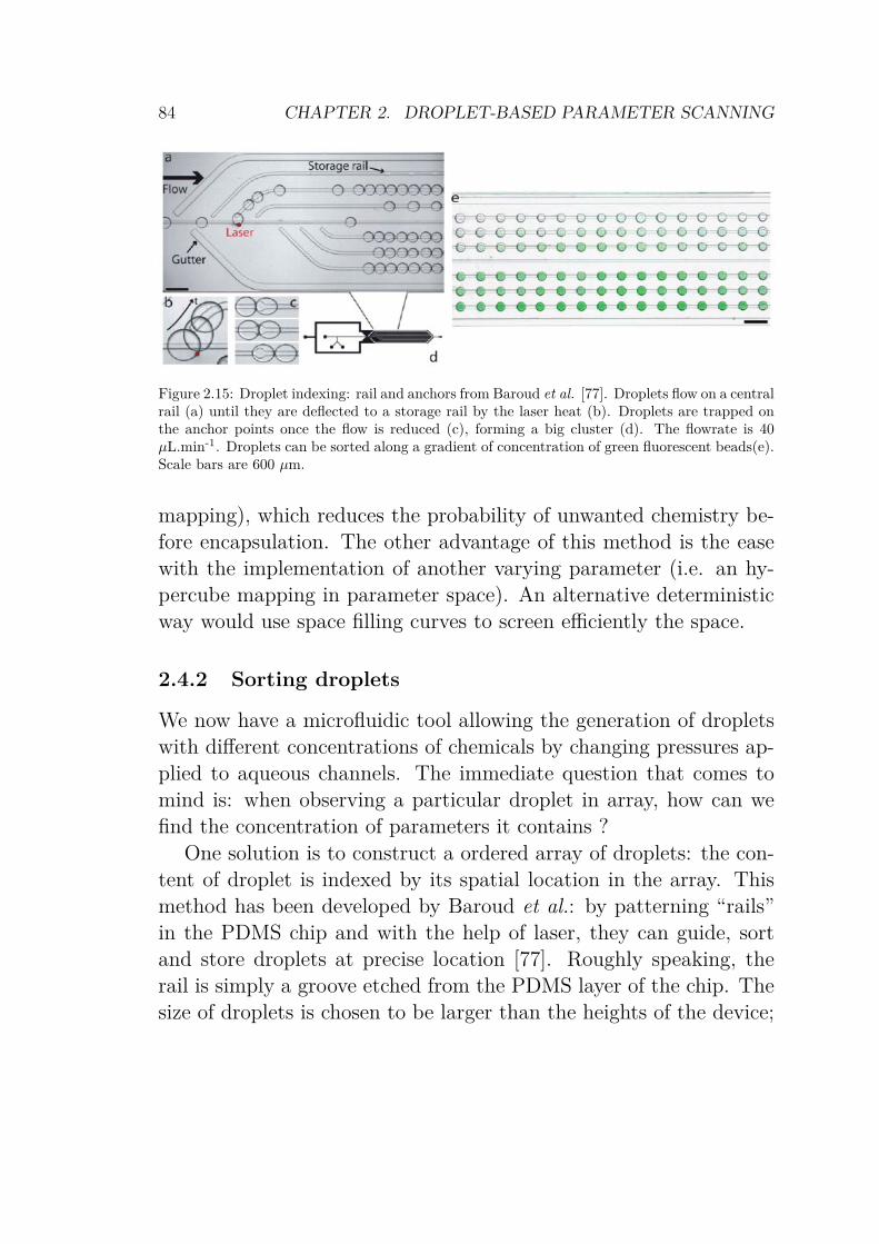
84 CHAPTER 2. DROPLET-BASED PARAMETER SCANNING
Figure 2.15: Droplet indexing: rail and anchors from Baroud et al. [77]. Droplets flow on a centralrail (a) until they are deflected to a storage rail by the laser heat (b). Droplets are trapped onthe anchor points once the flow is reduced (c), forming a big cluster (d). The flowrate is 40µL.min-1. Droplets can be sorted along a gradient of concentration of green fluorescent beads(e).Scale bars are 600 µm.
mapping), which reduces the probability of unwanted chemistry be-fore encapsulation. The other advantage of this method is the easewith the implementation of another varying parameter (i.e. an hy-percube mapping in parameter space). An alternative deterministicway would use space filling curves to screen efficiently the space.
2.4.2 Sorting droplets
We now have a microfluidic tool allowing the generation of dropletswith different concentrations of chemicals by changing pressures ap-plied to aqueous channels. The immediate question that comes tomind is: when observing a particular droplet in array, how can wefind the concentration of parameters it contains ?
One solution is to construct a ordered array of droplets: the con-tent of droplet is indexed by its spatial location in the array. Thismethod has been developed by Baroud et al.: by patterning “rails”in the PDMS chip and with the help of laser, they can guide, sortand store droplets at precise location [77]. Roughly speaking, therail is simply a groove etched from the PDMS layer of the chip. Thesize of droplets is chosen to be larger than the heights of the device;
2.4. SCRIPT GENERATION, BARCODING, AND PARAMETER SPACE 85
droplets are flattened like “pancakes” which cause a large buildupof surface energy. Droplets anchor to grooves because they offer anadditional volume to locally relieve the pancake shape into a sphere,which decreases surface tension. If the external convective flow ofthe continuous phase is not too strong, droplets remains tucked andsmoothly follow the contours of the grooves. The device shown inthe article is made of a central rail from which emerge 6 storage railswith anchors (Fig.2.15, a). To move a droplet from the central railto its storage area, a laser is activated to deflect a droplet to its des-tined storage rail. The force coming from the local heat producedis enough to eject the droplet from the rail (Fig.2.15, b). Anchorpoints along the storage rail ensure that a droplet is trapped at eachanchor site. If the laser is synchronized with the droplet generation,it becomes possible to temporally sort droplets. The authors demon-strate an example of controlled filling along droplets with a gradientof green fluorescent beads (Fig.2.15, e). Depending on the number ofanchor points and rails, the storage capacity is the main limitation.Indeed, in our system with the usual ratio of water/oil pressure, thefrequency of droplet generation is higher than 1 kHz. Knowing thatthe scanning time for the simplest mapping (i.e the line) is around10 seconds, it means that the device should be able to store at least10000 droplets. The cube mapping will require more than 1 millionanchor points for one scan. Another limitation of spatial sortingis that it is sensitive to sorting errors: slight desynchronization be-tween generation and sorting will build up over time and result inthe incorrect indexing of a large swath of droplets.
Another technical solution is a direct, online, readout within themicrofluidic chip. After generation, a droplet flows inside a channeluntil it crosses a detector which reads its content (Fig.2.16). Thistechnique is used in digital PCR and protein engineering, and al-lows high throughput analysis. Ismagilov and colleagues developedit to investigate the kinetics of an enzymatic reaction with a resolu-tion lower than the millisecond [78]. Droplets are generated from a
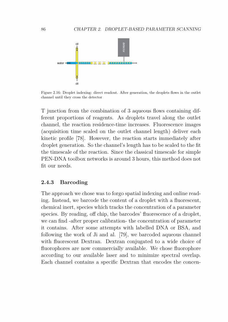
86 CHAPTER 2. DROPLET-BASED PARAMETER SCANNING
Figure 2.16: Droplet indexing: direct readout. After generation, the droplets flows in the outletchannel until they cross the detector
T junction from the combination of 3 aqueous flows containing dif-ferent proportions of reagents. As droplets travel along the outletchannel, the reaction residence-time increases. Fluorescence images(acquisition time scaled on the outlet channel length) deliver eachkinetic profile [78]. However, the reaction starts immediately afterdroplet generation. So the channel’s length has to be scaled to the fitthe timescale of the reaction. Since the classical timescale for simplePEN-DNA toolbox networks is around 3 hours, this method does notfit our needs.
2.4.3 Barcoding
The approach we chose was to forgo spatial indexing and online read-ing. Instead, we barcode the content of a droplet with a fluorescent,chemical inert, species which tracks the concentration of a parameterspecies. By reading, off chip, the barcodes’ fluorescence of a droplet,we can find -after proper calibration- the concentration of parameterit contains. After some attempts with labelled DNA or BSA, andfollowing the work of Ji and al. [79], we barcoded aqueous channelwith fluorescent Dextran. Dextran conjugated to a wide choice offluorophores are now commercially available. We chose fluorophoreaccording to our available laser and to minimize spectral overlap.Each channel contains a specific Dextran that encodes the concen-
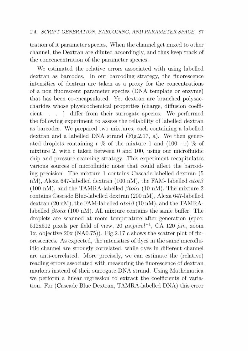
2.4. SCRIPT GENERATION, BARCODING, AND PARAMETER SPACE 87
tration of it parameter species. When the channel get mixed to otherchannel, the Dextran are diluted accordingly, and thus keep track ofthe concencentration of the parameter species.
We estimated the relative errors associated with using labelleddextran as barcodes. In our barcoding strategy, the fluorescenceintensities of dextran are taken as a proxy for the concentrationsof a non fluorescent parameter species (DNA template or enzyme)that has been co-encapsulated. Yet dextran are branched polysac-charides whose physicochemical properties (charge, diffusion coeffi-cient. . . ) differ from their surrogate species. We performedthe following experiment to assess the reliability of labelled dextranas barcodes. We prepared two mixtures, each containing a labelleddextran and a labelled DNA strand (Fig.2.17, a). We then gener-ated droplets containing r % of the mixture 1 and (100 - r) % ofmixture 2, with r taken between 0 and 100, using our microfluidicchip and pressure scanning strategy. This experiment recapitulatesvarious sources of microfluidic noise that could affect the barcod-ing precision. The mixture 1 contains Cascade-labelled dextran (5nM), Alexa 647-labelled dextran (100 nM), the FAM- labelled αtoiβ(100 nM), and the TAMRA-labelled βtoiα (10 nM). The mixture 2contains Cascade Blue-labelled dextran (200 nM), Alexa 647-labelleddextran (20 nM), the FAM-labelled αtoiβ (10 nM), and the TAMRA-labelled βtoiα (100 nM). All mixture contains the same buffer. Thedroplets are scanned at room temperature after generation (spec:512x512 pixels per field of view, 20 µs.pixel≠1, CA 120 µm, zoom1x, objective 20x (NA0.75)). Fig.2.17 c shows the scatter plot of flu-orescences. As expected, the intensities of dyes in the same microflu-idic channel are strongly correlated, while dyes in different channelare anti-correlated. More precisely, we can estimate the (relative)reading errors associated with measuring the fluorescence of dextranmarkers instead of their surrogate DNA strand. Using Mathematicawe perform a linear regression to extract the coefficients of varia-tion. For (Cascade Blue Dextran, TAMRA-labelled DNA) this error
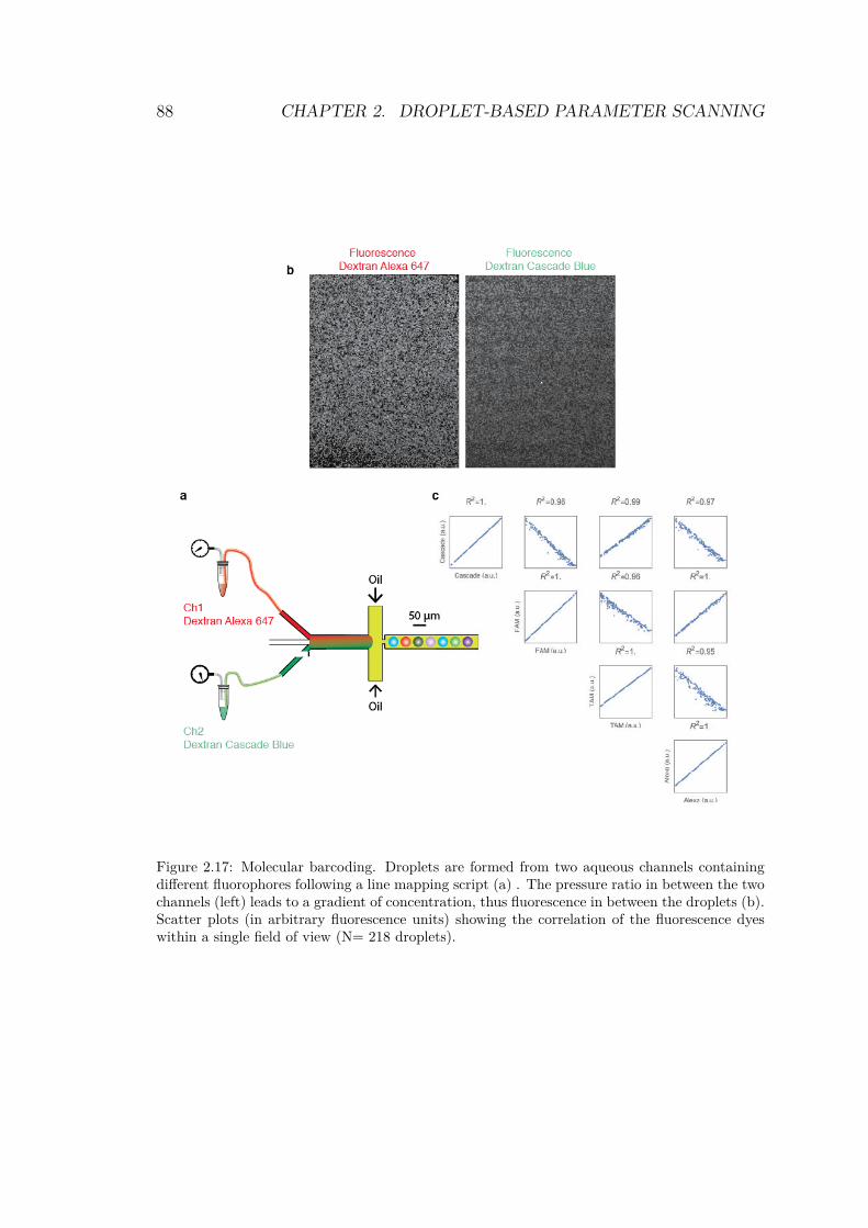
88 CHAPTER 2. DROPLET-BASED PARAMETER SCANNING
Figure 2.17: Molecular barcoding. Droplets are formed from two aqueous channels containingdifferent fluorophores following a line mapping script (a) . The pressure ratio in between the twochannels (left) leads to a gradient of concentration, thus fluorescence in between the droplets (b).Scatter plots (in arbitrary fluorescence units) showing the correlation of the fluorescence dyeswithin a single field of view (N= 218 droplets).
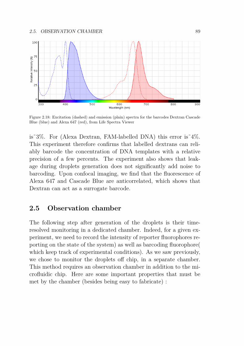
2.5. OBSERVATION CHAMBER 89
Figure 2.18: Excitation (dashed) and emission (plain) spectra for the barcodes Dextran CascadeBlue (blue) and Alexa 647 (red), from Life Spectra Viewer
is˜3%. For (Alexa Dextran, FAM-labelled DNA) this error is˜4%.This experiment therefore confirms that labelled dextrans can reli-ably barcode the concentration of DNA templates with a relativeprecision of a few percents. The experiment also shows that leak-age during droplets generation does not significantly add noise tobarcoding. Upon confocal imaging, we find that the fluorescence ofAlexa 647 and Cascade Blue are anticorrelated, which shows thatDextran can act as a surrogate barcode.
2.5 Observation chamber
The following step after generation of the droplets is their time-resolved monitoring in a dedicated chamber. Indeed, for a given ex-periment, we need to record the intensity of reporter fluorophores re-porting on the state of the system) as well as barcoding fluorophore(which keep track of experimental conditions). As we saw previously,we chose to monitor the droplets off chip, in a separate chamber.This method requires an observation chamber in addition to the mi-crofluidic chip. Here are some important properties that must bemet by the chamber (besides being easy to fabricate) :
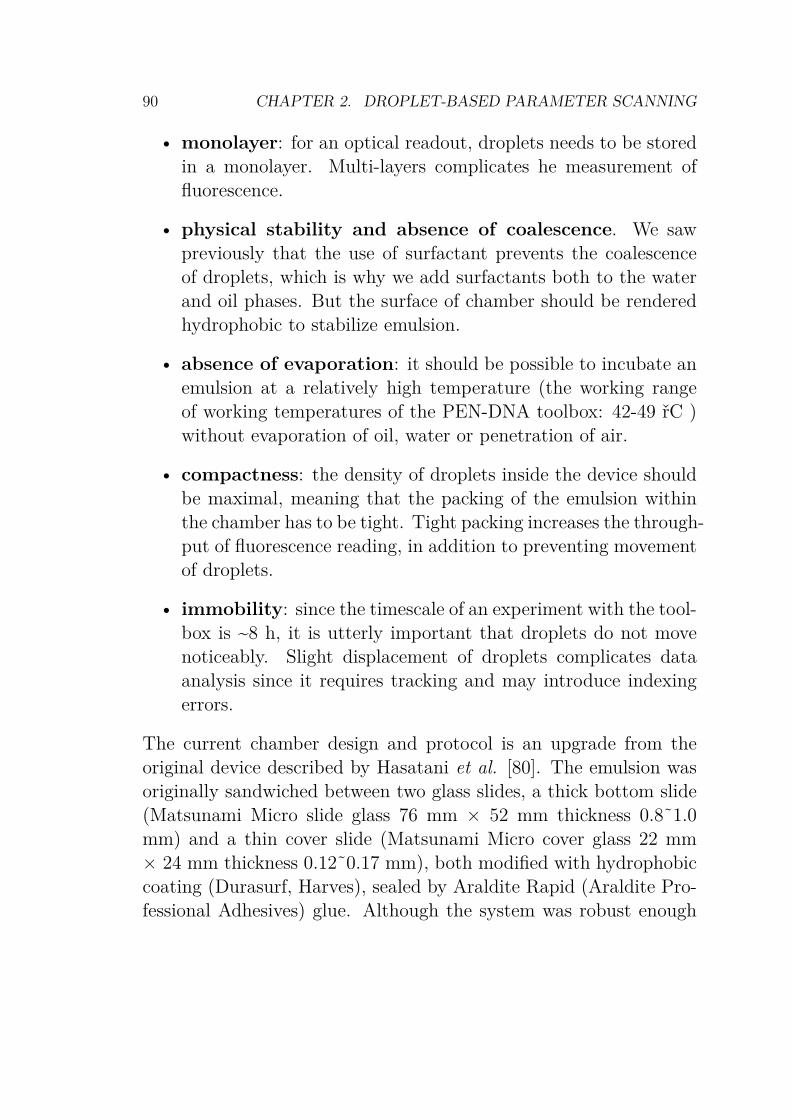
90 CHAPTER 2. DROPLET-BASED PARAMETER SCANNING
• monolayer: for an optical readout, droplets needs to be storedin a monolayer. Multi-layers complicates he measurement offluorescence.
• physical stability and absence of coalescence. We sawpreviously that the use of surfactant prevents the coalescenceof droplets, which is why we add surfactants both to the waterand oil phases. But the surface of chamber should be renderedhydrophobic to stabilize emulsion.
• absence of evaporation: it should be possible to incubate anemulsion at a relatively high temperature (the working rangeof working temperatures of the PEN-DNA toolbox: 42-49 řC )without evaporation of oil, water or penetration of air.
• compactness: the density of droplets inside the device shouldbe maximal, meaning that the packing of the emulsion withinthe chamber has to be tight. Tight packing increases the through-put of fluorescence reading, in addition to preventing movementof droplets.
• immobility: since the timescale of an experiment with the tool-box is ~8 h, it is utterly important that droplets do not movenoticeably. Slight displacement of droplets complicates dataanalysis since it requires tracking and may introduce indexingerrors.
The current chamber design and protocol is an upgrade from theoriginal device described by Hasatani et al. [80]. The emulsion wasoriginally sandwiched between two glass slides, a thick bottom slide(Matsunami Micro slide glass 76 mm × 52 mm thickness 0.8˜1.0mm) and a thin cover slide (Matsunami Micro cover glass 22 mm× 24 mm thickness 0.12˜0.17 mm), both modified with hydrophobiccoating (Durasurf, Harves), sealed by Araldite Rapid (Araldite Pro-fessional Adhesives) glue. Although the system was robust enough
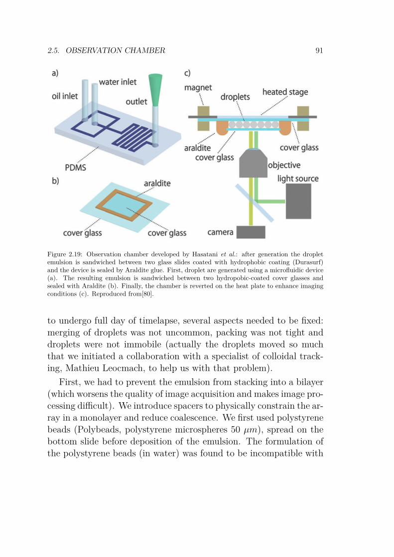
2.5. OBSERVATION CHAMBER 91
Figure 2.19: Observation chamber developed by Hasatani et al.: after generation the dropletemulsion is sandwiched between two glass slides coated with hydrophobic coating (Durasurf)and the device is sealed by Araldite glue. First, droplet are generated using a microfluidic device(a). The resulting emulsion is sandwiched between two hydropobic-coated cover glasses andsealed with Araldite (b). Finally, the chamber is reverted on the heat plate to enhance imagingconditions (c). Reproduced from[80].
to undergo full day of timelapse, several aspects needed to be fixed:merging of droplets was not uncommon, packing was not tight anddroplets were not immobile (actually the droplets moved so muchthat we initiated a collaboration with a specialist of colloidal track-ing, Mathieu Leocmach, to help us with that problem).
First, we had to prevent the emulsion from stacking into a bilayer(which worsens the quality of image acquisition and makes image pro-cessing difficult). We introduce spacers to physically constrain the ar-ray in a monolayer and reduce coalescence. We first used polystyrenebeads (Polybeads, polystyrene microspheres 50 µm), spread on thebottom slide before deposition of the emulsion. The formulation ofthe polystyrene beads (in water) was found to be incompatible with
92 CHAPTER 2. DROPLET-BASED PARAMETER SCANNING
our system (hydrophobic glass coating, water-in-oil droplets) so weturned to glass beads instead (Polysciences Inc.) filtered on 50 µmCellTrics filter (Partec). The spacers’ diameter controls the depthof device and was chosen to match the targeted size of droplets:~50 µm. The distribution of the spacers all over the surface ensuresthat the bottom slide and cover slide remain parallel. The spacersalso support the cover slide and reduce the pressure it exerts on thedroplets, which was a factor contributing to coaslecence. Finally, thespacers are also useful to avoid that the droplets arrange in bilayers(Fig.2.20, left), this conformation making the optical readout muchmore complicated. However, droplets in contact with the spacerstend to merge because spacers are not treated with a hydrophobiccoating.
Having eliminated one cause of coalescence (the pressure exertedby the coverslide on the droplets) we turned to other culprits. Themain interaction between the emulsion and the chamber is througha thin hydrophobic coating. We changed the Durasurf coating for aCytop 809M (10% diluted in the provided solvent, Asahi glass), anamorphous fluoropolymer widely used in microfluidic for hydropho-bic coating (water contact angle of 112o, against 53o for hexadecane),and compatible with optical measurements [81]. This coating is ap-plied by spincoating at 500 rpm for 5 seconds then 2000 rpm for 30seconds. The freshly coated glass slides are then baked at 180 oC for60 minutes. The emulsion was found to be much more stable, andthe residual merging events were often due to dust speckles comingfrom the continuous or dispersed phase.
The last issue to solve was the air tightness over the long term. Weoften found that air bubbles appeared, grew and thereby disruptedthe droplet array. The presence of air bubbles is not a problem perse, but their disruptive movement seriously complicated the trackingof droplets. In fact sudden jiggles were such a serious problems thatit made unusable a large number of droplets (typically a few dozenspercents of the population).
2.5. OBSERVATION CHAMBER 93
Where do the bubbles come from ? We suspect that our majorsource of air bubble is the sealing of the chamber, when we (carefully)deposit the cover slide on the emulsion and spacer, and then sealthe assembly with an adhesive. Also, the spacers possibly enhancethe growth of bubbles by nucleation. So we investigated both thefilling and the sealing of the device. The choice of Araldite as aglue seal was discussed. This highly viscous two-components glueis uneasy to handle, and its optical properties (autofluorescence ingreen) make it difficult to scan droplet near the edge. But its mainadvantage, compared to other tested glues, that it is relatively inertregarding the chemistry happening inside the droplets. To ensure atight junction between the edge of the cover slide and the bottomslide, we decided to supplement Araldite with a photocurable glueon the whole perimeter of the chamber. We focused on one gluein particular: NOA81 (Norland Products Inc.). The advantage isthat this glue has already been used for cell management [82], so weguessed it would not interfere with our biochemistry. As it turns outexperimentally, NOA spacers do interfere with the chemistry in theneighboring droplets, as we can see on (Fig.2.20, right).
We suspect that NOA monomers remain after curing and thattheir diffusion through the oil phase induces side-reactions withinthe droplets. As a consequence, we extended the exposure time toone minute to thoroughly crosslink the monomers. We also avoid asmuch as possible using data from droplets next to NOA materials(border or spacers), and removed the central spacer that served as apillar.
The other front was the improvement of the filling technique. In-stead of simply “dropping” the cover slide on the emulsion (whichhad to deposited perfectly parallel and without shudder to preventthe emulsion from moving or air bubbles from being introduced), wethought about a way to directly prepare the chamber before filling itwith the emulsion. This pre-assembly would solve both the bubbleand packing problems. After some work, we managed to do it thank
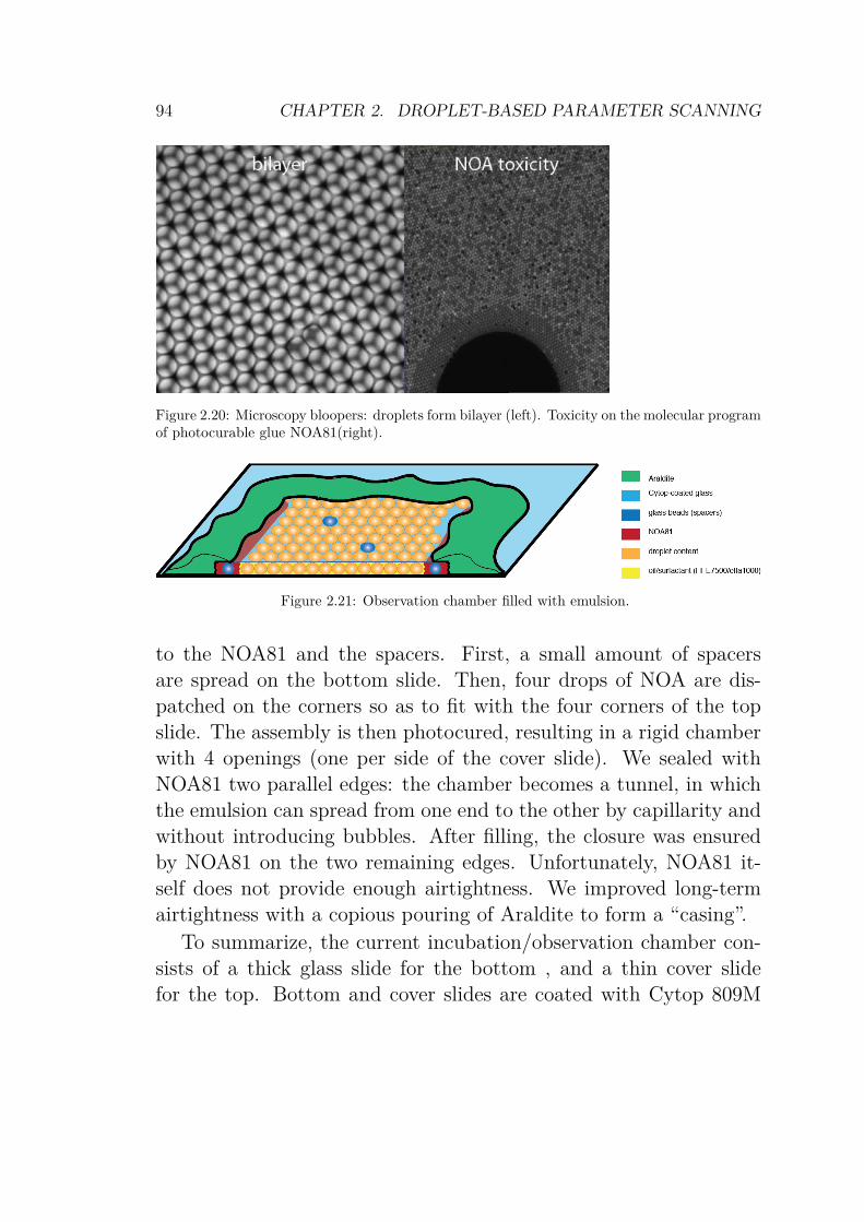
94 CHAPTER 2. DROPLET-BASED PARAMETER SCANNING
Figure 2.20: Microscopy bloopers: droplets form bilayer (left). Toxicity on the molecular programof photocurable glue NOA81(right).
Figure 2.21: Observation chamber filled with emulsion.
to the NOA81 and the spacers. First, a small amount of spacersare spread on the bottom slide. Then, four drops of NOA are dis-patched on the corners so as to fit with the four corners of the topslide. The assembly is then photocured, resulting in a rigid chamberwith 4 openings (one per side of the cover slide). We sealed withNOA81 two parallel edges: the chamber becomes a tunnel, in whichthe emulsion can spread from one end to the other by capillarity andwithout introducing bubbles. After filling, the closure was ensuredby NOA81 on the two remaining edges. Unfortunately, NOA81 it-self does not provide enough airtightness. We improved long-termairtightness with a copious pouring of Araldite to form a “casing”.
To summarize, the current incubation/observation chamber con-sists of a thick glass slide for the bottom , and a thin cover slidefor the top. Bottom and cover slides are coated with Cytop 809M
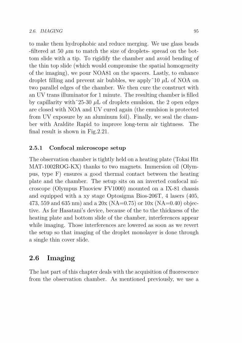
2.6. IMAGING 95
to make them hydrophobic and reduce merging. We use glass beads-filtered at 50 µm to match the size of droplets- spread on the bot-tom slide with a tip. To rigidify the chamber and avoid bending ofthe thin top slide (which would compromise the spatial homogeneityof the imaging), we pour NOA81 on the spacers. Lastly, to enhancedroplet filling and prevent air bubbles, we apply˜10 µL of NOA ontwo parallel edges of the chamber. We then cure the construct withan UV trans illuminator for 1 minute. The resulting chamber is filledby capillarity with˜25-30 µL of droplets emulsion, the 2 open edgesare closed with NOA and UV cured again (the emulsion is protectedfrom UV exposure by an aluminum foil). Finally, we seal the cham-ber with Araldite Rapid to improve long-term air tightness. Thefinal result is shown in Fig.2.21.
2.5.1 Confocal microscope setup
The observation chamber is tightly held on a heating plate (Tokai HitMAT-1002ROG-KX) thanks to two magnets. Immersion oil (Olym-pus, type F) ensures a good thermal contact between the heatingplate and the chamber. The setup sits on an inverted confocal mi-croscope (Olympus Fluoview FV1000) mounted on a IX-81 chassisand equipped with a xy stage Optosigma Bios-206T, 4 lasers (405,473, 559 and 635 nm) and a 20x (NA=0.75) or 10x (NA=0.40) objec-tive. As for Hasatani’s device, because of the to the thickness of theheating plate and bottom slide of the chamber, interferences appearwhile imaging. Those interferences are lowered as soon as we revertthe setup so that imaging of the droplet monolayer is done througha single thin cover slide.
2.6 Imaging
The last part of this chapter deals with the acquisition of fluorescencefrom the observation chamber. As mentioned previously, we use a
96 CHAPTER 2. DROPLET-BASED PARAMETER SCANNING
confocal microscope to record the fluorescence levels for each droplet,rather than a classical wide-field epifluorescence. The main advan-tage of confocal microscopy is its ability to generate small opticalsections (above the micrometer size) that excludes light from out-of-focus objects (such as dust). Because it is a scanning technique,there are also less spatial inhomogeneities, as described in Fig.2.22.
Why did we choose confocal imaging ? The information of oursystem is encoded in fluorescence levels which can be very close (theindirect reporting of N-quenching shifts fluorescence by only a fewdozens percent). Our need of a very high signal-to-noise ratio is aclincher that decided the use of confocal microscopy.
However, confocal scanning has a few drawbacks. The limitednumber of laser wavelength available (four in our microscope) is one,since we need one wavelength per barcode and observable. (See Table2.4 for a non exhaustive list of available fluorophores.) This problemwould be less significant with an epifluorescence microscope, whichhas a much wider range of excitation sources (mercury lamp or LED)and filters. The second limitation is that confocal scanning is slow, asthe laser raster the sample to form an image. Acquisition of a singlefield of view typically takes ~10 seconds, which must be compared tothe 0.1-1 s required for wide-field fluorescence microscopy. Becausethis time-limit is a serious bottleneck, we have spent considerabletime optimizing the acquisition protocol to maximize the number ofdroplets scanned per unit of time.
2.6.1 Time-lapse
The chamber is heated at a given temperature by the hotplate, andfluorescence data is recorded for each droplet. For each droplet,the fluorescence levels of the barcodes indicate the initial parameterconditions (i.e. the coordinates in the parameter space), while thefluorescence levels of the input and output give the final state of thesystem (the color in the bifurcation diagram).
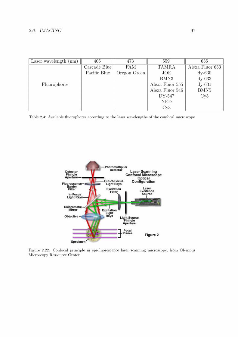
2.6. IMAGING 97
Laser wavelength (nm) 405 473 559 635Cascade Blue FAM TAMRA Alexa Fluor 633Pacific Blue Oregon Green JOE dy-630
BMN3 dy-633Fluorophores Alexa Fluor 555 dy-631
Alexa Fluor 546 BMN5DY-547 Cy5NEDCy3
Table 2.4: Available fluorophores according to the laser wavelengths of the confocal microscope
Figure 2.22: Confocal principle in epi-fluorescence laser scanning microscopy, from OlympusMicroscopy Ressource Center
98 CHAPTER 2. DROPLET-BASED PARAMETER SCANNING
2.6.1.1 Fast settings
We have to set the confocal properties for the experiment. Thedetector pinhole value reflects the number of photons reaching thedetector. A smaller aperture leads to less background, but also lesssignal. On the contrary, a high pinhole aperture emphasizes back-ground . Usually, we set the value of the pinhole to ~100 µm to getthe maximum amount of light and avoiding interferences (see above).The PMT collects light from the sample, and gives an intensity foreach pixel. Depending on the laser intensity, the PMT needs to beadjusted so that weak signals are detected ( high laser intensity, lowPMT) without too much photobleaching (avoided with lower laserintensity, and higher PMT). The ideal values (maximum number ofphotons collected for minimal laser intensity) are empirically set foreach experiment.
We also use a simple formula to approximate the number of pho-tons hitting the sample: zoom2 · N.A.2 · laserpower · time.pixel≠1 ·C.A.2 · mag2 · npix , where npix is the number of pixel and mag themagnificence.
2.6.1.2 Time constraint
Another dimension that one should take care about is how long cana scan be. The dwell time is defined as the amount of time that thelaser beam lingers in an unit of space corresponding to one pixel inthe image. Long dwell time provide more photons per pixels. Butit also leads to more photobleaching and longer acquisition time.The global timescale of the studied network also constrains the dwelltime. In the case of a endpoint measurement (like the bistable switchwhere we only need the final state of the system), a long dwell time,and thus a long acquisition time, can be tolerated. In the case of atimelapse experiment, time-resolved measurements are required andlong dwell time cannot be used. These factors, combined with thenumber of droplets required defines the time spent to acquire one
2.6. IMAGING 99
image.
2.6.1.3 Colors
The limited number of laser wavelengths available (405 nm, 473 nm,559 nm, 635 nm, which is a respectable number for a laser confocal)makes some mapping quite delicate. In the case of a network withtwo different fluorescence observables, explored along 3 parameters,we need 5 colors to map the diagram of the network.
One solution to maps more than 4 dimensions is to simultaneouslyuse one of the reporter dye as a barcode. This is possible if the dy-namic of the observable is easily deconvolved. For example, initiallyreading the fluorescence of dye attached to a predator/prey templatewill provide the initial concentration of this template. Reading thevariations of intensity of this dye over time will inform us about theoscillations of concentrations of preys binding to the template. An-other option would be to use a XLdye: a fluorophore which exhibitsa big gap between excitation and emission wavelengths (Stoke shift).Imaging the sample with one laser gives access to two parameter in-formations by using two different monochromator value as emissionfilters.
2.6.1.4 Optical defects
One of the biggest challenge in the confocal imaging of droplets arrayswas the suppression of optical interferences. The laser goes throughseveral layers of materials (oil, water, glass, air...) with different re-fractive indexes. Reflections occurring at interfaces whose refractiveindexes are mismatched were found to severely compromise the qual-ity of fluorescence readings, especially near the green wavelength. Tosmoothen the transition between materials with different refractiveindexes, Booth and Wilson [83] provide some advices, such as reduc-ing the pupil size to improve the focal distribution, or tuning therefractive index of the immersion medium to reduce mismatch. The
100 CHAPTER 2. DROPLET-BASED PARAMETER SCANNING
first improvement we undertook was to revert the heating plate. The«classical» position, where the heating plate sits at the bottom, leadsto 5 interfaces (air/heating plate, heating plate/immersion oil, im-mersion oil/bottom slide, bottom slide/droplet oil and finally dropletoil/droplet content). By reverting the hotplate, we reeducate stack-ing to 3 interfaces (air/cover slide, cover slide/oil, and oil/droplets).An added benefit is that glass layers are now much thinner, goingfrom a few millimeters (heating plate+ bottom slide) to hundreds ofmicrons (coverslide). Glass thickness is important because most ob-jective are optimized for a standard glass thickness of ~170 microns.
The second improvement was to upgrade objectives to the bestnumerical aperture available. Numerical Aperture is the most im-portant parameter of the most important component of the micro-scope: the objective. NA characterize the «opening» of an objectivelens, that is its ability to collect lights from off-axis rays. In epiflu-orescence, NA is doubly important because the objective acts alsoas a condenser: it capture and condenses light from the illuminationsource. As a rule of thumb, the number of photon collected from asample scales like NA4! Even minor improvements to the NA canimprove the imaging of dim samples. Importantly, the performancesof an objective depend on the wavelength. Thus the choice of colorsand working objectives should not be neglected when planning anexperiments. In our case, the worst spherical aberrations were seenat the lowest wavelength: 405 nm and 473 nm. The best settingswere then the use of a 20 x objective (UPlanSApo 20x, N.A.: 0.75nm, Olympus).
2.6.2 Endpoint method
This method suits experiments for which a time-lapse is not necessaryand the final steady-state of the system contains the information.
Droplets are collected after generation in a PCR tube, in an incu-bator so that the network can compute at a constant temperature.
2.7. CONCLUSION 101
The incubation time and temperatures depend on the system, typi-cally between 42 and 49 °C, from 3 to 24 hours.
One classical issue during the heating process of an emulsion isthe coalescence of the droplets. This phenomenon is consecutive tothe drainage of the oil phase, thinning the liquid phase in betweenthe droplets. V. Taly and coworkers proposed a solution to avoidthe merging of water-in-oil emulsion happening during a digital PCRexperiment [56]. First, a cylindrical PDMS plug is thrust in the PCRtube. The plug shows with two thin holes (one inlet, one outlet). Theemulsion is then injected inside the tube through the inlet, makingsure that no air or oil is trapped in the device. After tubing removal,the PCR experiment can start.
An other solution, less efficient though, would be to cover thecream by another -lighter- oil (typically mineral oil) to prevent theevaporation. Surprisingly, we observe very little merging withoutusing a plug or different oil film covering. This could be explainedby the fact that, in the case of a PCR experiment, the tempera-tures reached are much higher than ours (moreover we do not cycletemperature). The emulsion turns out to be quite stable, no or fewcoalescence was observed.
Once the steady state is presumed to be reached, we fill the ob-serving chamber with the incubated emulsion (as described before),and record its fluorescence over the whole array using confocal scan-ning.
2.7 Conclusion
In this chapter we detailed the development of a microfluidic toolfor the experimental mapping of a bifurcation diagram. Our devicegenerates millions of water-in-oil droplets with different compositionby focusing aqueous flows. The composition is controlled by indi-vidually adjusting in real-time the pressure of each aqueous channel.The script executed by the pressure controller sample the parameter
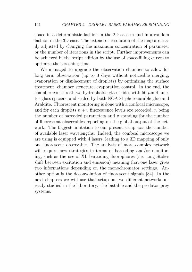
102 CHAPTER 2. DROPLET-BASED PARAMETER SCANNING
space in a deterministic fashion in the 2D case m and in a randomfashion in the 3D case. The extend or resolution of the map are eas-ily adjusted by changing the maximum concentration of parameteror the number of iterations in the script. Further improvements canbe achieved in the script edition by the use of space-filling curves tooptimize the screening time.
We managed to upgrade the observation chamber to allow forlong term observation (up to 3 days without noticeable merging,evaporation or displacement of droplets) by optimizing the surfacetreatment, chamber structure, evaporation control. In the end, thechamber consists of two hydrophobic glass slides with 50 µm diame-ter glass spacers, and sealed by both NOA 81 photocurable glue andAraldite. Fluorescent monitoring is done with a confocal microscope,and for each droplets n + v fluorescence levels are recorded, n beingthe number of barcoded parameters and v standing for the numberof fluorescent observables reporting on the global output of the net-work. The biggest limitation to our present setup was the numberof available laser wavelengths. Indeed, the confocal microscope weare using is equipped with 4 lasers, leading to a 3D mapping of onlyone fluorescent observable. The analysis of more complex networkwill require new strategies in terms of barcoding and/or monitor-ing, such as the use of XL barcoding fluorophores (i.e. long Stokesshift between excitation and emission) meaning that one laser givestwo informations depending on the monochromator settings. An-other option is the deconvolution of fluorescent signals [84]. In thenext chapters we will use that setup on two different networks al-ready studied in the laboratory: the bistable and the predator-preysystems.
Chapter 3
Mapping a bistable circuit
3.1 Introduction
3.1.1 bistability: two examples in biology
Bistability can be intuitively understood as the existence of two sta-ble steady states within a dynamic chemical system. This means thatthe long term dynamic of a bistable system depends not only on itsparameter, but also its history, a phenomenon known as hysteresis.Additionally, the system can often be perturbed by a chemical stim-uli to jump from a stable state to another. Such switching in bistablesystems can be seen as a storage function, or memory and has founduses in many biological processes.
As an example, Bhalla et al. showed that the Mitogen-ActivatedProtein Kinase signaling network (MAPK) -a major cellular pathwaydealing with cell cycle and the whole secretory function- exhibits abistable activity [85]. The simplified network (Fig.3.1, green panel)is a positive feedback loop in which the activity of MAPK is linkedto the activity of Protein Kinase C (PKC) through the activation ofmultiple intermediates. The activation of MAPK or PKC inducesa rise of the concentrations, which are then sustained. The sys-tem is therefore bistable, with a basal and activated state. The au-thors showed a simulated bistability plot by running the simulationwith a fixed concentration of MAPK and reading the value of active
103
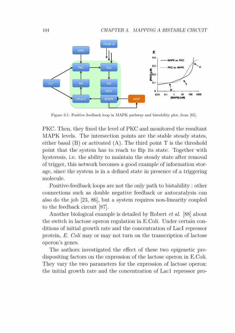
104 CHAPTER 3. MAPPING A BISTABLE CIRCUIT
Figure 3.1: Positive feedback loop in MAPK pathway and bistability plot, from [85].
PKC. Then, they fixed the level of PKC and monitored the resultantMAPK levels. The intersection points are the stable steady states,either basal (B) or activated (A). The third point T is the thresholdpoint that the system has to reach to flip its state. Together withhysteresis, i.e. the ability to maintain the steady state after removalof trigger, this network becomes a good example of information stor-age, since the system is in a defined state in presence of a triggeringmolecule.
Positive-feedback loops are not the only path to bistability : otherconnections such as double negative feedback or autocatalysis canalso do the job [23, 86], but a system requires non-linearity coupledto the feedback circuit [87].
Another biological example is detailed by Robert et al. [88] aboutthe switch in lactose operon regulation in E.Coli. Under certain con-ditions of initial growth rate and the concentration of LacI repressorprotein, E. Coli may or may not turn on the transcription of lactoseoperon’s genes.
The authors investigated the effect of these two epigenetic pre-dispositing factors on the expression of the lactose operon in E.Coli.They vary the two parameters for the expression of lactose operon:the initial growth rate and the concentration of Lac1 repressor pro-
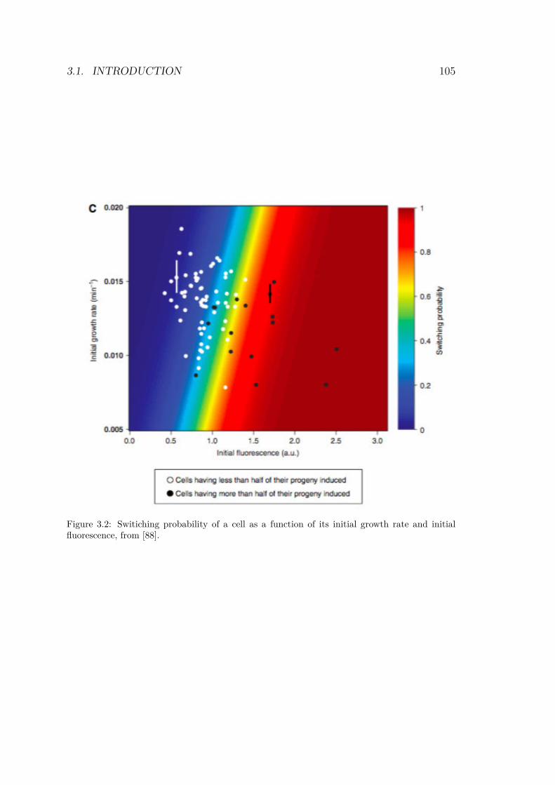
3.1. INTRODUCTION 105
Figure 3.2: Switiching probability of a cell as a function of its initial growth rate and initialfluorescence, from [88].
106 CHAPTER 3. MAPPING A BISTABLE CIRCUIT
tein -inhibiting the production of lac operon- and monitor the pu-tative expression of lactose operon in E.Coli. They finally map adiagram showing the result (expression or inhibition of the lactoseoperon) in function of both factors and the resulting switch proba-bility (Fig.3.2).
3.1.2 Introduction to bifurcation theory
Many levels of modeling are available to represent a dynamic sys-tem like a gene regulatory network. At the higher level, Booleanor Bayesian networks capture the overall function of a network, buttheir abstraction omits -almost by definition- important lower lev-els mechanisms (such as kinetics and thermodynamic aspects). Tofaithfully encompass kinetics effects and understand how changingkinetic parameters will affect the system, a lower level model made ofparametrized Ordinary Differential Equations (ODE) is more appro-priate. (See [89] for an extensive comparison between modelizationmethods). The limitation of the modelization by ODE is the increas-ing number of parameters as soon as the network topology expands.For a given network, each behavior (e.g. bistability, monostabilityor oscillations) can be characterized as a family of solutions of theODE, each family corresponding to a set of parameters, that are dif-ferent from the variables. In other words, the goal of the molecularengineer is to find the parameters that give rise to a desired dynamic.
Let us consider a dynamical system·x = f(x, µ), where x are the
dynamic variable in the phase space Rn, µ are the parameters in
the parameter space Rm and f : Rm,n æ R
n is the function definingthe dynamical system. We define the phase portrait as the partitionof the phase space in orbits with their direction in respect to time.These orbits can be equilibria, periodics... depending on the solutionsthey represent. The phase portrait holds all the states the systemtends to (i.e. all orbits). It can be seen as «a flow of some fluid,where the orbits show the paths of liquid particles as they follow the
3.1. INTRODUCTION 107
current» [90].
Two systems whose phase portraits are homeomorphic (i.e. oneshape can be continuously deformed to become the second one) arecalled topologically equivalent. A bifurcation occurs when -for agiven dynamical system- a change of the parameter leads to a topo-logically non-equivalent phase portrait. A bifurcation diagram isthen a lamination of the parameter space of a dynamical system,representing the phase portraits for each layer.
Many types of bifurcation exist, depending on their conditions ofoccurrence and the kind of change they characterize in the phaseportrait. In this manuscript we consider in particular three types ofbifurcations. First, the Andronov-Hopf bifurcation, which is charac-terized by the apparition or disapparition of a periodic orbit whenchanging the value of the stable point. The second type is the saddle-node bifurcation, which corresponds to the collision and disappear-ance of two equilibrium points in the phase portraits, and delimitshere the area of monostable and bistable behaviors, and finally aparticular kind of bifurcation for which the eigenvalues of the equi-librium are null.
3.1.3 Two PEN-DNA-toolbox examples
We now explain in more details how bistability can be implementedin the PEN-DNA toolbox. We showed that bistability is a verycommon feature in biological networks and data mining has exposedmany simple motifs that can support bistability in the biologicalworld [91, 92]. A common point is that bistability requires at leastone positive feedback loop. The modularity of the PEN-DNA tool-box (which allows the connection of positive and negative feedbackloops) makes it possible to design a bistable circuit, by connectingtwo inversion modules in an antagonistic way therefore creating abistable loop [45]. Each autocatalyst stimulates its own productionand the production of the other catalyst’s inhibitor. This system
108 CHAPTER 3. MAPPING A BISTABLE CIRCUIT
a priori leads to four possibles final states (no species surviving,only one species surviving, both species surviving), depending onthe initial conditions (Fig.3.3, top). The implementation in DNAstrands compatible with the PEN-DNA toolbox was conducted asfollows (Fig.3.3, bottom): trigger α binds to the the template αtoα
(named the input region) that is designed to generate autocatalysis(its sequence is a repeat of the complementary strand of the trigger).The polymerase then elongates the trigger into an adduct trigger-template, which exhibits a recognition site for the nicking enzyme.After cutting, two α strands are released. In the same way, the au-tocatalyst βtoβ produces β. The trigger β can also interact with thetemplate βtoiα to generate the iα, the inhibitor of the autocatalytictemplate αtoα. Likewise, αtoiβ produces iβ, the inhibitor of βtoβ.
Adrien Padirac successfully implemented this network and usedit as a footboard for the implementation of more complex networks,such as a binary counter [45]. An alternative design of a bistablesystem is in principe possible, which does not rely on cross inhibi-tion and requires only one autocatalytic module [93] (Fig.3.4). Thedifference with the previous bistable system lays in an undegradablepool of triggering agent γ that ensures a constant production of astrand β, which in turn produces iα, the inhibitor of α. On the otherhand, α is produced in an autocatalytic way, thus generating iβγ theinhibitor of β production. Such a system is compatible with the DNAtoolbox and the network is quite easy to design (Fig.3.4, bottom),the trigger γ being protected from the exonuclease by addition ofphosphorothioates modifications at the 5’ end of the strand).
Despite being rudimentary , the one-autocatalyst bistable circuitis less robust than the two autocatalysts one. Indeed, let us considera simple mathematical model based on Michaelis-Menten kinetics onthe amplification of a template T (xtoy):
x + Tk1
⌦k−1
xTk2æ x + y + T
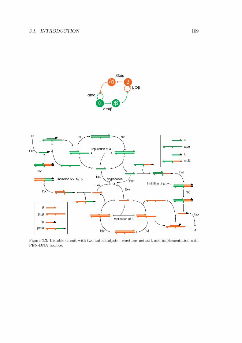
3.1. INTRODUCTION 109
Figure 3.3: Bistable circuit with two autocatalysts : reactions network and implementation withPEN-DNA toolbox
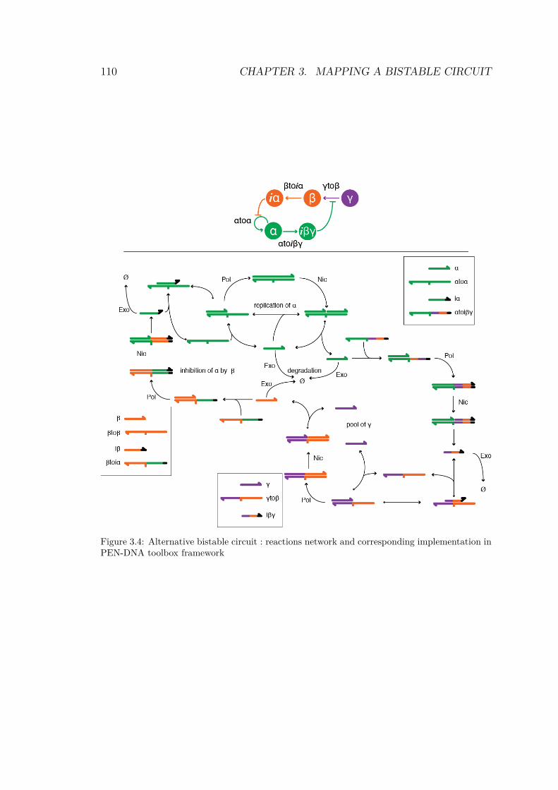
110 CHAPTER 3. MAPPING A BISTABLE CIRCUIT
Figure 3.4: Alternative bistable circuit : reactions network and corresponding implementation inPEN-DNA toolbox framework
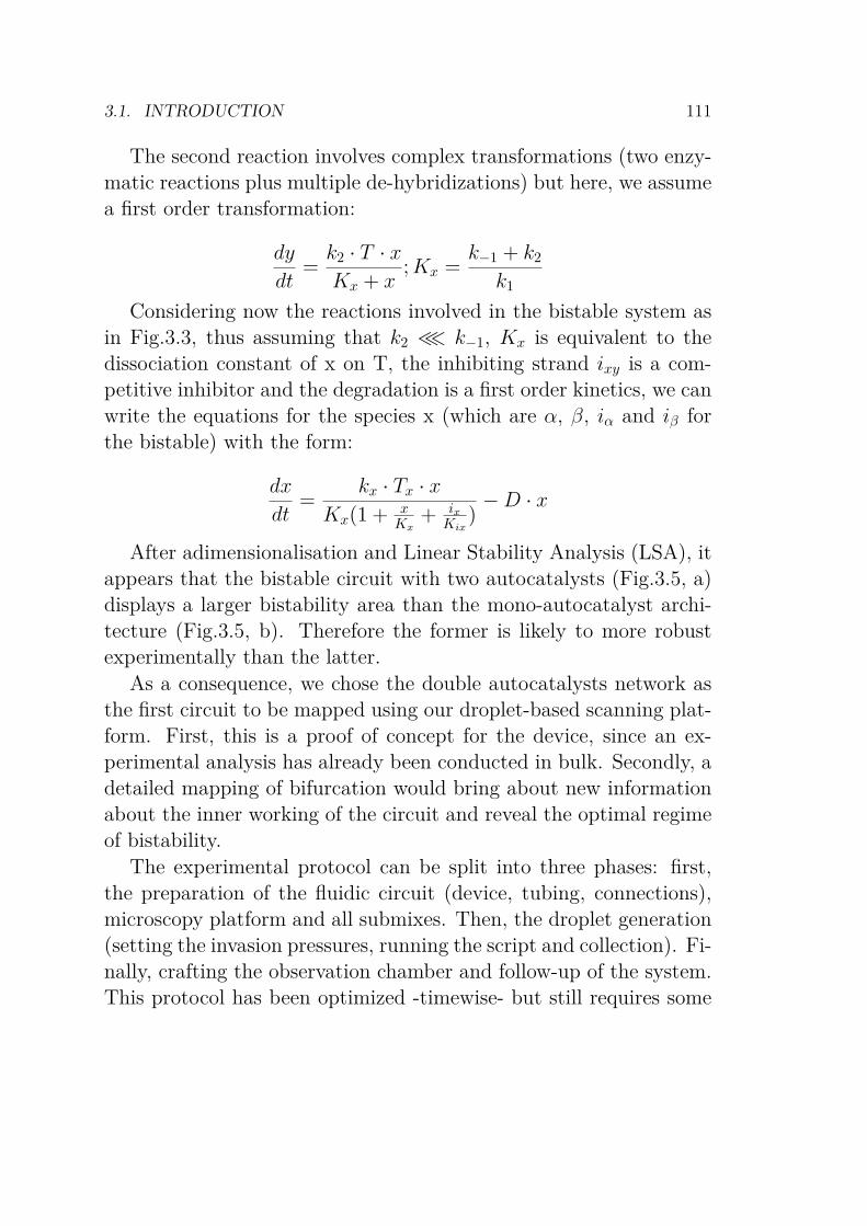
3.1. INTRODUCTION 111
The second reaction involves complex transformations (two enzy-matic reactions plus multiple de-hybridizations) but here, we assumea first order transformation:
dy
dt=
k2 · T · x
Kx + x; Kx =
k≠1 + k2
k1
Considering now the reactions involved in the bistable system asin Fig.3.3, thus assuming that k2 n k≠1, Kx is equivalent to thedissociation constant of x on T, the inhibiting strand ixy is a com-petitive inhibitor and the degradation is a first order kinetics, we canwrite the equations for the species x (which are α, β, iα and iβ forthe bistable) with the form:
dx
dt=
kx · Tx · x
Kx(1 + xKx
+ ix
Kix)
≠ D · x
After adimensionalisation and Linear Stability Analysis (LSA), itappears that the bistable circuit with two autocatalysts (Fig.3.5, a)displays a larger bistability area than the mono-autocatalyst archi-tecture (Fig.3.5, b). Therefore the former is likely to more robustexperimentally than the latter.
As a consequence, we chose the double autocatalysts network asthe first circuit to be mapped using our droplet-based scanning plat-form. First, this is a proof of concept for the device, since an ex-perimental analysis has already been conducted in bulk. Secondly, adetailed mapping of bifurcation would bring about new informationabout the inner working of the circuit and reveal the optimal regimeof bistability.
The experimental protocol can be split into three phases: first,the preparation of the fluidic circuit (device, tubing, connections),microscopy platform and all submixes. Then, the droplet generation(setting the invasion pressures, running the script and collection). Fi-nally, crafting the observation chamber and follow-up of the system.This protocol has been optimized -timewise- but still requires some
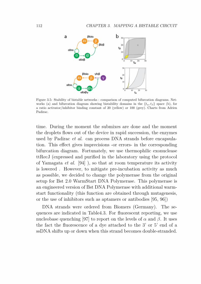
112 CHAPTER 3. MAPPING A BISTABLE CIRCUIT
Figure 3.5: Stability of bistable networks : comparison of computed bifurcation diagrams. Net-works (a) and bifurcation diagram showing bistability domains in the {tα, tβ} space (b), fora ratio activator/inhibitor binding constant of 20 (yellow) or 100 (grey). Charts from AdrienPadirac.
time. During the moment the submixes are done and the momentthe droplets flows out of the device in rapid succession, the enzymesused by Padirac et al. can process DNA strands before encapsula-tion. This effect gives imprecisions -or errors- in the correspondingbifurcation diagram. Fortunately, we use thermophilic exonucleasettRecJ (expressed and purified in the laboratory using the protocolof Yamagata et al. [94] ), so that at room temperature its activityis lowered . However, to mitigate pre-incubation activity as muchas possible, we decided to change the polymerase from the originalsetup for Bst 2.0 WarmStart DNA Polymerase. This polymerase isan engineered version of Bst DNA Polymerase with additional warm-start functionality (this function are obtained through mutagenesis,or the use of inhibitors such as aptamers or antibodies [95, 96])
DNA strands were ordered from Biomers (Germany). The se-quences are indicated in Table4.3. For fluorescent reporting, we usenucleobase quenching [97] to report on the levels of α and β. It usesthe fact the fluorescence of a dye attached to the 3’ or 5’ end of assDNA shifts up or down when this strand becomes double-stranded.
3.2. RESULTS 113
Sequence 5Õ æ 3Õ 3’ modificationαtoα C*C*A*AGACTCAGCCAAGACTCAG Phosphateβtoβ A*A*C*AGACUCGAAACAGACTCGA Phosphateβtoiα A*C*T*CAGCCAAGACAACAGACTCGA TAMRAαtoiβ A*C*T*CGAAACAGACCCAAGACTCAG FAM
α CTGAGTCTTGGβ TCGAGTCTGTT
Table 3.1: Sequences of DNA strands used in the bistable switch. Stars correspond to a phos-phorothioate modification, to prevent degradation by the exonuclease ttRecJ.
We attach a TAMRA dye (positive shift upon binding of β) to thetemplate βtoiα and a FAM dye (negative shift upon binding of α) tothe 3’ of the template αtoiβ. It must be kept in mind that fluores-cence shifts do not vary linearly with concentration of free triggers,although their relation is expected to be monotonic.
3.2 Results
3.2.1 Reaction assembly
For generating the diagram of the bistable switch (Fig.3.9), the mas-ter mix contains the following reagents: Tris-HCl (45 mM, pH~8.4),NaCl (50 mM), KCl (10 mM), Mg2+ (from MgCl2 + MgSO4, 8 mM intotal), (NH4)2SO4 (10 mM), dNTPs (400 µM each, New England Bi-olabs, NEB), Synperonic F108 (0,1% v/w, Sigma-Aldrich), Netropsin(2 µM, Sigma-Aldrich), Dithiothreitol (3 mM, Sigma-Aldrich), BSA9000S (500 µg.mL-1, NEB); the enzymes: polymerase Bst 2.0 Warm-Start™ (4 units.mL-1, NEB), exonuclease ttRecJ (20 nM), and nick-ase Nt.BstNBI (100 units.mL-1, NEB), the inhibitor-producer tem-plates (βtoiα and αtoiβ, 20 nM each). We use a Warmstart versionof the polymerase to mitigate production delays associated with themicrofluidic protocol.
This mix is then split into 2 sets of 3 tubes and completed withparametric species and their fluorescent barcodes (summarized in
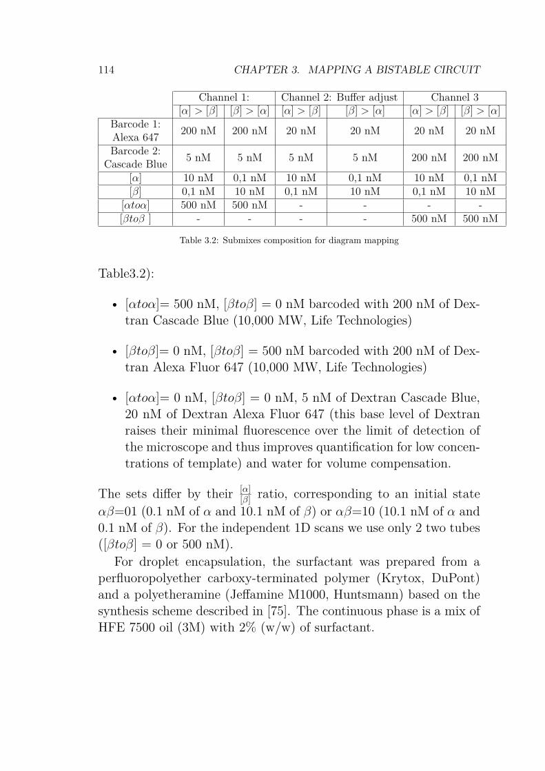
114 CHAPTER 3. MAPPING A BISTABLE CIRCUIT
Channel 1: Channel 2: Buffer adjust Channel 3[α] > [β] [β] > [α] [α] > [β] [β] > [α] [α] > [β] [β] > [α]
Barcode 1:200 nM 200 nM 20 nM 20 nM 20 nM 20 nM
Alexa 647Barcode 2:
5 nM 5 nM 5 nM 5 nM 200 nM 200 nMCascade Blue
[α] 10 nM 0,1 nM 10 nM 0,1 nM 10 nM 0,1 nM[β] 0,1 nM 10 nM 0,1 nM 10 nM 0,1 nM 10 nM
[αtoα] 500 nM 500 nM - - - -[βtoβ ] - - - - 500 nM 500 nM
Table 3.2: Submixes composition for diagram mapping
Table3.2):
• [αtoα]= 500 nM, [βtoβ] = 0 nM barcoded with 200 nM of Dex-tran Cascade Blue (10,000 MW, Life Technologies)
• [βtoβ]= 0 nM, [βtoβ] = 500 nM barcoded with 200 nM of Dex-tran Alexa Fluor 647 (10,000 MW, Life Technologies)
• [αtoα]= 0 nM, [βtoβ] = 0 nM, 5 nM of Dextran Cascade Blue,20 nM of Dextran Alexa Fluor 647 (this base level of Dextranraises their minimal fluorescence over the limit of detection ofthe microscope and thus improves quantification for low concen-trations of template) and water for volume compensation.
The sets differ by their [α][β] ratio, corresponding to an initial state
αβ=01 (0.1 nM of α and 10.1 nM of β) or αβ=10 (10.1 nM of α and0.1 nM of β). For the independent 1D scans we use only 2 two tubes([βtoβ] = 0 or 500 nM).
For droplet encapsulation, the surfactant was prepared from aperfluoropolyether carboxy-terminated polymer (Krytox, DuPont)and a polyetheramine (Jeffamine M1000, Huntsmann) based on thesynthesis scheme described in [75]. The continuous phase is a mix ofHFE 7500 oil (3M) with 2% (w/w) of surfactant.
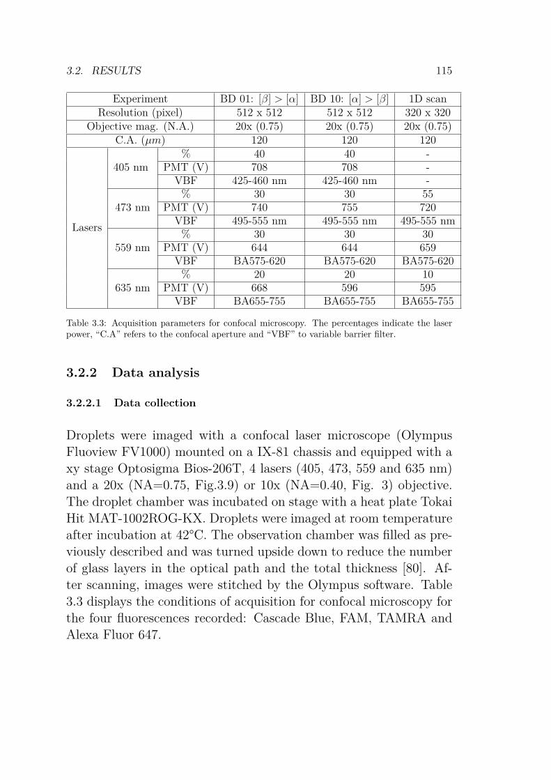
3.2. RESULTS 115
Experiment BD 01: [β] > [α] BD 10: [α] > [β] 1D scanResolution (pixel) 512 x 512 512 x 512 320 x 320
Objective mag. (N.A.) 20x (0.75) 20x (0.75) 20x (0.75)C.A. (µm) 120 120 120
Lasers
405 nm% 40 40 -
PMT (V) 708 708 -VBF 425-460 nm 425-460 nm -
473 nm% 30 30 55
PMT (V) 740 755 720VBF 495-555 nm 495-555 nm 495-555 nm
559 nm% 30 30 30
PMT (V) 644 644 659VBF BA575-620 BA575-620 BA575-620
635 nm% 20 20 10
PMT (V) 668 596 595VBF BA655-755 BA655-755 BA655-755
Table 3.3: Acquisition parameters for confocal microscopy. The percentages indicate the laserpower, “C.A” refers to the confocal aperture and “VBF” to variable barrier filter.
3.2.2 Data analysis
3.2.2.1 Data collection
Droplets were imaged with a confocal laser microscope (OlympusFluoview FV1000) mounted on a IX-81 chassis and equipped with axy stage Optosigma Bios-206T, 4 lasers (405, 473, 559 and 635 nm)and a 20x (NA=0.75, Fig.3.9) or 10x (NA=0.40, Fig. 3) objective.The droplet chamber was incubated on stage with a heat plate TokaiHit MAT-1002ROG-KX. Droplets were imaged at room temperatureafter incubation at 42°C. The observation chamber was filled as pre-viously described and was turned upside down to reduce the numberof glass layers in the optical path and the total thickness [80]. Af-ter scanning, images were stitched by the Olympus software. Table3.3 displays the conditions of acquisition for confocal microscopy forthe four fluorescences recorded: Cascade Blue, FAM, TAMRA andAlexa Fluor 647.
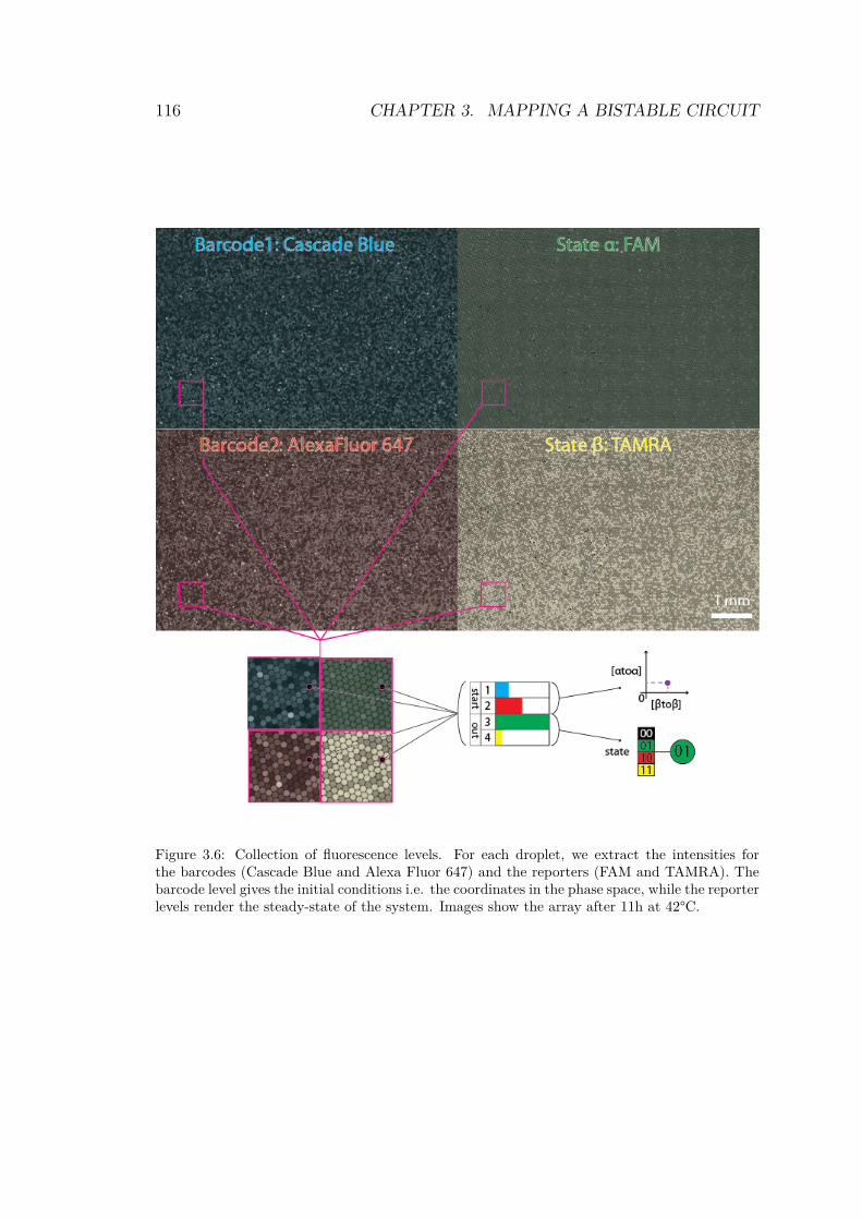
116 CHAPTER 3. MAPPING A BISTABLE CIRCUIT
Figure 3.6: Collection of fluorescence levels. For each droplet, we extract the intensities forthe barcodes (Cascade Blue and Alexa Fluor 647) and the reporters (FAM and TAMRA). Thebarcode level gives the initial conditions i.e. the coordinates in the phase space, while the reporterlevels render the steady-state of the system. Images show the array after 11h at 42°C.
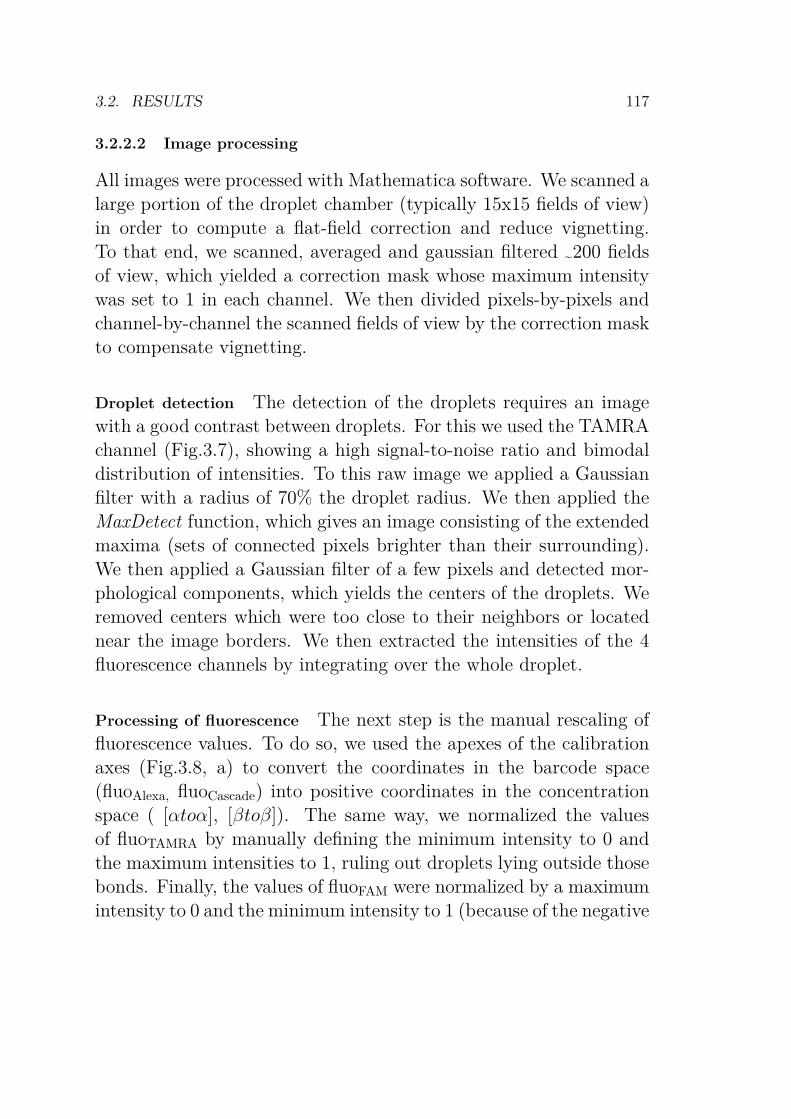
3.2. RESULTS 117
3.2.2.2 Image processing
All images were processed with Mathematica software. We scanned alarge portion of the droplet chamber (typically 15x15 fields of view)in order to compute a flat-field correction and reduce vignetting.To that end, we scanned, averaged and gaussian filtered ~200 fieldsof view, which yielded a correction mask whose maximum intensitywas set to 1 in each channel. We then divided pixels-by-pixels andchannel-by-channel the scanned fields of view by the correction maskto compensate vignetting.
Droplet detection The detection of the droplets requires an imagewith a good contrast between droplets. For this we used the TAMRAchannel (Fig.3.7), showing a high signal-to-noise ratio and bimodaldistribution of intensities. To this raw image we applied a Gaussianfilter with a radius of 70% the droplet radius. We then applied theMaxDetect function, which gives an image consisting of the extendedmaxima (sets of connected pixels brighter than their surrounding).We then applied a Gaussian filter of a few pixels and detected mor-phological components, which yields the centers of the droplets. Weremoved centers which were too close to their neighbors or locatednear the image borders. We then extracted the intensities of the 4fluorescence channels by integrating over the whole droplet.
Processing of fluorescence The next step is the manual rescaling offluorescence values. To do so, we used the apexes of the calibrationaxes (Fig.3.8, a) to convert the coordinates in the barcode space(fluoAlexa, fluoCascade) into positive coordinates in the concentrationspace ( [αtoα], [βtoβ]). The same way, we normalized the valuesof fluoTAMRA by manually defining the minimum intensity to 0 andthe maximum intensities to 1, ruling out droplets lying outside thosebonds. Finally, the values of fluoFAM were normalized by a maximumintensity to 0 and the minimum intensity to 1 (because of the negative
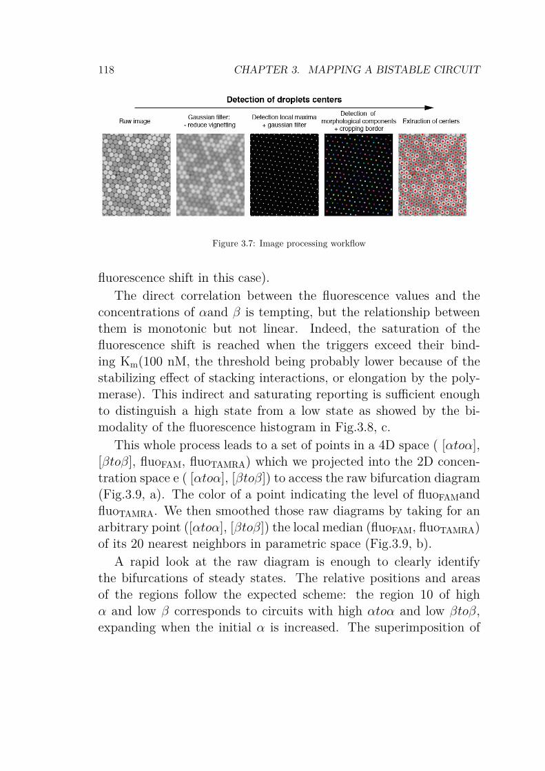
118 CHAPTER 3. MAPPING A BISTABLE CIRCUIT
Figure 3.7: Image processing workflow
fluorescence shift in this case).
The direct correlation between the fluorescence values and theconcentrations of αand β is tempting, but the relationship betweenthem is monotonic but not linear. Indeed, the saturation of thefluorescence shift is reached when the triggers exceed their bind-ing Km(100 nM, the threshold being probably lower because of thestabilizing effect of stacking interactions, or elongation by the poly-merase). This indirect and saturating reporting is sufficient enoughto distinguish a high state from a low state as showed by the bi-modality of the fluorescence histogram in Fig.3.8, c.
This whole process leads to a set of points in a 4D space ( [αtoα],[βtoβ], fluoFAM, fluoTAMRA) which we projected into the 2D concen-tration space e ( [αtoα], [βtoβ]) to access the raw bifurcation diagram(Fig.3.9, a). The color of a point indicating the level of fluoFAMandfluoTAMRA. We then smoothed those raw diagrams by taking for anarbitrary point ([αtoα], [βtoβ]) the local median (fluoFAM, fluoTAMRA)of its 20 nearest neighbors in parametric space (Fig.3.9, b).
A rapid look at the raw diagram is enough to clearly identifythe bifurcations of steady states. The relative positions and areasof the regions follow the expected scheme: the region 10 of highα and low β corresponds to circuits with high αtoα and low βtoβ,expanding when the initial α is increased. The superimposition of
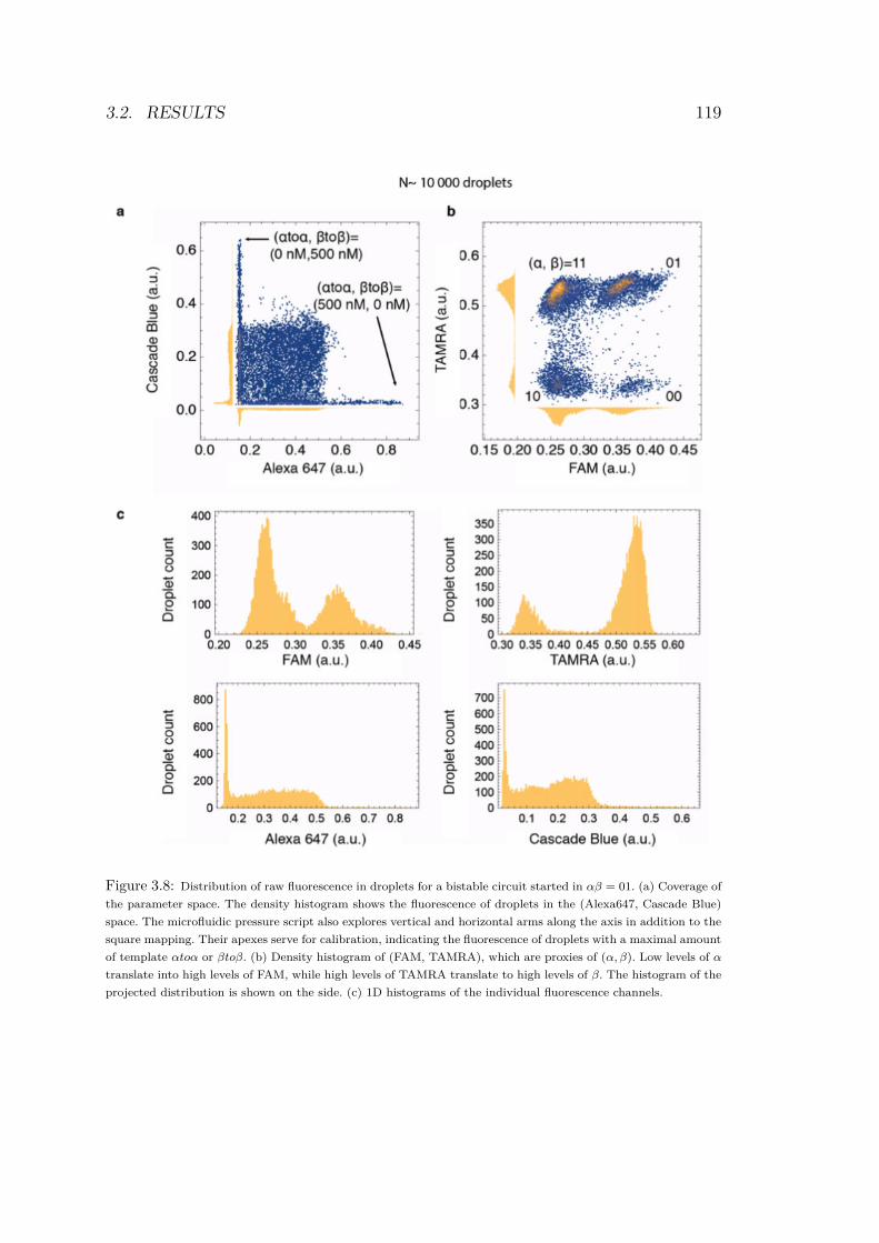
3.2. RESULTS 119
Figure 3.8: Distribution of raw fluorescence in droplets for a bistable circuit started in αβ = 01. (a) Coverage of
the parameter space. The density histogram shows the fluorescence of droplets in the (Alexa647, Cascade Blue)
space. The microfluidic pressure script also explores vertical and horizontal arms along the axis in addition to the
square mapping. Their apexes serve for calibration, indicating the fluorescence of droplets with a maximal amount
of template αtoα or βtoβ. (b) Density histogram of (FAM, TAMRA), which are proxies of (α, β). Low levels of α
translate into high levels of FAM, while high levels of TAMRA translate to high levels of β. The histogram of the
projected distribution is shown on the side. (c) 1D histograms of the individual fluorescence channels.
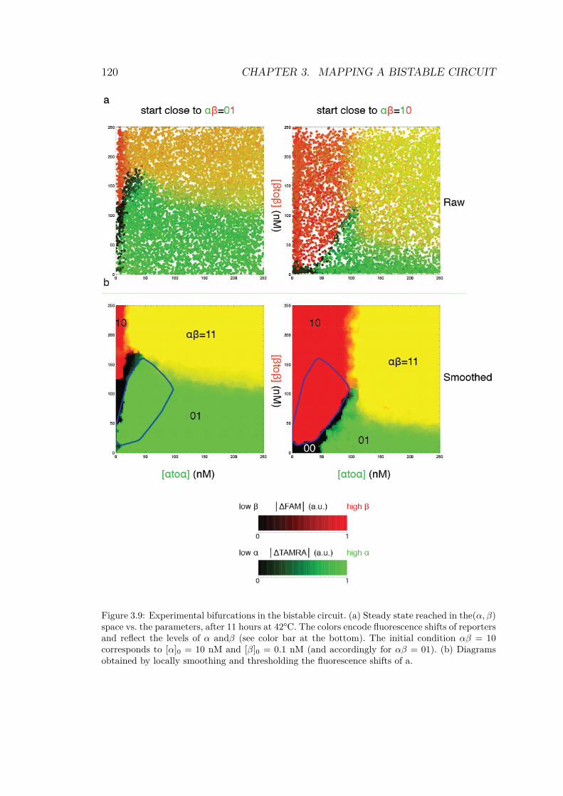
120 CHAPTER 3. MAPPING A BISTABLE CIRCUIT
Figure 3.9: Experimental bifurcations in the bistable circuit. (a) Steady state reached in the(α, β)space vs. the parameters, after 11 hours at 42°C. The colors encode fluorescence shifts of reportersand reflect the levels of α andβ (see color bar at the bottom). The initial condition αβ = 10corresponds to [α]0 = 10 nM and [β]0 = 0.1 nM (and accordingly for αβ = 01). (b) Diagramsobtained by locally smoothing and thresholding the fluorescence shifts of a.
3.3. INTERPRETATION 121
the two diagrams displays a bistable region where the circuit showshysteresis (Fig.3.9,b). The frontiers’ sharpness (as assessed by themagnitude of the gradient of α or β) also agrees with qualitativepredictions from bifurcation theory [98]: the fold (or saddle-node)bifurcations connecting the bistable to monostable areas (sudden lossof stability of one state) appear as abrupt frontiers. By contrast,transcritical bifurcations (collision and exchange of stability betweentwo fixed points, e.g. green to yellow transitions in Fig.3.9, a and b)materialize as a smooth gradient.
We performed an independent 1D scanning along two vertical linesto confirm the trends seen on the diagram, thus eliminating aboutpotential artifacts from barcoding accuracy (Fig.3.10).
3.3 Interpretation
3.3.1 Simulations
A realistic prediction of the evolution of concentrations requires theintegration of many side reactions and intermediate species, whoserates and concentrations are often not directly accessible experimen-tally. Even when the underlying chemistry of individual reactionsis faithfully understood, connecting them in a network can result incounter-intuitive outcomes. As we saw in the introduction, mathe-matical tools such as Linear stability analysis can link the dynamicsof the network with its topology and parameters. But analyticalapproaches often fail for large and complex systems and their scopeis even more limited when the underlying chemistry is not preciselyknown. In well-mixed systems, the potential number of interactionsgrows like the square of the number of species; keeping track of allthese interactions and their kinetic consequences quickly becomes im-possible for the human brain. It gets even worse when global effectslike enzymatic saturation and competition are taken into account.
In order to model in silico the PEN-DNA, the DACCAD software
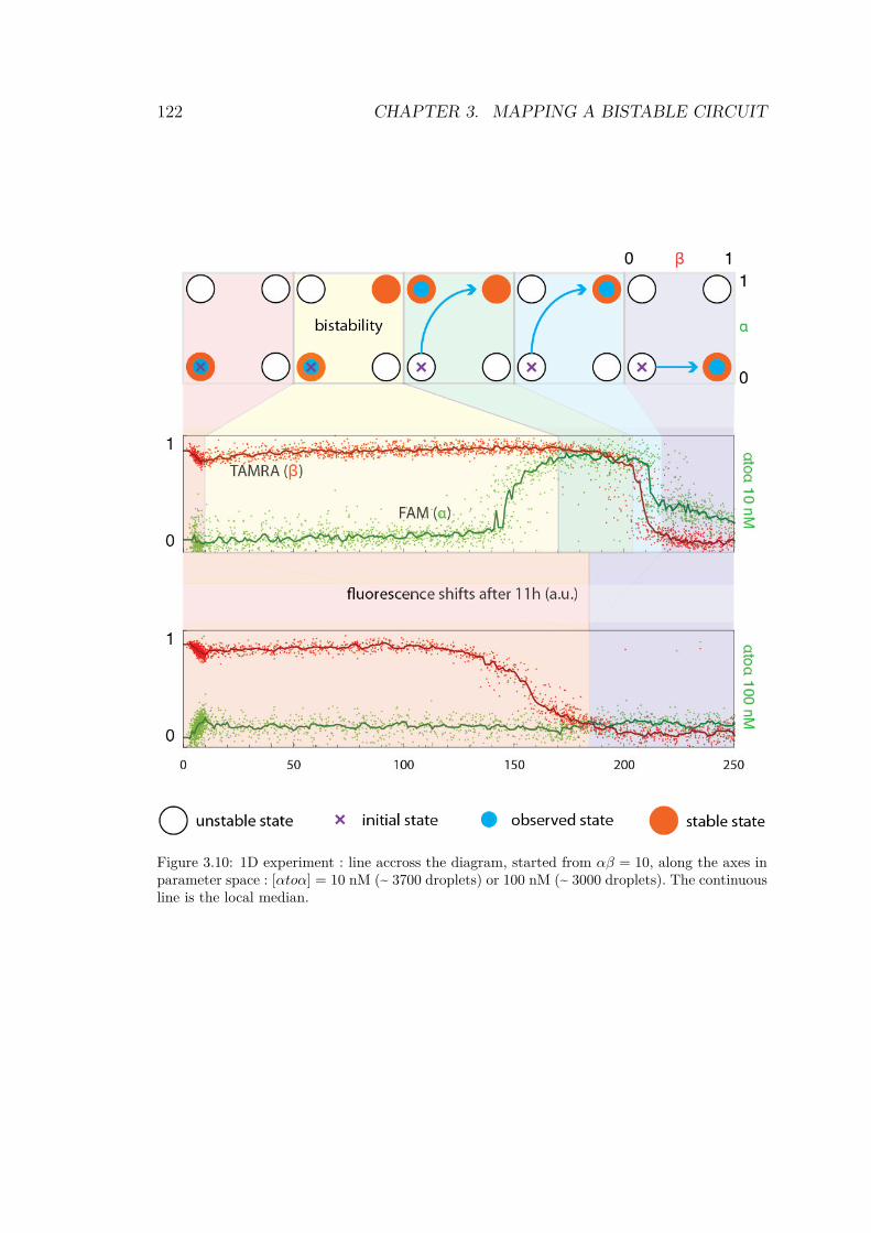
122 CHAPTER 3. MAPPING A BISTABLE CIRCUIT
Figure 3.10: 1D experiment : line accross the diagram, started from αβ = 10, along the axes inparameter space : [αtoα] = 10 nM (~ 3700 droplets) or 100 nM (~ 3000 droplets). The continuousline is the local median.
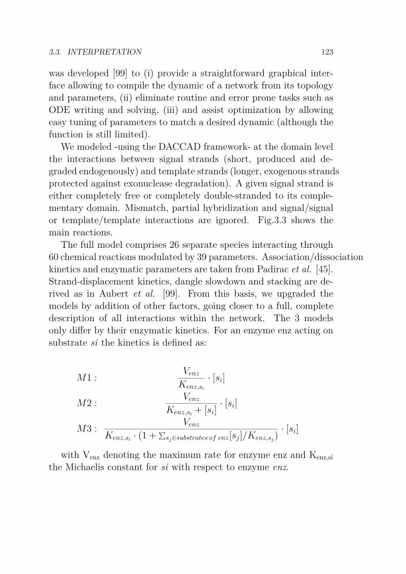
3.3. INTERPRETATION 123
was developed [99] to (i) provide a straightforward graphical inter-face allowing to compile the dynamic of a network from its topologyand parameters, (ii) eliminate routine and error prone tasks such asODE writing and solving, (iii) and assist optimization by allowingeasy tuning of parameters to match a desired dynamic (although thefunction is still limited).
We modeled -using the DACCAD framework- at the domain levelthe interactions between signal strands (short, produced and de-graded endogenously) and template strands (longer, exogenous strandsprotected against exonuclease degradation). A given signal strand iseither completely free or completely double-stranded to its comple-mentary domain. Mismatch, partial hybridization and signal/signalor template/template interactions are ignored. Fig.3.3 shows themain reactions.
The full model comprises 26 separate species interacting through60 chemical reactions modulated by 39 parameters. Association/dissociationkinetics and enzymatic parameters are taken from Padirac et al. [45].Strand-displacement kinetics, dangle slowdown and stacking are de-rived as in Aubert et al. [99]. From this basis, we upgraded themodels by addition of other factors, going closer to a full, completedescription of all interactions within the network. The 3 modelsonly differ by their enzymatic kinetics. For an enzyme enz acting onsubstrate si the kinetics is defined as:
M1 :Venz
Kenz,si
· [si]
M2 :Venz
Kenz,si+ [si]
· [si]
M3 :Venz
Kenz,si· (1 +
q
sjœsubstrates of enz[sj]/Kenz,sj)
· [si]
with Venz denoting the maximum rate for enzyme enz and Kenz,si
the Michaelis constant for si with respect to enzyme enz.
124 CHAPTER 3. MAPPING A BISTABLE CIRCUIT
In other words, M1 is first order, M2 follows the classical Michaelis-Menten law while ignoring competition effects, and M3 generalizesit by including the load of all substrates of an enzyme. For eachmodel, we iteratively optimize its parameters to fit the experimentalbifurcation diagrams of Fig.3.9 (the target function), the set of op-timized parameters depending on the model (e.g. M1 does not haveenzymatic saturation, thus does not optimize Michaelis parameters).
We assign a fitness to a set of parameters by comparing the bi-furcation diagram it predicts to the experimental diagram. Evolu-tionary algorithms are known to perform particularly well in suchcontext as they require few assumptions on the search space. Weuse CMA-ES [100, 101] which locally approximates the fitness gradi-ents through stochastic sampling and evaluates the fitness sensitiv-ity in order to avoid the pitfalls of premature convergence and flatfitness landscape. We further constrain the search to a bounded re-gion by assigning the worst fitness to individuals whose parametersexceed specified bounds (typically 10-fold variations for enzymaticparameters and 100-fold for other parameters). Penalizing such in-dividuals allows us to skip unnecessary ODE evaluation (which getsprohibitively slow for unrealistic parameters). We perform 10 runsfor each model, one run typically comprising 2000 evaluations (i.e.diagram evaluation) over 40 generations of 50 individuals. A sharedset of 6 parameters (stabilization effect of stacking on all 4 tem-plates, as well as the ratios pol/exo and nic/exo ) is optimizedfor all models. Five additional parameters (Michaelis constants forall enzyme/substrate combinations) are optimized for M2 and M3(Fig.3.11).
Optimized parameters for each model, along with their defaultvalues, are shown in Table3.4. We accelerate the evaluation of bi-furcation diagrams -a major computational bottleneck- by sparsing.First, we coarse-grain the experimental diagrams of Fig.3.9, b (goingfrom a˜100×100 binning to a 20×20 binning). Secondly, we sparsethese coarse diagrams by removing large and homogenous regions
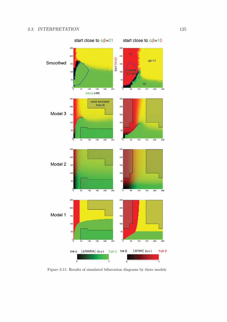
3.3. INTERPRETATION 125
Figure 3.11: Results of simulated bifurcation diagrams by three models
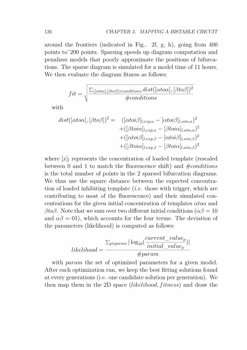
126 CHAPTER 3. MAPPING A BISTABLE CIRCUIT
around the frontiers (indicated in Fig.. 2f, g, h), going from 400points to˜200 points. Sparsing speeds up diagram computation andpenalizes models that poorly approximate the positions of bifurca-tions. The sparse diagram is simulated for a model time of 11 hours.We then evaluate the diagram fitness as follows:
fit =
ˆ
ı
ı
ı
Ù
q
([αtoα],[βtoβ])œconditions dist([αtoα], [βtoβ])2
#conditions
with
dist([αtoα], [βtoβ])2 = ([αtoiβ]l,exp,α ≠ [αtoiβ]l,sim,α)2
+([βtoiα]l,exp,α ≠ [βtoiα]l,sim,α)2
+([αtoiβ]l,exp,β ≠ [αtoiβ]l,sim,β)2
+([βtoiα]l,exp,β ≠ [βtoiα]l,sim,β)2
where [x]l represents the concentration of loaded template (rescaledbetween 0 and 1 to match the fluorescence shift) and #conditionsis the total number of points in the 2 sparsed bifurcation diagrams.We thus use the square distance between the expected concentra-tion of loaded inhibiting template (i.e. those with trigger, which arecontributing to most of the fluorescence) and their simulated con-centrations for the given initial concentration of templates αtoα andβtoβ. Note that we sum over two different initial conditions (αβ = 10and αβ = 01), which accounts for the four terms. The deviation ofthe parameters (likelihood) is computed as follows:
likelihood =
q
pœparam | log10(current_valuep
initial_valuep)|
#param
with param the set of optimized parameters for a given model.After each optimization run, we keep the best fitting solutions foundat every generations (i.e. one candidate solution per generation). Wethen map them in the 2D space (likelihood, fitness) and draw the
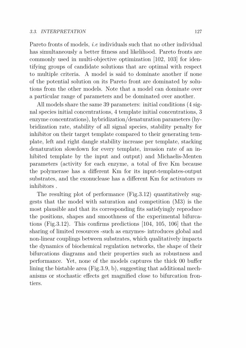
3.3. INTERPRETATION 127
Pareto fronts of models, i.e individuals such that no other individualhas simultaneously a better fitness and likelihood. Pareto fronts arecommonly used in multi-objective optimization [102, 103] for iden-tifying groups of candidate solutions that are optimal with respectto multiple criteria. A model is said to dominate another if noneof the potential solution on its Pareto front are dominated by solu-tions from the other models. Note that a model can dominate overa particular range of parameters and be dominated over another.
All models share the same 39 parameters: initial conditions (4 sig-nal species initial concentrations, 4 template initial concentrations, 3enzyme concentrations), hybridization/denaturation parameters (hy-bridization rate, stability of all signal species, stability penalty forinhibitor on their target template compared to their generating tem-plate, left and right dangle stability increase per template, stackingdenaturation slowdown for every template, invasion rate of an in-hibited template by the input and output) and Michaelis-Mentenparameters (activity for each enzyme, a total of five Km becausethe polymerase has a different Km for its input-templates-outputsubstrates, and the exonuclease has a different Km for activators vsinhibitors .
The resulting plot of performance (Fig.3.12) quantitatively sug-gests that the model with saturation and competition (M3) is themost plausible and that its corresponding fits satisfyingly reproducethe positions, shapes and smoothness of the experimental bifurca-tions (Fig.3.12). This confirms predictions [104, 105, 106] that thesharing of limited resources -such as enzymes- introduces global andnon-linear couplings between substrates, which qualitatively impactsthe dynamics of biochemical regulation networks, the shape of theirbifurcations diagrams and their properties such as robustness andperformance. Yet, none of the models captures the thick 00 bufferlining the bistable area (Fig.3.9, b), suggesting that additional mech-anisms or stochastic effects get magnified close to bifurcation fron-tiers.
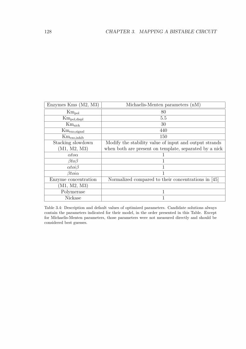
128 CHAPTER 3. MAPPING A BISTABLE CIRCUIT
Enzymes Kms (M2, M3) Michaelis-Menten parameters (nM)
Kmpol 80Kmpol,displ 5.5
Kmnick 30Kmexo,signal 440Kmexo,inhib 150
Stacking slowdown Modify the stability value of input and output strands(M1, M2, M3) when both are present on template, separated by a nick
αtoα 1βtoβ 1αtoiβ 1βtoiα 1
Enzyme concentration Normalized compared to their concentrations in [45](M1, M2, M3)
Polymerase 1Nickase 1
Table 3.4: Description and default values of optimized parameters. Candidate solutions alwayscontain the parameters indicated for their model, in the order presented in this Table. Exceptfor Michaelis-Menten parameters, those parameters were not measured directly and should beconsidered best guesses.
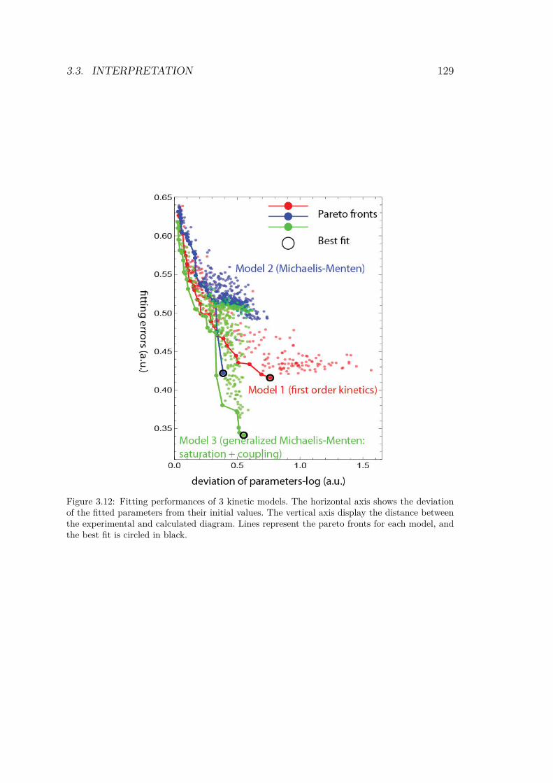
3.3. INTERPRETATION 129
Figure 3.12: Fitting performances of 3 kinetic models. The horizontal axis shows the deviationof the fitted parameters from their initial values. The vertical axis display the distance betweenthe experimental and calculated diagram. Lines represent the pareto fronts for each model, andthe best fit is circled in black.
130 CHAPTER 3. MAPPING A BISTABLE CIRCUIT
3.3.2 Discussion
A close inspection of the diagrams highlights some unexpected fea-tures. First, we expect that all steady states should yield at leastone surviving trigger - except in the small 00 area close to the ori-gin. Indeed, assuming continuous dynamic and first-order amplifi-cation, we expect the 00 zone (the set of template concentrationsthat yield a null steady state) to be a rectangle independent of theinitial concentrations of triggers. Because we assume that the dy-namic is continuous and deterministic, the concentration of a speciesthat is initially strictly positive can never become identically null. Inother words, both species cannot lose simultaneously, provided thereis enough autocatalytic template.
Let us look at this assertion in more detail. We consider a simpli-fied model that was validated experimentally by Padirac et al. [45].Triggers are amplified according to a first-order Michaelis-Mentenamplification whose rate is modulated by the concentrations of au-tocatalytic template, polymerase and the nickase. The triggers aredegraded according to linear kinetics by the exonuclease:
αÕ =pα · [αtoα] · α
Kα + α + iα≠ kα · α
βÕ =pβ · [βtoβ] · β
Kβ + β + iβ≠ kββ
The constants pα and pβ capture the overall replication rates ofthe triggers by the polymerase and nickase. The variables iα andiβ are the concentrations of species inhibiting α and β respectively(whose kinetics need not be written explicitly here). The constant kα
and kβ encompass the degradation rates of the exonuclease. For am-plification of α to occur (αÕ > 0), it is necessary that the level of au-tocatalytic template [αtoα] exceeds a threshold concentration Kα·kα
pα
(and similarly for β). This contrasts with second-order autocatal-ysis, where the concentrations of the initial catalyst and template
3.3. INTERPRETATION 131
must both exceed a critical threshold to ignite replication. In otherwords, the steady states α = 0 or β = 0 are never stable in first-orderamplification once the threshold is crossed because any infinisitimallevel of trigger will be amplified. Let us define the rectangle R00 inthe parameter space (αtoα, βtoβ) by
R00 = {0 Æ [αtoα] Æ Kα · kα
pα, 0 Æ [βtoβ] Æ Kβ · kβ
pβ}
This rectangle is thus necessarily included in the 00 zone. Now weprove the reverse inclusion, namely that the 00 zone is included in therectangle. Suppose that we start outside R00 (at least one templateexceeds its threshold level) but that α and β both asymptoticallydecay to zero. Then the inhibitors also eventually decay to zero.After a (possibly long) relaxation time TŒ, we have β, iβ π Kβ andα, iα π Kα and thus
αÕ = (pα · [αtoα]
Kα≠ kα) · α
βÕ = (pβ · [βtoβ]
Kβ≠ kβ) · β
Given α and β are both non null (because of to their deterministicand continuous evolution), at least one species is amplifying (thespecies whose template exceeds its threshold concentration), whichcontradicts the assumptions that the system is converging toward thenull state. This simple model predicts that the 00 zone should bea rectangle whose shape is independent of the initial concentrationsof triggers. This is clearly not the case in Fig.3.9 where the blackareas are highly asymmetrical and extend around the bistable zone,meaning that at least one of our hypothesis must be false.
One argument is that the actual mechanism of replication may behigher order, which would provide the necessary hysteresis to sta-bilize the steady state α = 0 or β = 0. The second argument isthat low volume effect may be at play. The concentrations of α and
132 CHAPTER 3. MAPPING A BISTABLE CIRCUIT
β cannot be arbitrarily low without being null (40 fM ◊ 65 pL ¥ 1molecule). In their race against degradation and caviting the stochas-ticity of chemical reactions, the autocatalytic templates may some-time lose and the copy numbers of α and β both reach and remain at0 (something impossible in a well-posed, deterministic ODE becauseof the uniqueness of its solution). Since a template cannot replicatea strand that is absent, the 00 zone in our diagram may thereforerepresent circuits that are “stochastically trapped” in the null state00. Lastly, when the levels of templates are close (but superior) totheir thresholds, the relaxation may drastically slow own and exceedour experimental time scale (10 hours). This phenomenon would bereminiscent of critical slowdown, where some dynamic systems havebeen shown to take a very long time to recover from quasi-lethalperturbations [107].
proves the failure of our prediction and signals that either conver-gence to the local steady state(s) is drastically slowed down like in acatastrophic slowdown [107].
Also, some frontiers show a pronounced non-monotonicity. Forinstance in Fig. 3.9, up-left, it is counter-intuitive that βtoβ initiallyrepresses α for βtoβ between 150 and 200 nM, but eventually permitsits survival for βtoβ over 200 nM. (Similar non-monoticity is seen forthe 01 frontier in Fig. 3.9). This suggests a hidden mechanism per-haps indirectly cross-activating α and β, whereas the designed circuittopology enforces cross-inhibition between them and DNA sequenceswere specifically engineered to avoid such undesired interactions.
Note that this non-monotous shape is correctly reproduced onlyin model 3, suggesting that it is an effect of global coupling throughcompetitive enzyme saturation.
3.4 Conclusion
In conclusion we successfully implemented the bistable circuit de-signed by Adrien Padirac after modification to fit the device (warm
3.4. CONCLUSION 133
start to avoid early reaction starting before encapsulation). Then,we generated droplets with different rations of [βtoβ]
[αtoα] for two initial
conditions of [β][α] , recorded the fluorescence levels after 11h of evolu-
tion, thanks to a home-made data-extraction protocol. The resultingdiagrams, once superimposed, display the expected features: an areawhere β survives, a distinct region where α survives, correspondingto the monostability areas, a region where both triggers survive andthe overlap of the two monostable domains defining the bistable area(Fig. 3.9).
More surprisingly, the diagrams display features that were notpredicted by the mathematical model. A null area, where none ofthe triggers survives sits next to the origin of the graph and itsshape is different according to the initial conditions, meaning thatinitial conditions play a role in the putative stochastic trapping ofthese droplets and provide another level of bistability. at least onthe timescale of the experiment, within this system. The shape ofthe 00 area either signals that either convergence to the local steadystate(s) is drastically slowed down (e.g. by catastrophic slowdown[107]) or even arrested (e.g. by small number effects [108]), or thatan alternative stable state emerges from an unsuspected mechanism[109].In any case, these trapped states could provide alternative op-tions for memories on practical time scales.Another feature is thenon monotonicity of some frontiers of the diagram, suggesting globalcoupling in competitive saturation of enzymes. Finally, we upgradedthe mathematical model by addition of parameters and dependencesbetween the variables, and evolved the parameters for them to fitwith the experimental diagram.
In this process, we established the proof-of-concept for this mi-crofluidic platform for fast and thorough analysis of a network. Thenext step will be to implement and map another system, with theaddition of a new dimension in the parameter space.

134 CHAPTER 3. MAPPING A BISTABLE CIRCUIT
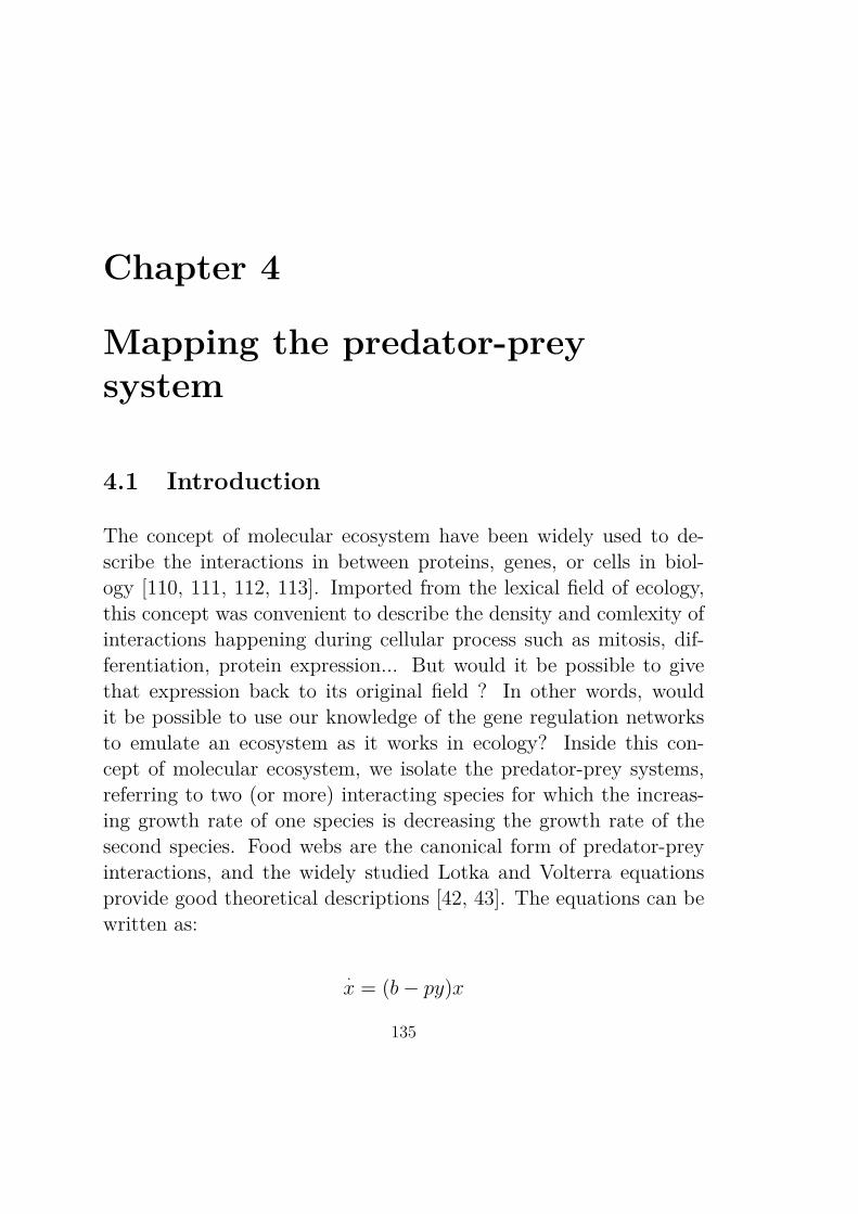
Chapter 4
Mapping the predator-preysystem
4.1 Introduction
The concept of molecular ecosystem have been widely used to de-scribe the interactions in between proteins, genes, or cells in biol-ogy [110, 111, 112, 113]. Imported from the lexical field of ecology,this concept was convenient to describe the density and comlexity ofinteractions happening during cellular process such as mitosis, dif-ferentiation, protein expression... But would it be possible to givethat expression back to its original field ? In other words, wouldit be possible to use our knowledge of the gene regulation networksto emulate an ecosystem as it works in ecology? Inside this con-cept of molecular ecosystem, we isolate the predator-prey systems,referring to two (or more) interacting species for which the increas-ing growth rate of one species is decreasing the growth rate of thesecond species. Food webs are the canonical form of predator-preyinteractions, and the widely studied Lotka and Volterra equationsprovide good theoretical descriptions [42, 43]. The equations can bewritten as:
·x = (b ≠ py)x
135
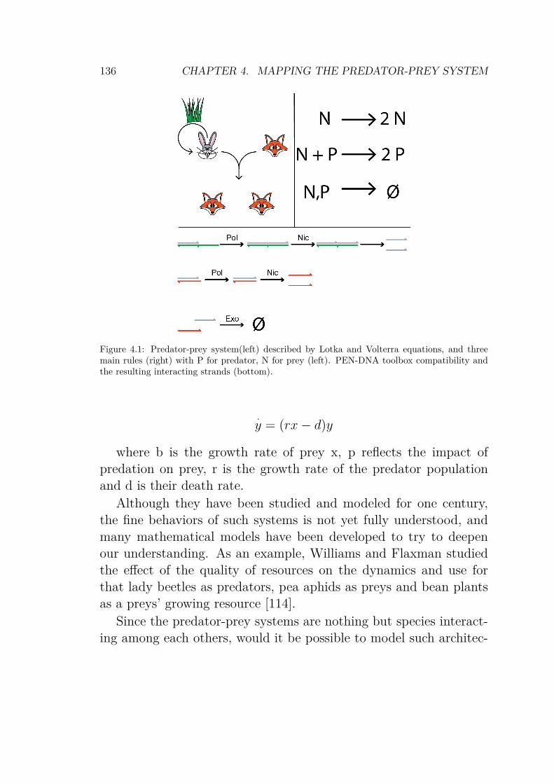
136 CHAPTER 4. MAPPING THE PREDATOR-PREY SYSTEM
Figure 4.1: Predator-prey system(left) described by Lotka and Volterra equations, and threemain rules (right) with P for predator, N for prey (left). PEN-DNA toolbox compatibility andthe resulting interacting strands (bottom).
·y = (rx ≠ d)y
where b is the growth rate of prey x, p reflects the impact ofpredation on prey, r is the growth rate of the predator populationand d is their death rate.
Although they have been studied and modeled for one century,the fine behaviors of such systems is not yet fully understood, andmany mathematical models have been developed to try to deepenour understanding. As an example, Williams and Flaxman studiedthe effect of the quality of resources on the dynamics and use forthat lady beetles as predators, pea aphids as preys and bean plantsas a preys’ growing resource [114].
Since the predator-prey systems are nothing but species interact-ing among each others, would it be possible to model such architec-
4.1. INTRODUCTION 137
Figure 4.2: Reaction network of the predator-prey system. A prey (L5) replicates by an autocat-alytic mechanism identical to the bistable switch involving a grass template (G5). In addition, apredation reaction converts a prey into a predator (R5), catalyzed by a predator and pol: bind-ing of a prey to a predator forms a partial duplex that is elongated by pol to yield two boundpredators. Those melt readily at experimental temperature, yielding two free predators.
tures with the PEN-DNA toolbox? Considering the three rules com-ing from the equations: (1) prey growth is autocatalytic, (2) preda-tion is also autocatalytic and (3) both predator and preys populationsare decaying, it is possible to draw a compatible network (Fig.4.1).This network is suited for PEN-DNA toolbox and was implementedsince 2012 by Rondelez et al [41], as described in Fig.4.3. The dy-namics are intuitively understood when one considers the amountof prey over time: at first, in the absence of predators, preys growexponentially fast, and so are growing predators because of the num-ber of available preys. At one point, the growth of predator reachesthe level of the growth of preys and overcomes it. The number ofpreys dramatically decreases and the lack of preys prevent the pro-duction of predators. Predators finally die, the system is back toits original conditions -low level of both preys and predators- thusready for another cycle. The inner life cycle of each species is de-scribed in Fig.4.2. Experiments confirm this prediction as shown inintroduction section.
138 CHAPTER 4. MAPPING THE PREDATOR-PREY SYSTEM
Among real animal populations, the dynamics of predator-preysystems seem much richer than simple limit cycles oscillations, drivenby the spatialization and trophic complexity of the system [115]. Thenext step was then to spatialize the molecular ecosystem to explorethe pattern formation and global dynamics [116].
Our approach will be slightly different: instead of looking for spa-tialization and out-of-system effects on the dynamics, we will focuson finding-out how the inner parameters of the network can triggerexotic behavior. To do so, we will map the bifurcation diagram ofthe system in function of 3 parameters.
4.2 Mapping the bifurcation diagram
Using the same approach than for the bistable switch, we aim atmapping the predator-prey system in a three dimensional parameterspace. The nature of each parameter is given by the mechanism ofthis molecular ecosystem. It entails 3 catalytic steps whose rates canbe parameterized by the concentration of their exogenous catalysts:1) the autocatalytic growth of DNA preys, 2) predation: autocat-alytic conversion of preys into predators (catalyzed by endogenouspredators and pol), 3) degradation of predators and preys (catalyzedby an exonuclease exo).
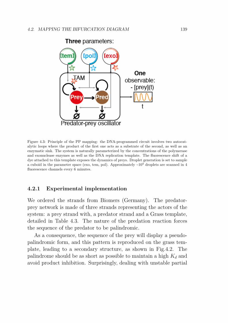
4.2. MAPPING THE BIFURCATION DIAGRAM 139
Figure 4.3: Principle of the PP mapping: the DNA-programmed circuit involves two autocat-alytic loops where the product of the first one acts as a substrate of the second, as well as anenzymatic sink. The system is naturally parameterized by the concentrations of the polymeraseand exonuclease enzymes as well as the DNA replication template. The fluorescence shift of adye attached to this template exposes the dynamics of preys. Droplet generation is set to samplea cuboid in the parameter space (exo, tem, pol). Approximately ~104 droplets are scanned in 4fluorescence channels every 6 minutes.
4.2.1 Experimental implementation
We ordered the strands from Biomers (Germany). The predator-prey network is made of three strands representing the actors of thesystem: a prey strand with, a predator strand and a Grass template,detailed in Table 4.3. The nature of the predation reaction forcesthe sequence of the predator to be palindromic.
As a consequence, the sequence of the prey will display a pseudo-palindromic form, and this pattern is reproduced on the grass tem-plate, leading to a secondary structure, as shown in Fig.4.2. Thepalindrome should be as short as possible to maintain a high Kd andavoid product inhibition. Surprisingly, dealing with unstable partial
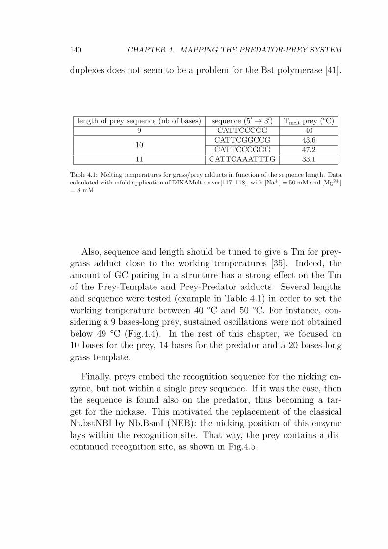
140 CHAPTER 4. MAPPING THE PREDATOR-PREY SYSTEM
duplexes does not seem to be a problem for the Bst polymerase [41].
length of prey sequence (nb of bases) sequence (5Õ æ 3Õ) Tmelt prey (°C)9 CATTCCCGG 40
10CATTCGGCCG 43.6CATTCCCGGG 47.2
11 CATTCAAATTTG 33.1
Table 4.1: Melting temperatures for grass/prey adducts in function of the sequence length. Datacalculated with mfold application of DINAMelt server[117, 118], with [Na+] = 50 mM and [Mg2+]= 8 mM
Also, sequence and length should be tuned to give a Tm for prey-grass adduct close to the working temperatures [35]. Indeed, theamount of GC pairing in a structure has a strong effect on the Tmof the Prey-Template and Prey-Predator adducts. Several lengthsand sequence were tested (example in Table 4.1) in order to set theworking temperature between 40 °C and 50 °C. For instance, con-sidering a 9 bases-long prey, sustained oscillations were not obtainedbelow 49 °C (Fig.4.4). In the rest of this chapter, we focused on10 bases for the prey, 14 bases for the predator and a 20 bases-longgrass template.
Finally, preys embed the recognition sequence for the nicking en-zyme, but not within a single prey sequence. If it was the case, thenthe sequence is found also on the predator, thus becoming a tar-get for the nickase. This motivated the replacement of the classicalNt.bstNBI by Nb.BsmI (NEB): the nicking position of this enzymelays within the recognition site. That way, the prey contains a dis-continued recognition site, as shown in Fig.4.5.
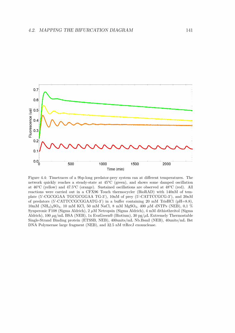
4.2. MAPPING THE BIFURCATION DIAGRAM 141
Figure 4.4: Timetraces of a 9bp-long predator-prey system ran at different temperatures. Thenetwork quickly reaches a steady-state at 45°C (green), and shows some damped oscillationat 46°C (yellow) and 47.5°C (orange). Sustained oscillations are observed at 48°C (red). Allreactions were carried out in a CFX96 Touch thermocycler (BioRAD) with 140nM of tem-plate (5’-CGCGGAA TGCGCGGAA TG-3’), 10nM of prey (5’-CATTCCGCG-3’), and 20nMof predators (5’-CATTCCGCGGAATG-3’) in a buffer containing 20 mM TrisHCl (pH=8.8),10mM (NH4)2SO4, 10 mM KCl, 50 mM NaCl, 8 mM MgSO4, 400 µM dNTPs (NEB), 0,1 %Synperonic F108 (Sigma Aldrich), 2 µM Netropsin (Sigma Aldrich), 4 mM dithiothreitol (SigmaAldrich), 100 µg/mL BSA (NEB), 1x EvaGreen® (Biotium), 30 pg/µL Extremely ThermostableSingle-Strand Binding protein (ETSSB, NEB), 400units/mL Nb.BsmI (NEB), 40units/mL BstDNA Polymerase large fragment (NEB), and 32.5 nM ttRecJ exonuclease.
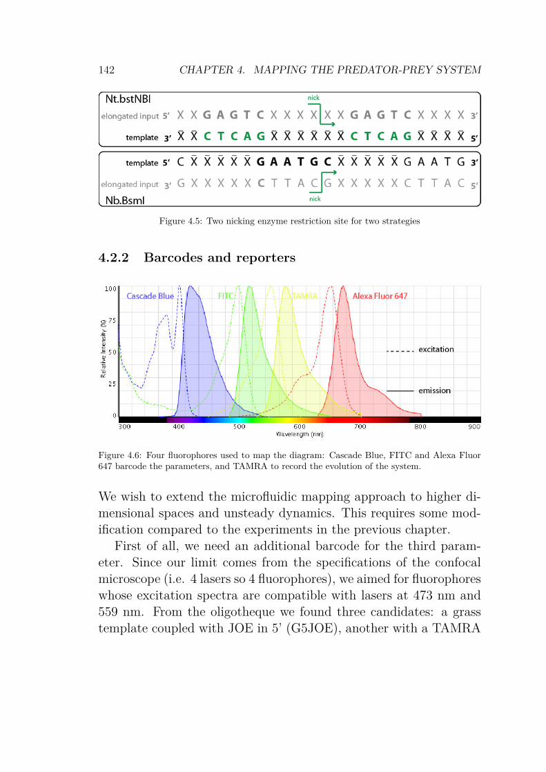
142 CHAPTER 4. MAPPING THE PREDATOR-PREY SYSTEM
Figure 4.5: Two nicking enzyme restriction site for two strategies
4.2.2 Barcodes and reporters
Figure 4.6: Four fluorophores used to map the diagram: Cascade Blue, FITC and Alexa Fluor647 barcode the parameters, and TAMRA to record the evolution of the system.
We wish to extend the microfluidic mapping approach to higher di-mensional spaces and unsteady dynamics. This requires some mod-ification compared to the experiments in the previous chapter.
First of all, we need an additional barcode for the third param-eter. Since our limit comes from the specifications of the confocalmicroscope (i.e. 4 lasers so 4 fluorophores), we aimed for fluorophoreswhose excitation spectra are compatible with lasers at 473 nm and559 nm. From the oligotheque we found three candidates: a grasstemplate coupled with JOE in 5’ (G5JOE), another with a TAMRA
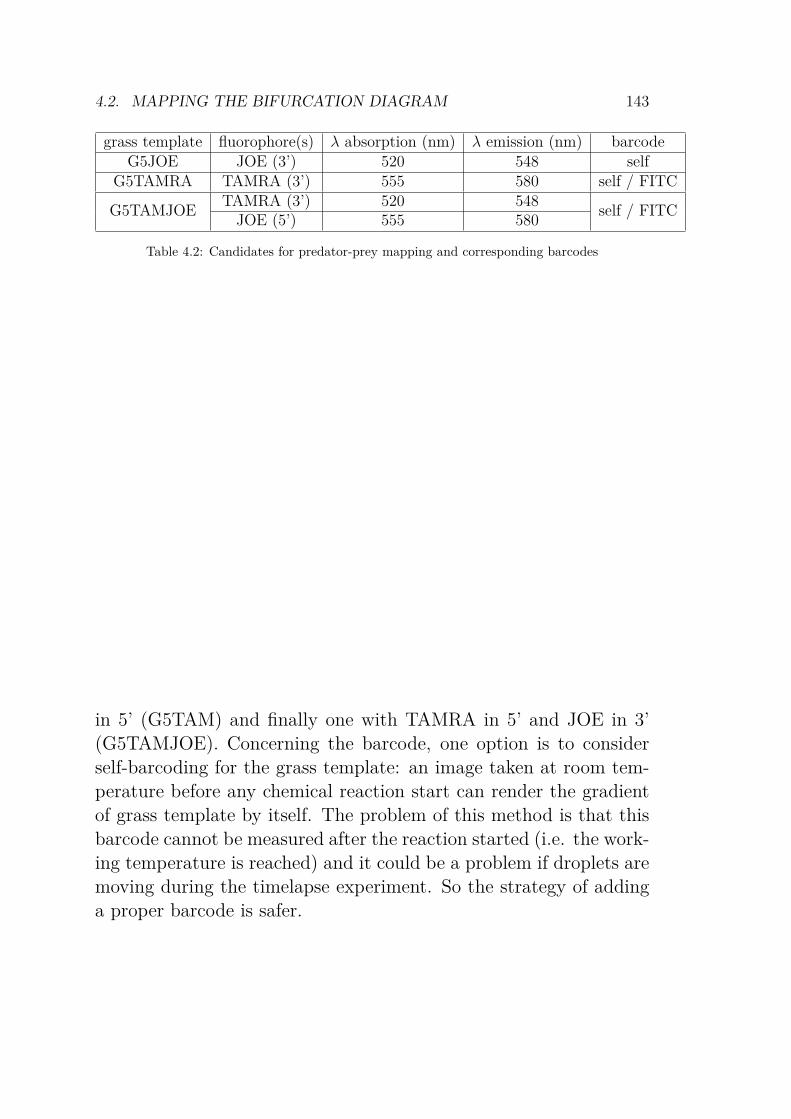
4.2. MAPPING THE BIFURCATION DIAGRAM 143
grass template fluorophore(s) λ absorption (nm) λ emission (nm) barcodeG5JOE JOE (3’) 520 548 self
G5TAMRA TAMRA (3’) 555 580 self / FITC
G5TAMJOETAMRA (3’) 520 548
self / FITCJOE (5’) 555 580
Table 4.2: Candidates for predator-prey mapping and corresponding barcodes
in 5’ (G5TAM) and finally one with TAMRA in 5’ and JOE in 3’(G5TAMJOE). Concerning the barcode, one option is to considerself-barcoding for the grass template: an image taken at room tem-perature before any chemical reaction start can render the gradientof grass template by itself. The problem of this method is that thisbarcode cannot be measured after the reaction started (i.e. the work-ing temperature is reached) and it could be a problem if droplets aremoving during the timelapse experiment. So the strategy of addinga proper barcode is safer.
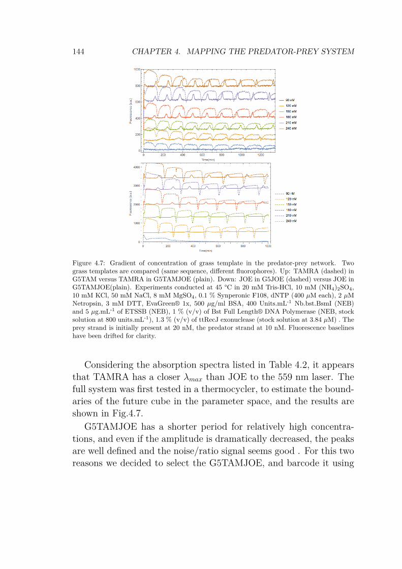
144 CHAPTER 4. MAPPING THE PREDATOR-PREY SYSTEM
Figure 4.7: Gradient of concentration of grass template in the predator-prey network. Twograss templates are compared (same sequence, different fluorophores). Up: TAMRA (dashed) inG5TAM versus TAMRA in G5TAMJOE (plain). Down: JOE in G5JOE (dashed) versus JOE inG5TAMJOE(plain). Experiments conducted at 45 °C in 20 mM Tris-HCl, 10 mM (NH4)2SO4,10 mM KCl, 50 mM NaCl, 8 mM MgSO4, 0.1 % Synperonic F108, dNTP (400 µM each), 2 µMNetropsin, 3 mM DTT, EvaGreen® 1x, 500 µg/ml BSA, 400 Units.mL-1 Nb.bst.BsmI (NEB)and 5 µg.mL-1 of ETSSB (NEB), 1 % (v/v) of Bst Full Length® DNA Polymerase (NEB, stocksolution at 800 units.mL-1), 1.3 % (v/v) of ttRecJ exonuclease (stock solution at 3.84 µM) . Theprey strand is initially present at 20 nM, the predator strand at 10 nM. Fluorescence baselineshave been drifted for clarity.
Considering the absorption spectra listed in Table 4.2, it appearsthat TAMRA has a closer λmax than JOE to the 559 nm laser. Thefull system was first tested in a thermocycler, to estimate the bound-aries of the future cube in the parameter space, and the results areshown in Fig.4.7.
G5TAMJOE has a shorter period for relatively high concentra-tions, and even if the amplitude is dramatically decreased, the peaksare well defined and the noise/ratio signal seems good . For this tworeasons we decided to select the G5TAMJOE, and barcode it using
4.2. MAPPING THE BIFURCATION DIAGRAM 145
FITC-labelled dextran. Another curious feature is that, compared toG5JOE and G5TAM, the signal of G5TAMJOE is reverted, positiveshifts are observed for each cycle of prey population.
4.2.3 Timelapse
Unlike the bistable, the predator-prey network has a dynamic behav-ior, it is thus necessary to record the fluorescence signal overtime. Wehad to adapt the setup to this new technical challenge, un which thescanning area is a crucial parameter.
4.2.3.1 Scanning time
Scanning time should be shorter than the timescale of the reaction.Indeed, if the scanning area is too large, or the scanning too slow,the first and last images of the first frame will not be chemicallyequivalent (Fig.4.8), meaning that the reactions started prior to thescanning for the last images of the frame. Even if it is not a bigissue in general, it can become critical when one of the parameter isself-barcoded. In this case, we loose the coordinates of all dropletsthat started earlier. As a rule of thumb, we limited the scanningtime around 7min.
The scanning area is defined by two criteria. First, the resolutionof the final diagram. Indeed, a good coverage of the parameter spacerequires the acquisition of fluorescence levels of many droplets (eachdroplet leads to one point in the diagram). Empirically, we considerthat having a precision ~3% for each parameter is good enough. Itmeans that we need ~104droplets to map in three dimensions. Onthe other hand, the scanning time has to be in the range of 7 min,keeping in mind that the stage movement (most time consuming)and the optical settings (scanning time per pixel, image resolution,number of image in the frame) cannot be reduced.
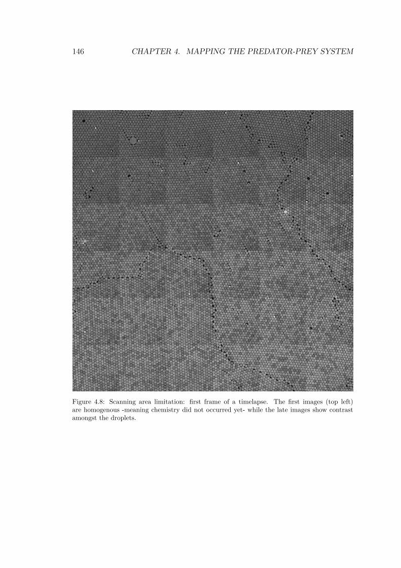
146 CHAPTER 4. MAPPING THE PREDATOR-PREY SYSTEM
Figure 4.8: Scanning area limitation: first frame of a timelapse. The first images (top left)are homogenous -meaning chemistry did not occurred yet- while the late images show contrastamongst the droplets.
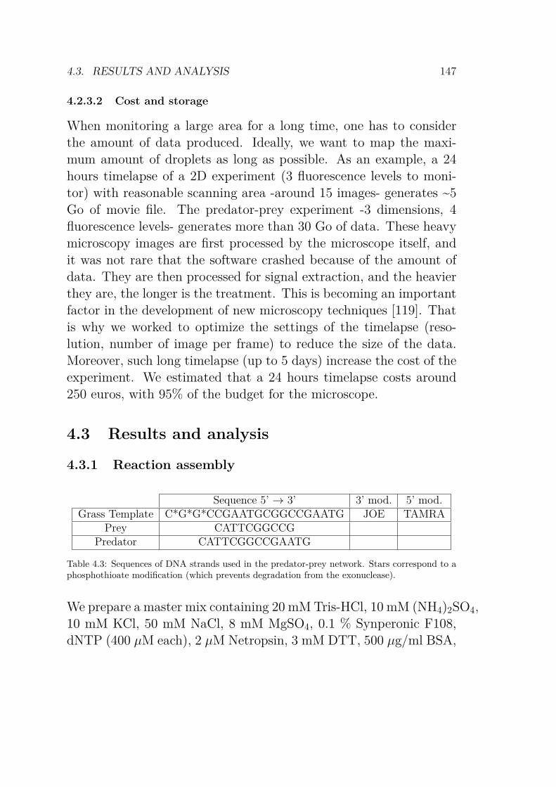
4.3. RESULTS AND ANALYSIS 147
4.2.3.2 Cost and storage
When monitoring a large area for a long time, one has to considerthe amount of data produced. Ideally, we want to map the maxi-mum amount of droplets as long as possible. As an example, a 24hours timelapse of a 2D experiment (3 fluorescence levels to moni-tor) with reasonable scanning area -around 15 images- generates ~5Go of movie file. The predator-prey experiment -3 dimensions, 4fluorescence levels- generates more than 30 Go of data. These heavymicroscopy images are first processed by the microscope itself, andit was not rare that the software crashed because of the amount ofdata. They are then processed for signal extraction, and the heavierthey are, the longer is the treatment. This is becoming an importantfactor in the development of new microscopy techniques [119]. Thatis why we worked to optimize the settings of the timelapse (reso-lution, number of image per frame) to reduce the size of the data.Moreover, such long timelapse (up to 5 days) increase the cost of theexperiment. We estimated that a 24 hours timelapse costs around250 euros, with 95% of the budget for the microscope.
4.3 Results and analysis
4.3.1 Reaction assembly
Sequence 5’ æ 3’ 3’ mod. 5’ mod.Grass Template C*G*G*CCGAATGCGGCCGAATG JOE TAMRA
Prey CATTCGGCCGPredator CATTCGGCCGAATG
Table 4.3: Sequences of DNA strands used in the predator-prey network. Stars correspond to aphosphothioate modification (which prevents degradation from the exonuclease).
We prepare a master mix containing 20 mM Tris-HCl, 10 mM (NH4)2SO4,10 mM KCl, 50 mM NaCl, 8 mM MgSO4, 0.1 % Synperonic F108,dNTP (400 µM each), 2 µM Netropsin, 3 mM DTT, 500 µg/ml BSA,
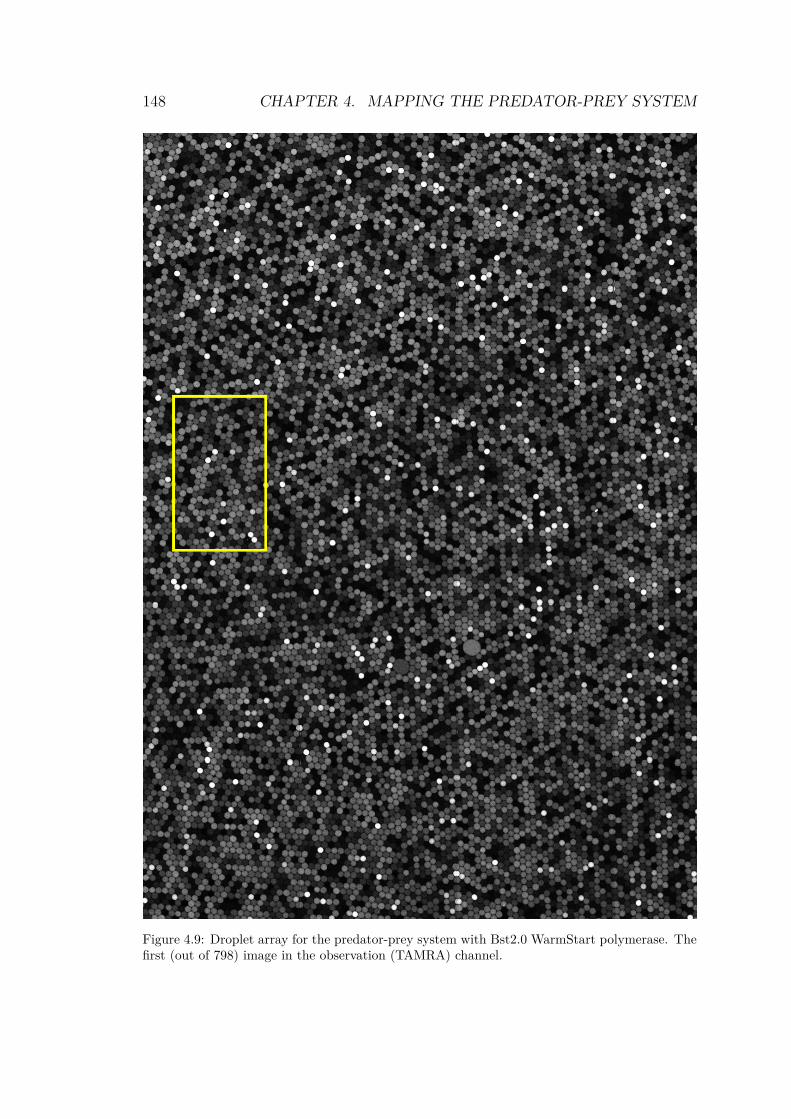
148 CHAPTER 4. MAPPING THE PREDATOR-PREY SYSTEM
Figure 4.9: Droplet array for the predator-prey system with Bst2.0 WarmStart polymerase. Thefirst (out of 798) image in the observation (TAMRA) channel.
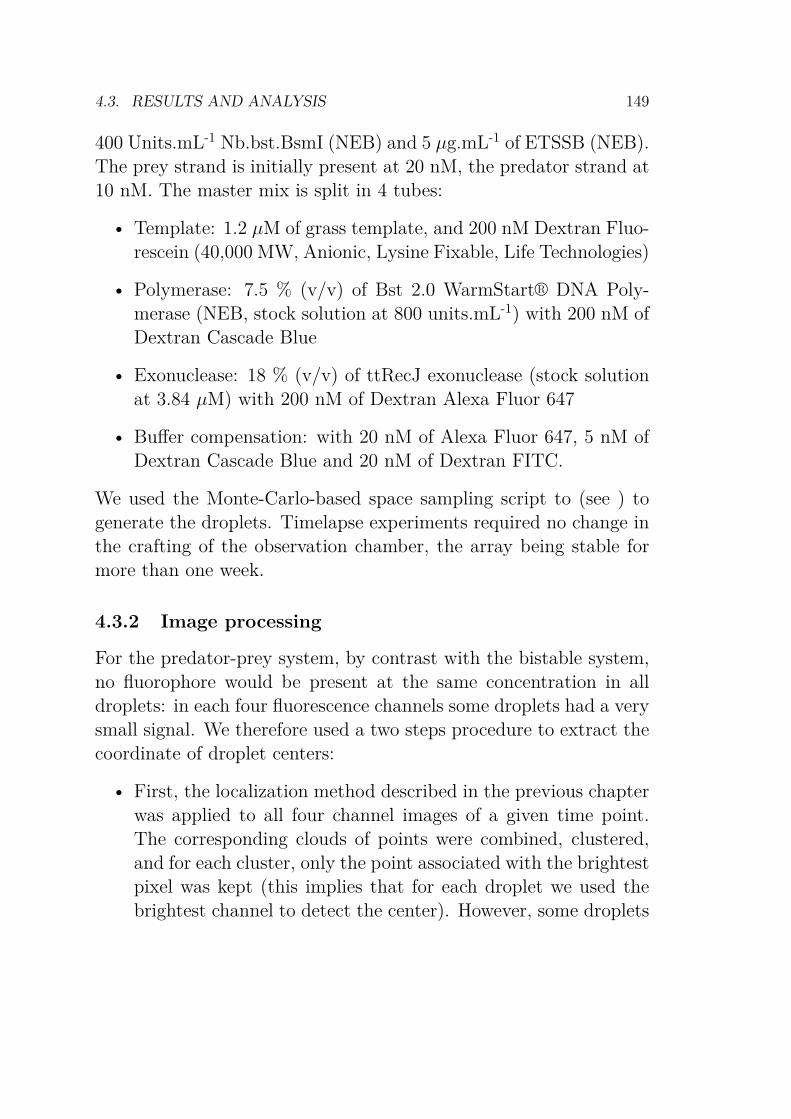
4.3. RESULTS AND ANALYSIS 149
400 Units.mL-1 Nb.bst.BsmI (NEB) and 5 µg.mL-1 of ETSSB (NEB).The prey strand is initially present at 20 nM, the predator strand at10 nM. The master mix is split in 4 tubes:
• Template: 1.2 µM of grass template, and 200 nM Dextran Fluo-rescein (40,000 MW, Anionic, Lysine Fixable, Life Technologies)
• Polymerase: 7.5 % (v/v) of Bst 2.0 WarmStart® DNA Poly-merase (NEB, stock solution at 800 units.mL-1) with 200 nM ofDextran Cascade Blue
• Exonuclease: 18 % (v/v) of ttRecJ exonuclease (stock solutionat 3.84 µM) with 200 nM of Dextran Alexa Fluor 647
• Buffer compensation: with 20 nM of Alexa Fluor 647, 5 nM ofDextran Cascade Blue and 20 nM of Dextran FITC.
We used the Monte-Carlo-based space sampling script to (see ) togenerate the droplets. Timelapse experiments required no change inthe crafting of the observation chamber, the array being stable formore than one week.
4.3.2 Image processing
For the predator-prey system, by contrast with the bistable system,no fluorophore would be present at the same concentration in alldroplets: in each four fluorescence channels some droplets had a verysmall signal. We therefore used a two steps procedure to extract thecoordinate of droplet centers:
• First, the localization method described in the previous chapterwas applied to all four channel images of a given time point.The corresponding clouds of points were combined, clustered,and for each cluster, only the point associated with the brightestpixel was kept (this implies that for each droplet we used thebrightest channel to detect the center). However, some droplets
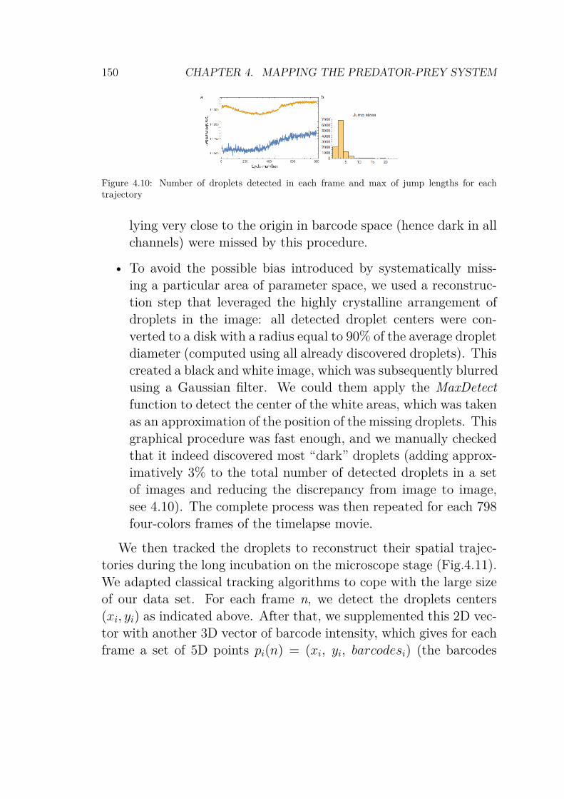
150 CHAPTER 4. MAPPING THE PREDATOR-PREY SYSTEM
Figure 4.10: Number of droplets detected in each frame and max of jump lengths for eachtrajectory
lying very close to the origin in barcode space (hence dark in allchannels) were missed by this procedure.
• To avoid the possible bias introduced by systematically miss-ing a particular area of parameter space, we used a reconstruc-tion step that leveraged the highly crystalline arrangement ofdroplets in the image: all detected droplet centers were con-verted to a disk with a radius equal to 90% of the average dropletdiameter (computed using all already discovered droplets). Thiscreated a black and white image, which was subsequently blurredusing a Gaussian filter. We could them apply the MaxDetectfunction to detect the center of the white areas, which was takenas an approximation of the position of the missing droplets. Thisgraphical procedure was fast enough, and we manually checkedthat it indeed discovered most “dark” droplets (adding approx-imatively 3% to the total number of detected droplets in a setof images and reducing the discrepancy from image to image,see 4.10). The complete process was then repeated for each 798four-colors frames of the timelapse movie.
We then tracked the droplets to reconstruct their spatial trajec-tories during the long incubation on the microscope stage (Fig.4.11).We adapted classical tracking algorithms to cope with the large sizeof our data set. For each frame n, we detect the droplets centers(xi, yi) as indicated above. After that, we supplemented this 2D vec-tor with another 3D vector of barcode intensity, which gives for eachframe a set of 5D points pi(n) = (xi, yi, barcodesi) (the barcodes
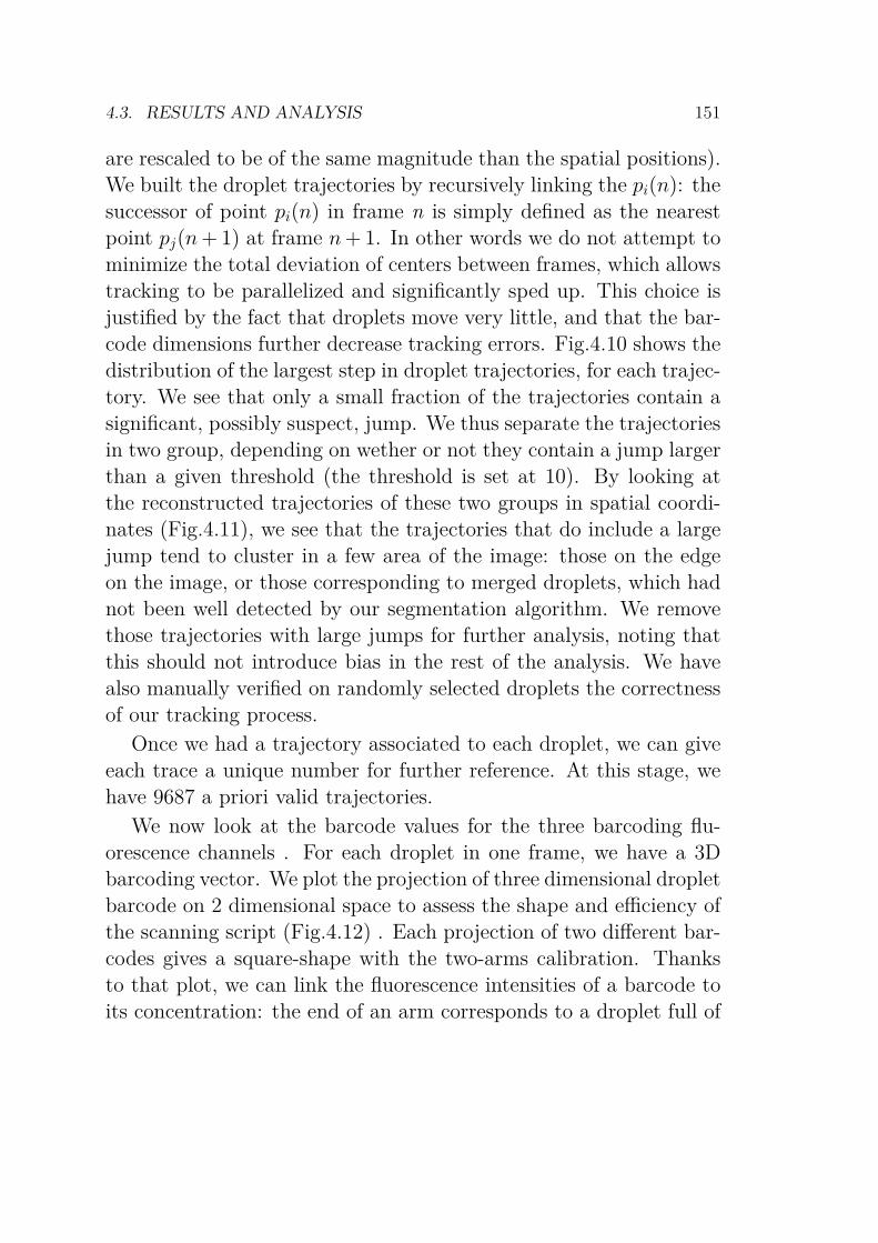
4.3. RESULTS AND ANALYSIS 151
are rescaled to be of the same magnitude than the spatial positions).We built the droplet trajectories by recursively linking the pi(n): thesuccessor of point pi(n) in frame n is simply defined as the nearestpoint pj(n + 1) at frame n + 1. In other words we do not attempt tominimize the total deviation of centers between frames, which allowstracking to be parallelized and significantly sped up. This choice isjustified by the fact that droplets move very little, and that the bar-code dimensions further decrease tracking errors. Fig.4.10 shows thedistribution of the largest step in droplet trajectories, for each trajec-tory. We see that only a small fraction of the trajectories contain asignificant, possibly suspect, jump. We thus separate the trajectoriesin two group, depending on wether or not they contain a jump largerthan a given threshold (the threshold is set at 10). By looking atthe reconstructed trajectories of these two groups in spatial coordi-nates (Fig.4.11), we see that the trajectories that do include a largejump tend to cluster in a few area of the image: those on the edgeon the image, or those corresponding to merged droplets, which hadnot been well detected by our segmentation algorithm. We removethose trajectories with large jumps for further analysis, noting thatthis should not introduce bias in the rest of the analysis. We havealso manually verified on randomly selected droplets the correctnessof our tracking process.
Once we had a trajectory associated to each droplet, we can giveeach trace a unique number for further reference. At this stage, wehave 9687 a priori valid trajectories.
We now look at the barcode values for the three barcoding flu-orescence channels . For each droplet in one frame, we have a 3Dbarcoding vector. We plot the projection of three dimensional dropletbarcode on 2 dimensional space to assess the shape and efficiency ofthe scanning script (Fig.4.12) . Each projection of two different bar-codes gives a square-shape with the two-arms calibration. Thanksto that plot, we can link the fluorescence intensities of a barcode toits concentration: the end of an arm corresponds to a droplet full of
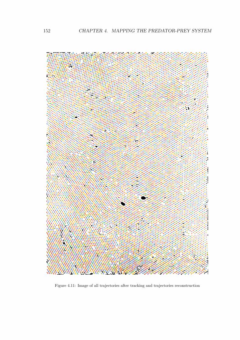
152 CHAPTER 4. MAPPING THE PREDATOR-PREY SYSTEM
Figure 4.11: Image of all trajectories after tracking and trajectories reconstruction
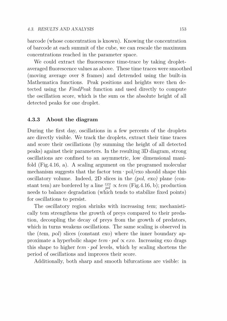
4.3. RESULTS AND ANALYSIS 153
barcode (whose concentration is known). Knowing the concentrationof barcode at each summit of the cube, we can rescale the maximumconcentrations reached in the parameter space.
We could extract the fluorescence time-trace by taking droplet-averaged fluorescence values as above. These time traces were smoothed(moving average over 8 frames) and detrended using the built-inMathematica functions. Peak positions and heights were then de-tected using the FindPeak function and used directly to computethe oscillation score, which is the sum os the absolute height of alldetected peaks for one droplet.
4.3.3 About the diagram
During the first day, oscillations in a few percents of the dropletsare directly visible. We track the droplets, extract their time tracesand score their oscillations (by summing the height of all detectedpeaks) against their parameters. In the resulting 3D diagram, strongoscillations are confined to an asymmetric, low dimensional mani-fold (Fig.4.16, a). A scaling argument on the programed molecularmechanism suggests that the factor tem·pol/exo should shape thisoscillatory volume. Indeed, 2D slices in the (pol, exo) plane (con-stant tem) are bordered by a line exo
pol à tem (Fig.4.16, b); productionneeds to balance degradation (which tends to stabilize fixed points)for oscillations to persist.
The oscillatory region shrinks with increasing tem; mechanisti-cally tem strengthens the growth of preys compared to their preda-tion, decoupling the decay of preys from the growth of predators,which in turns weakens oscillations. The same scaling is observed inthe (tem, pol) slices (constant exo) where the inner boundary ap-proximate a hyperbolic shape tem · pol à exo. Increasing exo dragsthis shape to higher tem · pol levels, which by scaling shortens theperiod of oscillations and improves their score.
Additionally, both sharp and smooth bifurcations are visible: in
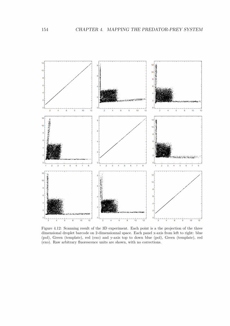
154 CHAPTER 4. MAPPING THE PREDATOR-PREY SYSTEM
Figure 4.12: Scanning result of the 3D experiment. Each point is a the projection of the threedimensional droplet barcode on 2-dimensionnal space. Each panel x-axis from left to right: blue(pol), Green (template), red (exo) and y-axis top to down blue (pol), Green (template), red(exo). Raw arbitrary fluorescence units are shown, with no corrections.
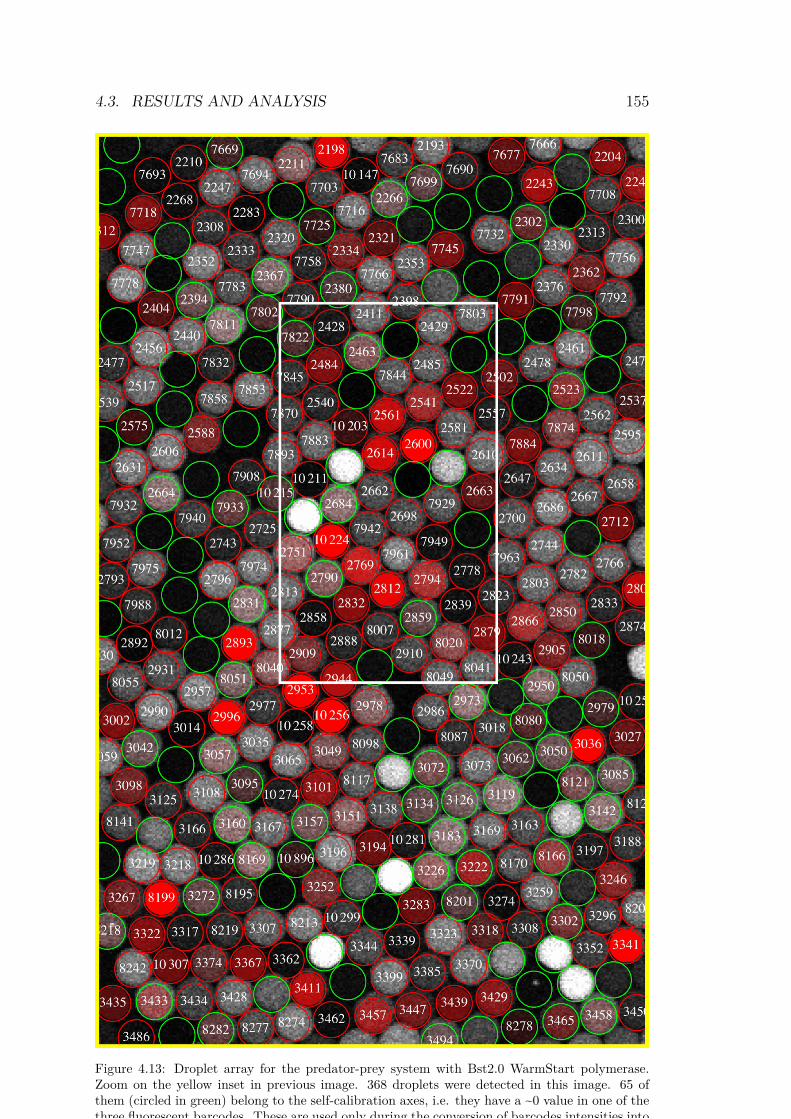
4.3. RESULTS AND ANALYSIS 155
Figure 4.13: Droplet array for the predator-prey system with Bst2.0 WarmStart polymerase.Zoom on the yellow inset in previous image. 368 droplets were detected in this image. 65 ofthem (circled in green) belong to the self-calibration axes, i.e. they have a ~0 value in one of thethree fluorescent barcodes. These are used only during the conversion of barcodes intensities into
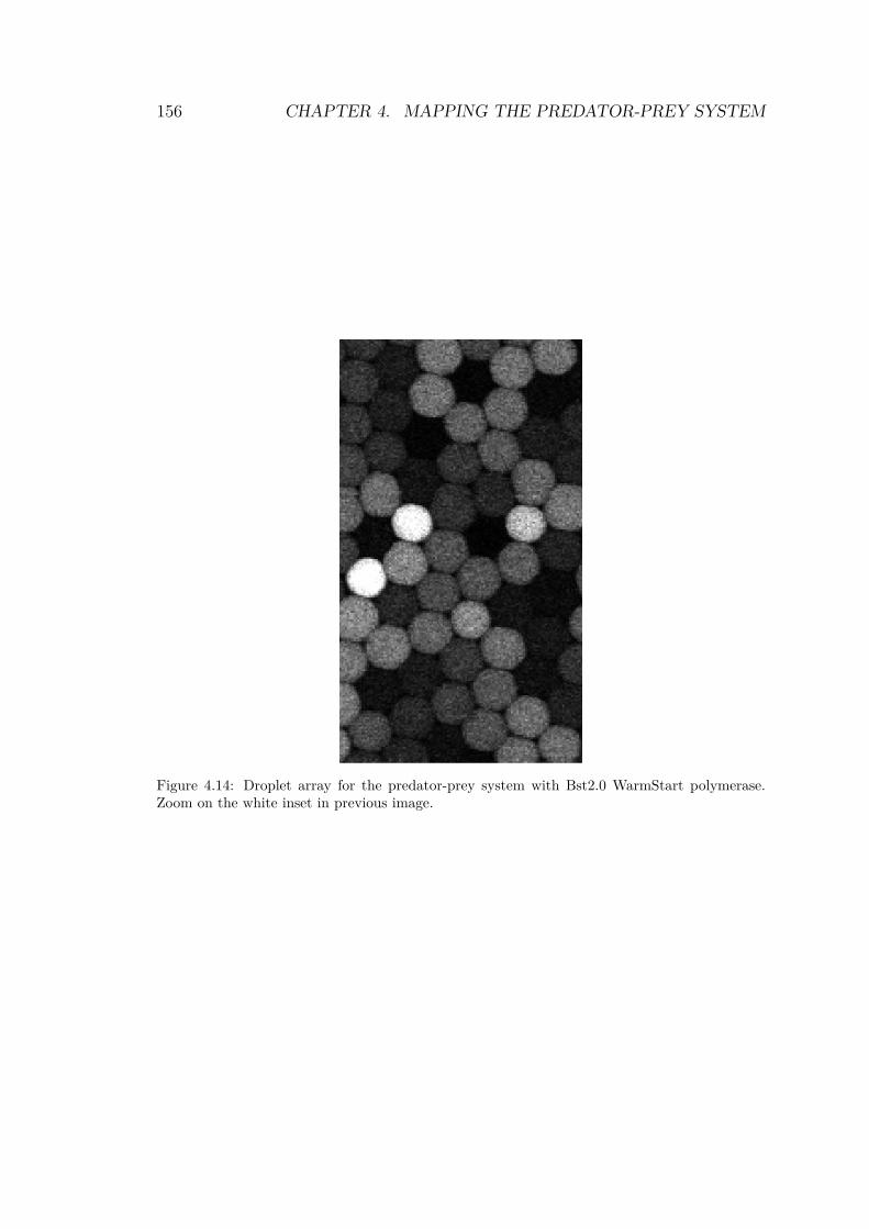
156 CHAPTER 4. MAPPING THE PREDATOR-PREY SYSTEM
Figure 4.14: Droplet array for the predator-prey system with Bst2.0 WarmStart polymerase.Zoom on the white inset in previous image.
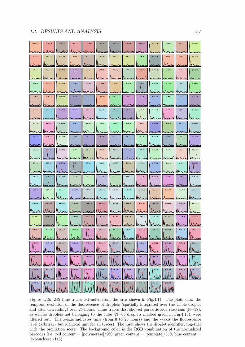
4.3. RESULTS AND ANALYSIS 157
Figure 4.15: 245 time traces extracted from the area shown in Fig.4.14. The plots show thetemporal evolution of the fluorescence of droplets (spatially integrated over the whole dropletand after detrending) over 25 hours. Time traces that showed parasitic side reactions (N=58),as well as droplets not belonging to the cube (N=65 droplets marked green in Fig.4.13), werefiltered out. The x-axis indicates time (from 0 to 25 hours) and the y-axis the fluorescencelevel (arbitrary but identical unit for all traces). The inset shows the droplet identifier, togetherwith the oscillation score. The background color is the RGB combination of the normalizedbarcodes (i.e. red content = [polymerase]/260; green content = [template]/350; blue content =[exonuclease]/115)
158 CHAPTER 4. MAPPING THE PREDATOR-PREY SYSTEM
Fig.4.16, b, starting from low pol, oscillations start sharply but grad-ually weaken into damped oscillations (dashed line and inset). Thissuggests that the Hopf bifurcation leads to trajectories spiraling downto a stable coexistence focus on one side, but to an extinction statewith no oscillatory potential on the other side. These observationsagree with a simple analytical model of the predator-prey system(see Introduction).
After the first day, the emergence of opportunistic DNA replica-tors overcomes the predator-prey system in most droplets [120]. Weinspect the dynamics of the remaining droplets looking for traceswith low autocorrelation and observed surprising stochastic behav-iors (Fig.4.16, c). While most of those surviving droplets eitherdampen (bottom right in Fig.4.16, c), oscillate sustainably (diagonalin Fig.4.16, c and Fig.4.16, d) or fail to oscillate at all (dark pointsin bottom left in Fig.4.16, c) - in line with qualitative predictionsfor deterministic dynamical system - a small fraction of droplets ex-hibit “bursting” oscillations that spontaneously switch ON or OFF(Fig.4.16, e. Those droplets originated from a small, well-definedregion of the parameter space lining the low pol, low temp face ofthe oscillatory region (Fig.4.16, a). Remarkably, stability analysisof the kinetic model does predict the existence of a small manifoldof bimodal steady/oscillatory (i.e. hard-excitable) systems, locatedprecisely at the inner edge of the oscillatory region, and where smallamplitude noise could induce a similar bursting behavior. In thiscase, stochasticity originating from the small size of the compart-ments would in fact be instrumental to uncover (and possibly exploit)alternative attractors of the molecular system [121].
4.4 Discussion
The mathematical derivation and analysis of a two-variable modelfor the predator-prey system is presented in the introduction and isonly sketched here for reference.
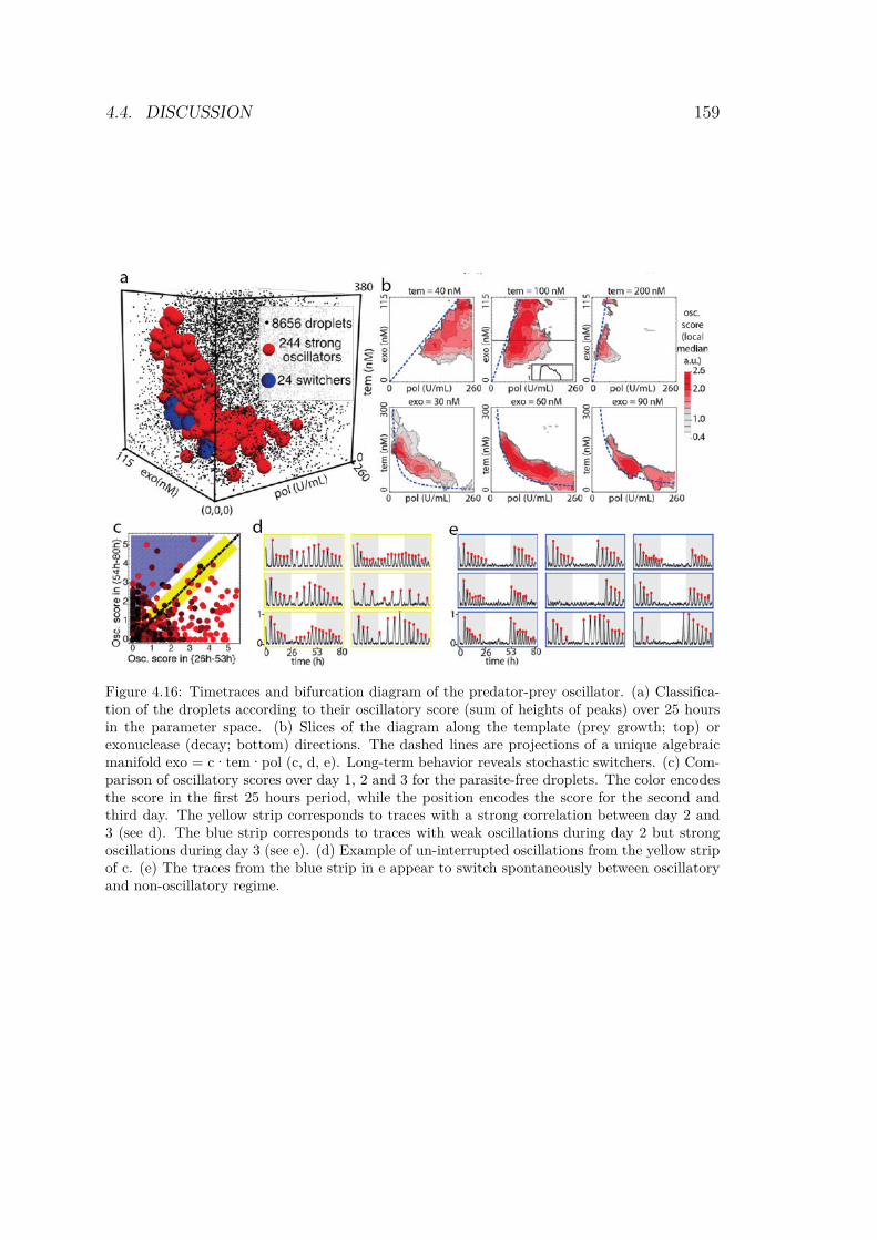
4.4. DISCUSSION 159
Figure 4.16: Timetraces and bifurcation diagram of the predator-prey oscillator. (a) Classifica-tion of the droplets according to their oscillatory score (sum of heights of peaks) over 25 hoursin the parameter space. (b) Slices of the diagram along the template (prey growth; top) orexonuclease (decay; bottom) directions. The dashed lines are projections of a unique algebraicmanifold exo = c·tem·pol (c, d, e). Long-term behavior reveals stochastic switchers. (c) Com-parison of oscillatory scores over day 1, 2 and 3 for the parasite-free droplets. The color encodesthe score in the first 25 hours period, while the position encodes the score for the second andthird day. The yellow strip corresponds to traces with a strong correlation between day 2 and3 (see d). The blue strip corresponds to traces with weak oscillations during day 2 but strongoscillations during day 3 (see e). (d) Example of un-interrupted oscillations from the yellow stripof c. (e) The traces from the blue strip in e appear to switch spontaneously between oscillatoryand non-oscillatory regime.
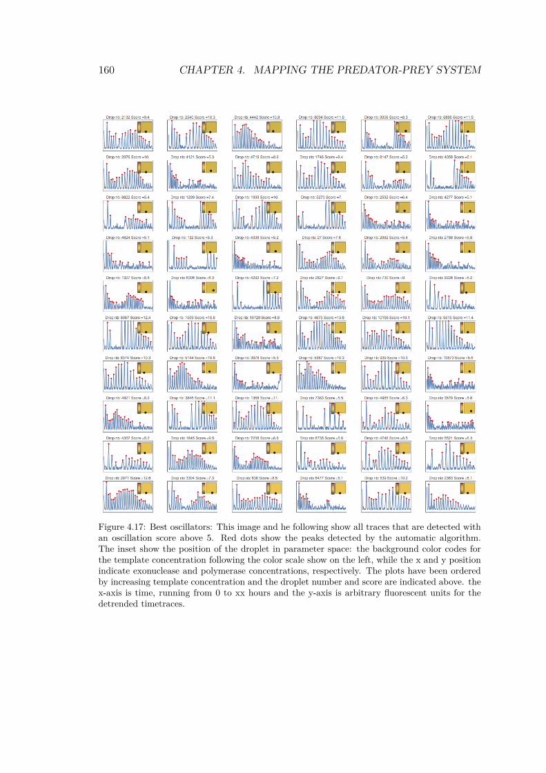
160 CHAPTER 4. MAPPING THE PREDATOR-PREY SYSTEM
Figure 4.17: Best oscillators: This image and he following show all traces that are detected withan oscillation score above 5. Red dots show the peaks detected by the automatic algorithm.The inset show the position of the droplet in parameter space: the background color codes forthe template concentration following the color scale show on the left, while the x and y positionindicate exonuclease and polymerase concentrations, respectively. The plots have been orderedby increasing template concentration and the droplet number and score are indicated above. thex-axis is time, running from 0 to xx hours and the y-axis is arbitrary fluorescent units for thedetrended timetraces.
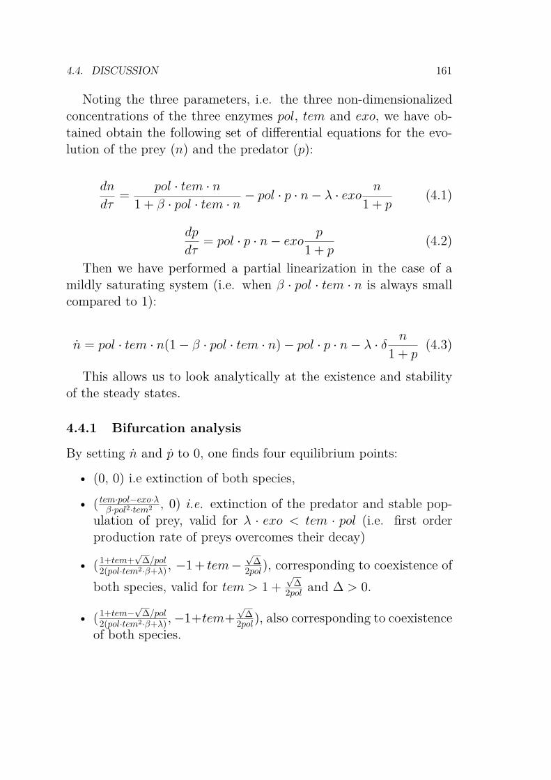
4.4. DISCUSSION 161
Noting the three parameters, i.e. the three non-dimensionalizedconcentrations of the three enzymes pol, tem and exo, we have ob-tained obtain the following set of differential equations for the evo-lution of the prey (n) and the predator (p):
dn
dτ=
pol · tem · n
1 + β · pol · tem · n≠ pol · p · n ≠ λ · exo
n
1 + p(4.1)
dp
dτ= pol · p · n ≠ exo
p
1 + p(4.2)
Then we have performed a partial linearization in the case of amildly saturating system (i.e. when β · pol · tem · n is always smallcompared to 1):
n = pol · tem · n(1 ≠ β · pol · tem · n) ≠ pol · p · n ≠ λ · δn
1 + p(4.3)
This allows us to look analytically at the existence and stabilityof the steady states.
4.4.1 Bifurcation analysis
By setting n and p to 0, one finds four equilibrium points:
• (0, 0) i.e extinction of both species,
• ( tem·pol≠exo·λβ·pol2·tem2 , 0) i.e. extinction of the predator and stable pop-
ulation of prey, valid for λ · exo < tem · pol (i.e. first orderproduction rate of preys overcomes their decay)
• (1+tem+Ô
∆/pol2(pol·tem2·β+λ) , ≠1 + tem ≠
Ô∆
2pol), corresponding to coexistence of
both species, valid for tem > 1 +Ô
∆
2pol and ∆ > 0.
• (1+tem≠Ô
∆/pol2(pol·tem2·β+λ) , ≠1+tem+
Ô∆
2pol), also corresponding to coexistenceof both species.
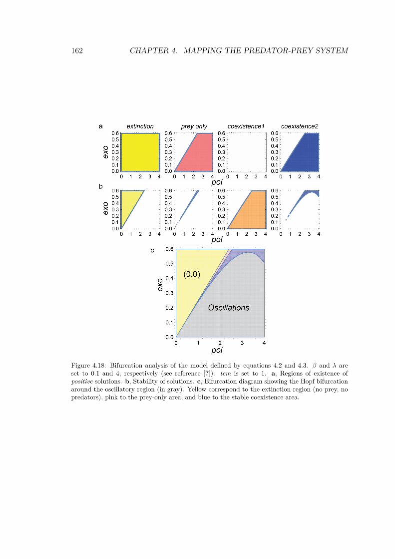
162 CHAPTER 4. MAPPING THE PREDATOR-PREY SYSTEM
Figure 4.18: Bifurcation analysis of the model defined by equations 4.2 and 4.3. β and λ areset to 0.1 and 4, respectively (see reference [?]). tem is set to 1. a, Regions of existence ofpositive solutions. b, Stability of solutions. c, Bifurcation diagram showing the Hopf bifurcationaround the oscillatory region (in gray). Yellow correspond to the extinction region (no prey, nopredators), pink to the prey-only area, and blue to the stable coexistence area.
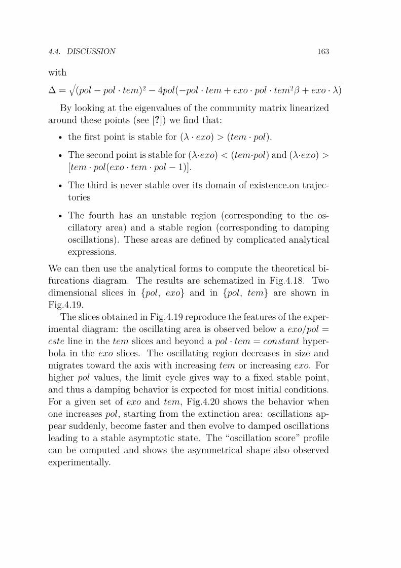
4.4. DISCUSSION 163
with
∆ =Ò
(pol ≠ pol · tem)2 ≠ 4pol(≠pol · tem + exo · pol · tem2β + exo · λ)
By looking at the eigenvalues of the community matrix linearizedaround these points (see [?]) we find that:
• the first point is stable for (λ · exo) > (tem · pol).
• The second point is stable for (λ·exo) < (tem·pol) and (λ·exo) >[tem · pol(exo · tem · pol ≠ 1)].
• The third is never stable over its domain of existence.on trajec-tories
• The fourth has an unstable region (corresponding to the os-cillatory area) and a stable region (corresponding to dampingoscillations). These areas are defined by complicated analyticalexpressions.
We can then use the analytical forms to compute the theoretical bi-furcations diagram. The results are schematized in Fig.4.18. Twodimensional slices in {pol, exo} and in {pol, tem} are shown inFig.4.19.
The slices obtained in Fig.4.19 reproduce the features of the exper-imental diagram: the oscillating area is observed below a exo/pol =cste line in the tem slices and beyond a pol · tem = constant hyper-bola in the exo slices. The oscillating region decreases in size andmigrates toward the axis with increasing tem or increasing exo. Forhigher pol values, the limit cycle gives way to a fixed stable point,and thus a damping behavior is expected for most initial conditions.For a given set of exo and tem, Fig.4.20 shows the behavior whenone increases pol, starting from the extinction area: oscillations ap-pear suddenly, become faster and then evolve to damped oscillationsleading to a stable asymptotic state. The “oscillation score” profilecan be computed and shows the asymmetrical shape also observedexperimentally.
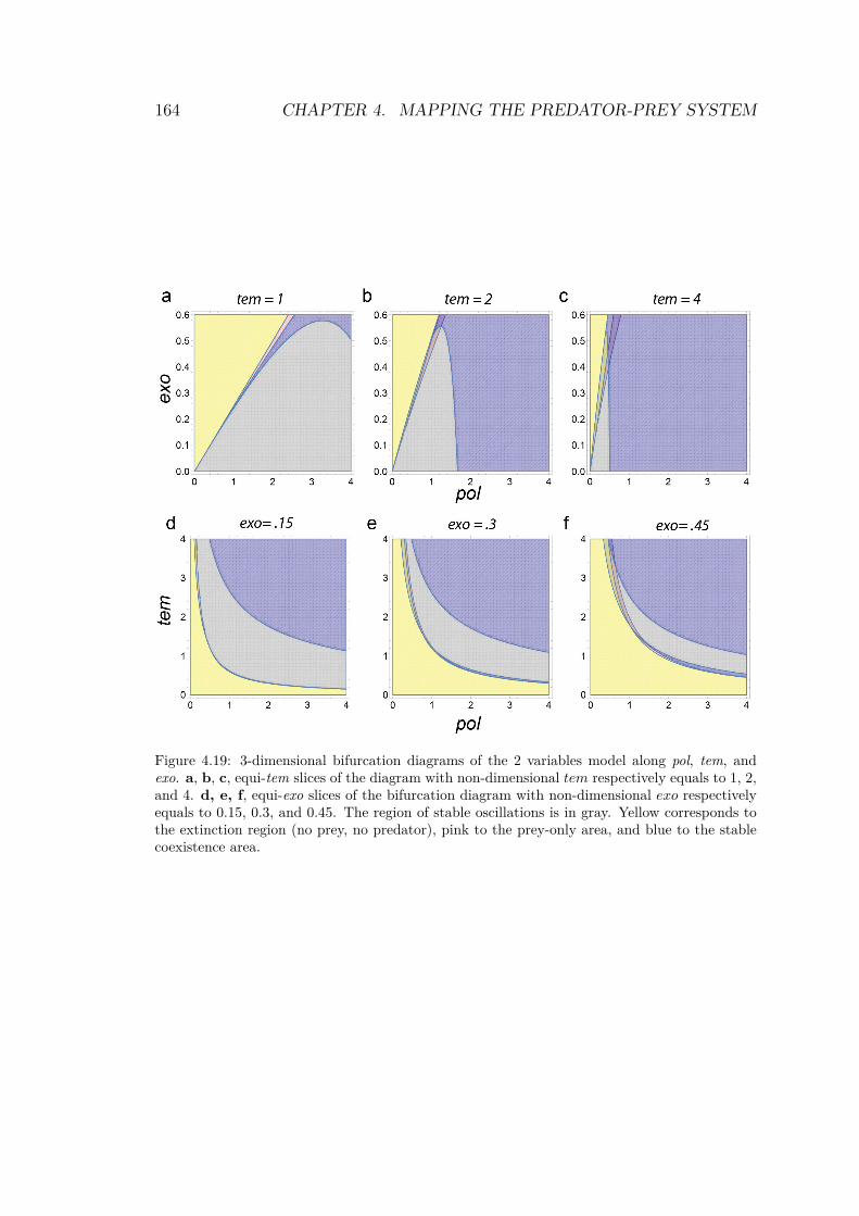
164 CHAPTER 4. MAPPING THE PREDATOR-PREY SYSTEM
Figure 4.19: 3-dimensional bifurcation diagrams of the 2 variables model along pol, tem, andexo. a, b, c, equi-tem slices of the diagram with non-dimensional tem respectively equals to 1, 2,and 4. d, e, f, equi-exo slices of the bifurcation diagram with non-dimensional exo respectivelyequals to 0.15, 0.3, and 0.45. The region of stable oscillations is in gray. Yellow corresponds tothe extinction region (no prey, no predator), pink to the prey-only area, and blue to the stablecoexistence area.
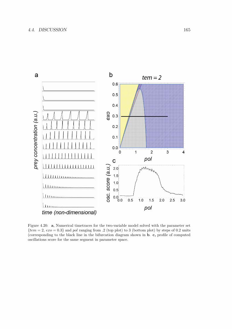
4.4. DISCUSSION 165
Figure 4.20: a, Numerical timetraces for the two-variable model solved with the parameter set{tem = 2, exo = 0.3} and pol ranging from .2 (top plot) to 3 (bottom plot) by steps of 0.2 units(corresponding to the black line in the bifurcation diagram shown in b. c, profile of computedoscillations score for the same segment in parameter space.
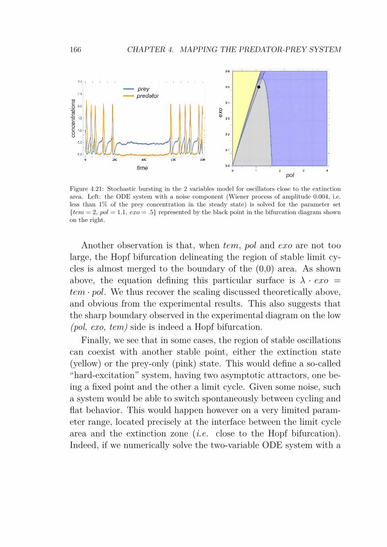
166 CHAPTER 4. MAPPING THE PREDATOR-PREY SYSTEM
Figure 4.21: Stochastic bursting in the 2 variables model for oscillators close to the extinctionarea. Left: the ODE system with a noise component (Wiener process of amplitude 0.004, i.e.less than 1% of the prey concentration in the steady state) is solved for the parameter set{tem = 2, pol = 1.1, exo = .5} represented by the black point in the bifurcation diagram shownon the right.
Another observation is that, when tem, pol and exo are not toolarge, the Hopf bifurcation delineating the region of stable limit cy-cles is almost merged to the boundary of the (0,0) area. As shownabove, the equation defining this particular surface is λ · exo =tem · pol. We thus recover the scaling discussed theoretically above,and obvious from the experimental results. This also suggests thatthe sharp boundary observed in the experimental diagram on the low(pol, exo, tem) side is indeed a Hopf bifurcation.
Finally, we see that in some cases, the region of stable oscillationscan coexist with another stable point, either the extinction state(yellow) or the prey-only (pink) state. This would define a so-called“hard-excitation” system, having two asymptotic attractors, one be-ing a fixed point and the other a limit cycle. Given some noise, sucha system would be able to switch spontaneously between cycling andflat behavior. This would happen however on a very limited param-eter range, located precisely at the interface between the limit cyclearea and the extinction zone (i.e. close to the Hopf bifurcation).Indeed, if we numerically solve the two-variable ODE system with a
4.4. DISCUSSION 167
noise component (Langevin dynamic) within this multimodal regionwe observe a bursting behavior similar to the experimental results(Fig.4.21).
Globally, linear stability analysis of a very simple two-variablemodel is in good agreement with the shape of the experimental di-agram. It confirms that we do experimentally observe the Hopf bi-furcation on the low concentration side, while its exact position onthe other side is masked by the existence of damped trajectories.The effect of molecular noise in these small droplets appears to beamplified by the non linear dynamics, especially when the systemis close to multiple bifurcations. The spectacular bursting of someoscillating droplets is a good example of this combination.

168 CHAPTER 4. MAPPING THE PREDATOR-PREY SYSTEM
Chapter 5
Conclusion
Molecular programming is a new, still emergent field which takesinspiration from information processing as it is observed in livingorganisms. The goal is to create information-managing systems atthe molecular level. In the process, we hope to better understandthe inner machinery of a cell, but also to exploit the properties ofsuch unconventionnal computating schemes to bypass issues in other,more classical approaches (e.g. solid-state electronic devices). Maybethe molecular programing approach will one day allow us to designor engineer new and useful molecular architectures displaying uniquebehaviors.
In this context we developed in the laboratory the PEN-DNA tool-box, which is composed of three cascadable reactions inspired by generegulation networks found in cells, or even in viruses (the lambdaphage and its spectacular lytic “switch” was one of the proeminentcase-study that allowed researchers to better understand the dynam-ics of regulation of genetic expression and its dramatic effects onphenotypes).
Using the PEN-DNA toolbox, activation, inhibition and degrada-tion are generic reactions that can be connected in arbitrary topolo-gies. These test-tube networks reproduce biological-relevant behav-iors such as bistability or oscillations. In this work, we tried to go onestep further in the global understanding of how such networks behave
169
170 CHAPTER 5. CONCLUSION
by extracting -experimentaly- their bifurcation diagrams. For that,we first developed a microfluidic tool for the experimental mappingof concentration parameter spaces. Our device generates millions ofwater-in-oil droplets with different composition thanks to a pressurecontroller for which we developed scripts adapted to the 2D and 3Dmapping. In the current implementation the mesh (and therefore theresolution of our maps) is fixed by the iteration number and the num-ber of droplet that we can ultimately image. We have also worked alot on the observation chamber to make it leak-proof, movement-free,and compatible with long-term timelapse (more than 3 days).
The first system that we tested was the bistable switch fromPadirac et al. [45]. We successfully mapped the bifurcation dia-gram of this network as a function of two parameters depicting theautocatalysis strength of each side. The results showed monostabil-ity and bistability areas, concurring with previous theoretical stud-ies, but also revealed some unexpected features. For example, weobserved the surprising shape of the 00 domain, which extends as-symetrically on both sides of the bistable area. Therfore, in somearea of its parameter space, the system remains in a “forbidden”state (accoring to simple linear stability analysis (LSA) arguments)even after 11h of evolution. This singularity may come from the net-work itself, showing the existence of a third stable point because ofunaccounted nonlinearities in the interactions between the species.Alternatively, it could be the consequence of small number effects inthese tiny compartments. Further investigations should unveil thereasons underlying such particularity. For example, droplet scan-ning experiments focusing on this particular area and performed fora longer time (up to several days) will help to decide wether there isreal stochastic trapping or if the effect is due to a strong slowdownof the system.
We then decided to add a third dimension to the map and tostudy a predator-prey system [41]. We focused on the effects ofgrowth and decay rate parameters by varying the concentration of
171
polymerase (a catalytic ressource for the growth of predators andpreys), the concentration of exonuclease (a catalytic ressource for thedegradation of both species) and the concentration of grass template(involved in prey growth only). After extraction of the timetraces,it appeared that the strong oscillating area is circumscribed in anasymmetric, low dimensional manifold. We hypothesized a scalingmechanism to shape the oscillatory volume according to the equa-tion: exo = c · tem · pol . The diagram showed both sharp andsmooth bifurcations, suggesting that the orbits in shape portraitslead to stable coexistence or extinction, while LSA predicted the ex-istence of a narrow, hard-excitations domain. We observed a smallfraction of droplets exhibiting “bursting” oscillations that sponta-neously switched ON or OFF, all coming from the small, well-definedregion of parameter space lining the low pol, low temp face of theoscillatory region. Such switches may originate from the molecularconfinement in low-concentration droplets. This should be confirmedin the future by changing the size of the compartment for a set ofparametric conditions lying within this small area.
One may question the technical limits of such an approach. Howfar can we push this technology? How many parameters can wescan? Which resolution can we achieve in order to reveal rare andexotic behaviors? In the future, more more accurate pressure controlscripts using space-filling curves will improve the scanning time. Thiswill allow us to decrease the mesh size and makes the system moreuser-friendly. The actual generation of droplets -although serial- isnot an immediate bottleneck. We routinely generate ~1 million ofdroplets in ~45 min, and faster rates of 1 MHz have been achieved inthe litterature [122] (although without combinatorial preparation).Programming the pressure profiles to mix more than 4 inlets shouldnot be beyond the reach of a skilled operator. Incubation of dropletsis not a bottleneck since reactions run in parallel. Fluorescence scan-ning of the droplets proves to be the most time-consuming operation.We chose confocal laser microscopy because of its high signal-to-noise
172 CHAPTER 5. CONCLUSION
ratio. But this scanning method is serial and thus slow. Scanning ~10000 droplets requires about ~ 5 min. Faster rates could be achievedby decreasing the scanning resolution and the time spent on eachpixel, pushing up the laser power if needed to compensate for thelower number of photons collected per droplet. Faster methods ofscanning could also be considered. Droplet flow cytometry (a sequen-tial method) scans ~2000 droplets/s (~ 600 000 droplets/ 5 min) [72].Among parallel acquisition methods, a sCMOS camera coupled withepifluorescence microscopy is an attractive option. A 5 megapixelsCMOS camera can nominally scan ~50 000 droplets simultaneouslyat a resolution of 100 pixels/droplet. Assuming an exposure timeon the order of 10 seconds per frame (including stage translation,filter switching and acquisition), a sCMOS setup will acquire the flu-orescence of 1.5 millions droplets per 5 minutes. Note that parallelscanning methods require more careful calibration than sequentialones to account for the spatial dependence of the illumination andsensors. Fluorescence overlap will also have to be dealt with, but itis realistic to encode the concentration of 6 variables simultaneously[123].
More generally, our microfluidic platform for bifurcation diagrammapping is a great tool in understanding the inner machinery, asmuch as unveiling the possibilities of any network compatible withthe PEN-DNA toolbox. Because of their experimental, assumption-free origin, these maps are more accurate than any model. At themoment, they cannot be used to predic untested conditions, butwe expect that they will lead to a next generation of more accuratemathematical models -boosted with feedbacks from the experimentalbifurcation diagrams- which in turn will allow more realistic compu-tationnal predictions.
Finally, our platform will find applications in other molecular con-texts where interactions between nodes of a chemical reaction net-work gives rise to nontrivial dynamics. For example it could bepossible to apply our approach to interogate cellular regulatory net-

173
works and progress in the understanding of system biology. Ulti-mately these visual diagrams will offer mechanistic insights that willsharpen our understanding of design principles in molecular systemsin a very general way.

174 CHAPTER 5. CONCLUSION
Bibliography
[1] Ralf Dahm. Discovering DNA: Friedrich Miescher and the early years ofnucleic acid research., 2008.
[2] J D Watson and F H C Crick. A structure for deoxyribose nucleic acid.1953., 2003.
[3] S N Cohen, A C Chang, H W Boyer, and R B Helling. Construction ofbiologically functional bacterial plasmids in vitro. Proceedings of the NationalAcademy of Sciences of the United States of America, 70(11):3240–3244,1973.
[4] F Sanger, S Nicklen, and A R Coulson. DNA sequencing with chain-terminating inhibitors. Proceedings of the National Academy of Sciencesof the United States of America, 74(12):5463–5467, 1977.
[5] R K Saiki, D H Gelfand, S Stoffel, S J Scharf, R Higuchi, G T Horn, K BMullis, and H A Erlich. Primer-directed enzymatic amplification of DNAwith a thermostable DNA polymerase. Science, 239(4839):487–491, 1988.
[6] A Fire, S Q Xu, M K Montgomery, S A Kostas, and S E Driver. Potentand specific genetic interference by double-stranded RNA in Caenorhabditiselegans. Nature, 1998.
[7] M Jinek, K Chylinski, I Fonfara, M Hauer, and J A Doudna. A pro-grammable dual-RNA–guided DNA endonuclease in adaptive bacterial im-munity. Science, 2012.
[8] Leslie E Orgel. Prebiotic chemistry and the origin of the RNA world. Criticalreviews in biochemistry and molecular biology, 39(2):99–123, 2004.
[9] John SantaLucia and Donald Hicks. The thermodynamics of DNA structuralmotifs. Annual review of biophysics and biomolecular structure, 33:415–440,2004.
175
176 BIBLIOGRAPHY
[10] B Yurke, A J Turberfield, A P Mills, F C Simmel, and J L Neumann. ADNA-fuelled molecular machine made of DNA. Nature, 406(6796):605–608,2000.
[11] David Yu Zhang and Erik Winfree. Control of DNA Strand Displacement Ki-netics Using Toehold Exchange. Journal of the American Chemical Society,131(47):17303–17314, 2009.
[12] David Yu Zhang and Georg Seelig. Dynamic DNA nanotechnology usingstrand-displacement reactions. Nature chemistry, 3(2):103–113, 2011.
[13] F JACOB and J MONOD. Genetic regulatory mechanisms in the synthesisof proteins. Journal of Molecular Biology, 3:318–356, June 1961.
[14] J Chen and N C Seeman. Synthesis from DNA of a molecule with theconnectivity of a cube. Nature, 1991.
[15] E Winfree, F Liu, L A Wenzler, and N C Seeman. Design and self-assemblyof two-dimensional DNA crystals. Nature, 394(6693):539–544, 1998.
[16] Paul W K Rothemund. Folding DNA to create nanoscale shapes and pat-terns. Nature, 440(7082):297–302, 2006.
[17] Dongran Han, Suchetan Pal, Jeanette Nangreave, Zhengtao Deng, Yan Liu,and Hao Yan. DNA origami with complex curvatures in three-dimensionalspace. Science, 332(6027):342–346, 2011.
[18] Dongran Han, Suchetan Pal, Yan Liu, and Hao Yan. Folding and cuttingDNA into reconfigurable topological nanostructures. Nature nanotechnology,5(10):712–717, 2010.
[19] Kyle Lund, Anthony J Manzo, Nadine Dabby, Nicole Michelotti, AlexanderJohnson-Buck, Jeanette Nangreave, Steven Taylor, Renjun Pei, Milan NStojanovic, Nils G Walter, Erik Winfree, and Hao Yan. Molecular robotsguided by prescriptive landscapes. Nature, 465(7295):206–210, 2010.
[20] Peng Yin, Harry M T Choi, Colby R Calvert, and Niles A Pierce. Pro-gramming biomolecular self-assembly pathways. Nature, 451(7176):318–322,2008.
[21] Yonggang Ke, Luvena L Ong, William M Shih, and Peng Yin.Three-dimensional structures self-assembled from DNA bricks. Science,338(6111):1177–1183, 2012.
BIBLIOGRAPHY 177
[22] L M Adleman. Molecular computation of solutions to combinatorial prob-lems. Science, 266(5187):1021–1024, 1994.
[23] John J Tyson, Katherine C Chen, and Béla Novák. Sniffers, buzzers, togglesand blinkers: dynamics of regulatory and signaling pathways in the cell.Current Opinion in Cell Biology, 15(2):221–231, 2003.
[24] Denise M Wolf and Adam P Arkin. Motifs, modules and games in bacteria.Current Opinion in Microbiology, 6(2):125–134, 2003.
[25] Kevin Montagne, Raphael Plasson, Yasuyuki Sakai, Teruo Fujii, and Yan-nick Rondelez. Programming an in vitro DNA oscillator using a molecularnetworking strategy. Molecular Systems Biology, 7:1–7, 2011.
[26] Jongmin Kim, Kristin S White, and Erik Winfree. Construction of an in vitrobistable circuit from synthetic transcriptional switches. Molecular SystemsBiology, 2, 2006.
[27] Shotaro Ayukawa, Masahiro Takinoue, and Daisuke Kiga. RTRACS: a mod-ularized RNA-dependent RNA transcription system with high programma-bility. Accounts of Chemical Research, 44(12):1369–1379, 2011.
[28] Jongmin Kim and Erik Winfree. Synthetic in vitro transcriptional oscillators.Molecular Systems Biology, 7:1–15, 2011.
[29] Masahiro Takinoue, Daisuke Kiga, Koh-ichiroh Shohda, and Akira Suyama.Experiments and simulation models of a basic computation element of anautonomous molecular computing system. Physical Review E, 78(4):041921,2008.
[30] Y Sakai, Y Mawatari, K Yamasaki, and K Shohda. Construction of ANDGate for RTRACS with the Capacity of Extension to NAND Gate. DNAComputing and . . . , 2009.
[31] A Kan, Y Sakai, K Shohda, and A Suyama. A DNA based molecular logicgate capable of a variety of logical operations. Natural Computing, 2014.
[32] M Takinoue, D Kiga, K Shohda, and A Suyama. RNA Oscillator: limitcycle oscillations based on artificial biomolecular reactions. New GenerationComputing, 2009.
[33] Joseph N Zadeh, Conrad D Steenberg, Justin S Bois, Brian R Wolfe, Mar-shall B Pierce, Asif R Khan, Robert M Dirks, and Niles A Pierce. NUPACK:analysis and design of nucleic acid systems. Journal of computational chem-istry, 32(1):170–173, 2011.
178 BIBLIOGRAPHY
[34] Jeffrey Van Ness, Lori K Van Ness, and David J Galas. Isothermal reac-tions for the amplification of oligonucleotides. Proceedings of the NationalAcademy of Sciences of the United States of America, 100(8):4504–4509,2003.
[35] Alexandre Baccouche, Kevin Montagne, Adrien Padirac, Teruo Fujii, andYannick Rondelez. Dynamic DNA-toolbox reaction circuits: a walkthrough.Methods, 67(2):234–249, 2014.
[36] Luca Giorgetti, Trevor Siggers, Guido Tiana, Greta Caprara, Samuele Notar-bartolo, Teresa Corona, Manolis Pasparakis, Paolo Milani, Martha L Bulyk,and Gioacchino Natoli. Noncooperative interactions between transcriptionfactors and clustered DNA binding sites enable graded transcriptional re-sponses to environmental inputs. Molecular cell, 37(3):418–428, 2010.
[37] R Sarpeshkar. Analog versus digital: extrapolating from electronics to neu-robiology. Neural computation, 10(7):1601–1638, 1998.
[38] R Sarpeshkar. Analog synthetic biology. Philosophical transactions. SeriesA, Mathematical, physical, and engineering sciences, 372(2012):20130110,2014.
[39] Lulu Qian and Erik Winfree. Scaling up digital circuit computation withDNA strand displacement cascades. Science, 332(6034):1196–1201, 2011.
[40] Lulu Qian and Erik Winfree. A simple DNA gate motif for synthesizinglarge-scale circuits. Journal of The Royal Society Interface, 8(62):1281–1297,2011.
[41] Teruo Fujii and Yannick Rondelez. Predator–Prey Molecular Ecosystems.ACS Nano, 7(1):27–34, 2013.
[42] A J Lotka. Undamped oscillations derived from the law of mass action.Journal of the American Chemical Society, 1920.
[43] V Volterra. Variations and fluctuations of the number of individuals inanimal species living together. J Cons Int Explor Mer, 1928.
[44] Xi Chen and Andrew D Ellington. Shaping up nucleic acid computation.Current Opinion in Biotechnology, 21(4):392–400, 2010.
[45] Adrien Padirac, Teruo Fujii, and Yannick Rondelez. Bottom-up constructionof in vitro switchable memories. Proceedings of the National Academy ofSciences of the United States of America, 109(47):E3212–E3220, 2012.
BIBLIOGRAPHY 179
[46] Ron Milo, Shalev Itzkovitz, Nadav Kashtan, Reuven Levitt, Shai Shen-Orr,Inbal Ayzenshtat, Michal Sheffer, and Uri Alon. Superfamilies of evolvedand designed networks. Science, 303(5663):1538–1542, 2004.
[47] N Rosenfeld, M B Elowitz, and U Alon. Negative autoregulation speedsthe response times of transcription networks. Journal of Molecular Biology,2002.
[48] Klaus Jähnisch, Volker Hessel, Holger Löwe, and Manfred Baerns. Chem-istry in microstructured reactors. Angewandte Chemie (International ed. inEnglish), 43(4):406–446, 2004.
[49] J Wagner and J M Köhler. Continuous synthesis of gold nanoparticles in amicroreactor. Nano letters, 5(4):685–691, 2005.
[50] Jianing Yang, Yingjie Liu, Cory B Rauch, Rauch L Stevens, Randall H Liu,Robin Lenigk, and Piotr Grodzinski. High sensitivity PCR assay in plasticmicro reactors. Lab on a chip, 2(4):179–187, 2002.
[51] Robert C Wootton, Robin Fortt, and Andrew J de Mello. On-chip gen-eration and reaction of unstable intermediates-monolithic nanoreactors fordiazonium chemistry: azo dyes. Lab on a chip, 2(1):5–7, 2002.
[52] V Hessel and H Löwe. Mikroverfahrenstechnik: Komponenten–Anlagenkonzeption–Anwenderakzeptanz–Teil 1. Chemie Ingenieur Technik,2002.
[53] Bo Zheng, L Spencer Roach, and Rustem F Ismagilov. Screening of proteincrystallization conditions on a microfluidic chip using nanoliter-size droplets.Journal of the American Chemical Society, 125(37):11170–11171, 2003.
[54] L Zhang, J M Koo, L Jiang, and M Asheghi. Measurements and modelingof two-phase flow in microchannels with nearly constant heat flux boundaryconditions. . . . Systems, 2002.
[55] Michihiko Nakano, Jun Komatsu, Shun-ichi Matsuura, Kazunori Takashima,Shinji Katsura, and Akira Mizuno. Single-molecule PCR using water-in-oilemulsion. Journal of biotechnology, 102(2):117–124, 2003.
[56] Deniz Pekin, Yousr Skhiri, Jean-Christophe Baret, Delphine Le Corre, LinasMazutis, Chaouki Ben Salem, Florian Millot, Abdeslam El Harrak, J BrianHutchison, Jonathan W Larson, Darren R Link, Pierre Laurent-Puig, An-drew D Griffiths, and Valérie Taly. Quantitative and sensitive detection ofrare mutations using droplet-based microfluidics. Lab on a chip, 11(13):2156–2166, 2011.
180 BIBLIOGRAPHY
[57] Irving R Epstein, Vladimir K Vanag, Anna C Balazs, Olga Kuksenok,Pratyush Dayal, and Amitabh Bhattacharya. Chemical Oscillators in Struc-tured Media. Accounts of Chemical Research, 45(12):2160–2168, 2012.
[58] G F Christopher and S L Anna. Microfluidic methods for generating contin-uous droplet streams. Journal of Physics D: Applied Physics, 2007.
[59] Carsten Cramer, Peter Fischer, and Erich J Windhab. Drop formation in aco-flowing ambient fluid. Chemical Engineering Science, 59(15):3045–3058,2004.
[60] T Thorsen, R W Roberts, F H Arnold, and S R Quake. Dynamic pattern for-mation in a vesicle-generating microfluidic device. Physical Review Letters,2001.
[61] S L Anna, N Bontoux, and H A Stone. Formation of dispersions using “flowfocusing” in microchannels. Applied physics letters, 2003.
[62] Helen Song, Delai L Chen, and Rustem F Ismagilov. Reactions in dropletsin microfluidic channels. Angewandte Chemie (International ed. in English),45(44):7336–7356, 2006.
[63] Jean-Christophe Baret. Surfactants in droplet-based microfluidics. Lab on achip, 12(3):422–433, 2012.
[64] Thomas Ward, Magalie Faivre, Manouk Abkarian, and Howard A Stone.Microfluidic flow focusing: drop size and scaling in pressure versus flow-rate-driven pumping. Electrophoresis, 26(19):3716–3724, 2005.
[65] Elodie Sollier, Coleman Murray, Pietro Maoddi, and Dino Di Carlo. Rapidprototyping polymers for microfluidic devices and high pressure injections.Lab on a chip, 11(22):3752–3765, 2011.
[66] J C McDonald, D C Duffy, J R Anderson, D T Chiu, H Wu, O JSchueller, and G M Whitesides. Fabrication of microfluidic systems inpoly(dimethylsiloxane). Electrophoresis, 21(1):27–40, 2000.
[67] Y Xia and G M Whitesides. Soft lithography. Annual review of materialsscience, 1998.
[68] Shohei Kaneda, Koichi Ono, Tatsuhiro Fukuba, Takahiko Nojima, TakatokiYamamoto, and Teruo Fujii. Modification of the glass surface property inPDMS-glass hybrid microfluidic devices. Analytical sciences : the interna-tional journal of the Japan Society for Analytical Chemistry, 28(1):39–44,2012.
BIBLIOGRAPHY 181
[69] I M Lifshitz and V V Slyozov. The kinetics of precipitation from supersat-urated solid solutions. Journal of Physics and Chemistry of Solids, 1961.
[70] M J Rosen and J T Kunjappu. Surfactants and interfacial phenomena, 2012.
[71] Qun Zhong, Smiti Bhattacharya, Steven Kotsopoulos, Jeff Olson, ValérieTaly, Andrew D Griffiths, Darren R Link, and Jonathan W Larson. Multiplexdigital PCR: breaking the one target per color barrier of quantitative PCR.Lab on a chip, 11(13):2167, 2011.
[72] Jenifer Clausell-Tormos, Diana Lieber, Jean-Christophe Baret, AbdeslamEl Harrak, Oliver J Miller, Lucas Frenz, Joshua Blouwolff, Katherine JHumphry, Sarah Köster, Honey Duan, Christian Holtze, David A Weitz,Andrew D Griffiths, and Christoph A Merten. Droplet-based microfluidicplatforms for the encapsulation and screening of Mammalian cells and mul-ticellular organisms. Chemistry & Biology, 15(5):427–437, 2008.
[73] F J Ghadessy, J L Ong, and P Holliger. Directed evolution of polymerasefunction by compartmentalized self-replication. Proceedings of the NationalAcademy of Sciences of the United States of America, 98(8):4552–4557, 2001.
[74] Yunpeng Bai, Ximin He, Dingsheng Liu, Santoshkumar N Patil, Dan Brat-ton, Ansgar Huebner, Florian Hollfelder, Chris Abell, and Wilhelm T SHuck. A double droplet trap system for studying mass transport across adroplet-droplet interface. Lab on a chip, 10(10):1281–1285, 2010.
[75] C Holtze, A C Rowat, J J Agresti, J B Hutchison, F E Angilè, C H J Schmitz,S Köster, H Duan, K J Humphry, R A Scanga, J S Johnson, D Pisignano, andD A Weitz. Biocompatible surfactants for water-in-fluorocarbon emulsions.Lab on a chip, 8(10):1632–1639, 2008.
[76] Maximilian Weitz, Jongmin Kim, Korbinian Kapsner, Erik Winfree, ElisaFranco, and Friedrich C Simmel. Diversity in the dynamical behaviour of acompartmentalized programmable biochemical oscillator. Nature chemistry,6(4):295–302, 2014.
[77] Etienne Fradet, Craig McDougall, Paul Abbyad, Rémi Dangla, David Mc-Gloin, and Charles N Baroud. Combining rails and anchors with laser forc-ing for selective manipulation within 2D droplet arrays. Lab on a chip,11(24):4228–4234, 2011.
[78] Helen Song and Rustem F Ismagilov. Millisecond kinetics on a microfluidicchip using nanoliters of reagents. Journal of the American Chemical Society,125(47):14613–14619, 2003.
182 BIBLIOGRAPHY
[79] Xing-Hu Ji, Wei Cheng, Feng Guo, Wei Liu, Shi-Shang Guo, Zhi-Ke He,and Xing-Zhong Zhao. On-demand preparation of quantum dot-encoded mi-croparticles using a droplet microfluidic system. Lab on a chip, 11(15):2561–2568, 2011.
[80] Koshi Hasatani, Mathieu Leocmach, Anthony J Genot, André Estévez-Torres, Teruo Fujii, and Yannick Rondelez. High-throughput and long-termobservation of compartmentalized biochemical oscillators. Chemical commu-nications (Cambridge, England), 49(73):8090–8092, 2013.
[81] Soo Hyeon Kim, Shino Iwai, Suguru Araki, Shouichi Sakakihara, Ryota Iino,and Hiroyuki Noji. Large-scale femtoliter droplet array for digital countingof single biomolecules. Lab on a chip, 12(23):4986–4991, 2012.
[82] Mathieu Morel, Denis Bartolo, Jean-Christophe Galas, Maxime Dahan, andVincent Studer. Microfluidic stickers for cell- and tissue-based assays inmicrochannels. Lab on a chip, 9(7):1011–1013, 2009.
[83] M J Booth and T Wilson. Strategies for the compensation of specimen-induced spherical aberration in confocal microscopy of skin. Journal of mi-croscopy, 200(Pt 1):68–74, 2000.
[84] J M Murray. Methods for Imaging Thick Specimens: Confocal Microscopy,Deconvolution, and Structured Illumination. Cold Spring Harbor Protocols,2011(12):pdb.top066936–pdb.top066936, 2011.
[85] Upinder S Bhalla, Prahlad T Ram, and Ravi Iyengar. MAP kinase phos-phatase as a locus of flexibility in a mitogen-activated protein kinase signal-ing network. Science, 297(5583):1018–1023, 2002.
[86] M Laurent and N Kellershohn. Multistability: a major means of differen-tiation and evolution in biological systems. Trends in biochemical sciences,24(11):418–422, 1999.
[87] James E Ferrell. Self-perpetuating states in signal transduction: positivefeedback, double-negative feedback and bistability. Current Opinion in CellBiology, 14(2):140–148, April 2002.
[88] Lydia Robert, Gregory Paul, Yong Chen, François Taddei, Damien Baigl,and Ariel B Lindner. Pre-dispositions and epigenetic inheritance in the Es-cherichia coli lactose operon bistable switch. Molecular Systems Biology,6:357, 2010.
BIBLIOGRAPHY 183
[89] N Vijesh, S K Chakrabarti, and J Sreekumar. Modeling of gene regulatorynetworks: A review. Journal of Biomedical . . . , 2013.
[90] Y A Kuznetsov. Elements of Applied Bifurcation Theory. Springer Science& Business Media, June 2004.
[91] N Ramakrishnan and U S Bhalla. Memory switches in chemical reactionspace. 2008.
[92] Paul François and Vincent Hakim. Design of genetic networks with specifiedfunctions by evolution in silico. Proceedings of the National Academy ofSciences of the United States of America, 101(2):580–585, 2004.
[93] S Widder, J Macía, and R Solé. Monomeric bistability and the role ofautoloops in gene regulation. PLoS ONE, pages 1–7, 2009.
[94] A Yamagata, R Masui, Y Kakuta, S Kuramitsu, and K Fukuyama. Over-expression, purification and characterization of RecJ protein from Thermusthermophilus HB8 and its core domain. Nucleic Acids Research, 29(22):4617–4624, 2001.
[95] Pei-Chung Hsieh and Romualdas Vaisvila. Protein engineering: single ormultiple site-directed mutagenesis. Methods in molecular biology (Clifton,N.J.), 978:173–186, 2013.
[96] R J Russell and G L Taylor. Engineering thermostability: lessons from ther-mophilic proteins. Current Opinion in Biotechnology, 6(4):370–374, August1995.
[97] Adrien Padirac, Teruo Fujii, and Yannick Rondelez. Quencher-free mul-tiplexed monitoring of DNA reaction circuits. Nucleic Acids Research,40(15):e118, 2012.
[98] J D Crawford. Introduction to bifurcation theory. Reviews of modern physics,1991.
[99] Nathanaël Aubert, Clément Mosca, Teruo Fujii, Masami Hagiya, and Yan-nick Rondelez. Computer-assisted design for scaling up systems based onDNA reaction networks. Journal of the Royal Society, Interface / the RoyalSociety, 11(93):20131167, 2014.
[100] N Hansen and A Ostermeier. Completely Derandomized Self-Adaptation inEvolution Strategies. Evolutionary Computation, 9(2):159–195, 2011.
184 BIBLIOGRAPHY
[101] Nikolaus Hansen, Sibylle D Müller, and Petros Koumoutsakos. Reducingthe time complexity of the derandomized evolution strategy with covariancematrix adaptation (CMA-ES). Evolutionary Computation, 11(1):1–18, 2003.
[102] R T Marler and J S Arora. Survey of multi-objective optimization methodsfor engineering. Structural and multidisciplinary optimization, 2004.
[103] A E Eiben and J E Smith. Multiobjective Evolutionary Algorithms. Intro-duction to Evolutionary Computing, 2015.
[104] Anthony J Genot, Teruo Fujii, and Yannick Rondelez. Computing with com-petition in biochemical networks. Physical Review Letters, 109(20):208102,2012.
[105] Arthur Prindle, Jangir Selimkhanov, Howard Li, Ivan Razinkov, Lev S Tsim-ring, and Jeff Hasty. Rapid and tunable post-translational coupling of geneticcircuits. Nature, 508(7496):387–391, 2014.
[106] Hendrik W H van Roekel, Lenny H H Meijer, Saeed Masroor, Zandra CFélix Garza, André Estévez-Torres, Yannick Rondelez, Antonios Zagaris,Mark A Peletier, Peter A J Hilbers, and Tom F A de Greef. Automateddesign of programmable enzyme-driven DNA circuits. ACS synthetic biology,4(6):735–745, 2015.
[107] Lei Dai, Daan Vorselen, Kirill S Korolev, and Jeff Gore. Generic indicatorsfor loss of resilience before a tipping point leading to population collapse.Science, 336(6085):1175–1177, 2012.
[108] Rui Ma, Jichao Wang, Zhonghuai Hou, and Haiyan Liu. Discreteness-inducedstochastic steady state in reaction diffusion systems: self-consistent analy-sis and stochastic simulations. Physica D: Nonlinear Phenomena, 205(1-4):248107, 2012.
[109] Sui Huang. Reprogramming cell fates: reconciling rarity with robustness.BioEssays : news and reviews in molecular, cellular and developmental biol-ogy, 31(5):546–560, 2009.
[110] Jeroen Raes and Peer Bork. Molecular eco-systems biology: towards an un-derstanding of community function. Nature reviews. Microbiology, 6(9):693–699, 2008.
[111] Scott F Gilbert. The Generation of Novelty: The Province of DevelopmentalBiology. Biological Theory, 1(2):209–212, 2006.
BIBLIOGRAPHY 185
[112] D H Lee, K Severin, and M R Ghadiri. Autocatalytic networks: the transitionfrom molecular self-replication to molecular ecosystems. Current opinion inchemical biology, 1(4):491–496, 1997.
[113] R Chignola, P Dai Pra, L M Morato, and P Siri. Proliferation and death ina binary environment: a stochastic model of cellular ecosystems. Bulletin ofmathematical biology, 68(7):1661–1680, 2006.
[114] Amanda C Williams and Samuel M Flaxman. Can predators assess thequality of their prey’s resource? Animal Behaviour, 83(4):883–890,2012.
[115] Gui-Quan Sun, Juan Zhang, Li-Peng Song, Zhen Jin, and Bai-Lian Li. Pat-tern formation of a spatial predator–prey system. Applied Mathematicsand Computation, 218(22):11151–11162, 2012.
[116] Adrien Padirac, Teruo Fujii, André Estévez-Torres, and Yannick Rondelez.Spatial waves in synthetic biochemical networks. Journal of the AmericanChemical Society, 2013.
[117] Nicholas R Markham and Michael Zuker. DINAMelt web server for nu-cleic acid melting prediction. Nucleic Acids Research, 33(Web Serverissue):W577–81, 2005.
[118] Michael Zuker. Mfold web server for nucleic acid folding and hybridizationprediction. Nucleic Acids Research, 31(13):3406–3415, 2003.
[119] Hans-Ulrich Dodt, Ulrich Leischner, Anja Schierloh, Nina Jährling,Christoph Peter Mauch, Katrin Deininger, Jan Michael Deussing, MatthiasEder, Walter Zieglgänsberger, and Klaus Becker. Ultramicroscopy: three-dimensional visualization of neuronal networks in the whole mouse brain.Nature methods, 4(4):331–336, 2007.
[120] O Decroly and A Goldbeter. Birhythmicity, chaos, and other patterns oftemporal self-organization in a multiply regulated biochemical system. InProceedings of the National . . . , 1982.
[121] Eric Tan, Barbara Erwin, Shale Dames, Tanya Ferguson, Megan Buechel,Bruce Irvine, Karl Voelkerding, and Angelika Niemz. Specific versus non-specific isothermal DNA amplification through thermophilic polymerase andnicking enzyme activities. Biochemistry, 47(38):9987–9999, 2008.
[122] Kasturi Saha, Yoshitomo Okawachi, Bonggu Shim, Jacob S Levy, RezaSalem, Adrea R Johnson, Mark A Foster, Michael R E Lamont, Michal

186 BIBLIOGRAPHY
Lipson, and Alexander L Gaeta. Modelocking and femtosecond pulse gen-eration in chip-based frequency combs. Optics express, 21(1):1335–1343,January 2013.
[123] S Kijani, U Yrlid, M Heyden, M Levin, and J Borén. Filter-Dense MulticolorMicroscopy. dx.plos.org.
Related Documents


