FUNCTION THEORY ON THE QUANTUM ANNULUS AND OTHER DOMAINS A Dissertation Presented to the Faculty of the Department of Mathematics University of Houston In Partial Fulfillment of the Requirements for the Degree Doctor of Philosophy By Meghna Mittal August 2010

Welcome message from author
This document is posted to help you gain knowledge. Please leave a comment to let me know what you think about it! Share it to your friends and learn new things together.
Transcript

FUNCTION THEORY ON THE QUANTUM ANNULUS
AND
OTHER DOMAINS
A Dissertation
Presented to
the Faculty of the Department of Mathematics
University of Houston
In Partial Fulfillment
of the Requirements for the Degree
Doctor of Philosophy
By
Meghna Mittal
August 2010
FUNCTION THEORY ON THE QUANTUM ANNULUS
AND
OTHER DOMAINS
Meghna Mittal
APPROVED:
Dr. Vern I. Paulsen (Committee Chair)Department of Mathematics, University of Houston
Dr. Scott A. McCulloughDepartment of Mathematics, University of Florida
Dr. David BlecherDepartment of Mathematics, University of Houston
Dr. Bernhard BodmannDepartment of Mathematics, University of Houston
Dean, College of Natural Sciences and Mathematics
ii
Acknowledgements
“If I have seen further it is by standing on the shoulders of giants.” — Isaac Newton,
Letter to Robert Hooke, February 5, 1675.
It would be an understatement if I say I would like to extend my profound thanks to my
thesis adviser, Prof. Vern Paulsen, for all his support and guidance throughout my thesis
work. I have learned a lot from him, both on the research and non-technical side, and all
that will help me in my future. I have great respect for his wide knowledge, logical way
of thinking, and his ability to simplify complicated arguments. His patience and support
helped me overcome many crisis situations and made this dissertation possible.
Next, I would like to thank Professor Scott McCullough, Professor Bernhard Bodmann,
and Professor David Blecher for serving on my defense committee, and for their insightful
suggestions for improving the presentations of this thesis.
I would like to extend sincere thanks to the Chairman of the Mathematics department
at the University of Houston, Dr. Jeff Morgan for having faith in me. He has not only
been a constant source of encouragement but also a great academic adviser. I would also
like to thank the faculty and staff of the department.
I owe a lot to Dr. Dinesh Singh and other members of the Mathematical Sciences
Foundation for giving me the opportunity to pursue my PhD here at the University of
Houston. I sincerely appreciate their effort in building my strong math foundation and
nurturing my research skills. Without their guidance, it would have been impossible to
make it this far.
On a more personal note, I would like to thank my family (my father Suresh Mittal,
iii

my mother Suman Mittal, my brothers Varun and Abhinav, and my sister Ankita), to
whom this work is dedicated, for their unparalleled care and love. I hope, with all my work
throughout my PhD, I am able to make up for at least something for the time that I could
not spend with them.
I am extremely fortunate to have my fiance, Vivek Aseeja, who has given me nothing
but unconditional love and support throughout the past years. I would like to thank Vivek
for spending countless hours listening to me talk on about my research, while understanding
very little of it over the phone and also for carefully reviewing the chapters of my thesis,
politely pointing out glaring mistakes, and for expanding my vocabulary.
I would like to thank my dear friend and colleague, Sneh Lata with whom I worked
closely during this thesis and my other friends both here in the Mathematics department
over the years, and on “the outside” (you know who you are!).
I have thanked just a small fraction of people who have been instrumental for shap-
ing my career so far and I ask forgiveness from those who have been omitted unintentionally.
Thank you all!
iv

FUNCTION THEORY ON THE QUANTUM ANNULUS
AND
OTHER DOMAINS
An Abstract of a Dissertation
Presented to
the Faculty of the Department of Mathematics
University of Houston
In Partial Fulfillment
of the Requirements for the Degree
Doctor of Philosophy
By
Meghna Mittal
August 2010
v
Abstract
We are interested in studying a quantum analogue of the classical function theory on
various domains in CN . The original motivation for this work comes from the work of Jim
Agler which appeared in 1990 [2], and has origins in the work done by Nevanlinna and
Pick in the area of classical interpolation theory. In the last two decades, the work of Agler
has been generalized in multiple directions and for many domains, such as half planes by
D. Kalyuzhnyi-Verbovetzkii in 2004 and the family of domains in CN that are given by
matrix-valued polynomials by Ambrozie-Timotin in 2003 and Ball-Bolotnikov in 2004.
In this thesis, we present a theory of special class of abelian operator algebras that we
call operator algebras of functions which allows us to answer many interesting questions
about these algebras in a unified manner. As a consequence, we are able to develop a
quantized function theory for various domains that extends and unifies the work done
by Agler, Ambrozie-Timotin, Ball-Bolotinov and D. Kalyuzhnyi-Verbovetzkii. We obtain
analogous interpolation theorems, and prove that the algebras that we obtain are dual
operator algebras. We also show that for many domains, supremums over all commuting
tuples of operators satisfying certain inequalities are obtained over all commuting tuples
of matrices. Also, we prove an abstract characterization of abelian operator algebras that
are completely isometrically isomorphic to multiplier algebras of vector-valued reproducing
kernel Hilbert spaces. Finally, we shall study a quantum analogue of annulus in great detail
and present a study of some intrinsic properties of the algebra of functions defined on it.
vi

Contents
1 Background and Motivation 1
1.1 Nevanlinna-Pick Interpolation . . . . . . . . . . . . . . . . . . . . . . . . . . 1
1.2 Von Neumann’s Inequality . . . . . . . . . . . . . . . . . . . . . . . . . . . . 4
1.3 Agler Factorization . . . . . . . . . . . . . . . . . . . . . . . . . . . . . . . . 6
1.4 Ball-Bolotnikov Factorization . . . . . . . . . . . . . . . . . . . . . . . . . . 10
1.5 Overview of Thesis . . . . . . . . . . . . . . . . . . . . . . . . . . . . . . . . 15
2 Operator Algebras of Functions 18
2.1 Introduction . . . . . . . . . . . . . . . . . . . . . . . . . . . . . . . . . . . . 18
2.2 Local and BPW Complete OPAF . . . . . . . . . . . . . . . . . . . . . . . . 23
2.2.1 Local OPAF . . . . . . . . . . . . . . . . . . . . . . . . . . . . . . . 23
2.2.2 BPW Complete OPAF . . . . . . . . . . . . . . . . . . . . . . . . . . 25
2.2.3 Examples . . . . . . . . . . . . . . . . . . . . . . . . . . . . . . . . . 30
2.3 A Characterization of Local OPAF . . . . . . . . . . . . . . . . . . . . . . . 35
2.4 Residually Finite Dimensional Operator Algebras . . . . . . . . . . . . . . . 43
3 Quantized Function Theory on Domains 50
3.1 Introduction . . . . . . . . . . . . . . . . . . . . . . . . . . . . . . . . . . . . 50
3.2 Connection with OPAF . . . . . . . . . . . . . . . . . . . . . . . . . . . . . 52
vii

CONTENTS
3.3 GNFT and GNPP . . . . . . . . . . . . . . . . . . . . . . . . . . . . . . . . 53
3.4 Main Result . . . . . . . . . . . . . . . . . . . . . . . . . . . . . . . . . . . . 61
3.5 Examples and Applications . . . . . . . . . . . . . . . . . . . . . . . . . . . 77
4 Fejer Kernels 88
4.1 Introduction . . . . . . . . . . . . . . . . . . . . . . . . . . . . . . . . . . . . 88
4.2 Application of Fejer kernels . . . . . . . . . . . . . . . . . . . . . . . . . . . 90
4.2.1 Balls in CN . . . . . . . . . . . . . . . . . . . . . . . . . . . . . . . . 91
4.2.2 Annulus . . . . . . . . . . . . . . . . . . . . . . . . . . . . . . . . . . 97
5 Case Study of the Quantum Annulus 103
5.1 Introduction . . . . . . . . . . . . . . . . . . . . . . . . . . . . . . . . . . . . 103
5.2 GNFT and GNPP . . . . . . . . . . . . . . . . . . . . . . . . . . . . . . . . 106
5.3 Distance Formulae . . . . . . . . . . . . . . . . . . . . . . . . . . . . . . . . 111
5.4 Spectral Constant . . . . . . . . . . . . . . . . . . . . . . . . . . . . . . . . 125
Bibliography 136
viii
Chapter 1Background and Motivation
1.1 Nevanlinna-Pick Interpolation
There has been an intense interest in the classical Nevanlinna-Pick interpolation problem
for purposes of many engineering applications such as system theory and H-infinity control
theory. Attempts to extend this theory have lead to a great deal of development of various
areas of mathematics such as operator theory, operator algebras, harmonic analysis, and
complex function theory.
The classical Nevanlinna-Pick interpolation problem(NPP) was originally studied by
Pick in 1916 [66] and independently by Nevanlinna in 1919 [57]. The statement of the
problem is as follows. Given n points z1, · · · , zn in the open unit disk D and n points
w1, · · · , wn in the open unit disk D characterize, in terms of the data z1, · · · , zn, w1, · · · , wn,
the existence of a holomorphic map f : D → D such that f(zi) = wi. Pick’s characterization
was that such a function exists if and only if the matrix(
1−wiwj
1−zizj
)is positive definite. This
matrix is referred to as the Pick matrix. We call a matrix A positive definite if for every
1
1.1. NEVANLINNA-PICK INTERPOLATION
x ∈ CN we have that 〈Ax, x〉CN ≥ 0. Pick’s result can be restated as follows:
Theorem 1.1.1. Given 2n points z1, · · · , zn and w1, · · · , wn in the open unit disk D. Then
there exists a holomorphic function f : D → D such that f(zi) = wi if and only if there is
a positive definite matrix (Kij) such that
1− wiwj = (1− zizj)Kij
for every 1 ≤ i, j ≤ n.
The original proof of this result by Pick relied on techniques from complex function
theory. In particular, he used the Schwarz lemma and an inductive argument to obtain the
result. Pick also established the fact that the solution to the interpolating function is unique
if and only if the Pick matrix is singular. Nevanlinna working in Finland was unaware of
Pick’s result because of the First World War, though it was published in Mathematische
Annalen. He also solved the same problem in [57]; however his conditions were rather
implicit. His proof uses an idea of Schur [71], [72], and results in a different characterization.
In 1929, Nevanlinna [58] gave a parametrization of all solutions in the nonunique case,
i.e., when the Pick matrix is invertible. In fact, he characterized the set of all analytic
function f : D → D in terms of positive definite functions. By a positive definite function,
we mean a complex-valued function K : X × X → C such that for every finite subset
x1, x2, · · · , xn ⊆ X we have that that matrix (K(xi, xj)) is positive definite.
Theorem 1.1.2. A function f : D → D is analytic if and only if there exists a positive
definite function K : D× D → C such that
1− f(z)f(w) = (1− zw)K(z, w) ∀ z, w ∈ D. (1.1)
We refer to this theorem as the Nevanlinna Factorization theorem(NFT).
2
1.1. NEVANLINNA-PICK INTERPOLATION
Many people since Pick and Nevanlinna have contributed to the study of interpolation;
in fact, too numerous for us to list here. The transparent nature of the statement of the
problem has attracted researchers from various areas of analysis and hence it has been
solved in many different ways. For example, in 1956, B.Sz.-Nagy and A. Koranyi [49] gave
a proof of this result using Hilbert space techniques. In 1967, Sarason established the
connection between the Nevanlinna-Pick problem and operator theory in his seminal paper
[69]. His proof of Pick’s theorem used the key idea that operators that commuted with
the backward shift on an invariant subspace could be lifted to operators that commute
with it on all of H2 which was later generalized by B. Sz-Nagy and C. Foias in [41] to the
commutant lifting theorem.
In order to apply operator theoretic techniques to this problem, Sarason did a refor-
mulation of this problem. We will describe that reformulation here as this is of interest to
us as well. The set of bounded analytic functions on the disk will be denoted by H∞(D).
The norm on H∞(D) is the usual supremum norm
‖f‖∞ := sup|f(z)| : z ∈ D.
When endowed with this norm, H∞(D) is a Banach algebra and the maximum modulus
theorem [8, page 134, Theorem 12] shows that the function f : D → D if and only if f is in
the closed unit ball of H∞(D). Therefore, the Nevanlinna-Pick theorem characterizes the
existence of an element f in H∞(D) such that ‖f‖∞ ≤ 1 and f(zi) = wi.
Nevanlinna’s factorization theorem completely characterizes the unit ball of H∞(D)
and can be restated as follows; f is in the closed unit ball of H∞(D) if and only if there
exists a positive definite function K : D× D → C such that
1− f(z)f(w) = (1− zw)K(z, w)
for every z, w ∈ D.
3
1.2. VON NEUMANN’S INEQUALITY
Many variants of Pick’s theorem and Nevanlinna Factorization theorem are known but
much remains unknown.
1. If one replaces the domain of the function (open unit disk) by some other domain
in CN , then things get more complicated. For example, Abrahamse [1] gave a solu-
tion of the Pick’s theorem for n-holed domains, but his conditions are nearly non-
computable. Almost nothing is known for domains in several complex variable except
the bidisk.
2. If one replaces the range of the function (open unit disk) by some other domain in
CN , for instance, if we want a function that takes values in an annulus, or in the
intersection of two disks, then the problem gets even harder.
In our work, we address the first of the above two variants of a Nevanlinna-Pick inter-
polation problem and Nevanlinna factorization theorem, but only for a special subclass of
H∞(G) where G is some “nice” domain in CN . We refer to these variants as the Generalized
Nevanlinna-Pick interpolation problem (GNPP) and Generalized Nevanlinna factorization
theorem (GNFT) respectively. We outline the motivational factor to study that subclass
of H∞(G) in the next few sections and the full description of it can be found in Chapter 3.
1.2 Von Neumann’s Inequality
In 1951, von Neumann [81] proved that for every f ∈ H∞(D), sup‖f(T )‖ ≤ ‖f‖∞,
where the supremum is taken over all strict contractions T ∈ B(H) and all Hilbert spaces
H, and ‖A‖ is the operator norm of a bounded operator A on H. This is referred to as
von Neumann inequality. As an immediate consequence of this inequality, we find that for
4
1.2. VON NEUMANN’S INEQUALITY
every f ∈ H∞(D),
‖f‖∞ = sup‖f(T )‖ : ‖T‖ < 1.
This remarkable result was a major contribution of von Neumann to an important field of
functional analysis: Operator Theory.
Von Neumann proved this result by first proving that the inequality holds for the
Mobius transformation of the disk, and then reducing the case of any general analytic
function to this special case. Since then this result has been proved in many different
ways. In the book [62] by Paulsen alone, there are five different proofs of this result. The
most popular proof was given by Sz.-Nagy [76] in 1953 as an application of his dilation
theorem. Sz.-Nagy’s dilation theorem asserts that every contraction operator can be dilated
to an unitary operator. In fact, it is known that Sz.-Nagy’s dilation theorem [62, Theorem
4.3] is equivalent to the von Neumann inequality for polynomials.
A two variable analogue of Sz.-Nagy dilation theorem was proved by T. Ando [12] in
1963. The statement of Ando’s dilation theorem is as follows:
Theorem 1.2.1. Let T1 and T2 be commuting contractions on a Hilbert space H. Then
there exist a Hilbert space K that contains H as a subspace, and commuting unitaries U1, U2
on K, such that
Tn1 Tm
2 = PHUn1 Um
2 |H
for all non negative integers n, m.
It is also shown that this dilation theorem is equivalent to the two variable version of
the von Neumann inequality for the matrices of polynomials which asserts that for every
matrix of polynomials in two variables P = (pij), ‖P‖∞ = sup‖P (T1, T2)‖ : ‖Ti‖ < 1
where the supremum is taken over all commuting pairs of strict contractions T1, T2 ∈ B(H)
5
1.3. AGLER FACTORIZATION
and all Hilbert spaces H. As opposed to the one variable von Neumann inequality, there is
only one proof known for this result that is by invoking Ando’s dilation theorem which is
proved using some geometric argument. Thus, the two variable version of the von Neumann
inequality is referred as Ando’s inequality.
It is surprising that the difference between the case of two and three or more contractions
is still not very well understood. The corresponding analogue of Ando’s theorem and the
von Neumann inequality fails for three or more contractions. Several counterexamples have
been produced but the first one was given by N. Th. Varopoulos [80] in 1974. Later in 1994,
B.A. Lotto and T. Sterger[52] constructed three commuting diagonalizable contractions by
perturbing Varopoulos’s commuting contractions which also provides a counterexample to
the multi-variable von Neumann inequality.
1.3 Agler Factorization
The remarkable extension of NPP and NFT for the bidisk were given by Jim Agler in
1988[2] and 1990[3], respectively. His statement of the Nevanlinna-Pick problem for the
bidisk is as follows.
Theorem 1.3.1. Given n points z1, · · · , zn in the open unit bidisk D2 and n points
w1, · · · , wn in the open unit disk D. Then there exists an analytic function f : D2 → D
such that f(zi) = wi if and only if there exists positive definite matrices Ki : D2 × D2 →
C, 1 ≤ i ≤ 2, such that
1− wiwj = (1− z1i z1
j )K1(zi, zj) + (1− z2i z2
j )K2(zi, zj) (1.2)
for every 1 ≤ i, j ≤ n, where zi = (z1i , z2
i ) ∈ D2.
6

1.3. AGLER FACTORIZATION
In a similar vein, Agler proved a natural extension of the Nevanlinna Factorization
theorem for the bidisk.
Theorem 1.3.2. A function f : D2 → D is analytic if and only if there exist positive
definite functions Ki : D2 × D2 → C, 1 ≤ i ≤ 2, such that for every z = (z1, z2), w =
(w1, w2) ∈ D2,
1− f(z)f(w) = (1− z1w1)K1(z, w) + (1− z2w2)K2(z, w). (1.3)
An alternative proof of Pick’s theorem using the notion of hyperconvex sets was given
by Cole and Wermer [28]. Later in [60], Paulsen gave another proof of the same using an
object that he called Schur Ideals which serves as a natural dual object for hyperconvex
sets. The full matrix-valued version of this result was first obtained by Ball and Trent
[19] and later independently by Agler and McCarthy [7]. Paulsen [61] also obtained the
full matrix-valued version of this result in his follow up paper in which he defined the
concept of “Matricial Schur Ideals”. As for the Pick’s theorem, several different proofs of
the Nevanlinna Factorization theorem for the bidisk are known in the literature. But the
key ingredient of all these proofs of NPP and NFT is Ando’s inequality. In fact, Agler’s
Nevanlinna-Pick result (Pick’s theorem for the bidisk) is known to be equivalent to Ando’s
inequality.
To explain Agler’s idea of the proof, we need to first introduce the Schur-Agler algebra
of analytic functions on a open unit polydisk DN . Given a natural number N and I =
(i1, . . . , iN ) ∈ NN we set zI = zi11 · · · z
iNN , so that every bounded analytic function f : DN →
C can be written as a power series, f(z) =∑
I aIzI . If T = (T1, . . . , TN ) is an N -tuple of
operators on some Hilbert space H which pairwise commute and satisfy ‖Ti‖ < 1 for every
i = 1, . . . , N, then we will call T a commuting N -tuple of strict contractions. It is easily
seen that if T is a commuting N -tuple of strict contractions then the power series f(T ) =
7
1.3. AGLER FACTORIZATION
∑I aIT
I converges and defines a bounded operator on H. The space denoted by H∞R (DN )
is defined to be the set of analytic functions on DN such that ‖f‖R = sup‖f(T )‖ is finite,
where the supremum is taken over all sets of commuting N -tuples of strict contractions and
all Hilbert spaces. In fact, the same supremum is attained by restricting to all commuting
N -tuples of strict contractions on a fixed separable infinite dimensional Hilbert space. The
significance of this subscript R will become clear in Chapter 3. It is fairly easy to see that
H∞R (DN ) is a Banach algebra in the norm ‖ · ‖R. This algebra is called the Schur-Agler
algebra and the set of all functions f ∈ H∞R (DN ) with ‖f‖R ≤ 1 is called the Schur-Agler
class which is denoted by SAN . Later in [18], the notion of Schur-Agler class was extended
to the operator-valued case and was denoted by SAN (E,E′) where E,E′ are Hilbert spaces.
SAN (E,E′) = f : DN → B(E,E′) : ‖f‖R ≤ 1
Note that when the Hilbert space is one-dimensional, then every commuting N-tuple of
strict contractions T is of the form T = z = (z1, . . . , zN ) ∈ DN , so that ‖f‖∞ = sup|f(z)| :
z ∈ DN ≤ ‖f‖u and hence, H∞R (DN ) ⊆ H∞(DN ), where this latter space denotes the set
of bounded analytic functions on the polydisk DN . When N = 1, 2, it is known that these
two spaces of functions are equal and that ‖.‖R = ‖.‖∞. For N ≥ 3, it is known that
these two norms are not equal, see Section 1.2. However, it is still unknown, for a general
N ≥ 3 if these two Banach spaces define the same sets of functions, since by the bounded
inverse theorem, H∞R (DN ) = H∞(DN ) if and only if there is a constant KN such that
‖f‖R ≤ KN‖f‖∞. The existence of such a constant is a problem that has been open since
the early 1960’s. For more details on all of these ideas one can see Chapters 5 and 18 of
[62].
In [2] and [3], Jim Agler in fact proved the Pick’s and the Nevanlinna factorization
theorem for SAN . We now present the statement of the Nevanlinna factorization theorem
8
1.3. AGLER FACTORIZATION
in the form in which it appeared in [3].
Theorem 1.3.3. A complex-valued function f is in the closed unit ball of H∞R (DN ) (f ∈
SAN ) iff there exist positive definite functions Ki, 1 ≤ i ≤ N, such that
1− f(z)f(w) =N∑
i=1
(1− ziwi)Ki(z, w) (1.4)
for every z = (z1, · · · , zN ), w = (w1, · · · , wN ) ∈ DN .
This type of factorization is often referred to as Agler Factorization.
Other than the polydisk, there has been an extensive research done on the space of
bounded holomorphic functions defined on the unit ball BN in CN with this new norm
which is defined analogously as in the case of the polydisk. That is, the space denoted by
H∞R (BN ) is defined to be the set of analytic functions on BN such that ‖f‖R = sup‖f(T )‖
is finite, where the supremum is taken over all sets of commuting N -tuples of strict row
contractions and all Hilbert spaces. By a row contraction, we mean a tuple of operators
(T1, T2, · · · , TN ) that satisfy the condition∑N
i=1 TiT∗i < 1. This was first studied by S.W.
Drury[39] in the context of von Neumann’s inequality. The set of all functions f ∈ H∞R (BN )
with ‖f‖R ≤ 1 is called the Schur-Agler class for the unit ball. Several others such as
Davidson and Pitts [35], Popescu [68] and Agler and McCarthy [6] have worked on this
space and have proved the scalar-valued Nevanlinna-Pick type result. Later this result
was generalized for the matrix-valued functions which appeared in the work of Arveson
[15] and Agler and McCarthy [7]. The algebra H∞R (BN ) is also sometimes referred as the
Arveson-Drury-Popescu algebra.
This motivated researchers to study H∞ spaces on different domains equipped with
this new norm and consider these as the right object for the generalization of NPP and
NFT. Since then, there has been a constant progress in this direction. Essentially our work
9

1.4. BALL-BOLOTNIKOV FACTORIZATION
is also centered around obtaining such results for these spaces. In the following section, we
would like to mention the work done by Ambrozie-Timotin [10], Ball-Bolotnikov[17] since
it is closely related to our work which we will describe in Chapter 3.
Before we move on to the next section, we would like to remark that even to this date
very little is known about the classical H∞ spaces even for the generic domains such as
polydisk DN and unit ball BN for N > 2 in the context of NFT and NPP. No factorization
result exists for H∞(BN ), N > 2. In contrast, there was no factorization result known for
H∞(DN ), N > 2 until very recently. In 2009, A. Grinshpan, D. Kaliuzhnyi-Verbovetskyi,
V. Vinnikov and H. Woerdeman [43] gave a necessary condition to solve the GNPP for the
polydisk. Still, it is unknown if their condition is also sufficient. They proved this result by
obtaining a factorization that is analogous to Agler factorization(GNFT). We state their
factorization result in the scalar-valued case but it holds in the operator-valued case as
well.
Theorem 1.3.4. [43] A necessary condition for any complex-valued function f to be in
the closed unit ball of H∞(DN ), is that for every 1 ≤ p < q ≤ N , there are positive
semi-definite matrices Kp and Kq such that
1− f(z)f(w)∗ =∏i6=p
(1− ziwi)Kp(z, w) +∏j 6=q
(1− zjwj)Kq(z, w).
1.4 Ball-Bolotnikov Factorization
Inspired by the work of Agler, Ambrozie, and Timotin [10] defined a generalized Schur-
Agler class of functions on some natural class of domains in CN and gave a unified proof
of the existing Nevanlinna-Pick type result for domains such as polydisk, unit ball and for
other domains in this natural class.
10
1.4. BALL-BOLOTNIKOV FACTORIZATION
Let us keep the notation in mind that Mp,q denote the set of p × q matrices over C
and in particular when p = q, then Mp denote the set of p× p matrices over C. Ambrozie-
Timotin considered the following class of domains which are defined by a multivariable
matrix-valued polynomial, P : CN → Mp,q(C),
Ω = z ∈ CN : ‖P (z)‖ < 1.
It is easy to see that the polydisk and the unit ball are examples of the domain which
are defined using polynomials. Indeed if we take P (z) = diag(z1, z2, · · · , zN ) ∈ MN then
Ω = DN and if we take P (z) = (z1, z2, · · · , zN ) ∈ CN then Ω = BN .
Their idea was to study a space of analytic functions that generalizes the Schur-Agler
class, that is, the space of analytic functions that satisfies the von Neumann inequality.
To be able to understand their approach, we need the following. Let f be an analytic
function defined on an open set G ⊆ CN and T = (T1, · · · , TN ) be a pairwise commuting
N -tuple of operator in B(H). To be able to make sense of f(T ), we need a functional
calculus. We would like something which is analogous to the Riesz-Dunford functional
calculus for a single operator [29], whereby one can define f(T ) for every function analytic
in a neighbourood of the spectrum of T. Moreover, we would like this spectrum to be as
small as possible so that the functional calculus is as large as possible. There are many
ways one can define the spectrum of an N -tuple of operators. The best way, in the sense of
the above desired properties, seems to be the Taylor spectrum which was introduced by J.L.
Taylor in [77] and [78]. We use the notation σ(T ) for the Taylor spectrum of the operator
T and is defined as the set of all points λ ∈ CN so that the Koszul complex of T −λI is not
exact. For the precise meaning of the terms used in the definition of the Taylor spectrum,
we refer the reader to [77], [78], [79]. Here, we shall list some of its important properties
that we will be using throughout this thesis:
11
1.4. BALL-BOLOTNIKOV FACTORIZATION
1. The Taylor spectrum σ(T ) is compact and non-empty.
2. If p : CN → CM is a polynomial mapping, then
σ(p(T )) = p(σ(T )).
3. Let G be an open set in CN containing σ(T ). Then there is a continuous unital
homomorphism π : Hol(G) → B(H) from the algebra of holomorphic functions on G
into B(H) which is defined via the map π(f) = f(T ).
4. For all bounded open sets G1 for which σ(T ) ⊆ G1 ⊆ G1− ⊆ G, there exists a
constant C (depending on T and G1) such that
‖f(T )‖ ≤ C sup|f(z)| : z ∈ G1.
We refer the reader to [11] for short proofs of some of the above properties and to [32] for
a detailed exposition on the Taylor spectrum.
Ambrozie-Timotin proved that every commuting N -tuple of operator T that satisfies
‖P (T )‖ < 1, the Taylor spectrum of T is contained in the domain Ω = z ∈ CN : ‖P (z)‖ <
1. Thus, by using the Taylor functional calculus, f(T ) can be defined for every f analytic
on ω.. We are now in a position to define the generalized Schur-Agler class of analytic
functions,
SAP = f : Ω → C : ‖f(T )‖ ≤ 1 whenever ‖P (T )‖ < 1.
Their main result generalizes both Nevanlinna Factorization theorem and the Nevanlinna-
Pick result for the above defined generalized Schur-Agler class. The statement of their result
is as follows:
Theorem 1.4.1. Given a subset X ⊆ Ω and a complex-valued function φ : X → C. Then
there is a function Φ ∈ SAP such that Φ|X = φ iff there exist a matrix-valued positive
12
1.4. BALL-BOLOTNIKOV FACTORIZATION
definite function Γ : X ×X → Mp such that
1− φ(z)φ(w)∗ = Tr((I − P (z)P (w)∗)Γ(z, w)).
Remark 1.4.2. Note that if we take X = Ω then this theorem gives a GNFT and if we
take X to be finite then this gives a solution of the GNPP for the above defined generalized
Schur-Agler class. Also, it is easy to see that this result unifies the results for the two
generic settings (Polydisk and Unit Ball) defined above and covers some more interesting
examples.
In 2004, Ball and Bolotnikov [17] extended this work of Ambrozie-Timotin [10] to the
operator-valued case. They defined a generalized Schur-Agler class as the class of operator-
valued analytic functions that satisfies the von Neumann inequality.
SAP (E,E′) = f : Ω → B(E,E′) : ‖f(T )‖ ≤ 1 whenever ‖P (T )‖ < 1.
In particular, if we take E = E′ = C then SAP (E,E′) coincides with the class introduced
by Ambrozie-Timotin. Their main result also proves both NFT and NPP but for their
operator-valued generalized Schur-Agler class. However, no new factorization result for
the class introduced by Ambrozie-Timotin arise in this way: the factorization obtained by
Ball-Bolotnikov coincides with the existing one.
Their statement of the main result had many equivalences but here we only state the
ones that are relevant to our discussion. Also, the factorization that we state here is some-
what different looking, though equivalent to the one that was stated by Ball-Bolotnikobv
in [17] as part of their main result. This formulation of the factorization makes it easy for
us to be able to compare their result with the factorization obtained by Ambrozie-Timotin.
13

1.4. BALL-BOLOTNIKOV FACTORIZATION
Theorem 1.4.3. Let Ω and P be as defined above. Given a subset X ⊆ Ω and a operator-
valued function φ : X → B(E,E′). Then there is a function Φ ∈ SAP (E,E′) such that
Φ|X = φ iff there exist a positive definite kernel K : X ×X → B(Cp ⊗ E′) such that
IE′ − φ(z)φ(w)∗ = Tr ((I − P (z)P (w)∗)K(z, w)) .
Now, we would like to obtain the factorization that they state in their main result as it
will be convenient for the reader to compare this factorization with the one that we obtain
in Chapter 3. Before we assert this, we would like to record a useful fact about positive
definite kernels.
Theorem 1.4.4. Let K be a B(L)−valued positive definite kernel on some set X. Then
there is a Hilbert space L and functions F : X → B(H,L) such that K can be represented
as K(z, w) = F (z)F (w)∗.
For the proof of the above result, we refer the reader to [5, Theorem 2.62].
Note that the positive definite kernel obtained in 1.4.3 can be written as Γ(z, w) =
G(z)G(w)∗ where G(z) ∈ B(H, Cp ⊗ E′) for some Hilbert space H. Further, we can write
G(z) =
G1(z)
...
Gp(z)
where Gi(z) ∈ B(H,E′) for every 1 ≤ i ≤ p. The direct calculations yield that the
factorization stated in 1.4.3 is equivalent to the following factorization. For details, please
see [17, Page 54].
IE′ − φ(z)φ(w)∗ = H(z)(ICp⊗E′ − P (z)P (w)∗)H(w)∗
where H(z) = [G1(z), · · · , Gp(z)] is a function defined on B(Cp ⊗H,E′) for some Hilbert
space H. We refer to this factorization as Agler-Ball-Bolotnikov Factorization.
14

1.5. OVERVIEW OF THESIS
The approach to the GNFT and GNPP used by Agler, Ambrozie-Timotin and Ball-
Bolotnikov is quite similar. Their main tools include separation arguments from Banach
space theory and methods from the dilation theory. We employ methods from the theory
of operator algebras to extend the work of Ball and Bolotnikov with slight but necessary
modification which offers a new look at the Generalized Schur-Agler class. In a true sense,
our work is an extension of the work of Ambrozie-Timotin, this will become clear in later
sections.
We summarize the events described in the earlier sections and the aim of this thesis
using the following diagram. Let P be the matrix-valued polynomial and F be the matrix-
valued analytic function.
GNFT for SAN︸ ︷︷ ︸Agler
−→ GNFT forSAP︸ ︷︷ ︸Ambrozie-Timotin
−→ GNFT forSAP (E,E′)︸ ︷︷ ︸Ball-Bolotnikov
−→ GNFT for SAF (E,E′)︸ ︷︷ ︸Thesis
.
1.5 Overview of Thesis
The main goal of this thesis is to study the generalized Schur-Agler class of functions
defined on the “most” general class of domains using methods from the theory of operator
algebras and also to reformulate these ideas in terms of algebras of operators. In the
following chapter, we develop a theory of a “special” subclass of operator algebras that we
call Operator Algebras of Functions. These objects are a nice blend of objects like operator
algebras, function algebras, and reproducing kernel Hilbert spaces. Thus, it is not very
surprising to find out that these objects possess some interesting theory.
In Chapter 3, we give a formal terminology to the process that has been carried out
by Agler, Ambrozie-Timotin, and Ball-Bolotnikov and is described above. Basically, we
15

1.5. OVERVIEW OF THESIS
formalize the process by which one begins with a complex domain defined by a family of
inequalities and creates a quantized version of the domain by considering the operators that
satisfy the same inequalities and then studies the function theory on the quantized domain.
Furthermore, as an application of the theory of Operator Algebras of Functions, we prove a
number of new facts about the algebras of bounded analytic functions on these quantized
domains. We prove that they are dual operator algebras, that they can be represented as
the multiplier algebras of reproducing kernel Hilbert spaces and that appropriate analogues
of Agler-Ball-Bolotnikov factorization theorem hold. We also prove that in many cases it
is sufficient to replace the operator variables by matrices when defining the norms.
In Chapter 4, we show that the existence of Fejer-like kernels gives us another way to
prove GNFT for a generalized Schur-Agler class. In a joint work with Lata and Paulsen
[51], we gave a shorter and more informative proof of the Agler result for the polydisk
using the existence of these kernels. In Section 4.2, we show that Fejer-like kernels exist
for many domains in CN such as annulus and unit ball in CN for any norm. This allows
us to extend the ideas of the proof of the Agler’s result for the polydisk to the case of the
annulus and the unit balls in CN for some norm.
Finally in Chapter 5, we present the case study of the function theory on the space of
bounded analytic functions on quantum annulus. By using a natural embedding into the
bidisk, we present a third proof of the GNFT and an expected solution of the GNPP for this
particular domain. In Section 5.3, we introduce the generalized notion of pseudo-hyperbolic
distance induced by an operator algebra of functions on any set X and establish a connec-
tion of this distance formula with the two dimensional representations of operator algebra
of functions. In particular, for the quantum annulus, we prove a direct generalization of
Schwarz-Pick lemma.
16
1.5. OVERVIEW OF THESIS
In Section 5.4, we mention two different approaches to estimate the constant K that
occurs in the inequality ‖f‖R ≤ K‖f‖∞. One uses the pseudohyperbolic distance and the
other one uses the idea of hyperconvex sets [27], [60].
The results in Chapter 2 and 3 are joint work with my adviser, Vern Paulsen and
appears in [55]. The parts of this thesis which do not appear in [55], are also done under
the constant guidance of my adviser.
17
Chapter 2Operator Algebras of Functions
2.1 Introduction
Operator algebras originated in quantum mechanics, where operators were used to repre-
sent physical quantities and describe noncommutative phenomena found in nature. Today
operator algebras have found widespread application to such diverse areas as group rep-
resentations, dynamical systems, differential geometry, knot theory, and various areas of
physics.
A concrete operator algebra A is just a subalgebra of B(H), the bounded operators on
a Hilbert space H. The operator norm on B(H) gives rise to a norm on A. Moreover, the
identification
Mn(A) ∼= A⊗Mn ⊆ B(H⊗ Cn) ∼= B(Hn) = B(H⊕ · · · ⊕ H︸ ︷︷ ︸n copies
)
endows the matrices over A with a family of norms in a natural way, where Mn denotes
the algebra of n × n matrices. The collection of these norms ‖.‖n is called the matrix
18
2.1. INTRODUCTION
norm structure of A.
Given two operator algebras A and B and a map φ : A → B, we obtain maps φ(n) :
Mn(A) → Mn(B) via the formula
φ(n)((ai,j)) = (φ(ai,j)).
This map φ(n) is called the nth-amplification of φ. It is natural to consider such maps
between operator algebras because of their matrix norm structure. Before the arrival of the
theory of operator algebras, such amplifications were extensively studied for C∗-algebras.
We say φ is completely bounded if each φn is bounded and ‖φ‖cb := supn ‖φ(n)‖ < ∞. We
say φ is a complete contraction if ‖φ‖cb ≤ 1 and a complete isometry if each φ(n) is an
isometry. In particular, if φ(n) is a contraction, then we say φ is n-contractive and if φ(n)
is an isometry, then we say φ is an n-isometry.
It is common practice to identify two operator algebras A and B as being the “same”
if and only if there exists an algebra isomorphism π : A → B that is not only an isom-
etry, but which also preserves all the matrix norms, that is such that ‖(π(ai,j))‖Mn(B) =
‖(ai,j)‖Mn(A), for every n and every element (ai,j) ∈ Mn(A). Such a map π is called a
completely isometric isomorphism.
An algebra A with matrix norms ‖.‖n is called an abstract operator algebra if it
satisfies the following axioms that are called Blecher-Ruan-Sinclair axioms, abbreviated as
BRS axioms:
(1) ‖αxβ‖n ≤ ‖α‖‖x‖n‖β‖, for all n ∈ N and all α, β ∈ Mn, and x ∈ Mn(A).
(2) ‖x⊕ y‖m+n = max‖x‖n, ‖y‖m for all x ∈ Mn(A) and y ∈ Mm(A). Here ⊕ denotes
the diagonal direct sum of matrices.
19
2.1. INTRODUCTION
(3) ‖xy‖n ≤ ‖x‖n‖y‖n for all x, y ∈ Mn(A).
Axiom (1) and (2) together are called Ruan’s axioms (characterizes an operator space)
and when (3) hold true then we say that the product on the algebra A is completely
contractive. If A also has a unit e with ‖e‖ = 1, then we call A an abstract unital operator
algebra. For the purpose of our work in this thesis, we may assume that our operator
algebras are unital.
In 1990, Blecher, Ruan, and Sinclair [25] gave their abstract characterizations of oper-
ator algebras that “frees us” from always having to regard operator algebras as concrete
subalgebras of some Hilbert space and at the same time, allows us to consider them as
concrete whenever needed. This characterization result serves as the fundamental result in
the theory of operator algebras and since then its theory has greatly evolved. The following
theorem, known as the BRS theorem, shows that every abstract unital operator algebra is,
in fact, a concrete operate algebra.
Theorem 2.1.1. Let A be an unital abstract operator algebra. Then there exist a Hilbert
space H and a completely isometric homomorphism φ : A → B(H).
For more details on the abstract theory of operator algebras, see [23], [62] or [67].
In this chapter we present a theory for a special class of abstract abelian operator
algebras that we call operator algebras of functions. There are a number of significant
reasons for us to develop the theory of such algebras. These algebras contains many
important examples arising in function theoretic operator theory, including the Schur-
Agler and the Arveson-Drury-Popescu algebras. In the next chapter, we will exhibit the
application of the theory of these operator algebras to study “quantized function theories”
on various domains.
20

2.1. INTRODUCTION
In addition to this impressive application, this subclass of operator algebras seems to
be interesting in its own right. The work that follows will show that this theory allows us
to answer certain kinds of questions about such algebras in a unified manner. We will prove
an abstract characterization of abelian operator algebras that are completely isometrically
isomorphic to multiplier algebras of vector-valued reproducing kernel Hilbert spaces. This
result can be viewed as expanding on the Agler-McCarthy concept of realizable algebras
[5].
Our results will show that under certain mild hypotheses, operator algebra norms,
which are defined by taking the supremum of certain families of operators on Hilbert
spaces of arbitrary dimensions, can be obtained by restricting the family of operators to
finite dimensional Hilbert spaces. Thus, in a certain sense, which will be explained later,
our results give conditions that guarantee that an algebra is residually finite dimensional.
This chapter is organized as follows. In Section 2.2, we introduce a subclass of operator
algebras of functions: local and BPW (stands for bounded pointwise) complete operator
algebras of functions. To illustrate and justify the natural definitions of these properties,
we dedicate Section 2.2.3 for the examples of these algebras. In the subsequent section, we
show that this subclass of operator algebra of functions can be characterized as the class of
multiplier algebra of a vector-valued reproducing kernel Hilbert space. In the same section,
we provide sufficient condition for an operator algebra of function to be a dual operator
algebra. Finally, in the last section of this chapter, we extend the notion of RFD from
C∗-algebras to operator algebras. In closing, we illustrate the connection of the theory
developed in the earlier sections with the residually finite dimensional operator algebras of
functions through some results and examples.
21

2.1. INTRODUCTION
We now give the relevant definitions. Recall that given any set X the set of all complex-
valued functions on X is an algebra over the field of complex numbers.
Definition 2.1.2. We call A an operator algebra of functions(abbreviated as OPAF)
on a set X provided:
1. A is a subalgebra of the algebra of functions on X equipped with the usual point-wise
multiplication,
2. A separates the points of X and contains the constant functions,
3. for each n, Mn(A) is equipped with a norm ‖.‖Mn(A), such that the set of norms
satisfy the BRS axioms [25] to be an abstract operator algebra,
4. for each x ∈ X, the evaluation functional, πx : A → C, given by πx(f) = f(x) is
bounded.
A few remarks and observations are in order. First note that if A is an operator algebra
of functions on X and B ⊆ A is any subalgebra, which contains the constant functions and
still separates points, then B, equipped with the norms that Mn(B) inherits as a subspace
of Mn(A) is still an operator algebra of functions.
The basic example of an operator algebra of functions is `∞(X), the algebra of all
bounded functions on X. If for (fi,j) ∈ Mn(`∞(X)) we set
‖(fi,j)‖Mn(`∞(X)) = ‖(fi,j)‖∞ ≡ sup‖(fi,j(x))‖Mn : x ∈ X,
where ‖ · ‖Mn is the norm on Mn obtained via the identification Mn = B(Cn), then it
readily follows that properties (1)–(4) of the above definition are satisfied. Thus, `∞(X)
is an operator algebra of functions on X in our sense and any subalgebra of `∞(X) that
22
2.2. LOCAL AND BPW COMPLETE OPAF
contains the constants and separates points will be an operator algebra of functions on X
when equipped with the subspace norms.
Proposition 2.1.3. Let A be an operator algebra of functions on X, then A ⊆ `∞(X),
and for every n and every (fi,j) ∈ Mn(A), we have ‖(fi,j)‖∞ ≤ ‖(fi,j)‖Mn(A).
Proof. Since πx : A → C is bounded and the norm is sub-multiplicative, we have that for
any f ∈ A, |f(x)|n = |πx(fn)| ≤ ‖πx‖‖fn‖ ≤ ‖πx‖‖f‖n. Taking the n-th root of each side
of this inequality and letting n → +∞, yields |f(x)| ≤ ‖f‖, and hence, f ∈ `∞(X). Note
also that ‖πx‖ = 1.
We repeat this argument for the amplification of πx. Since every bounded, linear
functional on an operator space is completely bounded and the norm and the cb-norm are
equal, we have that ‖πx‖cb = ‖πx‖ = 1. Thus, for (fi,j) ∈ Mn(A), we have ‖(fi,j(x))‖Mn =
‖(πx(fi,j))‖Mn ≤ ‖πx‖cb‖fi,j‖ ≤ ‖(fi,j)‖Mn(A).
2.2 Local and BPW Complete OPAF
We have divided this section into three subsections. In the first two, we introduce the
concept of the local and BPW complete operator algebra of functions and in the third
subsection, we give examples to illustrate the concept.
2.2.1 Local OPAF
Given an operator algebra A of functions on a set X and F = x1, ..., xk a set of k ≥ 1
distinct points in X, we set IF = f ∈ A : f(x) = 0 for all x ∈ F. Note that for each
n, Mn(IF ) = f ∈ Mn(A) : f(x) = 0 for all x ∈ F. The quotient space A/IF has a
23
2.2. LOCAL AND BPW COMPLETE OPAF
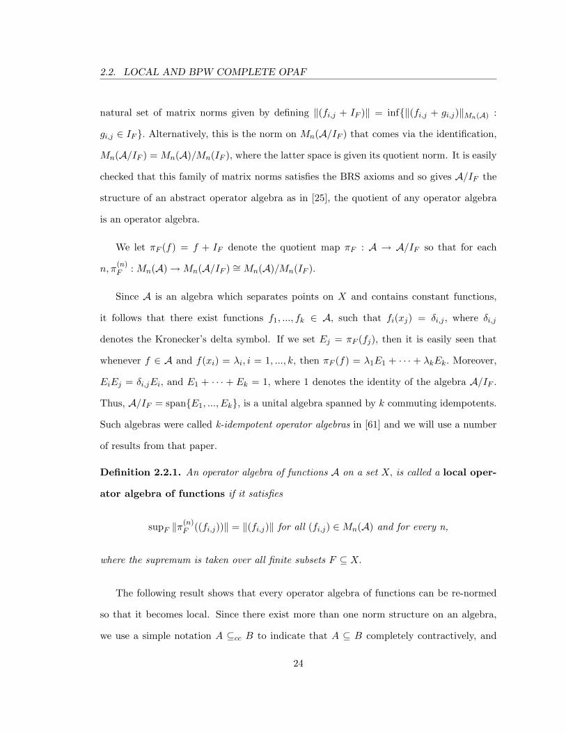
natural set of matrix norms given by defining ‖(fi,j + IF )‖ = inf‖(fi,j + gi,j)‖Mn(A) :
gi,j ∈ IF . Alternatively, this is the norm on Mn(A/IF ) that comes via the identification,
Mn(A/IF ) = Mn(A)/Mn(IF ), where the latter space is given its quotient norm. It is easily
checked that this family of matrix norms satisfies the BRS axioms and so gives A/IF the
structure of an abstract operator algebra as in [25], the quotient of any operator algebra
is an operator algebra.
We let πF (f) = f + IF denote the quotient map πF : A → A/IF so that for each
n, π(n)F : Mn(A) → Mn(A/IF ) ∼= Mn(A)/Mn(IF ).
Since A is an algebra which separates points on X and contains constant functions,
it follows that there exist functions f1, ..., fk ∈ A, such that fi(xj) = δi,j , where δi,j
denotes the Kronecker’s delta symbol. If we set Ej = πF (fj), then it is easily seen that
whenever f ∈ A and f(xi) = λi, i = 1, ..., k, then πF (f) = λ1E1 + · · · + λkEk. Moreover,
EiEj = δi,jEi, and E1 + · · · + Ek = 1, where 1 denotes the identity of the algebra A/IF .
Thus, A/IF = spanE1, ..., Ek, is a unital algebra spanned by k commuting idempotents.
Such algebras were called k-idempotent operator algebras in [61] and we will use a number
of results from that paper.
Definition 2.2.1. An operator algebra of functions A on a set X, is called a local oper-
ator algebra of functions if it satisfies
supF ‖π(n)F ((fi,j))‖ = ‖(fi,j)‖ for all (fi,j) ∈ Mn(A) and for every n,
where the supremum is taken over all finite subsets F ⊆ X.
The following result shows that every operator algebra of functions can be re-normed
so that it becomes local. Since there exist more than one norm structure on an algebra,
we use a simple notation A ⊆cc B to indicate that A ⊆ B completely contractively, and
24
2.2. LOCAL AND BPW COMPLETE OPAF
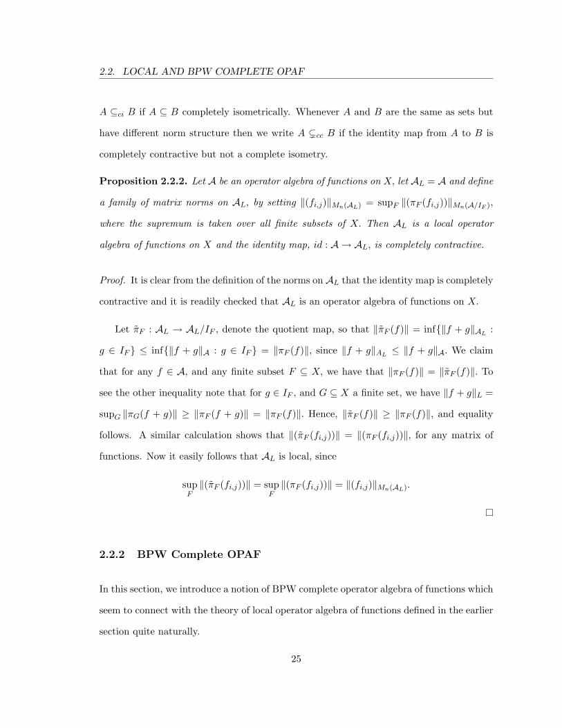
A ⊆ci B if A ⊆ B completely isometrically. Whenever A and B are the same as sets but
have different norm structure then we write A (cc B if the identity map from A to B is
completely contractive but not a complete isometry.
Proposition 2.2.2. Let A be an operator algebra of functions on X, let AL = A and define
a family of matrix norms on AL, by setting ‖(fi,j)‖Mn(AL) = supF ‖(πF (fi,j))‖Mn(A/IF ),
where the supremum is taken over all finite subsets of X. Then AL is a local operator
algebra of functions on X and the identity map, id : A → AL, is completely contractive.
Proof. It is clear from the definition of the norms on AL that the identity map is completely
contractive and it is readily checked that AL is an operator algebra of functions on X.
Let πF : AL → AL/IF , denote the quotient map, so that ‖πF (f)‖ = inf‖f + g‖AL:
g ∈ IF ≤ inf‖f + g‖A : g ∈ IF = ‖πF (f)‖, since ‖f + g‖AL≤ ‖f + g‖A. We claim
that for any f ∈ A, and any finite subset F ⊆ X, we have that ‖πF (f)‖ = ‖πF (f)‖. To
see the other inequality note that for g ∈ IF , and G ⊆ X a finite set, we have ‖f + g‖L =
supG ‖πG(f + g)‖ ≥ ‖πF (f + g)‖ = ‖πF (f)‖. Hence, ‖πF (f)‖ ≥ ‖πF (f)‖, and equality
follows. A similar calculation shows that ‖(πF (fi,j))‖ = ‖(πF (fi,j))‖, for any matrix of
functions. Now it easily follows that AL is local, since
supF‖(πF (fi,j))‖ = sup
F‖(πF (fi,j))‖ = ‖(fi,j)‖Mn(AL).
2.2.2 BPW Complete OPAF
In this section, we introduce a notion of BPW complete operator algebra of functions which
seem to connect with the theory of local operator algebra of functions defined in the earlier
section quite naturally.
25
2.2. LOCAL AND BPW COMPLETE OPAF
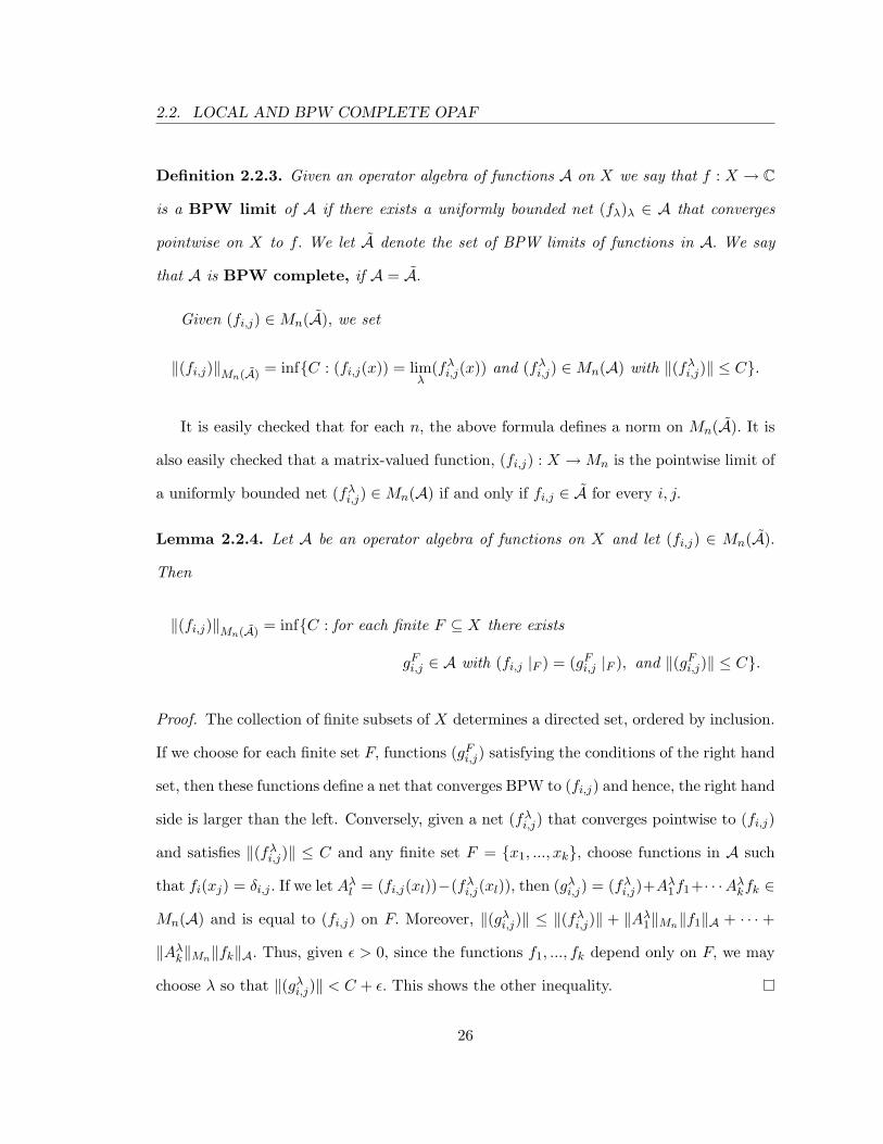
Definition 2.2.3. Given an operator algebra of functions A on X we say that f : X → C
is a BPW limit of A if there exists a uniformly bounded net (fλ)λ ∈ A that converges
pointwise on X to f. We let A denote the set of BPW limits of functions in A. We say
that A is BPW complete, if A = A.
Given (fi,j) ∈ Mn(A), we set
‖(fi,j)‖Mn(A) = infC : (fi,j(x)) = limλ
(fλi,j(x)) and (fλ
i,j) ∈ Mn(A) with ‖(fλi,j)‖ ≤ C.
It is easily checked that for each n, the above formula defines a norm on Mn(A). It is
also easily checked that a matrix-valued function, (fi,j) : X → Mn is the pointwise limit of
a uniformly bounded net (fλi,j) ∈ Mn(A) if and only if fi,j ∈ A for every i, j.
Lemma 2.2.4. Let A be an operator algebra of functions on X and let (fi,j) ∈ Mn(A).
Then
‖(fi,j)‖Mn(A) = infC : for each finite F ⊆ X there exists
gFi,j ∈ A with (fi,j |F ) = (gF
i,j |F ), and ‖(gFi,j)‖ ≤ C.
Proof. The collection of finite subsets of X determines a directed set, ordered by inclusion.
If we choose for each finite set F, functions (gFi,j) satisfying the conditions of the right hand
set, then these functions define a net that converges BPW to (fi,j) and hence, the right hand
side is larger than the left. Conversely, given a net (fλi,j) that converges pointwise to (fi,j)
and satisfies ‖(fλi,j)‖ ≤ C and any finite set F = x1, ..., xk, choose functions in A such
that fi(xj) = δi,j . If we let Aλl = (fi,j(xl))−(fλ
i,j(xl)), then (gλi,j) = (fλ
i,j)+Aλ1f1+· · ·Aλ
kfk ∈
Mn(A) and is equal to (fi,j) on F. Moreover, ‖(gλi,j)‖ ≤ ‖(fλ
i,j)‖ + ‖Aλ1‖Mn‖f1‖A + · · · +
‖Aλk‖Mn‖fk‖A. Thus, given ε > 0, since the functions f1, ..., fk depend only on F, we may
choose λ so that ‖(gλi,j)‖ < C + ε. This shows the other inequality.
26
2.2. LOCAL AND BPW COMPLETE OPAF
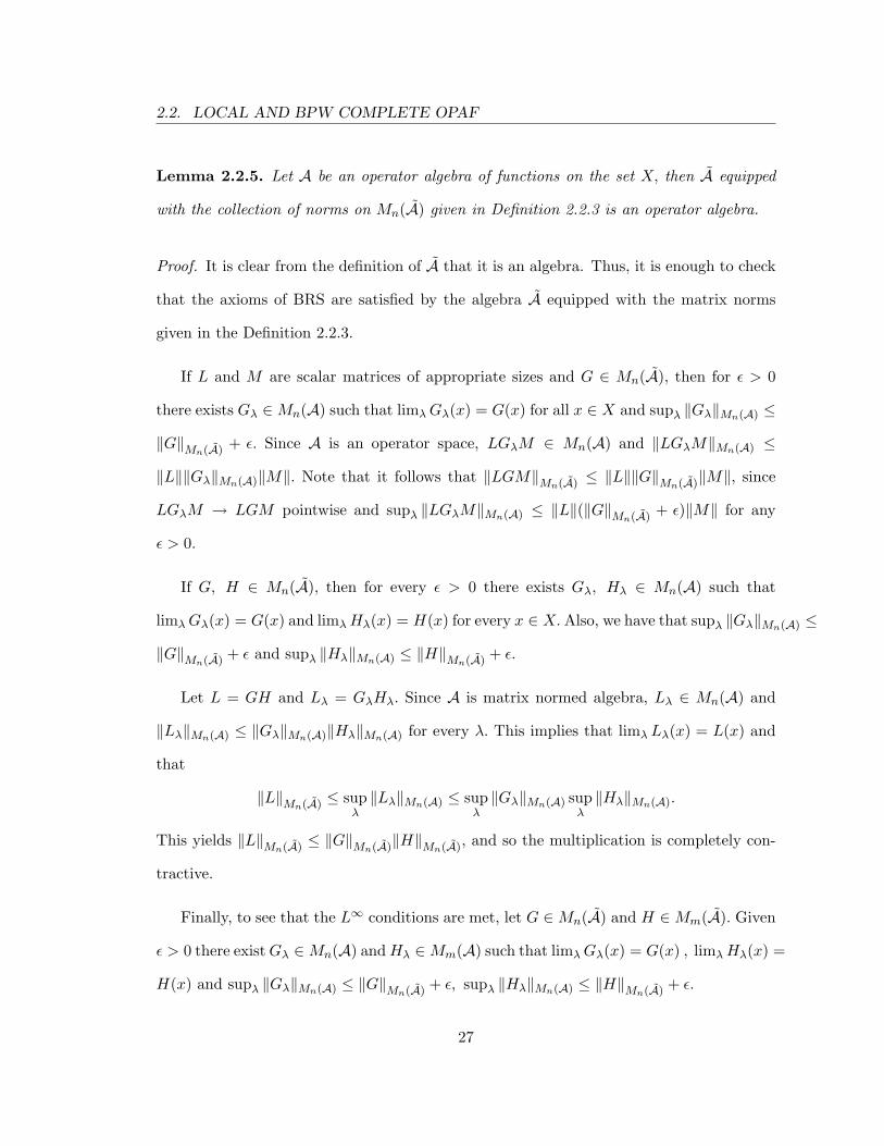
Lemma 2.2.5. Let A be an operator algebra of functions on the set X, then A equipped
with the collection of norms on Mn(A) given in Definition 2.2.3 is an operator algebra.
Proof. It is clear from the definition of A that it is an algebra. Thus, it is enough to check
that the axioms of BRS are satisfied by the algebra A equipped with the matrix norms
given in the Definition 2.2.3.
If L and M are scalar matrices of appropriate sizes and G ∈ Mn(A), then for ε > 0
there exists Gλ ∈ Mn(A) such that limλ Gλ(x) = G(x) for all x ∈ X and supλ ‖Gλ‖Mn(A) ≤
‖G‖Mn(A) + ε. Since A is an operator space, LGλM ∈ Mn(A) and ‖LGλM‖Mn(A) ≤
‖L‖‖Gλ‖Mn(A)‖M‖. Note that it follows that ‖LGM‖Mn(A) ≤ ‖L‖‖G‖Mn(A)‖M‖, since
LGλM → LGM pointwise and supλ ‖LGλM‖Mn(A) ≤ ‖L‖(‖G‖Mn(A) + ε)‖M‖ for any
ε > 0.
If G, H ∈ Mn(A), then for every ε > 0 there exists Gλ, Hλ ∈ Mn(A) such that
limλ Gλ(x) = G(x) and limλ Hλ(x) = H(x) for every x ∈ X. Also, we have that supλ ‖Gλ‖Mn(A) ≤
‖G‖Mn(A) + ε and supλ ‖Hλ‖Mn(A) ≤ ‖H‖Mn(A) + ε.
Let L = GH and Lλ = GλHλ. Since A is matrix normed algebra, Lλ ∈ Mn(A) and
‖Lλ‖Mn(A) ≤ ‖Gλ‖Mn(A)‖Hλ‖Mn(A) for every λ. This implies that limλ Lλ(x) = L(x) and
that
‖L‖Mn(A) ≤ supλ‖Lλ‖Mn(A) ≤ sup
λ‖Gλ‖Mn(A) sup
λ‖Hλ‖Mn(A).
This yields ‖L‖Mn(A) ≤ ‖G‖Mn(A)‖H‖Mn(A), and so the multiplication is completely con-
tractive.
Finally, to see that the L∞ conditions are met, let G ∈ Mn(A) and H ∈ Mm(A). Given
ε > 0 there exist Gλ ∈ Mn(A) and Hλ ∈ Mm(A) such that limλ Gλ(x) = G(x) , limλ Hλ(x) =
H(x) and supλ ‖Gλ‖Mn(A) ≤ ‖G‖Mn(A) + ε, supλ ‖Hλ‖Mn(A) ≤ ‖H‖Mn(A) + ε.
27
2.2. LOCAL AND BPW COMPLETE OPAF
Note that Gλ ⊕Hλ ∈ Mn+m(A) and ‖Gλ ⊕Hλ‖ = max‖Gλ‖Mn(A), ‖Hλ‖Mn(A) for every
λ which implies that G⊕H ∈ Mn+m(A), and
‖G⊕H‖Mn+m(A) ≤ supλ‖Gλ ⊕Hλ‖ = sup
λ[max‖Gλ‖Mn(A), ‖Hλ‖Mm(A)]
= maxsupλ‖Gλ‖Mn(A), sup
λ‖Hλ‖Mm(A)
≤ max‖G‖Mn(A) + ε, ‖H‖Mm(A) + ε.
This shows that ‖G⊕H‖Mn+m(A) ≤ max‖G‖Mn(A), ‖H‖Mm(A), and so the L∞ condition
follows. This completes the proof of the result.
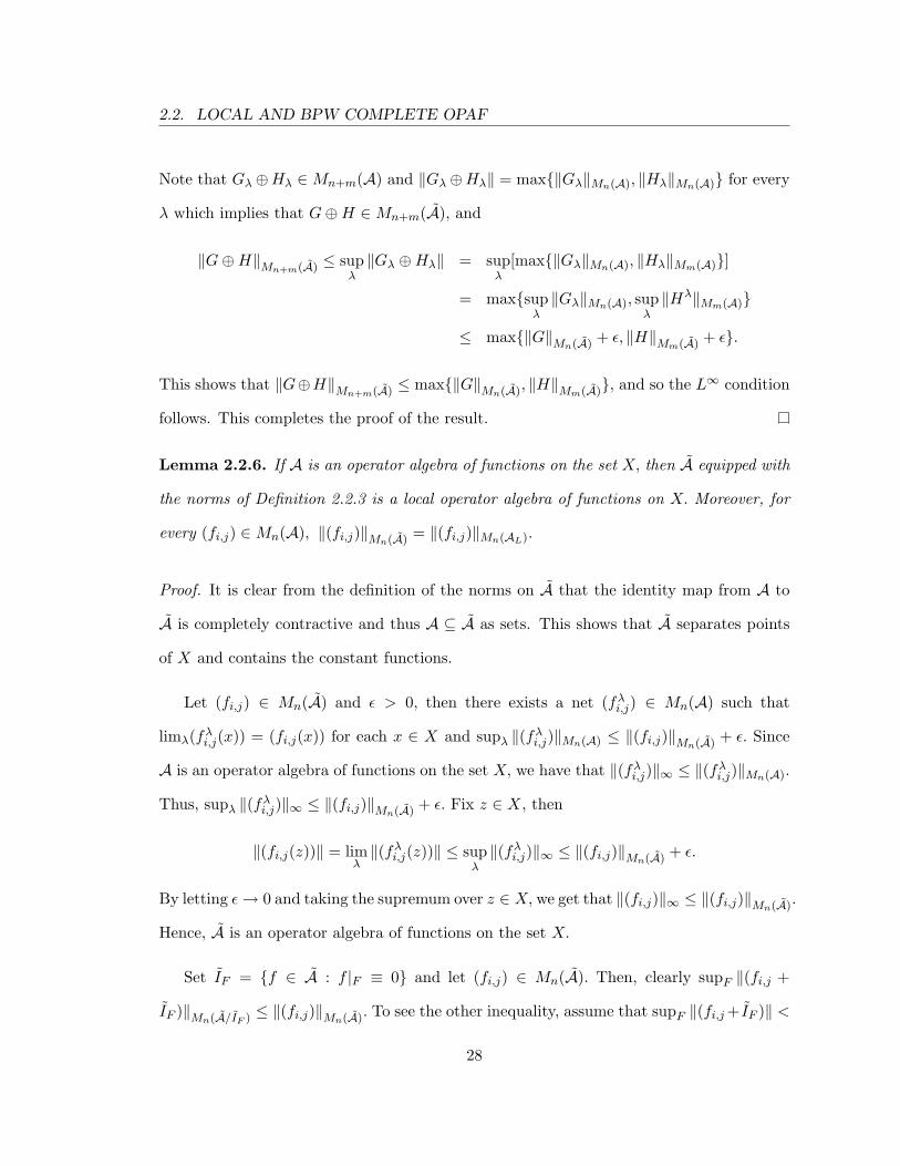
Lemma 2.2.6. If A is an operator algebra of functions on the set X, then A equipped with
the norms of Definition 2.2.3 is a local operator algebra of functions on X. Moreover, for
every (fi,j) ∈ Mn(A), ‖(fi,j)‖Mn(A) = ‖(fi,j)‖Mn(AL).
Proof. It is clear from the definition of the norms on A that the identity map from A to
A is completely contractive and thus A ⊆ A as sets. This shows that A separates points
of X and contains the constant functions.
Let (fi,j) ∈ Mn(A) and ε > 0, then there exists a net (fλi,j) ∈ Mn(A) such that
limλ(fλi,j(x)) = (fi,j(x)) for each x ∈ X and supλ ‖(fλ
i,j)‖Mn(A) ≤ ‖(fi,j)‖Mn(A) + ε. Since
A is an operator algebra of functions on the set X, we have that ‖(fλi,j)‖∞ ≤ ‖(fλ
i,j)‖Mn(A).
Thus, supλ ‖(fλi,j)‖∞ ≤ ‖(fi,j)‖Mn(A) + ε. Fix z ∈ X, then
‖(fi,j(z))‖ = limλ‖(fλ
i,j(z))‖ ≤ supλ‖(fλ
i,j)‖∞ ≤ ‖(fi,j)‖Mn(A) + ε.
By letting ε → 0 and taking the supremum over z ∈ X, we get that ‖(fi,j)‖∞ ≤ ‖(fi,j)‖Mn(A).
Hence, A is an operator algebra of functions on the set X.
Set IF = f ∈ A : f |F ≡ 0 and let (fi,j) ∈ Mn(A). Then, clearly supF ‖(fi,j +
IF )‖Mn(A/IF ) ≤ ‖(fi,j)‖Mn(A). To see the other inequality, assume that supF ‖(fi,j + IF )‖ <
28
2.2. LOCAL AND BPW COMPLETE OPAF
1. Then for every finite F ⊆ X there exists (hFi,j) ∈ Mn(A) such that (hF
i,j)|F = (fFi,j)|F
and supF ‖hFi,j‖ ≤ 1. Fix a set F ⊆ X and (hF
i,j) ∈ Mn(A). Then for all finite F ′ ⊆ X there
exists (kF ′i,j ) ∈ Mn(A) such that (kF ′
i,j )|F ′ = (hFi,j)|F ′ and supF ′ ‖kF ′
i,j‖ ≤ 1.
In particular, let F ′ = F then (kFi,j)|F = (hF
i,j)|F = (fi,j)|F and supF ‖kFi,j‖ ≤ 1.
Hence, ‖(fi,j)‖Mn(A) ≤ 1, and ‖(fi,j)‖Mn(A) ≤ supF ‖(fi,j + IF )‖Mn(A/IF ). Thus, for every
(fi,j) ∈ Mn(A),
‖(fi,j)‖Mn(A) = supF‖(fi,j + IF )‖Mn(A/IF ).
Note that for any F ⊆ X we have ‖(fi,j + IF )‖Mn(A/IF ) ≤ ‖(fi,j + IF )‖Mn(A/IF ), since
IF ⊆ IF . We claim that ‖(fi,j + IF )‖ = ‖(fi,j + IF )‖ for every (fi,j) ∈ Mn(A), and for
every finite subset F ⊆ X. To see the other inequality, let (gi,j) ∈ Mn(IF ). Then for
ε > 0 and G ⊆ X, we may choose (hfGi,j) ∈ Mn(A) such that (hG
i,j)|G = (fi,j + gi,j)|G
and supG ‖(hGi,j)‖ ≤ ‖(fi,j + gi,j)‖ + ε. Hence, ‖(fi,j + IF )‖ = ‖(hF
i,j + IF )‖ ≤ ‖(hFi,j)‖ ≤
‖(fi,j + gi,j)‖+ ε. Since ε > 0 was arbitrary, the equality follows.
Now it is clear that,
‖(fi,j)‖Mn(A) = supF‖(fi,j + IF )‖ = ‖(fi,j)‖Mn(AL),
and so the result follows.
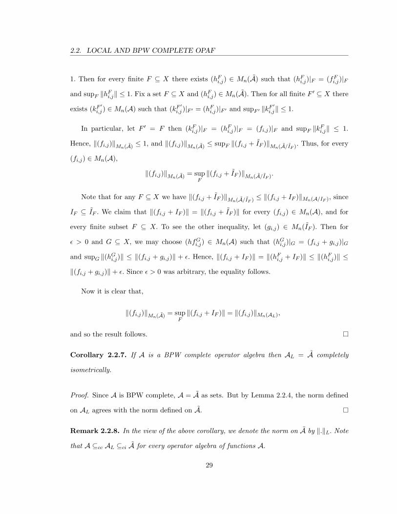
Corollary 2.2.7. If A is a BPW complete operator algebra then AL = A completely
isometrically.
Proof. Since A is BPW complete, A = A as sets. But by Lemma 2.2.4, the norm defined
on AL agrees with the norm defined on A.
Remark 2.2.8. In the view of the above corollary, we denote the norm on A by ‖.‖L. Note
that A ⊆cc AL ⊆ci A for every operator algebra of functions A.
29
2.2. LOCAL AND BPW COMPLETE OPAF
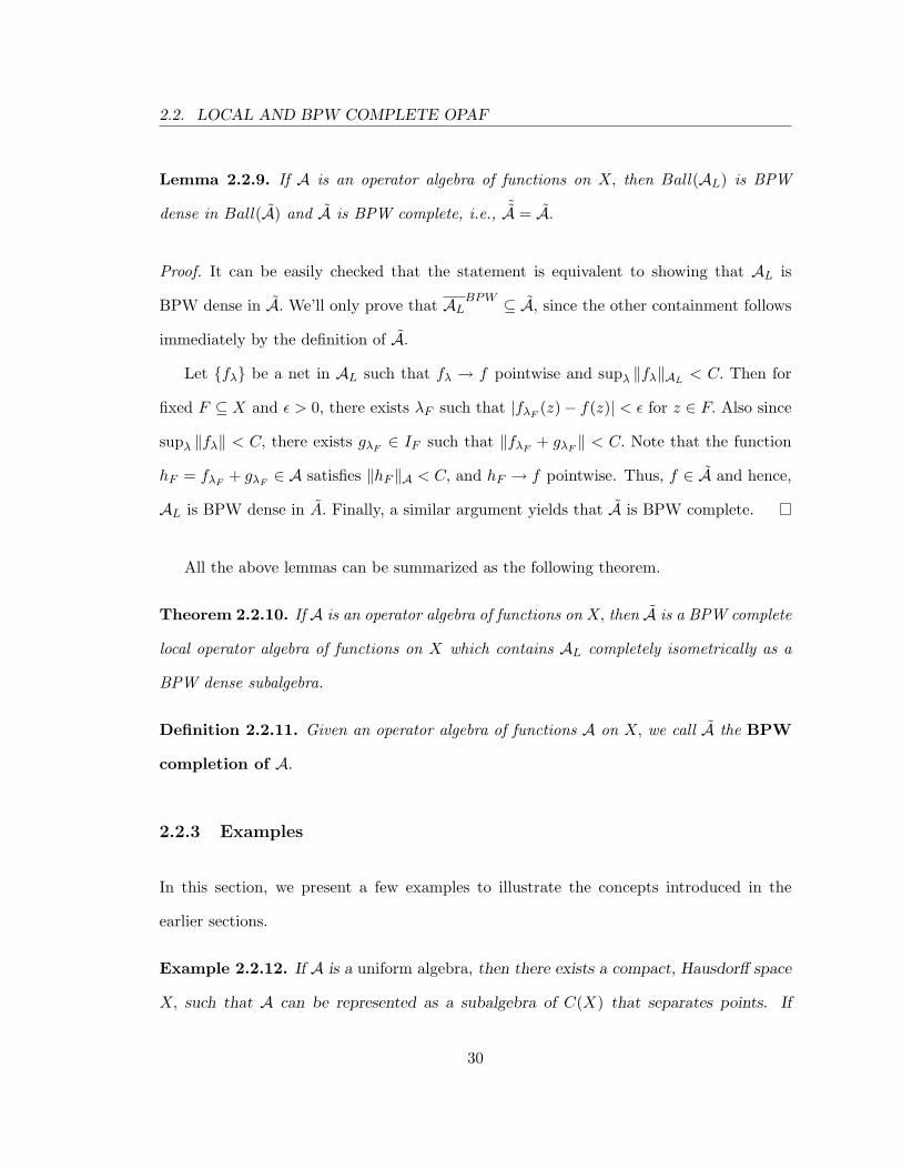
Lemma 2.2.9. If A is an operator algebra of functions on X, then Ball(AL) is BPW
dense in Ball(A) and A is BPW complete, i.e., ˜A = A.
Proof. It can be easily checked that the statement is equivalent to showing that AL is
BPW dense in A. We’ll only prove that ALBPW ⊆ A, since the other containment follows
immediately by the definition of A.
Let fλ be a net in AL such that fλ → f pointwise and supλ ‖fλ‖AL< C. Then for
fixed F ⊆ X and ε > 0, there exists λF such that |fλF(z)− f(z)| < ε for z ∈ F. Also since
supλ ‖fλ‖ < C, there exists gλF∈ IF such that ‖fλF
+ gλF‖ < C. Note that the function
hF = fλF+ gλF
∈ A satisfies ‖hF ‖A < C, and hF → f pointwise. Thus, f ∈ A and hence,
AL is BPW dense in A. Finally, a similar argument yields that A is BPW complete.
All the above lemmas can be summarized as the following theorem.
Theorem 2.2.10. If A is an operator algebra of functions on X, then A is a BPW complete
local operator algebra of functions on X which contains AL completely isometrically as a
BPW dense subalgebra.
Definition 2.2.11. Given an operator algebra of functions A on X, we call A the BPW
completion of A.
2.2.3 Examples
In this section, we present a few examples to illustrate the concepts introduced in the
earlier sections.
Example 2.2.12. If A is a uniform algebra, then there exists a compact, Hausdorff space
X, such that A can be represented as a subalgebra of C(X) that separates points. If
30

2.2. LOCAL AND BPW COMPLETE OPAF
we endow A with the matrix-normed structure that it inherits as a subalgebra of C(X),
namely, ‖(fi,j)‖ = ‖(fi,j)‖∞ ≡ sup‖(fi,j)‖Mn : x ∈ X, then A is a local operator algebra
of functions on X. Indeed, to achieve the norm, it is sufficient to take the supremum
over all finite subsets consisting of one point. In this case the BPW completion A is
completely isometrically isomorphic to the subalgebra of `∞(X) consisting of functions
that are bounded, pointwise limits of functions in A.
Example 2.2.13. Let A = A(D) ⊆ C(D−) be the subalgebra of the algebra of continuous
functions on the closed disk consisting of the functions that are analytic on the open
disk D. Identifying Mn(A(D)) ⊆ Mn(C(D−)) as a subalgebra of the algebra of continuous
functions from the closed disk to the matrices, equipped with the supremum norm, gives
A(D) the usual operator algebra structure. With this structure it can be regarded as a local
operator algebra of functions on D or on D−. If we regard it as a local operator algebra
of functions on D−, then A(D) ( A(D). To see that the containment is strict, note that
f(z) = (1 + z)/2 ∈ A(D) and fn(z) → χ1, the characteristic function of the singleton
1.
However, if we regard A(D) as a local operator algebra of functions on D, then its
BPW completion A(D) = H∞(D), the bounded analytic functions on the disk, with its
usual operator structure.
Example 2.2.14. Let X = εD, 0 < ε < 1 and A = f |X : f ∈ H∞(D). If we endow A
with the matrix-normed structure on H∞(D), then A is an operator algebra of functions on
X. Also, it can be verified that A is a local operator algebra of functions and that A = A.
Indeed, if F = (fi,j) ∈ Mn(A) with ‖(fi,j + IY )‖∞ < 1 for all finite subset Y ⊆ X, then
there exists HY ∈ Mn(A) such that ‖HY ‖∞ ≤ 1 and HY → F pointwise on X. Note by
Montel’s theorem [30] there exist a subnet HY ′ and G ∈ Mn(H∞(D)) such that ‖G‖∞ ≤ 1
31

2.2. LOCAL AND BPW COMPLETE OPAF
and HY ′ → G uniformly on compact subsets of D. Thus, by the identity theorem F ≡ G on
D. Hence, ‖F‖Mn(A) ≤ 1 and so A is a local operator algebra. A similar argument shows
that if f is a BPW limit on X, then there exists g ∈ H∞(D) such that g|X = f, and so A
is BPW complete. By Lemma 2.2.9, A = A completely isometrically.
Example 2.2.15. Let A = H∞(D) but endowed with a new norm. Since for every
fixed b > 1, the spectrum of
0 b
0 0
is trivially contained in D, thus F (
0 b
0 0
) can
be defined for every F ∈ MA by using functional calculus. For every F ∈ Mn(A), set
‖F‖ = max‖F‖∞, ‖F (
0 b
0 0
)‖. It can be easily verified that A is a BPW complete
operator algebra of functions. However, we also claim that A is local. To prove this
we proceed by contradiction. Suppose there exists F = (fi,j) ∈ Mn(H∞(D)) such that
‖F‖ > 1 > c, where c = supY ‖(fi,j + IY )‖.
In this case, ‖F‖ = ‖F (
0 b
0 0
)‖, since ‖(fi,j + IY )‖ = ‖F (λ)‖ when Y = λ. Let
ε = 1−c4b and Y = 0, ε ⊆ D, then there exists G ∈ Mn(H∞(D)) such that G|Y = 0 and
‖F + G‖ < 1+c2 .
Thus, we can write BY (z) = z−ε1−εz , so that G(z) = zBY (z)H(z), for some H ∈ Mn(H∞).
It follows that ‖H‖∞ < 2, since ‖G‖∞ < 2. We now consider
1 <
∥∥∥∥∥∥∥F (
0 b
0 0
)
∥∥∥∥∥∥∥ ≤∥∥∥∥∥∥∥(F + G)(
0 b
0 0
)
∥∥∥∥∥∥∥+
∥∥∥∥∥∥∥G(
0 b
0 0
)
∥∥∥∥∥∥∥≤ 1 + c
2+
∥∥∥∥∥∥∥0 bG′(0)
0 0
∥∥∥∥∥∥∥ =
1 + c
2+ b|BY (0)|‖H(0)‖
≤ 1 + c
2+ 2bε =
1 + c
2+ 2b
1− c
4b= 1,
which is a contradiction.
32

2.2. LOCAL AND BPW COMPLETE OPAF
Example 2.2.16. This is an example of a non-local algebra that arises from boundary
behavior. Let A = A(D) equipped with the family of matrix norms
‖F‖ = max‖F‖∞, ‖F (
1 1
0 −1
)‖, F ∈ Mn(A)
where F (
1 1
0 −1
) is defined by using power series exapansion. Note that when F (1) =
F (−1), then ‖F‖ = ‖F‖∞. It is easy to check that A is an operator algebra of functions
on the set D that is not BPW complete. Also, it can be verified that A is not local. To
see this, note that ‖z‖ =
∥∥∥∥∥∥∥1 1
0 −1
∥∥∥∥∥∥∥ > 1. Fix α > 0, such that 1 + 2α < ‖z‖. For
each Y = z1, z2, . . . , zn, we define BY (z) = Πni=1(
z−zi1−ziz
) and choose h ∈ A such that
h(1) = −BY (1), h(−1) = BY (−1), and ‖h‖∞ ≤ 2.
Let g(z) = z+BY (z)h(z)α, then g ∈ A, g(1) = g(−1) and g|Y = z|Y . Hence, ‖πY (z)‖ =
‖πY (g)‖ ≤ ‖g‖ = ‖g‖∞ ≤ 1 + 2α < ‖z‖. Thus, since α was arbitrary, supY⊆D ‖πY (z)‖ =
1 < ‖z‖ and hence A is not local.
Example 2.2.17. This example shows that one can easily build non-local algebras by
adding “values” outside of the set X. Let A be the algebra of polynomials regarded as
functions on the set X = D. Then A endowed with the matrix-normed structure as
‖(pi,j)‖ = max‖(pi,j)‖∞, ‖(pi,j(2))‖, is an operator algebra of functions on the set X.
To see that A is not local, let p ∈ A be such that ‖p‖∞ < |p(2)|. For each finite sub-
set Y = z1, . . . , zn of X, let hY (z) = Πni=1(z − zi) and gY (z) = p(z) − αhY (z)p(2),
where α = |p(2)|−‖p‖∞2|p(2)|‖hY ‖∞ > 0. Note that ‖gY ‖ ≤ (1 − α)|p(2)| and gY |Y = p|Y . Hence,
‖πY (p)‖ = ‖πY (gY )‖ ≤ ‖gY ‖ ≤ (1− α)|p(2)| < ‖p‖. It follows that A is not local.
Finally, observe that in this case, A cannot be BPW complete. For example, if we take
pn = 13
∑ni=0(
z3)i ∈ A then pn(z) → f(z) = 1
3−z for z ∈ D and ‖pn‖ < ‖f‖, which implies
33
2.2. LOCAL AND BPW COMPLETE OPAF
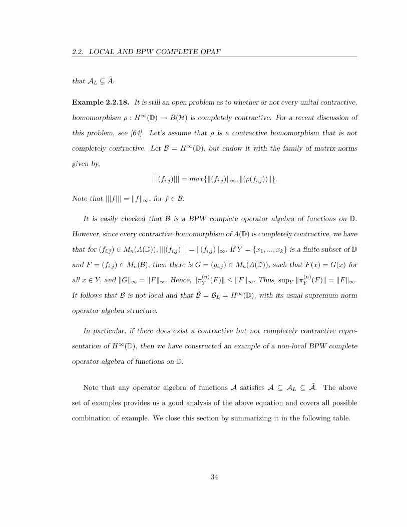
that AL ( A.
Example 2.2.18. It is still an open problem as to whether or not every unital contractive,
homomorphism ρ : H∞(D) → B(H) is completely contractive. For a recent discussion of
this problem, see [64]. Let’s assume that ρ is a contractive homomorphism that is not
completely contractive. Let B = H∞(D), but endow it with the family of matrix-norms
given by,
|||(fi,j)||| = max‖(fi,j)‖∞, ‖(ρ(fi,j))‖.
Note that |||f ||| = ‖f‖∞, for f ∈ B.
It is easily checked that B is a BPW complete operator algebra of functions on D.
However, since every contractive homomorphism of A(D) is completely contractive, we have
that for (fi,j) ∈ Mn(A(D)), |||(fi,j)||| = ‖(fi,j)‖∞. If Y = x1, ..., xk is a finite subset of D
and F = (fi,j) ∈ Mn(B), then there is G = (gi,j) ∈ Mn(A(D)), such that F (x) = G(x) for
all x ∈ Y, and ‖G‖∞ = ‖F‖∞. Hence, ‖π(n)Y (F )‖ ≤ ‖F‖∞. Thus, supY ‖π
(n)Y (F )‖ = ‖F‖∞.
It follows that B is not local and that B = BL = H∞(D), with its usual supremum norm
operator algebra structure.
In particular, if there does exist a contractive but not completely contractive repre-
sentation of H∞(D), then we have constructed an example of a non-local BPW complete
operator algebra of functions on D.
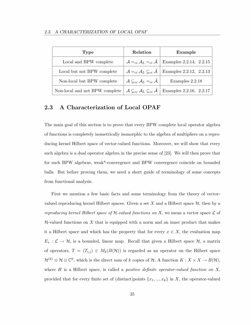
Note that any operator algebra of functions A satisfies A ⊆ AL ⊆ A. The above
set of examples provides us a good analysis of the above equation and covers all possible
combination of example. We close this section by summarizing it in the following table.
34
2.3. A CHARACTERIZATION OF LOCAL OPAF
Type Relation Example
Local and BPW complete A =ci AL =ci A Examples 2.2.14, 2.2.15
Local but not BPW complete A =ci AL (ci A Examples 2.2.12, 2.2.13
Non-local but BPW complete A (cc AL =ci A Examples 2.2.18
Non-local and not BPW complete A (cc AL (ci A Examples 2.2.16, 2.2.17
2.3 A Characterization of Local OPAF
The main goal of this section is to prove that every BPW complete local operator algebra
of functions is completely isometrically isomorphic to the algebra of multipliers on a repro-
ducing kernel Hilbert space of vector-valued functions. Moreover, we will show that every
such algebra is a dual operator algebra in the precise sense of [23]. We will then prove that
for such BPW algebras, weak*-convergence and BPW convergence coincide on bounded
balls. But before proving them, we need a short guide of terminology of some concepts
from functional analysis.
First we mention a few basic facts and some terminology from the theory of vector-
valued reproducing kernel Hilbert spaces. Given a set X and a Hilbert space H, then by a
reproducing kernel Hilbert space of H-valued functions on X, we mean a vector space L of
H-valued functions on X that is equipped with a norm and an inner product that makes
it a Hilbert space and which has the property that for every x ∈ X, the evaluation map
Ex : L → H, is a bounded, linear map. Recall that given a Hilbert space H, a matrix
of operators, T = (Ti,j) ∈ Mk(B(H)) is regarded as an operator on the Hilbert space
H(k) ≡ H⊗ Ck, which is the direct sum of k copies of H. A function K : X ×X → B(H),
where H is a Hilbert space, is called a positive definite operator-valued function on X,
provided that for every finite set of (distinct)points x1, ..., xk in X, the operator-valued
35

2.3. A CHARACTERIZATION OF LOCAL OPAF
matrix, (K(xi, xj)) is positive semidefinite. Given a reproducing kernel Hilbert space L of
H-valued functions, if we set K(x, y) = ExE∗y , where Ex : L → H is the point evaluation
map, then K is positive definite and is called the reproducing kernel of L. The proof
of this involves direct matrix calculation. On the contrary, the proof of the converse to
this fact is not that straightforward and is generally called Moore’s theorem, which states
that given any positive definite operator-valued function K : X ×X → B(H), then there
exists a unique reproducing kernel Hilbert space of H-valued functions on X, such that
K(x, y) = ExE∗y . We will denote this space by L(K,H).
Given v, w ∈ H, we let v ⊗ w∗ : H → H denote the rank one operator given by
(v⊗w∗)(h) = 〈h, w〉v. A function g : X → H belongs to L(K,H) if and only if there exists
a constant C > 0 such that the function
C2K(x, y)− g(x)⊗ g(y)∗
is positive definite. In which case the norm of g is the least such constant. Finally, given
any reproducing kernel Hilbert space L of H-valued functions with reproducing kernel K,
a function f : X → C is called a (scalar) multiplier provided that for every g ∈ L, the
function fg ∈ L. In this case it follows by an application of the closed graph theorem that
the map Mf : L → L, defined by Mf (g) = fg, is a bounded, linear map. The set of all
multipliers is denoted by M(K) and is easily seen to be an algebra of functions on X and
a subalgebra of B(L). The reader can find proofs of the above facts in [26] and [9]. Also,
we refer to the fundamental work of Pedrick [65] for further treatment of vector-valued
reproducing kernel Hilbert spaces. Another good source is [5].
Given a normed space Y , we define the dual of Y as the set of all linear functionals
on Y and denote it by Y ∗. Then the weak*-topology on Y ∗ is the smallest topology on
Y ∗ that makes all the linear functionals in Fy : y ∈ Y continuous. Thus a net φλ → φ
36

2.3. A CHARACTERIZATION OF LOCAL OPAF
in Y ∗ in the weak*-topology if and only if φλ(y) → φ(y) for all y ∈ Y. A space is called
weak*-closed if it is closed in the weak*-topology. We record an important and a very
useful theorem concerning weak*-topology called Krein-Smulian theorem. There are many
parts to this theorem but we only need the following.
Theorem 2.3.1. Let Y be a dual Banach space, and let V be a linear subspace of Y . Then
V is weak*-closed in Y if and only if Ball(V ) is closed in the weak*-topology on Y . In this
case, V is also a dual Banach space.
The proof of the above can be found in many standard texts on functional analysis.
We refer the reader to [23, Section 1.4]. We are now in a position to state and prove the
following result about the multiplier algebras of a reproducing kernel Hilbert spaces.
Lemma 2.3.2. Let L be a reproducing kernel Hilbert space of H-valued functions with
reproducing kernel K : X×X → B(H). Then M(K) ⊆ B(L) is a weak*-closed subalgebra.
Proof. It is enough to show that the unit ball is weak*-closed by the Krein-Smulian the-
orem. So let Mfλ be a net of multipliers in the unit ball of B(L) that converges in the
weak*-topology to an operator T. We must show that T is a multiplier.
Let x ∈ X be fixed and assume that there exists g ∈ L, with g(x) = h 6= 0. Then
〈Tg, E∗xh〉L = limλ〈Mfλ
g,E∗xh〉L = limλ〈Ex(Mfλ
g), h〉H = limλ fλ(x)‖h‖2. This shows that
at every such x the net fλ(x) converges to some value. Set f(x) equal to this limit and
for all other x’s set f(x) = 0. We claim that f is a multiplier and that T = Mf .
Note that if g(x) = 0 for every g ∈ L, then Ex = E∗x = 0. Thus, we have that for
any g ∈ L and any h ∈ H, 〈Ex(Tg), h〉H = limλ〈Ex(Mfλg), h〉H = limλ fλ(x)〈g(x), h〉H =
f(x)〈g(x), h〉H. Since this holds for every h ∈ H, we have that Ex(Tg) = f(x)g(x), and so
T = Mf and f is a multiplier.
37
2.3. A CHARACTERIZATION OF LOCAL OPAF
In a fashion similar to operator algebras, by an operator space we mean a space that
has both a vector space structure and matrix norm structure that satisfies Ruan’s axioms.
An operator space V is said to be a dual operator space if V is completely isometrically
isomorphic to the operator space dual Y ∗ of an operator space Y . The reader can find the
proof of the fact that “the dual operator spaces and weak*-closed subspaces of bounded
operators on a Hilbert space are essentially the same thing” in [23, Section 1.4]. Thus,
every weak*-closed subspace V ⊆ B(H) has a predual and it is the operator space dual of
this predual. Also, if an abstract operator algebra is the dual of an operator space, then
it can be represented completely isometrically and weak*-continuously as a weak*-closed
subalgebra of the bounded operators on some Hilbert space. For this reason an operator
algebra that has a predual as an operator space is called a dual operator algebra. See
[23] for the proofs of these facts. Thus, in summary, the above lemma shows that every
multiplier algebra is a dual operator algebra in the sense of [23].
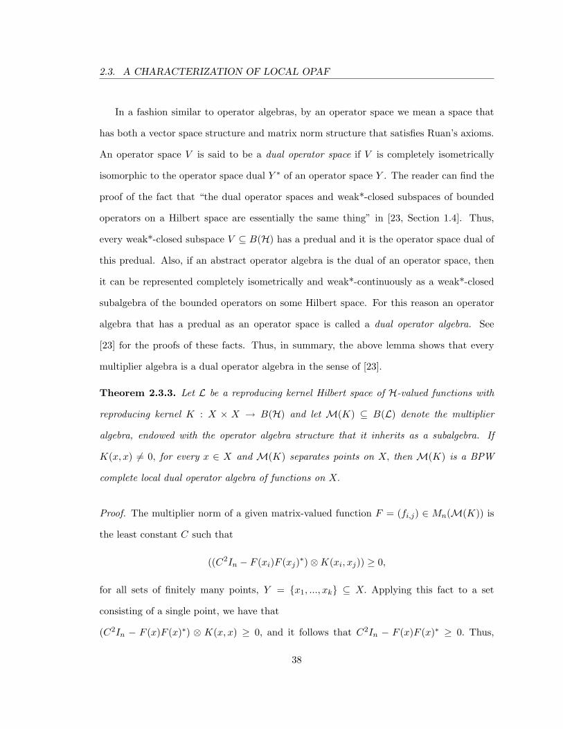
Theorem 2.3.3. Let L be a reproducing kernel Hilbert space of H-valued functions with
reproducing kernel K : X × X → B(H) and let M(K) ⊆ B(L) denote the multiplier
algebra, endowed with the operator algebra structure that it inherits as a subalgebra. If
K(x, x) 6= 0, for every x ∈ X and M(K) separates points on X, then M(K) is a BPW
complete local dual operator algebra of functions on X.
Proof. The multiplier norm of a given matrix-valued function F = (fi,j) ∈ Mn(M(K)) is
the least constant C such that
((C2In − F (xi)F (xj)∗)⊗K(xi, xj)) ≥ 0,
for all sets of finitely many points, Y = x1, ..., xk ⊆ X. Applying this fact to a set
consisting of a single point, we have that
(C2In − F (x)F (x)∗) ⊗ K(x, x) ≥ 0, and it follows that C2In − F (x)F (x)∗ ≥ 0. Thus,
38

2.3. A CHARACTERIZATION OF LOCAL OPAF
‖F (x)‖ ≤ C = ‖F‖ and we have that point evaluations are completely contractive on
M(K). Since M(K) contains the constants and separates points by hypotheses, it is an
operator algebra of functions on X.
Suppose that M(K) was not local, then there would exist F ∈ Mn(M(K)), and a real
number C, such that supY ‖π(n)Y ‖ < C < ‖F‖. Then for each finite set Y = x1, ..., xk
we could choose G ∈ Mn(M(K)), with ‖G‖ < C, and G(x) = F (x), for every x ∈ Y. But
then we would have that ((C2In − F (xi)F (xj)∗) ⊗K(xi, xj)) = ((C2In −G(xi)G(xj)∗) ⊗
K(xi, xj)) ≥ 0, and since Y was arbitrary, ‖F‖ ≤ C, a contradiction. Thus, M(K) is local.
Finally, assume that fλ ∈ M(K), is a net in M(K), with ‖fλ‖ ≤ C, and limλ fλ(x) =
f(x), pointwise. If g ∈ L with ‖g‖L = M, then
(MC)2K(x, y)− fλ(x)g(x)⊗ (fλ(y)g(y))∗
is positive definite. By taking pointwise limits, we obtain that (MC)2K(x, y)−f(x)g(x)⊗
(f(y)g(y))∗ is positive definite. From the earlier characterization of functions in L and their
norms in a reproducing kernel Hilbert space, this implies that fg ∈ L, with ‖fg‖L ≤ MC.
Hence, f ∈M(K) with ‖Mf‖ ≤ C. Thus, M(K) is BPW complete.
In general, M(K) need not separate points on X. In fact, it is possible that L does not
separate points and if g(x1) = g(x2), for every g ∈ L, then necessarily f(x1) = f(x2) for
every f ∈M(K).
Following [61], we call C a concrete k-idempotent operator algebra, provided that there
are k operators, E1, ..., Ek on some Hilbert space H, such that EiEj = EjEi = δi,jEi,
I = E1 + · · · + Ek and C = spanE1, ..., Ek. Recall, if C is an abstract operator algebra
then can be represented on some Hilbert space K via a completely isometric homomorphism
π : C → B(K). We call C an abstract k-idempotent operator algebra if the image of C under
39

2.3. A CHARACTERIZATION OF LOCAL OPAF
the map π is a concrete k-idempotent operator algebra. We shall drop the term concrete
and abstract whenever it is clear from the context.
Proposition 2.3.4. Let C = spanE1, ..., Ek be a k-idempotent operator algebra on the
Hilbert space H, let Y = x1, ..., xk be a set of k distinct points and define K : Y × Y →
B(H) by K(xi, xj) = EiE∗j . Then K is positive definite and C is completely isometrically
isomorphic to M(K) via the map that sends a1E1 + · · ·+akEk to the multiplier f(xi) = ai.
Proof. It is easily checked that K is positive definite. We first prove that the map is an
isometry. Given B =∑k
i=1 ai ⊗ Ei ∈ C, let f : Y → C be defined by f(xi) = ai. We have
that f ∈M(K) with ‖f‖ ≤ C if and only if P = ((C2 − f(xi)f(xj)∗)K(xi, xj)) is positive
semidefinite in B(H(k)). Let v = e1 ⊗ v1 + · · · ek ⊗ vk ∈ H(k), let h =∑k
j=1 E∗j vj and note
that E∗j h = E∗
j vj . Finally, set h =∑k
i=1 hi. Thus,
〈Pv, v〉 =k∑
i,j=1
(C2 − aiaj)〈EiE∗j vj , vi〉 =
k∑i,j=1
(C2 − aiaj)〈E∗j h, E∗
i h〉
= C2‖h‖2 − 〈B∗h, B∗h〉 = C2‖h‖2 − ‖B∗h‖2.
Hence, ‖B‖ ≤ C implies that P is positive and so ‖Mf‖ ≤ ‖B‖.
For the converse, given any h let v =∑k
j=1 ej⊗E∗j h, and note that 〈Pv, v〉 ≥ 0, implies
that ‖B∗h‖ ≤ C, and so ‖B‖ ≤ ‖Mf‖. The proof of the complete isometry is similar but
notationally cumbersome.
Theorem 2.3.5. Let A be an operator algebra of functions on the set X then there exist a
Hilbert space, H and a positive definite function K : X×X → B(H) such that M(K) = A
completely isometrically.
Proof. Let Y be a finite subset of X. Since A/IY is a |Y |-idempotent operator algebra,
by the above lemma, there exists a vector-valued kernel KY such that A/IY = M(KY )
40

2.3. A CHARACTERIZATION OF LOCAL OPAF
completely isometrically.
Define
KY (x, y) =
KY (x, y) when (x, y) ∈ Y × Y,
0 when (x, y) 6∈ Y × Y
and set K =∑
Y ⊕KY , where the direct sum is over all finite subsets of X.
It is easily checked that K is positive definite. Let f ∈ Mn(M(K)) with ‖Mf‖ ≤ 1,
which is equivalent to ((In − f(x)f(y)∗)⊗K(x, y)) being positive definite. This is in turn
equivalent to ((In− f(x)f(y)∗)⊗KY (x, y)) being positive definite for every finite subset Y
of X. This last condition is equivalent to the existence for each such Y of some fY ∈ Mn(A)
such that ‖πY (fY )‖ ≤ 1 and fY = f on Y. The net of functions fY then converges BPW
to f. Hence, f ∈ A with ‖f‖L ≤ 1. This proves that Mn(M(K)) = Mn(A) isometrically,
for every n, and the result follows.
The above result draws a connection with the concept of realizable Banach algebras,
introduced by Agler-McCarthy [5, Chapter 13] to study Pick’s problem for algebras that
are not multiplier algebras of Pick kernels. They call a commutative Banach algebra A of
functions on the set X, realizable if there is a set of kernels kα : α ∈ I on X such that
A =⋂
α∈I Mult(Hkα) and ‖φ‖A = supα∈I ‖φ‖Mult(Hkα ). It is clear that the algebras that
are local and BPW complete are examples of realizable algebras.
Corollary 2.3.6. Every BPW complete local operator algebra of functions is a dual oper-
ator algebra.
Proof. In this case we have thatA = A = M(K) completely isometrically. By Lemma 2.3.2,
this latter algebra is a dual operator algebra.
41

2.3. A CHARACTERIZATION OF LOCAL OPAF
The above result gives a weak*-topology to a local operator algebra of functions A by
using the identification A ⊆ A = M(K) and taking the weak*-topology of M(K). The
following proposition proves that convergence of bounded nets in this weak*-topology on
A is same as BPW convergence.
Proposition 2.3.7. Let A be a local operator algebra of functions on the set X. Then the
net (fλ)λ ∈ Ball(A) converges in the weak*-topology if and only if it converges pointwise
on X.
Proof. Let L denote the reproducing kernel Hilbert space of H-valued functions on X with
kernel K for which A = M(K). Recall that if Ex : L → H, is the linear map given by
evaluation at x, then K(x, y) = ExE∗y . Also, if v ∈ H, and h ∈ L, then 〈h, E∗
xv〉L =
〈h(x), v〉H.
First assume that the net (fλ)λ ∈ Ball(A) converges to f in the weak*-topology. Using
the identification of A = M(K), we have that the operators Mfλof multiplication by fλ,
converge in the weak*-topology of B(L) to Mf . Then for any x ∈ X, h ∈ L, v ∈ H, we have
that
fλ(x)〈h(x), v〉H = 〈f(x)h(x), v〉H = 〈Mfλh, E∗
xv〉L −→ 〈Mfh, E∗xv〉L = f(x)〈h(x), v〉H.
Thus, if there is a vector in H and a vector in L such that 〈h(x), v〉H 6= 0, then we have
that fλ(x) → f(x). It is readily seen that such vectors exist if and only if Ex 6= 0, or
equivalently, K(x, x) 6= 0. But this follows from the construction of K as a direct sum of
positive definite functions over all finite subsets of X. For fixed x ∈ X and the one element
subset Y0 = x, we have that the 1-idempotent algebra A/IY0 6= 0 and so KY0(x, x) 6= 0,
which is one term in the direct sum for K(x, x).
Conversely, assume that ‖fλ‖ < K, for all λ and fλ → f pointwise on X. We must prove
42

2.4. RESIDUALLY FINITE DIMENSIONAL OPERATOR ALGEBRAS
that Mfλ→ Mf in the weak*-topology on B(L). But since this is a bounded net of oper-
ators, it will be enough to show convergence in the weak operator topology and arbitrary
vectors can be replaced by vectors from a spanning set. Thus, it will be enough to show that
for v1, v2 ∈ H and x1, x2 ∈ X, we have that 〈MfλE∗
x1v1, E
∗x2
v2〉L → 〈MfE∗x1
v1, E∗x2
v2〉L.
But we have,
〈MfλE∗
x1v1, E
∗x2
v2〉L = 〈Ex2(MfλE∗
x1v1), v2〉H = fλ(x2)〈K(x2, x1)v1, v2〉H
−→ f(x2)〈K(x2, x1)v1, v2〉H = 〈MfE∗x1
v1, E∗x2
v2〉L,
and the result follows.
Corollary 2.3.8. The ball of a local operator algebra of functions is weak*-dense in the
ball of its BPW completion.
2.4 Residually Finite Dimensional Operator Algebras
A C∗-algebra is a Banach algebra A (complete normed algebra for which the product
is contractive) having an involution ∗ (that is, conjugate linear map into itself satisfying
x∗∗ = x and (xy)∗ = y∗x∗ that satisfies ‖x∗x‖ = ‖x‖2 for all x ∈ A. The celebrated theorem
of Gelfand-Naimark-Segal states that every C∗-algebra is isometrically ∗-isomorphic to
a subalgebra of B(H) for some Hilbert space H. It is a standard fact in a C∗-algebra
theory that ∗-homomophisms are contractive, in fact, they are completely contractive since
amplification of a ∗-homomorphism is also a ∗-homomorphism. Thus, for every (ai,j) ∈
Mn(A), we have that
‖(ai,j)‖Mn(A) = sup‖(π(ai,j))‖
where the supremum is taken over all ∗-homomorphisms π : A → B(H) and all Hilbert
spaces H.
43

2.4. RESIDUALLY FINITE DIMENSIONAL OPERATOR ALGEBRAS
The notion of residually finite dimensional C∗-algebra has been around since quite some
time now and has been useful for numerous reasons; they have been widely used as a tool
in studying approximation theory of quasidiagonal C∗-algebras and various other classes of
C∗-algebras. Also, they have been quite useful in the theory of groups due to its immense
application.
Definition 2.4.1. A C∗-algebra A is called residually finite-dimensional, abbreviated as
RFD, if it has a separating family of finite-dimensional representations, that is, a family
of ∗-homomorphisms into matrix algebras.
Thus, to achieve a norm of an element of a RFD C∗-algebra A, it is enough to take the
supremum over only finite dimensional representations. For every (ai,j) ∈ Mn(A), we have
that
‖(ai,j)‖Mn(A) = supπ‖(π(ai,j))‖
where the supremum is taken over all finite dimensional ∗-homomorphisms, π : A → Mk
and all k. More details on these algebras can found in [42], [22], [33],and [13].
In this section we give a natural and obvious way of extending this notion to general
operator algebras. In connection with the theory of operator algebras described in earlier
sections, we will show that there exists a large class of examples of RFD operator algebras.
Recall from Section 1.1, the BRS Theorem 2.1.1 states that every operator algebra A
can be represented completely isometrically on a Hilbert space. Thus, for every element
(ai,j) ∈ Mn(A), we have that
‖(ai,j)‖Mn(A) = sup‖(π(ai,j))‖
where the supremum is taken over all completely contractive homomorphisms π : A →
B(H) and all Hilbert spaces H. This together with the consequence of GNS theorem for
44
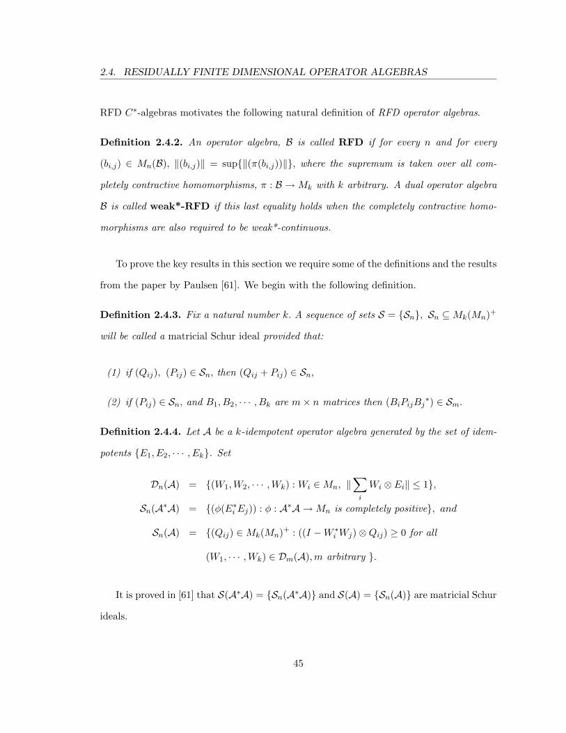
2.4. RESIDUALLY FINITE DIMENSIONAL OPERATOR ALGEBRAS
RFD C∗-algebras motivates the following natural definition of RFD operator algebras.
Definition 2.4.2. An operator algebra, B is called RFD if for every n and for every
(bi,j) ∈ Mn(B), ‖(bi,j)‖ = sup‖(π(bi,j))‖, where the supremum is taken over all com-
pletely contractive homomorphisms, π : B → Mk with k arbitrary. A dual operator algebra
B is called weak*-RFD if this last equality holds when the completely contractive homo-
morphisms are also required to be weak*-continuous.
To prove the key results in this section we require some of the definitions and the results
from the paper by Paulsen [61]. We begin with the following definition.
Definition 2.4.3. Fix a natural number k. A sequence of sets S = Sn, Sn ⊆ Mk(Mn)+
will be called a matricial Schur ideal provided that:
(1) if (Qij), (Pij) ∈ Sn, then (Qij + Pij) ∈ Sn,
(2) if (Pij) ∈ Sn, and B1, B2, · · · , Bk are m× n matrices then (BiPijBj∗) ∈ Sm.
Definition 2.4.4. Let A be a k-idempotent operator algebra generated by the set of idem-
potents E1, E2, · · · , Ek. Set
Dn(A) = (W1,W2, · · · ,Wk) : Wi ∈ Mn, ‖∑
i
Wi ⊗ Ei‖ ≤ 1,
Sn(A∗A) = (φ(E∗i Ej)) : φ : A∗A → Mn is completely positive, and
Sn(A) = (Qij) ∈ Mk(Mn)+ : ((I −W ∗i Wj)⊗Qij) ≥ 0 for all
(W1, · · · ,Wk) ∈ Dm(A),m arbitrary .
It is proved in [61] that S(A∗A) = Sn(A∗A) and S(A) = Sn(A) are matricial Schur
ideals.
45
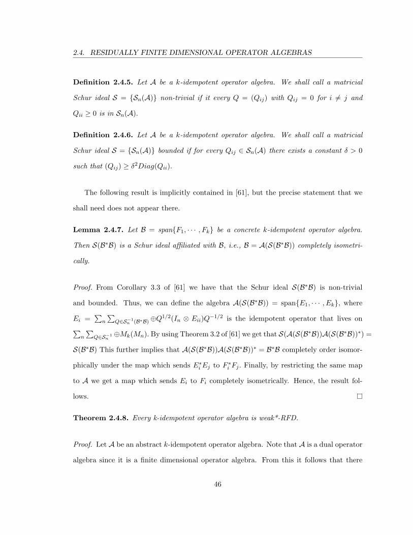
2.4. RESIDUALLY FINITE DIMENSIONAL OPERATOR ALGEBRAS
Definition 2.4.5. Let A be a k-idempotent operator algebra. We shall call a matricial
Schur ideal S = Sn(A) non-trivial if it every Q = (Qij) with Qij = 0 for i 6= j and
Qii ≥ 0 is in Sn(A).
Definition 2.4.6. Let A be a k-idempotent operator algebra. We shall call a matricial
Schur ideal S = Sn(A) bounded if for every Qij ∈ Sn(A) there exists a constant δ > 0
such that (Qij) ≥ δ2Diag(Qii).
The following result is implicitly contained in [61], but the precise statement that we
shall need does not appear there.
Lemma 2.4.7. Let B = spanF1, · · · , Fk be a concrete k-idempotent operator algebra.
Then S(B∗B) is a Schur ideal affiliated with B, i.e., B = A(S(B∗B)) completely isometri-
cally.
Proof. From Corollary 3.3 of [61] we have that the Schur ideal S(B∗B) is non-trivial
and bounded. Thus, we can define the algebra A(S(B∗B)) = spanE1, · · · , Ek, where
Ei =∑
n
∑Q∈S−1
n (B∗B)⊕Q1/2(In ⊗ Eii)Q−1/2 is the idempotent operator that lives on∑n
∑Q∈S−1
n⊕Mk(Mn). By using Theorem 3.2 of [61] we get that S(A(S(B∗B))A(S(B∗B))∗) =
S(B∗B) This further implies that A(S(B∗B))A(S(B∗B))∗ = B∗B completely order isomor-
phically under the map which sends E∗i Ej to F ∗
i Fj . Finally, by restricting the same map
to A we get a map which sends Ei to Fi completely isometrically. Hence, the result fol-
lows.
Theorem 2.4.8. Every k-idempotent operator algebra is weak*-RFD.
Proof. Let A be an abstract k-idempotent operator algebra. Note that A is a dual operator
algebra since it is a finite dimensional operator algebra. From this it follows that there
46
2.4. RESIDUALLY FINITE DIMENSIONAL OPERATOR ALGEBRAS
exist a Hilbert space, H and a weak*-continuous completely isometric homomorphism,
π : A → B(H). Note that B = π(A) is a concrete k-idempotent algebra generated by the
idempotents, B = spanF1, F2, ..., Fk contained in B(H). Thus, from the above lemma B =
A(S(B∗B)) completely isometrically. Further, as defined in the above lemma A(S(B∗B)) =
spanE1, · · · , Ek, where Ei =∑
n
∑Q∈S−1
n (B∗B)⊕Q1/2(In ⊗ Eii)Q−1/2 is the idempotent
operator that lives on∑
n
∑Q∈S−1
n (B∗B)⊕Mk(Mn)..
For each n ∈ N and Q ∈ Sn(B∗B)−1, we define πQn : B → Mk(Mn) via
πQn (Fi) = Q1/2(In ⊗ Eii)Q−1/2.
Assume for the moment that we have proven that πQn is a weak*-continuous completely
contractive homomorphism. Then for every (bi,j) ∈ Mk(B) we must have that
supn,Q∈S−1
n
‖(πQn (bi,j))‖ = ‖(bi,j)‖,
and hence ‖(bi,j)‖ = sup‖(ρ(bi,j))‖, where the supremum is taken over all weak*-continuous
completely contractive homomorphisms ρ : B → Mm with m arbitrary.
Since π : A → B is a complete isometry and weak*-continuous, this would imply the
result for A by composition.
Thus, it remains to show that πQn is a weak*-continuous completely contractive homo-
morphism on B. Note that it is easy to check that it is a completely contractive homomor-
phism and it is completely isometric by the proof of the previous lemma.
Finally, the weak*-continuity of the maps πQn for every n follows from the fact that B
is finite dimensional so that the weak*-topology and the norm topology are equal.
Theorem 2.4.9. Every BPW complete local operator algebra of functions is weak*-RFD.
Proof. Let A be a BPW complete local operator algebra of functions on the set X and
let F be a finite subset of X, so that A/IF is an |F |-idempotent operator algebra. It
47

2.4. RESIDUALLY FINITE DIMENSIONAL OPERATOR ALGEBRAS
follows from the above lemma that A/IF is weak*-RFD, i.e., for ([fi,j ]) ∈ Mk(A/IF ) we
have ‖([fi,j ])‖ = sup‖(ρ([fi,j ]))‖ where the supremum is taken over all weak*-continuous
completely contractive homomorphisms ρ from A/IF into matrix algebras.
Let (fi,j) ∈ Mk(A), then ‖(fi,j)‖Mk(A) = supF ‖([fi,j ])‖ since A is local. Recall, that the
weak*-topology on A requires all the quotient maps of the form πF : A → A/IF , πF (f) =
[f ] to be weak*-continuous. Thus, for each finite subset F ⊆ X, πF is a weak*-continuous
completely contractive homomorphism. The result now follows by considering the compo-
sition of the weak*-continuous quotient maps with the weak*-continuous finite dimensional
representations of each quotient algebra.
Corollary 2.4.10. Every local dual operator algebra of functions is weak*-RFD.
Proof. It follows easily by using the proof of the above theorem.
Corollary 2.4.11. Every local operator algebra of functions is RFD.
Proof. This result follows immediately from Therem 2.2.10 which asserts that every local
operator algebra is completely isometrically contained in a BPW complete local operator
algebra.
The converse of the above may not hold true. It is easy to see that the algebra considered
in Example 2.2.16, 2.2.17 serve as the counter-example for this. Both the examples were
neither local nor BPW complete but one can easily see that they are RFD. Indeed, if we
take A = P : D → C : P is a polynomial to be the algebra of polynomials equipped
with the matrix normed structure such as ‖(pi,j)‖ = max‖(pi,j)‖∞, ‖(pi,j(2))‖ then we
can achieve the same norm by supping over point evaluation maps which are, in fact, one
48
2.4. RESIDUALLY FINITE DIMENSIONAL OPERATOR ALGEBRAS
dimensional completely contractive representations. Note that,
‖(pi,j)‖∞ = sup‖(Ex(pi,j))‖
where Ex : A → C denote the usual evaluation map and the supremum is taken over all
points in X = D. Thus,
‖(pi,j)‖ = supy∈X∪2
‖(Ey(pi,j))‖
where the supremum is taken over all point evaluation maps Ey corresponding to y which
belongs to X ∪ 2. Similarly, one can work out the detail for Example 2.2.16. Thus,
“local” and “BPW complete” properties of an algebra are only sufficient conditions for an
operator algebra of function to be RFD.
It’ll be interesting to find an example of a non-local BPW complete OPAF that is RFD.
As was illustrated in the example 2.2.18 of the Section 2.2.3, constructing an example of a
non-local BPW complete algebra was connected with the open problem. As of this writing,
we do not have any example of such an algebra without referring to that problem. This
makes us believe that it is not easy to construct an example of non-local BPW complete
operator algebra that is also RFD. Our list of examples remain incomplete without an
example of an algebra that is not RFD.
49
Chapter 3Quantized Function Theory on Domains
3.1 Introduction
As an application of the theory of operator algebras of functions presented in the last
chapter, we shall study “Function theory on Quantum domains”. By “Function theory on
a classical domain”, we mean the study of the properties of the space of bounded analytic
functions on the classical domain in CN . In this chapter we will develop a quantum analog
of this function theory.
Whenever scalar variables are replaced by operator variables in a problem or definition,
then this process is often referred to as quantization. It is in this sense that we would like
to quantize the function theory on a family of complex domains. We mentioned earlier in
Chapter 1 that in some sense this process has already been carried out for balls in the work
of Drury [39], Popescu [68], Arveson [15], and Davidson and Pitts [35] and for polydisks in
the work of Agler [2], [3], and Ball and Trent [19]. Our work is closely related to the idea of
“quantizing” other domains defined by inequalities that occurs in the work of Ambrozie and
50

3.1. INTRODUCTION
Timotin [10], Ball and Bolotnikov [17], and Kalyuzhnyi-Verbovetzkii [48], but we approach
these ideas via different path of operator algebras and also the terminology is our own.
We will show that in many cases this process yields local operator algebras of functions
to which the results of the earlier chapter can be applied.
We begin by defining a family of open sets for which our techniques will apply.
Definition 3.1.1. Let G ⊆ CN be an open set. If there exists a set of matrix-valued
functions, Fk = (fk,i,j) : G → Mmk,nk, k ∈ I, whose components are analytic functions on
G, and satisfy ‖Fk(z)‖ < 1, k ∈ I, then we call G an analytically presented domain and
we call the set of functions R = Fk : G → Mmk,nk: k ∈ I an analytic presentation
of G. The subalgebra A of the algebra of bounded analytic functions on G generated by the
component functions fk,i,j : 1 ≤ i ≤ mk, 1 ≤ j ≤ nk, k ∈ I and the constant function
is called the algebra of the presentation. We say that R is a separating analytic
presentation provided that the algebra A separates points of G.
Remark 3.1.2. An analytic presentation of G by a finite set of matrix-valued non-zero
functions, Fk : G → Mmk,nk, 1 ≤ k ≤ K, can always be replaced by the single block diagonal
matrix-valued function, F (z) = F1(z)⊕· · ·⊕FK(z) into Mm,n with m = m1+· · ·+mK , n =
n1 + · · ·+ nK and we will sometimes do this to simplify proofs. But it is often convenient
to think in terms of the set, especially since this will explain the sums that occur in Agler’s
factorization formula.
Remark 3.1.3. Most of the results in this chapter can be proved without the assumption
that the algebra A generated by the component functions and constant function, separates
points of G. However, we make this assumption to be consistent with the theory developed
in the last chapter.
51
3.2. CONNECTION WITH OPAF
3.2 Connection with OPAF
In the last section, we defined a notion of the algebra of the presentation A, that possesses
some of nice properties such as it is clearly an algebra of functions that separates points
of the domain. As the reader can probably guess we aim at turning this algebra into an
operator algebra of functions. Thus, we need to find an appropriate norm structure for A
so that it becomes an operator algebra of functions.
Definition 3.2.1. Let G ⊆ CN be an analytically presented domain with presentation R =
Fk = (fk,i,j) : G → Mmk,nk, k ∈ I, let A be the algebra of the presentation and let H be a
Hilbert space. A homomorphism π : A → B(H) is called an admissible representation
provided that ‖(π(fk,i,j))‖ ≤ 1 in Mmk,nk(B(H)) = B(Hnk ,Hmk), for every k ∈ I. We call
the homomorphism π an admissible strict representation when these inequalities are
all strictly less than 1. Given (gi,j) ∈ Mn(A) we set ‖(gi,j)‖u = sup‖(π(gi,j))‖, where
the supremum is taken over all admissible representations π of A. We let ‖(gi,j)‖u0 denote
the supremum that is obtained when we restrict to admissible strict representations.
The theory of [10] and [17] studies domains defined as above with the additional re-
strictions that the set of defining functions is a finite set of polynomials. However, they
do not need their polynomials to separate points, while we shall shortly assume that our
presentations are separating, in order to invoke the results of the previous sections. This
latter assumption can, generally, be dropped in our theory, but it requires some additional
argument. There are several other places where our results and definitions given below
differ from theirs. So while our results extend their results in many cases, in other cases
we are using different definitions and direct comparisons of the results are not so clear.
Proposition 3.2.2. Let G have a separating analytical presentation and let A be the
52
3.3. GNFT AND GNPP
algebra of the presentation. Then A endowed with either of the family of norms ‖ · ‖u or
‖ · ‖u0 is an operator algebra of functions on G.
Proof. It is clear that it is an operator algebra and by definition it is an algebra of functions
on G. It follows from the hypotheses that it separates points of G. Finally, for every
λ = (λ1, ..., λN ) ∈ G, we have a representation of A on the one-dimensional Hilbert space
given by πλ(f) = f(λ). Hence, |f(λ)| ≤ ‖f‖u and so A is an operator algebra of functions
on G.
For the rest of the discussion, we may denote the operator algebra (A, ‖.‖u) by A and
(A, ‖.‖u0) by A0. Note that we only have A ⊆cc A0, even though A = A0 as sets.
3.3 GNFT and GNPP
In this section, we obtain a generalized Nevanlinna factorization theorem and a generalized
solution to the Nevanlinna Pick problem for the algebra of the presentation. The results in
this section form a building block of our strategy to be able to prove results similar to the
ones obtained by Ball-Bolotnikov, details of which can be found in Section 1.4. To prove
results in this section, we use an important tool from the theory of operator algebras, that
is, the BRS theorem.
First, we give some necessary terminology. It will be convenient to say that matrices,
A1, . . . Am are of compatible sizes if the product, A1 · · ·Am exists, that is, provided that
each Ai is an ni × ni+1 matrix.
Given an analytically presented domain G, with an analytic presentation R = Fk :
k ∈ I. Let F1 denote the constant function 1. By an admissible block diagonal
53

3.3. GNFT AND GNPP
matrix over G we mean a block diagonal matrix-valued function of the form D(z) =
diag(Fk1 , ..., Fkm) where ki ∈ I ∪ 1 for 1 ≤ i ≤ m. Thus, we are allowing blocks of 1’s
in D(z). Finally, given a matrix B we let B(q) = diag(B, ...., B) denote the block diagonal
matrix that repeats B q times.
Theorem 3.3.1. Let G be an analytically presented domain with presentation R = Fk =
(fk,i,j) : G → Mmk,nk, k ∈ I, let A be the algebra of the presentation and let P = (pij) ∈
Mm,n(A), where m,n are arbitrary. Then the following are equivalent:
(i) ‖P‖u < 1,
(ii) there exist an integer l, matrices of scalars Cj , 1 ≤ j ≤ l with ‖Cj‖ < 1 , and
admissible block diagonal matrices Dj(z), 1 ≤ j ≤ l, which are of compatible sizes
and are such that
P (z) = C1D1(z) · · ·ClDl(z),
(iii) there exist a positive, invertible matrix R ∈ Mm, and matrices P0, Pk ∈ Mm,rk(A), k ∈
K, where K ⊆ I is a finite set, such that
Im − P (z)P (w)∗ = R + P0(z)P0(w)∗ +∑k∈K
Pk(z)(I − Fk(z)Fk(w)∗)(qk)Pk(w)∗
where rk = qkmk and z = (z1, ..., zN ), w = (w1, ..., wN ) ∈ G.
Proof. Although we will not logically need it, we first show that (ii) implies (i), since this is
the easiest implication and helps to illustrate some ideas. Note that if π : A → B(H) is any
admissible representation, then the norm of π of any admissible block diagonal matrix is
at most 1. Thus, if P has the form of (ii), then for any admissible π, we will have (π(pi,j))
expressed as a product of scalar matrices and operator matrices all of norm at most one
and hence, ‖(π(Pi,j))‖ ≤ ‖C1‖ · · · ‖Cl‖ < 1. Thus, ‖P‖u ≤ ‖C1‖ · · · ‖Cl‖ < 1.
54

3.3. GNFT AND GNPP
We now prove that (i) implies (ii). The ideas of the proof are similar to [62, Corol-
lary 18.2], [24, Corollary 2.11] and [51, Theorem 1] and use in an essential way the abstract
characterization of operator algebras. For each m,n ∈ N, one proves that ‖P‖m,n :=
inf‖C1‖ . . . ‖Cl‖, defines a norm on Mm,n(A), where the infimum is taken over all l
and all ways to factor P (z) = C1D1(zi1) · · ·ClDl(zil) as a product of matrices of com-
patible sizes with scalar matrices Cj , 1 ≤ j ≤ l and admissible block diagonal matrices
Dj , 1 ≤ j ≤ l.
Moreover, one can verify that Mm,n(A) with this family ‖.‖m,nm,n of norms satisfies
the BRS axioms for an abstract unital operator algebra mentioned in the Chapter 2 and
hence by the Blecher-Ruan-Sinclair representation theorem [25](see also [62]) there exists
a Hilbert space H and a unital completely isometric isomorphism π : A −→ B(H).
Thus, for every m,n ∈ N and for every P = (pij) ∈ Mm,n(A), we have that ‖P‖m,n =
‖(π(pij))‖. However, ‖π(mk,nk)(Fk)‖ = ‖(π(fk,i,j))‖ ≤ 1 for 1 ≤ i ≤ K, and so, π is an
admissible representation. Thus, ‖P‖m,n = ‖(π(pij))‖ ≤ ‖P‖u. Hence, if ‖P‖u < 1, then
‖P‖m,n < 1 which implies that such a factorization exists. This completes the proof that
(i) implies (ii).
We will now prove that (ii) implies (iii). Suppose that P has a factorization as in (ii).
Let K ⊆ I be the finite subset of all indices that appear in the block-diagonal matrices
appearing in the factorization of P. We will use induction on l to prove that (iii) holds.
First, assume that l = 1 so that P (z) = C1D1(z). Then,
Im − P (z)P (w)∗ = Im − (C1D1(z))(C1D1(w))∗
= (Im − C1C∗1 ) + C1 (I −D1(z)D1(w)∗) C∗
1 .
Since D1(z) is an admissible block diagonal matrix the (i, i)-th block diagonal entry of
I −D1(z)D1(w)∗ is I − Fki(z)Fki
(w)∗ for some finite collection, ki.
55
3.3. GNFT AND GNPP
Let Ek be the diagonal matrix that has 1’s wherever Fk appears(so Ek = 0 when there
is no Fk term in D1). Hence,
C1(I −D1(z)D1(w)∗)C∗1 =
∑k
C1Ek(I − Fk(z)Fk(w)∗)EkC∗1 .
Therefore, gathering terms for common values of i,
Im − P (z)P (w)∗ = R0 +∑k∈K
Pk(I − Fk(z)Fk(w)∗)P ∗k ,
where R0 = Im − C1C∗1 is a positive, invertible matrix and Pi is, in this case a constant.
Thus, the form (iii) holds, when l = 1.
We now assume that the form (iii) holds for any R(z) that has a factorization of length
at most l − 1, and assume that
P (z) = C1D1(z) · · ·Dl−1(z)ClDl(z) = C1D1(z)R(z),
where R(z) has a factorization of length l − 1.
Note that a sum of expressions such as on the right hand side of (iii) is again such an
expression. This follows by using the fact that given any two expressions A(z), B(z), we
can write
A(z)A(w)∗ + B(z)B(w)∗ = C(z)C(w)∗,
where C(z) = (A(z), B(z)).
Thus, it will be sufficient to show that Im−P (z)P (w)∗ is a sum of expressions as above.
To this end we have that,
Im−P (z)P (w)∗ = (Im−C1D1(z)D1(w)∗C∗1 )+(C1D1(z))(I−R(z)R(w)∗)(D1(w)∗C∗
1 ).
The first term of the above equation is of the form as on the right hand side of (iii) by
case l = 1. Also, the quantity (I −R(z)R(w)∗) = R0R∗0 + R0(z)R0(w)∗ +
∑k∈K Rk(z)(I −
56
3.3. GNFT AND GNPP
Fk(z)Fk(w)∗)(qk)Rk(w)∗ by the inductive hypothesis. Hence,
C1D1(z)(I −R(z)R(w)∗)D1(w)∗C∗1 =
(C1D1(z)R0)(C1D(w)R0)∗ + [C1D1(z)R0(z)][C1D1(w)R0(w)]∗+∑k∈K
[C1D1(z)Rk(z)](I − Fk(z)Fk(w)∗)(qk)[C1D1(w)Rk(w)]∗.
Thus, we have expressed (I − P (z)P (w)∗) as a sum of two terms both of which can be
written in the form desired. Using again our remark that the sum of two such expressions
is again such an expression, we have the required form.
Finally, we will prove (iii) implies (i). Let π : A → B(H) be an admissible representation
and let P = (pi,j) ∈ Mm,n(A) have a factorization as in (iii). To avoid far too many
superscripts we simplify π(m,n) to Π.
Now observe that
Im −Π(P )Π(P )∗ = Π(R) + Π(P0)Π(P0)∗ +∑k∈K
Π(Pk)(I −Π(Fk)Π(Fk)∗)(qk)(Π(Pk))∗.
Clearly the first two terms of the sum are positive. But since π is an admissible represen-
tation, ‖Π(Fk)‖ ≤ 1 and hence, (I − Π(Fk)Π(Fk)∗) ≥ 0. Hence, each term on the right
hand side of the above inequality is positive and since R is strictly positive, say R ≥ δIm
for some scalar δ > 0, we have that Im −Π(P )Π(P )∗ ≥ δIm.
Therefore, ‖Π(P )‖ ≤√
1− δ. Thus, since π was an arbitrary admissible representation,
‖P‖u ≤√
1− δ < 1, which proves (i).
When we require the functions in the presentation to be row vector-valued, then the
above theory simplifies somewhat and begins to look more familiar. Let G be an analytically
presented domain with presentation Fk : G → M1,nk, k ∈ I. We identify M1,n with the
57

3.3. GNFT AND GNPP
Hilbert space Cn so that 1 − Fk(z)Fk(w)∗ = 1 − 〈Fk(z), Fk(w)〉, where the inner product
is in Cn. In this case we shall say that G is presented by vector-valued functions.
Corollary 3.3.2. Let G be presented by vector-valued functions, Fk = (fk,j) : G →
M1,nk, k ∈ I, let A be the algebra of the presentation and let P = (pij) ∈ Mm,n(A).
Then the following are equivalent:
(i) ‖P‖u < 1,
(ii) there exist an integer l, matrices of scalars Cj , 1 ≤ j ≤ l with ‖Cj‖ < 1 , and
admissible block diagonal matrices Dj(z), 1 ≤ j ≤ l, which are of compatible sizes
and are such that
P (z) = C1D1(z) · · ·ClDl(z),
(iii) there exist a positive, invertible matrix R ∈ Mm, and matrices P0 ∈ Mm,r0(A),
Pk ∈ Mm,rk(A), k ∈ K, where K ⊆ I is finite, such that
Im − P (z)P (w)∗ = R + P0(z)P0(w)∗ +∑k∈K
(1− 〈Fk(z), Fk(w)〉)Pk(z)Pk(w)∗
where z = (z1, ..., zN ), w = (w1, ..., wN ) ∈ G.
Corollary 3.3.3. Let Y be a subset of an analytically presented domain G with analytic
presentation Fk = (fk,i,j) : G− → Mmk,nk, 1 ≤ k ≤ K and let πY : A → A/IY be the
quotient map, where IY = f ∈ A : f |Y = 0. Let A be the algebra of the presentation and
let P = (pij) ∈ Mm,n(A), where m,n are arbitrary. Then the following are equivalent:
(i) ‖(πY (pij))‖u < 1,
(ii) there exist an integer l, matrices of scalars Cj , 1 ≤ j ≤ l with ‖Cj‖ < 1 , and
admissible block diagonal matrices Dj(z), 1 ≤ j ≤ l, which are of compatible sizes
and are such that P (z) = C1D1(z) · · ·ClDl(z) for every z ∈ Y,
58
3.3. GNFT AND GNPP
(iii) there exist a positive, invertible matrix R ∈ Mm, and matrices Pk ∈ Mm,rk(A), 0 ≤
k ≤ K, such that
Im − P (z)P (w)∗ = R + P0(z)P0(w)∗ +K∑
k=1
Pk(z)(I − Fk(z)Fk(w)∗)(qk)Pk(w)∗
where rk = qkmk and z = (z1, ..., zN ), w = (w1, ..., wN ) ∈ S.
Proof. To show (i) implies (ii) we assume that ‖(πY (pij))‖u < 1. Then there exists qij ∈ IY
such that ‖(pij + qij)‖u < 1 and hence by using theorem 3.3.1 we get (ii). For the converse,
assume that there exists an integer l, matrices of scalars Cj , 1 ≤ j ≤ l with ‖Cj‖ < 1 and
admissible block diagonal matrices Dj(z), 1 ≤ j ≤ l, which are of compatible sizes and are
such that P (z) = C1D1(z) · · ·ClDl(z) for every z ∈ S. Let (rij(z)) = C1D1(z) · · ·ClDl(z)
then ‖(rij)‖u < 1 and rij(λ) = pij(λ) ∀ λ ∈ Y. This shows that ‖(πY (pij))‖u ≤ ‖(pij) +
(rij − pij)‖u = ‖(rij)‖u < 1.
Remark 3.3.4. It can be proved that (ii) in the above corollary implies that the factoriza-
tion formula given in (iii) of Theorem 3.3.1 hold true for all the points in the set S by the
same proof as given in the Theorem 3.3.1.
The following result gives us a Nevanlinna-type result for the algebra of presentation.
Theorem 3.3.5. Let Y be a finite subset of an analytically presented domain G with
separating analytic presentation Fk = (fk,i,j) : G → Mmk,nk, k ∈ I, let A be the algebra
of the presentation and let P be a Mm,n-valued function defined on a finite subset Y =
x1, · · · , xl of G. Then the following are equivalent:
(i) there exists P ∈ Mmn(A) such that P |Y = P and ‖P‖u < 1,
59
3.3. GNFT AND GNPP
(ii) there exist a positive, invertible matrix R ∈ Mm, and matrices P0 ∈ Mm,r0(A),
Pk ∈ Mm,rk(A), k ∈ K, where K ⊆ I is a finite set, such that
Im − P (z)P (w)∗ = R + P0(z)P0(w)∗ +∑k∈K
Pk(z)(I − Fk(z)Fk(w)∗)(qk)Pk(w)∗,
where rk = qkmk and z = (z1, ..., zN ), w = (w1, ..., wN ) ∈ Y.
Proof. Note that (i) ⇒ (ii) follows immediately as a corollary of Theorem 3.3.1. Thus it
only remains to show that (ii) ⇒ (i). Since A is an operator algebra of functions, therefore,
A/IY is a finite dimensional operator algebra of idempotents andA/IY = spanE1, · · · , El
where l = |Y |. Thus there exists a Hilbert space HY and a completely isometric representa-
tion π of A/IY . By Theorem 2.3.5, there exists a kernel KY such that π(A/IY ) = M(KY )
completely isometrically under the map ρ : π(A/IY ) →M(KY ) which sends π(B) to Mf ,
where B =∑l
i=1 aiπ(Ei) and f : Y → C is a function defined by f(xi) = ai. Note that
((I − Fk(xi)Fk(xj))⊗KY (xi, xj)) =
((I − π(Fk + IY )(xi)π(Fk + IY )(xj)∗)⊗KY (xi, xj))ij ≥ 0,
since ‖π(Fk + IY )‖ ≤ ‖Fk‖u ≤ 1 for all k ∈ I. From this it follows that ((Im − (π(P +
IY ))(xi)(π(P +IY ))(xj)∗)⊗KY (xi, xj))ij ≥ 0. Using that R > 0, we get that ‖π(P +IY )‖ <
1. This shows that there exists P ∈ A such that P |Y = P and ‖P‖u < 1. This completes
the proof.
Before we close this section, it would be valuable to make a note that the results in this
section can be proved for a non-commutative algebra as well. The proofs of all the results
in this section hold good for any algebra that is generated by any set of free generators.
60

3.4. MAIN RESULT
3.4 Main Result
In this section, we do justice to the title of this chapter and prove the main result of this
chapter. In a true sense, we study “quantized function theory” in this section. First, we de-
fine quantized version of an analytically presented domain. Second, we aim at establishing
a relation between the algebra of the presentation and the bounded analytic functions on
these domains which is achieved by our main result. In the main result, we obtain a “neat”
connection between the two algebras which allows us to pull back results from the previous
chapter. Also, with the help of this connection and the factorization results obtained in
the earlier section for the algebra of the presentation, we are able to prove GNFT for the
algebra of bounded analytic functions on quantum domains.
First, we turn towards defining quantized versions of the bounded analytic functions
on these domains. For this we need to recall that the joint Taylor spectrum [77] of a
commuting N -tuple of operators T = (T1, ..., TN ), is a compact set, σ(T ) ⊆ CN and that
there is an analytic functional calculus [78], [79] defined for any function that is holomorphic
in a neighborhood of σ(T ).
Definition 3.4.1. Let G ⊆ CN be an analytically presented domain, with presentation
R = Fk : G− → Mmk,nk, k ∈ I. We define the quantized version of G to be the
collection of all commuting N -tuples of operators,
Q(G) = T = (T1, T2, . . . , TN ) ∈ B(H) : σ(T ) ⊆ G and ‖Fk(T )‖ ≤ 1, ∀ k ∈ I,
where H is an arbitrary Hilbert space. We set
Q0,0(G) = T = (T1, T2, . . . , TN ) ∈ Mn : σ(T ) ⊆ G and ‖Fk(T )‖ ≤ 1, ∀ k ∈ I,
where n is an arbitrary positive integer.
61
3.4. MAIN RESULT
Note that if we identify a point (λ1, ..., λN ) ∈ CN with an N -tuple of commuting
operators on a one-dimensional Hilbert space, then we have that G ⊆ Q(G).
If T = (T1, ..., TN ) ∈ Q(G), is a commuting N -tuple of operators on the Hilbert space
H, then since the joint Taylor spectrum of T is contained in G, we have that if f is analytic
on G, then there is an operator f(T ) defined and the map π : Hol(G) → B(H) is a unital
continuous homomorphism, where Hol(G) denotes the algebra of analytic functions on G
[79].
Definition 3.4.2. Let G ⊆ CN be an analytically presented domain, with presentation
R = Fk : G− → Mmk,nk, k ∈ I. We define H∞
R (G) to be the set of functions f ∈ Hol(G),
such that ‖f‖R ≡ sup‖f(T )‖ : T ∈ Q(G) is finite. Given (fi,j) ∈ Mn(H∞R (G)), we set
‖(fi,j)‖R = sup‖(fi,j(T ))‖ : T ∈ Q(G).
We are interested in determining a connection between the algebra of the presentation
and H∞R (G) and whether or not the ‖·‖R norm is attained on the smaller set Q0,0(G). Note
that since each point in G ⊆ Q(G), we have that H∞R (G) ⊆ H∞(G), and ‖f‖∞ ≤ ‖f‖R.
Also, we have that A ⊆ H∞R (G) and for (fi,j) ∈ Mn(A), ‖(fi,j)‖R ≤ ‖(fi,j)‖u. Indeed, it
follows from the fact that every T ∈ Q(G) gives rise to an admissible representation of
H∞R (G). The inclusion of A into H∞
R (G) might not even be isometric.
Recall, A0 = (A, ‖.‖u0) where ‖.‖u0 is a norm on A obtained by supping over all strict
admissible representations on A. It is natural to wonder about the connection of the algebra
A0 with H∞R (G). We know that A ⊆cc A0 and A = A0 as sets, still the connection between
A0 and H∞R (G) is not at all obvious.
Lemma 3.4.3. Let π : H∞R (G) → C be completely contractive and weak*-continuous
homomorphism. If F = (fi,j) ∈ R, then ‖(π(fi,j))‖ < 1.
62
3.4. MAIN RESULT
Proof. We know that ‖(π(fi,j))‖ ≤ 1. Suppose that it has norm equal to 1, then since it
is a finite matrix, there are unit vectors v, w such that 〈(π(fi,j))v, w〉 = 1. Let h(z) =
〈(fi,j(z))v, w〉, then π(h) = 1.
Since ‖F (z)‖ < 1 for each z ∈ G, we have that |h(z)| < 1 for each z ∈ G. Hence,
h(z)k → 0 for each z, which further yields that hk → 0 in the weak*-topology, which
implies that π(h)k → 0. This contradicts π(h) = 1.
We would like to record a fact from matrix theory that for every abelian subalgebra
B of Mn there exists an unitary U ∈ Mn such that UBU∗ ⊆ Tn, where Tn is the space
of upper triangular matrices, see [46]. Thus, in particular, if π : H∞R (G) → Mn is a
completely contractive and weak*-continuous homomorphism then there exists an unitary
U such that σ : H∞R (G) → Tn defined via σ(.) = Uπ(.)U∗ is also a completely contractive
and weak*-continuous homomorphism.
Lemma 3.4.4. Let σ : H∞R (G) → Tn be a completely contractive and weak*-continuous
homomorphism. If F = (fi,j) ∈ R, then |〈(σ(fi,j))ek, ek〉| < 1 for all k.
Proof. We define
δ : H∞R (G) → C via δ(.) = 〈σ(.)ei, ei〉.
Then it follows that δ is a homomorphism from the hypothesis that σ is a homomorphism.
Indeed, if we let f, g ∈ H∞R (G) then
σ(fg) = 〈π(f)π(g)U∗ei, U∗ei〉
homo.= 〈Uπ(f)U∗Uπ(g)U∗ei, ei〉
∗= 〈Uπ(f)U∗ei, ei〉〈Uπ(g)U∗ei, ei〉 = σ(f)σ(g).
The equality (*) follows from the fact that the diagonal entry of the product of two triangu-
lar matrices is equal to the product of the diagonal entries of the two triangular matrices.
63

3.4. MAIN RESULT
It follows from a straightforward argument that δ is also a completely contractive and
weak*-continuous map. Finally, the result follows by using Lemma 3.4.3.
Lemma 3.4.5. Let σ : H∞R (G) → Tn be a completely contractive and weak*-continuous ho-
momorphism. If F = (fi,j) ∈ R, then there exists a completely contractive homomorphism
σz : H∞R (G) → Tn such that ‖(σz(fij))‖ < 1 for every z ∈ D.
Proof. For a fixed z ∈ D and a triangular matrix
T =
t11 t12 . . . t1n
0 t22 . . . t2n
......
......
0 0 . . . tnn
we define a triangular matrix Tz = VzTV ∗
z where Vz = diag(1, z, z2, · · · , zn−1). Thus,
Tz =
t11 zt12 . . . zn−1t1n
0 t22 . . . zn−2t2n
......
......
0 0 . . . tnn
Using this operation, we define the desired map σz : H∞
R (G) → Tn as σz(f) = (σ(f))z.
It is not so hard to see that σz is a homomorphism by brute force calculations. To avoid
calculations, one can even adopt a slicker way of proving this by invoking the maximum
modulus theorem. Note that σz is an analytic function of z on the unit disc D and on the
unit circle Vz turns out to be a unitary matrix. For a fixed f, g ∈ H∞R (G), it is is obvious
that
σeiθ(fg) = σeiθ(f)σeiθ(g).
64
3.4. MAIN RESULT
If we define a linear functional L : D → C for a fixed pair of α, β ∈ Cn with ‖α‖ = 1, ‖β‖ =
1 via Lα,β(z) = 〈(σz(fg)− σz(f)σz(g))α, β〉, then L is a complex-valued analytic function
on D and Lα,β(eiθ) = 0 for every θ ∈ [0, 2π]. Thus, by the maximum modulus theorem we
have that Lα,β(z) = 0 for every α, β ∈ Cn and z ∈ D. This proves that σz(gh) = σz(g)σz(h)
for every g, h ∈ H∞R (G) and z ∈ D.
To prove the final conclusion, note that by the maximum modulus theorem for a fixed
z ∈ D, we have that
|〈σz(g)α, β〉| ≤ |〈σeiθ(g)α, β〉| ≤ |〈Ueiθσ(g)U∗eiθα, β〉| ≤ ‖σ(g)‖.
By taking the supremum over all α, β ∈ Cn, ‖α‖ = ‖β‖ = 1 and z ∈ D, we get that
supz∈D
‖σz(g)‖ ≤ ‖σ(g)‖
for every g ∈ H∞R (D). Similar arguments can be used to prove that supz∈D ‖(σz(gij))‖ ≤
‖(σ(gij))‖. This together with the fact that ‖(σ(fij))‖ ≤ 1 implies that ‖(σz(fij))‖ ≤ 1 for
every F = (fij) ∈ R and z ∈ D. Also, note that ‖(σ0(fij))‖ = maxk |〈(π(fij)ek, ek〉| < 1,
because of the previous lemma. Finally, if there exists z0 ∈ D such that the conclusion
fails, that is, ‖(σz0(fij))‖ = 1. Then by a compactness argument, there exist k1, k2 such
that
|〈(σz0(fij))k1, k2〉| = 1 ≥ |〈(σz(fij))k1, k2〉|
for every z ∈ D. Thus, by the maximum modulus theorem we have that |〈(σz(fij))k1, k2〉| =
1 for every z ∈ D which contradicts the fact ‖(σ0(fij))‖ < 1.
In summary, the above series of lemmas proves that for every finite dimensional com-
pletely contractive weak*-continuous homomorphism π : H∞R (G) → Mn there exists a set
of strict admissible representations σz : H∞R (G) → Tn and ‖(σz(gij))‖ ≤ ‖(σ(gij))‖ ≤
‖(π(gij))‖ for every gij ∈ H∞R (G).
65

3.4. MAIN RESULT
We are now in a position to prove a theorem that establishes a connection between the
algebra of the presentation of the domain G equipped with ‖.‖u0 norm and H∞R (G).
Theorem 3.4.6. Let G be an analytically presented domain and let A be the algebra of
the presentation. Then ‖H‖R ≤ ‖H‖u0 for every H ∈ Mn(A) and for all n.
Proof. Let π : H∞R (G) → Mn be a completely contractive weak*-continuous homomor-
phism. Then, for every z ∈ D, there exists a homomorphism σz : H∞R (G) → Tn such that
‖(σz(fij))‖ < 1 and ‖(σz(hij))‖ ≤ ‖(π(hij))‖ for every (hij) ∈ Mn(H∞R (G)).
We claim that supz∈D ‖(σz(hij))‖ ≥ ‖(π(hij))‖. To prove this claim, we need to recall
that σz = VzUπU∗Vz where Vz = diag(1, z, · · · , zn−1) and U is the unitary matrix in Mn.
Clearly,
|〈(π(hij))ej , ei〉| = limr1
|〈(σreiθ(hij))U∗ej , U∗ei〉|.
Note that the above equality holds true for any two column vectors h, k in an appropriate
finite dimensional space. Let us assume that ‖h‖ = ‖k‖ = 1. Thus,
|〈(π(hij))h, k〉| = limr1
|〈(σreiθ(hij))U∗h, U∗k〉| ≤ lim supr1
‖(σreiθ(hij))‖ ≤ supz∈D
‖(σz(hij))‖.
By taking the supremum over all h, k with ‖h‖ = ‖k‖ = 1, we obtain our claim. This
further implies that ‖(pi(hij))‖ ≤ ‖(hij)‖u0 . Finally, by Theorem 3.4.11, it is enough to
take the supremum over all completely contractive weak*-continuous homomorphisms to
obtain ‖f‖R and hence our result.
We shall see in the example section that for most of the algebras A, we can prove that
A ∼= A0 completely isometrically, still we do not know this in general.
Corollary 3.4.7. Let G be an analytically presented domain and let A be the algebra of the
presentation. If A is a local operator algebra of functions, then A =ci A0, that is, A = A0
66
3.4. MAIN RESULT
completely isometrically.
Remark 3.4.8. If we look closely then we can prove that A =ci A0 under a weaker as-
sumption that the algebra is RFD by constructing a finite dimensional strict admissible
representation using a finite dimensional completely contractive representation as done in
Lemma 3.4.3. However, we believe that the converse of this may not hold true. Though,
we do not have any counter-example to support our belief. Note that to be able to establish
this, we would need an example of a non-RFD algebra and we remarked earlier in Chapter
2 that problem of finding an example of non-RFD algebra is still open.
Recall, the norm on the BPW completion of an operator algebra of functions depends
on the norm of the algebra. Thus, for each norm on A we get a norm structure on A. It
is natural to wonder if anything can be said about the BPW completion of these algebras:
A and A0.
Corollary 3.4.9. Let G be an analytically presented domain and let A be the algebra of
the presentation. Then A =ci A0.
Proof. Recall, if f ∈ A then ‖f‖ = infC : ∃ fλ ∈ A, fλ → f, ‖fλ‖u ≤ C. We may
denote the norm on the BPW completion of A0 by ‖.‖0. It is obvious that ‖f‖u0 ≤ ‖f‖u
for every f ∈ A and consequently, it follows that for every g ∈ A we have that ‖g‖0 ≤ ‖g‖.
Suppose that g ∈ A0 with ‖g‖0 ≤ 1. Thus, there exists a sequence gλ of functions in A
such that gλ → g pointwise and ‖gλ‖u0 ≤ 1.
For a given ε > 0 and a fixed x ∈ G, there exists λ0 such that |gλ0(x) − g(x)| < ε.
From the above theorem, we get ‖gλ‖L ≤ 1 which further implies that there exists a net
gFλ0 ∈ A such that ‖gF
λ0‖u ≤ 1 and |gF
λ0(x) − g(x)| → 0. This shows that ‖g‖u ≤ 1. On
the similar lines, we can prove this for matrices. With this we conclude, A is completely
67
3.4. MAIN RESULT
isometrically isomorphic to A0.
Corollary 3.4.10. Let G be an analytically presented domain and let A be the algebra of
the presentation. If A =ci A, then A0 =ci A0.
Proof. The proof is immediate from the above corollary.
We are now in a position to state and prove our main result which establishes a very
precise connection between the algebra of the presentation (A0 or A) and H∞R (G). The
algebra of the bounded analytic function on a quantum domain turns out to be completely
isometrically isomorphic to the BPW completion of the algebra of the presentation, that
is, H∞R (G) = A = A0 completely isometrically. This theorem ties the theory of operator
algebras of functions with the quantized function theory quite nicely. In particular, it
allows us to extend the results to H∞R (G) from the previous chapter.
Theorem 3.4.11. Let G be an analytically presented domain with a separating presentation
R = Fk : G → Mmk,nk: k ∈ I, let A be the algebra of the presentation and let A be the
BPW-completion of A. Then
(i) A = H∞R (G), completely isometrically,
(ii) H∞R (G) is a local weak*-RFD dual operator algebra.
Proof. Let f ∈ Mn(A), with ‖f‖L < 1. Then there exists a net of functions, fλ ∈ Mn(A),
such that ‖fλ‖u < 1 and limλ fλ(z) = f(z) for every z ∈ G. Since ‖fλ‖∞ < 1, by Montel’s
Theorem, there is a subsequence fn of this net that converges to f uniformly on compact
sets. Hence, if T ∈ Q(G), then limn ‖f(T )−fn(T )‖ = 0 and so ‖f(T )‖ ≤ supn ‖fn(T )‖ ≤ 1.
Thus, we have that f ∈ Mn(H∞R (G)), with ‖f‖R ≤ 1. This proves that A ⊆ H∞
R (G) and
that ‖f‖L ≤ ‖f‖R.
68

3.4. MAIN RESULT
Conversely, let g ∈ Mn(H∞R (G)) with ‖g‖R < 1. Given any finite set Y = y1, ..., yt ⊆
G, let A/IY = spanE1, ..., Et be the corresponding t-idempotent algebra and let πY :
A → A/IY denote the quotient map. Write yi = (yi,1, ..., yi,N ), 1 ≤ i ≤ t and let Tj =
y1,jE1+· · ·+yt,jEt, 1 ≤ j ≤ N so that T = (T1, ..., TN ) is a commuting N -tuple of operators
with σ(T ) = Y. For k ∈ I, we have that ‖Fk(T )‖ = ‖Fk(y1) ⊗ E1 + · · · + Fk(yt) ⊗ Et‖ =
‖πY (Fk)‖ ≤ ‖Fk‖u = 1. Thus, T ∈ Q(G), and so,
‖g(T )‖ = ‖g(y1)⊗ E1 + · · ·+ g(yt)⊗ Et‖ ≤ ‖g‖R < 1.
Since A separates points, we may pick f ∈ Mn(A) such that f = g on Y. Hence, πY (f) =
f(T ) = g(T ) and ‖πY (f)‖ < 1. Thus, we may pick fY ∈ Mn(A), such that πY (fY ) = πY (f)
and ‖fY ‖u < 1. This net of functions, fY converges to g pointwise and is bounded.
Therefore, g ∈ Mn(A) and ‖g‖L ≤ 1. This proves that H∞R (G) ⊆ A and that ‖g‖L ≤ ‖g‖R.
Thus, A = H∞R (G) and the two matrix norms are equal for matrices of all sizes. The
rest of the conclusions follow from the results on BPW-completions.
Remark 3.4.12. The above result yields that for every f ∈ H∞R (G), ‖f‖R = sup‖π(f)‖
where the supremum is taken over all finite dimensional weak*-continuous representations,
π : H∞R (G) → Mn with n arbitrary. For many examples, we can show that ‖f‖R =
sup‖f(T )‖ : T ∈ Q00(G) for any f ∈ H∞R (G). Also, we can verify these hypotheses are
met for most of the algebras given in the example section. In particular, for Examples
3.5.1, 3.5.2, 3.5.3, 3.5.4, 3.5.6, 3.5.7, and 3.5.8. It would be interesting to know if this
can be done in general.
Corollary 3.4.13. Let G be an analytically presented domain with a separating presenta-
tion R = Fk : G → Mmk,nk: k ∈ I, let A be the algebra of the presentation and let A be
the BPW-completion of A. If we assume that
69
3.4. MAIN RESULT
1. A contains the coordinate functions, and
2. the Taylor spectrum of Tπ = (π(z1), ..., π(zn)) ⊂ G, where π is a strict finite dimen-
sional weak*-continuous completely contractive representation,
then for every f ∈ Mn(H∞R (G)) we have that ‖f‖R = sup‖f(T )‖ : T ∈ Q0,0(G).
Proof. Let π : H∞R (G) → Mn be a weak*-continuous representation such that the Taylor
spectrum of T = (π(z1), ..., π(zN )) ⊂ G. Then π(f) = f(T ) for every f ∈ A and for every
f ∈ H∞R (G) there exists a net of functions, fλ ∈ A which converges to f in the BPW limit,
since A = H∞R (G) completely isometrically. It follows from the Prop. 2.3.7 of Chapter 2
that fλ → f in the weak*-topology. This further implies that π(fλ) = fλ(T ) → π(f), and
by the Taylor functional calculus fλ(T ) → f(T ). Thus, we have that π(f) = f(T ) for every
f ∈ H∞R (G) and hence
sup‖f(T )‖ : T ∈ Q0,0(G) ≥ sup‖π(f)‖
where the supremum is taken over all finite dimensional weak*-continuous representations
of H∞R (G) such that the Taylor spectrum of T = (π(z1), ..., π(zN )) ⊂ G.
From the above theorem and the hypotheses, we get that for every f ∈ H∞R (G), ‖f‖R =
sup‖π(f)‖ where the supremum is taken over all finite dimensional weak*-continuous
representations of H∞R (G), π : H∞
R (G) → Mn ∀ n.
It is interesting to analyze the condition that the Taylor spectrum of Tπ = (π(z1), ..., π(zn)) ⊆
G where π is a finite dimensional weak*-continuous completely contractive homomorphism.
In the following proposition, we prove that this condition is met if we assume that every
complex homomorphism of the algebra of the presentation is given by a point evaluation
map.
70
3.4. MAIN RESULT
Proposition 3.4.14. Let G be a analytically presented domain, let π : H∞R (G) → Mn
be a finite dimensional weak*-continuous completely contractive homomorphism. If the
algebra of the presentation A contains the coordinate functions and we assume that every
weak*-continuous completely contractive complex homomorphism of H∞R (G) is given by
evaluation at some point in CN where the functions in R are analytic and Ti = π(zi), then
Tπ = (T1, ..., TN ) is a commuting N-tuple of operators whose joint Taylor spectrum of T is
contained in G.
Proof. Note that π(H∞R (G)) is an abelian subalgebra of Mn, thus there exists an unitary
U ∈ Mn such that δ : H∞R (G) → Tn defined via δ(.) = Uπ(.)U∗ is also a completely
contractive and weak*-continuous homomorphism. By the unitary invariance property of
a spectrum, we have that σ(Tπ) = σ((δ(z1), ..., δ(zN ))). We denote δ(zi) by Si for every i =
1, ..., N. Since S = (S1, ..., SN ) is a commuting N-tuple of triangular matrices, the Taylor
spectrum of S is equal to the joint point spectrum of S, that is, σ(S) = σ(S1)×· · ·×σ(SN )
where σ(Si) is the ordinary spectrum of a triangular matrix Si for every i = 1, ..., N.
Fix 1 ≤ k ≤ N, let ek denote the column vector with 1 in the k-th position and 0
elsewhere. We define ρk : H∞R (G) → C via ρk(.) = 〈δ(.)ek, ek〉. It is easy to check that
ρk is a weak*-continuous contractive homomorphism. Thus, by the hypthoses there exists
a λk ∈ CN such that ρk(f) = f(λk) for every f ∈ R. It follows from the Lemma 3.4.3
that ‖ρ(fij)‖ < 1 for every (fij) ∈ R. Thus, we have that σ(T ) = λ1, ..., λN ⊆ G. This
completes the proof.
Remark 3.4.15. We wish to justify one of our assumption in the previous result. In
classical complex analysis of functions on several complex variables, the problem of finding
a good characterization of complex domains G for which every weak*-continuous completely
contractive complex homomorphism of H∞(Ω) is given by a point evaluation has been of
71
3.4. MAIN RESULT
interest since a long time. But as of this writing, no reasonable characterization of such
domains is known. It is easy to see that it holds true for many examples such as any
connected open set in C, polydisk, and ball in CN . For an example where it fails, consider
a shell in CN , in particular, take Ω = z ∈ C2 : 1 < ‖z‖C2 < 3. We refer the interested
reader for more details to the book by Steven G. Krantz [50].
Note that finding a characterization of an analytically presented domain G for which
every weak*-continuous completely contractive complex homomorphism of H∞R (G) is given
by a point evaluation map is even more difficult since H∞R (G) ⊆ H∞(G) completely con-
tractively.
We now seek other characterizations of the functions in H∞R (G). In particular, we wish
to obtain analogues of Agler’s factorization theorem and of the results in [10] and [17]. By
Theorem 2.3.5, if we are given an analytically presented domain G ⊆ CN , with presentation
R = Fk : G → Mmk,nk, k ∈ I, then there exist a Hilbert space H and a positive definite
function, K : G×G → B(H) such that A = M(K). We shall denote any kernel satisfying
this property by KR.
Definition 3.4.16. Let G ⊆ CN be an analytically presented domain, with presentation
R = Fk : G− → Mmk,nk, k ∈ I. We shall call a function H : G×G → Mm an R-limit,
provided that H is the pointwise limit of a net of functions Hλ : G×G → Mm of the form
given by Theorem 3.3.1(iii).
Corollary 3.4.17. Let G ⊆ CN be an analytically presented domain, with a separating
presentation R = Fk : G− → Mmk,nk, k ∈ I. Then the following are equivalent:
(i) f ∈ Mm(H∞R (G)) and ‖f‖R ≤ 1,
(ii) (Im − f(z)f(w)∗)⊗KR(z, w) is positive definite,
72
3.4. MAIN RESULT
(iii) Im − f(z)f(w)∗ is an R-limit.
In the case when the presentation contains only finitely many functions we can say
considerably more about R-limits.
Proposition 3.4.18. Let G be an analytically presented domain with a finite presentation
R = Fk = (fk,i,j) : G → Mmk,nk, 1 ≤ k ≤ K. For each compact subset S ⊆ G, there
exists a constant C, depending only on S, such that given a factorization of the form,
Im − P (z)P (w)∗ = R + P0(z)P0(w)∗ +K∑
k=1
Pk(z)(I − Fk(z)Fk(w)∗)(qk)Pk(w)∗,
then ‖Pk(z)‖ ≤ C for all k ∈ I and for all z ∈ S.
Proof. By the continuity of the functions, there is a constant δ > 0, such that ‖Fk(z)‖ ≤
1− δ, for all k ∈ I and for all z ∈ S. Thus, we have that I −Fk(z)Fk(z)∗ ≥ δI, for all k ∈ I
and for all z ∈ S. Also, we have that
Im ≥ Im − P (z)P (z)∗ ≥ Pk(z)(I − Fk(z)Fk(z)∗)(qk)Pk(z)∗ ≥ δPk(z)Pk(z)∗.
This shows that ‖Pk(z)‖ ≤ 1/δ for all k ∈ I and for all z ∈ S.
The proof of the following result is essentially contained in [17, Lemma 3.3].
Proposition 3.4.19. Let G be a bounded domain in CN and let F = (fi,j) : G → Mm,n be
analytic with ‖F (z)‖ < 1 for z ∈ G. If H : G ×G → Mp is analytic in the first variables,
coanalytic in the second variables and there exists a net of matrix-valued functions Pλ ∈
Mp,rλ(Hol(G)) which are uniformly bounded on compact subsets of G, such that H(z, w) is
the pointwise limit of Hλ(z, w) = Pλ(z)(Im−F (z)F (w)∗)(qλ)Pλ(w)∗ where rλ = qλm, then
there exist a Hilbert space H and an analytic function, R : G → B(H⊗ Cm, Cp) such that
H(z, w) = R(z)[(Im − F (z)F (w)∗)⊗ IH]R(w)∗.
73

3.4. MAIN RESULT
Proof. We identify (Im − F (z)F (w)∗)(qλ) = (Im − F (z)F (w)∗) ⊗ ICqλ , and the p × mqλ
matrix-valued function Pλ as an analytic function, Pλ : G → B(Cm ⊗ Cqλ , Cp). Writing
Cm⊗Cqλ = Cqλ ⊕ · · · ⊕Cqλ(m times) allows us to write Pλ(z) = [P λ1 (z), . . . , P λ
m(z)] where
each P λi (z) is p× qλ. Also, if we let f1(z), ..., fm(z) be the (1, n) vectors that represent the
rows of the matrix F, then we have that F (z)F (w)∗ =∑m
i,j=1 fi(z)fj(w)∗Ei,j .
Finally, we have that
Hλ(z, w) =m∑
i=1
P λi (z)P λ
i (w)∗ −m∑
i,j=1
fi(z)fj(w)∗P λi (z)P λ
j (w).
Let Kλ(z, w) = (P λi (z)P λ
j (w)∗), so that Kλ : G × G → Mm(Mp) = B(Cm ⊗ Cp), is
a positive definite function that is analytic in z and co-analytic in w. By dropping to a
subnet, if necessary, we may assume that Kλ converges uniformly on compact subsets of G
to K = (Ki,j) : G×G → Mm(Mp). Note that this implies that P λi (z)P λ
j (w)∗ → Ki,j(z, w)
for all i, j and that K is a positive definite function that is analytic in z and coanalytic in
w.
The positive definite function K gives rise to a reproducing kernel Hilbert space H of
analytic Cm ⊗ Cp-valued functions on G. If we let E(z) : H → Cm ⊗ Cp be the evaluation
functional, then K(z, w) = E(z)E(w)∗ and E : G → B(H, Cm⊗Cp) is analytic. Identifying
Cm⊗Cp = Cp⊕· · ·⊕Cp(m times), yields analytic functions, Ei : G → B(H, Cp), i = 1, ...,m,
such that (Ki,j(z, w)) = K(z, w) = E(z)E(w)∗ = (Ei(z)Ej(w)∗).
Define an analytic map R : G → B(H⊗Cm, Cp) by identifying H⊗Cm = H⊕· · ·⊕H(m
74

3.4. MAIN RESULT
times) and setting R(z)(h1 ⊕ · · · ⊕ hm) = E1(z)h1 + · · ·+ Em(z)hm. Thus, we have that
R(z)[(Im − F (z)F (w)∗)⊗ IH]R(w)∗ =m∑
i=1
Ei(z)Ei(w)∗ −m∑
i,j=1
fi(z)fj(w)∗Ei(z)Ej(w)∗ =
m∑i=1
Ki,i(z, w)−m∑
i,j=1
fi(z)fj(w)∗Ki,j(z, w) =
limλ
m∑i=1
P λi (z)P λ
i (w)∗ −m∑
i,j=1
fi(z)fj(w)∗P λi (z)P λ
j (w)∗ = H(z, w),
and the proof is complete.
Remark 3.4.20. Conversely, any function that can be written in the form H(z, w) =
R(z)[(Im − F (z)F (w)∗) ⊗ IH]R(w)∗ can be expressed as a limit of a net as above by
considering the directed set of all finite dimensional subspaces of H and for each finite
dimensional subspace setting HF (z, w) = RF (z)[(Im − F (z)F (w)∗) ⊗ IF ]RF (w)∗, where
RF (z) = R(z)(PF ⊗ Im) with PF the orthogonal projection onto F .
Definition 3.4.21. We shall refer to a function H : G × G → Mm(Mp) that can be
expressed as H(z, w) = R(z)[(Im − F (z)F (w)∗) ⊗H]R(w)∗ for some Hilbert space H and
some analytic function R : G → B(H⊗ Cm, Cp), as an F-limit.
Theorem 3.4.22. Let G be an analytically presented domain with a finite separating pre-
sentation R = Fk = (fk,i,j) : G → Mmk,nk, 1 ≤ k ≤ K, let f = (fij) be a Mm,n-valued
function defined on G. Then the following are equivalent:
(1) f ∈ Mmn(H∞R (G)) and ‖f‖R ≤ 1,
(2) there exist an analytic operator-valued function R0 : G → B(H0, Cm) and Fk-limits,
Hk : G×G → Mm, such that
I − f(z)f(w)∗ = R0(z)R0(w)∗ +K∑
k=1
Hk(z, w) ∀ z, w ∈ G,
75

3.4. MAIN RESULT
(3) there exist Fk-limits, Hk(z, w), such that
I − f(z)f(w)∗ =K∑
k=1
Hk(z, w) ∀z, w ∈ G.
Proof. Recall that A = H∞R (G). Let us first assume that f ∈ Mmn(A) and ‖f‖Mmn(A) < 1.
Then for each finite set Y , there exists fY ∈ Mmm(A) such that fY converges to f pointwise
and ‖fY ‖u ≤ 1. We may assume that ‖fY ‖u < 1 by replacing fY by fY
1+1/|Y | , where |Y |
denotes the cardinality of the set Y .
Thus by Theorem 3.3.1 there exists a positive, invertible matrix RY ∈ Mm and matrices
P Yk ∈ Mm,rkY
(A), 0 ≤ k ≤ K, such that
Im − fY (z)fY (w)∗ = RY + P Y0 (z)P Y
0 (w)∗ +K∑
k=1
P Yk (z)(I − Fk(z)Fk(w)∗)(qkY
)P Yk (w)∗,
where rkY= qkY
mk and z, w ∈ G. If we define a map F0 : G → Mm0,n0 as the zero map
then the above factorization can be written as
Im − fY (z)fY (w)∗ = RY +K∑
k=0
P Yk (z)(I − Fk(z)Fk(w)∗)(qkY
)P Yk (w)∗
where rkY= qkY
mk and z, w ∈ G.
Note that the net RY is uniformly bounded above by 1, thus there exist R ∈ Mm and
a subnet RYs which converges to R.
Finally, since the net fY converges to f pointwise we have that the net∑K
k=1 P Yk (z)(I−
Fk(z)Fk(w)∗)(qkY)P Y
k (w)∗ converges pointwise on G. Also note that for each k, P Yk is a
net of vector-valued holomorphic functions and is uniformly bounded on compact subsets
of G by Proposition 3.4.18.
Thus by Proposition 3.4.19 there exist Fk-limits for each 0 ≤ k ≤ K, that is, there exist
K +1 Hilbert spaces Hk and K +1 analytic function, Rk : G → B(Hk⊗CM , Cp) such that
76

3.5. EXAMPLES AND APPLICATIONS
Hk(z, w) = Rk(z)[(Im−Fk(z)Fk(w)∗)⊗IHk]Rk(w)∗ and the corresponding subnet of the net∑K
k=0 P Yk (z)(I − Fk(z)Fk(w)∗)(qkY
)P Yk (w)∗ converges to
∑Kk=0 Hk(z, w) for all z, w ∈ G.
This completes the proof that (1) implies (2).
To show the converse, assume that there exists an analytic operator-valued function
R0 : G → B(H0, Cm) and K analytic functions, Rk : G → B(Hk⊗CM , Cp) on some Hilbert
spacesHk such that I−f(z)f(w)∗ = R0(z)R0(w)∗+∑K
k=1 Rk(z)(I−Fk(z)Fk(w)∗)(qk)Rk(w)∗
for every z, w ∈ G.
By using Theorem 2.3.5 there exists a vector-valued kernel K such that Mn(M(K)) =
Mn(A) completely isometrically for every n. It is easy to see that ((I − f(z)f(w)∗) ⊗
K(z, w)) ≥ 0 for z, w ∈ G. This is equivalent to f ∈ Mm(M(K)) and ‖Mf‖ ≤ 1 which in
turn is equivalent to (1). Thus, (1) and (2) are equivalent.
Clearly, (3) implies (2). The argument for why (2) implies (3) is contained in [17] and
we recall it. If we fix any k0, then since ‖Fk0(z)‖ < 1 on G, we have that |fk0,1,1(z)|2 +
· · ·+ |fko,1,m(z)|2 < 1 on G. From this it follows that H(z, w) = (1− fk0,1,1(z)fk0,1,1(w)−
· · · − fk0,1,m(z)fk0,1,m(w)) is an Fk0-limit and that H−1(z, w) is positive definite. Now we
have that R0(z)R0(w)∗H−1(z, w) is positive definite and so we may write,
R0(z)R0(w)∗H−1(z, w) = G0(z)G0(w)∗ and we have that R0(z)R0(w)∗ = G0(z)H(z, w)G(w)∗.
This shows that R0(z)R0(w)∗ is an Fk-limit and so it may be absorbed into the sum.
3.5 Examples and Applications
In this section we present a few examples to illustrate the above definitions and results.
Example 3.5.1. Let G = DN be the polydisk which has a presentation given by the
coordinate functions Fi(z) = zi, 1 ≤ i ≤ N. Then the algebra of this presentation is
77
3.5. EXAMPLES AND APPLICATIONS
the algebra of polynomials and an admissible representation is given by any choice of N
commuting contractions, (T1, ..., TN ) on a Hilbert space. Given a matrix of polynomials,
‖(pi,j)‖u = sup ‖(pi,j(T1, ..., TN ))‖ where the supremum is taken over all N -tuples of com-
muting contractions. This is the norm considered by Agler in [2], which is sometimes called
the Schur-Agler norm [51]. Our Q(DN ) = T = (T1, ..., TN ) : σ(T ) ⊆ DN and ‖Ti‖ ≤ 1.
Note that if we replace such a T by rT = (rT1, ..., rTN ) then ‖rTi‖ < 1, rT ∈ QR(DN )
and taking suprema over all T ∈ QR(DN ) will be the same as taking a suprema over this
smaller set. Thus, the algebra H∞R (DN ) consists of those analytic functions f such that
‖f‖R = sup‖f(T1, ..., TN )‖ : ‖Ti‖ < 1, i = 1, ..., N < +∞.
Our result that this is a weak*-RFD algebra shows that this supremum is also attained
by considering commuting N -tuples of matrices satisfying ‖Ti‖ < 1, i = 1, ..., N. By Theo-
rem 3.4.22 for f ∈ Mm,n(H∞R (DN )), we have that ‖f‖R ≤ 1 if and only if
Im − f(z)f(w)∗ =N∑
i=1
(1− ziwi)Ki(z, w),
for some analytic-coanalytic positive definite functions, Ki : DN × DN → Mm.
Example 3.5.2. Let G = BN denote the unit Euclidean ball in CN . If we let F1(z) =
(z1, ..., zN ) : BN → M1,N , then this gives us a polynomial presentation. Again the algebra
of the presentation is the polynomial algebra. An admissible representation corresponds to
an N-tuple of commuting operators (T1, ..., Tn) such that T1T∗1 + · · ·+ TNT ∗N ≤ I, which is
commonly called a row contraction and an admissible strict representation is given when
T1T∗1 + · · ·+ TNT ∗N < I, which is generally referred to as a strict row contraction. In this
case one can again easily see that ‖ · ‖u = ‖ · ‖u0 by using the same r < 1 argument as in
the last example and that f ∈ H∞R (BN ) if and only if
‖f‖R = sup‖f(T )‖ : T1T∗1 + · · ·+ TNT ∗N < I < +∞.
78
3.5. EXAMPLES AND APPLICATIONS
These are the norms on polynomials considered by Drury[39], Popescu [68], Arve-
son [15], and Davidson and Pitts [35].
Again our weak*-RFD result shows that ‖f‖R is attained by taking the supremum
over commuting N -tuples of matrices satisfying T1T∗1 + · · ·+ TNT ∗N < I.
By Theorem 3.4.22 we will have for f ∈ Mm,n(H∞R (BN )) that ‖f‖R ≤ 1 if and only if
Im − f(z)f(w)∗ = (1− 〈z, w〉)K(z, w),
for some analytic-coanalytic positive definite functions, K : BN × BN → Mm.
Example 3.5.3. Let G = BN as above and let F1(z) = (z1, ..., zN )t : BN → MN,1. Again
this is a polynomial presentation of G and the algebra of the presentation is the polyno-
mials. An admissible representation corresponds to an N -tuple of commuting operators
(T1, ..., TN ) such that ‖(T1, ..., TN )t‖ ≤ 1, i.e., such that T ∗1 T1 + · · · + T ∗NTN ≤ I, which
is generally referred to as a column contraction. This time the norm on H∞R (BN ) will
be defined by taking suprema over all strict column contractions and we will have that
‖f‖R ≤ 1 if and only if
Im − f(z)f(w)∗ = R1(z)[(IN − (ziwj))⊗ IH]R1(w)∗
for some R1 : BN → B(Cm,H), analytic. Again, the weak*-RFD result shows that ‖f‖R
is attained by taking the supremum over matrices that form strict column contractions.
Example 3.5.4. Let G = BN as above, let F1(z) = (z1, ..., zN ) : BN → M1,N and F2(z) =
(z1, ..., zN )t : BN → MN,1. Again this is a polynomial presentation of G and the algebra
of the presentation is the polynomials. An admissible representation corresponds to an
N -tuple of commuting operators (T1, ..., TN ) such that T1T∗1 + · · ·+TNT ∗N ≤ I and T ∗1 T1 +
79
3.5. EXAMPLES AND APPLICATIONS
· · · + T ∗NTN ≤ I, that is, which is both a row and column contraction. This time the
norm on H∞R (BN ) is defined as the supremum over all commuting N -tuples that are both
strict row and column contractions and again this is attained by restricting to commuting
N -tuples of matrices that are strict row and column contractions. We will have that
f ∈ Mm,n(H∞R (BN )) with ‖f‖R ≤ 1 if and only if
Im − f(z)f(w)∗ = (1− 〈z, w〉)K1(z, w) + R1(z)[(IN − (ziwj))⊗ IH]R1(w)∗,
where K1 and R1 are as before.
The last three examples illustrate that it is possible to have multiple polynomial rep-
resentations of G, all with the same algebra, but which give rise to (possibly) different
operator algebra norms on A. Thus, the operator algebra norm depends not just on G,
but also on the particular presentation of G that one has chosen. We have suppressed this
dependence on R to keep our notation simplified.
Example 3.5.5. Let G = D the open unit disk in the complex plane and let F1(z) =
z2, F2(z) = z3. It is easy to check that the algebra A of this presentation is generated by
the component functions and the constant function so that A is the span of the monomials,
1, zn : n ≥ 2. Also, A separates the points of G. In this case an (strict)admissible repre-
sentation, π : A → B(H), is given by any choice of a pair of commuting (strict)contractions,
A = π(z2), B = π(z3), satisfying A3 = B2. Again, it is easy to see that ‖.‖u = ‖.‖u0 . On
the other hand
Q(D) = T : σ(T ) ⊆ D and ‖T 2‖ ≤ 1, ‖T 3‖ ≤ 1
and it can be seen that H∞R (D) is defined by
‖f‖R = sup‖f(T )‖ : ‖T 2‖ < 1, ‖T 3‖ < 1 < +∞.
80

3.5. EXAMPLES AND APPLICATIONS
In this case we have that f ∈ Mm,n(H∞R (D)) and ‖f‖R ≤ 1 if and only if
Im − f(z)f(w)∗ = (1− z2w2)K1(z, w) + (1− z3w3)K2(z, w).
However, our weak*-RFD result only guarantees that ‖f‖R is attained by taking the
supremum all finite dimensional representations π such that π(z2) = A and π(z3) = B are
commuting strict contractions satisfying A3 = B2. However, given such a pair there is, in
general, no single matrix T such that T 2 = A and T 3 = B. So our results do not guarantee,
that ‖f‖R is attained by taking the supremum over all matrices T satisfying ‖T 2‖ < 1 and
‖T 3‖ < 1.
Example 3.5.6. Let L = z ∈ C : |z − a| < 1, |z − b| < 1, where |a − b| < 1, then the
functions f1(z) = z − a, f2(z) = z − b give a polynomial presentation of this “lens”. The
algebra of this presentation is again the algebra of polynomials. An admissible represen-
tation of this algebra is defined by choosing any operator satisfying ‖T − aI‖ ≤ 1 and
‖T − bI‖ ≤ 1, with strict inequalities for the admissible strict representations. In this case
we easily see that ‖ · ‖u = ‖ · ‖u0 , since given any operator T satisfying ‖T − aI‖ ≤ 1 and
‖T − bI‖ ≤ 1, and r < 1, Sr = rT + (1 − r)(a + b) corresponds to the admissible strict
representations and for any matrix of polynomials ‖(pi,j(T ))‖ = limr→1 ‖(pij(Sr))‖. This
algebra with this norm was studied in [21]. Their work shows that this norm is completely
boundedly equivalent to the usual supremum norm and consequently, H∞R (L) = H∞(L),
as sets, but the norms are different.
Our results imply that f ∈ Mm,n(H∞R (L)) and ‖f‖R ≤ 1 if and only if
Im − f(z)f(w)∗ = (1− (z − a)(w − b))K1(z, w) + (1− (z − b)(w − b))K2(z, w).
81
3.5. EXAMPLES AND APPLICATIONS
Since the coordinate function z belongs to the algebra A, our weak*-RFD results again
show that ‖f‖R is attained by choosing matrices satisfying ‖T − aI‖ < 1, ‖T − bI‖ < 1.
Example 3.5.7. Let G = (zi,j) ∈ MM,N : ‖(zi,j)‖ < 1 and let F : G → MM,N be the
identity map F (z) = (zi,j). Then this is a polynomial presentation of G and the algebra of
the presentation is the algebra of polynomials in the MN variables zi,j. An admissible
representation of this algebra is given by any choice of MN commuting operators Ti,j
on a Hilbert space H, such that ‖(Ti,j)‖ ≤ 1 in MM,N (B(H)) and as above, one can show
that ‖ · ‖R is achieved by taking suprema over all commuting MN -tuples of matrices for
which ‖(Ti,j)‖ < 1. We have that f ∈ Mm,n(H∞R (G) and ‖f‖R ≤ 1 if and only if
Im − f(z)f(w)∗ = R1(z)[(IM − (zi,j)(wi,j)∗)⊗ IH]R1(w)∗,
for some appropriately chosen R1.
All of the above examples are also covered by the theory of [10] and [17], except that
their definition of the norm is slightly different and the fact that the suprema are attained
over matrices rather than operators, i.e., the weak*-RFD consequences, seem to be new.
We address the difference between their definition of the norm and ours in a later remark.
We now turn to some examples that are not covered by these other theories.
Example 3.5.8. Let 0 < r < 1 be fixed and let Ar = z ∈ C : r < |z| < 1 be an annulus.
Then this has a rational presentation given by F1(z) = z and F2(z) = rz−1, and the
algebra of this presentation is just the Laurent polynomials. Admissible representations
of this algebra are given by selecting any invertible operator T satisfying ‖T‖ ≤ 1 and
‖T−1‖ ≤ r−1. Admissible strict representations are given by invertible operators satisfying
‖T‖ < 1 and ‖T−1‖ < r−1. The algebra that we denote H∞R (Ar) is also introduced in [5]
where it is called the Douglas-Paulsen algebra.
82

3.5. EXAMPLES AND APPLICATIONS
It is no longer immediate that ‖ · ‖u = ‖ · ‖u0 . However, this algebra with these norms
are studied more carefully in the last chapter and among other results the equality of these
norms was shown. Consequently, ‖f‖R is attained by taking the supremum over matrices
T satisfying ‖T‖ < 1 and ‖T−1‖ < r−1.
The formula for the norm is given by ‖f‖R ≤ 1 if and only if
Im − f(z)f(w)∗ = (1− zw)K1(z, w) + (1− r2z−1w−1)K2(z, w).
The scalar version of this formula is also shown in [5].
Douglas and Paulsen showed in [35] that ‖ · ‖u is completely boundedly equivalent to
the usual supremum norm, but that the two norms are not equal. In fact, they exhibit
an explicit function for which the norms are different. Since the norms are equivalent, it
follows that H∞R (Ar) = H∞(Ar) as sets. Badea, Beckermann and Crouzeix [16] show that
not only are the norms equivalent, but that there is a universal constant C, independent
of r, such that ‖f‖∞ ≤ ‖f‖R ≤ C‖f‖∞.
Example 3.5.9. Let G be a simply connected domain in C and φ : G → D be a biholomor-
phic map. Then G = z ∈ C : |φ(z)| < 1 and Q(G) = T : σ(T ) ⊆ G and ‖φ(T )‖ ≤ 1
where R = φ. In this case the algebra A of the presentation is just the algebra of all
polynomials in φ, regarded as a subalgebra of the algebra of analytic functions on G. Thus,
an admissible representation of this algebra is defined by choosing an operator B ∈ B(H)
that satisfies ‖B‖ ≤ 1 and defining π : A → B(H) via π(p(φ)) = p(B), where p is a
polynomial. A strict admissible representation is defined similarly by first choosing a strict
contraction. In this case, it is immediate that ‖.‖u = ‖.‖u0 and that f ∈ H∞R (G) if and
only if f ∈ Hol(G) and
‖f‖R = sup‖f(T )‖ : T ∈ QR(G) < +∞.
83
3.5. EXAMPLES AND APPLICATIONS
Our results imply that ‖f‖R ≤ 1 if and only if
1− f(z)f(w)∗ = (1− φ(z)φ(w)∗)K(z, w).
In particular, if we take φ(z) = 1−z1+z then it maps the half plane H = z : Re(z) > 0 onto
the unit disk. For this particular φ, we have that QR = T : σ(T ) ⊆ H and Re(T ) ≥ 0.
Example 3.5.10. Similarly, if we let H = z ∈ CN : |φi(z)| < 1, i = 1, ..., N where each
φi(z) = 1−zi1+zi
, then G is an intersection of half planes and QR consists of all commuting N -
tuples of operators, (T1, ..., TN ) such that σ(Ti) ⊆ H and Re(Ti) ≥ 0 for all i. Applying our
results, we obtain a factorization result for half planes. These algebras have been studied
by D. Kalyuzhnyi-Verbovetzkii in [48]. In this case, the algebra of the presentation is the
algebra of polynomials in N -variables: φ1, · · · , φN . In other words, A is the linear span of
the elements of the type φl1i1
φl2i2
...φlNiN
. Thus, an admissible representation of this algebra is
defined by choosing a tuple of operators (S1, . . . , SN ) such that each Si is an operator on
some Hilbert space, H and ‖Si‖ ≤ 1. Given r < 1, we may define πr : A → B(H) via
πr(φl1i1
φl2i2
...φlNiN
) = rl1+l2+...+lnSi1l1Si2
l2 ...SiNlN .
Note that πr is a well-defined map for each r < 1. Indeed, it follows from the fact that every
finite subset of φl11 φl2
2 ...φlNN : lj ∈ N∪ 0, 1 ≤ j ≤ N is a linearly independent set which
in turn follows from the easy fact that the set wl11 wl2
2 ...wlNN : lj ∈ N ∪ 0 ∀ 1 ≤ j ≤ N
is a linearly independent set where each wi ∈ D. By extending this map linearly on A, we
get a strict admissible representation for each r < 1 such that limr1 πr(f) = π(f). Now,
it is straightforward to conclude that ‖.‖u = ‖.‖u0 for matrices of all sizes.
Example 3.5.11. Let G ⊆ C be an open convex set and represent it as an intersection
of half planes Hθ. Each half plane can be expressed as z : |Fθ(z)| < 1 for some family of
linear fractional maps. If we let R = Fθ, then QR(G) = T : σ(T ) ⊆ G and ‖Fθ(T )‖ ≤
84
3.5. EXAMPLES AND APPLICATIONS
1 ∀θ. Moreover, each inequality ‖Fθ(T )‖ ≤ 1 can be re-written as an operator inequality
for the real part of some translate and rotation of T. For example, when G = D, we may
take Fθ(z) = zz−2eiθ , for 0 ≤ θ < 2π. In this case, one checks that ‖Fθ(T )‖ ≤ 1 if and only
if Re(eiθT ) ≤ I. Thus, it follows that
Q(D) = T : σ(T ) ⊆ D and w(T ) ≤ 1,
where w(T ) denotes the numerical radius of T. Thus, H∞R (D) becomes the “universal”
operator algebra that one obtains by substituting an operator of numerical radius less
than one for the variable z and we have a quite different quantization of the unit disk. Our
results give a formula for this norm, but only in terms of R-limits, so further work would
need to be done to make it explicit.
Example 3.5.12. There is a second way that one can quantize many convex sets. Let
G = z : |z − ak| < rk, k ∈ I ⊆ C be an open, bounded convex set that can be expressed
as an intersection of a possibly infinite set of open disks. For example, the open unit square
can not be expressed as such an intersection, but any convex set with a smooth boundary
with uniformly bounded curvature can be expressed in such a fashion. Then G has a
rational presentation given by Fk(z) = r−1k (z − ak), k ∈ I the algebra of the presentation
is just the polynomial algebra and an admissible representation is given by selecting any
operator T ∈ B(H) satisfying, ‖T −akI‖ ≤ rk, k ∈ I and a strict admissible representation
is defined similarly using a strict contraction. If we take r < 1, then Tr = rT is a strict
contraction such that ‖rT − ak‖ ≤ rrk < rk which further implies that for each r < 1 we
get a strict admissible representation πr : A → B(H) which can be defined via the map
πr(f) = f(rπ(z)). From this it follows that ‖.‖u = ‖.‖u0 . Note, we again get a factorization
result, but only in terms of R-limits.
The above definitions allow one to consider many other examples. For example, one
85
3.5. EXAMPLES AND APPLICATIONS
could fix 0 < r < 1 and let G = z ∈ BN : r < |z1|, with rational presentation
f1(z) = (z1, ..., zN ) ∈ M1,N , and f2(z) = rz−11 . An admissible representation would then
correspond to a commuting row contraction with T1 invertible and ‖T−11 ‖ ≤ r−1.
We now compare and contrast some of our hypotheses with those of [10] and [17].
Remark 3.5.13. Let G = z ∈ CN : ‖Fk(z)‖ < 1, k = 1, · · · ,K where the Fk’s are
matrix-valued polynomials defined on G. Then for f ∈ Hol(G), [10] and [17] really study a
norm given by ‖f‖s = sup‖f(T )‖ where the supremum is taken over all commuting N -
tuples of operators T with ‖Fk(T )‖ < 1, for 1 ≤ k ≤ K. We wish to contrast this norm with
our ‖f‖R. In [10] it is shown that the hypotheses ‖Fk(T )‖ < 1, k = 1, ...,K implies that
σ(T ) ⊆ G. Thus, we have that ‖f‖s ≤ ‖f‖R. In fact, we have that ‖f‖s = ‖f‖R. This can
be seen by the fact that they obtain identical factorization theorems to ours. This can also
be seen directly in some cases where the algebra A contains the polynomials and when it can
be seen that ‖ · ‖R is attained by taking the supremum over matrices(see Remark 3.4.12).
Indeed, if ‖f‖R is attained as the supremum over commuting N -tuples of finite matrices
T = (T1, ..., TN ) satisfying σ(T ) ⊆ G and ‖Fk(T )‖ ≤ 1 then such an N -tuple of commuting
matrices, can be conjugated by a unitary to be simultaneously put in upper triangular form.
Now it is easily argued that the strictly upper triangular entries can be shrunk slightly so
that one obtains new N -tuples Tε = (T1,ε, ..., TN,ε) satisfying, ‖Fk(Tε)‖ < 1, k = 1, ...,K
and ‖Ti − Ti,ε‖ < ε. But we do not have a simple direct argument that works in all cases.
Remark 3.5.14. We do not know how generally it is the case that ‖ · ‖u is a local norm.
That is, we do not know if ‖f‖u = ‖f‖R for f ∈ Mn(A). In particular, we do not know
if this is the case for Example 3.5.5. In this case, the algebra of the of the presentation is
A = spanzn : n ≥ 0, n 6= 1. If we write a polynomial p ∈ A in terms of its even and odd
86

3.5. EXAMPLES AND APPLICATIONS
decomposition, p = pe + po, then pe(z) = q(z2) and po = z3r(z2) for some polynomials q, r.
In this case it is easily seen that
‖p‖u = sup‖q(A) + Br(A)‖ : ‖A‖ ≤ 1, ‖B‖ ≤ 1, AB = BA,A3 = B2,
while
‖p‖L = ‖p‖R = sup‖p(T )‖ : ‖T 2‖ ≤ 1, ‖T 3‖ ≤ 1.
87

Chapter 4Fejer Kernels
4.1 Introduction
The Fejer kernel is a trigonometric polynomial that first arose in Fourier analysis. It is
named after the brilliant Hungarian mathematicians Lipot Fejer. In 1900, when Fejer was
only 20 years old, he made a fundamental discovery by expressing the effect of Cesaro
summation on the Fourier series. The Cesaro means of a special Fourier series which came
up in this discovery, turned out to be extremely useful and gives rise to the Fejer kernel.
If f is a complex-valued Lebesgue-integrable function on the unit circle T, then the
Fourier series for f is the formal power series∑∞
n=−∞ cneinx, where the complex numbers
cn’s are called Fourier coefficients of f and are given by
cn =12π
∫ 2π
0f(x)einxdx
The n-th partial sum of the series is given by
sn(x; f) =n∑
k=−n
cneinx
88

4.1. INTRODUCTION
and the Cesaro means are the arithmetic means of these partial sums. The n-th Cesaro
mean of the function f is given by
σn(x; f) =1n
(s0(x; f) + s1(x; f) + · · ·+ sn−1(x; f)).
The obvious desire is to be able to recapture f from its Fourier series. One might
hope that the partial sums of the Fourier series of a continuous functions f converge
uniformly to a continuous function. To everybody’s surprise, in 1876 Du Bois-Reymond
constructed a continuous function whose Fourier series diverges somewhere. Then in 1900,
Fejer suggested his method of arithmetic mean summation and saw that although partial
sums of a Fourier series could fail to converge, their averages might behave rather better.
He proved the remarkable result that if f is a 2π periodic continuous function then the
Cesaro means of its Fourier series converges to f uniformly. This is often referred to as
Fejer’s Theorem. In the proof of this theorem, Fejer made use of an integral representation
of the Cesaro means of the Fourier series of f. This involved a sequence of functions Fn’s
in a way so that
σn(x; f) =12π
∫ 2π
0f(x− t)Fn(t)dt = Fn ∗ f,
where ∗ is the convolution product and Fn(t) =∑n
k=−n12π (1− |k|
n+1)eikt is called the Fejer
kernel which happens to be the n-th Cesaro mean of the Fourier series∑∞
k=−∞ eikt. This
kernel function has remarkable properties which makes it an extremely useful in the study
of Fourier series. In fact, Fn turns out to be an approximate identity for the space of
integrable functions on the unit circle with respect to the convolution product. We record
some of the properties of the Fejer kernel here which are relevant to us:
1. Fn ≥ 0,
89

4.2. APPLICATION OF FEJER KERNELS
2. 12π
∫T Fn(t)dt = 1,
3. Fn(t) = 1n+1
∑nk,l=0 ei(k−l)t.
A more detailed description of Fejer kernel and its properties can be found in most of the
books on classical harmonic analysis. We refer the reader to [45].
We now turn towards the usefulness of the kernel function in our context. In our joint
paper [51] with Lata and Paulsen, we gave a proof of Agler’s factorization for the polydisk
without appealing to the theory of operator algebras of functions. Instead, we used the
idea of approximation by using the Fejer kernel, an idea that was suggested to us by S.
McCullough. In this chapter, we wish to outline that proof and exhibit the importance of
Fejer kernel methods by giving an elementary proof of the GNFT for certain other domains
as well.
4.2 Application of Fejer kernels
Let G ⊆ CN be an analytically presented domain and let A be the algebra of the pre-
sentation. In this section we present an application of the existence of the approximating
sequence of functions in the algebra of the presentation for certain analytically presented
domains by using Fejer kernel theory.
We have divided this section into two subsections to be able to treat two different sets
of examples separately. In the first section we treat a class of examples which share similar
characteristics, that is, the unit balls of some norm in CN , and in the second section
we present the similar study for the domain which possess some distinctively different
properties, that is, the annulus.
90
4.2. APPLICATION OF FEJER KERNELS
4.2.1 Balls in CN
Let G ⊆ CN be the unit ball of some norm and we assume that G has some analytic
presentation for which the algebra of the presentation is the algebra of polynomials.
Fix an n ∈ N and consider the Fejer kernel,
Fn(θ) = 1n+1
∑nk,l=0 ei(k−l)θ for θ ∈ [0, 2π].
Recall that Fn(θ) ≥ 0 and 12π
∫ 2π0 Fn(θ) = 1.
Given an analytic function f : G → C, we define
φn(f)(z1, ..., zN ) =12π
∫ 2π
0f(eiθz1, ..., e
iθzN )Fn(θ)dθ,
so that φn(f) is a polynomial of total degree n.
Using the power series expansion of f about 0, it is easy to check that the sequence
of polynomials φn(f) converges pointwise to f on G and that at each point, |φn(f)(z)| ≤
|f(z)|. Thus, when f is bounded, we have that ‖φn(f)‖∞ ≤ ‖f‖∞.
Recall that there exist three norms on the algebra of any presentation: ‖·‖u0 , ‖·‖u, ‖·‖R.
Let f ∈ A, then
‖f‖u = sup‖π(f)‖
where the supremum is taken over all admissible representations π : A → B(H) and all
Hilbert spaces H,
‖f‖u0 = sup‖π(f)‖
where the supremum is taken over all strict admissible representations π : A → B(H) and
all Hilbert spaces H, and
‖f‖R = sup‖f(T )‖
91

4.2. APPLICATION OF FEJER KERNELS
where the supremum is taken over all commuting tuple of operators T = (T1, · · · , TN ) such
that ‖Fk(T )‖ ≤ 1 and σ(T ) ⊆ G.
Proposition 4.2.1. Let G ⊆ CN be the open unit ball for some norm and assume that
G has an analytic presentation given by a set of non-constant functions, Fk : G →
Mmk,nk, k ∈ I, where I is the indexing set. Then ‖f‖u0 ≤ ‖f‖R ≤ ‖f‖u for every
f ∈ A.
Proof. Note that the inequality ‖f‖R ≤ ‖f‖u is immediate. Since the algebra of the
presentation is the algebra of the polynomial and contains all the coordinates functions,
we have by the Proposition 3.4.14 that ‖f‖u0 ≤ ‖f‖R. This completes the proof of this
result.
In the next proposition, we prove that all three norms on A are equal under an ad-
ditional reasonable hypothesis. We know that every unit ball G in CN is circular, i.e.,
eiθG ⊆ G for every θ ∈ [0, 2π]. It is quite natural to expect the same for Q(G). One way
to impose this condition is to require Fθ defined by Fθ(.) := F (eiθ.) belong to R for every
F ∈ R or Fθ ∈ H∞R (G) and ‖Fθ‖ ≤ 1. Note that the former entirely depends on the choice
of the presentation. On the other hand, the latter is equivalent to the condition that Q(G)
is circular. Unfortunately, we haven’t been able to prove this condition, so we make this
an assumption to prove the following result.
Proposition 4.2.2. Let G ⊆ CN be the open unit ball for some norm and assume that
G has an analytic presentation given by a set of non-constant functions, Fk : G →
Mmk,nk, k ∈ I, where I is the indexing set and that eiθQ(G) ⊆ Q(G) for every θ ∈ [0, 2π].
Then, A = A0 completely isometrically and thus the inclusion of A into H∞R (G) is com-
pletely isometric.
92
4.2. APPLICATION OF FEJER KERNELS
Proof. Since the defining functions are all non-constant, we have by the maximum modulus
theorem and the hypothesis that for each 0 < r < 1, ‖Fk(rT )‖ ≤ δr < 1,∀ k.
From this it follows that, if π is an admissible representation such that π(zi) = Ti
then πr(zi) = rTi defines a strict admissible representation. Hence, for each (fi,j) ∈
Mn(A), ‖(fi,j(T ))‖u ≤ sup0<r<1‖(fi,j(rT ))‖ ≤ ‖(fi,j)‖u0 . Thus, ‖(fi,j)‖u ≤ ‖(fi,j)‖u0 ,
and equality of all three operator algebra norms on A follows.
Remark 4.2.3. If we assume that G is a complete circular domain, that is, for every
z ∈ G and for every λ such that ‖λ‖ ≤ 1 we have that λz ∈ G so that its quantized version
is also a complete circular domain. Then by mimicking the above proof, we can prove that
A = A0 completely isometrically, where A is an algebra of the presentation of G with a
presentation given by non-constant functions.
Theorem 4.2.4. Let G ⊆ CN be the open unit ball for some norm and assume that G
has an analytic presentation given by a set of non-constant functions, Fk : G → Mmk,nk
and that eiθQ(G) ⊆ Q(G) for every θ ∈ [0, 2π]. Let F ∈ Mm,n(H∞R (G)) with F (z) =∑
I AIzI for z ∈ G. Then the sequence of matrices of polynomials φn(F )(z) =
∑|I|≤n(1−
|I|n+1)AIz
I converges locally uniformly to F and ‖φn(F )‖R ≤ ‖F‖R for each n. Conversely,
if there is a sequence of matrices of polynomials φn(F ) converging to F pointwise on G
with ‖φn(F )‖R ≤ 1 for each n, then ‖F‖R ≤ 1.
Proof. Fix an n ∈ N and consider the Fejer kernel,
Fn(θ) = 1n+1
∑nk,l=0 ei(k−l)θ for θ ∈ [0, 2π].
Note that for each fixed z ∈ G the function θ 7→ F (zeiθ) = F (z1eiθ, . . . , zNeiθ) is continuous.
We define φn(F )(z) = 12π
∫ 2π0 F (zeiθ)Fn(eiθ)dθ for every z ∈ G, where the integration is
93
4.2. APPLICATION OF FEJER KERNELS
in the Riemann sense. A direct calculation shows that φn(F )(z) =∑|I|≤n(1 − |I|
n+1)AIzI ,
where |I| = i1 + · · ·+ iN .
Next check that for a fixed commuting N -tuple of operators, T = (T1, . . . , TN ) ∈ Q(G),
on a Hilbert space H, the map θ 7→ F (T1eiθ, . . . , TNeiθ) is continuous from the interval
into B(H) equipped with the norm topology. This follows from the fact that σ(eiθT ) ⊂
G, F (Teiθ) is a norm limit of partial sums of its power series. It now follows that
φn(F )(T ) = 12π
∫ 2π0 F (Teiθ)Fn(eiθ)dθ,
where the integration is again in the Riemann sense.
Thus, by using the properties of Fejer kernel we get that
‖φn(F )(T )‖ ≤ 12π
∫ 2π
0‖F (Teiθ)‖Fn(eiθ)dθ ≤ ‖F‖R
and hence ‖φn(F )‖R ≤ ‖F‖R.
The fact that φn(F ) converges to F locally uniformly is a standard result for scalar-
valued functions. To see it directly in our case note that for z ∈ G, we have that
φn(F )(z) =∑|I|≤n
(n + 1− |I|)n + 1
AIzI =
S0(z) + · · ·+ Sn(z)n + 1
,
where Sk(z) =∑|I|≤k AIz
I , k = 1, . . . , n, and hence, φn(F ) → F locally uniformly on G.
For the converse, let φn(F ) be a sequence ofMm,n valued polynomials with ‖φn(F )‖R ≤
1 and converging to F pointwise on G. For each n, ‖φn(F )‖∞ ≤ ‖φn(F )‖R ≤ 1. This implies
that there exist a subsequence φnk(F ) which converges to a function H ∈Mm,n(H∞(G))
in the weak*-topology and, hence, that φnk(F ) converges to H uniformly on compact
subsets of G. Thus, H = F and φnk(F ) converges to F uniformly on compact subsets
of G. If we now take T = (T1, . . . , TN ) a commuting N -tuple of operators in Q(G), then
94

4.2. APPLICATION OF FEJER KERNELS
by the Taylor functional calculus we have that φnk(F )(T1, . . . , TN ) −→ F (T1, . . . , TN ) in
norm. Therefore, ‖F (T )‖ = limk→∞ ‖φnk(F )(T )‖ ≤ 1, and hence ‖F‖R ≤ 1.
Remark 4.2.5. The existence of the Fejer kernel gives us a concrete way to approximate
elements of H∞R (G) by functions of the algebra of the presentation corresponding to G. In
view of Theorem 4.2.2, the above result gives us another way to show that the inclusion of
H∞R (G) into A is isometric.
The above theorem is the key ingredient in the proof of the GNFT. We now recall
another important ingredient, Theorem 3.3.1 — which we actually proved for the algebra
of the presentation of any analytically presented domain. We would like to remind the
reader that the proof of this result does not depend on the theory of operator algebras of
functions. Instead it only uses BRS characterization of operator algebras and elementary
factorization argument.
Theorem 4.2.6. Let G ⊆ CN be the open unit ball for some norm and assume that G has
a finite set of non-constant functions, R = Fk : G → Mmk,nk: 1 ≤ k ≤ K as its analytic
presentation such that the algebra of the presentation A is the algebra of polynomials. Let
P = (pij) ∈ Mm,n(A), where m, n are arbitrary. Then the following are equivalent:
(i) ‖P‖u < 1,
(ii) there exist an integer l, matrices of scalars Cj , 1 ≤ j ≤ l with ‖Cj‖ < 1 , and
admissible block diagonal matrices Dj(z), 1 ≤ j ≤ l, which are of compatible sizes
and are such that
P (z) = C1D1(z) · · ·ClDl(z).
(iii) there exist a positive, invertible matrix R ∈ Mm, and matrices P0, Pk ∈ Mm,rk(A), 1 ≤
95
4.2. APPLICATION OF FEJER KERNELS
k ≤ m such that
Im − P (z)P (w)∗ = R + P0(z)P0(w)∗ +K∑
k=1
Pk(z)(I − Fk(z)Fk(w)∗)(qk)Pk(w)∗,
where rk = qkmk and z = (z1, ..., zN ), w = (w1, ..., wN ) ∈ G.
We now a give a proof of the GNFT by putting the above two ingredients together.
Theorem 4.2.7. Let G ⊆ CN be the open unit ball for some norm and assume that G has
a finite set of non-constant functions, R = Fk : G → Mmk,nk: 1 ≤ k ≤ K as its analytic
presentation such that the algebra of the presentation A is the algebra of polynomials and
that eiθQ(G) ⊆ Q(G) for every θ ∈ [0, 2π]. Let f = (fij) be a Mm,n-valued function defined
on G. Then the following are equivalent:
(1) f ∈ Mmn(H∞R (G)) and ‖f‖R ≤ 1,
(2) there exist an analytic operator-valued function R0 : G → B(H0, Cm) and there exist
a Hilbert spaces Hi and an analytic function, Ri : G → B(Hi ⊗ Cm, Cn) such that
In − f(z)f(w)∗ = R0(z)R0(w)∗ +K∑
i=1
Ri(z)[(1− Fi(z)Fi(w)∗)⊗ IHi ]Ri(w)∗
for every z, w ∈ G.
Proof. Assume that f ∈ Mmn(H∞R (G)) and ‖f‖R ≤ 1. By Theorem 4.2.4, there exists a
sequence of matrices of polynomials Pn that converges to f locally uniformly on G with
‖Pn‖R < 1 for each n.
By Proposition 4.2.2 and Theorem 4.2.6 there exists a positive, invertible matrix R(n) ∈
Mm and matrices P(n)0 , P
(n)k ∈ Mm,rk,n
(A), 1 ≤ k ≤ K such that
Im − Pn(z)Pn(w)∗ = R(n) + P(n)0 (z)P (n)
0 (w)∗ +K∑
k=1
P(n)k (z)(I − Fk(z)Fk(w)∗)(qk,n)P
(n)k (w)∗
96

4.2. APPLICATION OF FEJER KERNELS
where rk,n = qk,nmk and z = (z1, ..., zN ), w = (w1, ..., wN ) ∈ G.
Now the result follows by using Proposition 3.4.19 and the standard argument of finding
the limit points as done in Theorem 3.4.22 .
Remark 4.2.8. Since the Examples 3.5.1, 3.5.2, 3.5.3, 3.5.4, and 3.5.7 satisfy the hy-
potheses of the above theorem, the above result gives us an alternate way to prove GNFT
for them.
4.2.2 Annulus
Our primary aim is to obtain results analogous to Proposition 4.2.2 and Theorem 4.2.4 for
the annulus.
First we highlight the basic difference between the annulus and the class of domains
that we described in the earlier section. Note that in the case of the annulus there is no
natural family of analytic maps of the annulus into itself that play the role that the maps
z → rz played in the proof of Proposition 4.2.2, since an annulus is determined up to
biholomorphic equivalence by the ratio of the inner and outer radii. Instead, the proof
that ‖ · ‖u = ‖ · ‖R is carried out on the level of individual operators. The existence of the
sequence of Laurent polynomials that approximates the functions in the H∞R (Ar) arises
from integrating a suitable Fejer-like kernel over the unit circle.
Fix 0 < r < 1, we define the classical annulus as
Ar = z ∈ C : r < |z| < 1 ∗= z ∈ C : |z| < 1, |z−1| < r−1
The (*) equality suggests that the annulus is an analytically presented domain with R =
F1, F2 : F1(z) = z, F2(z) = rz−1 as its analytic presentation and the algebra of the
presentation, A is the algebra of Laurent polynomials.
97
4.2. APPLICATION OF FEJER KERNELS
Thus, the quantized version of the annulus is given by
Q(Ar) = T ∈ B(H) : ‖T‖ ≤ 1, ‖T−1‖ ≤ r−1, σ(T ) ⊆ Ar.
An admissible representation is given by an invertible operator T on some Hilbert space
H that satisfies ‖T‖ ≤ 1 and ‖T−1‖ ≤ r−1 and a strict admissible representation is given
by an invertible operator S on some Hilbert space that satisfies the strict inequalities, that
is, ‖S‖ < 1 and ‖S−1‖ < r−1.
As we saw in the case of the unit ball in CN , we have three possible norm structures
on the algebra of the presentation. In the next proposition, we prove that they are equal.
Note that the annulus is a circular domain and eiθQ(Ar) ⊆ Q(Ar) for every θ ∈ [0, 2π],
but still the proof of Theorem 4.2.2 fails in this case. Thus, we employ other techniques to
obtain the similar result.
Proposition 4.2.9. Let A be the algebra of the presentation generated by the above defined
functions F1 and F2. Then, A = A0 completely isometrically and the inclusion of A into
H∞R (G) is isometric.
Proof. It is easy to see that every strict admissible representation is given by an invertible
operator T that belongs to Q(Ar) and every operator T ∈ Q(Ar) gives rise to an admissible
representation π such that π(z) = T. Thus, ‖f‖u0 ≤ ‖f‖R ≤ ‖f‖u for every f ∈ A.
Let π be an admissible representation such that π(z) = T, then ‖T‖ ≤ 1 and ‖T−1‖ ≤
r−1. Since T is invertible, thus by polar decomposition, there exists an unitary U and a
positive operator P such that T = UP. The fact that P is positive together with ‖T‖ ≤ 1
and ‖T−1‖ ≤ r−1 implies that r ≤ P ≤ 1.
Let ε > 0, take Pε = P+ε(1+r)1+2ε . Then obviously Pε is a positive operator for every ε > 0.
98
4.2. APPLICATION OF FEJER KERNELS
It is easy to see that the spectrum of Pε satisfies
σ(Pε) ⊆[r + ε(1 + r)
1 + 2ε,1 + ε(1 + r)
1 + 2ε
].
The property that r < 1 and a simple calculation shows that[r + ε(1 + r)
1 + 2ε,1 + ε(1 + r)
1 + 2ε
]⊆ (r, 1).
This shows that r < Pε < 1 and thus, we define Tε = UPε which satisfies the required
inequalities: ‖Tε‖ < 1 and ‖T−1ε ‖ < r−1.
Let f ∈ A, so that f(z) =∑d
k=−d αkzk. Then
‖f(T )− f(Tε)‖ ≤d∑
k=−d
|αk|‖(UP )k − (UPε)k‖.
Note that
‖(UP )k − (UPε)k‖ ≤
k‖P − Pε‖ if k > 0,
−k‖P−1 − P−1ε ‖ if k < 0.
Since ‖Pε−P‖ → 0 and ‖P−1ε −P−1‖ → 0 as ε → 0, we have that limε→0 ‖f(T )−f(Tε)‖ = 0.
This shows that
‖f(T )‖ = limε→0
‖f(Tε)‖ ≤ ‖f(S)‖ : ‖S‖ < 1, ‖S−1‖ < r−1 = ‖f‖u0
for every T such that ‖T‖ ≤ 1 and ‖T−1‖ ≤ r−1. Thus, we obtain that ‖f‖u0 = ‖f‖R =
‖f‖u for every f ∈ A. This proves that A = A0 isometrically and also the inclusion of A
into H∞R (Ar) is isometric.
The complete proof of the result can be obtained by following the exact same proof as
above for the matrices in A.
Let f : Ar → C be an analytic function then the Laurent series expansion of f is given
by f(z) =∑∞
k=−∞ αkzk. We can write f(z) = f1(z) + f2(z) where f1(z) =
∑∞k=0 αkz
k is
99
4.2. APPLICATION OF FEJER KERNELS
analytic over z : |z| < 1 and f2(z) =∑∞
k=1 α−kz−k is analytic over z : |z−1| < r−1.
Thus, the natural way to obtain approximating Laurent polynomials is by integrating f1
and f2 against respective Fejer kernels which can be obtained by similar argument as
in the case of the unit ball. Instead, we find a different Fejer-like kernel to obtain an
approximating sequence of Laurent polynomials.
Fix an n ∈ N and we define the Fejer-like kernel,
F ′n(θ) = F2n(θ),
where Fn(theta) = 1n+1
∑nk,l=0 ei(k−l)θ for every θ ∈ [0, 2π], as defined in the last section.
Thus, it is easy to see that F ′n(θ) ≥ 0, 1
2π
∫ 2π0 F ′
n(θ) = 1, and F ′n(θ) = 1
2n+1
∑nk,l=−n ei(k−l)θ =∑2n
k=−2n(1− |k|2n+1)eikθ.
Theorem 4.2.10. Let F ∈Mm,n(H∞R (Ar)) with F (z) =
∑∞i=−∞Aiz
i for z ∈ Ar. Then the
sequence Pn of matrices of Laurent polynomials Pn(z) =∑|i|≤2n(1− |i|
2n+1)Aizi converges
locally uniformly to F and ‖Pn‖R ≤ ‖F‖R for each n. Conversely, if there is a sequence
of Pn, matrices of Laurent polynomials, converging to F pointwise on Ar with ‖Pn‖R ≤ 1
for each n, then ‖F‖R ≤ 1.
Proof. Fix an n ∈ N and consider the Fejer-like kernel,
F ′n(θ) = 1
2n+1
∑nk,l=−n ei(k−l)θ for θ ∈ [0, 2π].
Note that for each fixed z ∈ Ar the function θ 7→ F (zeiθ) = F (z1eiθ, . . . , zNeiθ) is continu-
ous. We define Pn(z) = 12π
∫ 2π0 F (zeiθ)F ′
n(eiθ)dθ for z ∈ Ar, where the integration is in
the Riemann sense. A direct calculation shows that Pn(z) =∑|i|≤2n(1− |i|
2n+1)Aizi.
Next check that for a fixed commuting N -tuple of operators, T = (T1, . . . , TN ) ∈ Q(G),
100
4.2. APPLICATION OF FEJER KERNELS
on a Hilbert space H, the map θ 7→ F (T1eiθ, . . . , TNeiθ) is continuous from the interval
into B(H) equipped with the norm topology. This follows from the fact that σ(eiθT ) ⊂
G, F (Teiθ) is a norm limit of partial sums of its Laurent series. It now follows that
Pn(T ) = 12π
∫ 2π0 F (Teiθ)F ′
n(eiθ)dθ,
where the integration is again in the Riemann sense.
Thus, by using the properties of the Fejer kernel we get that
‖Pn(T )‖ ≤ 12π
∫ 2π
0‖F (Teiθ)‖F ′
n(eiθ)dθ ≤ ‖F‖R
and we have shown that ‖Pn‖R ≤ ‖F‖R.
The fact that Pn converges to F locally uniformly is a standard result for scalar-valued
functions. To see it directly in our case note that for z ∈ Ar, we have that
Pn(z) =∑|i|≤2n
(2n + 1− |i|)2n + 1
Aizi =
S0(z) + · · ·+ S2n(z)2n + 1
,
where Sk(z) =∑|i|≤k Aiz
i, and hence, Pn → F locally uniformly on Ar.
For the converse, let Pn be a sequence of Mm,n valued polynomials with ‖Pn‖R ≤ 1
and converging to F pointwise on Ar. For each n, ‖Pn‖∞ ≤ ‖Pn‖R ≤ 1. This implies that
there exists a subsequence Pnk which converges to a function H ∈ Mm,n(H∞(Ar)) in
the weak*-topology. This further implies that Pnk converges to H uniformly on compact
subsets of Ar. Thus, H = F and Pnk converges to F uniformly on compact subsets of
Ar. If we now take T = (T1, . . . , TN ) a commuting N -tuple of operators in Q(Ar), then by
the Taylor functional calculus we have that Pnk(T1, . . . , TN ) −→ F (T1, . . . , TN ) in norm.
Therefore, ‖F (T )‖ = limk→∞ ‖Pnk(T )‖ ≤ 1 and hence, ‖F‖R ≤ 1.
101
4.2. APPLICATION OF FEJER KERNELS
Remark 4.2.11. In the above theorem, for every function f ∈ H∞R (G) we have constructed
a sequence of Laurent polynomials that approximates f . Thus, this gives us another way
to prove that H∞R (G) ⊆ A completely isometrically.
In the view of the above theorem, we can obtain GNFT for the annulus using Proposi-
tion 4.2.9 and Theorem 3.3.1 as in the case of the unit ball. We study this example in more
detail in the next chapter where we sketch another proof of the GNFT for the annulus
using Agler’s factorization result.
102

Chapter 5Case Study of the Quantum Annulus
5.1 Introduction
This chapter is dedicated to the study of the quantum analogue of one of the important
domains in classical complex analysis.
For fixed 0 < R1 < R2, the annulus is defined by the set
A = z ∈ C : R1 < |z| < R2.
By using the standard fact about the annulus, that two annuli with the same inner and
outer radius ratio are conformally equivalent (i.e., there exists a bijective analytic map
between them), we get that the annulus with inner radius R1 and outer radius R2 is
conformally equivalent to the annulus with inner radius r = R1R2
and outer radius 1. Thus,
it is enough to lead the discussion by restricting to an annulus that has inner radius equal
to r and a fixed outer radius 1.
103
5.1. INTRODUCTION
For fixed 0 < r < 1, let
Ar = z ∈ C : r < |z| < 1
denote the annulus with inner radius r and outer radius 1. As illustrated in Chapter 3, we
will consider a quantized version of an annulus which is defined via the set
Q(Ar) = T : ‖T‖ ≤ 1, ‖T−1‖ ≤ r−1, σ(T ) ⊆ Ar.
We refer to this set as the quantum annulus.
The space of all bounded analytic functions on Ar is denoted by
H∞(Ar) = f : Ar → C : f is analytic and ‖f‖∞ < ∞
where ‖f‖∞ = sup|f(z)| : z ∈ Ar.
We denote the algebra of Laurent polynomials by PL. Recall from the example section
of Chapter 3 that Ar is an analytically presented domain and the algebra of the presenta-
tion turns out to be the algebra of Laurent polynomials. The space of analytic functions
bounded on the quantum annulus is denoted by
H∞R (Ar) = f : Ar → C : f is analytic and ‖f‖R < ∞
where ‖f‖R = sup‖f(T )‖ : T ∈ Q(Ar).
For a fixed constant K ≥ 1, a closed subset X of the complex plane which contains the
spectrum σ(T ) is called a K-spectral set for T if the inequality
‖f(T )‖ ≤ K‖f‖X , where ‖f‖X := supx∈X
|f(x)|,
holds for all complex-valued bounded rational functions on X, and K is called a spectral
constant. Furthermore, if K = 1, the set X is said to be a spectral set for T . The set X
104
5.1. INTRODUCTION
is said to be a complete K-spectral for T if the inequality
‖F (T )‖ ≤ K‖F‖X , where ‖F‖X = supx∈X
‖F (x)‖,
holds for all n × n matrix-valued bounded rational functions F defined on X, and for all
values of n. The constant K is called a complete spectral constant. In the case K = 1,
the set X is said to be a complete spectral set for T . We refer to the expository article
by Paulsen which appeared in [59], and to the book [62] for modern surveys of known
properties of K-spectral and complete K-spectral sets.
It was shown long ago that the annulus is a K-spectral set with K > 1 for any operator
T ∈ Q(Ar). In fact, it is a complete K-spectral set. The problem of finding the smallest C
such that the annulus is a C-spectral set or complete C-spectral set for all T ∈ Q(Ar) is
a long standing problem. Unfortunately, no satisfactory result is known yet. We attempt
to tackle this problem via two different approaches; a concrete and an abstract approach.
A concrete approach uses pseudohyperbolic distance and an abstract approach uses the
theory of hyperconvex sets [27]. We illustrate these ideas in Section 5.6.
This chapter is organized as follows. In Section 5.2, we derive another proof of GNFT
and GNPP by embedding the annulus into the bidisk. This will be the third proof of
GNFT for the annulus presented in this thesis, including the one in Chapter 3 and the
other in Chapter 4. In the next section, we define an appropriate quantum analogue of
pseudohyperbolic distance of points in the annulus, and we use this to obtain the solution
of the two-point interpolation problem for the quantum annulus in terms of the distance
formula, as in the case of the solution of the two-point classical Nevanlinna-Pick interpo-
lation problem. Finally, in the last section we employ two different approaches to find an
estimate of the lower bound of the optimal spectral constant.
105

5.2. GNFT AND GNPP
5.2 GNFT and GNPP
We embed the annulus Ar = z : r < |z| < 1 into the bidisk D2 = (z1, z2) : |z1| < 1, |z2| <
1 via the natural embedding map γ : Ar → D2 which is defined as γ(z) = (z, rz−1). Let
P2 denote the algebra of polynomials in two variables. Let I =< z1z2 − r > be the ideal
generated by z1z2− r and let V be the algebraic set defined as V := Z(I) := (λ1, λ2) ∈
C2 : λ1λ2 − r = 0. Note that the ideal can be written as
I = p ∈ P2 : p|V = 0 = p ∈ P2 : p(λ, rλ−1) = 0 ∀ λ ∈ C r 0.
We may extend the map γ to the whole of C r 0 via the same definition,
γ : C r 0 → C2, γ(z) = (z, rz−1).
This allows us to define a map γ∗ : P2 → PL such that γ∗(p) := p γ = p(z, rz−1) for every
p ∈ P2. It is easy to see that this map is onto and the kernel of this map, Ker(γ∗) = I.
Thus, this map induces a matrix-norm structure on PL by using the matrix-norm structure
on P2 and the identification P2I∼= PL. Let (pij) ∈ Mn(PL), then
‖(pij)‖q = inf‖(hij)‖∞ : γ∗(hij) = pij
where ‖(hij)‖∞ = sup‖(hij(z))‖ : z ∈ D2. It then follows from the main theorem of
[25] that PL satisfies the axioms to be an operator algebra. We now recall other norm
structures on Mn(PL) which comes from the fact that it is an algebra of the presentation
of the annulus. Let (pij) ∈ Mn(PL), then
‖(pij)‖u = ‖(pij(T ))‖ : ‖T‖ ≤ 1, ‖T−1‖ ≤ r−1
and
‖(pij)‖u0 = ‖(pij(T ))‖ : ‖T‖ < 1, ‖T−1‖ < r−1.
106
5.2. GNFT AND GNPP
Proposition 5.2.1. Let P = (pij) ∈ Mn(PL), then ‖P‖u = ‖P‖u0 = ‖P‖q.
Proof. It was shown in Proposition 4.2.9 that ‖P‖u = ‖P‖u0 for every P ∈ Mn(PL), and for
every n. Suppose ‖P‖q < 1, then there exists H = (hij) ∈ Mn(P2) such that ‖H‖∞ < 1 and
γ∗(hij) = pij for every i, j. Hence, for T ∈ B(H) which satisfy ‖T‖ ≤ 1 and ‖rT−1‖ ≤ 1,
we have pij(T ) = hij(T, rT−1). But A = T and B = rT−1 are commuting contractions so
that
‖(pij(T ))‖ = ‖(hij(A,B))‖∗≤ ‖(hij)‖∞ < 1
where the inequality (*) follows from Ando’s inequality. By taking the supremum over all
T ∈ B(H) with ‖T‖ ≤ 1, ‖rT−1‖ ≤ 1 and Hilbert space H, we get that ‖P‖u ≤ 1. This
proves that ‖P‖u ≤ ‖P‖q.
Since (PL, ‖.‖q) is an operator algebra, it follows by Theorem 2.1.1 that there exist a
Hilbert space H and an algebra homomorphism π : PL → B(H) such that ‖(π(aij))‖ =
‖(aij)‖q for every (aij) ∈ Mn(PL), and for every n. Note π(z) = T, then we have that
‖T‖ = inf‖h‖∞ : h(z, rz−1) = z ≤ ‖z1‖∞ ≤ 1
and
‖rT−1‖ = inf‖h‖∞ : h(z, rz−1) = rz−1 ≤ ‖z2‖∞ ≤ 1.
This further implies that
‖(pij)‖q = ‖(π(pij))‖ = ‖(pij(T ))‖ ≤ ‖(pij)‖u
and hence completes the proof of the result.
We now wish to define a norm on the bounded analytic functions on the annulus,
H∞(Ar), using the embedding map γ. It is easy to see that the map γ∗ : H∞(D2) →
107
5.2. GNFT AND GNPP
H∞(Ar) defined via γ∗(f) = f γ is a well-defined homomorphism with Ker(γ∗) = g ∈
H∞(D2) : g(λ, rλ−1) = 0 ∀ λ ∈ Ar.
Proposition 5.2.2. The above defined map γ∗ : H∞(D2) → H∞(Ar) is an onto map.
Proof. Let f ∈ H∞(Ar), then f(z) =∑∞
j=−∞ ajzj such that f+(z) =
∑∞j=0 ajz
j and
f−(z) =∑−1
j=−∞ ajzj satisfy ‖f+‖∞,Ar ≤ C1(r)‖f‖∞,Ar and ‖f−‖∞,Ar ≤ C2(r)‖f‖∞,Ar
where C1(r) and C2(r) are constants that depends on r, see [74]. If we define g+(z1, z2) :=
f+(z1), then clearly g+ is an analytic function on D2 such that ‖g+‖∞,D2 ≤ C1(r)‖f‖∞,Ar .
Clearly, if we let g−(z1, z2) := f−(r/z2) =∑∞
j=1 a−j(z2/r)j , then g− is an analytic function
on D2. To see that g− ∈ H∞(D2), consider
‖g−‖∞,D2 = sup|f−(r/z2)| : |z2| ≤ 1 = sup|∞∑
j=1
a−jwj | : |w| ≤ r−1
∗= sup|∞∑
j=1
a−jwj | : |w| = r−1 = sup|
∞∑j=1
a−jz−j | : |z| = r = ‖f−‖∞,Ar ≤ C1(r)‖
where the equality (*) follows from the maximum modulus theorem. Thus, if we define
g(z1, z2) = g+(z1, z2)+g−(z1, z2), then g ∈ H∞(D2) satisfies γ∗(g) = f and hence completes
the proof of the result.
Define a norm on Mk(H∞(Ar)) using the identification H∞(D2)Ker(γ∗)
∼= H∞(Ar). Given
F = (fij) ∈ Mk(H∞(Ar)), we have that ‖F‖q′ = inf‖(hij)‖∞ : γ∗(hij) = fij ∀ i, j.
Recall, there is another norm structure on Mk(H∞(Ar)),
‖F‖R = sup‖F (T )‖ : T ∈ Q(Ar) = sup‖F (T )‖ : ‖T‖ ≤ 1, ‖T−1‖ ≤ r−1 and σ(T ) ⊆ Ar.
Theorem 5.2.3. Let F = (fij) ∈ Mk(H∞(Ar)). Then ‖F‖q′ < 1 if and only if there exists
Pn ∈ Mk(PL) such that Pn(z) → F (z) for every z ∈ Ar and ‖Pn‖q < 1. Consequently,
‖F‖q′ = ‖F‖R.
108
5.2. GNFT AND GNPP
Proof. Assume ‖F‖q′ < 1, then this implies that there exists H = (hij) ∈ Mk(H∞(D2))
such that fij(z) = hij(z, rz−1) and ‖H‖∞,D2 < 1. Since ‖H‖∞,D2 < 1, there exists a
sequence of matrices of polynomials Gn such that Gn → H pointwise on D2 and ‖Gn‖∞,D2 <
1. Let Pn(z) = Gn(z, rz−1), then Pn → F pointwise on Ar and ‖Pn‖q ≤ ‖G‖∞,D2 < 1.
Conversely, suppose there exists Pn ∈ Mk(PL) such that Pn(z) → F (z) for every z ∈ Ar
and ‖Pn‖q < 1. Note that ‖Pn‖q < 1 implies that there exists a sequence of matrices of
polynomials Gn such that Gn(z, rz−1) = Pn(z) and ‖Gn‖∞,D2 < 1. A standard fact that the
unit ball of H∞(D2) is weak*-compact implies that there exists G ∈ H∞(D2), a weak*-limit
of Gn. Thus, we have that G(z, rz−1) = F (z) for every z ∈ Ar and ‖G‖∞,D2 < 1. This proves
that ‖F‖q′ < 1. Note that the last statement of the result follows from Theorem 4.2.10.
Corollary 5.2.4. For P ∈ Mk(PL), ‖P‖q = ‖P‖q′ .
Lemma 5.2.5. Let F ∈ Mk(H∞(Ar)) with ‖F‖q′ = 1, then there exists H ∈ Mk(H∞(D2))
such that γ∗(k)
(H) = F and ‖H‖∞ = 1.
Proof. By the definition of the ‖.‖q norm there exists a sequence Hn ∈ Mk(H∞(D2)) such
that γ∗(Hn) = F and ‖Hn‖∞ ≤ (1 + 1n). Let H be a weak*-limit point of Hn. Then
‖H‖∞ ≤ 1, and H(z, rz−1) = F (z).
The above lemma allows us to present another proof of the generalized Nevanlinna
Factorization theorem.
Theorem 5.2.6. Let F ∈ Mk(H∞(Ar)). Then ‖F‖q′ ≤ 1 if and only if there exist positive
definite functions P,Q on Ar such that
I − F (z)F (w)∗ = (1− zw)P (z, w) + (1− r2z−1w−1)Q(z, w)
holds for every z, w ∈ Ar.
109
5.2. GNFT AND GNPP
Proof. First, we assume that ‖F‖q′ ≤ 1. Then pick H ∈ Mk(H∞(D2)), such that H(z, rz−1) =
F (z) for every z ∈ Ar and ‖H‖∞ = ‖F‖q′ ≤ 1. By Theorem 3.4.22 or by Agler’s factor-
ization result [3], we get that there exist two positive definite function P1, Q1 on D2 such
that
I − H(z1, z2)H(w1, w2)∗ = (1 − z1w1)P1(z1, z2, w1, w2) + (1 − z2w2)Q1(z1, z2, w1, w2)
holds for every (z1, z2), (w1, w2) ∈ D2. We define P : Ar × Ar → Mk and Q : Ar ×
Ar → Mk via the maps P (z, w) = P1(z, rz−1, w, rw−1) and Q(z, w) = Q1(z, rz−1, w, rw−1)
respectively. Note that each of P and Q are positive definite functions on Ar × Ar such
that
I − F (z)F (w)∗ = (1− zw)P (z, w) + (1− r2z−1w−1)Q(z, w)
holds for every z, w ∈ Ar.
To show the reverse implication, we assume that there exist positive definite functions
P,Q on Ar × Ar such that
I − F (z)F (w)∗ = (1− zw)P (z, w) + (1− r2z−1w−1)Q(z, w)
holds for every z, w ∈ Ar. By using Theorem 1.4.4, we can factor P, Q such that P (z, w) =
P ′(z)P ′∗(w) and Q(z, w) = Q′(z)Q′∗(w). Fix T ∈ Q(Ar), then I − F (T )F (T )∗ ≥ 0 which
further implies that ‖F (T )‖ ≤ 1 for every T ∈ Q(G). By Theorem 5.2.3, we get that
‖F‖q = ‖F‖R ≤ 1 and hence it completes the proof.
The following theorem gives us the solution of the generalized Nevanlinna-Pick inter-
polation problem for the annulus.
Theorem 5.2.7. Let z1, z2, ..., zn ⊆ Ar and W1, ...,Wn ∈ Mk. Then there exists F ∈
Mk(H∞(Ar)) such that F (zi) = Wi for every i and ‖F‖q′ ≤ 1 if and only if there exists
110

5.3. DISTANCE FORMULAE
positive definite matrices (Aij), (Bij) ∈ Mn(Mk) such that
I −WiWj∗ = (1− zizj)Aij + (1− r2zi
−1zj−1)Bij
for every 1 ≤ i, j ≤ n.
Proof. By using the same idea as in the above theorem and the solution of the Nevanlinna-
Pick interpolation problem for the bidisk [2], we can easily get the proof of this result. We
leave the details for the reader to verify.
5.3 Distance Formulae
We begin this section by recalling some of the important notions from geometric function
theory. We shall use Hol(X, D) to denote the set of holomorphic functions from X to the
unit disk D. Given two points λ1 and λ2 in D the pseudohyperbolic distance between them
is defined to be
ρ(λ1, λ2) =∣∣∣∣ λ1 − λ2
1− λ1λ2
∣∣∣∣ = φλ2(λ1)
where φa(z) := z−a1−az defines an automorphism of the unit disk D for every a ∈ D. These
maps are often called Mobius transformations.
The following variant of the Schwarz lemma after Pick’s result [66] is known as the
Schwarz-Pick lemma [70]. The statement is as follows:
Theorem 5.3.1 (Schwarz-Pick). Suppose λ1, λ2, w1, w2 are points in D. Then there exists
a holomorphic function φ : D → D that maps λ1 to w1 and λ2 to w2 if and only if
ρ(w1, w2) ≤ ρ(λ1, λ2).
111

5.3. DISTANCE FORMULAE
This theorem implies that among all holomorphic maps from D to D that vanish at λ1,
the Mobius map φλ1 has the maximum modulus at λ2,
ρ(λ1, λ2) = sup|f(λ2)| : f ∈ Hol(D, D), f(λ1) = 0.
A generalized notion of pseudodistance arises from the above observation. This gives
rise to a notion of pseudodistance on any domain G ⊆ CN which Jarnicki and Pflug [47]
call the Mobius pseudodistance:
ρ(z1, z2) = sup|f(z2)| : f ∈ Hol(G, D), f(z1) = 0.
For this pseudodistance, Jarnicki and Pflug [47] have proved an analogue of the Schwarz-
Pick lemma for any domain G ⊆ CN which they call the general Schwarz-Pick lemma, see
Theorem 2.1.1[47].
This notion of pseudodistance was further generalized to Gleason distance, see [20]. Let
C(X) be the set of all bounded continuous functions on a compact set X and let A ⊂ C(X)
be a uniform algebra equipped with the sup norm. Let p, q be two points in X. Then the
Gleason distance between p and q for the uniform algebra A is defined to be
dA(p, q) = sup|f(p)| : f ∈ A, ‖f‖∞ < 1, f(q) = 0.
Note that when X = D and A = H∞(D), dA(p, q) = ρ(p, q).
The definition of dA(p, q) can be formally extended to the case where A is an operator
algebra of functions on some set X. Let A be an operator algebra of functions on some set
X, then an appropriate analogue of the Gleason distance is given by
dA(p, q) := sup|f(p)| : f ∈ A, ‖f‖A < 1, f(q) = 0.
Recall, the inclusion of every operator algebra of functions into `∞(X) is completely con-
tractive. This guarantees that the above supremum is finite. We call this the generalized
112
5.3. DISTANCE FORMULAE
pseudohyperbolic distance, which we abbreviate as GPHD. Since we are dealing with opera-
tor algebras, thus it is natural to introduce a notion of “complete” GPHD. We call dnA(p, q)
n-GPHD if
dnA(p, q) := sup‖(fij(p))‖ : (fij) ∈ Mn(A), (fij(q)) = 0, ‖(fij)‖Mn(A) < 1
and we call dcbA(p, q) “complete” GPHD if dcb
A(p, q) := supn dnA(p, q). Note that d1
A(p, q) =
dA(p, q) for every p, q ∈ X. Obviously, 0 ≤ dA(p, q) ≤ dnA(p, q) ≤ 1 for every p, q ∈ X and
for every n ∈ N.
Proposition 5.3.2. Let A be an operator algebra of functions on the set X and let dA(p, q)
and dnA(p, q) be as defined above. Then dn
A(p, q) ≤ dA(p, q) for every n and for every
p, q ∈ X. Consequently, dA(p, q) = dnA(p, q) = dcb
A(p, q) for every p, q ∈ X and for every n.
Proof. Fix p, q ∈ X and n. Let F = (fij) ∈ Mn(A) be such that F (q) = 0 and ‖F‖Mn(A) ≤
1. By using the fact that the unit ball of finite dimensional normed space is compact, we
find that there exists v, w ∈ Cn with ‖v‖ = ‖w‖ = 1 so that ‖F (p)‖ = | 〈F (p)v, w〉 |.
If we define f(z) = 〈F (z)v, w〉 for every z ∈ X, then it is easy to see that f ∈ A and it
is straightforward from the definition of f that f(q) = 0 and |f(p)| = ‖F (p)‖.
Since A is an operator algebra, there exist a Hilbert space H and a completely isometric
homomorphism π : A → B(H). Observe that π(f) = 〈(π(fij))v, w〉 ∈ B(H). From this it
follows that
‖f‖A = ‖π(f)‖ = ‖ 〈(π(fij))v, w〉 ‖
= sup| 〈[〈(π(fij))v, w〉]α, β〉 | : α, β ∈ H such that ‖α‖ = 1, ‖β‖ = 1
= sup| 〈(π(fij))α⊗ v, β ⊗ w〉 | : α, β ∈ H such that ‖α‖ = 1, ‖β‖ = 1∗≤ ‖(π(fij))‖‖α⊗ v‖‖β ⊗ w‖ = ‖((fij))‖Mn(A) ≤ 1.
113
5.3. DISTANCE FORMULAE
where (*) follows from the classical Cauchy-Schwarz inequality.
Hence, ‖F (p)‖ = |f(p)| ≤ dA(p, q), and thus by taking the the supremum over all F
that satisfy the above properties we get that dnA(p, q) ≤ dA(p, q), which is the required
inequality.
The final conclusion follows by combining the above result with the obvious inequality
that dA(p, q) ≤ dnA(p, q) for every n.
Traditionally, the concept of pseudodistance is closely tied with the two-point interpo-
lation problem, for instance, see Theorem 5.3.1. The solution of the two-point interpolation
problem for an algebra on some set X sometimes provides a neat way of calculating the
pseudodistance on the set X induced by that algebra.
Interestingly but certainly not surprisingly, the pseudodistance also shows up in study-
ing the two dimensional representations of an algebra of functions defined on some set
X. In [56], a necessary and sufficient condition for a representation of an uniform algebra
A ⊆ C(X) to be contractive was obtained in terms of the pseudodistance on the set X
induced by the algebra A. A closer look into their proof suggests that a similar result can
be obtained for the two dimensional representations of an operator algebra of functions in
terms of the corresponding pseudohyperbolic distance. It seems that the operator algebra
of functions serves as an appropriate object for the generalization of this theorem.
We introduce some of the relevant notations that we require to state the theorem. Let
A be an operator algebra of functions on some set X. Let F = z1, z2 be a two element
subset of X and let IF := f ∈ A : f(z1) = 0 = f(z2) be the ideal of functions in A.
Since A separates points of X, there exist functions fi ∈ A such that fi(zj) = δji for every
i, j = 1, 2. Then for every (fij) ∈ Mn(A), we have that (fij−fij(z1)f1−fij(z2)f2) ∈ Mn(IF ).
114

5.3. DISTANCE FORMULAE
This further implies that every (fij + IF ) ∈ Mn(A/IF ) can be written as (fij + IF ) =
(fij(z1)f1 + fij(z2)f2 + IF ). If π : A/IF → B(H) is a unital homomorphism then it is easy
to see that E1 = π(f1 + IF ) and E2 = π(f2 + IF ) are idempotent operators that sum to
the identity operator on H. Further, we may decompose H = H1 ⊕ H2, where H1 is the
range of the operator E1 and write E1 and E2 as operator matrices with respect to this
decomposition. We find that there exists a bounded operator B : H2 → H1 such that
π(E1) =
IH1 B
0 0
and π(E2) =
0 −B
0 IH2
. (5.1)
We need a series of lemmas to prove the theorem, the one that follows is a standard
result about J-contractions. We call an operator of the form U =
A B
C D
∈ M2(B(H))
J-contraction if U∗JU ≤ J, where J =
IH 0
0 −IH
. For more details on this, we refer
the reader to the notes by Paulsen [63].
Lemma 5.3.3. Let A,B, C, D, X ∈ B(H), be such that CX + D is invertible and U = A B
C D
is a J-contraction. If we define ΨU (X) = (AX + B)(CX + D)−1, then
‖ΨU (X)‖ < 1 whenever ‖X‖ < 1.
Proof. It follows from the fact U∗JU ≤ J that [ X∗ I ]U∗JU
X
1
≤ [ X∗ I ]J
X
1
.
After performing block matrix multiplication, we get that
(AX + B)∗(AX + B)− (CX + D)∗(CX + D) ≤ X∗X − IH.
Since ‖X‖ < 1, we have that X∗X − IH < 0 and
(AX + B)∗(AX + B) < (CX + D)∗(CX + D).
115

5.3. DISTANCE FORMULAE
Pre-multiplying by (CX + D)∗−1 and post-multiplying by (CX+D)−1, the above equation
turns into
(CX + D)∗−1(AX + B)∗(AX + B)(CX + D)−1 < 1 =⇒ ‖ΨU (X)‖ < 1.
Lemma 5.3.4. Let A be an operator algebra of functions on the set X. We assume that A
is a Banach algebra. Let F and IF be as in the discussion above the lemma. Then a unital
homomorphism π : A/IF → B(H) is n-contractive if and only if ‖(π(fij))‖ ≤ ‖(fij + IF )‖
for every (fij) ∈ Mn(A) such that (fij(z1)) = 0.
Proof. Let π be a unital homomorphism such that ‖(π(fij))‖ ≤ ‖(fij + IF )‖ for every
(fij) ∈ Mn(A) with (fij(z1)) = 0. Let G = (gij) ∈ Mn(A) be such that ‖G‖ < 1 and
G(z1) 6= 0. Note that ‖G(z)‖ ≤ ‖G‖ < 1 for every z ∈ X. This together with the fact that
A is a Banach algebra implies that I−G(z1)∗G(.) is invertible in Mn(A). Thus, if we define
H(.) = (G(z1) − G(.))(1 − G(z1)∗G(.))−1, then H ∈ Mn(A) and H(z1) = 0. This further
implies that ‖π(n)(H)‖ ≤ ‖H‖.
Since A/IF is an operator algebra, it can be represented on some Hilbert space K via a
completely isometric map φ : A/IF → B(K). We thus have that ‖φ(n)(G)‖ = ‖G‖ < 1. It
is easy to see that U =
−IHn G(z1)IHn
−G(z1)∗IHn IHn
is a J-contraction. From the above
lemma, we see that ‖ΨU (X)‖ < 1 for every bounded operator X with ‖X‖ < 1 and thus
‖φ(n)(H)‖ = ‖ΨU (φ(n)(G))‖ < 1. From this, it follows that ‖H‖ < 1 which implies that
‖π(n)(H)‖ < 1.
Finally to prove ‖π(n)(G)‖ < 1, note that π(n)(G) = ΨV (π(n)(H)), where
116

5.3. DISTANCE FORMULAE
V =
IHn G(z1)IHn
G(z1)∗IHn IHn
is a J-contraction. This completes the proof of the result.
Theorem 5.3.5. Let A be an operator algebra of functions on the set X such that A is
also a Banach algebra. Let F = z1, z2 be a two element subset of X and IF be the ideal of
function in A that vanish on the set F. Then the unital homomorphism π : H∞R (G)/IF →
B(H) is completely contractive if and only if ‖B‖ ≤ (dA(z1, z2) − 1)−1/2 where B is the
operator that appears in Equation (5.1). Moreover for the case n = 1, equality holds if and
only if π is isometric.
Proof. From the above lemma, it is enough to show that ‖(π(fij))‖ ≤ ‖(fij +IF )‖ for every
(f(ij)) ∈ Mn(A) with (fij(z1)) = 0 and for every n if and only if ‖B‖ ≤ (dA(z1, z2)−1)−1/2.
Let (f(ij)) ∈ Mn(A) such that (fij(z1)) = 0 and ‖(fij)‖ ≤ 1. Then
‖(π(fij + IF ))‖2 = (π(fij + IF ))(π(fij + IF ))∗
= [(fij(z2))⊗ π(E1)][(fij(z2))⊗ π(E1)]∗
=
∥∥∥∥∥∥∥ 0 0
0 (fij(z2))(fij(z2))∗ ⊗ (IH1 + BB∗)
∥∥∥∥∥∥∥ .
Thus,
‖(π(fij + IF ))‖2 = ‖(fij(z2))‖2(1 + ‖B‖2). (5.2)
First we assume that ‖B‖ ≤ ((dA(z1, z2))−2 − 1)1/2 then it immediately follows that
‖(π(fij + IF ))‖2 = ‖(fij(z1))‖2(1 + ‖B‖2) ≤ (dA(z1, z2))2(1 + ‖B‖2) ≤ 1.
117
5.3. DISTANCE FORMULAE
To prove the converse, we assume that π is completely contractive and take f ∈ A such
that f(z1) = 0 and ‖f‖ ≤ 1. Then
‖f(z1)‖2(1 + ‖B‖2) = ‖π(f + IF )‖2 ≤ ‖f + IF ‖2 ≤ 1.
By taking the supremum over all f ∈ A that satisfy (fij(z1)) = 0 and ‖(fij)‖ ≤ 1, we get
the required inequality. Note that it was enough to assume that π is contractive.
To prove the final assertion, we assume that n = 1. First, we claim that |f(z2)| =
dA(z1, z2)‖f + IF ‖ for every f ∈ A with f(z1) = 0. Clearly, |f(z2)| ≤ dA(z1, z2)‖f + IF ‖.
Let g ∈ A such that g(z1) = 0, g(z2) 6= 0 and ‖g‖ < 1, then h(.) = −f(.) + f(z2)g(z2)g(.) ∈ IF .
Thus, ‖f + IF ‖ ≤ ‖f + h‖ =∥∥∥f(z2)
g(z2)g∥∥∥ ≤ ∣∣∣f(z2)
g(z2)
∣∣∣ . By taking the supremum over all such g’s
we get that dA(z1, z2)‖f + IF ‖ ≤ |f(z2)| which proves our claim.
Finally we get the result by using this claim together with the Equation 5.2,
‖π(f + IF )‖2 = ‖f(z2)‖2(1 + ‖B‖2)‖ = d2A(z1, z2)‖f + IF ‖2(1 + ‖B‖2)
and hence completes the proof of the result.
Remark 5.3.6. Note that the proof of the condition for an isometry in the above theorem
requires that one finds a function h in A that satisfies h(z1) = 0. Our method of constructing
such a function is unsuitable for the generalization to matrix-valued functions.
In [34], the authors explicitly constructed a completely isometric representation of two
dimensional quotient uniform algebra into M2 using the pseudo-metric on the set X induced
by the algebra A which allows them to compute the C∗-envelope of this quotient algebra.
A careful review of their proof brings out the interesting fact that it works perfectly well
for any operator algebra of functions. We shall include it here for completeness, but before
giving the proof of the theorem we shall prove the following lemma which will aid us in
proving the theorem.
118
5.3. DISTANCE FORMULAE
Lemma 5.3.7. Let Wi ∈ Mn for every i = 1, 2 and let B : H2 → H1 be bounded operator
from a Hilbert space H2 into a Hilbert space H1. Then∥∥∥∥∥∥∥ W1 ⊗ IH1 (W1 −W2)⊗B
0 W2 ⊗ IH2
∥∥∥∥∥∥∥ =
∥∥∥∥∥∥∥ W1 (W1 −W2)‖B‖
0 W2
∥∥∥∥∥∥∥ .
Proof. Denote
W1 ⊗ IH1 (W1 −W2)⊗B
0 W2 ⊗ IH2
by T and
W1 (W1 −W2)‖B‖
0 W2
by S.
To prove ‖T‖ = ‖S‖, we write a polar decomposition of B as B = UP where U is a
partial isometry and P is a positive operator such that ‖P‖ = ‖B‖ and U∗U is a projection
onto the closure of the range of P.
If we let K be any infinite dimensional Hilbert space, then by a reshuffling argument
we get that ∥∥∥∥∥∥∥ W1 ⊗ (IH1 ⊕ IK) (W1 −W2)⊗ (B ⊕ 0K)
0⊕ 0K W2 ⊗ (IH2 ⊕ IK)
∥∥∥∥∥∥∥ = ‖T‖
where 0K : K → K is the zero map.
Note that B ⊕ 0 = (U ⊕ 0K)(P ⊕ 0K) and U ⊕ 0K is a partial isometry from the range
of P ⊕ 0K onto the range of B ⊕ 0K. Since K is an infinite dimensional Hilbert space,
the complements of the range of P ⊕ 0 and the range of B ⊕ 0K are infinite dimensional
and consequently, there exists an unitary V : (Ran(P ⊕ 0K))⊥ → (Ran(B ⊕ 0K))⊥. Then
W =
U ⊕ 0K 0
0 V
: H1 ⊕K → H2 ⊕K is an onto isometry.
119
5.3. DISTANCE FORMULAE
It is now easy to see that∥∥∥∥∥∥∥ I ⊗W 0
0 I ⊗ I
W1 ⊗ (IH1 ⊕ IK) (W1 −W2)⊗ (B ⊕ 0K)
0 W2 ⊗ (IH2 ⊕ IK)
I ⊗W ∗ 0
0 I ⊗ I
∥∥∥∥∥∥∥
=
∥∥∥∥∥∥∥ W1 ⊗ (IH1 ⊕ IK) (W1 −W2)⊗ (P ⊕ 0K)
0 W2 ⊗ (IH2 ⊕ IK)
∥∥∥∥∥∥∥ .
Let C∗(P ) be the C∗-algebra generated by IH2 ⊕ IK and P ⊕0K then it is commutative
and is isometrically isomorphic to the space of continuous functions on σ(P⊕0K). From this
it follows that
W1 ⊗ (IH1 ⊕ IK) (W1 −W2)⊗ (P ⊕ 0K)
0 W2 ⊗ (IH2 ⊕ IK)
∈ M2(Mn(C∗(P ))). There-
fore, by functional calculus∥∥∥∥∥∥∥ W1 ⊗ (IH1 ⊕ IK) (W1 −W2)⊗ (P ⊕ 0K)
0 W2 ⊗ (IH2 ⊕ IK)
∥∥∥∥∥∥∥ = sup
t∈σ(P⊕0K)
∥∥∥∥∥∥∥ W1 (W1 −W2)f(t)
0 W2
∥∥∥∥∥∥∥ .
Finally, the result follows by recalling that ‖P‖ = ‖B‖.
Theorem 5.3.8. Let X be any set and let A be an operator algebra of functions defined on
X. If we let F = z1, z2 be a two element subset of X and set b = (dA(z1, z2)−2 − 1)1/2.
Then the representation π : A/IF → M2 defined by
π(f) =
f(z1) (f(z1)− f(z2))b
0 f(z2)
is completely isometric.
Proof. Since A is an operator algebra, it is easy to see that A/IF is an operator algebra
and consequently there exist a Hilbert space H and a complete isometric representation
φ : A/IF → B(H). Recall, there exists a bounded operator B such that
φ(E1) =
IH1 B
0 0
and φ(E2) =
0 −B
0 IH2
120

5.3. DISTANCE FORMULAE
where E1 and E2 are bounded operators that span A/IF .
It is now immediate that ‖Ei‖2 = ‖π(Ei)‖2 = 1 + ‖B‖2 for every i = 1, 2. Recall that
the pseudohyperbolic distance on A is given by
dA(z1, z2) = sup|f(z2)| : ‖f‖A ≤ 1, f(z1) = 0.
Let f ∈ A such that ‖f‖A ≤ 1, f(z1) = 0. Thus, the fact A/IF = spanE1, E2 implies
that f + IF = f(z2)E2 and ‖f + IF ‖ ≤ 1. From which it follows that dA(z1, z2) ≤ ‖E2‖−1.
The other inequality immediately follows from the fact that E2 = f2 + IF and f2(zi) = δi2.
Thus, we have that dA(z1, z2) = ‖E2‖−1.
Since φ is a completely isometric representation on A, we see that ‖(fij + IF )‖ =
‖(φ(fij + IF ))‖ for every (fij) ∈ Mn(A) and for all n. Note that fij + IF = fij(z1)E1 +
fij(z2)E2 for every i, j, which further implies that
‖(fij(z1))⊗ E1 + (fij(z2))⊗ E2‖ =
∥∥∥∥∥∥∥ (fij(z1))⊗ IH1 ((fij(z1))− (fij(z2)))⊗B
0 (fij(z2))⊗ IH2
∥∥∥∥∥∥∥ .
Finally by using Lemma 5.3.7, we see that
‖(fij(z1))⊗ E1 + (fij(z2))⊗ E2‖ =
∥∥∥∥∥∥∥ (fij(z1)) ((fij(z1))− (fij(z2)))‖B‖
0 (fij(z2))
∥∥∥∥∥∥∥ .
Thus, if we define a homomorphism π : A/IF → M2 via the map
π(f + IF ) =
f(z1) (f(z1)− f(z2))b
0 f(z2)
where b = ‖B‖, then by the canonical reshuffling argument we get that
‖(π(fij + IF ))‖ =
∥∥∥∥∥∥∥ (fij(z1)) ((fij(z1))− (fij(z2)))‖B‖
0 (fij(z2))
∥∥∥∥∥∥∥ = ‖(fij + IF )‖.
This completes the proof of the result.
121

5.3. DISTANCE FORMULAE
We believe that an interesting theory can be developed using these notions of pseu-
dodistances but we do not intend to digress in that direction at this moment.
Instead, we would like to draw the reader’s attention towards our particular example
of an analytically presented domain. Fix r < 1, and z1, z2 ∈ Ar, define
dH∞R (Ar)(z1, z2) := sup|f(z1)| : f ∈ H∞
R (Ar), ‖f‖R < 1, f(z2) = 0.
To avoid far too many subscripts, we denote dH∞R (Ar)(z1, z2) by dr(z1, z2).
It is a standard exercise to show that dH∞(D2)(ζ, η) = maxdH∞(D)(ζ1, η1), dH∞(D)(ζ2, η2),
where ζ = (ζ1, ζ2) and η = (η1, η2). In particular for every z1, z2 ∈ Ar, we get that
dH∞(D2)((z1, rz1−1), (z2, rz2
−1)) = maxdH∞(D)(z1, z2), dH∞(D)(rz−11 , rz−1
2 ).
Before we prove a direct generalization of Schwarz-Pick lemma for H∞R (Ar), we have a
quick observation in order.
Proposition 5.3.9. If z1, z2 ∈ Ar then dr(z1, z2) = maxdH∞(D)(z1, z2), dH∞(D)(rz−11 , rz−1
2 ),
and dcbr (z1, z2) = maxdcb
H∞(D)(z1, z2), dcbH∞(D)(rz
−11 , rz−1
2 ).
Proof. Let f ∈ H∞(D2) such that ‖f‖∞,D2 ≤ 1 and f(z2, rz−12 ) = 0. If we define g : Ar → C
via g(z) = f(z, rz−1), then g ∈ H∞(Ar) and ‖g‖R ≤ ‖f‖∞,D2 ≤ 1. From this it follows
that
dH∞(D2)((z1, rz−11 ), (z2, rz
−12 )) ≤ dr(z1, z2).
Conversely, let f ∈ H∞R (Ar) be such that ‖f‖R ≤ 1 and f(z2) = 0. By using Theo-
rem 5.2.2 there exists a function g ∈ H∞R (D2) such that ‖g‖∞,D2 ≤ 1 and g(z, rz−1) = f(z)
for every z ∈ Ar. Note that
|f(z1)| = |g(z1, rz−11 )| ≤ sup|h(z1, rz
−11 )| : h ∈ H∞(D2), ‖h‖∞,D2 ≤ 1, h(z2, rz2
−1) = 0.
122

5.3. DISTANCE FORMULAE
Finally by taking the supremum of the left hand side of the above inequality over all
f ∈ H∞R (Ar) with ‖f‖R ≤ 1 and f(z2) = 0, we get that
dr(z1, z2) ≤ dH∞(D2)((z1, rz−11 ), (z2, rz
−12 )).
This proves that
dr(z1, z2) = maxdcbH∞(D)(z1, z2), dcb
H∞(D)(rz−11 , rz−1
2 ).
Note that the above argument hold for matrix-valued functions as well.
As a direct consequence of the above proposition and general Schwarz-Pick lemma for
the bidisk, we get
Theorem 5.3.10 (Schwarz-Pick lemma for the annulus). Given two points λ1, λ2 ∈ Ar
and w1, w2 ∈ C. Then there exists a function f ∈ H∞R (Ar) that maps λ1 to w1 and λ2 to
w2 and ‖f‖R ≤ 1 if and only if
dr(w1, w2) ≤ dr(λ1, λ2).
Moreover, if f is biholomorphic then equality holds.
We now obtain another proof of the above theorem without appealing to the general
Schwarz-Pick lemma for the bidisk by using simple but useful observations and the Schwarz-
Pick lemma for the disk.
Lemma 5.3.11. For any two points λ1, λ2 in Ar, we have the following.
(1) |λ1λ2| ≥ r if and only if(
1−r2λi−1
λ−1j
1−λiλj
)≥ 0.
(2) |λ1λ2| ≤ r if and only if(
1−λiλj
1−r2λi−1
λ−1j
)≥ 0.
123
5.3. DISTANCE FORMULAE
Proof. Note that both the matrices A =(
1−r2λi−1
λ−1j
1−λiλj
)and B =
(1−λiλj
1−r2λi−1
λ−1j
)are self
adjoint and have positive diagonal entries for every λ1, λ2 ∈ Ar. Thus, it is enough to show
that |λ1λ2| ≥ r if and only if det(A) ≥ 0 and |λ1λ2| ≤ r if and only if det(B) ≥ 0. We see
that
det(A) ≥ 0 ⇐⇒ (|λ1|2 − r2|)(|λ2|2 − r2)(|1− λ1λ2|2) ≥ |λ1λ2 − r2|2(1− |λ1|2)(1− |λ2|2)
⇐⇒ (1− r2)[r2(λ1λ2 + λ1λ2) + (|λ1λ2|2 − r2)(|λ1|2 + |λ2|2)− |λ1λ2|2(λ1λ2 + λ1λ2)
]≥ 0
⇐⇒ (1− r2)|λ1 − λ2|2(|λ1λ2|2 − r2) ≥ 0 ⇐⇒ |λ1λ2| ≥ r.
Note that the result follows from the observation that det(B) ≥ 0 if and only if det(A) ≤
0.
Recall that dH∞(D)(z1, z2) = ρ(z1, z2) =∣∣∣ z1−z21−z1z2
∣∣∣ . A simple calculation yields the fol-
lowing result.
Lemma 5.3.12. Given two points λ1, λ2 in Ar, then
dr(λ1, λ2) =
ρ(rλ−11 , rλ2
−1) if |λ1λ2| ≤ r
ρ(λ1, λ2) if |λ1λ2| ≥ r.
In particular, when |λ1λ2| = r then ρ(λ1, λ2) = ρ(rλ1−1, rλ2
−1).
Proof of Theorem 5.3.10:
We know by Theorem 5.2.7 that there exists a function f ∈ H∞R (Ar) such that f(λi) = wi
for every i and ‖f‖R ≤ 1 if and only if there exist positive matrices (pij) and (qij) such
that
1− wiwj = (1− λiλj)pij + (1− r2λi−1
λj−1)qij .
If we now divide this equation by (1−λiλj) and assume that |λ1λ2| ≥ r then by Lemma 5.3.11
we get that(
1−wiwj
1−λiλj
)≥ 0. It follows from the classical Nevanlinna-Pick that
(1−wiwj
1−λiλj
)≥ 0
124

5.4. SPECTRAL CONSTANT
if and only if there exists g ∈ H∞(D) such that ‖g‖∞,D ≤ 1 and g(λi) = wi for every
i = 1, 2. By the definition of norm, we have that ‖g‖R ≤ ‖g‖∞,D which implies that
g ∈ H∞(Ar) and ‖g‖R ≤ 1. This shows that for λ1, λ2 ∈ Ar, that satisfies the inequal-
ity |λ1λ2| ≥ 0, there exists a function f ∈ H∞R (Ar) such that f(λi) = wi for every i
and ‖f‖R ≤ 1 if and only if(
1−wi−1w−1
j
1−λiλj
)≥ 0. By using Theorem 5.3.1, we get that(
1−wi−1w−1
j
1−λiλj
)≥ 0 ⇐⇒ ρ(w1, w2) ≤ ρ(λ1, λ2).
Similarly, we can show that for λ1, λ2 ∈ Ar, with |λ1λ2| ≥ 0, there exists a function
f ∈ H∞R (Ar) such that f(λi) = wi for every i and ‖f‖R ≤ 1 if and only if ρ(w1, w2) ≤
ρ(rλ1−1, rλ2
−1).
Combining the two together, we get that there exists a function f ∈ H∞R (Ar) such that
f(λi) = wi for every i and ‖f‖R ≤ 1 if and only if
ρ(w1, w2) ≤ maxρ(λ1, λ2), ρ(rλ1−1, rλ2
−1) = dr(λ1, λ2).
Before we close this section, we would like remark that our original motivation for
introducing the concept of pseudohyperbolic metric on H∞R (Ar) was to develop a tool that
allows us to tackle the long-standing problem of finding a satisfactory lower bound for the
spectral constant for annulus. But we haven’t been able to find any good result as yet. We
will highlight the difficulties that arise in doing so in the last section of this chapter.
5.4 Spectral Constant
Spectral sets were introduced and studied by J. von Neumann [81] in 1951. The concept of
spectral sets is partially motivated by von Neumann’s inequality, which can be interpreted
as saying that an operator T is a contraction if and only if the closed unit disk is a spectral
125
5.4. SPECTRAL CONSTANT
set for T. Note that the closed annulus, Ar = z : r ≤ |z| ≤ 1 is the intersection of two
closed disks: D = z : |z| ≤ 1 and Dr = z ∈ C : ‖z−1‖ ≤ r−1 such that each closed
disk is a spectral set. It is natural to wonder if the intersection of two spectral sets is
a spectral set. Unfortunately, this is false, it was noticed by Shields [74] in 1974 and he
proved that the annulus provides a counter-example. A very simple counter-example can
be found in [59]. In the same article [74], Shields proved that the annulus is a K-spectral
set where K = 2 + (1+r1−r )1/2. The same proof of Shields shows that annulus is in fact Kcb-
complete spectral set with Kcb ≤ K. From this it follows that the two norms on H∞(Ar)
are equivalent norms: ‖(fij)‖∞ ≤ ‖(fij)‖R ≤ Kcb‖(fij)‖∞ for every (fij) ∈ Mn(H∞(Ar)).
In 1974, Shields raised the question of what is the smallest such constant and if this
constant remains bounded as r → 1? Very recently, this question has been answered
positively that the optimal constant remains bounded in [16]. Their result states that
21 + r
≤ Kr ≤ Kcbr ≤ 2 +
√r + 1√√
r + r + 1≤ 2 +
2√3
where Kcbr is the smallest complete spectral constant and Kr is the smallest spectral con-
stant. In particular, we only know that the optimal constant independent of r lies between
43 and 2 + 2√
3. Many researchers have worked on the problem of improving the bounds for
spectral constant. Still, the problem of finding the optimal (complete) spectral constant
remains open. We attempt to tackle this problem via two different approaches; a concrete
approach and an abstract approach. A concrete approach uses pseudohyperbolic distance
as its main tool and an abstract approach involves the use of hyperconvex sets which
were introduced in [27]. Both of these approaches presents a viable method for finding an
estimate for the lower bound of Kr and Kcbr .
126
5.4. SPECTRAL CONSTANT
First, we present an approach that involves Nevanlinna-Pick interpolation and pseudo-
hyperbolic distance. We know that
‖(fij)‖∞ ≤ ‖(fij)‖R ≤ Kcbr ‖(fij)‖∞
for every (fij) ∈ Mn(H∞(Ar)) and for every n. In particular for n = 1, Kcbr is replaced by
Kr.
Recall the definition of GPHD for H∞R (Ar) and H∞(Ar) from Section 5.3,
dr(z1, z2) = sup|f(z2)| : ‖f‖R ≤ 1, f(z1) = 0
and
dH∞(Ar)(z1, z2) = sup|f(z2)| : ‖f‖∞ ≤ 1, f(z1) = 0.
It is now easy to see that for every z1, z2 ∈ Ar, we have
dr(z1, z2) ≤ dH∞(Ar)(z1, z2) ≤ Kr dr(z1, z2).
Note that
Kr ≥ supz1 6=z2∈Ar
dH∞(Ar)(z1, z2)
dr(z1, z2)
.
Since Kr ≤ Kcbr , we have that
Kcbr ≥ Kr ≥ sup
z1 6=z2∈Ar
dH∞(Ar)(z1, z2)
dr(z1, z2)
.
Thus, the problem of finding a lower bound of Kr, Kcbr is transformed into the problem
of finding an estimate of the ratio of the “quantum” and the “classical” pseudohyperbolic
distances on the annulus.
We can compute the classical pseudohyperbolic distance on the annulus by using Abra-
hamse’s interpolation theorem [1]. According to which there exists f ∈ H∞(Ar) with
127
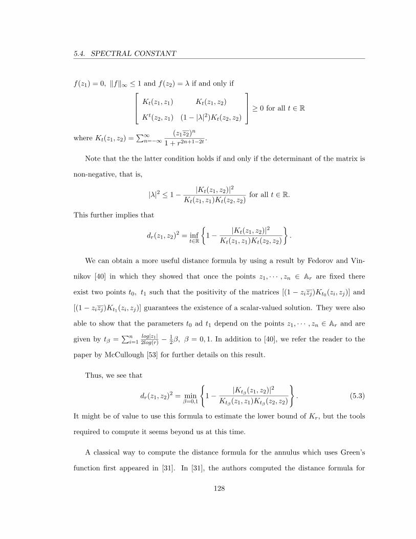
5.4. SPECTRAL CONSTANT
f(z1) = 0, ‖f‖∞ ≤ 1 and f(z2) = λ if and only if Kt(z1, z1) Kt(z1, z2)
Kt(z2, z1) (1− |λ|2)Kt(z2, z2)
≥ 0 for all t ∈ R
where Kt(z1, z2) =∑∞
n=−∞(z1z2)n
1 + r2n+1−2t.
Note that the the latter condition holds if and only if the determinant of the matrix is
non-negative, that is,
|λ|2 ≤ 1− |Kt(z1, z2)|2
Kt(z1, z1)Kt(z2, z2)for all t ∈ R.
This further implies that
dr(z1, z2)2 = inft∈R
1− |Kt(z1, z2)|2
Kt(z1, z1)Kt(z2, z2)
.
We can obtain a more useful distance formula by using a result by Fedorov and Vin-
nikov [40] in which they showed that once the points z1, · · · , zn ∈ Ar are fixed there
exist two points t0, t1 such that the positivity of the matrices [(1 − zizj)Kt0(zi, zj)] and
[(1− zizj)Kt1(zi, zj)] guarantees the existence of a scalar-valued solution. They were also
able to show that the parameters t0 ad t1 depend on the points z1, · · · , zn ∈ Ar and are
given by tβ =∑n
i=1log|z1|2log(r) −
12β, β = 0, 1. In addition to [40], we refer the reader to the
paper by McCullough [53] for further details on this result.
Thus, we see that
dr(z1, z2)2 = minβ=0,1
1−
|Ktβ (z1, z2)|2
Ktβ (z1, z1)Ktβ (z2, z2)
. (5.3)
It might be of value to use this formula to estimate the lower bound of Kr, but the tools
required to compute it seems beyond us at this time.
A classical way to compute the distance formula for the annulus which uses Green’s
function first appeared in [31]. In [31], the authors computed the distance formula for
128

5.4. SPECTRAL CONSTANT
the annulus A(1/R,R) which has inner radius 1/R and outer radius R and for the points
z1, z2 ∈ A(1/R,R) where 1/R < z1 < R. Later in [73], the authors computed the distance
formula dH∞(Ar)(ρ, z2) when r < ρ < 1 for the annulus Ar, by using the invariance of this
pseudohyperbolic distance under biholomorphic maps. Thus, from this result, we know
that the minimum in the Equation 5.3 is equal to this formula when z1 = ρ. Because of
the complicated form of dH∞(Ar)(ρ, z2), we only state it for a particular set of points in the
annulus.
For instance, take z1 =√
r, z2 =√
reiθ for some θ ∈ (0, 2π) then from the result that
appeared in [31], we have that
dH∞(Ar)(√
r,√
reiθ) = 2√
r√
2− 2cosθ
∞∏n=1
fngn(θ)
where fn =(
1 + r2n
1 + r2n−1
)2
and gn(θ) =1− 2r2ncosθ + r4n
1− 2r2n−1cosθ + r4n−2.
We now use this formula of dH∞(Ar) to estimate the lower bound of Kr.
Also, we know by Lemma 5.3.12 that
dr(z1, z2) =
ρ(rz−11 , rz2
−1) if |z1z2| ≤ r
ρ(z1, z2) if |z1z2| ≥ r.
Thus, for z1 =√
r, z2 =√
reiθ, we get that
dr(z1, z2) = ρ(√
r,√
reiθ) =
√r(2− 2cosθ)
1 + r2 − 2rcosθ.
Finally, we get that
Kr ≥ supz1 6=z2∈Ar
dH∞(Ar)(z1, z2)
dr(z1, z2)
≥ 2√
1 + r2 − 2rcosθ
∞∏n=1
fngn(θ) for every θ ∈ (0, 2π),
where fn and gn(θ) are as above.
129

5.4. SPECTRAL CONSTANT
In particular, if we take θ = π and θ = π/2 then after simplifying we get
Kr ≥ 2(1 + r)
( ∞∏n=1
1 + r2n
1 + r2n−1
)4
and
Kr ≥ 2√
1 + r2
∞∏n=1
(1 + r4n)(1 + r2n)2
(1 + r4n−2)(1 + r2n−1)2.
Calculating the lower bound of Kr requires us to estimate the lower bound of the infinite
product in the above equation. A simple calculation shows that the above bound is greater
than the existing lower bound, 21+r . Thus, as of this writing, the estimate 2
1+r is the best
known estimate. We are currently working on this problem. We believe that the above
approach together with the classical work done on infinite products and infinite series can
be worthy in finding a better estimate than 21+r .
We now present our second approach, albeit an abstract approach, to find an estimate
of the smallest spectral constant for the annulus. This involves hyperconvex sets which
were introduced in [27].
Let A ⊆ C(X) be a uniform algebra, fix a finite subset F = x1, x2, · · · , xn ⊆ X and
let IF denote the ideal of functions in A that vanish on the set F, IF = f ∈ A : f(zi) =
0 ∀ 1 ≤ i ≤ n. Cole, Lewis, and Wermer define the set
D(A;x1, · · · , xn) = (w1, w2, · · · , wn) : ‖f + IF ‖ ≤ 1, f(zi) = wi for every 1 ≤ i ≤ n.
Such sets were also called interpolation body. It was shown in [75] that this serves as
the natural coordinatization of the closed unit ball of the operator algebra A/IF . In [60],
Paulsen introduced the concept of matricial hyperconvex sets which serves as the natural
coordinatization of the closed unit ball of the operator algebra Mn(A/IF ). We now extend
these definitions for operator algebras of functions. Given an operator algebra of functions
130
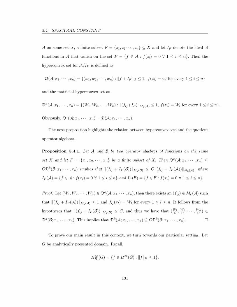
5.4. SPECTRAL CONSTANT
A on some set X, a finite subset F = z1, z2 · · · , zn ⊆ X and let IF denote the ideal of
functions in A that vanish on the set F = f ∈ A : f(zi) = 0 ∀ 1 ≤ i ≤ n. Then the
hyperconvex set for A/IF is defined as
D(A;x1, · · · , xn) = (w1, w2, · · · , wn) : ‖f + IF ‖A ≤ 1, f(zi) = wi for every 1 ≤ i ≤ n
and the matricial hyperconvex set as
Dk(A;x1, · · · , xn) = (W1,W2, · · · ,Wn) : ‖(fij+IF )‖Mk(A) ≤ 1, f(zi) = Wi for every 1 ≤ i ≤ n.
Obviously, D1(A;x1, · · · , xn) = D(A;x1, · · · , xn).
The next proposition highlights the relation between hyperconvex sets and the quotient
operator algebras.
Proposition 5.4.1. Let A and B be two operator algebras of functions on the same
set X and let F = x1, x2, · · · , xn be a finite subset of X. Then Dk(A;x1, · · · , xn) ⊆
CDk(B;x1, · · · , xn) implies that ‖(fij + IF (B))‖Mk(B) ≤ C‖(fij + IF (A))‖Mk(A), where
IF (A) = f ∈ A : f(xi) = 0 ∀ 1 ≤ i ≤ n and IF (B) = f ∈ B : f(xi) = 0 ∀ 1 ≤ i ≤ n.
Proof. Let (W1,W2, · · · ,Wn) ∈ Dk(A;x1, · · · , xn), then there exists an (fij) ∈ Mk(A) such
that ‖(fij + IF (A))‖Mk(A) ≤ 1 and fij(xl) = Wl for every 1 ≤ l ≤ n. It follows from the
hypotheses that ‖(fij + IF (B))‖Mk(B) ≤ C, and thus we have that (W1C , W2
C , · · · , WnC ) ∈
Dk(B;x1, · · · , xn). This implies that Dk(A;x1, · · · , xn) ⊆ CDk(B;x1, · · · , xn).
To prove our main result in this context, we turn towards our particular setting. Let
G be analytically presented domain. Recall,
H∞R (G) = f ∈ H∞(G) : ‖f‖R ≤ 1,
131

5.4. SPECTRAL CONSTANT
where ‖f‖ = sup‖f(T )‖ : T ∈ Q(G) and Q(G) is the quantized version of G. As a
shorthand, we write D∞(G; z1, . . . , zn) for D∞(H∞(G); z1, . . . , zn) and DR(G; z1, . . . , zn)
for DR(H∞(G); z1, . . . , zn). We define
kn(G; z1, . . . , zn) = infC : D∞(G; z1, . . . , zn) ⊆ CDR(G; z1, . . . , zn)
and
kn(G) = supkn(G; z1, . . . , zn) : z1, . . . , zn ⊆ G.
For the matrix-analogue, we define
kln(G; z1, . . . , zn) = infC : Dl
∞(G; z1, . . . , zn) ⊆ CDlR(G; z1, . . . , zn)
and
kln(G) = supkl
n(G; z1, . . . , zn) : z1, . . . , zn ⊆ G.
Let G be an analytically presented domain. Then in the view of the fact that σ(T ) ⊆ G
for every T ∈ Q(G), we redefine the notion of K-spectral set for analytically presented
domains.
Definition 5.4.2. An analytically presented domain G is called a joint complete K-spectral
set for Q(G) if ‖(fij)‖R ≤ K‖(fij)‖∞ for every (fij) ∈ Mn(H∞(G)). We call an analyt-
ically presented domain G a joint K-spectral set for Q(G) if ‖f‖R ≤ K‖f‖∞ for every
f ∈ H∞(G).
Clearly, the annulus is an example of a joint complete K-spectral set. It is known that
the intersection of two closed disks of the Riemann sphere is a K-spectral set. If we choose
an appropriate analytic presentation of a domain then the intersection of two closed disk
turn out to be a joint complete K-spectral set. For instance, the domain in Example 3.5.6
132
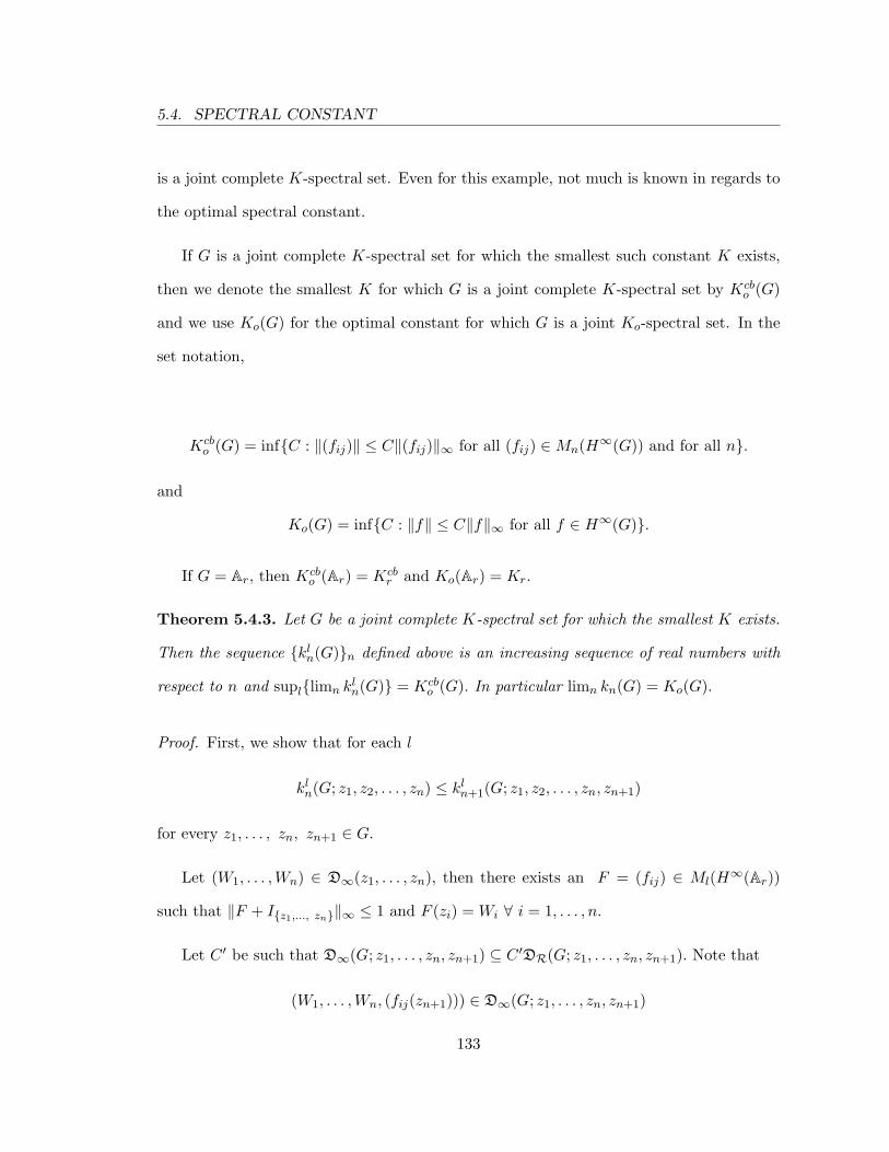
5.4. SPECTRAL CONSTANT
is a joint complete K-spectral set. Even for this example, not much is known in regards to
the optimal spectral constant.
If G is a joint complete K-spectral set for which the smallest such constant K exists,
then we denote the smallest K for which G is a joint complete K-spectral set by Kcbo (G)
and we use Ko(G) for the optimal constant for which G is a joint Ko-spectral set. In the
set notation,
Kcbo (G) = infC : ‖(fij)‖ ≤ C‖(fij)‖∞ for all (fij) ∈ Mn(H∞(G)) and for all n.
and
Ko(G) = infC : ‖f‖ ≤ C‖f‖∞ for all f ∈ H∞(G).
If G = Ar, then Kcbo (Ar) = Kcb
r and Ko(Ar) = Kr.
Theorem 5.4.3. Let G be a joint complete K-spectral set for which the smallest K exists.
Then the sequence kln(G)n defined above is an increasing sequence of real numbers with
respect to n and supllimn kln(G) = Kcb
o (G). In particular limn kn(G) = Ko(G).
Proof. First, we show that for each l
kln(G; z1, z2, . . . , zn) ≤ kl
n+1(G; z1, z2, . . . , zn, zn+1)
for every z1, . . . , zn, zn+1 ∈ G.
Let (W1, . . . ,Wn) ∈ D∞(z1, . . . , zn), then there exists an F = (fij) ∈ Ml(H∞(Ar))
such that ‖F + Iz1,..., zn‖∞ ≤ 1 and F (zi) = Wi ∀ i = 1, . . . , n.
Let C ′ be such that D∞(G; z1, . . . , zn, zn+1) ⊆ C ′DR(G; z1, . . . , zn, zn+1). Note that
(W1, . . . ,Wn, (fij(zn+1))) ∈ D∞(G; z1, . . . , zn, zn+1)
133

5.4. SPECTRAL CONSTANT
which further implies that there exists a function G = (gij) ∈ Ml(H∞R (Ar)) such that
‖(gij + Iz1,...,zn,zn+1)‖ ≤ C ′, G(zn+1) = F (zn+1) and G(zi) = Wi for every i = 1, . . . , n.
It is easy to see that the ideal of functions obey the containment rule, Iz1,...,zn ⊆
Iz1,...,zn,zn+1. This implies that ‖(gij + Iz1,...,zn)‖R ≤ ‖(gij + Iz1,...,zn,zn+1)‖R. Since
‖(gij + Iz1,...,zn,zn+1)‖R ≤ C ′, we get that ‖(gij + Iz1,...,zn)‖R ≤ C ′.
It follows from fij − gij ∈ Iz1,...,zn for every i, j that ‖(fij + Iz1,...,zn)‖R = ‖(gij +
Iz1,...,zn)‖R ≤ C ′. Thus, we find that ‖(fij +Iz1,...,zn)‖R ≤ C ′ which further implies that
Dl∞(G; z1, · · · , zn) ⊆ C ′Dl
R(G; z1, · · · , zn) for every l. From this, we get kln(G; z1, z2, . . . , zn) ≤
C ′ for every C ′ that satisfies
Dl∞(G; z1, · · · , zn, zn+1) ⊆ C ′Dl
R(G; z1, · · · , zn, zn+1).
By taking the infimum over all such C ′, we obtain
kln(G; z1, . . . , zn) ≤ kl
n+1(G; z1, . . . , zn, zn+1)
for every z1, . . . , zn ⊆ G and for every l. This proves that kln(G)n is an increasing
sequence of positive real numbers for every l.
Lastly, we need to prove supllimn kln(G) = Kcb
o (G). Obviously, we have that
Dl∞(G; z1, · · · , zn) ⊆ kl
nDlR(G; z1, · · · , zn).
It is easy to see that each kln(G) is bounded above by Kcb
o (G) which is a finite number by
the assumption. Therefore, limn kln(G) = supn kl
n(G) ≤ Kcbo (G) for every l.
By Proposition 5.4.1, we see that
‖(fij + IF )‖R ≤ supn
kln(G)‖(fij + IF )‖R
134
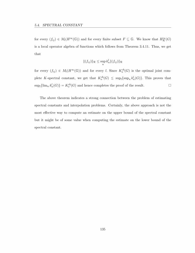
5.4. SPECTRAL CONSTANT
for every (fij) ∈ Ml(H∞(G)) and for every finite subset F ⊆ G. We know that H∞R (G)
is a local operator algebra of functions which follows from Theorem 3.4.11. Thus, we get
that
‖(fij)‖R ≤ supn
kln‖(fij)‖R
for every (fij) ∈ Ml(H∞(G)) and for every l. Since Kcbo (G) is the optimal joint com-
plete K-spectral constant, we get that Kcbo (G) ≤ suplsupn kl
n(G). This proves that
supllimn kln(G) = Kcb
o (G) and hence completes the proof of the result.
The above theorem indicates a strong connection between the problem of estimating
spectral constants and interpolation problems. Certainly, the above approach is not the
most effective way to compute an estimate on the upper bound of the spectral constant
but it might be of some value when computing the estimate on the lower bound of the
spectral constant.
135
Bibliography
[1] M. Abrahamse, The Pick interpolation theorem for finitely connected domains, Mich.Math. J. 26(2), 195–203, 1979.
[2] J. Agler, Some interpolation theorems of Nevanlinna-Pick type, preprint, 1988.
[3] J. Agler, On the representation of certain holomorphic functions defined on a polydisk,Topics in Operator Theory: Ernst D. Hellinger Memorial Volume 48, 47–66, 1990.
[4] J. Agler, An abstract approach to model theory, Surveys of some recent results inoperator theory, Vol. II, Pitman Research Notes in Mathematics Series 192, JohnWiley and Sons, New York, 1–23, 1988.
[5] J. Agler and J.E. McCarthy, Pick interpolation and Hilbert function spaces, GraduateStudies in Mathematics, Vol. 44, American Mathematical Society, Providence, RhodeIsland, 2002.
[6] J. Agler and J.E. McCarthy, Nevanlinna-Pick kernels and localization, Operator the-oretical methods (Timioara, 1998), Theta Found., Bucharest, 1–20, 2000.
[7] J. Agler and J.E. McCarthy, Complete Nevanlinna-Pick kernels, J. Funct. Anal.175(1), 111–124, 2000.
[8] L. V. Ahlfors, Complex analysis, third ed., McGraw-Hill, 1979.
[9] D. Alpay, A. Dijksma, J. Rovnyak and H. de Snoo, Schur functions, operator col-ligation, and reproducing kernel Pontryagin spaces, Operator Theory Advances andApplications 96, Birkhauser, Basel, 1–13, 1997.
[10] C.G. Ambrozie and D. Timotin, A von Neumann type inequality for certain domainsin Cn, Proc. Amer. Math. Soc. 131(3), 859–869, 2003.
[11] M. Andersson and S. Sandberg, A constructive proof of the composition rule for Tay-lor’s functional calculus, Studia Math. 142(1), 65–69, 2000.
136

BIBLIOGRAPHY
[12] T. Ando, On a pair of commutative contractions, Acta Sci. Math. (Szeged) 24, 88–90,1963.
[13] R. J. Archbold, On residually finite-dimensional C∗-algebras, Proc. Amer. Math. Soc.123(9), 2935–2937, 1995.
[14] W. Arveson, Subalgebras of C∗-algebras. II., Acta Math. 123, 271–308, 1972.
[15] W. Arveson, Subalgebras of C∗-algebras. III., Acta Math. 181(2), 159–228, 1998.
[16] C. Badea, B. Beckermann and M. Crouzeix, Intersections of several disks of the Rie-mann sphere as K-spectral sets, Commun. Pure Appl. Anal. 8(1), 37–54, 2009.
[17] J.A. Ball and V. Bolotnikov, Realization and interpolation for Schur-Agler-class func-tions on domains with matrix polynomial defining functions in Cn, J. Funct. Anal.213(1), 45–87, 2004.
[18] J.A. Ball, W.S. Li, D. Timotin and T.T. Trent, A commutant lifting theorem on thepolydisc, Indiana Univ. Math. J. 48(2), 653–675, 1999.
[19] J.A. Ball and T.T. Trent, Unitary colligations, reproducing kernel Hilbert spaces andNevanlinna-Pick interpolation in several variables, J. Funct. Anal. 197, 1–61, 1998.
[20] H.S. Bear, Lectures on Gleason parts, Lecture Notes in Mathematics, Vol. 121,Springer-Verlag, Berlin, 1970.
[21] B. Beckermann, M. Crouzeix, A lenticular version of a von Neumann inequality, Arch.Math. (Basel) 86(4), 352–355, 2006.
[22] B. Blackadar, Operator algebras. Theory of C∗-algebras and von Neumann alge-bras, Encyclopaedia of Mathematical Sciences 122, Operator Algebras and Non-commutative Geometry III, Springer-Verlag, Berlin, 2006.
[23] D.P. Blecher and C. Le Merdy, Operator algebras and their modules–an operator spaceapproach, Oxford Univ. Press, Oxford, 2004.
[24] D.P. Blecher and V.I. Paulsen, Explicit construction of universal operator algebras andan application to polynomial factorization, Proc. Amer. Math. Soc. 112(3), 839–850,1991.
[25] D.P. Blecher, Z.J. Ruan, A.M. Sinclair, A characterization of operator algebras, J.Funct. Anal. 89, 188–201, 1990.
[26] J. Burbea and P. Masani, Banach and Hilbert spaces of vector-valued functions. Theirgeneral theory and applications to holomorphy, Research Notes in Mathematics 90,Pitman (Advanced Publishing Program), Boston MA, 1984.
137

BIBLIOGRAPHY
[27] B.J. Cole, K. Lewis and J. Wermer, Pick conditions on a uniform algebra and vonNeumann inequalities, J. Funct. Anal. 107(2), 235–254, 1992.
[28] B.J. Cole and J. Wermer, Pick interpolation, von Neumann inequalities, and hyper-convex sets, Complex Potential Theory, Kluwer Acad. Publ., Dordrecht, 89–129, 1994.
[29] J.B. Conway, A course in functional analysis, Second edition, Graduate Texts in Math-ematics 96, Springer, 1990.
[30] J.B. Conway, Functions of one complex variable I, Springer-Verlag, New York, 1978.
[31] R. Courant and D. Hilbert, Methods of Mathematical Physics, Vol. I, IntersciencePublishers, Inc., New York, N.Y., 1953.
[32] R.E. Curto, Applications of several complex variables to multiparameter spectral the-ory, Surveys of recent results in operator theory, Vol. II, Pitman Res. Notes Math.Ser., 192, Longman Sci. Tech., Harlow, 25–90, 1988.
[33] M. Dadarlat, Residually finite dimensional C∗-algebras, Operator algebras and oper-ator theory (Shanghai, 1997), Contemp. Math., 228, Amer. Math. Soc., Providence,R.I., 45–50, 1998.
[34] K.R. Davidson, V.I. Paulsen, M. Raghupathi and D. Singh, A constrained Nevanlinna-Pick interpolation problem, Indiana Univ. Math. J. 58(2), 709–732, 2009.
[35] K.R. Davidson and D. Pitts, Nevanlinna-Pick interpolation for non-commutative an-alytic Toeplitz algebras, Integral Equations Operator Theory Integral Equations Op-erator Theory 31(3), 321–337, 1998.
[36] R.G. Douglas and V.I. Paulsen, Completely bounded maps and hypo-Dirichlet algebras,Acta Sci. Math. (Szeged) 50(1-2), 143–157, 1986.
[37] M. A. Dritschel and S. McCullough, Model theory for hyponormal contractions, Inte-gral Equations Operator Theory 36(2), 182–192, 2000.
[38] M. A. Dritschel, S. McCullough and H. J. Woerdeman, Model theory for ρ-contractions, ρ < 2, J. Operator Theory 41(2), 321–350, 1999.
[39] S.W. Drury, A generalization of von Neumann’s inequality to the complex ball, Proc.Amer. Math. Soc. 68(3), 300–304, 1978.
[40] S. Federov and V. Vinnikov, On the Nevanlinna-Pick interpolation problem in multiplyconnected domains, J. of Math. Sci. 105(4), 2109–2126, 2001.
[41] C. Foias and B. Sz.-Nagy, Commutants de certains operateurs, Acta Sci. Math.(Szeged) 29, 1–17, 1968.
138
BIBLIOGRAPHY
[42] K. R. Goodearl and P. Menal, Free and residually finite-dimensional C∗-algebras, J.Funct. Anal. 90(2), 391–410, 1990.
[43] A. Grinshpan, D. Kaliuzhnyi-Verbovetskyi, V. Vinnikov, and H. Woerdeman, Classesof tuples of commuting contractions satisfying the multivariable von Neumann inequal-ity, J. Funct. Anal. 256(9), 3035–3054, 2009.
[44] M. Hamana, Injective envelopes of operator systems, Publ. Res. Inst. Math. Sci. 15(3),773–785, 1979.
[45] K. Hoffman, Banach spaces of analytic functions, Prentice-Hall, Englewood Cliffs, N.J. , 1962.
[46] R.A. Horn and C. R. Johnson, Matrix Analysis, Cambridge University Press, Cam-bridge, 1985.
[47] M. Jarnicki, P. Pflug, Invariant Distances and Metrics in Complex Analysis, deGruyter Expositions in Mathematics 9, Walter de Gruyter & Co., Berlin, 1993.
[48] D. Kalyuzhnyi-Verbovetzkii, On the Bessmertnyi class of homogeneous positive holo-morphic functions of several variables, Current trends in operator theory and its ap-plications, 255–289, 2004.
[49] A. Koranyi and B.Sz.-Nagy, Relations dun Probleme de Nevanlinna et Pick avec laTheorie des Operateurs de Lespace Hilbertien, Acta Math. Acad. Sci. Hungar. 7, 295–303, 1957.
[50] S. G. Krantz, Function theory of several complex variables, second edition, Wadsworth& Brooks/Cole Mathematics series, 1992.
[51] S. Lata, M. Mittal and V.I. Paulsen, An operator algebraic proof of Agler’s factoriza-tion theorem, Proc. Amer. Math. Soc. 137(11), 3741–3748, 2009.
[52] B.A. Lotto and T. Steger, von Neumann’s inequality for commuting diagonalizablecontractions. II, Proc. Amer. Math. Soc. 120(3), 897–907, 1994.
[53] S. McCullough, Isometric representations of some quotients of H∞ of an annulus,Integral Equations Operator Theory 39(3), 335–362, 2001.
[54] S. McCullough and V.I. Paulsen, C∗-envelopes and interpolation theory, Indiana Univ.Math. J. 51(2), 479–505, 2002.
[55] M. Mittal and V.I. Paulsen, Operator algebras of functions, J. of Funct. Anal. 258(9),3195–3225, 2010.
[56] T. Nakazi and K. Takahashi, Two-dimensional representations of uniform algebras,Proc. Amer. Math. Soc. 123(9), 2777–2784, 1995.
139

BIBLIOGRAPHY
[57] R. Nevanlinna, Uber beschrankte Funktionen die in gegebenen Punkten vor-geschriebene Werte annehmen, Ann. Acad. Sci. Fenn. 13(1), 1–72, 1919.
[58] R. Nevanlinna, Uber beschrankte analytische Funktionen, Ann. Acad. Sci. Fenn. SerA 32(7), 1929.
[59] V.I. Paulsen, Toward a theory of K-spectral sets, “Surveys of Some Recent Results inOperator Theory”, Vol. I, 221–240, Pitman Res. Notes Math. Series, 171, LongmanSci. Tech., Harlow, 1988.
[60] V. I. Paulsen, Matrix-valued interpolation and hyperconvex sets, Integral EquationsOperator Theory 41(1), 38–62, 2001.
[61] V.I. Paulsen, Operator algebras of idempotents, J. Funct. Anal. 181, 209–226, 2001.
[62] V.I. Paulsen, Completely bounded maps and operator algebras, Cambridge studies inAdvanced Mathematics, Vol. 78, 2002.
[63] V. I. Paulsen, An introduction to the theory of reproducing kernel Hilbert spaces, un-published manuscript.
[64] V.I. Paulsen and M. Raghupathi, Representations of logmodular algebras, Trans. Amer.Math. Soc., to appear.
[65] G.B. Pedrick, Theory of reproducing kernels in Hilbert spaces of vector-valued func-tions, Univ. of Kansas Tech. Rep. 19, Lawrence, 1957.
[66] G. Pick, Uber die Beschrankungen analytischer Funktionen, welche durch vorgegebeneFunktionswerte bewirkt werden, Math Ann. 77(1), 7–23, 1915.
[67] G. Pisier, Introduction to operator space theory, London Mathematical Society LectureNote Series 294, Cambridge University Press, Cambridge, 2003.
[68] G. Popescu, Interpolation problems in several variables, J. Math. Anal. Appl. 227(1),227–250, 1998.
[69] D. Sarason, Generalized interpolation in H∞, Trans. Amer. Math. Soc. 127, 179–203,1967.
[70] D. Sarason, Notes on complex function theory, Texts and Readings in Mathematics 5,Hindustan Book Agency, New Delhi, 1994.
[71] I. Schur, Uber Potenzreihen, die im Innern des Einheitskreises beschrankt sind I, J.Reine Angew. Math. 147, 205–232, 1917.
[72] I. Schur, Uber Potenzreihen, die im Innern des Einheitskreises beschrankt sind II, J.Reine Angew. Math. 148, 122–145, 1918.
140

BIBLIOGRAPHY
[73] A. Schuster, The maximum principle for the Bergman Space and the Mobius pseu-dodistance for the annulus, Proc. Amer. Math. Soc.134(12), 3525–3530, 2006.
[74] A. L. Shields, Weighted shift operators and analytic function theory, Topics in operatortheory, 49–128, Math. Surveys, No. 13, Amer. Math. Soc., Providence, R.I., 1974.
[75] J. Solazzo, Interpolation and computability, Ph.D. Thesis, University of Houston, 2000.
[76] B. Sz.-Nagy, Sur les contractions de l’espace de Hilbert, Acta Sci. Math. (Szeged) 15,87–92, 1953.
[77] J.L. Taylor, A joint spectrum for several commuting operators, J. Funct. Anal. 6,172–191, 1970.
[78] J.L. Taylor, The analytic-functional calculus for several commuting contractions, ActaMath. 125, 1–38, 1970.
[79] J.L. Taylor, Analytic functional calculus and spectral decompositions, Math. and itsAppl.(East European Series), 1, D. Reidel Publishing Co. Dordrecht, Bucharest, 1982.
[80] N. Varopoulos, Sur une inequalite de von Neumann, C. R. Acad. Sci. Paris, Ser A-B277, A19–A22, 1973.
[81] J. von Neumann, Eine Spektraltheorie fur allgemeine Operatoren eines unitarenRaumes, Math. Nachr. 4, 258– 281, 1951.
[82] K. Zhu, An introduction to operator algebras, Studies in Advanced Mathematics, CRCPress, 1993.
141
Related Documents