Fully Distributed Zonal Statistics of Big Raster + Vector Data

Raptor Zonal Statistics: Fully Distributed ZonalStatistics of Big Raster + Vector Data

Samriddhi SinglaComputer Science and EngineeringUniversity of California, Riverside

[email protected]

Ahmed EldawyComputer Science and EngineeringUniversity of California, Riverside

[email protected]

Abstract—Recent advancements in remote sensing technologyhave resulted in petabytes of data in raster format. This data isoften processed in combination with high resolution vector datathat represents, for example, city boundaries. One of the commonoperations that combine big raster and vector data is the zonalstatistics which computes some statistics for each polygon in thevector dataset. This paper proposes a novel distributed system tosolve the zonal statistics problem which can scale to petabytes ofraster and vector data. The proposed method does not requireany preprocessing or indexing which makes it perfect for ad-hocqueries that scientists usually want to run. We devise a theoreticalcost model that proves the efficiency of our algorithm over thebaseline method. Furthermore, we run an extensive experimentalevaluation on large scale satellite data with up-to a trillion pixels,and big vector data with up-to hundreds of millions of edges, andwe show that our method can perfectly scale to big data withup-to two orders of magnitude performance gain over Rasdamanand Google Earth Engine.

Index Terms—Big Spatial Data, Zonal Statistics, SatelliteImagery, Raster data, Vector data

I. INTRODUCTION

Advancements in remote sensing technology have led to atremendous increase in the amount of remote sensing data.For example, NASA EOSDIS provides public access to morethan 33 petabytes of Earth Observational data and is estimatedto grow to more than 330 petabytes by 2025 [1]. EuropeanSpace Agency (ESA) has collected over five petabytes of datawithin two years of the launch of the Sentinel-1A satelliteand is expected to receive data continuously until 2030 [2].This big remote sensing data is available as raster data whichis represented as multidimensional arrays. Many applicationsneed to combine the raster data with vector data which isrepresented as points, lines, and polygons. This paper studiesthe zonal statistics problem which combines raster data, e.g.,temperature, with vector data, e.g., city boundaries, to computeaggregate values for each polygon, e.g., average temperature ineach city. This problem has several applications including thestudy by ecologists on the effect of vegetation and temperatureon human settlement [3], [4], analyzing terabytes of socio-economic and environmental data [5], [6], and studying of

This work is supported in-part by USDA National Institute of Food andAgriculture Grants no. 2019-67022-29696 and 2020-69012-31914

land use and land cover classification [7]. It can also be usedfor areal interpolation [8] and to assess the risk of wildfires [9].

There exist many big spatial data systems which eitherefficiently process big vector data, e.g., SpatialHadoop [10],GeoSpark [11], and Simba [12], or big raster data, e.g.,SciDB [13], RasDaMan [14], GeoTrellis [15], and GoogleEarth Engine [16]. Unfortunately, none of these systems arewell-equipped to combine raster and vector data together andthey all become very inefficient for the zonal statistics problemfor big raster and vector data.

Traditional methods to process the zonal statistics problemfocus on either vectorizing the raster dataset [17] or rasterizingthe vector data [5], [18]. The first approach converts eachpixel to a point and then runs a traditional spatial join withpolygons using a point-in-polygon predicate [17]. Finally, itgroups the pixels by polygon ID and computes the desiredaggregate function. This algorithm suffers from the big com-putation overhead of the the point-in-polygon query. Even ifthe polygons are indexed, this algorithm is still impractical.Furthermore, when the vector data is very large, a disk-basedindex is needed which makes this algorithm even slower. Thesecond approach rasterizes the vector data by converting eachpolygon to a raster (mask) layer with the same resolutionas the input raster layer and then combines the two rasterlayers to compute the desired aggregate function [5], [18].This algorithm suffers from the computation overhead of therasterization step and the disk overhead of randomly accessingthe pixels that overlap each polygon.

To further show the limitation of the baseline algorithm, thispaper provides a theoretical analysis of the two existing ap-proaches by making an analogy to traditional join algorithms.First, we show that the vector-based approach resembles anindex nested loop join which suffers from the repetitive accessof the index. This means that it should be used only if thenon-indexed dataset is very small, i.e., the raster dataset. Onthe other hand, the raster-based approach resembles a hash-join algorithm which suffers from the excessive size of thehashtable, i.e., the number of pixels. This reveals that thisalgorithm would work well if the number of pixels that overlapthe polygons is very small.

This paper proposes a fully distributed algorithm, termedRaptor Zonal Statistics (RZS), which overcomes the limi-tations of the two baseline algorithms. RZS overcomes the978-1-7281-6251-5/20/$31.00 © 2020 IEEE

limitations of existing algorithms since it scans the rasterdata sequentially while aggregating pixels without running anypoint-in-polygon queries. The key idea is to generate an in-termediate structure, termed intersection file, which accuratelymaps vector polygon to raster pixels. Further, this intersectionfile is sorted in a way that matches the raster file structurewhich optimizes the disk access to raster data, hence, speedsup the algorithm; this results in a linear-time algorithm formerging raster and vector data that is analogous to sort-merge.In general, the proposed algorithm runs in three steps, namely,intersection, selection and aggregation. The intersection steppartitions the vector data and generates the intersection filethat contains a compact representation of the intersection of thevector and raster datasets. The intersection file is then sorted tomatch the raster file by only reading the metadata of the rasterfile, e.g., resolution and tile size, i.e., without reading the pixelvalues. The selection step concurrently scans the intersectionfile and the raster file to produce the set of 〈polygon ID,pixel value〉 pairs. To run this step, we introduce two newcomponents, RaptorInputFormat and RaptorSplit, that allowsthis step to read both raster and vector data and process themin parallel. Finally, the aggregation step groups these pairsby polygon ID and calculates the desired aggregate function.A previous work (presented as a poster [19]) proposed astraight-forward parallelization of an efficient single-machinealgorithm [20], [21] which showed some promising results butwas limited since it used the single-machine algorithm as ablack-box. In this paper, we redesign the algorithm to make itfully distributed and we make a cost analysis to theoreticallyprove its efficiency over the baselines.

Experiments on real datasets, with nearly a trillion pixelsand 330 million polygon segments, show that the proposedalgorithm (RZS) outperform all baselines for big data, includ-ing Rasdaman and Google Earth Engine, and show perfectscalability with large data and big clusters. Furthermore, RZSis up-to 100× faster in data loading since it does not requireany preprocessing while baseline systems need a heavy dataloading phase to organize the data for efficient processing.

The rest of this paper is organized as follows. Section IIcovers the related work in literature. Section III describesthe proposed system, Raptor Zonal Statistics. Section IVprovides a theoretical analysis and comparison of the proposedapproach as well as the raster-based baseline. Section V pro-vides an extensive experimental evaluation. Finally, Section VIconcludes the paper.

II. RELATED WORK

In this section, we cover the relevant work in the literature.First, we give an overview of big spatial data systems andclassify them according to whether they primarily target vectordata, raster data, or both. After that, we cover the work thatspecifically targets the zonal statistics problem.

A. Big Vector Data

In this research direction, some research efforts aimed toprovide big spatial data solutions for vector data types and

operations. There are several systems in this category includingSpatialHadoop [10], Hadoop-GIS [22], MD-HBase [23], Esrion Hadoop [24], GeoSpark [11], and Simba [12], amongothers. The work in this category covers (1) spatial indexessuch as R-tree [10]–[12], Quad-tree [23], [24], and grid [10],(2) spatial operations such as range query [10]–[12], [23],[24], k nearest neighbor [10]–[12], [23], spatial join [10]–[12],and computational geometry [25], (3) spatial data visualizationincluding single-level and multilevel [26], and (4) high-levelprogramming languages such as Pigeon [27].

Vector-based systems can support the zonal statistics prob-lem by utilizing the index-nested loop join operation withthe point-in-polygon predicate. Shahed [28] further improvesthis query by building an aggregate Quad-tree index for theraster layer but it only supports rectangular regions while thispaper considers complex polygons without the need to prebuildan index. When it comes to complicated polygons and high-resolution raster data, all these techniques become impractical.

B. Big Raster Data

Systems in this research direction focus on processingraster datasets which are represented as multidimensionalarrays. Popular systems include SciDB [13], RasDaMan [14],GeoTrellis [15], and Google Earth Engine [16]. The set ofoperations supported for raster datasets are completely differ-ent from those provided for vector datasets. They are usuallycategorized into four categories, namely, local, focal, zonal,and global operations [29] and the computational model isbased on linear algebra.

To support the zonal statistics operation in these systems,each polygon is first rasterized to create a mask layer. Then,the mask layer is combined with the input raster layer toselect overlapping pixels which are finally aggregated. Thisprocess is repeated for each polygon separately since thepolygons might be overlapping in the mask layer. There aretwo drawbacks to this approach. First, if the raster data hasa very high resolution, the size of each mask layer canbe excessively large. Second, for nearby and overlappingpolygons, this algorithm will need to read the same regions ofthe raster data many times. A parallel algorithm can be usedfor efficient rasterization [30] but this does not address the twolimitations described above.

C. Big Raster-Vector Combination

Systems like PostGIS and QGIS [31] can work with bothvector and raster data but they internally use two isolatedlibraries, one for each type, and they are still limited to theapproaches described above for the zonal statistics problem.Other research suggests an alternative data representation forvector and raster data [32], [33] that can speed up somequeries that combine both data types. However, these methodsare impractical since they require an expensive preprocessingphase for rewriting and indexing all the data. On the otherhand, the proposed approach does not require any indexconstruction while achieving a better query performance.

Vector Data

Raster Data

1-Intersection Step

Metadata

VectorChunks

Raptor SplitsIntersectionFiles

3-Aggregation Step2-Selection Step

Intersections

〈pi,m〉{ }

〈pi,m〉{ }

〈pi,m〉{ }

PartialAggregates

〈pi,Σm〉{ }

〈pi,Σm〉{ }

〈pi,Σm〉{ }

FinalAggregates

<p1,Σm>...

<p2,Σm>

<pn,Σm>

Fig. 1: Overview of the Raptor Zonal Statistics (RZS) algorithm

D. Zonal Statistics

The zonal statistics problem is a basic problem that isused in several domains including ecology [3], [4] and ge-ography [5], [6]. However, there was only a little work inthe query processing aspect of the problem. ArcGIS [18]supports this query by first rasterizing the polygons datasetand then overlaying it with raster dataset which resembles ahash-join. Zhang et al. [17], [34] solve the zonal statisticsproblem using an algorithm that resembles the index nested-loop join. It converts each pixel to a point and relies on GPUsto speed up the calculation. The drawback is that it has toload the entire raster dataset in GPU memory which is a veryexpensive operation and is impractical for very large rasterdatasets. Zhao et al. [35] aimed at increasing the performanceof existing zonal statistics method using python in a sharedmemory multi-processor system. That method utilizes threadsby sending each thread a set of files of raster dataset andrequires rasterizing the polygon dataset as a separate step.

Recent work in Terra Populus [5], [6] demonstrate the com-plexity of the problem on big raster and big vector datasets.The Scanline algorithm [20], [21] was a first step in efficientlyprocessing the zonal statistics problem by combining vectorand raster data but it was limited to a single machine. In [19](a poster), we tried a straight-forward parallelization of theScanline approach that showed some performance improve-ment but it was limited as it used Scanline as a black-box.In particular, it only parallelized the second phase that readsthe raster data but still processes the vector data on a singlemachine which made it limited to small vector data.

This paper proposes a novel scalable algorithm that fol-lows a sort-merge approach for processing the zonal statisticsproblem on big raster and vector data using MapReduce. Itis different than the work described above in four ways. 1) Itleverages the MapReduce programming paradigm to scale outon multiple machines. 2) It is a fully distributed approachto the zonal statistics problem which allows it to scale tobig raster and vector data. 3) It provides a novel mechanismfor parallel task distribution that combines raster-plus-vector(Raptor) in one unit of work. 4) It can efficiently prune non-rel-evant parts in the raster layer to speed up query processing.

III. RAPTOR ZONAL STATISTICS (RZS)

This section describes the proposed Raptor Zonal Statis-tics (RZS) algorithm that follows a sort-merge approach tocombine raster and vector data and answer the zonal statisticsquery. By observing the analogy between the two baselineapproaches and the two join algorithms, hash join and indexnested loop, the reader can see why neither of them scalesto big raster and vector data. The rasterization approach doesnot scale due to the large number of pixels that overlap thepolygons which needs to be retrieved from disk and decom-pressed. The vectorization approach does not scale either dueto the overwhelming computation cost of index lookups or thelarge size of the index which has to be stored on disk. Thismakes us think of using a sort-merge-like algorithm, however,it requires an expensive sorting phase which outweighs thesaving in the merge step. We show below that we can minimizethe overhead of the sorting phase using a novel data structurenamed, intersection file.

Raster data is inherently sorted, the pixels can be indexedbased on the tiles in the raster layer to which they belongas well as based on their row and column numbers. Hence,the key idea of the proposed algorithm is that we exploitthis internal structure of the raster data, and produce anintermediate compact representation of the vector data, calledintersection file, which perfectly matches the order of the rasterdata. Furthermore, to produce the intersection file, we onlyneed to process the vector layer and the metadata of the rasterlayer which means that the raster dataset needs to be scannedonly once. Finally, the intersection file is generated and storedin a distributed fashion which allows the proposed algorithmto be parallelized over a cluster of machines.

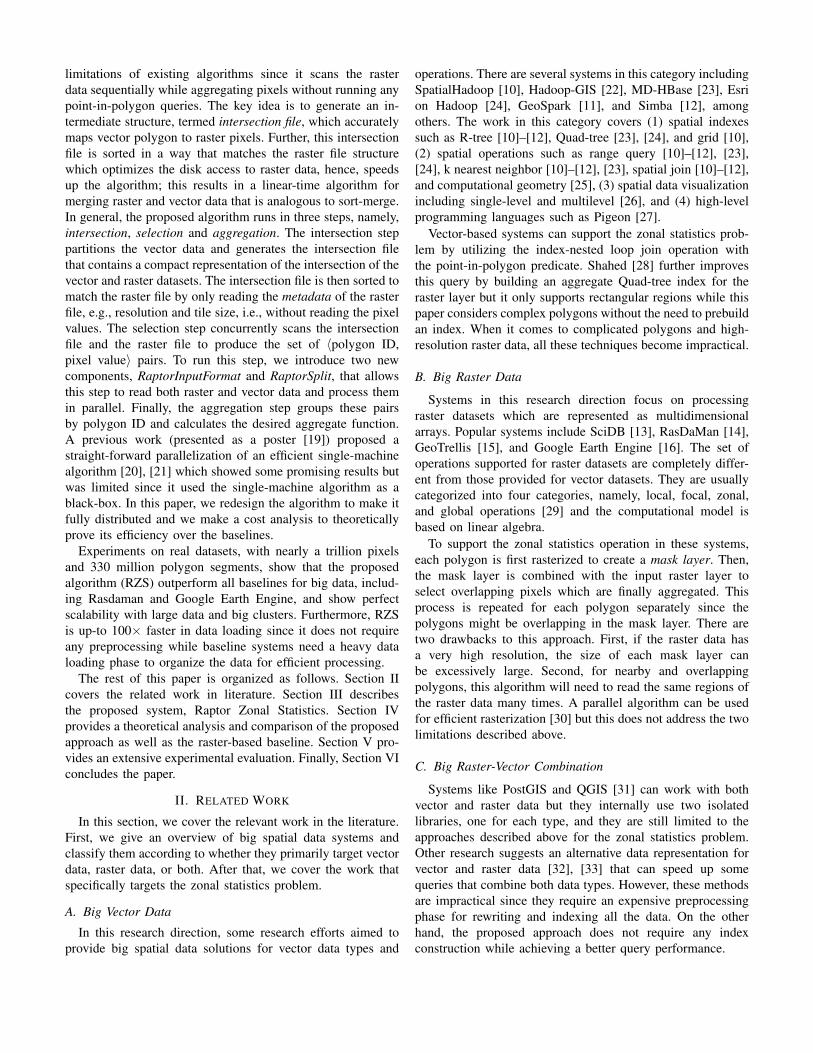
This algorithm as shown in Figure 1 runs in three steps,namely, intersection, selection, and aggregation. The intersec-tion step computes the intersection file which captures theintersections between the vector and raster data and sortsthese intersections to match the raster data. The selection stepuses the intersection file to read the pixels in the raster layerthat intersect each polygon in the vector layer. Finally, theaggregation step groups the pixel values by polygon ID andcomputes the desired aggregate function, e.g., average. Thedetails of the three steps are given below.

A. Step 1: Intersection

This step runs as a map-only job and is responsible forintersection file generation. It takes as input the vector layerand the metadata of the raster layer and computes a com-mon structure, called intersection file, which is stored in thedistributed file system to be used in the selection step. Thevector layer consists of a set of polygons each represented asa list of straight line segments. The metadata of the raster layerconsists of the dimensions (number of rows and columns), twoaffine matrix transformations G2W and W2G (which definemapping from raster to vector layer and vice-versa), and thesize of each tile in the raster layer, i.e., number of rows andcolumn, and is only a few kilobytes.

The input vector layer is partitioned into fixed-size chunks,128 mb by default, and each chunk is assigned to onetask. While any partitioning technique works fine, we em-ploy the R*-Grove partitioning technique [36] which maxi-mizes the spatial locality of partitions while ensuring loadbalance. In Spark, each chunk can be processed using themapPartitions transformation while in Hadoop it can beprocessed as a map task using the run method.

For each chunk, this step computes all the intersectionsbetween each row in the raster layer and each segment of eachpolygon in the vector layer. To compute these intersections,each line segment is mapped to the raster layer using theW2G transformation to find the range of rows that it intersects.Then, it is a simple constant-time computation to find the x-coordinate of the intersection. Since we only need to knowthe intersection at the pixel level, the intersection is mappedto the raster space and the integer coordinate of the pixel iscomputed. We record the intersection as the triple 〈pid, x, y〉where pid is the polygon ID to which the segment belongsand (x, y) is the coordinate of the intersection in the rasterlayer. All these triplets are kept in memory and can be spilledto disk if needed.

After all the intersections are computed, we run a sort-ing phase which sorts the intersections lexicographically by(tid, y, pid, x)

1, where tid is the raster tile ID that contains theintersection. Notice that the raster tile ID does not have to beexplicitly stored since it can be computed in a constant timefor each intersection using the metadata of the raster layer.

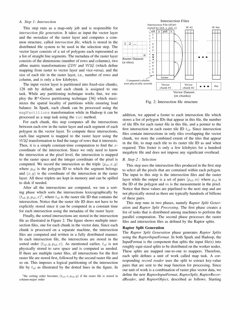
Finally, the sorted intersections are stored in the intersectionfile as illustrated in Figure 2. The figure shows multiple inter-section files, one for each chunk in the vector data. Since eachchunk is processed on a separate machine, the intersectionfiles are computed and written in a fully distributed manner.In each intersection file, the intersections are stored in thesorted order (tid, y, pid, x). As mentioned earlier, tid is notphysically stored to save space and is computed as needed.If there are multiple raster files, all intersections for the firstraster file are stored first, followed by the second raster file andso on. This imposes a logical partitioning of the intersectionfile by tid as illustrated by the dotted lines in the figure. In

1the sorting order becomes (tid, x, pid, y) if the raster file is stored incolumn-major order

Vector Dataset (m chunks)

Raster Dataset(n tiles)

Intersection Files

Vectorchunk #1

Intersection File (IF)#1sorted by (tid, y, pid, x)

footer

pid xytid11

222

nnnn

Computed column (not physically stored)

#m

IF #2 IF #m

Vectorchunk #2

1 2

n

...

Fig. 2: Intersection file structure

addition, we append a footer to each intersection file whichstores a list of polygon IDs that appear in this file, the numberof tile IDs for each raster file in this file, and a pointer to thefirst intersection in each raster tile ID tid. Since intersectionfiles contain intersections in only tiles overlapping the vectorchunk, we store the combined extent of the tiles that appearin the file, to map each tile to its raster tile ID as and whenrequired. This footer is only a few kilobytes for a hundredmegabyte file and does not impose any significant overhead.

B. Step 2 : Selection

This step uses the intersection files produced in the first stepto select all the pixels that are contained within each polygon.The input to this step is the intersection files and the rasterlayer while the output is a set of pairs 〈pid,m〉 where pid isthe ID of the polygon and m is the measurement in the pixel.Notice that these values are pipelined to the next step and arenot physically stored as there are typically hundreds of billionsof these pairs.

This step runs in two phases, namely Raptor Split Gener-ation and Raptor Split Processing. The first phase creates alist of tasks that is distributed among machines to perform theparallel computation. The second phase processes the rasterfiles and intersection files as defined by the Raptor splits.

Raptor Split GenerationThe Raptor Split Generation phase generates Raptor Splitsusing the RaptorInputFormat. In both Spark and Hadoop, theInputFormat is the component that splits the input file(s) intoroughly equi-sized splits to be distributed on the worker nodes.These splits are mapped one-to-one to mappers. Therefore,each split defines a unit of work called map task. A cor-responding record reader uses the split to extract key-valuepairs that are sent to the map function for processing. Sinceour unit of work is a combination of raster plus vector data, wedefine the new RaptorInputFormat, RaptorSplit, RaptorRecor-dReader, and RaptorObject, described as follows. Starting

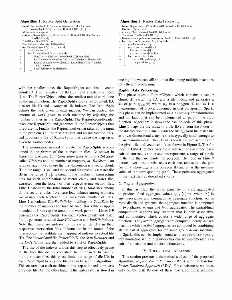
Algorithm 1: Raptor Split GenerationInput: TileSizes[m][r]: Number of intersecting tiles for each

VectorChunkID∈ [1,m] and RasterFileID∈ [1, r]M: Number of mappersOutput: RaptorSplits : {( VectorChunkID, RasterFileID, StartTileIndex,

EndTileIndex)}1 TotalTiles = Sum(TileSizes)2 TilesPerSplit = Max

(10, TotalTiles

M

)3 for V ectorChunkID ← 1 to m do4 StartTileIndex = 05 for RasterFileID ← 1 to r do6 NumTiles = TileSizes[VectorChunkID][RasterFile]7 EndTileIndex = Min(NumTiles, StartTileIndex + TilesPerSplit)8 RaptorSplits.add(VectorChunkID, RasterFileID, StartTileIndex,

EndTileIndex-1)9 StartTileIndex = EndTileIndex

with the smallest one, the RaptorObject contains a vectorchunk ID [1,m], a raster file ID [1, r], and a raster tile index[1, n]. The RaptorObject defines the smallest unit of work doneby the map function. The RaptorSplit stores a vector chunk ID,a raster file ID and a range of tile indexes. The RaptorSplitdefines the task given to each mapper. We can control theamount of work given to each machine by adjusting thenumber of tiles in the RaptorSplit. The RaptorRecordReadertakes one RaptorSplit and generates all the RaptorObjects thatit represents. Finally, the RaptorInputFormat takes all the inputto the problem, i.e., the raster dataset and all intersection files,and produces a list of RaptorSplits that define the map tasksgiven to worker nodes.

The information needed to create the RaptorSplits is con-tained in the footers of the intersection files. As shown inalgorithm 1, Raptor Split Generation takes as input a 2-d arraycalled TileSizes and the number of mappers, M. TileSizes is anarray of size m×r, where the first dimension is a vector chunkID in the range [1,m], and the second dimension is a raster fileID in the range [1, r]. It contains the number of intersectingtiles for each combination of vector chunk and raster file,extracted from the footers of their respective intersection files.Line 1 calculates the total number of tiles, TotalTiles amongall the vector chunks. To ensure load balance among workers,we assign each RaptorSplit a maximum number of tiles.Line 2 calculates TilesPerSplit by dividing the TotalTiles bythe number of mappers for load balance; this value is upper-bounded at 10 to cap the amount of work per split. Lines 3-9generates the RaptorSplits. For each vector chunk and rasterfile, it generates a set of StartTileIndexes and EndTileIndexes.Note that these are indexes to the raster tile IDs in theirrespective intersection files. Information in the footer of theintersection file facilitate the mapping of indexes to actual tileIDs. The VectorChunkID, RasterFileID the StartTileIndex andthe EndTileIndex are then added to a list of RaptorSplits.

The use of tile indexes allows this step to effectively pruneall the tiles that do not contribute to the answer. In case ofmultiple raster files, this phase limits the range of tile IDs ineach RaptorSplit to only one file, as can be seen in algorithm 1This ensures that each machine in this step will need to processonly one file. On the other hand, if the raster layer is stored in

Algorithm 2: Raptor Data ProcessingInput: RaptorObject: (VectorChunkID, RasterFileID, TileIndex)Output: {〈pid,m〉}

1 tid = getTileID(VectorChunkID, TileIndex)2 Tile = loadTile(RasterFileID, tid)3 Intersections = getIntersections(VectorChunkID, RasterFileID, tid)4 for i← 1 to Intersections.length by 2 do5 y = Intersections[i].y6 pid = Intersections[i].pid7 x1 = Intersections[i].x8 x2 = Intersections[i + 1].x9 for x← x1 to x2 do

10 m = Tile.getPixel(y, x)11 output.add(pid,m)

one big file, we can still split that file among multiple machinesfor efficient processing.

Raptor Data ProcessingThis phase takes a RaptorObject, which contains a vectorchunk ID, raster file ID, and a tile index, and generates aset of pairs 〈pid,m〉 where pid is a polygon ID and m is ameasurement of a pixel contained in that polygon. In Spark,this phase can be implemented as a flatMap transformationand in Hadoop, it can be implemented as part of the mapfunction. Algorithm 2 shows the pseudo-code of this phase.Line 1 maps the tile index to a tile ID tid from the footer ofthe intersection file. Line 2 loads the tile tid from the raster fileas a two-dimensional array. A tile is typically small enough tofit in main-memory. Then, Line 3 loads the intersections forthe given tile and vector chunk as shown in Figure 2. The forloop in Line 4 iterates over these intersections in order; eachpair of consecutive intersections represents a range of pixelsin the tile that are inside the polygon. The loop in Line 9iterates over these pixels, reads each one, and output the pair〈pid,m〉 where pid is the polygon ID and m is the measurevalue of the corresponding pixel. These pairs are aggregatedin the next step as described shortly.

C. Step 3: Aggregation

In this last step, the set of pairs 〈pid,m〉 are aggregatedto produce final aggregate values 〈pid,

∑m〉, where

∑is

any associative and commutative aggregate function. As inmost distributed systems, the aggregate function is computedin two phases, partial and final aggregates. The partial/finalcomputation supports any function that is both associativeand commutative which covers a wide range of aggregatefunctions. The partial aggregates are computed locally in eachmachine while the final aggregates are computed by combiningall the partial aggregates for the same group in one machine.In Spark, this can be implemented as a aggregateByKeytransformation while in Hadoop this can be implemented as apair of combine and reduce functions.

IV. THEORETICAL ANALYSIS

This section presents a theoretical analysis of the proposedalgorithm, Raptor Zonal Statistics (RZS) and the baselineRaster Database Approach (RDA). For conciseness, we focusonly on the disk IO cost of these two algorithms; previous

TABLE I: Parameters for Cost Estimation

Symbol Meaningr Number of rows in rasterc Number of columns in rasterwt Tile width in pixelsht Tile height in pixelsp Pixel size in degreesnp Number of polygonsns Number of line segments in all polygons

ns = nsnp

Average number of line segments per polygonwp Average polygon width in longitudinal degreeshp Average polygon height in latitudinal degreesI Input size in bytesB HDFS block size in bytesC Chunk size. Number of polygons per chunk

work showed that the vector database approach (VDA) isnot competent [20]. Table I summarizes the parameters usedthroughout the analysis.

A. Raster Database Approach (RDA)

The RDA algorithm scans the polygons and for each poly-gon it clips the overlapping portion of the raster layer andaggregates the pixel values. We first estimate the average diskcost per polygon DRDA and the total cost is simply computedby multiplying by the total number of polygons np.

The key point in this analysis is that the smallest accessunit in raster files is a tile of size wt × ht pixels. Raster datais stored in compressed blocks of that size so the entire blockhas to be decompressed even if only one pixel needs to beprocessed. On average, each polygon overlaps with nt tiles ascalculated below.

nt =

⌈wp

wt · p

⌉×⌈

hp

ht · p

⌉(1)

where wp and hp are the average width and height of a polygonin degrees. This makes wp

p and hp

p the average width andheight of a polygon in pixels. Next, we can calculate theaverage amount of disk access per polygon DRDA as follows:

DRDA =

⌈wp

wt · p

⌉×⌈

hp

ht · p

⌉× wt × ht (2)

Hence, the total disk cost for RDA, DRDA = np ×DRDA.

B. Raptor Zonal Statistics (RZS)

In RZS, the unit of work is a vector chunk. The input fileis first loaded into HDFS and split into blocks using the R*-Grove [36] partitioning algorithm. Then, each block is furthersplit into chunks of C polygons each. In the following part,we first analyze the characteristics of each chunk, i.e., widthand height, and then we present the cost estimate for each one.

Vector Chunks: Given a vector file of size I , R*-Grovewill create nB blocks with roughly equal size. The number ofblocks is nB = dI/Be. The average number of pixels coveredby each block =c · r/nB . Assuming square-like partitions, thewidth and height of each block is wB = hB =

√c · r/nB .

Next, each block is split into chunks where each chunk has

roughly C polygons each. Since a block is split based onnumber of polygons not the location of the polygons, the widthand height of each chunk is equal to that of a block.

wc = hc =√c · r/nB =

√c · rdI/Be

(3)

Keep in mind that the above width and height are in pixels.Disk Access per Chunk: To estimate the disk access per

chunk, we follow a similar analysis to the one we did withRDA where we need to read all tiles that intersect the chunk.Unlike RDA where the same tile can be read many times forall overlapping polygons, the proposed intersection file allowsus to read each tile at most once. Therefore, the average diskaccess per chunk for RZS is calculated as follows:

DRZS =

⌈wc

wt

⌉×⌈hc

ht

⌉× wt × ht (4)

Assuming balanced partitioning of the np polygons in theinput into equi-sized chunks of C polygons each, the numberof chunks would be nc = dnp/Ce.

Finally, the overall disk access for RZS is:

DRZS = dnp/Ce ·DRZS (5)

This approach is analogous to sort-merge join, whichachieves a very efficient computation time by sorting only thesmaller dataset, i.e., the vector dataset. Unlike the traditionalsort-merge algorithm, the sorted files might be scanned severaltimes due to the overlap between chunks.

C. Discussion

The disk IO cost of RZS is much lower than that ofRDA because the size of vector chunks is much biggerthan that of a single polygon. This results in much smalleroverlap between chunks, hence, lower disk IO cost. Noticethat this is only possible thanks to the intersection file structurewhich enables RZS to transform the complex computation ofmultiple, possibly overlapping polygons, to a single scan overthe raster data. In the experiments section, we will verify theaccuracy of our model using real data.

V. EXPERIMENTS

This section provides an experimental evaluation of theproposed algorithm, Raptor Zonal Statistics (RZS). We com-pare the distributed RZS algorithm to the single-machineScanline Method [20], Rasdaman (a RasterDB approach) [14],Google Earth Engine (GEE) [16] and our previous distributedalgorithm EMI [19]. We show that the proposed RZS is up-tothree orders of magnitude faster than Rasdaman, is twice asfast as GEE while using an order of magnitude fewer machinesand is able to scale to much bigger vector datasets than EMI.We evaluate them on real data and also show the effect ofvector partitioning on RZS.

Section V-A describes the experimental setup, the systemsetup and the datasets. Section V-B provides a comparisonof the proposed RZS, Scanline method, EMI, Rasdaman andGoogle Earth Engine based on the total running time. It is

106 108100

103

106

No. of line segments (ns)

Run

ning

time

(log

secs

)

GLC2000

Rasdaman RZS ScanLine Google Earth Engine EMI

106 108

102

104

106

No. of line segments (ns)R

unni

ngtim

e(l

ogse

cs)

MERIS

106 108

102

104

No. of line segments (ns)

Run

ning

time

(log

secs

)

US ASTER

106 108

102

104

No. of line segments (ns)

Run

ning

time

(log

secs

)

TREECOVER

Fig. 3: Comparison of total running time of RZS, Scanline, EMI, Google Earth Engine and Rasdaman

TABLE II: Vector and Raster Datasets

Vector datasetsDataset np ns wp hp File Size ICounties 3k 52k 0.82 0.51 978 KBStates 49 165k 12.18 4.28 2.6 MBBoundaries 284 3.8m 18.61 8.18 60 MBTRACT 74k 38m 0.096 0.068 632 MBZCTA5 33k 53m 0.19 0.15 851 MBParks 10m 336m 0.0067 0.0043 8.5 GB

Raster datasetsDataset image size c× r tile size wt × ht resolution pglc2000 40, 320× 16, 353 128× 128 0.0089MERIS 129, 600× 64, 800 256× 256 0.0027US-Aster 208, 136× 89, 662 208136× 1 0.00028Tree cover 1, 296, 036× 648, 018 36001× 1 0.00028

followed by a discussion of the vector and raster datasetingestion time for each of these methods. Section V-E givesa verification of the proposed cost model for RZS and RDAmethods. Section V-F discusses two applications where theproposed RZS algorithm has been used. Section V-G showsthe effect of size of vector chunks on the performance of RZS.

A. Setup

We run all the experiments on a Amazon AWS EMR clusterwith one head node and 19 worker nodes of type m4.2xlargewith 2.4 GHz Intel Xeon E5 − 2676 v3 processor, 32 GBof RAM, up to 100 GB of SSD, and 2×8-core processors.The methods are implemented using the open source GeoToolslibrary 17.0.

In all the techniques, we compute the four aggregate values,minimum, maximum, sum, and count. We measure the end-to-end running time as well as the performance metrics whichinclude reading both datasets from disk and producing thefinal answer. Table II lists the datasets that are used in theexperiments along with their attributes using the terminologyin Table I. All these datasets are publicly available as detailedin [19]. The boundaries and parks datasets cover the entireworld while the other four datasets cover only the continentalUS. All raster datasets cover the entire world except US-asterwhich only covers the continental US.

RZS is implemented in Hadoop 2.9. We chose to implementit in Hadoop rather than Spark for two reasons. First, itwas simpler because Hadoop can easily support custom inputformat, i.e., the RaptorInputFormat while Spark does not havea specialized method to define a new input format; it justreuses Hadoop’s InputFormat architecture. Second, Spark isoptimized for in-memory processing while RZS is a disk-intensive query that does not have a huge memory footprint.

For RDA, we used Rasdaman 10.0 running on a single ma-chine since the distributed version is not publicly available. Wealso used Google Earth Engine (GEE) which runs on GoogleCloud Engine. GEE is still experimental and is currently freeto use. The caveat is that it is completely opaque and we donot know which algorithms or how much compute resourcesare used to run queries but it uses up-to 1,000 nodes accordingto their published report [16]. We run each operation on GEE3-5 times at different times and report the average to accountfor any variability in the load. For large vector data, we hitthe limit of GEE of 2GB vector file. To work around it, wesplit the file into 2GB smaller files, run on each file separately,and add up the results. All the running times are collected asreported by GEE in the dashboard.

B. Overall Execution Time

This part compares RZS, Scanline, EMI, Rasdaman, andGEE based on the end-to-end execution time. This experimentis run for all the combinations of vector and raster datasetsshown in Table II, and its results can be seen in Figure 3.For the cases when Rasdaman takes more than 48 hours, weextrapolate the results based on our cost model and mark themwith a dotted line. All experiments on RZS run on a clusterof 20 machines except the TreeCover dataset which runs on100 nodes due to its huge size. GEE runs on up-to 1,000nodes [16].

As can be observed from Figure 3, the proposed distributedRZS algorithm is orders of magnitude faster than Rasdamanfor all combinations of raster and vector datasets. RZS is up-totwo orders of magnitude faster than GEE and twice as fast forthe largest input (Parks./TreeCover), despite using an orderof magnitude less machines.

109 1010 1011 1012100

102

104

No. of Pixels (c× r)

Tim

e(l

ogse

cs)

RZS Rasdaman GEE

(a) Raster Dataset

106 108

102

104

No. of line segments (ns)

Tim

e(l

ogse

cs)

(b) Vector Dataset

Fig. 4: Ingestion time

Rasdaman failed to ingest the US-Aster file due to its hugesize (48GB as a single BigGeoTIFF file). In addition to beinga single machine, Rasdaman does not scale due to using theRDA method which scans the polygons, clips the raster layerfor each polygon, and aggregates the clipped values. Basedon the overlap of polygons and raster tiles, the same tilecould be read tens of times. RZS overcomes this problem bygenerating intersection files that are ordered based on the rasterfile structure to reduce the number of scans of the raster file.

When compared to GEE for large datasets, RZS is atleast 2x faster for the large datasets and up-to two orders ofmagnitude faster. This is an impressive result knowing thatGEE runs on up-to a 1,000 machines. In particular, the speedupof RZS is much higher for large vector datasets since GEEis a raster-oriented system that does not handle big vectordata well [16]. While GEE is faster for small vector datasets,this is due to the overhead of using Hadoop for small inputs.Indeed, the single machine Scanline [20] algorithm is an orderof magnitude faster than both for these small datasets, e.g.,GLC2000 and MERIS and small vector data. Therefore, if wewant to be always faster than GEE, we just need to switchto Scanline for small datasets but we leave this for a futurework. GEE is a free tool (for now) but the knowledge of how itimplements the zonal statistics operation2 is not public. Also,the amount of resources available to users at any time can varyand this is why we report the average of 3-5 runs.

When compared to the single-machine Scanline we observetwo orders of magnitude speedup of RZS due to the parallelimplementation. We also observe that Scanline cannot scaleto large vector data due to the limitations of the intersectionstep which runs on a single machine and that is why thestraight-forward parallelization of Scanline on Hadoop [19],EMI does not scale either. RZS shows performance on paror better than the previously proposed EMI, however, EMIruns out of memory for the parks dataset, which is the largestvector dataset.

C. Ingestion Time

Figure 4 shows the ingestion time of the raster and vectordatasets for the proposed RZS algorithm, Rasdaman and GEE.

2reduceRegions function in Google Earth Engine (GEE)

100 102 104

100

102

104

No. of polygons (np) - Parks dataset

Run

ning

time

(log

secs

)

RasdamanRZS

Fig. 5: Scalability of Rasdaman and RZS on MERIS dataset

Scanline method can read data from disk and hence does nothave the overhead of ingestion time. RZS algorithm requiresboth raster and vector datasets to be stored into HDFS, whileGEE requires them to be uploaded to its web interface as well.We do not upload US Aster and Treecover to GEE as theyare available in its data repository. Rasdaman only requiresto ingest the raster datasets, although it failed to ingest theUS Aster dataset as explained earlier. As can be observedfrom the Figure 4a RZS has a lower raster data ingestion timeas compared to Rasdaman and GEE. Figure 4b shows thatRZS has an order of magnitude lower vector data ingestiontime when compared to GEE. The reason for that is that RZSfollows an in-situ data processing methodology which doesnot need to read the data until the query is executed. Thismakes it a perfect choice for ad-hoc exploratory queries.

D. Closeup Scalability of Rasdaman

Since Rasdaman preloads the raster data but not the vectordata, it could be a good choice if only a few polygons needto be processed on a large raster dataset. Figure 5 shows theresults of zonal statistics query using the MERIS dataset andvarying the number of polygons in the parks dataset. It can beobserved that Rasdaman is optimized for a very few polygons.However, its running time has a steep ascent as the number ofpolygons increase. This happens because Rasdaman processeseach polygon in a separate query which results in overlappingwork. RZS is able to scale more steadily as it can combinethe overlapping work using the intersection file structure.

E. Verification of Cost Models

This part verifies our cost models described in Section IVand uses that analysis to better explain the results that we gotearlier. Since zonal statistics is a disk IO-intensive operation,we only use the disk cost estimation. Also, to be able tocompare the actual running time to the estimated cost, wenormalize all values and compare the trends rather than theabsolute values. All cost models are computed based on theparameters in Table II, the system parameters B = 128MBand C = 5, 000, and the equations in Section IV.

Figure 6a compares the actual running time of RZS to theestimated cost (both normalized) when processing GLC2000and TreeCover datasets. As shown in figure, the trends gener-ally match for both the small and the large datasets showingthe robustness of the cost model. Notice that there is still some

106 108

109

1010

No. of line segments (ns)

Nor

mal

ized

cost

(Log

scal

e) Spearman’s Correlation rs = 0.94

DRZS (Estimate) RZS (Actual)

(a) GLC2000

106 108

1012

1013

No. of line segments (ns)

Nor

mal

ized

cost

(Log

scal

e) Spearman’s Correlation rs = 0.77

(b) TreeCover

Fig. 6: Verification of the cost model of RZS

105 106 107 108

108

109

No. of line segments (ns)

Nor

mal

ized

cost

(Log

scal

e) Correlation rs = 1.0, rs = 0.9

Cost Model Rasdaman GEE

(a) GLC2000

106 108 10101010

1011

1012

No. of line segments (ns)

Nor

mal

ized

cost

(Log

scal

e) Correlation rs = 1.0, rs = 0.83

(b) TreeCover

Fig. 7: Verification of the cost model of RDA

deviation due to our assumptions of uniform distribution ofthe vector data which does not hold in reality. To quantify therelationship, we calculated Spearman’s correlation coefficientfor both cases and it turned out to be 0.94 and 0.77 forGLC2000 and TreeCover respectively. Notice that we did notuse the Pearson’s correlation coefficient as it will result ina misleading value of almost 0.999 due to the exponentialincrease on the the x and y values.

Figure 7 shows the estimated cost of RDA and the actualcost of both Rasdaman and GEE. It is evident from the chartthat the trend of the the cost model and the actual times arevery similar. While we do not have definite information aboutGEE, we highly predict that they use the RDA algorithmgiven the almost perfect match in trends. The correlationcoefficient with Rasdaman in GLC2000 is perfect, and forGEE 0.9 and 0.83. We did not have enough data points forRasdaman with the TreeCover dataset to plot the figure orcalculate the coefficient. We believe the cost model for RDA ismore accurate since it does not make an assumption about theuniformity of the data as we do with RZS. Still, it is amazinghow accurate the results are given that we only relied on thestatistics shown in the Table II.

F. Applications

This section discusses two real-life applications of our pro-posed system, population estimation and wildfire combating.

0.11 2 3 4 5 6 7 8 910

0.5

1

Vector Chunk Size (x103)

Tim

eR

atio

US Aster

Counties States Boundaries TRACT ZCTA5

1 2 3 4 5 6 7 8 9100.4

0.6

0.8

1

Vector Chunk Size (x103)

Tim

eR

atio

Treecover

Fig. 8: Effect of vector chunk size on total running time

The first application of RZS is to estimate the populationof arbitrary regions using landcover data [8]. The problemis that the US Census Bureau reports the population at thegranularity of census tracts which are regions chosen by theBureau to keep the privacy of the data. Areal interpolationtransforms these counts from source polygons, i.e., tracts, totarget polygons, e.g., ZIP Codes, with unknown counts. Oneaccurate method [8] uses the National Land Cover database(NLCD) [37] raster dataset as a reference to disaggregate thepopulation counts into pixels and then aggregate them backinto target polygons. To speed up the process, we apply RZS tocompute the histogram for each polygon in the TRACT dataseton the NLCD dataset. We compared our single-machine im-plementation to the original Python implementation used bythe developers of that algorithm, which was a vector databaseapproach (VDA). Using RZS, the entire process completed in10 seconds for the state of Pennsylvania while the python-based script took over 100 minutes to complete. Given thatimpressive speedup, the authors were able to scale their workto the entire US which took under 2 hours on a single machine.

The second application of RZS is in combating wildfires.The goal of this application is to co-create probabilisticdecision theoretic models to combat wildfires, which woulduse RZS for pre-processing satellite wildfire data. The rasterdata used has a size of 60 GB and the vector data has over3 million polygons, both spanning over California. We havebeen able to compute zonal statistics for it in under 2 hoursusing an AWS cluster of 20 machines.

G. Vector Chunks

This experiment studies the effect of splitting the vectorfile into chunks. In particular, this experiment varies the sizesof vector chunk used in RZS starting with 100, then 1000to 10,000, incremented in steps of 1000. Figure 8 shows theoverall running time for the two larger raster datasets as thechunk size increases. Since each line in this graph representsa different vector dataset, we are only interested in the trendof the lines. Therefore, each line is normalized independentlyto fit all of them in one figure. We omit the running timesfor the extreme cases that run out of memory. We observe inthis experiment that a very low chunk size of 100 results in areduction in the performance due to the overhead of creating

and running too many RaptorSplits. On the other hand, usinga very large chunk size eventually results in some job failuresdue to the memory overhead. This is equivalent to not splittingthe vector file.

After chunk size of 3000, the number of vector chunksgenerated for Counties and Boundaries, become stable whichleads to marginal variation in their running times. The variationof chunk size on larger vector datasets and Tree Cover ismore prominent than the other vector datasets. This is due thelarge size of the Tree Cover dataset. The increase in vectorchunk size leads to a decrease in the number of chunks beinggenerated and hence, less number of raptor splits. This leadsto each machine having more amount of work to do, and anon-optimal distribution of work. It can be concluded thatthe choice of vector chunk size should neither be too big(10,000) or too small(100). We chose it to be 5,000 based onthe experiments and according to our system configuration.

VI. CONCLUSION

This paper proposes a novel distributed MapReduce al-gorithm, Raptor Zonal Statistics (RZS) to solve the zonalstatistics problem. First, RZS runs an intersection step thatcomputes the intersection file which maps vector polygons toraster pixels. Second, the selection step concurrently scans theintersection file and the raster file to find the join result. Toprocess the two files in parallel, the paper introduces two newcomponents RaptorInputFormat and RaptorSplit which definethe smallest unit of work for each parallel task. Third, it runsan aggregate phase that computes the desired statistics foreach polygon. Our experiments with large scale real data showthat the proposed algorithm is up-to two orders of magnitudefaster than the baselines including Rasdaman and GoogleEarth Engine (GEE). We also presented a cost model whichhelped us explaining the results of both RZS and the baselinetechniques.

REFERENCES

[1] “EOSDIS Annual Metrics Reports,” 2020,https://earthdata.nasa.gov/eosdis/system-performance/eosdis-annual-metrics-reports.

[2] “The ESA Earth Observation Payload Data Long Term Storage Ac-tivities,” 2017, https://www.cosmos.esa.int/documents/946106/991257/13 Pinna-Ferrante ESALongTermStorageActivities.pdf.

[3] G. D. Jenerette et al., “Regional Relationships Between Surface Tem-perature, Vegetation, and Human Settlement in a Rapidly UrbanizingEcosystem,” Landscape Ecology, vol. 22, pp. 353–365, 2007.

[4] G. D. Jenerette, S. L. Harlan, W. L. Stefanov, and C. A. Martin,“Ecosystem Services and Urban Heat Riskscape Moderation: Water,Green Spaces, and Social Inequality in Phoenix, USA,” EcologicalApplications, vol. 21, pp. 2637–2651, 2011.

[5] D. Haynes, S. Manson, and E. Shook, “Terra Populus’ Architecture forIntegrated Big Gepspatial Services,” Transactions on GIS, 2017.

[6] D. Haynes, S. Ray, S. M. Manson, and A. Soni, “High PerformanceAnalysis of Big Spatial Data,” in Big Data, Santa Clara, CA, Nov. 2015,pp. 1953–1957.

[7] H. Saadat, J. Adamowski, R. Bonnell, F. Sharifi, M. Namdar, and S. Ale-Ebrahim, “Land use and land cover classification over a large area iniran based on single date analysis of satellite imagery,” ISPRS Journalof Photogrammetry and Remote Sensing, vol. 66, no. 5, pp. 608–619,2011.

[8] M. Reibel and A. Agrawal, “Areal interpolation of population countsusing pre-classified land cover data,” Population Research and PolicyReview, vol. 26, no. 5-6, pp. 619–633, 2007.

[9] O. Ghorbanzadeh et al., “Spatial prediction of wildfire susceptibilityusing field survey gps data and machine learning approaches,” Fire,vol. 2, no. 3, p. 43, 2019.

[10] A. Eldawy and M. F. Mokbel, “SpatialHadoop: A MapReduce Frame-work for Spatial Data,” in ICDE, Seoul, South Korea, Apr. 2015.

[11] J. Yu, M. Sarwat, and J. Wu, “GeoSpark: A Cluster Computing Frame-work for Processing Large-Scale Spatial Data,” in SIGSPATIAL, Seattle,WA, Nov. 2015, pp. 70:1–70:4.

[12] D. Xie, F. Li, B. Yao, G. Li, L. Zhou, and M. Guo, “Simba: EfficientIn-Memory Spatial Analytics,” in SIGMOD, Jun. 2016.

[13] M. Stonebraker, P. Brown, D. Zhang, and J. Becla, “SciDB: A DatabaseManagement System for Applications with Complex Analytics,” Com-puting in Science and Engineering, vol. 15, no. 3, pp. 54–62, 2013.

[14] P. Baumann, A. Dehmel, P. Furtado, R. Ritsch, and N. Widmann, “TheMultidimensional Database System RasDaMan,” in SIGMOD, Seattle,WA, Jun. 1998, pp. 575–577.

[15] A. Kini and R. Emanuele, “Geotrellis: Adding Geospatial Capabilitiesto Spark,” 2014.

[16] N. Gorelick et al., “Google earth engine: Planetary-scale geospatialanalysis for everyone,” Remote sensing of Environment, vol. 202, 2017.

[17] J. Zhang, S. You, and L. Gruenwald, “Efficient Parallel Zonal Statisticson Large-Scale Global Biodiversity Data on GPUs,” in BIGSPATIAL,Bellevue, WA, Nov. 2015, pp. 35–44.

[18] “Zonal Statistics in ArcGIS,” http://desktop.arcgis.com/en/arcmap/10.3/tools/spatial-analyst-toolbox/h-how-zonal-statistics-works.htm, 2017.

[19] S. Singla and A. Eldawy, “(Poster) Distributed Zonal Statistics of BigRaster and Vector Data,” in SIGSPATIAL, 2018.

[20] A. Eldawy, L. Niu, D. Haynes, and Z. Su, “Large scale analytics ofvector+raster big spatial data,” in SIGSPATIAL, 2017.

[21] S. Singla, A. Eldawy, R. Alghamdi, and M. F. Mokbel, “Raptor: LargeScale Analysis of Big Raster and Vector Data,” PVLDB, vol. 12, no. 12,pp. 1950 – 1953, 2019.

[22] A. Aji et al., “Hadoop-GIS: A High Performance Spatial Data Warehous-ing System over MapReduce,” PVLDB, vol. 6, no. 11, pp. 1009–1020,2013.

[23] S. Nishimura, S. Das, D. Agrawal, and A. El Abbadi, “MD-HBase:Design and Implementation of an Elastic Data Infrastructure for Cloud-scale Location Services,” DAPD, vol. 31, no. 2, pp. 289–319, 2013.

[24] R. T. Whitman et al., “Spatial Indexing and Analytics on Hadoop,” inSIGSPATIAL, Nov. 2014.

[25] A. Eldawy, Y. Li, M. F. Mokbel, and R. Janardan, “CG Hadoop:computational geometry in MapReduce,” in SIGSPATIAL, Nov. 2013,pp. 284–293.

[26] A. Eldawy, M. F. Mokbel, and C. Jonathan, “HadoopViz: A MapReduceFramework for Extensible Visualization of Big Spatial Data,” in ICDE,Helsinki, Finland, May 2016, pp. 601–612.

[27] A. Eldawy and M. F. Mokbel, “Pigeon: A Spatial MapReduce Lan-guage,” in ICDE, Chicago, IL, Mar. 2014, pp. 1242–1245.

[28] A. Eldawy, M. F. Mokbel, S. Alharthi, A. Alzaidy, K. Tarek, andS. Ghani, “SHAHED: A mapreduce-based system for querying andvisualizing spatio-temporal satellite data,” in ICDE, 2015, pp. 1585–1596.

[29] S. Shekhar and S. Chawla, Spatial Databases: A Tour. Prentice HallUpper Saddle River, NJ, 2003.

[30] Y. Wang, Z. Chen, L. Cheng, M. Li, and J. Wang, “Parallel scanlinealgorithm for rapid rasterization of vector geographic data,” Computers& geosciences, vol. 59, pp. 31–40, 2013.

[31] “QGIS,” http://www.qgis.org/, 2015.[32] D. J. Peuquet, “A hybrid structure for the storage and manipulation of

very large spatial data sets,” Computer Vision, Graphics, and ImageProcessing, vol. 24, no. 1, pp. 14–27, 1983.

[33] N. R. Brisaboa, G. d. Bernardo, G. Gutierrez, M. R. Luaces, and J. R.Parama, “Efficiently querying vector and raster data,” The ComputerJournal, vol. 60, no. 9, pp. 1395–1413, 2017.

[34] J. Zhang and D. Wang, “High-Performance Zonal Histogramming onLarge-Scale Geospatial Rasters Using GPUs and GPU-AcceleratedClusters,” in IPDPS Workshops, Phoenix, AZ, May 2014, pp. 993–1000.

[35] G. Zhao, B. A. Bryan, D. King, X. Song, and Q. Yu, “Parallelizationand optimization of spatial analysis for large scale environmental modeldata assembly,” Computers and electronics in agriculture, vol. 89, 2012.

[36] T. Vu and A. Eldawy, “R*-grove: Balanced spatial partitioning for large-scale datasets,” Frontiers in Big Data, vol. 3, p. 28, 2020.

[37] “NLCD dataset,” https://www.mrlc.gov/data/type/land-cover, 2020.