Fully distributed absolute blood flow velocity …frostiglab.bio.uci.edu/Li et al. Biomedical Optics Express.pdfmeasurement for middle cerebral arteries using Doppler optical coherence

Fully distributed absolute blood flow velocity measurement for middle cerebral arteries using

Doppler optical coherence tomography

Li Qi,1,2 Jiang Zhu,2,3 Aneeka M. Hancock,4,5 Cuixia Dai,2 Xuping Zhang,1 Ron D. Frostig,3,4,5 and Zhongping Chen2,3,*

1Institute of Optical Communication Engineering and College of Engineering and Applied Sciences, Nanjing University, Nanjing, Jiangsu, 210093, China

2Beckman Laser Institute, University of California, Irvine, Irvine, California 92612, USA 3Department of Biomedical Engineering, University of California, Irvine, Irvine, California 92697, USA

4Department of Neurobiology and Behavior, University of California, Irvine, Irvine, California, USA 5The Center for the Neurobiology of Learning and Memory, University of California, Irvine, Irvine, California, USA

*[email protected]

Abstract: Doppler optical coherence tomography (DOCT) is considered one of the most promising functional imaging modalities for neuro biology research and has demonstrated the ability to quantify cerebral blood flow velocity at a high accuracy. However, the measurement of total absolute blood flow velocity (BFV) of major cerebral arteries is still a difficult problem since it is related to vessel geometry. In this paper, we present a volumetric vessel reconstruction approach that is capable of measuring the absolute BFV distributed along the entire middle cerebral artery (MCA) within a large field-of-view. The Doppler angle at each point of the MCA, representing the vessel geometry, is derived analytically by localizing the artery from pure DOCT images through vessel segmentation and skeletonization. Our approach could achieve automatic quantification of the fully distributed absolute BFV across different vessel branches. Experiments on rodents using swept-source optical coherence tomography showed that our approach was able to reveal the consequences of permanent MCA occlusion with absolute BFV measurement.

©2016 Optical Society of America

OCIS codes: (110.4500) Optical coherence tomography; (170.2655) Functional monitoring and imaging; (100.2960) Image analysis.

References and links

1. Z. Chen, T. E. Milner, S. Srinivas, X. Wang, A. Malekafzali, M. J. C. van Gemert, and J. S. Nelson, “Noninvasive imaging of in vivo blood flow velocity using optical Doppler tomography,” Opt. Lett. 22(14), 1119–1121 (1997).

2. Z. Chen, T. E. Milner, X. Wang, S. Srinivas, and J. S. Nelson, “Optical Doppler tomography: imaging in vivo blood flow dynamics following pharmacological intervention and photodynamic therapy,” Photochem. Photobiol. 67(1), 56–60 (1998).

3. Z. Chen, T. E. Milner, D. Dave, and J. S. Nelson, “Optical Doppler tomographic imaging of fluid flow velocity in highly scattering media,” Opt. Lett. 22(1), 64–66 (1997).

4. Y. Zhao, Z. Chen, C. Saxer, S. Xiang, J. F. de Boer, and J. S. Nelson, “Phase-resolved optical coherence tomography and optical Doppler tomography for imaging blood flow in human skin with fast scanning speed and high velocity sensitivity,” Opt. Lett. 25(2), 114–116 (2000).

5. J. A. Izatt, M. D. Kulkarni, S. Yazdanfar, J. K. Barton, and A. J. Welch, “In vivo bidirectional color Doppler flow imaging of picoliter blood volumes using optical coherence tomography,” Opt. Lett. 22(18), 1439–1441 (1997).

6. R. A. Leitgeb, R. M. Werkmeister, C. Blatter, and L. Schmetterer, “Doppler optical coherence tomography,” Prog. Retin. Eye Res. 41, 26–43 (2014).

7. D. Huang, E. A. Swanson, C. P. Lin, J. S. Schuman, W. G. Stinson, W. Chang, M. R. Hee, T. Flotte, K. Gregory, C. A. Puliafito, and J. G. Fujimoto, “Optical coherence tomography,” Science 254(5035), 1178–1181 (1991).

#254363 Received 23 Nov 2015; revised 8 Jan 2016; accepted 8 Jan 2016; published 20 Jan 2016 (C) 2016 OSA 1 Feb 2016 | Vol. 7, No. 2 | DOI:10.1364/BOE.7.000601 | BIOMEDICAL OPTICS EXPRESS 601

8. M. Sehi, I. Goharian, R. Konduru, O. Tan, S. Srinivas, S. R. Sadda, B. A. Francis, D. Huang, and D. S. Greenfield, “Retinal blood flow in glaucomatous eyes with single-hemifield damage,” Ophthalmology 121(3), 750–758 (2014).

9. B. Rao, L. Yu, H. K. Chiang, L. C. Zacharias, R. M. Kurtz, B. D. Kuppermann, and Z. Chen, “Imaging pulsatile retinal blood flow in human eye,” J. Biomed. Opt. 13(4), 040505 (2008).

10. L. Yu and Z. Chen, “Doppler variance imaging for three-dimensional retina and choroid angiography,” J. Biomed. Opt. 15(1), 016029 (2010).

11. W. Choi, B. Baumann, J. J. Liu, A. C. Clermont, E. P. Feener, J. S. Duker, and J. G. Fujimoto, “Measurement of pulsatile total blood flow in the human and rat retina with ultrahigh speed spectral/Fourier domain OCT,” Biomed. Opt. Express 3(5), 1047–1061 (2012).

12. S. Yazdanfar, M. Kulkarni, and J. Izatt, “High resolution imaging of in vivo cardiac dynamics using color Doppler optical coherence tomography,” Opt. Express 1(13), 424–431 (1997).

13. L. M. Peterson, M. W. Jenkins, S. Gu, L. Barwick, M. Watanabe, and A. M. Rollins, “4D shear stress maps of the developing heart using Doppler optical coherence tomography,” Biomed. Opt. Express 3(11), 3022–3032 (2012).

14. P. Li, A. Liu, L. Shi, X. Yin, S. Rugonyi, and R. K. Wang, “Assessment of strain and strain rate in embryonic chick heart in vivo using tissue Doppler optical coherence tomography,” Phys. Med. Biol. 56(22), 7081–7092 (2011).

15. Y. Zhao, K. M. Brecke, H. Ren, Z. Ding, J. S. Nelson, and Z. Chen, “Three-dimensional reconstruction of in vivo blood vessels in human skin using phase-resolved optical Doppler tomography,” IEEE J. Sel. Top. Quantum Electron. 7(6), 931–935 (2001).

16. G. Liu, W. Jia, J. S. Nelson, and Z. Chen, “In vivo, high-resolution, three-dimensional imaging of port wine stain microvasculature in human skin,” Lasers Surg. Med. 45(10), 628–632 (2013).

17. G. Liu, W. Jia, V. Sun, B. Choi, and Z. Chen, “High-resolution imaging of microvasculature in human skin in-vivo with optical coherence tomography,” Opt. Express 20(7), 7694–7705 (2012).

18. Y. Zhao, Z. Chen, C. Saxer, Q. Shen, S. Xiang, J. F. de Boer, and J. S. Nelson, “Doppler standard deviation imaging for clinical monitoring of in vivo human skin blood flow,” Opt. Lett. 25(18), 1358–1360 (2000).

19. G. Liu, L. Chou, W. Jia, W. Qi, B. Choi, and Z. Chen, “Intensity-based modified Doppler variance algorithm: application to phase instable and phase stable optical coherence tomography systems,” Opt. Express 19(12), 11429–11440 (2011).

20. Y. Satomura, J. Seki, Y. Ooi, T. Yanagida, and A. Seiyama, “In vivo imaging of the rat cerebral microvessels with optical coherence tomography,” Clin. Hemorheol. Microcirc. 31(1), 31–40 (2004).

21. H. Ren, C. Du, Z. Yuan, K. Park, N. D. Volkow, and Y. Pan, “Cocaine-induced cortical microischemia in the rodent brain: clinical implications,” Mol. Psychiatry 17(10), 1017–1025 (2012).

22. L. Yu, E. Nguyen, G. Liu, B. Choi, and Z. Chen, “Spectral Doppler optical coherence tomography imaging of localized ischemic stroke in a mouse model,” J. Biomed. Opt. 15(6), 066006 (2010).

23. V. J. Srinivasan, D. N. Atochin, H. Radhakrishnan, J. Y. Jiang, S. Ruvinskaya, W. Wu, S. Barry, A. E. Cable, C. Ayata, P. L. Huang, and D. A. Boas, “Optical coherence tomography for the quantitative study of cerebrovascular physiology,” J. Cereb. Blood Flow Metab. 31(6), 1339–1345 (2011).

24. Z. Yuan, Z. C. Luo, H. G. Ren, C. W. Du, and Y. Pan, “A digital frequency ramping method for enhancing Doppler flow imaging in Fourier-domain optical coherence tomography,” Opt. Express 17(5), 3951–3963 (2009).

25. G. Liu and Z. Chen, “Optical Coherence Tomography for Brain Imaging,” in S. J. Madson (ed.), Optical Methods and Instrumentation in Brain Imaging and Therapy, Bioanalysis 3, 157–172 (2013).

26. Y. Wang, B. A. Bower, J. A. Izatt, O. Tan, and D. Huang, “In vivo total retinal blood flow measurement by Fourier domain Doppler optical coherence tomography,” J. Biomed. Opt. 12(4), 041215 (2007).

27. S. Makita, T. Fabritius, and Y. Yasuno, “Quantitative retinal-blood flow measurement with three-dimensional vessel geometry determination using ultrahigh-resolution Doppler optical coherence angiography,” Opt. Lett. 33(8), 836–838 (2008).

28. V. J. Srinivasan, S. Sakadzić, I. Gorczynska, S. Ruvinskaya, W. Wu, J. G. Fujimoto, and D. A. Boas, “Quantitative cerebral blood flow with Optical Coherence Tomography,” Opt. Express 18(3), 2477–2494 (2010).

29. J. You, C. Du, N. D. Volkow, and Y. Pan, “Optical coherence Doppler tomography for quantitative cerebral blood flow imaging,” Biomed. Opt. Express 5(9), 3217–3230 (2014).

30. C. Du, N. D. Volkow, A. P. Koretsky, and Y. Pan, “Low-frequency calcium oscillations accompany deoxyhemoglobin oscillations in rat somatosensory cortex,” Proc. Natl. Acad. Sci. U.S.A. 111(43), E4677–E4686 (2014).

31. J. Lee, H. Radhakrishnan, W. Wu, A. Daneshmand, M. Climov, C. Ayata, and D. A. Boas, “Quantitative imaging of cerebral blood flow velocity and intracellular motility using dynamic light scattering-optical coherence tomography,” J. Cereb. Blood Flow Metab. 33(6), 819–825 (2013).

32. A. M. Hancock, C. C. Lay, M. F. Davis, and R. D. Frostig, “Sensory stimulation-based complete protection from ischemic stroke remains stable at 4 months post-occlusion of MCA,” J. Neurol. Disord. 1(4), 135 (2013).

33. C. C. Lay, M. F. Davis, C. H. Chen-Bee, and R. D. Frostig, “Mild sensory stimulation completely protects the adult rodent cortex from ischemic stroke,” PLoS One 5(6), e11270 (2010).

34. J. Dehmeshki, H. Amin, M. Valdivieso, and X. Ye, “Segmentation of pulmonary nodules in thoracic CT scans: a region growing approach,” IEEE Trans. Med. Imaging 27(4), 467–480 (2008).


35. Y. Lu, T. Jiang, and Y. Zang, “Region growing method for the analysis of functional MRI data,” Neuroimage 20(1), 455–465 (2003).

36. H. Yu, S. B. Reeder, A. Shimakawa, J. H. Brittain, and N. J. Pelc, “Field map estimation with a region growing scheme for iterative 3-point water-fat decomposition,” Magn. Reson. Med. 54(4), 1032–1039 (2005).

37. J. Fan, D. Y. Yau, A. K. Elmagarmid, and W. G. Aref, “Automatic image segmentation by integrating color-edge extraction and seeded region growing,” IEEE Trans. Image Process. 10(10), 1454–1466 (2001).

38. D. Lesage, E. D. Angelini, I. Bloch, and G. Funka-Lea, “A review of 3D vessel lumen segmentation techniques: models, features and extraction schemes,” Med. Image Anal. 13(6), 819–845 (2009).

39. G. K. Batchelor, An Introduction to Fluid Dynamics (Cambridge University, 2000). 40. V. L. Roger, A. S. Go, D. M. Lloyd-Jones, R. J. Adams, J. D. Berry, T. M. Brown, M. R. Carnethon, S. Dai, G.

de Simone, E. S. Ford, C. S. Fox, H. J. Fullerton, C. Gillespie, K. J. Greenlund, S. M. Hailpern, J. A. Heit, P. M. Ho, V. J. Howard, B. M. Kissela, S. J. Kittner, D. T. Lackland, J. H. Lichtman, L. D. Lisabeth, D. M. Makuc, G. M. Marcus, A. Marelli, D. B. Matchar, M. M. McDermott, J. B. Meigs, C. S. Moy, D. Mozaffarian, M. E. Mussolino, G. Nichol, N. P. Paynter, W. D. Rosamond, P. D. Sorlie, R. S. Stafford, T. N. Turan, M. B. Turner, N. D. Wong, and J. Wylie-Rosett; American Heart Association Statistics Committee and Stroke Statistics Subcommittee, “Heart disease and stroke statistics--2011 update: a report from the American Heart Association,” Circulation 123(4), e18–e209 (2011).

41. Y. Wang-Fischer, ed., Manual of Stroke Models in Rats (CRC, 2008).

1. Introduction

Doppler Optical Coherence Tomography (DOCT) [1–6], or Optical Doppler Tomography, is a functional imaging modality based on Optical Coherence Tomography [7] which is used to image optical scattering media with high resolution based on light interference. First developed in the late ‘90s, DOCT takes advantage of Doppler effects happening at the intersection of light and moving substances (e.g., flowing particles in blood vessels) that result in shifts in the phase component of the back-scattering light. Leveraging this phase shift (Doppler shift), the velocity of such moving substances can be derived. DOCT has been used extensively for ophthalmology [8–11], cardiology [12–14], and dermatology [15–19] due to its flexibility to detect blood flow velocity at a high accuracy.

Recently, DOCT has been shown to be able to image cerebral blood vessel networks in the brain cortex and to reveal changes in blood flow velocity (BFV) within the brain cortex during different types of brain damage such as dura removal [20], cocaine administration [21], and ischemia induced by photodynamic therapy (PDT) [22]. Moreover, quantitative cerebral BFV measurement was investigated using DOCT to reveal better functional information from brain imaging [23–31]. Flow velocity is a unique parameter, distinct from the flow rate, because it is independent of the vessel diameter and area. Given the laser central wavelength λ and the refractive index n of the scattering media, the absolute velocity of the moving particles can be described by

=4 cos

fv

n T

λπ θΔ

(1)

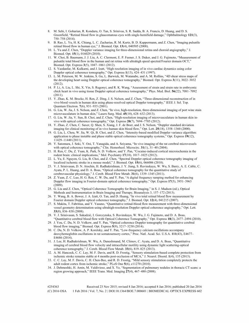
where f is the Doppler phase shift, ΔT is the time interval between two samplings, and θ is the Doppler angle. Equation (1) indicates that the velocity measurement not only relates to the properties of the laser and the scattering particles, but it also relates to the geometry of both directions of the laser beam and the flow. Therefore, one of the major difficulties with measuring absolute BFV is to determine the Doppler angle at each position along the vessel since this angle is continuously changing with respect to the vessel geometry, as is shown in Fig. 1. To solve this, Wang et al. [26] proposed to determine the Doppler angle by connecting successive vessel centers; Makita et al. [27] presented the Doppler angle detection method incorporating both en face vessel image and multiple cross-sectional images; Srinivasan et al. [28] introduced an en face Doppler signal integration method to determine the blood flow rate at multiple locations within a specific depth; and You et al. [29] proposed a gradient vessel center tracking method that can quantify the Doppler angle within a certain portion of the vessel of interest. Although these approaches provide a method for Doppler angle correction, the measuring positions are still limited (usually, they can only detect the BFV at one or


multiple manual labeled locations). Effective methods for measuring the fully distributed absolute BFV along a vessel, which may reveal the overall hemodynamics of that entire vessel, are still limited. The underlying problem is being able to determine the vessel geometry quantitatively and thus obtain Doppler angles at every spot from the DOCT volumetric images.

Fig. 1. Changing Doppler angles according to the vessel geometry.

As one of the major arteries that supply blood to the cortex, the middle cerebral artery (MCA) plays an important role in brain activity and physiology. Investigation of blood flow velocity and its changes in MCA is of significant interest for revealing middle cerebral artery syndromes such as ischemic stroke [32, 33]. Focusing on the analysis of cerebral hemodynamics, this paper presents a method to quantify the total absolute blood flow velocity in MCA based on volumetric vessel reconstruction from pure DOCT images. A modified region growing segmentation method is first used to localize the MCA on successive DOCT B-scan images. Vessel skeletonization, followed by an averaging gradient angle calculation method, is then carried out to obtain Doppler angles along the entire MCA. Once the Doppler angles are determined, the absolute blood flow velocity of each position on the MCA is easily found. Given a seed point position on the MCA, our approach could achieve automatic quantification of the fully distributed absolute BFV. Experiments on rodents based on swept-source OCT demonstrated the feasibility of our approach and revealed the complex cerebrovascular physiology during permanent MCA occlusion.

2. Method

2.1 Animal preparation

To conduct the absolute BFV measurement studies, three 295–400g male Sprague Dawley rats were used. The animals were injected intraperitoneally with a Nembutal bolus [55 mg/kg body weight (b.w.)] at the beginning. Supplemental injections of Nembutal (27.5 mg/kg b.w.) were given as necessary. After resection of soft tissue, a 6.5 × 8mm imaging area of the skull over the left primary somatosensory cortex (rostromedial corner positioned ~1 mm caudal and 2 mm lateral from the bregma) was thinned to ~150 µm using a dental drill. Body temperature was measured via a rectal probe and maintained at 37°C by a self-regulating thermal blanket.

2.2. The swept-source OCT system

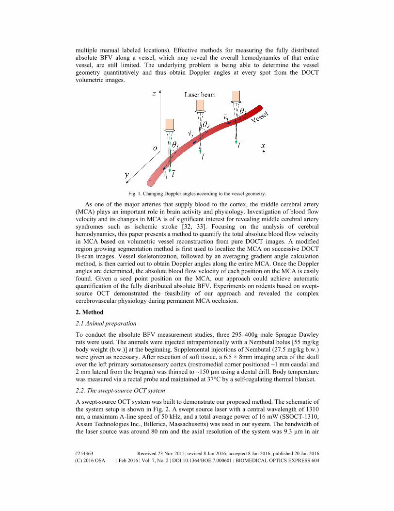
A swept-source OCT system was built to demonstrate our proposed method. The schematic of the system setup is shown in Fig. 2. A swept source laser with a central wavelength of 1310 nm, a maximum A-line speed of 50 kHz, and a total average power of 16 mW (SSOCT-1310, Axsun Technologies Inc., Billerica, Massachusetts) was used in our system. The bandwidth of the laser source was around 80 nm and the axial resolution of the system was 9.3 μm in air


(6.6 μm in tissue). A Michelson type interferometer was used, and 90% of the laser power was sent to the sample arm and 10% of the light to the reference arm. In the sample arm, a fiber collimator, a two-axial galvo mirror scanning system, and an achromatic doublet was used to deliver the beam to the rat brain. The fiber collimator gave a beam diameter of 2 mm, and with the 30 mm focusing length doublet, the system gave a lateral resolution of 14.6 μm. C + + platform based data acquisition software running on a 64 bit Windows 7 operation systems was used to control the galvo scanner and acquire the data.

Fig. 2. The DOCT structure used in experiments.

2.3. Algorithm overview and pre-processing

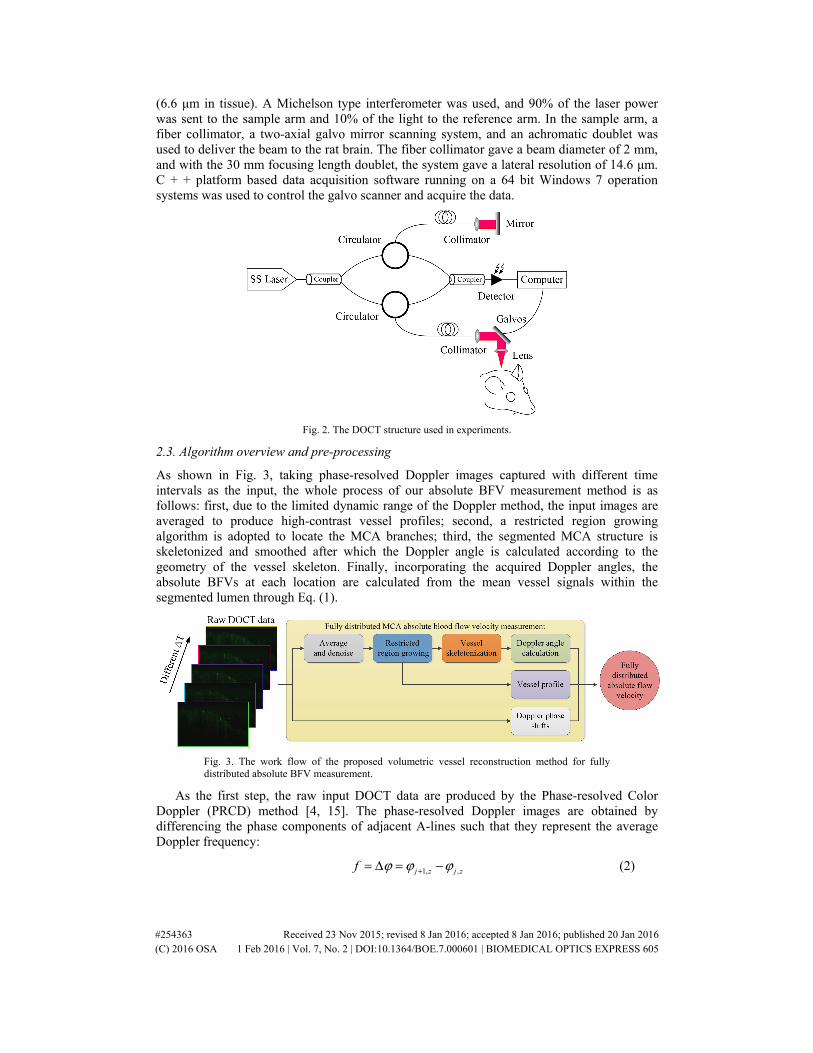
As shown in Fig. 3, taking phase-resolved Doppler images captured with different time intervals as the input, the whole process of our absolute BFV measurement method is as follows: first, due to the limited dynamic range of the Doppler method, the input images are averaged to produce high-contrast vessel profiles; second, a restricted region growing algorithm is adopted to locate the MCA branches; third, the segmented MCA structure is skeletonized and smoothed after which the Doppler angle is calculated according to the geometry of the vessel skeleton. Finally, incorporating the acquired Doppler angles, the absolute BFVs at each location are calculated from the mean vessel signals within the segmented lumen through Eq. (1).

Fig. 3. The work flow of the proposed volumetric vessel reconstruction method for fully distributed absolute BFV measurement.

As the first step, the raw input DOCT data are produced by the Phase-resolved Color Doppler (PRCD) method [4, 15]. The phase-resolved Doppler images are obtained by differencing the phase components of adjacent A-lines such that they represent the average Doppler frequency:

1, ,j z j zf ϕ ϕ ϕ+= Δ = − (2)


where φj + 1,z and φj,z are the phases for the signal at depth z of the j + 1th and jth A-line. Using the autocorrelation algorithm and letting Re(Aj,z) and Im(Aj,z) be the real and imaginary part of the complex data, respectively, Eq. (2) can be rewritten as [15]

1, , , 1,1

, 1, 1, ,

Im( ) Re( ) Im( ) Re( )tan .

Re( ) Re( ) Im( ) Im( )j z j z j z j z

j z j z j z j z

A A A Af

A A A A+ +−

+ +

−=

+ (3)

In our implementation, after the calculation of all the Doppler phase shifts in a B-scan frame, the final DOCT image was filtered with an average filter (window size: 4-by-4) to smooth out the noise.

Using Eq. (1) and Eq. (3), the absolute value of the flow velocity could be determined given the Doppler angle. However, subject to the arc-tangent operation in Eq. (3), the acquired Doppler phase shift suffers from limited dynamic range (Δφ: [-π, π]), resulting in phase wrapping artifacts if the time interval ΔT is not accommodated to the flow velocity. Moreover, since the BFV and the Doppler angles at different positions along the MCA are different, not all the vessel profiles are prominent in different B-scans. As illustrated in Fig. 4, MCA branches at frame 123 can be seen clearly in ΔT = 2t (t is the minimum time interval between two adjacent A-lines), while the other branches at frame 180 can only be distinguished in ΔT = 20t. Therefore, in order to provide a solid foundation for vessel segmentation in the next step, images at different time intervals are acquired, normalized and averaged as a pre-processing procedure. Two advantages could be realized by doing so: all the vessels could be clearly seen in the averaged cross section since the contrast between the vessel and the background tissue is higher than the non-averaged profiles; and the speckle noise, along with the bulk motion artifacts, is suppressed from averaging the data. Moreover, before proceeding to the next step, each B-scan of the averaged OCT volume is further filtered by a 2D median filter. Figure 4 depicts the vessel profiles at the averaged frames from which can be seen the prominent vessels.

Fig. 4. The acquired frame 123 and frame 180 of a total of 256 frames from a rat brain imaging experiment. The limited dynamic range of the resolved Doppler phase can be seen clearly: the cross-sectional profiles of different vessels are only prominent at particular time intervals while in the averaged profile, these vessels all stood out from the background.

2.4. Vessel segmentation

Due to its simplicity and fast speed in segmenting regions with well-defined edges, the region growing algorithm is widely employed in different image processing applications from object detection to CT/MRI structure segmentation [34–37]. Given one or multiple initial seed points in multi-dimensional images, this algorithm examines the neighboring pixels of these seed points and determines whether they should be added to the region. However, this algorithm commonly suffers from the “leaking” problem in images with blurred edges [38] resulting in odd regions with a huge discontinuity. Meanwhile, the vessel signals in the DOCT images are affected by the Doppler angles and the flow pulses, resulting in discontinuities in boundary pixel intensities. To overcome these problems and effectively segment the MCA from stacked DOCT images, a restricted region growing algorithm is


proposed. The algorithm is named “restricted” because the growing process is constrained simultaneously by the adaptive threshold and a circular shape prior.

1) The adaptive threshold t is given by the compounding of the mean gray value t1 of the boundary at the previous frame and a hard threshold t2 derived from a Region-of-Interest (ROI) at a current frame: t = (t1 + t2)/α, where α is the compounding ratio. In this study, the ROI at a current frame is given by the neighboring region of the previous vessel center, and threshold t2 is defined as a specific portion of the maximum gray value in this ROI.

2) The circular shape prior is a circular boundary where the vessel region will stop growing when they encounter each other. The center c of the circular boundary is given by the previous vessel center coordinates while its radius r is derived from the mean vessel radius at the previous frame. Moreover, due to the fact that the diameter of the MCA decreases when moving from the main vessel to side branches, the diameter of the shape prior at the next frame will be reduced when the maximum diameter of the current vessel is less than the diameter of the shape prior of the previous frame, resulting in a smaller shape prior at all successive B-scans.

Fig. 5. (a) Ordinary region growing method leads to a diffuse vessel border; (b) the vessel lumen was successfully controlled by the two constraints using the proposed restricted region growing method.

By introducing the adaptive threshold which incorporates the gray scale information across sequential frames, the boundary pixel intensity fluctuation caused by changes in Doppler angle and blood flow pulse is overcome; by constraining the growing process with a shape prior, a ‘leaking problem’ can be prevented. Figure 5 shows how the segmentation of the vessel lumen is restricted by the aforementioned constraints. The growing process starts with a seed point on a branch of the middle cerebral artery and grows at B-scan-wise. The stopping criteria are (1) no pixel satisfies the constraints, (2) the variance of the current ROI is smaller than a pre-defined value and (3) the displacement between the vessel centers of adjacent frames is larger than a threshold. For clarity, Algorithm 1 summarizes the entire process of the proposed method.

Algorithm 1: The restricted region growing algorithm for MCA segmentation

Input: Pre-processed DOCT images and seed point location ck. Output: Volumetric MCA structure including vessel lumen and skeleton. 1 Initialized parameters: t1

0, t21, α, r0, and k;

2 while stopping criteria not met do 3 Get the k frame of DOCT B-scan images; 4 Update the adaptive threshold tk = (t1

k-1 + t2k)/α;

5 Update the shape prior parameters: center ck[xk-1,yk-1], radius rk; 6 Update the k frame region seed points by propagating the k-1 frame regions that satisfies the constraint tk, to the current frame; 7 Region grows from the seed points until all constraints are met; 8 Get the stopping criteria status; 9 k = k + 1; 10 end.


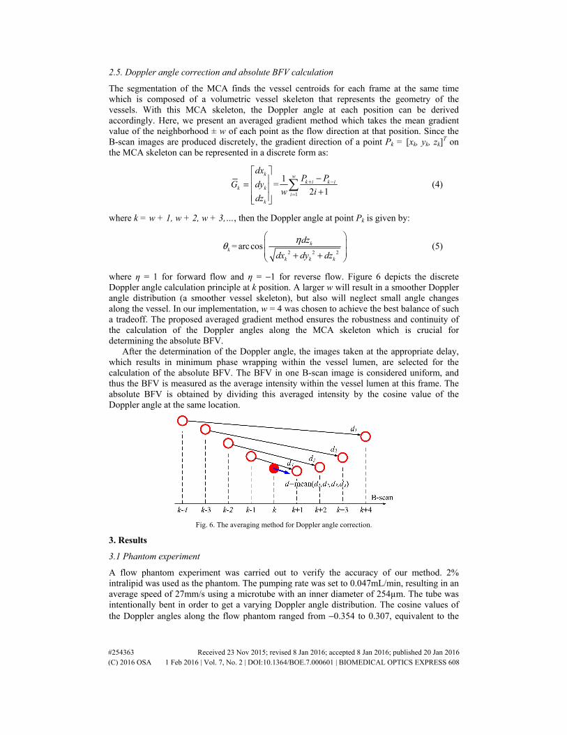
2.5. Doppler angle correction and absolute BFV calculation

The segmentation of the MCA finds the vessel centroids for each frame at the same time which is composed of a volumetric vessel skeleton that represents the geometry of the vessels. With this MCA skeleton, the Doppler angle at each position can be derived accordingly. Here, we present an averaged gradient method which takes the mean gradient value of the neighborhood ± w of each point as the flow direction at that position. Since the B-scan images are produced discretely, the gradient direction of a point Pk = [xk, yk, zk]

T on the MCA skeleton can be represented in a discrete form as:

1

1=

2 1

k wk i k i

k ki

k

dxP P

G dyw i

dz

+ −

=

− = +

(4)

where k = w + 1, w + 2, w + 3,…, then the Doppler angle at point Pk is given by:

2 2 2

= arccos kk

k k k

dz

dx dy dz

ηθ + +

(5)

where η = 1 for forward flow and η = −1 for reverse flow. Figure 6 depicts the discrete Doppler angle calculation principle at k position. A larger w will result in a smoother Doppler angle distribution (a smoother vessel skeleton), but also will neglect small angle changes along the vessel. In our implementation, w = 4 was chosen to achieve the best balance of such a tradeoff. The proposed averaged gradient method ensures the robustness and continuity of the calculation of the Doppler angles along the MCA skeleton which is crucial for determining the absolute BFV.

After the determination of the Doppler angle, the images taken at the appropriate delay, which results in minimum phase wrapping within the vessel lumen, are selected for the calculation of the absolute BFV. The BFV in one B-scan image is considered uniform, and thus the BFV is measured as the average intensity within the vessel lumen at this frame. The absolute BFV is obtained by dividing this averaged intensity by the cosine value of the Doppler angle at the same location.

Fig. 6. The averaging method for Doppler angle correction.

3. Results

3.1 Phantom experiment

A flow phantom experiment was carried out to verify the accuracy of our method. 2% intralipid was used as the phantom. The pumping rate was set to 0.047mL/min, resulting in an average speed of 27mm/s using a microtube with an inner diameter of 254µm. The tube was intentionally bent in order to get a varying Doppler angle distribution. The cosine values of the Doppler angles along the flow phantom ranged from −0.354 to 0.307, equivalent to the


angles of 72.12 to 110.75 degrees. During the calculation of the flow velocity, the phantom was segmented from the DOCT images using the proposed restricted region growing algorithm, and the Doppler angle distribution was calculated afterward (as shown in Fig. 7). However, because the Doppler angle was near 90 degrees in the center portion of the tube (resulting in a very small cosine value), the velocity at this portion could not be quantified accurately. Therefore, the velocity quantification was carried out at portions with absolute cosine values larger than 0.05 (Doppler angle outside the range of 87.134 to 92.866 degrees). As a result, the flow phantom was divided into two different segments, as shown in the flow velocity distributions in Fig. 7. The flow velocities of the two segments before Doppler angle correction were 4.718 ± 1.014mm/s and 6.484 ± 1.358mm/s. After Doppler correction, these velocity values go up to −26.424 ± 2.835mm/s and 26.272 ± 2.391mm/s, accordingly. The corrected absolute flow speed was very close to the theoretical velocity of the pumping rate, and the deviation was within 10.8% of the measured velocity.

Fig. 7. Flow phantom experiment. From left to right: the Doppler angle; the flow velocity before Doppler angle correction; the flow velocity after Doppler angle correction. (See text for detailed explanation).

3.2 Fully distributed absolute BFV measurement for MCA

Fully distributed absolute BFV quantification for MCA was demonstrated by the proposed volumetric reconstruction method. Three-dimensional OCT data were acquired at A-line rates of 50 kHz, 25 kHz, 10 kHz, 5 kHz, and 2.5 kHz resulting in time intervals of 0.02 ms, 0.04 ms, 0.1 ms, 0.2 ms and 0.4 ms, respectively. According to Eqs. (1)–(3), the axial velocity ranges for PRCD were ± 11.70 mm/s, ± 5.85 mm/s, ± 2.34 mm/s, ± 1.17 mm/s and ± 0.58 mm/s for ΔT = 0.02 ms, 0.04 ms, 0.1 ms, 0.2 ms, and 0.4 ms, respectively. Also, the tilted angle of the output laser beam was carefully tuned to avoid the phase wrapping of the blood flow. The imaging area for subject 1 was 8.4 mm by 8.4 mm while for subjects 2 and 3, it was 4.2 mm by 4.2 mm. These data were processed later to obtain the three-dimensional OCT structural and DOCT images, the dimensions of which were 512x1024x256. The DOCT images were then fed into our algorithm to verify the algorithm’s applicability. For better reference of the vessel distribution, the intensity-based Doppler variance (IBDV) [19] was used to visualize vessel densities during the experiment. The principle of IBDV can be expressed as [19]

( )

( )1, ,

1 122 2 2

1, ,1 1

11 .

1

2

J N

j z j zj z

J N

j z j zj z

A A

TA A

σ+

= =

+= =

= − +

(6)

The IBDV method uses only the intensity information such that it is suitable for phase instable OCT systems. J = 4, N = 4 were used for the calculation of IBDV in our experiments.

The far left column of Fig. 8 shows the en face maximum intensity projections (MIP) of the IBDV images for all three subjects. The white arrows indicate the branches of the MCA.


After vessel segmentation, MCA structures were reconstructed (2nd column of Fig. 8) and further smoothed by averaging neighboring pixel coordinates to produce the refined vessel lumen structures (3rd column of Fig. 8). The MCA skeletons were obtained afterward as displayed in the far right column of Fig. 8 with artery branches coded in different colors. The reconstructed vessel structures coincide with the en face image and reveal the necessary vessel geometry for absolute BFV measurement, and the overlapping of different vessels and the MCAs was successfully avoided.

Fig. 8. Vessel reconstruction results for subjects 1, 2 and 3. First column: IBDV en face images; second column: reconstructed vessels before lumen refinement; third column: vessel structures after lumen refinement; fourth column: extracted vessel skeleton.

Doppler angles on the entire reconstructed MCA skeletons were calculated using the proposed averaged gradient method. Figure 9(a) shows the angle measurement result for subject 1 with the cosine value of the Doppler angle at each position coded in red and black. It can be seen that the cosine value was in good accordance with the vessel geometry where the red color represents a steeper vessel, and the black color represents the Doppler angle of 90°. Figures 9(b) and 9(c) show the enlarged details of the dashed-line-frames in Fig. 9(a) with arrows showing the flow direction at each discrete point which represent the vessel center at each B-scan image. The flow directions are correctly identified using our method. Figures 9(d) and 9(e) further show the Doppler angle measured for subject 2 and subject 3.


Fig. 9. Doppler angle measurement. (a): Doppler angle calculation results (cosine value) for subject 1; (b) and (c): details of the flow direction in (a); (d) and (e): Doppler angle calculated for subject 2 and subject 3.

Once the Doppler angles were derived, the absolute BFV along all the MCA was found. Among all these vessel branches, the images captured at 50 kHz (ΔT = 0.02ms) were used to calculate the absolute BFV, resulting in an axial velocity range of ± 11.70mm/s for the PRCD method. Figure 10 shows the BFV calculation results for all three subjects obtained before and after Doppler angle correction. In the corrected BFV distributions (2nd column, Fig. 10), non-uniformity was clearly seen at the corrected absolute BFV distribution (indicated by the changing color of the vessels). This velocity fluctuation was believed to be caused by the natural cardiac cycle of the animal. Since the OCT was operating at a point-by-point scanning scheme, each sampling was acquired at slightly different time points. Therefore, when scanning a pulsatile flow, the changes in flow velocity were captured and resulted in the discontinuity of BFV distribution. Also, in the uncorrected BFV distributions (1st column, Fig. 10), the blood flow signals were too weak to measure at the bottom of the main branches (limited by the penetration depth of the OCT system) and at the tips of the side branches (due to Doppler angles near 90°). Thus, the absolute BFV shown in the second column of Fig. 10 was extended in these sections using the mean branch BFV values. Among all the artery branches we measured, the overall mean absolute BFVs of 15.27 mm/s for subject 1, 13.65 mm/s for subject 2, and 17.75 mm/s for subject 3 were found, and the overall ratio between corrected and uncorrected BFV was 1.7249-fold, 2.9148-fold and 3.0590-fold for these subjects, respectively. Also note that the ratios between the corrected and uncorrected BFVs varied across different branches which was caused by the varying vessel geometry (i.e., different cosine value at different vessels/positions). Moreover, a failure case of our algorithm can be found in the second bifurcation of subject 3 (the bottom graph in the 2nd column, Fig. 10) where very low BFV was obtained. This failure was due to the loss of vessel signal caused by the 90 degree Doppler angle. However, the flow signal in those segments could be revealed at a longer time interval.


Fig. 10. Fully distributed absolute BFV measurement. First column: color coded BFV measured without Doppler angle correction. M1 and M2 are the two main branches, and B1-B4 are the side branches of the MCA, respectively. Second column: the reconstructed absolute BFV distributed along the entire vessel. The velocity difference is caused by scanning of a pulsatile flow. Third column: comparison between corrected and uncorrected flow measurement results of different main branches and side branches.

The total average fluxes of the MCA blood flow in different branches were further calculated for validation. We first measured the average diameters for all the branches of the MCAs in different subjects, and then calculated the total average flux for these branches with the diameters and absolute BFVs using the following equation:

2

Flux2

Dv π = ⋅

(7)

where v is the average absolute BFV, and D is the average diameter of the vessel branch. The results are listed in Table 1. The main branches have larger diameters than the side branches, and the flux in the main branches coincides with the total flux in the side branches across different subjects. The maximum deviation of the flux in the main and side branches is 0.04-mm3/s. This error was believed to be introduced by the error of the angle calculation and the ambiguity of scanning a pulsatile flow.

Table 1. Comparison of flux in different MCA branches

Subject No.

Main branch

No.

Average Diameter

(μm)

Flux (mm3/s)

Side branch

No.

Average diameter

(μm)

Flux (mm3/s)

Total flux (mm3/s)

1 M1 114.21 0.1420

B1 74.23 0.0742 0.1696

B2 94.55 0.0954

M2 124.08 0.2121 B3 88.12 0.0883

0.2157 B4 103.86 0.1274

2 M1 118.76 0.1593 B1 64.02 0.0475

0.1993 B2 101.68 0.0929 B3 73.20 0.0589

3 M1 136.47 0.2680 B1 62.71 0.0483

0.2958 B2 110.98 0.1563 B3 74.52 0.0911


3.3 Quantification of MCA absolute BFV changes reveals the consequences of permanent MCA occlusion

Stroke is one of the leading causes of death and long-term disability worldwide. Ischemia, with cell death resulting from decreased blood supply to a brain area, characterizes approximately 90% of all strokes [40, 41]. Here, we propose to use DOCT to determine absolute blood flow velocity changes during permanent MCA occlusion. Ischemic conditions were achieved via surgical occlusion and transection of the M1 segment (just distal to lenticulostriate branching) of the left middle cerebral artery such that only MCA cortical branches were affected. The permanent MCA occlusion surgery follows the same protocol as in [31]. A double ligature was tied and tightened around the MCA, and the vessel was then transected (completely severed) between the two knots. Three-dimensional OCT data were obtained before (baseline) and right after the occlusion surgery, and the DOCT images were produced afterward.

Figure 11 displays the en face standard deviation projection of the acquired IBDV images and the en face MIP projection of the Phase-Resolved Color Doppler (PRCD) images for baseline and post-occlusions at different time intervals. A reduction of the flow velocity was found in the MCA immediately after the occlusion. The velocity in all the MCA branches dropped to an undetectable level until acquired with an effective 5K A-line rate. Using the proposed Doppler angle correction algorithm, the absolute BFV was measured in different MCA branches. Figures 11(a)-11(f) display the absolute BFV changes in six different positions indicated in the PRCD MIP images, respectively. The velocity in the main MCA branches (a) and (b) suffered from sharp decreases of 93.11% and 82.37% while the side branches (c-f) witnessed larger BFV reductions at 94.17%, 91.49%, 95.32%, and 93.88% of the original flow velocity. Notably, in one of the MCA branches (c), blood existed with greatly reduced but opposite flow direction post-occlusion. The BFV fluctuations in the side branches (c–f) were further monitored by repetitively sampling the B-scans 100 times. It was found that the BFV ranged from −23.04% to + 33.97% across all four branches at baseline but was reduced to −19.7% to + 30.88% after the occlusion. The proposed absolute BFV measurement approach shows good potential for further investigation of hemodynamic changes during permanent MCA occlusion.


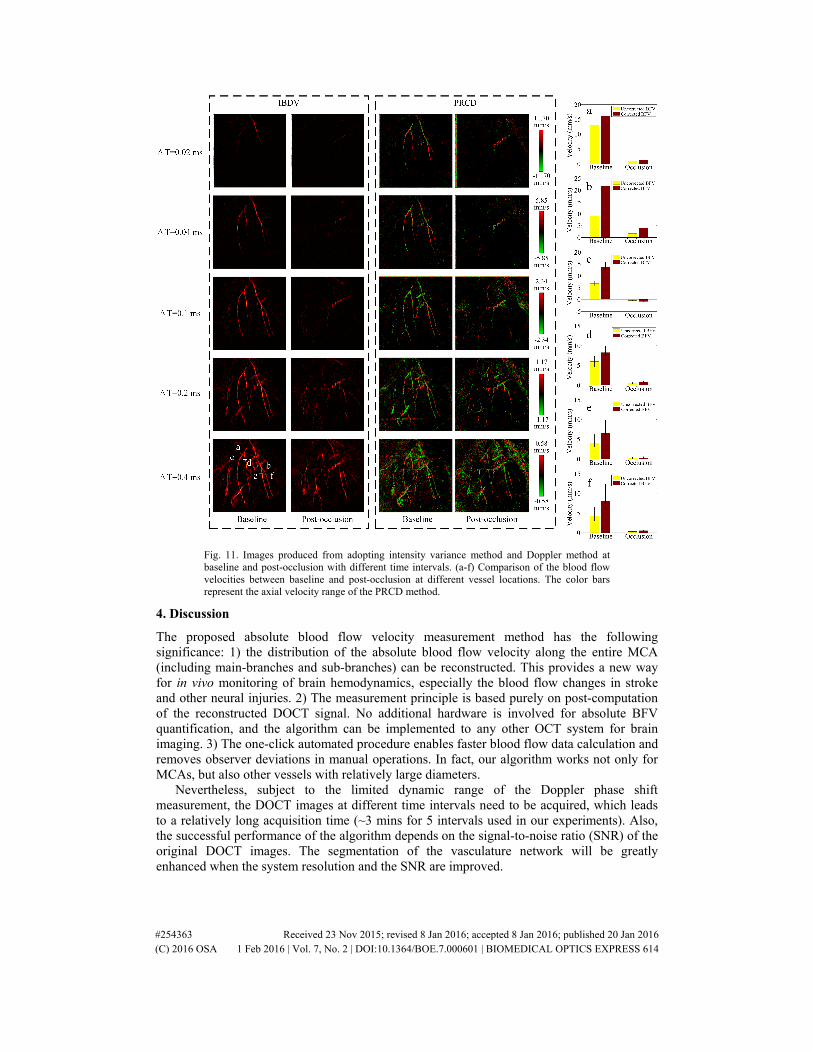
Fig. 11. Images produced from adopting intensity variance method and Doppler method at baseline and post-occlusion with different time intervals. (a-f) Comparison of the blood flow velocities between baseline and post-occlusion at different vessel locations. The color bars represent the axial velocity range of the PRCD method.

4. Discussion

The proposed absolute blood flow velocity measurement method has the following significance: 1) the distribution of the absolute blood flow velocity along the entire MCA (including main-branches and sub-branches) can be reconstructed. This provides a new way for in vivo monitoring of brain hemodynamics, especially the blood flow changes in stroke and other neural injuries. 2) The measurement principle is based purely on post-computation of the reconstructed DOCT signal. No additional hardware is involved for absolute BFV quantification, and the algorithm can be implemented to any other OCT system for brain imaging. 3) The one-click automated procedure enables faster blood flow data calculation and removes observer deviations in manual operations. In fact, our algorithm works not only for MCAs, but also other vessels with relatively large diameters.

Nevertheless, subject to the limited dynamic range of the Doppler phase shift measurement, the DOCT images at different time intervals need to be acquired, which leads to a relatively long acquisition time (~3 mins for 5 intervals used in our experiments). Also, the successful performance of the algorithm depends on the signal-to-noise ratio (SNR) of the original DOCT images. The segmentation of the vasculature network will be greatly enhanced when the system resolution and the SNR are improved.


5. Conclusion

We demonstrated the fully distributed measurement of absolute blood flow velocity for the middle cerebral artery by reconstructing the vessel geometry using pure DOCT stack images. Given a seed point location in the MCA images, the algorithm automatically localizes the vessel lumens, calculates the Doppler angle, and then quantifies the absolute BFV on each position of the whole MCA, including the main vessels and side branches. Our approach is verified by quantifying the hemodynamics of cerebral arteries during permanent MCA occlusion with custom-built, swept-source optical coherence tomography.

Acknowledgments

We thank Shenghai Huang for his helpful discussion. This work was supported by the National Institutes of Health (NIH) under grants R01EB-10090, R01HL-125084, R01HL-105215, R01HL-127271, R01EY-021529, P41-EB015890; and the Natural Science Foundation of China (No. 61307015), the Program for Professor of Special Appointment (Eastern Scholar) at Shanghai Institutions of Higher Learning (No. TP2014061). NIH grant NS-066001 to Dr. Ron D. Frostig also supported this work. Dr. Zhongping Chen has a financial interest in OCT Medical Inc., which, however, did not provide support for this work.


Fully distributed absolute blood flow velocity …frostiglab.bio.uci.edu/Li et al. Biomedical Optics Express.pdfmeasurement for middle cerebral arteries using Doppler optical coherence

Documents